Primary school attendance in Honduras

Primary school attendance in Honduras

Arjun S. Bedia,*, Jeffery H. Marshallb

a Institute of Social Studies, Kortenaerkade 12, 2518 AX, Den Haag, NetherlandsbStanford University, Palo Alto, CA, USA

Received 1 August 2000; accepted 1 September 2001

Abstract

Honduras has recorded impressive gains in expanding educational access in the 1990s, with the

result that primary education is available to almost all children. With improved access, the focus has

shifted to quality and efficiency issues. Previous research suggests that academic achievement is still

quite low, while repetition and school desertion rates continue to remain high. An important cause of

these outcomes appears to lie in patterns of school attendance. Low levels of school attendance may

be responsible for low academic achievement, which, in turn, is linked to high repetition and

desertion rates. Recognizing this probable chain of events, this paper focuses on the school

attendance decision. We rely on recently collected data from a national sample of Honduran primary

schools to specify and estimate a model of school attendance. We find that increases in the expected

benefits of attending school exert a strong impact on the school attendance decision.

D 2002 Elsevier Science B.V. All rights reserved.

JEL classification: D1; I2

Keywords: Primary school; Attendance; Honduras; School inputs; Supply of schooling

1. Introduction

Investments in education are widely recognized as a key component of a country’s

development strategy. Increases in the quantity and quality of educational provision have

been associated with a wide range of benefits including enhanced productivity, reduced

poverty and income inequality, improved health and economic growth.1 Spurred by such

0304-3878/02/$ - see front matter D 2002 Elsevier Science B.V. All rights reserved.

PII: S0304 -3878 (02 )00056 -1

* Corresponding author. Tel.: +31-70-4260493; fax: +31-70-4260799.

E-mail addresses: [email protected] (A.S. Bedi), [email protected] (J.H. Marshall).

www.elsevier.com/locate/econbase

1 See Lockheed and Associates (1991) for a detailed review.

Journal of Development Economics 69 (2002) 129–153

evidence, governments in developing countries devote a substantial fraction of their total

expenditure to the education sector.2

Honduras is no exception, as successive governments have invested substantial

resources in education. Between 1993 and 1996, public expenditure on education

accounted for 16.5% of total government outlays (UNDP, 1999). These investments have

expanded coverage and access at all levels and, as a result, the gross enrollment ratio for

Hondurans aged 6–23 (in primary, secondary and tertiary education) has risen from 47%

in 1980 to 60% in 1995 (UNESCO, 1999).3 The expansion in educational opportunities

has been especially notable in the pre-primary and primary sectors, and recent initiatives

have targeted the most needy populations in Honduras.4

However, these impressive gains in coverage have been tempered somewhat by low

levels of academic achievement and high rates of grade repetition and desertion. A recent

national application of criterion-referenced Spanish and Mathematics exams resulted in

national averages in Grade 3 of 39.7% and 35.9% in Spanish and Mathematics,

respectively (UMCE, 1998).5 In 1996, official grade repetition rates were 19.4% in

Grade 1, 11.6% in Grade 2 and 8.6% in Grade 3, although real rates are likely to be even

higher (Van Steenwyck, 1997; Marshall, 2000). Although difficult to calculate, the World

Bank (1995) estimates that about 5.0% of Honduran primary school students desert

annually.

While part of the reason for low achievement and consequently high repetition and

desertion rates may lie in student ability, it is likely that such outcomes are largely driven

by other factors. In a review of the Honduran education system, the World Bank identified

low attendance rates and poor school inputs as the two main factors responsible for high

repetition rates, which, in turn, was identified as the most important cause of the high

dropout rate (World Bank, 1995).

The economic contribution of children to families in developing countries (especially in

rural areas) and accordingly the opportunity cost associated with school attendance may be

substantial. Attendance will suffer when parents perceive that the return associated with

2 According to UNDP (1999), between 1993 and 1996, the average (unweighted) expenditure on education

as a percentage of total government expenditure for developing countries was 14.8%.3 Gross enrollment ratios at the primary and secondary level were 112% and 32%, respectively. For a more

detailed overview of Honduran educational coverage, see Edwards (1995), Edwards et al. (1996) and Van

Steenwyck and Mejia (1996).4 Examples include the expansion of community-based preschools (Centros Comunitarios de Iniciacion

Escolar—CCIEs) that are designed to reach rural populations (World Bank, 1995) and the recent creation of 500

community-based primary schools (Proyecto Hondureno de Educacion Comunitaria—PROHECO) based on the

EDUCO (Educacion con Participacion de la Comunidad) program in El Salvador.5 The UMCE exams are designed to measure the implemented curriculum and are not intended for pass/fail

decisions, so deciding on a cutoff point for passing and failing is an inherently arbitrary exercise. Nevertheless,

the exams do pretend to measure ‘‘mastery’’ for each curriculum component that is covered, which usually

include three questions per component. Students who can answer at least two of the three questions correctly are

considered to have mastered the component. These aggregated averages show that few Honduran primary

students are mastering a significant portion of the curriculum, according to the UMCE standards. Furthermore,

since the UMCE exams comprise multiple-choice questions with four options, averages below 40% are indicative

of low levels of achievement.

A.S. Bedi, J.H. Marshall / Journal of Development Economics 69 (2002) 129–153130

time spent in school does not justify the loss of a child’s economic contribution. Parental

perceptions of school inputs may also affect the attendance cost–benefit calculus as low-

quality teachers or limited availability of teaching materials may attenuate the expected

benefits from attending school. A reduction in days attended probably exerts a negative

influence on academic achievement and increases the probability of repetition and

desertion. There may also be a more direct link between school attendance and repetition

as some school systems require minimum levels of attendance before allowing a student to

appear for exams (see Jacoby, 1994).

Recognition of these indirect and direct links between school attendance and educa-

tional outcomes suggests that a focus on the factors underlying the school attendance

decision itself may be quite useful in understanding the dynamics of human capital

formation in a developing country. While there is a substantial amount of literature that has

examined the determinants of school enrollment, test scores, grade repetition and

desertion, there is limited work on the factors that motivate school attendance (for a

review, see Strauss and Thomas, 1995).6 A handful of authors have included a measure of

school attendance as an explanatory variable in educational production functions. One

example is Tan et al. (1997), who use data from the Philippines and find that the number of

days missed has a negative and statistically significant effect on Mathematics test scores.

Fuller et al. (1999) also include this variable as a regressor in their analysis of the

determinants of academic achievement in Brazil, although the point estimates are not

significant. While including attendance as an explanatory variable does highlight the

influence of attendance on test scores, it ignores the potential endogeneity of school

attendance and achievement and does not permit an analysis of the factors that determine

school attendance.7

This paper builds on our earlier work (Bedi and Marshall, 1999) and focuses primarily

on the school attendance decision. We use nationally representative data collected by the

External Unit for the Measurement of School Quality (Unidad Externa de Medicion de la

Calidad de la Educacion—UMCE) in Honduras to specify and estimate a model of

primary school attendance. We assume that parents determine the particular pattern of

school attendance for their children on the basis of expected gains and the costs of

attending school. We proceed in two steps. First, we estimate the effect of child, family and

school characteristics on test scores and obtain predicted test scores. In the second step, we

estimate a school attendance model that includes predicted test scores as a measure of the

expected gains of school attendance. This paper improves on our earlier work in two ways.

First, the UMCE database includes a nationally representative sample of primary schools,

while our earlier work was based on a limited sample drawn from one province of rural

Honduras, which limited the generalizability of our results. Second, the measure of school

attendance that we use in this paper allows a decomposition of school attendance into

6 Enrolling in school is clearly the first step before one may begin to examine patterns of school attendance.

In the Honduran context, where there is almost universal enrollment, the important issue is not whether a child is

enrolled in school but how often does a child attend school.7 Although the main aim of their paper is to compare test scores across school types, Jimenez and Sawada

(1999) do provide estimates of school attendance regressions that allow them to examine the determinants of

attendance as well as make comparisons across school types.

A.S. Bedi, J.H. Marshall / Journal of Development Economics 69 (2002) 129–153 131

demand and supply components. This feature of the data is discussed in a subsequent

section.

Section 2 introduces the analytical framework that we use to motivate our empirical

work. Section 3 describes the data and the variables used in the analysis. Section 4

presents results and Section 5 concludes.

2. Costs, benefits and school attendance—an analytical framework

School attendance patterns in developing countries vary substantially across house-

holds. Some children may never enter school, while others may attend only part time. The

degree of part-time schooling may vary from missing a few weeks to missing several

months. The variation in attendance patterns suggests that parents evaluate differently the

costs and benefits of attending school and that this evaluation for the same household may

also vary according to the particular time of the year. For instance, during the harvest

season, the opportunity costs of attending school may far outweigh the benefits, resulting

in temporary withdrawal, while at other times, the benefits may outweigh the costs and

result in regular school attendance.8 Thus, school attendance over the year may be viewed

as the consequence of a daily household decision where a child attends school on a

particular day if the expected benefits from attending school on that day are greater than

the associated costs.

To formalize these notions and to motivate our empirical work this section presents a

framework tailored to our needs.9 Consider that the school year consists of n days, and it is

Day i of the school year. We assume that each household has a utility function defined over

bi and ci, where bi denotes the benefits associated with attending school on Day i, and ci is

household consumption on Day i. While attending school yields benefits, it comes at a

cost. Direct and opportunity costs associated with school attendance lower resources

available for household consumption. Accordingly, household utility on Day i conditional

on school attendance (denoted by subscript 1) is given as

Ui1 ¼ Uðbi; ci1Þ: ð1Þ

The associated budget constraint is

yi ¼ ci1 þ pi; ð2Þ

where yi is household income and pi represents the total cost associated with school

attendance.

8 This is especially true in rural Honduras, where children may drop out of school for several months during

the harvest season only to return the next year. See World Bank (1995, p. 9). School attendance patterns in our

data are discussed later on in the text.9 The framework used here is similar to those in Gertler and Van Der Gaag (1988) and Gertler and Glewwe

(1990).


In a similar fashion, the utility associated with not attending school may be defined

by

Ui0 ¼ Uðci0Þ: ð3Þ

The budget constraint is yi = ci0. Given the utility associated with both options,

households choose the option that yields the highest utility. The solution to the daily

unconditional utility maximizing problem is

Ui* ¼ maxðUi1;Ui0Þ; ð4Þ

where Ui* is the maximum utility. Alternatively, school attendance may be defined in

terms of a dichotomous variable, ai, where ai = 1 if a child attends school and 0

otherwise. A child attends school, i.e., ai = 1 if Ui1>Ui0. Summing up the outcomes of

these daily decisions, over the school year, leads to the observed pattern of school

attendance.

2.1. Empirical specification

Since our purpose is to empirically explore the role of expected gains and costs on the

school attendance decision, we proceed by specifying linear forms of the conditional

utility function. For the schooling option,

Ui1 ¼ b1bi þ b2ci1 þ ei1 ð5Þ

where the b’s are coefficients to be estimated and ei1 is assumed to be a mean zero,

normally distributed error term with positive variance. Since ci1 = yi� pi, we may rewrite

Eq. (5) to obtain

Ui1 ¼ b1bi þ b2ðyi � piÞ þ ei1 ð6Þ

The utility function for the nonschooling option is

Ui0 ¼ b2yi þ ei0 ð7Þ

Thus, an individual attends school, i.e., ai= 1 if b1bi� b2pi + ei1� ei0>0.The chances of attending school on a particular day may be expressed in terms of a

linear probability model that may be written as

ai ¼ b1bi � b2pi þ eia; ð8Þ

where eia is a normally distributed, mean zero, positive variance composite error

term.10

10 In this linear utility specification, income has been differenced out of the decision rule and does not

directly affect the school attendance decision. Household endowments are assumed to influence the school

attendance decision through opportunity costs.


Eq. (8) depicts the probability of attending school on any particular day. Since we are

interested in the yearly pattern of school attendance, we may sum up the outcome of the

daily attendance decision over the course of the school year,

Xn

i¼1

ai ¼Xn

i¼1

ðb1bi � b2pi þ eiaÞ ð9Þ

to yield

A ¼ b1Bþ b2P þ eA; ð10Þ

where yearly school attendance, A, depends on B, the expected benefits associated with

school attendance over the school year, and P, the yearly costs of attending school.

2.2. Costs of attending school

The total cost (P) of sending a child to school includes monetary (direct) and indirect or

opportunity costs. Since education is largely subsidized the main cost incurred by

households is likely to be in the form of opportunity costs. Attending school reduces a

child’s availability for work in and outside the home. If a child makes substantial

contributions to family income, or plays an important role in supporting other working

members, then the opportunity cost of attending school is likely to be high and this may

curtail the attractiveness of the schooling option.11

Both of these cost components are likely to differ across households. For instance,

direct costs may vary due to differences in transportation costs. Opportunity costs and the

value of a child’s time may also differ due to personal characteristics of the child (age, sex)

and the value that parents place on a child’s time. Since we do not directly observe the

costs of attending school we allow P to depend on a vector of child, family and other

characteristics that capture the cost of attending school.

2.3. Benefits of attending school

Parents have to ascertain the total benefits (B) associated with school attendance. We

consider two types of benefits that may influence parental decision making. The main

benefit associated with attending school is likely to be the expected addition to a child’s

human capital. To capture this effect, we need a measure of the human capital gains

associated with school attendance. For this study, we incorporate a measure that is widely

used to indicate the benefits derived from education: test scores. However, using actual test

scores is obviously incorrect due to the potential endogeneity between test scores and

11 For example, Patrinos and Psacharopoulos (1995) show that child earnings account for 27.8% of total

income in urban households in Paraguay, while Patrinos and Psacharopoulos (1997) show that child labor

contributes 17.7% of household income in rural Peru. A number of studies have also demonstrated that the

presence of younger siblings in the household may affect educational outcomes. Using Honduran household

survey data, Edwards et al. (1996) show that children are likely to delay initial enrollment, and attain fewer years

of education, when an infant sibling is present in the home.


attendance. In order to derive an appropriate measure of human capital gains, we proceed

by estimating educational production functions, one for each subject, for those students for

whom test score data are available. These test score equations are specified as

H ¼ dZ þ eH ; ð11Þ

where H is a measure of human capital or in this case test scores, Z is a vector of

individual, family and school characteristics that influence H and eH is an error term.

Estimates from the educational production functions are used to predict test sores for each

individual. These predicted values (H) are included in Eq. (10) in order to capture the

human capital benefits associated with attending school.

In addition to school characteristics that have an impact on test scores, there may be

other school characteristics that do not affect academic achievement but do signal the

quality (Q) of a school and directly influence the benefits that parents attribute to school

attendance. For instance, whether a school has a telephone connection or a sports field may

not directly influence academic achievement. However, these are easily observed signals

that may be used by parents to judge the quality of a school and, in turn, may directly

influence the benefits that parents associate with school attendance. Thus, some school

inputs and facilities may directly influence parental evaluation of the benefits associated

with school attendance, while others may exert an influence on benefits through their

impact on test scores.

To account for the different kinds of benefits that parents may associate with school

attendance, Eq. (10) may be adjusted to accommodate both the expected human capital

benefits (H) and direct benefits (Q) and may be rewritten as

A ¼ b1H H þ b2QQþ b3P þ eA; ð12Þ

where b1H is a coefficient to be estimated and b2Q and b3 are conformable coefficient

vectors to be estimated. As this equation depicts, school attendance is treated as a function

of expected human capital benefits, other benefits and costs.

3. Data description and specification

The data used in this paper are drawn from the second national application of

standardized tests administered by the UMCE in October 1998 and March 1999.12 The

sample includes 586 schools from 17 of 18 states13 (departamentos) and represents

approximately 7% of Honduran primary schools. In this application, Spanish and

Mathematics tests were administered to students in Grades 2 and 4. In addition, second

and fourth grade teachers were administered questionnaires, as were school directors in

12 The two primary functions of the UMCE are to develop and apply standardized tests covering the basic

learning objectives and study the factors associated with academic achievement, especially in student cohorts. See

UMCE (1998) and World Bank (1995) for descriptions of the project.13 Gracias a Dios, an extremely isolated state in eastern Honduras, was not included in the sample due to the

relatively small number of schools and students in this region and the difficulty of school access.


each school. Test administration personnel filled out observation instruments in each

school detailing variables such as school type, enrollment, days worked, school character-

istics (including materials and hardware) and special programs. They also copied student

data including days missed during the school year, work attitudes and Spanish and

Mathematics grades from teacher grade books in second and fourth grades. Finally, parents

with children in second or fourth grades were interviewed to collect data on parental

characteristics such as education and work experiences, attitudes towards education and

specific problems in their school, among other variables. Further details on the data are

available in UMCE (1999).

In this paper, we restrict our analysis to students in second and fourth grade for whom

we have complete information on test scores, attendance, child, family and school

characteristics. These restrictions result in sample sizes of 7210 for Grade 2 Spanish

and 6938 for Grade 2 Mathematics. The Grade 2 attendance equation is estimated over a

sample of 6139 observations. For Grade 4, the sample sizes are 5359 for Spanish, 5024 for

Mathematics and 4501 for the attendance equation.14 Descriptive statistics and variable

definitions by grade are provided in Tables 1 and 2.

Turning to the empirical implementation, two educational production functions—one

for each subject—are estimated for each grade, yielding a total of four equations. The

dependent variables (H) are standardized test scores on Spanish and Mathematics

examinations. The independent variables are classified into child, family, teacher and

classroom/school characteristics. The child-specific variables include age and sex, as well

as an indicator of whether Spanish or Mathematics is a child’s favorite subject among the

four main subjects that also include sciences and social studies. This variable is included to

control for the effect that inclination towards a particular subject may have on test scores.

Family characteristics include variables that reflect parental attitudes towards education

such as whether a child attended preschool, whether parents help children with their

homework and parental participation in school activities. Household resources are

measured by mean years of education of the parents and an index of household wealth

(see Table 1 for details).

Several variables are included to control for the quality of instruction received by the

child. An instructor’s knowledge of the subject is captured by years of education, years of

experience, the number of teaching seminars attended and test scores on Spanish and

Mathematics examinations. The test score variable is expected to be a more accurate and

current measure of an instructor’s knowledge. In an attempt to control for unobserved

teaching attributes and skills, our regressions include a self-reported measure of teacher’s

self-confidence. Class characteristics include the size of the class, an indicator of whether

several grades are taught simultaneously in the same grade (i.e., a multigrade classroom),

and the availability of textbooks.

The dependent variable (A) in the school attendance Eq. (12) is the number of days that

a child attends school during the school year. This measure is created by subtracting the

number of days that a child misses school from the number of days the school was in

14 The number of observations available for estimating the attendance equation estimations drops, because in

some schools, we have data on children (including test scores), parents, teachers and schools, but the teacher

grade books were not available and, therefore, it was not possible to construct the attendance variable.


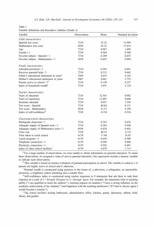
Table 1

Variable definitions and descriptive statistics (Grade 2)

Variable Observations Mean Standard deviation

Child characteristics

Spanish test score 7210 35.22 15.989

Mathematics test score 6938 43.22 17.819

Age 7210 8.967 1.402

Female = 1 7210 0.504 0.500

Favorite subject—Spanish = 1 7210 0.289 0.453

Favorite subject—Mathematics = 1 6938 0.425 0.494

Family characteristics

Attended preschool = 1 7210 0.595 0.491

Receives parental help = 1 7210 0.313 0.463

Father’s educational attainment in yearsa 1844 4.635 4.142

Mother’s educational attainment in years 2007 4.661 3.753

Parents active in school = 1b 7210 0.150 0.357

Index of household wealthc 7210 3.031 2.124

Teacher characteristics

Years of education 7210 12.563 0.982

Years of experience 7210 12.007 8.088

Seminars attended 7210 0.957 1.358

Test score—Spanish 7210 80.84 0.121

Test score—Mathematics 6938 51.37 0.190

Index of self-confidenced 7210 4.154 0.536

Classroom/school characteristics

Multigrade classroom= 1 7210 0.347 0.476

Adequate supply of Spanish texts = 1 7210 0.283 0.448

Adequate supply of Mathematics texts = 1 6938 0.434 0.493

Class size 7210 40.35 12.25

Time taken to reach school 6139 17.44 16.43

Lunch program= 1 6139 0.056 0.300

Telephone connection = 1 6139 0.208 0.406

Electricity connection = 1 6139 0.592 0.491

Index of other school facilitiese 6139 4.078 1.713

a For a large number of observations, we were unable to obtain information on parental education. To retain

these observations, we assigned a value of zero to parental education. Our regressions include a dummy variable

to indicate such observations.b This variable is based on teacher evaluation of parental participation in school. The variable is coded as 1 if

parents are highly active in school and 0 otherwise.c Parental wealth is constructed using presence in the house of: a television, a refrigerator, an automobile,

electricity, a telephone, indoor plumbing and a nondirt floor.d Self-confidence index is constructed using teacher responses to 9 statements that ask them to rank their

response on a scale of 1 = Strongly Disagree to 5 = Strongly Agree. For example, the statements refer to teaching

ability (‘‘I am qualified to teach the subjects’’), teaching impacts on students (‘‘I have a strong influence on the

academic achievement of my students’’) and happiness with the teaching profession (‘‘If I had to choose again I

would become a teacher’’).e The school facilities include bathrooms, administrative office, kitchen, pantry, laboratory, athletic field,

library and garden.


Table 2

Variable definitions and descriptive statistics (Grade 4)

Variable Observations Mean Standard deviation


Spanish test score 5359 39.39 15.450

Mathematics test score 5024 32.02 11.195

Age 5359 10.85 1.435

Female = 1 5359 0.531 0.499

Favorite subject—Spanish = 1 5359 0.208 0.406

Favorite subject—Mathematics = 1 5024 0.401 0.490


Attended preschool = 1 5359 0.573 0.494

Receives parental help = 1 5359 0.385 0.486

Father’s educational attainment in yearsa 2157 4.969 4.358

Mother’s educational attainment in years 2335 4.976 4.058

Parents active in school = 1b 5359 0.140 0.346

Index of household wealthc 5359 3.387 2.181


Years of education 5359 12.653 1.081

Years of experience 5359 13.288 8.116

Seminars attended 5359 1.203 1.736

Test score—Spanish 5359 79.41 12.52

Test score—Mathematics 5024 49.43 15.69

Index of self-confidenced 5359 4.149 0.482

Classroom/school characteristics

Multigrade classroom= 1 5024 0.396 0.489

Adequate supply of Spanish texts = 1 5359 0.346 0.475

Adequate supply of Mathematics texts = 1 5024 0.412 0.492

Class size 5359 38.30 10.51

Time taken to reach school 4501 15.88 14.31

Lunch program= 1 4501 0.050 0.217

Telephone connection = 1 4501 0.202 0.401

Electricity connection = 1 4501 0.590 0.492

Index of other school facilitiese 4501 4.118 1.728

a For a large number of observations, we were unable to obtain information on parental education. To retain

these observations, we assigned a value of zero to parental education. Our regressions include a dummy variable

to indicate such observations.b This variable is based on teacher evaluation of parental participation in school. The variable is coded as 1 if

parents are highly active in school and 0 otherwise.c Parental wealth is constructed using presence in the house of: a television, a refrigerator, an automobile,

electricity, a telephone, indoor plumbing and a nondirt floor.d Self-confidence index is constructed using teacher responses to 9 statements that ask them to rank their

response on a scale of 1 = Strongly Disagree to 5 = Strongly Agree. For example, the statements refer to teaching

ability (‘‘I am qualified to teach the subjects’’), teaching impacts on students (‘‘I have a strong influence on the

academic achievement of my students’’) and happiness with the teaching profession (‘‘If I had to choose again I

would become a teacher’’).e The school facilities include bathrooms, administrative office, kitchen, pantry, laboratory, athletic field,

library and garden.


operation during the 1998 school year. A detailed analysis of this variable is provided in

Section 4. Attendance is specified as a function of the benefits and costs associated with

schooling. Benefits are represented by the expected human capital gains from schooling, H

(obtained from the production function estimates), and by school facilities that signal the

quality (Q) of the school and from which parents may directly derive benefits. The

specific school facility variables include the presence of a telephone connection, an

electricity connection and a composite variable that sums other school facilities that a

school may possess. Since we do not have any direct measures of opportunity costs (such

as child wages), we specify opportunity costs (P) as a function of child and family

characteristics. The child characteristics include the age and sex of the child. Variation in

parental evaluation of child time is controlled by the same set of family characteristics that

are included in the educational production functions. School related characteristics that

may influence the cost of school attendance are the time taken to get to school and whether

the school has a lunch program.

Before turning to the results, a number of econometric issues must be dealt with. First,

the educational production functions are estimated using data only on those students who

attended school on the day that the tests were administered. Using data only on test takers

may result in inconsistent estimates, since children who are not in attendance on the day of

the test may not have the same characteristics as those who were in school on the day of

the test.15 To account for this source of bias, we estimate selection-corrected educational

production functions.16

Another concern while estimating educational production functions is the potential

endogeneity of school inputs. If parents migrate in response to differences in school inputs,

or if educational planners distribute school inputs to compensate for low student achieve-

ment, then estimates of the effect of school input characteristics may be biased.

Endogeneity due to parental migration appears to be quite unlikely in the Honduran

context. Analysis of household survey data indicates that 90% of individuals migrate in

order to find work and the remaining migrate for family reasons (see Bedi, 1997).

Endogeneity due to the second source is quite possible. However, examination of our data

does not reveal any clear and consistent pattern between the distribution of school

resources and the general economic characteristics of a region. For instance, in Grade 2,

16 While we have fairly complete information on 7210 individuals for Grade 2 Spanish and 6938 for Grade 2

mathematics, there are around 4500 additional students enrolled in Grade 2 who did not take the exam. The

selection-corrected specifications are estimated over this larger sample. We lose some of these observations since

we do not have complete information on all of the explanatory variables. The selection correction estimates are

based on sample sizes of 10,054 and 9985 for Grade 2 Spanish and Grade 2 mathematics, respectively. In Grade

4, there are around 3000 students who did not attend school on the day of the exam. Here, we also lose some

observations due to missing information on the explanatory variables and the selection corrected estimates for

Grade 4 Spanish and mathematics are estimated over sample sizes of 7220 and 7078, respectively.

15 There are other potential sources of selection bias that may have a bearing on estimates of the academic

achievement equations. For instance, children may never enroll in school or may drop out of school before

reaching Grade 2/Grade 4 and, thus, those who do enroll and do reach these grades may be regarded as a

selective cohort of students. Since almost all children enroll in school, any selection bias from this source is

likely to be small. However, since a large number of students do leave the school system before reaching Grade

2/Grade 4, our analysis should be viewed as conditional and restricted to those individuals who have reached

Grade 2/Grade 4.


schools in metropolitan areas have slightly larger class sizes (approximately 40 students)

as compared to schools in towns (around 38 students), however, test scores of teachers is

slightly higher in metropolitan schools (85 versus 81%).17

Finally, the school-specific nature of our data raises the possibility that students

attending the same school (i.e., sharing the same observable characteristic) may also

share the same unobservable characteristics, which may lead to the presence of intraschool

error correlation (see Moulton, 1986). Although least squares is still consistent, the

presence of these effects results in biased standard errors and consequently misleading

statistical inference. To account for this, an appropriate robust variance–covariance matrix

is computed, and the reported t statistics for our various estimates are based on this

adjusted matrix.

4. Results

The results are divided into three sections. In Section 4.1, we examine patterns of

school attendance and present a decomposition of attendance into demand and supply side

components. Section 4.2 discusses the determinants of academic achievement in Math-

ematics and Spanish, while Section 4.3 presents estimates of the school attendance

equation.

4.1. School attendance patterns

The total number of days that a child attends school is determined by parental or child

demand for schooling and the supply of schooling. While a decomposition of the days

missed due to demand and supply factors does not affect the basic notion that school

attendance is important in determining educational outcomes, identifying whether a child

misses school due to demand or supply factors is important from a policy perspective. If

the main problem is one of low demand for schooling, then the appropriate response may

be policies designed to lower costs of schooling or a policy of enhanced investments in

school inputs to increase the expected returns from schooling. On the other hand, limited

supply of schooling would suggest another set of policy responses.

An important feature of the data used in this paper is that we have information not only

on the number of days that each student missed during the 1998 school year, but also on

the number of days that each school in the UMCE sample was open during the school

year.18 This information combined with our knowledge of the number of days that a school

18 This additional information was collected as a consequence of our initial investigation into this issue when

we were forced to assume that each school remained open for 160 days and the entire school attendance issue was

treated as a demand side problem. As the data used in this study clearly demonstrate, this is an unrealistic

assumption, especially for a nationally representative sample of primary schools.

17 Notwithstanding these patterns, it is possible that the distribution of school inputs and student achievement

are systematically related. Due to lack of suitable data, we are unable to use an instrumental variables (IV)

approach. However, we are able to provide some clues on the direction of the potential bias by referring to our

earlier work (Bedi and Marshall, 1999). In our previous paper, we found that the coefficients on the school inputs

in IV regressions were systematically larger (in absolute terms) than the corresponding OLS estimates.


is expected to remain open helps us identify whether a child misses school due to lack of

demand for schooling or due to lack of school supply. In terms of an equation, Dm, the

days missed may be decomposed into

Dm ¼ ðDo � DaÞ þ ð172� DoÞ; ð13Þ

where Do is the number of days that school is offered and Da represents days attended. The

first term in parentheses on the right-hand side represents days missed due to lack of

demand for schooling. School is offered on those days, but parents do not send their

children to school. The second term represents days missed due to lack of school supply.

Schools are meant to be operating 172 days during the school year, and the gap between

the expected days of operation and the days that a school is actually offered represents

days missed due to lack of supply.19

The patterns of school attendance and a demand–supply decomposition of days missed

for students in Grade 2 and Grade 4 are displayed in Table 3a and b. On average, a child

attends 143–144 days of school, which translates into a loss of around 5 weeks of

schooling. The number of days attended varies from 121 at the 10th percentile to 161 at

the 90th percentile for Grade 2 and 124 and 162 for the same percentiles in Grade 4, i.e., a

range of about 1.5–9.5 weeks of missed classes.20

Of particular interest to the present analysis is the decomposition of days missed into

demand–supply components. This decomposition on the basis of Eq. (13) is displayed in

Table 3a and b. For Grade 2, at the mean, the 29 missed days may be decomposed into 10

days missed due to lack of demand for schooling and 19 days missed due to lack of supply.

A similar pattern prevails for Grade 4, with 9 days accounted for by lack of demand and 19

days missed due to lack of supply. For both grades, the decomposition at the mean or at

different points of the distribution clearly indicates that while both demand and supply

20 An immediate question that arises is whether these missed days translate into lower levels of human capital

or are students are able to make up despite missing school? Although educational achievement and school

attendance are endogenous, to establish the effect of school attendance on educational outcomes, we estimated

educational production functions for both subjects and both grades that included the number of days attended as a

regressor. For all four regressions, we found that the number of days attended had a positive impact on test scores

and was statistically significant. For Grade 2, the point estimates indicated that an increase in school attendance

by one standard deviation (14 days) would increase educational achievement by 3.1–4.4%. For Grade 4, the

corresponding calculation yielded increases of 2.2–4.4%. A detailed examination of the effect of attendance on

test scores is available in Marshall and White (2000).

19 This decomposition may lead to an exaggeration of the supply side of the problem. If parental (lack of)

demand for schooling on a particular day coincides with a day that school is not offered, it will lead to an

overemphasis of the supply side of the problem. Except for noting this possibility, we are not able to offer any

additional information on the extent of such an exaggeration. It is also possible that the lack of supply may

dissuade parents from sending their children to school. If this is the case, then the decomposition presented here

would underestimate the true extent of the supply side problem. Our data show that there is a positive correlation

(0.18 for Grade 2 and 0.13 for Grade 4) between student absences and the number of days that a school is closed.

Exploratory regressions of days that a student is absent on days that a school is closed (controlling for other

characteristics) provide some support for a positive relationship between these two variables. However, the

statistical significance of the relationship is sensitive to the inclusion of provincial controls. Detailed results are

available.


factors are responsible for limiting school attendance a larger share of the problem

(between 60% and 71%) may be attributed to lack of school supply.

Due to limited information on the supply side, the primary focus of this paper is on

factors that inhibit attendance from the demand side. Although our data are not particularly

well suited in terms of analyzing the supply side, some clues may be gleaned from the

information that we have. First, variation in the supply of schooling may be associated with

the type of school administration. While most schools in Honduras are publicly provided

and administered, there are a small number of schools that are run privately. As shown in

Table 4 (rows 1 and 3), there are 24 private schools in our sample, and on average, private

schools offer 2 more weeks of schooling as compared to public schools. At first glance, this

would suggest that the type of school administration plays a key role in determining the

supply of schooling. However, conditioning on the location of the schools (rural or urban)

suggests that the differences in supply of schooling have more to do with the location of the

school rather than the school administration (Table 4, rows 2, 4, rows 2, 4, 5 and 6).

Differences in the supply of schooling appear to be more pronounced across location than

Table 3

School attendance—a decomposition

Statistic Days school

open

Days

attended

Days missed

demandaDays missed

supplybTotal days

missed

(a) Grade 2

Mean (standard deviation) 153 (10.91) 143 (15.73) 10 (9.53) 19 29

Percentiles

10 138 121 17 34 51

20 145 131 14 27 41

30 148 137 11 24 35

40 152 142 10 20 30

50 155 145 10 17 27

60 157 149 8 15 23

70 159 153 6 13 19

80 162 156 6 10 16

90 165 161 4 7 11

(b) Grade 4

Mean (standard deviation) 153 (11.14) 145 (15.21) 9 (8.93) 19 28

Percentiles

10 139 124 15 33 48

20 145 134 11 27 38

30 148 139 9 24 33

40 153 144 9 19 28

50 155 147 8 17 25

60 158 151 7 14 21

70 160 154 6 12 18

80 163 157 6 9 15

90 166 162 4 6 10

a Days missed due to lack of demand for schooling is computed by subtracting days attended from the days

that a school was open.b Days missed due to lack of school supply is computed by subtracting the days that a school is open from the

official length of the school year (172 days).


across school types. As displayed in Table 4, urban private schools offer 5 more days of

schooling than urban public schools, while urban public schools offer 11 more days of

schooling than rural public schools. Turning to another dimension, Table 4 also presents the

mean supply of schooling by the kind of teacher resources available in a school. Schools

with multiple teachers offer around 9 more days of schooling as compared to schools with a

single teacher. An additional factor that may be related to the supply of schooling is the

distance of the school from the state capital. It is possible that remote schools are less likely

to remain open as compared to schools located closer to state capitals.

To examine the relative impact of these various factors, we present OLS estimates from

regressions of the days a school is open on variables that represent the type and location of

a school. These estimates are presented in Table A1 in Appendix A. As suggested by the

foregoing discussion, the estimates show that (see column 2) the type of administration is

not as important in determining school supply as compared to some of the other factors.

Limited teacher resources are clearly associated with reduced supply of schooling. The

location of a school appears to be particularly important. Schools located far away from a

state capital are less likely to remain open. For instance, a school that is a 3-hour drive

from the state capital is likely to offer around 2 days less schooling as compared to a

school that is an hour’s drive. Rural schools offer almost 8 days less schooling than urban

schools. There is also substantial provincial variation in the supply of schooling. The

coefficients on the provincial indicators (not reported in the table) show that some

provinces offer almost 10 school days less than the average, while other provinces offer

7–8 days more than the average. The overall picture appears to be that the supply of

schooling is more closely related to the rural or provincial location of a school than the

type of administration.21

Table 4

Supply of schoolinga

School administration and locationb n Mean (standard deviation)

1. Public 548 150.37 (11.08)

2. Public-urban 113 159.06 (6.988)

3. Public-rural 435 148.12 (10.83)

4. Private 24 163.54 (4.662)

5. Private-urban 21 164 (4.593)

6. Private-rural 3 160.33 (4.618)

Teacher resources in schoolc

7. Single-teacher school 83 144.85 (11.67)

8. Two-teacher school 142 148.10 (10.96)

9. Multiple-teacher school 347 153.54 (10.34)

a Supply of schooling is defined as the number of days that a school is open during the school year.b t Tests (at the 5% level) reject the null hypothesis that there is no difference in the mean number of days that

schools are open across school administration and location.c t Tests (at the 5% level) reject the null hypothesis that there is no difference in the mean number of days that

schools are open across schools with different teacher resources.

21 The province level averages mask substantial intraprovince differences in the supply of schooling. Within

the same state, the supply of schooling may vary from 110 to 172 days in a school year.


While our examination of the data has provided some idea about the source of supply

differentials, it also raises questions. What are the factors underlying the regional variation

in the supply of schooling? Observations during the data gathering exercise suggest that

these variations may be related to differences in policy regarding teacher pay collection,

local holidays and teacher meetings. For example, in some rural areas, teachers are

allowed 3 days to collect their monthly pay from the district administrative office. Some

teachers use their weekends to collect their pay, while others collect their pay on

weekdays. The frequency of teacher training seminars/meetings also varies substantially.

Teachers in some districts attend one seminar/meeting a week, while in other districts,

there are very few seminars/meetings. Another explanation for regional differences in

supply lies in different levels of school supervision across districts. In several rural areas,

there is almost no supervision, and school closures may be unknown to district supervisors

(Marshall and White, 2000).

As is clear from the discussion, a complete study of school attendance requires an

analysis of the demand for and the supply of schooling. Despite the limited supply side

analysis, our ability to identify the relative influence of demand and supply factors in

determining school attendance is by itself an important step in incorporating supply side

issues into an analysis of school attendance.

4.2. Educational production functions

Least squares and selection-corrected estimates of the four educational production

functions for Grade 2 and Grade 4 are presented in Tables 5 and 6, respectively. The

selection-corrected results control for the potential bias that may arise from estimating

regressions over samples of students who attended school on the days that the tests were

administered.22 For Grade 2, the selection patterns for both Spanish and Mathematics are

positive and statistically significant, indicating that unobserved characteristics that have a

bearing on test scores are positively correlated with school attendance. For Grade 4, the

selection patterns are not as clear. A comparison of the two sets of results (OLS versus

selection corrected) shows that there are very few sign changes on the estimated

coefficients, and while the magnitude of the coefficients for Grade 2 are substantially

affected, for Grade 4, the changes are minimal. Since we detect some signs of selection

bias, the discussions in this section are based on the selection-corrected estimates.23

We now examine the effect of various sets of characteristics on test scores. The age of a

child does not appear to play an important role in determining test scores, although there

are clear gender differences. Girls score higher than boys do by about 1–1.7 points on

Spanish examinations, although in Mathematics, at least for Grade 4, it appears that boys

perform better. The favorite subject dummy variable is included in order to control for

23 It is well known that the selection procedure is quite sensitive to specification of the selection equation as

well as to departures from normality. We experimented with some minor changes in specification, but the limited

availability of identifying information precludes a through examination. A prudent approach may be to repose

greater confidence in those coefficients that are robust to changes in the estimation approach.

22 The selection-corrected estimates are maximum likelihood estimates based on Heckman’s (1979)

correction procedure. The probability of attending school on the day of the test was specified as a function of

individual, school and teacher variables. Detailed estimates are available on request.


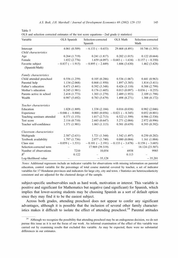
subject-specific unobservables such as hard work, motivation or interest. This variable is

positive and significant for Mathematics but negative (and significant) for Spanish, which

implies that lower-scoring students may be choosing Spanish as a sort of default option

since they may find it to be the easiest subject.

Across both grades, attending preschool does not appear to confer any significant

advantages, although it is possible that the inclusion of several other family character-

istics makes it difficult to isolate the effect of attending preschool.24 Parental attitudes

24 Although we recognize the possibility that attending preschool may be an endogenous decision, we do not

pursue this issue as it is not the focus of our work. An informal examination of the effect of this variable was

carried out by examining results that excluded this variable. As may be expected, there were no substantial

differences in our estimates.

Table 5

OLS and selection corrected estimates of the test score equations—2nd grade (t statistics)

Variable OLS Spanish Selection-corrected

Spanish

OLS Math Selection-corrected

Math

Intercept 4.061 (0.509) � 6.133 (� 0.653) 29.468 (4.491) 10.746 (1.393)


Age 0.264 (1.719) 0.241 (1.817) 0.202 (1.015) 0.122 (0.664)

Female 1.032 (2.776) 1.659 (4.097) � 0.683 (� 1.634) � 0.157 (� 0.350)

Favorite subject

(Spanish/Math)

� 0.837 (� 1.915) � 0.895 (� 2.449) 1.606 (3.630) 1.462 (3.428)


Child attended preschool 0.556 (1.259) 0.105 (0.286) 0.536 (1.067) 0.441 (0.963)

Parental help 1.134 (2.068) 0.868 (1.950) 1.897 (3.385) 1.814 (3.411)

Father’s education 0.471 (3.441) 0.392 (3.348) 0.426 (3.110) 0.388 (2.799)

Mother’s education 0.245 (1.981) 0.176 (1.605) 0.013 (0.097) � 0.036 (� 0.255)

Parents active in school 2.418 (1.773) 1.303 (1.279) 2.489 (1.953) 2.109 (1.798)

Wealth 0.987 (5.692) 0.783 (5.679) 1.498 (8.271) 1.388 (8.172)


Education 1.028 (1.889) 1.338 (2.184) 0.016 (0.038) 0.982 (2.046)

Experience � 0.046 (� 0.886) 0.003 (0.056) � 0.021 (� 0.345) 0.052 (0.801)

Teaching seminars attended 0.371 (1.153) 1.017 (2.713) 0.522 (1.599) 0.986 (2.530)

Test score 2.116 (0.710) 2.443 (0.647) 5.271 (2.084) 2.972 (0.996)

Teacher self-confidence 1.371 (1.901) 1.063 (1.113) 0.501 (0.659) 0.393 (0.392)

Classroom characteristics

Multigrade 2.587 (2.631) 1.721 (1.344) 1.542 (1.497) 0.250 (0.202)

Textbook availability 1.797 (1.736) 2.077 (1.740) 0.080 (0.084) 1.161 (1.004)

Class size � 0.059 (� 1.531) � 0.101 (� 2.191) � 0.133 (� 3.678) � 0.158 (� 3.685)

Selection-corrected term – 17.969 (39.319) – 18.124 (23.507)

Number of observations 7210 10,054 6938 9985

R2 0.122 – 0.113 –

Log-likelihood value – � 35,128 � 35,201

Notes: Additional regressors include an indicator variable for observations with missing information on parental

education, control variable for the percentage of total course material covered by teacher, a set of indicator

variables for 17 Honduran provinces and indicators for large city, city and town. t Statistics are heteroscedasticity

consistent and are adjusted for the clustered design of the sample.


towards a child’s education are measured by two variables: parental help and parental

activity in school. Parental help appears to boost performance by about 1–1.8 points in

Grade 2 (in both subjects) and in Grade 4 (Spanish), but the dissipation of this effect for

Mathematics in Grade 4 probably reflects limited parental ability. The point estimates for

parental activity in the school are generally positive but not significant. Finally, the

parental education and wealth variables serve as proxies for household access to

resources, attitudes towards education and genetic ability. Except for Grade 2 Mathe-

matics, the effect of these variables is positive and statistically significant across our

estimates.

The teacher characteristics include conventional measures such as teacher education

and experience. In addition, we also have information on the current stock of teacher

Table 6

OLS and selection-corrected estimates of the test score equations—4th grade (t statistics)

Variable OLS Spanish Selection-corrected

Spanish

OLS Math Selection-corrected

Math

Intercept 21.140 (2.646) 23.558 (2.892) 20.041 (2.854) 20.476 (2.855)


Age 0.054 (0.328) 0.060 (0.370) 0.045 (0.339) 0.046 (0.351)

Female 1.487 (3.565) 1.383 (3.315) � 0.817 (� 2.459) � 0.837 (� 2.510)

Favorite subject

(Spanish/Math)

� 1.476 (� 2.889) � 1.483 (� 2.910) 1.164 (3.329) 1.164 (3.343)


Child attended preschool � 0.647 (� 1.420) � 0.659 (� 1.457) � 0.149 (� 0.424) � 0.149 (� 0.428)

Parental help 1.189 (2.372) 1.187 (2.377) 0.089 (0.205) 0.089 (0.208)

Father’s education 0.419 (4.015) 0.419 (4.025) 0.354 (4.439) 0.353 (4.456)

Mother’s education 0.312 (2.716) 0.314 (2.748) 0.211 (2.552) 0.211 (2.568)


Wealth 1.244 (7.420) 1.235 (7.421) 0.665 (4.226) 0.665 (4.241)


Education 0.733 (1.085) 0.578 (0.842) 0.600 (1.042) 0.575 (0.981)

Experience � 0.134 (� 2.914) � 0.142 (� 2.998) � 0.041 (� 1.155) � 0.043 (� 1.198)

Teaching seminars attended 0.129 (0.593) 0.112 (0.513) � 0.019 (� 0.098) � 0.021 (� 0.108)

Test score 3.335 (0.551) 3.176 (0.537) 1.453 (0.565) 1.491 (0.579)

Teacher self-confidence � 0.184 (� 0.258) � 0.225 (� 0.313) 0.087 (0.151) 0.084 (0.145)

Classroom characteristics

Multigrade 0.892 (0.845) 1.198 (1.142) 0.367 (0.426) 0.406 (0.473)

Textbook availability 0.720 (0.932) 0.583 (0.742) � 1.291 (� 2.093) � 1.327 (� 2.146)

Class size � 0.050 (� 1.591) � 0.041 (� 1.259) � 0.044 (� 1.671) � 0.043 (� 1.632)

Selection-corrected term – � 2.618 (� 2.316) – � 0.398 (0.351)

Number of observations 5359 7220 5024 7078

R2 0.189 – 0.119 –

Log-likelihood value – � 25,541 � 22,917

Notes: Additional regressors include an indicator variable for observations with missing information on parental

education, control variable for the percentage of total course material covered by teacher, a set of indicator

variables for 17 Honduran provinces and indicators for large city, city and town. t Statistics are heteroscedasticity

consistent and are adjusted for the clustered design of the sample.


knowledge as measured by test scores on Spanish and Math exams. The number of

teaching seminars attended controls for knowledge of teaching skills, while unobserved

teaching ability may be captured by a self-reported measure of teacher confidence. For

Grade 2, the education level of the instructor and the number of seminars attended exert a

positive effect on test scores. For Grade 4, none of the teacher characteristics appears to be

systematically related to performance.

Classroom characteristics indicate whether several grades are simultaneously being

taught in the same classroom, whether there are enough textbooks available and the

number of students in the class. Except for class size, which indicates that a reduction in

the number of students in a class by one standard deviation would increase mean test

scores by 3.6–4.3% for Grade 2, and around 1.4% for Grade 4, none of the other class

characteristics are associated with test performance.

Despite the size of the sample and the presence of several variables that are not

conventionally available, we are unable to identify clear-cut, policy-relevant variables that

influence educational achievement.25 There could be several data-related reasons for the

limited effects of the teacher and classroom characteristics on test performance. For

instance, there may be limited variation in these characteristics. A look at the means and

standard deviations of these variables suggests that while this may be true for some of the

variables (e.g., teacher education), there does appear to be substantial variation in the data.

Correlation among these variables also does not appear to be a serious problem.26 Another

possible explanation is that the most important school and teacher variables that determine

academic achievement are unobserved (such as teacher ability or school management) in

our data set.27

4.3. School attendance28

As depicted in Eq. (12), we specify school attendance as a function of opportunity costs

(P) and benefits in the form of expected human capital gains (H) and the quality of school

facilities (Q), which may influence attendance but may not have a direct bearing on

student achievement. The estimates of the school attendance equation for Grades 2 and 4

are presented in Tables 7 and 8, respectively. The independent variables in these estimates

comprise three sets of variables corresponding to each of the three elements that may have

a bearing on school attendance. In Tables 7 and 8, the child, family and the first two school

25 Our inability to identify a clear set of policy-relevant inputs that boost academic achievement is not very

unusual (see Hanushek, 1986).

27 Regressions that include child and family characteristics and indicator variables for each school increase

the explanatory power of the models from a range of 0.113–0.188 to a range of 0.24–0.29. This suggests that

while differences across schools do influence test scores, we are unable to detect the factors that are responsible

for these differences.

26 Correlation among these variables does not appear to be substantial, as the condition number for the

correlation matrix of the teacher and class variables is less than 5.

28 Although we recognize that a large part of the variation in school attendance is due to differences in the

supply of schooling, we would like to reiterate that our attention in this section is restricted to factors that motivate

the demand for schooling.


characteristics (time taken to reach school and whether the school has a lunch program) are

associated with the opportunity costs of school attendance. The next three variables, the

presence of a telephone connection, electricity and a composite variable of all other school

facilities, comprise the Q vector. The final variable is our measure of the expected human

capital gains of attending school. We have two measures of H, one from the OLS estimates

and the other from the selection-corrected estimates of the educational production

functions. Estimates of the attendance equation with both of these measures are presented

in each table.

Identification is always an issue in such models. The dilemma is deciding which

variables belong solely in the educational production function and may legitimately be

excluded from the school attendance equation. We present two sets of estimates based on

different exclusion restrictions. The first two columns of Tables 7 and 8 present estimates

based on the assumption that teacher and classroom characteristics influence the attend-

ance decision only through their effect on test scores. However, this assumption, especially

Table 7

Estimates of school attendance equation—2nd grade (t statistics)

Variable 1 2 3 4

Intercept 114.17 (13.567) 131.50 (23.813) 91.307 (7.439) 121.62 (15.650)


Age � 0.884 (� 4.803) � 0.731 (� 4.140) � 1.099 (� 5.717) � 0.824 (� 4.646)

Female � 0.073 (� 0.228) � 0.274 (� 0.758) � 0.225 (� 0.714) � 0.592 (� 1.501)


Child attended preschool � 0.432 (� 0.729) � 0.152 (� 0.265) � 0.867 (� 1.383) � 0.192 (� 0.330)

Parental help 0.013 (0.021) 0.855 (1.552) � 1.059 (� 1.405) 0.315 (0.517)

Father’s education � 0.339 (� 2.367) � 0.106 (� 0.898) � 0.661 (� 3.469) � 0.258 (� 1.772)

Mother’s education � 0.047 (� 0.486) 0.020 (0.223) � 0.152 (� 1.462) � 0.000 (� 0.003)

Parents active in school � 2.342 (� 1.193) � 0.516 (� 0.279) � 4.396 (� 2.231) � 1.218 (� 0.682)

Wealth � 0.366 (� 0.976) 0.268 (0.922) � 1.310 (� 2.600) � 0.171 (� 0.475)

School characteristics

Time taken to get to school � 0.021 (� 1.388) � 0.021 (� 1.406) � 0.020 (� 1.347) � 0.020 (� 1.375)

Lunch program 2.644 (1.201) 2.685 (1.224) 2.833 (1.352) 2.831 (1.342)

Telephone connection 2.067 (1.130) 2.069 (1.160) 3.211 (1.703) 2.689 (1.455)

Electricity connection 2.952 (2.219) 2.644 (1.987) 2.814 (2.082) 2.803 (2.032)

Other services 0.481 (1.294) 0.445 (1.188) 0.332 (0.842) 0.416 (1.063)

Estimated test score

H—from OLS specifications 0.911 (3.358) – 1.636 (4.225) –

H—from selection-corrected

specifications

– 0.460 (2.002) – 0.843 (2.819)


R2 0.408 0.401 0.419 0.408

Notes: Additional regressors include an indicator variable for observations with missing parental education, a set

of indicator variables for 17 Honduran provinces and indicators for large city, city and town. t Statistics are

heteroscedasticity consistent and are adjusted for the clustered design of the sample. Estimates in columns 3 and 4

include a set of classroom characteristics.


for the classroom characteristics (which may be easily observed), is probably too strong.

Acknowledging this possibility, the set of estimates in columns 3 and 4 includes classroom

characteristics in the attendance equation. This set of estimates is based on excluding only

the set of teacher characteristics.29

We now turn to a discussion of the estimates. For all specifications in both grades,

age reduces the number of days attended. While it seems clear that as children age and

opportunity costs of attendance increase, it becomes less likely that they will attend

school, the marginal impact of this variable does not appear to be very large. For

Table 8

Estimates of school attendance equation—4th grade (t statistics)

Variable 1 2 3 4

Intercept 119.25 (9.634) 118.28 (9.184) 101.58 (7.679) 100.98 (7.533)


Age � 0.786 (� 4.817) � 0.796 (� 4.833) � 0.855 (� 5.390) � 0.862 (� 5.416)

Female 0.310 (0.796) 0.362 (0.944) 0.186 (0.484) 0.270 (0.711)


Child attended preschool 0.836 (1.361) 0.853 (1.385) 1.022 (1.704) 1.037 (1.721)

Parental help � 0.033 (� 0.048) � 0.042 (� 0.062) � 0.369 (� 0.573) � 0.382 (� 0.588)

Father’s education � 0.359 (� 2.079) � 0.363 (� 2.071) � 0.524 (� 3.080) � 0.524 (� 3.065)

Mother’s education � 0.200 (� 1.459) � 0.205 (� 1.482) � 0.353 (� 2.585) � 0.356 (� 2.614)


Wealth � 0.000 (� 0.002) � 0.001 (� 0.003) � 0.502 (� 1.189) � 0.495 (� 1.172)

School characteristics

Time taken to get to school � 0.019 (� 1.253) � 0.019 (� 1.229) � 0.016 (� 1.057) � 0.016 (� 1.059)

Lunch program � 0.998 (� 0.418) � 1.001 (� 0.420) � 0.739 (� 0.308) � 0.795 (� 0.331)

Telephone connection 5.155 (2.825) 5.132 (2.811) 4.690 (2.742) 4.699 (2.739)

Electricity connection 1.377 (0.976) 1.444 (1.018) 1.412 (1.011) 1.437 (1.027)

Other services 0.446 (1.170) 0.463 (1.214) 0.257 (0.693) 0.280 (0.753)

Estimated test score

H—from OLS specifications 0.883 (2.109) – 1.367 (3.298) –

H—from selection-corrected

specifications

– 0.895 (2.102) – 1.369 (3.286)


R2 0.431 0.431 0.444 0.443

Notes: Additional regressors include an indicator variable for observations with missing parental education, a set

of indicator variables for 17 Honduran provinces and indicators for large city, city and town. t statistics are

heteroscedasticity consistent and are adjusted for the clustered design of the sample. Estimates in columns 3 and 4

include a set of classroom characteristics.

29 Even this exclusion restriction may not be appropriate for all the teacher characteristics. It is possible that

the educational qualifications or experience of a teacher may have a direct bearing on school attendance.

However, some of the other teacher characteristics such as seminars attended, self-confidence and test scores—

which are difficult for parents to observe—may be legitimate exclusions from the attendance equation.


instance, a 12-year-old child in Grade 2 may miss 3–6 more days of school as

compared to a 7-year-old colleague. This effect translates into a 2–4% reduction in

attendance.

None of the family characteristics appear to be significantly associated with attend-

ance. While this may seem surprising, it is likely that these variables are exerting their

influence on the attendance decision through their effect on expected test scores.30 As

expected, the time taken to get to school is negatively associated with school attendance

in both grades, although the effect of this variable is not statistically significant, which

suggests that most children do not spend a prohibitively long time travelling to school.

As the descriptive statistics show, the mean travel time is only around 15–16 min. The

presence of a school lunch program defrays the costs of attending school and is expected

to be positively associated with attendance, however, the estimates show no evidence of

a systematic link.

We hypothesized that parents are more likely to send their children to school if it has

better facilities. There is some evidence to support this hypothesis. In Grade 2, the

presence of electricity in the school is associated with around 3 more days of school

attendance. The effect of this set of variables is slightly higher in Grade 4, where the

availability of a telephone connection appears to encourage 5 more days of school

attendance. Of course, these results should not be interpreted literally but with a view

that school facilities that may not have a direct bearing on test scores may nevertheless

send out easily observed quality signals that may encourage parents to send their children

to school.

The novel empirical result in these estimates is the effect of expected achievement gains

on the school attendance decision. Consistent with our hypothesis, the expected achieve-

ment variable suggests that the benefits derived from attending school plays an important

role in shaping parental decisions. Across both grades and all specifications, the effect of

this variable is statistically significant. An increase in the average score by about five

points increases school attendance in Grade 2 by 3–8 days. A similar increase for Grade 4

results in increases in school attendance by about 5–7 days. These effects translate into an

attendance increases of between 2% and 5% and show that expected achievement gains

exert an important influence on the demand for schooling. This finding is similar to Willis

and Rosen (1979) who found that expected earnings influences the decision to attend

college.

Overall, the school attendance estimates show that opportunity costs and the

expected benefits of attending school play a role in determining school attendance.

A comparison of the relative magnitudes of the two effects suggests that the impact of

opportunity costs in determining attendance may not be as important as the expected

benefits of attending schools. Of the several variables associated with the cost of

attending school, only the age of the child appears to exert a negative and modest

influence on school attendance. On the other hand, the effect of expected benefits on

30 Specifications that do not include the predicted human capital variables display a strong link between

some of the family characteristics, especially family wealth and school attendance patterns.


school attendance appears to be quite large. The estimates indicate that a one-point

increase in expected benefits would be able to counteract the negative effect of a 1-year

increase in age.

The results suggest that rather than trying to reduce opportunity costs, policies designed

to increase school attendance may achieve their objective by encouraging appropriate

investments in school inputs. These investments may take the form of school facilities that

have a direct bearing on school attendance or on school inputs that influence educational

achievement, which, in turn, will encourage greater attendance. While this link appears to

be straightforward, identifying the appropriate school inputs that improve student achieve-

ment is still a difficult task.

5. Conclusion

In recent years, the substantial investments in the education sector in Honduras have

resulted in a rapid expansion of the primary education system. Access to primary school is

nearly universal and almost all children enroll in primary school. Thus, the focal issue is,

conditional on enrollment, how often does a child attend school?

The frequency of school attendance is an important determinant of academic

achievement, which is subsequently linked to repetition and desertion. Noting this chain

of events, this paper used recently collected data from a nationally drawn sample of

schools to specify and estimate a model of school attendance. Attendance was treated as

a function of opportunity costs and the benefits associated with school attendance. The

results from the estimated models displayed that while opportunity costs played a role,

perhaps a more important factor in determining school attendance are the expected

human capital benefits. The effect of expected achievement gains is important from a

policy perspective, as it suggests that investments in school inputs may be used to

achieve the same objective as programs designed to reduce opportunity costs of school

attendance.31

While school attendance was treated primarily from a demand perspective, an important

aspect of the paper was a decomposition of the school days missed into demand and

supply components. This decomposition indicated that between 60% and 71% of the days

missed during the school year may be attributed to the limited supply of schooling. The

magnitude of the supply side effect clearly indicates that a better understanding of school

attendance patterns in Honduras requires a detailed analysis of the factors that motivate the

supply of schooling.

Although limited by data constraints, we were able to provide some information on

the factors that influence the supply of schooling. Our analysis displayed that school

location plays a more important role in determining the number of days that a school is

31 Before following this course of action, one requires an assessment of the exact school inputs towards

which expenditure should be directed, as well as a cost-effectiveness analysis of programs designed to reduced

opportunity costs versus programs geared towards enhancing school inputs.


open as compared to whether a school is publicly or privately administered. The regional

variation in the supply of schooling suggested that provincial or district level differences

in the manner in which schooling is organized may largely be responsible for variations

in the supply of schooling. From a policy perspective, the results suggest that allowing

greater private participation in the schooling system may not be enough to enhance the

supply of schooling. In order to isolate and understand the underlying factors that may

be driving supply and to design appropriate policy responses requires more information

on the manner in which the educational system is supervised in each province, as well as

information on policies regarding pay collection, local holidays and teacher meetings.

Notwithstanding the limited supply side analysis, our paper shows that a more fruitful

approach towards raising school attendance may lie not in reducing opportunity costs or

enhancing school inputs but in policies that target the supply of schooling.

Acknowledgements

We thank an anonymous referee for useful suggestions and Graham Pyatt for a helpful

discussion.

Appendix A

References

Bedi, A.S., 1997. The importance of school quality as a determinant of earnings in a developing country.

International Journal of Educational Development 17, 427–437.

Bedi, A.S., Marshall, J.H., 1999. School attendance and student achievement: evidence from Rural Honduras.

Economic Development and Cultural Change 47, 657–682.

Table A1

Supply of schooling (t statistics)

Variable 1 2 3 [Mean (standard deviation)]

Intercept 159.49 (168.24) 162.29 (124.48) –

School type

Public 5.799 (2.67) 3.732 (1.87) 0.958 (0.200)

Single-teacher school � 4.427 (� 3.42) � 3.672 (� 3.07) 0.145 (0.352)

Two teachers in school � 1.992 (� 1.90) � 0.871 (� 0.90) 0.248 (0.432)

School location

Time taken to reach school from

state capital in an automobile

� 0.013 (� 2.01) � 0.019 (� 3.06) 74.5 (68.26)

Rural � 8.731 (� 7.72) � 7.553 (� 7.15) 0.765 (0.423)

Province indicators No Yes –

Number of observations 572 569 572

R2 0.231 0.408

Notes: Supply of schooling is defined as the number of days that a school is open during the school year. Estimates

in column 2 include a set of indicator variables for 17 Honduran provinces.


Edwards, J.H.Y., 1995. The Status of Primary Education in Honduras USAID, Tegucigalpa, Honduras.

Edwards, J.H.Y., Fuller, B., Parandekar, S., 1996. Primary Education Efficiency in Honduras: What Remains to

be Done? USAID, Tegucigalpa, Honduras.

Fuller, B., Dellagnelo, L., Strath, A., Bastos, E.S.B., Maia, M.H., Lopes de Matos, K.S., Portela, A.L., Vieira,

S.L., 1999. How to raise children’s early literacy? The influence of family, teacher, and classroom in northeast

Brazil. Comparative Education Review 43, 1–35.

Gertler, P., Glewwe, P., 1990. The willingness to pay for education in developing countries: evidence from Rural

Peru. Journal of Public Economics 42, 251–275.

Gertler, P., van der Gaag, J., 1998. Measuring the willingness to pay for social services in developing countries.

LSMS Working Paper No.45. World Bank, Washington DC.

Hanushek, E., 1986. The economics of schooling: production and efficiency in public schools. Journal of

Economic Literature 24, 1141–1177.

Heckman, J.J., 1979. Sample selection bias as a specification error. Econometrica 47, 153–162.

Jacoby, H., 1994. Borrowing constraints and progress through school: evidence from Peru. Review of Economics

and Statistics 76, 151–160.

Jimenez, E., Sawada, Y., 1999. Do community-managed schools work? An evaluation of El Salvador’s EDUCO

program. World Bank Economic Review 13, 415–441.

Lockheed, M., Verspoor, A., and Associates, 1991. Improving Primary Education in Developing Countries.

Oxford Univ. Press, London.

Marshall, J.H., 2000. Grade failure, repetition and teacher evaluation in Honduran primary schools. Unpublished

manuscript.

Marshall, J.H., White, K.A., 2000. Academic achievement, school attendance and teacher quality in Honduras: an

empirical analysis. Unpublished manuscript.

Moulton, B.R., 1986. Random group effects and the precision of regression estimates. Journal of Econometrics

32, 385–397.

Patrinos, H.A., Psacharopoulos, G., 1995. Educational performance and child labor in Paraguay. International

Journal of Educational Development 15, 47–60.

Patrinos, H.A., Psacharopoulos, G., 1997. Family size, schooling and child labor in Peru—an empirical analysis.

Population Economics 10, 387–405.

Strauss, J., Thomas, D., 1995. Human resources, empirical modeling of household and family decisions. In:

Behrman, J., Srinivasan, T.N. (Eds.), Handbook of Development Economics, vol. 3A. North-Holland, Am-

sterdam, pp. 1883–2023.

UMCE, 1998. Factores asociados con el rendimiento escolar en la escuela primaria hondurena (Factors Asso-

ciated With Primary School Academic Achievement in Honduras). UPNFM/MOE, Tegucigalpa, Honduras.

UMCE, 1999. Factores asociados con el rendimiento escolar en la escuela primaria hondurena (Factors Asso-

ciated With Primary School Academic Achievement in Honduras). UPNFM/MOE, Tegucigalpa, Honduras.

UNDP, 1999. Human Development Report. Oxford Univ. Press, Oxford.

UNESCO, 1999. Statistical yearbook. UNESCO, Paris.

Tan, J.P., Lane, J., Coustere, P., 1997. Putting inputs to work in elementary schools: what can be done in the

Philippines? Economic Development and Cultural Change 45, 857–879.

Van Steenwyck, N., 1997. Los Rendimientos Academicos y la Reprobacion de Alumnos (Academic Achieve-

ment and Repetition). USAID/PEEP, Tegucigalpa, Honduras.

Van Steenwyck, N., Meija, M.T., 1996. Honduras 2000: Recursos Humanos y Perspectivas Para el Crecimiento

Economico (Honduras 2000: Human Resources and Perspectives on Economic Growth). USAID, Tegucigal-

pa, Honduras.

Willis, R., Rosen, S., 1979. Education and self-selection. Journal of Political Economy 87, S1–S36.

World Bank, 1995. Staff Appraisal Report: Honduras Basic Education Project. World Bank, Washington, DC.


Documents

Primary school attendance in Honduras