Embed Size (px)
Citation preview
Privacy Preserving Clustering On Horizontally Partitioned Data1
Ali İnan, Selim V. Kaya, Yücel Saygın, Erkay Savaş, Ayça A. Hintoğlu, Albert Levi
Faculty of Engineering and Natural Sciences, Sabancı University, Istanbul, Turkey
{inanali, selimvolkan, aycah}@su.sabanciuniv.edu
{ysaygin, erkays, levi}@sabanciuniv.edu
Abstract
Data mining has been a popular research area for more than a decade due to its vast spectrum of applications..
However, the popularity and wide availability of data mining tools also raised concerns about the privacy of
individuals. The aim of privacy preserving data mining researchers is to develop data mining techniques that could
be applied on databases without violating the privacy of individuals. Privacy preserving techniques for various data
mining models have been proposed, initially for classification on centralized data then for association rules in
distributed environments. In this work, we propose methods for constructing the dissimilarity matrix of objects from
different sites in a privacy preserving manner which can be used for privacy preserving clustering as well as
database joins, record linkage and other operations that require pair-wise comparison of individual private data
objects horizontally distributed to multiple sites. We show communication and computation complexity of our
protocol by conducting experiments over synthetically generated and real datasets. Each experiment is also
performed for a baseline protocol which has no privacy concern to show that the overhead comes with security and
privacy by comparing the baseline protocol and our protocol.
Keywords: Privacy, Data Mining, Distributed Clustering, Security
1 This work was partially funded by the Information Society Technologies Programme of the European Commission, Future and
Emerging Technologies under IST-014915 GeoPKDD project.
A preliminary version of this paper appeared in PDM 2006.
1. Introduction
Data mining research deals with the extraction of potentially useful information from large collections
of data with a variety of application areas such as customer relationship management, market basket
analysis, and bioinformatics. The extracted information could be in the form of patterns, clusters or
classification models. Association rules in a supermarket, for example, could describe the relationship
among items bought together. Customers could be clustered in segments for better customer relationship
management. Classification models could be built on customer profiles and shopping behavior to do
targeted marketing.
The power of data mining tools to extract hidden information from large collections of data lead to
increased data collection efforts by companies and government agencies. Naturally this raised privacy
concerns about collected data. In response to that, data mining researchers started to address privacy
concerns by developing special data mining techniques under the framework of “privacy preserving data
mining”. As opposed to regular data mining techniques, privacy preserving data mining can be applied to
databases without violating the privacy of individuals. Privacy preserving techniques for many data
mining models have been proposed in the past 5 years. Agrawal and Srikant from IBM Almaden
proposed data perturbation techniques for privacy preserving classification model construction on
centralized data [8]. Techniques for privacy preserving association rule mining in distributed
environments were proposed by Kantarcioglu and Clifton [4]. Privacy preserving techniques for
clustering over vertically partitioned data was proposed by Vaidya and Clifton [6]. In this paper, we
propose a privacy preserving clustering technique on horizontally partitioned data. Our method is based
on constructing the dissimilarity matrix of objects from different sites in a privacy preserving manner
which can be used for privacy preserving clustering, as well as database joins, record linkage and other
operations that require pair-wise comparison of individual private data objects distributed over multiple
sites. We handle both numeric and alphanumeric valued attributes. To the best of our knowledge this is
the first work on privacy preserving distributed clustering on horizontally partitioned data. We
implemented our protocols and tested them on both real and synthetic datasets. This, again to the best of
our knowledge, is one of the first attempts to implement secure multiparty computation based privacy
preserving data mining protocols. Since this is the first work on privacy preserving clustering on
horizontally partitioned data, we are only able to show that our protocols run on a reasonable time scale
compared to a baseline algorithm. We hope that our implementation will form a benchmark for future
research in the area.
Our main contributions can be summarized as follows:
• Introduction of a protocol for secure multi-party computation of a dissimilarity matrix over
horizontally partitioned data,
• Proof of security of the protocol, analysis of communication costs,
• Secure comparison methods for numeric, alphanumeric and categorical attributes,
• Application to privacy preserving clustering,
• Implementation and performance results on communication and computation complexity of
our protocol.
In Section 2, we provide the background and related work together with the preliminaries for our
protocol. Section 3 gives the problem formulation for privacy preserving clustering of horizontally
partitioned data. Section 4 provides privacy preserving comparison protocols for numeric, alphanumeric
and categorical attributes that will be later used for dissimilarity matrix construction, and explains
communication cost and security analysis of our privacy preserving comparison protocols. In Section 5,
the construction method for global dissimilarity matrix which will be input for clustering is given in
detail. Section 6 provides experimental results for numerical and alphanumerical attributes that are
performed over synthetically generated and real datasets with comparison to a baseline protocol with no
privacy concerns to give a better understanding of the overhead comes with privacy and security. In
Section 7, we discuss application of our protocol over vertically partitioned data. We conclude the paper
in Section 8.
2. Related Work and Background
Researchers developed methods to enable data mining techniques to be applied while preserving the
privacy of individuals. Mainly two approaches are employed in these methods: data sanitization and
secure multi-party computation. Data mining on sanitized data results in loss of accuracy, while secure
multi-party computation protocols give accurate results at the expense of high computation or
communication costs. Most data mining techniques, i.e. association rule mining and classification, are
well studied by followers of both approaches. [14] and [8] are data sanitization techniques; [4], [6] and
[15] are based on secure multi-party computation techniques.
Privacy preserving clustering is not studied as intensively as other data mining techniques. In [11] and
[12], Oliveira and Zaïane focus on different transformation techniques that enable the data owner to share
the mining data with another party who will cluster it. In [13], they propose new methods for clustering
centralized data: dimensionality reduction and object similarity based representation. Methods in [13] are
also applicable on vertically partitioned data, in which case each partition is transformed by its owner and
joined by one of the involved parties who will construct a dissimilarity matrix to be input to hierarchical
clustering algorithms. [9] and [3] propose model-based solutions for the privacy preserving clustering
problem. Data holder parties build local models of their data that is subject to privacy constraints. Then a
third party builds a global model from these local models and cluster the data generated by this global
model. All of these works follow the sanitization approach and therefore trade accuracy for privacy.
Except [9], none of them address privacy preserving clustering on horizontally partitioned data.
Clifton and Vaidya propose a secure multi-party computation of k-means algorithm on vertically
partitioned data in [5]. More recent work in [10] by Kruger et al. proposes a privacy preserving,
distributed k-means protocol on horizontally partitioned data. We primarily focus on hierarchical
clustering methods in this paper, rather than partitioning methods that tend to result in spherical clusters.
Hierarchical methods can both discover clusters of arbitrary shapes and deal with different data types. For
example, partitioning algorithms cannot handle string data type for which a “mean” is not defined.
Private comparison of sequences of letters chosen from a finite alphabet is also related to our work
since we aim at clustering alphanumeric attributes as well. Atallah et al. propose an edit distance
computation protocol in [2]. The algorithm is not feasible for clustering private data due to high
communication costs. We propose a new protocol for comparing alphanumeric attributes.
Our work is closest to [13] and [10] since we consider the problem of privacy preserving clustering on
horizontally partitioned data by means of secure multi-party computation of the global dissimilarity
matrix, which can then be input to hierarchical clustering methods. The protocol for secure comparison of
numeric data was applied to the specific case of privacy preserving spatio-temporal trajectory comparison
in [1] without any implementation. There is no loss of accuracy as is the case in [13], clustering method is
independent of partitioning methods and alphanumeric attributes can be used in clustering with the
proposed protocols. Our dissimilarity matrix construction algorithm is also applicable to privacy
preserving record linkage and outlier detection problems.
2.1. Data Matrix
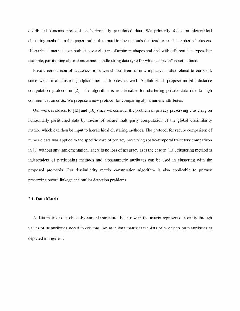
A data matrix is an object-by-variable structure. Each row in the matrix represents an entity through
values of its attributes stored in columns. An m×n data matrix is the data of m objects on n attributes as
depicted in Figure 1.
⎥⎥⎥⎥⎥⎥
⎦
⎤
⎢⎢⎢⎢⎢⎢
⎣
⎡
=
mnmjm
iniji
nj
aaa
aaa
aaa
D
LL
MMMMM
LL
MMMMM
LL
1
1
1111
⎥⎥⎥⎥⎥⎥
⎦
⎤
⎢⎢⎢⎢⎢⎢
⎣
⎡
=
0)2,()1,(0
0)2,3()1,3(0)1,2(
0
LL
MMM
mdistmdist
distdistdist
d
Figure 1. Data matrix D and dissimilarity matrix d
The attributes of objects are not necessarily chosen from the same domain. In this paper, we focus on
categorical, numerical and alphanumerical attributes. Each data type requires different comparison
functions and corresponding protocols. Therefore local data matrices are usually accessed in columns,
denoted as Di for the ith attribute of a data matrix D. Notice that Di is a vector of size m. Size of Di is
denoted as Di.Length.
Data matrix D is said to be horizontally partitioned if rows of D are distributed among different parties.
In that case each party j has its own data matrix, denoted as Dj. Dji denotes the ith column of party j’s data
matrix, Dj.
Data matrix is not normalized in our protocol. We rather choose to normalize the dissimilarity matrix.
The reason is that each horizontal partition may contain values from a different range in which case
another privacy preserving protocol for finding the global minimum and maximum of each attribute
would be required. Normalization on the dissimilarity matrix yields the same effect, without loss of
accuracy and the need for another protocol.
2.2. Dissimilarity Matrix
A dissimilarity matrix is an object-by-object structure. An m×m dissimilarity matrix stores the distance
or dissimilarity between each pair of objects as depicted in Figure 1. Intuitively, the distance of an object
to itself is 0. Also notice that only the entries below the diagonal are filled, since d[i][j] = d[j][i], due to
symmetric nature of the comparison functions.
Each party that holds a horizontal partition of a data matrix D can construct its local dissimilarity
matrix as long as comparison functions for object attributes are public. However privacy preserving
comparison protocols need to be employed in order to calculate an entry d[i][j] of dissimilarity matrix d,
if objects i and j are not held by the same party.
Involved parties construct separate dissimilarity matrices for each attribute in our protocol. Then these
matrices are merged into a single matrix using a weight function on the attributes. The dissimilarity
matrix for attribute i is denoted as di.
2.3. Comparison Functions
The distance between two numeric attributes is simply the absolute value of the difference between
them. Categorical attributes are only compared for equality so that any categorical value is equally distant
to all other values but itself. The distance between alphanumeric attributes is measured in terms of the edit
distance that is heavily used in bioinformatics.
Edit distance algorithm returns the number of operations required to transform a source string into a
target string. Available operations are insertion, deletion and transformation of a character. The algorithm
makes use of the dynamic programming paradigm. An (n+1) × (m+1) matrix is iteratively filled, where n
and m are lengths of source and target strings respectively. Comparison result is symmetric with respect
to the inputs. Details of the algorithm can be found in [2].
Input of the edit distance algorithm need not be the input strings. An n×m equality comparison matrix
for all pairs of characters in source and target strings is equally expressive. We call such matrices
“character comparison matrices” and denote them as CCMST for source string s and target string t.
CCMST[i][j] is 0 if the ith character of s is equal to the jth character of t and non-zero otherwise.
3. Problem Formulation
In this section, we formally define the problem; give details on trust levels of the involved parties and
the amount of preliminary information that must be known by each one.
There are k data holders, such that k ≥ 2, each of which owns a horizontal partition of the data matrix
D, denoted as Dk. These parties want to cluster their data by means of a third party so that the clustering
results will be public to data holders at the end of the protocol. The third party, denoted as TP, does not
have any data but serves as a means of computation power and storage space. Third party’s duty in the
protocol is to govern the communication between data holders, construct the dissimilarity matrix and
publish clustering results to data holders.
Every party, including the third party, is semi-trusted, that is to say, they follow the protocol as they
are supposed to but may store any data that is revealed to them in order to infer private information in the
future. Semi-trusted behavior is also called honest-but-curious behavior. Involved parties are also
assumed to be non-colluding.
Every data holder and the third party must have access to the comparison functions so that they can
compute distance/dissimilarity between objects. Data holders are supposed to have agreed on the list of
attributes that are going to be used for clustering beforehand. This attribute list is also shared with the
third party so that TP can run appropriate comparison functions for different data types.
At the end of the protocol, the third party will have constructed the dissimilarity matrices for each
attribute separately. These dissimilarity matrices are weighted using a weight vector sent by data holders
such that the final dissimilarity matrix is built. Then the third party runs a hierarchical clustering
algorithm on the final dissimilarity matrix and publishes the results. Every data holder can impose a
different weight vector and clustering algorithm of its own choice.

4. Comparison Protocols
As described in Section 2.2, dissimilarity matrix, d, is an object-by-object structure in which d[i][j] is
the distance between objects i and j. Now consider an entry in d, d[i][j]: If both objects are held by the
same data holder, the third party need not intervene in the computation of the distance between objects i
and j. The data holder that has these objects simply computes the distance between them and sends the
result to the third party. However, if objects i and j are from different parties, a privacy preserving
comparison protocol must be employed between owners of these objects. It follows from this distinction
that, in order to construct the dissimilarity matrix, each data holder must send its local dissimilarity matrix
to the third party and also run a privacy preserving comparison protocol with every other data holder.
Evidently, if there are k data holders, comparison protocol for each attribute must be repeated C(k, 2)
times, for every pair of data holders.
In this section we describe the comparison protocols for numeric, alphanumeric and categorical
attributes that will be the building blocks of the dissimilarity matrix construction algorithm explained in
the next section. Security and communication cost analysis of the protocols are provided right after the
protocols are presented.
4.1. Numeric Attributes
Distance function for numeric attributes is the absolute value of the difference between the values,
formally:
distance(x, y) = | x – y |.
There are three participants of the protocol: data holders DHJ and DHK, and the third party, TP. DHJ
and DHK share a secret number rJ K that will be used as the seed of a pseudo-random number generator,
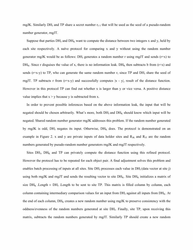
rngJK. Similarly DHJ and TP share a secret number rJ T that will be used as the seed of a pseudo-random
number generator, rngJT.
Suppose that parties DHJ and DHK want to compute the distance between two integers x and y, held by
each site respectively. A naïve protocol for comparing x and y without using the random number
generator rngJK would be as follows: DHJ generates a random number r using rngJT and sends (r+x) to
DHK. Since r disguises the value of x, there is no information leak. DHK then subtracts b from (r+x) and
sends (r+x-y) to TP, who can generate the same random number r, since TP and DHJ share the seed of
rngJT. TP subtracts r from (r+x-y) and successfully computes |x - y|, result of the distance function.
However in this protocol TP can find out whether x is larger than y or vice versa. A positive distance
value implies that x > y because y is subtracted from x.
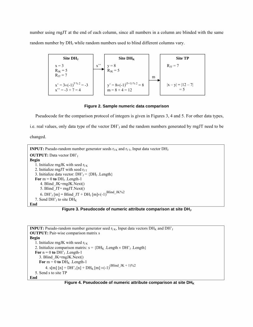
In order to prevent possible inferences based on the above information leak, the input that will be
negated should be chosen arbitrarily. What’s more, both DHJ and DHK should know which input will be
negated. Shared random number generator rngJK addresses this problem. If the random number generated
by rngJK is odd, DHJ negates its input. Otherwise, DHK does. The protocol is demonstrated on an
example in Figure 2. x and y are private inputs of data holder sites and RJK and RJT are the random
numbers generated by pseudo-random number generators rngJK and rngJT respectively.
Sites DHJ, DHK and TP can privately compute the distance function using this refined protocol.
However the protocol has to be repeated for each object pair. A final adjustment solves this problem and
enables batch processing of inputs at all sites. Site DHJ processes each value in DHJ (data vector at site j)
using both rngJK and rngJT and sends the resulting vector to site DHK. Site DHK initializes a matrix of
size DHK .Length × DHJ .Length to be sent to site TP. This matrix is filled column by column, each
column containing intermediary comparison values for an input from DHJ against all inputs from DHK. At
the end of each column, DHK creates a new random number using rngJK to preserve consistency with the
oddness/evenness of the random numbers generated at site DHJ. Finally, site TP, upon receiving this
matrix, subtracts the random numbers generated by rngJT. Similarly TP should create a new random
number using rngJT at the end of each column, since all numbers in a column are blinded with the same
random number by DHJ while random numbers used to blind different columns vary.
x = 3 RJK = 5 RJT = 7 x’ = 3×(-1)5 % 2 = -3 x’’ = -3 + 7 = 4
y = 8 RJK = 5 y’ = 8×(-1)(5+1) % 2 = 8 m = 8 + 4 = 12
RJT = 7 |x – y| = |12 – 7| = 5
x’’
m
Site DHJ Site DHK Site TP
Figure 2. Sample numeric data comparison
Pseudocode for the comparison protocol of integers is given in Figures 3, 4 and 5. For other data types,
i.e. real values, only data type of the vector DH’J and the random numbers generated by rngJT need to be
changed.
INPUT: Pseudo-random number generator seeds rJ K and rJ T, Input data vector DHJ
OUTPUT: Data vector DH’JBegin 1. Initialize rngJK with seed rJ K 2. Initialize rngJT with seed rJ T 3. Initialize data vector: DH’J = {DHJ .Length} For m = 0 to DHJ .Length-1 4. Blind_JK=rngJK.Next() 5. Blind_JT= rngJT.Next() 6. DH’J [m] = Blind_JT + DHJ [m]×(-1)Blind_JK%2
7. Send DH’J to site DHKEnd
Figure 3. Pseudocode of numeric attribute comparison at site DHJ
INPUT: Pseudo-random number generator seed rJ K, Input data vectors DHK and DH’J OUTPUT: Pair-wise comparison matrix s Begin 1. Initialize rngJK with seed rJ K
2. Initialize comparison matrix: s = {DHK .Length × DH’J .Length} For n = 0 to DH’J .Length-1 3. Blind_JK=rngJK.Next() For m = 0 to DHK .Length-1 4. s[m] [n] = DH’J [n] + DHK [m] ×(-1)(Blind_JK + 1)%2
5. Send s to site TP End
Figure 4. Pseudocode of numeric attribute comparison at site DHK
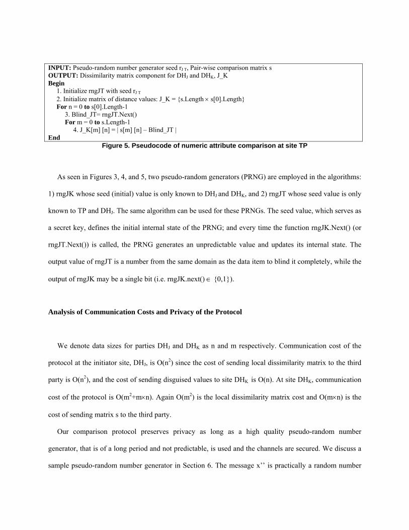
INPUT: Pseudo-random number generator seed rJ T, Pair-wise comparison matrix s OUTPUT: Dissimilarity matrix component for DHJ and DHK, J_K Begin 1. Initialize rngJT with seed rJ T
2. Initialize matrix of distance values: J_K = {s.Length × s[0].Length} For n = 0 to s[0].Length-1 3. Blind_JT= rngJT.Next() For m = 0 to s.Length-1 4. J_K[m] [n] = | s[m] [n] – Blind_JT | End
Figure 5. Pseudocode of numeric attribute comparison at site TP
As seen in Figures 3, 4, and 5, two pseudo-random generators (PRNG) are employed in the algorithms:
1) rngJK whose seed (initial) value is only known to DHJ and DHK, and 2) rngJT whose seed value is only
known to TP and DHJ. The same algorithm can be used for these PRNGs. The seed value, which serves as
a secret key, defines the initial internal state of the PRNG; and every time the function rngJK.Next() (or
rngJT.Next()) is called, the PRNG generates an unpredictable value and updates its internal state. The
output value of rngJT is a number from the same domain as the data item to blind it completely, while the
output of rngJK may be a single bit (i.e. rngJK.next() ∈ {0,1}).
Analysis of Communication Costs and Privacy of the Protocol
We denote data sizes for parties DHJ and DHK as n and m respectively. Communication cost of the
protocol at the initiator site, DHJ, is O(n2) since the cost of sending local dissimilarity matrix to the third
party is O(n2), and the cost of sending disguised values to site DHK is O(n). At site DHK, communication
cost of the protocol is O(m2+m×n). Again O(m2) is the local dissimilarity matrix cost and O(m×n) is the
cost of sending matrix s to the third party.
Our comparison protocol preserves privacy as long as a high quality pseudo-random number
generator, that is of a long period and not predictable, is used and the channels are secured. We discuss a
sample pseudo-random number generator in Section 6. The message x’’ is practically a random number
for party DHK since the pseudo-random number generated using rngJT is not available. Inference by TP,
using message m, is not possible since given ±(x-y) there are infinitely many points that are | x –y | apart
from each other. The same idea is used and explained in detail in Section 5.
We now explain the reason why secure channels must be used. TP can predict the values of both x and
y if it listens the channel between DHJ and DHK. Notice that x’’ = r ± x and TP knows the value of r.
Therefore it infers that the value of x is either (x’’– r) or (r – x’’). For each possible value of x, y can take
two values: either (x – | x – y |) or (x + | x – y |). In order to prevent such inferences, the channel
between DHJ and DHK must be secured. Another threat is eavesdropping by DHJ on the channel between
DHK and TP. This channel carries the message m = r ± (x – y) and DHJ knows the values of both r and x.
Therefore this channel must be secured as well.
Although comparing a pair of numeric inputs using our protocol preserves privacy, as shown above,
comparing many pairs at once introduces a threat of privacy breaches by means of a frequency analysis
attack by the third party, TP. Notice that ith column of the pair-wise comparison matrix s, received by TP
from DHK, is “private data vector of DHK” plus “identity vector times (ith input of DHJ – ith random
number of rngJT)” or negation of the expression. If the range of values for numeric attributes is limited
and there is enough statistics to realize a frequency attack, TP can infer input values of site DHK. In such
cases, site DHK can request omitting batch processing of inputs and using unique random numbers for
each object pair.
4.2. Alphanumeric Attributes
Alphanumeric attributes are compared in terms of the edit distance. Similar to the comparison protocol
for numeric attributes, two data holder parties and a third party are involved in the protocol. While data
holders DHJ and DHK build their local dissimilarity matrices using the edit distance algorithm, third party
cannot use this algorithm to compare inputs from distinct data sources since input strings, source and
target, are private information in the latter case. Therefore we devise a new protocol below, which allows
the third party to securely compute the distance between all inputs of data holders. The idea behind the
protocol is privately building a character comparison matrix (CCM), as explained in Section 2.3.
Alphabet of the strings that are to be compared is assumed to be finite. This assumption enables
modulo operations on alphabet size, such that addition of a random number and a character is another
alphabet character.
The third party and data holder party DHJ shares a secret number which will be seed of a pseudo-
random number generator. In order to compare a string s at site DHJ with a string t at site DHK, DHJ first
generates a random vector of size s.Length and adds this random vector to s. The outcome, denoted as s’,
is practically a random vector for DHK. DHJ sends s’ to DHK, who generates t.Length copies of s’ and
builds a matrix of size (t.Length)×(s’.Length). Then DHK subtracts its input, t, from every column of the
matrix and sends the resultant matrix to the third party. The third party can generate the same pseudo-
random numbers as DHJ since they share the seed to the generator. Finally the third party generates the
same random vector of size s’.Length as DHJ did and subtracts this vector from every row of the matrix
received from DHK to obtain the CCM for s and t.
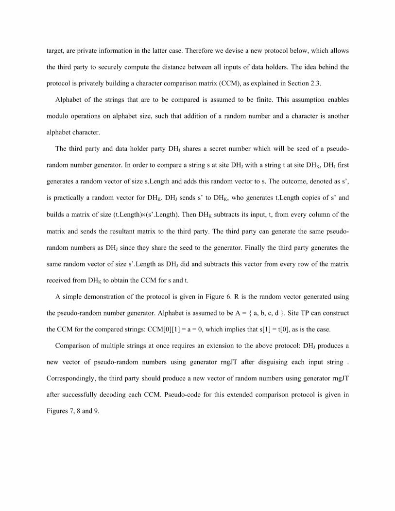
A simple demonstration of the protocol is given in Figure 6. R is the random vector generated using
the pseudo-random number generator. Alphabet is assumed to be A = { a, b, c, d }. Site TP can construct
the CCM for the compared strings: CCM[0][1] = a = 0, which implies that s[1] = t[0], as is the case.
Comparison of multiple strings at once requires an extension to the above protocol: DHJ produces a
new vector of pseudo-random numbers using generator rngJT after disguising each input string .
Correspondingly, the third party should produce a new vector of random numbers using generator rngJT
after successfully decoding each CCM. Pseudo-code for this extended comparison protocol is given in
Figures 7, 8 and 9.
Site DHJ Site DHK Site TP
S = “abc” R = “013” S’ = “acb ”
T = “bd”
M = ⎥⎦
⎤⎢⎣
⎡−−−−−−
dbdcdabbbcba = ⎥
⎦
⎤⎢⎣
⎡cdbabd
R = “013”
CCM = ⎥⎦
⎤⎢⎣
⎡−−−−−−
310310
cdbabd
= ⎥⎦
⎤⎢⎣
⎡dcbbad
S’
M
Figure 6. Sample alphanumeric data comparison
Analysis of Communication Costs and Privacy of the Protocol
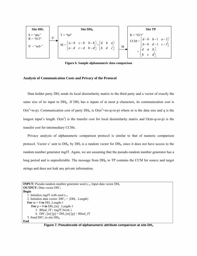
Data holder party DHJ sends its local dissimilarity matrix to the third party and a vector of exactly the
same size of its input to DHK. If DHJ has n inputs of at most p characters, its communication cost is
O(n2+n×p). Communication cost of party DHK is O(m2+m×q×n×p) where m is the data size and q is the
longest input’s length. O(m2) is the transfer cost for local dissimilarity matrix and O(m×q×n×p) is the
transfer cost for intermediary CCMs.
Privacy analysis of alphanumeric comparison protocol is similar to that of numeric comparison
protocol. Vector s’ sent to DHK by DHJ is a random vector for DHK since it does not have access to the
random number generator rngJT. Again, we are assuming that the pseudo-random number generator has a
long period and is unpredictable. The message from DHK to TP contains the CCM for source and target
strings and does not leak any private information.
INPUT: Pseudo-random number generator seed rJ T, Input data vector DHJOUTPUT: Data vector DH’JBegin 1. Initialize rngJT with seed rJ T 2. Initialize data vector: DH’J = {DHJ . Length} For m = 0 to DHJ .Length-1 For p = 0 to DHJ [m] . Length-1
3. Blind_JT= rngJT.Next( ) 4. DH’J [m] [p] = DHJ [m] [p] + Blind_JT 5. Send DH’J to site DHKEnd
Figure 7. Pseudocode of alphanumeric attribute comparison at site DHJ
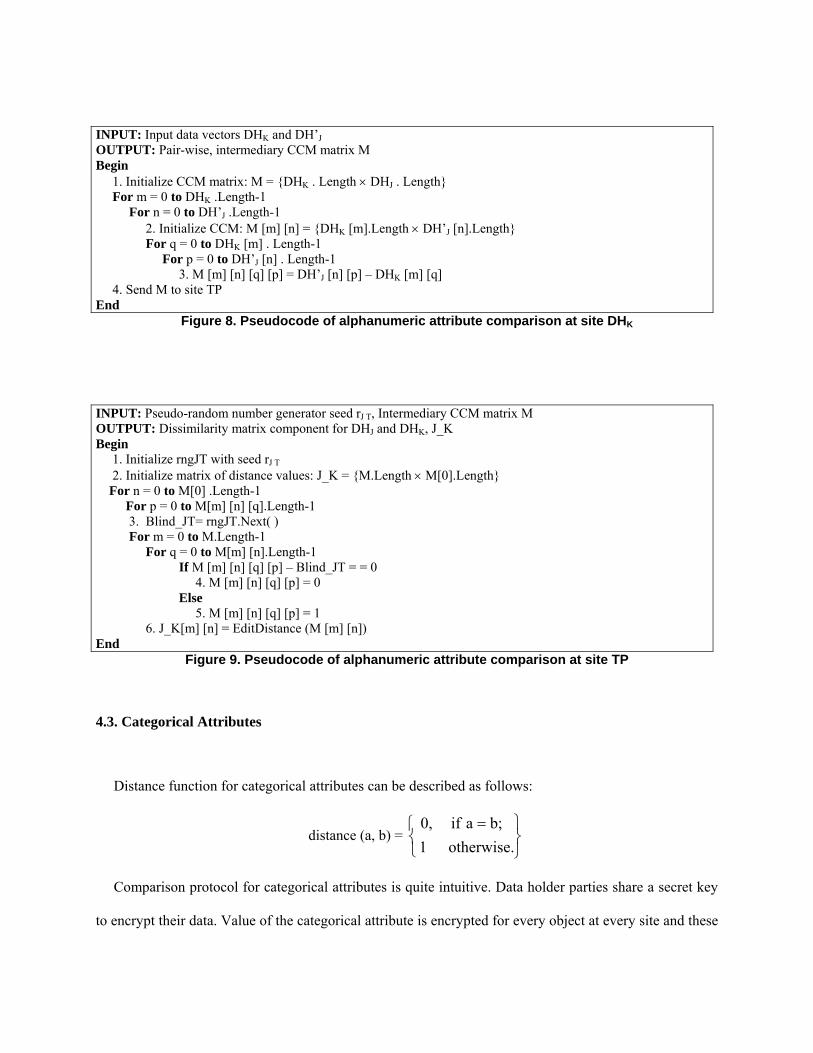
INPUT: Input data vectors DHK and DH’JOUTPUT: Pair-wise, intermediary CCM matrix M Begin 1. Initialize CCM matrix: M = {DHK . Length × DHJ . Length} For m = 0 to DHK .Length-1 For n = 0 to DH’J .Length-1 2. Initialize CCM: M [m] [n] = {DHK [m].Length × DH’J [n].Length} For q = 0 to DHK [m] . Length-1 For p = 0 to DH’J [n] . Length-1 3. M [m] [n] [q] [p] = DH’J [n] [p] – DHK [m] [q] 4. Send M to site TP End
Figure 8. Pseudocode of alphanumeric attribute comparison at site DHK
INPUT: Pseudo-random number generator seed rJ T, Intermediary CCM matrix M OUTPUT: Dissimilarity matrix component for DHJ and DHK, J_K Begin 1. Initialize rngJT with seed rJ T
2. Initialize matrix of distance values: J_K = {M.Length × M[0].Length} For n = 0 to M[0] .Length-1 For p = 0 to M[m] [n] [q].Length-1 3. Blind_JT= rngJT.Next( ) For m = 0 to M.Length-1 For q = 0 to M[m] [n].Length-1 If M [m] [n] [q] [p] – Blind_JT = = 0 4. M [m] [n] [q] [p] = 0 Else 5. M [m] [n] [q] [p] = 1 6. J_K[m] [n] = EditDistance (M [m] [n]) End
Figure 9. Pseudocode of alphanumeric attribute comparison at site TP
4.3. Categorical Attributes
Distance function for categorical attributes can be described as follows:
distance (a, b) = ⎭⎬⎫
⎩⎨⎧ =
otherwise. 1 b;a if 0,
Comparison protocol for categorical attributes is quite intuitive. Data holder parties share a secret key
to encrypt their data. Value of the categorical attribute is encrypted for every object at every site and these
encrypted data are sent to the third party, who can easily compute the distance between categorical
attributes of any pair of objects. If ciphertext of two categorical values are the same, then plaintexts must
be the same. Third party merges encrypted data and runs the local dissimilarity matrix construction
algorithm in Figure 10. Outcome is not a local dissimilarity matrix for the categorical attribute, since data
from all parties is input to the algorithm.
Analysis of Communication Costs and Privacy of the Protocol
Each party sends its data in encrypted format, therefore communication cost for a party with n objects
is O(n).
The third party cannot infer any private information unless the encryption key is available. However
this is not possible since data holders and the third party are non-colluding and semi-honest.
5. Dissimilarity Matrix Construction
In this section, we explain how to build dissimilarity matrices for different data types using the
comparison protocols of Section 4. The third party should run the appropriate construction algorithm for
every attribute in the list of attributes chosen for clustering such that a corresponding dissimilarity matrix
is built.
Construction algorithm for numeric and alphanumeric attributes are essentially the same. Every data
holder first builds his local dissimilarity matrix using the algorithm in Figure 10 and sends the result to
the third party. Then for each pair of data holders, the comparison protocol of the attribute is carried out.
Finally the third party merges all portions of the dissimilarity matrix from local matrices and comparison
protocol outputs. The process ends after a normalization step that scales distance values into [0, 1]
interval. Details of the algorithm are given in Figure 11.
Publishing local dissimilarity matrices does not cause private information leakage as proven in [13].
The proof relies on the fact that given the distance between two secret points, there are infinitely many
pairs of points that are equally distant. Unless there is an inference channel that helps finding out one of
these points, dissimilarity matrix sharing does not result in privacy breaches.
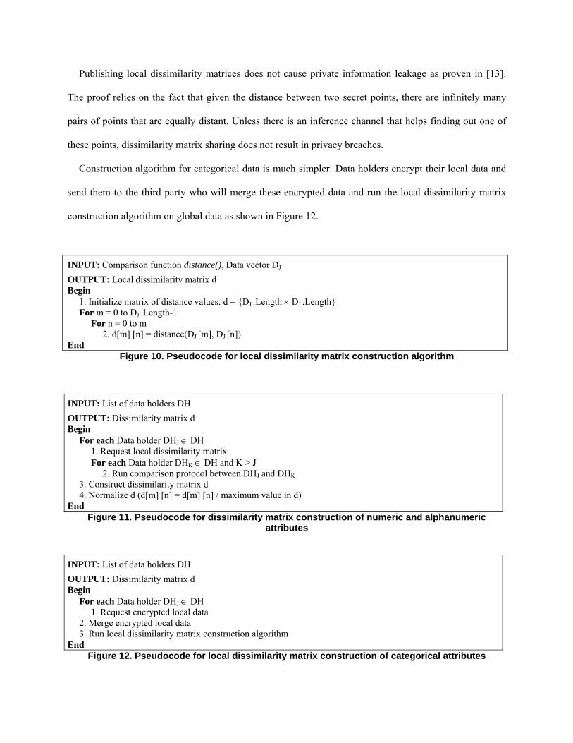
Construction algorithm for categorical data is much simpler. Data holders encrypt their local data and
send them to the third party who will merge these encrypted data and run the local dissimilarity matrix
construction algorithm on global data as shown in Figure 12.
INPUT: Comparison function distance(), Data vector DJ
OUTPUT: Local dissimilarity matrix d Begin 1. Initialize matrix of distance values: d = {DJ .Length × DJ .Length} For m = 0 to DJ .Length-1 For n = 0 to m 2. d[m] [n] = distance(DJ [m], DJ [n]) End
Figure 10. Pseudocode for local dissimilarity matrix construction algorithm
INPUT: List of data holders DH OUTPUT: Dissimilarity matrix d Begin For each Data holder DHJ ∈ DH 1. Request local dissimilarity matrix For each Data holder DHK ∈ DH and K > J 2. Run comparison protocol between DHJ and DHK 3. Construct dissimilarity matrix d 4. Normalize d (d[m] [n] = d[m] [n] / maximum value in d) End
Figure 11. Pseudocode for dissimilarity matrix construction of numeric and alphanumeric attributes
INPUT: List of data holders DH OUTPUT: Dissimilarity matrix d Begin For each Data holder DHJ ∈ DH 1. Request encrypted local data 2. Merge encrypted local data 3. Run local dissimilarity matrix construction algorithm End
Figure 12. Pseudocode for local dissimilarity matrix construction of categorical attributes
Upon the construction of dissimilarity matrices for all attributes, third party notifies the data holders,
asking for their attribute weight vectors and hierarchical clustering algorithm choices. Then dissimilarity
matrices of attributes are merged into a final dissimilarity matrix, which will be input to the appropriate
clustering algorithm.
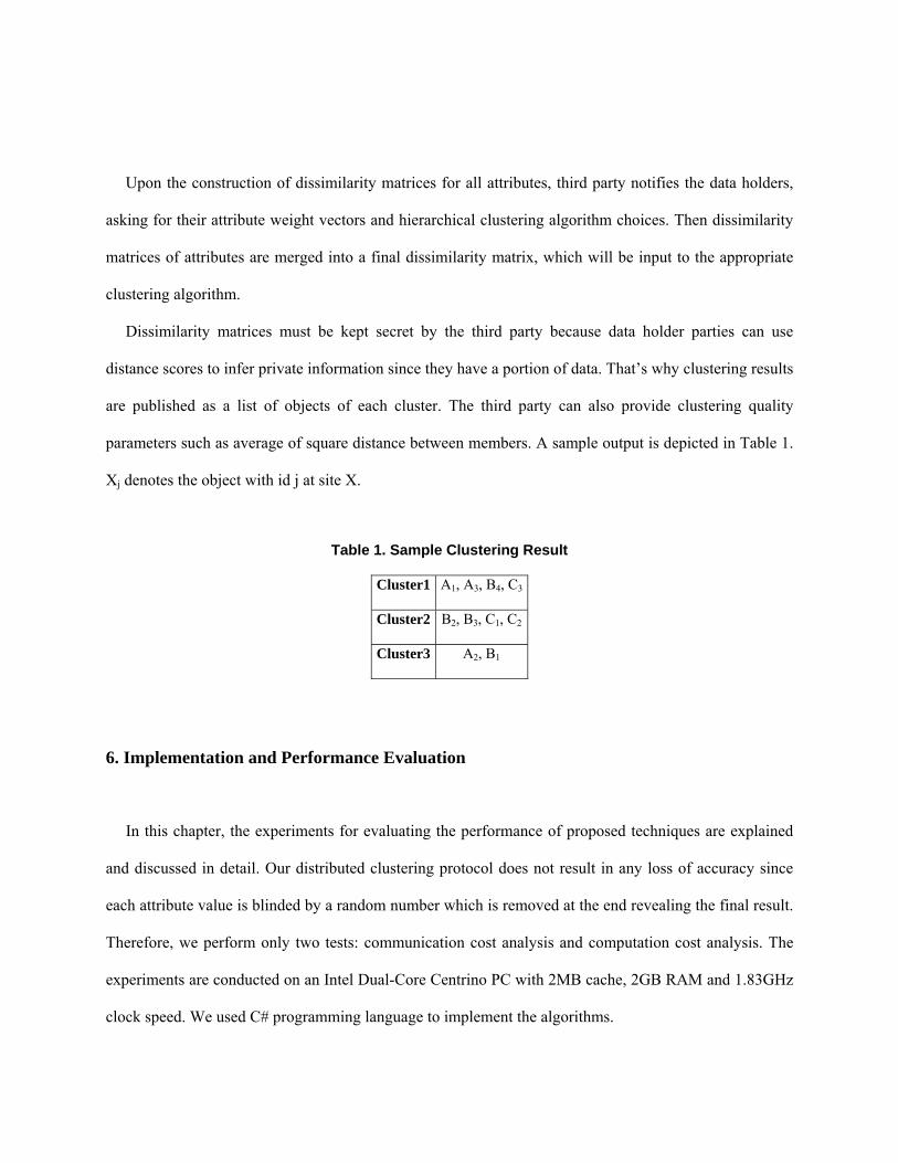
Dissimilarity matrices must be kept secret by the third party because data holder parties can use
distance scores to infer private information since they have a portion of data. That’s why clustering results
are published as a list of objects of each cluster. The third party can also provide clustering quality
parameters such as average of square distance between members. A sample output is depicted in Table 1.
Xj denotes the object with id j at site X.
Table 1. Sample Clustering Result
Cluster1 A1, A3, B4, C3
Cluster2 BB2, B3, C1, C2
Cluster3 A2, B1
6. Implementation and Performance Evaluation
In this chapter, the experiments for evaluating the performance of proposed techniques are explained
and discussed in detail. Our distributed clustering protocol does not result in any loss of accuracy since
each attribute value is blinded by a random number which is removed at the end revealing the final result.
Therefore, we perform only two tests: communication cost analysis and computation cost analysis. The
experiments are conducted on an Intel Dual-Core Centrino PC with 2MB cache, 2GB RAM and 1.83GHz
clock speed. We used C# programming language to implement the algorithms.
6.1. Experimental Setup
Three test cases are identified to measure the performance of the proposed distributed clustering
protocol. In these test cases we use different values for (1) total number of entities (total database size),
(2) average length of alphanumeric attributes, and (3) number of data holders. The test cases are applied
over numeric and alphanumeric attributes to show performance of our protocol over different attribute
types. For numeric attributes, we use two different data types: integer and double. However test results for
these two data types for numeric attributes are similar; hence due to space consideration, only test results
for double data type are included.
For each experiment, we measure the communication and computation overhead of our protocol
against a baseline protocol, where no privacy protection method is employed. In the baseline protocol,
private information of each data holder is sent to the third party as plaintext without any protection (e.g.
blinding or encryption). The third party forms dissimilarity matrices using that information. The baseline
protocol and our protocol only differ in the formation of the global dissimilarity matrix. After global
dissimilarity matrix is formed, a clustering algorithm takes this matrix as input and the clustering is
performed the same way in both baseline protocol and the proposed protocol. Therefore, comparisons of
these protocols in the experiments are done with respect to formation of the global dissimilarity matrices
and clustering is not taken into consideration. For all the experiments, we denote our protocol as
“protocol” and the baseline protocol as “baseline” in the figures. Except for the experiments on the
number of data holders, we partitioned the generated datasets into two by distributing them into two
datasets evenly so that each data holder has a balanced share.
For test case (1), we used total database sizes of 2K, 4K, 6K, 8K and 10K. Test case (2) shows the
behavior of the baseline protocol and our protocol for varying average lengths of the alphanumeric
attribute which are 5, 10, 15, 20, and 25. In test case (3), number of data holders, excluding the third
party, is 2, 4, 6, 8, and 10.
For each test case, we first use synthetically generated datasets. Synthetic datasets are more
appropriate for our experiments since we try to evaluate scalability and efficiency of our protocol for
varying parameters, and synthetic datasets can be generated by controlling the number of entities, number
of data holders, and average length of attributes. Data generator is developed in Eclipse Java environment.
For the numeric attributes, each entity is chosen from the interval [0, 10000] uniformly, where precision
for double data type is set to three. For alphanumeric attributes, we created sequence of characters whose
length is chosen in accordance with normal distribution, the mean value being equal to average length of
the attribute and alphabet size is equal to four. The reason for choosing alphabet size as four is to imitate
behavior of DNA data in our experiments.
We also use KDD’99 Network Intrusion Detection stream dataset [7] to show the performance of our
protocol over real datasets. We chose ‘src_bytes’ attribute of this dataset as our target attribute, which is
numeric. To make tests over real numeric datasets compatible with tests over synthetic datasets, we divide
real datasets into datasets of size 2K, 4K, 6K, 8K and 10K.
In our experiments, we use Advanced Encryption Standard (AES) cipher to generate pseudo-random
numbers to hide data holders’ inputs. AES is originally a block cipher algorithm; however it can be used
as a PRNG when used in output feedback (OFB) mode. Block ciphers in OFB mode, in general, produces
unpredictable sequence of bits and are strong against statistical attacks. For our experiments, we use
Cryptography namespace of MS .Net platform to perform AES encryption in the implementation of our
protocol. Seeds for pseudo-random number generator shared between data holders are used as keys for
encryption of a initialization vector (IV) globally known to every data holder, and the resulting ciphertext
is used as the pseudo-random number. For the next random number generation, random number
(ciphertext) generated in the previous step is used as the message (plaintext) to be encrypted which yields
the next random number as a result. In our implementation, we use 128 bits AES encryption which means
shared pseudo-random number generator seeds have a length of 128 bits. We preferred AES for sake of
simplicity and safety. Nevertheless, a faster PRNG based on a stream cipher (such as SEAL) can also be
used to decrease the overhead in the computation complexity of the proposed protocol.
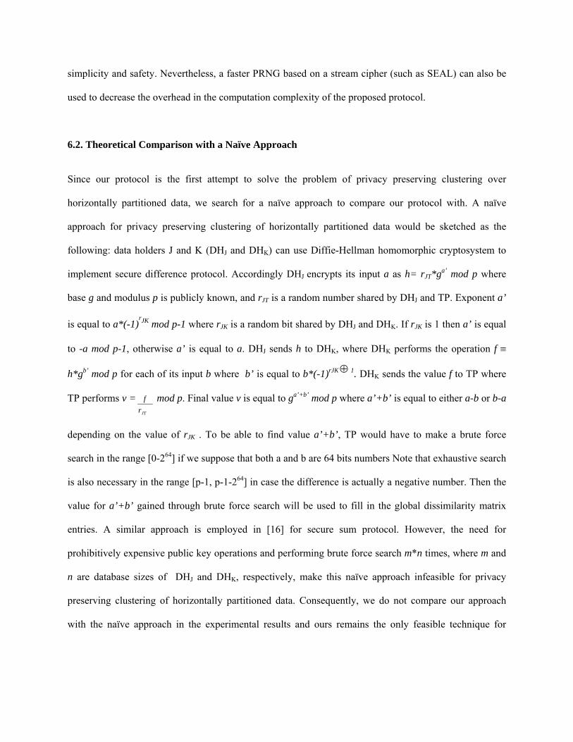
6.2. Theoretical Comparison with a Naïve Approach
Since our protocol is the first attempt to solve the problem of privacy preserving clustering over
horizontally partitioned data, we search for a naïve approach to compare our protocol with. A naïve
approach for privacy preserving clustering of horizontally partitioned data would be sketched as the
following: data holders J and K (DHJ and DHK) can use Diffie-Hellman homomorphic cryptosystem to
implement secure difference protocol. Accordingly DHJ encrypts its input a as h= rJT*ga’ mod p where
base g and modulus p is publicly known, and rJT is a random number shared by DHJ and TP. Exponent a’
is equal to a*(-1)rJK mod p-1 where rJK is a random bit shared by DHJ and DHK. If rJK is 1 then a’ is equal
to -a mod p-1, otherwise a’ is equal to a. DHJ sends h to DHK, where DHK performs the operation f ≡
h*gb’ mod p for each of its input b where b’ is equal to b*(-1)rJK⊕ 1. DHK sends the value f to TP where
TP performs v =JTrf mod p. Final value v is equal to ga’+b’ mod p where a’+b’ is equal to either a-b or b-a
depending on the value of rJK . To be able to find value a’+b’, TP would have to make a brute force
search in the range [0-264] if we suppose that both a and b are 64 bits numbers Note that exhaustive search
is also necessary in the range [p-1, p-1-264] in case the difference is actually a negative number. Then the
value for a’+b’ gained through brute force search will be used to fill in the global dissimilarity matrix
entries. A similar approach is employed in [16] for secure sum protocol. However, the need for
prohibitively expensive public key operations and performing brute force search m*n times, where m and
n are database sizes of DHJ and DHK, respectively, make this naïve approach infeasible for privacy
preserving clustering of horizontally partitioned data. Consequently, we do not compare our approach
with the naïve approach in the experimental results and ours remains the only feasible technique for
privacy preserving clustering of horizontally partitioned data, which will hopefully serve as a benchmark
for future research.
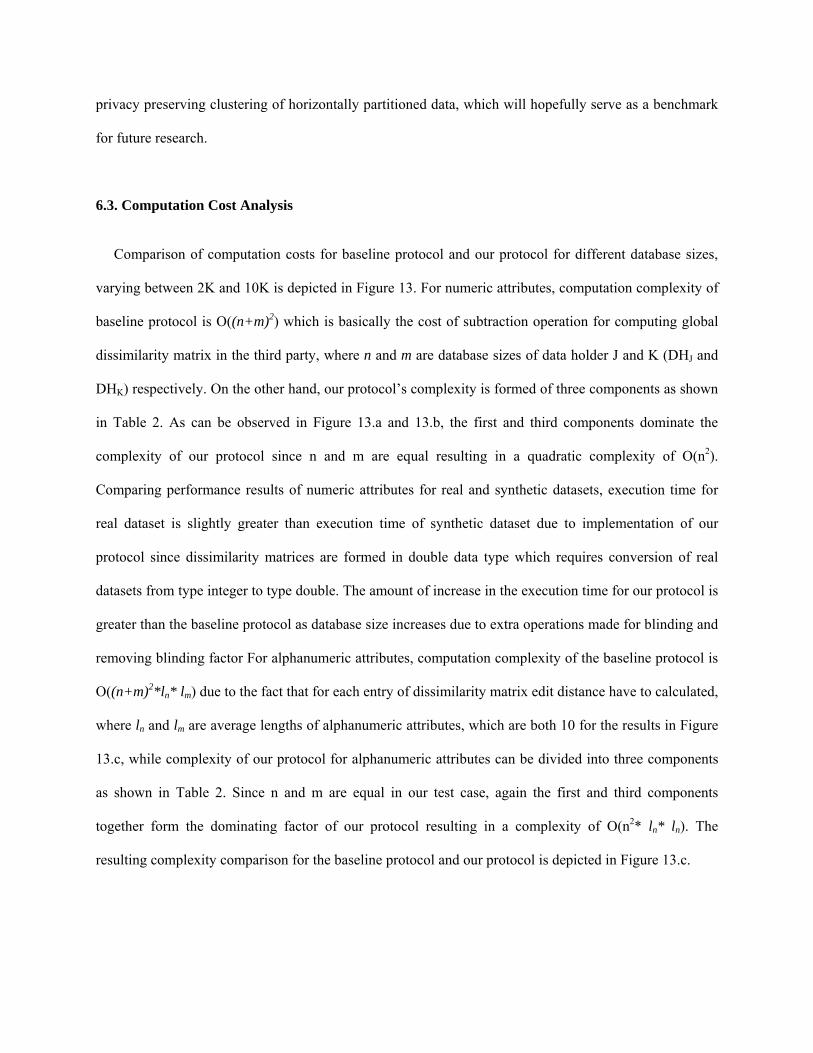
6.3. Computation Cost Analysis
Comparison of computation costs for baseline protocol and our protocol for different database sizes,
varying between 2K and 10K is depicted in Figure 13. For numeric attributes, computation complexity of
baseline protocol is O((n+m)2) which is basically the cost of subtraction operation for computing global
dissimilarity matrix in the third party, where n and m are database sizes of data holder J and K (DHJ and
DHK) respectively. On the other hand, our protocol’s complexity is formed of three components as shown
in Table 2. As can be observed in Figure 13.a and 13.b, the first and third components dominate the
complexity of our protocol since n and m are equal resulting in a quadratic complexity of O(n2).
Comparing performance results of numeric attributes for real and synthetic datasets, execution time for
real dataset is slightly greater than execution time of synthetic dataset due to implementation of our
protocol since dissimilarity matrices are formed in double data type which requires conversion of real
datasets from type integer to type double. The amount of increase in the execution time for our protocol is
greater than the baseline protocol as database size increases due to extra operations made for blinding and
removing blinding factor For alphanumeric attributes, computation complexity of the baseline protocol is
O((n+m)2*ln* lm) due to the fact that for each entry of dissimilarity matrix edit distance have to calculated,
where ln and lm are average lengths of alphanumeric attributes, which are both 10 for the results in Figure
13.c, while complexity of our protocol for alphanumeric attributes can be divided into three components
as shown in Table 2. Since n and m are equal in our test case, again the first and third components
together form the dominating factor of our protocol resulting in a complexity of O(n2* ln* ln). The
resulting complexity comparison for the baseline protocol and our protocol is depicted in Figure 13.c.
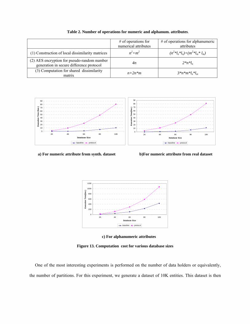
Table 2. Number of operations for numeric and alphanum. attributes.
# of operations for numerical attributes
# of operations for alphanumeric attributes
(1) Construction of local dissimilarity matrices n2+m2 (n2*ln*ln)+(m2*lm* lm)
(2) AES encryption for pseudo-random number generation in secure difference protocol 4n 2*n*ln
(3) Computation for shared dissimilarity matrix n+2n*m 3*n*m*ln*lm
0
10
20
30
40
50
60
70
80
90
2K 4K 6K 8K 10K
Database Size
Exec
utio
n Ti
me
(Sec
.)
baseline protocol
0
10
20
30
40
50
60
70
80
90
2K 4K 6K 8K 10K
Database Size
Exec
utio
n Ti
me(
Sec
.)
baseline protocol
a) For numeric attribute from synth. dataset b)For numeric attribute from real dataset
0
200
400
600
800
1000
1200
2K 4K 6K 8K 10K
Database Size
Exe
cutio
n Ti
me(
Sec
.)
baseline protocol
c) For alphanumeric attributes
Figure 13. Computation cost for various database sizes
One of the most interesting experiments is performed on the number of data holders or equivalently,
the number of partitions. For this experiment, we generate a dataset of 10K entities. This dataset is then
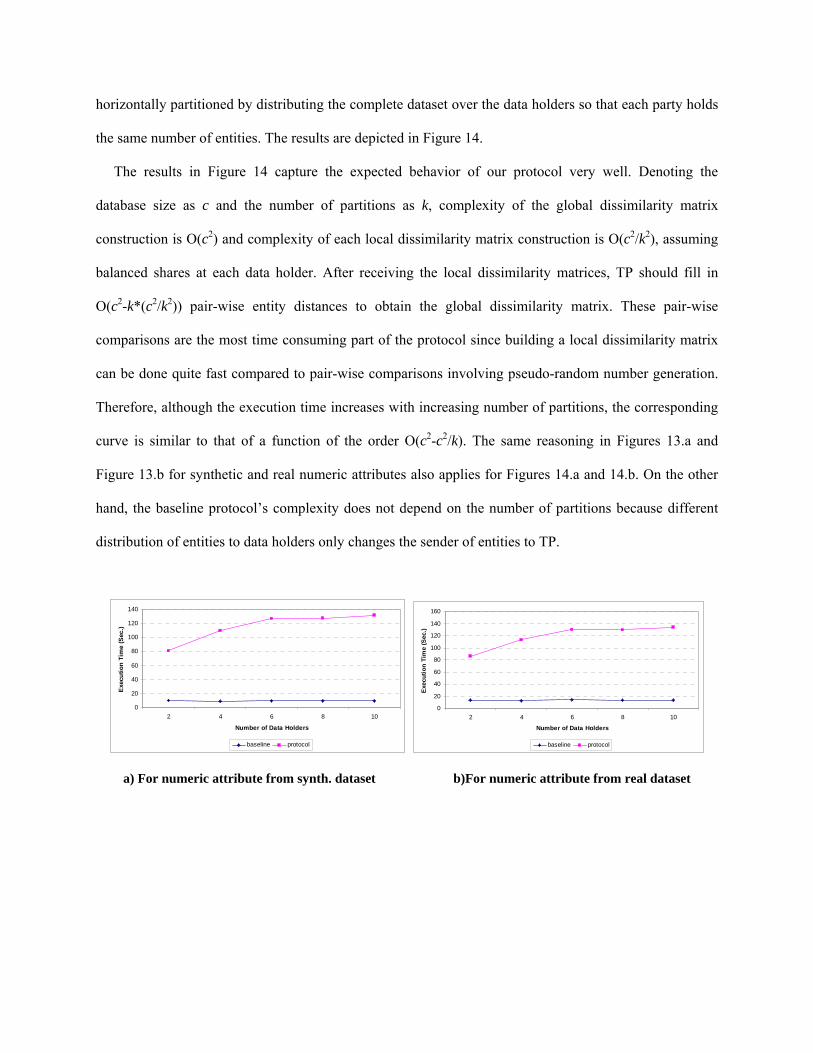
horizontally partitioned by distributing the complete dataset over the data holders so that each party holds
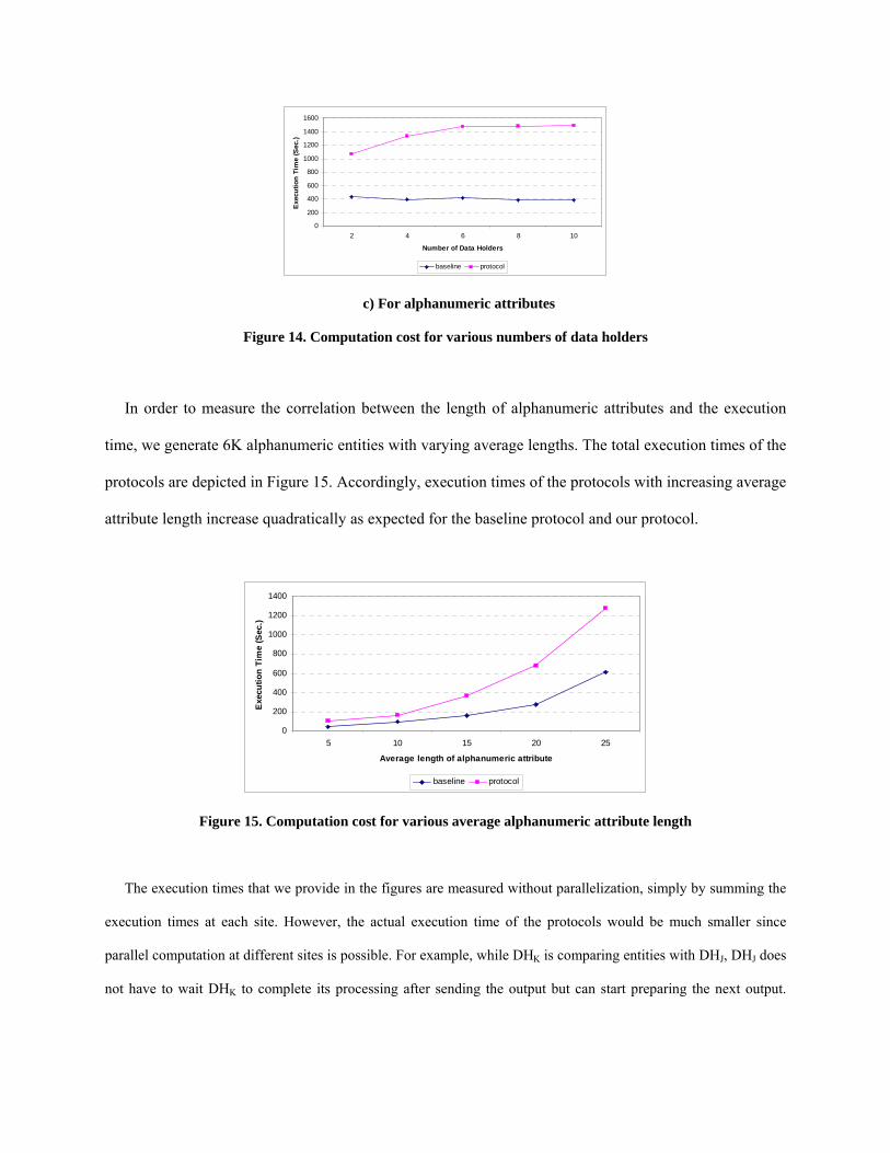
the same number of entities. The results are depicted in Figure 14.
The results in Figure 14 capture the expected behavior of our protocol very well. Denoting the
database size as c and the number of partitions as k, complexity of the global dissimilarity matrix
construction is O(c2) and complexity of each local dissimilarity matrix construction is O(c2/k2), assuming
balanced shares at each data holder. After receiving the local dissimilarity matrices, TP should fill in
O(c2-k*(c2/k2)) pair-wise entity distances to obtain the global dissimilarity matrix. These pair-wise
comparisons are the most time consuming part of the protocol since building a local dissimilarity matrix
can be done quite fast compared to pair-wise comparisons involving pseudo-random number generation.
Therefore, although the execution time increases with increasing number of partitions, the corresponding
curve is similar to that of a function of the order O(c2-c2/k). The same reasoning in Figures 13.a and
Figure 13.b for synthetic and real numeric attributes also applies for Figures 14.a and 14.b. On the other
hand, the baseline protocol’s complexity does not depend on the number of partitions because different
distribution of entities to data holders only changes the sender of entities to TP.
0
20
40
60
80
100
120
140
2 4 6 8 10
Number of Data Holders
Exe
cutio
n Ti
me
(Sec
.)
baseline protocol
0
20
40
60
80
100
120
140
160
2 4 6 8 10
Number of Data Holders
Exe
cutio
n Ti
me
(Sec
.)
baseline protocol
a) For numeric attribute from synth. dataset b)For numeric attribute from real dataset
0
200
400
600
800
1000
1200
1400
1600
2 4 6 8 10
Number of Data Holders
Exec
utio
n Ti
me
(Sec
.)
baseline protocol
c) For alphanumeric attributes
Figure 14. Computation cost for various numbers of data holders
In order to measure the correlation between the length of alphanumeric attributes and the execution
time, we generate 6K alphanumeric entities with varying average lengths. The total execution times of the
protocols are depicted in Figure 15. Accordingly, execution times of the protocols with increasing average
attribute length increase quadratically as expected for the baseline protocol and our protocol.
0
200
400
600
800
1000
1200
1400
5 10 15 20 25
Average length of alphanumeric attribute
Exe
cutio
n Ti
me
(Sec
.)
baseline protocol
Figure 15. Computation cost for various average alphanumeric attribute length
The execution times that we provide in the figures are measured without parallelization, simply by summing the
execution times at each site. However, the actual execution time of the protocols would be much smaller since
parallel computation at different sites is possible. For example, while DHK is comparing entities with DHJ, DHJ does
not have to wait DHK to complete its processing after sending the output but can start preparing the next output.
Ideally, complexity of the protocol would boil down to the complexity of the third party, assuming no network
delay.
6.4. Communication Cost Analysis
We discuss the communication cost of our protocol by providing two sets of tests on (1)
communication cost of transferring dissimilarity matrices to TP, and (2) communication cost of secure
pair-wise entity comparisons among different data holders.
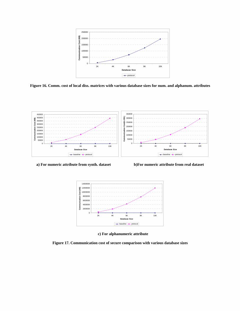
For the baseline protocol, there is no communication cost of transferring local dissimilarity matrix
since each data holder sends their dataset to the third party in plaintext. Overall communication cost for
the baseline protocol is O(n+m) where n and m are dataset sizes of data holders J and K, respectively. For
our protocol, communication cost of transferring local dissimilarity matrices is O(n2+ m2) for both
numerical and alphanumeric attributes. As shown in Figure 16, communication cost increases
quadratically with respect to local dissimilarity matrices for different database sizes. Communication cost
of secure pair-wise entity comparison is O(n*m) for numerical attributes while for alphanumeric attributes
this value is O(n*m*ln*lm) where ln and lm are the average lengths of attributes of data holders A and B,
respectively. Figure 17 depicts linear behavior of the baseline protocol and quadratic behavior of our
protocol with respect to varying database sizes. As seen in Figure 17, communication cost increases
dramatically in our protocol due to secure comparison protocol, and communication cost of the baseline
protocol is negligible compared to our protocol for the same reason. According to Figure 17.a and Figure
17.b, communication cost of numerical attribute for synthetic dataset is much more than real dataset due
to the fact that synthetic dataset is in double data format stored in 64 bits while real dataset is in integer
data format stored in 32 bits.
0
50000
100000
150000
200000
250000
2K 4K 6K 8K 10K
Database Size
Com
mun
icat
ion
Cos
t (KB
)
protocol
Figure 16. Comm. cost of local diss. matrices with various database sizes for num. and alphanum. attributes
0
50000
100000
150000
200000
250000
300000
350000
400000
450000
2K 4K 6K 8K 10K
Database Size
Com
mun
icat
ion
Cos
t (KB
)
baseline protocol
0
50000
100000
150000
200000
250000
300000
350000
2K 4K 6K 8K 10K
Database Size
Com
mun
icat
ion
Cost
(in K
B.)
baseline protocol
a) For numeric attribute from synth. dataset b)For numeric attribute from real dataset
0
2000000
4000000
6000000
8000000
10000000
12000000
14000000
2K 4K 6K 8K 10K
Database Size
Com
mun
icat
ion
Cos
t (KB
)
baseline protocol
c) For alphanumeric attribute
Figure 17. Communication cost of secure comparison with various database sizes
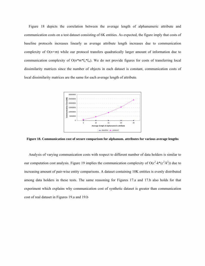
Figure 18 depicts the correlation between the average length of alphanumeric attribute and
communication costs on a test dataset consisting of 6K entities. As expected, the figure imply that costs of
baseline protocols increases linearly as average attribute length increases due to communication
complexity of O(n+m) while our protocol transfers quadratically larger amount of information due to
communication complexity of O(n*m*ln*lm). We do not provide figures for costs of transferring local
dissimilarity matrices since the number of objects in each dataset is constant, communication costs of
local dissimilarity matrices are the same for each average length of attribute.
0
5000000
10000000
15000000
20000000
25000000
30000000
5 10 15 20 25
Average lentgh of alphanumeric attribute
Com
mun
icat
ion
Cost
(KB
)
baseline protocol
Figure 18. Communication cost of secure comparison for alphanum. attributes for various average lengths
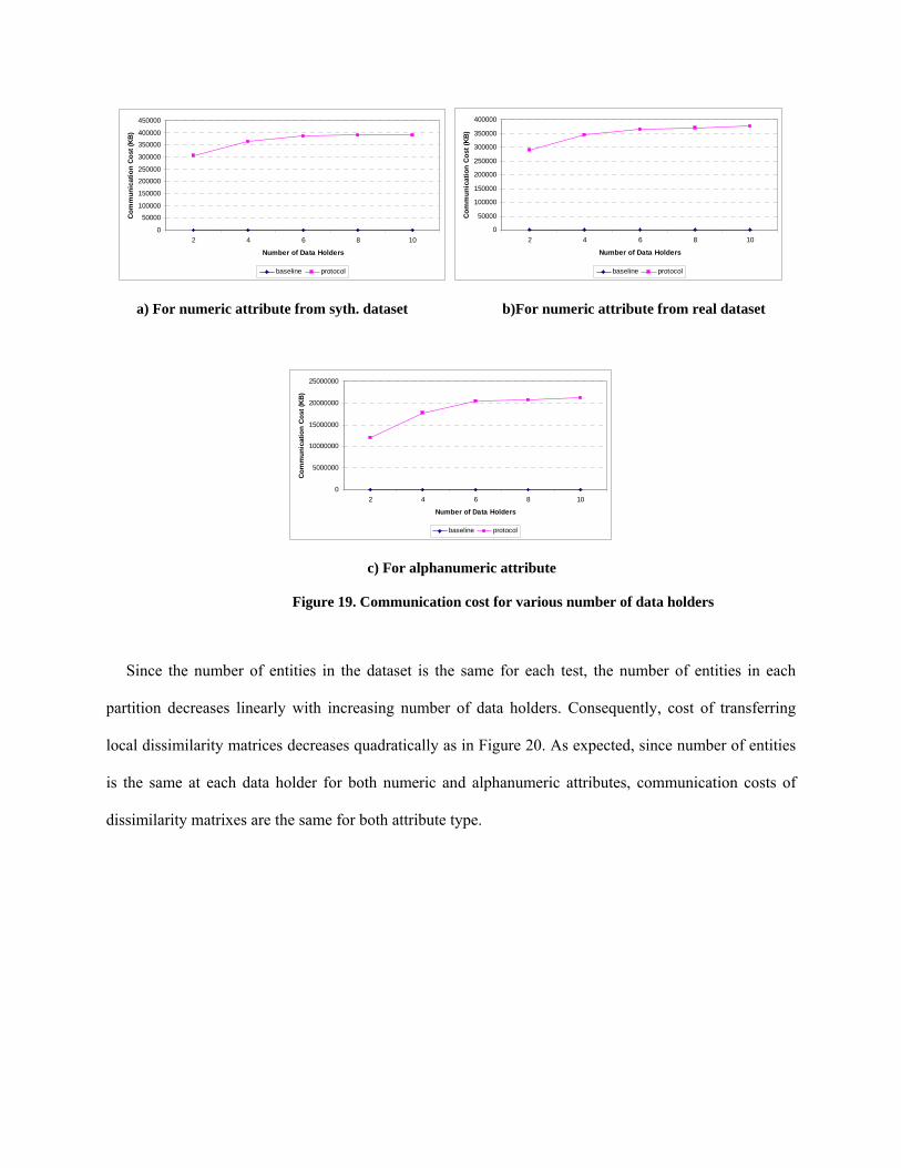
Analysis of varying communication costs with respect to different number of data holders is similar to
our computation cost analysis. Figure 19 implies the communication complexity of O(c2-k*(c2/k2)) due to
increasing amount of pair-wise entity comparisons. A dataset containing 10K entities is evenly distributed
among data holders in these tests. The same reasoning for Figures 17.a and 17.b also holds for that
experiment which explains why communication cost of synthetic dataset is greater than communication
cost of real dataset in Figures 19.a and 19.b
0
50000
100000
150000
200000
250000
300000
350000
400000
450000
2 4 6 8 10
Number of Data Holders
Com
mun
icat
ion
Cos
t (KB
)
baseline protocol
0
50000
100000
150000
200000
250000
300000
350000
400000
2 4 6 8 10
Number of Data Holders
Com
mun
icat
ion
Cos
t (K
B)
baseline protocol
a) For numeric attribute from syth. dataset b)For numeric attribute from real dataset
0
5000000
10000000
15000000
20000000
25000000
2 4 6 8 10
Number of Data Holders
Com
mun
icat
ion
Cos
t (K
B)
baseline protocol
c) For alphanumeric attribute
Figure 19. Communication cost for various number of data holders
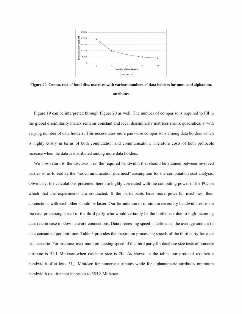
Since the number of entities in the dataset is the same for each test, the number of entities in each
partition decreases linearly with increasing number of data holders. Consequently, cost of transferring
local dissimilarity matrices decreases quadratically as in Figure 20. As expected, since number of entities
is the same at each data holder for both numeric and alphanumeric attributes, communication costs of
dissimilarity matrixes are the same for both attribute type.
0
50000
100000
150000
200000
250000
2 4 6 8 10
Number of Data Holders
Com
mun
icat
ion
Cos
t (K
B)
protocol
Figure 20. Comm. cost of local diss. matrices with various numbers of data holders for num. and alphanum.
attributes
Figure 19 can be interpreted through Figure 20 as well. The number of comparisons required to fill in
the global dissimilarity matrix remains constant and local dissimilarity matrices shrink quadratically with
varying number of data holders. This necessitates more pair-wise comparisons among data holders which
is highly costly in terms of both computation and communication. Therefore costs of both protocols
increase when the data is distributed among more data holders.
We now return to the discussion on the required bandwidth that should be attained between involved
parties so as to realize the “no communication overhead” assumption for the computation cost analysis.
Obviously, the calculations presented here are highly correlated with the computing power of the PC, on
which that the experiments are conducted. If the participants have more powerful machines, their
connections with each other should be faster. Our formulation of minimum necessary bandwidth relies on
the data processing speed of the third party who would certainly be the bottleneck due to high incoming
data rate in case of slow network connections. Data processing speed is defined as the average amount of
data consumed per unit time. Table 3 provides the maximum processing speeds of the third party for each
test scenario. For instance, maximum processing speed of the third party for database size tests of numeric
attribute is 51,1 Mbit/sec when database size is 2K. As shown in the table, our protocol requires a
bandwidth of at least 51,1 Mbit/sec for numeric attributes while for alphanumeric attributes minimum
bandwidth requirement increases to 385,8 Mbit/sec.
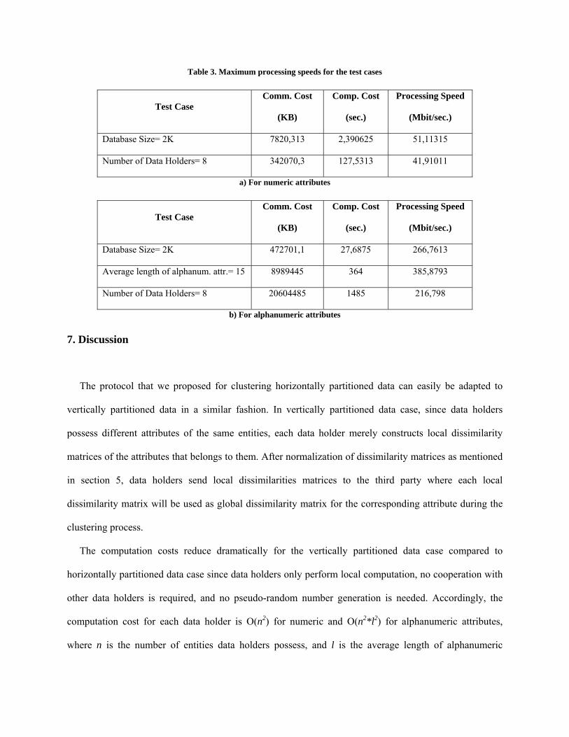
Table 3. Maximum processing speeds for the test cases
Test Case Comm. Cost
(KB)
Comp. Cost
(sec.)
Processing Speed
(Mbit/sec.)
Database Size= 2K 7820,313 2,390625 51,11315
Number of Data Holders= 8 342070,3 127,5313 41,91011
a) For numeric attributes
Test Case Comm. Cost
(KB)
Comp. Cost
(sec.)
Processing Speed
(Mbit/sec.)
Database Size= 2K 472701,1 27,6875 266,7613
Average length of alphanum. attr.= 15 8989445 364 385,8793
Number of Data Holders= 8 20604485 1485 216,798
b) For alphanumeric attributes
7. Discussion
The protocol that we proposed for clustering horizontally partitioned data can easily be adapted to
vertically partitioned data in a similar fashion. In vertically partitioned data case, since data holders
possess different attributes of the same entities, each data holder merely constructs local dissimilarity
matrices of the attributes that belongs to them. After normalization of dissimilarity matrices as mentioned
in section 5, data holders send local dissimilarities matrices to the third party where each local
dissimilarity matrix will be used as global dissimilarity matrix for the corresponding attribute during the
clustering process.
The computation costs reduce dramatically for the vertically partitioned data case compared to
horizontally partitioned data case since data holders only perform local computation, no cooperation with
other data holders is required, and no pseudo-random number generation is needed. Accordingly, the
computation cost for each data holder is O(n2) for numeric and O(n2*l2) for alphanumeric attributes,
where n is the number of entities data holders possess, and l is the average length of alphanumeric
attribute. Considering communication cost, there is again a huge reduction with respect to horizontally
partitioned data case since data holders only send their local dissimilarity matrix to the third party. The
communication cost is O(p*n2) for both numeric and alphanumeric attributes, where p is the number of
data holders.
8. Conclusion
In this paper we proposed a method for privacy preserving clustering over horizontally partitioned
data. Our method is based on the dissimilarity matrix construction using a secure comparison protocol for
numerical, alphanumeric, and categorical data. Previous work on privacy preserving clustering over
horizontally partitioned data was on a specific clustering algorithm and only for numerical attributes. The
main advantage of our method is its generality in applicability to different clustering methods such as
hierarchical clustering. Hierarchical clustering methods can both discover clusters of arbitrary shapes and
deal with diverse data types. For example, we can cluster alphanumeric data that is of outmost importance
in bioinformatics researches, besides numeric and categorical data. Another major contribution is that
quality of the resultant clusters can easily be measured and conveyed to data owners without any leakage
of private information.
We also provided the security analysis of our protocol and discussed the computation and
communication complexity of our protocol. Experimental results over synthetically generated and real
datasets comply with the complexity analysis, proving that preservation of individual privacy is possible
under reasonable assumptions such as non-collusion and semi-honesty of data holders and the third party.
However, as expected, ensuring privacy has its costs, considering the comparison against the baseline
protocol where private data is shared with third parties. Although we used the proposed secure
comparison protocols for clustering horizontally partitioned datasets, there are various other application
areas of these methods such as record linkage and outlier detection problems.
9. References
[1] A. Inan, Y. Saygin, Privacy-preserving spatio-temporal clustering on horizontally partitioned data, Proceedings
of DAWAK06, 8th International Conference on Data Warehousing and Knowledge Discovery, 2006.
[2] M. J. Atallah, F. Kerschbaum, W. Du, Secure and Private Sequence Comparisons, Proceedings of the 2003 ACM
Workshop on Privacy in the Electronic Society (2003) 39-44
[3] M. Klusch, S. Lodi, G. Moro, Distributed Clustering Based on Sampling Local Density Estimates, Proceedings
of the Eighteenth International Joint Conference on Artificial Intelligence (2003) 485-490
[4] M. Kantarcioglu, C. Clifton, Privacy-Preserving Distributed Mining of Association Rules on Horizontally
Partitioned Data, IEEE TKDE, 16(9)(2004)
[5] J. Vaidya, C. Clifton, Privacy-Preserving K-Means Clustering over Vertically Partitioned Data, Proceedings of
the 9th ACM SIGKDD International Conference on Knowledge Discovery and Data Mining (2003) 206-215
[6] J. Vaidya, C. Clifton, Privacy Preserving Association Rule Mining in Vertically Partitioned Data, Proceedings of
the Eighth ACM SIGKDD International Conference on Knowledge Discovery and Data Mining (2002) 639-644
[7] Referenced at KDD’99 Classifier Learning Contest: http://www-cse.ucsd.edu/users/elkan/clresults.htm (2006)
[8] R. Agrawal, R. Srikant, Privacy Preserving Data Mining, Proc. of the 2000 ACM SIGMOD Conference on
Management of Data (2000) 439-450
[9] S. Merugu, J. Ghosh, Privacy-Preserving Distributed Clustering Using Generative Models, Proceedings of the
Third IEEE International Conference on Data Mining (2003) 211-218
[10] S. Jha, L. Kruger , P. McDaniel, Privacy Preserving Clustering, Proceedings of the 10th European Symposium
on Research in Computer Security (2005) 397-417
[11] S. R. M. Oliveira, O. R. Zaïane, Achieving Privacy Preservation When Sharing Data for Clustering,
Proceedings of the International Workshop on Secure Data Management in a Connected World (2004) 67-82
[12] S. R. M. Oliveira, O. R. Zaïane, Privacy Preserving Clustering By Data Transformation, Proceedings of the
18th Brazilian Symposium on Databases (2003) 304-318
[13] S. R. M. Oliveira, O. R. Zaïane, Privacy Preserving Clustering By Object Similarity-Based Representation and
Dimensionality Reduction Transformation, Proceedings of the 2004 ICDM Workshop on Privacy and Security
Aspects of Data Mining (2004) 40-46
[14] S. Vassilios, A. Elmagarmid, E. Bertino, Y. Saygin, E. Dasseni, Association Rule Hiding. IEEE Transactions
on Knowledge and Data Engineering 4 (16)( 2004)
[15] W. Du, Z. Zhan, Building Decision Tree Classifier on Private Data, Proceedings of the IEEE ICDM Workshop
on Privacy, Security and Data Mining (2002) 1-8
[16] Z. Yang, S. Zhong , R. N. Wright, Privacy-preserving classification of customer data without loss of accuracy,
2005 SIAM International Conference on Data Mining (SDM 2005) (2005)


