Embed Size (px)
Citation preview

Proceedingsofthe37thWICSymposiumonInformationTheoryintheBenelux
and
The6thJointWIC/IEEESymposiumonInformationTheoryandSignalProcessing
intheBenelux
UniversitécatholiquedeLouvainLouvain-la-Neuve,Belgium
May19–20,2016

Previoussymposia1.1980Zoetermeer,TheNetherlands,DelftUniversityofTechnology2.1981Zoetermeer,TheNetherlands,DelftUniversityofTechnology3.1982Zoetermeer,TheNetherlands,DelftUniversityofTechnology4.1983Haasrode,Belgium ISBN90-334-0690-X5.1984Aalten,TheNetherlands ISBN90-71048-01-26.1985Mierlo,TheNetherlands ISBN90-71048-02-07.1986Noordwijkerhout,TheNetherlands ISBN90-6275-272-18.1987Deventer,TheNetherlands ISBN90-71048-03-99.1988Mierlo,TheNetherlands ISBN90-71048-04-710.1989Houthalen,Belgium ISBN90-71048-05-511.1990Noordwijkerhout,TheNetherlands ISBN90-71048-06-312.1991Veldhoven,TheNetherlands ISBN90-71048-07-113.1992Enschede,TheNetherlands ISBN90-71048-08-X14.1993Veldhoven,TheNetherlands ISBN90-71048-09-815.1994Louvain-la-Neuve,Belgium ISBN90-71048-10-116.1995Nieuwekerka/dIJssel,TheNetherlands ISBN90-71048-11-X17.1996Enschede,TheNetherlands ISBN90-365-0812-618.1997Veldhoven,TheNetherlands ISBN90-71048-12-819.1998Veldhoven,TheNetherlands ISBN90-71048-13-620.1999Haasrode,Belgium ISBN90-71048-14-421.2000Wassenaar,TheNetherlands ISBN90-71048-15-222.2001Enschede,TheNetherlands ISBN90-365-1598-X23.2002Louvain-la-Neuve,Belgium ISBN90-71048-16-024.2003Veldhoven,TheNetherlands ISBN90-71048-18-725.2004Kerkrade,TheNetherlands ISBN90-71048-20-926.2005Brussels,Belgium ISBN90-71048-21-727.2006Noordwijk,TheNetherlands ISBN90-71048-22-728.2007Enschede,TheNetherlands ISBN978-90-365-2509-129.2008Leuven,Belgium ISBN978-90-9023135-830.2009Eindhoven,TheNetherlands ISBN978-90-386-1852-431.2010Rotterdam,TheNetherlands ISBN978-90-710-4823-432.2011Brussels,Belgium ISBN978-90-817-2190-533.2012Enschede,TheNetherlands ISBN978-90-365-3383-634.2013Leuven,Belgium ISBN978-90-365-0000-535.2014Eindhoven,TheNetherlands ISBN978-90-386-3646-735.2015Brussels,Belgium ISBN978-2-8052-0277-3
Proceedings
Proceedingsofthe37thSymposiumonInformationTheoryintheBeneluxandthe6thJointWIC/IEEESymposiumonInformationTheoryandSignalProcessingintheBenelux.EditedbyFrançoisGlineurandJérômeLouveaux.ISBN:978-2-9601884-0-0

The37thSymposiumonInformationTheoryintheBeneluxandthe6thJointWIC/IEEESymposiumonInformationTheoryandSignalProcessingintheBeneluxhavebeenorganizedby
UniversitécatholiquedeLouvain,Louvain-la-Neuve,Belgium
http://sites.uclouvain.be/sitb2016/ onbehalfoftheWerkgemeenschapvoorInformatie-enCommunicatietheorie,theIEEEBeneluxInformationTheoryChapterandtheIEEEBeneluxSignalProcessingChapter.
FinancialsupportfromtheIEEEBeneluxInformationTheoryChapter,theIEEEBeneluxSignalProcessingChapterandtheWerkgemeenschapvoorInformatie-enCommunicatietheorieisgratefullyacknowledgedOrganizingcommitteeFrançoisGlineur(UCL)JérômeLouveaux(UCL)
[/]
WordItOut [/]
Create [/wordcloud/makeanewone]
Discover [/discoverwordclouds]
Community [/community]
About [/about]
Blog [/blog]
Help [/community/questions]
Fonts [/about/fonts]
Facebook [https://www.facebook.com/worditout]
Twitter [https://twitter.com/worditout]
Feed [/blog/rss]
Share [http://www.addtoany.com/share_save]
Create [/wordcloud/makeanewone]
Learn why the Create page [/wordcloud/makeanewone] has changed in the blog[/blog/20150817/howanewpagelayoutmakeswordcloudgeneratingeasierthanever]
signaldata
power
informationtime
channelsystem
user
algorithm
rate
IEEEdifferent
frequency
resultsscheme
number
detection
noise
probabilitymodel
protocol
function
systemsperformance
privacy
problemoptimal
phase
signals
use
proposed
first order
graph
filter
matrix
linear
case
analysis
users
randomkey
messagevector process
dBvalue
security
received
shown
wireless
SWIPTencryption
log
communication
processing
quantum
work nodesmethod
messages
softwarevalues
test
network
designnetworks
face
allocation
band
statemultiple
error
pilotresearch
possible
energy
encrypted
SNR
motion
homomorphic
receiver
delay
output
Therefore
high
shows
reference
block
sensingalgorithms
imagedevice
eID
subcarriers
!
#
Help & Feedback

Table of contents
1 Delay Performance Enhancement for DSL Networks through Cross-Layer Op-timizationJeremy Van den Eynde, Jeroen Verdyck, Chris Blondia, Marc Moonen . . . 1
2 Analysis of Modulation Techniques for SWIPT with Software Defined RadiosSteven Claessens, Ning Pan, Mohammad Rajabi, Sofie Pollin, DominiqueSchreurs . . . . . . . . . . . . . . . . . . . . . . . . . . . . . . . . . . . . 9
3 Joint Multi-objective Transmit Precoding and Receiver Time Switching Designfor MISO SWIPT SystemsNafiseh Janatian, Ivan Stupia, Luc Vandendorpe . . . . . . . . . . . . . . . 17
4 Target detection for DVB-T based passive radars using pilot subcarrier signalOsama Mahfoudia, Francois Horlin, Xavier Neyt . . . . . . . . . . . . . . . 25
5 Noise Stabilization with Simultaneous Orthogonal Matching PursuitJean-Francois Determe, Jerome Louveaux, Laurent Jacques, Francois Horlin 33
6 Camera Motion for DeblurringBart Kofoed, Peter H.N. de With, Eric Janssen . . . . . . . . . . . . . . . . 41
7 Person-Independent Discomfort Detection System for InfantsC. Li, S. Zinger, W. E. Tjon a Ten, P. H. N. de With . . . . . . . . . . . . . 49
8 Wavelet-based coherence between large-scale resting state networks: neurody-namics marker for autism?Antoine Bernas, Svitlana Zinger, Albert P. Aldenkamp . . . . . . . . . . . . 57
9 TouchSpeaker, a Multi-Sensor Context-Aware Application for Mobile DevicesJona Beysens, Alessandro Chiumento, Sofie Pollin, Min Li . . . . . . . . . . 65
10 A Non-Convex Approach to Blind Calibration from Linear Sub-Gaussian Ran-dom MeasurementsValerio Cambareri, Laurent Jacques . . . . . . . . . . . . . . . . . . . . . . 73
11 Effect of power amplifier nonlinearity in Massive MIMO: in-band and out-of-band distortionSteve Blandino, Claude Desset, Sofie Pollin, Liesbet Van der Perre . . . . . . 81
12 Bandwidth Impacts of a Run-Time Multi-sine Excitation Based SWIPTNing Pan, Mohammad Rajabi , Dominique Schreurs, Sofie Pollin . . . . . . 89
13 Generalized Optimal Pilot Allocation for Channel Estimation in MulticarrierSystemsFrancois Rottenberg, Francois Horlin, Eleftherios Kofidis, Jerome Louveaux . 99
14 Co-existence of Cognitive Satellite Uplink and Fixed-Service TerrestrialJeevan Shrestha, Luc Vandendorpe . . . . . . . . . . . . . . . . . . . . . . 107
15 Low-Complexity Laser Phase Noise Compensation for Filter Bank Multicar-rier Offset-QAM Optical Fiber SystemsTrung-Hien Nguyen, Simon-Pierre Gorza, Jerome Louveaux, Francois Horlin 111

16 8-state unclonable encryptionBoris Skoric . . . . . . . . . . . . . . . . . . . . . . . . . . . . . . . . . . 117
17 Optimizing the discretization in Zero Leakage Helper Data SystemsTaras Stanko, Fritria Nur Andini, Boris Skoric . . . . . . . . . . . . . . . . 118
18 Zero-Leakage Multiple Key-Binding Scenarios for SRAM-PUF Systems Basedon the XOR-MethodLieneke Kusters, Tanya Ignatenko, Frans M.J. Willems . . . . . . . . . . . . 119
19 Localization in Long Range Communication Networks Based on Machine Learn-ingHazem Sallouha, Sofie Pollin . . . . . . . . . . . . . . . . . . . . . . . . . . 127
20 Privacy-Preserving Alpha Algorithm for Software AnalysisGamze Tillem, Zekeriya Erkin, Reginald Lagendijk . . . . . . . . . . . . . . 135
21 A framework for processing cardiac signals acquired by multiple unobtrusivewearable sensorsAttila Para, Silviu Dovancescu, Dan Stefanoiu . . . . . . . . . . . . . . . . 143
22 Proof of the Median PathsThijs Veugen . . . . . . . . . . . . . . . . . . . . . . . . . . . . . . . . . . 151
23 Enhancing privacy of users in eID schemesKris Shrishak, Zekeriya Erkin, Remco Schaar . . . . . . . . . . . . . . . . . 157
24 A Privacy-Preserving GWAS Computation with Homomorphic EncryptionChibuike Ugwuoke, Zekeriya Erkin, Reginald Lagendijk . . . . . . . . . . . 165
25 Security Analysis of the Authentication of Classical Messages by an ArbitratedQuantum SchemeHelena Bruyninckx, Dirk Van Heule . . . . . . . . . . . . . . . . . . . . . . 173
26 Fighting asymmetry with asymmetry in Reverse Fuzzy ExtractorsBoris Skoric, Andre Schaller, Taras Stanko, Stefan Katzenbeisser . . . . . . 181
27 Linear Cryptanalysis of Reduced-Round SpeckDaniel Bodden, Tomer Ashur . . . . . . . . . . . . . . . . . . . . . . . . . 182
28 An Efficient Privacy-Preserving Comparison Protocol in Smart Metering Sys-temsMajid Nateghizad, Zekeriya Erkin, Reginald Lagendijk . . . . . . . . . . . . 190
29 Security Analysis of the Drone Communication Protocol: Fuzzing the MAVLinkprotocolKarel Domin, Eduard Marin, Iraklis Symeonidis . . . . . . . . . . . . . . . 198
30 Parallel optimization on the Entropic ConeBenoıt Legat, Raphael M. Jungers . . . . . . . . . . . . . . . . . . . . . . . 205
31 Compute-and-forward on the Multiple-access Channel with Distributed CSITShokoufeh Mardani, Jasper Goseling . . . . . . . . . . . . . . . . . . . . . 211
32 Autoregressive Moving Average Graph Filter DesignJiani Liu, Elvin Isufi, Geert Leus . . . . . . . . . . . . . . . . . . . . . . . 219

33 Greedy Gossip Algorithm with Synchronous Communication for Wireless Sen-sor NetworksJie Zhang, Richard C. Hendriks, Richard Heusdens . . . . . . . . . . . . . . 227

Delay Performance Enhancement for DSLNetworks through Cross-Layer Scheduling
Jeremy Van den Eynde1 Jeroen Verdyck2 Chris Blondia1 Marc Moonen2
1University of Antwerp, Department of Mathematics-Computer SciencesMOSAIC Modeling of Systems And Internet Communication
[email protected] [email protected] Leuven, Department of Electrical Engineering (ESAT)
STADIUS Center for Dynamical Systems, Signal Processing and Data [email protected] [email protected]
Abstract
The quality of experience of many modern network services depends on thedelay performance of the underlying communications network. In DSL networks,cross talk introduces competition for bandwidth among users. In such a com-petitive environment, delay performance is largely determined by the manner inwhich the cross-layer scheduler assigns bandwidth to the different users. Existingcross-layer schedulers optimize a simple metric, and do not consider importantinformation that is contained within individual packets. In this paper, we presenta new cross-layer scheduler, referred to as the minimal delay violation (MDV)scheduler, which optimizes a more elaborate metric that closely resembles thequality of experience of the users. Complementary to the MDV scheduler, a fastphysical layer resource allocation algorithm has been developed that is based onnetwork utility maximization. Through simulations, it is shown that the newscheduler outperforms the state of the art in cross-layer scheduling algorithms.
1 Introduction
In communications, maintaining a low delay is important for many applications such asvideo conferencing, VoIP, gaming, and live streaming. If many delay violations occur,quality of experience (QoE) suffers considerably for these applications. In multi-usercommunication systems, competition for bandwidth among users motivates the need fora scheduler that assigns bandwidth to the users. This scheduler then has a significantinfluence on the achieved delay performance of all applications in the network. In DSLnetworks, competition for bandwidth arises from physical layer resource allocationtechniques that combat crosstalk, i.e. interference that results from electromagneticcoupling between different wires in a single cable binder. In the design of a schedulerfor DSL systems, these physical layer mechanisms can be taken into account throughthe framework of cross-layer optimization.
Part of this research work was carried out at UAntwerpen, in the frame of Research Project FWO nr. G.0912.13’Cross-layer optimization with real-time adaptive dynamic spectrum management for fourth generation broadband accessnetworks’. Part of this research work was carried out carried out at the ESAT Laboratory of KU Leuven, in the frameof 1) KU Leuven Research Council CoE PFV/10/002 (OPTEC), 2) the Interuniversity Attractive Poles Programmeinitiated by the Belgian Science Policy Office: IUAP P7/23 ‘Belgian network on stochastic modeling analysis design andoptimization of communication systems’ (BESTCOM) 2012-2017, 3) Research Project FWO nr. G.0912.13 ’Cross-layeroptimization with real-time adaptive dynamic spectrum management for fourth generation broadband access networks’,4) IWT O&O Project nr. 140116 ’Copper Next-Generation Access’. The scientific responsibility is assumed by itsauthors.
1
A cross-layer scheduler makes its scheduling decisions based on the solution to anetwork utility maximization (NUM) problem. Existing cross-layer schedulers optimizea simple metric, such as queue length, head-of-line delay, or average waiting time, anddo not consider important information that is contained within the individual packets.In this paper, we introduce the new minimal delay violation (MDV) scheduler, whichoptimizes a function of the delay percentile, a measure that closely resembles the truequality of service requirements of delay sensitive traffic. Complementary to the newMDV scheduler, a fast physical layer resource allocation algorithm is developed thatsolves the corresponding NUM problem. The resource allocation algorithm, referred toas the NUM-DSB algorithm, is inspired by the distributed spectrum balancing (DSB)algorithm for spectrum coordination in DSL networks. The NUM-DSB algorithm de-cides on the appropriate power allocation for the physical layer, and can be shown toconverge to a local optimum of the original NUM problem. Convergence is fast, whichenables verification of the MDV scheduling algorithm through simulations.
Simulation results are obtained using the OMNeT++ framework and Matlab. Theperformance of the MDV scheduler is evaluated in a downstream DSL system, and iscompared to the performance of both the max-weight (MW) and the max-delay utility(MDU) scheduler. Simulation results show that the MDV scheduler outperforms theMDU and MW scheduler. The MDV scheduler sometimes also demonstrates betterperformance with respect to throughput. Overall, when the MDV scheduler is used, itis seen that significantly fewer delay violations occur.
2 DSL system model
2.1 Physical layer
We consider an N user DSL system. DSL employs discrete multitone (DMT) modula-tion in order to establish K orthogonal sub channels or tones. As signal coordinationis assumed not to be available, each of these tones k can be modeled as an interferencechannel.
yk = Hkxk + zk (1)
In (1), xk =[x1k, . . . , x
Nk
]Tis a vector containing the transmitted signal of all N users
on tone k. Also, let xn = [xn1 , . . . , xnK ]T and let x =
[x1T , . . . ,xN
T ]T. Similar vector
notation will be used for other signals, as well as for variables introduced later suchas the bit loading, total power consumption, and data rate. Furthermore, yk and zkcontain the received signal and noise for all N users on tone k. The average power ofxnk is given as snk = ∆fE |xnk |2, with E· the expected value operator and ∆f thetone spacing. Also, σnk = ∆fE |znk |2 is the average noise power received by user n ontone k. Finally, Hk is the N ×N channel matrix, where [Hk]n,m = hn,mk is the transferfunction between the transmitter of user m and the receiver of user n, evaluated ontone k.
The maximum achievable bit loading for user n on tone k, given transmit powerssk, is calculated as
bnk(sk) = log2
(1 +
1
Γ
|hn,nk |2snk∑n6=m |hn,mk |2smk + σnk
), (2)
with Γ the SNR gap to capacity, which incorporates the gap between ideal Gaussiansignaling and the actual constellation in use. The SNR gap also accounts for thecoding gain and noise margin. The data rate of user n, and the total transmit power
2
0 50 100 1500
50
100
R
r1 (Mbps)
r2(M
bps)
Figure 1: Rate region of a 2-user G.Fastsystem.
0 0.5 10
0.5
1
1.5
Dv/Tv
fn(·)
streambest-effort
Figure 2: Weight functions for best-effortand streaming applications.
consumption of user n, are given as
Rn(bn) = fs
K∑
k=1
bnk P n(sn) =K∑
k=1
snk , (3)
where fs is the symbol rate.The total transmit power of each user is limited to P tot. The set of all possible
power loadings of user n can thus be described as
Sn =sn ∈ RK
+ | P n(sn) ≤ P tot. (4)
The set of all possible power loadings of the whole multi-user system is S = S1× . . .×SN . The resulting set of achievable bit loadings is
B = b(S) (5)
Finally, we define the rate region as
R =r ∈ RN
+ | ∃ r′ ∈ R(B) : r ≤ r′. (6)
For DSL networks with tone spacing small relative to the coherence bandwidth of thepower transfer function, the rate region is a convex set [1].
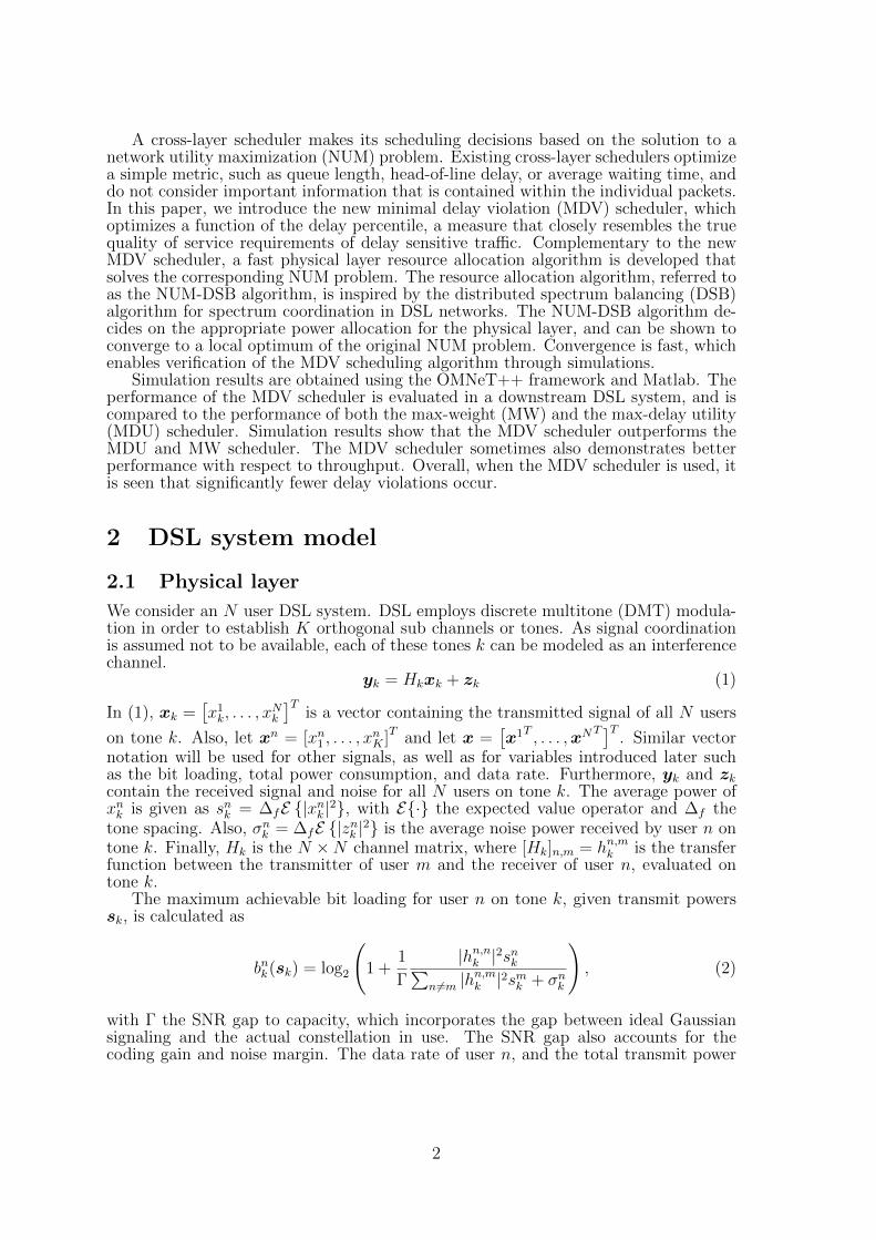
As an example, the rate region of a 2-user G.Fast system that employs spectrumcoordination is depicted in Figure 1. Generally, there is no power allocation thatsimultaneously maximizes the data rate of all users, as observed in the rate regionof Figure 1. Instead, there are a number of Pareto optimal power allocation settingsthat achieve a data rate on the edge of the rate region. This implies the need forscheduling, i.e. choosing one of these Pareto optimal power allocation settings as thepoint of operation.
2.2 Upper layer & scheduling
The scheduling occurs in the upper layer, since it has the information that can helpdeciding the optimal point of operation. We assume that each of the N users hasone traffic stream with delay upper bound T n and allowed violation probability εn, orequivalently, conformance probability ηn = 1 − εn. Time is divided in slots of length
3
τ . At slot t ∈ N the upper layer requests the physical layer for new rates, based on allavailable info up to time t, such as queue lengths and arrival rates. At the start of slott + 1, rates r(t + 1) are applied in the interval [t + 1, t + 2[. There is thus a delay τbetween the request and application of rates.
Traffic arrives in an infinite buffer. We denote by anl (t) and Qnl (t) respectively the
arrival time and length in bit of user n’s l-th queued packet at the beginning of time
slot t, and Qn(t) =∑Nn(t)−1
l=0 Qnl (t) where Nn(t) is the number of packets in user n’s
queue.At the start of every slot the scheduler has to find a feasible scheduling policy
that maximizes the system performance with respect to the QoS requirements. Sucha policy will pick a rate r within the rate region R. The requirements are expressedusing utility functions. Such a function un(rn) quantifies the usefulness to user n ofreceiving a service rn. Data rates r ∈ R are then selected such that they maximizethe sum of the utilities.
arg maxr∈R
N∑
n=1
un(rn) (7)
Ideally, un(·) is monotonically increasing, concave, and differentiable for all n.A large family of scheduling algorithms is linear in r, i.e.
un(rn) = ωnrn. (8)
For example, the Max-Weight scheduler (MW) [2] has ωn(t) = Qn(t). For the Max-
Delay Utility (MDU) scheduler [3], the authors give ωn(t) = |u′n(Wn)|λn
, where u′n is
the derivative of the utility function, W n the average waiting time, and λn the averagearrival rate. It is important to note that for these linear scheduling algorithms, efficientDSL physical layer resource allocation algorithms exist [4].
The QoS requirements are expressed as a delay upper bound T n with delay violationprobability εn: PDn > T n ≤ εn, where Dn is the packet’s delay. If this delayexceeds the upper bound T n, the packet is useless to the application. The consideredperformance metrics are delay violations and throughput.
3 Minimal Delay Violation Scheduler
In general, schedulers that take QoS into account aim to minimize the average delay.However, this metric offers a skewed view. Imagine twenty packets, alternating betweena delay of 5ms and 55ms. This gives an average delay of 30ms per packet. If the delayrequirements were 40ms, then 50% of the packets could be considered useless.
The Minimal Delay Violation (MDV) scheduler aims to minimize the delay viola-tions, rather than the average delay. First it estimates the ηn-percentile delay Dn(t)for the coming slots, based on the queue and observed past delays. Then, dependingon the proximity of Dn(t) to T n, a weight is defined for the user to reflect its impor-
tance. For example, if for a video v the normalized delay Dv(t)
T vis small, then v is not
important, as its delay requirements will probably not be violated, and hence it can
have a lower rate assigned. If, on the other hand, Dv(t)
T vapproaches 1, then its weight
should be much larger, to express it is approaching its delay upper bound.This updated delay is then finally converted into a bit length cn which, when divided
by rn(t+ 1), gives an approximation to the ηn-percentile of user n’s delay. It is this cthat is passed on to the physical layer to find the optimal rates r.
The Minimal Delay Violation (MDV) scheduler uses the utility function un(r) =− cn
rn, which is increasing, concave and differentiable on ]0,+∞[. At the start of every
4

slot, it minimizes the average of all users’ ηn-percentile of the delay:
arg maxr∈R
N∑
n=1
−cn(t)
rn= arg min
r∈R
N∑
n=1
cn(t)
rn(9)
We now look how cn is constructed. Let’s call Dn(t) = αn qn(t)
λn(t)+ (1 − αn)dn(t),
the weighted average of predicted and observed delays. Here αn ∈ [0, 1] indicates theimportance of the queue. A small value means that mainly past behavior, i.e. dn(t)which is the ηn-percentile of past delays, will influence the weight. This is useful forusers that prefer a long-term average data rate, such as background jobs. A large αn on
the other hand will place more importance on the predicted delay qn(t)
λn(t). Here qn(t) is a
measure for the queue and further explained below, and λn(t) = 14(λn(t)+
∑ts=t−2 r
n(s))
is an estimate of the future rn(t+1), with λn(t) an average of the arrival rate. Streamingtraffic benefits from this, as it can fluctuate heavily.
qn(t) is the ηn-percentile of the user’s cumulative queue size Qnl (t), l ∈ [0, Nn− 1] :
Qnl (t) = an0r
n +l′−1∑
m=0
Qnm
λn
rn+
l∑
m=l′
Qnm
The first term accounts for the head-of-line delay. The second for the packets that willbe sent in the interval [t, t+ 1], for which we already know the rates. l′ is the numberof packets that are transmitted in [t, t + 1[. The final term accounts for the packetsthat depart in the slots [t+ 1, . . . [ at a yet unknown rate. The delay of queued packetl at a rate rn can now simply be calculated using Qn
l /rn.
The parameter c can be expressed by cn =[λnT nfn( D
n
Tn)]
1.
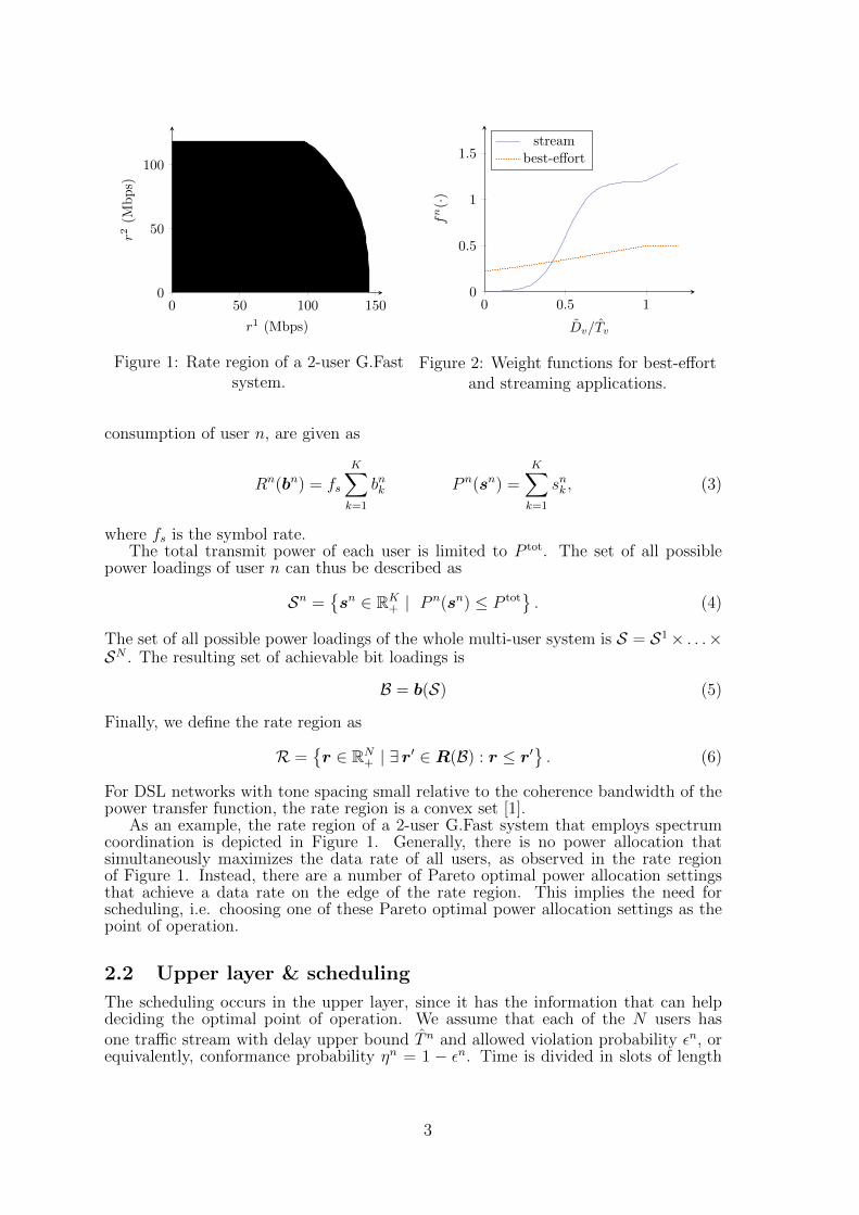
The weight function fn(·) transforms its argument, the proximity to T n, into aweight that reflects its importance with respect to the QoS requirements. The followingfunctions have been defined
fstream(d) = s(γ = 1.2, µ = 0.5, σ = 0.08, ρ = 1, x = d)fbe(d) = s(γ = 1.0, µ = 1.0, σ = 0.80, ρ = 0, x = d)
with
s(γ, µ, σ, ρ, x) =
S(x) if x ≤ 1
S(1) + (x− 1)ρ if x > 1
and the sigmoid
S(x) =γ
1 + e−x−µσ
They are depicted in Figure 2. These functions are tuned such that video and best-effort cooperate: if a video’s delay is low then it will spare best-effort channel capacity.However if the video’s delay is close to or over its delay upper bound, its weight willincrease more quickly than best-effort’s, which causes video’s rate to increase at thecost of best-effort receiving less capacity.
4 Distributed Spectrum Balancing for Network
Utility Maximization
Here, the NUM-DSB algorithm is delineated, which solves an instance of (7) for everyslot t. NUM-DSB yields the optimal data rate r∗, as well as the corresponding power
5

allocation s∗. The NUM problem is non-convex on account of the bit loading beinga non-convex function of the power allocation (2). Inspired by the DSB algorithm forspectrum coordination [4], our solution strategy is to construct successive per-user ap-proximations of the rate region by defining an approximation for the bit loading that isa convex function of the power allocation. By iteratively constructing new approxima-tions at the solution of the previous iteration, a local solution, i.e. a stationary point,of the original problem can be found.
In each iteration ` of the NUM-DSB algorithm, a user n will construct its ownconvex inner approximation of the original rate region R. The approximation of Rdepends on the current power allocation s(`), and is denoted as R(s(`)). Let it be clearthat, although this is not reflected in notation, the approximation R(s(`)) is specific touser n. In order to construct R(s(`)), it is assumed that all other users do not changetheir power allocation, i.e. sm = sm(`) ,∀m 6= n. Furthermore, the bit loading of allother users m is approximated with a lower bound hyperplane, i.e.
bn(sn; s(`)) = bn(s) (10)
bm(sn; s(`)) = bm(s(`)) + βm(s(`)) (sn − sn(`)
), (11)
where A B denotes the Hadamard product of matrices A and B, and with βmk (sk(`))
the directional derivative of bmk (·) at sk(`) along the nth vector in the standard basis of
Rn. We want to guarantee that the value of the approximate bit loading bmk remainsnon-negative. This can be ensured by adding a constraint on sn. Keeping in mind thatβmk (sk
(`)) < 0, the appropriate constraint is
snk ≤ sk = snk(`) −max
m6=n
bmk (sk(`))
βmk (sk(`)). (12)
The corresponding sets of all possible power loadings and resulting achievable approx-imate bit loadings are
Sn(s(`)) = sn ∈ Sn | sn ≤ s B(s(`)) = b(Sn(s(`)); s(`)
). (13)
Finally, the approximate rate region is defined as
R(s(`)) =r ∈ RN
+ | ∃ r′ ∈ R(B(s(`))
): r ≤ r′
. (14)
User n thus solves the following problem, and extracts the power allocation sn thatachieves the optimal r.
arg maxr∈R(s)
N∑
n=1
un(rn) (15)
The algorithm of choice to solve (15) is the Frank-Wolfe algorithm, which exhibitslinear convergence [5] and requires no parameter tuning. This algorithm can be usedas the utilities un(·) are concave and continuously differentiable by assumption, andas the rate region R(s(`)) can be shown to be a compact convex set. The delails ofthe optimization algorithm are however omitted for conciseness. Then, after problem(15) has been solved, a subsequent approximation is constructed by another user atthe obtained power allocation. The solutions of these successive approximations canbe shown to converge to a stationary point of (7).
6
5 Performance
5.1 Simulation setup
The simulation consists of two parts. The NUM-DSB algorithm which is run in Matlab.The simulation of the network and upper layer scheduling is run in the OMNeT++framework. Every τ = 50ms , OMNeT++ gathers c, and sends it to Matlab using theMATLAB Engine API for C. In the next slot, the rates r are read from Matlab, andapplied to the simulated channels.
The physical layer parameters are the following. The transfer function and noise areobtained from a 99% worst case model for the physical layer of a G.Fast system withN = 2 users, where the respective line lengths are 450m for n = 1, and 390m for n = 2.The twisted pair cables have a line diameter of 0, 5mm, which corresponds to 24AWG.For a G.Fast system, the available per-user total transmit power is P tot = 4dBm, thesymbol rate is fs = 4009Hz, the number of tones is K = 2047, and the tone spacingis ∆f = 51.75kHz. The SNR gap is chosen to be Γ = 12.6dB, which corresponds toBER = 10−7, a coding gain of 3dB, and a noise margin of 6dB. The rate region thatcorresponds to these physical layer parameter settings is depicted in Figure 1.
The performance of the network is evaluated for 12 different traffic scenarios. Everyscenario is the equivalent of one hour simulated time. Each of the N users is assignedexactly one traffic stream, the characteristics of which depend on the traffic scenario.A mix of three different kinds of traffic has been used. For video traffic, “Starwars” and“Alice in Wonderland” [6] and a 4k video entitled “The Beauty of Taiwan”∗ are used.Each video’s packet lengths are multiplied by a constant such that the load would becloser to 1. For the second type of traffic, arrivals are determined by a Poisson processwith fixed-length packets. The final traffic type kept the user’s queue backlogged atall times, saturating the line. The users send packets that are encapsulated in UDPdatagrams. At arrival at the next hop, the delay statistics of unfragmented packets aretracked.
5.2 Results
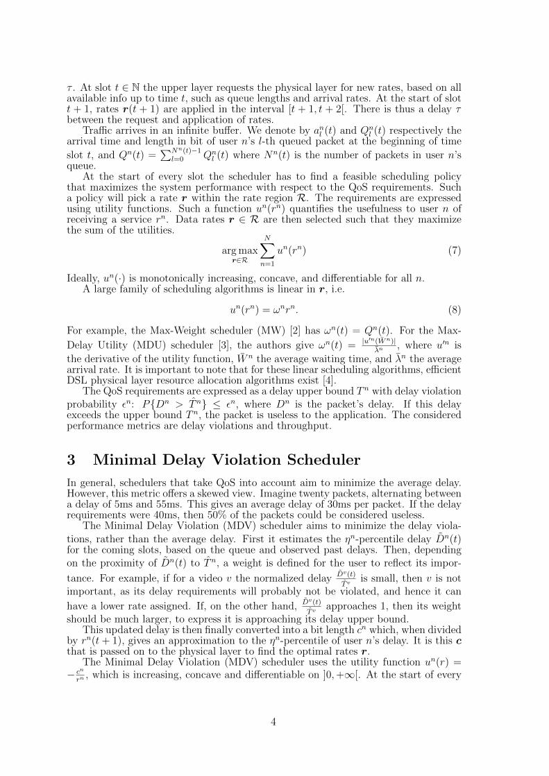
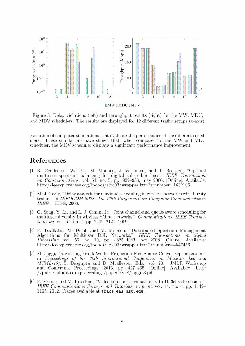
The simulations have been executed for the MDV scheduler, as well as for the MDU andMW scheduler. Results are displayed in Figure 3. The left plot shows the percentageof packets that violate their delay requirements. On average, MW has 7.2% of delayviolations, MDU 7.4% and MDV 5.6%. Both MDV and MDU have non-zero violationsin four scenarios, while MW violates delays in nine scenarios. These violations for MDVand MDU occur for scenarios in which the 4k video was playing, a very bursty video.On three out of the four scenarios, MDV outperforms MDU. The right plot of Figure 3shows the throughput in Mbps. The results show that on average the MDV schedulerhas a higher throughput (122.8 Mbps) than both the MW and MDU scheduler (121Mbps), with differences of up to 7 Mbps (compared to MDU).
6 Conclusion
The novel cross-layer MDV scheduler has been presented, which employs a utilityfunction to communicate its rate requirements to the physical layer. An accompany-ing power allocation algorithm for the physical layer (NUM-DSB) has been developed.NUM-DSB displays exceedingly fast convergence, which in turn enables the efficient
∗http://tempestvideos.skyfire.com/Sales_Optimization_Demo/beauty_taiwan_4k_final-ed.mp4
7
2 4 6 8 10 12
100
150
200
Troughput(M
bps)
2 4 6 8 10 1210−2
10−1
100
101
102Delay
violations(%
)
MW MDU MDV
Figure 3: Delay violations (left) and throughput results (right) for the MW, MDU,and MDV schedulers. The results are displayed for 12 different traffic setups (x-axis).
execution of computer simulations that evaluate the performance of the different sched-ulers. These simulations have shown that, when compared to the MW and MDUscheduler, the MDV scheduler displays a significant performance improvement.
References
[1] R. Cendrillon, Wei Yu, M. Moonen, J. Verlinden, and T. Bostoen, “Optimalmultiuser spectrum balancing for digital subscriber lines,” IEEE Transactionson Communications, vol. 54, no. 5, pp. 922–933, may 2006. [Online]. Available:http://ieeexplore.ieee.org/lpdocs/epic03/wrapper.htm?arnumber=1632106
[2] M. J. Neely, “Delay analysis for maximal scheduling in wireless networks with burstytraffic,” in INFOCOM 2008. The 27th Conference on Computer Communications.IEEE. IEEE, 2008.
[3] G. Song, Y. Li, and L. J. Cimini Jr, “Joint channel-and queue-aware scheduling formultiuser diversity in wireless ofdma networks,” Communications, IEEE Transac-tions on, vol. 57, no. 7, pp. 2109–2121, 2009.
[4] P. Tsiaflakis, M. Diehl, and M. Moonen, “Distributed Spectrum ManagementAlgorithms for Multiuser DSL Networks,” IEEE Transactions on SignalProcessing, vol. 56, no. 10, pp. 4825–4843, oct 2008. [Online]. Available:http://ieeexplore.ieee.org/lpdocs/epic03/wrapper.htm?arnumber=4547456
[5] M. Jaggi, “Revisiting Frank-Wolfe: Projection-Free Sparse Convex Optimization,”in Proceedings of the 30th International Conference on Machine Learning(ICML-13), S. Dasgupta and D. Mcallester, Eds., vol. 28. JMLR Workshopand Conference Proceedings, 2013, pp. 427–435. [Online]. Available: http://jmlr.csail.mit.edu/proceedings/papers/v28/jaggi13.pdf
[6] P. Seeling and M. Reisslein, “Video transport evaluation with H.264 video traces,”IEEE Communications Surveys and Tutorials, in print, vol. 14, no. 4, pp. 1142–1165, 2012, Traces available at trace.eas.asu.edu.
8
Analysis of Modulation Techniques for SWIPTwith Software Defined Radios
Steven Claessens Ning Pan Mohammad Rajabi Dominique Schreurs Sofie PollinTELEMIC Division, Department of Electrical Engineering
University of Leuven, Leuven, 3000, [email protected]
ning.pan,mohammad.rajabi,dominique.schreurs,[email protected]
Abstract
This work demonstrates the performance of software defined radios (SDRs) whentransmitting multi-sine signals, which are already shown to increase RF to DCpower conversion efficiency (PCE) at the receiver in a wireless power transfersystem (WPT) [1]. In a system for simultaneous wireless information and powertransfer (SWIPT) where the generated waveforms are modulated, however, weexpect the transmitter efficiency to also be of great importance. Our goal is toevaluate the impacts on information transfer when transmitting QAM or PSKmodulated power optimized waveforms (POWs) with two different SDRs. QAMand PSK modulated multi-sine waveforms are generated at fixed power levelswhile varying the amount of tones and modulation size and type. Error vectormagnitude (EVM) is used as figure or merit for transmitter efficiency. Theperformed measurements show that generally, EVM decreases with increasingamount of tones. However, a high order QAM modulation of a high tone multi-sine signal at high power levels will increase EVM. Our work also shows thattransmitter efficiency should not be neglected in SWIPT systems.
1 Introduction
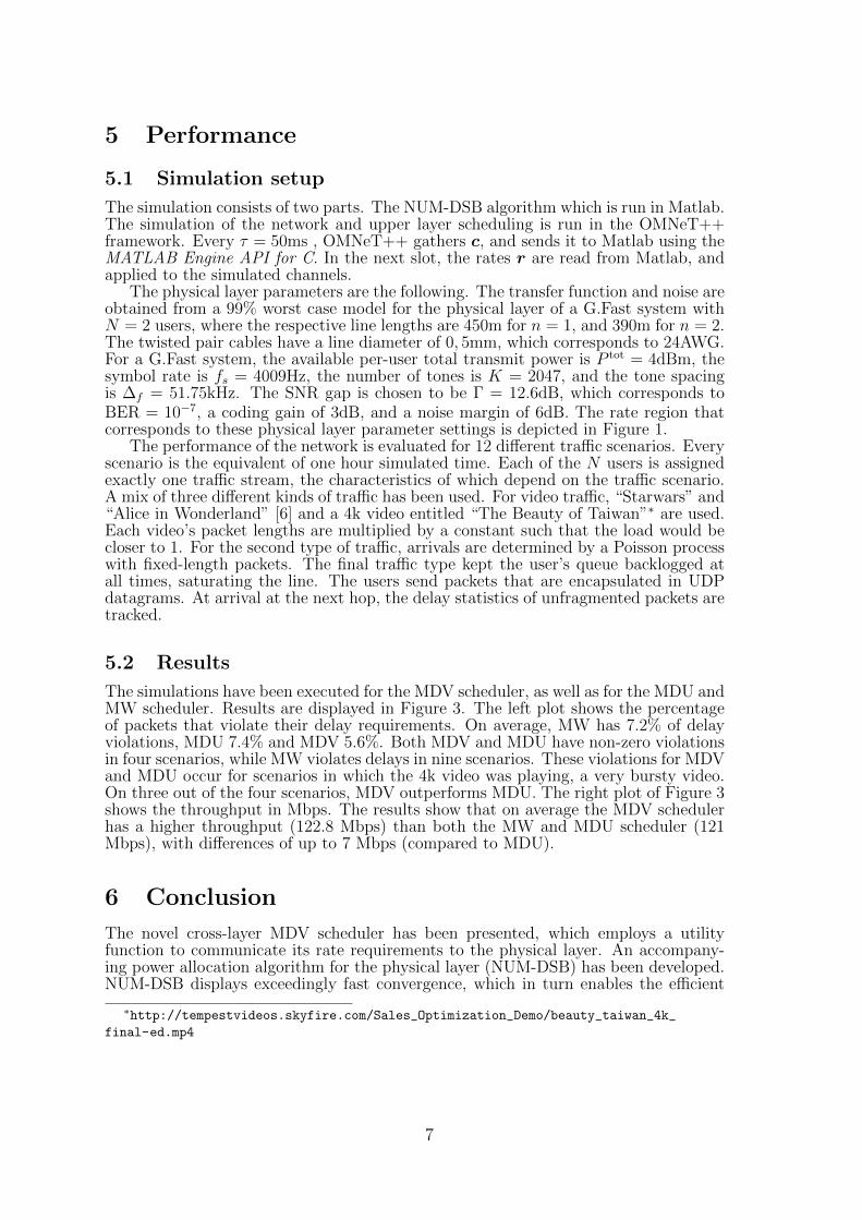
Simultaneous wireless information and power transfer (SWIPT) is gaining interest overthe last years. Increasing the radio frequency (RF) to direct current (DC) power con-version efficiency (PCE) at the receiver becomes key in SWIPT. The transmitted signalwaveform can be optimized to improve PCE. The typical non-linear behavior of thediode at the rectifier results in higher PCE when excited with high PAPR signals,called power-optimized waveforms (POWs). In Figure 1, the improvement of usingPOWs on PCE is shown. Multi-sine waveform is a popular POW since it’s PAPR canbe easily controlled as explained in subsection 2.2 [2],[3].
In [4], a polynomial diode model is constructed to illustrate this phenomena. Theeven-order terms cause a self biasing mechanism meaning a higher time-invariant out-put level. It is further shown that for multi-sine POWs this DC mechanism is optimallyexploited by choosing a multi-tone excitation without phase variation, resulting in alarger output DC voltage. It is later theoretically [5] and experimentally [6] shownthat an upper limit on the amount of tones exists due to circuit mismatch because ofincreasing bandwidth and destruction of the biasing mechanism when exceeding thediode reverse breakdown voltage.However, none of the research on SWIPT considers the impacts of different modula-tion schemes regarding signal distortion and received DC power. Also, WPT researchgenerally focusses on the receiver efficiency, not taking into account the transmitter ef-ficiency. High PAPR signals will be distorted at the transmitter because of non-linearcomponents such as the power amplifier (PA). This paper investigates how the multi-sine signals with different modulations affect error vector magnitude (EVM) of thetransmitter at various power levels. We consider different constellation sizes for PSK
9
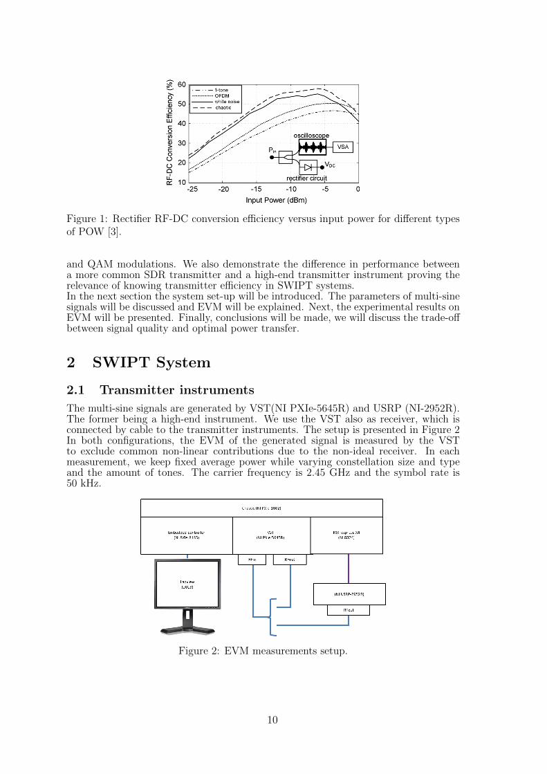
Figure 1: Rectifier RF-DC conversion efficiency versus input power for different typesof POW [3].
and QAM modulations. We also demonstrate the difference in performance betweena more common SDR transmitter and a high-end transmitter instrument proving therelevance of knowing transmitter efficiency in SWIPT systems.In the next section the system set-up will be introduced. The parameters of multi-sinesignals will be discussed and EVM will be explained. Next, the experimental results onEVM will be presented. Finally, conclusions will be made, we will discuss the trade-offbetween signal quality and optimal power transfer.
2 SWIPT System
2.1 Transmitter instruments
The multi-sine signals are generated by VST(NI PXIe-5645R) and USRP (NI-2952R).The former being a high-end instrument. We use the VST also as receiver, which isconnected by cable to the transmitter instruments. The setup is presented in Figure 2In both configurations, the EVM of the generated signal is measured by the VSTto exclude common non-linear contributions due to the non-ideal receiver. In eachmeasurement, we keep fixed average power while varying constellation size and typeand the amount of tones. The carrier frequency is 2.45 GHz and the symbol rate is50 kHz.
Figure 2: EVM measurements setup.
10
2.2 Multi-sine signals
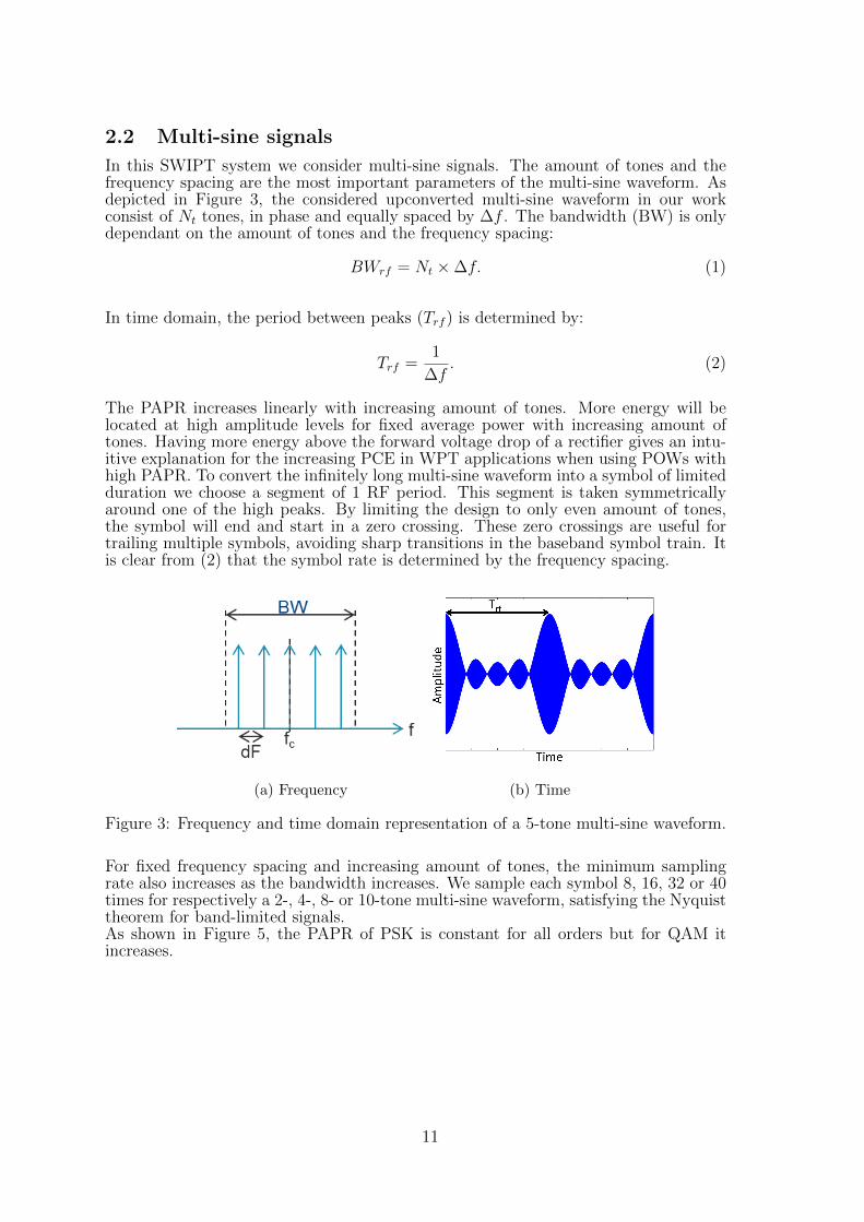
In this SWIPT system we consider multi-sine signals. The amount of tones and thefrequency spacing are the most important parameters of the multi-sine waveform. Asdepicted in Figure 3, the considered upconverted multi-sine waveform in our workconsist of Nt tones, in phase and equally spaced by ∆f . The bandwidth (BW) is onlydependant on the amount of tones and the frequency spacing:
BWrf = Nt ×∆f. (1)
In time domain, the period between peaks (Trf ) is determined by:
Trf =1
∆f. (2)
The PAPR increases linearly with increasing amount of tones. More energy will belocated at high amplitude levels for fixed average power with increasing amount oftones. Having more energy above the forward voltage drop of a rectifier gives an intu-itive explanation for the increasing PCE in WPT applications when using POWs withhigh PAPR. To convert the infinitely long multi-sine waveform into a symbol of limitedduration we choose a segment of 1 RF period. This segment is taken symmetricallyaround one of the high peaks. By limiting the design to only even amount of tones,the symbol will end and start in a zero crossing. These zero crossings are useful fortrailing multiple symbols, avoiding sharp transitions in the baseband symbol train. Itis clear from (2) that the symbol rate is determined by the frequency spacing.
(a) Frequency (b) Time
Figure 3: Frequency and time domain representation of a 5-tone multi-sine waveform.
For fixed frequency spacing and increasing amount of tones, the minimum samplingrate also increases as the bandwidth increases. We sample each symbol 8, 16, 32 or 40times for respectively a 2-, 4-, 8- or 10-tone multi-sine waveform, satisfying the Nyquisttheorem for band-limited signals.As shown in Figure 5, the PAPR of PSK is constant for all orders but for QAM itincreases.
11
2.3 Error vector magnitude
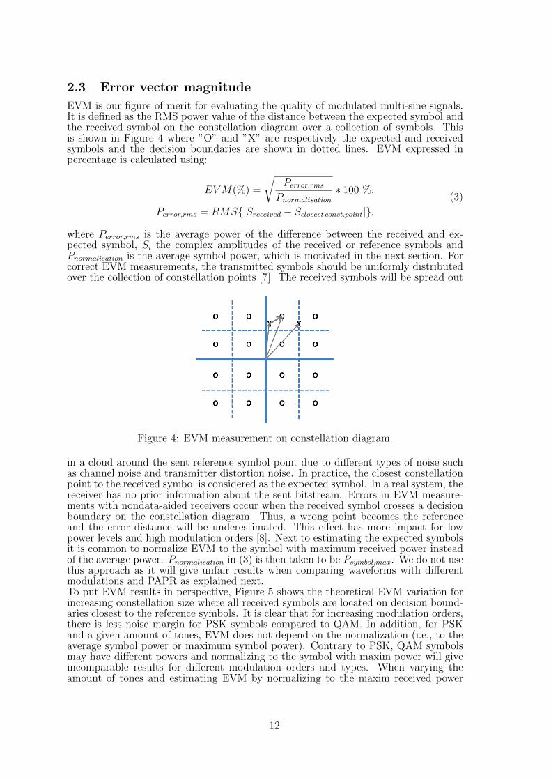
EVM is our figure of merit for evaluating the quality of modulated multi-sine signals.It is defined as the RMS power value of the distance between the expected symbol andthe received symbol on the constellation diagram over a collection of symbols. Thisis shown in Figure 4 where ”O” and ”X” are respectively the expected and receivedsymbols and the decision boundaries are shown in dotted lines. EVM expressed inpercentage is calculated using:
EVM(%) =
√Perror,rms
Pnormalisation∗ 100 %,
Perror,rms = RMS|Sreceived − Sclosest const.point|,(3)
where Perror,rms is the average power of the difference between the received and ex-pected symbol, Si the complex amplitudes of the received or reference symbols andPnormalisation is the average symbol power, which is motivated in the next section. Forcorrect EVM measurements, the transmitted symbols should be uniformly distributedover the collection of constellation points [7]. The received symbols will be spread out
Figure 4: EVM measurement on constellation diagram.
in a cloud around the sent reference symbol point due to different types of noise suchas channel noise and transmitter distortion noise. In practice, the closest constellationpoint to the received symbol is considered as the expected symbol. In a real system, thereceiver has no prior information about the sent bitstream. Errors in EVM measure-ments with nondata-aided receivers occur when the received symbol crosses a decisionboundary on the constellation diagram. Thus, a wrong point becomes the referenceand the error distance will be underestimated. This effect has more impact for lowpower levels and high modulation orders [8]. Next to estimating the expected symbolsit is common to normalize EVM to the symbol with maximum received power insteadof the average power. Pnormalisation in (3) is then taken to be Psymbol,max. We do not usethis approach as it will give unfair results when comparing waveforms with differentmodulations and PAPR as explained next.To put EVM results in perspective, Figure 5 shows the theoretical EVM variation forincreasing constellation size where all received symbols are located on decision bound-aries closest to the reference symbols. It is clear that for increasing modulation orders,there is less noise margin for PSK symbols compared to QAM. In addition, for PSKand a given amount of tones, EVM does not depend on the normalization (i.e., to theaverage symbol power or maximum symbol power). Contrary to PSK, QAM symbolsmay have different powers and normalizing to the symbol with maxim power will giveincomparable results for different modulation orders and types. When varying theamount of tones and estimating EVM by normalizing to the maxim received power
12
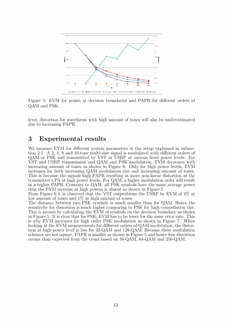
Figure 5: EVM for points at decision boundaries and PAPR for different orders ofQAM and PSK.
level, distortion for waveforms with high amount of tones will also be underestimateddue to increasing PAPR.
3 Experimental results
We measure EVM for different system parameters in the setup explained in subsec-tion 2.1. A 2, 4, 8 and 10-tone multi-sine signal is modulated with different orders ofQAM or PSK and transmitted by VST or USRP at various fixed power levels. ForVST and USRP transmission and QAM and PSK modulation, EVM decreases withincreasing amount of tones as shown in Figure 6. Only for high power levels, EVMincreases for both increasing QAM modulation size and increasing amount of tones.This is because the signals high PAPR resulting in more non-linear distortion at thetransmitter’s PA at high power levels. For QAM, a higher modulation order will resultin a higher PAPR. Contrary to QAM, all PSK symbols have the same average powerthus the EVM increase at high powers is absent as shown in Figure 7.From Figure 6 it is observed that the VST outperforms the USRP by EVM of 4% atlow amount of tones and 1% at high amount of tones.The distance between two PSK symbols is much smaller than for QAM. Hence thesensitivity for distortion is much higher comparing to PSK for high constellation size.This is proven by calculating the EVM of symbols on the decision boundary as shownin Figure 5. It is clear that for PSK, EVM has to be lower for the same error rate. Thisis why EVM increases for high order PSK modulation as shown in Figure 7. Whenlooking at the EVM measurements for different orders of QAM modulation, the distor-tion at high power level is less for 32-QAM and 128-QAM. Because these modulationschemes are not square, PAPR is smaller as shown in Figure 5 and hence less distortionoccurs than expected from the trend based on 16-QAM, 64-QAM and 256-QAM.
13
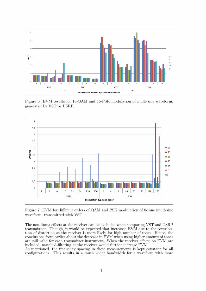
Figure 6: EVM results for 16-QAM and 16-PSK modulation of multi-sine waveform,generated by VST or USRP.
Figure 7: EVM for different orders of QAM and PSK modulation of 8-tone multi-sinewaveform, transmitted with VST.
The non-linear effects at the receiver can be excluded when comparing VST and USRPtransmission. Though, it would be expected that increased EVM due to the contribu-tion of distortion at the receiver is more likely for high number of tones. Hence, theconclusions from earlier about the decrease in EVM when using higher amount of tonesare still valid for each transmitter instrument. When the receiver effects on EVM areincluded, matched-filtering at the receiver would further increase EVM.As mentioned, the frequency spacing in these measurements is kept constant for allconfigurations. This results in a much wider bandwidth for a waveform with more
14
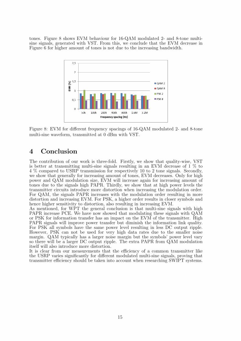
tones. Figure 8 shows EVM behaviour for 16-QAM modulated 2- and 8-tone multi-sine signals, generated with VST. From this, we conclude that the EVM decrease inFigure 6 for higher amount of tones is not due to the increasing bandwidth.
Figure 8: EVM for different frequency spacings of 16-QAM modulated 2- and 8-tonemulti-sine waveform, transmitted at 0 dBm with VST.
4 Conclusion
The contribution of our work is three-fold. Firstly, we show that quality-wise, VSTis better at transmitting multi-sine signals resulting in an EVM decrease of 1 % to4 % compared to USRP transmission for respectively 10 to 2 tone signals. Secondly,we show that generally for increasing amount of tones, EVM decreases. Only for highpower and QAM modulation size, EVM will increase again for increasing amount oftones due to the signals high PAPR. Thirdly, we show that at high power levels thetransmitter circuits introduce more distortion when increasing the modulation order.For QAM, the signals PAPR increases with the modulation order resulting in moredistortion and increasing EVM. For PSK, a higher order results in closer symbols andhence higher sensitivity to distortion, also resulting in increasing EVM.As mentioned, for WPT the general conclusion is that multi-sine signals with highPAPR increase PCE. We have now showed that modulating these signals with QAMor PSK for information transfer has an impact on the EVM of the transmitter. HighPAPR signals will improve power transfer but diminish the information link quality.For PSK all symbols have the same power level resulting in less DC output ripple.However, PSK can not be used for very high data rates due to the smaller noisemargin. QAM typically has a larger noise margin but the symbols’ power level varyso there will be a larger DC output ripple. The extra PAPR from QAM modulationitself will also introduce more distortion.It is clear from our measurements that the efficiency of a common transmitter likethe USRP varies significantly for different modulated multi-sine signals, proving thattransmitter efficiency should be taken into account when researching SWIPT systems.
15

References
[1] Matthew S. Trotter, Joshua D. Griffin, and Gregory D. Durgin. Power-optimizedwaveforms for improving the range and reliability of RFID systems. 2009 IEEEInternational Conference on RFID, RFID 2009, pages 80–87, 2009.
[2] Matthew S. Trotter and Gregory D. Durgin. Survey of range improvement ofcommercial RFID tags with power optimized waveforms. RFID 2010: InternationalIEEE Conference on RFID, pages 195–202, 2010.
[3] a. Collado and a. Georgiadis. Optimal waveforms for efficient wireless power trans-mission. IEEE Microwave and Wireless Components Letters, 24(5):354–356, 2014.
[4] Alirio Soares Boaventura and Nuno Borges Carvalho. Maximizing DC Power inEnergy Harvesting Circuits Using Multisine Excitation. 2011 IEEE MTT-S Inter-national Microwave Symposium, 1(1):1–4, 2011.
[5] Christopher R. Valenta and Gregory D. Durgin. Rectenna performance underpower-optimized waveform excitation. 2013 IEEE International Conference onRFID, RFID 2013, pages 237–244, 2013.
[6] Ning Pan, Alirio Soares Boaventura, Mohammad Rajabi, Dominique Schreurs,Nuno Borges Carvalho, and Sofie Pollin. Amplitude and Frequency Analy-sis of Multi-sine Wireless Power Transfer. Integrated Nonlinear Microwave andMillimetre-wave Circuits Workshop (INMMiC), 2015, (1):1–3, 2015.
[7] Michael D Mckinley, Kate a Remley, Maciej Myslinski, J Stevenson Kenney, andBart Nauwelaers. EVM Calculation for Broadband Modulated Signals. 64thARFTG Conf Dig, pages 45–52, 2004.
[8] Hisham A. Mahmoud and Huseyin Arslan. Error vector magnitude to SNR conver-sion for nondata-aided receivers. IEEE Transactions on Wireless Communications,8(5):2694–2704, 2009.
16
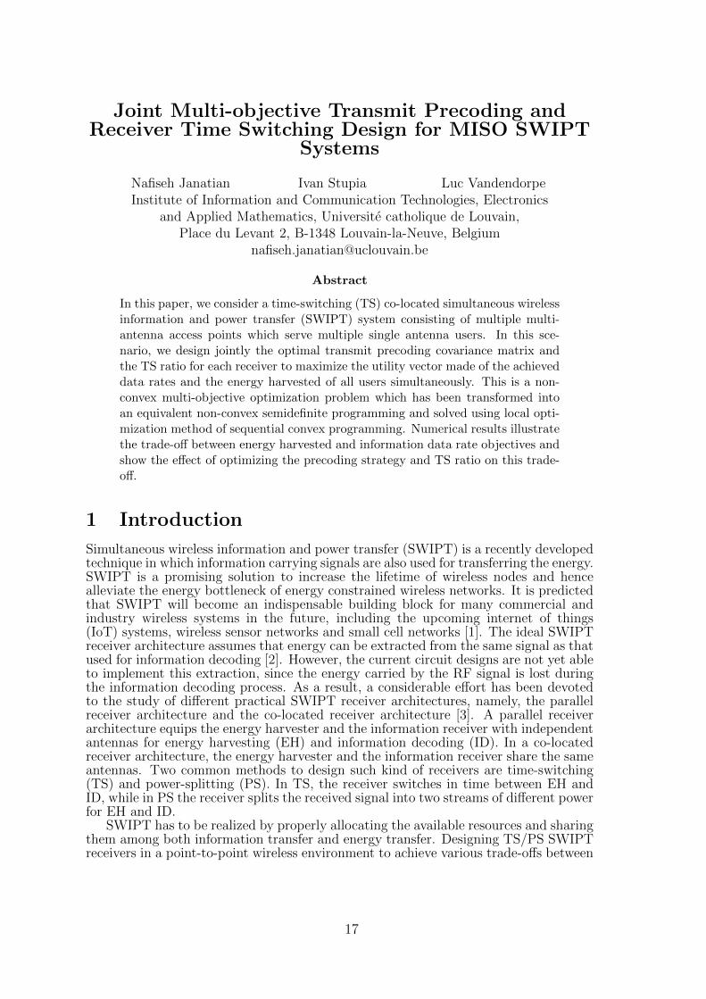
Joint Multi-objective Transmit Precoding andReceiver Time Switching Design for MISO SWIPT
Systems
Nafiseh Janatian Ivan Stupia Luc VandendorpeInstitute of Information and Communication Technologies, Electronics
and Applied Mathematics, Universite catholique de Louvain,Place du Levant 2, B-1348 Louvain-la-Neuve, Belgium
Abstract
In this paper, we consider a time-switching (TS) co-located simultaneous wirelessinformation and power transfer (SWIPT) system consisting of multiple multi-antenna access points which serve multiple single antenna users. In this sce-nario, we design jointly the optimal transmit precoding covariance matrix andthe TS ratio for each receiver to maximize the utility vector made of the achieveddata rates and the energy harvested of all users simultaneously. This is a non-convex multi-objective optimization problem which has been transformed intoan equivalent non-convex semidefinite programming and solved using local opti-mization method of sequential convex programming. Numerical results illustratethe trade-off between energy harvested and information data rate objectives andshow the effect of optimizing the precoding strategy and TS ratio on this trade-off.
1 Introduction
Simultaneous wireless information and power transfer (SWIPT) is a recently developedtechnique in which information carrying signals are also used for transferring the energy.SWIPT is a promising solution to increase the lifetime of wireless nodes and hencealleviate the energy bottleneck of energy constrained wireless networks. It is predictedthat SWIPT will become an indispensable building block for many commercial andindustry wireless systems in the future, including the upcoming internet of things(IoT) systems, wireless sensor networks and small cell networks [1]. The ideal SWIPTreceiver architecture assumes that energy can be extracted from the same signal as thatused for information decoding [2]. However, the current circuit designs are not yet ableto implement this extraction, since the energy carried by the RF signal is lost duringthe information decoding process. As a result, a considerable effort has been devotedto the study of different practical SWIPT receiver architectures, namely, the parallelreceiver architecture and the co-located receiver architecture [3]. A parallel receiverarchitecture equips the energy harvester and the information receiver with independentantennas for energy harvesting (EH) and information decoding (ID). In a co-locatedreceiver architecture, the energy harvester and the information receiver share the sameantennas. Two common methods to design such kind of receivers are time-switching(TS) and power-splitting (PS). In TS, the receiver switches in time between EH andID, while in PS the receiver splits the received signal into two streams of different powerfor EH and ID.
SWIPT has to be realized by properly allocating the available resources and sharingthem among both information transfer and energy transfer. Designing TS/PS SWIPTreceivers in a point-to-point wireless environment to achieve various trade-offs between
17
wireless information transfer and energy harvesting is considered in [4]. In multiuser en-vironments, researches on SWIPT focus on the power and subcarrier allocation amongdifferent users such that some criteria (throughput, harvested power, fairness, etc.) aremet. For the multiuser downlink channel, various policies have been proposed for sin-gle input-single output (SISO) and multi input-single output (MISO) configurations.Resource allocation algorithm design aiming at the maximization of data transmissionenergy efficiency in a SISO PS SWIPT multi-user system is considered in [5] with anorthogonal frequency division multiple access (OFDMA). A MISO configuration offersthe additional degree of freedom of beamforming vector optimization at the transmitter.In [6], a joint beamforming and PS ratio allocation scheme was designed to minimizethe power cost under the constraints of throughput and harvested energy. The problemof joint power control and time switching in MISO SWIPT systems by considering thelong-term power consumption and heterogeneous QoS requirements for different typesof traffics is also studied in [7]. A MIMO interference channel with two transmitter-receiver pairs is studied in [8]. The SWIPT beamforming design for multiple cells withcoordinated multipoint approach (CoMP) is also addressed in [9]. Literature overviewin SWIPT shows that most of SWIPT works have considered single objective optimiza-tion (SOO) framework to formulate the problem of resource allocation or beamformingoptimization. Popular objectives are classical performance metrics such as (weighted)sum rate/ throughput (to be maximized), or transmit power (to be minimized), or sumof energy harvested (to be maximized). In SOO one of these objectives is selected asthe sole objective while the others are considered as constraints. This approach as-sumes that one of the objectives is of dominating importance and also it requires priorknowledge about the accepted values of the constraints related to the other objectives.Therefore, the fundamental approach used in this paper is the multi-objective opti-mization (MOO) which investigates the optimization of the vector of objectives, fornontrivial situations where there is a competition between objectives. This approachhas been proposed lately for wireless information systems and is only considered for aparallel SWIPT system in [10] very recently. The system considered in [10] consists of amulti-antenna transmitter, a single-antenna information receiver, and multiple energyharvesting receivers equipped with multiple antennas. In this scenario, the trade-offbetween the maximization of the energy efficiency of information transmission and themaximization of the wireless power transfer efficiency is studied by means of resourceallocation using an MOO framework.
In this paper, we consider a TS co-located SWIPT system consisting of multiplemulti-antenna access points which serve multiple single antenna users with wirelessinformation and power transfer. In the considered SWIPT system, we design theoptimal transmit precoding covariance matrix and the time switching ratio of eachreceiver jointly to maximize the utility vector including the achieved information datarates and harvested energies of all users simultaneously. Since an MOO problem cannotbe solved in a globally optimal way, the Pareto optimality of the resource allocationwill be adopted as optimality criterion. Pareto optimality is a state of allocating theresources in which none of the objectives can be improved without degrading the otherobjectives [11].
The rest of this paper is organized as follows. Section II describes the system modeland problem formulation. Joint multi-objective design of spatial precoding and receivertime switching is studied in section III. In Section IV, we present numerical results andfinally the paper is concluded in Section V.
2 System Model and Problem Formulation
We consider a multiuser MISO downlink system for SWIPT over one single frequencyband. The system consists of NAP access points (APs) which are equipped withNAj
, j = 1, .., NAP antennas and serve NUE single antenna user equipments (UEs).
18
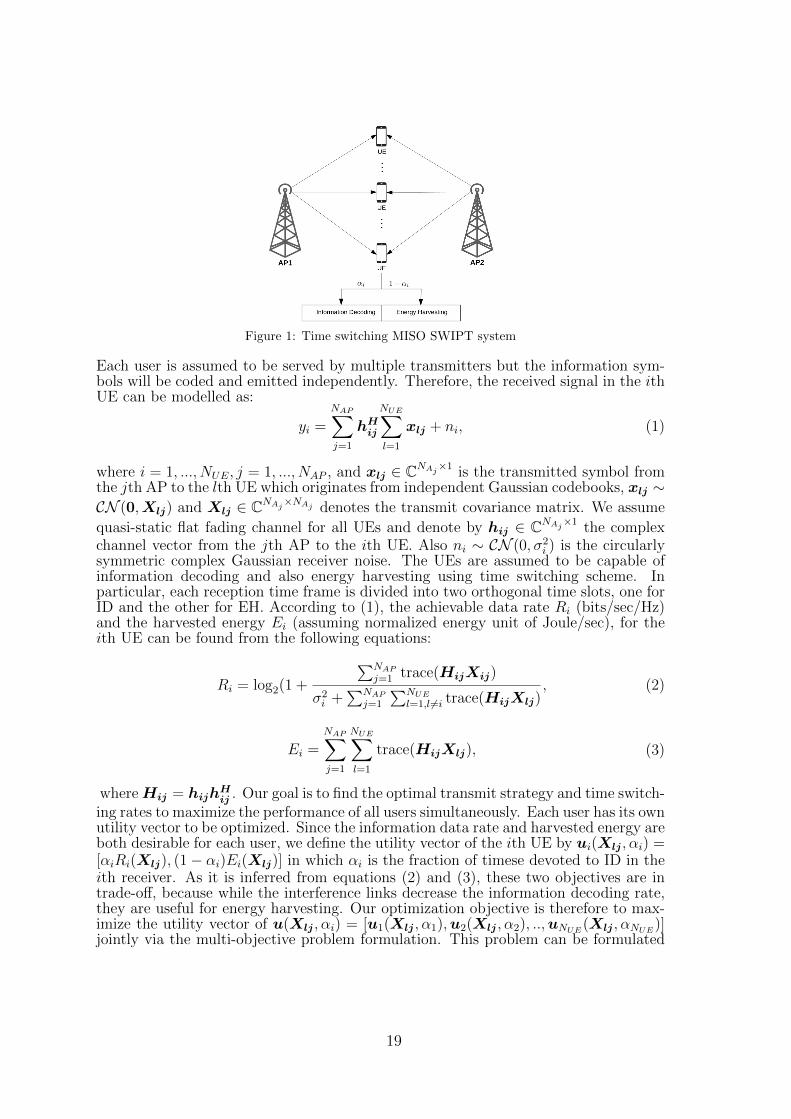
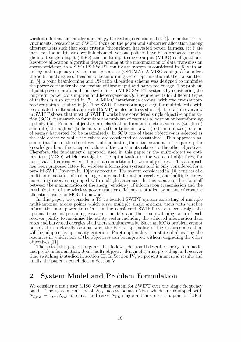
Figure 1: Time switching MISO SWIPT system
Each user is assumed to be served by multiple transmitters but the information sym-bols will be coded and emitted independently. Therefore, the received signal in the ithUE can be modelled as:
yi =
NAP∑
j=1
hHij
NUE∑
l=1
xlj + ni, (1)
where i = 1, ..., NUE, j = 1, ..., NAP , and xlj ∈ CNAj×1 is the transmitted symbol from
the jth AP to the lth UE which originates from independent Gaussian codebooks, xlj ∼CN (0,Xlj) and Xlj ∈ CNAj
×NAj denotes the transmit covariance matrix. We assume
quasi-static flat fading channel for all UEs and denote by hij ∈ CNAj×1 the complex
channel vector from the jth AP to the ith UE. Also ni ∼ CN (0, σ2i ) is the circularly
symmetric complex Gaussian receiver noise. The UEs are assumed to be capable ofinformation decoding and also energy harvesting using time switching scheme. Inparticular, each reception time frame is divided into two orthogonal time slots, one forID and the other for EH. According to (1), the achievable data rate Ri (bits/sec/Hz)and the harvested energy Ei (assuming normalized energy unit of Joule/sec), for theith UE can be found from the following equations:
Ri = log2(1 +
∑NAP
j=1 trace(HijXij)
σ2i +
∑NAP
j=1
∑NUE
l=1,l 6=i trace(HijXlj), (2)
Ei =
NAP∑
j=1
NUE∑
l=1
trace(HijXlj), (3)
whereHij = hijhHij . Our goal is to find the optimal transmit strategy and time switch-
ing rates to maximize the performance of all users simultaneously. Each user has its ownutility vector to be optimized. Since the information data rate and harvested energy areboth desirable for each user, we define the utility vector of the ith UE by ui(Xlj , αi) =[αiRi(Xlj), (1− αi)Ei(Xlj)] in which αi is the fraction of timese devoted to ID in theith receiver. As it is inferred from equations (2) and (3), these two objectives are intrade-off, because while the interference links decrease the information decoding rate,they are useful for energy harvesting. Our optimization objective is therefore to max-imize the utility vector of u(Xlj , αi) = [u1(Xlj , α1),u2(Xlj , α2), ..,uNUE
(Xlj , αNUE)]
jointly via the multi-objective problem formulation. This problem can be formulated
19

as:Maximize
Xlj ,αi
u(Xlj , αi)
subject to (1)
NUE∑
l=1
E(xHlj xlj) =
NUE∑
l=1
trace(Xlj) ≤ Pmaxj
(2) Xlj 0
(3) αi ∈ [0, 1],
(4)
where l, i = 1, ..., NUE, j = 1, ..., NAP and the first constraint denotes the average powerconstraint for each AP across all transmitting antennas. In the following, we convertthis problem into a SOO problem using scalarization method and then we propose analgorithm to solve this problem.
3 Joint transmit precoding and receiver time switch-
ing design
To solve the MOO problem (4), we use the weighted Chebyshev method [12] whichprovides complete Pareto optimal set by varying predefined preference parameters.The weighted Chebyshev goal function is:
fch(.) = Min1≤i≤NUE ,m=1,2
umivmi
, (5)
where umi denotes the mth element of ui(Xlj , αi) and v11, v21, ..., v
1NUE
, v2NUEare positive
weights that specify the priority of each objective. If we write the problem in epigraphform [13], this scalarization is equivalent to the following problem:
MaximizeXlj ,αi,λ
λ
subject to (1) αiRi(Xlj) ≥ λv1i
(2) (1− αi)Ei(Xlj) ≥ λv2i
(3)
NUE∑
l=1
trace(Xlj) ≤ Pmaxj
(4) Xlj 0
(5) αi ∈ [0, 1].
(6)
This problem is a non-convex semidefinite programming (SDP) due to not only thecoupled TS ratios and Ri, Ei in the first and second constraints but also the definitionof Ri as presented in (2). However, using the monotonicity and concavity properties
of logarithm function, and introducing the new variables λ = log(λ), Ri, Ei, Ii and βi,problem (6) can be represented as:
20
MaximizeXlj ,αi,βi,Ri,Ei,Ii,λ
λ
subject to (C1) log(αi) + log(Ri) ≥ λ+ log(v1i )
(C2) log(βi) + log(Ei) ≥ λ+ log(v2i )
(C3) Ei =
NAP∑
j=1
NUE∑
l=1
trace(HijXlj)
(C4) Ii =
NAP∑
j=1
NUE∑
l=1,l 6=itrace(HijXlj)
(C5) Ri = log(σ2i + Ei)− log(σ2
i + Ii)
(C6)
NUE∑
l=1
trace(Xlj) ≤ Pmaxj
(C7) Xlj 0
(C8) αi + βi = 1
(C9) αi ∈ [0, 1], βi ∈ [0, 1],
(P )
where (C5) is directly obtained from substituting the definition of Ei and Ii in thedefinition of Ri given by equation (2). This problem is a non-convex SDP because ofthe nonlinear equality in (C5). This problem can be solved using local optimizationmethod of sequential convex programming (SCP). In particular, the main difficultyof problem (P ) is concentrated in the nonlinear equality of (C5). This issue can beovercome by linearizing (C5) around the current iteration point and maintaining theremaining convexity of the original problem. To this end we use the first order Taylorexpansion to write the linearized version of (C5) as follows:
RLi = Ri(E
0i , I
0i ) +∇TRi(E
0i , I
0i )[Ei − E0
i , Ii − I0i ] =
log(σ2i + E0
i
σ2i + I0i
)+
1
σ2i + E0
i
(Ei − E0i )−
1
σ2i + I0i
(Ii − I0i ),
(7)
where E0i and I0i are the points around which the equation is linearized. Now we can
replace problem (P ) in the kth step by the following subproblem:
MaximizeXlj ,αi,βi,Ri,Ei,Ii,λ
λ
subject to (C1)-(C4)
(C6)-(C9)
Ri ' log(σ2i + Ek
i
σ2i + Iki
)+
1
σ2i + Ek
i
(Ei − Eki )−
1
σ2i + Iki
(Ii − Iki ).
(Pk)
21
Algorithm 1 SCP Algorithm
1: Step 0: Choose an initial point w0i = [E0
i , I0i ] inside the convex set defined by
(C1)-(C4), (C6)-(C9), γ ∈ R and a given tolerance ε > 0. Set k := 0.2: Step 1: For a given wk
i , solve the convex SDP of (Pk) to obtain the solutionwi(w
ki ) = [Ei(E
ki ), Ii(I
ki )].
3: Step 2: If ‖wi(wki )−wk
i ‖ 6 ε then stop. Otherwise setwki = wk
i +γ(wi(wki )−wk
i ).
4: Step 3: increase k by 1 and go back to step 1.
This problem is a convex SDP and it can be solved by standard optimization techniquessuch as Interior-point Method. In this paper, we have used CVX package to solve (Pk).The linearization point is updated with each iteration until it satisfies the terminationcriterion as described in Algorithm 1. It can be shown that if Algorithm 1 terminatesafter some iterations then wk
i = [Eki , I
ki ], i = 1, ..., NUE is a stationary point of problem
(P ). The local convergence of Algorithm 1 to a KKT point is proven in [14], undermild assumptions, and the rate of convergence is shown to be linear.
4 Numerical Results
In this section, we present numerical results to demonstrate the performance of theproposed multi-objective precoding and time switching algorithm in MISO SWIPTsystems. The system is set up as follows. There are NAP = 2 APs equipped withNA1 = NA2 = 2 antennas and NUE = 2 single antenna user equipments. Denoting thedistance of the ith user from the jth AP by dij, we assume a scenario with dij = 10m i = 1, ..., NUE, j = 1, ..., NAP . At this location, channel gains are generated withRayleigh fading and path loss effect with path loss exponent of 2. Channel bandwidthis set to 200 KHz and the spectral noise density is assumed to be N0 = −100 dBm/Hz.We have set the power constraints to be Pmax
j = 1 watt j = 1, 2. Also 100 realizationsof the channel are used for averaging in simulations.
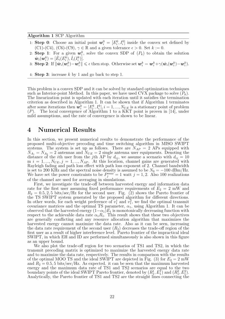
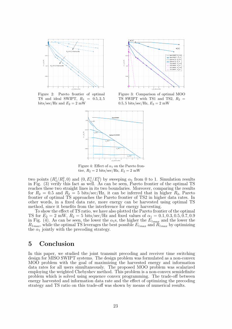
First, we investigate the trade-off between harvested energy and information datarate for the first user assuming fixed performance requirements of E2 = 2 mW andR2 = 0.5, 2, 5 bits/sec/Hz for the second user. Fig. (2) shows the Pareto frontier ofthe TS SWIPT system generated by the proposed algorithm for different directions.In other words, for each weight preference of v11 and v21, we find the optimal transmitcovariance matrices and the optimal TS parameter, α1, using Algorithm 1. It can beobserved that the harvested energy (1−α1)E1 is monotonically decreasing function withrespect to the achievable data rate α1R1. This result shows that these two objectivesare generally conflicting and any resource allocation algorithm that maximizes theharvested energy cannot maximize the data rate. Also as it can be seen, increasingthe data rate requirement of the second user (R2) decreases the trade-off region of thefirst user as a result of higher interference level. Pareto frontier of the impractical idealSWIPT, in which EH and ID are performed simultaneously is also shown in this figureas an upper bound.
We also plot the trade-off region for two scenarios of TS1 and TS2, in which thetransmit precoding matrix is optimized to maximize the harvested energy data rateand to maximize the data rate, respectively. The results in comparison with the resultsof the optimal MOO TS and the ideal SWIPT are depicted in Fig. (3) for E2 = 2 mWand R2 = 0.5, 5 bits/sec/Hz. As expected. it can be seen that the maximum harvestedenergy and the maximum data rate of TS1 and TS2 scenarios are equal to the twoboundary points of the ideal SWIPT Pareto frontier, denoted by (R1
1, E11) and (R2
1, E21).
Analytically, the Pareto frontier of TS1 and TS2 are the straight lines connecting the
22
α1R
1(bits/sec/Hz)
0 1 2 3 4 5 6 7 8 9 10 11
(1-α
1)E
1(W
)
0
0.005
0.01
0.015
0.02
R2=0.5,2,5 bits/sec/Hz
R2=0.5,2,5 bits/sec/Hz
Figure 2: Pareto frontier of optimalTS and ideal SWIPT, R2 = 0.5, 2, 5bits/sec/Hz and E2 = 2 mW
α1R
1(bits/sec/Hz)
0 1 2 3 4 5 6 7 8 9 10 11
(1-α
1)E
1(W
)
0
0.005
0.01
0.015
0.02
Ideal SWIPT, R2=0.5
Ideal SWIPT, R2=5
Optimal TS, R2=0.5
Optimal TS, R2=5
TS2 SWIPT, R2=0.5
TS2 SWIPT, R2=5
TS1 SWIPT, R2=0.5
TS1 SWIPT, R2=5
(R1
1,E
1
1)
(R1
2,E
1
2)
Figure 3: Comparison of optimal MOOTS SWIPT with TS1 and TS2, R2 =0.5, 5 bits/sec/Hz, E2 = 2 mW
α1R
1(bits/sec/Hz)
0 1 2 3 4 5 6 7 8 9 10
(1-α
1)E
1(W
)
0
0.005
0.01
0.015
0.02
0.025
Ideal SWIPT
α1=0.1
α1=0.3
α1=0.5
α1=0.7
α1=0.9
Optimal TS SWIPT
Figure 4: Effect of α1 on the Pareto fron-tier, R2 = 2 bits/sec/Hz, E2 = 2 mW
two points (R11/R
21, 0) and (0, E1
1/E21) by sweeping α1 from 0 to 1. Simulation results
in Fig. (3) verify this fact as well. As can be seen, Pareto frontier of the optimal TSreaches these two straight lines in its two boundaries. Moreover, comparing the resultsfor R2 = 0.5 and R2 = 5 bits/sec/Hz, it can be inferred that in higher R2, Paretofrontier of optimal TS approaches the Pareto frontier of TS2 in higher data rates. Inother words, in a fixed data rate, more energy can be harvested using optimal TSmethod, since it benefits from the interference for energy harvesting.
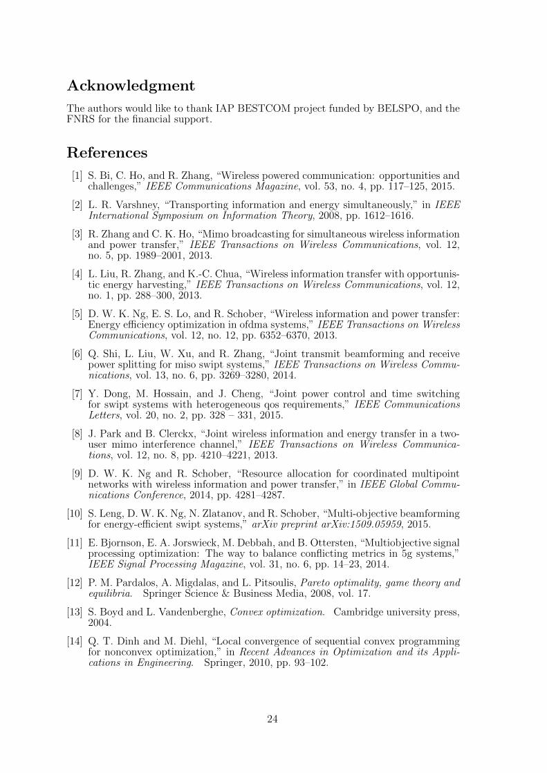
To show the effect of TS ratio, we have also plotted the Pareto frontier of the optimalTS for E2 = 2 mW, R2 = 5 bits/sec/Hz and fixed values of α1 = 0.1, 0.3, 0.5, 0.7, 0.9in Fig. (4). As can be seen, the lower the α1s, the higher the E1max and the lower theR1max, while the optimal TS leverages the best possible E1max and R1max by optimizingthe α1 jointly with the precoding strategy.
5 Conclusion
In this paper, we studied the joint transmit precoding and receiver time switchingdesign for MISO SWIPT systems. The design problem was formulated as a non-convexMOO problem with the goal of maximizing the harvested energy and informationdata rates for all users simultaneously. The proposed MOO problem was scalarizedemploying the weighted Chebyshev method. This problem is a non-convex semidefiniteproblem which is solved using sequence convex programming. The trade-off betweenenergy harvested and information data rate and the effect of optimizing the precodingstrategy and TS ratio on this trade-off was shown by means of numerical results.
23
Acknowledgment
The authors would like to thank IAP BESTCOM project funded by BELSPO, and theFNRS for the financial support.
References
[1] S. Bi, C. Ho, and R. Zhang, “Wireless powered communication: opportunities andchallenges,” IEEE Communications Magazine, vol. 53, no. 4, pp. 117–125, 2015.
[2] L. R. Varshney, “Transporting information and energy simultaneously,” in IEEEInternational Symposium on Information Theory, 2008, pp. 1612–1616.
[3] R. Zhang and C. K. Ho, “Mimo broadcasting for simultaneous wireless informationand power transfer,” IEEE Transactions on Wireless Communications, vol. 12,no. 5, pp. 1989–2001, 2013.
[4] L. Liu, R. Zhang, and K.-C. Chua, “Wireless information transfer with opportunis-tic energy harvesting,” IEEE Transactions on Wireless Communications, vol. 12,no. 1, pp. 288–300, 2013.
[5] D. W. K. Ng, E. S. Lo, and R. Schober, “Wireless information and power transfer:Energy efficiency optimization in ofdma systems,” IEEE Transactions on WirelessCommunications, vol. 12, no. 12, pp. 6352–6370, 2013.
[6] Q. Shi, L. Liu, W. Xu, and R. Zhang, “Joint transmit beamforming and receivepower splitting for miso swipt systems,” IEEE Transactions on Wireless Commu-nications, vol. 13, no. 6, pp. 3269–3280, 2014.
[7] Y. Dong, M. Hossain, and J. Cheng, “Joint power control and time switchingfor swipt systems with heterogeneous qos requirements,” IEEE CommunicationsLetters, vol. 20, no. 2, pp. 328 – 331, 2015.
[8] J. Park and B. Clerckx, “Joint wireless information and energy transfer in a two-user mimo interference channel,” IEEE Transactions on Wireless Communica-tions, vol. 12, no. 8, pp. 4210–4221, 2013.
[9] D. W. K. Ng and R. Schober, “Resource allocation for coordinated multipointnetworks with wireless information and power transfer,” in IEEE Global Commu-nications Conference, 2014, pp. 4281–4287.
[10] S. Leng, D. W. K. Ng, N. Zlatanov, and R. Schober, “Multi-objective beamformingfor energy-efficient swipt systems,” arXiv preprint arXiv:1509.05959, 2015.
[11] E. Bjornson, E. A. Jorswieck, M. Debbah, and B. Ottersten, “Multiobjective signalprocessing optimization: The way to balance conflicting metrics in 5g systems,”IEEE Signal Processing Magazine, vol. 31, no. 6, pp. 14–23, 2014.
[12] P. M. Pardalos, A. Migdalas, and L. Pitsoulis, Pareto optimality, game theory andequilibria. Springer Science & Business Media, 2008, vol. 17.
[13] S. Boyd and L. Vandenberghe, Convex optimization. Cambridge university press,2004.
[14] Q. T. Dinh and M. Diehl, “Local convergence of sequential convex programmingfor nonconvex optimization,” in Recent Advances in Optimization and its Appli-cations in Engineering. Springer, 2010, pp. 93–102.
24
Target detection for DVB-T based passive radarsusing pilot subcarrier signal
Osama Mahfoudia1,2, Francois Horlin2 and Xavier Neyt1
1Dept. CISS,Royal Military Academy, Brussels, Belgium2Dept. OPERA,Universite Libre de Bruxelles, Brussels, Belgium
Abstract
Passive coherent location (PCL) radars employ non-cooperative transmitters fortarget detection. The cross-correlation (CC) detector, as an approximation ofthe optimum detector, is widely applied in PCL radars: it cross-correlates thereference signal and the surveillance signal. The CC detector is sensitive tosignal-to-noise ratio (SNR) in the reference signal and thus a pre-processing ofthe reference signal is required. DVB-T based PCL radars can benefit from thepossibility of reference signal reconstruction for SNR enhancement. The recon-struction process requires an SNR level that allows accurate signal demodulation.Hence, for low SNR values, signal reconstruction performance is limited. In thispaper, we present a new approach that employs the subcarrier pilot signal forCC detection in DVB-T based PCL radars. We demonstrate the effectiveness ofreplacing the noisy reference signal with the a locally generated subcarrier pilotsignal for CC detection.
1 IntroductionPassive coherent location (PCL) radars exploit radiations from illuminators of oppor-tunity (IO), non-cooperative transmitter, to detect and track targets in an area ofinterest. The essential advantages of PCL radars are low cost, interception immunity,ease of deployment, and stealth aircraft detection capability [1, 2]. Several commercialtransmitters for communication and broadcasting have been used as IO. For example,FM radio broadcast [3], satellite illumination [4], digital audio and video broadcast(DAB and DVB-T) [5] and Global System for Mobile communications (GSM) basestations [6, 7]. The architecture of PCL radars in the bistatic configuration consists oftwo receiving channels: a reference channel (RC) and a surveillance channel (SC). TheRC captures the direct-path signal from the IO and the SC receives the target echoes.
The majority of existing PCL systems employs a cross-correlation (CC) detector.The CC detection approach is an approximation of the matched filter (MF) where acopy of the transmitted waveform is cross-correlated with the received echo to performtarget detection. The exact transmitted waveform employed in MF is inaccessible inPCL radars since the IO is non-cooperative. PCL systems replace the exact waveformused in MF with the reference signal (received through RC). The reference signal isoften corrupted by noise and interferences which decreases the coherent integrationgain and thus degrades the CC detection performance[8].
1
25
PCL systems that exploit the DVB-T broadcasters can benefit from an enhance-ment of the signal-to-noise ratio (SNR) of the reference signal by demodulating andreconstructing the transmitted data. However, The reference signal reconstructionstrategy is limited since it requires an SNR that allows accurate demodulation of thereceived signal [9, 10].
DVB-T broadcasters have attracted the interest of PCL researchers for their rel-atively wide bandwidth (8 MHz) allowing good range resolution. In addition, asa digital waveform its spectrum is independent of the signal content. Furthermore,the high radiated power of the DVB-T transmitters permits a considerable detectionrange. The DVB-T signal consists of two components: a stochastic component thatresults from the transmitted data randomness and a deterministic one due to the pilotsubcarriers.
In this work, we consider a DVB-T based PCL radar and we introduce a newdetection strategy. Precisely, we investigate the use of pilot carriers signal for detectionas an alternative to the noisy reference signal. In order to do so, we adopt the statisticalmodel developed in [8] and prove that using a locally generated pilot subcarrier signaloutperforms employing the noisy reference signal for CC detection.
This paper is organized as follows. Section 2 reviews the DVB-T signal structureand introduces the average power ratio between the stochastic component and the de-terministic one. Section 3 introduces the proposed detection strategy and provides thereceived signals model. In section 4, we derive closed-form expressions for false alarmand detection probabilities. In section 5, the simulation results validate the derivedclosed-form expression and show that the proposed detection strategy outperforms theuse of the full noisy reference signal. Section 6 concludes the paper.
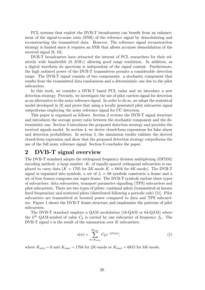
2 DVB-T signal overviewThe DVB-T standard adopts the orthogonal frequency division multiplexing (OFDM)encoding method: a large number -K- of equally-spaced orthogonal subcarriers is em-ployed to carry data (K = 1705 for 2K-mode K = 6816 for 8K-mode). The DVB-Tsignal is organized into symbols, a set of L = 68 symbols constructs a frame and aset of four frames composes one super-frame. The DVB-T symbols enclose three typesof subcarriers: data subcarriers, transport parameter signalling (TPS) subcarriers andpilot subcarriers. There are two types of pilots: continual pilots (transmitted at knownfixed frequencies) and scattered pilots (distributed following a periodic rule) [11]. Pilotsubcarriers are transmitted at boosted power compared to data and TPS subcarri-ers. Figure 1 shows the DVB-T frame structure and emphasizes the patterns of pilotsubcarriers.
The DVB-T standard employs a QAM modulation (16-QAM or 64-QAM) wherethe kth QAM-symbol of value Ck is carried by one subcarrier of frequency fk. TheDVB-T signal s is the result of the summation over K subcarriers:
s(n) =Kmax∑
k=Kmin
Cke−j2πfkn, (1)
where Kmin = 0 and Kmax = 1704 for 2K-mode or Kmax = 6815 for 8K-mode.
26
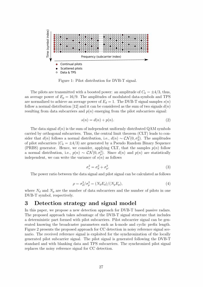
Figure 1: Pilot distribution for DVB-T signal.
The pilots are transmitted with a boosted power: an amplitude of Ck = ±4/3, thus,an average power of Ep = 16/9. The amplitudes of modulated data-symbols and TPSare normalized to achieve an average power of Ed = 1. The DVB-T signal samples s(n)follow a normal distribution [12] and it can be considered as the sum of two signals d(n)resulting from data subcarriers and p(n) emerging from the pilot subcarriers signal:
s(n) = d(n) + p(n). (2)
The data signal d(n) is the sum of independent uniformly distributed QAM symbolscarried by orthogonal subcarriers. Thus, the central limit theorem (CLT) leads to con-sider that d(n) follows a normal distribution, i.e., d(n) ∼ CN (0, σ2
d). The amplitudesof pilot subcarriers (Ck = ±4/3) are generated by a Pseudo Random Binary Sequence(PRBS) generator. Hence, we consider, applying CLT, that the samples p(n) followa normal distribution, i.e., p(n) ∼ CN (0, σ2
p). Since d(n) and p(n) are statisticallyindependent, we can write the variance of s(n) as follows
σ2s = σ2
d + σ2p. (3)
The power ratio between the data signal and pilot signal can be calculated as follows
ρ = σ2d/σ
2p = (NdEd)/(NpEp), (4)
where Nd and Np are the number of data subcarriers and the number of pilots in oneDVB-T symbol, respectively.
3 Detection strategy and signal modelIn this paper, we propose a new detection approach for DVB-T based passive radars.The proposed approach takes advantage of the DVB-T signal structure that includesa deterministic part formed with pilot subcarriers. Pilot subcarrier signal can be gen-erated knowing the broadcaster parameters such as k-mode and cyclic prefix length.Figure 2 presents the proposed approach for CC detection in noisy reference signal sce-nario. The received reference signal is exploited for the synchronization of the locallygenerated pilot subcarrier signal. The pilot signal is generated following the DVB-Tstandard and with blanking data and TPS subcarriers. The synchronized pilot signalreplaces the noisy reference signal for CC detection.
27
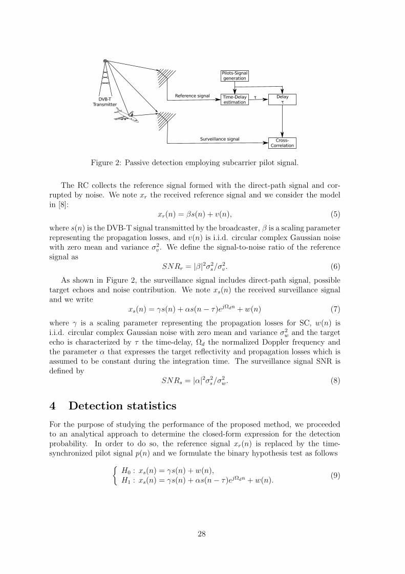
Figure 2: Passive detection employing subcarrier pilot signal.
The RC collects the reference signal formed with the direct-path signal and cor-rupted by noise. We note xr the received reference signal and we consider the modelin [8]:
xr(n) = βs(n) + v(n), (5)
where s(n) is the DVB-T signal transmitted by the broadcaster, β is a scaling parameterrepresenting the propagation losses, and v(n) is i.i.d. circular complex Gaussian noisewith zero mean and variance σ2
v . We define the signal-to-noise ratio of the referencesignal as
SNRr = |β|2σ2s/σ
2v . (6)
As shown in Figure 2, the surveillance signal includes direct-path signal, possibletarget echoes and noise contribution. We note xs(n) the received surveillance signaland we write
xs(n) = γs(n) + αs(n− τ)ejΩdn + w(n) (7)
where γ is a scaling parameter representing the propagation losses for SC, w(n) isi.i.d. circular complex Gaussian noise with zero mean and variance σ2
w and the targetecho is characterized by τ the time-delay, Ωd the normalized Doppler frequency andthe parameter α that expresses the target reflectivity and propagation losses which isassumed to be constant during the integration time. The surveillance signal SNR isdefined by
SNRs = |α|2σ2s/σ
2w. (8)
4 Detection statistics
For the purpose of studying the performance of the proposed method, we proceededto an analytical approach to determine the closed-form expression for the detectionprobability. In order to do so, the reference signal xr(n) is replaced by the time-synchronized pilot signal p(n) and we formulate the binary hypothesis test as follows
H0 : xs(n) = γs(n) + w(n),H1 : xs(n) = γs(n) + αs(n− τ)ejΩdn + w(n).
(9)
28

Under both hypotheses H0 and H1, we calculate the statistics of the cross-correlationdetector. For each range-Doppler cell, the reference signal is time-delayed and fre-quency shifted to match the possible target echo in the cell under test (CUT) and thedetection test is given by:
T =∣∣T 2
∣∣ =∣∣∣∣∣N−1∑
n=0
Tn
∣∣∣∣∣
2H1
≷H0
λ, (10)
with λ the detection threshold and Tn is the CC detector result given by
Tn = x∗s(n)p(n− τ)exp(jΩdn). (11)
Under the alternative hypothesis H1, we calculate the mean and the variance of Tn (toretrieve the statistics for the null hypothesis, we set α = 0). The mean value of Tn is
ETn = α∗σ2p , (12)
and its variance is
var Tn = |γ|2 (σ2d + σ2
p)σ2p + |α|2 (σ2
dσ2p + φ) + σ2
wσ2p, (13)
we introduce the pilot-data power ratio (Eq. 4)
var Tn = |γ|2 σ4p(1 + ρ) + |α|2 (ρσ4
p + φ) + σ2wσ
2p, (14)
withφ = var|d(n− τ)|2. (15)
For a coherent integration time of N samples, the CC output is represented by thequantity T . It follows a normal distribution with parameters (µ0, σ
20) under the null
hypothesis and (µ1, σ21) under the alternative one:
µ0 = 0, (16)
σ20 = N(|γ|2 σ4
p(1 + ρ) + σ2wσ
2p), (17)
µ1 = N(α∗σ2p), (18)
σ21 = N(|γ|2 σ4
p(1 + ρ) + |α|2 (ρσ4p + φ) + σ2
wσ2p). (19)
The statistic T = |T |2 underH0 follows a central chi-squared distribution of two degreesof freedom. Thus, the false alarm probability is calculated as follows
PFA = exp
(− λ
σ20
), (20)
the detection probability is given by the Marcum Q-function of first order:
PD = Q1
√
2|µ1|2σ21
,
√2σ2
0ln(P−1FA)
σ21
. (21)
29
5 Numerical results and discussionIn order to verify the validity of the detection probability expression in (21), we carriedout Monte-Carlo (MC) simulations. Simulation parameters are: signal-to-noise ratioin the reference signal SNRr = −10dB, coherent integration time N = 105 and false-alarm probability PFA = 10−2 (N and PFA are constant for this section). Figure 3shows the detection probability variation versus the surveillance signal SNR value forMC simulations and expression in (21). As can be seen from this figure, the analyt-ical expression matches perfectly MC results which validates the derived closed-formexpressions and the feasibility of pilot subcarrier signal detection for DVB-T basedpassive radars.
−40 −35 −30 −25 −200
0.1
0.2
0.3
0.4
0.5
0.6
0.7
0.8
0.9
1
SNR in the surveillance signal [dB]
Det
ectio
n P
roba
bilit
y
TheoreticalMonte Carlo
Figure 3: Validation of the detection probability expression.
After validating the feasibility of using pilot subcarrier signal as reference signalfor the CC detector, the proposed method is compared to two variants of referencesignal: a received reference signal with signal-to-noise ratio SNRr = −10dB and areconstructed reference signal. Figure 4 presents the results of MC simulations for de-tection probability considering two variants of reference signal and the pilot subcarriersignal. For the considered scenario with SNRr = −10dB, CC detection employingpilot subcarrier signal outperforms that using a noisy reference signal. Detection usingreconstructed reference signal surpasses slightly that using the proposed method. Thisis due to the fact that the reconstructed signal contains noise-free pilot subcarriers. Inaddition, even if the demodulation introduces errors for SNRr = −10dB, the SNR lossin the reconstructed signal is slightly higher than that due to using pilot-only signal.
To investigate the behavior of CC detection employing pilot subcarrier signal, weperformed MC simulations for detection probability for a set of SNRr values and afixed value of SNRs = −30dB. Figure 5 shows MC simulation results. As the pilotsubcarrier signal is unrelated to SNRr, the detection probability is constant for agiven value of SNRs. For the reconstructed reference signal, the detection probabilityconverges to a non-null value for low SNRr values. This is due to the fact thatsignal reconstruction for low SNRr generates noise (caused by demodulation errors)but provides noise-free subcarrier pilots. Hence, the non-null convergence value of
30
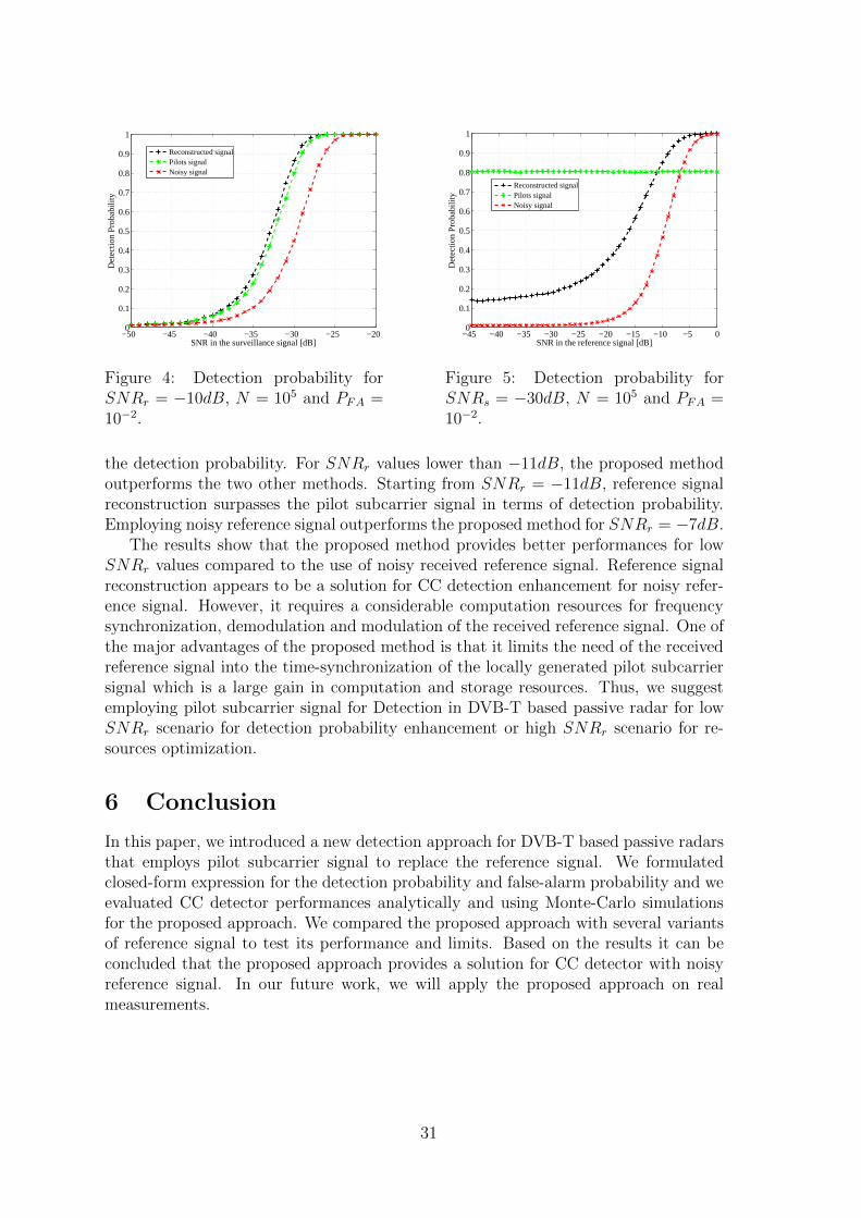
−50 −45 −40 −35 −30 −25 −200
0.1
0.2
0.3
0.4
0.5
0.6
0.7
0.8
0.9
1
SNR in the surveillance signal [dB]
Det
ectio
n P
roba
bilit
y
Reconstructed signalPilots signalNoisy signal
Figure 4: Detection probability forSNRr = −10dB, N = 105 and PFA =10−2.
−45 −40 −35 −30 −25 −20 −15 −10 −5 00
0.1
0.2
0.3
0.4
0.5
0.6
0.7
0.8
0.9
1
SNR in the reference signal [dB]
Det
ectio
n P
roba
bilit
y
Reconstructed signalPilots signalNoisy signal
Figure 5: Detection probability forSNRs = −30dB, N = 105 and PFA =10−2.
the detection probability. For SNRr values lower than −11dB, the proposed methodoutperforms the two other methods. Starting from SNRr = −11dB, reference signalreconstruction surpasses the pilot subcarrier signal in terms of detection probability.Employing noisy reference signal outperforms the proposed method for SNRr = −7dB.
The results show that the proposed method provides better performances for lowSNRr values compared to the use of noisy received reference signal. Reference signalreconstruction appears to be a solution for CC detection enhancement for noisy refer-ence signal. However, it requires a considerable computation resources for frequencysynchronization, demodulation and modulation of the received reference signal. One ofthe major advantages of the proposed method is that it limits the need of the receivedreference signal into the time-synchronization of the locally generated pilot subcarriersignal which is a large gain in computation and storage resources. Thus, we suggestemploying pilot subcarrier signal for Detection in DVB-T based passive radar for lowSNRr scenario for detection probability enhancement or high SNRr scenario for re-sources optimization.
6 Conclusion
In this paper, we introduced a new detection approach for DVB-T based passive radarsthat employs pilot subcarrier signal to replace the reference signal. We formulatedclosed-form expression for the detection probability and false-alarm probability and weevaluated CC detector performances analytically and using Monte-Carlo simulationsfor the proposed approach. We compared the proposed approach with several variantsof reference signal to test its performance and limits. Based on the results it can beconcluded that the proposed approach provides a solution for CC detector with noisyreference signal. In our future work, we will apply the proposed approach on realmeasurements.
31
References
[1] H. D. Griffiths and C. J. Baker, “Passive coherent location radar systems. part1: performance prediction,” IEE Proceedings - Radar, Sonar and Navigation,vol. 152, pp. 153–159, June 2005.
[2] C. J. Baker, H. D. Griffiths, and I. Papoutsis, “Passive coherent location radarsystems. part 2: waveform properties,” IEE Proceedings - Radar, Sonar and Nav-igation, vol. 152, pp. 160–168, June 2005.
[3] S. Bayat, M. Nayebi, and Y. Norouzi, “Target detection by passive coherent FMbased bistatic radar,” in Radar, 2008 International Conference on, pp. 412–415,Sept 2008.
[4] P. Marques, A. Ferreira, F. Fortes, P. Sampaio, H. Rebelo, and L. Reis, “A ped-agogical passive radar using DVB-S signals,” in Synthetic Aperture Radar (AP-SAR), 2011 3rd International Asia-Pacific Conference on, pp. 1–4, Sept 2011.
[5] C. Berger, B. Demissie, J. Heckenbach, P. Willett, and S. Zhou, “Signal processingfor passive radar using OFDM waveforms,” Selected Topics in Signal Processing,IEEE Journal of, vol. 4, pp. 226–238, Feb 2010.
[6] X. Neyt, J. Raout, M. Kubica, V. Kubica, S. Roques, M. Acheroy, and J. Verly,“Feasibility of STAP for passive GSM-based radar,” in Radar, 2006 IEEE Con-ference on, pp. 6 pp.–, April 2006.
[7] M. Kubica, V. Kubica, X. Neyt, J. Raout, S. Roques, and M. Acheroy, “Opti-mum target detection using illuminators of opportunity,” in Radar, 2006 IEEEConference on, pp. 8 pp.–, April 2006.
[8] J. Liu, H. Li, and B. Himed, “Analysis of cross-correlation detector for passiveradar applications,” in Radar Conference (RadarCon), 2015 IEEE, pp. 0772–0776,May 2015.
[9] J. Palmer, H. Harms, S. Searle, and L. Davis, “DVB-T passive radar signal pro-cessing,” Signal Processing, IEEE Transactions on, vol. 61, pp. 2116–2126, April2013.
[10] M. Baczyk and M. Malanowski, “Reconstruction of the reference signal in dvb-t-based passive radar,” International Journal of Electronics and Telecommunica-tions, vol. 57, no. 1, pp. 43–48, 2011. cited By 18.
[11] Digital Video Broadcasting (DVB);Framing structure, channel coding and modu-lation for digital terrestrial television. European Telecommunications StandardsInstitute, 2004.
[12] K. Polonen and V. Koivunen, “Detection of DVB-T2 control symbols in passiveradar systems,” in Sensor Array and Multichannel Signal Processing Workshop(SAM), 2012 IEEE 7th, pp. 309–312, June 2012.
32
Noise Stabilization with Simultaneous OrthogonalMatching Pursuit
Jean-Francois Determe∗ † Jerome Louveaux† Laurent Jacques† Francois Horlin∗
Universite Libre de Bruxelles∗ Universite Catholique de Louvain†
OPERA-WCG department ICTEAM departmentAvenue F. Roosevelt 50, CP 165/81 Avenue G. Lemaıtre 4, bte L4.05.01
1050 Brussels, Belgium 1348 Louvain-la-Neuve, Belgium
[email protected] [email protected]
[email protected] [email protected]
Abstract
This paper addresses the problem of recovering several sparse signals acquiredby means of a noisy linear measurement process returning fewer observationsthan the dimension of the sparse signals of interest. The proposed signal modelassumes that the noise is additive and Gaussian. Within the aforementionedframework, theoretical developments making use of the theory of compressivesensing show that sparse signals with similar supports can be jointly and reliablyrecovered by means of the greedy algorithm entitled simultaneous orthogonalmatching pursuit (SOMP) provided that the linear measurements are appropri-ately designed. A variant of SOMP weighting each measurement vector accordingto its noise level is then presented. Finally, simulations confirm the benefits ofweighting the measurement vectors in SOMP and show that the optimal weightspredicted by the theory match the empirical ones under proper conditions.
1 Introduction to compressive sensing
In this paper, we examine the recovery of a signal f ∈ Rn on the basis of a pre-scribed set of linear measurements. The matrix Φ ∈ Rm×n, which describes the linearmeasurement process, generates the measurement vector y ∈ Rm:
y = Φf . (1)
Assuming that m < n, standard results in linear algebra show that there is no way toretrieve an arbitrary signal f on the basis of y and Φ as rank(Φ) ≤ min(m,n) = m < n.However, many signals are known to be expressible using only a small percentage ofvectors from the appropriate basis. For example, images such as those encountered inphotography or medical imaging admit sparse representations in wavelet bases, i.e.,representations that only require a few wavelets to map “most” of the image. As weare about to discuss, this sparsity property can be exploited and enforced to recover fon the basis of y even though m n. Formally, we write f = Ψx =
∑nj=1 xjψj where
Ψ represents the basis (e.g. a wavelet basis), ψj is the jth vector (or column) of Ψ,and x denotes the coefficients of f in that basis. The vector x is assumed to be sparse,i.e., ‖x‖0 := |supp(x)| := |j : xj 6= 0| is low where supp(x) is called the supportof x and | · | denotes the cardinality. Any signal x such that ‖x‖0 ≤ s is referredto as a s-sparse signal. The compressive sensing (CS) literature [6] has shown that ifx is sufficiently sparse when compared to m and n and if Φ satisfies some properties(see after), then it is possible to retrieve x on the basis of Φ and the measurementsy = Φf = ΦΨx. The measurement matrix Φ is often generated randomly by using
33
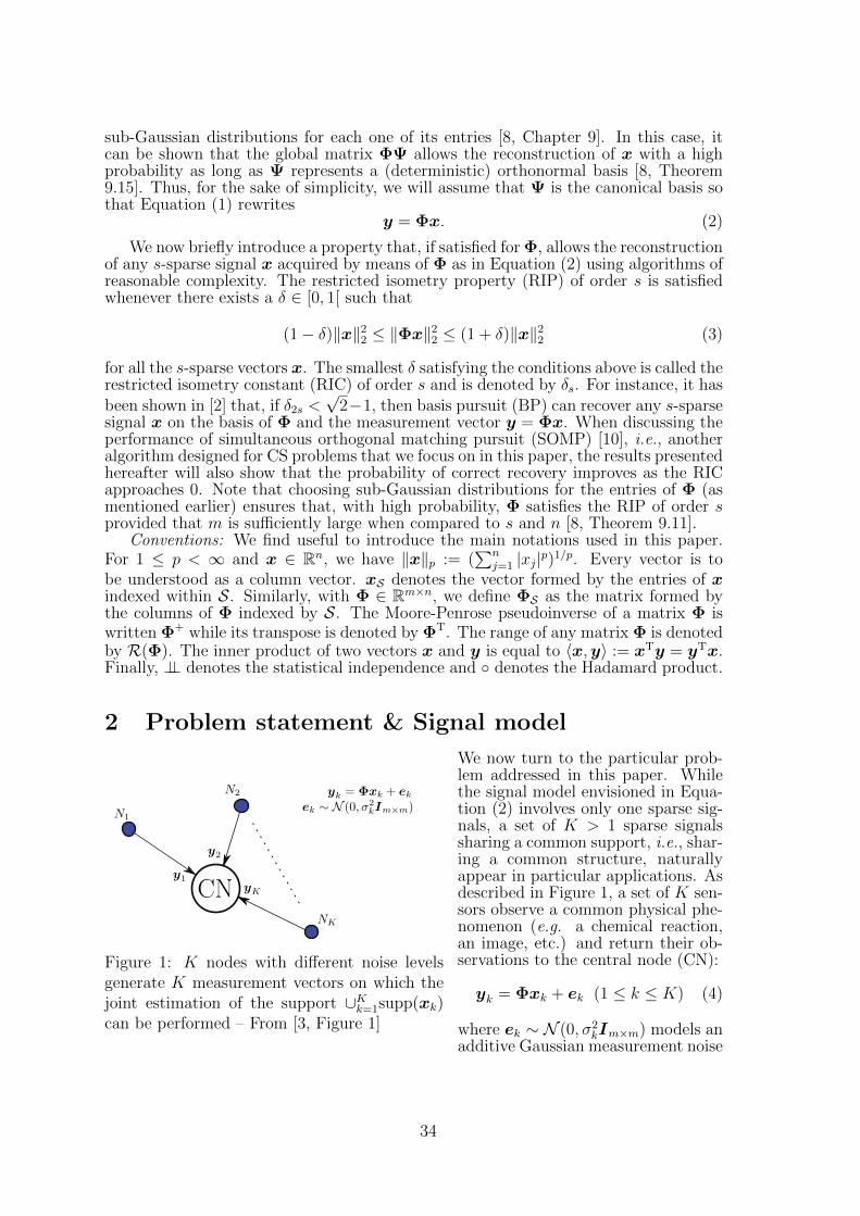
sub-Gaussian distributions for each one of its entries [8, Chapter 9]. In this case, itcan be shown that the global matrix ΦΨ allows the reconstruction of x with a highprobability as long as Ψ represents a (deterministic) orthonormal basis [8, Theorem9.15]. Thus, for the sake of simplicity, we will assume that Ψ is the canonical basis sothat Equation (1) rewrites
y = Φx. (2)
We now briefly introduce a property that, if satisfied for Φ, allows the reconstructionof any s-sparse signal x acquired by means of Φ as in Equation (2) using algorithms ofreasonable complexity. The restricted isometry property (RIP) of order s is satisfiedwhenever there exists a δ ∈ [0, 1[ such that
(1− δ)‖x‖22 ≤ ‖Φx‖22 ≤ (1 + δ)‖x‖22 (3)
for all the s-sparse vectors x. The smallest δ satisfying the conditions above is called therestricted isometry constant (RIC) of order s and is denoted by δs. For instance, it hasbeen shown in [2] that, if δ2s <
√2−1, then basis pursuit (BP) can recover any s-sparse
signal x on the basis of Φ and the measurement vector y = Φx. When discussing theperformance of simultaneous orthogonal matching pursuit (SOMP) [10], i.e., anotheralgorithm designed for CS problems that we focus on in this paper, the results presentedhereafter will also show that the probability of correct recovery improves as the RICapproaches 0. Note that choosing sub-Gaussian distributions for the entries of Φ (asmentioned earlier) ensures that, with high probability, Φ satisfies the RIP of order sprovided that m is sufficiently large when compared to s and n [8, Theorem 9.11].
Conventions: We find useful to introduce the main notations used in this paper.For 1 ≤ p < ∞ and x ∈ Rn, we have ‖x‖p := (
∑nj=1 |xj|p)1/p. Every vector is to
be understood as a column vector. xS denotes the vector formed by the entries of xindexed within S. Similarly, with Φ ∈ Rm×n, we define ΦS as the matrix formed bythe columns of Φ indexed by S. The Moore-Penrose pseudoinverse of a matrix Φ iswritten Φ+ while its transpose is denoted by ΦT. The range of any matrix Φ is denotedby R(Φ). The inner product of two vectors x and y is equal to 〈x,y〉 := xTy = yTx.Finally, ⊥⊥ denotes the statistical independence and denotes the Hadamard product.
2 Problem statement & Signal model
N1
N2
NK
y1
y2
yK
yk = Φxk + ekek ∼ N (0, σ2
kIm×m)
CN
Figure 1: K nodes with different noise levelsgenerate K measurement vectors on which thejoint estimation of the support ∪Kk=1supp(xk)can be performed – From [3, Figure 1]
We now turn to the particular prob-lem addressed in this paper. Whilethe signal model envisioned in Equa-tion (2) involves only one sparse sig-nals, a set of K > 1 sparse signalssharing a common support, i.e., shar-ing a common structure, naturallyappear in particular applications. Asdescribed in Figure 1, a set of K sen-sors observe a common physical phe-nomenon (e.g. a chemical reaction,an image, etc.) and return their ob-servations to the central node (CN):
yk = Φxk + ek (1 ≤ k ≤ K) (4)
where ek ∼ N (0, σ2kIm×m) models an
additive Gaussian measurement noise
34
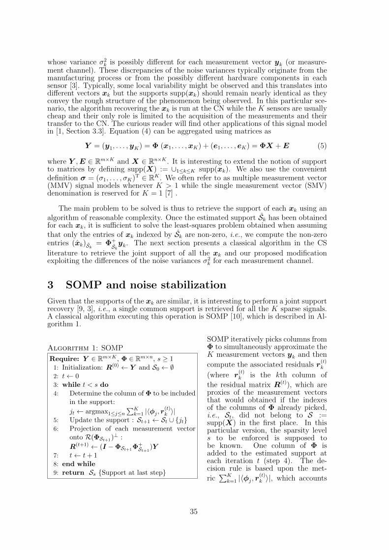
whose variance σ2k is possibly different for each measurement vector yk (or measure-
ment channel). These discrepancies of the noise variances typically originate from themanufacturing process or from the possibly different hardware components in eachsensor [3]. Typically, some local variability might be observed and this translates intodifferent vectors xk but the supports supp(xk) should remain nearly identical as theyconvey the rough structure of the phenomenon being observed. In this particular sce-nario, the algorithm recovering the xk is run at the CN while the K sensors are usuallycheap and their only role is limited to the acquisition of the measurements and theirtransfer to the CN. The curious reader will find other applications of this signal modelin [1, Section 3.3]. Equation (4) can be aggregated using matrices as
Y = (y1, . . . ,yK) = Φ (x1, . . . ,xK) + (e1, . . . , eK) = ΦX +E (5)
where Y ,E ∈ Rm×K and X ∈ Rn×K . It is interesting to extend the notion of supportto matrices by defining supp(X) := ∪1≤k≤K supp(xk). We also use the convenientdefinition σ = (σ1, . . . , σK)T ∈ RK . We often refer to as multiple measurement vector(MMV) signal models whenever K > 1 while the single measurement vector (SMV)denomination is reserved for K = 1 [7] .
The main problem to be solved is thus to retrieve the support of each xk using analgorithm of reasonable complexity. Once the estimated support Sk has been obtainedfor each xk, it is sufficient to solve the least-squares problem obtained when assumingthat only the entries of xk indexed by Sk are non-zero, i.e., we compute the non-zeroentries (xk)Sk = Φ+
Skyk. The next section presents a classical algorithm in the CS
literature to retrieve the joint support of all the xk and our proposed modificationexploiting the differences of the noise variances σ2
k for each measurement channel.
3 SOMP and noise stabilization
Given that the supports of the xk are similar, it is interesting to perform a joint supportrecovery [9, 3], i.e., a single common support is retrieved for all the K sparse signals.A classical algorithm executing this operation is SOMP [10], which is described in Al-gorithm 1.
Algorithm 1: SOMP
Require: Y ∈ Rm×K , Φ ∈ Rm×n, s ≥ 11: Initialization: R(0) ← Y and S0 ← ∅2: t← 03: while t < s do4: Determine the column of Φ to be included
in the support:
jt ← argmax1≤j≤n∑K
k=1 |〈φj , r(t)k 〉|
5: Update the support : St+1 ← St ∪ jt6: Projection of each measurement vector
onto R(ΦSt+1)⊥ :
R(t+1) ← (I −ΦSt+1Φ+St+1
)Y7: t← t+ 18: end while9: return Ss Support at last step
SOMP iteratively picks columns fromΦ to simultaneously approximate theK measurement vectors yk and then
compute the associated residuals r(t)k
(where r(t)k is the kth column of
the residual matrix R(t)), which areproxies of the measurement vectorsthat would obtained if the indexesof the columns of Φ already picked,i.e., St, did not belong to S :=supp(X) in the first place. In thisparticular version, the sparsity levels to be enforced is supposed tobe known. One column of Φ isadded to the estimated support ateach iteration t (step 4). The de-cision rule is based upon the met-
ric∑K
k=1 |〈φj, r(t)k 〉|, which accounts
35
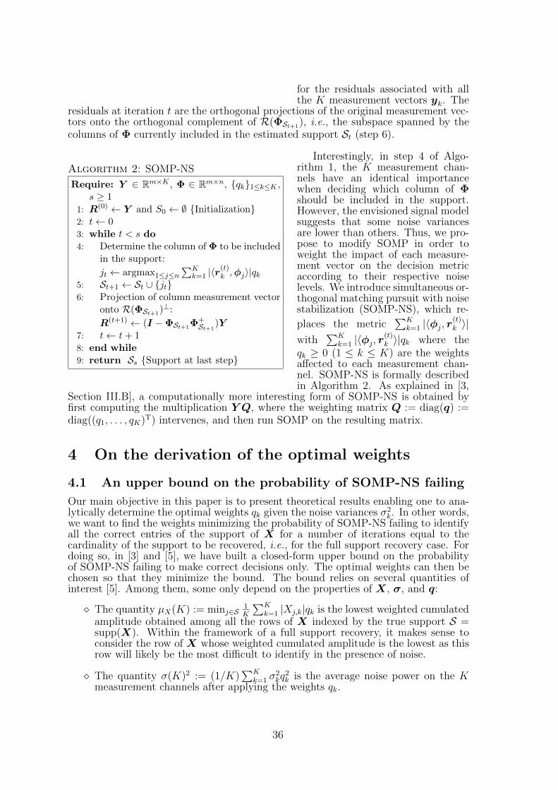
for the residuals associated with allthe K measurement vectors yk. The
residuals at iteration t are the orthogonal projections of the original measurement vec-tors onto the orthogonal complement of R(ΦSt+1), i.e., the subspace spanned by thecolumns of Φ currently included in the estimated support St (step 6).
Algorithm 2: SOMP-NS
Require: Y ∈ Rm×K , Φ ∈ Rm×n, qk1≤k≤K ,s ≥ 1
1: R(0) ← Y and S0 ← ∅ Initialization2: t← 03: while t < s do4: Determine the column of Φ to be included
in the support:
jt ← argmax1≤j≤n∑K
k=1 |〈r(t)k ,φj〉|qk
5: St+1 ← St ∪ jt6: Projection of column measurement vector
onto R(ΦSt+1)⊥:
R(t+1) ← (I −ΦSt+1Φ+St+1
)Y7: t← t+ 18: end while9: return Ss Support at last step
Interestingly, in step 4 of Algo-rithm 1, the K measurement chan-nels have an identical importancewhen deciding which column of Φshould be included in the support.However, the envisioned signal modelsuggests that some noise variancesare lower than others. Thus, we pro-pose to modify SOMP in order toweight the impact of each measure-ment vector on the decision metricaccording to their respective noiselevels. We introduce simultaneous or-thogonal matching pursuit with noisestabilization (SOMP-NS), which re-
places the metric∑K
k=1 |〈φj, r(t)k 〉|
with∑K
k=1 |〈φj, r(t)k 〉|qk where the
qk ≥ 0 (1 ≤ k ≤ K) are the weightsaffected to each measurement chan-nel. SOMP-NS is formally describedin Algorithm 2. As explained in [3,
Section III.B], a computationally more interesting form of SOMP-NS is obtained byfirst computing the multiplication Y Q, where the weighting matrix Q := diag(q) :=diag((q1, . . . , qK)T) intervenes, and then run SOMP on the resulting matrix.
4 On the derivation of the optimal weights
4.1 An upper bound on the probability of SOMP-NS failing
Our main objective in this paper is to present theoretical results enabling one to ana-lytically determine the optimal weights qk given the noise variances σ2
k. In other words,we want to find the weights minimizing the probability of SOMP-NS failing to identifyall the correct entries of the support of X for a number of iterations equal to thecardinality of the support to be recovered, i.e., for the full support recovery case. Fordoing so, in [3] and [5], we have built a closed-form upper bound on the probabilityof SOMP-NS failing to make correct decisions only. The optimal weights can then bechosen so that they minimize the bound. The bound relies on several quantities ofinterest [5]. Among them, some only depend on the properties of X, σ, and q:
The quantity µX(K) := minj∈S1K
∑Kk=1 |Xj,k|qk is the lowest weighted cumulated
amplitude obtained among all the rows of X indexed by the true support S =supp(X). Within the framework of a full support recovery, it makes sense toconsider the row of X whose weighted cumulated amplitude is the lowest as thisrow will likely be the most difficult to identify in the presence of noise.
The quantity σ(K)2 := (1/K)∑K
k=1 σ2kq
2k is the average noise power on the K
measurement channels after applying the weights qk.
36
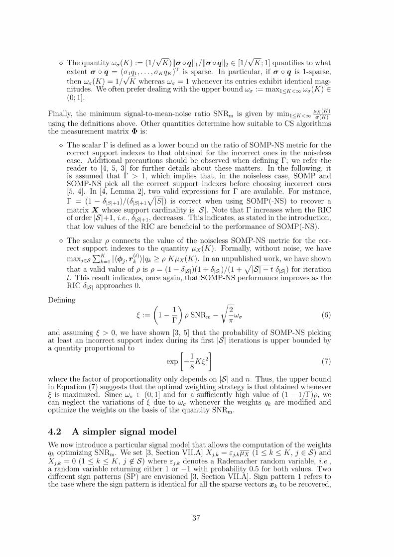
The quantity ωσ(K) := (1/√K)‖σ q‖1/‖σ q‖2 ∈ [1/
√K; 1] quantifies to what
extent σ q = (σ1q1, . . . , σKqK)T is sparse. In particular, if σ q is 1-sparse,
then ωσ(K) = 1/√K whereas ωσ = 1 whenever its entries exhibit identical mag-
nitudes. We often prefer dealing with the upper bound ωσ := max1≤K<∞ ωσ(K) ∈(0; 1].
Finally, the minimum signal-to-mean-noise ratio SNRm is given by min1≤K<∞µX(K)σ(K)
using the definitions above. Other quantities determine how suitable to CS algorithmsthe measurement matrix Φ is:
The scalar Γ is defined as a lower bound on the ratio of SOMP-NS metric for thecorrect support indexes to that obtained for the incorrect ones in the noiselesscase. Additional precautions should be observed when defining Γ; we refer thereader to [4, 5, 3] for further details about these matters. In the following, itis assumed that Γ > 1, which implies that, in the noiseless case, SOMP andSOMP-NS pick all the correct support indexes before choosing incorrect ones[5, 4]. In [4, Lemma 2], two valid expressions for Γ are available. For instance,
Γ = (1 − δ|S|+1)/(δ|S|+1
√|S|) is correct when using SOMP(-NS) to recover a
matrix X whose support cardinality is |S|. Note that Γ increases when the RICof order |S|+1, i.e., δ|S|+1, decreases. This indicates, as stated in the introduction,that low values of the RIC are beneficial to the performance of SOMP(-NS).
The scalar ρ connects the value of the noiseless SOMP-NS metric for the cor-rect support indexes to the quantity µX(K). Formally, without noise, we have
maxj∈S∑K
k=1 |〈φj, r(t)k 〉|qk ≥ ρ KµX(K). In an unpublished work, we have shown
that a valid value of ρ is ρ = (1− δ|S|)(1 + δ|S|)/(1 +√|S| − t δ|S|) for iteration
t. This result indicates, once again, that SOMP-NS performance improves as theRIC δ|S| approaches 0.
Defining
ξ :=
(1− 1
Γ
)ρ SNRm −
√2
πωσ (6)
and assuming ξ > 0, we have shown [3, 5] that the probability of SOMP-NS pickingat least an incorrect support index during its first |S| iterations is upper bounded bya quantity proportional to
exp
[−1
8Kξ2
](7)
where the factor of proportionality only depends on |S| and n. Thus, the upper boundin Equation (7) suggests that the optimal weighting strategy is that obtained wheneverξ is maximized. Since ωσ ∈ (0; 1] and for a sufficiently high value of (1 − 1/Γ)ρ, wecan neglect the variations of ξ due to ωσ whenever the weights qk are modified andoptimize the weights on the basis of the quantity SNRm.
4.2 A simpler signal model
We now introduce a particular signal model that allows the computation of the weightsqk optimizing SNRm. We set [3, Section VII.A] Xj,k = εj,kµX (1 ≤ k ≤ K, j ∈ S) andXj,k = 0 (1 ≤ k ≤ K, j 6∈ S) where εj,k denotes a Rademacher random variable, i.e.,a random variable returning either 1 or −1 with probability 0.5 for both values. Twodifferent sign patterns (SP) are envisioned [3, Section VII.A]. Sign pattern 1 refers tothe case where the sign pattern is identical for all the sparse vectors xk to be recovered,
37
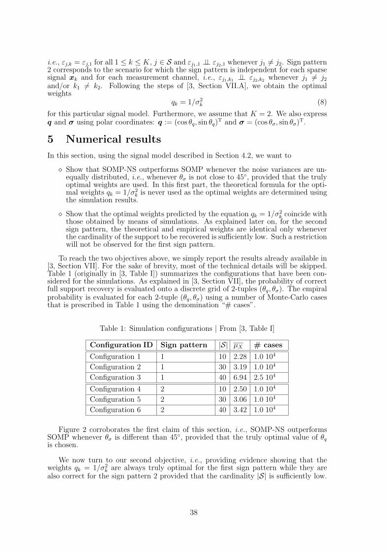
i.e., εj,k = εj,1 for all 1 ≤ k ≤ K, j ∈ S and εj1,1 ⊥⊥ εj2,1 whenever j1 6= j2. Sign pattern2 corresponds to the scenario for which the sign pattern is independent for each sparsesignal xk and for each measurement channel, i.e., εj1,k1 ⊥⊥ εj2,k2 whenever j1 6= j2and/or k1 6= k2. Following the steps of [3, Section VII.A], we obtain the optimalweights
qk = 1/σ2k (8)
for this particular signal model. Furthermore, we assume that K = 2. We also expressq and σ using polar coordinates: q := (cos θq, sin θq)
T and σ = (cos θσ, sin θσ)T.
5 Numerical results
In this section, using the signal model described in Section 4.2, we want to
Show that SOMP-NS outperforms SOMP whenever the noise variances are un-equally distributed, i.e., whenever θσ is not close to 45, provided that the trulyoptimal weights are used. In this first part, the theoretical formula for the opti-mal weights qk = 1/σ2
k is never used as the optimal weights are determined usingthe simulation results.
Show that the optimal weights predicted by the equation qk = 1/σ2k coincide with
those obtained by means of simulations. As explained later on, for the secondsign pattern, the theoretical and empirical weights are identical only wheneverthe cardinality of the support to be recovered is sufficiently low. Such a restrictionwill not be observed for the first sign pattern.
To reach the two objectives above, we simply report the results already available in[3, Section VII]. For the sake of brevity, most of the technical details will be skipped.Table 1 (originally in [3, Table I]) summarizes the configurations that have been con-sidered for the simulations. As explained in [3, Section VII], the probability of correctfull support recovery is evaluated onto a discrete grid of 2-tuples (θq, θσ). The empiralprobability is evaluated for each 2-tuple (θq, θσ) using a number of Monte-Carlo casesthat is prescribed in Table 1 using the denomination “# cases”.
Table 1: Simulation configurations | From [3, Table I]
Configuration ID Sign pattern |S| µX # cases
Configuration 1 1 10 2.28 1.0 104
Configuration 2 1 30 3.19 1.0 104
Configuration 3 1 40 6.94 2.5 104
Configuration 4 2 10 2.50 1.0 104
Configuration 5 2 30 3.06 1.0 104
Configuration 6 2 40 3.42 1.0 104
Figure 2 corroborates the first claim of this section, i.e., SOMP-NS outperformsSOMP whenever θσ is different than 45, provided that the truly optimal value of θqis chosen.
We now turn to our second objective, i.e., providing evidence showing that theweights qk = 1/σ2
k are always truly optimal for the first sign pattern while they arealso correct for the sign pattern 2 provided that the cardinality |S| is sufficiently low.
38
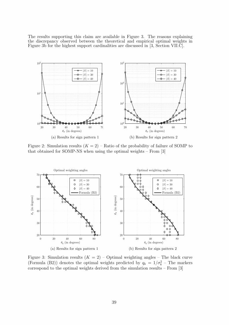
The results supporting this claim are available in Figure 3. The reasons explainingthe discrepancy observed between the theoretical and empirical optimal weights inFigure 3b for the highest support cardinalities are discussed in [3, Section VII.C].
|S| = 40
|S| = 30
|S| = 10
θσ (in degrees)20 30 40 50 60 70
100
101
102
(a) Results for sign pattern 1
|S| = 40
|S| = 30
|S| = 10
θσ (in degrees)20 30 40 50 60 70
100
101
102
103
(b) Results for sign pattern 2
Figure 2: Simulation results (K = 2) – Ratio of the probability of failure of SOMP tothat obtained for SOMP-NS when using the optimal weights – From [3]
Formula (B2)
|S| = 40
|S| = 30
|S| = 10
Optimal weighting angles
θ σ(indegrees)
θq (in degrees)0 20 40 60 80
20
30
40
50
60
70
(a) Results for sign pattern 1
Formula (B2)
|S| = 40
|S| = 30
|S| = 10
Optimal weighting angles
θ σ(indegrees)
θq (in degrees)0 20 40 60 80
20
30
40
50
60
70
(b) Results for sign pattern 2
Figure 3: Simulation results (K = 2) – Optimal weighting angles – The black curve(Formula (B2)) denotes the optimal weights predicted by qk = 1/σ2
k – The markerscorrespond to the optimal weights derived from the simulation results – From [3]
39
6 Conclusion
This paper presents a novel SOMP algorithm, entitled simultaneous orthogonal match-ing pursuit with noise stabilization (SOMP-NS). SOMP-NS weights the impact of eachmeasurement vector according to its noise level, which is assumed to be known. More-over, theoretical developments suggesting that the weighting capabilities of SOMP-NSprovide performance enhancements have been briefly exposed. Further, these devel-opments have been shown to provide weighting strategies for particular signal models.Finally, numerical results have established that the weights introduced in SOMP-NSyield performance improvements provided that they are appropriately chosen. Thesimulations have also revealed that the weighting strategies stemming from the theo-retical results are optimal in specific cases.
Disclaimer & Acknowledgements: This paper presents results [3, 4, 5] that havebeen published in or submitted to IEEE journals. This research has also been partiallyfunded by the Belgian science fondation (FNRS).
References
[1] D. Baron, M. F. Duarte, M. B. Wakin, S. Sarvotham, and R. G. Baraniuk, “Dis-tributed compressive sensing,” arXiv preprint arXiv:0901.3403, 2009.
[2] E. J. Candes, “The restricted isometry property and its implications for com-pressed sensing,” Comptes Rendus Mathematique, vol. 346, no. 9, pp. 589–592,2008.
[3] J.-F. Determe, J. Louveaux, L. Jacques, and F. Horlin, “Simultaneous orthogonalmatching pursuit with noise stabilization: theoretical analysis,” arXiv preprintarXiv:1506.05324, 2015.
[4] ——, “On the exact recovery condition of simultaneous orthogonal matching pur-suit,” Signal Processing Letters, IEEE, vol. 23, no. 1, pp. 164–168, 2016.
[5] ——, “On the noise robustness of simultaneous orthogonal matching pursuit,”arXiv preprint arXiv:1602.03400, 2016.
[6] D. L. Donoho, “Compressed sensing,” Information Theory, IEEE Transactionson, vol. 52, no. 4, pp. 1289–1306, 2006.
[7] Y. C. Eldar and M. Mishali, “Robust recovery of signals from a structured unionof subspaces,” Information Theory, IEEE Transactions on, vol. 55, no. 11, pp.5302–5316, 2009.
[8] S. Foucart and H. Rauhut, A mathematical introduction to compressive sensing.Springer, 2013.
[9] R. Gribonval, H. Rauhut, K. Schnass, and P. Vandergheynst, “Atoms of all chan-nels, unite! average case analysis of multi-channel sparse recovery using greedyalgorithms,” Journal of Fourier analysis and Applications, vol. 14, no. 5-6, pp.655–687, 2008.
[10] J. A. Tropp, A. C. Gilbert, and M. J. Strauss, “Algorithms for simultaneoussparse approximation. part i: Greedy pursuit,” Signal Processing, vol. 86, no. 3,pp. 572–588, 2006.
40
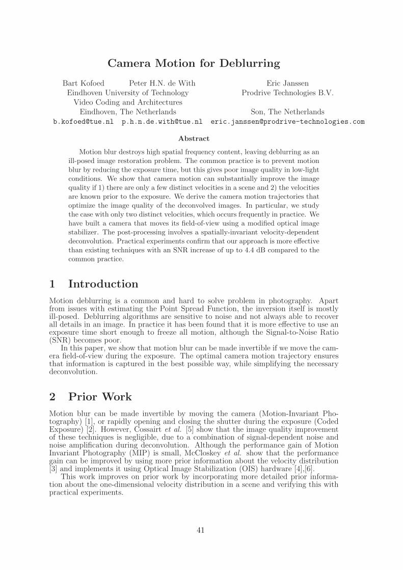
Camera Motion for Deblurring
Bart Kofoed Peter H.N. de With Eric JanssenEindhoven University of Technology Prodrive Technologies B.V.Video Coding and ArchitecturesEindhoven, The Netherlands Son, The Netherlands
[email protected] [email protected] [email protected]
Abstract
Motion blur destroys high spatial frequency content, leaving deblurring as anill-posed image restoration problem. The common practice is to prevent motionblur by reducing the exposure time, but this gives poor image quality in low-lightconditions. We show that camera motion can substantially improve the imagequality if 1) there are only a few distinct velocities in a scene and 2) the velocitiesare known prior to the exposure. We derive the camera motion trajectories thatoptimize the image quality of the deconvolved images. In particular, we studythe case with only two distinct velocities, which occurs frequently in practice. Wehave built a camera that moves its field-of-view using a modified optical imagestabilizer. The post-processing involves a spatially-invariant velocity-dependentdeconvolution. Practical experiments confirm that our approach is more effectivethan existing techniques with an SNR increase of up to 4.4 dB compared to thecommon practice.
1 Introduction
Motion deblurring is a common and hard to solve problem in photography. Apartfrom issues with estimating the Point Spread Function, the inversion itself is mostlyill-posed. Deblurring algorithms are sensitive to noise and not always able to recoverall details in an image. In practice it has been found that it is more effective to use anexposure time short enough to freeze all motion, although the Signal-to-Noise Ratio(SNR) becomes poor.
In this paper, we show that motion blur can be made invertible if we move the cam-era field-of-view during the exposure. The optimal camera motion trajectory ensuresthat information is captured in the best possible way, while simplifying the necessarydeconvolution.
2 Prior Work
Motion blur can be made invertible by moving the camera (Motion-Invariant Pho-tography) [1], or rapidly opening and closing the shutter during the exposure (CodedExposure) [2]. However, Cossairt et al. [5] show that the image quality improvementof these techniques is negligible, due to a combination of signal-dependent noise andnoise amplification during deconvolution. Although the performance gain of MotionInvariant Photography (MIP) is small, McCloskey et al. show that the performancegain can be improved by using more prior information about the velocity distribution[3] and implements it using Optical Image Stabilization (OIS) hardware [4],[6].
This work improves on prior work by incorporating more detailed prior informa-tion about the one-dimensional velocity distribution in a scene and verifying this withpractical experiments.
41

3 Noise, Motion and Blur
3.1 Noise
Camera images suffer from numerous sources of degradation, among which noise isone of the most problematic in low-light conditions. Noise is either caused by elec-tronic noise on the sensor or by the random nature of photons interacting with thedetector. The latter photon noise is signal-dependent noise that arises from the Pois-son distribution of photons reaching the detector. The variance of photon noise isapproximately proportional to the number of interacting photons. In anticipation offuture image sensor developments, we consider photon-noise limited detectors with aQuantum Efficiency of 100% during the remainder of this paper.
3.2 Motion Blur
To analyze motion blur, we adopt the space-time analysis described by Levin et al. [1].This section provides a brief overview of the method. We consider one-dimensionalmotion blur and use one-dimensional images to facilitate the analysis.
Let s(x) denote the projection of the scene, normalized such that E (s(x)) = 1. Thelight level L represents the average photon flux per pixel, i.e. the number of photonsdetected per pixel per second. Hence, the photon flux at location x is L · s(x).
At relatively fast shutter speeds, the subject motion is approximated by a transla-tion with constant velocity v along the x-axis. The camera moves along the x -axis aswell and its position is denoted as xc(t). The image sensor integrates incoming lightintensity on its surface during the exposure time T . Hence, the image captured by thesensor is written as the integral of the convolution of s(x) with the light integrationcurve hv(t, x):
z(x) =
∫ T
0
hv(t, x) ∗ s(x)dt+ n = s(x) ∗∫ T
0
hv(t, x)dt+ n, (1)
with n the photon noise with variance σ2n and
hv(t, x) = L · δ(x+ vt− xc(t)). (2)
We analyze the properties of the convolution with hv(t, x) in the frequency domain,where convolution is equivalent to multiplication. First, set v = 0 and transformthe light integration curve h0(t, x) to the frequency domain H0(ωt, kx). This Fouriertransform is rewritten as the one-dimensional Fourier transform.
H0(ωt, kx) =
∫ T
0
∫ ∞
−∞h0(t, x)e
−j2π(ωtt+kxx)dxdt
=
∫ T
0
∫ ∞
−∞L · δ(x− xc(t))e
−j2π(ωtt+kxx)dxdt = L
∫ T
0
e−j2πkxxc(t)e−j2πωttdt
(3)
Next, we use the fact that for a subject velocity v, time integration is equivalent toprojection of h0(t, x) on the line x = vt and hence Hv(kx) = H0(vkx, kx), i.e. the infor-mation lies on the line ωt = vkx. Consequently, the frequency-domain representationof the image captured by the sensor is given by:
Z(kx) = H0(vkx, kx)S(kx) +N(kx) = Hv(kx)S(kx) +N(kx), (4)
where S(kx) and N(kx) denote the frequency-domain representations of the originalimage and the noise, respectively.
42

3.3 Noise Equivalent Quanta
We aim to minimize the noise variance in the reconstructed image. A useful tool foranalyzing the noise variance is the Noise Equivalent Quanta (NEQ) [7]. The NEQmeasures the SNR as a function of spatial frequency kx. For a relatively low-contrastimage, photon noise is spatially white and has a variance equal to the average numberof photons detected per pixel:
E(|N(kx)|2
)= σ2
n = Hv(0) = H(0, 0) = LT. (5)
We obtain the following expressions for the NEQ:
NEQ(ωt, kx) =|H(ωt, kx)|2|S(kx)|2
H(0, 0),NEQv(kx) =
|Hv(kx)|2|S(kx)|2Hv(0)
. (6)
An useful property is that linear operations do not change the NEQ, since the numer-ator and denominator are affected equally. Consequently, the NEQ is an indicator ofimage quality regardless of any subsequent linear filtering operations, such as decon-volution.
3.4 Energy Preservation
Levin [1] points out that the energy in the slice∫ 0.5
−0.5|H(ωt, kx)|2dωt for a given kx is
proportional to L2T , which defines a fixed budget over the integration interval. Giventhat the noise variance is equal to H(0, 0) and therefore proportional to LT , we seethat:
∫ 0.5
−0.5
NEQ(ωt, kx)dωt =|S(kx)|2H(0, 0)
∫ 0.5
−0.5
|H(ωt, kx)|2dωt ∝ |S(kx)|2L. (7)
Hence, for each slice of spatial frequency kx we have a fixed NEQ budget proportionalto |S(kx)|2L. The distribution of the NEQ budget across ωt is determined by both theexposure time and the camera motion path. Recall that for a subject with velocity v,the direct relation ωt = vkx holds. Therefore, there is a fixed NEQ budget that we candistribute across the various velocities in a scene.
3.5 Deconvolution
The image captured by the sensor is blurred in a specific way due to the relative motionbetween the camera and the subject. This blur is removed through deconvolution,which is a division by the blur kernel response in the frequency domain. Note thatif the frequency response of the blur kernel is zero for some spatial frequency, thedeconvolution becomes unstable. We therefore use the Wiener deconvolution filter,which minimizes the Mean Squared Error (MSE) of the deconvolved image:
W (kx) =H∗
v (kx)|S(kx)|2|Hv(kx)|2|S(kx)|2 + |N(kx)|2
. (8)
We then derive the expression for the MSE:
MSE v(kx) = E(|Sv(kx)− Sv(kx)|2
)
=Hv(0)|S(kx)|2
|Hv(kx)|2|S(kx)|2 +Hv(0)=
|S(kx)|21 + NEQv(kx)
.(9)
43

We see that the MSE of the deconvolved image is inversly proportional to theNEQ and recall that there is a fixed NEQ budget (Equation (7)). Hence, we shoulddistribute the NEQ budget in an efficient way in order to minimize the reconstructionerror (MSE).
4 Optimal Camera Motion
In order to minimize the total MSE, we use the following two optimality criteria whichwere introduced by Bando et al. [9]:
⋄ Effectiveness: The NEQ budget must only be spent on regions in H0(ωt, kx)that correspond to velocities that appear in the scene;
⋄ Uniformity: The NEQ budget must be distributed uniformly among all veloci-ties in a scene.
To facilitate the analysis, we define the function ρ(v) which indicates whether a velocityoccurs in a scene (ρ(v) = 1) or not (ρ(v) = 0). The function ρ(v) consists of a series ofM rectangle functions (denoted by Π):
ρ(v) = ΣMm=1Π(
v − vm2∆vm
), (10)
where vm denotes central velocities sorted in ascending order and ∆vm denotes thewidth of the interval around the corresponding velocity. For example, if is knownthat a vehicle moves at a speed of 20 pixels/second (px/s) with an uncertainty of ±2px/s, then vm = 20 px/s and ∆vm = 2 px/s. The blocks should not overlap, hence:vm+1 − vm ≥ ∆vm +∆vm+1.
Intuitively, the camera velocity should be equal to every velocity where ρ(v) = 1 foran equal amount of time. Levin et al. [1] show that this is the case if the camera field-of-view (FOV) moves with a constant acceleration and also proves that this cameramotion optimizes the information capture. If we consider each of the blocks Π( v−vm
2∆vm)
individually, we capture the necessary information using this constant accelerationmotion. Each of these M motion paths is defined by the starting velocity vm,1, endingvelocity vm,2 and time interval Tm as follows:
xm(τ) =vm,2 − vm,1
2Tm
τ 2 + vm,1τ + C, (11)
with C being an arbitrary offset. The motion paths corresponding to the separateblocks are then concatenated over time into a continuous motion path xc(t) that cap-tures all the necessary information. The corresponding exposure time is determinedby the sum of the M time intervals: T = ΣM
m=1Tm.Recall that the energy in a slice for a given kx is fixed and ωt = vkx. Hence, energy
is spread out more as the spatial frequency kx increases. As a result, the responseHv(kx) and consequently NEQv(kx) are minimal at the Nyquist frequency kx = ±0.5.We define a minimum magnitude Hmin at kx = ±0.5, such that
∀v : ρ(v)Hmin ≤ |Hv(0.5)| ≤ |Hv(kx)|. (12)
We find values for vm,1, vm,2 and Tm such that Equation (12) holds while minimizingTm. Minimizing Tm ensures that as little as possible of the available NEQ budget isspent on velocities where ρ(v) = 0, fulfilling the effectiveness criterion. Moreover, wealso ensure that we do not overspend our budget on velocities where ρ(v) = 1. Hence,
44
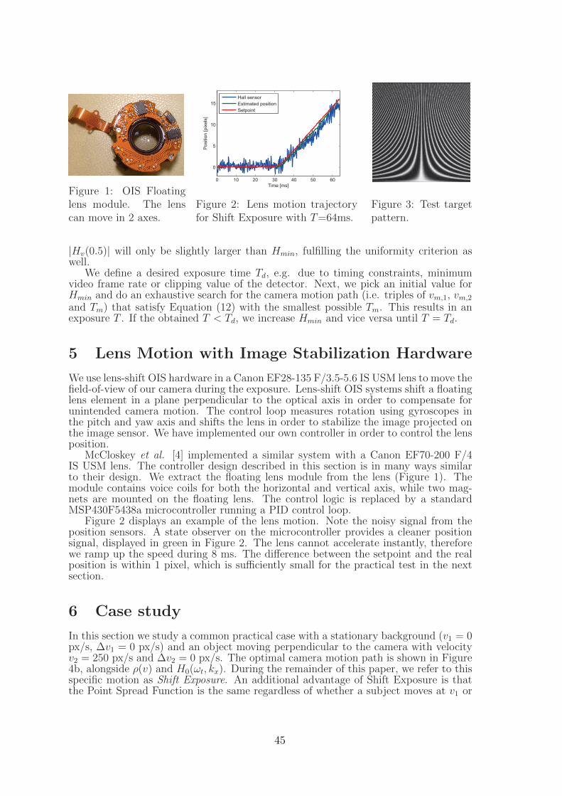
Figure 1: OIS Floatinglens module. The lenscan move in 2 axes.
0 10 20 30 40 50 60
0
5
10
15
Time [ms]
Positio
n [
pix
els
]
Hall sensor
Estimated position
Setpoint
Figure 2: Lens motion trajectoryfor Shift Exposure with T=64ms.
Figure 3: Test targetpattern.
|Hv(0.5)| will only be slightly larger than Hmin, fulfilling the uniformity criterion aswell.
We define a desired exposure time Td, e.g. due to timing constraints, minimumvideo frame rate or clipping value of the detector. Next, we pick an initial value forHmin and do an exhaustive search for the camera motion path (i.e. triples of vm,1, vm,2
and Tm) that satisfy Equation (12) with the smallest possible Tm. This results in anexposure T . If the obtained T < Td, we increase Hmin and vice versa until T = Td.
5 Lens Motion with Image Stabilization Hardware
We use lens-shift OIS hardware in a Canon EF28-135 F/3.5-5.6 IS USM lens to move thefield-of-view of our camera during the exposure. Lens-shift OIS systems shift a floatinglens element in a plane perpendicular to the optical axis in order to compensate forunintended camera motion. The control loop measures rotation using gyroscopes inthe pitch and yaw axis and shifts the lens in order to stabilize the image projected onthe image sensor. We have implemented our own controller in order to control the lensposition.
McCloskey et al. [4] implemented a similar system with a Canon EF70-200 F/4IS USM lens. The controller design described in this section is in many ways similarto their design. We extract the floating lens module from the lens (Figure 1). Themodule contains voice coils for both the horizontal and vertical axis, while two mag-nets are mounted on the floating lens. The control logic is replaced by a standardMSP430F5438a microcontroller running a PID control loop.
Figure 2 displays an example of the lens motion. Note the noisy signal from theposition sensors. A state observer on the microcontroller provides a cleaner positionsignal, displayed in green in Figure 2. The lens cannot accelerate instantly, thereforewe ramp up the speed during 8 ms. The difference between the setpoint and the realposition is within 1 pixel, which is sufficiently small for the practical test in the nextsection.
6 Case study
In this section we study a common practical case with a stationary background (v1 = 0px/s, ∆v1 = 0 px/s) and an object moving perpendicular to the camera with velocityv2 = 250 px/s and ∆v2 = 0 px/s. The optimal camera motion path is shown in Figure4b, alongside ρ(v) and H0(ωt, kx). During the remainder of this paper, we refer to thisspecific motion as Shift Exposure. An additional advantage of Shift Exposure is thatthe Point Spread Function is the same regardless of whether a subject moves at v1 or
45
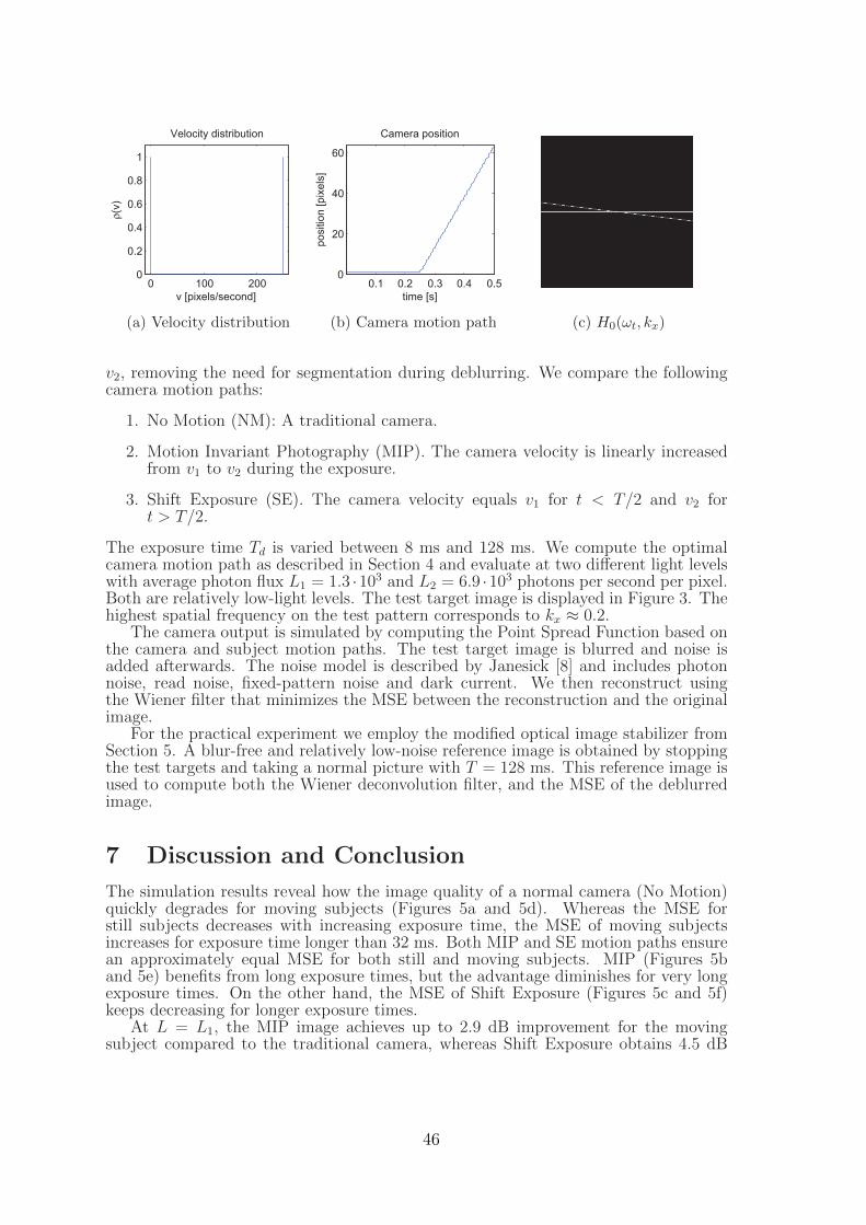
0 100 2000
0.2
0.4
0.6
0.8
1
Velocity distribution
v [pixels/second]
ρ(v
)
(a) Velocity distribution
0.1 0.2 0.3 0.4 0.50
20
40
60
Camera position
time [s]
positio
n [
pix
els
](b) Camera motion path (c) H0(ωt, kx)
v2, removing the need for segmentation during deblurring. We compare the followingcamera motion paths:
1. No Motion (NM): A traditional camera.
2. Motion Invariant Photography (MIP). The camera velocity is linearly increasedfrom v1 to v2 during the exposure.
3. Shift Exposure (SE). The camera velocity equals v1 for t < T/2 and v2 fort > T/2.
The exposure time Td is varied between 8 ms and 128 ms. We compute the optimalcamera motion path as described in Section 4 and evaluate at two different light levelswith average photon flux L1 = 1.3 ·103 and L2 = 6.9 ·103 photons per second per pixel.Both are relatively low-light levels. The test target image is displayed in Figure 3. Thehighest spatial frequency on the test pattern corresponds to kx ≈ 0.2.
The camera output is simulated by computing the Point Spread Function based onthe camera and subject motion paths. The test target image is blurred and noise isadded afterwards. The noise model is described by Janesick [8] and includes photonnoise, read noise, fixed-pattern noise and dark current. We then reconstruct usingthe Wiener filter that minimizes the MSE between the reconstruction and the originalimage.
For the practical experiment we employ the modified optical image stabilizer fromSection 5. A blur-free and relatively low-noise reference image is obtained by stoppingthe test targets and taking a normal picture with T = 128 ms. This reference image isused to compute both the Wiener deconvolution filter, and the MSE of the deblurredimage.
7 Discussion and Conclusion
The simulation results reveal how the image quality of a normal camera (No Motion)quickly degrades for moving subjects (Figures 5a and 5d). Whereas the MSE forstill subjects decreases with increasing exposure time, the MSE of moving subjectsincreases for exposure time longer than 32 ms. Both MIP and SE motion paths ensurean approximately equal MSE for both still and moving subjects. MIP (Figures 5band 5e) benefits from long exposure times, but the advantage diminishes for very longexposure times. On the other hand, the MSE of Shift Exposure (Figures 5c and 5f)keeps decreasing for longer exposure times.
At L = L1, the MIP image achieves up to 2.9 dB improvement for the movingsubject compared to the traditional camera, whereas Shift Exposure obtains 4.5 dB
46
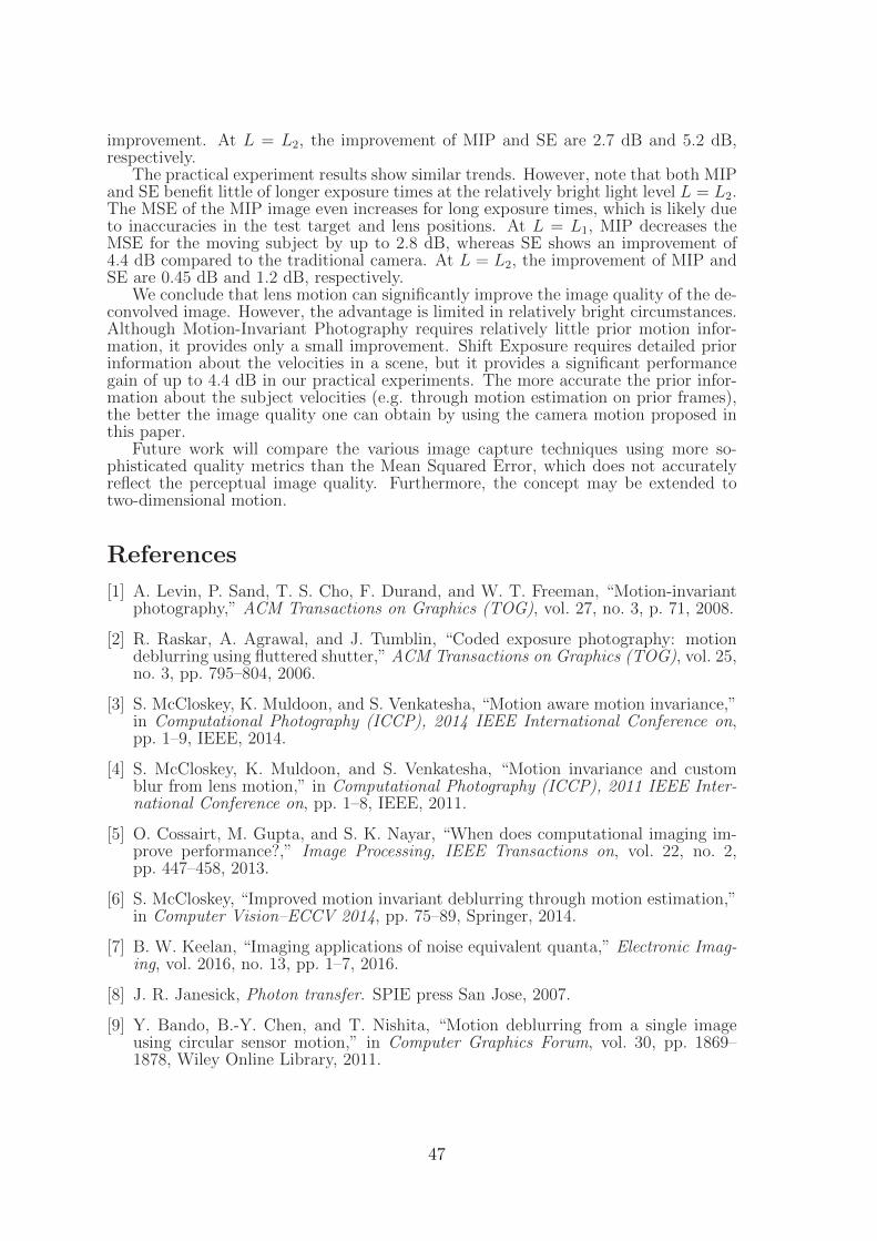
improvement. At L = L2, the improvement of MIP and SE are 2.7 dB and 5.2 dB,respectively.
The practical experiment results show similar trends. However, note that both MIPand SE benefit little of longer exposure times at the relatively bright light level L = L2.The MSE of the MIP image even increases for long exposure times, which is likely dueto inaccuracies in the test target and lens positions. At L = L1, MIP decreases theMSE for the moving subject by up to 2.8 dB, whereas SE shows an improvement of4.4 dB compared to the traditional camera. At L = L2, the improvement of MIP andSE are 0.45 dB and 1.2 dB, respectively.
We conclude that lens motion can significantly improve the image quality of the de-convolved image. However, the advantage is limited in relatively bright circumstances.Although Motion-Invariant Photography requires relatively little prior motion infor-mation, it provides only a small improvement. Shift Exposure requires detailed priorinformation about the velocities in a scene, but it provides a significant performancegain of up to 4.4 dB in our practical experiments. The more accurate the prior infor-mation about the subject velocities (e.g. through motion estimation on prior frames),the better the image quality one can obtain by using the camera motion proposed inthis paper.
Future work will compare the various image capture techniques using more so-phisticated quality metrics than the Mean Squared Error, which does not accuratelyreflect the perceptual image quality. Furthermore, the concept may be extended totwo-dimensional motion.
References
[1] A. Levin, P. Sand, T. S. Cho, F. Durand, and W. T. Freeman, “Motion-invariantphotography,” ACM Transactions on Graphics (TOG), vol. 27, no. 3, p. 71, 2008.
[2] R. Raskar, A. Agrawal, and J. Tumblin, “Coded exposure photography: motiondeblurring using fluttered shutter,” ACM Transactions on Graphics (TOG), vol. 25,no. 3, pp. 795–804, 2006.
[3] S. McCloskey, K. Muldoon, and S. Venkatesha, “Motion aware motion invariance,”in Computational Photography (ICCP), 2014 IEEE International Conference on,pp. 1–9, IEEE, 2014.
[4] S. McCloskey, K. Muldoon, and S. Venkatesha, “Motion invariance and customblur from lens motion,” in Computational Photography (ICCP), 2011 IEEE Inter-national Conference on, pp. 1–8, IEEE, 2011.
[5] O. Cossairt, M. Gupta, and S. K. Nayar, “When does computational imaging im-prove performance?,” Image Processing, IEEE Transactions on, vol. 22, no. 2,pp. 447–458, 2013.
[6] S. McCloskey, “Improved motion invariant deblurring through motion estimation,”in Computer Vision–ECCV 2014, pp. 75–89, Springer, 2014.
[7] B. W. Keelan, “Imaging applications of noise equivalent quanta,” Electronic Imag-ing, vol. 2016, no. 13, pp. 1–7, 2016.
[8] J. R. Janesick, Photon transfer. SPIE press San Jose, 2007.
[9] Y. Bando, B.-Y. Chen, and T. Nishita, “Motion deblurring from a single imageusing circular sensor motion,” in Computer Graphics Forum, vol. 30, pp. 1869–1878, Wiley Online Library, 2011.
47
10−2
10−1
10−3
10−2
10−1
Exposure time [ms]
MS
E
still
moving
(a) L = L1, No Motion
10−2
10−1
10−3
10−2
10−1
Exposure time [ms]M
SE
still
moving
(b) L = L1, Motion-Invariant
10−2
10−1
10−3
10−2
10−1
Exposure time [ms]
MS
E
still
moving
(c) L = L1, Shift Exposure
10−2
10−1
10−3
10−2
10−1
Exposure time [ms]
MS
E
still
moving
(d) L = L2, No Motion
10−2
10−1
10−3
10−2
10−1
Exposure time [ms]
MS
E
still
moving
(e) L = L2, Motion-Invariant
10−2
10−1
10−3
10−2
10−1
Exposure time [ms]
MS
E
still
moving
(f) L = L2, Shift Exposure
Figure 5: Simulation results
10−2
10−1
10−3
10−2
10−1
Exposure time [ms]
MS
E
still
moving
(a) L = L1, No Motion
10−1
10−3
10−2
10−1
Exposure time [ms]
MS
E
still
moving
(b) L = L1, Motion-Invariant
10−1
10−3
10−2
10−1
Exposure time [ms]
MS
E
still
moving
(c) L = L1, Shift Exposure
10−2
10−1
10−3
10−2
10−1
Exposure time [ms]
MS
E
still
moving
(d) L = L2, No Motion
10−1
10−3
10−2
10−1
Exposure time [ms]
MS
E
still
moving
(e) L = L2, Motion-Invariant
10−1
10−3
10−2
10−1
Exposure time [ms]
MS
E
still
moving
(f) L = L2, Shift Exposure
Figure 6: Experimental results
48
Person-Independent Discomfort Detection System
for Infants
C. Li1, S. Zinger1, W. E. Tjon a Ten2, P. H. N. de With1
1Eindhoven University of Technology 2Maxima Medical Center5600MB, Eindhoven, the Netherlands 5500MB, Veldhoven, the Netherlands
c.li2, s.zinger, [email protected] [email protected]
Abstract
Automatic discomfort detection for infants is important in healthcare, sinceinfants have no ability to express their discomfort. We propose a video analysissystem, based on supervised learning and classifying previously unseen infantsfrom the testing set in a fully automated way. The first stage of our system con-sists of fame-based face detection, and then fit a face shape to the detected facearea by using a Constrained Local Model (CLM). In the second stage, we analyzeexpression features by using Elongated Local Binary Patterns (ELBP), and clas-sify expression features with an Support Vector Machine (SVM) for discomfortdetection. The key contribution of our system is that the face model is infant-independent by employing a Constrained Local Model without prior knowledgeabout previously unseen infants. The system detects discomfort with an accu-racy of 84.3%, a sensitivity of 82.4%, and specificity of 84.9% on the testing setcontaining videos of 11 infants. In addition, in order to increase the robustnessof the system to head rotation, we introduce a face recovery method based onthe symmetry of the face. With this step, the previous performance parametersincrease by 3.1− 3.8% tested with videos of 2 infants containing 2, 010 frames.
1 Introduction
Discomfort and pain assessment for infants is an important and challenging task, sinceinfants are not able to verbally communicate their discomfort. Neglecting discomfort orpain of infants can cause problems in their further development [1]. Therefore, nursesor parents normally take the responsibility of monitoring and assessing pain of infantswhen they are admitted to a hospital. Several behavioral and physiological changes canindicate potential discomfort of infants, such as crying, facial tension, frequent bodymovements, heart rate, respiratory response, blood pressure, and levels of oxygen andcarbon dioxide in the blood.
To assess pain, various infant pain scoring methods have been developed, such as thePIPP (Premature Infant Pain Profile) and the COMFORT pain scale, which are basedon the above-mentioned clinical parameters. All nurses responsible for infant pain as-sessment have to be trained to apply a pain scoring, while observing infants for a certaintime period for pain estimation. However, monitoring by nurses is time consuming, ex-pensive and, as assessments are done in intervals, changes in pain/discomfort intensitybetween the intervals are not detected. Therefore an automated discomfort detectionsystem is highly attractive. Besides monitoring infants for a long period, such a systemopens new possibilities for reliable disease diagnosis, such as Gastro-Esophageal RefluxDisease (GERD).
Automatic discomfort detection for infants based on video analysis is a challengingtask for several reasons. At first, infants are often sleeping, so that their eyeballs areinvisible. Therefore, many face detectors based on finding eyes cannot be used for thistask. Secondly, most infants need pacifiers to stay calm, and this partially occludes
49
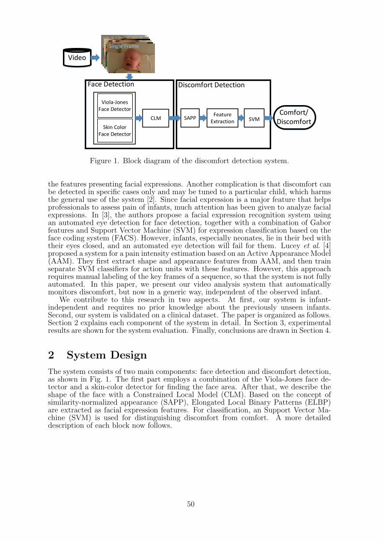
CLM SAPPFeature
Extraction SVMComfort/
Discomfort
Viola-Jones Face Detector
Discomfort Detection
Single Frame
Face Detection
Video
Skin Color Face Detector
Figure 1. Block diagram of the discomfort detection system.
the features presenting facial expressions. Another complication is that discomfort canbe detected in specific cases only and may be tuned to a particular child, which harmsthe general use of the system [2]. Since facial expression is a major feature that helpsprofessionals to assess pain of infants, much attention has been given to analyze facialexpressions. In [3], the authors propose a facial expression recognition system usingan automated eye detection for face detection, together with a combination of Gaborfeatures and Support Vector Machine (SVM) for expression classification based on theface coding system (FACS). However, infants, especially neonates, lie in their bed withtheir eyes closed, and an automated eye detection will fail for them. Lucey et al. [4]proposed a system for a pain intensity estimation based on an Active Appearance Model(AAM). They first extract shape and appearance features from AAM, and then trainseparate SVM classifiers for action units with these features. However, this approachrequires manual labeling of the key frames of a sequence, so that the system is not fullyautomated. In this paper, we present our video analysis system that automaticallymonitors discomfort, but now in a generic way, independent of the observed infant.
We contribute to this research in two aspects. At first, our system is infant-independent and requires no prior knowledge about the previously unseen infants.Second, our system is validated on a clinical dataset. The paper is organized as follows.Section 2 explains each component of the system in detail. In Section 3, experimentalresults are shown for the system evaluation. Finally, conclusions are drawn in Section 4.
2 System Design
The system consists of two main components: face detection and discomfort detection,as shown in Fig. 1. The first part employs a combination of the Viola-Jones face de-tector and a skin-color detector for finding the face area. After that, we describe theshape of the face with a Constrained Local Model (CLM). Based on the concept ofsimilarity-normalized appearance (SAPP), Elongated Local Binary Patterns (ELBP)are extracted as facial expression features. For classification, an Support Vector Ma-chine (SVM) is used for distinguishing discomfort from comfort. A more detaileddescription of each block now follows.
50
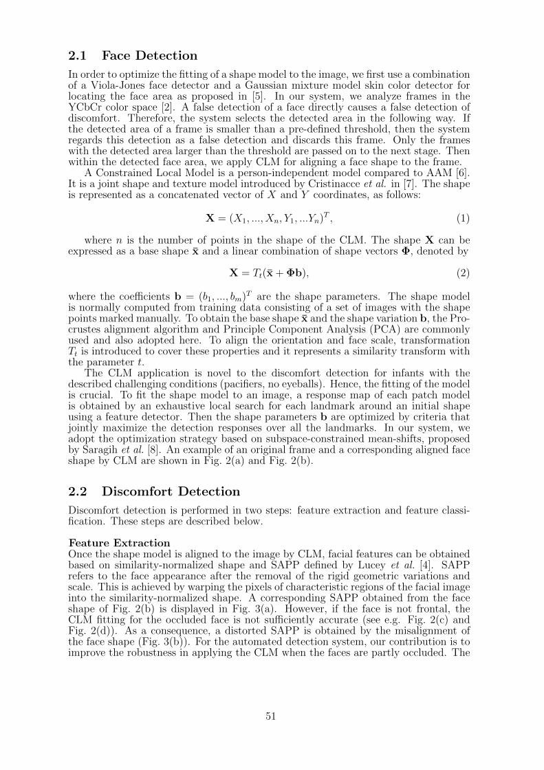
2.1 Face Detection
In order to optimize the fitting of a shape model to the image, we first use a combinationof a Viola-Jones face detector and a Gaussian mixture model skin color detector forlocating the face area as proposed in [5]. In our system, we analyze frames in theYCbCr color space [2]. A false detection of a face directly causes a false detection ofdiscomfort. Therefore, the system selects the detected area in the following way. Ifthe detected area of a frame is smaller than a pre-defined threshold, then the systemregards this detection as a false detection and discards this frame. Only the frameswith the detected area larger than the threshold are passed on to the next stage. Thenwithin the detected face area, we apply CLM for aligning a face shape to the frame.
A Constrained Local Model is a person-independent model compared to AAM [6].It is a joint shape and texture model introduced by Cristinacce et al. in [7]. The shapeis represented as a concatenated vector of X and Y coordinates, as follows:
X = (X1, ..., Xn, Y1, ...Yn)T , (1)
where n is the number of points in the shape of the CLM. The shape X can beexpressed as a base shape x and a linear combination of shape vectors Φ, denoted by
X = Tt(x + Φb), (2)
where the coefficients b = (b1, ..., bm)T are the shape parameters. The shape modelis normally computed from training data consisting of a set of images with the shapepoints marked manually. To obtain the base shape x and the shape variation b, the Pro-crustes alignment algorithm and Principle Component Analysis (PCA) are commonlyused and also adopted here. To align the orientation and face scale, transformationTt is introduced to cover these properties and it represents a similarity transform withthe parameter t.
The CLM application is novel to the discomfort detection for infants with thedescribed challenging conditions (pacifiers, no eyeballs). Hence, the fitting of the modelis crucial. To fit the shape model to an image, a response map of each patch modelis obtained by an exhaustive local search for each landmark around an initial shapeusing a feature detector. Then the shape parameters b are optimized by criteria thatjointly maximize the detection responses over all the landmarks. In our system, weadopt the optimization strategy based on subspace-constrained mean-shifts, proposedby Saragih et al. [8]. An example of an original frame and a corresponding aligned faceshape by CLM are shown in Fig. 2(a) and Fig. 2(b).
2.2 Discomfort Detection
Discomfort detection is performed in two steps: feature extraction and feature classi-fication. These steps are described below.
Feature ExtractionOnce the shape model is aligned to the image by CLM, facial features can be obtainedbased on similarity-normalized shape and SAPP defined by Lucey et al. [4]. SAPPrefers to the face appearance after the removal of the rigid geometric variations andscale. This is achieved by warping the pixels of characteristic regions of the facial imageinto the similarity-normalized shape. A corresponding SAPP obtained from the faceshape of Fig. 2(b) is displayed in Fig. 3(a). However, if the face is not frontal, theCLM fitting for the occluded face is not sufficiently accurate (see e.g. Fig. 2(c) andFig. 2(d)). As a consequence, a distorted SAPP is obtained by the misalignment ofthe face shape (Fig. 3(b)). For the automated detection system, our contribution is toimprove the robustness in applying the CLM when the faces are partly occluded. The
51
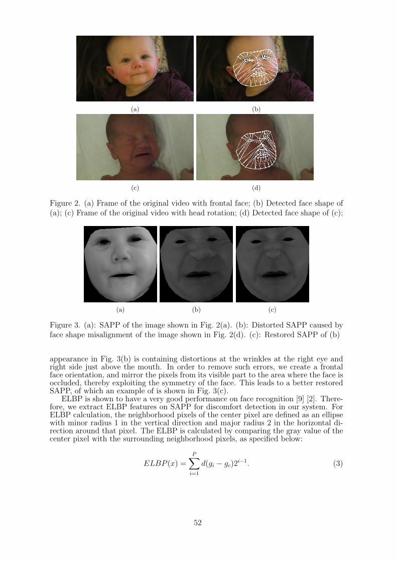
(a) (b)
(c) (d)
Figure 2. (a) Frame of the original video with frontal face; (b) Detected face shape of(a); (c) Frame of the original video with head rotation; (d) Detected face shape of (c);
(a) (b) (c)
Figure 3. (a): SAPP of the image shown in Fig. 2(a). (b): Distorted SAPP caused byface shape misalignment of the image shown in Fig. 2(d). (c): Restored SAPP of (b)
appearance in Fig. 3(b) is containing distortions at the wrinkles at the right eye andright side just above the mouth. In order to remove such errors, we create a frontalface orientation, and mirror the pixels from its visible part to the area where the face isoccluded, thereby exploiting the symmetry of the face. This leads to a better restoredSAPP, of which an example of is shown in Fig. 3(c).
ELBP is shown to have a very good performance on face recognition [9] [2]. There-fore, we extract ELBP features on SAPP for discomfort detection in our system. ForELBP calculation, the neighborhood pixels of the center pixel are defined as an ellipsewith minor radius 1 in the vertical direction and major radius 2 in the horizontal di-rection around that pixel. The ELBP is calculated by comparing the gray value of thecenter pixel with the surrounding neighborhood pixels, as specified below:
ELBP (x) =P∑
i=1
d(gi − gc)2i−1. (3)
52

Figure 4. Examples of frames from Database I and Database II.
Here parameter P denotes the number of the neighborhood pixels and gc, gi denotethe gray values of the center pixel and the neighborhood pixels, respectively. Thebinary output function d is defined by
d(gi − gc) =
1, for (gi − gc) ≥ 0;0, for (gi − gc) < 0.
(4)
Feature ClassificationSVM has been demonstrated to be useful in a number of facial recognition and ex-pression recognition tasks [10]. This classifier defines the optimal hyperplane by max-imizing the margin between positive and negative samples for a specified class. Fordetecting discomfort, we train an SVM with a linear kernel to distinguish discomfortfrom comfort, based on ELBP features extracted from SAPP, as described above, withthe LIBSVM library [11]. The combination of the previous algorithm steps enablesautomated discomfort detection.
3 Experiments
In this section, we first introduce the databases used for training and testing oursystem. Then we describe the applied evaluation metrics. Finally, we present keyperformance parameters: accuracy, specificity and sensitivity for face detection anddiscomfort detection in our system.
3.1 Database
For training the discomfort classifier, we re-use the database from Fotiadou et al. [2].This database consists of 15 videos of 8 infants, 5 displaying comfort, 1 discomfort and9 videos containing both. Each video has a frame rate of 25 frames per second witha resolution of 1920× 1080 pixels, which is denoted as Database I. For the purpose oftesting, we also use a database of 106 videos from 38 infants that have been recorded atthe Maxima Medical Center (MMC), Veldhoven, the Netherlands, by Slaats et al. [5].Videos of the faces of infants experiencing pain resulting from various interventions,like a heel prick, placing an intravenous line, a venipuncture, a vaccination or frompost-operative pain, are recorded. However, this database includes various children andsituations, such as premature neonates, infants with tubes and pacifiers, and occlusionson the face. Therefore, we choose a collection of 13 videos from 11 infants withoutocclusion of the face, which we call Database II. From the 13 videos, 5 videos displaydiscomfort, 7 videos display comfort and 1 video displays both. Each video has a framerate of 30 frames per second and a spatial resolution of 1280×720 pixels. A descriptionof both datasets is shown in Table 1. Examples of video frames from both databasesare portrayed by Fig. 4.
53

Table 1. Database descriptions
Infants Videos Total FramesDatabase I 8 15 43,823Database II 11 13 13,917
(a) (b)
Figure 5. (a) Manually labeled ground-truth image; (b) Detected face surrounded bya rectangle.
3.2 Evaluation Results
We evaluate our system in two aspects: face detection rate and discomfort detectionrate. For face detection, we consider a detection to be correct when a rectangle encom-passing the face mesh fitted in the image has a 70% overlap area with the rectanglein the ground-truth image. A ground-truth image has a manually annotated rectangleencompassing the eyes, nose and mouth. Fig. 5 shows an example of a manually labeledground-truth image and a face mesh surrounded by a rectangle.
For discomfort detection, we evaluate the SVM classifier based on single frames.For each video frame in the database, the ground-truth of discomfort is provided bynurses from the Veldhoven MMC, who are experienced in giving pain scores. Theperformance of discomfort detection is obtained by comparing the output of the SVMclassifier with the ground-truth. To measure the performance, we calculate accuracy,specificity and sensitivity of the classification results.
3.2.1 Face Detection
The Viola-Jones detector is trained with 25 infants from the database obtained bySlaats et al. [5], excluding the infant videos we use from Database II. Table 2 showsthe performance of our CLM-based face detection system evaluated with Database Iand Database II. In this table, “total frame” means all frames of each dataset, and“output frames” means frames with a face mesh detected by the face detection stage.It shows that the true detection rate over all frames is 70.9% and 81.5%. However,more importantly, the rate of true detection over the output from the CLM-based facedetector is 91.6% and 96.9% for Database I and Database II, respectively.
3.2.2 Discomfort Detection
We have used infants included in Database I proposed by Fotiadou et al. [2] for trainingthe discomfort detection classifier. For testing the performance of the discomfort detec-tion, we apply infant videos from Database II. These infants are all unseen subjects toour discomfort classifier. Table 3 shows the performance of ELBP features extractedfrom SAPP for discomfort detection evaluated with Database II without face inter-polation. It can be observed that our system achieves an accuracy of 84.3%, with a
54
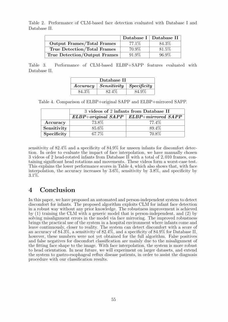
Table 2. Performance of CLM-based face detection evaluated with Database I andDatabase II.
Database I Database IIOutput Frames/Total Frames 77.1% 84.3%True Detection/Total Frames 70.9% 81.5%
True Detection/Output Frames 91.9% 96.9%
Table 3. Performance of CLM-based ELBP+SAPP features evaluated withDatabase II.
Database IIAccuracy Sensitivity Specificity
84.3% 82.4% 84.9%
Table 4. Comparison of ELBP+original SAPP and ELBP+mirrored SAPP.
3 videos of 2 infants from Database IIELBP+original SAPP ELBP+mirrored SAPP
Accuracy 73.8% 77.4%Sensitivity 85.6% 89.4%Specificity 67.7% 70.8%
sensitivity of 82.4% and a specificity of 84.9% for unseen infants for discomfort detec-tion. In order to evaluate the impact of face interpolation, we have manually chosen3 videos of 2 head-rotated infants from Database II with a total of 2, 010 frames, con-taining significant head rotations and movements. These videos form a worst-case test.This explains the lower performance scores in Table 4, which also shows that, with faceinterpolation, the accuracy increases by 3.6%, sensitivity by 3.8%, and specificity by3.1%.
4 Conclusion
In this paper, we have proposed an automated and person-independent system to detectdiscomfort for infants. The proposed algorithm exploits CLM for infant face detectionin a robust way without any prior knowledge. The robustness improvement is achievedby (1) training the CLM with a generic model that is person-independent, and (2) bysolving misalignment errors in the model via face mirroring. The improved robustnessbrings the practical use of the system in a hospital environment where infants come andleave continuously, closer to reality. The system can detect discomfort with a score ofan accuracy of 84.3%, a sensitivity of 82.4%, and a specificity of 84.9% for Database II,however, these numbers were not yet obtained for the full algorithm. False positivesand false negatives for discomfort classification are mainly due to the misalignment ofthe fitting face shape to the image. With face interpolation, the system is more robustto head orientation. In near future, we will experiment on larger datasets, and extendthe system to gastro-esophageal reflux disease patients, in order to assist the diagnosisprocedure with our classification results.
55

References
[1] F. L. Porter, R. E. Grunau, and K. J. Anand, “Long-term effects of pain ininfants,” J. Dev. Behav. Pediatr., vol. 20, pp. 253–261, 1999.
[2] E. Fotiadou, S. Zinger, W. E. Tjon a Ten, S. Oetomo, and P. H. N. de With,“Video-based facial discomfort analysis for infants,” in Proc. SPIE 9029, Vi-sual Information Processing and Communication V, 90290F, 2014, pp. 90 290F–90 290F–14.
[3] M. Bartlett, G. Littlewort, M. Frank, C. Lainscsek, I. Fasel, and J. Movellan,“Recognizing facial expression: machine learning and application to spontaneousbehavior,” in Computer Vision and Pattern Recognition. CVPR. IEEE ComputerSociety Conference on, vol. 2, June 2005, pp. 568–573.
[4] S. Lucey, I. Matthews, C. Hu, Z. Ambadar, F. De la Torre, and J. Cohn, “AAMderived face representations for robust facial action recognition,” in AutomaticFace and Gesture Recognition. FGR. 7th International Conference on, April 2006,pp. 155–160.
[5] B. Slaats, S. Zinger, P. H. N. de With, W. Tjon a Ten, and S. Bambang Oetomo,“Video analysis for acute pain detection in infants,” in 5th joint WIC/IEEE SPSymosium on Information Theory and Signal Processing, May 2015, pp. 50–57.
[6] S. Chew, P. Lucey, S. Lucey, J. Saragih, J. Cohn, and S. Sridharan, “Person-independent facial expression detection using constrained local models,” in Auto-matic Face Gesture Recognition and Workshops, IEEE International Conferenceon, March 2011, pp. 915–920.
[7] D. Cristinacce and T. F. Cootes, “Feature detection and tracking with constrainedlocal models,” in Britisch Machine Vision Conference (BMVC), 2006, pp. 95.1–95.10.
[8] J. M. Saragih, S. Lucey, and J. Cohn, “Face alignment through subspace con-strained mean-shifts,” in International Conference of Computer Vision (ICCV),September 2009.
[9] S. Liao and A. Chung, “Face recognition by using elongated local binary pat-terns with average maximum distance gradient magnitude,” in Computer VisionACCV, ser. Lecture Notes in Computer Science, Y. Yagi, S. Kang, I. Kweon, andH. Zha, Eds. Springer Berlin Heidelberg, 2007, vol. 4844, pp. 672–679.
[10] C. Cortes and V. Vapnik, “Support-vector networks,” Mach. Learn., vol. 20, no. 3,pp. 273–297, Sep. 1995.
[11] C.-C. Chang and C.-J. Lin, “LIBSVM: A library for support vector machines,”ACM Transactions on Intelligent Systems and Technology, vol. 2, pp. 27:1–27:27,2011, software available at http://www.csie.ntu.edu.tw/ cjlin/libsvm.
56
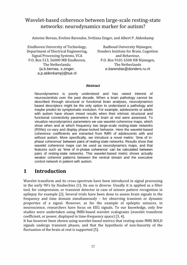
Wavelet-based coherence between large-scale resting-state networks: neurodynamics marker for autism?
Antoine Bernas, Evelien Barendse, Svitlana Zinger, and Albert P. Aldenkamp
Eindhoven University of Technology, Department of Electrical Engineering,
Signal Processing Systems, VCA P.O. Box 513, 56000 MB Eindhoven,
The Netherlands; a.b.bernas, s.zinger,
Radboud University Nijmegen, Donders Institute for Brain, Cognition
and Behaviour, P.O. Box 9101 6500 HB Nijmegen,
The Netherlands [email protected]
Abstract
Neurodynamics is poorly understood and has raised interest of
neuroscientists over the past decade. When a brain pathology cannot be described through structural or functional brain analyses, neurodynamics based descriptors might be the only option to understand a pathology and maybe predict its symptomatic evolution. For example, adolescents or adults with autism have shown mixed results when their intrinsic structural and functional connectivity parameters in the brain at rest were assessed. To visualize neurodynamics parameters we use wavelet coherence maps, which show when and at which frequency two large-scale resting-state networks (RSNs) co-vary and display phase-locked behavior. Here the wavelet-based coherence coefficients are extracted from fMRI of adolescents with and without autism. More specifically, we introduce a novel metric: ‘time of in-phase coherence’ between pairs of resting-state networks. Results show that wavelet coherence maps can be used as neurodynamics maps, and that features such as ‘time of in-phase coherence’ can be calculated between pairs of resting-state networks. This wavelet-based metric shows actually weaker coherent patterns between the ventral stream and the executive control network in patient with autism.
1 Introduction Wavelet transform and its cross-spectrum have been introduced in signal processing in the early 90’s by Daubechies [1]. Its use is diverse. Usually it is applied as a filter tool, for compression, or transient detector in case of seizure pattern recognition in epilepsy for example [2]. Several trials have been done to assess brain signals in the frequency and time domain simultaneously – for observing transient or dynamic properties of a signal. However, as for the example of epileptic seizures, in neuroscience, researchers have focus on EEG signals. To our knowledge, only few studies were undertaken using fMRI-based wavelet scalograms (wavelet transform coefficient, or power, displayed in time-frequency space) [3, 4]. It has however been shown using wavelet-based metrics that resting-state fMRI BOLD signals undergo transient phases, and that the hypothesis of non-linearity of the fluctuation of the brain at rest is supported [5].
57

It remains unclear, though, whether in time series of larger scale of neuronal populations, such as resting-state networks, fluctuations display temporal correlations at different scale (periods), and whether these neurodynamics patterns differ from one population to another. Here, we study the correlation matrices in terms of wavelet coherence maps between pairs of RSN time-series. Wavelet coherence is an interesting measure first applied in geophysics by Torrence and Compo (1998)[6], extracted from wavelet transform and the cross-spectrum between two time series. With such maps, one can look at correlation coefficient matrices (time x frequency) showing phase-locked behavior (when adding cross-wavelet phase information). Hence, significant ‘areas’ in a wavelet-coherence scalogram based on RSN time series can reveal when and at which frequency two RSNs are correlated, and whether these correlations are in phase or anti-phase or even in between, i.e, in a sense of one RSN signal leading or lagging behind another. This provides us neurodynamics descriptors in a sense of causality. We extract coherence maps from resting-state networks of adolescents with an autism spectrum disorder (ASD). As compared to their age- and IQ-matched typically developing peers (or controls), adolescents with autism displayed a less coherent covariation between the ventral stream and executive control network. The method used for extracting wavelet-based coherence descriptors and the results when applied upon the autistic brain are described in the following sections.
2 Methods
2.1 Resting-state ICA time series extraction In order to conduct the wavelet-coherence-based analysis using resting-state time series, we first extract spatial RSN maps, using a group Independent Component Analysis (gICA) on resting-state fMRI preprocessed dataset. Then, a dual-regression is used to extract subject-specific RSN time series [7]. Finally we selected the most relevant RSNs, using an in-house built ‘godness-of-fit’ MatLab (The MathWorks, Inc., Natick, Massachusetts, United States) function and the resting-state networks NifTi template from Smith et al. (2009) [8].
2.2 Wavelet Coherence and time of in-phase coherence Using the aforementioned selected RSN time series, one can build wavelet coherence maps between pairs of the time series. These maps represent localized correlation between two time series in the frequency (scale) and time space, also called scalograms. More details of how wavelet-coherence scalogram are constructed can be found in Torrence and Compo’s paper (1998) [6]. Briefly, they define
𝑅2(𝑠, 𝑡) =|⟨𝑠−1𝑊𝑋𝑌(𝑠,𝑡)⟩|2
⟨𝑠−1|𝑊𝑋(𝑠,𝑡)|2
⟩ ⟨𝑠−1|𝑊𝑌(𝑠,𝑡)|2
⟩ (1)
as a measure of coherence between two signals X and Y in the wavelet domain, i.e., after a wavelet transform 𝑊𝑋(𝑠, 𝑡) and 𝑊𝑌(𝑠, 𝑡) was applied on the signals. As a cross-correlation, or a cross-spectrum in the Fourier space, we can extract the wavelet
58
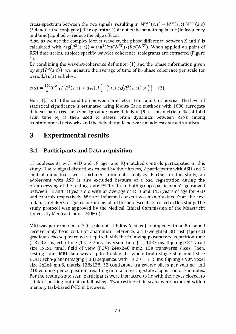
cross-spectrum between the two signals, resulting in 𝑊𝑋𝑌(𝑠, 𝑡) = 𝑊𝑋(𝑠, 𝑡). 𝑊𝑌∗(𝑠, 𝑡) (* denotes the conjugate). The operator ⟨.⟩ denotes the smoothing factor (in frequency and time) applied to reduce the edge effects. Also, as we use the complex Morlet wavelet, the phase difference between X and Y is calculated with arg(𝑅2(𝑠, 𝑡)) = tan1(𝐼𝑚(W𝑋𝑌)/(𝑅𝑒(WXY). When applied on pairs of
RSN time series, subject-specific wavelet-coherence scalograms are extracted (Figure 1). By combining the wavelet-coherence definition (1) and the phase information given by arg(𝑅2(𝑠, 𝑡)) we measure the average of time of in-phase coherence per scale (or
periods) 𝑐(𝑠) as below.
𝑐(𝑠) =100
𝑁∑ 𝐼𝑅2(𝑠, 𝑡) > 𝑎95𝑁
𝑡=1 . 𝐼 −𝜋
4< arg(𝑅2(𝑠, 𝑡)) >
𝜋
4 (2)
Here, I. is 1 if the condition between brackets is true, and 0 otherwise. The level of statistical significance is estimated using Monte Carlo methods with 1000 surrogate data set pairs (red noise background; more details in [9]). This metric in % (of total scan time N) is then used to assess brain dynamics between RSNs among frontotemporal networks and the default mode network of adolescents with autism.
3 Experimental results 3.1 Participants and Data acquisition 15 adolescents with ASD and 18 age- and IQ-matched controls participated in this study. Due to signal distortions caused by their braces, 2 participants with ASD and 5 control individuals were excluded from data analysis. Further in the study, an adolescent with ASD is also excluded because of a bad registration during the preprocessing of the resting-state fMRI data. In both groups participants’ age ranged between 12 and 18 years old with an average of 15.3 and 14.5 years of age for ASD and controls respectively. Written informed consent was also obtained from the next of kin, caretakers, or guardians on behalf of the adolescents enrolled in this study. The study protocol was approved by the Medical Ethical Commission of the Maastricht University Medical Center (MUMC).
MRI was performed on a 3.0-Tesla unit (Philips Achieva) equipped with an 8-channel receiver-only head coil. For anatomical reference, a T1-weighted 3D fast (spoiled) gradient echo sequence was acquired with the following parameters: repetition time (TR) 8.2 ms, echo time (TE) 3.7 ms, inversion time (TI) 1022 ms, flip angle 8°, voxel size 1x1x1 mm3, field of view (FOV) 240x240 mm2, 150 transverse slices. Then, resting-state fMRI data was acquired using the whole brain single-shot multi-slice BOLD echo-planar imaging (EPI) sequence, with TR 2 s, TE 35 ms, flip angle 90°, voxel size 2x2x4 mm3, matrix 128x128, 32 contiguous transverse slices per volume, and 210 volumes per acquisition; resulting in total a resting-state acquisition of 7 minutes. For the resting-state scan, participants were instructed to lie with their eyes closed, to think of nothing but not to fall asleep. Two resting-state scans were acquired with a memory task-based fMRI in between.
59
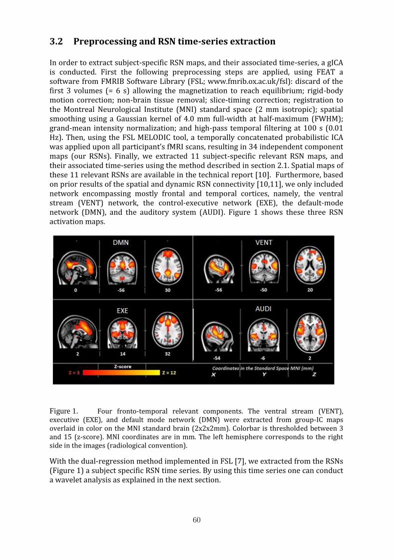
3.2 Preprocessing and RSN time-series extraction In order to extract subject-specific RSN maps, and their associated time-series, a gICA is conducted. First the following preprocessing steps are applied, using FEAT a software from FMRIB Software Library (FSL; www.fmrib.ox.ac.uk/fsl): discard of the first 3 volumes (= 6 s) allowing the magnetization to reach equilibrium; rigid-body motion correction; non-brain tissue removal; slice-timing correction; registration to the Montreal Neurological Institute (MNI) standard space (2 mm isotropic); spatial smoothing using a Gaussian kernel of 4.0 mm full-width at half-maximum (FWHM); grand-mean intensity normalization; and high-pass temporal filtering at 100 s (0.01 Hz). Then, using the FSL MELODIC tool, a temporally concatenated probabilistic ICA was applied upon all participant’s fMRI scans, resulting in 34 independent component maps (our RSNs). Finally, we extracted 11 subject-specific relevant RSN maps, and their associated time-series using the method described in section 2.1. Spatial maps of these 11 relevant RSNs are available in the technical report [10]. Furthermore, based on prior results of the spatial and dynamic RSN connectivity [10,11], we only included network encompassing mostly frontal and temporal cortices, namely, the ventral stream (VENT) network, the control-executive network (EXE), the default-mode network (DMN), and the auditory system (AUDI). Figure 1 shows these three RSN activation maps.
Figure 1. Four fronto-temporal relevant components. The ventral stream (VENT), executive (EXE), and default mode network (DMN) were extracted from group-IC maps overlaid in color on the MNI standard brain (2x2x2mm). Colorbar is thresholded between 3 and 15 (z-score). MNI coordinates are in mm. The left hemisphere corresponds to the right side in the images (radiological convention).
With the dual-regression method implemented in FSL [7], we extracted from the RSNs (Figure 1) a subject specific RSN time series. By using this time series one can conduct a wavelet analysis as explained in the next section.
60
3.3 Wavelet transforms, cross-spectrum, and coherence Wavelet coherence maps, or scalograms, are calculated using the method and toolbox
from Grindsted et al., (2004) [9] (http://www.glaciology.net/wavelet-coherence). We use the complex Morlet wavelet as it has best Fourier period-wavelet scale ration of 1.03 (wavelet scale ≈ Fourier period), which helps interpreting results in frequency domain. Also, it is a complex wavelet and therefore gives us phase information, and it allows us to have directionality in the dynamic between signals (in-phase, leading, lagging, or anti-phase).
Figure 2. Example of wavelet scalograms. continuous wavelet transform on two resting-state signals: default mode network (top-left scalogram) and auditory system (top-right scalogram), and their cross wavelet transform (middle scalogram), and wavelet coherence (bottom scalogram) for the 1st scan of the 6th ASD subject. Arrows in the middle scalogram represent phase lags between the two signals. An arrow pointing to the right means that the signals are in-phase; pointing to the left: anti-phased; 90° downward: DMN leads AUDI; and 90° upward: AUDI leads DMN. This is also marked with colors in the coherent areas of the WTC, when taking the four phase difference ranges (in rad.): [0 ± π/4]; [π ± π/4] ; [-π/2 ± π/4]; [π/2 ± π/4]. For each scalogram, x-axis is time space, y-axis is scale space (in Fourier periods).
We obtained scalograms of in-phase wavelet-coherence (Figure 1, bottom scalogram, red area), for each subject and for each pair of relevant RSN time series. The ration of the red area over the full time length (7 min) of a row (a specific period) of these wavelet-coherence scalograms represents our time of in-phase coherence (in % of scan length).
61
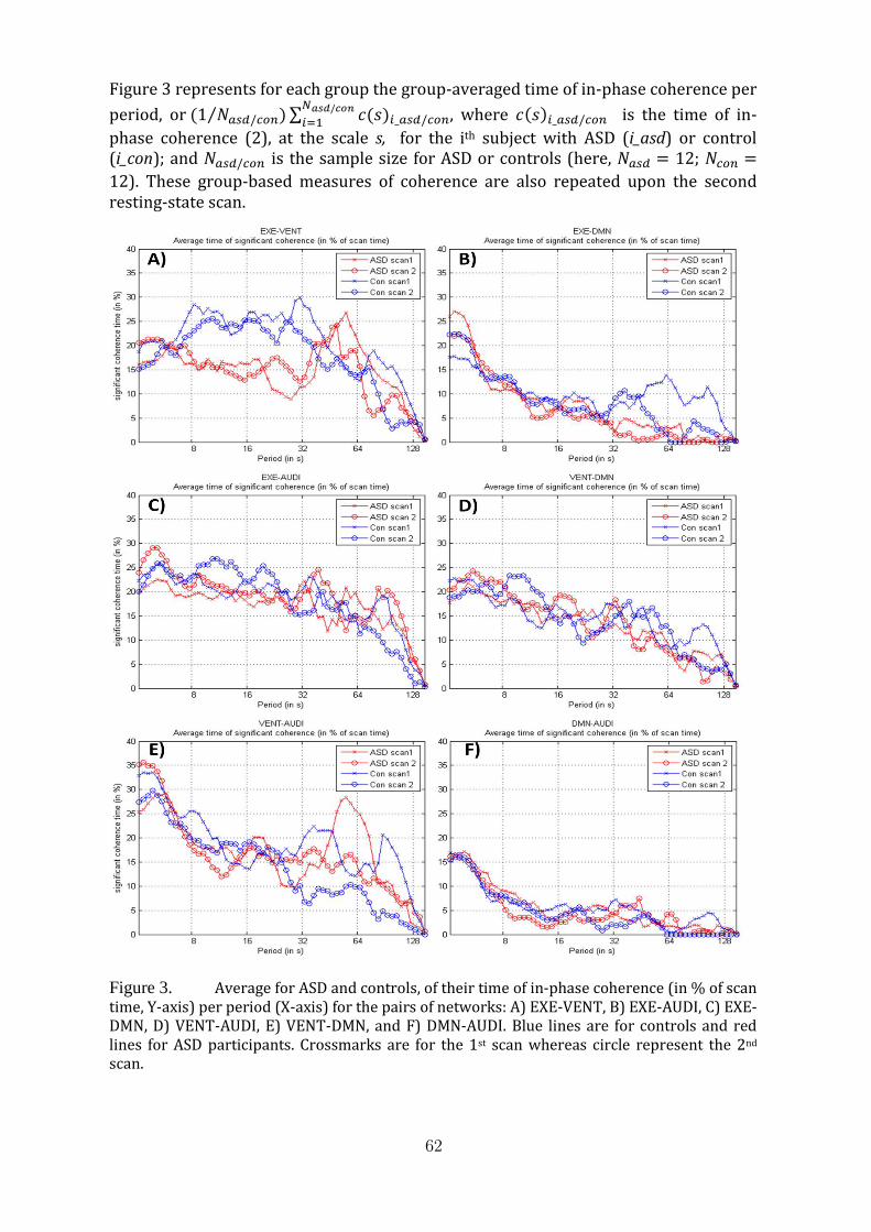
Figure 3 represents for each group the group-averaged time of in-phase coherence per
period, or (1 𝑁𝑎𝑠𝑑/𝑐𝑜𝑛⁄ ) ∑ 𝑐(𝑠)𝑖_𝑎𝑠𝑑/𝑐𝑜𝑛𝑁𝑎𝑠𝑑/𝑐𝑜𝑛
𝑖=1, where 𝑐(𝑠)𝑖_𝑎𝑠𝑑/𝑐𝑜𝑛 is the time of in-
phase coherence (2), at the scale s, for the ith subject with ASD (i_asd) or control (i_con); and 𝑁𝑎𝑠𝑑/𝑐𝑜𝑛 is the sample size for ASD or controls (here, 𝑁𝑎𝑠𝑑 = 12; 𝑁𝑐𝑜𝑛 =
12). These group-based measures of coherence are also repeated upon the second resting-state scan.
Figure 3. Average for ASD and controls, of their time of in-phase coherence (in % of scan time, Y-axis) per period (X-axis) for the pairs of networks: A) EXE-VENT, B) EXE-AUDI, C) EXE-DMN, D) VENT-AUDI, E) VENT-DMN, and F) DMN-AUDI. Blue lines are for controls and red lines for ASD participants. Crossmarks are for the 1st scan whereas circle represent the 2nd scan.
62
The main result in Figure 3 is that ASD adolescents show less correlation between two network time series EXE and VENT for a wide range of periods (from 8 s to 32 s, Figure 3.A). This reflects our previous findings in the report [10], where it is described that, using multivariate conditional Granger causality (measure of directed causality between multiple signals), these two networks presented a weaker effective connectivity in the direction VENT -> EXE. These two networks encompass brain areas coding for emotional processess, social interaction and executive function (cognition or behavioral outcome) – brain functions known to be a weak point in ASD.
4 Conclusion Using the well-described wavelet coherence upon fMRI brain signals, we can visualize localized correlations in time and frequency space, between two functional networks. We present a metric of average time of in-phase coherences and show that this could have future application in assessing neurodynamics, and gain knowledge in the transient properties of large-scale network oscillations. Also, our features of average time of coherence can potentially describe and possibly even diagnose a chronic or a developmental brain disorder where structural and functional connectivity maps are incapable of distinguishing patients from healthy controls. . Here we apply wavelet coherence upon functional networks extracted from an ICA decomposition using resting-state fMRI of adolescents with and without ASD. Results show that two networks coding for executive function and emotional processes display discrepancies between ASD and control adolescents. Finally other measures such as time of anti-phase coherences, or occurrences of continuous coherences per frequency can be worth investigating, especially concerning their role as brain dynamics descriptors for classifying/diagnosing a pathology.
References [1] I. Daubechies, “The wavelet transform, time-frequency localization and signal analysis,” Inf. Theory, IEEE Trans., vol. 36, no. 5, pp. 961–1005, 1990.
[2] P. Indic and J. Narayanan, “Wavelet based algorithm for the estimation of frequency flow from electroencephalogram data during epileptic seizure,” Clin. Neurophysiol., vol. 122, no. 4, pp. 680–686, 2011.
[3] K. Müller, G. Lohmann, J. Neumann, M. Grigutsch, T. Mildner, and D. Y. von Cramon, “Investigating the wavelet coherence phase of the BOLD signal,” J. Magn. Reson. Imaging, vol. 20, no. 1, pp. 145–152, 2004.
[4] R. X. Smith, K. Jann, B. Ances, and D. J. J. Wang, “Wavelet-based regularity analysis reveals recurrent spatiotemporal behavior in resting-state fMRI,” Hum. Brain Mapp., vol. 3620, no. October 2014, pp. 3603–3620, 2015.
[5] C. Chang and G. H. Glover, “Time-frequency dynamics of resting-state brain connectivity measured with fMRI,” Neuroimage, vol. 50, no. 1, pp. 81–98, 2010.
63

[6] C. Torrence and G. P. Compo, “A practical guide to wavelet analysis”. Bull. Amer. Meteor. Soc., 79, 61–78, 1998
[7] C. F. Beckmann, C. E. Mackay, N. Filippini, and S. M. Smith, “Group comparison of resting-state FMRI data using multi-subject ICA and dual regression,” Hum. Brain Mapp. Conf., p. 181, 2009.
[8] S. M. Smith, P. T. Fox, K. L. Miller, D. C. Glahn, P. M. Fox, C. E. Mackay, N. Filippini, K. E. Watkins, R. Toro, A. R. Laird, and C. F. Beckmann, “Correspondence of the brain’s functional architecture during activation and rest.,” Proc. Natl. Acad. Sci. U. S. A., vol. 106, no. 31, pp. 13040–5, 2009.
[9] A. Grindsted, J. C. Moore, and S. Jevrejava, “Application of the cross wavelet transform and wavelet coherence to geophysical time series,” Nonlinear Process. Geophys., vol. 11, pp. 561–566, 2004.
[10] A. Bernas, “Neurodynamics in functional MRI and its clinical application”, Eindhoven University of Technology, SAI Tech. Rep., Feb. 2016. ISBN: 978-90-444-1444-8
[11] L. Q. Uddin, K. Supekar, C. J. Lynch, A. Khouzam, J. Phillips, C. Feinstein, S. Ryali, and V. Menon, “Salience network-based classification and prediction of symptom severity in children with autism.,” JAMA psychiatry, vol. 70, no. 8, pp. 869–79, 2013.
64
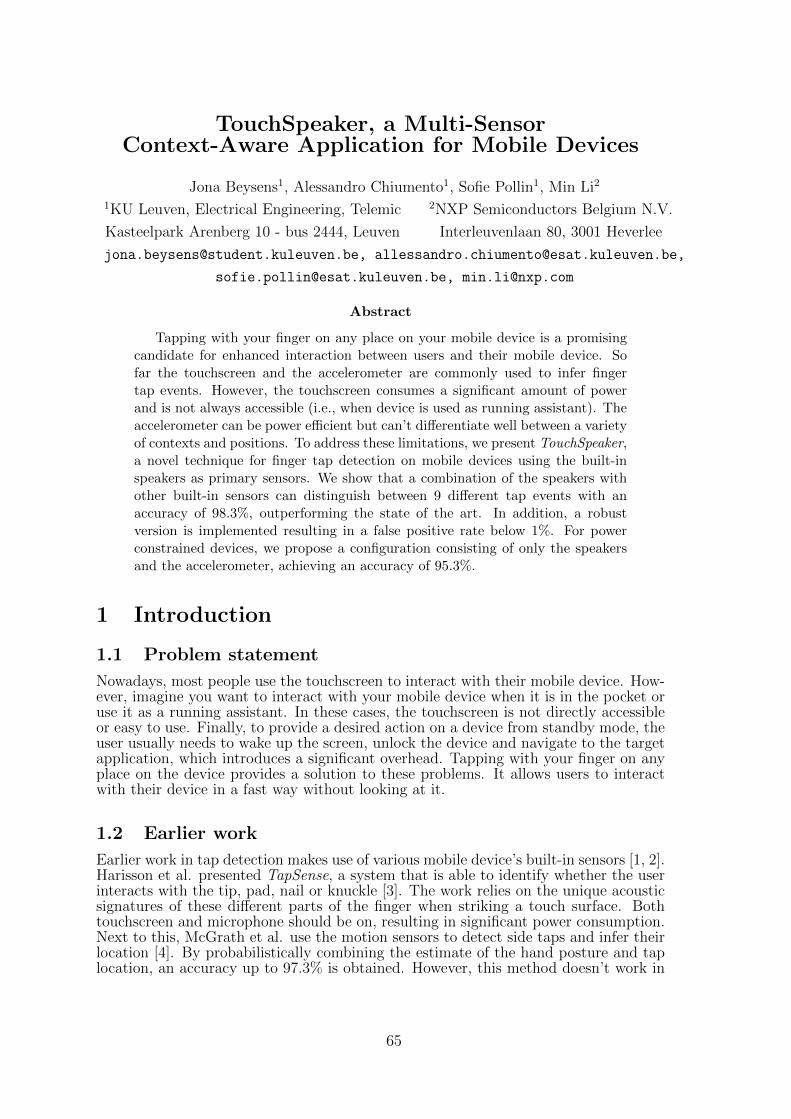
TouchSpeaker, a Multi-SensorContext-Aware Application for Mobile Devices
Jona Beysens1, Alessandro Chiumento1, Sofie Pollin1, Min Li2
1KU Leuven, Electrical Engineering, Telemic 2NXP Semiconductors Belgium N.V.
Kasteelpark Arenberg 10 - bus 2444, Leuven Interleuvenlaan 80, 3001 Heverlee
[email protected], [email protected],
[email protected], [email protected]
Abstract
Tapping with your finger on any place on your mobile device is a promisingcandidate for enhanced interaction between users and their mobile device. Sofar the touchscreen and the accelerometer are commonly used to infer fingertap events. However, the touchscreen consumes a significant amount of powerand is not always accessible (i.e., when device is used as running assistant). Theaccelerometer can be power efficient but can’t differentiate well between a varietyof contexts and positions. To address these limitations, we present TouchSpeaker,a novel technique for finger tap detection on mobile devices using the built-inspeakers as primary sensors. We show that a combination of the speakers withother built-in sensors can distinguish between 9 different tap events with anaccuracy of 98.3%, outperforming the state of the art. In addition, a robustversion is implemented resulting in a false positive rate below 1%. For powerconstrained devices, we propose a configuration consisting of only the speakersand the accelerometer, achieving an accuracy of 95.3%.
1 Introduction
1.1 Problem statement
Nowadays, most people use the touchscreen to interact with their mobile device. How-ever, imagine you want to interact with your mobile device when it is in the pocket oruse it as a running assistant. In these cases, the touchscreen is not directly accessibleor easy to use. Finally, to provide a desired action on a device from standby mode, theuser usually needs to wake up the screen, unlock the device and navigate to the targetapplication, which introduces a significant overhead. Tapping with your finger on anyplace on the device provides a solution to these problems. It allows users to interactwith their device in a fast way without looking at it.
1.2 Earlier work
Earlier work in tap detection makes use of various mobile device’s built-in sensors [1, 2].Harisson et al. presented TapSense, a system that is able to identify whether the userinteracts with the tip, pad, nail or knuckle [3]. The work relies on the unique acousticsignatures of these different parts of the finger when striking a touch surface. Bothtouchscreen and microphone should be on, resulting in significant power consumption.Next to this, McGrath et al. use the motion sensors to detect side taps and infer theirlocation [4]. By probabilistically combining the estimate of the hand posture and taplocation, an accuracy up to 97.3% is obtained. However, this method doesn’t work in
65
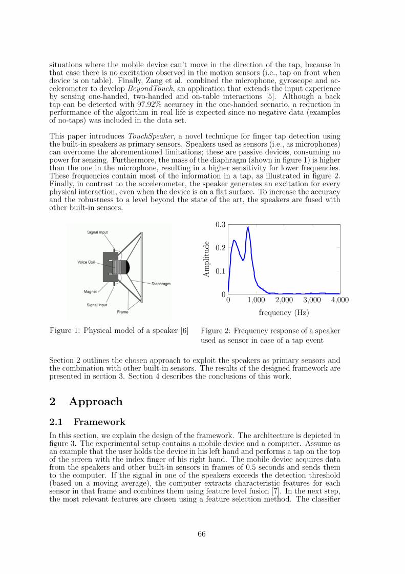
situations where the mobile device can’t move in the direction of the tap, because inthat case there is no excitation observed in the motion sensors (i.e., tap on front whendevice is on table). Finally, Zang et al. combined the microphone, gyroscope and ac-celerometer to develop BeyondTouch, an application that extends the input experienceby sensing one-handed, two-handed and on-table interactions [5]. Although a backtap can be detected with 97.92% accuracy in the one-handed scenario, a reduction inperformance of the algorithm in real life is expected since no negative data (examplesof no-taps) was included in the data set.
This paper introduces TouchSpeaker, a novel technique for finger tap detection usingthe built-in speakers as primary sensors. Speakers used as sensors (i.e., as microphones)can overcome the aforementioned limitations; these are passive devices, consuming nopower for sensing. Furthermore, the mass of the diaphragm (shown in figure 1) is higherthan the one in the microphone, resulting in a higher sensitivity for lower frequencies.These frequencies contain most of the information in a tap, as illustrated in figure 2.Finally, in contrast to the accelerometer, the speaker generates an excitation for everyphysical interaction, even when the device is on a flat surface. To increase the accuracyand the robustness to a level beyond the state of the art, the speakers are fused withother built-in sensors.
Figure 1: Physical model of a speaker [6]
0 1,000 2,000 3,000 4,0000
0.1
0.2
0.3
frequency (Hz)
Am
plitu
de
Figure 2: Frequency response of a speakerused as sensor in case of a tap event
Section 2 outlines the chosen approach to exploit the speakers as primary sensors andthe combination with other built-in sensors. The results of the designed framework arepresented in section 3. Section 4 describes the conclusions of this work.
2 Approach
2.1 Framework
In this section, we explain the design of the framework. The architecture is depicted infigure 3. The experimental setup contains a mobile device and a computer. Assume asan example that the user holds the device in his left hand and performs a tap on the topof the screen with the index finger of his right hand. The mobile device acquires datafrom the speakers and other built-in sensors in frames of 0.5 seconds and sends themto the computer. If the signal in one of the speakers exceeds the detection threshold(based on a moving average), the computer extracts characteristic features for eachsensor in that frame and combines them using feature level fusion [7]. In the next step,the most relevant features are chosen using a feature selection method. The classifier
66
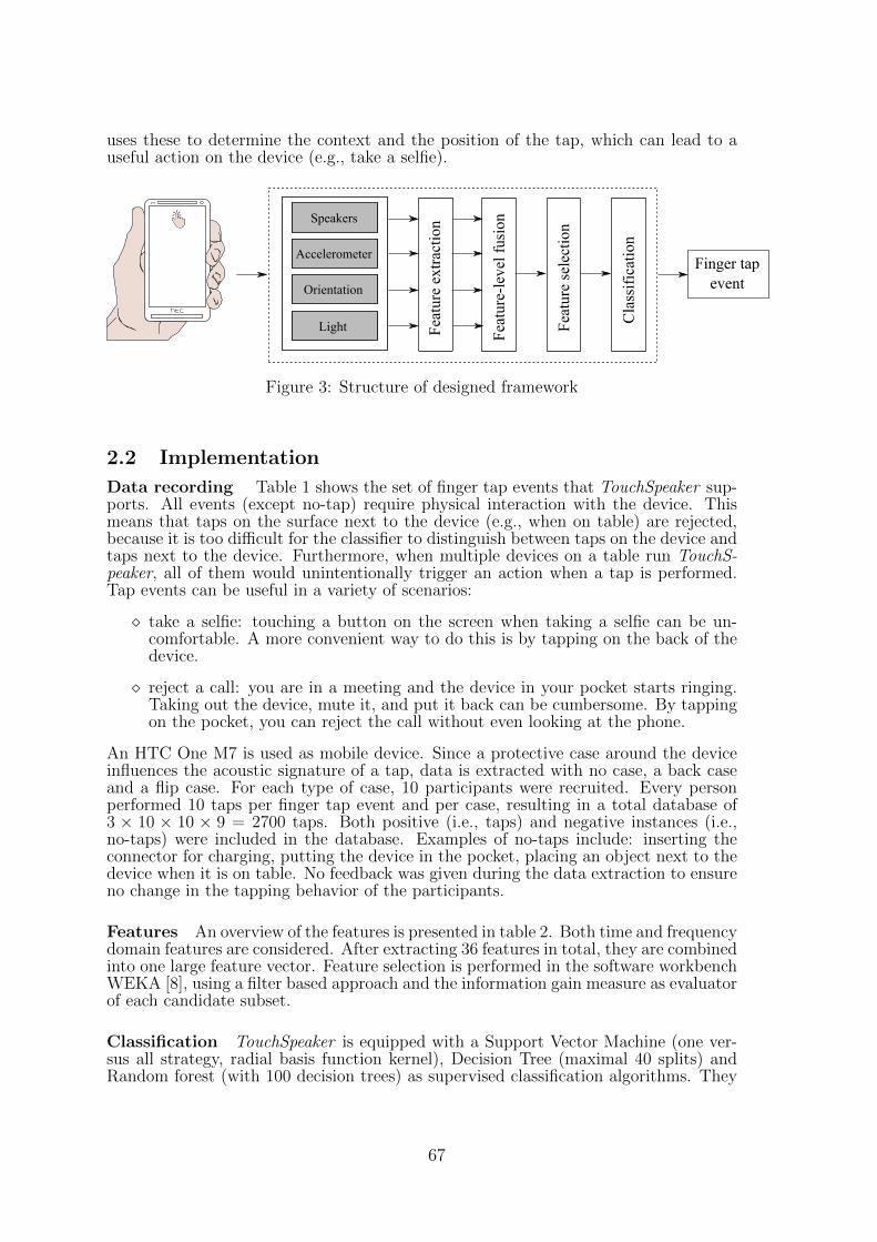
uses these to determine the context and the position of the tap, which can lead to auseful action on the device (e.g., take a selfie).
htc
Speakers
Accelerometer
Orientation
Light
Fea
ture
-lev
el f
usi
on
Finger tap
event
Fea
ture
extr
acti
on
Fea
ture
sel
ecti
on
Cla
ssif
icat
ion
Figure 3: Structure of designed framework
2.2 Implementation
Data recording Table 1 shows the set of finger tap events that TouchSpeaker sup-ports. All events (except no-tap) require physical interaction with the device. Thismeans that taps on the surface next to the device (e.g., when on table) are rejected,because it is too difficult for the classifier to distinguish between taps on the device andtaps next to the device. Furthermore, when multiple devices on a table run TouchS-peaker, all of them would unintentionally trigger an action when a tap is performed.Tap events can be useful in a variety of scenarios:
take a selfie: touching a button on the screen when taking a selfie can be un-comfortable. A more convenient way to do this is by tapping on the back of thedevice.
reject a call: you are in a meeting and the device in your pocket starts ringing.Taking out the device, mute it, and put it back can be cumbersome. By tappingon the pocket, you can reject the call without even looking at the phone.
An HTC One M7 is used as mobile device. Since a protective case around the deviceinfluences the acoustic signature of a tap, data is extracted with no case, a back caseand a flip case. For each type of case, 10 participants were recruited. Every personperformed 10 taps per finger tap event and per case, resulting in a total database of3 × 10 × 10 × 9 = 2700 taps. Both positive (i.e., taps) and negative instances (i.e.,no-taps) were included in the database. Examples of no-taps include: inserting theconnector for charging, putting the device in the pocket, placing an object next to thedevice when it is on table. No feedback was given during the data extraction to ensureno change in the tapping behavior of the participants.
Features An overview of the features is presented in table 2. Both time and frequencydomain features are considered. After extracting 36 features in total, they are combinedinto one large feature vector. Feature selection is performed in the software workbenchWEKA [8], using a filter based approach and the information gain measure as evaluatorof each candidate subset.
Classification TouchSpeaker is equipped with a Support Vector Machine (one ver-sus all strategy, radial basis function kernel), Decision Tree (maximal 40 splits) andRandom forest (with 100 decision trees) as supervised classification algorithms. They
67

ScenarioDevice Tap
Orientation Position
Table
Front Top
Front Bottom
Back Top
Back Bottom
Hand
Front Top
Front Bottom
Back Top
Pocket N/A N/A
No-tap N/A N/A
Table 1: Overview of possible fin-ger tap events
Sensor #Feat. Examples
Top & bottomSpeakers
18 Difference amplitude,energy in tail, cumu-lative density functionof frequency response
Accelerometer 13 Amount of peaks, signof peaks, energy
Orientation 4 Energy in pitch
Light 1 Mean
Table 2: Overview of sensors and features
have 9 classes, corresponding to the 9 possible tap events. After training on the dataset described above, they are evaluated based on 10-fold cross validation and leaving-one-user-out (LOUO) cross validation. The 2nd method measures the predictive per-formance on new users that are not included in the training data, leading to morerealistic results compared to random cross validation.
3 Experimental Results and Discussion
This section presents the results of the designed framework. Accuracy is reported asthe sum of the correctly classified instances over the total amount of instances.
3.1 General performance
Table 3 shows the accuracy and complexity of the different classifiers. All sensors areused together and no feature selection is performed. The complexity of the trainingand testing phase (i.e., classifying a new instance) is measured using Matlab Profiler[9]. Although the Random Forest takes most time to classify a new unseen instancebased on the built model, it achieves the best results. Therefore, this classifier will beanalyzed in the remainder of this section.
Accuracy(%) Complexity(s)Classifiers
10-fold CV LOUO CV Training Testing
SVM 96.2 91.4 5.68 0.17
Decision Tree 92.7 88.3 1.17 0.09
Random Forest 98.3 95.8 4.92 0.66
Table 3: Accuracy and complexity of classifiers
Table 4 presents the 9 × 9 confusion matrix C using 10-fold cross validation for allpossible events. The abbreviations in the table originate from the concatenation of
68
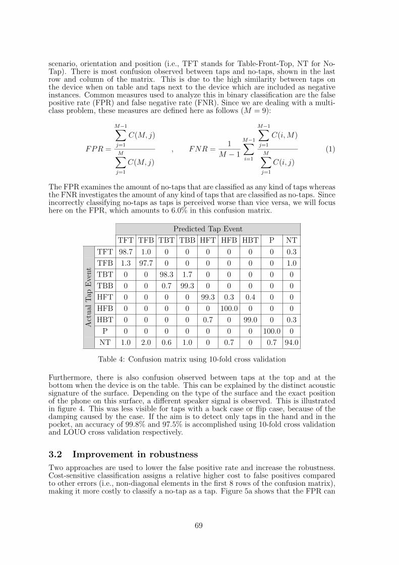
scenario, orientation and position (i.e., TFT stands for Table-Front-Top, NT for No-Tap). There is most confusion observed between taps and no-taps, shown in the lastrow and column of the matrix. This is due to the high similarity between taps onthe device when on table and taps next to the device which are included as negativeinstances. Common measures used to analyze this in binary classification are the falsepositive rate (FPR) and false negative rate (FNR). Since we are dealing with a multi-class problem, these measures are defined here as follows (M = 9):
FPR =
M−1∑
j=1
C(M, j)
M∑
j=1
C(M, j)
, FNR =1
M − 1
M−1∑
i=1
M−1∑
j=1
C(i,M)
M∑
j=1
C(i, j)
(1)
The FPR examines the amount of no-taps that are classified as any kind of taps whereasthe FNR investigates the amount of any kind of taps that are classified as no-taps. Sinceincorrectly classifying no-taps as taps is perceived worse than vice versa, we will focushere on the FPR, which amounts to 6.0% in this confusion matrix.
Predicted Tap Event
TFT TFB TBT TBB HFT HFB HBT P NT
TFT 98.7 1.0 0 0 0 0 0 0 0.3
TFB 1.3 97.7 0 0 0 0 0 0 1.0
TBT 0 0 98.3 1.7 0 0 0 0 0
TBB 0 0 0.7 99.3 0 0 0 0 0
HFT 0 0 0 0 99.3 0.3 0.4 0 0
HFB 0 0 0 0 0 100.0 0 0 0
HBT 0 0 0 0 0.7 0 99.0 0 0.3
P 0 0 0 0 0 0 0 100.0 0
Act
ual
Tap
Eve
nt
NT 1.0 2.0 0.6 1.0 0 0.7 0 0.7 94.0
Table 4: Confusion matrix using 10-fold cross validation
Furthermore, there is also confusion observed between taps at the top and at thebottom when the device is on the table. This can be explained by the distinct acousticsignature of the surface. Depending on the type of the surface and the exact positionof the phone on this surface, a different speaker signal is observed. This is illustratedin figure 4. This was less visible for taps with a back case or flip case, because of thedamping caused by the case. If the aim is to detect only taps in the hand and in thepocket, an accuracy of 99.8% and 97.5% is accomplished using 10-fold cross validationand LOUO cross validation respectively.
3.2 Improvement in robustness
Two approaches are used to lower the false positive rate and increase the robustness.Cost-sensitive classification assigns a relative higher cost to false positives comparedto other errors (i.e., non-diagonal elements in the first 8 rows of the confusion matrix),making it more costly to classify a no-tap as a tap. Figure 5a shows that the FPR can
69
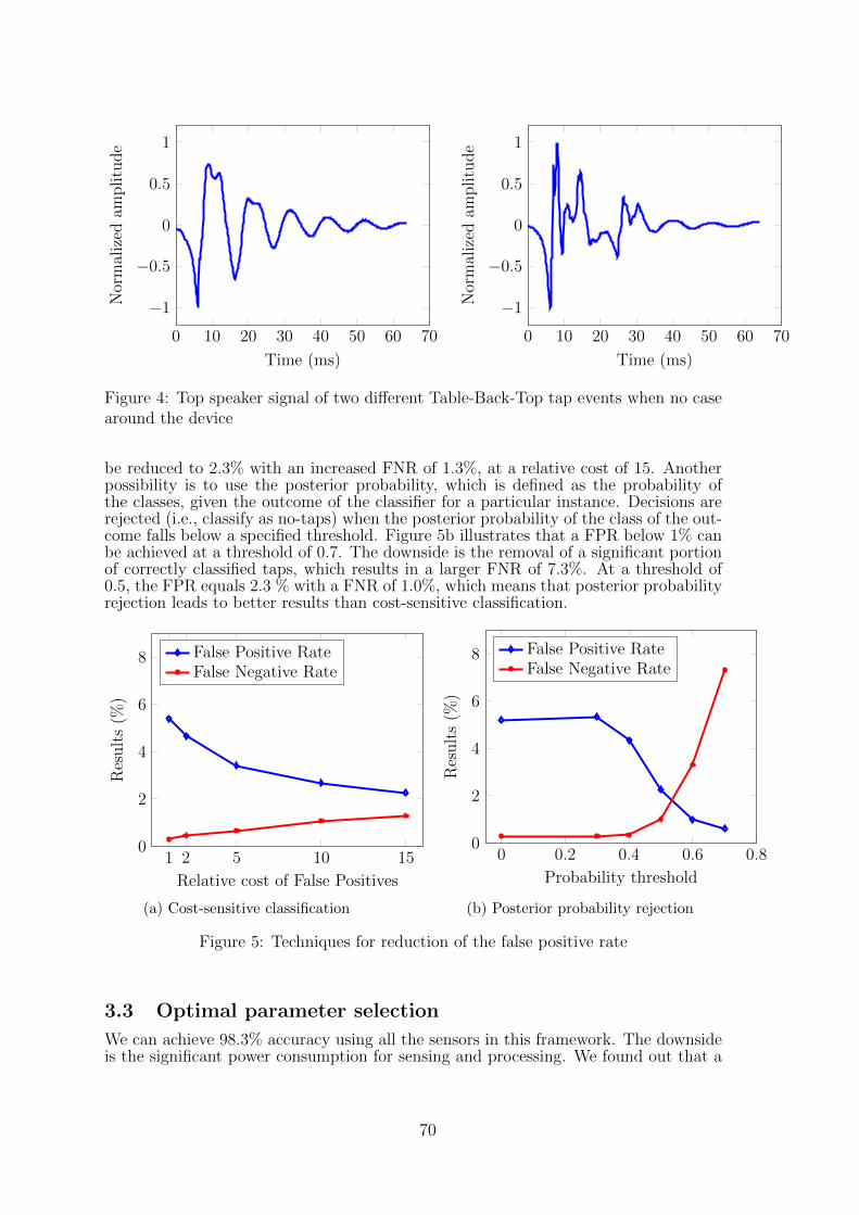
0 10 20 30 40 50 60 70
−1
−0.5
0
0.5
1
Time (ms)
Nor
mal
ized
amplitu
de
0 10 20 30 40 50 60 70
−1
−0.5
0
0.5
1
Time (ms)
Nor
mal
ized
amplitu
de
Figure 4: Top speaker signal of two different Table-Back-Top tap events when no casearound the device
be reduced to 2.3% with an increased FNR of 1.3%, at a relative cost of 15. Anotherpossibility is to use the posterior probability, which is defined as the probability ofthe classes, given the outcome of the classifier for a particular instance. Decisions arerejected (i.e., classify as no-taps) when the posterior probability of the class of the out-come falls below a specified threshold. Figure 5b illustrates that a FPR below 1% canbe achieved at a threshold of 0.7. The downside is the removal of a significant portionof correctly classified taps, which results in a larger FNR of 7.3%. At a threshold of0.5, the FPR equals 2.3 % with a FNR of 1.0%, which means that posterior probabilityrejection leads to better results than cost-sensitive classification.
1 2 5 10 150
2
4
6
8
Relative cost of False Positives
Res
ult
s(%
)
False Positive RateFalse Negative Rate
(a) Cost-sensitive classification
0 0.2 0.4 0.6 0.80
2
4
6
8
Probability threshold
Res
ult
s(%
)
False Positive RateFalse Negative Rate
(b) Posterior probability rejection
Figure 5: Techniques for reduction of the false positive rate
3.3 Optimal parameter selection
We can achieve 98.3% accuracy using all the sensors in this framework. The downsideis the significant power consumption for sensing and processing. We found out that a
70
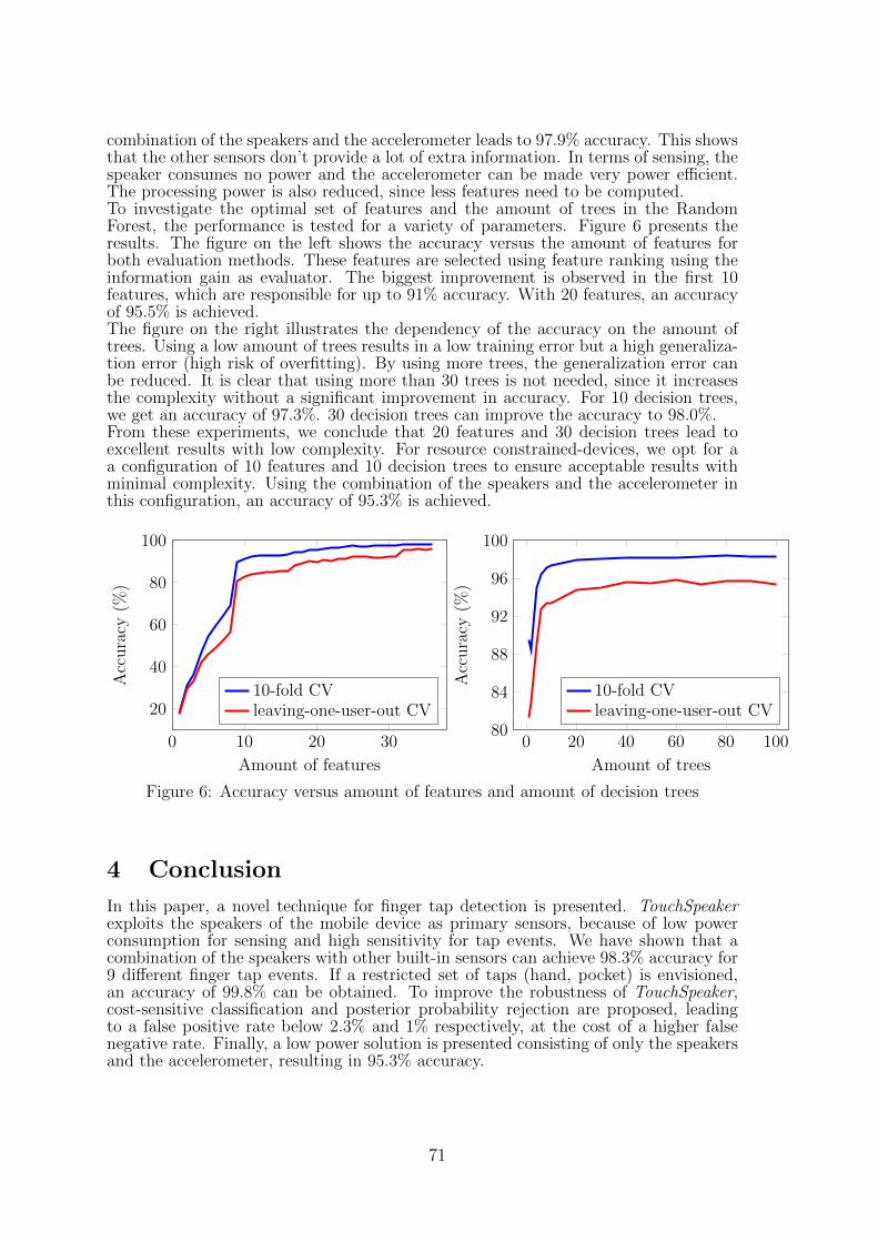
combination of the speakers and the accelerometer leads to 97.9% accuracy. This showsthat the other sensors don’t provide a lot of extra information. In terms of sensing, thespeaker consumes no power and the accelerometer can be made very power efficient.The processing power is also reduced, since less features need to be computed.To investigate the optimal set of features and the amount of trees in the RandomForest, the performance is tested for a variety of parameters. Figure 6 presents theresults. The figure on the left shows the accuracy versus the amount of features forboth evaluation methods. These features are selected using feature ranking using theinformation gain as evaluator. The biggest improvement is observed in the first 10features, which are responsible for up to 91% accuracy. With 20 features, an accuracyof 95.5% is achieved.The figure on the right illustrates the dependency of the accuracy on the amount oftrees. Using a low amount of trees results in a low training error but a high generaliza-tion error (high risk of overfitting). By using more trees, the generalization error canbe reduced. It is clear that using more than 30 trees is not needed, since it increasesthe complexity without a significant improvement in accuracy. For 10 decision trees,we get an accuracy of 97.3%. 30 decision trees can improve the accuracy to 98.0%.From these experiments, we conclude that 20 features and 30 decision trees lead toexcellent results with low complexity. For resource constrained-devices, we opt for aa configuration of 10 features and 10 decision trees to ensure acceptable results withminimal complexity. Using the combination of the speakers and the accelerometer inthis configuration, an accuracy of 95.3% is achieved.
0 10 20 30
20
40
60
80
100
Amount of features
Acc
ura
cy(%
)
10-fold CVleaving-one-user-out CV
0 20 40 60 80 10080
84
88
92
96
100
Amount of trees
Acc
ura
cy(%
)
10-fold CVleaving-one-user-out CV
Figure 6: Accuracy versus amount of features and amount of decision trees
4 Conclusion
In this paper, a novel technique for finger tap detection is presented. TouchSpeakerexploits the speakers of the mobile device as primary sensors, because of low powerconsumption for sensing and high sensitivity for tap events. We have shown that acombination of the speakers with other built-in sensors can achieve 98.3% accuracy for9 different finger tap events. If a restricted set of taps (hand, pocket) is envisioned,an accuracy of 99.8% can be obtained. To improve the robustness of TouchSpeaker,cost-sensitive classification and posterior probability rejection are proposed, leadingto a false positive rate below 2.3% and 1% respectively, at the cost of a higher falsenegative rate. Finally, a low power solution is presented consisting of only the speakersand the accelerometer, resulting in 95.3% accuracy.
71

References
[1] H. Lu and Y. Li, “Gesture On: Enabling Always-On Touch Gestures for FastMobile Access from the Device Standby Mode,” Proceedings of the 33rd AnnualACM Conference on Human Factors in Computing Systems - CHI ’15, vol. 1, pp.3355–3364, 2015.
[2] P. Daniel, “KnockOn app brings double-tap to lock to most An-droids and wake to ones with OLED displays.” [Online]. Avail-able: http://www.phonearena.com/news/KnockOn-app-brings-double-tap-to-lock-to-most-Androids.-and-wake-to-ones-with-OLED-displays id75033
[3] C. Harrison, J. Schwarz, and S. E. Hudson, “TapSense: enhancing finger interac-tion on touch surfaces,” Proceedings of the 24th annual ACM symposium on Userinterface software and technology - UIST ’11, pp. 627–636, 2011.
[4] W. McGrath and Y. Li, “Detecting tapping motion on the side of mobile devices byprobabilistically combining hand postures,” Proceedings of the 27th annual ACMsymposium on User interface software and technology - UIST ’14, pp. 215–219,2014.
[5] C. Zhang, A. Guo, D. Zhang, C. Southern, R. Arriaga, and G. Abowd, “Beyond-Touch: Extending the Input Language with Built-in Sensors on Commodity Smart-phones,” Proceedings of the 20th International Conference on Intelligent User In-terfaces - IUI ’15, pp. 67–77, 2015.
[6] D. Gouveia, “Creating a Basic Synth in XNA 4.0 Part I.” [Online]. Available:http://www.david-gouveia.com/portfolio/creating-a-basic-synth-in-xna-part-i/
[7] M. Yacoub and G.-Z. Yang, Body Sensor Networks. Springer Science & BusinessMedia, 2007.
[8] University of Waikato, “Weka 3 - Data Mining with Open Source Machine LearningSoftware in Java.” [Online]. Available: http://www.cs.waikato.ac.nz/ml/weka/
[9] MathWorks Benelux, “MATLAB Profile execution time for functions.” [Online].Available: http://nl.mathworks.com/help/matlab/ref/profile.html
72
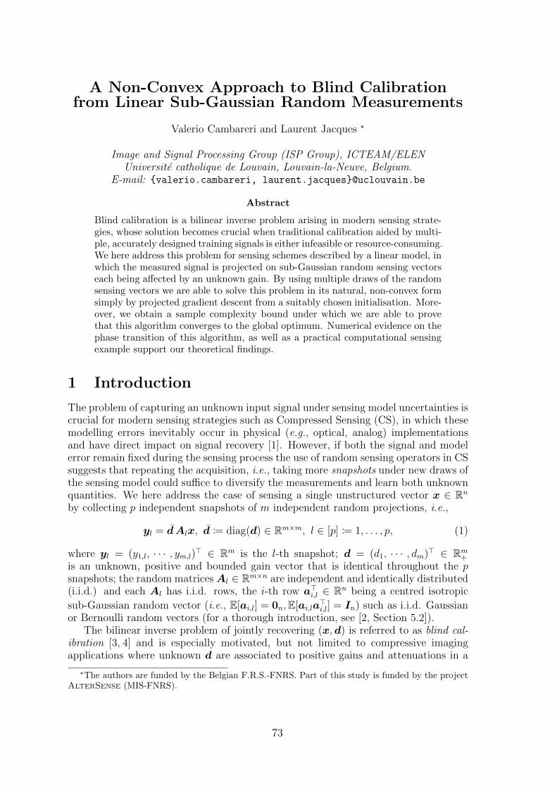
A Non-Convex Approach to Blind Calibrationfrom Linear Sub-Gaussian Random Measurements
Valerio Cambareri and Laurent Jacques ∗
Image and Signal Processing Group (ISP Group), ICTEAM/ELENUniversite catholique de Louvain, Louvain-la-Neuve, Belgium.
E-mail: valerio.cambareri, [email protected]
Abstract
Blind calibration is a bilinear inverse problem arising in modern sensing strate-gies, whose solution becomes crucial when traditional calibration aided by multi-ple, accurately designed training signals is either infeasible or resource-consuming.We here address this problem for sensing schemes described by a linear model, inwhich the measured signal is projected on sub-Gaussian random sensing vectorseach being affected by an unknown gain. By using multiple draws of the randomsensing vectors we are able to solve this problem in its natural, non-convex formsimply by projected gradient descent from a suitably chosen initialisation. More-over, we obtain a sample complexity bound under which we are able to provethat this algorithm converges to the global optimum. Numerical evidence on thephase transition of this algorithm, as well as a practical computational sensingexample support our theoretical findings.
1 Introduction
The problem of capturing an unknown input signal under sensing model uncertainties iscrucial for modern sensing strategies such as Compressed Sensing (CS), in which thesemodelling errors inevitably occur in physical (e.g., optical, analog) implementationsand have direct impact on signal recovery [1]. However, if both the signal and modelerror remain fixed during the sensing process the use of random sensing operators in CSsuggests that repeating the acquisition, i.e., taking more snapshots under new draws ofthe sensing model could suffice to diversify the measurements and learn both unknownquantities. We here address the case of sensing a single unstructured vector x ∈ Rnby collecting p independent snapshots of m independent random projections, i.e.,
yl = dAlx, d := diag(d) ∈ Rm×m, l ∈ [p] := 1, . . . , p, (1)
where yl = (y1,l, · · · , ym,l)> ∈ Rm is the l-th snapshot; d = (d1, · · · , dm)> ∈ Rm+is an unknown, positive and bounded gain vector that is identical throughout the psnapshots; the random matricesAl ∈ Rm×n are independent and identically distributed(i.i.d.) and each Al has i.i.d. rows, the i-th row a>i,l ∈ Rn being a centred isotropic
sub-Gaussian random vector (i.e., E[ai,l] = 0n,E[ai,la>i,l] = In) such as i.i.d. Gaussian
or Bernoulli random vectors (for a thorough introduction, see [2, Section 5.2]).The bilinear inverse problem of jointly recovering (x,d) is referred to as blind cal-
ibration [3, 4] and is especially motivated, but not limited to compressive imagingapplications where unknown d are associated to positive gains and attenuations in a
∗The authors are funded by the Belgian F.R.S.-FNRS. Part of this study is funded by the projectAlterSense (MIS-FNRS).
73
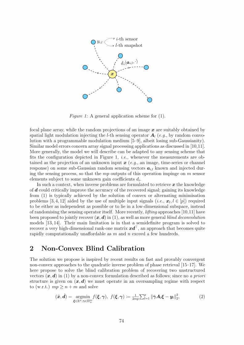
x
yi,li-th sensor
l-th snapshot
di〈ai,l, ·〉
Figure 1: A general application scheme for (1).
focal plane array, while the random projections of an image x are suitably obtained byspatial light modulation injecting the l-th sensing operator Al (e.g., by random convo-lution with a programmable modulation medium [5–9], albeit losing sub-Gaussianity).Similar model errors concern array signal processing applications as discussed in [10,11].More generally, the model we will describe can be adapted to any sensing scheme thatfits the configuration depicted in Figure 1, i.e., whenever the measurements are ob-tained as the projection of an unknown input x (e.g., an image, time-series or channelresponse) on some sub-Gaussian random sensing vectors ai,l known and injected dur-ing the sensing process, so that the mp outputs of this operation impinge on m sensorelements subject to some unknown gain coefficients di.
In such a context, when inverse problems are formulated to retrieve x the knowledgeof d could critically improve the accuracy of the recovered signal; gaining its knowledgefrom (1) is typically achieved by the solution of convex or alternating minimisationproblems [3, 4, 12] aided by the use of multiple input signals (i.e., xl, l ∈ [p]) requiredto be either as independent as possible or to lie in a low-dimensional subspace, insteadof randomising the sensing operator itself. More recently, lifting approaches [10,11] havebeen proposed to jointly recover (x,d) in (1), as well as more general blind deconvolutionmodels [13, 14]. Their main limitation is in that a semidefinite program is solved torecover a very high-dimensional rank-one matrix xd>, an approach that becomes quiterapidly computationally unaffordable as m and n exceed a few hundreds.
2 Non-Convex Blind Calibration
The solution we propose is inspired by recent results on fast and provably convergentnon-convex approaches to the quadratic inverse problem of phase retrieval [15–17]. Wehere propose to solve the blind calibration problem of recovering two unstructuredvectors (x,d) in (1) by a non-convex formulation described as follows; since no a prioristructure is given on (x,d) we must operate in an oversampling regime with respectto (w.r.t.) mp ≥ n+m and solve
(x, d) = argminξ∈Rn,γ∈Πm+
f(ξ,γ), f(ξ,γ) := 12mp
∑pl=1 ‖γAlξ − yl‖2
2, (2)
74

Quantity Finite-sample (p <∞) Expectation (Eai,l , p→∞)
Objective: f(ξ,γ) 12mp
∑pl=1
∥∥γAlξ − dAlx∥∥2
21
2m‖ξγ> − xd>‖2
F
Signal gradient: ∇ξf(ξ,γ) 1mp
∑pl=1A
>l γ(γAlξ − dAlx
)1m
[‖γ‖2
2ξ − (γ>d)x]
Gain gradient: ∇γf(ξ,γ) 1mp
∑pl=1Alξ
(γAlξ − dAlx
)1m
[‖ξ‖2
2γ − (ξ>x)d]
Projected gain gradient: ∇⊥γ f(ξ,γ) 1mp
∑pl=1Alξ (εAlξ − ωAlx) 1
m
[‖ξ‖2
2ε− (ξ>x)ω]
Hessian matrix: Hf(ξ,γ) 1mp
∑pl=1
[A>l γ
2Al A>l 2γAlξ−dAlx
2γAlξ−dAlxAl Alξ2
]1m
[‖γ‖22In 2ξγ>−xd>
2γξ>−dx> ‖ξ‖22Im
]
Initialisation: (ξ0, γ0)(
1mp
∑pl=1 (Al)
> dAlx, 1m
) (‖d‖1mx, 1m
)
Table 1: Finite-sample and expected values of the objective function; its gradientcomponents and Hessian matrix; the initialisation point (ξ0,γ0).
given ylpl=1, Alpl=1 with Πm+ := γ ∈ Rm+ , 1>mγ = m being the scaled probabil-
ity simplex. The geometry of this problem can be studied by observing the objec-tive f(ξ,γ) with its gradient ∇f(ξ,γ) = [ (∇ξf(ξ,γ))> (∇γf(ξ,γ))> ]> and Hessian matrixHf(ξ,γ), all computed in Table 1 for p < ∞. The finite-sample expressions thereinare unbiased estimates of their expectation w.r.t. the i.i.d. sensing vectors ai,l. There,we evince that the set
(ξ,γ) ∈ Rn × Rm : ξ = 1
αx,γ = αd, α ∈ R \ 0
contains the
global minimisers of f(ξ,γ). Moreover f(ξ,γ) is shown to be generally non-convex† asthere exist plenty of counterexamples (ξ′,γ ′) for which Hf(ξ′,γ ′) 0.
We now elaborate on the constraint γ ∈ Πm+ . Firstly, we see that only one minimiser
(x?,d?) :=(‖d‖1
mx, m‖d‖1d
)remains for mp ≥ n+m, which amounts to the exact solution
up to a fixed α = m/‖d‖1. Secondly, assuming that d ∈ Rm+ in (1) is positive andbounded amounts to letting d? ∈ Cρ ⊂ Πm
+ , Cρ := 1m + 1⊥m ∩ ρBm∞ for a maximumdeviation ρ > ‖d? − 1m‖∞, ρ < 1 (where we denoted the orthogonal complement1⊥m := v ∈ Rm : 1>mv = 0 and Bqp the `p-ball in Rq). In particular, we can specify
d? = 1m + ω for ω ∈ 1⊥m ∩ ρBm∞, as well as γ = 1m + ε for ε ∈ 1⊥m ∩ ρBm∞ providedthat the algorithm solving (2) is so that γ remains in Cρ. This allows us to recast (2)in terms of the variations ω, ε ∈ 1⊥m ∩ ρBm∞ on the simplex Πm
+ .While applying this constraint to the minimisation of f(ξ,γ) will not grant convex-
ity in the domain of (2), we proceed by defining a neighbourhood of the global minimiser(x?,d?) as follows. To begin with, we will require a notion of distance, i.e.,
∆(ξ,γ) := ‖ξ − x?‖22 +
‖x?‖22m‖γ − d?‖2
2.
Then, to account for the constraint in the gain domain we define our neighbourhood
Dκ,ρ := (ξ,γ) ∈ Rn × Cρ : ∆(ξ,γ) ≤ κ2‖x?‖22, ρ ∈ [0, 1).
Thus, Dκ,ρ is the intersection of an ellipsoid in Rn × Rm, as defined by ∆(ξ,γ) ≤κ2‖x?‖2
2, with Rn × Cρ (and as such is a convex set). While we anticipate that local
†It is biconvex [11], i.e., convex once either ξ or γ are fixed.
75
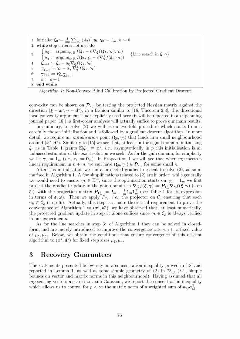
1: Initialise ξ0 := 1mp
∑pl=1 (Al)
> yl, γ0 := 1m, k := 0.
2: while stop criteria not met do
3:
µξ := argminυ∈R f(ξk − υ∇ξf(ξk,γk),γk)
µγ := argminυ∈R f(ξk,γk − υ∇⊥γ f(ξk,γk))Line search in ξ,γ
4: ξk+1 := ξk − µξ∇ξf(ξk,γk)5: γ
k+1:= γk − µγ∇⊥γ f(ξk,γk)
6: γk+1 := PCργk+17: k := k + 18: end while
Algorithm 1: Non-Convex Blind Calibration by Projected Gradient Descent.
convexity can be shown on Dκ,ρ by testing the projected Hessian matrix against thedirection (ξ − x?,γ − d?), in a fashion similar to [16, Theorem 2.3], this directionallocal convexity argument is not explicitly used here (it will be reported in an upcomingjournal paper [18]); a first-order analysis will actually suffice to prove our main results.
In summary, to solve (2) we will use a two-fold procedure which starts from acarefully chosen initialisation and is followed by a gradient descent algorithm. In moredetail, we require an initialisation point (ξ0,γ0) that lands in a small neighbourhoodaround (x?,d?). Similarly to [15] we see that, at least in the signal domain, initialisingξ0 as in Table 1 grants E[ξ0] ≡ x?, i.e., asymptotically in p this initialisation is anunbiased estimator of the exact solution we seek. As for the gain domain, for simplicitywe let γ0 := 1m (i.e., ε0 := 0m). In Proposition 1 we will see that when mp meets alinear requirement in n+m, we can have (ξ0,γ0) ∈ Dκ,ρ for some small κ.
After this initialisation we run a projected gradient descent to solve (2), as sum-marised in Algorithm 1. A few simplifications related to (2) are in order: while generallywe would need to ensure γk ∈ Πm
+ , since the optimisation starts on γ0 = 1m we firstproject the gradient update in the gain domain as ∇⊥γ f(ξ,γ) := P1⊥
m∇γf(ξ,γ) (step
5:) with the projection matrix P1⊥m
:= Im − 1m1m1
>m (see Table 1 for its expression
in terms of ε,ω). Then we apply PCρ , i.e., the projector on Cρ ensuring that eachγk ∈ Cρ (step 6:). Actually, this step is a mere theoretical requirement to prove theconvergence of Algorithm 1 to (x?,d?); we have observed that, at least numerically,the projected gradient update in step 5: alone suffices since γk ∈ Cρ is always verifiedin our experiments.
As for the line searches in step 3: of Algorithm 1 they can be solved in closed-form, and are merely introduced to improve the convergence rate w.r.t. a fixed valueof µξ, µγ . Below, we obtain the conditions that ensure convergence of this descentalgorithm to (x?,d?) for fixed step sizes µξ, µγ .
3 Recovery Guarantees
The statements presented below rely on a concentration inequality proved in [18] andreported in Lemma 1, as well as some simple geometry of (2) in Dκ,ρ (i.e., simplebounds on vector and matrix norms in this neighbourhood). Having assumed that allmp sensing vectors ai,l are i.i.d. sub-Gaussian, we report the concentration inequalitywhich allows us to control for p <∞ the matrix norm of a weighted sum of ai,la
>i,l.
76

Lemma 1 (Weighted Concentration Inequality). Let ai,l ∈ Rn : i ∈ [m], l ∈ [p]be a set of random vectors, each formed by n i.i.d. copies of a sub-Gaussian randomvariable X [2, Section 5.2.3] with EX = 0, EX2 = 1 and sub-Gaussian norm ‖X‖ψ2.Given δ ∈ (0, 1) and t > 1 we have, with probability exceeding
1− Ce−cδ2mp − (mp)−t (3)
for some C, c > 0 depending only on ‖X‖ψ2, that∥∥ 1mp
∑mi=1
∑pl=1 θi(ai,la
>i,l − In)
∥∥2≤ δ ‖θ‖∞, ∀θ = θimi=1 ∈ Rm (4)
provided n & t log(mp) and mp & δ−2(n+m) log(nδ).
We now establish the sample complexity required for the initialisation to lie in Dκ,ρwith very high probability for some κ and ρ fixed by the entity of the model error.
Proposition 1 (Initialisation Proximity). Let (ξ0,γ0) be as in Table 1. For any ε ∈(0, 1) we have, with probability exceeding 1 − Ce−cε
2mp − (mp)−t for some C, c > 0,that ‖ξ0 − x?‖2 ≤ ε‖x?‖2 provided n & t log(mp) and mp & ε−2(n + m) log
(nε−1
).
Since γ0 = 1m we also have ‖γ0 − d?‖∞ ≤ ρ < 1. Thus (ξ0,γ0) ∈ Dκ,ρ with the same
probability and κ :=√ε2 + ρ2 ≤
√2.
With analogue tools (and more general concentration properties of isotropic sub-Gaussian ai,l [2, Section 5.2]) we are able to state when a single gradient descent stepfrom any (ξ,γ) ∈ Dκ,ρ reduces, with very high probability, the distance w.r.t. the globalminimum. This requires establishing a regularity condition on the projected gradient∇⊥f(ξ,γ) := [ (∇ξf(ξ,γ))> (∇⊥
γ f(ξ,γ))> ]> holding uniformly, i.e., for all (ξ,γ) ∈ Dκ,ρ(similarly to [15, Condition 7.9]).
Proposition 2 (Regularity condition in Dκ,ρ). For any δ ∈ (0, 1) there exist a constantη ∈ (0, 1), t > 1 and a value L < 3(1+κ)(4+‖x?‖2) such that, with probability exceeding
1− C[me−cδ
2p + e−cδ2mp + (mp)−t
]
for some C, c > 0, we have for all (ξ,γ) ∈ Dκ,ρ, ρ ∈ [0, 1),
⟨∇⊥f(ξ,γ),
[ξ−x?γ−d?
]⟩≥ 1
2η∆(ξ,γ) (Bounded curvature)
‖∇⊥f(ξ,γ)‖22 ≤ L2 ∆(ξ,γ) (Lipschitz gradient)
provided ρ < 114
(1−η−3δ), n & t log(mp), p & δ−2 logm and mp & δ−2(n+m) log(nδ).
We now use Proposition 2 to show that the neighbourhood Dκ,ρ is a basin ofattraction to the solution (x?,d?). If we update ξ+ := ξ − µξ∇ξf(ξ,γ),γ
+:=
γ − µγ∇⊥γ f(ξ,γ),γ+ := PCργ+from any (ξ,γ) ∈ Dκ,ρ we have that, when µξ :=
µ, µγ ∝ mµ and µ is sufficiently small, (i) ∆(ξ+,γ+) < ∆(ξ,γ) and (ii) (ξ,γ) ∈ Dκ,ρ.Note that the role of PCρ (i.e., a convex `∞-ball, that is a contraction) is technical inensuring (i), (ii) above by verifying ‖γ+ − d?‖2 ≤ ‖γ+
− d?‖2. By a recursive applica-
tion of these facts (which will be expanded in [18]) we obtain the following convergenceresult.
77
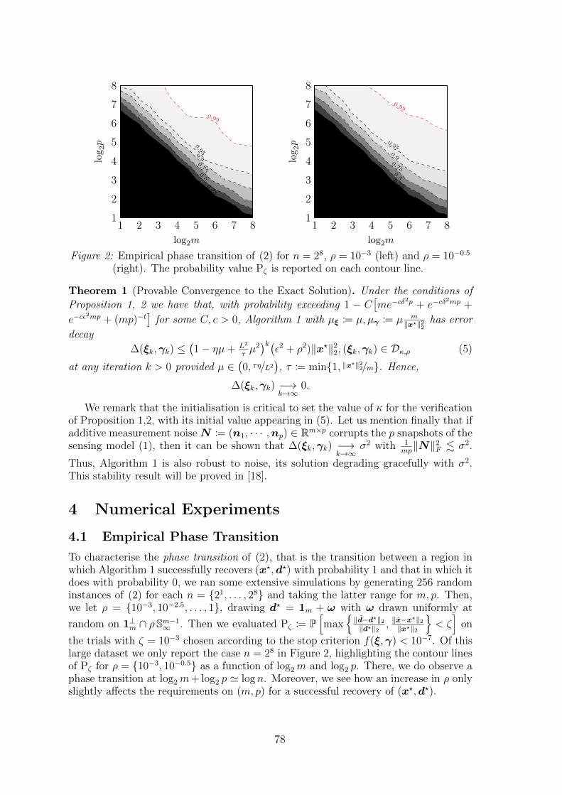
1 2 3 4 5 6 7 81
2
3
4
5
6
7
8
0.25
0.5
0.75
0.90.95
0.99
log2m
log
2p
1 2 3 4 5 6 7 81
2
3
4
5
6
7
8
0.25
0.50.75
0.9
0.95
0.99
log2m
log
2p
Figure 2: Empirical phase transition of (2) for n = 28, ρ = 10−3 (left) and ρ = 10−0.5
(right). The probability value Pζ is reported on each contour line.
Theorem 1 (Provable Convergence to the Exact Solution). Under the conditions of
Proposition 1, 2 we have that, with probability exceeding 1 − C[me−cδ
2p + e−cδ2mp +
e−cε2mp + (mp)−t
]for some C, c > 0, Algorithm 1 with µξ := µ, µγ := µ m
‖x?‖22has error
decay
∆(ξk,γk) ≤(1− ηµ+ L2
τµ2)k(
ε2 + ρ2)‖x?‖22, (ξk,γk) ∈ Dκ,ρ (5)
at any iteration k > 0 provided µ ∈(0, τη/L2
), τ := min1, ‖x?‖22/m. Hence,
∆(ξk,γk) −→k→∞
0.
We remark that the initialisation is critical to set the value of κ for the verificationof Proposition 1,2, with its initial value appearing in (5). Let us mention finally that ifadditive measurement noise N := (n1, · · · ,np) ∈ Rm×p corrupts the p snapshots of thesensing model (1), then it can be shown that ∆(ξk,γk) −→
k→∞σ2 with 1
mp‖N‖2
F . σ2.
Thus, Algorithm 1 is also robust to noise, its solution degrading gracefully with σ2.This stability result will be proved in [18].
4 Numerical Experiments
4.1 Empirical Phase Transition
To characterise the phase transition of (2), that is the transition between a region inwhich Algorithm 1 successfully recovers (x?,d?) with probability 1 and that in which itdoes with probability 0, we ran some extensive simulations by generating 256 randominstances of (2) for each n = 21, . . . , 28 and taking the latter range for m, p. Then,we let ρ = 10−3, 10−2.5, . . . , 1, drawing d? = 1m + ω with ω drawn uniformly at
random on 1⊥m ∩ ρSm−1∞ . Then we evaluated Pζ := P
[max
‖d−d?‖2‖d?‖2 , ‖x−x
?‖2‖x?‖2
< ζ]
on
the trials with ζ = 10−3 chosen according to the stop criterion f(ξ,γ) < 10−7. Of thislarge dataset we only report the case n = 28 in Figure 2, highlighting the contour linesof Pζ for ρ = 10−3, 10−0.5 as a function of log2m and log2 p. There, we do observe aphase transition at log2m+ log2 p ' log n. Moreover, we see how an increase in ρ onlyslightly affects the requirements on (m, p) for a successful recovery of (x?,d?).
78
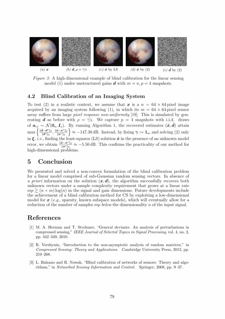
(a) x (b) d, ρ = 1/2 (c) x by LS (d) x by (2) (e) d by (2)
Figure 3: A high-dimensional example of blind calibration for the linear sensingmodel (1) under unstructured gains d with m = n, p = 4 snapshots.
4.2 Blind Calibration of an Imaging System
To test (2) in a realistic context, we assume that x is a n = 64 × 64 pixel imageacquired by an imaging system following (1), in which its m = 64 × 64 pixel sensorarray suffers from large pixel response non-uniformity [19]. This is simulated by gen-erating d as before with ρ = 1/2. We capture p = 4 snapshots with i.i.d. draws
of ai,l ∼ N (0n, In). By running Algorithm 1, the recovered estimates (x, d) attain
max‖d−d?‖2‖d?‖2 , ‖x−x
?‖2‖x?‖2
≈ −147.38 dB. Instead, by fixing γ := 1m and solving (2) only
in ξ, i.e., finding the least-squares (LS) solution x in the presence of an unknown model
error, we obtain ‖x−x?‖2‖x?‖2 ≈ −5.50 dB. This confirms the practicality of our method for
high-dimensional problems.
5 Conclusion
We presented and solved a non-convex formulation of the blind calibration problemfor a linear model comprised of sub-Gaussian random sensing vectors. In absence ofa priori information on the solution (x,d), the algorithm successfully recovers bothunknown vectors under a sample complexity requirement that grows at a linear ratemp & (n + m) log(n) in the signal and gain dimensions. Future developments includethe achievement of a blind calibration method for CS by exploiting a low-dimensionalmodel for x (e.g., sparsity, known subspace models), which will eventually allow for areduction of the number of samples mp below the dimensionality n of the input signal.
References
[1] M. A. Herman and T. Strohmer, “General deviants: An analysis of perturbations incompressed sensing,” IEEE Journal of Selected Topics in Signal Processing, vol. 4, no. 2,pp. 342–349, 2010.
[2] R. Vershynin, “Introduction to the non-asymptotic analysis of random matrices,” inCompressed Sensing: Theory and Applications. Cambridge University Press, 2012, pp.210–268.
[3] L. Balzano and R. Nowak, “Blind calibration of networks of sensors: Theory and algo-rithms,” in Networked Sensing Information and Control. Springer, 2008, pp. 9–37.
79

[4] C. Bilen, G. Puy, R. Gribonval, and L. Daudet, “Convex Optimization Approachesfor Blind Sensor Calibration Using Sparsity,” IEEE Transactions on Signal Processing,vol. 62, no. 18, pp. 4847–4856, Sep. 2014.
[5] J. Romberg, “Compressive sensing by random convolution,” SIAM Journal on ImagingSciences, vol. 2, no. 4, pp. 1098–1128, 2009.
[6] T. Bjorklund and E. Magli, “A parallel compressive imaging architecture for one-shotacquisition,” in 2013 IEEE Picture Coding Symposium (PCS). IEEE, 2013, pp. 65–68.
[7] K. Degraux, V. Cambareri, B. Geelen, L. Jacques, G. Lafruit, and G. Setti, “Com-pressive Hyperspectral Imaging by Out-of-Focus Modulations and Fabry-Perot SpectralFilters,” in International Traveling Workshop on Interactions between Sparse models andTechnology (iTWIST), 2014.
[8] S. Bahmani and J. Romberg, “Lifting for Blind Deconvolution in Random Mask Imaging:Identifiability and Convex Relaxation,” SIAM Journal on Imaging Sciences, vol. 8, no. 4,pp. 2203–2238, 2015.
[9] J. P. Dumas, M. A. Lodhi, W. U. Bajwa, and M. C. Pierce, “Computationalimaging with a highly parallel image-plane-coded architecture: challenges andsolutions,” Opt. Express, vol. 24, no. 6, pp. 6145–6155, Mar 2016. [Online]. Available:http://www.opticsexpress.org/abstract.cfm?URI=oe-24-6-6145
[10] B. Friedlander and T. Strohmer, “Bilinear compressed sensing for array self-calibration,”in 2014 48th Asilomar Conference on Signals, Systems and Computers, Nov. 2014, pp.363–367.
[11] S. Ling and T. Strohmer, “Self-calibration and biconvex compressive sensing,” InverseProblems, vol. 31, no. 11, p. 115002, 2015.
[12] J. Lipor and L. Balzano, “Robust blind calibration via total least squares,” in Acous-tics, Speech and Signal Processing (ICASSP), 2014 IEEE International Conference on.IEEE, 2014, pp. 4244–4248.
[13] A. Ahmed, B. Recht, and J. Romberg, “Blind deconvolution using convex programming,”IEEE Transactions on Information Theory, vol. 60, no. 3, pp. 1711–1732, 2014.
[14] S. Ling and T. Strohmer, “Blind Deconvolution Meets Blind Demixing: Algorithms andPerformance Bounds,” arXiv preprint arXiv:1512.07730, 2015.
[15] E. Candes, X. Li, and M. Soltanolkotabi, “Phase Retrieval via Wirtinger Flow: Theoryand Algorithms,” IEEE Transactions on Information Theory, vol. 61, no. 4, pp. 1985–2007, Apr. 2015.
[16] C. D. White, S. Sanghavi, and R. Ward, “The local convexity of solving systems ofquadratic equations,” arXiv:1506.07868 [math, stat], Jun. 2015, arXiv: 1506.07868.
[17] J. Sun, Q. Qu, and J. Wright, “A geometric analysis of phase retrieval,” arXiv preprintarXiv:1602.06664, 2016.
[18] V. Cambareri and L. Jacques, “Through the Haze: A Non-Convex Approach to BlindCalibration for Linear Random Sensing Models,” 2016, in preparation.
[19] M. M. Hayat, S. N. Torres, E. Armstrong, S. C. Cain, and B. Yasuda, “Statisticalalgorithm for nonuniformity correction in focal-plane arrays,” Applied Optics, vol. 38,no. 5, pp. 772–780, 1999.
80
Effect of power amplifier nonlinearity in MassiveMIMO: in-band and out-of-band distortion.
Steve Blandino1,2 Claude Desset2 Sofie Pollin1,2 Liesbet Van der Perre1
1 KUL ESAT-TELEMIC, Kasteelpark Arenberg 10, B-3001 Leuven, Belgium2 Imec, Kapeldreef 75, B-3001 Leuven, Belgium
Contact author: [email protected]
Abstract
Nonlinear power amplifiers distort the transmitted signal driving to signaldegradation, in addition, out-of-band (OOB) radiation becomes a source of in-terference for users operating in adjacent channels. Massive MIMO relies onchannel based precoding which ensures the signal is added constructively at thereceiver user equipment. However, the effect of the precoding on the nonlineardistortion should be investigated since users could experience an higher bit errorrate and a random user operating in adjacent bandwidth could be exposed toan increased interference. Assuming a third order polynomial model to describethe behavior of nonlinear power amplifier, we first show that in-band interfer-ence does not represent a problem in Massive MIMO due to the averaging ofthe signal over many antennas. Then, motivated by numerical results we findthat OOB does not recombine constructively avoiding large interference. MassiveMIMO allows to increase the in-band received power for the target users with-out increasing the interference in adjacent bands. In other words, less stringentrequirements are demanded for power amplifier design, confirming that in Mas-sive MIMO simpler hardware with respect to conventional transmission schemeis sufficient.
1 Introduction
5G, the next mobile communication standard is requiring a thousand fold system ca-pacity increase but also reduced power consumption, high reliability and low latency,to satisfy the continuously increasing number of connected devices. Massive MIMO(MaMi) is a technology developed over the last 5 years to address these challenges. Itcan achieve many of the 5G design goals using existing hardware and without large newspectral resources thus it has been considered a most promising 5G radio technology.
MaMi relies on the use of a large number of independent antennas at the basestation (BS) and serves simultaneously on a single resource tens of users exploiting thelarge multiplexing and antenna gain. These results can be achieved even with simplelinear precoding and simpler hardware compared to previous communication systems[1].
MaMi must be designed with low-cost components to limit the implementation costand power consumption of many RF chains. However, these low cost components aresuffering from imperfections and non-idealities introducing distortion of the transmit-ted signal. Co-channel and adjacent channel interference arise in wireless transmissionmostly due to nonlinear components, especially power amplifiers (PAs). The in-banddistortion causes amplitude and phase deviation of the modulated symbol which de-grades the received modulation increasing the bit error rate (BER). Moreover, distor-tion spreads the transmitted power into other bands, potentially disturbing neighboringbands. In order to limit this problems, RF power amplifiers have to be designed un-der constraints of limited distortion and restricted unwanted transmissions minimizing
81
harmful interference to devices operating in neighboring bands. The design of a newcommunication system should be concerned about those constraints. For example,based on LTE specs, the error vector magnitude for QPSK schemes shall be betterthan 17.5% and OOB radiation should not exceed −13 dBm/MHz [2].
Modeling and simulation of non-ideal systems plays an important role in the eval-uation of the overall communication system performance. Such analysis is essentialfor both design and standardization of the future communication system and shouldnot be neglected in low cost and low power hardware solutions. In [3] the study ofnonlinear PA in the context of the CDMA is proposed and the characterization ofspectral regrowth at the output of nonlinear PA is derived. In MaMi scenarios, [4]quantifies the impact of PA nonlinear distortion in terms of the received signal-to-interference-plus-noise ratio (SINR) but no insight on the OOB is given. [5] studiesthe spatial distribution of the OOB concluding that the power received outside theband is substantially lower in MaMi than when only a single antenna is used.
In this paper we give a complete analysis of the behavior of power amplifier inMaMi in different scenario assuming a polynomial memoryless model to reproducethe behaviour of an nonlinear PA. We first verify whether in-band interference are alimiting factor in MaMi. Then we aim to verify whether coherent combination of thesignal outside the band of interest occurs. In particular, we quantify the interferencereceived by a random user operating in an adjacent band exploiting the concept ofMIMO-ACLR introduced in [5]. We propose the analysis of the OOB for differentsystem solutions and different precoding schemes.
Section 2 introduces the transmission scheme and the PA model. In Section 3 wemodel the transmitted PSD. Section 4 proposes numerical simulations and Section 5concludes the paper.
2 System Model
This paper analyzes the downlink (DL) of a multiuser OFDM MaMi system. Due tothe high peak-to-average power ratio (PAPR) OFDM-based systems are sensitive tononlinear distortion, which drives the power amplifier into nonlinear region.
The base station (BS) is equipped with M antennas and serves simultaneously Ksingle antenna users. The received DL signal y ∈ CK×1 is modeled as:
yf = HfWfsf + zf (1)
where the index f represents the subcarrier. The stochastic channel between the BSand the user equipments (UEs) is Hf ∈ CK×M and it is modeled as CN (0,R). TDD isused, including an uplink (UL) pilot phase in order to let the BS estimate the channel.Based on this knowledge, the precoder Wf ∈ CM×K is computed. s ∈ CK×1 are theactual stochastic zero-mean data symbols and we further assume E[||s||2] = γ. Theadditive term zf ∈ CK×1 is the independent receiver noise generated with distributionCN (0, σ2I). The transmitter chain is simplified in Figure 1. The IFFT is performedon the precoded transmitted symbol vector xf = Wfsf and the cyclic prefix is addedobtaining the time domain symbol vector x which is fed to M RF chains and identicalpower amplifiers (PAs) before the antennas. To model the behavior of the PAs, weassume a polynomial memoryless model [3]:
x[n] =P∑
p=1p: odd
bpx[n]|x[n]|p−1, (2)
82

Figure 1: Simplified block diagram of the downlink of a OFDM-MaMi transmitter.
where bp are complex coefficients representing the p-th order amplitude and phasedistortions of the amplifier. Assuming xf to be the corresponding frequency-domainof x, (1) can thus be rewritten as:
yf = b1Hfxf + Hf
P∑
p=3p: odd
bpxpf + zf , (3)
which separates the extra term introduced by the PA nonlinearities from the desiredsignal.
3 Analysis of PA non-linearity
In this section we describe the effect of the PA nonlinearity on the transmitted PSD.The power spectrum density of the signal at the output of the nonlinear device can
be computed from the autocorrelation function of the output signal by using Wiener-Khinchin theorem:
Sxx(f) = F (Rxx(η)). (4)
We first assume s a circularly symmetric i.i.d. stationary process which gives thefollowing data covariance matrix:
Rss(η) =Es[n]sH [n+ η] = γ
KIK , if η = 0
0K , otherwise,
(5)
where γ represents the total output power. The autocorrelation function of the pre-coded signal is:
Rxx(η) =Ex[n]xH [n+ η]=E(W[n] ∗ s[n])(W[n+ η] ∗ s[n+ η])H
=γ
K
∑
n
W[n]WH [n+ η].(6)
83
The probability distribution of the precoded symbol x can be assumed to follow aGaussian distribution. The Gaussian assumption holds by central limit theorem be-cause the DL signal consists of the combination of many independent streams. Theformulation of the autocorrelation function of the output of nonlinearity is greatly sim-plified if the input signal is assumed to have Gaussian probability distribution and inparticular following [3][6][7] we can write:
Rxx(η) =Ex[n]xH [n+ η]=E(b1x[n] + b3x[n]|x[n]|2)·· (b1x[n+ η] + b3x[n+ η]|x|2)H
=|b1|2Rxx +[4<(b1b
∗3)Rxx(0) + 4(b3)
2Rxx(0)]Rxx+
+ 2|b3|2Rxx3,
(7)
where for simplicity P = 3 has been considered. Now we can insert (7) in (4):
Sxx(f) =b1F (Rxx) + b2F (Rxx) + b3F (Rxx3) =
(b1 + b2)Sxx(f) + b3(Sxx(f) ∗ Sxx(f) ∗ Sxx(f)),(8)
where b1 = |b1|2, b2 = 4<(b1b∗3)Rxx(0) + 4(b3)
2Rxx(0), b3 = 2|b3|2 and Sxx = F (Rxx).We also observe that in an OFDM system Sxx(f) = 0,∀|f | > B/2, where B indicatesthe transmission bandwidth. The first component in (8) corresponds to the linear
output term and the coefficient b1 models the amplifier gain. The second term corre-sponds to the in-band nonlinear effect and depends on the input power level Rxx(0).The last term in (8) gives rise to the spectral regrowth. The convolution product indeedproduces a spectral spreading over the baseband bandwidth.
4 Impact of nonlinear PAs in MaMi
The impact of the nonlinear PAs in MaMi systems is now studied numerically. Firstwe introduce the metrics used to analyze the system performance. Then we verify theeffect of the in-band interference on the BER. Moreover the received PSD is simulatedand the impact of nonlinear PA on the OOB is quantified, for different system loadand precoding design.
To quantify the received constellation error we use the error vector magnitude(EVM). EVM is a measure of the difference between the ideal symbols and the measuredsymbols after the equalization. The difference is called the error vector. The EVMresult is defined as the square root of the ratio of the mean error vector power to themean reference power [2].
To evaluate the OOB radiation traditionally in single antenna system the AdjacentChannel Leakage power Ratio (ACLR) is used as a measure of the amount of powerleaking into adjacent channels. The authors in [5] extended the ACLR for a multi-antenna system, in a random point in space for a fading environment as:
ACLR =max
(∫ Fl+B2
Fl−B2E[Syθyθ(f)]df,
∫ Fh+B2
Fh−B2E[Syθyθ(f)]df
)
∫ Fc+B2
Fc−B2E[Syθyθ(f)]df
, (9)
where Fc indicate the carrier frequency, Fl and Fh respectively the lower and the higherBS adjacent channel center frequency. Based on [2], assuming a channel bandwidthBch = 20 MHz, we set B = 18 MHz, Fl = Fc −Bch and Fh = Fc +Bch.
84
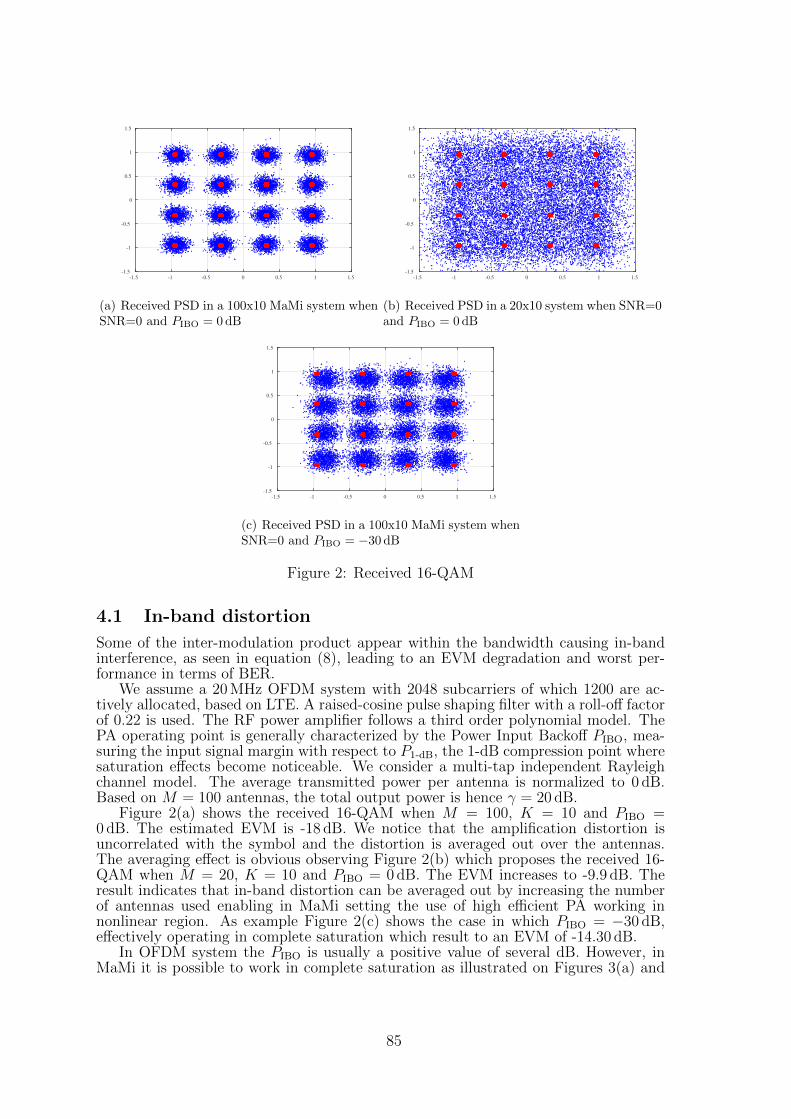
-1.5 -1 -0.5 0 0.5 1 1.5
-1.5
-1
-0.5
0
0.5
1
1.5
(a) Received PSD in a 100x10 MaMi system whenSNR=0 and PIBO = 0 dB
-1.5 -1 -0.5 0 0.5 1 1.5
-1.5
-1
-0.5
0
0.5
1
1.5
(b) Received PSD in a 20x10 system when SNR=0and PIBO = 0 dB
-1.5 -1 -0.5 0 0.5 1 1.5
-1.5
-1
-0.5
0
0.5
1
1.5
(c) Received PSD in a 100x10 MaMi system whenSNR=0 and PIBO = −30 dB
Figure 2: Received 16-QAM
4.1 In-band distortion
Some of the inter-modulation product appear within the bandwidth causing in-bandinterference, as seen in equation (8), leading to an EVM degradation and worst per-formance in terms of BER.
We assume a 20 MHz OFDM system with 2048 subcarriers of which 1200 are ac-tively allocated, based on LTE. A raised-cosine pulse shaping filter with a roll-off factorof 0.22 is used. The RF power amplifier follows a third order polynomial model. ThePA operating point is generally characterized by the Power Input Backoff PIBO, mea-suring the input signal margin with respect to P1-dB, the 1-dB compression point wheresaturation effects become noticeable. We consider a multi-tap independent Rayleighchannel model. The average transmitted power per antenna is normalized to 0 dB.Based on M = 100 antennas, the total output power is hence γ = 20 dB.
Figure 2(a) shows the received 16-QAM when M = 100, K = 10 and PIBO =0 dB. The estimated EVM is -18 dB. We notice that the amplification distortion isuncorrelated with the symbol and the distortion is averaged out over the antennas.The averaging effect is obvious observing Figure 2(b) which proposes the received 16-QAM when M = 20, K = 10 and PIBO = 0 dB. The EVM increases to -9.9 dB. Theresult indicates that in-band distortion can be averaged out by increasing the numberof antennas used enabling in MaMi setting the use of high efficient PA working innonlinear region. As example Figure 2(c) shows the case in which PIBO = −30 dB,effectively operating in complete saturation which result to an EVM of -14.30 dB.
In OFDM system the PIBO is usually a positive value of several dB. However, inMaMi it is possible to work in complete saturation as illustrated on Figures 3(a) and
85
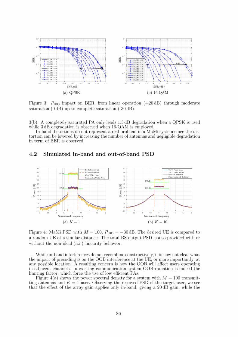
SNR (dB)
-17 -16.5 -16 -15.5 -15 -14.5 -14 -13.5 -13
BE
R
10-4
10-3
10-2
10-1
100
PA_IBO = 20
PA_IBO = 2
PA_IBO = 0
PA_IBO = -2
PA_IBO = -4
PA_IBO = -6
PA_IBO = -8
PA_IBO = -10
PA_IBO = -20
PA_IBO = -30
1.3 dB
(a) QPSK
SNR (dB)
-10 -9.5 -9 -8.5 -8 -7.5 -7 -6.5 -6 -5.5
BE
R
10-4
10-3
10-2
10-1
100
PA_IBO = 20
PA_IBO = 2
PA_IBO = 0
PA_IBO = -2
PA_IBO = -4
PA_IBO = -6
PA_IBO = -8
PA_IBO = -10
PA_IBO = -20
PA_IBO = -30
3 dB
(b) 16-QAM
Figure 3: PIBO impact on BER, from linear operation (+20 dB) through moderatesaturation (0 dB) up to complete saturation (-30 dB).
3(b). A completely saturated PA only leads 1.3 dB degradation when a QPSK is usedwhile 3 dB degradation is observed when 16-QAM is employed.
In-band distortions do not represent a real problem in a MaMi system since the dis-tortion can be lowered by increasing the number of antennas and negligible degradationin term of BER is observed.
4.2 Simulated in-band and out-of-band PSD
Normalized Frequency
-2 -1.5 -1 -0.5 0 0.5 1 1.5 2
Pow
er [
dB
]
-10
-5
0
5
10
15
20
25
30
35
40
45
18.7 dB
37.5dB
Tot Tx Power w n.i.
Tot Tx Power w/o n.i.
Mean UE Rx Power
Mean random UE Rx Power
(a) K = 1
Normalized Frequency
-2 -1.5 -1 -0.5 0 0.5 1 1.5 2
Pow
er [
dB
]
-10
-5
0
5
10
15
20
25
30
35
40
45
18.6 dB
27.5 dB
Tot Tx Power w n.i.
Tot Tx Power w/o n.i.
Mean UE Rx Power
Mean random UE Rx Power
(b) K = 10
Figure 4: MaMi PSD with M = 100, PIBO = −30 dB. The desired UE is compared toa random UE at a similar distance. The total BS output PSD is also provided with orwithout the non-ideal (n.i.) linearity behavior.
While in-band interferences do not recombine constructively, it is now not clear whatthe impact of precoding is on the OOB interference at the UE, or more importantly, atany possible location. A resulting concern is how the OOB will affect users operatingin adjacent channels. In existing communication system OOB radiation is indeed thelimiting factor, which force the use of low efficient PAs.
Figure 4(a) shows the power spectral density for a system with M = 100 transmit-ting antennas and K = 1 user. Observing the received PSD of the target user, we seethat the effect of the array gain applies only in-band, giving a 20 dB gain, while the
86
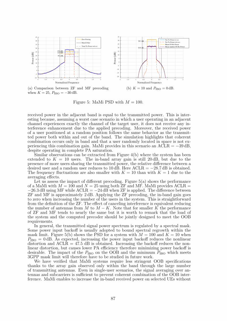
Normalized Frequency
-2 -1.5 -1 -0.5 0 0.5 1 1.5 2
Pow
er [
dB
]
-10
-5
0
5
10
15
20
25
30
35
40
45
18.7 dB
22.9 dB25.0 dB
Zero Forcing
Match Filter
Total Tx Power w/o n.i
(a) Comparison between ZF and MF precodingwhen K = 25, PIBO = −30 dB.
Normalized Frequency
-2 -1.5 -1 -0.5 0 0.5 1 1.5 2
Pow
er [
dB
]
-20
-15
-10
-5
0
5
10
15
20
25
30
35
18.8 dB
28.3 dBTot Tx Power w n.i.
Tot Tx Power w/o n.i.
Mean UE Rx Power
Mean random UE Rx Power
(b) K = 10 and PIBO = 0 dB.
Figure 5: MaMi PSD with M = 100.
received power in the adjacent band is equal to the transmitted power. This is inter-esting because, assuming a worst case scenario in which a user operating in an adjacentchannel experiences exactly the channel of the target user, it does not receive any in-terference enhancement due to the applied precoding. Moreover, the received powerof a user positioned at a random position follows the same behavior as the transmit-ted power both within and out of the band. The simulation highlights that coherentcombination occurs only in band and that a user randomly located in space is not ex-periencing this combination gain. MaMi provides in this scenario an ACLR = −39 dB,despite operating in complete PA saturation.
Similar observations can be extracted from Figure 4(b) where the system has beenextended to K = 10 users. The in-band array gain is still 20 dB, but due to thepresence of more users sharing the transmitted power, the relative difference between adesired user and a random user reduces to 10 dB. Here ACLR = −28.7 dB is obtained.The frequency fluctuations are also smaller with K = 10 than with K = 1 due to theaveraging effects.
Let us assess the impact of different precoding. Figure 5(a) shows the performanceof a MaMi with M = 100 and N = 25 using both ZF and MF. MaMi provides ACLR =−26.3 dB using MF while ACLR = −24 dB when ZF is applied. The difference betweenZF and MF is approximately 2 dB. Applying the ZF precoding, the in-band gain goesto zero when increasing the number of the users in the system. This is straightforwardfrom the definition of the ZF. The effect of canceling interference is equivalent reducingthe number of antennas from M to M −K. Note that for smaller K the performanceof ZF and MF tends to nearly the same but it is worth to remark that the load ofthe system and the computed precoder should be jointly designed to meet the OOBrequirements.
In general, the transmitted signal power spectrum is regulated by a spectral mask.Some power input backoff is usually adopted to bound spectral regrowth within themask limit. Figure 5(b) shows the PSD for a system with M = 100 and K = 10 whenPIBO = 0 dB. As expected, increasing the power input backoff reduces the nonlineardistortion and ACLR = 47.5 dB is obtained. Increasing the backoff reduces the non-linear distortion, but causes lower PA efficiency therefore minimizing power backoff isdesirable. The impact of the PIBO on the OOB and the minimum PIBO which meets3GPP mask limit will therefore have to be studied in future work.
We have verified that MaMi systems require less stringent OOB specificationsthanks to the array gain observed only within the band through the large numberof transmitting antennas. Even in single-user scenarios, the signal averaging over an-tennas and subcarriers is sufficient to prevent coherent combination of the OOB inter-ference. MaMi enables to increase the in-band received power on selected UEs without
87
increasing the interference on adjacent bands.
5 Conclusion
This paper analyzes the effect of nonlinear PAs in MaMi. The analysis presented isbased on the polynomial model of the PA. We show that both in-band interference andOOB interference do not recombine constructively and the array gain is experiencedonly inside the desired bandwidth. PAs working in complete saturation lead to negligi-ble BER degradation and do not generate harmful interference to devices operating inneighboring bandwidth. Even in worst case scenario, when a random user shares thesame channel as a target user, OOB radiations are not increased. Simulations confirmthe benefit of the non-coherent addition of components coming from the different an-tennas. We prove that fully saturated PAs in MaMi provide better ACLR comparedto traditional communication systems. Due to the high antenna gain, MaMi radiatesless power while providing the same QoS as traditional systems, hence the amount ofinterference a user in adjacent channel is experiencing is lower with a MaMi setting.
Usually the power from the different PAs dominates the BS power consumption,due to the large output power. The use of high-efficiency nonlinear PAs would enablegreat gains in terms of energy efficiency. The operating region of the PAs is oftendetermined by the OOB radiations and MaMi systems require less stringent OOBspecifications thus PAs need relaxed linearity requirements with respect to traditionalcommunication system.
In conclusion, in MaMi systems, in-band interference and OOB radiations are notlimiting factors enabling the use of highly efficient saturated PAs and reducing the BSpower consumption.
References
[1] E. Larsson, O. Edfors, F. Tufvesson, and T. Marzetta, “Massive MIMO for nextgeneration wireless systems,” IEEE Communications Magazine, vol. 52, no. 2, pp.186–195, February 2014.
[2] Access, Evolved Universal Terrestrial Radio, Base Station BS Radio Transmissionand Reception, 3GPP TS 36.104, V10, 2011.
[3] K. G. Gard, H. M. Gutierrez, and M. B. Steer, “Characterization of spectral re-growth in microwave amplifiers based on the nonlinear transformation of a complexgaussian process,” IEEE Transactions on Microwave Theory and Techniques, vol.47, no. 7, Jul 1999.
[4] Y. Zou, O. Raeesi, L. Antilla, A. Hakkarainen, J. Vieira, F. Tufvesson, Q. Cui,and M. Valkama, “Impact of power amplifier nonlinearities in multi-user massiveMIMO downlink,” in 2015 IEEE Globecom Workshops (GC Wkshps), Dec 2015.
[5] C. Mollen, U. Gustavsson, T. Eriksson, and E. G. Larsson, “Out-of-band radi-ation measure for MIMO arrays with beamformed transmission,” arXiv preprintarXiv:1510.05513, 2015.
[6] I. Reed, “On a moment theorem for complex gaussian processes,” IRE Transactionson Information Theory, vol. 8, no. 3, pp. 194–195, 1962.
[7] KM Gharaibeh, KG Gard, and MB Steer, “Estimation of co-channel nonlineardistortion and sndr in wireless systems,” Microwaves, Antennas & Propagation,IET, vol. 1, no. 5, pp. 1078–1085, 2007.
88
Bandwidth Impacts of a Run-Time Multi-sineExcitation Based SWIPT
Ning Pan Mohammad Rajabi Dominique Schreurs Sofie PollinTELEMIC Division
Department of Electrical EngineeringUniversity of Leuven, Leuven, 3000, Belgium
ning.pan, mohammad.rajabi, dominique.schreurs,[email protected]
Abstract
Simultaneous wireless information and power transfer (SWIPT) utilizes ra-dio frequency (RF) source as an information and energy carrier, which enableswireless networks consisting of a large amount of devices operating permanentlywithout replacing batteries. SWIPT has attracted considerable attention sinceit is a promising method towards realization of future information and communi-cation technology concepts such as internet of things (IoT). A number of studieshave investigated techniques such as pre-coding and resource allocation to im-prove SWIPT performance. However, the transmission signal bandwidth (BW)impacts on the system have never been studied yet. Our paper originally scruti-nizes how the transmission signal’s BW affects received information and power.We consider a single link SWIPT system composed of a transmitter emittingRF signals and a receiver that is able to decode information and harvest en-ergy simultaneously, which includes a power splitter after the antenna at thereceiver. In addition, this SWIPT system is assumed as run-time forbidding anyhardware modifications. A theoretical model describing channel capacity and re-ceived power depending on the circuit, which is a function of the input signal, isconstructed specifically for SWIPT. In the simulation, the power splitting coeffi-cient is fixed. The network throughput and harvested power is calculated basedon the integrated SWIPT model. Simulation results show that a larger BW maylead to higher network throughput while the harvested power is degraded.
1 Introduction
The past decade has seen the rapid development in SWIPT techniques, since it is oneof the possible approaches to realize permanently operating wireless networks withoutbattery replacement [1]-[2]. There exist a growing number of studies investigating anefficient SWIPT system, benefiting from the ubiquitous and controllable characteristicsof the radio frequency (RF) source [2]-[5].
Two performance metrics, the link throughput and harvested RF power, are consid-ered to evaluate SWIPT system performance. Most of the previous studies are devotedto optimize the system applying techniques such as scheduling, resource allocation, andbeamforming by trading-off the link-throughput and harvested power [2]-[4]. However,most of them ignore signal waveform’s influence on the harvested power, by simplifyingpower conversion efficiency (PCE) as constant. Researchers in the hardware commu-nity have reported that the PCE depends not only on the circuit design but also thesignal waveform design [6]-[16].
89
A group of research have proved experimentally that high peak-to-average-ratio(PAPR) waveform improve the PCE [6]-[8][13], while another work shows that CW ex-citations has a higher PCE compared to modulated signals. In order to have a concreteunderstanding for these ad-hoc measurements, theoretical model including excitationsignals’ characteristics and rectifier’s non-linear behavior is necessary. Several studiesinvestigating transmission signals have been carried out to model the rectifier’s behav-ior [8][15][16]. The authors of [8] have varified that a multi-sine signal with zero-phasedifference between tones will have the highest PCE, by approximating the diode’s non-linearity behavior using Taylor expansions. Their work would have been more completeif the other circuits’ components influence are included. Reference [15] constructed atheoretical model calculating PCE specifically for high PAPR waveform excited rec-tifier based on the measured output voltage. However, this model is only valid inhigh input power case since it assumes perfect matching and ideal diode. The work of[16] analyzed amplitude and bandwidth impacts of the multi-sine signal based on thestatistical information of output signal after the rectifier. The authors have showedthat the PCE improves with a higher PAPR waveform, while the system performancedegraded with increasing BW because of input network mismatch. Nevertheless, thisanalysis is unable to neglect the matching network’s influence.
In a SWIPT system, BW has both effects on capacity and power. The BW analysisof capacity typically follows Shannon’s theory [17], where a higher BW is preferred.Referring to [16], a wide BW may restrict system performance because of the inputmatching network. However, there is no work on the BW analysis for the multi-sinebased SWIPT system to the best of our knowledge. This work analyzes BW impactson capacity and PCE based on a combined information and power transfer modelspecifically for a multi-sine based run-time SWIPT, where only transmission signalscan be tuned.
The rest of this paper is organized as follows. Section 2 demonstrates the single-link SWIPT model involving the related parameters and the performance metrics inSWIPT. Section 3 analyzes BW influence on the run-time system performance. In theend, section 4 concludes this work’s contributions.
2 System Model
We are considering a multi-sine based run-time SWIPT system consisting of a sourceand a destination node transferring information and power simultaneously as can beenseen in Fig. 1. The source transmits multi-sine signals to the destination via a wirelesschannel. After reception by the antenna with adapted matching network, the signalis divided into two parts with a fixed ratio ρ. One part goes through the informationdecoder to achieve the required data. In the information decoder, the received RF signalis first converted into baseband by the mixer; then the baseband signal passes throughthe signal processor to retrieve the source information. Additionally, the remainingsignal is harvested by the rectifier. The RF signal goes through a non-linear rectifyingcomponent such as a diode after the adapted matching network. The DC output isfinally obtained after an RC filter. The DC output is accumulated in the energy storagedevice with a feeding line connected to the information decoder for charging purposes.
90
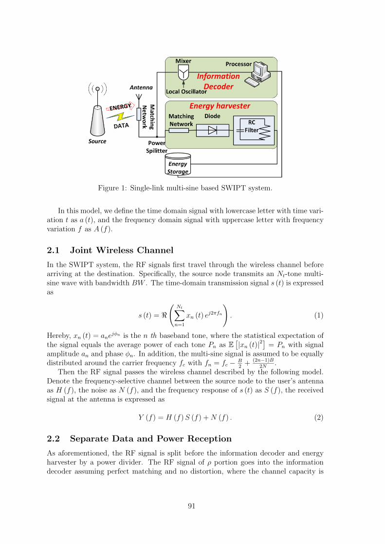
Figure 1: Single-link multi-sine based SWIPT system.
In this model, we define the time domain signal with lowercase letter with time vari-ation t as a (t), and the frequency domain signal with uppercase letter with frequencyvariation f as A (f).
2.1 Joint Wireless Channel
In the SWIPT system, the RF signals first travel through the wireless channel beforearriving at the destination. Specifically, the source node transmits an Nt-tone multi-sine wave with bandwidth BW . The time-domain transmission signal s (t) is expressedas
s (t) = <(
Nt∑
n=1
xn (t) ej2πfn
). (1)
Hereby, xn (t) = anejφn is the n th baseband tone, where the statistical expectation of
the signal equals the average power of each tone Pn as E[|xn (t)|2
]= Pn with signal
amplitude an and phase φn. In addition, the multi-sine signal is assumed to be equallydistributed around the carrier frequency fc with fn = fc − B
2+ (2n−1)B
2N.
Then the RF signal passes the wireless channel described by the following model.Denote the frequency-selective channel between the source node to the user’s antennaas H (f), the noise as N (f), and the frequency response of s (t) as S (f), the receivedsignal at the antenna is expressed as
Y (f) = H (f)S (f) +N (f) . (2)
2.2 Separate Data and Power Reception
As aforementioned, the RF signal is split before the information decoder and energyharvester by a power divider. The RF signal of ρ portion goes into the informationdecoder assuming perfect matching and no distortion, where the channel capacity is
91
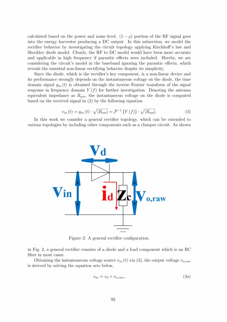
calculated based on the power and noise level. (1− ρ) portion of the RF signal goesinto the energy harvester producing a DC output. In this subsection, we model therectifier behavior by investigating the circuit topology applying Kirchhoff’s law andShockley diode model. Clearly, the RF to DC model would have been more accurateand applicable in high frequency if parasitic effects were included. Hereby, we areconsidering the circuit’s model in the baseband ignoring the parasitic effects, whichreveals the essential non-linear rectifying behavior despite its simplicity.
Since the diode, which is the rectifier’s key component, is a non-linear device andits performance strongly depends on the instantaneous voltage on the diode, the timedomain signal yin (t) is obtained through the inverse Fourier transform of the signalresponse in frequency domain Y (f) for further investigation. Denoting the antennaequivalent impedance as Rant, the instantaneous voltage on the diode is computedbased on the received signal in (2) by the following equation
vin (t) = yin (t) ·√|Rant| = F−1 Y (f) ·
√|Rant|. (3)
In this work we consider a general rectifier topology, which can be extended tovarious topologies by including other components such as a clamper circuit. As shown
Figure 2: A general rectifier configuration.
in Fig. 2, a general rectifier consists of a diode and a load component which is an RCfilter in most cases.
Obtaining the instantaneous voltage source vin (t) via (3), the output voltage vo,rawis derived by solving the equation sets below,
vin = vd + vo,raw, (4a)
92

vo,raw = id × zc, (4b)
id = is
(e
vdnVT − 1
), (4c)
where the diode voltage is vd, the diode current is id, the equivalent load impedance isdenoted as zc, and is, n, VT represent the diode characteristic parameters. Herewith,(4c) describes the diode’s current-voltage curve within the Shockley diode model whichproperly approximates the non-linearity.
After the diode, the RC circuit functions as a filter passing baseband signal whileblocking the other frequency components in order to convey vo,raw to a stable DCvoltage. The RC filter is described by a cut-off frequency fcut−off at which the signalis attenuated by 3 dB from the nominal passband value in frequency domain. Denotethe frequency domain response of vo,raw as Vo,raw and the frequency mask of RC filteras M (fcut−off ), the output DC voltage Vout is computed in frequency domain as
Vout = Vo ×M (fcut−off ) . (5)
2.3 Performance Metrics
In SWIPT, two performance metrics are mainly considered, which is link throughputand harvested power. The link throughput evaluates the information transfer quality,while the harvested power measures the power transfer efficiency. Since RF signalsare reused as information and power carrier in SWIPT, these two performance metricsmay easily conflict with each other in the overall optimization problems [2]-[4]. How-ever, BW impact on both metrics has not been considered before to the best of ourknowledge. We relate BW to these two metrics in this subsection.
The SNR of the received signal Y is computed as
SNR =ρY 2
N. (6)
Hereby, the noise N = kT × BW is a function determined by thermal temperature Tand signal bandwidth BW ; ρ is the power ratio sent to the information decoder. Thusthe total throughput is
C = BW · log2 (1 + SNR) . (7)
The effective harvested power depends on the DC output of the energy harvester(5). Denote the load resistance as RL, the harvested power is
Po =V 2out
RL
. (8)
This equation is valid when the antenna matching is properly designed. Otherwise, theactual harvested power is calculated by including reflections in (8). In fact, since Voutis a value derived by (4) and (5) which strongly depends on the input instantaneoussignal (3), Vout is a BW dependent parameter.
93
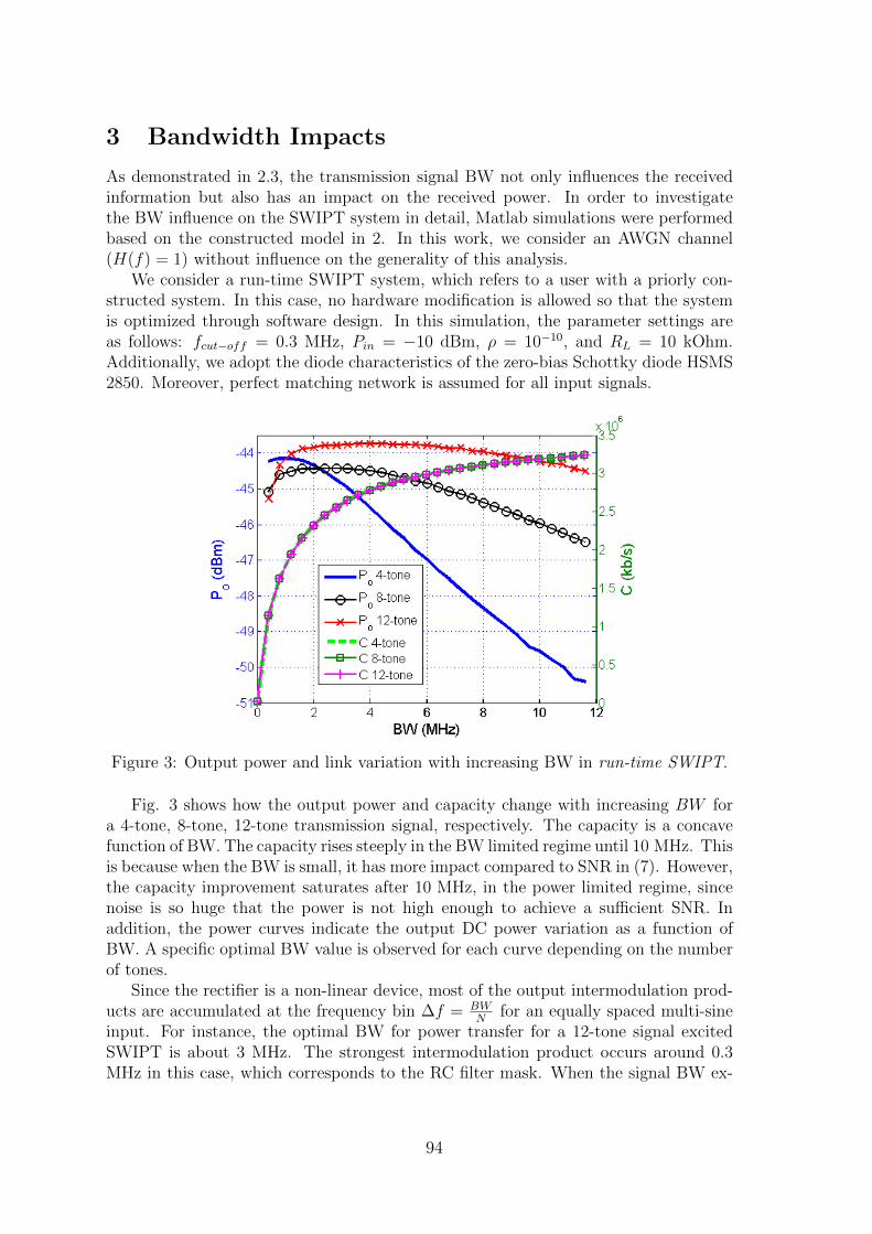
3 Bandwidth Impacts
As demonstrated in 2.3, the transmission signal BW not only influences the receivedinformation but also has an impact on the received power. In order to investigatethe BW influence on the SWIPT system in detail, Matlab simulations were performedbased on the constructed model in 2. In this work, we consider an AWGN channel(H(f) = 1) without influence on the generality of this analysis.
We consider a run-time SWIPT system, which refers to a user with a priorly con-structed system. In this case, no hardware modification is allowed so that the systemis optimized through software design. In this simulation, the parameter settings areas follows: fcut−off = 0.3 MHz, Pin = −10 dBm, ρ = 10−10, and RL = 10 kOhm.Additionally, we adopt the diode characteristics of the zero-bias Schottky diode HSMS2850. Moreover, perfect matching network is assumed for all input signals.
Figure 3: Output power and link variation with increasing BW in run-time SWIPT.
Fig. 3 shows how the output power and capacity change with increasing BW fora 4-tone, 8-tone, 12-tone transmission signal, respectively. The capacity is a concavefunction of BW. The capacity rises steeply in the BW limited regime until 10 MHz. Thisis because when the BW is small, it has more impact compared to SNR in (7). However,the capacity improvement saturates after 10 MHz, in the power limited regime, sincenoise is so huge that the power is not high enough to achieve a sufficient SNR. Inaddition, the power curves indicate the output DC power variation as a function ofBW. A specific optimal BW value is observed for each curve depending on the numberof tones.
Since the rectifier is a non-linear device, most of the output intermodulation prod-ucts are accumulated at the frequency bin ∆f = BW
Nfor an equally spaced multi-sine
input. For instance, the optimal BW for power transfer for a 12-tone signal excitedSWIPT is about 3 MHz. The strongest intermodulation product occurs around 0.3MHz in this case, which corresponds to the RC filter mask. When the signal BW ex-
94
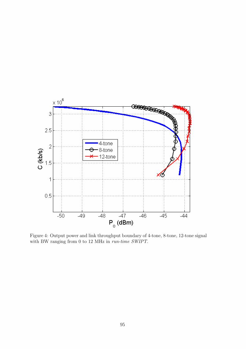
Figure 4: Output power and link throughput boundary of 4-tone, 8-tone, 12-tone signalwith BW ranging from 0 to 12 MHz in run-time SWIPT.
95
ceeds 3 MHz, the first intermodulation product is filtered out by the RC filter resultingin a power transfer deterioration. Interestingly, a small rise before the optimal BW isobserved in all power curves; with increasing number of tones, the power rises sharperin the beginning. This is because when the BW is small, the time period between highpeaks is so large that the RC filter cannot charge to the saturation level, which is moresevere for signals with larger number of tones. In short, a multi-signal consisting ofmore tones enables a larger optimal BW with the same RC filter as can be seen inFig. 3.
Fig. 4 depicts the power and capacity bound of the 4-tone, 8-tone, and 12-toneexcited SWIPT, respectively. It is observed that there is a trade-off between harvestedpower and link throughput. What’s more, the SWIPT system with more multi-sinesmay have a higher harvested power while the link throughput remains the same.
Clearly, a proper BW choice will improve SWIPT performance when the systemis constructed beforehand. In the BW limited regime, a larger BW produces morecapacity, where a multi-sine with more tones is necessary to ensure enough convertedpower.
4 Conclusion
This paper established an integrated SWIPT model including the conventional wirelesscommunication channel and the RF to DC channel. BW is related to the output powerand link throughput through the constructed model. It is demonstrated that optimalBW and multi-sine signal choice, depending on the RC filter and tone number, improvesthe SWIPT performance significantly in the run-time SWIPT.
Acknowledgement
The acknowledgement goes to FWO and Hercules for the financial support on thisresearch.
References
[1] S. Ulukus, A. Yener, E. Erkip, O. Simeone, M. Zorzi, P. Grover, and K. Huang,“Energy harvesting wireless communications: A review of recent advances,” IEEEJournal of Selected Areas in Communications, vol. 33, no. 3, pp. 360–381, 2015.
[2] X. Lu, P. Wang, D. Niyato, D. I. Kim, and Z. Han, “Wireless Networks with RFEnergy Harvesting: A Contemporaty Survey,” IEEE Communications Surveysand Tutorials, vol. 17, no. 2, pp. 757–789, May 2015.
[3] B. Clerckx, E. Bayguzina, D. Yates, and P. D. Mitcheson, “Waveform Optimiza-tion for Wireless Power Transfer with Nonlinear Energy Harvester Modeling,” in2015 IEEE Int. Symp. on Wireless Communications Systems, Brussels, August2015.
96
[4] E. Boshkovska, D. W. K. Ng, N. Zlatanov, and R. Schober, “Practical Non-LinearEnergy Harvesting Model and Resource Allocation for SWIPT Systems,” IEEECommunications Letters, vol. 19, no. 12, pp. 2082–2085, Sep. 2015.
[5] B. Clerckx, “Waveform optimization for swipt with nonlinear energy harvestermodeling,” in 20th Int. Workshop on Smart Antennas, Munich, March 2016.
[6] M. S. Trotter, J. D. Griffin, and G. D. Durgin, “Power-Optimized Waveforms forImproving the Range and Reliability of RFID Systems,” in IEEE Int. Conf. onRFID Virtual J., April 2009, pp. 80–87.
[7] C.-C. Lo, Y.-L. Yang, C.-L. Tsai, C.-S. Lee, and C.-L. Yang, “Novel WirelessImpulsive Power Transmission to Enhance the Conversion Efficiency for Low In-put Power,” in Int. Microwave Workshop Series on Innovative Wireless PowerTransmission, May 2011, pp. 55–58.
[8] A. Boaventura and N. B. Carvalho, “Maximizing DC Power in Energy HarvestingCircuits,” in IEEE MTT-S International Microwave Symp. Dig., June 2011, pp.1–4.
[9] C.-L. Yang, C.-L. Tsai, Y.-L. Yang, and C.-S. Lee, “Enhancement of WirelessPower Transmission by Using Novel Multitone Approaches for Wireless Recharg-ing,” IEEE Antennas Wireless Propag. Lett., vol. 10, pp. 1353–1357, Dec. 2011.
[10] A. Collado and A. Georgiadis, “Improving Wireless Power Transmission EfficiencyUsing Chaotic Waveforms,” in IEEE MTT-S International Microwave Symp. Dig.,June 2012, pp. 1–3.
[11] C. Valenta and G. Durgin, “Rectenna Performance Under Power-optimized Wave-form Excitation,” in IEEE Int. Conf. on RFID, May 2013, pp. 237–244.
[12] A. Boaventura, A. Collado, A. Georgiadis, and N. Carvalho, “Spatial Power Com-bining of Multi-Sine Signals for Wireless Power Transmission Applications,” IEEETrans. Microw. Theory Techn., vol. 62, no. 4, pp. 1022–1030, Apr. 2014.
[13] A. Collado and A. Georgiadis, “Optimal Waveforms for Efficient Wireless PowerTransmission,” IEEE Microw. Compon. Lett., vol. 24, no. 5, pp. 354–356, May2014.
[14] H. Sakaki, T. Kuwahara, S. Yoshida, S. Kawasaki, and K. Nishikawa, “Analysisof Rectifier RF-DC Power Conversion Behavior with QPSK and 16QAM InputSignals for WiCoPT System,” in Asia-Pacific Microwave Conference, Sendai, Nov.2014, pp. 603–605.
[15] C. R. Valenta, M. M. Morys, and G. D. Durgin, “Theoretical energy-conversionefficiency for energy-harvesting circuits under power-optimized waveform excita-tion,” IEEE Trans. Microw. Theory and Techn., vol. 63, no. 5, pp. 1758–1767,April 2015.
97

[16] N. Pan, A. S. Boaventura, M. Rajabi, D. Schreurs, N. B. Carvalho, and S. Pollin,“Amplitude and Frequency Analysis of Multi-sine Wireless Power Transfer,” in2015 IEEE Int. Workshop on Integrated Nonlinear Microwave and Millimetre-wave Circuits, Taormina, Oct. 2015, pp. 1–3.
[17] C. E. Shannon, “A mathematical theory of communication,” The Bell SsystemTechnical Journal, vol. 27, pp. 379–423, July 1948.
98
Generalized Optimal Pilot Allocation for ChannelEstimation in Multicarrier Systems
François Rottenberg*, François Horlin**, Eleftherios Kofidis*** and JérômeLouveaux*
*ICTEAM, Université catholique de Louvain, Belgiumfrancois.rottenberg,[email protected]
**OPERA, Université libre de Bruxelles, [email protected]
***Department of Statistics and Insurance Science, University of Piraeus, [email protected]
Abstract
This paper∗ addresses the design of MSE-optimal preambles for multicarrier chan-nel estimation under a maximum likelihood or minimum mean squared error crite-rion. The derived optimality condition gives insight on how to allocate the powerof the pilots that compose the preamble. While many papers show that equis-paced and equipowered allocation is optimal, the generalized condition demon-strates that there exist many different configurations that offer the same optimalperformance. Furthermore, the condition applies not only to maximum likelihoodbut also to minimum mean squared error channel estimation. An application ofthe generalized condition in the presence of inactive subcarriers (virtual subcar-riers problem) is shown such that a non equispaced allocation can achieve thesame optimal performance as if an equispaced one could be used.
1 IntroductionMulticarrier systems aim at dividing a wideband signal into multiple narrowband sig-nals centered around different subcarriers [1]. If the number of subcarriers is large withrespect to the delay spread of the channel, each narrowband channel can be consideredas frequency flat, which greatly simplifies the equalization task at the receiver. It ismainly for the their ability to effectively address the channel distortion that multicarriersystems have been so popular.
Channel estimation for multicarrier systems has been extensively studied; see, forinstance, [2, 3] for recent review papers concerning channel estimation for orthogo-nal frequency division multiplexing (OFDM) or [4] for a review in offset QAM-basedfilterbank multicarrier (FBMC/OQAM) modulations. Specifically, the problem of op-timizing the pilot allocation (including their position in frequency and their relativepower) to minimize the mean squared error (MSE) of the channel estimate has beenaddressed in a number of works. Most of them focus on the case of least squares(LS) channel estimation, which corresponds to the maximum likelihood (ML) estima-tor under the Gaussian noise assumption and their main common conclusion is thatthe pilots should be equispaced and equipowered [5, 6]. The authors in [7] extend thisresult to the MIMO case and it is shown that optimal pilot sequences are equipowered,equispaced, and phase shift orthogonal.
Surprisingly, there are only few works addressing optimal pilot allocation for theminimum mean squared error (MMSE) estimator, even in the single-antenna case.In [8], the pilot allocation that maximizes the capacity for a MMSE channel estimatoris shown to also correspond to equipowered, equispaced pilots. In [9], the authorsderive the MSE-optimal training condition for the MMSE estimator in the context ofa two-way relay OFDM-based network.∗The material in this paper has been partially submitted at IEEE SPAWC2016.
99
Very few papers actually investigate if other pilot configurations also satisfy theoptimality condition and therefore offer the same performance as the equispaced con-figuration. In this paper, we find a sufficient and necessary condition for optimal pilotallocation that holds for both the maximum likelihood (ML) and the MMSE chan-nel estimators. This result can be seen as generalizing the classical equispaced pilotconfiguration. Indeed, it is shown that a much wider family of pilot allocations maybe optimal. Furthermore, the optimality condition can be directly used to solve theproblem of allocating the pilots in the more realistic (and more challenging) case whereinactive (virtual) subcarriers are present. The problem of virtual subcarriers is widelystudied in the literature; see, for example, [10] for the single antenna case and [11] forthe multiple antennas case. The originality of the work presented here is that it givesa methodology for finding optimal allocations, when the problem is feasible, whichattains the same performance as if no null subcarriers were present.
The rest of the paper is organized as follows. Section 2 first serves as a reminder ofchannel estimation in multicarrier systems using the ML and the MMSE criteria. Sec-tion 3 derives a general optimality condition for pilot allocation that holds for the MLcase and the MMSE estimator if the channel taps are assumed uncorrelated. Section 4shows a possible application of the generalized condition to the virtual subcarriersproblem. Simulation results are presented in Section 5. Section 6 concludes the paper.
Notations : Vectors and matrices are denoted by bold lowercase and uppercaseletters, respectively. Superscripts ∗, T and H stand for conjugate, transpose and Her-mitian transpose operators. tr, E, = and < denote trace, expectation, imaginary andreal parts, respectively.
2 Channel Estimation in Multicarrier SystemsWe consider a multicarrier system withM subcarriers. Let us assume that the differentsubchannels can be considered flat and orthogonal to each other. A preamble of onemulticarrier symbol is transmitted. The preamble vector composed of the transmittedpilots at the M subcarriers is denoted by d ∈ CM×1. The channel impulse responseh ∈ CLh×1 is assumed to be quasi-static† and Lh is the channel length. The vector ofsamples received after demodulation can be written as
y = DFΣh + η
where F ∈ CM×M is the unitary discrete Fourier transform (DFT) matrix, D =diag(d) ∈ CM×M contains the vector of transmitted pilot symbols d on its diago-nal and η ∼ CN (0,Cη) is additive Gaussian noise. Moreover, the noise is assumed tobe white, i.e. Cη = σ2IM .‡ Σ =
(ILh 0H(M−Lh)×Lh
)Hcan be seen either as a selection
matrix of the first Lh columns of F or as a zero padding matrix that appends M − Lh0’s to the vector h.
Note that this model fits both an OFDM system if the cyclic prefix is at least as longas the channel order [2] and an FBMC/OQAM system if the channel frequency selectiv-ity is sufficiently mild and the noise correlation is neglected [4]. Then d represents theso-called pseudo-pilots (for fully loaded preambles) or the pilots (otherwise) [12–14].†We assume, as usual, that the channel remains invariant in the duration of a multicarrier symbol.‡The whiteness of the noise samples makes sense in an OFDM system while this is a stronger
assumption in an FBMC system where correlation exists in both time and frequency [4].
100

2.1 Maximum likelihood channel estimatorWe here assume that h is deterministic and unknown. Denoting by f(y|h) the con-ditional probability density function of y given h, the ML estimator of the channel isgiven by [15]
hML = argmax f(y|h)=(ΣHFHPFΣ
)−1ΣHFHDHy
where P = DHD is a diagonal matrix containing the power of each pilot on its diagonal.We define p ∈ CM×1 as the vector containing the power of each pilot, such thatpk = |dk|2 and P = diag(p). One can note that the ML estimator coincides here withthe weighted LS estimator. The MSE is given by
MSEML(P) = σ2tr[(
ΣHFHPFΣ)−1]
.
This expression only depends on the power of the transmitted pilots p and not ontheir phase, which can be appropriately chosen for other purposes such as e.g., peak-to-average-power-ratio (PAPR) reduction [16].
2.2 MMSE channel estimatorWe here consider that h follows a zero mean Gaussian distribution with correlationmatrix denoted by Ch, i.e. h ∼ CN (0,Ch) ∈ CLh×1. The MMSE estimate hMMSE isthe one that minimizes E(‖h− hMMSE‖2). It can be shown to be equal to [15]
hMMSE = E(h|y)
=
(C−1h +
1
σ2ΣHFHPFΣ
)−11
σ2ΣHFHDHy
and the corresponding MSE is
MSEMMSE(P) = σ2tr[(σ2C−1h + ΣHFHPFΣ
)−1]. (1)
One can check that MSEMMSE(P) ≤ MSEML(P) and they will eventually converge athigh signal-to-noise ratio (SNR), i.e. when σ2 → 0.
3 Optimality Condition for Channel EstimationThis section aims at deriving a sufficient and necessary condition for pilot allocationsthat solve the following pilot allocation problem subject to a training power constraint:
minp
MSEML/MMSE(P) s.t. tr [P] = PT . (2)
The following proposition gives an alternative necessary and sufficient condition thatcharacterizes the optimal power allocations for the ML case. The condition also holdsfor the MMSE case under the (common) assumption that the channel taps are uncor-related, i.e. Ch is a diagonal matrix with elements Ch = diag(λ1h, . . . , λ
Lhh ).
101

Proposition 3.1. Under the previous assumptions, any pilot allocation p ∈ RM×1+ is
optimal in the sense of the minimum MSE for the ML and the MMSE estimators undera training power constraint if and only if (iff) p satisfies
√MΣHFHp =
(PT
0
). (3)
Proof. The matrix FHPF is circulant and has thus equal diagonal elements that wedenote by x. Given the training power constraint, the value of x is independent of thestructure of P and always equals
tr[FHPF
]=Mx
x =PTM
where we used the cyclic trace property and the fact that tr [P] = PT . The matrixΣHFHPFΣ is the upper left Lh × Lh submatrix of FHPF and therefore has diagonalelements equal to x. Using the fact that for a positive definite matrix A, the followinginequality [15, p. 65] holds,
tr(A−1
)≥
Lh∑
i=1
a−1ii (4)
where aii is the i-th diagonal element of A and equality holds iff A is diagonal, (1) canbe lower bounded by
MSEMMSE(P) ≥Lh∑
l=1
(1
λlh+
1
σ2
PTM
)−1(5)
where equality holds iff ΣHFHPFΣ is diagonal. This condition can be rewritten as
[ΣHFHPFΣ]l,m =1
M
M−1∑
k=0
pkej 2πMk(l−m)
=
PTM
if l = m
0 if l 6= m
where l = 0, 1, . . . , Lh−1 andm = 0, 1, . . . , Lh−1. ΣHFHPFΣ is a Toeplitz Hermitianmatrix. Then, it is sufficient to impose that its first column is 0 except for its firstentry, i.e.
M−1∑
k=0
pkej 2πMkl = 0 ∀l = 1, 2, . . . , Lh − 1
which means that the inverse Fourier transform of the power allocation should be zeroat indexes between 1 and Lh − 1 or in matrix form,
√MΣHFHp =
(PT
0
).
102
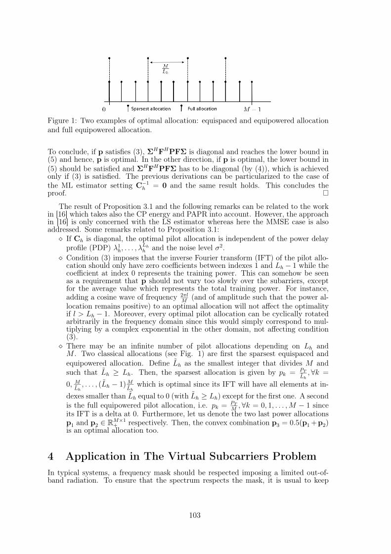
Figure 1: Two examples of optimal allocation: equispaced and equipowered allocationand full equipowered allocation.
To conclude, if p satisfies (3), ΣHFHPFΣ is diagonal and reaches the lower bound in(5) and hence, p is optimal. In the other direction, if p is optimal, the lower bound in(5) should be satisfied and ΣHFHPFΣ has to be diagonal (by (4)), which is achievedonly if (3) is satisfied. The previous derivations can be particularized to the case ofthe ML estimator setting C−1h = 0 and the same result holds. This concludes theproof.
The result of Proposition 3.1 and the following remarks can be related to the workin [16] which takes also the CP energy and PAPR into account. However, the approachin [16] is only concerned with the LS estimator whereas here the MMSE case is alsoaddressed. Some remarks related to Proposition 3.1: If Ch is diagonal, the optimal pilot allocation is independent of the power delay
profile (PDP) λ1h, . . . , λLhh and the noise level σ2.
Condition (3) imposes that the inverse Fourier transform (IFT) of the pilot allo-cation should only have zero coefficients between indexes 1 and Lh − 1 while thecoefficient at index 0 represents the training power. This can somehow be seenas a requirement that p should not vary too slowly over the subarriers, exceptfor the average value which represents the total training power. For instance,adding a cosine wave of frequency 2πl
M(and of amplitude such that the power al-
location remains positive) to an optimal allocation will not affect the optimalityif l > Lh − 1. Moreover, every optimal pilot allocation can be cyclically rotatedarbitrarily in the frequency domain since this would simply correspond to mul-tiplying by a complex exponential in the other domain, not affecting condition(3). There may be an infinite number of pilot allocations depending on Lh andM . Two classical allocations (see Fig. 1) are first the sparsest equispaced andequipowered allocation. Define Lh as the smallest integer that divides M andsuch that Lh ≥ Lh. Then, the sparsest allocation is given by pk = PT
Lh,∀k =
0, MLh, . . . , (Lh − 1)M
Lhwhich is optimal since its IFT will have all elements at in-
dexes smaller than Lh equal to 0 (with Lh ≥ Lh) except for the first one. A secondis the full equipowered pilot allocation, i.e. pk = PT
M,∀k = 0, 1, . . . ,M − 1 since
its IFT is a delta at 0. Furthermore, let us denote the two last power allocationsp1 and p2 ∈ RM×1
+ respectively. Then, the convex combination p3 = 0.5(p1+p2)is an optimal allocation too.
4 Application in The Virtual Subcarriers ProblemIn typical systems, a frequency mask should be respected imposing a limited out-of-band radiation. To ensure that the spectrum respects the mask, it is usual to keep
103
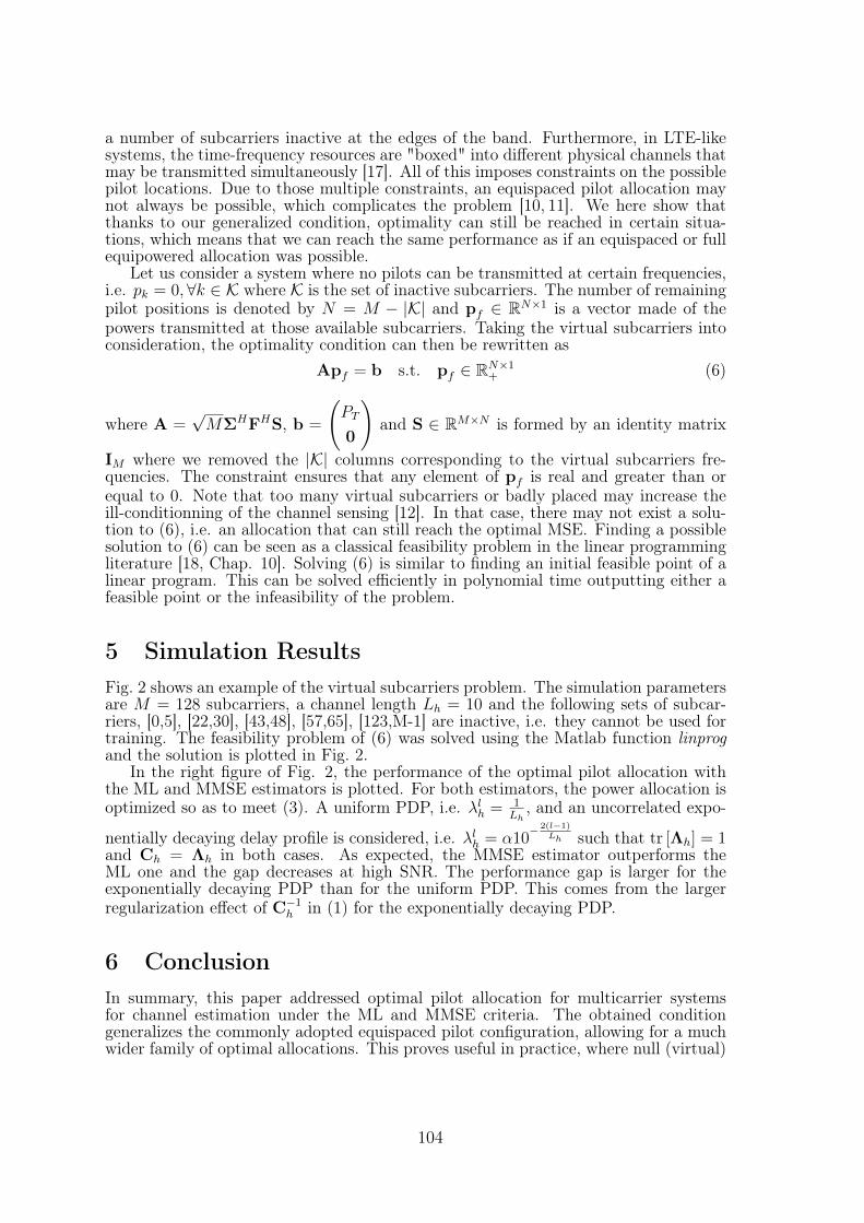
a number of subcarriers inactive at the edges of the band. Furthermore, in LTE-likesystems, the time-frequency resources are "boxed" into different physical channels thatmay be transmitted simultaneously [17]. All of this imposes constraints on the possiblepilot locations. Due to those multiple constraints, an equispaced pilot allocation maynot always be possible, which complicates the problem [10, 11]. We here show thatthanks to our generalized condition, optimality can still be reached in certain situa-tions, which means that we can reach the same performance as if an equispaced or fullequipowered allocation was possible.
Let us consider a system where no pilots can be transmitted at certain frequencies,i.e. pk = 0,∀k ∈ K where K is the set of inactive subcarriers. The number of remainingpilot positions is denoted by N = M − |K| and pf ∈ RN×1 is a vector made of thepowers transmitted at those available subcarriers. Taking the virtual subcarriers intoconsideration, the optimality condition can then be rewritten as
Apf = b s.t. pf ∈ RN×1+ (6)
where A =√MΣHFHS, b =
(PT
0
)and S ∈ RM×N is formed by an identity matrix
IM where we removed the |K| columns corresponding to the virtual subcarriers fre-quencies. The constraint ensures that any element of pf is real and greater than orequal to 0. Note that too many virtual subcarriers or badly placed may increase theill-conditionning of the channel sensing [12]. In that case, there may not exist a solu-tion to (6), i.e. an allocation that can still reach the optimal MSE. Finding a possiblesolution to (6) can be seen as a classical feasibility problem in the linear programmingliterature [18, Chap. 10]. Solving (6) is similar to finding an initial feasible point of alinear program. This can be solved efficiently in polynomial time outputting either afeasible point or the infeasibility of the problem.
5 Simulation ResultsFig. 2 shows an example of the virtual subcarriers problem. The simulation parametersare M = 128 subcarriers, a channel length Lh = 10 and the following sets of subcar-riers, [0,5], [22,30], [43,48], [57,65], [123,M-1] are inactive, i.e. they cannot be used fortraining. The feasibility problem of (6) was solved using the Matlab function linprogand the solution is plotted in Fig. 2.
In the right figure of Fig. 2, the performance of the optimal pilot allocation withthe ML and MMSE estimators is plotted. For both estimators, the power allocation isoptimized so as to meet (3). A uniform PDP, i.e. λlh =
1Lh
, and an uncorrelated expo-
nentially decaying delay profile is considered, i.e. λlh = α10− 2(l−1)
Lh such that tr [Λh] = 1and Ch = Λh in both cases. As expected, the MMSE estimator outperforms theML one and the gap decreases at high SNR. The performance gap is larger for theexponentially decaying PDP than for the uniform PDP. This comes from the largerregularization effect of C−1h in (1) for the exponentially decaying PDP.
6 ConclusionIn summary, this paper addressed optimal pilot allocation for multicarrier systemsfor channel estimation under the ML and MMSE criteria. The obtained conditiongeneralizes the commonly adopted equispaced pilot configuration, allowing for a muchwider family of optimal allocations. This proves useful in practice, where null (virtual)
104
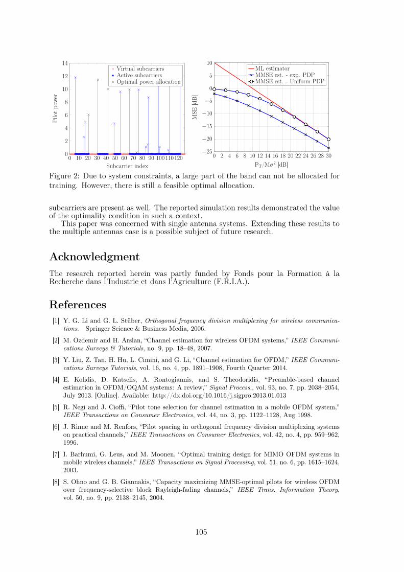
0 10 20 30 40 50 60 70 80 90 1001101200
2
4
6
8
10
12
14
Subcarrier index
Pilo
tpo
wer
Virtual subcarriersActive subcarriersOptimal power allocation
0 2 4 6 8 10 12 14 16 18 20 22 24 26 28 30−25
−20
−15
−10
−5
0
5
10
PT/Mσ2 [dB]
MSE
[dB
]
ML estimatorMMSE est. - exp. PDPMMSE est. - Uniform PDP
Figure 2: Due to system constraints, a large part of the band can not be allocated fortraining. However, there is still a feasible optimal allocation.
subcarriers are present as well. The reported simulation results demonstrated the valueof the optimality condition in such a context.
This paper was concerned with single antenna systems. Extending these results tothe multiple antennas case is a possible subject of future research.
AcknowledgmentThe research reported herein was partly funded by Fonds pour la Formation à laRecherche dans l’Industrie et dans l’Agriculture (F.R.I.A.).
References[1] Y. G. Li and G. L. Stüber, Orthogonal frequency division multiplexing for wireless communica-
tions. Springer Science & Business Media, 2006.
[2] M. Ozdemir and H. Arslan, “Channel estimation for wireless OFDM systems,” IEEE Communi-cations Surveys & Tutorials, no. 9, pp. 18–48, 2007.
[3] Y. Liu, Z. Tan, H. Hu, L. Cimini, and G. Li, “Channel estimation for OFDM,” IEEE Communi-cations Surveys Tutorials, vol. 16, no. 4, pp. 1891–1908, Fourth Quarter 2014.
[4] E. Kofidis, D. Katselis, A. Rontogiannis, and S. Theodoridis, “Preamble-based channelestimation in OFDM/OQAM systems: A review,” Signal Process., vol. 93, no. 7, pp. 2038–2054,July 2013. [Online]. Available: http://dx.doi.org/10.1016/j.sigpro.2013.01.013
[5] R. Negi and J. Cioffi, “Pilot tone selection for channel estimation in a mobile OFDM system,”IEEE Transactions on Consumer Electronics, vol. 44, no. 3, pp. 1122–1128, Aug 1998.
[6] J. Rinne and M. Renfors, “Pilot spacing in orthogonal frequency division multiplexing systemson practical channels,” IEEE Transactions on Consumer Electronics, vol. 42, no. 4, pp. 959–962,1996.
[7] I. Barhumi, G. Leus, and M. Moonen, “Optimal training design for MIMO OFDM systems inmobile wireless channels,” IEEE Transactions on Signal Processing, vol. 51, no. 6, pp. 1615–1624,2003.
[8] S. Ohno and G. B. Giannakis, “Capacity maximizing MMSE-optimal pilots for wireless OFDMover frequency-selective block Rayleigh-fading channels,” IEEE Trans. Information Theory,vol. 50, no. 9, pp. 2138–2145, 2004.
105
[9] M. T. Tran, J. S. Wang, I. Song, and Y. H. Kim, “Channel estimation and optimal training withthe LMMSE criterion for OFDM-based two-way relay networks,” EURASIP Journal on WirelessCommunications and Networking, vol. 2013, no. 1, pp. 1–11, 2013.
[10] S. Ohno, E. Manasseh, and M. Nakamoto, “Preamble and pilot symbol design for channel estima-tion in OFDM systems with null subcarriers,” EURASIP Journal on Wireless Communicationsand Networking, vol. 2011, no. 1, pp. 1–17, 2011.
[11] E. G. Larsson and J. Li, “Preamble design for multiple-antenna OFDM-based WLANs with nullsubcarriers,” IEEE Signal Processing Letters, vol. 8, no. 11, pp. 285–288, 2001.
[12] F. Rottenberg, Y. Medjahdi, E. Kofidis, and J. Louveaux, “Preamble-based channel estimationin asynchronous FBMC-OQAM distributed MIMO systems,” in 12th International Symposiumon Wireless Communication Systems (ISWCS), 2015.
[13] L. Caro, V. Savaux, D. Boiteau, M. Djoko-Kouam, and Y. Louët, “Preamble-based LMMSEchannel estimation in OFDM/OQAM modulation,” in 2015 IEEE 81st Vehicular TechnologyConference (VTC Spring). IEEE, 2015, pp. 1–5.
[14] D. Katselis, E. Kofidis, A. Rontogiannis, and S. Theodoridis, “Preamble-based channel estima-tion for CP-OFDM and OFDM/OQAM systems: A comparative study,” IEEE Trans. SignalProcessing, vol. 58, pp. 2911–2916, May 2010.
[15] S. M. Kay, Fundamentals of Statistical Signal Processing. Vol. I: Estimation Theory. Prentice-Hall, 1993.
[16] D. Katselis, “Some preamble design aspects in CP-OFDM systems,” IEEE Communications Let-ters, vol. 16, no. 3, pp. 356–359, 2012.
[17] E. Dahlman, S. Parkvall, and J. Skold, 4G: LTE/LTE-Advanced for Mobile Broadband. AcademicPress, 2013.
[18] P. Bürgisser and F. Cucker, Condition: The Geometry of Numerical Algorithms. Springer Science& Business Media, 2013, vol. 349.
106
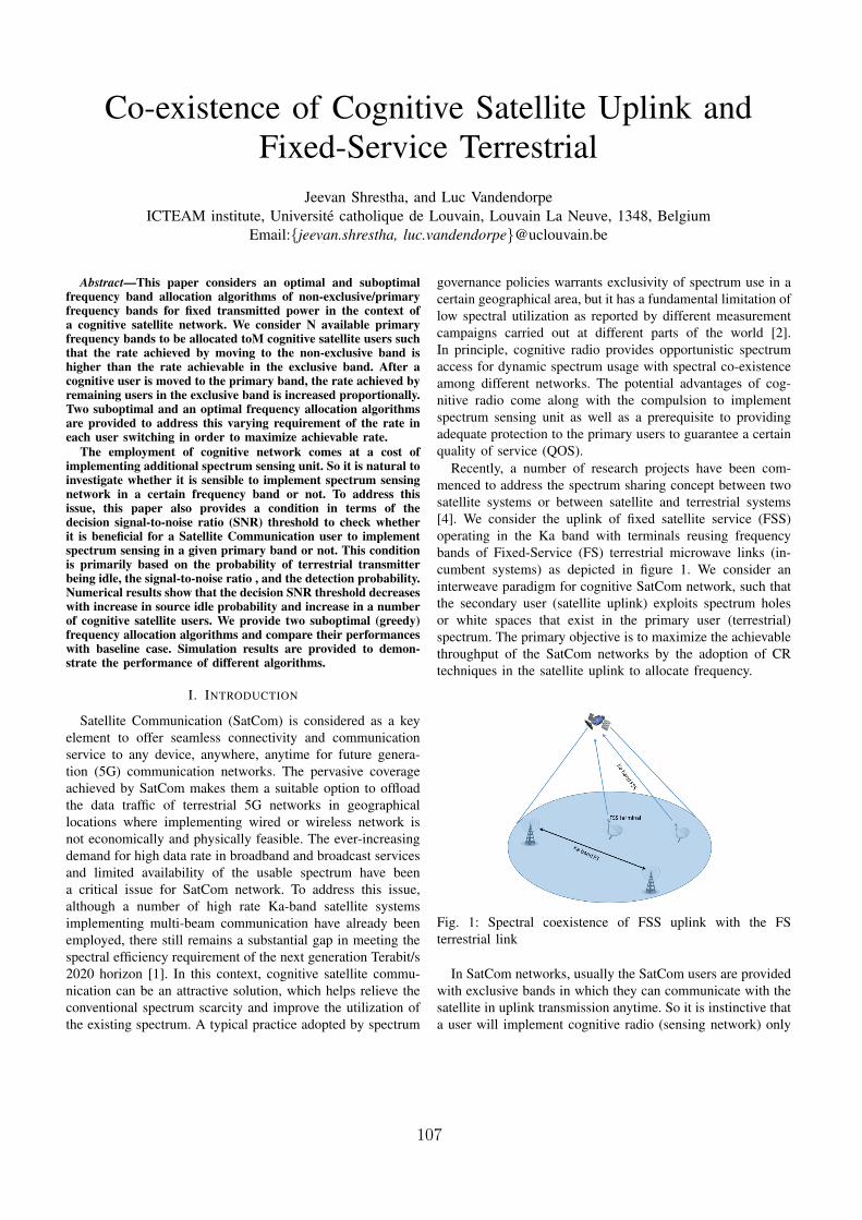
Co-existence of Cognitive Satellite Uplink andFixed-Service Terrestrial
Jeevan Shrestha, and Luc VandendorpeICTEAM institute, Universite catholique de Louvain, Louvain La Neuve, 1348, Belgium
Email:jeevan.shrestha, [email protected]
Abstract—This paper considers an optimal and suboptimalfrequency band allocation algorithms of non-exclusive/primaryfrequency bands for fixed transmitted power in the context ofa cognitive satellite network. We consider N available primaryfrequency bands to be allocated toM cognitive satellite users suchthat the rate achieved by moving to the non-exclusive band ishigher than the rate achievable in the exclusive band. After acognitive user is moved to the primary band, the rate achieved byremaining users in the exclusive band is increased proportionally.Two suboptimal and an optimal frequency allocation algorithmsare provided to address this varying requirement of the rate ineach user switching in order to maximize achievable rate.
The employment of cognitive network comes at a cost ofimplementing additional spectrum sensing unit. So it is natural toinvestigate whether it is sensible to implement spectrum sensingnetwork in a certain frequency band or not. To address thisissue, this paper also provides a condition in terms of thedecision signal-to-noise ratio (SNR) threshold to check whetherit is beneficial for a Satellite Communication user to implementspectrum sensing in a given primary band or not. This conditionis primarily based on the probability of terrestrial transmitterbeing idle, the signal-to-noise ratio , and the detection probability.Numerical results show that the decision SNR threshold decreaseswith increase in source idle probability and increase in a numberof cognitive satellite users. We provide two suboptimal (greedy)frequency allocation algorithms and compare their performanceswith baseline case. Simulation results are provided to demon-strate the performance of different algorithms.
I. INTRODUCTION
Satellite Communication (SatCom) is considered as a keyelement to offer seamless connectivity and communicationservice to any device, anywhere, anytime for future genera-tion (5G) communication networks. The pervasive coverageachieved by SatCom makes them a suitable option to offloadthe data traffic of terrestrial 5G networks in geographicallocations where implementing wired or wireless network isnot economically and physically feasible. The ever-increasingdemand for high data rate in broadband and broadcast servicesand limited availability of the usable spectrum have beena critical issue for SatCom network. To address this issue,although a number of high rate Ka-band satellite systemsimplementing multi-beam communication have already beenemployed, there still remains a substantial gap in meeting thespectral efficiency requirement of the next generation Terabit/s2020 horizon [1]. In this context, cognitive satellite commu-nication can be an attractive solution, which helps relieve theconventional spectrum scarcity and improve the utilization ofthe existing spectrum. A typical practice adopted by spectrum
governance policies warrants exclusivity of spectrum use in acertain geographical area, but it has a fundamental limitation oflow spectral utilization as reported by different measurementcampaigns carried out at different parts of the world [2].In principle, cognitive radio provides opportunistic spectrumaccess for dynamic spectrum usage with spectral co-existenceamong different networks. The potential advantages of cog-nitive radio come along with the compulsion to implementspectrum sensing unit as well as a prerequisite to providingadequate protection to the primary users to guarantee a certainquality of service (QOS).
Recently, a number of research projects have been com-menced to address the spectrum sharing concept between twosatellite systems or between satellite and terrestrial systems[4]. We consider the uplink of fixed satellite service (FSS)operating in the Ka band with terminals reusing frequencybands of Fixed-Service (FS) terrestrial microwave links (in-cumbent systems) as depicted in figure 1. We consider aninterweave paradigm for cognitive SatCom network, such thatthe secondary user (satellite uplink) exploits spectrum holesor white spaces that exist in the primary user (terrestrial)spectrum. The primary objective is to maximize the achievablethroughput of the SatCom networks by the adoption of CRtechniques in the satellite uplink to allocate frequency.
Fig. 1: Spectral coexistence of FSS uplink with the FSterrestrial link
In SatCom networks, usually the SatCom users are providedwith exclusive bands in which they can communicate with thesatellite in uplink transmission anytime. So it is instinctive thata user will implement cognitive radio (sensing network) only
107
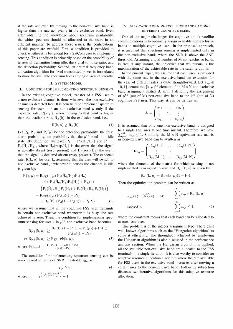
if the rate achieved by moving to the non-exclusive band ishigher than the rate achievable in the exclusive band. Evenafter obtaining the knowledge about spectrum availability,the white spectrum should be allocated to the users in anefficient manner. To address these issues, the contributionsof this paper are twofold. First, a condition is provided tocheck whether it is beneficial for a SatCom user to implementsensing. This condition is primarily based on the probability ofterrestrial transmitter being idle, the signal-to-noise ratio, andthe detection probability. Second, an optimal frequency bandallocation algorithm for fixed transmitted power is formulatedto share the available spectrum holes amongst users efficiently.
II. SYSTEM MODEL
III. CONDITION FOR IMPLEMENTING SPECTRUM SENSING
In the existing cognitive model, transfer of a FSS user toa non-exclusive channel is done whenever the non-exclusivechannel is detected free. It is beneficial to implement spectrumsensing for user k in an non-exclusive band µ only if theexpected rate, R(k, µ), when moving to that band is higherthan the available rate, RE(k), in the exclusive band, i.e.,
R(k, µ) ≥ RE(k). (1)
Let Pd, Pf, and Ps(µ) be the detection probability, the falsealarm probability, the probability that the µth band is in idlestate. By definition, we have Pf = Pr(H1/H0) and Pd =Pr(H1/H1), where H0(resp.H1) is the event that the signalis actually absent (resp. present) and H0(resp.H1) the eventthat the signal is declared absent (resp. present). The expectedrate, R(k, µ) for user k, assuming that the user will switch tonon-exclusive band µ whenever it senses the channel is idleis given by:
R(k, µ) = RNE(k, µ) Pr(H0/H0)Pr(H0)
+ 0 ∗ Pr(H0/H1)Pr(H1) + RE(k)(Pr(H1/H1)Pr(H1) + Pr(H1/H0)Pr(H0)
)
= RNE(k, µ) Ps(µ)(1− Pf)
+ RE(k) (Pd(1− Ps(µ)) + PfPs) , (2)
where we assume that if the cognitive FSS user transmitsin certain non-exclusive band whenever it is busy, the rateachieved is zero. Then, the condition for implementing spec-trum sensing for user k in µth non-exclusive band becomes
RNE(k, µ) ≥ RE(k) (1− Pd(1− Ps(µ)) + PfPs)
Ps(µ)(1− Pf)
⇔ RNE(k, µ) ≥ RE(k)Φ(k, µ), (3)
where Φ(k, µ) = (1−Pd(1−Ps(µ))+PfPs)Ps(µ)(1−Pf )
.
The condition for implementing spectrum sensing can bere-expressed in terms of SNR threshold, γth, as
γk,µ ≥ γth, (4)
where γth = 2
(RE(k)Φ(k,µ)T
BNE(T−Ts)
)− 1.
IV. ALLOCATION OF NON-EXCLUSIVE BANDS AMONGDIFFERENT COGNITIVE USERS
One of the major challenges for cognitive uplink satellitecommunications is to optimally assign available non-exclusivebands to multiple cognitive users. In the proposed approach,it is assumed that spectrum sensing is implemented only inthe non-exclusive bands where the SNR is above the SNRthreshold. Assuming a total number of M non-exclusive bandsis free at any instant, the objective that we pursue is themaximization of the achievable rate in the satellite uplink.
In the current paper, we assume that each user is providedwith the same rate in the exclusive band but extension forthe case of different rates is quite straightforward. Let akµ ∈0, 1 denote the k, µth element of an M×N non-exclusiveband assignment matrix A with 1 denoting the assignmentof µth (out of M) non-exclusive band to the kth (out of N)cognitive FSS user. This way, A can be written as:
A =
a11 . . . a1N...
. . ....
aM1 . . . aMN
.
It is assumed that only one non-exclusive band is assignedto a single FSS user at one time instant. Therefore, we have∑Mµ=1 akµ ≤ 1. Similarly, the M × N equivalent rate matrix
in non-exclusive band can be written as
Req =
Req(1, 1) . . . Req(1,N)...
. . ....
Req(M, 1) . . . Req(M,N)
,
where the elements of the matrix for which sensing is notimplemented is assigned to zero and Req(k, µ) is given by
Req(k, µ) = RNE(k, µ)(1− Pf).
Then the optimization problem can be written as
maxakµ,k∈1,...,N,µ∈1,...,M
M∑
k=1
akµ ∗ Req(k, µ)
subject toM∑
µ=1
akµ ≤ 1, (5)
where the constraint means that each band can be allocated toat most one user.
This problem is of the integer assignment type. There existwell known algorithms such as the “Hungarian algorithm” tosolve it efficiently. The throughput achieved by employingthe Hungarian algorithm is also discussed in the performanceanalysis section. When the Hungarian algorithm is applied,all the available non-exclusive band are allocated to the FSSterminals in a single iteration. It is also worthy to consider anadaptive resource allocation algorithm where the rate availablefor FSS users in the exclusive band increases after moving acertain user to the non-exclusive band. Following subsectiondiscuses two iterative algorithms for this adaptive resourceallocation.
108

A. Greedy Algorithm I
This resource allocation algorithm is adaptive to the chang-ing rate in exclusive band. The algorithm starts with identi-fying the FSS user that has the largest benefit to move. Letus denote this user by k0. This user has one or several bandswhere the following condition is met:
Req(k0, µ) ≥ RE(k0)0 (6)
where RE(k)0 is the initial rate for FSS users in theexclusive band. User k0 is moved to the non-exclusive band µ0
corresponding to the highest Req(k0, µ) in the first iteration,and band µ0 becomes unavailable for the subsequent iteration.After this move, for other users the available rate in exclusiveband becomes
RE(k)1 =N
N− 1RE(k)0.
Actually the same procedure takes place at any iteration i: theFSS user that has the largest benefit to move into one of theremaining non-exclusive bands is identified and the rate for theusers remaining in the exclusive band is updated as follows:
RE(k)i =N− (i− 1)
N− iRE(k)i−1
⇔ RE(k)i =N
N− iRE(k)0.
The iterations stop when there is no FSS user having benefitto move to the non-exclusive band. This algorithm is actuallygreedy since the FSS user with maximum profit is moved atany iteration but this may not be the best decision to take. Thenext algorithm is an optimal algorithm where switching of FSSuser is done in such a way that the throughput is maximized.
B. Greedy Algorithm II
This algorithm starts with creating an index matrix whereeach element of the index matrix is a maximum integer valuewhich satisfies following inequility:
i(k, µ) ≤ N− NRE(k)0Req(k, µ)
. (7)
The inequility is straightforward extension of equation 7. Theindex matrix I is then can be written as:
I =
i11 . . . i1N...
. . ....
iM1 . . . iMN
The k, µth element, ikµ, in the index matrix indicates uptowhich iteration it is benificial to move to µth non-exclusiveband for the kth user. The assignment of non-exclusive bandto a user is done in reverse fashion. Let imax be the maximulvalue of index in matrix I. The index elements with greaterof equal to certain value are grouped together.
Let U be the set of elements in matrix I such that ikµ ≥ in.Then a FSS user k∗ is assigned to the µ∗ exclusive band ifk∗, µ∗ ∈ U and Req(k∗, µ∗) ≥ Req(k, µ)∀k, µ ∈ U. Thenthe particular user k∗ and non-exclusive band µ∗ is removed
Parameter ValueNon-exclusive Band 27.5-29.5 GHz
Exclusive Band 19.7-20.2 GHz (25 Users)Parameters for FSS System
EIRP 50dBWGFSS
Tx (0) 42.1 dBiD 35,786 km
[G/T]SATRx 19.3dB/k
Sensing Network parametersDetection probability, Pd 0.85
False detection probability, Pf 0.2Channel idle probability, Ps 0.4
T 10µsTotal rate in exclusive band, RT 500Mbps
TABLE I: Simulation Parameters
from the next iteration. The iteration goes in reverse mannerand will be finished when iteration reches index value of 1.In this algorithm the user with maximum benifit is swithed atfinal iteration.
V. PERFORMANCE EVALUATION
In this section, we present some numerical results to showthe performance of the proposed resource allocation techniqueto give Ka-band cognitive uplink access to the FSS terminalsreusing frequency bands of FS terrestrial microwave links withpriority protection. It has been shown in BRIFIC FS database[7] that only around 60% of the FS Ka spectrum band (27.5to 29.5 GHz) is occupied in terrestrial transmission. Hence,the uplink band could benefit from more than 800 MHz ofadditional bandwidth at any instant.
A. Simulation Parameters
We present link budget and numerical parameters for FSSusers in Table I. For the performance analysis setup, the 40%of non-exclusive band (27.5-29.5 GHz) used for terrestrialtransmission is divided into 23 sub bands in the interval of35 MHz and the exclusive band (19.7-20.2 GHz) is assumedto be used by 25 exclusive users. We assume that the exclusiveusers are randomly distributed over circular area of radius150 km. The corresponding SNR matrices were obtainedconsidering all the carrier-user arrangements for non-exclusivecases. For exclusive band communication, it is assumed thatall the user are provided with same rate with appropriateresource allocation. We consider a geostationary satellite orbittransmission where average distance from satellite to earth is35786 km.
B. Numerical Results
At the first part of our numerical analysis, we calculated theSNR threshold for a given FSS user to implement spectrumsensing unit at given FS non-exclusive band. The SNR thresh-old is calculated by changing the channel idle probability andnumber of user in exclusive band. Figure 3 shows the variationof SNR threshold with respect to channel idle probability. Allthe other parameters of interest are kept fixed. The variationof SNR threshold with respect to number of user in exclusive
109
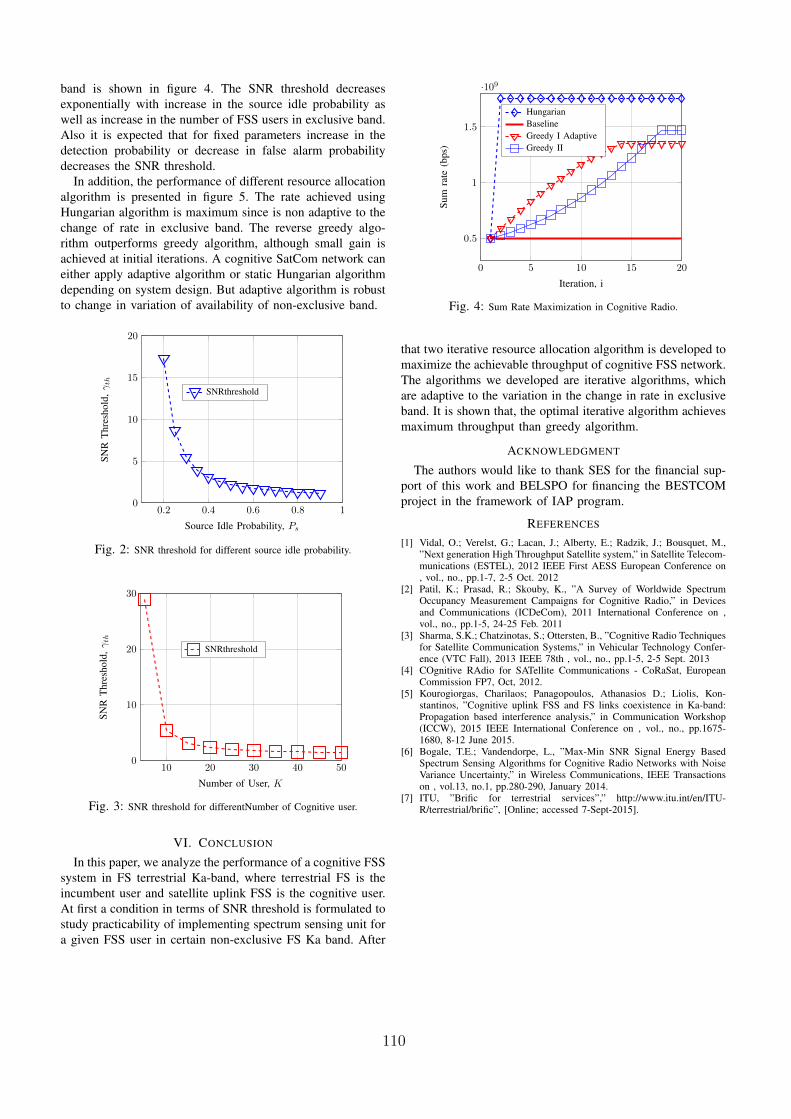
band is shown in figure 4. The SNR threshold decreasesexponentially with increase in the source idle probability aswell as increase in the number of FSS users in exclusive band.Also it is expected that for fixed parameters increase in thedetection probability or decrease in false alarm probabilitydecreases the SNR threshold.
In addition, the performance of different resource allocationalgorithm is presented in figure 5. The rate achieved usingHungarian algorithm is maximum since is non adaptive to thechange of rate in exclusive band. The reverse greedy algo-rithm outperforms greedy algorithm, although small gain isachieved at initial iterations. A cognitive SatCom network caneither apply adaptive algorithm or static Hungarian algorithmdepending on system design. But adaptive algorithm is robustto change in variation of availability of non-exclusive band.
0.2 0.4 0.6 0.8 10
5
10
15
20
Source Idle Probability, Ps
SNR
Thr
esho
ld,γ
th
SNRthreshold
Fig. 2: SNR threshold for different source idle probability.
10 20 30 40 500
10
20
30
Number of User, K
SNR
Thr
esho
ld,γ
th
SNRthreshold
Fig. 3: SNR threshold for differentNumber of Cognitive user.
VI. CONCLUSION
In this paper, we analyze the performance of a cognitive FSSsystem in FS terrestrial Ka-band, where terrestrial FS is theincumbent user and satellite uplink FSS is the cognitive user.At first a condition in terms of SNR threshold is formulated tostudy practicability of implementing spectrum sensing unit fora given FSS user in certain non-exclusive FS Ka band. After
0 5 10 15 20
0.5
1
1.5
·109
Iteration, i
Sum
rate
(bps
)
HungarianBaselineGreedy I AdaptiveGreedy II
Fig. 4: Sum Rate Maximization in Cognitive Radio.
that two iterative resource allocation algorithm is developed tomaximize the achievable throughput of cognitive FSS network.The algorithms we developed are iterative algorithms, whichare adaptive to the variation in the change in rate in exclusiveband. It is shown that, the optimal iterative algorithm achievesmaximum throughput than greedy algorithm.
ACKNOWLEDGMENT
The authors would like to thank SES for the financial sup-port of this work and BELSPO for financing the BESTCOMproject in the framework of IAP program.
REFERENCES
[1] Vidal, O.; Verelst, G.; Lacan, J.; Alberty, E.; Radzik, J.; Bousquet, M.,”Next generation High Throughput Satellite system,” in Satellite Telecom-munications (ESTEL), 2012 IEEE First AESS European Conference on, vol., no., pp.1-7, 2-5 Oct. 2012
[2] Patil, K.; Prasad, R.; Skouby, K., ”A Survey of Worldwide SpectrumOccupancy Measurement Campaigns for Cognitive Radio,” in Devicesand Communications (ICDeCom), 2011 International Conference on ,vol., no., pp.1-5, 24-25 Feb. 2011
[3] Sharma, S.K.; Chatzinotas, S.; Ottersten, B., ”Cognitive Radio Techniquesfor Satellite Communication Systems,” in Vehicular Technology Confer-ence (VTC Fall), 2013 IEEE 78th , vol., no., pp.1-5, 2-5 Sept. 2013
[4] COgnitive RAdio for SATellite Communications - CoRaSat, EuropeanCommission FP7, Oct, 2012.
[5] Kourogiorgas, Charilaos; Panagopoulos, Athanasios D.; Liolis, Kon-stantinos, ”Cognitive uplink FSS and FS links coexistence in Ka-band:Propagation based interference analysis,” in Communication Workshop(ICCW), 2015 IEEE International Conference on , vol., no., pp.1675-1680, 8-12 June 2015.
[6] Bogale, T.E.; Vandendorpe, L., ”Max-Min SNR Signal Energy BasedSpectrum Sensing Algorithms for Cognitive Radio Networks with NoiseVariance Uncertainty,” in Wireless Communications, IEEE Transactionson , vol.13, no.1, pp.280-290, January 2014.
[7] ITU, ”Brific for terrestrial services”,” http://www.itu.int/en/ITU-R/terrestrial/brific”, [Online; accessed 7-Sept-2015].
110
Low-Complexity Laser Phase Noise Compensationfor Filter Bank Multicarrier Offset-QAM Optical
Fiber Systems
T.-H. Nguyen, S.-P. Gorza, F. Horlin J. LouveauxUniversite libre de Bruxelles Universite catholique de Louvain
OPERA department ICTEAM institute1050 Brussels, Belgium 1348 Louvain-la-Neuve, Belgium
[email protected] [email protected]
Abstract
We report on a low-complexity modified blind phase search (BPS) for the carrierphase estimation in optical filter bank multicarrier offset quadrature modulationformat (FBMC-OQAM) systems. More particularly, the distance calculationsin the complex plane in state-of-the-art BPS method are replaced by simplemultiplication-free operations in the real plane. Moreover, a modified phasesearching strategy is also applied, leading to further reduction of the compu-tational complexity. The proposed methods are numerically validated in a 5-subcarriers FBMC-16OQAM system. Similar to conventional BPS method, thetolerated normalized linewidth (the product of laser linewidth and symbol dura-tion) of the proposed BPS method is 10−4 for a 1 dB SNR penalty of BER = 10−3
with about twice the reduction of computational complexity.
1 Introduction
Filter bank multicarrier offset quadrature modulation format (FBMC-OQAM) is aninteresting alternative to orthogonal frequency-division multiplexing (OFDM) and hasrecently received much attention in optical fiber communication systems [1, 2, 3] thanksto its optimized spectral efficiency (SE) and its robustness to the channel variationin optical fibers. On each subcarrier of FBMC-OQAM systems, a half-symbol timedelay between the in-phase and quadrature components of the signal is introduced,in order to achieve the orthogonality between adjacent subcarriers [4]. However, inthe presence of the laser phase noise, inter-carrier interference appears between theOQAM subcarriers in addition to the corresponding rotation [5]. As a consequence,the frequently-used carrier phase estimation (CPE) methods for QAM constellationsare no longer suitable, unless the laser linewidth is of several kHz [4]. Several CPEsolutions for OQAM signals have been proposed so far. The pilot used in [4] can beexploited to the CPE, however, suffering from the reduced SE. An innovative phasetracking combined with the equalizer has been reported in [1], at the cost of extrafeedback loop delay. Recently, the modified blind phase search (M-BPS) has recentlybeen proposed in [5], taking the advantage of the feedforward operation [6]. However,the computation effort (CE) is increased associated with the increase of the OQAMmodulation level.In this paper, a modified BPS of lower complexity (LC-BPS) is proposed for FBMC-OQAM systems, in which the distance calculations in the complex plane in M-BPSmethod is replaced by simple multiplication-free operations in the real plane. Moreover,a modified phase searching strategy is also applied, leading to further reduction ofthe CE. The proposed methods are numerically validated in a 5-subcarriers FBMC-16OQAM system. Similar to M-BPS method, the tolerated normalized linewidth (theproduct of laser linewidth and symbol duration) of the LC-BPS method is 10−4 for a1 dB SNR penalty of BER = 10−3 with about twice the reduction of CE.
111
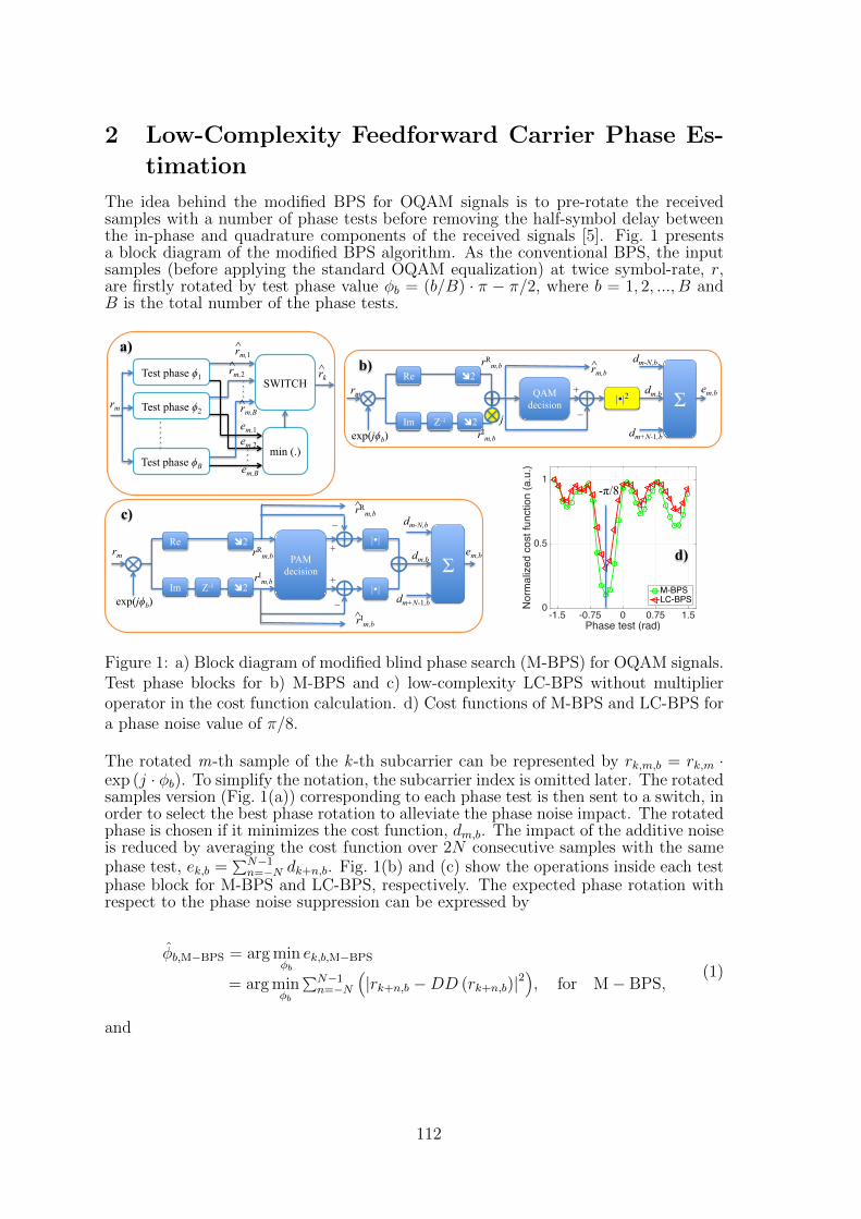
2 Low-Complexity Feedforward Carrier Phase Es-
timation
The idea behind the modified BPS for OQAM signals is to pre-rotate the receivedsamples with a number of phase tests before removing the half-symbol delay betweenthe in-phase and quadrature components of the received signals [5]. Fig. 1 presentsa block diagram of the modified BPS algorithm. As the conventional BPS, the inputsamples (before applying the standard OQAM equalization) at twice symbol-rate, r,are firstly rotated by test phase value φb = (b/B) · π − π/2, where b = 1, 2, ..., B andB is the total number of the phase tests.
Phase test (rad)-1.5 -0.75 0 0.75 1.5
Nor
mal
ized
cos
t fun
ctio
n (a
.u.)
0
0.5
1
M-BPSLC-BPS
Re
Im
î2
î2 Z-1
PAM decision
|| +
−
exp(jϕb)
rm rRm,b
rIm,b
Σ dm,b
dm-N,b
dm+N-1,b
+
− ||
^ rRm,b
^ rIm,b
em,b
Re
Im
î2
î2 Z-1 j
QAM decision ||2
+
−
exp(jϕb)
rm
rRm,b
rIm,b
Σ dm,b
dm-N,b
dm+N-1,b
rm,b ^
em,b
a) b)
c)
Test phase ϕ1
Test phase ϕ2
Test phase ϕB
SWITCH
min (.) em,B
em,2
em,1
rk ^ rm,1 ^
rm,2 ^
rm,B ^ rm
d)
-π/8
Figure 1: a) Block diagram of modified blind phase search (M-BPS) for OQAM signals.Test phase blocks for b) M-BPS and c) low-complexity LC-BPS without multiplieroperator in the cost function calculation. d) Cost functions of M-BPS and LC-BPS fora phase noise value of π/8.
The rotated m-th sample of the k -th subcarrier can be represented by rk,m,b = rk,m ·exp (j · φb). To simplify the notation, the subcarrier index is omitted later. The rotatedsamples version (Fig. 1(a)) corresponding to each phase test is then sent to a switch, inorder to select the best phase rotation to alleviate the phase noise impact. The rotatedphase is chosen if it minimizes the cost function, dm,b. The impact of the additive noiseis reduced by averaging the cost function over 2N consecutive samples with the samephase test, ek,b =
∑N−1n=−N dk+n,b. Fig. 1(b) and (c) show the operations inside each test
phase block for M-BPS and LC-BPS, respectively. The expected phase rotation withrespect to the phase noise suppression can be expressed by
φb,M−BPS = arg minφb
ek,b,M−BPS
= arg minφb
∑N−1n=−N
(|rk+n,b −DD (rk+n,b)|2
), for M− BPS,
(1)
and
112
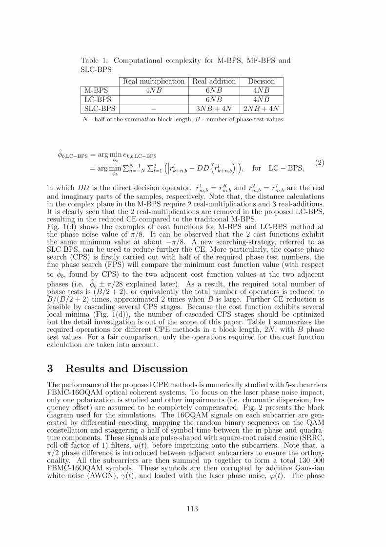
Table 1: Computational complexity for M-BPS, MF-BPS andSLC-BPS
Real multiplication Real addition DecisionM-BPS 4NB 6NB 4NBLC-BPS − 6NB 4NBSLC-BPS − 3NB + 4N 2NB + 4N
N - half of the summation block length; B - number of phase test values.
φb,LC−BPS = arg minφb
ek,b,LC−BPS
= arg minφb
∑N−1n=−N
∑2l=1
(∣∣∣rlk+n,b −DD(rlk+n,b
)∣∣∣), for LC− BPS,
(2)
in which DD is the direct decision operator. r1m,b = rRm,b and r2m,b = rIm,b are the realand imaginary parts of the samples, respectively. Note that, the distance calculationsin the complex plane in the M-BPS require 2 real-multiplications and 3 real-additions.It is clearly seen that the 2 real-multiplications are removed in the proposed LC-BPS,resulting in the reduced CE compared to the traditional M-BPS.Fig. 1(d) shows the examples of cost functions for M-BPS and LC-BPS method atthe phase noise value of π/8. It can be observed that the 2 cost functions exhibitthe same minimum value at about −π/8. A new searching-strategy, referred to asSLC-BPS, can be used to reduce further the CE. More particularly, the coarse phasesearch (CPS) is firstly carried out with half of the required phase test numbers, thefine phase search (FPS) will compare the minimum cost function value (with respect
to φb, found by CPS) to the two adjacent cost function values at the two adjacent
phases (i.e. φb ± π/28 explained later). As a result, the required total number ofphase tests is (B/2 + 2), or equivalently the total number of operators is reduced toB/(B/2 + 2) times, approximated 2 times when B is large. Further CE reduction isfeasible by cascading several CPS stages. Because the cost function exhibits severallocal minima (Fig. 1(d)), the number of cascaded CPS stages should be optimizedbut the detail investigation is out of the scope of this paper. Table 1 summarizes therequired operations for different CPE methods in a block length, 2N , with B phasetest values. For a fair comparison, only the operations required for the cost functioncalculation are taken into account.
3 Results and Discussion
The performance of the proposed CPE methods is numerically studied with 5-subcarriersFBMC-16OQAM optical coherent systems. To focus on the laser phase noise impact,only one polarization is studied and other impairments (i.e. chromatic dispersion, fre-quency offset) are assumed to be completely compensated. Fig. 2 presents the blockdiagram used for the simulations. The 16OQAM signals on each subcarrier are gen-erated by differential encoding, mapping the random binary sequences on the QAMconstellation and staggering a half of symbol time between the in-phase and quadra-ture components. These signals are pulse-shaped with square-root raised cosine (SRRC,roll-off factor of 1) filters, u(t), before imprinting onto the subcarriers. Note that, aπ/2 phase difference is introduced between adjacent subcarriers to ensure the orthog-onality. All the subcarriers are then summed up together to form a total 130 000FBMC-16OQAM symbols. These symbols are then corrupted by additive Gaussianwhite noise (AWGN), γ(t), and loaded with the laser phase noise, ϕ(t). The phase
113
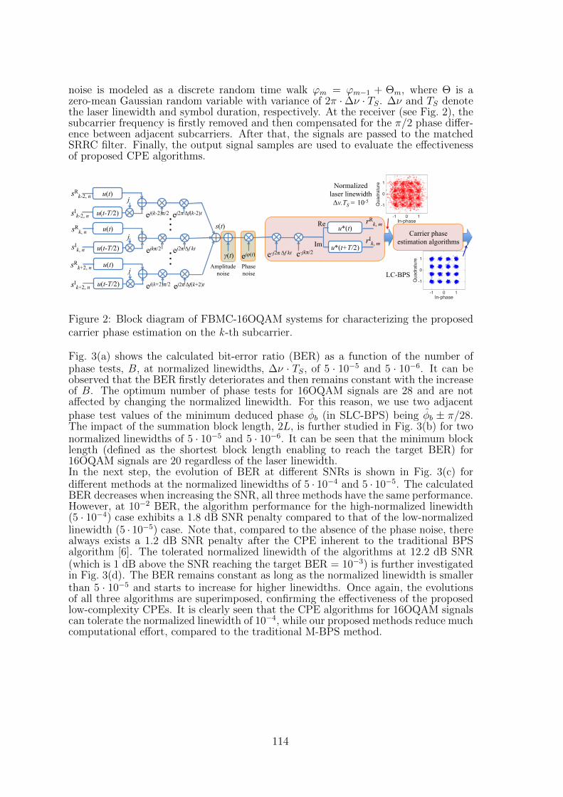
noise is modeled as a discrete random time walk ϕm = ϕm−1 + Θm, where Θ is azero-mean Gaussian random variable with variance of 2π ·∆ν · TS. ∆ν and TS denotethe laser linewidth and symbol duration, respectively. At the receiver (see Fig. 2), thesubcarrier frequency is firstly removed and then compensated for the π/2 phase differ-ence between adjacent subcarriers. After that, the signals are passed to the matchedSRRC filter. Finally, the output signal samples are used to evaluate the effectivenessof proposed CPE algorithms.
u(t)
u(t-T/2)
j
ej(k-2)π/2 ej2π Δf(k-2)t
sRk-2, n
sIk-2, n
u(t)
u(t-T/2) j
ejkπ/2 ej2π Δf kt
sRk, n
sIk, n
u(t)
u(t-T/2)
j
ej(k+2)π/2 ej2π Δf(k+2)t
sRk+2, n
sIk+2, n
γ(t) ejφ(t) e-jkπ/2 e-j2π Δf kt
u*(t)
u*(t+T/2)
Re
Im
rRk, m
rIk, m
s(t)
Amplitude noise
Phase noise
Carrier phase estimation algorithms
In-phase-1 0 1
Quadrature
-1
0
1
In-phase-1 0 1
Quadrature
-1
0
1
Normalized laser linewidth Δν.TS = 10-5
LC-BPS
Figure 2: Block diagram of FBMC-16OQAM systems for characterizing the proposedcarrier phase estimation on the k -th subcarrier.
Fig. 3(a) shows the calculated bit-error ratio (BER) as a function of the number ofphase tests, B, at normalized linewidths, ∆ν · TS, of 5 · 10−5 and 5 · 10−6. It can beobserved that the BER firstly deteriorates and then remains constant with the increaseof B. The optimum number of phase tests for 16OQAM signals are 28 and are notaffected by changing the normalized linewidth. For this reason, we use two adjacentphase test values of the minimum deduced phase φb (in SLC-BPS) being φb ± π/28.The impact of the summation block length, 2L, is further studied in Fig. 3(b) for twonormalized linewidths of 5 · 10−5 and 5 · 10−6. It can be seen that the minimum blocklength (defined as the shortest block length enabling to reach the target BER) for16OQAM signals are 20 regardless of the laser linewidth.In the next step, the evolution of BER at different SNRs is shown in Fig. 3(c) fordifferent methods at the normalized linewidths of 5 · 10−4 and 5 · 10−5. The calculatedBER decreases when increasing the SNR, all three methods have the same performance.However, at 10−2 BER, the algorithm performance for the high-normalized linewidth(5 · 10−4) case exhibits a 1.8 dB SNR penalty compared to that of the low-normalizedlinewidth (5 · 10−5) case. Note that, compared to the absence of the phase noise, therealways exists a 1.2 dB SNR penalty after the CPE inherent to the traditional BPSalgorithm [6]. The tolerated normalized linewidth of the algorithms at 12.2 dB SNR(which is 1 dB above the SNR reaching the target BER = 10−3) is further investigatedin Fig. 3(d). The BER remains constant as long as the normalized linewidth is smallerthan 5 · 10−5 and starts to increase for higher linewidths. Once again, the evolutionsof all three algorithms are superimposed, confirming the effectiveness of the proposedlow-complexity CPEs. It is clearly seen that the CPE algorithms for 16OQAM signalscan tolerate the normalized linewidth of 10−4, while our proposed methods reduce muchcomputational effort, compared to the traditional M-BPS method.
114
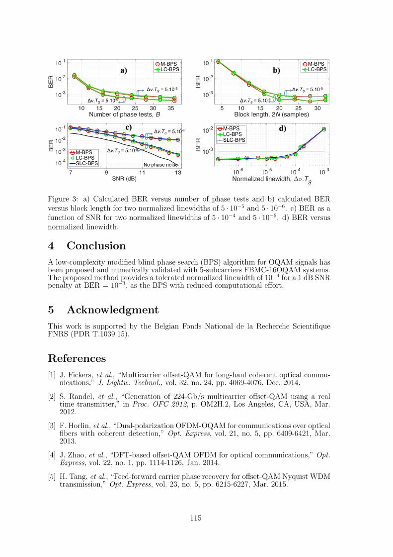
Number of phase tests, B10 15 20 25 30 35
BER
10-3
10-2
10-1 M-BPSLC-BPS
Block length, 2N (samples)5 10 15 20 25 30
BER
10-3
10-2
10-1 M-BPSLC-BPS
Normalized linewidth, "8.TS10-6 10-5 10-4 10-3
BER
10-3
10-2 M-BPSLC-BPSSLC-BPS
SNR (dB)7 9 11 13
BER
10-4
10-3
10-2
10-1
M-BPSLC-BPSSLC-BPS
a) b)
c)
No phase noise
d)
Δν.TS = 5.10-5
Δν.TS = 5.10-4
Δν.TS = 5.10-5
Δν.TS = 5.10-6
Δν.TS = 5.10-5
Δν.TS = 5.10-6
Figure 3: a) Calculated BER versus number of phase tests and b) calculated BERversus block length for two normalized linewidths of 5 · 10−5 and 5 · 10−6. c) BER as afunction of SNR for two normalized linewidths of 5 · 10−4 and 5 · 10−5. d) BER versusnormalized linewidth.
4 Conclusion
A low-complexity modified blind phase search (BPS) algorithm for OQAM signals hasbeen proposed and numerically validated with 5-subcarriers FBMC-16OQAM systems.The proposed method provides a tolerated normalized linewidth of 10−4 for a 1 dB SNRpenalty at BER = 10−3, as the BPS with reduced computational effort.
5 Acknowledgment
This work is supported by the Belgian Fonds National de la Recherche ScientifiqueFNRS (PDR T.1039.15).
References
[1] J. Fickers, et al., “Multicarrier offset-QAM for long-haul coherent optical commu-nications,” J. Lightw. Technol., vol. 32, no. 24, pp. 4069-4076, Dec. 2014.
[2] S. Randel, et al., “Generation of 224-Gb/s multicarrier offset-QAM using a realtime transmitter,” in Proc. OFC 2012, p. OM2H.2, Los Angeles, CA, USA, Mar.2012.
[3] F. Horlin, et al., “Dual-polarization OFDM-OQAM for communications over opticalfibers with coherent detection,” Opt. Express, vol. 21, no. 5, pp. 6409-6421, Mar.2013.
[4] J. Zhao, et al., “DFT-based offset-QAM OFDM for optical communications,” Opt.Express, vol. 22, no. 1, pp. 1114-1126, Jan. 2014.
[5] H. Tang, et al., “Feed-forward carrier phase recovery for offset-QAM Nyquist WDMtransmission,” Opt. Express, vol. 23, no. 5, pp. 6215-6227, Mar. 2015.
115

[6] T. Pfau, et al., “Hardware-efficient coherent digital receiver concept with feedfor-ward carrier recovery for M-QAM constellation,” J. Lightw. Technol., vol. 27, no.8, pp. 989-999, Apr. 2009.
116
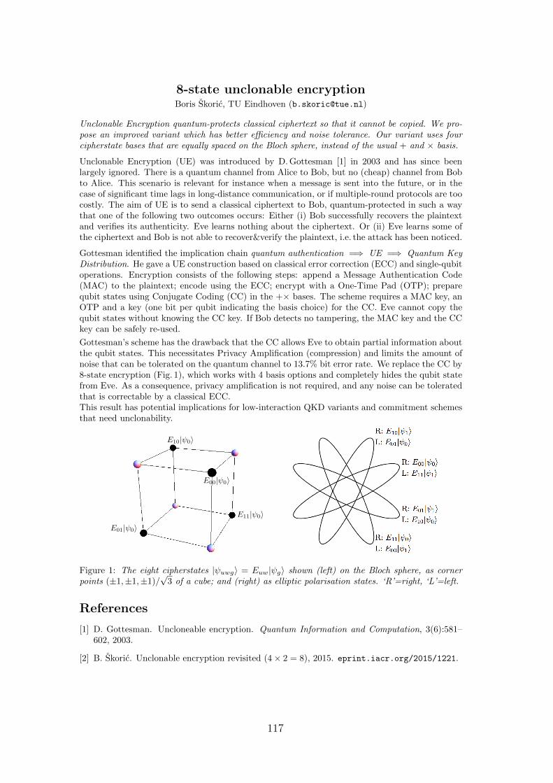
8-state unclonable encryptionBoris Skoric, TU Eindhoven ([email protected])
Unclonable Encryption quantum-protects classical ciphertext so that it cannot be copied. We pro-pose an improved variant which has better efficiency and noise tolerance. Our variant uses fourcipherstate bases that are equally spaced on the Bloch sphere, instead of the usual + and × basis.
Unclonable Encryption (UE) was introduced by D. Gottesman [1] in 2003 and has since beenlargely ignored. There is a quantum channel from Alice to Bob, but no (cheap) channel from Bobto Alice. This scenario is relevant for instance when a message is sent into the future, or in thecase of significant time lags in long-distance communication, or if multiple-round protocols are toocostly. The aim of UE is to send a classical ciphertext to Bob, quantum-protected in such a waythat one of the following two outcomes occurs: Either (i) Bob successfully recovers the plaintextand verifies its authenticity. Eve learns nothing about the ciphertext. Or (ii) Eve learns some ofthe ciphertext and Bob is not able to recover&verify the plaintext, i.e. the attack has been noticed.
Gottesman identified the implication chain quantum authentication =⇒ UE =⇒ Quantum KeyDistribution. He gave a UE construction based on classical error correction (ECC) and single-qubitoperations. Encryption consists of the following steps: append a Message Authentication Code(MAC) to the plaintext; encode using the ECC; encrypt with a One-Time Pad (OTP); preparequbit states using Conjugate Coding (CC) in the +× bases. The scheme requires a MAC key, anOTP and a key (one bit per qubit indicating the basis choice) for the CC. Eve cannot copy thequbit states without knowing the CC key. If Bob detects no tampering, the MAC key and the CCkey can be safely re-used.
Gottesman’s scheme has the drawback that the CC allows Eve to obtain partial information aboutthe qubit states. This necessitates Privacy Amplification (compression) and limits the amount ofnoise that can be tolerated on the quantum channel to 13.7% bit error rate. We replace the CC by8-state encryption (Fig. 1), which works with 4 basis options and completely hides the qubit statefrom Eve. As a consequence, privacy amplification is not required, and any noise can be toleratedthat is correctable by a classical ECC.This result has potential implications for low-interaction QKD variants and commitment schemesthat need unclonability.
B. Skoric 7
E00| 0i
E11| 0iE01| 0i
E10| 0i
Fig. 2. Relation between the codes C and D? C..
We thank Christian Scha↵ner, Serge Fehr and Andreas Hulsing for useful discussions.
References
1. W.K. Wootters and W.H. Zurek. A single quantum cannot be cloned. Nature, 299:802–803, 1982.2. C.H. Bennett, G. Brassard, C. Crepeau, R. Jozsa, A. Peres, and W.K. Wootters. Teleporting
an unknown quantum state via dual classical and Einstein-Podolsky-Rosen channels. Phys. Rev.Lett., 70:1895–1899, 1993.
3. D.N. Matsukevich and A. Kuzmich. Quantum state transfer between matter and light. Science,306(5696):663–666, 2004.
4. C.H. Bennett and G. Brassard. Quantum cryptography: Public key distribution and coin tossing.IEEE International Conference on Computers, Systems and Signal Processing, pages 175–179,1984.
5. A.K. Ekert. Quantum cryptography based on Bell’s theorem. Phys. Rev. Lett., 67:661 – 663, 1991.6. D. Gottesman and J. Preskill. Quantum Information with Continuous Variables, chapter Se-
cure quantum key exchange using squeezed states, pages 317–356. Springer, 2003. arXiv:quant-ph/0008046v2.
7. C.H. Bennett, G. Brassard, S. Breidbard, and S. Wiesner. Quantum cryptography, or unforgeablesubway tokens. In CRYPTO, pages 267–275, 1982.
8. I.B. Damgard, S. Fehr, L. Salvail, and C. Scha↵ner. Cryptography in the bounded quantum-storage model. In IEEE Symposium on Foundations of Computer Science (FOCS), page 449,2005.
9. C. Scha↵ner. Simple protocols for oblivious transfer and secure identification in the noisy-quantum-storage model. Phys.Rev.A, 82:032308, 2010.
10. H. Barnum, C. Crepeau, D. Gottesman, A. Smith, and A. Tapp. Authentication of quantummessages. In IEEE Symposium on Foundations of Computer Science, pages 449–458, 2002. Fullversion at http://arxiv.org/abs/quant-ph/0205128.
11. P.O. Boykin and V. Roychowdhury. Optimal encryption of quantum bits. Phys.Rev.A, 67:042317,2003.
12. A. Ambainis, M. Mosca, A. Tapp, and R. De Wolf. Private quantum channels. In IEEE Symposiumon Foundations of Computer Science (FOCS), pages 547–553, 2000.
13. B. Skoric. Quantum Readout of Physical Unclonable Functions. International Journal of QuantumInformation, 10(1):1250001–1 – 125001–31, 2012.
14. S.A. Goorden, M. Horstmann, A.P. Mosk, B. Skoric, and P.W.H. Pinkse. Quantum-Secure Au-thentication of a physical unclonable key. Optica, 1(6):421–424, Dec. 2014.
Figure 1: The eight cipherstates |ψuwg〉 = Euw|ψg〉 shown (left) on the Bloch sphere, as cornerpoints (±1,±1,±1)/
√3 of a cube; and (right) as elliptic polarisation states. ‘R’=right, ‘L’=left.
References
[1] D. Gottesman. Uncloneable encryption. Quantum Information and Computation, 3(6):581–602, 2003.
[2] B. Skoric. Unclonable encryption revisited (4× 2 = 8), 2015. eprint.iacr.org/2015/1221.
117
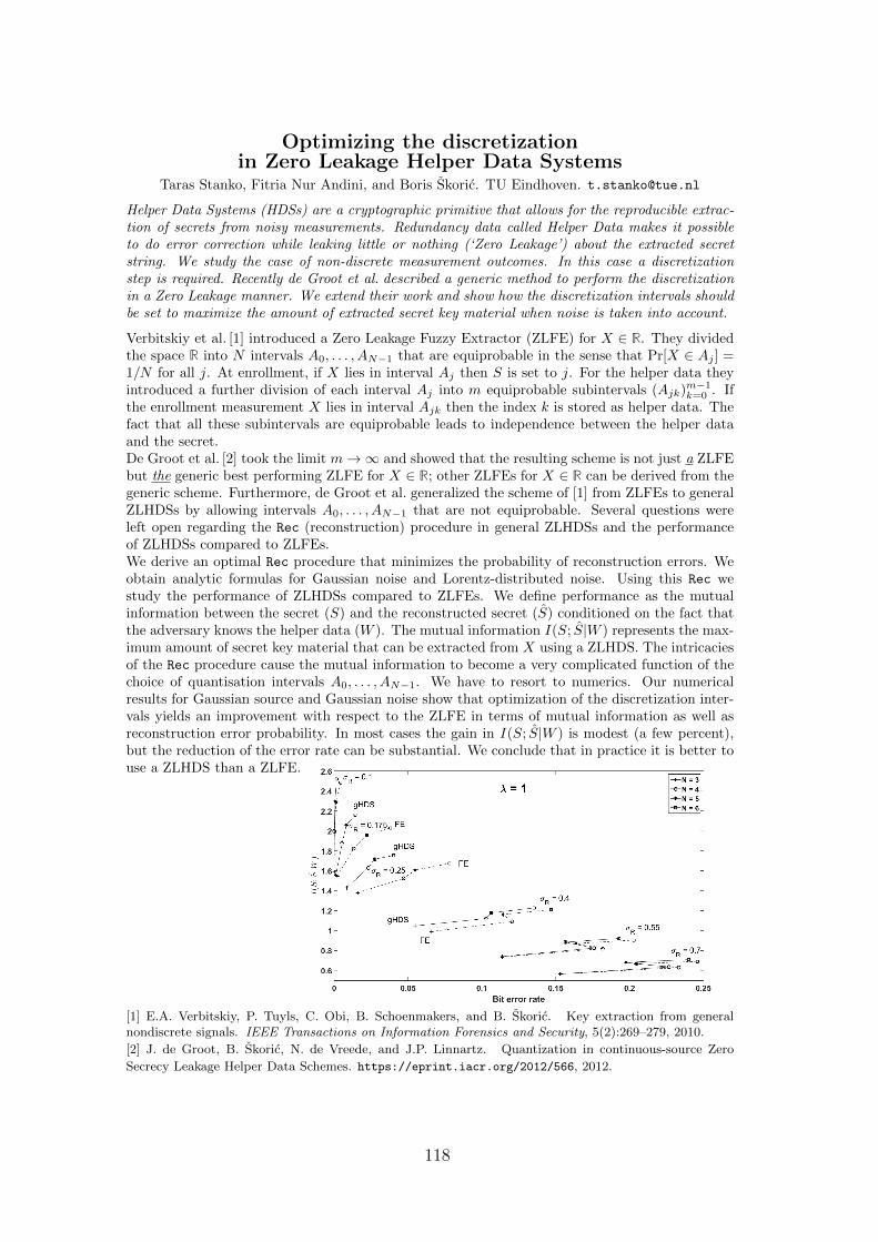
Optimizing the discretizationin Zero Leakage Helper Data Systems
Taras Stanko, Fitria Nur Andini, and Boris Skoric. TU Eindhoven. [email protected]
Helper Data Systems (HDSs) are a cryptographic primitive that allows for the reproducible extrac-tion of secrets from noisy measurements. Redundancy data called Helper Data makes it possibleto do error correction while leaking little or nothing (‘Zero Leakage’) about the extracted secretstring. We study the case of non-discrete measurement outcomes. In this case a discretizationstep is required. Recently de Groot et al. described a generic method to perform the discretizationin a Zero Leakage manner. We extend their work and show how the discretization intervals shouldbe set to maximize the amount of extracted secret key material when noise is taken into account.
Verbitskiy et al. [1] introduced a Zero Leakage Fuzzy Extractor (ZLFE) for X ∈ R. They dividedthe space R into N intervals A0, . . . , AN−1 that are equiprobable in the sense that Pr[X ∈ Aj ] =1/N for all j. At enrollment, if X lies in interval Aj then S is set to j. For the helper data theyintroduced a further division of each interval Aj into m equiprobable subintervals (Ajk)m−1
k=0 . Ifthe enrollment measurement X lies in interval Ajk then the index k is stored as helper data. Thefact that all these subintervals are equiprobable leads to independence between the helper dataand the secret.De Groot et al. [2] took the limit m→∞ and showed that the resulting scheme is not just a ZLFEbut the generic best performing ZLFE for X ∈ R; other ZLFEs for X ∈ R can be derived from thegeneric scheme. Furthermore, de Groot et al. generalized the scheme of [1] from ZLFEs to generalZLHDSs by allowing intervals A0, . . . , AN−1 that are not equiprobable. Several questions wereleft open regarding the Rec (reconstruction) procedure in general ZLHDSs and the performanceof ZLHDSs compared to ZLFEs.We derive an optimal Rec procedure that minimizes the probability of reconstruction errors. Weobtain analytic formulas for Gaussian noise and Lorentz-distributed noise. Using this Rec westudy the performance of ZLHDSs compared to ZLFEs. We define performance as the mutualinformation between the secret (S) and the reconstructed secret (S) conditioned on the fact thatthe adversary knows the helper data (W ). The mutual information I(S; S|W ) represents the max-imum amount of secret key material that can be extracted from X using a ZLHDS. The intricaciesof the Rec procedure cause the mutual information to become a very complicated function of thechoice of quantisation intervals A0, . . . , AN−1. We have to resort to numerics. Our numericalresults for Gaussian source and Gaussian noise show that optimization of the discretization inter-vals yields an improvement with respect to the ZLFE in terms of mutual information as well asreconstruction error probability. In most cases the gain in I(S; S|W ) is modest (a few percent),but the reduction of the error rate can be substantial. We conclude that in practice it is better touse a ZLHDS than a ZLFE.
[1] E.A. Verbitskiy, P. Tuyls, C. Obi, B. Schoenmakers, and B. Skoric. Key extraction from generalnondiscrete signals. IEEE Transactions on Information Forensics and Security, 5(2):269–279, 2010.
[2] J. de Groot, B. Skoric, N. de Vreede, and J.P. Linnartz. Quantization in continuous-source Zero
Secrecy Leakage Helper Data Schemes. https://eprint.iacr.org/2012/566, 2012.
118
Zero-Leakage Multiple Key-Binding Scenarios forSRAM-PUF Systems Based on the XOR-Method
Lieneke Kusters Tanya Ignatenko Frans M.J. WillemsEindhoven University of Technology
Dept. Electrical Engineering, SPS GroupP.O. Box 513, 5600 MB, Eindhoven
[email protected] [email protected] [email protected]
Abstract
We show that the XOR-method based on linear error-correcting codes canbe applied to achieve the secret-key capacity of binary-symmetric SRAM-PUFs.Then we focus on multiple key-bindings. We prove that no information is leakedby all the helper data about a single secret key both in the case where we use thesame key all the time and when we use different keys. The notion of symmetryis crucial in these proofs.∗
1 Introduction
The power-on state of static random-access memory (SRAM) can be used as a physicalunclonable function (PUF)[7][3]. A PUF results from randomness in the productionprocess of a device, and is hard to predict or to copy while at the same time theresponse is reliable. These properties make PUFs useful for various security systems.
In this paper, we investigate the XOR-method for secret-key binding to an SRAM-PUF. We show that as a result of symmetry in the state of the SRAM cells there is noleakage in multiple key-binding scenario’s.
2 Secret-Key Binding Scheme
It is our goal to share a secret key S, assuming values in 1, 2, · · · , |S|, betweenan encoder and a decoder using a secret-key binding scheme as in Figure 1. Bothparties observe the same SRAM-PUF, resulting in binary observation vectors XN =(X1, X2, · · · , XN) and Y N = (Y1, Y2, · · · , YN) respectively, corresponding to the start-up values of the N cells of the SRAM. First, the secret key S is generated uniformly atrandom and presented to the encoder. The encoder then binds this secret key to theobservation vector XN by generating helper data M , hence M = E(S,XN). Now the
decoder can construct an estimate S of the secret key using the helper data M and hisown observation vector Y N , hence S = D(M,Y N). Ideally, the helper data M provides
sufficient information to correctly reconstruct the secret key, and then S = S. At thesame time M should not leak any information about the secret to a third party, henceI(S;M) = 0. We assume that the SRAM-PUF is binary-symmetric, hence
Pr(XN , Y N) = (xN , yN) =∏
n=1,N
Q(xn, yn),
∗Research carried out in the E! 9629 PATRIOT project, which is funded by the Eurostars-2 jointprogramme with co-funding from the European Union Horizon 2020 research and innovation pro-gramme.
119

where Q(0, 1) = Q(1, 0) = p and Q(0, 0) = Q(1, 1) = 1 − p, for a parameter p thatsatisfies 0 ≤ p ≤ 1/2. It is our goal to maximize the achievable secret-key rate for oursystem.
Definition 1 A secret-key rate Rs with Rs ≥ 0 is said to be achievable if for all ε > 0and for all N large enough, there exist encoders and decoders such that:
PrS 6= S ≤ ε,
1
Nlog2 |S| ≥ Rs − ε,I(S;M) = 0.
The maximum secret-key rate that is achievable is called the secret-key capacity and isdenoted by Cs.
Theorem 1 The secret-key capacity of a binary-symmetric SRAM-PUF with param-eter p is
Cs = 1− h(p),
where the binary entropy function h(·) is defined as h(α) = α log21α
+ (1−α) log21
1−α ,for 0 ≤ α ≤ 1.
In the next section, we first show that secret-key rates larger than Cs = 1 − h(p) arenot achievable (converse). After that, we show that secret-key rate Cs = 1 − h(p) isachievable. We achieve this result by applying the so called code-offset method or theXOR-method [4].
3 Proof of Theorem 1
3.1 Converse result
We show here that there exists no secure and reliable scheme that meets the conditionsin Definition 1 when Rs > 1− h(p). Consider the information in the secret key
log2 |S| = H(S)
= I(S;M,Y N) +H(S|M,Y N)
(a)= I(S;M,Y N) +H(S|M,Y N , S)
≤ I(S;M,Y N) +H(S|S)
(b)
≤ I(S;M,Y N) + h(Pe) + Pe log2 |S|= I(S;M) + I(S;Y N |M) + h(Pe) + Pe log2 |S|(c)= 0 +H(Y N |M)−H(Y N |M,S) + h(Pe) + Pe log2 |S|≤ H(Y N |M)−H(Y N |M,S,XN) + h(Pe) + Pe log2 |S|(d)
≤ H(Y N)−H(Y N |XN) + h(Pe) + Pe log2 |S|= I(XN ;Y N) + h(Pe) + Pe log2 |S|(e)= N(1− h(p)) + h(Pe) + Pe log2 |S|,
120

encoder
XN
decoderS M
Y N
S
Figure 1: The secret-key binding scheme.
where (a) follows from the fact that S = D(M,Y N), (b) from Fano’s inequality where
Pe = PrS 6= S, (c) from the requirement I(S;M) = 0, (d) from the Markov relation(S,M) − XN − Y N , and (e) follows from the fact that all bit-pairs (Xn, Yn) in theobservation vectors are identically distributed according to Q(·, ·).
From this derivation we can conclude that
1
Nlog2 |S| ≤
1− h(p) + h(Pe)/N
(1− Pe),
and a rate Rs is now achievable if
Rs − ε ≤1
Nlog2 |S| ≤
1− h(p) + h(ε)/N
(1− ε) ,
for all ε > 0 and all N large enough. By letting ε ↓ 0 and N → ∞ we can concludethat achievable rates satisfy Rs ≤ 1− h(p) and consequently Cs ≤ 1− h(p).
3.2 Achievability
We have shown that the secret-key capacity Cs of the secret-key binding model cannotexceed 1 − h(p). Here we will show that the XOR-method [4], which is based onerror-correcting codes, see Figure 2, can be used to achieve capacity Cs = 1− h(p).
3.2.1 XOR-method and linear coding
The secret key SK is now assumed to be a K-bit uniformly chosen binary vector. It ismapped to a codeword CN by an encoder EL corresponding to a linear error-correctingcode, hence CN = EL(SK). Subsequently the helper data MN , a binary vector oflength N , is generated by adding modulo-2 the codeword CN to the observation vectorXN . Similarly, at the receiver side, a decoder DL transforms a noisy version codewordCN into an estimate of the secret key, i.e., SK = DL(CN). The noisy version CN ofthe codeword results from adding, modulo-2, the helper data MN to the observationvector Y N .
Clearly, since CN = CN ⊕XN ⊕Y N , bit-errors occur with probability p. Thereforewe can model the behavior of the XOR-scheme as a binary-symmetric channel with
EL ⊕
XN
⊕SK CN MN = CN ⊕XN
Y N
DLCN SK
Figure 2: The XOR-method for secret-key binding.
121

cross-over probability p. We show that for this scheme a linear error-correcting codeexists that achieves secret-key capacity Cs = 1− h(p).
We will use a random coding argument but will here generate a linear code at ran-dom, see [2]. We assume that a binary generator matrix GK×N is generated uniformlyat random. Now a codeword corresponding to a secret SK is constructed by matrixmultiplication as follows
CN = SKGK×N =K∑
k=1
SkGNk ,
where GNk corresponds to the kth row of the matrix and the additions are modulo-2.
The receiver decodes a received codeword CN by evaluating all 2K possible secret keysand decodes SK , if SK is the unique key satisfing
dH(SKGK×N , CN) < δN, (1)
where dH(·, ·) denotes Hamming distance, and δ is appropriately chosen. Note thatminimizing the Hamming distance is the best strategy for finding the most probablesecret, since the secrets are equally likely and the channel is binary-symmetric.
In the presented linear coding scheme an error can occur in two cases. An error ofthe first kind occurs when the channel output CN is not close enough to the channelinput CN , and therefore the Hamming distance in (1) is too large for the correct secretkey SK . The probability of occurrence of this event is
PrdH(SKGK×N , CN) ≥ δN = PrdH(CN , CN) ≥ δN
= PrdH(XN , Y N) ≥ δN(a)
≤ 2−Nd(δ||p), (2)
where (a) follows from the Chernoff bound (see Appendix A), with δ > p.An error of the second kind occurs when the channel output CN is close to possible
channel input CN = SKGK×N , for some SK 6= SK . The probability that this occurs is
PrdH(CN , CN) < δN
= PrdH(SKGK×N , SKGK×N ⊕XN ⊕ Y N) < δN(b)
≤ 2−Nd(δ||1/2),
where (b) follows from the fact that CN and CN are independent and Chernoff’s bound(see Appendix A) can be applied, with δ < 1/2. Furthermore, the independence of CN
and CN follows from the fact that SK and SK differ in it least one bit, and thereforethe resulting codewords CN and CN differ at least by one randomly generated matrixrow and are thus independent.
There are 2K − 1 messages SK 6= SK , and therefore the probability of occurrenceof an error of the second kind, using the union bound, is bounded as
∑
SK 6=SK
PrdH(CN , CN) < δN ≤ (2K − 1)2−Nd(δ||1/2) ≤ 2−N(1−h(δ)−K/N), (3)
It follows from the equations (2) and (3) that the error probability converges to zerofor large N , as long as K/N < 1 − h(δ) and p < δ < 1/2. Therefore, K/N can getarbitrarily close to Cs = 1− h(p) for δ → p.
The above results show, that averaged over the random linear code, the error prob-ability vanishes for N →∞ for all K/N = 1
Nlog 2K arbitrarily close to Cs. Therefore,
we can conclude that there are linear codes that achieve the capacity Cs, although weshould still verify that I(MN ;SK) = 0.
122

3.2.2 Information leakage by the helper data
We use the XOR-scheme (Figure 2) to bind a secret key SK to an SRAM-PUF bycreating helper data MN , based on the observation vector XN . In order for the schemeto be secure, we require that the (public) helper data MN by itself does not leak anyinformation about the secret key SK . We can easily show that this is true for onesecret SK and helper data MN :
I(MN ;SK)(a)
≤ I(MN ;CN)
= I(CN ⊕XN ;CN)
= H(CN ⊕XN)−H(CN ⊕XN |CN)
≤ N −H(XN) = N −N = 0,
where (a) follows from the data-processing inequality, see Cover and Thomas [1], p.35. This concludes the achievability part of the proof of Theorem 1.
4 Multiple SRAM-PUF Observations
4.1 Introduction
So far we have considered a single run of the key-binding scheme only, i.e. a bindingstep in which a key is bound to an SRAM observation followed by a reconstruction ofthe secret from a second observation of the SRAM and the public helper data.
However, it is not so obvious whether information leakage occurs when the sameSRAM-PUF is used to bind secret keys multiple times. In this case the encoder con-structs T helper data sequences
MN
1 ,MN2 , · · · ,MN
T
by binding each secret key to
another observation of the SRAM-PUFXN
1 , XN2 , · · · , XN
T
. In this section we prove
that even if all helper data is observed, no information is leaked about any single secret.However, before we can investigate the information leakage resulting from multiple
key-binding using the XOR-scheme, we first analyze the relation between multipleobservations of the same SRAM-PUF.
4.2 SRAM model
An SRAM is composed of N cells of which the start-up values can be observed multipletimes. We assume that all observations of cell n are i.i.d. where the probability of a 1being observed is given by the cell’s state θn. The states θN = (θ1, θ2, · · · , θN) of thecells are i.i.d. given by a random variable Θn which has probability density function(see e.g. [6], [5]):
pΘn(θ) = pΘ(θ), 0 ≤ θ ≤ 1. (4)
In the following, we analyze multiple observations of a single cell with index n ∈1, 2, · · · , N. For this purpose we define the cell-observation vector XT = (X1, X2 · · · XT ),with Xt the tth observation of the nth SRAM cell. Now, we can start our analysis.First, we use (4) and the fact that the observations are i.i.d. to find that for somecell-observation vector XT
PrXT = xT =
∫ 1
0
(1− θ)T−wH(xT )θwH(xT )pΘ(θ)dθ,
123

where wH(xT ) is the Hamming weight, or the number of ones in vector xT . Notethat the probability of the vector xT only depends on its Hamming weight wH(xT ).Therefore, there are T + 1 elementary probabilities
π(w) ,∫ 1
0
(1− θ)T−wθwpΘ(θ)dθ,
for w = 0, 1, · · · , T , that determine the cell vector probabilities
PrXT = xT = π(wH(xT )).
4.3 Symmetric SRAM model
Next, we assume that for SRAM-PUFs the density pΘ(θ) of the state θ is symmetric,that is
pΘ(θ) = pΘ(1− θ), 0 ≤ θ ≤ 1.
It turns out that the symmetry of the probability density function of the state of theSRAM-PUF cells is an essential feature needed in our later proofs. As a result theelementary probabilities also show symmetric behavior:
π(T − w) =
∫ 1
0
(1− θ)wθT−wpΘ(θ)dθ =
∫ 1
0
(1− θ)wθT−wpΘ(1− θ)dθ
=
∫ 1
0
(θ′)w(1− θ′)T−wpΘ(θ′)dθ′ = π(w),
for w = 0, 1, · · · , T .
Lemma 1 A consequence of the symmetry is that for the probability of the cell vector
PrXT = x1, · · · , xT = π(wH(x1, · · · , xT ))
= π(T − wH(x1, · · · , xT ))
= π(wH(x1, · · · , xT )) = PrXT = x1, · · · , xT,where x corresponds to the inverse of a bit x.
From this lemma we can conclude for any t ∈ 1, 2, · · · , T and x1, x2, · · · , xTPrXT = x1, · · · , xT = π(wH(x1, · · · , xT ))
= π(wH(x1 ⊕ xt, · · · , xt ⊕ xt, · · · , xT ⊕ xt))
= PrX1 = x1 ⊕ xt, · · · , Xt = 0, · · · , XT = xT ⊕ xt).
Until now, we have looked at T observations XT of a single cell with index n ∈1, 2, · · · , N. However, recall that we are interested in the relation between two ormore observation vectors, that each correspond to an observation of all the N cells inthe SRAM-PUF. Therefore, we now define T observation vectors XN
1 , XN2 , · · ·XN
T ,each corresponding to an observation of all N SRAM cells, and we can state the fol-lowing corollary.
Corollary 1 For all xN1 , xN2 , · · · , xNT we have that for any t ∈ 1, 2, · · · , T
PrXN1 = xN1 , · · · , XN
t = xNt , · · · , XNT = xNT
= PrXN1 = xN1 ⊕ xNt , · · · , XN
t = 0N , · · · , XNT = xNT ⊕ xNt .
124
4.4 Information leakage for multiple key-binding
We use the results from Corollary 1 to prove that no information leakage is resultingfrom observing multiple helper data corresponding to multiple key-binding with thesame SRAM-PUF. For key binding of the tth key SKt with t ∈ 1, 2, · · · , T, helperdata MN
t is generated from the codeword CNt and SRAM observation XN
t , accordingto MN
t = CNt ⊕XN
t , see also Figure 2.
Different Keys: First, we look at multiple key-binding with different secret keysSKt and thus different codewords CN
t = EL(SKt ), for which we find that for any of thecodewords CN
t , with t ∈ 1, · · ·TPrMN
1 = mN1 , · · · ,MN
T = mNT |CN
t = cNt
=∑
cN1 ∈CN· · ·
∑
cNt−1∈CN
∑
cNt+1∈CN· · ·
∑
cNT ∈CN
1
|CN |T−1PrXN
1 = mN1 ⊕ cN1 , · · · , XN
T = mNT ⊕ cNT
(a)=∑
cN1 ∈CN· · ·
∑
cNt−1∈CN
∑
cNt+1∈CN· · ·
∑
cNT ∈CN
1
|CN |T−1PrXN
1 = mN1 ⊕mN
t ⊕ cN1 ⊕ cNt , · · ·
· · · , XNt = 0N , · · · , XN
T = mNT ⊕mN
t ⊕ cNT ⊕ cNt
=∑
c′N1 ∈CN· · ·
∑
c′Nt−1∈CN
∑
c′Nt+1∈CN· · ·
∑
c′NT ∈CN
1
|CN |T−1PrXN
1 = mN1 ⊕mN
t ⊕ c′N1 , · · ·
· · · , XNt = 0N , · · · , XN
T = mNT ⊕mN
t ⊕ c′NT = f(mN
1 , · · · ,mNT ),
where f(·) is some function that does not depend on cNt . Moreover in (a) we usedCorollary 1. We can now conclude that
PrMN1 = mN
1 , · · · ,MNT = mN
T =∑
cN∈CNPrMN
1 = mN1 , · · · ,MN
T = mNT |CN
t = cNPrCNt = cN
=∑
cN∈CNf(mN
1 , · · · ,mNT ) PrCN
t = cN
= f(mN1 , · · · ,mN
T ) = PrMN1 = mN
1 , · · · ,MNT = mN
T |CNt = cNt ,
for any cNt and any t ∈ 1, 2, · · ·T. Now I(CNt ;MN
1 , · · · ,MNT ) = H(MN
1 , · · · ,MNT )−
H(MN1 , · · · ,MN
T |CNt ) = 0. By the data-processing inequality
I(SKt ;MN1 , · · · ,MN
T ) ≤ I(CNt ;MN
1 , · · · ,MNT ) = 0,
and thus observation of the helper data does not leak any information about any ofthe secrets SKt , with t ∈ 1, 2, · · ·T.
Single Key: Similarly for multiple bindings with a single secret-key SK and thus asingle codeword CN , we can show that
PrMN1 = mN
1 , · · · ,MNT = mN
T |CN = cN= PrXN
1 = mN1 ⊕ cN , · · · , XN
T = mNT ⊕ cN
(a)= PrXN
1 = mN1 ⊕mN
t , · · · , XNt = 0N , · · · , XN
T = mNT ⊕mN
t = g(mN1 , · · · ,mN
T ),
125

where g(·) is some function that does not depend on cN , and (a) follows from Corol-lary 1. Following similar reasoning as used for different keys, we can conclude thatI(SK ;MN
1 , · · · ,MNT ) = 0, and thus observation of the helper data does not leak any
information about the secret SK .
5 Conclusion
We have shown that the secret key SK can be shared, using the XOR-scheme shownin Figure 2 and linear coding, with a rate Rs arbitrary close to 1 − h(p), where pis the cross-over probability between two observations of the same SRAM-PUF cell.Furthermore, we have shown that the presented scheme is secure in the sense that noinformation is leaked by the helper data MN about the secret key SK , even if the samescheme (and SRAM-PUF) is used multiple times to bind either the same or differentsecret keys. This result follows from the key-assumption that the probability densityfunction of the states of the SRAM cells is symmetric.
A Chernoff bound
Let U1, · · · , UN be independent random variables with Ui ∈ 0, 1 and PrUi = 1 = p,for i = 1, · · · , N . Then, for any a ∈ (p, 1] and b ∈ [0, p), we have
Pr
N∑
i=1
Ui ≥ aN
≤ 2−Nd(a||p), and Pr
N∑
i=1
Ui ≤ bN
≤ 2−Nd(b||p),
with d(x||y) , x log2xy
+ (1− x) log21−x1−y .
References
[1] Thomas M. Cover and Joy A. Thomas. Elements of information theory. John Wiley& Sons, 2nd edition, 2006.
[2] Peter Elias. Coding for noisy channels. IRE Conv. Rec., Pt. 4:37–46, 1955.
[3] Daniel E. Holcomb, Wayne P. Burleson, and Kevin Fu. Power-Up SRAM stateas an identifying fingerprint and source of true random numbers. IEEE Trans.Comput., 58(9):1198–1210, 2009.
[4] Ari Juels and Martin Wattenberg. A fuzzy commitment scheme. In 6th ACMConf. Comput. Commun. Secur. - CCS ’99, pages 28–36, New York, New York,USA, 1999. ACM Press.
[5] Roel Maes. An Accurate Probabilistic Reliability Model for Silicon PUFs. InCryptogr. Hardw. Embed. Syst. - CHES 2013 15th Int. Work. St. Barbar. CA,USA, pages 73–89. 2013.
[6] Roel Maes, Pim Tuyls, and Ingrid Verbauwhede. A soft decision helper data algo-rithm for SRAM PUFs. In IEEE Int. Symp. Inf. Theory, pages 2101–2105, 2009.
[7] Vincent van der Leest, Geert-Jan Schrijen, Helena Handschuh, and Pim Tuyls.Hardware intrinsic security from D flip-flops. In Fifth ACM Work. Scalable Trust.Comput. - STC ’10, page 53, New York, New York, USA, 2010. ACM Press.
126
Localization in Long Range CommunicationNetworks Based on Machine Learning
Hazem Sallouha Sofie PollinKU Leuven
Dept. Elektrotechniek, TeleMicKasteelpark Arenberg, 10 - 2444
[email protected] [email protected]
Abstract
As the number of devices connected to internet is rapidly increasing, it is ex-pected that by 2025, every device will have a wireless connection, hence leadingto trillions of wirelessly connected devices. Therefore, internet of things (IoT)with long range, low power and low throughput (e.g., Sigfox and LoRa) are rais-ing as a new paradigm enabling to connect those trillions of devices efficiently.In such networks with low power and throughput, localization became morechallenging. However, in most of IoT applications (e.g., asset tracking) we areinterested in localizing the nodes within a certain area, rather than estimatingthe exact position with global positioning system (GPS) coordinates. Therefore,the problem can be simplified to estimate the node’s sector. In this paper wepropose a localization mechanism based on machine learning and assuming thatsome nodes in the sector are integrated with a GPS. By using these GPS-nodesas a reference the network can learn the position of the other nodes. The re-sults revealed that using the user back-end measurements (e.g., received signalstrength (RSS), number of base stations and the end-to-end delay) nodes canbe divided in sectors. Then, the GPS-node is used to define the coordinates ofthe sector. Moreover, a trade off between number of messages and localizationaccuracy is illustrated.
1 Introduction
Wireless technologies penetrate in all layers of our daily live. Concepts such as ”Inter-net of Things (IoT)” and ”Location-Based Services” are rising as a new communicationparadigms. The idea behind IoT is to have the objects of our daily life equipped withmicrocontrollers, transceivers for digital communication, and suitable protocol stacksthat will make them able to communicate and becoming an integral part of the In-ternet [1]. In such networks location information can be exploited in different layersfrom communication aided perpouses to application level where location informationare needed to meaningfully interpret any physical measurements collected by sensornodes (SN) [1], [2].
In order to enable connectivity for hundreds of SN , the currently deployed IoT net-works are using long-rage, low power and low throughput communications [4]-[5]. Thesecharacteristics made the localization problem more challenging. In one hand it is tooexpensive to integrate a GPS receiver in each SN and on the other hand, ranging-based localization techniques face lack of accuracy because of low bandwidth and longdistances [7]. An alternative promising localization method is fingerprinting-based lo-calization [8]-[10]. Fingerprinting localization usually works in two phases: offline phaseand online phase. In offline phase measurements are collected form SN at differentlocations and stored as a training data. During the online phase, the measurements of
127
the SN are compared with the training data to estimate their location. The comparingprocess is usually done using machine learning algorithms [9]. A comparison betweenvarious machine learning algorithms is presented in [11]. It has been shown that de-cision tree J48 [12] is one of the top accurate algorithms. A localization method forIoT is introduced in [13] which can satisfy diverse requirements for indoor and outdoorscenarios. However, the long range communication is not considered.
In this work we propose a localization algorithm for long range IoT networks based onmachine learning. Assuming some nodes are equipped with a GPS receiver the wideserved region can be split up into sectors based on the GPS sensor nodes (GPS-SNs).Then, the other SN will be classified to one of the sectors using messages fingerprinting.
The rest of the paper is organized as follows, section 2 present localization in longrange IoT networks. First, the problem is defined then the details of the proposed al-gorithm is described. Section 3 demonstrates the experimental results. Finally, Section4 concludes this paper.
2 Localization in Long range IoT Networks
An IoT network is basically a network where massive number of nodes is connected tothe same cloud. One kind of IoT networks is the long range networks [4]-[5]. This kindof networks enable connectivity for hundreds of nodes using relativity low number ofbase stations [3]. Example of these networks is Sigfox network [4]. Sigfox network iscellular based where the uplink data flow from nodes to base stations is assumed to be97% of the data traffic. However, in some cases a hybrid networks can be used wherenodes forward data to a getaway node which in turn send the data to base stations [1].
2.1 Problem Definition
Since long range IoT networks are cellular based, one may suggest to use multilaterationranging-based techniques for localization. Although they are cellular based, there aretwo main differences that make ranging-based localization inaccurate. First of all,since each base station covers a relatively large area (long range base station can coverbe up to 40 km [3]), using multilateration will lead to a relatively large predictionzone. Secondly, multilateration is a ranging based techniques. Therefore, the accuracyis depend on the estimated distance between base station and nodes. The distancebetween base station and nodes can be calculated using received signal strength (RSS)and/or time of arrival (ToA). The Cramr-Rao lower bound (CRLB) of a distance
estimate d derived from RSS estimation provides the following inequality [6]
√V ar(d) > ln 10
10
σshnpd (1)
where V ar· is the variance, d is the distance between the base station and thenode, np is the path loss factor, and σsh is the standard deviation of the zero meanGaussian random variable representing the log-normal channel shadowing effect. FromEq. (1) we observe that increasing the distance d, which is the case in long rangecommunication, will decease the estimation accuracy by increasing the variance. On
the other hand, the best achievable accuracy of a distance estimate d derived from ToAestimation satisfies the following inequality [6]
√V ar(d) > c
2√
2π√SNRβ
(2)
128

where c is the speed of light, SNR is the signal-to-noise ratio, and β is the effective (orroot mean square) signal bandwidth. Unlike RSS ranging technique, the accuracy ofToA is based on the signal bandwidth. However, long range communication is mainlybased on ultra-narrow-band (UNB) (100Hz) transmission [4]. Therefore, this UNBproperty leads to extremely inaccurate location estimates using time-based techniques.
2.2 Proposed Sector-Based Localization
Consider an outdoor long range communication network (i.e., Sigfox) with a massivenumber of nodes distributed in a wide area (>40km) with two types of nodes: (i)normal sensor node (SN), without GPS, use to collect data and forward it to basestations, and (ii) sensor node that has an extra GPS receiver (GPS-SN), therefore, itsmessages have a GPS coordinates included. The GPS-SNs with their known locationcan be used to virtually partition the wide coverage region to a smaller sectors asshown in Fig. 1 where each sector is assumed to has at least one GPS-SN . Note that,Fig. 1 does not give any indication about the cell coverage since every message beingsent form any sector Ci,j will be received by at least 3 base station.
Figure 1: Illustrative example of how a wide region can be partitioned to a smallerregions each with a GPS-SN . Each cluster Ci,j has a GPS-SN
We propose a localization algorithm based on machine learning that uses fingerprinting(RSSI, received SNR and base stations that have received the message) of the GPS-SNmessages as a reference training data for classifying the other SN to one of the sectors.The machine learning algorithm (i.e., Decision Tree [12], Nave Bayes [14]) will assigneach SN to one of the GPS-SN ’s sector based on their fingerprinting. Let N be thenumber of GPS-SNs in a defined region and M be the number of base stations thathave received a message form a SN . We define region around the GPS-SN as a sectorand denote a given sector by Ci,j. Then, the complete set of all sectors are given by
C = ∪Ci,j,∀i, j (3)
where i ∈ 1, 2, ..,M and j ∈ 1, 2, .., N. The proposed algorithm shown in flowchart in Fig. 2 has two main steps:
129
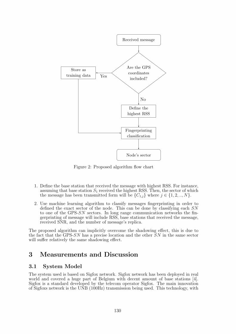
Received message
Are the GPS
coordinates
included?
Define the
highest RSS
Fingerprinting
classification
Node’s sector
Store as
training data
No
Yes
Figure 2: Proposed algorithm flow chart
1. Define the base station that received the message with highest RSS. For instance,assuming that base station S1 received the highest RSS. Then, the sector of whichthe message has been transmitted form will be C1,j where j ∈ 1, 2, .., N.
2. Use machine learning algorithm to classify messages fingerprinting in order todefined the exact sector of the node. This can be done by classifying each SNto one of the GPS-SN sectors. In long range communication networks the fin-gerprinting of message will include RSS, base stations that received the message,received SNR, and the number of message’s replica.
The proposed algorithm can implicitly overcome the shadowing effect, this is due tothe fact that the GPS-SN has a precise location and the other SN in the same sectorwill suffer relatively the same shadowing effect.
3 Measurements and Discussion
3.1 System Model
The system used is based on Sigfox network. Sigfox network has been deployed in realworld and covered a huge part of Belgium with decent amount of base stations [4].Sigfox is a standard developed by the telecom operator Sigfox. The main innovationof Sigfoxs network is the UNB (100Hz) transmission being used. This technology, with
130

the low spectral bandwidth, guarantees a long range communication between nodesand base stations while maintaining a limited transmission power. Binary phase shiftkeying (BPSK) is used as modulation technique. Because of BPSK spectral efficiencythe bit rate is fixed to 100 bits per second.
Many Sigfox modules has been developed by different vendors. Some of these modulesare integrated with a GPS receiver (i.e., TD1024 by TD next). Two modules with GPSreceiver have been used in the measurements. These two modules will divide test areainto two sectors.
3.2 Test Setup
Six nodes in different position have been used in the measurements. A map of thenode’s positioned on top of two different buildings in Arenberg campus is shown inFig. 3. Using this setup the proposed algorithm can be tested in order to localize thesector of SN where each GPS-SN will represent a sector. Moreover, with the nodeon Mechanical engineering department we can check how different their measurementsare form the other nodes on ESAT building. Each node has sent 240 messages, alongwith each message information such as base station IDs that received the message,RSS at each base station and SNR can be seen on the user back end. As illustratedin the algorithm flow chart the messages received from the GPS-SNs will be used as atraining data in order to classify the other received messages.
Figure 3: Map of the Arenberg campus with the position of the nodes used in themeasurements
3.3 Results Analysis
This section details some initial simulation results of the proposed sector-based lo-calization. WEKA software has been used during measurements analysis [15]. Fig.4 present the highest RSS measurements verses both device ID and base station ID.Obviously, since the measurements have been done in a relatively small region, thesame base station (1F23) has mostly received the highest RSS from the different SN .Moreover, Fig. 4a shows that the RSS values of the two nodes GPS-SN1 and GPS-SN2
are separated with 23 dB.
One can say that, based on the two figures Fig. 4a and Fig. 4b, we can easily de-fined the nodes into two sectors. However, in practical scenario, this will require alarge number of messages which is challenging in terms of the delay required to collect
131
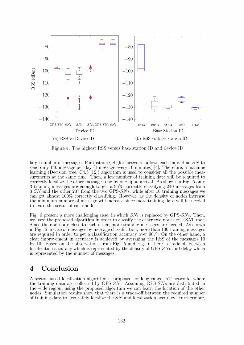
GPS-SN1 SN1 SN2 SN3 GPS-SN2 SN4
−140
−130
−120
−110
−100
−90
−80
Device ID
RS
S(d
Bm
)
(a) RSS vs Device ID
1F23 12BB 2C94 1057 11D8
−140
−130
−120
−110
−100
−90
−80
Base Station ID
(b) RSS vs Base station ID
Figure 4: The highest RSS versus base station ID and device ID
large number of messages. For instance, Sigfox networks allows each individual SN tosend only 140 message per day (1 message every 10 minutes) [4]. Therefore, a machinelearning (Decision tree, C4.5 [12]) algorithm is used to consider all the possible mea-surements at the same time. Then, a low number of training data will be required tocorrectly localize the other messages one by one upon arrival. As shown in Fig. 5 only3 training messages are enough to get a 95% correctly classifying 240 messages from3 SN and the other 237 from the two GPS-SNs, while after 10 training messages wecan get almost 100% correctly classifying. However, as the density of nodes increasethe minimum number of message will increase since more training data will be neededto learn the sector of each node.
Fig. 6 present a more challenging case, in which SN1 is replaced by GPS-SN2. Then,we used the proposed algorithm in order to classify the other two nodes on ESAT roof.Since the nodes are close to each other, more training messages are needed. As shownin Fig. 6 in case of messages by message classification, more than 100 training messagesare required in order to get a classification accuracy over 90%. On the other hand, aclear improvement in accuracy is achieved by averaging the RSS of the messages 10by 10. Based on the observations from Fig. 5 and Fig. 6 there is trade-off betweenlocalization accuracy which is represented by the density of GPS-SNs and delay whichis represented by the number of messages.
4 Conclusion
A sector-based localization algorithm is proposed for long range IoT networks wherethe training data are collected by GPS-SN . Assuming GPS-SNs are distributed inthe wide region, using the proposed algorithm we can learn the location of the othernodes. Simulation results show that there is a trade-off between the required numberof training data to accurately localize the SN and localization accuracy. Furthermore,
132
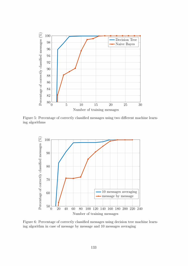
0 5 10 15 20 25 3080
82
84
86
88
90
92
94
96
98
100
Number of training messages
Per
centa
geof
corr
ectl
ycl
assi
fied
mes
sage
s(%
)Decision TreeNaive Bayes
Figure 5: Percentage of correctly classified messages using two different machine learn-ing algorithms
0 20 40 60 80 100 120 140 160 180 200 220 24050
60
70
80
90
100
Number of training messages
Per
centa
geof
corr
ectl
ycl
assi
fied
mes
sage
s(%
)
10 messages averagingmessage by message
Figure 6: Percentage of correctly classified messages using decision tree machine learn-ing algorithm in case of message by message and 10 messages averaging
133

the results show that averaging the messages finger printing measurements can improveclassification accuracy and decrease the number of training messages required.
References
[1] A. Zanella, N. Bui, A. Castellani, and L. Vangelista, “Internet of Things for SmartCities,” IEEE Internet Things J., vol. 1, no. 1, pp. 2232, Feb. 2014.
[2] R. D. Taranto, R. Raulefs, D. Slock, T. Svensson, and H. Wymeersch, “Location-aware communications for 5G networks,”IEEE Signal Process. Mag., vol. 31, no. 6,pp. 102112, Nov. 2014.
[3] B. Reynders, W. Meert, and S. Pollin, “Range and Coexistence Analysis of LongRange Unlicensed Communication,” 23rd International Conference on Telecommu-nications (ICT), pp. 390-395, May 2016.
[4] Sigfox, “http://www.sigfox.com,” 2014, accessed: May 2016.
[5] Lora alliance, http://lora-alliance.org, 2015, accessed: May 2016.
[6] S. Gezici, Z. Tian, G.B. Giannakis, H. Kobayashi, A.F. Molisch, H.V. Poor, and Z.Sahinoglu, “Localization via ultra-wideband radios,” IEEE Signal Processing Mag.,vol. 22, no. 4, pp. 7084 2005.
[7] S. Halder1 and Ghosal , “A survey on mobile anchor assisted localization techniquesin wireless sensor networks,” Springer, Wireless Networks, pp. 120, 2015.
[8] S. Fang, T. Lin, and K. Lee, “A Novel Algorithm for Multipath Fingerprinting inIndoor WLAN Environments,” IEEE Trans, Wireless Comm., vol. 7, no. 9, pp.3579-3588, Sep. 2008.
[9] K. Mikkel and Baun, “A taxonomy for radio location fingerprinting, Lecture Notesin Computer Science,” Springer vol. 4718, pp. 139156, 2007.
[10] J. Torres-Sospedra, R. Montoliu, A. Martnez-Us, T. J., J. P., Avariento, M.,Benedito Bordonau, and J., Huerta, “UJIIndoorLoc: A New Multi-building andMulti-floor Database for WLAN Fingerprintbased Indoor Localization Problems,”5th International Conference on Indoor Positioning and Indoor Navigation, 2014.
[11] S. Bozkurt1, G. Elibol, S. Gunal and U. Yayan “A Comparative Study on MachineLearning Algorithms for Indoor Positioning,” INISTA, 2015 International Sympo-sium, pp. 1-8, Sep. 2015.
[12] J. R. Quinlan, “C4.5: programs for machine learning,” Elsevier, 2014.
[13] Z. chen, F. Xia, F. Bu and H. Wang, “A localization method for the Internet ofThings,” Springer Super computing, pp. 657674, Sep 2013.
[14] G. H. John, and P. Langley, “Estimating Continuous Distributions in BayesianClassifiers,” 11th Conference on Uncertainty in Artificial Intelligence, pp., 338-345,1995.
[15] http://www.cs.waikato.ac.nz/ml/weka/, WEKA.
134
Privacy-Preserving Alpha Algorithm for SoftwareAnalysis
Gamze Tillem Zekeriya Erkin Reginald L. LagendijkDelft University of Technology
Department of Intelligent Systems, Cyber Security GroupDelft, The Netherlands
[email protected] [email protected] [email protected]
Abstract
Validation in a big software system can be managed by analysis of its be-haviour through occasionally collected event logs. Process mining is a techniqueto perform software validation by discovering process models from event logs orby checking the conformance of the logs to a process model. A well-known algo-rithm in process mining to discover process models is alpha algorithm. However,while utilising alpha algorithm is useful for software validation, the existence ofsome sensitive information in the log files may become a threat for the privacy ofusers. In this work, we propose a protocol for privacy-preserving alpha algorithmon encrypted data. Our protocol aims to generate process models for a softwarewithout leaking any information about its users. It achieves same computationalcomplexity with the original algorithm despite the additional computation over-head.
1 IntroductionSoftware systems have an evolving nature which enables them to grow continuouslywith new updates and interactions. While growth of software systems is beneficial forits functionality, conversely, it complicates managing its validation. In the traditionalapproach software validation is maintained by analysing the conformance of pre-definedcases in the design time. However, for complex software systems which has interactionswith several external tools, a priori prediction of cases is challenging. This challengeintroduces a new approach for software validation which shifts the validation procedureto online phase, namely, analysis of software in the run time. The event logs thatare generated during the execution of software, enable observation of behaviour andchecking the conformance of design requirements.
A non-trivial technique to monitor software behaviour for validation is processmining. As a field between data mining and process modeling, the aim of processmining is to discover, monitor and improve the real processes by extracting informationfrom the event logs [13]. Process mining utilises log information in three categories.The first category is process discovery which generates a process model from log data.The second category is conformance checking whose purpose is to indicate that the realbehaviour of the system conforms to the model by comparing event log of a processwith an existing process model. Finally, the third category is enhancement where anexisting process model is improved by comparing it with event logs.
As the core component of process mining, log data has a crucial role to determinein which way the software behaviour is modelled. Software log can contain informationabout user, system settings (e.g. type of operating system, number of cores, mem-ory usage), interactions with other components and the date or duration of execution.Aforementioned information is valuable for process miner to obtain knowledge aboutthe software behaviour. On the other hand, the content of information is vulnerable
135
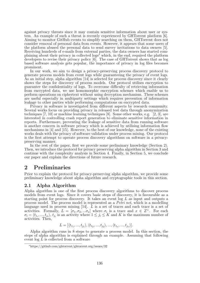
against privacy threats since it may contain sensitive information about user or sys-tem. An example of such a threat is recently experienced by GHTorrent platform [6].Aiming to monitor GitHub events to simplify searching on them, GHTorrent does notconsider removal of personal data from events. However, it appears that some users ofthe platform abused the personal data to send survey invitations to data owners [5].Receiving hundreds of e-mails from external parties, the data owners has started com-plaining about their privacy in collected logs∗ which, in the end, required the platformdevelopers to revise their privacy policy [6]. The case of GHTorrent shows that as logbased software analysis gets popular, the importance of privacy in log files becomesprominent.
In our work, we aim to design a privacy-preserving process discovery protocol togenerate process models from event logs while guaranteeing the privacy of event logs.As an initial step, alpha algorithm [14] is selected for process discovery since it clearlyshows the steps for discovery of process models. Our protocol utilises encryption toguarantee the confidentiality of logs. To overcome difficulty of retrieving informationfrom encrypted data, we use homomorphic encryption schemes which enable us toperform operations on ciphertext without using decryption mechanism. These schemesare useful especially in multiparty settings which requires prevention of informationleakage to other parties while performing computations on encrypted data.
Privacy in software is investigated from different aspects by research community.Several works focus on providing privacy in released test data through anonymizationtechniques [7, 10] or machine learning techniques [8]. Some other works, e.g. [2, 3], areinterested in controlling crash report generation to eliminate sensitive information inreports. Furthermore, preventing the leakage of sensitive data from running softwareis another concern in software privacy which is achieved by utilising information flowmechanisms in [4] and [15]. However, to the best of our knowledge, none of the existingworks deals with the privacy of software validation under process mining. Our protocolis the first attempt to operate process discovery algorithms on software in a privacy-preserving manner.
In the rest of the paper, first we provide some preliminary knowledge (Section 2).Then, we introduce the protocol for privacy preserving alpha algorithm in Section 3 andcontinue with the complexity analysis in Section 4. Finally, in Section 5, we concludeour paper and explain the directions of future research.
2 PreliminariesPrior to explain the protocol for privacy-preserving alpha algorithm, we provide somepreliminary knowledge about alpha algorithm and cryptographic tools in this section.
2.1 Alpha AlgorithmAlpha algorithm is one of the first process discovery algorithms to discover processmodels from event logs. Since it covers basic steps of discovery, it is favourable as astarting point for process discovery. It takes an event log L as input and outputs aprocess model. The process model is represented as a Petri net, which is a modellinglanguage used in process mining [14]. L is a set of traces and each trace is a set ofactivities. Formally, L = [σ1, σ2, ...σx] where σi is a trace and x ∈ Z+. For eachσi = 〈t1i , ..., tji〉, tji is an activity where 1 ≤ ji ≤ K and K is the maximum number ofactivities. Then,
L = [〈t11 , ..., tj1〉, 〈t12 , ..., tj2〉, ..., 〈t1x , ..., tjx〉].Alpha algorithm runs in 8 steps to generate a process model. In this section, the
steps of alpha algorithm is explained through an example. Assuming that followingevent log L is collected from a software
∗https://github.com/ghtorrent/ghtorrent.org/issues/32
136
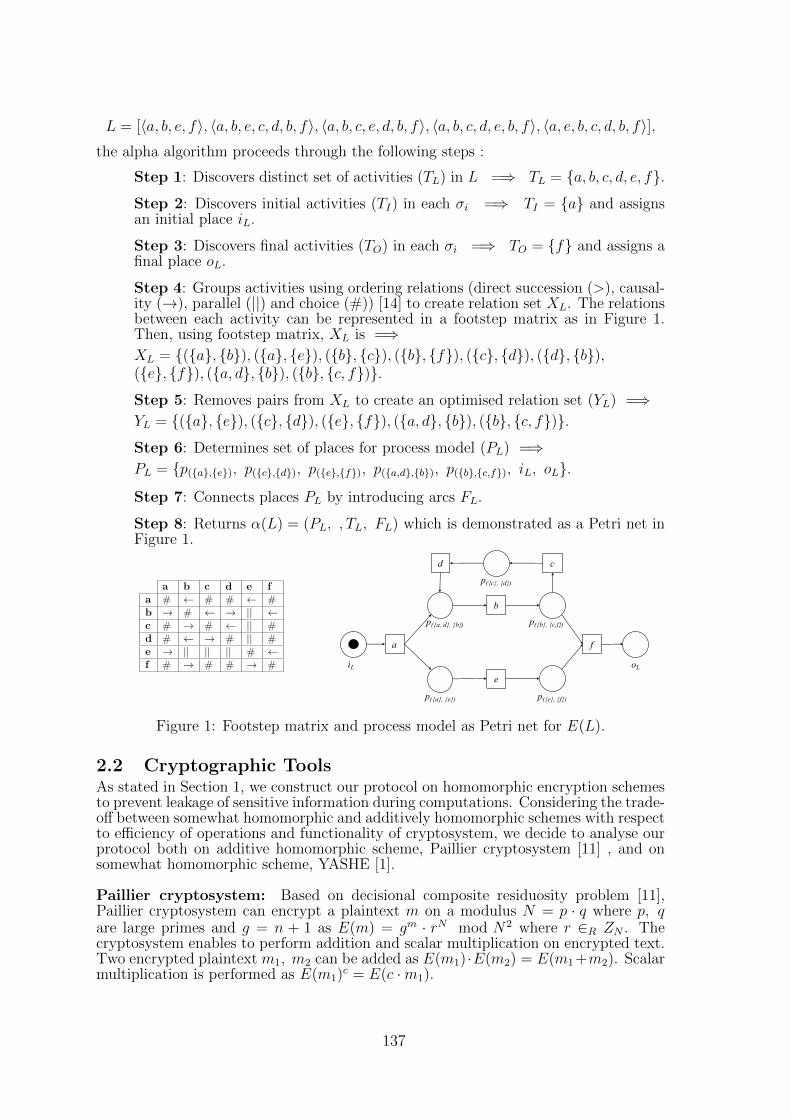
L = [〈a, b, e, f〉, 〈a, b, e, c, d, b, f〉, 〈a, b, c, e, d, b, f〉, 〈a, b, c, d, e, b, f〉, 〈a, e, b, c, d, b, f〉],the alpha algorithm proceeds through the following steps :
Step 1: Discovers distinct set of activities (TL) in L =⇒ TL = a, b, c, d, e, f.Step 2: Discovers initial activities (TI) in each σi =⇒ TI = a and assignsan initial place iL.
Step 3: Discovers final activities (TO) in each σi =⇒ TO = f and assigns afinal place oL.
Step 4: Groups activities using ordering relations (direct succession (>), causal-ity (→), parallel (||) and choice (#)) [14] to create relation set XL. The relationsbetween each activity can be represented in a footstep matrix as in Figure 1.Then, using footstep matrix, XL is =⇒XL = (a, b), (a, e), (b, c), (b, f), (c, d), (d, b),(e, f), (a, d, b), (b, c, f).Step 5: Removes pairs from XL to create an optimised relation set (YL) =⇒YL = (a, e), (c, d), (e, f), (a, d, b), (b, c, f).Step 6: Determines set of places for process model (PL) =⇒PL = p(a,e), p(c,d), p(e,f), p(a,d,b), p(b,c,f), iL, oL.Step 7: Connects places PL by introducing arcs FL.
Step 8: Returns α(L) = (PL, , TL, FL) which is demonstrated as a Petri net inFigure 1.
a b c d e fa # ← # # ← #b → # ← → || ←c # → # ← || #d # ← → # || #e → || || || # ←f # → # # → # iL oL
p(b, c,f)
p(e, f)
p(c, d)
a
p(a, d, b)
p(a, e)
d
b
c
e
f
Figure 1: Footstep matrix and process model as Petri net for E(L).
2.2 Cryptographic ToolsAs stated in Section 1, we construct our protocol on homomorphic encryption schemesto prevent leakage of sensitive information during computations. Considering the trade-off between somewhat homomorphic and additively homomorphic schemes with respectto efficiency of operations and functionality of cryptosystem, we decide to analyse ourprotocol both on additive homomorphic scheme, Paillier cryptosystem [11] , and onsomewhat homomorphic scheme, YASHE [1].
Paillier cryptosystem: Based on decisional composite residuosity problem [11],Paillier cryptosystem can encrypt a plaintext m on a modulus N = p · q where p, qare large primes and g = n + 1 as E(m) = gm · rN mod N2 where r ∈R ZN . Thecryptosystem enables to perform addition and scalar multiplication on encrypted text.Two encrypted plaintext m1, m2 can be added as E(m1) ·E(m2) = E(m1 +m2). Scalarmultiplication is performed as E(m1)c = E(c ·m1).
137
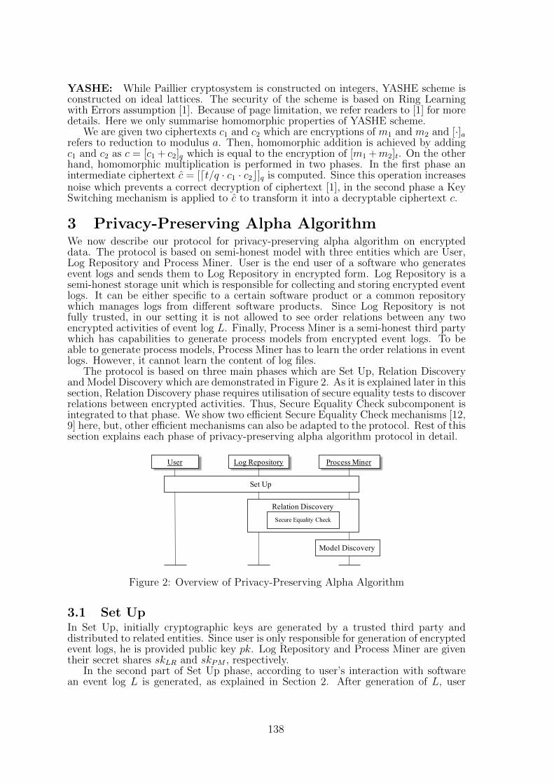
YASHE: While Paillier cryptosystem is constructed on integers, YASHE scheme isconstructed on ideal lattices. The security of the scheme is based on Ring Learningwith Errors assumption [1]. Because of page limitation, we refer readers to [1] for moredetails. Here we only summarise homomorphic properties of YASHE scheme.
We are given two ciphertexts c1 and c2 which are encryptions of m1 and m2 and [·]arefers to reduction to modulus a. Then, homomorphic addition is achieved by addingc1 and c2 as c = [c1 + c2]q which is equal to the encryption of [m1 +m2]t. On the otherhand, homomorphic multiplication is performed in two phases. In the first phase anintermediate ciphertext c = [dt/q · c1 · c2c]q is computed. Since this operation increasesnoise which prevents a correct decryption of ciphertext [1], in the second phase a KeySwitching mechanism is applied to c to transform it into a decryptable ciphertext c.
3 Privacy-Preserving Alpha AlgorithmWe now describe our protocol for privacy-preserving alpha algorithm on encrypteddata. The protocol is based on semi-honest model with three entities which are User,Log Repository and Process Miner. User is the end user of a software who generatesevent logs and sends them to Log Repository in encrypted form. Log Repository is asemi-honest storage unit which is responsible for collecting and storing encrypted eventlogs. It can be either specific to a certain software product or a common repositorywhich manages logs from different software products. Since Log Repository is notfully trusted, in our setting it is not allowed to see order relations between any twoencrypted activities of event log L. Finally, Process Miner is a semi-honest third partywhich has capabilities to generate process models from encrypted event logs. To beable to generate process models, Process Miner has to learn the order relations in eventlogs. However, it cannot learn the content of log files.
The protocol is based on three main phases which are Set Up, Relation Discoveryand Model Discovery which are demonstrated in Figure 2. As it is explained later in thissection, Relation Discovery phase requires utilisation of secure equality tests to discoverrelations between encrypted activities. Thus, Secure Equality Check subcomponent isintegrated to that phase. We show two efficient Secure Equality Check mechanisms [12,9] here, but, other efficient mechanisms can also be adapted to the protocol. Rest of thissection explains each phase of privacy-preserving alpha algorithm protocol in detail.
User LogRepositoryLog Repository Process Miner
Set Up
Relation Discovery
Secure Equality Check
Model Discovery
Figure 2: Overview of Privacy-Preserving Alpha Algorithm
3.1 Set UpIn Set Up, initially cryptographic keys are generated by a trusted third party anddistributed to related entities. Since user is only responsible for generation of encryptedevent logs, he is provided public key pk. Log Repository and Process Miner are giventheir secret shares skLR and skPM , respectively.
In the second part of Set Up phase, according to user’s interaction with softwarean event log L is generated, as explained in Section 2. After generation of L, user
138
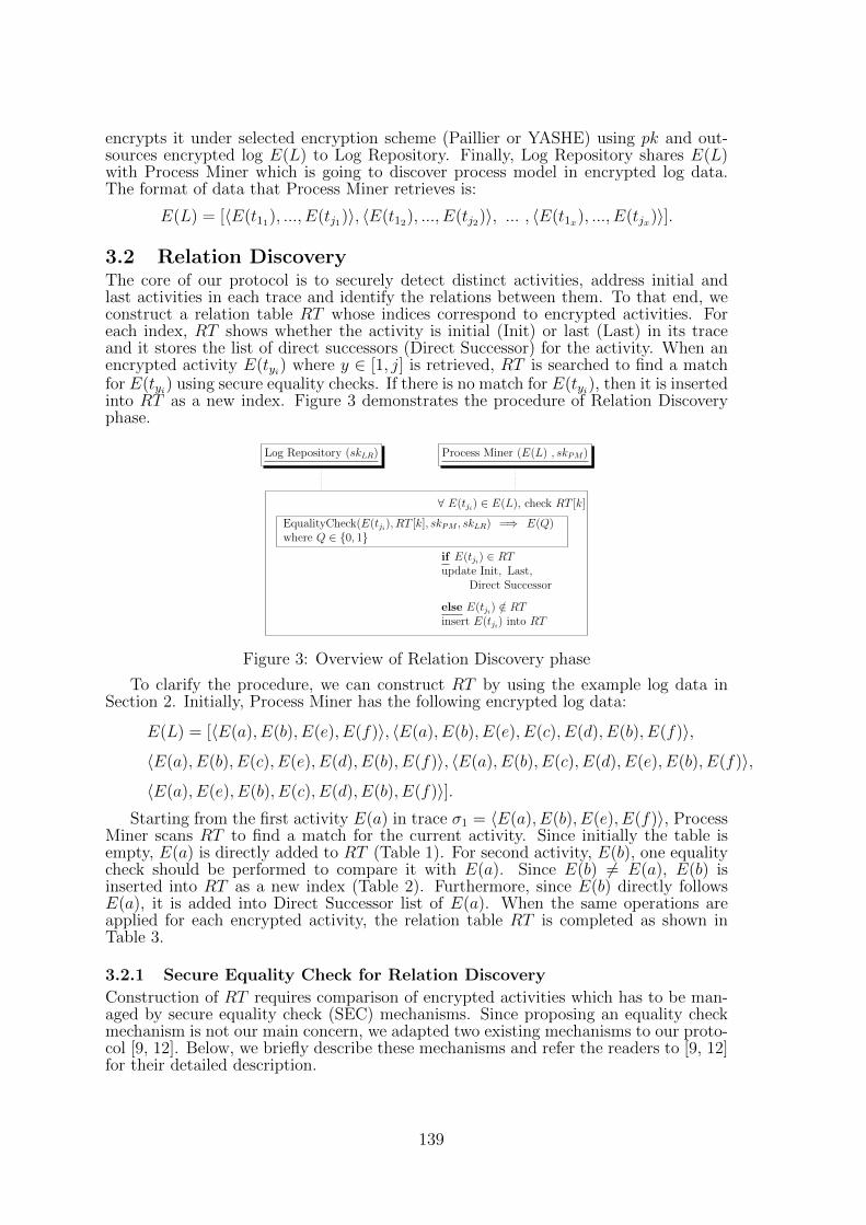
encrypts it under selected encryption scheme (Paillier or YASHE) using pk and out-sources encrypted log E(L) to Log Repository. Finally, Log Repository shares E(L)with Process Miner which is going to discover process model in encrypted log data.The format of data that Process Miner retrieves is:
E(L) = [〈E(t11), ..., E(tj1)〉, 〈E(t12), ..., E(tj2)〉, ... , 〈E(t1x), ..., E(tjx)〉].
3.2 Relation DiscoveryThe core of our protocol is to securely detect distinct activities, address initial andlast activities in each trace and identify the relations between them. To that end, weconstruct a relation table RT whose indices correspond to encrypted activities. Foreach index, RT shows whether the activity is initial (Init) or last (Last) in its traceand it stores the list of direct successors (Direct Successor) for the activity. When anencrypted activity E(tyi) where y ∈ [1, j] is retrieved, RT is searched to find a matchfor E(tyi) using secure equality checks. If there is no match for E(tyi), then it is insertedinto RT as a new index. Figure 3 demonstrates the procedure of Relation Discoveryphase.
Log Repository (skLR) Process Miner (E(L) , skPM)
∀ E(tji) ∈ E(L), check RT [k]
if E(tji) ∈ RTupdate Init, Last,
Direct Successor
else E(tji) /∈ RTinsert E(tji) into RT
EqualityCheck(E(tji), RT [k], skPM , skLR) =⇒ E(Q)where Q ∈ 0, 1
Figure 3: Overview of Relation Discovery phase
To clarify the procedure, we can construct RT by using the example log data inSection 2. Initially, Process Miner has the following encrypted log data:
E(L) = [〈E(a), E(b), E(e), E(f)〉, 〈E(a), E(b), E(e), E(c), E(d), E(b), E(f)〉,〈E(a), E(b), E(c), E(e), E(d), E(b), E(f)〉, 〈E(a), E(b), E(c), E(d), E(e), E(b), E(f)〉,〈E(a), E(e), E(b), E(c), E(d), E(b), E(f)〉].
Starting from the first activity E(a) in trace σ1 = 〈E(a), E(b), E(e), E(f)〉, ProcessMiner scans RT to find a match for the current activity. Since initially the table isempty, E(a) is directly added to RT (Table 1). For second activity, E(b), one equalitycheck should be performed to compare it with E(a). Since E(b) 6= E(a), E(b) isinserted into RT as a new index (Table 2). Furthermore, since E(b) directly followsE(a), it is added into Direct Successor list of E(a). When the same operations areapplied for each encrypted activity, the relation table RT is completed as shown inTable 3.
3.2.1 Secure Equality Check for Relation Discovery
Construction of RT requires comparison of encrypted activities which has to be man-aged by secure equality check (SEC) mechanisms. Since proposing an equality checkmechanism is not our main concern, we adapted two existing mechanisms to our proto-col [9, 12]. Below, we briefly describe these mechanisms and refer the readers to [9, 12]for their detailed description.
139

Index Init LastDirect
SuccessorE(a) 0 + +
Table 1: RT with one element
Index Init LastDirect
SuccessorE(a) 0 + + 1E(b) 1 - -
Table 2: Inserting E(b) into RT
Index Init LastDirect
SuccessorE(a) 0 + + 1, 2E(b) 1 - - 2, 3, 4E(e) 2 - - 1, 3, 4, 5E(f) 3 - + -E(c) 4 - - 2, 5E(d) 5 - - 1, 2
Table 3: Complete version of relation table RT
SEC by Toft [12]: Toft [12] proposes a SEC protocol by employing Jacobi symbol.The protocol requires a virtual trusted third party which is Arithmetic Black Box(ABB) to provide secure storage and to perform arithmetic computations. The equalityof two values is tested by testing whether their difference d is equal to 0. For anencryption modulus M , if d = 0, then Jacobi symbol for d + r2 where r ∈R M is
Jd+r2 =
(d+ r2
M
)= 1. Otherwise, if d 6= 0, Jd+r2 = −1. Although, Toft’s scheme is
efficient, the result is correct with 1/2 probability due to probabilistic nature of Jacobisymbol. Thus, reducing the probability to a negligible degree requires the repetitionof protocol κ times with the same input.
SEC by Lipmaa & Toft [9]: Different from [12], Lipmaa and Toft [9] introduce aSEC protocol which utilises Hamming distance. Similar to [12], the protocol is basedon zero check for difference d and ABB is responsible for secure storage and arithmeticcomputations. Hamming distance is computed between a random r and m = r + d.To reduce the complexity of operations in Hamming distance computation, an offlinepreprocessing phase to compute random values, random inverses and random exponentsis proposed. Furthermore, for online phase Lagrange interpolation is used. Althoughthe result of the protocol is deterministic, it has drawback of computational complexitywhich is bounded by the bit length of encryption modulus M .
3.3 Model DiscoveryAfter discovery of the order relations between encrypted activities, the final phase ofour protocol generates the process model using the information in RT . In the originalalgorithm, a footstep matrix is constructed to demonstrate casual, parallel and choicerelations between activities based on direct successions (see Section 2). In the samemanner, our protocol constructs the footstep matrix using Direct Successor lists in RT .Finally, the process model as a Petri net is generated using the ordering relations infootstep matrix as it is showed in Figure 4.
4 Complexity AnalysisUtilising encryption is advantageous to maintain the confidentiality of log files. How-ever, a qualified scheme for software analysis should also consider the efficiency ofcomputations for practicability. Thus, in this section we analyse the complexity of ourprotocol.
To evaluate performance of our protocol, initially we have to investigate the com-plexity of original alpha algorithm. Since in the original algorithm computations are
140
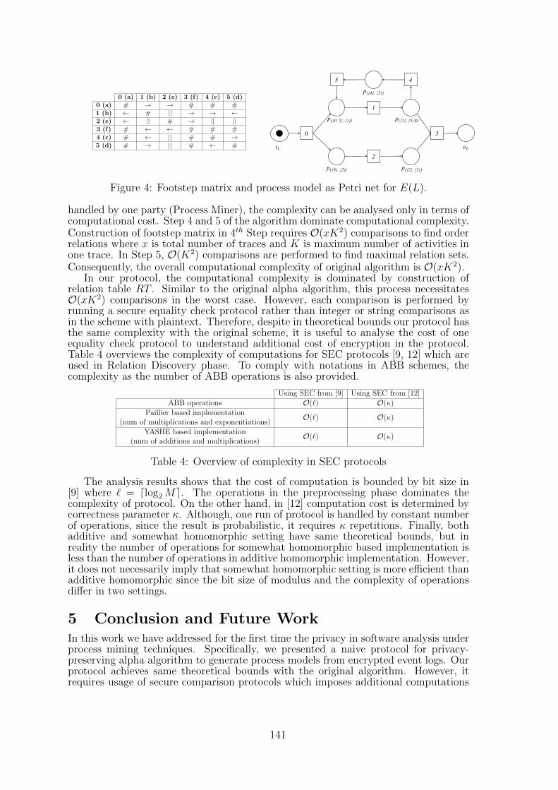
0 (a) 1 (b) 2 (e) 3 (f) 4 (c) 5 (d)0 (a) # → → # # #1 (b) ← # || → → ←2 (e) ← || # → || ||3 (f) # ← ← # # #4 (c) # ← || # # →5 (d) # → || # ← # iL oL
p(1, 3,4)
p(2, 3)
p(4, 5)
0
p(0, 5, 1)
p(0, 2)
5
1
4
2
3
Figure 4: Footstep matrix and process model as Petri net for E(L).
handled by one party (Process Miner), the complexity can be analysed only in terms ofcomputational cost. Step 4 and 5 of the algorithm dominate computational complexity.Construction of footstep matrix in 4th Step requires O(xK2) comparisons to find orderrelations where x is total number of traces and K is maximum number of activities inone trace. In Step 5, O(K2) comparisons are performed to find maximal relation sets.Consequently, the overall computational complexity of original algorithm is O(xK2).
In our protocol, the computational complexity is dominated by construction ofrelation table RT . Similar to the original alpha algorithm, this process necessitatesO(xK2) comparisons in the worst case. However, each comparison is performed byrunning a secure equality check protocol rather than integer or string comparisons asin the scheme with plaintext. Therefore, despite in theoretical bounds our protocol hasthe same complexity with the original scheme, it is useful to analyse the cost of oneequality check protocol to understand additional cost of encryption in the protocol.Table 4 overviews the complexity of computations for SEC protocols [9, 12] which areused in Relation Discovery phase. To comply with notations in ABB schemes, thecomplexity as the number of ABB operations is also provided.
Using SEC from [9] Using SEC from [12]ABB operations O(`) O(κ)
Paillier based implementation(num of multiplications and exponentiations)
O(`) O(κ)
YASHE based implementation(num of additions and multiplications)
O(`) O(κ)
Table 4: Overview of complexity in SEC protocols
The analysis results shows that the cost of computation is bounded by bit size in[9] where ` = dlog2Me. The operations in the preprocessing phase dominates thecomplexity of protocol. On the other hand, in [12] computation cost is determined bycorrectness parameter κ. Although, one run of protocol is handled by constant numberof operations, since the result is probabilistic, it requires κ repetitions. Finally, bothadditive and somewhat homomorphic setting have same theoretical bounds, but inreality the number of operations for somewhat homomorphic based implementation isless than the number of operations in additive homomorphic implementation. However,it does not necessarily imply that somewhat homomorphic setting is more efficient thanadditive homomorphic since the bit size of modulus and the complexity of operationsdiffer in two settings.
5 Conclusion and Future WorkIn this work we have addressed for the first time the privacy in software analysis underprocess mining techniques. Specifically, we presented a naive protocol for privacy-preserving alpha algorithm to generate process models from encrypted event logs. Ourprotocol achieves same theoretical bounds with the original algorithm. However, itrequires usage of secure comparison protocols which imposes additional computations
141

with larger bit sizes. In the future, we continue exploring privacy issues in differentalgorithms of process mining for software analysis. Furthermore, we extend our re-search with implementation of algorithms and utilisation of other privacy enhancingtechnologies.
References[1] Joppe W Bos, Kristin Lauter, Jake Loftus, and Michael Naehrig. Improved security for a ring-based fully homo-
morphic encryption scheme. In Cryptography and Coding, pages 45–64. Springer, 2013.
[2] Pete Broadwell, Matt Harren, and Naveen Sastry. Scrash: A system for generating secure crash information. InProceedings of the 12th conference on USENIX Security Symposium-Volume 12, pages 19–19. USENIX Association,2003.
[3] Miguel Castro, Manuel Costa, and Jean-Philippe Martin. Better bug reporting with better privacy. In ACMSigplan Notices, volume 43, pages 319–328. ACM, 2008.
[4] William Enck, Peter Gilbert, Seungyeop Han, Vasant Tendulkar, Byung-Gon Chun, Landon P Cox, Jaeyeon Jung,Patrick McDaniel, and Anmol N Sheth. Taintdroid: an information-flow tracking system for realtime privacymonitoring on smartphones. ACM Transactions on Computer Systems (TOCS), 32(2):5, 2014.
[5] Arnoud Engelfriet. Is it legal for ghtorrent to aggregate github user data? https://legalict.com/privacy/
is-it-legal-for-ghtorrent-to-aggregate-github-user-data/, 2016. Accessed May 3, 2016.
[6] Georgios Gousios. The issue 32 incident an update. http://gousios.gr/blog/Issue-thirty-two, 2016. AccessedMay 3, 2016.
[7] Mark Grechanik, Christoph Csallner, Chen Fu, and Qing Xie. Is data privacy always good for software testing?In Software Reliability Engineering (ISSRE), 2010 IEEE 21st International Symposium on, pages 368–377. IEEE,2010.
[8] Boyang Li. Enhancing utility and privacy of data for software testing. In Software Testing, Verification andValidation Workshops (ICSTW), 2014 IEEE Seventh International Conference on, pages 233–234. IEEE, 2014.
[9] Helger Lipmaa and Tomas Toft. Secure equality and greater-than tests with sublinear online complexity. InAutomata, Languages, and Programming, pages 645–656. Springer, 2013.
[10] David Lo, Lingxiao Jiang, Aditya Budi, et al. kbe-anonymity: test data anonymization for evolving programs. InProceedings of the 27th IEEE/ACM International Conference on Automated Software Engineering, pages 262–265.ACM, 2012.
[11] Pascal Paillier. Public-key cryptosystems based on composite degree residuosity classes. In Advances in cryptol-ogy–EUROCRYPT–99, pages 223–238. Springer, 1999.
[12] Tomas Toft. Sub-linear, secure comparison with two non-colluding parties. In Public Key Cryptography–PKC2011, pages 174–191. Springer, 2011.
[13] Wil Van Der Aalst, Arya Adriansyah, Ana Karla Alves de Medeiros, Franco Arcieri, Thomas Baier, Tobias Blickle,Jagadeesh Chandra Bose, Peter van den Brand, Ronald Brandtjen, Joos Buijs, et al. Process mining manifesto.In Business process management workshops, pages 169–194. Springer, 2011.
[14] Wil Van der Aalst, Ton Weijters, and Laura Maruster. Workflow mining: Discovering process models from eventlogs. Knowledge and Data Engineering, IEEE Transactions on, 16(9):1128–1142, 2004.
[15] David Yu Zhu, Jaeyeon Jung, Dawn Song, Tadayoshi Kohno, and David Wetherall. Tainteraser: protecting sensitivedata leaks using application-level taint tracking. ACM SIGOPS Operating Systems Review, 45(1):142–154, 2011.
142
A framework for processing cardiac signalsacquired by multiple unobtrusive wearable sensors
Silviu Dovancescu 1 Attila Para 1,2 Dan Stefanoiu 2
1 Philips ResearchEindhoven, The Netherlands
2 Politehnica University of BucharestDept. of Automatic Control and Systems Engineering
Bucharest, [email protected]
Abstract
Emerging wearable technologies, such as smartwatches or band aid-like sensors,enable unobtrusive continuous monitoring of cardiac signals anytime and any-where. Users of these technologies generate an increasing demand for personalhealth applications to support disease prevention as well as a healthy lifestyle.As a first step in the development of personal health applications for wearables,researchers usually perform studies which include data collection using wearablephysiological sensors in parallel with clinically accepted monitoring systems thatserve as a reference. Handling the resulting large amounts of heterogeneous dataremains challenging. In this paper, we present a framework for cardiac signalprocessing that facilitates research into personal health applications based onwearable sensors. We showcase the use of the framework in a feasibility studyof unobtrusive blood pressure (BP) monitoring based on photoplethysmographic(PPG) and electrocardiographic (ECG) signals from wearable sensors.
1 Introduction
Cardiac signals represent a rich source of information on the general health statusand the well-being of individuals. Monitored continuously over long periods of time,these signals may reveal concealed cardiac disorders or indicate early stages of healthdegradation.
Traditionally, the electrical activity of the heart, reflected by the electrocardiogram(ECG), has been the target of long term monitoring. ECG monitoring consists ofmeasuring the potential between two or more points on the body. Beside the in-hospital use, ECG is also widely used both in home health care (e.g. Holter monitor,peel-and-stick patch) and sports applications (e.g. chest strap).
The photoplethysmogram (PPG) is a non-invasive circulatory signal which reflectsthe total volume changes in all blood vessels. It uses a single point measurement withoptical skin contact, which is less obtrusive compared to the traditional ECG. PPGrequires a LED to irradiate the tissue and a photodetector, which measures the lightintensity. There are two different techniques for PPG monitoring: transmission modeand reflexive mode PPG. In transmission mode the LED and the photodetector are onthe opposite side of a thinner part of the body (e.g. finger, earlobe), while in reflexivemode the photodetector is placed alongside the LED. In the latter case the light isreflected by deeper structures and absorbed in blood vessels [1].
143
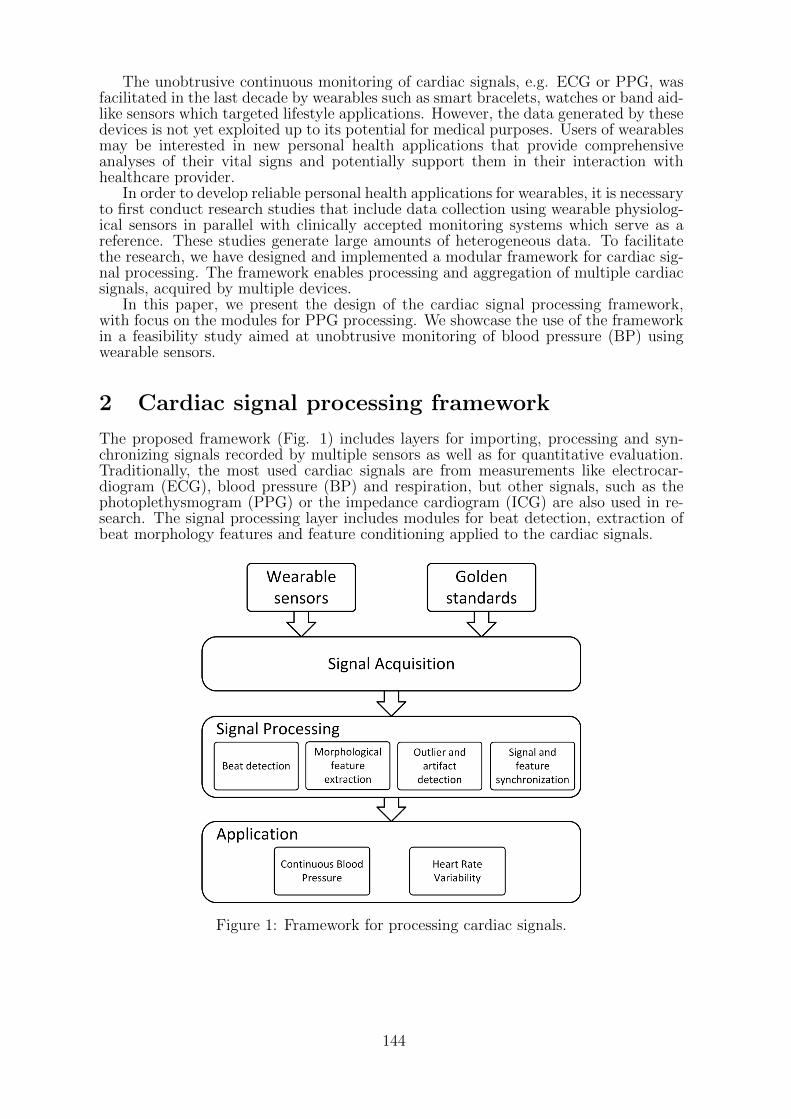
The unobtrusive continuous monitoring of cardiac signals, e.g. ECG or PPG, wasfacilitated in the last decade by wearables such as smart bracelets, watches or band aid-like sensors which targeted lifestyle applications. However, the data generated by thesedevices is not yet exploited up to its potential for medical purposes. Users of wearablesmay be interested in new personal health applications that provide comprehensiveanalyses of their vital signs and potentially support them in their interaction withhealthcare provider.
In order to develop reliable personal health applications for wearables, it is necessaryto first conduct research studies that include data collection using wearable physiolog-ical sensors in parallel with clinically accepted monitoring systems which serve as areference. These studies generate large amounts of heterogeneous data. To facilitatethe research, we have designed and implemented a modular framework for cardiac sig-nal processing. The framework enables processing and aggregation of multiple cardiacsignals, acquired by multiple devices.
In this paper, we present the design of the cardiac signal processing framework,with focus on the modules for PPG processing. We showcase the use of the frameworkin a feasibility study aimed at unobtrusive monitoring of blood pressure (BP) usingwearable sensors.
2 Cardiac signal processing framework
The proposed framework (Fig. 1) includes layers for importing, processing and syn-chronizing signals recorded by multiple sensors as well as for quantitative evaluation.Traditionally, the most used cardiac signals are from measurements like electrocar-diogram (ECG), blood pressure (BP) and respiration, but other signals, such as thephotoplethysmogram (PPG) or the impedance cardiogram (ICG) are also used in re-search. The signal processing layer includes modules for beat detection, extraction ofbeat morphology features and feature conditioning applied to the cardiac signals.
Figure 1: Framework for processing cardiac signals.
144
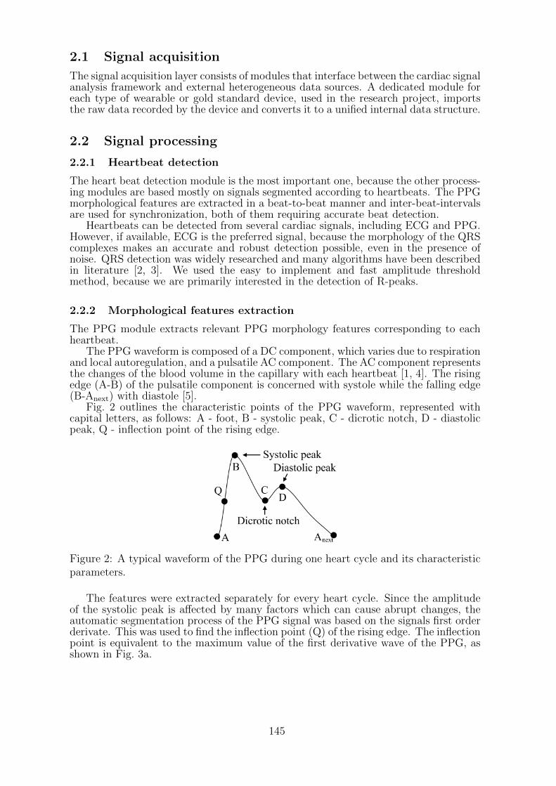
2.1 Signal acquisition
The signal acquisition layer consists of modules that interface between the cardiac signalanalysis framework and external heterogeneous data sources. A dedicated module foreach type of wearable or gold standard device, used in the research project, importsthe raw data recorded by the device and converts it to a unified internal data structure.
2.2 Signal processing
2.2.1 Heartbeat detection
The heart beat detection module is the most important one, because the other process-ing modules are based mostly on signals segmented according to heartbeats. The PPGmorphological features are extracted in a beat-to-beat manner and inter-beat-intervalsare used for synchronization, both of them requiring accurate beat detection.
Heartbeats can be detected from several cardiac signals, including ECG and PPG.However, if available, ECG is the preferred signal, because the morphology of the QRScomplexes makes an accurate and robust detection possible, even in the presence ofnoise. QRS detection was widely researched and many algorithms have been describedin literature [2, 3]. We used the easy to implement and fast amplitude thresholdmethod, because we are primarily interested in the detection of R-peaks.
2.2.2 Morphological features extraction
The PPG module extracts relevant PPG morphology features corresponding to eachheartbeat.
The PPG waveform is composed of a DC component, which varies due to respirationand local autoregulation, and a pulsatile AC component. The AC component representsthe changes of the blood volume in the capillary with each heartbeat [1, 4]. The risingedge (A-B) of the pulsatile component is concerned with systole while the falling edge(B-Anext) with diastole [5].
Fig. 2 outlines the characteristic points of the PPG waveform, represented withcapital letters, as follows: A - foot, B - systolic peak, C - dicrotic notch, D - diastolicpeak, Q - inflection point of the rising edge.
Figure 2: A typical waveform of the PPG during one heart cycle and its characteristicparameters.
The features were extracted separately for every heart cycle. Since the amplitudeof the systolic peak is affected by many factors which can cause abrupt changes, theautomatic segmentation process of the PPG signal was based on the signals first orderderivate. This was used to find the inflection point (Q) of the rising edge. The inflectionpoint is equivalent to the maximum value of the first derivative wave of the PPG, asshown in Fig. 3a.
145
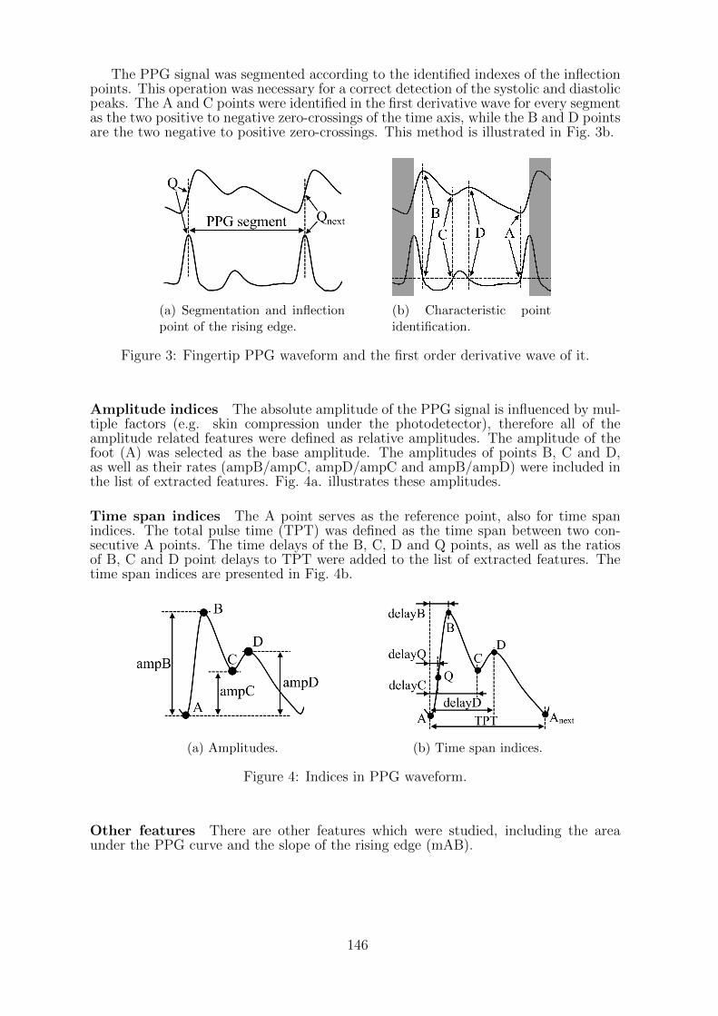
The PPG signal was segmented according to the identified indexes of the inflectionpoints. This operation was necessary for a correct detection of the systolic and diastolicpeaks. The A and C points were identified in the first derivative wave for every segmentas the two positive to negative zero-crossings of the time axis, while the B and D pointsare the two negative to positive zero-crossings. This method is illustrated in Fig. 3b.
(a) Segmentation and inflectionpoint of the rising edge.
(b) Characteristic pointidentification.
Figure 3: Fingertip PPG waveform and the first order derivative wave of it.
Amplitude indices The absolute amplitude of the PPG signal is influenced by mul-tiple factors (e.g. skin compression under the photodetector), therefore all of theamplitude related features were defined as relative amplitudes. The amplitude of thefoot (A) was selected as the base amplitude. The amplitudes of points B, C and D,as well as their rates (ampB/ampC, ampD/ampC and ampB/ampD) were included inthe list of extracted features. Fig. 4a. illustrates these amplitudes.
Time span indices The A point serves as the reference point, also for time spanindices. The total pulse time (TPT) was defined as the time span between two con-secutive A points. The time delays of the B, C, D and Q points, as well as the ratiosof B, C and D point delays to TPT were added to the list of extracted features. Thetime span indices are presented in Fig. 4b.
(a) Amplitudes. (b) Time span indices.
Figure 4: Indices in PPG waveform.
Other features There are other features which were studied, including the areaunder the PPG curve and the slope of the rising edge (mAB).
146
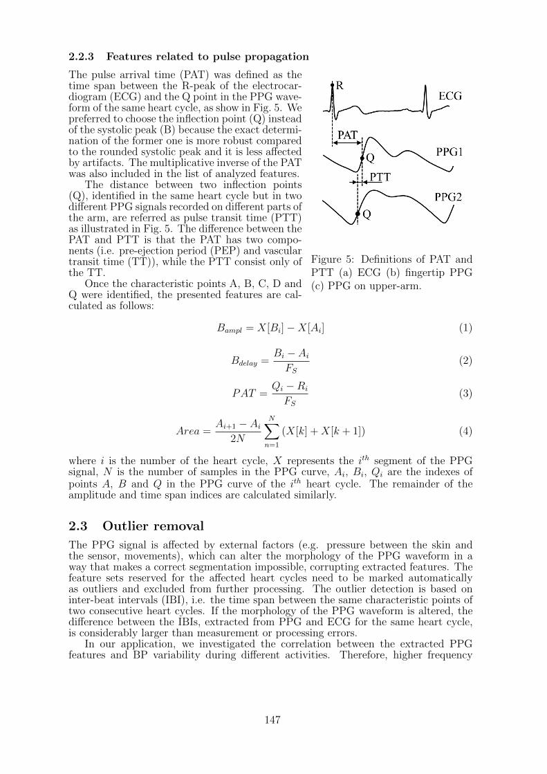
2.2.3 Features related to pulse propagation
Figure 5: Definitions of PAT andPTT (a) ECG (b) fingertip PPG(c) PPG on upper-arm.
The pulse arrival time (PAT) was defined as thetime span between the R-peak of the electrocar-diogram (ECG) and the Q point in the PPG wave-form of the same heart cycle, as show in Fig. 5. Wepreferred to choose the inflection point (Q) insteadof the systolic peak (B) because the exact determi-nation of the former one is more robust comparedto the rounded systolic peak and it is less affectedby artifacts. The multiplicative inverse of the PATwas also included in the list of analyzed features.
The distance between two inflection points(Q), identified in the same heart cycle but in twodifferent PPG signals recorded on different parts ofthe arm, are referred as pulse transit time (PTT)as illustrated in Fig. 5. The difference between thePAT and PTT is that the PAT has two compo-nents (i.e. pre-ejection period (PEP) and vasculartransit time (TT)), while the PTT consist only ofthe TT.
Once the characteristic points A, B, C, D andQ were identified, the presented features are cal-culated as follows:
Bampl = X[Bi]−X[Ai] (1)
Bdelay =Bi − AiFS
(2)
PAT =Qi −Ri
FS(3)
Area =Ai+1 − Ai
2N
N∑
n=1
(X[k] +X[k + 1]) (4)
where i is the number of the heart cycle, X represents the ith segment of the PPGsignal, N is the number of samples in the PPG curve, Ai, Bi, Qi are the indexes ofpoints A, B and Q in the PPG curve of the ith heart cycle. The remainder of theamplitude and time span indices are calculated similarly.
2.3 Outlier removal
The PPG signal is affected by external factors (e.g. pressure between the skin andthe sensor, movements), which can alter the morphology of the PPG waveform in away that makes a correct segmentation impossible, corrupting extracted features. Thefeature sets reserved for the affected heart cycles need to be marked automaticallyas outliers and excluded from further processing. The outlier detection is based oninter-beat intervals (IBI), i.e. the time span between the same characteristic points oftwo consecutive heart cycles. If the morphology of the PPG waveform is altered, thedifference between the IBIs, extracted from PPG and ECG for the same heart cycle,is considerably larger than measurement or processing errors.
In our application, we investigated the correlation between the extracted PPGfeatures and BP variability during different activities. Therefore, higher frequency
147
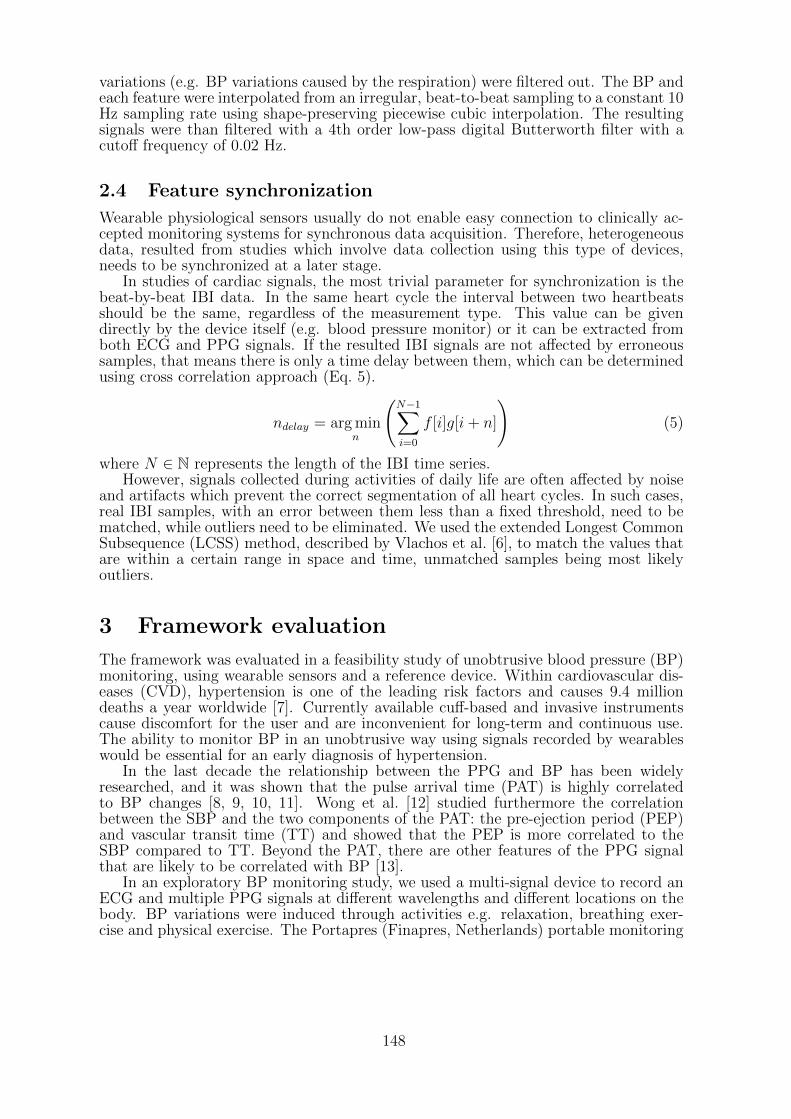
variations (e.g. BP variations caused by the respiration) were filtered out. The BP andeach feature were interpolated from an irregular, beat-to-beat sampling to a constant 10Hz sampling rate using shape-preserving piecewise cubic interpolation. The resultingsignals were than filtered with a 4th order low-pass digital Butterworth filter with acutoff frequency of 0.02 Hz.
2.4 Feature synchronization
Wearable physiological sensors usually do not enable easy connection to clinically ac-cepted monitoring systems for synchronous data acquisition. Therefore, heterogeneousdata, resulted from studies which involve data collection using this type of devices,needs to be synchronized at a later stage.
In studies of cardiac signals, the most trivial parameter for synchronization is thebeat-by-beat IBI data. In the same heart cycle the interval between two heartbeatsshould be the same, regardless of the measurement type. This value can be givendirectly by the device itself (e.g. blood pressure monitor) or it can be extracted fromboth ECG and PPG signals. If the resulted IBI signals are not affected by erroneoussamples, that means there is only a time delay between them, which can be determinedusing cross correlation approach (Eq. 5).
ndelay = arg minn
(N−1∑
i=0
f [i]g[i+ n]
)(5)
where N ∈ N represents the length of the IBI time series.However, signals collected during activities of daily life are often affected by noise
and artifacts which prevent the correct segmentation of all heart cycles. In such cases,real IBI samples, with an error between them less than a fixed threshold, need to bematched, while outliers need to be eliminated. We used the extended Longest CommonSubsequence (LCSS) method, described by Vlachos et al. [6], to match the values thatare within a certain range in space and time, unmatched samples being most likelyoutliers.
3 Framework evaluation
The framework was evaluated in a feasibility study of unobtrusive blood pressure (BP)monitoring, using wearable sensors and a reference device. Within cardiovascular dis-eases (CVD), hypertension is one of the leading risk factors and causes 9.4 milliondeaths a year worldwide [7]. Currently available cuff-based and invasive instrumentscause discomfort for the user and are inconvenient for long-term and continuous use.The ability to monitor BP in an unobtrusive way using signals recorded by wearableswould be essential for an early diagnosis of hypertension.
In the last decade the relationship between the PPG and BP has been widelyresearched, and it was shown that the pulse arrival time (PAT) is highly correlatedto BP changes [8, 9, 10, 11]. Wong et al. [12] studied furthermore the correlationbetween the SBP and the two components of the PAT: the pre-ejection period (PEP)and vascular transit time (TT) and showed that the PEP is more correlated to theSBP compared to TT. Beyond the PAT, there are other features of the PPG signalthat are likely to be correlated with BP [13].
In an exploratory BP monitoring study, we used a multi-signal device to record anECG and multiple PPG signals at different wavelengths and different locations on thebody. BP variations were induced through activities e.g. relaxation, breathing exer-cise and physical exercise. The Portapres (Finapres, Netherlands) portable monitoring
148
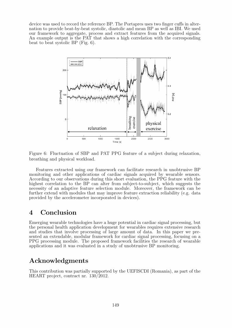
device was used to record the reference BP. The Portapres uses two finger cuffs in alter-nation to provide beat-by-beat systolic, diastolic and mean BP as well as IBI. We usedour framework to aggregate, process and extract features from the acquired signals.An example output is the PAT that shows a high correlation with the correspondingbeat to beat systolic BP (Fig. 6).
Figure 6: Fluctuation of SBP and PAT PPG feature of a subject during relaxation,breathing and physical workload.
Features extracted using our framework can facilitate research in unobtrusive BPmonitoring and other applications of cardiac signals acquired by wearable sensors.According to our observations during this short evaluation, the PPG feature with thehighest correlation to the BP can alter from subject-to-subject, which suggests thenecessity of an adaptive feature selection module. Moreover, the framework can befurther extend with modules that may improve feature extraction reliability (e.g. dataprovided by the accelerometer incorporated in devices).
4 Conclusion
Emerging wearable technologies have a huge potential in cardiac signal processing, butthe personal health application development for wearables requires extensive researchand studies that involve processing of large amount of data. In this paper we pre-sented an extendable, modular framework for cardiac signal processing, focusing on aPPG processing module. The proposed framework facilities the research of wearableapplications and it was evaluated in a study of unobtrusive BP monitoring.
Acknowledgments
This contribution was partially supported by the UEFISCDI (Romania), as part of theHEART project, contract nr. 130/2012.
149
References
[1] A. Reisner, P. Shaltis, D. McCombie, and H. Asada, “Utility of the photoplethys-mogram in circulatory monitoring,” Anesthesiology, vol. 108, no. 5, p. 950, 2008.
[2] P. Hamilton, “Open source ECG analysis,” in Computers in Cardiology, pp.101104, 2002.
[3] M. Elgendi, B. Eskofier, S. Dokos, and D. Abbott, “Revisiting QRS DetectionMethodologies for Portable, Wearable, Battery-Operated, and Wireless ECG Sys-tems,” PLoS ONE, vol. 9, no. 1, p. e84018, Jan. 2014.
[4] J. Allen, “Photoplethysmography and its application in clinical physiological mea-surement,” Physiol. Meas., vol. 28, no. 3, pp. R1R39, Mar. 2007.
[5] M. Elgendi, “On the Analysis of Fingertip Photoplethysmogram Signals,” Curr.Cardiol. Rev., vol. 8, no. 1, pp. 1425, Feb. 2012.
[6] M. Vlachos, M. Hadjieleftheriou, D. Gunopulos, and E. Keogh, “Indexing multi-dimensional time-series with support for multiple distance measures,” in Proceed-ings of the ninth ACM SIGKDD international conference on Knowledge discoveryand data mining, pp. 216225, 2003.
[7] S. S. Lim, et al., “A comparative risk assessment of burden of disease and injuryattributable to 67 risk factors and risk factor clusters in 21 regions, 19902010: asystematic analysis for the Global Burden of Disease Study 2010,” Lancet, vol.380, no. 9859, pp. 22242260, Dec. 2012.
[8] S. Ye, G.-R. Kim, D.-K. Jung, S. Baik, and G. Jeon, “Estimation of systolic anddiastolic pressure using the pulse transit time,” World Acad. Sci. Eng. Technol.,vol. 67, pp. 726731, 2010.
[9] P. Fung, G. Dumont, C. Ries, C. Mott, and M. Ansermino, “Continuous non-invasive blood pressure measurement by pulse transit time,” in Engineering inMedicine and Biology Society, IEMBS04. 26th Annual International Conferenceof the IEEE, vol. 1, pp. 738741, 2004.
[10] J. Lass, K. Meigas, D. Karai, R. Kattai, J. Kaik, and M. Rossmann, “Continuousblood pressure monitoring during exercise using pulse wave transit time measure-ment,” in Engineering in Medicine and Biology Society, IEMBS04. 26th AnnualInternational Conference of the IEEE, vol. 1, pp. 22392242, 2004.
[11] T. Ma and Y. T. Zhang, “A correlation study on the variabilities in pulse transittime, blood pressure, and heart rate recorded simultaneously from healthy sub-jects,” in Engineering in Medicine and Biology Society, IEEE-EMBS 2005. 27thAnnual International Conference of the, pp. 996999, 2005.
[12] M. Y. M. Wong, E. Pickwell-MacPherson, Y. T. Zhang, and J. C. Y. Cheng, “Theeffects of pre-ejection period on post-exercise systolic blood pressure estimationusing the pulse arrival time technique,” Eur. J. Appl. Physiol., vol. 111, no. 1, pp.135144, Jan. 2011.
[13] Y. Li, Z. Wang, L. Zhang, X. Yang, and J. Song, “Characters available in pho-toplethysmogram for blood pressure estimation: beyond the pulse transit time,”Australas. Phys. Eng. Sci. Med., vol. 37, no. 2, pp. 367376, Jun. 2014.
150
Proof of the Median Paths
Thijs VeugenTNO
Technical SciencesThe Hague, The Netherlands
Abstract
We consider the problem of coding for discrete memoryless channels with noise-less feedback. When studying Horstein’s sequential coding scheme, Schalkwijk in1971 found a regular behaviour of the so-called median paths for certain channelerror probabilities, which led to the development of repetition strategies. Weproof that Schalkwijk’s block decoding scheme exactly follows Horstein’s regularmedian paths.
1 Introduction
We consider the problem of coding for discrete memoryless channels with noiselessfeedback [4], which is strongly related to Ulam’s game [3, p. 281]. In this game, personA knows a secret integer m, which person B should guess by constructing sets one byone, and asking whether m is in it or not. Person A is allowed to lie a fixed number oftimes, and B wants to minimise the number of required questions.
During the game, person B is maintaining a probability distribution on the possibleintegers of A. We will show that the median of this distribution plays a very impor-tant role. In 1963, Horstein [1] developed a sequential coding scheme for the binarysymmetric channel with noiseless feedback, by closely following the median of the re-ceiver’s distribution. Schalkwijk [2] in 1971 found out that, for certain channel errorprobabilities, these medians exhibit a regular pattern, which led to the development ofa simple block coding scheme, achieving channel capacity for those particular channelerror probabilities.
However, this regular behaviour of the median, visualised by median paths, hasnever been proven. In this paper we present a proof, which has been known since 1997,but has never been published.
2 Median paths
In 1963, Horstein [1] developed a sequential coding scheme for the binary symmetricchannel with noiseless feedback. Let p, 0 ≤ p < 1
2, be the error probability of the
binary symmetric channel, and q = 1− p. Suppose the sender has an (infinite) binarymessage, presented as a point m in the message interval [0, 1], which he would liketo send towards the receiver. Assuming each message being equally likely, the initialmessage distribution of the receiver will be a uniform distribution over the interval[0, 1]. The idea of Horstein was as follows. He introduced a parameter a, 0 < a < 1.Before transmitting the nth bit, the sender will compute the currently expected messagedistribution, from the viewpoint of the receiver, and a message point mn, such thatPr(m ≥ mn) = a. In case m ≥ mn, the sender will transmit a 1, and a 0, otherwise.Because of the assumed noiseless feedback link, the sender learns which output bitshave been received by the receiver, which enables him to compute the expected messagedistribution.
151
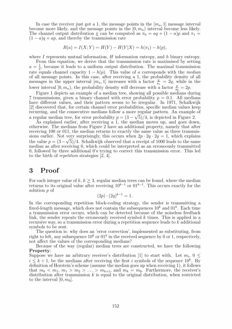
In case the receiver just got a 1, the message points in the [mn, 1] message intervalbecome more likely, and the message points in the [0,mn) interval become less likely.The channel output distribution π can be computed as π0 = aq + (1 − a)p and π1 =(1− a)q + ap, and thereby the transmission rate
R(a) = I(X;Y ) = H(Y )−H(Y |X) = h(π1)− h(p),
where I represents mutual information, H information entropy, and h binary entropy.From this equation, we derive that the transmission rate is maximised by setting
a = 12, because it leads to a uniform output distribution. The maximal transmission
rate equals channel capacity 1 − h(p). This value of a corresponds with the medianof all message points. In this case, after receiving a 1, the probability density of allmessages in the upper interval [mn, 1] increases with a factor q
π1= 2q, while in the
lower interval [0,mn), the probability density will decrease with a factor pπ0
= 2p.Figure 1 depicts an example of a median tree, showing all possible medians during
7 transmissions, given a binary channel with error probability p = 0.1. All medianshave different values, and their pattern seems to be irregular. In 1971, Schalkwijk[2] discovered that, for certain channel error probabilities, specific median values keeprecurring, and the consecutive medians follow a more regular pattern. An example ofa regular median tree, for error probability p = (3−
√5)/4, is depicted in Figure 2.
As explained earlier, after receiving a 1, the median moves up, and goes down,otherwise. The medians from Figure 2 have an additional property, namely that afterreceiving 100 or 011, the median returns to exactly the same value as three transmis-sions earlier. Not very surprisingly, this occurs when 2p · 2q · 2q = 1, which explainsthe value p = (3−
√5)/4. Schalkwijk observed that a receipt of 1000 leads to the same
median as after receiving 0, which could be interpreted as an erroneously transmitted0, followed by three additional 0’s trying to correct this transmission error. This ledto the birth of repetition strategies [2, 4].
3 Proof
For each integer value of k, k ≥ 3, regular median trees can be found, where the medianreturns to its original value after receiving 10k−1 or 01k−1. This occurs exactly for thesolution p of
(2p) · (2q)k−1 = 1.
In the corresponding repetition block-coding strategy, the sender is transmitting afixed-length message, which does not contain the subsequences 10k and 01k. Each timea transmission error occurs, which can be detected because of the noiseless feedbacklink, the sender repeats the erroneously received symbol k times. This is applied in arecursive way, so a transmission error during a repetition sequence leads to k additionalsymbols to be sent.
The question is: why does an ’error correction’, implemented as substituting, fromright to left, any subsequence 10k or 01k in the received sequence by 0 or 1, respectively,not affect the values of the corresponding medians?
Because of the way (regular) median trees are constructed, we have the followingProperty:Suppose we have an arbitrary receiver’s distribution [1] to start with. Let mi, 0 ≤i ≤ k + 1, be the medians after receiving the first i symbols of the sequence 10k. Bydefinition of Horstein’s scheme (assume the median goes up when receiving 1), it followsthat m0 < m1, m1 > m2 > . . . > mk+1, and mk = m0. Furthermore, the receiver’sdistribution after transmission k is equal to the original distribution, when restrictedto the interval [0,m0].
152
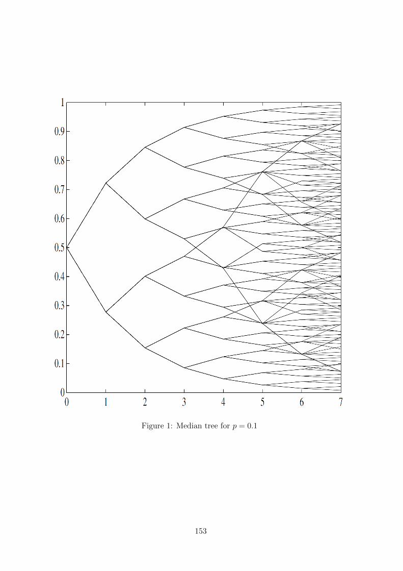
Figure 1: Median tree for p = 0.1
153
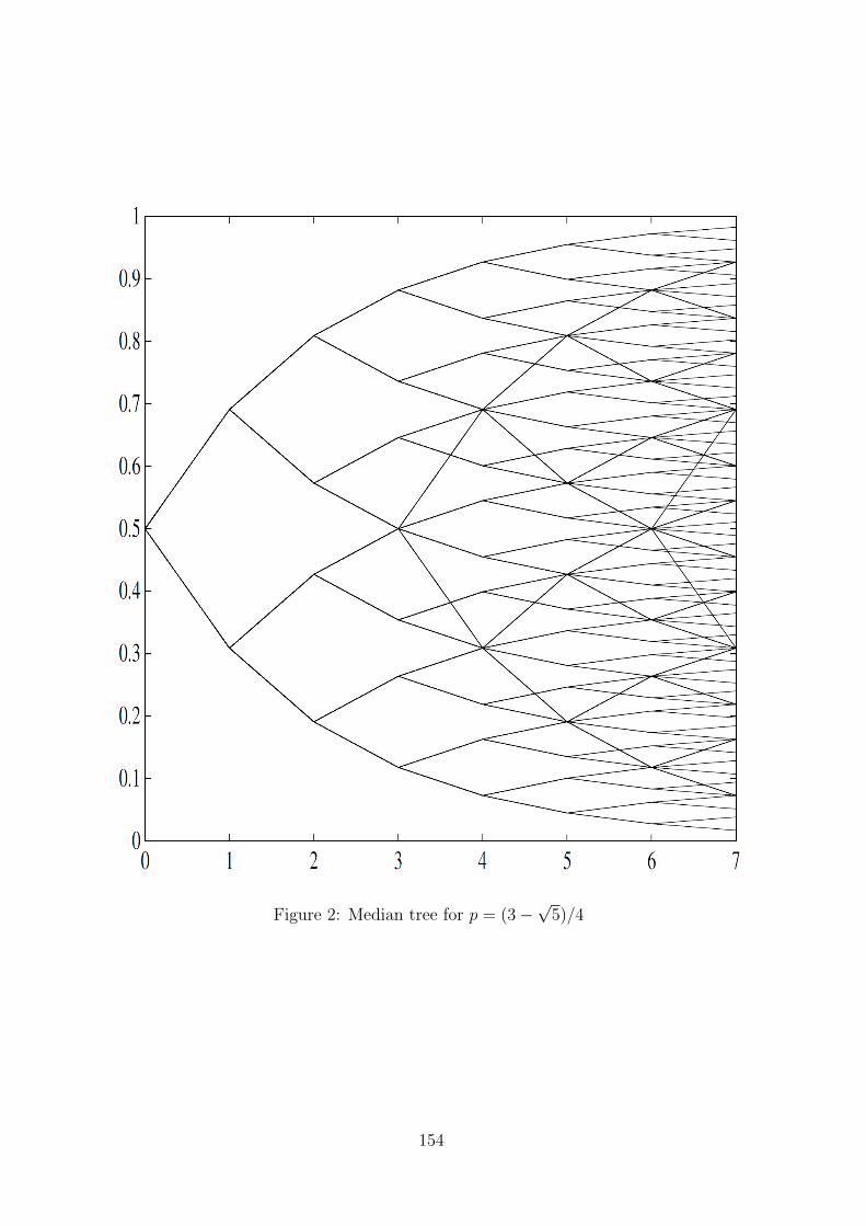
Figure 2: Median tree for p = (3−√5)/4
154
Using this property, we can proof the following lemma.Lemma 1. Let x = x1 . . . xN be an arbitrary received sequence without forbidden
subsequences. Let mi, 0 ≤ i ≤ N , be the medians after receiving x1 . . . xi. If x1 = 0,then mi ≤ m0 for 0 ≤ i ≤ N .
Proof: Assume x1 = 0. We proof by natural induction mi ≤ m0 for 0 ≤ i ≤ N .The basis is n = 0. The induction step is as follows. Suppose that for some n, n ≥ 0,we have mi ≤ m0 for all i, 0 ≤ i < n. Assume mn > m0. Since mn−1 ≤ m0 < mn, itfollows that xn = 1. If xn−1 = 0, then mn−2 ≥ mn, according to the property above,which would contradict mn−2 ≤ m0, so xn−1 = 1. Similarly, it is shown that xn−2 = 1,and xn−3 = 1, etc., until xn−k+1 = xn−k+2 = . . . = xn = 1. Now, because x contains noforbidden subsequences, we conclude xn−k = xn−k−1 = . . . x1 = 1, which contradictsour first assumption x1 = 0. So it must be that mn ≤ m0.
This lemma is used in the proof of our main theorem, which answers the researchquestion.
Theorem 1. Let x = x1 . . . xN be an arbitrary received sequence. Let mi, 0 ≤ i ≤N , be the medians after receiving x1 . . . xi. Let xn . . . xn+k be the rightmost forbiddensubsequence. Let x′ = x′
1 . . . x′N−k be the sequence after substitution of xn . . . xn+k by
xn+k in x. Let m′i, 0 ≤ i ≤ N − k, be the medians after receiving x′
1 . . . x′i. Then
m′i = mi+k, n ≤ i ≤ N − k.
Proof: Since x1 . . . xn−1 = x′1 . . . x
′n−1, it follows thatmn−1 = m′
n−1. Furthermore, bythe previous property, mn+k−1 = mn−1. Assume w.l.o.g. xn = 1. Since xn . . . xn+k is aforbidden subsequence, xn+k = 0. Because xn+k . . . xN is a sequence without forbiddensubsequences, it follows from our Lemma that mi ≤ mn+k−1 for n + k − 1 ≤ i ≤ N .Due to our property, the receiver’s distribution after receipt of xn+k−1 is equal to thereceiver’s distribution after receiving xn−1, when restricted to the interval [0,mn+k−1].Since each median after transmission n + k − 1 lies in this interval, it is easily shownthat m′
i = mi+k for i = n− 1, n, . . . , N − k, respectively. The theorem explains that substituting the rightmost forbidden subsequence does
not affect the corresponding median values. Therefore, the entire decoding processas a whole will not affect the median values of the original message (assuming alltransmission errors have been corrected). This affirms that Schalkwijks repetitionblock coding strategies naturally fit into Horstein’s sequential coding scheme.
4 Conclusion
We introduced Horstein’s sequential coding scheme for the binary symmetric channelwith noiseless feedback. We showed the existence of regular median trees, which ledSchalkwijk to the discovery of repetition block coding strategies. Although at first sight,these repetition strategies seem to form a natural extension of Horstein’s scheme, it isnot straightforward to see that the behaviour of the medians is in line with the entiredecoding process. We were able to prove this, affirming their conceptual coherence.
References
[1] Michael Horstein. Sequential transmission using noiseless feedback. IEEE Transac-tions on Information Theory, 9: 136-143, July 1963.
[2] J. Pieter M. Schalkwijk. A class of simple and optimal strategies for block codingon the binary symmetric channel with noiseless feedback. IEEE Transactions onInformation Theory, 22(9): 1369-1373, May 1971.
155

[3] S.M. Ulam. Adventures of a mathematician. Charles Scribner’s sons, 1976.
[4] Thijs Veugen. Multiple-repetition coding for channels with feedback. PhD thesis.Eindhoven, University of Technology. June 1997.
156
Enhancing privacy of users in eID schemes
Kris Shrishak Zekeriya Erkin Remco SchaarCyber Security Group, Department of Intelligent Systems UL Transaction Security
Delft University of Technology, The Netherlands The [email protected] [email protected] [email protected]
Abstract
In todays world transactions are increasingly being performed over the Internetbut require identification of users as in face-to-face transactions. In order to facil-itate eGovernance as well as other eCommerce services Electronic Identification(eID) schemes, which intend to provide unique and reliable identification andauthentication of the users, have been introduced. eID schemes commonly involvea Service Provider which provides a service, such as online shopping, to the userand an Identity Provider which verifies the users identity and facilitates the userto identify itself to the Service Provider. Every transaction made over the Internetreveals bits of information about the user which can be accumulated and abused,thus necessitating security and privacy in order to prevent misuse of data andinvasion of personal privacy. In this work, five eID schemes which are in use orare proposed in EU countries is surveyed and the strengths and weaknesses ofthese schemes is investigated. All the schemes have given importance to securitywhile only a few of them are designed with privacy in mind. Identity Providersin federated eID schemes are observed to be a privacy hotspot as they storeuser information and can uniquely identify the user. The use of homomorphicencryption and block chain in eID schemes is further explored in order to preventthe Identity Provider from becoming a privacy hotspot while fulfilling its role inthe scheme.
1 IntroductionLong before the Internet came into existence, Governments have had public authentica-tion schemes by issuing Identity documents to identify a person or verify aspects of aperson’s personal identity. These documents were trusted not only by the governmentsbut also by businesses that required reliable authentication of users [1]. Today thenumber of services offered online is increasing rapidly and this growth has forced users tomaintain multiple credentials for authentication and identification to service providers,which has caused security and usability issues. Password-based authentication mecha-nism employed by most service providers has lead to users reusing the same passwordor writing them on paper. Usage of other authentication mechanisms such as hardwaresecurity tokens is also not convenient. As a result, many countries in the EuropeanUnion (EU) have either developed an electronic identification (eID) scheme or are inthe process of developing one. All schemes have put security at the forefront but fewhave considered the privacy implications of a nation-wide single identification scheme.We consider it essential that designers of eID systems focus on privacy, specificallyinformational privacy of users which we interpret such that when a user mentions ‘myinformation’, the ‘my’
“is not the same as ‘my’ in ‘my car’ but rather the same as ‘my’ in ‘my body’or ‘my feelings’; it expresses a sense of constitutive belonging, not of externalownership, a sense in which my body, my feelings, and my information arepart of me but are not my possessions [2].”
157

We survey five eID schemes in the EU and provide brief descriptions of two solutionswhich could be applied in eID schemes to improve privacy. Information privacy in eIDschemes is investigated in terms of the following properties [3]:
1. Anonymity: Users may use a service without disclosing their identity.2. Pseudonimity: Users may utilise a service by using pseudonyms.3. Data minimization: Only the required information about the user must be shared
in order to prevent misuse.4. Unlinkability: User should be able to use resources and services without others
being able to link these activities.5. Unobservability: Users should be able to use services without being observed by
others.6. Transparency: User data should be obtained only when necessary and after user
consent.
2 eID SchemeseID systems intend to provide reliable identification and authentication of the users.The eID systems discussed in this section were designed for use by both public andprivate services. The parties involved in these systems differ widely but commonlyinvolve the following:
User - wants to authenticate her/himself to the Service Provider to access aresource. Service Provider (SP) - provides a service, such as online shopping or government
tax services, and makes transaction decisions based upon the acceptance of ausers authenticated credentials and attributes. Identity Provider (IDP) - verifies the user’s identity or credentials and facilitates
the user to authenticate her/himself to the SP. It improves the overall usabilitysince the user does not need to remember multiple authentication credentials.
2.1 Belgian eID scheme
The Belgian eID scheme is a nation-wide Public Key Infrastructure (PKI) which requireseach citizen to present her/himself at the municipality for strong user authenticationduring the issuing phase. Thus it can be inferred that the Belgian government has takenup the role of IDP. The user is issued a smart card and is required to buy a card readerfor online use. The objective of the Belgian eID card has been to fulfil four functions,namely, citizen identification, authentication, digital signature and access control [4].
The eID card has the name, title, nationality, place and date of birth, gender, and aphoto of its holder printed on it in addition to a hand written signature of its holderand of the civil servant who issued the card. All this information is also stored on thechip in an Identity file which is signed by the National Register (RRN). The chip alsocontains an address file which is kept independently as the address of its holder maychange within the validity period of the card. The RRN signs the address file togetherwith the identity file to guarantee the link between these two files. The correspondingsignature is stored as the address file’s signature.
Privacy Analysis
The main concern with the Belgium eID card is privacy. The user’s identity is revealedfor all transactions and (s)he does not have control over the data that is sharedwith the SPs while it remains possible for colluding SPs to link user activities as theauthentication certificate contains the RRN. Verhaeghe et. al [5] provide further privacyand security threats if the card or the middleware is compromised.
158
2.2 GOV.UK Verify
GOV.UK Verify is the eID scheme of the United Kingdom. It is a federated identificationinfrastructure where an online central hub mediates user authentications betweenIDPs and SPs. The role of the hub is to ensure interoperable identification andauthentication as well as provide privacy benefits by hiding the IDP from the SP.The eID scheme has been designed considering nine Identity Assurance Principles -user control, transparency, multiplicity, data minimization, data quality, service useraccess and portability, certification, dispute resolution and exceptional circumstances [6].Users of the eID scheme are identified by a pseudonym (u) at the hub. In addition toIDPs, SPs and hub, the scheme also includes (1) Attribute Providers (ATP), whichare responsible for establishing attributes and (2) Matching Service (MS), which helpsvalidate assertions from IDPs and derives a pseudonym v from u for the SPs it serves [7].
Privacy Analysis
In spite of claiming that privacy is one of the design criteria for the eID scheme,GOV.UK Verify has multiple privacy issues. The hub, which has full visibility of theuser pseudonym and personal information of citizens can link interactions of the sameuser across different SPs as well as undetectably impersonate users at any SP withoutuser authentication. The MS, which has the task of matching pseudonyms and theattributes into a local account, can link the user and the SPs that choose the same MS.Colluding SPs using the same MS can link user activities as the same pseudonym isused. Thus it can be inferred that GOV.UK Verify actually degrades the privacy ofcitizens instead of enhancing it. Finally, the hub can be used for undetectable masssurveillance.
2.3 Dutch eID scheme using polymorphic pseudonyms
The Dutch eID scheme utilises a federated eID infrastructure. Some variations of theDutch eID scheme have been proposed during the planning stage. In the following, theversion with polymorphic pseudonyms [8] is considered as it is the most privacy friendlyversion among those proposed. In addition to IDPs and SPs, the scheme also includes(1) a Pseudonym Provider (PP), which generates polymorphic pseudonym when theIDP sends a unique identifier(U-id) (2) brokers, which mediate user authenticationbetween the various eID parties, essentially IDPs and the many SPs. Other partiesinclude Attribute Providers (ATP) and Authorization Providers, a Key ManagementAuthority (KMA) and a investigation authority. The pseudonymization in this schemeinvolves three levels of pseudonyms, namely, (1) polymorphic pseudonyms (2) encryptedpseudonyms and (3) pseudonyms.
Privacy Analysis
The Dutch eID scheme with polymorphic pseudonyms has few of the privacy propertiesmentioned in section 1. It provides pseudonimity to the users such that SPs get auser specific pseudonym from the IDP, but the pseudonym is independent of the IDP.Meanwhile, the pseudonym obtained by different SPs for the same user is not the same,thus preventing colluding SPs from being able to link user activities. Finally, encryptedpseudonyms are randomized such that the broker cannot identify the same user onmultiple occasions.
In spite of efforts made to provide privacy to the users, this scheme has countableissues. IDP is a privacy hotspot which knows the attributes of users, which SPs arevisited by users and how often. This information might be considered very sensitivein some cases. The IDP does not need to know this information in order to performits role. An alternative proposed in [8] is to store polymorphic pseudonyms in a smartcard and use chip authentication as in the German eID scheme. The Dutch eID schemeis complex and it is possible that in the future SPs might outsource the decryption ofencrypted pseudonyms to a third party allowing them to learn users visiting patterns.
159
2.4 German eID scheme
The German eID scheme uses a direct authentication eID infrastructure. The designgoals of this scheme were data minimization, data security and transparency. In order touse this scheme, the user needs an eID card, a reader and the Ausweisapp software whilethe SP needs an authorization certificate, an eID-Server that handles authentication bycommunicating with the card. The eID card contains a chip which stores the informationprinted on the card as well as the fingerprints of the holder, if the holder wishes. Thedocument number and the fingerprints can be read offline only by authorities who havemachines certified by the Federal Office for Information Security (BSI).
The German eID scheme makes use of cryptographic protocols, to perform mutualidentification, which are also used in EU passports [9]. Password AuthenticatedConnection Establishment (PACE) protocol provides secure communication and explicitpassword-based authentication of the eID card and the terminal while the ExtendedAccess Control (EAC) protocol provides secure key establishment between a chipcard and a terminal, using a PKI. It serves the purpose of limiting access to thesensitive data stored on the chip card. EAC comprises of terminal authenticationand chip authentication. Finally Restricted Identification (RI) protocol generates asector-specific identifier for each card, enabling the pseudonymous identification of thecard-holder.
Privacy Analysis
The German eID scheme provides pseudonimity to the users and reduces sharing ofexcessive data with SPs. For instance, to verify if the age of the user is above 18, only ayes/no is sent instead of the age. By using secure channels, user data is not observablein transit. However the security of eID authentication relies on the tamper-resistanceof the smart card chips. If an attacker manages to extract the chip authentication keyfrom any eID card, then this attacker would be able to forge arbitrary identities. Also,user data that is transmitted after selective disclosure by the user does not contain anysignature in order to verify if it is indeed the data that was originally issued by BSIand sent by a legitimate eID cardholder [1]. Only the context of the EAC protocols runand the secure channel thus established assure the eID-Server of the authenticity ofthe eID data. Finally, The eID-Server is recommended to be implemented by the SPbut can also be implemented by third parties, thus creating a privacy risk as it servesmore than one SP and can learn the visiting patterns of users as the attributes that arerevealed by the users are identifying. Until 2012, eID servers implemented by only twothird parties were being used by the SPs [10].
2.5 IRMA (I Reveal My Attributes)
IRMA (I Reveal My Attributes) is a attribute-based credentials (ABC) eID scheme.The credential issuer or the IDP issues credentials to the user and vouches for thevalidity of the attributes contained in the credential. After issuing the credentials,the IDP cannot recognise the credential as it is signed using blind signatures. Thiseliminates the possibility of the issuer tracking the card owner. The user can usethe credentials to prove the possession of an attribute to the SP. Two importanttechnologies that make use of an ABC approach are Microsoft’s U-Prove [11] and IBM’sIdentity Mixer (Idemix) [12]. Idemix is built upon the concept of Camenisch-Lysyankayasignature scheme and its protocols [13]. IRMA is a partial implementation of Idemixthat demonstrates the applicability of ABCs on smart cards [14]. The implementationincludes privacy enhancing features of ABCs such as selective disclosure of attributesusing zero-knowledge protocols.
Privacy Analysis
Users can perform transactions anonymously for transactions that do not need anidentity but can be completed if the credentials are satisfactory. IRMA provides issuer
160
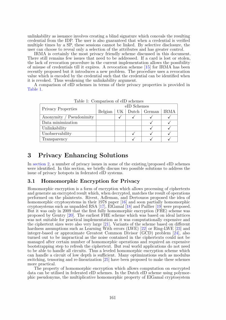
unlinkability as issuance involves creating a blind signature which conceals the resultingcredential from the IDP. The user is also guaranteed that when a credential is verifiedmultiple times by a SP, these sessions cannot be linked. By selective disclosure, theuser can choose to reveal only a selection of the attributes and has greater control.
IRMA is certainly the most privacy friendly scheme discussed in this document.There still remains few issues that need to be addressed. If a card is lost or stolen,the lack of revocation procedure in the current implementation allows the possibilityof misuse of credentials till it expires. A revocation scheme [15] for IRMA has beenrecently proposed but it introduces a new problem. The procedure uses a revocationvalue which is encoded by the credential such that the credential can be identified whenit is revoked. Thus weakening the unlinkability argument.
A comparison of eID schemes in terms of their privacy properties is provided inTable 1.
Table 1: Comparison of eID schemes
Privacy PropertieseID Schemes
Belgian UK Dutch German IRMAAnonymity / Pseudonimity X X X XData minimization X XUnlinkability X XUnobservability X X XTransparency X X X
3 Privacy Enhancing Solutions
In section 2, a number of privacy issues in some of the existing/proposed eID schemeswere identified. In this section, we briefly discuss two possible solutions to address theissue of privacy hotspots in federated eID systems.
3.1 Homomorphic Encryption for Privacy
Homomorphic encryption is a form of encryption which allows processing of ciphertextsand generate an encrypted result which, when decrypted, matches the result of operationsperformed on the plaintexts. Rivest, Adleman, and Dertouzos proposed the idea ofhomomorphic cryptosystems in their 1978 paper [16] and soon partially homomorphiccryptosystems such as unpadded RSA [17], ElGamal [18] and Paillier [19] were proposed.But it was only in 2009 that the first fully homomorphic encryption (FHE) scheme wasproposed by Gentry [20]. The earliest FHE scheme which was based on ideal latticeswas not suitable for practical implementation as it was computationally expensive andthe ciphertext sizes were also very large [21]. Variants of the scheme based on differenthardness assumptions such as Learning With errors (LWE) [22] or Ring-LWE [23] andinteger-based or approximate Greatest Common Divisor (GCD) problem [24], alsoturned out to be impractical as the noise contained in the ciphertexts could not bemanaged after certain number of homomorphic operations and required an expensivebootstrapping step to refresh the ciphertext. But real world applications do not needto be able to handle all circuits. Thus a leveled homomorphic encryption scheme whichcan handle a circuit of low depth is sufficient. Many optimizations such as modulusswitching, tensoring and re-linearization [25] have been proposed to make these schemesmore practical.
The property of homomorphic encryption which allows computation on encrypteddata can be utilised in federated eID schemes. In the Dutch eID scheme using polymor-phic pseudonyms, the multiplicative homomorphic property of ElGamal cryptosystem
161
is utilised to transform pseudonyms. A similar approach could be used for attributes aswell. But multiplicative homomorphism may not be sufficient if we want to prevent IDPsfrom having direct access to user data during authentication. Leveled homomorphicencryption schemes may find application in this scenario.
3.2 Block chain for Decentralization
Block chain was introduced by Satoshi Nakamoto as a timestamp server as part of theBitcoin protocol [26]. A block chain is a public ledger shared by all nodes participatingin a system based on the Bitcoin protocol [27]. A full copy of a block chain containsevery transaction ever executed. Every block contains a hash of the previous block suchthat a chain of blocks is created from the first block of the chain, also known as genesisblock, to the current block. This way the blocks are arranged in chronological order. Itis also computationally infeasible to modify a block as every block that follows mustalso be regenerated.
Block chain allows to eliminate the necessity of a central party. But it introducesadditional issues. A public ledger provides everyone in the network access to the dataon the block chain. This means that instead of one central party having access to allthe data, now all parties in the network have access. So block chain as it is, cannotbe used to store private data and hence does not address the problem of privacy butmerely shifts the problem. Even though Bitcoin protocol allows the usage of multiplepseudonyms or public keys, it is possible to link the activity of users [28]. Enigma [29],a decentralized computation platform which allows storage and computation of privatedata, uses off-chains in addition to the block chain to store private data. A similarapproach has been used in [30] but it requires a minimally trusted manager.
As a primitive idea we propose that block chain could be used in federated eIDsystems by using off-chain consisting of IDPs. User data can be split up among theIDPs thus preventing any one IDP from having complete information about its users,thus decentralizing the role of IDP. This ideas requires further research and refinementbefore it can be considered for nation-scale eID systems.
4 ConclusionWe have surveyed five eID schemes in the EU and analysed their privacy properties.Belgian, GOV.UK and Dutch schemes use the approach of identifying entities by aunique number at the IDP. This approach is convenient for bookkeeping but it is notprivacy friendly. Unique identifiers can be used to trace the user and her/his activities.IDPs have been identified as a privacy hotspot due to the large trove of user data thatthey store and process, which allows them to link user activities. Finally, we proposedtwo possible solutions - homomorphic encryption and block chain - to allow the IDP toperform its role of authenticating users to SPs without becoming privacy hotspots.
References
[1] A. Poller, U. Waldmann, S. Vowe, and S. Turpe, “Electronic identity cards for userauthentication - promise and practice,” IEEE Security & Privacy, vol. 10, no. 1,pp. 46–54, 2012.
[2] L. Floridi, “The ontological interpretation of informational privacy,” Ethics andInformation Technology, vol. 7, no. 4, pp. 185–200, 2005.
[3] ISO15408-2:2005, “Information technology - security techniques - evaluation criteriafor it security - part 2: Security functional requirements,” tech. rep., InternationalStandard Organization, 2005.
[4] D. D. Cock, C. Wolf, and B. Preneel, “The belgian electronic identity card(overview),” in Sicherheit, vol. 77 of LNI, pp. 298–301, GI, 2006.
162

[5] P. Verhaeghe, J. Lapon, B. D. Decker, V. Naessens, and K. Verslype, “Securityand privacy improvements for the belgian eid technology,” in SEC, vol. 297 of IFIPAdvances in Information and Communication Technology, pp. 237–247, Springer,2009.
[6] “Identity assurance principles,” tech. rep. Available at https://www.gov.uk/government/uploads/system/uploads/attachment_data/file/361496/PCAG_IDA_Principles_3.1__4_.pdf.
[7] L. T. A. N. Brandao, N. Christin, G. Danezis, and anonymous, “Toward mendingtwo nation-scale brokered identification systems,” PoPETs, vol. 2015, no. 2, pp. 135–155, 2015.
[8] “Polymorphic pseudonymization.” Available at https://www.idensys.nl/fileadmin/bestanden/idensys/documenten/basisdocumentatie/documentatieset/PP_Scheme_091.pdf.
[9] BSI, “Advanced security mechanisms for machine readable travel documents andeIDAS token part 2 protocols for electronic identification, authentication and trustservices (eIDAS),” tr-03110-2, Bundesamt fur Sicherheit in der Informationstechnik,2015.
[10] R. Bjones, I. Krontiris, P. Paillier, and K. Rannenberg, “Integrating anonymouscredentials with eids for privacy-respecting online authentication,” in APF, vol. 8319of Lecture Notes in Computer Science, pp. 111–124, Springer, 2012.
[11] S. Brands, Rethinking Public Key Infrastructures and Digital Certificates: Buildingin Privacy. MIT Press, 2000.
[12] IBM Research Zurich Security team, “Specification of the identity mixer crypto-graphic library,” tech. rep., IBM Research, April 2010.
[13] J. Camenisch and A. Lysyanskaya, “An efficient system for non-transferable anony-mous credentials with optional anonymity revocation,” in EUROCRYPT, vol. 2045of Lecture Notes in Computer Science, pp. 93–118, Springer, 2001.
[14] P. Vullers and G. Alpar, “Efficient selective disclosure on smart cards usingidemix,” in IDMAN, vol. 396 of IFIP Advances in Information and CommunicationTechnology, pp. 53–67, Springer, 2013.
[15] W. Lueks, G. Alpar, J. Hoepman, and P. Vullers, “Fast revocation of attribute-based credentials for both users and verifiers,” in SEC, vol. 455 of IFIP Advancesin Information and Communication Technology, pp. 463–478, Springer, 2015.
[16] R. L. Rivest, L. Adleman, and M. L. Dertouzos, “On data banks and privacyhomomorphisms,” in Foundations of Secure Computation (R. A. DeMillo, D. P.Dobkin, A. K. Jones, and R. J. Lipton, eds.), pp. 165–179, Academic Press.
[17] R. L. Rivest, A. Shamir, and L. M. Adleman, “A method for obtaining digitalsignatures and public-key cryptosystems,” Commun. ACM, vol. 21, no. 2, pp. 120–126, 1978.
[18] T. E. Gamal, “A public key cryptosystem and a signature scheme based on discretelogarithms,” in CRYPTO, vol. 196 of Lecture Notes in Computer Science, pp. 10–18,Springer, 1984.
[19] P. Paillier, “Public-key cryptosystems based on composite degree residuosity classes,”in EUROCRYPT, vol. 1592 of Lecture Notes in Computer Science, pp. 223–238,Springer, 1999.
163

[20] C. Gentry, A fully homomorphic encryption scheme. PhD thesis, Stanford Univer-sity, 2009.
[21] C. Gentry and S. Halevi, “Implementing gentry’s fully-homomorphic encryptionscheme,” in EUROCRYPT, vol. 6632 of Lecture Notes in Computer Science,pp. 129–148, Springer, 2011.
[22] Z. Brakerski and V. Vaikuntanathan, “Efficient fully homomorphic encryption from(standard) LWE,” in IEEE 52nd Annual Symposium on Foundations of ComputerScience, FOCS 2011, Palm Springs, CA, USA, October 22-25, 2011, pp. 97–106.
[23] Z. Brakerski and V. Vaikuntanathan, “Fully homomorphic encryption from ring-lweand security for key dependent messages,” in CRYPTO, vol. 6841 of Lecture Notesin Computer Science, pp. 505–524, Springer, 2011.
[24] M. van Dijk, C. Gentry, S. Halevi, and V. Vaikuntanathan, “Fully homomorphicencryption over the integers,” in EUROCRYPT, vol. 6110 of Lecture Notes inComputer Science, pp. 24–43, Springer, 2010.
[25] Z. Brakerski, C. Gentry, and V. Vaikuntanathan, “(leveled) fully homomorphicencryption without bootstrapping,” 2012.
[26] S. Nakamoto, “Bitcoin: A peer-to-peer electronic cash system,” 2008. https://bitcoin.org/bitcoin.pdf.
[27] “Blockchain.” https://en.bitcoin.it/wiki/Block_chain.
[28] E. Androulaki, G. Karame, M. Roeschlin, T. Scherer, and S. Capkun, “Evaluatinguser privacy in bitcoin,” in Financial Cryptography, vol. 7859 of Lecture Notes inComputer Science, pp. 34–51, Springer, 2013.
[29] G. Zyskind, O. Nathan, and A. Pentland, “Enigma: Decentralized computationplatform with guaranteed privacy,” CoRR, vol. abs/1506.03471, 2015.
[30] A. E. Kosba, A. Miller, E. Shi, Z. Wen, and C. Papamanthou, “Hawk: Theblockchain model of cryptography and privacy-preserving smart contracts,” IACRCryptology ePrint Archive, vol. 2015, p. 675, 2015.
164
A Privacy-Preserving GWAS Computation withHomomorphic Encryption.
Chibuike Ugwuoke Zekeriya Erkin Reginald L. LagendijkDelft University of Technology
Department of Intelligent Systems, Cyber Security Group.Delft, The Netherlands
[email protected] [email protected] [email protected]
Abstract
The continuous decline in the cost of DNA sequencing has contributed bothpositive and negative feelings in the academia and research community. It hasnow become possible to harvest large amounts of genetic data, which researchesbelieve their study will help improve preventive and personalised healthcare,better understanding of diseases and response to treatments. However, thereare more information embedded in genes than are currently understood, just asa genomic data contains information of not just the owner, but relatives whomight not subscribe to sharing them. Unrestricted access to genomic data canbe privacy invasive, hence the urgent need to regulate access to them and developprotocols that would allow privacy-preserving techniques in both computationsand analysis that involve these very sensitive data. In this work, we discusshow a careful combination of cryptographic primitives such as homomorphicencryption, can be used to privately implement common algorithms peculiarto genome-wide association studies (GWAS). This obviously comes at a cost,where we have to accommodate the trade-off between speed of computationsand privacy.
1 Introduction
Biomedical research has long shown that human genome contain data from whichinformation about their individual owners, and those related to them can be ex-tracted [1, 2, 3, 4]. A lot of privacy-sensitive information are laced all over genomicdata, which constitutes enormous worry for individuals whose data are available inelectronic format [5, 6, 7]. The benefits of continuous research involving the genomicdata are equally rife, these include: preventive and personalised healthcare, patient’sresponse to treatment, predisposition to diseases, identification of new drug targetsand perhaps a better understanding of cancer [1, 8, 4, 9, 10, 11, 12, 13, 14]. On theother hand, when genomic data is used for research or processed by medical personnels,they become exposed to possible misuse and even loss to unauthorised hands. In theface of this possibility, the risk of re-identifying individuals from an available genomicdata calls for serious concern [5, 9, 15, 4, 3, 7], and has been recognised as a realisticthreat. Other unwanted scenarios which could occur as direct consequence of leakinggenomic data include: stigmatisation, discrimination, loss of insurance and even lossof employment opportunities for persons whose genomic data is public [16].
What is more worrisome about misuse of genomic data is the fact that the genomehas longevity, when leaked, it can neither be revoked nor modified. So, it is obvious thatthis piece of data is highly sensitive and requires protection that should be adaptive tofuture security threats. Hence one can claim that any realistic solution should be onewhich, the security guarantees of the underlying primitives used for implementation
165

should withstand post quantum attacks. Therefore privacy protection techniques havebeen proposed as an adaptive solution by the cryptography community. The aimwill be to allow productive research that utilise genomic data, while eliminating theprivacy-risks inherent around these procedures.
Being that no standalone solution can best fit the challenge posed, it is consideredthat a good combination of ethical, legal and technological constraints can be employed,to properly manage the risks of privacy leaks that are otherwise possible within thisresearch domain. Owing to this premise, our work seeks to contribute a technologicalsolution to the underlying problem.
In the era of distributed computing, even the medical field has not been left out. Ithas been common for researchers and medical personnels to work without boundariesof country borders, albeit, via a virtual collaboration [17, 7, 2]. This means that moredata can now be shared for research purposes and even diagnosis of diseases [6]. Italso presents us with the possibility of allowing cloud services process medical data,even when they do not reside in the same country as the owners of the data. This needfor collaboration, data sharing and cloud processing of genomic data further pushes forprivacy-preserving secure computing protocols [2, 17].
Having a genomic dataset and controlling access to it is the main aim of this work.In a nutshell, this means that while these data is not available to the public, expertswho need them for research are granted restricted access to only subsets relevant totheir work [15]. Such access for processing data may include string searching and com-parison, as well as GWAS computations.
Genome Wide Association Studies: As highlighted in [1, 18], the first ever humangenome sequencing was achievable in 2001, after directly gulping a whooping US-$300million from the initial budget of US-$3 billion. Fast-forward 6 years later, and thesame feat is feasible for about US-$100,000. In 2006 [18], it was anticipated that in2014, a further reduction to US-$1,000 was possible for sequencing the human genome.Recent literature [19, 11] have even suggested that a meagre US-$100, will be a realityin the very near future. If that be the case, one can deduce that amongst other possi-bilities, a direct consequences of affordable genomic data would be the torrential flow ofgenomic data in silico. It is obviously a good development for researchers, who wouldheavily rely on these data to improve on their research, refine and optimise diagnosisand many others positive possibilites. With a wealth of data in the form of genomicdata lying at the disposal of researchers and medical personnels, learning and inferringfrom these data becomes an indisputable objective.
Without loss of generality in description, GWAS can simply be simplified to theactivities presented above, it is about gathering genetic data, processing them andrelying on them to investigate relationship (association) of genes to common knowndiseases. It will be possible to even detect unknown diseases and the effect of drugs ontreatments. With GWAS researchers can now measure, analyse and predict previouslyunknown genetic influence on a person, this can help in early detection and preventionof certain diseases, as well as personalised healthcare. For useful gene-disease associa-tions to be estimated, some computations become handy, and these will be discussed insubsection 2.1. Nonetheless, most of the computations can easily put the data ownersat privacy-risk. It has led to the suggestion that protection of genomic data is a ne-cessity, to address possible ethical, political, technological and privacy concerns. Fromthe technological solution approach, we hope to address the privacy-threats using cryp-tographic primitives. Just to mention, with genomic data, data anonymization is notenough guarantee to avoid re-identification and also, conventional encryption mightnot offer much better protection against envisaged privacy-threats. These can simplybe derived from the fact that the said data have longevity, their importance persistseven after the demise of the data owner.
Related Works: Realising the privacy-sensitive nature of genomic data, researchers
166
have delved into search for privacy-preserving solutions, in the hope to protect pri-vacy of owners while still being able to process and compute operations using thesedata. Some of these works are discussed here. Privacy-preserving GWAS spans acrossmore possibilities than just GWAS-Computations. According to [15], other importantcategories include:
• Private string searching and comparison.
• Private release of aggregated data.
• Private read mapping.
of course, this list is not in itself exhaustive, but we will only consider works thatdirectly address computations very peculiar to GWAS. As early as 1999 [20, 21, 22],some researchers had anticipated privacy risks involved with genomic data. So theyproposed denominalization and de-identification as protection schemes, to preserveprivacy. This did not stop re-identification attacks from being hugely successful, asdiscussed in [9]. Other authors [23] have subsequently recommended Trusted ThirdParties and Semitrusted Third Parties but then, it is not always easy to completelytrust a third party, who could still be susceptible to coercion, compulsion and evencorruption to be compromised. More recently in [24], attempts were made to analysegenomic data while avoiding privacy-invasion of participants of the data. Summarily,they adopted differential privacy as a privacy-preserving technique, and documented tohave obtained utility with their procedure. However, addition of noise using differentialprivacy is not a silver bullet to deflate possible re-identification. Especially when thepublished data can be augmented with other side information. But most importantly isthe fact that differential privacy contains noise, which will evidently affect the utility, nomatter the degree of noise. This is a huge trade-off, but it is only left for the geneticistsand biostatisticians to decide if the noise only contributes a negligible disturbance tothe final results.
While the last paper approach to resolving possible privacy breaches is via differ-ential privacy, [25] chooses to adopt a different approach. The authors adopt ho-momorphic encryption as a tool to enable analysis of these privacy sensitive data.Homomorphic Encryption holds a lot of promises, and if its capabilities are optimallyharnessed, can become a very productive primitive in guaranteeing privacy for pro-cessing genomic data. In this work, different scenarios are considered which includea setting that allows outsourcing encrypted genomic data to a cloud service. In thementioned scenario, operations on the data by the cloud are still possible, withoutdivulging the decryption keys but still hopeful of achieving utility.
Homomorphic Encryption was further relied on by some other team of researchers [26].A shot was given to providing privacy guarantees on processing of genomic data, onlythat this time the focus was on homomorphic encryption scheme whose structures relyon RLWE (Ring Learning With Error). [26] documents an efficiency-improvementfrom existing implementation of GWAS using homomorphic encryption. They showedthat χ2 test for independence was achievable with improvement in both computationand communication time from existing implementations.
Subsequently, another team of researchers went further to demonstrate how muchinformation can be extracted from computation of genomic data, even on the encrypteddomain [27]. Basic genomic algorithms which are common to GWAS are shown to beimplementable on encrypted genotype and phenotype data. Lauter et al. [27] report re-sults that preserve utility of the original implementation (computation on unencryptedgenomic data). Some of the algorithms demonstrated in their work include:
• Estimation Maximization (EM) algorithm for haplotyping.
• The D′
and r2-measures of linkage disequilibrium.
167

• Cochran-Armitage Test for Trend.
Also worth mentioning is the fact that this implementation relied on HomomorphicEncryption with assumption on RLWE.Scenario and Assumptions: For the sake of this work, we will explicitly spell out thescenario in which our proposed protocol is targeted, and necessary assumptions. Oursetting adopts the semi-honest security model, hence we assume that all parties willcorrectly follow the protocol by performing the right computations, but with a curiosityto observe the transitions of the protocol with a view to learning more details thanthey are statutorily allowed to learn. We assume that a researcher Alice is interestedin a particular computation, say Minor Allele Frequency (MAF). The data source orcloud Bob, who happens to have the computational powers not acquired by Alice, istrusted to perform all requests by performing the computation on encrypted data. Theresult of the computation (which however, is also encrypted), is returned to Alice.
2 Preliminaries
Up until here, we have established a clear direction to the challenge we hope to address.A genomic dataset is at our disposal and we intend to preserve privacy of data in theface of effective computations. So, we propose a protocol that encrypts all genomicdata and outsources storage of these data to a semi-honest cloud service who possessesthe computational requirements to run these expensive computations. It will be per-tinent to have a mental picture of typical algorithms that will be deployed to performcomputation, and how our cryptographic privacy enhancing technology optimally fitsfor a solution. Most of the algorithms are statistical operations that are often requiredby biostatisticians when trying to learn information from a dataset. And just like moststatistical equations require simple arithmetic operation at the least, we show that ouradopted primitive (homomorphic encryption), does provide us with the capabilities toperform simple addition, multiplication, and with a little more effort division.
2.1 GWAS Computation
Only a few statistical computations that are usually handy in GWAS are presented.
Minor Allele Frequency: Finding the ratio for which an allele of interest thatis at a locus, occurs in a particular population of study is the allele frequency. MAFis therefore the allele frequency of the least common allele, which appears in thatpopulation. If we have a gene with two possible alleles say A and S, then in a monoploidgene setting, the allele frequency f() for A is simply computed as follow:
f(A) =
∑n1 AA∑n
1 AA +∑m
1 SS(1)
where N = n+m is the total population sample, and n and m are the counts of alleles Aand S respectively. That was rather too easy, owing to the fact that we only have two possiblegenotypes, which are results of pure combination of possible alleles. What happens when weconsider diploid gene settings? Using the same alleles at a particular locus, we consider thefollowing expressions: AA, AS and SS. Just like we did above, we shall try to compute thefrequency of the allele A. Let genotype distribution be as follows: A = 19,AS = 21,SS = 07.
f(A) =2 ∗∑n
1 AA +∑k
1 AS
2(∑n
1 AA +∑k
1 AS +∑m
1 SS)(2)
The total genotype count in this case is N = n+ k+m, where n, k and m are counts forAA, AS and SS respectively. to compute the allele frequency of A using the values already
168
presented, we will have
f(A) =2 ∗AA + AS
2 ∗ (AA + AS + SS)=
2 ∗ 19 + 21
2 ∗ (19 + 21 + 07)=
59
94= 0.6277 (3)
Since we only have two possible alleles in this population, the least common allele should beS, with MAF of (1− 0.6277) = 0.3723
To calculate the genotype frequencies we have AA = nN , AS = k
N , SS = mN
Linkage Disequilibrium: This is the non-random association of alleles at differentloci. Unlike the single locus alleles considered previously, we will be considering two loci butmainly retaining the basic statistics we have developed thus far. The aim of this test is tosuggest if SNPs at particular loci of interest behave or occur in such a manner that is notbelieved to be random. So we present two loci with the following alleles: A, a and S, s.When two genotype at different loci are independent of each other, Linkage Equilibrium isconsidered to have occurred. Simply put, this means that Linkage Disequilibrium happenswhen there is some degree of dependency between the two loci of interest. Leading to theHardy-Weinberg Equilibrium (HWE ), which is said to hold if allele frequencies are preservedin a population across generations, except otherwise altered by an external factor, includingevolutional influences. To measure linkage disequilibrium, the following equations are used
to compute D′
and r2.
D′
=
f(AS)f(as)−f(As)f(aS)min(f(A)f(s),f(a)f(S))
if f(AS)f(aa)− f(As)f(aS) > 0
f(AS)f(as)−f(As)f(aS)min(f(A)f(S),f(a)f(s))
if f(AS)f(aa)− f(As)f(aS) < 0
(4)
r2 =(f(AS)f(as)− f(As)f(aS))2
f(A)f(S)f(a)f(s)(5)
On the assumption that the allele frequencies can be obtained from encrypted genomicdata, then it follows that the above computations can be computed.
2.2 Homomorphic Encryption
Homomorphic Encryption (HE) is a cryptographic primitive that allows for simple arithmeticoperations over a ciphertext space. A HE scheme can either allow for simple addition, multi-plication or even both. We have an additive scheme if it can only allow for addition operationsand a fully homomorphic encryption (FHE) scheme if both addition and multiplication canbe harnessed from the scheme. Give two messages m1 and m2, an encryption and decryptionfunctions Enc() and Dec() respectively. We have that:
Enc(m1)⊕ Enc(m2)→ Enc(m1 +m2) : Dec(Enc(m1 +m2)) := (m1 +m2) (6)
Enc(m1)⊗ Enc(m2)→ Enc(m1 ∗m2) : Dec(Enc(m1 ∗m2)) := (m1 ∗m2) (7)
In 2009, [28] proposed an FHE scheme, which reduced its security to some well knowndifficult lattice problem. Further works were done to improve the original scheme, due to thecomplexity involved in implementation. Bringing about works like [29, 30, 31], which havebeen able to present a levelled homomorphic encryption scheme, that is capable of handlingmultiplication to a certain degree or depth, before the ciphertext becomes un-decryptable.The main idea is that for every operation, some noise is added to the ciphertext, and whenthis noise grows above a certain threshold, decryption of the ciphertext becomes a problem.While addition contributes small degree of noise, multiplication allows the noise to growvery fast. These schemes often reduce their security to lattice based problems like shortestvector problem (SVP) including ring learning with error problems (RLWE). Because the
169
multiplication function obtainable from these homomorphic encryptions are not arbitrary(as to control the noise growth), it is labelled levelled or somewhat homomorphic encryption(SHE). To show that the multiplication depth can only go as deep as the specified level,during parameter setup.
With a SHE scheme handy, and statistical algorithms available, we can then deploy thisprimitive to solve the arithmetic operations we identified earlier. It can be demonstrated thatwith SHE, these algorithms can be computed while preserving the utility and not tradingprivacy of the genomic data concerned.
3 Privacy Preserving χ2 Statistic
In GWAS computation, X2 is often computed and compared to the χ2 distribution. Acommon test can be applied to know if the HWE holds in a given distribution. An exampleof a computation is presented below:
X2 =∑
i=AA,AS,SS
(Oi − Ei)2
Ei(8)
Oi and Ei represent observed frequency allele and Expected frequency allele of the popula-tion. Since the frequency allele can easily be computed by simple addition and multiplication,and the required arithmetic operations are obtainable in our discussed Homomorphic En-cryption. It can be concluded that the χ2 statistics can be computed in a privacy-preservingmanner, over encrypted datasets. Other computations such as the Cochran-Armitage Testfor Trend can equally be computed using this procedure, and even meta-analysis of datafrom different experiments can be produced as well. For simplicity, we shall show how X2
test statistic can be computed, borrowing the suggestions in [27, 26, 32], with a subtlemodification. Every SNP representation is assumed to belong to a genotype classification.And for a single locus test, we produce 3 encryptions, Enc(x)c,d : x ∈ 0, 1, c and d arerow and column indexes respectively. The rows depict the SNPs for participants, while thecolumns depict genotype (AA, AS, SS). Assuming that all loci representation correctly fall
into a genotype class, then the summation of the row values∑N
c=1 will produce n, k and m,recall that N = n + k + m. It then becomes feasible to calculate the sum of the genotypesby simply adding the encrypted values for each column. This will require a constant cost of3N numbers of additions using homomorphic encryption.
X2 =(n− EAA)2
EAA+
(k − EAS)2
EAS+
(m− ESS)2
ESS=
(n− EAA)2 ∗ Eb ∗ Ec + (k − EAS)2 ∗ Ea ∗ Ec + (n− ESS)2 ∗ Ea ∗ Ec
EAA ∗ EAS ∗ ESS(9)
Again, to compute the X2 test statistic, it becomes evident that this computation willrequire at least, (3N + 5) additions, 14 multiplications and a single division. We delib-erately ignore the computation of Ei=AA,AS,SS, since those can be easily precomputed andstored. But if we have a (2× 2) or (2× 3) contingency table as presented in [32], we can stillshow that these complex looking computations can be reduced to additions, multiplications,and a single division. Since our SHE scheme can perform addition and multiplication ef-ficiently, we are left to show that a trivial non-cryptographically secure means can be usedto efficiently carry out the division. We offer this trivial solution, with the knowledge that acryptographically secure division will involve a multiparty computation, of which we do notwish to discuss, due to the complexities involve. The non-trivial solution would be as follows:
Enc(x)
Enc(y), r ← R,
Enc(x)⊗ Enc(r)Enc(y)⊗ Enc(r) (10)
Both numerator and denominator are presented to the researcher, who can decrypt themand perform the division in clear. The test statistic is therefore obtained and compared tothe appropriate p−value that was chosen, with 1 degree of freedom. The obtained result willnot lose utility, and yet achieves a privacy guarantee on the semi-honest settings. The cloud
170
to whom data processing is outsourced, does not know what values are encrypted, but canperform operations using only the ciphertext, and the researcher who queries the databasefor X2 value can be sure to obtain a correct value.
Complexity: The complexity of the proposed protocol can only be as efficient as theHE scheme deployed to solve the problem. For instance, when computing allele frequencies,several additions and a few multiplications are required. Which means that the computationalcomplexity can be bounded by the computational complexity of the underlying HE scheme.However, if an additive HE scheme is to be deployed, we envisage an extra cost associatedwith communication. This is because multiplication in additive schemes are often performedas a multi-party computation (MPC). For the simple case of computing X2, we have a costof 3N + 5 additions, 14 multiplications and 1 division. Which will involve many rounds ofcommunication for an additive homomorphic encryption scheme.
For future work, we strongly recommend adoption of SHE scheme over an additive HEscheme like Paillier .We will attempt to address the issue of division over encrypted domain.This should be an important addition to this work, and perhaps one can leverage on that toperform even faster computations of statistical GWAS algorithms.
4 Conclusion
With major enhancement of the described cryptographic primitives, we foresee further de-ployment of privacy enhancing techniques to create protocols for processing of genomic data.We believe that this is an achievable feat in the near future, as to prepare for the bloat inavailability of genomic data in silico. This protocol should be able to preserve the utility ofresults as obtainable in unencrypted data scenario and better than anonymised data imple-mentation. Though the performance values will be expensive as a result of the encrypteddata and encoding needed to be done, we believe that with further attention paid to this areaof research, performance optimization is very realistic.
References[1] E. S. Lander, L. M. Linton, B. Birren, C. Nusbaum, M. C. Zody, J. Baldwin, K. Devon, K. Dewar, M. Doyle,
W. FitzHugh, et al., “Initial sequencing and analysis of the human genome,” Nature, vol. 409, no. 6822, pp. 860–921, 2001.
[2] M. M. Baig, J. Li, J. Liu, H. Wang, and J. Wang, Privacy protection for genomic data: current techniques andchallenges. Springer, 2010.
[3] S. Jha, L. Kruger, and V. Shmatikov, “Towards practical privacy for genomic computation,” in Security andPrivacy, 2008. SP 2008. IEEE Symposium on, pp. 216–230, IEEE, 2008.
[4] F. Bruekers, S. Katzenbeisser, K. Kursawe, and P. Tuyls, “Privacy-preserving matching of dna profiles.,” IACRCryptology ePrint Archive, vol. 2008, p. 203, 2008.
[5] C. J. Willer, Y. Li, and G. R. Abecasis, “Metal: fast and efficient meta-analysis of genomewide association scans,”Bioinformatics, vol. 26, no. 17, pp. 2190–2191, 2010.
[6] W. Xie, M. Kantarcioglu, W. S. Bush, D. Crawford, J. C. Denny, R. Heatherly, and B. A. Malin, “Securema:protecting participant privacy in genetic association meta-analysis,” Bioinformatics, p. btu561, 2014.
[7] J. Wagner, J. N. Paulson, X.-S. Wang, B. Bhattacharjee, and H. C. Bravo, “Privacy-preserving microbiome analysisusing secure computation,” bioRxiv, p. 025999, 2015.
[8] C. Cao and J. Moult, “Gwas and drug targets,” BMC Genomics., p. 15(Suppl 4):S5, 2014.
[9] B. A. Malin, “An evaluation of the current state of genomic data privacy protection technology and a roadmap forthe future,” Journal of the American Medical Informatics Association, vol. 12, no. 1, pp. 28–34, 2005.
171

[10] J. Zhang, K. Jiang, L. Lv, H. Wang, Z. Shen, Z. Gao, B. Wang, Y. Yang, Y. Ye, and S. Wang, “Use of genome-wideassociation studies for cancer research and drug repositioning,” PloS one, vol. 10, no. 3, p. e0116477, 2015.
[11] D. L. Selwood, “Beyond the hundred dollar genome–drug discovery futures,” Chemical biology & drug design,vol. 81, no. 1, pp. 1–4, 2013.
[12] L. A. Hindorff, P. Sethupathy, H. A. Junkins, E. M. Ramos, J. P. Mehta, F. S. Collins, and T. A. Manolio,“Potential etiologic and functional implications of genome-wide association loci for human diseases and traits,”Proceedings of the National Academy of Sciences, vol. 106, no. 23, pp. 9362–9367, 2009.
[13] F. Liu, A. Arias-Vasquez, K. Sleegers, Y. S. Aulchenko, M. Kayser, P. Sanchez-Juan, B.-J. Feng, A. M. Bertoli-Avella, J. van Swieten, T. I. Axenovich, et al., “A genomewide screen for late-onset alzheimer disease in a geneticallyisolated dutch population,” The American Journal of Human Genetics, vol. 81, no. 1, pp. 17–31, 2007.
[14] C. C. Spencer, Z. Su, P. Donnelly, and J. Marchini, “Designing genome-wide association studies: sample size,power, imputation, and the choice of genotyping chip,” PLoS Genet, vol. 5, no. 5, p. e1000477, 2009.
[15] E. Ayday, M. Humbert, J. Fellay, M. Laren, P. Jack, J. Rougemont, J. L. Raisaro, A. Telenti, and J.-P. Hubaux,“Protecting personal genome privacy: Solutions from information security,” tech. rep., EPFL, 2012.
[16] Z. Lin, A. B. Owen, and R. B. Altman, “Genomic research and human subject privacy,” SCIENCE-NEW YORKTHEN WASHINGTON-., pp. 183–183, 2004.
[17] M. Kantarcioglu, W. Jiang, Y. Liu, and B. Malin, “A cryptographic approach to securely share and query genomicsequences,” Information Technology in Biomedicine, IEEE Transactions on, vol. 12, no. 5, pp. 606–617, 2008.
[18] G. Church, “The race for the $1000 genome,” Science, vol. 311, 2006.
[19] D. McMorrow, “The $100 genome: Implications for the dod,” tech. rep., DTIC Document, 2010.
[20] D. Gaudet, S. Arsenault, C. Belanger, T. Hudson, P. Perron, M. Bernard, and P. Hamet, “Procedure to protectconfidentiality of familial data in community genetics and genomic research,” Clinical genetics, vol. 55, no. 4,pp. 259–264, 1999.
[21] L. Burnett, K. Barlow-Stewart, A. Proos, and H. Aizenberg, “The” genetrustee”: a universal identification systemthat ensures privacy and confidentiality for human genetic databases.,” Journal of Law and Medicine, vol. 10,no. 4, pp. 506–513, 2003.
[22] J. E. Wylie and G. P. Mineau, “Biomedical databases: protecting privacy and promoting research,” Trends inbiotechnology, vol. 21, no. 3, pp. 113–116, 2003.
[23] G. De Moor, B. Claerhout, F. De Meyer, et al., “Privacy enhancing techniques the key to secure communicationand management of clinical and genomic data,” Methods Archive, vol. 42, no. 2, pp. 148–153, 2003.
[24] A. Johnson and V. Shmatikov, “Privacy-preserving data exploration in genome-wide association studies,” in Pro-ceedings of the 19th ACM SIGKDD international conference on Knowledge discovery and data mining, pp. 1079–1087, ACM, 2013.
[25] J. W. Bos, K. Lauter, and M. Naehrig, “Private predictive analysis on encrypted medical data,” Journal ofbiomedical informatics, vol. 50, pp. 234–243, 2014.
[26] W. Lu, Y. Yamada, and J. Sakuma, “Efficient secure outsourcing of genome-wide association studies,” in Securityand Privacy Workshops (SPW), 2015 IEEE, pp. 3–6, IEEE, 2015.
[27] K. Lauter, A. Lopez-Alt, and M. Naehrig, “Private computation on encrypted genomic data,” in Progress inCryptology-LATINCRYPT 2014, pp. 3–27, Springer, 2014.
[28] C. Gentry, A fully homomorphic encryption scheme. PhD thesis, Stanford University, 2009.
[29] Z. Brakerski and V. Vaikuntanathan, “Fully homomorphic encryption from ring-lwe and security for key dependentmessages,” in Advances in Cryptology–CRYPTO 2011, pp. 505–524, Springer, 2011.
[30] Z. Brakerski, C. Gentry, and V. Vaikuntanathan, “(leveled) fully homomorphic encryption without bootstrapping,”in Proceedings of the 3rd Innovations in Theoretical Computer Science Conference, pp. 309–325, ACM, 2012.
[31] M. Yagisawa, “Fully homomorphic encryption without bootstrapping.,” IACR Cryptology ePrint Archive,vol. 2015, p. 474, 2015.
[32] L. Kamm, D. Bogdanov, S. Laur, and J. Vilo, “A new way to protect privacy in large-scale genome-wide associationstudies,” Bioinformatics, vol. 29, no. 7, pp. 886–893, 2013.
172
Security Analysis of the Authentication of ClassicalMessages by an Arbitrated Quantum Scheme
Helena Bruyninckx Dirk Van HeuleRoyal Military Academy, Brussels, Belgium
Avenue de la Renaissance, 30, B-1000, [email protected] [email protected]
Abstract
In this paper, we consider the quantum authentication protocol among twodistrustful parties from [1]. This protocol offers authentication of classical bitsequences which are encoded into quantum ciphertexts by using quantum en-cryption. The protocol can be implemented with the same technology as whatis needed for quantum key distribution. Since the classical message is publiclyavailable, the security of the protocol is analyzed with respect to an adversarywho can perform a known plaintext attack. By using her knowledge of the plain-text, the adversary can perform an optimal measurement on the quantum statesthat constitute the ciphertext.
1 Introduction
Quantum cryptography exploits quantum mechanical effects in order to perform cryp-tographic tasks. Information is typically encoded in quantum states, called quantumbits or qubits, and the security is mainly derived by exploiting the counter-intuitiveproperties of those quantum states. Quantum Key Distribution is the most well-knownexample of a quantum protocol, but researchers are also working on other topics in or-der to enlarge the application domain of quantum cryptography.
The subject of this paper will be a two-party quantum scheme for the authenti-cation of classical messages. The scheme is based on symmetric key principles, andsince the participants do not trust each other, a semi-trusted arbiter is present duringthe first phase in order to generate the non-repudiation token. The scheme can beimplemented with the same technology as what is needed for quantum key distributionand uses photon polarization to encode the classical information. Since the scheme issymmetrical, the intended receiver can correctly measure the qubits and thus retrievethe classical information without errors. An adversary however needs to gain informa-tion about unknown qubits, which means that she needs to have a certain strategy tomeasure the qubits. By using her knowledge of the classical plaintext, which is pub-licly available, the adversary can perform an optimal measurement on the quantumstates. In this paper, we will provide a first theoretical security analysis by analyzingthe information gathered by an adversary.
Paper outline. The paper is organized as follows. In section 2, we introduce theterminology and concepts that are needed for this paper. The restrictions and as-sumptions for the security analysis is discussed in section 3. A brief description of thequantum authentication scheme with arbitration from [1] is given in section 4. Wefocus on the proposed construction and present its analysis in section 5. Finally, wedraw our conclusions and discuss future work.
173

2 Preliminaries
2.1 Classical cryptography
One-way hash functions. Informally, a function f is called a one-way function if itis unfeasible to invert f . A one-way hash function is a one-way function h : 0, 1∗ →0, 1l that takes as input a string of arbitrary length to produce an output string,called the tag, of fixed length, l.
Authentication. Authentication allows a receiver to verify that the transmittedmessage arrives without modification. This is usually performed by sending a messagetogether with a tag t, where the tag is calculated from the message. Verification isdone by recalculating the tag from the received message and comparing it with thereceived tag. The algorithm to generate the tag that will be considered in this paper,is based on universal hashing.
Universal hashing. We denote M the set of classical messages, T the set of tagsand K the set of shared keys. LetH = hk :M→ T k∈K be a family of hash functions.Each family is indexed by a n-bit key k and consists of 2n hash functions mapping amessage m ∈ M into a l-bit hash output. From this family, a hash function is chosenuniformly at random by means of the shared key k ∈ K. An authentication scheme withkey recycling offers information-theoretic security, if the hash function is selected froman ε−almost XOR universal2 (ε−AXU2) family of hash functions [3]. Alice appendshk1(m) ⊕ r to her message m, where k1 is used for all messages and r is a one-timepad (OTP). Note that a key k chosen uniformly at random (i.e., k ∈R 0, 1n) canefficiently select a hash function from the total family at random.
2.2 Quantum tools
Single and multiple quantum bit systems. Quantum bits, or qubits, can beseen as the quantum equivalent of classical bits and are described as two-dimensionalnormalized vectors in a complex Hilbert space: |ψ〉 = α |0〉 + β |1〉 , α, β ∈ C :|α|2 + |β|2 = 1. The conjugate transpose is denoted as 〈ψ|. The set |0〉 , |1〉 denotesthe orthonormal basis of the two-dimensional Hilbert space H2, and is also called thestandard basis. The pair |+〉 , |−〉 denotes the diagonal or Hadamard basis, where|±〉 = (|0〉 ± |−〉) /
√2. The standard and diagonal bases are two most commonly used
conjugate bases and are referred to as the set +,×.Quantum systems consisting of two or more qubits are composite systems. The
joint state of this system is given by the tensor product |ψ1〉 ⊗ . . . ⊗ |ψn〉 and the setS = H⊗n2 denotes all n−qubit quantum states. Suppose a quantum system is in onestate |ψi〉 and that there are n possible pure states (i = 1, . . . , n), where each state hasprobability pi, pi ≥ 0,
∑ni=1 pi = 1. The entire system |ψi〉 , pi has density operator ρ
given by a positive semi-definite density matrix, ρ =∑n
i=1 pi |ψi〉 〈ψi|, where pi denotesthe eigenvalues of ρ. In a completely mixed state, the probability for the system tobe in each state is identical. Therefore, considering a state space of n dimensions, wehave ρ = 1
nIn = 1
n
∑ni=1 |i〉 〈i|.
174
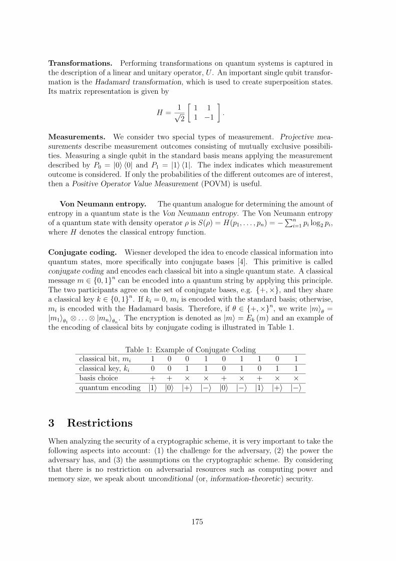
Transformations. Performing transformations on quantum systems is captured inthe description of a linear and unitary operator, U . An important single qubit transfor-mation is the Hadamard transformation, which is used to create superposition states.Its matrix representation is given by
H =1√2
[1 11 −1
].
Measurements. We consider two special types of measurement. Projective mea-surements describe measurement outcomes consisting of mutually exclusive possibili-ties. Measuring a single qubit in the standard basis means applying the measurementdescribed by P0 = |0〉 〈0| and P1 = |1〉 〈1|. The index indicates which measurementoutcome is considered. If only the probabilities of the different outcomes are of interest,then a Positive Operator Value Measurement (POVM) is useful.
Von Neumann entropy. The quantum analogue for determining the amount ofentropy in a quantum state is the Von Neumann entropy. The Von Neumann entropyof a quantum state with density operator ρ is S(ρ) = H(p1, . . . , pn) = −∑n
i=1 pi log2 pi,where H denotes the classical entropy function.
Conjugate coding. Wiesner developed the idea to encode classical information intoquantum states, more specifically into conjugate bases [4]. This primitive is calledconjugate coding and encodes each classical bit into a single quantum state. A classicalmessage m ∈ 0, 1n can be encoded into a quantum string by applying this principle.The two participants agree on the set of conjugate bases, e.g. +,×, and they sharea classical key k ∈ 0, 1n. If ki = 0, mi is encoded with the standard basis; otherwise,mi is encoded with the Hadamard basis. Therefore, if θ ∈ +,×n, we write |m〉θ =|m1〉θ1 ⊗ . . .⊗ |mn〉θn . The encryption is denoted as |m〉 = Ek (m) and an example ofthe encoding of classical bits by conjugate coding is illustrated in Table 1.
Table 1: Example of Conjugate Codingclassical bit, mi 1 0 0 1 0 1 1 0 1classical key, ki 0 0 1 1 0 1 0 1 1basis choice + + × × + × + × ×quantum encoding |1〉 |0〉 |+〉 |−〉 |0〉 |−〉 |1〉 |+〉 |−〉
3 Restrictions
When analyzing the security of a cryptographic scheme, it is very important to take thefollowing aspects into account: (1) the challenge for the adversary, (2) the power theadversary has, and (3) the assumptions on the cryptographic scheme. By consideringthat there is no restriction on adversarial resources such as computing power andmemory size, we speak about unconditional (or, information-theoretic) security.
175
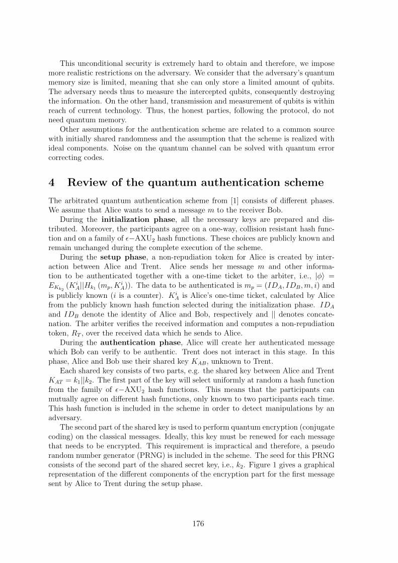
This unconditional security is extremely hard to obtain and therefore, we imposemore realistic restrictions on the adversary. We consider that the adversary’s quantummemory size is limited, meaning that she can only store a limited amount of qubits.The adversary needs thus to measure the intercepted qubits, consequently destroyingthe information. On the other hand, transmission and measurement of qubits is withinreach of current technology. Thus, the honest parties, following the protocol, do notneed quantum memory.
Other assumptions for the authentication scheme are related to a common sourcewith initially shared randomness and the assumption that the scheme is realized withideal components. Noise on the quantum channel can be solved with quantum errorcorrecting codes.
4 Review of the quantum authentication scheme
The arbitrated quantum authentication scheme from [1] consists of different phases.We assume that Alice wants to send a message m to the receiver Bob.
During the initialization phase, all the necessary keys are prepared and dis-tributed. Moreover, the participants agree on a one-way, collision resistant hash func-tion and on a family of ε−AXU2 hash functions. These choices are publicly known andremain unchanged during the complete execution of the scheme.
During the setup phase, a non-repudiation token for Alice is created by inter-action between Alice and Trent. Alice sends her message m and other informa-tion to be authenticated together with a one-time ticket to the arbiter, i.e., |φ〉 =EKk2
(KiA||Hk1 (mp, K
iA)). The data to be authenticated is mp = (IDA, IDB,m, i) and
is publicly known (i is a counter). KiA is Alice’s one-time ticket, calculated by Alice
from the publicly known hash function selected during the initialization phase. IDA
and IDB denote the identity of Alice and Bob, respectively and || denotes concate-nation. The arbiter verifies the received information and computes a non-repudiationtoken, RT , over the received data which he sends to Alice.
During the authentication phase, Alice will create her authenticated messagewhich Bob can verify to be authentic. Trent does not interact in this stage. In thisphase, Alice and Bob use their shared key KAB, unknown to Trent.
Each shared key consists of two parts, e.g. the shared key between Alice and TrentKAT = k1||k2. The first part of the key will select uniformly at random a hash functionfrom the family of ε−AXU2 hash functions. This means that the participants canmutually agree on different hash functions, only known to two participants each time.This hash function is included in the scheme in order to detect manipulations by anadversary.
The second part of the shared key is used to perform quantum encryption (conjugatecoding) on the classical messages. Ideally, this key must be renewed for each messagethat needs to be encrypted. This requirement is impractical and therefore, a pseudorandom number generator (PRNG) is included in the scheme. The seed for this PRNGconsists of the second part of the shared secret key, i.e., k2. Figure 1 gives a graphicalrepresentation of the different components of the encryption part for the first messagesent by Alice to Trent during the setup phase.
176

mp |mT 〉 = EKk2(mT )
k2
Hk1(mp, KiA)
mT = KiA||Hk1 (mp, K
iA)
PRNG Kk2
K iA
QE
KAT = k1||k2mp = (IDA, IDB,m, i)
Figure 1: Construction for the encryption and authentication of a publicly knownclassical message mp, by means of a shared key KAT = k1||k2. The authentication tagof the message mp||Ki
A is computed by the hash function Hk1 , resulting in a n1−bittag. Then, encrypting the message mT ∈ 0, 1n2 is performed by the quantum cipherwith secret-key Kk2 ∈ 0, 1n2 .
5 Analysis
We will analyze the security of this construction depicted in Figure 1. An externalopponent (which could also be Bob) is considered. The goal of the adversary can consistof (partially) breaking the quantum cipher, and thus obtaining some information onthe shared key. Moreover, since the hash key Hk1 is reused for several messages andthe scheme is classified as an authentication scheme satisfying the non-repudiationproperty, her ultimate goal is to perform a substitution attack, that is to produce avalid message-authentication pair on a previously unseen message.
In [5], the authors introduce quantum ciphers with perfect security. Even if anadversary knows the plaintext and applies an optimal measurement on the quantummessages, her Shannon uncertainty on the key is almost maximal. In the constructionfrom Figure 1, the encryption key is generated by a cryptographic PRNG. The qualityof this generator determines the security of the scheme. In order to perform an attack,the adversary needs to know some information on the sequence of output bits producedby the generator.
The analysis of the scheme constitutes thus of several parts: (1) demonstrate thatthe principle of conjugate coding is a quantum cipher respecting the properties from[5, 6]; (2) demonstrate that attacking the PRNG isn’t possible, due to the limitedinformation an adversary can retrieve on the generated sequence; (3) include the factthat several messages are exchanged using the same hash function.
5.1 Conjugate coding is a quantum cipher with perfect secu-rity
Conjugate coding (see Subsection 2.2) can be considered as a quantum cipher to encryptclassical messages using classical keys and produces quantum states. The encryptionand decription processes are modeled by unitary operations on the plaintext. Following[5], we give a formal definition of the conjugate coding cipher, denoted as Cn−cipher:
Definition 1. The Cn−cipher is an (n, n)−quantum cipher. Given a classical messagem ∈ 0, 1n and a classical key k ∈ 0, 1n, it outputs the following n−qubit state as
177

ciphertext:|φ〉 = Hk1 ⊗Hk2 ⊗ . . .⊗Hkn |m1m2 . . .mn〉 ,
where H is the Hadamard transform.
This technique deals with each (qu)bit separately and is described as follows. Alicetransforms the classical message she wants to transmit into an n−bit quantum state|ψ〉, consisting of |0〉 and |1〉 states, and described by ρ. Then, she applies to each qubitof this state the Hadamard transformation, only if the corresponding bit of the sharedkey equals 1. Afterwards, she sends the result |φ〉 to Bob. Knowing the key k, Bob candecrypt the received qubits by reversing the Hadamard transformation, retrieving ρ.
The data hiding and key hiding properties of a general quantum cipher are satisfied.They guarantee that an adversary cannot obtain any information about the key andthe message when an arbitrary ciphertext is seen [5]. Therefore, we require that Eve,who does not know the key, always obtains the same density matrix ρE by monitoringthe channel. This property is captured in the scenario of a Private Quantum Channel,formalized as follows [6].
Definition 2. Let S ⊆ H2n be a set of pure n−qubit states, E =√
piUi|1 ≤ i ≤ n
be a superoperator where each Ui is a unitary mapping on H2n ,∑n
i=1 pi = 1, and ρEbe an n−bit density operator. Then [S, E , ρE] is called a Private Quantum Channel(PQC) if and only if for all |ψ〉 ∈ S we have
E (|ψ〉 〈ψ|) =n∑
i=1
piUi (|ψ〉 〈ψ|)U †i = ρE,
where U †i is the complex-transpose of Ui. E denotes the superoperator which appliesUi with probability pi to its argument.
The Cn−cipher, with key k ∈ 0, 1n, applies a Hadamard transform to each qubitindividually if ki = 1, otherwise, the qubit remains unchanged (denoted by applyingthe identity operator In). If mi = 0, a uniform mixture of |0〉 and |1〉 is sent acrossthe quantum channel, expressed by ρ0 = 1
2|0〉 〈0| + 1
2|+〉 〈+|. Similarly, if mi = 1, we
obtain ρ1 = 12|1〉 〈1|+ 1
2|−〉 〈−|. We use Hk to denote the n−bit unitary transformation
Hk1 ⊗Hk2 ⊗ . . .⊗Hkn .
Theorem 3. IfH2 = cos θ |0〉+ sin θ |1〉 |θ ∈ 0, π/2, S = H⊗n2 , E =
1√2nHk|k ∈ 0, 1n
and ρE =1
2nI2n, then [S, E , ρE] is a Private Quantum Channel.
Proof. To each qubit |ψi〉, we apply the Hadamard transformation H or the identityoperator, each with probability 1/2. This action puts each qubit in a completely mixedstate. The superoperator E applies this strategy to each of the n qubits individually,hence E (|ψ〉 〈ψ|) = 1
2nI2n for every |ψ〉 ∈ H⊗n2 .
We now calculate the Von Neumann entropy of the quantum state |φ〉, i.e., S(ρ).For the quantum state |ψ〉, which is the tensor product of n qubits, we have thatE (|ψ〉 〈ψ|) = 1
2nI2n . Therefore, we can calculate the Von Neumann entropy as follows:
S(ρ) = S
(1
2nI2n
)= S
(1
2I2 ⊗ . . .⊗
1
2I2
)= nS
(1
2I2
)= n
(1
2+
1
2
)= n.
178
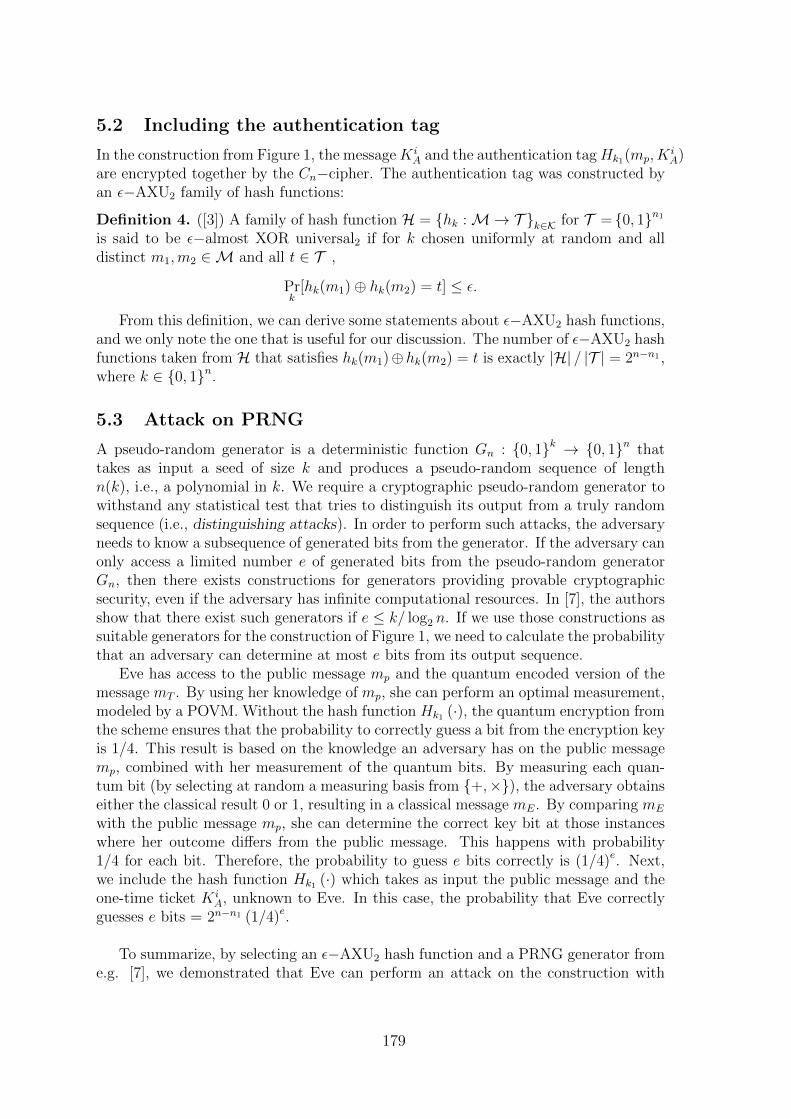
5.2 Including the authentication tag
In the construction from Figure 1, the messageKiA and the authentication tagHk1(mp, K
iA)
are encrypted together by the Cn−cipher. The authentication tag was constructed byan ε−AXU2 family of hash functions:
Definition 4. ([3]) A family of hash function H = hk :M→ T k∈K for T = 0, 1n1
is said to be ε−almost XOR universal2 if for k chosen uniformly at random and alldistinct m1,m2 ∈M and all t ∈ T ,
Prk
[hk(m1)⊕ hk(m2) = t] ≤ ε.
From this definition, we can derive some statements about ε−AXU2 hash functions,and we only note the one that is useful for our discussion. The number of ε−AXU2 hashfunctions taken from H that satisfies hk(m1)⊕hk(m2) = t is exactly |H| / |T | = 2n−n1 ,where k ∈ 0, 1n.
5.3 Attack on PRNG
A pseudo-random generator is a deterministic function Gn : 0, 1k → 0, 1n thattakes as input a seed of size k and produces a pseudo-random sequence of lengthn(k), i.e., a polynomial in k. We require a cryptographic pseudo-random generator towithstand any statistical test that tries to distinguish its output from a truly randomsequence (i.e., distinguishing attacks). In order to perform such attacks, the adversaryneeds to know a subsequence of generated bits from the generator. If the adversary canonly access a limited number e of generated bits from the pseudo-random generatorGn, then there exists constructions for generators providing provable cryptographicsecurity, even if the adversary has infinite computational resources. In [7], the authorsshow that there exist such generators if e ≤ k/ log2 n. If we use those constructions assuitable generators for the construction of Figure 1, we need to calculate the probabilitythat an adversary can determine at most e bits from its output sequence.
Eve has access to the public message mp and the quantum encoded version of themessage mT . By using her knowledge of mp, she can perform an optimal measurement,modeled by a POVM. Without the hash function Hk1 (·), the quantum encryption fromthe scheme ensures that the probability to correctly guess a bit from the encryption keyis 1/4. This result is based on the knowledge an adversary has on the public messagemp, combined with her measurement of the quantum bits. By measuring each quan-tum bit (by selecting at random a measuring basis from +,×), the adversary obtainseither the classical result 0 or 1, resulting in a classical message mE. By comparing mE
with the public message mp, she can determine the correct key bit at those instanceswhere her outcome differs from the public message. This happens with probability1/4 for each bit. Therefore, the probability to guess e bits correctly is (1/4)e. Next,we include the hash function Hk1 (·) which takes as input the public message and theone-time ticket Ki
A, unknown to Eve. In this case, the probability that Eve correctlyguesses e bits = 2n−n1 (1/4)e.
To summarize, by selecting an ε−AXU2 hash function and a PRNG generator frome.g. [7], we demonstrated that Eve can perform an attack on the construction with
179
probability 2n−n1 (1/4)e, where e = k/log2n2 and Alice and Bob share a secret-keyKAT = k1||k2 of size k + n2;
6 Conclusion and future work
In this paper, we analyzed the security of the construction used in an arbitrated quan-tum authentication scheme on which an adversary can perform a known-message at-tack. We demonstrated that the quantum encryption from the scheme is a quantumcipher with perfect security. Then, we explained that an adversary can retrieve onlya limited amount of information on the keystream. This is insufficient to mount anattack when a suitable generator is used. In future work, we will consider the effect ofreusing the same hash function and give a mathematical proof of the security of thecomplete scheme.
References
[1] H. Bruyninckx, and D. Van Heule, “Arbitrated Secure Authentication realized byusing quantum principles,” Communications (ICC), 2015 IEEE International Con-ference on, London, June 2015, pp. 7420-7425.
[2] N. Asokan, G. Tsudik, and M. Waidner, “Server-supported signatures,” Journal ofComputer Security, vol. 5, n°1, pp. 91-108, Jan 1997.
[3] Rogaway, “Bucket hashing and its application to fast message authentication,”Journal of Cryptology, vol. 12, n°2, pp. 91–115, 1999.
[4] S. Wiesner. “Conjugate coding,” SIGACT News, 15 (1): 78-88, 1983.
[5] I. Damgard, T. Pedersen, and L. Salvail, “On the Key-Uncertainty of QuantumCiphers and the Computational Security of One-way Quantum Transmission,” inAdvances in Cryptology - EUROCRYPT 2004, Springer-Verlag, 2004, pp. 91-108.
[6] A. Ambainis, M. Mosca, A. Tapp and R. deWolf, “Private Quantum Channels,”Proceedings of the 41st Annual Symposium on Foundations of Computer Science,2000, pp. 547–553.
[7] U. Maurer and J. Massey, “Local Randomness in Pseudorandom Sequences,” Jour-nal of Cryptology, vol. 4, pp. 135–149, 1991.
180
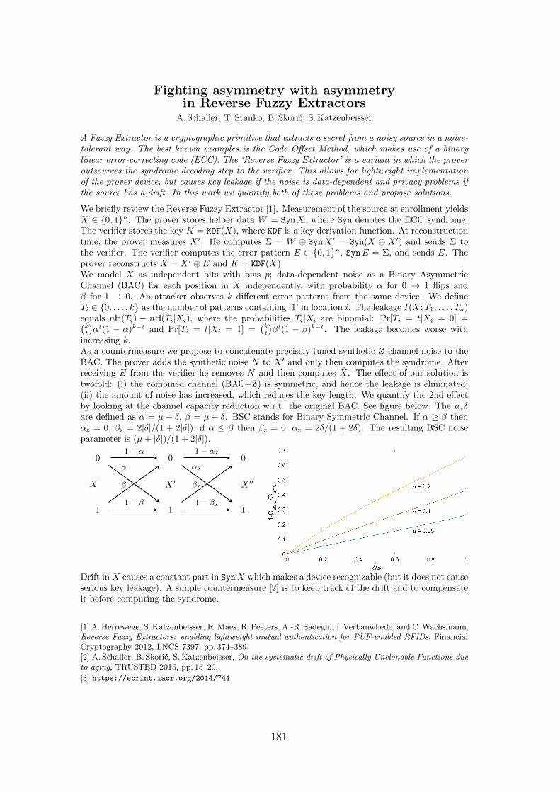
Fighting asymmetry with asymmetryin Reverse Fuzzy Extractors
A. Schaller, T. Stanko, B. Skoric, S. Katzenbeisser
A Fuzzy Extractor is a cryptographic primitive that extracts a secret from a noisy source in a noise-tolerant way. The best known examples is the Code Offset Method, which makes use of a binarylinear error-correcting code (ECC). The ‘Reverse Fuzzy Extractor’ is a variant in which the proveroutsources the syndrome decoding step to the verifier. This allows for lightweight implementationof the prover device, but causes key leakage if the noise is data-dependent and privacy problems ifthe source has a drift. In this work we quantify both of these problems and propose solutions.
We briefly review the Reverse Fuzzy Extractor [1]. Measurement of the source at enrollment yieldsX ∈ 0, 1n. The prover stores helper data W = SynX, where Syn denotes the ECC syndrome.The verifier stores the key K = KDF(X), where KDF is a key derivation function. At reconstructiontime, the prover measures X ′. He computes Σ = W ⊕ SynX ′ = Syn(X ⊕ X ′) and sends Σ tothe verifier. The verifier computes the error pattern E ∈ 0, 1n, SynE = Σ, and sends E. Theprover reconstructs X = X ′ ⊕ E and K = KDF(X).We model X as independent bits with bias p; data-dependent noise as a Binary AsymmetricChannel (BAC) for each position in X independently, with probability α for 0 → 1 flips andβ for 1 → 0. An attacker observes k different error patterns from the same device. We defineTi ∈ 0, . . . , k as the number of patterns containing ‘1’ in location i. The leakage I(X;T1, . . . , Tn)equals nH(Ti) − nH(Ti|Xi), where the probabilities Ti|Xi are binomial: Pr[Ti = t|Xi = 0] =(kt
)αt(1 − α)k−t and Pr[Ti = t|Xi = 1] =
(kt
)βt(1 − β)k−t. The leakage becomes worse with
increasing k.As a countermeasure we propose to concatenate precisely tuned synthetic Z-channel noise to theBAC. The prover adds the synthetic noise N to X ′ and only then computes the syndrome. Afterreceiving E from the verifier he removes N and then computes X. The effect of our solution istwofold: (i) the combined channel (BAC+Z) is symmetric, and hence the leakage is eliminated;(ii) the amount of noise has increased, which reduces the key length. We quantify the 2nd effectby looking at the channel capacity reduction w.r.t. the original BAC. See figure below. The µ, δare defined as α = µ − δ, β = µ + δ. BSC stands for Binary Symmetric Channel. If α ≥ β thenαz = 0, βz = 2|δ|/(1 + 2|δ|); if α ≤ β then βz = 0, αz = 2δ/(1 + 2δ). The resulting BSC noiseparameter is (µ+ |δ|)/(1 + 2|δ|).
0
1
0
1
0
1
X X ′ X ′′
1 − α
1 − β
1 − αZ
1 − βZ
β
α
βZ
αZ
Drift in X causes a constant part in SynX which makes a device recognizable (but it does not causeserious key leakage). A simple countermeasure [2] is to keep track of the drift and to compensateit before computing the syndrome.
[1] A. Herrewege, S. Katzenbeisser, R. Maes, R. Peeters, A.-R. Sadeghi, I. Verbauwhede, and C. Wachsmann,Reverse Fuzzy Extractors: enabling lightweight mutual authentication for PUF-enabled RFIDs, FinancialCryptography 2012, LNCS 7397, pp. 374–389.[2] A. Schaller, B. Skoric, S. Katzenbeisser, On the systematic drift of Physically Unclonable Functions dueto aging, TRUSTED 2015, pp. 15–20.
[3] https://eprint.iacr.org/2014/741
181
Linear Cryptanalysis of Reduced-Round Speck
Tomer Ashur Daniel BoddenKU Leuven and iMinds
Dept. ESAT, Group COSICAddress Kasteelpark Arenberg 10 bus 2452, B-3001 Leuven-Heverlee, [email protected] [email protected]
Abstract
Since DES became the first cryptographic standard, block ciphers have been apopular construction in cryptology. Speck is a recent block cipher developedby the NSA in 2013. It belongs to the cipher family known as ARX. ARXconstructions are popular because of their efficiency in software. The security ofthe cipher is derived from using modular addition, bitwise rotation and xor. Inthis paper we employ linear cryptanalysis for variants of Speck with block sizesof 32, 48, 64, 96, and 128 bits. We illustrate that linear approximations withhigh bias exist in variants of Speck.
1 Introduction
A recent surge of new block cipher designs has urged the need for cryptanalysts toscrutinize their security. Lightweight ciphers are designed for resource-constraineddevices. Designing ciphers for these devices means that one has to make design trade-offs keeping in mind the limitation that such an environment presents, such as limitedmemory, restricted computational and energy resources, etc.
A popular construction for block ciphers is Addition, Rotation and XOR, abbre-viated as ARX. In this construction a block is split into 2 or more words, which arethen added, XORed and rotated by the round function. The popularity of ARX con-struction stems from its good performance in software. Confusion is achieved by usingmodular addition in the round function, whereas diffusion is achieved by using cyclicrotation and xor.
In this paper we analyse the security of Speck, a block cipher that has been pub-lished by the NSA in 2013 [2]. Speck is a lightweight block cipher designed to achievegood performance in software. The block consists of two words, each 16/24/32/48, or64 bits, which are processed a number of times by the round function. At the end ofthe last round a ciphertext is obtained. Speck comes in different variants for whichdifferent security and performance levels are provided; see Table 1.
Since the publication of the cipher in 2013, several papers have analyzed its security[1, 4, 7]. The best published attacks on Speck are differential cryptanalytic attacksdescribed in [7]. In this paper we analyse the resistance of all variants of Speck againstlinear cryptanalysis.
Linear cryptanalysis is a known plaintext attack developed in 1993 by Matsui [9].When using this method the adversary searches for possible correlations between bitsof the input and bits of the output. Once such a correlation is found, the knownplaintexts and ciphertexts can be used to recover bits of the secret key. In our analysiswe find linear approximations covering 7, 8, 11, 10, and 11 rounds for versions of Speckwith block size 32, 48, 64, 96, and 128, respectively. These approximations can befurther extended to attack more rounds using methods such as those presented in [8].
This paper is structured as follow: In section 2 we describe Speck. In section 3we discuss shortly the related work. In section 4 we explain the automatic searchmethod that has been used to obtain linear approximations for Speck. In section 5
182

Figure 1: Speck round function
we present the approximations we found. In section 6 we explain how to obtain alinear distinguisher from the linear trails presented in section 5. Finally, in section 7we conclude this paper.
2 A Brief Description of Speck
The cipher comes in several versions sharing the same Feistel-structure and roundfunction. The different parameters of all Speck versions are presented in Table 1.
Table 1: Variants of the Speck-family [2]
Block Size n Key Size Word Size α β Rounds
32 64 16 7 2 22
48 72 24 8 3 2296 23
64 96 32 8 3 26128 27
96 96 48 8 3 28144 29
128 128 64 8 3 32192 33256 34
The round function uses three operations: Modular addition, . Left and right circular bit-shifts, by α and β. Bitwise XOR, ⊕.
The output of the round function is:xi+1 = (xi≫ α) (yi)yi+1 = ((xi≫ α) (yi))⊕ (yi≪ β))
The output words xi+1 and yi+1 are the input words for the next round, and the outputof the last round is the ciphertext. In Figure 1 the round function of Speck is shown.
183

Table 2: Previous attacks concerning Speck
Variantn/keysize
RoundsAttacked/
Total Rounds
Time Data Memory Source
32/64 11/22 246.7 230.1 237.1 [1]14/22 263 231 222 [7]
48/72 12/22 243 243 na [4]14/22 265 241 222 [7]
48/96 12/23 243 243 na [4]15/23 289 241 222 [7]
64/96 16/26 263 263 na [4]18/26 293 261 222 [7]
64/128 16/27 263 263 na [4]19/27 2125 261 222 [7]
96/96 15/28 289.1 289 248 [1]16/28 285 285 222 [7]
96/144 16/29 2135.9 290.9 294.5 [1]17/29 2133 285 222 [7]
128/128 16/32 2116 2116 264 [1]17/32 2113 2113 222 [7]
128/192 18/33 2182.7 2126.9 2121.9 [1]18/33 2177 2113 222 [7]
128/256 18/34 2182.7 2126.9 2121.9 [1]19/34 2241 2113 222 [7]
3 Related Work
Since the publication of Speck there has been a fair amount of analyzing done on thesecurity and performance of the cipher. The best attacks to date are of the familyof differential cryptanalysis [1, 4, 7]. Differential cryptanalysis has been developed byBiham and Shamir in 1990 [3]. When using differential cryptanalysis the adversaryinvestigates how differences in the input affect the output, trying to discover non-random behavior. Several specialized techniques of differential cryptanalysis have beenused to analyse Speck, such as the boomerang and the rectangle attacks [4, 7].
Results of previous attacks concerning Speck are presented in Table 2. From theseresults we gather that these methods are successful in attacking a large number ofrounds in the chosen plaintext model. Looking at the design of Speck we might expectthat linear cryptanalysis be effective as well. This paper complements previous workby evaluating the resistance of Speck against linear cryptanalysis.
3.1 Linear Cryptanalysis
Linear cryptanalysis [9] is a powerful cryptanalytic tool with regards to cryptanaly-sis of block ciphers. When using linear cryptanalysis, an adversary tries to find alinear expression that approximates a non-linear function with a probability differentthan 1
2. When a good approximation, consisting of a relation between the plaintext
and ciphertext, is found, the adversary gains information about the secret key. Theapproximation has the form:
Pi ⊕ . . .⊕ Pj ⊕ Ck . . .⊕ Cl = Km . . .⊕Kn (1)
184

with Pi . . . Pj being plaintext bits, Ck . . . Cl ciphertext bits and Km . . . Kn key bits.The approximation holds with some probability p, and its quality is usually measuredby the bias which is defined as ε = |p− 1
2|.
Knowing the probability of the linear approximation, the adversary can determinethe number of required known plaintexts, i.e., the data complexity ε−2.
Once a good approximation is found the adversary can retrieve one bit of the key.To combine linear approximations we use the Piling Up Lemma [9]. This will tell usthe bias of the combined approximation, which is the amount the probability deviatesfrom 1
2. For two approximations, with ε1 and ε2 as their respective biases, combining
them gives an overall bias of:ε = 2 · ε1ε2. (2)
This can be generalized for σ approximations:
ε = 2σ−1 ·σ∏
i=1
εi. (3)
The combined approximations can be used to form a linear distinguisher ζ for thecipher. This ζ can be used to detect non-random behavior in supposed to be randomsignals. Meaning that ζ can be used to detect if a certain cipher is being used. Whena good ζ is found, the input bits are masked by λx1 ;λy1, and the output bits aremasked using λxr ;λyr, resulting in:
T = # λx1 · x1 ⊕ λy1 · y1 ⊕ λxr · xr ⊕ λyr · yr = 0 (4)
with x1 and y1 being the plaintexts, xr and yr the ciphertexts, r the length of ζ, T acounter and · the dot product. This should be repeated for at least ε−2 messages. If Tis around:
ε−2 · (1
2± ε) (5)
the cipher can be distinguished from a random permutation.
3.2 Properties of Modular Addition
The modular addition operation, which is used as the nonlinear operation of Speck,consists of an xor and a carry. A chain of carries means using the previous carry inthe current operation. This makes the behavior of modular addition nonlinear. Toapproximate the behavior of Speck, we have to deal with modular addition in such away that accounts for this nonlinear behavior. The property of modular addition thatwe use is exploring the correlation between two neighboring bits. Suppose we have 3words x, y and z with z = x y. According to Cho and Pieperzyk [5], each single z(i)bit written as function of x(i),· · · ,x(0) and y(i),· · · ,y(0) bits can be expressed as:
z(i) = x(i) ⊕ y(i) ⊕ x(i−1) ⊕ y(i−1) ⊕i−2∑
j=0
x(j)y(j)
i−1∏
k=j+1
x(k) ⊕ y(k), i = 1, . . . , n− 1 (6)
with xi and yi each representing 1 bit each. The carry is represented by xi−1 ⊕ yi−1 ⊕∑i−2j=0 xjyj
∏i−1k=j+1 xk ⊕ yk which we refer to as Ri(x, y). The parity of two consecutive
bits can be approximated as:
z(i) ⊕ z(i−1) = x(i) ⊕ y(i) ⊕ x(i−1) ⊕ y(i−1), p =3
4(7)
185
In this expression, we use a property of modular addition mentioned in another paperby Cho and Pieperzyk [6] that removes the carry chain from Equation 6. Meaning thatif a mask λ contains only two consecutive bits, one can write:
P [λ · (x y) = λ · (x⊕ y)] =3
4. (8)
This expression means that using a mask λ to mask the bits we want to throw awayand keep the bits we are interested in (e.g two consecutive bits), we linearize the leftside of the expression by replacing it with the right-side. This approximation holdswith probability 3
4and has a bias 1
4. For an ARX construction, Equation 8 remains
valid as long as the following two conditions are avoided:
1. Bitwise rotation moves a pair of approximated bits to the MSB (most significantbit position) and LSB (least significant bit position) hence not adhering to theCho and Pieperzyk framework; or
2. Xor creates a single bit hence not adhering to the Cho and Pieperzyk framework.
4 Automated Search for Linear Approximations in
ARX Constructions
In order to automate the search for a good linear approximation, we have designedan ARX toolbox. The toolbox is implemented using a parallel programming languagecalled OpenCL. The configuration on which the computation was run has been a 40core Intel Xeon machine with a clock speed of 3.10GHz, exclusively using CPU’s. Thetime it took to compute all pairs of consecutive bits for the 32-bit input variant ofSpeck was less than 0.01 seconds to less than a week for the largest version of Speck.
We have analyzed in our work all possible pairs of consecutive bits over the lengthof a word (e.g. starting with one pair of two consecutive bits up to n
2pairs of two con-
secutive bits). We have done this analysis in three ways, forward direction, backwarddirection and combining forward and backward together. We have iterated over allpairs of consecutive bits until one of the two stop conditions was met. The first stopcondition is when a mask containing non-consecutive bits is encountered in the roundfunction entering into the modular addition. The other condition upon which the com-putation will be stopped is when the counter exceeds the maximum bias. In order tofind approximations with good bias we restrict the allowable counter to T ≤ n
2+ 1.
The bias for one pair of consecutive bits is 1 − P [Ri(x, y) = 0] = 14. Generalized to `
pairs of consecutive bits the bias can be calculated using the Piling Up Lemma:
2`−1 · (1− P [Ri(x, y) = 0])` (9)
with values for ` = 1, . . . , n2. The bias is calculated with the value obtained by the ham-
ming weight of the mask passing the modular addition in the round function dividedby 2, plus the bias of the previous rounds, calculated on the approximated modularaddition λ · (x⊕ y).
5 Linear Approximation of the Round Function of
Speck
Linear cryptanalysis relies on collecting a large amount of input and output pairs inorder to verify whether the approximation has been satisfied or not. In this work we
186

started with fixing one mask λx1 with one pair of consecutive bits (0x3, 0x6, . . .) andkeeping the other mask λy1 zero, checking how the masks evolve both in the forwardand backward direction. After receiving promising results for one pair we extended thecomputation to all possible pairs of two consecutive bits given a block size.
An overview of the obtained results from our experiments is shown in Table 3. Theseresults show that the distinguisher can cover up to 11-rounds for different versions ofSpeck. More details of linear cryptanalysis on Speck are given in Table 4.
A careful note to the reader when reviewing the results in Table 4 is that for 96-bitversion of Speck we retrieved 10-rounds, whereas for the 64 and 128-bit versions weretrieved 11-rounds each. The reason for the different r between these versions is stopcondition 1. For each version of Speck, the length of a word and mask vary accordingto n. Meaning that bitwise rotation operates over a different length (i.e., n
2).
We present in Table 5 the full linear trail in the forward and in the backwarddirection for the 32/64 variant. The information found in this table gives an ideawhy the computation broke in that particular round. Using this information in futureresearch could extend the distinguisher further.
Table 3: Distinguisher length for different versions of SpeckVariant n Distinguished rounds /
Total roundsBias Time
ComplexityData
Complexity
32 7/22 2−14 228 228
48 8/22 2−22 244 244
64 11/26 2−32 264 264
96 10/28 2−47 292 292
128 11/32 2−63 2144 2144
Table 4: Combined results for different versions of Speck
Variant n Distinguishedrounds / Total
rounds
Bias ε λx1 λy1 Number ofrounds
backward
Number ofroundsforward
32 7/22 2−14 0x0006 0x0000 3 448 8/22 2−22 0x000003 0x000000 5 364 11/26 2−32 0x00000003 0x00000000 8 396 10/28 2−47 0x000000000000 0x01800000000c 5 5128 11/32 2−63 0x0000003000000003 0x0000000000000000 8 3
187

Table 5: Linear trail for Speck32/64
Direction Cost λxi λyi λxi+1 λyi+1 Reasons stopped
0x0300 0xe0c7 broke consecutive for 0x300⊕ 0xe0c7
1 0x0300 0xe0c7 0x8301 0x8307
2 0x8301 0x8307 0x0300 0x0006
Backward 1 0x0300 0x0006 0x0006 0x0000
Forward 1 0x0006 0x0000 0x3c00 0x3000
2 0x3c00 0x3000 0xc198 0xc1e0
3 0xc198 0xc1e0 0xf00c 0xc18f
3 0xf00c 0xc18f 0x785f 0x61bf
0x785f 0x61bf broke consecutive for 0x785f≫ α
6 A Linear Distinguisher for Speck
Using the results from this paper we can build a linear distinguisher for each versionof Speck. We present here a distinguisher for the 32-bit version. To build the lineardistinguisher we use Equation 4 and fill in with information from Table 4, giving:
228 · (1
2± 2−14) (10)
using this distinguisher we can distinguish Speck32/64 from a random permutation. InAlgorithm 1 a pseudo code of the distinguishing attack is shown.
Data: 228 messages, input masks λx1 ;λy1, output masks λxr ;λyrset T = 0for 228 messages do
if λx1 · x⊕ λy1 · y ⊕ λxr · x⊕ λyr · y = 0 thenT = T + 1
end
endif T ≈ 228 · (1
2± 2−14) then
return 1else
return 0end
Algorithm 1: A pseudo-code of the distinguishing attack
188
7 Conclusion
In this paper we investigated the linear behavior of Speck in the known plaintext model.We explained the theory behind our method, presented linear approximations for eachversion of Speck and gave one example a linear distinguisher for Speck32/64.
The analysis in this paper tested the strength of the Speck round function anddemonstrated that the cipher offers sufficient resistance against linear cryptanalysis.Future work may find better linear approximations. Proven that linear cryptanalysiscan achieve a meaningful distinguisher, we believe that future research on ARX con-structions may deliver good linear approximations for these ciphers. Our tool can beused to test the resistance of such constructions performing the computation with thelatest parallel computing techniques.
Acknowledgments. The authors wish to Thank Vincent Rijmen for his support,Mathy Vanhoef for reviewing an earlier version of this paper, and R. Tzach for somethought provoking discussions.
This work was partially supported by the Research Fund KU Leuven, OT/13/071.The first author was also supported by Google Europe Scholarship for Students withDisabilities.
References
[1] Abed, F., List, E., Wenzel, J., Lucks, S.: Differential cryptanalysis of round-reducedsimon and speck. Preproceedings of Fast Software Encryption (FSE 2014)(2014, toappear) (2014)
[2] Beaulieu, R., Shors, D., Smith, J., Treatman-Clark, S., Weeks, B., Wingers, L.:The simon and speck families of lightweight block ciphers. IACR Cryptology ePrintArchive (2013) 404
[3] Biham, E., Shamir, A.: Differential cryptanalysis of the data encryption standard.Volume 28. Springer-Verlag New York (1993)
[4] Biryukov, A., Roy, A., Velichkov, V.: Differential analysis of block ciphers simonand speck. In: International Workshop on Fast Software Encryption-FSE. (2014)
[5] Cho, J.Y., Pieprzyk, J.: Algebraic attacks on sober-t32 and sober-t16 withoutstuttering. In: Fast Software Encryption, Springer (2004) 49–64
[6] Cho, J.Y., Pieprzyk, J.: Multiple modular additions and crossword puzzle attackon nlsv2. In: Information Security. Springer (2007) 230–248
[7] Dinur, I.: Improved differential cryptanalysis of round-reduced speck. In: SelectedAreas in Cryptography–SAC 2014. Springer (2014) 147–164
[8] Knudsen, L.R., Mathiassen, J.E.: A chosen-plaintext linear attack on des. In: FastSoftware Encryption, Springer (2001) 262–272
[9] Matsui, M.: Linear cryptanalysis method for des cipher. In: Advances inCryptology—EUROCRYPT’93, Springer (1994) 386–397
189
An Efficient Privacy-Preserving ComparisonProtocol in Smart Metering Systems
Majid Nateghizad Zekeriya Erkin Reginald L. LagendijkDelft University of Technology
Department of Intelligent Systems, Cyber Security GroupDelft, The Netherlands
[email protected] [email protected] [email protected]
Abstract
In smart grids, providing power consumption statistics to the customers andgenerating recommendations for managing electrical devices are considered to beeffective methods that can help to reduce energy consumption. Unfortunately,providing power consumption statistics and generating recommendations relyon highly privacy-sensitive smart meter consumption data. From past experi-ence, we see that it is essential to find scientific solutions that enable the utilityproviders to provide such services for their customers without damaging cus-tomers’ privacy. One effective approach relies on cryptography, where sensitivedata is only given in the encrypted form to the utility provider and is processedunder encryption without leaking content. The proposed solutions using thisapproach are very effective for privacy protection but very expensive in termsof computation. In this paper, we focus on an essential operation for designinga privacy-preserving recommender system for smart grids, namely comparison,that takes two encrypted values and outputs which one is greater than the otherone. We improve the state-of-the-art comparison protocol based on Homomor-phic Encryption in terms of computation by 56% by introducing algorithmicchanges and data packing. As the smart meters are very limited devices, theoverall improvement achieved is promising for the future deployment of suchcryptographic protocols for enabling privacy enhanced services in smart grids.
1 Introduction
Smart grids, as the next generation of power grid, are utilizing both communica-tion technologies and information processing to monitor and manage power grids toenhance reliability, efficiency, and sustainability of power generation. One of the ad-vantages of smart grids compared to traditional power grids is the ability to observethe power consumption of households in very short time intervals in the order of sec-onds to minutes. As a result of the fine-coarse data reporting, it is possible to providepower consumption statistics to the consumers, which might help to reduce the overallconsumption by changing customer behavior, as pointed out in several works [1]. Forexample, Honebein et al. [2] defined people as the only true smart part of a smart grid;therefore monitoring, understanding, and promoting the end-users’ roles from passiveto active is considered as a fundamental action in smart grids. To this end, there arealready several utility companies providing their customers devices and smart phoneapplications to monitor their real time consumption. Furthermore, one of the goalsof the utility providers, balancing the supply and the demand, also known as demandresponse (DR), can be achieved more effectively if the utility provider can also providestatistics about the power usage in the surrounding area and generate personalizedrecommendations, for example to manage electrical devices like electric cars, heatingsystems, and ovens in the household [3].
190
Providing statistics on power consumption and generating personalized recommen-dations to inform customers are heavily dependent on the smart meter consumptionreadings. Unfortunately, these readings are highly privacy-sensitive [4]. The utilityprovider can use the readings from the smart meters for other purposes, misuse themor even transfer them to other entities without the consent of the customers. As seenin many cases, privacy is considered to be a big challenge for using smart meters to thefullest extent, e.g. enabling personalized services such as generating recommendations.
In this paper, we assume that the utility provider generates statistics and recom-mendations for the customers so that the customers can adjust the electrical devicesfor the most cost-effective and environmentally friendly manner. To achieve this, werely on cryptography, which provides us tools to create Privacy by Design algorithms.For instance, there are already a number of studies for computing bills and aggregatingdata [5, 6]. The main idea in this research line is to provide only the encrypted powerconsumption to the utility provider and enable processing the encrypted data withoutdecrypting any sensitive information. This way, the utility provider cannot access tothe content but at the same time can perform the algorithms required for the service.Unfortunately, the cryptographic algorithms for this purpose are expensive in termsof computation, which mostly require smart meters to be involved in the computation[7, 8, 9]. Since the smart meters are very limited devices, improving the efficiency ofthe cryptographic algorithms is a challenge.
We address the efficiency problem of a fundamental operation, namely comparison,which is required to design any recommender system. In our setting, the encryptedconsumption readings are collected from the customers by an aggregator and the utilityprovider has the decryption key. For privacy reasons, the aggregator cannot transferthe data directly to the utility provider but can co-operate with the utility providerto generate recommendations. One important step in the system is to compare values,which are only available in the encrypted form. More precisely, the aggregator has twoencrypted values, and it needs to know which one is greater than the other one withoutrevealing their contents to anyone including itself.
There are numerous comparison protocols designed for comparing encrypted values[7, 9]. In this paper, we improve the state-of-the-art comparison protocol that relieson homomorphic encryption in terms of run-time by 56% by introducing algorithmicchanges. Furthermore, we also reduce decryption cost of the protocol by deployingdata packing [10]. Together, these improvements increase the overall efficiency of thecomparison protocol with encrypted inputs, bringing smart meters one step closer torun privacy-preserving cryptographic protocols based on homomorphic encryption.
2 Preliminaries
In this section, we describe the application setting, the security assumptions, andthe cryptographic tools used in this work.
Application Setting
In our application setting, we define three roles: 1) smart meters installed at thehouseholds, 2) a data aggregator, and 3) a utility provider. Smart meters measure,encrypt, and send consumers’ power consumption to the data aggregator, which col-lects and analyzes encrypted power consumption. Then, the utility provider generatesrecommendations for its customers by running a cryptographic protocol with the dataaggregator. The output of the cryptographic protocol, which depends on the purposeof the recommender system, is in the encrypted form, thus it is not available neitherto the data aggregator nor to the utility provider. The output is then revealed to thecustomer by using another a secure decryption protocol.
191
Security Model
The proposed protocol in this work is built on the semi-honest adversarial model,where the data aggregator, and the utility provider are honest in the sense that theyfaithfully follow the designed protocol but will try to infer information from the protocolexecution transcript. This assumption is realistic since companies are expected toproperly perform required services mentioned in the service level agreement, whenengaging in a collaboration. We assume that the utility provider is the only partyholding the private keys, while the smart meters and the data aggregator have thepublic keys for the encryption schemes. We assume that neither party colludes.
Homomorphic Encryption
In this work, we rely on two additively homomorphic cryptosystems, Paillier [11] andDGK (Damgard, Geislet and Krøigaard) [7]. An additively homomorphic encryptionscheme preserves certain structure that can be exploited to process ciphertexts withoutdecryption. Given Epk(m1) and Epk(m2), a new ciphertext whose decryption yields thesum of the plaintext messages m1 and m2 can be obtained by performing a certainoperation over the ciphertexts: Dsk(Epk(m1))⊗ (Epk(m2)) = m1 +m2.
Consequently, exponentiation of any ciphertext with a public value yields the en-crypted product of the original plaintext and the exponent: Dsk(Epk(m)e) = e ·m.
In the rest of the paper, we denote the ciphertext of a message m by [m] for thePaillier cryptosystem and JmK for the DGK.
3 Secure Comparison Protocol with Secret Inputs
In this section, we describe the state-of-the-art secure comparison protocol (SCP),which takes two encrypted inputs and outputs the greater one in the encrypted form.SCP based on the DGK construction introduced in [12] is one of the widely-usedcomparison protocols due to its efficiency. The DGK comparison protocol is a sub-protocol in the SCP, where each party possesses a secret but plaintext value. Thesub-protocol also uses the DGK cryptosystem for efficiency reasons.
The comparison protocol in [12] is modified and used by Erkin et al. in [8], and Veu-gen proposed an improved DGK comparison protocol (IDCP) in [9]. In the following,we describe the SCP construction.
For the sake of simplicity, we use the names Alice and Bob as the data aggregatorand the utility provider, respectively. We assume that Bob has the secret key sk andAlice has access to two encrypted values, [a] and [b], and wants to know if a < b.
Initially, Alice computes [z] = [2` + a − b] = [2`] · [a] · [b]−1, and then obtains theresult of comparison as follows:
[z`] = [2−` · (z − (z mod 2`))] = ([z] · [z mod 2`]−1)2−`
, (1)
where [z`] is the most significant bit of [z] and the result of comparison. If z` = 1then we have a > b, and otherwise a < b. A more efficient method of computing [z`]is based on the IDCP, where we can compute z` = bz/2`c and [a < b] = [1 − z`] =[1] · [z`]
−1, but we still need to compute [z mod 2`]. A more detailed explanationregarding computation of [z`] is provided in the following sections.
Computing [z mod 2`]
Notice that Alice has access only to [z], and interaction with Bob, who has theprivate key, is needed to compute modulo reduction, [z mod 2`]. However, Alice cannot
192

give [z] directly to Bob since this value reveals information on the difference of a andb. Therefore, Alice masks [z] using a random value as follows:
[d] = [z + r] = [z] · [r] , (2)
where r is a (κ+ `)-bit uniformly random number and κ is a security parameter. Aftermasking, Alice sends [d] to Bob to perform modulo reduction, where Bob first decrypts
[d], then computes d = d mod 2` and sends [d] and [d/2`] back to Alice. Subsequently,
to obtain [z mod 2`], Alice computes [z mod 2`] = [d−r mod 2`] = [d] · [r mod 2`]−1.Note that z mod 2` = z mod 2` if d > r mod 2`. When d < r mod 2`, an under-
flow occurs, and Alice has to add 2` to [z] to make the value positive again. Therefore,
Alice needs to determine whether d > r mod 2` or not. This is achieved by computingan encrypted value, [λ], which shows the relation between d and r mod 2`. Then, Alicecan perform following computation to obtain [z mod 2`]:
[z mod 2`] = [z + λ2`] = [z] · [λ]2`
. (3)
Alice can obtain [z`] by using Equation 1. [z`] can be computed more efficiently asfollow:
[z`] = [Ψ(z)] = [Ψ(d)] · [Ψ(r)]−1 · [λ]−1 (4)
where Ψ(x) = bx/2`c. For computing [λ], we run a secure comparison protocol withprivate inputs as described in the following section.
Computing [λ]
This protocol outputs an encrypted bit, which shows whether d > r = r mod 2` ornot. However, different than the original problem of comparing encrypted a and b, inthis protocol Alice and Bob possess r and d in plaintext, respectively. Based on thissetting, the IDCP for computing [λ] securely works as follows:
1. Bob sends a bitwise encryption of his input, Jd0K, ..., Jd`−1K, to Alice.
2. Alice chooses uniformly random bit δ, where δ ∈ 0, 1. Then she computess = 1− 2 · δ and JciK as follows,
JciK = Jdi − ri + s+ 3`−1∑
j=i+1
dj ⊕ rjK
= JdiK · JriK−1 · JsK ·( `−1∏
j=i+1
Jdj ⊕ rjK)3
, (5)
where Jdj ⊕ rjK = JdjK · JrjK · JdjK−2·rj , and i = 0, ..., `− 1.
3. Alice blinds each JciK with a uniformly random hi ∈R Z∗u such that
JeiK = Jci · hiK = JciKhi , (6)
then permutes JeiK and sends them to Bob. Note that if ct = 0, where t ∈0, ..., `− 1 then et = 0 as well.
193

4. Bob checks whether there is a zero among JeiK values. If none of the JeiK values
are encrypted zero then he sets λ = 0, otherwise λ = 1. Then he encrypts λ andsends [λ] to Alice.
5. Alice corrects [λ] to obtain [λ] as follows:
[λ] =
[λ] if s = 1
[1] · [λ]−1 if s = −1
After obtaining [λ], Alice computes [z mod 2`] and [z`] based on Equations 3 and 1respectively.
4 Efficient Privacy-Preserving Comparison Proto-
col (EPPCP)
In this section, we describe a new version of the original SCP based on the DGKconstruction, which is significantly more efficient in terms of run-time cost.
Proposed Comparison Protocol
Complexity analysis and experimental results reveal that the XOR operation incomputing JciK, in Equation 5, has a significant impact on the overall efficiency of theDGK comparison protocol for the following two reasons:
1. Computing XOR is computationally expensive, since Jr ⊕ dK = JrK · JdK · JdK−2·r.Veugen [9] proposed a more efficient technique of computing XOR, where Jr⊕dK =
JdK when r = 0; otherwise, Jr⊕ dK = J1K · JdK−1 (Recall that Alice and Bob have
access to values r and d, respectively and Alice is computing XOR). Thus, if requals to 1, one multiplication and one exponentiation with negative exponentshould be computed over DGK ciphertexts, which affects the performance ofDGK comparison protocol significantly.
2. Since the equation that involves XOR is computed during the protocol withencrypted inputs, it is not possible to introduce pre-computation for JciK to obtaina more efficient protocol.
Table 1 shows that computing JciK constitutes 70% of the overall run-time of the IDCPfor Alice.
Based on these two facts, we propose a more efficient way of computing JciK, whichdoes not rely on the original XOR computation. The value JciK can be re-written asfollows:
JciK = Jdi − ri + s+`−1∑
j=i+1
(dj · 2j − rj · 2j)K . (7)
Alice computes Equation 7 in three steps:
1. Bob computes JtiK = Jdi +∑`−1
j=i+1 dj · 2jK, and sends JtiK to Alice,
2. Alice computes JviK = Js− ri −∑`−1
j=i+1 rj · 2jK, and
194

3. Alice computes JciK as follows,
JciK = Jti + viK = JtiK · JviK . (8)
Note that Alice can pre-compute JviK and factor ‘3’ is not needed in the computationof JciK. After computing all JciK values, Alice masks each JciK and sends masked values
to Bob, where he checks if any of the given masked JciK is zero, then generates [λ], and
sends it to Alice. She corrects [λ] based on value s to obtain [λ], computes Equation
3, and 1 to obtain [z`] as in the original protocol. Note that we compare 2d and 2r
instead of d and r respectively for technical reasons explained in the following section.
Table 1: Run-time performance for several steps of the IDCP.
Function Time (second) Overal computation (%)
Alice
Computing JciK 15 70JeiK ← Masking JciK 3.15 15Other 3.15 15
Bob
DGK zero-check 27.3 38Paillier decryption 44.4 62
Total 93
4.1 Data Packing
According to Table 1, Paillier decryption of [d] (Equation 2) dominates more than62% of the comparison protocol execution time at Bob side. We decrease the run-timeof Paillier decryption by employing data packing similar to [10, ?]. The main ideabehind data packing is to efficiently use the message space of the Paillier cryptosystemthat is much larger than the values to be compared.
Assume that z and r are ` and `+κ-bit integers, respectively. Then, [d] = [z+ r] isa (`+κ+ 1)-bit integer. Let the message space of the Paillier cryptosystem be η = pq,then Alice packs ρ = b(`+ κ+ 1)/ηc into one Paillier message as follows:
[d] =
ρ−1∑
j=0
[d]j · (2`+κ+1)j , (9)
and sends [d] to Bob. Then, Bob computes Dsk([d]), unpacks ρ different values andperforms modulo reduction on each unpacked value.
Employing the data packing technique not only reduces the number of very expen-sive Paillier decryption to be performed, but also decreases the number of encryptedmessages to be transmitted.
195
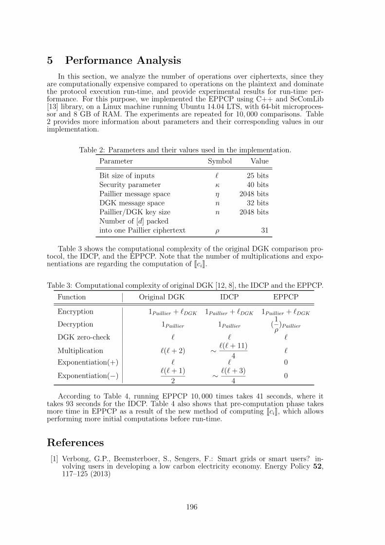
5 Performance Analysis
In this section, we analyze the number of operations over ciphertexts, since theyare computationally expensive compared to operations on the plaintext and dominatethe protocol execution run-time, and provide experimental results for run-time per-formance. For this purpose, we implemented the EPPCP using C++ and SeComLib[13] library, on a Linux machine running Ubuntu 14.04 LTS, with 64-bit microproces-sor and 8 GB of RAM. The experiments are repeated for 10, 000 comparisons. Table2 provides more information about parameters and their corresponding values in ourimplementation.
Table 2: Parameters and their values used in the implementation.
Parameter Symbol Value
Bit size of inputs ` 25 bitsSecurity parameter κ 40 bitsPaillier message space η 2048 bitsDGK message space n 32 bitsPaillier/DGK key size n 2048 bitsNumber of [d] packedinto one Paillier ciphertext ρ 31
Table 3 shows the computational complexity of the original DGK comparison pro-tocol, the IDCP, and the EPPCP. Note that the number of multiplications and expo-nentiations are regarding the computation of JciK.
Table 3: Computational complexity of original DGK [12, 8], the IDCP and the EPPCP.
Function Original DGK IDCP EPPCP
Encryption 1Paillier + `DGK 1Paillier + `DGK 1Paillier + `DGK
Decryption 1Paillier 1Paillier (1
ρ)Paillier
DGK zero-check ` ` `
Multiplication `(`+ 2) ∼ `(`+ 11)
4`
Exponentiation(+) ` ` 0
Exponentiation(−)`(`+ 1)
2∼ `(`+ 3)
40
According to Table 4, running EPPCP 10, 000 times takes 41 seconds, where ittakes 93 seconds for the IDCP. Table 4 also shows that pre-computation phase takesmore time in EPPCP as a result of the new method of computing JciK, which allowsperforming more initial computations before run-time.
References
[1] Verbong, G.P., Beemsterboer, S., Sengers, F.: Smart grids or smart users? in-volving users in developing a low carbon electricity economy. Energy Policy 52,117–125 (2013)
196
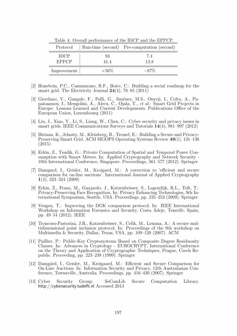
Table 4: Overall performance of the IDCP and the EPPCP.
Protocol Run-time (second) Pre-computation (second)
IDCP 93 7.4EPPCP 41.4 13.8
Improvement +56% −87%
[2] Honebein, P.C., Cammarano, R.F., Boice, C.: Building a social roadmap for thesmart grid. The Electricity Journal 24(4), 78–85 (2011)
[3] Giordano, V., Gangale, F., Fulli, G., Jimenez, M.S., Onyeji, I., Colta, A., Pa-paioannou, I., Mengolini, A., Alecu, C., Ojala, T., et al.: Smart Grid Projects inEurope: Lessons Learned and Current Developments. Publications Office of theEuropean Union, Luxembourg (2011)
[4] Liu, J., Xiao, Y., Li, S., Liang, W., Chen, C.: Cyber security and privacy issues insmart grids. IEEE Communications Surveys and Tutorials 14(4), 981–997 (2012)
[5] Birman, K., Jelasity, M., Kleinberg, R., Tremel, E.: Building a Secure and Privacy-Preserving Smart Grid. ACM SIGOPS Operating Systems Review 49(1), 131–136(2015)
[6] Erkin, Z., Tsudik, G.: Private Computation of Spatial and Temporal Power Con-sumption with Smart Meters. In: Applied Cryptography and Network Security -10th International Conference, Singapore. Proceedings, 561–577 (2012). Springer
[7] Damgard, I., Geisler, M., Kroigard, M.: A correction to ’efficient and securecomparison for on-line auctions’. International Journal of Applied Cryptography1(4), 323–324 (2009)
[8] Erkin, Z., Franz, M., Guajardo, J., Katzenbeisser, S., Lagendijk, R.L., Toft, T.:Privacy-Preserving Face Recognition. In: Privacy Enhancing Technologies, 9th In-ternational Symposium, Seattle, USA. Proceedings, pp. 235–253 (2009). Springer
[9] Veugen, T.: Improving the DGK comparison protocol. In: IEEE InternationalWorkshop on Information Forensics and Security, Costa Adeje, Tenerife, Spain,pp. 49–54 (2012). IEEE
[10] Troncoso-Pastoriza, J.R., Katzenbeisser, S., Celik, M., Lemma, A.: A secure mul-tidimensional point inclusion protocol. In: Proceedings of the 9th workshop onMultimedia & Security, Dallas, Texas, USA, pp. 109–120 (2007). ACM
[11] Paillier, P.: Public-Key Cryptosystems Based on Composite Degree ResiduosityClasses. In: Advances in Cryptology - EUROCRYPT, International Conferenceon the Theory and Application of Cryptographic Techniques, Prague, Czech Re-public. Proceeding, pp. 223–238 (1999). Springer
[12] Damgard, I., Geisler, M., Krøigaard, M.: Efficient and Secure Comparison forOn-Line Auctions. In: Information Security and Privacy, 12th Australasian Con-ference, Townsville, Australia. Proceedings, pp. 416–430 (2007). Springer
[13] Cyber Security Group: SeComLib Secure Computation Library.http://cybersecurity.tudelft.nl Accessed 2013
197
Security Analysis of the Drone CommunicationProtocol: Fuzzing the MAVLink protocol
Karel Domin Eduard Marin Iraklis SymeonidisKU Leuven
ESAT-COSIC and iMindsKasteelpark Arenberg 10, B-3001 Leuven-Heverlee, Belgium
[email protected] [email protected]
Abstract
The MAVLink protocol, used for bidirectional communication between a droneand a ground control station, will soon become a worldwide standard. Theprotocol has been the subject of research many times before. Through thispaper, we introduce the method of fuzzing as a complementing technique tothe other research, to find vulnerabilities that have not been found before bydifferent techniques. The goal is to identify possible vulnerabilities in the protocolimplementation in order to make it more secure.
1 Introduction
Currently, drones are used to support critical services such as forest fire and illegalhunting detection, search and rescue operations or to deliver medical supplies. For thispurpose, they are often equipped with a navigation system (GPS), a camera and anaudio interface. Furthermore, they have a radio that enables wireless communicationwith the Ground Control Station (GCS) or a remote control. Besides the clear benefitsof using drones in all these services, they can also pose important security and privacythreats. The wireless communication channel opens up the door for several types ofremote attacks. For example, adversaries could attempt to obtain sensitive data byeavesdropping the wireless medium, send malicious commands to the drone, or alterits software.
Previous research has focused on analysing the wireless communication protocolsof commercial drones [3], and exploiting the lack of security measures in the communi-cation channel [4, 5]. However, we are not aware of any security analysis of the drone’ssoftware. In this paper, we tackle this problem, and carry out a software securityanalysis of the MAVLink protocol, which is expected to become a world-wide standardwithin the DroneCode project [2]. More specifically, we investigate potential design orimplementation protocol flaws using fuzzing techniques. The goal is to inject invalid orsemi-invalid data to produce an unexpected software behaviour. We briefly formulatethree different research questions that we would like to explore more in detail in therest of this paper. This includes: (i) how can we identify software security flaws inthe MAVLink framework?, (ii) what are the consequences of exploiting these securityflaws? and (iii) can we provide countermeasures to mitigate such issues?.
2 Related Work
Most of the research conducted in the past years resulted in attacks against the secu-rity of drones. When a vulnerability was found, the vulnerability was exploited andthe drone could be hijacked or could crash. Academic research had the goal of re-producing a certain attack, make a theoretical background or proof and try to comeup with countermeasures to assure the security of the drone. A large portion of the
198
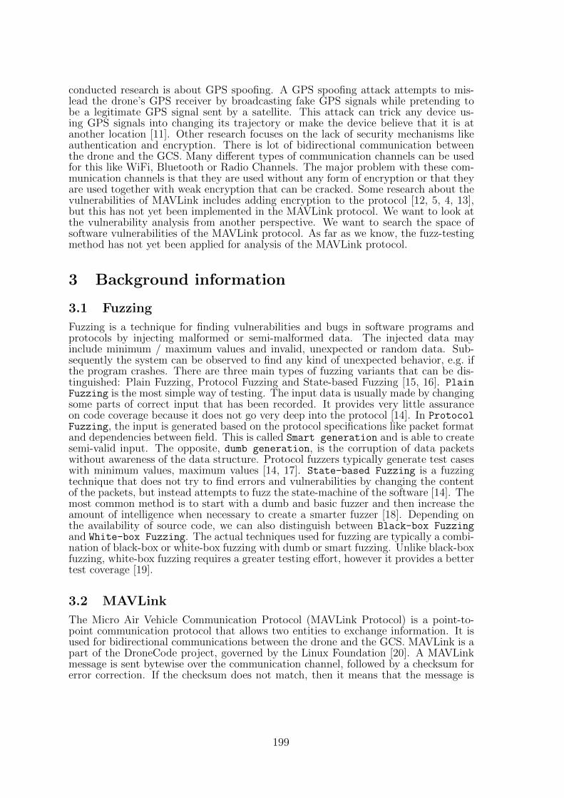
conducted research is about GPS spoofing. A GPS spoofing attack attempts to mis-lead the drone’s GPS receiver by broadcasting fake GPS signals while pretending tobe a legitimate GPS signal sent by a satellite. This attack can trick any device us-ing GPS signals into changing its trajectory or make the device believe that it is atanother location [11]. Other research focuses on the lack of security mechanisms likeauthentication and encryption. There is lot of bidirectional communication betweenthe drone and the GCS. Many different types of communication channels can be usedfor this like WiFi, Bluetooth or Radio Channels. The major problem with these com-munication channels is that they are used without any form of encryption or that theyare used together with weak encryption that can be cracked. Some research about thevulnerabilities of MAVLink includes adding encryption to the protocol [12, 5, 4, 13],but this has not yet been implemented in the MAVLink protocol. We want to look atthe vulnerability analysis from another perspective. We want to search the space ofsoftware vulnerabilities of the MAVLink protocol. As far as we know, the fuzz-testingmethod has not yet been applied for analysis of the MAVLink protocol.
3 Background information
3.1 Fuzzing
Fuzzing is a technique for finding vulnerabilities and bugs in software programs andprotocols by injecting malformed or semi-malformed data. The injected data mayinclude minimum / maximum values and invalid, unexpected or random data. Sub-sequently the system can be observed to find any kind of unexpected behavior, e.g. ifthe program crashes. There are three main types of fuzzing variants that can be dis-tinguished: Plain Fuzzing, Protocol Fuzzing and State-based Fuzzing [15, 16]. PlainFuzzing is the most simple way of testing. The input data is usually made by changingsome parts of correct input that has been recorded. It provides very little assuranceon code coverage because it does not go very deep into the protocol [14]. In ProtocolFuzzing, the input is generated based on the protocol specifications like packet formatand dependencies between field. This is called Smart generation and is able to createsemi-valid input. The opposite, dumb generation, is the corruption of data packetswithout awareness of the data structure. Protocol fuzzers typically generate test caseswith minimum values, maximum values [14, 17]. State-based Fuzzing is a fuzzingtechnique that does not try to find errors and vulnerabilities by changing the contentof the packets, but instead attempts to fuzz the state-machine of the software [14]. Themost common method is to start with a dumb and basic fuzzer and then increase theamount of intelligence when necessary to create a smarter fuzzer [18]. Depending onthe availability of source code, we can also distinguish between Black-box Fuzzingand White-box Fuzzing. The actual techniques used for fuzzing are typically a combi-nation of black-box or white-box fuzzing with dumb or smart fuzzing. Unlike black-boxfuzzing, white-box fuzzing requires a greater testing effort, however it provides a bettertest coverage [19].
3.2 MAVLink
The Micro Air Vehicle Communication Protocol (MAVLink Protocol) is a point-to-point communication protocol that allows two entities to exchange information. It isused for bidirectional communications between the drone and the GCS. MAVLink is apart of the DroneCode project, governed by the Linux Foundation [20]. A MAVLinkmessage is sent bytewise over the communication channel, followed by a checksum forerror correction. If the checksum does not match, then it means that the message is
199

corrupted and will be discarded. Figure. 1 shows the structure of a MAVLink message.We will now give a brief description of the fields included in the message:
Magic: indicates the beginning of anew messages.
Length: indicates the length of thepayload field.
Sequence number : indicates the se-quence number of the packet.
System ID : ID of the sending system.
Component ID : ID of the sendingcomponent.
Message ID : ID of the message in thepayload.
Payload : payload of the packet,which contains the parameters of themessage.
CRC : checksum for validation.
MAVLink messages are handled by the handleMessage(msg) function. This func-tion has a switch statement, handling the different message IDs [21].
Magic︸ ︷︷ ︸
1 byte
Len︸ ︷︷ ︸1 byte
Seq︸ ︷︷ ︸1 byte
SysID︸ ︷︷ ︸
1 byte
CompID︸ ︷︷ ︸
1 byte
MsgID︸ ︷︷ ︸
1 byte
Payload︸ ︷︷ ︸
x byte
CRC︸ ︷︷ ︸2 byte
Figure 1: MAVLink packet structure
3.3 Fuzzing Methodology
For our experiments we built a fuzzer capable of creating custom MAVLink messages.Several strategies are applied to construct the messages that are sent to the drone.Initially, we started with a random dumb fuzzing to observe how the software handlesinvalid messages. We then made a smarter fuzzer which takes into account the mes-sage format, and constructs semi-valid messages. The techniques for constructing thepayload of the messages are different for every test case.
4 Methodology
4.1 Lab Setup
Our laboratory setup employs the Software In The Loop environment (SITL) [7], whichprovides simulators for the ArduCopter, ArduPlane and ArduRover. We use the dronesimulator for the ArduCopter [1]. The simulator is run on a Linux virtual machineand the fuzzer on a host machine. The host system is running OS X El Capitan (8gbRAM, 2,4 GHz Intel Core i5) and the virtual machine for the virtual drone is runningUbuntu 14.04 TLS 64-bit. The communication between both machines is via a TCPconnection.Configuration:
Name Specification Function IP-addressHost System Mac OSX Host 192.168.56.1System 2 VM2: Ubuntu Virtual Drone 192.168.56.102
200
4.1.1 Case Studies
Our fuzzer, which is implemented in Python, is capable of constructing valid MAVLinkmessages. We now discuss how every field in the packet is constructed in our fuzzer.The Magic is a fixed value and is set to "fe", whereas the Length field is set tothe size of the payload field. In every transmitted message the Seq is increased byone, and it is reset to zero if it reaches the value of 255. The SysID and CompIDare kept fixed, i.e. "ff" and "00", respectively. The MsgId is a value in the rangeof 0-255. The payload contains the parameters that are used internally, (e.g. theheight of the drone), and is generated based on different strategies, which we willdiscuss more in detail for each experiment. The CRC value is generated using a CRC-16function; its polynomial generator is 0x1021, the initial value is FFFF, the input databytes are reversed, and the CRC result is reversed before the final XOR operation.The CRC parameters were obtained by looking at the available documentation andtesting the generator on [23]. The input to the generation function is as follows:Length+seq+SysID+CompID+MsgID+Payload+Seed.The seed is a x25 checksum generated over the message name, followed by the typeand name of each field. This seed is used to capture changes in the XML describingthe message definitions. This results in messages being rejected by the recipient if theydo not have the same XML structure.
There are some properties that a fuzzer needs to have. A fuzzer must be able torecord the test cases for reproduction. Therefore, every constructed message is writtento a file before it is sent to the virtual drone. Another property is the ability oftransmitting the test cases to the system under test. Since we are using SITL with aTCP connection therefore, the fuzzer initiates a three-way handshake with the virtualdrone and a connection is established via sockets. The generated messages can now besent to the drone over this socket. To observe the behaviour of the drone, we can usedifferent approaches. A simple observation is to check whether or not the connectionwith the drone is still alive. To further investigate its behaviour, the virtual drone canbe run inside gdb [22].
To start the virtual drone, the command in Listing 1 is used. This starts theArducopter simulation for a quadcopter, at a certain location with all of the memoryerased and faster operation. We define the following test cases.
Listing 1: Startup command
./ arducopter.elf --home -35,149,584,270 --model quad
--speedup 100 --wipe
Test Case 1 We establish a connection to the drone and start to send completelyrandom data including numbers, letters and characters. The actual structure of aMAVLink message is ignored at the moment. The length of the data sent to thevirtual drone ranges from 1 to 1000 characters. We do this to test how the softwarehandles incorrect data.
Test Case 2 For every message ID, we create a message with payloads of lengthranging from the minimum length (i.e. 1 byte) to the maximum length (i.e. 255 bytes).The payload consists of completely random combinations of hexadecimal values. Werepeat this test several times. This test is used to give an indication of how semi-validmessages are handled. This is important since these messages can go deeper into thesoftware.
Test Case 3 We also test the system’s behaviour when messages without any pay-load are sent. For every message id, a new message (with no payload) will be con-structed with the length set to zero. This test aims to find vulnerabilities that do notdepend on the payload.
Test Case 4 We construct payloads consisting entirely out of the minimum value.This test investigates how the implementation handles the minimum value "00". Thisis done for payloads with a length ranging from 1 to 255 bytes.
201

Test Case 5 following the previous test case, we do the same for the maximumvalue "ff".
Test Case 6 Within this test case, we do not send the messages byte per byte.An entire message with all the necessary fields is included in one TCP packet. Weincrementally increase the length of the random payload from 1 to 255 bytes extendingthe length of the entire message.
Test Case 7 Within this test case, we try to identify vulnerabilities depending onthe value of the length field and the actual value of the payload. In a first run, weconstructed messages with up to 5 bytes of payload and set the value of the length fieldto the length of the payload minus one. In the second run, we did the same, exceptthat the value of the length field was set to the length of the payload plus one.
5 Results Obtained and Discussion
Resulting from the listed test cases, we were able to identify a few security flaws.Particularly, from the sixth test case, where the payload increased randomly, the fuzzingscript was able to crash the virtual drone. The error caused by the fuzzing script canbe seen in Listing. 2.
Listing 2: Flaoting Point Exception
ERROR: Floating point exception - aborting
Aborted (core dumped)
To investigate the cause of the exceptions we used the gdb debugger and the coredump of the memory when the kernel crash occurred. From an analysis we identifiedthat errors corresponds to three specific functions. However, further investigation needsto be performed to identify the exact cause of the exceptions.
The next step of our work is to complete the entire range of the test cases aimingto gain more results identifying error flaws of the MAVLink software implementation.Moreover, we aim to further investigate the causes of the identified software flaws.However, we have to stress that fuzzing all possible test cases is a resource demandingoperation. For instance, there is a limitation concerning to the memory usage. Withthe current setup, it is not possible to try all possible permutations of payloads, for allpossible message and payload lengths. Currently, we are looking to further improvethe fuzzing scripts aiming to make the fuzzing operations more memory efficient.
6 Conclusion
This work aims to identify software vulnerabilities, by using the technique of fuzzing.Currently we focused our research on the MAVLink protocol. MAVLink is used as acommunication protocol between a drone and a ground control station. The protocolis actively developed by the community and aims to become one of the drone commu-nication standards. Our aim is to contribute to the identification of the security flawsof the protocol and to help the development community to mitigate these flaws. Atthe same time, we want to proof the suitability of fuzzing techniques for discoveringvulnerabilities in the implementation of the protocol. Currently, we have identifiedsoftware vulnerabilities that we are further investigating.
Many fuzzing platforms do already exist and can be used for the software analysisof the MAVLink protocol. Our next step is to further research and extend our fuzzingscripts aiming to generate more complex fuzzing scenarios.
202

7 Acknowledgements
This work was supported in part by the Research Council KU Leuven (C16/15/058).
References
[1] ArduCopter, https://www.dronecode.org/, 24 03 2016.
[2] DroneCode, http://ardupilot.org/copter/index.html, 24 03 2016.
[3] B. Hond, Fuzzing the GSM Protocol, Radboud University Nijmegen, Netherlands,2011.
[4] J. A. Marty, Vulnerability Analysis of the MAVLink Protocol for Command andcontrol of Unmanned Aircraft Air Force Institute of Technology, USA, 2014.
[5] N. Butcher, A. Stewart and Dr. S. Biaz , Securing the MAVLink CommunicationProtocol for Unmanned Aircraft Systems, Appalachian State University, AuburnUniversity, USA, 2013.
[6] Sulley Manual, http://www.fuzzing.org/wp-content/SulleyManual.pdf, 24 032016.
[7] Software In The Loop, http://ardupilot.org/dev/docs/sitl-simulator-software-in-the-loop.html, 24 03 2016.
[8] AR drone that infects other drones with virus winsdronegames, http://spectrum.ieee.org/automaton/robotics/diy/ar-drone-that-infects-other-drones-with-virus-wins-dronegames, 0305 2016.
[9] SkyJack, https://github.com/samyk/skyjack, 03 05 2016.
[10] Maldrone, http://garage4hackers.com/entry.php?b=3105, 03 05 2016.
[11] GPS Spoofing, https://capec.mitre.org/data/definitions/628.html, 03 052016.
[12] Thomas M. DuBuisson, Galois, Inc.1 , SMACCMPilot Secure MAVLink Commu-nications, Galois, Inc.1, 2013.
[13] MAVLink 2.0 packet signing proposal, https://docs.google.com/document/d/1ETle6qQRcaNWAmpG2wz0oOpFKSF_bcTmYMQvtTGI8ns, 03 05 2016.
[14] B. Hond, Fuzzing the GSM Protocol, Radboud University Nijmegen, 2011.
[15] A. Takanen, C. Miller, J. DeMott Fuzzing for Software Security Testing and Qual-ity Assurance, ARTECH HOUSE, INC., 2008.
[16] A. Greene, M. Sutton, P. Amini Fuzzing Brute Force Vulnerability Discovery,Addison-Wesley, 2007.
[17] OWASP Fuzzing, https://www.owasp.org/index.php/Fuzzing, 03 05 2016.
[18] 15 Minute Guide to Fuzzing, https://www.mwrinfosecurity.com/our-thinking/15-minute-guide-to-fuzzing/, 03 05 2016.
203

[19] J.eystadt, Automated Penetration Testing with White-Box Fuzzing, Microsoft Cor-poration, 2008.
[20] MAVLink Protocol, http://qgroundcontrol.org/mavlink/start, 03 05 2016.
[21] S. Balasubramanian, MAVLink Tutorial for Absolute Dummies (part-I),http://dev.ardupilot.com/wp-content/uploads/sites/6/2015/05/MAVLINK_FOR_DUMMIESPart1_v.1.1.pdf, 03 05 2016.
[22] GDB: The GNU Project Debugger , https://www.gnu.org/software/gdb/, 0305 2016.
[23] CRC Generator, http://www.zorc.breitbandkatze.de/crc.html, 03 05 2016.
204
Parallel optimization on the Entropic ConeBenoît Legat Raphaël Jungers
Université catholique de LouvainICTEAM
4 Av. G. Lemaître1348 Louvain-la-Neuve, Belgium
[email protected] [email protected]
Abstract
We introduce a parallelizable algorithm for approximate optimization on the en-tropic cone. We also present the toolbox EntropicCone.jl. Its aim is to improvethe computational repoducibility of the recent progress on the approximation ofthe entropic cone and to make them easily accessible for its many applications.These applications include the capacity region of multi-source network coding,converse theorems for multi-terminal problems of information theory, bounds onthe information ratios in secret sharing schemes and conditional independenceamong subvectors of a random vector.
1 The problem settingGiven n random variables, we can compute the entropy of any of the 2n subsets ofthese n variables. The set En , R2n−1 of vectors indexed by the nonempty subsets of[n] , 1, . . . , n is called the entropy space.The entropy vector of a set of n randomvariables is the entropy vector h such that hI is the entropy of the set Xi | i ∈ I .
We denote the set of vectors of R2n−1 that are entropic as:
Hn , h ∈ R2n−1 | ∃X1, . . . , Xn,∀∅ 6= S ⊆ [n], hS = Hb(Xi | i ∈ S ) .
It is known that the set Hn is not a cone for n ≥ 3 but its closure clHn is a convexcone [20]. The difference between Hn and clHn is only on the boundary of clHn. Moreprecisely, it has been shown that the relative interior of clHn is contained in Hn [15].
For n ≤ 3, clHn is equal to the polymatroid cone Pn. This is the set of entropyvectors h that are
nonnegative: hI ≥ 0 for any I ⊆ [n],
nondecreasing: hI ≤ hJ for any I ⊆ J ⊆ [n] and
submodular : hJ + hK ≥ hJ∪K + hJ∩K for any J,K ⊆ [n].
These three sets of conditions are linear inequalites on the entropy vector h. Since Pn
is defined by a finite subset of linear inequalities, it is a polyhedral cone.For n ≥ 4, clHn is a strict subset Pn. Moreover, clHn is not polyhedral [14] and
not even semialgebraic∗ [17].The entropic cone has a varietie of applications including the capacity region of
multi-source network coding [1], converse theorems for multi-terminal problems of in-formation theory [19], bounds on the information ratios in secret sharing schemes [2]∗A set is semialgebraic if it is the projection of an algebraic set. A set is algebraic if it can be
defined by finitely many polynomial inequalities.
205

and conditional independence among subvectors of a random vector [18]. This moti-vates the research on filling the gap between Pn and clHn.
In Section 2, we review the methods used to find tighter approximations of Hn thanPn. The current methods are linear and generate polyhedral outer approximations.However, as one can anticipate, the number of facets of a polyhedral approximation thatwould be “everywhere close” to Hn would have a sizeable amount of facets since it ishigh-dimensional and not semialgebraic. In practical applications, one is often lookingat the simpler problem of solving an optimization problem involving the entropic coneso we are only looking for an outer approximation that is “close” to Hn “near” theoptimum. In Section 3, we show a parallelizable algorithm for this problem.
2 Generating Non-Shannon InequalitiesThe inequalities that are valid for Pn are called Shannon inequalities and those thatare valid for Hn but not for Pn are called non-Shannon inequalities.
The current approach in generating an outer bound for Hn is to generate non-Shannon inequalities and to intersect Pn with the halfspaces they define.
There are currently four known methods for generating non-Shannon inequalities.The first one, which is the most commonly used, was introduced by Zhang and Yeungin order to generate the first non-Shannon inequality [21]; its description and analysiscan be found in [13]. The three other methods are respectively described in [12], [15]and [6].
The first two methods are equivalent [10] and it is still unknown whether the thirdand four methods can generate inequalities that cannot be generated by the first twoones. It is also unknown whether these four methods can generate all non-Shannoninequalities. In this paper, we will only use the first method which is described inSection 2.1.
2.1 Entropic Cone and adhesivityWe define the inner-adhesivity and self-adhesivity operators respectively as
iaJ,K|I(h) = g ∈ En′ | ∀I ⊆ L ⊆ J ∪K, gL = hL∩J + hL∩K − hI , I = J ∩K,saJ |I(h) = g ∈ En′ | ∀I ⊆ L ⊆ J ′ ∪K, gL = hL∩J ′ + hL∩K − hI , I ⊆ J.
where for inner-adhesivity, n′ = |J ∪K| and for self-adhesivity n′ = n+ |J \ I|, J ′ = [n]and K = ([n′] \ J ′) ∪ I.Definition 1. We say that a family of sets Sn ⊆ En is inner-adhesive if for any n,x ∈ Sn and J,K ⊆ [n], there exists y ∈ S|J∪K| such that y ∈ iaJ,K|J∩K(x) and we saythat it is self-adhesive if for any n, x ∈ Sn and I ⊆ J ⊆ [n], there exists y ∈ Sn+|J\I|such that y ∈ saJ |I(x).
The following theorem gives the relation between adhesivity and the entropic cone.Theorem 1. The entropic cone Hn is inner-adhesive and self-adhesive.Proof. Consider h ∈ Hn and n jointly distributed random variables Xi of joint proba-bility mass function p such that h is their entropy vector. Let pI denote the probabilitymass function of the marginal distribution of I. For inner-adhesivity, the entropy vectorg ∈ H|S∪T | of the probability function
pJ(xJ)pK(xK)pI(xI) = pJ |I(xJ |xI)pK|I(xK |xI)pI(xI)
206

belongs to iaJ,K|I(h) and for self-adhesivity, the entropy vector g ∈ Hn+|J\I| of theprobability function
pJ ′(xJ ′)pJ(xK)pI(xI) = pJ ′|I(xJ ′|xI)pJ |I(xK |xI)pI(xI),
where J ′ = [n], belongs to saJ |I(h).
Let ia−1J,K|I(S) (resp. sa−1
J |I(S)) be the set of vectors x such that there exists y ∈ Ssuch that y ∈ iaJ,K|I(x) (resp. y ∈ saJ |I(S)(x)). By Theorem 1, given an integer n0and a sequence (J1, I1), . . . , (Jm, Im) such that Ii ⊆ Ji ⊆ [ni] and ni = ni−1 + |Ji \ Ii|for i = 1, . . . ,m, the set†
(sa−1J1|I1 · · · sa−1
Jm|Im)(Pnm)
provides an outer approximations of Hn0 . Therefore an outer approximation of Hn0can be obtained by projecting the polyhedral cone of dimension ∑m
i=0 2ni − 1 given by
(h0, h1, . . . , hm) ∈ Pn0 × Pn1 × · · · × Pnm|hi ∈ saJ |I(hi−1), i = 1, . . . ,m . (1)
on the first 2n0 − 1 variables.This method was used to generate hundreds of non-Shannon inequalities in [8].
Using Benson’s algorithm [3] to compute the projection of (1), even more non-Shannoninequalities were uncovered in [7, 11].
As mentioned earlier, clHn is strictly included in Pn for n ≥ 4. As the dimension ofHn is exponential in n, the methods are usually benchmarked using H4. An importantnumerical quantity, related with the geometric properties of H4 is the Ingleton scoredefined as
I∗ , inf06=h∈H4
Iij(h)
where Iij(h) = 〈ij, h〉/h[n] [8, Definition 3] and ij is the Ingleton dual entropy vector[9]. The current best lower bound on I∗ is equal to −0.15789 [8]. Upper bounds on I∗can be obtained from exhibiting four jointly distributed variables for which the entropyvector has low Ingleton score. The current best upper bound on I∗ is equal to −0.09243[16].
3 Parallelizable optimization on the Entropic ConeIn this section, we show how to decompose polyhedra such as described by (1) to solveoptimization problems on it in an efficient and parallelizable manner using ideas fromStochastic Programming [5]. In stochastic programming, large scale linear programsare decomposed into smaller linear programs linked together by a markov chain. Thelinear program at each state u of the markov chain is:
Q(x, u) = minimize cTy +Qu(y)s.t.Wuy = hu − Tux,
x ≥ 0
where Qu(y) is the sum of Q(x, v) for each state v accessible from u weighted by theprobability to go from state u to state v. When the program is infeasible for some x,†Of course this also works if we include inner-adhesive operations in the sequence, we have only
included self-adhesivity in the sequence to keep simple notation.
207
Q(x, u) =∞. At the initial state of the markov chain, there is no term −Tux and thesolution at this stage is the solution of the original large scale linear program. Notethat if v is accessible from different states u, u′, the number of variables at u and u′must match for Q(·, v) to be well-defined.
For the adhesive operations, we propose to define a state for each dimension nand adhesive operation. That is, for every n, J,K, we have a state for the operationiaJ,K|J∩K and for every n, J, I with I ⊆ J , we have a state for the operation saJ |I . Thelinear program at the initial state is
minimize cTh+Q0(h)s.t.h ∈ Pn0 ,
the linear program for each state representing an inner-adhesivity is
Q(h, (n, iaJ,K|J∩K)) = minimize Q(n,iaJ,K|J∩K)(g)s.t. g ∈ iaJ,K|J∩K(h)
g ∈ P|J∪K|
and the linear program for each state representing an self-adhesivity is
Q(h, (n, saJ |I)) = minimize Q(n,saJ|I)(g)s.t. g ∈ saJ |I(h)
g ∈ Pn+|J\I|.
A state (n, a) is accessible from a state u if the dimension‡ of the linear programat u is 2n − 1. Since there is no objective in states other than the initial state, theprobability assigned for each transition does not matter. The only relevant informationin Q(h, (n, a)) is whether it is infinite or zero.
In stochastic programming, the domain of Q(·, (n, a)) is approximated by a polyhe-dron by starting with the approximation Rn and adding feasibility cuts. The feasibilitycuts are computed as follows: the linear program is solved for some h, if it is infeasi-ble, an unbounded ray of the dual linear program is computed and used to generate afeasibility cut.
These observations lead to Algorithm 1 for approximate optimization on the en-tropic cone that is inspired from the Stochastic Dual Dynamic Programming algorithmused in stochastic programming. Note that the initial node can have a nonlinearobjective function and additionnal nonlinear constraints. This algorithm is easily par-allelizable as the linear programs of the different states only need to communicate cutsand optimal solutions.
We developed a new toolbox EntropicCone.jl in Julia [4] for working with theentropic cone. This algorithm is one of the features implemented in the toolbox. Wetested Algorithm 1 to find lower bounds for the Ingleton score and obtained the bestknown lower bound −0.15789 in under a minute.
4 ConclusionSearching for non-Shannon inequalities to provide tighter outer approximations of theentropic cone may seem computationally demanding due to the use of a projectionalgorithm in high-dimensional space. However, if we restrict ourself to the optimization‡the number of variables of the linear program
208

Algorithm 1 Approximate minimization of c(h) subject to x ∈ Hn∩F for parametersnmax, K,m, ρ.Given a maximal value nmax for n, generate all states such that the dimension of thelinear program is at most 2nmax − 1for k = 1, 2, . . . , K doPick a set P of ρ random paths of length m starting at the initial state.Solve the optimization program
minimize c(h)s.t.h ∈ Pn0 ∩ F ∩ dom(Q0),
where the domain of Q0(h) is approximated by the feasibility cuts.if the program is infeasible thenreturn Infeasible
end iffor i = 1, 2, . . . ,m dofor all p ∈ P doSolve Q(h, (np,i, ap,i)) where h is the value of the optimal solution of the pre-vious state in the path.if the program is infeasible thenAdd a feasibility cut for dom(Q(·, (np,i, ap,i)))Remove p from P
end ifend for
end forend for
of a (possibly nonlinear) objective on the entropic cone (possibly under additionnalconstraints), the algorithms used in stochastic programming can be used to provide aparallelizable algorithm that can provide bounds on the objective.This method is ableto obtain current best lower bound on the Ingleton score in under a minute.
References[1] Riccardo Bassoli, Hugo Marques, Jose Rodriguez, Kenneth W Shum, and Rahim
Tafazolli. Network coding theory: A survey. Communications Surveys & Tutorials,IEEE, 15(4):1950–1978, 2013.
[2] Amos Beimel. Secret-sharing schemes: a survey. In Coding and cryptology, pages11–46. Springer, 2011.
[3] Harold P Benson. An outer approximation algorithm for generating all efficientextreme points in the outcome set of a multiple objective linear programmingproblem. Journal of Global Optimization, 13(1):1–24, 1998.
[4] Jeff Bezanson, Stefan Karpinski, Viral B Shah, and Alan Edelman. Julia: A fastdynamic language for technical computing. arXiv preprint arXiv:1209.5145, 2012.
209

[5] John R Birge and Francois Louveaux. Introduction to stochastic programming.Springer Science & Business Media, 2011.
[6] Laszlo Csirmaz. Book inequalities. Information Theory, IEEE Transactions on,60(11):6811–6818, 2014.
[7] László Csirmaz. Using multiobjective optimization to map the entropy region.Computational Optimization and Applications, 63(1):45–67, 2016.
[8] Randall Dougherty, Chris Freiling, and Kenneth Zeger. Non-Shannon informationinequalities in four random variables. arXiv preprint arXiv:1104.3602, 2011.
[9] AW Ingleton. Conditions for representability and transversality of matroids. InThéorie des Matroïdes, pages 62–66. Springer, 1971.
[10] Tarik Kaced. Equivalence of two proof techniques for non-Shannon-type inequal-ities. In Information Theory Proceedings (ISIT), 2013 IEEE International Sym-posium on, pages 236–240. IEEE, 2013.
[11] Andreas Löhne and BenjaminWeißing. The vector linear program solver Bensolve–notes on theoretical background. arXiv preprint arXiv:1510.04823, 2015.
[12] Konstantin Makarychev, Yury Makarychev, Andrei Romashchenko, and NikolaiVereshchagin. A new class of non-Shannon-type inequalities for entropies. Com-munications in Information and Systems, 2(2):147–166, 2002.
[13] František Matúš. Adhesivity of polymatroids. Discrete Mathematics,307(21):2464–2477, 2007.
[14] František Matúš. Infinitely many information inequalities. In Information Theory,2007. ISIT 2007. IEEE International Symposium on, pages 41–44. IEEE, 2007.
[15] František Matúš. Two constructions on limits of entropy functions. InformationTheory, IEEE Transactions on, 53(1):320–330, 2007.
[16] F. Matúš and L. Csirmaz. Entropy region and convolution. ArXiv e-prints, Octo-ber 2013.
[17] Carolina Mejia and J Andres Montoya. The almost-entropic regions are not semi-algebraic. arXiv preprint arXiv:1510.02658, 2015.
[18] Milan Studená. Probabilistic conditional independence structures. Springer Sci-ence & Business Media, 2006.
[19] Raymond W Yeung. A first course in information theory. Springer Science &Business Media, 2012.
[20] Zhen Zhang and Raymond W Yeung. A non-Shannon-type conditional inequalityof information quantities. Information Theory, IEEE Transactions on, 43(6):1982–1986, 1997.
[21] Zhen Zhang and Raymond W Yeung. On characterization of entropy function viainformation inequalities. Information Theory, IEEE Transactions on, 44(4):1440–1452, 1998.
210
Compute-and-forward on the Multiple-accessChannel with Distributed CSIT
Shokoufeh Mardani, Jasper Goseling
Stochastic Operations Research, University of Twente, The Netherlands
s.mardanikorani, [email protected]
Abstract
This paper considers the two-user block-fading multiple access channel inwhich each user knows its own channel gain, but not the channel gain of the otheruser (distributed CSIT). The receiver has complete channel state information.We consider the use of lattice codes and a compute-and-forward strategy in whichmultiple linear combinations of the messages are decoded in order to recover themessages themselves. Users choose their rate and scale their lattice as a functionof their channel gain. It is shown that under certain constraints on the channelgains this strategy is sum-rate optimal if no outage is tolerated. Finally, thestrategy is extended to the case that outage is allowed.
1 Introduction
Lattice codes have received great interest after Erez and Zamir showed that they canachieve the capacity of the additive white Gaussian Noise (AWGN) point-to-pointchannel [1]. It was, for instance, shown that lattice codes can achieve the capacityof the Gaussian Multiple-access channel (MAC) [2] which is commonly used to modeluplink communication in wireless networks. In wireless communications there is signalfading owing to multipath transmission of signal, shadowing or inherent variability ofthe channel, which makes the communication less reliable. In [2], the full capacityregion of the multiple-access channel in a fading scenario was achieved by using latticecodes. More precisely, in [2] it is assumed that both transmitters and the receiver haveaccess to the full channel state information (full CSI).
In this paper we consider the case of distributed channel state information at thetransmitters. More precisely, we consider a slow-fading two-user symmetric Gaussianmultiple access channel in which each user knows its own channel gain, but not thechannel gain of the other user (distributed CSIT). The receiver has complete channelstate information. For this channel we consider the adaptive-rate capacity, in whichusers adapt their rate and power in each block and no outage is tolerated, i.e. theemployed rate-pairs of transmitter in each block should be inside the instantiated MACcapacity region. The adaptive-rate capacity of this channel is given in [3]. In [4, 5] asimple distributed strategy is presented for choosing power and rate. It is shown thatthis strategy achieves the adaptive sum-rate capacity for the case that the channelstate statistics are symmetric. Moreover, a rate-splitting strategy is presented in [4]that enables successive decoding at the receiver, providing an alternative to the jointtypicality decoding given in [3].
The contribution of the current paper is to use lattice codes in a compute-and-forward framework [6]. Two linear combinations of the messages are decoded in orderto recover the messages themselves. By this we provide another practical encoding anddecoding mechanism for the multiple-access channel with distributed CSIT. Similar tothe strategies that are presented in [2] we provide scaling of the lattices at the encodersto deal with the varying channel gains. The difference of our strategy compared to [2]is that in our case the rate and lattice scaling can be a function of the channel stateof one user only. Our main result is that under certain constraints on the channel
211
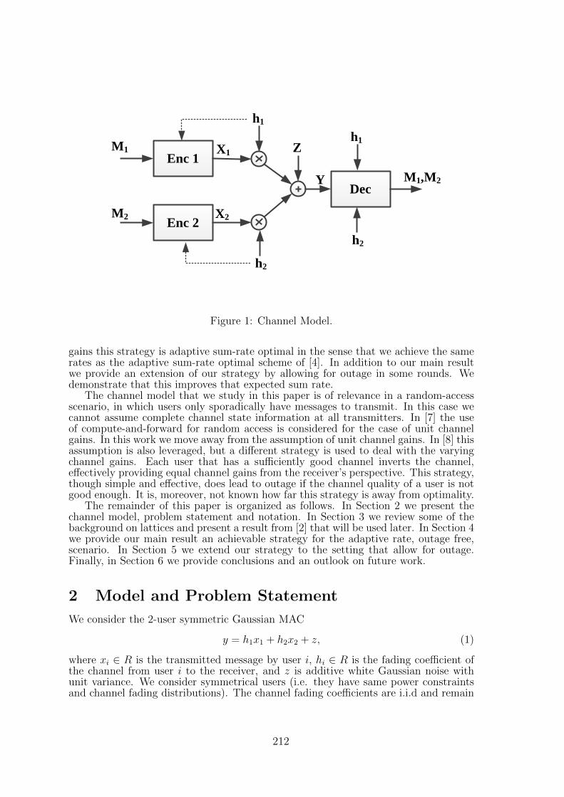
Enc 1
Enc 2
X1
X2
Z
Y
h1
h2
M1
M2
Dec
h1
h2
M1,M2
Figure 1: Channel Model.
gains this strategy is adaptive sum-rate optimal in the sense that we achieve the samerates as the adaptive sum-rate optimal scheme of [4]. In addition to our main resultwe provide an extension of our strategy by allowing for outage in some rounds. Wedemonstrate that this improves that expected sum rate.
The channel model that we study in this paper is of relevance in a random-accessscenario, in which users only sporadically have messages to transmit. In this case wecannot assume complete channel state information at all transmitters. In [7] the useof compute-and-forward for random access is considered for the case of unit channelgains. In this work we move away from the assumption of unit channel gains. In [8] thisassumption is also leveraged, but a different strategy is used to deal with the varyingchannel gains. Each user that has a sufficiently good channel inverts the channel,effectively providing equal channel gains from the receiver’s perspective. This strategy,though simple and effective, does lead to outage if the channel quality of a user is notgood enough. It is, moreover, not known how far this strategy is away from optimality.
The remainder of this paper is organized as follows. In Section 2 we present thechannel model, problem statement and notation. In Section 3 we review some of thebackground on lattices and present a result from [2] that will be used later. In Section 4we provide our main result an achievable strategy for the adaptive rate, outage free,scenario. In Section 5 we extend our strategy to the setting that allow for outage.Finally, in Section 6 we provide conclusions and an outlook on future work.
2 Model and Problem Statement
We consider the 2-user symmetric Gaussian MAC
y = h1x1 + h2x2 + z, (1)
where xi ∈ R is the transmitted message by user i, hi ∈ R is the fading coefficient ofthe channel from user i to the receiver, and z is additive white Gaussian noise withunit variance. We consider symmetrical users (i.e. they have same power constraintsand channel fading distributions). The channel fading coefficients are i.i.d and remain
212

fixed for a sufficiently large blocks over which the codewords last. We assume thefading states have Rayleigh distribution and each transmitter has access to own fadingcoefficient and can use this information to adapt its rate. All fading coefficients areknown at the receiver.The model is illustrated in Figure 1.
In the proposed coding scheme, we represent the messages as M1 and M2. Useri has a message Mi ∈ 1, . . . , 2nRi to transmit and maps it to the channel inputxi,1, . . . , xi,n, satisfying a fixed power constraint P . We will refer to the throughput ofa strategy as the expected sum-rate, namely,
T = E[R1 (h1)] + E[R2 (h2)], (2)
where averages are over all values of h1 and h2, respectively. Note that it is possible toadapt the power over different blocks. We do not analyze such power control strategiesexplicitly, but instead rely on results from [4] that indicate that our proposed strategyis optimal if the right power control strategy is used.
In this work we consider MAC with individual CSI which each transmitter hasinstantaneous access to its own fading and choose its rate based on this information.This is possible since the users have channel state information available. Therefore,in our rate-strategy, the user i employs a code-book of rate Ri(hi) according to the
individual fading state hi. Let CMAC
(h)
denotes the instantaneous capacity region of
a Gaussian MAC with fixed channel gains h
CMAC
(h)
=
R : ∀S ⊆ 1, 2 ,
∑
i∈SRi ≤
1
2log
(1 +
∑
i∈S|hi|2P
). (3)
A strategy under individual CSI, is called outage-free if
∀h ∈ H, (R1 (h1) , R2 (h2)) ∈ CMAC
(h), (4)
where H is the fading space.The goal of the present paper is to provide an encoding and decoding mechanism
that is achieving the maximum achievable throughput that is outage free and that isbased on lattice codes.
Throughout this paper, vectors are denoted by bold letters.
3 Preliminaries
Lattice code are a discrete subgroup of Rn and can be written as a linear transformationof integer vector as
Λ = λ = Gx : x ∈ Zn , (5)
where λ is a lattice point of Λ. More details about lattice and lattice code can be foundin [1]. Similar to [2] we will use a nested lattice code combined with the compute-and-forward technique of Nazer and Gastpar [6] to decode two linearly independentequations of the messages as a1M1 + a2M2 (first equation) and b1M1 + b2M2 (secondequation). These equations are decoded sequentially, enabling successive cancellationtechniques after decoding the first equation. The messages M1 and M2 can be obtainedfrom the linear equations that are decoded.
The proposed scheme in [2] allows users to use full CSI for controlling transmittedrate by scaling second moment of the coarse lattice. In general, not the whole dominantface of the capacity region can be achieved. By defining A = h1h2P√
1+h21P+h22P, if A < 3/4
213

any points on the capacity region can not be achieved via this strategy, if 3/4 ≤ A < 1parts of the capacity region can be achieved, and if A ≥ 1 the full dominant face areachieved [2].
Assume β1, β2 are positive numbers, we can construct lattices Λsk ⊆ Λ for k = 1, 2
which both lattices are simultaneously good with second moment, i.e.
σ2 (Λk) = β2k . (6)
We collect both βs into one vector β. The following theorem gives achievable messagerate-pairs for the 2-user Gaussian MAC.
Theorem 1 ( [2]). Consider 2-user multiple access channel in (1) with full-CSI. Thefollowing rate pair is achievable
Rk =
rk (a,β) , if bk = 0,rk (b|a,β) , if ak = 0,
min rk (a,β) , rk (b|a,β) , otherwise.(7)
where
rk (a,β) =1
2log
β2k (1 + h21P + h22P )
K (a,β), (8)
rk (b|a,β) =1
2log
β2kK (a,β)
β21β
22(a2b1 − a1b2)2
, (9)
K (a,β) =∑
k
a2kβ2k + P (a1β1h2 − a2β2h1)2. (10)
4 Proposed Strategy
The main contribution of this work consists of a proposed means of scaling β1 = 1 andβ2 as a function of h2 and the selection of rates as following
R1 =1
4log2
(1 + 2h21P
), R2 =
1
4log2
(1 + 2h22P
). (11)
This choice of the rates correspond to the midpoint strategy that is presented in [4].Therefore, we know from [4] that these rates are sum-rate optimal.
In our strategy we use a = (1, 1) and b = (0, 1). For our choice of the rates, it followsfrom Theorem 1 that these equations can be decoded if β1 = 1 and β
′2 ≤ β2 ≤ β
′′2 , or
equivalently A ≥ 3/4, where
β′2(h1, h2) =
2h1h2P + S −√SD
2 (1 + h21P ), β
′′2 (h1, h2) =
2h1h2P + S +√SD
2 (1 + h21P ), (12)
S =√
1 + h21P + h22P , D = 4h1h2P − 3S. (13)
The following theorem provides the value of β2 that is used by our strategy.
214

Theorem 2. Let β∗ be a positive real variable and 0 < u < v be arbitrary constants.If u ≤ h1 ≤ v and for every values of h1,
√1 + 2h22P ≤ K (a, β∗) ≤ 1 + h21P + h22P√
1 + 2h21P(14)
andsup
u≤h1≤vβ′2(h1, h2) ≤ β∗ ≤ inf
u≤h1≤vβ′′2 (h1, h2), (15)
where
β∗ = β2(h2) =
h22P +
√(1 + h22P )
(√1 + 2h22P − 1
)− h22P
1 + h22P
andK (a, β∗) = 1 + β∗2 + P (h2 − β∗h1)2,
then Users 1 and 2 can send at rate-pair (11) and receiver can reliably decode M1 andM2. Moreover, this rate pair is adaptive sum-rate optimal.
Proof. We use lattice code combined with a compute-and-forward technique such as [2]and set equation coefficient vectors to be a = (1, 1) and b = (0, 1). User 2 choose β∗
in[β
′, β
′′]for all values of h1, since β′2 and β′′2 are decreasing function over h1, this
condition will be reduced to supu≤h1≤v β′2(h1, h2) ≤ β∗ ≤ infu≤h1≤v β
′′2 (h1, h2). Hence
the achievable rate points via lattice code for each values of h1 is
R1 = r1 (a, β∗) , R2 = r2 (b|a, β∗) . (16)
For reliable communication, the rate-point (11) should be inside the instantiated achiev-able rate region given by (16) which makes error probability arbitrarily small, or equiv-alently
r1 (a, β∗) ≥ 1
4log(1 + 2h21P
), r2 (b|a, β∗) ≥ 1
4log(1 + 2h22P
), (17)
which leads to the following constraint
√1 + 2h22P ≤ K (a, β∗) ≤ 1 + h21P + h22P√
1 + 2h21P. (18)
Figure 2 illustrates this result. It can be seen that the achievable rate pairs(r1(a; β2); r2(b|a; β2)) lies on the dominant area of the capacity region. Figure 3, showsthe acceptable region in terms of h21P and h22P for u = 1.2 and v = 8.
5 Proposed Strategy with Outage
The proposed strategy in the previous section is throughput-optimal without outage,but in general tolerating outage leads to higher performance in term of expectedthroughput [4]. We can modify the constraints given by (14) and (15), in the casethat a user has a high channel gain. Since based on the fading distribution (Rayleigh)the probability of having a large channel coefficient is small, the transmitter will take
215
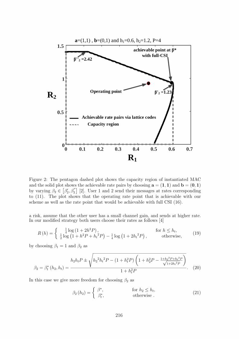
0 0.1 0.2 0.3 0.4 0.5 0.6 0.70
0.5
1
1.5
R1
R2
Achievable rate pairs via lattice codes
Capacity region
Operating point
β''2 =2.42
a=(1,1) , b=(0,1) and h1=0.6, h2=1.2, P=4
achievable point at β*
with full-CSI
β'2 =1.23
Figure 2: The pentagon dashed plot shows the capacity region of instantiated MACand the solid plot shows the achievable rate pairs by choosing a = (1,1) and b = (0,1)by varying β2 ∈
[β′2, β
′′2
][2]. User 1 and 2 send their messages at rates corresponding
to (11). The plot shows that the operating rate point that is achievable with ourscheme as well as the rate point that would be achievable with full CSI (16).
a risk, assume that the other user has a small channel gain, and sends at higher rate.In our modified strategy both users choose their rates as follows [4]
R (h) =
14
log (1 + 2h2P ) , for h ≤ ht,12
log(1 + h2P + ht
2P)− 1
4log(1 + 2ht
2P), otherwise,
(19)
by choosing β1 = 1 and β2 as
β2 = β∗t (h2, ht) =
h2htP ±√h2
2ht2P − (1 + h2tP )
(1 + h22P − 1+h2
2P+ht2P√
1+2ht2P
)
1 + h2tP. (20)
In this case we give more freedom for choosing β2 as
β2 (h2) =
β∗, for h2 ≤ ht,β∗t , otherwise .
(21)
216
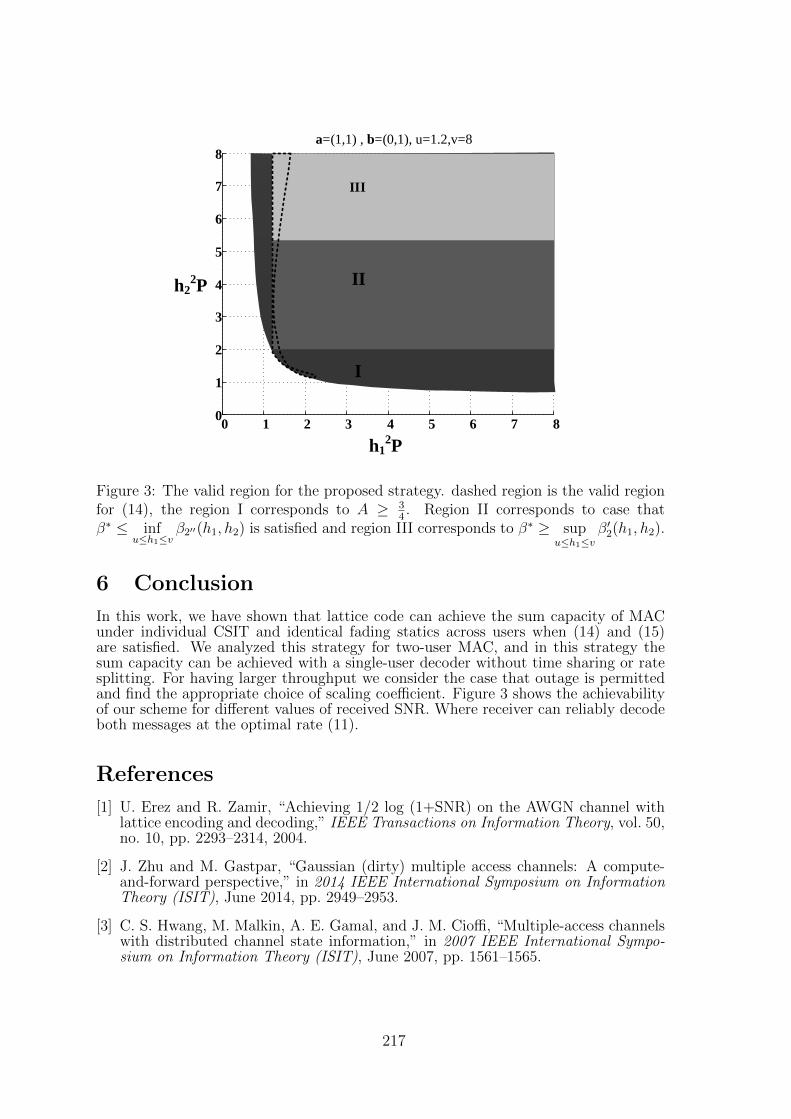
0 1 2 3 4 5 6 7 80
1
2
3
4
5
6
7
8
h12P
h22P
I
II
III
a=(1,1) , b=(0,1), u=1.2,v=8
Figure 3: The valid region for the proposed strategy. dashed region is the valid regionfor (14), the region I corresponds to A ≥ 3
4. Region II corresponds to case that
β∗ ≤ infu≤h1≤v
β2′′(h1, h2) is satisfied and region III corresponds to β∗ ≥ supu≤h1≤v
β′2(h1, h2).
6 Conclusion
In this work, we have shown that lattice code can achieve the sum capacity of MACunder individual CSIT and identical fading statics across users when (14) and (15)are satisfied. We analyzed this strategy for two-user MAC, and in this strategy thesum capacity can be achieved with a single-user decoder without time sharing or ratesplitting. For having larger throughput we consider the case that outage is permittedand find the appropriate choice of scaling coefficient. Figure 3 shows the achievabilityof our scheme for different values of received SNR. Where receiver can reliably decodeboth messages at the optimal rate (11).
References
[1] U. Erez and R. Zamir, “Achieving 1/2 log (1+SNR) on the AWGN channel withlattice encoding and decoding,” IEEE Transactions on Information Theory, vol. 50,no. 10, pp. 2293–2314, 2004.
[2] J. Zhu and M. Gastpar, “Gaussian (dirty) multiple access channels: A compute-and-forward perspective,” in 2014 IEEE International Symposium on InformationTheory (ISIT), June 2014, pp. 2949–2953.
[3] C. S. Hwang, M. Malkin, A. E. Gamal, and J. M. Cioffi, “Multiple-access channelswith distributed channel state information,” in 2007 IEEE International Sympo-sium on Information Theory (ISIT), June 2007, pp. 1561–1565.
217

[4] Y. Deshpande, S. R. B. Pillai, and B. K. Dey, “On the sum capacity of multiaccessblock-fading channels with individual side information,” in 2011 IEEE InformationTheory Workshop (ITW), Oct 2011, pp. 588–592.
[5] S. Sreekumar, B. K. Dey, and S. R. B. Pillai, “Distributed rate adaptation andpower control in fading multiple access channels,” IEEE Transactions on Informa-tion Theory, vol. 61, no. 10, pp. 5504–5524, 2015.
[6] B. Nazer and M. Gastpar, “Compute-and-forward: Harnessing interference throughstructured codes,” IEEE Transactions on Information Theory, vol. 57, no. 10, pp.6463–6486, 2011.
[7] J. Goseling, M. Gastpar, and J. H. Weber, “Random access with physical-layernetwork coding,” IEEE Transactions on Information Theory, vol. 61, no. 7, pp.3670–3681, 2015.
[8] J. Goseling, C. Stefanovic, and P. Popovski, “Sign-compute-resolve for tree splittingrandom access,” Preprint, arXiv:1602.02612, 2016.
218
Autoregressive Moving AverageGraph Filter Design
Jiani Liu Elvin Isufi Geert LeusDelft University of Technology
Faculty of EEMCS2826 CD Delft, The Netherlands
[email protected] [email protected] [email protected]
Abstract
To accurately match a finite-impulse response (FIR) graph filter to a desired re-sponse, high filter orders are generally required leading to a high implementationcost. Autoregressive moving average (ARMA) graph filters can alleviate thisproblem but their design is more challenging. In this paper, we focus on ARMAgraph filter design for a known graph. The fundamental aim of our ARMA de-sign is to create a good match to the desired response but with less coefficientsthan a FIR filter. Our design methods are inspired by Prony’s method but usingproper modifications to fit the design to the graph context. Compared with FIRgraph filters, our ARMA graph filters show better results for the same numberof coefficients.
1 Introduction
Graph signal processing (GSP) extends classical digital signal processing to signals con-nected with the topology of a graph [1], [2]. More and more concepts and tools fromclassical signal processing are transferred to the field of GSP, including the uncertaintyprinciple [3], graph wavelets [4], graph signal classification [5], graph signal recovery[6],[7], and graph signal sampling [8].
Depending on the definition of the graph frequency and the graph Fourier transform(GFT) [1], [2], many different kinds of graph filters have been designed as linear opera-tors acting upon a graph signal. Similar to traditional digital signal processing, graphfilters amplify or attenuate the graph signal at different graph frequencies. Graph filtershave been used for many signal processing applications [9]. Traditionally, graph filtersare expressed as a polynomial in the so-called graph shift matrix (e.g., the adjacencymatrix, the graph Laplacian, or any of their modifications), resulting in a so-calledfinite-impulse response (FIR) graph filter [10], [12]. However, to accurately matchsome given filter specifications, FIR filters require high filter orders leading to a highimplementation cost.
An alternative filter approach is the so-called infinite impulse response (IIR) graphfilter [13]. Compared with FIR graph filters, characterized by a polynomial frequencyresponse, IIR graph filters have a rational polynomial response, which brings moreflexibility to their design. As such, IIR graph filters have the potential to fit compli-cated filter specifications with small degrees. As a particular instance of IIR graphfilters, autoregressive moving average (ARMA) graph filters have been introduced in[14] [15]. ARMA graph filters were introduced as universal filters that do not dependon the particular topology of the graph, although in this paper we will design themfor a particular graph in mind. Note that ARMA graph filters are capable of not onlyshaping the graph signal in the graph frequency domain, but also in the regular tempo-ral frequency domain, in case the graph signal is time varying [15]. And although our
219

proposed designs can be used in that context, we will only focus on the graph domainin this paper.
Although ARMA graph filters show great promises, their design is challenging. Thispaper tries to tackle this issue for known graphs, which means that we only have tomatch the ARMA graph filter to the desired response in a set of known frequencies. Wewill present two design procedures, both inspired by Prony’s method. The first designtransforms the problem from the graph frequency domain to the coefficient domain (asdone in the classical Prony’s method). However, in contrast to the regular time do-main, in the graph domain, this transformation is generally not optimal and does notlead to a good solution. Our second design shows that staying in the graph frequencydomain preserves the optimality of the solution and also simplifies the problem. Weconclude the paper by showing some simulation results for our two ARMA graph filterdesign procedures based on a known graph. They illustrate that in some cases, theFIR filter can be outperformed for the same number of filter coefficients.
2 FIR Graph Filter
Consider an undirected graph G = (V,E), where V is a set of N nodes and E is the setof edges. We indicate with M the symmetric graph shift matrix, which could be theadjacency matrix, the graph Laplacian or any of their modifications. An eigenvaluedecomposition of M leads to M = UΛUT , where UT is the graph Fourier transform(GFT) matrix and Λ is a diagonal matrix with on the diagonal, the graph frequenciesλn.
A graph filter G is a linear operator that acts upon a graph signal x, leading to theoutput y = Gx. A finite impulse response (FIR) graph filter of order K, or FIR(K)in short, can be expressed as a K-th order polynomial in M:
G = g(M) =∑K
k=0gkM
k, (1)
where gk are the FIR filter coefficients. This means that G is diagonizable by the GFTmatrix UT , i.e., UTGU = g(Λ), and the filter indeed reshapes the spectrum of theinput:
y = UTy = UTGUUTx = g(Λ)x,
where x and y represent that GFT of the input and output signal, respectively. Thefrequency response of the filter at frequency λn, n = 1, 2, . . . , N , is thus given by
gn = g(λn) =K∑
k=0
gkλkn. (2)
Define now the N × (K + 1) Vandermonde matrix ΨK+1 as the N × (K + 1) matrixwith entries [Ψ]n,k = λk−1n . Then stacking the filter coefficients gk in the (K + 1) × 1vector g and the frequency response gn in the N × 1 vector g, we have
g = ΨK+1g. (3)
From [11] we know that if the graph is known and if the graph frequencies are distinct,the filter coefficients can be computed as
g = Ψ†K+1g, (4)
220
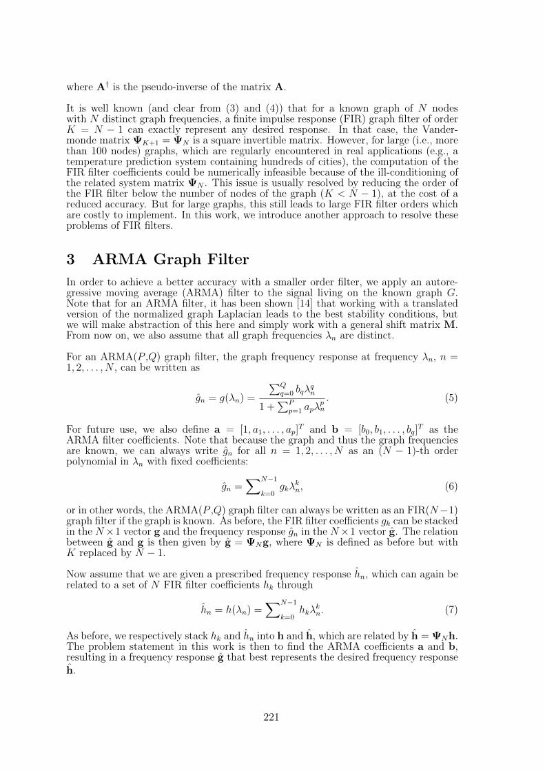
where A† is the pseudo-inverse of the matrix A.
It is well known (and clear from (3) and (4)) that for a known graph of N nodeswith N distinct graph frequencies, a finite impulse response (FIR) graph filter of orderK = N − 1 can exactly represent any desired response. In that case, the Vander-monde matrix ΨK+1 = ΨN is a square invertible matrix. However, for large (i.e., morethan 100 nodes) graphs, which are regularly encountered in real applications (e.g., atemperature prediction system containing hundreds of cities), the computation of theFIR filter coefficients could be numerically infeasible because of the ill-conditioning ofthe related system matrix ΨN . This issue is usually resolved by reducing the order ofthe FIR filter below the number of nodes of the graph (K < N − 1), at the cost of areduced accuracy. But for large graphs, this still leads to large FIR filter orders whichare costly to implement. In this work, we introduce another approach to resolve theseproblems of FIR filters.
3 ARMA Graph Filter
In order to achieve a better accuracy with a smaller order filter, we apply an autore-gressive moving average (ARMA) filter to the signal living on the known graph G.Note that for an ARMA filter, it has been shown [14] that working with a translatedversion of the normalized graph Laplacian leads to the best stability conditions, butwe will make abstraction of this here and simply work with a general shift matrix M.From now on, we also assume that all graph frequencies λn are distinct.
For an ARMA(P ,Q) graph filter, the graph frequency response at frequency λn, n =1, 2, . . . , N , can be written as
gn = g(λn) =
∑Qq=0 bqλ
qn
1 +∑P
p=1 apλpn
. (5)
For future use, we also define a = [1, a1, . . . , ap]T and b = [b0, b1, . . . , bq]
T as theARMA filter coefficients. Note that because the graph and thus the graph frequenciesare known, we can always write gn for all n = 1, 2, . . . , N as an (N − 1)-th orderpolynomial in λn with fixed coefficients:
gn =∑N−1
k=0gkλ
kn, (6)
or in other words, the ARMA(P ,Q) graph filter can always be written as an FIR(N−1)graph filter if the graph is known. As before, the FIR filter coefficients gk can be stackedin the N×1 vector g and the frequency response gn in the N×1 vector g. The relationbetween g and g is then given by g = ΨNg, where ΨN is defined as before but withK replaced by N − 1.
Now assume that we are given a prescribed frequency response hn, which can again berelated to a set of N FIR filter coefficients hk through
hn = h(λn) =∑N−1
k=0hkλ
kn. (7)
As before, we respectively stack hk and hn into h and h, which are related by h = ΨNh.The problem statement in this work is then to find the ARMA coefficients a and b,resulting in a frequency response g that best represents the desired frequency responseh.
221

4 ARMA Filter Design
Optimally, we would try to minimize the error between g, which is parameterized bya and b, and h, or in other words, we would try to solve
mina,b
∑N
n=1
∣∣∣∣∣hn −∑Q
q=0 bqλqn
1 +∑P
p=1 apλpn
∣∣∣∣∣
2
. (8)
But since that is a difficult problem to solve, as in Prony’s method, we choose to solvethe related (yet not equivalent) problem
mina,b
∑N
n=1
∣∣∣hn(
1 +∑P
p=1apλ
pn
)−∑Q
q=0bqλ
qn
∣∣∣2
. (9)
Following a similar idea as in Prony’s method, we use (7) to expand hn in (9), resultingin
mina,b
∑N
n=1
∣∣∣(∑N−1
k=0hkλ
kn
)(1 +
∑P
p=1apλ
pn
)−∑Q
q=0bqλ
qn
∣∣∣2
.
Using some simple algebra, this can be transformed into the following least squares(LS) problem, written in matrix form as
mina,b‖ΨN+PHa−ΨQ+1b‖2, (10)
where H is the (N + P )× (P + 1) Toeplitz matrix expressed by
H =
h0 . . . 0...
. . ....
hN−1 . . . h0...
. . ....
0 . . . hN−1
.
Note that the two terms in this LS problem are nothing more than the frequencyresponse of the concatenation of the filter h and a on the left and the frequency responseof the filter b on the right. More specifically, defining a = ΨP+1a and b = ΨQ+1b asthe frequency responses of the graph filters a and b, we can also write (10) as
mina,b‖h a− b‖2, (11)
where represents the element-wise Hadamard product.
Again, following Prony’s approach, we now try to transform the problem (10) fromthe frequency domain to the filter coefficient domain. This can be done by observingthat the matrices ΨN+P and ΨQ+1 can both be written as a function of the frequencytransformation matrix ΨN as
ΨN+P = ΨN [IN ,T], ΨQ+1 = ΨN
[IQ+1
0(N−Q−1)×(Q+1)
],
222

where T is some N × P transformation matrix that can be computed from the firstequation since both ΨN and ΨN+P are known. So defining
H = [IN ,T]H, b =
[IQ+1
0(N−Q−1)×(Q+1)
]b =
[b
0(N−Q−1)×1
],
we can rewrite (10) asmina,b‖ΨNHa−ΨN b‖2, (12)
Multiplying both terms with Ψ−1N (note that this corresponds to a loss of optimality),we finally transform the problem from the frequency domain to the filter coefficientdomain:
mina,b‖Ha− b‖2. (13)
Since b has N−Q−1 zeros at the bottom, we can use the bottom N−Q−1 equationsof (13) to solve for a. The vector b can then be estimated using the top Q+1 equationsof (13). Alternatively, we can use (12) (or (10)) after plugging in the estimate for a.
In the time domain, this works well since ΨN then simply is the discrete Fouriertransform (DFT) matrix, which is well-conditioned and even unitary up to a scale. Inthe general graph domain, however, ΨN can be very badly conditioned, especially forlarge graphs. So computing the desired filter coefficients hk (and thus the matrix H)as well as the transformation matrix T, is numerically infeasible. Moreover, since ΨN
is generally far from a scaled unitary matrix, the problems (12) and (13) are far fromequivalent. Hence, we need to tackle this problem in a different way.
The basic idea is not to expand hn in (9), and to rewrite it in matrix form as
mina,b‖[ΨP+1 (h⊗ 11×(P+1))]a−ΨQ+1b‖2, (14)
where ⊗ represents the Kronecker product. Then, instead of trying to move from thefrequency domain to the filter coefficient domain, in order to exploit the finite order ofb, we simply project out this term using the orthogonal projection matrix
P⊥ΨQ+1= IN −ΨQ+1Ψ
†Q+1, (15)
which is generally well-conditioned. Staying in the frequency domain not only pre-serves the optimality of the LS problem, but also simplifies the solution procedure. Bymultiplying the objective function in (14) with P⊥ΨQ+1
we obtain the equivalent problem
mina‖P⊥ΨQ+1
[ΨP+1 (h⊗ 11×(P+1))]a‖2, (16)
which can be used to solve for a. The vector b can be estimated using (14) afterplugging in the estimate for a.
5 Numerical evaluation
Similar to [15], for our numerical simulations, we will adopt the translated normalizedLaplacian as the symmetric graph shift matrix M = I−Ln, where Ln is the normalizedgraph Laplacian. Due to Sylvester’s matrix theorem, the eigenvalues of M which canbe seen as shifted graph frequencies are within (-1,1]. As shown in [15], such a choice
223
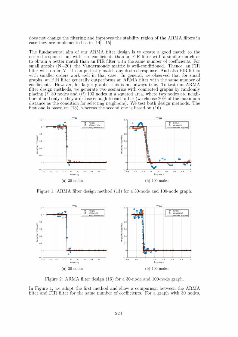
does not change the filtering and improves the stability region of the ARMA filters incase they are implemented as in [14], [15].
The fundamental aim of our ARMA filter design is to create a good match to thedesired response, but with less coefficients than an FIR filter with a similar match orto obtain a better match than an FIR filter with the same number of coefficients. Forsmall graphs (N=20), the Vandermonde matrix is well-conditioned. Thence, an FIRfilter with order N − 1 can perfectly match any desired response. And also FIR filterswith smaller orders work well in that case. In general, we observed that for smallgraphs, an FIR filter generally outperforms an ARMA filter with the same number ofcoefficients. However, for larger graphs, this is not always true. To test our ARMAfilter design methods, we generate two scenarios with connected graphs by randomlyplacing (i) 30 nodes and (ii) 100 nodes in a squared area, where two nodes are neigh-bors if and only if they are close enough to each other (we choose 20% of the maximumdistance as the condition for selecting neighbors). We test both design methods. Thefirst one is based on (13), whereas the second one is based on (16).
frequency-0.8 -0.6 -0.4 -0.2 0 0.2 0.4 0.6 0.8 1
freq
uenc
y re
spon
se
-0.2
0
0.2
0.4
0.6
0.8
1
1.2N=30
FIR(19)
designed response
(a) 30 nodes
frequency-0.6 -0.4 -0.2 0 0.2 0.4 0.6 0.8 1
freq
uenc
y re
spon
se
-0.2
0
0.2
0.4
0.6
0.8
1
1.2N=100
FIR(10)ARMA(3,7)designed response
(b) 100 nodes
Figure 1: ARMA filter design method (13) for a 30-node and 100-node graph.
frequency-0.8 -0.6 -0.4 -0.2 0 0.2 0.4 0.6 0.8 1
freq
uenc
y re
spon
se
-0.2
0
0.2
0.4
0.6
0.8
1
1.2N=30
FIR(27)ARMA(4,23)designed response
(a) 30 nodes
frequency-0.4 -0.2 0 0.2 0.4 0.6 0.8 1
freq
uenc
y re
spon
se
-0.2
0
0.2
0.4
0.6
0.8
1
1.2N=100
FIR(26)ARMA(4,22)designed response
(b) 100 nodes
Figure 2: ARMA filter design (16) for a 30-node and 100-node graph.
In Figure 1, we adopt the first method and show a comparison between the ARMAfilter and FIR filter for the same number of coefficients. For a graph with 30 nodes,
224
an FIR filter (28) is applied for the first step. We choose the order of the FIR filterclose to the number of nodes which gives a good performance for this graph. TheARMA filter design starts by fixing a specific order P N and then searching forthe Q that leads to the best fit. Only the number of filter orders Q smaller thanK − P need to be investigated. The MSE between the desired response and ARMAfilter response is used as evaluation index. Given the initial condition P = 3, the bestperformance comes from ARMA (3, 16). For this graph with 30 nodes, the ARMAfilter clearly outperforms the FIR filter. The performance comparison of the ARMAfilter with the FIR filter for larger graphs (100 nodes) depends on the selection of Pand Q. Even though the ARMA filter also seems to outperform the FIR filter for 100nodes, the ARMA filter shows errors. This is due to the fact that the first methodloses optimality when we go from the frequency domain to the filter coefficient domain.
In Figure 2, we focus on the second design method (i.e., (16)), which is appropri-ate for graphs of any size. We apply our second method on the same graphs as before.As for the first method, we pick an order P N and search for Q. Then we com-pare the resulting ARMA design with a FIR filter of order P + Q. For the graphwith 30 nodes, the ARMA filter almost matches perfectly. For the larger graph of 100nodes, the performance of the ARMA filter only shows a mismatch around the cutofffrequency. Clearly, this ARMA filter design shows a better performance than the FIRfilter design with the same number of coefficients.
The two methods only seem to make sense here if Q is larger than P . However, thestability of the ARMA filter (for an implementation according to [14], [15]) depends onthe initial P and the construction of the graph. For the same graph, when we changethe order P , the best performing ARMA filter may lose stability. Also, for differentgraphs and with the same denominator order P the stability is not guaranteed.
6 Conclusion
In this work, we have considered the design of ARMA graph filters when the graphstructure is known. We have seen that Prony’s method cannot be directly appliedbut needs some proper modifications in the graph context. The proposed ARMAfilter design outperforms a same-order FIR filter in large graphs with a relatively smallnumber of filter coefficients. Even though in different scenarios the designed filter leadsto stable implementations according to [14], [15], stability is not guaranteed. Futurework will be based on stable ARMA filter design.
References
[1] D. I. Shuman, S. K. Narang, P. Frossard, A. Ortega, and P. Vandergheynst, “TheEmerging Field of Signal Processing on Graphs: Extending High-DimensionalData Analysis to Networks and Other Irregular Domains,” IEEE Signal ProcessingMagazine, vol. 30, no. 3, pp. 83 - 98, May. 2013.
[2] A. Sandryhaila and J. M. Moura, “Discrete Signal Processing on Graphs,”IEEETransactions on Signal Processing, vol. 61, no. 7, pp. 1644-1656, Jan. 2013.
[3] Agaskar and Y. M. Lu, “A Spectral Graph Uncertainty Principle, ” IEEE Trans-actions Information Theory, vol.59, no. 7,pp. 4338-4356, July 2013.
[4] D. K. Hammond, and P. Vandergheynst, “Wavelets on graphs via spectral graphtheory”, Applied and Computational Harmonic Analysis , vol. 30, no. 2, pp. 129-150, Mar. 2011.
225
[5] A. Sandryhaila, and J. M. F. Moura, “Classification via regularization on graphs”,in IEEE Global Conference on Signal and Information Processing (GlobalSIP),Austin, TX, pp. 495 - 498, Dec. 2013.
[6] S. Chen, A. Sandryhaila, and J. M. F. Moura, “Signal recovery on graph: variationminimization ,” IEEE Transactions on Signal Processing, vol. 63, no. 17, pp. 4609- 4624, Jun. 2015.
[7] S. Chen, R. Varma, and A. Singh, “Signal recovery on graphs: Random versusexperimentally designed sampling”, in IEEE, Sampling Theory and Applications(SampTA), 2015 International Conference, Washington, DC, pp. 337 - 341, May2015.
[8] A. Anis, A. Gadde, and A. Ortega, “Toward a sampling theory for signals onarbitrary graphs”, in IEEE International Conference on Acoustics, Speech andSignal Processing (ICASSP), Florence, pp. 3864 - 3868, May. 2014.
[9] S. Chen, A. Sandryhaila, J. M. Moura, and J. Kovacevic, “Signal Denoising onGraphs via Graph Filtering”, in IEEE Global Conference on Signal and Informa-tion Processing (GlobalSIP), Atlanta, GA, USA, pp. 872-876, Dec. 2014.
[10] A. Sandryhaila, S. Kar, and J. M. F. Moura, “Finite-time distributed consensusthrough graph filters,” in IEEE International Conference on Acoustics, Speech andSignal Processing (ICASSP), Florence, pp. 1080-1084, May. 2014.
[11] A Sandryhaila, JMF Moura, “Discrete signal processing on graphs: Graph fil-ters”, in IEEE International Conference on Acoustics, Speech and Signal Process-ing (ICASSP), Vancouver, BC, pp. 6163 - 6166, May. 2013.
[12] A. Sandryhaila and J. M. F. Moura, “Discrete signal processing on graphs: Fre-quency analysis”, IEEE Transactions Signal Processing, vol. 62, no.12, pp. 3042-3054, May. 2014.
[13] X. Shi, H. Feng, M. Zhai, T. Yang, and B. Hu, “Infinite impulse response graphfilters in wireless sensor networks”, IEEE Signal Processing Letters, vol. 22, no. 8,pp. 1113 - 1117, Jan. 2015.
[14] A. Loukas, A. Simonetto, and G. Leus, “Distributed Autoregressive Moving Av-erage Graph Filters”, IEEE Signal Processing Letters, vol. 22, no. 11, pp. 1931 -1935, Jun. 2015.
[15] E. Isufi, A. Loukas, A. Simonetto, and G. Leus, “Distributed Time-Varying GraphFiltering”, arXiv preprint, arXiv:1602.04436v1, 2016.
[16] M. H. Hayes, Statistical Digital Signal Processing and Modeling, Georgia Instituteof Technology, sec. 4.3, pp. 133-144, 1996.
226
Greedy Gossip Algorithm with Synchronous Communication for WirelessSensor Networks
Jie Zhang, Richard C. Hendriks and Richard HeusdensSignal and Information Processing Lab.,
Dept. of Microelectronics, Delft University of Technology,2628 CD Delft, The Netherlands
j.zhang-7, r.c.hendriks, [email protected]
Abstract
Randomized gossip (RG) based distributed averaging has been popular forwireless sensor networks (WSNs) in multiple areas. With RG, randomly twoadjacent nodes are selected to communicate and exchange information itera-tively until consensus is reached. One way to improve the convergence speedof RG is to use greedy gossip with eavesdropping (GGE). Instead of randomlyselecting two nodes, GGE selects the two nodes based on the maximum dif-ference between nodes in each iteration. To further increase the convergencespeed in terms of transmissions, we present in this paper a synchronous versionof the GGE algorithm, called greedy gossip with synchronous communication(GGwSC). The presented algorithm allows multiple node pairs to exchange theirvalues synchronously. Because of the selection criterion of the maximum differ-ence between the values at the nodes, there is at least one node pair with differentinformation, such that the relative error must be reduced after each iteration.The convergence rate in terms of the number of transmissions is demonstrated tobe improved compared to GGE. Experimental results validate that the proposedGGwSC is quite effective for the random geometric graph (RGG) as well as forseveral other special network topologies.
1 Introduction
Distributed signal processing in wireless sensor networks (WSNs) has many operationaladvantages. For instance, there is no need to have a fusion centre (or host) for facilitat-ing computations, communication and time-synchronization. Positions of the networknodes are not necessarily known a priori, and the network topology might change asnodes join or disappear. For the design of fault-tolerant computation and informationexchange algorithms over such WSNs, decentralized randomized gossip (RG) basedaveraging consensus is attractive, because it does not require any special routing, thereis no bottleneck or single point of failure, and it is robust to unreliable and changingwireless network conditions. Moreover, the decentralized RG puts no constraints onthe network topology and requires no information about the actual topology.
Since the original RG algorithm was proposed in [1], many derivatives were proposedto improve its convergence rate, and it has been employed into various applications (seee.g., [2] and references therein). Dimakies introduced a geographic gossip [3], whichenables information exchange over multiple hops with the assumption that nodes haveknowledge of their geographic locations, such that it is a good alternative for thegrid network topology. In [4], a synchronous communication process was consideredand improvements were made to the synchronous RG of [1] in a speech enhancementcontext. They allowed multiple node pairs to exchange their current values per iterationsynchronously. Other improvements to increase the convergence speed are to use clique-based RG (CbRG) and cluster-based RG (see e.g., [5] and [6]), where cliques or clusters
227
are used to compress the original graph. Deniz et al presented a greedy gossip witheavesdropping (GGE) to accelerate the convergence [7]. Instead of randomly choosingtwo nodes, they chose the two nodes to communicate that have the maximum differencebetween values per iteration. Another more competitive broadcasting based algorithmwas proposed in [8], although it cannot guarantee to reach the actual consensus surely.
To further increase the convergence speed in terms of transmissions, we presentin this paper a synchronous version of the GGE algorithm, called greedy gossip withsynchronous communication (GGwSC). Each time slot is divided into two time scales,one is the time used for node pairs selection, and the other is for the gossip exchangebetween every node pair. The simultaneous communicating node pairs are chosenrecursively. Each time, one node selects the node from its neighbors that has the maxi-mum difference. Then, the additional communicating node pairs are chosen recursivelyby excluding the node pairs that are already formed. Finally, the chosen node pairscommunicate synchronously. Thus, unlike the synchronous gossip in [1] or [4], whichperforms updates completely at random, the GGwSC, like GGE, makes use of thegreedy neighbor selection procedure. Whereas unlike GGE, we also permit multiplenode pairs to communicate so as to accelerate the convergence rate. Experiments havedemonstrated the effectiveness of the proposed method. The convergence rate in termsof the number of transmissions for random geographic graphs (RGGs) is acceleratedcompared to the GGE algorithm. Additionally, we also test the improvement on theconvergence rate of the proposed method under different conditions in this paper, e.g.,different initializations for the nodes and different network topologies.
2 Fundamentals of GGE
To guide the reader, we first give a brief overview of the GGE algorithm presentedin [7]. We consider a network of N nodes and represent network connectivity as agraph, G = (V,E), with vertices V = 1, 2, ..., N and edge set E ⊂ V × V suchthat (i, j) ∈ E if and only if nodes i and j directly communicate. We assume thatcommunication relationships are symmetric and that the graph is connected. LetNi = j : (i, j) ∈ E denote the set of neighbors of node i (excluding i). Each nodein the network has an initial value yi, and the goal is to use only local informationexchanges to arrive at a state where every node knows the average y = 1
N
∑Ni=1 yi.
Each node is initialized with xi(0) = yi.At the kth iteration of GGE [7], an activated node sk is chosen uniformly at random.
This can be accomplished using the asynchronous time model, where each node “ticks”according to a Poisson clock with rate 1. Then, sk identifies a neighboring node tksatisfying
tk ∈ arg maxt∈Nj
1
2(xsk(k − 1)− xt(k − 1))2
, (1)
in other words, sk identifies a neighbor that currently has the most different valuefrom itself. This choice is possible because each node i maintains not only its ownlocal variable, xi(k − 1), but also a copy of the current values at its direct neighbors,xj(k−1), for j ∈ Ni, because of eavesdropping with wireless communications. When skhas multiple neighbors whose values are equally (and maximally) different from sk’s, itchooses one of these neighbors at random. Then the update is performed by enforcingthe average 1
2(xsk(k − 1) − xtk(k − 1)) to sk and tk, while all other nodes i 6∈ sk, tk
hold their values at xi(k) = xi(k−1). Finally, the two nodes, sk and tk, broadcast thesenew values so that their neighbors have up-to-date information. If the values xi on allsensors are stacked as a vector, i.e., x(k) = [x1(k), x2(k), ..., xN(k)]T , we can formulatethe above update as
x(k) = UGGE(k)x(k − 1), (2)
228
where UGGE(k) is an n×n dimensional update matrix, which is dependent across time.For two communicating nodes xsk and xtk at iteration k, the update matrix is
UGGE(k) = I − 1
2(esk − etk)(esk − etk)T , (3)
where ei = [0, ..., 1, 0, ..., 0]T is an N− dimensional vector with the ith entry equal to 1.Note that similar to the standard RG, the update matrix is doubly stochastic, whichimplies UGGE1 = 1 and 1TUGGE = 1T with 1 denoting a vector of all ones.
Given the initial vector of a network x(0) = [x1(0), x2(0), ..., xN(0)]T , the theoreticalconsensus will be xave = 1x(0)/N . To measure the convergence rate, we use the relativeconvergence error defined as
RE =‖x(k)− xave1‖‖x(0)− xave1‖
, (4)
such that the iteration can be quitted when RE ≤ ε (or after a fixed amount ofiterations).
3 GGwSC
In this section, we will present the proposed GGwSC algorithm based on GGE. Asmentioned above, in GGE, a node selects a neighboring node whose state value is mostdifferent from its own value. This strategy can indeed accelerate the convergence atthe cost of additional communication bandwidth compared to the original gossip al-gorithm [1], because it has to send (broadbast) the new values (eavesdrop) to all itsneighbors. In spite of this, it still has a relatively slow convergence because only twonodes are allowed to exchange their state values at each iteration. In [4], a synchronousrandomized gossip (SRG) was proposed for distributed delay and sum beamforming(DDSB) based speech enhancement in WSNs, where each node is permitted to commu-nicate with one of its neighbors randomly at each iteration, such that the state valuesof multiple nodes are updated after each iteration. Given sufficient communicationbandwidth, we combine the idea of GGE and SRG to further accelerate the conver-gence. Hence for the GGwSC, multiple node pairs can communicate at each iteration.These active node pairs are constrained to be disjoint, and the communicating nodepairs are chosen according to argmax distance vectors.
This newly proposed GGWSC algorithm can generally be described as in Algo-rithm 1. For the practical realization, there are several points worthy to be noted:
Given N (even) nodes, the desired case is that N/2 node pairs are chosen syn-chronously by the SelectNodePair function at each iteration. This would bemost efficient. However, this will not always happen. For example, at kth itera-tion, when the node sk is randomly activated, but all of its neighbors are selectedalready (i.e., Nsk = O), sk has a bye (i.e., xsk = xsk−1
) and needs to wait for thenext iteration k + 1.
For the kth iteration, the update matrix UGGwSC(k) is a manifold stochasticprocess approximately, that is, UGGwSC(k) =
∏sk,tk∈V U
sk,tkGGE(k).
Note that for a communicating node pair, two transmissions are required duringan iteration, e.g., sk computes the average, such that sk broadcasts it to itsneighbors, and tk also needs to broadcast the received average from sk to itsneighbors.
229

Algorithm 1: GGwSC
Input: x(0) = [x1(0), x2(0), ..., xN(0)]T , G = (V,E)1 while RE > ε do2 function SelectNodePair(G)3 sk = N × rand;
4 tk ∈ arg maxt∈Nsk
12(xsk(k − 1)− xt(k − 1))2
;
5 updating topology by excluding sk, tk to G′ = (V ′, E ′);6 if (V ′ 6= O) SelectNodePair(G′);7 else break;8 end function
9 U sk,tkGGE(k) = I − (esk − etk)(esk − etk)T/2;
10 UGGwSC(k) =∏sk,tk∈V U
sk,tkGGE(k);
11 x(k) = UGGwSC(k)x(k − 1);
12 end13 return x(k)
3.1 Convergence Rate: GGwSC versus GGE
In the following, we investigate the convergence rate in terms of the underlying commu-nication topology. The convergence rate for gossip algorithms [1] is typically definedin terms of the ε−avergaing time
Tave(ε) = supx(0)6=0
infk : Pr
(‖x(k)− xave1‖‖x(0)− xave1‖
> ε)≤ ε. (5)
The averaging time Tave(ε, Pr) is bounded by the second largest eigenvalue of theexpected value of the update matrix E[UGGwSC ], that is [1]
0.5 log ε−1
log λ2(E[UGGwSC ])−1≤ Tave(ε, Pr) ≤
3 log ε−1
log λ2(E[UGGwSC ])−1. (6)
Although this bound is suitable for the GGwSC as well, it is hard to relate it as ahomogeneous Markov chain, and Tave(ε, Pr) is difficult to calculate as a function ofλ2(E[UGGwSC ]), because E[UGGwSC ] depends on the network topology. Therefore, weuse here an alternative bound to investigate the convergence rate, which is based onresults from [7]. Given a graph G = (V,E), we will have
E[‖x(k)− Xave1‖2] ≤ A(G)k‖x(0)− Xave1‖2, (7)
where A(G) is the graph-dependent constant defined as
A(G) = maxx6=xave1
1
N
N∑
s=1
(1− ‖gs(k)‖2
4‖x− xave1‖2), (8)
where g(k) is the subgradient function defined in [7]. Indeed, A(G) is equivalent toλ2(E[UGGWSC ]) functionally. Obviously, the smaller of A(G), the faster of the conver-gence rate. For the kth iteration of GGwSC, there is at least one node pair (sk, tk)communicating synchronously, such that g(k) has more than two elements unequal
230
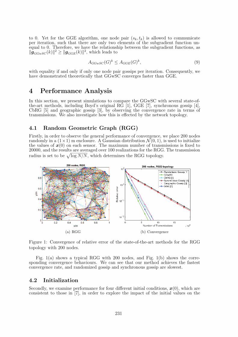
to 0. Yet for the GGE algorithm, one node pair (sk, tk) is allowed to communicateper iteration, such that there are only two elements of the subgradient function un-equal to 0. Therefore, we have the relationship between the subgradient functions, as‖gGGwSC(k)‖2 ≥ ‖gGGE(k)‖2, which leads to
AGGwSC(G)k ≤ AGGE(G)k, (9)
with equality if and only if only one node pair gossips per iteration. Consequently, wehave demonstrated theoretically that GGwSC converges faster than GGE.
4 Performance Analysis
In this section, we present simulations to compare the GGwSC with several state-of-the-art methods, including Boyd’s original RG [1], GGE [7], synchronous gossip [4],CbRG [5] and geographic gossip [3], by observing the convergence rate in terms oftransmissions. We also investigate how this is effected by the network topology.
4.1 Random Geometric Graph (RGG)
Firstly, in order to observe the general performance of convergence, we place 200 nodesrandomly in a (1×1) m enclosure. A Gaussian distribution N (0, 1), is used to initializethe values of x(0) on each sensor. The maximum number of transmissions is fixed to20000, and the results are averaged over 100 realizations for the RGG. The transmissionradius is set to be
√logN/N , which determines the RGG topology.
(a) RGG (b) Convergence
Figure 1: Convergence of relative error of the state-of-the-art methods for the RGGtopology with 200 nodes.
Fig. 1(a) shows a typical RGG with 200 nodes, and Fig. 1(b) shows the corre-sponding convergence behaviours. We can see that our method achieves the fastestconvergence rate, and randomized gossip and synchronous gossip are slowest.
4.2 Initialization
Secondly, we examine performance for four different initial conditions, x(0), which areconsistent to those in [7], in order to explore the impact of the initial values on the
231
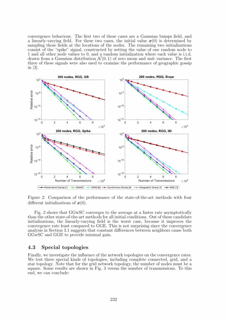
convergence behaviour. The first two of these cases are a Gaussian bumps field, anda linearly-varying field. For these two cases, the initial value x(0) is determined bysampling these fields at the locations of the nodes. The remaining two initializationsconsist of the “spike” signal, constructed by setting the value of one random node to1 and all other node values to 0, and a random initialization where each value is i.i.d.drawn from a Gaussian distribution N (0, 1) of zero mean and unit variance. The firstthree of these signals were also used to examine the performance of geographic gossipin [3].
Figure 2: Comparison of the performance of the state-of-the-art methods with fourdifferent initializations of x(0).
Fig. 2 shows that GGwSC converges to the average at a faster rate asymptoticallythan the other state-of-the-art methods for all initial conditions. Out of these candidateinitializations, the linearly-varying field is the worst case, because it improves theconvergence rate least compared to GGE. This is not surprising since the convergenceanalysis in Section 3.1 suggests that constant differences between neighbors cause bothGGwSC and GGE to provide minimal gain.
4.3 Special topologies
Finally, we investigate the influence of the network topologies on the convergence rates.We test three special kinds of topologies, including complete connected, grid, and astar topology. Note that for the grid network topology, the number of nodes must be asquare. Some results are shown in Fig. 3 versus the number of transmissions. To thisend, we can conclude:
232
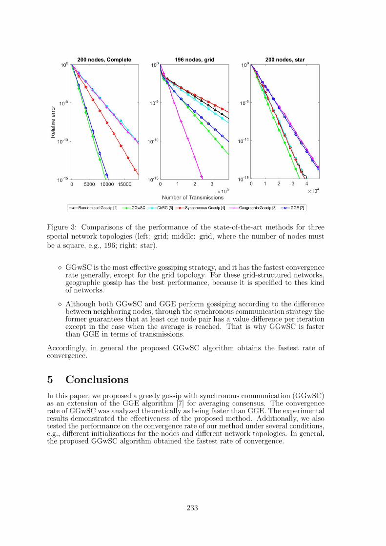
Figure 3: Comparisons of the performance of the state-of-the-art methods for threespecial network topologies (left: grid; middle: grid, where the number of nodes mustbe a square, e.g., 196; right: star).
GGwSC is the most effective gossiping strategy, and it has the fastest convergencerate generally, except for the grid topology. For these grid-structured networks,geographic gossip has the best performance, because it is specified to thes kindof networks.
Although both GGwSC and GGE perform gossiping according to the differencebetween neighboring nodes, through the synchronous communication strategy theformer guarantees that at least one node pair has a value difference per iterationexcept in the case when the average is reached. That is why GGwSC is fasterthan GGE in terms of transmissions.
Accordingly, in general the proposed GGwSC algorithm obtains the fastest rate ofconvergence.
5 Conclusions
In this paper, we proposed a greedy gossip with synchronous communication (GGwSC)as an extension of the GGE algorithm [7] for averaging consensus. The convergencerate of GGwSC was analyzed theoretically as being faster than GGE. The experimentalresults demonstrated the effectiveness of the proposed method. Additionally, we alsotested the performance on the convergence rate of our method under several conditions,e.g., different initializations for the nodes and different network topologies. In general,the proposed GGwSC algorithm obtained the fastest rate of convergence.
233

References
[1] S. Boyd, A. Ghosh, B. Prabhakar, and D. Shah, “Randomized gossip algorithms,”IEEE Trans. Information Theory, vol. 52, no. 6, pp. 2508–2530, 2006.
[2] A. G. Dimakis, S. Kar, J. Moura, M. G. Rabbat, and A. Scaglione, “Gossip algo-rithms for distributed signal processing,” Proceedings of the IEEE, vol. 98, no. 11,pp. 1847–1864, 2010.
[3] A. G. Dimakis, A. D. Sarwate, and M. J. Wainwright, “Geographic gossip: efficientaggregation for sensor networks,” in ACM Int. Conf. Inform. Process. in SensorNetworks (IPSN), 2006, pp. 69–76.
[4] Y. Zeng and R. C. Hendriks, “Distributed delay and sum beamformer for speechenhancement via randomized gossip,” IEEE/ACM Trans. Audio, Speech, LanguageProcess., vol. 22, no. 1, pp. 260–273, 2014.
[5] Y. Zeng, R. C. Hendriks, and R. Heusdens, “Clique-based distributed beamformingfor speech enhancement in wireless sensor networks,” in EURASIP Europ. SignalProcess. Conf. (EUSIPCO), 2013, pp. 1–5.
[6] W. Li and H. Dai, “Cluster-based distributed consensus,” IEEE Transactions onWire. Communicat., vol. 8, no. 1, pp. 28–31, 2009.
[7] D. Ustebay, B. N. Oreshkin, M. J. Coates, and M. G. Rabbat, “Greedy gossip witheavesdropping,” IEEE Trans. Signal Process., vol. 58, no. 7, pp. 3765–3776, 2010.
[8] T. C. Aysal, M. E. Yildiz, A. D. Sarwate, and A. Scaglione, “Broadcast gossipalgorithms for consensus,” IEEE Trans. Signal Process., vol. 57, no. 7, pp. 2748–2761, 2009.
234


