Project 62: SEAPODYM applications in WCPO

SCIENTIFIC COMMITTEE

NINTH REGULAR SESSION

Pohnpei, Federated States of Micronesia 6‐14 August 2013

Project 62: SEAPODYM applications in WCPO

WCPFC‐SC9‐2012/EB‐WP‐03 Rev 1

08/08/2013

P.Lehodey1, I.Senina1, O.Titaud1, B.Calmettes1,

S.Nicol2, J.Hampton2, S.Caillot2, P.Williams2

1 Marine Ecosystem Department, CLS, France. 2 Oceanic Fisheries Programme, Secretariat of the Pacific Community.

2

ExecutiveSummary

Recommendation

The SC is advised that the reference fits presented for skipjack, bigeye and south pacific albacore are

currently the best available for each species. The biomass estimates however remain above those of

MULTIFAN‐CL for skipjack and bigeye unless the mortality rates and initial biomass in SEAPODYM are

scaled to those estimated by MULTIFAN‐CL. For albacore, the last optimization including

improvements in both the fisheries definition and the code of the model resulted in a new

unconstrained estimate with lower biomass than in the MFCL last assessment. The SC is encouraged

to note that the use of finer resolution data has captured more meso‐scale variation in tuna

distribution which is resulting in the convergence in population estimates between SEAPODYM and

MULTIFAN‐CL. The SC should also be encouraged by the code developments to incorporate tagging

data into the model. The first experiments with this code have resulted in improved estimation of

movement parameters and early indications suggest that these data will result in lower biomass

estimation and improvement in model fits.

The SC is also advised that the model ensemble approach currently being applied to the construction

of physical forcing data to be used in future climate change analyses will allow uncertainties in tuna

responses to climate change to be better evaluated.

The SC is requested to note the 2013‐2014 work plan for Project 62 which includes the generation of

historical reference fits for all species with the inclusion of tagging data, further applications of high

resolution data, and new analyses of climate change impacts. The SC is also requested to

acknowledge the projects and donors that are continuing to contribute to the development and

application of SEAPODYM to the work programme of the WCPFC‐SC and requested to endorse the

inclusion of all presented projects within the scope of Project 62.

The SC is also invited to note that development of the SEAPODYM model has now progressed to the

stage where it can be used to assist the WCPFC and its committees with decisions associated with:

Developing criteria for the allocation of the total allowable catch or the total level of fishing effort;

Assessing the impacts of climate variability and change and fishing impacts;

Marine spatial planning and CMM evaluation; and

Providing fixed input into MFCL (e.g. recruitment and movement parameters).

The SC is advised to schedule a scientific review of all historical and climate change reference fits (in

the agenda of SC10) to facilitate the use of this model in the future work programs of WCPFC and its

committees. The review should aim to determine which applications SEAPODYM reference fits are

endorsed.

Introduction

SEAPODYM is a model developed for investigating spatial tuna population dynamics, under the

influence of both fishing and environmental effects. In addition to fisheries data the model utilises

environmental data in a manner that allows high resolution modelling. In this regard the model

3

complements the Scientific Committee’s MULTIFAN‐CL models by providing more detailed

information on how tuna distributions are structured in space and time. The continued

development and application of the SEAPODYM model to the work of the WCPFC Scientific

Committee is facilitated through Project 62. The project affiliates the independently funded work on

SEAPODYM into the SC’s work programme.

Progress

Code Development

Twelve modifications to the SEAPODYM code have been completed since SC8. The two most

significant modifications are capacity for sub‐regional modelling at high resolution and the

incorporation of tagging data.

Reference Fits

Reference fits using SODA 1 degree (1998‐2008) and NCEP‐ORCA2 2 degrees (1960‐2008) physical

forcing have been completed for skipjack, bigeye and south pacific albacore tuna. Reference fits

using IPSL CMIP4 physical forcing have also been completed for skipjack, bigeye and south pacific

albacore tuna for forecasting the impacts of climate change on tuna resources within the WCPO. In

all reference fits the correspondence between the predicted and observed catch, length and CPUE

was satisfactory for most of the fisheries defined. However for some fisheries the fit deteriorated

over the last years of the optimisation. The estimation of diffusion rate was unsatisfactory for all

models and was fixed at its upper boundary.

Current and Future Work Plan

Significant progress has been made on developing the first application of SEAPODYM to

swordfish. Development of a second generation model will commence in December 2013 for this

species which will incorporate updated fisheries data provided to the WCPFC for this species.

The incorporation of Pacific Ocean tagging data will commence once new physical forcing data

(either SODA 1 degree and MERCATOR ¼ degree) are pre‐processed for use in SEAPODYM. The

revised SODA forcing should extend the modelling period to December 2009 and the MERCATOR

forcing until December 2012. It is expected that new reference fits for each species will results

through the applications of these new data sources (forcing and tagging).

The development of the model for yellowfin tuna will commence in the later 2013 with the

incorporation of tagging and new physical forcing data.

The biomass estimates from exisitng reference fits for skipjack, bigeye and south pacific albacore

tuna have been prepared for distribution to WCPFC members. Opportunistically, WCPFC members

have been provided with initial training in interpreting and extracting these estimates.

The current physical forcing for the evaluation of climate change scenarios is restricted to a single

CMIP4 model (IPSL). To capture the uncertainty in climate change projections an ensemble of CMIP5

models is being developed. For the historical period a revised physical forcing that has realistic

simulation of oceanic conditions, under the influence of ENSO and PDO variability, has been

generated. The coupled NEMO‐PISCES model has been forced by observed winds of the ERA‐Interim

4

reanalysis using the latest version (IFS5) covering the period 1979‐present. Five to six CMIP5 models

will be coupled with the NEMO‐PISCES model to generate physical forcings under climate

change. The choice of CMIP5 models has been determined by their compatibility with the historical

forcing (so the jump from the historical forcing to the climate anomaly is minimised) and that they

have realistic ENSO and PDO variability. This approach means that SEAPODYM only needs to be

optimised once for each species before simulation of various climate change scenarios can be

implemented.

The software SEAPODYMview which provides for easy display of SEAPODYM output is currently

being revised to allow use on non‐Linux operating systems and to provide improved visualisation

options.

Acknowledgements and Donors

Project 62 is currently supported by 6 projects with financial support provided by Secretariat of the

Pacific Community, Collecte Localisation Satellites, Australian Government Overseas Aid Program

(AUSAID), 10th European Development Fund (EDF), Deutsche Gesellschaft für Internationale

Zusammenarbeit (GIZ), Western Pacific Regional Fishery Management Council, Government of

Indonesia, Agence Francais de Developpement, and Pelagic Fisheries Research Program. The Inter

American Tropical Tuna Commission has provided access to non‐public domain data for the

purposes of progressing the work programme of the WCPFC‐SC.

5

1. INTRODUCTION

SEAPODYM is a model developed for investigating spatial tuna population dynamics, under the

influence of both fishing and environmental effects. The model is based on advection‐diffusion‐

reaction equations, and population dynamics (spawning, movement, mortality) are constrained by

environmental data (temperature, currents, primary production and dissolved oxygen

concentration) and simulated distribution of mid‐trophic (micronektonic tuna forage) functional

groups. The model simulates tuna age‐structured populations with length and weight relationships

obtained from independent studies. Different life stages are considered: larvae, juveniles and

(immature and mature) adults. After juvenile phase, fish become autonomous, i.e., they have their

own movement (linked to their size and habitat) in addition to be transported by oceanic currents.

Fish are considered immature until pre‐defined age at first maturity and mature after this age, i.e.,

contributing to the spawning biomass and with their displacements controlled by a seasonal switch

between feeding and spawning habitat, effective outside of the equatorial region where changes in

the gradient of day length is marked enough and above a threshold value. The last age class is a

“plus class” where all oldest individuals are accumulated. The model includes a representation of

fisheries and predicts total catch and size frequency of catch by fleet when fishing data (catch and

effort) are available. A Maximum Likelihood Estimation approach is used to optimize the model

parameters. Additional information can be found in the references listed at the end of this

document.

2. AFFILIATEDPROJECTS

The continued development and application of the SEAPODYM model to the work of the WCPFC

Scientific Committee is facilitated through Project 62. The project affiliates the independently

funded work on SEAPODYM into the SC’s work programme.

This modelling effort started in 1995 at the Secretariat of the Pacific Community in Noumea, New

Caledonia, under two consecutive EU‐funded projects: SPR‐TRAMP (1995‐2000) and PROCFISH

(2002‐2005). The model development also benefited of a grant (# 651438) from the PFRP (Pelagic

Fisheries Research Program) of the University of Hawaii. Since 2006, the development has

continued within the Space Oceanography Division of CLS, a subsidiary of the French CNES and

IFREMER Institutes in collaboration with SPC (under the EU SCIFISH project and a grant from the

Australian Department of Climate Change and Energy Efficiency) and PFRP (project number 657425,

659708 and 661551). Current projects are described in Table 2.1.

6

Table 2.1: Current projects and donors affiliated with Project 62.

Title Purpose Donor

Scientific Support for the Management of Coastal and Oceanic Fisheries in the Pacific Islands Region (SciCOFish)

Develop reference fits for the historical period for skipjack, bigeye and south pacific albacore. Develop reference fit for the IPSL CMIP4 model and provide first simulation of Climate Change Impacts for skipjack, bigeye and south pacific albacore

10th European Development Fund

SPC‐Australian Climate Change Support Programme 2011‐2013

Analysis of climate change impacts for skipjack, bigeye, yellowfin and south pacific albacore to assist national and regional policy formation

Australian Government Overseas Aid Program (AUSAID)

Enhanced estimates of climate change impacts on WCPO tuna, including estimates of uncertainty

Application of a model ensemble approach to capture the uncertainty in climate change forecasts for Pacific tuna populations

Deutsche Gesellschaft für Internationale Zusammenarbeit (GIZ)

Skipjack resource assessment for the Mariana Islands

High resolution modelling to estimate the skipjack resource status in the Mariana Islands

Western Pacific Regional Fishery Management Council

Integrating conventional and electronic tagging data into the spatial ecosystem and population model SEAPODYM

Modify the code of SEAPODYM to incorporate tagging data

Pelagic Fisheries Research Program

Infrastructure Development of Space Oceanography for IUU Fishing and Coral Monitoring (INDESO Project)

Modify the code to allow operational and sub‐regional modelling

Government of Indonesia, Agence Française de Développement

3. CODEDEVELOPMENT

The code of SEAPODYM is continually enhanced to improve the model skills and to facilitate its use

by non‐developers colleagues. A major code development has been the inclusion of tagging data in

the optimisation. Other changes since those reported at SC8 include:

a) Integration of dynamics equations over age was corrected to match exactly with the time step of simulations to increase the accuracy of model numerical solution.

b) The robustified log‐likelihood has been implemented and is now used instead of normal log‐likelihood for the length‐frequencies data component in parameter estimation. Robustified log‐likelihood accounts for the size and the variance of length‐frequencies samples.

c) The code has been upgraded to allow running optimization tasks at higher temporal and spatial resolutions; the highest resolution being limited by those of the environmental forcing.

d) The fishing data resolution can be degraded to lower resolution if necessary. The interest of doing so is to account for a lack of good mesoscale representation or to reduce the biases due to the errors in the fine‐resolution fishing data.

7

e) The adjoint code has been fully revised in order to enhance the computational efficiency of the code. Part of the adjoint routines were re‐written to allow re‐computation of variables instead of storing them in the gradient stack thus reducing the memory required to save variables to compute gradients by about 15%. This is a critical issue to enable higher spatial resolution runs and/or integration of more data (e.g., tagging) in the Maximum Likelihood Estimation (MLE). The code was also enhanced by avoiding Input/Output operations during optimization runs.

Various options and external routines were also developed to facilitate the use of the model and the

analyses of simulations:

f) Options are now available to run various fishing effort scenarios based on spatial management measures. Using a mask file, EEZ or any area defined by a polygon can be closed to any fishery. The corresponding effort can be chosen to be lost; redistributed proportionally to CPUE outside the selected area, or transferred to another fishery (e.g. FAD to school sets). Example of application is provided in Sibert et al., (2012). Also, scenarios with increased fishing effort in the area of interest (defined by number codes in the mask file) can be simulated. Besides the possibility to select fisheries from the list, the user can also choose the mode of effort allocation within the given area: 1) proportional to existing effort; 2) homogeneous distribution.

g) Routines (R scripts) for the analysis of outputs at EEZ scale have been updated and now account for the exact area of the EEZ in each cell (i.e., surface area of partial cells are computed).

Several diagnostic routines were added to the code and routines were developed to facilitate the

analysis and validation of simulation outputs:

h) Predicted mean mortality at age computed as weighted average by the density of cohort i) Predicted mean diffusion rate at age and mean advection rate at age j) Predicted density of larvae by SST bins, allowing an easy comparison with existing

observations k) Predicted timing in the seasonal switch between feeding and spawning migration according

to latitude l) Level of exploitation, based on the decrease of spawning (adult) biomass relatively to a

virgin stock (i.e. a simulation without fishing mortality) m) EEZ‐level plots, showing seasonal variability of model variables within EEZ as well as

observed vs. predicted data (mean catch and CPUE) within EEZ. The latter can be used as well for validation purposes.

8

4. INTEGRATIONOFTAGGINGDATAINSEAPODYMOPTIMIZATION

A major area of development concerns the use of tagging data in the optimization approach of tuna

population dynamics. The method to integrate conventional (release‐recapture) tagging data has

required substantial changes in the code structure. A test application of this code revision has been

completed for Pacific skipjack with the constraint of physical forcing only being available until

December 2008.

Technicalcodedevelopments

Combining tagging data with SEAPODYM age‐structured population model leads to augmentation of

the model state vector through inclusion of variables describing the density of the cohorts of tags.

Part of the adjoint code was rewritten in order to reduce the size of the memory required for saving

the intermediate variables for computation of the cost function gradient. This allowed decrease of

the gradient stack size by 15%. Also, the IO operations were eliminated completely from the runs

with optimization. In addition, the code was adapted and recompiled with more recent versions of

gcc4.4 and the AUTODIF library. This allowed allocation of more than 4Gb of RAM for computation

of the cost function gradient.

Modeldescription

Let us denote N(a,x,t) the population density at age a, where xR2 and t[t0,tn]. Similarly, R(k,a,x,t) is

the density of tags of k‐th cohort; here the time t[k,tk] is defined by the time of release k of k‐th cohort and the time of recapture tk within the modeled time interval. By definition the cohort of tags

is the ensemble of individuals, tagged with conventional method, which were recaptured at the

same time period (month – quarter, depending on the time scale chosen for the age structure).

According to this definition, only the tags which were recaptured will be integrated into the model

and hence drive the maximum likelihood estimation. This approach has been chosen to improve the

estimation of habitat and movement parameters in SEAPODYM and these are the parameters, which

are explicitly observed from conventional tagging data. It also avoid possible bias in the estimation

of natural mortality due to misreporting problem or absence of fishing effort associated with tag

recapture.

The model with tags is hence represented by the following system of PDE equations with initial and

boundary conditions:

∙ ; ∙ , , ;

, , , ; 0, , ∙ , 0; , , , 0

∙ | ∈ ∙ N| ∈ ∙ R| ∈ =0

Hence, each population of tags has the same age structure as the actual population of modeled

species; and the spatial and temporal dynamics are described with help of the same advection‐

diffusion equations with the reaction term set to zero (i.e., no recruit nor mortality) and the only

reaction term is to account for the change of the density due to the tag releases within the cohort.

9

The equations for densities of tags R are solved numerically using the same ADI solver implemented

in SEAPODYM.

MethodImplementation

A new dimension was added to the existing population structure to allow simultaneous integration

of PDE equations for as many tagged cohorts as specified in the parameter file. The life span of each

cohort of tags is defined according to the age of youngest and oldest tagged individuals in a given

cohort. The input files with tagging data must be prepared in the ASCII format, each file containing

the data for one cohort: positions and time of release and recaptures and the length of fish at

release. In case if tagging data are used in the optimization experiment, the likelihood function is

augmented with the third component being the sum of errors of the predicted vs observed number

of tags in the model grid cell.

Validationandsensitivityanalysis

The validation of the approach included 1) the derivative check, which is necessary to assure that the

derivative (adjoint) code is correct and 2) twin experiments which consist in creating pseudo‐data

sets for conventional data and running the model in optimization mode to test if the original solution

used to create the artificial tagging data can be retrieved. Set of such experiments were done for the

cases with minimization of the recapture likelihood only and compared with minimization of the full

likelihood with catch, length and recapture components. The sensitivity analyses were done in order

to reveal the parameters which can be estimated due to integration of the tagging data. As

expected, the parameters driving the movement, i.e. maximal sustainable speed, diffusion, and

movement habitat parameters have higher sensitivity (relative sensitivity > 5%, see Figure 4.1) when

using tagging data in the likelihood. This result is also corroborated by the twin experiment study,

showing that the optimal movement and habitat parameters can be retrieved even while minimizing

the three‐component likelihood function.

Figure 4.1: Results of sensitivity analysis for the experiment with 2008 tagging data. Each color corresponds to the sensitivity metrics obtained with single likelihood component.

10

ApplicationtoPacificskipjack

Using compiled tagging datasets provided by NIFSF and SPC the cohorts of tags were defined. The

first experiments were done for Pacific skipjack tuna on 1‐degree and monthly resolution based on

SODA physical forcing, VGPM primary production and Levitus climatological oxygen. Eight monthly

tagged cohorts recaptured during 2008 were selected for these experiments (see the two examples

with most contrasting movement patterns on Figure 4.2). The time period of model run was limited

to 7/2006‐12/2008 in order to cover entirely the observed time at liberty of tags released under

PTTP tagging programme, which started in 2006.

Figure 4.2: Cohorts of tags defined by the date of tag recaptures. Colours represent different cohorts of releases.

The optimization experiments with identical model configuration were performed with two‐ and

three‐component likelihood. The results show that integration of tagging data leads to estimation of

smaller diffusion and much higher advection rates (see Table 4.1), which results in less spread‐out

distribution of skipjack (Figure 4.3) and hence much smaller total biomass (4 vs. 10 million tonnes in

this experiment). However, it is too early to assert that this estimate is better than the one obtained

with catch data only, since the 2.5 years time period used for this experiment is not long enough to

get reliable estimates of total stock.

11

Table 4.1: Control parameter estimates for skipjack using 2006-2008 time period and likelihood components with catch and catch and tags data

Parameters estimated by the model Unit Value

L_catch L_catch + L_tags

Ts

Spaw

ning Optimum of the spawning temperature function

oC 31.3 31.35

s Std. Err. of the spawning temperature function oC 2.25* 2.25*

Ta

Feed

ing habitat

Optimum of the adult temperature function at maximum age oC 18] 18]

a Std. Err. of the adult temperature function at maximum age oC 4.5] 4.5]

Ô Oxygen threshold value at O =0.5 mL L‐1 2.19 3.13

Mp Slope coefficient in predation mortality 0.09 0.03

Mmax Maximal mortality rate due to predation month‐1 0.5] 0.35

Ms Slope coefficient in senescence mortality 1.98 1.94

Dmax

Movemen

t Diffusion parameter 0.15] 0.11

Vmax Maximum sustainable speed B.L. s‐1 0.53 4.43

[val = value close to minimum boundary value; val] = value close to maximum boundary value, *=fixed

Figure 4.3: Predicted distributions of skipjack tuna (average of 2007 and 2008) in g/m2 (both young and adult life stages) as the result of experiments conducted with different likelihood composition: (left) including CPUE and length frequencies components only; (right) CPUE, LF and tagging data.

12

5. REFERENCEFITFORPACIFICSKIPJACKFORTHEHISTORICALPERIOD(SKJ2.1SODA‐v2.1)

Physicalforcing:SODAreanalysis

Reference fits for skipjack were achieved using a new release of the SODA (Carton et al. 2000;

http://soda.tamu.edu/) ocean physical reanalysis and satellite derived primary production. Due to

data assimilation techniques and the use of satellites data, this environmental forcing is more

realistic than previous forcings used from coupled physical biogeochemical models. However, the

series is limited to the period 1998‐2008. The resolution is 1° x 1° x month. The necessary variables

(temperature, currents, primary production and euphotic depth) were processed using the model

definition of vertical layers (linked to the euphotic depth) and used to produce the biomass

distributions of the 6 micronekton functional groups. Monthly climatological data from the World

Ocean Atlas (WOA2010) were used for the dissolved oxygen concentration.

Initial conditions were required for this analyses (biomass and distribution) and this was achieved

using a ORCA2 hindcast simulation (1958‐2008). Both past climatic and fishing mortality define the

initial conditions of the stock when starting a simulation at any given date. Unfortunately, the lack of

historical synoptic datasets for oceanic physical variables before the 1980s, and before 1998 for the

ocean color (i.e., SeaWiFS), ocean reanalyses are not available to simulate tuna dynamics with

SEAPODYM for periods before 1998. As an alternative, hindcast simulations with coupled ocean

physical‐biogeochemical models can be used. These simulations are forced by atmospheric data for

which a few reanalyses are available (e.g. NCEP, ERA40). To produce the initial conditions used for

the reference configuration the biogeochemical model is PISCES (Pelagic Interaction Scheme for

Carbon and Ecosystem Studies; Aumont and Bopp, 2006) was used. It incorporates both multi‐

nutrient limitation (NO3, NH4, PO4, SiO3 and Fe) and a description of the plankton community

structure with four plankton functional groups (Diatoms, Nano‐phytoplankton, Micro‐zooplankton

and Meso‐zooplankton). PISCES is coupled to the ORCA2 configuration of the ocean circulation

model OPA (http://www.nemo‐ocean.eu/), and driven by the NCEP‐NCAR reanalysis, that provides

50‐year record of global analyses of atmospheric fields based on the recovery of land surface, ship,

rawinsonde, pibal, aircraft, satellite, and other data.

(http://www.cgd.ucar.edu/cas/guide/Data/ncep‐ncar_reanalysis.html). This hindcast simulates

reasonable seasonal, interannual and decadal variability at basin‐scale at a coarse resolution of

2°x2°x month.

Fishingdata

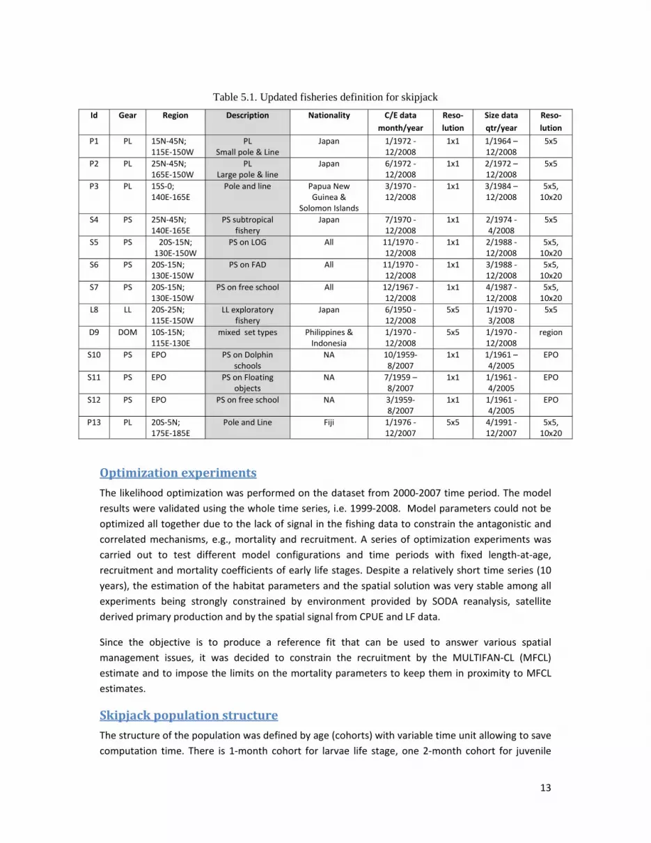
A new dataset of fishing data was used for skipjack fisheries in the WCPFC (Table 5.1). Except for the

Philippine‐Indonesia fishery and the longline fishery, all catch and effort fishing data were at a

resolution of 1°x1°x month, which is a major improvement from the previous studies where these

data were at a 5°x5° resolution. Based on discussion with Japanese colleagues, the two Japanese

pole and line (P1 and P2) were revised to describe small and large pole‐and‐line boats rather than

western and central fleets. Philippines and Indonesia fleets have been combined and not used in the

optimization approach due to a lack of accuracy.

13

Table 5.1. Updated fisheries definition for skipjack

Id Gear Region Description

Nationality C/E data

month/year

Reso‐

lution

Size data

qtr/year

Reso‐

lution

P1 PL 15N‐45N; 115E‐150W

PL Small pole & Line

Japan 1/1972 ‐ 12/2008

1x1 1/1964 – 12/2008

5x5

P2 PL 25N‐45N; 165E‐150W

PL Large pole & line

Japan 6/1972 ‐ 12/2008

1x1 2/1972 – 12/2008

5x5

P3 PL 15S‐0; 140E‐165E

Pole and line Papua New Guinea &

Solomon Islands

3/1970 ‐ 12/2008

1x1 3/1984 – 12/2008

5x5, 10x20

S4 PS 25N‐45N; 140E‐165E

PS subtropical fishery

Japan 7/1970 ‐ 12/2008

1x1 2/1974 ‐ 4/2008

5x5

S5 PS 20S‐15N; 130E‐150W

PS on LOG All 11/1970 ‐12/2008

1x1 2/1988 ‐ 12/2008

5x5, 10x20

S6 PS 20S‐15N; 130E‐150W

PS on FAD All 11/1970 ‐12/2008

1x1 3/1988 ‐ 12/2008

5x5, 10x20

S7 PS 20S‐15N; 130E‐150W

PS on free school All 12/1967 ‐12/2008

1x1 4/1987 ‐ 12/2008

5x5, 10x20

L8 LL 20S‐25N; 115E‐150W

LL exploratory fishery

Japan 6/1950 ‐ 12/2008

5x5 1/1970 ‐ 3/2008

5x5

D9 DOM 10S‐15N; 115E‐130E

mixed set types Philippines & Indonesia

1/1970 ‐ 12/2008

5x5 1/1970 ‐ 12/2008

region

S10 PS EPO PS on Dolphin schools

NA 10/1959‐8/2007

1x1 1/1961 – 4/2005

EPO

S11 PS EPO PS on Floating objects

NA 7/1959 – 8/2007

1x1 1/1961 ‐ 4/2005

EPO

S12 PS EPO PS on free school NA 3/1959‐8/2007

1x1 1/1961 ‐ 4/2005

EPO

P13 PL 20S‐5N; 175E‐185E

Pole and Line Fiji 1/1976 ‐12/2007

5x5 4/1991 ‐ 12/2007

5x5, 10x20

Optimizationexperiments

The likelihood optimization was performed on the dataset from 2000‐2007 time period. The model

results were validated using the whole time series, i.e. 1999‐2008. Model parameters could not be

optimized all together due to the lack of signal in the fishing data to constrain the antagonistic and

correlated mechanisms, e.g., mortality and recruitment. A series of optimization experiments was

carried out to test different model configurations and time periods with fixed length‐at‐age,

recruitment and mortality coefficients of early life stages. Despite a relatively short time series (10

years), the estimation of the habitat parameters and the spatial solution was very stable among all

experiments being strongly constrained by environment provided by SODA reanalysis, satellite

derived primary production and by the spatial signal from CPUE and LF data.

Since the objective is to produce a reference fit that can be used to answer various spatial

management issues, it was decided to constrain the recruitment by the MULTIFAN‐CL (MFCL)

estimate and to impose the limits on the mortality parameters to keep them in proximity to MFCL

estimates.

Skipjackpopulationstructure

The structure of the population was defined by age (cohorts) with variable time unit allowing to save

computation time. There is 1‐month cohort for larvae life stage, one 2‐month cohort for juvenile

14

stage, five 1‐month and one 2‐month cohorts for young fish (before age at maturity) and 9 cohorts

for adult stages (two of 2 months, two of 3 months and the last five of 4, 5, 6, 7, 9 months

correspondingly). The last “+ cohort” accumulates older fish. Age at maturity is set to 10 months.

Age‐length and age‐weight relationships (Fig. 6.1) are derived from the last MULTIFAN‐CL estimate

(Hoyle et al., 2011).

Figure 5.1. Skipjack size (FL in cm) at age (month) and weight (kg) at age functions used in SEAPODYM simulation, based on MULTIFAN-CL 2010 and 2011 estimates (Hoyle et al, 2011)

Fittocatchdata

The spatial CPUE and length‐frequencies data contributed to the total likelihood function. Overall

spatial fit to predicted catch is close to the previous solution with SODA reanalysis 2.4 but a

significant improvement is particularly visible for the eastern Pacific fisheries (Figure 5.2).

Catchability by fishery was estimated to increase since 1998 for the western purse seine fisheries (

Table 5.2) with the largest annual increase for the FAD and LOG fisheries (+3.6%) followed by the

free school fishery (+1.6%). Conversely, in the eastern Pacific the catchability of the purse seine

fishery on floating objects is estimated to have decreased since 1998 with an annual decrease of

1.8%.

15

Selectivity coefficients (Fig. 5.3) were obtained with all parameters being estimated within their

bounds. These selectivity estimates allowed a good fit with size frequency data for all fisheries. The

fit to length frequency data is reasonable for all fisheries (Fig 5.4) with fisheries P1 (Japanese small

pole‐and‐line boats) and S11 (eastern Pacific FAD‐associated sets) showing a mode peaking in the

smallest sizes while occasional catch in the longline fishery consisted of very large individuals.

The total catch of all fisheries is well predicted until 2003 but the correlation in fluctuations

decreases after this year, though in average the predicted total catch remains consistent with

observed catch. It appears that this lower correlation is due mainly to the fit for purse seine fisheries

of the western Pacific using either Log of FAD (S5 and S6), especially during 2003‐04, while predicted

CPUEs of other fisheries correlated fairly well with observations (Figure 5.4). Reasons for this lack of

fit are still unclear and need further investigation, but one explanation could be that the estimate

was forced to be scaled to the MULTIFAN‐CL biomass of region 2 (see below), thus leading to too

high depletion in this area given the very strong fishing effort deployed there.

1st Optimization experiment New Optimization experiment

Figure 5.2. Comparison of fit to fishing data between previous (Lehodey et al. 2011) and new optimization experiments over all the period 1998-2008 with SODA-Psat environmental forcing.

From top to bottom: R-squared goodness of fit and relative error in predicted catch for all fisheries; Black circles are proportional to the level of catch.

16

Table 5.2. Estimates of catchability by fishery and annual increase (%) since 1998.

Fishery Q slope annual % change since 1998 P1 PL small boats 0.01128 0.00000 0.0% P2 PL large boats 0.00797 0.00000 0.0% P3 Pole and line PNG+ SOL 0.00901 0.00000 0.0% S4 PS subtropical 0.16297 0.00000 0.0% S5 PS on LOG 0.04395 0.00300 3.6% S6 PS on FAD 0.04245 0.00300 3.6% S7 PS on free school 0.04191 0.00100 1.2% L8 LL exploratory fishery 0.00012 -0.00050 -0.6% D9 mixed set types 0.00400 0.00100 1.2% S10 PS on Dolphin schools 0.00335 0.00075 0.9% S11 PS on Floating objects 0.04681 -0.00150 -1.8% S12 PS on free school 0.04642 0.00000 0.0% P13 Pole and Line 0.00710 0.00000 0.0%

length (cm)

length (cm) length (cm) length (cm)

Figure 5.3. Optimized functions of selectivity by fishery.

P1 P2 P3 S4

S5 S6 S7 L8

S10 S11 S12 P13

17

18

19

Figure 5.4. Total predicted (continuous line) and observed (dotted line) skipjack catch rates (CPUEs) and size frequencies.

OptimalParameterization

The optimization was not able to correctly estimate some of parameters for habitat and movements (Table 5.3). Optimum of the spawning temperature function and its standard error, and the diffusion parameter were fixed. A wider range of temperature was fixed for the spawning function. The standard error of the adult temperature function at maximum age and the maximum sustainable speed were estimated near their upper and lower boundaries respectively.

Table 5.3: Habitats and movement parameter estimates for skipjack application

Parameters estimated by the model Unit SODA 1° v1 SODA 1° v2

Ts

Spaw

ning Optimum of the spawning temperature function oC 28.67 29.5*

s Std. Err. of the spawning temperature function oC 0.75* 3.0*

Larvae food‐predator trade‐off coefficient ‐ 1.03 0.51

Ta

Feed

ing

habitat

Optimum of the adult temperature function at maximum age

oC 20.64 20

a Std. Err. of the adult temperature function at maximum age oC 4.5] 3.5]


Dmax

Move‐

men

t Diffusion parameter 0.065* 0.08*

Vmax Maximum sustainable speed B.L. s‐1 [0.9 [0.75

*Fixed; [val = value close to minimum boundary value; val] = value close to maximum boundary value

NaturalmortalityNatural mortality in SEAPODYM is estimated with an average mortality coefficient by cohort, and

variability is allowed around this average value according to an index for food requirement and

competition (Figure 5.5). This is a major difference in the representation of this key population

20

dynamics parameter in comparison to MUTLIFAN‐CL. Due to such variability and depending on its

estimated range the local mortality rates estimated in SEAPODYM can be very different from the

average value. To estimate the actual average mortality rates resulting from these mechanisms for

each cohort, the weighted means of variable mortality coefficients, with the weights being the

cohort density, were computed. These weighted means are much closer to what is estimated by

MULTIFAN‐CL, with lower values due to the representation of fish movements in the model allowing

fish to escape unfavourable habitats (with higher mortality rates) and concentrate in good habitats

(with lower mortality rates). The main discrepancy between both models is an opposite trend in the

early life stages with MFCL values increasing from juvenile to young cohorts before decreasing and

converging with SEAPODYM estimates. This sort of trend is not permitted in SEAPODYM that

assumes much higher mortality of larvae and juveniles stages than in older stages.

SpawningandlarvalrecruitmentOptimal spawning temperature (SST) was fixed at 29.5 °C with standard error being 3.0 °C. This

resulted in a predicted distribution of larvae starting to be abundant in water with SST above 25‐

26°C as proposed in the literature (Figure 5.6). The model estimate for the seasonal timing of

spawning migration indicates that the switch from feeding to spawning habitat controlling the

movement of fish peaks at Julian date ~5 (5 January) in the north hemisphere, but in latitude higher

than 35° (Figure 5.6). Since this latitude corresponds to the extreme range of the species habitat

(Figure 5.2), this mechanism has very limited impact. Movements of fish between latitude 35° north

and south, i.e., most of the stock, is always controlled by the feeding habitat while spawning occurs

year‐round opportunistically and proportionally to the spawning habitat index and the density of

adult fish (Figure 5.6), following the larval stock‐recruitment relationship expressed in SEAPODYM, ie

at the cell level.

Figure 5.5: Natural mortality rates (month-1) estimated from SEAPODYM optimization experiments. Black dotted line corresponds to the theoretical average mortality curve whereas blue dots indicate the

mean mortality rates weighted by the cohort density and orange and red dots are the MUTLTIFAN-CL estimates for 2010 and 2011 assessments.

21

a Spawning index

b Predicted larvae density with SST

SST°C

C d

Figure 5.6: Spawning and larval recruitment. a: spawning index in relation to SST and food-predator tradeoff ratio. b: Distribution of larvae according to SST and the estimated parameters of spawning

index. c: Seasonal timing of spawning migration. d: SEAPODYM larval stock-recruitment relationship estimated for skipjack. Densities are in number of individual per km2 for adult and 1000’s

of individual per km2 for larvae.

FeedingHabitatThe optimal value for the oldest cohort was estimated at 20 °C but the standard error reached the maximum fixed boundary (3.5 °C). The threshold value for the oxygen tolerance reached the minimum fixed 2.2 ml/l (Figure 5.7).

SST°C

ml/l

Figure 5.7: Optimized functions for temperature and oxygen habitats.

22

MovementsThe value for maximum sustainable speed was estimated to 0.75 body length/s and the estimate for

the diffusion coefficient for fish movements reached the upper boundary. Thus movement

parameter optimization is not yet fully satisfactory. Estimation of diffusion coefficient is a key issue

as high diffusion can quickly lead to overestimation of biomass. Further ongoing progress to use

higher resolution and tagging data in the likelihood approach should be a major step for resolving

this recurrent issue. When weighted by the cohort density, maximum diffusion rates remain below

700 nmi2 month‐1 and the mean of maximum sustainable speed (in BL/s) shows an exponential

decrease with age (size) which is linked to the increasing accessibility with age (size) to forage

biomass of deeper layers, thereby decreasing the horizontal gradients of the feeding habitat index

controlling the movement (Figure 5.8).

Figure 5.8: Maximum speed and diffusion rates by cohort (depending of age/size and habitat value / gradient) based on SEAPODYM parameterization (dotted lines) and predicted means weighted by the

cohort density (black dots) with one standard error (red bars).

Biomassestimatesandpopulationdynamics

In average, spawning grounds and larvae are predicted to concentrate in the warm waters of the

equatorial (10°N‐10°S) western central Pacific Ocean with a prolongation of a relatively favourable

habitat between 5°N and 10°N reaching the eastern Pacific coast (Figure 5.9). Distribution of young

immature fish (until 42 cm) is very close to this distribution while adult fish extend their habitat

towards central and eastern Pacific where they are caught occasionally by longline fisheries, and

towards medium latitudes, especially under the influence of circulation of the warm western

boundary currents: the Kuroshio and the Eastern Australian Currents.

There are a few regions where high biomass is due to obvious spurious accumulation, especially in

the Arafura Sea. The biomass in the South China Sea seems also overestimated given the level of

catch in this region. This is due to regions with shallow bathymetry and complex topography for

which 1° resolution is insufficient to be realistic. This is particularly the case for the western

boundaries of the model domain within the South‐East Asia region.

23

The diffusion used to simulate random dispersion of fish may be also a source of overestimation of

biomass in areas where there is no fishing data to bring information in the Maximum Likelihood

Estimation. The result can be a smoothing of the contrast between higher and lower productive

regions.

Figure 5.9. Change in average biomass distribution between first and revised reference fits using SODA configuration (here without fishing).

The revised reference fit for skipjack is characterized by reduction of total biomass with respect to

previous estimate, which is more noticeable in EPO (see Fig. 5.5). However, this solution

demonstrates similar variability of the stock. The skipjack spawning biomass in WCPO is estimated

around 4 million metric tons, lower than MFCL prediction in this area (Fig. 5.10). The variability

predicted over the last decade is still stronger in MFCL and driven by recruitment estimates. Though

the average level of both biomass estimates is similar at the scale of the WPCO, there are regional

differences. In both models the lowest biomass occurs in region 1 (north west Pacific) with MFCL

estimate roughly 30‐50% below the SEAPODYM estimate. However to be comparable, a data mask

restricted to just the spatial areas where fishing occurs in region 1 should be applied when extracting

the biomass estimates from SEAPODYM. As the fishing data is very restricted spatially in this region

it is not unexpected that the MFCL estimate of biomass is smaller (ie. there is little data for MFCL to

estimate biomass). The highest biomass is estimated in region 3 (central equatorial region) for MFCL

but region 2 for SEAPODYM. The amplitude of fluctuation in biomass are always much larger in MFCL

(Fig. 5.10).

SKJ2.0‐SODA01 SKJ2.1‐SODA01

Young im

mature fish

(t km

‐2)

Adult m

ature fish

(t km

‐2)

24

OPTIMIZATION with scaling to MFCL recruitment

Figure 5.10. Comparison between SEAPODYM (1st and 2nd optimization in grey and black respectively) and MULTIFAN-CL (red curves) recruitment, spawning biomass and total skipjack

biomass estimates for WCPO and by region 1 to 3.

25

6. REFERENCEFITFORPACIFICBIGEYEFORTHEHISTORICALPERIOD(BET2.0SODA‐v2.1)

Physicalforcing:SODAreanalysis

Reference fits for bigeye were achieved using a new release of the SODA (Carton et al. 2000;

http://soda.tamu.edu/) ocean physical reanalysis and satellite derived primary production. Due to

data assimilation techniques and the use of satellites data, this environmental forcing is much more

realistic than previous forcings used from coupled physical biogeochemical models. The series is

limited to the period 1998‐2008. The resolution is 1° x 1° x month. The necessary variables

(temperature, currents, primary production and euphotic depth) were processed using the model

definition of vertical layers (linked to the euphotic depth) and used to produce the biomass

distributions of the 6 micronekton functional groups. Monthly climatological data from the World

Ocean Atlas (WOA2010) were used for the dissolved oxygen concentration.

Initial conditions were required for this analysis (biomass and distribution) and this was achieved

using a ORCA2 hindcast simulation (1958‐2008). Both past climatic and fishing mortality define the

initial conditions of the stock when starting a simulation at any given date. Unfortunately, the lack of

historical synoptic datasets for oceanic physical variables before the 1980s, and before 1998 for the

ocean color (i.e., SeaWiFS), ocean reanalyses are not available to simulate tuna dynamics with

SEAPODYM for periods before 1998. As an alternative, hindcast simulations with coupled ocean

physical‐biogeochemical models can be used. These simulations are forced by atmospheric data for

which a few reanalyses are available (e.g. NCEP, ERA40). To produce the initial conditions used for

the reference configuration the biogeochemical model is PISCES (Pelagic Interaction Scheme for

Carbon and Ecosystem Studies; Aumont and Bopp, 2006) was used. It incorporates both multi‐

nutrient limitation (NO3, NH4, PO4, SiO3 and Fe) and a description of the plankton community

structure with four plankton functional groups (Diatoms, Nano‐phytoplankton, Micro‐zooplankton

and Meso‐zooplankton). PISCES is coupled to the ORCA2 configuration of the ocean circulation

model OPA (http://www.nemo‐ocean.eu/), and driven by the NCEP‐NCAR reanalysis, that provides

50‐year record of global analyses of atmospheric fields based on the recovery of land surface, ship,




2°x2°x month. The time period 1980‐2008 was used for optimization.

Fishingdata

The definition of fisheries for bigeye tuna is provided in Table 6.1. The traditional longline fishery

was divided into western (L1) and central (L22) Pacific longline fishery (Table 5.1). Also given the

small amount of bigeye catch in the dolphin associated purse seine fishery in the EPO, this fleet was

merged with the non‐associated purse seine fleet (S17). All longline catch and effort fishing data are

at a resolution of 5° x 5° x month while for surface gears (purse seine and pole‐and‐line) the

resolution is 1°x 1° x month, excepted for Philippine and Indonesia fisheries. Size frequency data are

at a resolution of 5°x 5° (WCPO purse seine) 10°x 20°, or aggregated over a region for the EPO.

26

Table 6.1: Fisheries definition for bigeye tuna

ID Gear Region Description Nationality C/E data month/year

Reso‐lution

Size dataqtr/year

Reso‐lution

L1 LL WPO110E‐165E 15N‐15S

Traditional, BET, YFT target

Japan, Korea, Chinese Taipei

(DWFN)

6/1950 ‐ 12/2007 5x5 2/1948 –1/2007

10x20

L22 LL CPO 165E‐150W 15N‐15S


Japan, Korea, Chinese Taipei

(DWFN)

6/1950 ‐ 12/2007 5x5 2/1948 –1/2007

10x20

L2 LL 10S‐45N 110E‐140W

Night Shallow China, Chinese Taipei

1/1958 ‐ 11/2007 5x5 2/1991 –2/2007

10x20

L3 LL 40S‐10S 140E‐140W

Albacore target

Chinese Taipei, Vanuatu (DWFN), Korea, Japan

7/1952 ‐ 12/2007 5x5 2/1951 –4/2006

10x20

L4 LL 40S‐10S 145E‐140W

Pac. Islands ALB target

US (Am. Sam), Fiji, Samoa,

Tonga, NC, FP, Vanuatu (local)

2/1982 ‐ 12/2007 5x5 3/1991 –4/2007

10x20

L5 LL 20S‐15N 140E‐175E

Pac. Islands BET, YFT target

PNG, Solomon Is.

10/1981 ‐ 5/2007 5x5 2/1996 –4/2006

10x20

L6 LL 40S‐10S; 140E‐175E

Australia East Coast

Australia 10/1985 ‐ 3/2007 5x5 3/1992 –4/2006

10x20

L7 LL 10S‐50N; 130E‐140W

Hawaii LL US (Hawaii) 1/1991 ‐ 12/2006 5x5 4/1992 –3/2006

10x20

S8 PS 40S‐20N; 114E‐140W

PS dFAD & log All 12/1967 ‐ 2/2008 1x1 2/1988 –3/2007

5x5

S9 PS 40S‐20N; 115E‐140W

PS aFAD All 7/1979 ‐ 1/2008 1x1 2/1984 –2/2007

5x5

S10 PS 40S‐20N; 114E‐140W

PS School All 12/1967 ‐ 1/2008 1x1 3/1984 –3/2007

5x5

S11 PS 10N‐50N; 120E‐180E

PS Japan domestic

Japan 7/1970 ‐ 8/2007 1x1 ‐ ‐

Misc. 10S‐15N; 115E‐180E

PH domestic Philippines 1/1970 ‐ 9/2007 5x5 4/1980 –4/2007

10x20

HL 0N‐15N; 115E‐130E

PH Handline Philippines 1/1970 ‐ 12/2006(E missing before

1997)

5x5 1993‐2007 10x20

Misc 10S‐10N; 120E‐180E

ID domestic Indonesia 1/1970 ‐ 1/2007(E partially missing)

5x5 2006 10x20

P15 PL 40S‐48N; 115E‐140W

Pole‐and‐line Japan, Solomon Islands, PNG, Fiji

3/1970 ‐ 12/2006 1x1 2/1965 –1/2005

10x20

S17 PS EPO YFT, Dolphin schools

NA (public data) 1/1959 – 8/2007 1x1 1/1961 –4/2004

EPO

S17 PS EPO YFT, Not associated

NA (public data) 1/1959 – 8/2007 1x1 1/1961 –4/2004

EPO

S18 PS EPO YFT, Floating objects

NA (public data) 2/1959 – 8/2007 1x1 1/1961 –4/2004

EPO

L23 LL 10N‐50N; 150W‐90W


Japan, Korea,Chinese Taipei

11/1954 –6/2006

5x5 1/1965 –4/2003

= reg

L24 LL 40S‐10N; 150W‐70W


Japan, Korea,Chinese Taipei

10/1954 –7/2006

5x5 4/1954 –4/2003

= reg

27


Philippine and Indonesia fishing data are not used in the optimization due to a lack of accuracy.

Bigeyepopulationstructure

The structure of the population (Figure 5.1) was defined with 1‐month cohort for larvae life stage, two 1‐month cohort for juvenile stage, two 2‐month and five 3‐month cohorts for young fish (before age at maturity) and 11 cohorts for adult stages (three of 4 months, two of 5 months and the last six of 6, 8, 9, 11, 15, and 60 months correspondingly). The last “+ cohort” accumulates older fish. Age at maturity was set to 24 months. Age‐length and age‐weight relationships are derived from the last MULTIFAN‐CL estimate (Davies et al., 2011).

Age

SODA 1°

Figure 6.1: Bigeye size (FL in cm) at age (month) and weight (kg) at age functions used in SEAPODYM simulation (left), based on MULTIFAN-CL estimates (Davies et al., 2011), and

Population structure (average 1998-2008) in % metric tonnes resulting from the new optimization with SEAPODYM and the SODA-Psat environmental forcing.

Fittocatchdata

While the largest catch of bigeye comes from the equatorial band (10°N‐10°S), the species habitat

ranges between 45°N and 40°S as demonstrated by catch distribution. The overall spatial fit between

prediction and observation is provided by the standard R‐squared goodness of fit (Figure 6.2). There

is a good fit between total observed and predicted catch in the major fishing grounds of the species

(Figure 6.3) providing realistic overall fishing mortality. A weak fit is observed in the subtropical

gyres where the catch is usually low and the relative error between observed and predicted catch

can be larger than 70% in these regions (Figure 6.2:). The fit is also poor in the eastern Pacific

between equator and 5°N east of 120°W. The Pearson R‐squared provides additional information on

the coherence between dynamics of predicted and observed catch (i.e., if their low and high peaks

are correlated). The same spatial patterns emerge with this metric however improved fit in the

temperate latitude is observed suggesting satisfactory representation of seasonality.

The spatial discrepancies observed originate from several fisheries that can be identified from Figure

5.3. While the model predicted satisfactory fit for all traditional Asian longline fisheries (L1, L2, L23,

L24) targeting bigeye and yellowfin tuna, the series for the Pacific islands domestic fisheries (L6)

shows a very clear shift before and after the year 2002. Future optimisations would benefit from

28

investigating the explanation for this shift and should consider splitting the fishery into a pre and

post 2002. The predicted CPUE for the western purse seine drifting FAD and log fishery (S8) cannot

fit several observed very large peaks, particularly in the second half of 1999, 2000, 2003 and 2005.

Similarly a very high variability of observed CPUE cannot be reproduced for the eastern FAD

associated purse seine fishery (S18). The fit is much better for the eastern dolphin‐associated purse

seine fishery (S17) that shows the highest catch rates. Despite the lack of size data, the seasonality in

the Japanese water (S11) and the pole and line fisheries (P15) is well predicted.

Figure 6.2: Spatial fit to catch data.

Spatial fit for all BET fisheries over the optimization period simulation. Area of circles is proportional to total observed catch. Note that the R‐squared goodness of fit is negative in cells where there is nearly zero catch or very frequent null catch events. Top: Map of R‐squared goodness of fit metrics representing the spatial fit over the period used for optimization (white squares indicate negative correlation between observations and predictions), overlaid with the total catch in each cell (black circles proportional to catch) . Middle: Map of Pearson r‐squared metric, which quantifies the percentage of the catch variance explained by the model in each cell, overlaid with the number of observations (fishing events). Bottom: Map of the mean error.

29

Total observed (dashed line) and predicted (continuous line) monthly catch

30

31

32

Figure 6.3: Total predicted (continuous line) and observed (dotted line) catch for all fisheries and predicted and observed CPUEs and size frequencies for all fisheries.


The optimization was not able to correctly estimate some of parameters for habitat and movements (Table 6.2). The standard error of the spawning temperature function and the diffusion parameter were fixed. The standard error of the adult temperature function at maximum age was estimated near its lower boundary.

NaturalmortalityThe resulting average mortality rates (weighted by the cohort density) gives values rapidly decreasing from above 0.6 mo‐1 for the first (larvae) cohort to less than 0.1 mo‐1 for cohorts older than 1.5 year (Figure 6.4).

SpawningandlarvalrecruitmentOptimal spawning temperature (SST) was estimated to 28.29 °C with standard error being fixed to 1°C. This resulted in a predicted distribution of larvae with maximum abundance between 27 and 29°C (Figure 6.5). The seasonal timing of spawning migration estimated with the SODA 1° configuration is quite different from the previous one achieved with NCEP‐ORCA2 (Figure 6.6). In this latter simulation based on a long time series of data, the seasonal switch peaked near the spring

33

equinox and was effective above latitude 13°. In the new simulation with SODA, the peak occurs much later and impacts fish only in latitude higher than 34°. It is likely that the shorter time series for this new configuration does not allow a good estimate of these parameters. This is certainly one feature that will need to be examined in future optimization experiments.

Table 6.2: Estimates of habitats and movement parameters of previous simulations and the new one using environmental forcings from SODA and IPSL-CM4 before and after correction of temperature

fields.

Parameters estimated by the model Unit NCEP‐ORCA2

SODA

Ts

Spaw

ning

Optimum of the spawning temperature function

oC 26.13 28.29

s Std. Err. of the spawning temperature function

oC 2* 1*

Larvae food‐predator trade‐off coefficient

‐ 0.33 4.93

Ta

Feed

ing

habitat

Optimum of the adult temperature function at maximum age

oC [6.5 [8

a Std. Err. of the adult temperature function at maximum age

oC 4.5] 2.8


Dmax

Move‐

men


Vmax Maximum sustainable speed B.L. s‐1 0.834 0.32

SODA 1°

Figure 6.4: Natural mortality rates (month-1) estimated from SEAPODYM optimization experiments. Black dotted line corresponds to the theoretical average mortality curve whereas blue dots indicate the

mean mortality rates weighted by the cohort density.

34

a Spawning index

SST°C


SST°C

Figure 6.5: Spawning and larval recruitment. a) Spawning index in relation to SST and food-predator tradeoff ratio and b) Distribution of larvae according to SST and the estimated parameters of

spawning index.

a Bigeye NCEP‐ORCA2

b Bigeye SODA

Figure 6.6: Seasonal timing of spawning migration estimated with a) NCEP-ORCA2 hindcast and b) SODA 1°.

FeedinghabitatThe optimal value for the oldest cohort was estimated systematically at the lower boundary 8.0 °C

but the standard error was estimated. The threshold value for the oxygen tolerance was estimated

0.61 ml/l (Figure 6.7), slightly lower than in previous experiment. However it should be noted that

the SODA configuration using primary production derived from satellite data is relying on a monthly

climatology of dissolved oxygen concentration, i.e., without interannual variability, rather than on a

prognostic variable estimated by a biogeochemical model as in the case of NCEP‐ORCA2.

35

SST (°C)

O2 (ml/l)

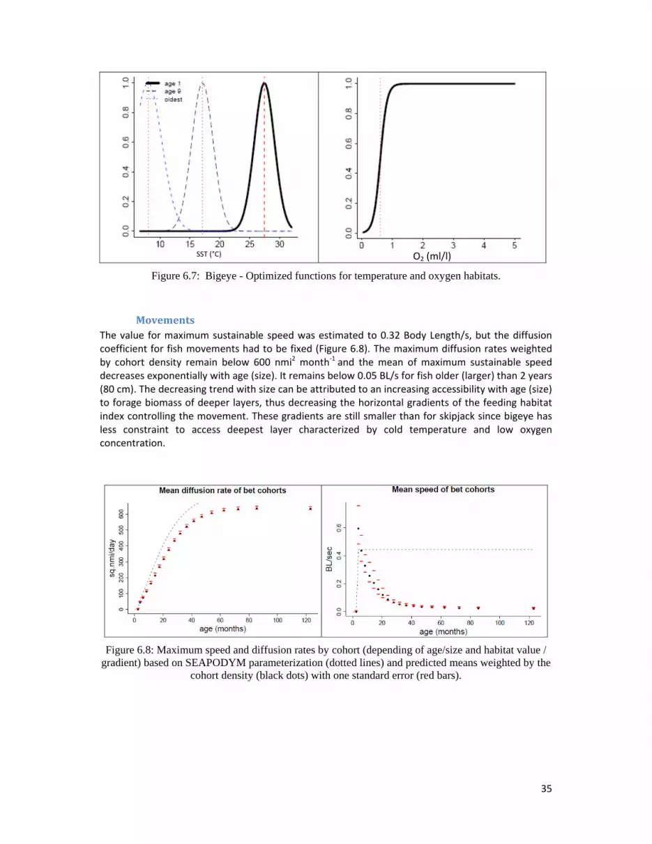
Figure 6.7: Bigeye - Optimized functions for temperature and oxygen habitats.

MovementsThe value for maximum sustainable speed was estimated to 0.32 Body Length/s, but the diffusion coefficient for fish movements had to be fixed (Figure 6.8). The maximum diffusion rates weighted by cohort density remain below 600 nmi2 month‐1 and the mean of maximum sustainable speed decreases exponentially with age (size). It remains below 0.05 BL/s for fish older (larger) than 2 years (80 cm). The decreasing trend with size can be attributed to an increasing accessibility with age (size) to forage biomass of deeper layers, thus decreasing the horizontal gradients of the feeding habitat index controlling the movement. These gradients are still smaller than for skipjack since bigeye has less constraint to access deepest layer characterized by cold temperature and low oxygen concentration.

Figure 6.8: Maximum speed and diffusion rates by cohort (depending of age/size and habitat value / gradient) based on SEAPODYM parameterization (dotted lines) and predicted means weighted by the

cohort density (black dots) with one standard error (red bars).

36


The total biomass estimates (Figure 6.9) are presented with those estimated from the previous 2° x

month optimisation using (NCEP‐ORCA2‐PISCES with the initial conditions of the SEAPODYM

simulation starting in 1977). The estimate is approximately 40% higher than these alternate values.

a

b

Figure 6.9: Estimates of total Pacific biomass of bigeye: a) with stock assessment model MULTIFAN-CL (red) and SEAPODYM -NCEP 2° configuration using no constraint (black) or initial

conditions provided by MUTIFAN-CL (purple) and b) with the new estimate using SODA 1° configuration (black) compared to stock assessment model MULTIFAN-CL (red) and SEAPODYM

NCEP 2° configuration with initial conditions provided by MUTIFAN-CL (grey).

The mean spatial distribution (Figure 6.10) shows the highest concentration to be in the central‐

eastern equatorial region extending east to the coast of Central America. Secondary areas with

lower density of bigeye occur in the South west Pacific, especially the Coral Sea, off the coast of

Mexico and Baja California and in the North‐east off the coast of Philippines islands and south of

Japan.

Seasonality in the biomass of adult fish was not estimated (Figure 6.11). The predicted spawning

grounds and highest larvae concentration occur in the central and eastern equatorial region (Figure

6.12) with a seasonal peak in the central area during the 3rd quarter. In the Coral Sea, a north‐south

spatial shift is predicted likely in relation with the seasonal warming of waters; the most southern

extension occurring during the austral summer (Q1). The first quarter was the most favourable

season for spawning in the north‐western quadrant of the basin, with the highest density off the

Philippines. The young immature fish are particularly concentrated in the central equatorial region

(Figure 6.13).

37

NCEP 2°

SODA 1°

Figure 6.10: Predicted total biomass of Pacific bigeye, average over 2002-2006.

Figure 6.11: Seasonal distributions of adult bigeye, average over 2002-2006 years.

Q1 Q2

Q3 Q4

38

Figure 6.12: Seasonal distributions of bigeye larvae, average over 2002-2006 years.

Figure 6.13: Seasonal distributions of young bigeye, average over 2002-2006 years.

Q1 Q2

Q3 Q4

Q1 Q2

Q4Q3

39

7. REFERENCEFITFORSOUTHPACIFICALBACOREFORTHEHISTORICALPERIOD(SPALB1.1NCEP‐ORCA2‐v2)

Physicalforcing:NCEP‐ORCA2‐PISCEShindcastsimulation(1958‐2003)

In absence of historical synoptic datasets for oceanic physical variables before the 1980s, and before

1998 for the ocean color (i.e., SeaWiFS), ocean reanalyses are not available to simulate tuna

dynamics with SEAPODYM for the past decades before 1998. As an alternative, hindcast simulations

with coupled ocean physical‐biogeochemical models can be used. These simulations are forced by

atmospheric data for which a few reanalyses are available (e.g. NCEP, ERA40). To produce the first

initial conditions used in optimization experiments with the reference configuration, or to run

specific applications requiring long historical simulations, one such hindcast is used to drive the

model SEAPODYM. The biogeochemical model is PISCES (Pelagic Interaction Scheme for Carbon and

Ecosystem Studies; Aumont and Bopp, 2006). It incorporates both multi‐nutrient limitation (NO3,

NH4, PO4, SiO3 and Fe) and a description of the plankton community structure with four plankton

functional groups (Diatoms, Nano‐phytoplankton, Micro‐zooplankton and Meso‐zooplankton).

PISCES is coupled to the ORCA2 configuration of the ocean circulation model OPA

(http://www.nemo‐ocean.eu/), and driven by the NCEP‐NCAR reanalysis, that provides 50‐year

record of global analyses of atmospheric fields based on the recovery of land surface, ship,




2°x2°x month.

Fishingdata

The definition of fisheries for south Pacific albacore tuna (Table 9.1) was slightly modified from the

previous one used for SCIFISH project. The Japanese longline fishery was divided into two fisheries

based on the geographical fishing ground, i.e., either tropical (Equator to 25°S) or temperate (25°S‐

50°S). Further, the island fisheries, previously groupped into a single fishery, were separated. All

longline catch and effort fishing data are at a solution of 5° x 5° x month. Size frequency data are at a

resolution varying from 5°x 5° to 10°x 20°.

Discussions with colleagues at SPC concerning a possible upgrade of fishing data to enhance spatial

resolution at 1°x1° led to a new definition of fisheries that should include one set of incomplete high

resolution (1°x month) and one set of complete but low resolution data. Part of these new data sets

was provided but it is still too partial to be used in optimization.

40

Table 7.1: Fisheries definition for south Pacific albacore

N

Gear Region Description Nationality C/E data

month/year

Reso‐

lution

Size data

qtr/year

Reso‐

lution

(L1)

L1

LL 50S‐25S;

140E‐110W

JP, JPDW Japan high

latitude

1/1952‐

12/2006

5x5 3/1964‐

3/2005

10x20

(L1)

L12

LL 25S‐0;

140E‐110W

JP, JPDW

Japan low

latitude

1/1952‐

12/2006

5x5 3/1964‐

3/2005

10x20

L2

LL 50S‐0;

140E‐110W

Korea 3/1962‐

12/2008

5x5 1/1966‐

2/2006

5x5

L3

LL 50S‐0;

140E‐110W

Distant‐water

fleet

Chinese Taipei 7/1964‐

12/2008

5x5 3/1964‐

2/2007

5x5;

10x20

L4 LL 50S‐10S;

140E‐175E

LL targeting

Alb

Australia 3/1985‐

12/2007

5x5 2/2002‐

2/2007

5x5;

10x20

L5

LL 25S‐0;

150E‐180E

LL targeting

Alb

New Caledonia 11/1983‐

12/2007

5x5 1/1993‐

4/2007

5x5;

10x20

L5 LL 25S‐5S;

180E‐140W

LL targeting

Alb

Tonga 2/1982‐

3/2008

5x5 3/1995‐

242006

5x5;

10x20

L5 LL 25S‐0;

180E‐110W

LL targeting

Alb

French

Polynesia

1/1992‐

5/2007

5x5 2/1991‐

4/2007

5x5;

10x20

(L5)

L11

LL 25S‐0;

180E‐155W

LL targeting

Alb

American

Samoa, Samoa

1/1993‐

5/2008

5x5 1/1998‐

3/2007

5x5;

10x20

L6

LL 50S‐0;

140E‐180W

LL targeting

Alb

Other 11/1957‐

12/2008

5x5 3/1963‐

3/2005

5x5;

10x20

L7 LL 50S‐25S;

145E‐180E

LL targeting

Alb

New Zealand 8/1989‐

12/2007

5x5 2/1992‐

4/2006

5x5;

10x20

L5 LL 25S‐0;

150E‐180E

LL targeting

Alb

Fiji 8/1989‐

12/2007

5x5 3/1992‐

3/2007

5x5;

10x20

T8 T 50S‐25S;

140E‐110W

Troll New Zealand,

United States

1/1967‐

12/2007

5x5 4/1986‐

2/2006

5x5;

5x10;

10x20

G9 D 45S‐25S;

140E‐125W

Driftnet Japan, Chinese

Taipei

11/1983‐

1/1991

5x5 4/1988‐

1/1990

5x5;

10x20

L10 LL 50S‐0;

180‐70W

LL targeting

Alb

Other 11/1957‐

12/2008

5x5 3/1963‐

3/2005

5x5;

10x20


The first likelihood optimization for south Pacific albacore was performed with a first NCEP‐ORCA2‐

PISCES ocean hindcast simulation over the period 1980‐2001 (SCIFISH project). Outputs from this

first experiment were used for defining initial conditions of a second optimization experiment using

SODA ocean reanalysis and satellite derived primary production at 1°x month resolution over the

period 1998‐2008.

This third optimization experiment uses a new definition of fisheries (cf above) and an updated

NCEP‐ORCA2‐PISCES forcing (1958‐2008). It was conducted over the period 1975‐2000, with the

revised fine age‐structure.

41

SouthPacificalbacorepopulationstructure

The structure of the population was defined with 1‐month cohorts for all life stages. Such fine age

structure has been chosen to match the time stepping for the integration of the model equations.

The last “+ cohort” accumulates older fish. Age at maturity is thus set to 53.5 months. Age‐length

and age‐weight relationships (Figure 7.1) are derived from the last MULTIFAN‐CL estimate (Hoyle et

al. 2012).

NCEP-ORCA2-PISCES_v2

Figure 7.1: South pacific size (FL in cm) at age (month) and weight (kg) at age functions used in SEAPODYM simulation (left), based on MULTIFAN-CL estimates (Hoyle et al 2012), and

population structure (average 1998-2008) in % metric tonnes resulting from the new optimization with SEAPODYM and the SODA-Psat environmental forcing.

Fittocatchdata

The south Pacific albacore habitat extends between the equator and 45°S (Figure 7.2). The maximum amount of catch occurs in the 10°S‐20°S latitudinal band and catch levels are also higher in the west than in the east. There is almost no catch in the eastern equatorial Pacific, likely in relation to the hypoxic waters that characterize the sub‐surface layer of this region. The overall spatial fit between prediction and observation is provided in Figure 7.2. The fit between the southern limit of the species habitat and 10°S was good but degraded in the band 10°S ‐ 0°. The total catch in this area however was generally well predicted (Figure 7.3). Dissolved oxygen concentration in the equatorial

42

region is closely linked to primary productivity and varies strongly with ENSO events. The lack of interannual variability for the oxygen variable may be the reason for the poor fit, especially the Pearson r‐ squared, in this area with this configuration.

Figure 7.2: Spatial fit to catch data. From top to bottom: 1) Map of R-squared goodness of fit in 5deg cell (mean value 0.68). The cells without color mean no significant fit has been achieved for these

usually accidental data. 2) Pearson r-squared metric (mean value 0.78), which quantifies the percentage of the catch variance explained by the model in each cell, overlaid with the number of

observations (fishing events). 3) Map of the mean relative error.

43

The fisheries that show the lowest fit between observed and predicted CPUE are mainly the

domestic fisheries (Tonga, Wallis and Futuna, Samoa, Australia). The use of fishing data at 1°x month

resolution for these fisheries could help to improve the model skills. The quality of Japanese fishery

CPUE (L1 and L12) was poor fact due to the lack of fit in the tropical and transition zones. However,

in the sub‐tropical (presumably feeding) zones it was good. Comparison of climatological time series

of predicted vs observed variables shows reasonable fit for the largest albacore fisheries.

Observed (dashed line) and predicted (continuous line) total monthly catch (x1000 mt)

44

Figure 7.3: Time series of total predicted and observed catch and CPUE by main albacore fisheries (dashed line - observations, solid line - model predictions) with corresponding size frequency for all

the domain and time period (bars: observations, red line: model predictions).

Additional model validation was done within specific geographic zones, where the fishing data show

the greatest seasonality, assumingly linked to albacore migration cycle. Thus, several regions (Figure

7.4) were chosen with regions R1 and R2 (separated by longitude 180°E) representing known

spawning zone; R3 (between 25S and 35S) a transition zone ; R4 (below 35S) the feeding WCPO zone

and two EPO zones (R5 and R6) split at 115W.

Figures 7.5 to 7.7 provide the seasonal fit (average over 1975‐2000) in these regions for the main

longline fisheries, i.e., Japan and Chinese Taipei fleets. Observed and predicted monthly total catch

and average CPUE are shown with the total exploited biomass, i.e., the total biomass caught if the

catchability was equal to 1. It is calculated as the total biomass multiplied by the selectivity for cell

where there is effort.

45

The fit is very good for the Chinese Taipei fleet (L3) in all regions, and less good for the Japanese

fleets, especially the tropical fleet (L12) that progressively focused on bigeye tuna and catch

albacore more and more as a by‐catch. Based on L1 and L3, the seasonality in spawning grounds R1

and R2 is marked by a high peak in the last quarter and a low peak between March and June (Figure

7.5). During this latter period a high peak occurs in the feeding region R4 and transition region R3

(Figure 7.6). The two eastern regions R5 and R6 have quite different seasonal patterns (Figure 7.7),

with a high peak between March and May in the most eastern (R6) and during the last quarter in

region R5, ie coinciding with those of spawning region R1 and R2. These complex dynamics may

reflect two different migration paths, e.g. north‐south in the Coral Sea and west Pacific and following

the border of the gyre in the east.

Figure 7.4: Regions used to compare seasonal dynamics of predicted and observed statistics for albacore

46

F Total Catch Total exploited biomass Average CPUE

L2 R2 L2 R1

L3 R2 L3 R1

L12 R2 L12 R1

Figure 7.5: Monthly climatology of model predictions vs. observations in two spawning zones (see map on Fig. 8.4). Shaded zone in average CPUE series corresponds to 95% CI.

47


L1 R4 L1 R3

L3 R4 L3 R3

Figure 7.6: Monthly climatology of model predictions vs. observations in WCPO transition and feeding zones (see map on Fig. 8.4). Shaded zone in average CPUE series corresponds to 95% CI.

48


L2 R6 L2 R5

L3 R6 L3 R5

L12 R5

Figure 7.7: Monthly climatology of model predictions vs. observations in two EPO check zones (see map on Fig. 8.4). Shaded zone in average CPUE series corresponds to 95% CI.

49


This optimization experiment using the new fine age structure allowed estimating all key parameters

of albacore, including the new larvae predator function parameter, which limits spatial boundaries

of spawning ground by the critical values of MTL biomass (parameter in Table 7.2).

Table 7.2: Estimates of habitats and movement parameters for south Pacific albacore using environmental forcings from NCEP-ORCA2

Parameters estimated by the model Unit SODA 1° v1 SODA 1° v2

Ts

Spaw

ning Optimum of the spawning temperature function

oC [24.5 [24.5

s Std. Err. of the spawning temperature function oC 2.5] 2.5*

Larvae food‐predator trade‐off coefficient ‐ [3 4.98

Ta

Feed

ing

habitat Optimum of the adult temperature function at maximum age oC 7.9 7.88

a Std. Err. of the adult temperature function at maximum age oC 4] 5]


Dmax

Move‐

men


Vmax Maximum sustainable speed B.L. s‐1

1.8 1.8

*Fixed; [val = value close to minimum boundary value; val] = value close to maximum boundary value

NaturalmortalityIn the last stock assessment with MULTIFAN‐CL (Hoyle et al 2012) the natural mortality was fixed to

0.4 yr‐1 (0.033 mo‐1). For this revised experiment with SEAPODYM and NCEP configuration the

mortality rate was estimated around 0.18 mo‐1 for the larvae cohort decreasing rapidly to a value

below 0.04 mo‐1 (O.48 yr‐1) for the cohorts with age between 30 and 60 months (63‐87 cm in size),

then increasing again for the remaining oldest cohorts attaining the maximum value 0.08 mo‐1

(Figure 7.8). Thus, the mortality rates estimated for the young fraction of the exploited stock is close

to those used for the stock assessment with MULTIFAN‐CL while adult mortality rates are estimated

to be 50‐100% higher.

50

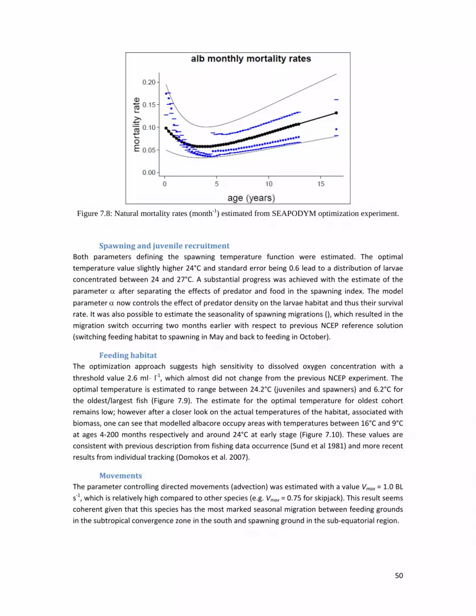
Figure 7.8: Natural mortality rates (month-1) estimated from SEAPODYM optimization experiment.

SpawningandjuvenilerecruitmentBoth parameters defining the spawning temperature function were estimated. The optimal

temperature value slightly higher 24°C and standard error being 0.6 lead to a distribution of larvae

concentrated between 24 and 27°C. A substantial progress was achieved with the estimate of the

parameter after separating the effects of predator and food in the spawning index. The model

parameter now controls the effect of predator density on the larvae habitat and thus their survival rate. It was also possible to estimate the seasonality of spawning migrations (), which resulted in the

migration switch occurring two months earlier with respect to previous NCEP reference solution

(switching feeding habitat to spawning in May and back to feeding in October).

FeedinghabitatThe optimization approach suggests high sensitivity to dissolved oxygen concentration with a

threshold value 2.6 ml l‐1, which almost did not change from the previous NCEP experiment. The

optimal temperature is estimated to range between 24.2°C (juveniles and spawners) and 6.2°C for

the oldest/largest fish (Figure 7.9). The estimate for the optimal temperature for oldest cohort

remains low; however after a closer look on the actual temperatures of the habitat, associated with

biomass, one can see that modelled albacore occupy areas with temperatures between 16°C and 9°C

at ages 4‐200 months respectively and around 24°C at early stage (Figure 7.10). These values are

consistent with previous description from fishing data occurrence (Sund et al 1981) and more recent

results from individual tracking (Domokos et al. 2007).

MovementsThe parameter controlling directed movements (advection) was estimated with a value Vmax = 1.0 BL

s‐1, which is relatively high compared to other species (e.g. Vmax = 0.75 for skipjack). This result seems

coherent given that this species has the most marked seasonal migration between feeding grounds

in the subtropical convergence zone in the south and spawning ground in the sub‐equatorial region.

51

a Spawning index

SST °C


SST°C

c d

Larval stock-recruitment

Figure 7.9: Spawning and larval recruitment. a: spawning index in relation to SST and food-predator tradeoff ratio. b: Distribution of larvae according to SST and the estimated parameters of spawning

index.c: Seasonal timing of spawning migration. d: SEAPODYM larval stock-recruitment relationship estimated for albacore. Densities are in number of individual per km2 for adult and 1000’s

of individual per km2 for larvae.

52

age (months)

Figure 7.10: Optimized functions for temperature and oxygen habitats.


In the previous optimization experiments (both NCEP 2° and SODA 1° based) without the estimation

of seasonality parameters and using an age structure discretization inconsistent with the model time

step, the total biomass estimate with SEAPODYM was much higher than the MULTIFAN‐CL estimate

conducted in 2008 and 2012 (Hoyle et al 2008; Hoyle et al., 2012). Then, initial conditions of these

first two SEAPODYM optimization experiments were forced to be close to those of MULTIFAN‐CL. As

a result both model estimates had similar biomass levels and temporal trends.

In this new experiment, the (unconstrained) total biomass estimate from SEAPODYM has decreased

to ~1 million t, while in the same time the revised assessment with MULTIFAN‐CL (Hoyle et al 2012)

has more than doubled with an average value of ~1.4 million t between 2000‐2007 (Figure 7.11).

Therefore, the two most recent estimates form MULTIFAN‐CL and SEAPODYM are converging.

Averageseasonalvariability

The mean spatial distributions (Figure 7.12 and Figure 7.13) show a clear distinction between life

stages. Young immature albacore are predicted to concentrate in the western half part of the south

Pacific basin between 20°S and 40°S with a decreasing eastward gradient of density, and without any

apparent seasonal change in this pattern despite of the observed variability of catch, likely linked to

ocean conditions. Conversely, adult fish show a clear north‐south seasonal migration pattern. The

density of adult is maximum in the latitudinal band 10°S‐25°S during the 4th and still high during the

53

1st quarter and below 20°S or in the central Pacific between 10‐20°S during the second quarter. Thus,

the adult fish tend to concentrate seasonally in warm waters of the southern tropical area in austral

summer for spawning and then move for feeding either south or toward the central sub‐equatorial

region.

Though the model predicts continuous spawning over the year opportunistically according to the

environmental conditions, there is a strong seasonal peak in spring‐ summer coinciding with the

maximum concentration of adult in the latitudinal band 10°S ‐ 25°S. This is consistent with the result

observed by Farley et al. (2013) in their stock‐wide examination of the reproductive biology of south

Pacific albacore.

Figure 7.11: Estimates of total biomass of south Pacific albacore: top) estimates of total spawning biomass given by SEAPODYM (dark blue) and MULTIFAN-CL in 2012 (red) (Hoyle et al 2012);

bottom) the same comparison but for the total albacore biomass (young + adult).

54

January ‐ March April ‐ June

July ‐ September October ‐ December

Figure 7.12 Seasonal spatial distributions of young (immature) albacore. Temporal average over 1990-1999.

January – March April – June

July – September October ‐ December

Figure 7.13: Seasonal spatial distributions of adult (mature) albacore. Temporal average over 1990-1999.

55

8. REFERENCEFITFORPACIFICSKIPJACKFORCLIMATECHANGEANALYSES

No change to the reference fit presented to 2011 WCPFC Scientific Committee meeting (SC7).

9. REFERENCEFITFORPACIFICBIGEYEFORCLIMATECHANGEANALYSES

Physicalforcing:IPSLCM4

The IPSL‐PISCES Earth Climate simulation provided physical‐biogeochemical fields used to drive

SEAPODYM and to investigate the responses of tuna population dynamics to global warming. The

IPSL climate model (Marti et al., 2006) is composed of an oceanic physical component OPA, a sea ice

component LIM, an atmospheric component LMDZ, and a land surface component ORCHIDEE,

coupled through the OASIS coupler. The global climate simulation starts with climatological

conditions and the only variable forcing is the change in atmospheric CO2 concentration. The

simulation uses the historical atmospheric CO2 concentration between 1860 and 2000, which then

increases according to the SRES A2 IPCC scenario for the 21st century, i.e., atmospheric CO2

concentrations reaching 850 ppm in the year 2100. Physical forcing fields from the climate

simulation have then been used to force an offline version of the oceanic biogeochemical model

PISCES (Aumont and Bopp, 2006) over a similar period (1860‐2100) and for the global ocean. A

detailed description and evaluation of those simulations is provided in Sarmiento et al. (2004), and

Schneider et al. (2007). The latitudinal anomaly in temperature was corrected as per the methods

reported to SC7 and published in Lehodey et al. (2013).

Fishingdata

The fishing data used was the same as the reference fit for the historical period.

Populationstructure

The population structure used was the same as the reference fit for the historical period.

Fittocatchdata

The optimization experiment using corrected IPSL‐CM4 temperature fields provided reasonable fit to

fishing data for the historical period used (1982‐2000) with good estimation of size frequency

distribution by fishery. Relative error in catch was high only in regions with very low level of catch

with an interesting exception along the latitudinal band 10°N‐15°N in the WCPO (Figure 8.1).


The optimization was not able to correctly estimate some of parameters for habitat and movements

(Table 8.1). The standard error of the spawning temperature function and the diffusion parameter

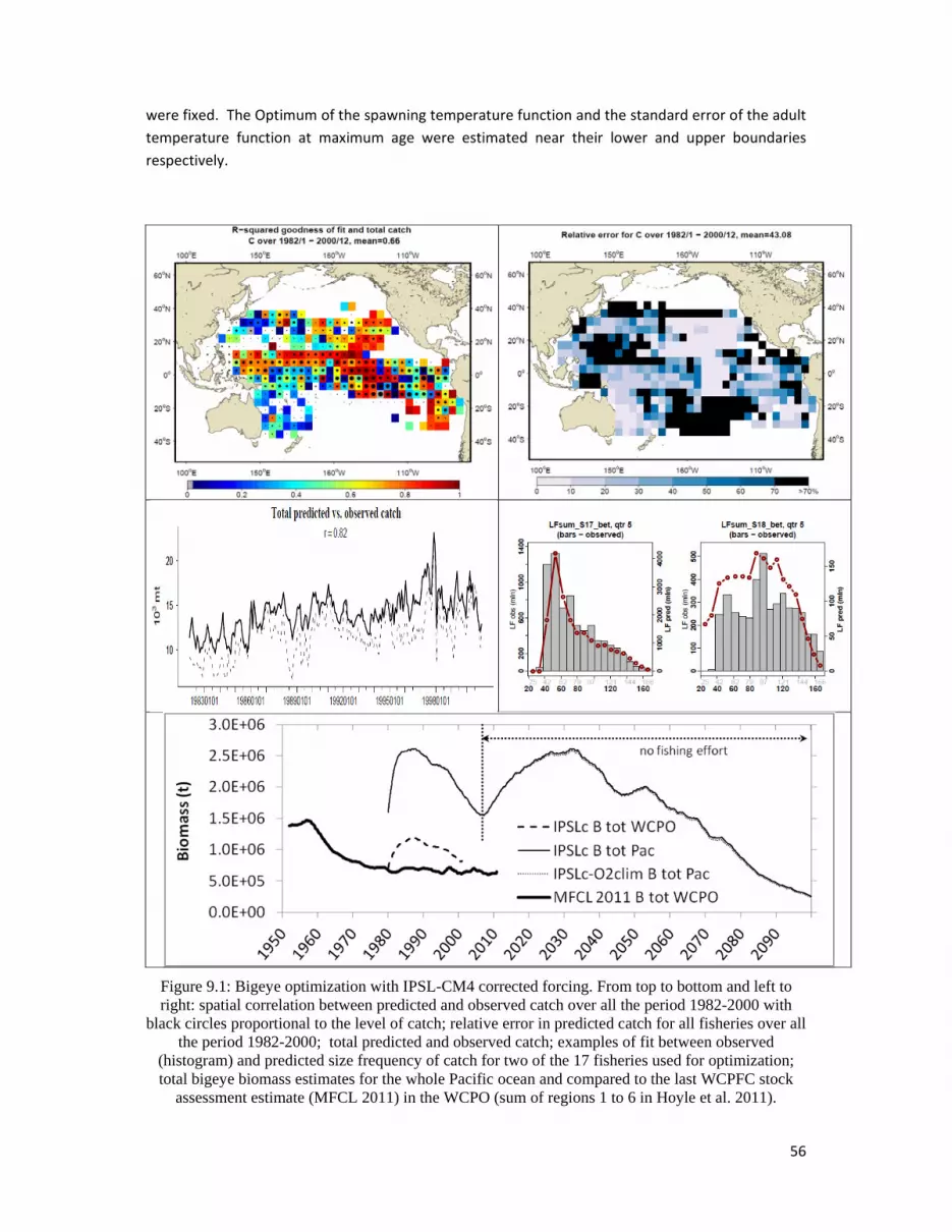
56

were fixed. The Optimum of the spawning temperature function and the standard error of the adult

temperature function at maximum age were estimated near their lower and upper boundaries

respectively.

Figure 9.1: Bigeye optimization with IPSL-CM4 corrected forcing. From top to bottom and left to right: spatial correlation between predicted and observed catch over all the period 1982-2000 with

black circles proportional to the level of catch; relative error in predicted catch for all fisheries over all the period 1982-2000; total predicted and observed catch; examples of fit between observed

(histogram) and predicted size frequency of catch for two of the 17 fisheries used for optimization; total bigeye biomass estimates for the whole Pacific ocean and compared to the last WCPFC stock

assessment estimate (MFCL 2011) in the WCPO (sum of regions 1 to 6 in Hoyle et al. 2011).

57

The estimates of parameter values indicates that the movement parameter is very low (< 0.2 body

length s‐1), the standard error of spawning temperature (s) function is narrow (0.75°C) while the

larvae prey‐predator tradeoff coefficient ( is high (4.7). Usually, there is a correlation between s

and ; when one is increasing the other decreases, compensating their effect upon each other to

some degree. To obtain convergence s was fixed to a low value resulting in a high value of This means that spawning grounds were defined by concentrated, highly favourable areas and periods. A

consequence of this parameterisation was a declining population contracting around its predicted

core habitat where both spawning and feeding conditions need to exist together since mature fish

were estimated to have small displacement capacity. Since tagging data analyses suggest that

bigeye tuna can migrate long distances, this scenario seems highly less plausible, and optimization

experiments including sensitivity analyses for these parameters need to be continued, in particular

to investigate where are the bifurcation points from which opposite trends can emerge.

Table 8.1. Summary of parameters values estimated by optimization approach with IPSL forcing before (IPSL) and after correction (IPSLc) of bias in temperature fields. Colors give an indication of

confidence (green = good; orange = low confidence; red = large uncertainty).

Parameters estimated by the model

Unit BET

IPSL IPSLc

Habitats

1 Ts Optimum of the spawning temperature function oC 26.2 28.4

2 s Std. Err. of the spawning temperature function oC 0.9 0.75*

3 Larvae food‐predator trade‐off coefficient ‐ 0.34 4.7

4 Ta Optimum of the adult temperature function at maximum age

oC [8 10.6

5 a Std. Err. of the adult temperature function at maximum age oC 5] 4.45

6 Ô Oxygen threshold ml l‐1 1.02 1.23

Movements

8 VM Maximum sustainable speed B.L.s‐1 0.1 0.19

* fixed; [ ] reaching min or max value boundary


The total bigeye stock biomass in the WCPO (west of 150°W) was slightly over the estimate with the

stock assessment model MFCL (Figure 8.1) but the decreasing trend in SEAPODYM was stronger.

Biomass estimate at Pacific basin scale was more than the double with the decline in biomass since

1990 stronger than that observed for the WCPO. Fishing effort information was unavailable from

2008 for the simulation and the future projections are made in the absence of fishing mortality. The

simulation suggests that at least two decades are required for the stock to rebuild and reach a new

equilibrium.

The optimization with the corrected IPSL‐CM4 forcing led to a continuous decline under the A2

scenario, even in the eastern Pacific, and the population finally collapses by the end of the Century.

A second simulation using climatological fields of oxygen did not modify this result (Figure 8.1),

58

providing verification that this trend is not due to the predicted change for this variable. The validity

of this simulation result however should be interpreted with caution as model exploration indicates

some inconsistencies.

1st experiment with IPSL‐CM4

Larvae 2000 Total biomass 2000


2nd experiment with IPSL‐CM4 after T° correction



Figure 9.2: Mean annual density of bigeye larvae (ind. km-2) and total biomass (t km-2) predicted from the A2 climate scenario in 2000 and 2099 before and after temperature correction and new

optimization experiment.

59

10. REFERENCEFITFORSOUTHPACIFICALBACOREFORCLIMATECHANGEANALYSES

No change to the reference fit presented to 2012 WCPFC Scientific Committee meeting (SC8).

11. CURRENTANDFUTUREWORKPLAN

Swordfish

The first application of SEAPODYM to swordfish was presented to SC8. Development of a second

generation model will commence in December 2013 for this species which will incorporate updated

fisheries data provided to the WCPFC for this species.

OperationalBasinscalemodel

A pre‐operational model configuration of SEAPODYM has been developed for the Pacific skipjack

population at weekly ¼° resolution, based on optimization achieved with SODA configuration

(Lehodey et al. WCPFC 8). The environmental variables are provided by the ocean reanalysis

GLORYSv2 and the Satellite derived primary production for the historical period and the operational

ocean circulation model PSY3 of Mercator‐Ocean for real‐time and forecast. The stratification of

fisheries is the same as the reference optimisation experiment with SODA, but with a monthly

average fishing effort based on the last 2 years. The high resolution simulation shows the same large

basin‐scale patterns as the lower resolution (Figure 11.1Figure 11.1) but with a detailed

representation of mesoscale activity.

2012, week 13 2013, week 13

Figure 11.1. Pre-operational model at 0.25°x week. Distribution of larvae density predicted without fishing effort, for the calendar week 13 (March 25-31) in 2012 compared to 2013.

60

Sub‐regionalModelling

There are technical challenges to implementing operational models at the sub‐regional scale. First,

tuna species are highly migratory species, and their habitats cover the whole ocean. Simulating the

dynamics of these fish stocks at high resolution in a sub‐region region requires accounting for the

exchanges (fluxes) with the rest of the populations outside of the regional domain, under the

influence of both environmental variability (e.g., El Niño events) and fishing mortality. Following the

approach used in physical oceanography, the basin‐scale SEAPODYM configuration at resolution of

1/4°x week can provide the open boundary conditions for a sub‐regional model. This requires new

technical developments in the code of the model to adapt its numerical scheme to the

regionalisation.

A first application of this approach will be implemented for the EEZ of Indonesia. The sub‐regional

SEAPODYM operational model will be at resolution of 1/12°x day (Figure 11.2) and will use a

climatological data set (i.e. monthly average) of fishing effort for the Indonesian waters prepared

from the best available information to apply an average fishing mortality. This initiative should

complements WCPFC efforts to improve the monitoring and management of tuna fisheries in this

region that is of critical importance for the sustainability of tuna resources in the western and

central Pacific Ocean generally. At the same time it will support the development of SEAPODYM

operational model for skipjack yellowfin and bigeye tuna since these basin‐scale configurations are

necessary to provide boundary conditions for the regional Indonesian model configuration. The main

objectives of this development are to:

evaluate the operational model of tuna spatial dynamics (SEAPODYM) at a resolution of

1/12°x day for three species: skipjack, yellowfin and bigeye;

promote the use of VMS data for estimating fishing effort and produce a database of

operational fishing effort estimates that can be used both in the operational chain of

modelling and to consolidate the national fishing statistics;

provide capacity‐building for a PhD Indonesian student working on Indonesian tuna fisheries

and several engineers and technicians.

demonstrate the interest of developing an Electronic catch Report System (ERS) that can be

coupled to operational VMS and SEAPODYM to validate and monitor in real time the tuna

stock and fisheries in the Indonesian EEZ.

61

Figure 11.2. Domain of the regional operational model for the INDESO project illustrated with the 1st test for skipjack model.

Incorporationoftaggingdata

The incorporation of Pacific Ocean tagging data will commence once new physical forcing data

(either SODA 1 degree and MERCATOR ¼ degree) are pre‐processed for use in SEAPODYM. The

revised SODA forcing should extend the modelling period to December 2009 and the MERCATOR

forcing until December 2012. It is expected that new reference fits for each species will results

through the applications of these new data sources (forcing and tagging).

YellowfinTuna

The development of the model for yellowfin tuna will commence in the later 2013 with the

incorporation of tagging and new physical forcing data. The SC is expected to review at reference fit

for this model at SC10.

ClimateChangeModelling

The current physical forcing for the evaluation of climate change scenarios is restricted to a single

CMIP4 model (IPSL). To capture the uncertainty in climate change projections an ensemble of CMIP5

models is under development. For the historical period a revised physical forcing that has realistic

simulation of oceanic conditions, under the influence of ENSO and PDO variability, has been

generated. The coupled NEMO‐PISCES model has been forced by observed winds of the ERA‐Interim

reanalysis using the latest version (IFS5) covering the period 1979‐present. Five to six CMIP5 models

will be coupled with the NEMO‐PISCES model to generate physical forcings under climate change.

The choice of CMIP5 models has been determined by their compatibility with the historical forcing

(so the jump from the historical forcing to the climate anomaly is minimised) and that they have

realistic ENSO and PDO variability. This approach means that SEAPODYM only needs to be optimised

62

once for each species before simulation of various climate change scenarios can be implemented. A

first version of these climate change simulations are expected to be presented to SC10.

SEAPODYMview

The software SEAPODYMview which provides for easy display of SEAPODYM output is currently

being revised to allow use on non‐Linux operating systems and to provide improved visualisation

options.

63

12. REFERENCES

Bell JD, Ganachaud A., Gehrke PC, Griffiths SP, Hobday AJ, Hoegh‐Guldberg O, Johnson, JE Le Borgne R, Lehodey P, Lough JM, Matear RJ, Pickering TD, Pratchett MS, Sen Gupta A, Senina I and Waycott M., (2013) Tropical Pacific fisheries and aquaculture will respond differently to climate change. Nature Climate Change, 3: 591‐599

Farley, J.H., A.J. Williams, C.R. Davies, S.J. Nicol. 2013. Reproductive dynamics of South Pacific albacore tuna (Thunnus alalunga). Plos ONE, 8: e60577.

Lehodey P., Murtugudde R., Senina I. (2010). Bridging the gap from ocean models to population dynamics of large marine predators: a model of mid‐trophic functional groups. Progress in Oceanography, 84: 69–84

Lehodey P., Senina I., & Murtugudde R. (2008). A Spatial Ecosystem And Populations Dynamics Model (SEAPODYM) ‐ Modelling of tuna and tuna‐like populations. Progress in Oceanography, 78: 304‐318.

Lehodey P., Senina I., Calmettes B, Hampton J, Nicol S. (2013). Modelling the impact of climate change on Pacific skipjack tuna population and fisheries. Climatic Change, 119: 95–109.

Lehodey P., Senina I., Calmettes B., Hampton J., Nicol S., Williams P., Jurado Molina J., Ogura M., Kiyofuji H., Okamoto S. (2011). SEAPODYM working progress and applications to Pacific skipjack tuna population and fisheries. 7th regular session of the Scientific Steering Committee, 8‐17 August 2011, Pohnpei, Federate States of Micronesia. WCPFC‐SC7‐2011/EB‐ WP 06.

Lehodey P., Senina I., Sibert J., Bopp L, Calmettes B., Hampton J., Murtugudde R. (2010). Preliminary forecasts of population trends for Pacific bigeye tuna under the A2 IPCC scenario. Progress in Oceanography. 86: 302–315

Lehodey, P., Hampton, J., Brill, R.W., Nicol, S., Senina, I., Calmettes, B., Pörtner, H.O., Bopp, L., Ilyina,T., Johann D. Bell, and J. Sibert (in press). Vulnerability of oceanic fisheries in the tropical Pacific to climate change. In Bell J., Johnson JE, Hobday AJ (Ed.), Vulnerability of Tropical Pacific Fisheries and Aquaculture to Climate Change. Secretariat of the Pacific Community. Noumea New Caledonia.

Lehodey, P., Senina, I., Hampton, J, Nicol, S, Williams, P., Jurado Molina J., Abecassis, M., Polovina J. Project 62: SEAPODYM working progress and applications to Pacific tuna and billfish populations and fisheries. 8th regular session of the Scientific Steering Committee, 7‐15 August 2012, Busan, Korea. WCPFC‐SC8‐2012/EB‐IP‐06.

Senina I, Royer F, Lehodey P, Hampton J, Nicol S, Ogura M, Kiyofuji H, Sibert J (2012). Integrating conventional and electronic tagging data into SEAPODYM. Pelagic Fisheries Research Program, Newsletter 16(1): 9‐14

Senina I., Sibert J., & Lehodey P. (2008). Parameter estimation for basin‐scale ecosystem‐linked population models of large pelagic predators: application to skipjack tuna. Progress in Oceanography, 78: 319‐335.

Sibert J, Senina I, Lehodey P, Hampton J. (2012). Shifting from marine reserves to maritime zoning for conservation of Pacific bigeye tuna (Thunnus obesus). Proceedings of the National Academy of Sciences 109(44): 18221‐18225.

Documents

Project 62: SEAPODYM applications in WCPO