Quantitative law describing market dynamics before and after interest-rate change

Alexander M. Petersen,1 Fengzhong Wang,1 Shlomo Havlin,1,2 and H. Eugene Stanley1

1Center for Polymer Studies and Department of Physics, Boston University, Boston, Massachusetts 02215, USA2Minerva Center and Department of Physics, Bar-Ilan University, Ramat-Gan 52900, Israel

Received 7 December 2009; revised manuscript received 3 May 2010; published 28 June 2010

We study the behavior of U.S. markets both before and after U.S. Federal Open Market Commissionmeetings and show that the announcement of a U.S. Federal Reserve rate change causes a financial shock,where the dynamics after the announcement is described by an analog of the Omori earthquake law. Wequantify the rate nt of aftershocks following an interest-rate change at time T and find power-law decaywhich scales as nt−Tt−T−, with positive. Surprisingly, we find that the same law describes the ratent−T of “preshocks” before the interest-rate change at time T. This study quantitatively relates the size ofthe market response to the news which caused the shock and uncovers the presence of quantifiable preshocks.We demonstrate that the news associated with interest-rate change is responsible for causing both the antici-pation before the announcement and the surprise after the announcement. We estimate the magnitude offinancial news using the relative difference between the U.S. Treasury Bill and the Federal Funds effective rate.Our results are consistent with the “sign effect,” in which “bad news” has a larger impact than “good news.”Furthermore, we observe significant volatility aftershocks, confirming a “market under-reaction” that lasts atleast one trading day.

DOI: 10.1103/PhysRevE.81.066121 PACS numbers: 89.65.Gh, 91.30.Px, 89.75.Da, 64.60.av

I. INTRODUCTION

Interest-rate changes by the Federal Reserve provide asignificant perturbation to financial markets, which we ana-lyze from the perspective of statistical physics 1–6. TheFederal Reserve Board Fed, in charge of monetary policyas the central bank of the United States, is one of the mostinfluential financial institutions in the world. During FederalOpen Market Commission FOMC meetings, the Fed deter-mines whether or not to change key interest rates. Theseinterest rates serve as a benchmark and a barometer for bothAmerican and international economies. The publicly releasedstatements from the scheduled FOMC meetings providegrounds for widespread speculation in financial markets, of-ten with significant consequences.

In this paper, we show that markets respond sharply toFOMC news in a complex way reminiscent of physicalearthquakes described by the Omori law 7,8. For financialmarkets, the Omori law was first observed in market crashesby Lillo and Mantegna 9, followed by a further study ofWeber et al. 10, which found the same behavior inmedium-sized aftershocks. However, the market crash isonly an extreme example of information flow in financialmarkets. This paper extends the Omori law observed in largefinancial crises to the more common Federal Reserve an-nouncements and suggests that large market news dissipatesvia power-law relaxation Omori law of the volatility. Inaddition to the standard Omori dynamics following the an-nouncement, we also find unique Omori dynamics before theannouncement.

The market dynamics following the release of FOMCnews are consistent with previous studies of price discoveryin foreign exchange markets following marcroeconomicnews releases 11,12. Furthermore, we hypothesize that theuncertainty in Fed actions, coupled with the preannouncedschedule of FOMC meetings, can increase speculation

among market traders, which can lead to the observed mar-ket under-reaction 13. Market under-reaction, meaning thatmarkets take a finite time to readjust prices following news,is not consistent with the efficient market hypothesis; severaltheories have been proposed to account for these phenomena14.

We analyze all 66 scheduled FOMC meetings in the 8year period of 2000–2008 using daily data from 15. Also,for the 2 year period of 2001–2002, we analyze the intradaybehavior for 19 FOMC meetings using Trades and QuoteTAQ data on the 1 min time scale.

The paper is organized as follows. In Sec. II we describethe FOMC meetings and the Fed interest rate relevant to ouranalysis. In Sec. III A we analyze the response of the S&P100, the top 100 stocks ranked by 12 month sales accordingto a 2002 BusinessWeek report belonging to the 2002 S&P500 index, over the 2000–2008 period using daily data. Us-ing the relative spread between the 6 month Treasury Billand the Federal Funds effective rates, we relate the specula-tion prior to the FOMC meetings to the daily market vola-tility, measured here as the logarithmic difference betweenthe intraday high and low prices for a given stock on the dayof the announcement. In Sec. III B we study high-frequencyintraday TAQ data on the 1 min scale for the S&P 100 andfind an Omori law with positive exponent immediately fol-lowing the announcement of Fed rate changes. Further, werelate the intraday market response quantified by both theOmori exponent and Omori amplitude to the change in mar-ket expectations before and after the announcement.

II. FOMC MEETINGS, FED INTEREST RATES,AND TREASURY BILLS

There are many economic indicators that determine thehealth of the U.S. economy. In turn, the health of the U.S.economy sets a global standard due to the ubiquity of both

PHYSICAL REVIEW E 81, 066121 2010

1539-3755/2010/816/06612111 ©2010 The American Physical Society066121-1

the U.S. Dollar and the economic presence maintainedthrough imports, exports, and the global market 16. TheU.S. Federal Reserve target rate, along with the effective“overnight” rate, sets the scale for interest rates in the UnitedStates and abroad. The target rate is determined at FOMCmeetings, which are scheduled throughout the year, with de-tailed minutes publicly released from these meetings. Theeffective rate is a “weighted average of rates on brokeredtrades” between the Fed and large banks and financial insti-tutions and is a market realization of the target rate 17. InFig. 1 we plot the federal interest rates over the 8 year periodof 2000–2008.

Our analysis focuses on the FOMC meetings after January2000. Historically, the methods for releasing the meeting de-tails have varied. In the 1990s, there was a transition from avery secretive policy toward the current transparent policy18. Since the year 2000, the Fed has released statementsdetailing the views and goals of the FOMC. This increase inpublic information has led to an era of mass speculation inthe markets, revolving mainly around key economic indica-tors such as the unemployment rate, the consumer price in-dex, the money supply, etc. These economic indicators alsoinfluence the FOMC in their decision to either change ormaintain key interest rates. Speculation has assumed manyforms and new heights, evident in the implementation of newtypes of derivatives based on federal securities. For instance,options and futures are available at the Chicago Board ofTrade, which are based on Federal Funds, Treasury Bills, andEuro-Dollar foreign exchange. These contracts can be usedto estimate the implied probability of interest-rate changes,utilizing sophisticated methods focused on the price move-ment of expiring derivative contracts 19–24.

In the next section, we outline a simple method to mea-sure speculation prior to a scheduled FOMC meeting usingthe 6 month Treasury Bill and the Federal Funds effectiveovernight rate. These data are readily available and are up-dated frequently at the website of the Federal Reserve 17.Because each FOMC meeting is met with speculation in theweeks before the meeting and anticipation in the hours be-fore the announcement, we identify the decision to changeor not to change key interest rates as a market perturbation.The market response results from the systematic stress asso-ciated with the speculation and anticipation, which are notalways in line with the FOMC decision.

III. EMPIRICAL RESULTS

A. Response to FOMC meetings on daily time scale

In this section we analyze the daily activity before andafter 66 scheduled FOMC meetings over the 8 year period of2000–2008, where scheduled meetings are publicly an-nounced at least a year in advance 17. We do not considerunscheduled meetings resulting in rate change, which con-tain an intrinsic element of surprise and are historically in-frequent only four unexpected target rate changes over thesame period. Of primary importance is the FOMC commit-tee’s decision to change or not change the target rate Rt bysome percent Rt, where the absolute relative changeRt /Rt−1 has typically filled the range between 0.0 and

0.25. This section serves as an initial motivation for the in-traday analysis and will also serve as a guide in developing ametric that captures market speculation. In this section weuse the intraday high-low price range to quantify the magni-tude of price fluctuations. In particular, we analyze the com-panies belonging to the S&P 100 and also the subset of 18banking and finance companies referred to here as the“bank” sector.

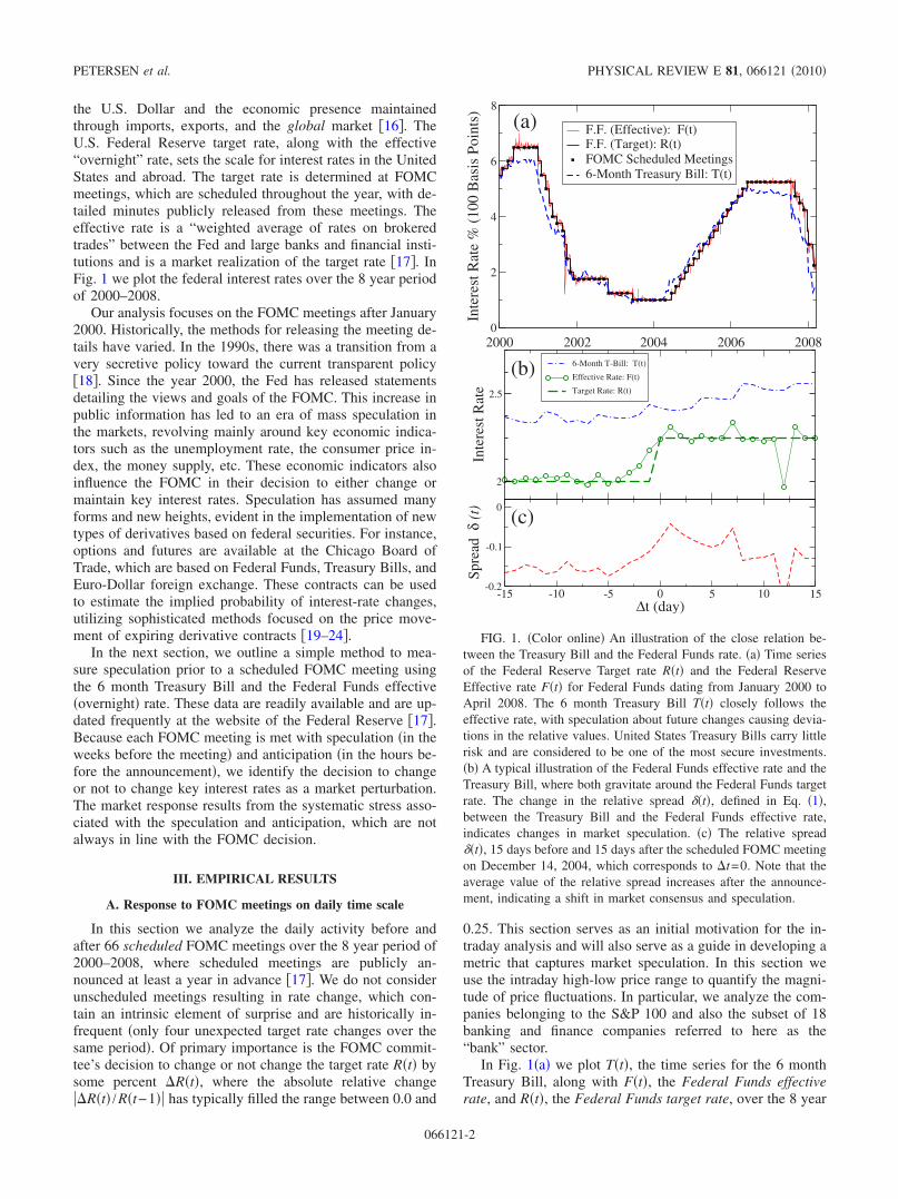
In Fig. 1a we plot Tt, the time series for the 6 monthTreasury Bill, along with Ft, the Federal Funds effectiverate, and Rt, the Federal Funds target rate, over the 8 year

2000 2002 2004 2006 20080

2

4

6

8

Inte

rest

Rat

e%

(100

Bas

isPo

ints

)

F.F. (Effective): F(t)F.F. (Target): R(t)FOMC Scheduled Meetings6-Month Treasury Bill: T(t)

(a)

2

2.5

Inte

rest

Rat

e

6-Month T-Bill: T(t)

Effective Rate: F(t)

Target Rate: R(t)

-15 -10 -5 0 5 10 15∆t (day)

-0.2

-0.1

0

Spre

adδ

(t)

(b)

(c)

FIG. 1. Color online An illustration of the close relation be-tween the Treasury Bill and the Federal Funds rate. a Time seriesof the Federal Reserve Target rate Rt and the Federal ReserveEffective rate Ft for Federal Funds dating from January 2000 toApril 2008. The 6 month Treasury Bill Tt closely follows theeffective rate, with speculation about future changes causing devia-tions in the relative values. United States Treasury Bills carry littlerisk and are considered to be one of the most secure investments.b A typical illustration of the Federal Funds effective rate and theTreasury Bill, where both gravitate around the Federal Funds targetrate. The change in the relative spread t, defined in Eq. 1,between the Treasury Bill and the Federal Funds effective rate,indicates changes in market speculation. c The relative spreadt, 15 days before and 15 days after the scheduled FOMC meetingon December 14, 2004, which corresponds to t=0. Note that theaverage value of the relative spread increases after the announce-ment, indicating a shift in market consensus and speculation.

PETERSEN et al. PHYSICAL REVIEW E 81, 066121 2010

066121-2

period beginning in January 2000. The relative differencebetween the 6 month Treasury Bill and the Federal Fundseffective rate is an indicator of the future expectations of theFederal Funds target rate 18. Note that the 6 month Trea-sury Bill has anticipatory behavior with respect to the Fed-eral Funds target and hence effective rates. Other more so-phisticated models utilize futures on Federal Funds andEuro-Dollar exchange, but these markets are rather new andrepresent the highly complex nature of contemporary mar-kets and hedging programs 20–24. Hence, we use a simpleand intuitive method for estimating market speculation andanticipation by analyzing the relative difference between the6 month Treasury Bill and the Federal Funds effective rate.

Figure 1b exhibits the typical interplay between the 6month Treasury Bill and the Federal Funds effective ratebefore and after a FOMC meeting. The change in the valueof the effective rate results from market speculation, startingapproximately one trading week five trading days prior tothe announcement. This change follows from the forward-looking Treasury Bill, which in the example in Fig. 1b, ispriced above the Federal Funds rate even 15 trading daysbefore the announcement.

In order to quantify speculation and anticipation in themarket prior to each scheduled FOMC meeting, we analyzethe time series t of the relative spread between Ft andTt,

t lnFtTt

. 1

As an example of this relation, in Fig. 1c we plot t for15 days before and after a typical FOMC meeting resultingin a rate change. In order to study the speculation precedingthe ith scheduled FOMC meeting, we calculate the averagerelative spread over the L1=15 day period. We weight thedays in the L1 day period leading up to the FOMC meetingday exponentially, such that the relative spread on the tthday before the announcement has the weight wt=e−t/.Without loss of generality, we choose the value of =10 days corresponding to two trading weeks 25. We de-fine the speculation metric,

i = ti t

ti − twt

t

wt, 2

which is a weighted average of t before the announce-ment, where the sums are computed over the range t 1,L1. The metric i for the ith FOMC meeting can bepositive or negative, depending on the market’s forward-looking expectations.

In order to quantify the market response to the speculationi, we analyze the market volatility around each FOMCmeeting. For a particular stock around the ith scheduledFOMC meeting, we take the daily high price phiti+t andthe daily low price plowti+t, for t −20,20, wheret=0 corresponds to ti, the day of the meeting. We thencompute the high-low range for each trading day,

rti + t ln phiti + tplowti + t . 3

For each stock and each meeting, we scale the range by r,the average range over the 41 day time sequence centeredaround the meeting day, resulting in the normalized volatilityvti+trti+t / r. Similarly, we use ti+t, thetime series for the volume traded over the same period, tocompute a weight for each stock corresponding to the nor-malized volume on the day of the FOMC meeting. We cal-culate this weight as iti / i, where i is the aver-age daily volume over the 41 day time sequence centeredaround the ith meeting day. We use a volume weight in orderto emphasize the price impact resulting from relatively hightrading volume, since there are significant cross correlationsbetween volume and price changes 26. Finally, we computethe weighted average volatility time series over all stocksand all meetings,

vt vti + ti

i

. 4

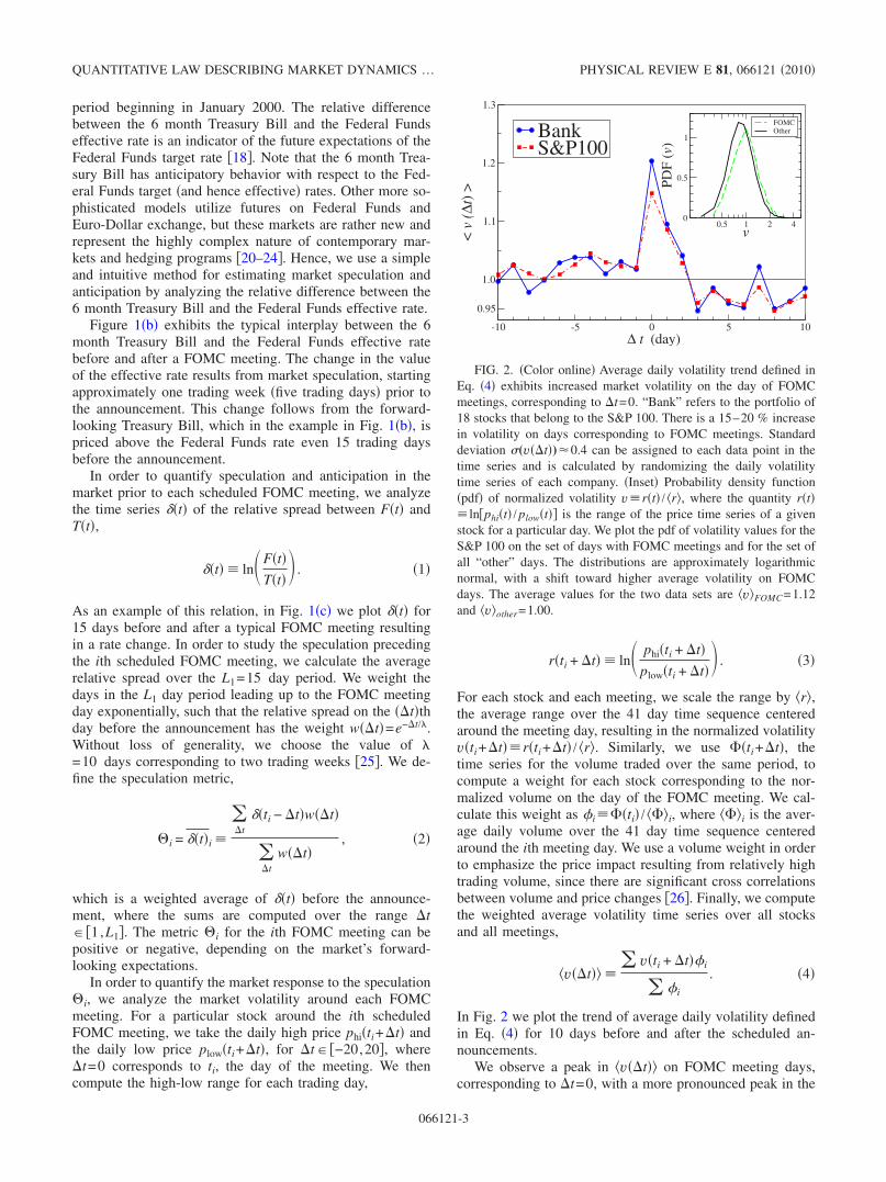
In Fig. 2 we plot the trend of average daily volatility definedin Eq. 4 for 10 days before and after the scheduled an-nouncements.

We observe a peak in vt on FOMC meeting days,corresponding to t=0, with a more pronounced peak in the

-10 -5 0 5 10∆ t (day)

0.95

1.0

1.1

1.2

1.3

<v

(∆t)

>

BankS&P100

0.5 1 2 4v

0

0.5

1

PDF

(v)

FOMCOther

FIG. 2. Color online Average daily volatility trend defined inEq. 4 exhibits increased market volatility on the day of FOMCmeetings, corresponding to t=0. “Bank” refers to the portfolio of18 stocks that belong to the S&P 100. There is a 15–20 % increasein volatility on days corresponding to FOMC meetings. Standarddeviation (vt) 0.4 can be assigned to each data point in thetime series and is calculated by randomizing the daily volatilitytime series of each company. Inset Probability density functionpdf of normalized volatility vrt / r, where the quantity rt lnphit / plowt is the range of the price time series of a givenstock for a particular day. We plot the pdf of volatility values for theS&P 100 on the set of days with FOMC meetings and for the set ofall “other” days. The distributions are approximately logarithmicnormal, with a shift toward higher average volatility on FOMCdays. The average values for the two data sets are vFOMC=1.12and vother=1.00.

QUANTITATIVE LAW DESCRIBING MARKET DYNAMICS … PHYSICAL REVIEW E 81, 066121 2010

066121-3

bank sector Fig. 2. Stocks in the bank sector are stronglyimpacted by changes in Fed rates, which immediately influ-ence both their holding and lending rates. On average there isa 15–20 % increase in volatility on days corresponding toFOMC meetings.

In order to quantify the impact of a single FOMC an-nouncement on day ti, we define the average market volatil-ity,

Vi = vti i

vtii

i

i

. 5

Here, ¯ i and i refer to the average and sum overrecords corresponding only to the day ti. Again, iti / is a normalized weight, where now is theaverage daily volume over the entire 8 year period, since wecompare many meetings across a large time span.

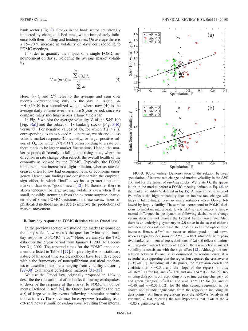
In Fig. 3 we plot the average volatility Vi of the S&P 100Fig. 3a and the subset of 18 banking stocks Fig. 3bversus i. For negative values of i, for which TtFtcorresponding to an expected rate increase, we observe a lessvolatile market response. Conversely, for larger positive val-ues of i, for which TtFt corresponding to a rate cut,there tends to be larger market fluctuations. Hence, the mar-ket responds differently to falling and rising rates, where thedirection in rate change often reflects the overall health of theeconomy as viewed by the FOMC. Typically, the FOMCimplements rate increases to fight inflation, whereas rate de-creases often follow bad economic news or economic emer-gency. Hence, our findings are consistent with the empiricalsign effect, in which “bad” news has a greater impact inmarkets than does “good” news 12. Furthermore, there isalso a tendency for large average volatility even when i issmall, possibly stemming from the extreme surprise charac-teristic of some FOMC decisions. In these cases, more so-phisticated methods are needed to improve the predictions ofmarket movement.

B. Intraday response to FOMC decision via an Omori law

In the previous section we studied the market response onthe daily scale. Now we ask the question “what is the intra-day response to FOMC news?” Here, we analyze the TAQdata over the 2 year period from January 1, 2001 to Decem-ber 31, 2002. The reported times for the FOMC announce-ment are listed in Table I 27. Inspired by the nonstationarynature of financial time series, methods have been developedwithin the framework of nonequilibrium statistical mechan-ics to describe phenomena ranging from volatility clustering28–30 to financial correlation matrices 31–33.

We use the Omori law, originally proposed in 1894 todescribe the relaxation of aftershocks following earthquakes,to describe the response of the market to FOMC announce-ments. Defined in Ref. 9, the Omori law quantifies the ratent of large volatility events following a singular perturba-tion at time T. The shock may be exogenous resulting fromexternal news stimuli or endogenous resulting from internal

-0.6 -0.4 -0.2 0 0.2 0.4 0.6 0.8Speculation, Θ

0.7

0.8

0.9

1

1.1

1.2

1.3

1.4

1.5

1.6

S&P

100

Vol

atili

ty,V

∆R = 0∆R < 0∆R > 0

(a)

-0.6 -0.4 -0.2 0 0.2 0.4 0.6 0.8Speculation, Θ

0.5

1

1.5

2

Ban

kSe

ctor

Vol

atili

ty,V

∆R = 0∆R < 0∆R > 0

(b)

FIG. 3. Color online Demonstration of the relation betweenspeculation of interest-rate change and market volatility in the S&P100 and for the subset of banking stocks. We relate i, the specu-lation in the market before a FOMC meeting defined in Eq. 2, tothe market volatility Vi defined in Eq. 5. A large absolute value ofi reflects the high probability that an interest-rate change willhappen. Interestingly, there are many instances where i 0, fol-lowed by large volatility. These values correspond to FOMC deci-sions to maintain interest-rate levels R=0 and suggest a funda-mental difference in the dynamics following decisions to changeversus decisions not change the Federal Funds target rate. Also,there is an underlying symmetry in R since in the case of either arate increase or a rate decrease, the FOMC also has the option of noincrease. Hence, R=0 can occur as either good or bad news,whereas typically decisions of R0 reflect situations with posi-tive market sentiment whereas decisions of R0 reflect situationswith negative market sentiment. Hence, the asymmetry in marketvolatility is consistent with the sign effect 12. Although the cor-relation between i and Vi is dominated by residual error, it isnevertheless supporting that the regression captures the crossover at ,V= 0,1. Including all data points, the regression correlationcoefficient is r2=0.34, and the slope of the regression is m=0.360.13 for a, and r2=0.30 and m=0.540.22 for b. Re-stricting data points corresponding only to interest-rate changes redand green triangles: r2=0.48 and m=0.370.12 for a, and r2

=0.40 and m=0.530.21 for b this second regression is notshown and is indistinguishable from the regression including alldata points. All linear regressions pass the ANOVA Analysis ofvariance F test, rejecting the null hypothesis that m=0 at the =0.05 significance level.

PETERSEN et al. PHYSICAL REVIEW E 81, 066121 2010

066121-4

correlations, e.g., “herding effect” 34–38. This rate is de-fined as

nt − T t − T−, 6

where is the Omori power-law exponent.Here, we study the rate of events greater than a volatility

threshold q, using the high-frequency intraday price time se-ries pt. The intraday volatility absolute returns is ex-pressed as vtlnpt / pt−t, where we use t=1 min. To compare stocks, we scale each raw time series interms of the standard deviation over the entire period ana-lyzed, and then remove the average intraday trading patternas described in Ref. 10. This establishes a common volatil-ity threshold q, in units of standard deviation, for all stocksanalyzed.

In the analysis that follows, we focus on Nt−T, thecumulative number of events above threshold q,

Nt − T = T

t

nt − Tdt t − T1−, 7

which is less noisy compared to nt−T. Using Nt−T,we examine the intraday market dynamics for 100 S&Pstocks before tT and after tT the ith FOMC an-

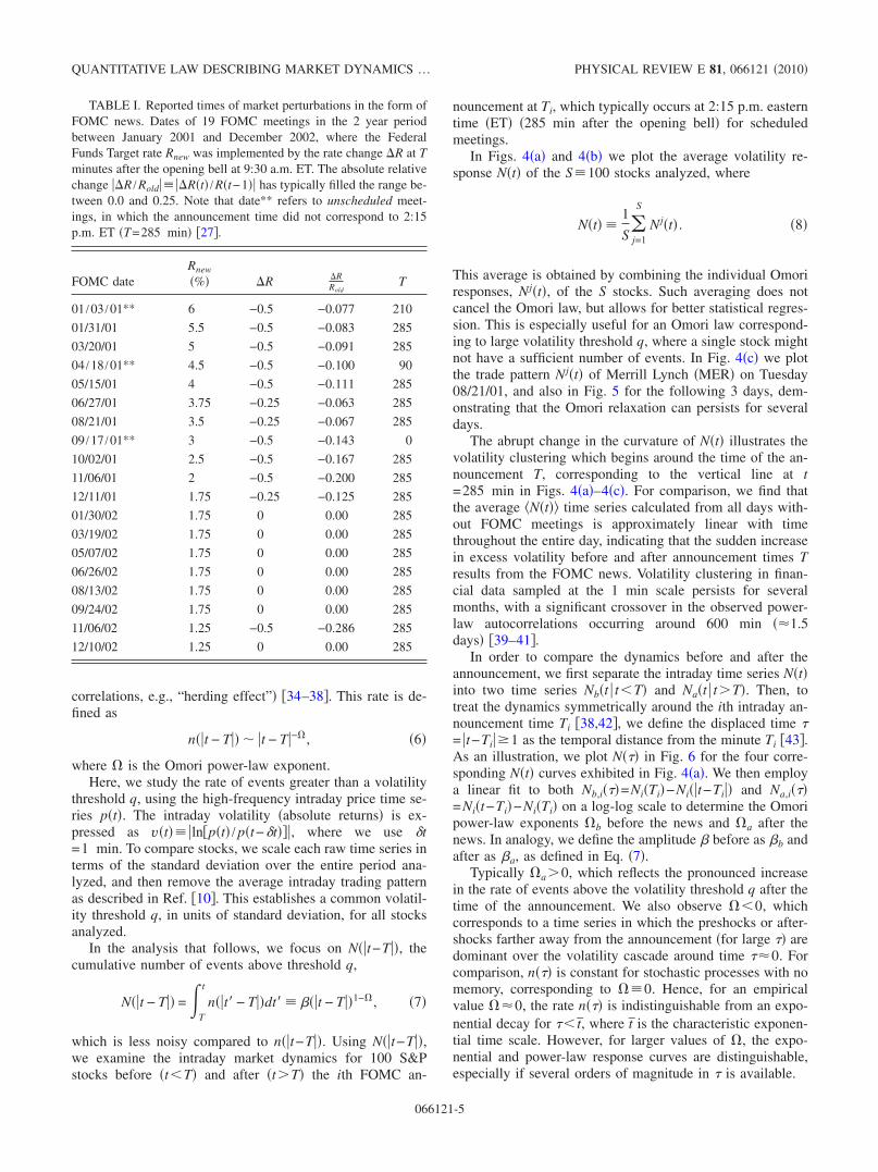
nouncement at Ti, which typically occurs at 2:15 p.m. easterntime ET 285 min after the opening bell for scheduledmeetings.

In Figs. 4a and 4b we plot the average volatility re-sponse Nt of the S100 stocks analyzed, where

Nt 1

Sj=1

S

Njt . 8

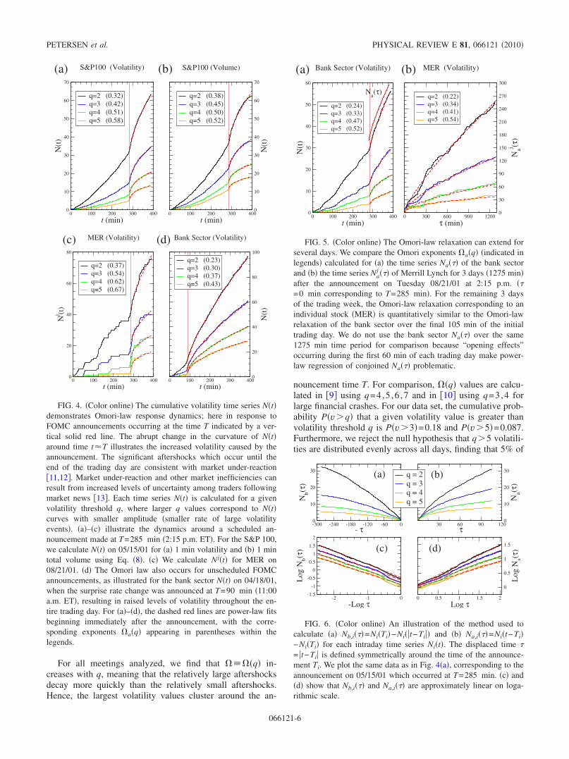
This average is obtained by combining the individual Omoriresponses, Njt, of the S stocks. Such averaging does notcancel the Omori law, but allows for better statistical regres-sion. This is especially useful for an Omori law correspond-ing to large volatility threshold q, where a single stock mightnot have a sufficient number of events. In Fig. 4c we plotthe trade pattern Njt of Merrill Lynch MER on Tuesday08/21/01, and also in Fig. 5 for the following 3 days, dem-onstrating that the Omori relaxation can persists for severaldays.

The abrupt change in the curvature of Nt illustrates thevolatility clustering which begins around the time of the an-nouncement T, corresponding to the vertical line at t=285 min in Figs. 4a–4c. For comparison, we find thatthe average Nt time series calculated from all days with-out FOMC meetings is approximately linear with timethroughout the entire day, indicating that the sudden increasein excess volatility before and after announcement times Tresults from the FOMC news. Volatility clustering in finan-cial data sampled at the 1 min scale persists for severalmonths, with a significant crossover in the observed power-law autocorrelations occurring around 600 min 1.5days 39–41.

In order to compare the dynamics before and after theannouncement, we first separate the intraday time series Ntinto two time series Nbt tT and Nat tT. Then, totreat the dynamics symmetrically around the ith intraday an-nouncement time Ti 38,42, we define the displaced time = t−Ti1 as the temporal distance from the minute Ti 43.As an illustration, we plot N in Fig. 6 for the four corre-sponding Nt curves exhibited in Fig. 4a. We then employa linear fit to both Nb,i=NiTi−Nit−Ti and Na,i=Nit−Ti−NiTi on a log-log scale to determine the Omoripower-law exponents b before the news and a after thenews. In analogy, we define the amplitude before as b andafter as a, as defined in Eq. 7.

Typically a0, which reflects the pronounced increasein the rate of events above the volatility threshold q after thetime of the announcement. We also observe 0, whichcorresponds to a time series in which the preshocks or after-shocks farther away from the announcement for large aredominant over the volatility cascade around time 0. Forcomparison, n is constant for stochastic processes with nomemory, corresponding to 0. Hence, for an empiricalvalue 0, the rate n is indistinguishable from an expo-nential decay for t, where t is the characteristic exponen-tial time scale. However, for larger values of , the expo-nential and power-law response curves are distinguishable,especially if several orders of magnitude in is available.

TABLE I. Reported times of market perturbations in the form ofFOMC news. Dates of 19 FOMC meetings in the 2 year periodbetween January 2001 and December 2002, where the FederalFunds Target rate Rnew was implemented by the rate change R at Tminutes after the opening bell at 9:30 a.m. ET. The absolute relativechange R /RoldRt /Rt−1 has typically filled the range be-tween 0.0 and 0.25. Note that date** refers to unscheduled meet-ings, in which the announcement time did not correspond to 2:15p.m. ET T=285 min 27.

FOMC dateRnew

% R RRold

T

01 /03 /01** 6 −0.5 −0.077 210

01/31/01 5.5 −0.5 −0.083 285

03/20/01 5 −0.5 −0.091 285

04 /18 /01** 4.5 −0.5 −0.100 90

05/15/01 4 −0.5 −0.111 285

06/27/01 3.75 −0.25 −0.063 285

08/21/01 3.5 −0.25 −0.067 285

09 /17 /01** 3 −0.5 −0.143 0

10/02/01 2.5 −0.5 −0.167 285

11/06/01 2 −0.5 −0.200 285

12/11/01 1.75 −0.25 −0.125 285

01/30/02 1.75 0 0.00 285

03/19/02 1.75 0 0.00 285

05/07/02 1.75 0 0.00 285

06/26/02 1.75 0 0.00 285

08/13/02 1.75 0 0.00 285

09/24/02 1.75 0 0.00 285

11/06/02 1.25 −0.5 −0.286 285

12/10/02 1.25 0 0.00 285

QUANTITATIVE LAW DESCRIBING MARKET DYNAMICS … PHYSICAL REVIEW E 81, 066121 2010

066121-5

For all meetings analyzed, we find that q in-creases with q, meaning that the relatively large aftershocksdecay more quickly than the relatively small aftershocks.Hence, the largest volatility values cluster around the an-

nouncement time T. For comparison, q values are calcu-lated in 9 using q=4,5 ,6 ,7 and in 10 using q=3,4 forlarge financial crashes. For our data set, the cumulative prob-ability Pvq that a given volatility value is greater thanvolatility threshold q is Pv3=0.18 and Pv5=0.087.Furthermore, we reject the null hypothesis that q5 volatili-ties are distributed evenly across all days, finding that 5% of

0 100 200 300 400

t (min)0

10

20

30

40

50

60

70

N(t

)

q=2 (0.32)q=3 (0.42)q=4 (0.51)q=5 (0.58)

S&P100 (Volatility)

0 100 200 300 400

t (min)0

10

20

30

40

50

60

70

N(t

)

q=2 (0.38)q=3 (0.45)q=4 (0.50)q=5 (0.52)

S&P100 (Volume)(a) (b)

0 100 200 300 400

t (min)0

20

40

60

80

Nj (t

)

q=2 (0.37)q=3 (0.54)q=4 (0.62)q=5 (0.67)

MER (Volatility)

0 100 200 300 400

t (min)0

20

40

60

80

100

N(t

)q=2 (0.23)q=3 (0.30)q=4 (0.37)q=5 (0.43)

Bank Sector (Volatility)(c) (d)

FIG. 4. Color online The cumulative volatility time series Ntdemonstrates Omori-law response dynamics; here in response toFOMC announcements occurring at the time T indicated by a ver-tical solid red line. The abrupt change in the curvature of Ntaround time t T illustrates the increased volatility caused by theannouncement. The significant aftershocks which occur until theend of the trading day are consistent with market under-reaction11,12. Market under-reaction and other market inefficiencies canresult from increased levels of uncertainty among traders followingmarket news 13. Each time series Nt is calculated for a givenvolatility threshold q, where larger q values correspond to Ntcurves with smaller amplitude smaller rate of large volatilityevents. a–c illustrate the dynamics around a scheduled an-nouncement made at T=285 min 2:15 p.m. ET. For the S&P 100,we calculate Nt on 05/15/01 for a 1 min volatility and b 1 mintotal volume using Eq. 8. c We calculate Njt for MER on08/21/01. d The Omori law also occurs for unscheduled FOMCannouncements, as illustrated for the bank sector Nt on 04/18/01,when the surprise rate change was announced at T=90 min 11:00a.m. ET, resulting in raised levels of volatility throughout the en-tire trading day. For a–d, the dashed red lines are power-law fitsbeginning immediately after the announcement, with the corre-sponding exponents aq appearing in parentheses within thelegends.

0 300 600 900 1200

τ (min)0

30

60

90

120

150

180

210

240

270

300

Naj (τ

)

q=2 (0.22)q=3 (0.34)q=4 (0.41)q=5 (0.54)

MER (Volatility)

0 100 200 300 400

t (min)0

10

20

30

40

50

60

N(t

)

q=2 (0.24)q=3 (0.33)q=4 (0.47)q=5 (0.52)

Bank Sector (Volatility)(a) (b)

Na(τ)

FIG. 5. Color online The Omori-law relaxation can extend forseveral days. We compare the Omori exponents aq indicated inlegends calculated for a the time series Na of the bank sectorand b the time series Na

j of Merrill Lynch for 3 days 1275 minafter the announcement on Tuesday 08/21/01 at 2:15 p.m. =0 min corresponding to T=285 min. For the remaining 3 daysof the trading week, the Omori-law relaxation corresponding to anindividual stock MER is quantitatively similar to the Omori-lawrelaxation of the bank sector over the final 105 min of the initialtrading day. We do not use the bank sector Na over the same1275 min time period for comparison because “opening effects”occurring during the first 60 min of each trading day make power-law regression of conjoined Na problematic.

-300 -240 -180 -120 -60 0- τ

0

10

20

30

Nb(τ

)

30 60 90 120τ

0

10

20

30

Na(τ

)

q = 2q = 3q = 4q = 5

-2 -1 0

-Log τ-1.5

-1

-0.5

0

0.5

1

1.5

2

Log

Nb(τ

)

0 0.5 1 1.5 2

Log τ

0

0.5

1

1.5

Log

Na(τ

)

(a) (b)

(c) (d)

FIG. 6. Color online An illustration of the method used tocalculate a Nb,i=NiTi−Nit−Ti and b Na,i=Nit−Ti−NiTi for each intraday time series Nit. The displaced time = t−Ti is defined symmetrically around the time of the announce-ment Ti. We plot the same data as in Fig. 4a, corresponding to theannouncement on 05/15/01 which occurred at T=285 min. c andd show that Nb,i and Na,i are approximately linear on loga-rithmic scale.

PETERSEN et al. PHYSICAL REVIEW E 81, 066121 2010

066121-6

the volatility values greater than q=5 are found on FOMCmeeting days, whereas only 4% are expected under the nullhypothesis that large volatilities are distributed uniformlyacross all trading days. The 25% increase for q=5 indicatesthat FOMC meetings days are more volatile than other daysat the 0 significance level. We also observe that the am-plitudes of the Omori law generally obey the inequality ba, resulting from the large response immediately follow-ing the news.

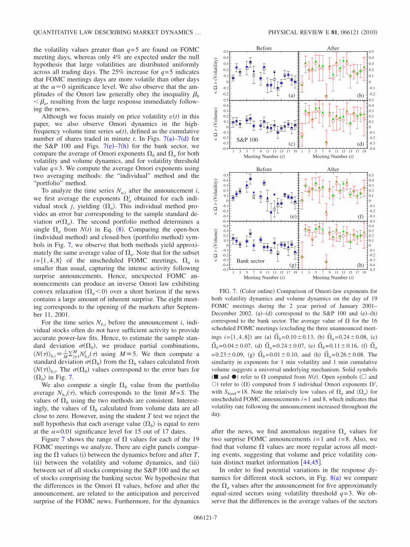
Although we focus mainly on price volatility vt in thispaper, we also observe Omori dynamics in the high-frequency volume time series t, defined as the cumulativenumber of shares traded in minute t. In Figs. 7a–7d forthe S&P 100 and Figs. 7e–7h for the bank sector, wecompare the average of Omori exponents b and a for bothvolatility and volume dynamics, and for volatility thresholdvalue q=3. We compute the average Omori exponents usingtwo averaging methods: the “individual” method and the“portfolio” method.

To analyze the time series Na,i after the announcement i,we first average the exponents a

j obtained for each indi-vidual stock j, yielding a. This individual method pro-vides an error bar corresponding to the sample standard de-viation a. The second portfolio method determines asingle a from Nt in Eq. 8. Comparing the open-boxindividual method and closed-box portfolio method sym-bols in Fig. 7, we observe that both methods yield approxi-mately the same average value of a. Note that for the subseti= 1,4 ,8 of the unscheduled FOMC meetings, a issmaller than usual, capturing the intense activity followingsurprise announcements. Hence, unexpected FOMC an-nouncements can produce an inverse Omori law exhibitingconvex relaxation a0 over a short horizon if the newscontains a large amount of inherent surprise. The eight meet-ing corresponds to the opening of the markets after Septem-ber 11, 2001.

For the time series Nb,i before the announcement i, indi-vidual stocks often do not have sufficient activity to provideaccurate power-law fits. Hence, to estimate the sample stan-dard deviation b, we produce partial combinations,Nb,i

1M j=1

M Nb,ij using M 5. We then compute a

standard deviation b from the b values calculated fromNb,i. The b values correspond to the error bars forb in Fig. 7.

We also compute a single b value from the portfolioaverage Nb,i, which corresponds to the limit M =S. Thevalues of b using the two methods are consistent. Interest-ingly, the values of b calculated from volume data are allclose to zero. However, using the student T test we reject thenull hypothesis that each average value b is equal to zeroat the =0.01 significance level for 15 out of 17 dates.

Figure 7 shows the range of values for each of the 19FOMC meetings we analyze. There are eight panels compar-ing the values i between the dynamics before and after T,ii between the volatility and volume dynamics, and iiibetween set of all stocks comprising the S&P 100 and the setof stocks comprising the banking sector. We hypothesize thatthe differences in the Omori values, before and after theannouncement, are related to the anticipation and perceivedsurprise of the FOMC news. Furthermore, for the dynamics

after the news, we find anomalous negative a values fortwo surprise FOMC announcements i=1 and i=8. Also, wefind that volume values are more regular across all meet-ing events, suggesting that volume and price volatility con-tain distinct market information 44,45.

In order to find potential variations in the response dy-namics for different stock sectors, in Fig. 8a we comparethe a values after the announcement for five approximatelyequal-sized sectors using volatility threshold q=3. We ob-serve that the differences in the average values of the sectors

Before

-0.2

-0.1

0

0.1

0.2

0.3

0.4

0.5

<Ω

>(V

olat

ility

)

After

-0.2

-0.1

0

0.1

0.2

0.3

0.4

0.5

1 3 5 7 9 11 13 15 17 19

Meeting Number (i)

-0.4-0.3-0.2-0.1

00.10.20.30.40.5

<Ω

>(V

olum

e)

1 3 5 7 9 11 13 15 17 19

Meeting Number (i)

-0.4-0.3-0.2-0.100.10.20.30.40.5

(a) (b)

(c) (d)S&P 100

Before

-0.4-0.3-0.2-0.1

00.10.20.30.40.5

<Ω

>(V

olat

ility

)

After

-0.4-0.3-0.2-0.100.10.20.30.40.5

1 3 5 7 9 11 13 15 17 19

Meeting Number (i)

-0.5-0.4-0.3-0.2-0.1

00.10.20.30.4

<Ω

>(V

olum

e)

1 3 5 7 9 11 13 15 17 19

Meeting Number (i)

-0.5-0.4-0.3-0.2-0.100.10.20.30.4

(e) (f)

(g) (h)Bank sector

FIG. 7. Color online Comparison of Omori-law exponents forboth volatility dynamics and volume dynamics on the day of 19FOMC meetings during the 2 year period of January 2001–December 2002. a–d correspond to the S&P 100 and e–hcorrespond to the bank sector. The average value of for the 16scheduled FOMC meetings excluding the three unannounced meet-

ings i= 1,4 ,8 are a b=0.100.13, b a=0.240.08, cb=0.040.07, d a=0.240.07, e b=0.110.16, f a

=0.230.09, g b=0.010.10, and h a=0.260.08. Thesimilarity in exponents for 1 min volatility and 1 min cumulativevolume suggests a universal underlying mechanism. Solid symbols and refer to computed from Nt. Open symbols and refer to computed from S individual Omori exponents j,with Sbank=18. Note the relatively low values of a and a forunscheduled FOMC announcements i=1 and 8, which indicates thatvolatility rate following the announcement increased throughout theday.

QUANTITATIVE LAW DESCRIBING MARKET DYNAMICS … PHYSICAL REVIEW E 81, 066121 2010

066121-7

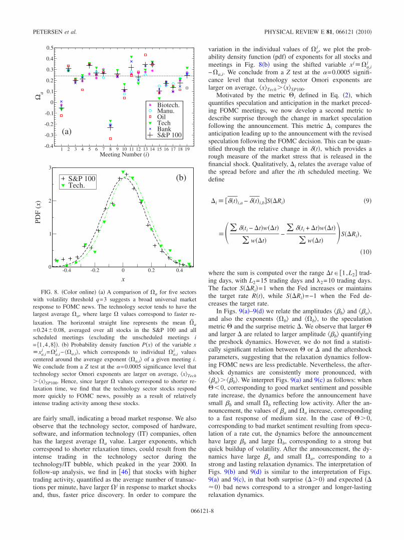
are fairly small, indicating a broad market response. We alsoobserve that the technology sector, composed of hardware,software, and information technology IT companies, oftenhas the largest average a value. Larger exponents, whichcorrespond to shorter relaxation times, could result from theintense trading in the technology sector during thetechnology/IT bubble, which peaked in the year 2000. Infollow-up analysis, we find in 46 that stocks with highertrading activity, quantified as the average number of transac-tions per minute, have larger j in response to market shocksand, thus, faster price discovery. In order to compare the

variation in the individual values of aj , we plot the prob-

ability density function pdf of exponents for all stocks andmeetings in Fig. 8b using the shifted variable xj a,i

j

−a,i. We conclude from a Z test at the =0.0005 signifi-cance level that technology sector Omori exponents arelarger on average, xTech xSP100.

Motivated by the metric i defined in Eq. 2, whichquantifies speculation and anticipation in the market preced-ing FOMC meetings, we now develop a second metric todescribe surprise through the change in market speculationfollowing the announcement. This metric i compares theanticipation leading up to the announcement with the revisedspeculation following the FOMC decision. This can be quan-tified through the relative change in t, which provides arough measure of the market stress that is released in thefinancial shock. Qualitatively, i relates the average value ofthe spread before and after the ith scheduled meeting. Wedefine

i ti,a − ti,bSRi 9

ti − twt

wt−

ti + twt

wtSRi ,

10

where the sum is computed over the range t 1,L2 trad-ing days, with L2=15 trading days and 2=10 trading days.The factor SRi=1 when the Fed increases or maintainsthe target rate Rt, while SRi=−1 when the Fed de-creases the target rate.

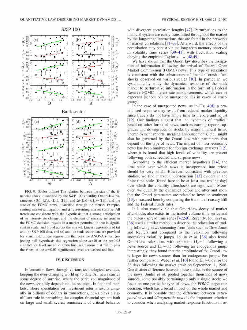
In Figs. 9a–9d we relate the amplitudes b and a,and also the exponents b and b, to the speculationmetric and the surprise metric . We observe that larger and larger are related to larger amplitude b quantifyingthe preshock dynamics. However, we do not find a statisti-cally significant relation between or and the aftershockparameters, suggesting that the relaxation dynamics follow-ing FOMC news are less predictable. Nevertheless, the after-shock dynamics are consistently more pronounced, witha b. We interpret Figs. 9a and 9c as follows: when0, corresponding to good market sentiment and possiblerate increase, the dynamics before the announcement havesmall b and small b reflecting low activity. After the an-nouncement, the values of a and a increase, correspondingto a fast response of medium size. In the case of 0,corresponding to bad market sentiment resulting from specu-lation of a rate cut, the dynamics before the announcementhave large b and large b, corresponding to a strong butquick buildup of volatility. After the announcement, the dy-namics have large a and small a, corresponding to astrong and lasting relaxation dynamics. The interpretation ofFigs. 9b and 9d is similar to the interpretation of Figs.9a and 9c, in that both surprise 0 and expected 0 bad news correspond to a stronger and longer-lastingrelaxation dynamics.

1 2 3 4 5 6 7 8 9 10 11 12 13 14 15 16 17 18 19Meeting Number (i)

-0.4

-0.3

-0.2

-0.1

0

0.1

0.2

0.3

0.4

0.5

Ωa

Biotech.Manu.OilTechBankS&P 100(a)

-0.4 -0.2 0 0.2 0.4

x

0

1

2

3

PDF

(x)

S&P 100Tech.

(b)

FIG. 8. Color online a A comparison of a for five sectorswith volatility threshold q=3 suggests a broad universal marketresponse to FOMC news. The technology sector tends to have thelargest average a, where large values correspond to faster re-

laxation. The horizontal straight line represents the mean a

=0.240.08, averaged over all stocks in the S&P 100 and allscheduled meetings excluding the unscheduled meetings i= 1,4 ,8. b Probability density function Px of the variable xxa,i

j =a,ij − a,i, which corresponds to individual a,i

j valuescentered around the average exponent a,i of a given meeting i.We conclude from a Z test at the =0.0005 significance level thattechnology sector Omori exponents are larger on average, xTech

xSP100. Hence, since larger values correspond to shorter re-laxation time, we find that the technology sector stocks respondmore quickly to FOMC news, possibly as a result of relativelyintense trading activity among these stocks.

PETERSEN et al. PHYSICAL REVIEW E 81, 066121 2010

066121-8

IV. DISCUSSION

Information flows through various technological avenues,keeping the ever-changing world up to date. All news carriessome degree of surprise, where the perceived magnitude ofthe news certainly depends on the recipient. In financial mar-kets, where speculation on investment returns results annu-ally in billions of dollars in transactions, news plays a sig-nificant role in perturbing the complex financial system bothon large and small scales, reminiscent of critical behavior

with divergent correlation lengths 47. Perturbations to thefinancial system are easily transmitted throughout the marketby the long-range interactions that are found in the networksof market correlations 31–33. Afterward, the effects of theperturbation may persist via the long-term memory observedin volatility time series 39–41, with fluctuation scalingobeying the empirical Taylor’s law 48,49.

We have shown that the Omori law describes the dissipa-tion of information following the arrival of Federal OpenMarket Commission FOMC news. This type of relaxationis consistent with the substructure of financial crash after-shocks observed on various scales 10. In particular, wesystematically study the dynamical response of the stockmarket to perturbative information in the form of a FederalReserve FOMC interest-rate announcements, which can beexpected scheduled or unexpected as in cases of emer-gency.

In the case of unexpected news, as in Fig. 4d, a pro-nounced response may result from reduced market liquiditysince traders do not have ample time to prepare and adjust12. Our findings suggest that the dynamics of “rallies”based on other forms of news, such as earning reports, up-grades and downgrades of stocks by major financial firms,unemployment reports, merging announcements, etc., mightalso be governed by the Omori law with parameters thatdepend on the type of news. The impact of macroeconomicnews has been analyzed for foreign exchange markets 12,where it is found that high levels of volatility are presentfollowing both scheduled and surprise news.

According to the efficient market hypothesis 14, thetime scale over which news is incorporated into pricesshould be very small. However, consistent with previousstudies, we find market under-reaction 13 evident in thefinite time scale found here to be at least one trading dayover which the volatility aftershocks are significant. More-over, we quantify the dynamics before and after and showthat the Omori parameters are related to investor sentiment13, measured here by comparing the 6 month Treasury Billand the Federal Funds rates.

It is also conceivable that Omori-law decay of marketaftershocks also exists in the traded volume time series andthe bid-ask spread time series 42,50. Recently, Joulin et al.36 used a similar method to describe the relaxation of trad-ing following news streaming from feeds such as Dow Jonesand Reuters and compared to the relaxation followinganomalous volatility jumps. Joulin et al. 36 also foundOmori-law relaxation, with exponent a 1 following anews source and a 0.5 following an endogenous jump;interestingly, they found that the amplitude of the Omori lawis larger for news sources than for endogenous jumps. Forfurther comparison, Weber et al. 10 found a 0.69 for the38 days following the market crash on September 11, 1986.One distinct difference between these studies is the source ofthe news: Joulin et al. pooled together thousands of newssources, some possibly pertaining to only a single stock; wefocus on one particular type of news, the FOMC target ratedecision, which has a broad impact on the whole market andeconomy. It is possible that the difference between antici-pated news and idiosyncratic news is the important criterionto consider when analyzing market response functions in re-

0.10.20.30.40.5

<β b

>

0.10.20.30.40.5

<β

b>

0.40.60.8

1

<β a

>

0.40.60.81

<β a

>

-0.10

0.10.20.3

<Ω

b>

-0.100.10.20.3

<Ω

b>

0.1

0.2

0.3

<Ω

a>

0.1

0.2

0.3

<Ω

a>

-0.2 -0.1 0 0.1 0.2

Θ-0.2

00.20.4

∆(<

Ω>)

-0.1 -0.05 0 0.05 0.1 0.15 0.2

∆-0.200.20.4

∆(<

Ω>)

(a) (b)

S&P 100

0.150.3

0.450.6

<β b

>

0.150.30.450.6

<β

b>

0.40.60.8

1

<β a

>

0.40.60.81

<β a

>

-0.150

0.150.3

0.45

<Ω

b>

-0.1500.150.30.45

<Ω

b>

0.10.20.30.4

<Ω

a>

0.10.20.30.4

<Ω

a>

-0.2 -0.1 0 0.1 0.2

Θ-0.2

00.20.4

∆(<

Ω>)

-0.1 -0.05 0 0.05 0.1 0.15 0.2

∆-0.200.20.4

∆(<

Ω>)

(c) (d)

Bank sector

FIG. 9. Color online The relation between the size of the fi-nancial shock, quantified by the S&P 100 volatility Omori-law pa-rameters b, a, b, a, and = a− b, and thesize of the FOMC news, quantified through the metrics repre-senting market anticipation and representing market surprise. Alltrends are consistent with the hypothesis that a strong anticipationof an interest-rate change, and the element of surprise inherent inthe FOMC decision, results in a market perturbation that is signifi-cant in scale, and broad across the market. Linear regressions of aand b S&P 100 data, and c and d bank sector data are providedfor visual aid. Linear regressions that pass the ANOVA F test re-jecting null hypothesis that regression slope m=0 at the =0.05significance level are solid green line; regressions that fail to passthe F test at the =0.05 significance level are dashed red line.

QUANTITATIVE LAW DESCRIBING MARKET DYNAMICS … PHYSICAL REVIEW E 81, 066121 2010

066121-9

lation to exogenous events. Here, we find unique dynamicsbefore anticipated announcements.

In the case of FOMC news, speculation can be quantifiedby measuring the relative difference between the effectiveFederal Funds rate and the Treasury Bill in the weeks leadingup to a scheduled meeting. We develop a speculation metric and relate it to V, the volatility on the day of the meetings,finding that the market behaves more erratically when theTreasury Bill predicts a decrease in the Federal Funds targetrate. A rate decrease often occurs in response to economicshocks, whereas a rate increase is often used to fight infla-tion. Hence, the asymmetric response in Fig. 3 to rising andfalling rates is consistent with the sign effect, where it hasbeen found that bad news causes a larger market reactionthan good news 12, and that the asymmetry may resultfrom the increased uncertainty in expectations among trad-ers.

We analyze the four Omori-law parameters b, a, b,and a calculated for 19 FOMC meetings. We conjecture thatthe Omori-law parameters are related to the market’s specu-lation, anticipation, and surprise on the day of the FOMCmeeting. In order to quantify speculation of rate cuts and rate

increases, we define the measure , which is the relativespread between the Treasury Bill and the Federal Fundsrates, before the meeting. In order to quantify surprise, wedevelop , which measures the change in the relative spreadbetween the Treasury Bill and the Federal Funds rates, be-fore and after the meeting. We relate both and to thedynamical response of the market on the day of the meeting.We find that relatively small values and relatively largeamplitude values, corresponding to longer relaxation timeand large response, follow from bad news, as in the case ofthe market reaction to the World Trade Center attacks in2001. All in all, these results show that markets relax accord-ing to the Omori law following large crashes and Federalinterest-rate changes, suggesting that the perturbative re-sponse of markets belongs to a universal class of Omorilaws, independent of the magnitude of news.

ACKNOWLEDGMENTS

We thank L. DeArcangelis and M. Levy for helpful sug-gestions and NSF for financial support.

1 R. N. Mantegna and H. E. Stanley, Econophysics: An Intro-duction Cambridge University Press, Cambridge, England,1999.

2 J. P. Bouchaud and M. Potters, Theory of Financial Risk Cam-bridge University Press, Cambridge, England, 2000.

3 J. P. Bouchaud, Quant. Finance 1, 105 2001.4 X. Gabaix, P. Gopikrishnan, V. Plerou, and H. E. Stanley, Na-

ture London 423, 267 2003.5 J. D. Farmer, M. Shubik, and E. Smith, Phys. Today 589, 37

2005.6 H. E. Stanley, V. Plerou, and X. Gabaix, Physica A 387, 3967

2008.7 F. Omori, J. Coll. Sci., Imp. Univ. Tokyo 7, 111 1894.8 T. Utsu, Geophys. Mag. 30, 521 1961.9 F. Lillo and R. N. Mantegna, Phys. Rev. E 68, 016119 2003.

10 P. Weber, F. Wang, I. Vodenska-Chitkushev, S. Havlin, and H.E. Stanley, Phys. Rev. E 76, 016109 2007.

11 A. Almeida, C. Goodhart, and R. Payne, J. Financ. Quant.Anal. 33, 383 1998.

12 T. G. Andersen, T. Bollerslev, F. X. Diebold, and C. Vega, Am.Econ. Rev. 93, 38 2003.

13 N. Barberis, A. Shleifer, and R. Vishny, J. Financ. Econ. 49,307 1998.

14 V. L. Bernard and J. K. Thomas, J. Account. Econ. 13, 3051990.

15 http://finance.yahoo.com16 W. N. Goetzmann, L. Li, and K. G. Rouwenhorst, J. Business

78, 1 2005.17 Historical Data for Key Federal Reserve Interest Rates, http://

www.federalreserve.gov/releases/h15/data.htm;http://www.federalreserve.gov/fomc/fundsrate.htm

18 J. D. Hamilton and O. Jorda, J. Polit. Econ. 110, 1135 2002.19 J. D. Hamilton and O. Jorda, J. Money, Credit Banking 41 4,

567 2009.20 J. B. Calrson, B. R. Craig, and W. R. Melick, J. Futures Mar-

kets 25, 1203 2005.21 M. Piazzesi and E. Swanson, J. Futures Markets 55 4, 677

2008.22 K. N. Kuttner, J. of Monetary Economics 47, 523 2001.23 S. Kwan, FRBSF Economic Letter 15, 1 2007.24 J. B. Carlson, B. Craig, P. Higgins, and W. R. Melick, Eco-

nomic Commentary of the Federal Reserve Bank of ClevelandFed. Reserve Bank, Cleveland, 2006, pp. 1–3.

25 For the calculation of and , we choose values of L and tobe on the order of a couple of trading weeks prior to the an-nouncement, so that we isolate fresh speculation leading intothe meeting. The parameter provides an effective cutoff pe-riod, after which the weights begin to decrease quickly. Con-versely, the weights corresponding to days close to the meet-ing, t=0, are effectively constant. The values of and donot change much with varying choice of L 5,15 or

5,15. Without loss of generality, we choose L=15 daysand =10 days.

26 B. Podobnik, D. Horvatic, A. M. Petersen, and H. E. Stanley,Proc. Natl. Acad. Sci. U.S.A. 106, 22079 2009.

27 We find historical information about FOMC meetings usingresources at the Federal Reserve website and using newspaperarchives. Intraday time of announcement, T, is often quoted inNew York Times finance articles by Richard W. Stevenson theday after FOMC announcements. They are also evident in theintraday Omori plots of Nt in Fig. 4.

28 K. Yamasaki, L. Muchnik, S. Havlin, A. Bunde, and H. E.Stanley, Proc. Natl. Acad. Sci. U.S.A. 102, 9424 2005.

29 F. Wang, K. Yamasaki, S. Havlin, and H. E. Stanley, Phys.Rev. E 73, 026117 2006.

30 F. Wang, P. Weber, K. Yamasaki, S. Havlin, and H. E. Stanley,

PETERSEN et al. PHYSICAL REVIEW E 81, 066121 2010

066121-10

Eur. Phys. J. B 55, 123 2007.31 R. N. Mantegna, Eur. Phys. J. B 11, 193 1999.32 L. Laloux, P. Cizeau, J. P. Bouchaud, and M. Potters, Phys.

Rev. Lett. 83, 1467 1999.33 V. Plerou, P. Gopikrishnan, B. Rosenow, L. A. Nunes Amaral,

and H. E. Stanley, Phys. Rev. Lett. 83, 1471 1999; V. Plerou,P. Gopikrishnan, B. Rosenow, Luis A. Nunes Amaral, T. Guhr,and H. E. Stanley, Phys. Rev. E 65, 066126 2002.

34 D. Sornette and A. Helmstetter, Physica A 318, 577 2003.35 D. Sornette, Y. Malevergne, and J. F. Muzy, Risk 16, 67

2003.36 A. Joulin, A. Lefevre, D. Grunberg, and J. P. Bouchaud, Wil-

mott Magazine 46, 1 2008; e-print arXiv:0803.1769.37 O. Guedj and J. Bouchaud, IJTAF 8 7, 933 2005..38 R. Crane and D. Sornette, Proc. Natl. Acad. Sci. U.S.A. 105,

15649 2008.39 R. Cont, M. Potters, and J. P. Bouchaud, in Scale Invariance

and Beyond, edited by B. Dubrulle, F. Graner, and D. SornetteSpringer, Berlin, 1997.

40 Y. Liu, P. Cizeau, M. Meyer, C.-K. Peng, and H. E. Stanley,Physica A 245, 437 1997; Y. Liu, P. Gopikrishnan, P. Cizeau,M. Meyer, C.-K. Peng, and H. E. Stanley, Phys. Rev. E 60,1390 1999.

41 P. Gopikrishnan, V. Plerou, L. A. Nunes Amaral, M. Meyer,and H. E. Stanley, Phys. Rev. E 60, 5305 1999.

42 A. G. Zawadowski, G. Andor, and J. Kertész, Quant. Finance6, 283 2006.

43 In Fig. 4 we plot Nt, where t=0 corresponds to the openingbell at 9:30 a.m. Quantitatively, we calculate the Omori expo-nents using the displaced time from the announcement timeT. In terms of the displaced time t−Ti, we separate Nitinto two separate time series Nb,i=NiTi−Nit−Ti, wherep tTi and Na,i=Nit−Ti−NiTi with tTi. The param-eter p is a “padding” that eliminates the last 60 min of Nb,ithe first 60 min of Nit, which eliminates opening effectsand improves the regression analysis around Ti.

44 D. Morse, J. Account. Res. 19, 374 1981.45 O. Kim and R. E. Verrecchia, J. Account. Res. 29, 302 1991.46 A. M. Petersen, F. Wang, S. Havlin, and H. E. Stanley, e-print

arXiv:1006.1882.47 H. E. Stanley, Rev. Mod. Phys. 71, S358 1999.48 Z. Eisler and J. Kertész, Phys. Rev. E 73, 046109 2006.49 Z. Eisler, I. Bartos, and J. Kertész, Adv. Phys. 57, 89 2008.50 A. Ponzi, F. Lillo, and R. N. Mantegna, Phys. Rev. E 80,

016112 2009.

QUANTITATIVE LAW DESCRIBING MARKET DYNAMICS … PHYSICAL REVIEW E 81, 066121 2010

066121-11