Embed Size (px)
Citation preview
PHYSICAL REVIEW B 104, 054415 (2021)
Quantum versus classical dynamics in spin models: Chains, ladders, and square lattices
Dennis Schubert,1,* Jonas Richter ,2,† Fengping Jin ,3 Kristel Michielsen,3 Hans De Raedt,4 and Robin Steinigeweg 1,‡
1Department of Physics, University of Osnabrück, D-49069 Osnabrück, Germany2Department of Physics and Astronomy, University College London, Gower Street, London WC1E 6BT, United Kingdom3Institute for Advanced Simulation, Jülich Supercomputing Centre, Forschungszetrum Jülich, D-52425 Jülich, Germany
4Zernike Institute for Advanced Materials, University of Groningen, NL-9747 AG Groningen, Netherlands
(Received 8 April 2021; revised 7 July 2021; accepted 28 July 2021; published 11 August 2021)
We present a comprehensive comparison of spin and energy dynamics in quantum and classical spin modelson different geometries, ranging from one-dimensional chains, over quasi-one-dimensional ladders, to two-dimensional square lattices. Focusing on dynamics at formally infinite temperature, we particularly consider theautocorrelation functions of local densities, where the time evolution is governed either by the linear Schrödingerequation in the quantum case or the nonlinear Hamiltonian equations of motion in the case of classical mechanics.While, in full generality, a quantitative agreement between quantum and classical dynamics can therefore notbe expected, our large-scale numerical results for spin-1/2 systems with up to N = 36 lattice sites in factdefy this expectation. Specifically, we observe a remarkably good agreement for all geometries, which is bestfor the nonintegrable quantum models in quasi-one or two dimensions, but still satisfactory in the case ofintegrable chains, at least if transport properties are not dominated by the extensive number of conservationlaws. Our findings indicate that classical or semiclassical simulations provide a meaningful strategy to analyzethe dynamics of quantum many-body models, even in cases where the spin quantum number S = 1/2 is smalland far away from the classical limit S → ∞.
DOI: 10.1103/PhysRevB.104.054415
I. INTRODUCTION
Understanding the properties of quantum many-body sys-tems out of equilibrium is a notoriously difficult task withrelevance to various areas of modern physics, ranging fromfundamental aspects of statistical mechanics [1,2] to moreapplied issues in material science and quantum informationtechnology. Quantum spin systems are of particular impor-tance in this context, since they describe the magnetism ofcertain compounds in nature [3], can be realized in new ex-perimental platforms [4,5], or can be simulated on alreadyavailable or future quantum computers [6,7].
From a theoretical point of view, quantum spin sys-tems routinely serve as test beds to study concepts such asthe eigenstate thermalization hypothesis [8–12] or the phe-nomenon of many-body localization [13,14]. Moreover, inthe case of one-dimensional chain geometries, the integrabil-ity of certain spin models, accompanied by the existence ofan extensive set of (quasi)local conserved charges [15–17],paves the way to obtain analytical insights, e.g., regardingtheir transport and relaxation behavior in the thermodynamiclimit [18–21]. At the same time, the development of so-phisticated numerical techniques [22–24] has significantlyadvanced our understanding of out-of-equilibrium processesin quantum spin models. Yet, most of these methods are
*[email protected]†[email protected]‡[email protected]
best suited for (quasi-)one-dimensional situations, while thenumerical treatment of spin systems in higher dimensionscontinues to be a hard task due to the exponentially growingHilbert space and the fast buildup of entanglement [25–30].
As opposed to quantum systems, the phase space ofclassical systems grows only linearly with the number ofconstituents, such that simulations of systems with severalthousands of lattice sites pose no problem and higher dimen-sions are feasible with today’s machinery as well. In fact,ranging back to the seminal work by Fermi, Pasta, Ulam,and Tsingou [31], numerical simulations of equilibration andthermalization in classical many-body systems have a longhistory [32,33]. In particular, most relevant in the context ofthe present work, transport of spin and energy in classicalspin models has been scrutinized extensively over the pastdecades [34–50]. However, within the large body of literatureon classical spin systems [34–55], less attention has beendevoted to a quantitative comparison of dynamics in classicaland quantum spin models [56,57]. Such a comparison is in thecenter of the present paper.
On one hand, in the case of quantum dynamics, thetime evolution is governed by the linear Schrödinger equa-tion and, for certain one-dimensional models, integrabilitycan strongly impact their dynamics, leading to nondecayingcurrents and ballistic transport due to overlap with the exten-sively many conservation laws. On the other hand, classicalspin systems evolve according to the nonlinear Hamiltonianequations of motion, and (except for some notable exam-ples [46,58]) even one-dimensional chains are nonintegrableand highly chaotic [59]. While it seems likely that quantum
2469-9950/2021/104(5)/054415(10) 054415-1 ©2021 American Physical Society
DENNIS SCHUBERT et al. PHYSICAL REVIEW B 104, 054415 (2021)
0.01
0.1
1
0.1 1 10 100
0
0.5
1
1.5
0 20
C(M
)(t
)/C
(M)(0
)
t S
∝ t−2/3
1/Lx
C(M
)(t
)/C
(M)(0
)
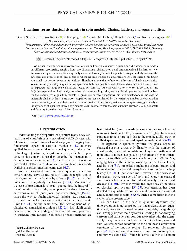
FIG. 1. Magnetization and 1D chain. Decay of the equal-sitecorrelation C (M)(t ) in different quantum cases (S = 1/2, 1, and 3/2)and in the classical case (S = ∞), shown in a (a) lin.-lin. plot and(b) log.-log. plot. In all cases, we have length Lx = 14 and anisotropy� = 1. In (a), curves are shifted for better visibility. In (b), a powerlaw ∝t−2/3 and the expected long-time value C(t → ∞) = 1/Lx areindicated.
and classical systems become more and more similar if thespin quantum number S is successively increased from S =1/2, 1, . . . [60,61] towards the classical limit S → ∞, it stillis a nontrivial question whether and to which degree theirdynamics agree with each other. While substantial differencesmost likely emerge at low temperatures T , a quantitativeagreement between quantum and classical dynamics can, infull generality, not be expected at high temperatures either,especially when considering the most quantum case S = 1/2.In particular, integrability of certain S = 1/2 models reflectsitself in their dynamics even at T → ∞. Moreover, certainphenomena, such as the onset of many-body localization instrongly disordered quantum systems, have no classical coun-terpart such that an agreement between quantum and classicaldynamics is unlikely in these cases [57,62].
In this paper, we explore the question of quantumversus classical dynamics in spin systems by analyzingtime-dependent autocorrelation functions of local densi-ties [as defined below in Eq. (5)], which are intimatelyrelated to transport processes in these models and havebeen studied before, both in the classical and the quantumcase [34–36,45,49,57,63]. Our main finding is exemplifiedin Fig. 1, which shows the temporal decay of infinite-temperature spin autocorrelation functions C(M)(t ) in isotropicHeisenberg chains with different quantum numbers S =1/2, 1, 3/2 and S = ∞ (classical). As becomes apparentfrom Fig. 1(a), quantum and classical dynamics agree verywell with each other on short as well as long time scales
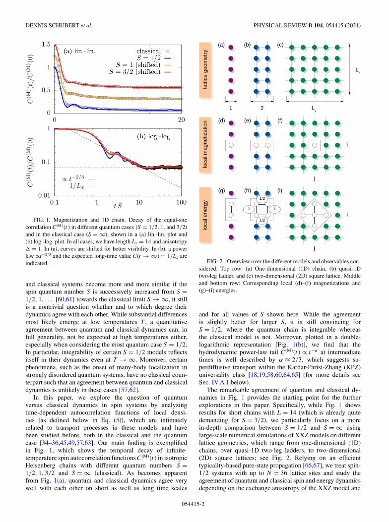
FIG. 2. Overview over the different models and observables con-sidered. Top row: (a) One-dimensional (1D) chain, (b) quasi-1Dtwo-leg ladder, and (c) two-dimensional (2D) square lattice. Middleand bottom row: Corresponding local (d)–(f) magnetizations and(g)–(i) energies.
and for all values of S shown here. While the agreementis slightly better for larger S, it is still convincing forS = 1/2, where the quantum chain is integrable whereasthe classical model is not. Moreover, plotted in a double-logarithmic representation [Fig. 1(b)], we find that thehydrodynamic power-law tail C(M)(t ) ∝ t−α at intermediatetimes is well described by α ≈ 2/3, which suggests su-perdiffusive transport within the Kardar-Parisi-Zhang (KPZ)universality class [18,19,58,60,64,65] (for more details seeSec. IV A 1 below).
The remarkable agreement of quantum and classical dy-namics in Fig. 1 provides the starting point for the furtherexplorations in this paper. Specifically, while Fig. 1 showsresults for short chains with L = 14 (which is already quitedemanding for S = 3/2), we particularly focus on a morein-depth comparison between S = 1/2 and S = ∞ usinglarge-scale numerical simulations of XXZ models on differentlattice geometries, which range from one-dimensional (1D)chains, over quasi-1D two-leg ladders, to two-dimensional(2D) square lattices; see Fig. 2. Relying on an efficienttypicality-based pure-state propagation [66,67], we treat spin-1/2 systems with up to N = 36 lattice sites and study theagreement of quantum and classical spin and energy dynamicsdepending on the exchange anisotropy of the XXZ model and
054415-2
QUANTUM VERSUS CLASSICAL DYNAMICS IN SPIN … PHYSICAL REVIEW B 104, 054415 (2021)
the lattice geometry chosen. In doing so, we find a remarkablygood agreement for all lattice geometries, which is best fornonintegrable quantum models in quasi-one or two dimen-sions, and (as already indicated in Fig. 1) still convincing forintegrable quantum chains, at least in cases where transport isnot ballistic due to the extensive set of conservation laws.
The rest of this paper is structured as follows. First, weintroduce in Sec. II the considered models and observablesin the quantum case and discuss their classical counterpartsas well. Here, we also comment on the diffusive decay ofequal-site autocorrelations. Then, we describe in Sec. IIIthe numerical techniques used by us, where we focus onthe concept of dynamical quantum typicality. Eventually, wepresent our numerical results in Sec. IV and compare classicaland quantum dynamics of local magnetization and energyin different lattice geometries. We summarize and concludein Sec. V.
II. MODELS AND OBSERVABLES
A. Models
In this paper, we consider the anisotropic Heisenbergmodel (XXZ model) on a rectangular lattice with periodicboundary conditions (PBC), consisting of N = Lx × Ly sitesin total, where Lx and Ly are the lattice extension in the x andy direction, respectively. The Hamiltonian is given by
H = J∑〈r,r′〉
hr,r′ , (1)
where the sum runs over all bonds 〈r, r′〉 of nearest-neighboring sites r = (i, j) and r′ = (i′, j′). The antiferro-magnetic exchange coupling constant J > 0 is set to J = 1in the following. The local terms in Eq. (1) read
hr,r′ = Sxr Sx
r′ + SyrSy
r′ + �SzrSz
r′ , (2)
where � parametrizes the anisotropy in the z direction andthe components Sμ
r , μ ∈ {x, y, z} are spin-S operators at site r,which fulfill the usual commutator relations (h = 1)
[Sμr , Sν
r′ ] = ı δrr′ εμνλ Sλr , (3)
where δrr′ is the Kronecker-Delta symbol and εμνλ is theantisymmetric Levi-Civita tensor. For the specific case ofS = 1/2, these components can be expressed in terms of Paulimatrices, Sμ
r = σμr /2.
While total energy is naturally conserved, i.e., [H,H] = 0,H is also invariant under rotation about the z axis, i.e., the totalmagnetization in this direction is preserved for all �,
[Sz,H] = 0, Sz =∑
r
Szr. (4)
In this paper, we consider the spin- and energy-transport prop-erties of H depending on the lattice geometry, the value of �,and the model being quantum or classical. In particular, westudy three special cases of the Lx × Ly lattice: (i) Ly = 1, i.e.,a one-dimensional chain; (ii) Ly = 2, i.e., a quasi-1D two-legladder; (iii) Ly = Lx, i.e., a two-dimensional square lattice;see the sketch in Fig. 2. Concerning integrability, it is wellknown that the spin-1/2 chain is integrable in terms of theBethe ansatz independent of the value of � [68,69], while in-tegrability is broken for models with either S > 1/2 or D > 1.
This integrability will play a crucial role for our comparison ofquantum and classical dynamics below. Specifically, it is wellknown that energy transport is purely ballistic in the integrablequantum chain, which will be in stark contrast to the dynamicsof the chaotic classical chain. At the same time, integrabilityas such not necessarily rules out that quantum and classicaltransport properties can agree with each other. For instance,as demonstrated below, both the quantum and classical chainshow diffusive spin transport for � > 1.
B. Observables
As one of the simplest quantities, we focus on the dynamicsof local densities ρr, which can be either magnetization orenergy, as defined below in detail. More precisely, we considerthe time-dependent density-density correlation function,
Cr,r′ (t ) = 〈ρr(t )ρr′ 〉, (5)
where 〈•〉 = tr[exp(−βH)•]/Z with Z = tr[exp(−βH)] isa canonical expectation value at inverse temperature β =1/T (kB = 1), and the time argument of an operator hasto be understood w.r.t. the Heisenberg picture, ρr(t ) =exp(ıHt ) ρr exp(−ıHt ).
In the following, we discuss the equal-site autocorrelationfunction, i.e., r = r′ in Eq. (5). Due to our choice of PBC, theautocorrelation function does not depend on the specific siter = (i, j) and we can concisely write C(t ) = Cr,r(t ). More-over, we here focus on the limit of high temperatures β → 0for which exp(−βH)/Z → 1/D, such that C(t ) is given by
C(t ) = tr[ρr(t )ρr]
D , (6)
where D = (2S + 1)N is the Hilbert-space dimension, e.g.,D = 2L for S = 1/2. Note that for our numerical results, wealways consider the dynamics in the full Hilbert space, i.e., weaverage over all sectors of fixed Sz.
Next, we define the local densities ρr and start with the caseof magnetization. While such a definition is not unique anddepends on the chosen unit cell, we use the natural definition,
ρ(M)i, j =
⎧⎪⎨⎪⎩
Szi,1, 1D (Ly = 1)
Szi,1 + Sz
i,2, quasi-1D (Ly = 2)
Szi, j, 2D (Lx = Ly)
, (7)
see the sketch in Fig. 2. In the case of energy, a naturaldefinition is
ρ(E)i, j = J h(i,1),(i+1,1), (8)
for a 1D chain, i.e., just a single bond, and,
ρ(E)i, j = J [h(i,1),(i+1,1) + h(i,2),(i+1,2)]
+ J
2[h(i,1),(i,2) + h(i+1,1),(i+1,2)], (9)
for a quasi 1D two-leg ladder, i.e., a plaquette consisting ofone bond for each leg and two rungs. Note that the factor 1/2appears, since the sum over all local energies must be identicalto the total energy. For the 2D square lattice, we define,
ρ(E)i, j = J
2[h(i−1, j),(i, j) + h(i, j),(i+1, j)]
+ J
2[h(i, j−1),(i, j) + h(i, j),(i, j+1)], (10)
054415-3
DENNIS SCHUBERT et al. PHYSICAL REVIEW B 104, 054415 (2021)
see the sketch in Fig. 2 again.We note that for each local density defined above, the sum
rule C(t = 0) can be calculated analytically. For instance, inthe case of local magnetization, we have for S = 1/2,
C(M)(t = 0) =
⎧⎪⎨⎪⎩
1/4, 1D (Ly = 1)
1/2, quasi-1D (Ly = 2)
1/4, 2D (Lx = Ly)
. (11)
Assuming that the system thermalizes at long times, this initialvalue also determines the long-time value (although there canbe subtleties in some cases, see Sec. IV B),
C(t → ∞) = C(t = 0)
n, (12)
where n is the total number of unit cells, i.e., n = Lx in 1Dor quasi-1D and n = Lx × Ly in 2D. Therefore, only in thethermodynamic limit n → ∞, we can expect a full decayC(t → ∞) = 0.
C. Classical limit
The quantum spin models discussed so far also have aclassical counterpart, which results by taking the limit of bothPlanck’s constant h → 0 and spin quantum number S → ∞,under the constraint h
√S(S + 1) = const. In this limit, the
commutator relations in Eq. (3) then turn into
{Sμr , Sν
r′ } = δrr′εμνλ Sλr , (13)
where {•, •} denotes the Poisson bracket [70], and the spin op-erators become real three-dimensional vectors Sr of constantlength, |Sr| = 1. In particular, all symmetries mentioned be-fore carry over to the classical case. The relations in Eq. (13)lead to the Hamiltonian equations of motion, which read
d
dtSr = ∂H
∂Sr× Sr (14)
and describe the precession of a spin around a local mag-netic field resulting from the interaction with the neighboringspins. The equations (14) form a set of coupled differ-ential equations, which is nonintegrable by means of theLiouville-Arnold theorem [53,70]. Therefore, they can besolved analytically only for a small number of special initialconfigurations, and solving them for nontrivial initial statesrequires numerical techniques.
The infinite-temperature density-density correlation inEq. (6) can be obtained in the classical case by taking 〈•〉 asan average over trajectories in phase space,
C(t ) ≈ 1
R
R∑r=1
ρr(t )ρr(0), (15)
where the initial configurations ρr(0) are drawn at random foreach realization r, and R � 1 has to be chosen sufficientlylarge to reduce statistical fluctuations. For the values of Rchosen by us, see the discussion in Sec. III B.
In this paper, our central goal is to compare classical andquantum dynamics. Thus, for a fair comparison, we have totake into account that the sum rule C(t = 0) is different. Forinstance, in the case of local magnetization, the classical sum
rule is
C(M)(t = 0) =
⎧⎪⎨⎪⎩
1/3, 1D (Ly = 1)
2/3, quasi-1D (Ly = 2)
1/3, 2D (Lx = Ly)
, (16)
and differs from the one in Eq. (7). Thus, we always considerthe rescaled data C(t )/C(0), cf. Fig. 1. Moreover, we haveto rescale the time entering the quantum simulations by afactor [57],
S =√
S(S + 1), (17)
in order to account for the different length of quantum andclassical spins (S = 1 in the classical case). However, for S =1/2, this factor is S = √
3/4 ≈ 0.87 and rather close to 1.
D. Diffusion
In both the classical and the quantum case, the time evo-lution of the autocorrelation function C(t ) follows from theunderlying microscopic equations of motion and naturallydepends on the specific model and its parameters. Thus, aprecise statement on the functional form of this time evolutionrequires to solve the given many-body problem analytically ornumerically. Due to the conservation of total energy and mag-netization, however, one generally expects that the dynamicsof local densities acquire a hydrodynamic behavior at suffi-ciently long times. In particular, in a generic nonintegrablesituation, one might expect the emergence of normal diffusivetransport.
In the context of the autocorrelation function C(t ), theemergence of hydrodynamics reflects itself in terms of apower-law tail [18],
C(t ) ∝ t−α, (18)
where normal diffusive transport corresponds to α = D/2,where D is the lattice dimension, i.e., α = 1/2 in 1D orquasi-1D, and α = 1 in 2D. In contrast to the case of normaldiffusion, anomalous superdiffusion (cf. Fig. 1) and subdif-fusion go along with an exponent α > D/2 and α < D/2,respectively, while ballistic transport is indicated by α = D.
Clearly, such a hydrodynamic power-law decay can onlyset in for times t > τ after some mean-free time τ . Moreover,due to the saturation at a value C(t → ∞) > 0 in any finitesystem, diffusion must break down for long times. Thus, inour numerical simulations below, the power-law decay inEq. (18) can only be expected to appear in an intermediatetime window, as already demonstrated in Fig. 1 above. Whilethe analysis of the particular type of transport for a givenmodel and lattice geometry is not the main aspect of thispaper, it naturally arises while comparing the spin and energydynamics of quantum and classical systems in Sec. IV.
III. NUMERICAL TECHNIQUES
Next, we discuss the methods used in our numerical sim-ulations, both for the quantum and the classical case. In theformer, we particularly employ the concept of dynamicalquantum typicality (DQT) which gives access to autocorre-lation functions for comparatively large system sizes beyondthe range of full exact diagonalization.
054415-4
QUANTUM VERSUS CLASSICAL DYNAMICS IN SPIN … PHYSICAL REVIEW B 104, 054415 (2021)
A. Dynamical quantum typicality
DQT essentially relies on the fact that even a single purestate |ψ〉 can imitate the full statistical ensemble. More pre-cisely, the pure-state expectation value of an observable istypically close to the one in the statistical ensemble [71–74].This fact can be utilized to calculate the time dependenceof correlation functions, e.g., the one of the density-densitycorrelator in Eq. (5), by replacing the trace by a scalar productbetween two auxiliary pure states |ϕβ (t )〉 and |�β (t )〉 [75–77],
C(t ) = 〈ϕβ (t )|ρr|�β (t )〉〈ϕβ (0)|ϕβ (0)〉 + ε(|ψ〉), (19)
where the two auxiliary pure states are given by
|ϕβ (t )〉 = e−ıHt e−βH/2 |ψ〉, (20)
|�β (t )〉 = e−iHt ρr e−βH/2 |ψ〉, (21)
involving the reference pure state,
|ψ〉 =D∑
k=1
(ak + ıbk )|k〉. (22)
This reference pure state is drawn at random from the fullHilbert space according to the unitary invariant Haar mea-sure [78]. In practice, for any given orthogonal basis |k〉, thecoefficients ak and bk are drawn randomly from a Gaussianprobability distribution with zero mean.
While the statistical error ε(|ψ〉) in Eq. (19) depends on thespecific realization of the random |ψ〉, the standard deviationof this statistical error can be bounded from above [67],
σ (ε) � b ∝ 1√Deff.
, (23)
where Deff. = tr{exp[−β(H − E0)]} denotes an effective di-mension and E0 is the ground-state energy of H. Thus, athigh temperatures β → 0, Deff. → D = (2S + 1)N and σ (ε)is negligibly small for the finite but large system sizes weare interested in. In turn, the typicality-based approximationin Eq. (19) is very accurate even for a single |ψ〉, and noaveraging is required.
In the high-temperature limit β → 0, the correlation func-tion C(t ) can also be approximated on the basis of just oneauxiliary pure state [79],
|ψ ′(t )〉 = e−ıHt |ψ ′(0)〉, |ψ ′(0)〉 =√
ρr + c |ψ〉√〈ψ |ψ〉 , (24)
where |ψ〉 is again the reference pure state in Eq. (22) andthe constant c is chosen in such a way that ρr + c has non-negative eigenvalues. Then, the correlation function can berewritten as a standard expectation value [7,57,80],
C(t ) = 〈ψ ′(t )|ρr|ψ ′(t )〉 + ε(|ψ〉), (25)
where we have employed tr[ρr] = 0. From a numerical pointof view, Eq. (25) is more efficient than Eq. (19) as only onestate has to be evolved in time. It is crucial, however, thatthe square root of the operator in Eq. (24) can be carried out.In the case of local magnetization, this task is trivial, at leastin the Ising basis. In the case of local energy, the task also
is feasible and requires only a local basis transformation,involving a few lattice sites.
The central advantage of the typicality approximations inEqs. (19) and (25) is the fact that the time dependence appearsas a property of the pure states. In particular, this time evo-lution can be obtained by an iterative forward propagation inreal time,
|ψ ′(t + δt )〉 = e−ıHδt |ψ ′(t )〉, (26)
where δt � J is a small discrete time step. Note that, eventhough not required for our purposes as we focus on β = 0,the action of exp(−βH/2) in Eqs. (20) and (21) can beobtained by an analogous forward propagation in imaginarytime [81].
While various sophisticated methods exist to approximatethe action of the matrix exponential in Eq. (26), the massivelyparallelized simulations on supercomputers used by us relyon both Trotter decompositions and Chebyshev-polynomialexpansions [82,83]. Since the matrix-vector multiplicationsrequired in these methods can be carried out efficiently w.r.t.memory, it is possible to treat systems as large as N = 36spins or even more [84].
B. Classical averaging
In the classical case, we solve the Hamiltonian equationsof motion in Eq. (14) numerically by means of a fourth-orderRunge-Kutta scheme (RK4), with a small time step δt . Inparticular, δt is chosen small enough such that the total energyand the total magnetization of H are conserved to very highaccuracy during the time evolution. (For other algorithms, seeRef. [85].)
Since classical mechanics is not concerned with the expo-nential growth of the Hilbert space with system size N , muchlarger systems can be accessed in this case. In fact, as thephase space increases only linearly with N , several thousandsof sites or more pose no problem. While we indeed present re-sults for such large systems, we also consider classical chainswith fewer sites N � 36 to ensure a fair comparison with thequantum case.
Importantly, there is no analog of typicality in classicalmechanics. Hence, to obtain the correlation function C(t ),just a single random initial configuration is not sufficientand an average over many samples R � 1 is needed instead,see Eq. (15). As a consequence, the computational cost ismainly set by R and not so much by N . For instance, in ournumerical simulations below, we will use as many samples asR = O(105) to ensure that the calculation of the correlationfunction goes along with small statistical errors. Note thatthe choice of a proper R also depends on the consideredtime scale, i.e., a good signal-to-noise ratio at long times,where C(t ) has already decayed substantially, requires a largervalue of R.
IV. RESULTS
We turn to the discussion of our numerical results and startin Sec. IV A with the dynamics of local magnetization, wherewe particularly compare our classical and quantum resultsfor the different cases of 1D chains (Sec. IV A 1), quasi-1D
054415-5
DENNIS SCHUBERT et al. PHYSICAL REVIEW B 104, 054415 (2021)
0.01
0.1
1
0.1 1 10 100
Δ = 0.5
α = 1/2
0.01
0.1
1
0.1 1 10 100
LxΔ = 1.0
α = 2/3
0.01
0.1
1
0.1 1 10 100
α = 1/2
Δ = 1.5
C(M
)(t
)/C
(M)(0
)
S = 1/2
C(M
)(t
)/C
(M)(0
)
1/Lx∝ t−α
C(M
)(t
)/C
(M)(0
)
t S
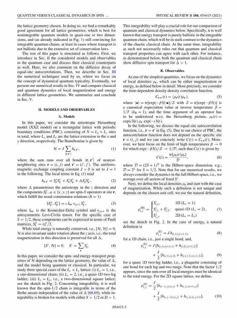
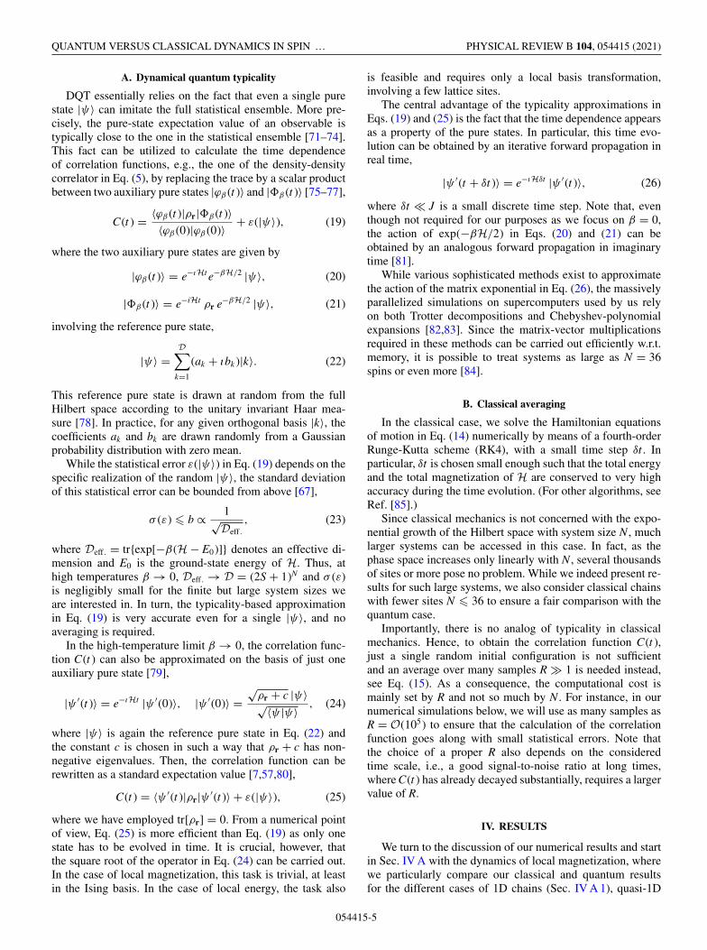
FIG. 3. Magnetization and 1D chain. Decay of the equal-sitecorrelation C (M)(t ) in a single quantum case (S = 1/2) and inthe classical case (S = ∞) for different anisotropies (a) � = 0.5,(b) � = 1.0, and (c) � = 1.5, shown in a log.-log. plot. In all cases,we have length Lx = 32 and indicate the expected long-time valueC(t → ∞) = 1/Lx as well as power laws ∝t−α . Classical data for amuch larger Lx = 1024 are additionally depicted.
two-leg ladders (Sec. IV A 2), and 2D square lattices(Sec. IV A 2). Corresponding results for the dynamics of localenergy are then presented in Sec. IV B.
A. Dynamics of local magnetization
1. 1D chain
We start with the dynamics of magnetization in a 1D chain.In Fig. 1 above, we have already presented results for theautocorrelation function C(M)(t ) at the isotropic point � = 1,where we have found that quantum dynamics for all quantumnumbers S = 1/2, 1, 3/2 agree remarkably well with the dy-namics of the classical chain.
Next, we discuss the role of the anisotropy �, where wefocus on the comparison between the most quantum caseS = 1/2 and the classical case S = ∞. Thus, compared toFig. 1, we are able to access larger system sizes Lx = 32 > 14.In Fig. 3, we summarize results for C(M)(t ) for anisotropies� = 0.5, 1, and 1.5, in a double-logarithmic plot. For � = 1in Fig. 3(b), the situation is like the one in Fig. 1(b) discussedbefore. Due to the larger Lx, the long-time saturation value be-comes smaller and the power-law behavior persists on a longertime scale. Furthermore, when calculating classical data for a
much larger Lx = 1024, this range further increases. In partic-ular, the data are still consistent with an exponent α = 2/3. Onone hand, in the case of the quantum chain, this superdiffusivebehavior is by now well established at the isotropic point (seeRef. [19] and references therein). On the other hand, in thecase of the classical chain, the nature of spin transport atthe isotropic point has been quite controversial [34–40]. Whilesome recent works argue that the nonintegrability eventuallycauses the onset of normal diffusion with α = 1/2 when goingto sufficiently large systems and long time scales [45,49,60],Ref. [86] provides compelling arguments that the power-lawtail of C(M)(t ) additionally acquires logarithmic corrections.Numerically, these scenarios are naturally very hard todistinguish.
For the larger � = 1.5 in Fig. 3(c), we also observe a verygood agreement between quantum and classical dynamics.Compared to � = 1, the main difference is a change of theexponent α from 2/3 to 1/2. Hence, this value indicates adiffusive decay, which is by now well known to occur in theregime � > 1, even in the case of the integrable quantumsystem [18]. The results in Figs. 3(b) and 3(c) demonstratethat integrability of the quantum model as such not necessarilyprevents that its dynamics are well approximated by a simula-tion of a classical system instead.
For the smaller � = 0.5 in Fig. 3(a), we find a worseagreement between quantum and classical data, with oscilla-tory behavior for S = 1/2. While one might be tempted toconclude that the power-law decay of quantum and classicaldynamics is similar at short times t � 10, such a conclusionis certainly not correct at longer times. On one hand, asshown in Fig. 3(a), classical dynamics for a long chain oflength Lx = 1024 is diffusive with α = 1/2. On the otherhand, quantum dynamics must be ballistic (α = 1) in thethermodynamic limit, which has been proven rigorously usingquasilocal conserved charges [15–17]. Thus, in such cases,where the quantum dynamics is dominated by the exten-sive set of conservation laws, the remarkable correspondencebetween quantum and classical dynamics necessarily has tobreak down.
2. Quasi-1D two-leg ladder and 2D square lattice
Next, we move from 1D chains to lattice geometries ofhigher dimension, i.e., quasi-1D two-leg ladders and 2Dsquare lattices. By doing so, we break the integrability of thequantum system with S = 1/2. This nonintegrable situation iscertainly more generic and might be seen as a fair test bed forthe comparison between the dynamics in models with S = 1/2and S = ∞. As before, we focus on the decay of local mag-netization and consider different values of the anisotropy �.
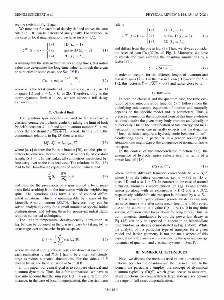
For the quasi-1D two-leg ladder, we show in Fig. 4 theequal-site correlation C(M)(t ) for � = 0.5, 1, and 1.5, wherewe fix the length of the ladder to Lx = 16. In contrast to theintegrable case discussed before, we find a convincing agree-ment between quantum and classical relaxation for all threevalues of �. In particular, the time dependence of C(M)(t ) atintermediate times turns out to be well described by a powerlaw t−α with the same diffusive exponent α = 1/2 [84]. ForLx = 16, this power-law behavior can be seen more clearlyfor larger � while, for classical systems with a much larger
054415-6
QUANTUM VERSUS CLASSICAL DYNAMICS IN SPIN … PHYSICAL REVIEW B 104, 054415 (2021)
0.01
0.1
1
0.1 1 10 100
Δ = 0.5
0.01
0.1
1
0.1 1 10 100
LxΔ = 1.0
0.01
0.1
1
0.1 1 10 100
Δ = 1.5
C(M
)(t
)/C
(M)(0
)
S = 1/2
C(M
)(t
)/C
(M)(0
)
1/Lx
∝ t−1/2
C(M
)(t
)/C
(M)(0
)
t S
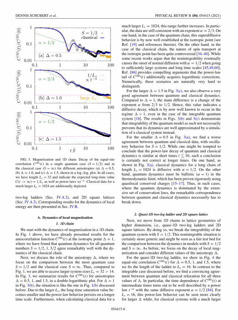
FIG. 4. Magnetization and quasi-1D two-leg ladder. Relaxationof the equal-site correlation C (M)(t ) in the quantum case (S = 1/2)and in the classical case (S = ∞) for different anisotropies (a) � =0.5, (b) � = 1.0, and (c) � = 1.5, depicted in a log.-log. plot. In allcases, we have length Lx = 16 and indicate the expected long-timevalue C(t → ∞) = 1/Lx as well as a power law ∝t−1/2. Classicaldata for a much larger Lx = 512 are also shown.
Lx = 512, it becomes even more pronounced. In view ofnonintegrability, the qualitative similarity of quantum andclassical mechanics might not be too surprising. However, itis quite remarkable that the curves in Fig. 4 agree even on aquantitative level to high accuracy.
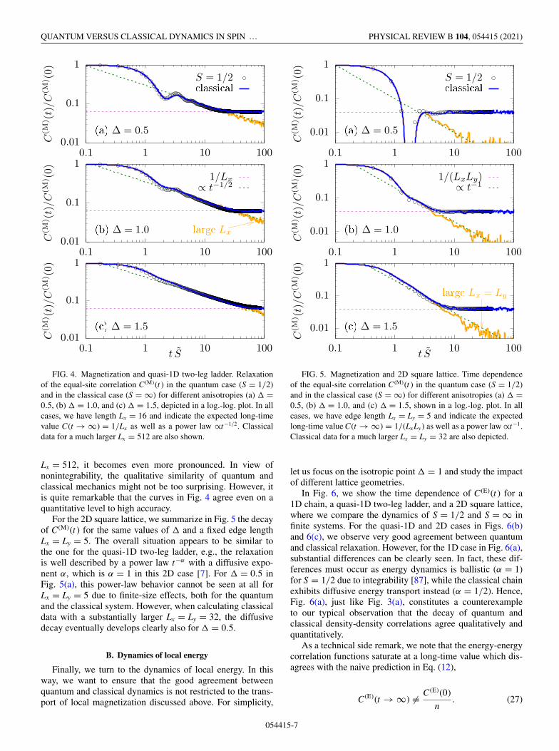
For the 2D square lattice, we summarize in Fig. 5 the decayof C(M)(t ) for the same values of � and a fixed edge lengthLx = Ly = 5. The overall situation appears to be similar tothe one for the quasi-1D two-leg ladder, e.g., the relaxationis well described by a power law t−α with a diffusive expo-nent α, which is α = 1 in this 2D case [7]. For � = 0.5 inFig. 5(a), this power-law behavior cannot be seen at all forLx = Ly = 5 due to finite-size effects, both for the quantumand the classical system. However, when calculating classicaldata with a substantially larger Lx = Ly = 32, the diffusivedecay eventually develops clearly also for � = 0.5.
B. Dynamics of local energy
Finally, we turn to the dynamics of local energy. In thisway, we want to ensure that the good agreement betweenquantum and classical dynamics is not restricted to the trans-port of local magnetization discussed above. For simplicity,
0.01
0.1
1
0.1 1 10 100
Δ = 0.5
0.01
0.1
1
0.1 1 10 100
Δ = 1.0
0.01
0.1
1
0.1 1 10 100
Lx = Ly
Δ = 1.5
C(M
)(t
)/C
(M)(0
)
S = 1/2
C(M
)(t
)/C
(M)(0
)
1/(LxLy)∝ t−1
C(M
)(t
)/C
(M)(0
)
t S
FIG. 5. Magnetization and 2D square lattice. Time dependenceof the equal-site correlation C (M)(t ) in the quantum case (S = 1/2)and in the classical case (S = ∞) for different anisotropies (a) � =0.5, (b) � = 1.0, and (c) � = 1.5, shown in a log.-log. plot. In allcases, we have edge length Lx = Ly = 5 and indicate the expectedlong-time value C(t → ∞) = 1/(LxLy ) as well as a power law ∝t−1.Classical data for a much larger Lx = Ly = 32 are also depicted.
let us focus on the isotropic point � = 1 and study the impactof different lattice geometries.
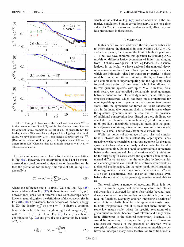
In Fig. 6, we show the time dependence of C(E)(t ) for a1D chain, a quasi-1D two-leg ladder, and a 2D square lattice,where we compare the dynamics of S = 1/2 and S = ∞ infinite systems. For the quasi-1D and 2D cases in Figs. 6(b)and 6(c), we observe very good agreement between quantumand classical relaxation. However, for the 1D case in Fig. 6(a),substantial differences can be clearly seen. In fact, these dif-ferences must occur as energy dynamics is ballistic (α = 1)for S = 1/2 due to integrability [87], while the classical chainexhibits diffusive energy transport instead (α = 1/2). Hence,Fig. 6(a), just like Fig. 3(a), constitutes a counterexampleto our typical observation that the decay of quantum andclassical density-density correlations agree qualitatively andquantitatively.
As a technical side remark, we note that the energy-energycorrelation functions saturate at a long-time value which dis-agrees with the naive prediction in Eq. (12),
C(E)(t → ∞) = C(E)(0)
n. (27)
054415-7
DENNIS SCHUBERT et al. PHYSICAL REVIEW B 104, 054415 (2021)
0.01
0.1
1
0.1 1 10 100
α = 1/2α = 1
0.01
0.1
1
0.1 1 10 100
0.01
0.1
1
0.1 1 10 100
×2
C(E
)(t
)/C
(E)(0
)
S = 1/2
C(E
)(t
)/C
(E)(0
)
1/n∝ t−d/2
C(E
)(t
)/C
(E)(0
)
t S
FIG. 6. Energy. Relaxation of the equal-site correlation C (E)(t )in the quantum case (S = 1/2) and in the classical case (S = ∞)for different lattice geometries, (a) 1D chain, (b) quasi-1D two-legladder, and (c) 2D square lattice, depicted in a log.-log. plot. In allcases, we have anisotropy � = 1 and indicate a power-law ∝t−d/2.[Due to overlaps of local energies, the long-time value C(t → ∞)differs from 1/n.] Classical data for a much larger N = Lx × Ly =1024 are also shown.
This fact can be seen most clearly for the 2D square latticein Fig. 6(c). However, this observation should not be misun-derstood as a breakdown of equipartition or thermalization. Infact, the prediction for the long-time value of C(t ) in Eq. (12)generally is
C(t → ∞) = 1
n
∑r′
〈ρr ρr′ 〉, (28)
where the reference site r is fixed. We note that Eq. (28)is only identical to Eq. (12) if there is no overlap 〈ρr ρr′ 〉between local densities at different sites. Such overlaps occurhowever naturally, given the definitions of the local energies inEqs. (8)–(10). For instance, for our choice of the local energyin 2D, the density ρ
(E)i, j on site r = (i, j) shares a common
bond with each of the four neighboring local energies ρ(E)i′, j′ ,
with i′ = i ± 1, j′ = j ± 1, see Fig. 2(i). Hence, these bondscontribute to Eq. (28) and give rise to a correction by a factorof 2, i.e.,
C(E)2D (t → ∞) = C(E)
2D (0)
2n, (29)
which is indicated in Fig. 6(c) and coincides with the nu-merical simulation. Similar corrections apply to the long-timevalue of C(E)(t ) in chains and ladders as well, albeit they areless pronounced in these cases.
V. SUMMARY
In this paper, we have addressed the question whether andto which degree the dynamics in spin systems with S = 1/2and S = ∞ agree, focusing on the limit of high temperaturesT → ∞. We have explored this question by studying XXZmodels on different lattice geometries of finite size, rangingfrom 1D chains, over quasi-1D two-leg ladders, to 2D squarelattices. In particular, we have analyzed the temporal decayof autocorrelation functions of local spin or energy densities,which are intimately related to transport properties in thesemodels. In order to mitigate finite-size effects, we have reliedon a combination of supercomputing and the typicality-basedforward propagation of pure states, which has allowed usto treat quantum systems with up to N = 36 in total. As amain result, we have unveiled a remarkably good agreementbetween quantum and classical dynamics for all lattice ge-ometries considered, which has been most pronounced fornonintegrable quantum systems in quasi-one or two dimen-sions. Still, the agreement has turned out to be satisfactoryalso in the integrable quantum chain, at least in cases wherethe quantum dynamics is not ballistic due to the presenceof additional conservation laws. Based on these findings, weconclude that classical or semiclassical/hybrid simulationsmight provide a meaningful strategy to investigate the quan-tum dynamics of strongly interacting quantum spin models,even if S is small and far away from the classical limit.
While the numerical advantage of such classical simula-tions is obvious due to the substantially larger system sizestreatable, we have yet neither a rigorous argument for the goodagreement observed nor an analytical estimate for the dif-ferences remaining. On one hand, an approximate agreementbetween the quantum and classical versions of C(t ) might notbe too surprising in cases where the quantum chain exhibitsnormal diffusive transport, as the emerging hydrodynamicson a coarse-grained level should be effectively describable asa classical phenomenon. On the other hand, notwithstandingthese arguments, the nice agreement between S = 1/2 andS = ∞ on a quantitative level, and on all time scales (evenbefore the onset of hydrodynamics), remains remarkable tous.
Our work raises a number of questions. First, it is notclear if a similar agreement between quantum and classi-cal dynamics is expected for other observables beyond localdensities or other out-of-equilibrium quantities beyond cor-relation functions. Secondly, another interesting direction ofresearch is to clarify how far this agreement carries overto finite temperatures. Yet, it is clear that there should besome low-energy scale, where the specific excitations of agiven quantum model become most relevant and likely causelarge differences to the classical counterpart. Eventually, itwould be interesting to compare the dynamics of quantumand classical models in the presence of disorder. Whilestrongly disordered one-dimensional quantum models are be-lieved to undergo a many-body localization transition, such a
054415-8
QUANTUM VERSUS CLASSICAL DYNAMICS IN SPIN … PHYSICAL REVIEW B 104, 054415 (2021)
0
0.5
1
1.5
0 1 2 3 4
0
0.5
1
1.5
0 1 2 3 4
0
0.5
1
1.5
0 1 2 3 4
C(M
)(ω
)/S
2
S = 1/2
C(M
)(ω
)/S
2C
(M)(ω
)/S
2
ω /S
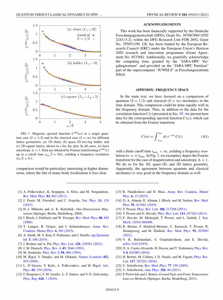
FIG. 7. Magnetic spectral function C (M)(ω) in a single quan-tum case (S = 1/2) and in the classical case (S = ∞) for differentlattice geometries, (a) 1D chain, (b) quasi-1D two-leg ladder, and(c) 2D square lattice, shown in a lin.-lin. plot. In all cases, we haveanisotropy � = 1. Data are obtained by Fourier transforming C (M)(t )up to a cutoff time tmax S = 10π , yielding a frequency resolutionδω/S = 0.1.
comparison would be particulary interesting in higher dimen-sions, where the fate of many-body localization is less clear.
ACKNOWLEDGMENTS
This work has been financially supported by the DeutscheForschungsgemeinschaft (DFG), Grant No. 397067869 (STE2243/3-2), within the DFG Research Unit FOR 2692, GrantNo. 355031190. J.R. has been funded by the European Re-search Council (ERC) under the European Union’s Horizon2020 research and innovation programme (Grant Agree-ment No. 853368). Additionally, we gratefully acknowledgethe computing time, granted by the “JARA-HPC Ver-gabegremium” and provided on the “JARA-HPC Partition”part of the supercomputer “JUWELS” at ForschungszentrumJülich.
APPENDIX: FREQUENCY SPACE
In the main text, we have focused on a comparison ofquantum (S = 1/2) and classical (S = ∞) mechanics in thetime domain. This comparison could be done equally well inthe frequency domain. Thus, in addition to the data for thecorrelation function C(t ) presented in Sec. IV, we present heredata for the corresponding spectral function C(ω), which canbe obtained from the Fourier transform
C(ω) =∫ tmax
−tmax
dt e−ıωt C(t ) (A1)
with a finite cutoff time tmax. < ∞, yielding a frequency reso-lution δω = π/tmax. In Fig. 7, we exemplary depict the Fouriertransform for the case of magnetization and anisotropy � = 1.We do so for the 1D, quasi-1D, and 2D lattice geometry.Apparently, the agreement between quantum and classicalmechanics is very good in the frequency domain as well.
[1] A. Polkovnikov, K. Sengupta, A. Silva, and M. Vengalattore,Rev. Mod. Phys. 83, 863 (2011).
[2] J. Eisert, M. Friesdorf, and C. Gogolin, Nat. Phys. 11, 124(2015).
[3] H.-J. Mikeska and A. K. Kolezhuk, One-Dimensional Mag-netism (Springer, Berlin, Heidelberg, 2004).
[4] I. Bloch, J. Dalibard, and W. Zwerger, Rev. Mod. Phys. 80, 885(2008).
[5] T. Langen, R. Geiger, and J. Schmiedmayer, Annu. Rev.Condens. Matter Phys. 6, 201 (2015).
[6] A. Smith, M. S. Kim, F. Pollmann, and J. Knolle, npj QuantumInf. 5, 106 (2019).
[7] J. Richter and A. Pal, Phys. Rev. Lett. 126, 230501 (2021).[8] J. M. Deutsch, Phys. Rev. A 43, 2046 (1991).[9] M. Srednicki, Phys. Rev. E 50, 888 (1994).
[10] M. Rigol, V. Dunjko, and M. Olshanii, Nature (London) 452,854 (2008).
[11] L. D’Alessio, Y. Kafri, A. Polkovnikov, and M. Rigol, Adv.Phys. 65, 239 (2016).
[12] F. Borgonovi, F. M. Izrailev, L. F. Santos, and V. G. Zelevinsky,Phys. Rep. 626, 1 (2016).
[13] R. Nandkishore and D. Huse, Annu. Rev. Condens. MatterPhys. 6, 15 (2015).
[14] D. A. Abanin, E. Altman, I. Bloch, and M. Serbyn, Rev. Mod.Phys. 91, 021001 (2019).
[15] T. Prosen, Phys. Rev. Lett. 106, 217206 (2011).[16] T. Prosen and E. Ilievski, Phys. Rev. Lett. 111, 057203 (2013).[17] E. Ilievski, M. Medenjak, T. Prosen, and L. Zadnik, J. Stat.
Mech. (2016) 064008.[18] B. Bertini, F. Heidrich-Meisner, C. Karrasch, T. Prosen, R.
Steinigeweg, and M. Žnidaric, Rev. Mod. Phys. 93, 025003(2021).
[19] V. B. Bulchandani, S. Gopalakrishnan, and E. Ilievski,arXiv:2103.01976.
[20] O. A. Castro-Alvaredo, B. Doyon, and T. Yoshimura, Phys. Rev.X 6, 041065 (2016).
[21] B. Bertini, M. Collura, J. D. Nardis, and M. Fagotti, Phys. Rev.Lett. 117, 207201 (2016).
[22] U. Schollwöck, Rev. Mod. Phys. 77, 259 (2005).[23] U. Schollwöck, Ann. Phys. 326, 96 (2011).[24] P. Prelovšek and J. Bonca, Ground State and Finite Temperature
Lanczos Methods (Springer, Berlin, Heidelberg, 2013).
054415-9
DENNIS SCHUBERT et al. PHYSICAL REVIEW B 104, 054415 (2021)
[25] P. Czarnik, J. Dziarmaga, and P. Corboz, Phys. Rev. B 99,035115 (2019).
[26] J. Gan and K. R. A. Hazzard, Phys. Rev. A 102, 013318 (2020).[27] R. Verdel, M. Schmitt, Y.-P. Huang, P. Karpov, and M. Heyl,
Phys. Rev. B 103, 165103 (2021).[28] E. Leviatan, F. Pollmann, J. H. Bardarson, D. A. Huse, and E.
Altman, arXiv:1702.08894.[29] J. Richter, T. Heitmann, and R. Steinigeweg, SciPost Phys. 9,
31 (2020).[30] S. De Nicola, arXiv:2103.16468.[31] T. Dauxois, Phys. Today 61(1), 55 (2008).[32] C. G. Windsor, Proc. Phys. Soc. 91, 353 (1967).[33] N. A. Lurie, D. L. Huber, and M. Blume, Phys. Rev. B 9, 2171
(1974).[34] G. Müller, Phys. Rev. Lett. 60, 2785 (1988).[35] R. W. Gerling and D. P. Landau, Phys. Rev. Lett. 63, 812 (1989).[36] R. W. Gerling and D. P. Landau, Phys. Rev. B 42, 8214
(1990).[37] O. F. de Alcantara Bonfim and G. Reiter, Phys. Rev. Lett. 69,
367 (1992).[38] O. F. de Alcantara Bonfim and G. Reiter, Phys. Rev. Lett. 70,
249 (1993).[39] M. Böhm, R. W. Gerling, and H. Leschke, Phys. Rev. Lett. 70,
248 (1993).[40] N. Srivastava, J.-M. Liu, V. S. Viswanath, and G. Müller,
J. Appl. Phys. 75, 6751 (1994).[41] V. Constantoudis and N. Theodorakopoulos, Phys. Rev. E 55,
7612 (1997).[42] V. Oganesyan, A. Pal, and D. A. Huse, Phys. Rev. B 80, 115104
(2009).[43] R. Steinigeweg, Europhys. Lett. 97, 67001 (2012).[44] D. L. Huber, Physica B 407, 4274 (2012).[45] D. Bagchi, Phys. Rev. B 87, 075133 (2013).[46] T. Prosen and B. Žunkovic, Phys. Rev. Lett. 111, 040602
(2013).[47] B. Jencic and P. Prelovšek, Phys. Rev. B 92, 134305 (2015).[48] A. Das, K. Damle, A. Dhar, D. A. Huse, M. Kulkarni, C. B.
Mendl, and H. Spohn, J. Stat. Phys. 180, 238 (2019).[49] N. Li, Phys. Rev. E 100, 062104 (2019).[50] P. Glorioso, L. Delacrétaz, X. Chen, R. Nandkishore, and A.
Lucas, SciPost Phys. 10, 015 (2021).[51] A. Lagendijk and H. De Raedt, Phys. Rev. B 16, 293 (1977).[52] H. De Raedt, J. Fivez, and B. De Raedt, Phys. Rev. B 24, 1562
(1981).[53] R. Steinigeweg and H.-J. Schmidt, Math. Phys. Anal. Geom. 12,
19 (2009).[54] F. Jin, T. Neuhaus, K. Michielsen, S. Miyashita, M. A. Novotny,
M. I. Katsnelson, and H. De Raedt, New J. Phys. 15, 033009(2013).
[55] A. Das, S. Chakrabarty, A. Dhar, A. Kundu, D. A. Huse, R.Moessner, S. S. Ray, and S. Bhattacharjee, Phys. Rev. Lett. 121,024101 (2018).
[56] O. Gamayun, Y. Miao, and E. Ilievski, Phys. Rev. B 99, 140301(2019).
[57] J. Richter, D. Schubert, and R. Steinigeweg, Phys. Rev.Research 2, 013130 (2020).
[58] A. Das, M. Kulkarni, H. Spohn, and A. Dhar, Phys. Rev. E 100,042116 (2019).
[59] A. S. de Wijn, B. Hess, and B. V. Fine, Phys. Rev. Lett. 109,034101 (2012).
[60] M. Dupont and J. E. Moore, Phys. Rev. B 101, 121106 (2020).[61] J. Richter, N. Casper, W. Brenig, and R. Steinigeweg, Phys.
Rev. B 100, 144423 (2019).[62] J. Ren, Q. Li, W. Li, Z. Cai, and X. Wang, Phys. Rev. Lett. 124,
130602 (2020).[63] J. Wurtz and A. Polkovnikov, Phys. Rev. E 101, 052120 (2020).[64] S. Gopalakrishnan and R. Vasseur, Phys. Rev. Lett. 122, 127202
(2019).[65] M. Ljubotina, M. Žnidaric, and T. Prosen, Nat. Commun. 8,
16117 (2017).[66] T. Heitmann, J. Richter, D. Schubert, and R. Steinigeweg,
Z. Naturforsch. A 75, 421 (2020).[67] F. Jin, D. Willsch, M. Willsch, H. Lagemann, K. Michielsen,
and H. De Raedt, J. Phys. Soc. Jpn. 90, 012001 (2021).[68] H. Bethe, Z. Phys. 71, 205 (1931).[69] F. Levkovich-Maslyuk, J. Phys. A: Math. Theor. 49, 323004
(2016).[70] V. I. Arnold, Mathematical Methods of Classical Mechanics
(Springer, New York, 1978).[71] S. Lloyd, arXiv:1307.0378.[72] J. Gemmer, M. Michel, and G. Mahler, Quantum Thermody-
namics (Springer, Berlin, Heidelberg, 2009).[73] S. Goldstein, J. L. Lebowitz, R. Tumulka, and N. Zanghì, Phys.
Rev. Lett. 96, 050403 (2006).[74] P. Reimann, Phys. Rev. Lett. 99, 160404 (2007).[75] T. Iitaka and T. Ebisuzaki, Phys. Rev. E 69, 057701 (2004).[76] T. A. Elsayed and B. V. Fine, Phys. Rev. Lett. 110, 070404
(2013).[77] R. Steinigeweg, J. Gemmer, and W. Brenig, Phys. Rev. Lett.
112, 120601 (2014).[78] C. Bartsch and J. Gemmer, Phys. Rev. Lett. 102, 110403 (2009).[79] J. Richter and R. Steinigeweg, Phys. Rev. E 99, 012114 (2019).[80] C. Chiaracane, F. Pietracaprina, A. Purkayastha, and J. Goold,
Phys. Rev. B 103, 184205 (2021).[81] A. Hams and H. De Raedt, Phys. Rev. E 62, 4365 (2000).[82] V. V. Dobrovitski and H. A. De Raedt, Phys. Rev. E 67, 056702
(2003).[83] A. Weisse, G. Wellein, A. Alvermann, and H. Fehske, Rev.
Mod. Phys. 78, 275 (2006).[84] J. Richter, F. Jin, L. Knipschild, J. Herbrych, H. De Raedt, K.
Michielsen, J. Gemmer, and R. Steinigeweg, Phys. Rev. B 99,144422 (2019).
[85] M. Krech, A. Bunker, and D. P. Landau, Comput. Phys.Commun. 111, 1 (1998).
[86] J. De Nardis, M. Medenjak, C. Karrasch, and E. Ilievski, Phys.Rev. Lett. 124, 210605 (2020).
[87] X. Zotos, F. Naef, and P. Prelovsek, Phys. Rev. B 55, 11029(1997).
054415-10


