arX

iv:c

ond-

mat

/050

7262

v1

12

Jul 2

005

Symplectic integrators for classical spin

systems

Robin Steinigeweg and Heinz-Jurgen Schmidt ∗

Universitat Osnabruck, Fachbereich Physik, Barbarastr. 7, 49069 Osnabruck,

Germany

Abstract

We suggest a numerical integration procedure for solving the equations of motion ofcertain classical spin systems which preserves the underlying symplectic structureof the phase space. Such symplectic integrators have been successfully utilized forother Hamiltonian systems, e. g. for molecular dynamics or non-linear wave equa-tions. Our procedure rests on a decomposition of the spin Hamiltonian into a sumof two completely integrable Hamiltonians and on the corresponding Lie-Trotterdecomposition of the time evolution operator. In order to make this method widelyapplicable we provide a large class of integrable spin systems whose time evolutionconsists of a sequence of rotations about fixed axes. We test the proposed symplec-tic integrator for small spin systems, including the model of a recently synthesizedmagnetic molecule, and compare the results for variants of different order.

Key words: symplectic integrators, classical spin systemsPACS: 02.60.Cb, 75.10.Hk

1 Introduction

To calculate the time evolution of classical spin systems is an important task incondensed matter physics. For example, the cross section of neutron scatteringat a spin system is proportional to the Fourier transform of the time-dependingauto-correlation function, see [1], which can often be calculated in the classi-cal limit. Completely integrable spin systems are rare, that is, in most casesan analytical calculation of the time evolution is not possible and one is lead

∗

Email address: hschmidt@uos.de (Heinz-Jurgen Schmidt).

Preprint submitted to Elsevier Science 13 July 2005

to employ numerical integration methods. Since classical spin systems are in-stances of Hamiltonian systems, it is advisable to use numerical integratorswhich preserve the underlying symplectic structure of the phase space. Such“symplectic integrators” have been considered in the last decades [2] and havebeen applied to a variety of problems, ranging from molecular dynamics [3] tothe nonlinear Schrodinger equation [4,5].Unfortunately, symplectic integrators for spin systems have only rarely beenconsidered in the literature, see [6,7,8]. The method of the independent timeevolution of sublattices, proposed in [6,9,10], is volume-preserving but notsymplectic, see 2.2.1 and [6]. Inspired by [10], we suggest to construct sym-plectic integrators based on a splitting of the spin Hamiltonian into two com-pletely integrable Hamiltonians belonging to a special kind of systems [11,12].These systems are called “B-partitioned systems” and their time evolution canbe calculated as a sequence of rotations about fixed axes [12]. This general-izes the Stormer/Verlet scheme based on separable Hamiltonians of the formH = T (p) + V (q).In section 2 we provide the general definitions and results we need from an-alytical mechanics (section 2.1) and from the field of symplectic integratorsbased on Lie-Trotter decompositions of the time evolution operator (section2.2). The reader who is not familiar with the differential geometric backgroundmay skip the technical details and only draw the moral that a symplectic inte-grator approximates the exact time evolution by a sequence of calculable timeevolutions corresponding to auxiliary Hamiltonians. In section 3 we shortly re-capitulate the theory of B-partitioned systems from [12]. In order to test oursuggestions we have implemented various variants of symplectic integratorsand applied them to selected small spin systems, see section 4. We report thefluctuation of the total energy about its initial value as opposed to the con-stant drift for a non-symplectic Runge-Kutta method (RK4), see section 4.1.For two integrable spin systems we compare the errors of the various symplec-tic methods, including RK4, see sections 4.2.1 and 4.2.2. Finally, we comparethe errors of five symplectic integrators for the integrable N = 5 spin pyramidand fixed runtime, see section 4.3. We close with a summary and outlook.

2 Definitions and general results

We will only formulate the pertinent definitions for symplectic integrators inthe context of spin systems. For the general case there are excellent sourcesavailable in the literature, see e. g. [13,14] for analytical mechanics and [2] forsymplectic integrators.

2

2.1 Generalities

Classical spin configurations can be represented by N -tuples of unit 3-vectorss = (~s1, . . . , ~sN), |~sµ|

2 = 1 for µ = 1, . . . , N . The compact, 2N -dimensionalmanifold of all such configurations is the phase space of the spin system

P = PN ={

(~s1, . . . , ~sN)∣

∣

∣ |~sµ|2 = 1 for µ = 1, . . . , N

}

. (1)

A special coordinate system is given by the 2N local functionsϕµ, zµ : P → R, implicitly defined by

~sµ =

√

1 − z2µ cos ϕµ

√

1 − z2µ sin ϕµ

zµ

, µ = 1, . . . , N . (2)

A tangent vector of P at a point s ∈ P can be represented by an N -tuplet = (~t1, . . . ,~tN) of 3-vectors satisfying the constraint

~tµ · ~sµ = 0, µ = 1, . . . , N . (3)

If a,b are two tangent vectors at s ∈ P, the assignment

ω(a,b) =N

∑

µ=1

(~aµ ×~bµ) · ~sµ (4)

defines a non-degenerate, closed 2-form, that is, a symplectic form ω. In thecoordinate system (2) ω can locally be written in the form

ω =N

∑

µ=1

dϕµ ∧ dzµ , (5)

hence (ϕµ, zµ)µ=1,...,N are canonical coordinates w. r. t. ω. The volume formdP is defined by

dP = ωN = ω ∧ ω ∧ . . . ∧ ω (6)

and has the local coordinate representation

dP = dϕ1 ∧ dz1 ∧ . . . ∧ dϕN ∧ dzN . (7)

3

A smooth Hamiltonian H : P → R generates the Hamiltonian vector field XH

implicitly defined by

iXHω ≡ ω(XH , ) = dH . (8)

The corresponding Hamiltonian equations of motion are

d

dts(t) = XH(s(t)) (9)

and assume their usual form

d

dtϕµ(t) =

∂H

∂zµ

,d

dtzµ(t) = −

∂H

∂ϕµ

, µ = 1, . . . , N , (10)

in the canonical coordinate system (2). By writing the solution s(t) of (10) inthe form s(t) = Ft(H)(s(0)) we obtain the Hamiltonian flow Ft(H) : P → P.It is defined for all initial values s(0) and for all t ∈ R since P is compact,i. e. XH is a complete vector field. Analogously, the flow of a general vectorfield can be defined.

A smooth map φ : P → P is called symplectic iff it preserves the symplec-tic form, i. e. iff φ∗ω = ω. Every symplectic map preserves the phase spacevolume, but not conversely, see the counter-example below. Any Hamiltonianflow Ft(H) is symplectic, cf. , for example, theorem 8.1.9 in [15]. Conversely,if the flow Ft of a complete vector field X is symplectic, then

LXω(s) =d

dt(F∗t ω) (s)|t=0 = 0 , (11)

where LX is the Lie derivative. Hence 0 = LXω = iX dω + diXω = 0 + diXω ,that is, iXω is a closed 1-form, and has, by the Poincare lemma, locally theform iXω = dK. To summarize: symplectic flows are, at least locally, generatedby suitable Hamiltonians K.

2.2 Symplectic integrators

From an abstract point of view, a symplectic integrator is an approximationof some exact flow Ft(H) by the composition of symplectic maps φν : P → P,which can be calculated analytically or numerically exact. In this article we

4

Table 1Various decompositions of the form (16) which give rise to different symplecticintegrators.

Name Abbr. Order Coefficients Ref.

Suzuki-Trotter ST1 1 a1 = b1 = 12 [16]

Suzuki-Trotter ST2 2 a1 = a2 = 12 , b1 = 1, b2 = 0 [17]

Suzuki-Trotter ST4 4 a1 = a6 = p2 , b6 = 0 [18]

b1 = a2 = b2 = b4 = a5 = b5 = p

a3 = a4 = 1−3p2 , b3 = 1 − 4p

p = 14−41/3

Forest-Ruth FR 4 a1 = a4 = θ2 , a2 = a3 = 1−θ

2 [19]

b1 = b3 = θ, b4 = 0

b2 = 1 − 2θ, θ = 12−21/3

Optimized OFR 4 a1 = a5 = ξ, a2 = a4 = χ, b5 = 0 [20]

Forest-Ruth a3 = 1 − 2(ξ + χ), b1 = b4 = 1−2λ2

b2 = b3 = λ = −0.09156203

ξ = 0.17208656, χ = −0.16162176

assume that the Hamiltonian H is decomposable into completely integrableHamiltonians Hi in the form

H =∑

i

Hi (12)

and that the φν are the Hamiltonian flows corresponding to certain Hi. Theprecise form of the correspondence is given by a Lie-Trotter decomposition ofthe flow Ft(H) written as an exponential operator

Ft(H) = etH . (13)

In order to make sense of (13) we have to linearize the Hamiltonian equationsof motion. To this end we consider Ft(H) acting on functions f : P → C via

Ft(H)∗f(s) ≡ f(

F−t(H)(s))

. (14)

If f runs through L2(P, dP), the Hilbert space of (equivalence classes of)square-integrable complex functions, (14) defines a continuous, unitary 1-parameter group, see section 7.4 of [15] for details. By Stone’s theorem, this

5

group has the form (13) with an anti-selfadjoint operator H. One can showthat H can be expressed by means of the Poisson bracket according to

Hf = {H, f} ≡ ω(XH, Xf), f smooth , (15)

but we will not need this in the sequel. (13) is only needed to provide a basisfor using the techniques of Lie-Trotter decomposition for Hamiltonian flows.

For sake of simplicity let us consider the special case H = H1 + H2 and henceH = H1 +H2. We are looking for ℓ-th order Lie-Trotter decompositions whichhave the form

et(H1+H2) =k

∏

i=1

eaitH1ebitH2 + O(tℓ+1) . (16)

Both sides of (16) are expanded into power series in terms of t and set equalup to terms including tℓ. This yields a system of, in general, non-linear equa-tions for the unknown coefficients ai, bi. Except for ℓ = 1 the correspondingsolutions are not unique. Hence there exist several decompositions and thusseveral symplectic integrators of the same order ℓ. In this article we will usethe decompositions enumerated in table 1. All corresponding integrators aresymmetric, or time-reversible, see [2]. Obviously, the Lie-Trotter decomposi-tion (16) is a good approximation only for small t. Therefore the given timeinterval [0, t] is usually split into L intervals of length ∆ and (16) is separatelyapplied to each time step ∆. Hence, apart from the choice of the decomposi-tion, ∆ is a further parameter of the integration procedure, see section 4.

2.2.1 A counter-example

It seems plausible that an arbitrary splitting XH = X1 +X2 of a Hamiltonianvector field need not correspond to a splitting of the Hamiltonian H = H1+H2,such that Xi = XHi

for i = 1, 2. Hence the decomposition XH = X1 +X2 doesnot necessarily lead to symplectic integrators. Nevertheless, we will illustratethis by an example which is connected with a numerical integrator used forbi-partite spin systems, see [6,9,10]. Such spin systems can be divided into twodisjoint subsets of spins A and B, such that the interaction is only non-zerobetween spins of different subsets. The first step of the numerical procedureconsists of fixing the A-spins and calculating the time evolution of all B-spins.In the second step the role of A and B is interchanged, and so on. In a singlestep each spin of one subset rotates about the fixed (weighted) sum of all itsneighboring spins; hence the numerical integrator preserves the volume of thetotal phase space. But, as we will show, this integrator is not symplectic, see

6

also the corresponding remark in [6].It suffices to consider just two spins and a single step of the described numericalintegrator which solves the equations of motion

d

dt~s1 = ~s2 × ~s1,

d

dt~s2 = ~0 , (17)

defining a vector field X on P2. We adopt canonical coordinates ϕ1, z1, ϕ2, z2

defined in (2) and use the local expression ω = dϕ1 ∧ dz1 + dϕ2 ∧ dz2 of thesymplectic form. After some elementary calculations we obtain

iXω = ϕ1dz1 − z1dϕ1 (18)

=(

z2 − z1

√

1−z2

2

1−z2

1

cos(ϕ1 − ϕ2))

dz1

−√

(1 − z21)(1 − z2

2) sin(ϕ1 − ϕ2)dϕ1 . (19)

Obviously, iXω is not closed, and hence X does not generate a symplecticflow, cf. the discussion after (11).

3 B-partitioned spin systems

The symplectic integrators considered in section 2.2 are based on a splittingof the spin Hamiltonian into a sum of completely integrable Hamiltonians:H =

∑

i Hi. For Heisenberg Hamiltonians

H(s) =∑

µ<ν

Jµν~sµ · ~sν , where Jµν ∈ R , (20)

such a splitting is always possible; in fact, each summand in (20) is a com-pletely integrable dimer Hamiltonian. However, it seems favorable to workwith as few summands as possible, or, equivalently, to work with “large” in-tegrable Hamiltonians. To this end we will define a special class of completelyintegrable spin systems called B-partitioned systems, following [12].As an example, consider the Heisenberg Hamiltonian of the spin square

H� = ~s1 · ~s2 + ~s2 · ~s3 + ~s3 · ~s4 + ~s4 · ~s1 . (21)

It is integrable because it can be written as

H� = 12

(

(~s1 + ~s2 + ~s3 + ~s4)2 − (~s1 + ~s3)

2 − (~s2 + ~s4)2)

. (22)

7

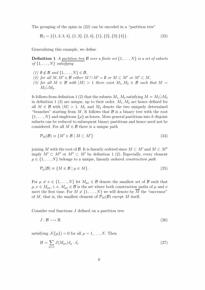
The grouping of the spins in (22) can be encoded in a “partition tree”

B� = {{1, 2, 3, 4}, {1, 3}, {2, 4}, {1}, {2}, {3} {4}} . (23)

Generalizing this example, we define

Definition 1 A partition tree B over a finite set {1, . . . , N} is a set of subsetsof {1, . . . , N} satisfying

(1) ∅ /∈ B and {1, . . . , N} ∈ B,(2) for all M, M ′ ∈ B either M ∩ M ′ = ∅ or M ⊂ M ′ or M ′ ⊂ M ,(3) for all M ∈ B with |M | > 1 there exist M1, M2 ∈ B such that M =

M1∪M2.

It follows from definition 1 (2) that the subsets M1, M2 satisfying M = M1∪M2

in definition 1 (3) are unique, up to their order. M1, M2 are hence defined forall M ∈ B with |M | > 1. M1 and M2 denote the two uniquely determined“branches” starting from M . It follows that B is a binary tree with the root{1, . . . , N} and singletons {µ} as leaves. More general partitions into k disjointsubsets can be reduced to subsequent binary partitions and hence need not beconsidered. For all M ∈ B there is a unique path

PM(B) ≡ {M ′ ∈ B | M ⊂ M ′} (24)

joining M with the root of B. It is linearly ordered since M ⊂ M ′ and M ⊂ M ′′

imply M ′ ⊂ M ′′ or M ′′ ⊂ M ′ by definition 1 (2). Especially, every elementµ ∈ {1, . . . , N} belongs to a unique, linearly ordered construction path

Pµ(B) ≡ {M ∈ B | µ ∈ M} . (25)

For µ 6= ν ∈ {1, . . . , N} let Mµν ∈ B denote the smallest set of B such thatµ, ν ∈ Mµν , i. e. Mµν ∈ B is the set where both construction paths of µ and νmeet the first time. For M 6= {1, . . . , N} we will denote by M the “successor”of M , that is, the smallest element of PM(B) except M itself.

Consider real functions J defined on a partition tree

J : B −→ R (26)

satisfying J({µ}) = 0 for all µ = 1, . . . , N . Then

H =∑

µ<ν

J(Mµν)~sµ · ~sν (27)

8

defines a Heisenberg Hamiltonian. The corresponding spin system will becalled a B-partitioned system or sometimes, more precisely, a (B, J)−system.For example, the spin square (21) is obtained by the partition tree (23) andby the function J with J({1, 2, 3, 4}) = 1 and J(M) = 0 else.

Let ~SM denote the total spin vector of the subsystem M ⊂ {1, . . . , N} withlength SM . Further, let D(~ω, t) denote the 3-dimensional rotation matrix withaxis ~ω and angle |~ω| t. In the special case ~ω = ~0, D(~ω, t) denotes the identitymatrix I. Then the following can be proven, see [12]:

Theorem 2 Let H be the Hamiltonian of a (B, J)-system. Then its time evo-lution is given by

~sµ(t) =←∏

M∈Pµ(B)D

(

~SM(0), (J(M) − J(M))t)

~sµ(0) , µ = 1, . . . , N, (28)

where the arrow above the product symbol denotes a product according to adecreasing sequence of sets M ∈ Pµ(B) from left to right and J(M) ≡ 0 forM = {1, . . . , N}.

We note that the time evolution in the presence of a Zeeman term in a Hamil-tonian of the form H + ~B · ~S, where ~B is the dimensionless magnetic field, isobtained by multiplying (28) from the left with D( ~B, t).

If we stick to the symplectic integrators of table 1 and to B-partitioned systemsas completely integrable spin systems, our method only applies to those spinsystems whose Hamiltonian can be written as the sum of two Hamiltonians ofB-partitioned subsystems. The spin cube with one additional space diagonalis an example which can only be decomposed into at least three B-partitionedsubsystems. But our method can, in principle, be extended to decompositionsof the Hamiltonian into more than two summands. As an non-trivial examplewhere our method works without modification we mention the spin system ofN = 30 spins which are uniformly coupled according to the edges of an icosi-dodecahedron, see [21]. Such a spin system has been physically realized as anorganic molecule containing 30 paramagnetic Fe-ions, see [22]. In figure 1 theplanar graph of the icosidodecahedron is decomposed into two B-partitionedsubsystems A and B. A consists of 6 disjoint “bow ties” of the form 1 and Bof 8 disjoint triangles together with 6 single spins.

9

Fig. 1. Decomposition of the graph of the icosidodecahedron into 6 bow ties (dashedlines) and 8 triangles (solid lines). This is the basis of the symplectic integratorsapproximately solving the equations of motion for the corresponding classical spinsystem.

4 Results

We have implemented the various symplectic integrators described above us-ing the computer algebra software MATHEMATICA 4.0 and have appliedthem to small spin systems. This seems to be sufficient in order to test gen-eral properties of the algorithms and to compare the different decompositionsaccording to table 1. For more extensive tests and “real life” applications animplementation using other computer languages would be advisable.For a non-integrable spin system it is impossible to compare the results ofa numerical integration with the exact result since the exact result is notknown by definition. Possible tests are observations of conserved quantitiesas the total energy H for non-integrable spin systems or observations of non-conserved quantities for integrable spin systems. These tests will be reportedand discussed in the next subsections.

10

0 20 40 60 80 100t

4

5

6

7

8

9

SH3L

SH2L

SH1L

H

ST1, D = 0.1

Fig. 2. Total energy and the three components of the total spin ~S of the icosidodec-ahedron as a function of time calculated by ST1.

4.1 Total energy

Figure 2 and 3 show results of numerical integrations of the Hamiltonian equa-tions of motion for the spin system corresponding to the icosidodecahedron, seefigure 1. We choose physical units such that the coupling constant J assumesthe value 1. For all integrations the time interval is chosen as [0, 100] and thetime step is ∆ = 0.1. The initial spin configuration is chosen randomly. Thesymplectic integrators applied to this problem are based on a decompositionof the icosidodecahedron into 6 bow ties and 8 triangles as explained above.Figure 2 shows the total energy and the three components of the total spin~S as a function of time calculated by the first order integrator ST1. Whereas~S is exactly conserved by all symplectic integrators considered in this article,the total energy fluctuates about its initial value with a maximal deviation ofapproximately 7%.For symplectic integrators of 4th order the same behavior of the total energycan be observed, except that the range of the fluctuation is much smaller. Theabsolute maximal deviation is about 5 · 10−4 for FR and 5 · 10−5 for OFR andST4, see figure 3. In contrast to these results, a 4th order Runge-Kutta method(RK4) yields a systematic drift of the total energy which reaches a deviation of1.5 ·10−3 at t = 100. This is typical for non-symplectic integrators, see [2], andone of the main reasons to adopt symplectic methods for Hamiltonian systems.

11

0 20 40 60 80 100t

8.56325

8.5635

8.56375

8.564

8.56425

8.5645

8.56475

8.565

H

RK4

OFR

FR

ST4

4th order, D = 0.1

Fig. 3. Total energy of the icosidodecahedron as a function of time calculated byST4, FR, OFR and RK4.

Fig. 4. Three integrable spin systems used for tests of numerical integrators: The bowtie, Nicholas’ house and the pyramid. The decomposition into integrable subsystemsused for symplectic integrators is indicated by solid and dashed lines.

4.2 Comparison with exact solutions

We compare non-conserved quantities calculated by the various numericalmethods with the exact solutions for two integrable systems, the bow tie and“Nicholas’ house”, see figure 4. The latter is named after a German nursery-rhyme (“Das ist das Haus vom Nikolaus”). The time interval [0, 100], the timestep ∆ = 0.1 and the random choice of the initial configuration is similar asin the previous sections. Although the results of the comparison with exactsolutions shed some light on the respective merits of the different methods,it seems dangerous to generalize them to non-integrable problems where thedistance between near-by solutions may increase exponentially.

12

0 20 40 60 80 100

t

-1

-0.75

-0.5

-0.25

0

0.25

0.5

0.75

s®1*s®5+

s®2*s®5+

s®3*s®5

Fig. 5. ~s1 · ~s5 + ~s2 · ~s5 + ~s3 · ~s5 as an exact function of time for the bow tie.

4.2.1 Bow tie

Figure 5 shows the quantity ~s1 · ~s5 + ~s2 · ~s5 + ~s3 · ~s5 as an exact functionof time. Figure 6 shows the absolute deviation δ(~s1 · ~s5 + ~s2 · ~s5 + ~s3 · ~s5)between the numerical and the exact value in logarithmic scale for the 4thorder integrators considered above. These deviations seem to increase linearlyin time (note the logarithmic scale) but with different orders of magnitude. Thesharp minima of the logarithmic deviations in this and the following figuresare due to intersections between the exact and the approximate functions.At t = 100 the four integrators can be ordered into a decreasing sequenceaccording to their deviations, namely FR, RK4, OFR, ST4, where the ratiobetween two neighbors of this sequence is approximately a factor of 10. Itis somewhat surprising that the non-symplectic RK4 is better than FR, butw r. t. conserved quantities FR should outperform RK4, as shown in section4.1.

4.2.2 Nicholas’ house

It is advisable to consider another example in order to see whether the abovefindings for the bow tie are typical. Figure 7 shows the quantity ~s1·~s3+~s2·~s4 forthe spin system called “Nicholas’ house” as an exact function of time. Figure8 shows the absolute deviation δ(~s1 · ~s3 + ~s2 · ~s4) between the numerical andthe exact value in logarithmic scale for the 4th order integrators consideredabove. These deviations seem to increase again linearly in time (note thelogarithmic scale). At t = 100 we have two groups, (FR, RK4) and (OFR,ST4) with comparable deviations within these groups, where the deviationsof the second group are almost two orders of magnitude smaller that those ofthe first group.

13

0 20 40 60 80 100t

-8

-7

-6

-5

-4

log10∆Hs®1*s®5+

s®2*s®5+

s®3*s®5L

-8

-7

-6

-5

-4

RK4

OFR

FR

ST4

4th order, D = 0.1

Fig. 6. log10 δ(~s1 · ~s5 + ~s2 · ~s5 + ~s3 · ~s5) as a function of time for the bow tie and theintegrators ST4, FR, OFR, and RK4.

0 20 40 60 80 100

t

-1.8

-1.6

-1.4

-1.2

-1

-0.8

s®1*s®3+

s®2*s®4

Fig. 7. ~s1 · ~s3 + ~s2 · ~s4 as an exact function of time for Nicholas’ house.

4.3 Comparison for given runtime

From a practical point of view it is not important which numerical proce-dure shows the smallest deviations for a fixed time step ∆ but rather for afixed runtime. We will provide a first test of this kind. For this test we haveto exclude the Runge-Kutta procedures since they are implemented in theNDSolve-command of MATHEMATICA and hence their runtime cannot becompared with the symplectic integrators programmed in MATHEMATICAcode. The NDSolve-command of MATHEMATICA 5.0 also allows the choiceof symplectic integrators, but these integrators are not suited for spin systemssince they rest on a splitting of the form H = T (p) + V (q), where p,q are

14

0 20 40 60 80 100

t

-8

-7

-6

-5

-4

-3

log10∆Hs®1*s®3+

s®2*s®4L

-8

-7

-6

-5

-4

-3

RK4

OFR

FR

ST4

4th order, D = 0.1

Fig. 8. log10 δ(~s1 · ~s3 + ~s2 · ~s4) as a function of time for Nicholas’ house and theintegrators ST4, FR, OFR, and RK4.

0 20 40 60 80 100

t

-1.5

-1

-0.5

0

0.5

1

s®1*s®5+

s®2*s®5

Fig. 9. ~s1 · ~s5 + ~s2 · ~s5 as an exact function of time for the pyramid.

sets of canonical coordinates.

The runtime will be measured in terms of the number of “basic operations”.A basic operation is the calculation of the exact time evolution F∆(Hi) forthe Hamiltonian Hi of an integrable subsystem. All basic operations approxi-mately require the same cpu-time. The common task is to calculate the quan-tity ~s1 ·~s5+~s2 ·~s5 as a function of t ∈ [0, 100] for a random start configuration ofthe spin pyramid, see figure 4, using maximal 10.000 basic operations. For ev-ery numerical procedure the appropriate step size ∆ is separately chosen. Theresults are compared with the exact solution, see figure 9, and the deviationsare plotted as functions of t in logarithmic scale, see figure 10. The deviations

15

0 20 40 60 80 100

t

-8

-7

-6

-5

-4

-3

-2

-1

0

log10∆Hs®1*s®5+

s®2*s®5L

-8

-7

-6

-5

-4

-3

-2

-1

0

ST4

OFR

FR

ST2

ST1

Fig. 10. log10 δ(~s1 · ~s5 + ~s2 · ~s5) as a function of time for the pyramid and theintegrators ST1, ST2, ST4, FR, and OFR.

vary over 8 orders of magnitude and seem to increase with t. It turns out thatST4 is three orders of magnitude more precise than ST2 and even five ordersof magnitude more precise than ST1. Whereas FR lies between ST2 and ST4,OFR is close to ST4, although its maximal deviation is about two times largerthan that of ST4. These results indicate that it might be worth while to adoptsymplectic integrators of even higher order, say, for example, ST6 or ST8.

5 Summary and outlook

We have proposed a symplectic integrator scheme for classical spin systemsbased on a splitting of the spin Hamiltonian into two completely integrablecomponents corresponding to B-partitioned subsystems. Further, we have im-plemented several variants of this integrator for a selection of small spin sys-tems and performed certain tests and comparisons. The results largely conformwith the expectations; an interesting finding is that, for fixed runtime, higherorder algorithms yield marked improvements of the precision. This accordswith the results of [2], section V.3.2, where, however, no further improvementoccurs beyond the order of 8.Of course, these tests are only preliminary and should be extended to include,for instance, more spin systems, the longtime behavior and the influence ofdifferent decompositions of the Hamiltonian. Also we have not compared ourmethod with other methods which are energy- and volume-preserving, but notsymplectic [6,9,10]. Our method cannot be applied to an arbitrary Hamilto-nian spin system without taking additional measures. This is a draw-back, butsimultaneously an advantage since it means that one has to adapt the methodfor a given system in order to find an optimal algorithm. In view of the ap-

16

plicability the perhaps most pressing generalization would be to consider thecase of more than two integrable components of the Hamiltonian.

Acknowledgement

We thank P. Hage, M. Krech, and S.-H. Tsai for interesting discussions anduseful remarks on an earlier version of the manuscript and D. P. Landau fordrawing our attention to some relevant literature.

References

[1] L. van Hove, Time-dependent correlations between spins and neutron scatteringin ferromagnetic crystals, Phys. Rev. 95 (1954) 1374

[2] E. Hairer, C. Lubich, G. Wanner, Geometric Numerical Integration, Springer,New York, 2002

[3] L. Verlet, Computer “experiments” on classical fluids, I. Thermodynamicalproperties of Lennard-Jones molecules, Phys. Rev. 159 (1967) 98

[4] M. J. Ablowitz, J. F. Ladik, A nonlinear difference scheme and inversescattering, Studies in Appl. Math. 55 (1976) 213

[5] A. L. Islas, D. A. Karpeev, C. M. Schober, Geometric integrators for thenonlinear Schrodinger equation, J. Comput. Phys. 173 (2001) 116

[6] J. Frank, W. Huang, B. Leimkuhler, Geometric integrators for classical spinsystems, J. Comp. Phys. 133 (1997) 160

[7] I. P. Omelyan, I. M. Mryglod, R. Folk, Algorithm for molecular dynamicssimulations of spin liquids, Phys. Rev. Lett. 86 5 (2001) 898

[8] I. P. Omelyan, I. M. Mryglod, R. Folk, Molecular dynamics simulations of spinand pure liquids with preservation of all the conservation laws, Phys. Rev. E 641 (2001) 016105

[9] M. Krech, A. Bunker, D. P. Landau, Fast Spin Dynamics Algorithms forClassical Spin Systems, Comput. Phys. Commun. 111 (1998) 1

[10] S. Tsai, M. Krech, D. P. Landau, Symplectic integration methods in molecularand spin dynamics, Braz. J .Phys. 40 2 (2004) 384

[11] M. Ameduri, B. Gerganov and R. A. Klemm, Classification of integrable clustersof classical Heisenberg spins, Preprint cond-mat/0502323

[12] R. Steinigeweg, H.-J. Schmidt, Classes of integrable spin systems, Preprint

math-ph/0504009

17

[13] V. I. Arnold, Mathematical Methods of Classical Mechanics, Springer, NewYork, 1978

[14] R. Abraham, J. E. Marsden, Foundations of Mechanics, 2nd edition, Addison-Wesley, London, 1978

[15] R. Abraham, J. E. Marsden, T. S. Ratiu, Manifolds, Tensor Analysis, andApplications, Addison-Wesley, London, 1983

[16] H. F. Trotter, On the product of semi-groups of operators,Proc. Am. Math. Soc. 10 (1959) 545

[17] G. Strang, On the construction and comparison of difference schemes, SIAMJ. Numer. Anal. 5 (1968) 506

[18] M. Suzuki, Fractal decomposition of exponential operators with applications tomany-body theories and Monte Carlo simulations, Phys. Lett. A 146 (1990) 319

[19] E. Forest, R. D. Ruth, Fourth-order symplectic integration, Phys. D 43 (1990)105

[20] I. P. Omelyan, I. M. Mryglod, and R. Folk, Comput. Phys. Commun. 146(2002) 188

[21] Webpage http://mathworld.wolfram.com/topics/Polyhedra.html

[22] A. Muller, et al., Archimedean synthesis and magic numbers: “Sizing”giant molybdenum-oxide-based molecular spheres of the Keplerate type,Angew. Chem. , Int. Ed. 38 (1999) 3238

18

3

21

4

5

1

2

4

3

5

5

1

23

4