Embed Size (px)
Citation preview
arX
iv:0
712.
3036
v2 [
hep-
th]
16
Mar
200
8
Preprint typeset in JHEP style - HYPER VERSION BNL-NT-07/56
IFUP-TH/2007-36
NI07089
Quenched mesonic spectrum at large N
Luigi Del Debbio
SUPA, School of Physics and Astronomy, University of Edinburgh
Edinburgh EH9 3JZ, Scotland∗,
and Isaac Newton Institute for Mathematical Sciences
20 Clarkson Road, Cambridge CB3 0EH, UK
E-mail: [email protected]
Biagio Lucini
Physics Department, Swansea University
Singleton Park, Swansea SA2 8PP, UK∗,
and Isaac Newton Institute for Mathematical Sciences
20 Clarkson Road, Cambridge CB3 0EH, UK
E-mail: [email protected]
Agostino Patella
Scuola Normale Superiore, Piazza dei Cavalieri 27, 56126 Pisa, Italy
and INFN Pisa, Largo B. Pontecorvo 3 Ed. C, 56127 Pisa, Italy
E-mail: [email protected]
Claudio Pica
Physics Department, Brookhaven National Lab
Upton, NY 11973-5000, USA
E-mail: [email protected]
Abstract: We compute the masses of the π and of the ρ mesons in the quenched
approximation on a lattice with fixed lattice spacing a ≃ 0.145 fm for SU(N) gauge
theory with N = 2, 3, 4, 6. We find that a simple linear expression in 1/N2 correctly
captures the features of the lowest-lying meson states at those values of N . This
enables us to extrapolate to N = ∞ the behaviour of mπ as a function of the quark
mass and of mρ as a function of mπ. Our results for the latter agree within 5% with
recent predictions obtained in the AdS/CFT framework.
Keywords: Lattice Gauge Theory, Large N , Meson Spectrum.
∗Permanent address.
Contents
1. Introduction 1
2. Lattice formulation 2
3. Numerical results 5
3.1 Extracting masses from correlators 5
3.2 Meson masses at finite N 7
3.3 PCAC 11
4. Extrapolation to SU(∞) 13
5. Discussion and conclusions 16
1. Introduction
The theory of strong interactions, Quantum Chromodynamics (QCD), is a SU(3)
gauge theory with nf flavors of fermionic matter fields in the fundamental represen-
tation of the color group. For sufficiently small nf , QCD displays many interesting
non–perturbative phenomena, which are not captured by the conventional expansion
in powers of the coupling constant. However, if we consider a SU(N) gauge theory,
with a generic number of colors N , in the limit where N becomes large, the pertur-
bative expansion can be reorganized in powers of 1/N , and the contribution of each
diagram can be directly related to its topology [1, 2]. The leading contribution in
this expansion is given by planar diagrams, and a simple power counting argument
suggests that corrections are O(1/N2) in a pure gauge theory, while the fermionic
determinant yields corrections O(nf/N).
The large–N expansion is a powerful tool to explore the strongly interacting
regime of gauge theories, and recent developments in string theory have provided
beautiful insights in our understanding of the planar limit through the gauge-gravity
correspondence [3] (see [4] for an introductory review of recent developments). The
lattice formulation of gauge theories allows one to study the non-perturbative dy-
namics from first principles by numerical simulations, and can therefore be used to
investigate how the N = ∞ limit is approached. A number of studies in recent
years [5, 6, 7, 8, 9, 10, 11] have analyzed in detail several features of pure gauge
theories for N ≥ 2, including the spectrum of glueballs, the k-string tension, and
– 1 –
topology, both at zero and finite temperature. A very precocious scaling has been
observed for all observables that have been considered so far, with 1/N2 corrections
being able to accommodate the values of the observables already for N = 3 and in
most of the cases also for N = 2.
The convergence to the large–N limit for theories with fermions could also be
addressed by dynamical simulations. The contributions of the fermionic determinant
should increase the size of the corrections, as pointed out above. An intermediate
step at a lesser computational cost is the study of properties of mesons and baryons
in theories with quenched fermions. Note that since the fermionic determinant is
suppressed in the large–N limit, simulations in the quenched approximation should
converge to the same limit as in the theory with dynamical fermions, but with cor-
rections O(1/N2).
This paper focuses on the low–lying states of the mesonic spectrum for SU(N)
theories in the quenched approximation and N = 2, 3, 4, 6. By generalizing the lattice
Dirac operator to handle spinors of arbitrary dimension in color space, we compute
two-point functions for Wilson fermions at one value of the lattice spacing and several
values of the bare quark mass. The mass dependence of the spectrum is studied, and
extrapolated to the large–N limit. Our results are consistent with a 1/N2 scaling,
and the results for N = ∞ can be used as an input for analytical approaches that
study the meson spectrum of strongly–interacting gauge theories. Some aspects of
the meson spectrum at large N (in particular, the dependence of the mass of the
pion from the quark mass) have also been investigated in [12].
We stress that this calculation is meant to be exploratory, trying to favor a
first overall physical picture over more formal and technical points. A more detailed
calculation is currently in progress and will be reported elsewhere.
The paper is organized as follows. Sect. 2 recalls the basic framework that is used
for extracting the mesonic spectrum from field correlators in quenched lattice gauge
theories and summarizes the choice of bare parameters for each value of N . The
numerical results and their analysis are presented in Sect. 3. Finally, we conclude
by discussing the large–N extrapolation in Sect. 4 and its relevance for AdS/QCD
studies (see [13] for a review) in Sect. 5.
As this work was being completed we noticed that similar problems have been
investigated in Ref. [14]. The preliminary results presented there are obtained on
slightly smaller lattices (in physical units) with a finer lattice spacing. The two
sets of data are complementary and in qualitative agreement. Future calculations
will hopefully achieve precise continuum results for the large–N limit of the mesonic
spectrum.
2. Lattice formulation
A Monte Carlo ensemble of gauge fields is generated using the Wilson formulation
– 2 –
of pure SU(N) gauge theory on the lattice, defined by the plaquette action
S = −β
2N
∑
x,µ>ν
Tr[
U(x, µ)U(x + µ, ν)U †(x + ν, µ)U †(x, ν) + h.c.]
, (2.1)
where U(x, µ) ∈ SU(N) are the link variables. The link variables are updated using
a Cabibbo–Marinari algorithm [15], where each SU(2) subgroup of SU(N) is updated
in turn. We have alternated microcanonical and heat–bath steps in a ratio 4:1. We
call sweep the sequence of four microcanonical and one heat–bath update.
The action of the massive Dirac operator on a generic spinor field φ(x) is:
Dmφ(x) = (D + m)φ(x)
= −1
2
{
∑
µ
[
(1 − γµ) U(x, µ)φ(x + µ) + (1 + γµ) U(x − µ, µ)†φ(x − µ)]
−
−(8 + 2m)φ(x)} . (2.2)
The bare mass is related to the hopping parameter used in the actual simulations by
1/(2κ) = 4 + m . (2.3)
The complete set of bare parameters used in our simulations is summarized in Tab. 1.
For this preliminary study we have run simulations for values of N ranging from 2
to 6 at one value of the lattice spacing only. The values of β have been chosen in
such a way that the lattice spacing is constant across the various N . More in detail,
at each N we chose the critical value of β for the deconfinement phase transition
at Nt = 5 [7]. To set the scale, another physical quantity (like e.g. the string
tension) can be used. Since different quantities have different large–N corrections,
a different choice for the scale will affect the size of the 1/N2 corrections, but not
the N = ∞ value. Using the value Tc = 270 MeV, for the lattice spacing a we get
a ≃ 0.145 fm. For our simulations, we used a N3s × Nt lattice with the spatial size
Ns = 16 (which corresponds to about 2.3 fm) and the temporal size Nt = 32 (about
4.6 fm in physical units). For the quark masses used in this work, our calculation
should be free from noticeable finite size effects. For the fermion fields we used
periodic boundary conditions in the spatial directions and antiperiodic boundary
conditions in the temporal direction. For the gauge field we used periodic boundary
conditions in all directions.
We have performed a chiral extrapolation using data from meson correlators at
five values of κ for each N . The choice of values for κ relies on previous experience
with SU(3) simulations to yield pseudoscalar meson masses ≥ 450 MeV. The same
values of κ have been used for all values of N ≥ 3, while for SU(2) a different choice
turned out to be necessary, since all κ’s but the lowest one were higher than κc.
Because of the different additive renormalization, these values of κ yield different
values for the bare PCAC mass as N is varied.
– 3 –
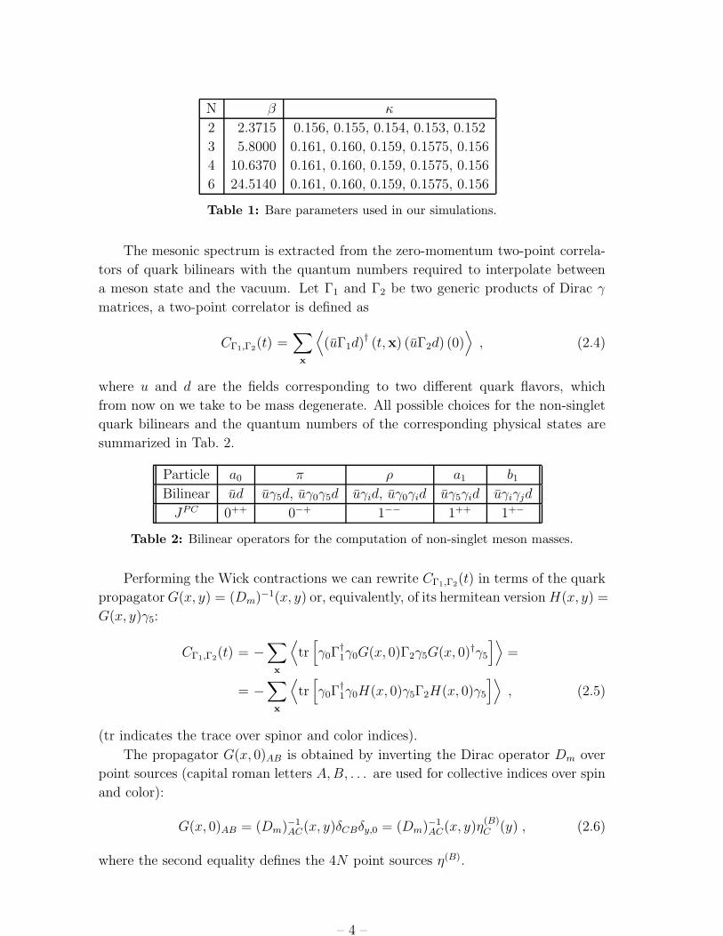
N β κ
2 2.3715 0.156, 0.155, 0.154, 0.153, 0.152
3 5.8000 0.161, 0.160, 0.159, 0.1575, 0.156
4 10.6370 0.161, 0.160, 0.159, 0.1575, 0.156
6 24.5140 0.161, 0.160, 0.159, 0.1575, 0.156
Table 1: Bare parameters used in our simulations.
The mesonic spectrum is extracted from the zero-momentum two-point correla-
tors of quark bilinears with the quantum numbers required to interpolate between
a meson state and the vacuum. Let Γ1 and Γ2 be two generic products of Dirac γ
matrices, a two-point correlator is defined as
CΓ1,Γ2(t) =
∑
x
⟨
(uΓ1d)† (t,x) (uΓ2d) (0)⟩
, (2.4)
where u and d are the fields corresponding to two different quark flavors, which
from now on we take to be mass degenerate. All possible choices for the non-singlet
quark bilinears and the quantum numbers of the corresponding physical states are
summarized in Tab. 2.
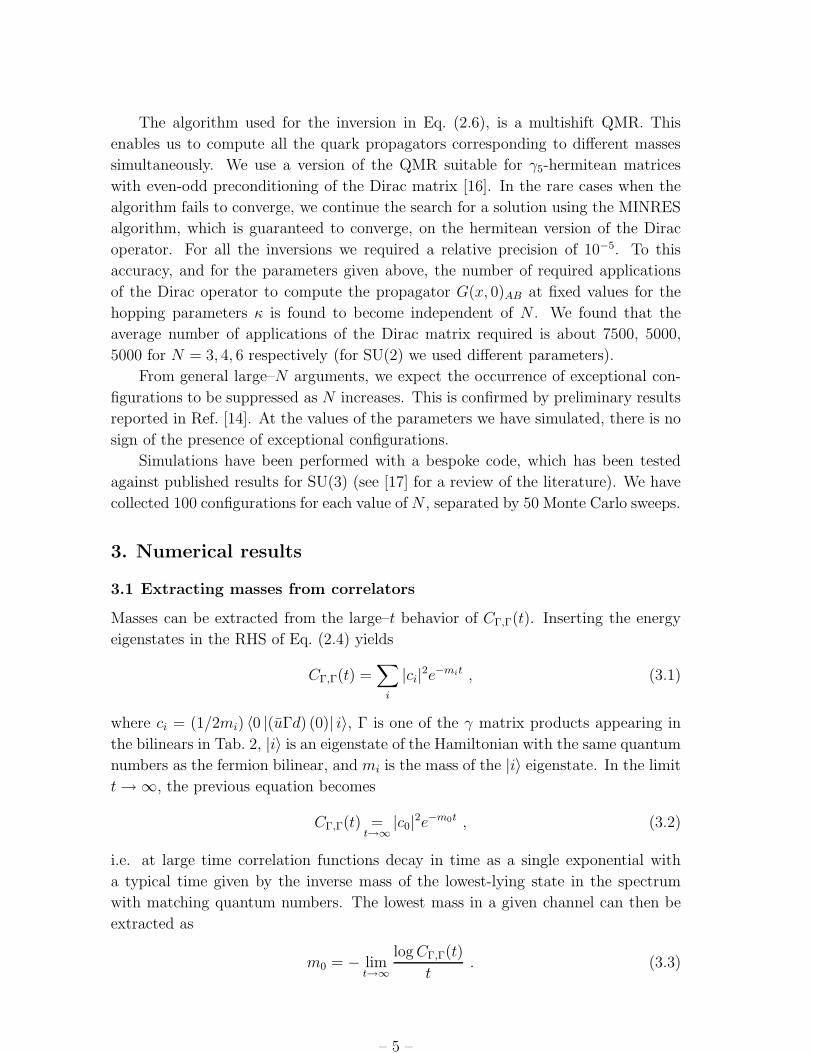
Particle a0 π ρ a1 b1
Bilinear ud uγ5d, uγ0γ5d uγid, uγ0γid uγ5γid uγiγjd
JPC 0++ 0−+ 1−− 1++ 1+−
Table 2: Bilinear operators for the computation of non-singlet meson masses.
Performing the Wick contractions we can rewrite CΓ1,Γ2(t) in terms of the quark
propagator G(x, y) = (Dm)−1(x, y) or, equivalently, of its hermitean version H(x, y) =
G(x, y)γ5:
CΓ1,Γ2(t) = −
∑
x
⟨
tr[
γ0Γ†1γ0G(x, 0)Γ2γ5G(x, 0)†γ5
]⟩
=
= −∑
x
⟨
tr[
γ0Γ†1γ0H(x, 0)γ5Γ2H(x, 0)γ5
]⟩
, (2.5)
(tr indicates the trace over spinor and color indices).
The propagator G(x, 0)AB is obtained by inverting the Dirac operator Dm over
point sources (capital roman letters A, B, . . . are used for collective indices over spin
and color):
G(x, 0)AB = (Dm)−1AC(x, y)δCBδy,0 = (Dm)−1
AC(x, y)η(B)C (y) , (2.6)
where the second equality defines the 4N point sources η(B).
– 4 –
The algorithm used for the inversion in Eq. (2.6), is a multishift QMR. This
enables us to compute all the quark propagators corresponding to different masses
simultaneously. We use a version of the QMR suitable for γ5-hermitean matrices
with even-odd preconditioning of the Dirac matrix [16]. In the rare cases when the
algorithm fails to converge, we continue the search for a solution using the MINRES
algorithm, which is guaranteed to converge, on the hermitean version of the Dirac
operator. For all the inversions we required a relative precision of 10−5. To this
accuracy, and for the parameters given above, the number of required applications
of the Dirac operator to compute the propagator G(x, 0)AB at fixed values for the
hopping parameters κ is found to become independent of N . We found that the
average number of applications of the Dirac matrix required is about 7500, 5000,
5000 for N = 3, 4, 6 respectively (for SU(2) we used different parameters).
From general large–N arguments, we expect the occurrence of exceptional con-
figurations to be suppressed as N increases. This is confirmed by preliminary results
reported in Ref. [14]. At the values of the parameters we have simulated, there is no
sign of the presence of exceptional configurations.
Simulations have been performed with a bespoke code, which has been tested
against published results for SU(3) (see [17] for a review of the literature). We have
collected 100 configurations for each value of N , separated by 50 Monte Carlo sweeps.
3. Numerical results
3.1 Extracting masses from correlators
Masses can be extracted from the large–t behavior of CΓ,Γ(t). Inserting the energy
eigenstates in the RHS of Eq. (2.4) yields
CΓ,Γ(t) =∑
i
|ci|2e−mit , (3.1)
where ci = (1/2mi) 〈0 |(uΓd) (0)| i〉, Γ is one of the γ matrix products appearing in
the bilinears in Tab. 2, |i〉 is an eigenstate of the Hamiltonian with the same quantum
numbers as the fermion bilinear, and mi is the mass of the |i〉 eigenstate. In the limit
t → ∞, the previous equation becomes
CΓ,Γ(t) =t→∞
|c0|2e−m0t , (3.2)
i.e. at large time correlation functions decay in time as a single exponential with
a typical time given by the inverse mass of the lowest-lying state in the spectrum
with matching quantum numbers. The lowest mass in a given channel can then be
extracted as
m0 = − limt→∞
log CΓ,Γ(t)
t. (3.3)
– 5 –
0 10 20 30t
1e-06
0.0001
0.01
1C
Γ,Γ(t
)
k=0.161k=0.160k=0.159k=0.1575k=0.156
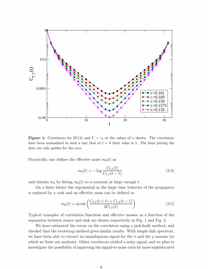
Figure 1: Correlators for SU(4) and Γ = γ5 at the values of κ shown. The correlators
have been normalized in such a way that at t = 0 their value is 1. The lines joining the
data are only guides for the eyes.
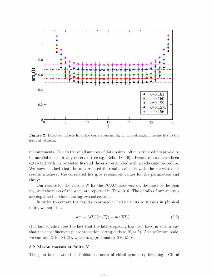
Practically, one defines the effective mass m0(t) as
m0(t) = − logCΓ,Γ(t)
CΓ,Γ(t − 1)(3.4)
and obtains m0 by fitting m0(t) to a constant at large enough t.
On a finite lattice the exponential in the large–time behavior of the propagator
is replaced by a cosh and an effective mass can be defined as
m0(t) = acosh
(
CΓ,Γ(t + 1) + CΓ,Γ(t − 1)
2CΓ,Γ(t)
)
. (3.5)
Typical examples of correlation functions and effective masses as a function of the
separation between source and sink are shown respectively in Fig. 1 and Fig. 2.
We have estimated the errors on the correlators using a jack-knife method, and
checked that the bootstrap method gives similar results. With simple link operators,
we have been able to extract an unambiguous signal for the π and the ρ mesons (to
which we limit our analysis). Other correlators yielded a noisy signal, and we plan to
investigate the possibility of improving the signal-to-noise ratio by more sophisticated
– 6 –
0 5 10 15 20 25 30t
0
0.2
0.4
0.6
0.8
1
am0(t
)
k=0.161k=0.160k=0.159k=0.1575k=0.156
Figure 2: Effective masses from the correlators in Fig. 1. The straight lines are fits to the
data at plateau.
measurements. Due to the small number of data points, often correlated fits proved to
be unreliable, as already observed (see e.g. Refs. [18, 19]). Hence, masses have been
extracted with uncorrelated fits and the error estimated with a jack-knife procedure.
We have checked that the uncorrelated fit results coincide with the correlated fit
results whenever the correlated fits give reasonable values for the parameters and
the χ2.
Our results for the various N for the PCAC mass mPCAC, the mass of the pion
mπ, and the mass of the ρ mρ are reported in Tabs. 3–6. The details of our analysis
are explained in the following two subsections.
In order to convert the results expressed in lattice units to masses in physical
units, we note that
am = (aTc)(m/Tc) = m/(5Tc) (3.6)
(the last equality uses the fact that the lattice spacing has been fixed in such a way
that the deconfinement phase transition corresponds to Nt = 5). As a reference scale,
we can use Tc for SU(3), which is approximately 270 MeV.
3.2 Meson masses at finite N
The pion is the would-be Goldstone boson of chiral symmetry breaking. Chiral
– 7 –
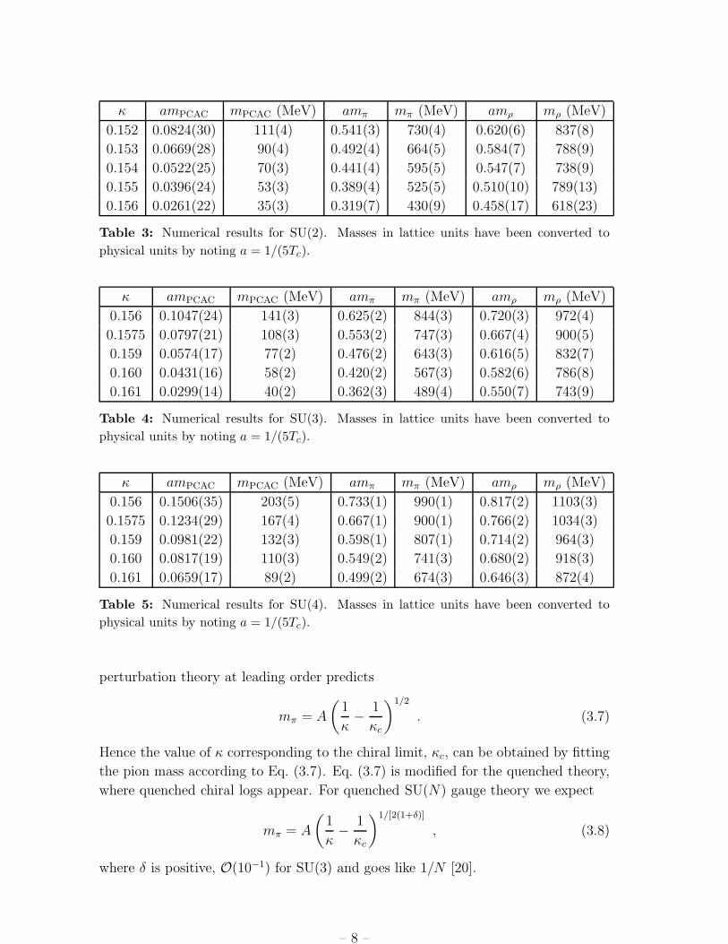
κ amPCAC mPCAC (MeV) amπ mπ (MeV) amρ mρ (MeV)
0.152 0.0824(30) 111(4) 0.541(3) 730(4) 0.620(6) 837(8)
0.153 0.0669(28) 90(4) 0.492(4) 664(5) 0.584(7) 788(9)
0.154 0.0522(25) 70(3) 0.441(4) 595(5) 0.547(7) 738(9)
0.155 0.0396(24) 53(3) 0.389(4) 525(5) 0.510(10) 789(13)
0.156 0.0261(22) 35(3) 0.319(7) 430(9) 0.458(17) 618(23)
Table 3: Numerical results for SU(2). Masses in lattice units have been converted to
physical units by noting a = 1/(5Tc).
κ amPCAC mPCAC (MeV) amπ mπ (MeV) amρ mρ (MeV)
0.156 0.1047(24) 141(3) 0.625(2) 844(3) 0.720(3) 972(4)
0.1575 0.0797(21) 108(3) 0.553(2) 747(3) 0.667(4) 900(5)
0.159 0.0574(17) 77(2) 0.476(2) 643(3) 0.616(5) 832(7)
0.160 0.0431(16) 58(2) 0.420(2) 567(3) 0.582(6) 786(8)
0.161 0.0299(14) 40(2) 0.362(3) 489(4) 0.550(7) 743(9)
Table 4: Numerical results for SU(3). Masses in lattice units have been converted to
physical units by noting a = 1/(5Tc).
κ amPCAC mPCAC (MeV) amπ mπ (MeV) amρ mρ (MeV)
0.156 0.1506(35) 203(5) 0.733(1) 990(1) 0.817(2) 1103(3)
0.1575 0.1234(29) 167(4) 0.667(1) 900(1) 0.766(2) 1034(3)
0.159 0.0981(22) 132(3) 0.598(1) 807(1) 0.714(2) 964(3)
0.160 0.0817(19) 110(3) 0.549(2) 741(3) 0.680(2) 918(3)
0.161 0.0659(17) 89(2) 0.499(2) 674(3) 0.646(3) 872(4)
Table 5: Numerical results for SU(4). Masses in lattice units have been converted to
physical units by noting a = 1/(5Tc).
perturbation theory at leading order predicts
mπ = A
(
1
κ−
1
κc
)1/2
. (3.7)
Hence the value of κ corresponding to the chiral limit, κc, can be obtained by fitting
the pion mass according to Eq. (3.7). Eq. (3.7) is modified for the quenched theory,
where quenched chiral logs appear. For quenched SU(N) gauge theory we expect
mπ = A
(
1
κ−
1
κc
)1/[2(1+δ)]
, (3.8)
where δ is positive, O(10−1) for SU(3) and goes like 1/N [20].
– 8 –
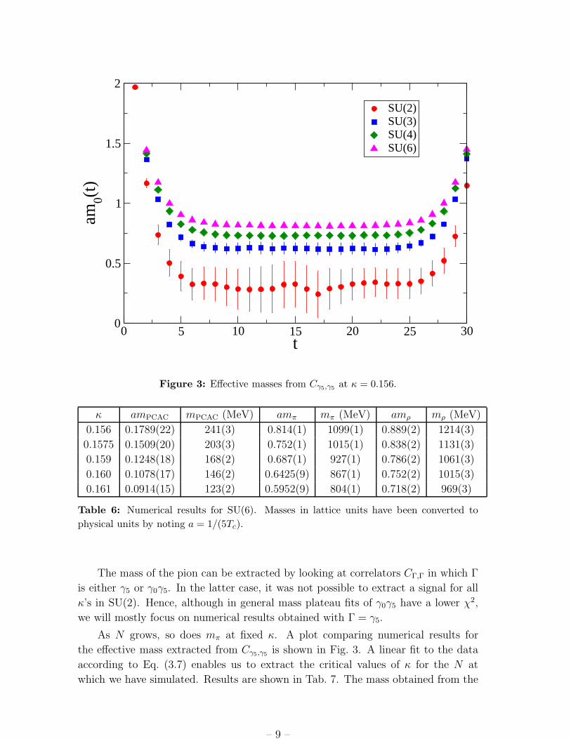
0 5 10 15 20 25 30t
0
0.5
1
1.5
2am
0(t)
SU(2)SU(3)SU(4)SU(6)
Figure 3: Effective masses from Cγ5,γ5at κ = 0.156.
κ amPCAC mPCAC (MeV) amπ mπ (MeV) amρ mρ (MeV)
0.156 0.1789(22) 241(3) 0.814(1) 1099(1) 0.889(2) 1214(3)
0.1575 0.1509(20) 203(3) 0.752(1) 1015(1) 0.838(2) 1131(3)
0.159 0.1248(18) 168(2) 0.687(1) 927(1) 0.786(2) 1061(3)
0.160 0.1078(17) 146(2) 0.6425(9) 867(1) 0.752(2) 1015(3)
0.161 0.0914(15) 123(2) 0.5952(9) 804(1) 0.718(2) 969(3)
Table 6: Numerical results for SU(6). Masses in lattice units have been converted to
physical units by noting a = 1/(5Tc).
The mass of the pion can be extracted by looking at correlators CΓ,Γ in which Γ
is either γ5 or γ0γ5. In the latter case, it was not possible to extract a signal for all
κ’s in SU(2). Hence, although in general mass plateau fits of γ0γ5 have a lower χ2,
we will mostly focus on numerical results obtained with Γ = γ5.
As N grows, so does mπ at fixed κ. A plot comparing numerical results for
the effective mass extracted from Cγ5,γ5is shown in Fig. 3. A linear fit to the data
according to Eq. (3.7) enables us to extract the critical values of κ for the N at
which we have simulated. Results are shown in Tab. 7. The mass obtained from the
– 9 –
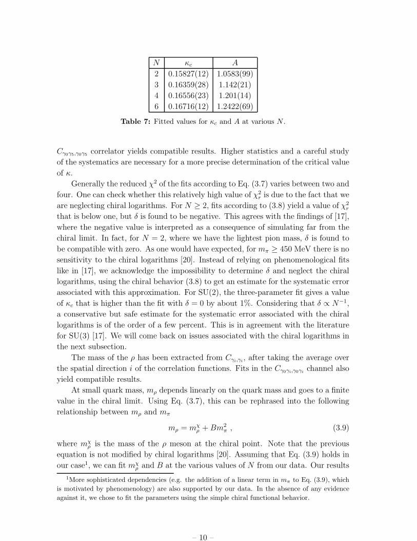
N κc A
2 0.15827(12) 1.0583(99)
3 0.16359(28) 1.142(21)
4 0.16556(23) 1.201(14)
6 0.16716(12) 1.2422(69)
Table 7: Fitted values for κc and A at various N .
Cγ0γ5,γ0γ5correlator yields compatible results. Higher statistics and a careful study
of the systematics are necessary for a more precise determination of the critical value
of κ.
Generally the reduced χ2 of the fits according to Eq. (3.7) varies between two and
four. One can check whether this relatively high value of χ2r is due to the fact that we
are neglecting chiral logarithms. For N ≥ 2, fits according to (3.8) yield a value of χ2r
that is below one, but δ is found to be negative. This agrees with the findings of [17],
where the negative value is interpreted as a consequence of simulating far from the
chiral limit. In fact, for N = 2, where we have the lightest pion mass, δ is found to
be compatible with zero. As one would have expected, for mπ ≥ 450 MeV there is no
sensitivity to the chiral logarithms [20]. Instead of relying on phenomenological fits
like in [17], we acknowledge the impossibility to determine δ and neglect the chiral
logarithms, using the chiral behavior (3.8) to get an estimate for the systematic error
associated with this approximation. For SU(2), the three-parameter fit gives a value
of κc that is higher than the fit with δ = 0 by about 1%. Considering that δ ∝ N−1,
a conservative but safe estimate for the systematic error associated with the chiral
logarithms is of the order of a few percent. This is in agreement with the literature
for SU(3) [17]. We will come back on issues associated with the chiral logarithms in
the next subsection.
The mass of the ρ has been extracted from Cγi,γi, after taking the average over
the spatial direction i of the correlation functions. Fits in the Cγ0γi,γ0γichannel also
yield compatible results.
At small quark mass, mρ depends linearly on the quark mass and goes to a finite
value in the chiral limit. Using Eq. (3.7), this can be rephrased into the following
relationship between mρ and mπ
mρ = mχρ + Bm2
π , (3.9)
where mχρ is the mass of the ρ meson at the chiral point. Note that the previous
equation is not modified by chiral logarithms [20]. Assuming that Eq. (3.9) holds in
our case1, we can fit mχρ and B at the various values of N from our data. Our results
1More sophisticated dependencies (e.g. the addition of a linear term in mπ to Eq. (3.9), which
is motivated by phenomenology) are also supported by our data. In the absence of any evidence
against it, we chose to fit the parameters using the simple chiral functional behavior.
– 10 –
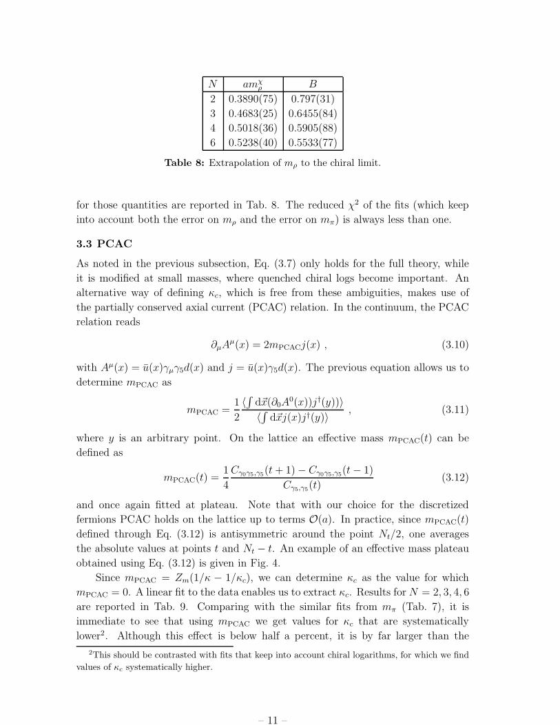
N amχρ B
2 0.3890(75) 0.797(31)
3 0.4683(25) 0.6455(84)
4 0.5018(36) 0.5905(88)
6 0.5238(40) 0.5533(77)
Table 8: Extrapolation of mρ to the chiral limit.
for those quantities are reported in Tab. 8. The reduced χ2 of the fits (which keep
into account both the error on mρ and the error on mπ) is always less than one.
3.3 PCAC
As noted in the previous subsection, Eq. (3.7) only holds for the full theory, while
it is modified at small masses, where quenched chiral logs become important. An
alternative way of defining κc, which is free from these ambiguities, makes use of
the partially conserved axial current (PCAC) relation. In the continuum, the PCAC
relation reads
∂µAµ(x) = 2mPCACj(x) , (3.10)
with Aµ(x) = u(x)γµγ5d(x) and j = u(x)γ5d(x). The previous equation allows us to
determine mPCAC as
mPCAC =1
2
〈∫
d~x(∂0A0(x))j†(y))〉
〈∫
d~xj(x)j†(y)〉, (3.11)
where y is an arbitrary point. On the lattice an effective mass mPCAC(t) can be
defined as
mPCAC(t) =1
4
Cγ0γ5,γ5(t + 1) − Cγ0γ5,γ5
(t − 1)
Cγ5,γ5(t)
(3.12)
and once again fitted at plateau. Note that with our choice for the discretized
fermions PCAC holds on the lattice up to terms O(a). In practice, since mPCAC(t)
defined through Eq. (3.12) is antisymmetric around the point Nt/2, one averages
the absolute values at points t and Nt − t. An example of an effective mass plateau
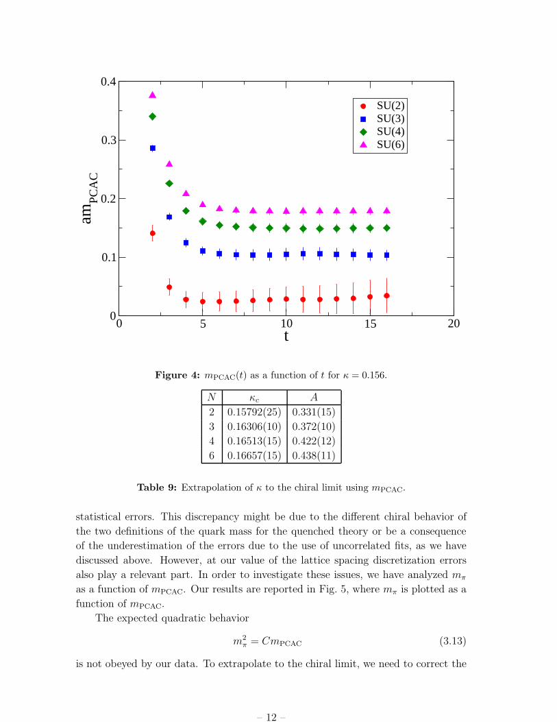
obtained using Eq. (3.12) is given in Fig. 4.
Since mPCAC = Zm(1/κ − 1/κc), we can determine κc as the value for which
mPCAC = 0. A linear fit to the data enables us to extract κc. Results for N = 2, 3, 4, 6
are reported in Tab. 9. Comparing with the similar fits from mπ (Tab. 7), it is
immediate to see that using mPCAC we get values for κc that are systematically
lower2. Although this effect is below half a percent, it is by far larger than the
2This should be contrasted with fits that keep into account chiral logarithms, for which we find
values of κc systematically higher.
– 11 –
0 5 10 15 20t
0
0.1
0.2
0.3
0.4am
PCA
CSU(2)SU(3)SU(4)SU(6)
Figure 4: mPCAC(t) as a function of t for κ = 0.156.
N κc A
2 0.15792(25) 0.331(15)
3 0.16306(10) 0.372(10)
4 0.16513(15) 0.422(12)
6 0.16657(15) 0.438(11)
Table 9: Extrapolation of κ to the chiral limit using mPCAC.
statistical errors. This discrepancy might be due to the different chiral behavior of
the two definitions of the quark mass for the quenched theory or be a consequence
of the underestimation of the errors due to the use of uncorrelated fits, as we have
discussed above. However, at our value of the lattice spacing discretization errors
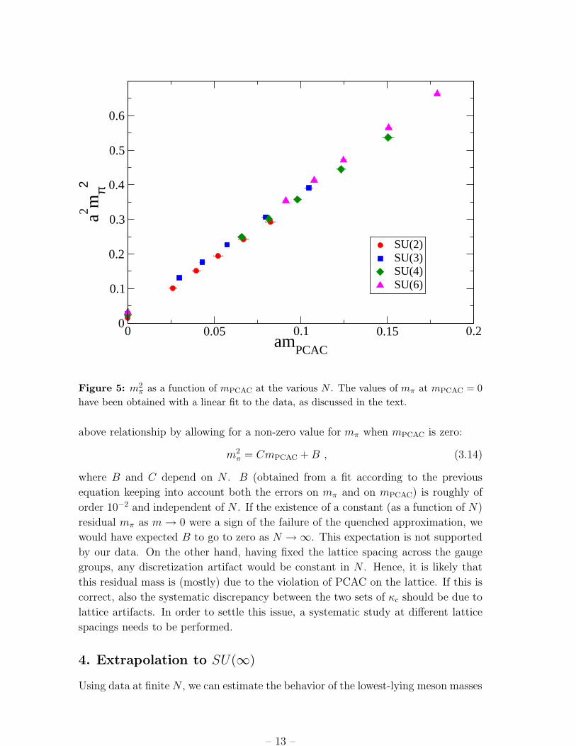
also play a relevant part. In order to investigate these issues, we have analyzed mπ
as a function of mPCAC. Our results are reported in Fig. 5, where mπ is plotted as a
function of mPCAC.
The expected quadratic behavior
m2π = CmPCAC (3.13)
is not obeyed by our data. To extrapolate to the chiral limit, we need to correct the
– 12 –
0 0.05 0.1 0.15 0.2am
PCAC
0
0.1
0.2
0.3
0.4
0.5
0.6
a2 mπ2
SU(2)SU(3)SU(4)SU(6)
Figure 5: m2π as a function of mPCAC at the various N . The values of mπ at mPCAC = 0
have been obtained with a linear fit to the data, as discussed in the text.
above relationship by allowing for a non-zero value for mπ when mPCAC is zero:
m2π = CmPCAC + B , (3.14)
where B and C depend on N . B (obtained from a fit according to the previous
equation keeping into account both the errors on mπ and on mPCAC) is roughly of
order 10−2 and independent of N . If the existence of a constant (as a function of N)
residual mπ as m → 0 were a sign of the failure of the quenched approximation, we
would have expected B to go to zero as N → ∞. This expectation is not supported
by our data. On the other hand, having fixed the lattice spacing across the gauge
groups, any discretization artifact would be constant in N . Hence, it is likely that
this residual mass is (mostly) due to the violation of PCAC on the lattice. If this is
correct, also the systematic discrepancy between the two sets of κc should be due to
lattice artifacts. In order to settle this issue, a systematic study at different lattice
spacings needs to be performed.
4. Extrapolation to SU(∞)
Using data at finite N , we can estimate the behavior of the lowest-lying meson masses
– 13 –
at N = ∞. Following similar analysis performed in pure gauge [5, 6, 7, 8, 9, 10, 11],
we use predictions from the large–N expansion to see whether they hold in the non-
perturbative regime. In practice, we take the asymptotic expansion for an observable
O in the quenched case [1]
O(N) = O(∞) +∑
i
αi
N2i(4.1)
and we check whether a reasonable (as dictated by the number of data) truncation
of this series accommodates our numerical values. In the pure gauge case, a preco-
cious onset of the large–N behavior has been found for all the observables that have
been studied (which include glueball masses, deconfining temperature and topolog-
ical susceptibility): the O(1/N2) correction correctly describes the data down to at
least N = 3, often including also the case N = 2. From a qualitative point of view,
it is already clear from what we have seen so far that the quantities we have investi-
gated have a mild dependence on N . In this section, we want to study whether this
dependence is correctly described by a large–N -inspired expansion.
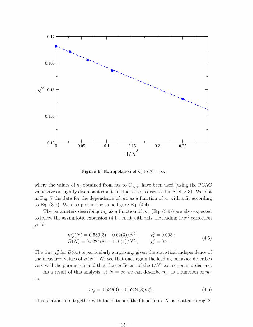
κc can be computed in lattice perturbation theory [21]. The result at one loop
is in agreement with the predictions of the large–N limit: this quantity receives a
correction O(1/N2). This motivates the fit
κc(N) = κc(∞) +a
N2. (4.2)
For κc obtained via Eq. (3.7), we get κc(∞) = 0.1682(1) and a = −0.0398(6), with
χ2r = 0.6. The quality of the fit is good, and the coefficient of the 1/N2 correction
is small, as one would expect for a series expansion. Similarly to the pure gauge
case, we observe an early onset of the asymptotic behavior, which captures also the
SU(2) value. Our data and the large–N extrapolation are plotted in Fig. 6. The
same extrapolation for the critical value of κ obtained using the PCAC relation
yields κc(∞) = 0.1675(2), a = −0.039(1) and χ2r = 1.3. The discrepancy between
the values of κc(∞) could be due to lattice discretization artifacts, as discussed in
Sect. 3.3. We take the difference between the two determinations should be seen as
an estimate of the systematic error. The fact that the angular coefficient a has the
same value seems to corroborate this hypothesis. A more precise determination of
κc is beyond the scope of this work.
The slope A in Eq. (3.7) can also be extrapolated to the N = ∞ limit, with
corrections that are O(1/N2):
A(N) = A(∞) + a/N2 . (4.3)
For the Cγ5,γ5results, the fit gives A(∞) = 1.262(8) and a = −0.82(6) with χ2
r = 1.2.
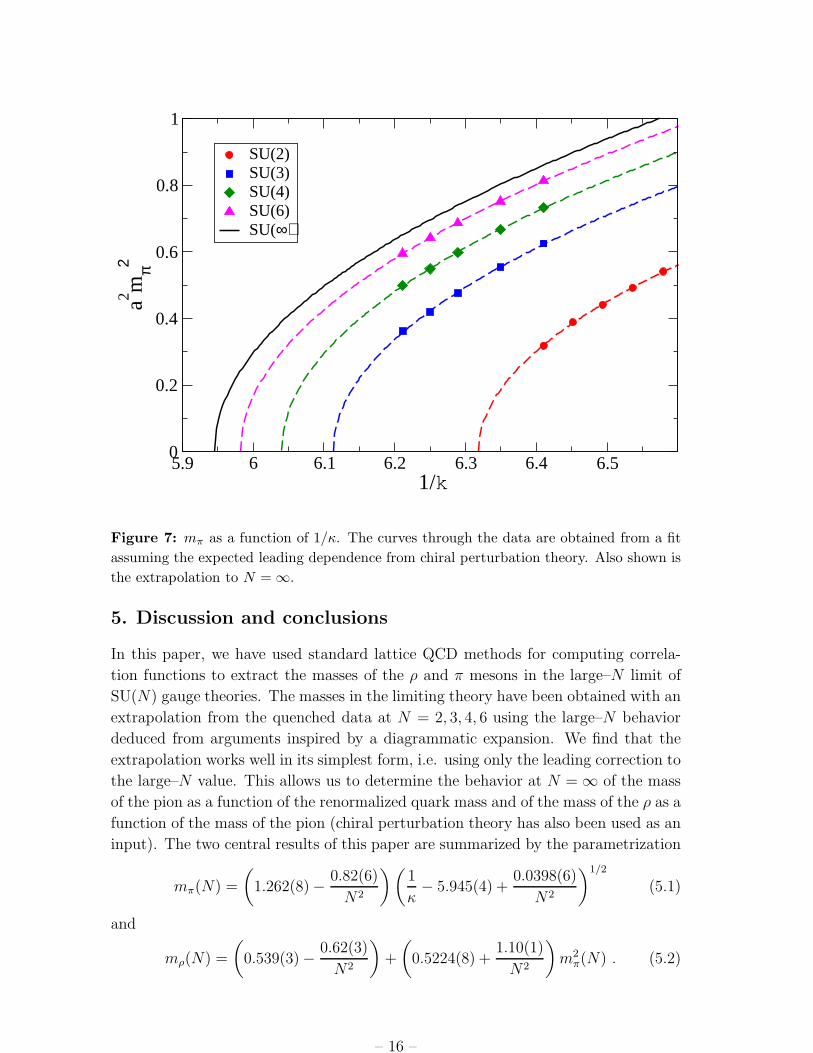
This allows us to write the mass of the π as a function of κ at N = ∞ as
mπ = 1.262(8) (1/κ − 5.945(4))1/2 , (4.4)
– 14 –
0 0.05 0.1 0.15 0.2 0.25
1/N2
0.15
0.155
0.16
0.165
0.17kc
Figure 6: Extrapolation of κc to N = ∞.
where the values of κc obtained from fits to Cγ5,γ5have been used (using the PCAC
value gives a slightly discrepant result, for the reasons discussed in Sect. 3.3). We plot
in Fig. 7 the data for the dependence of m2π as a function of κ, with a fit according
to Eq. (3.7). We also plot in the same figure Eq. (4.4).
The parameters describing mρ as a function of mπ (Eq. (3.9)) are also expected
to follow the asymptotic expansion (4.1). A fit with only the leading 1/N2 correction
yields
mχρ (N) = 0.539(3) − 0.62(3)/N2 , χ2
r = 0.008 ;
B(N) = 0.5224(8) + 1.10(1)/N2 , χ2r = 0.7 .
(4.5)
The tiny χ2r for B(∞) is particularly surprising, given the statistical independence of
the measured values of B(N). We see that once again the leading behavior describes
very well the parameters and that the coefficient of the 1/N2 correction is order one.
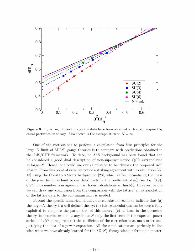
As a result of this analysis, at N = ∞ we can describe mρ as a function of mπ
as
mρ = 0.539(3) + 0.5224(8)m2π . (4.6)
This relationship, together with the data and the fits at finite N , is plotted in Fig. 8.
– 15 –
5.9 6 6.1 6.2 6.3 6.4 6.5 1/k
0
0.2
0.4
0.6
0.8
1a2 m
π2
SU(2)SU(3)SU(4)SU(6)SU(∞)
Figure 7: mπ as a function of 1/κ. The curves through the data are obtained from a fit
assuming the expected leading dependence from chiral perturbation theory. Also shown is
the extrapolation to N = ∞.
5. Discussion and conclusions
In this paper, we have used standard lattice QCD methods for computing correla-
tion functions to extract the masses of the ρ and π mesons in the large–N limit of
SU(N) gauge theories. The masses in the limiting theory have been obtained with an
extrapolation from the quenched data at N = 2, 3, 4, 6 using the large–N behavior
deduced from arguments inspired by a diagrammatic expansion. We find that the
extrapolation works well in its simplest form, i.e. using only the leading correction to
the large–N value. This allows us to determine the behavior at N = ∞ of the mass
of the pion as a function of the renormalized quark mass and of the mass of the ρ as a
function of the mass of the pion (chiral perturbation theory has also been used as an
input). The two central results of this paper are summarized by the parametrization
mπ(N) =
(
1.262(8) −0.82(6)
N2
) (
1
κ− 5.945(4) +
0.0398(6)
N2
)1/2
(5.1)
and
mρ(N) =
(
0.539(3) −0.62(3)
N2
)
+
(
0.5224(8) +1.10(1)
N2
)
m2π(N) . (5.2)
– 16 –
0 0.1 0.2 0.3 0.4 0.5 0.6
a2mπ2
0.3
0.4
0.5
0.6
0.7
0.8
0.9am
ρ
SU(2)SU(3)SU(4)SU(6)N = inf.
Figure 8: mρ vs. mπ. Lines through the data have been obtained with a plot inspired by
chiral perturbation theory. Also shown is the extrapolation to N = ∞.
One of the motivations to perform a calculation from first principles for the
large–N limit of SU(N) gauge theories is to compare with predictions obtained in
the AdS/CFT framework. To date, no AdS background has been found that can
be considered a good dual description of non-supersymmetric QCD extrapolated
at large–N . Hence, one could use our calculation to benchmark the proposed AdS
ansatz. From this point of view, we notice a striking agreement with a calculation [22,
13] using the Constable-Myers background [23], which (after normalizing the mass
of the ρ in the chiral limit to our data) finds for the coefficient of m2π (see Eq. (3.9))
0.57. This number is in agreement with our calculations within 5%. However, before
we can draw any conclusion from the comparison with the lattice, an extrapolation
of the lattice data to the continuum limit is needed.
Beyond the specific numerical details, our calculation seems to indicate that (a)
the large–N theory is a well defined theory; (b) lattice calculations can be successfully
exploited to compute the parameters of this theory; (c) at least in the quenched
theory, to describe results at any finite N only the first term in the expected power
series in 1/N2 is required; (d) the coefficient of the correction is at most order one,
justifying the idea of a power expansion. All these indications are perfectly in line
with what we have already learned for the SU(N) theory without fermionic matter.
– 17 –
Although this can be considered obvious, since our calculation is quenched, we stress
that the N = ∞ limit is also quenched. In other words, to describe the limiting
theory a quenched calculation suffices. The inclusion of the full fermion determinant
becomes mandatory if one is interested in the actual size of the finite N corrections.
In particular, one expects larger corrections (O(nf/N)) in the unquenched theory.
As we have stressed several times, one of the main limitations of this calculation
is that our chiral extrapolations are not sensitive to the expected chiral log behavior.
We have conservatively estimated that this approximation produces a 3% systematic
error. This error does not affect our conclusions. Moreover, we note that chiral
logarithms do not modify Eq. (5.2). In any case, in order to make more robust
estimates, better control on the chiral extrapolation should be achieved. This requires
simulating at smaller pion masses. It would also be nice to check that the chiral log
effects decrease as N increases.
Another source of systematic error in our calculation is the fact that simulations
have been performed at one single lattice spacing. For this reason we regard our
results as exploratory. As discussed in Sect. 3.3, lattice artifacts do seem to play a
role, although they are not big enough to spoil the features of the theory and the
way in which the large–N behavior is approached. Nevertheless, a study closer to
the continuum is necessary to clarify these issues. Work for the extrapolation to the
continuum limit is already in progress. For this extrapolation, the use of an improved
fermion action can mitigate the discretization artifacts, decreasing considerably the
required numerical effort. We shall explore this possibility in the future. As for finite
size effects, we have argued in Sect. 2 that with our choice of parameters they can
be neglected, but this also ought to be verified directly.
Aside from technicalities, other features of the large–N theory, like the spec-
trum in the flavor singlet channel and masses of heavier mesons, also deserve to be
investigated. While the latter problem can probably be dealt with using improved
techniques for computing correlation functions (e.g. with smeared links replacing
straight links and smeared sources replacing point sources), for the scalar mesons,
for which disconnected contributions are important, different strategies need to be
adopted. An adaptation of the techniques exposed in [24, 25] is in progress. Results
will be reported in a future publication.
Acknowledgments
We thank C. Allton, G. Bali, F. Bursa and C. Nunez for useful comments on this
manuscript. Discussions with A. Armoni, N. Dorey, N. Evans, L. Lellouch, P. Orland,
G. Semenoff, M. Shifman and G. Veneziano are gratefully acknowledged. Numerical
simulations have been performed on a 60 core Beowulf cluster partially funded by
the Royal Society and STFC. We thank SUPA for financial support for the workshop
Strongly interacting dynamics beyond the Standard Model, during which many of the
– 18 –
ideas reported in this paper were discussed. B.L. and L.D.D. thank the hospitality
of the Isaac Newton Institute, where this work was finalized. L.D.D. is supported
by an STFC Advanced Fellowship. B.L. is supported by a Royal Society University
Research Fellowship. The work of C.P. has been supported by contract DE-AC02-
98CH10886 with the U.S. Department of Energy.
References
[1] G. ’t Hooft, A planar diagram theory for strong interactions, Nucl. Phys. B72 (1974)
461.
[2] G. Veneziano, Regge intercepts and unitarity in planar dual models, Nucl. Phys. B74
(1974) 365.
[3] J. M. Maldacena, The large n limit of superconformal field theories and supergravity,
Adv. Theor. Math. Phys. 2 (1998) 231–252, [hep-th/9711200].
[4] H. Nastase, Introduction to ads-cft, 0712.0689.
[5] B. Lucini and M. Teper, Su(n) gauge theories in four dimensions: Exploring the
approach to n = infinity, JHEP 06 (2001) 050, [hep-lat/0103027].
[6] B. Lucini, M. Teper, and U. Wenger, The high temperature phase transition in su(n)
gauge theories, JHEP 01 (2004) 061, [hep-lat/0307017].
[7] B. Lucini, M. Teper, and U. Wenger, Topology of su(n) gauge theories at t approx. 0
and t approx. t(c), Nucl. Phys. B715 (2005) 461–482, [hep-lat/0401028].
[8] L. Del Debbio, H. Panagopoulos, P. Rossi, and E. Vicari, Spectrum of confining
strings in su(n) gauge theories, JHEP 01 (2002) 009, [hep-th/0111090].
[9] L. Del Debbio, H. Panagopoulos, and E. Vicari, Theta dependence of su(n) gauge
theories, JHEP 08 (2002) 044, [hep-th/0204125].
[10] L. Del Debbio, H. Panagopoulos, and E. Vicari, Topological susceptibility of su(n)
gauge theories at finite temperature, JHEP 09 (2004) 028, [hep-th/0407068].
[11] L. Del Debbio, G. M. Manca, H. Panagopoulos, A. Skouroupathis, and E. Vicari,
theta-dependence of the spectrum of su(n) gauge theories, JHEP 06 (2006) 005,
[hep-th/0603041].
[12] R. Narayanan and H. Neuberger, The quark mass dependence of the pion mass at
infinite n, Phys. Lett. B616 (2005) 76–84, [hep-lat/0503033].
[13] J. Erdmenger, N. Evans, I. Kirsch, and E. Threlfall, Mesons in gauge/gravity duals -
a review, 0711.4467.
[14] G. Bali and F. Bursa, Meson masses at large nc, 0708.3427.
– 19 –
[15] N. Cabibbo and E. Marinari, A new method for updating su(n) matrices in computer
simulations of gauge theories, Phys. Lett. B119 (1982) 387–390.
[16] A. Frommer, B. Nockel, S. Gusken, T. Lippert, and K. Schilling, Many masses on
one stroke: Economic computation of quark propagators, Int. J. Mod. Phys. C6
(1995) 627–638, [hep-lat/9504020].
[17] M. Gockeler et. al., Scaling of non-perturbatively o(a) improved wilson fermions:
Hadron spectrum, quark masses and decay constants, Phys. Rev. D57 (1998)
5562–5580, [hep-lat/9707021].
[18] C. Michael, Fitting correlated data, Phys. Rev. D49 (1994) 2616–2619,
[hep-lat/9310026].
[19] C. Michael and A. McKerrell, Fitting correlated hadron mass spectrum data, Phys.
Rev. D51 (1995) 3745–3750, [hep-lat/9412087].
[20] S. R. Sharpe, Quenched chiral logarithms, Phys. Rev. D46 (1992) 3146–3168,
[hep-lat/9205020].
[21] J. Stehr and P. H. Weisz, Note on gauge fixing in lattice qcd, Lett. Nuovo Cim. 37
(1983) 173–177.
[22] J. Babington, J. Erdmenger, N. J. Evans, Z. Guralnik, and I. Kirsch, Chiral
symmetry breaking and pions in non-supersymmetric gauge / gravity duals, Phys.
Rev. D69 (2004) 066007, [hep-th/0306018].
[23] N. R. Constable and R. C. Myers, Exotic scalar states in the ads/cft correspondence,
JHEP 11 (1999) 020, [hep-th/9905081].
[24] J. Foley et. al., Practical all-to-all propagators for lattice qcd, Comput. Phys.
Commun. 172 (2005) 145–162, [hep-lat/0505023].
[25] S. Collins, G. Bali, and A. Schafer, Disconnected contributions to hadronic structure:
a new method for stochastic noise reduction, 0709.3217.
– 20 –


