ORIGINAL ARTICLE

Radial basis function classifiers to help in the diagnosisof the obstructive sleep apnoea syndrome from nocturnaloximetry

J. Vıctor Marcos Æ Roberto Hornero Æ Daniel Alvarez ÆFelix del Campo Æ Miguel Lopez Æ Carlos Zamarron

Received: 3 May 2007 / Accepted: 9 October 2007 / Published online: 30 October 2007

� International Federation for Medical and Biological Engineering 2007

Abstract The aim of this study is to assess the ability of

radial basis function (RBF) classifiers as an assistant tool

for the diagnosis of the obstructive sleep apnoea syndrome

(OSAS). A total of 187 subjects suspected of suffering

from OSAS were available for our research. The initial

population was divided into training, validation and test

sets for deriving and testing our neural classifiers. We used

nonlinear features from nocturnal oxygen saturation (SaO2)

to perform patients’ classification. We evaluated three

different RBF construction techniques based on the fol-

lowing algorithms: k-means (KM), fuzzy c-means (FCM)

and orthogonal least squares (OLS). A diagnostic accuracy

of 86.1, 84.7 and 85.5% was provided by the networks

developed with KM, FCM and OLS, respectively. The

three proposed networks achieved an area under the

receiver operating characteristic (ROC) curve over 0.90.

Our results showed that a useful non-invasive method

could be applied to diagnose OSAS from nonlinear features

of SaO2 with RBF classifiers.

Keywords Obstructive sleep apnoea syndrome �Nocturnal oximetry � Radial basis function neural network �Data clustering � Nonlinear analysis

1 Introduction

Obstructive sleep apnoea syndrome (OSAS) is the most

common sleep disordered-breathing with an estimated

prevalence from 1 to 5% in the adult men of western coun-

tries [40]. OSAS is characterized by recurrent episodes of

upper airway occlusion during sleep. The morbidity of this

condition relates principally to the cardiovascular system.

The recurrent hypoxaemia and hypercapnia may lead to both

pulmonary and systemic hypertension, cardiac arrhythmias

and decreased survival. Moreover, unrecognized OSAS has

been reported to be a cause of mortality from traffic and

industrial accidents [38]. The most frequent symptoms

include excessive daytime sleepiness, snoring and nocturnal

arousals reported by bedfellow [26, 38]. However, these

symptoms are not definitive to detect the condition. Nowa-

days, polysomnography (PSG) is the gold-standard method

to diagnose OSAS. It is a monitoring process that must

be carried out in a sleep care unit. Complete PSG

includes the monitoring of electroencephalography (EEG),

electrooculography (EOG), electromyography (EMG),

electrocardiography (ECG), airflow measurement, effort to

breath, oximetry and body position [26]. Subsequently, a

final diagnosis is obtained through medical examination

of these recordings. Nevertheless, PSG presents some

drawbacks since it is a complex, time-consuming and

expensive procedure. Therefore, research on new simplified

diagnostic methods has increased in the past few years [36].

Nocturnal oximetry arises as an alternative to PSG since

it is readily available, relatively inexpensive and can be

J. V. Marcos (&) � R. Hornero � D. Alvarez � M. Lopez

Biomedical Engineering Group, E.T.S.I. de Telecomunicacion,

University of Valladolid, Camino del cementerio, s/n,

47011 Valladolid, Spain

e-mail: jvmarcos@gmail.com

F. del Campo

Servicio de Neumologıa, Hospital del Rıo Hortega,

Valladolid, Spain

C. Zamarron

Servicio de Neumologıa, Hospital Clınico Universitario,

Santiago de Compostela, Spain

123

Med Biol Eng Comput (2008) 46:323–332

DOI 10.1007/s11517-007-0280-0

performed at home [36]. Oximetry is a widely used tech-

nique in pulmonary medicine, critical care and anaesthesia

[8]. It allows to monitor arterial oxygen saturation (SaO2)

during sleep in a non-invasively manner. Nocturnal

oximetry has been widely used in sleep medicine for the

analysis of respiratory patterns [32]. Specifically, SaO2

recordings can be a powerful tool for OSAS detection.

Apnoeic events occurred during sleep are frequently

accompanied by oxygen desaturations. As a result, a dif-

ferent behaviour can be appreciated in recordings from

OSAS positive and negative subjects. Signals from patients

suffering from OSAS are characterized by an increased

instability, whereas signals from control subjects tend to

present a constant value round 97% of saturation [32].

Several studies have evaluated the utility of SaO2 signal in

OSAS diagnosis. Usually, classic oximetry indices were

used in such studies: the oxygen desaturation index (ODI)

over 2, 3 and 4%, the cumulative time spent below 90% of

saturation (CT90) and the D index (a measure of the

variability of SaO2) [30, 32, 35, 39]. Moreover, signal

processing techniques have been applied to SaO2 study.

Nonlinear analysis of this recording has reported promising

results in OSAS detection [2, 23].

In this study, we applied neural network-based classifiers

to the OSAS diagnosis problem. The flexibility and self-

adaptive nature of neural networks make them an appro-

priate technique for clinical assistance. Neural networks

represent an accurate and powerful technique for classifi-

cation problems. These algorithms suitably adapt to medical

diagnosis since it can be modelled as a pattern classification

task [4]. We propose a novel method to help in OSAS

diagnosis based on radial basis function (RBF) neural net-

works [21]. A three-element input vector was used for

patients’ classification by means of these networks. We

computed input features from non-linear analysis of SaO2

recordings. The following methods were applied: approxi-

mate entropy (ApEn), central tendency measure (CTM) and

Lempel-Ziv (LZ) complexity. These methods have been

employed over a wide range of diseases and signals. ApEn

has been used on respiratory patterns to study sleep stages

[9] and panic disorder [10]. Moreover, previous studies

have proved the utility of ApEn, CTM and LZ complexity

in OSAS diagnosis from SaO2 processing [2, 23]. The aim

of this study is to evaluate the ability of these RBF classi-

fiers to discriminate between OSAS and non-OSAS patients

using nonlinear features from SaO2 signals.

2 Subjects and signals

A total of 187 subjects suspected of suffering from OSAS

gave their consent to participate in this research. Sleep

studies were carried out usually from midnight to 8:00 AM

in the Sleep Unit of the Hospital Clınico Universitario de

Santiago de Compostela (Spain). The Review Board on

Human Studies at this institution approved the protocol.

Subjects underwent conventional PSG simultaneously to

nocturnal pulse oximetry. Recording of SaO2 signals was

performed by means of a Criticare 504 oximeter (CSI,

Waukeska, USA) at a sampling frequency of 0.2 Hz. The

equipment used to perform PSG was a polygraph

(Ultrasom Network, Nicolet, Madison, WI, USA). Poly-

somnographic recordings were analyzed according to the

system by Rechtschaffen and Kales [34] to obtain a

medical diagnosis for each subject. Apnoea was defined as

a cessation of airflow for 10 s or longer. Hypopnoea was

defined as a reduction, without complete cessation, in air-

flow of at least 50%, accompanied by a decrease of more

than 4% in the saturation of haemoglobin. The average

apnoea–hypopnoea index (AHI) was calculated for hourly

periods of sleep from apnoeic/hypopnoeic episodes cap-

tured in PSG. Finally, a threshold of AHI C 10 events/h

was established to determine the presence of OSAS in a

subject.

A positive diagnosis of OSAS was confirmed in 111

subjects (59.36%), whereas the remaining 76 subjects

(40.64%) presented an AHI below the threshold. There

were no significant differences between OSAS positive and

negative groups in age, body mass index and recording

time. On the other hand, the percentage of males was

higher in the OSAS positive group (84.68%) than in the

OSAS negative (69.74%). The initial population was ran-

domly divided into training, validation and test sets to

develop our neural network-based method. The proportion

of OSAS positive and negative subjects was preserved in

each of these sets. The training set with 74 subjects was

assigned to RBF construction. The validation set with 30

subjects was used for model selection. Finally, the test set

including 83 subjects was applied to evaluate the classifi-

cation performance of the three selected RBF classifiers.

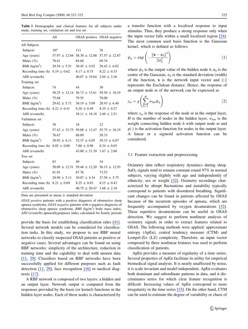
Table 1 summarizes the demographic and clinical data for

the whole population as well as for training, validation and

test sets.

3 Methods

Neural networks have emerged as an important tool for

classification. Opposite to traditional statistical procedures

such as discriminant analysis, several advantages can be

derived from using neural networks for classification

problems [41]. Neural networks are nonlinear models,

which makes them flexible in modelling real world com-

plex relationships. No knowledge of the underlying

probability distribution is required. Moreover, neural net-

works are able to estimate the posterior probabilities, which

324 Med Biol Eng Comput (2008) 46:323–332

123

provide the basis for establishing classification rules [41].

Several network models can be considered for classifica-

tion tasks. In this study, we propose to use RBF neural

networks to classify suspected OSAS patients as positive or

negative cases. Several advantages can be found on using

RBF networks: simplicity of the architecture, reduction in

training time and the capability to deal with unseen data

[11, 29]. Classifiers based on RBF networks have been

successfully applied for different purposes such as fault

detection [11, 29], face recognition [16] or medical diag-

nosis [17].

A RBF network is composed of two layers: a hidden and

an output layer. Network output is computed from the

responses provided by the basis (or kernel) functions in the

hidden layer nodes. Each of these nodes is characterized by

a transfer function with a localized response to input

stimulus. Thus, they produce a strong response only when

the input vector falls within a small localized region [24].

The most common used basis function is the Gaussian

kernel, which is defined as follows:

wh ¼ exp � x� chk k2

2r2h

!ð1Þ

where wh is the output value of the hidden node h, ch is the

centre of the Gaussian, rh is the standard deviation (width)

of the function, x is the network input vector and k�krepresents the Euclidean distance. Hence, the response of

an output node m of the network can be expressed as

ym ¼ gXH

h¼1

whmwh

!ð2Þ

where ym is the response of the node m in the output layer,

H is the number of nodes in the hidden layer, whm is the

weight connecting hidden node h with output node m and

g(�) is the activation function for nodes in the output layer.

A linear or a sigmoid activation function can be

considered.

3.1 Feature extraction and preprocessing

Oximetry data reflect respiratory dynamics during sleep.

SaO2 signals tend to remain constant round 97% in normal

subjects, varying slightly with age and independently of

ethnicity, sex or weight [32]. Oximetry recordings char-

acterized by abrupt fluctuations and instability typically

correspond to patients with disordered breathing. Signifi-

cant changes can be found in patients affected by OSAS

because of the recurrent episodes of apnoea, which are

frequently accompanied by oxygen desaturations [32].

These repetitive desaturations can be useful in OSAS

detection. We suggest to perform nonlinear analysis of

oximetry signals in order to extract features related to

OSAS. The following methods were applied: approximate

entropy (ApEn), central tendency measure (CTM) and

Lempel-Ziv (LZ) complexity. Therefore, an input vector

composed by three nonlinear features was used to perform

classification of patients.

ApEn provides a measure of regularity of a time series.

Several properties of ApEn facilitate its utility for empirical

biomedical signal analysis. It is nearly unaffected by noise,

it is scale invariant and model independent. ApEn evaluates

both dominant and subordinate patterns in data, and it dis-

criminates series for which clear feature recognition is

difficult. Increasing values of ApEn correspond to more

irregularity in the time series [33]. On the other hand, CTM

can be used to estimate the degree of variability or chaos of

Table 1 Demographic and clinical features for all subjects under

study, training set, validation set and test set

All OSAS positive OSAS negative

All Subjects

Subjects 187 111 76

Age (years) 57.97 ± 12.84 58.30 ± 12.88 57.57 ± 12.87

Males (%) 78.61 84.68 69.74

BMI (kg/m2) 29.54 ± 5.51 30.45 ± 4.92 28.42 ± 6.02

Recording time (h) 8.19 ± 0.62 8.17 ± 0.75 8.22 ± 0.33

AHI (events/h) 40.07 ± 19.64 2.04 ± 2.36

Training set

Subjects 74 44 30

Age (years) 58.25 ± 12.14 56.73 ± 13.61 59.59 ± 10.19

Males (%) 75.68 79.55 70.00

BMI (kg/m2) 29.62 ± 5.71 30.19 ± 5.09 28.93 ± 6.40

Recording time (h) 8.22 ± 0.41 8.20 ± 0.49 8.25 ± 0.27

AHI (events/h) 38.11 ± 18.18 2.60 ± 2.51

Validation set

Subjects 30 18 12

Age (years) 57.42 ± 15.75 59.08 ± 13.47 55.75 ± 18.19

Males (%) 76.67 88.89 58.33

BMI (kg/m2) 30.92 ± 6.11 32.37 ± 6.05 29.33 ± 6.07

Recording time (h) 8.05 ± 0.80 7.86 ± 0.98 8.34 ± 0.03

AHI (events/h) 43.00 ± 21.39 1.67 ± 2.60

Test set

Subjects 83 49 34

Age (years) 58.09 ± 12.51 59.46 ± 12.20 56.15 ± 12.93

Males (%) 81.93 87.76 73.53

BMI (kg/m2) 28.99 ± 5.11 30.07 ± 4.34 27.58 ± 5.75

Recording time (h) 8.21 ± 0.69 8.25 ± 0.83 8.15 ± 0.43

AHI (events/h) 40.75 ± 20.47 1.68 ± 2.10

Data are presented as mean ± standard deviation

OSAS positive patients with a positive diagnosis of obstructive sleep

apnoea syndrome, OSAS negative patients with a negative diagnosis of

obstructive sleep apnoea syndrome, BMI (kg/m2) body mass index,

AHI (events/h) apnoea/hypopnoea index calculated for hourly periods

Med Biol Eng Comput (2008) 46:323–332 325

123

a signal. A quantitative variability measure was obtained

via second-order difference plots. These kinds of scatter

plots are very useful in modelling biological systems such

as haemodynamics and heart rate variability. Low CTM

values correspond to signals with high variability [13].

Finally, LZ complexity is a non-parametric, simple-to-cal-

culate measure of complexity in a one-dimensional signal.

It is based on the Kolmogorov’s sense of complexity: LZ

complexity measures the number of steps that a computer

program which uses recursive copy and paste operations

will need to reproduce a coarse-grained sequence derived

from the original signal. The higher the value provided by

the LZ complexity, the higher the complexity of the ana-

lyzed time series [28]. Although the value of both ApEn and

LZ complexity increases for SaO2 signals characterized by

unstable ventilation, these methods provide a different

measure from our oximetry data. The difference between

regularity and complexity was illustrated in the study by

Goldberger et al. [18]. It was proved that an increase in

ApEn is not necessarily synonymous with an increase in

physiological complexity. Thus, it was derived that ApEn is

fundamentally a ‘‘regularity’’ statistic, not a direct index of

physiological complexity [18].

These three methods present suitable properties for bio-

medical signal processing. In fact, they have been applied to

different biomedical time series analysis [1, 14, 22]. Par-

ticularly, previous researches evaluated their utility in OSAS

diagnosis from SaO2 analysis [2, 23]. In the present research,

optimum input parameters derived from these studies were

used. SaO2 signals were divided into epochs of 200 samples

to estimate ApEn, CTM and LZ complexity. The measures

obtained from every epoch were averaged to compute final

values. To perform SaO2 analysis with ApEn, the run length

parameter (m) and the size of the tolerance window (r) were

set to 1 and 0.25 times the standard deviation of the original

sequence, respectively [23]. A radius (q) equal to 0.25 was

selected for CTM [2]. LZ complexity was computed by

converting SaO2 data into a 0–1 sequence. The median value

of SaO2 samples in each epoch was used as threshold [2]. It

was shown that the recurrence of apnoea events in patients

with OSAS produces a significant increase in ApEn and LZ

complexity values as well as lower CTM values [2, 23].

Finally, input features were linearly preprocessed to avoid

significant differences between their magnitudes. Features

were normalized to fall in the range between -1 and +1 [3].

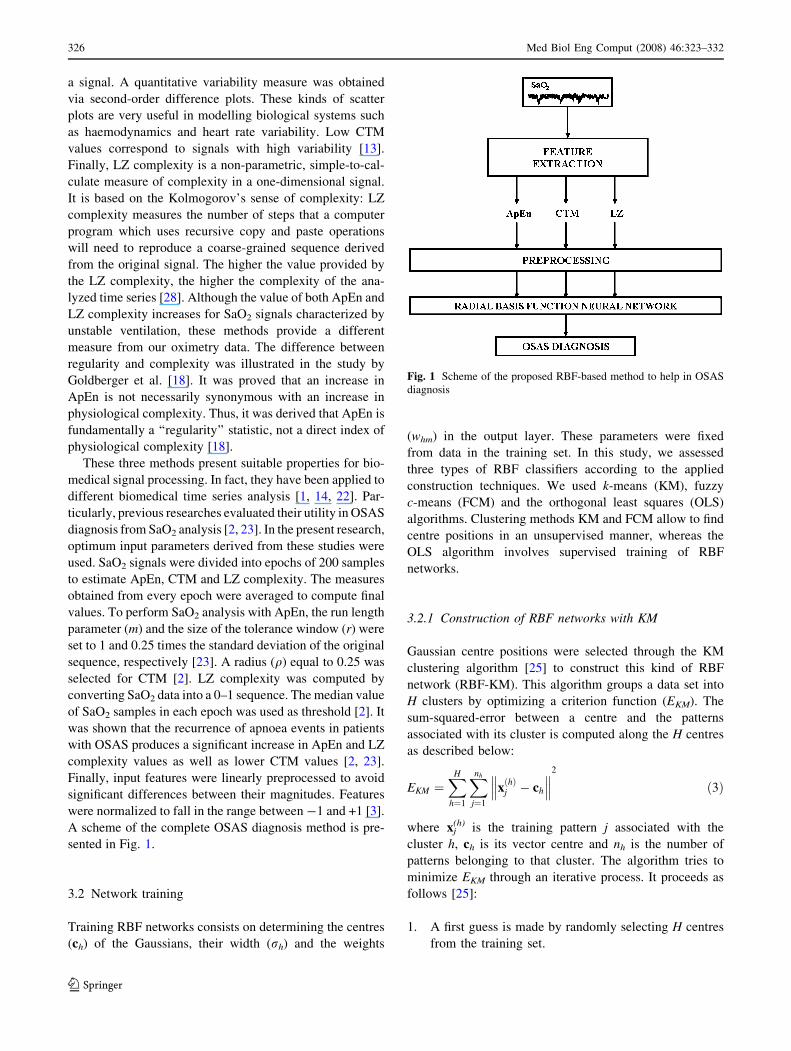
A scheme of the complete OSAS diagnosis method is pre-

sented in Fig. 1.

3.2 Network training

Training RBF networks consists on determining the centres

(ch) of the Gaussians, their width (rh) and the weights

(whm) in the output layer. These parameters were fixed

from data in the training set. In this study, we assessed

three types of RBF classifiers according to the applied

construction techniques. We used k-means (KM), fuzzy

c-means (FCM) and the orthogonal least squares (OLS)

algorithms. Clustering methods KM and FCM allow to find

centre positions in an unsupervised manner, whereas the

OLS algorithm involves supervised training of RBF

networks.

3.2.1 Construction of RBF networks with KM

Gaussian centre positions were selected through the KM

clustering algorithm [25] to construct this kind of RBF

network (RBF-KM). This algorithm groups a data set into

H clusters by optimizing a criterion function (EKM). The

sum-squared-error between a centre and the patterns

associated with its cluster is computed along the H centres

as described below:

EKM ¼XH

h¼1

Xnh

j¼1

xðhÞj � ch

��� ���2

ð3Þ

where xj(h) is the training pattern j associated with the

cluster h, ch is its vector centre and nh is the number of

patterns belonging to that cluster. The algorithm tries to

minimize EKM through an iterative process. It proceeds as

follows [25]:

1. A first guess is made by randomly selecting H centres

from the training set.

Fig. 1 Scheme of the proposed RBF-based method to help in OSAS

diagnosis

326 Med Biol Eng Comput (2008) 46:323–332

123

2. Each pattern xj is associated with the cluster whose

centre ch is closest to it.

3. The centres are recalculated to be the mean (centroid)

of the patterns in the cluster:

ch ¼1

nh

Xnh

j¼1

xðhÞj ð4Þ

4. The criterion function EKM is computed. If convergence

criteria (e.g. target error or maximum number of

iterations) are not met, process is repeated from step

2 by reassigning each of the patterns in the data set.

Then, the p-nearest neighbour heuristic was applied to

determine the width (rh) of the basis functions. According

to this rule, the standard deviation of a Gaussian is

computed as the root mean square of the distances from its

centre to the p nearest centres:

rh ¼1

p

Xp

j¼1

ch � cj

�� ��2

!12

ð5Þ

where cj are the p-nearest neighbours of ch. A p value equal

to 3 was assumed, as it was applied in [11].

A hyperbolic tangent activation function [6] was con-

sidered for neurons in the output layer of our RBF-KM

networks. It is a nonlinear sigmoid function whose output

lies in the range between -1 and +1. Then, the determi-

nation of the second layer weights is not a linear problem,

and hence a nonlinear optimization of these weights is

required [6]. The scaled conjugate gradient (SCG) algo-

rithm was applied for optimizing output layer weights in a

supervised manner [31]. It avoids crucial user-dependant

parameters and time-consuming line search [31]. SCG has

been widely used for nonlinear optimization such as train-

ing multilayer perceptron (MLP) neural networks [6, 21].

The following data were involved in weight optimization:

w ¼ ½w1. . .wH � ð6Þ

wh ¼ wh x1ð Þ. . .wh xNð Þ½ �T; h ¼ 1; . . .;H ð7ÞW ¼ w1; . . .;wM½ � ð8Þ

wm ¼ w1m; . . .;wHm½ �T; m ¼ 1; . . .;M ð9ÞD ¼ d1; . . .; dM½ � ð10Þ

dm ¼ dm x1ð Þ. . .dm xNð Þ½ �T ; m ¼ 1; . . .;M ð11Þ

where, given a RBF network with M output nodes and a

training set with N samples, w is the N 9 H matrix con-

taining the hidden node activation vectors, W is the H 9 M

matrix of weights to be determined and D is the N 9 M

matrix with output target vectors. Hidden node activation

vectors were computed from feature vectors in the training

set and were used for weight optimization. A target vector

was associated with each of them according to the initial

training patterns. During weight optimization, SCG aims to

minimize the mean squared error between network outputs

and their corresponding target values.

3.2.2 Construction of RBF networks with FCM

The FCM clustering algorithm [5] was used to construct

the second RBF network (RBF-FCM). As the KM algo-

rithm, FCM finds Gaussian centres from training data. The

algorithm aims to minimize a criterion function EFCM

(H,f ), which is defined as follows:

EFCM H; fð Þ ¼XH

h¼1

XN

n¼1

U h; nð Þf xn � chk k2 ð12Þ

where U is the H 9 N membership matrix and f (f [ 1) is

the fuzziness index. Unlike KM clustering, the elements of

matrix U(uhn) take a value in [0,1] to represent the grade of

membership of a training pattern xn to a cluster ch. The

FCM algorithm works as follows [5]:

1. The membership function U is initialized. Its elements

must to fulfil the next condition:

XH

h¼1

uhn ¼ 1 ð13Þ

2. The centres of the basis functions are computed

according to the expression:

ch ¼PN

n¼1 ufhnxnPN

n¼1 ufhn

ð14Þ

3. The U elements are updated according to

uhn ¼1

PHj¼1

xn�chk k2

xn�cjk k2

� � 2f�1

ð15Þ

4. Steps 2 and 3 are repeated until the change in

EFCM (H,f) is less than a threshold value or the

maximum number of iterations has been reached.

Subsequently, the p-nearest neighbour heuristic was

applied to determine Gaussian widths, as in RBF-KM. In

addition, a hyperbolic tangent activation function was

considered for nodes in the output layer of our RBF-FCM

networks. As described earlier, the SCG algorithm was

applied to optimize weights in the output layer.

3.2.3 Construction of RBF networks with OLS

The OLS algorithm [12] was applied to construct the third

RBF network (RBF-OLS). Whereas KM and FCM perform

Med Biol Eng Comput (2008) 46:323–332 327

123

unsupervised centre selection, the OLS algorithm finds

centres and weights in a supervised manner. A linear

activation function is assumed by OLS for nodes in the

output layer. The OLS procedure is implemented by con-

sidering the RBF network as a special case of the linear

regression model. Then, Eq. 2 is expressed as

dmðxnÞ ¼XH

h¼1

whmwh þ em ð16Þ

where dm is the desired output value corresponding with the

input pattern xn for the output node m and em is the

associated error. In OLS, all the training samples are

considered as candidates for centres. Thus, it refers to a

problem of subset model selection. In the matrix form,

Eq. 16 can be expressed as follows:

D ¼ WWþ E ð17Þ

where

E ¼ e1. . .eM½ � ð18Þ

em ¼ emðx1Þ. . .emðxNÞ½ �T; m ¼ 1; . . .;M ð19Þ

Matrices w; W and D were previously defined in

expressions (6), (8) and (10), respectively. Row vectors

of w are known as the regressors which form a set of basis

vectors of the space defined by nodes in the hidden layer.

These regressors are usually correlated. The influence of

each of them on the network output cannot be assessed. To

avoid this, the OLS method involves finding a set of

orthogonal basis vectors for the space defined by these

regressors. Thus, matrix w can be decomposed as

w ¼ VA ð20Þ

where A is a H 9 H triangular matrix, with 1s on the

diagonal and 0s below the diagonal, and V=[v1…vH] is a

N 9 H matrix with orthogonal columns. Equation 17 can

then be rewritten as

D ¼ VGþ E ð21Þ

The H 9 M matrix G represents the OLS solution. It

satisfies the next condition

AW ¼ G ¼g11 � � � g1M

..

. . .. ..

.

gH1 � � � gHM

264

375 ð22Þ

The standard Gram–Schmidt method can be used to

derive A and G [7]. Thus, the weight matrix W can be

computed by solving the triangular system in (22). On the

other hand, the OLS algorithm is used to select the

significant regressors, i.e. to take the appropriate centres

from the set of candidates. The selection process is based

on the orthogonal basis formed by columns of V. An error

reduction ratio is defined for each of these basis vectors vh:

err½ �h ¼XM

m¼1

g2hm

!vT

h vh=trace DTD� �

; h¼ 1; . . .;H ð23Þ

At iteration h of the algorithm, a candidate is selected as

the regressor h if it provides the largest error reduction ratio

from the rest of H - h + 1 candidates. The algorithm

finishes either when the number of centres is reached or

adding new centres does not decrease the error ratio

significantly.

In contrast to RBF-KM and RBF-FCM networks, a

single width value is applied for all the Gaussians in RBF-

OLS networks. Moreover, it must be defined by the user

before applying the OLS method. Since all the training

samples can be selected as centres, the width (r) of the

Gaussians was computed as follows [21]:

r ¼ gdmaxffiffiffiffiffiffiffi

2Hp ð24Þ

where dmax represents the maximum distance between two

training patterns and g is an empirical scale factor. To

evaluate this parameter, we applied ten different values

from 0.1 to 1.

3.3 Network design

Several modelling decisions relating to our classification

method must be specified. We decided to use a single output

node since output space must be only divided into two

regions: OSAS negative or OSAS positive. These regions

were identified by their target values (+1 and -1) to carry

out network training. Thus, a negative or zero network

output value was interpreted as OSAS positive. The

remaining design dilemma consists on determining the

architecture of our RBF networks, i.e., the number of

Gaussian centres in the network. There is not an exact rule

to establish the size of the hidden layer. Selecting the most

appropriate network size is termed as the model-order

selection problem and it arises in every neural network

application [6]. In our study, we propose a network-growing

approach to select the most suitable number of centres.

Multiple network configurations were evaluated for each of

the RBF types by varying the number of centres [6].

We used the Matlab1 software to implement our RBF

classifiers. The training set with 74 subjects was used to

train the networks. The architecture of the three RBF net-

works was optimized by varying the number of hidden

nodes from 2 up to 74, i.e., the size of the training set.

Network architecture directly affects the generalization

capability of the classifier, i.e., its ability to classify well

new input data [21]. The best generalization performance is

achieved by a network whose complexity is neither too

small nor too large [6, 21]. There is a trade-off between the

328 Med Biol Eng Comput (2008) 46:323–332

123

bias and the variance of the model. A too simple model

(large bias) could lead to underfit the data. The model may

not have the ability to learn enough the underlying distri-

bution. A too complex model (large variance) could

capture the noise present in the training data, leading to

overfitting [6]. Accuracy was considered to assess the

classification performance of a network configuration. The

average accuracy on the validation set was computed from

50 runs. In addition, we observed the influence of the

parameter g to adjust the width of the Gaussians in RBF-

OLS networks. We assessed ten different values of g by

varying it from 0.1 to 1. The best classification perfor-

mance on the validation set was obtained with g = 0.8.

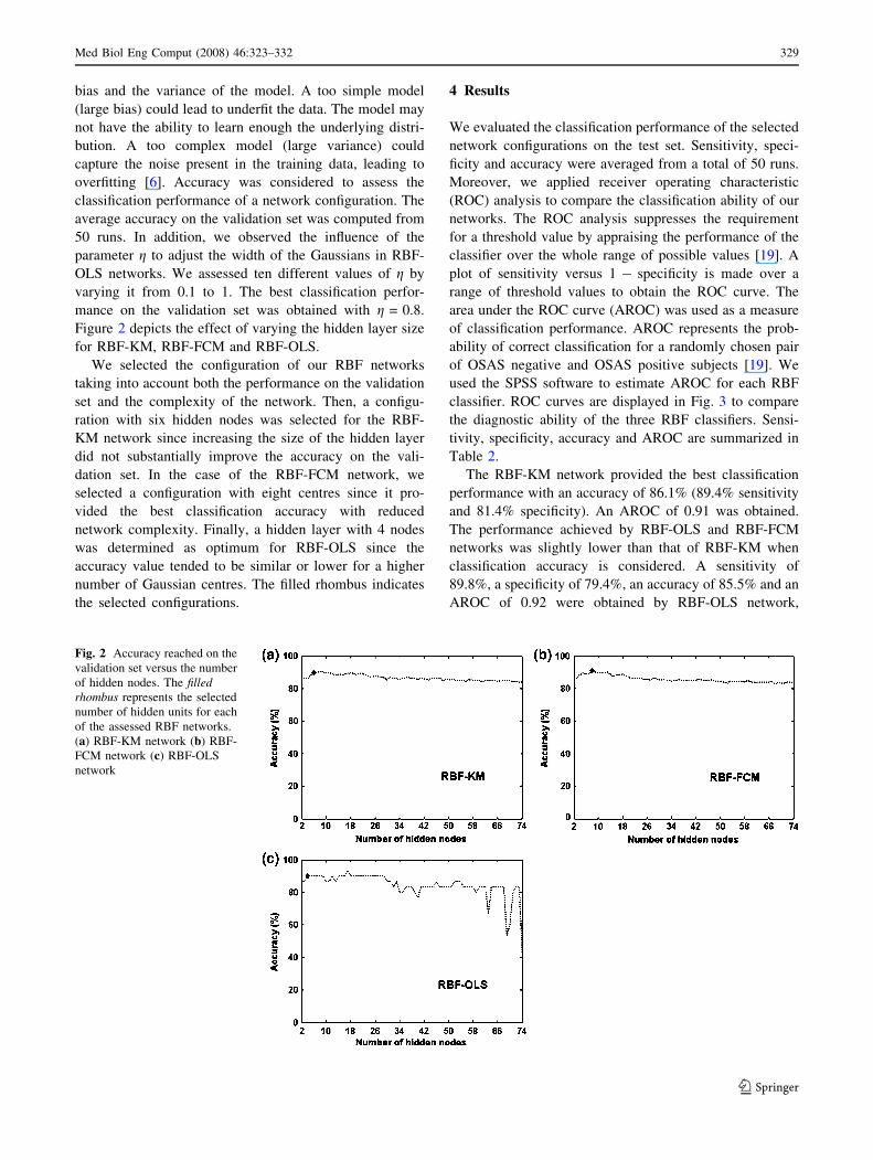
Figure 2 depicts the effect of varying the hidden layer size

for RBF-KM, RBF-FCM and RBF-OLS.

We selected the configuration of our RBF networks

taking into account both the performance on the validation

set and the complexity of the network. Then, a configu-

ration with six hidden nodes was selected for the RBF-

KM network since increasing the size of the hidden layer

did not substantially improve the accuracy on the vali-

dation set. In the case of the RBF-FCM network, we

selected a configuration with eight centres since it pro-

vided the best classification accuracy with reduced

network complexity. Finally, a hidden layer with 4 nodes

was determined as optimum for RBF-OLS since the

accuracy value tended to be similar or lower for a higher

number of Gaussian centres. The filled rhombus indicates

the selected configurations.

4 Results

We evaluated the classification performance of the selected

network configurations on the test set. Sensitivity, speci-

ficity and accuracy were averaged from a total of 50 runs.

Moreover, we applied receiver operating characteristic

(ROC) analysis to compare the classification ability of our

networks. The ROC analysis suppresses the requirement

for a threshold value by appraising the performance of the

classifier over the whole range of possible values [19]. A

plot of sensitivity versus 1 - specificity is made over a

range of threshold values to obtain the ROC curve. The

area under the ROC curve (AROC) was used as a measure

of classification performance. AROC represents the prob-

ability of correct classification for a randomly chosen pair

of OSAS negative and OSAS positive subjects [19]. We

used the SPSS software to estimate AROC for each RBF

classifier. ROC curves are displayed in Fig. 3 to compare

the diagnostic ability of the three RBF classifiers. Sensi-

tivity, specificity, accuracy and AROC are summarized in

Table 2.

The RBF-KM network provided the best classification

performance with an accuracy of 86.1% (89.4% sensitivity

and 81.4% specificity). An AROC of 0.91 was obtained.

The performance achieved by RBF-OLS and RBF-FCM

networks was slightly lower than that of RBF-KM when

classification accuracy is considered. A sensitivity of

89.8%, a specificity of 79.4%, an accuracy of 85.5% and an

AROC of 0.92 were obtained by RBF-OLS network,

Fig. 2 Accuracy reached on the

validation set versus the number

of hidden nodes. The filledrhombus represents the selected

number of hidden units for each

of the assessed RBF networks.

(a) RBF-KM network (b) RBF-

FCM network (c) RBF-OLS

network

Med Biol Eng Comput (2008) 46:323–332 329

123

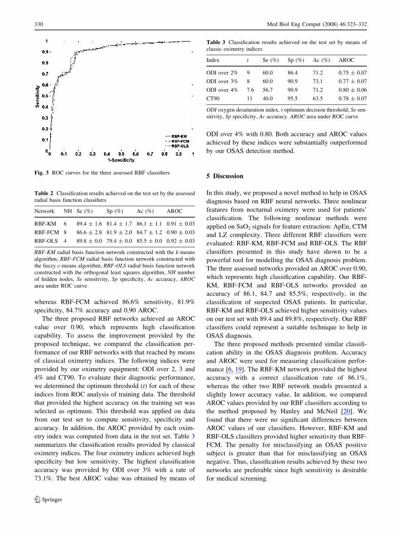
whereas RBF-FCM achieved 86.6% sensitivity, 81.9%

specificity, 84.7% accuracy and 0.90 AROC.

The three proposed RBF networks achieved an AROC

value over 0.90, which represents high classification

capability. To assess the improvement provided by the

proposed technique, we compared the classification per-

formance of our RBF networks with that reached by means

of classical oximetry indices. The following indices were

provided by our oximetry equipment: ODI over 2, 3 and

4% and CT90. To evaluate their diagnostic performance,

we determined the optimum threshold (t) for each of these

indices from ROC analysis of training data. The threshold

that provided the highest accuracy on the training set was

selected as optimum. This threshold was applied on data

from our test set to compute sensitivity, specificity and

accuracy. In addition, the AROC provided by each oxim-

etry index was computed from data in the test set. Table 3

summarizes the classification results provided by classical

oximetry indices. The four oximetry indices achieved high

specificity but low sensitivity. The highest classification

accuracy was provided by ODI over 3% with a rate of

73.1%. The best AROC value was obtained by means of

ODI over 4% with 0.80. Both accuracy and AROC values

achieved by these indices were substantially outperformed

by our OSAS detection method.

5 Discussion

In this study, we proposed a novel method to help in OSAS

diagnosis based on RBF neural networks. Three nonlinear

features from nocturnal oximetry were used for patients’

classification. The following nonlinear methods were

applied on SaO2 signals for feature extraction: ApEn, CTM

and LZ complexity. Three different RBF classifiers were

evaluated: RBF-KM, RBF-FCM and RBF-OLS. The RBF

classifiers presented in this study have shown to be a

powerful tool for modelling the OSAS diagnosis problem.

The three assessed networks provided an AROC over 0.90,

which represents high classification capability. Our RBF-

KM, RBF-FCM and RBF-OLS networks provided an

accuracy of 86.1, 84.7 and 85.5%, respectively, in the

classification of suspected OSAS patients. In particular,

RBF-KM and RBF-OLS achieved higher sensitivity values

on our test set with 89.4 and 89.8%, respectively. Our RBF

classifiers could represent a suitable technique to help in

OSAS diagnosis.

The three proposed methods presented similar classifi-

cation ability in the OSAS diagnosis problem. Accuracy

and AROC were used for measuring classification perfor-

mance [6, 19]. The RBF-KM network provided the highest

accuracy with a correct classification rate of 86.1%,

whereas the other two RBF network models presented a

slightly lower accuracy value. In addition, we compared

AROC values provided by our RBF classifiers according to

the method proposed by Hanley and McNeil [20]. We

found that there were no significant differences between

AROC values of our classifiers. However, RBF-KM and

RBF-OLS classifiers provided higher sensitivity than RBF-

FCM. The penalty for misclassifying an OSAS positive

subject is greater than that for misclassifying an OSAS

negative. Thus, classification results achieved by these two

networks are preferable since high sensitivity is desirable

for medical screening.

Fig. 3 ROC curves for the three assessed RBF classifiers

Table 2 Classification results achieved on the test set by the assessed

radial basis function classifiers

Network NH Se (%) Sp (%) Ac (%) AROC

RBF-KM 6 89.4 ± 1.6 81.4 ± 1.7 86.1 ± 1.1 0.91 ± 0.03

RBF-FCM 8 86.6 ± 2.8 81.9 ± 2.0 84.7 ± 1.2 0.90 ± 0.03

RBF-OLS 4 89.8 ± 0.0 79.4 ± 0.0 85.5 ± 0.0 0.92 ± 0.03

RBF-KM radial basis function network constructed with the k-means

algorithm, RBF-FCM radial basis function network constructed with

the fuzzy c-means algorithm, RBF-OLS radial basis function network

constructed with the orthogonal least squares algorithm, NH number

of hidden nodes, Se sensitivity, Sp specificity, Ac accuracy, AROCarea under ROC curve

Table 3 Classification results achieved on the test set by means of

classic oximetry indices

Index t Se (%) Sp (%) Ac (%) AROC

ODI over 2% 9 60.0 86.4 71.2 0.75 ± 0.07

ODI over 3% 8 60.0 90.9 73.1 0.77 ± 0.07

ODI over 4% 7.6 56.7 90.9 71.2 0.80 ± 0.06

CT90 11 40.0 95.5 63.5 0.78 ± 0.07

ODI oxygen desaturation index, t optimum decision threshold, Se sen-

sitivity, Sp specificity, Ac accuracy. AROC area under ROC curve

330 Med Biol Eng Comput (2008) 46:323–332

123

Classifiers based on neural networks have been previ-

ously pointed out as a robust alternative to traditional

statistical procedures [41]. Neural networks arise as a

useful data analysis tool to improve medical diagnosis. In

the present research, RBF networks provided satisfactory

accuracy and AROC values in OSAS diagnosis. Several

types of neural networks can be used for classification

purposes, although MLP neural networks trained with the

backpropagation algorithm are the most widely studied and

used neural classifiers [41]. In our study, we propose to use

RBF networks due to its simplified architecture and

reduced training time [24]. Moreover, training MLP net-

works with backpropagation requires a larger number of

user-dependant parameters to be a priori specified, such as

learning rate, momentum or number of training epochs

[21]. Other studies have previously applied neural net-

works to OSAS detection. Only clinical information was

used in these studies. Kirby et al. [27] proposed a

generalized regression neural network to classify patients

from 23 clinical variables. A sensitivity of 98.9% and a

specificity of 80% were reported by this study. Neverthe-

less, sensitivity and specificity measurements were not

complemented with ROC analysis. El-Solh et al. [15]

developed a neural network from anthropomorphic and

clinical measurements. A sensitivity of 94.9% and a

specificity of 64.7% were reached. Both studies reported

high sensitivity. However, in the methodology applied in

these studies any independent data set was used for

determining network architecture. As suggested in [6], the

performance of the selected networks should be confirmed

on a third set of data.

To our knowledge, this is the first study where neural

networks have been applied to OSAS diagnosis from

oximetry data. Our RBF classifiers outperformed classical

oximetry indices such as ODI over 2, 3 and 4%, and CT90

by using nonlinear features from SaO2. Nocturnal oximetry

recordings have been previously analyzed to compare their

diagnostic accuracy with that of PSG. Different techniques

have been developed with this purpose. Traditionally, the

mentioned oximetry indices were used for OSAS detection.

Netzer et al. [32] reviewed several significant studies

regarding to OSAS diagnosis by means of nocturnal

oximetry. Vazquez et al. [39] reported the highest diag-

nostic accuracy (98% sensitivity and 88% specificity) by

using ODI over 4%. However, a conservative threshold for

OSAS (AHI C 15 events/h) was used in such study. In

addition, a definition of arousals that differs from the cri-

teria of the Atlas task force was applied [37]. Magalang

et al. [30] proposed a combination of oximetry indices to

detect OSAS. A threshold of AHI C 15 events/h was

applied. This study reported a high sensitivity (90%) but a

low specificity (70%). Roche et al. [35] used information

from SaO2 (the cumulative time spent below 80% of sat-

uration) together with clinical variables to develop two

OSAS prediction models. A 62.1% accuracy was reached,

which is lower than our diagnostic accuracy by means of

RBF networks. Finally, previous studies analyzed the

utility of ApEn, CTM and LZ complexity from SaO2 data

in OSAS diagnosis [2, 23]. We verified that our RBF

classifiers improved the diagnostic performance of these

nonlinear methods. Neural networks provide an effective

method to process these features in order to achieve the

highest accuracy in OSAS diagnosis.

Nevertheless, an appropriate comparison with other

techniques cannot be carried out. Several approaches have

been proposed to solve the OSAS diagnosis problem.

However, data sets used for testing vary from one study to

another. Thus, it would be necessary to compare the dif-

ferent OSAS diagnosis techniques on the same group of

subjects to determine which is best. A large database of

suitable SaO2 signals was used in our study. For a future

research, we propose to use our data to validate such

techniques on a same test set. In addition, the assessment of

other Gaussian models, such as probabilistic neural net-

works (PNN) or constructive probabilistic neural networks

(CPNN), will be considered.

Some limitations can be found in our research. The

artefact rate is high in overnight pulse oximetry due to

movements during sleep. In addition, OSAS negative

patients who suffer from lung disease (e.g., chronic

obstructive pulmonary disease) may present desaturation

events that could lead to incorrect classification. Further-

more, a larger patients’ database could improve

classification performance since neural networks require an

important amount of training data to achieve good gener-

alization ability [21, 24].

In summary, we verified the capability of RBF classi-

fiers to help in OSAS diagnosis. Nonlinear information

from nocturnal oximetry was used for patients’ classifica-

tion by means of RBF neural networks. Our three RBF

models showed a high classification performance with

AROC values greater than 0.90. RBF-KM, RBF-FCM and

RBF-OLS provided a classification accuracy of 86.1, 84.7

and 85.5%, respectively. Particularly, RBF-KM and RBF-

OLS reached higher sensitivity values with 89.4 and

89.8%, respectively. Our results showed that the proposed

neural networks improve previous OSAS diagnosis tech-

niques based on nocturnal oximetry [32]. Therefore, our

method could represent an alternative to PSG for early

OSAS detection.

Acknowledgments This research has been supported by Consejerıa

de Sanidad de la Junta de Castilla y Leon under project SAN/191/

VA03/06. The authors are also thankful for the fruitful comments of

the referees.

Med Biol Eng Comput (2008) 46:323–332 331

123

References

1. Aboy M, Hornero R, Abasolo D et al (2006) Interpretation of the

Lempel-Ziv complexity measure in the context of biomedical

signal analysis. IEEE Trans Biomed Eng 53:2282–2288

2. Alvarez D, Hornero R, Abasolo D et al (2006) Nonlinear

characteristics of blood oxygen saturation from nocturnal

oximetry for obstructive sleep apnoea detection. Physiol Meas

27:399–412

3. Basheer IA, Hajmeer M (2000) Artificial neural networks: fun-

damentals, computing, design, and application. J Microbiol

Methods 43:3–31

4. Baxt WG (1995) Application of artificial neural networks to

clinical medicine. Lancet 346:1135–1138

5. Bezdek JC (1981) Pattern recognition with fuzzy objective

function algorithms. Plenum Press, New York

6. Bishop CM (1995) Neural networks for pattern recognition.

Oxford University Press, Oxford

7. Bjorck A (1967) Solving linear least squares problems by Gram–

Schmidt orthogonalization. BIT 7:1–21

8. Bloch KE (2003) Getting the most out of nocturnal pulse oxim-

etry. Chest 124:1628–1630

9. Burioka N, Cornelissen G, Halberg F et al (2003) Approximate

entropy of human respiratory movement during eye-closed

waking and different sleep stages. Chest 123:80–86

10. Caldirola D, Bellodi L, Caumo A et al (2004) Approximate

entropy of respiratory patterns in panic disorder. Am J Psychiatr

161:79–87

11. Catelani M, Fort A (2000) Fault diagnosis of electronic analog

circuits using a radial basis function network classifier. Mea-

surement 28:147–158

12. Chen S, Cowan CFN, Grant PM (1991) Orthogonal least squares

learning algorithm for radial basis function networks. IEEE Trans

Neural Netw 2:302–309

13. Cohen ME, Hudson DL, Deedwania PC (1996) Applying con-

tinuous chaotic modeling to cardiac signals. IEEE Eng Med Biol

Mag 15:97–102

14. Cohen ME, Hudson DL (2000) New chaotic methods for bio-

medical signal analysis. In: Proceedings of the IEEE EMBS

international conference on information technology applications

in biomedicine, pp 123–128

15. El-Solh AA, Mador MJ, Ten-Brock E et al (1999) Validity of

neural network in sleep apnea. Sleep 22:105–111

16. Er MJ, Chen W, Wu S (2005) High-speed face recognition based

on discrete cosine transform and RBF neural networks. IEEE

Trans Neural Netw 16:679–691

17. Folland R, Hines EL, Boilot P et al (2002) Classifying coronary

dysfunction using neural networks through cardiovascular aus-

cultation. Med Biol Eng Comput 40:339–343

18. Goldberger AL, Peng CK, Lipsitz LA (2002) What is physiologic

complexity and how does it change with aging and disease?

Neurobiol Aging 23:23–26

19. Hanley JA, McNeil BJ (1982) The meaning and use of the area

under a receiving operating characteristic (ROC) curve. Radiol-

ogy 143:29–36

20. Hanley JA, McNeil BJ (1983) A method of comparing the areas

under receiver operating characteristic curves derived from the

same case. Radiology 148:839–843

21. Haykin S (1999) Neural networks: a comprehensive foundation.

Prentice-Hall, Englewood Cliffs

22. Hornero R, Abasolo D, Aboy M et al (2005) Interpretation of

approximate entropy: analysis of intracranial pressure approxi-

mate entropy during acute intracranial hypertension. IEEE Trans

Biomed Eng 52:1671–1680

23. Hornero R, Alvarez D, Abasolo D et al (2007) Utility of

approximate entropy from overnight pulse oximetry data in the

diagnosis of the obstructive sep apnea syndrome. IEEE Trans

Biomed Eng 54:107–113

24. Hush DR, Horne BG (1993) Progress in supervised neural net-

works. IEEE Signal Process Mag 10:8–39

25. Jain AK, Murty MN, Flynn PJ (1999) Data clustering: a review.

ACM Comput Surv 31:264–323

26. Jureyda S, Shucard DW (2004) Obstructive sleep apnea: an

overview of the disorder and its consequences. Semin Orthod

10:63–72

27. Kirby SD, Danter W, George CFP et al (1999) Neural network

prediction of obstructive sleep apnea from clinical criteria. Chest

116:409–415

28. Lempel A, Ziv J (1976) On the complexity of finite sequences.

IEEE Trans Inf Theory 22:75–81

29. Leonard JA, Kramer MA (1991) Radial basis function networks

for classifying process faults. IEEE Control Syst Mag 11:31–38

30. Magalang UJ, Dmochowski J, Veeramachaneni S et al (2003)

Prediction of the apnea-hypopnea index from overnight pulse

oximetry. Chest 124:1694–1701

31. Moller MF (1993) A scaled conjugate gradient algorithm for fast

supervised learning. Neural Netw 6:525–533

32. Netzer N, Eliasson AH, Netzer C et al (2001) Overnight pulse

oximetry for sleep-disordered-breathing in adults: a review. Chest

120:625–633

33. Pincus SM (2001) Assessing serial irregularity and its implica-

tions for health. Ann N Y Acad Sci 954:245–267

34. Rechtschaffen A, Kales A (1968) A manual of standardized ter-

minology, techniques and scoring system for sleep stages of

human subjects. Brain information services, Brain research

institute, University of California, Los Angeles

35. Roche N, Herer B, Roig C et al (2002) Prospective testing of two

models based on clinical and oximetric variables for prediction of

obstructive sleep apnea. Chest 121:747–752

36. Schlosshan D, Elliot MW (2004) Sleep 3: clinical presentation

and diagnosis of the obstructive sleep apnoea hypopnoea syn-

drome. Thorax 59:347–352

37. The Atlas Task Force (1992) EEG arousals: scoring rules and

examples. A preliminary report from the Sleep Disorder Task

Force of the American Sleep Disorders Association. Sleep

15:173–184

38. Van Houwelingen KG, Van Uffelen R, Van Vliet ACM (1999)

The sleep apnoea syndromes. Eur Heart J 20:858–866

39. Vazquez JC, Tsai WH, Flemons WW et al (2000) Automated

analysis of digital oximetry in the diagnosis of obstructive sleep

apnoea. Thorax 55:302–307

40. Young T, Peppard PE, Gottlieb DJ (2002) Epidemiology of

obstructive sleep apnea: a population health perspective. Am J

Respir Crit Care Med 165:1217–1239

41. Zhang GP (2000) Neural networks for classification: a survey.

IEEE Trans Syst Man Cybern Part C Appl Rev 30:451–462

332 Med Biol Eng Comput (2008) 46:323–332

123