Embed Size (px)
Citation preview

Real-time Processing of Ground BasedSynthetic Aperture Radar (GB-SAR)
Measurements
Heft 33 Darmstadt, Oktober 2011Schriftenreihe der Fachrichtung GeodäsieFachbereich Bauingenieurwesen und GeodäsieTechnische Universität DarmstadtISBN 978-3-935631-22-8

Heft 33
Darmstadt, Oktober 2011
Sabine Rödelsperger
Real-time Processing of Ground Based Synthetic ApertureRadar (GB-SAR) Measurements
SchriftenreiheFachrichtung Geodäsie
Fachbereich Bauingenieurwesen und GeodäsieTechnische Universität Darmstadt
ISBN 978-3-935631-22-8

Schriftenreihe Fachrichtung Geodäsie der Technischen Universität Darmstadt
Online unter: http://tuprints.ulb.tu-darmstadt.deDiese Arbeit ist gleichzeitig veröffentlicht in DGK Reihe C 688,ISBN 978-3-7696-5080-8, München 2011
Verantwortlich für die Herausgabe der Schriftenreihe:
Der Sprecher der Fachrichtung Geodäsieim Fachbereich Bauingenieurwesen und Geodäsieder Technischen Universität Darmstadt
Bezugsnachweis:
Technische Universität DarmstadtInstitut für Physikalische GeodäsiePetersenstraße 1364287 Darmstadt
ISBN: 978-3-935631-22-8

Real-time Processing of Ground Based Synthetic Aperture Radar (GB-SAR) Measurements
Vom Fachbereich 13 Bauingenieurwesen und Geodäsieder Technischen Universität Darmstadtzur Erlangung des akademischen Grades einesDoktor-Ingenieurs (Dr.-Ing.) genehmigte Dissertation
vorgelegt vonDipl.-Ing. Sabine Rödelspergeraus Offenbach am Main
Referent: Prof. Dr.-Ing. Carl GersteneckerKorreferent: Prof. Dr.-Ing. Matthias BeckerTag der Einreichung: 11. Januar 2011Tag der mündlichen Prüfung: 15. Juni 2011
Darmstadt, Oktober 2011D17

Vorwort
Die vorliegende Arbeit entstand während meiner Zeit als wissenschaftliche Mitarbeiterin am Institutfür Physikalische Geodäsie. IBIS wurde im Rahmen des Exupery Projektes angeschafft, gefördert durchdas Geotechnologien Programm des BMBF (Fördernummer 03G0646C). Für die programmiertechnischeUmsetzung der Daten-Prozessierung hat IDS freundlicherweise den Quellcode zum Ein- und Auslesender IBIS-Daten bereitgestellt.
Mein Dank gilt all denen Menschen, die zum Gelingen dieser Doktorarbeit in vielfältiger Weise beigetra-gen haben. Mein ganz besonderer Dank gilt meinem Doktorvater, Herrn Prof. Dr.-Ing. Carl Gerstenecker.Sie haben mich immer unterstützt und mir alle Möglichkeiten gegeben, die Arbeit umzusetzen. Ich möch-te bei Ihnen ganz herzlich für die Motivation, wertvollen Anregungen und Ideen bedanken. Des Weiterenmöchte ich mich herzlich bei Herrn Prof. Dr.-Ing. Matthias Becker bedanken für die Unterstützung beimErstellen dieser Arbeit und die Übernahme des Korreferats. Herrn Prof. Dr.-Ing. Andreas Eichhorn dankeich ganz herzlich für die Möglichkeiten mit IBIS in Österreich zu messen.
Allen Kollegen und Kolleginnen danke ich für die angenehme Zeit am Institut, insbesondere meinerZimmerkollegin Frau Dr.-Ing. Gwendolyn Läufer für die gute Zusammenarbeit und die hilfreichen Dis-kussionen, Herrn Dr.-Ing. Milo Hirsch für die Hilfestellung und Denkanstöße, Herrn Dipl.-Ing. DieterSteineck für die große Unterstützung bei den Messungen, Vorbereitungen und die zahlreichen Tage undNächte bei IBIS, Herrn Dipl.-Ing. Volker Buhl für die Hilfe bei den Messungen, Herrn Joachim Winterfür die stetige Unterstützung bei Material und den Vorbereitungen, Herrn Dipl.-Ing. Jens Martin für dieHilfe bei allen Computerfragen und -problemen, Herrn Dipl.-Ing. Ulrich Threin für die Hilfe bei allenelektrotechnischen Fragestellungen, Herrn Günther Abt für die Unterstützung bei technischen Aufgabenund Problemen.
Bedanken möchte ich mich außerdem bei meinen Freunden die mich seit Kindergarten-, Schul- undStudienzeiten begleiten und stets für die erforderliche Abwechslung sorgten.
Zu guter Letzt danke ich meinen Eltern. Eure Unterstützung, Bestärkungen und Liebe haben mich alldie Jahre durch mein Studium und Leben begleitet.
i

ii
Zusammenfassung
In den letzten Jahren hat sich bodengestütztes Radar mit synthetischer Apertur (GB-SAR) zu einemleistungsstarken Instrument für die Überwachung von Bewegungen und Deformationen bei Massenbe-wegungen, z. Bsp. Hangrutschungen, Gletscher und Vulkane, entwickelt. Das Ziel dieser Arbeit ist dieEntwicklung eines echtzeitfähigen Verfahrens für die Analyse von GB-SAR Daten, um den Status einerMassenbewegung mit der geringstmöglichen Verzögerung nach der Datenerfassung zu bestimmen.
Das GB-SAR Instrument IBIS-L ermöglicht die Fernerkundung eines Objektes bis zu einer Entfernungvon 4 km, indem es Mikrowellen mit einer Frequenz von 17.2 GHz aussendet und die reflektierten Echosempfängt. Alle 5 bis 10 Minuten wird ein zweidimensionales Amplituden- und Phasen-Bild generiertmit einer Auflösung von 0.75 m in Entfernung und 4.4 mrad in Azimut (4.4 m in 1 km Entfernung).Die gemessene Amplitude hängt von Objektgeometrie und -reflektivität ab. Aus der Differenz zweierPhasenbilder, die zu unterschiedlichen Zeitpunkten gemessen wurden, können für jede AuflösungszelleBewegungen in Blickrichtung abgeleitet werden. Es können ausschließlich relative Phasendifferenzengebildet werden (zwischen−π und+π), dass heißt, die Anzahl der Phasendurchgänge (Mehrdeutigkeit)ist unbekannt.
Außer von Bewegungen, wird die Phasendifferenz auch von atmosphärischen Störungen und Rauschenbeeinflusst. Um die Bewegungen abzuleiten, müssen für alle Auflösungzellen im Bild sowie für alle Zeit-schritte die Phasenmehrdeutigkeiten bestimmt und der atmosphärische Effekt geschätzt werden. Es exis-tiert bereits eine Vielzahl von Techniken zum Bestimmen der Phasenmehrdeutigkeiten, die speziell fürweltraumgestütztes SAR entwickelt wurden. Der Begriff Persistent Scatterer Interferometrie (PSI) stehtfür Techniken, die nur Zeitreihen von Punkten (PS) betrachten deren Phasenmessgenauigkeit gut ist(Standardabweichung unter 0.3 bis 0.4 rad) (Ferretti et al., 2001; Kampes, 2006). Die bekannten PSITechniken sind allerdings nur bedingt echtzeitfähig, da sie Zeitreihen analysieren.
Das in dieser Arbeit beschriebene, echtzeitfähige Verfahren wurde speziell für die Anforderungen vonbodengestütztem SAR entwickelt. Es ist eine Kombination von PSI mit Multi Model Adaptive Estimation(MMAE) (Marinkovic et al., 2005; Brown and Hwang, 1997). Die PS werden gemäß Ferretti et al. (2001)aus der Amplitudendispersion bestimmt, die ein Maß für die Phasenmessgenauigkeit darstellt. Darauswird eine Untermenge (PS Candidates (PSC)) ausgewählt, die zur Schätzung von Mehrdeutigkeiten undAtmosphäre herangezogen werden. Aufgrund zeitlicher Änderungen der Qualität der Punkte durch z.Bsp. Steinschläge, ist die PSC Auswahl abhängig von der Zeit.
Zur Vereinfachung der Bestimmung der Mehrdeutigkeiten werden sie nicht aus den Zeitreihen selbst ge-schätzt, sondern aus der Differenz der Zeitreihen zweier benachbarter PSC, da dadurch atmosphärischeEffekte reduziert werden. Für jede mögliche Mehrdeutigkeitslösung einer Zeitreihendifferenz existiertein Kalman Filter um sequentiell den Status eines kinematischen Prozesses zu schätzen. In jedem Zeit-schritt werden die neuen Beobachtungen den Filtern hinzugefügt. Die beste Mehrdeutigkeitslösung wirdmit Hilfe von Wahrscheinlichkeiten bestimmt, die anhand der Differenz der beobachteten und prädi-zierten Phase berechnet werden. Nach der rein zeitlichen Mehrdeutigkeitsbestimmung wird für jedenZeitschritt die räumliche Konsistenz geprüft und die Mehrdeutigkeiten der eigentlichen PSC Zeitrei-hen abgeleitet. Der atmosphärische Effekt wird aus einer Kombination von meteorologischen Daten undFilterung geschätzt. Anschließend werden die PS in das Netzwerk integriert.
Mit diesem Verfahren erhält man eine erste Schätzung der Bewegungen an den PS innerhalb weni-ger Sekunden bis Minuten nach der Datenerfassung. Mit jedem Zeitschritt werden neue Beobachtungenhinzugefügt und die Bestimmung der Mehrdeutigkeiten verbessert bis sie schließlich festgesetzt wer-den. Die endgültige Schätzung der Bewegungen liegt daher einige Minuten bis eine Stunde nach derDatenerfassung vor.
iii

Die Leistungsfähigkeit der Technik wird anhand von synthetischen sowie beobachteten Daten gezeigt.Die Ergebnisse von Kampagnen an vier verschiedenen Orten werden dargestellt: ein Steinbruch in Die-burg, Deutschland, eine Felswand in Bad Reichenhall, Deutschland, eine Kraterflanke auf Sao Miguel,Azoren und eine Hangrutschung in der Nähe von Innsbruck in den Österreichischen Alpen.
iv
Summary
In the last years, Ground based Synthetic Aperture Radar (GB-SAR) has proven to be a powerful toolfor monitoring displacements and deformation that accompany mass movements like e.g. landslides,glaciers and volcanic hazards. The goal of this thesis is to develop a real-time capable technique thatallows to analyse GB-SAR data and assess the state of a mass movement with the least delay possibleafter a GB-SAR measurement is acquired.
The GB-SAR instrument IBIS-L allows the remote monitoring of an object at a distance of up to 4 kmby transmitting microwaves at a frequency of 17.2 GHz and receiving the reflected echoes. Every 5to 10 minutes, it delivers a two-dimensional amplitude and phase image with a range resolution of0.75 m and a cross-range (azimuth) resolution of 4.4 mrad (4.4 m at a distance of 1 km). The amplitudedepends on object geometry and reflectivity. By computing the difference of two phase images observedat two different points in time, displacements in line-of-sight can be derived for each resolution cell.Only relative phase differences can be formed (ranging between −π and +π), thus, the number of fullphase cycles (i.e. phase ambiguity) is unknown.
Apart from displacements, the phase difference is also influenced by atmospheric disturbances andnoise. To determine displacements, it is necessary to unwrap the phase differences (i.e. determine thephase ambiguities) and estimate the atmospheric effect for each resolution cell and for each time step.Many different methods exist for phase unwrapping, mainly developed for spaceborne SAR. The termPersistent Scatterer Interferometry (PSI) describes a set of techniques, which analyses only phase timeseries at persistent scatterers (PS), i.e. resolution cells with a good phase standard deviation (usually lessthen 0.3 to 0.4 rad) (Ferretti et al., 2001; Kampes, 2006). The common PSI methods are, however, notdirectly real-time capable as they analyse time series.
The real-time analysis tool described in this thesis is especially designed for GB-SAR requirements. It isa combination of PSI with Multi Model Adaptive Estimation (MMAE) (Marinkovic et al., 2005; Brownand Hwang, 1997). The PS are selected according to Ferretti et al. (2001) using the amplitude dispersionindex, which describes the phase accuracy. Only a subset of this selection, the PS candidates (PSC), areused for phase unwrapping and estimation of the atmosphere. Due to temporal changes of PS quality,caused by e.g. rock falls, the PSC selection is changing with time.
To simplify the unwrapping, the ambiguities are not estimated from the time series itself but rather onthe difference of the time series of two neighbouring PSC. By that the atmospheric effect is reduced. Foreach possible ambiguity solution of a time series difference, a Kalman Filter exists to sequentially estimatethe state of a kinematic process. At each time step new observations are added to the filter. The bestambiguity solution is selected based on probabilities, which are computed from the difference betweenobserved and predicted phase. After this temporal unwrapping, a spatial unwrapping is performed foreach time step to make sure that the determined solution is spatially consistent. The atmospheric effectis estimated after the unwrapping using a combination of meteorological data and filtering. Finally, theremaining PS are integrated into the network.
With this technique, a first estimation of the displacements at the PS is available a few seconds to minutesafter the data acquisition. With every time step, new observations are added, which will improve thedetermination of ambiguities until they can be fixed. Thus, the final estimation of displacements isavailable a few minutes to one hour after the data acquisition.
The performance of the technique is shown by unwrapping synthetic data and real data from observationcampaigns at four different locations: a quarry in Dieburg, Germany, a mountain side in Bad Reichenhall,Germany, a caldera flank on Sao Miguel, Azores and a landslide near Innsbruck in the Austrian Alps.
v

vi
Contents
1. Introduction 1
2. Principles of GB-SAR 32.1. GB-SAR Technique . . . . . . . . . . . . . . . . . . . . . . . . . . . . . . . . . . . . . . . . . . . . 4
2.1.1. Range Resolution . . . . . . . . . . . . . . . . . . . . . . . . . . . . . . . . . . . . . . . . . 42.1.2. Cross Range Resolution . . . . . . . . . . . . . . . . . . . . . . . . . . . . . . . . . . . . . 52.1.3. Focusing . . . . . . . . . . . . . . . . . . . . . . . . . . . . . . . . . . . . . . . . . . . . . . 62.1.4. Geometric Properties . . . . . . . . . . . . . . . . . . . . . . . . . . . . . . . . . . . . . . 92.1.5. Radiometric Properties . . . . . . . . . . . . . . . . . . . . . . . . . . . . . . . . . . . . . 11
2.2. Interferometric SAR . . . . . . . . . . . . . . . . . . . . . . . . . . . . . . . . . . . . . . . . . . . . 132.2.1. Atmosphere . . . . . . . . . . . . . . . . . . . . . . . . . . . . . . . . . . . . . . . . . . . . 152.2.2. Topography . . . . . . . . . . . . . . . . . . . . . . . . . . . . . . . . . . . . . . . . . . . . 162.2.3. Displacement . . . . . . . . . . . . . . . . . . . . . . . . . . . . . . . . . . . . . . . . . . . 182.2.4. Signal to Noise Ratio and Coherence . . . . . . . . . . . . . . . . . . . . . . . . . . . . . 182.2.5. Statistics of Phase Observation . . . . . . . . . . . . . . . . . . . . . . . . . . . . . . . . 19
2.3. IBIS-L . . . . . . . . . . . . . . . . . . . . . . . . . . . . . . . . . . . . . . . . . . . . . . . . . . . . 202.3.1. Advantages and Disadvantages . . . . . . . . . . . . . . . . . . . . . . . . . . . . . . . . 222.3.2. Monitoring Requirements and Concepts . . . . . . . . . . . . . . . . . . . . . . . . . . . 23
3. Analysis of GB-SAR Data 263.1. Phase Unwrapping . . . . . . . . . . . . . . . . . . . . . . . . . . . . . . . . . . . . . . . . . . . . 263.2. Conventional InSAR Analysis . . . . . . . . . . . . . . . . . . . . . . . . . . . . . . . . . . . . . . 27
3.2.1. InSAR processing . . . . . . . . . . . . . . . . . . . . . . . . . . . . . . . . . . . . . . . . . 283.2.2. Atmospheric Correction . . . . . . . . . . . . . . . . . . . . . . . . . . . . . . . . . . . . . 30
3.3. Persistent Scatterer Interferometry . . . . . . . . . . . . . . . . . . . . . . . . . . . . . . . . . . . 313.3.1. Permanent Scatterers Technique . . . . . . . . . . . . . . . . . . . . . . . . . . . . . . . 343.3.2. Stanford Method for Persistent Scatterers . . . . . . . . . . . . . . . . . . . . . . . . . . 353.3.3. Delft PS-InSAR Processing Package . . . . . . . . . . . . . . . . . . . . . . . . . . . . . . 35
4. Real-time Monitoring Concept 364.1. Network Configuration . . . . . . . . . . . . . . . . . . . . . . . . . . . . . . . . . . . . . . . . . . 38
4.1.1. PS Selection . . . . . . . . . . . . . . . . . . . . . . . . . . . . . . . . . . . . . . . . . . . . 384.1.2. PSC Selection . . . . . . . . . . . . . . . . . . . . . . . . . . . . . . . . . . . . . . . . . . . 384.1.3. Triangulation . . . . . . . . . . . . . . . . . . . . . . . . . . . . . . . . . . . . . . . . . . . 394.1.4. Temporal Variability of PS/PSC Selection . . . . . . . . . . . . . . . . . . . . . . . . . . 40
4.2. Temporal Unwrapping . . . . . . . . . . . . . . . . . . . . . . . . . . . . . . . . . . . . . . . . . . 414.2.1. Kalman Filter Equations . . . . . . . . . . . . . . . . . . . . . . . . . . . . . . . . . . . . 424.2.2. Process Model . . . . . . . . . . . . . . . . . . . . . . . . . . . . . . . . . . . . . . . . . . . 444.2.3. Multiple Model Adaptive Estimation (MMAE) . . . . . . . . . . . . . . . . . . . . . . . 444.2.4. Success Rate . . . . . . . . . . . . . . . . . . . . . . . . . . . . . . . . . . . . . . . . . . . . 47
4.3. Spatial Unwrapping . . . . . . . . . . . . . . . . . . . . . . . . . . . . . . . . . . . . . . . . . . . . 484.3.1. Minimum Cost Flow (MCF) . . . . . . . . . . . . . . . . . . . . . . . . . . . . . . . . . . 494.3.2. Simplex Method for Solving MCF Problems . . . . . . . . . . . . . . . . . . . . . . . . . 514.3.3. Spatial Integration . . . . . . . . . . . . . . . . . . . . . . . . . . . . . . . . . . . . . . . . 55
4.4. Atmospheric Correction . . . . . . . . . . . . . . . . . . . . . . . . . . . . . . . . . . . . . . . . . 55
vii

4.5. Real-time Monitoring . . . . . . . . . . . . . . . . . . . . . . . . . . . . . . . . . . . . . . . . . . . 564.5.1. Hardware Configuration . . . . . . . . . . . . . . . . . . . . . . . . . . . . . . . . . . . . 564.5.2. Real-time Analysis Software . . . . . . . . . . . . . . . . . . . . . . . . . . . . . . . . . . 57
5. Field Tests 605.1. Quarry (Dieburg, Germany) . . . . . . . . . . . . . . . . . . . . . . . . . . . . . . . . . . . . . . . 615.2. Mountain Side (Bad Reichenhall, Germany) . . . . . . . . . . . . . . . . . . . . . . . . . . . . . 655.3. Caldera (Sao Miguel, Lagoa de Fogo, Azores) . . . . . . . . . . . . . . . . . . . . . . . . . . . . 685.4. Landslide (Gries im Sellrain, Austria) . . . . . . . . . . . . . . . . . . . . . . . . . . . . . . . . . 72
6. Conclusion and Outlook 78
References 80
List of Acronyms 84
List of Symbols 85
Appendix 89
A. Standard Deviation of Interferometric Phase 89A.1. Atmosphere . . . . . . . . . . . . . . . . . . . . . . . . . . . . . . . . . . . . . . . . . . . . . . . . . 89A.2. Topography . . . . . . . . . . . . . . . . . . . . . . . . . . . . . . . . . . . . . . . . . . . . . . . . . 89A.3. Coherence, SNR and Phase Standard Deviation . . . . . . . . . . . . . . . . . . . . . . . . . . . 91
B. Results for Quarry (Dieburg, Germany) 92
viii
1 Introduction
Hazards involving ground movements can lead to enormous human and economic losses. Ground move-ment and instabilities can either be caused by natural conditions and processes (e.g. climatic variations,volcanic activities, tectonic processes, glaciers) or by anthropogenic actions (e.g. mining, ground waterwithdrawal, deforestation). Every year, one Million people are exposed to weather-related landslidehazards around the globe (ISDR, 2009). Due to the recent climate change it is likely that the decrease ofpermafrost areas, changes in precipitation patterns and increase of extreme weather events will influencethe weather-related mass movement activities (IPCC, 2007). Studies on the effect of climate change onlandslides showed no significant increase of such events up to now but the geographic distribution, fre-quency and intensity is likely to change (ISDR, 2009; Collison et al., 2000; Modaressi, 2006). Continuousmonitoring of such regions can give insight into mechanisms and triggers of hazardous events.
The monitoring of ground movements typically comprises the actual observation of displacement anddeformation as well as the observation of triggering factors, such as e.g. rainfall or temperature. Geodeticmethods, e.g. Global Positioning System (GPS), total stations and leveling, allow the continuous moni-toring of displacements and deformation with high accuracy (e.g. Angeli et al., 2000; Gili et al., 2000).They are, however, limited to observations at distinct points. Laser scanning and photogrammetry de-liver areal displacements by generating and comparing DEMs at different times (e.g. Bitelli et al., 2004).Photogrammetry can only be applied during day time and both methods are only operable during goodweather conditions. Since the late 1970s, spaceborne Interferometric Synthetic Aperture Radar (InSAR)enables the monitoring of displacements of large areas with high spatial resolution during all weatherconditions (Bamler and Hartl, 1998; Massonnet and Feigl, 1998). The temporal resolution, however, islimited by the repeat cycle of the satellite, which is usually several days. With the recent development ofGround based Synthetic Aperture Radar (GB-SAR), it is possible to determine displacements and defor-mation of areas, up to 4 km2 in size with high spatial resolution (few meters), high temporal resolution(several minutes) and high accuracy (submillimeters to millimeters) (Pieraccini et al., 2003; Luzi et al.,2006; Herrera et al., 2009). Due to the use of microwaves, the monitoring can continue during allweather conditions.
The result of one GB-SAR acquisition is a two-dimensional image with range and azimuth resolutioncontaining amplitude and phase. The phase is dependent on the distance between instrument andresolution cell at the object. By acquiring two images, an interferogram, i.e. the areal phase differencemap can be formed. It depends on displacement and deformation of the object relative to the instrument,atmospheric changes between object and instrument and noise. Only the relative phase difference,ranging between −π and +π, can be measured. The number of full phase cycles (2π), i.e. ambiguity, isunknown. Thus, the maximum object velocity observable is limited by the sampling rate. Additionally,noise and atmospheric disturbances can make it difficult to find the correct ambiguity, which has to bedetermined for each time step at each resolution cell.
The objective of this thesis is, to develop a tool to analyse GB-SAR data in real-time, i.e. with the leastdelay possible, which can then act as basis for making rapid decisions, e.g. in terms of countermeasuresor evacuation. The analysis of GB-SAR data comprises the determination of ambiguities, i.e. phaseunwrapping in space and time, and the correction of atmospheric effects.
In chapter 2, the basic principles and concepts of the Synthetic Aperture Radar (SAR) technique withfocus on GB-SAR are discussed. The instrument IBIS-L, which was used for all tests and developmentsis introduced and its advantages and disadvantages to other common displacement monitoring tech-niques are described. Due to the use of microwaves, the geometry and properties of SAR images differcompletely from those of optical images. Amplitude and achievable accuracy for phase differences are
1

dependent on object geometry and material. Areas densely covered with vegetation are generally notobservable while rock faces and barren land can be monitored with high accuracy.
In chapter 3, the state of the art of post processing SAR data is given. The chapter is focused on two im-portant techniques: the conventional InSAR analysis, which evaluates interferogram by interferogram,and the Persistent Scatterer Interferometry (PSI), which evaluates the phase time series at distinct points.The disadvantage of the conventional InSAR analysis is that it is only based on interferograms, whichworks well for high quality data but fails completely when the noise is high due to e.g. poorly reflect-ing surfaces and atmospheric distortions. PSI only evaluates the phase at points of high quality. Bothmethods are described and similarities and differences between spaceborne SAR and GB-SAR analysisare pointed out.
In contrary to the InSAR analysis, PSI is usually not directly real-time capable due to the analysis of timeseries. Chapter 4 introduces a new PSI approach, especially designed for GB-SAR, which is capable ofderiving displacements in near-real-time, i.e. with the least delay possible. This technique combines thebenefits of the conventional PSI approach with Multi Model Adaptive Estimation (MMAE) (Marinkovicet al., 2005; Brown and Hwang, 1997).
In chapter 5, the results of four measurement campaigns carried out with IBIS-L are presented: mon-itoring of an active quarry in Dieburg, Germany, monitoring of a mountain side in Bad Reichenhall,Germany, monitoring of a caldera wall on island Sao Miguel, Azores and monitoring of a landslide in theAustrian Alps in Gries im Sellrain. These four campaigns show the flexibility of the instrument and thereal-time analysis technique.
Chapter 6 summarizes the findings and gives a short conclusion and outlook.
2
2 Principles of GB-SAR
Ground based Synthetic Aperture Radar (GB-SAR) is a novel technique based on microwave interfe-rometry designed for monitoring displacements due to natural hazards and man-made structures. Itprovides two dimensional displacement maps with high spatial resolution (several meters) and high ac-curacy (i.e. standard deviation 1/10 mm to 1 mm). As an active remote sensing technology, it does notdepend on external illumination and can therefore operate day and night under all weather conditions.
GB-SAR makes use of three basic techniques:
• Stepped Frequency Continuous Wave (SFCW): for obtaining range resolution;
• Synthetic Aperture Radar (SAR): for obtaining azimuth or cross-range resolution;
• Interferometry: for the determination of object displacements with high precision and accuracy.
The principles of the SFCW and SAR technique are described in section 2.1, while the interferometrictechnique is discussed in section 2.2.
The first proposal concerning the possibility of increasing the spatial resolution of radar observationsusing the SAR technique was made by Carl Wiley in the year 1951 (Curlander and McDonough, 1991).After several successful airborne SAR missions, the first civil spaceborne SAR mission (Seasat) waslaunched in 1978 by NASA. Since then, many SAR missions have been flown by various space agen-cies. The first European spaceborne mission was launched by ESA with ERS-1 in 1991 and later ERS-2in 1995.
Up to now SAR has proven to be a valuable tool for all kinds of applications as
• Military tasks, e.g. reconnaissance and surveillance (Leachtenauer and Driggers, 2001);
• Ocean monitoring, e.g. tracking of sea ice (Rothrock et al., 1992), monitoring of oil spills (Brekkeand Solberg, 2005) and measurement of wave properties (Schuler et al., 2004);
• Monitoring and characterization of ice, snow and glaciers (König et al., 2001);
• Monitoring mass movements (displacements) with interferometric SAR, e.g. earthquakes (Wrightet al., 2001) and landslides (Strozzi et al., 2005);
• Thematic mapping, e.g. biomass mapping (Bergen and Dobson, 1999);
• Generation of Digital Elevation Models (DEMs) (Moreira et al., 2004), e.g. Shuttle Radar Topogra-phy Mission (SRTM) (Rabus et al., 2003).
The use of the SAR technique on the ground was proposed by the Joint Research Center (JRC) of theEuropean Commission in the late 90s and the device named LiSA (Linear Synthetic Aperture Radar)was developed (Rudolf et al., 1999; Tarchi et al., 2000). At the beginning, test measurements wereperformed in a controlled environment until in 1998 the first outdoor measurement campaigns werecarried out. In the following years, the main application was displacement monitoring of landslidesand slopes (e.g. Antonello et al., 2004; Tarchi et al., 2003). The results were validated by means ofconventional measurements with e.g. extensometers, distometers and GPS. The successful tests ledto the foundation of the JRC spin-off company LiSALab srl in 2003 (http://www.lisalab.com). Thecompany offers mainly monitoring services of natural hazards and man made structures with LiSA.
The first commercially available GB-SAR was developed by the Italian company Ingegneria dei SistemiS.p.A. (IDS) in collaboration with the Department of Electronics and Telecommunication of the FlorenceUniversity. It is named IBIS-L (Image By Interferometric Survey) and is being manufactured and sold by
3
IDS (http://www.idscompany.it). All measurements presented in this study are carried out with thisinstrument. The specifications of IBIS-L are described in details in section 2.3.
2.1 GB-SAR Technique
SAR is an abbreviation for Synthetic Aperture Radar. While in Real Aperture Radar (RAR), image reso-lution is limited by the physical dimension of the antenna, in SAR the antenna is synthetically elongatedby moving the sensor perpendicular to the look direction (Curlander and McDonough, 1991).
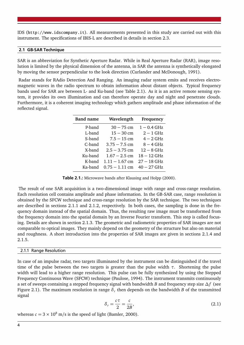
Radar stands for RAdio Detection And Ranging. An imaging radar system emits and receives electro-magnetic waves in the radio spectrum to obtain information about distant objects. Typical frequencybands used for SAR are between L- and Ku-band (see Table 2.1). As it is an active remote sensing sys-tem, it provides its own illumination and can therefore operate day and night and penetrate clouds.Furthermore, it is a coherent imaging technology which gathers amplitude and phase information of thereflected signal.
Band name Wavelength Frequency
P-band 30− 75 cm 1− 0.4 GHzL-band 15− 30 cm 2− 1 GHzS-band 7.5− 15 cm 4− 2 GHzC-band 3.75− 7.5 cm 8− 4 GHzX-band 2.5− 3.75 cm 12− 8 GHz
Ku-band 1.67− 2.5 cm 18− 12 GHzK-band 1.11− 1.67 cm 27− 18 GHz
Ka-band 0.75− 1.11 cm 40− 27 GHz
Table 2.1.: Microwave bands after Klausing and Holpp (2000).
The result of one SAR acquisition is a two-dimensional image with range and cross-range resolution.Each resolution cell contains amplitude and phase information. In the GB-SAR case, range resolution isobtained by the SFCW technique and cross-range resolution by the SAR technique. The two techniquesare described in sections 2.1.1 and 2.1.2, respectively. In both cases, the sampling is done in the fre-quency domain instead of the spatial domain. Thus, the resulting raw image must be transformed fromthe frequency domain into the spatial domain by an Inverse Fourier transform. This step is called focus-ing. Details are shown in section 2.1.3. The geometric and radiometric properties of SAR images are notcomparable to optical images. They mainly depend on the geometry of the structure but also on materialand roughness. A short introduction into the properties of SAR images are given in sections 2.1.4 and2.1.5.
2.1.1 Range Resolution
In case of an impulse radar, two targets illuminated by the instrument can be distinguished if the traveltime of the pulse between the two targets is greater than the pulse width τ. Shortening the pulsewidth will lead to a higher range resolution. This pulse can be fully synthesized by using the SteppedFrequency Continuous Wave (SFCW) technique (Paulose, 1994). The instrument transmits continuouslya set of sweeps containing a stepped frequency signal with bandwidth B and frequency step size∆ f (seeFigure 2.1). The maximum resolution in range δr then depends on the bandwidth B of the transmittedsignal
δr =cτ
2=
c
2B, (2.1)
whereas c = 3× 10⁸ m/s is the speed of light (Bamler, 2000).
4
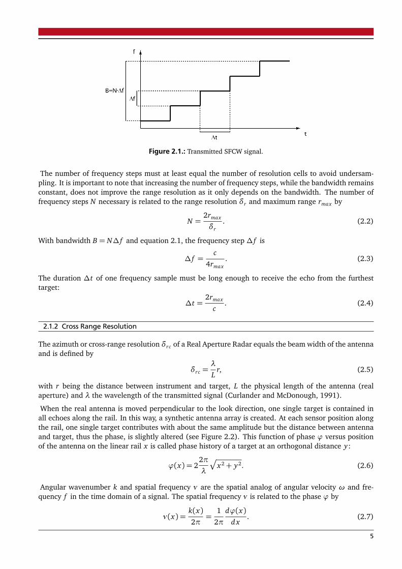
Figure 2.1.: Transmitted SFCW signal.
The number of frequency steps must at least equal the number of resolution cells to avoid undersam-pling. It is important to note that increasing the number of frequency steps, while the bandwidth remainsconstant, does not improve the range resolution as it only depends on the bandwidth. The number offrequency steps N necessary is related to the range resolution δr and maximum range rmax by
N =2rmax
δr. (2.2)
With bandwidth B = N∆ f and equation 2.1, the frequency step ∆ f is
∆ f =c
4rmax. (2.3)
The duration ∆t of one frequency sample must be long enough to receive the echo from the furthesttarget:
∆t =2rmax
c. (2.4)
2.1.2 Cross Range Resolution
The azimuth or cross-range resolution δrc of a Real Aperture Radar equals the beam width of the antennaand is defined by
δrc =λ
Lr, (2.5)
with r being the distance between instrument and target, L the physical length of the antenna (realaperture) and λ the wavelength of the transmitted signal (Curlander and McDonough, 1991).
When the real antenna is moved perpendicular to the look direction, one single target is contained inall echoes along the rail. In this way, a synthetic antenna array is created. At each sensor position alongthe rail, one single target contributes with about the same amplitude but the distance between antennaand target, thus the phase, is slightly altered (see Figure 2.2). This function of phase ϕ versus positionof the antenna on the linear rail x is called phase history of a target at an orthogonal distance y:
ϕ(x) = 22π
λ
p
x2+ y2. (2.6)
Angular wavenumber k and spatial frequency ν are the spatial analog of angular velocity ω and fre-quency f in the time domain of a signal. The spatial frequency ν is related to the phase ϕ by
ν(x) =k(x)2π=
1
2π
dϕ(x)d x
. (2.7)
5
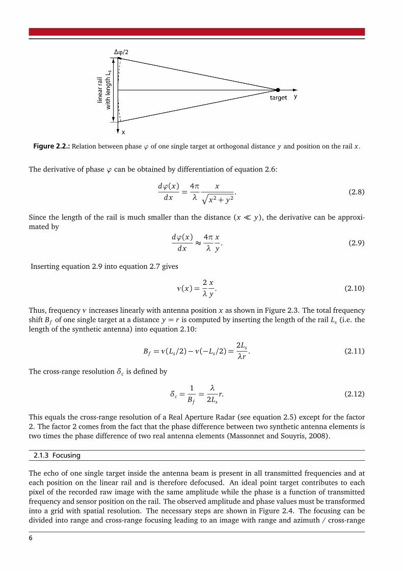
Figure 2.2.: Relation between phase ϕ of one single target at orthogonal distance y and position on the rail x .
The derivative of phase ϕ can be obtained by differentiation of equation 2.6:
dϕ(x)d x
=4π
λ
xp
x2+ y2. (2.8)
Since the length of the rail is much smaller than the distance (x � y), the derivative can be approxi-mated by
dϕ(x)d x
≈4π
λ
x
y. (2.9)
Inserting equation 2.9 into equation 2.7 gives
ν(x) =2
λ
x
y. (2.10)
Thus, frequency ν increases linearly with antenna position x as shown in Figure 2.3. The total frequencyshift B f of one single target at a distance y = r is computed by inserting the length of the rail Ls (i.e. thelength of the synthetic antenna) into equation 2.10:
B f = ν(Ls/2)− ν(−Ls/2) =2Ls
λr. (2.11)
The cross-range resolution δc is defined by
δc =1
B f=λ
2Lsr. (2.12)
This equals the cross-range resolution of a Real Aperture Radar (see equation 2.5) except for the factor2. The factor 2 comes from the fact that the phase difference between two synthetic antenna elements istwo times the phase difference of two real antenna elements (Massonnet and Souyris, 2008).
2.1.3 Focusing
The echo of one single target inside the antenna beam is present in all transmitted frequencies and ateach position on the linear rail and is therefore defocused. An ideal point target contributes to eachpixel of the recorded raw image with the same amplitude while the phase is a function of transmittedfrequency and sensor position on the rail. The observed amplitude and phase values must be transformedinto a grid with spatial resolution. The necessary steps are shown in Figure 2.4. The focusing can bedivided into range and cross-range focusing leading to an image with range and azimuth / cross-range
6
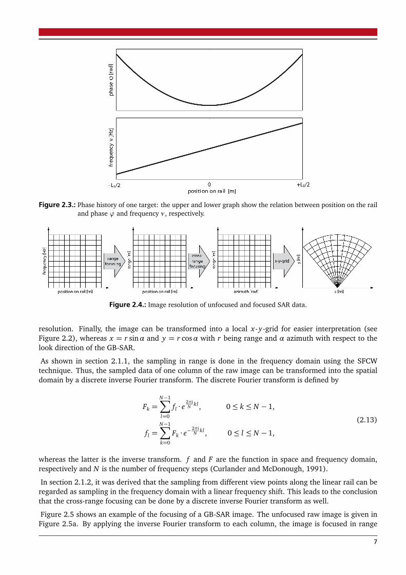
Figure 2.3.: Phase history of one target: the upper and lower graph show the relation between position on the railand phase ϕ and frequency ν , respectively.
Figure 2.4.: Image resolution of unfocused and focused SAR data.
resolution. Finally, the image can be transformed into a local x-y-grid for easier interpretation (seeFigure 2.2), whereas x = r sinα and y = r cosα with r being range and α azimuth with respect to thelook direction of the GB-SAR.
As shown in section 2.1.1, the sampling in range is done in the frequency domain using the SFCWtechnique. Thus, the sampled data of one column of the raw image can be transformed into the spatialdomain by a discrete inverse Fourier transform. The discrete Fourier transform is defined by
Fk =N−1∑
l=0
fl · e2πiN kl , 0≤ k ≤ N − 1,
fl =N−1∑
k=0
Fk · e−2πiN kl , 0≤ l ≤ N − 1,
(2.13)
whereas the latter is the inverse transform. f and F are the function in space and frequency domain,respectively and N is the number of frequency steps (Curlander and McDonough, 1991).
In section 2.1.2, it was derived that the sampling from different view points along the linear rail can beregarded as sampling in the frequency domain with a linear frequency shift. This leads to the conclusionthat the cross-range focusing can be done by a discrete inverse Fourier transform as well.
Figure 2.5 shows an example of the focusing of a GB-SAR image. The unfocused raw image is given inFigure 2.5a. By applying the inverse Fourier transform to each column, the image is focused in range
7
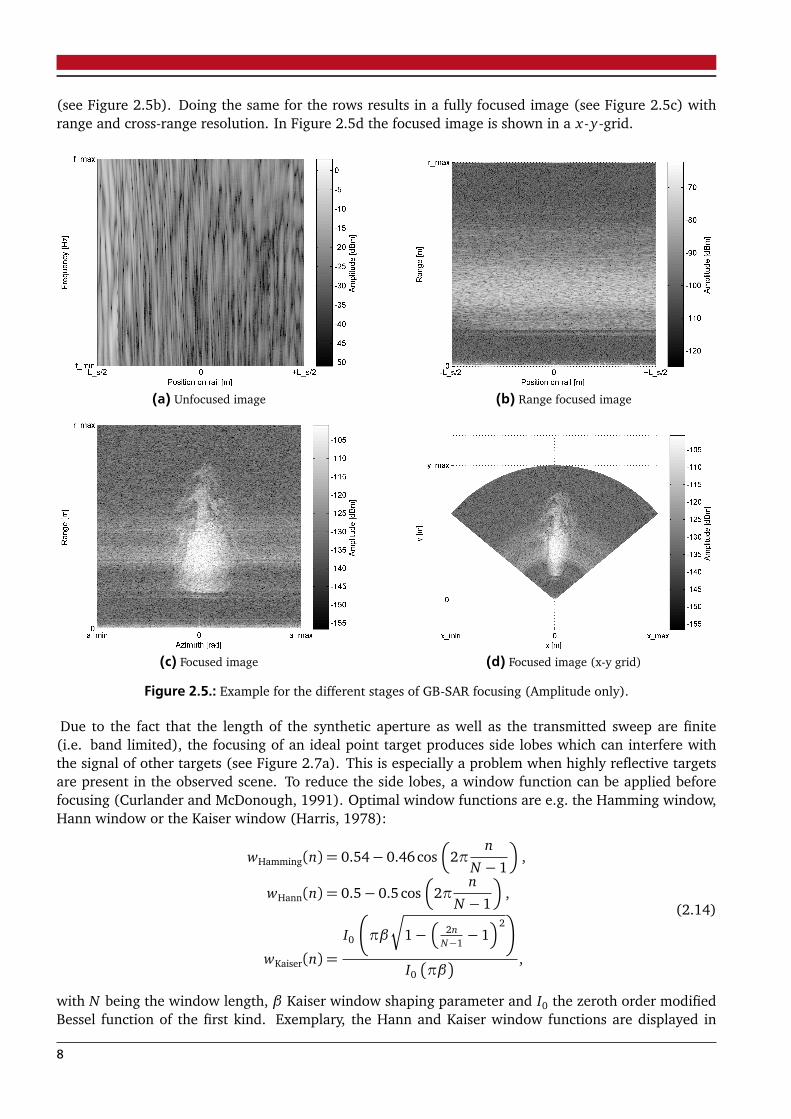
(see Figure 2.5b). Doing the same for the rows results in a fully focused image (see Figure 2.5c) withrange and cross-range resolution. In Figure 2.5d the focused image is shown in a x-y-grid.
(a) Unfocused image (b) Range focused image
(c) Focused image (d) Focused image (x-y grid)
Figure 2.5.: Example for the different stages of GB-SAR focusing (Amplitude only).
Due to the fact that the length of the synthetic aperture as well as the transmitted sweep are finite(i.e. band limited), the focusing of an ideal point target produces side lobes which can interfere withthe signal of other targets (see Figure 2.7a). This is especially a problem when highly reflective targetsare present in the observed scene. To reduce the side lobes, a window function can be applied beforefocusing (Curlander and McDonough, 1991). Optimal window functions are e.g. the Hamming window,Hann window or the Kaiser window (Harris, 1978):
wHamming(n) = 0.54− 0.46cos�
2πn
N − 1
�
,
wHann(n) = 0.5− 0.5 cos�
2πn
N − 1
�
,
wKaiser(n) =
I0
�
πβ
Ç
1−�
2nN−1− 1�2�
I0�
πβ� ,
(2.14)
with N being the window length, β Kaiser window shaping parameter and I0 the zeroth order modifiedBessel function of the first kind. Exemplary, the Hann and Kaiser window functions are displayed in
8
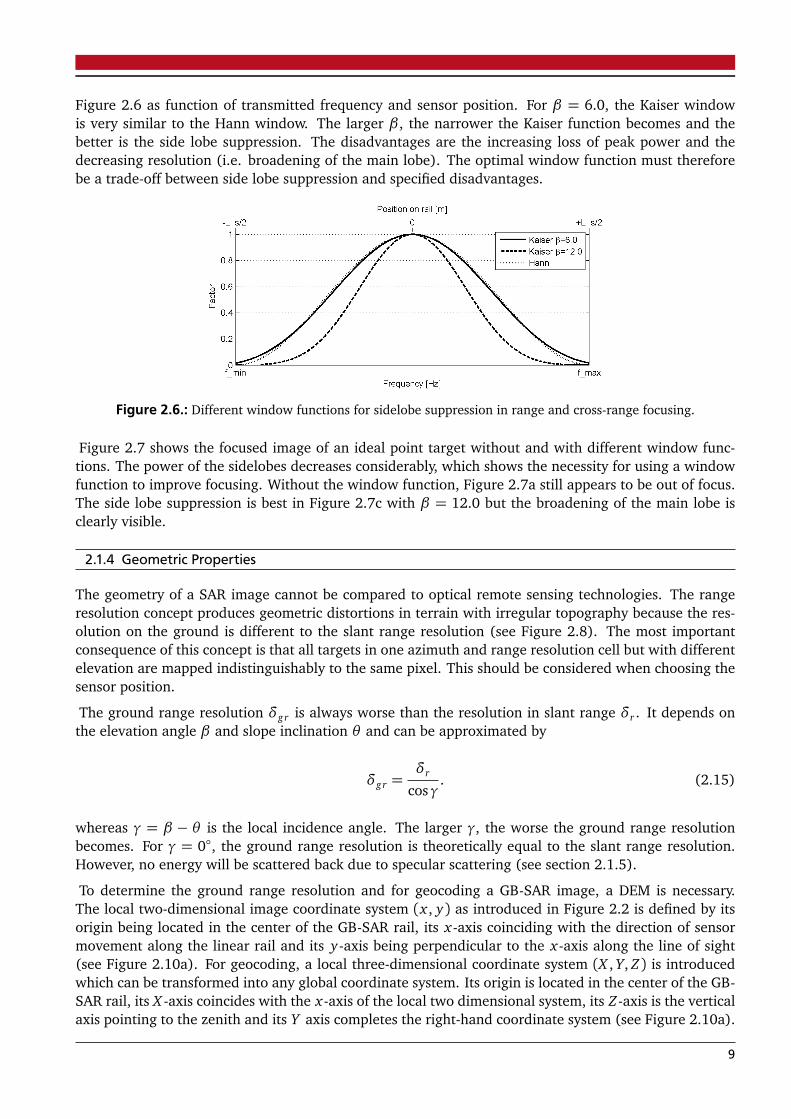
Figure 2.6 as function of transmitted frequency and sensor position. For β = 6.0, the Kaiser windowis very similar to the Hann window. The larger β , the narrower the Kaiser function becomes and thebetter is the side lobe suppression. The disadvantages are the increasing loss of peak power and thedecreasing resolution (i.e. broadening of the main lobe). The optimal window function must thereforebe a trade-off between side lobe suppression and specified disadvantages.
Figure 2.6.: Different window functions for sidelobe suppression in range and cross-range focusing.
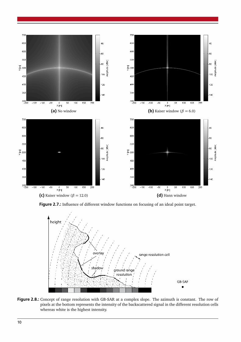
Figure 2.7 shows the focused image of an ideal point target without and with different window func-tions. The power of the sidelobes decreases considerably, which shows the necessity for using a windowfunction to improve focusing. Without the window function, Figure 2.7a still appears to be out of focus.The side lobe suppression is best in Figure 2.7c with β = 12.0 but the broadening of the main lobe isclearly visible.
2.1.4 Geometric Properties
The geometry of a SAR image cannot be compared to optical remote sensing technologies. The rangeresolution concept produces geometric distortions in terrain with irregular topography because the res-olution on the ground is different to the slant range resolution (see Figure 2.8). The most importantconsequence of this concept is that all targets in one azimuth and range resolution cell but with differentelevation are mapped indistinguishably to the same pixel. This should be considered when choosing thesensor position.
The ground range resolution δgr is always worse than the resolution in slant range δr . It depends onthe elevation angle β and slope inclination θ and can be approximated by
δgr =δr
cosγ. (2.15)
whereas γ = β − θ is the local incidence angle. The larger γ, the worse the ground range resolutionbecomes. For γ = 0◦, the ground range resolution is theoretically equal to the slant range resolution.However, no energy will be scattered back due to specular scattering (see section 2.1.5).
To determine the ground range resolution and for geocoding a GB-SAR image, a DEM is necessary.The local two-dimensional image coordinate system (x , y) as introduced in Figure 2.2 is defined by itsorigin being located in the center of the GB-SAR rail, its x-axis coinciding with the direction of sensormovement along the linear rail and its y-axis being perpendicular to the x-axis along the line of sight(see Figure 2.10a). For geocoding, a local three-dimensional coordinate system (X , Y, Z) is introducedwhich can be transformed into any global coordinate system. Its origin is located in the center of the GB-SAR rail, its X -axis coincides with the x-axis of the local two dimensional system, its Z-axis is the verticalaxis pointing to the zenith and its Y axis completes the right-hand coordinate system (see Figure 2.10a).
9
(a) No window (b) Kaiser window (β = 6.0)
(c) Kaiser window (β = 12.0) (d) Hann window
Figure 2.7.: Influence of different window functions on focusing of an ideal point target.
Figure 2.8.: Concept of range resolution with GB-SAR at a complex slope. The azimuth is constant. The row ofpixels at the bottom represents the intensity of the backscattered signal in the different resolution cellswhereas white is the highest intensity.
10
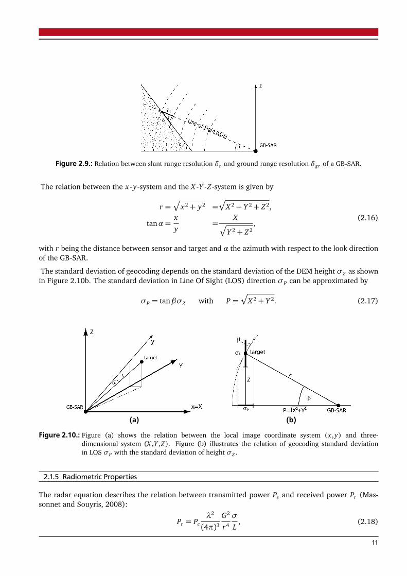
Figure 2.9.: Relation between slant range resolution δr and ground range resolution δgr of a GB-SAR.
The relation between the x-y-system and the X -Y -Z-system is given by
r =p
x2+ y2 =p
X 2+ Y 2+ Z2,
tanα=x
y=
Xp
Y 2+ Z2,
(2.16)
with r being the distance between sensor and target and α the azimuth with respect to the look directionof the GB-SAR.
The standard deviation of geocoding depends on the standard deviation of the DEM height σZ as shownin Figure 2.10b. The standard deviation in Line Of Sight (LOS) direction σP can be approximated by
σP = tanβσZ with P =p
X 2+ Y 2. (2.17)
(a) (b)
Figure 2.10.: Figure (a) shows the relation between the local image coordinate system (x ,y) and three-dimensional system (X ,Y ,Z). Figure (b) illustrates the relation of geocoding standard deviationin LOS σP with the standard deviation of height σZ .
2.1.5 Radiometric Properties
The radar equation describes the relation between transmitted power Pe and received power Pr (Mas-sonnet and Souyris, 2008):
Pr = Peλ2
(4π)3G2
r4
σ
L, (2.18)
11
with λ being the wavelength, G the antenna gain, r the distance, L the loss due to atmosphere and σthe Radar Cross Section (RCS) of the target. The RCS depends on target geometry and material anddescribes the effective area of an object measured in square meters. A target that radiates perfectlyisotropic (e.g. a sphere) has a RCS that equals the target’s physical extent. The larger the RCS, thehigher is the amount of energy reflected back.
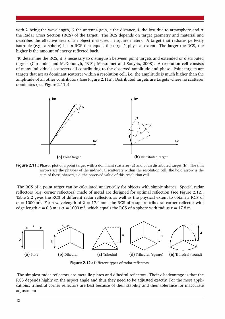
To determine the RCS, it is necessary to distinguish between point targets and extended or distributedtargets (Curlander and McDonough, 1991; Massonnet and Souyris, 2008). A resolution cell consistsof many individuals scatterers all contributing to the observed amplitude and phase. Point targets aretargets that act as dominant scatterer within a resolution cell, i.e. the amplitude is much higher than theamplitude of all other contributors (see Figure 2.11a). Distributed targets are targets where no scattererdominates (see Figure 2.11b).
(a) Point target (b) Distributed target
Figure 2.11.: Phasor plot of a point target with a dominant scatterer (a) and of an distributed target (b). The thinarrows are the phasors of the individual scatterers within the resolution cell; the bold arrow is thesum of these phasors, i.e. the observed value of this resolution cell.
The RCS of a point target can be calculated analytically for objects with simple shapes. Special radarreflectors (e.g. corner reflectors) made of metal are designed for optimal reflection (see Figure 2.12).Table 2.2 gives the RCS of different radar reflectors as well as the physical extent to obtain a RCS ofσ = 1000 m2. For a wavelength of λ = 17.4 mm, the RCS of a square trihedral corner reflector withedge length a = 0.3 m is σ = 1000 m2, which equals the RCS of a sphere with radius r = 17.8 m.
(a) Plate (b) Dihedral (c) Trihedral (d) Trihedral (square) (e) Trihedral (round)
Figure 2.12.: Different types of radar reflectors.
The simplest radar reflectors are metallic plates and dihedral reflectors. Their disadvantage is that theRCS depends highly on the aspect angle and thus they need to be adjusted exactly. For the most appli-cations, trihedral corner reflectors are best because of their stability and their tolerance for inaccurateadjustment.
12
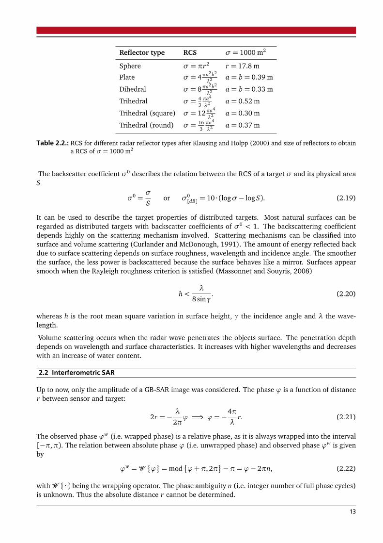
Reflector type RCS σ = 1000 m2
Sphere σ = πr2 r = 17.8 m
Plate σ = 4πa2 b2
λ2 a = b = 0.39 m
Dihedral σ = 8πa2 b2
λ2 a = b = 0.33 m
Trihedral σ = 43πa4
λ2 a = 0.52 m
Trihedral (square) σ = 12πa4
λ2 a = 0.30 m
Trihedral (round) σ = 163πa4
λ2 a = 0.37 m
Table 2.2.: RCS for different radar reflector types after Klausing and Holpp (2000) and size of reflectors to obtaina RCS of σ = 1000 m2
The backscatter coefficient σ0 describes the relation between the RCS of a target σ and its physical areaS
σ0 =σ
Sor σ0
[dB] = 10 · (logσ− log S). (2.19)
It can be used to describe the target properties of distributed targets. Most natural surfaces can beregarded as distributed targets with backscatter coefficients of σ0 < 1. The backscattering coefficientdepends highly on the scattering mechanism involved. Scattering mechanisms can be classified intosurface and volume scattering (Curlander and McDonough, 1991). The amount of energy reflected backdue to surface scattering depends on surface roughness, wavelength and incidence angle. The smootherthe surface, the less power is backscattered because the surface behaves like a mirror. Surfaces appearsmooth when the Rayleigh roughness criterion is satisfied (Massonnet and Souyris, 2008)
h<λ
8sinγ. (2.20)
whereas h is the root mean square variation in surface height, γ the incidence angle and λ the wave-length.
Volume scattering occurs when the radar wave penetrates the objects surface. The penetration depthdepends on wavelength and surface characteristics. It increases with higher wavelengths and decreaseswith an increase of water content.
2.2 Interferometric SAR
Up to now, only the amplitude of a GB-SAR image was considered. The phase ϕ is a function of distancer between sensor and target:
2r =−λ
2πϕ =⇒ ϕ =−
4π
λr. (2.21)
The observed phase ϕw (i.e. wrapped phase) is a relative phase, as it is always wrapped into the interval[−π,π). The relation between absolute phase ϕ (i.e. unwrapped phase) and observed phase ϕw is givenby
ϕw =W�
ϕ
=mod�
ϕ+π, 2π
−π= ϕ− 2πn, (2.22)
withW { · } being the wrapping operator. The phase ambiguity n (i.e. integer number of full phase cycles)is unknown. Thus the absolute distance r cannot be determined.
13
Comparing two SAR images of the same area, either collected at different time periods and/or fromdifferent sensor positions, the phase difference φw, i.e interferometric phase, is related to the changes indistance between sensor and target ∆r = r2− r1 by
φw =W¦
ϕw1 −ϕ
w2
©
=W�
−4π
λ(r1− r2)
�
=W�
4π
λ∆r�
. (2.23)
This technique is referred to as Interferometric Synthetic Aperture Radar (InSAR) (Hanssen, 2002). Themaximum unambiguous change of distance ∆rmax is restricted by the wavelength λ:
∆rmax =±λ/4. (2.24)
If amplitude a and phase ϕ are represented as complex value z with
z = a · eiϕ = a · (cosϕ+ i sinϕ), (2.25)
an interferogram is formed by
z1z∗2 = a1a2 · ei(ϕ1−ϕ2), (2.26)
whereas z∗ is the complex conjugated of z.
If an interferogram is formed using two SAR images collected at different time periods but from the samesensor position, the resulting phase difference is related to temporal changes of the distance betweensensor and target (e.g. displacements). The difference between the two time periods is referred to as thetemporal baseline Bt .
If the two SAR images are collected at the same time period but from different sensor positions, theresulting phase difference depends on the topography of the illuminated area. The effective distancebetween the two sensors is referred to as spatial baseline Bs. In conventional spaceborne InSAR, atemporal and spatial baseline are present whereas in GB-SAR the spatial baseline is usually zero, if it isnot introduced intentionally.
Depending on the type of baseline, the interferometric phase φw is the sum of several effects:
φw = φtopo︸︷︷︸
f (Bs)
+φdisp +φatm︸ ︷︷ ︸
f (Bt )
+φnoise − 2πn. (2.27)
φtopo is the phase difference due the topography in case of a spatial baseline, φdisp andφatm are temporalphase changes due to displacement and atmospheric effects, φnoise is noise and n is the integer phaseambiguity. The different components of the interferometric phase equation are described in detail in thefollowing sections 2.2.1, 2.2.2 and 2.2.3. Its stochastic properties are discussed in sections 2.2.4 and2.2.5.
The left side of equation 2.27 is the observed phase difference while the right side contains the unknownparameters. In case the application is to determine a DEM, equation 2.27 can be rearranged to solve forφtopo:
φtopo = φw −φdisp −φatm−φnoise + 2πn. (2.28)
If the spatial baseline is produced by shifting the sensor vertically in-between two acquisitions also atemporal baseline exists. Thus, the time-dependent components are still part of the equation. Theequation could be simplified considerably by using two vertically displaced antennas receiving at thesame time. Then all time-dependent components of the functional model (φdisp and φatm) would beeliminated.
14
For displacement monitoring applications, φdisp can be determined by
φdisp = φw −φatm−φnoise + 2πn, (2.29)
whereas it is assumed that the spatial baseline is zero. The phase unwrapping, i.e. the determination ofinteger ambiguity n of equations 2.28 and 2.29 is the key of InSAR processing. As it is a non-linear andnon-unique problem, it is also the most difficult task (Ghiglia and Pritt, 1998), which cannot be solvedwithout additional assumptions. If the sampling interval is ∆t, the linear displacement rate v of a singletarget is limited to v < λ
4∆tto avoid phase ambiguities. Phase unwrapping algorithms will be briefly
discussed in section 3.1.
2.2.1 Atmosphere
The propagation of the radar wave through the atmosphere is influenced by the variation of atmosphericproperties. In the used frequency band, the atmospheric delay is independent of frequency. The atmos-pheric effect of the interferometric phase is a function of changes of the refractive index ∆n (Luzi et al.,2004)
φatm =4π
λ∆nr, (2.30)
where∆n can be computed from temperature, humidity and pressure differences. As proposed in Zebkeret al. (1997), the atmospheric phase can be expressed by
φatm =4π
λ
7.76× 10⁻⁵
∫ R
0
P
Tdr + 3.73× 10⁻¹
∫ R
0
e
T 2 dr
!
, (2.31)
with P being the atmospheric pressure in hPa, T the temperature in Kelvin, e the partial pressure ofthe water vapour in hPa and R is the distance between target and instrument. The first part of theequation is the hydrostatic or dry component and the second part the wet component. Generally, not thepartial pressure of the water vapour is observed by weather stations but relative humidity h. The relationbetween e and h is given by (Kraus, 2004)
e =hE
100with E = 6.107 · exp
�
17.27 · (T − 273)T − 35.86
�
. (2.32)
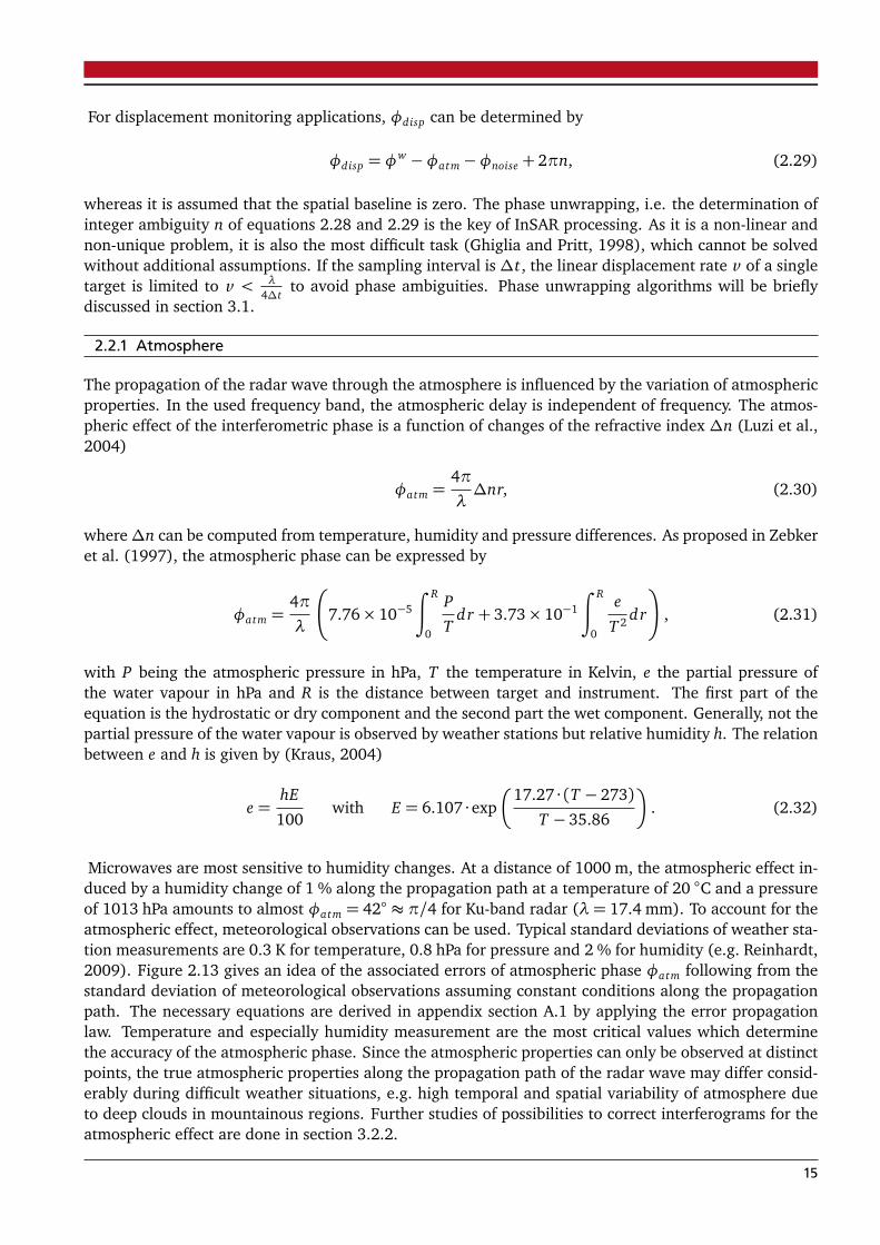
Microwaves are most sensitive to humidity changes. At a distance of 1000 m, the atmospheric effect in-duced by a humidity change of 1 % along the propagation path at a temperature of 20 ◦C and a pressureof 1013 hPa amounts to almost φatm = 42◦ ≈ π/4 for Ku-band radar (λ= 17.4 mm). To account for theatmospheric effect, meteorological observations can be used. Typical standard deviations of weather sta-tion measurements are 0.3 K for temperature, 0.8 hPa for pressure and 2 % for humidity (e.g. Reinhardt,2009). Figure 2.13 gives an idea of the associated errors of atmospheric phase φatm following from thestandard deviation of meteorological observations assuming constant conditions along the propagationpath. The necessary equations are derived in appendix section A.1 by applying the error propagationlaw. Temperature and especially humidity measurement are the most critical values which determinethe accuracy of the atmospheric phase. Since the atmospheric properties can only be observed at distinctpoints, the true atmospheric properties along the propagation path of the radar wave may differ consid-erably during difficult weather situations, e.g. high temporal and spatial variability of atmosphere dueto deep clouds in mountainous regions. Further studies of possibilities to correct interferograms for theatmospheric effect are done in section 3.2.2.
15
Figure 2.13.: Standard deviation of atmospheric phase φatm estimated from weather data with respect to standarddeviations of temperature σT , humidity σh and pressure σP at a temperature of 20 ◦C, a humidity of50 % and a pressure of 1013 hPa. The total standard deviation σφatm
can be computed by applyingthe error propagation law: σ2
φatm= σ2
φatm(T )+σ2
φatm(h)+σ2
φatm(P). Please note the different scaling
of the axes.
2.2.2 Topography
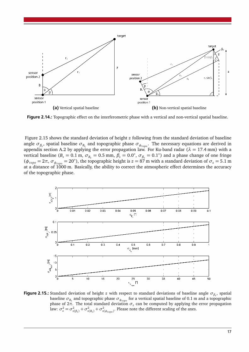
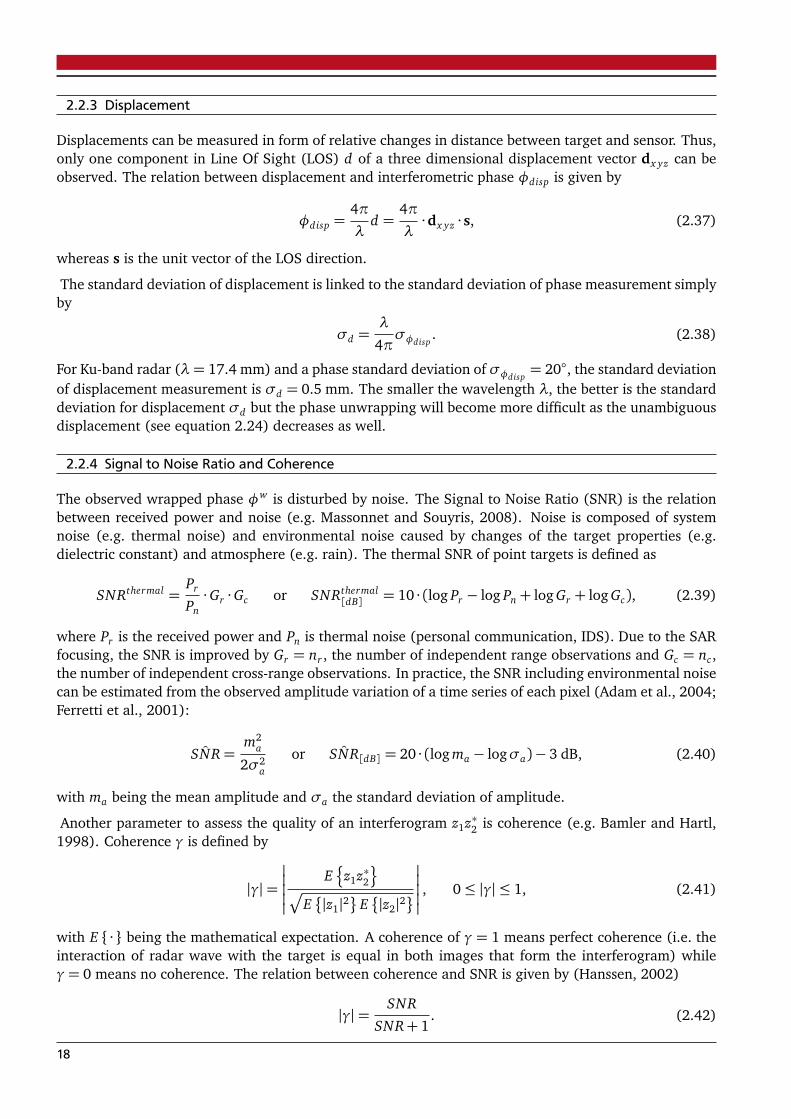
In general, topographic phase φtopo is zero for GB-SAR. If a spatial baseline is deliberately introducedin-between two acquisitions, the height difference between sensor and target can be determined due tothe different path length r1 and r2 of the two acquisitions (see Figure 2.14a). In case the radar sensor isshifted perfectly vertical, the interferometric phase φtopo is related to height z of the target by (Noferiniet al., 2007)
φtopo =4π
λ(r2− r1),
with r2 =Æ
B2s + r2
1 − 2Bsr1 cosθ ,
and cosθ =z
r1.
(2.33)
The height z can be determined by
z =Bs
2+λ
4π
r1
Bsφtopo −
�
λ
4π
�2 1
2Bsφ2
topo. (2.34)
Since r1� Bs and r1� r1− r2, equation 2.34 can be approximated by
z =λ
4π
r1
Bsφtopo. (2.35)
If the spatial baseline is not vertical, height z has to be corrected for the baseline angle βs (see Fig-ure 2.14b):
z = z cosβs + r0 sinβs with r0 =Æ
r21 − z2. (2.36)
16
(a) Vertical spatial baseline (b) Non-vertical spatial baseline
Figure 2.14.: Topographic effect on the interferometric phase with a vertical and non-vertical spatial baseline.
Figure 2.15 shows the standard deviation of height z following from the standard deviation of baselineangle σβs
, spatial baseline σBsand topographic phase σφtopo
. The necessary equations are derived inappendix section A.2 by applying the error propagation law. For Ku-band radar (λ = 17.4 mm) with avertical baseline (Bs = 0.1 m, σBs
= 0.5 mm, βs = 0.0◦, σβs= 0.1◦) and a phase change of one fringe
(φtopo = 2π, σφtopo= 20◦), the topographic height is z = 87 m with a standard deviation of σz = 5.1 m
at a distance of 1000 m. Basically, the ability to correct the atmospheric effect determines the accuracyof the topographic phase.
Figure 2.15.: Standard deviation of height z with respect to standard deviations of baseline angle σβs, spatial
baseline σBsand topographic phase σφtopo
for a vertical spatial baseline of 0.1 m and a topographicphase of 2π. The total standard deviation σz can be computed by applying the error propagationlaw: σ2
z = σ2z(βs)+σ2
z(Bs)+σ2
z(φtopo). Please note the different scaling of the axes.
17
2.2.3 Displacement
Displacements can be measured in form of relative changes in distance between target and sensor. Thus,only one component in Line Of Sight (LOS) d of a three dimensional displacement vector dx yz can beobserved. The relation between displacement and interferometric phase φdisp is given by
φdisp =4π
λd =
4π
λ·dx yz · s, (2.37)
whereas s is the unit vector of the LOS direction.
The standard deviation of displacement is linked to the standard deviation of phase measurement simplyby
σd =λ
4πσφdisp
. (2.38)
For Ku-band radar (λ= 17.4 mm) and a phase standard deviation of σφdisp= 20◦, the standard deviation
of displacement measurement is σd = 0.5 mm. The smaller the wavelength λ, the better is the standarddeviation for displacement σd but the phase unwrapping will become more difficult as the unambiguousdisplacement (see equation 2.24) decreases as well.
2.2.4 Signal to Noise Ratio and Coherence
The observed wrapped phase φw is disturbed by noise. The Signal to Noise Ratio (SNR) is the relationbetween received power and noise (e.g. Massonnet and Souyris, 2008). Noise is composed of systemnoise (e.g. thermal noise) and environmental noise caused by changes of the target properties (e.g.dielectric constant) and atmosphere (e.g. rain). The thermal SNR of point targets is defined as
SNRthermal =Pr
Pn· Gr · Gc or SNRthermal
[dB] = 10 · (log Pr − log Pn+ log Gr + log Gc), (2.39)
where Pr is the received power and Pn is thermal noise (personal communication, IDS). Due to the SARfocusing, the SNR is improved by Gr = nr , the number of independent range observations and Gc = nc,the number of independent cross-range observations. In practice, the SNR including environmental noisecan be estimated from the observed amplitude variation of a time series of each pixel (Adam et al., 2004;Ferretti et al., 2001):
ˆSNR=m2
a
2σ2a
or ˆSNR[dB] = 20 · (log ma − logσa)− 3 dB, (2.40)
with ma being the mean amplitude and σa the standard deviation of amplitude.
Another parameter to assess the quality of an interferogram z1z∗2 is coherence (e.g. Bamler and Hartl,1998). Coherence γ is defined by
|γ|=
�
�
�
�
�
E¦
z1z∗2©
p
E�
|z1|2
E�
|z2|2
�
�
�
�
�
, 0≤ |γ| ≤ 1, (2.41)
with E { · } being the mathematical expectation. A coherence of γ = 1 means perfect coherence (i.e. theinteraction of radar wave with the target is equal in both images that form the interferogram) whileγ= 0 means no coherence. The relation between coherence and SNR is given by (Hanssen, 2002)
|γ|=SNR
SNR+ 1. (2.42)
18
Expressed in logarithmic scale, a SNR of 0 dB equals a coherence of γ = 0.5. Theoretically, a coherenceof γ = 1.0 implies an infinite SNR. In appendix section A.3 a table is given for the conversion of SNRand coherence.
The coherence is influenced by a variety of factors and thus the total coherence of a interferogram pixelcan be expressed as
γ= γthermalγspatialγtemporal . (2.43)
The thermal coherence is directly related to the thermal noise by equation 2.42. In case of zero-baselineobservations, the spatial coherence is 1. The temporal coherence depends on environmental conditionsand is generally decreasing with increasing temporal baseline. Thus, the temporal baseline should be asshort as possible to avoid temporal decorrelation (i.e. loss of coherence with time).
In practise, the coherence can be estimated for each pixel by obtaining the expected values in equa-tion 2.41 by a 2D moving average of n observations (Hanssen, 2002; Bamler and Hartl, 1998):
|γ|=
�
�
�
�
�
∑ni=1(z1z∗2)
p∑n
i=1 |z1|2∑n
i=1 |z2|2
�
�
�
�
�
(2.44)
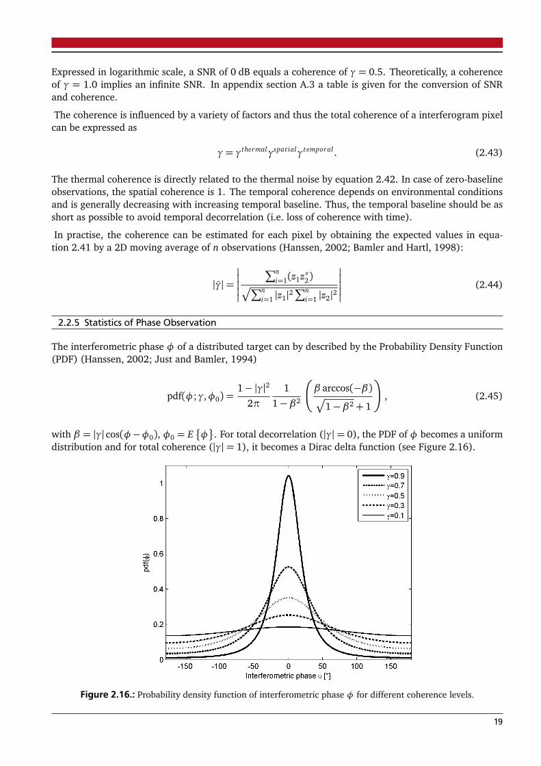
2.2.5 Statistics of Phase Observation
The interferometric phase φ of a distributed target can by described by the Probability Density Function(PDF) (Hanssen, 2002; Just and Bamler, 1994)
pdf(φ;γ,φ0) =1− |γ|2
2π
1
1− β2
β arccos(−β)p
1− β2+ 1
, (2.45)
with β = |γ| cos(φ−φ0), φ0 = E�
φ
. For total decorrelation (|γ|= 0), the PDF of φ becomes a uniformdistribution and for total coherence (|γ|= 1), it becomes a Dirac delta function (see Figure 2.16).
Figure 2.16.: Probability density function of interferometric phase φ for different coherence levels.
19
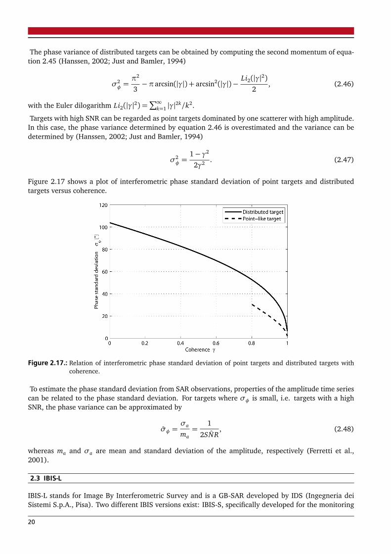
The phase variance of distributed targets can be obtained by computing the second momentum of equa-tion 2.45 (Hanssen, 2002; Just and Bamler, 1994)
σ2φ =
π2
3−πarcsin(|γ|) + arcsin2(|γ|)−
Li2(|γ|2)2
, (2.46)
with the Euler dilogarithm Li2(|γ|2) =∑∞
k=1 |γ|2k/k2.
Targets with high SNR can be regarded as point targets dominated by one scatterer with high amplitude.In this case, the phase variance determined by equation 2.46 is overestimated and the variance can bedetermined by (Hanssen, 2002; Just and Bamler, 1994)
σ2φ =
1− γ2
2γ2 . (2.47)
Figure 2.17 shows a plot of interferometric phase standard deviation of point targets and distributedtargets versus coherence.
Figure 2.17.: Relation of interferometric phase standard deviation of point targets and distributed targets withcoherence.
To estimate the phase standard deviation from SAR observations, properties of the amplitude time seriescan be related to the phase standard deviation. For targets where σφ is small, i.e. targets with a highSNR, the phase variance can be approximated by
σφ =σa
ma=
1
2 ˆSNR, (2.48)
whereas ma and σa are mean and standard deviation of the amplitude, respectively (Ferretti et al.,2001).
2.3 IBIS-L
IBIS-L stands for Image By Interferometric Survey and is a GB-SAR developed by IDS (Ingegneria deiSistemi S.p.A., Pisa). Two different IBIS versions exist: IBIS-S, specifically developed for the monitoring
20
of engineering structures and IBIS-L, specifically developed for the monitoring of landslides and relatedobjects. In contrary to IBIS-L, IBIS-S is no GB-SAR. The radar sensor with transmitting and receivingantennas is mounted on a tripod. By that, only range resolution is obtained but a higher sampling rateis possible (up to 200 Hz). Thus, the applications of IBIS-S are mainly
• Monitoring of man made structures as bridges, towers, buildings, etc.;
• Determination of eigenfrequencies and eigenmodes of structures.
Applications of IBIS-L can be summarized as
• Monitoring of large-scale man made structures as buildings, dams, etc. (Alba et al., 2008);
• Monitoring of mining activities, subsidence, etc;
• Monitoring of natural hazards as landslides, glaciers, volcanoes (Tarchi et al., 2003; Noferini et al.,2006);
• Snow cover and avalanche monitoring (Martinez-Vazquez and Fortuny-Guash, 2006);
• Generation of Digital Elevation Model (Pieraccini et al., 2001; Rödelsperger et al., 2010a).
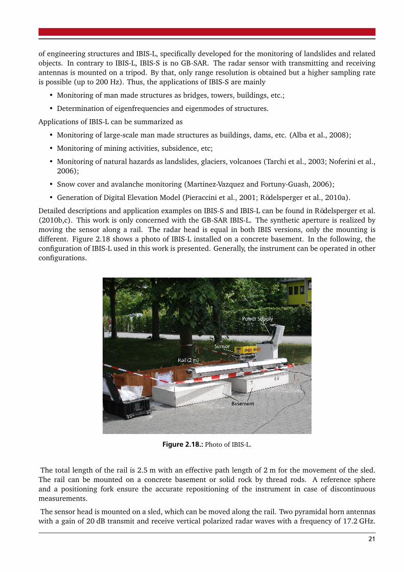
Detailed descriptions and application examples on IBIS-S and IBIS-L can be found in Rödelsperger et al.(2010b,c). This work is only concerned with the GB-SAR IBIS-L. The synthetic aperture is realized bymoving the sensor along a rail. The radar head is equal in both IBIS versions, only the mounting isdifferent. Figure 2.18 shows a photo of IBIS-L installed on a concrete basement. In the following, theconfiguration of IBIS-L used in this work is presented. Generally, the instrument can be operated in otherconfigurations.
Figure 2.18.: Photo of IBIS-L.
The total length of the rail is 2.5 m with an effective path length of 2 m for the movement of the sled.The rail can be mounted on a concrete basement or solid rock by thread rods. A reference sphereand a positioning fork ensure the accurate repositioning of the instrument in case of discontinuousmeasurements.
The sensor head is mounted on a sled, which can be moved along the rail. Two pyramidal horn antennaswith a gain of 20 dB transmit and receive vertical polarized radar waves with a frequency of 17.2 GHz.
21
The −3 dB beamwidth is 17◦ horizontal by 15◦ vertical. The sensor can be tilted along the antenna axisto direct the antenna beam to the object under observation.
The power supply unit contains two batteries (each 12 V, 70 Ah) which can supply the instrument for24 h. External power can either be provided by AC mains power, a generator or solar modules.
The instrument is controlled by a PC via USB interface and the IBIS Controller software operating underWindows. After starting the acquisition, the software automatically repeats the measurements with agiven delay time. The generation of one radar image with range and cross-range resolution takes 5 to 10min (depending on the maximum range). The raw data (unfocused) is stored on the PC as file with theextension gbd (one file per acquisition). The file size depends on the chosen resolution and maximumrange. With full resolution (0.75 m in range by 4.4 mrad in cross-range), the file size is about 32 MB fora distance of 4 km. The file size of the focused image (extension gbf) is half the size of a raw image file.
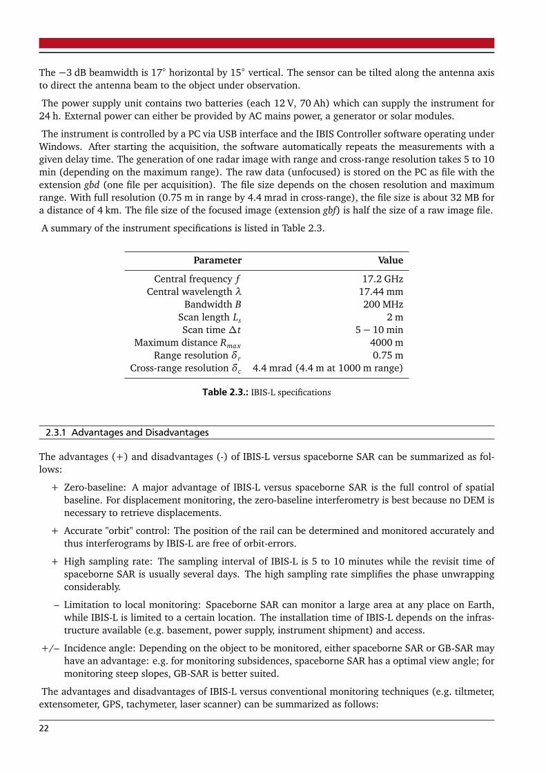
A summary of the instrument specifications is listed in Table 2.3.
Parameter Value
Central frequency f 17.2 GHzCentral wavelength λ 17.44 mm
Bandwidth B 200 MHzScan length Ls 2 mScan time ∆t 5− 10 min
Maximum distance Rmax 4000 mRange resolution δr 0.75 m
Cross-range resolution δc 4.4 mrad (4.4 m at 1000 m range)
Table 2.3.: IBIS-L specifications
2.3.1 Advantages and Disadvantages
The advantages (+) and disadvantages (-) of IBIS-L versus spaceborne SAR can be summarized as fol-lows:
+ Zero-baseline: A major advantage of IBIS-L versus spaceborne SAR is the full control of spatialbaseline. For displacement monitoring, the zero-baseline interferometry is best because no DEM isnecessary to retrieve displacements.
+ Accurate "orbit" control: The position of the rail can be determined and monitored accurately andthus interferograms by IBIS-L are free of orbit-errors.
+ High sampling rate: The sampling interval of IBIS-L is 5 to 10 minutes while the revisit time ofspaceborne SAR is usually several days. The high sampling rate simplifies the phase unwrappingconsiderably.
– Limitation to local monitoring: Spaceborne SAR can monitor a large area at any place on Earth,while IBIS-L is limited to a certain location. The installation time of IBIS-L depends on the infras-tructure available (e.g. basement, power supply, instrument shipment) and access.
+/– Incidence angle: Depending on the object to be monitored, either spaceborne SAR or GB-SAR mayhave an advantage: e.g. for monitoring subsidences, spaceborne SAR has a optimal view angle; formonitoring steep slopes, GB-SAR is better suited.
The advantages and disadvantages of IBIS-L versus conventional monitoring techniques (e.g. tiltmeter,extensometer, GPS, tachymeter, laser scanner) can be summarized as follows:
22
+ Remote sensing instrument: The remote sensing capability is clearly an advantage over a varietyof common monitoring equipments which necessitate access to the monitored structure. Especiallywhen monitoring natural hazards (e.g. landslides, volcanoes), entering the endangered zone isoften impossible. With a maximum distance of 4 km, even inaccessible parts of a structure as largetowers, dams or landslides can be monitored.
+ Independence of daylight and weather: Due to the use of radar waves, the monitoring can continueduring night and when visibility is limited due to fog, clouds or rain.
+ Simultaneous monitoring of all targets within the beam with high accuracy and spatial resolution:Most monitoring equipment is limited to either high accuracy or high spatial resolution while IBIS-Lprovides both. Due to cost limitations, it is often not possible to cover the whole structure withhigh-accuracy instrumentation while IBIS-L can monitor the surface displacements at all targetswithin the antenna beam simultaneously with an accuracy of 0.1 to 1 mm depending on distanceto the target and target conditions.
+ Undisturbed by passing objects: If in case of a laser scanner or tachymeter a person is passing byand covers the direct line of sight for a short time period, some measurements at distinct pointsare lost. In case of IBIS-L short disturbances do not matter due to the sampling being done in thefrequency domain.
– Accuracy depends on target reflectivity: Slopes and surfaces entirely covered with vegetation orstructures without well reflecting points cannot be monitored without additional artificial reflec-tors. At Ku-band, the radar waves do not penetrate ground vegetation and mainly the vegetationsurface is observed, which leads to a loss of coherence. The installation of passive radar reflectorshowever requires access to the structure.
– Atmospheric delay: The most limiting factor for accuracy is the atmosphere. In long-term moni-toring the atmospheric delay has to be corrected which makes either additional weather sensorsand/or stable targets in the monitored area necessary.
– LOS displacements: The monitoring of displacements is limited to one-dimensional displacements.Thus, some knowledge or assumptions must exist if horizontal or vertical displacements shall bederived from the LOS displacements.
– Ambiguous displacements: Since no absolute phase is determined, the obtained displacement isambiguous. The ambiguities can only be determined with certain assumptions, e.g. that the move-ment is below λ/4 per image.
– Difficult point localization: The point localization in radar images is more difficult than in otherareal observation techniques as e.g. laser scanning. To map the radar image into a global referencesystem, a DEM is necessary. Targets at equal distance and azimuth but with different heightsare mapped to the same resolution cell. If the monitored structure has a complex appearance,this can become a major problem as different displacement behaviours of two targets might beindistinguishable. This effect can be compensated by choosing the position of the instrumentcarefully.
2.3.2 Monitoring Requirements and Concepts
How suitable a structure or slope is for monitoring its displacements with IBIS-L depends on object prop-erties as e.g. expected displacement rate, object dimension and appearance. The maximum unambiguousdisplacement rate of a target follows from equation 2.24 and is limited by wavelength λ and samplingrate ∆t
|vmax |=λ
4∆t. (2.49)
23
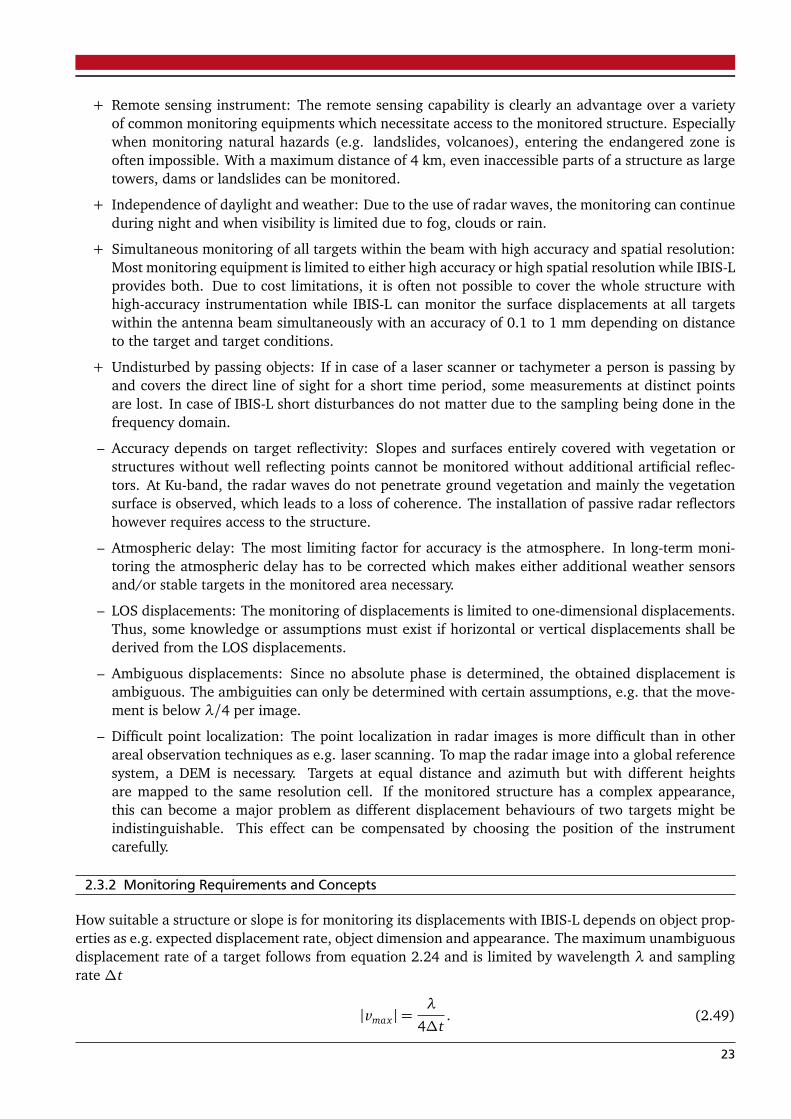
For wavelengths between Ku- and L-band, the maximum unambiguous velocity is between 0.6 m/dayand 10 m/day at a 10 min sampling interval. Using the velocity scale for landslides of IUGS-WGL (1995),landslides between class 1 (extremely slow) and class 4 (moderate) can be monitored unambiguously.Table 2.4 shows the time until the displacement of∆r = λ/4 is reached for wavelengths between Ku andL-band. If this time is below the sampling interval, the phase ambiguities cannot be resolved withoutadditional information or assumptions. If this time exceeds several months and no increase of velocityis expected, a continuous monitoring is not reasonable. In such a case, monitoring campaigns of severaldays with time spans of several months in-between the campaigns are more efficient. It has to be madesure that the instrument can be reinstalled accurately to avoid spatial decorrelation. Further informationon discontinuous measurements with GB-SAR can be found in Noferini et al. (2008b) and Pieracciniet al. (2006). This thesis deals with continuous monitoring campaigns.
Time to reach ∆r = λ/4Velocity Class Ku-band C-band L-band[mm/d] (λ= 17 mm) (λ= 56 mm) (λ= 235 mm)
10000 4 0.6 min 2 min 8 min2000 4 3 min 10 min 42 min
400 3 15 min 50 min 3.5 h80 3 1.2 h 4 h 18 h16 3 6 h 21 h 3.7 d
3.2 2 1.3 d 4.4 d 18 d0.6 2 7 d 23 d 98 d0.1 2 43 d 140 d 1.6 y
0.03 1 142 d 1.3 y 5 y
Table 2.4.: Time to reach a displacement of ∆r = λ/4 with wavelengths between Ku and L-band for differentobject velocities.
The maximum dimension of the object to be monitored is restricted by the distance of the instrumentand the beam width. The beam width of IBIS-L depends on the used antenna. In this work, an antennawith horizontal −3 dB beam width of 17◦ was used. This results in maximum horizontal dimensionof about 300 m at a distance of 1000 m and accordingly a horizontal dimension of about 1200 m at adistance of 4000 m. The maximum object dimension is a smooth boundary and also depends on theobject reflectivity. A good reflecting target may still be monitored with high accuracy outside the mainbeam but the SNR is dropping rapidly with increasing azimuth. Generally, IBIS-L can be operated withdifferent antennas but it must be considered that a wider main beam results in a lower SNR.
A key to successful monitoring is the selection of the installation side which must fulfill certain require-ments:
• The most important requirement is the stability, i.e. the instrument must not move during themeasurements.
• In case of hazard monitoring, the safety of the instrument must be assured. The instrument shouldnot be mounted in the endangered zone.
• The expected displacements must be considered as only LOS displacements can be observed. Theinstrument should positioned such that the line of sight coincides as best as possible with theexpected direction of displacement.
• The choice of the incidence angle is a trade off between ground range resolution and power of thebackscattered signal. For decreasing incidence angles, the ground range resolution is improvingbut the power of backscattered signal is decreasing (see also Figure 2.9 and section 2.1.4).
24

• Overlays (i.e. targets at different heights that are mapped into one image pixel) should be avoidedbecause the displacement signal of the individual targets cannot be reconstructed.
In the following section, the state of the art of data post processing is presented. In chapter 4, a real-timeapproach is described.
25
3 Analysis of GB-SAR Data
In last chapter, the properties of GB-SAR images and interferograms were described. From now on,when talking about GB-SAR, it is assumed that the spatial baseline is zero, as this is usually the case fordisplacement monitoring applications. As illustrated in section 2.2, the observed interferometric phase iswrapped into the interval [−π,π) and is a sum of several effects (displacement, atmosphere and noise).The goal of data analysis is the phase unwrapping, i.e. the determination of phase ambiguities to re-trieve the absolute interferometric phase, and the separation of the different effects. In the followingsections, the state of the art of relevant techniques for processing and analysing SAR data for displace-ment monitoring applications is described. A brief summary of phase unwrapping methods is given insection 3.1.
The conventional InSAR analysis is based on the processing and analysis of interferograms. The differentsteps necessary to retrieve geocoded displacement maps out of a set of raw images are described insection 3.2.
In spaceborne SAR, the conventional InSAR analysis suffers from temporal and spatial decorrelation.Temporal decorrelation (i.e. loss of coherence with time) increases with temporal baseline and is worstin vegetated areas. Spatial decorrelation increases with spatial baseline. Thus, only a limited numberof interferograms is usable and the analysis is limited to high coherent areas. Especially in denselyvegetated areas, the conventional analysis fails whereas, even if within decorrelated areas, single targetswith good coherence may exist.
As a result, the Permanent Scatterers Technique was developed and patented by A. Ferretti, C. Pratiand F. Rocca (EU patent 1 183 551 B1) to overcome these difficulties (Ferretti et al., 2000, 2001).The technique selects so-called permanent scatterers (i.e. pixels with high coherence) and performs anestimation of displacement, topography and atmospheric delay using the phase time series. Diversealgorithms exist, similar to the Permanent Scatterers Technique, which are all summarized by the termPersistent Scatterer Interferometry (PSI) (Kampes, 2006). A short summary of the Permanent ScatterersTechnique, as well as other PSI algorithms, is given in section 3.3.
3.1 Phase Unwrapping
Phase unwrapping is an essential part of all analysis techniques. The interferometric phase φw iswrapped into the interval [−π,π) and related to the true phase φ by φw = φ − 2πn. The correctdetermination of phase ambiguity n is the key to successful displacement monitoring and is called phaseunwrapping. Generally, phase unwrapping is a three-dimensional problem (2D spatial and 1D temporal).
Many papers on all kinds of unwrapping methods exist for 1D up to 3D unwrapping techniques (Itoh,1982; Goldstein et al., 1988; Cusack et al., 1995; Ghiglia and Pritt, 1998; Huntley, 2001). The simplestmethod of unwrapping a sampled signal in 1D space is described by e.g. Itoh (1982). Considering asequence of m discrete wrapped phase measurements [ϕw
1 ,ϕw2 , ...,ϕw
m], the unwrapped interferometricphase φk = ϕ1−ϕk can be obtained by summing all wrapped phase differences
φk =W¦
ϕw1 −ϕ
w2
©
+W¦
ϕw2 −ϕ
w3
©
+ · · ·+W¦
ϕwk−1−ϕ
wk
©
= ϕw1 −ϕ
w2 − 2πn12+ϕ
w2 −ϕ
w3 − 2πn23+ · · ·+ϕw
k−1−ϕwk − 2πnk−1,k
= ϕw1 −ϕ
wk − 2π(n12+ n23+ · · ·+ nk−1,k).
(3.1)
This algorithm produced correct results as long as the sampling rate of the signal is high enough todetect phase jumps (i.e. the Nyquist criteria is satisfied) and noise is limited. In Figure 3.1, an example
26
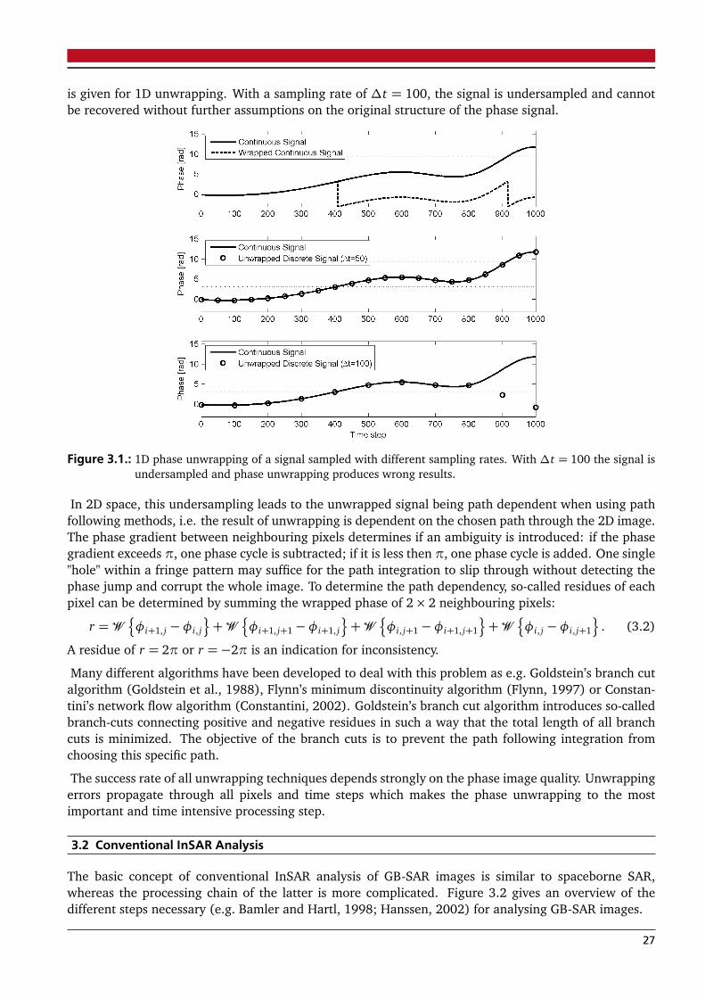
is given for 1D unwrapping. With a sampling rate of ∆t = 100, the signal is undersampled and cannotbe recovered without further assumptions on the original structure of the phase signal.
Figure 3.1.: 1D phase unwrapping of a signal sampled with different sampling rates. With ∆t = 100 the signal isundersampled and phase unwrapping produces wrong results.
In 2D space, this undersampling leads to the unwrapped signal being path dependent when using pathfollowing methods, i.e. the result of unwrapping is dependent on the chosen path through the 2D image.The phase gradient between neighbouring pixels determines if an ambiguity is introduced: if the phasegradient exceeds π, one phase cycle is subtracted; if it is less then π, one phase cycle is added. One single"hole" within a fringe pattern may suffice for the path integration to slip through without detecting thephase jump and corrupt the whole image. To determine the path dependency, so-called residues of eachpixel can be determined by summing the wrapped phase of 2× 2 neighbouring pixels:
r =W¦
φi+1, j −φi, j
©
+W¦
φi+1, j+1−φi+1, j
©
+W¦
φi, j+1−φi+1, j+1
©
+W¦
φi, j −φi, j+1
©
. (3.2)
A residue of r = 2π or r =−2π is an indication for inconsistency.
Many different algorithms have been developed to deal with this problem as e.g. Goldstein’s branch cutalgorithm (Goldstein et al., 1988), Flynn’s minimum discontinuity algorithm (Flynn, 1997) or Constan-tini’s network flow algorithm (Constantini, 2002). Goldstein’s branch cut algorithm introduces so-calledbranch-cuts connecting positive and negative residues in such a way that the total length of all branchcuts is minimized. The objective of the branch cuts is to prevent the path following integration fromchoosing this specific path.
The success rate of all unwrapping techniques depends strongly on the phase image quality. Unwrappingerrors propagate through all pixels and time steps which makes the phase unwrapping to the mostimportant and time intensive processing step.
3.2 Conventional InSAR Analysis
The basic concept of conventional InSAR analysis of GB-SAR images is similar to spaceborne SAR,whereas the processing chain of the latter is more complicated. Figure 3.2 gives an overview of thedifferent steps necessary (e.g. Bamler and Hartl, 1998; Hanssen, 2002) for analysing GB-SAR images.
27
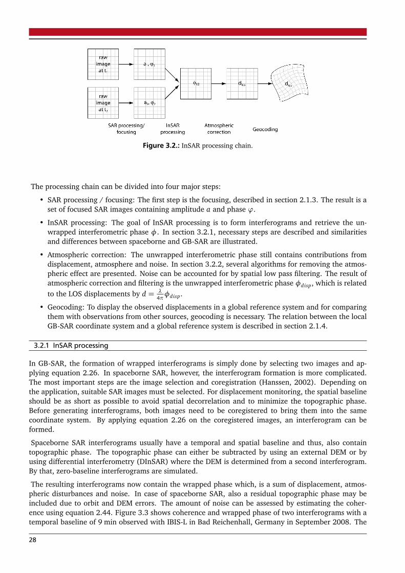
Figure 3.2.: InSAR processing chain.
The processing chain can be divided into four major steps:
• SAR processing / focusing: The first step is the focusing, described in section 2.1.3. The result is aset of focused SAR images containing amplitude a and phase ϕ.
• InSAR processing: The goal of InSAR processing is to form interferograms and retrieve the un-wrapped interferometric phase φ. In section 3.2.1, necessary steps are described and similaritiesand differences between spaceborne and GB-SAR are illustrated.
• Atmospheric correction: The unwrapped interferometric phase still contains contributions fromdisplacement, atmosphere and noise. In section 3.2.2, several algorithms for removing the atmos-pheric effect are presented. Noise can be accounted for by spatial low pass filtering. The result ofatmospheric correction and filtering is the unwrapped interferometric phase φdisp, which is relatedto the LOS displacements by d = λ
4πφdisp.
• Geocoding: To display the observed displacements in a global reference system and for comparingthem with observations from other sources, geocoding is necessary. The relation between the localGB-SAR coordinate system and a global reference system is described in section 2.1.4.
3.2.1 InSAR processing
In GB-SAR, the formation of wrapped interferograms is simply done by selecting two images and ap-plying equation 2.26. In spaceborne SAR, however, the interferogram formation is more complicated.The most important steps are the image selection and coregistration (Hanssen, 2002). Depending onthe application, suitable SAR images must be selected. For displacement monitoring, the spatial baselineshould be as short as possible to avoid spatial decorrelation and to minimize the topographic phase.Before generating interferograms, both images need to be coregistered to bring them into the samecoordinate system. By applying equation 2.26 on the coregistered images, an interferogram can beformed.
Spaceborne SAR interferograms usually have a temporal and spatial baseline and thus, also containtopographic phase. The topographic phase can either be subtracted by using an external DEM or byusing differential interferometry (DInSAR) where the DEM is determined from a second interferogram.By that, zero-baseline interferograms are simulated.
The resulting interferograms now contain the wrapped phase which, is a sum of displacement, atmos-pheric disturbances and noise. In case of spaceborne SAR, also a residual topographic phase may beincluded due to orbit and DEM errors. The amount of noise can be assessed by estimating the coher-ence using equation 2.44. Figure 3.3 shows coherence and wrapped phase of two interferograms with atemporal baseline of 9 min observed with IBIS-L in Bad Reichenhall, Germany in September 2008. The
28
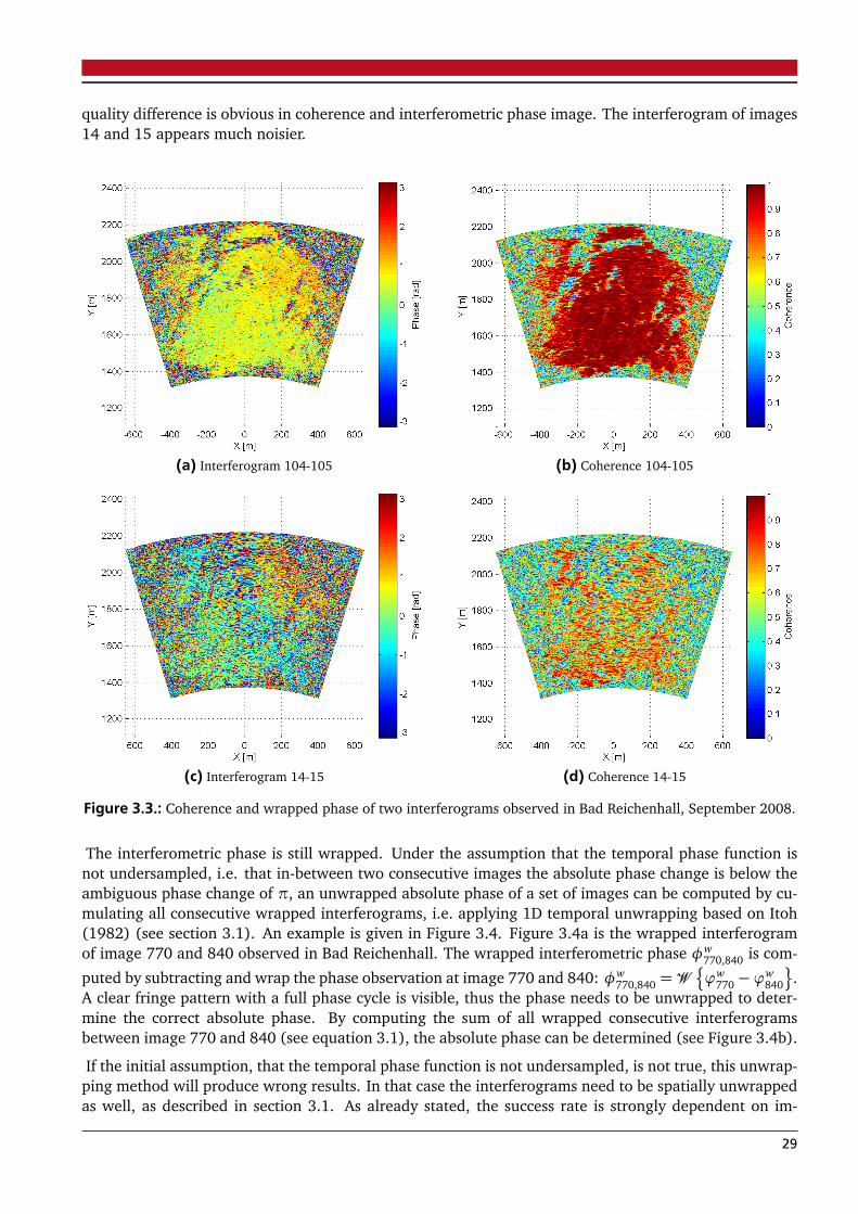
quality difference is obvious in coherence and interferometric phase image. The interferogram of images14 and 15 appears much noisier.
(a) Interferogram 104-105 (b) Coherence 104-105
(c) Interferogram 14-15 (d) Coherence 14-15
Figure 3.3.: Coherence and wrapped phase of two interferograms observed in Bad Reichenhall, September 2008.
The interferometric phase is still wrapped. Under the assumption that the temporal phase function isnot undersampled, i.e. that in-between two consecutive images the absolute phase change is below theambiguous phase change of π, an unwrapped absolute phase of a set of images can be computed by cu-mulating all consecutive wrapped interferograms, i.e. applying 1D temporal unwrapping based on Itoh(1982) (see section 3.1). An example is given in Figure 3.4. Figure 3.4a is the wrapped interferogramof image 770 and 840 observed in Bad Reichenhall. The wrapped interferometric phase φw
770,840 is com-
puted by subtracting and wrap the phase observation at image 770 and 840: φw770,840 =W
¦
ϕw770−ϕ
w840
©
.A clear fringe pattern with a full phase cycle is visible, thus the phase needs to be unwrapped to deter-mine the correct absolute phase. By computing the sum of all wrapped consecutive interferogramsbetween image 770 and 840 (see equation 3.1), the absolute phase can be determined (see Figure 3.4b).
If the initial assumption, that the temporal phase function is not undersampled, is not true, this unwrap-ping method will produce wrong results. In that case the interferograms need to be spatially unwrappedas well, as described in section 3.1. As already stated, the success rate is strongly dependent on im-
29
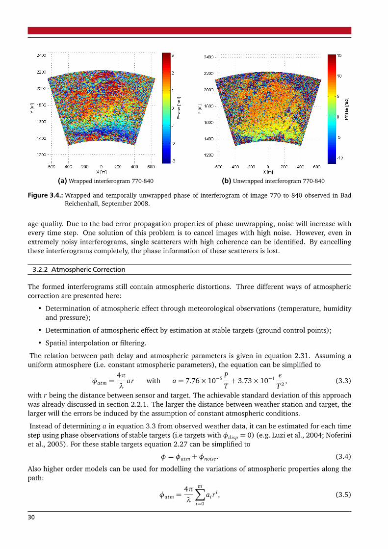
(a) Wrapped interferogram 770-840 (b) Unwrapped interferogram 770-840
Figure 3.4.: Wrapped and temporally unwrapped phase of interferogram of image 770 to 840 observed in BadReichenhall, September 2008.
age quality. Due to the bad error propagation properties of phase unwrapping, noise will increase withevery time step. One solution of this problem is to cancel images with high noise. However, even inextremely noisy interferograms, single scatterers with high coherence can be identified. By cancellingthese interferograms completely, the phase information of these scatterers is lost.
3.2.2 Atmospheric Correction
The formed interferograms still contain atmospheric distortions. Three different ways of atmosphericcorrection are presented here:
• Determination of atmospheric effect through meteorological observations (temperature, humidityand pressure);
• Determination of atmospheric effect by estimation at stable targets (ground control points);
• Spatial interpolation or filtering.
The relation between path delay and atmospheric parameters is given in equation 2.31. Assuming auniform atmosphere (i.e. constant atmospheric parameters), the equation can be simplified to
φatm =4π
λar with a = 7.76× 10⁻⁵ P
T+ 3.73× 10⁻¹ e
T 2 , (3.3)
with r being the distance between sensor and target. The achievable standard deviation of this approachwas already discussed in section 2.2.1. The larger the distance between weather station and target, thelarger will the errors be induced by the assumption of constant atmospheric conditions.
Instead of determining a in equation 3.3 from observed weather data, it can be estimated for each timestep using phase observations of stable targets (i.e targets with φdisp = 0) (e.g. Luzi et al., 2004; Noferiniet al., 2005). For these stable targets equation 2.27 can be simplified to
φ = φatm+φnoise. (3.4)
Also higher order models can be used for modelling the variations of atmospheric properties along thepath:
φatm =4π
λ
m∑
i=0
ai ri, (3.5)
30
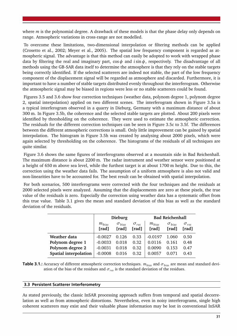
where m is the polynomial degree. A drawback of these models is that the phase delay only depends onrange. Atmospheric variations in cross-range are not modelled.
To overcome these limitations, two-dimensional interpolation or filtering methods can be applied(Crosetto et al., 2002; Meyer et al., 2005). The spatial low frequency component is regarded as at-mospheric signal. The advantage is that this method can easily be adopted to work with wrapped phasedata by filtering the real and imaginary part, cosφ and i sinφ, respectively. The disadvantage of allmethods using the GB-SAR data itself to determine the atmosphere is that they rely on the stable targetsbeing correctly identified. If the selected scatterers are indeed not stable, the part of the low frequencycomponent of the displacement signal will be regarded as atmosphere and discarded. Furthermore, it isimportant to have a number of stable targets distributed evenly throughout the interferogram. Otherwisethe atmospheric signal may be biased in regions were less or no stable scatterers could be found.
Figures 3.5 and 3.6 show four correction techniques (weather data, polynom degree 1, polynom degree2, spatial interpolation) applied on two different scenes. The interferogram shown in Figure 3.5a isa typical interferogram observed in a quarry in Dieburg, Germany with a maximum distance of about300 m. In Figure 3.5b, the coherence and the selected stable targets are plotted. About 200 pixels wereidentified by thresholding on the coherence. They were used to estimate the atmospheric correction.The residuals for the different correction techniques can be seen in Figure 3.5c to 3.5f. The differencesbetween the different atmospheric corrections is small. Only little improvement can be gained by spatialinterpolation. The histogram in Figure 3.5h was created by analysing about 2000 pixels, which wereagain selected by thresholding on the coherence. The histograms of the residuals of all techniques arequite similar.
Figure 3.6 shows the same figures of interferograms observed at a mountain side in Bad Reichenhall.The maximum distance is about 2200 m. The radar instrument and weather sensor were positioned ata height of 650 m above sea level, while the furthest target is at about 1700 m height. Due to this, thecorrection using the weather data fails. The assumption of a uniform atmosphere is also not valid andnon-linearities have to be accounted for. The best result can be obtained with spatial interpolation.
For both scenarios, 500 interferograms were corrected with the four techniques and the residuals at2000 selected pixels were analyzed. Assuming that the displacements are zero at these pixels, the truevalue of the residuals is zero. Especially the correction using weather data has a systematic offset fromthis true value. Table 3.1 gives the mean and standard deviation of this bias as well as the standarddeviation of the residuals.
Dieburg Bad Reichenhallmbias σbias σres mbias σbias σres[rad] [rad] [rad] [rad] [rad] [rad]
Weather data -0.0027 0.126 0.33 -0.0197 1.060 0.50Polynom degree 1 -0.0033 0.018 0.32 0.0116 0.161 0.48Polynom degree 2 -0.0031 0.018 0.32 0.0090 0.153 0.47Spatial interpolation -0.0008 0.016 0.32 0.0057 0.071 0.43
Table 3.1.: Accuracy of different atmospheric correction techniques. mbias and σbias are mean and standard devi-ation of the bias of the residues and σres is the standard deviation of the residues.
3.3 Persistent Scatterer Interferometry
As stated previously, the classic InSAR processing approach suffers from temporal and spatial decorre-lation as well as from atmospheric distortions. Nevertheless, even in noisy interferograms, single highcoherent scatterers may exist and their valuable phase information may be lost in conventional InSAR
31
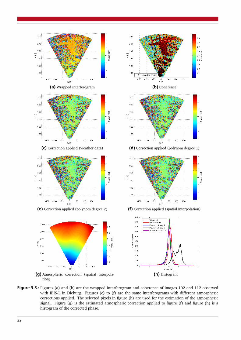
(a) Wrapped interferogram (b) Coherence
(c) Correction applied (weather data) (d) Correction applied (polynom degree 1)
(e) Correction applied (polynom degree 2) (f) Correction applied (spatial interpolation)
(g) Atmospheric correction (spatial interpola-tion)
(h) Histogram
Figure 3.5.: Figures (a) and (b) are the wrapped interferogram and coherence of images 102 and 112 observedwith IBIS-L in Dieburg. Figures (c) to (f) are the same interferograms with different atmosphericcorrections applied. The selected pixels in figure (b) are used for the estimation of the atmosphericsignal. Figure (g) is the estimated atmospheric correction applied to figure (f) and figure (h) is ahistogram of the corrected phase.
32
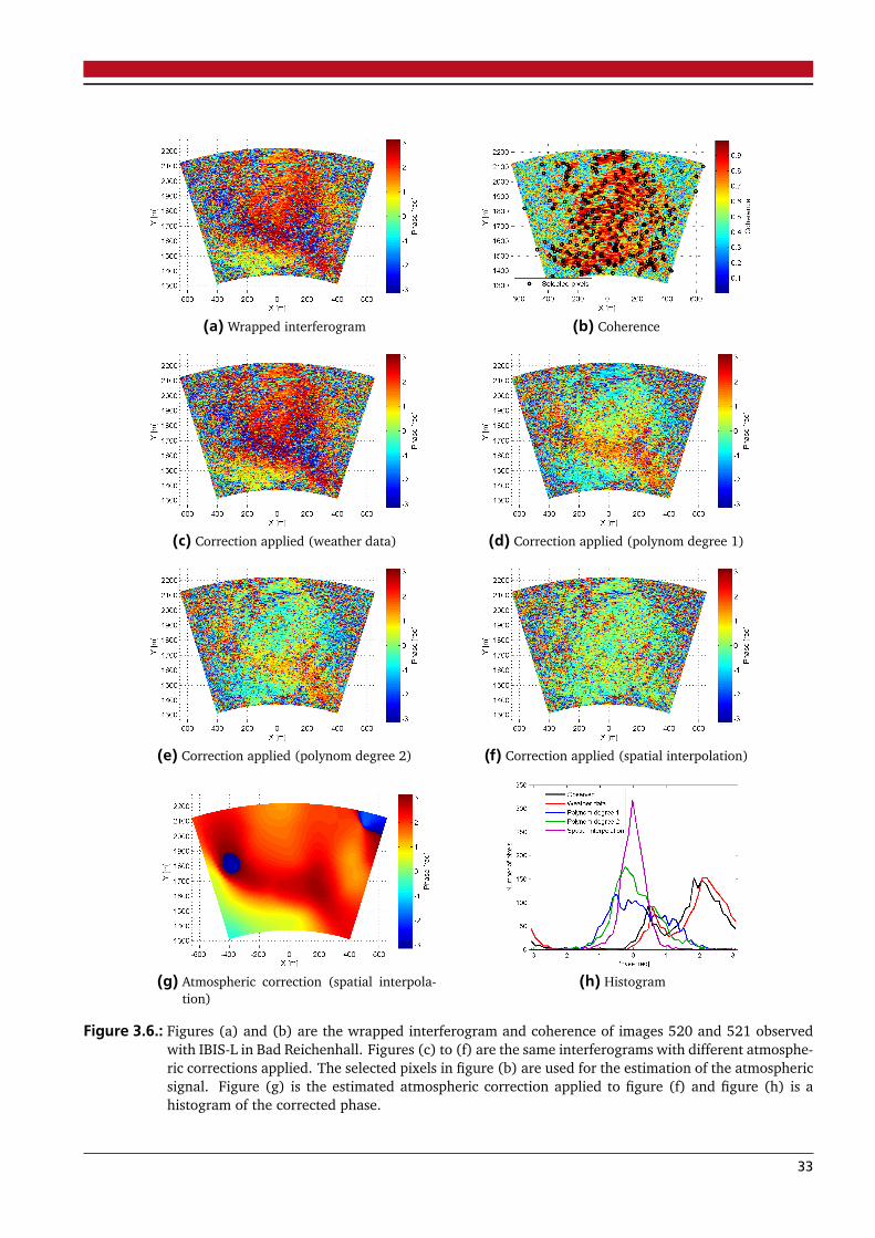
(a) Wrapped interferogram (b) Coherence
(c) Correction applied (weather data) (d) Correction applied (polynom degree 1)
(e) Correction applied (polynom degree 2) (f) Correction applied (spatial interpolation)
(g) Atmospheric correction (spatial interpola-tion)
(h) Histogram
Figure 3.6.: Figures (a) and (b) are the wrapped interferogram and coherence of images 520 and 521 observedwith IBIS-L in Bad Reichenhall. Figures (c) to (f) are the same interferograms with different atmosphe-ric corrections applied. The selected pixels in figure (b) are used for the estimation of the atmosphericsignal. Figure (g) is the estimated atmospheric correction applied to figure (f) and figure (h) is ahistogram of the corrected phase.
33
processing. As a result, the Permanent Scatterers Technique was developed and patented by A. Ferretti,C. Prati and F. Rocca (EU patent 1 183 551 B1) exploiting all available phase information of these highcoherent scatterers (i.e. permanent scatterers) (Ferretti et al., 2000, 2001). In section 3.3.1, the basicprinciples of the Permanent Scatterers Technique are described.
Shortly after, a number of techniques have been developed using similar approaches as the PermanentScatterers Technique summarized by the term Persistent Scatterer Interferometry (PSI) (Kampes, 2006).The basic idea of all PSI methods is the same: instead of analyzing interferograms, they estimate dis-placement rate, topography, atmosphere, orbit error and other parameters using the phase time seriesat selected permanent/persistent scatterers. The difference of the diverse algorithms lies mainly in theused assumptions, estimation methods and implementation. Exemplary, the Stanford Method for Persis-tent Scatterers (StaMPS) and the Delft PS-InSAR Processing Package (DePSI) and their differences withrespect to the Permanent Scatterers Technique are described shortly.
Although the conditions for GB-SAR are much better than for spaceborne SAR (short temporal baseline,no spatial baseline), the conventional InSAR processing approach still suffers from temporal decorre-lation and atmospheric artefacts. Thus, PSI techniques can increase the quality and reliability of theresults. Since the conditions for GB-SAR differ somewhat from spaceborne SAR, the developed PSI tech-niques cannot be directly applied. In the next chapter, the assumptions of the reviewed PSI techniquesare compared to the requirements and conditions of GB-SAR observations and a real-time approach forPSI is described.
3.3.1 Permanent Scatterers Technique
The main steps of the Permanent Scatterers Technique for spaceborne SAR are illustrated in the following(Ferretti et al., 2000, 2001; Kampes, 2006). One master image is selected and interferograms are formedwith respect to this master image. By means of a DEM, differential interferograms are formed, whichsimulate zero-baseline interferograms. Due to orbit and DEM errors, these interferograms still contain aresidual topographic phase.
The technique distinguishes between Permanent Scatterers (PSs) and Permanent Scatterer Candidates(PSCs), whereas the latter are used to estimate the Atmospheric Phase Screen (APS). The PSC areselected by analyzing the amplitude time series and thresholding on the Amplitude Dispersion Index(ADI) Da, which equals the phase standard deviation for targets with high coherence (see equation 2.48)
Da = σφ =σa
ma, (3.6)
whereas ma and σa are mean and standard deviation of the amplitude. For estimation of the different
signal contributions, the phase differences ψwi j =W
n
φwj −φ
wi
o
at all neighbouring PSCs (i, j) (i.e. dou-ble differenced phase observations) within a certain radius are formed. The unwrapped phase differenceis the sum of the residual topographic phase, atmospheric artefacts, displacement and noise
ψ=ψtopo +ψdisp +ψatm+ψnoise. (3.7)
The phase model can be divided into a deterministic and stochastic part. The deterministic part modelsthe residual topographic phase and linear displacement (ψl in = ψtopo + ψl indisp) whereas ψtopo is alinear function of spatial baseline and ψl indisp a linear function of time. The stochastic part contains thecontributions from atmosphere, non-linear displacement and noise (ψnonlin =ψatm+ψnonlindisp+ψnoise).The standard deviation of ψnonlin is expected to be small due to the fact that the selected PSs have ahigh coherence (i.e. ψnoise is small) and that the phase difference between neighbouring pixels due toatmosphere (ψatm) and nonlinear motion (ψnonlindisp) will be rather small, assuming a spatial correlationof displacement and atmosphere.
34
With these assumptions, ψtopo and ψl indisp can be determined from the wrapped data by means of spec-tral analysis of the two-dimensional complex signal representation. Since |ψnonlin| < π, the unwrappedphase difference ψ can directly be determined. If all estimations were correct, the interferometric phaseφ at each PS could be directly computed with respect to a reference PS. Since this assumption is usuallynot correct, a weighted least-square integration algorithm is used whereas the weights are computedfrom the residual phase ψnonlin. For estimating the APS, the spatio-temporal correlation characteristicof the atmospheric distortions is exploited, i.e. that atmospheric artefacts are a spatially low frequencysignal and uncorrelated in time. Atmospheric artefacts can be considered uncorrelated in time because ofthe low sampling rate of spaceborne SAR. In two consecutive acquisitions the atmospheric properties aretotally different. Thus, the APS can be determined by temporal high pass and spatial low pass filteringψnonlin. After the APS is estimated, more PSs can be identified by analysing the phase time series andthe estimates for ψtopo and ψl indisp are improved.
The advantage of this technique is that even interferograms with large spatial baselines can be used anddisplacements of single coherent scatterers in vegetated areas can be estimated. The disadvantage is thata least about 30 images are needed before this estimation technique can be used.
3.3.2 Stanford Method for Persistent Scatterers
The Stanford Method for Persistent Scatterers (StaMPS) (Hooper et al., 2004, 2007) assumes that noprior knowledge about the temporal behaviour of the object displacement exists. It is rather assumedthat the displacement is spatially smooth. The Persistent Scatterer (PS) selection is done based on thespatial phase stability. By that, a single stable scatterer that behaves different to its surroundings mightnot be detected as PS. After the selection, similar to Ferretti et al. (2000), the residual topographic phaseis estimated as a linear function of spatial baseline. The 3D phase unwrapping is regarded as a seriesof 2D problems as, due to the spatial smoothness assumption, the differences between neighbouringPSs are expected to be small. The 2D unwrapping is solved using an iterative least square technique.The temporal phase signal can be obtained by summing all spatially unwrapped values with respect toa reference PS. The spatially correlated error (atmosphere, orbit, residual topographic error) can beestimated by temporal high pass and spatial low pass filtering.
3.3.3 Delft PS-InSAR Processing Package
Similar to Ferretti et al. (2000), the Delft PS-InSAR Processing Package (DePSI) (Kampes and Hanssen,2004; Kampes, 2006) selects PSs based on the ADI. According to Sousa et al. (2009), this leads to alower PS density in non-urban areas compared to StaMPS because low ADI can mainly be found in ur-ban areas. A subset of the selected PSs is used as reference network to estimate the APS. Displacementscan be modeled as linear with time (or higher order models). Thus, some knowledge about the tempo-ral behaviour must exist beforehand. The temporal unwrapping and estimation of residual topographicphase and displacement is done with the Integer Least Squares (ILS) and the APS is determined by filter-ing the residuals similar to Ferretti et al. (2000). After that, the unknown parameters of the remainingPS are determined using ILS.
35
4 Real-time Monitoring Concept
Different approaches must be considered in the monitoring of object displacements with GB-SAR depend-ing on the expected rate of movement. In case of fast movements (v > 0.5 mm/day), the object shouldbe monitored continuously with sampling rates of 5 to 10 min. Even for velocities v < 0.5 mm/day acontinuous monitoring with a high sampling rate should be considered, to be able to assess the atmos-pheric effects and avoid phase unwrapping problems as best as possible. For velocities< 20 mm/year themonitoring can be done in campaigns with a duration of several days and a time span of several weeks tomonth in-between the campaigns. This work is concerned with continuous monitoring of displacements.
The real-time evaluation of displacement monitoring can act as basis for making rapid decisions in termsof countermeasures and evacuation. Here, real-time evaluation means the creation of displacementmaps with the shortest delay possible. Generally, the InSAR analysis described in section 3.2 can bedone in real-time, due to the analysis being done interferogram by interferogram. However, from theinterferogram examples shown in section 3.2.1, it can be seen that even for GB-SAR with short timeintervals, temporal decorrelation can prevent the successful InSAR analysis. Thus, PSI can increasequality and reliability of the estimated displacements. The described PSI techniques in section 3.3 weredeveloped for spaceborne SAR and therefore use some assumptions which have to be reviewed carefullyfor GB-SAR.
The most profound difference between spaceborne and GB-SAR is the zero-baseline condition and there-fore no residual topographic phase exists. Another difference is the observation period and sampling rate.While the sampling rate of spaceborne SAR is usually several days or weeks, it is several minutes for GB-SAR. Thus, the observation period might be limited to a few hours, days or weeks. The assumptionof all PSI techniques, that the atmospheric phase is temporally uncorrelated, is therefore not true. Fur-thermore, the displacement monitoring should not be limited to a linear displacement model only. Thealgorithm should rather be flexible in the choice of displacement model and even be able to operatewhen almost no prior information about the expected displacements exist.
Since PSI operates on time series, the algorithms are only partly real-time capable. If one observation isadded, the whole analysis must be repeated, which is not efficient. To avoid this, the analysis could bedone on a moving window (i.e. use only the last n samples), but nevertheless the computational effortis immense. Here, a concept for a true real-time PSI algorithm using Kalman Filtering is presented,particularly trying to fulfill all conditions and requirements for GB-SAR.
The processing concept is based on the PSI techniques described in section 3.3. According to Ferrettiet al. (2000) and Kampes (2006), it is distinguished between PS and Persistent Scatterer Candidate(PSC). Here, PSs are all scatterers matching a certain selection criteria, while the PSCs are a subset ofthis selection. The PSCs are used to initially estimate phase ambiguity, atmosphere and displacement byusing temporal and spatial unwrapping techniques. The PSs are integrated later.
The goal is to determine the displacement for each time step at each PS in near-real-time, i.e. with theleast delay possible after the measurement at this time step is finished. The displacement d is connectedto the observed wrapped interferometric phase φw by
φw =λ
4πd +φatm+φnoise − 2πn. (4.1)
Since part of the phase signal (e.g. atmosphere) is assumed to be spatially low frequent, the phaseunwrapping, i.e. determination of n, can be simplified by considering the double differenced phase oftwo neighbouring PSCs (Ferretti et al., 2000; Kampes, 2006). The neighbouring PSCs are determined by
36
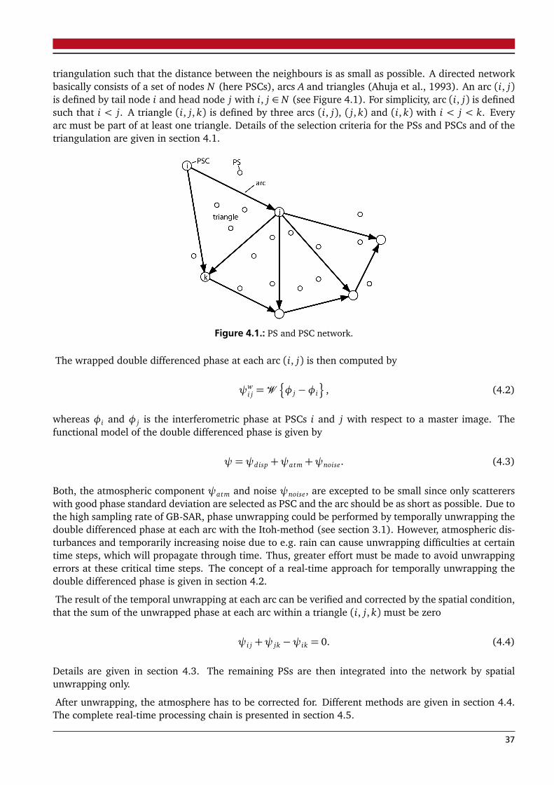
triangulation such that the distance between the neighbours is as small as possible. A directed networkbasically consists of a set of nodes N (here PSCs), arcs A and triangles (Ahuja et al., 1993). An arc (i, j)is defined by tail node i and head node j with i, j ∈ N (see Figure 4.1). For simplicity, arc (i, j) is definedsuch that i < j. A triangle (i, j, k) is defined by three arcs (i, j), ( j, k) and (i, k) with i < j < k. Everyarc must be part of at least one triangle. Details of the selection criteria for the PSs and PSCs and of thetriangulation are given in section 4.1.
Figure 4.1.: PS and PSC network.
The wrapped double differenced phase at each arc (i, j) is then computed by
ψwi j =W
¦
φ j −φi
©
, (4.2)
whereas φi and φ j is the interferometric phase at PSCs i and j with respect to a master image. Thefunctional model of the double differenced phase is given by
ψ=ψdisp +ψatm+ψnoise. (4.3)
Both, the atmospheric component ψatm and noise ψnoise, are excepted to be small since only scattererswith good phase standard deviation are selected as PSC and the arc should be as short as possible. Due tothe high sampling rate of GB-SAR, phase unwrapping could be performed by temporally unwrapping thedouble differenced phase at each arc with the Itoh-method (see section 3.1). However, atmospheric dis-turbances and temporarily increasing noise due to e.g. rain can cause unwrapping difficulties at certaintime steps, which will propagate through time. Thus, greater effort must be made to avoid unwrappingerrors at these critical time steps. The concept of a real-time approach for temporally unwrapping thedouble differenced phase is given in section 4.2.
The result of the temporal unwrapping at each arc can be verified and corrected by the spatial condition,that the sum of the unwrapped phase at each arc within a triangle (i, j, k) must be zero
ψi j +ψ jk −ψik = 0. (4.4)
Details are given in section 4.3. The remaining PSs are then integrated into the network by spatialunwrapping only.
After unwrapping, the atmosphere has to be corrected for. Different methods are given in section 4.4.The complete real-time processing chain is presented in section 4.5.
37
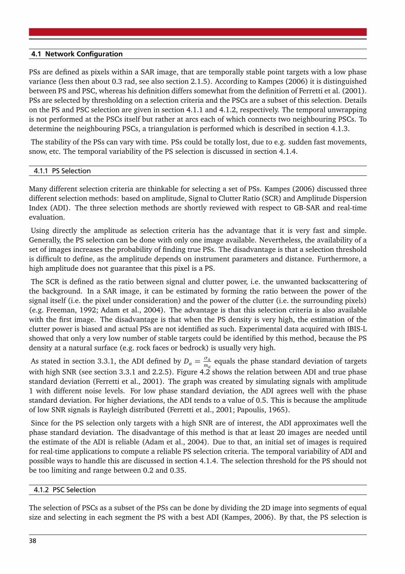
4.1 Network Configuration
PSs are defined as pixels within a SAR image, that are temporally stable point targets with a low phasevariance (less then about 0.3 rad, see also section 2.1.5). According to Kampes (2006) it is distinguishedbetween PS and PSC, whereas his definition differs somewhat from the definition of Ferretti et al. (2001).PSs are selected by thresholding on a selection criteria and the PSCs are a subset of this selection. Detailson the PS and PSC selection are given in section 4.1.1 and 4.1.2, respectively. The temporal unwrappingis not performed at the PSCs itself but rather at arcs each of which connects two neighbouring PSCs. Todetermine the neighbouring PSCs, a triangulation is performed which is described in section 4.1.3.
The stability of the PSs can vary with time. PSs could be totally lost, due to e.g. sudden fast movements,snow, etc. The temporal variability of the PS selection is discussed in section 4.1.4.
4.1.1 PS Selection
Many different selection criteria are thinkable for selecting a set of PSs. Kampes (2006) discussed threedifferent selection methods: based on amplitude, Signal to Clutter Ratio (SCR) and Amplitude DispersionIndex (ADI). The three selection methods are shortly reviewed with respect to GB-SAR and real-timeevaluation.
Using directly the amplitude as selection criteria has the advantage that it is very fast and simple.Generally, the PS selection can be done with only one image available. Nevertheless, the availability of aset of images increases the probability of finding true PSs. The disadvantage is that a selection thresholdis difficult to define, as the amplitude depends on instrument parameters and distance. Furthermore, ahigh amplitude does not guarantee that this pixel is a PS.
The SCR is defined as the ratio between signal and clutter power, i.e. the unwanted backscattering ofthe background. In a SAR image, it can be estimated by forming the ratio between the power of thesignal itself (i.e. the pixel under consideration) and the power of the clutter (i.e. the surrounding pixels)(e.g. Freeman, 1992; Adam et al., 2004). The advantage is that this selection criteria is also availablewith the first image. The disadvantage is that when the PS density is very high, the estimation of theclutter power is biased and actual PSs are not identified as such. Experimental data acquired with IBIS-Lshowed that only a very low number of stable targets could be identified by this method, because the PSdensity at a natural surface (e.g. rock faces or bedrock) is usually very high.
As stated in section 3.3.1, the ADI defined by Da =σama
equals the phase standard deviation of targetswith high SNR (see section 3.3.1 and 2.2.5). Figure 4.2 shows the relation between ADI and true phasestandard deviation (Ferretti et al., 2001). The graph was created by simulating signals with amplitude1 with different noise levels. For low phase standard deviation, the ADI agrees well with the phasestandard deviation. For higher deviations, the ADI tends to a value of 0.5. This is because the amplitudeof low SNR signals is Rayleigh distributed (Ferretti et al., 2001; Papoulis, 1965).
Since for the PS selection only targets with a high SNR are of interest, the ADI approximates well thephase standard deviation. The disadvantage of this method is that at least 20 images are needed untilthe estimate of the ADI is reliable (Adam et al., 2004). Due to that, an initial set of images is requiredfor real-time applications to compute a reliable PS selection criteria. The temporal variability of ADI andpossible ways to handle this are discussed in section 4.1.4. The selection threshold for the PS should notbe too limiting and range between 0.2 and 0.35.
4.1.2 PSC Selection
The selection of PSCs as a subset of the PSs can be done by dividing the 2D image into segments of equalsize and selecting in each segment the PS with a best ADI (Kampes, 2006). By that, the PS selection is
38

Figure 4.2.: Relation between ADI and phase standard deviation derived by simulation after Ferretti et al. (2001).
basically thinned out. Figure 4.3 shows a simulated PS selection. 1831 PSs were selected by thresholdingon the ADI. The 189 PSCs were selected using segments of size 5 × 5 m2. In each segment only one PSis marked as PSC.
The choice of the size of the segments to thin out the PS selection depends on the maximum rangeand spatial resolution of the image. Furthermore, the expected spatial distribution of the displacementsshould be considered in the decision e.g. if it is known that only a small area is moving, the spatialdensity of the PSC should be high enough to cover this area. Thus, it is recommended that the size of thesegments ranges between a few square meters up to 30 × 30 m2. The larger the distance between thePSC, the higher is the danger of unwrapping errors due to atmospheric artefacts, since the atmosphericeffect at the arcs connecting the neighbouring PSC is assumed to be small.
(a) Simulated PS selection (b) PSC selection
Figure 4.3.: Simulated PS/PSC network. The PSC selection was done by dividing the grid into segments of size 5x 5 m.
4.1.3 Triangulation
For triangulation of the PSCs, the Delaunay triangulation is used as basis (Delaunay, 1934; Lee andSchachter, 1980). It finds a set of triangles by maximizing the minimum angles of all triangles. Thecondition, that the atmospheric phase is small, is only valid if the arc length is small. Thus, triangleswhere the maximum arc length exceeds a certain threshold are deleted. The maximum arc length should
39
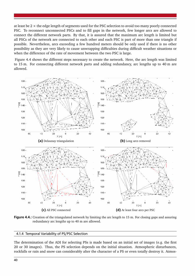
at least be 2× the edge length of segments used for the PSC selection to avoid too many poorly connectedPSC. To reconnect unconnected PSCs and to fill gaps in the network, few longer arcs are allowed toconnect the different network parts. By that, it is assured that the maximum arc length is limited butall PSCs of the network are connected to each other and each PSC is part of more than one triangle ifpossible. Nevertheless, arcs exceeding a few hundred meters should be only used if there is no otherpossibility as they are very likely to cause unwrapping difficulties during difficult weather situations orwhen the difference of the rate of movement between the two PSC is large.
Figure 4.4 shows the different steps necessary to create the network. Here, the arc length was limitedto 15 m. For connecting different network parts and adding redundancy, arc lengths up to 40 m areallowed.
(a) Delaunay triangulation (b) Long arcs removed
(c) All PSC connected (d) At least four arcs per PSC
Figure 4.4.: Creation of the triangulated network by limiting the arc length to 15 m. For closing gaps and assuringredundancy arc lengths up to 40 m are allowed.
4.1.4 Temporal Variability of PS/PSC Selection
The determination of the ADI for selecting PSs is made based on an initial set of images (e.g. the first20 or 30 images). Thus, the PS selection depends on the initial situation. Atmospheric disturbances,rockfalls or rain and snow can considerably alter the character of a PS or even totally destroy it. Atmos-
40
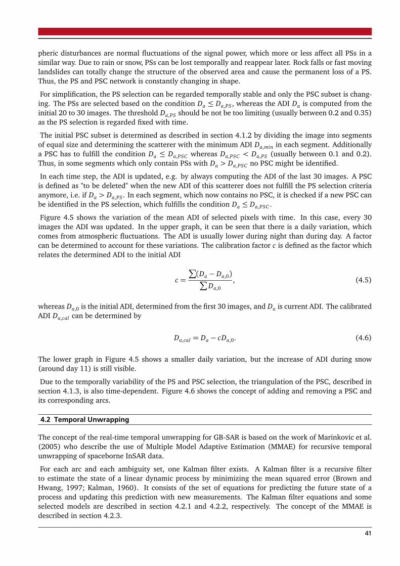
pheric disturbances are normal fluctuations of the signal power, which more or less affect all PSs in asimilar way. Due to rain or snow, PSs can be lost temporally and reappear later. Rock falls or fast movinglandslides can totally change the structure of the observed area and cause the permanent loss of a PS.Thus, the PS and PSC network is constantly changing in shape.
For simplification, the PS selection can be regarded temporally stable and only the PSC subset is chang-ing. The PSs are selected based on the condition Da ≤ Da,PS, whereas the ADI Da is computed from theinitial 20 to 30 images. The threshold Da,PS should be not be too limiting (usually between 0.2 and 0.35)as the PS selection is regarded fixed with time.
The initial PSC subset is determined as described in section 4.1.2 by dividing the image into segmentsof equal size and determining the scatterer with the minimum ADI Da,min in each segment. Additionallya PSC has to fulfill the condition Da ≤ Da,PSC whereas Da,PSC < Da,PS (usually between 0.1 and 0.2).Thus, in some segments which only contain PSs with Da > Da,PSC no PSC might be identified.
In each time step, the ADI is updated, e.g. by always computing the ADI of the last 30 images. A PSCis defined as "to be deleted" when the new ADI of this scatterer does not fulfill the PS selection criteriaanymore, i.e. if Da > Da,PS. In each segment, which now contains no PSC, it is checked if a new PSC canbe identified in the PS selection, which fulfills the condition Da ≤ Da,PSC .
Figure 4.5 shows the variation of the mean ADI of selected pixels with time. In this case, every 30images the ADI was updated. In the upper graph, it can be seen that there is a daily variation, whichcomes from atmospheric fluctuations. The ADI is usually lower during night than during day. A factorcan be determined to account for these variations. The calibration factor c is defined as the factor whichrelates the determined ADI to the initial ADI
c =
∑
(Da − Da,0)∑
Da,0, (4.5)
whereas Da,0 is the initial ADI, determined from the first 30 images, and Da is current ADI. The calibratedADI Da,cal can be determined by
Da,cal = Da − cDa,0. (4.6)
The lower graph in Figure 4.5 shows a smaller daily variation, but the increase of ADI during snow(around day 11) is still visible.
Due to the temporally variability of the PS and PSC selection, the triangulation of the PSC, described insection 4.1.3, is also time-dependent. Figure 4.6 shows the concept of adding and removing a PSC andits corresponding arcs.
4.2 Temporal Unwrapping
The concept of the real-time temporal unwrapping for GB-SAR is based on the work of Marinkovic et al.(2005) who describe the use of Multiple Model Adaptive Estimation (MMAE) for recursive temporalunwrapping of spaceborne InSAR data.
For each arc and each ambiguity set, one Kalman filter exists. A Kalman filter is a recursive filterto estimate the state of a linear dynamic process by minimizing the mean squared error (Brown andHwang, 1997; Kalman, 1960). It consists of the set of equations for predicting the future state of aprocess and updating this prediction with new measurements. The Kalman filter equations and someselected models are described in section 4.2.1 and 4.2.2, respectively. The concept of the MMAE isdescribed in section 4.2.3.
41
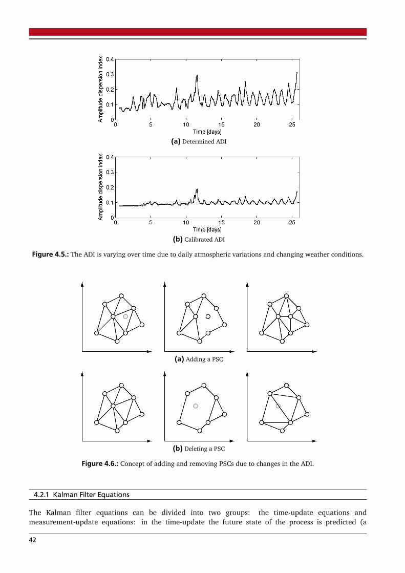
(a) Determined ADI
(b) Calibrated ADI
Figure 4.5.: The ADI is varying over time due to daily atmospheric variations and changing weather conditions.
(a) Adding a PSC
(b) Deleting a PSC
Figure 4.6.: Concept of adding and removing PSCs due to changes in the ADI.
4.2.1 Kalman Filter Equations
The Kalman filter equations can be divided into two groups: the time-update equations andmeasurement-update equations: in the time-update the future state of the process is predicted (a
42
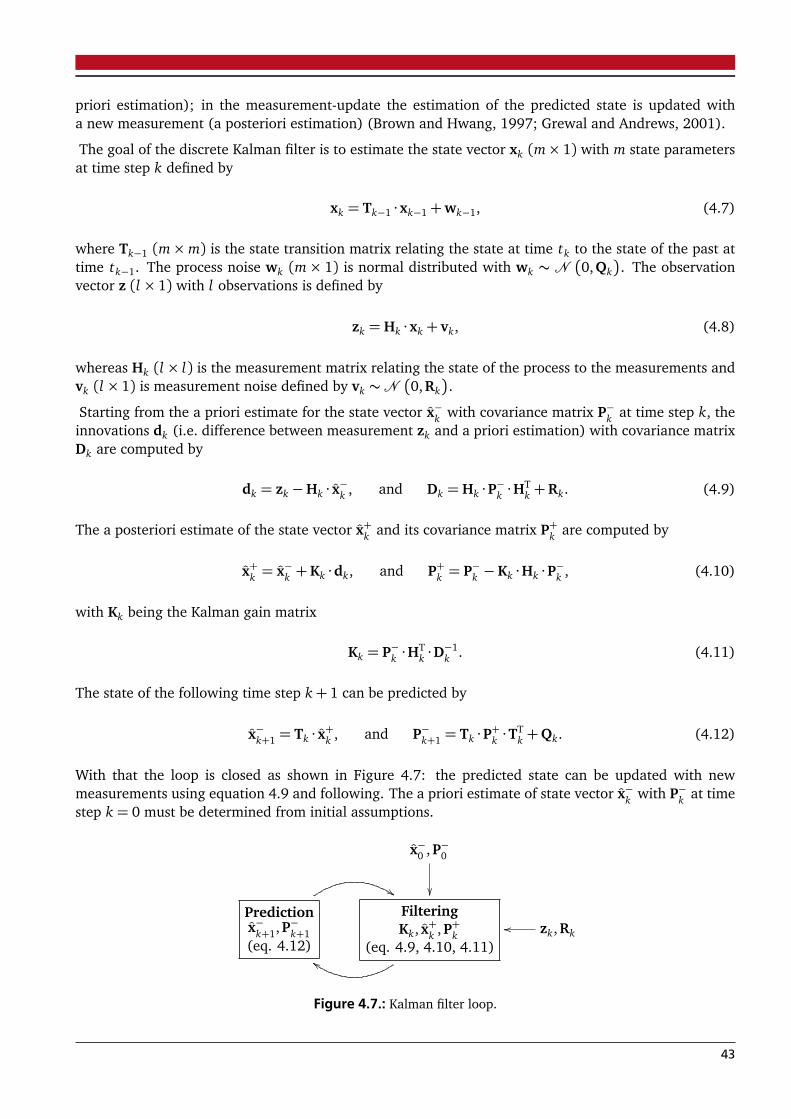
priori estimation); in the measurement-update the estimation of the predicted state is updated witha new measurement (a posteriori estimation) (Brown and Hwang, 1997; Grewal and Andrews, 2001).
The goal of the discrete Kalman filter is to estimate the state vector xk (m× 1) with m state parametersat time step k defined by
xk = Tk−1 ·xk−1+wk−1, (4.7)
where Tk−1 (m×m) is the state transition matrix relating the state at time tk to the state of the past attime tk−1. The process noise wk (m× 1) is normal distributed with wk ∼ N
�
0,Qk�
. The observationvector z (l × 1) with l observations is defined by
zk = Hk ·xk + vk, (4.8)
whereas Hk (l × l) is the measurement matrix relating the state of the process to the measurements andvk (l × 1) is measurement noise defined by vk ∼N
�
0,Rk�
.
Starting from the a priori estimate for the state vector x−k with covariance matrix P−k at time step k, theinnovations dk (i.e. difference between measurement zk and a priori estimation) with covariance matrixDk are computed by
dk = zk −Hk · x−k , and Dk = Hk ·P−k ·HTk +Rk. (4.9)
The a posteriori estimate of the state vector x+k and its covariance matrix P+k are computed by
x+k = x−k +Kk ·dk, and P+k = P−k −Kk ·Hk ·P−k , (4.10)
with Kk being the Kalman gain matrix
Kk = P−k ·HTk ·D−1
k . (4.11)
The state of the following time step k+ 1 can be predicted by
x−k+1 = Tk · x+k , and P−k+1 = Tk ·P+k ·TTk +Qk. (4.12)
With that the loop is closed as shown in Figure 4.7: the predicted state can be updated with newmeasurements using equation 4.9 and following. The a priori estimate of state vector x−k with P−k at timestep k = 0 must be determined from initial assumptions.
x−0 ,P−0
��
Predictionx−k+1,P−k+1(eq. 4.12)
$$
FilteringKk, x+k ,P+k
(eq. 4.9, 4.10, 4.11)dd
zk,Rkoo
Figure 4.7.: Kalman filter loop.
43
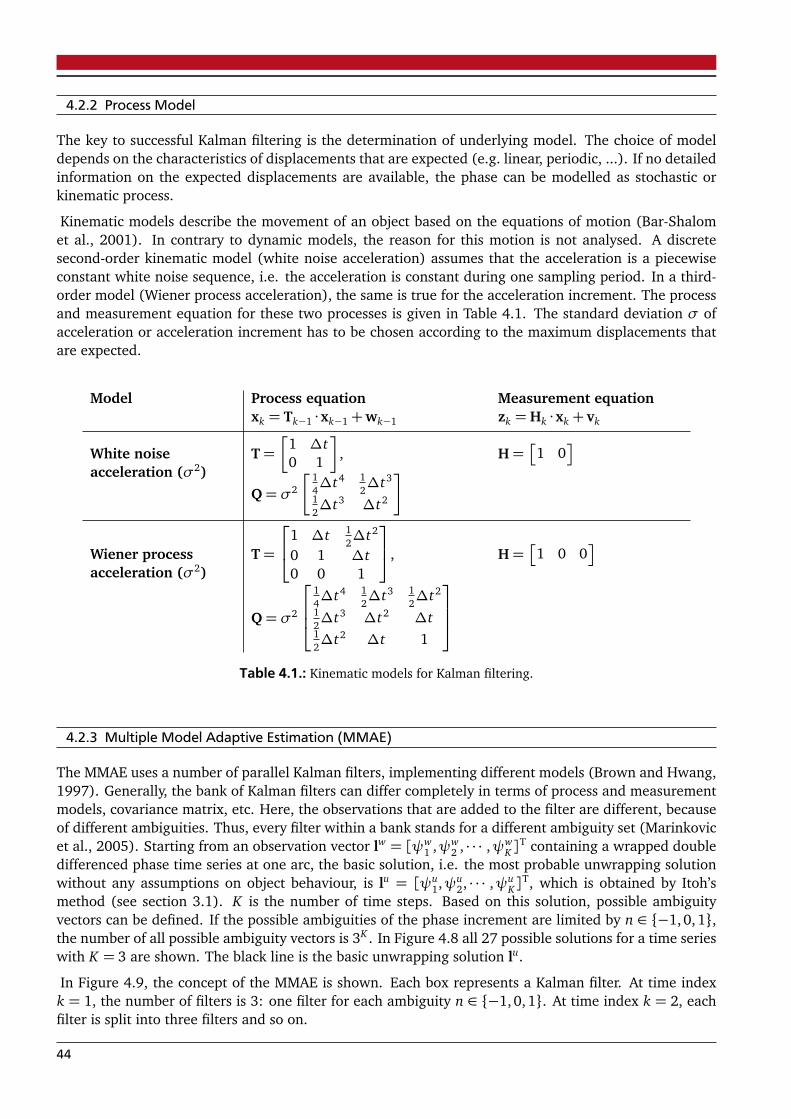
4.2.2 Process Model
The key to successful Kalman filtering is the determination of underlying model. The choice of modeldepends on the characteristics of displacements that are expected (e.g. linear, periodic, ...). If no detailedinformation on the expected displacements are available, the phase can be modelled as stochastic orkinematic process.
Kinematic models describe the movement of an object based on the equations of motion (Bar-Shalomet al., 2001). In contrary to dynamic models, the reason for this motion is not analysed. A discretesecond-order kinematic model (white noise acceleration) assumes that the acceleration is a piecewiseconstant white noise sequence, i.e. the acceleration is constant during one sampling period. In a third-order model (Wiener process acceleration), the same is true for the acceleration increment. The processand measurement equation for these two processes is given in Table 4.1. The standard deviation σ ofacceleration or acceleration increment has to be chosen according to the maximum displacements thatare expected.
Model Process equationxk = Tk−1 ·xk−1+wk−1
Measurement equationzk = Hk ·xk + vk
White noiseacceleration (σ2)
T=�
1 ∆t0 1
�
,
Q= σ2
�14∆t4 1
2∆t3
12∆t3 ∆t2
�
H=�
1 0�
Wiener processacceleration (σ2)
T=
1 ∆t 12∆t2
0 1 ∆t0 0 1
,
Q= σ2
14∆t4 1
2∆t3 1
2∆t2
12∆t3 ∆t2 ∆t
12∆t2 ∆t 1
H=�
1 0 0�
Table 4.1.: Kinematic models for Kalman filtering.
4.2.3 Multiple Model Adaptive Estimation (MMAE)
The MMAE uses a number of parallel Kalman filters, implementing different models (Brown and Hwang,1997). Generally, the bank of Kalman filters can differ completely in terms of process and measurementmodels, covariance matrix, etc. Here, the observations that are added to the filter are different, becauseof different ambiguities. Thus, every filter within a bank stands for a different ambiguity set (Marinkovicet al., 2005). Starting from an observation vector lw = [ψw
1 ,ψw2 , · · · ,ψw
K ]T containing a wrapped double
differenced phase time series at one arc, the basic solution, i.e. the most probable unwrapping solutionwithout any assumptions on object behaviour, is lu = [ψu
1,ψu2, · · · ,ψu
K]T, which is obtained by Itoh’s
method (see section 3.1). K is the number of time steps. Based on this solution, possible ambiguityvectors can be defined. If the possible ambiguities of the phase increment are limited by n ∈ {−1,0, 1},the number of all possible ambiguity vectors is 3K . In Figure 4.8 all 27 possible solutions for a time serieswith K = 3 are shown. The black line is the basic unwrapping solution lu.
In Figure 4.9, the concept of the MMAE is shown. Each box represents a Kalman filter. At time indexk = 1, the number of filters is 3: one filter for each ambiguity n ∈ {−1, 0,1}. At time index k = 2, eachfilter is split into three filters and so on.
44
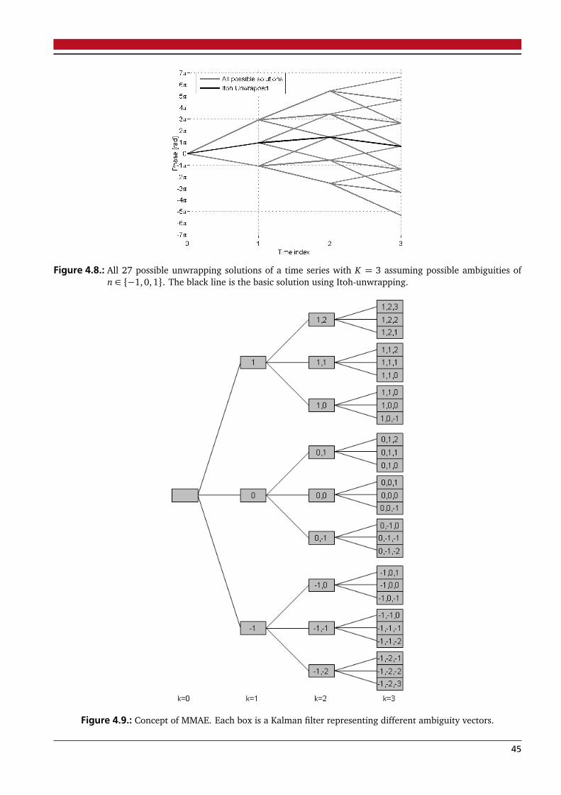
Figure 4.8.: All 27 possible unwrapping solutions of a time series with K = 3 assuming possible ambiguities ofn ∈ {−1,0, 1}. The black line is the basic solution using Itoh-unwrapping.
Figure 4.9.: Concept of MMAE. Each box is a Kalman filter representing different ambiguity vectors.
45
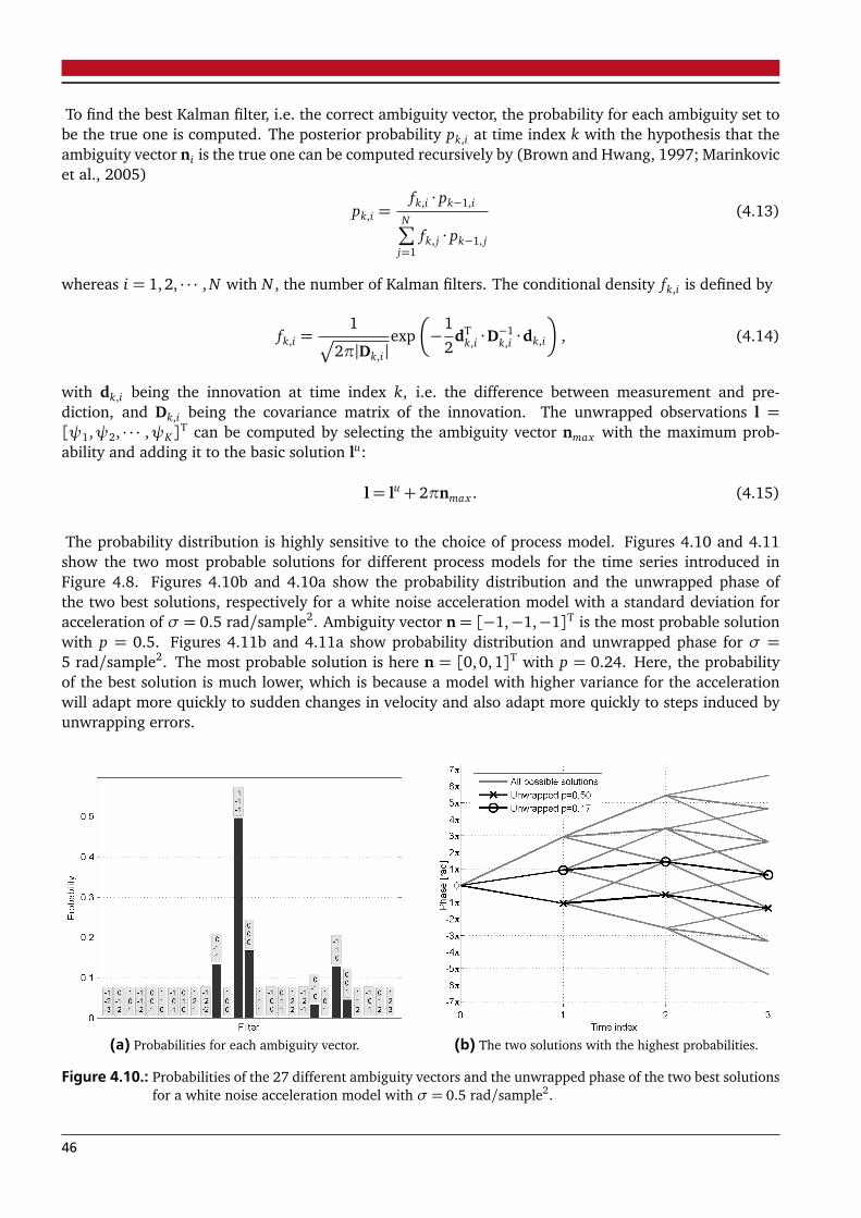
To find the best Kalman filter, i.e. the correct ambiguity vector, the probability for each ambiguity set tobe the true one is computed. The posterior probability pk,i at time index k with the hypothesis that theambiguity vector ni is the true one can be computed recursively by (Brown and Hwang, 1997; Marinkovicet al., 2005)
pk,i =fk,i · pk−1,i
N∑
j=1fk, j · pk−1, j
(4.13)
whereas i = 1, 2, · · · , N with N , the number of Kalman filters. The conditional density fk,i is defined by
fk,i =1
p
2π|Dk,i|exp�
−1
2dT
k,i ·D−1k,i ·dk,i
�
, (4.14)
with dk,i being the innovation at time index k, i.e. the difference between measurement and pre-diction, and Dk,i being the covariance matrix of the innovation. The unwrapped observations l =[ψ1,ψ2, · · · ,ψK]T can be computed by selecting the ambiguity vector nmax with the maximum prob-ability and adding it to the basic solution lu:
l= lu+ 2πnmax . (4.15)
The probability distribution is highly sensitive to the choice of process model. Figures 4.10 and 4.11show the two most probable solutions for different process models for the time series introduced inFigure 4.8. Figures 4.10b and 4.10a show the probability distribution and the unwrapped phase ofthe two best solutions, respectively for a white noise acceleration model with a standard deviation foracceleration of σ = 0.5 rad/sample2. Ambiguity vector n= [−1,−1,−1]T is the most probable solutionwith p = 0.5. Figures 4.11b and 4.11a show probability distribution and unwrapped phase for σ =5 rad/sample2. The most probable solution is here n = [0,0, 1]T with p = 0.24. Here, the probabilityof the best solution is much lower, which is because a model with higher variance for the accelerationwill adapt more quickly to sudden changes in velocity and also adapt more quickly to steps induced byunwrapping errors.
(a) Probabilities for each ambiguity vector. (b) The two solutions with the highest probabilities.
Figure 4.10.: Probabilities of the 27 different ambiguity vectors and the unwrapped phase of the two best solutionsfor a white noise acceleration model with σ = 0.5 rad/sample2.
46
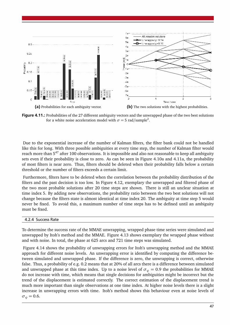
(a) Probabilities for each ambiguity vector. (b) The two solutions with the highest probabilities.
Figure 4.11.: Probabilities of the 27 different ambiguity vectors and the unwrapped phase of the two best solutionsfor a white noise acceleration model with σ = 5 rad/sample2.
Due to the exponential increase of the number of Kalman filters, the filter bank could not be handledlike this for long. With three possible ambiguities at every time step, the number of Kalman filter wouldreach more than 547 after 100 observations. It is impossible and also not reasonable to keep all ambiguitysets even if their probability is close to zero. As can be seen in Figure 4.10a and 4.11a, the probabilityof most filters is near zero. Thus, filters should be deleted when their probability falls below a certainthreshold or the number of filters exceeds a certain limit.
Furthermore, filters have to be deleted when the correlation between the probability distribution of thefilters and the past decision is too low. In Figure 4.12, exemplary the unwrapped and filtered phase ofthe two most probable solutions after 20 time steps are shown. There is still an unclear situation attime index 5. By adding new observations, the probability ratio between the two best solutions will notchange because the filters state is almost identical at time index 20. The ambiguity at time step 5 wouldnever be fixed. To avoid this, a maximum number of time steps has to be defined until an ambiguitymust be fixed.
4.2.4 Success Rate
To determine the success rate of the MMAE unwrapping, wrapped phase time series were simulated andunwrapped by Itoh’s method and the MMAE. Figure 4.13 shows exemplary the wrapped phase withoutand with noise. In total, the phase at 625 arcs and 721 time steps was simulated.
Figure 4.14 shows the probability of unwrapping errors for Itoh’s unwrapping method and the MMAEapproach for different noise levels. An unwrapping error is identified by computing the difference be-tween simulated and unwrapped phase. If the difference is zero, the unwrapping is correct, otherwisefalse. Thus, a probability of e.g. 0.2 means that at 20% of all arcs there is a difference between simulatedand unwrapped phase at this time index. Up to a noise level of σψ = 0.9 the probabilities for MMAEdo not increase with time, which means that single decisions for ambiguities might be incorrect but thetrend of the displacement is estimated correctly. The correct estimation of the displacement trend ismuch more important than single observations at one time index. At higher noise levels there is a slightincrease in unwrapping errors with time. Itoh’s method shows this behaviour even at noise levels ofσψ = 0.6.
47
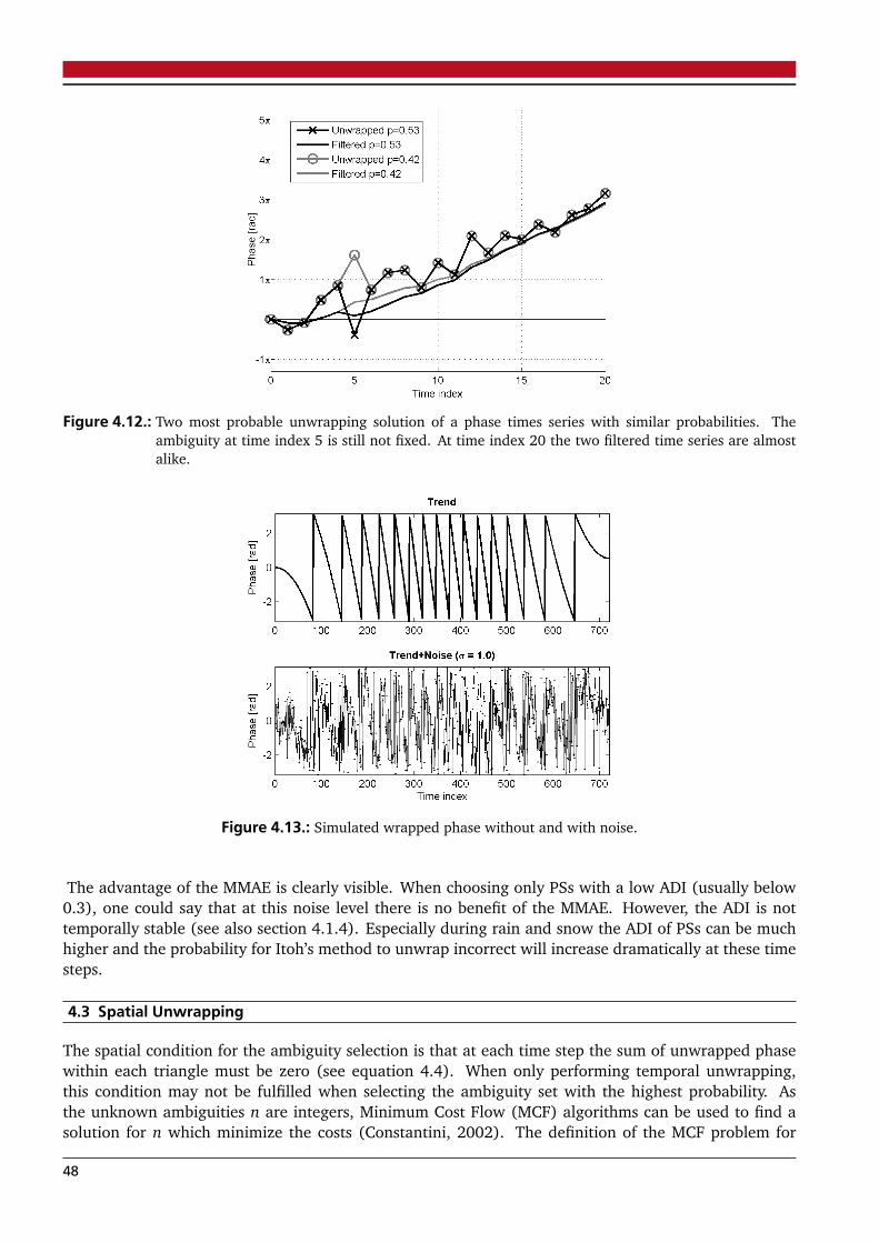
Figure 4.12.: Two most probable unwrapping solution of a phase times series with similar probabilities. Theambiguity at time index 5 is still not fixed. At time index 20 the two filtered time series are almostalike.
Figure 4.13.: Simulated wrapped phase without and with noise.
The advantage of the MMAE is clearly visible. When choosing only PSs with a low ADI (usually below0.3), one could say that at this noise level there is no benefit of the MMAE. However, the ADI is nottemporally stable (see also section 4.1.4). Especially during rain and snow the ADI of PSs can be muchhigher and the probability for Itoh’s method to unwrap incorrect will increase dramatically at these timesteps.
4.3 Spatial Unwrapping
The spatial condition for the ambiguity selection is that at each time step the sum of unwrapped phasewithin each triangle must be zero (see equation 4.4). When only performing temporal unwrapping,this condition may not be fulfilled when selecting the ambiguity set with the highest probability. Asthe unknown ambiguities n are integers, Minimum Cost Flow (MCF) algorithms can be used to find asolution for n which minimize the costs (Constantini, 2002). The definition of the MCF problem for
48
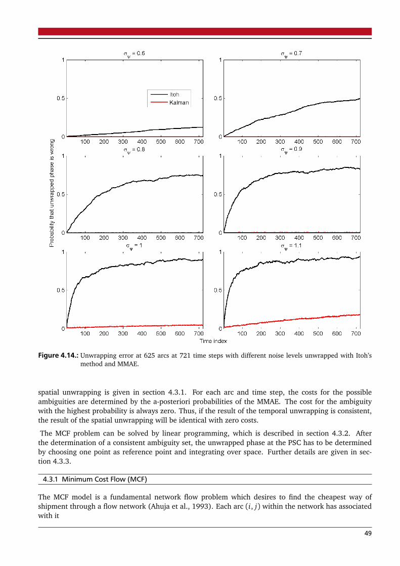
Figure 4.14.: Unwrapping error at 625 arcs at 721 time steps with different noise levels unwrapped with Itoh’smethod and MMAE.
spatial unwrapping is given in section 4.3.1. For each arc and time step, the costs for the possibleambiguities are determined by the a-posteriori probabilities of the MMAE. The cost for the ambiguitywith the highest probability is always zero. Thus, if the result of the temporal unwrapping is consistent,the result of the spatial unwrapping will be identical with zero costs.
The MCF problem can be solved by linear programming, which is described in section 4.3.2. Afterthe determination of a consistent ambiguity set, the unwrapped phase at the PSC has to be determinedby choosing one point as reference point and integrating over space. Further details are given in sec-tion 4.3.3.
4.3.1 Minimum Cost Flow (MCF)
The MCF model is a fundamental network flow problem which desires to find the cheapest way ofshipment through a flow network (Ahuja et al., 1993). Each arc (i, j) within the network has associatedwith it
49
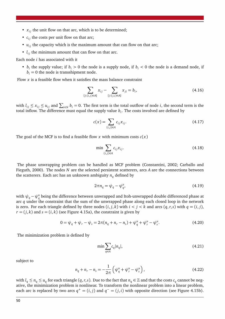
• x i j the unit flow on that arc, which is to be determined;
• ci j the costs per unit flow on that arc;
• ui j the capacity which is the maximum amount that can flow on that arc;
• li j the minimum amount that can flow on that arc.
Each node i has associated with it
• bi the supply value; if bi > 0 the node is a supply node, if bi < 0 the node is a demand node, ifbi = 0 the node is transshipment node.
Flow x is a feasible flow when it satisfies the mass balance constraint∑
{ j:(i, j)∈A}
x i j −∑
{ j:( j,i)∈A}
x ji = bi, (4.16)
with li j ≤ x i j ≤ ui j and∑
i∈N bi = 0. The first term is the total outflow of node i, the second term is thetotal inflow. The difference must equal the supply value bi. The costs involved are defined by
c(x) =∑
(i, j)∈A
ci j x i j. (4.17)
The goal of the MCF is to find a feasible flow x with minimum costs c(x)
min∑
(i, j)∈A
ci j x i j. (4.18)
The phase unwrapping problem can be handled as MCF problem (Constantini, 2002; Carballo andFieguth, 2000). The nodes N are the selected persistent scatterers, arcs A are the connections betweenthe scatterers. Each arc has an unknown ambiguity nq defined by
2πnq =ψq −ψuq, (4.19)
with ψq−ψuq being the difference between unwrapped and Itoh-unwrapped double differenced phase at
arc q under the constraint that the sum of the unwrapped phase along each closed loop in the networkis zero. For each triangle defined by three nodes (i, j, k) with i < j < k and arcs (q, r, s) with q = (i, j),r = ( j, k) and s = (i, k) (see Figure 4.15a), the constraint is given by
0=ψq +ψr −ψs = 2π(nq + nr − ns) +ψuq +ψ
ur −ψ
us . (4.20)
The minimization problem is defined by
min∑
q∈A
cq|nq|, (4.21)
subject to
nq + nr − ns =−1
2π
�
ψuq +ψ
ur −ψ
us
�
, (4.22)
with lq ≤ nq ≤ uq for each triangle (q, r, s). Due to the fact that nq ∈ Z and that the costs cq cannot be neg-ative, the minimization problem is nonlinear. To transform the nonlinear problem into a linear problem,each arc is replaced by two arcs q+ = (i, j) and q− = ( j, i) with opposite direction (see Figure 4.15b).
50
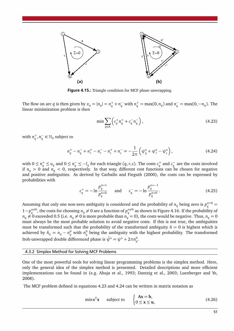
(a) (b)
Figure 4.15.: Triangle condition for MCF phase unwrapping.
The flow on arc q is then given by xq = |nq|= n+q +n−q with n+q =max(0, nq) and n−q =max(0,−nq). Thelinear minimization problem is then
min∑
q∈A
�
c+q n+q + c−q n−q�
, (4.23)
with n+q , n−q ∈ N0 subject to
n+q − n−q + n+r − n−r − n+s + n−s =−1
2π
�
ψuq +ψ
ur −ψ
us
�
, (4.24)
with 0 ≤ n+q ≤ uq and 0 ≤ n−q ≤ −lq for each triangle (q, r, s). The costs c+q and c−q are the costs involvedif nq > 0 and nq < 0, respectively. In that way, different cost functions can be chosen for negativeand positive ambiguities. As derived by Carballo and Fieguth (2000), the costs can be expressed byprobabilities with
c+q =− lnpn=1
q
pn=0q
and c−q =− lnpn=−1
q
pn=0q
. (4.25)
Assuming that only one non-zero ambiguity is considered and the probability of nq being zero is pn=0q =
1−pn6=0q , the costs for choosing nq 6= 0 are a function of pn6=0
q as shown in Figure 4.16. If the probability ofnq 6= 0 exceeded 0.5 (i.e. nq 6= 0 is more probable than nq = 0), the costs would be negative. Thus, nq = 0must always be the most probable solution to avoid negative costs. If this is not true, the ambiguitiesmust be transformed such that the probability of the transformed ambiguity n = 0 is highest which isachieved by nq = nq − n0
q with n0q being the ambiguity with the highest probability. The transformed
Itoh-unwrapped double differenced phase is ψu =ψu+ 2πn0q.
4.3.2 Simplex Method for Solving MCF Problems
One of the most powerful tools for solving linear programming problems is the simplex method. Here,only the general idea of the simplex method is presented. Detailed descriptions and more efficientimplementations can be found in (e.g. Ahuja et al., 1993; Dantzig et al., 2003; Luenberger and Ye,2008).
The MCF problem defined in equations 4.23 and 4.24 can be written in matrix notation as
mincTx subject to�
Ax= b,0≤ x≤ u, (4.26)
51
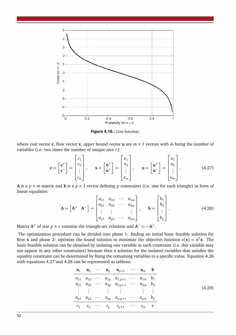
Figure 4.16.: Cost function.
where cost vector c, flow vector x, upper bound vector u are m× 1 vectors with m being the number ofvariables (i.e. two times the number of unique arcs r):
c=�
c+
c−
�
=
c1c2...
cm
, x=�
n+
n−
�
=
x1x2...
xm
, u=�
u+
u−
�
=
u1u2...
um
. (4.27)
A is a p×m matrix and b is a p× 1 vector defining p constraints (i.e. one for each triangle) in form oflinear equalities:
A=�
A+ A−�
=
a11 a12 · · · a1ma21 a22 · · · a2m...
......
ap1 ap2 · · · apm
, b=
b1b2...
bp
. (4.28)
Matrix A+ of size p× r contains the triangle-arc relations and A− =−A+.
The optimization procedure can be divided into phase 1: finding an initial basic feasible solution forflow x and phase 2: optimize the found solution to minimize the objective function z(x) = cTx. Thebasic feasible solution can be obtained by isolating one variable in each constraint (i.e. this variable maynot appear in any other constraints) because then a solution for the isolated variables that satisfies theequality constraint can be determined by fixing the remaining variables to a specific value. Equation 4.26with equations 4.27 and 4.28 can be represented as tableau:
a1 a2 · · · ap ap+1 · · · am b
a11 a12 · · · a1p a1,p+1 · · · a1m b1
a21 a22 · · · a2p a2,p+1 · · · a2m b2...
......
......
...ap1 ap2 · · · app ap,p+1 · · · apm bp
c1 c2 · · · cp cp+1 · · · cm z
(4.29)
52
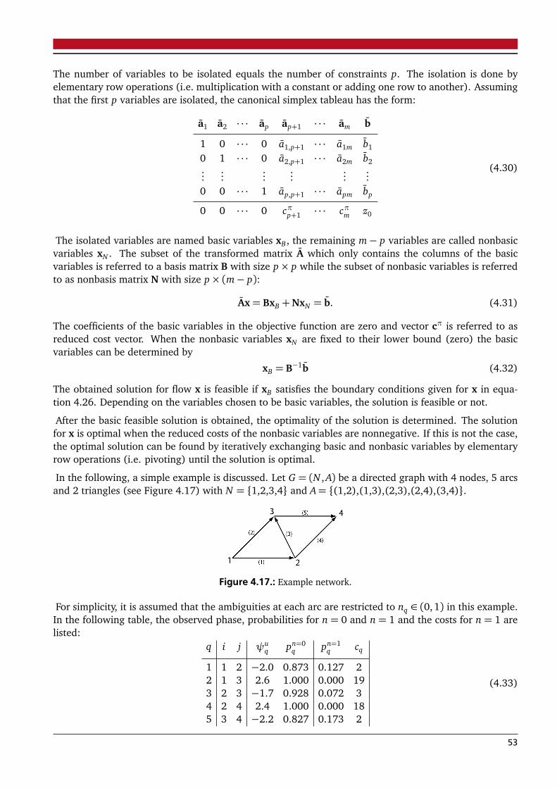
The number of variables to be isolated equals the number of constraints p. The isolation is done byelementary row operations (i.e. multiplication with a constant or adding one row to another). Assumingthat the first p variables are isolated, the canonical simplex tableau has the form:
a1 a2 · · · ap ap+1 · · · am b
1 0 · · · 0 a1,p+1 · · · a1m b1
0 1 · · · 0 a2,p+1 · · · a2m b2...
......
......
...0 0 · · · 1 ap,p+1 · · · apm bp
0 0 · · · 0 cπp+1 · · · cπm z0
(4.30)
The isolated variables are named basic variables xB, the remaining m− p variables are called nonbasicvariables xN . The subset of the transformed matrix A which only contains the columns of the basicvariables is referred to a basis matrix B with size p× p while the subset of nonbasic variables is referredto as nonbasis matrix N with size p× (m− p):
Ax= BxB +NxN = b. (4.31)
The coefficients of the basic variables in the objective function are zero and vector cπ is referred to asreduced cost vector. When the nonbasic variables xN are fixed to their lower bound (zero) the basicvariables can be determined by
xB = B−1b (4.32)
The obtained solution for flow x is feasible if xB satisfies the boundary conditions given for x in equa-tion 4.26. Depending on the variables chosen to be basic variables, the solution is feasible or not.
After the basic feasible solution is obtained, the optimality of the solution is determined. The solutionfor x is optimal when the reduced costs of the nonbasic variables are nonnegative. If this is not the case,the optimal solution can be found by iteratively exchanging basic and nonbasic variables by elementaryrow operations (i.e. pivoting) until the solution is optimal.
In the following, a simple example is discussed. Let G = (N , A) be a directed graph with 4 nodes, 5 arcsand 2 triangles (see Figure 4.17) with N = {1,2,3,4} and A= {(1,2),(1,3),(2,3),(2,4),(3,4)}.
Figure 4.17.: Example network.
For simplicity, it is assumed that the ambiguities at each arc are restricted to nq ∈ (0, 1) in this example.In the following table, the observed phase, probabilities for n = 0 and n = 1 and the costs for n = 1 arelisted:
q i j ψuq pn=0
q pn=1q cq
1 1 2 −2.0 0.873 0.127 22 1 3 2.6 1.000 0.000 193 2 3 −1.7 0.928 0.072 34 2 4 2.4 1.000 0.000 185 3 4 −2.2 0.827 0.173 2
(4.33)
53

The costs were computed according to equation 4.25. The minimization problem can be written inmatrix form by equation 4.26 with
c=
2193
182
, x=
n1n2n3n4n5
, u=
11111
, A=�
1 −1 1 0 00 0 1 −1 1
�
, b=�
11
�
. (4.34)
In tableau form the minimization problem looks as follows:
a1 a2 a3 a4 a5 b
1 −1 1 0 0 10 0 1 −1 1 1
2 19 3 18 2
(4.35)
The basic variables to be initially chosen can immediately be identified (variable 1 and 5) and the linearprogram can be brought into canonical form by adding −2×row 1 and −2×row 2 to the row containingthe costs:
a1 a2 a3 a4 a5 b
1 −1 1 0 0 10 0 1 −1 1 1
0 21 −1 20 0 4
(4.36)
If all nonbasic variables are set to zero (x2 = x3 = x4 = 0), the value of the basic variables x1 and x5 canbe determined by Ax= b. Thus, the basic feasible solution is
xT =�
1 0 0 0 1�
, (4.37)
with objective function z(x) = cTx= 4.
To find the optimal solution, the variable with negative costs is defined as entering variable (i.e. thenonbasic variable to become basic), in this case x3. To identify the corresponding leaving variable (i.e.the basic variable to become nonbasic), it is important that the feasibility of the solution is preserved.Here, x3 is at its lower bound and to find the leaving variable, x3 is set to its upper bound 1. The valuesx1 = 0 and x5 = 0 can be determined by Ax = b, which is still a feasible solution as it satisfies thecondition 0 ≤ x ≤ u. Here, one of the two basic variables x1 and x5 can be chosen to become nonbasicas both values are zero. If x5 is defined as the leaving variable, the simplex tableau can be updated tobring it into the canonical form by adding −1× row 1 to row 2 and then adding 1× row 1 to the rowcontaining the costs.
a1 a2 a3 a4 a5 b
1 −1 1 0 0 1−1 1 0 −1 1 0
1 20 0 20 0 3
(4.38)
All nonbasic variables are again set to zero x1 = x2 = x4 = 0 and the value of the basic variables can bedetermined by Ax = b. Now all costs are positive and thus the minimum is found. The feasible solutionminimizing the costs is
xT =�
0 0 1 0 0�
, (4.39)
with objective function z(x) = cTx= 3. Thus, the unwrapped phase at arc 3 is ψ=−1.7+ 2π.
54
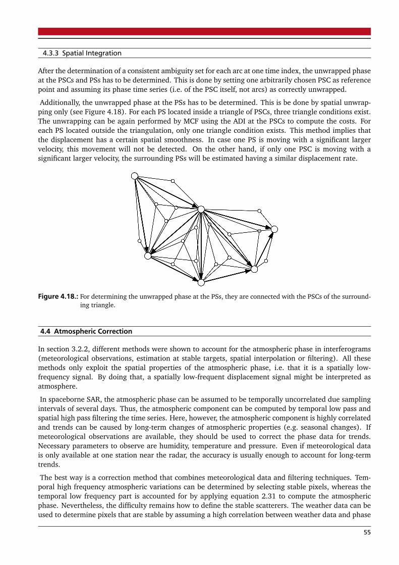
4.3.3 Spatial Integration
After the determination of a consistent ambiguity set for each arc at one time index, the unwrapped phaseat the PSCs and PSs has to be determined. This is done by setting one arbitrarily chosen PSC as referencepoint and assuming its phase time series (i.e. of the PSC itself, not arcs) as correctly unwrapped.
Additionally, the unwrapped phase at the PSs has to be determined. This is be done by spatial unwrap-ping only (see Figure 4.18). For each PS located inside a triangle of PSCs, three triangle conditions exist.The unwrapping can be again performed by MCF using the ADI at the PSCs to compute the costs. Foreach PS located outside the triangulation, only one triangle condition exists. This method implies thatthe displacement has a certain spatial smoothness. In case one PS is moving with a significant largervelocity, this movement will not be detected. On the other hand, if only one PSC is moving with asignificant larger velocity, the surrounding PSs will be estimated having a similar displacement rate.
Figure 4.18.: For determining the unwrapped phase at the PSs, they are connected with the PSCs of the surround-ing triangle.
4.4 Atmospheric Correction
In section 3.2.2, different methods were shown to account for the atmospheric phase in interferograms(meteorological observations, estimation at stable targets, spatial interpolation or filtering). All thesemethods only exploit the spatial properties of the atmospheric phase, i.e. that it is a spatially low-frequency signal. By doing that, a spatially low-frequent displacement signal might be interpreted asatmosphere.
In spaceborne SAR, the atmospheric phase can be assumed to be temporally uncorrelated due samplingintervals of several days. Thus, the atmospheric component can be computed by temporal low pass andspatial high pass filtering the time series. Here, however, the atmospheric component is highly correlatedand trends can be caused by long-term changes of atmospheric properties (e.g. seasonal changes). Ifmeteorological observations are available, they should be used to correct the phase data for trends.Necessary parameters to observe are humidity, temperature and pressure. Even if meteorological datais only available at one station near the radar, the accuracy is usually enough to account for long-termtrends.
The best way is a correction method that combines meteorological data and filtering techniques. Tem-poral high frequency atmospheric variations can be determined by selecting stable pixels, whereas thetemporal low frequency part is accounted for by applying equation 2.31 to compute the atmosphericphase. Nevertheless, the difficulty remains how to define the stable scatterers. The weather data can beused to determine pixels that are stable by assuming a high correlation between weather data and phase
55
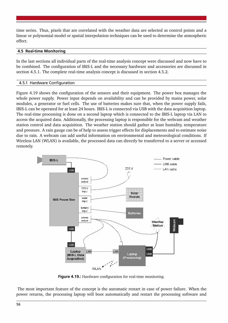
time series. Thus, pixels that are correlated with the weather data are selected as control points and alinear or polynomial model or spatial interpolation techniques can be used to determine the atmosphericeffect.
4.5 Real-time Monitoring
In the last sections all individual parts of the real-time analysis concept were discussed and now have tobe combined. The configuration of IBIS-L and the necessary hardware and accessories are discussed insection 4.5.1. The complete real-time analysis concept is discussed in section 4.5.2.
4.5.1 Hardware Configuration
Figure 4.19 shows the configuration of the sensors and their equipment. The power box manages thewhole power supply. Power input depends on availability and can be provided by mains power, solarmodules, a generator or fuel cells. The use of batteries makes sure that, when the power supply fails,IBIS-L can be operated for at least 24 hours. IBIS-L is connected via USB with the data acquisition laptop.The real-time processing is done on a second laptop which is connected to the IBIS-L laptop via LAN toaccess the acquired data. Additionally, the processing laptop is responsible for the webcam and weatherstation control and data acquisition. The weather station should gather at least humidity, temperatureand pressure. A rain gauge can be of help to assess trigger effects for displacements and to estimate noisedue to rain. A webcam can add useful information on environmental and meteorological conditions. IfWireless LAN (WLAN) is available, the processed data can directly be transferred to a server or accessedremotely.
Figure 4.19.: Hardware configuration for real-time monitoring.
The most important feature of the concept is the automatic restart in case of power failure. When thepower returns, the processing laptop will boot automatically and restart the processing software and
56
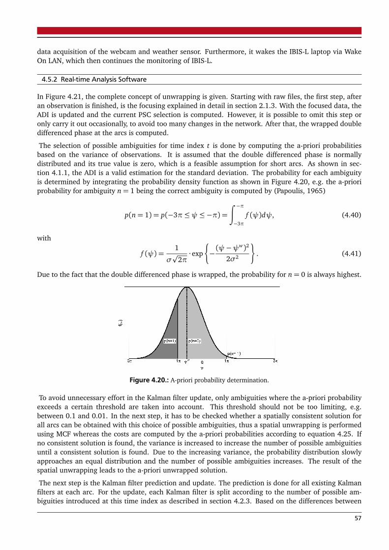
data acquisition of the webcam and weather sensor. Furthermore, it wakes the IBIS-L laptop via WakeOn LAN, which then continues the monitoring of IBIS-L.
4.5.2 Real-time Analysis Software
In Figure 4.21, the complete concept of unwrapping is given. Starting with raw files, the first step, afteran observation is finished, is the focusing explained in detail in section 2.1.3. With the focused data, theADI is updated and the current PSC selection is computed. However, it is possible to omit this step oronly carry it out occasionally, to avoid too many changes in the network. After that, the wrapped doubledifferenced phase at the arcs is computed.
The selection of possible ambiguities for time index t is done by computing the a-priori probabilitiesbased on the variance of observations. It is assumed that the double differenced phase is normallydistributed and its true value is zero, which is a feasible assumption for short arcs. As shown in sec-tion 4.1.1, the ADI is a valid estimation for the standard deviation. The probability for each ambiguityis determined by integrating the probability density function as shown in Figure 4.20, e.g. the a-prioriprobability for ambiguity n= 1 being the correct ambiguity is computed by (Papoulis, 1965)
p(n= 1) = p(−3π≤ψ≤−π) =∫ −π
−3π
f (ψ)dψ, (4.40)
with
f (ψ) =1
σp
2π· exp
¨
−(ψ−ψw)2
2σ2
«
. (4.41)
Due to the fact that the double differenced phase is wrapped, the probability for n= 0 is always highest.
Figure 4.20.: A-priori probability determination.
To avoid unnecessary effort in the Kalman filter update, only ambiguities where the a-priori probabilityexceeds a certain threshold are taken into account. This threshold should not be too limiting, e.g.between 0.1 and 0.01. In the next step, it has to be checked whether a spatially consistent solution forall arcs can be obtained with this choice of possible ambiguities, thus a spatial unwrapping is performedusing MCF whereas the costs are computed by the a-priori probabilities according to equation 4.25. Ifno consistent solution is found, the variance is increased to increase the number of possible ambiguitiesuntil a consistent solution is found. Due to the increasing variance, the probability distribution slowlyapproaches an equal distribution and the number of possible ambiguities increases. The result of thespatial unwrapping leads to the a-priori unwrapped solution.
The next step is the Kalman filter prediction and update. The prediction is done for all existing Kalmanfilters at each arc. For the update, each Kalman filter is split according to the number of possible am-biguities introduced at this time index as described in section 4.2.3. Based on the differences between
57
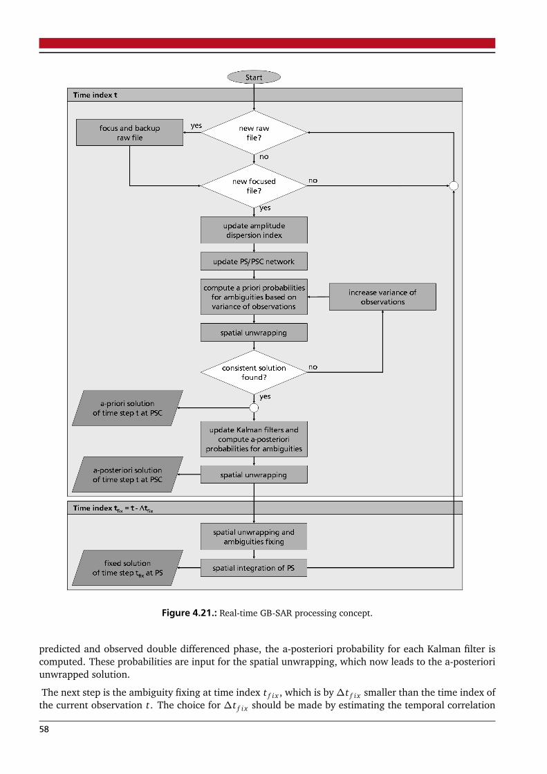
Figure 4.21.: Real-time GB-SAR processing concept.
predicted and observed double differenced phase, the a-posteriori probability for each Kalman filter iscomputed. These probabilities are input for the spatial unwrapping, which now leads to the a-posterioriunwrapped solution.
The next step is the ambiguity fixing at time index t f i x , which is by∆t f i x smaller than the time index ofthe current observation t. The choice for ∆t f i x should be made by estimating the temporal correlation
58
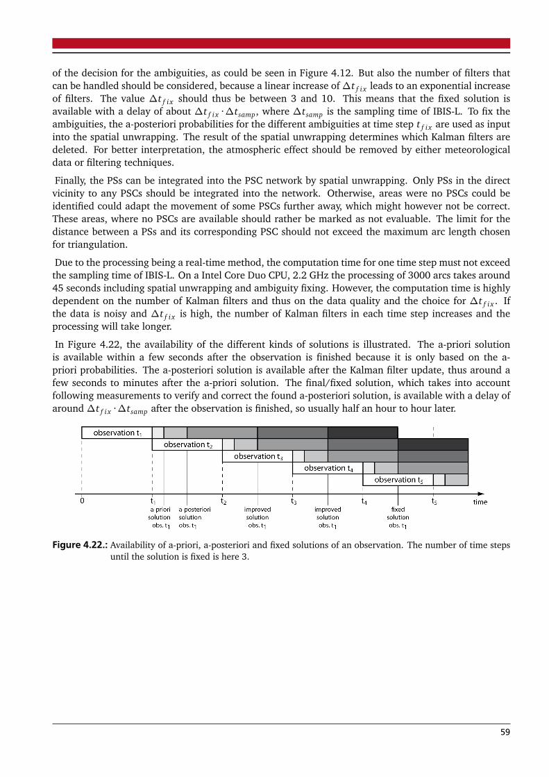
of the decision for the ambiguities, as could be seen in Figure 4.12. But also the number of filters thatcan be handled should be considered, because a linear increase of∆t f i x leads to an exponential increaseof filters. The value ∆t f i x should thus be between 3 and 10. This means that the fixed solution isavailable with a delay of about ∆t f i x ·∆tsamp, where ∆tsamp is the sampling time of IBIS-L. To fix theambiguities, the a-posteriori probabilities for the different ambiguities at time step t f i x are used as inputinto the spatial unwrapping. The result of the spatial unwrapping determines which Kalman filters aredeleted. For better interpretation, the atmospheric effect should be removed by either meteorologicaldata or filtering techniques.
Finally, the PSs can be integrated into the PSC network by spatial unwrapping. Only PSs in the directvicinity to any PSCs should be integrated into the network. Otherwise, areas were no PSCs could beidentified could adapt the movement of some PSCs further away, which might however not be correct.These areas, where no PSCs are available should rather be marked as not evaluable. The limit for thedistance between a PSs and its corresponding PSC should not exceed the maximum arc length chosenfor triangulation.
Due to the processing being a real-time method, the computation time for one time step must not exceedthe sampling time of IBIS-L. On a Intel Core Duo CPU, 2.2 GHz the processing of 3000 arcs takes around45 seconds including spatial unwrapping and ambiguity fixing. However, the computation time is highlydependent on the number of Kalman filters and thus on the data quality and the choice for ∆t f i x . Ifthe data is noisy and ∆t f i x is high, the number of Kalman filters in each time step increases and theprocessing will take longer.
In Figure 4.22, the availability of the different kinds of solutions is illustrated. The a-priori solutionis available within a few seconds after the observation is finished because it is only based on the a-priori probabilities. The a-posteriori solution is available after the Kalman filter update, thus around afew seconds to minutes after the a-priori solution. The final/fixed solution, which takes into accountfollowing measurements to verify and correct the found a-posteriori solution, is available with a delay ofaround ∆t f i x ·∆tsamp after the observation is finished, so usually half an hour to hour later.
Figure 4.22.: Availability of a-priori, a-posteriori and fixed solutions of an observation. The number of time stepsuntil the solution is fixed is here 3.
59
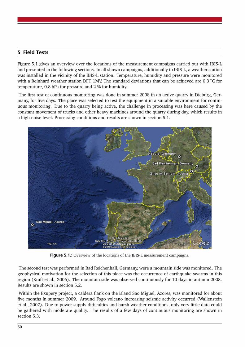
5 Field Tests
Figure 5.1 gives an overview over the locations of the measurement campaigns carried out with IBIS-Land presented in the following sections. In all shown campaigns, additionally to IBIS-L, a weather stationwas installed in the vicinity of the IBIS-L station. Temperature, humidity and pressure were monitoredwith a Reinhard weather station DFT 1MV. The standard deviations that can be achieved are 0.3 ◦C fortemperature, 0.8 hPa for pressure and 2 % for humidity.
The first test of continuous monitoring was done in summer 2008 in an active quarry in Dieburg, Ger-many, for five days. The place was selected to test the equipment in a suitable environment for contin-uous monitoring. Due to the quarry being active, the challenge in processing was here caused by theconstant movement of trucks and other heavy machines around the quarry during day, which results ina high noise level. Processing conditions and results are shown in section 5.1.
Figure 5.1.: Overview of the locations of the IBIS-L measurement campaigns.
The second test was performed in Bad Reichenhall, Germany, were a mountain side was monitored. Thegeophysical motivation for the selection of this place was the occurrence of earthquake swarms in thisregion (Kraft et al., 2006). The mountain side was observed continuously for 10 days in autumn 2008.Results are shown in section 5.2.
Within the Exupery project, a caldera flank on the island Sao Miguel, Azores, was monitored for aboutfive months in summer 2009. Around Fogo volcano increasing seismic activity occurred (Wallensteinet al., 2007). Due to power supply difficulties and harsh weather conditions, only very little data couldbe gathered with moderate quality. The results of a few days of continuous monitoring are shown insection 5.3.
60
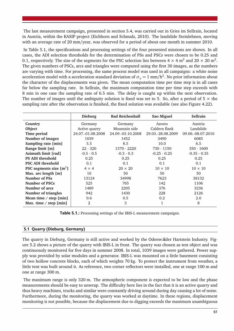
The last measurement campaign, presented in section 5.4, was carried out in Gries im Sellrain, locatedin Austria, within the KASIP project (Eichhorn and Schmalz, 2010). The landslide Steinlehnen, movingwith an average rate of 20 mm/year, was observed for a period of about one month in summer 2010.
In Table 5.1, the specifications and processing settings of the four presented missions are shown. In allcases, the ADI selection thresholds for the determination of PSs and PSCs were chosen to be 0.25 and0.1, respectively. The size of the segments for the PSC selection lies between 4 × 4 m2 and 20 × 20 m2.The given numbers of PSCs, arcs and triangles were computed using the first 30 images, as the numbersare varying with time. For processing, the same process model was used in all campaigns: a white noiseacceleration model with a acceleration standard deviation of σa = 1 mm/h2. No prior information aboutthe character of the displacements was given. The mean computation time per time step is in all casesfar below the sampling rate. In Sellrain, the maximum computation time per time step exceeds with8 min in one case the sampling rate of 6.5 min. The delay is caught up within the next observation.The number of images until the ambiguity solution is fixed was set to 5. So, after a period of 5 × thesampling rate after the observation is finished, the fixed solution was available (see also Figure 4.22).
Dieburg Bad Reichenhall Sao Miguel Sellrain
Country Germany Germany Azores AustriaObject Active quarry Mountain side Caldera flank LandslideTime period 24.07.-01.08.2008 24.09.-03.10.2008 29.03.-28.08.2009 09.06.-08.07.2010Number of images 1039 1452 3490 6085Sampling rate [min] 5.5 8.5 10.0 6.5Range limit [m] 22 - 320 1370 - 2220 730 - 1150 350 - 1600Azimuth limit [rad] -0.5 - 0.5 -0.3 - 0.3 -0.25 - 0.25 -0.35 - 0.35PS ADI threshold 0.25 0.25 0.25 0.25PSC ADI threshold 0.1 0.1 0.1 0.1PSC segments size [m2] 4 × 4 20 × 20 10 × 10 10 × 10Max. arc length [m] 10 50 50 50Number of PSs 13124 34998 7623 38132Number of PSCs 525 765 142 1106Number of arcs 1489 2205 376 3236Number of triangles 942 1430 228 2126Mean time / step [min] 0.6 0.5 0.2 2.0Max. time / step [min] 2 3 1 8
Table 5.1.: Processing settings of the IBIS-L measurement campaigns.
5.1 Quarry (Dieburg, Germany)
The quarry in Dieburg, Germany is still active and worked by the Odenwälder Hartstein Industry. Fig-ure 5.2 shows a picture of the quarry with IBIS-L in front. The quarry was chosen as test object and wascontinuously monitored for five days in summer 2008. In total, 1039 images were gathered. Power sup-ply was provided by solar modules and a generator. IBIS-L was mounted on a little basement consistingof two hollow concrete blocks, each of which weights 70 kg. To protect the instrument from weather, alittle tent was built around it. As reference, two corner reflectors were installed, one at range 100 m andone at range 300 m.
The maximum range is only 320 m. The atmospheric component is expected to be low and the phasemeasurements should be easy to unwrap. The difficulty here lies in the fact that it is an active quarry andthus heavy machines, trucks and similar were constantly driving around during day causing a lot of noise.Furthermore, during the monitoring, the quarry was worked at daytime. In these regions, displacementmonitoring is not possible, because the displacement due to digging exceeds the maximum unambiguous
61
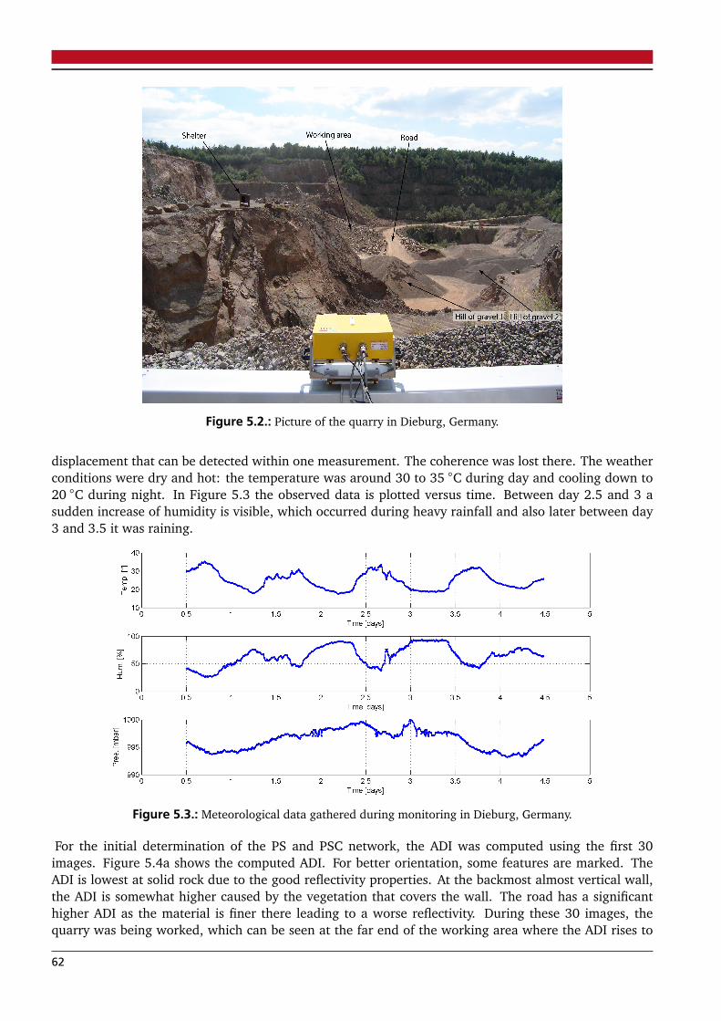
Figure 5.2.: Picture of the quarry in Dieburg, Germany.
displacement that can be detected within one measurement. The coherence was lost there. The weatherconditions were dry and hot: the temperature was around 30 to 35 ◦C during day and cooling down to20 ◦C during night. In Figure 5.3 the observed data is plotted versus time. Between day 2.5 and 3 asudden increase of humidity is visible, which occurred during heavy rainfall and also later between day3 and 3.5 it was raining.
Figure 5.3.: Meteorological data gathered during monitoring in Dieburg, Germany.
For the initial determination of the PS and PSC network, the ADI was computed using the first 30images. Figure 5.4a shows the computed ADI. For better orientation, some features are marked. TheADI is lowest at solid rock due to the good reflectivity properties. At the backmost almost vertical wall,the ADI is somewhat higher caused by the vegetation that covers the wall. The road has a significanthigher ADI as the material is finer there leading to a worse reflectivity. During these 30 images, thequarry was being worked, which can be seen at the far end of the working area where the ADI rises to
62
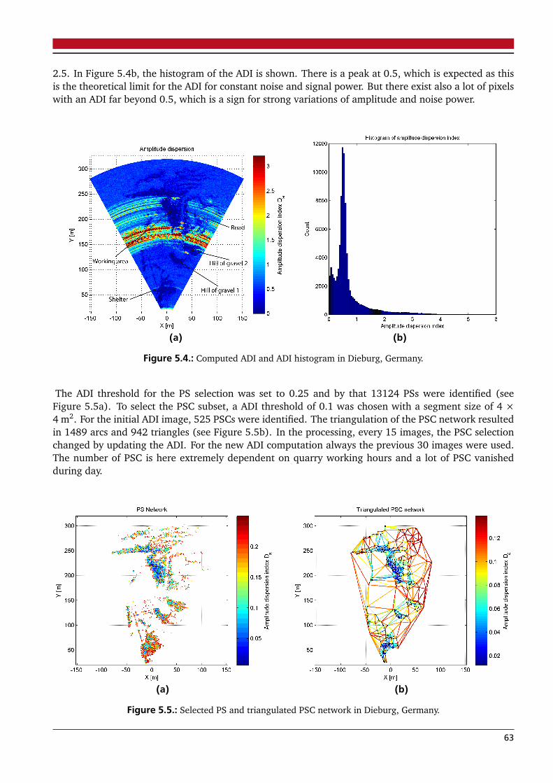
2.5. In Figure 5.4b, the histogram of the ADI is shown. There is a peak at 0.5, which is expected as thisis the theoretical limit for the ADI for constant noise and signal power. But there exist also a lot of pixelswith an ADI far beyond 0.5, which is a sign for strong variations of amplitude and noise power.
(a) (b)
Figure 5.4.: Computed ADI and ADI histogram in Dieburg, Germany.
The ADI threshold for the PS selection was set to 0.25 and by that 13124 PSs were identified (seeFigure 5.5a). To select the PSC subset, a ADI threshold of 0.1 was chosen with a segment size of 4 ×4 m2. For the initial ADI image, 525 PSCs were identified. The triangulation of the PSC network resultedin 1489 arcs and 942 triangles (see Figure 5.5b). In the processing, every 15 images, the PSC selectionchanged by updating the ADI. For the new ADI computation always the previous 30 images were used.The number of PSC is here extremely dependent on quarry working hours and a lot of PSC vanishedduring day.
(a) (b)
Figure 5.5.: Selected PS and triangulated PSC network in Dieburg, Germany.
63
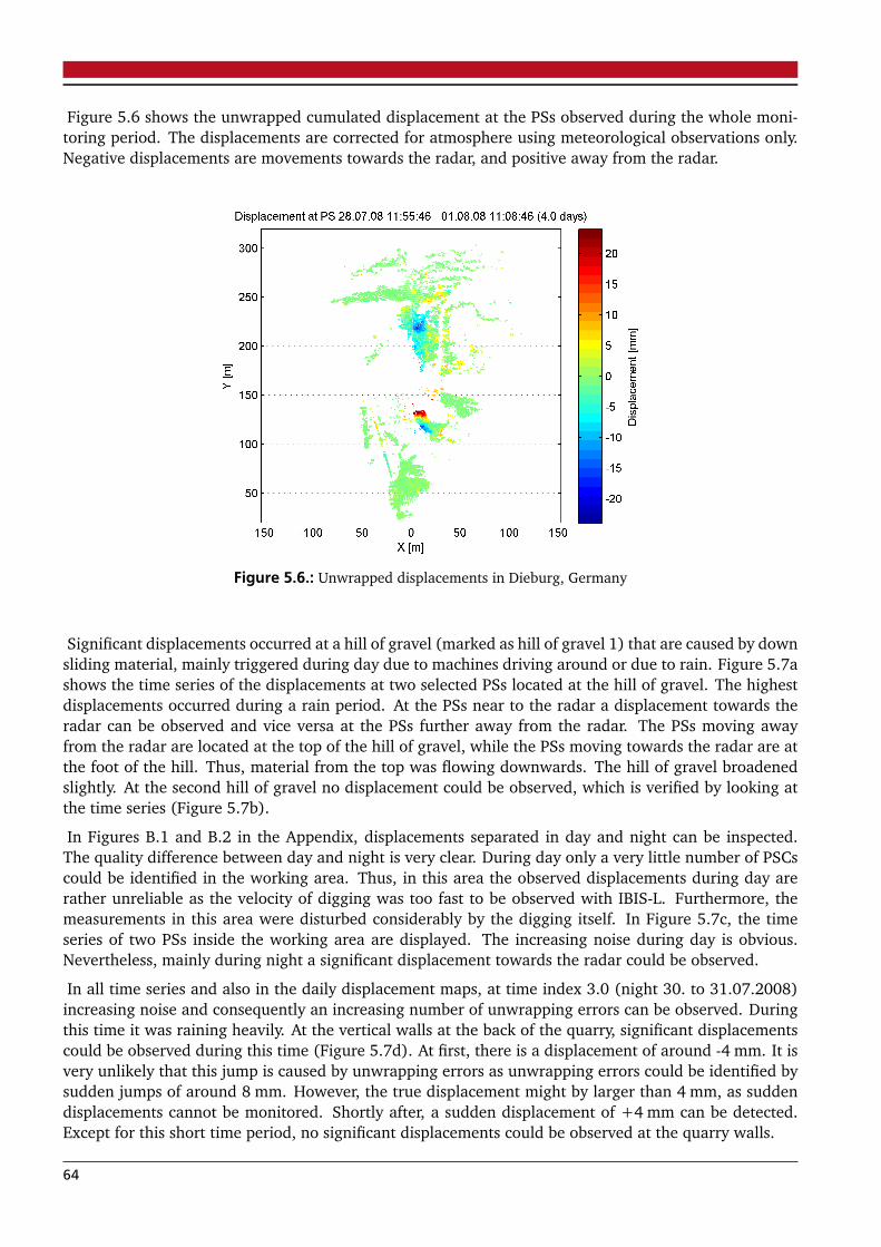
Figure 5.6 shows the unwrapped cumulated displacement at the PSs observed during the whole moni-toring period. The displacements are corrected for atmosphere using meteorological observations only.Negative displacements are movements towards the radar, and positive away from the radar.
Figure 5.6.: Unwrapped displacements in Dieburg, Germany
Significant displacements occurred at a hill of gravel (marked as hill of gravel 1) that are caused by downsliding material, mainly triggered during day due to machines driving around or due to rain. Figure 5.7ashows the time series of the displacements at two selected PSs located at the hill of gravel. The highestdisplacements occurred during a rain period. At the PSs near to the radar a displacement towards theradar can be observed and vice versa at the PSs further away from the radar. The PSs moving awayfrom the radar are located at the top of the hill of gravel, while the PSs moving towards the radar are atthe foot of the hill. Thus, material from the top was flowing downwards. The hill of gravel broadenedslightly. At the second hill of gravel no displacement could be observed, which is verified by looking atthe time series (Figure 5.7b).
In Figures B.1 and B.2 in the Appendix, displacements separated in day and night can be inspected.The quality difference between day and night is very clear. During day only a very little number of PSCscould be identified in the working area. Thus, in this area the observed displacements during day arerather unreliable as the velocity of digging was too fast to be observed with IBIS-L. Furthermore, themeasurements in this area were disturbed considerably by the digging itself. In Figure 5.7c, the timeseries of two PSs inside the working area are displayed. The increasing noise during day is obvious.Nevertheless, mainly during night a significant displacement towards the radar could be observed.
In all time series and also in the daily displacement maps, at time index 3.0 (night 30. to 31.07.2008)increasing noise and consequently an increasing number of unwrapping errors can be observed. Duringthis time it was raining heavily. At the vertical walls at the back of the quarry, significant displacementscould be observed during this time (Figure 5.7d). At first, there is a displacement of around -4 mm. It isvery unlikely that this jump is caused by unwrapping errors as unwrapping errors could be identified bysudden jumps of around 8 mm. However, the true displacement might by larger than 4 mm, as suddendisplacements cannot be monitored. Shortly after, a sudden displacement of +4 mm can be detected.Except for this short time period, no significant displacements could be observed at the quarry walls.
64
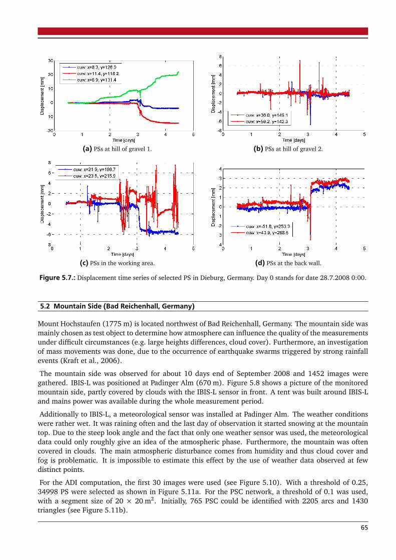
(a) PSs at hill of gravel 1. (b) PSs at hill of gravel 2.
(c) PSs in the working area. (d) PSs at the back wall.
Figure 5.7.: Displacement time series of selected PS in Dieburg, Germany. Day 0 stands for date 28.7.2008 0:00.
5.2 Mountain Side (Bad Reichenhall, Germany)
Mount Hochstaufen (1775 m) is located northwest of Bad Reichenhall, Germany. The mountain side wasmainly chosen as test object to determine how atmosphere can influence the quality of the measurementsunder difficult circumstances (e.g. large heights differences, cloud cover). Furthermore, an investigationof mass movements was done, due to the occurrence of earthquake swarms triggered by strong rainfallevents (Kraft et al., 2006).
The mountain side was observed for about 10 days end of September 2008 and 1452 images weregathered. IBIS-L was positioned at Padinger Alm (670 m). Figure 5.8 shows a picture of the monitoredmountain side, partly covered by clouds with the IBIS-L sensor in front. A tent was built around IBIS-Land mains power was available during the whole measurement period.
Additionally to IBIS-L, a meteorological sensor was installed at Padinger Alm. The weather conditionswere rather wet. It was raining often and the last day of observation it started snowing at the mountaintop. Due to the steep look angle and the fact that only one weather sensor was used, the meteorologicaldata could only roughly give an idea of the atmospheric phase. Furthermore, the mountain was oftencovered in clouds. The main atmospheric disturbance comes from humidity and thus cloud cover andfog is problematic. It is impossible to estimate this effect by the use of weather data observed at fewdistinct points.
For the ADI computation, the first 30 images were used (see Figure 5.10). With a threshold of 0.25,34998 PS were selected as shown in Figure 5.11a. For the PSC network, a threshold of 0.1 was used,with a segment size of 20 × 20 m2. Initially, 765 PSC could be identified with 2205 arcs and 1430triangles (see Figure 5.11b).
65
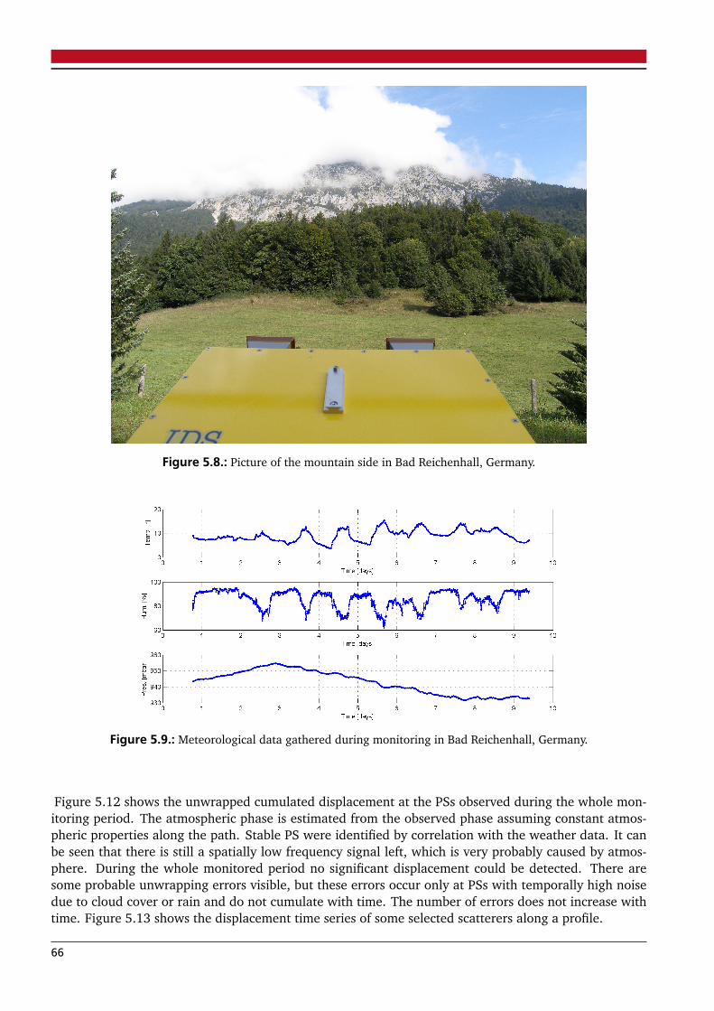
Figure 5.8.: Picture of the mountain side in Bad Reichenhall, Germany.
Figure 5.9.: Meteorological data gathered during monitoring in Bad Reichenhall, Germany.
Figure 5.12 shows the unwrapped cumulated displacement at the PSs observed during the whole mon-itoring period. The atmospheric phase is estimated from the observed phase assuming constant atmos-pheric properties along the path. Stable PS were identified by correlation with the weather data. It canbe seen that there is still a spatially low frequency signal left, which is very probably caused by atmos-phere. During the whole monitored period no significant displacement could be detected. There aresome probable unwrapping errors visible, but these errors occur only at PSs with temporally high noisedue to cloud cover or rain and do not cumulate with time. The number of errors does not increase withtime. Figure 5.13 shows the displacement time series of some selected scatterers along a profile.
66
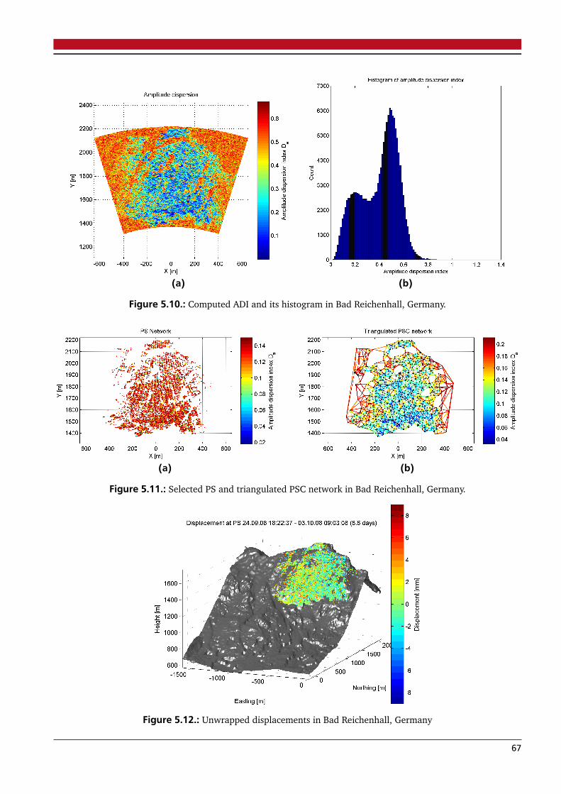
(a) (b)
Figure 5.10.: Computed ADI and its histogram in Bad Reichenhall, Germany.
(a) (b)
Figure 5.11.: Selected PS and triangulated PSC network in Bad Reichenhall, Germany.
Figure 5.12.: Unwrapped displacements in Bad Reichenhall, Germany
67
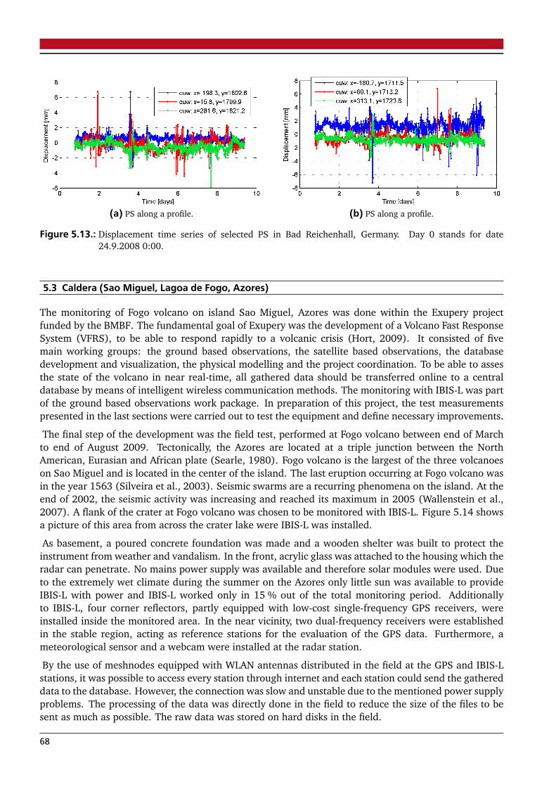
(a) PS along a profile. (b) PS along a profile.
Figure 5.13.: Displacement time series of selected PS in Bad Reichenhall, Germany. Day 0 stands for date24.9.2008 0:00.
5.3 Caldera (Sao Miguel, Lagoa de Fogo, Azores)
The monitoring of Fogo volcano on island Sao Miguel, Azores was done within the Exupery projectfunded by the BMBF. The fundamental goal of Exupery was the development of a Volcano Fast ResponseSystem (VFRS), to be able to respond rapidly to a volcanic crisis (Hort, 2009). It consisted of fivemain working groups: the ground based observations, the satellite based observations, the databasedevelopment and visualization, the physical modelling and the project coordination. To be able to assesthe state of the volcano in near real-time, all gathered data should be transferred online to a centraldatabase by means of intelligent wireless communication methods. The monitoring with IBIS-L was partof the ground based observations work package. In preparation of this project, the test measurementspresented in the last sections were carried out to test the equipment and define necessary improvements.
The final step of the development was the field test, performed at Fogo volcano between end of Marchto end of August 2009. Tectonically, the Azores are located at a triple junction between the NorthAmerican, Eurasian and African plate (Searle, 1980). Fogo volcano is the largest of the three volcanoeson Sao Miguel and is located in the center of the island. The last eruption occurring at Fogo volcano wasin the year 1563 (Silveira et al., 2003). Seismic swarms are a recurring phenomena on the island. At theend of 2002, the seismic activity was increasing and reached its maximum in 2005 (Wallenstein et al.,2007). A flank of the crater at Fogo volcano was chosen to be monitored with IBIS-L. Figure 5.14 showsa picture of this area from across the crater lake were IBIS-L was installed.
As basement, a poured concrete foundation was made and a wooden shelter was built to protect theinstrument from weather and vandalism. In the front, acrylic glass was attached to the housing which theradar can penetrate. No mains power supply was available and therefore solar modules were used. Dueto the extremely wet climate during the summer on the Azores only little sun was available to provideIBIS-L with power and IBIS-L worked only in 15 % out of the total monitoring period. Additionallyto IBIS-L, four corner reflectors, partly equipped with low-cost single-frequency GPS receivers, wereinstalled inside the monitored area. In the near vicinity, two dual-frequency receivers were establishedin the stable region, acting as reference stations for the evaluation of the GPS data. Furthermore, ameteorological sensor and a webcam were installed at the radar station.
By the use of meshnodes equipped with WLAN antennas distributed in the field at the GPS and IBIS-Lstations, it was possible to access every station through internet and each station could send the gathereddata to the database. However, the connection was slow and unstable due to the mentioned power supplyproblems. The processing of the data was directly done in the field to reduce the size of the files to besent as much as possible. The raw data was stored on hard disks in the field.
68
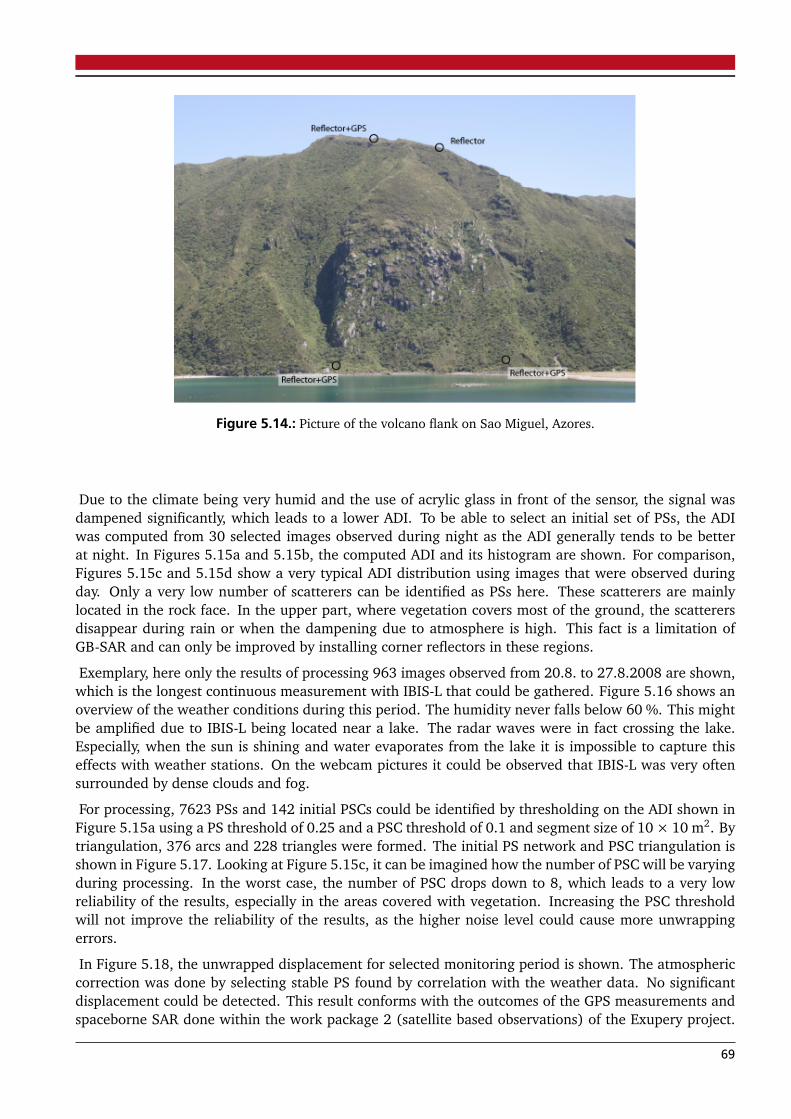
Figure 5.14.: Picture of the volcano flank on Sao Miguel, Azores.
Due to the climate being very humid and the use of acrylic glass in front of the sensor, the signal wasdampened significantly, which leads to a lower ADI. To be able to select an initial set of PSs, the ADIwas computed from 30 selected images observed during night as the ADI generally tends to be betterat night. In Figures 5.15a and 5.15b, the computed ADI and its histogram are shown. For comparison,Figures 5.15c and 5.15d show a very typical ADI distribution using images that were observed duringday. Only a very low number of scatterers can be identified as PSs here. These scatterers are mainlylocated in the rock face. In the upper part, where vegetation covers most of the ground, the scatterersdisappear during rain or when the dampening due to atmosphere is high. This fact is a limitation ofGB-SAR and can only be improved by installing corner reflectors in these regions.
Exemplary, here only the results of processing 963 images observed from 20.8. to 27.8.2008 are shown,which is the longest continuous measurement with IBIS-L that could be gathered. Figure 5.16 shows anoverview of the weather conditions during this period. The humidity never falls below 60 %. This mightbe amplified due to IBIS-L being located near a lake. The radar waves were in fact crossing the lake.Especially, when the sun is shining and water evaporates from the lake it is impossible to capture thiseffects with weather stations. On the webcam pictures it could be observed that IBIS-L was very oftensurrounded by dense clouds and fog.
For processing, 7623 PSs and 142 initial PSCs could be identified by thresholding on the ADI shown inFigure 5.15a using a PS threshold of 0.25 and a PSC threshold of 0.1 and segment size of 10 × 10 m2. Bytriangulation, 376 arcs and 228 triangles were formed. The initial PS network and PSC triangulation isshown in Figure 5.17. Looking at Figure 5.15c, it can be imagined how the number of PSC will be varyingduring processing. In the worst case, the number of PSC drops down to 8, which leads to a very lowreliability of the results, especially in the areas covered with vegetation. Increasing the PSC thresholdwill not improve the reliability of the results, as the higher noise level could cause more unwrappingerrors.
In Figure 5.18, the unwrapped displacement for selected monitoring period is shown. The atmosphericcorrection was done by selecting stable PS found by correlation with the weather data. No significantdisplacement could be detected. This result conforms with the outcomes of the GPS measurements andspaceborne SAR done within the work package 2 (satellite based observations) of the Exupery project.
69
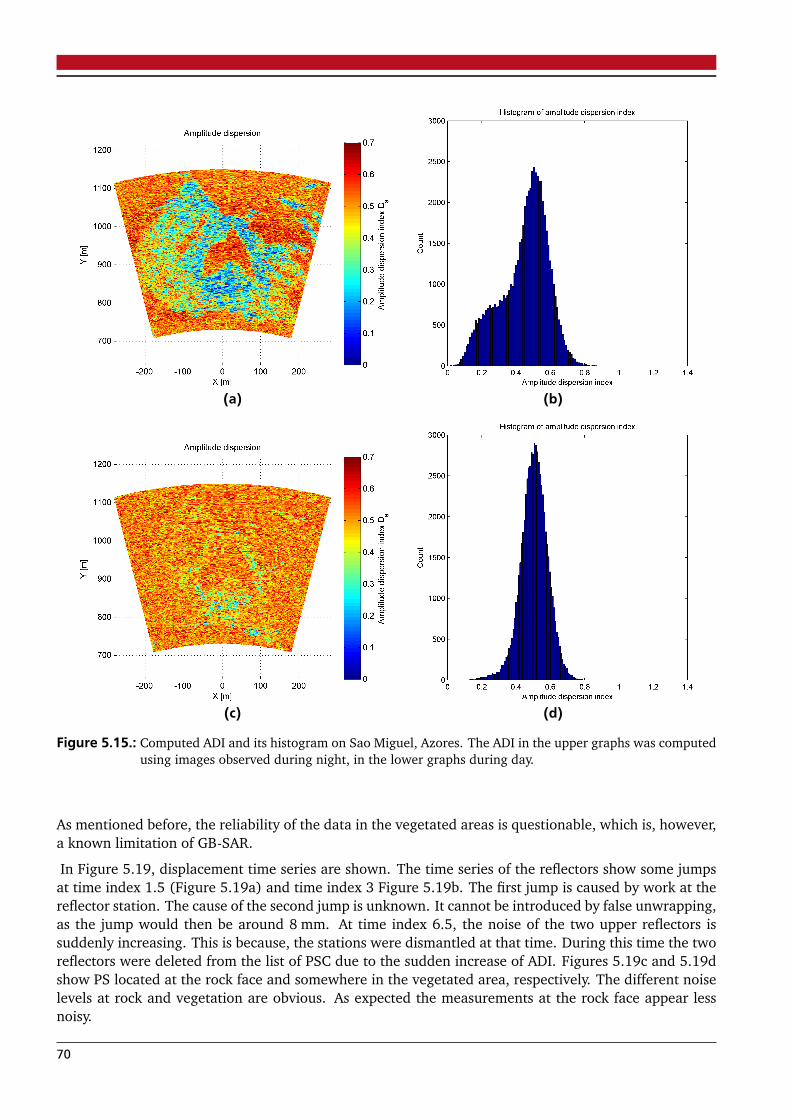
(a) (b)
(c) (d)
Figure 5.15.: Computed ADI and its histogram on Sao Miguel, Azores. The ADI in the upper graphs was computedusing images observed during night, in the lower graphs during day.
As mentioned before, the reliability of the data in the vegetated areas is questionable, which is, however,a known limitation of GB-SAR.
In Figure 5.19, displacement time series are shown. The time series of the reflectors show some jumpsat time index 1.5 (Figure 5.19a) and time index 3 Figure 5.19b. The first jump is caused by work at thereflector station. The cause of the second jump is unknown. It cannot be introduced by false unwrapping,as the jump would then be around 8 mm. At time index 6.5, the noise of the two upper reflectors issuddenly increasing. This is because, the stations were dismantled at that time. During this time the tworeflectors were deleted from the list of PSC due to the sudden increase of ADI. Figures 5.19c and 5.19dshow PS located at the rock face and somewhere in the vegetated area, respectively. The different noiselevels at rock and vegetation are obvious. As expected the measurements at the rock face appear lessnoisy.
70
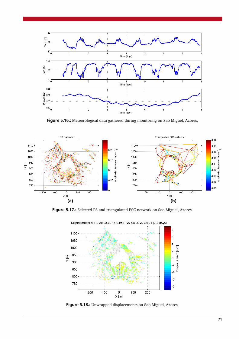
Figure 5.16.: Meteorological data gathered during monitoring on Sao Miguel, Azores.
(a) (b)
Figure 5.17.: Selected PS and triangulated PSC network on Sao Miguel, Azores.
Figure 5.18.: Unwrapped displacements on Sao Miguel, Azores.
71
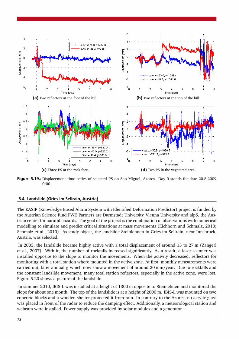
(a) Two reflectors at the foot of the hill. (b) Two reflectors at the top of the hill.
(c) Three PS at the rock face. (d) Two PS in the vegetated area.
Figure 5.19.: Displacement time series of selected PS on Sao Miguel, Azores. Day 0 stands for date 20.8.20090:00.
5.4 Landslide (Gries im Sellrain, Austria)
The KASIP (Knowledge-Based Alarm System with Identified Deformation Predictor) project is funded bythe Austrian Science fund FWF. Partners are Darmstadt University, Vienna University and alpS, the Aus-trian center for natural hazards. The goal of the project is the combination of observations with numericalmodelling to simulate and predict critical situations at mass movements (Eichhorn and Schmalz, 2010;Schmalz et al., 2010). As study object, the landslide Steinlehnen in Gries im Sellrain, near Innsbruck,Austria, was selected.
In 2003, the landslide became highly active with a total displacement of around 15 to 27 m (Zangerlet al., 2007). With it, the number of rockfalls increased significantly. As a result, a laser scanner wasinstalled opposite to the slope to monitor the movements. When the activity decreased, reflectors formonitoring with a total station where mounted in the active zone. At first, monthly measurements werecarried out, later annually, which now show a movement of around 20 mm/year. Due to rockfalls andthe constant landslide movement, many total station reflectors, especially in the active zone, were lost.Figure 5.20 shows a picture of the landslide.
In summer 2010, IBIS-L was installed at a height of 1300 m opposite to Steinlehnen and monitored theslope for about one month. The top of the landslide is at a height of 2000 m. IBIS-L was mounted on twoconcrete blocks and a wooden shelter protected it from rain. In contrary to the Azores, no acrylic glasswas placed in front of the radar to reduce the damping effect. Additionally, a meteorological station andwebcam were installed. Power supply was provided by solar modules and a generator.
72
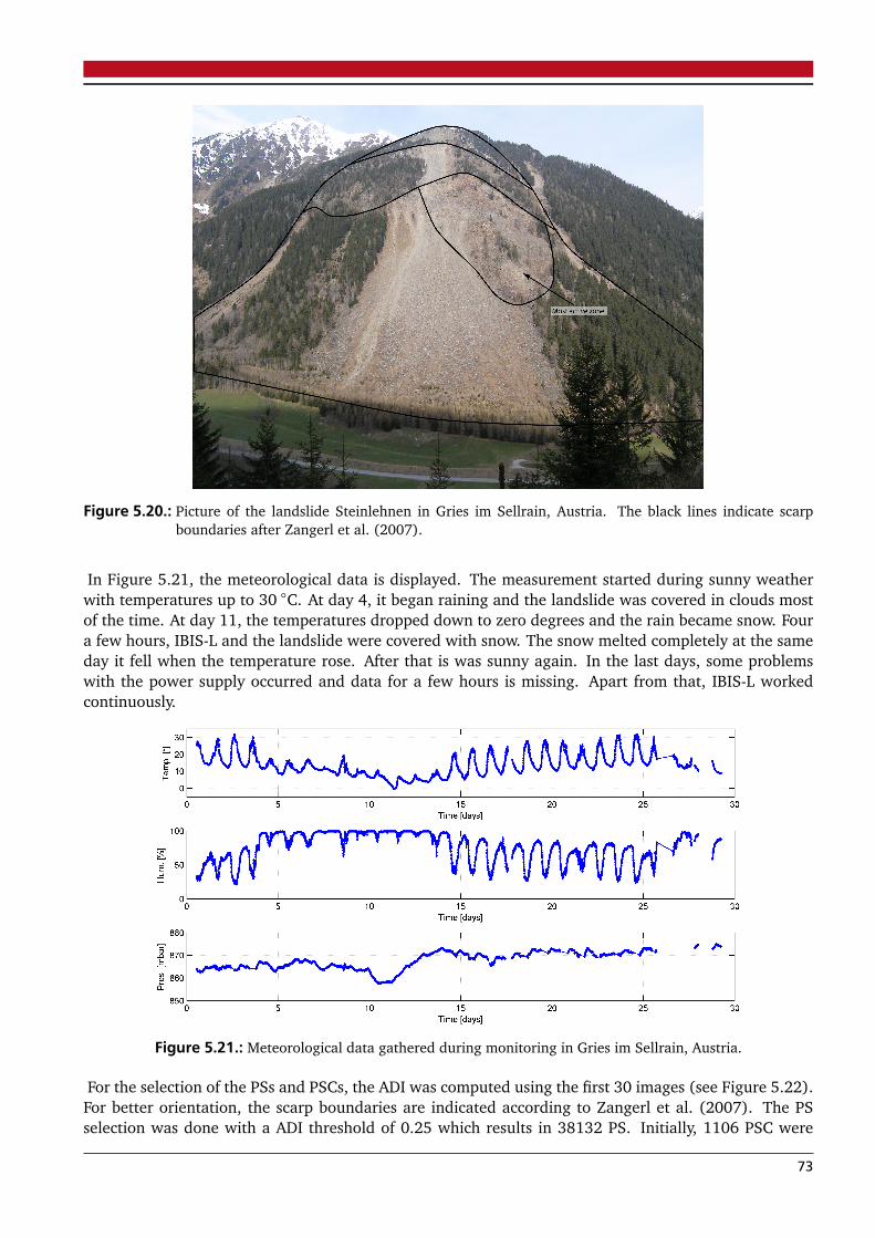
Figure 5.20.: Picture of the landslide Steinlehnen in Gries im Sellrain, Austria. The black lines indicate scarpboundaries after Zangerl et al. (2007).
In Figure 5.21, the meteorological data is displayed. The measurement started during sunny weatherwith temperatures up to 30 ◦C. At day 4, it began raining and the landslide was covered in clouds mostof the time. At day 11, the temperatures dropped down to zero degrees and the rain became snow. Foura few hours, IBIS-L and the landslide were covered with snow. The snow melted completely at the sameday it fell when the temperature rose. After that is was sunny again. In the last days, some problemswith the power supply occurred and data for a few hours is missing. Apart from that, IBIS-L workedcontinuously.
Figure 5.21.: Meteorological data gathered during monitoring in Gries im Sellrain, Austria.
For the selection of the PSs and PSCs, the ADI was computed using the first 30 images (see Figure 5.22).For better orientation, the scarp boundaries are indicated according to Zangerl et al. (2007). The PSselection was done with a ADI threshold of 0.25 which results in 38132 PS. Initially, 1106 PSC were
73
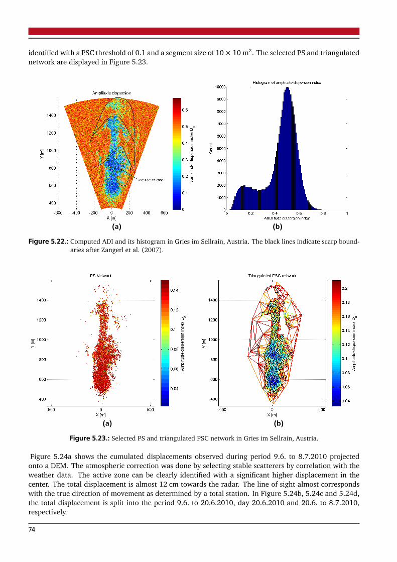
identified with a PSC threshold of 0.1 and a segment size of 10× 10 m2. The selected PS and triangulatednetwork are displayed in Figure 5.23.
(a) (b)
Figure 5.22.: Computed ADI and its histogram in Gries im Sellrain, Austria. The black lines indicate scarp bound-aries after Zangerl et al. (2007).
(a) (b)
Figure 5.23.: Selected PS and triangulated PSC network in Gries im Sellrain, Austria.
Figure 5.24a shows the cumulated displacements observed during period 9.6. to 8.7.2010 projectedonto a DEM. The atmospheric correction was done by selecting stable scatterers by correlation with theweather data. The active zone can be clearly identified with a significant higher displacement in thecenter. The total displacement is almost 12 cm towards the radar. The line of sight almost correspondswith the true direction of movement as determined by a total station. In Figure 5.24b, 5.24c and 5.24d,the total displacement is split into the period 9.6. to 20.6.2010, day 20.6.2010 and 20.6. to 8.7.2010,respectively.
74
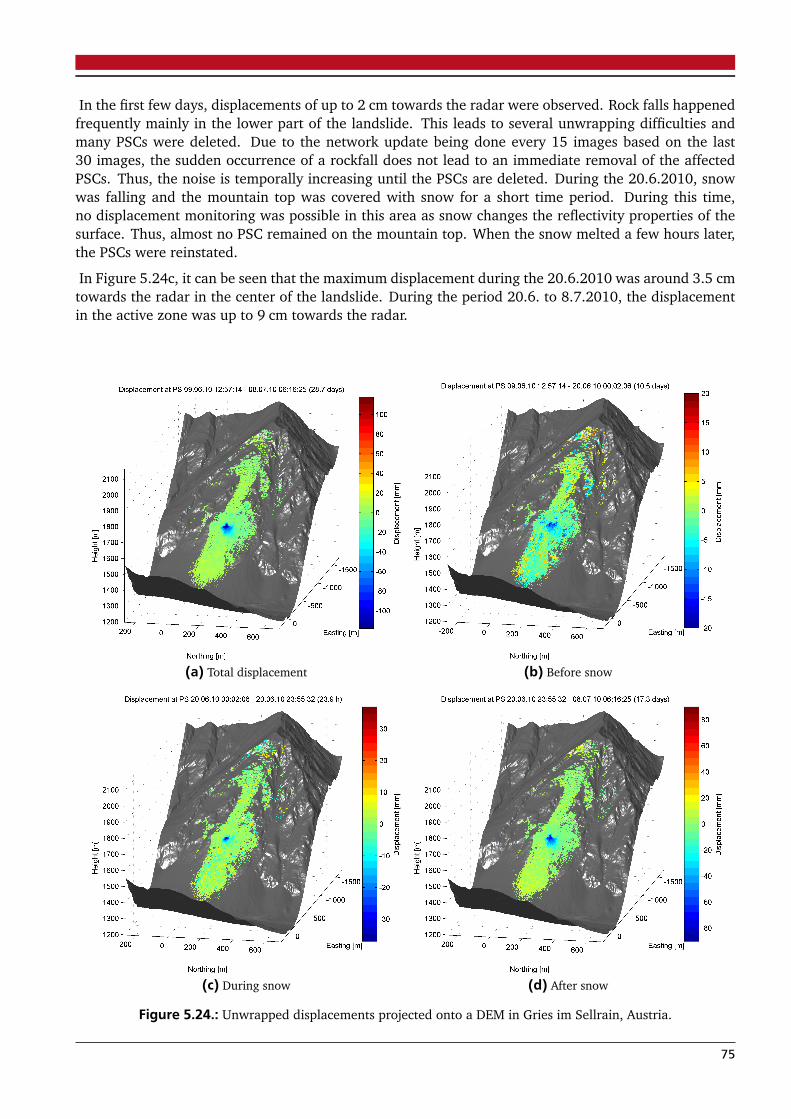
In the first few days, displacements of up to 2 cm towards the radar were observed. Rock falls happenedfrequently mainly in the lower part of the landslide. This leads to several unwrapping difficulties andmany PSCs were deleted. Due to the network update being done every 15 images based on the last30 images, the sudden occurrence of a rockfall does not lead to an immediate removal of the affectedPSCs. Thus, the noise is temporally increasing until the PSCs are deleted. During the 20.6.2010, snowwas falling and the mountain top was covered with snow for a short time period. During this time,no displacement monitoring was possible in this area as snow changes the reflectivity properties of thesurface. Thus, almost no PSC remained on the mountain top. When the snow melted a few hours later,the PSCs were reinstated.
In Figure 5.24c, it can be seen that the maximum displacement during the 20.6.2010 was around 3.5 cmtowards the radar in the center of the landslide. During the period 20.6. to 8.7.2010, the displacementin the active zone was up to 9 cm towards the radar.
(a) Total displacement (b) Before snow
(c) During snow (d) After snow
Figure 5.24.: Unwrapped displacements projected onto a DEM in Gries im Sellrain, Austria.
75
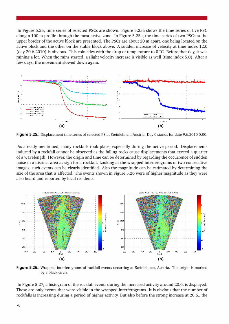
In Figure 5.25, time series of selected PSCs are shown. Figure 5.25a shows the time series of five PSCalong a 100 m-profile through the most active zone. In Figure 5.25a, the time series of two PSCs at theupper border of the active block are presented. The PSCs are about 20 m apart, one being located on theactive block and the other on the stable block above. A sudden increase of velocity at time index 12.0(day 20.6.2010) is obvious. This coincides with the drop of temperature to 0 ◦C. Before that day, it wasraining a lot. When the rains started, a slight velocity increase is visible as well (time index 5.0). After afew days, the movement slowed down again.
(a) (b)
Figure 5.25.: Displacement time series of selected PS at Steinlehnen, Austria. Day 0 stands for date 9.6.2010 0:00.
As already mentioned, many rockfalls took place, especially during the active period. Displacementsinduced by a rockfall cannot be observed as the falling rocks cause displacements that exceed a quarterof a wavelength. However, the origin and time can be determined by regarding the occurrence of suddennoise in a distinct area as sign for a rockfall. Looking at the wrapped interferograms of two consecutiveimages, such events can be clearly identified. Also the magnitude can be estimated by determining thesize of the area that is affected. The events shown in Figure 5.26 were of higher magnitude as they werealso heard and reported by local residents.
(a) (b)
Figure 5.26.: Wrapped interferograms of rockfall events occurring at Steinlehnen, Austria. The origin is markedby a black circle.
In Figure 5.27, a histogram of the rockfall events during the increased activity around 20.6. is displayed.These are only events that were visible in the wrapped interferograms. It is obvious that the number ofrockfalls is increasing during a period of higher activity. But also before the strong increase at 20.6., the
76
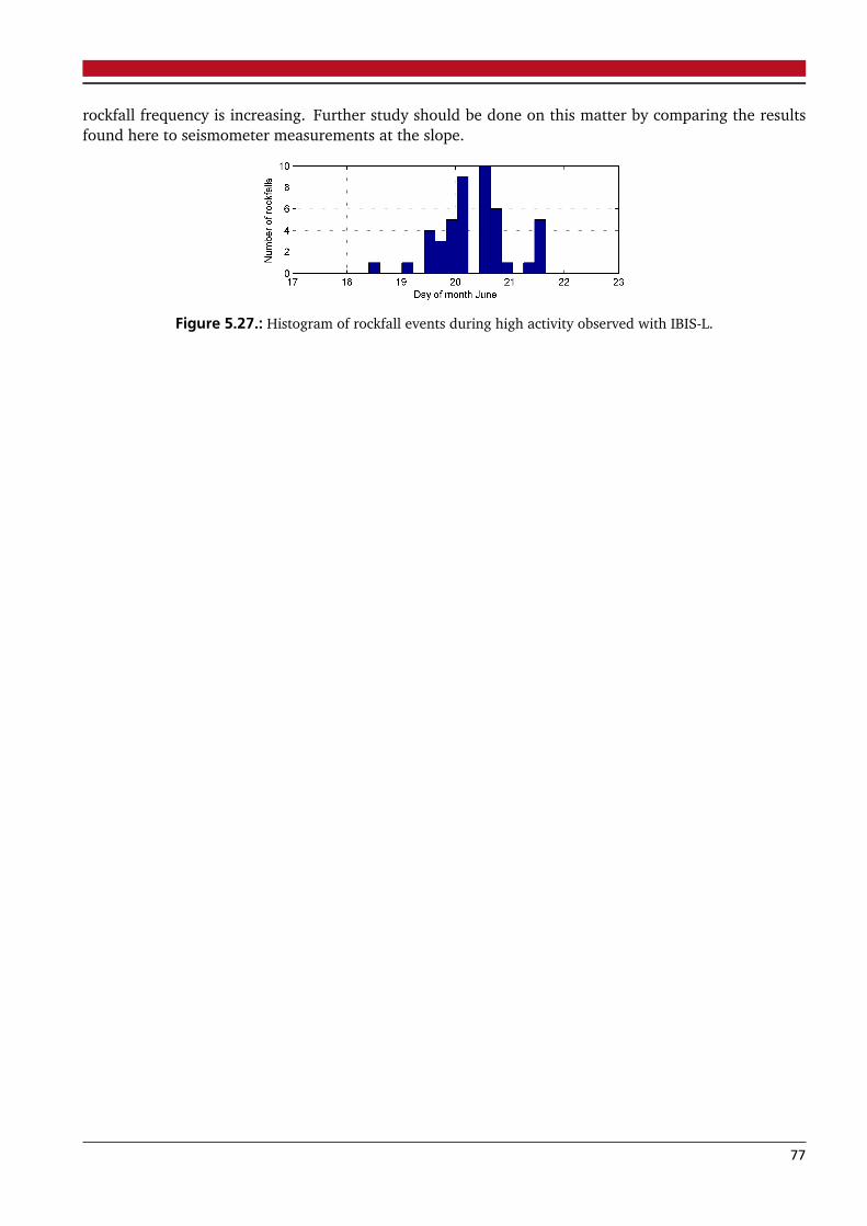
rockfall frequency is increasing. Further study should be done on this matter by comparing the resultsfound here to seismometer measurements at the slope.
Figure 5.27.: Histogram of rockfall events during high activity observed with IBIS-L.
77
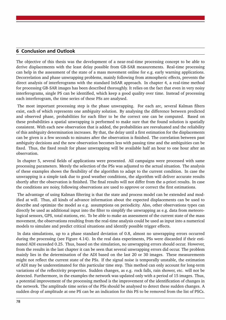
6 Conclusion and Outlook
The objective of this thesis was the development of a near-real-time processing concept to be able toderive displacements with the least delay possible from GB-SAR measurements. Real-time processingcan help in the assessment of the state of a mass movement online for e.g. early warning applications.Decorrelation and phase unwrapping problems, mainly following from atmospheric effects, prevents thedirect analysis of interferograms with the standard InSAR approach. In chapter 4, a real-time methodfor processing GB-SAR images has been described thoroughly. It relies on the fact that even in very noisyinterferograms, single PS can be identified, which keep a good quality over time. Instead of processingeach interferogram, the time series of these PSs are analysed.
The most important processing step is the phase unwrapping. For each arc, several Kalman filtersexist, each of which represents one ambiguity solution. By analysing the difference between predictedand observed phase, probabilities for each filter to be the correct one can be computed. Based onthese probabilities a spatial unwrapping is performed to make sure that the found solution is spatiallyconsistent. With each new observation that is added, the probabilities are reevaluated and the reliabilityof this ambiguity determination increases. By that, the delay until a first estimation for the displacementscan be given is a few seconds to minutes after the observation is finished. The correlation between pastambiguity decisions and the new observation becomes less with passing time and the ambiguities can befixed. Thus, the fixed result for phase unwrapping will be available half an hour to one hour after anobservation.
In chapter 5, several fields of applications were presented. All campaigns were processed with sameprocessing parameters. Merely the selection of the PSs was adjusted to the actual situation. The analysisof these examples shows the flexibility of the algorithm to adapt to the current condition. In case theunwrapping is a simple task due to good weather conditions, the algorithm will deliver accurate resultsshortly after the observation is finished. The final results will not differ from the a-priori results. In casethe conditions are noisy, following observations are used to approve or correct the first estimations.
The advantage of using Kalman filtering is that the state and process model can be extended and mod-ified at will. Thus, all kinds of advance information about the expected displacements can be used todescribe and optimize the model as e.g. assumptions on periodicity. Also, other observations types candirectly be used as additional input into the filter to simplify the unwrapping as e.g. data from meteoro-logical sensors, GPS, total stations, etc. To be able to make an assessment of the current state of the massmovement, the observations resulting from the real-time analysis could be used as input into a numericalmodels to simulate and predict critical situations and identify possible trigger effects.
In data simulations, up to a phase standard deviation of 0.8, almost no unwrapping errors occurredduring the processing (see Figure 4.14). In the real data experiments, PSs were discarded if their esti-mated ADI exceeded 0.25. Thus, based on the simulation, no unwrapping errors should occur. However,from the results in the last chapter it can be seen that several unwrapping errors did occur. The problemmainly lies in the determination of the ADI based on the last 20 or 30 images. These measurementsmight not reflect the current state of the PSs. If the signal noise is temporally unstable, the estimationof ADI may be underestimated for this particular time step. This method can only account for long-termvariations of the reflectivity properties. Sudden changes, as e.g. rock falls, rain shower, etc. will not bedetected. Furthermore, in the examples the network was updated only with a period of 15 images. Thus,a potential improvement of the processing method is the improvement of the identification of changes inthe network. The amplitude time series of the PSs should be analysed to detect these sudden changes. Asudden drop of amplitude at one PS can be an indication for this PS to be removed from the list of PSCs.
78

A further improvement, which is actually very important for interpretation, is to identify and distinguishreliable and unreliable estimations. Unwrapping errors can probably not be prevented but they shouldbe identified and a value for the reliability, e.g. in form of probabilities, should be made available.One indication can be the probabilities, that are delivered as output from the Kalman filters. A lowprobability of the finally selected ambiguity indicates a higher chance for unwrapping errors. A furthertest, for unwrapping errors can be to identify typical patterns, in form of sudden jumps of around 8 mmin time and space, that occur when the ambiguity determination is wrong.
Finally, it can be said that based on the results of the measurement campaigns shown in the last chapter,the algorithm has proven to deliver plausible results even under difficult circumstances. Nevertheless, itis important for the observer to have a sound knowledge about the GB-SAR techniques and the difficultiesof analysis to be able to determine the reliability of the measurements.
79
References
N. Adam, B. Kampes, and M. Eineder. Development of a scientific permanent scatterer system: Modifications for mixedERS/ENVISAT time series. In ERS-ENVISAT Symposium, 6-10 September 2004, Salzburg, Austria, 2004.
R.K. Ahuja, T.L. Magnanti, and J.B. Orlin. Network flows: theory, algorithms, and applications. Prentic Hall Inc., EnglewoodCliffs (NJ), 1993.
M. Alba, G. Bernadini, A. Giussani, P. Ricci, F. Roncoroni, M. Scaioni, P. Valgoi, and K. Zhang. Measurement of Dam Defor-mations by Terrestrial Interferometric Techniques. In International Archives of the Photogrammetry, Remote Sensing andSpatial Information Sciences. Vol. XXXVII. Part B1, 3-11 July 2008, Beijing, China, 2008.
M.G. Angeli, A. Pasuto, and S. Silvano. A critical review of landslide monitoring experiences. Engineering Geology, 55(3):133–147, 2000. ISSN 0013-7952.
G. Antonello, N. Casagli, P. Farina, D. Leva, G. Nico, A. Sieber, and D. Tarchi. Ground-based SAR interferometry for monitoringmass movements. Landslides, 1:21–28, 2004. doi: 10.1007/s10346-003-0009-6.
R. Bamler. Principles of Synthetic Aperture Radar. Surveys in Geophysics, 21:147–157, 2000.
R. Bamler and P. Hartl. Synthetic aperture radar interferometry. Inverse Problems, 14:R1–R54, 1998.
Y. Bar-Shalom, X.R. Li, and T. Kirubarajan. Estimation with applications to tracking and navigation. Wiley-Interscience, 2001.
K.M. Bergen and M.C. Dobson. Integration of remotely sensed radar imagery in modeling and mapping of forest biomass andnet primary production. Ecological Modelling, 122(3):257–274, 1999.
G. Bitelli, M. Dubbini, and A. Zanutta. Terrestrial laser scanning and digital photogrammetry techniques to monitor landslidebodies. In Proceedings of the XXth ISPRS Congress, Istanbul, volume 35, pages 246–251, 2004.
C. Brekke and A.H.S. Solberg. Oil spill detection by satellite remote sensing. Remote Sensing of Environment, 95(1):1–13,2005.
R.G. Brown and P.Y.C. Hwang. Introduction to Random Signals and Applied Kalman Filtering. John Wiley & Sons, inc., 1997.
G.F. Carballo and P.W. Fieguth. Probabilistic cost functions for network flow phase unwrapping. Transactions on Geoscienceand Remote Sensing, 38(5):2192–2201, 2000.
A. Collison, S. Wade, J. Griffiths, and M. Dehn. Modelling the impact of predicted climate change on landslide frequency andmagnitude in SE England. Engineering Geology, 55(3):205–218, 2000. ISSN 0013-7952.
M. Constantini. A novel phase unwrapping method based on network programming. Transactions on Geoscience and RemoteSensing, 36(3):813–821, 2002. ISSN 0196-2892.
M. Crosetto, C.C. Tscherning, B. Crippa, and M. Castillo. Subsidence monitoring using SAR interferometry - Reduction of theatmospheric effects using stochastic filtering. Geophysical Research Letters, 29(9):26–1, 2002.
J.C. Curlander and R.N. McDonough. Synthetic Aperture Radar: Systems and Signal Processing. John Wiley & Sons, inc., 1991.
R. Cusack, JM Huntley, and HT Goldrein. Improved noise-immune phase-unwrapping algorithm. Applied Optics, 34(5):781–789, 1995.
G.B. Dantzig, A. Orden, and P. Wolfe. The generalized simplex method for minimizing a linear form under linear inequalityrestraints. In The basic George B. Dantzig. Stanford University Press, 2003.
B. Delaunay. Sur la sphère vide. Bulletin of Academy of Sciences of the USSR, VII:793–800, 1934.
A. Eichhorn and T. Schmalz. Investigations to the Calibration of a Numerical Slope Model by Means of Adaptive Kalman-Filtering. In FIG Congress 2010, Facing the Challenges - Building the Capacity, 11-16 April 2010, Sydney, Australia, 2010.
A. Ferretti, C. Prati, and F. Rocca. Nonlinear subsidence rate estimation using permanent scatterers in differential SARinterferometry. Transactions on Geoscience and Remote Sensing, 38(5):2202–2212, 2000.
A. Ferretti, C. Prati, F. Rocca, et al. Permanent scatterers in SAR interferometry. Transactions on Geoscience and RemoteSensing, 39(1):8–20, 2001.
T.J. Flynn. Two-dimensional phase unwrapping with minimum weighted discontinuity. Journal of the Optical Society ofAmerica A, 14(10):2692–2701, 1997.
A. Freeman. SAR calibration: An overview. Transactions on Geoscience and Remote sensing, 30(6):1107–1121, 1992.
D.C. Ghiglia and M.D. Pritt. Two-dimensional Phase Unwrapping: Theory, Algorithms, and Software. Wiley New York, 1998.
J.A. Gili, J. Corominas, and J. Rius. Using Global Positioning System techniques in landslide monitoring. Engineering Geology,55(3):167–192, 2000. ISSN 0013-7952.
80
R. Goldstein, H. Zebker, and C. Werner. Satellite radar interferometry - Two-dimensional phase unwrapping. Radio Science,23(4):713–720, 1988.
M.S. Grewal and A.P. Andrews. Kalman filtering: theory and practice using MATLAB. Wiley New York, 2001.
R.F. Hanssen. Radar Interferometry: Data Interpretation and Error Analysis. Kluwer Academic Publishers, 2002.
F.J. Harris. On the use of windows for harmonic analysis with the discrete Fourier transform. Proceedings of the IEEE, 66(1):51–83, 1978. ISSN 0018-9219.
G. Herrera, J.A. Fernández-Merodo, J. Mulas, M. Pastor, G. Luzi, and O. Monserrat. A landslide forecasting model usingground based SAR data: The Portalet case study. Engineering Geology, 105:220–230, 2009.
A. Hooper, H. Zebker, P. Segall, and B. Kampes. A new method for measuring deformation on volcanoes and other naturalterrains using InSAR persistent scatterers. Geophysical Research Letters, 31(23):L23611, 2004.
A. Hooper, P. Segall, and H. Zebker. Persistent scatterer InSAR for crustal deformation analysis, with application to VolcánAlcedo, Galápagos. Journal of Geophysical Research, 112(B07407):19, 2007.
M.K. Hort. Exupéry-a mobile fast response system for managing a volcanic crisis. In AGU Fall Meeting Abstracts, volume 1,page 2050, 2009.
J.M. Huntley. Three-dimensional noise-immune phase unwrapping algorithm. Applied Optics, 40(23):3901–3908, 2001.
IPCC. Climate Change 2007: Synthesis Report. Contribution of Working Groups I, II and III to the Fourth Assessment Report ofthe Intergovernmental Panel on Climate Change. IPCC, Geneva, Switzerland, 2007.
ISDR. Global Assessment Report on Disaster Risk Reduction. United Nations, Geneva, Switzerland, 2009.
K. Itoh. Analysis of the phase unwrapping algorithm. Applied Optics, 21(14):2470–2470, 1982.
IUGS-WGL. A suggested method for describing the rate of movement of a landslide. Bulletin of the International Associationof Engineering Geology, 52:75–78, 1995.
D. Just and R. Bamler. Phase statistics of interferograms with applications to synthetic aperture radar. Applied Optics, 33(20):4361–4368, 1994.
R.E. Kalman. A new approach to linear filtering and prediction problems. Journal of Basic Engineering, 82(1):35–45, 1960.
B. Kampes. Radar Interferometry: Persistent Scatterer Technique. Springer, 2006.
B.M. Kampes and R.F. Hanssen. Ambiguity resolution for permanent scatterer interferometry. IEEE Transactions on Geoscienceand Remote Sensing, 42(11):2446–2453, 2004.
H. Klausing and W. Holpp, editors. Radar mit realer und synthetischer Apertur: Konzeption und Realisierung. OldenbourgWissenschaftsverlag, 2000.
M. König, J.G. Winther, and E. Isaksson. Measuring snow and glacier ice properties from satellite. Reviews of Geophysics, 39(1):1–27, 2001.
T. Kraft, J. Wassermann, E. Schmedes, and H. Igel. Meteorological triggering of earthquake swarms at Mt. Hochstaufen,SE-Germany. Tectonophysics, 424(3-4):245–258, 2006.
H. Kraus. Die Atmosphäre der Erde. Springer, 2004.
J.C. Leachtenauer and R.G. Driggers. Surveillance and reconnaissance imaging systems: modeling and performance prediction.Artech House Publishers, 2001. ISBN 1580531326.
D.T. Lee and B.J. Schachter. Two algorithms for constructing a Delaunay triangulation. International Journal of ParallelProgramming, 9(3):219–242, 1980.
D.G. Luenberger and Y. Ye. Linear and nonlinear programming. Springer Verlag, 2008.
G. Luzi, M. Pieraccini, D. Mecatti, L. Noferini, G. Guidi, F. Moia, and C. Atzeni. Ground-based radar interferometry for land-slides monitoring: Atmospheric and instrumental decorrelation sources on experimental data. Transactions on Geoscienceand Remote Sensing, 42:2454–2466, 2004.
G. Luzi, M. Pieraccini, D. Mecatti, L. Noferini, G. Macaluso, A. Galgaro, and C. Atzeni. Advances in groundbased microwaveinterferometry for landslide survey: a case study. International Journal of Remote Sensing, 27:2331–2350, 2006. doi:doi:10.1080/01431160600554975.
P. Marinkovic, F. van Leijen, G. Ketelaar, and R. Hanssen. Recursive Persistent Scatterer Interferometry. In Fringe Workshop,28 November - 2 December 2005, Frascati, Italy, volume 610, page 23, 2005.
A. Martinez-Vazquez and J. Fortuny-Guash. Snow Cover Monitoring in the Swiss Alps with a GB-SAR. Geoscience and RemoteSensing Society Newsletter, March 2006:11–14, 2006.
D. Massonnet and K.L. Feigl. Radar interferometry and its application to changes in the Earth’s surface. Reviews of Geophysics,36(4):441–500, 1998.
D. Massonnet and J.C. Souyris. Imaging with Synthetic Aperture Radar. EFPL Press, 2008.
81

F. Meyer, B. Kampes, R. Bamler, and J. Fischer. Methods for Atmospheric Correction in INSAR Data. In Fringe Workshop, 28November - 2 December 2005, Frascati, Italy, 2005.
H. Modaressi. Climate Change and ground Movements. Geosciences, 3:44–49, 2006.
A. Moreira, G. Krieger, I. Hajnsek, M. Werner, D. Hounam, S. Riegger, and E. Settelmeyer. TanDEM-X: A TerraSAR-X add-on satellite for single-pass SAR interferometry. In IEEE International Geoscience and Remote Sensing Symposium, IGARSS,20-24 September 2004, Anchorage, USA, pages 1000–1003, 2004.
L. Noferini, M. Pieraccini, D. Mecatti, G. Luzi, C. Atzeni, A. Tamburini, and M. Broccolato. Permanent scatterers analysisfor atmospheric correction in ground-based SAR interferometry. Transactions on Geoscience and Remote Sensing, 43(7):1459–1471, 2005. doi: 10.1109/TGRS.2005.848707.
L. Noferini, M. Pieraccini, G. Luzi, D. Mecatti, G. Macaluso, and C. Atzeni. Ground-based Radar Interferometry for TerrainMapping. In IEEE International Geoscience and Remote Sensing Symposium, IGARSS, 31 July - 4 August 2006, Denver, USA,2006.
L. Noferini, M. Pieraccini, D. Mecatti, G. Macaluso, G. Luzi, and C. Atzeni. DEM by Ground-Based SAR Interferometry.Geoscience and Remote Sensing Letters, 4(4):659–663, 2007. doi: 10.1109/LGRS.2007.905118.
L. Noferini, G. Luzi, M. Pieraccini, T. Strozzi, and C. Werner. DEM reconstruction examples. Technical report, GALAHADProject Deliverable D3.8, 2008a.
L. Noferini, T. Takayama, M. Pieraccini, D. Mecatti, G. Macaluso, G. Luzi, and C. Atzeni. Analysis of Ground-Based SARData With Diverse Temporal Baselines. Transactions on Geoscience and Remote Sensing, 46(6):1614–1623, 2008b. doi:10.1109/TGRS.2008.916216.
A. Papoulis. Probability, random variables, and stochastic processes, volume 73660116. McGraw-Hill New York, 1965.
A. Paulose. High radar range resolution with the step frequency waveform. Master’s thesis, Naval Postgraduate School, 1994.
M. Pieraccini, G. Luzi, and C. Atzeni. Terrain mapping by ground-based interferometric radar. Transactions on Geoscience andRemote Sensing, 39(10):2176–2181, 2001. doi: 10.1109/36.957280.
M. Pieraccini, N. Casagli, G. Luzi, D. Tarchi, D. Mecatti, L. Noferini, and C. Atzeni. Landslide monitoring by ground-basedradar interferometry: a field test in Valdarno (Italy). International Journal of Remote Sensing, 24:1385–1391, 2003. doi:10.1080/0143116021000044869.
M. Pieraccini, G. Luzi, D. Mecatti, L. Noferini, and C. Atzeni. Ground-based SAR for short and long term monitoring ofunstable slopes. In Proceedings of the 3rd European Radar Conference, EuRAD, September 2006, Manchester, UK, 2006.
B. Rabus, M. Eineder, A. Roth, and R. Bamler. The shuttle radar topography mission- a new class of digital elevation modelsacquired by spaceborne radar. ISPRS Journal of Photogrammetry and Remote Sensing, 57(4):241–262, 2003.
P. Reinhardt. Bedienungsanleitung Sensoren mit Datalogger. Reinhardt System- und Messelectronic GmbH, July 2009.
S. Rödelsperger, M. Becker, C. Gerstenecker, G. Läufer, K. Schilling, and D. Steineck. Digital elevation model with the ground-based SAR IBIS-L as basis for volcanic deformation monitoring. Journal of Geodynamics, 49(3-4):241–246, 2010a. ISSN0264-3707.
S. Rödelsperger, G. Läufer, C. Gerstenecker, and M. Becker. Monitoring of displacements with ground-based microwaveinterferometry: IBIS-S and IBIS-L. Journal of Applied Geodesy, 4(1):41–54, 2010b. ISSN 1862-9016.
S. Rödelsperger, G. Läufer, C. Gerstenecker, and M. Becker. Terrestrische Mikrowelleninterferometrie - Prinzip und Anwen-dungen. Allgemeine Vermessungsnachrichten, 10:324–333, 2010c.
D.A. Rothrock, F.D. Carsey, J.C. Curlander, B. Holt, R. Kwok, and W.F. Weeks. Ice tracking techniques, implementation,performance, and applications. Advances in Space Research, 12:141–147, 1992.
H. Rudolf, D. Leva, D. Tarchi, and AJ. Sieber. A mobile and versatile SAR system. In IEEE 1999 International Geoscience andRemote Sensing Symposium, 1999. IGARSS’99 Proceedings, volume 1, 1999.
T. Schmalz, V. Buhl, and A. Eichhorn. An adaptive Kalman-filtering approach for the calibration of finite difference models ofmass movements. Journal of Applied Geodesy, in press:9, 2010. ISSN 1862-9016.
D.L. Schuler, J.S. Lee, D. Kasilingam, and E. Pottier. Measurement of ocean surface slopes and wave spectra using polarimetricSAR image data. Remote Sensing of Environment, 91(2):198–211, 2004.
R. Searle. Tectonic pattern of the Azores spreading centre and triple junction. Earth and Planetary Science Letters, 51(2):415–434, 1980. ISSN 0012-821X.
D. Silveira, JL Gaspar, T. Ferreira, and G. Queiroz. Reassessment of the historical seismic activity with major impact on S.Miguel Island (Azores). Natural Hazards and Earth System Sciences, 3:615–623, 2003.
J.J. Sousa, A.J. Hooper, R.F. Hanssen, and L.C. Bastos. Comparative Study of Two Different PS-InSAR Approaches: DePSI vs.StaMPS. In Fringe Workshop, 30 November - 4 December 2009, Frascati Italy, 2009.
T. Strozzi, P. Farina, A. Corsini, C. Ambrosi, M. Thüring, J. Zilger, A. Wiesmann, U. Wegmüller, and C. Werner. Survey andmonitoring of landslide displacements by means of L-band satellite SAR interferometry. Landslides, 2(3):193–201, 2005.
82

D. Tarchi, H. Rudolf, M. Pieraccini, and C. Atzeni. Remote monitoring of buildings using a ground-based SAR: appli-cation to cultural heritage survey. International Journal of Remote Sensing, 21(18):3545–3551, 2000. doi: 10.1080/014311600750037561.
D. Tarchi, N. Casagli, R. Fanti, D. Leva, G. Luzi, A. Pasuto, M. Pieraccini, and S. Silvano. Landslide monitoring by usingground-based SAR interferometry: an example of application to the Tessina landslide in Italy. Engineering Geology, 68:15–30, 2003.
N. Wallenstein, A. Duncan, D. Chester, and R. Marques. Fogo volcano (Sao Miguel, Azores): a hazardous edifice. Geomor-phologie: relief, processus, environnement, 3:259–270, 2007.
T. Wright, E. Fielding, and B. Parsons. Triggered slip: observations of the 17 August 1999 Izmit (Turkey) earthquake usingradar interferometry. Geophysical Research Letters, 28(6):1079–1082, 2001.
C. Zangerl, E. Eberhardt, H. Schönlaub, and J. Anegg. Deformation behaviour of deep-seated rockslides in crystalline rock.In Proceeding of the 1st Canada-US Rock Mechanics Symposium, Vancouver, Canada, pages 901–908, 2007.
H.A. Zebker, P.A. Rosen, and S. Hensley. Atmospheric effects in interferometric synthetic aperture radar surface deformationand topographic maps. Journal of Geophysical Research, 102(B4):7547–7563, 1997.
83

List of Acronyms
ADI Amplitude Dispersion Index
APS Atmospheric Phase Screen
BMBF Bundesministerium für Bildung und Forschung
DEM Digital Elevation Model
DePSI Delft PS-InSAR Processing Package
ERS European Remote Sensing SatelliteESA European Space Agency
GB-SAR Ground based Synthetic Aperture Radar
GPS Global Positioning System
IBIS-L Image By Interferometric Survey
InSAR Interferometric Synthetic Aperture Radar
IDS Ingegneria dei Sistemi S.p.A.ILS Integer Least Squares
JRC Joint Research CenterKASIP Knowledge-Based Alarm System with Identified Deformation Predictor
LAN Local Area NetworkLiSA Linear Synthetic Aperture Radar
LOS Line Of Sight
MCF Minimum Cost FlowMMAE Multiple Model Adaptive Estimation
NASA National Aeronautics and Space Administration
PDF Probability Density Function
PS Persistent ScattererPS Permanent ScattererPSC Persistent Scatterer CandidatePSC Permanent Scatterer CandidatePSI Persistent Scatterer Interferometry
RCS Radar Cross SectionSAR Synthetic Aperture Radar
SCR Signal to Clutter Ratio
SFCW Stepped Frequency Continuous Wave
SNR Signal to Noise Ratio
SRTM Shuttle Radar Topography Mission
StaMPS Stanford Method for Persistent ScatterersUSB Universal Serial BusVFRS Volcano Fast Response System
WLAN Wireless LAN
84

List of Symbols
Scalars
a Amplitudea Polynomial coefficienta Reflector edge lengthA Set of arcsb Reflector edge lengthb Supply valueB BandwidthB f Bandwidth (total frequency shift due to movement on rail)Bs Spatial baselineBt Temporal baselinec Calibration factor for amplitude dispersion indexc Costsc Speed of lightd Displacement in line of sightDa Amplitude dispersion indexe Partial pressure of water vapourE Saturation vapour pressuref Frequencyf Function in time domainf Conditional densityF Function in frequency domainG Antenna gainG Directed graphGc Number of independent cross-range observationsGr Number of independent range observationsh Relative humidityh Root mean square variation of surface heightH Objective functioni Imaginary numberi, j,k,l,m,n IndexI0 Zeroth order modified Bessel function of the first kindk Angular wavenumberK Number of possible ambiguitiesl Atmospheric lossl Lower limit for ambiguitiesl Number of observationsL Length of antennaLs Length of synthetic antenna (rail)
85

m Number of state parametersm Polynomial degreema Mean amplituden Phase ambiguityn Refractive indexN Number of frequency stepsN Number of Kalman filtersN Set of nodesN Window lengthp Number of constraintsp ProbabilityP Horizontal distanceP Atmospheric pressurePe Transmitted powerPn Noise powerPr Received powerq, r, s Indices for arcsr Number of arcsr, R RangeS Physical effective area of a radar reflectorSNR Signal to noise ratio
SNRthermal Thermal signal to noise ratiot TimeT Temperatureu Upper limit for ambiguitiesU Radial basis functionv Velocityw Window functionx Flowx , y Local 2D coordinate system with origin in center of railX , Y , Z Local 3D coordinate system with origin in center of railz Complex observationz Minimum cost flow objective functionz, z Heightα Azimuth with respect to the look direction of the instrumentβ Elevation angleβ Kaiser window shaping parameterβs Spatial baseline angle with respect to the verticalγ Coherenceγ Local incidence angle with respect to slope inclinationδc Cross range resolutionδgr Ground range resolutionδr Range resolutionδrc Real Aperture Radar cross range resolution
86

θ Slope inclination with respect to horizontalλ Wavelengthν Spatial frequencyσ Radar cross sectionσ Standard deviationσ0 Backscatter coefficientτ Pulse widthϕ Absolute / unwrapped phaseϕw Wrapped phaseφ Absolute / unwrapped interferometric phaseφw Wrapped interferometric phaseφatm Interferometric phase due to atmospheric changesφdisp Interferometric phase due to object displacementφnoise Interferometric phase due to noiseφtopo Interferometric phase due to topographyψ Absolute / unwrapped double differenced phase at arcψu Itoh-unwrapped double differenced phase at arcψw Wrapped double differenced phase at arcψatm Double differenced phase due to atmosphereψdisp Double differenced phase due to displacementψl in Double differenced phase containing only linear signalsψl indisp Double differenced phase containing only linear displacementψnoise Double differenced phase due to noiseψnonlin Double differenced phase containing only nonlinear signalsψnonlindisp Double differenced phase containing only nonlinear displacementψtopo Double differenced phase due to topographyω Angular velocity
Vector and matrices
ai Column i of matrix AA Triangle - arc relations for minimum cost flowb ConstraintsB Basis matrixc Cost vectord Innovationsdx yz 3D displacement vectorD Covariance matrix of innovationsH Measurement matrixK Kalman gain matrixlw Observation vector containing ψw
lu Observation vector containing ψu
n Ambiguity vectorN Nonbasis matrix
87
P− A priori covariance matrix of state vectorP+ A posteriori covariance matrix of state vectorQ Covariance matrix of process noiseR Covariance matrix of measurement noises Unit vector of line of sight directionT State transition matrixu Upper bound vectorv Measurement noisew Process noisew Weightsx Flow vectorx State vectorx− A priori estimate of state vectorx+ A posteriori estimate of state vectorxB Basis variables vectorxN Nonbasis variables vectorz Measurement vector
Operators
d( · ), ∂ ( · ) Differential operator∆( · ) Difference operatorE { · } Expectation valueW { · } Wrapping operator
W { · }= mod { · +π}( · )∗ Complex conjugationmod{ · , 2π} Modulus 2π
88
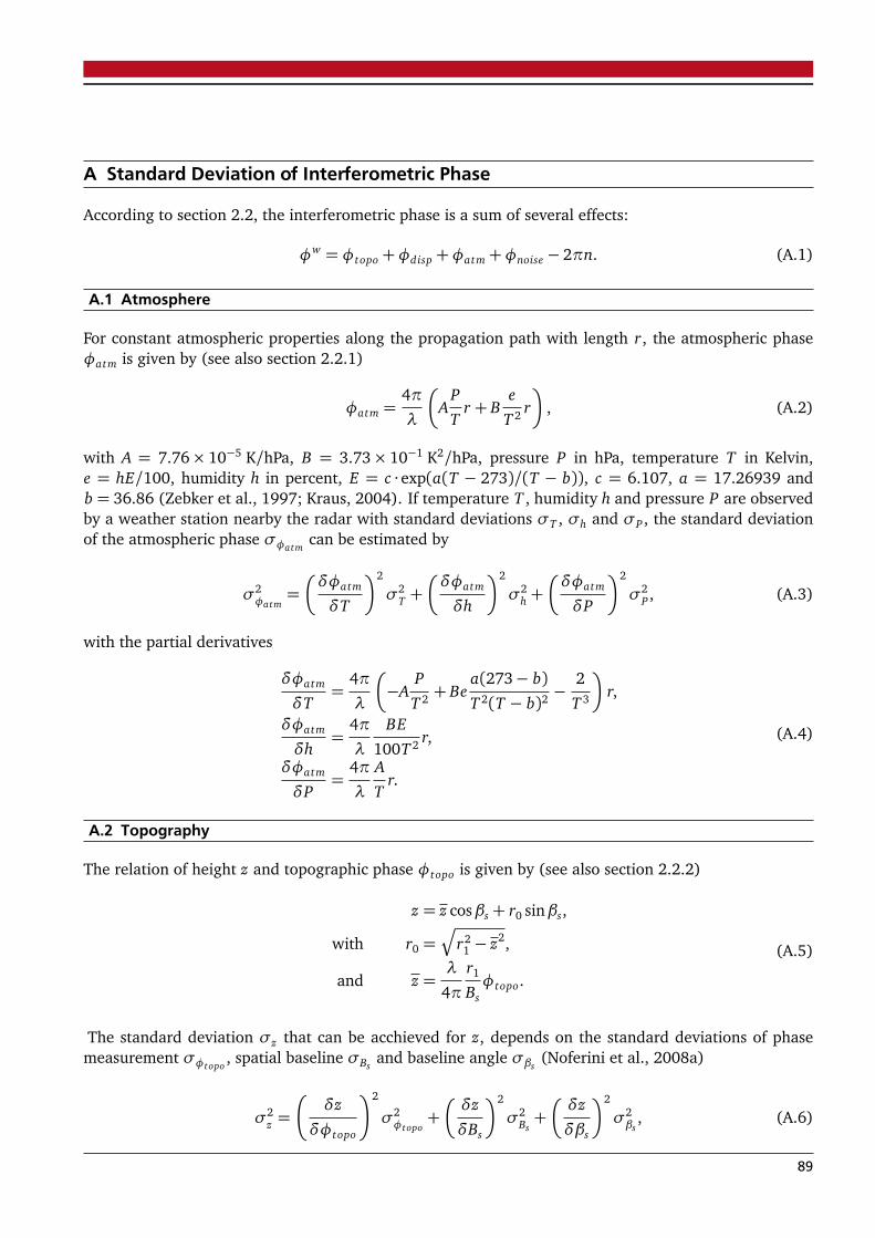
A Standard Deviation of Interferometric Phase
According to section 2.2, the interferometric phase is a sum of several effects:
φw = φtopo +φdisp +φatm+φnoise − 2πn. (A.1)
A.1 Atmosphere
For constant atmospheric properties along the propagation path with length r, the atmospheric phaseφatm is given by (see also section 2.2.1)
φatm =4π
λ
�
AP
Tr + B
e
T 2 r�
, (A.2)
with A = 7.76× 10⁻⁵ K/hPa, B = 3.73× 10⁻¹ K2/hPa, pressure P in hPa, temperature T in Kelvin,e = hE/100, humidity h in percent, E = c · exp(a(T − 273)/(T − b)), c = 6.107, a = 17.26939 andb = 36.86 (Zebker et al., 1997; Kraus, 2004). If temperature T , humidity h and pressure P are observedby a weather station nearby the radar with standard deviations σT , σh and σP , the standard deviationof the atmospheric phase σφatm
can be estimated by
σ2φatm=�
δφatm
δT
�2
σ2T +�
δφatm
δh
�2
σ2h +�
δφatm
δP
�2
σ2P , (A.3)
with the partial derivatives
δφatm
δT=
4π
λ
�
−AP
T 2 + Bea(273− b)T 2(T − b)2
−2
T 3
�
r,
δφatm
δh=
4π
λ
BE
100T 2 r,
δφatm
δP=
4π
λ
A
Tr.
(A.4)
A.2 Topography
The relation of height z and topographic phase φtopo is given by (see also section 2.2.2)
z = z cosβs + r0 sinβs,
with r0 =Æ
r21 − z2,
and z =λ
4π
r1
Bsφtopo.
(A.5)
The standard deviation σz that can be acchieved for z, depends on the standard deviations of phasemeasurement σφtopo
, spatial baseline σBsand baseline angle σβs
(Noferini et al., 2008a)
σ2z =
�
δz
δφtopo
�2
σ2φtopo
+�
δz
δBs
�2
σ2Bs+�
δz
δβs
�2
σ2βs
, (A.6)
89

with the partial derivatives
δz
δφtopo=�
cosβs +z sinβs
r0
�
λ
4π
r1
Bs,
δz
δBs=−
�
cosβs +z sinβs
r0
�
λ
4π
r1
B2s
φtopo,
δz
δβs= r0 cosβs − z sinβs.
(A.7)
90

A.3 Coherence, SNR and Phase Standard Deviation
Coherence |γ| SNR accordingto equation 2.42
Phase standarddeviation σφ according
to equation 2.47
Standard deviation ofdisplacement for Ku-band
radar (λ= 17.4 mm)
0.5 0 dB0.8 6.0 dB 0.53 rad (30◦) 1.50 mm0.9 9.5 dB 0.34 rad (20◦) 0.95 mm
0.95 12.8 dB 0.23 rad (13◦) 0.65 mm0.99 20.0 dB 0.10 rad (5.8◦) 0.28 mm0.999 30.0 dB 0.03 rad (1.8◦) 0.09 mm
0.9999 40.0 dB 0.01 rad (0.6◦) 0.03 mm
Table A.1.: Relation between coherence, SNR and standard deviation of phase and displacement measurement.
91
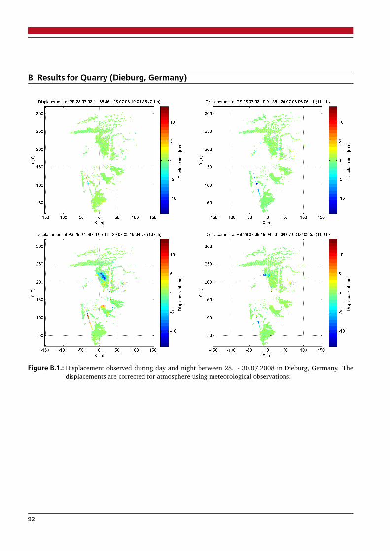
B Results for Quarry (Dieburg, Germany)
Figure B.1.: Displacement observed during day and night between 28. - 30.07.2008 in Dieburg, Germany. Thedisplacements are corrected for atmosphere using meteorological observations.
92
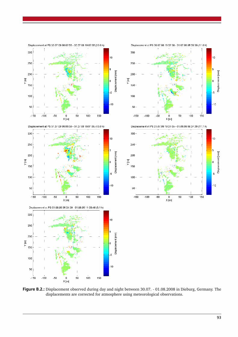
Figure B.2.: Displacement observed during day and night between 30.07. - 01.08.2008 in Dieburg, Germany. Thedisplacements are corrected for atmosphere using meteorological observations.
93
A. Schriftenreihe Fachrichtung Vermessungswesen (ab 1996)
Heft Nr. 1 J. SHEN Entwicklung eines dreidimensionalen Online-MesssystemsDarmstadt 1996ISBN 978-3-9804926-0-7
Heft Nr. 2 D. FLOHRSCHÜTZ Untersuchungen zum Einsatz von 3D-Animationen imVermessungswesen. Darmstadt 1998ISBN 978-3-9804926-1-4
Heft Nr. 3 FachbereichVermessungswesen
Jahresbericht 1998. Darmstadt 1999ISBN 978-3-9804926-2-1
Heft Nr. 4 J. HARTMANN
R. SEUSS
K. ZIMMERMANN
Pilothafte Realisierung des ALKIS®/ATKIS®-Datenmodells zur Abbil-dung bestehender und zukünftiger Anforderungen der Geodatenhal-tung in der Hessischen Kataster- und Vermessungsverwaltung.Darmstadt 2000ISBN 978-3-9804926-3-8
Heft Nr. 5 M. SEUSS Raumbezogene Planung - ein Gegenstand der Automation?Darmstadt 2000ISBN 978-3-9804926-4-5
Heft Nr. 6 R. SEUSS Implementierung und Nutzung eines Kommunalen Geoinformations-systems auf Landkreisebene. Darmstadt 2000ISBN 978-3-9804926-5-2
Heft Nr. 7 SchriftenreiheFachrichtung Geodäsie
Jahresbericht 1999. Darmstadt 2000ISBN 978-3-9804926-6-9
Heft Nr. 8 E. BARTSCH In ländlichen Räumen der VR China. Darmstadt 2000ISBN 978-3-9804926-7-6
Heft Nr. 9 J. HARTMANN
C. HEIL
R. SEUSS
Pilothafte Realisierung des ALKIS®/ATKIS®-Datenmodells zur Abbil-dung bestehender und zukünftiger Anforderungen der Geodatenhal-tung in der Hessischen Kataster- und Vermessungsverwaltung, Teil II.Darmstadt 2000ISBN 978-3-9804926-8-3
Heft Nr. 10 Autorenteam Festschrift anlässlich der Vollendung des 65. Lebensjahres vonProf. Dr. Ing. Bernhard P. Wrobel. Darmstadt 2000ISBN 978-3-9804926-9-0
Heft Nr. 11 SchriftenreiheFachrichtung Geodäsie
Jahresberichte 2000. Darmstadt 2001ISBN 978-3-35631-00-6
Heft Nr. 12 SchriftenreiheFachrichtung Geodäsie
Jahresberichte 2001. Darmstadt 2002ISBN 978-3-935631-01-3
Heft Nr. 13 J. HARTMANN Umsetzung und prototypische Entwicklung zur zukünftigen Führungdes Liegenschaftskatasters (ALKIS). Darmstadt 2002ISBN 978-3-935631-02-0
Heft Nr. 14 R.-H. BORCHERT Struktur eines Daten-Kommunikations-Kernsystems für den Geoin-formationsmarkt. Darmstadt 2002ISBN 978-3-935631-03-7
Heft Nr. 15 V. STAHL Entwicklung eines interdisziplinären QM-Systems im Ingenieursek-tor. Darmstadt 2002.ISBN 978-3-935631-04-4
Heft Nr. 16 SchriftenreiheFachrichtung Geodäsie
Jahresberichte 2002. Darmstadt 2003ISBN 978-3-935631-05-1
Heft Nr. 17 SchriftenreiheFachrichtung Geodäsie
Jahresberichte 2003. Darmstadt 2004ISBN 978-3-935631-06-8
Heft Nr. 18 SchriftenreiheFachrichtung Geodäsie
Jahresberichte 2004. Darmstadt 2005ISBN 978-3-935631-07-5
94
Heft Nr. 19 S.-H. KLEBER Beitrag zur ALKIS-Implementierung in Hessen und Untersuchung derAnwendersicht. Darmstadt 2005ISBN 978-3-935631-08-2
Heft Nr. 20 M. VOGEL Vom Pixel zur Richtung - Die räumlichen Beziehungen zwischen Ab-bildungsstrahlen und Tachymeter-Richtungen. Darmstadt 2006ISBN 978-3-935631-09-9
Heft Nr. 21 SchriftenreiheFachrichtung Geodäsie
Jahresberichte 2005. Darmstadt 2006ISBN 978-3-935631-10-5
Heft Nr. 22 M. METZNER Schaffung einer einheitlichen kommunalen Informationsbasis durchdie Integration von Geodaten. Darmstadt 2006ISBN 978-3-935631-11-2
Heft Nr. 23 D. WENZEL Einsatz von unabhängigen Prüfverfahren und modernen Testwerk-zeugen zur Qualitätssteigerung in der Geoinformatik.Darmstadt 2006ISBN 978-3-935631-12-9
Heft Nr. 24 A. HENDRICKS Einsatz von städtebaulichen Verträgen nach §11 BauGB bei der Bau-landbereitstellung - eine interdisziplinäre theoretische Analyse undAbleitung eines integrierten Handlungskonzeptes für die Praxis.Darmstadt 2006ISBN 978-3-935631-13-6
Heft Nr. 25 TH. ROSSMANITH Prototypische Realisierung einer kommunalen Geodateninfrastrukturauf Landkreisebene. Darmstadt 2007ISBN 978-3-935631-14-3
Heft Nr. 26 A. ADAMS Vergleich und Optimierung von GIS-basierten Planungen in der Kom-munikationstechnik. Darmstadt 2007ISBN 978-3-935631-15-0
Heft Nr. 27 Autorenteam Festschrift anlässlich der Vollendung des 65. Lebensjahres vonProf. Dr.-Ing. Harald Schlemmer. Darmstadt 2007ISBN 978-3-935631-16-7
Heft Nr. 28 Autorenteam Festschrift anlässlich der Vollendung des 65. Lebensjahres vonProf. Dr.-Ing. Carl-Erhard Gerstenecker. Darmstadt 2008ISBN 978-3-935631-17-4
Heft Nr. 29 A. NORRDINE Präzise Positionierung und Orientierung innerhalb von Gebäuden.Darmstadt 2009ISBN 978-3-935631-18-1
Heft Nr. 30 Autorenteam Festschrift anlässlich der Pensionierung von Dr.-Ing. Rolf-Dieter Düp-pe nach 36 Jahren am Institut für Photogrammetrie und Kartogra-phie. Darmstadt 2010ISBN 978-3-935631-19-8
Heft Nr. 31 H. SCHLEMMER 100 Jahre Geodätisches Institut und 150 Jahre Geodäsie an der Tech-nischen Universität Darmstadt. Darmstadt 2010ISBN 978-3-935631-20-4
Heft Nr. 32 M. SCHAFFERT Szenariotechnik und GIS - Ein Beitrag zur demographierobusten Pla-nung in Kommunen. Darmstadt 2011ISBN 978-3-935631-21-1
Heft Nr. 33 S. RÖDELSPERGER Real-time Processing of Ground Based Synthetic Aperture Radar (GB-SAR) Measurements. Darmstadt 2011ISBN 978-3-935631-22-8
95

B. Veröffentlichungen Fachrichtung Vermessungswesen
I. Veröffentlichungen des Geodätischen Institutes (1982 - 1993)
Heft Nr. 1 G. EICHHORN Zur Höhenfestlegung bei Ingenieurprojekten
-vergriffen- G. EICHHORN Ausbildung der Vermessungsingenieure für die Bearbeitung von Landin-formationssystemen
G. EICHHORN
K. EGREDER
Zur Reproduzierbarkeit des zyklischen Fehlers beim Tellurometer MA 100
K. EGREDER Elektrooptische Entfernungsmessung unter Verwendung von Planspiegeln
W. FROHWEIN Genauigkeitsuntersuchung an Dehnungsmessstreifen- Brückenschaltun-gen
Darmstadt 1982
Heft Nr. 2 O. WOLFRUM Die Theorie der Normalschnitte und ihre AnwendungenDarmstadt 1984
Heft Nr. 3 H. GROSSE Testnetz der Technischen Hochschule DarmstadtBand 1: Geodätische UnterlagenBand 2: Die Streckenmessung 1974-1976 und 1981-1985Band 3: Streckenverzeichnisse nach den EDM-RichtlinienBand 4: Prüfung der Messgeräte von 1974 bis 1986
G. BRUNKEN Band 5: Auswertung des TestnetzesDarmstadt 1986
Heft Nr. 4 E. WIESER Aufbau eines kommunalen LandinformationssystemsDarmstadt 1986
Heft Nr. 5 E. WIESER
U. BASTIAN
Das Liegenschaftskataster als Raumbezugssystem kommunaler und regio-naler Landinformationssysteme- Autorenreferate zu Diplomarbeiten -Darmstadt 1987
Heft Nr. 6 Festschrift Prof. Günter PaulC. GERSTENECKER BegrüßungG. EICHHORN Leben und Wirken von Prof. Dipl.-Ing. Günter Paul
W. SEELE Leitmotive für die Landumlegung gestern und heute - zu aktuellen Anfor-derungen an Gesetzgebung, Praxis und Wissenschaft
G. PAUL DankanspracheFachwissenschaftliche Arbeiten von Prof. Günter Paul
G. BRUNKEN Berechnung von Lotabweichungen aus topographischen MassenG. BRUNKEN Digitalisiertablett als PlanimeterG. BRUNKEN Eichung von Basislatten
C. LONGFEI Ergebnisse meines einjährigen Aufenthalts an der Technischen Hochschu-le Darmstadt
S. RÜHL Aufbau und Einsatzmöglichkeiten einer Grünflächendatenbank und einesBaumkatasters - Autorreferat -
Darmstadt 1987
Heft Nr. 7Band 1
H. GROSSE Gewässervermessungen auf Binnenseen und Talsperren - Konzept einerautomatischen Datenerfassung und Auswertung
-vergriffen- H. GROSSE Die MessgeräteH. GROSSE Die Konzeption einer automatischen Tiefenvermessung eines Gewässers
H. GROSSE Ergebnis der ersten Versuche auf dem See der Grube "Prinz von Hes-sen"1987
W. MÜLLER Die Programmgestaltung des Messverfahrens
96
U. THREIN Der Zusammenschluss der verschiedenen MesssystemeDarmstadt 1989
Heft Nr. 7Band 2
H. GROSSE Gewässervermessung auf dem See der Grube "Prinz von Hessen"1987 und1988
-vergriffen- H. GROSSE Die Vermessungsarbeiten auf dem See
H. GROSSE Ergebnis der Vermessungsarbeiten auf dem See und Vorschläge für weite-re Verbesserungen
G. BRUNKEN Automatische Datenverarbeitung der Dreidimensionalen Koordinaten -Darstellung des Seeuntergrundes
K. FAHLBUSCHE Zur Geologie der Grube Prinz von HessenH. KRANZ Geodätische Unterlagen für die Gewässervermessung
Darmstadt 1989
Heft Nr. 8 G. EICHHORN
T. RUPPERT
I. SOBORN
E. WIESER
Organisation, Aufbau und Nutzung eines Kommunalen Landinformations-systems KLIS
G. BRUNKEN EDV -gestützte Bearbeitung topographischer Geländeaufnahmen von derMesswertregistrierung bis zur Kartierung:Teil I: Registrierung von Messungsdaten des WILD T2000 auf EPSON HX-20 und Auswertung auf CMB 8032
Darmstadt 1988Heft Nr. 9 E. WIESER Systemanalytische Aspekte kommunaler Landinformationssysteme
G. BRUNKEN EDV -gestützte Bearbeitung topographischer Geländeaufnahmen von derMesswertregistrierung bis zur Kartierung:Teil II: Verarbeitung einer Koordinatendatei zu einer Kartierung mitSituations- und Höhendarstellung
G. BRUNKEN Genaue Azimutbestimmung mit Kreisel MOM Gi-B IG. BRUNKEN Transformation lokaler Festpunkte mit Abstandsgewichten
I. WASSERTHAL Datenerfassung zum Aufbau einer kommunalen Straßendatenbank undderen Präsentation in einem graphisch-interaktiven System - Autorreferat
A. SCHWEITZER Untersuchung einer DMS-bestückten Invarbandlatte der Firma Nedo hin-sichtlich mechanisch und thermisch bedingter Längenveränderungen -Autorreferat -
Darmstadt 1989
Heft Nr. 10 G. EICHHORN
T. RUPPERT
I. SOBORN
Konzeption und Pilotprojekt eines regionalen Landinformationssystems
G. BRUNKEN Dreidimensionale NetzausgleichungDarmstadt 1990
Heft Nr. 11 G. BRUNKEN Automatisierter Datenfluss von der Punktaufnahme zur NetzausgleichungG. BRUNKEN Auswertung topographischer Geländeaufnahmen
G. BRUNKEN Industriemesssystem IMS und Weiterverarbeitung der gewonnenen Daten- Autorenreferate zu Diplomarbeiten -
Darmstadt 1993
97
II. Veröffentlichungen des Institutes für Photogrammmetrie und Kartographie (1982 - 1987)
Heft Nr. 1 H. DEKER Arbeiten am Institut zum Einsatz der Elektronik an photogrammetrischenGeräten 1972 - 1980. Darmstadt 1982
Heft Nr. 2 W. LICHTNER
(Hrsg.)Funktion und Gestaltung der Deutschen Grundkarte 1:5000(THD/DVW Seminar vom 16. bis 18. März 1983 in Darmstadt)Darmstadt 1983
Heft Nr. 3 Autorenteam Professor Dr.-Ing. Hermann Deker zum 65. GeburtstagDarmstadt 1984
Heft Nr. 4 B. WROBEL Photogrammmetrie III (Vorlesungsskript)Darmstadt 1987
III. Veröffentlichungen des Institutes für Physikalische Geodäsie (1976 - 1981)
Heft Nr. 1 E. GROTEN Beiträge zur Gravimetrischen Geodäsie und GezeitenforschungErschienen in DGK Reihe B, Nr. 217, 1976
Heft Nr. 2 E. GROTEN Beiträge zur Physikalischen GeodäsieErschienen in DGK Reihe B, Nr. 233, 1978
Heft Nr. 3 Beiträge zur Astronomischen Geodäsie und Geodynamik
J. LATKA The Use of Satellite Gradiometry for the Determination of Gravity Anoma-lies
C. GERSTENECKER Beiträge zur simultanen Bestimmung von Breite und Länge mit Zeiss Ni2-Pendelastrolabien
G. HEIN Bestimmung der Schwereanomalien, Lotabweichungen und des Geoidesim Oberrheingraben aus zweiten Ableitungen des Schwerepotentials
C. GERSTENECKER The Influence of Air Pressure Changes on Precise Gravity Measurements
C. GERSTENECKER Ergebnisse der Registrierung der horizontalen Erdgezeitenkomponentenmit Hughes-Tiltmetern in der Gipsgrube Obrigheim
C. GERSTENECKER Untersuchung von SekundenlibellenC. GERSTENECKER Luftdruck- und Temperatureinflüsse auf Hughes-TiltmeterE. GROTEN Anwendung von interferometrischen Messungen in der Geodäsie
Darmstadt 1978Heft Nr. 4 TEIL 1 Physikalische Geodäsie
B. STOCK Abbruchfehler bei der Berechnung von Geoidhöhen für verschiedene In-tegralkerne und Randwerte
B. STOCK Genauigkeitsuntersuchungen bei der Berechnung von Lotabweichungenfür verschiedene Integralkerne und Randwerte
H. JOCHEMCZYK Überlegungen zur Stützpunktverteilung bei Reihenentwicklungen in Ku-gelflächenfunktionen
E. GROTEN Was sind Höhenwertänderungen?TEIL II Ausgleichungsrechnung und Statistik
H. JOCHEMCZYK Einige Bemerkungen zu linearen Abhängigkeiten bei der Auswertung vonVLBI-Messungen
H. JOCHEMCZYK Arbeitsstudie zu Maximum-Entropy-Spektral Methoden
R. KISTERMANN
G. HEIN
Überlegungen zur Ausreißersuche in multivariaten Daten
Darmstadt 1981
98


