page 1 of 210

Reduction and Testing of Greenhouse Gas Emissions from Heavy Duty Vehicles - LOT 2

Development and testing of a certification procedure for CO2 emissions and fuel consumption of HDV

Contract N° 070307/2009/548300/SER/C3

Final Report 9 January 2012

Coordination: University of Technology Graz

Institute for Internal Combustion Engines and Thermodynamics Inffeldgasse 21a, AT-8010 Graz

Tel.: +43 (0)316 / 873 - 7212, Fax: +43 (0)316 / 873 - 8080 http://ivt.tugraz.at

page 2 of 210

CONTENT 1. Introduction 4

2. Short description of the proposed test procedure 5

2.1. Overview 5

2.2. Vehicle and engine selection 6

2.3. Driving cycles 9

2.4. Component testing 11

2.4.1. Driving resistances 11

2.4.2. Engine Test 24

2.4.3. Drivetrain 29

2.4.4. Auxiliary units 30

2.5. Simulation of fuel consumption and CO2 31

2.5.1. User interface for import of standardised input data 32

2.5.2. Default database 32

2.5.3. The core model 32

2.5.4. Driver model 32

2.5.5. Drivetrain model 32

2.5.6. Auxiliary model 33

2.5.7. Vehicle longitudinal dynamics 33

2.5.8. Interpolation from the fuel map 33

2.5.9. Data post-processing 33

2.5.10. Further work needed to develop the HDV CO2 simulator 33

2.5.11. Interface of the simulation model for OEM-specific technology 34

2.6. Metrics of results 35

2.7. Hybrid technologies 37

2.8. Validation of results 39

2.9. Proposal for a future regulatory approach 40

3. Background information to chapter 2 43

3.1. Review of activities to establish a whole-vehicle testing- and CO2-labelling method 43

3.1.1. U.S. EPA / NHTSA Final Rule 43

3.1.2. Japanese Law 56

3.1.3. Activities in Europe 64

3.1.4. China 65

3.2. Vehicle and engine selection 68

3.2.1. Truck segmentation 68

3.2.2. Trailer segmentation 70

3.2.3. Bodywork segmentation 71

3.2.4. Bus and coach segmentation 72

3.3. Develop appropriate CO2 emission metrics 74

3.4. General options for the certification of fuel consumption and CO2 emissions from HDV 79

page 3 of 210

3.4.1. Comparison of different approaches for a certification 79

3.4.2. PEMS 81

3.4.3. Chassis dynamometer testing 90

3.4.4. Responsibilities 92

3.4.5. Sensitivity analysis for HDV components 93

3.5. Technical description of methods for component testing 99

3.5.1. Measurement of the road load curve 99

3.5.2. Set up of the test equipment on the vehicle 114

3.5.3. The engine fuel consumption map 116

3.5.4. Drivetrain losses 116

3.5.5. Power consumption of auxiliary units 120

3.5.6. Standard driving cycles for different HDV classes 133

3.5.7. Consideration of alternative technologies in the simulation tool 143

3.6. Verification of the recommended procedure with new measurements and model data 145

3.6.1. Long haul truck 40 t 146

3.6.2. Delivery truck 12t 156

3.7. Elaboration of a classification scheme 168

3.7.1. Annual mileage and CO2 emissions of different HDV classes 169

3.7.2. Engine family criteria according to Directive 2005/55/EC and Euro VI successors 179

3.7.3. European heavy-duty vehicle classification scheme (Directive 2007/46/EC and Commission Directive 678/2011) 180

3.7.4. Criteria for the declaration of a CO2 value for specified vehicles grouped in a family 181

3.7.5. Axle configurations and bodies of rigid trucks 185

3.7.6. Norm bodies and norm semi-trailers 187

3.7.7. Possible strategy with respect to bodies 191

4. Stakeholder consultation 192

5. Annex 193

5.1. Details on existing measurement standards 193

5.1.1. SAE J1263 193

5.1.2. 70/220/EEC (UN/ECE 83) 196

5.1.3. SAE J2263 197

5.1.4. ISO 10521-1, chapter 5.5 199

5.1.5. EPA-HQ-OAR-2010-0162 200

5.2. Comparison of standard semi-trailers of several manufacturers and FAT proposal 201

5.3. Standards for the measurement of HDV components 202

5.4. List of responsible authors 202

5.5. List of literature 203

5.6. List of abbreviations 206

page 4 of 210

1. Introduction Since 1990 the CO2 emissions of the transportation sector have been rising substantially. In the meantime, CO2 emission legislation for passenger cars has been introduced to reduce energy consumption. Although passenger cars have the largest overall energy consumption within the transportation sector, the projections of rising truck transportation volumes as well as further increasing energy consumption and CO2 emissions, (1), suggest regulations in the HDV sector, too. Therefore, a test procedure for fuel consumption or CO2 for heavy-duty vehicles is desired, too. A test procedure shall give standardised and neutral information to customers on the fuel efficiency of the HDV and thus enhance the development and introduction of fuel efficient technologies. Contrary to cars, Heavy Duty Vehicles (HDV) are used in a wider range of applications and with a large variation in cargo weight and combinations of single components, such as driver cabin, vehicle body, gearbox, engine, axis and auxiliaries. This suggested putting effort into the development of a test procedure designed especially for the needs of HDV. The main targets for the test procedure are:

1. Repeatable (within same laboratory) and reproducible (between different laboratories) 2. Incentive to apply efficient technologies and to optimise the entire vehicle set-up 3. High sensitivity for fuel saving measures 4. Reasonable costs and efforts to run and examine the procedure 5. Simple and robust

Target 2 needs to address each single component which has a reasonable share in the fuel consumption of the HDV fleet. Since optimising the interaction between all components has a reasonable potential for reducing energy consumption1, the ideal test procedure also has to consider the entire vehicle, as it is sold later to the customer under test conditions which reflect real world driving conditions. From this point of view, the test of the entire vehicle on a roller test bed or on the road would be ideal. However, due to the manifold variations in HDV designs, testing of all models would be a costly approach which does not seem to be justified since many of these HDV set-ups have very low sales numbers. The actual type approval for regulated emission components from HDV (NOx, CO, HC PN and PM) is tested on an engine test bed and expressed in gram per kWh. This test procedure, therefore, would only cover engine efficiency if it would also be applied directly as a certification method for fuel consumption and CO2. As a result of these considerations, a new test procedure has been designed, which is based on tests of the individual components of the vehicle and simulations of the fuel consumption and CO2 emissions of the entire HDV. In the project, options were developed and tested to fulfil the demands for a type approval method with such a test procedure. For the promising options, details of the methodology were elaborated to be able to apply the test methods on three different HDV. To cover the range of HDV categories, a semi-trailer, a solo truck and one bus were used to test the options developed previously. In the process of the work, a

1 Typical options are for example * optimising transmission ratios and gear shift strategies for driving resistances, which depend on the vehicle body size and design, the vehicle weight and the tires mounted, to meet the demands of the vehicles mission profile at engine loads with best fuel efficiency for the given engine, * energy management which uses the brake energy of the vehicle * optimising the thermal management of the engine, the driver cabin and the cooling demand, etc.

page 5 of 210

close cooperation was established with national projects, especially with a project funded by the German Umweltbundesamt2 and with a project run by ACEA members dealing with the same topic (2). Due to the large influence of the size and mission profile of the HDV on the specific energy consumption, a procedure simply based on g/km would not be very meaningful. Thus, metrics for the fuel efficiency of HDV were also elaborated which makes it easier for customers to assess fuel efficiency. The report is structured as follows: Chapter 2 describes the recommended way to apply the test procedure in a first pilot phase. This part of the report shall serve as the basis for the next phase of the development of the test procedure. In a next phase, it is recommended to

• apply the test procedure, • test existing options where a decision has not been made yet on which option is the most suitable

and • close the remaining gaps (such as default values) by analysing the test data and conducting further

research. Close cooperation with the industry is recommended in this phase since some of the data needed as input for the test procedure cannot be gained by independent consultants in a cost efficient way (e.g. engine map, gear box efficiency maps, data on auxiliary efficiencies etc.). Chapter 3 describes the work performed in LOT 2 in a structure compatible to the tender and provides all background material necessary to understand the decisions that led to the test procedure in chapter 2.

2. Short description of the proposed test procedure The test procedure is based on component testing. The test data of the individual vehicle components is collected in standardised formats and fed into a simulation tool which calculates the engine power necessary to overcome the driving resistances of the vehicle, the losses in the transmission system and the power demand from auxiliaries for defined test cycles. The engine speed course is calculated from the vehicle speed, tire dimensions, the transmission ratios, and a driver model. With the engine power and engine speed in 1 Hz course over the test cycle, the fuel consumption of the entire vehicle is then interpolated from the engine map of the vehicle. The recommendations for the design of the HDV CO2 test procedure given below are valid for a first pilot phase. Thus, they include different options for the test procedure at several points. These are options, where the data from LOT 2 was not sufficient to finally decide which of them will work best. Where possible, these options shall be applied in a subsequent measurement program to gain a better data base for the selection of the proper options.

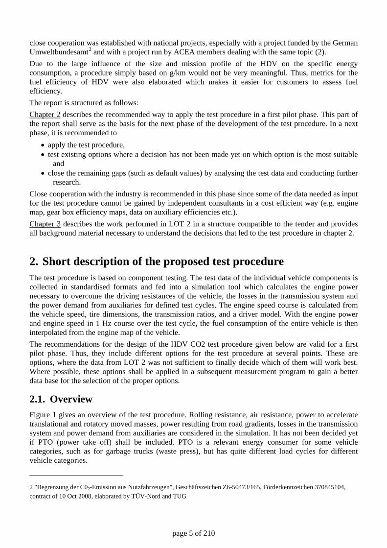
2.1. Overview Figure 1 gives an overview of the test procedure. Rolling resistance, air resistance, power to accelerate translational and rotatory moved masses, power resulting from road gradients, losses in the transmission system and power demand from auxiliaries are considered in the simulation. It has not been decided yet if PTO (power take off) shall be included. PTO is a relevant energy consumer for some vehicle categories, such as for garbage trucks (waste press), but has quite different load cycles for different vehicle categories.

2 "Begrenzung der C02-Emission aus Nutzfahrzeugen", Geschäftszeichen Z6-50473/165, Förderkennzeichen 370845104, contract of 10 Oct 2008, elaborated by TÜV-Nord and TUG

page 6 of 210

The simulation shall be done by one official simulator, eventually via web-access. The basic equations to be calculated are described later. These follow physical dependencies and are typically used in existing vehicle simulators. The official simulator, however, needs several additional functions to handle, for instance, the generic driver model, the auxiliaries and variations in vehicle bodies and tires. Furthermore, a robust and easy-to-handle interface is necessary to exchange data on the components and the results of the simulation between manufacturers and type approval authorities in standard forms. Due to the large number of HDV combinations that will have to go through such a type approval procedure in the future, the need for a robust and user friendly tool is obvious. In addition, some of the input data from OEM’s may have to be treated confidentially. Thus, the security issues of such a simulator and the corresponding data base also have to be elaborated carefully.In LOT 2, all simulations were done using the model PHEM (Passenger car and Heavy duty Emission Model), see e.g. (3). PHEM provided most of the functions necessary to compute the fuel consumption of the HDV tested. The conversion of results from component tests to PHEM input data was done usingextra tools, mainly MS Excel sheets with some VBA scripts. In the next phase of the project, the functionality of these additional tools should be integrated into a complete simulator to allow efficient and consistent assessment of the test results at all participating manufacturers. This pilot phase simulator does not need to offer data security systems since it can be used as a stand-alone tool at eachparticipating lab during the pilot phase.

Figure 1: Schematic picture of the test procedure (text in black font marks options which have not been definitelyselected yet and red text marks options which have not been developed yet)

2.2. Vehicle and engine selectionWhen a HDV has to be type approved, the first step is the correct allocation to a vehicle segment. We assume that not all segments have to be type approved for CO2 in the first step of the introduction of the regulation. Thus, the segmentation already defines if the vehicle has to go through the HDV CO2 test procedure.If it is found that the vehicle has to be type approved, then the allocation to the segment defines the test cycle which will be used and the payload in tons which will be simulated by the HDV CO2 vehicle simulator.

page 7 of 210

A vehicle segment is defined by the • vehicle class and • mission profile.

For each segment, the following values are defined in the HDV-CO2 simulator: CO2 test cycle Reference loading (see definition below) Norm body for the measurement of the aerodynamic drag (Optional: If a truck is tested as a rigid truck only or as a truck and trailer combination)3

A vehicle can fit basically only into one vehicle class but into more vehicle segments, if the category is typically used for different missions, e.g. a 8t rigid truck can be used for urban delivery and also for regional delivery. These two mission profiles have different representative CO2 test cycles, thus the vehicle will be simulated in both cycles and two sets of results will be produced, one for the urban delivery cycle with the typical vehicle loading for urban delivery and one for the regional delivery cycle with the typical vehicle loading for regional delivery. All the other data for this vehicle is the same in the HDV CO2 simulator. In the test pilot phase, the manufacturer just has to select the corresponding vehicle class, and the corresponding cycle allocation is already defined. After the pilot phase, it has to be discussed if segmentation is sufficient or if adaptations are required. This can be part of a general questionnaire to HDV customers on whether the information produced is sufficient (see also “Metrics” chapter). Table 1 shows the segmentation proposed for the HDV CO2 test pilot phase. With this table, each heavy goods vehicle shall be applicable to a vehicle class number. With this number, the reference payload, the test cycle and the “norm body” for measurement of the aerodynamic drag of the basic vehicle are defined. One cell in the “cycle allocation” columns represents one HDV segment. In the final HDV CO2 test procedure, one could reduce the test load for aerodynamic drag measurements for those HDV categories which seldom drive at higher speeds, e.g. for all construction HDV. These vehicle categories could be simulated with a generic Cd value. These vehicles are indicated by “W” in the columns for “norm body allocation”, meaning that the weight of the “norm body no. i” shall be applied, but the aerodynamic drag does not have to be measured on the test track. The OEM data for the vehicle should be used for all the other data such as vehicle weight, gear box etc.

3 For some truck classes, ACEA proposes that the mission profile “Long haul” shall be certified as “truck & trailer” combination. In this regard it has to be further evaluated if the differences in aerodynamic performance between rigid truck and truck and trailer operation are significant enough that for both vehicle configurations the cd-value has to be determined. As an option the cd-value could only be determined for the rigid truck and this cd-value than also would be applied in the calculations for the Rigid & Body & Trailer combination.

page 8 of 210

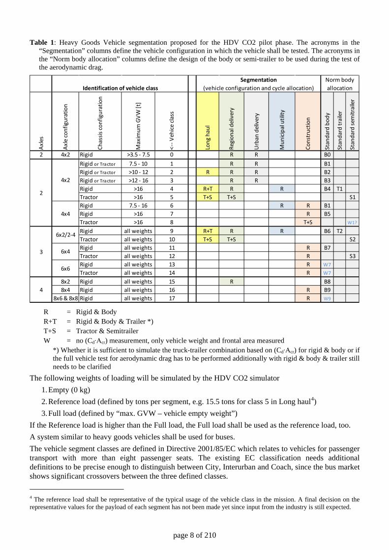
Table 1: Heavy Goods Vehicle segmentation proposed for the HDV CO2 pilot phase. The acronyms in the “Segmentation” columns define the vehicle configuration in which the vehicle shall be tested. The acronyms in the “Norm body allocation” columns define the design of the body or semi-trailer to be used during the test of the aerodynamic drag.

R = Rigid & Body R+T = Rigid & Body & Trailer *) T+S = Tractor & Semitrailer W = no (Cd∙Acr) measurement, only vehicle weight and frontal area measured

*) Whether it is sufficient to simulate the truck-trailer combination based on (Cd∙Acr) for rigid & body or if the full vehicle test for aerodynamic drag has to be performed additionally with rigid & body & trailer still needs to be clarified

The following weights of loading will be simulated by the HDV CO2 simulator 1. Empty (0 kg) 2. Reference load (defined by tons per segment, e.g. 15.5 tons for class 5 in Long haul4) 3. Full load (defined by “max. GVW – vehicle empty weight”)

If the Reference load is higher than the Full load, the Full load shall be used as the reference load, too. A system similar to heavy goods vehicles shall be used for buses. The vehicle segment classes are defined in Directive 2001/85/EC which relates to vehicles for passenger transport with more than eight passenger seats. The existing EC classification needs additional definitions to be precise enough to distinguish between City, Interurban and Coach, since the bus market shows significant crossovers between the three defined classes. 4 The reference load shall be representative of the typical usage of the vehicle class in the mission. A final decision on the representative values for the payload of each segment has not been made yet since input from the industry is still expected.

Axle

s

Axle

conf

igur

atio

n

Chas

sis co

nfig

urat

ion

Max

imum

GVW

[t]

<-- V

ehice

clas

s

Long

hau

l

Regi

onal

del

iver

y

Urb

an d

eliv

ery

Mun

icipa

l util

ity

Cons

truc

tion

Stan

dard

bod

y

Stan

dard

trai

ler

Stan

dard

sem

itrai

ler

2 4x2 Rigid >3.5 - 7.5 0 R R B0Rigid or Tractor 7.5 - 10 1 R R B1Rigid or Tractor >10 - 12 2 R R R B2Rigid or Tractor >12 - 16 3 R R B3Rigid >16 4 R+T R R B4 T1Tractor >16 5 T+S T+S S1Rigid 7.5 - 16 6 R R B1Rigid >16 7 R B5Tractor >16 8 T+S W1?

Rigid all weights 9 R+T R R B6 T2Tractor all weights 10 T+S T+S S2Rigid all weights 11 R B7Tractor all weights 12 R S3Rigid all weights 13 R W7Tractor all weights 14 R W7

8x2 Rigid all weights 15 R B88x4 Rigid all weights 16 R B9

8x6 & 8x8 Rigid all weights 17 R W9

2

4x2

4x4

Segmentation (vehicle configuration and cycle allocation)Identification of vehicle class

Norm body allocation

3

6x2/2-4

6x4

6x6

4

page 9 of 210

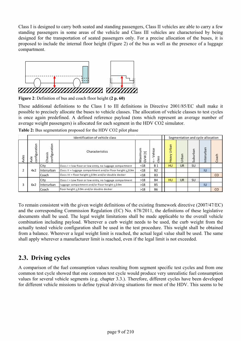
Class I is designed to carry both seated and standing passengers, Class II vehicles are able to carry a fewstanding passengers in some areas of the vehicle and Class III vehicles are characterised by being designed for the transportation of seated passengers only. For a precise allocation of the buses, it is proposed to include the internal floor height (Figure 2) of the bus as well as the presence of a luggage compartment.

Figure 2: Definition of bus and coach floor height (2 p. 60)

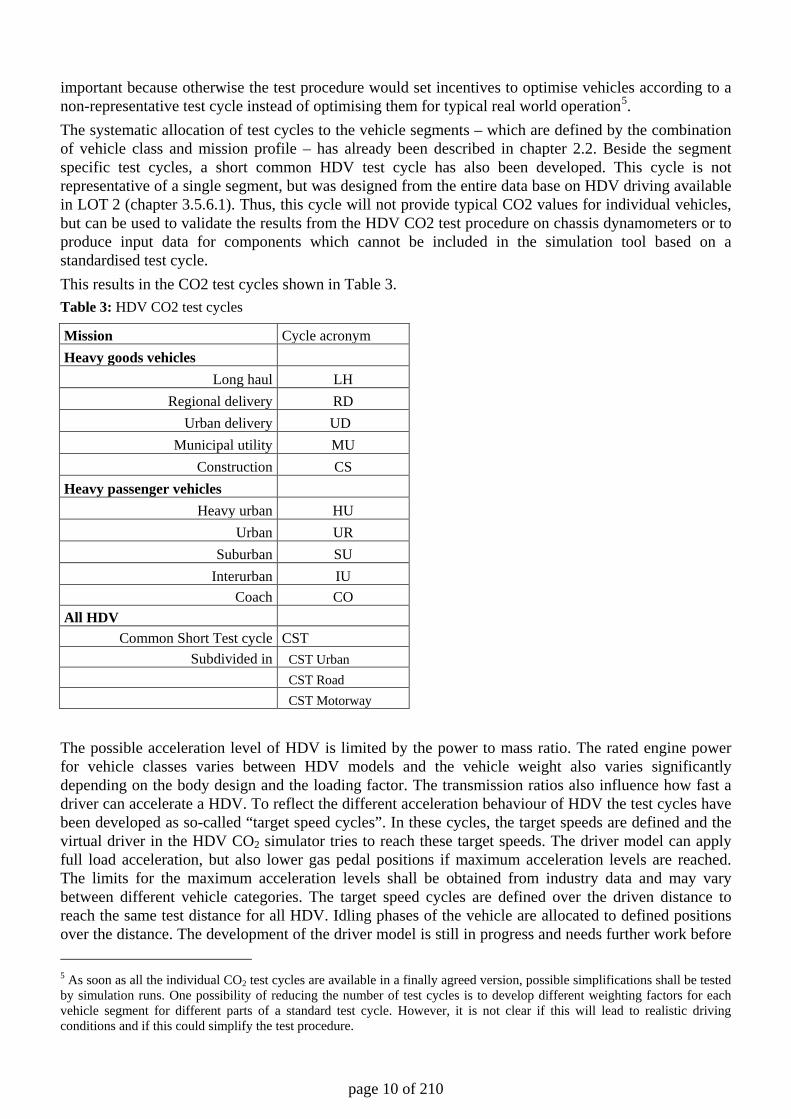
These additional definitions to the Class I to III definitions in Directive 2001/85/EC shall make it possible to precisely allocate the buses to vehicle classes. The allocation of vehicle classes to test cycles is once again predefined. A defined reference payload (tons which represent an average number of average weight passengers) is allocated for each segment in the HDV CO2 simulator.Table 2: Bus segmentation proposed for the HDV CO2 pilot phase

To remain consistent with the given weight definitions of the existing framework directive (2007/47/EC) and the corresponding Commission Regulation (EC) No. 678/2011, the definitions of these legislative documents shall be used. The legal weight limitations shall be made applicable to the overall vehicle combination including payload. Wherever a curb weight needs to be used, the curb weight from the actually tested vehicle configuration shall be used in the test procedure. This weight shall be obtainedfrom a balance. Wherever a legal weight limit is reached, the actual legal value shall be used. The same shall apply wherever a manufacturer limit is reached, even if the legal limit is not exceeded.

2.3. Driving cyclesA comparison of the fuel consumption values resulting from segment specific test cycles and from one common test cycle showed that one common test cycle would produce very unrealistic fuel consumption values for several vehicle segments (e.g. chapter 3.3.). Therefore, different cycles have been developed for different vehicle missions to define typical driving situations for most of the HDV. This seems to be

Axle

s

Axle

co

nfig

urat

ion

Chas

sis

conf

igur

atio

n

Characteristics

Max

imum

GV

W [t

]

<-- V

ehice

cla

ss

Heav

y U

rban

Urb

an

Subu

rban

Inte

rurb

an

Coac

h

City Class I + low floor or low entry, no luggage compartment <18 B 1 HU UR SUInterurban Class I I + luggage compartment and/or floor height < 0.9m <18 B2 IUCoach Class I I I + floor height > 0.9m and/or double decker <18 B3 COCity Class I + Low floor or low entry, no luggage compartment >18 B4 HU UR SUInterurban luggage compartment and/or floor height < 0.9m >18 B5 IUCoach floor height > 0.9m and/or double decker >18 B6 CO

3

4x2

6x2

Identification of vehicle class Segmentation and cycle allocation

2

page 10 of 210

important because otherwise the test procedure would set incentives to optimise vehicles according to a non-representative test cycle instead of optimising them for typical real world operation5. The systematic allocation of test cycles to the vehicle segments – which are defined by the combination of vehicle class and mission profile – has already been described in chapter 2.2. Beside the segment specific test cycles, a short common HDV test cycle has also been developed. This cycle is not representative of a single segment, but was designed from the entire data base on HDV driving available in LOT 2 (chapter 3.5.6.1). Thus, this cycle will not provide typical CO2 values for individual vehicles, but can be used to validate the results from the HDV CO2 test procedure on chassis dynamometers or to produce input data for components which cannot be included in the simulation tool based on a standardised test cycle. This results in the CO2 test cycles shown in Table 3. Table 3: HDV CO2 test cycles

Mission Cycle acronym Heavy goods vehicles

Long haul LH Regional delivery RD

Urban delivery UDs Municipal utility MU

Construction CS Heavy passenger vehicles

Heavy urban HU Urban UR

Suburban SU Interurban IU

Coach CO All HDV

Common Short Test cycle CST Subdivided in CST Urban

CST Road CST Motorway

The possible acceleration level of HDV is limited by the power to mass ratio. The rated engine power for vehicle classes varies between HDV models and the vehicle weight also varies significantly depending on the body design and the loading factor. The transmission ratios also influence how fast a driver can accelerate a HDV. To reflect the different acceleration behaviour of HDV the test cycles have been developed as so-called “target speed cycles”. In these cycles, the target speeds are defined and the virtual driver in the HDV CO2 simulator tries to reach these target speeds. The driver model can apply full load acceleration, but also lower gas pedal positions if maximum acceleration levels are reached. The limits for the maximum acceleration levels shall be obtained from industry data and may vary between different vehicle categories. The target speed cycles are defined over the driven distance to reach the same test distance for all HDV. Idling phases of the vehicle are allocated to defined positions over the distance. The development of the driver model is still in progress and needs further work before 5 As soon as all the individual CO2 test cycles are available in a finally agreed version, possible simplifications shall be tested by simulation runs. One possibility of reducing the number of test cycles is to develop different weighting factors for each vehicle segment for different parts of a standard test cycle. However, it is not clear if this will lead to realistic driving conditions and if this could simplify the test procedure.

page 11 of 210

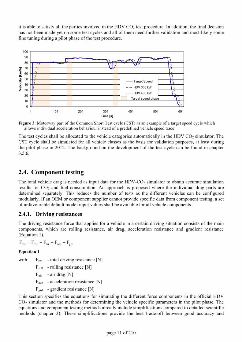
it is able to satisfy all the parties involved in the HDV CO2 test procedure. In addition, the final decision has not been made yet on some test cycles and all of them need further validation and most likely some fine tuning during a pilot phase of the test procedure.

Figure 3: Motorway part of the Common Short Test cycle (CST) as an example of a target speed cycle which allows individual acceleration behaviour instead of a predefined vehicle speed trace

The test cycles shall be allocated to the vehicle categories automatically in the HDV CO2 simulator. The CST cycle shall be simulated for all vehicle classes as the basis for validation purposes, at least during the pilot phase in 2012. The background on the development of the test cycle can be found in chapter 3.5.6.

2.4. Component testingThe total vehicle drag is needed as input data for the HDV-CO2 simulator to obtain accurate simulation results for CO2 and fuel consumption. An approach is proposed where the individual drag parts are determined separately. This reduces the number of tests as the different vehicles can be configuredmodularly. If an OEM or component supplier cannot provide specific data from component testing, a set of unfavourable default model input values shall be available for all vehicle components.

2.4.1. Driving resistancesThe driving resistance force that applies for a vehicle in a certain driving situation consists of the main components, which are rolling resistance, air drag, acceleration resistance and gradient resistance (Equation 1).

grdaccairrollres FFFFF +++=

Equation 1

with: Fres - total driving resistance [N]Froll - rolling resistance [N]Fair - air drag [N]Facc - acceleration resistance [N]Fgrd - gradient resistance [N]

This section specifies the equations for simulating the different force components in the official HDV CO2 simulator and the methods for determining the vehicle specific parameters in the pilot phase. The equations and component testing methods already include simplifications compared to detailed scientific methods (chapter 3). These simplifications provide the best trade-off between good accuracy and

010

20304050

607080

90100

1 101 201 301 401 501 601Time [s]

Vel

ocity

[km

/h]

Target Speed

HDV 300 kW

HDV 400 kWTarget speed phase

page 12 of 210

sensitivity of method, on the one hand, and the complexity and the effort of the procedure, on the other hand. The standard method in HDV certification is to determine the CO2 value for a certain HDV configuration (rigid truck or combination of truck/tractor and trailer). In this case, the HDV configuration is tested with a standard body and/or standard trailer and the air drag is determined using the method described in section 2.4.1.2. In a later stage of the implementation of the HDV certification, bodies and trailers shall also be certified by comparing the resulting driving resistance for the HDV configuration against the value with the standard body / trailer. The respective options for the measurement procedure are discussed in section 2.4.1.2.1.

2.4.1.1. Rolling resistance

The rolling resistance for the simulation of the CO2 emissions of a particular vehicle configuration shall be simulated on the basis of the tire specific rolling resistance values, which have to be specified according to EC No. 1222/2009. The total rolling resistance of the entire HDV configuration is then calculated using Equation 2.

∑ ⋅⋅=axles

ii,ziroll,corrroll FRRCCF

Equation 2

with: Froll - total rolling resistance [N] RRC - rolling resistance coefficient according to EC No. 1222/2009 [-] Fz - vertical axle load [N] Ccorr,roll - correction factor for conversion of test drum results to average real world conditions The application of Equation 2 in the HDV CO2 simulator results in a constant rolling resistance in all driving conditions, i.e. potential dependencies of the rolling resistance on particular driving conditions (e.g. dependency on vehicle speed or ambient temperature) are neglected. The question of whether a general correction of rolling resistance levels from the test drum conditions to average real world conditions (Ccorr,roll) is required will be the subject of further investigations (4). A correction factor for the conversion of test drum results to flat road conditions according to Equation 3 can be found in the literature (5 p. 96).

tiredrum

drumroll,corr rr

rC+

=

Equation 3: draft for a conversion factor for the RRC norm values

With rdrum - drum diameter [m] (=2 meters for values according to EC No 1222/2009) rtire - tire diameter For the most common HDV tire dimension (315/80 R22.5), this correction factor is 0.815, which means that the rolling resistance from the drum test overestimates flat conditions by about 20%. Real world operation is influenced by other factors too (e.g. tire wear, road surface). The definition of the overall factor Ccorr,roll has to be investigated further (e.g. by final “model calibration” in such a way that fuel consumption values calculated by the HDV CO2 simulator in the pilot phase agree with fuel consumption data from vehicle operators). The axle loads Fz,i of the HDV configurations have to be known to use Equation 2. In this context, detailed calculation for any vehicle configuration would be too complicated as the exact weights and positions of the vehicle components, (chassis, engine etc.) have to be available. Thus, it is suggested to use a simplified approach (Equation 4).

page 13 of 210

i,zvehi,z sFgmF ⋅⋅= Equation 4

With Fz,i - axle load for axle i [N] mveh - total vehicle mass including payload [N] g - gravitation constant, 9.81 m/s² sFz,i - share of axle i of the total vehicle weight [-] The total vehicle weight mveh is available from the respective definition in the vehicle segmentation (see the discussion in section 3.2.1. There are three options for assessing the axles’ share of the total vehicle weight:

a) Apply an equal distribution of the total weight of the vehicle configuration b) Apply a predefined axle load distribution, which is specified for all vehicle classes c) Use the percentages of the maximum released axle loads

Which of the three options is most suitable for the final CO2 certification procedure shall be the subject of further investigations. For the pilot phase, it is recommended to apply approach c).

2.4.1.2. Air Drag

The air drag is the resistance force, which acts in the opposite direction to the movement of the vehicle. In the HDV CO2 simulator, it is recommended to simulate this force according to Equation 5:

air,corr2

vehref,air

crdair C)v2

AC(F ⋅⋅ρ

⋅⋅=

Equation 5

with: Fair - air drag [N] Cd - air drag coefficient [-] Acr - cross sectional area of the vehicle [m²] ρair,ref - air density at reference conditions, 1.188 kg/m³ vveh - vehicle velocity [m/s] Ccorr,air - optional correction factor for depiction of average real world side wind conditions [-] In Equation 5, the air drag is calculated based on the vehicle speed. In reality, ambient wind also has an important influence on the air drag. Particularly for truck-trailer combinations and articulated trucks, the air drag is very sensitive to crosswind conditions. In a scientific approach, this cross-wind sensitivity can be expressed by a dependency of the Cd value on the yaw angle “β” (angle between total air-flow and vehicle longitudinal axis). Explicit determination of this Cd =f(β) dependency in the HDV certification process is not recommended due to the enormous efforts which would be required. However, in average real world conditions, ambient wind increases the air drag and hence substantially increases the overall fuel consumption. This influence might be considered by the introduction of a generic correction factor Ccorr,air. ACEA proposes determining such a correction as a function of vehicle speed based on generic Cd=f(ß) curves and average ambient wind speeds, which shall be defined for each vehicle class. However, the final definition for this correction factor has not been specified yet. The parameter which has to be determined for each particular HDV configuration is the product (Cd·Acr) of the air drag coefficient and the cross sectional area of the vehicle. This value shall be measured by full vehicle constant speed tests on a test track. The test procedure for this is described in detail below. In a later stage of the implementation of the HDV CO2 certification procedure, the option of quantifying the aerodynamic variations in the vehicle set-up by CFD simulation (such as deflectors) of the air drag

page 14 of 210

might be provided instead of testing each variation on the test track. For this purpose, a procedure for validating the CFD model would have to be defined.

2.4.1.2.1. Constant speed tests The aim of the test procedure is to determine the product of the air drag coefficient and the cross sectional area (Cd·Acr) of the HDV configuration. Basic principles The driving torque is measured at four different constant speeds on a circular test track. The measured total driving drag is corrected for road gradient, variations of vehicle speed and

optional ambient wind speed. Whether the ambient wind correction shall be allowed in the final proposal for the test procedure has to be investigated in the pilot test phase.

The rolling resistance and the air drag of the vehicle are separated by a mathematical approach. The (Cd·Acr) value is calculated based on the total air drag and is normalised to standard ambient

conditions (1bar and 20°C). During the constant speed tests it is also suggested to measure the fuel consumption by mobile

fuel-flow measurement devices. This data shall be used for a standard validation of the HDV CO2 simulator and as a possible option for calibrating the idling losses of the auxiliary units.

Detailed description of proposed method Test track - The layout of the test track has to allow maintaining maximum vehicle speed (90 km/h for trucks and 100 km/h for coaches) even in the bends in between the straights. - The pavement shall be made of asphalt or concrete. The road shall be dry, clean and smooth. As the rolling resistance in the measurement runs is eliminated from the test results, more detailed specification of the test track surface is not required. - The detailed altitude profile of the straights of the test track shall be made available. The proposed accuracy requirements are +/-3cm for a grid of no more than 100 meters for the driving lane under consideration. Whether boundary conditions for maximum and minimum allowable road gradient have to be defined, shall be investigated in the pilot test phase. Ambient conditions Since a final decision has not been reached yet on the methods for correcting the influence of ambient conditions on the test results, the definition of boundary conditions for valid measurements also has to be left open for the moment. For the pilot phase, it is suggested to define the ambient temperature in the range of 5 to 35 °C. A decision shall be made on the definition of a valid range of ambient wind conditions after evaluations from the pilot test phase. Vehicle setup

• The HDV configuration shall be tested without payload in order to achieve more accurate results for air drag.

• Commercially available tires according to the real use of the vehicle shall be used. The tire inflation pressure shall be set to the maximum allowable value.

• The HDV configuration shall be set up according to normal use of the vehicle, i.e. all mirrors have to be in the correct position, all windows and outer flaps shall be closed. The A/C shall be turned off or in recirculation mode.

• For HDV configurations which are tested as a truck-trailer combination or as an articulated truck the provisions for the trailer setup as specified in the norm body definitions must be applied.

page 15 of 210

Measurement equipment • The driving torque of all driven axles Tqwh,(l,r) [Nm] shall be measured by rim torque meters or

flanges between rim and the wheel end. • The vehicle ground speed vveh [km/h] shall be measured by a GPS system or by more accurate

measurement systems. • The vehicle position (longitude and latitude) shall be recorded by a GPS system. • The fuel consumption shall be measured by a mobile fuel flow meter. The use of ECU data for this

purpose is not recommended. • The ambient conditions (temperature Tamb [K], pressure pamb [mbar] and wind velocity vw [km/h])

during the vehicle tests shall be recorded by a stationary weather station. The suitability of the measurement position at the test track area has to be proven, see for example (6 p. 57480) § 1066.310 /3/

• In the pilot test phase, the actual air flow conditions which apply to the tested HDV (total air flow velocity vair [km/h] and yaw angle ß [°] between total air flow and vehicle longitudinal axis) shall be measured by a mobile anemometer. For this task, the anemometer has to be mounted on the vehicle in such a way that the total air flow speed and yaw angle for undisturbed conditions (i.e. not influenced by the anemometer position and the turbulences from the vehicle itself) can be determined from the measured air flow speed and direction. Furthermore, the aerodynamic of the vehicle shall not be significantly influenced by the anemometer construction. Whether the measurement of the actual air flow conditions on the vehicle shall be part of the final test procedure, shall be decided on the basis of the test results in 2012.

Based on the experiences gained in LOT2, the benefit of considering the actual air flow conditions in the data analysis is questionable. The complexity of deriving reliable data for undisturbed air flow conditions clearly acts contrary to the value of the additional information available for the evaluation of the measured driving resistances. To guarantee a test procedure which is robust against cheating, several standards would have to be elaborated, for instance:

• a definition of a norm position of the anemometer on the vehicle, • a definition of a norm frame construction which connects the anemometer to the vehicle, • and - most important - a definition of a calibration procedure for the measured air flow data.

In general, detailed specifications of acceptable measurement systems and the respective required measurement accuracies shall be defined in cooperation with ACEA during the pilot test phase. In particular, practical experience in measuring wheel torque has to be gathered. These kinds of systems have not been available within the work of LOT2 and are actually not standard equipment in the development of HDV by OEMs.

page 16 of 210

Measurement procedure for the constant speed tests proposed for the pilot phase

• Warm-up of vehicle: at the beginning of the test series, the vehicle shall be driven a minimum of 30 minutes at 80 km/h in order to achieve engine and drivetrain components at normal operating conditions.

• The constant speed tests shall be performed at the following velocities: 90km/h for trucks, 100 km/h for coaches (or the maximum design speed of the vehicle if this is lower than 90km/h), 65km/h, 40km/h and 15 km/h. Maximum velocity and 15 km/h are mandatory, the other velocities are optional.6

• Each constant speed test shall be preconditioned by constant speed driving for at least 45 minutes. After the preconditioning phase, the measurement data has to be recorded without interruption of the constant speed driving.

• For each measured velocity and each straight of the test track, a minimum of 20 valid datasets each with a duration of 20s has to be available. The number of evaluated datasets per velocity and per straight shall be similar. This definition of the amount of required valid measurement data has to be reviewed after the open details in the data evaluation (particularly the verification of the accuracy of the test results) have been clarified in the pilot test phase.

• In the test procedure, an inversion of the driving direction on the test track is not required. • Each constant speed has to be driven in a single gear. The applied gear has to be selected in such a

way that the engine speed is within the range of 40% to 80% normalised engine speed according to the definition in Equation 6.

idlerated

idleCSnorm nn

nnn−

−=

Equation 6

with: nnorm - normalised engine speed [-] nCS - engine speed in the selected gear at the particular constant speed [rpm] nidle - engine idling speed [rpm] nrated - engine rated speed [rpm] The selected gear in the constant speed test influences the measured data on fuel consumption, which is foreseen for validation purposes and optional for calibrating of the idling losses of the auxiliary units. Depending on the final definition of the processing of the fuel consumption data, this definition might have to be revised within the pilot test phase.

• According to discussions with ACEA, the measured driving resistances at low vehicle speeds might be affected by uncertainties when measured using a wheel rim torque meter. As a fall back strategy, ACEA proposes a full vehicle pull test at the lowest vehicle speed, where the drive shafts are removed. The driving resistance is then measured by a load cell in the pull bar. This issue shall be further investigated in the pilot test phase.

Data evaluation 1. Only data which has been recorded at the straights of the test track, where no cornering forces apply

to the vehicle, shall be analysed.

6 From the data available so far and discussions with the OEMs, the preliminary conclusion has been drawn that constant speed tests based on two velocities (a low speed e.g. at 15km/h and the maximum speed of 90km/h) might be the best solution regarding accuracy and measurement time. In the pilot phase; however, several measured velocities would support the final decision.

page 17 of 210

2. All measurement quantities shall be converted to 1 Hz time resolution. 3. The following quantities shall be calculated in based on the measurement data and the vehicle

specifications (i = time index in measurement data): i. Traction force Ftrac [N] (Equation 7)

e

axles driven

i,rwhi,lwh

i,trac r

)TqTq(F

∑ −− +

=

Equation 7

with: Tqwh-l - measured torque in the left wheel [Nm] Tqwh-r - measured torque in the right wheel [Nm] re - effective tire rolling radius [m] calculated based on Equation 21

ii. Longitudinal vehicle acceleration ax [m/s²]:

2vv

6.31a 1i,veh1i,veh

i,x−+ −

=

Equation 8

with: vveh - vehicle speed [km/h] iii. The altitude shall be interpolated from the altitude profile of the test track. The allocation of the

actual vehicle speed to the altitude profile shall use the recorded GPS coordinates. iv. Optional: if the evaluation of constant speed tests includes mobile anemometry data, the

respective values for air flow speed vair [km/h] and yaw angle between total air flow and vehicle longitudinal axis ß [°] shall be determined. Depending on the position of the anemometer, these quantities have to be calculated by applying correction factors/functions to the original measured data. Approvable methods for this task (e.g. calibration of correction functions) still need to be defined. In the proposed evaluation, either the total air flow vair or the air speed in vehicle longitudinal direction vair,x can be applied. At the moment the approach on total air flow vair is favoured. If the second approach is chosen, vair,x shall be calculated according to Equation 9.

)cos(vv ii,airi,x,air β⋅= Equation 9

with: vair - air-flow velocity [km/h] vair,x - air flow velocity in driving direction x [km/h] ß - yaw angle [°]

5. The 1Hz data shall be grouped into datasets of 20 seconds. 6. For each 20s dataset based on Equation 10, the average values for the following quantities shall be

calculated: vehicle speed vveh [km/h], vehicle acceleration ax [m/s²], traction force Ftrac [N], ambient temperature Tamb [°C], ambient pressure pamb [mbar]

∑=

⋅=20

1iij X

201X

Equation 10

page 18 of 210

with: X - measurement quantity under consideration [] i - time index of 1 Hz data within 20s dataset [s] j - index of 20s dataset []

7. For each 20s dataset, the average traction force is then corrected for the average impact of road gradient and accelerations due to speed deviations. The resulting drag force Fdrag,meas then consists of rolling and air resistance in measurement conditions only (Equation 11).

j,accj,grdj,tracj,meas,drag FFFF −−=

Equation 11

with: Fdrag,meas - sum of rolling and air resistance in measurement conditions [N] Ftrac - traction force [N] Fgrd - gradient resistance [N] Facc - acceleration resistance [N] The average gradient resistance in the 20s dataset is calculated based on Equation 12.

j

jvehj,grd s

hgmF

∆

∆⋅⋅=

Equation 12

with: mveh - total vehicle mass including payload [kg] g - gravitation constant, 9.81 [m/s²] ∆hj - altitude difference travelled in 20s dataset [m] ∆sj - distance travelled in 20s dataset [m] The average acceleration resistance in Equation 11 is calculated based on Equation 13.

j,xwh,rotvehj,acc a)mm(F ⋅+= Equation 13

with: mveh - total vehicle mass including payload [kg] mrot,wh - equivalent mass of rotating wheels [kg] ax - vehicle acceleration in driving direction [m]

Based on the measurement data available in LOT2, the result (Cd·Acr) did not significantly change whether the correction for road gradient force and acceleration force for the single 20s datasets was included or not. This is due to the levelling effect from measuring for longer time periods over both directions of a test circuit. Nevertheless, applying the gradient and acceleration correction shall provide the benefit of increased interpretability of the measured data and a more robust test procedure.

8. The exclusion of measurement data, which do not fulfil certain quality criteria, has to be checked. For this purpose, a maximum tolerable speed deviation within the single datasets is defined in ISO 10521-1 (which describes constant speed tests for the road load determination for vehicles ≤3.5t). In the evaluation method proposed here, the need for such an exclusion criterion has not presented itself so far. The requirement of such exclusion criteria has to be evaluated based on the data measured in the pilot test phase.

9. The accuracy of the measurement results has to be verified. If the measured drag forces are analysed on the basis of vehicle speed (and not the on-board measured air flow), this verification could be done using the “statistical accuracy p” parameter as defined in ISO 10521-1 page 15. It

page 19 of 210

is recommended to calculate this parameter p for each set of drag forces Fdrag,meas,j for a certain speed level and a particular driving direction. A valid result is obtained if the statistical error is less than 3%. If the measurement data is analysed on the basis of the on-board measured air flow, this method of verification of measurement results is not applicable. If the final procedure of constant speed tests allows for onboard anemometry, a method for doing this has to be elaborated.

10. In the next step of the evaluation, a regression curve according to Equation 14 shall be fitted to all pairs of vveh,j and Fdrag,meas,j from the 20s datasets (j = index of 20s dataset). If the test evaluation includes mobile anemometry data, the quantities of vair,j or vair,x,j shall be used instead of vveh,j in the regression curve.

2veh

meas,2meas,0meas,drag 6,3vffF

⋅+=

Equation 14

with: Fdrag,meas - sum of rolling and air resistance in measurement conditions [N] f0,meas - constant road load term in measurement conditions [N] f2,meas - quadratic road load term in measurement conditions [Ns²/m²] vveh - vehicle speed [km/h]

In the regression analysis, the single data points shall be weighted in such a way that the sum of the weighting factors for each measured velocity (90, 65, 40 and 15 km/h) is equal to 25%. This shall guarantee equal weighting of the measured forces at each velocity independent of the number of datasets available for the individual velocities.

11. Then the drag function shall be converted from measurement conditions to reference conditions (defined as 20°C and 1000mbar) according to Equation 15.

15.293pT1000

K

)15.293T(k1K

s1s 6.3

vff

fs

)KsKs(FF

j,meas,amb

j,meas,ambj,air

j,meas,ambj,roll

j,rollj,air

2veh

meas,2meas,0

meas,0j,roll

j,airj,airj,rollj,rollj,meas,dragj,ref,drag

⋅

⋅=

−⋅+=

−=

⋅+

=

⋅+⋅⋅=

Equation 15

with: Fdrag,ref - sum of rolling and air resistance in reference conditions [N] Fdrag,meas sum of rolling and air resistance in measurement conditions [N] sroll - share of rolling resistance of total drag [-] Kroll - correction factor for rolling resistance [-] sair - share of air resistance of total drag [-] Kair - correction factor for air resistance [-] f0,meas - constant road load term in measurement conditions [N] f2,meas - quadratic road load term in measurement conditions [Ns²/m²] vveh - vehicle speed [km/h]

page 20 of 210

k - correction coefficient for influence of ambient temperature on tire rolling resistance, 0.006 [K-1] Tamb - ambient temperature [K] pamb - ambient pressure [mbar]

In the evaluation procedure, the correction of tire rolling resistance on ambient temperature shall compensate the difference in ambient condition for the individual datasets. The final parameterisation of the correction coefficient for the influence of temperature on tire rolling resistance “k” has to be reviewed in further investigations (4).

12. Based on the drag forces corrected to reference conditions, a regression curve according to Equation 16 shall be fitted to all pairs of vveh,j and Fdrag,ref,j for the 20s datasets. In the regression, the weighting factors shall be applied like in evaluation step 10. If the test evaluation includes mobile anemometry data, the quantities of either vair,j or vair,x,j shall be used instead of vveh,j in the regression curve.

2veh

ref,2ref,0ref,drag 6.3vffF

⋅+=

Equation 16

with: f0,ref - constant road load term in reference conditions [N] f2,ref - quadratic road load term in reference conditions [Ns²/m²]

13. Equation 17 yields the resulting product (Cd·Acr) of the air drag coefficient and the cross sectional area of the vehicle.

⋅ρ⋅

=⋅ref,air

ref,2crd

f2AC

Equation 17

with: Cd - air drag coefficient [-] Acr - cross sectional area of the vehicle [m²] ρair,ref - air density at reference conditions, 1.188 kg/m³

A separation of the product (Cd·Acr) is not required. This value is used directly as input for the HDV simulator.

2.4.1.2.2. Coast Down Tests Coast down tests are still considered an option for testing the aerodynamic drag of alternative bodies and semi-trailers as well as a fall back strategy if the torque measurement method for constant speeds proves to have some yet unknown disadvantages. The evaluation of coast down tests is described in chapter 3.5.1.6.

2.4.1.2.3. Norm HDV bodies, trailers and semi-trailers As listed in Table 1, the aerodynamic resistance of a HDV shall be tested with “norm bodies”, “norm trailers” and “norm semi-trailers”. The norm design to be used is defined by the respective character-number combination in Table 1. In total,

9 norm bodies (B1 to B9) 2 norm trailers (t1 to t2) 3 norm semi-trailers (S1 to S3)

page 21 of 210

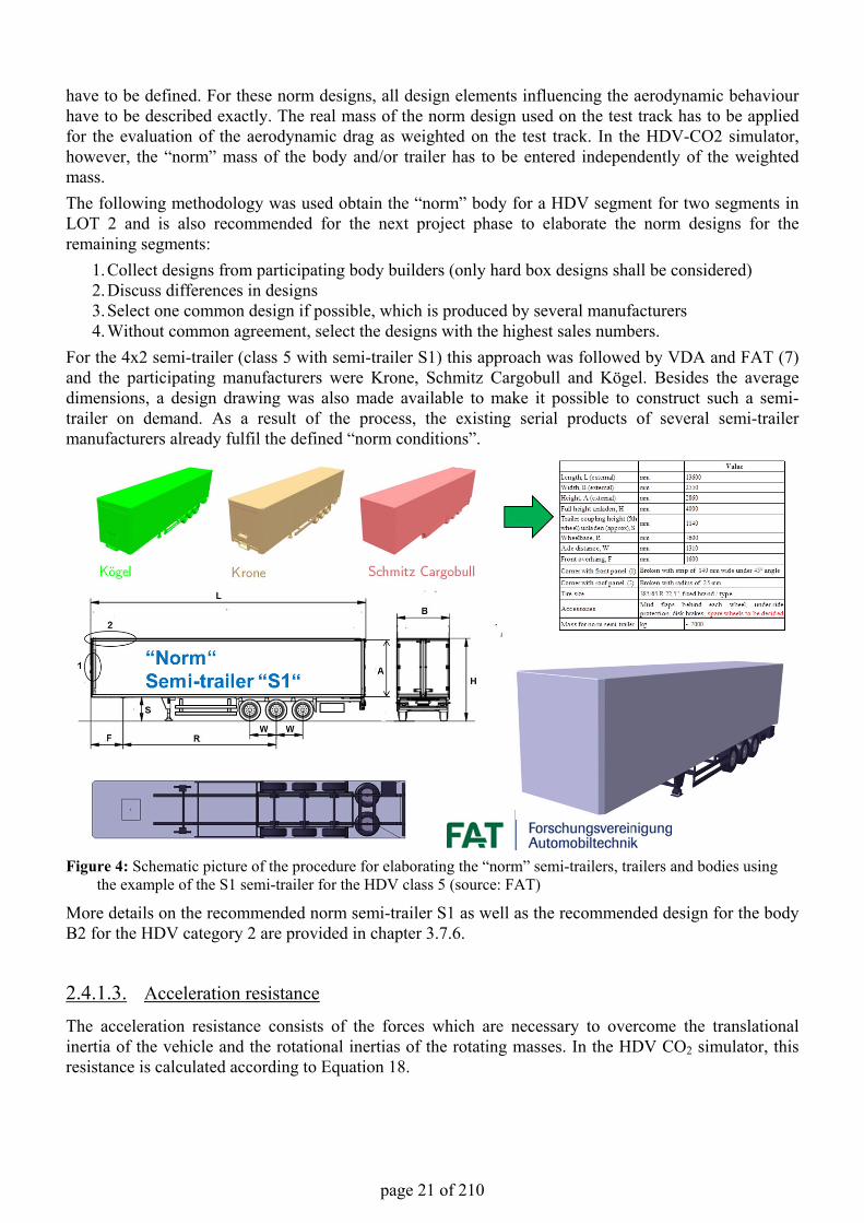
have to be defined. For these norm designs, all design elements influencing the aerodynamic behaviour have to be described exactly. The real mass of the norm design used on the test track has to be applied for the evaluation of the aerodynamic drag as weighted on the test track. In the HDV-CO2 simulator,however, the “norm” mass of the body and/or trailer has to be entered independently of the weighted mass.The following methodology was used obtain the “norm” body for a HDV segment for two segments in LOT 2 and is also recommended for the next project phase to elaborate the norm designs for the remaining segments:

1.Collect designs from participating body builders (only hard box designs shall be considered)2.Discuss differences in designs3.Select one common design if possible, which is produced by several manufacturers4.Without common agreement, select the designs with the highest sales numbers.

For the 4x2 semi-trailer (class 5 with semi-trailer S1) this approach was followed by VDA and FAT (7)and the participating manufacturers were Krone, Schmitz Cargobull and Kögel. Besides the average dimensions, a design drawing was also made available to make it possible to construct such a semi-trailer on demand. As a result of the process, the existing serial products of several semi-trailer manufacturers already fulfil the defined “norm conditions”.

Figure 4: Schematic picture of the procedure for elaborating the “norm” semi-trailers, trailers and bodies using the example of the S1 semi-trailer for the HDV class 5 (source: FAT)

More details on the recommended norm semi-trailer S1 as well as the recommended design for the body B2 for the HDV category 2 are provided in chapter 3.7.6.

2.4.1.3. Acceleration resistance

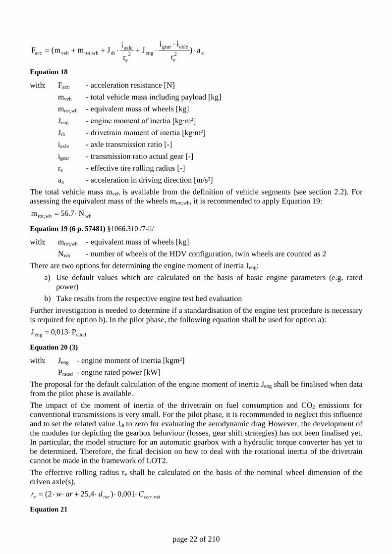
The acceleration resistance consists of the forces which are necessary to overcome the translationalinertia of the vehicle and the rotational inertias of the rotating masses. In the HDV CO2 simulator, this resistance is calculated according to Equation 18.

page 22 of 210

x2e

axlegeareng2

e

axledtwh,rotvehacc a)

rii

JriJmm(F ⋅

⋅⋅+⋅++=

Equation 18

with: Facc - acceleration resistance [N] mveh - total vehicle mass including payload [kg] mrot,wh - equivalent mass of wheels [kg] Jeng - engine moment of inertia [kg∙m²] Jdt - drivetrain moment of inertia [kg∙m²] iaxle - axle transmission ratio [-] igear - transmission ratio actual gear [-] re - effective tire rolling radius [-] ax - acceleration in driving direction [m/s²] The total vehicle mass mveh is available from the definition of vehicle segments (see section 2.2). For assessing the equivalent mass of the wheels mrot,wh, it is recommended to apply Equation 19:

whwh,rot N7.56m ⋅=

Equation 19 (6 p. 57481) §1066.310 /7-ii/

with: mrot,wh - equivalent mass of wheels [kg] Nwh - number of wheels of the HDV configuration, twin wheels are counted as 2 There are two options for determining the engine moment of inertia Jeng:

a) Use default values which are calculated on the basis of basic engine parameters (e.g. rated power)

b) Take results from the respective engine test bed evaluation Further investigation is needed to determine if a standardisation of the engine test procedure is necessary is required for option b). In the pilot phase, the following equation shall be used for option a):

ratedeng P013,0J ⋅=

Equation 20 (3)

with: Jeng - engine moment of inertia [kgm²] Prated - engine rated power [kW] The proposal for the default calculation of the engine moment of inertia Jeng shall be finalised when data from the pilot phase is available. The impact of the moment of inertia of the drivetrain on fuel consumption and CO2 emissions for conventional transmissions is very small. For the pilot phase, it is recommended to neglect this influence and to set the related value Jdt to zero for evaluating the aerodynamic drag. However, the development of the modules for depicting the gearbox behaviour (losses, gear shift strategies) has not been finalised yet. In particular, the model structure for an automatic gearbox with a hydraulic torque converter has yet to be determined. Therefore, the final decision on how to deal with the rotational inertia of the drivetrain cannot be made in the framework of LOT2. The effective rolling radius re shall be calculated on the basis of the nominal wheel dimension of the driven axle(s).

radcorrrime Cdarwr ,001,0)4,252( ⋅⋅⋅+⋅⋅=

Equation 21

page 23 of 210

with: re - effective rolling radius [m] w - nominal tire width [mm] ar - aspect ratio [%] drim - nominal rim width [inch] Ccorr,rad - correction factor for effective rolling radius If a correction factor Ccorr,rad is needed to ensure that the effective rolling radius calculated on the basis of the nominal dimensions meets average real world conditions (influence of tire wear, loading conditions …), shall be investigated in the pilot test phase. At the moment, it is recommended to set this factor to 1.

2.4.1.4. Gradient resistance

In the HDV CO2 simulation model the gradient resistance must be considered since the driving cycles for the different vehicle mission profiles include an altitude profile. The respective gradient resistance shall be calculated according to Equation 22:

∆∆

⋅⋅=sharctansingmF vehgrd

Equation 22

with: mveh - total vehicle mass including payload [kg] g - gravitation constant, 9.81 [m/s²] ∆h/∆s - road gradient [-] No additional input data from component testing are required to apply this equation in the simulation. For typical road gradients, the sin(arctan(∆h/∆s)) is almost identical to the road gradient (∆h/∆s). This leads to the more common Equation 23:

∆∆

⋅⋅=shgmF vehgrd

Equation 24

2.4.1.5. Option for testing vehicle bodies and trailers

The test procedure for measuring the aerodynamic drag of alternative bodies and semi-trailers shall follow the test procedure described for the vehicle with the “norm body” and the “norm semi-trailer” respectively. The final design of the individual norm bodies has not been decided (see chapter 3.7.6). In LOT 2, coast down tests have also been performed as an alternative test procedure for the aerodynamic drag of alternative bodies and trailers. This option shall be tested further in the pilot phase since it could be a cost efficient alternative to constant speed tests. The test procedure shall result in a (Cd·Acr) value for the alternative body design for a given chassis. This alternative value shall then replace the value obtained with the norm body in the HDV-CO2 simulator, as previously described in chapter 2.1. Whether the tests must be performed with both set ups, i.e. the alternative body and the norm body, and only the relative difference in (Cd·Acr) shall be fed into the simulator, has not been decided yet. An ICCT and VDA project is currently analysing if the approach using the relative change in aerodynamic drag significantly increases accuracy. The cheaper method would certainly be to use the absolute measured (Cd·Acr), since this would eliminate the need to test the norm set up, too. For alternative semi-trailers, it is currently recommended to measure the ratio against the “norm semi-trailer”, since it will not be possible to design a “norm tractor”, which then could

page 24 of 210

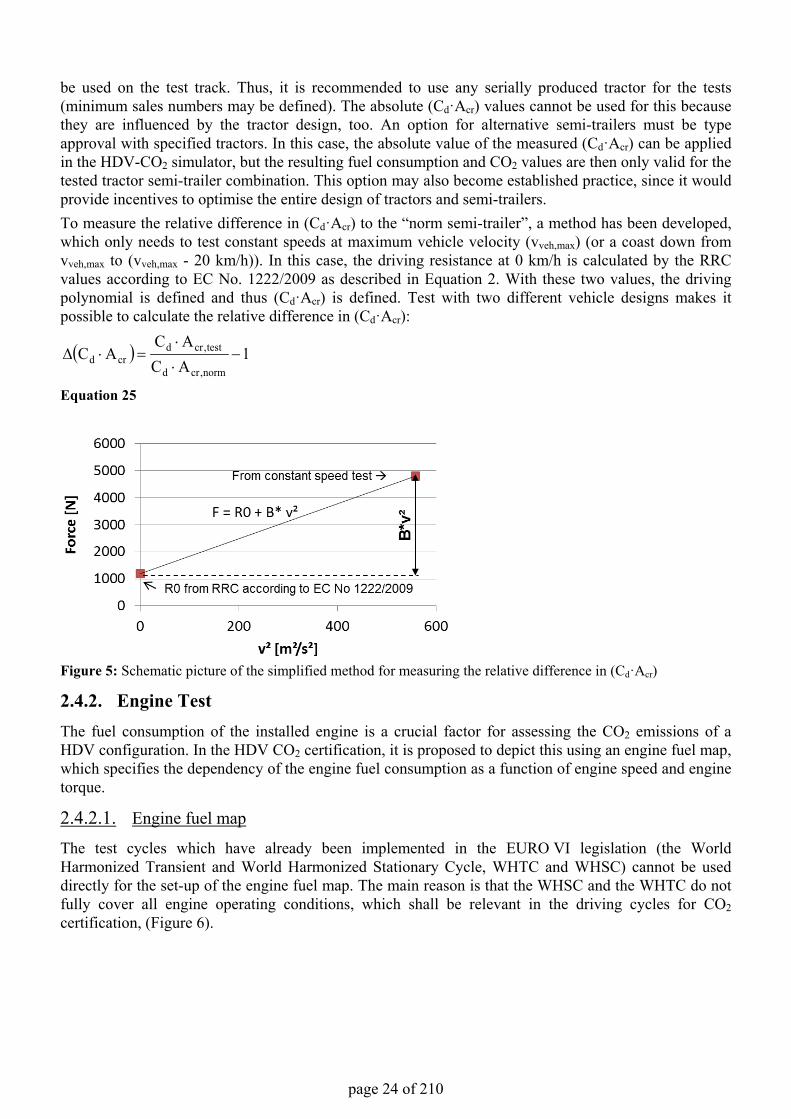
be used on the test track. Thus, it is recommended to use any serially produced tractor for the tests (minimum sales numbers may be defined). The absolute (Cd·Acr) values cannot be used for this because they are influenced by the tractor design, too. An option for alternative semi-trailers must be type approval with specified tractors. In this case, the absolute value of the measured (Cd·Acr) can be applied in the HDV-CO2 simulator, but the resulting fuel consumption and CO2 values are then only valid for the tested tractor semi-trailer combination. This option may also become established practice, since it would provide incentives to optimise the entire design of tractors and semi-trailers.To measure the relative difference in (Cd·Acr) to the “norm semi-trailer”, a method has been developed,which only needs to test constant speeds at maximum vehicle velocity (vveh,max) (or a coast down from vveh,max to (vveh,max - 20 km/h)). In this case, the driving resistance at 0 km/h is calculated by the RRC values according to EC No. 1222/2009 as described in Equation 2. With these two values, the driving polynomial is defined and thus (Cd·Acr) is defined. Test with two different vehicle designs makes it possible to calculate the relative difference in (Cd·Acr):

( ) 1ACAC

ACnorm,crd

test,crdcrd −

⋅⋅

=⋅∆

Equation 25

Figure 5: Schematic picture of the simplified method for measuring the relative difference in (Cd·Acr)

2.4.2. Engine TestThe fuel consumption of the installed engine is a crucial factor for assessing the CO2 emissions of a HDV configuration. In the HDV CO2 certification, it is proposed to depict this using an engine fuel map, which specifies the dependency of the engine fuel consumption as a function of engine speed and engine torque.

2.4.2.1. Engine fuel map

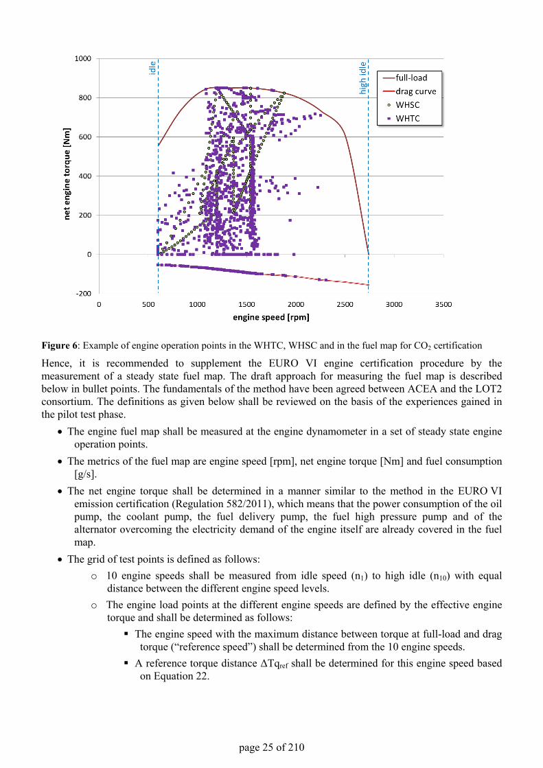
The test cycles which have already been implemented in the EURO VI legislation (the World Harmonized Transient and World Harmonized Stationary Cycle, WHTC and WHSC) cannot be useddirectly for the set-up of the engine fuel map. The main reason is that the WHSC and the WHTC do not fully cover all engine operating conditions, which shall be relevant in the driving cycles for CO2certification, (Figure 6).

page 25 of 210

Figure 6: Example of engine operation points in the WHTC, WHSC and in the fuel map for CO2 certification

Hence, it is recommended to supplement the EURO VI engine certification procedure by the measurement of a steady state fuel map. The draft approach for measuring the fuel map is described below in bullet points. The fundamentals of the method have been agreed between ACEA and the LOT2 consortium. The definitions as given below shall be reviewed on the basis of the experiences gained in the pilot test phase.

• The engine fuel map shall be measured at the engine dynamometer in a set of steady state engine operation points.

• The metrics of the fuel map are engine speed [rpm], net engine torque [Nm] and fuel consumption [g/s].

• The net engine torque shall be determined in a manner similar to the method in the EURO VI emission certification (Regulation 582/2011), which means that the power consumption of the oil pump, the coolant pump, the fuel delivery pump, the fuel high pressure pump and of the alternator overcoming the electricity demand of the engine itself are already covered in the fuel map.

• The grid of test points is defined as follows:o 10 engine speeds shall be measured from idle speed (n1) to high idle (n10) with equal

distance between the different engine speed levels.o The engine load points at the different engine speeds are defined by the effective engine

torque and shall be determined as follows: The engine speed with the maximum distance between torque at full-load and drag

torque (“reference speed”) shall be determined from the 10 engine speeds. A reference torque distance ΔTqref shall be determined for this engine speed based

on Equation 22.

page 26 of 210

10TqTq

ΔTq ref,dragrefmax,ref

+=

Equation 26 with: ΔTqref - reference torque distance [Nm] Tqmax,ref - full-load torque at the reference engine speed [Nm] Tqdrag,ref - drag torque at the reference engine speed [Nm]

Then, the number of load points to be measured shall be determined for each engine speed “n” based on Equation 27.

lueinteger vahigher next the torounded z ,Tq

TqTqz n

ref

n,dragnmax,n ∆

+=

Equation 27 with: zn - number of load points to be measured at engine speed “n” [-] Tqmax,n - full-load torque at engine speed “n” [Nm] Tqdrag,n - drag torque engine speed “n” [Nm] Then, the effective engine torque values Tqj,n for the load points “j” from 1 to zn shall be determined for each engine speed “n” based on Equation 28.

n

n,dragnmax,n,dragn,j z

TqTqjTqTq

++−=

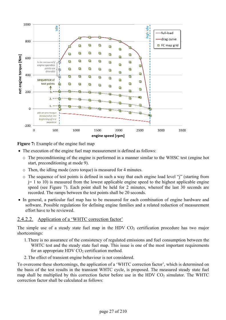
Equation 28 At engine idling speed (n1), load points greater than 50% of the full-load torque may be skipped if the points are not driveable on the engine test bed. Figure 7 offers an example of the resulting engine operation points for the engine fuel map.

page 27 of 210

Figure 7: Example of the engine fuel map• The execution of the engine fuel map measurement is defined as follows:o The preconditioning of the engine is performed in a manner similar to the WHSC test (engine hot

start, preconditioning at mode 9).o Then, the idling mode (zero torque) is measured for 4 minutes.o The sequence of test points is defined in such a way that each engine load level “j” (starting from

j= 1 to 10) is measured from the lowest applicable engine speed to the highest applicable engine speed (see Figure 7). Each point shall be held for 2 minutes, whereof the last 30 seconds are recorded. The ramps between the test points shall be 20 seconds.

• In general, a particular fuel map has to be measured for each combination of engine hardware and software. Possible regulations for defining engine families and a related reduction of measurement effort have to be reviewed.

2.4.2.2. Application of a ‘WHTC correction factor’

The simple use of a steady state fuel map in the HDV CO2 certification procedure has two major shortcomings:

1.There is no assurance of the consistency of regulated emissions and fuel consumption between the WHTC test and the steady state fuel map. This issue is one of the most important requirements for an appropriate HDV CO2 certification method.

2.The effect of transient engine behaviour is not considered.To overcome these shortcomings, the application of a ‘WHTC correction factor’, which is determined on the basis of the test results in the transient WHTC cycle, is proposed. The measured steady state fuel map shall be multiplied by this correction factor before use in the HDV CO2 simulator. The WHTC correction factor shall be calculated as follows:

page 28 of 210

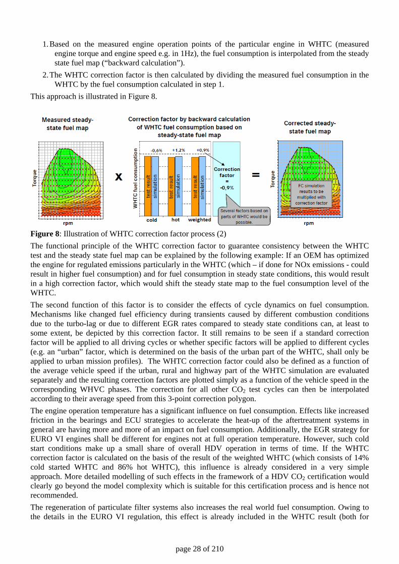
1. Based on the measured engine operation points of the particular engine in WHTC (measured engine torque and engine speed e.g. in 1Hz), the fuel consumption is interpolated from the steady state fuel map (“backward calculation”).

2. The WHTC correction factor is then calculated by dividing the measured fuel consumption in the WHTC by the fuel consumption calculated in step 1.

This approach is illustrated in Figure 8.

Figure 8: Illustration of WHTC correction factor process (2) The functional principle of the WHTC correction factor to guarantee consistency between the WHTC test and the steady state fuel map can be explained by the following example: If an OEM has optimized the engine for regulated emissions particularly in the WHTC (which – if done for NOx emissions - could result in higher fuel consumption) and for fuel consumption in steady state conditions, this would result in a high correction factor, which would shift the steady state map to the fuel consumption level of the WHTC. The second function of this factor is to consider the effects of cycle dynamics on fuel consumption. Mechanisms like changed fuel efficiency during transients caused by different combustion conditions due to the turbo-lag or due to different EGR rates compared to steady state conditions can, at least to some extent, be depicted by this correction factor. It still remains to be seen if a standard correction factor will be applied to all driving cycles or whether specific factors will be applied to different cycles (e.g. an “urban” factor, which is determined on the basis of the urban part of the WHTC, shall only be applied to urban mission profiles). The WHTC correction factor could also be defined as a function of the average vehicle speed if the urban, rural and highway part of the WHTC simulation are evaluated separately and the resulting correction factors are plotted simply as a function of the vehicle speed in the corresponding WHVC phases. The correction for all other CO2 test cycles can then be interpolated according to their average speed from this 3-point correction polygon. The engine operation temperature has a significant influence on fuel consumption. Effects like increased friction in the bearings and ECU strategies to accelerate the heat-up of the aftertreatment systems in general are having more and more of an impact on fuel consumption. Additionally, the EGR strategy for EURO VI engines shall be different for engines not at full operation temperature. However, such cold start conditions make up a small share of overall HDV operation in terms of time. If the WHTC correction factor is calculated on the basis of the result of the weighted WHTC (which consists of 14% cold started WHTC and 86% hot WHTC), this influence is already considered in a very simple approach. More detailed modelling of such effects in the framework of a HDV CO2 certification would clearly go beyond the model complexity which is suitable for this certification process and is hence not recommended. The regeneration of particulate filter systems also increases the real world fuel consumption. Owing to the details in the EURO VI regulation, this effect is already included in the WHTC result (both for

page 29 of 210

continuous and non-continuous regenerating systems) and hence is also depicted by the WHTC correction factor. However, the influence on the total fuel consumption is expected to be negligible in most of the HDV operation conditions. The use of AdBlue in SCR systems also causes CO2 emissions. The CO2 is generated as a by-product of the chemical decomposition of urea to ammonia. However, in the case of EURO V engines, the respective CO2 share is about 0.5% of the total CO2 emissions. For EURO VI engines, this share can be expected to be even lower. Hence, it is recommended to ignore this influence in the CO2 certification procedure.

2.4.2.3. Other engine parameters required in the HDV CO2 simulator

For simulating engine operation in the HDV CO2 simulator, other engine characteristics are required besides the fuel map. The main parameters needed are:

1. The engine full-load curve (maximum torque as a function of engine speed) 2. The engine drag curve (drag moment at fuel cut-off as a function of engine speed) 3. Engine characteristics regarding torque build-up

Data on 1. and 2. are available from standardised procedures on the engine test bed. The method for modelling torque build up in the HDV CO2 simulator has not been decided yet. This model element has to be designed in connection with the development of the driver model. In this context, a simple generic approach (e.g. a PT1 time lag element as a function of engine speed) is recommended. The definition of a standardised test at the engine dyno might be necessary for the parameterisation of this model element. The option of using a default parameterisation for torque build-up characteristics in general shall also be investigated in the next project phase.

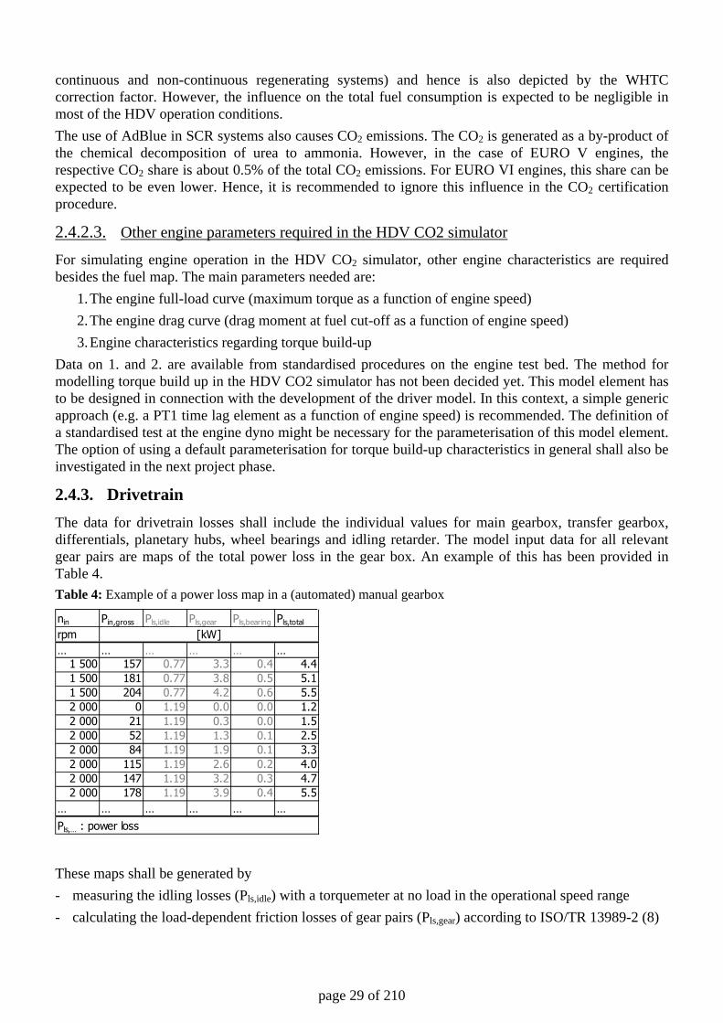
2.4.3. Drivetrain The data for drivetrain losses shall include the individual values for main gearbox, transfer gearbox, differentials, planetary hubs, wheel bearings and idling retarder. The model input data for all relevant gear pairs are maps of the total power loss in the gear box. An example of this has been provided in Table 4. Table 4: Example of a power loss map in a (automated) manual gearbox

These maps shall be generated by - measuring the idling losses (Pls,idle) with a torquemeter at no load in the operational speed range - calculating the load-dependent friction losses of gear pairs (Pls,gear) according to ISO/TR 13989-2 (8)

nin Pin,gross Pls,idle Pls,gear Pls,bearing Pls,total

rpm… … … … … …

1 500 157 0.77 3.3 0.4 4.41 500 181 0.77 3.8 0.5 5.11 500 204 0.77 4.2 0.6 5.52 000 0 1.19 0.0 0.0 1.22 000 21 1.19 0.3 0.0 1.52 000 52 1.19 1.3 0.1 2.52 000 84 1.19 1.9 0.1 3.32 000 115 1.19 2.6 0.2 4.02 000 147 1.19 3.2 0.3 4.72 000 178 1.19 3.9 0.4 5.5

… … … … … …Pls,… : power loss

[kW]

page 30 of 210

- calculating the bearing friction losses (Pls,bearing) in the gearboxes and of the wheel bearings according to an appropriate method, e. g. (9 p. G90 eq. 18). Whether the bearing losses need to be considered has not been decided yet. Further options may be tested in the pilot phase. The results are maps of the power loss as shown above with, for instance, 50 points (input shaft speed / input shaft power / power loss) for each gear pair. The sum of all individual losses from the gearbox input to the wheel bearings is the total driveline drag. The transmission of multiple wheel drive HDV is treated in the same way, but the power split in the transfer gearboxes has to be considered by weighted losses of the multiple powered axles. If no measurement or calculation values for gear pairs or bearings are available, default values shall be used, which represent the lowest realistic performance of actual components. These default values shall be elaborated for all HDV classes and gearbox types during the pilot phase by using the measured losses of the gearboxes of the tested HDV. Ideally the default maps can be simplified by normalisation to, for instance, maximum power transmittable to reduce the need for many category specific default values. Exactly how automatic gear boxes of city buses with hydraulic transmission elements, planetary gear sets and hydro-mechanical powersplits shall be taken into account has not been decided yet. Existing options are listed in chapter 3.5.4. A proposal is expected to be elaborated together with manufacturers and the ACEA in 2012.

2.4.4. Auxiliary units The power demand of the oil pump, the coolant pump, the fuel delivery pump, the fuel high pressure pump and of the alternator overcoming the electricity demand of the engine itself are already covered in the fuel map, so there is no need for a separate model. For the remaining auxiliaries, an additional model is necessary to depict them if the HDV CO2 test procedure shall be in a position to set incentives to improve these components. The main auxiliaries are the cooling fan, the air compressor, the steering pump, the alternator and the air conditioner. More details can be found in chapter 3.5.5. There are several possible approaches to include the power demand of these auxiliary units. A physically based approach may be a reasonable solution, in which the work consumed by an auxiliary (e.g. electric energy over the test cycle) is defined and the engine power demand is then calculated from the efficiency map of the auxiliary including the idling losses that occur whenever the auxiliary is connected to the engine. In the future, this could include a battery model and a controller model. The development of these parts of the test procedure shall be integrated into the work done on hybrid HDV test procedures to obtain harmonized approaches. For the pilot phase, it is recommended to apply the model approaches described in chapter 3.5.5. to obtain experience and the relevant input data. If the model approaches no longer apply in a future type approval procedure, the data can be used to provide HDV segment specific default values, too. In both cases, the data can be included as mechanical and/or electrical power courses over the test cycles, which then lead to an additional power demand from the engine. In the model, electrical power demand is converted into mechanical power by the efficiency of the alternator. It must be mentioned that not all auxiliaries are operated continuously. Particularly the cooling fan, the air compressor and the steering pump run intermittently, depending on a variety of factors. Therefore, assuming continuous average power consumption can lead to an over-simplification, since it may stimulate the optimisation of the auxiliary in non-representative load points. Regardless of the chosen approach, default values shall be elaborated in case no component-specific data is available. These default values shall represent the lower, realistic end of performance to motivate manufacturers to make more precise data available. These default values may also be used in general in a first step of the test procedure. The default values could be replaced in a later step by OEM specific

page 31 of 210

data from component testing as soon as standardised test procedures and simulation tools are elaborated for the relevant auxiliaries.

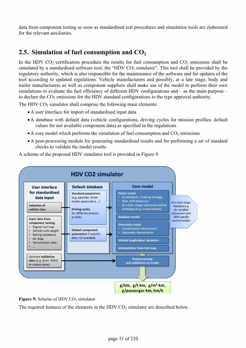
2.5. Simulation of fuel consumption and CO2

In the HDV CO2 certification procedure the results for fuel consumption and CO2 emissions shall be simulated by a standardised software tool, the “HDV CO2 simulator”. This tool shall be provided by the regulatory authority, which is also responsible for the maintenance of the software and for updates of the tool according to updated regulations. Vehicle manufacturers and possibly, at a late stage, body and trailer manufacturers as well as component suppliers shall make use of the model to perform their own simulations to evaluate the fuel efficiency of different HDV configurations and – as the main purpose –to declare the CO2 emissions for the HDV standard configurations to the type approval authority.The HDV CO2 simulator shall comprise the following main elements:

•A user interface for import of standardised input data•A database with default data (vehicle configurations, driving cycles for mission profiles, default

values for not available component data) as specified in the regulations•A core model which performs the simulation of fuel consumption and CO2 emissions •A post-processing module for generating standardised results and for performing a set of standard

checks to validate the model results.A scheme of the proposed HDV simulator tool is provided in Figure 9

Figure 9: Scheme of HDV CO2 simulator

The required features of the elements in the HDV CO2 simulator are described below.

page 32 of 210

2.5.1. User interface for import of standardised input data The HDV CO2 simulator shall have a user interface, which manages the regulated vehicle configurations and which handles the import of the standardised input data. Only the standardised formats as defined in the legislation shall be supported. The evaluation of the important component tests (e.g. the constant speed test for determining the air drag of the HDV configuration) might be integrated into this module of the HDV CO2 simulator or might be provided as separate tools.

2.5.2. Default database The default database shall comprise all standard data as laid down in the HDV CO2 legislation. The database has to contain:

• all standard parameters for the regulated HDV configurations (e.g. vehicle payload, driver model parameters),

• the driving cycles for the different mission profiles, and • the tables with default parameters for all vehicle components, for which specific data are not

available from component testing.

2.5.3. The core model The core model comprises all simulation algorithms required for assessing the fuel consumption and CO2 emissions according to the provisions in the legislation. The core model simulates HDV operation according to the target speed cycles in a time-resolved scale. The following sections provide a short description of the modules required within the core model.

2.5.4. Driver model HDV driving behaviour is significantly influenced by the vehicle mass and the motorisation of the HDV configuration. The driving behaviour (amongst others characterised by vehicle acceleration and gear shift strategy) has a major impact on fuel consumption and travel time. A simulation approach based on target speed cycles, see section 3.5.6, and a driver model are proposed for depicting a realistic driving style for all possible combinations of mission profiles and HDV configurations. The driver model shall follow the target speed cycles based on strategies for accelerating and braking as well as for gear shifts. The driver model shall be based on a generally valid algorithm, i.e. that a single driver algorithm can be applied to all HDV categories. The driver model shall use a set of generic parameters (e.g. desired acceleration as a function of vehicle speed; different parameter sets for the various HDV categories), which cannot be changed by the model user. In a particular time step in the simulation run, the output of the driver model run is the engine torque demand (or a brake or clutch operation) and the selected gear. In a later stage of the implementation of the HDV CO2 certification, a set of advanced control strategies, which are commonly applied in the HDV fleet (e.g. cruise control, free rolling mode), shall also be implemented into the driver model of the official HDV CO2 simulator. Again, a generic (i.e. a generally valid) algorithm shall be used for each advanced control function. A set of OEM specific parameters (e.g. the ramp-up speed) can be used in the model. In this regard, all specific parameters have to be declared by a verifiable process.

2.5.5. Drivetrain model The main tasks of this module are to calculate the torque transmission in the drivetrain (gearbox and differential) and the related torque losses. The structures of the algorithms have to be defined in accordance with the provisions for the associated component tests, (see section 3.5.4). For gearboxes, the following two main technological concepts have to be covered in the model:

page 33 of 210

• conventional transmissions, which cover manual transmissions and automated transmissions and • automatic gearboxes with hydrodynamic torque converters, which are mainly used in city bus

applications.

2.5.6. Auxiliary model In the auxiliary model, the power consumption of the auxiliary units shall be calculated. Depending on the approach chosen for considering these components in the HDV CO2 certification procedure – which has not been fully decided yet – the implemented functions shall comprise different modelling levels, from the use of constant power demand values to more detailed generic functions, for the different auxiliary components. At a later stage, this module might be implemented using an interface for certified interaction with OEM specific auxiliary control models.

2.5.7. Vehicle longitudinal dynamics The vehicle longitudinal dynamics module has to solve the equations of motion based on the supplied torque from the engine, the power consumption of the auxiliaries, the drivetrain behaviour and the driving resistances. The main dynamic engine characteristics (e.g. the limitations in dynamic torque build-up) shall also be depicted in this module by a simple generic approach. The outputs of the module are acceleration, speed of vehicle and engine and – depending on the degree of detail of the drivetrain model (e.g. for automatic transmissions) – the rotating drivetrain parts.

2.5.8. Interpolation from the fuel map Based on the calculated engine torque and engine speed, the fuel consumption in the actual time step has to be interpolated from the engine fuel map. An appropriate method is described in (10 p. 51). For this purpose, a reviewed and documented interpolation algorithm shall be implemented in the HDV simulator. The CO2 emissions are then calculated on the basis of fuel consumption using fuel specific conversion factors.

2.5.9. Data post-processing The HDV simulator shall contain a set of data verification and post-processing routines which carry out the following tasks:

• Execution of plausibility checks on the HDV model compiled from the component data (e.g. by a comparison of simulated fuel consumption at constant speed with the measured values from the respective test procedure)

• Generation of average cycle results for fuel consumption and CO2 emissions in the metrics relevant for the HDV configuration for declaring the official certification results

• As a potential option, execution of validation procedures e.g. by comparison with data from precisely defined PEMS tests or from the chassis dyno.

2.5.10. Further work needed to develop the HDV CO2 simulator In LOT 2, all simulations were done with the model PHEM (Passenger car and Heavy duty Emission Model) (3). PHEM provided all functions necessary to compute the fuel consumption of the HDV tested. The conversion of results from component tests to PHEM input data was done using extra tools, most of them MS Excel sheets with some VBA scripts. In the next phase of the project, the functionality of these additional tools should be integrated into a complete simulator to allow efficient and consistent assessment of the test results at all participating manufacturers. This pilot phase simulator does not need

page 34 of 210

to offer data security systems since it can be used as a stand-alone tool at each participating lab during the pilot phase. Such a tool shall be developed as a stand-alone executable application together with a user manual, which can be distributed to all OEMs and other manufacturers who have to apply the test procedure. This simulation tool shall be considered to be a demonstrator, which includes all mathematical functions as well as all default data sets required to allow the user to execute the complete certification procedure. Default data sets not available from LOT 2 results shall be prepared as dummies which have to be replaced during the course of the project in common efforts of ACEA and a consultant of the EU. The final certification tool can then be based on this tested, and, if necessary, improved and corrected demonstrator. The final certification tool shall need to add security and access items as well as a potential web portal and data server functionalities. These tasks are typically the responsibility of software engineers and are not part of the demonstrator. Final versions of several model elements are not available from LOT 2 and have to be finalised during the next phase of development of the HDV CO2 certification procedure: Driver model

OEM-specific modelling of automated gear shifts

OEM-specific modelling of automatic transmission systems

OEM-specific modelling of auxiliaries

OEM-specific modelling of common advanced vehicle control strategies (e.g. cruise control, free-rolling functions etc.)

A very important task of the last stage of development of the HDV CO2 certification is proving the validity of the complete approach – including the algorithms in the HDV CO2 simulator, the input data from component tests and the default parameters like mission profiles and auxiliary operation data. Investigations will have to show whether the requirements regarding ranking and relative quantification of different vehicle configurations with respect to fuel and CO2 and the provision of realistic absolute values for the fuel consumption of different vehicle segments, which can be accepted by customers as a realistic reference value for real world operation, are fulfilled. Furthermore, the applicability of PEMS data from in-service compliance tests for validating the certification data is discussed. As an option an additional test round during PEMS measurements on a test track or on a road segment, where road gradients, ambient wind conditions and fuel flow can be measured accurately, could serve as validation data. To enable such a validation, the simulation tool has to be extended to provide simulation results if the PEMS test data is used as the input (instead of the standard test cycles).

2.5.11. Interface of the simulation model for OEM-specific technology Not every vehicle component or control strategy can be implemented in the standard simulation tool for the whole European HDV fleet. This would lead to a complex simulator, which users may not be able to handle properly in a type approval procedure. But individual OEM offer their own technology approaches with different fuel saving potentials. These could be considered to some extent using a standardised interface to connect the model of the special OEM technology to the official European simulation tool. Some examples of relevant technologies are listed below: EGR cooler with Brayton heat engine, automatically reduced air drag at high velocities, brake energy recovery, terrain-dependent drivetrain control, Start-Stop Automatic, limit for acceleration, shifting advice for manually operated transmissions, and steerable rear axles at truck or trailer. A description of these approaches and their possible interaction with the simulation model is provided in section 3.5.7.

page 35 of 210

The list above is only an example and is not complete. Since new fuel saving technologies are constantly being developed, no standard simulation tool will ever be "complete" and there is a clear need for a defined interface to feed the OEM-specific model data into the official tool. A standard for this interface in terms of data format and channels, e. g. engine power output, air consumption, cooling fan power, electric power demand, alternative gear shift points, engine stop etc. needs to be developed and discussed with the industry. This approach leads to the demand for an external validation of the OEM sub-models by the type approval authorities or technical services to avoid misuse. Methods for verifying the model structures and validating the calculated results shall be developed.

2.6. Metrics of results A comparison of different options for defining metrics for the fuel consumption and for the CO2 emissions obtained from the HDV-CO2 test procedure is provided in chapter 3.3. While the metrics related to the payload [g/(ton∙km)] and volume [g/(m³∙km)] typically show decreasing values as the maximum gross vehicle weight (GVW) increases, the gram per vehicle kilometre typically increases as the GVW increases. In principle, a weighted result between [g/(ton∙km)], [g/(m³∙km)] and [g/(vehicle∙km)] can be found, which results in comparable values across various HDV classes, as long as the vehicles have similar mission profiles and thus the same driving cycles and similar design characteristics. Since the actual test approach calls for differentiation into vehicle segments with different test cycles per mission profile, no sound physical metrics have been found yet, which can make the fuel consumption test result comparable between HDV segments7. For the pilot phase, it therefore seems relevant to compute all specific fuel consumption and CO2 values, which can be of relevance for the decision of customers. These are:

g/(ton∙km) ................. typical driving with average load (using the average payload defined in tons for the corresponding HDV segment). Seems to be the most relevant metric to describe the work done.

g/(tonmax∙km) ............ driving at maximum payload (simulation result with fully loaded vehicle). Lightweight construction provides the highest benefit here, since a higher payload can be loaded.

g/(m³∙km) .................. driving loaded to maximum available volume, but below maximum payload (typical specific volumes of the load will have to be defined (e.g. 25m³/ton which would represent foam material), as an alternative the maximum loadable number of EURO palettes according to DIN EN 13698 (1.2 m ∙ 0.8 m (length ∙ width)) with a defined height (e.g. 2.4 m).

g/km .......................... relevant during empty trips For buses and coaches, the unit g/ton∙km is not common, therefore we recommend using

g/(passenger∙km) ...... replaces the g/(ton∙km) for buses and coaches in average load and full load calculation with a standard mass per passenger. Seems to be the most relevant metric to describe the work done for passenger transport.

Since each of these metrics carries information which can be important to customers, all values shall be computed and reported in the pilot phase of the HDV-CO2 test procedure. Since all values can be calculated quickly with the simulation approach, not much effort is required to produce the numbers. A questionnaire among typical customers may then be applied to select the most important values.

7 It is questionable if it would be advantageous to produce just one value which is comparable across HDV categories since customers would then lose information on which vehicle category would have the highest fuel efficiency within the options fulfilling their demands.

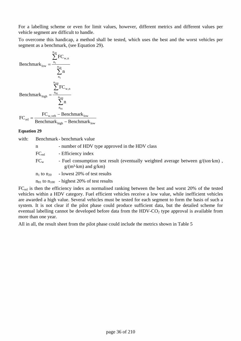
page 36 of 210

For a labelling scheme or even for limit values, however, different metrics and different values per vehicle segment are difficult to handle. To overcome this handicap, a method shall be tested, which uses the best and the worst vehicles per segment as a benchmark, (see Equation 29).

lowhigh

lowveh,wrel

n

n

n

nn,w

high

n

n

n

nn,w

low

BenchmarkBenchmarkBenchmarkFC

FC

n

FCBenchmark

n

FCBenchmark

100

81

100

81

20

1

20

1

−

−=

=

=

∑

∑

∑

∑

Equation 29

with: Benchmark - benchmark value n - number of HDV type approved in the HDV class FCrel - Efficiency index FCw - Fuel consumption test result (eventually weighted average between g/(ton∙km) ,

g/(m³∙km) and g/km) n1 to n20 - lowest 20% of test results n81 to n100 - highest 20% of test results FCrel is then the efficiency index as normalised ranking between the best and worst 20% of the tested vehicles within a HDV category. Fuel efficient vehicles receive a low value, while inefficient vehicles are awarded a high value. Several vehicles must be tested for each segment to form the basis of such a system. It is not clear if the pilot phase could produce sufficient data, but the detailed scheme for eventual labelling cannot be developed before data from the HDV-CO2 type approval is available from more than one year. All in all, the result sheet from the pilot phase could include the metrics shown in Table 5

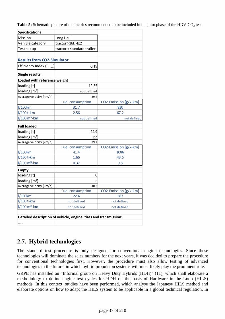
page 37 of 210

Table 5: Schematic picture of the metrics recommended to be included in the pilot phase of the HDV-CO2 test

2.7. Hybrid technologies The standard test procedure is only designed for conventional engine technologies. Since these technologies will dominate the sales numbers for the next years, it was decided to prepare the procedure for conventional technologies first. However, the procedure must also allow testing of advanced technologies in the future, in which hybrid propulsion systems will most likely play the prominent role. GRPE has installed an “Informal group on Heavy Duty Hybrids (HDH)" (11), which shall elaborate a methodology to define engine test cycles for HDH on the basis of Hardware in the Loop (HILS) methods. In this context, studies have been performed, which analyse the Japanese HILS method and elaborate options on how to adapt the HILS system to be applicable in a global technical regulation. In

SpecificationsMission Long HaulVehicle category tractor >16t, 4x2Test set up tractor + standard trailer

Results from CO2-SimulatorEfficiency Index (FCrel) 0.19

Single results:Loaded with reference weightloading [t] 12.35loading [m³] not defined

Average velocity [km/h] 39.8

Fuel consumption CO2-Emission [g/x-km]l/100km 31.7 830l/100 t-km 2.56 67.2l/100 m³-km not defined not defined

Full loadedloading [t] 24.9loading [m³] 110Average velocity [km/h] 39.2

Fuel consumption CO2-Emission [g/x-km]l/100km 41.4 1086l/100 t-km 1.66 43.6l/100 m³-km 0.37 9.8

Emptyloading [t] 0loading [m³] 0Average velocity [km/h] 40.2

Fuel consumption CO2-Emission [g/x-km]l/100km 22.4 587l/100 t-km not defined not defined

l/100 m³-km not defined not defined

Detailed description of vehicle, engine, tires and transmission:…..

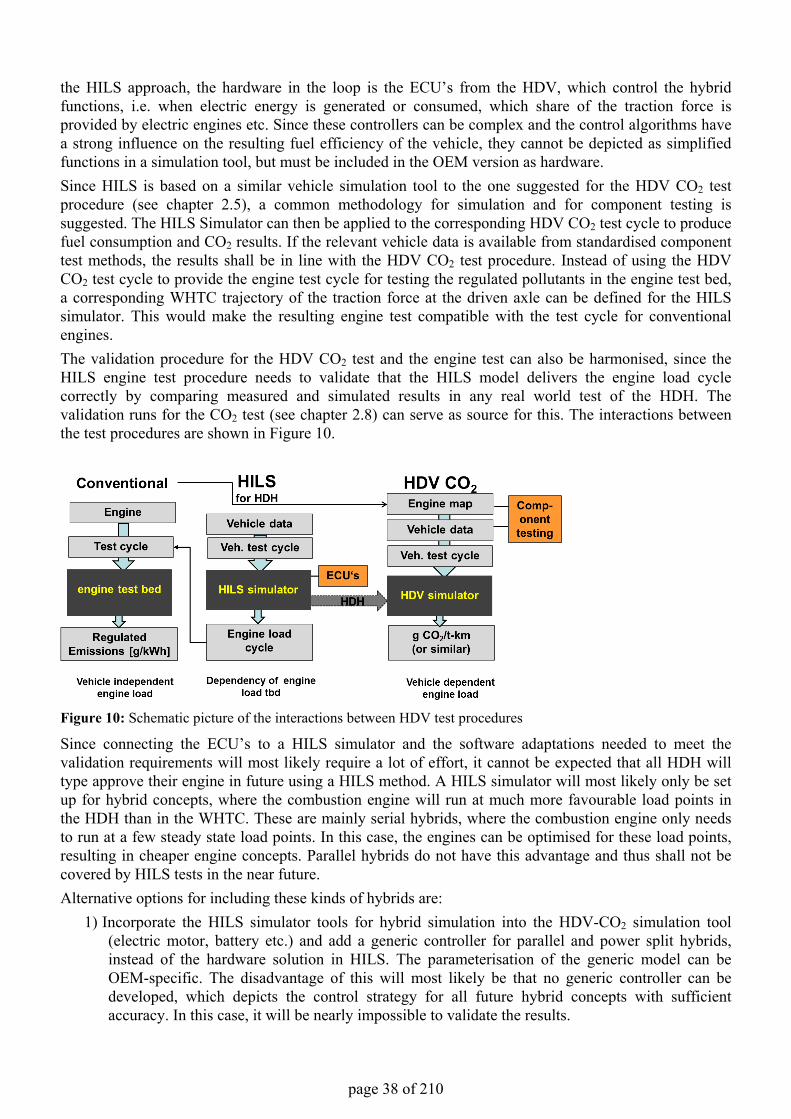
page 38 of 210

the HILS approach, the hardware in the loop is the ECU’s from the HDV, which control the hybrid functions, i.e. when electric energy is generated or consumed, which share of the traction force is provided by electric engines etc. Since these controllers can be complex and the control algorithms have a strong influence on the resulting fuel efficiency of the vehicle, they cannot be depicted as simplified functions in a simulation tool, but must be included in the OEM version as hardware.Since HILS is based on a similar vehicle simulation tool to the one suggested for the HDV CO2 test procedure (see chapter 2.5), a common methodology for simulation and for component testing is suggested. The HILS Simulator can then be applied to the corresponding HDV CO2 test cycle to produce fuel consumption and CO2 results. If the relevant vehicle data is available from standardised component test methods, the results shall be in line with the HDV CO2 test procedure. Instead of using the HDVCO2 test cycle to provide the engine test cycle for testing the regulated pollutants in the engine test bed, a corresponding WHTC trajectory of the traction force at the driven axle can be defined for the HILS simulator. This would make the resulting engine test compatible with the test cycle for conventional engines.The validation procedure for the HDV CO2 test and the engine test can also be harmonised, since the HILS engine test procedure needs to validate that the HILS model delivers the engine load cycle correctly by comparing measured and simulated results in any real world test of the HDH. The validation runs for the CO2 test (see chapter 2.8) can serve as source for this. The interactions between the test procedures are shown in Figure 10.

Figure 10: Schematic picture of the interactions between HDV test procedures

Since connecting the ECU’s to a HILS simulator and the software adaptations needed to meet the validation requirements will most likely require a lot of effort, it cannot be expected that all HDH will type approve their engine in future using a HILS method. A HILS simulator will most likely only be set up for hybrid concepts, where the combustion engine will run at much more favourable load points in the HDH than in the WHTC. These are mainly serial hybrids, where the combustion engine only needs to run at a few steady state load points. In this case, the engines can be optimised for these load points,resulting in cheaper engine concepts. Parallel hybrids do not have this advantage and thus shall not be covered by HILS tests in the near future.Alternative options for including these kinds of hybrids are:

1) Incorporate the HILS simulator tools for hybrid simulation into the HDV-CO2 simulation tool (electric motor, battery etc.) and add a generic controller for parallel and power split hybrids,instead of the hardware solution in HILS. The parameterisation of the generic model can be OEM-specific. The disadvantage of this will most likely be that no generic controller can be developed, which depicts the control strategy for all future hybrid concepts with sufficientaccuracy. In this case, it will be nearly impossible to validate the results.

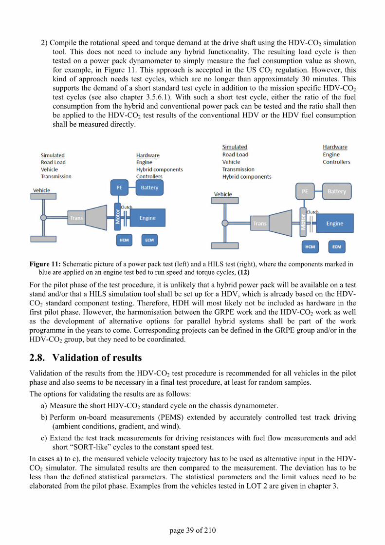
page 39 of 210

2) Compile the rotational speed and torque demand at the drive shaft using the HDV-CO2 simulation tool. This does not need to include any hybrid functionality. The resulting load cycle is then tested on a power pack dynamometer to simply measure the fuel consumption value as shown,for example, in Figure 11. This approach is accepted in the US CO2 regulation. However, this kind of approach needs test cycles, which are no longer than approximately 30 minutes. This supports the demand of a short standard test cycle in addition to the mission specific HDV-CO2test cycles (see also chapter 3.5.6.1). With such a short test cycle, either the ratio of the fuel consumption from the hybrid and conventional power pack can be tested and the ratio shall thenbe applied to the HDV-CO2 test results of the conventional HDV or the HDV fuel consumption shall be measured directly.

Figure 11: Schematic picture of a power pack test (left) and a HILS test (right), where the components marked in blue are applied on an engine test bed to run speed and torque cycles, (12)

For the pilot phase of the test procedure, it is unlikely that a hybrid power pack will be available on a test stand and/or that a HILS simulation tool shall be set up for a HDV, which is already based on the HDV-CO2 standard component testing. Therefore, HDH will most likely not be included as hardware in the first pilot phase. However, the harmonisation between the GRPE work and the HDV-CO2 work as well as the development of alternative options for parallel hybrid systems shall be part of the work programme in the years to come. Corresponding projects can be defined in the GRPE group and/or in the HDV-CO2 group, but they need to be coordinated.

2.8. Validation of resultsValidation of the results from the HDV-CO2 test procedure is recommended for all vehicles in the pilot phase and also seems to be necessary in a final test procedure, at least for random samples. The options for validating the results are as follows:

a) Measure the short HDV-CO2 standard cycle on the chassis dynamometer. b) Perform on-board measurements (PEMS) extended by accurately controlled test track driving

(ambient conditions, gradient, and wind).c) Extend the test track measurements for driving resistances with fuel flow measurements and add

short “SORT-like” cycles to the constant speed test.In cases a) to c), the measured vehicle velocity trajectory has to be used as alternative input in the HDV-CO2 simulator. The simulated results are then compared to the measurement. The deviation has to beless than the defined statistical parameters. The statistical parameters and the limit values need to be elaborated from the pilot phase. Examples from the vehicles tested in LOT 2 are given in chapter 3.

page 40 of 210

In a), the road load cannot be validated, since the road load on the chassis dynamometer is simulated by the electric motor of the test bed according to the settings provided by the test bed driver. Thus, the road load from the HDV-CO2 test results have to be used for the chassis dynamometer tests. Chassis dynamometer testing for HDV has not been included in the regulations yet. The “best practices” described in chapter 3.4.3 shall be followed for the pilot phase. For b), the standard PEMS procedure does not seem to be sufficient in terms of repeatability and reproducibility to allow for reasonably strict limits for the deviation between the HDV-CO2 test result and the validation result. The reproducibility of PEMS shall be improved by driving the vehicle on a test track or on a well-defined road section f or the CO2 part, where the road gradient is accurately known and where ambient conditions can be measured during the PEMS tests. The demand on the measurands shall follow the conditions of the road load measurements (chapters 2.4.1 and 3.5.1). The accuracy can be improved further by using an accurate fuel flow meter in addition to the PEMS CO2 measurement. Technically speaking, option c) is similar to option b), but it would be done during the HDV-CO2 road load tests while option b) can be added to the in-use test procedure defined in the EURO VI regulation. The latter is related to vehicles taken from in-use service, whereas option c) is performed with the type approval vehicle. For the pilot phase, it is recommended to apply option c) for (almost) all vehicles tested, since adding a fuel flow meter is a reasonable effort in a pilot programme. Where possible, chassis dyno tests can also be added to option c) in the pilot phase, since chassis dyno tests can provide useful data on the variability of influences from auxiliaries (this requires several repetitions of the test cycle, and the test cycle can be the “SORT-like” cycle from the test track driving or the short common HDV-CO2 vehicle cycle). Since the power demand of the auxiliaries will most likely not be measured during the road load tests in a final test procedure, the contribution of auxiliaries to the measured fuel consumption shall remain a main uncertainty in the validation process. In the final version of the test procedure an extension to the PEMS tests for the already installed In-use tests for the regulated pollutants from HDV seems to be advantageous if a reasonable accuracy and reproducibility can be reached. From the pilot phase the possible accuracy shall be gained. The pilot phase shall also give information if the power consumption from auxiliaries needs to be measured during the CO2-PEMS to reach sufficient accuracy.

2.9. Proposal for a future regulatory approach From today’s point of view, the manufacturers with a technical service to provide expertise and the type approval authority to provide type approval shall mainly be responsible for running the tests in the final type approval procedure. The OEM shall have to obtain the measurement data for all components either by their own measurements or by tests from the component supplier. Tests must follow the defined standard conditions, which have to be controlled by a technical service or a type approval authority. The data must be provided in the standard formats of the type approval simulation tool. After compiling all the necessary input data in the type approval simulation tool, the OEM can run the simulator to check the results for CO2 and fuel consumption. After the checks, the data shall be submitted officially. The data for each component as well as the results for the entire vehicle shall be stored in a database owned by the commission. This would allow a rather simple multi-stage approach for vehicles which are not sold by the manufacturer of the chassis, but, for example, by the body builder. The body builder shall then get access to the data of all components in the chassis (engine, gear box, etc.) and can then just add parts which are in his responsibility (aerodynamic drag and weight from the entire vehicle,..). For intellectual property rights (IPR) reasons access could be given to data from suppliers to encrypted data formats which can be read by the simulation tool only.

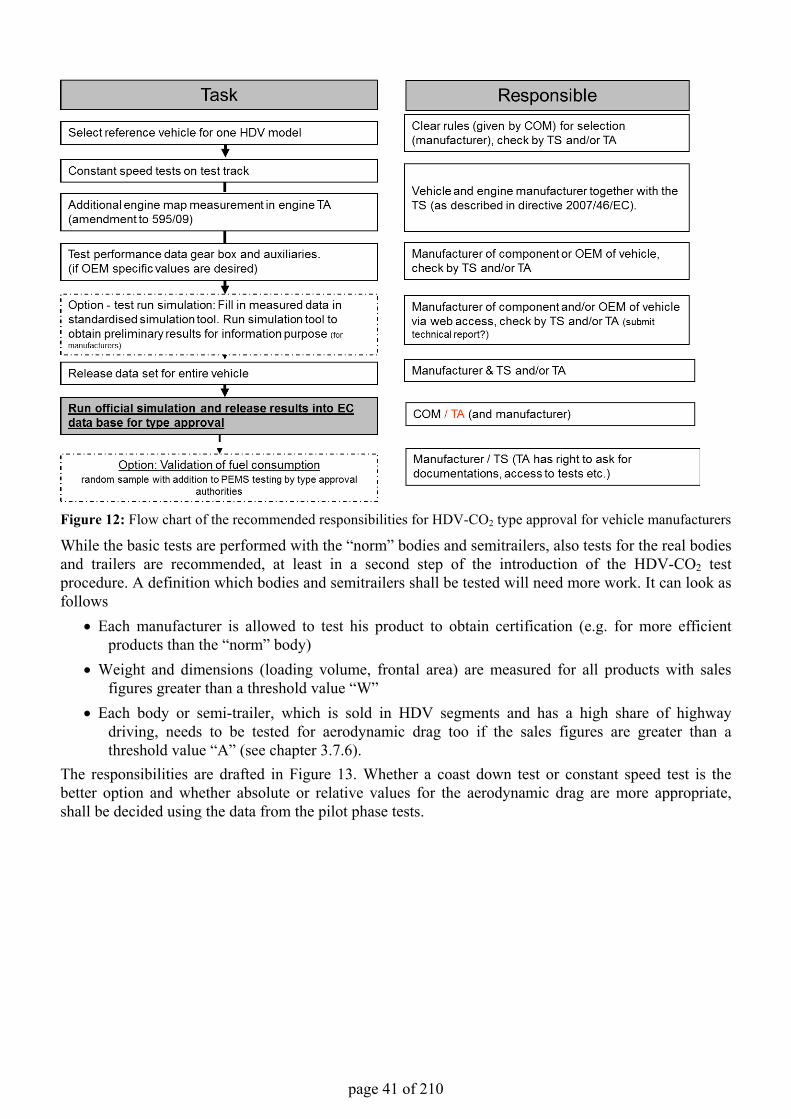
page 41 of 210

Figure 12: Flow chart of the recommended responsibilities for HDV-CO2 type approval for vehicle manufacturers

While the basic tests are performed with the “norm” bodies and semitrailers, also tests for the real bodies and trailers are recommended, at least in a second step of the introduction of the HDV-CO2 test procedure. A definition which bodies and semitrailers shall be tested will need more work. It can look as follows

• Each manufacturer is allowed to test his product to obtain certification (e.g. for more efficient products than the “norm” body)

• Weight and dimensions (loading volume, frontal area) are measured for all products with sales figures greater than a threshold value “W”

• Each body or semi-trailer, which is sold in HDV segments and has a high share of highway driving, needs to be tested for aerodynamic drag too if the sales figures are greater than a threshold value “A” (see chapter 3.7.6).

The responsibilities are drafted in Figure 13. Whether a coast down test or constant speed test is the better option and whether absolute or relative values for the aerodynamic drag are more appropriate, shall be decided using the data from the pilot phase tests.

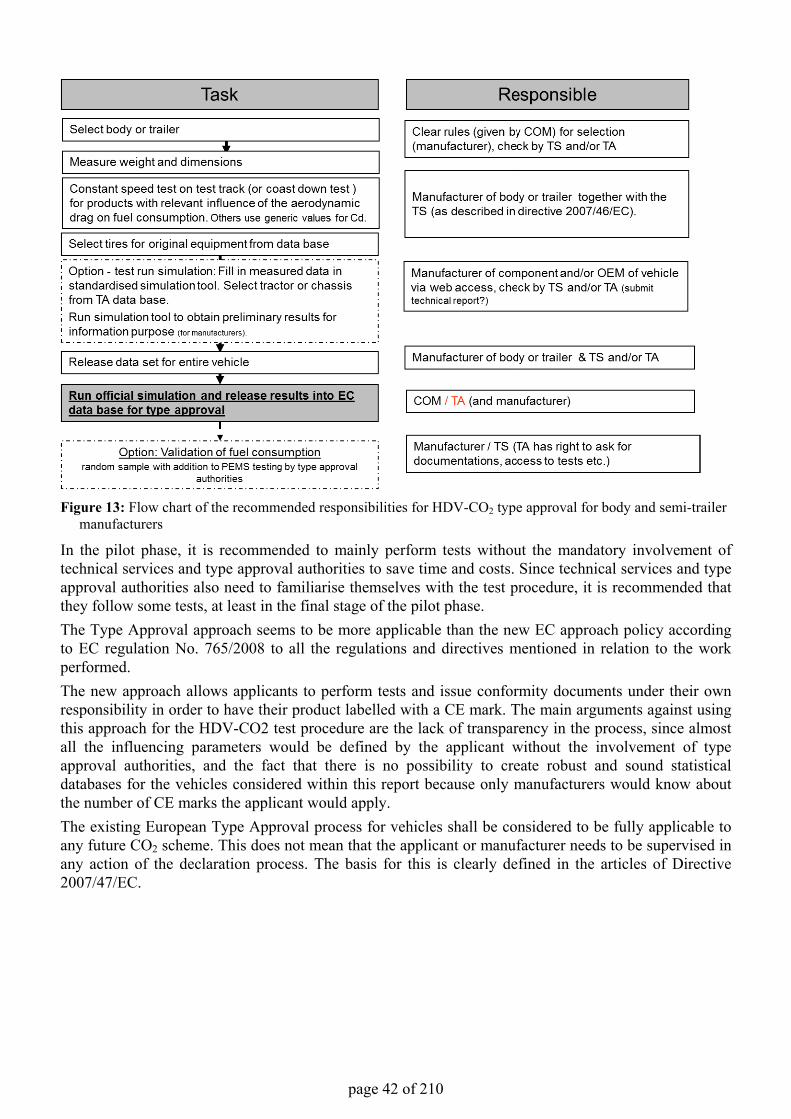
page 42 of 210

Figure 13: Flow chart of the recommended responsibilities for HDV-CO2 type approval for body and semi-trailer manufacturers

In the pilot phase, it is recommended to mainly perform tests without the mandatory involvement of technical services and type approval authorities to save time and costs. Since technical services and type approval authorities also need to familiarise themselves with the test procedure, it is recommended that they follow some tests, at least in the final stage of the pilot phase.The Type Approval approach seems to be more applicable than the new EC approach policy according to EC regulation No. 765/2008 to all the regulations and directives mentioned in relation to the work performed.The new approach allows applicants to perform tests and issue conformity documents under their own responsibility in order to have their product labelled with a CE mark. The main arguments against using this approach for the HDV-CO2 test procedure are the lack of transparency in the process, since almost all the influencing parameters would be defined by the applicant without the involvement of type approval authorities, and the fact that there is no possibility to create robust and sound statistical databases for the vehicles considered within this report because only manufacturers would know about the number of CE marks the applicant would apply.The existing European Type Approval process for vehicles shall be considered to be fully applicable to any future CO2 scheme. This does not mean that the applicant or manufacturer needs to be supervised in any action of the declaration process. The basis for this is clearly defined in the articles of Directive 2007/47/EC.

page 43 of 210

3. Background information to chapter 2 The work performed within LOT 2 is described following the structure of the tender for LOT 2. The content of this chapter gives the background information for chapter 2.

3.1. Review of activities to establish a whole-vehicle testing- and CO2-labelling method This chapter describes the work performed according to Task 1.1 of the tender and gives an overview on existing regulations and related work on European national level as well as for US, Japan and China.

3.1.1. U.S. EPA / NHTSA Final Rule At September 15, 2011 the final rule of “Greenhouse Gas Emissions Standards for Medium- and Heavy-Duty Engines and Vehicles” (6) was published in the U.S. Code of Federal Regulations. The proposed rule was firstly published in November 2010. Most parts for this approach can be found in Part 1037 of the 40 U.S. Code of Federal Regulations (6 pp. 57399-57437). This document includes testing and verification provisions as well as standards for CO2 emissions and the fuel consumption of heavy-duty trucks and vehicles. The CO2-emission standards are set to values in gram/ton-mile and the standard for the Fuel Consumption is expressed in gallon/1000 ton-miles. The CO2 standard is set by EPA (Environmental Protection Agency) and the fuel consumption standard by the NHTSA (National Highway Traffic Safety Administration) as a part of the U.S. Department of Transportation (DOT). Along with the CO2, EPA is also regulating CH4 (Methane) and N2O (Nitrous Oxide) in a set of greenhouse gases (GHG). CO2 credits from an ATB (Averaging, Trading and Banking) program can be used if the CH4 or N2O limit values are “slightly” exceeded. Further on the proposal comprise new engine standards with respect to CO2 in g/bhp-hr and Fuel Consumption in gallon/100 bhp-hr. For that reason the whole approach can be split up in a vehicle and in an engine program. Due to the fact that the U.S. truck market allows the vehicle buyer to choose between different engines (also by means of manufacturer) the approach to differ between the engine and vehicle can be understood. This combined proposal for rulemaking was directed by the U.S. government to EPA and NHTSA in order to develop a joint national program for reducing GHG and fuel consumption in the U.S. Heavy-Duty Sector (13)

3.1.1.1. Applicability

In the U.S. vehicles are usually classified according to the Vehicle Inventory and Use Survey (VIUS) issued by the U.S. Department of Transportation (DOT). In general the U.S. vehicle fleet is scaled down to eight major vehicle classes starting with light-duty / passenger cars without a minimum weight restriction at the lower end (Class 1) and going up to so-called heavy heavy-duty vehicles at the other end (Class 8). Table 6 shows the VIUS vehicle classifications.

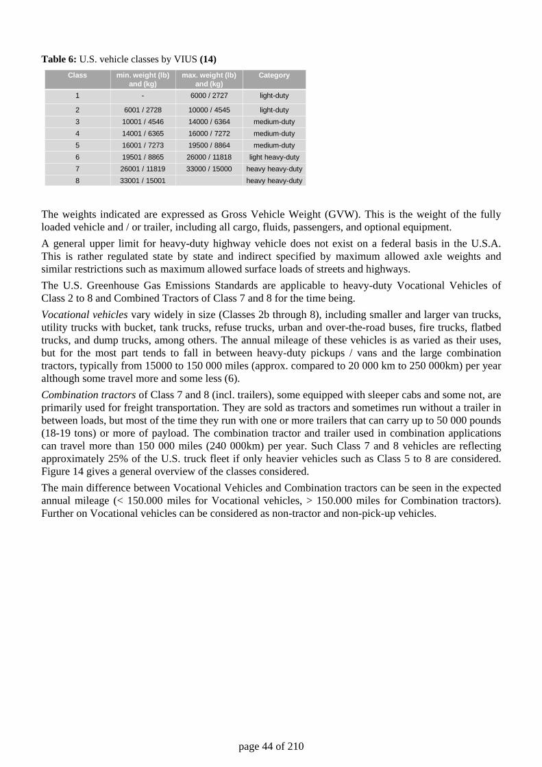
page 44 of 210

Table 6: U.S. vehicle classes by VIUS (14)

The weights indicated are expressed as Gross Vehicle Weight (GVW). This is the weight of the fully loaded vehicle and / or trailer, including all cargo, fluids, passengers, and optional equipment. A general upper limit for heavy-duty highway vehicle does not exist on a federal basis in the U.S.A. This is rather regulated state by state and indirect specified by maximum allowed axle weights and similar restrictions such as maximum allowed surface loads of streets and highways. The U.S. Greenhouse Gas Emissions Standards are applicable to heavy-duty Vocational Vehicles of Class 2 to 8 and Combined Tractors of Class 7 and 8 for the time being. Vocational vehicles vary widely in size (Classes 2b through 8), including smaller and larger van trucks, utility trucks with bucket, tank trucks, refuse trucks, urban and over-the-road buses, fire trucks, flatbed trucks, and dump trucks, among others. The annual mileage of these vehicles is as varied as their uses, but for the most part tends to fall in between heavy-duty pickups / vans and the large combination tractors, typically from 15000 to 150 000 miles (approx. compared to 20 000 km to 250 000km) per year although some travel more and some less (6). Combination tractors of Class 7 and 8 (incl. trailers), some equipped with sleeper cabs and some not, are primarily used for freight transportation. They are sold as tractors and sometimes run without a trailer in between loads, but most of the time they run with one or more trailers that can carry up to 50 000 pounds (18-19 tons) or more of payload. The combination tractor and trailer used in combination applications can travel more than 150 000 miles (240 000km) per year. Such Class 7 and 8 vehicles are reflecting approximately 25% of the U.S. truck fleet if only heavier vehicles such as Class 5 to 8 are considered. Figure 14 gives a general overview of the classes considered. The main difference between Vocational Vehicles and Combination tractors can be seen in the expected annual mileage (< 150.000 miles for Vocational vehicles, > 150.000 miles for Combination tractors). Further on Vocational vehicles can be considered as non-tractor and non-pick-up vehicles.

Class min. weight (lb)and (kg)

max. weight (lb)and (kg)

Category

1 - 6000 / 2727 light-duty

2 6001 / 2728 10000 / 4545 light-duty3 10001 / 4546 14000 / 6364 medium-duty4 14001 / 6365 16000 / 7272 medium-duty5 16001 / 7273 19500 / 8864 medium-duty6 19501 / 8865 26000 / 11818 light heavy-duty7 26001 / 11819 33000 / 15000 heavy heavy-duty8 33001 / 15001 heavy heavy-duty

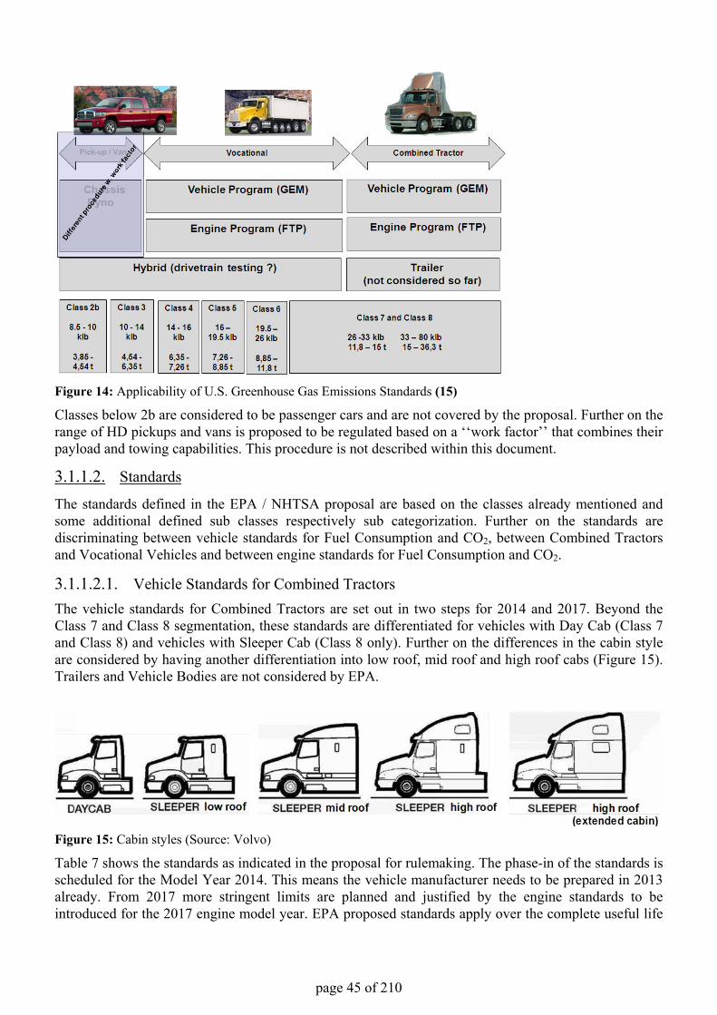
page 45 of 210

Figure 14: Applicability of U.S. Greenhouse Gas Emissions Standards (15)

Classes below 2b are considered to be passenger cars and are not covered by the proposal. Further on the range of HD pickups and vans is proposed to be regulated based on a ‘‘work factor’’ that combines their payload and towing capabilities. This procedure is not described within this document.

3.1.1.2. Standards

The standards defined in the EPA / NHTSA proposal are based on the classes already mentioned and some additional defined sub classes respectively sub categorization. Further on the standards are discriminating between vehicle standards for Fuel Consumption and CO2, between Combined Tractors and Vocational Vehicles and between engine standards for Fuel Consumption and CO2.

3.1.1.2.1. Vehicle Standards for Combined TractorsThe vehicle standards for Combined Tractors are set out in two steps for 2014 and 2017. Beyond the Class 7 and Class 8 segmentation, these standards are differentiated for vehicles with Day Cab (Class 7 and Class 8) and vehicles with Sleeper Cab (Class 8 only). Further on the differences in the cabin style are considered by having another differentiation into low roof, mid roof and high roof cabs (Figure 15). Trailers and Vehicle Bodies are not considered by EPA.

Figure 15: Cabin styles (Source: Volvo)

Table 7 shows the standards as indicated in the proposal for rulemaking. The phase-in of the standards is scheduled for the Model Year 2014. This means the vehicle manufacturer needs to be prepared in 2013 already. From 2017 more stringent limits are planned and justified by the engine standards to be introduced for the 2017 engine model year. EPA proposed standards apply over the complete useful life

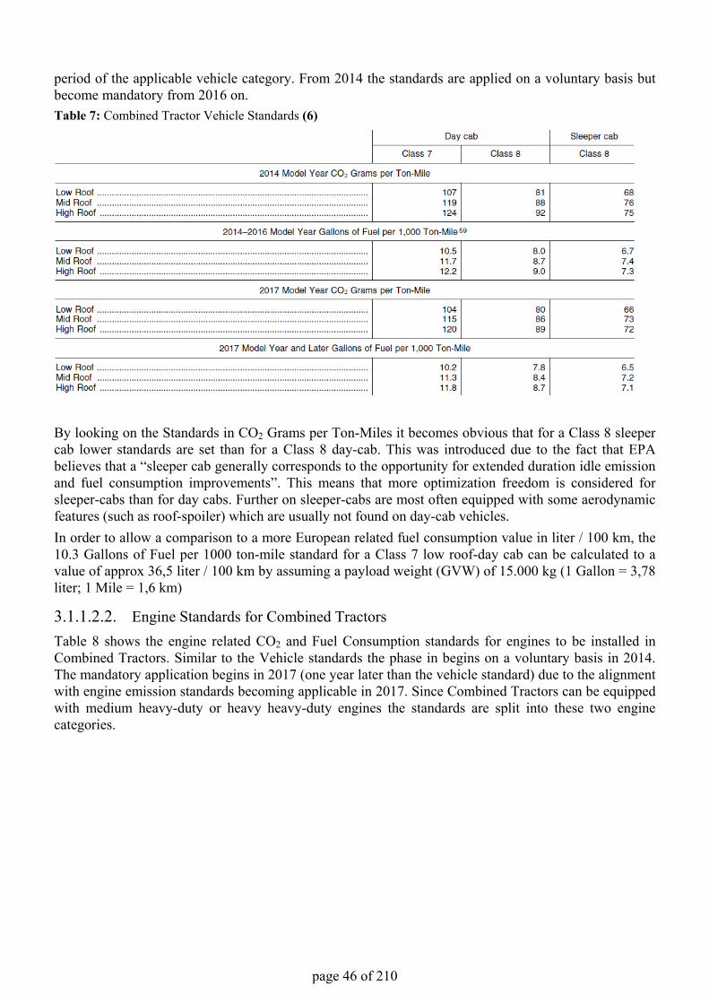
page 46 of 210

period of the applicable vehicle category. From 2014 the standards are applied on a voluntary basis but become mandatory from 2016 on.Table 7: Combined Tractor Vehicle Standards (6)

By looking on the Standards in CO2 Grams per Ton-Miles it becomes obvious that for a Class 8 sleeper cab lower standards are set than for a Class 8 day-cab. This was introduced due to the fact that EPA believes that a “sleeper cab generally corresponds to the opportunity for extended duration idle emission and fuel consumption improvements”. This means that more optimization freedom is considered for sleeper-cabs than for day cabs. Further on sleeper-cabs are most often equipped with some aerodynamic features (such as roof-spoiler) which are usually not found on day-cab vehicles.In order to allow a comparison to a more European related fuel consumption value in liter / 100 km, the 10.3 Gallons of Fuel per 1000 ton-mile standard for a Class 7 low roof-day cab can be calculated to a value of approx 36,5 liter / 100 km by assuming a payload weight (GVW) of 15.000 kg (1 Gallon = 3,78 liter; 1 Mile = 1,6 km)

3.1.1.2.2. Engine Standards for Combined TractorsTable 8 shows the engine related CO2 and Fuel Consumption standards for engines to be installed in Combined Tractors. Similar to the Vehicle standards the phase in begins on a voluntary basis in 2014. The mandatory application begins in 2017 (one year later than the vehicle standard) due to the alignment with engine emission standards becoming applicable in 2017. Since Combined Tractors can be equipped with medium heavy-duty or heavy heavy-duty engines the standards are split into these two engine categories.

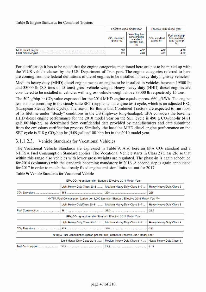
page 47 of 210

Table 8: Engine Standards for Combined Tractors

For clarification it has to be noted that the engine categories mentioned here are not to be mixed up with the VIUS vehicle classes by the U.S. Department of Transport. The engine categories referred to here are coming from the federal definitions of diesel engines to be installed in heavy-duty highway vehicles.Medium heavy-duty (MHD) diesel engine means an engine to be installed in vehicles between 19500 lb and 33000 lb (8,8 tons to 15 tons) gross vehicle weight. Heavy heavy-duty (HHD) diesel engines are considered to be installed in vehicles with a gross vehicle weight above 33000 lb respectively 15 tons.The 502 g/bhp-hr CO2 value expressed for the 2014 MHD engine equals approx. 660 g/kWh. The engine test is done according to the steady state SET (supplemental engine test) cycle, which is an adjusted ESC (European Steady State Cycle). The reason for this is that Combined Tractors are expected to run most of its lifetime under “steady” conditions in the US (highway long-haulage). EPA considers the baseline HHD diesel engine performance for the 2010 model year on the SET cycle is 490 g CO2/bhp-hr (4.81 gal/100 bhp-hr), as determined from confidential data provided by manufacturers and data submitted from the emissions certification process. Similarly, the baseline MHD diesel engine performance on the SET cycle is 518 g CO2/bhp-hr (5.09 gallon/100-bhp-hr) in the 2010 model year.

3.1.1.2.3. Vehicle Standards for Vocational VehiclesThe Vocational Vehicle Standards are expressed in Table 9. Also here an EPA CO2 standard and a NHTSA Fuel Consumption Standard applies. The Vocational Vehicle starts in Class 2 (Class 2b) so that within this range also vehicles with lower gross weights are regulated. The phase-in is again scheduled for 2014 (voluntary) with the standards becoming mandatory in 2016. A second step is again announced for 2017 in order to match the already fixed engine emission limits set-out for 2017.Table 9: Vehicle Standards for Vocational Vehicle

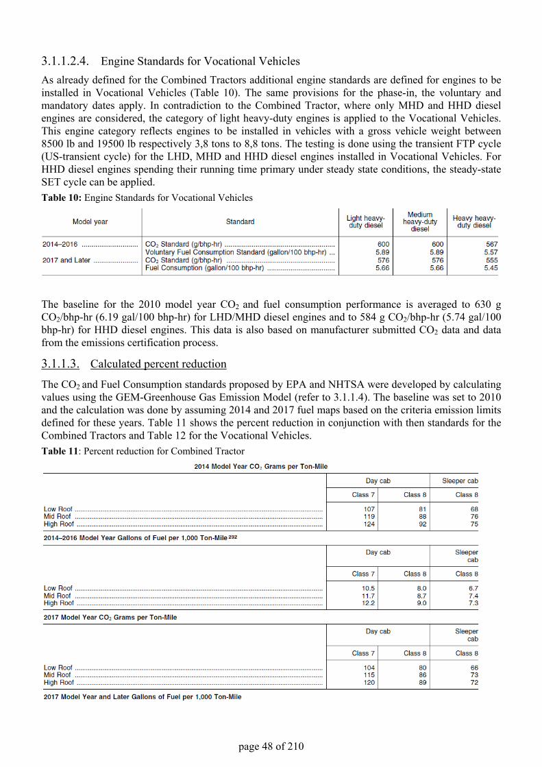
page 48 of 210

3.1.1.2.4. Engine Standards for Vocational VehiclesAs already defined for the Combined Tractors additional engine standards are defined for engines to be installed in Vocational Vehicles (Table 10). The same provisions for the phase-in, the voluntary and mandatory dates apply. In contradiction to the Combined Tractor, where only MHD and HHD diesel engines are considered, the category of light heavy-duty engines is applied to the Vocational Vehicles. This engine category reflects engines to be installed in vehicles with a gross vehicle weight between 8500 lb and 19500 lb respectively 3,8 tons to 8,8 tons. The testing is done using the transient FTP cycle (US-transient cycle) for the LHD, MHD and HHD diesel engines installed in Vocational Vehicles. For HHD diesel engines spending their running time primary under steady state conditions, the steady-state SET cycle can be applied.Table 10: Engine Standards for Vocational Vehicles

The baseline for the 2010 model year CO2 and fuel consumption performance is averaged to 630 g CO2/bhp-hr (6.19 gal/100 bhp-hr) for LHD/MHD diesel engines and to 584 g CO2/bhp-hr (5.74 gal/100 bhp-hr) for HHD diesel engines. This data is also based on manufacturer submitted CO2 data and data from the emissions certification process.

3.1.1.3. Calculated percent reduction

The CO2 and Fuel Consumption standards proposed by EPA and NHTSA were developed by calculating values using the GEM-Greenhouse Gas Emission Model (refer to 3.1.1.4). The baseline was set to 2010 and the calculation was done by assuming 2014 and 2017 fuel maps based on the criteria emission limits defined for these years. Table 11 shows the percent reduction in conjunction with then standards for the Combined Tractors and Table 12 for the Vocational Vehicles.Table 11: Percent reduction for Combined Tractor

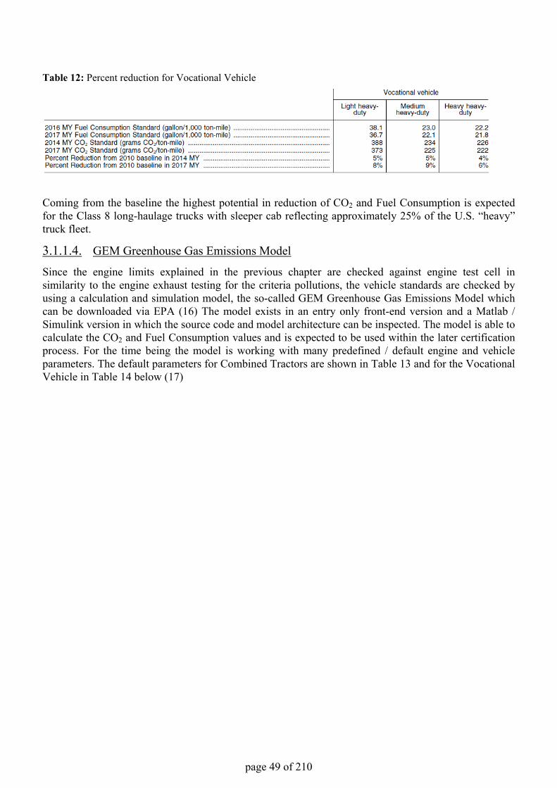
page 49 of 210

Table 12: Percent reduction for Vocational Vehicle

Coming from the baseline the highest potential in reduction of CO2 and Fuel Consumption is expected for the Class 8 long-haulage trucks with sleeper cab reflecting approximately 25% of the U.S. “heavy” truck fleet.

3.1.1.4. GEM Greenhouse Gas Emissions Model

Since the engine limits explained in the previous chapter are checked against engine test cell in similarity to the engine exhaust testing for the criteria pollutions, the vehicle standards are checked by using a calculation and simulation model, the so-called GEM Greenhouse Gas Emissions Model which can be downloaded via EPA (16) The model exists in an entry only front-end version and a Matlab / Simulink version in which the source code and model architecture can be inspected. The model is able to calculate the CO2 and Fuel Consumption values and is expected to be used within the later certification process. For the time being the model is working with many predefined / default engine and vehicle parameters. The default parameters for Combined Tractors are shown in Table 13 and for the Vocational Vehicle in Table 14 below (17)

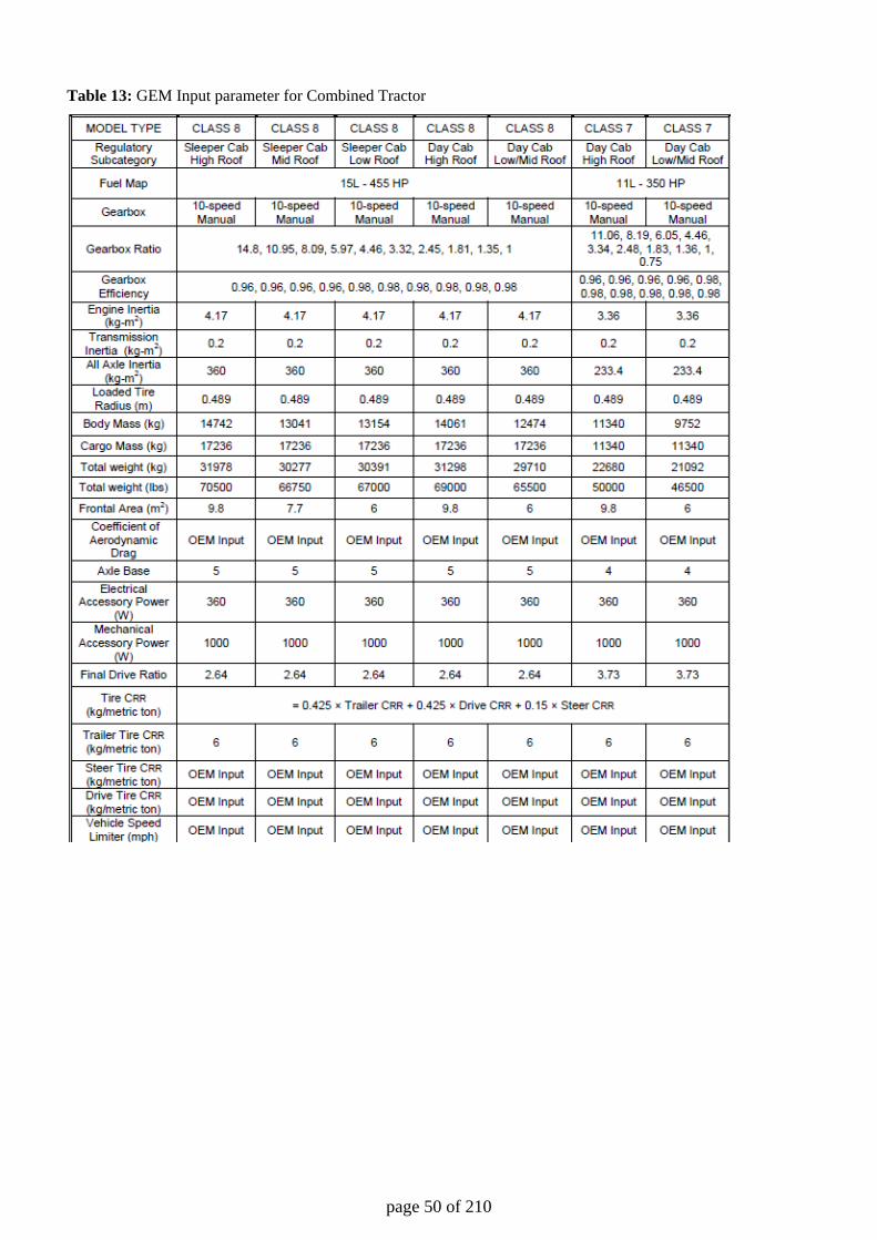
page 50 of 210

Table 13: GEM Input parameter for Combined Tractor

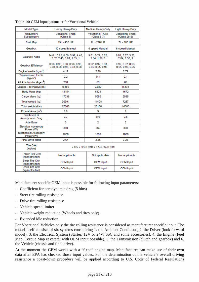
page 51 of 210

Table 14: GEM Input parameter for Vocational Vehicle

Manufacturer specific GEM input is possible for following input parameters: - Coefficient for aerodynamic drag (5 bins) - Steer tire rolling resistance - Drive tire rolling resistance - Vehicle speed limiter - Vehicle weight reduction (Wheels and tires only) - Extended idle reduction. For Vocational Vehicles only the tire rolling resistance is considered as manufacturer specific input. The model itself consists of six systems considering 1. the Ambient Conditions, 2. the Driver (look forward model), 3. the Electrical System (Starter, 12V or 24V, SoC and some accessories), 4. the Engine (Fuel Map, Torque Map et cetera; with OEM input possible), 5. the Transmission (clutch and gearbox) and 6. the Vehicle (chassis and final drive). At the moment the GEM works with a “fixed” engine map. Manufacturer can make use of their own data after EPA has checked those input values. For the determination of the vehicle’s overall driving resistance a coast-down procedure will be applied according to U.S. Code of Federal Regulations

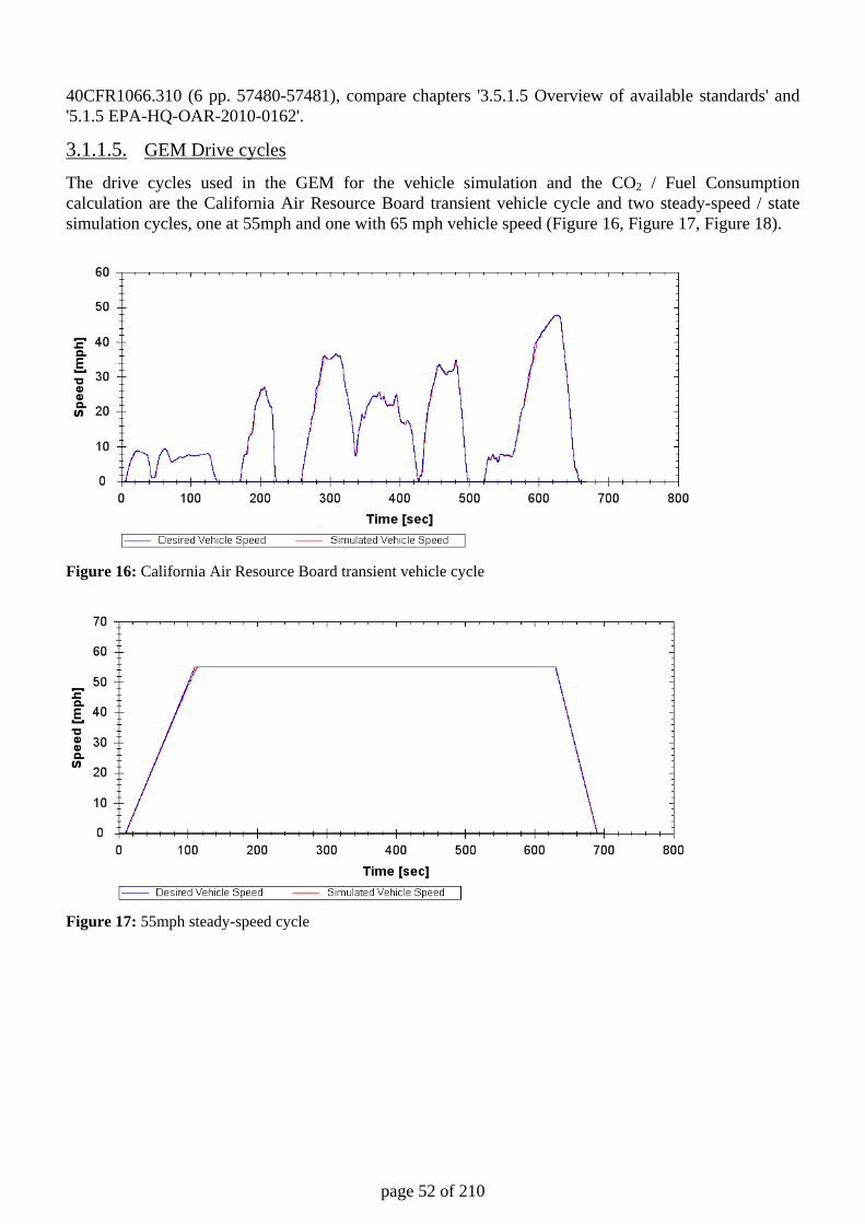
page 52 of 210

40CFR1066.310 (6 pp. 57480-57481), compare chapters '3.5.1.5 Overview of available standards' and '5.1.5 EPA-HQ-OAR-2010-0162'.

3.1.1.5. GEM Drive cycles

The drive cycles used in the GEM for the vehicle simulation and the CO2 / Fuel Consumption calculation are the California Air Resource Board transient vehicle cycle and two steady-speed / state simulation cycles, one at 55mph and one with 65 mph vehicle speed (Figure 16, Figure 17, Figure 18).

Figure 16: California Air Resource Board transient vehicle cycle

Figure 17: 55mph steady-speed cycle

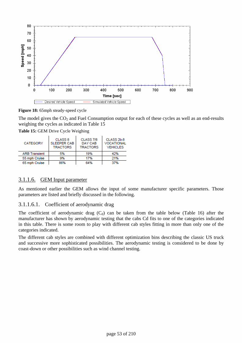
page 53 of 210

Figure 18: 65mph steady-speed cycle

The model gives the CO2 and Fuel Consumption output for each of these cycles as well as an end-results weighing the cycles as indicated in Table 15 Table 15: GEM Drive Cycle Weighing

3.1.1.6. GEM Input parameter

As mentioned earlier the GEM allows the input of some manufacturer specific parameters. Those parameters are listed and briefly discussed in the following.

3.1.1.6.1. Coefficient of aerodynamic drag The coefficient of aerodynamic drag (Cd) can be taken from the table below (Table 16) after the manufacturer has shown by aerodynamic testing that the cabs Cd fits to one of the categories indicated in this table. There is some room to play with different cab styles fitting in more than only one of the categories indicated. The different cab styles are combined with different optimization bins describing the classic US truck and successive more sophisticated possibilities. The aerodynamic testing is considered to be done by coast-down or other possibilities such as wind channel testing.

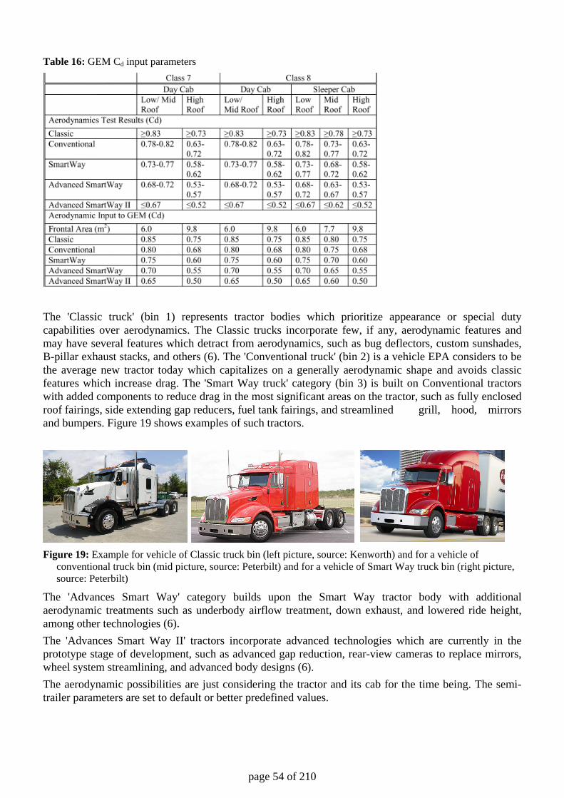
page 54 of 210

Table 16: GEM Cd input parameters

The 'Classic truck' (bin 1) represents tractor bodies which prioritize appearance or special duty capabilities over aerodynamics. The Classic trucks incorporate few, if any, aerodynamic features and may have several features which detract from aerodynamics, such as bug deflectors, custom sunshades, B-pillar exhaust stacks, and others (6). The 'Conventional truck' (bin 2) is a vehicle EPA considers to be the average new tractor today which capitalizes on a generally aerodynamic shape and avoids classic features which increase drag. The 'Smart Way truck' category (bin 3) is built on Conventional tractors with added components to reduce drag in the most significant areas on the tractor, such as fully enclosed roof fairings, side extending gap reducers, fuel tank fairings, and streamlined grill, hood, mirrors and bumpers. Figure 19 shows examples of such tractors.

Figure 19: Example for vehicle of Classic truck bin (left picture, source: Kenworth) and for a vehicle of

conventional truck bin (mid picture, source: Peterbilt) and for a vehicle of Smart Way truck bin (right picture, source: Peterbilt)

The 'Advances Smart Way' category builds upon the Smart Way tractor body with additional aerodynamic treatments such as underbody airflow treatment, down exhaust, and lowered ride height, among other technologies (6). The 'Advances Smart Way II' tractors incorporate advanced technologies which are currently in the prototype stage of development, such as advanced gap reduction, rear-view cameras to replace mirrors, wheel system streamlining, and advanced body designs (6). The aerodynamic possibilities are just considering the tractor and its cab for the time being. The semi-trailer parameters are set to default or better predefined values.

page 55 of 210

3.1.1.6.2. Tire rolling resistance The tractor’s tire rolling resistance input to the GEM is determined by either the tire manufacturer or tractor manufacturer using the test method adopted by the International Organization for Standardization, ISO 28580:2009. The results would be expressed as a rolling resistance coefficient and measured as kilogram per metric ton (kg/metric ton) (6).The semi-trailers tire resistance is set to a predefined value since EPA is not considering trailer within the GEM for the time being. All together the possibilities to design tires in such a way that reasonable changes in the rolling resistance can be achieved seems to be somehow limited since the tires need to be designed in a defined way by means of durability, safety, et cetera. The European Regulation No. 1222/2009 on the labelling of tires with respect to fuel efficiency also makes use of the provisions of ISO 28580. For that reason the procedures applied in the U.S. and Europe can be considered being relatively similar.

3.1.1.6.3. Weight reduction assessment EPA and NHTSA are proposing to specify the baseline vehicle weight for each regulatory category (including the tires and wheels), but allow manufacturers to quantify weight reductions based on the wheel material selection and single wide versus dual tires. The agencies assume the baseline wheel and tire configuration contains dual tires with steel wheels because these represent the vast majority of new vehicle configurations today (6). Vehicle weight reduction inputs for components other than wheels are also specified and possible. Those weight reductions can be applied by making use of the vehicles with innovative technology provisions and can be considered as overall vehicle weight reduction in the GEM.

3.1.1.6.4. Extended Idle Reduction Technology The agencies are proposing to include extended idle reduction technology as an input to the GEM for Class 8 sleeper cabs. The manufacturer would input the value based on the idle reduction technology installed on the truck. EPA is expecting high potential in idle reduction because it is usual for long-haulage trucks in the US to keep the engine running almost 24 hours a day (Cab air-conditioning, cooling or heating, power supply on cab, et cetera).

3.1.1.6.5. Vehicle speed limiters The GEM will not provide a fuel consumption reduction for a limiter that can be overridden. In order to obtain a benefit for the program, the manufacturer must preset the limiter in such a way that the setting will not be capable of being easily overridden by the fleet or the owner (6).

3.1.1.7. Program Flexibility

As usual EPA makes use of an ABT- (Averaging, Banking and Trading) Program in order to ease the introduction of new requirements and criteria. The ABT is limited to the given categories including the sub categories. Any transfer between the categories is not foreseen and thus limiting the freedom of using credits. Further on a CO2 credit can be used for balancing out a CH4 and / or N2O off-set related to the limit values of these exhaust components. The use of the ABT provisions is allowed for up to five years.

3.1.1.8. Summary

The EPA and NHTSA final rule is a combination of engine and vehicle standards and for that reason also a combination of engine test cell testing and vehicle simulation by a model (GEM). The reason for this is surely based on the U.S. truck market where a vehicle (on order of the customer) can be equipped with an engine produced by another manufacturer than the vehicle.

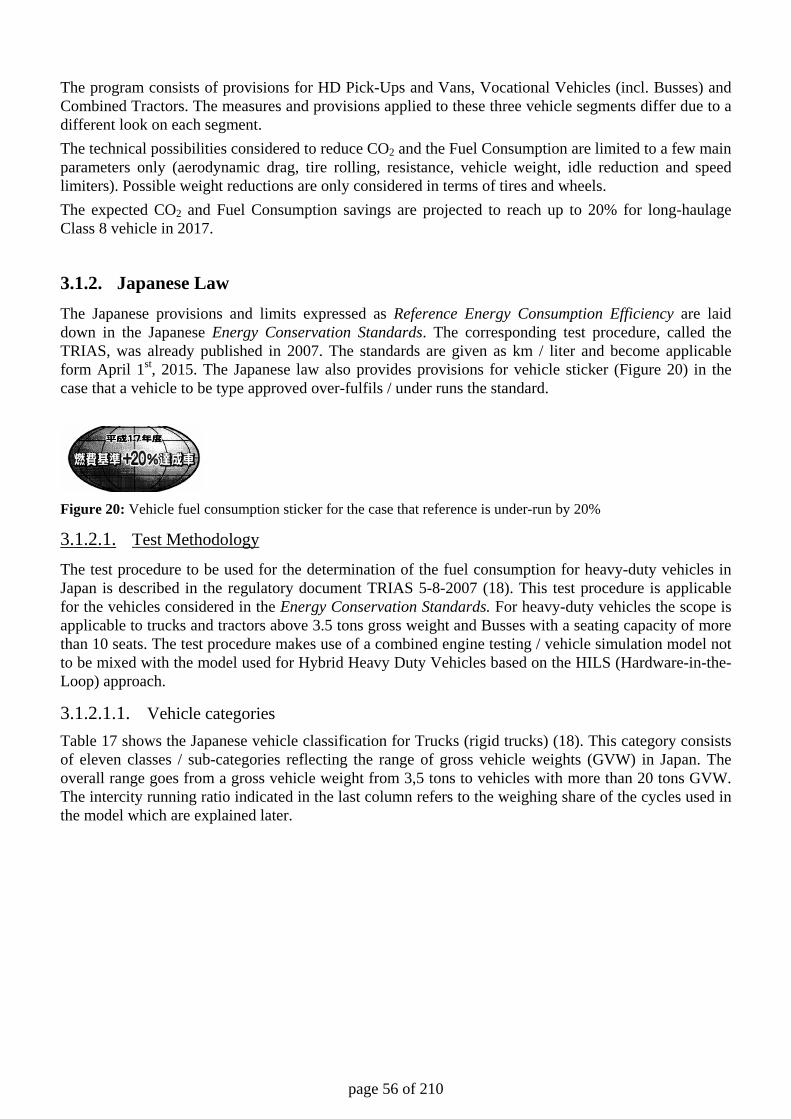
page 56 of 210

The program consists of provisions for HD Pick-Ups and Vans, Vocational Vehicles (incl. Busses) and Combined Tractors. The measures and provisions applied to these three vehicle segments differ due to a different look on each segment. The technical possibilities considered to reduce CO2 and the Fuel Consumption are limited to a few main parameters only (aerodynamic drag, tire rolling, resistance, vehicle weight, idle reduction and speed limiters). Possible weight reductions are only considered in terms of tires and wheels. The expected CO2 and Fuel Consumption savings are projected to reach up to 20% for long-haulage Class 8 vehicle in 2017.

3.1.2. Japanese Law The Japanese provisions and limits expressed as Reference Energy Consumption Efficiency are laid down in the Japanese Energy Conservation Standards. The corresponding test procedure, called the TRIAS, was already published in 2007. The standards are given as km / liter and become applicable form April 1st, 2015. The Japanese law also provides provisions for vehicle sticker (Figure 20) in the case that a vehicle to be type approved over-fulfils / under runs the standard.

Figure 20: Vehicle fuel consumption sticker for the case that reference is under-run by 20%

3.1.2.1. Test Methodology

The test procedure to be used for the determination of the fuel consumption for heavy-duty vehicles in Japan is described in the regulatory document TRIAS 5-8-2007 (18). This test procedure is applicable for the vehicles considered in the Energy Conservation Standards. For heavy-duty vehicles the scope is applicable to trucks and tractors above 3.5 tons gross weight and Busses with a seating capacity of more than 10 seats. The test procedure makes use of a combined engine testing / vehicle simulation model not to be mixed with the model used for Hybrid Heavy Duty Vehicles based on the HILS (Hardware-in-the-Loop) approach.

3.1.2.1.1. Vehicle categories Table 17 shows the Japanese vehicle classification for Trucks (rigid trucks) (18). This category consists of eleven classes / sub-categories reflecting the range of gross vehicle weights (GVW) in Japan. The overall range goes from a gross vehicle weight from 3,5 tons to vehicles with more than 20 tons GVW. The intercity running ratio indicated in the last column refers to the weighing share of the cycles used in the model which are explained later.

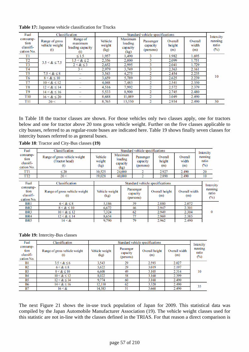
page 57 of 210

Table 17: Japanese vehicle classification for Trucks

In Table 18 the tractor classes are shown. For those vehicles only two classes apply, one for tractors below and one for tractor above 20 tons gross vehicle weight. Further on the five classes applicable to city busses, referred to as regular-route buses are indicated here. Table 19 shows finally seven classes for intercity busses referred to as general buses. Table 18: Tractor and City-Bus classes (19)

Table 19: Intercity-Bus classes

The next Figure 21 shows the in-use truck population of Japan for 2009. This statistical data was compiled by the Japan Automobile Manufacturer Association (19). The vehicle weight classes used for this statistic are not in-line with the classes defined in the TRIAS. For that reason a direct comparison is

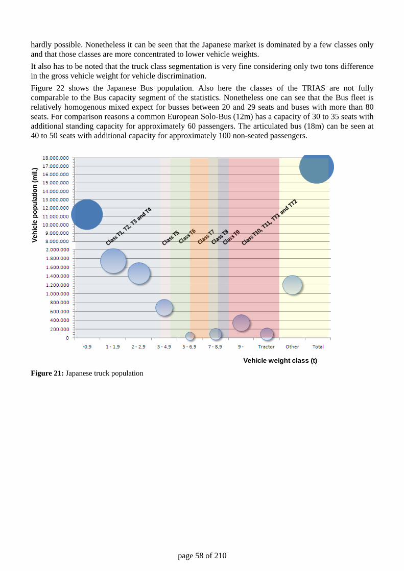
page 58 of 210

hardly possible. Nonetheless it can be seen that the Japanese market is dominated by a few classes only and that those classes are more concentrated to lower vehicle weights. It also has to be noted that the truck class segmentation is very fine considering only two tons difference in the gross vehicle weight for vehicle discrimination. Figure 22 shows the Japanese Bus population. Also here the classes of the TRIAS are not fully comparable to the Bus capacity segment of the statistics. Nonetheless one can see that the Bus fleet is relatively homogenous mixed expect for busses between 20 and 29 seats and buses with more than 80 seats. For comparison reasons a common European Solo-Bus (12m) has a capacity of 30 to 35 seats with additional standing capacity for approximately 60 passengers. The articulated bus (18m) can be seen at 40 to 50 seats with additional capacity for approximately 100 non-seated passengers.

Figure 21: Japanese truck population

Vehicle weight class (t)

Vehi

cle

popu

latio

n(m

il.)

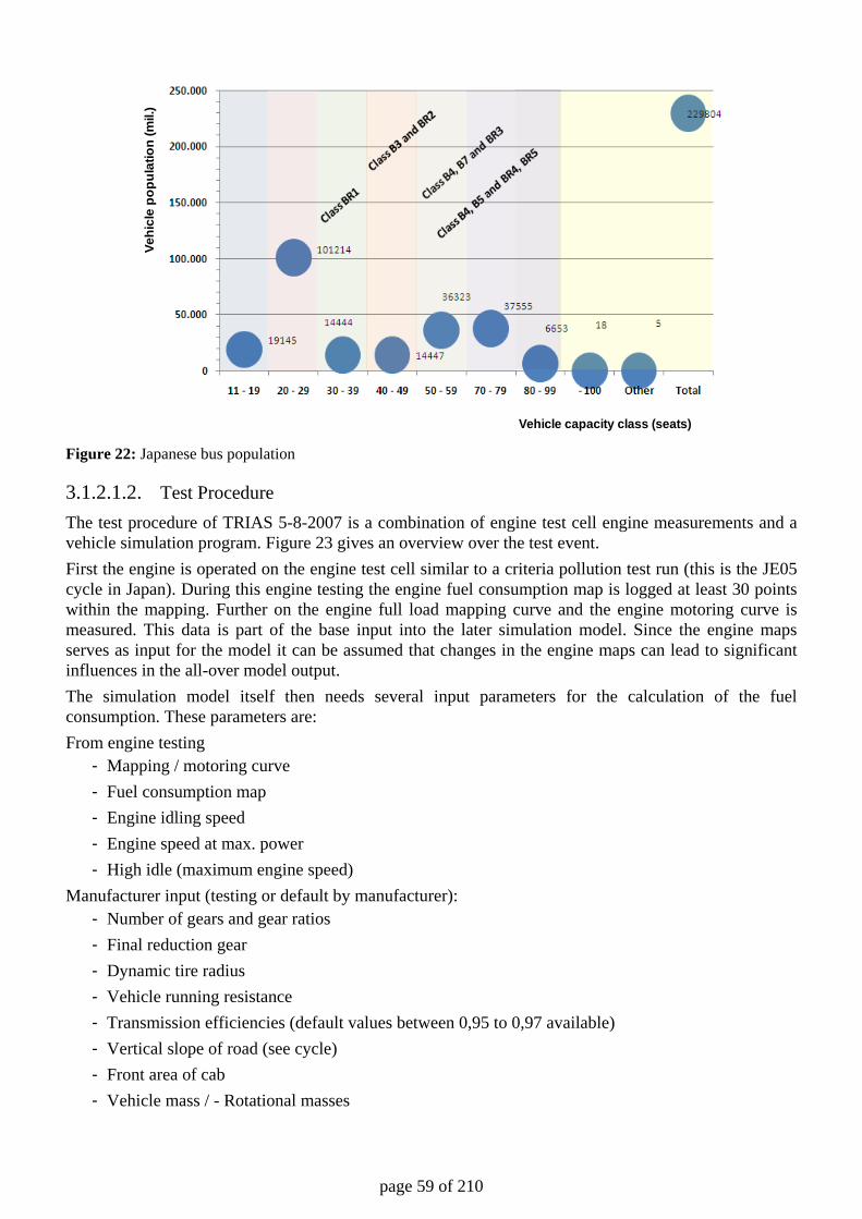
page 59 of 210

Figure 22: Japanese bus population

3.1.2.1.2. Test Procedure The test procedure of TRIAS 5-8-2007 is a combination of engine test cell engine measurements and a vehicle simulation program. Figure 23 gives an overview over the test event. First the engine is operated on the engine test cell similar to a criteria pollution test run (this is the JE05 cycle in Japan). During this engine testing the engine fuel consumption map is logged at least 30 points within the mapping. Further on the engine full load mapping curve and the engine motoring curve is measured. This data is part of the base input into the later simulation model. Since the engine maps serves as input for the model it can be assumed that changes in the engine maps can lead to significant influences in the all-over model output. The simulation model itself then needs several input parameters for the calculation of the fuel consumption. These parameters are: From engine testing

- Mapping / motoring curve - Fuel consumption map - Engine idling speed - Engine speed at max. power - High idle (maximum engine speed)

Manufacturer input (testing or default by manufacturer): - Number of gears and gear ratios - Final reduction gear - Dynamic tire radius - Vehicle running resistance - Transmission efficiencies (default values between 0,95 to 0,97 available) - Vertical slope of road (see cycle) - Front area of cab - Vehicle mass / - Rotational masses

Vehi

cle

popu

latio

n(m

il.)

Vehicle capacity class (seats)

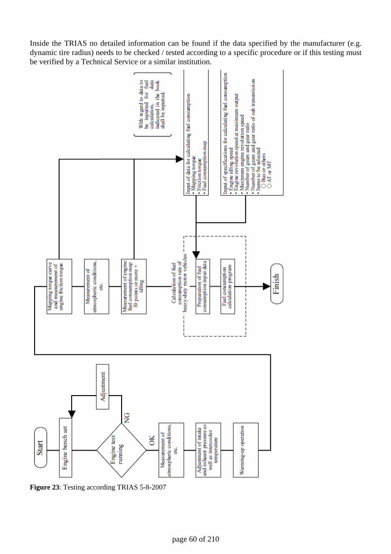
page 60 of 210

Inside the TRIAS no detailed information can be found if the data specified by the manufacturer (e.g. dynamic tire radius) needs to be checked / tested according to a specific procedure or if this testing must be verified by a Technical Service or a similar institution.

Figure 23: Testing according TRIAS 5-8-2007

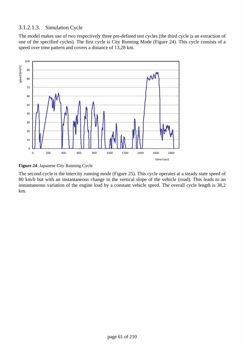
page 61 of 210

3.1.2.1.3. Simulation Cycle The model makes use of two respectively three pre-defined test cycles (the third cycle is an extraction of one of the specified cycles). The first cycle is City Running Mode (Figure 24). This cycle consists of a speed over time pattern and covers a distance of 13,28 km.

Figure 24: Japanese City Running Cycle

The second cycle is the intercity running mode (Figure 25). This cycle operates at a steady state speed of 80 km/h but with an instantaneous change in the vertical slope of the vehicle (road). This leads to an instantaneous variation of the engine load by a constant vehicle speed. The overall cycle length is 38,2 km.

0

10

20

30

40

50

60

70

80

90

100

0 200 400 600 800 1000 1200 1400 1600 1800

time (sec)

spee

d (km

/h)

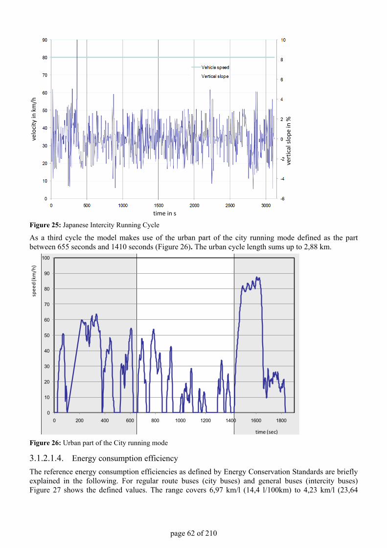
page 62 of 210

Figure 25: Japanese Intercity Running Cycle

As a third cycle the model makes use of the urban part of the city running mode defined as the part between 655 seconds and 1410 seconds (Figure 26). The urban cycle length sums up to 2,88 km.

Figure 26: Urban part of the City running mode

3.1.2.1.4. Energy consumption efficiencyThe reference energy consumption efficiencies as defined by Energy Conservation Standards are briefly explained in the following. For regular route buses (city buses) and general buses (intercity buses) Figure 27 shows the defined values. The range covers 6,97 km/l (14,4 l/100km) to 4,23 km/l (23,64

time in s

velo

city

in k

m/h

vert

ical

slope

in %

0

10

20

30

40

50

60

70

80

90

100

0 200 400 600 800 1000 1200 1400 1600 1800

time (sec)

spee

d (k

m/h

)

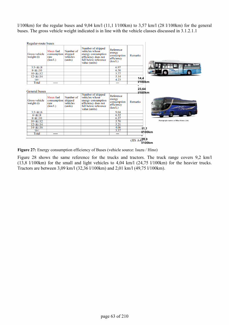
page 63 of 210

l/100km) for the regular buses and 9,04 km/l (11,1 l/100km) to 3,57 km/l (28 l/100km) for the general buses. The gross vehicle weight indicated is in line with the vehicle classes discussed in 3.1.2.1.1

Figure 27: Energy consumption efficiency of Buses (vehicle source: Isuzu / Hino)

Figure 28 shows the same reference for the trucks and tractors. The truck range covers 9,2 km/l (13,8 l/100km) for the small and light vehicles to 4,04 km/l (24,75 l/100km) for the heavier trucks.Tractors are between 3,09 km/l (32,36 l/100km) and 2,01 km/l (49,75 l/100km).

14,4 l/100km-23,64 l/100km

11,1 l/100km-28,0 l/100km

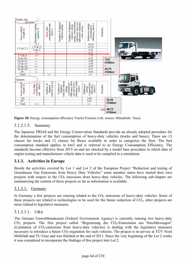
page 64 of 210

Figure 28: Energy consumption efficiency Trucks/Tractors (veh. source: Mitsubishi / Isuzu

3.1.2.1.5. Summary The Japanese TRIAS and the Energy Conservation Standards provide an already adopted procedure for the determination of the fuel consumption of heavy-duty vehicles (trucks and buses). There are 13 classes for trucks and 12 classes for Buses available in order to categorize the fleet. The fuel consumption standard applies in km/l and is referred to as Energy Consumption Efficiency. The standards become effective from 2015 on and are checked by a model base procedure in which data of engine testing and manufacturer vehicle data is used to be compiled in a simulation.

3.1.3. Activities in EuropeBeside the activities covered by Lot 1 and Lot 2 of the European Project “Reduction and testing of Greenhouse Gas Emissions from Heavy Duty Vehicles” some member states have started their own projects with respect to the CO2 emissions from heavy-duty vehicles. The following sub-chapter are summarizing the content of these projects as far as information is available.

3.1.3.1. Germany

In Germany a few projects are running related to the CO2 emissions of heavy-duty vehicles. Some of these projects are related to technologies to be used for the future reduction of CO2, other projects are more related to legislative measures.

3.1.3.1.1. UBA The German Umweltbundesamt (Federal Environment Agency) is currently running two heavy-duty CO2 projects. The first project called “Begrenzung der CO2-Emissionen aus Nutzfahrzeugen” (Limitation of CO2-emissions from heavy-duty vehicles) is dealing with the legislative measures necessary to introduce a future CO2-regulation for such vehicles. The project is in-service at TÜV Nord Mobilität and TU Graz and was finished at the end of 2011. Since the very beginning of the Lot 2 works it was considered to incorporate the findings of this project into Lot 2.

13,8l/100km-24,75 l/100km

32,36l/100km-49,75 l/100km

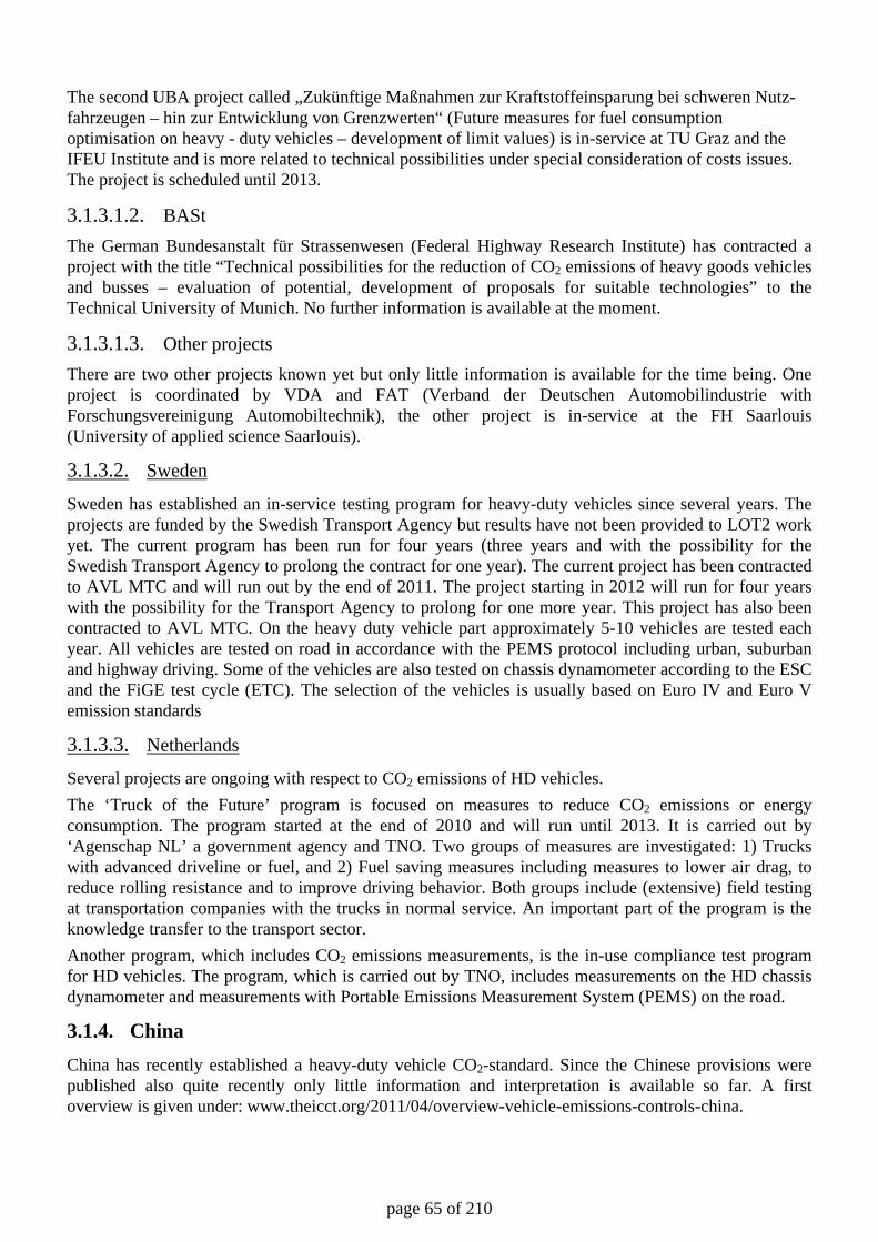
page 65 of 210

The second UBA project called „Zukünftige Maßnahmen zur Kraftstoffeinsparung bei schweren Nutz-fahrzeugen – hin zur Entwicklung von Grenzwerten“ (Future measures for fuel consumption optimisation on heavy - duty vehicles – development of limit values) is in-service at TU Graz and the IFEU Institute and is more related to technical possibilities under special consideration of costs issues. The project is scheduled until 2013.

3.1.3.1.2. BASt The German Bundesanstalt für Strassenwesen (Federal Highway Research Institute) has contracted a project with the title “Technical possibilities for the reduction of CO2 emissions of heavy goods vehicles and busses – evaluation of potential, development of proposals for suitable technologies” to the Technical University of Munich. No further information is available at the moment.

3.1.3.1.3. Other projects There are two other projects known yet but only little information is available for the time being. One project is coordinated by VDA and FAT (Verband der Deutschen Automobilindustrie with Forschungsvereinigung Automobiltechnik), the other project is in-service at the FH Saarlouis (University of applied science Saarlouis).

3.1.3.2. Sweden

Sweden has established an in-service testing program for heavy-duty vehicles since several years. The projects are funded by the Swedish Transport Agency but results have not been provided to LOT2 work yet. The current program has been run for four years (three years and with the possibility for the Swedish Transport Agency to prolong the contract for one year). The current project has been contracted to AVL MTC and will run out by the end of 2011. The project starting in 2012 will run for four years with the possibility for the Transport Agency to prolong for one more year. This project has also been contracted to AVL MTC. On the heavy duty vehicle part approximately 5-10 vehicles are tested each year. All vehicles are tested on road in accordance with the PEMS protocol including urban, suburban and highway driving. Some of the vehicles are also tested on chassis dynamometer according to the ESC and the FiGE test cycle (ETC). The selection of the vehicles is usually based on Euro IV and Euro V emission standards

3.1.3.3. Netherlands

Several projects are ongoing with respect to CO2 emissions of HD vehicles. The ‘Truck of the Future’ program is focused on measures to reduce CO2 emissions or energy consumption. The program started at the end of 2010 and will run until 2013. It is carried out by ‘Agenschap NL’ a government agency and TNO. Two groups of measures are investigated: 1) Trucks with advanced driveline or fuel, and 2) Fuel saving measures including measures to lower air drag, to reduce rolling resistance and to improve driving behavior. Both groups include (extensive) field testing at transportation companies with the trucks in normal service. An important part of the program is the knowledge transfer to the transport sector. Another program, which includes CO2 emissions measurements, is the in-use compliance test program for HD vehicles. The program, which is carried out by TNO, includes measurements on the HD chassis dynamometer and measurements with Portable Emissions Measurement System (PEMS) on the road.

3.1.4. China China has recently established a heavy-duty vehicle CO2-standard. Since the Chinese provisions were published also quite recently only little information and interpretation is available so far. A first overview is given under: www.theicct.org/2011/04/overview-vehicle-emissions-controls-china.

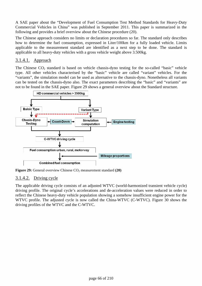
page 66 of 210

A SAE paper about the “Development of Fuel Consumption Test Method Standards for Heavy-Duty Commercial Vehicles in China” was published in September 2011. This paper is summarized in the following and provides a brief overview about the Chinese procedure (20). The Chinese approach considers no limits or declaration procedures so far. The standard only describes how to determine the fuel consumption, expressed in Liter/100km for a fully loaded vehicle. Limits applicable to the measurement standard are identified as a next step to be done. The standard is applicable to all heavy-duty vehicles with a gross vehicle weight above 3.500kg.

3.1.4.1. Approach

The Chinese CO2 standard is based on vehicle chassis-dyno testing for the so-called “basic” vehicle type. All other vehicles characterised by the “basic” vehicle are called “variant” vehicles. For the “variants”, the simulation model can be used as alternative to the chassis-dyno. Nonetheless all variants can be tested on the chassis-dyno also. The exact parameters describing the “basic” and “variants” are not to be found in the SAE paper. Figure 29 shows a general overview about the Standard structure.

Figure 29: General overview Chinese CO2 measurement standard (20)

3.1.4.2. Driving cycle

The applicable driving cycle consists of an adjusted WTVC (world-harmonized transient vehicle cycle) driving profile. The original cycle’s accelerations and de-acceleration values were reduced in order to reflect the Chinese heavy-duty vehicle population showing a somehow insufficient engine power for the WTVC profile. The adjusted cycle is now called the China-WTVC (C-WTVC). Figure 30 shows the driving profiles of the WTVC and the C-WTVC.

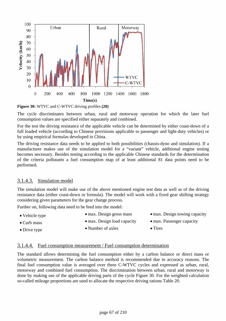
page 67 of 210

Figure 30: WTVC and C-WTVC driving profiles (20)

The cycle discriminates between urban, rural and motorway operation for which the later fuel consumption values are specified either separately and combined. For the test the driving resistance of the applicable vehicle can be determined by either coast-down of a full loaded vehicle (according to Chinese provisions applicable to passenger and light-duty vehicles) or by using empirical formulas developed in China. The driving resistance data needs to be applied to both possibilities (chassis-dyno and simulation). If a manufacturer makes use of the simulation model for a “variant” vehicle, additional engine testing becomes necessary. Besides testing according to the applicable Chinese standards for the determination of the criteria pollutants a fuel consumption map of at least additional 81 data points need to be performed.

3.1.4.3. Simulation model

The simulation model will make use of the above mentioned engine test data as well as of the driving resistance data (either coast-down or formula). The model will work with a fixed gear shifting strategy considering given parameters for the gear change process. Further on, following data need to be feed into the model:

• Vehicle type • max. Design gross mass • max. Design towing capacity

• Curb mass • max. Design load capacity • max. Passenger capacity

• Drive type • Number of axles • Tires

3.1.4.4. Fuel consumption measurement / Fuel consumption determination

The standard allows determining the fuel consumption either by a carbon balance or direct mass or volumetric measurement. The carbon balance method is recommended due to accuracy reasons. The final fuel consumption value is averaged over three C-WTVC cycles and expressed as urban, rural, motorway and combined fuel consumption. The discrimination between urban, rural and motorway is done by making use of the applicable driving parts of the cycle Figure 30. For the weighted calculation so-called mileage proportions are used to allocate the respective driving rations Table 20.

page 68 of 210

Table 20: Mileage proportions (20)

3.2. Vehicle and engine selection As described in chapter 2 the vehicle classification defines the corresponding test cycle and the vehicle loading in the simulation and also the “norm body” to be used for the measurement of the aerodynamic drag. To save costs only variations of components from HDV should be measured mandatory, which have a measurable influence on the resulting fuel consumption. This could be reached by a proper definition of vehicle families. Costly measurements are attributed to the engine (fuels map etc.), to the body (aerodynamic drag), to the gearbox (efficiency map) and to auxiliaries. Background data which lead to the proposal in chapter 2.2 is discussed in the following chapters.

3.2.1. Truck segmentation The vehicle segmentation shall help to develop a regulatory approach for future CO2-measures for heavy-duty vehicles which considers the typical in-service use of such vehicles on the one hand but also reflects the already established vehicle classification of the existing framework directive (2007/47/EC) and the corresponding Commission Regulation (EC) No. 678/2011 on the other hand. With this classification it should be possible to define family criteria for a later regulatory approach (compare chapter 3.7). The vehicle classification described and developed in the following chapters is based on data made available by ACEA and date establisher in the Lot 1 report (1) as well as on projections performed in the project consortium. For the time being the segmentation applies to heavy-duty vehicles with a gross weight above 7,5 tons only. Although there is no type-approval related vehicle category using the 7,5 tons threshold (this value is solely used for driving licence purposes; Class C1), this value will be applied since every vehicle above this value is recognized as heavy-duty vehicle. Of course there are also vehicles below 7,5 tons which are clearly in the heavy-duty vehicle range but this is not yet defined properly. Commission Regulation (EC) 715/2007 defines certain vehicles categories (M1, M2, N1 and N2) with a reference mass not exceeding 2610 kg as being within the scope of passenger cars regulation. Under special circumstances, when the applicant holds already an approval, the reference mass can extended to 2840 kg. In the converse argument this means every vehicle above the mentioned threshold is considered to be more or less a heavy duty vehicle.

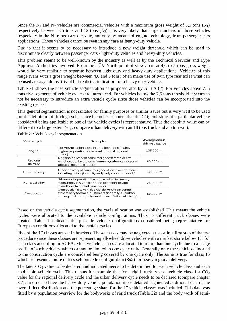
page 69 of 210

Since the N1 and N2 vehicles are commercial vehicles with a maximum gross weight of 3,5 tons (N1) respectively between 3,5 tons and 12 tons (N2) it is very likely that large numbers of those vehicles (especially in the N1 range) are derivate, not only by means of engine technology, from passenger cars applications. Those vehicles cannot be seen in any case as heavy-duty vehicle. Due to that it seems to be necessary to introduce a new weight threshold which can be used to discriminate clearly between passenger cars / light-duty vehicles and heavy-duty vehicles. This problem seems to be well-known by the industry as well as by the Technical Services and Type Approval Authorities involved. From the TÜV-North point of view a cut at 4,6 to 5 tons gross weight would be very realistic to separate between light-duty and heavy-duty applications. Vehicles of this range (vans with a gross weight between 4,6 and 5 tons) often make use of twin tyre rear axles what can be used as easy, almost trivial but realistic, indication for a heavy duty vehicle. Table 21 shows the base vehicle segmentation as proposed also by ACEA (2). For vehicles above 7, 5 tons five segments of vehicle cycles are introduced. For vehicles below the 7,5 tons threshold it seems to not be necessary to introduce an extra vehicle cycle since those vehicles can be incorporated into the existing cycles. This general segmentation is not suitable for family purposes or similar issues but is very well to be used for the definition of driving cycles since it can be assumed, that the CO2 emissions of a particular vehicle considered being applicable to one of the vehicle cycles is representative. Thus the absolute value can be different to a large extent (e.g. compare urban delivery with an 18 tons truck and a 5 ton van). Table 21: Vehicle cycle segmentation

Based on the vehicle cycle segmentation, the cycle allocation was established. This means the vehicle cycles were allocated to the available vehicle configurations. Thus 17 different truck classes were created. Table 1 indicates the possible vehicle configurations considered being representative for European conditions allocated to the vehicle cycles. Five of the 17 classes are set in brackets. These classes may be neglected at least in a first step of the test procedure since these classes are representing all-wheel drive vehicles with a market share below 1% for each class according to ACEA. Most vehicle classes are allocated to more than one cycle due to a usage profile of such vehicles which cannot be limited to one cycle only. Generally only the vehicles allocated to the construction cycle are considered being covered by one cycle only. The same is true for class 15 which represents a more or less seldom axle configuration (8x2) for heavy regional delivery. The later CO2 value to be declared and indicated needs to be determined for each vehicle class and each applicable vehicle cycle. This means for example that for a rigid truck type of vehicle class 1 a CO2 value for the regional delivery cycle and the urban delivery cycle needs to be declared (compare chapter 3.7). In order to have the heavy-duty vehicle population more detailed segmented additional data of the overall fleet distribution and the percentage share for the 17 vehicle classes was included. This data was fitted by a population overview for the bodyworks of rigid truck (Table 22) and the body work of semi-

Vehicle cycle Description Averageannualdriving distance

Long haul

Regional delivery

Urban delivery

Municipal utility

Construction

135.000 km

60.000 km

40.000 km

25.000 km

60.000 km

Delivery to national and international sites (mainlyhighwayoperationand a small share of regional roads).Regional delivery of consumer goods from a central warehouse to local stores (innercity, suburban, regional and also mountain roads)

Urban delivery of consumer goods from a central store to selling points (innercity and partly suburban roads)

Urban truck operation like refuse collection (many stops, partly low vehicle speed operation, driving to and back to central base point) Construction site vehicleswith delivery from centralstore to very few local customers (innercity, suburbanand regional roads; only small share of off-roaddriving)

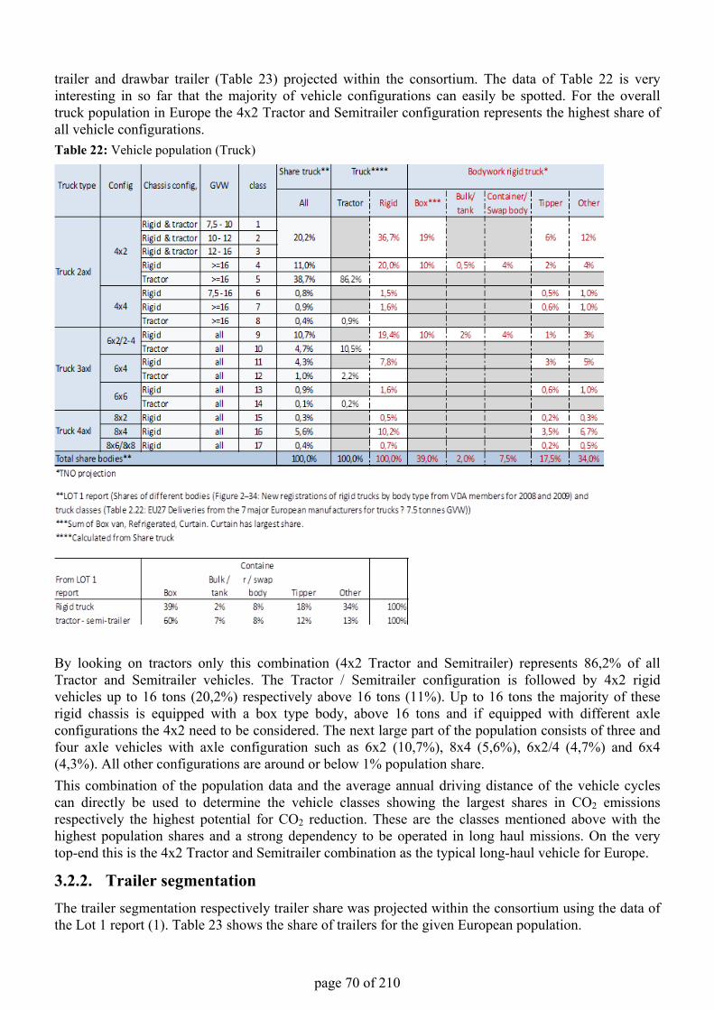
page 70 of 210

trailer and drawbar trailer (Table 23) projected within the consortium. The data of Table 22 is very interesting in so far that the majority of vehicle configurations can easily be spotted. For the overall truck population in Europe the 4x2 Tractor and Semitrailer configuration represents the highest share of all vehicle configurations.Table 22: Vehicle population (Truck)

By looking on tractors only this combination (4x2 Tractor and Semitrailer) represents 86,2% of all Tractor and Semitrailer vehicles. The Tractor / Semitrailer configuration is followed by 4x2 rigid vehicles up to 16 tons (20,2%) respectively above 16 tons (11%). Up to 16 tons the majority of these rigid chassis is equipped with a box type body, above 16 tons and if equipped with different axle configurations the 4x2 need to be considered. The next large part of the population consists of three and four axle vehicles with axle configuration such as 6x2 (10,7%), 8x4 (5,6%), 6x2/4 (4,7%) and 6x4 (4,3%). All other configurations are around or below 1% population share.This combination of the population data and the average annual driving distance of the vehicle cycles can directly be used to determine the vehicle classes showing the largest shares in CO2 emissions respectively the highest potential for CO2 reduction. These are the classes mentioned above with the highest population shares and a strong dependency to be operated in long haul missions. On the very top-end this is the 4x2 Tractor and Semitrailer combination as the typical long-haul vehicle for Europe.

3.2.2. Trailer segmentationThe trailer segmentation respectively trailer share was projected within the consortium using the data of the Lot 1 report (1). Table 23 shows the share of trailers for the given European population.

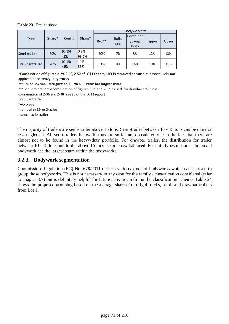
page 71 of 210

Table 23: Trailer share

The majority of trailers are semi-trailer above 15 tons. Semi-trailer between 10 - 15 tons can be more or less neglected. All semi-trailers below 10 tons are so far not considered due to the fact that there are almost not to be found in the heavy-duty portfolio. For drawbar trailer, the distribution for trailer between 10 - 15 tons and trailer above 15 tons is somehow balanced. For both types of trailer the boxed bodywork has the largest share within the bodyworks.

3.2.3. Bodywork segmentation Commission Regulation (EC) No. 678/2011 defines various kinds of bodyworks which can be used to group those bodyworks. This is not necessary in any case for the family / classification considered (refer to chapter 3.7) but is definitely helpful for future activities refining the classification scheme. Table 24 shows the proposed grouping based on the average shares from rigid trucks, semi- and drawbar trailers from Lot 1.

Box**Bulk/tank

Container/Swap body

Tipper Other

10-15t 0,5%>15t 99,5%10-15t 44%>15t 56%

**Sum of Box van, Refrigurated, Curtain. Curtain has largest share.

Drawbar trailerTwo types:- full trailer (2- or 3-axles)- centre axle trailer

*Combination of figures 2-29, 2-49, 2-50 of LOT1 report, <10t is removed because it is most likely not applicable for Heavy Duty trucks

***For Semi trailers a combination of figures 2-35 and 2-37 is used, for drawbar-trailers a combination of 2-36 and 2-38 is used of the LOT1 report

Type Share* Config Share*

Bodywork***

12% 13%

Drawbar trailer 20% 31% 4% 16% 18% 31%

Semi trailer 80% 60% 7% 8%

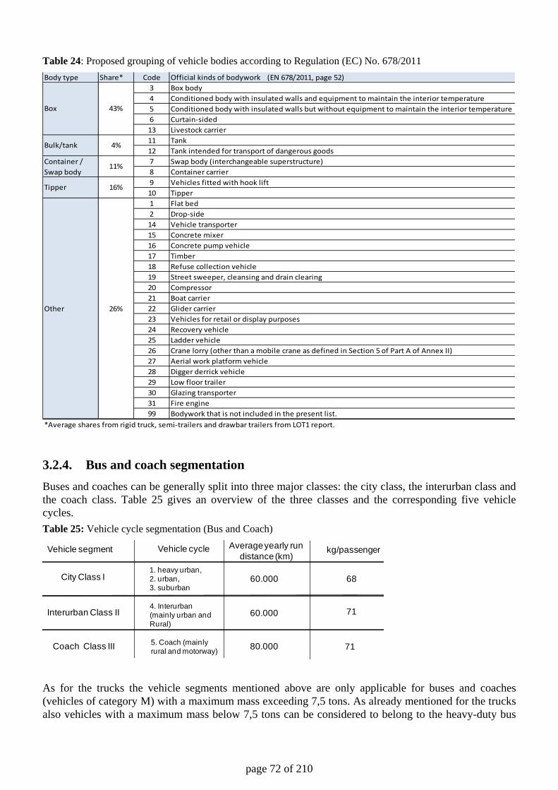
page 72 of 210

Table 24: Proposed grouping of vehicle bodies according to Regulation (EC) No. 678/2011

3.2.4. Bus and coach segmentation Buses and coaches can be generally split into three major classes: the city class, the interurban class and the coach class. Table 25 gives an overview of the three classes and the corresponding five vehicle cycles. Table 25: Vehicle cycle segmentation (Bus and Coach)

As for the trucks the vehicle segments mentioned above are only applicable for buses and coaches (vehicles of category M) with a maximum mass exceeding 7,5 tons. As already mentioned for the trucks also vehicles with a maximum mass below 7,5 tons can be considered to belong to the heavy-duty bus

Body type Share* Code Official kinds of bodywork (EN 678/2011, page 52)3 Box body4 Conditioned body with insulated walls and equipment to maintain the interior temperature5 Conditioned body with insulated walls but without equipment to maintain the interior temperature6 Curtain-sided13 Livestock carrier11 Tank12 Tank intended for transport of dangerous goods7 Swap body (interchangeable superstructure)8 Container carrier9 Vehicles fitted with hook lift10 Tipper1 Flat bed2 Drop-side14 Vehicle transporter15 Concrete mixer16 Concrete pump vehicle17 Timber18 Refuse collection vehicle19 Street sweeper, cleansing and drain clearing20 Compressor21 Boat carrier22 Glider carrier23 Vehicles for retail or display purposes24 Recovery vehicle25 Ladder vehicle26 Crane lorry (other than a mobile crane as defined in Section 5 of Part A of Annex II)27 Aerial work platform vehicle28 Digger derrick vehicle29 Low floor trailer30 Glazing transporter31 Fire engine99 Bodywork that is not included in the present list.

*Average shares from rigid truck, semi-trailers and drawbar trailers from LOT1 report.

Tipper 16%

Other 26%

Box 43%

Bulk/tank 4%

Container / Swap body

11%

Vehicle segment Vehicle cycle Average yearly run distance (km)

Interurban Class II

Coach Class III

60.000

60.000

80.000

City Class I

kg/passenger

68

71

71

1. heavy urban, 2. urban, 3. suburban

4. Interurban(mainly urban andRural)

5. Coach (mainlyrural and motorway)

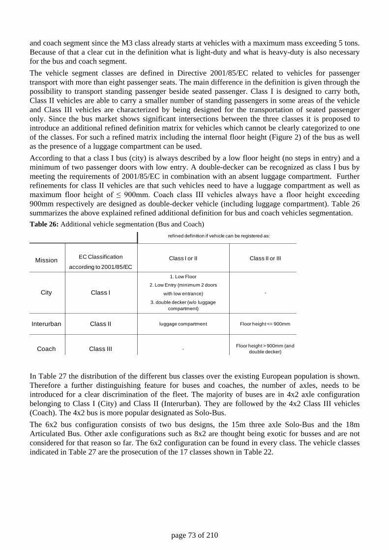
page 73 of 210

and coach segment since the M3 class already starts at vehicles with a maximum mass exceeding 5 tons. Because of that a clear cut in the definition what is light-duty and what is heavy-duty is also necessary for the bus and coach segment. The vehicle segment classes are defined in Directive 2001/85/EC related to vehicles for passenger transport with more than eight passenger seats. The main difference in the definition is given through the possibility to transport standing passenger beside seated passenger. Class I is designed to carry both, Class II vehicles are able to carry a smaller number of standing passengers in some areas of the vehicle and Class III vehicles are characterized by being designed for the transportation of seated passenger only. Since the bus market shows significant intersections between the three classes it is proposed to introduce an additional refined definition matrix for vehicles which cannot be clearly categorized to one of the classes. For such a refined matrix including the internal floor height (Figure 2) of the bus as well as the presence of a luggage compartment can be used. According to that a class I bus (city) is always described by a low floor height (no steps in entry) and a minimum of two passenger doors with low entry. A double-decker can be recognized as class I bus by meeting the requirements of 2001/85/EC in combination with an absent luggage compartment. Further refinements for class II vehicles are that such vehicles need to have a luggage compartment as well as maximum floor height of ≤ 900mm. Coach class III vehicles always have a floor height exceeding 900mm respectively are designed as double-decker vehicle (including luggage compartment). Table 26 summarizes the above explained refined additional definition for bus and coach vehicles segmentation. Table 26: Additional vehicle segmentation (Bus and Coach)

In Table 27 the distribution of the different bus classes over the existing European population is shown. Therefore a further distinguishing feature for buses and coaches, the number of axles, needs to be introduced for a clear discrimination of the fleet. The majority of buses are in 4x2 axle configuration belonging to Class I (City) and Class II (Interurban). They are followed by the 4x2 Class III vehicles (Coach). The 4x2 bus is more popular designated as Solo-Bus. The 6x2 bus configuration consists of two bus designs, the 15m three axle Solo-Bus and the 18m Articulated Bus. Other axle configurations such as 8x2 are thought being exotic for busses and are not considered for that reason so far. The 6x2 configuration can be found in every class. The vehicle classes indicated in Table 27 are the prosecution of the 17 classes shown in Table 22.

refined definition if vehicle can be registered as:

Mission EC Classification

according to 2001/85/ECClass I or II Class II or III

City Class I

1. Low Floor

2. Low Entry (minimum 2 doors

with low entrance)

3. double decker (w/o luggagecompartment)

-

Interurban Class II luggage compartment Floor height <= 900mm

Coach Class III - Floor height > 900mm (anddouble decker)

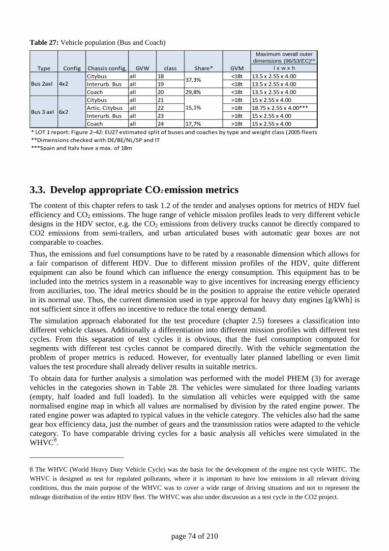
page 74 of 210

Table 27: Vehicle population (Bus and Coach)

3.3. Develop appropriate CO2 emission metrics The content of this chapter refers to task 1.2 of the tender and analyses options for metrics of HDV fuel efficiency and CO2 emissions. The huge range of vehicle mission profiles leads to very different vehicle designs in the HDV sector, e.g. the CO2 emissions from delivery trucks cannot be directly compared to CO2 emissions from semi-trailers, and urban articulated buses with automatic gear boxes are not comparable to coaches. Thus, the emissions and fuel consumptions have to be rated by a reasonable dimension which allows for a fair comparison of different HDV. Due to different mission profiles of the HDV, quite different equipment can also be found which can influence the energy consumption. This equipment has to be included into the metrics system in a reasonable way to give incentives for increasing energy efficiency from auxiliaries, too. The ideal metrics should be in the position to appraise the entire vehicle operated in its normal use. Thus, the current dimension used in type approval for heavy duty engines [g/kWh] is not sufficient since it offers no incentive to reduce the total energy demand. The simulation approach elaborated for the test procedure (chapter 2.5) foresees a classification into different vehicle classes. Additionally a differentiation into different mission profiles with different test cycles. From this separation of test cycles it is obvious, that the fuel consumption computed for segments with different test cycles cannot be compared directly. With the vehicle segmentation the problem of proper metrics is reduced. However, for eventually later planned labelling or even limit values the test procedure shall already deliver results in suitable metrics. To obtain data for further analysis a simulation was performed with the model PHEM (3) for average vehicles in the categories shown in Table 28. The vehicles were simulated for three loading variants (empty, half loaded and full loaded). In the simulation all vehicles were equipped with the same normalised engine map in which all values are normalised by division by the rated engine power. The rated engine power was adapted to typical values in the vehicle category. The vehicles also had the same gear box efficiency data, just the number of gears and the transmission ratios were adapted to the vehicle category. To have comparable driving cycles for a basic analysis all vehicles were simulated in the WHVC8.

8 The WHVC (World Heavy Duty Vehicle Cycle) was the basis for the development of the engine test cycle WHTC. The WHVC is designed as test for regulated pollutants, where it is important to have low emissions in all relevant driving conditions, thus the main purpose of the WHVC was to cover a wide range of driving situations and not to represent the mileage distribution of the entire HDV fleet. The WHVC was also under discussion as a test cycle in the CO2 project.

Maximum overall outer dimensions (96/53/EC)**

l x w x hCitybus all 18 <18t 13.5 x 2.55 x 4.00Interurb. Bus all 19 <18t 13.5 x 2.55 x 4.00Coach all 20 29,8% <18t 13.5 x 2.55 x 4.00Citybus all 21 >18t 15 x 2.55 x 4.00Artic. Citybus all 22 >18t 18.75 x 2.55 x 4.00***Interurb. Bus all 23 >18t 15 x 2.55 x 4.00Coach all 24 17,7% >18t 15 x 2.55 x 4.00

* LOT 1 report: Figure 2–42: EU27 estimated split of buses and coaches by type and weight class (2005 fleets)**Dimensions checked with DE/BE/NL/SP and IT***Spain and Italy have a max. of 18m

Bus 2axl 4x237,3%

Bus 3 axl 6x215,1%

Share* GVMType Config Chassis config, GVW class

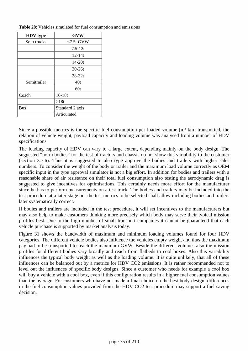
page 75 of 210

Table 28: Vehicles simulated for fuel consumption and emissions

HDV type GVW Solo trucks <7.5t GVW

7.5-12t 12-14t 14-20t 20-26t 28-32t

Semitrailer 40t 60t

Coach 16-18t >18t Bus Standard 2 axis Articulated Since a possible metrics is the specific fuel consumption per loaded volume [m³-km] transported, the relation of vehicle weight, payload capacity and loading volume was analysed from a number of HDV specifications. The loading capacity of HDV can vary to a large extent, depending mainly on the body design. The suggested “norm bodies” for the test of tractors and chassis do not show this variability to the customer (section 3.7.6). Thus it is suggested to also type approve the bodies and trailers with higher sales numbers. To consider the weight of the body or trailer and the maximum load volume correctly as OEM specific input in the type approval simulator is not a big effort. In addition for bodies and trailers with a reasonable share of air resistance on their total fuel consumption also testing the aerodynamic drag is suggested to give incentives for optimisations. This certainly needs more effort for the manufacturer since he has to perform measurements on a test track. The bodies and trailers may be included into the test procedure at a later stage but the test metrics to be selected shall allow including bodies and trailers later systematically correct. If bodies and trailers are included in the test procedure, it will set incentives to the manufacturers but may also help to make customers thinking more precisely which body may serve their typical mission profiles best. Due to the high number of small transport companies it cannot be guaranteed that each vehicle purchase is supported by market analysis today. Figure 31 shows the bandwidth of maximum and minimum loading volumes found for four HDV categories. The different vehicle bodies also influence the vehicles empty weight and thus the maximum payload to be transported to reach the maximum GVW. Beside the different volumes also the mission profiles for different bodies vary broadly and reach from flatbeds to cool boxes. Also this variability influences the typical body weight as well as the loading volume. It is quite unlikely, that all of these influences can be balanced out by a metrics for HDV CO2 emissions. It is rather recommended not to level out the influences of specific body designs. Since a customer who needs for example a cool box will buy a vehicle with a cool box, even if this configuration results in a higher fuel consumption values than the average. For customers who have not made a final choice on the best body design, differences in the fuel consumption values provided from the HDV-CO2 test procedure may support a fuel saving decision.

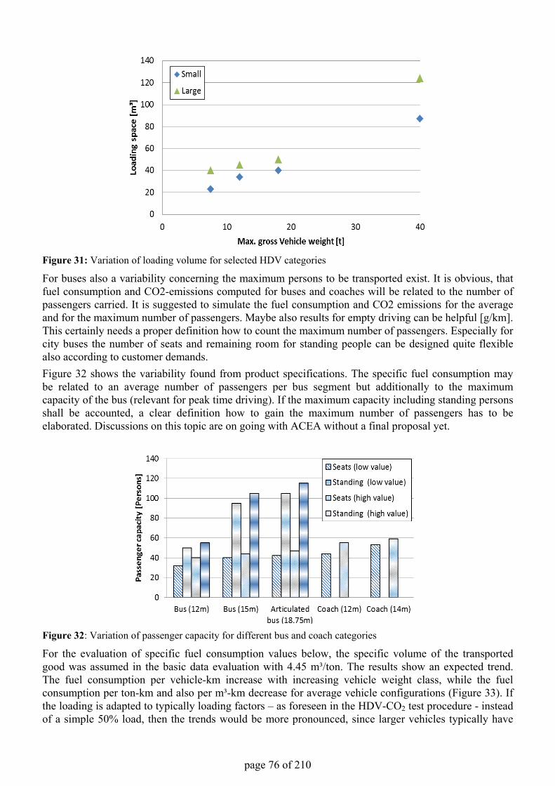
page 76 of 210

Figure 31: Variation of loading volume for selected HDV categories

For buses also a variability concerning the maximum persons to be transported exist. It is obvious, that fuel consumption and CO2-emissions computed for buses and coaches will be related to the number of passengers carried. It is suggested to simulate the fuel consumption and CO2 emissions for the average and for the maximum number of passengers. Maybe also results for empty driving can be helpful [g/km]. This certainly needs a proper definition how to count the maximum number of passengers. Especially for city buses the number of seats and remaining room for standing people can be designed quite flexible also according to customer demands.Figure 32 shows the variability found from product specifications. The specific fuel consumption may be related to an average number of passengers per bus segment but additionally to the maximum capacity of the bus (relevant for peak time driving). If the maximum capacity including standing persons shall be accounted, a clear definition how to gain the maximum number of passengers has to be elaborated. Discussions on this topic are on going with ACEA without a final proposal yet.

Figure 32: Variation of passenger capacity for different bus and coach categories

For the evaluation of specific fuel consumption values below, the specific volume of the transported good was assumed in the basic data evaluation with 4.45 m³/ton. The results show an expected trend. The fuel consumption per vehicle-km increase with increasing vehicle weight class, while the fuel consumption per ton-km and also per m³-km decrease for average vehicle configurations (Figure 33). If the loading is adapted to typically loading factors – as foreseen in the HDV-CO2 test procedure - instead of a simple 50% load, then the trends would be more pronounced, since larger vehicles typically have

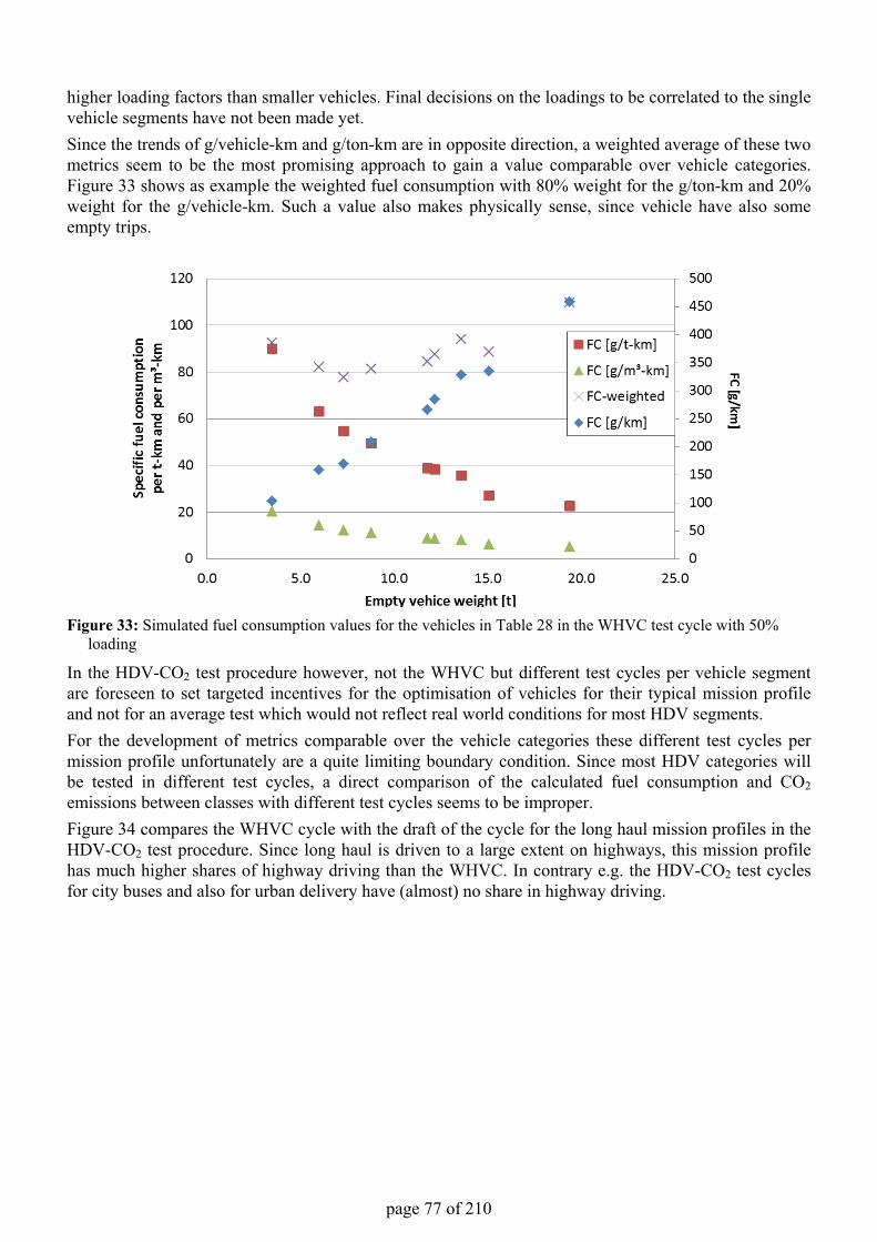
page 77 of 210

higher loading factors than smaller vehicles. Final decisions on the loadings to be correlated to the single vehicle segments have not been made yet.Since the trends of g/vehicle-km and g/ton-km are in opposite direction, a weighted average of these two metrics seem to be the most promising approach to gain a value comparable over vehicle categories. Figure 33 shows as example the weighted fuel consumption with 80% weight for the g/ton-km and 20% weight for the g/vehicle-km. Such a value also makes physically sense, since vehicle have also some empty trips.

Figure 33: Simulated fuel consumption values for the vehicles in Table 28 in the WHVC test cycle with 50% loading

In the HDV-CO2 test procedure however, not the WHVC but different test cycles per vehicle segment are foreseen to set targeted incentives for the optimisation of vehicles for their typical mission profile and not for an average test which would not reflect real world conditions for most HDV segments.For the development of metrics comparable over the vehicle categories these different test cycles per mission profile unfortunately are a quite limiting boundary condition. Since most HDV categories will be tested in different test cycles, a direct comparison of the calculated fuel consumption and CO2emissions between classes with different test cycles seems to be improper. Figure 34 compares the WHVC cycle with the draft of the cycle for the long haul mission profiles in the HDV-CO2 test procedure. Since long haul is driven to a large extent on highways, this mission profile has much higher shares of highway driving than the WHVC. In contrary e.g. the HDV-CO2 test cycles for city buses and also for urban delivery have (almost) no share in highway driving.

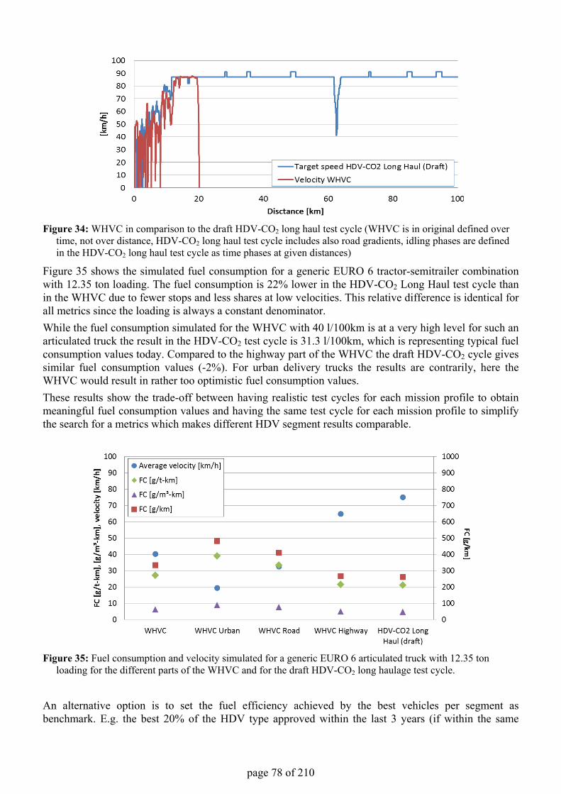
page 78 of 210

Figure 34: WHVC in comparison to the draft HDV-CO2 long haul test cycle (WHVC is in original defined over time, not over distance, HDV-CO2 long haul test cycle includes also road gradients, idling phases are defined in the HDV-CO2 long haul test cycle as time phases at given distances)

Figure 35 shows the simulated fuel consumption for a generic EURO 6 tractor-semitrailer combination with 12.35 ton loading. The fuel consumption is 22% lower in the HDV-CO2 Long Haul test cycle than in the WHVC due to fewer stops and less shares at low velocities. This relative difference is identical for all metrics since the loading is always a constant denominator.While the fuel consumption simulated for the WHVC with 40 l/100km is at a very high level for such an articulated truck the result in the HDV-CO2 test cycle is 31.3 l/100km, which is representing typical fuel consumption values today. Compared to the highway part of the WHVC the draft HDV-CO2 cycle gives similar fuel consumption values (-2%). For urban delivery trucks the results are contrarily, here the WHVC would result in rather too optimistic fuel consumption values.These results show the trade-off between having realistic test cycles for each mission profile to obtain meaningful fuel consumption values and having the same test cycle for each mission profile to simplify the search for a metrics which makes different HDV segment results comparable.

Figure 35: Fuel consumption and velocity simulated for a generic EURO 6 articulated truck with 12.35 ton loading for the different parts of the WHVC and for the draft HDV-CO2 long haulage test cycle.

An alternative option is to set the fuel efficiency achieved by the best vehicles per segment as benchmark. E.g. the best 20% of the HDV type approved within the last 3 years (if within the same

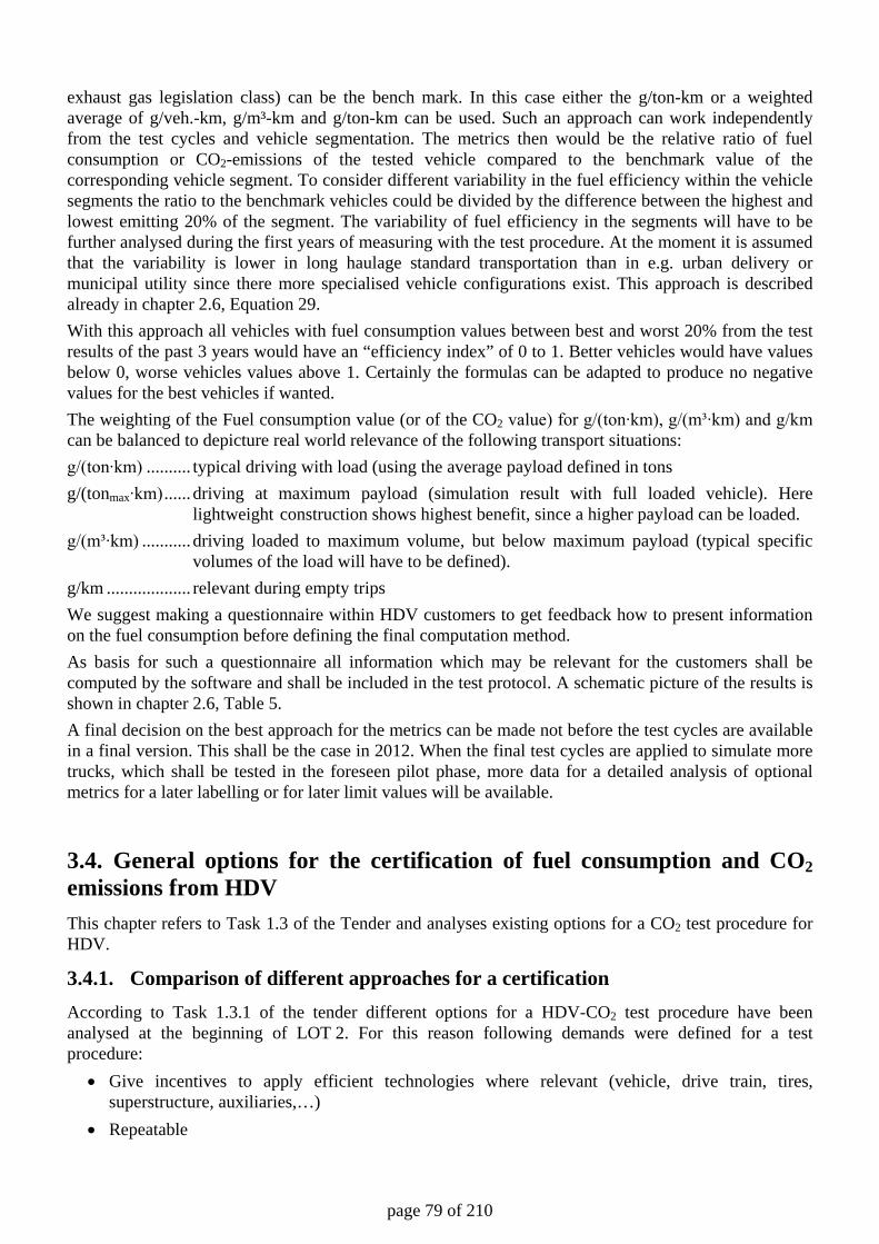
page 79 of 210

exhaust gas legislation class) can be the bench mark. In this case either the g/ton-km or a weighted average of g/veh.-km, g/m³-km and g/ton-km can be used. Such an approach can work independently from the test cycles and vehicle segmentation. The metrics then would be the relative ratio of fuel consumption or CO2-emissions of the tested vehicle compared to the benchmark value of the corresponding vehicle segment. To consider different variability in the fuel efficiency within the vehicle segments the ratio to the benchmark vehicles could be divided by the difference between the highest and lowest emitting 20% of the segment. The variability of fuel efficiency in the segments will have to be further analysed during the first years of measuring with the test procedure. At the moment it is assumed that the variability is lower in long haulage standard transportation than in e.g. urban delivery or municipal utility since there more specialised vehicle configurations exist. This approach is described already in chapter 2.6, Equation 29. With this approach all vehicles with fuel consumption values between best and worst 20% from the test results of the past 3 years would have an “efficiency index” of 0 to 1. Better vehicles would have values below 0, worse vehicles values above 1. Certainly the formulas can be adapted to produce no negative values for the best vehicles if wanted. The weighting of the Fuel consumption value (or of the CO2 value) for g/(ton∙km), g/(m³∙km) and g/km can be balanced to depicture real world relevance of the following transport situations: g/(ton∙km) .......... typical driving with load (using the average payload defined in tons g/(tonmax∙km) ...... driving at maximum payload (simulation result with full loaded vehicle). Here

lightweight construction shows highest benefit, since a higher payload can be loaded. g/(m³∙km) ........... driving loaded to maximum volume, but below maximum payload (typical specific

volumes of the load will have to be defined). g/km ................... relevant during empty trips We suggest making a questionnaire within HDV customers to get feedback how to present information on the fuel consumption before defining the final computation method. As basis for such a questionnaire all information which may be relevant for the customers shall be computed by the software and shall be included in the test protocol. A schematic picture of the results is shown in chapter 2.6, Table 5. A final decision on the best approach for the metrics can be made not before the test cycles are available in a final version. This shall be the case in 2012. When the final test cycles are applied to simulate more trucks, which shall be tested in the foreseen pilot phase, more data for a detailed analysis of optional metrics for a later labelling or for later limit values will be available.

3.4. General options for the certification of fuel consumption and CO2 emissions from HDV This chapter refers to Task 1.3 of the Tender and analyses existing options for a CO2 test procedure for HDV.

3.4.1. Comparison of different approaches for a certification According to Task 1.3.1 of the tender different options for a HDV-CO2 test procedure have been analysed at the beginning of LOT 2. For this reason following demands were defined for a test procedure:

• Give incentives to apply efficient technologies where relevant (vehicle, drive train, tires, superstructure, auxiliaries,…)

• Repeatable

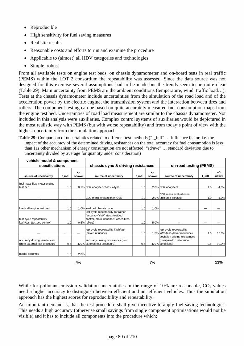
page 80 of 210

• Reproducible • High sensitivity for fuel saving measures • Realistic results • Reasonable costs and efforts to run and examine the procedure • Applicable to (almost) all HDV categories and technologies • Simple, robust

From all available tests on engine test beds, on chassis dynamometer and on-board tests in real traffic (PEMS) within the LOT 2 consortium the repeatability was assessed. Since the data source was not designed for this exercise several assumptions had to be made but the trends seem to be quite clear (Table 29). Main uncertainty from PEMS are the ambient conditions (temperature, wind, traffic load…). Tests at the chassis dynamometer include uncertainties from the simulation of the road load and of the acceleration power by the electric engine, the transmission system and the interaction between tires and rollers. The component testing can be based on quite accurately measured fuel consumption maps from the engine test bed. Uncertainties of road load measurement are similar to the chassis dynamometer. Not included in this analysis were auxiliaries. Complex control systems of auxiliaries would be depictured in the most realistic way with PEMS (but with worse repeatability) and from today’s point of view with the highest uncertainty from the simulation approach. Table 29: Comparison of uncertainties related to different test methods (“f_infl” … influence factor, i.e. the

impact of the accuracy of the determined driving resistances on the total accuracy for fuel consumption is less than 1as other mechanism of energy consumption are not affected; “sd/ave” … standard deviation due to uncertainty divided by average for quantity under consideration)

While for pollutant emission validation uncertainties in the range of 10% are reasonable, CO2 values need a higher accuracy to distinguish between efficient and not efficient vehicles. Thus the simulation approach has the highest scores for reproducibility and repeatability. An important demand is, that the test procedure shall give incentive to apply fuel saving technologies. This needs a high accuracy (otherwise small savings from single component optimisations would not be visible) and it has to include all components into the procedure which:

source of uncertainty f_infl+/-

sd/ave source of uncertainty f_infl+/-

sd/ave source of uncertainty f_infl+/-

sd/ave

fuel mass flow meter engine test bed 1.0 0.1% CO2 analyser chassis dyno 1.0 2.0% CO2 analysers 1.0 4.0%

--- --- --- CO2 mass evaluation in CVS 1.0 2.0%CO2 mass evaluation in undiluted exhaust 1.0 4.0%

load cell engine test bed 1.0 1.0% load cell chassis dyno 1.0 1.0% --- --- ---

test cycle repeatability kWh/test (testbed control) 1.0 0.5%

test cycle repeatability (or rather: "accuracy") kWh/test (testbed control, main influence: losses tires-rollers) 1.0 5.0% --- --- ---

--- --- ---test cycle repeatability kWh/test (driver influence) 1.0 1.5%

test cycle repeatability kWh/test (driver influence) 1.0 10.0%

accuracy driving resistances (from external test procedure) 0.5 5.0%

accuracy driving resistances (from external test procedure) 0.5 5.0%

deviation driving resistances (compared to reference conditions) 0.5 10.0%

model accuracy 1.0 2.0%

4% 7% 13%

vehicle model & component specifications chassis dyno & driving resistances on-road testing (PEMS)

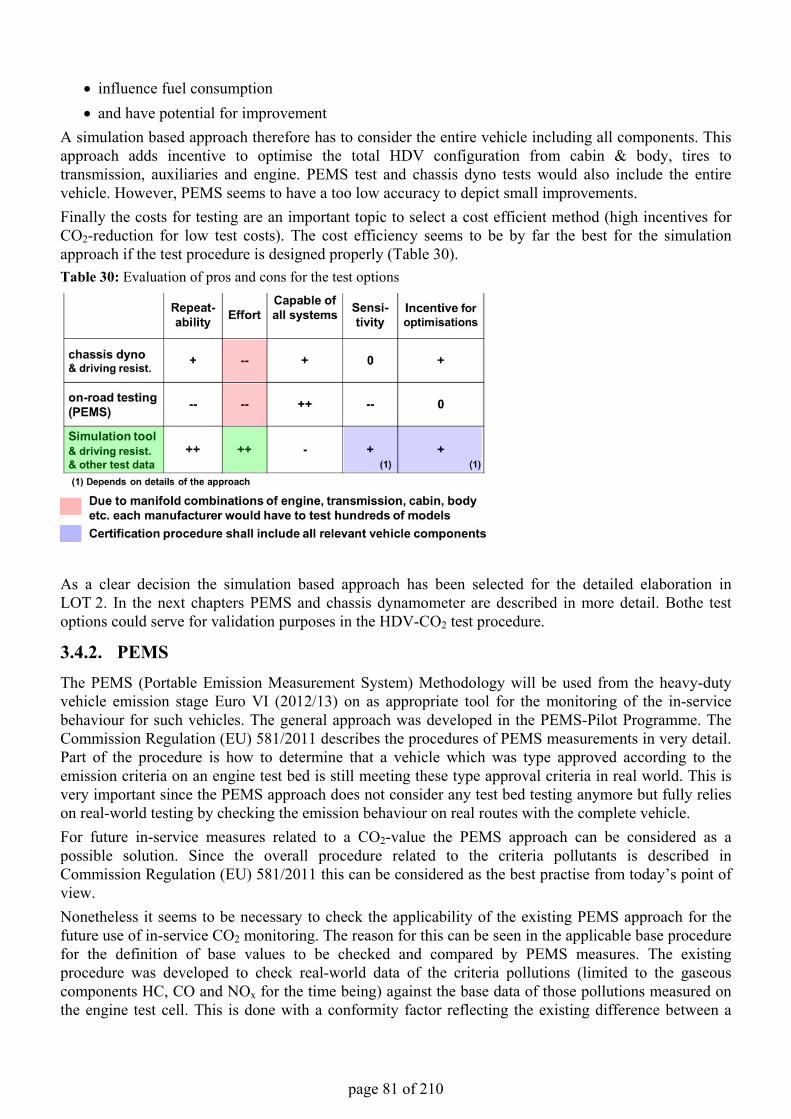
page 81 of 210

• influence fuel consumption • and have potential for improvement

A simulation based approach therefore has to consider the entire vehicle including all components. This approach adds incentive to optimise the total HDV configuration from cabin & body, tires to transmission, auxiliaries and engine. PEMS test and chassis dyno tests would also include the entire vehicle. However, PEMS seems to have a too low accuracy to depict small improvements.Finally the costs for testing are an important topic to select a cost efficient method (high incentives for CO2-reduction for low test costs). The cost efficiency seems to be by far the best for the simulation approach if the test procedure is designed properly (Table 30).Table 30: Evaluation of pros and cons for the test options

As a clear decision the simulation based approach has been selected for the detailed elaboration in LOT 2. In the next chapters PEMS and chassis dynamometer are described in more detail. Bothe test options could serve for validation purposes in the HDV-CO2 test procedure.

3.4.2. PEMS The PEMS (Portable Emission Measurement System) Methodology will be used from the heavy-duty vehicle emission stage Euro VI (2012/13) on as appropriate tool for the monitoring of the in-service behaviour for such vehicles. The general approach was developed in the PEMS-Pilot Programme. The Commission Regulation (EU) 581/2011 describes the procedures of PEMS measurements in very detail. Part of the procedure is how to determine that a vehicle which was type approved according to the emission criteria on an engine test bed is still meeting these type approval criteria in real world. This is very important since the PEMS approach does not consider any test bed testing anymore but fully relies on real-world testing by checking the emission behaviour on real routes with the complete vehicle. For future in-service measures related to a CO2-value the PEMS approach can be considered as a possible solution. Since the overall procedure related to the criteria pollutants is described in Commission Regulation (EU) 581/2011 this can be considered as the best practise from today’s point of view.Nonetheless it seems to be necessary to check the applicability of the existing PEMS approach for the future use of in-service CO2 monitoring. The reason for this can be seen in the applicable base procedure for the definition of base values to be checked and compared by PEMS measures. The existing procedure was developed to check real-world data of the criteria pollutions (limited to the gaseous components HC, CO and NOx for the time being) against the base data of those pollutions measured on the engine test cell. This is done with a conformity factor reflecting the existing difference between a

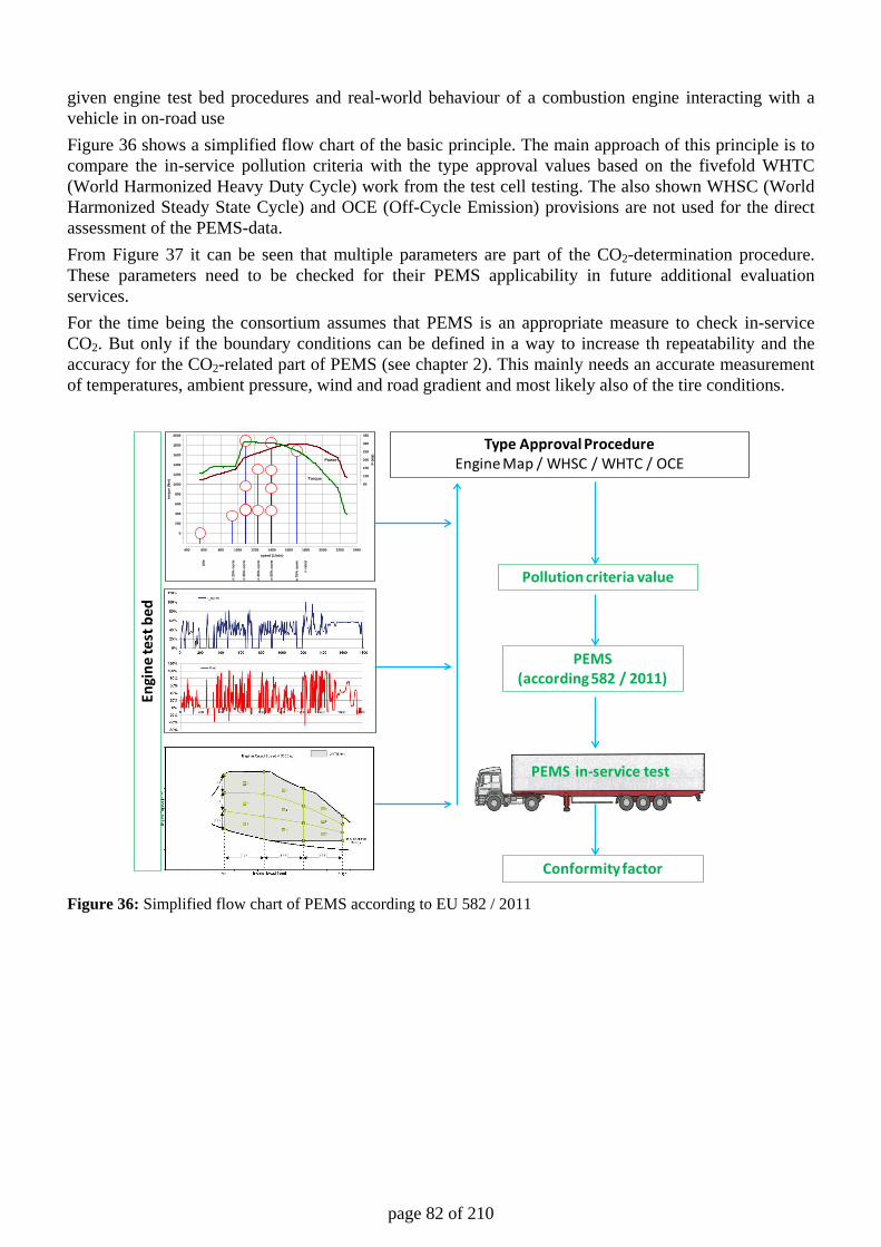
page 82 of 210

given engine test bed procedures and real-world behaviour of a combustion engine interacting with a vehicle in on-road use Figure 36 shows a simplified flow chart of the basic principle. The main approach of this principle is to compare the in-service pollution criteria with the type approval values based on the fivefold WHTC (World Harmonized Heavy Duty Cycle) work from the test cell testing. The also shown WHSC (World Harmonized Steady State Cycle) and OCE (Off-Cycle Emission) provisions are not used for the direct assessment of the PEMS-data. From Figure 37 it can be seen that multiple parameters are part of the CO2-determination procedure. These parameters need to be checked for their PEMS applicability in future additional evaluation services. For the time being the consortium assumes that PEMS is an appropriate measure to check in-service CO2. But only if the boundary conditions can be defined in a way to increase th repeatability and the accuracy for the CO2-related part of PEMS (see chapter 2). This mainly needs an accurate measurement of temperatures, ambient pressure, wind and road gradient and most likely also of the tire conditions.

Figure 36: Simplified flow chart of PEMS according to EU 582 / 2011

torq

ue (N

m)

0

200

400

600

800

1000

1200

1400

1600

1800

2000

speed (1/min)400 600 800 1000 1200 1400 1600 1800 2000 2200 2400

n 25

% n

orm

n 35

% n

orm

n 45

% n

orm

n 55

% n

orm

n 75

% n

orm

n ra

ted

Power

P (k

W)

50

100

150

200

250

300

350

idle

Torque

Type Approval ProcedureEngine Map / WHSC / WHTC / OCE

Pollution criteria value

PEMS (according582 / 2011)

PEMS in-service test

Conformityfactor

Engi

ne te

stbe

d

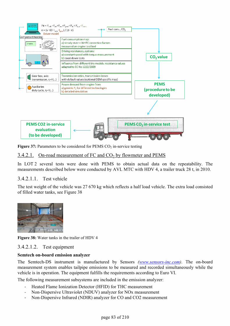
page 83 of 210

Figure 37: Parameters to be considered for PEMS CO2 in-service testing

3.4.2.1. On-road measurement of FC and CO2 by flowmeter and PEMS

In LOT 2 several tests were done with PEMS to obtain actual data on the repeatability. The measurements described below were conducted by AVL MTC with HDV 4, a trailer truck 28 t, in 2010.

3.4.2.1.1. Test vehicleThe test weight of the vehicle was 27 670 kg which reflects a half load vehicle. The extra load consisted of filled water tanks, see Figure 38

Figure 38: Water tanks in the trailer of HDV 4

3.4.2.1.2. Test equipmentSemtech on-board emission analyzerThe Semtech-DS instrument is manufactured by Sensors (www.sensors-inc.com). The on-board measurement system enables tailpipe emissions to be measured and recorded simultaneously while the vehicle is in operation. The equipment fulfills the requirements according to Euro VI.The following measurement subsystems are included in the emission analyzer:

- Heated Flame Ionization Detector (HFID) for THC measurement- Non-Dispersive Ultraviolet (NDUV) analyzer for NOx measurement- Non-Dispersive Infrared (NDIR) analyzer for CO and CO2 measurement

CO2 value

PEMS (procedure to be

developed)

PEMS CO2 in-service testPEMS CO2 in-serviceevaluation

(to be developed)

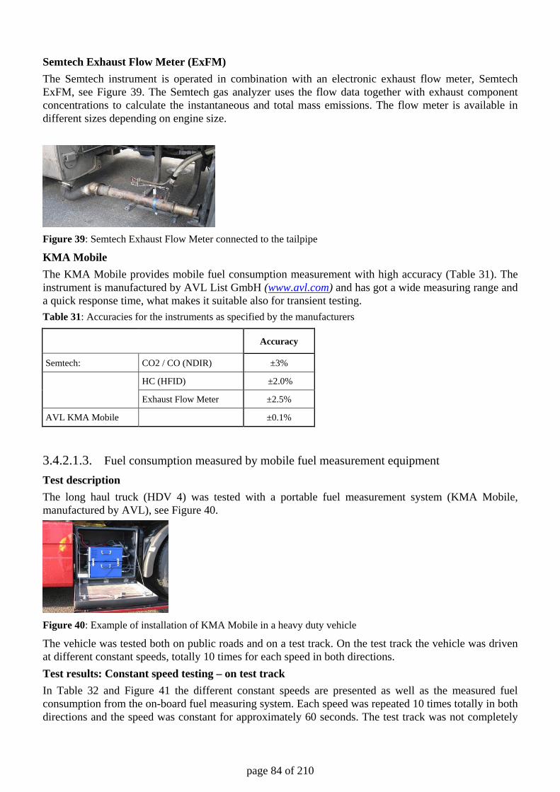
page 84 of 210

Semtech Exhaust Flow Meter (ExFM) The Semtech instrument is operated in combination with an electronic exhaust flow meter, Semtech ExFM, see Figure 39. The Semtech gas analyzer uses the flow data together with exhaust component concentrations to calculate the instantaneous and total mass emissions. The flow meter is available in different sizes depending on engine size.

Figure 39: Semtech Exhaust Flow Meter connected to the tailpipe

KMA Mobile The KMA Mobile provides mobile fuel consumption measurement with high accuracy (Table 31). The instrument is manufactured by AVL List GmbH (www.avl.com) and has got a wide measuring range and a quick response time, what makes it suitable also for transient testing. Table 31: Accuracies for the instruments as specified by the manufacturers

Accuracy

Semtech: CO2 / CO (NDIR) ±3%

HC (HFID) ±2.0%

Exhaust Flow Meter ±2.5%

AVL KMA Mobile ±0.1%

3.4.2.1.3. Fuel consumption measured by mobile fuel measurement equipment Test description The long haul truck (HDV 4) was tested with a portable fuel measurement system (KMA Mobile, manufactured by AVL), see Figure 40.

Figure 40: Example of installation of KMA Mobile in a heavy duty vehicle

The vehicle was tested both on public roads and on a test track. On the test track the vehicle was driven at different constant speeds, totally 10 times for each speed in both directions. Test results: Constant speed testing – on test track In Table 32 and Figure 41 the different constant speeds are presented as well as the measured fuel consumption from the on-board fuel measuring system. Each speed was repeated 10 times totally in both directions and the speed was constant for approximately 60 seconds. The test track was not completely

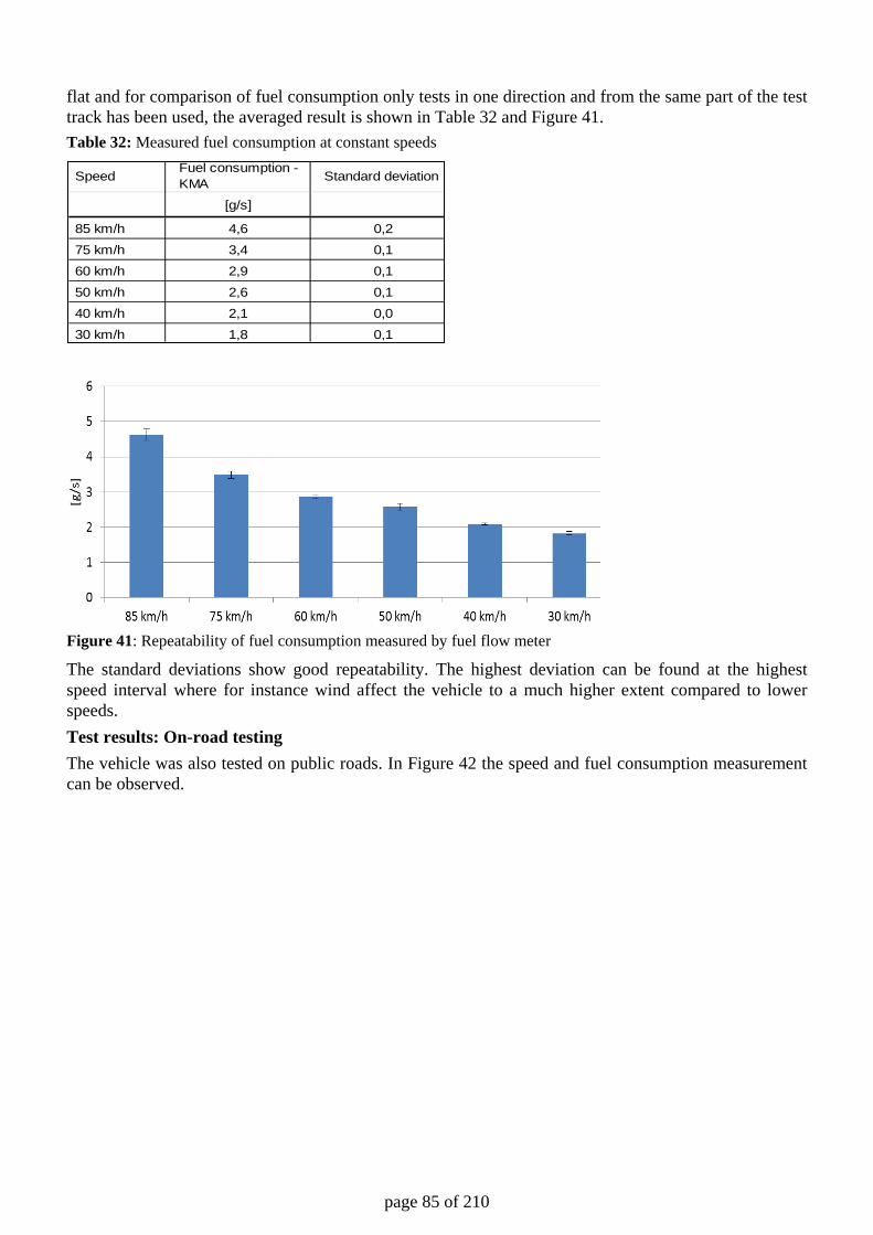
page 85 of 210

flat and for comparison of fuel consumption only tests in one direction and from the same part of the test track has been used, the averaged result is shown in Table 32 and Figure 41. Table 32: Measured fuel consumption at constant speeds

Figure 41: Repeatability of fuel consumption measured by fuel flow meter

The standard deviations show good repeatability. The highest deviation can be found at the highest speed interval where for instance wind affect the vehicle to a much higher extent compared to lower speeds. Test results: On-road testing The vehicle was also tested on public roads. In Figure 42 the speed and fuel consumption measurement can be observed.

SpeedFuel consumption - KMA Standard deviation

[g/s]

85 km/h 4,6 0,2

75 km/h 3,4 0,1

60 km/h 2,9 0,1

50 km/h 2,6 0,1

40 km/h 2,1 0,0

30 km/h 1,8 0,1

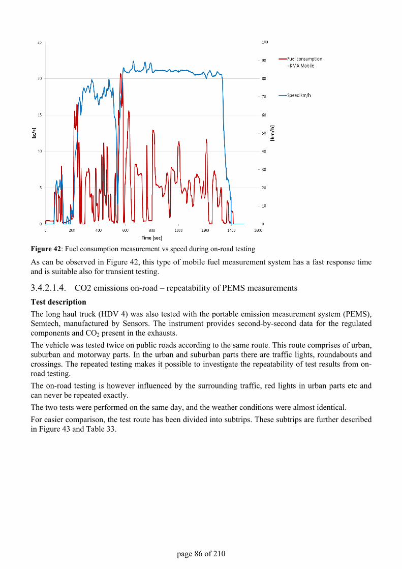
page 86 of 210

Figure 42: Fuel consumption measurement vs speed during on-road testing

As can be observed in Figure 42, this type of mobile fuel measurement system has a fast response time and is suitable also for transient testing.

3.4.2.1.4. CO2 emissions on-road – repeatability of PEMS measurementsTest descriptionThe long haul truck (HDV 4) was also tested with the portable emission measurement system (PEMS), Semtech, manufactured by Sensors. The instrument provides second-by-second data for the regulated components and CO2 present in the exhausts. The vehicle was tested twice on public roads according to the same route. This route comprises of urban, suburban and motorway parts. In the urban and suburban parts there are traffic lights, roundabouts and crossings. The repeated testing makes it possible to investigate the repeatability of test results from on-road testing. The on-road testing is however influenced by the surrounding traffic, red lights in urban parts etc and can never be repeated exactly.The two tests were performed on the same day, and the weather conditions were almost identical. For easier comparison, the test route has been divided into subtrips. These subtrips are further described in Figure 43 and Table 33.

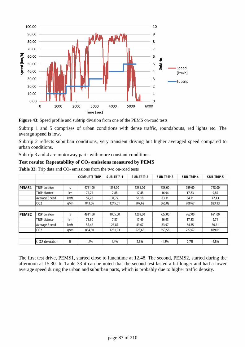
page 87 of 210

Figure 43: Speed profile and subtrip division from one of the PEMS on-road tests

Subtrip 1 and 5 comprises of urban conditions with dense traffic, roundabouts, red lights etc. The average speed is low. Subtrip 2 reflects suburban conditions, very transient driving but higher averaged speed compared to urban conditions. Subtrip 3 and 4 are motorway parts with more constant conditions. Test results: Repeatability of CO2 emissions measured by PEMS Table 33: Trip data and CO2 emissions from the two on-road tests

The first test drive, PEMS1, started close to lunchtime at 12.48. The second, PEMS2, started during the afternoon at 15.30. In Table 33 it can be noted that the second test lasted a bit longer and had a lower average speed during the urban and suburban parts, which is probably due to higher traffic density.

COMPLETE TRIP SUB-TRIP-1 SUB-TRIP-2 SUB-TRIP-3 SUB-TRIP-4 SUB-TRIP-5

PEMS1 TRIP duration s 4761,00 893,00 1231,00 733,00 759,00 748,00TRIP distance km 75,75 7,88 17,48 16,94 17,83 9,85Average Speed km/h 57,28 31,77 51,18 83,31 84,71 47,43CO2 g/km 843,06 1245,01 907,62 665,82 708,67 923,33

PEMS2 TRIP duration s 4911,00 1055,00 1269,00 727,00 762,00 691,00TRIP distance km 75,60 7,87 17,49 16,93 17,83 9,71Average Speed km/h 55,42 26,87 49,67 83,97 84,35 50,61CO2 g/km 854,50 1261,93 928,63 653,58 727,67 879,01

CO2 deviation % 1,4% 1,4% 2,3% -1,8% 2,7% -4,8%

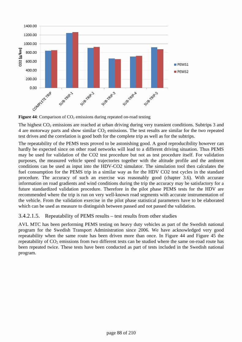
page 88 of 210

Figure 44: Comparison of CO2 emissions during repeated on-road testing

The highest CO2 emissions are reached at urban driving during very transient conditions. Subtrips 3 and 4 are motorway parts and show similar CO2 emissions. The test results are similar for the two repeated test drives and the correlation is good both for the complete trip as well as for the subtrips. The repeatability of the PEMS tests proved to be astonishing good. A good reproducibility however can hardly be expected since on other road networks will lead to a different driving situation. Thus PEMS may be used for validation of the CO2 test procedure but not as test procedure itself. For validation purposes, the measured vehicle speed trajectories together with the altitude profile and the ambient conditions can be used as input into the HDV-CO2 simulator. The simulation tool then calculates the fuel consumption for the PEMS trip in a similar way as for the HDV CO2 test cycles in the standard procedure. The accuracy of such an exercise was reasonably good (chapter 3.6). With accurate information on road gradients and wind conditions during the trip the accuracy may be satisfactory for a future standardized validation procedure. Therefore in the pilot phase PEMS tests for the HDV are recommended where the trip is run on very well-known road segments with accurate instrumentation of the vehicle. From the validation exercise in the pilot phase statistical parameters have to be elaborated which can be used as measure to distinguish between passed and not passed the validation.

3.4.2.1.5. Repeatability of PEMS results – test results from other studies AVL MTC has been performing PEMS testing on heavy duty vehicles as part of the Swedish national program for the Swedish Transport Administration since 2006. We have acknowledged very good repeatability when the same route has been driven more than once. In Figure 44 and Figure 45 the repeatability of CO2 emissions from two different tests can be studied where the same on-road route has been repeated twice. These tests have been conducted as part of tests included in the Swedish national program.

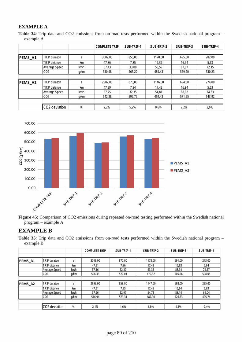
page 89 of 210

EXAMPLE A Table 34: Trip data and CO2 emissions from on-road tests performed within the Swedish national program –

example A

Figure 45: Comparison of CO2 emissions during repeated on-road testing performed within the Swedish national

program – example A

EXAMPLE B Table 35: Trip data and CO2 emissions from on-road tests performed within the Swedish national program –

example B

COMPLETE TRIP SUB-TRIP-1 SUB-TRIP-2 SUB-TRIP-3 SUB-TRIP-4

PEMS_A1 TRIP duration s 3002,00 855,00 1170,00 695,00 282,00TRIP distance km 47,86 7,85 17,39 16,94 5,63Average Speed km/h 57,43 33,08 53,59 87,87 72,15CO2 g/km 530,48 563,20 489,43 559,20 530,23

PEMS_A2 TRIP duration s 2987,00 873,00 1146,00 694,00 274,00TRIP distance km 47,89 7,84 17,42 16,94 5,63Average Speed km/h 57,75 32,35 54,81 88,02 74,33CO2 g/km 542,38 592,72 492,43 571,65 543,92

CO2 deviation % 2,2% 5,2% 0,6% 2,2% 2,6%

COMPLETE TRIP SUB-TRIP-1 SUB-TRIP-2 SUB-TRIP-3 SUB-TRIP-4

PEMS_B1 TRIP duration s 3019,00 877,00 1178,00 691,00 273,00TRIP distance km 47,91 7,86 17,43 16,93 5,64Average Speed km/h 57,16 32,30 53,33 88,34 74,67CO2 g/km 506,33 570,01 479,32 505,56 508,05

PEMS_B2 TRIP duration s 2993,00 858,00 1147,00 693,00 295,00TRIP distance km 47,91 7,85 17,43 16,94 5,63Average Speed km/h 57,66 32,97 54,78 88,14 69,04CO2 g/km 516,94 579,31 487,90 526,53 495,74

CO2 deviation % 2,1% 1,6% 1,8% 4,1% -2,4%

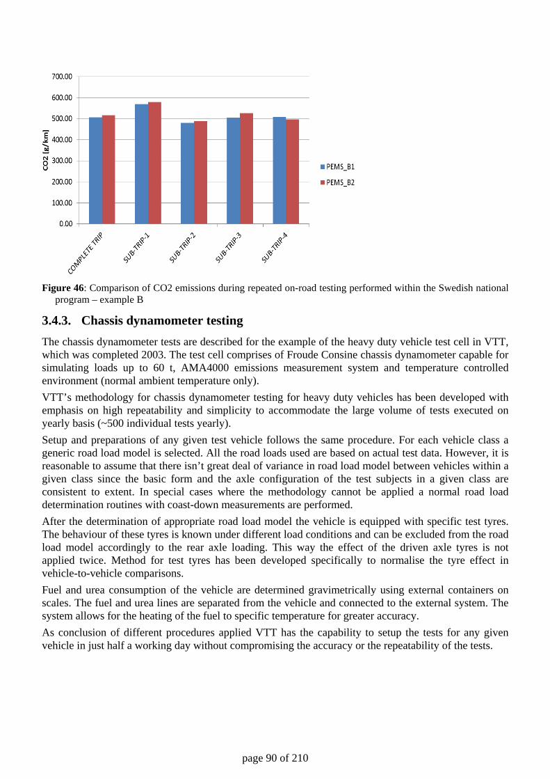
page 90 of 210

Figure 46: Comparison of CO2 emissions during repeated on-road testing performed within the Swedish national

program – example B

3.4.3. Chassis dynamometer testing The chassis dynamometer tests are described for the example of the heavy duty vehicle test cell in VTT, which was completed 2003. The test cell comprises of Froude Consine chassis dynamometer capable for simulating loads up to 60 t, AMA4000 emissions measurement system and temperature controlled environment (normal ambient temperature only). VTT’s methodology for chassis dynamometer testing for heavy duty vehicles has been developed with emphasis on high repeatability and simplicity to accommodate the large volume of tests executed on yearly basis (~500 individual tests yearly). Setup and preparations of any given test vehicle follows the same procedure. For each vehicle class a generic road load model is selected. All the road loads used are based on actual test data. However, it is reasonable to assume that there isn’t great deal of variance in road load model between vehicles within a given class since the basic form and the axle configuration of the test subjects in a given class are consistent to extent. In special cases where the methodology cannot be applied a normal road load determination routines with coast-down measurements are performed. After the determination of appropriate road load model the vehicle is equipped with specific test tyres. The behaviour of these tyres is known under different load conditions and can be excluded from the road load model accordingly to the rear axle loading. This way the effect of the driven axle tyres is not applied twice. Method for test tyres has been developed specifically to normalise the tyre effect in vehicle-to-vehicle comparisons. Fuel and urea consumption of the vehicle are determined gravimetrically using external containers on scales. The fuel and urea lines are separated from the vehicle and connected to the external system. The system allows for the heating of the fuel to specific temperature for greater accuracy. As conclusion of different procedures applied VTT has the capability to setup the tests for any given vehicle in just half a working day without compromising the accuracy or the repeatability of the tests.

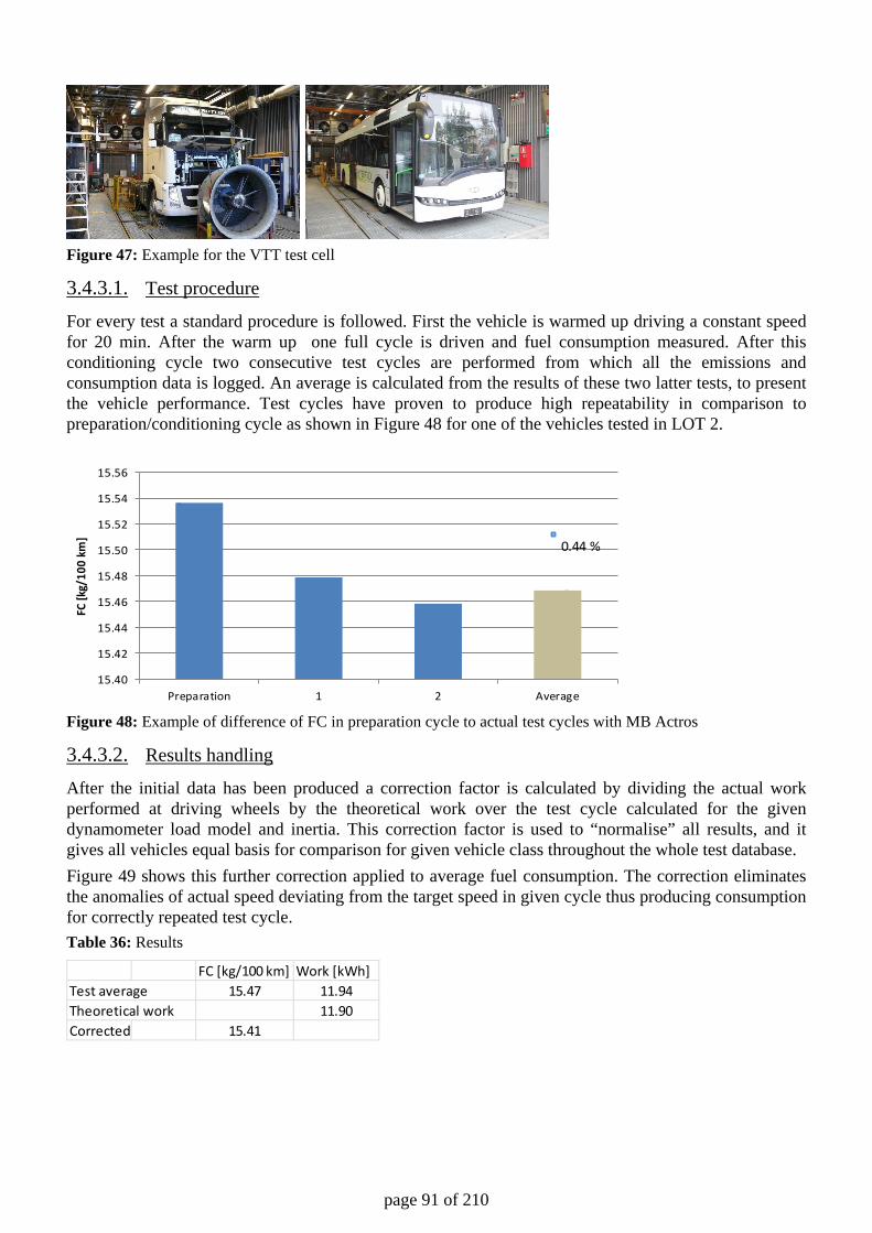
page 91 of 210

Figure 47: Example for the VTT test cell

3.4.3.1. Test procedure

For every test a standard procedure is followed. First the vehicle is warmed up driving a constant speed for 20 min. After the warm up one full cycle is driven and fuel consumption measured. After this conditioning cycle two consecutive test cycles are performed from which all the emissions and consumption data is logged. An average is calculated from the results of these two latter tests, to present the vehicle performance. Test cycles have proven to produce high repeatability in comparison to preparation/conditioning cycle as shown in Figure 48 for one of the vehicles tested in LOT 2.

Figure 48: Example of difference of FC in preparation cycle to actual test cycles with MB Actros

3.4.3.2. Results handling

After the initial data has been produced a correction factor is calculated by dividing the actual work performed at driving wheels by the theoretical work over the test cycle calculated for the given dynamometer load model and inertia. This correction factor is used to “normalise” all results, and it gives all vehicles equal basis for comparison for given vehicle class throughout the whole test database. Figure 49 shows this further correction applied to average fuel consumption. The correction eliminates the anomalies of actual speed deviating from the target speed in given cycle thus producing consumption for correctly repeated test cycle. Table 36: Results

15.40

15.42

15.44

15.46

15.48

15.50

15.52

15.54

15.56

Preparation 1 2 Average

FC [k

g/10

0 km

]

0.44 %

FC [kg/100 km] Work [kWh]Test average 15.47 11.94Theoretical work 11.90Corrected 15.41

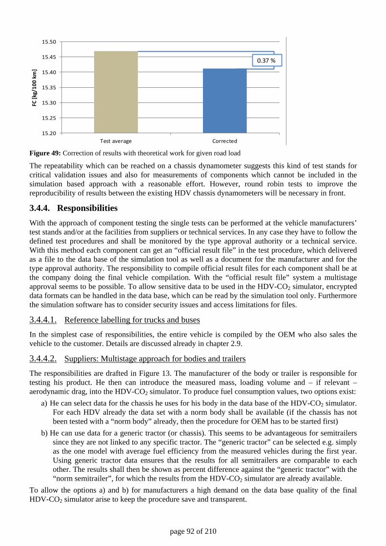
page 92 of 210

Figure 49: Correction of results with theoretical work for given road load

The repeatability which can be reached on a chassis dynamometer suggests this kind of test stands for critical validation issues and also for measurements of components which cannot be included in the simulation based approach with a reasonable effort. However, round robin tests to improve the reproducibility of results between the existing HDV chassis dynamometers will be necessary in front.

3.4.4. Responsibilities With the approach of component testing the single tests can be performed at the vehicle manufacturers’ test stands and/or at the facilities from suppliers or technical services. In any case they have to follow the defined test procedures and shall be monitored by the type approval authority or a technical service. With this method each component can get an “official result file” in the test procedure, which delivered as a file to the data base of the simulation tool as well as a document for the manufacturer and for the type approval authority. The responsibility to compile official result files for each component shall be at the company doing the final vehicle compilation. With the “official result file” system a multistage approval seems to be possible. To allow sensitive data to be used in the HDV-CO2 simulator, encrypted data formats can be handled in the data base, which can be read by the simulation tool only. Furthermore the simulation software has to consider security issues and access limitations for files.

3.4.4.1. Reference labelling for trucks and buses

In the simplest case of responsibilities, the entire vehicle is compiled by the OEM who also sales the vehicle to the customer. Details are discussed already in chapter 2.9.

3.4.4.2. Suppliers: Multistage approach for bodies and trailers

The responsibilities are drafted in Figure 13. The manufacturer of the body or trailer is responsible for testing his product. He then can introduce the measured mass, loading volume and – if relevant –aerodynamic drag, into the HDV-CO2 simulator. To produce fuel consumption values, two options exist:

a) He can select data for the chassis he uses for his body in the data base of the HDV-CO2 simulator. For each HDV already the data set with a norm body shall be available (if the chassis has not been tested with a “norm body” already, then the procedure for OEM has to be started first)

b) He can use data for a generic tractor (or chassis). This seems to be advantageous for semitrailers since they are not linked to any specific tractor. The “generic tractor” can be selected e.g. simply as the one model with average fuel efficiency from the measured vehicles during the first year. Using generic tractor data ensures that the results for all semitrailers are comparable to each other. The results shall then be shown as percent difference against the “generic tractor” with the “norm semitrailer”, for which the results from the HDV-CO2 simulator are already available.

To allow the options a) and b) for manufacturers a high demand on the data base quality of the final HDV-CO2 simulator arise to keep the procedure save and transparent.

15.20

15.25

15.30

15.35

15.40

15.45

15.50

Test average Corrected

FC [k

g/10

0 km

]

0.37 %

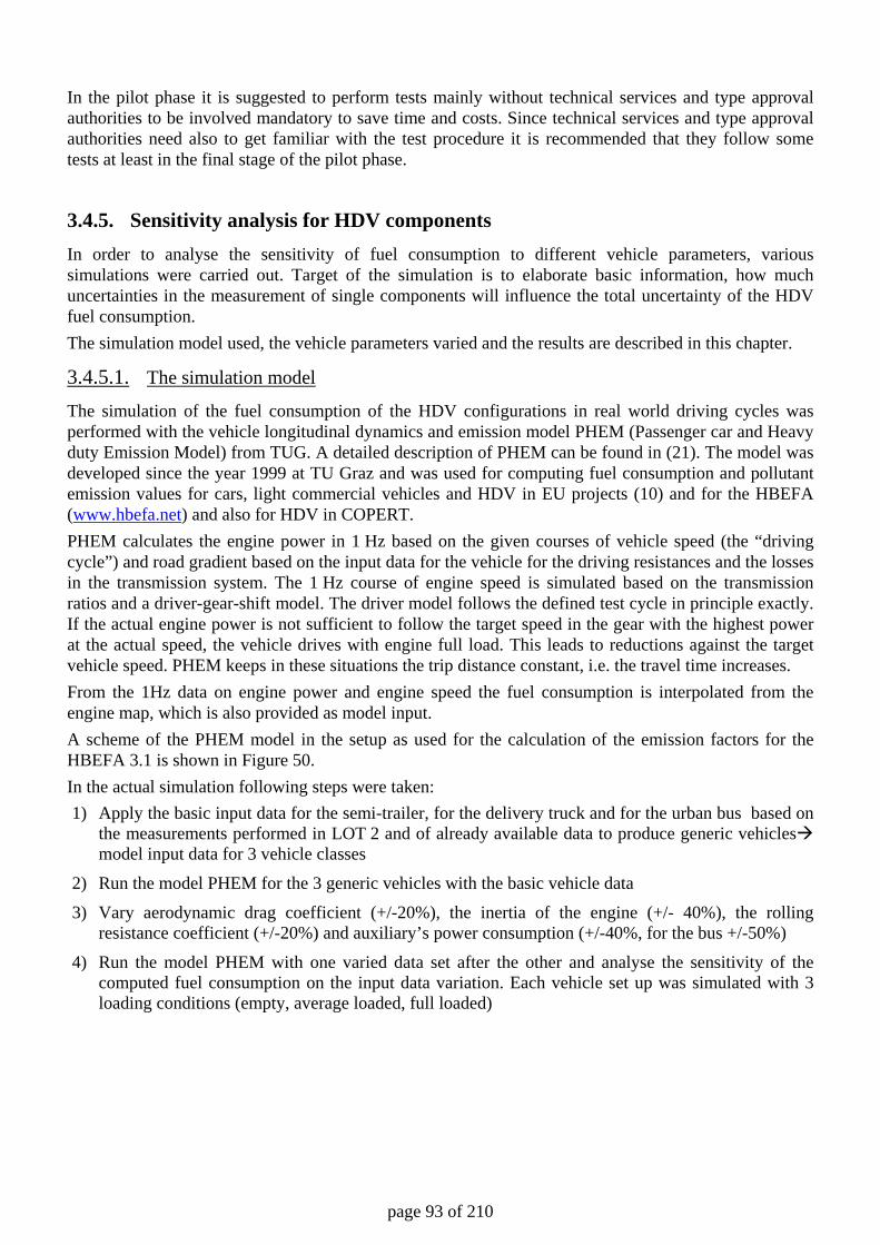
page 93 of 210

In the pilot phase it is suggested to perform tests mainly without technical services and type approval authorities to be involved mandatory to save time and costs. Since technical services and type approval authorities need also to get familiar with the test procedure it is recommended that they follow some tests at least in the final stage of the pilot phase.

3.4.5. Sensitivity analysis for HDV components In order to analyse the sensitivity of fuel consumption to different vehicle parameters, various simulations were carried out. Target of the simulation is to elaborate basic information, how much uncertainties in the measurement of single components will influence the total uncertainty of the HDV fuel consumption. The simulation model used, the vehicle parameters varied and the results are described in this chapter.

3.4.5.1. The simulation model

The simulation of the fuel consumption of the HDV configurations in real world driving cycles was performed with the vehicle longitudinal dynamics and emission model PHEM (Passenger car and Heavy duty Emission Model) from TUG. A detailed description of PHEM can be found in (21). The model was developed since the year 1999 at TU Graz and was used for computing fuel consumption and pollutant emission values for cars, light commercial vehicles and HDV in EU projects (10) and for the HBEFA (www.hbefa.net) and also for HDV in COPERT. PHEM calculates the engine power in 1 Hz based on the given courses of vehicle speed (the “driving cycle”) and road gradient based on the input data for the vehicle for the driving resistances and the losses in the transmission system. The 1 Hz course of engine speed is simulated based on the transmission ratios and a driver-gear-shift model. The driver model follows the defined test cycle in principle exactly. If the actual engine power is not sufficient to follow the target speed in the gear with the highest power at the actual speed, the vehicle drives with engine full load. This leads to reductions against the target vehicle speed. PHEM keeps in these situations the trip distance constant, i.e. the travel time increases. From the 1Hz data on engine power and engine speed the fuel consumption is interpolated from the engine map, which is also provided as model input. A scheme of the PHEM model in the setup as used for the calculation of the emission factors for the HBEFA 3.1 is shown in Figure 50. In the actual simulation following steps were taken: 1) Apply the basic input data for the semi-trailer, for the delivery truck and for the urban bus based on

the measurements performed in LOT 2 and of already available data to produce generic vehicles model input data for 3 vehicle classes

2) Run the model PHEM for the 3 generic vehicles with the basic vehicle data

3) Vary aerodynamic drag coefficient (+/-20%), the inertia of the engine (+/- 40%), the rolling resistance coefficient (+/-20%) and auxiliary’s power consumption (+/-40%, for the bus +/-50%)

4) Run the model PHEM with one varied data set after the other and analyse the sensitivity of the computed fuel consumption on the input data variation. Each vehicle set up was simulated with 3 loading conditions (empty, average loaded, full loaded)

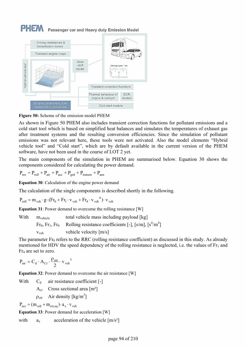
page 94 of 210

Figure 50: Scheme of the emission model PHEMAs shown in Figure 50 PHEM also includes transient correction functions for pollutant emissions and a cold start tool which is based on simplified heat balances and simulates the temperatures of exhaust gas after treatment systems and the resulting conversion efficiencies. Since the simulation of pollutant emissions was not relevant here, these tools were not activated. Also the model elements “Hybrid vehicle tool” and “Cold start”, which are by default available in the current version of the PHEM software, have not been used in the course of LOT 2 yet.The main components of the simulation in PHEM are summarised below. Equation 30 shows the components considered for calculating the power demand.

auxtransmgrdaccairrollres P+ P+ P+ P+ P+ P=P

Equation 30: Calculation of the engine power demand

The calculation of the single components is described shortly in the following.

veh4

veh4veh10vehroll v)vFrvFr(FrgmP ⋅⋅+⋅+⋅⋅=

Equation 31: Power demand to overcome the rolling resistance [W]

With mvehicle total vehicle mass including payload [kg]Fr0, Fr1, Fr4 Rolling resistance coefficients [-], [s/m], [s4/m4]vveh vehicle velocity [m/s]

The parameter Fr0 refers to the RRC (rolling resistance coefficient) as discussed in this study. As already mentioned for HDV the speed dependency of the rolling resistance is neglected, i.e. the values of Fr1 and Fr4 are set to zero.

3veh

airCrdair v

2ACP ⋅

ρ⋅⋅=

Equation 32: Power demand to overcome the air resistance [W]

With Cd air resistance coefficient [-]Acr Cross sectional area [m²]ρair Air density [kg/m3]

vehxeq,rotvehacc va)mm(P ⋅⋅+=Equation 33: Power demand for acceleration [W]

with ax acceleration of the vehicle [m/s²]

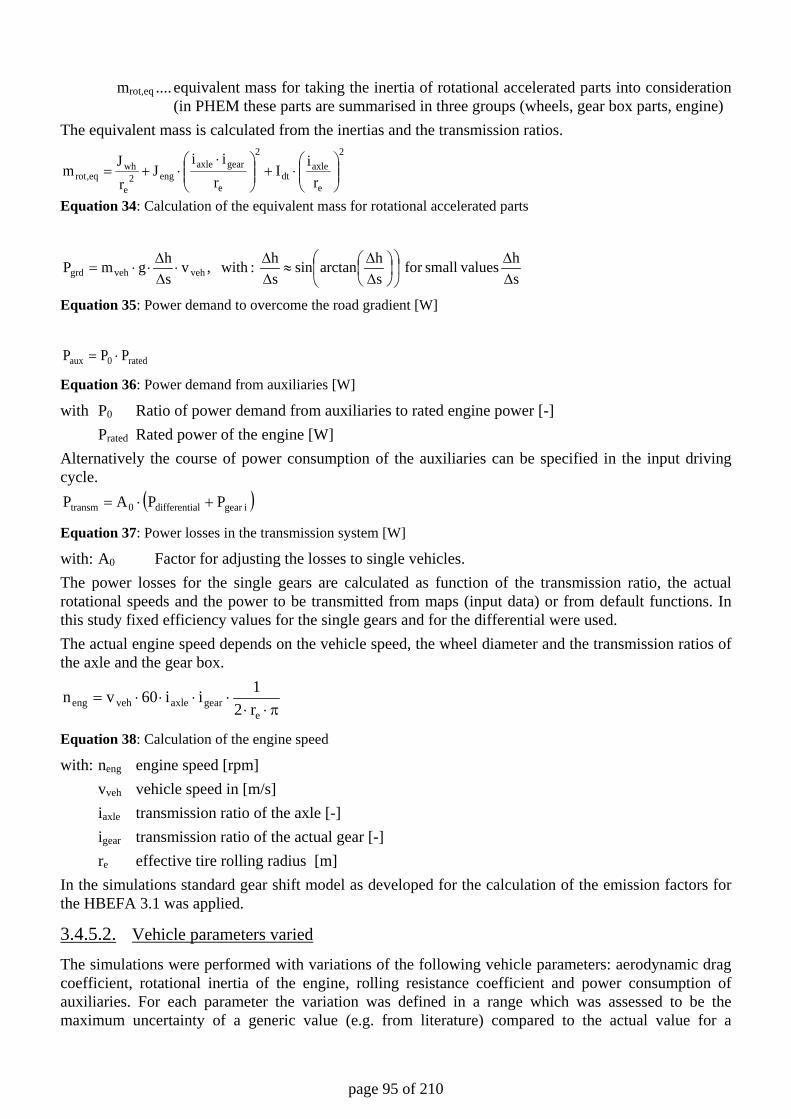
page 95 of 210

mrot,eq .... equivalent mass for taking the inertia of rotational accelerated parts into consideration (in PHEM these parts are summarised in three groups (wheels, gear box parts, engine)

The equivalent mass is calculated from the inertias and the transmission ratios. 2

e

axledt

2

e

gearaxleeng2

e

wheq,rot r

iIr

iiJ

rJm

⋅+

⋅⋅+=

Equation 34: Calculation of the equivalent mass for rotational accelerated parts

sh valuessmallfor

sharctansin

sh : with,v

shgmP vehvehgrd ∆

∆

∆∆

≈∆∆

⋅∆∆

⋅⋅=

Equation 35: Power demand to overcome the road gradient [W]

rated0aux PPP ⋅= Equation 36: Power demand from auxiliaries [W]

with P0 Ratio of power demand from auxiliaries to rated engine power [-] Prated Rated power of the engine [W] Alternatively the course of power consumption of the auxiliaries can be specified in the input driving cycle.

( )igear aldifferenti0transm PPAP +⋅= Equation 37: Power losses in the transmission system [W]

with: A0 Factor for adjusting the losses to single vehicles. The power losses for the single gears are calculated as function of the transmission ratio, the actual rotational speeds and the power to be transmitted from maps (input data) or from default functions. In this study fixed efficiency values for the single gears and for the differential were used. The actual engine speed depends on the vehicle speed, the wheel diameter and the transmission ratios of the axle and the gear box.

π⋅⋅⋅⋅⋅⋅=

egearaxleveheng r2

1ii60vn

Equation 38: Calculation of the engine speed

with: neng engine speed [rpm] vveh vehicle speed in [m/s] iaxle transmission ratio of the axle [-] igear transmission ratio of the actual gear [-] re effective tire rolling radius [m] In the simulations standard gear shift model as developed for the calculation of the emission factors for the HBEFA 3.1 was applied.

3.4.5.2. Vehicle parameters varied

The simulations were performed with variations of the following vehicle parameters: aerodynamic drag coefficient, rotational inertia of the engine, rolling resistance coefficient and power consumption of auxiliaries. For each parameter the variation was defined in a range which was assessed to be the maximum uncertainty of a generic value (e.g. from literature) compared to the actual value for a

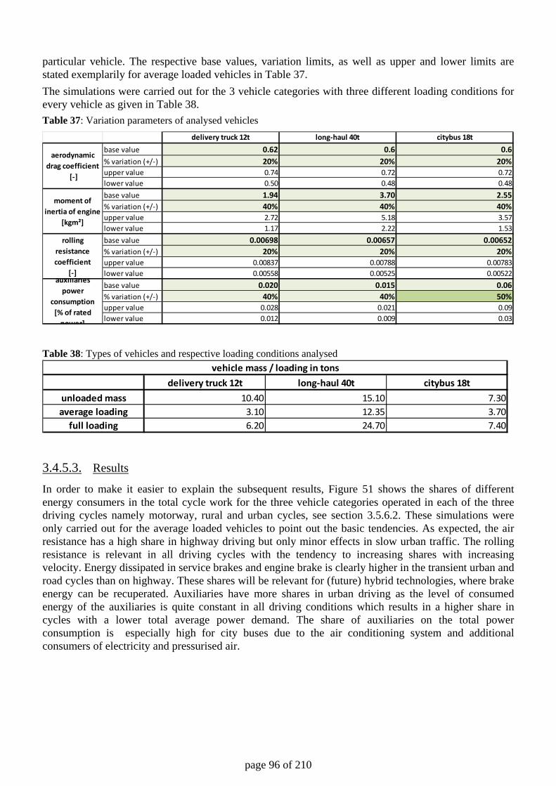
page 96 of 210

particular vehicle. The respective base values, variation limits, as well as upper and lower limits are stated exemplarily for average loaded vehicles in Table 37. The simulations were carried out for the 3 vehicle categories with three different loading conditions for every vehicle as given in Table 38. Table 37: Variation parameters of analysed vehicles

Table 38: Types of vehicles and respective loading conditions analysed

3.4.5.3. Results

In order to make it easier to explain the subsequent results, Figure 51 shows the shares of different energy consumers in the total cycle work for the three vehicle categories operated in each of the three driving cycles namely motorway, rural and urban cycles, see section 3.5.6.2. These simulations were only carried out for the average loaded vehicles to point out the basic tendencies. As expected, the air resistance has a high share in highway driving but only minor effects in slow urban traffic. The rolling resistance is relevant in all driving cycles with the tendency to increasing shares with increasing velocity. Energy dissipated in service brakes and engine brake is clearly higher in the transient urban and road cycles than on highway. These shares will be relevant for (future) hybrid technologies, where brake energy can be recuperated. Auxiliaries have more shares in urban driving as the level of consumed energy of the auxiliaries is quite constant in all driving conditions which results in a higher share in cycles with a lower total average power demand. The share of auxiliaries on the total power consumption is especially high for city buses due to the air conditioning system and additional consumers of electricity and pressurised air.

delivery truck 12t long-haul 40t citybus 18tbase value 0.62 0.6 0.6% variation (+/-) 20% 20% 20%upper value 0.74 0.72 0.72lower value 0.50 0.48 0.48base value 1.94 3.70 2.55% variation (+/-) 40% 40% 40%upper value 2.72 5.18 3.57lower value 1.17 2.22 1.53base value 0.00698 0.00657 0.00652% variation (+/-) 20% 20% 20%upper value 0.00837 0.00788 0.00783lower value 0.00558 0.00525 0.00522base value 0.020 0.015 0.06% variation (+/-) 40% 40% 50%upper value 0.028 0.021 0.09lower value 0.012 0.009 0.03

aerodynamicdrag coefficient

[-]

moment of inertia of engine

[kgm²]

rolling resistance coefficient

[-]auxiliaries

power consumption

[% of rated power]

delivery truck 12t long-haul 40t citybus 18tunloaded mass 10.40 15.10 7.30average loading 3.10 12.35 3.70

full loading 6.20 24.70 7.40

vehicle mass / loading in tons

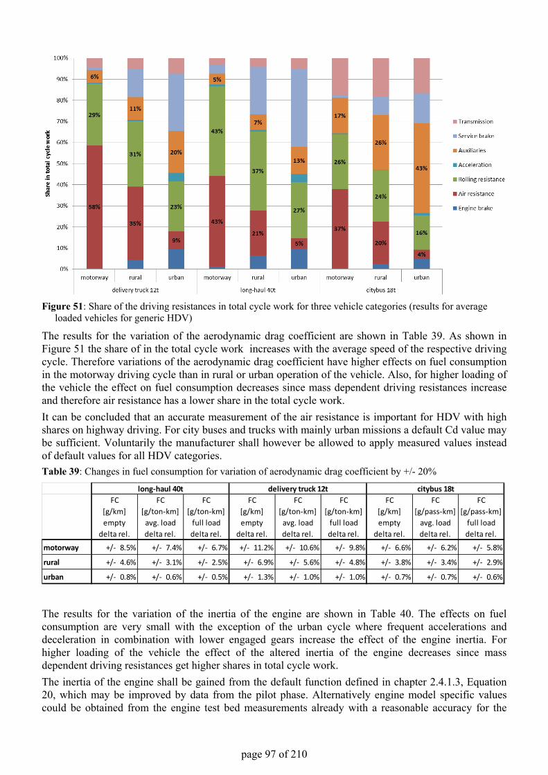
page 97 of 210

Figure 51: Share of the driving resistances in total cycle work for three vehicle categories (results for average loaded vehicles for generic HDV)

The results for the variation of the aerodynamic drag coefficient are shown in Table 39. As shown in Figure 51 the share of in the total cycle work increases with the average speed of the respective driving cycle. Therefore variations of the aerodynamic drag coefficient have higher effects on fuel consumption in the motorway driving cycle than in rural or urban operation of the vehicle. Also, for higher loading of the vehicle the effect on fuel consumption decreases since mass dependent driving resistances increase and therefore air resistance has a lower share in the total cycle work.It can be concluded that an accurate measurement of the air resistance is important for HDV with highshares on highway driving. For city buses and trucks with mainly urban missions a default Cd value may be sufficient. Voluntarily the manufacturer shall however be allowed to apply measured values instead of default values for all HDV categories.Table 39: Changes in fuel consumption for variation of aerodynamic drag coefficient by +/- 20%

The results for the variation of the inertia of the engine are shown in Table 40. The effects on fuel consumption are very small with the exception of the urban cycle where frequent accelerations and deceleration in combination with lower engaged gears increase the effect of the engine inertia. For higher loading of the vehicle the effect of the altered inertia of the engine decreases since mass dependent driving resistances get higher shares in total cycle work.The inertia of the engine shall be gained from the default function defined in chapter 2.4.1.3, Equation 20, which may be improved by data from the pilot phase. Alternatively engine model specific values could be obtained from the engine test bed measurements already with a reasonable accuracy for the

FC[g/km]empty

delta rel.

FC[g/ton-km]

avg. loaddelta rel.

FC[g/ton-km]

full loaddelta rel.

FC[g/km]empty

delta rel.

FC[g/ton-km]

avg. loaddelta rel.

FC[g/ton-km]

full loaddelta rel.

FC[g/km]empty

delta rel.

FC[g/pass-km]

avg. loaddelta rel.

FC[g/pass-km]

full loaddelta rel.

motorway +/- 8.5% +/- 7.4% +/- 6.7% +/- 11.2% +/- 10.6% +/- 9.8% +/- 6.6% +/- 6.2% +/- 5.8%

rural +/- 4.6% +/- 3.1% +/- 2.5% +/- 6.9% +/- 5.6% +/- 4.8% +/- 3.8% +/- 3.4% +/- 2.9%

urban +/- 0.8% +/- 0.6% +/- 0.5% +/- 1.3% +/- 1.0% +/- 1.0% +/- 0.7% +/- 0.7% +/- 0.6%

long-haul 40t delivery truck 12t citybus 18t

page 98 of 210

demands of the HDV CO2 test procedure. Elaborating a special test procedure for the inertia seems not to be cost efficient, thus this specific data won’t be based on a standardised test procedure. Table 40: Changes in fuel consumption for variation of inertia of the engine by +/- 40%

The results for the variation of the rolling resistance coefficient are shown in Table 41. As with the air resistance, the rolling resistance has higher shares in total cycle work, the higher the average cycle speed (see Figure 51). Increasing loading leads to increasing rolling resistance due to the higher axle weight. Thus a variation in RRC values has higher influence at the full loaded vehicles. Since the rolling resistance coefficient shall be available for all tires from the drum test procedure in future, in general tire specific RRC values can be applied in the test procedure. Depending on the road surface and on ambient conditions, transferring the RRC values from drum tests to real world conditions may have an uncertainty of approximately 20% at the moment. This has a reasonable influence on the resulting fuel consumption of HDV. However, as long as the relative difference between the tire models is depictured in a realistic way by the drum test, this uncertainty seems not to be a critical issue in the test procedure. Correlation studies between real world driving and drum test results are performed at the moment from VDA and FAT, thus the uncertainty related to the tires may be reduced in 2012. Table 41: Changes in fuel consumption for variation of rolling resistance coefficient by +/- 20%

The results for the variation of the power consumption of auxiliaries are shown in Table 42. As shown in Figure 51, the shares of the auxiliaries’ power consumption in total cycle work decrease with higher average speed of the driving cycle. Also, for higher loading of the vehicle the increasing mass dependent driving resistances reduce the effects of changes in the auxiliaries’ power consumption on total cycle work. Although the variation of the power consumption from auxiliaries was rather broad with +/-40% and +/-50% respectively, the effect on the fuel consumption is rather small, with exception of the city bus and empty driving of the two trucks.

FC[g/km]empty

delta rel.

FC[g/ton-km]

avg. loaddelta rel.

FC[g/ton-km]

full loaddelta rel.

FC[g/km]empty

delta rel.

FC[g/ton-km]

avg. loaddelta rel.

FC[g/ton-km]

full loaddelta rel.

FC[g/km]empty

delta rel.

FC[g/pass-km]

avg. loaddelta rel.

FC[g/pass-km]

full loaddelta rel.

motorway +/- 0.0% +/- 0.0% +/- 0.0% +/- 0.0% +/- 0.0% +/- 0.0% +/- 0.0% +/- 0.0% +/- 0.0%rural +/- 0.5% +/- 0.4% +/- 0.3% +/- 0.6% +/- 0.6% +/- 0.5% +/- 0.2% +/- 0.3% +/- 0.3%urban +/- 2.4% +/- 1.9% +/- 1.5% +/- 3.0% +/- 2.6% +/- 2.5% +/- 1.0% +/- 0.9% +/- 0.9%

long-haul 40t delivery truck 12t citybus 18t

FC[g/km]empty

delta rel.

FC[g/ton-km]

avg. loaddelta rel.

FC[g/ton-km]

full loaddelta rel.

FC[g/km]empty

delta rel.

FC[g/ton-km]

avg. loaddelta rel.

FC[g/ton-km]

full loaddelta rel.

FC[g/km]empty

delta rel.

FC[g/pass-km]

avg. loaddelta rel.

FC[g/pass-km]

full loaddelta rel.

motorway +/- 5.1% +/- 7.3% +/- 8.2% +/- 4.2% +/- 5.3% +/- 6.0% +/- 3.6% +/- 4.4% +/- 4.7%rural +/- 4.7% +/- 5.3% +/- 5.3% +/- 4.4% +/- 4.8% +/- 5.1% +/- 3.6% +/- 4.1% +/- 4.2%urban +/- 2.6% +/- 3.0% +/- 3.1% +/- 2.6% +/- 2.7% +/- 3.1% +/- 2.1% +/- 2.4% +/- 2.6%

long-haul 40t delivery truck 12t citybus 18t

page 99 of 210

Table 42: Changes in fuel consumption for variation of power consumption of auxiliaries by +/- 40% (by +/- 50% for the city bus)

3.5. Technical description of methods for component testing This chapter refers to task 1.3.2 of the tender and gives background information for the test methods suggested in chapter 2.

3.5.1. Measurement of the road load curve The road load of a vehicle is the force that is necessary to overcome the driving resistances and consists of multiple parts. The main forces which are acting on a driving vehicle are the air drag, the rolling resistance, the gradient force and the inertia force. In addition these forces are partially dependent on the ambient temperature, the air pressure and the wind velocity and direction. The road load curve is the most important vehicle data to be entered into the simulation model, therefore its single parts are described in this chapter. The reference ambient conditions for air pressure (pamb,ref) and temperature (Tamb,ref) are defined according 70/220/EEC (22 p. 79) pamb,ref = 1000 mbar Tamb,ref = 273,15 K

3.5.1.1. Rolling resistance - Tires

During rolling, the tire structure is compressed and expanded continuously. Modern tires consist of multiple layers which move relative to each other during this process, this leads to a continuous friction loss. That results in the rolling resistance coefficient, see Equation 39

w,z

t,roll

FF

RRC =

Equation 39: (23 p. 26)

with: RRC - rolling resistance coefficient Froll,t - horizontal resistance force caused by tire’s rolling resistance Fz,w - vertical wheel load The rolling resistance of a tire is influenced amongst others by velocity and wear status, which is shown in Figure 52

FC[g/km]empty

delta rel.

FC[g/ton-km]

avg. loaddelta rel.

FC[g/ton-km]

full loaddelta rel.

FC[g/km]empty

delta rel.

FC[g/ton-km]

avg. loaddelta rel.

FC[g/ton-km]

full loaddelta rel.

FC[g/km]empty

delta rel.

FC[g/pass-km]

avg. loaddelta rel.

FC[g/pass-km]

full loaddelta rel.

motorway +/- 1.9% +/- 1.7% +/- 1.5% +/- 2.3% +/- 2.2% +/- 2.0% +/- 7.0% +/- 6.7% +/- 6.2%rural +/- 2.7% +/- 1.9% +/- 1.5% +/- 3.6% +/- 2.9% +/- 2.5% +/- 12.7% +/- 11.4% +/- 10.1%urban +/- 3.2% +/- 2.2% +/- 1.7% +/- 4.2% +/- 3.3% +/- 3.1% +/- 19.9% +/- 17.7% +/- 16.3%

long-haul 40t delivery truck 12t citybus 18t

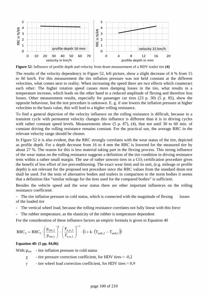
page 100 of 210

Figure 52: Influence of profile depth and velocity from drum measurement of a HDV trailer tire (4)

The results of the velocity dependency in Figure 52, left picture, show a slight decrease of 4 % from 15 to 60 km/h. For this measurement the tire inflation pressure was not held constant at the different velocities, what comes next to reality. When increasing the speed there are two effects which counteract each other: The higher rotation speed causes more damping losses in the tire, what results in a temperature increase, which leads on the other hand to a reduced amplitude of flexing and therefore less losses. Other measurement results, especially for passenger car tires (23 p. 30) (5 p. 85), show the opposite behaviour, but the test procedure is unknown. E. g. if one lowers the inflation pressure at higher velocities to the basis value, this will lead to a higher rolling resistance. To find a general depiction of the velocity influence on the rolling resistance is difficult, because in a transient cycle with permanent velocity changes this influence is different than it is in driving cycles with rather constant speed levels. Measurements show (5 p. 87), (4), that not until 30 to 60 min. of constant driving the rolling resistance remains constant. For the practical use, the average RRC in the relevant velocity range should be chosen. In Figure 52 it is also evident, that the RRC strongly correlates with the wear status of the tire, depicted as profile depth. For a depth decrease from 16 to 4 mm the RRC is lowered for the measured tire by about 27 %. The reason for this is less material taking part in the flexing process. This strong influence of the wear status on the rolling resistance suggests a definition of the tire condition in driving resistance tests within a rather small margin. The use of rather unworn tires in a CO2 certification procedure gives the benefit of low effort of tire preconditioning. The exact wear limit and its unit, (e.g. mileage or profile depth) is not relevant for the proposed test procedure since the RRC values from the standard drum test shall be used. For the tests of alternative bodies and trailers in comparison to the norm bodies it seems that a definition like “similar mileage for the tires used for the compared bodies” is sufficient. Besides the vehicle speed and the wear status there are other important influences on the rolling resistance coefficient: - The tire inflation pressure in cold status, which is connected with the magnitude of flexing losses of the loaded tire - The vertical wheel load, because the rolling resistance correlates not fully linear with this force - The rubber temperature, as the elasticity of the rubber is temperature dependent For the consideration of these influence factors an empiric formula is given in Equation 40

( )( )1,amb2,amb

1

1,w,z

2,w,z

1,tire

2,tire12 TTk1

FF

pp

RRCRRC −⋅+⋅

⋅

⋅=

−γχ

Equation 40: (5 pp. 84,86)

With: ptire - tire inflation pressure in cold status χ - tire pressure correction coefficient, for HDV tires ≈ -0,2 γ - tire wheel load correction coefficient, for HDV tires ≈ 0,9

0

1

2

3

4

5

0 10 20 30 40 50 60 70

RRC

in N

/kN

velocity in km/h

profile depth 16 mm0

1

2

3

4

5

0 4 8 12 16 20

RRC

in N

/kN

profile depth in mm

velocity 15 km/h

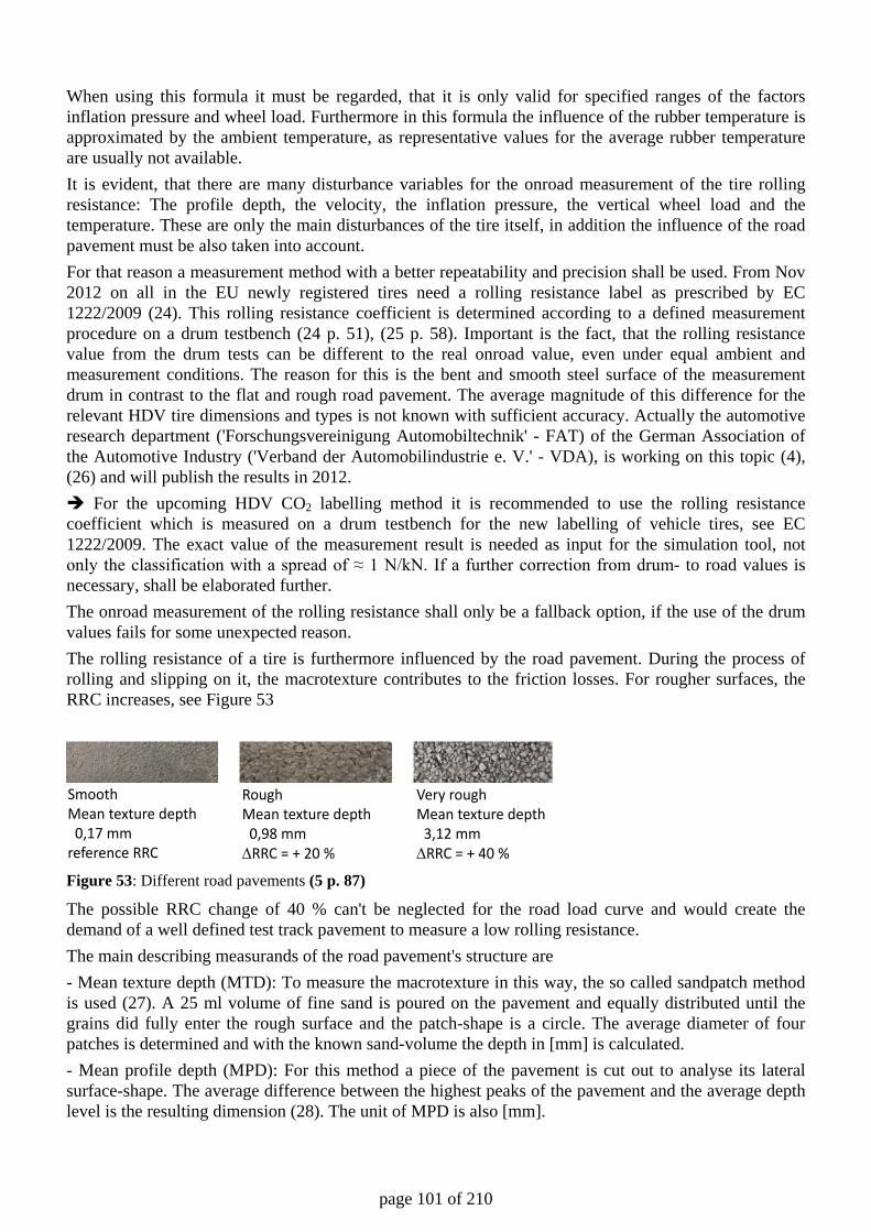
page 101 of 210

When using this formula it must be regarded, that it is only valid for specified ranges of the factors inflation pressure and wheel load. Furthermore in this formula the influence of the rubber temperature is approximated by the ambient temperature, as representative values for the average rubber temperature are usually not available. It is evident, that there are many disturbance variables for the onroad measurement of the tire rolling resistance: The profile depth, the velocity, the inflation pressure, the vertical wheel load and the temperature. These are only the main disturbances of the tire itself, in addition the influence of the road pavement must be also taken into account. For that reason a measurement method with a better repeatability and precision shall be used. From Nov 2012 on all in the EU newly registered tires need a rolling resistance label as prescribed by EC 1222/2009 (24). This rolling resistance coefficient is determined according to a defined measurement procedure on a drum testbench (24 p. 51), (25 p. 58). Important is the fact, that the rolling resistance value from the drum tests can be different to the real onroad value, even under equal ambient and measurement conditions. The reason for this is the bent and smooth steel surface of the measurement drum in contrast to the flat and rough road pavement. The average magnitude of this difference for the relevant HDV tire dimensions and types is not known with sufficient accuracy. Actually the automotive research department ('Forschungsvereinigung Automobiltechnik' - FAT) of the German Association of the Automotive Industry ('Verband der Automobilindustrie e. V.' - VDA), is working on this topic (4), (26) and will publish the results in 2012. For the upcoming HDV CO2 labelling method it is recommended to use the rolling resistance coefficient which is measured on a drum testbench for the new labelling of vehicle tires, see EC 1222/2009. The exact value of the measurement result is needed as input for the simulation tool, not only the classification with a spread of ≈ 1 N/kN. If a further correction from drum- to road values is necessary, shall be elaborated further. The onroad measurement of the rolling resistance shall only be a fallback option, if the use of the drum values fails for some unexpected reason. The rolling resistance of a tire is furthermore influenced by the road pavement. During the process of rolling and slipping on it, the macrotexture contributes to the friction losses. For rougher surfaces, the RRC increases, see Figure 53

Figure 53: Different road pavements (5 p. 87)

The possible RRC change of 40 % can't be neglected for the road load curve and would create the demand of a well defined test track pavement to measure a low rolling resistance. The main describing measurands of the road pavement's structure are - Mean texture depth (MTD): To measure the macrotexture in this way, the so called sandpatch method is used (27). A 25 ml volume of fine sand is poured on the pavement and equally distributed until the grains did fully enter the rough surface and the patch-shape is a circle. The average diameter of four patches is determined and with the known sand-volume the depth in [mm] is calculated. - Mean profile depth (MPD): For this method a piece of the pavement is cut out to analyse its lateral surface-shape. The average difference between the highest peaks of the pavement and the average depth level is the resulting dimension (28). The unit of MPD is also [mm].

SmoothMean texture depth

0,17 mmreference RRC

RoughMean texture depth

0,98 mm∆RRC = + 20 %

Very roughMean texture depth

3,12 mm∆RRC = + 40 %

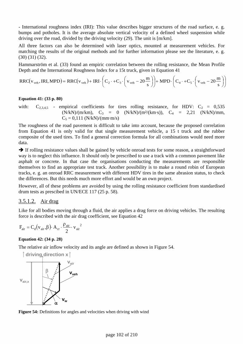
page 102 of 210

- International roughness index (IRI): This value describes bigger structures of the road surface, e. g. bumps and potholes. It is the average absolute vertical velocity of a defined wheel suspension while driving over the road, divided by the driving velocity (29). The unit is [m/km]. All three factors can also be determined with laser optics, mounted at measurement vehicles. For matching the results of the original methods and for further information please see the literature, e. g. (30) (31) (32). Hammarström et al. (33) found an empiric correlation between the rolling resistance, the Mean Profile Depth and the International Roughness Index for a 15t truck, given in Equation 41

( ) ( )

−⋅+⋅⋅+

−⋅+⋅⋅+=

sm20vCCMPD

sm20vCCIRIvRRCMPD,IRI,vRRC veh54veh32vehveh

Equation 41: (33 p. 80)

with: C2,3,4,5 - empirical coefficients for tires rolling resistance, for HDV: C2 = 0,535 (N/kN)/(m/km), C3 = 0 (N/kN)/(m²/(km∙s)), C4 = 2,21 (N/kN)/mm, C5 = 0,111 (N/kN)/(mm∙m/s)

The roughness of the road pavement is difficult to take into account, because the proposed correlation from Equation 41 is only valid for that single measurement vehicle, a 15 t truck and the rubber composite of the used tires. To find a general correction formula for all combinations would need more data. If rolling resistance values shall be gained by vehicle onroad tests for some reason, a straightforward way is to neglect this influence. It should only be prescribed to use a track with a common pavement like asphalt or concrete. In that case the organisations conducting the measurements are responsible themselves to find an appropriate test track. Another possibility is to make a round robin of European tracks, e. g. an onroad RRC measurement with different HDV tires in the same abrasion status, to check the differences. But this needs much more effort and would be an own project. However, all of these problems are avoided by using the rolling resistance coefficient from standardised drum tests as prescibed in UN/ECE 117 (25 p. 58).

3.5.1.2. Air drag

Like for all bodies moving through a fluid, the air applies a drag force on driving vehicles. The resulting force is described with the air drag coefficient, see Equation 42

( ) 2air

aircrairdair v

2A,vCF ⋅

ρ⋅⋅β=

Equation 42: (34 p. 28)

The relative air inflow velocity and its angle are defined as shown in Figure 54.

Figure 54: Definitions for angles and velocities when driving with wind

driving direction x

α

vair

vveh

vw

vair,x

β

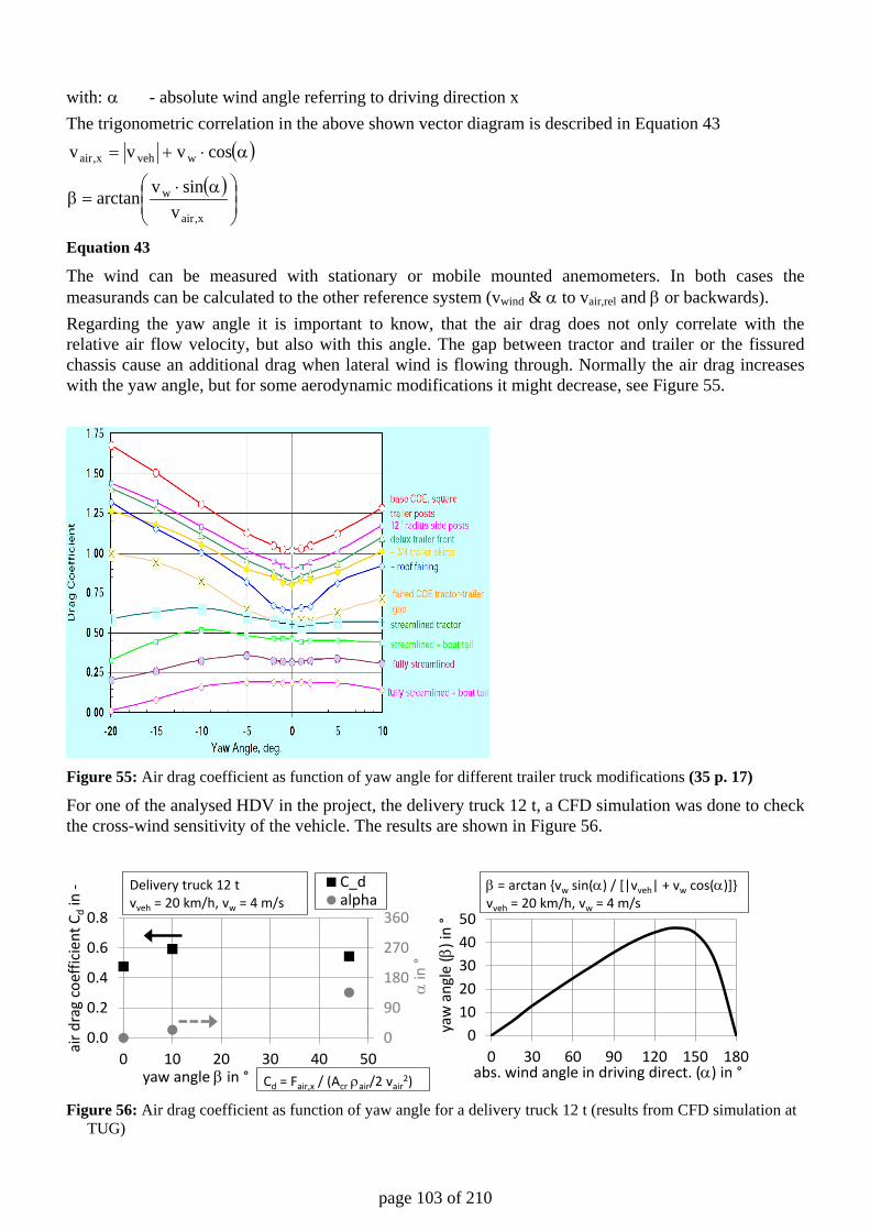
page 103 of 210

with: α - absolute wind angle referring to driving direction x The trigonometric correlation in the above shown vector diagram is described in Equation 43

( )( )

α⋅=β

α⋅+=

x,air

w

wvehx,air

vsinvarctan

cosvvv

Equation 43

The wind can be measured with stationary or mobile mounted anemometers. In both cases the measurands can be calculated to the other reference system (vwind & α to vair,rel and β or backwards). Regarding the yaw angle it is important to know, that the air drag does not only correlate with the relative air flow velocity, but also with this angle. The gap between tractor and trailer or the fissured chassis cause an additional drag when lateral wind is flowing through. Normally the air drag increases with the yaw angle, but for some aerodynamic modifications it might decrease, see Figure 55.

Figure 55: Air drag coefficient as function of yaw angle for different trailer truck modifications (35 p. 17)

For one of the analysed HDV in the project, the delivery truck 12 t, a CFD simulation was done to check the cross-wind sensitivity of the vehicle. The results are shown in Figure 56.

Figure 56: Air drag coefficient as function of yaw angle for a delivery truck 12 t (results from CFD simulation at

TUG)

0

90

180

270

360

0.0

0.2

0.4

0.6

0.8

0 10 20 30 40 50

αin

°

air d

rag

coef

ficie

nt C

din

-

yaw angle β in °

C_dalpha

Delivery truck 12 tvveh = 20 km/h, vw = 4 m/s

Cd = Fair,x / (Acr ρair/2 vair2)

01020304050

0 30 60 90 120 150 180

yaw

ang

le (β

) in

°

β = arctan {vw sin(α) / [|vveh| + vw cos(α)]}vveh = 20 km/h, vw = 4 m/s

abs. wind angle in driving direct. (α) in °

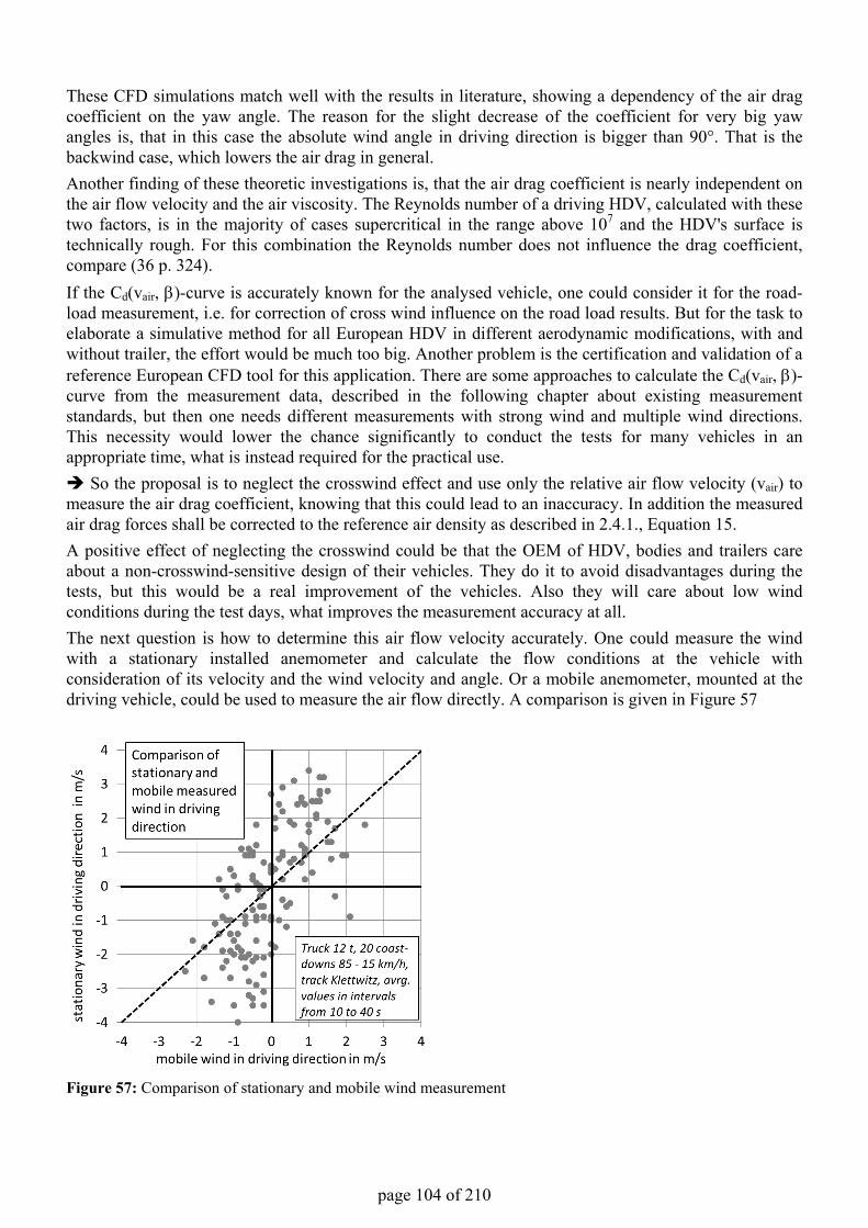
page 104 of 210

These CFD simulations match well with the results in literature, showing a dependency of the air drag coefficient on the yaw angle. The reason for the slight decrease of the coefficient for very big yaw angles is, that in this case the absolute wind angle in driving direction is bigger than 90°. That is the backwind case, which lowers the air drag in general.Another finding of these theoretic investigations is, that the air drag coefficient is nearly independent on the air flow velocity and the air viscosity. The Reynolds number of a driving HDV, calculated with these two factors, is in the majority of cases supercritical in the range above 107 and the HDV's surface is technically rough. For this combination the Reynolds number does not influence the drag coefficient, compare (36 p. 324).If the Cd(vair, β)-curve is accurately known for the analysed vehicle, one could consider it for the road-load measurement, i.e. for correction of cross wind influence on the road load results. But for the task to elaborate a simulative method for all European HDV in different aerodynamic modifications, with and without trailer, the effort would be much too big. Another problem is the certification and validation of a reference European CFD tool for this application. There are some approaches to calculate the Cd(vair, β)-curve from the measurement data, described in the following chapter about existing measurement standards, but then one needs different measurements with strong wind and multiple wind directions. This necessity would lower the chance significantly to conduct the tests for many vehicles in an appropriate time, what is instead required for the practical use. So the proposal is to neglect the crosswind effect and use only the relative air flow velocity (vair) to measure the air drag coefficient, knowing that this could lead to an inaccuracy. In addition the measuredair drag forces shall be corrected to the reference air density as described in 2.4.1., Equation 15.A positive effect of neglecting the crosswind could be that the OEM of HDV, bodies and trailers care about a non-crosswind-sensitive design of their vehicles. They do it to avoid disadvantages during the tests, but this would be a real improvement of the vehicles. Also they will care about low wind conditions during the test days, what improves the measurement accuracy at all.The next question is how to determine this air flow velocity accurately. One could measure the wind with a stationary installed anemometer and calculate the flow conditions at the vehicle with consideration of its velocity and the wind velocity and angle. Or a mobile anemometer, mounted at the driving vehicle, could be used to measure the air flow directly. A comparison is given in Figure 57

Figure 57: Comparison of stationary and mobile wind measurement

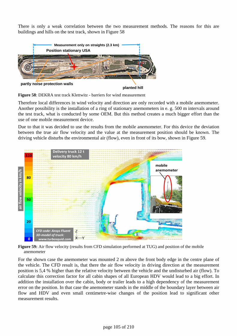
page 105 of 210

There is only a weak correlation between the two measurement methods. The reasons for this are buildings and hills on the test track, shown in Figure 58

Figure 58: DEKRA test track Klettwitz - barriers for wind measurement

Therefore local differences in wind velocity and direction are only recorded with a mobile anemometer. Another possibility is the installation of a ring of stationary anemometers in e. g. 500 m intervals around the test track, what is conducted by some OEM. But this method creates a much bigger effort than the use of one mobile measurement device. Due to that it was decided to use the results from the mobile anemometer. For this device the deviation between the true air flow velocity and the value at the measurement position should be known. The driving vehicle disturbs the environmental air (flow), even in front of its bow, shown in Figure 59.

Figure 59: Air flow velocity (results from CFD simulation performed at TUG) and position of the mobile

anemometer

For the shown case the anemometer was mounted 2 m above the front body edge in the centre plane of the vehicle. The CFD result is, that there the air flow velocity in driving direction at the measurement position is 5,4 % higher than the relative velocity between the vehicle and the undisturbed air (flow). To calculate this correction factor for all cabin shapes of all European HDV would lead to a big effort. In addition the installation over the cabin, body or trailer leads to a high dependency of the measurement error on the position. In that case the anemometer stands in the middle of the boundary layer between air flow and HDV and even small centimetre-wise changes of the position lead to significant other measurement results.

partly noise protection wallsplanted hill

Position stationary USAMeasurement only on straights (2.3 km)

110

80

50

0

20

Delivery truck 12 tvelocity 80 km/h

airf

low

velo

city

in k

m/h

mobileanemometer

CFD code: Ansys Fluent3D-model of truck:

www.turbosquid.com

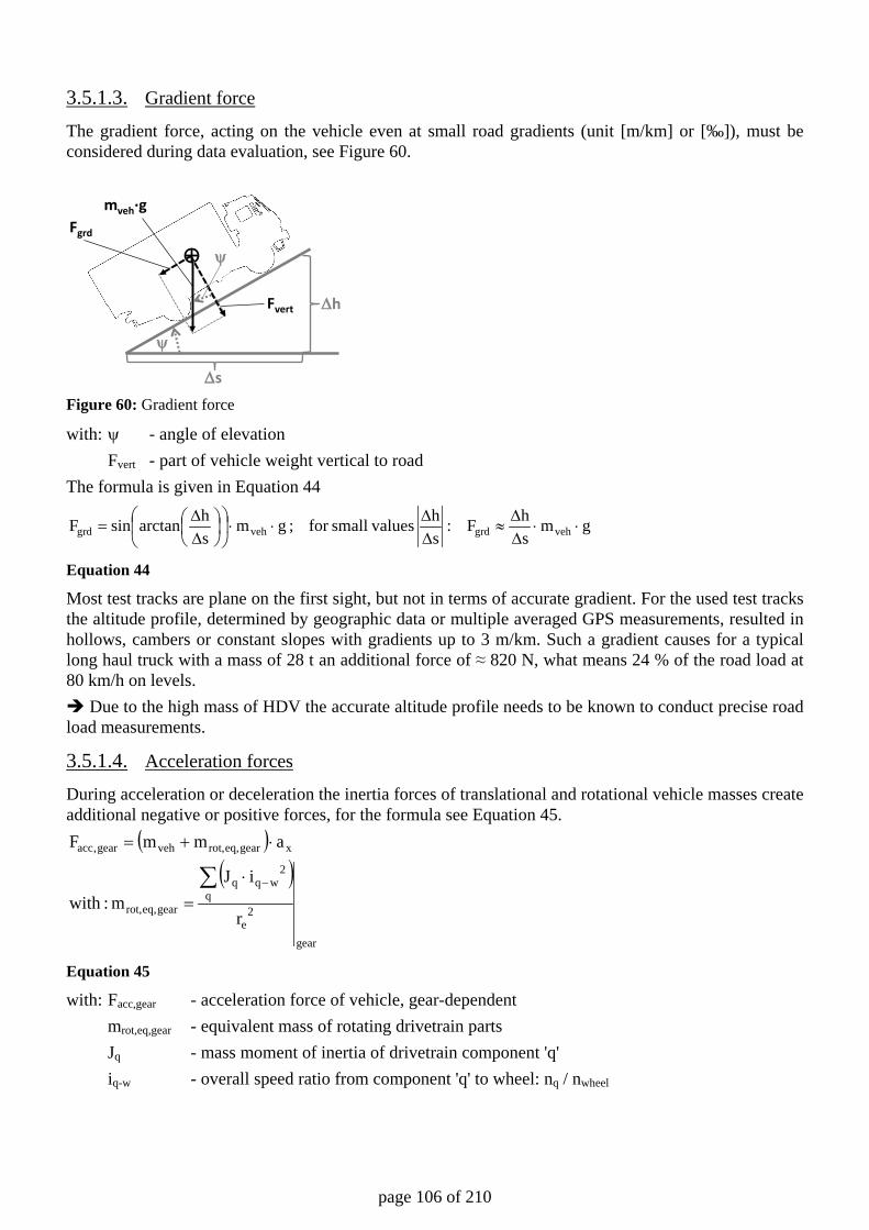
page 106 of 210

3.5.1.3. Gradient force

The gradient force, acting on the vehicle even at small road gradients (unit [m/km] or [‰]), must be considered during data evaluation, see Figure 60.

Figure 60: Gradient force

with: ψ - angle of elevation Fvert - part of vehicle weight vertical to road The formula is given in Equation 44

gmshF :

sh valuessmallfor ; gm

sharctansinF vehgrdvehgrd ⋅⋅

∆∆

≈∆∆

⋅⋅

∆∆

=

Equation 44

Most test tracks are plane on the first sight, but not in terms of accurate gradient. For the used test tracks the altitude profile, determined by geographic data or multiple averaged GPS measurements, resulted in hollows, cambers or constant slopes with gradients up to 3 m/km. Such a gradient causes for a typical long haul truck with a mass of 28 t an additional force of ≈ 820 N, what means 24 % of the road load at 80 km/h on levels. Due to the high mass of HDV the accurate altitude profile needs to be known to conduct precise road load measurements.

3.5.1.4. Acceleration forces

During acceleration or deceleration the inertia forces of translational and rotational vehicle masses create additional negative or positive forces, for the formula see Equation 45.

( )( )

gear

2e

q

2wqq

geareq,rot,

xgeareq,rot,vehgear,acc

r

iJm :with

ammF

∑ −⋅=

⋅+=

Equation 45

with: Facc,gear - acceleration force of vehicle, gear-dependent mrot,eq,gear - equivalent mass of rotating drivetrain parts Jq - mass moment of inertia of drivetrain component 'q' iq-w - overall speed ratio from component 'q' to wheel: nq / nwheel

ψ

ψ

∆h

∆s

Fvert

mveh∙gFgrd

page 107 of 210

The 'equivalent mass of rotating drivetrain parts' (mrot,eq) is a calculation-only value which represents the rotational inertia of the drivetrain, converted to a mass value which is added to the gross vehicle mass. All rotating drivetrain parts engine, gears, shafts, and wheels should be regarded for an accurate simulation of fuel consumption, also the different transmission ratios of the single gears. This leads to the demand to determine an equivalent mass - value for every gear. For the constant speed tests it is sufficient to consider only the wheels, because by torque measurement in the rims the other rotating drivetrain parts are without influence. Heavy construction trucks with 8x8 all wheel drive and a 16 gear drivetrain offer the most complicated configuration, a picture is shown in section '3.5.4 Drivetrain losses', Figure 64 For these vehicles the equivalent mass in the short gears can be bigger than the total vehicle mass, which means that a higher force is needed to accelerate the gears and shafts than the loaded truck itself (23 p. 72). But most HDV use this two- or three-axle drivetrain configuration:

engine - main gear box - differential - rear wheels with one powered axle, what reduces the complexity significantly. The consideration of all drivetrain parts makes the simulation more accurate but also more complicated. But the inertia values themselves are comparatively easy to determine since modern CAD programs offer the possibility to calculate the mass moment of inertia of any component. Available will be default values for the equivalent mass of one wheel, namely 56,7 kg (6 p. 57481) and for the engines. The engine's rotational inertia is measured on the engine test bench during the transient tests. Options for the consideration of the other drivetrain parts shall be elaborated in the pilot phase.

3.5.1.5. Overview of available standards

In this overview of available measurement standards in Table 43 to Table 46 the measurands, measurement conditions, decisive values for validity and the corrections are shortly listed. For more information, the road load equations and comments please see section 5.1. For the sake of completeness it shall be mentioned, that the SAE standards J2881 'Measurement of Aerodynamic Performance for Mass-Produced Cars and Light-Duty Trucks', published 3 Jun 2010, and J2978 'Road Load Measurement Using Coastdown Techniques', work in progress, are not treated. J2978 will describe a coast-down procedure especially for trucks and buses. Regarding the entry "drivetrain coast down losses" in Table 46 it is important to know, that the concerned standards were created to measure the road load for the later adjustment of chassis dynamometers. In the drivetrain of a coasting vehicle idling losses appear which are different to the normal powered case. To include these losses for the dynamometer setup is appropriate, since the chassis dyno is also calibrated via a coastdown procedure on the roller. But for the measurement of the road load as input to the HDV-CO2 simulator these losses shall be eliminated. Therefore the magnitude and the velocity dependency shall be known, what is not the case for the majority of all road vehicles. Actually only measurements of a delivery truck by an OEM are documentated, where these coasting idling losses of the drivetrain accounted for 150 N at 15 km/h, what means about 19 % of the rolling resistance. The accuracies demanded by the existing procedures and the limitations for boundary conditions supported the definition of such values for the HDV-CO2 test procedure where relevant.

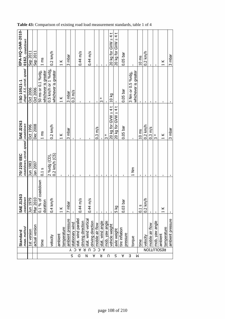
page 108 of 210

Table 43: Comparison of existing road load measurement standards, table 1 of 4

Stan

dard

mea

s. m

etho

dSA

E J1

263

coas

tdow

n70

/220

/EEC

coas

tdow

n, c

onst

. spe

edSA

E J2

263

coas

tdow

nIS

O 1

0521

-1

ch

apt.

5.5

, con

st. s

peed

EPA

-HQ

-OA

R-2

010-

0162

, coa

stdo

wn

1st

vers

ion

Jun

1979

Jun

1983

Oct

199

6O

ct 2

006

Sep

2011

actu

al v

ersi

onM

ar 2

010

Jan

2007

Dec

200

8O

ct 2

006

Sep

2011

time

0.1

% o

f co

astd

own

dura

tion

0.1

s1

ms

50 m

s or

0.1

%rd

g,

whi

chev

er is

gre

ater

1 m

s

velo

city

0.4

km/h

2 %

rdg

(CD

),

0.

2 km

/h (

CS)

0.2

km/h

0.5

km/h

or

1 %

rdg,

w

hich

ever

is g

reat

er0.

2 km

/h

ambi

ent

tem

pera

ture

1 K

-1

K1

K1

K

ambi

ent

pres

sure

7 m

bar

-3

mba

r3

mba

r3

mba

rst

atio

nary

win

d-

--

0.3

m/s

stat

. win

d pa

ralle

l dr

ivin

g di

rect

ion

0.44

m/s

--

-0.

44 m

/s

stat

. win

d ve

rtic

al

driv

ing

dire

ctio

n0.

44 m

/s-

--

0.44

m/s

mob

ile a

ir flo

w-

-0.

3 m

/s-

-st

at. w

ind

angl

e-

--

3 °

-m

ob. y

aw a

ngle

--

3 °

--

vehi

cle

wei

ght

--

20 k

g fo

r G

VW ≥

4 t

10 k

g20

kg

for

GVW

≥ 4

tax

le w

eigh

t5

kg-

20 k

g fo

r G

VW ≥

4 t

-20

kg

for

GVW

≥ 4

ttir

e in

flatio

n pr

essu

re0.

03 b

ar-

0.05

bar

0.05

bar

0.05

bar

torq

ue-

1 N

m-

3 N

m o

r 0.

5 %

rdg,

w

hich

ever

is g

reat

er-

time

0.1

s-

10 m

s-

10 m

sve

loci

ty0.

2 km

/h-

0.2

km/h

-0.

2 km

/hm

obile

air

flow

--

0.3

m/s

--

mob

. yaw

ang

le-

-3

°-

-am

bien

t te

mpe

ratu

re1

K-

1 K

-1

K

ambi

ent

pres

sure

--

3 m

bar

-3

mba

r

M E A S U R A N D S

RESOLUTIONA C C U R A C Y

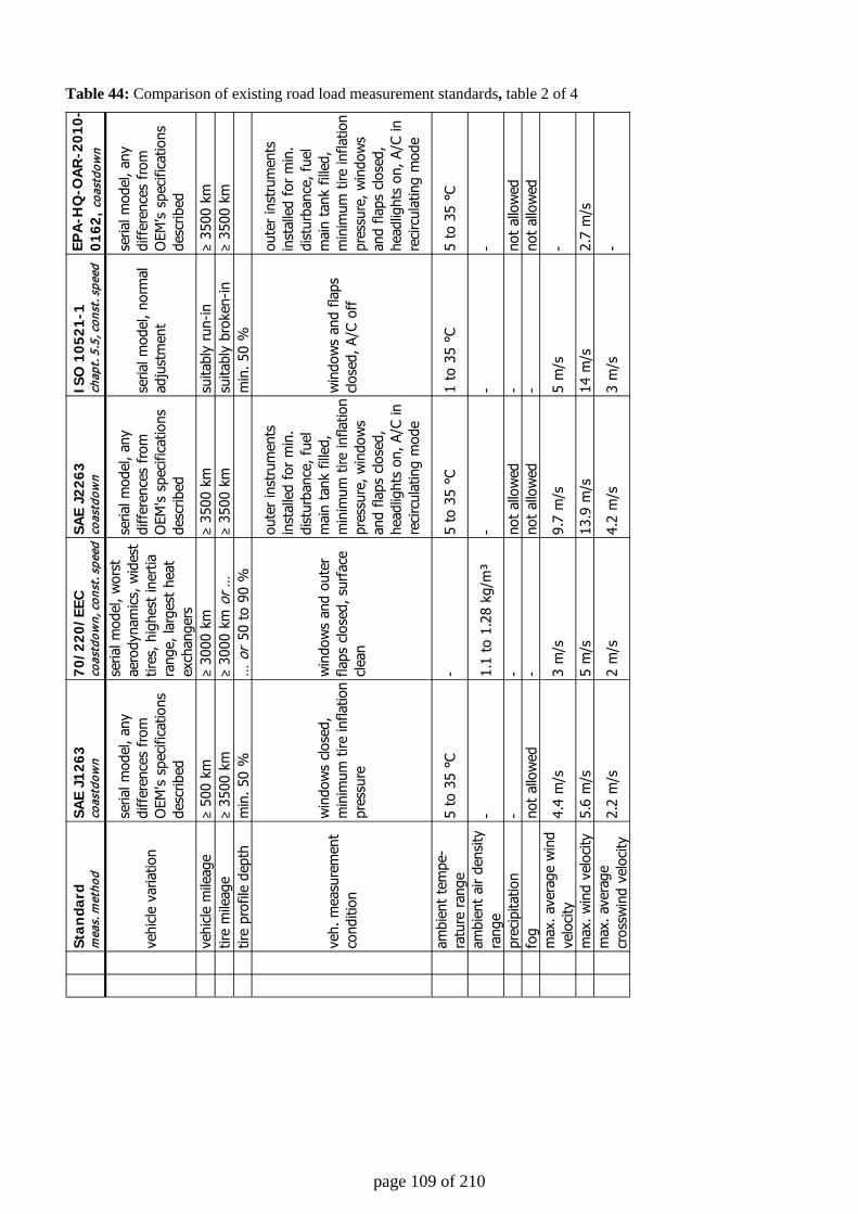
page 109 of 210

Table 44: Comparison of existing road load measurement standards, table 2 of 4

Stan

dard

mea

s. m

etho

dSA

E J1

263

coas

tdow

n70

/220

/EEC

coas

tdow

n, c

onst

. spe

edSA

E J2

263

coas

tdow

nIS

O 1

0521

-1

ch

apt.

5.5

, con

st. s

peed

EPA

-HQ

-OA

R-2

010-

0162

, coa

stdo

wn

vehi

cle

varia

tion

seria

l mod

el, a

ny

diff

eren

ces

from

O

EM's

spe

cific

atio

ns

desc

ribed

seria

l mod

el, w

orst

ae

rody

nam

ics,

wid

est

tires

, hig

hest

iner

tia

rang

e, la

rges

t he

at

exch

ange

rs

seria

l mod

el, a

ny

diff

eren

ces

from

O

EM's

spe

cific

atio

ns

desc

ribed

seria

l mod

el, n

orm

al

adju

stm

ent

seria

l mod

el, a

ny

diff

eren

ces

from

O

EM's

spe

cific

atio

ns

desc

ribed

vehi

cle

mile

age

≥ 50

0 km

≥ 30

00 k

m≥

3500

km

suita

bly

run-

in≥

3500

km

tire

mile

age

≥ 35

00 k

m≥

3000

km

or

…≥

3500

km

suita

bly

brok

en-in

≥ 35

00 k

mtir

e pr

ofile

dep

thm

in. 5

0 %

… o

r 50

to

90 %

min

. 50

%

veh.

mea

sure

men

t co

nditi

on

win

dow

s cl

osed

, m

inim

um t

ire in

flatio

n pr

essu

re

win

dow

s an

d ou

ter

flaps

clo

sed,

sur

face

cl

ean

oute

r in

stru

men

ts

inst

alle

d fo

r m

in.

dist

urba

nce,

fue

l m

ain

tank

fill

ed,

min

imum

tire

infla

tion

pres

sure

, win

dow

s an

d fla

ps c

lose

d,

head

light

s on

, A/C

in

reci

rcul

atin

g m

ode

win

dow

s an

d fla

ps

clos

ed, A

/C o

ff

oute

r in

stru

men

ts

inst

alle

d fo

r m

in.

dist

urba

nce,

fue

l m

ain

tank

fill

ed,

min

imum

tire

infla

tion

pres

sure

, win

dow

s an

d fla

ps c

lose

d,

head

light

s on

, A/C

in

reci

rcul

atin

g m

ode

ambi

ent

tem

pe-

ratu

re r

ange

5 to

35

°C-

5 to

35

°C1

to 3

5 °C

5 to

35

°C

ambi

ent

air

dens

ity

rang

e-

1.1

to 1

.28

kg/m

³-

--

prec

ipita

tion

--

not

allo

wed

-no

t al

low

edfo

gno

t al

low

ed-

not

allo

wed

-no

t al

low

edm

ax. a

vera

ge w

ind

velo

city

4.4

m/s

3 m

/s9.

7 m

/s5

m/s

-

max

. win

d ve

loci

ty5.

6 m

/s5

m/s

13.9

m/s

14 m

/s2.

7 m

/sm

ax. a

vera

ge

cros

swin

d ve

loci

ty2.

2 m

/s2

m/s

4.2

m/s

3 m

/s-

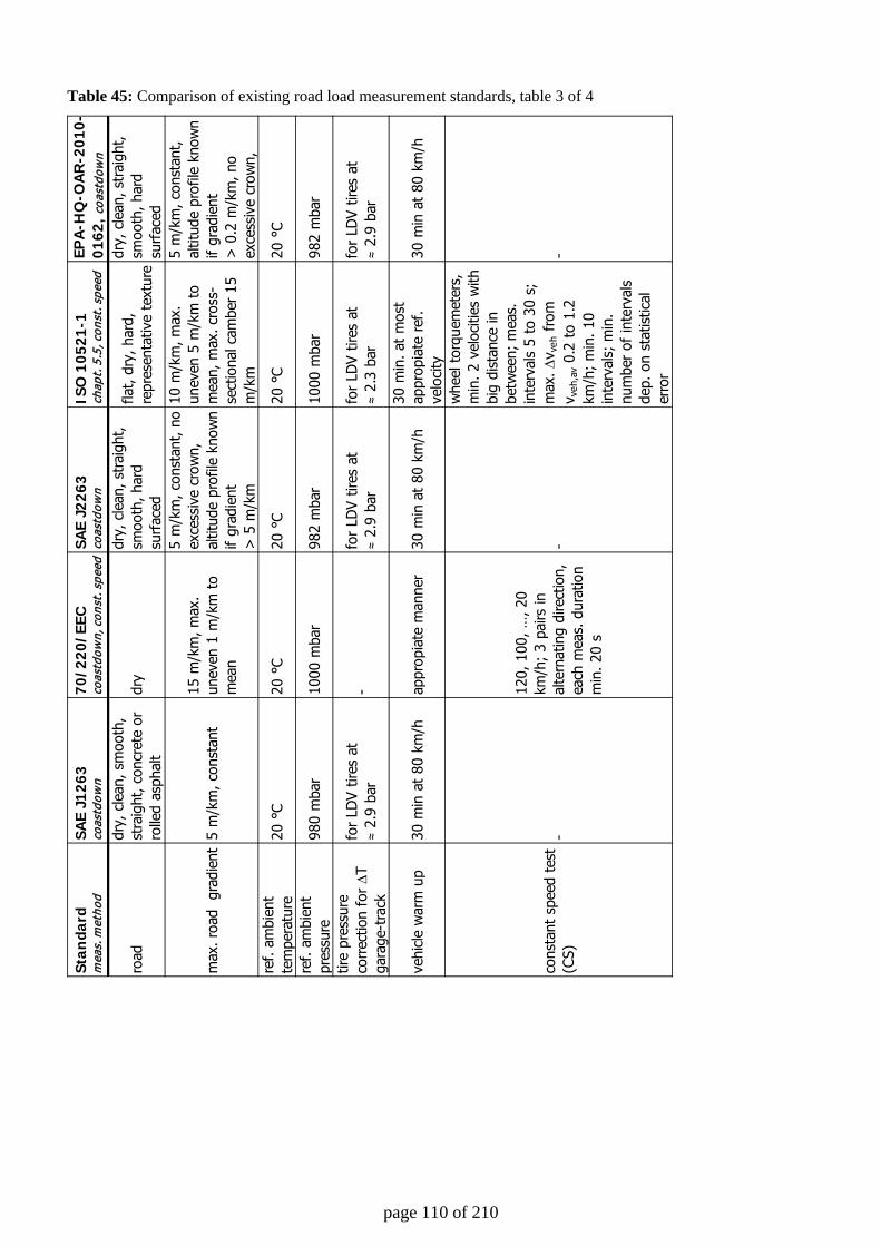
page 110 of 210

Table 45: Comparison of existing road load measurement standards, table 3 of 4

Stan

dard

mea

s. m

etho

dSA

E J1

263

coas

tdow

n70

/220

/EEC

coas

tdow

n, c

onst

. spe

edSA

E J2

263

coas

tdow

nIS

O 1

0521

-1

ch

apt.

5.5

, con

st. s

peed

EPA

-HQ

-OA

R-2

010-

0162

, coa

stdo

wn

road

dry,

cle

an, s

moo

th,

stra

ight

, con

cret

e or

ro

lled

asph

alt

dry

dry,

cle

an, s

trai

ght,

smoo

th, h

ard

surf

aced

flat,

dry,

har

d,

repr

esen

tativ

e te

xtur

e

dry,

cle

an, s

trai

ght,

smoo

th, h

ard

surf

aced

max

. roa

d g

radi

ent

5 m

/km

, con

stan

t15

m/k

m, m

ax.

unev

en 1

m/k

m t

o m

ean

5 m

/km

, con

stan

t, no

ex

cess

ive

crow

n,

altit

ude

prof

ile k

now

n if

grad

ient

> 5

m/k

m

10 m

/km

, max

. un

even

5 m

/km

to

mea

n, m

ax. c

ross

-se

ctio

nal c

ambe

r 15

m

/km

5 m

/km

, con

stan

t, al

titud

e pr

ofile

kno

wn

if gr

adie

nt

>

0.2

m/k

m, n

o ex

cess

ive

crow

n,re

f. am

bien

t te

mpe

ratu

re20

°C

20 °

C20

°C

20 °

C20

°C

ref.

ambi

ent

pres

sure

980

mba

r10

00 m

bar

982

mba

r10

00 m

bar

982

mba

r

tire

pres

sure

co

rrec

tion

for

∆T

gara

ge-t

rack

for

LDV

tires

at

≈ 2.

9 ba

r-

for

LDV

tires

at

≈ 2.

9 ba

rfo

r LD

V tir

es a

t

≈

2.3

bar

for

LDV

tires

at

≈ 2.

9 ba

r

vehi

cle

war

m u

p30

min

at

80 k

m/h

appr

opia

te m

anne

r30

min

at

80 k

m/h

30 m

in. a

t m

ost

appr

opia

te r

ef.

velo

city

30 m

in a

t 80

km

/h

cons

tant

spe

ed t

est

(CS)

-

120,

100

, …, 2

0 km

/h;

3 pa

irs in

al

tern

atin

g di

rect

ion,

ea

ch m

eas.

dur

atio

n m

in. 2

0 s

-

whe

el t

orqu

emet

ers,

m

in. 2

vel

ociti

es w

ith

big

dist

ance

in

betw

een;

mea

s.

inte

rval

s 5

to 3

0 s;

m

ax. ∆

v veh

fro

m

v veh

,av

0.2

to 1

.2

km/h

; m

in. 1

0 in

terv

als;

min

. nu

mbe

r of

inte

rval

s de

p. o

n st

atis

tical

er

ror

-

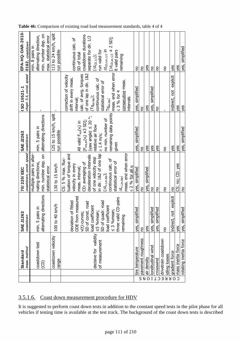
page 111 of 210

Table 46: Comparison of existing road load measurement standards, table 4 of 4

3.5.1.6. Coast down measurement procedure for HDV

It is suggested to perform coast down tests in addition to the constant speed tests in the pilot phase for all vehicles if testing time is available at the test track. The background of the coast down tests is described

Stan

dard

mea

s. m

etho

dSA

E J1

263

coas

tdow

n70

/220

/EEC

coas

tdow

n, c

onst

. spe

edSA

E J2

263

coas

tdow

nIS

O 1

0521

-1

ch

apt.

5.5

, con

st. s

peed

EPA

-HQ

-OA

R-2

010-

0162

, coa

stdo

wn

coas

tdow

n te

st

(CD

)m

in. 5

pai

rs in

al

tern

atin

g di

rect

ions

mul

tiple

pai

rs in

alte

r-na

ting

dire

ctio

ns,

min

. num

ber

dep.

on

stat

istic

al e

rror

min

. 5 p

airs

in

alte

rnat

ing

dire

ctio

ns-

min

. 8 p

airs

in

alte

rnat

ing

dire

ctio

n,

min

. num

ber

dep.

on

max

. sta

tistic

al e

rror

coas

tcow

n ve

loci

ty

rang

e10

0 to

40

km/h

130

to 1

5 km

/h12

5 to

15

km/h

, spl

it ru

n po

ssib

le-

113

to 2

4 km

/h, s

plit

run

poss

ible

deci

sive

for

va

lidity

of

mea

sure

men

t

devi

atio

n of

fitt

ed

OD

E fr

om m

easu

red

v(t)

-cur

ves;

SD o

f co

nst.

road

lo

ad c

oeff

icie

nt

≤

5 %

mea

n;

SD o

f qu

adr.

road

lo

ad c

oeff

icie

nt

≤ 3

%m

ean;

th

ree

valid

CD

-pai

rs

rem

aini

ng

CS:

5 %

max

. flu

c-tu

atio

n of

tor

que

and

velo

city

in e

very

m

eas.

inte

rval

;

CD

: av

erag

ing

of

dece

lera

tion

inte

rval

s of

one

vel

ocity

ste

p in

dir.

1&

2 of

one

lap

(∆t v

.i,av

,lap)

; co

ntin

uous

cal

c. o

f st

atis

tical

err

or o

f ∆t v

.i,av

,lap;

m

eas.

end

whe

n er

ror

≤ 2

% f

or a

ll v i

All v

alid

Fre

s(v i)

in

[Fre

s,av

(vi)

±3

SD];

|y

aw a

ngle

| ≤

20

°;

rela

tive

air

flow

≥ 1.

4 m

/s;

no m

in. n

umbe

r of

re

mai

ning

dat

a po

ints

gi

ven

corr

ectio

n of

vel

ocity

dr

ift in

eve

ry m

eas.

in

terv

al;

ca

lc. o

f av

rg. t

orqu

es

of o

ne la

p in

dir.

1&

2 (T

q av,

lap)

;

co

ntin

uous

cal

c. o

f st

atis

tical

err

or o

f Tq

av,la

p;

mea

s. e

nd w

hen

erro

r ≤

3 %

for

4

cons

ecut

ive

mea

s.

inte

rval

s

cont

inuo

us c

alc.

of

SD o

f to

tal

coas

tdow

n du

ratio

ns

sepa

rate

for

dir.

1/2

(∆

t CD

,1/2

);

run

valid

for

∆t C

D,r

un,1

/2 in

[∆

t CD

,av,

1/2

± 2

SD

];

8 va

lid p

airs

re

mai

ning

yes,

sim

plifi

edye

s, s

impl

ified

yes,

sim

plifi

edye

s, s

impl

ified

nono

nono

nono

yes

yes,

sim

plifi

edye

sye

sye

sye

s, s

impl

ified

noye

sye

s, s

impl

ified

noye

s, s

impl

ified

noye

sno

no

nono

no-

no

indi

rect

, not

ex

plic

itno

yes

indi

rect

, not

ex

plic

itye

sye

sCS

: no

; CD

: ye

sye

sye

sye

sye

s, s

impl

ified

noye

s, s

impl

ified

yes

yes,

sim

plifi

ed

C O R R E C T I O N Stire

tem

pera

ture

pave

men

t ro

ughn

ess

air

dens

itylo

nditu

dina

l win

dcr

ossw

ind

driv

etra

in c

oast

dow

n id

ling

loss

esgr

adie

nt f

orce

mas

s in

ertia

for

cero

tatin

g in

ertia

for

ce

page 112 of 210

here. The correction for ambient conditions (i.e. for the effect of ambient temperature and pressure on the air resistance and for temperature effects on the tires rolling resistance) is described already in chapter 2.4.1.2.1 for constant speed tests. These corrections shall also be applied for coast down data. The driving resistance force consists of rolling resistance, air drag, acceleration resistance and gradient resistance:

grdaccairrollres FFFFF +++= Equation 46

with: Fres total driving resistance [N] Froll rolling resistance [N] Fair air drag [N] Facc acceleration resistance [N] Fgrd gradient resistance [N] The target of the coast down tests is to obtain the air resistance values. In the procedure suggested for the HDV CO2 testing the rolling resistance shall be calculated from the rolling resistance coefficient (RRC) gained from the standardised drum test procedure EC No 1222/2009, if so corrected for the onroad operation, see Equation 3. For the evaluation of the Cd values from coast down tests however, the RRC value from the drum tests shall not be applied but the measured forces have to be used (the drum test RRC value may be applied if sounded test track specific correction functions can be elaborated in future). In the coast down tests sum of forces is zero (neutral gear position and disengaged clutch). Thus the sum of rolling resistance, air drag and gradient resistance has to be equal to the acceleration resistance.

( )t

mm whrotveh ∆∆

⋅+=++=⇔+++== veh,accgrdairrollaccgrdaccairrollres

vF : with,FFFFFFFF0F

Equation 47

With mveh mass of the vehicle (including payload, fuel and driver) [kg] mrot,wh ..... equivalent mass of rotating wheels calculated with Equation 19 [kg] vveh velocity of the vehicle [m/s] t time [s] In the coast down, recommended evaluation velocity intervals of (∆vveh = 10 km/h) from vveh,max to approx. 25 km/h shall be used for the calculation. To obtain correct results for the air drag and the rolling resistance, the force to overcome road gradients has to be subtracted:

( )

∆∆

=ψψ⋅⋅−=+sharctan : with,singmFFF vehaccairroll

Equation 48

With ∆h/∆s ......... road gradient For realistic road gradients sin(ψ) is similar to ∆h/∆s:

shgmFFF vehaccairroll ∆

∆⋅⋅−=+

Equation 49

The split into air resistance and rolling resistance is based on the assumption, that the rolling resistance force at measurement conditions (f0,meas) is independent of the vehicle speed and the air resistance coefficient (f2,meas) depends on the squared vehicle velocity (vveh

2) or the squared air flow velocity (vair

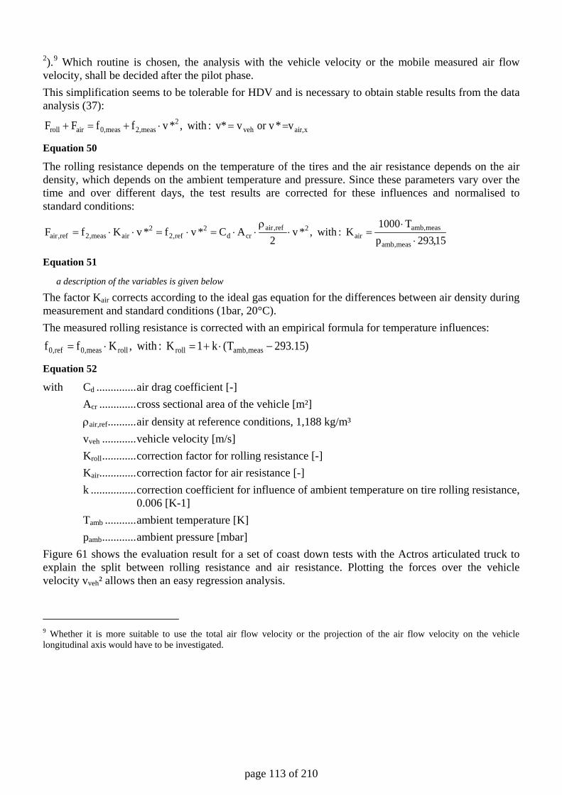
page 113 of 210

2).9 Which routine is chosen, the analysis with the vehicle velocity or the mobile measured air flow velocity, shall be decided after the pilot phase. This simplification seems to be tolerable for HDV and is necessary to obtain stable results from the data analysis (37):

xair,veh2

meas2,meas0,airroll v *or v v v*: with,*vffFF ==⋅+=+

Equation 50

The rolling resistance depends on the temperature of the tires and the air resistance depends on the air density, which depends on the ambient temperature and pressure. Since these parameters vary over the time and over different days, the test results are corrected for these influences and normalised to standard conditions:

15,293pT1000

K : with,*v2

AC*vf*vKfFmeas,amb

meas,ambair

2ref,aircrd

2ref,2

2airmeas,2ref,air ⋅

⋅=⋅

ρ⋅⋅=⋅=⋅⋅=

Equation 51

a description of the variables is given below

The factor Kair corrects according to the ideal gas equation for the differences between air density during measurement and standard conditions (1bar, 20°C).

The measured rolling resistance is corrected with an empirical formula for temperature influences: )15.293T(k1K : with,Kff meas,ambrollrollmeas,0ref,0 −⋅+=⋅=

Equation 52

with Cd .............. air drag coefficient [-] Acr ............. cross sectional area of the vehicle [m²] ρair,ref .......... air density at reference conditions, 1,188 kg/m³ vveh ............ vehicle velocity [m/s] Kroll ............ correction factor for rolling resistance [-] Kair............. correction factor for air resistance [-] k ................ correction coefficient for influence of ambient temperature on tire rolling resistance,

0.006 [K-1] Tamb ........... ambient temperature [K] pamb ............ ambient pressure [mbar] Figure 61 shows the evaluation result for a set of coast down tests with the Actros articulated truck to explain the split between rolling resistance and air resistance. Plotting the forces over the vehicle velocity vveh² allows then an easy regression analysis.

9 Whether it is more suitable to use the total air flow velocity or the projection of the air flow velocity on the vehicle longitudinal axis would have to be investigated.

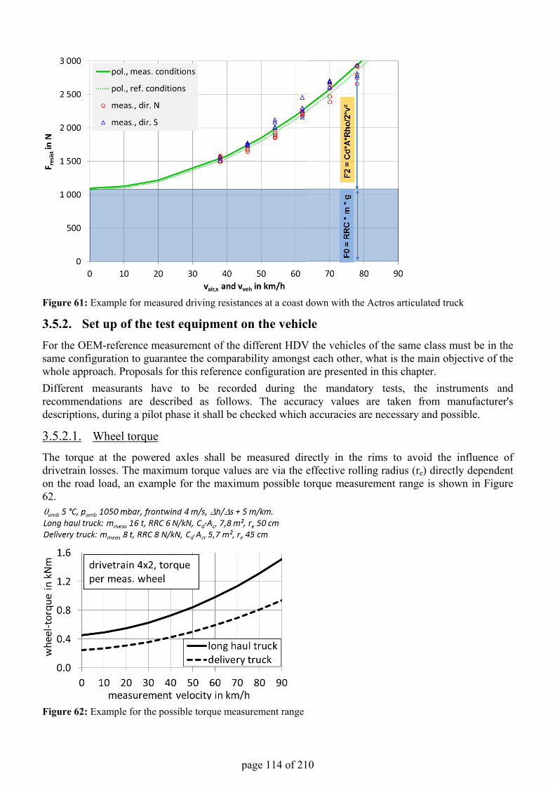
page 114 of 210

Figure 61: Example for measured driving resistances at a coast down with the Actros articulated truck

3.5.2. Set up of the test equipment on the vehicleFor the OEM-reference measurement of the different HDV the vehicles of the same class must be in the same configuration to guarantee the comparability amongst each other, what is the main objective of the whole approach. Proposals for this reference configuration are presented in this chapter.Different measurants have to be recorded during the mandatory tests, the instruments and recommendations are described as follows. The accuracy values are taken from manufacturer's descriptions, during a pilot phase it shall be checked which accuracies are necessary and possible.

3.5.2.1. Wheel torque

The torque at the powered axles shall be measured directly in the rims to avoid the influence of drivetrain losses. The maximum torque values are via the effective rolling radius (re) directly dependent on the road load, an example for the maximum possible torque measurement range is shown in Figure 62.

Figure 62: Example for the possible torque measurement range

page 115 of 210

It must be regarded, that these values are only valid for constant speed tests. During acceleration in small gears the wheel torque can be more than 10 times higher. It is not necessary to measure these big torques, but the torquemeters must withstand the maximum acceleration, which may be limited. The measurement error of commercially available torquemeters ranges from 0,1 to 1 %fso (38) (39). with: %fso - percentage of full scale output (maximum measurement value of an instrument). The full scale output in case of available HDV instruments is e. g. ≈ 6000 Nm. In ISO 10521 an accuracy of 0,5 %rdg is demanded, what is adequate for the road load measurement and shall be verified during the first test phase. with: %rdg - percentage of reading (actual measurement value)

3.5.2.2. Engine fuel flow

The fuel flow meter is to be installed in the fuel delivery- and return line. The result shall be the fuel mass flow consumed by the engine. If the instrument measures only the volume flow, the local temperature at the measurement position must be recorded in addition to determine the fuel density. Examples for the accuracy are 0,1 %rdg for an actual mass flow meter (40) or 1 %rdg for a volume flow meter (41). Because for the density-measurement also an inaccuracy must be regarded, 1 %rdg only for the volume flow doesn't reflect the entire uncertainty. For the HDV CO2 labelling procedure a maximum fuel mass flow error of 0,5 %rdg is recommended.

3.5.2.3. Vehicle velocity

The velocity of the test HDV shall be measured and recorded accurately. The standard speedometer in the cockpit is not precise enough. It uses the rotational speed of one wheel and its effective rolling radius, which is influenced by the wheel slip. The slip is dependent on the wheel torque and not constant for all velocities or during acceleration or braking. One possible separate speedometer is a satellite navigation instrument. Devices for the installation in vehicles are offered with an absolute accuracy of 0,1 km/h (42). But the experience shows, that the value from such instruments can be questionable and the measurand quality is highly dependent on the number of received satellites. Nevertheless it should work for constant speed tests and coastdowns in the case of good reception. Another measurement principle are optical sensors which are mounted besides the vehicle and record the relative movement to the road pavement. An example for the accuracy of such devices is 0,5 km/h (43). The demand of ISO 10521-1 is also 0,5 km/h. A high accuracy of the velocity measurement is necessary, because errors lead to a wrong velocity drift correction during constant speed tests. E. g. for a time interval of 20 s and a velocity error of 0,1 km/h the maximum theoretical correction error for the road load is ≈ 50 N for an long haul truck (mmeas = 16 t, mrot,wh = 860 kg). This means about 1,4 % of the total road load at 80 km/h. Which instrument type fullfills the demanded accuracy the best shall be further elaborated.

3.5.2.4. Road gradient

For the calculation of the gradient force the road gradient has to be known. A direct measurement with a mobile clinometer is difficult, because the absolute declination of the vehicle itself must be measured at first. So the best practice is to measure the altitude at fixed-points of the test track with known geographic position, e. g. every 100 m. With precise satellite navigation combined with landmarks a high accuracy of ≈ 3 cm is possible (44 p. 51), some test tracks are already measured with this method (45).

page 116 of 210

This accuracy is necessary, because the maximum altitude error (2 ∙ 3 cm / 100 m) would cause a gradient force error of ≈ 90 N for a 16 t truck, which means 2,5 % of the total road load at 80 km/h. When the position of the tested HDV is measured, the actual altitude and gradient can be interpolated between the fixed-points. The position accuracy of actual satellite navigation systems is about 3 m (42), what is sufficient for the altitude interpolation.

3.5.2.5. Air flow velocity and yaw angle

The relative air flow velocity and the yaw angle shall be measured with an anemometer mounted in a suitable position. The anemometer readings shall be calibrated in comparison to stationary anemometer readings performed at the same time near the driving vehicle . Possible measurement instruments are cup anemometers with separate wind direction sensors or ultrasonic anemometers. The accuracy of high precision cup anemometers is 1 %rdg (46), appropiate direction sensors reach 0,25 %rdg (47). Standard cup anemometers and direction sensors measure with 2 %rdg and 0,7 %rdg (48). The error of ultrasonic anemometers for the wind velocity is 2 %rdg, the direction error ranges between 0,3 and 0,8 %rdg (49) (50) (51). These instruments measure the wind velocity and its direction at once. For the practical use it must be regarded, that liquid water in the air, e. g. light rain or even fog, disturbs the measurement by changing the speed of sound. The recommendation for the pilot phase is an accuracy of at least 2 %rdg for air flow velocity and angle.

3.5.2.6. Engine rotational speed

The engine speed needs to be known to interpolate the fuel consumption in the referring map, please compare the chapter '3.5.3 The engine fuel consumption map'. It is a standard measurement value of every modern vehicle and can be received from the CAN Bus data. The serial measurement method is an inductive sensor at the flywheel (52 p. 332). With external optical sensors an accuracy of ≈ 0,1 %rdg is possible (53), what shall be reached with any method.

3.5.2.7. Others

Following settings and boundary conditions may have to be defined more precisely, depending on the sensitivity found in next measurements:

• Standard aerodynamic configuration • Design of the tractor for the test of semi-trailers • Preparation of the standard bodies and trailers • Tire conditions • Environmental conditions • Test track • Weather

3.5.3. The engine fuel consumption map The procedure of measuring the engine fuel consumption map is already described in chapter 2.4.2.

3.5.4. Drivetrain losses The drivetrain consists of all mechanical and hydraulic power transmission elements between the engine crankshaft and the wheel. They can contribute up to more than 10 % of the FC, dependent on the gear box type and on the operating point of the main gear box. A picture of the typical structure of a HDV drivetrain is shown in Figure 63

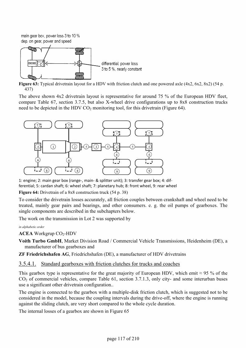
page 117 of 210

Figure 63: Typical drivetrain layout for a HDV with friction clutch and one powered axle (4x2, 6x2, 8x2) (54 p. 437)

The above shown 4x2 drivetrain layout is representative for around 75 % of the European HDV fleet, compare Table 67, section 3.7.5, but also X-wheel drive configurations up to 8x8 construction trucks need to be depicted in the HDV CO2 monitoring tool, for this drivetrain (Figure 64).

Figure 64: Drivetrain of a 8x8 construction truck (54 p. 38)To consider the drivetrain losses accurately, all friction couples between crankshaft and wheel need to be treated, mainly gear pairs and bearings, and other consumers. e. g. the oil pumps of gearboxes. The single components are described in the subchapters below.The work on the transmission in Lot 2 was supported byin alphabetic order

ACEA Workgrup CO2-HDVVoith Turbo GmbH, Market Division Road / Commercial Vehicle Transmissions, Heidenheim (DE), a

manufacturer of bus gearboxes andZF Friedrichshafen AG, Friedrichshafen (DE), a manufacturer of HDV drivetrains

3.5.4.1. Standard gearboxes with friction clutches for trucks and coaches

This gearbox type is representative for the great majority of European HDV, which emit ≈ 95 % of the CO2 of commercial vehicles, compare Table 61, section 3.7.1.3, only city- and some interurban buses use a significant other drivetrain configuration..The engine is connected to the gearbox with a multiple-disk friction clutch, which is suggested not to be considered in the model, because the coupling intervals during the drive-off, where the engine is running against the sliding clutch, are very short compared to the whole cycle duration.The internal losses of a gearbox are shown in Figure 65

1: engine; 2: main gear box (range-, main- & splitter unit); 3: transfer gear box; 4: dif-ferential; 5: cardan shaft; 6: wheel shaft; 7: planetary hub; 8: front wheel, 9: rear wheel

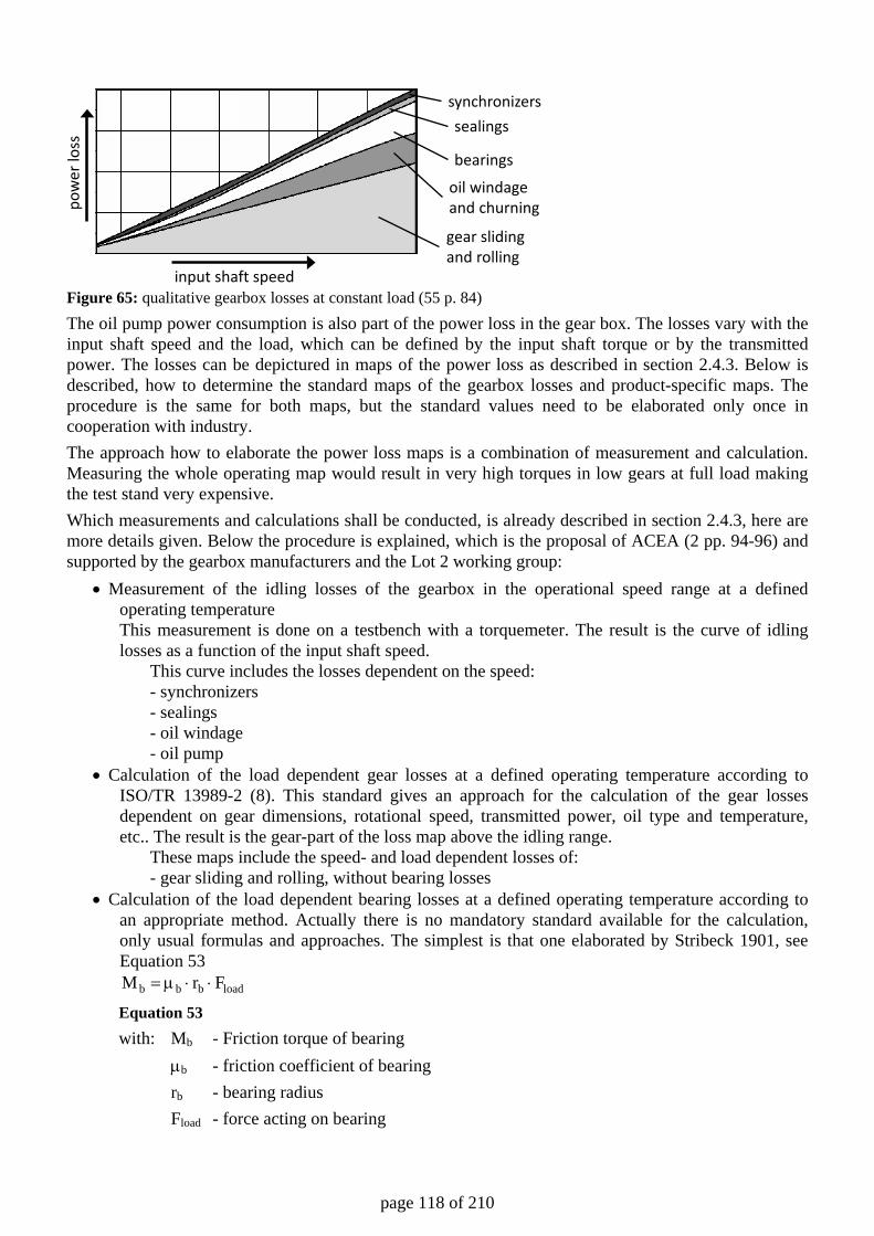
page 118 of 210

Figure 65: qualitative gearbox losses at constant load (55 p. 84) The oil pump power consumption is also part of the power loss in the gear box. The losses vary with the input shaft speed and the load, which can be defined by the input shaft torque or by the transmitted power. The losses can be depictured in maps of the power loss as described in section 2.4.3. Below is described, how to determine the standard maps of the gearbox losses and product-specific maps. The procedure is the same for both maps, but the standard values need to be elaborated only once in cooperation with industry. The approach how to elaborate the power loss maps is a combination of measurement and calculation. Measuring the whole operating map would result in very high torques in low gears at full load making the test stand very expensive. Which measurements and calculations shall be conducted, is already described in section 2.4.3, here are more details given. Below the procedure is explained, which is the proposal of ACEA (2 pp. 94-96) and supported by the gearbox manufacturers and the Lot 2 working group:

• Measurement of the idling losses of the gearbox in the operational speed range at a defined operating temperature This measurement is done on a testbench with a torquemeter. The result is the curve of idling losses as a function of the input shaft speed.

This curve includes the losses dependent on the speed: - synchronizers - sealings - oil windage - oil pump

• Calculation of the load dependent gear losses at a defined operating temperature according to ISO/TR 13989-2 (8). This standard gives an approach for the calculation of the gear losses dependent on gear dimensions, rotational speed, transmitted power, oil type and temperature, etc.. The result is the gear-part of the loss map above the idling range.

These maps include the speed- and load dependent losses of: - gear sliding and rolling, without bearing losses

• Calculation of the load dependent bearing losses at a defined operating temperature according to an appropriate method. Actually there is no mandatory standard available for the calculation, only usual formulas and approaches. The simplest is that one elaborated by Stribeck 1901, see Equation 53

loadbbb FrM ⋅⋅µ=

Equation 53 with: Mb - Friction torque of bearing µb - friction coefficient of bearing rb - bearing radius Fload - force acting on bearing

input shaft speed

pow

er lo

ss

synchronizerssealings

bearings

oil windageand churning

gear slidingand rolling

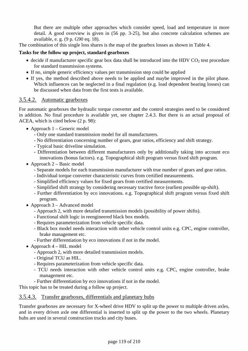
page 119 of 210

But there are multiple other approaches which consider speed, load and temperature in more detail. A good overview is given in (56 pp. 3-25), but also concrete calculation schemes are available, e. g. (9 p. G90 eq. 18).

The combination of this single loss shares is the map of the gearbox losses as shown in Table 4. Tasks for the follow up project, standard gearboxes

• decide if manufacturer specific gear box data shall be introduced into the HDV CO2 test procedure for standard transmission systems.

• If no, simple generic efficiency values per transmission step could be applied • If yes, the method described above needs to be applied and maybe improved in the pilot phase.

Which influences can be neglected in a final regulation (e.g. load dependent bearing losses) can be discussed when data from the first tests is available.

3.5.4.2. Automatic gearboxes

For automatic gearboxes the hydraulic torque converter and the control strategies need to be considered in addition. No final procedure is available yet, see chapter 2.4.3. But there is an actual proposal of ACEA, which is cited below (2 p. 98):

• Approach 1 – Generic model - Only one standard transmission model for all manufacturers. - No differentiation concerning number of gears, gear ratios, efficiency and shift strategy. - Typical basic driveline simulation. - Differentiation between different manufacturers only by additionally taking into account eco

innovations (bonus factors). e.g. Topographical shift program versus fixed shift program. • Approach 2 – Basic model

- Separate models for each transmission manufacturer with true number of gears and gear ratios. - Individual torque converter characteristic curves from certified measurements. - Simplified efficiency values for fixed gears from certified measurements. - Simplified shift strategy by considering necessary tractive force (earliest possible up-shift). - Further differentiation by eco innovations. e.g. Topographical shift program versus fixed shift

program. • Approach 3 – Advanced model

- Approach 2, with more detailed transmission models (possibility of power shifts). - Functional shift logic in reengineered black box models. - Requires parameterization from vehicle specific data. - Black box model needs interaction with other vehicle control units e.g. CPC, engine controller,

brake management etc. - Further differentiation by eco innovations if not in the model.

• Approach 4 – HIL model - Approach 2, with more detailed transmission models. - Original TCU as HIL. - Requires parameterization from vehicle specific data. - TCU needs interaction with other vehicle control units e.g. CPC, engine controller, brake

management etc. - Further differentiation by eco innovations if not in the model.

This topic has to be treated during a follow up project.

3.5.4.3. Transfer gearboxes, differentials and planetary hubs

Transfer gearboxes are necessary for X-wheel drive HDV to split up the power to multiple driven axles, and in every driven axle one differential is inserted to split up the power to the two wheels. Planetary hubs are used in several construction trucks and city buses.

page 120 of 210

These devices can be treated as one-gear gearbox, similar to the procedures described in section 3.5.4.1. The simplest approach is one average value for the mechanical efficiency. As for the gear boxes it has to be decided if model specific data for the losses in differentials or simple default values shall be applied.

3.5.4.4. Wheel bearings

For the vertical loaded wheel bearings the same calculation may be used like for the gearbox bearings, see section 3.5.4.1. If one uses the formula of Stribeck with typical values for a trailer truck 28 t (µb ≈ 0,0015 to 0,002 (57 p. 730); rb ≈ 4,8 cm; re ≈ 0,5 m), the resulting friction torque is about 20 Nm. This leads to an additional driving resistance force of 40 N, what is about 1 % of the total resistance at 80 km/h. This friction force is nearly constant in all driving conditions and small compared to the other driving resistances. If the friction torque has to be added to the measured road load, depends on the measurement procedure. For a torquemeter installed at the cardan shaft, multiple additional losses between the measurement point and the wheel, e. g. differential and wheel bearing friction have to be be added. If the torque is measured in the wheel rim, all drivetrain friction is excluded.

3.5.4.5. Miscellaneous

In addition there are some smaller power losses in the drivetrain: • Idling retarder brake • Sealings of the wheel mounts • Touching brake shoes

These are nearly independent of the engine power, vehicle weight or rotating speed. They may be depicted with one overall torque loss at the wheel axles or neglected completely in the test procedure. Furthermore it has to be decided, if different operating temperatures need to be considered in one HDV class. E. g. the oil cooler of the main gearbox, which determines its oil temperature, is integrated in the vehicle cooling circuit. The cooling system layout and temperature level vary among the HDV of different OEM in one class. In general, operating temperatures of the gear boxes in a test procedure may need a clear definition since the losses depend on the temperature level. A list, without claim to be complete, of available standards for the measurement of drivetrain losses is given in section 5.3.

3.5.5. Power consumption of auxiliary units Auxiliaries do not have a very high share on the fuel consumption of long haul trucks (Figure 66), but for some categories, such as city buses, they have a quite high share. Additionally it is expected that auxiliaries and their control strategies have potential for fuel savings in future.

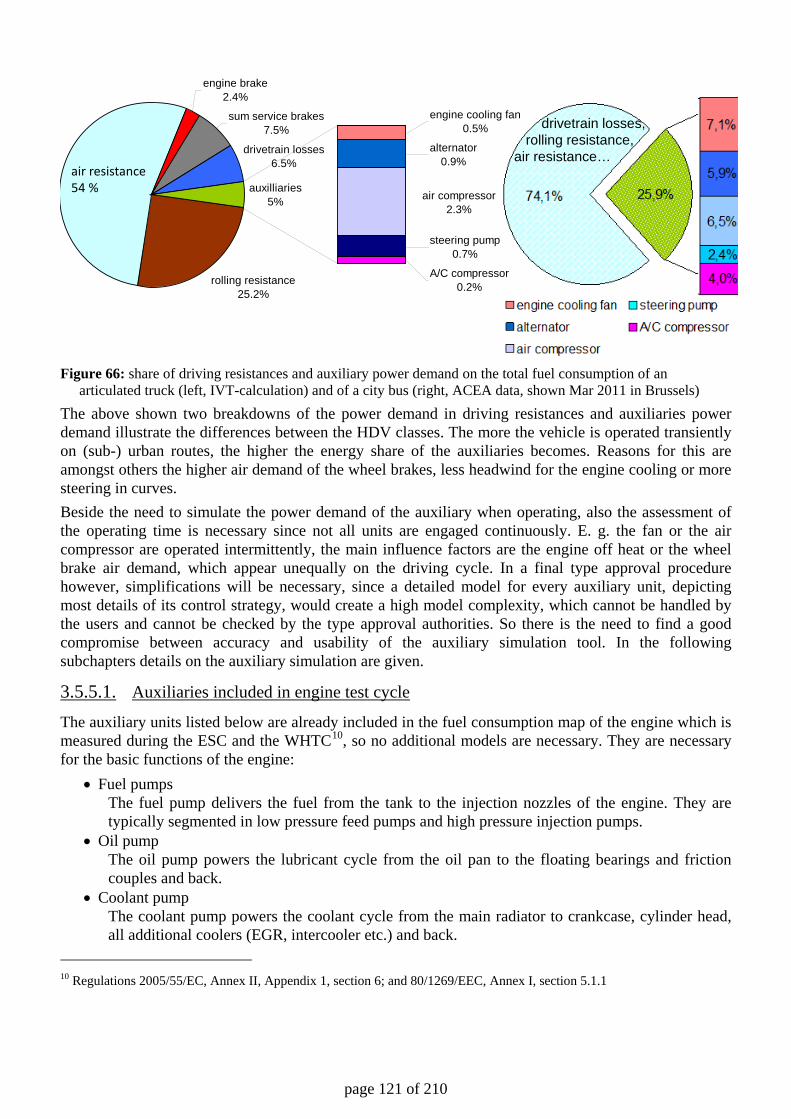
page 121 of 210

Figure 66: share of driving resistances and auxiliary power demand on the total fuel consumption of an

articulated truck (left, IVT-calculation) and of a city bus (right, ACEA data, shown Mar 2011 in Brussels) The above shown two breakdowns of the power demand in driving resistances and auxiliaries power demand illustrate the differences between the HDV classes. The more the vehicle is operated transiently on (sub-) urban routes, the higher the energy share of the auxiliaries becomes. Reasons for this are amongst others the higher air demand of the wheel brakes, less headwind for the engine cooling or more steering in curves. Beside the need to simulate the power demand of the auxiliary when operating, also the assessment of the operating time is necessary since not all units are engaged continuously. E. g. the fan or the air compressor are operated intermittently, the main influence factors are the engine off heat or the wheel brake air demand, which appear unequally on the driving cycle. In a final type approval procedure however, simplifications will be necessary, since a detailed model for every auxiliary unit, depicting most details of its control strategy, would create a high model complexity, which cannot be handled by the users and cannot be checked by the type approval authorities. So there is the need to find a good compromise between accuracy and usability of the auxiliary simulation tool. In the following subchapters details on the auxiliary simulation are given.

3.5.5.1. Auxiliaries included in engine test cycle

The auxiliary units listed below are already included in the fuel consumption map of the engine which is measured during the ESC and the WHTC10, so no additional models are necessary. They are necessary for the basic functions of the engine:

• Fuel pumps The fuel pump delivers the fuel from the tank to the injection nozzles of the engine. They are typically segmented in low pressure feed pumps and high pressure injection pumps.

• Oil pump The oil pump powers the lubricant cycle from the oil pan to the floating bearings and friction couples and back.

• Coolant pump The coolant pump powers the coolant cycle from the main radiator to crankcase, cylinder head, all additional coolers (EGR, intercooler etc.) and back.

10 Regulations 2005/55/EC, Annex II, Appendix 1, section 6; and 80/1269/EEC, Annex I, section 5.1.1

drivetrain losses,rolling resistance,

air resistance…

rolling resistance25.2%

engine brake2.4%

sum service brakes7.5%

drivetrain losses6.5%

engine cooling fan0.5%

alternator0.9%

air compressor2.3%

steering pump0.7%

A/C compressor0.2%

auxilliaries5%

air resistance54 %

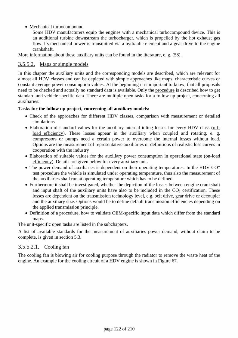
page 122 of 210

• Mechanical turbocompound Some HDV manufacturers equip the engines with a mechanical turbocompound device. This is an additional turbine downstream the turbocharger, which is propelled by the hot exhaust gas flow. Its mechanical power is transmitted via a hydraulic element and a gear drive to the engine crankshaft.

More information about these auxiliary units can be found in the literature, e. g. (58).

3.5.5.2. Maps or simple models

In this chapter the auxiliary units and the corresponding models are described, which are relevant for almost all HDV classes and can be depicted with simple approaches like maps, characteristic curves or constant average power consumption values. At the beginning it is important to know, that all proposals need to be checked and actually no standard data is available. Only the procedure is described how to get standard and vehicle specific data. There are multiple open tasks for a follow up project, concerning all auxiliaries: Tasks for the follow up project, concerning all auxiliary models:

• Check of the approaches for different HDV classes, comparison with measurement or detailed simulations

• Elaboration of standard values for the auxiliary-internal idling losses for every HDV class (off-load efficiency). These losses appear in the auxiliary when coupled and rotating, e. g. compressors or pumps need a certain power to overcome the internal losses without load. Options are the measurement of representative auxiliaries or definitions of realistic loss curves in cooperation with the industry

• Elaboration of suitable values for the auxiliary power consumption in operational state (on-load efficiency). Details are given below for every auxiliary unit.

• The power demand of auxiliaries is dependent on their operating temperatures. In the HDV-CO” test procedure the vehicle is simulated under operating temperature, thus also the measurement of the auxiliaries shall run at operating temperature which has to be defined.

• Furthermore it shall be investigated, whether the depiction of the losses between engine crankshaft and input shaft of the auxiliary units have also to be included in the CO2 certification. These losses are dependent on the transmission technology level, e.g. belt drive, gear drive or decoupler and the auxiliary size. Options would be to define default transmission efficiencies depending on the applied transmission principle.

• Definition of a procedure, how to validate OEM-specific input data which differ from the standard maps.

The unit-specific open tasks are listed in the subchapters. A list of available standards for the measurement of auxiliaries power demand, without claim to be complete, is given in section 5.3.

3.5.5.2.1. Cooling fan The cooling fan is blowing air for cooling purpose through the radiator to remove the waste heat of the engine. An example for the cooling circuit of a HDV engine is shown in Figure 67.

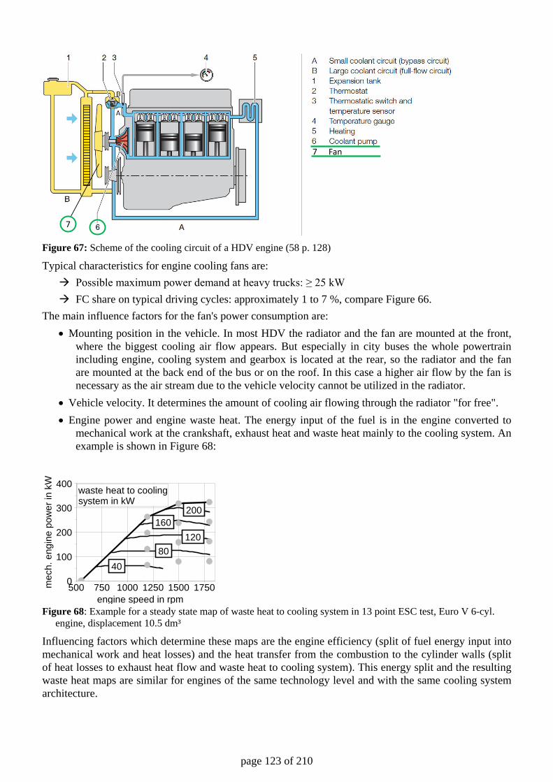
page 123 of 210

Figure 67: Scheme of the cooling circuit of a HDV engine (58 p. 128)

Typical characteristics for engine cooling fans are: Possible maximum power demand at heavy trucks: ≥ 25 kW FC share on typical driving cycles: approximately 1 to 7 %, compare Figure 66.

The main influence factors for the fan's power consumption are: • Mounting position in the vehicle. In most HDV the radiator and the fan are mounted at the front,

where the biggest cooling air flow appears. But especially in city buses the whole powertrain including engine, cooling system and gearbox is located at the rear, so the radiator and the fan are mounted at the back end of the bus or on the roof. In this case a higher air flow by the fan is necessary as the air stream due to the vehicle velocity cannot be utilized in the radiator.

• Vehicle velocity. It determines the amount of cooling air flowing through the radiator "for free". • Engine power and engine waste heat. The energy input of the fuel is in the engine converted to

mechanical work at the crankshaft, exhaust heat and waste heat mainly to the cooling system. An example is shown in Figure 68:

Figure 68: Example for a steady state map of waste heat to cooling system in 13 point ESC test, Euro V 6-cyl.

engine, displacement 10.5 dm³

Influencing factors which determine these maps are the engine efficiency (split of fuel energy input into mechanical work and heat losses) and the heat transfer from the combustion to the cylinder walls (split of heat losses to exhaust heat flow and waste heat to cooling system). This energy split and the resulting waste heat maps are similar for engines of the same technology level and with the same cooling system architecture.

Fan7

7

mec

h. e

ngin

e po

wer

in k

W

0

100

200

300

400

engine speed in rpm500 750 1000 1250 1500 1750

200160

12080

40

waste heat to coolingsystem in kW

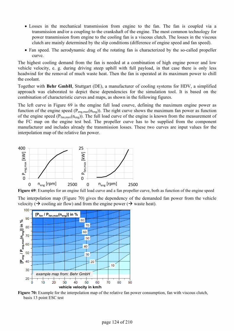
page 124 of 210

• Losses in the mechanical transmission from engine to the fan. The fan is coupled via a transmission and/or a coupling to the crankshaft of the engine. The most common technology for power transmission from engine to the cooling fan is a viscous clutch. The losses in the viscous clutch are mainly determined by the slip conditions (difference of engine speed and fan speed).

• Fan speed. The aerodynamic drag of the rotating fan is characterized by the so-called propeller curve.

The highest cooling demand from the fan is needed at a combination of high engine power and low vehicle velocity, e. g. during driving steep uphill with full payload, in that case there is only less headwind for the removal of much waste heat. Then the fan is operated at its maximum power to chill the coolant.Together with Behr GmbH, Stuttgart (DE), a manufacturer of cooling systems for HDV, a simplified approach was elaborated to depict these dependencies for the simulation tool. It is based on the combination of characteristic curves and maps, as shown in the following figures.

The left curve in Figure 69 is the emgine full load courve, defining the maximum engine power as function of the engine speed (Peng,max(neng)). The right curve shows the maximum fan power as function of the engine speed (Pfan,max(neng)). The full load curve of the engine is known from the measurement of the FC map on the engine test bed. The propeller curve has to be supplied from the component manufacturer and includes already the transmission losses. These two curves are input values for the interpolation map of the relative fan power.

Figure 69: Examples for an engine full load curve and a fan propeller curve, both as function of the engine speed

The interpolation map (Figure 70) gives the dependency of the demanded fan power from the vehicle velocity ( cooling air flow) and from the engine power ( waste heat).

Figure 70: Example for the interpolation map of the relative fan power consumption, fan with viscous clutch, basis 13 point ESC test

0

400

0 2500

P eng

,max

[kW

]

neng [rpm]0

25

0 2500

P fan

,max

[kW

]

neng [rpm]

vehicle velocity in km/h

[Pen

g/ P

eng,

max

(nen

g)] i

n %

[Pfan / Pfan,max(neng)] in %

example map from: Behr GmbH

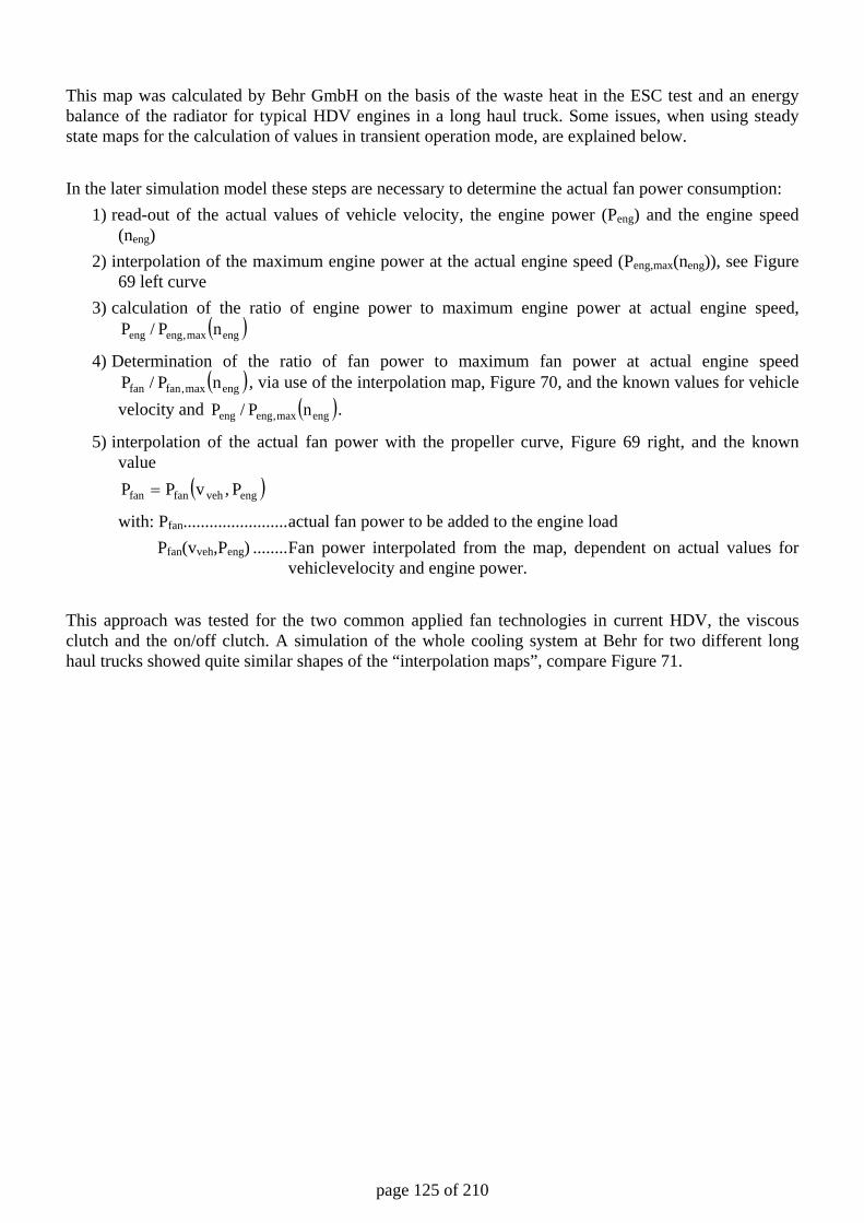
page 125 of 210

This map was calculated by Behr GmbH on the basis of the waste heat in the ESC test and an energy balance of the radiator for typical HDV engines in a long haul truck. Some issues, when using steady state maps for the calculation of values in transient operation mode, are explained below. In the later simulation model these steps are necessary to determine the actual fan power consumption:

1) read-out of the actual values of vehicle velocity, the engine power (Peng) and the engine speed (neng)

2) interpolation of the maximum engine power at the actual engine speed (Peng,max(neng)), see Figure 69 left curve

3) calculation of the ratio of engine power to maximum engine power at actual engine speed, ( )engmax,engeng nP/P

4) Determination of the ratio of fan power to maximum fan power at actual engine speed ( )engmax,fanfan nP/P , via use of the interpolation map, Figure 70, and the known values for vehicle

velocity and ( )engmax,engeng nP/P .

5) interpolation of the actual fan power with the propeller curve, Figure 69 right, and the known value

( )engvehfanfan P,vPP =

with: Pfan ........................ actual fan power to be added to the engine load Pfan(vveh,Peng) ........ Fan power interpolated from the map, dependent on actual values for

vehiclevelocity and engine power. This approach was tested for the two common applied fan technologies in current HDV, the viscous clutch and the on/off clutch. A simulation of the whole cooling system at Behr for two different long haul trucks showed quite similar shapes of the “interpolation maps”, compare Figure 71.

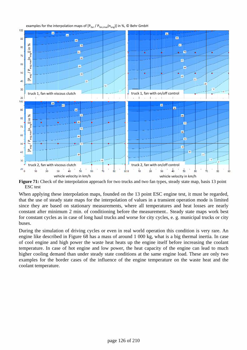
page 126 of 210

Figure 71: Check of the interpolation approach for two trucks and two fan types, steady state map, basis 13 point

ESC test When applying these interpolation maps, founded on the 13 point ESC engine test, it must be regarded, that the use of steady state maps for the interpolation of values in a transient operation mode is limited since they are based on stationary measurements, where all temperatures and heat losses are nearly constant after minimum 2 min. of conditioning before the measurement.. Steady state maps work best for constant cycles as in case of long haul trucks and worse for city cycles, e. g. municipal trucks or city buses. During the simulation of driving cycles or even in real world operation this condition is very rare. An engine like described in Figure 68 has a mass of around 1 000 kg, what is a big thermal inertia. In case of cool engine and high power the waste heat heats up the engine itself before increasing the coolant temperature. In case of hot engine and low power, the heat capacity of the engine can lead to much higher cooling demand than under steady state conditions at the same engine load. These are only two examples for the border cases of the influence of the engine temperature on the waste heat and the coolant temperature.

vehicle velocity in km/h vehicle velocity in km/h

[Pen

g/ P

eng,

max

(nen

g)] in

%[P

eng

/ Pen

g,m

ax(n

eng)]

in %

truck 1, fan with viscous clutch truck 1, fan with on/off control

truck 2, fan with viscous clutch truck 2, fan with on/off control

examples for the interpolation maps of [Pfan / Pfan,max(neng)] in %, © Behr GmbH

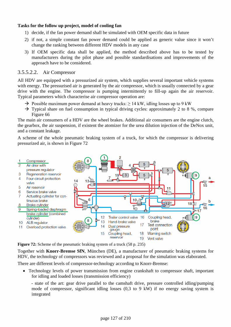
page 127 of 210

Tasks for the follow up project, model of cooling fan 1) decide, if the fan power demand shall be simulated with OEM specific data in future 2) if not, a simple constant fan power demand could be applied as generic value since it won’t

change the ranking between different HDV models in any case 3) If OEM specific data shall be applied, the method described above has to be tested by

manufacturers during the pilot phase and possible standardisations and improvements of the approach have to be considered.

3.5.5.2.2. Air Compressor All HDV are equipped with a pressurized air system, which supplies several important vehicle systems with energy. The pressurised air is generated by the air compressor, which is usually connected by a gear drive with the engine. The compressor is pumping intermittently to fill-up again the air reservoir. Typical parameters which characterise air compressor operation are: Possible maximum power demand at heavy trucks: ≥ 14 kW, idling losses up to 9 kW Typical share on fuel consumption in typical driving cycles: approximately 2 to 8 %, compare

Figure 66 The main air consumers of a HDV are the wheel brakes. Additional air consumers are the engine clutch, the gearbox, the air suspension, if existent the atomizer for the urea dilution injection of the DeNox unit, and a constant leakage. A scheme of the whole pneumatic braking system of a truck, for which the compressor is delivering pressurized air, is shown in Figure 72

Figure 72: Scheme of the pneumatic braking system of a truck (58 p. 235) Together with Knorr-Bremse SfN, München (DE), a manufacturer of pneumatic braking systems for HDV, the technology of compressors was reviewed and a proposal for the simulation was elaborated. There are different levels of compressor-technology according to Knorr-Bremse:

• Technology levels of power transmission from engine crankshaft to compressor shaft, important for idling and loaded losses (transmission efficiency) - state of the art: gear drive parallel to the camshaft drive, pressure controlled idling/pumping mode of compressor, significant idling losses (0,3 to 9 kW) if no energy saving system is integrated

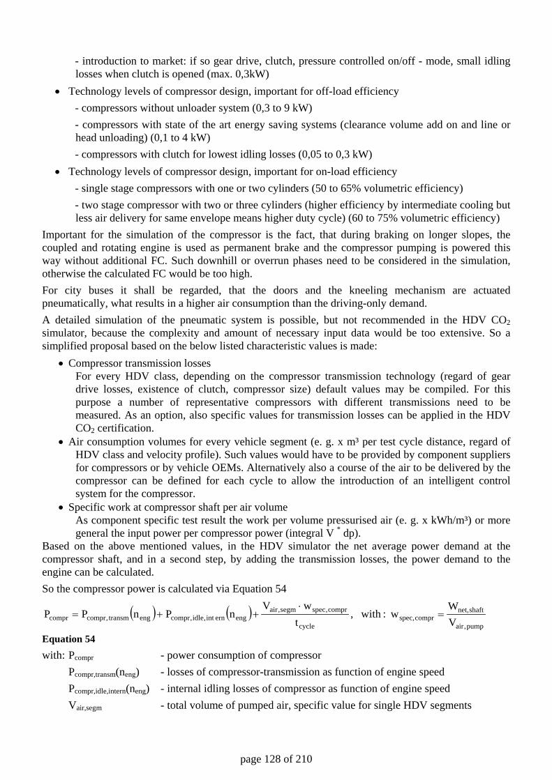
page 128 of 210

- introduction to market: if so gear drive, clutch, pressure controlled on/off - mode, small idling losses when clutch is opened (max. 0,3kW)

• Technology levels of compressor design, important for off-load efficiency - compressors without unloader system (0,3 to 9 kW) - compressors with state of the art energy saving systems (clearance volume add on and line or head unloading) (0,1 to 4 kW) - compressors with clutch for lowest idling losses (0,05 to 0,3 kW)

• Technology levels of compressor design, important for on-load efficiency - single stage compressors with one or two cylinders (50 to 65% volumetric efficiency) - two stage compressor with two or three cylinders (higher efficiency by intermediate cooling but less air delivery for same envelope means higher duty cycle) (60 to 75% volumetric efficiency)

Important for the simulation of the compressor is the fact, that during braking on longer slopes, the coupled and rotating engine is used as permanent brake and the compressor pumping is powered this way without additional FC. Such downhill or overrun phases need to be considered in the simulation, otherwise the calculated FC would be too high. For city buses it shall be regarded, that the doors and the kneeling mechanism are actuated pneumatically, what results in a higher air consumption than the driving-only demand. A detailed simulation of the pneumatic system is possible, but not recommended in the HDV CO2 simulator, because the complexity and amount of necessary input data would be too extensive. So a simplified proposal based on the below listed characteristic values is made:

• Compressor transmission losses For every HDV class, depending on the compressor transmission technology (regard of gear drive losses, existence of clutch, compressor size) default values may be compiled. For this purpose a number of representative compressors with different transmissions need to be measured. As an option, also specific values for transmission losses can be applied in the HDV CO2 certification.

• Air consumption volumes for every vehicle segment (e. g. x m³ per test cycle distance, regard of HDV class and velocity profile). Such values would have to be provided by component suppliers for compressors or by vehicle OEMs. Alternatively also a course of the air to be delivered by the compressor can be defined for each cycle to allow the introduction of an intelligent control system for the compressor.

• Specific work at compressor shaft per air volume As component specific test result the work per volume pressurised air (e. g. x kWh/m³) or more general the input power per compressor power (integral V * dp).

Based on the above mentioned values, in the HDV simulator the net average power demand at the compressor shaft, and in a second step, by adding the transmission losses, the power demand to the engine can be calculated. So the compressor power is calculated via Equation 54

( ) ( )pump,air

shaftnet,comprspec,

cycle

compr,specsegm,airengernint,idle,comprengtransm,comprcompr V

W w: with,

twV

nPnPP =⋅

++=

Equation 54 with: Pcompr - power consumption of compressor

Pcompr,transm(neng) - losses of compressor-transmission as function of engine speed Pcompr,idle,intern(neng) - internal idling losses of compressor as function of engine speed Vair,segm - total volume of pumped air, specific value for single HDV segments

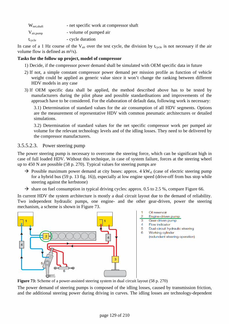
page 129 of 210

Wnet,shaft - net specific work at compressor shaft Vair,pump - volume of pumped air tcycle - cycle duration In case of a 1 Hz course of the Vair over the test cycle, the division by tcycle is not necessary if the air volume flow is defined as m³/s). Tasks for the follow up project, model of compressor

1) Decide, if the compressor power demand shall be simulated with OEM specific data in future 2) If not, a simple constant compressor power demand per mission profile as function of vehicle

weight could be applied as generic value since it won’t change the ranking between different HDV models in any case

3) If OEM specific data shall be applied, the method described above has to be tested by manufacturers during the pilot phase and possible standardisations and improvements of the approach have to be considered. For the elaboration of default data, following work is necessary:

3.1) Determination of standard values for the air consumption of all HDV segments. Options are the measurement of representative HDV with common pneumatic architectures or detailed simulations. 3.2) Determination of standard values for the net specific compressor work per pumped air volume for the relevant technology levels and of the idling losses. They need to be delivered by the compressor manufacturers.

3.5.5.2.3. Power steering pump The power steering pump is necessary to overcome the steering force, which can be significant high in case of full loaded HDV. Without this technique, in case of system failure, forces at the steering wheel up to 450 N are possible (58 p. 270). Typical values for steering pumps are Possible maximum power demand at city buses: approx. 4 kWel (case of electric steering pump

for a hybrid bus (59 p. 13 fig. 16)), especially at low engine speed (drive-off from bus stop while steering against the kerbstone)

share on fuel consumption in typical driving cycles: approx. 0.5 to 2.5 %, compare Figure 66. In current HDV the system architecture is mostly a dual circuit layout due to the demand of reliability. Two independent hydraulic pumps, one engine- and the other gear-driven, power the steering mechanism, a scheme is shown in Figure 73.

Figure 73: Scheme of a power-assisted steering system in dual circuit layout (58 p. 270) The power demand of steering pumps is composed of the idling losses, caused by transmission friction, and the additional steering power during driving in curves. The idling losses are technology-dependent

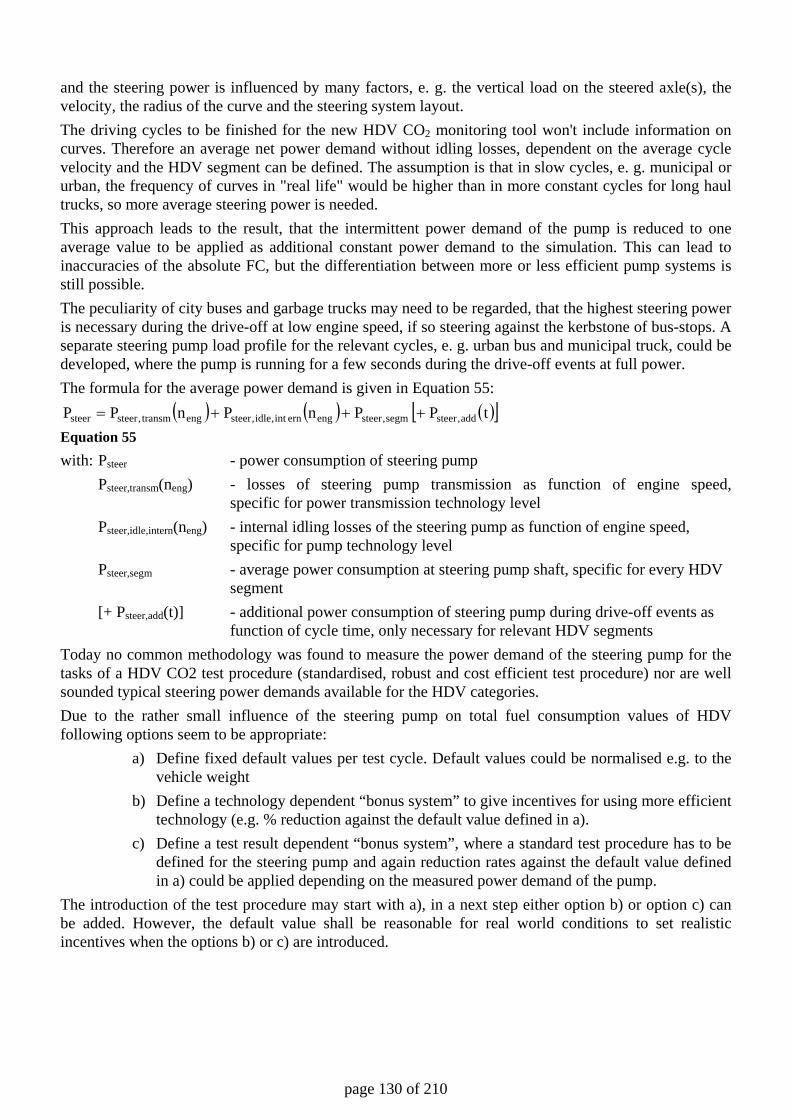
page 130 of 210

and the steering power is influenced by many factors, e. g. the vertical load on the steered axle(s), the velocity, the radius of the curve and the steering system layout. The driving cycles to be finished for the new HDV CO2 monitoring tool won't include information on curves. Therefore an average net power demand without idling losses, dependent on the average cycle velocity and the HDV segment can be defined. The assumption is that in slow cycles, e. g. municipal or urban, the frequency of curves in "real life" would be higher than in more constant cycles for long haul trucks, so more average steering power is needed. This approach leads to the result, that the intermittent power demand of the pump is reduced to one average value to be applied as additional constant power demand to the simulation. This can lead to inaccuracies of the absolute FC, but the differentiation between more or less efficient pump systems is still possible. The peculiarity of city buses and garbage trucks may need to be regarded, that the highest steering power is necessary during the drive-off at low engine speed, if so steering against the kerbstone of bus-stops. A separate steering pump load profile for the relevant cycles, e. g. urban bus and municipal truck, could be developed, where the pump is running for a few seconds during the drive-off events at full power. The formula for the average power demand is given in Equation 55:

( ) ( ) ( )[ ]tP PnPnPP add,steersegm,steerengernint,idle,steerengtransm,steersteer +++=

Equation 55 with: Psteer - power consumption of steering pump Psteer,transm(neng) - losses of steering pump transmission as function of engine speed, specific for power transmission technology level Psteer,idle,intern(neng) - internal idling losses of the steering pump as function of engine speed, specific for pump technology level Psteer,segm - average power consumption at steering pump shaft, specific for every HDV segment [+ Psteer,add(t)] - additional power consumption of steering pump during drive-off events as function of cycle time, only necessary for relevant HDV segments Today no common methodology was found to measure the power demand of the steering pump for the tasks of a HDV CO2 test procedure (standardised, robust and cost efficient test procedure) nor are well sounded typical steering power demands available for the HDV categories. Due to the rather small influence of the steering pump on total fuel consumption values of HDV following options seem to be appropriate:

a) Define fixed default values per test cycle. Default values could be normalised e.g. to the vehicle weight

b) Define a technology dependent “bonus system” to give incentives for using more efficient technology (e.g. % reduction against the default value defined in a).

c) Define a test result dependent “bonus system”, where a standard test procedure has to be defined for the steering pump and again reduction rates against the default value defined in a) could be applied depending on the measured power demand of the pump.

The introduction of the test procedure may start with a), in a next step either option b) or option c) can be added. However, the default value shall be reasonable for real world conditions to set realistic incentives when the options b) or c) are introduced.

page 131 of 210

This leads to following tasks for the follow up project: • Analysis of the relevant steering pump technology levels which shall be depicted and elaboration

of default values for the net average power demand. For this task the influence of vehicle weight, of average cycle velocity, of the number of steered axles and of the technology level of the system needs to be further analysed to define a proper normalisation of the default values. Options are measurement or detailed simulation.

3.5.5.2.4. Alternator Most alternators of HDV are self-excited 12- or 16-pole synchronous machines (58 p. 294) which convert mechanical to electrical power . Characteristic values for actual alternators are Possible maximum mechanical power demand at heavy trucks: up to approx. 6 kW share on fuel consumption in typical driving cycles: approx. 1 to 6 %, compare Figure 66

The operational behaviour of HDV alternators is described with the efficiency map for the constant DC voltage of 28 V. The efficiency is the ratio of the generated/consumed electrical power to the consumed/generated mechanical power. For the practical use in the simulation tool an additional engine load at the crankshaft is necessary, which is composed of the idling losses (belt- or gear-driven) and the operational power demand. Alternators are assumed not to have internal idling losses. The operational mechanical power at a given electrical power is dependent on the operating point of the alternator in its efficiency map. In the HDV CO2 test procedure following approach may be used:

1) Define an average electrical power demand or a normalised power demand cycle (ideally normalised e.g. to rated engine power, if necessary differentiated according to HDV segments)

2) Apply the efficiency map of the alternator to interpolate the mechanical power demand as function of the electric power demand and the rotational speed of the alternator.

Tasks for the follow up project, model of alternator 1) define a standardised test procedure for the measurement of the alternators efficiency map 2) define electrical power demand cycles per test cycle (a load cycle may be better than a constant load, since it would cover different load points of the alternator) 3) if no standardised test procedure for 1) can be defined in the year 2012, default values for the electric load shall be defined for a first phase of the test procedure.

3.5.5.2.5. Air conditioning Nearly all modern HDV are equipped with an air conditioning system (A/C) to keep the climate in the cabin comfortable. These systems are a combination of a compressor-driven refrigerator cycle and multiple blowers to cool the cabin, a scheme is shown in Figure 74

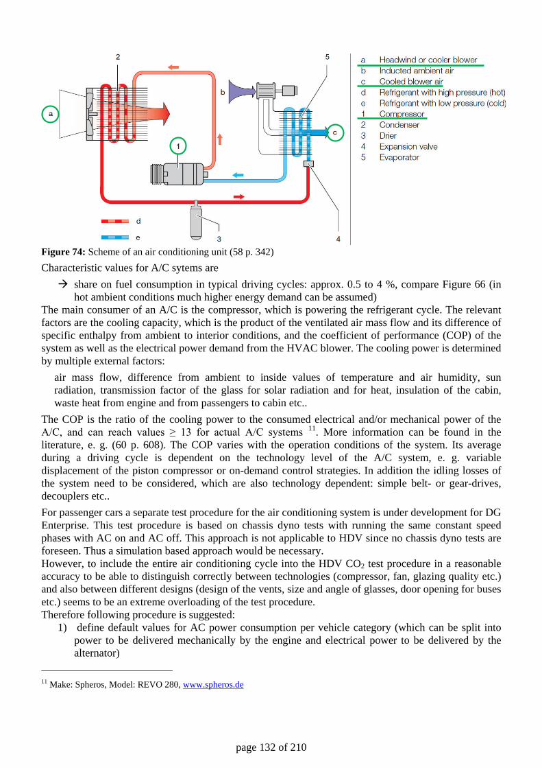
page 132 of 210

Figure 74: Scheme of an air conditioning unit (58 p. 342) Characteristic values for A/C sytems are share on fuel consumption in typical driving cycles: approx. 0.5 to 4 %, compare Figure 66 (in

hot ambient conditions much higher energy demand can be assumed) The main consumer of an A/C is the compressor, which is powering the refrigerant cycle. The relevant factors are the cooling capacity, which is the product of the ventilated air mass flow and its difference of specific enthalpy from ambient to interior conditions, and the coefficient of performance (COP) of the system as well as the electrical power demand from the HVAC blower. The cooling power is determined by multiple external factors:

air mass flow, difference from ambient to inside values of temperature and air humidity, sun radiation, transmission factor of the glass for solar radiation and for heat, insulation of the cabin, waste heat from engine and from passengers to cabin etc..

The COP is the ratio of the cooling power to the consumed electrical and/or mechanical power of the A/C, and can reach values ≥ 13 for actual A/C systems 11. More information can be found in the literature, e. g. (60 p. 608). The COP varies with the operation conditions of the system. Its average during a driving cycle is dependent on the technology level of the A/C system, e. g. variable displacement of the piston compressor or on-demand control strategies. In addition the idling losses of the system need to be considered, which are also technology dependent: simple belt- or gear-drives, decouplers etc.. For passenger cars a separate test procedure for the air conditioning system is under development for DG Enterprise. This test procedure is based on chassis dyno tests with running the same constant speed phases with AC on and AC off. This approach is not applicable to HDV since no chassis dyno tests are foreseen. Thus a simulation based approach would be necessary. However, to include the entire air conditioning cycle into the HDV CO2 test procedure in a reasonable accuracy to be able to distinguish correctly between technologies (compressor, fan, glazing quality etc.) and also between different designs (design of the vents, size and angle of glasses, door opening for buses etc.) seems to be an extreme overloading of the test procedure. Therefore following procedure is suggested:

1) define default values for AC power consumption per vehicle category (which can be split into power to be delivered mechanically by the engine and electrical power to be delivered by the alternator)

11 Make: Spheros, Model: REVO 280, www.spheros.de

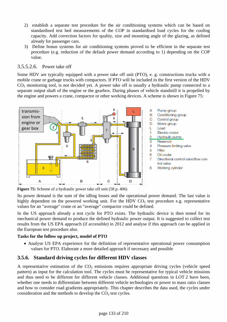
page 133 of 210

2) establish a separate test procedure for the air conditioning systems which can be based on standardised test bed measurements of the COP in standardised load cycles for the cooling capacity. Add correction factors for quality, size and mounting angle of the glazing, as defined already for passenger cars.

3) Define bonus systems for air conditioning systems proved to be efficient in the separate test procedure (e.g. reduction of the default power demand according to 1) depending on the COP value.

3.5.5.2.6. Power take off Some HDV are typically equipped with a power take off unit (PTO), e. g. constructions trucks with a mobile crane or garbage trucks with compactors. If PTO will be included in the first version of the HDV CO2 monitoring tool, is not decided yet. A power take off is usually a hydraulic pump connected to a separate output shaft of the engine or the gearbox. During phases of vehicle standstill it is propelled by the engine and powers a crane, compactor or other working devices. A scheme is shown in Figure 75:

Figure 75: Scheme of a hydraulic power take off unit (58 p. 406) Its power demand is the sum of the idling losses and the operational power demand. The last value is highly dependent on the powered working unit. For the HDV CO2 test procedure e.g. representative values for an "average" crane or an “average” compactor could be defined. In the US approach already a test cycle for PTO exists. The hydraulic device is then tested for its mechanical power demand to produce the defined hydraulic power output. It is suggested to collect test results from the US EPA approach (if accessible) in 2012 and analyse if this approach can be applied in the European test procedure also. Tasks for the follow up project, model of PTO

• Analyse US EPA experience for the definition of representative operational power consumption values for PTO. Elaborate a more detailed approach if necessary and possible

3.5.6. Standard driving cycles for different HDV classes A representative estimation of the CO2 emissions requires appropriate driving cycles (vehicle speed pattern) as input for the calculation tool. The cycles must be representative for typical vehicle missions and thus need to be different for different vehicle classes. Additional questions in LOT 2 have been, whether one needs to differentiate between different vehicle technologies or power to mass ratio classes and how to consider road gradients appropriately. This chapter describes the data used, the cycles under consideration and the methods to develop the CO2 test cycles.

transmis-sion fromengine orgear box

page 134 of 210

The following databases have been used for assessment and development work within this project: • The European part of the WHDC database. This database contains in-use data of 13 rigid trucks,

15 trailer/semitrailer trucks, 7 public transport buses, 1 coach and 1 garbage truck • Bus data from the ARTEMIS project (France, Belgium, Israel), • Bus data from PEMS measurement campaigns (several cities in Germany)

For trucks the power to mass ratio (rated power divided by gross vehicle mass, including trailer) ranges from 5 kW/t to 13 kW/t in the WHDC database. This range would justify different power to mass ratio classes, but one has to consider that there is a still on-going trend to higher rated power values, so that the range for the current and future fleet could be smaller. With respect to vehicle classes a first segmentation was made between trucks and buses. For pollutant emission calculations the trucks are normally classified with respect to GVW. For trailer and semitrailer trucks the GVW of tractor and trailer is considered. To a certain extend there is a correlation between GVW and vehicle mission. This is reflected in the vehicle classification system described in the previous chapter. In the first phase of the project the following vehicle mission classification was proposed:

• Long haul, • Delivery, • Municipal utility, • Construction

As a result of consultations within the consortium and with vehicle manufacturers (ACEA) the “Delivery” class was further split into “regional delivery” and “urban delivery”. For buses the following segmentation with respect to vehicle mission is proposed:

• City, o Heavy urban, o Urban, o suburban

• Inter urban, • Coach

With respect to the road network the vehicle operation can be divided into three different road categories:

• Urban, • Rural, • motorway

Normally the different vehicle missions consist of all three categories but with different mileage or operation time shares. Therefore, in principle, there are two possibilities for the assignment of appropriate driving cycles to the different vehicle/mission combinations:

1. Develop representative driving cycles of limited length or duration for the above mentioned road categories and calculate the CO2 emissions for the different vehicle/mission combinations by applying weighting factors to the three results in order to consider the different mileage or operation time shares appropriately.

2. Develop individual driving cycles for the different vehicle/mission combinations.

page 135 of 210

The first approach would at least require different cycles for trucks and buses and can hardly be applied to the HDV segments municipal utility and construction. But this approach was used to develop a short standard cycle verifiable with PEMS or on chassis dynamometer. It was decided to use the second approach as input for the simulation tool and develop individual cycles for each vehicle/mission combination. The development is based on driving cycles derived from real world in-use driving behaviour data. These cycles are then converted into target speed routes (target speeds versus distance) in order to reflect the influence of differences in power to mass ratio. This approach ensures that individual acceleration behaviour is considered in the CO2 emission calculation instead of the fixed driving behaviour related to a predefined vehicle speed trace.

Another important point is the appropriate consideration of road gradient by adding a gradient profile to the routes. It was agreed that this is necessary for a proper CO2 emission determination. The appropriate cycles and gradient profiles are currently under development with significant support by ACEA. The development is based on recent customer fleet data. A prototype for long haul missions was already presented by ACEA with the following major characteristics:

• Average speed 78 km/h, • Maximum target speed 85 km/h, • Distance share of speeds > 75 km/h = 75 – 85 %, • Start and end with 0 km/h and same altitude • Urban/rural parts at start and end with 2% of total driving time for urban and 13% for rural

operation Further improvements might be necessary, e.g. an increase of the maximum target speed to 88 km/h. Another cycle which is almost finalised is a municipal utility cycle for garbage trucks. The basis for this cycle is a self-developed vehicle speed trace versus time. This cycle was then converted into a target speed route and supplemented with a gradient trace by ACEA. It needs to be discussed whether corresponding cycles for other municipal utility must be added, e.g. for road sweeper. With respect to the two delivery mission cycles, the development work for the regional delivery cycle has already been started and shall be finalised in 2012. The same accounts for the construction cycle. The development of the urban delivery cycle is in its initial stage yet (definition phase); the finalisation is scheduled for the end of 2012. Also for buses it was decided to use the 2. approach for the development of appropriate cycles corresponding to the above mentioned vehicle/mission matrix, but to skip the conversion into target speed cycles for the city class, because the speed trace is more influenced by traffic conditions, road design and bus stop locations/positions rather than by the individual power to mass ratio of the vehicles. Furthermore, since public transport buses are standardised to a high degree, the differences in power to mass ratios are rather small compared to trucks. The ACEA members proposed to base the cycle development on analyses of in-use driving behaviour data from big public transport bus fleet operators within Europe, collected by two transmission manufacturers. Concrete cycles and gradient profiles (time based) were already delivered by ACEA. An assessment of the vehicle speed distributions showed good agreement with the author’s databases, but the gradient profiles show significant differences due to the chosen locations, so that further improvements seem to be necessary. The status of the cycles for the interurban and the coach class is almost the same as for the urban delivery cycle. The development is in its initial stage yet. Most probably the coach cycle will also be a target speed distance based cycle. Whether this approach can also be applied to the inter urban cycle depends on the outcome of the data analysis. In addition to that a standard cycle verifiable with PEMS or on chassis dynamometer was developed within the project and already used for validation purposes

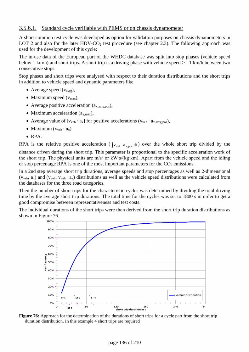
page 136 of 210

3.5.6.1. Standard cycle verifiable with PEMS or on chassis dynamometer

A short common test cycle was developed as option for validation purposes on chassis dynamometers in LOT 2 and also for the later HDV-CO2 test procedure (see chapter 2.3). The following approach was used for the development of this cycle: The in-use data of the European part of the WHDC database was split into stop phases (vehicle speed below 1 km/h) and short trips. A short trip is a driving phase with vehicle speed >= 1 km/h between two consecutive stops. Stop phases and short trips were analysed with respect to their duration distributions and the short trips in addition to vehicle speed and dynamic parameters like

• Average speed (vavrg), • Maximum speed (vmax), • Average positive acceleration (ax,avrg,pos), • Maximum acceleration (ax,max), • Average value of [vveh ∙ ax] for positive accelerations (vveh ∙ ax,avrg,pos), • Maximum (vveh ∙ ax) • RPA.

RPA is the relative positive acceleration ( ∫ ⋅ dt av pos,xveh ) over the whole short trip divided by the distance driven during the short trip. This parameter is proportional to the specific acceleration work of the short trip. The physical units are m/s² or kW∙s/(kg∙km). Apart from the vehicle speed and the idling or stop percentage RPA is one of the most important parameters for the CO2 emissions. In a 2nd step average short trip durations, average speeds and stop percentages as well as 2-dimensional (vveh, ax) and (vveh, vveh ∙ ax) distributions as well as the vehicle speed distributions were calculated from the databases for the three road categories. Then the number of short trips for the characteristic cycles was determined by dividing the total driving time by the average short trip durations. The total time for the cycles was set to 1800 s in order to get a good compromise between representativeness and test costs. The individual durations of the short trips were then derived from the short trip duration distributions as shown in Figure 76.

Figure 76: Approach for the determination of the durations of short trips for a cycle part from the short trip

duration distribution. In this example 4 short trips are required

0%

10%

20%

30%

40%

50%

60%

70%

80%

90%

100%

0 60 120 180 240 30

cum

freq

uenc

y

short trip duration in s

example distributionST 1

ST 2

ST 3 ST 4

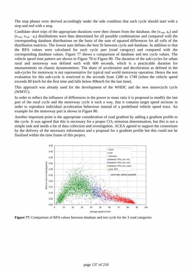
page 137 of 210

The stop phases were derived accordingly under the side condition that each cycle should start with a stop and end with a stop. Candidate short trips of the appropriate durations were then chosen from the database, the (vveh, ax) and (vveh, vveh ∙ ax) distributions were then determined for all possible combinations and compared with the corresponding database distributions on the basis of the sum of squared differences for all cells of the distribution matrices. The lowest sum defines the best fit between cycle and database. In addition to that the RPA values were calculated for each cycle part (road category) and compared with the corresponding database values. Figure 77 shows a comparison of database and test cycle values. The vehicle speed time pattern are shown in Figure 78 to Figure 80. The duration of the sub-cycles for urban rural and motorway was defined each with 600 seconds, which is a practicable duration for measurements on chassis dynamometers. The share of acceleration and deceleration as defined in the sub-cycles for motorway is not representative for typical real world motorway operation. Hence the test evaluation for this sub-cycle is restricted to the seconds from 1280 to 1749 (when the vehicle speed exceeds 80 km/h for the first time and falls below 80km/h for the last time). This approach was already used for the development of the WHDC and the new motorcycle cycle (WMTC). In order to reflect the influence of differences in the power to mass ratio it is proposed to modify the last part of the rural cycle and the motorway cycle it such a way, that it contains target speed sections in order to reproduce individual acceleration behaviour instead of a predefined vehicle speed trace. An example for the motorway part is shown in Figure 80. Another important point is the appropriate consideration of road gradient by adding a gradient profile to the cycle. It was agreed that this is necessary for a proper CO2 emission determination, but this is not a simple task and needs a lot of data collection and investigation. ACEA agreed to support the consortium by the delivery of the necessary information and a proposal for a gradient profile but this could not be finalised within the time frame of this project.

Figure 77: Comparison of RPA values between database and test cycle for the 3 road categories

0.00

0.05

0.10

0.15

0.20

0.25

0.30

0.35

0.40

0.45

0.50

0 10 20 30 40 50 60 70 80 90 100

RPA

in m

/s²

or k

Ws/

(kg*

km)

average speed in km/h

urbanruralmotorwaydatabase, RPA_ave, motdatabase, RPA_ave, ruraldatabase, RPA_ave, urbancycle, RPA

short trips, without standstill

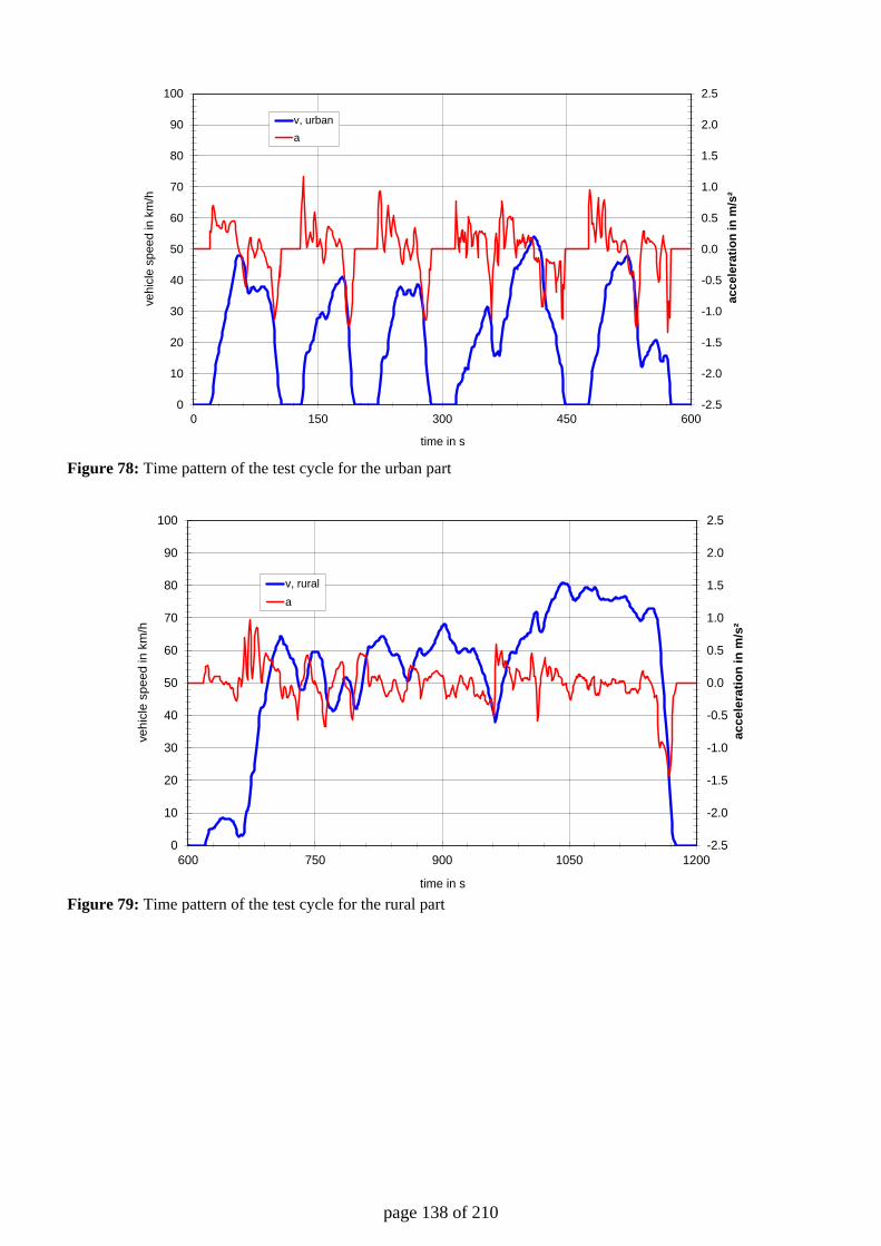
page 138 of 210

Figure 78: Time pattern of the test cycle for the urban part

Figure 79: Time pattern of the test cycle for the rural part

-2.5

-2.0

-1.5

-1.0

-0.5

0.0

0.5

1.0

1.5

2.0

2.5

0

10

20

30

40

50

60

70

80

90

100

0 150 300 450 600

acce

lera

tion

in m

/s²

vehi

cle

spee

d in

km

/h

time in s

v, urbana

-2.5

-2.0

-1.5

-1.0

-0.5

0.0

0.5

1.0

1.5

2.0

2.5

0

10

20

30

40

50

60

70

80

90

100

600 750 900 1050 1200

acce

lera

tion

in m

/s²

vehi

cle

spee

d in

km

/h

time in s

v, rurala

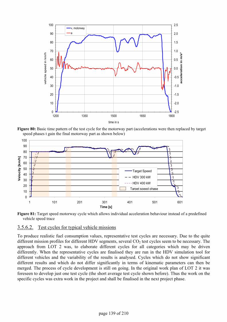
page 139 of 210

Figure 80: Basic time pattern of the test cycle for the motorway part (accelerations were then replaced by target speed phases t gain the final motorway part as shown below)

Figure 81: Target speed motorway cycle which allows individual acceleration behaviour instead of a predefined vehicle speed trace

3.5.6.2. Test cycles for typical vehicle missions

To produce realistic fuel consumption values, representative test cycles are necessary. Due to the quite different mission profiles for different HDV segments, several CO2 test cycles seem to be necessary. The approach from LOT 2 was, to elaborate different cycles for all categories which may be driven differently. When the representative cycles are finalised they are run in the HDV simulation tool fordifferent vehicles and the variability of the results is analysed. Cycles which do not show significant different results and which do not differ significantly in terms of kinematic parameters can then be merged. The process of cycle development is still on going. In the original work plan of LOT 2 it was foreseen to develop just one test cycle (the short average test cycle shown before). Thus the work on the specific cycles was extra work in the project and shall be finalised in the next project phase.

-2.5

-2.0

-1.5

-1.0

-0.5

0.0

0.5

1.0

1.5

2.0

2.5

0

10

20

30

40

50

60

70

80

90

100

1200 1350 1500 1650 1800

acce

lera

tio

n in

m/s

²

vehi

cle

spee

d in

km

/h

time in s

v, motorwaya

010

20304050

607080

90100

1 101 201 301 401 501 601Time [s]

Vel

oci

ty [k

m/h

]

Target Speed

HDV 300 kW

HDV 400 kWTarget speed phase

page 140 of 210

3.5.6.2.1. Test cycles for heavy goods vehicles In an early phase of the project the author was asked to develop and deliver characteristic driving cycles for the following vehicle mission classes as basis for further discussions and considerations:

• Distribution, • Long haulage, • Municipal utility (refuse truck)

The European part of the WHDC database contains data of 5 delivery trucks (gross vehicle mass between 5600 kg and 24000 kg), 8 long haulage vehicles with GVM of 40000 kg and 1 refuse truck. This data was used for the cycle development. The development approach was the same as described in the previous chapter but since the cycles were intended to be used as input for calculations rather than as basis for measurements the total duration was increased from 1800 s to 2700 s in order to enable the consideration of all relevant driving conditions from saturated urban traffic to free flowing traffic on motorways. The refuse truck cycle was used as basis for the development of the corresponding distance based target speed cycle described in chapter 2.3.

3.5.6.2.2. Test cycles for buses As already mentioned in chapter 2.3, for buses the following segmentation with respect to vehicle mission is proposed:

• City, o Heavy urban, o Urban, o suburban

• Inter urban, • Coach

Also for buses it was decided to use the 2. approach for the development of appropriate cycles corresponding to the above mentioned vehicle/mission matrix, but to skip the conversion into target speed cycles for the city class, because the speed trace is more influenced by traffic conditions, road design and bus stop locations/positions rather than by the individual power to mass ratio of the vehicles. Furthermore, since public transport buses are standardised to a high degree, the differences in power to mass ratios are rather small compared to trucks. The ACEA members proposed to base the cycle development on analyses of in-use driving behaviour data from big public transport bus fleet operators within Europe, collected by two transmission manufacturers. Concrete cycles and gradient profiles (time based) were already delivered by ACEA. The key parameter values of these cycles are listed in Table 47. The cumulative frequency distributions of vehicle speeds are shown in Figure 82. Figure 83 shows a comparison with in-use data measured in 2010 in 8 different German cities. Each curve represents averages of several journeys for individual bus lines. Figure 84 shows a comparison with data from Belgium and with the cycles used in the Handbook of Emission Factors version 2.1. These cycles are based on measurements in Switzerland. A coach was also measured within this measurement campaign. Its speed distribution is shown in Figure 84 in addition. The comparison shows generally a good accordance with the proposed cycles with two exceptions: The stop percentages of the urban and heavy urban cycles may be too high and the percentages of vehicle speeds between 35 km/h and 45 km/h may be somewhat too low. This needs to be further evaluated.

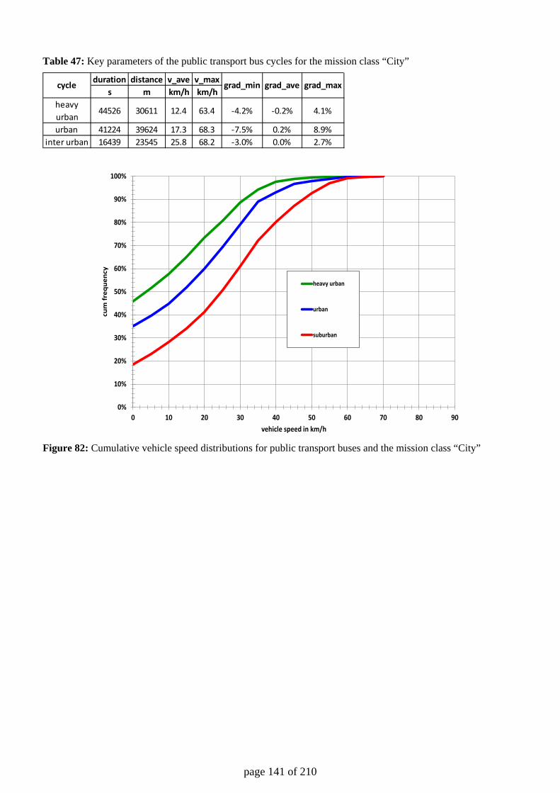
page 141 of 210

Table 47: Key parameters of the public transport bus cycles for the mission class “City”

Figure 82: Cumulative vehicle speed distributions for public transport buses and the mission class “City”

duration distance v_ave v_maxs m km/h km/h

heavy urban

44526 30611 12.4 63.4 -4.2% -0.2% 4.1%

urban 41224 39624 17.3 68.3 -7.5% 0.2% 8.9%inter urban 16439 23545 25.8 68.2 -3.0% 0.0% 2.7%

grad_min grad_ave grad_maxcycle

0%

10%

20%

30%

40%

50%

60%

70%

80%

90%

100%

0 10 20 30 40 50 60 70 80 90

cum

freq

uenc

y

vehicle speed in km/h

heavy urban

urban

suburban

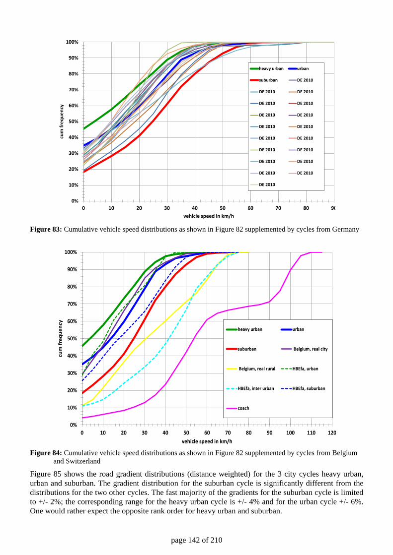
page 142 of 210

Figure 83: Cumulative vehicle speed distributions as shown in Figure 82 supplemented by cycles from Germany

Figure 84: Cumulative vehicle speed distributions as shown in Figure 82 supplemented by cycles from Belgium

and Switzerland

Figure 85 shows the road gradient distributions (distance weighted) for the 3 city cycles heavy urban, urban and suburban. The gradient distribution for the suburban cycle is significantly different from the distributions for the two other cycles. The fast majority of the gradients for the suburban cycle is limited to +/- 2%; the corresponding range for the heavy urban cycle is +/- 4% and for the urban cycle +/- 6%. One would rather expect the opposite rank order for heavy urban and suburban.

0%

10%

20%

30%

40%

50%

60%

70%

80%

90%

100%

0 10 20 30 40 50 60 70 80 90

cum

freq

uenc

y

vehicle speed in km/h

heavy urban urban

suburban DE 2010

DE 2010 DE 2010

DE 2010 DE 2010

DE 2010 DE 2010

DE 2010 DE 2010

DE 2010 DE 2010

DE 2010 DE 2010

DE 2010 DE 2010

DE 2010 DE 2010

DE 2010

0%

10%

20%

30%

40%

50%

60%

70%

80%

90%

100%

0 10 20 30 40 50 60 70 80 90 100 110 120

cum

freq

uenc

y

vehicle speed in km/h

heavy urban urban

suburban Belgium, real city

Belgium, real rural HBEfa, urban

HBEfa, inter urban HBEfa, suburban

coach

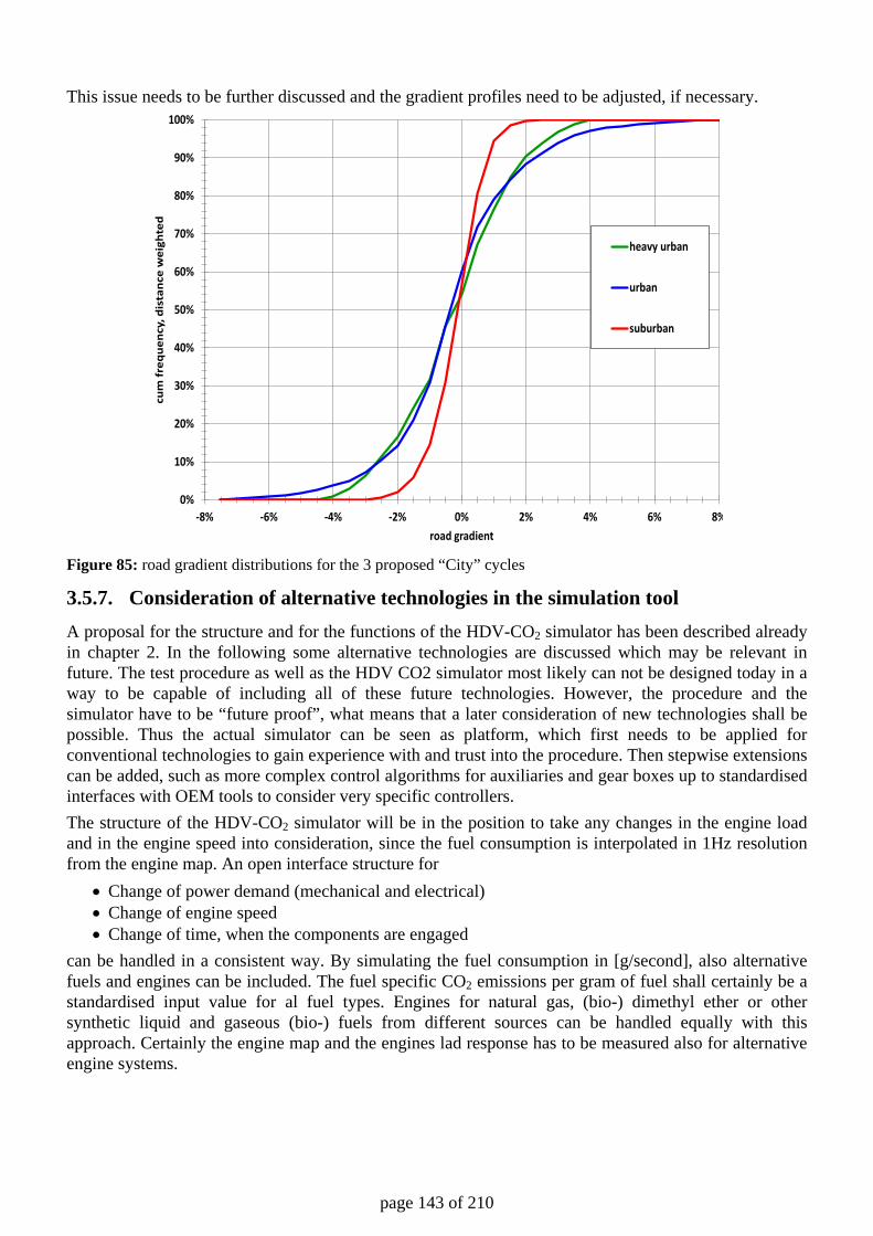
page 143 of 210

This issue needs to be further discussed and the gradient profiles need to be adjusted, if necessary.

Figure 85: road gradient distributions for the 3 proposed “City” cycles

3.5.7. Consideration of alternative technologies in the simulation tool A proposal for the structure and for the functions of the HDV-CO2 simulator has been described already in chapter 2. In the following some alternative technologies are discussed which may be relevant in future. The test procedure as well as the HDV CO2 simulator most likely can not be designed today in a way to be capable of including all of these future technologies. However, the procedure and the simulator have to be “future proof”, what means that a later consideration of new technologies shall be possible. Thus the actual simulator can be seen as platform, which first needs to be applied for conventional technologies to gain experience with and trust into the procedure. Then stepwise extensions can be added, such as more complex control algorithms for auxiliaries and gear boxes up to standardised interfaces with OEM tools to consider very specific controllers. The structure of the HDV-CO2 simulator will be in the position to take any changes in the engine load and in the engine speed into consideration, since the fuel consumption is interpolated in 1Hz resolution from the engine map. An open interface structure for

• Change of power demand (mechanical and electrical) • Change of engine speed • Change of time, when the components are engaged

can be handled in a consistent way. By simulating the fuel consumption in [g/second], also alternative fuels and engines can be included. The fuel specific CO2 emissions per gram of fuel shall certainly be a standardised input value for al fuel types. Engines for natural gas, (bio-) dimethyl ether or other synthetic liquid and gaseous (bio-) fuels from different sources can be handled equally with this approach. Certainly the engine map and the engines lad response has to be measured also for alternative engine systems.

0%

10%

20%

30%

40%

50%

60%

70%

80%

90%

100%

-8% -6% -4% -2% 0% 2% 4% 6% 8%

cum

freq

uenc

y, d

ista

nce

wei

ghte

d

road gradient

heavy urban

urban

suburban

page 144 of 210

Brake energy recovery A part of the kinetic energy during coasting or braking can be recovered with an electric generator installed in the drivetrain, what is a pre-stage of hybridization (61). The power consumption of the alternator and the retarder operation is linked with this technology. Terrain-dependent drivetrain control Different options exist to optimize the drivetrain control dependent on the terrain. This approach can be supported by knowing the altitude profile of the whole track, e. g. the fixed routes of city buses or the main highways for long haul trucks. Because most HDV are fitted with a satellite positioning system it is easy to determine the altitude profile of the next road strip. Then with a simplified simulation of vehicle dynamics the power demand is calculated and the result is used to determine the most fuel efficient drivetrain operation strategy, e. g. in combination with the cruise control the avoidance of unnecessary shifting or braking (1 p. 141). Another possibility is the declutching or shut down of the engine when not needed for powering during longer coasting phases (1 p. 145). A typical engine speed at 85 km/h is 1200 rpm. If the vehicle is rolling itself on small declines, the coupled engine consumes the corresponding idle fuel mass. If declutched, the fuel mass is reduced to the consumption at lowest idling speed or even cutted, when switched off. In the case of city buses terrain-dependent gearbox controls are available by default for automatic transmissions (62) (63). Start-Stop Automatic A simple and for urban vehicles effective fuelsaving measure is to stop the engine during longer phases of standstill, e. g. in case of city buses, garbage trucks or delivery trucks (1 p. 126). The need is a reinforced starter-generator and an engine design for many start events in terms of bearings and lubrication Waste heat recovery One example is using waste heat of the EGR cooler to run a heat engine operating in the Brayton cycle (64 p. 123). It works in principle like an open gas turbine process, but the working fluid is air which is heated up in the EGR heat exchanger and expanded in a turbine. This Brayton engine won't work in transient operation of the ICE but the best on constant highway rides with a continuous heat flow in the EGR cooler. The cooling fan operation and the electric power demand to the alternator are influenced by the Brayton engine. Automatically reduced air drag at high velocities Some actual tractors are offered with aerodynamic features to reduce the air drag at high velocities. E. g. the fifth wheel coupling is moved forwards to minimize the gap between semi-trailer and tractor, or flaps are closed to cut the air drag of the cabin steps or of the front heat exchanger, if not needed (61) (65). If this variable air drag is not regarded in the reference measurement, it may be taken into account otherwise. Limit for acceleration The full engine power is dependent on the demand of a trailer truck with full payload, which can be more than double than in case of the empty single truck. Therefore the full power is not needed to reach appropiate acceleration values for partial loaded trucks and leads to an unnecessary high fuel consumption. A countermeasure is an acceleration limit (1 p. 144) to avoid this effect. Reduction of electric power demand Multiple options exist to reduce the electric power demand, e. g. solar panels on the vehicle roof (61) or LED headlamps, taillights and marker lights (66). Dependent on the used components the electric power consumption is lower than the standard electric alternator load for every HDV class. Steerable rear axles at truck or trailer In case of fixed rear axles at trucks or trailers with more than one rear axle the last wheels are always pulled sidewise in curves, what creates an additional road load and fuel consumption especially for

page 145 of 210

urban vehicles. One or two steerable rear axles reduce this resistance and the tire wear significantly and are standard for some HDV classes (67). But the driving cycles for simulation do not include any curves, so this fuelsaving measure shall be considered in another way.

3.6. Verification of the recommended procedure with new measurements and model data This section refers to task 1.3.3 of the tender and gives an overview on the vehicle test performed in LOT 2. Details of test results have been presented in several meetings and are available as power point slides. To describe all single tests would go beyond the scope of the final report. This section also gives a comparison of results from a simulation model with measured fuel consumption from the vehicle tests. For this purpose in this study the vehicle longitudinal dynamic and emission model PHEM (Passenger car and Heavy Duty Emission Model) was used. A short description of PHEM is given in section 3.4.5.1 With the funding from the European Commission for LOT2 and from the German Umweltbundesamt measurements on 6 HDV were conducted (Table 48). In this context the consortium of LOT2 wants to thank ACEA for their support in making available three of the tested HDV and their input regarding vehicle functionalities and component data. Comprehensive datasets for the main input values for the simulation model, namely engine fuel consumption map, detailed gear box data, operation control and power demand of auxiliaries was to a large extend available for HDV 4, the long haul truck and for HDV 6, the delivery truck. None of the datasets is fully compatible to the certification method as proposed in chapter 2, as some of the component tests methods have been defined right at the end of the LOT2 project. For HDV 5, the 18 t city bus, most data is available, but detailed input for the hydro-mechanical powersplit in the automatic gearbox and its friction losses is not available in a final form. In addition it is not decided yet how the controller of automatic gear boxes shall be considered in the HDV-CO2 simulator. Thus a simulation of the bus according to the proposed CO2 test method is not possible at the moment. But all measured data at the 18 t city bus is evaluated and can be used for validation of the approach for buses as soon as the simulation structure for automatic gear boxes is decided.

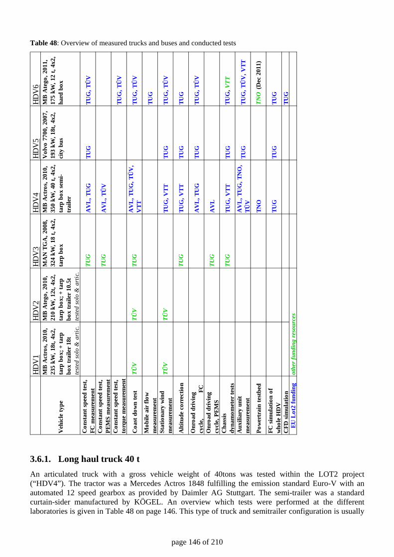
page 146 of 210

Table 48: Overview of measured trucks and buses and conducted tests

3.6.1. Long haul truck 40 t An articulated truck with a gross vehicle weight of 40tons was tested within the LOT2 project (“HDV4”). The tractor was a Mercedes Actros 1848 fulfilling the emission standard Euro-V with an automated 12 speed gearbox as provided by Daimler AG Stuttgart. The semi-trailer was a standard curtain-sider manufactured by KÖGEL. An overview which tests were performed at the different laboratories is given in Table 48 on page 146. This type of truck and semitrailer configuration is usually

HDV

1HD

V2

HDV

3HD

V4

HDV

5HD

V6

Veh

icle

type

MB

Act

ros,

201

0,

235

kW, 1

8t, 4

x2,

tarp

box

; + ta

rp

box

trai

ler

18t

test

ed s

olo

& a

rtic

.

MB

Ate

go, 2

010,

21

0 kW

, 12t

, 4x2

, ta

rp b

ox; +

tarp

bo

x tr

aile

r 10

.5t

test

ed s

olo

& a

rtic

.

MA

N T

GA

, 200

8,

324

kW, 1

8 t,

4x2,

ta

rp b

ox

MB

Act

ros,

201

0,

350

kW, 4

0 t,

4x2,

ta

rp b

ox s

emi-

trai

ler

Vol

vo 7

700,

200

7,

193

kW, 1

8t, 4

x2,

city

bus

MB

Ate

go, 2

011,

17

5 kW

, 12

t, 4x

2,

hard

box

Con

stan

t spe

ed te

st,

FC m

easu

rem

ent

TUG

AV

L, T

UG

TUG

TUG

, TÜ

V

Con

stan

t spe

ed te

st,

PEM

S m

easu

rem

ent

TUG

AV

L, T

ÜV

Con

stan

t spe

ed te

st,

torq

ue m

easu

rem

ent

TUG

, TÜ

V

Coa

st d

own

test

TÜV

TÜV

TUG

AV

L, T

UG

, TÜ

V,

VTT

TUG

, TÜ

V

Mob

ile a

ir fl

ow

mea

sure

men

tTU

G

Stat

iona

ry w

ind

mea

sure

men

tTÜ

VTÜ

VTU

G, V

TTTU

GTU

G, T

ÜV

Alti

tude

cor

rect

ion

TUG

TUG

, VTT

TUG

TUG

Onr

oad

driv

ing

cycl

e,

FC

AV

L, T

UG

TUG

TUG

, TÜ

V

Onr

oad

driv

ing

cycl

e, P

EMS

TUG

AV

L

Cha

ssis

dy

nam

omet

er te

sts

TUG

TUG

, VTT

TUG

TUG

, VTT

Aux

iliar

y un

it m

easu

rem

ent

AV

L, T

UG

, TN

O,

TÜV

TUG

TUG

, TÜ

V, V

TT

Pow

ertr

ain

test

bed

TNO

TNO

(Dec

201

1)

FC s

imul

atio

n of

w

hole

HD

VTU

GTU

GTU

G

CFD

sim

ulat

ion

TUG

EU

Lot

2 fu

ndin

got

her

fund

ing

reso

urce

s

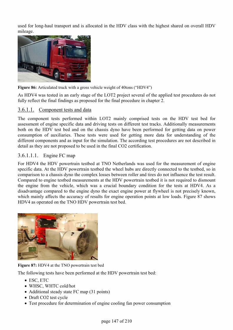
page 147 of 210

used for long-haul transport and is allocated in the HDV class with the highest shared on overall HDV mileage.

Figure 86: Articulated truck with a gross vehicle weight of 40tons (“HDV4”)

As HDV4 was tested in an early stage of the LOT2 project several of the applied test procedures do not fully reflect the final findings as proposed for the final procedure in chapter 2.

3.6.1.1. Component tests and data

The component tests performed within LOT2 mainly comprised tests on the HDV test bed for assessment of engine specific data and driving tests on different test tracks. Additionally measurements both on the HDV test bed and on the chassis dyno have been performed for getting data on power consumption of auxiliaries. These tests were used for getting more data for understanding of the different components and as input for the simulation. The according test procedures are not described in detail as they are not proposed to be used in the final CO2 certification.

3.6.1.1.1. Engine FC map For HDV4 the HDV powertrain testbed at TNO Netherlands was used for the measurement of engine specific data. At the HDV powertrain testbed the wheel hubs are directly connected to the testbed, so in comparison to a chassis dyno the complex losses between roller and tires do not influence the test result. Compared to engine testbed measurements at the HDV powertrain testbed it is not required to dismount the engine from the vehicle, which was a crucial boundary condition for the tests at HDV4. As adisadvantage compared to the engine dyno the exact engine power at flywheel is not precisely known, which mainly affects the accuracy of results for engine operation points at low loads. Figure 87 shows HDV4 as operated on the TNO HDV powertrain test bed.

Figure 87: HDV4 at the TNO powertrain test bed

The following tests have been performed at the HDV powertrain test bed:• ESC, ETC• WHSC, WHTC cold/hot• Additional steady state FC map (31 points)• Draft CO2 test cycle• Test procedure for determination of engine cooling fan power consumption

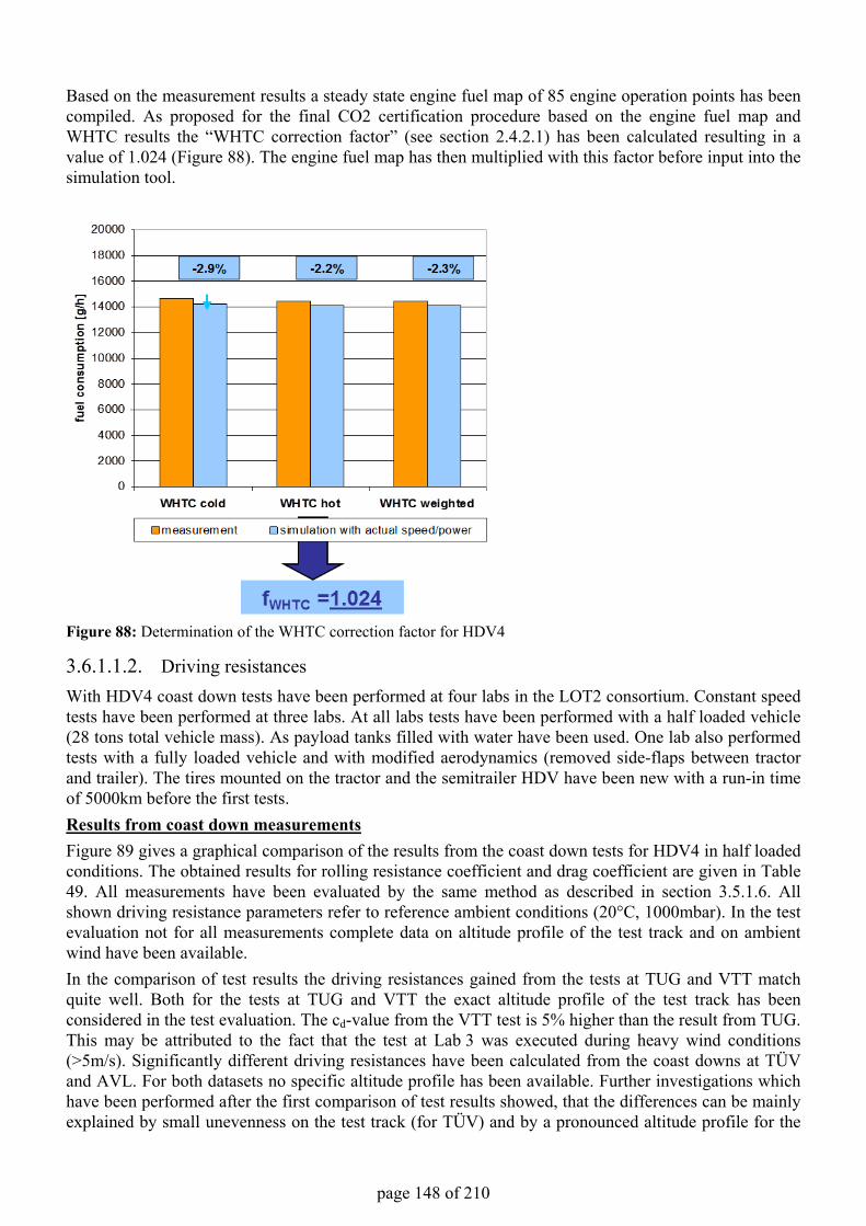
page 148 of 210

Based on the measurement results a steady state engine fuel map of 85 engine operation points has been compiled. As proposed for the final CO2 certification procedure based on the engine fuel map and WHTC results the “WHTC correction factor” (see section 2.4.2.1) has been calculated resulting in a value of 1.024 (Figure 88). The engine fuel map has then multiplied with this factor before input into the simulation tool.

Figure 88: Determination of the WHTC correction factor for HDV4

3.6.1.1.2. Driving resistancesWith HDV4 coast down tests have been performed at four labs in the LOT2 consortium. Constant speed tests have been performed at three labs. At all labs tests have been performed with a half loaded vehicle (28 tons total vehicle mass). As payload tanks filled with water have been used. One lab also performed tests with a fully loaded vehicle and with modified aerodynamics (removed side-flaps between tractor and trailer). The tires mounted on the tractor and the semitrailer HDV have been new with a run-in time of 5000km before the first tests.Results from coast down measurementsFigure 89 gives a graphical comparison of the results from the coast down tests for HDV4 in half loaded conditions. The obtained results for rolling resistance coefficient and drag coefficient are given in Table 49. All measurements have been evaluated by the same method as described in section 3.5.1.6. Allshown driving resistance parameters refer to reference ambient conditions (20°C, 1000mbar). In the test evaluation not for all measurements complete data on altitude profile of the test track and on ambient wind have been available.In the comparison of test results the driving resistances gained from the tests at TUG and VTT match quite well. Both for the tests at TUG and VTT the exact altitude profile of the test track has been considered in the test evaluation. The cd-value from the VTT test is 5% higher than the result from TUG. This may be attributed to the fact that the test at Lab 3 was executed during heavy wind conditions (>5m/s). Significantly different driving resistances have been calculated from the coast downs at TÜV and AVL. For both datasets no specific altitude profile has been available. Further investigations which have been performed after the first comparison of test results showed, that the differences can be mainly explained by small unevenness on the test track (for TÜV) and by a pronounced altitude profile for the

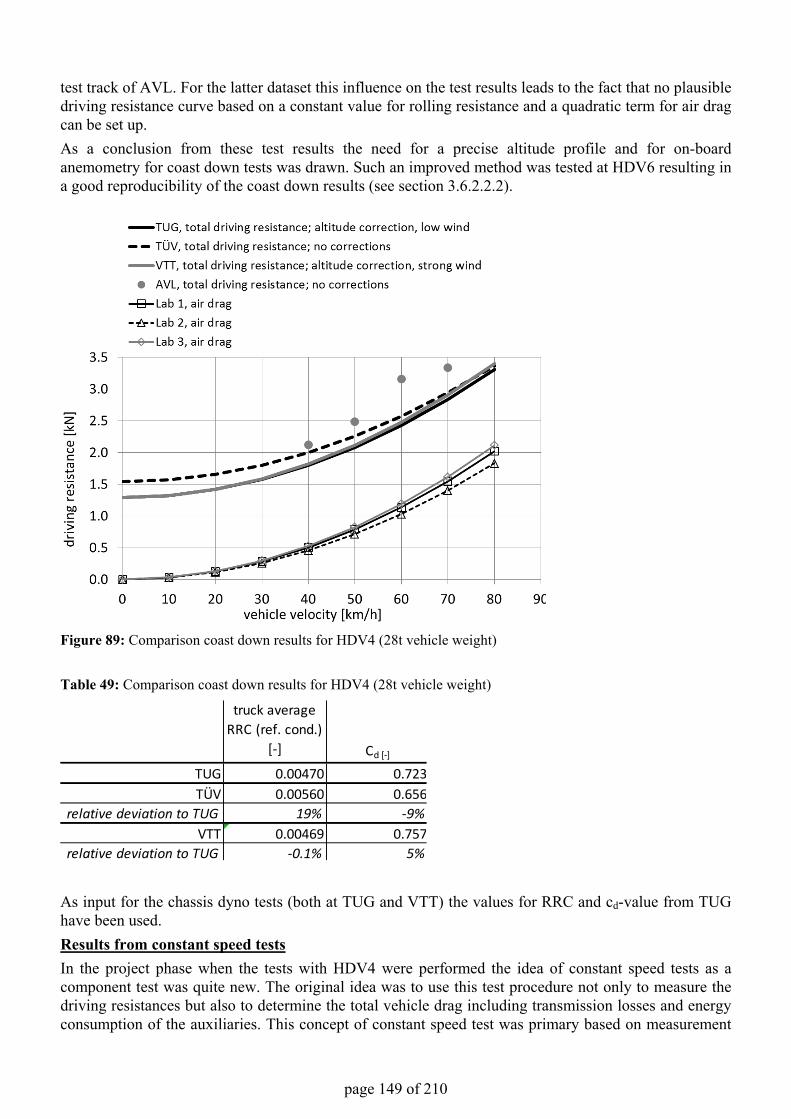
page 149 of 210

test track of AVL. For the latter dataset this influence on the test results leads to the fact that no plausible driving resistance curve based on a constant value for rolling resistance and a quadratic term for air drag can be set up.As a conclusion from these test results the need for a precise altitude profile and for on-board anemometry for coast down tests was drawn. Such an improved method was tested at HDV6 resulting in a good reproducibility of the coast down results (see section 3.6.2.2.2).

Figure 89: Comparison coast down results for HDV4 (28t vehicle weight)

Table 49: Comparison coast down results for HDV4 (28t vehicle weight)

As input for the chassis dyno tests (both at TUG and VTT) the values for RRC and cd-value from TUG have been used.Results from constant speed testsIn the project phase when the tests with HDV4 were performed the idea of constant speed tests as a component test was quite new. The original idea was to use this test procedure not only to measure the driving resistances but also to determine the total vehicle drag including transmission losses and energy consumption of the auxiliaries. This concept of constant speed test was primary based on measurement

truck average RRC (ref. cond.)

[-] Cd [-]

TUG 0.00470 0.723TÜV 0.00560 0.656

relative deviation to TUG 19% -9%VTT 0.00469 0.757

relative deviation to TUG -0.1% 5%

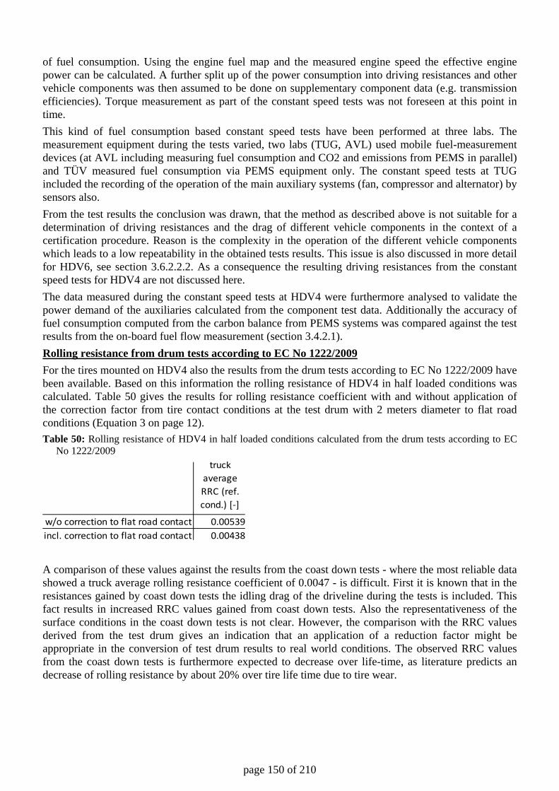
page 150 of 210

of fuel consumption. Using the engine fuel map and the measured engine speed the effective engine power can be calculated. A further split up of the power consumption into driving resistances and other vehicle components was then assumed to be done on supplementary component data (e.g. transmission efficiencies). Torque measurement as part of the constant speed tests was not foreseen at this point in time. This kind of fuel consumption based constant speed tests have been performed at three labs. The measurement equipment during the tests varied, two labs (TUG, AVL) used mobile fuel-measurement devices (at AVL including measuring fuel consumption and CO2 and emissions from PEMS in parallel) and TÜV measured fuel consumption via PEMS equipment only. The constant speed tests at TUG included the recording of the operation of the main auxiliary systems (fan, compressor and alternator) by sensors also. From the test results the conclusion was drawn, that the method as described above is not suitable for a determination of driving resistances and the drag of different vehicle components in the context of a certification procedure. Reason is the complexity in the operation of the different vehicle components which leads to a low repeatability in the obtained tests results. This issue is also discussed in more detail for HDV6, see section 3.6.2.2.2. As a consequence the resulting driving resistances from the constant speed tests for HDV4 are not discussed here. The data measured during the constant speed tests at HDV4 were furthermore analysed to validate the power demand of the auxiliaries calculated from the component test data. Additionally the accuracy of fuel consumption computed from the carbon balance from PEMS systems was compared against the test results from the on-board fuel flow measurement (section 3.4.2.1). Rolling resistance from drum tests according to EC No 1222/2009 For the tires mounted on HDV4 also the results from the drum tests according to EC No 1222/2009 have been available. Based on this information the rolling resistance of HDV4 in half loaded conditions was calculated. Table 50 gives the results for rolling resistance coefficient with and without application of the correction factor from tire contact conditions at the test drum with 2 meters diameter to flat road conditions (Equation 3 on page 12). Table 50: Rolling resistance of HDV4 in half loaded conditions calculated from the drum tests according to EC

No 1222/2009

A comparison of these values against the results from the coast down tests - where the most reliable data showed a truck average rolling resistance coefficient of 0.0047 - is difficult. First it is known that in the resistances gained by coast down tests the idling drag of the driveline during the tests is included. This fact results in increased RRC values gained from coast down tests. Also the representativeness of the surface conditions in the coast down tests is not clear. However, the comparison with the RRC values derived from the test drum gives an indication that an application of a reduction factor might be appropriate in the conversion of test drum results to real world conditions. The observed RRC values from the coast down tests is furthermore expected to decrease over life-time, as literature predicts an decrease of rolling resistance by about 20% over tire life time due to tire wear.

truck average RRC (ref. cond.) [-]

w/o correction to flat road contact 0.00539incl. correction to flat road contact 0.00438

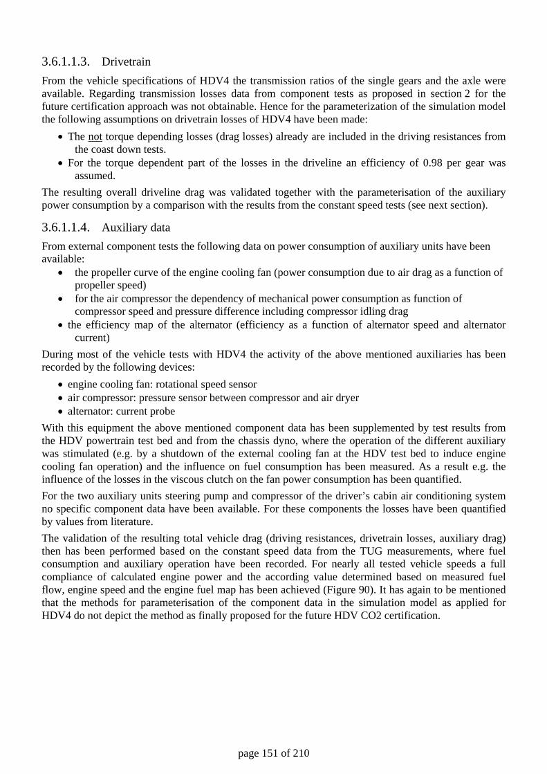
page 151 of 210

3.6.1.1.3. Drivetrain From the vehicle specifications of HDV4 the transmission ratios of the single gears and the axle were available. Regarding transmission losses data from component tests as proposed in section 2 for the future certification approach was not obtainable. Hence for the parameterization of the simulation model the following assumptions on drivetrain losses of HDV4 have been made:

• The not torque depending losses (drag losses) already are included in the driving resistances from the coast down tests.

• For the torque dependent part of the losses in the driveline an efficiency of 0.98 per gear was assumed.

The resulting overall driveline drag was validated together with the parameterisation of the auxiliary power consumption by a comparison with the results from the constant speed tests (see next section).

3.6.1.1.4. Auxiliary data From external component tests the following data on power consumption of auxiliary units have been available:

• the propeller curve of the engine cooling fan (power consumption due to air drag as a function of propeller speed)

• for the air compressor the dependency of mechanical power consumption as function of compressor speed and pressure difference including compressor idling drag

• the efficiency map of the alternator (efficiency as a function of alternator speed and alternator current)

During most of the vehicle tests with HDV4 the activity of the above mentioned auxiliaries has been recorded by the following devices:

• engine cooling fan: rotational speed sensor • air compressor: pressure sensor between compressor and air dryer • alternator: current probe

With this equipment the above mentioned component data has been supplemented by test results from the HDV powertrain test bed and from the chassis dyno, where the operation of the different auxiliary was stimulated (e.g. by a shutdown of the external cooling fan at the HDV test bed to induce engine cooling fan operation) and the influence on fuel consumption has been measured. As a result e.g. the influence of the losses in the viscous clutch on the fan power consumption has been quantified. For the two auxiliary units steering pump and compressor of the driver’s cabin air conditioning system no specific component data have been available. For these components the losses have been quantified by values from literature. The validation of the resulting total vehicle drag (driving resistances, drivetrain losses, auxiliary drag) then has been performed based on the constant speed data from the TUG measurements, where fuel consumption and auxiliary operation have been recorded. For nearly all tested vehicle speeds a full compliance of calculated engine power and the according value determined based on measured fuel flow, engine speed and the engine fuel map has been achieved (Figure 90). It has again to be mentioned that the methods for parameterisation of the component data in the simulation model as applied for HDV4 do not depict the method as finally proposed for the future HDV CO2 certification.

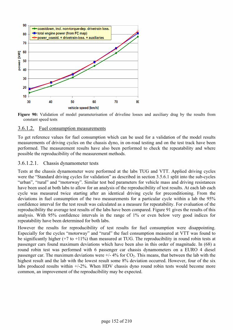
page 152 of 210

Figure 90: Validation of model parameterisation of driveline losses and auxiliary drag by the results from constant speed tests

3.6.1.2. Fuel consumption measurements

To get reference values for fuel consumption which can be used for a validation of the model results measurements of driving cycles on the chassis dyno, in on-road testing and on the test track have been performed. The measurement results have also been performed to check the repeatability and where possible the reproducibility of the measurement methods.

3.6.1.2.1. Chassis dynamometer testsTests at the chassis dynamometer were performed at the labs TUG and VTT. Applied driving cycles were the “Standard driving cycles for validation” as described in section 3.5.6.1 split into the sub-cycles “urban”, “rural” and “motorway”. Similar test bed parameters for vehicle mass and driving resistances have been used at both labs to allow for an analysis of the reproducibility of test results. At each lab each cycle was measured twice starting after an identical driving cycle for preconditioning. From the deviations in fuel consumption of the two measurements for a particular cycle within a lab the 95% confidence interval for the test result was calculated as a measure for repeatability. For evaluation of the reproducibility the average test results of the labs have been compared. Figure 91 gives the results of this analysis. With 95% confidence intervals in the range of 1% or even below very good indices for repeatability have been determined for both labs.However the results for reproducibility of test results for fuel consumption were disappointing. Especially for the cycles “motorway” and “rural” the fuel consumption measured at VTT was found to be significantly higher (+7 to +11%) than measured at TUG. The reproducibility in round robin tests at passenger cars found maximum deviations which have been also in this order of magnitude. In (68) around robin test was performed with 6 passenger car chassis dynamometers on a EURO 4 diesel passenger car. The maximum deviations were +/- 4% for CO2. This means, that between the lab with the highest result and the lab with the lowest result some 8% deviation occurred. However, four of the six labs produced results within +/-2%. When HDV chassis dyno round robin tests would become more common, an improvement of the reproducibility may be expected.

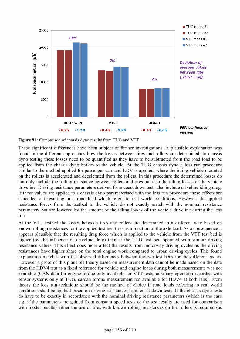
page 153 of 210

Figure 91: Comparison of chassis dyno results from TUG and VTT

These significant differences have been subject of further investigations. A plausible explanation was found in the different approaches how the losses between tires and rollers are determined. In chassis dyno testing these losses need to be quantified as they have to be subtracted from the road load to be applied from the chassis dyno brakes to the vehicle. At the TUG chassis dyno a loss run procedure similar to the method applied for passenger cars and LDV is applied, where the idling vehicle mounted on the rollers is accelerated and decelerated from the rollers. In this procedure the determined losses do not only include the rolling resistance between rollers and tires but also the idling losses of the vehicle driveline. Driving resistance parameters derived from coast down tests also include driveline idling drag. If these values are applied to a chassis dyno parameterised with the loss run procedure these effects are cancelled out resulting in a road load which refers to real world conditions. However, the applied resistance forces from the testbed to the vehicle do not exactly match with the nominal resistance parameters but are lowered by the amount of the idling losses of the vehicle driveline during the loss run.At the VTT testbed the losses between tires and rollers are determined in a different way based on known rolling resistances for the applied test bed tires as a function of the axle load. As a consequence it appears plausible that the resulting drag force which is applied to the vehicle from the VTT test bed is higher (by the influence of driveline drag) than at the TUG test bed operated with similar driving resistance values. This effect does more affect the results from motorway driving cycles as the driving resistances have higher share on the total engine work compared to urban driving cycles. This found explanation matches with the observed differences between the two test beds for the different cycles. However a proof of this plausible theory based on measurement data cannot be made based on the data from the HDV4 test as a fixed reference for vehicle and engine loads during both measurements was not available (CAN data for engine torque only available for VTT tests, auxiliary operation recorded with sensor systems only at TUG, cardan torque measurement not available for HDV4 at both labs). From theory the loss run technique should be the method of choice if road loads referring to real world conditions shall be applied based on driving resistances from coast down tests. If the chassis dyno tests do have to be exactly in accordance with the nominal driving resistance parameters (which is the case e.g. if the parameters are gained from constant speed tests or the test results are used for comparison with model results) either the use of tires with known rolling resistances on the rollers is required (as

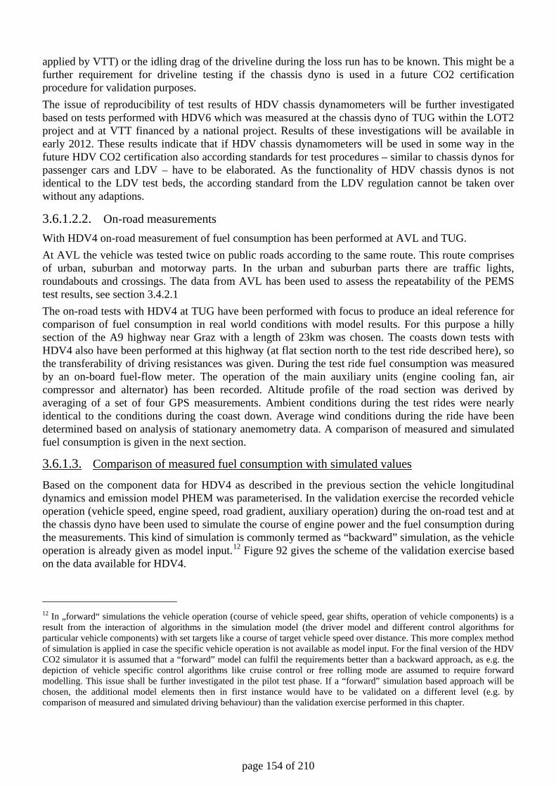
page 154 of 210

applied by VTT) or the idling drag of the driveline during the loss run has to be known. This might be a further requirement for driveline testing if the chassis dyno is used in a future CO2 certification procedure for validation purposes. The issue of reproducibility of test results of HDV chassis dynamometers will be further investigated based on tests performed with HDV6 which was measured at the chassis dyno of TUG within the LOT2 project and at VTT financed by a national project. Results of these investigations will be available in early 2012. These results indicate that if HDV chassis dynamometers will be used in some way in the future HDV CO2 certification also according standards for test procedures – similar to chassis dynos for passenger cars and LDV – have to be elaborated. As the functionality of HDV chassis dynos is not identical to the LDV test beds, the according standard from the LDV regulation cannot be taken over without any adaptions.

3.6.1.2.2. On-road measurements With HDV4 on-road measurement of fuel consumption has been performed at AVL and TUG. At AVL the vehicle was tested twice on public roads according to the same route. This route comprises of urban, suburban and motorway parts. In the urban and suburban parts there are traffic lights, roundabouts and crossings. The data from AVL has been used to assess the repeatability of the PEMS test results, see section 3.4.2.1 The on-road tests with HDV4 at TUG have been performed with focus to produce an ideal reference for comparison of fuel consumption in real world conditions with model results. For this purpose a hilly section of the A9 highway near Graz with a length of 23km was chosen. The coasts down tests with HDV4 also have been performed at this highway (at flat section north to the test ride described here), so the transferability of driving resistances was given. During the test ride fuel consumption was measured by an on-board fuel-flow meter. The operation of the main auxiliary units (engine cooling fan, air compressor and alternator) has been recorded. Altitude profile of the road section was derived by averaging of a set of four GPS measurements. Ambient conditions during the test rides were nearly identical to the conditions during the coast down. Average wind conditions during the ride have been determined based on analysis of stationary anemometry data. A comparison of measured and simulated fuel consumption is given in the next section.

3.6.1.3. Comparison of measured fuel consumption with simulated values

Based on the component data for HDV4 as described in the previous section the vehicle longitudinal dynamics and emission model PHEM was parameterised. In the validation exercise the recorded vehicle operation (vehicle speed, engine speed, road gradient, auxiliary operation) during the on-road test and at the chassis dyno have been used to simulate the course of engine power and the fuel consumption during the measurements. This kind of simulation is commonly termed as “backward” simulation, as the vehicle operation is already given as model input.12 Figure 92 gives the scheme of the validation exercise based on the data available for HDV4.

12 In „forward“ simulations the vehicle operation (course of vehicle speed, gear shifts, operation of vehicle components) is a result from the interaction of algorithms in the simulation model (the driver model and different control algorithms for particular vehicle components) with set targets like a course of target vehicle speed over distance. This more complex method of simulation is applied in case the specific vehicle operation is not available as model input. For the final version of the HDV CO2 simulator it is assumed that a “forward” model can fulfil the requirements better than a backward approach, as e.g. the depiction of vehicle specific control algorithms like cruise control or free rolling mode are assumed to require forward modelling. This issue shall be further investigated in the pilot test phase. If a “forward” simulation based approach will be chosen, the additional model elements then in first instance would have to be validated on a different level (e.g. by comparison of measured and simulated driving behaviour) than the validation exercise performed in this chapter.

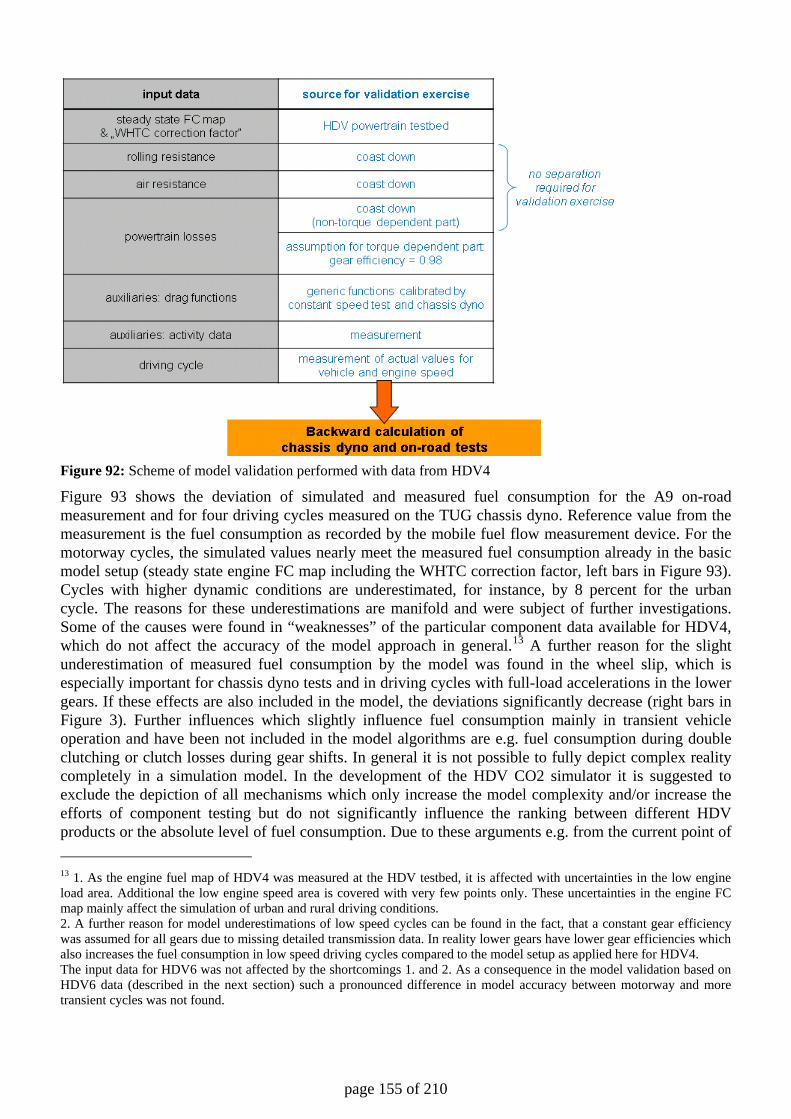
page 155 of 210

Figure 92: Scheme of model validation performed with data from HDV4

Figure 93 shows the deviation of simulated and measured fuel consumption for the A9 on-road measurement and for four driving cycles measured on the TUG chassis dyno. Reference value from the measurement is the fuel consumption as recorded by the mobile fuel flow measurement device. For the motorway cycles, the simulated values nearly meet the measured fuel consumption already in the basic model setup (steady state engine FC map including the WHTC correction factor, left bars in Figure 93). Cycles with higher dynamic conditions are underestimated, for instance, by 8 percent for the urban cycle. The reasons for these underestimations are manifold and were subject of further investigations. Some of the causes were found in “weaknesses” of the particular component data available for HDV4, which do not affect the accuracy of the model approach in general.13 A further reason for the slight underestimation of measured fuel consumption by the model was found in the wheel slip, which is especially important for chassis dyno tests and in driving cycles with full-load accelerations in the lower gears. If these effects are also included in the model, the deviations significantly decrease (right bars in Figure 3). Further influences which slightly influence fuel consumption mainly in transient vehicle operation and have been not included in the model algorithms are e.g. fuel consumption during double clutching or clutch losses during gear shifts. In general it is not possible to fully depict complex reality completely in a simulation model. In the development of the HDV CO2 simulator it is suggested to exclude the depiction of all mechanisms which only increase the model complexity and/or increase the efforts of component testing but do not significantly influence the ranking between different HDV products or the absolute level of fuel consumption. Due to these arguments e.g. from the current point of 13 1. As the engine fuel map of HDV4 was measured at the HDV testbed, it is affected with uncertainties in the low engine load area. Additional the low engine speed area is covered with very few points only. These uncertainties in the engine FC map mainly affect the simulation of urban and rural driving conditions. 2. A further reason for model underestimations of low speed cycles can be found in the fact, that a constant gear efficiency was assumed for all gears due to missing detailed transmission data. In reality lower gears have lower gear efficiencies which also increases the fuel consumption in low speed driving cycles compared to the model setup as applied here for HDV4. The input data for HDV6 was not affected by the shortcomings 1. and 2. As a consequence in the model validation based on HDV6 data (described in the next section) such a pronounced difference in model accuracy between motorway and more transient cycles was not found.

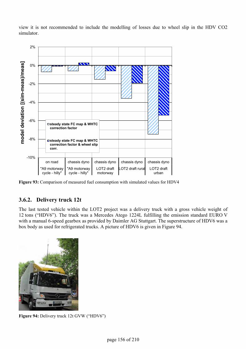
page 156 of 210

view it is not recommended to include the modelling of losses due to wheel slip in the HDV CO2 simulator.

Figure 93: Comparison of measured fuel consumption with simulated values for HDV4

3.6.2. Delivery truck 12tThe last tested vehicle within the LOT2 project was a delivery truck with a gross vehicle weight of 12 tons (“HDV6”). The truck was a Mercedes Atego 1224L fulfilling the emission standard EURO Vwith a manual 6-speed gearbox as provided by Daimler AG Stuttgart. The superstructure of HDV6 was a box body as used for refrigerated trucks. A picture of HDV6 is given in Figure 94.

Figure 94: Delivery truck 12t GVW (“HDV6”)

-10%

-8%

-6%

-4%

-2%

0%

2%

on road chassis dyno chassis dyno chassis dyno chassis dyno

"A9 motorwaycycle - hilly"

"A9 motorwaycycle - hilly"

LOT2 draftmotorway

LOT2 draft rural LOT2 drafturban

mod

el d

evia

tion

[(sim

-mea

s)/m

eas]

steady state FC map & WHTCcorrection factor

steady state FC map & WHTCcorrection factor & wheel slipcorr.

page 157 of 210

HDV6 was used for driving resistance tests by TUG and TÜV. At TUG also chassis dyno tests have been performed. These tests were covered by the LOT2 funding. Additional vehicle testing financed by national projects with HDV6 was done at VTT (driving resistance tests, chassis dyno) and at TNO (HDV powertrain testbed). Results from these tests will be published in spring 2012 in separate reports.

3.6.2.1. Applied measurement systems

Based on the experiences gained from the measurements with HDV4 it was decided to use identical vehicle instrumentation in all tests of all participating labs. The following measurement equipment has been installed at HDV6:

• Fuel flow measurement by an AVL KMA Mobile system • Cardan torque measurement by a wire strain gauge applied by HBM and a MANNER telemetry

system • Engine speed measured by a rotational speed sensor • Engine cooling fan operation measured by a rotational speed sensor • Air compressor operation recorded by a pressure sensor between compressor and air dryer • Alternator current measured by a wire strain gauge

For the vehicle tests on the test tracks additionally the following measurement systems have been used: • Ultra sonic anemometer for measurement of air inflow speed and direction • GPS system for measurement of vehicle speed and vehicle position

This measurement equipment does not fully match with the instrumentation as proposed for the vehicle tests in the pilot test phase (the according instrumentation is described in section 2.4.1.2), especially the torque measurement at constant speed was not based on the proposed wheel rim torque meters since this option was not considered at the time of the Atego tests. During the course of the LOT2 project many experiences with vehicle related measurement systems have been gained. As for most measurement techniques problems with stable operation and sensitivity of measured values to measurement conditions occurred. The measurement quantities which were found to be most sensitive are listed below: • Measurement of air inflow speed and inflow angle by mobile anemometry:

In the evaluation of vehicle tests the air inflow speed and inflow angle can give important information as the air stream on the vehicle can differ from vehicle speed by the superposition with ambient wind. However, when the anemometer is mounted on the vehicle the measured air flow is influenced by the air flow around the vehicle surface. Hence the recorded air flow can significantly differ from the undisturbed air flow, which would be required as input into the data analysis (see also section 3.5.1.2). As a consequence the measured data from the on-board anemometer have to be calibrated to “undisturbed conditions” either by CFD calculations or calibration measurements (e.g. constant speed tests in wind still conditions or correlation with stationary anemometry data). For HDV6 this calibration has been performed by both methods (CFD and calibration measurements for the vehicle tests with wind-shield, calibration measurements for the vehicle tests without windshield). From the experiences gained during this work it was concluded that these necessary calibration procedures always are affected with certain uncertainties and hence influence the measured results for total air inflow speed. If vehicle tests are evaluated based on on-board measured air inflow speed beside the additional information on actual air-flow conditions these uncertainties of the calibration are directly carried over into the result for air drag of the vehicle.

• Measurement of cardan torque by a wire strain gauge: The torque measurement at the cardan torque was calibrated by a lever mechanism at the dismounted cardan shaft directly after the application of the wire strain gauge. A measuring circuit was chosen which from theory should totally eliminate the temperature influence on the measurement result. The evaluation of measurement results was done on the assumption that the stiffness of the cardan shaft

page 158 of 210

does not change over the entire test series (as the stiffness can only be determined accurately at a dismounted cardan shaft). During the test series at each day the zero point of the system was determined, as it is known that the zero point shows a drift due to small plastic deformations of the cardan shaft during vehicle operation. In the course of vehicle tests it emerged, that this zero point shows a small dependency whether it was determined at a cold or at a warm vehicle. After this observation was made, always the zero point determined in warm conditions has been used in the test evaluation. However, this observed phenomenon indicates a potential inaccuracy of the measured torque, which was estimated to be in a range of about +/-7 Nm. For HDV6 this magnitude of uncertainty refers to about 7% of the cardan torque at very low vehicle speeds and to about 2% of the cardan torque at 90km/h. The cardan torque measurement of HDV6 will be recalibrated when the system will be dismounted from HDV6 (this has not happened yet when this report was written since the HDV was still running on the test bed at TNO). Further insights on this measurement technique are expected based on these data. It is expected, that based on comprehensive practical experience the accuracy of the cardan torque measurement can be improved compared to the accuracy estimated for the tests at HDV6. For the constant speed tests as proposed for the future CO2 certification it is suggested to use wheel rim torque meters or flanges between rim and the wheel end. Beside the fact that the measured torque is not influenced by the losses in the axle transmission these systems are assumed to be easier in handling and more accurate. However, these assumptions will have to be confirmed in the pilot test phase.

• Measurement of vehicle speed with a GPS system: From the experiences with several GPS systems for professional application it can be concluded that the accuracy of the measured velocity is clearly lower than specified from the manufacturers. This effect was especially found for measurement conditions with low satellites reception, but also in good reception conditions the quality of the recorded velocity was below the expectations. This is especially a problem for coast down tests in the low vehicle speed range, where very low accelerations have to be derived from the recorded velocity signal. Also the acceleration correction in the evaluation of the constant speed tests is affected by this low accuracy, but the overall test result of the constant speed test is not very sensitive on this factor (here it mainly worsens a quality criteria for the measurement data but does not significantly influence the obtained cd-value). In the pilot test phase also other options for recording of vehicle speed (optical sensors, vehicle speed from ECU) shall be investigated.

• Measurement of road gradient with a GPS system: For the evaluation of driving resistance tests the accuracy of the altitude as measured by a GPS system is clearly not appropriate. Instead it is recommended to take the altitude profile e.g. from a construction plan and interpolate the road gradient based on this information and the vehicle position as recorded from the GPS.

3.6.2.2. Component tests

Data on most vehicle components have been made available by Daimler. In the measurement programme of the LOT2 consortium the focus was set on vehicle tests for determination of the driving resistances. Late in 2011 tests with HDV6 were performed on the HDV powertrain testbed with focus on assessment of losses in the driveline.

3.6.2.2.1. Engine FC map All relevant engine specific data from engine test bed tests was made available by Daimler. The submitted data contained the following information:

• Engine full-load curve

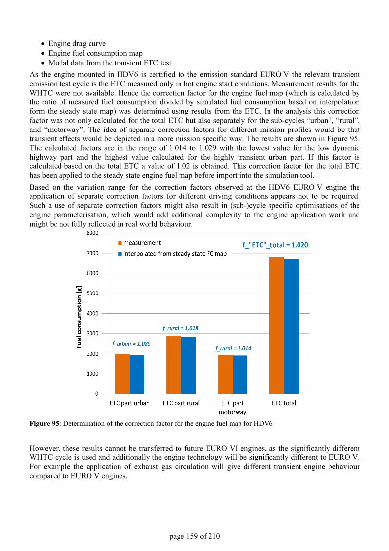
page 159 of 210

• Engine drag curve• Engine fuel consumption map• Modal data from the transient ETC test

As the engine mounted in HDV6 is certified to the emission standard EURO V the relevant transient emission test cycle is the ETC measured only in hot engine start conditions. Measurement results for the WHTC were not available. Hence the correction factor for the engine fuel map (which is calculated by the ratio of measured fuel consumption divided by simulated fuel consumption based on interpolation form the steady state map) was determined using results from the ETC. In the analysis this correction factor was not only calculated for the total ETC but also separately for the sub-cycles “urban”, “rural”, and “motorway”. The idea of separate correction factors for different mission profiles would be that transient effects would be depicted in a more mission specific way. The results are shown in Figure 95.The calculated factors are in the range of 1.014 to 1.029 with the lowest value for the low dynamic highway part and the highest value calculated for the highly transient urban part. If this factor is calculated based on the total ETC a value of 1.02 is obtained. This correction factor for the total ETC has been applied to the steady state engine fuel map before import into the simulation tool. Based on the variation range for the correction factors observed at the HDV6 EURO V engine the application of separate correction factors for different driving conditions appears not to be required. Such a use of separate correction factors might also result in (sub-)cycle specific optimisations of the engine parameterisation, which would add additional complexity to the engine application work and might be not fully reflected in real world behaviour.

Figure 95: Determination of the correction factor for the engine fuel map for HDV6

However, these results cannot be transferred to future EURO VI engines, as the significantly different WHTC cycle is used and additionally the engine technology will be significantly different to EURO V. For example the application of exhaust gas circulation will give different transient engine behaviour compared to EURO V engines.

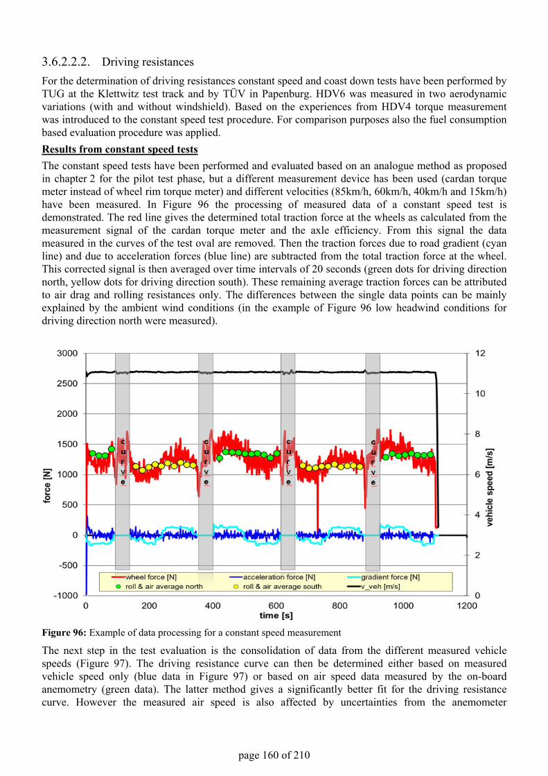
page 160 of 210

3.6.2.2.2. Driving resistancesFor the determination of driving resistances constant speed and coast down tests have been performed by TUG at the Klettwitz test track and by TÜV in Papenburg. HDV6 was measured in two aerodynamic variations (with and without windshield). Based on the experiences from HDV4 torque measurement was introduced to the constant speed test procedure. For comparison purposes also the fuel consumption based evaluation procedure was applied. Results from constant speed tests The constant speed tests have been performed and evaluated based on an analogue method as proposed in chapter 2 for the pilot test phase, but a different measurement device has been used (cardan torque meter instead of wheel rim torque meter) and different velocities (85km/h, 60km/h, 40km/h and 15km/h) have been measured. In Figure 96 the processing of measured data of a constant speed test is demonstrated. The red line gives the determined total traction force at the wheels as calculated from the measurement signal of the cardan torque meter and the axle efficiency. From this signal the data measured in the curves of the test oval are removed. Then the traction forces due to road gradient (cyan line) and due to acceleration forces (blue line) are subtracted from the total traction force at the wheel. This corrected signal is then averaged over time intervals of 20 seconds (green dots for driving direction north, yellow dots for driving direction south). These remaining average traction forces can be attributed to air drag and rolling resistances only. The differences between the single data points can be mainly explained by the ambient wind conditions (in the example of Figure 96 low headwind conditions for driving direction north were measured).

Figure 96: Example of data processing for a constant speed measurement

The next step in the test evaluation is the consolidation of data from the different measured vehicle speeds (Figure 97). The driving resistance curve can then be determined either based on measured vehicle speed only (blue data in Figure 97) or based on air speed data measured by the on-board anemometry (green data). The latter method gives a significantly better fit for the driving resistance curve. However the measured air speed is also affected by uncertainties from the anemometer

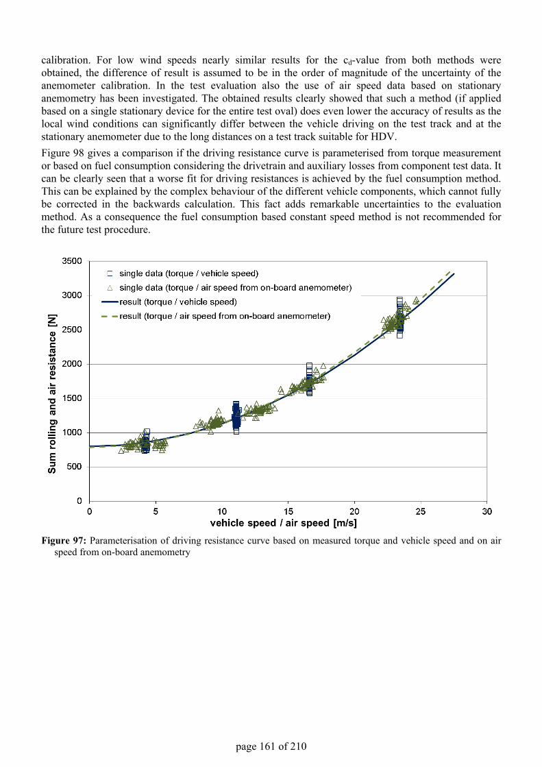
page 161 of 210

calibration. For low wind speeds nearly similar results for the cd-value from both methods were obtained, the difference of result is assumed to be in the order of magnitude of the uncertainty of the anemometer calibration. In the test evaluation also the use of air speed data based on stationary anemometry has been investigated. The obtained results clearly showed that such a method (if applied based on a single stationary device for the entire test oval) does even lower the accuracy of results as the local wind conditions can significantly differ between the vehicle driving on the test track and at the stationary anemometer due to the long distances on a test track suitable for HDV.Figure 98 gives a comparison if the driving resistance curve is parameterised from torque measurement or based on fuel consumption considering the drivetrain and auxiliary losses from component test data. It can be clearly seen that a worse fit for driving resistances is achieved by the fuel consumption method. This can be explained by the complex behaviour of the different vehicle components, which cannot fully be corrected in the backwards calculation. This fact adds remarkable uncertainties to the evaluation method. As a consequence the fuel consumption based constant speed method is not recommended for the future test procedure.

Figure 97: Parameterisation of driving resistance curve based on measured torque and vehicle speed and on air speed from on-board anemometry

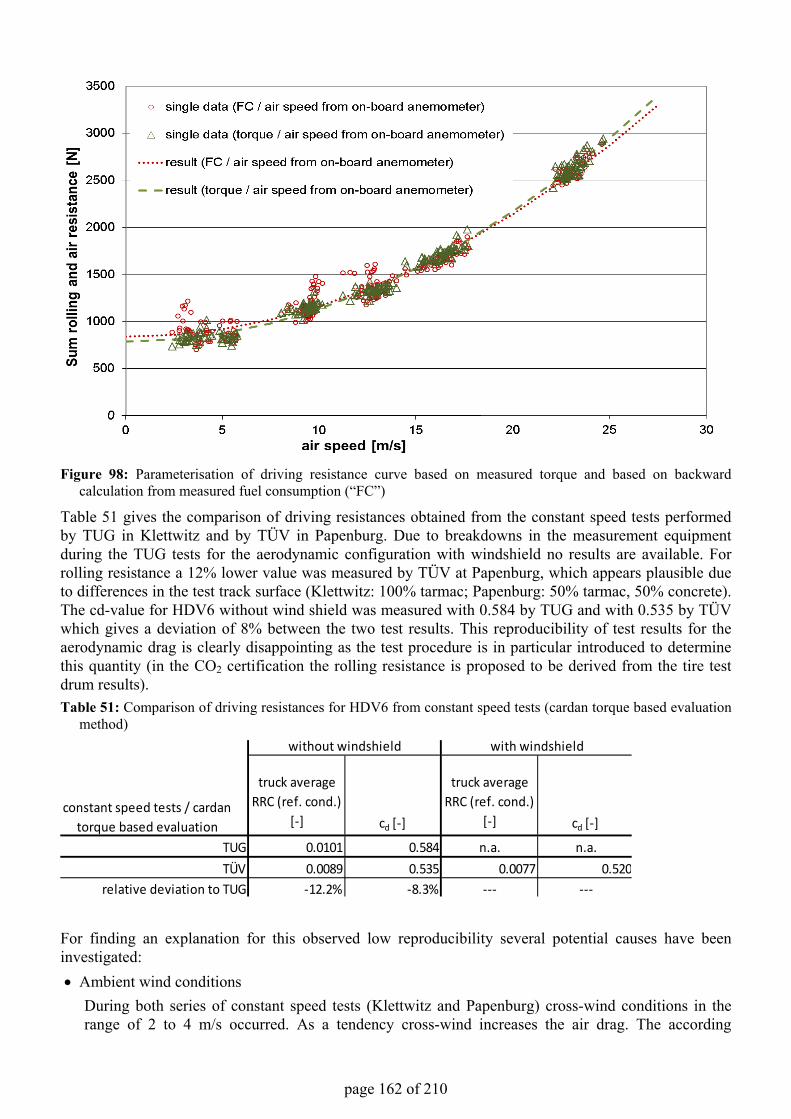
page 162 of 210

Figure 98: Parameterisation of driving resistance curve based on measured torque and based on backward calculation from measured fuel consumption (“FC”)

Table 51 gives the comparison of driving resistances obtained from the constant speed tests performed by TUG in Klettwitz and by TÜV in Papenburg. Due to breakdowns in the measurement equipment during the TUG tests for the aerodynamic configuration with windshield no results are available. For rolling resistance a 12% lower value was measured by TÜV at Papenburg, which appears plausible due to differences in the test track surface (Klettwitz: 100% tarmac; Papenburg: 50% tarmac, 50% concrete). The cd-value for HDV6 without wind shield was measured with 0.584 by TUG and with 0.535 by TÜV which gives a deviation of 8% between the two test results. This reproducibility of test results for the aerodynamic drag is clearly disappointing as the test procedure is in particular introduced to determine this quantity (in the CO2 certification the rolling resistance is proposed to be derived from the tire test drum results). Table 51: Comparison of driving resistances for HDV6 from constant speed tests (cardan torque based evaluation

method)

For finding an explanation for this observed low reproducibility several potential causes have been investigated: • Ambient wind conditions

During both series of constant speed tests (Klettwitz and Papenburg) cross-wind conditions in the range of 2 to 4 m/s occurred. As a tendency cross-wind increases the air drag. The according

truck average RRC (ref. cond.)

[-] cd [-]

truck average RRC (ref. cond.)

[-] cd [-]

TUG 0.0101 0.584 n.a. n.a.TÜV 0.0089 0.535 0.0077 0.520

relative deviation to TUG -12.2% -8.3% --- ---

without windshield with windshield

constant speed tests / cardan torque based evaluation

page 163 of 210

influence cannot be corrected based on the proposed evaluation method resulting in higher cd-values compared to conditions without side wind. However test results from a measurement series with different tractor – semitrailer combination (37 p. 23) showed no pronounced sensitivity of test results to low cross-wind conditions. As the according ambient wind conditions during the tests at HDV6 were more or less comparable, either the set up without windshield is much more sensitive against side wind conditions than the tests with the tractor semitrailers or an yet not fully understood uncertainty arose from the torque measurement.

• Ambient conditions regarding air density and temperature If the test results from TUG and TÜV would be compared without ambient correction, a much lower reproducibility would be obtained. However, an indication that the correction does not fully depict real world conditions can be found in the fact that the corrected data for resistance forces in general showed a slightly worse fit to the driving resistance curve than the uncorrected values (from theory it should be the other way round). In this context the correction of air density should robust. Remarkable uncertainties can be expected the in the correction of rolling resistance from measurement conditions to reference ambient conditions. As not all constant speeds are driven with similar ambient temperature this might also influence the results for cd-value. More data on correction factors for ambient temperature shall be investigated in the pilot phase. The sensitivity of the method to this uncertainty is also reduced if only two constant speeds are used (e.g. 15km/h and 90km/h). These tests can then be driven within rather similar ambient conditions reducing the cross sensitivity between obtained cd-value and rolling resistance.

• Cardan torque measurement During the test series a small sensitivity of the zero-point in the torque calibration to temperature conditions was observed. However, the cd-values should not be biased by this issue. If there are further inaccuracies in the applied cardan torque measurement technique is not known yet. In the pilot test phase more experiences shall be gained with the rim torque meters including the definition of a calibration procedure.

• Cross sensitivity of determined Cd-value to rolling resistance variance over vehicle speed The test evaluation is based on the simplification that the rolling resistance is a constant value over the full vehicle speed range. If a small influence of vehicle speed on rolling resistance shows different trends on different test tracks this would worsen the reproducibility of driving resistance tests. However, as a high reproducibility of driving resistances based on coast downs was found in the comparison of Klettwitz and Papenburg results (see discussion below) this is not assumed to be a main influence factor on reproducibility of constant speed tests for HDV6.

The repeatability of the constant speed method cannot be analysed based on the available data from LOT2 as multiple measurements of a particular vehicle configuration performed on different days on a similar test track are not available. From the ICCT project a repeatability of constant speed tests was found with about +/-3% for the 95% confidence interval of the Cd-value (37 p. 20). The evaluations there have been done with the fuel consumption based method, the potential of the torque based method is assumed to be significantly better. Results from coast down tests Compared to the coast down tests with HDV4 for HDV6 the altitude profile has been included in the test analysis for all measurements. For the TUG tests also on-board anemometry was available, hence the related data have been analysed based on measured air speed. For the TÜV tests in Papenburg the use of the on-board anemometry systems was not possible as the resulting total vehicle height exceeded the maximum overhead clearance of the test track. Hence the data from the TÜV has been evaluated based on vehicle speed only. The applied method of data evaluation is described in section 3.5.1.6 Table 52 gives the results from the coast down tests for the two investigated aerodynamic configurations of HDV6. Nearly identical cd-values have been obtained from both labs and both settings of the vehicle.

page 164 of 210

Rolling resistance was determined by 15% higher in Papenburg compared to Klettwitz conditions which approximately matches with the results from the constant speed tests. For both aerodynamic variations of HDV6 nearly similar rolling resistance coefficients have been obtained, which is plausible as both vehicle variants have nearly similar vehicle weight and similar tires. If the test results for cd-values of HDV6 from coast down are compared with the results from constant speed tests significant differences can be found. For the vehicle configuration without windshield the average cd-value from the constant speed tests was found at 0.56 whereas the coasts down results predict a cd-value of 0.67. Also for the change in aerodynamic drag due to the removal of windshield completely different values are obtained by the two test procedures. From the constant speed tests an increase in air drag by 3% is obtained compared to a test result of +17% obtained from the coast down tests. Such clear differences in the quantification of aerodynamic variants between constant speed tests and coast down have also been observed at the ICCT measurements. From the analysis it was concluded that in general constant speed tests should give more reliable results. As the main reason it was considered that the driving resistances for the low vehicle speed range obtained from coast down tests are systematically biased by the transmission idling drag and by the uncertainties related to the measurement of low accelerations. However, based on the experiences gained from the available measurements a full understanding of all relevant uncertainties was not achieved yet. Due to the above mentioned arguments from the current point of view the constant speed test procedure is preferred compared to coast down tests for the future CO2 certification. However, for the suitability of application this test procedure will have to prove a sufficient reproducibility in the pilot test phase. If this is not the case as a fall back strategy also the measurement of coast downs are recommended to be performed in the pilot phase. Table 52: Comparison of driving resistances for HDV6 from coast down

3.6.2.2.3. Auxiliary data For most of the auxiliary units Daimler provided detailed data from component tests. In particular the following data was available

• the propeller curve of the engine cooling fan (power consumption due to air drag as a function of propeller speed)

• for the air compressor the dependency of mechanical power consumption as function of compressor speed and pressure difference including compressor idling drag

• the efficiency map of the alternator (efficiency as a function of alternator speed and alternator current)

• for the steering pump the power consumption as a function of pump speed The power loss in the viscous clutch has been assessed by a downscaling of the losses determined for the viscous clutch in HDV4. The power losses of the compressor of the driver’s cabin air conditioning (A/C) system have been quantified by values from literature (69). During the vehicle tests the A/C was always shut off so only the power consumption in idling conditions had to be considered.

truck average RRC (ref. cond.)

[-] cd [-]

truck average RRC (ref. cond.)

[-] cd [-]

TUG 0.0089 0.665 0.0087 0.572TÜV 0.0077 0.669 0.0073 0.572

relative deviation to TUG -13.7% 0.5% -16.8% -0.1%

coast down tests

without windshield with windshield

page 165 of 210

3.6.2.2.4. Transmission data Daimler provided the transmission ratios of the single gears and of the axle transmission as well as fixed efficiency values for all transmission ratios. This data is not fully compatible to the proposal for the future certification procedure, where so far the input of much more specific data (including measurement of speed dependent losses and detailed calculation of torque depended losses) has been suggested.

3.6.2.3. Fuel consumption measurements

To obtain fuel consumption data for a validation of the simulation approach chassis dyno tests at the TUG test bed and measurements of a target speed cycle at the Klettwitz test track (performed by TUG) and at the Papenburg test track (performed by TÜV) have been executed with HDV6.

3.6.2.3.1. Chassis dynamometer tests The following measurements have been performed with HDV6 on the TUG chassis dyno:

• Constant speed tests (15, 40, 60, 85 km/h) • CST-urban (common short test cycle part “urban”) • CST-road (common short test cycle part “road”) • CST-motorway (common short test cycle part “motorway”)

In the parameterisation of the TUG chassis dyno the loss run procedure has been used for determination of the losses between tires and roller. If this test procedure is applied the idling losses of the transmission have to be known in order to obtain similar driving resistances applied to the vehicle than specified by the resistance parameters, as already discussed in section 3.6.1.2.1. These losses were known from the manufacturer and have been subtracted from the parameters determined with the loss run procedure. In order to validate this approach in the evaluation of the chassis dynamometer data a comparison of calculated target traction forces to be applied from the rollers to the vehicle with measured values from cardan torque measurement has been performed In this comparison a slightly lower level of measured forces (on average -2%) has been determined. This deviation is in the range of the measurement accuracy and indicates the validity of the assumed idling losses.

3.6.2.3.2. Test track measurements In order to gain data on fuel consumption measured in on-road conditions which can be used for model validation a target speed cycle was driven at both test tracks where driving resistance tests have been performed (Klettwitz, Papenburg). During the measurement fuel consumption and vehicle operation conditions were recorded (including auxiliary operation and ambient wind). Figure 99 shows as an example vehicle speed, road gradient and ambient wind for the target speed cycle driven in Klettwitz.

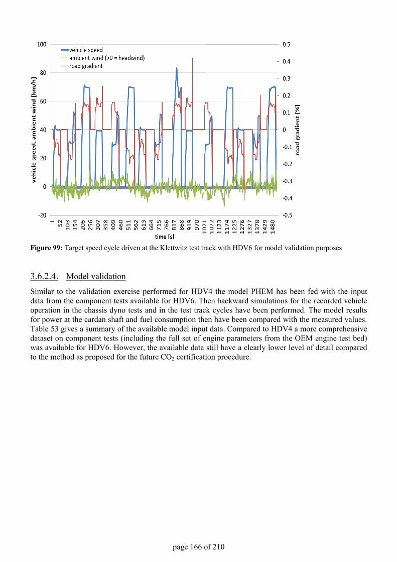
page 166 of 210

Figure 99: Target speed cycle driven at the Klettwitz test track with HDV6 for model validation purposes

3.6.2.4. Model validation

Similar to the validation exercise performed for HDV4 the model PHEM has been fed with the input data from the component tests available for HDV6. Then backward simulations for the recorded vehicle operation in the chassis dyno tests and in the test track cycles have been performed. The model results for power at the cardan shaft and fuel consumption then have been compared with the measured values. Table 53 gives a summary of the available model input data. Compared to HDV4 a more comprehensive dataset on component tests (including the full set of engine parameters from the OEM engine test bed) was available for HDV6. However, the available data still have a clearly lower level of detail compared to the method as proposed for the future CO2 certification procedure.

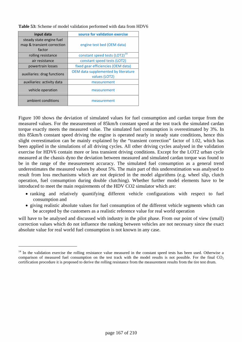
page 167 of 210

Table 53: Scheme of model validation performed with data from HDV6

input data source for validation exercise steady state engine fuel

map & transient correction factor

engine test bed (OEM data)

rolling resistance constant speed tests (LOT2)14 air resistance constant speed tests (LOT2)

powertrain losses fixed gear efficiencies (OEM data)

auxiliaries: drag functions OEM data supplemented by literature values (LOT2)

auxiliaries: activity data measurement

vehicle operation measurement

ambient conditions measurement

Figure 100 shows the deviation of simulated values for fuel consumption and cardan torque from the measured values. For the measurement of 85km/h constant speed at the test track the simulated cardan torque exactly meets the measured value. The simulated fuel consumption is overestimated by 3%. In this 85km/h constant speed driving the engine is operated nearly in steady state conditions, hence this slight overestimation can be mainly explained by the “transient correction” factor of 1.02, which has been applied in the simulations of all driving cycles. All other driving cycles analysed in the validation exercise for HDV6 contain more or less transient driving conditions. Except for the LOT2 urban cycle measured at the chassis dyno the deviation between measured and simulated cardan torque was found to be in the range of the measurement accuracy. The simulated fuel consumption as a general trend underestimates the measured values by about 5%. The main part of this underestimation was analysed to result from loss mechanisms which are not depicted in the model algorithms (e.g. wheel slip, clutch operation, fuel consumption during double clutching). Whether further model elements have to be introduced to meet the main requirements of the HDV CO2 simulator which are:

• ranking and relatively quantifying different vehicle configurations with respect to fuel consumption and

• giving realistic absolute values for fuel consumption of the different vehicle segments which can be accepted by the customers as a realistic reference value for real world operation

will have to be analysed and discussed with industry in the pilot phase. From our point of view (small) correction values which do not influence the ranking between vehicles are not necessary since the exact absolute value for real world fuel consumption is not known in any case.

14 In the validation exercise the rolling resistance value measured in the constant speed tests has been used. Otherwise a comparison of measured fuel consumption on the test track with the model results is not possible. For the final CO2 certification procedure it is proposed to derive the rolling resistance from the measurement results from the tire test drum.

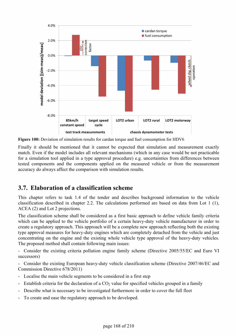
page 168 of 210

Figure 100: Deviation of simulation results for cardan torque and fuel consumption for HDV6

Finally it should be mentioned that it cannot be expected that simulation and measurement exactly match. Even if the model includes all relevant mechanisms (which in any case would be not practicable for a simulation tool applied in a type approval procedure) e.g. uncertainties from differences between tested components and the components applied on the measured vehicle or from the measurement accuracy do always affect the comparison with simulation results.

3.7. Elaboration of a classification schemeThis chapter refers to task 1.4 of the tender and describes background information to the vehicle classification described in chapter 2.2. The calculations performed are based on data from Lot 1 (1),ACEA (2) and Lot 2 projections.The classification scheme shall be considered as a first basic approach to define vehicle family criteria which can be applied to the vehicle portfolio of a certain heavy-duty vehicle manufacturer in order to create a regulatory approach. This approach will be a complete new approach reflecting both the existing type approval measures for heavy-duty engines which are completely detached from the vehicle and just concentrating on the engine and the existing whole vehicle type approval of the heavy-duty vehicles. The proposed method shall contain following main issues:- Consider the existing criteria pollution engine family scheme (Directive 2005/55/EC and Euro VI successors)- Consider the existing European heavy-duty vehicle classification scheme (Directive 2007/46/EC and Commission Directive 678/2011)- Localise the main vehicle segments to be considered in a first step- Establish criteria for the declaration of a CO2 value for specified vehicles grouped in a family- Describe what is necessary to be investigated furthermore in order to cover the full fleet- To create and ease the regulatory approach to be developed.

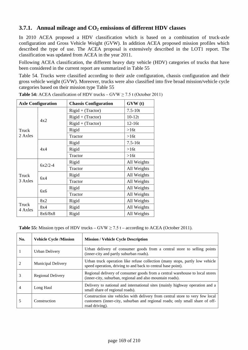
page 169 of 210

3.7.1. Annual mileage and CO2 emissions of different HDV classes In 2010 ACEA proposed a HDV classification which is based on a combination of truck-axle configuration and Gross Vehicle Weight (GVW). In addition ACEA proposed mission profiles which described the type of use. The ACEA proposal is extensively described in the LOT1 report. The classification was updated from ACEA in the year 2011. Following ACEA classification, the different heavy duty vehicle (HDV) categories of trucks that have been considered in the current report are summarized in Table 55 Table 54. Trucks were classified according to their axle configuration, chassis configuration and their gross vehicle weight (GVW). Moreover, trucks were also classified into five broad mission/vehicle cycle categories based on their mission type Table 55 Table 54: ACEA classification of HDV trucks – GVW ≥ 7.5 t (October 2011)

Axle Configuration Chassis Configuration GVW (t)

Truck 2 Axles

4x2

Rigid + (Tractor) 7.5-10t Rigid + (Tractor) 10-12t Rigid + (Tractor) 12-16t Rigid >16t Tractor >16t

4x4 Rigid 7.5-16t Rigid >16t Tractor >16t

Truck 3 Axles

6x2/2-4 Rigid All Weights Tractor All Weights

6x4 Rigid All Weights Tractor All Weights

6x6 Rigid All Weights Tractor All Weights

Truck 4 Axles

8x2 Rigid All Weights 8x4 Rigid All Weights 8x6/8x8 Rigid All Weights

Table 55: Mission types of HDV trucks – GVW ≥ 7.5 t – according to ACEA (October 2011).

No. Vehicle Cycle /Mission Mission / Vehicle Cycle Description

1 Urban Delivery Urban delivery of consumer goods from a central store to selling points (inner-city and partly suburban roads).

2 Municipal Delivery Urban truck operation like refuse collection (many stops, partly low vehicle speed operation, driving to and back to central base point).

3 Regional Delivery Regional delivery of consumer goods from a central warehouse to local stores (inner-city, suburban, regional and also mountain roads).

4 Long Haul Delivery to national and international sites (mainly highway operation and a small share of regional roads).

5 Construction Construction site vehicles with delivery from central store to very few local customers (inner-city, suburban and regional roads; only small share of off-road driving).

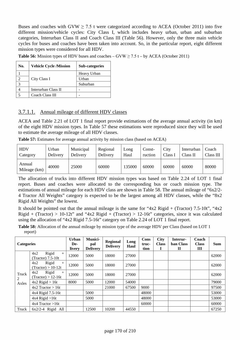
page 170 of 210

Buses and coaches with GVW ≥ 7.5 t were categorized according to ACEA (October 2011) into five different mission/vehicle cycles: City Class I, which includes heavy urban, urban and suburban categories, Interurban Class II and Coach Class III (Table 56). However, only the three main vehicle cycles for buses and coaches have been taken into account. So, in the particular report, eight different mission types were considered for all HDV. Table 56: Mission types of HDV buses and coaches – GVW ≥ 7.5 t – by ACEA (October 2011)

No. Vehicle Cycle /Mission Sub-categories

1 City Class I

Heavy Urban 2 Urban 3 Suburban 4 Interurban Class II - 5 Coach Class III -

3.7.1.1. Annual mileage of different HDV classes

ACEA and Table 2.21 of LOT 1 final report provide estimations of the average annual activity (in km) of the eight HDV mission types. In Table 57 these estimations were reproduced since they will be used to estimate the average mileage of all HDV classes. Table 57: Estimates for average annual activity by mission class (based on ACEA)

HDV Category

Urban Delivery

Municipal Delivery

Regional Delivery

Long Haul

Const-ruction

City Class I

Interurban Class II

Coach Class III

Annual Mileage (km) 40000 25000 60000 135000 60000 60000 60000 80000

The allocation of trucks into different HDV mission types was based on Table 2.24 of LOT 1 final report. Buses and coaches were allocated to the corresponding bus or coach mission type. The estimations of annual mileage for each HDV class are shown in Table 58. The annual mileage of “6x2/2-4 Tractor All Weights” category is expected to be the largest among all HDV classes, while the “8x2 Rigid All Weights” the lowest. It should be pointed out that the annual mileage is the same for “4x2 Rigid + (Tractor) 7.5-10t”, “4x2 Rigid + (Tractor) > 10-12t” and “4x2 Rigid + (Tractor) > 12-16t” categories, since it was calculated using the allocation of “4x2 Rigid 7.5-16t” category on Table 2.24 of LOT 1 final report. Table 58: Allocation of the annual mileage by mission type of the average HDV per Class (based on LOT 1

report)

Categories Urban

De-livery

Munici-pal

Delivery

Regional Delivery

Long Haul

Construc-tion

City Class

I

Interur-ban Class

II

Coach Class

III Sum

Truck 2 Axles

4x2 Rigid + (Tractor) 7.5-10t 12000 5000 18000 27000 62000

4x2 Rigid + (Tractor) > 10-12t 12000 5000 18000 27000 62000

4x2 Rigid + (Tractor) > 12-16t 12000 5000 18000 27000 62000

4x2 Rigid > 16t 8000 5000 12000 54000 79000 4x2 Tractor > 16t 21000 67500 9000 97500 4x4 Rigid 7.5-16t 5000 48000 53000 4x4 Rigid >16t 5000 48000 53000 4x4 Tractor >16t 60000 60000

Truck 6x2/2-4 Rigid All 12500 10200 44550 67250

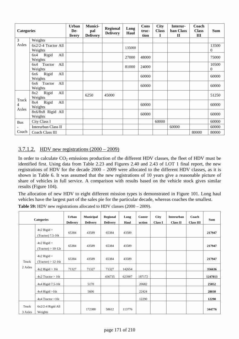
page 171 of 210

Categories Urban

De-livery

Munici-pal

Delivery

Regional Delivery

Long Haul

Construc-tion

City Class

I

Interur-ban Class

II

Coach Class

III Sum

3 Axles

Weights 6x2/2-4 Tractor All Weights 135000 13500

0 6x4 Rigid All Weights 27000 48000 75000

6x4 Tractor All Weights 81000 24000 10500

0 6x6 Rigid All Weights 60000 60000

6x6 Tractor All Weights 60000 60000

Truck 4 Axles

8x2 Rigid All Weights 6250 45000 51250

8x4 Rigid All Weights 60000 60000

8x6/8x8 Rigid All Weights 60000 60000

Bus - Coach

City Class I 60000 60000 Interurban Class II 60000 60000 Coach Class III 80000 80000

3.7.1.2. HDV new registrations (2000 – 2009)

In order to calculate CO2 emissions production of the different HDV classes, the fleet of HDV must be identified first. Using data from Table 2.23 and Figures 2.40 and 2.43 of LOT 1 final report, the new registrations of HDV for the decade 2000 – 2009 were allocated to the different HDV classes, as it is shown in Table 6. It was assumed that the new registrations of 10 years give a reasonable picture of share of vehicles in full service. A comparison with results based on the vehicle stock gives similar results (Figure 104). The allocation of new HDV to eight different mission types is demonstrated in Figure 101. Long haul vehicles have the largest part of the sales pie for the particular decade, whereas coaches the smallest. Table 59: HDV new registrations allocated to HDV classes (2000 – 2009).

Categories Urban

Delivery

Municipal

Delivery

Regional

Delivery

Long

Haul

Constr

uction

City

Class I

Interurban

Class II

Coach

Class III Sum

Truck

2 Axles

4x2 Rigid +

(Tractor) 7.5-10t 65384 43589 65384 43589 217947

4x2 Rigid +

(Tractor) > 10-12t 65384 43589 65384 43589 217947

4x2 Rigid +

(Tractor) > 12-16t 65384 43589 65384 43589 217947

4x2 Rigid > 16t 71327 71327 71327 142654 356636

4x2 Tractor > 16t 436735 623907 187172 1247813

4x4 Rigid 7.5-16t 5170 20682 25852

4x4 Rigid >16t 5606 22424 28030

4x4 Tractor >16t 12290 12290

Truck

3 Axles

6x2/2-4 Rigid All

Weights 172388 58612 113776 344776

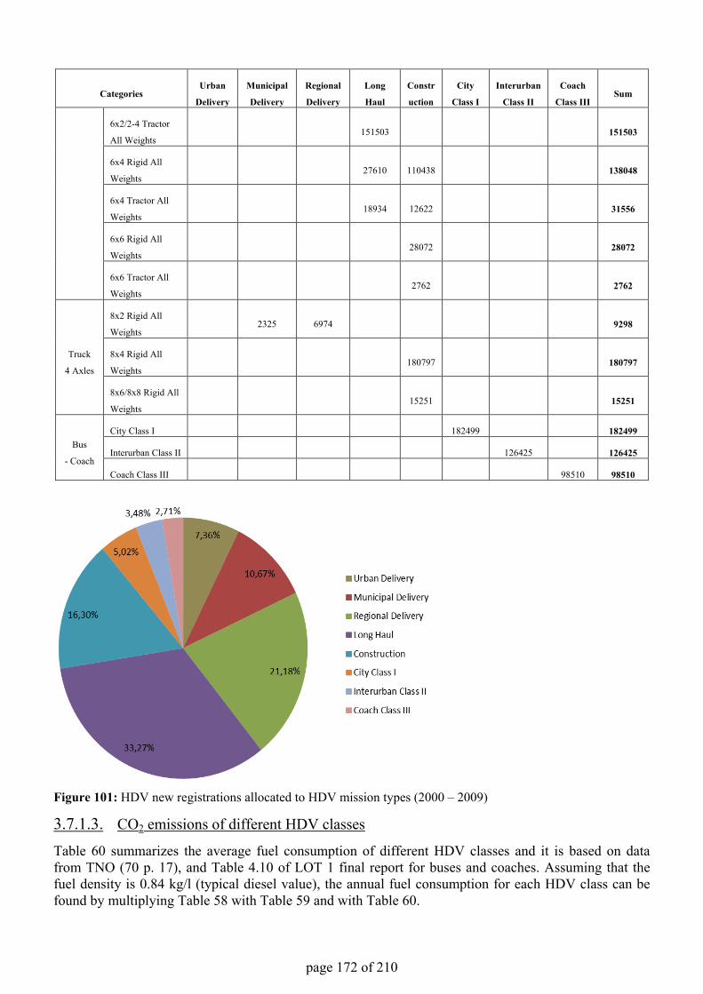
page 172 of 210

CategoriesUrban

Delivery

Municipal

Delivery

Regional

Delivery

Long

Haul

Constr

uction

City

Class I

Interurban

Class II

Coach

Class IIISum

6x2/2-4 Tractor

All Weights151503 151503

6x4 Rigid All

Weights27610 110438 138048

6x4 Tractor All

Weights18934 12622 31556

6x6 Rigid All

Weights28072 28072

6x6 Tractor All

Weights2762 2762

Truck

4 Axles

8x2 Rigid All

Weights2325 6974 9298

8x4 Rigid All

Weights180797 180797

8x6/8x8 Rigid All

Weights15251 15251

Bus

- Coach

City Class I 182499 182499

Interurban Class II 126425 126425

Coach Class III 98510 98510

Figure 101: HDV new registrations allocated to HDV mission types (2000 – 2009)

3.7.1.3. CO2 emissions of different HDV classes

Table 60 summarizes the average fuel consumption of different HDV classes and it is based on data from TNO (70 p. 17), and Table 4.10 of LOT 1 final report for buses and coaches. Assuming that the fuel density is 0.84 kg/l (typical diesel value), the annual fuel consumption for each HDV class can be found by multiplying Table 58 with Table 59 and with Table 60.

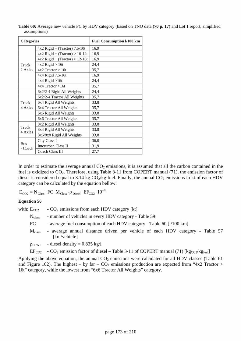
page 173 of 210

Table 60: Average new vehicle FC by HDV category (based on TNO data (70 p. 17) and Lot 1 report, simplified assumptions)

Categories Fuel Consumption l/100 km

Truck 2 Axles

4x2 Rigid + (Tractor) 7.5-10t 16,9 4x2 Rigid + (Tractor) > 10-12t 16,9 4x2 Rigid + (Tractor) > 12-16t 16,9 4x2 Rigid > 16t 24,4 4x2 Tractor > 16t 35,7 4x4 Rigid 7.5-16t 16,9 4x4 Rigid >16t 24,4 4x4 Tractor >16t 35,7

Truck 3 Axles

6x2/2-4 Rigid All Weights 24,4 6x2/2-4 Tractor All Weights 35,7 6x4 Rigid All Weights 33,8 6x4 Tractor All Weights 35,7 6x6 Rigid All Weights 33,8 6x6 Tractor All Weights 35,7

Truck 4 Axles

8x2 Rigid All Weights 33,8 8x4 Rigid All Weights 33,8 8x6/8x8 Rigid All Weights 33,8

Bus - Coach

City Class I 36,0 Interurban Class II 31,9 Coach Class III 27,7

In order to estimate the average annual CO2 emissions, it is assumed that all the carbon contained in the fuel is oxidized to CO2. Therefore, using Table 3-11 from COPERT manual (71), the emission factor of diesel is considered equal to 3.14 kg CO2/kg fuel. Finally, the annual CO2 emissions in kt of each HDV category can be calculated by the equation bellow:

82CODieselClassClass2CO 10EFMFCNE −⋅⋅ρ⋅⋅⋅=

Equation 56

with: ECO2 - CO2 emissions from each HDV category [kt] Nclass - number of vehicles in every HDV category - Table 59 FC - average fuel consumption of each HDV category - Table 60 [l/100 km] Mclass - average annual distance driven per vehicle of each HDV category - Table 57

[km/vehicle] ρDiesel - diesel density = 0.835 kg/l EFCO2 - CO2 emission factor of diesel – Table 3-11 of COPERT manual (71) [kgCO2/kgfuel] Applying the above equation, the annual CO2 emissions were calculated for all HDV classes (Table 61 and Figure 102). The highest – by far – CO2 emissions production are expected from “4x2 Tractor > 16t” category, while the lowest from “6x6 Tractor All Weights” category.

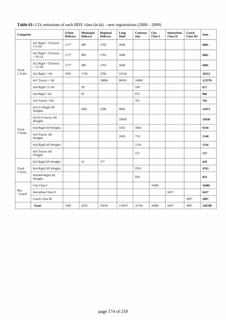
page 174 of 210

Table 61: CO2 emissions of each HDV class (in kt) – new registrations (2000 – 2009)

Categories Urban Delivery

Municipal Delivery

Regional Delivery

Long Haul

Construction

City Class I

Interurban Class II

Coach Class III Sum

Truck 2 Axles

4x2 Rigid + (Tractor) 7.5-10t 1177 490 1765 2648 6081

4x2 Rigid + (Tractor) > 10-12t 1177 490 1765 2648 6081

4x2 Rigid + (Tractor) > 12-16t 1177 490 1765 2648 6081

4x2 Rigid > 16t 1855 1159 2782 12518 18313

4x2 Tractor > 16t 24894 80016 10669 115579

4x4 Rigid 7.5-16t 58 558 617

4x4 Rigid >16t 91 875 966

4x4 Tractor >16t 701 701

Truck 3 Axles

6x2/2-4 Rigid All Weights 2801 2286 9984 15071

6x2/2-4 Tractor All Weights 19430 19430

6x4 Rigid All Weights 3355 5964 9318

6x4 Tractor All Weights 2428 719 3148

6x6 Rigid All Weights 1516 1516

6x6 Tractor All Weights 157 157

Truck 4 Axles

8x2 Rigid All Weights 52 377 429

8x4 Rigid All Weights 9763 9763

8x6/8x8 Rigid All Weights 824 824

Bus - Coach

City Class I 10482 10482

Interurban Class II 6437 6437

Coach Class III 5807 5807

Total: 5385 5633 35634 135675 31745 10482 6437 5807 236798

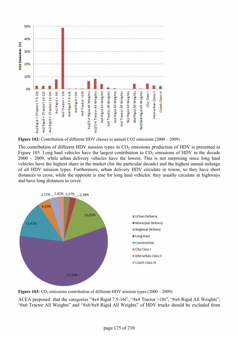
page 175 of 210

Figure 102: Contribution of different HDV classes to annual CO2 emissions (2000 – 2009)

The contribution of different HDV mission types in CO2 emissions production of HDV is presented in Figure 103. Long haul vehicles have the largest contribution to CO2 emissions of HDV in the decade 2000 – 2009, while urban delivery vehicles have the lowest. This is not surprising since long haul vehicles have the highest share in the market (for the particular decade) and the highest annual mileage of all HDV mission types. Furthermore, urban delivery HDV circulate in towns, so they have short distances to cross, while the opposite is true for long haul vehicles: they usually circulate in highways and have long distances to cover.

Figure 103: CO2 emissions contribution of different HDV mission types (2000 – 2009)

ACEA proposed that the categories “4x4 Rigid 7.5-16t”, “4x4 Tractor >16t”, “6x6 Rigid All Weights”, “6x6 Tractor All Weights” and “8x6/8x8 Rigid All Weights” of HDV trucks should be excluded from

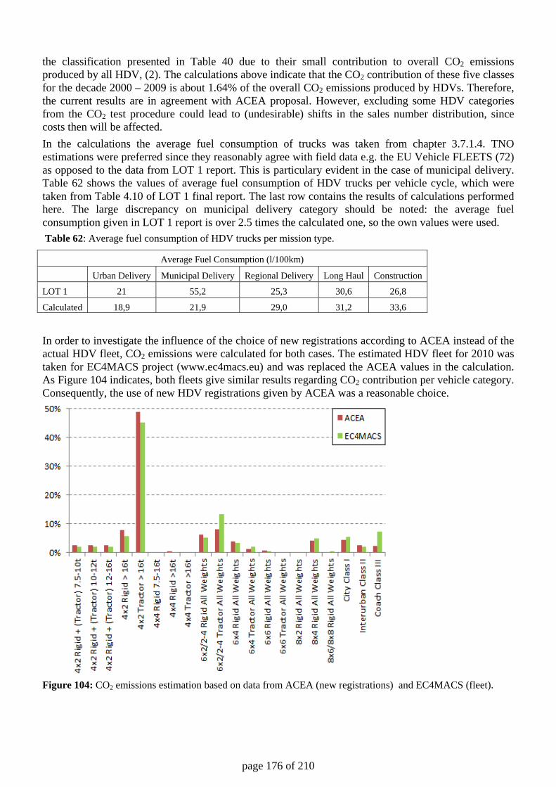
page 176 of 210

the classification presented in Table 40 due to their small contribution to overall CO2 emissions produced by all HDV, (2). The calculations above indicate that the CO2 contribution of these five classes for the decade 2000 – 2009 is about 1.64% of the overall CO2 emissions produced by HDVs. Therefore, the current results are in agreement with ACEA proposal. However, excluding some HDV categories from the CO2 test procedure could lead to (undesirable) shifts in the sales number distribution, since costs then will be affected. In the calculations the average fuel consumption of trucks was taken from chapter 3.7.1.4. TNO estimations were preferred since they reasonably agree with field data e.g. the EU Vehicle FLEETS (72) as opposed to the data from LOT 1 report. This is particulary evident in the case of municipal delivery. Table 62 shows the values of average fuel consumption of HDV trucks per vehicle cycle, which were taken from Table 4.10 of LOT 1 final report. The last row contains the results of calculations performed here. The large discrepancy on municipal delivery category should be noted: the average fuel consumption given in LOT 1 report is over 2.5 times the calculated one, so the own values were used. Table 62: Average fuel consumption of HDV trucks per mission type.

Average Fuel Consumption (l/100km)

Urban Delivery Municipal Delivery Regional Delivery Long Haul Construction

LOT 1 21 55,2 25,3 30,6 26,8

Calculated 18,9 21,9 29,0 31,2 33,6

In order to investigate the influence of the choice of new registrations according to ACEA instead of the actual HDV fleet, CO2 emissions were calculated for both cases. The estimated HDV fleet for 2010 was taken for EC4MACS project (www.ec4macs.eu) and was replaced the ACEA values in the calculation. As Figure 104 indicates, both fleets give similar results regarding CO2 contribution per vehicle category. Consequently, the use of new HDV registrations given by ACEA was a reasonable choice.

Figure 104: CO2 emissions estimation based on data from ACEA (new registrations) and EC4MACS (fleet).

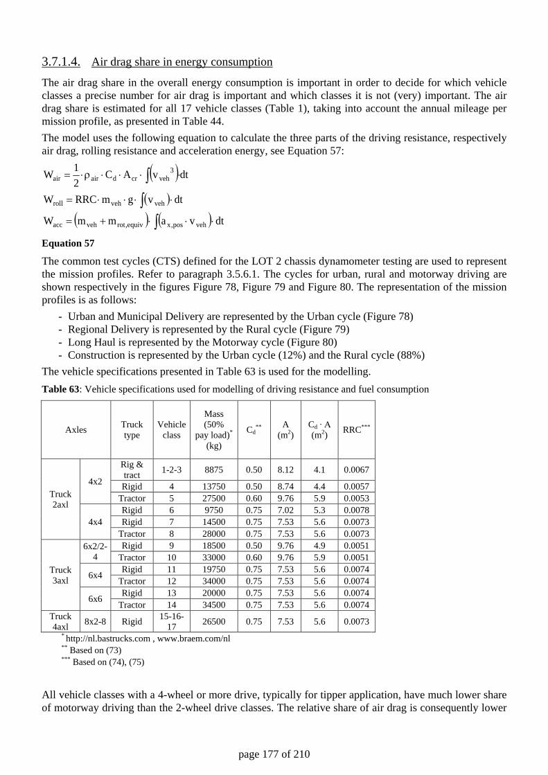
page 177 of 210

3.7.1.4. Air drag share in energy consumption

The air drag share in the overall energy consumption is important in order to decide for which vehicle classes a precise number for air drag is important and which classes it is not (very) important. The air drag share is estimated for all 17 vehicle classes (Table 1), taking into account the annual mileage per mission profile, as presented in Table 44. The model uses the following equation to calculate the three parts of the driving resistance, respectively air drag, rolling resistance and acceleration energy, see Equation 57:

( )( )

( ) ( )∫∫

∫

⋅⋅⋅+=

⋅⋅⋅⋅=

⋅⋅⋅⋅ρ⋅=

dtvammW

dtvgmRRCW

dtvAC21W

vehpos,xequiv,rotvehacc

vehvehroll

3vehcrdairair

Equation 57

The common test cycles (CTS) defined for the LOT 2 chassis dynamometer testing are used to represent the mission profiles. Refer to paragraph 3.5.6.1. The cycles for urban, rural and motorway driving are shown respectively in the figures Figure 78, Figure 79 and Figure 80. The representation of the mission profiles is as follows:

- Urban and Municipal Delivery are represented by the Urban cycle (Figure 78) - Regional Delivery is represented by the Rural cycle (Figure 79) - Long Haul is represented by the Motorway cycle (Figure 80) - Construction is represented by the Urban cycle (12%) and the Rural cycle (88%)

The vehicle specifications presented in Table 63 is used for the modelling. Table 63: Vehicle specifications used for modelling of driving resistance and fuel consumption

Axles Truck type

Vehicle class

Mass (50%

pay load)* (kg)

Cd** A

(m2) Cd ∙ A (m2) RRC***

Truck 2axl

4x2

Rig & tract 1-2-3 8875 0.50 8.12 4.1 0.0067

Rigid 4 13750 0.50 8.74 4.4 0.0057 Tractor 5 27500 0.60 9.76 5.9 0.0053

4x4 Rigid 6 9750 0.75 7.02 5.3 0.0078 Rigid 7 14500 0.75 7.53 5.6 0.0073

Tractor 8 28000 0.75 7.53 5.6 0.0073

Truck 3axl

6x2/2-4

Rigid 9 18500 0.50 9.76 4.9 0.0051 Tractor 10 33000 0.60 9.76 5.9 0.0051

6x4 Rigid 11 19750 0.75 7.53 5.6 0.0074 Tractor 12 34000 0.75 7.53 5.6 0.0074

6x6 Rigid 13 20000 0.75 7.53 5.6 0.0074 Tractor 14 34500 0.75 7.53 5.6 0.0074

Truck 4axl 8x2-8 Rigid 15-16-

17 26500 0.75 7.53 5.6 0.0073 * http://nl.bastrucks.com , www.braem.com/nl ** Based on (73) *** Based on (74), (75)

All vehicle classes with a 4-wheel or more drive, typically for tipper application, have much lower share of motorway driving than the 2-wheel drive classes. The relative share of air drag is consequently lower

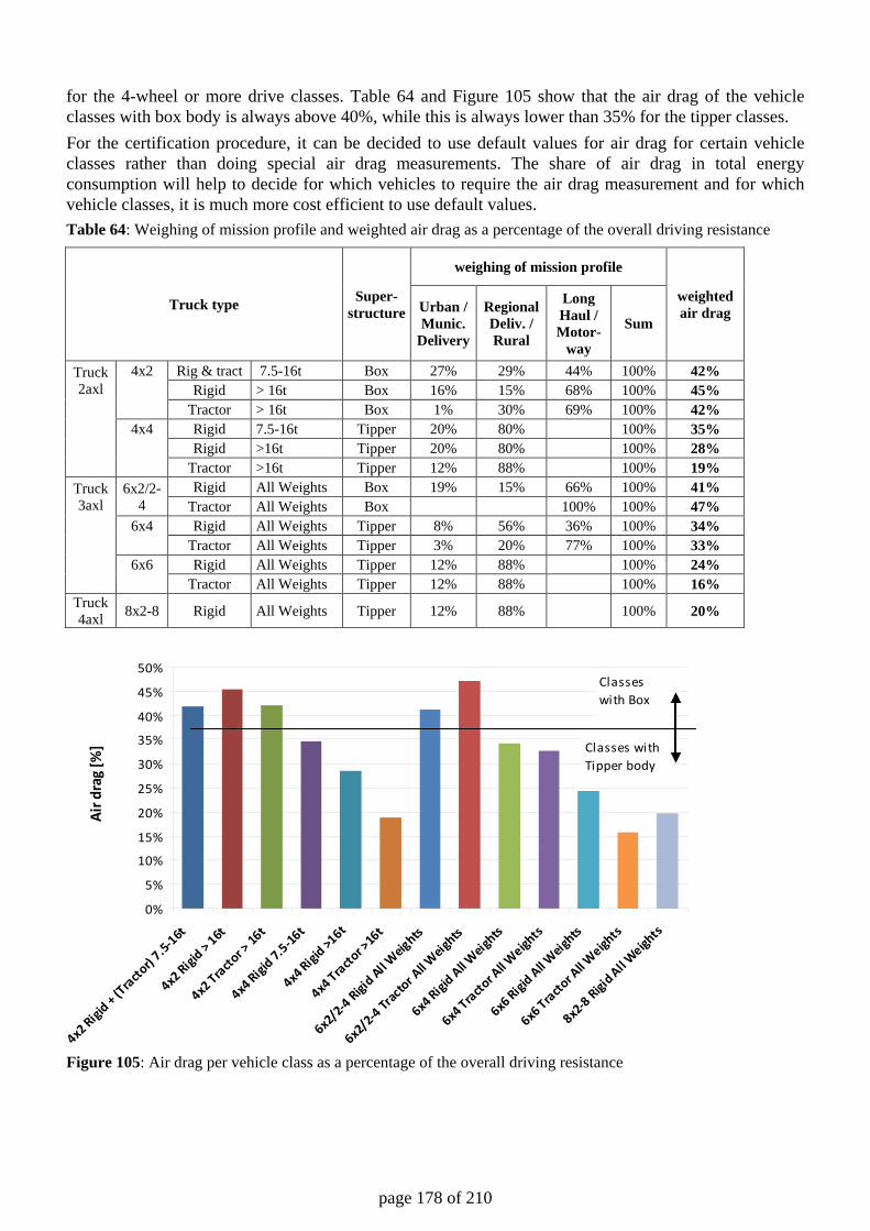
page 178 of 210

for the 4-wheel or more drive classes. Table 64 and Figure 105 show that the air drag of the vehicle classes with box body is always above 40%, while this is always lower than 35% for the tipper classes. For the certification procedure, it can be decided to use default values for air drag for certain vehicle classes rather than doing special air drag measurements. The share of air drag in total energy consumption will help to decide for which vehicles to require the air drag measurement and for which vehicle classes, it is much more cost efficient to use default values. Table 64: Weighing of mission profile and weighted air drag as a percentage of the overall driving resistance

Truck type Super-structure

weighing of mission profile

weighted air drag Urban /

Munic. Delivery

Regional Deliv. / Rural

Long Haul / Motor-

way

Sum

Truck 2axl

4x2 Rig & tract 7.5-16t Box 27% 29% 44% 100% 42% Rigid > 16t Box 16% 15% 68% 100% 45%

Tractor > 16t Box 1% 30% 69% 100% 42% 4x4 Rigid 7.5-16t Tipper 20% 80% 100% 35% Rigid >16t Tipper 20% 80% 100% 28% Tractor >16t Tipper 12% 88% 100% 19%

Truck 3axl

6x2/2-4

Rigid All Weights Box 19% 15% 66% 100% 41% Tractor All Weights Box 100% 100% 47%

6x4 Rigid All Weights Tipper 8% 56% 36% 100% 34% Tractor All Weights Tipper 3% 20% 77% 100% 33% 6x6 Rigid All Weights Tipper 12% 88% 100% 24% Tractor All Weights Tipper 12% 88% 100% 16%

Truck 4axl 8x2-8 Rigid All Weights Tipper 12% 88% 100% 20%

Figure 105: Air drag per vehicle class as a percentage of the overall driving resistance

0%

5%

10%

15%

20%

25%

30%

35%

40%

45%

50%

4x2 Rigi

d + (Tracto

r) 7.5-

16t

4x2 Rigi

d > 16t

4x2 Tracto

r > 16

t

4x4 Rigi

d 7.5-16

t

4x4 Rigi

d >16t

4x4 Tracto

r >16

t

6x2/2

-4 Rigid All W

eights

6x2/2

-4 Trac

tor All W

eights

6x4 Rigi

d All Weig

hts

6x4 Tracto

r All W

eights

6x6 Rigi

d All Weig

hts

6x6 Tracto

r All W

eights

8x2-8 Rigi

d All Weigh

ts

Air d

rag

[%]

Classes with Box

Classes with Tipper body

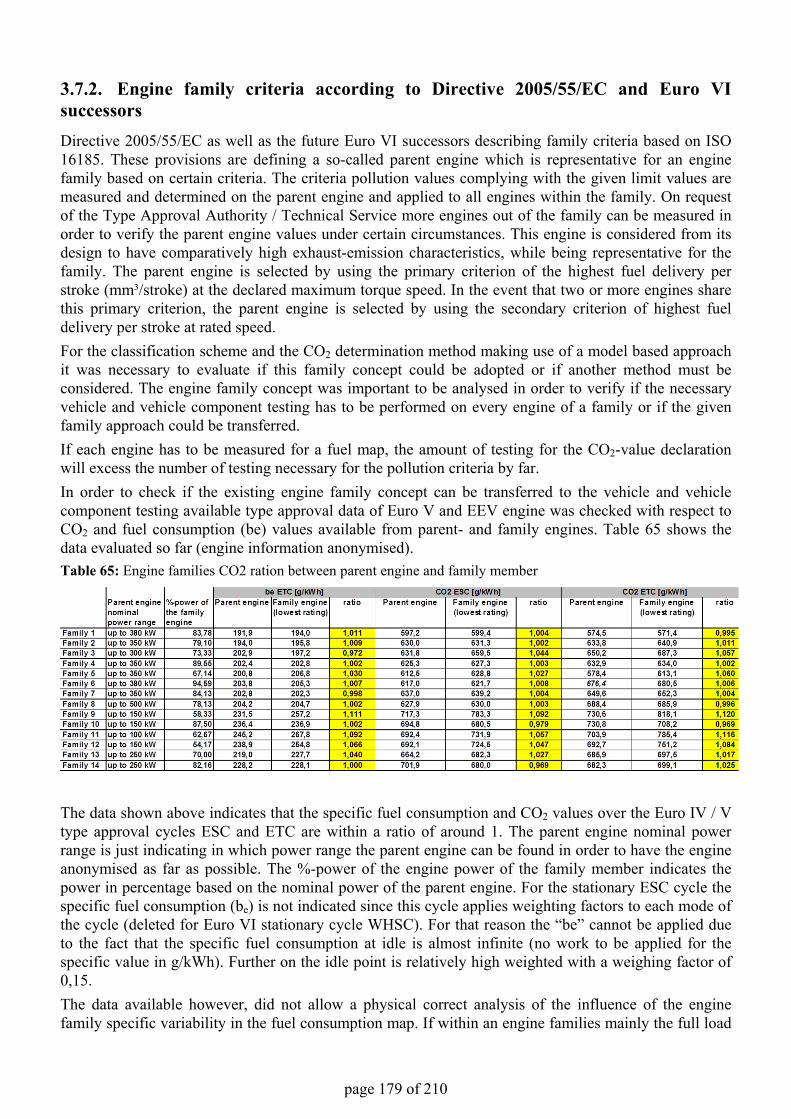
page 179 of 210

3.7.2. Engine family criteria according to Directive 2005/55/EC and Euro VI successorsDirective 2005/55/EC as well as the future Euro VI successors describing family criteria based on ISO 16185. These provisions are defining a so-called parent engine which is representative for an engine family based on certain criteria. The criteria pollution values complying with the given limit values are measured and determined on the parent engine and applied to all engines within the family. On request of the Type Approval Authority / Technical Service more engines out of the family can be measured in order to verify the parent engine values under certain circumstances. This engine is considered from its design to have comparatively high exhaust-emission characteristics, while being representative for the family. The parent engine is selected by using the primary criterion of the highest fuel delivery per stroke (mm³/stroke) at the declared maximum torque speed. In the event that two or more engines share this primary criterion, the parent engine is selected by using the secondary criterion of highest fuel delivery per stroke at rated speed.For the classification scheme and the CO2 determination method making use of a model based approach it was necessary to evaluate if this family concept could be adopted or if another method must be considered. The engine family concept was important to be analysed in order to verify if the necessary vehicle and vehicle component testing has to be performed on every engine of a family or if the given family approach could be transferred. If each engine has to be measured for a fuel map, the amount of testing for the CO2-value declaration will excess the number of testing necessary for the pollution criteria by far.In order to check if the existing engine family concept can be transferred to the vehicle and vehicle component testing available type approval data of Euro V and EEV engine was checked with respect to CO2 and fuel consumption (be) values available from parent- and family engines. Table 65 shows the data evaluated so far (engine information anonymised).Table 65: Engine families CO2 ration between parent engine and family member

The data shown above indicates that the specific fuel consumption and CO2 values over the Euro IV / V type approval cycles ESC and ETC are within a ratio of around 1. The parent engine nominal power range is just indicating in which power range the parent engine can be found in order to have the engine anonymised as far as possible. The %-power of the engine power of the family member indicates the power in percentage based on the nominal power of the parent engine. For the stationary ESC cycle the specific fuel consumption (be) is not indicated since this cycle applies weighting factors to each mode of the cycle (deleted for Euro VI stationary cycle WHSC). For that reason the “be” cannot be applied due to the fact that the specific fuel consumption at idle is almost infinite (no work to be applied for the specific value in g/kWh). Further on the idle point is relatively high weighted with a weighing factor of 0,15.The data available however, did not allow a physical correct analysis of the influence of the engine family specific variability in the fuel consumption map. If within an engine families mainly the full load

page 180 of 210

injection is reduce from a parent engine, then only the full lad cure is shifted down while the load points below the full load curve may remain unchanged in their specific fuel consumption value in [g/second]. Since the ETC and the WHTC have the engine power defined as function of the full load curve of the engine the load points can be quite different for the members of the family. Thus the results of the total cycle do not show if points with similar absolute torque and speed have similar fuel efficiencies. This data needs to be evaluated with data from more engines which then include also the HDV-CO2 fuel consumption map (also such engines to be installed in vehicle below the 7,5 maximum weight threshold and for engines designed to meet the Euro VI emission stage). But for the time being it can be concluded that the engine family approach for the determination of the criteria pollution may be applied to the vehicle component testing for the CO2 value determination.

3.7.3. European heavy-duty vehicle classification scheme (Directive 2007/46/EC and Commission Directive 678/2011)

The existing European heavy duty vehicle classification according to Directive 2007/46/EC and Commission Directive 678/2011 is of some secondary interest of the CO2-declaration procedure but it is of course necessary to have the CO2-declaration procedure designed in such a way that the existing categorisation for the whole vehicle type approval is considered and addressed. The conducted data analysis shows that the existing scheme can be used for a future CO2 procedure and can also help to classify vehicles properly. For the CO2-scheme almost all classes defined in Directive 2007/46/EC are of interest expect for vehicles belonging to the passenger car range as well as for the light-duty vehicle range, although as already mentioned the light-duty range may need to be adjusted, at least for CO2 classification in such a way that a clear distinction between light-duty and heavy-duty vehicles becomes possible. The vehicle categories according to 2007/46/EC are defined as: - Category M Motor vehicles designed and constructed primarily for the carriage of persons and their luggage. - Category M1 Vehicles of category M, comprising not more than eight seating positions in addition to the driver’s seating position. Vehicles belonging to category M1 shall have no space for standing passengers. The number of seating positions may be restricted to one (i.e. the driver’s seating position). - Category M2 Vehicles of category M, comprising more than eight seating positions in addition to the driver’s seating position and having a maximum mass not exceeding 5 tonnes. Vehicles belonging to category M2 may have space for standing passengers in addition to the seating positions. - Category M3 Vehicles of category M, comprising more than eight seating positions in addition to the driver’s seating position and having a maximum mass exceeding 5 tonnes. Vehicles belonging to category M3 may have space for standing passengers. Vehicles of Category M1 are clearly not applicable to the CO2-procedure described within this document. M2 vehicles are applicable at the moment based on the scope definition of Commission Directive 715/2007 but may need to be excluded by adjustment of the scope. M3 vehicles are the buses and coaches as defined in chapter 2.1. - Category N Motor vehicles designed and constructed primarily for the carriage of goods. - Category N1 Vehicles of category N having a maximum mass not exceeding 3,5 tonnes. - Category N2 Vehicles of category N having a maximum mass exceeding 3,5 tonnes but not exceeding 12 tonnes. - Category N3 Vehicles of category N having a maximum mass exceeding 12 tonnes. N1 Vehicles are not applicable to this procedure. They are light-duty related since their reference mass is most likely not exceeding the 2810 kg / 2840 kg reference mass threshold. N2 vehicles are fully applicable to the CO2 scheme as long as their reference mass is exceeding the said threshold. Also here a

page 181 of 210

certain cut to distinguish between light- and heavy-duty would help to ease the current situation. N3 are purely heavy duty vehicles. Coming to the trailer categories the situation is somehow different. 715/2007 defines trailer as follows: - Category O Trailers designed and constructed for the carriage of goods or of persons as well as for the accommodation of persons. - Category O1 Vehicles of category O having a maximum mass not exceeding 0,75 tonnes - Category O2 Vehicles of category O having a maximum mass exceeding 0,75 tonnes but not exceeding 3,5 tonnes. - Category O3 Vehicles of category O having a maximum mass exceeding 3,5 tonnes but not exceeding 10 tonnes. - Category O4 Vehicles of category O having a maximum mass exceeding 10 tonnes. Based on what was and on the Lot 1 findings, only trailers with a maximum mass above 10 tons should be considered applicable for heavy-duty purposes for the time being. These means only trailers of category O4 are applicable to the procedure. Main vehicle segments to be considered in a first step

According to the vehicle statistics and based on the approach that a CO2-declartion scheme may be introduced stepwise, the main vehicle segments to be considered in a first step could be those with high shares in the CO2 emissions: - 4x2 Tractor in combination with a three axle semi-trailer in gross vehicle combination weight configuration exceeding 16 tons. - 4x2 rigid trucks in gross vehicle weight configuration between 7,5 -10 tons and 10-12 tons without trailer and 12-16 tons combination with a drawbar trailer in two and / or three axle configuration (to be defined). - 6x2 rigid trucks and tractors in gross vehicle weight configuration exceeding 16 tons eventually in combination with a drawbar trailer (to be defined). - City buses configuration

3.7.4. Criteria for the declaration of a CO2 value for specified vehicles grouped in a family The family criteria to establish a procedure to group certain vehicle configurations is an important part for a future regulatory approach beside the technical provisions of the procedure. Based on chapter 2.2, the engine family concept according to 2005/55/EC respectively Euro VI and the vehicle categories according to 2007/46/EC a family concept can be developed in a further step. The main parameters defining a CO2-vehicle family are listed in the following. The base idea for such a family is to group vehicles of similar configurations within one declared CO2 value. With certain vehicle parameters not affecting the CO2-value respectively only having little impact on the CO2-value in a range to be defined later vehicle deviations can be applied without being considered for testing / simulation. It has to be emphasised that those family criteria are not used for separation of what is needed to be tested and what not. Many issues can be incorporated into a given family by simulation only. For the time being following design parameters are considered to be introduced for a vehicle family separation (Table 66).

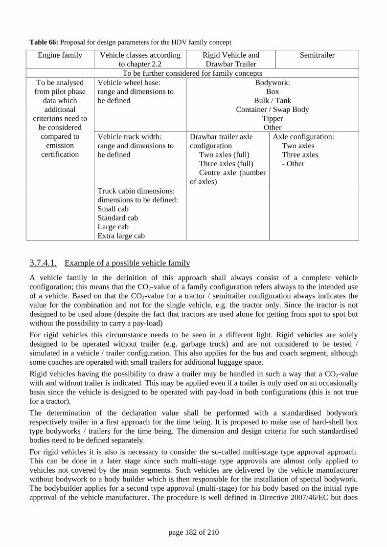
page 182 of 210

Table 66: Proposal for design parameters for the HDV family concept

Engine family Vehicle classes according to chapter 2.2

Rigid Vehicle and Drawbar Trailer

Semitrailer

To be further considered for family concepts To be analysed from pilot phase

data which additional

criterions need to be considered compared to

emission certification

Vehicle wheel base: range and dimensions to be defined

Bodywork: Box

Bulk / Tank Container / Swap Body

Tipper Other

Vehicle track width: range and dimensions to be defined

Drawbar trailer axle configuration Two axles (full) Three axles (full) Centre axle (number of axles)

Axle configuration: Two axles Three axles - Other

Truck cabin dimensions: dimensions to be defined: Small cab Standard cab Large cab Extra large cab

3.7.4.1. Example of a possible vehicle family

A vehicle family in the definition of this approach shall always consist of a complete vehicle configuration; this means that the CO2-value of a family configuration refers always to the intended use of a vehicle. Based on that the CO2-value for a tractor / semitrailer configuration always indicates the value for the combination and not for the single vehicle, e.g. the tractor only. Since the tractor is not designed to be used alone (despite the fact that tractors are used alone for getting from spot to spot but without the possibility to carry a pay-load) For rigid vehicles this circumstance needs to be seen in a different light. Rigid vehicles are solely designed to be operated without trailer (e.g. garbage truck) and are not considered to be tested / simulated in a vehicle / trailer configuration. This also applies for the bus and coach segment, although some coaches are operated with small trailers for additional luggage space. Rigid vehicles having the possibility to draw a trailer may be handled in such a way that a CO2-value with and without trailer is indicated. This may be applied even if a trailer is only used on an occasionally basis since the vehicle is designed to be operated with pay-load in both configurations (this is not true for a tractor). The determination of the declaration value shall be performed with a standardised bodywork respectively trailer in a first approach for the time being. It is proposed to make use of hard-shell box type bodyworks / trailers for the time being. The dimension and design criteria for such standardised bodies need to be defined separately. For rigid vehicles it is also is necessary to consider the so-called multi-stage type approval approach. This can be done in a later stage since such multi-stage type approvals are almost only applied to vehicles not covered by the main segments. Such vehicles are delivered by the vehicle manufacturer without bodywork to a body builder which is then responsible for the installation of special bodywork. The bodybuilder applies for a second type approval (multi-stage) for his body based on the initial type approval of the vehicle manufacturer. The procedure is well defined in Directive 2007/46/EC but does

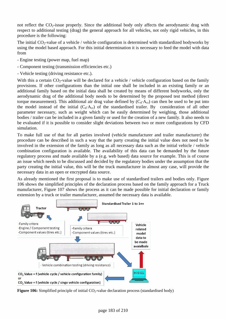
page 183 of 210

not reflect the CO2-issue properly. Since the additional body only affects the aerodynamic drag with respect to additional testing (drag) the general approach for all vehicles, not only rigid vehicles, in this procedure is the following: The initial CO2-value of a vehicle / vehicle configuration is determined with standardized bodyworks by using the model based approach. For this initial determination it is necessary to feed the model with data from - Engine testing (power map, fuel map) - Component testing (transmission efficiencies etc.) - Vehicle testing (driving resistance etc.). With this a certain CO2-value will be declared for a vehicle / vehicle configuration based on the family provisions. If other configurations than the initial one shall be included in an existing family or an additional family based on the initial data shall be created by means of different bodyworks, only the aerodynamic drag of the additional body needs to be determined by the proposed test method (direct torque measurement). This additional air drag value defined by (Cd∙Acr) can then be used to be put into the model instead of the initial (Cd∙Acr) of the standardised trailer. By consideration of all other parameter necessary, such as weight which can be easily determined by weighing, those additional bodies / trailer can be included in a given family or used for the creation of a new family. It also needs to be evaluated if it is possible to consider slight deviations between two or more configurations by CFD simulation. To make full use of that for all parties involved (vehicle manufacturer and trailer manufacturer) the procedure can be described in such a way that the party creating the initial value does not need to be involved in the extension of the family as long as all necessary data such as the initial vehicle / vehicle combination configuration is available. The availability of this data can be demanded by the future regulatory process and made available by a (e.g. web based) data source for example. This is of course an issue which needs to be discussed and decided by the regulatory bodies under the assumption that the party creating the initial value, this will be the truck manufacturer in almost any case, will provide the necessary data in an open or encrypted data source. As already mentioned the first proposal is to make use of standardised trailers and bodies only. Figure 106 shows the simplified principles of the declaration process based on the family approach for a Truck manufacturer, Figure 107 shows the process as it can be made possible for initial declaration or family extension by a truck or trailer manufacturer, assumed the necessary data is available.

Figure 106: Simplified principle of initial CO2-value declaration process (standardised body)

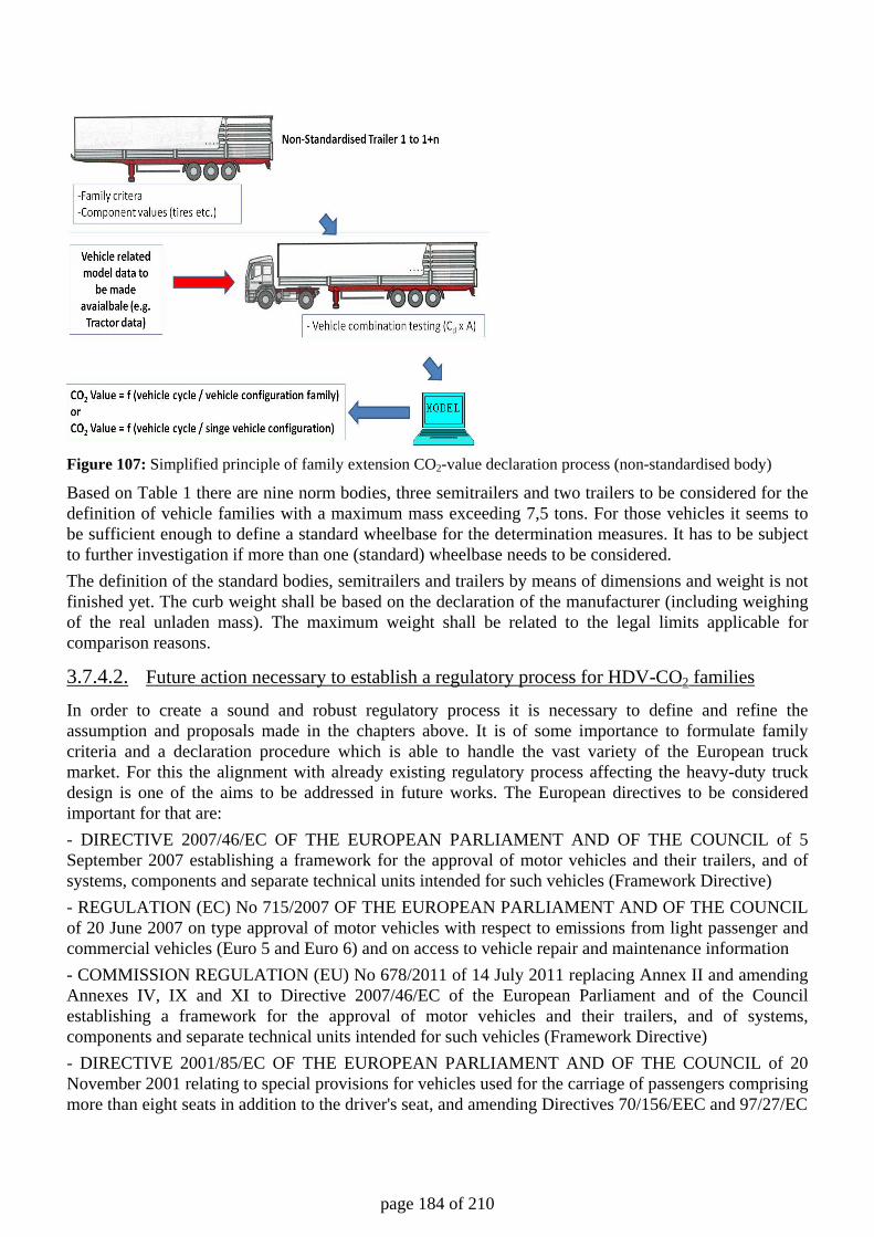
page 184 of 210

Figure 107: Simplified principle of family extension CO2-value declaration process (non-standardised body)

Based on Table 1 there are nine norm bodies, three semitrailers and two trailers to be considered for the definition of vehicle families with a maximum mass exceeding 7,5 tons. For those vehicles it seems to be sufficient enough to define a standard wheelbase for the determination measures. It has to be subject to further investigation if more than one (standard) wheelbase needs to be considered. The definition of the standard bodies, semitrailers and trailers by means of dimensions and weight is not finished yet. The curb weight shall be based on the declaration of the manufacturer (including weighing of the real unladen mass). The maximum weight shall be related to the legal limits applicable for comparison reasons.

3.7.4.2. Future action necessary to establish a regulatory process for HDV-CO2 families

In order to create a sound and robust regulatory process it is necessary to define and refine the assumption and proposals made in the chapters above. It is of some importance to formulate family criteria and a declaration procedure which is able to handle the vast variety of the European truck market. For this the alignment with already existing regulatory process affecting the heavy-duty truck design is one of the aims to be addressed in future works. The European directives to be considered important for that are: - DIRECTIVE 2007/46/EC OF THE EUROPEAN PARLIAMENT AND OF THE COUNCIL of 5 September 2007 establishing a framework for the approval of motor vehicles and their trailers, and of systems, components and separate technical units intended for such vehicles (Framework Directive) - REGULATION (EC) No 715/2007 OF THE EUROPEAN PARLIAMENT AND OF THE COUNCIL of 20 June 2007 on type approval of motor vehicles with respect to emissions from light passenger and commercial vehicles (Euro 5 and Euro 6) and on access to vehicle repair and maintenance information - COMMISSION REGULATION (EU) No 678/2011 of 14 July 2011 replacing Annex II and amending Annexes IV, IX and XI to Directive 2007/46/EC of the European Parliament and of the Council establishing a framework for the approval of motor vehicles and their trailers, and of systems, components and separate technical units intended for such vehicles (Framework Directive) - DIRECTIVE 2001/85/EC OF THE EUROPEAN PARLIAMENT AND OF THE COUNCIL of 20 November 2001 relating to special provisions for vehicles used for the carriage of passengers comprising more than eight seats in addition to the driver's seat, and amending Directives 70/156/EEC and 97/27/EC

page 185 of 210

- COMMISSION REGULATION (EU) No 582/2011 of 25 May 2011 implementing and amending Regulation (EC) No 595/2009 of the European Parliament and of the Council with respect to emissions from heavy duty vehicles (Euro VI) and amending Annexes I and III to Directive 2007/46/EC of the European Parliament and of the Council With respect to these Directives and Regulations it seems to be necessary to revise the given vehicle weight definitions to distinguish between light- and heavy-duty in order to create a sound legislative basis. The established vehicle segmentation shall be used to define the family criteria so that the entire truck market (truck manufacturer, vehicle manufacturer and bodybuilder) can make use of that in such a way that CO2-optimized products are forced to be introduced. For that reason the whole market picture needs to be considered with special regard to the majority of vehicles in the very beginning but with providing provisions for almost all vehicles with a certain market share later. Very specialized vehicles may need not to be covered but the procedure should allow declaring values for those vehicles also. The declaration process shall be aligned with the already existing whole vehicle type approval process. This adds ease to the later adoption into force by using the already existing provisions and methods from the type approval process where the Technical Services and Type Approval Authorities can be involved.

3.7.5. Axle configurations and bodies of rigid trucks In Table 67 the market share of body types per vehicle class is given. The number of axle - body configurations which are not possible or which do not occure in practice are set to zero. Consequently the information of Table 67 (for rigid truck) is used to estimate the remaining market share per axle-body type combination, while meeting the total market shares for both the axle configurations as well as the bodies. Axle-body combinations with a market share of 3.5% or higher are highlighted green in Table 67. In those boxes, the contribution to the yearly CO2 emission is given between parenthesis. This is bases on the kilometers per year from Table 58 and CO2 emission factors per vehicle category. From this it can be seen that the small trucks up till 16 tons have a market share in registrations of 37%, but its contribution to the yearly emitted CO2 is only about 25%.

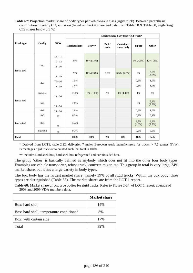
page 186 of 210

Table 67: Projection market share of body types per vehicle-axle class (rigid truck). Between parenthesis contribution to yearly CO2 emission (based on market share and data from Table 58 & Table 60, neglecting CO2 shares below 3.5 %)

Truck type Config. GVW

Market share body type rigid truck*

Market share Box*** Bulk/ tank

Container/ swap body Tipper Other

Truck 2axl

4x2

7,5 - 10 37% 19% (13%) 6% (4.5%) 12% (8%) 10 - 12

12 - 16

18 - 19 20% 10% (13%) 0,5% 3,5% (4.5%) 2% 4.0%

(5.0%)

4x4 7,5 -16 1,5% 0,5% 1,0%

18 - 19 1,6% 0,6% 1,0%

Truck 3axl

6x2/2-4 24 - 26

19,4% 10% (11%) 2% 4% (4.4%) 1% 3%

6x4 24 - 26

7,8% 3% 5,2% (7.7%)

6x6 24 - 26 1,6% 0,6% 1,0%

Truck 4axl

8x2 30 0,5% 0,2% 0,3%

8x4 30

10,2% 3,5% (4.0%)

6,6% (7.5%)

8x6/8x8 30 0,7% 0,2% 0,5%

Total 100% 39% 2% 8% 18% 34%

* Derived from LOT1, table 2.22: deliveries 7 major European truck manufacturers for trucks > 7.5 tonnes GVW. Percentages rigid trucks recalculated such that total is 100%.

** Includes Hard shell box, hard shell box refrigerated and curtain sided box.

The group ‘other’ is basically defined as anybody which does not fit into the other four body types. Examples are vehicle transporter, refuse truck, concrete mixer, etc. This group in total is very large, 34% market share, but it has a large variety in body types. The box body has the largest market share, namely 39% of all rigid trucks. Within the box body, three types are distinguished (Table 68). The market shares are from the LOT 1 report. Table 68: Market share of box type bodies for rigid trucks. Refer to Figure 2-34 of LOT 1 report: average of

2008 and 2009 VDA members data.

Market share

Box: hard shell 14%

Box: hard shell, temperature conditioned 8%

Box: with curtain side 17%

Total 39%

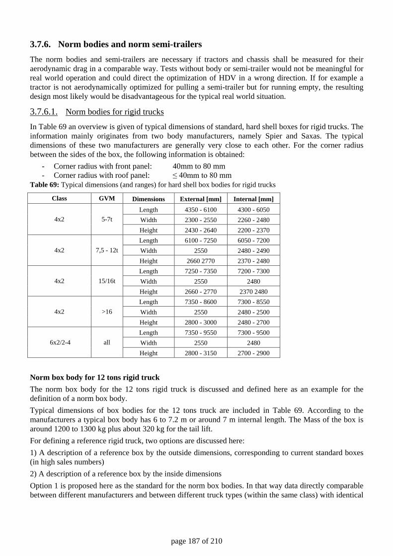
page 187 of 210

3.7.6. Norm bodies and norm semi-trailers The norm bodies and semi-trailers are necessary if tractors and chassis shall be measured for their aerodynamic drag in a comparable way. Tests without body or semi-trailer would not be meaningful for real world operation and could direct the optimization of HDV in a wrong direction. If for example a tractor is not aerodynamically optimized for pulling a semi-trailer but for running empty, the resulting design most likely would be disadvantageous for the typical real world situation.

3.7.6.1. Norm bodies for rigid trucks

In Table 69 an overview is given of typical dimensions of standard, hard shell boxes for rigid trucks. The information mainly originates from two body manufacturers, namely Spier and Saxas. The typical dimensions of these two manufacturers are generally very close to each other. For the corner radius between the sides of the box, the following information is obtained:

- Corner radius with front panel: 40mm to 80 mm - Corner radius with roof panel: ≤ 40mm to 80 mm

Table 69: Typical dimensions (and ranges) for hard shell box bodies for rigid trucks

Class GVM Dimensions External [mm] Internal [mm]

4x2 5-7t Length 4350 - 6100 4300 - 6050 Width 2300 - 2550 2260 - 2480 Height 2430 - 2640 2200 - 2370

4x2 7,5 - 12t Length 6100 - 7250 6050 - 7200 Width 2550 2480 - 2490 Height 2660 2770 2370 - 2480

4x2 15/16t Length 7250 - 7350 7200 - 7300 Width 2550 2480 Height 2660 - 2770 2370 2480

4x2 >16 Length 7350 - 8600 7300 - 8550 Width 2550 2480 - 2500 Height 2800 - 3000 2480 - 2700

6x2/2-4 all Length 7350 - 9550 7300 - 9500 Width 2550 2480 Height 2800 - 3150 2700 - 2900

Norm box body for 12 tons rigid truck The norm box body for the 12 tons rigid truck is discussed and defined here as an example for the definition of a norm box body. Typical dimensions of box bodies for the 12 tons truck are included in Table 69. According to the manufacturers a typical box body has 6 to 7.2 m or around 7 m internal length. The Mass of the box is around 1200 to 1300 kg plus about 320 kg for the tail lift. For defining a reference rigid truck, two options are discussed here: 1) A description of a reference box by the outside dimensions, corresponding to current standard boxes (in high sales numbers) 2) A description of a reference box by the inside dimensions Option 1 is proposed here as the standard for the norm box bodies. In that way data directly comparable between different manufacturers and between different truck types (within the same class) with identical

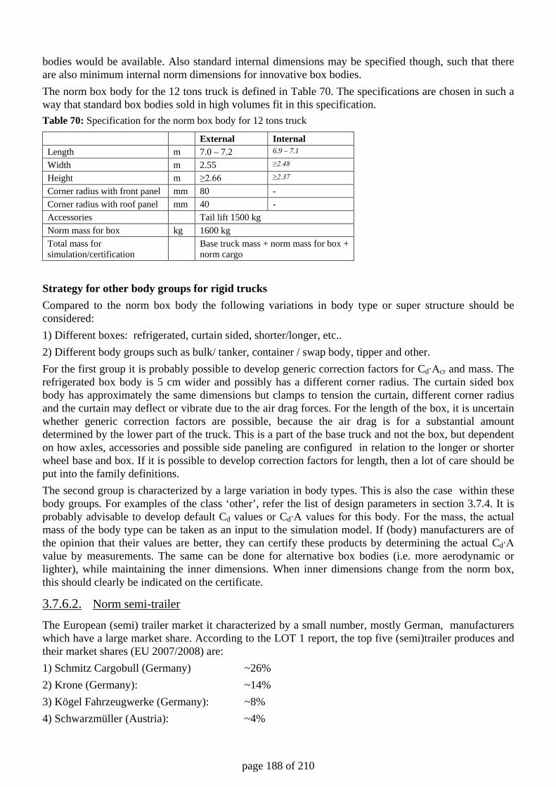
page 188 of 210

bodies would be available. Also standard internal dimensions may be specified though, such that there are also minimum internal norm dimensions for innovative box bodies. The norm box body for the 12 tons truck is defined in Table 70. The specifications are chosen in such a way that standard box bodies sold in high volumes fit in this specification. Table 70: Specification for the norm box body for 12 tons truck

External Internal Length m 7.0 – 7.2 6.9 – 7.1

Width m 2.55 ≥2.48

Height m ≥2.66 ≥2.37

Corner radius with front panel mm 80 - Corner radius with roof panel mm 40 - Accessories Tail lift 1500 kg Norm mass for box kg 1600 kg Total mass for simulation/certification

Base truck mass + norm mass for box + norm cargo

Strategy for other body groups for rigid trucks Compared to the norm box body the following variations in body type or super structure should be considered: 1) Different boxes: refrigerated, curtain sided, shorter/longer, etc.. 2) Different body groups such as bulk/ tanker, container / swap body, tipper and other. For the first group it is probably possible to develop generic correction factors for Cd∙Acr and mass. The refrigerated box body is 5 cm wider and possibly has a different corner radius. The curtain sided box body has approximately the same dimensions but clamps to tension the curtain, different corner radius and the curtain may deflect or vibrate due to the air drag forces. For the length of the box, it is uncertain whether generic correction factors are possible, because the air drag is for a substantial amount determined by the lower part of the truck. This is a part of the base truck and not the box, but dependent on how axles, accessories and possible side paneling are configured in relation to the longer or shorter wheel base and box. If it is possible to develop correction factors for length, then a lot of care should be put into the family definitions. The second group is characterized by a large variation in body types. This is also the case within these body groups. For examples of the class ‘other’, refer the list of design parameters in section 3.7.4. It is probably advisable to develop default Cd values or Cd∙A values for this body. For the mass, the actual mass of the body type can be taken as an input to the simulation model. If (body) manufacturers are of the opinion that their values are better, they can certify these products by determining the actual Cd∙A value by measurements. The same can be done for alternative box bodies (i.e. more aerodynamic or lighter), while maintaining the inner dimensions. When inner dimensions change from the norm box, this should clearly be indicated on the certificate.

3.7.6.2. Norm semi-trailer

The European (semi) trailer market it characterized by a small number, mostly German, manufacturers which have a large market share. According to the LOT 1 report, the top five (semi)trailer produces and their market shares (EU 2007/2008) are: 1) Schmitz Cargobull (Germany) ~26% 2) Krone (Germany): ~14% 3) Kögel Fahrzeugwerke (Germany): ~8% 4) Schwarzmüller (Austria): ~4%

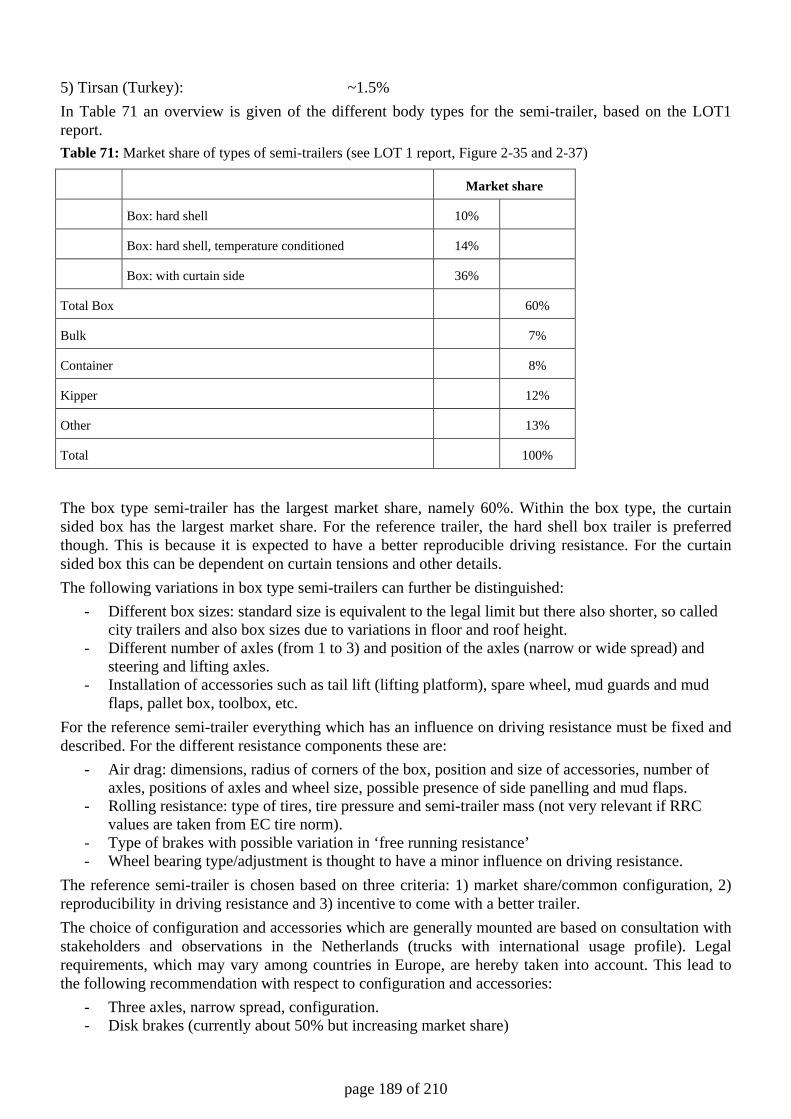
page 189 of 210

5) Tirsan (Turkey): ~1.5% In Table 71 an overview is given of the different body types for the semi-trailer, based on the LOT1 report. Table 71: Market share of types of semi-trailers (see LOT 1 report, Figure 2-35 and 2-37)

Market share

Box: hard shell 10%

Box: hard shell, temperature conditioned 14%

Box: with curtain side 36%

Total Box 60%

Bulk 7%

Container 8%

Kipper 12%

Other 13%

Total 100%

The box type semi-trailer has the largest market share, namely 60%. Within the box type, the curtain sided box has the largest market share. For the reference trailer, the hard shell box trailer is preferred though. This is because it is expected to have a better reproducible driving resistance. For the curtain sided box this can be dependent on curtain tensions and other details. The following variations in box type semi-trailers can further be distinguished:

- Different box sizes: standard size is equivalent to the legal limit but there also shorter, so called city trailers and also box sizes due to variations in floor and roof height.

- Different number of axles (from 1 to 3) and position of the axles (narrow or wide spread) and steering and lifting axles.

- Installation of accessories such as tail lift (lifting platform), spare wheel, mud guards and mud flaps, pallet box, toolbox, etc.

For the reference semi-trailer everything which has an influence on driving resistance must be fixed and described. For the different resistance components these are:

- Air drag: dimensions, radius of corners of the box, position and size of accessories, number of axles, positions of axles and wheel size, possible presence of side panelling and mud flaps.

- Rolling resistance: type of tires, tire pressure and semi-trailer mass (not very relevant if RRC values are taken from EC tire norm).

- Type of brakes with possible variation in ‘free running resistance’ - Wheel bearing type/adjustment is thought to have a minor influence on driving resistance.

The reference semi-trailer is chosen based on three criteria: 1) market share/common configuration, 2) reproducibility in driving resistance and 3) incentive to come with a better trailer. The choice of configuration and accessories which are generally mounted are based on consultation with stakeholders and observations in the Netherlands (trucks with international usage profile). Legal requirements, which may vary among countries in Europe, are hereby taken into account. This lead to the following recommendation with respect to configuration and accessories:

- Three axles, narrow spread, configuration. - Disk brakes (currently about 50% but increasing market share)

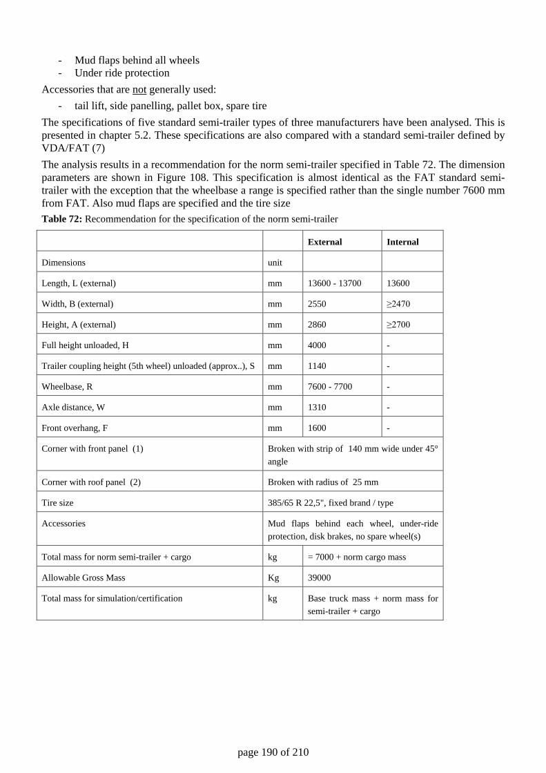
page 190 of 210

- Mud flaps behind all wheels - Under ride protection

Accessories that are not generally used: - tail lift, side panelling, pallet box, spare tire

The specifications of five standard semi-trailer types of three manufacturers have been analysed. This is presented in chapter 5.2. These specifications are also compared with a standard semi-trailer defined by VDA/FAT (7) The analysis results in a recommendation for the norm semi-trailer specified in Table 72. The dimension parameters are shown in Figure 108. This specification is almost identical as the FAT standard semi-trailer with the exception that the wheelbase a range is specified rather than the single number 7600 mm from FAT. Also mud flaps are specified and the tire size Table 72: Recommendation for the specification of the norm semi-trailer

External Internal

Dimensions unit

Length, L (external) mm 13600 - 13700 13600

Width, B (external) mm 2550 ≥2470

Height, A (external) mm 2860 ≥2700

Full height unloaded, H mm 4000 -

Trailer coupling height (5th wheel) unloaded (approx..), S mm 1140 -

Wheelbase, R mm 7600 - 7700 -

Axle distance, W mm 1310 -

Front overhang, F mm 1600 -

Corner with front panel (1) Broken with strip of 140 mm wide under 45° angle

Corner with roof panel (2) Broken with radius of 25 mm

Tire size 385/65 R 22,5", fixed brand / type

Accessories Mud flaps behind each wheel, under-ride protection, disk brakes, no spare wheel(s)

Total mass for norm semi-trailer + cargo kg = 7000 + norm cargo mass

Allowable Gross Mass Kg 39000

Total mass for simulation/certification kg Base truck mass + norm mass for semi-trailer + cargo

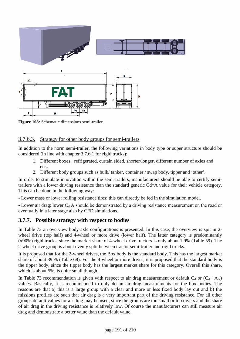
page 191 of 210

Figure 108: Schematic dimensions semi-trailer

3.7.6.3. Strategy for other body groups for semi-trailers

In addition to the norm semi-trailer, the following variations in body type or super structure should be considered (in line with chapter 3.7.6.1 for rigid trucks):

1. Different boxes: refrigerated, curtain sided, shorter/longer, different number of axles and etc..

2. Different body groups such as bulk/ tanker, container / swap body, tipper and ‘other’. In order to stimulate innovation within the semi-trailers, manufacturers should be able to certify semi-trailers with a lower driving resistance than the standard generic Cd*A value for their vehicle category. This can be done in the following way: - Lower mass or lower rolling resistance tires: this can directly be fed in the simulation model. - Lower air drag: lower Cd∙A should be demonstrated by a driving resistance measurement on the road or eventually in a later stage also by CFD simulations.

3.7.7. Possible strategy with respect to bodies In Table 73 an overview body-axle configurations is presented. In this case, the overview is spit in 2-wheel drive (top half) and 4-wheel or more drive (lower half). The latter category is predominantly (≈90%) rigid trucks, since the market share of 4-wheel drive tractors is only about 1.9% (Table 59). The 2-wheel drive group is about evenly split between tractor semi-trailer and rigid trucks. It is proposed that for the 2-wheel drives, the Box body is the standard body. This has the largest market share of about 39 % (Table 68). For the 4-wheel or more drives, it is proposed that the standard body is the tipper body, since the tipper body has the largest market share for this category. Overall this share, which is about 5%, is quite small though. In Table 73 recommendation is given with respect to air drag measurement or default Cd or (Cd ∙ Acr) values. Basically, it is recommended to only do an air drag measurements for the box bodies. The reasons are that a) this is a large group with a clear and more or less fixed body lay out and b) the missions profiles are such that air drag is a very important part of the driving resistance. For all other groups default values for air drag may be used, since the groups are too small or too divers and the share of air drag in the driving resistance is relatively low. Of course the manufacturers can still measure air drag and demonstrate a better value than the default value.

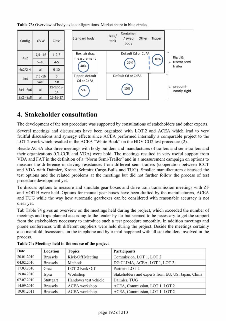
page 192 of 210

Table 73: Overview of body axle configurations. Market share in blue circles

4. Stakeholder consultationThe development of the test procedure was supported by consultations of stakeholders and other experts.Several meetings and discussions have been organized with LOT 2 and ACEA which lead to very fruitful discussions and synergy effects since ACEA performed internally a comparable project to the LOT 2 work which resulted in the ACEA “White Book” on the HDV CO2 test procedure (2).Beside ACEA also three meetings with body builders and manufactures of trailers and semi-trailers and their organizations (CLCCR and VDA) were hold. The meetings resulted in very useful support from VDA and FAT in the definition of a “Norm Semi-Trailer” and in a measurement campaign on options to measure the difference in driving resistances from different semi-trailers (cooperation between ICCT and VDA with Daimler, Krone. Schmitz Cargo-Bulls and TUG). Smaller manufacturers discussed the test options and the related problems at the meetings but did not further follow the process of test procedure development yet.To discuss options to measure and simulate gear boxes and drive train transmission meetings with ZF and VOITH were held. Options for manual gear boxes have been drafted by the manufacturers, ACEA and TUG while the way how automatic gearboxes can be considered with reasonable accuracy is not clear yet.Tab Table 74 gives an overview on the meetings held during the project, which exceeded the number of meetings and trips planned according to the tender by far but seemed to be necessary to get the support from the stakeholders necessary to introduce such a test procedure smoothly. In addition meetings and phone conferences with different suppliers were held during the project. Beside the meetings certainly also manifold discussions on the telephone and by e-mail happened with all stakeholders involved in the process.Table 74: Meetings held in the course of the project

Date Location Topics Participants20.01.2010 Brussels Kick-Off Meeting Commission, LOT 1, LOT 204.02.2010 Brussels Methods DG CLIMA, ACEA, LOT 1, LOT 217.03.2010 Graz LOT 2 Kick Off Partners LOT 219.04.2010 Ispra Workshop Stakeholders and experts from EU, US, Japan, China07.07.2010 Stuttgart Handover test vehicle Daimler, TUG14.09.2010 Brussels ACEA workshop ACEA, Commission, LOT 1, LOT 219.01.2011 Brussels ACEA workshop ACEA, Commission, LOT 1, LOT 2

Standard bodyBulk/ tank

Container / swap body

Other Tipper

7,5 - 16 1-2-3

>=16 4-5

6x2/2-4 all 9-10

7,5 -16 6>=16 7-8

6x4 - 6x6 all11-12-13-

148x2 - 8x8 all 15-16-17

4x4Default Cd or Cd*ATipper, default

Cd or Cd*A

Config GVW

4x2Box, air drag

measurementDefault Cd or Cd*A

Class

10%

5%

48%

10%

27%Rigid & tractor semi-trailer

predomi-nantly rigid

page 193 of 210

Date Location Topics Participants 16/17.03.2011 Brussels DG CLIMA Workshop Commission, LOT 2, ACEA 15.04.2011 Istanbul body+trailers Meeting CLCCR, VDA, TUG, TNO 11.05.2011 Graz body+trailers Meeting TUG, Krone 19.05.2011 Graz Gear box consultation TUG, ZF 09.06.2011 Graz City bus consultation TUG, Volvo 21.06.2011 Brussels Strategy discussion DG CLIMA, DG Enterprise, JRC, TUG 22.07.2011 Web Discuss GB activities Milbrooks, DFT, Ricardo, TUG 13.09.2011 Graz Discussion results

Daimler test vehicles Daimler, TUG

6./7.10.2011 Berlin body+trailers Meeting CLCCR, VDA, TUG 10.10.2011 Friedrichs-

hafen Gear box options ZF, VOITH, TUG

03.11.2011 Vienna White book ACEA ACEA, TUG 8./9.11.2011 Brussels ICCT workshop Stakeholders and experts from EU, US, Japan, China 05.12.2011 Brussels Commission workshop Commission, ACEA, Stakeholders, LOT 2

5. Annex

5.1. Details on existing measurement standards There are different standards available for the measurement of the road load curve of vehicles. In the following chapters they are enlisted and a short summary in headwords is given for the most important content. A first overview is already given in section 3.5.1.5, page 107, Table 43 to Table 46.

5.1.1. SAE J1263 In Jun 1979 SAE J1263 was the first official standard for the measurement of the road load curve of motor vehicles, the actual version is that one of Mar 2010 (76). It was created to determine the road load at 80 km/h for the setup of hydrokinetic chassis dynamometers, which are typically adjusted at one velocity only.

5.1.1.1. Data analysis

Summary: Constant gradient force neglected in calculation, but taken into account by rolling on the same road strip in both directions. Use of wheel mass or all-inclusive factor to calculate the effective vehicle weight including rotating devices. Application of the road load equation, see below. Correction of rolling resistance- and air drag coefficient to reference ambient pressure and temperature: See Equation 51 and Equation 52. During a coastdown (free rolling, clutch open, gear box neutral) the vehicle is decelerated only by the driving resistance forces. The road load equation is applied, see Equation 58

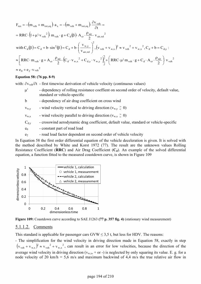
page 194 of 210

( ) ( )

( ) ( )

( ) ( ) ( )

( )2

veh20

2veh

aircrdveh

2y,wy,d

2x,wd

aircrveh

d,yd2

x,w2

veh2

xw,veh

2

rel,air

y,wd

2dd

2rel,air

aircrdveh

2veh

veheq,rotvehxeq,rotvehres

vee

v2

ACgm'RRCvCvC2

AgmRRC

:CbC,vvvv,vv

bCsinbCCwith

v2

ACgmv'1RRC

tvmmammF

⋅+≈

⋅

ρ

⋅⋅+⋅⋅µ⋅+

⋅+⋅⋅

ρ⋅+⋅⋅≈

=++≈+

⋅+=β⋅+=β

⋅ρ

⋅⋅β+⋅⋅⋅µ+⋅=

=∂

∂⋅+−=⋅+−=

Equation 58: (76 pp. 8-9)

with: ∂vveh/∂t - first timewise derivation of vehicle velocity (continuous values)µ' - dependency of rolling resistance coeffient on second order of velocity, default value,

standard or vehicle-specificb - dependency of air drag coefficient on cross wind

vw,y - wind velocity vertical to driving direction (vw,y>< 0)

vw,x - wind velocity parallel to driving direction (vw,x>< 0)

Cd,y - crosswind aerodynamic drag coefficient, default value, standard or vehicle-specifice0 - constant part of road loade2 - road load factor dependent on second order of vehicle velocity

In Equation 58 the first order differential equation of the vehicle deceleration is given. It is solved with the method described by White and Korst 1972 (77). The result are the unknown values Rolling Resistance Coefficient (RRC) and Air Drag Coefficient (Cd). An example of the solved differential equation, a function fitted to the measured coastdown curve, is shown in Figure 109

Figure 109: Coastdown curve according to SAE J1263 (77 p. 357 fig. 4) (stationary wind measurement)

5.1.1.2. Comments

This standard is applicable for passenger cars GVW ≤ 3,5 t, but less for HDV. The reasons:- The simplification for the wind velocity in driving direction made in Equation 58, exactly in step ( ) 2

x,w2

veh2

xw,veh vvvv +≈+ , can result in an error for low velocities, because the direction of the average wind velocity in driving direction (vw,x, + or -) is neglected by only squaring its value. E. g. for a node velocity of 20 km/h = 5,6 m/s and maximum backwind of 4,4 m/s the true relative air flow in

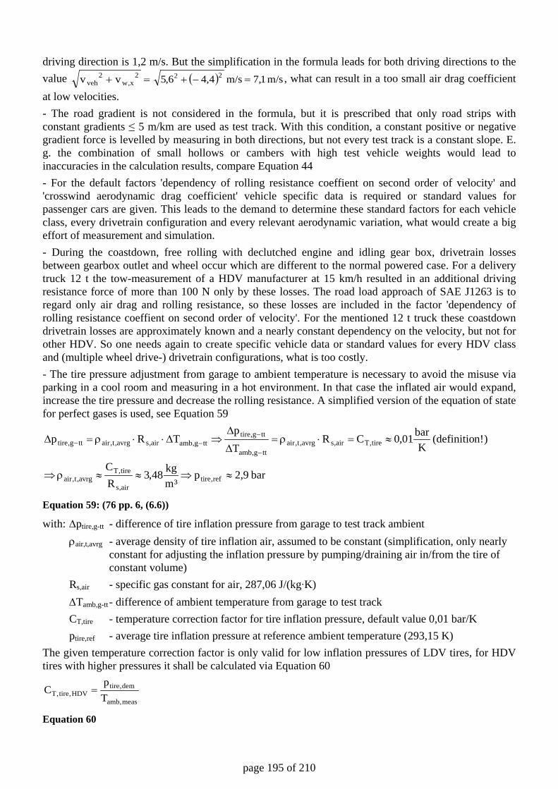
page 195 of 210

driving direction is 1,2 m/s. But the simplification in the formula leads for both driving directions to the value =+ 2

x,w2

veh vv ( ) m/s 1,7m/s 4,46,5 22 =−+ , what can result in a too small air drag coefficient at low velocities. - The road gradient is not considered in the formula, but it is prescribed that only road strips with constant gradients ≤ 5 m/km are used as test track. With this condition, a constant positive or negative gradient force is levelled by measuring in both directions, but not every test track is a constant slope. E. g. the combination of small hollows or cambers with high test vehicle weights would lead to inaccuracies in the calculation results, compare Equation 44 - For the default factors 'dependency of rolling resistance coeffient on second order of velocity' and 'crosswind aerodynamic drag coefficient' vehicle specific data is required or standard values for passenger cars are given. This leads to the demand to determine these standard factors for each vehicle class, every drivetrain configuration and every relevant aerodynamic variation, what would create a big effort of measurement and simulation. - During the coastdown, free rolling with declutched engine and idling gear box, drivetrain losses between gearbox outlet and wheel occur which are different to the normal powered case. For a delivery truck 12 t the tow-measurement of a HDV manufacturer at 15 km/h resulted in an additional driving resistance force of more than 100 N only by these losses. The road load approach of SAE J1263 is to regard only air drag and rolling resistance, so these losses are included in the factor 'dependency of rolling resistance coeffient on second order of velocity'. For the mentioned 12 t truck these coastdown drivetrain losses are approximately known and a nearly constant dependency on the velocity, but not for other HDV. So one needs again to create specific vehicle data or standard values for every HDV class and (multiple wheel drive-) drivetrain configurations, what is too costly. - The tire pressure adjustment from garage to ambient temperature is necessary to avoid the misuse via parking in a cool room and measuring in a hot environment. In that case the inflated air would expand, increase the tire pressure and decrease the rolling resistance. A simplified version of the equation of state for perfect gases is used, see Equation 59

bar 9,2p³m

kg48,3RC

)n!(definitio K

bar01,0CRTp

TRp

ref,tireair,s

tire,Tavrg,t,air

tire,Tair,savrg,t,airttg,amb

ttg,tirettg,ambair,savrg,t,airttg,tire

≈⇒≈≈ρ⇒

≈=⋅ρ=∆

∆⇒∆⋅⋅ρ=∆

−

−−−

Equation 59: (76 pp. 6, (6.6))

with: ∆ptire,g-tt - difference of tire inflation pressure from garage to test track ambient ρair,t,avrg - average density of tire inflation air, assumed to be constant (simplification, only nearly constant for adjusting the inflation pressure by pumping/draining air in/from the tire of constant volume) Rs,air - specific gas constant for air, 287,06 J/(kg∙K) ∆Tamb,g-tt - difference of ambient temperature from garage to test track CT,tire - temperature correction factor for tire inflation pressure, default value 0,01 bar/K ptire,ref - average tire inflation pressure at reference ambient temperature (293,15 K) The given temperature correction factor is only valid for low inflation pressures of LDV tires, for HDV tires with higher pressures it shall be calculated via Equation 60

meas,amb

dem,tireHDV,tire,T T

pC =

Equation 60

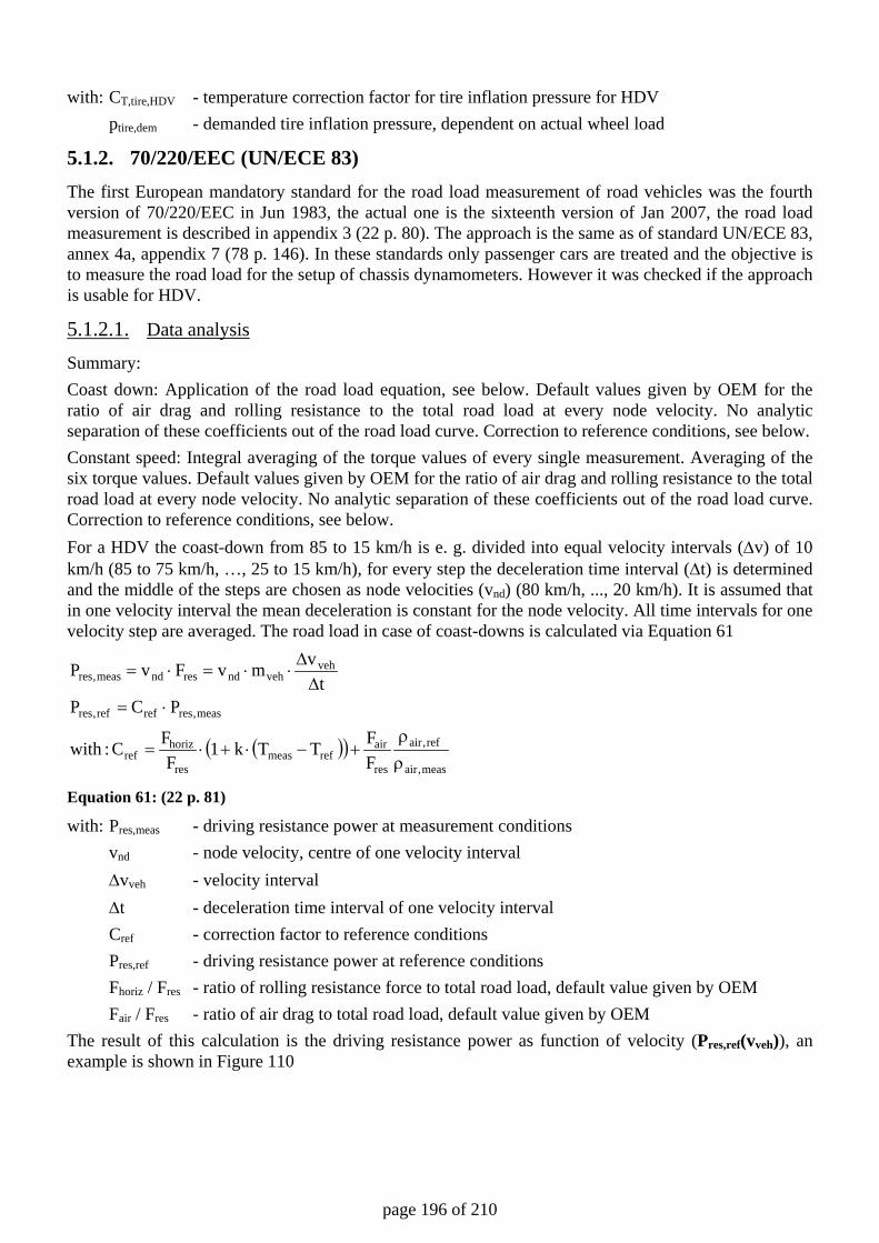
page 196 of 210

with: CT,tire,HDV - temperature correction factor for tire inflation pressure for HDV ptire,dem - demanded tire inflation pressure, dependent on actual wheel load

5.1.2. 70/220/EEC (UN/ECE 83) The first European mandatory standard for the road load measurement of road vehicles was the fourth version of 70/220/EEC in Jun 1983, the actual one is the sixteenth version of Jan 2007, the road load measurement is described in appendix 3 (22 p. 80). The approach is the same as of standard UN/ECE 83, annex 4a, appendix 7 (78 p. 146). In these standards only passenger cars are treated and the objective is to measure the road load for the setup of chassis dynamometers. However it was checked if the approach is usable for HDV.

5.1.2.1. Data analysis

Summary: Coast down: Application of the road load equation, see below. Default values given by OEM for the ratio of air drag and rolling resistance to the total road load at every node velocity. No analytic separation of these coefficients out of the road load curve. Correction to reference conditions, see below. Constant speed: Integral averaging of the torque values of every single measurement. Averaging of the six torque values. Default values given by OEM for the ratio of air drag and rolling resistance to the total road load at every node velocity. No analytic separation of these coefficients out of the road load curve. Correction to reference conditions, see below. For a HDV the coast-down from 85 to 15 km/h is e. g. divided into equal velocity intervals (∆v) of 10 km/h (85 to 75 km/h, …, 25 to 15 km/h), for every step the deceleration time interval (∆t) is determined and the middle of the steps are chosen as node velocities (vnd) (80 km/h, ..., 20 km/h). It is assumed that in one velocity interval the mean deceleration is constant for the node velocity. All time intervals for one velocity step are averaged. The road load in case of coast-downs is calculated via Equation 61

( )( )meas,air

ref,air

res

airrefmeas

res

horizref

meas,resrefref,res

vehvehndresndmeas,res

FFTTk1

FFC :with

PCPt

vmvFvP

ρρ

+−⋅+⋅=

⋅=∆

∆⋅⋅=⋅=

Equation 61: (22 p. 81)

with: Pres,meas - driving resistance power at measurement conditions vnd - node velocity, centre of one velocity interval ∆vveh - velocity interval ∆t - deceleration time interval of one velocity interval Cref - correction factor to reference conditions Pres,ref - driving resistance power at reference conditions Fhoriz / Fres - ratio of rolling resistance force to total road load, default value given by OEM Fair / Fres - ratio of air drag to total road load, default value given by OEM The result of this calculation is the driving resistance power as function of velocity (Pres,ref(vveh)), an example is shown in Figure 110

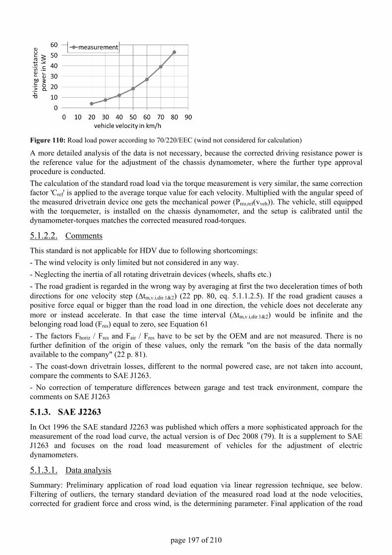
page 197 of 210

Figure 110: Road load power according to 70/220/EEC (wind not considered for calculation)

A more detailed analysis of the data is not necessary, because the corrected driving resistance power is the reference value for the adjustment of the chassis dynamometer, where the further type approval procedure is conducted.The calculation of the standard road load via the torque measurement is very similar, the same correction factor 'Cref' is applied to the average torque value for each velocity. Multiplied with the angular speed of the measured drivetrain device one gets the mechanical power (Pres,ref(vveh)). The vehicle, still equipped with the torquemeter, is installed on the chassis dynamometer, and the setup is calibrated until the dynamometer-torques matches the corrected measured road-torques.

5.1.2.2. Comments

This standard is not applicable for HDV due to following shortcomings:- The wind velocity is only limited but not considered in any way.- Neglecting the inertia of all rotating drivetrain devices (wheels, shafts etc.)- The road gradient is regarded in the wrong way by averaging at first the two deceleration times of both directions for one velocity step (∆tm,v.i,dir.1&2) (22 pp. 80, eq. 5.1.1.2.5). If the road gradient causes a positive force equal or bigger than the road load in one direction, the vehicle does not decelerate any more or instead accelerate. In that case the time interval (∆tm,v.i,dir.1&2) would be infinite and the belonging road load (Fres) equal to zero, see Equation 61- The factors Fhoriz / Fres and Fair / Fres have to be set by the OEM and are not measured. There is nofurther definition of the origin of these values, only the remark "on the basis of the data normally available to the company" (22 p. 81).- The coast-down drivetrain losses, different to the normal powered case, are not taken into account, compare the comments to SAE J1263.- No correction of temperature differences between garage and test track environment, compare the comments on SAE J1263

5.1.3. SAE J2263In Oct 1996 the SAE standard J2263 was published which offers a more sophisticated approach for the measurement of the road load curve, the actual version is of Dec 2008 (79). It is a supplement to SAE J1263 and focuses on the road load measurement of vehicles for the adjustment of electric dynamometers.

5.1.3.1. Data analysis

Summary: Preliminary application of road load equation via linear regression technique, see below. Filtering of outliers, the ternary standard deviation of the measured road load at the node velocities, corrected for gradient force and cross wind, is the determining parameter. Final application of the road

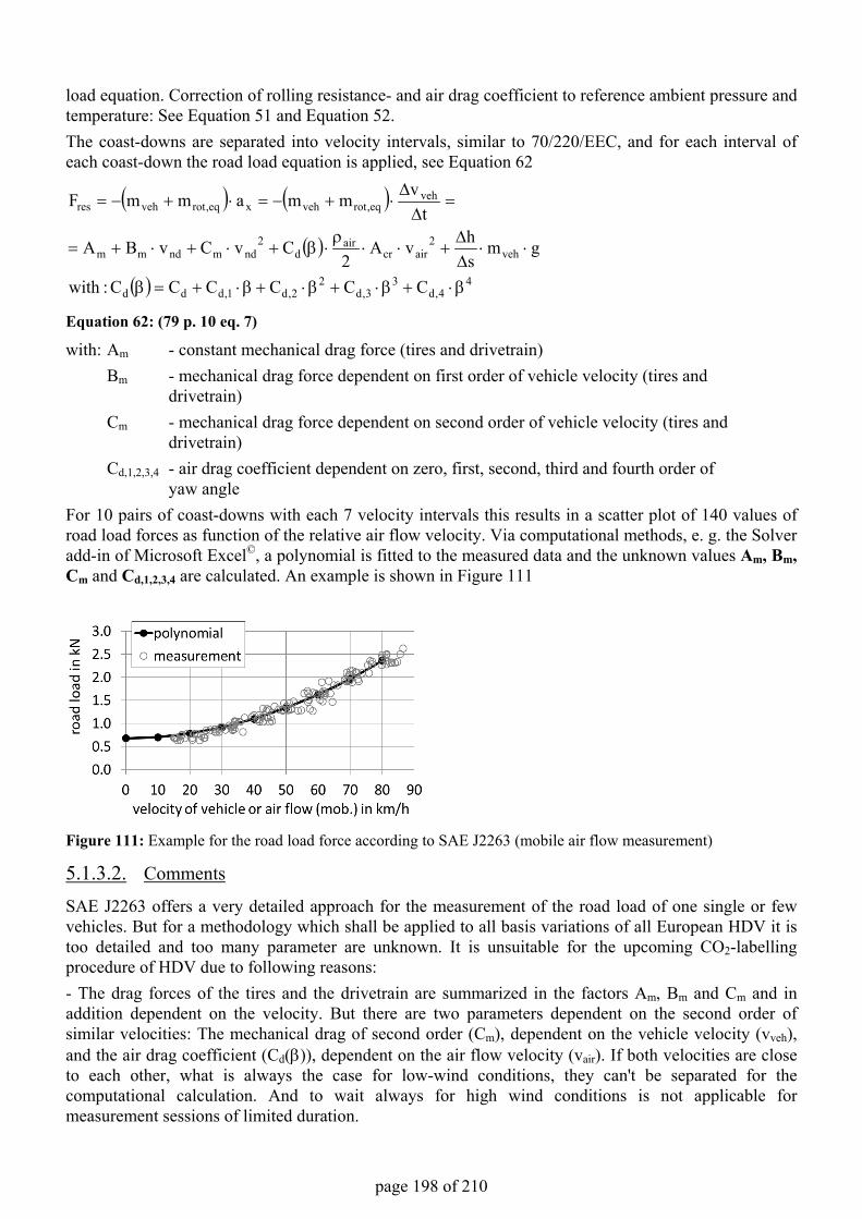
page 198 of 210

load equation. Correction of rolling resistance- and air drag coefficient to reference ambient pressure and temperature: See Equation 51 and Equation 52.The coast-downs are separated into velocity intervals, similar to 70/220/EEC, and for each interval of each coast-down the road load equation is applied, see Equation 62

( ) ( )

( )

( ) 44,d

33,d

22,d1,ddd

veh2

aircrair

d2

ndmndmm

veheq,rotvehxeq,rotvehres

CCCCCC:with

gmshvA

2CvCvBA

tvmmammF

β⋅+β⋅+β⋅+β⋅+=β

⋅⋅∆∆

+⋅⋅ρ

⋅β+⋅+⋅+=

=∆

∆⋅+−=⋅+−=

Equation 62: (79 p. 10 eq. 7)

with: Am - constant mechanical drag force (tires and drivetrain)Bm - mechanical drag force dependent on first order of vehicle velocity (tires and

drivetrain)Cm - mechanical drag force dependent on second order of vehicle velocity (tires and

drivetrain)Cd,1,2,3,4 - air drag coefficient dependent on zero, first, second, third and fourth order of

yaw angleFor 10 pairs of coast-downs with each 7 velocity intervals this results in a scatter plot of 140 values of road load forces as function of the relative air flow velocity. Via computational methods, e. g. the Solver add-in of Microsoft Excel©, a polynomial is fitted to the measured data and the unknown values Am, Bm,Cm and Cd,1,2,3,4 are calculated. An example is shown in Figure 111

Figure 111: Example for the road load force according to SAE J2263 (mobile air flow measurement)

5.1.3.2. Comments

SAE J2263 offers a very detailed approach for the measurement of the road load of one single or few vehicles. But for a methodology which shall be applied to all basis variations of all European HDV it is too detailed and too many parameter are unknown. It is unsuitable for the upcoming CO2-labelling procedure of HDV due to following reasons:- The drag forces of the tires and the drivetrain are summarized in the factors Am, Bm and Cm and in addition dependent on the velocity. But there are two parameters dependent on the second order of similar velocities: The mechanical drag of second order (Cm), dependent on the vehicle velocity (vveh), and the air drag coefficient (Cd(β)), dependent on the air flow velocity (vair). If both velocities are close to each other, what is always the case for low-wind conditions, they can't be separated for the computational calculation. And to wait always for high wind conditions is not applicable formeasurement sessions of limited duration.

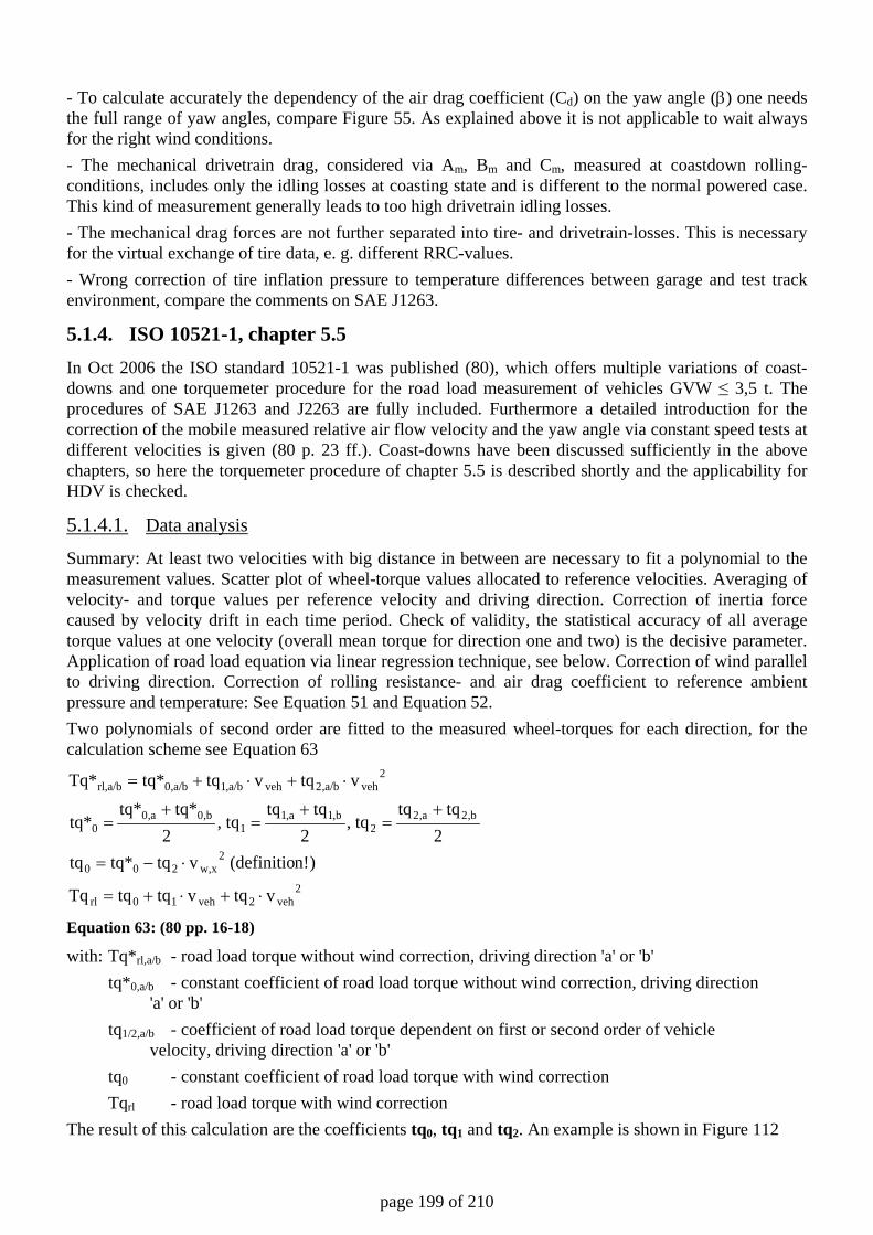
page 199 of 210

- To calculate accurately the dependency of the air drag coefficient (Cd) on the yaw angle (β) one needs the full range of yaw angles, compare Figure 55. As explained above it is not applicable to wait always for the right wind conditions. - The mechanical drivetrain drag, considered via Am, Bm and Cm, measured at coastdown rolling-conditions, includes only the idling losses at coasting state and is different to the normal powered case. This kind of measurement generally leads to too high drivetrain idling losses. - The mechanical drag forces are not further separated into tire- and drivetrain-losses. This is necessary for the virtual exchange of tire data, e. g. different RRC-values. - Wrong correction of tire inflation pressure to temperature differences between garage and test track environment, compare the comments on SAE J1263.

5.1.4. ISO 10521-1, chapter 5.5 In Oct 2006 the ISO standard 10521-1 was published (80), which offers multiple variations of coast-downs and one torquemeter procedure for the road load measurement of vehicles GVW ≤ 3,5 t. The procedures of SAE J1263 and J2263 are fully included. Furthermore a detailed introduction for the correction of the mobile measured relative air flow velocity and the yaw angle via constant speed tests at different velocities is given (80 p. 23 ff.). Coast-downs have been discussed sufficiently in the above chapters, so here the torquemeter procedure of chapter 5.5 is described shortly and the applicability for HDV is checked.

5.1.4.1. Data analysis

Summary: At least two velocities with big distance in between are necessary to fit a polynomial to the measurement values. Scatter plot of wheel-torque values allocated to reference velocities. Averaging of velocity- and torque values per reference velocity and driving direction. Correction of inertia force caused by velocity drift in each time period. Check of validity, the statistical accuracy of all average torque values at one velocity (overall mean torque for direction one and two) is the decisive parameter. Application of road load equation via linear regression technique, see below. Correction of wind parallel to driving direction. Correction of rolling resistance- and air drag coefficient to reference ambient pressure and temperature: See Equation 51 and Equation 52. Two polynomials of second order are fitted to the measured wheel-torques for each direction, for the calculation scheme see Equation 63

2veh2veh10rl

2w,x200

,b2,a22

,b1,a11

,b0,a00

2veh,a/b2veh,a/b1,a/b0rl,a/b

vtqvtqtqTq

)n!(definitio vtqtq*tq2

tqtq, tq

2tqtq

, tq2

tq*tq*tq*

vtqvtqtq*Tq*

⋅+⋅+=

⋅−=

+=

+=

+=

⋅+⋅+=

Equation 63: (80 pp. 16-18)

with: Tq*rl,a/b - road load torque without wind correction, driving direction 'a' or 'b' tq*0,a/b - constant coefficient of road load torque without wind correction, driving direction 'a' or 'b' tq1/2,a/b - coefficient of road load torque dependent on first or second order of vehicle velocity, driving direction 'a' or 'b' tq0 - constant coefficient of road load torque with wind correction Tqrl - road load torque with wind correction The result of this calculation are the coefficients tq0, tq1 and tq2. An example is shown in Figure 112

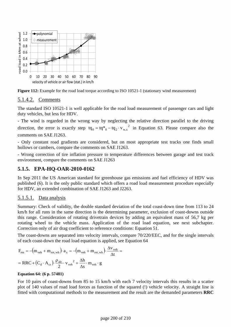
page 200 of 210

Figure 112: Example for the road load torque according to ISO 10521-1 (stationary wind measurement)

5.1.4.2. Comments

The standard ISO 10521-1 is well applicable for the road load measurement of passenger cars and light duty vehicles, but less for HDV. - The wind is regarded in the wrong way by neglecting the relative direction parallel to the driving direction, the error is exactly step 2

w,x200 vtqtq*tq ⋅−=

in Equation 63. Please compare also the comments on SAE J1263. - Only constant road gradients are considered, but on most appropriate test tracks one finds small hollows or cambers, compare the comments on SAE J1263. - Wrong correction of tire inflation pressure to temperature differences between garage and test track environment, compare the comments on SAE J1263

5.1.5. EPA-HQ-OAR-2010-0162 In Sep 2011 the US American standard for greenhouse gas emissions and fuel efficiency of HDV was published (6). It is the only public standard which offers a road load measurement procedure especially for HDV, an extended combination of SAE J1263 and J2263.

5.1.5.1. Data analysis

Summary: Check of validity, the double standard deviation of the total coast-down time from 113 to 24 km/h for all runs in the same direction is the determining parameter, exclusion of coast-downs outside this range. Consideration of rotating drivetrain devices by adding an equivalent mass of 56,7 kg per rotating wheel to the vehicle mass. Application of the road load equation, see next subchapter. Correction only of air drag coefficient to reference conditions: Equation 51. The coast-downs are separated into velocity intervals, compare 70/220/EEC, and for the single intervals of each coast-down the road load equation is applied, see Equation 64

( ) ( )

( ) gmshv

2ACRRC

tvmmammF

veh2

vehair

crd

vehwh,rotvehxwh,rotvehres

⋅⋅∆∆

+⋅ρ

⋅⋅+=

=∆

∆⋅+−=⋅+−=

Equation 64: (6 p. 57481)

For 10 pairs of coast-downs from 85 to 15 km/h with each 7 velocity intervals this results in a scatter plot of 140 values of road load forces as function of the squared (!) vehicle velocity. A straight line is fitted with computational methods to the measurement and the result are the demanded parameters RRC

0.00.20.40.60.81.01.2

0 10 20 30 40 50 60 70 80 90

road

load

in k

Nm

at

whe

el

velocity of vehicle or air flow (stat.) in km/h

polynomialmeasurement

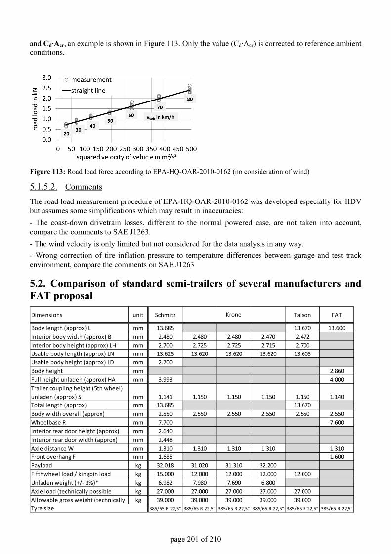
page 201 of 210

and Cd∙Acr, an example is shown in Figure 113. Only the value (Cd∙Acr) is corrected to reference ambient conditions.

Figure 113: Road load force according to EPA-HQ-OAR-2010-0162 (no consideration of wind)

5.1.5.2. Comments

The road load measurement procedure of EPA-HQ-OAR-2010-0162 was developed especially for HDV but assumes some simplifications which may result in inaccuracies:- The coast-down drivetrain losses, different to the normal powered case, are not taken into account, compare the comments to SAE J1263.- The wind velocity is only limited but not considered for the data analysis in any way.- Wrong correction of tire inflation pressure to temperature differences between garage and test track environment, compare the comments on SAE J1263

5.2. Comparison of standard semi-trailers of several manufacturers and FAT proposal

Dimensions unit Schmitz Talson FAT

Body length (approx) L mm 13.685 13.670 13.600Interior body width (approx) B mm 2.480 2.480 2.480 2.470 2.472Interior body height (approx) LH mm 2.700 2.725 2.725 2.715 2.700Usable body length (approx) LN mm 13.625 13.620 13.620 13.620 13.605Usable body height (approx) LD mm 2.700Body height mm 2.860Full height unladen (approx) HA mm 3.993 4.000Trailer coupling height (5th wheel) unladen (approx) S mm 1.141 1.150 1.150 1.150 1.150 1.140Total length (approx) mm 13.685 13.670Body width overall (approx) mm 2.550 2.550 2.550 2.550 2.550 2.550Wheelbase R mm 7.700 7.600Interior rear door height (approx) mm 2.640Interior rear door width (approx) mm 2.448Axle distance W mm 1.310 1.310 1.310 1.310 1.310Front overhang F mm 1.685 1.600Payload kg 32.018 31.020 31.310 32.200Fifthwheel load / kingpin load kg 15.000 12.000 12.000 12.000 12.000Unladen weight (+/- 3%)* kg 6.982 7.980 7.690 6.800Axle load (technically possible kg 27.000 27.000 27.000 27.000 27.000Allowable gross weight (technically kg 39.000 39.000 39.000 39.000 39.000

385/65 R 22,5" 385/65 R 22,5" 385/65 R 22,5" 385/65 R 22,5" 385/65 R 22,5" 385/65 R 22,5"

Krone

Tyre size

page 202 of 210

5.3. Standards for the measurement of HDV components Drivetrain losses ISO/TR 13989-2, Calculation of scuffing load capacity of cylindrical, bevel and hypoid gears -- Part 2: Integral temperature method, 2000 SAE J1266, Axle Efficiency Test Procedure, 2001 SAE J1540, Manual Transmission Efficiency and Parasitic Loss Measurement, 2000 Auxiliary power demand SAE J1339, Test Method for Measuring Performance of Engine Cooling Fans, 2009 SAE J1340, Test Method for Measuring Power Consumption of Air Conditioning and Brake Compressors for Trucks and Buses, 2011 SAE J1341, Test Method for Measuring Power Consumption of Hydraulic Pumps for Trucks and Buses, 2003 SAE J1342, Test Method for Determining Power Consumption of Engine Cooling Fan Drive Systems, 2007 SAE J1343, Information Relating to Duty Cycles and Average Power Requirements of Truck and Bus Engine Accessories, 2000

5.4. List of responsible authors Persons In alphabetic order: Hausberger, Stefan; Department of Emissions, Institute for Internal Combustion Engines and Thermodynamics (TUG), Graz University of Technology; AT-8010 Graz Kies, Antonius; Department of Emissions, Institute for Internal Combustion Engines and Thermodynamics (TUG), Graz University of Technology; AT-8010 Graz Laine, Petri; Department of Engines and Vehicles, Finnish Technical Research Centre (VTT); FI-02150 Espoo Rexeis, Martin; Department of Emissions, Institute for Internal Combustion Engines and Thermodynamics (TUG), Graz University of Technology; AT-8010 Graz Samaras, Zissis; Laboratory of Applied Thermodynamics (LAT), Mechanical Engineering Department, Aristotle University; GR-54124 Thessaloniki Sandström-Dahl, Charlotte; Unit of Air Quality, Motortestcenter, List Research Company for Internal Combustion Engines (AVL-MTC); SE-13623 Haninge Schulte, Leif-Erik; Institute for Vehicle Technology and Mobility, German Technical Inspection Association / Group North (TÜV-NORD); DE-45307 Essen Silberholz, Gérard, Department of Emissions, Institute for Internal Combustion Engines and Thermodynamics (TUG), Graz University of Technology; AT-8010 Graz Steven, Heinz; Heinz Steven Company for Data Analysis and Consultancy; DE-52525 Heinsberg Verbeek, Ruud; Department of Environmentally Sustainable Transport, Netherlands Organization for Applied Scientific Research (TNO); NL-2600CK Delft Allocation of responsibilities The partners in LOT2 distributed the responsibilities for reporting as follows

page 203 of 210

o AVL-MTC: Repeatability of PEMS tests (3.4.2.1), HDV CO2 program Sweden (3.1.3.2) o Heinz Steven: Driving cycles (sections 2.3, 3.5.6) o LAT: Vehicle stock, mileages and CO2 emissions per vehicle concept (section 3.7.1) o TNO: Norm bodies and semi-trailers and share of aerodynamic drag on total energy

consumption per HDV segment (sections 3.7.1.4, 3.7.5, 3.7.6, 3.7.7, 5.2) o TUG: Everything else and coordination. o TÜV-NORD: International legislation and family concepts (sections 3.1, 3.4.2: subchapter by

AVL, 3.7:multiple subchapters by LAT and TNO) o VTT: Standard procedures for chassis dynamometer testing of HDV (section 3.4.3)

Beside the reporting all partners performed the measurements allocated to their labs. Evaluation of the test data was mainly work of TUG.

5.5. List of literature 1. Hill, N. et al. Reduction and Testing of Greenhouse Gas (GHG) Emissions from Heavy Duty Vehicles Lot 1: Strategy. Didcot : AEA, 22 Feb 2011. 2. ACEA Workgroup CO2-HDV. White Book CO2 declaration procedure HDV, Status November 2011. Bruxelles : Association des Constructeurs Européens d'Automobiles (ACEA), 10 Nov 2011. 3. Rexeis, M. Ascertainment of Real World Emissions of Heavy Duty Vehicles. Graz : Graz University of Technology, Institute for ICE and Thermodynamics, Department Emissions, Oct. 2009. Doctoral thesis. 4. Bode, M. et al. Der Reifenrollwiderstand von Nutzfahrzeugen. Hannover : 13th VDI Congress Tires-Chassis-Road, 25/26 Oct. 2011. 5. Vincken, D. Der Reifen. Rollwiderstand und Kraftstoffersparnis. Karlsruhe : Michelin, 2005. ISBN 2067116584. 6. Greenhouse Gas Emissions Standards and Fuel Efficiency Standards for Medium- and Heavy-Duty Engines and Vehicles. EPA-HQ-OAR-2010-0162. 179, Washington D. C. : Office of the Federal Register, Sep 15, 2011, Federal register, Vol. 76, pp. 57106-57513. ISSN 0097–6326. 7. Devesa, A. et al. Verbrauchsreduktion an Nutzfahrzeugkombinationen durch aerodynamische Maßnahmen. Berlin : Forschungsvereinigung Automobiltechnik e.V. (FAT), 2 Nov 2011. FAT-Schriftenreihe Nr. 237. 8. ISO/TR 13989-2. Calculation of scuffing load capacity of cylindrical, bevel and hypoid gears -- Part 2: Integral temperature method. Genf : ISO, 2000. 9. Grote, K. & Feldhusen, H. (eds.). Dubbel. Taschenbuch für den Maschinenbau. Berlin : Springer, Sep 2011. ISBN 3642173055. 10. Rexeis, M. et al. Heavy duty vehicle emissions -Final Report for ARTEMIS WP 400. Graz : Graz University of Technology, Institute for ICE and Thermodynamics, Department Emissions, 27 Jul 2005. report no. I 02/2005/Hb 20/2000 I680. 11. HDH-07-02. Draft Agenda 7th HD Hybrids Informal Group meeting. Genf : UN/ECE, 12-14 Oct 2011. 12. Morgan, A. Powerpack evaluation for HD hybrid powertrains. Genf : UN/ECE, 16-18 Mar 2011. HDH-05-012. 13. Tamm, J. et al. Proposed Rulemaking to Establish 2014-18 Medium and Heavy Duty Vehicle Fuel Efficiency and GHG Standards. Washington D. C. : SAE Government/Industry Meeting, 26 Jan 2011. 14. White, K. Analysis of the Vehicle Inventory and Use Survey for Trucks with five axles or more. Washington, D.C. : Federal Highway Administration, May 2001.

page 204 of 210

15. Mirmino, B. Commercial Vehicle Regulations. Alexandria : Truck Renting and Leasing Association, 26 Oct 2010. http://www.trala.org/docs/ETAC/Cummins%20Inc..pdf. 16. Heavy-Duty Regulations. Washington D. C. : United States Environmental Protection Agency, 19 Nov 2011. Entry on homepage (www.epa.gov/otaq/climate/regulations.htm). 17. EPA-420-B-10-039. Greenhouse gas Emissions Model (GEM) User Guide. Washington D. C. : United States Environmental Protection Agency, Oct 2010. 18. Automobile Type Approval Handbook for Japanese Certification. Tokyo : Japan Automobile Standards Internationalization Centre (JASIC), 2010. 19. Motor Vehicle Statistics of Japan 2010. Tokyo : Japan Automobile Manufacturer Association (JAMA), Sep 2010. www.jama-english.jp/publications/MVS2010.pdf. 20. Zheng, T. et al. Development of Fuel Consumption Test Method Standards for Heavy-Duty Commercial Vehicles in China. Warrendale : SAE International, 2011. SAE-no. 2011-01-2292. 21. Luz, R. et al. User Guide for the Model PHEM, Version 10. Graz : Graz University of Technology, Institute for ICE and Thermodynamics, Department Emissions, 2009. 22. 70/220/EEC. Council directive of 20 March 1970 on the approximation of the laws of the Member States on measures to be taken against air pollution by emissions from motor vehicles, version 16. Brussels : European Commission, 1 Jan 2007. 23. Wallentowitz, H. Längsdynamik von Kraftfahrzeugen. Aachen : fka, 2007. ISBN 9783925194320. 24. EC 1222/2009. Regulation (EC) No 1222/2009 of the European parliament and of the council of 25 November 2009 on the labelling of tyres with respect to fuel efficiency and other essential parameters. Bruxelles : European Commission, 22 Dec 2009. 25. UN/ECE 117 Rev. 2. Uniform Provisions concerning the Approval of Tyres with regard to Rolling Sound Emissions and to Adhesion on Wet Surfaces and/or to Rolling Resistance. Genf : UN/ECE, 2011. 26. AK4 Dynamische Achslasten und Straßenbeanspruchung. Berlin : Forschungsvereinigung Automobiltechnik e. V. (FAT), 15 Nov 2011. Entry on homepage (via www.vda.de). 27. ASTM E965-96. Standard Test Method for Measuring Pavement Macrotexture Depth Using a Volumetric Technique. West Conshohocken : ASTM, 2006. 28. ASTM E1845-09. Standard Practice for Calculating Pavement Macrotexture Mean Profile Depth. West Conshohocken : ASTM, 2009. 29. ASTM E1926-08. Standard Practice for Computing International Roughness Index of Roads from Longitudinal Profile Measurements. West Conshohocken : ASTM, 2008. 30. Fisco, N. Comparison of Macrotexture Measurement Methods. Columbus : Ohio State University, Sep 2009. Master’s Thesis. 31. Asphalt Concrete Surfaces Macrotexture Determination From Still Images. Elunai, R. et al. 3, New York : Institute of Electrical and Electronics Engineers, 2011, IEEE Transactions on Intelligent Transportation Systems, Vol. 12. ISSN 1524-9050, DOI 10.1109/TITS.2011.2116784. 32. Sayers, M. et al. The little book of profiling. Ann Arbour : University of Michigan, 18 Sep 1998. 33. Hammarström, U. Road surface effects on rolling resistance – coastdown measurements with uncertainty analysis in focus. Linköping : VTI, 16 Apr 2009. 34. Mitschke, M. et al. (ed.). Dynamik der Kraftfahrzeuge. Berlin : Springer, 2004. ISBN 3540420118. 35. Cooper, K. Commercial Vehicle Aerodynamic Drag Reduction: Historical Perspective as a Guide. [book auth.] R. McCallen et al. (ed.). The Aerodynamics of Heavy Vehicles: Trucks, Buses, and Trains. Berlin : Springer, 2004. ISBN 3540220887. 36. Sigloch, H. Technische Fluidmechanik. Berlin : Springer, 2008. ISBN 9783540446330.

page 205 of 210

37. Hausberger, S. et al. Test of fuel efficiency improvements in the HDV sector from improved trailer and tire designs by application of a new test procedure. Carried out under contract of ICCT and VDA. Graz : Graz University of Technology, Institute for ICE and Thermodynamics, Department Emissions, 15 Dec 2011. report no. I-24/2011 Hb-Em 18/11/679. 38. Precision Reaction Torquemeters. Hoffman Estates : S. Himmelstein and Company, 2007. Datasheet, PDF download. 39. RoaDyn® P103/P106. Winterthur : Kistler AG, 2010. Datasheet, PDF download. 40. AVL KMA Mobile. Graz : AVL List GmbH, Jun 2008. Product guide, no. AT2262D, Rev. 02. 41. AIC 6004 Swissline Uniflowmaster series (700HP). Allschwil : AIC Systems AG, 2 Nov 2011. Entry on homepage. 42. VBOX 3i R2G2 / R10G10. Buckingham : Racelogic Ltd., 2010. Datasheet, PDF download. 43. Correvit® L-350 Aqua. Wetzlar : CORRSYS-DATRON Sensorsysteme GmbH, 2011. Datasheet, PDF download. 44. Bleeck, A., Krischker, R. Untersuchungen zur Höhenbestimmung in den amtlichen Nivellementnetzen Brandenburgs. Berlin : Beuth Hochschule für Technik, Department III Civil Engineering and Geoinformation, Jul 2006. Diploma thesis. 45. Survey plan Eurospeedway Lausitz. Klettwitz : DEKRA Automobil GmbH, 2008. 46. Wind Sensor first class advanced. Göttingen : Adolf Thies GmbH & Co. KG, 3 Nov 2011. Entry on homepage. 47. Wind Direction Sensor first class. Göttingen : Adolf Thies GmbH & Co. KG, 3 Nov 2011. Entry on homepage. 48. Combined Wind Sensor Classic. Göttingen : Adolf Thies GmbH & Co. KG, 3 Nov 2011. Entry on homepage. 49. Ultrasonic Wind Sensor. uSonic-2 Wind. Elmshorn : METEK GmbH, 2011. Datasheet, PDF download. 50. WindSonic™. Wind Speed & Direction Sensor. Lymington : Gill Instruments Ltd., 2011. Datasheet, PDF download. 51. Ultrasonic Anemometer 2D. Göttingen : Adolf Thies GmbH & Co. KG, 3 Nov 2011. Entry on homepage. 52. Reif, K. (ed.). Bosch Autoelektrik und Autoelektronik. Wiesbaden : Vieweg+Teubner, 2011. ISBN 9783834812742. 53. Tachometer RPM10. Waltham : Extech Instruments Corp., 2008. Datasheet, PDF download. 54. Hoepke, E. et al. (ed.). Nutzfahrzeugtechnik. Wiesbaden : Vieweg+Teubner, 2010. ISBN 9783834809957. 55. Naunheimer, H. et al. Fahrzeuggetriebe. Berlin : Springer, 2007. ISBN 9783540306252. 56. Koryciak, J. Einfluss der Ölmenge auf das Reibmoment von Wälzlagern mit Linienberührung. Bochum : Ruhr-University Bochum, Chair for machine parts and construction, 2007. Doctoral thesis. ISBN 3891941781. 57. Braess, H. et al. Vieweg Handbuch Kraftfahrzeugtechnik. Wiesbaden : Vieweg, 2005. ISBN 3528331143. 58. Jakowatz, Frédéric (ed.). Fundamentals of commercial vehicle technology. München : MAN Nutzfahrzeuge Group, 2009. 59. Campbell, S. et al. Superbus Phase I: Accessory Loads Onboard a Parallel Hybrid-Electric City Bus. Minneapolis : University of Minnesota, Center for Transportation Studies, Aug 2009. 60. Cengel, Y. et al. Thermodynamics. New York : McGrawhill, 2008. ISBN 9780073107684.

page 206 of 210

61. ltalienische Momente. Wolf, A. 12, pp. 23, Stuttgart : EuroTransportMedia, 2010, lastauto omnibus, Vol. 84. ISSN 0023-866x. 62. SensoTop. Heidenheim : Voith GmbH, 12 Nov 2011. Entry on homepage. 63. TopoDyn. Friedrichshafen : ZF Friedrichshafen AG, 12 Nov 2011. Entry on homepage. 64. Baker, H. et al. Review of low Carbon Technologies for Heavy Goods Vehicles - Annex 1. Shoreham-by-Sea : Ricardo plc., Jun 2009. report no. RD.09/182601.7. 65. Money, money, money. Zeitzen, F. 8, pp. 34, Stuttgart : EuroTransportMedia, 2011, lastauto omnibus, Vol. 85. ISSN 0023-866X. 66. Spot an! 11, pp. 34, Stuttgart : EuroTransportMedia, 2011, lastauto omnibus, Vol. 85. ISSN 0023-866X. 67. Mehr als Klimaretter. Rosenberger, T. 10, pp. 36, Stuttgart : EuroTransportMedia, 2010, lastauto omnibus, Vol. 84. ISSN 1613-1606. 68. Gurtner, R. et al. Ringvergleich. Abgasmessung auf Fahrzeugprüfständen in österreichischen Prüflabors. Graz : FH Joanneum, 2011. 69. Lunanova, M. Optimierung von Nebenaggregaten. Wiesbaden : Vieweg+Teubner, Jan 2009. ISBN 9783834807304. 70. Verbeek, R. et al. Brandstoffen voor het wegverkeer. Delft : TNO & CE, 9 Jun 2011. report no. TNO-RPT-2011-00607. 71. Ntziachristos, L. et al. Exhaust emissions from road transport. Kopenhagen : European Environment Agency (EEA), Jun 2010. 72. Ntziachristos, L. et. al. European Database of Vehicle Stock for the Calculation and Forecast of Pollutant and Greenhouse Gases Emissions with TREMOVE and COPERT. Thessaloniki : Aristotle University, Laboratory of Applied Thermodynamics (LAT), 2 Jul 2008. report no. 08.RE.0009.V2. 73. van Raemdonck, G. et al. Truck Aerodynamics. An overview of solutions for reducing aerodynamic drag. Delft : TU Delft & CINTEC, Jan 2009. 74. Reithmaier, W. et al. Determination of rolling noise and rolling-resistance coefficients and conduct of wet surface brake tests on utility-vehicle tires. München : TÜV Automotive GmbH, Tire/Wheel Test Center, Dec 2000. report no. UBA-FB 299 54 114. 75. Kytö, M. et al. Heavy-duty vehicles: Safety, environmental impacts and new technology. Espoo : VTT Technical Research Centre of Finland, Jun 2009. report no. VTT-R-04084-09. 76. SAE J1263. Road Load Measurement and Dynamometer Simulation Using Coastdown Techniques. Warrendale : SAE, 2010. 77. White, R. et al. The Determination of Vehicle Drag Contributions from Coast-Down Tests. Warrendale : SAE, 1972. SAE paper no. 720099, DOI 10.4271/720099. 78. UN/ECE 83 Rev. 4. Uniform provisions concerning the approval of vehicles with regard to the emission of pollutants according to engine fuel requirements. Genf : UN/ECE, 2011. 79. SAE J2263. Road Load Measurement Using Onboard Anemometry and Coastdown Techniques. Warrendale : SAE, 2008. 80. ISO 10521-1. Road vehicles- Road Load Part 1: Determination under reference. Genf : ISO, 2006.

5.6. List of abbreviations %fso percentage of full scale output (maximum measurement value of an instrument) %rdg percentage of reading (actual measurement value)

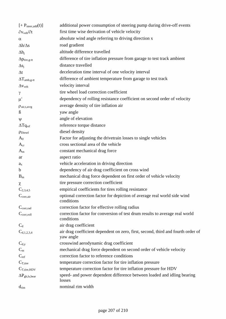
page 207 of 210

[+ Psteer,add(t)] additional power consumption of steering pump during drive-off events ∂vveh/∂t first time wise derivation of vehicle velocity α absolute wind angle referring to driving direction x ∆h/∆s road gradient ∆hj altitude difference travelled ∆ptire,g-tt difference of tire inflation pressure from garage to test track ambient ∆sj distance travelled ∆t deceleration time interval of one velocity interval ∆Tamb,g-tt difference of ambient temperature from garage to test track ∆vveh velocity interval γ tire wheel load correction coefficient µ' dependency of rolling resistance coefficient on second order of velocity ρair,t,avrg average density of tire inflation air ß yaw angle ψ angle of elevation ΔTqref reference torque distance ρDiesel diesel density A0 Factor for adjusting the drivetrain losses to single vehicles Acr cross sectional area of the vehicle Am constant mechanical drag force ar aspect ratio ax vehicle acceleration in driving direction b dependency of air drag coefficient on cross wind Bm mechanical drag force dependent on first order of vehicle velocity χ tire pressure correction coefficient C2,3,4,5 empirical coefficients for tires rolling resistance Ccorr,air optional correction factor for depiction of average real world side wind

conditions Ccorr,rad correction factor for effective rolling radius Ccorr,roll correction factor for conversion of test drum results to average real world

conditions Cd air drag coefficient Cd,1,2,3,4 air drag coefficient dependent on zero, first, second, third and fourth order of

yaw angle Cd,y crosswind aerodynamic drag coefficient Cm mechanical drag force dependent on second order of vehicle velocity Cref correction factor to reference conditions CT,tire temperature correction factor for tire inflation pressure CT,tire,HDV temperature correction factor for tire inflation pressure for HDV ∆Pgb,ls,bear speed- and power dependent difference between loaded and idling bearing

losses drim nominal rim width

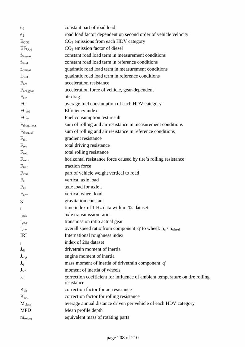
page 208 of 210

e0 constant part of road load e2 road load factor dependent on second order of vehicle velocity ECO2 CO2 emissions from each HDV category EFCO2 CO2 emission factor of diesel f0,meas constant road load term in measurement conditions f0,ref constant road load term in reference conditions f2,meas quadratic road load term in measurement conditions f2,ref quadratic road load term in reference conditions Facc acceleration resistance Facc,gear acceleration force of vehicle, gear-dependent Fair air drag FC average fuel consumption of each HDV category FCrel Efficiency index FCw Fuel consumption test result Fdrag,meas sum of rolling and air resistance in measurement conditions Fdrag,ref sum of rolling and air resistance in reference conditions Fgrd gradient resistance Fres total driving resistance Froll total rolling resistance Froll,t horizontal resistance force caused by tire’s rolling resistance Ftrac traction force Fvert part of vehicle weight vertical to road Fz vertical axle load Fz,i axle load for axle i Fz,w vertical wheel load g gravitation constant i time index of 1 Hz data within 20s dataset iaxle axle transmission ratio igear transmission ratio actual gear iq-w overall speed ratio from component 'q' to wheel: nq / nwheel

IRI International roughness index j index of 20s dataset Jdt drivetrain moment of inertia Jeng engine moment of inertia Jq mass moment of inertia of drivetrain component 'q' Jwh moment of inertia of wheels k correction coefficient for influence of ambient temperature on tire rolling

resistance Kair correction factor for air resistance Kroll correction factor for rolling resistance Mclass average annual distance driven per vehicle of each HDV category MPD Mean profile depth mrot,eq equivalent mass of rotating parts

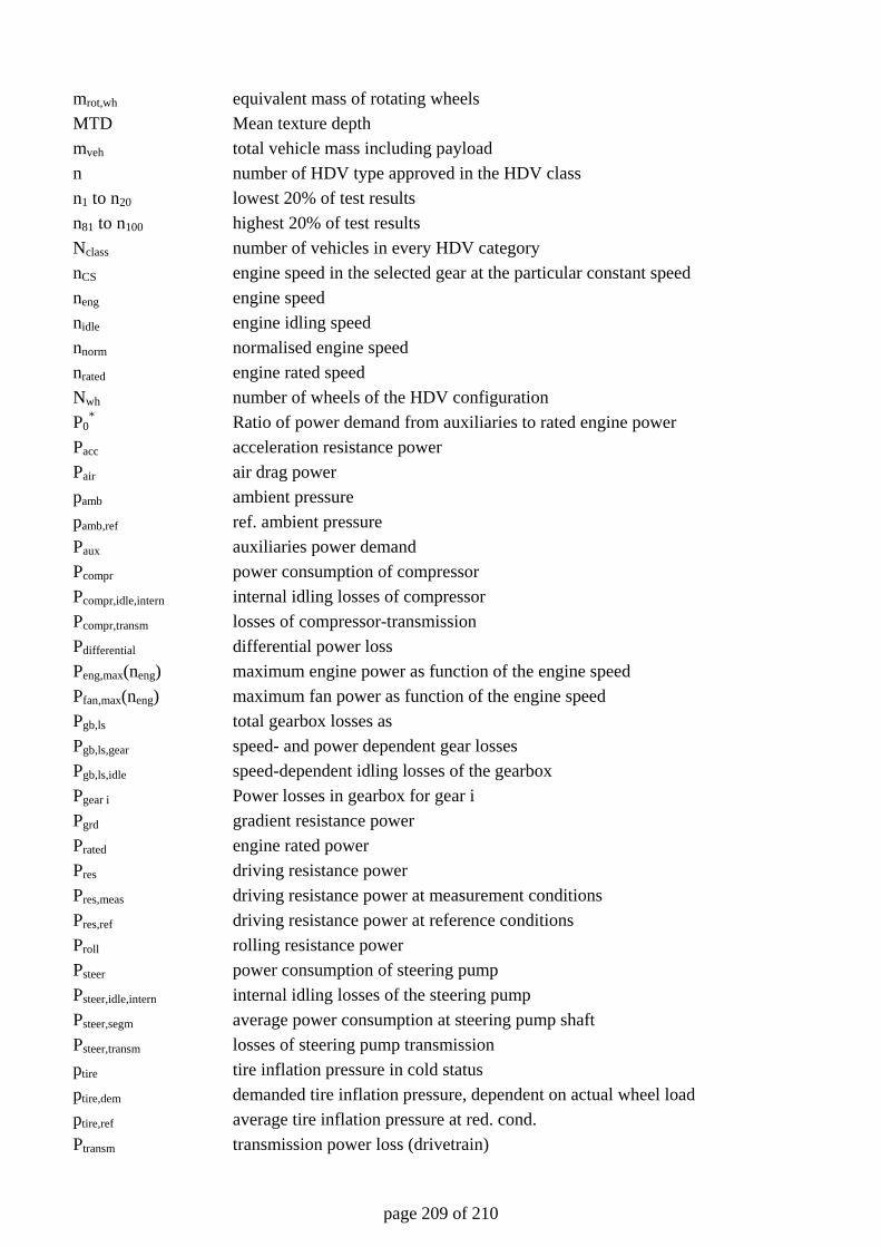
page 209 of 210

mrot,wh equivalent mass of rotating wheels MTD Mean texture depth mveh total vehicle mass including payload n number of HDV type approved in the HDV class n1 to n20 lowest 20% of test results n81 to n100 highest 20% of test results Nclass number of vehicles in every HDV category nCS engine speed in the selected gear at the particular constant speed neng engine speed nidle engine idling speed nnorm normalised engine speed nrated engine rated speed Nwh number of wheels of the HDV configuration P0

* Ratio of power demand from auxiliaries to rated engine power Pacc acceleration resistance power Pair air drag power pamb ambient pressure pamb,ref ref. ambient pressure Paux auxiliaries power demand Pcompr power consumption of compressor Pcompr,idle,intern internal idling losses of compressor Pcompr,transm losses of compressor-transmission Pdifferential differential power loss Peng,max(neng) maximum engine power as function of the engine speed Pfan,max(neng) maximum fan power as function of the engine speed Pgb,ls total gearbox losses as Pgb,ls,gear speed- and power dependent gear losses Pgb,ls,idle speed-dependent idling losses of the gearbox Pgear i Power losses in gearbox for gear i Pgrd gradient resistance power Prated engine rated power Pres driving resistance power Pres,meas driving resistance power at measurement conditions Pres,ref driving resistance power at reference conditions Proll rolling resistance power Psteer power consumption of steering pump Psteer,idle,intern internal idling losses of the steering pump Psteer,segm average power consumption at steering pump shaft Psteer,transm losses of steering pump transmission ptire tire inflation pressure in cold status ptire,dem demanded tire inflation pressure, dependent on actual wheel load ptire,ref average tire inflation pressure at red. cond. Ptransm transmission power loss (drivetrain)

page 210 of 210

ρair,ref air density at reference conditions rdrum drum diameter re effective tire rolling radius RRC rolling resistance coefficient Rs,air specific gas constant for air rtire tire diameter sair share of air resistance on total drag sFz,i share of axle i on the total vehicle weight sroll share of rolling resistance on total drag t time Tamb ambient temperature Tamb,ref ref. ambient temperature tcycle cycle duration tq*0,a/b constant coefficient of road load torque without wind correction, driving

direction 'a' or 'b' Tq*rl,a/b road load torque without wind correction, driving direction 'a' or 'b' tq0 constant coefficient of road load torque with wind correction tq1/2,a/b coefficient of road load torque dependent on first or second order of vehicle

velocity, driving direction 'a' or 'b' Tqdrag,n drag torque engine speed “n” Tqdrag,ref drag torque at the reference engine speed Tqmax,n full-load torque at engine speed “n” Tqmax,ref full-load torque at the reference engine speed Tqrl road load torque with wind correction Tqwh-l measured torque in the left wheel Tqwh-r measured torque in the right wheel vair air-flow velocity Vair,pump volume of pumped air Vair,segm total volume of pumped air, specific value for single HDV segments vair,x air-flow velocity in driving direction x vnd node velocity, centre of one velocity interval vveh vehicle velocity vw,x wind velocity parallel to driving direction vw,y wind velocity vertical to driving direction w nominal tire width Wnet,shaft net specific work at compressor shaft X measurement quantity under consideration zn number of load points to be measured at engine speed “n”