Reduction of predictive uncertainty in estimating irrigation

GMDD7, 7525–7558, 2014

Reduction ofpredictive

uncertainty inestimating irrigationwater requirement

S. Multsch et al.

Title Page

Abstract Introduction

Conclusions References

Tables Figures

J I

J I

Back Close

Full Screen / Esc

Printer-friendly Version

Interactive Discussion

Discussion

Paper

|D

iscussionP

aper|

Discussion

Paper

|D

iscussionP

aper|

Geosci. Model Dev. Discuss., 7, 7525–7558, 2014www.geosci-model-dev-discuss.net/7/7525/2014/doi:10.5194/gmdd-7-7525-2014© Author(s) 2014. CC Attribution 3.0 License.

This discussion paper is/has been under review for the journal Geoscientific ModelDevelopment (GMD). Please refer to the corresponding final paper in GMD if available.

Reduction of predictive uncertainty inestimating irrigation water requirementthrough multi-model ensembles andensemble averaging

S. Multsch1, J.-F. Exbrayat2,3, M. Kirby4, N. R. Viney4, H.-G. Frede1, andL. Breuer1

1Institute for Landscape Ecology and Resources Management (ILR), Research Centre forBioSystems, Land Use and Nutrition (IFZ), Justus Liebig University Giessen,Heinrich-Buff-Ring 26, 35390 Giessen, Germany2School of GeoSciences and National Centre for Earth Observation, University of Edinburgh,Edinburgh, UK3Climate Change Research Centre and ARC Centre of Excellence for Climate SystemScience, University of New South Wales, Sydney, New South Wales, Australia4CSIRO Land and Water, GP.O. Box 1666, Canberra, ACT 2601, Australia

7525

http://www.geosci-model-dev-discuss.net

http://www.geosci-model-dev-discuss.net/7/7525/2014/gmdd-7-7525-2014-print.pdf

http://www.geosci-model-dev-discuss.net/7/7525/2014/gmdd-7-7525-2014-discussion.html

http://creativecommons.org/licenses/by/3.0/

GMDD7, 7525–7558, 2014



S. Multsch et al.

Title Page



Tables Figures

J I

J I

Back Close

Full Screen / Esc



Discussion

Paper

|D

iscussionP

aper|

Discussion

Paper

|D

iscussionP

aper|

Received: 25 September 2014 – Accepted: 20 October 2014 – Published: 10 November 2014

Correspondence to: S. Multsch ([email protected])

Published by Copernicus Publications on behalf of the European Geosciences Union.

7526





GMDD7, 7525–7558, 2014



S. Multsch et al.

Title Page



Tables Figures

J I

J I

Back Close

Full Screen / Esc



Discussion

Paper

|D

iscussionP

aper|

Discussion

Paper

|D

iscussionP

aper|

Abstract

Irrigation agriculture plays an increasingly important role in food supply. Many evapo-transpiration models are used today to estimate the water demand for irrigation. Theyconsider different stages of crop growth by empirical crop coefficients to adapt evap-otranspiration throughout the vegetation period. We investigate the importance of the5

model structural vs. model parametric uncertainty for irrigation simulations by consid-ering six evapotranspiration models and five crop coefficient sets to estimate irrigationwater requirements for growing wheat in the Murray-Darling Basin, Australia. The studyis carried out using the spatial decision support system SPARE:WATER. We find thatstructural model uncertainty is far more important than model parametric uncertainty to10

estimate irrigation water requirement. Using the Reliability Ensemble Averaging (REA)technique, we are able to reduce the overall predictive model uncertainty by more than10 %. The exceedance probability curve of irrigation water requirements shows thata certain threshold, e.g. an irrigation water limit due to water right of 400 mm, wouldbe less frequently exceeded in case of the REA ensemble average (45 %) in compar-15

ison to the equally weighted ensemble average (66 %). We conclude that multi-modelensemble predictions and sophisticated model averaging techniques are helpful in pre-dicting irrigation demand and provide relevant information for decision making.

1 Introduction

1.1 Predicting crop water needs20

Globally, the proportion of fresh water consumption by agriculture is large(9087 km3 yr−1) (Hoekstra and Mekonnen, 2012) and is projected to increase in thefuture in order to support the increasing world population. More precisely, most ofthe change in freshwater consumption will arise from the increasing irrigation demandby crops (De Fraiture and Wichelns, 2010). Therefore, strategies based on improved25

7527





GMDD7, 7525–7558, 2014



S. Multsch et al.

Title Page



Tables Figures

J I

J I

Back Close

Full Screen / Esc



Discussion

Paper

|D

iscussionP

aper|

Discussion

Paper

|D

iscussionP

aper|

irrigation methods and local adaptions of management practices are likely to be im-plemented to anticipate this trend. Such strategies are often developed using decisionsupport systems that are informed by mathematical models. For example, irrigationmanagement has been optimized by modelling and measurements for crops grown inCentral Asia (Pereira et al., 2009) or for irrigated cotton in the High-Plains region of5

Texas (Howell et al., 2004). Others have investigated water use efficiency (Wang et al.,2001) or crop water productivity (Liu et al., 2007) by modelling experiments for irrigatedcrops grown in China.

All these models depend on the calculation of evapotranspiration (ET) which rep-resents the evaporation from a surface and transpiration from plants. In the case of10

agricultural crops, ET is equal to the crop water needed for crop growth and yield pro-duction. Globally, evapotranspiration represents about two thirds of the total rainfallon land, while evapotranspiration from crops amounts for about 8 % (Oki and Kanae,2006), and is insofar the most important term of the water balance. The basic conceptfor deriving crop water needs of irrigated crops has been initially reported by Jensen15

(1968) and is proposed by Allen et al. (1998) as the single crop coefficient concept.The crop specific evapotranspiration (ETc) is derived from reference evapotranspira-tion (ETo) and a crop specific coefficient (Kc):

ETc = ETo ·Kc (1)

with ETo given in [mm] and dimensionless Kc. ETo can be calculated by standardise po-20

tential evapotranspiration (PET) to a short (grass) or tall (alfalfa) reference crop. In thecase of the Penman–Monteith equation (Monteith, 1965; Penman, 1948) standardizedfixed values for albedo (0.23), plant height (0.12 cm) and surface resistance (70 ms−1)are assumed (Allen et al., 1998; Jensen et al., 1990). Kc is commonly calculated onthe basis of field experiments (e.g. Ko et al., 2009; da Silva et al., 2013) and varies with25

the crop development.Such an approach is part of many irrigation management models, including Crop-

wat (Smith, 1992), ISAREG (Pereira et al., 2009), ISM (George et al., 2000) or global7528





GMDD7, 7525–7558, 2014



S. Multsch et al.

Title Page



Tables Figures

J I

J I

Back Close

Full Screen / Esc



Discussion

Paper

|D

iscussionP

aper|

Discussion

Paper

|D

iscussionP

aper|

crop water models (Siebert and Döll, 2010). Moreover, the single crop coefficient con-cept is the basis for the simulation of crop water needs in many studies. For example,Lathuillière et al. (2012) have derived water use by terrestrial ecosystems and haveshown that ET declines over a 10 year period by about 25 % in response to deforesta-tion and replacement by agriculture in Brazil. They showed that irrigation water require-5

ment (IRR) is relevant for terrestrial water fluxes and a reliable estimation is crucial forthe closure of the water cycle. In another study future climate impacts on groundwaterin agriculture areas have been investigated (Toews and Allen, 2009). They showed thatlarger return flows to the groundwater can be related to increased IRR under warmertemperatures and longer vegetation periods. Moreover, the crop coefficient concept is10

also the basis for the water footprint (volume of water consumed or polluted to produceone unit of biomass) assessment of crops (Mekonnen and Hoekstra, 2011) and hasbeen used to determine water requirements and the water footprint of the agriculturesector in Saudi Arabia (Multsch et al., 2013).

1.2 Sources of predictive uncertainty15

Major sources of uncertainties should be considered in the study design, quantifiedthroughout the modelling process (Refsgaard et al., 2007) and communicated as partof the results to the end users. Uncertainties related to large scale estimations of theIRR have only rarely been analysed. For example, Siebert and Döll (2010) have studiedthe uncertainty in predicting green (rainfall consumed by crops) and blue (consumed20

surface and groundwater by crops in terms of irrigation) water consumption by usingdifferent ETo equations on a global scale. They observed a significant difference of bluewater consumption, i.e. required irrigation, and only a small change in green water con-sumption between model runs while using two classical ETo equations. More recently,Sheffield et al. (2012) pointed out that using a more up-to-date parameterization of PET25

to calculate drought indices led to different conclusions on drought occurrence globally.Generally, model predictive uncertainty can be lead back to four sources, input un-

certainty, output uncertainty, structural uncertainty and parametric uncertainty (Renard7529





GMDD7, 7525–7558, 2014



S. Multsch et al.

Title Page



Tables Figures

J I

J I

Back Close

Full Screen / Esc



Discussion

Paper

|D

iscussionP

aper|

Discussion

Paper

|D

iscussionP

aper|

et al., 2010). The last two, structural and parametric uncertainty, are addressed in thisstudy with a focus on the prediction of IRR. As part of the parametric uncertainty, theparameterization of equations to quantify natural or anthropogenic processes has re-ceived considerable interest, particularly in conceptual rainfall–runoff modelling (Beven,2006; Vrugt et al., 2009). In case of modelling crop water needs according to Eq. (1),5

Kc is an important model parameter. Kc values for a large number of crops are providedby the FAO56 irrigation guidelines (Allen et al., 1998) which are commonly used for ir-rigation planning. However, it has been highlighted that an adjustment to the global Kcis needed if the simulations are used for irrigation planning on a local to regional scale(Ko et al., 2009; da Silva et al., 2013). Nevertheless, it is still unclear whether a local10

adaption of Kc leads to a better model performance. For this reason, we quantify theparametric uncertainty of model parameterisation with different Kc sets.

The model structure also introduces uncertainties, as any model remains a simplifi-cation of the real world. In the context of modelling water resources, all hydrological andcrop growth models rely on the estimation of ET. According to Eq. (1), ETo is required15

to estimate crop specific evapotranspiration. ETo equations are often divided into cat-egories according to the input data (Bormann, 2011; Tabari et al., 2013): temperaturebased equations such as Hargreaves–Samani (HS) equation (Hargreaves and Samani,1985), radiation based equations such as Priestley–Taylor (PT) (Priestley and Taylor,1972) or combined equations such as the FAO56 Penman–Monteith (PM56) equation20

(Allen et al., 1998), that further takes wind speed into account. Nevertheless, in manycases it was shown that the variability among PET methods is large (Fisher et al.,2011; Kite and Droogers, 2000). Because most water resources models rely on somecalculation of ETo, we see it as a crucial source of structural uncertainty that is rarelyconsidered.25

1.3 Reduction of predictive uncertainty by ensemble modelling

Ensembles of model predictions can be developed by different sets of model parame-terization (single-model ensemble) and model structures (multi-model ensemble). The

7530





GMDD7, 7525–7558, 2014



S. Multsch et al.

Title Page



Tables Figures

J I

J I

Back Close

Full Screen / Esc



Discussion

Paper

|D

iscussionP

aper|

Discussion

Paper

|D

iscussionP

aper|

weighting of model ensembles according to their fit to observational data has becomeof interest to reduce the uncertainty and to derive a more robust predictions and pro-jections. Giorgi and Mearns (2002) have introduced the reliability ensemble averagingtechnique (REA) in climate research. Basically, different models are weighted accord-ing to their performance in representing measured data and according to the distance5

of individual models to the ensemble average prediction to quantify the convergence ofdifferent models. This approach has been applied more recently for predicting catch-ment nitrogen fluxes (Exbrayat et al., 2013) and calculating water balances and landuse interaction (Huisman et al., 2009).

In a first step, we analyse the relative contributions of the structural and paramet-10

ric model uncertainty in hind casts of IRR of wheat across the Murray-Darling-Basin(MDB), Australia. Simulations are calculated using the spatial decision support systemSPARE:WATER (Multsch et al., 2013). In a second step, we apply the REA methodol-ogy to reduce the predictive uncertainty of IRR. The general procedure is as follows:

– The applicability of six different ETo methods is evaluated by using available mea-15

sured class-A-pan evaporation measurements of 34 stations in the MDB overa 21 years time period;

– 30 different model realisations are setup in a multi-model ensemble by combiningvarious ETo equations (n = 6) and crop coefficient data sets (n = 5);

– IRR is calculated by forcing the multi-model ensemble with climate time series20

of 21 years (monthly data) for 3969 sites (each 1 km2 ×1 km2) in the MDB whereirrigated wheat has been grown according to the land use allocation in 2000;

– The 30 model realisations are weighted according to their performance in repre-senting measured data and their distance to the ensemble average.

By doing so, we quantify structural (ETo method) and parametric (Kc set) uncertainty25

and apply REA to provide a robust estimate of IRR and the confidence interval aroundit.

7531





GMDD7, 7525–7558, 2014



S. Multsch et al.

Title Page



Tables Figures

J I

J I

Back Close

Full Screen / Esc



Discussion

Paper

|D

iscussionP

aper|

Discussion

Paper

|D

iscussionP

aper|

2 Methods and data

2.1 Study site and data

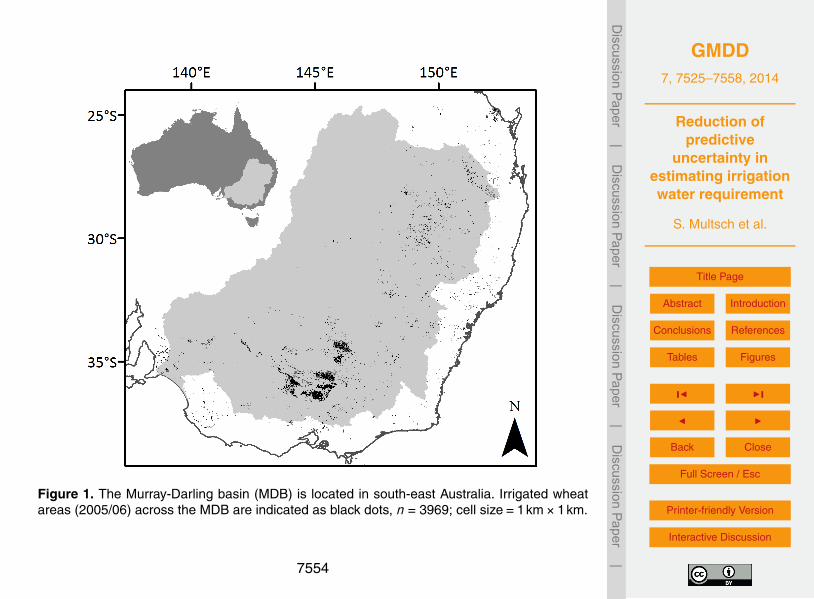
The MDB covers about 1 millionkm2 of south-east Australia (Fig. 1). Irrigation agri-culture in the MDB sums up to 17 600 km2, which is equal to 65 % of the total irriga-tion agriculture in Australia. Total water withdrawal for irrigation in 2006 amounted to5

7.36 km3 yr−1 (ABS, 2006). Wheat is the second most important crop grown in MDBafter grazing pastures, covering 3969 km2 in 2006 and was therefore selected for thiscase study for which IRR and its underlying uncertainty was calculated. The croppingareas have been taken from a land use map from 2006 (ABARES, 2010) with a spatialresolution of 0.01◦×0.01◦ (∼ 1km×1km). We assume a fixed land use distribution over10

time in our model study to clearly target the uncertainty in ETo method and crop coeffi-cients. Climate data for 1986–2006 were taken from the SILO Data Drill of the Queens-land Department of Natural resources and Water (https://longpaddock.qld.gov.au/silo/,Jeffrey et al., 2001) with a spatial resolution of 0.05◦ ×0.05◦ (∼ 5km×5km). We usedthe same weather dataset over all 3969 1×1 km land grid cells overlapped by a 5×5 km15

grid cell in the weather data. The model was forced with monthly data. For validation,we compared simulated ETo to measured class-A pan data from 34 stations through-out the MDB. The class-A pan data were obtained from Patched Point Dataset of theQueensland Department of Science, Information Technology, Innovation and the Arts,(http://www.longpaddock.qld.gov.au/silo/ppd/). Measured data have been adjusted with20

monthly pan-coefficients according to McMahon et al. (2013) to represent evaporationfrom open surface water. For stations where no pan-coefficient was available we usedthe one from the nearest station.

2.2 Simulation of irrigation requirement with SPARE:WATER

SPARE:WATER (Multsch et al., 2013) is a spatial decision support system for the cal-25

culation of crop specific water requirements and water footprints from local to regional

7532





https://longpaddock.qld.gov.au/silo/

http://www.longpaddock.qld.gov.au/silo/ppd/

GMDD7, 7525–7558, 2014



S. Multsch et al.

Title Page



Tables Figures

J I

J I

Back Close

Full Screen / Esc



Discussion

Paper

|D

iscussionP

aper|

Discussion

Paper

|D

iscussionP

aper|

scale. Input parameter for the simulation are climate data, irrigation management (ir-rigation water quality, irrigation efficiency, irrigation method), a digital elevation modeland crop characteristics such as maximum crop height and length of growing seasonas well as sowing and planting date. In a first step, the water requirement of growinga crop is simulated for each grid cell according to the spatial resolution of the input5

data. In a second step, the water footprint for spatial entities such as administrativeboundaries or catchments is calculated considering statistical data on crop yield andharvest area. Water footprints for geographic entities are given as volume of waterconsumed per year (e.g. km3 yr−1) and water footprints for specific crops as volumesof water consumed per biomass (m3 t−1).10

In this study the calculation of the IRR is calculated as the difference between ETcand effective rainfall (Peff). The latter one is estimated from the difference of surfacerun-off (RO) and precipitation (P ). RO is derived as a fixed fraction of 20 % of total P .On this basis, IRR is calculated according to Eq. (2):

IRR = max(ETc − Peff,0) (2)15

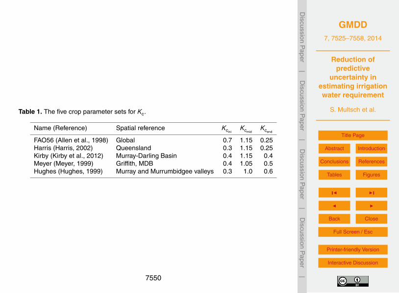
with IRR, ETc and Peff given in [mm]. ETc is calculated based on the single cropcoefficient approach initially proposed by Jensen (1968) and recommended by Allenet al. (1998) according to Eq. (1). The input parameters for this method are the lengthof four individual stages (initial season, growth season, mid-season and late season)during the growing season and three related crop coefficients (Kc). These define the20

ratio between ETo and ETc for each part of the growing season. We have consideredfive different Kc data sets (Table 1). The most common dataset has been proposedfrom the FAO56 Irrigation and Drainage Guidelines (Allen et al., 1998). This approachhas been applied for calculating crop water footprints (Mekonnen and Hoekstra, 2011)and is part of the widely used Cropwat model (Smith, 1992). It has been discussed25

that locally adapted Kc sets are superior in simulating site-specific crop water require-ment than global ones (Ko et al., 2009; da Silva et al., 2013). Thus, further data sets

7533





GMDD7, 7525–7558, 2014



S. Multsch et al.

Title Page



Tables Figures

J I

J I

Back Close

Full Screen / Esc



Discussion

Paper

|D

iscussionP

aper|

Discussion

Paper

|D

iscussionP

aper|

have been collected from various sources which represent site-specific relationshipsbetween ETo and ETc for areas in the MDB.

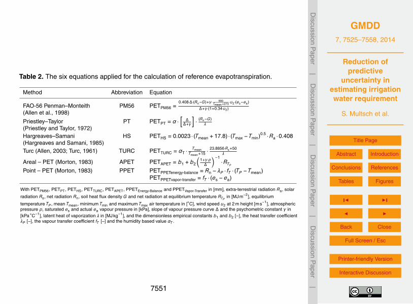
ETo has been calculated with six different methods (Table 2). Two of them are clas-sified as combined methods (PM56, PPET), three are radiation-based methods (PT,TURC, APET) and one is a temperature based method (HS). All of them are com-5

monly applied function, e.g. PM56 and HS are included in Cropwat (Smith, 1992) andAquacrop (Steduto et al., 2009), two models to quantify crop water and IRR, widelyused and promoted by the FAO. The cropping system model EPIC (Williams, 1989) ad-ditionally allows the use of the PT equation, while the global vegetation model LPJmL(Fader et al., 2010) and the global water model WaterGap (Döll et al., 2003) are re-10

stricted to PT. APET and PPET have been particularly tested for the utilisation underAustralian weather conditions in several (Chiew et al., 2002; Chiew and Leahy, 2003;Donohue et al., 2010).

2.3 Reliability ensemble averaging

We used two types of ensemble averaging techniques, which differ in the weighing15

technique. We calculated an equally weighted average of all 30 model realisations(6ETo methods×5Kc datasets) for every grid cell which sum up to 3969 cells (1×1 km)in the MDB where irrigated wheat is grown according to the land use allocation in 2006.However, this method does not consider the capability of its ensemble members to pre-dict a target value nor does it value the agreement of model predictions amongst each20

other. Therefore, we apply the REA technique that was initially proposed by Giorgi andMearns (2002) to reduce uncertainties in climate change projections (see Appendix Cfor details). Moreover, it was used in impact studies targeting land use change impactson hydrology (Huisman et al., 2009) and water quality scenario projections (Exbrayatet al., 2013).25

The strength of the REA method is that it considers both the quality of a model pre-diction (performance) and its position within an ensemble of prediction (convergence).The aim is to provide a best estimate of predictions and a robust assessment of the

7534





GMDD7, 7525–7558, 2014



S. Multsch et al.

Title Page



Tables Figures

J I

J I

Back Close

Full Screen / Esc



Discussion

Paper

|D

iscussionP

aper|

Discussion

Paper

|D

iscussionP

aper|

confidence interval around it. The REA weighting scheme estimates two factors, modelperformance (RB) and model convergence (RD). RB represents the capability of eachensemble member to represent real world data by its bias B. RD is a measure of thedistance D of a single model to the equally weighted ensemble average. Both are lim-ited by the natural background variability (ε). The combined effect known as reliability5

factor (R) is derived as:

R =

RB︷︸︸︷[ε

abs(B)

]·

RD︷︸︸︷[ε

abs(D)

](3)

In this study, ε is calculated from measured class-A pan evaporation for 34 climatestations in the study region for the time period from 1986 to 2006. The class-A pandata has been adjusted with monthly pan coefficients for climate stations in Australia10

(McMahon et al., 2013). We calculated the annual mean evaporation [mm] for each yearand each station and used the 50 % confidence interval (difference between the 25 and75 % percentile) of 224 mm to define ε. The consideration of the difference betweenupper and lower percentiles has been recommended by Giorgi and Mearns (2002).Model performance is measured by the RMSE between measured (class-A pan) and15

predicted ETo for each model (i ).The convergence criterion RD is calculated in an iterative procedure. The difference

between the average IRR of each ensemble member i and the ensemble averageis calculated. Under the consideration of the natural background variability ε a firstguess of RD (for each ensemble member) is predicted as well as a first guess of the20

REA average. This procedure is repeated by considering the newly derived REA aver-age until the ensemble convergence, so that the difference between ensemble mem-bers and the REA average cannot be reduced by additional iterations (see Giorgi andMearns, 2002, for a complete methodological description). The error of the equallyweighted ensemble average is described by the RMSE between IRRi predicted by25

model i (with n = 30 models) and the equally weighted ensemble average irrigation7535





GMDD7, 7525–7558, 2014



S. Multsch et al.

Title Page



Tables Figures

J I

J I

Back Close

Full Screen / Esc



Discussion

Paper

|D

iscussionP

aper|

Discussion

Paper

|D

iscussionP

aper|

water requirement (IRR). The error of the reliability ensemble average (RMSEREA) isderived from the reliability factor of each model (Ri ), the irrigation water requirementpredicted by model i (IRRi ) and the REA weighted ensemble average (IRRREA). TheRMSE represents an approximate 60–70 % confidence interval under the assumptionthat the amount of irrigation is distributed somewhere between normal and uniform.5

3 Results

3.1 Validation of ETo methods

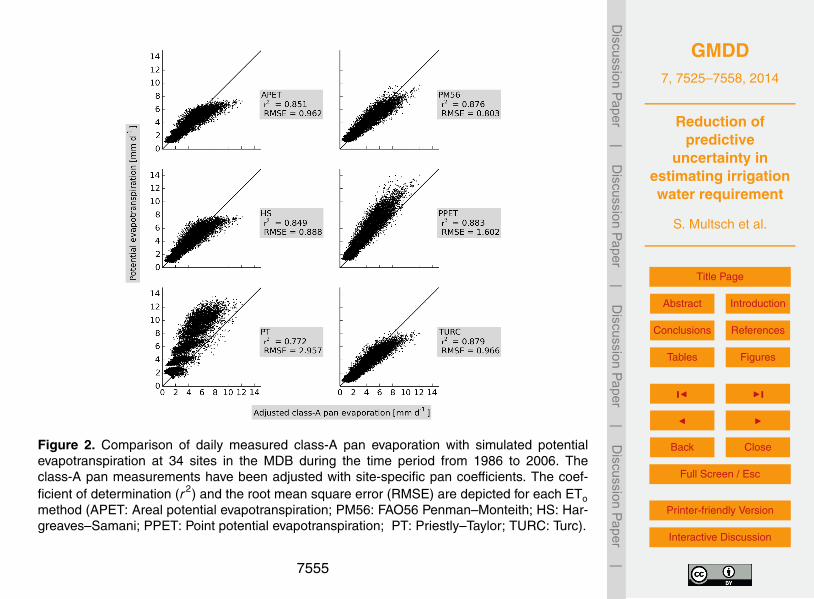
We applied six ETo equations to 34 sites in the MDB for which measured class-A panevaporation data were available from 1986 to 2006 (Fig. 2). Class-A pan data representthe evaporation from an open water surface and integrate all climate factors driving10

evaporation such as radiation, wind speed, humidity and temperature. Pan evapora-tion differs from evaporation from a cropped surface through a different albedo, heatstorage and humidity above the surface. For this reason, the class-A pan data havebeen adjusted with monthly pan coefficients (McMahon et al., 2013) to better comparethem with ETo simulations of open surface waters. On an annual average, class-A pan15

evaporation of 1558 mmyr−1 were reduced by 9 % to 1422 mmyr−1 across all stations.The median daily ETo for APET is 3.6 mmd−1, PM56 3.9 mmd−1, HS 3.8 mmd−1,

PPET 5.2 mmd−1, PT 6.4 mmd−1 and TURC 3.4 mmd−1. According to the root-mean-squared-error (RMSE) PM56 gave the most reliable results. The median of ETo forAPET, PM56 and HS are close to the median of the measured evaporation rate of20

3.7 mmd−1. Apart from PT and PPET, the other methods underestimate ETo, especiallywhere class-A pan data are larger than 6 mmd−1. The relationship between measuredand simulated ETo is linear as shown by the coefficients of determination r2 rangingfrom 77 % (PT) to 88 % (PPET).

7536





GMDD7, 7525–7558, 2014



S. Multsch et al.

Title Page



Tables Figures

J I

J I

Back Close

Full Screen / Esc



Discussion

Paper

|D

iscussionP

aper|

Discussion

Paper

|D

iscussionP

aper|

The simulated ETo is normally distributed if a single station and one year is tested(Shapiro test for normality: alpha > 0.1 for each year and station). The difference be-tween the 34 stations is up to two times larger than the inter-annual difference in the21 years period. Thus, spatial variability is larger than temporal variability in the MDB.The intra-annual variability shows a different picture. The median ETo in the summer5

months is up to four times larger than the ETo during winter months for all ETo methods,except PPET and PT with a six times larger ETo in summer than in winter months.

Four of the six methods simulate the measured data with a high r2 and a low RMSE.The difference between the methods itself is large, in particular through the high EToestimates by PT and PPET. Thus, the structural uncertainty through the ETo method is10

substantial and needs to be considered for the prediction of IRR which is addressed inthe next chapters.

3.2 Irrigation water requirement and its variability

The IRR of wheat has been simulated using an ensemble of thirty model realisations foreach of the 3969 1km×1km irrigated cells in the MDB for 21 years. Average values of15

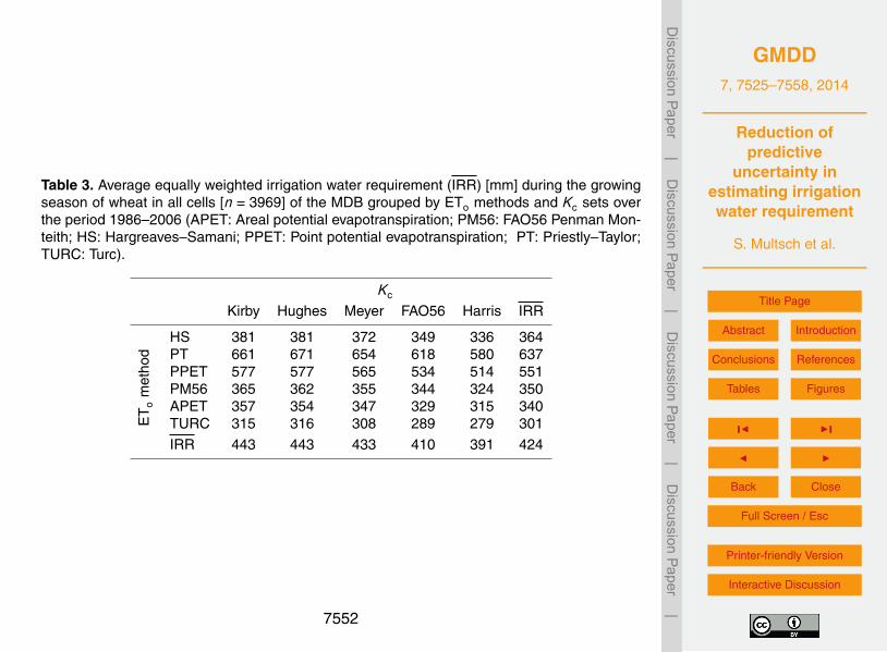
IRR for all model realisations are shown in Table 3. In most cases, the largest estimatesare given by the combinations of the Kc set Hughes with the ETo method PT. These arealmost 2.5 times higher than the lowest average IRR calculated by the combination ofTURC with the Kc set Harris. It is obvious that changing ETo method results in a largervariation of calculated IRR than using a different Kc set. Hence, the average IRR give20

a first idea about variability due to model structures and parameters.Over a large watershed such as the MDB local differences in IRR may be large while

catchment wide water management plans define thresholds for water withdrawal, forexample due to water rights or water resources protection measures. A given thresholdmay require heterogeneous local adaptations of irrigation management and a change25

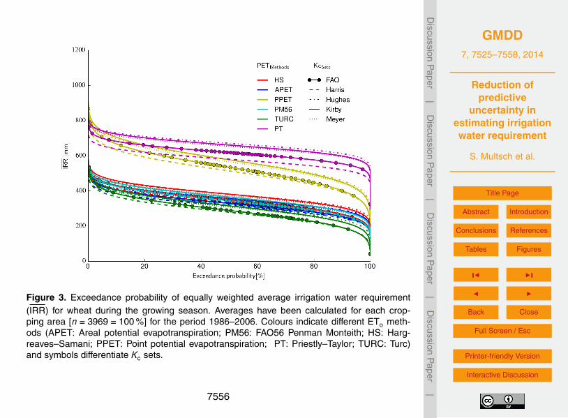
in cropping patterns. Figure 3 shows the probability that a certain amount of IRR isexceeded in the MDB on average over the 21 year period. It illustrates the range of IRRpredicted by the ensemble of all 30 model realisations for each grid cell. Two groups

7537





GMDD7, 7525–7558, 2014



S. Multsch et al.

Title Page



Tables Figures

J I

J I

Back Close

Full Screen / Esc



Discussion

Paper

|D

iscussionP

aper|

Discussion

Paper

|D

iscussionP

aper|

can be identified that are separated by ETo methods. The first group is composed ofPPET and PT calculations. In this case, IRR is up to twice as high as compared topredictions by other models. The second group is formed by APET, HS, PM56 andTURC with substantially lower calculations of less than 500 mm in most cases. Wenote that the parametric uncertainty is almost negligible compared to the uncertainty5

introduced by the various ETo methods.

3.3 Ensemble averaging, uncertainty and weighting

Ensemble predictions have become an important tool to account for different modelstructures and parameters (Exbrayat et al., 2013; Huisman et al., 2009; Wada et al.,2013). The consideration of ensembles is especially helpful to increase our confidence10

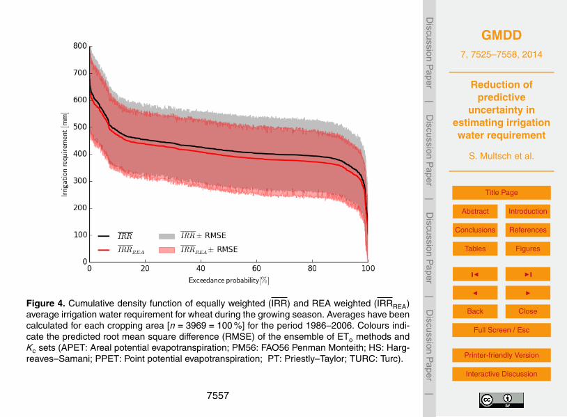
in simulations when no validation data are at hand, such as projections of Earth’s futureclimate under specified emission scenarios. Here we apply the concept of ensembleprediction to simulations of IRR. Two different ensemble averages, expressed as theexceedance probability of the IRR of wheat are shown in Fig. 4. The first one rep-resents the equally weighted average of irrigation (IRR, black line). The second one15

represents a weighted average using the reliability ensemble averaging (IRRREA, redline, see methods description) that weights predictions based on their performance andagreement with other ensemble members. This prevents dismissing some model struc-ture, a process that can be rather subjective. Also, even an overall poorly performingmodel can contribute to the optimal information extracted from the ensembles (Viney20

et al., 2009), or may outperform better performing models once boundary conditionsare changed (Exbrayat et al., 2013).

We use the inverse of the cumulative daily RMSE (Fig. 2) of the ETo methods duringthe growing season to calculate the criterion RB (RMSE 154 mm for APET, 123 mmfor PM56, 142 mm HS, 232 mm PPET, 373 mm PT, 166 mm TURC). The convergence25

criterion RD was calculated based on the difference of the predicted irrigation given bya single ensemble member and the equally weighted ensemble average (see Methods

7538





GMDD7, 7525–7558, 2014



S. Multsch et al.

Title Page



Tables Figures

J I

J I

Back Close

Full Screen / Esc



Discussion

Paper

|D

iscussionP

aper|

Discussion

Paper

|D

iscussionP

aper|

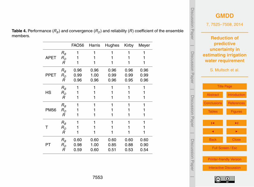
description). Overall, the PT model combinations have the lowest reliability factors ofbetween 0.51 and 0.6 followed by PPET with 0.96, a result driven by the poorer per-formance of these methods to simulate pan-evaporation (Fig. 2), and the outlying posi-tions of simulations using PT and PPET (Fig. 3). All other models are weighted similarly,a result in accordance with the similar performance and simulated values exhibited by5

these methods (see Table 4 for details).The application of the reliability factor leads to a decrease of the calculated total

IRR in each grid cell as well as to a decrease of its overall uncertainty (Fig. 4). Theuncertainty range is given by the ensemble average plus/minus the RMSE in each gridcell, assuming that modelling errors are normally distributed.10

Exceedance probability curves might support defining thresholds in irrigation plan-ning with consequences for decision makers through, for example, the adaptation ofimproved irrigation practice (e.g. from full to deficit irrigation, installation of advancedirrigation techniques) or the purchase of additional water rights. For example, a limitof available irrigation water of 400 mm per growing season will be exceeded less fre-15

quently in the MDB if the REA average IRR is considered (45 %) in comparison to theequally weighted average (66 %).

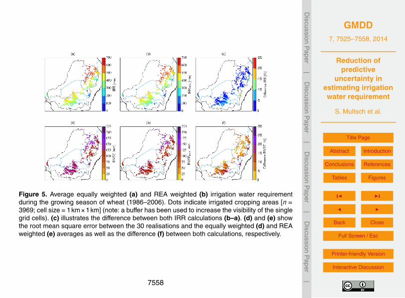
The spatial distribution of the equally weighted and the REA weighted ensembleaverages are shown in Fig. 5a and b. The equally weighted average of IRR rangesbetween 124 and 691 mm with an average across the MDB of 424 mm (Fig. 5a). Thus,20

spatial variability is large and western and northern areas require five to six times moreirrigation than in the south-east. The REA derived average IRR ranges between 104and 663 mm across the river basin (Fig. 5b) with an average of 405 mm. Dependingon the location this value is up to 18 % lower as compared to simulations based onthe equally weighted average (Fig. 5c). Also, the uncertainty range decreases as con-25

sequence of the REA method by about 10 % across the MDB with maximum valuesof around 26 % when comparing equally and REA weighted RMSE (Fig. 5d–f). Thelargest change in uncertainty can be found in the south-east of the MDB and also inareas towards the east (Fig. 5f). Thus, REA not only leads to a decrease of predicted

7539





GMDD7, 7525–7558, 2014



S. Multsch et al.

Title Page



Tables Figures

J I

J I

Back Close

Full Screen / Esc



Discussion

Paper

|D

iscussionP

aper|

Discussion

Paper

|D

iscussionP

aper|

IRR but also to a reduction of its uncertainty. The uncertainty is reduced because theREA is drawn toward the group of the better ETo methods that also agree well betweenthemselves.

4 Discussion and conclusions

The simulation of IRR strongly varies amongst ETo methods. Bormann (2011) recom-5

mended that the selection of the ETo method should be based on the validation of ETowith real world observations rather than only on the availability of climate input data.This is due to the general large variability among ETo methods, which was also re-vealed in a study where PT was set as a benchmark model and the RMSE betweenETo methods was analysed (McMahon et al., 2013). Likewise, the influence of a single10

ETo method on the prediction of crop yields was also reported for an agriculture sitein Europe (Balkovič et al., 2013) where ETo estimates by PT were 40 % higher andthose by Penman–Monteith 10 % lower in comparison to HS. We also found a largevariability among ETo methods in our study. However, similar ranges across Australiafor ETo have been reported by others (Chiew et al., 2002) for APET, PPET and PM5615

as well as lower values for PT. Lascano et al. (2010) as well as Lascano and Van Bavel(2007) have shown that methods to calculate ET based on combination methods, i.e.,Penman–Monteith, tend to underestimate ET by as much as 25 %, especially in dryclimates.

Bormann (2011) further recommended that the reliability of ETo equations should20

be tested in a spatial context, especially if applied on large scale. For various re-gions across Australia, a large range of mean annual ETo between 1700 mm (PT) and3670 mm (PPET) was reported (Donohue et al., 2010). To investigate the spatial het-erogeneity within the MDB we analysed results of the 34 class-A pan stations. Overall,the performance of four of the ETo methods was good with RMSEs around 1 mm day−1,25

except for three stations in the north. PPET performed less well with RSME increasing

7540





GMDD7, 7525–7558, 2014



S. Multsch et al.

Title Page



Tables Figures

J I

J I

Back Close

Full Screen / Esc



Discussion

Paper

|D

iscussionP

aper|

Discussion

Paper

|D

iscussionP

aper|

to 2 mm day−1 while the PT value ranged up to 4 mm day−1. However, we found noconsistent spatial pattern.

ETo estimates using the PM56 method revealed the best performance criteria inour study. PM56 considers the most meteorological input parameters thereby possiblybest representing the altering dry and wet conditions across the MDB over the year.5

The better performance of physically based equations in comparison to more empiricalapproaches for the simulation of ETo has also been reported by others (Donohue et al.,2010). PT performed least well in our study and resulted in up to two times larger esti-mates than other ETo methods. This is somewhat contrasting with other studies (Chiewet al., 2002; Donohue et al., 2010) where PT gave lower ETo values in comparison to10

methods such as APET and PPET.One reason is that Donohue et al. (2010) have considered the actual albedo from

remotely sensed vegetation cover (Donohue et al., 2008) for the estimation of the netincoming solar radiation. In our calculations, an albedo of a reference crop 0.23 (shortcrop, i.e. grass) has been considered according to the guidelines for ETo from Allen15

et al. (1998). Another likely reason for this observation is that the PT equation is basedon the Penman–Monteith equation in which the aerodynamic term is replaced by a con-stant (alpha) which is commonly set to 1.26 under Australian climatic conditions (Chiewand Leahy, 2003) and which we also applied. The consideration of region-specific alphafor the MDB could have increased the performance of PT in our study. The HS equation20

is commonly applied in situations where meteorological data are scarce, because theequation depends on more readily available temperature and extra-terrestrial radiationderived from latitude and day of the year. A reason for its good performance in ourstudy could be that the semi-arid climate in most of the MDB is favourable for the HSequation, which is supported by Tabari (2010) who conclude that HS is a good candi-25

date model for warm humid and semi-arid sites, but fails under cold humid climates.However, the poor response of HS to changing climatic boundary conditions has alsobeen criticized in a study on global drought simulations (Sheffield et al., 2012).

7541





GMDD7, 7525–7558, 2014



S. Multsch et al.

Title Page



Tables Figures

J I

J I

Back Close

Full Screen / Esc



Discussion

Paper

|D

iscussionP

aper|

Discussion

Paper

|D

iscussionP

aper|

We combined the six ETo methods with five Kc sets to address stochastic parametricuncertainty for irrigated wheat in the MDB. We show that the ETo method uncertaintyrange exceeded the uncertainty range of Kc sets. Thus, the Kc sets have a minor influ-ence on predicted IRR. At first sight, this seems to be contrasting to others who havestated that adapted, regional Kc sets are required to estimate reliable IRR rates. For5

instance, da Silva et al. (2013) reported that Kc sets from FAO56 lead to errors in plotscale irrigation planning under tropical conditions. Similar observations were reportedfor semi-arid conditions in the Texas High Plains region (Ko et al., 2009), highlightingthe importance of regionally based Kc sets. While regional adaptation of Kc might beimportant at smaller scales, e.g. on the farm level, we conclude that large scale appli-10

cations do not necessarily need to focus on this potential contribution of uncertainty.Rather, effort should be put into finding appropriate ETo methods, or even better, utilizeensemble predictions to cover a more realistic range of predictions. Our study confirmsthis latter recommendation, as we could not identify a single best ETo method for theMDB. Especially in cases where no data for a direct evaluation of model results are15

available the application of model ensembles gives insight to the predictive uncertainty,e.g., being helpful in the development of best management practices (Exbrayat et al.,2013), study of land use (Huisman et al., 2009) or climate change (Exbrayat et al.,2014).

Besides the uncertainty introduced by local to global Kc values the utilisation of the20

single crop coefficient concept itself comes along with errors, which are not addressedin this study. For example, Lascano (2000) shows how Kc varies as a function of time(50 days) and how it changes when using a daily, 3 and 8 day moving average. More-over, the temporal resolution of ETo calculation, i.e., hourly vs. daily is an importantcomponent and errors associated with the method of irrigation (surface, drip, sprin-25

kler) cannot be neglected, but are beyond the uncertainty calculation of this study.We acknowledge that we do not consider uncertainties in boundary conditions (e.g.relevance of CO2 concentration, land-use management options, climatic variability) al-though these may be non-negligible. For example, atmospheric CO2 has been reported

7542





GMDD7, 7525–7558, 2014



S. Multsch et al.

Title Page



Tables Figures

J I

J I

Back Close

Full Screen / Esc



Discussion

Paper

|D

iscussionP

aper|

Discussion

Paper

|D

iscussionP

aper|

as a driving factor of ET in North America, South America and Asia regions besidesclimate forcing (Shi et al., 2013). Others reported that changes in future precipitationregimes will have the greatest impact on the calculated water footprint (reflecting highET rates) of maize in Italy and that changes in CO2 and warming were less important(Bocchiola et al., 2013). Conversely, water use was more driven by agricultural man-5

agement than by regional climatic variation in a water footprint analysed for an irrigationdistrict in China (Sun et al., 2013). Statistical correction of model forcing data (such asbias correction of precipitation) has also been reported to alter ET estimates as shownby Ye et al. (2012) for the Upper Yellow River in China with changes of up to 29 % of ET.Thus, an even more complete picture of global model uncertainty can only be shown10

by considering all sorts of predictive uncertainty, including model input data, validationdata, and spatial input data in addition to the impact of model structural and parametricuncertainty as presented here.

However, we argue that future management practices or the impact of climatechange cannot be reliably evaluated due to the large uncertainty that exists in the ETo15

method, the basis of water resources modelling. We partially cope with this problemby applying the REA technique to extract the most relevant information from our sim-ulations. The advantage of REA in decision making has already been shown for otherfields of research, such as the development of N reduction scenarios to improve sur-face water quality (Exbrayat et al., 2013) or estimation of the effect of land use change20

on water budgets and hydrological fluxes (Huisman et al., 2009). Despite the growingimportance of IRR for today’s agriculture (Siebert and Döll, 2010) and the effect on sur-face (Hoekstra et al., 2012) and groundwater (Wada et al., 2010) resources, few studieshave dealt with the predictive uncertainty of this requirement (e.g. Wada et al., 2013)and how to reduce it.25

Acknowledgements. We acknowledge the generous funding of the Deutsche Forschungsge-meinschaft (DFG, grant BR2238/11-1) that allowed a cooperation visit of the first author toCSIRO Land and Water and the ARC Centre of Excellence for Climate System Science in

7543





GMDD7, 7525–7558, 2014



S. Multsch et al.

Title Page



Tables Figures

J I

J I

Back Close

Full Screen / Esc



Discussion

Paper

|D

iscussionP

aper|

Discussion

Paper

|D

iscussionP

aper|

Australia. The research was further supported by a grant from KACST, Saudi-Arabia and theCAWa project (AA7090002).

References

ABARES: Land Use of Australia, Version 4 2005/2006, Department of Agriculture Fisheries andForestry, Australian Bureau of Agriucultural and Resource Economics, 2010.5

ABS: Water Use on Australian Farms Murray-Darling basin 2005–2006, 46180DO012, 2006.Allen, R. G., Pereira, L. S., Raes, D., and Smith, M.: Crop evapotranspiration – guidelines for

computing crop water requirements, FAO Irrig. Drain. 56, 6541, 1998.Allen, R. G.: REF-ET User’s Guide, University of Idaho Kimberly Research Stations, Kimberly,

2003.10

Balkovič, J., van der Velde, M., Schmid, E., Skalsky, R., Khabarov, N., Obersteiner, M.,Stürmer, B., and Xiong, W.: Pan-European crop modelling with EPIC: implementation, up-scaling and regional crop yield validation, Agr. Syst., 120, 61–75, 2013.

Beven, K.: A manifesto for the equifinality thesis, J. Hydrol., 320, 18–36, 2006.Bocchiola, D., Nana, E., and Soncini, A.: Impact of climate change scenarios on crop yield and15

water footprint of maize in the Po valley of Italy, Agr. Water Manage., 116, 50–61, 2013.Bormann, H.: Sensitivity analysis of 18 different potential evapotranspiration models to ob-

served climatic change at German climate stations, Climatic Change, 104, 729–753, 2011.Chiew, F. H. S. and Leahy, C.: Comparison of evapotranspiration variables in evapotranspiration

maps for Australia with commonly used evapotranspiration variables, Australian Journal of20

Water Resources, 7, 1–11, 2003.Chiew, F., Wang, Q. J., McConachy, F., James, R., Wright, W., and deHoedt, G.: Evapotranspi-

ration maps for Australia, in: Hydrology and Water Resources Symposium 2002: the WaterChallenge, Balancing the Risks, Institution of Engineers, Australia, p. 167, 2002.

Da Silva, V. P., da Silva, B. B., Albuquerque, W. G., Borges, C. J., de Sousa, I. F., and Neto, J. D.:25

Crop coefficient, water requirements, yield and water use efficiency of sugarcane growth inBrazil, Agr. Water Manage., 128, 102–109, 2013.

De Fraiture, C. and Wichelns, D.: Satisfying future water demands for agriculture, Agr. WaterManage., 97, 502–511, 2010.

7544





GMDD7, 7525–7558, 2014



S. Multsch et al.

Title Page



Tables Figures

J I

J I

Back Close

Full Screen / Esc



Discussion

Paper

|D

iscussionP

aper|

Discussion

Paper

|D

iscussionP

aper|

Döll, P., Kaspar, F., and Lehner, B.: A global hydrological model for deriving water availabilityindicators: model tuning and validation, J. Hydrol., 270, 105–134, 2003.

Donohue, R. J., Roderick, M. L., and McVicar, T. R.: Deriving consistent long-term vegetationinformation from AVHRR reflectance data using a cover-triangle-based framework, RemoteSens. Environ., 112, 2938–2949, 2008.5

Donohue, R. J., McVicar, T. R., and Roderick, M. L.: Assessing the ability of potential evapora-tion formulations to capture the dynamics in evaporative demand within a changing climate, J.Hydrol., 386, 186–197, 2010.

Exbrayat, J.-F., Viney, N. R., Frede, H.-G., and Breuer, L.: Using multi-model averaging to im-prove the reliability of catchment scale nitrogen predictions, Geosci. Model Dev., 6, 117–125,10

doi:10.5194/gmd-6-117-2013, 2013.Exbrayat, J.-F., Buytaert, Timbe, E., Windhorst, D., and Breuer, L.: Addressing sources of un-

certainty in runoff projections for a data scarce catchment in the Ecuadorian Andes, ClimaticChange, 125, 221–235, 2014.

Fader, M., Rost, S., Müller, C., Bondeau, A., and Gerten, D.: Virtual water content of temperate15

cereals and maize: present and potential future patterns, J. Hydrol., 384, 218–231, 2010.Fisher, J. B., Whittaker, R. J., and Malhi, Y.: ET come home: potential evapotranspiration in

geographical ecology, Global Ecol. Biogeogr., 20, 1–18, 2011.George, B. A., Shende, S. A., and Raghuwanshi, N. S.: Development and testing of an irrigation

scheduling model, Agr. Water Manage., 46, 121–136, 2000.20

Giorgi, F. and Mearns, L. O.: Calculation of average, uncertainty range, and reliability of regionalclimate changes from AOGCM simulations via the “reliability ensemble averaging” (REA)method, J. Climate, 15, 1141–1158, 2002.

Hargreaves, G. H. and Samani, Z. A.: Reference crop evapotranspiration from temperature,Appl. Eng. Agric., 1, 96–99, 1985.25

Harris, G. A.: Irrigation: water balance scheduling, DPI Note FSO546, Queensland Departmentof Primary Industries and Fisheries, 2002.

Hoekstra, A. Y. and Mekonnen, M. M.: The water footprint of humanity, P. Natl. Acad. Sci. USA,109, 3232–3237, 2012.

Hoekstra, A. Y., Mekonnen, M. M., Chapagain, A. K., Mathews, R. E., and Richter, B. D.:30

Global monthly water scarcity: blue water footprints versus blue water availability, Plos One,7, e32688, doi:10.1371/journal.pone.0032688, 2012.

7545





http://dx.doi.org/10.5194/gmd-6-117-2013

http://dx.doi.org/10.1371/journal.pone.0032688

GMDD7, 7525–7558, 2014



S. Multsch et al.

Title Page



Tables Figures

J I

J I

Back Close

Full Screen / Esc



Discussion

Paper

|D

iscussionP

aper|

Discussion

Paper

|D

iscussionP

aper|

Howell, T. A., Evett, S. R., Tolk, J. A., and Schneider, A. D.: Evapotranspiration of full-, deficit-irrigated, and dryland cotton on the Northern Texas High Plains, J. Irrig. Drain. E.-ASCE,130, 277–285, 2004.

Hughes, J. D.: Southern Irrigation SOILpak. For Irrigated Broad Area Agriculture on the RiverinePlain in the Murray and Murrumbidgee Valleys, NSW Agriculture, Orange, 1999.5

Huisman, J. A., Breuer, L., Bormann, H., Bronstert, A., Croke, B. F. W., Frede, H.-G., Gräff, T.,Hubrechts, L., Jakeman, A. J., and Kite, G.: Assessing the impact of land use change onhydrology by ensemble modeling (LUCHEM), III: Scenario analysis, Adv. Water Resour., 32,159–170, 2009.

Jeffrey, S. J., Carter, J. O., Moodie, K. B., and Beswick, A. R.: Using spatial interpolation to10

construct a comprehensive archive of Australian climate data, Environ. Modell. Softw., 16,309–330, 2001.

Jensen, M. E.: Water consumption by agricultural plants, chapter 1, in: Water Deficits andPlant Growth, vol. II, Plant Water Consumption and Response, edited by: Kozlowski, T. T.,Academic Press, New York, London, 1–22, 1968.15

Jensen, M. E., Burman, R. D., and Allen, R. G.: Evapotranspiration and irrigation water require-ments, Amer. Soc. Civil Eng. Manuals and Reports on Engineering Practice, no. 70, ASCE,New York, USA, p. 332, 1990.

Kirby, M., Mainuddin, M., Gao, L., Connor, J. D., and Ahmad, M. D.: Integrated, dynamic eco-nomic–hydrology model of the Murray-Darling Basin, in: 2012 Conference (56th), Freeman-20

tle, Australia, 7–10 February 2012, Australian Agricultural and Resource Economics Society,No. 124487, 2012.

Kite, G. W. and Droogers, P.: Comparing evapotranspiration estimates from satellites, hydro-logical models and field data, J. Hydrol., 229, 3–18, 2000.

Ko, J., Piccinni, G., Marek, T., and Howell, T.: Determination of growth-stage-specific crop co-25

efficients (Kc) of cotton and wheat, Agr. Water Manage., 96, 1691–1697, 2009.Lascano, R. J.: A general system to measure and calculate daily crop water use, Agron. J., 92,

821–832, 2000.Lascano, R. J. and Van Bavel, C. H.: Explicit and recursive calculation of potential and actual

evapotranspiration, Agron. J., 99, 585–590, 2007.30

Lascano, R. J., Van Bavel, C. H. M., and Evett, S. R.: A field test of recursive calculation of cropevapotranspiration, T. ASABE, 53, 1117–1126, 2010.

7546





GMDD7, 7525–7558, 2014



S. Multsch et al.

Title Page



Tables Figures

J I

J I

Back Close

Full Screen / Esc



Discussion

Paper

|D

iscussionP

aper|

Discussion

Paper

|D

iscussionP

aper|

Lathuillière, M. J., Johnson, M. S., and Donner, S. D.: Water use by terrestrial ecosystems:temporal variability in rainforest and agricultural contributions to evapotranspiration in MatoGrosso, Brazil, Environ. Res. Lett., 7, 024024, doi:10.1088/1748-9326/7/2/024024, 2012.

Liu, J., Wiberg, D., Zehnder, A. J., and Yang, H.: Modeling the role of irrigation in winter wheatyield, crop water productivity, and production in China, Irrigation Sci., 26, 21–33, 2007.5

McMahon, T. A., Peel, M. C., Lowe, L., Srikanthan, R., and McVicar, T. R.: Estimating actual,potential, reference crop and pan evaporation using standard meteorological data: a prag-matic synthesis, Hydrol. Earth Syst. Sci., 17, 1331–1363, doi:10.5194/hess-17-1331-2013,2013.

Mekonnen, M. M. and Hoekstra, A. Y.: The green, blue and grey water footprint of crops and10

derived crop products, Hydrol. Earth Syst. Sci., 15, 1577–1600, doi:10.5194/hess-15-1577-2011, 2011.

Meyer, W. S.: Standard Reference Evaporation Calculation for Inland, South Eastern Australia,CSIRO Land and Water, 1999.

Monteith, J. L.: Evaporation and environment, in: Symp. Soc. Exp. Biol, Vol. 19, p. 4, 1965.15

Morton, F. I.: Operational estimates of areal evapotranspiration and their significance to thescience and practice of hydrology, J. Hydrol., 66, 1–76, 1983.

Multsch, S., Al-Rumaikhani, Y. A., Frede, H.-G., and Breuer, L.: A Site-sPecific Agriculturalwater Requirement and footprint Estimator (SPARE:WATER 1.0), Geosci. Model Dev., 6,1043–1059, doi:10.5194/gmd-6-1043-2013, 2013.20

Oki, T. and Kanae, S.: Global hydrological cycles and world water resources, Science, 313,1068–1072, 2006.

Penman, H. L.: Natural evaporation from open water, bare soil and grass, P. Roy. Soc. Lond. A.Math., 193, 120–145, 1948.

Pereira, L. S., Paredes, P., Cholpankulov, E. D., Inchenkova, O. P., Teodoro, P. R., and25

Horst, M. G.: Irrigation scheduling strategies for cotton to cope with water scarcity in theFergana Valley, Central Asia, Agr. Water Manage., 96, 723–735, 2009.

Priestley, C. H. B. and Taylor, R. J.: On the assessment of surface heat flux and evaporationusing large-scale parameters, Mon. Weather Rev., 100, 81–92, 1972.

Refsgaard, J. C., van der Sluijs, J. P., Højberg, A. L., and Vanrolleghem, P. A.: Uncertainty in30

the environmental modelling process–a framework and guidance, Environ. Modell. Softw.,22, 1543–1556, 2007.

7547





http://dx.doi.org/10.1088/1748-9326/7/2/024024

http://dx.doi.org/10.5194/hess-17-1331-2013




http://dx.doi.org/10.5194/gmd-6-1043-2013

GMDD7, 7525–7558, 2014



S. Multsch et al.

Title Page



Tables Figures

J I

J I

Back Close

Full Screen / Esc



Discussion

Paper

|D

iscussionP

aper|

Discussion

Paper

|D

iscussionP

aper|

Renard, B., Kavetski, D., Kuczera, G., Thyer, M., and Franks, S. W.: Understanding predictiveuncertainty in hydrologic modeling: the challenge of identifying input and structural errors,Water Resour. Res., 46, W05521, doi:10.1029/2009WR008328, 2010.

Sheffield, J., Wood, E. F., and Roderick, M. L.: Little change in global drought over the past60 years, Nature, 491, 435–438, 2012.5

Shi, X., Mao, J., Thornton, P. E., and Huang, M.: Spatiotemporal patterns of evapotranspira-tion in response to multiple environmental factors simulated by the Community Land Model,Environ. Res. Lett., 8, 024012, doi:10.1088/1748-9326/8/2/024012, 2013.

Siebert, S. and Döll, P.: Quantifying blue and green virtual water contents in global crop pro-duction as well as potential production losses without irrigation, J. Hydrol., 384, 198–217,10

2010.Smith, M.: CROPWAT: a Computer Program for Irrigation Planning and Management, Food and

Agriculture Organization of the United Nations, Rome, Italy, 1992.Steduto, P., Hsiao, T. C., Raes, D., and Fereres, E.: AquaCrop – the FAO crop model to simulate

yield response to water: I. Concepts and underlying principles, Agron. J., 101, 426–437,15

2009.Sun, S., Wu, P., Wang, Y., Zhao, X., Liu, J., and Zhang, X.: The impacts of interannual climate

variability and agricultural inputs on water footprint of crop production in an irrigation districtof China, Sci. Total Environ., 444, 498–507, 2013.

Tabari, H.: Evaluation of reference crop evapotranspiration equations in various climates, Water20

Resour. Manag., 24, 2311–2337, 2010.Tabari, H., Grismer, M. E., and Trajkovic, S.: Comparative analysis of 31 reference evapotran-

spiration methods under humid conditions, Irrigation Sci., 31, 107–117, 2013.Toews, M. W. and Allen, D. M.: Simulated response of groundwater to predicted recharge in

a semi-arid region using a scenario of modelled climate change, Environ. Res. Lett., 4,25

035003, doi:10.1088/1748-9326/4/3/035003, 2009.Turc, L.: Estimation of irrigation water requirements, potential evapotranspiration: a simple cli-

matic formula evolved up to date, Ann. Agron., 12, 13–49, 1961.Viney, N. R., Bormann, H., Breuer, L., Bronstert, A., Croke, B. F. W., Frede, H., Gräff, T.,

Hubrechts, L., Huisman, J. A., and Jakeman, A. J.: Assessing the impact of land use change30

on hydrology by ensemble modelling (LUCHEM) II: ensemble combinations and predictions,Adv. Water Resour., 32, 147–158, 2009.

7548





http://dx.doi.org/10.1029/2009WR008328

http://dx.doi.org/10.1088/1748-9326/8/2/024012

http://dx.doi.org/10.1088/1748-9326/4/3/035003

GMDD7, 7525–7558, 2014



S. Multsch et al.

Title Page



Tables Figures

J I

J I

Back Close

Full Screen / Esc



Discussion

Paper

|D

iscussionP

aper|

Discussion

Paper

|D

iscussionP

aper|

Vrugt, J. A., Ter Braak, C. J., Gupta, H. V., and Robinson, B. A.: Equifinality of formal (DREAM)and informal (GLUE) bayesian approaches in hydrologic modeling?, Stoch. Env. Res. RiskA, 23, 1011–1026, 2009.

Wada, Y., van Beek, L. P., van Kempen, C. M., Reckman, J. W., Vasak, S., andBierkens, M. F.: Global depletion of groundwater resources, Geophys. Res. Lett., 37, L20402,5

doi:10.1029/2010GL044571, 2010.Wada, Y., Wisser, D., Eisner, S., Flörke, M., Gerten, D., Haddeland, I., Hanasaki, N., Masaki, Y.,

Portmann, F. T., and Stacke, T.: Multimodel projections and uncertainties of irrigation waterdemand under climate change, Geophys. Res. Lett., 40, 4626–4632, 2013.

Wang, H., Zhang, L., Dawes, W. R., and Liu, C.: Improving water use efficiency of irrigated10

crops in the North China Plain – measurements and modelling, Agr. Water Manage., 48,151–167, 2001.

Williams, J. R., Jones, C. A., Kiniry, J. R., and Spanel, D. A.: The EPIC crop growth model, T.ASAE, 32, 497–511, 1989.

Ye, B., Yang, D., and Ma, L.: Effect of precipitation bias correction on water budget cal-15

culation in Upper Yellow River, China, Environ. Res. Lett., 7, 025201, doi:10.1088/1748-9326/7/2/025201, 2012.

7549





http://dx.doi.org/10.1029/2010GL044571

http://dx.doi.org/10.1088/1748-9326/7/2/025201

http://dx.doi.org/10.1088/1748-9326/7/2/025201

http://dx.doi.org/10.1088/1748-9326/7/2/025201

GMDD7, 7525–7558, 2014



S. Multsch et al.

Title Page



Tables Figures

J I

J I

Back Close

Full Screen / Esc



Discussion

Paper

|D

iscussionP

aper|

Discussion

Paper

|D

iscussionP

aper|

Table 1. The five crop parameter sets for Kc.

Name (Reference) Spatial reference KciniKcmid

Kcend

FAO56 (Allen et al., 1998) Global 0.7 1.15 0.25Harris (Harris, 2002) Queensland 0.3 1.15 0.25Kirby (Kirby et al., 2012) Murray-Darling Basin 0.4 1.15 0.4Meyer (Meyer, 1999) Griffith, MDB 0.4 1.05 0.5Hughes (Hughes, 1999) Murray and Murrumbidgee valleys 0.3 1.0 0.6

7550





GMDD7, 7525–7558, 2014



S. Multsch et al.

Title Page



Tables Figures

J I

J I

Back Close

Full Screen / Esc



Discussion

Paper

|D

iscussionP

aper|

Discussion

Paper

|D

iscussionP

aper|

Table 2. The six equations applied for the calculation of reference evapotranspiration.

Method Abbreviation Equation

FAO-56 Penman–Monteith(Allen et al., 1998)

PM56 PETPM56 =0.408·∆·(Rn−G)+γ· 900

Tmean+273 ·u2 ·(es−ea)

∆+γ·(1+0.34·u2)

Priestley–Taylor(Priestley and Taylor, 1972)

PT PETPT = α ·[

∆∆+γ

]· (Rn−G)

λ

Hargreaves–Samani(Hargreaves and Samani, 1985)

HS PETHS = 0.0023 · (Tmean +17.8) · (Tmax − Tmin)0.5 ·Ra ·0.408

Turc (Allen, 2003; Turc, 1961) TURC PETTURC = αT ·Tmean

Tmean+15 · 23.8856·Rs+50λ

Areal – PET (Morton, 1983) APET PETAPET = b1 +b2

(1+γ·p∆

)−1·RTP

Point – PET (Morton, 1983) PPET PETPPETenergy-balance = Rn − λP · fT · (TP − Tmean)PETPPETvapor-transfer = fT · (es −ea)

With PETPM56, PETPT, PETHS, PETTURC, PETAPET, PPETEnergy-Balance and PPETVapor-Transfer in [mm], extra-terrestrial radiation Ra, solar

radiation Rs, net radiation Rn, soil heat flux density G and net radiation at equilibrium temperature RTP in [MJm−2], equilibrium

temperature TP , mean Tmean, minimum Tmin and maximum Tmax air temperature in [◦C], wind speed u2 at 2 m height [ms−1], atmosphericpressure p, saturated es and actual ea vapour pressure in [kPa], slope of vapour pressure curve ∆ and the psychometric constant γ in[kPa ◦C−1], latent heat of vaporization λ in [MJkg−1], and the dimensionless empirical constants b1 and b2 [–], the heat transfer coefficientλP [–], the vapour transfer coefficient fT [–] and the humidity based value αT .

7551





GMDD7, 7525–7558, 2014



S. Multsch et al.

Title Page



Tables Figures

J I

J I

Back Close

Full Screen / Esc



Discussion

Paper

|D

iscussionP

aper|

Discussion

Paper

|D

iscussionP

aper|

Table 3. Average equally weighted irrigation water requirement (IRR) [mm] during the growingseason of wheat in all cells [n = 3969] of the MDB grouped by ETo methods and Kc sets overthe period 1986–2006 (APET: Areal potential evapotranspiration; PM56: FAO56 Penman Mon-teith; HS: Hargreaves–Samani; PPET: Point potential evapotranspiration; PT: Priestly–Taylor;TURC: Turc).

Kc

Kirby Hughes Meyer FAO56 Harris IRR

ET

om

etho

d

HS 381 381 372 349 336 364PT 661 671 654 618 580 637PPET 577 577 565 534 514 551PM56 365 362 355 344 324 350APET 357 354 347 329 315 340TURC 315 316 308 289 279 301

IRR 443 443 433 410 391 424

7552





GMDD7, 7525–7558, 2014



S. Multsch et al.

Title Page



Tables Figures

J I

J I

Back Close

Full Screen / Esc



Discussion

Paper

|D

iscussionP

aper|

Discussion

Paper

|D

iscussionP

aper|

Table 4. Performance (RB) and convergence (RD) and reliability (R) coefficient of the ensemblemembers.

FAO56 Harris Hughes Kirby Meyer

RB 1 1 1 1 1APET RD 1 1 1 1 1

R 1 1 1 1 1

RB 0.96 0.96 0.96 0.96 0.96PPET RD 0.99 1.00 0.99 0.99 0.99

R 0.96 0.96 0.96 0.95 0.96

RB 1 1 1 1 1HS RD 1 1 1 1 1

R 1 1 1 1 1

RB 1 1 1 1 1PM56 RD 1 1 1 1 1

R 1 1 1 1 1

RB 1 1 1 1 1T RD 1 1 1 1 1

R 1 1 1 1 1

RB 0.60 0.60 0.60 0.60 0.60PT RD 0.98 1.00 0.85 0.88 0.90

R 0.59 0.60 0.51 0.53 0.54

7553





GMDD7, 7525–7558, 2014



S. Multsch et al.

Title Page



Tables Figures

J I

J I

Back Close

Full Screen / Esc



Discussion

Paper

|D

iscussionP

aper|

Discussion

Paper

|D

iscussionP

aper|

27

1

2

Figure 1. The Murray-Darling basin (MDB) is located in south-east Australia. Irrigated wheat 3

areas (2005/06) across the MDB are indicated as black dots, n=3,969; cell size=1 x 1 km. 4

5

Figure 1. The Murray-Darling basin (MDB) is located in south-east Australia. Irrigated wheatareas (2005/06) across the MDB are indicated as black dots, n = 3969; cell size=1km×1km.

7554





GMDD7, 7525–7558, 2014



S. Multsch et al.

Title Page



Tables Figures

J I

J I

Back Close

Full Screen / Esc



Discussion

Paper

|D

iscussionP

aper|

Discussion

Paper

|D

iscussionP

aper|

28

1

2

Figure 2. Comparison of daily measured class-A pan evaporation with simulated potential 3

evapotranspiration at 34 sites in the MDB during the time period from 1986 to 2006. The class-A 4

pan measurements have been adjusted with site-specific pan coefficients. The coefficient of 5

determination (r²) and the root mean square error (RMSE) are depicted for each ETo method 6

(APET: Areal potential evapotranspiration; PM56: FAO56 Penman-Monteith; HS: Hargreaves-7

Samani; PPET: Point potential evapotranspiration; PT: Priestly-Taylor; TURC: Turc).8

Figure 2. Comparison of daily measured class-A pan evaporation with simulated potentialevapotranspiration at 34 sites in the MDB during the time period from 1986 to 2006. Theclass-A pan measurements have been adjusted with site-specific pan coefficients. The coef-ficient of determination (r2) and the root mean square error (RMSE) are depicted for each ETomethod (APET: Areal potential evapotranspiration; PM56: FAO56 Penman–Monteith; HS: Har-greaves–Samani; PPET: Point potential evapotranspiration; PT: Priestly–Taylor; TURC: Turc).

7555





GMDD7, 7525–7558, 2014



S. Multsch et al.

Title Page



Tables Figures

J I

J I

Back Close

Full Screen / Esc



Discussion

Paper

|D

iscussionP

aper|

Discussion

Paper

|D

iscussionP

aper|

29

1

2

Figure 3 Exceedance probability of equally weighted average irrigation water requirement ( IRR ) 3

for wheat during the growing season. Averages have been calculated for each cropping area [n = 4

3969 = 100%] for the period 1986-2006. Colours indicate different ETo methods (APET: Areal 5

potential evapotranspiration; PM56: FAO56 Penman Monteith; HS: Hargreaves-Samani; PPET: 6

Point potential evapotranspiration; PT: Priestly-Taylor; TURC: Turc) and symbols differentiate 7

Kc sets.8

Figure 3. Exceedance probability of equally weighted average irrigation water requirement(IRR) for wheat during the growing season. Averages have been calculated for each crop-ping area [n = 3969 = 100 %] for the period 1986–2006. Colours indicate different ETo meth-ods (APET: Areal potential evapotranspiration; PM56: FAO56 Penman Monteith; HS: Harg-reaves–Samani; PPET: Point potential evapotranspiration; PT: Priestly–Taylor; TURC: Turc)and symbols differentiate Kc sets.

7556





GMDD7, 7525–7558, 2014



S. Multsch et al.

Title Page



Tables Figures

J I

J I

Back Close

Full Screen / Esc



Discussion

Paper

|D

iscussionP

aper|

Discussion

Paper

|D

iscussionP

aper|

30

1

2

Figure 4 Cumulative density function of equally weighted ( IRR ) and REA weighted ( REAIRR ) 3

average irrigation water requirement for wheat during the growing season. Averages have been 4

calculated for each cropping area [n = 3969 = 100%] for the period 1986-2006. Colours indicate 5

the predicted root mean square difference (RMSE) of the ensemble of ETo methods and Kc sets 6

(APET: Areal potential evapotranspiration; PM56: FAO56 Penman Monteith; HS: Hargreaves-7

Samani; PPET: Point potential evapotranspiration; PT: Priestly-Taylor; TURC: Turc). 8

Figure 4. Cumulative density function of equally weighted (IRR) and REA weighted (IRRREA)average irrigation water requirement for wheat during the growing season. Averages have beencalculated for each cropping area [n = 3969 = 100 %] for the period 1986–2006. Colours indi-cate the predicted root mean square difference (RMSE) of the ensemble of ETo methods andKc sets (APET: Areal potential evapotranspiration; PM56: FAO56 Penman Monteith; HS: Harg-reaves–Samani; PPET: Point potential evapotranspiration; PT: Priestly–Taylor; TURC: Turc).

7557





GMDD7, 7525–7558, 2014



S. Multsch et al.

Title Page



Tables Figures

J I

J I

Back Close

Full Screen / Esc



Discussion

Paper

|D

iscussionP

aper|

Discussion

Paper

|D

iscussionP

aper|

31

1

Figure 5. Average equally weighted (a) and REA weighted (b) irrigation water requirement during the growing season of wheat (1986-2

2006). Dots indicate irrigated cropping areas [n=3,969; cell size=1 x 1 km] (note: a buffer has been used to increase the visibility of the 3

single grid cells). (c) illustrates the difference between both IRR calculations (b-a). (d) and (e) show the root mean square error between 4

the 30 realisations and the equally weighted (d) and REA weighted (e) averages as well as the difference (f) between both calculations, 5

respectively. 6

Figure 5. Average equally weighted (a) and REA weighted (b) irrigation water requirementduring the growing season of wheat (1986–2006). Dots indicate irrigated cropping areas [n =3969; cell size=1km×1km] (note: a buffer has been used to increase the visibility of the singlegrid cells). (c) illustrates the difference between both IRR calculations (b–a). (d) and (e) showthe root mean square error between the 30 realisations and the equally weighted (d) and REAweighted (e) averages as well as the difference (f) between both calculations, respectively.

7558





Documents

Reduction of predictive uncertainty in estimating irrigation