Embed Size (px)
Citation preview

23 October 2022
POLITECNICO DI TORINORepository ISTITUZIONALE
Topology optimization for energy problems / Pizzolato, Alberto. - (2018 Jun 28). [10.6092/polito/porto/2710567]Original
Topology optimization for energy problems
Publisher:
PublishedDOI:10.6092/polito/porto/2710567
Terms of use:Altro tipo di accesso
Publisher copyright
(Article begins on next page)
This article is made available under terms and conditions as specified in the corresponding bibliographic description inthe repository
Availability:This version is available at: 11583/2710567 since: 2018-07-06T12:18:12Z
Politecnico di Torino

Doctoral Dissertation
Doctoral Program in Energy Engineering (30thcycle)
Topology optimization for energyproblems
Thermal storage with phase change, district heatingnetworks and PEM fuel cells
By
Alberto Pizzolato******
Supervisor(s):Prof. Vittorio Verda, Supervisor
Prof. Adriano Sciacovelli, Co-SupervisorProf. Kurt Maute, Co-Supervisor
Doctoral Examination Committee:Prof. Casper Andreasen , Referee, Technical University of DenmarkProf. Oronzio Manca, Referee, Universita’ degli Studi della CampaniaProf. Niels Aage, Technical University of DenmarkProf. Perumal Nithiarasu, Swansea UniversityProf. Pierluigi Leone, Politecnico di Torino

Politecnico di TorinoJune 28, 2018
ii

Declaration
I hereby declare that the contents and organization of this dissertation constitute myown original work and does not compromise in any way the rights of third parties,including those relating to the security of personal data.
Alberto PizzolatoJune 28, 2018
* This dissertation is presented in partial fulfillment of the requirements for Ph.D.degree in the Graduate School of Politecnico di Torino (ScuDo).

To my parents and Ludovica,constant sources of support and inspiration

Acknowledgements
This thesis is the result of three years of research at the Department of Energy atPolitecnico di Torino and at the Department of Aerospace Sciences at Universityof Colorado. During this period, I benefited from the contributions of a number ofremarkable people that I wish to acknowledge.
First and foremost, I would like to thank my supervisors: Vittorio Verda, AdrianoSciacovelli and Kurt Maute. Vittorio has three extraordinary and rare abilities amongothers: analyzing the big picture, identifying promising research moves and spottingpotential high-impact innovations. Thanks for sharing these gifts with me in ourrevealing brainstormings, for giving me both guidance, support and freedom inpursuing my research curiosity and also for being a good friend. It was simply greatto have you as a supervisor. Adriano has an exceptional passion and enthusiasmfor science that makes him an expert on various engineering topics. Thanks forteaching me the art of multi-disciplinary research, for the long-distance stimulatingdiscussions over Skype and for coming at my desk three years back with a topologyoptimization paper [13], saying "we should do this". Kurt couples a true talent forresearch and a passion for clear teaching that impressed me from the first moment atDTU. During my stay at CU Boulder, I benefited from countless suggestions thatcleared long-standing doubts on optimization in the time span of a meeting. Thanksfor framing my mind as a scientist and for fueling my ambition to push researchfrontiers a little bit further.
During these Ph.D. years, I learned the importance of constructing a network of"allies" that I truly trust. At CU Boulder, I was lucky enough to meet three excellentindividuals that I consider as milestones in this network. Their feedback is essentialon any novel idea, research progress and professional move that I have in mind. First,I would like to acknowledge Ashesh Sharma as this thesis greatly benefited fromhis contributions. Thanks for being always there to help, from the first FEMDOC

compilation to the recent multi-scale hacks. Second, I am immensely grateful toReza Behrou for his rigorous and timely feedbacks and for his exemplary devotionto our research. Working with you on our "little kid" fuel cell framework was a greatlearning experience but also a great fun. Last, I am extremely grateful to LambertoDell’Elce that I sincerely consider my most trusted research advisor. Thanks foryour neat tips and instructions on the most disparate aspects of the academic life.
I owe a great deal of recognition also to my fellow office mates over the years.Each of them helped me either by listening and discussing research issues or simplyby creating a positive and amusing atmosphere. At Polito, a special mention isdeserved to Sara, Elisa, Jesus and Stefano. At CU Boulder, I would like to thank inparticular Markus, Jorge Luis and Matthew.
Every single day spent on this thesis, I realized the importance of the values Ilearned from my family. I would like to thank my sister Elisa, for showing me theneed for perseverance; my mother Fiorenza, for teaching me the art of curiosity;and my father Loris, for shaping my ambitions and for truly being my mentor inevery aspect of life. I am grateful also to my new family: Francesco, Giovanna andBaldo, for demonstrating their interest in this research and their enthusiasm aboutmy passion for science. Many thanks are owed to my loyal friends: Francesco, Luca,Lorenzo, Gabriele and Giacomo, for being an awesome distraction from research.
Finally, I want to thank my beloved soulmate Ludovica. This work would havebeen impossible without your unconditional and endless support, encouragementand inspiration. Thanks for constantly expanding my mind and motivating me topursue my life dreams.
vi
Abstract
The optimal design of energy systems is a challenge due to the large design space andthe complexity of the tightly-coupled multi-physics phenomena involved. Standarddesign methods consider a reduced design space, which heavily constrains thefinal geometry, suppressing the emergence of design trends. On the other hand,advanced design methods are often applied to academic examples with reducedphysics complexity that seldom provide guidelines for real-world applications. Thisdissertation offers a systematic framework for the optimal design of energy systemsby coupling detailed physical analysis and topology optimization.
Contributions entail both method-related and application-oriented innovations.The method-related advances stem from the modification of topology optimizationapproaches in order to make practical improvements to selected energy systems.We develop optimization models that respond to realistic design needs, analysismodels that consider full physics complexity and design models that allow dramaticdesign changes, avoiding convergence to unsatisfactory local minima and retaininganalysis stability. The application-oriented advances comprise the identification ofnovel optimized geometries that largely outperform industrial solutions. A thoroughanalysis of these configurations gives insights into the relationship between designand physics, revealing unexplored design trends and suggesting useful guidelines forpractitioners.
Three different problems along the energy chain are tackled. The first oneconcerns thermal storage with latent heat units. The topology of mono-scale andmulti-scale conducting structures is optimized using both density-based and level-setdescriptions. The system response is predicted through a transient conjugate heattransfer model that accounts for phase change and natural convection. The optimiza-tion results yield a large acceleration of charge and discharge dynamics throughthree-dimensional geometries, specific convective features and optimized assemblies

of periodic cellular materials. The second problem regards energy distribution withdistrict heating networks. A fully deterministic robust design model and an adjoint-based control model are proposed, both coupled to a thermal and fluid-dynamicanalysis framework constructed using a graph representation of the network. Thenumerical results demonstrate an increased resilience of the infrastructure thanksto particular connectivity layouts and its rapidity in handling mechanical failures.Finally, energy conversion with proton exchange membrane fuel cells is considered.An analysis model is developed that considers fluid flow, chemical species transportand electrochemistry and accounts for geometry modifications through a density-based description. The optimization results consist of intricate flow field layouts thatpromote both the efficiency and durability of the cell.
viii

Publications
The following publications constitute part of this thesis:
[J1] Pizzolato, A., Sharma, A., Maute, K., Sciacovelli, A., & Verda, V. (2017).Design of effective fins for fast PCM melting and solidification in shell-and-tubelatent heat thermal energy storage through topology optimization. Applied Energy,208, 210-227.
[J2] Pizzolato, A., Sharma, A., Maute, K., Sciacovelli, A., & Verda, V. (2017).Topology optimization for heat transfer enhancement in Latent Heat Thermal EnergyStorage. International Journal of Heat and Mass Transfer, 113, 875-888.
[J3] Pizzolato, A., Sciacovelli, A., & Verda, V. (in press), Centralized control ofdistrict heating networks during failure events using discrete adjoint sensitivities,Energy.
[J4] Pizzolato, A., Sciacovelli, A., & Verda, V. (2017). Topology optimization ofrobust district theating networks. Journal of Energy Resource Technology, 140-2,020905.
[J5] Behrou, R. & Pizzolato, A. Topology optimization of gas flow channels inProton Exchange Membrane fuel cells. Submitted to Applied Energy.
[J6] Pizzolato, A., Sharma, A., Maute, K., Sciacovelli, A., & Verda, V. Multi-scaletopology optimization of multi-material machinable structures using geometric prim-itives. In preparation for submission to Computer Methods in Applied Mechanicsand Engineering.
[C1] Pizzolato, A., Sharma, A., Maute, K., Sciacovelli, A., & Verda, V. (2017).Multi-scale concurrent material and structure design of a metal matrix for heattransfer enhancement in phase change materials. In Proceedings of the 12th WorldCongress of Structural and Multidisciplinary Optimisation, Braunschweig, Germany.

[C2] Pizzolato, A., Sharma, A., Maute, K., Sciacovelli, A., & Verda, V. (2017).Improved melting and solidification in thermal energy storage through topologyoptimization of highly conductive fins. In Proceedings of the 2017 ASME SummerHeat Transfer Conference, Bellevue, Washington, USA
[C3] Pizzolato, A., Sciacovelli, A., & Verda, V. (2016). Discrete Adjoint Sensitivitiesfor the Real-Time Optimal Control of Large District Heating Networks During Fail-ure Events. In Proceedings of the ASME 2016 International Mechanical EngineeringCongress and Exposition, Phoenix, USA.
[C4] Pizzolato, A., Sciacovelli, A., & Verda, V. (2016). Heat transfer enhancementin PCM storage tanks through topology optimization of finning material distribution.In Proceedings of the 4th International Conference on Computational Methods forThermal Problems, Atlanta, USA.
[C5] Pizzolato, A., Sciacovelli, A., & Verda, V. (2016). Robust design of largedistrict heating networks through topology optimization. In Proceedings of the29th International Conference on Efficiency, Cost, Optimisation, Simulation andEnvironmental Impact of Energy Systems, Portorož, Slovenia.
[C6] Behrou, R. & Pizzolato, A. (2018). A computational approach for the design ofhigh-power performance Proton Exchange Membrane fuel cells. In Proceedings ofthe 18th U.S. National Congress for Theoretical and Applied Mechanics, Chicago,USA.
The following publications were published within the Ph.D. research but do notconstitute part of this thesis:
[J7] Pizzolato, A., Donato, F., Verda, V., Santarelli, M., & Sciacovelli, A. (2017)CSP plants with thermocline thermal energy storage and integrated steam generator– Techno-economic modeling and design optimization, Energy 139, 231–246.
[J8] Pizzolato, A., Sciacovelli, A., & Verda, V. (2016). Transient local entropygeneration analysis for the design improvement of a thermocline thermal energystorage. Applied Thermal Engineering, 101, 622-629.
[J9] Pizzolato, A., Donato, F., Verda, V., & Santarelli, M. (2015). CFD-basedreduced model for the simulation of thermocline thermal energy storage systems.Applied Thermal Engineering, 76, 391-399.
x

[C7] Pizzolato, A., Sciacovelli, A., & Verda, V. (2015). Transient local entropygeneration analysis for the design improvement of a thermocline thermal energystorage. In Proceedings of the ASME-ATI-UIT 2015 Conference on Thermal EnergySystems: Production, Storage, Utilization and the Environment, Napoli, Italy.
[C8] Pizzolato, A., Sciacovelli, A., & Verda, V. (2015). Local entropy generationanalysis of transient processes-an innovative approach for the design improvementof a Thermal Energy Storage with Integrated Steam Generator. In Proceedings ofthe 9th Constructal and Second Law Conferernce, Parma, Italy.
[C9] Pizzolato, A., Sciacovelli, A., & Verda, V. (2015). Techno-economic optimiza-tion of Concentrated Solar Power plants with thermocline thermal energy storageand integrated steam generator. In Proceedings of the 28th International Conferenceon Efficiency,Cost, Optimisation, Simulation and Environmental Impact of EnergySystems, Pau, France.
xi

Contents
List of Figures xviii
List of Tables xxxiv
Abbreviations and acronyms xxxvii
1 Introduction 1
1.1 Context . . . . . . . . . . . . . . . . . . . . . . . . . . . . . . . . 1
1.2 Beyond barriers with topology optimization . . . . . . . . . . . . . 3
1.3 Outline of the dissertation . . . . . . . . . . . . . . . . . . . . . . . 5
2 Topology optimization as a design tool 9
2.1 Increasing design freedom . . . . . . . . . . . . . . . . . . . . . . 9
2.2 The design model . . . . . . . . . . . . . . . . . . . . . . . . . . . 11
2.2.1 Density approach . . . . . . . . . . . . . . . . . . . . . . . 12
2.2.2 Level-set approach . . . . . . . . . . . . . . . . . . . . . . 13
2.3 The optimization model . . . . . . . . . . . . . . . . . . . . . . . . 16
2.3.1 Method of Moving Asymptotes and its extension . . . . . . 19
2.3.2 Adjoint sensitivity analysis . . . . . . . . . . . . . . . . . . 24
2.4 Mapping the design model on the analysis model . . . . . . . . . . 27
2.4.1 Material interpolation . . . . . . . . . . . . . . . . . . . . . 27
Contents
2.4.2 Regularization . . . . . . . . . . . . . . . . . . . . . . . . 30
2.5 Steady-state diffusion example . . . . . . . . . . . . . . . . . . . . 37
2.6 Conclusions . . . . . . . . . . . . . . . . . . . . . . . . . . . . . . 44
3 Design of fins with a simplified phase change model 45
3.1 Review of state-of-the-art LHTES systems . . . . . . . . . . . . . . 47
3.2 Modeling diffusion-driven phase change . . . . . . . . . . . . . . . 54
3.2.1 Enthalpy method . . . . . . . . . . . . . . . . . . . . . . . 58
3.2.2 Apparent heat capacity method . . . . . . . . . . . . . . . . 59
3.2.3 Source method . . . . . . . . . . . . . . . . . . . . . . . . 62
3.3 Numerical model . . . . . . . . . . . . . . . . . . . . . . . . . . . 64
3.3.1 Governing equations . . . . . . . . . . . . . . . . . . . . . 66
3.3.2 Finite Element model . . . . . . . . . . . . . . . . . . . . . 67
3.3.3 Stabilization . . . . . . . . . . . . . . . . . . . . . . . . . 69
3.3.4 Temporal discretization . . . . . . . . . . . . . . . . . . . . 71
3.3.5 Nonlinear solution . . . . . . . . . . . . . . . . . . . . . . 74
3.3.6 Model verification . . . . . . . . . . . . . . . . . . . . . . 76
3.4 Design optimization problem . . . . . . . . . . . . . . . . . . . . . 78
3.4.1 Energy Minimization . . . . . . . . . . . . . . . . . . . . . 78
3.4.2 Time Minimization . . . . . . . . . . . . . . . . . . . . . . 79
3.4.3 Steadiness Maximization . . . . . . . . . . . . . . . . . . . 81
3.4.4 Material interpolation and regularization . . . . . . . . . . . 82
3.4.5 Sensitivity analysis . . . . . . . . . . . . . . . . . . . . . . 82
3.4.6 Verification of accuracy of sensitivity analysis . . . . . . . . 84
3.5 Numerical results and design trends . . . . . . . . . . . . . . . . . 85
3.5.1 Nominal longitudinal design . . . . . . . . . . . . . . . . . 85
3.5.2 The trade-off between time and discharged energy . . . . . 87
xiii

Contents
3.5.3 Towards a constant power output . . . . . . . . . . . . . . . 90
3.5.4 The effect of melting temperature and conductivity ratio . . 94
3.5.5 3D designs . . . . . . . . . . . . . . . . . . . . . . . . . . 99
3.6 Conclusions . . . . . . . . . . . . . . . . . . . . . . . . . . . . . . 103
4 Design of multi-scale conducting structures 106
4.1 Review of multi-scale heat transfer structures . . . . . . . . . . . . 107
4.1.1 Non-engineered structures . . . . . . . . . . . . . . . . . . 108
4.1.2 Engineered structures . . . . . . . . . . . . . . . . . . . . . 110
4.1.3 Literature/technology gaps and design opportunities . . . . 112
4.2 Homogenization . . . . . . . . . . . . . . . . . . . . . . . . . . . . 113
4.2.1 Two-scale asymptotic expansion . . . . . . . . . . . . . . . 115
4.2.2 Numerical solution of the cell problems . . . . . . . . . . . 118
4.2.3 Verification through forward homogenization . . . . . . . . 120
4.3 Multi-scale analysis and design . . . . . . . . . . . . . . . . . . . . 122
4.3.1 Material design . . . . . . . . . . . . . . . . . . . . . . . . 122
4.3.2 Multi-scale design . . . . . . . . . . . . . . . . . . . . . . 124
4.4 Multi-material analysis and design . . . . . . . . . . . . . . . . . . 129
4.4.1 Density-based mapping of level-sets . . . . . . . . . . . . . 134
4.4.2 Superposition of interfaces . . . . . . . . . . . . . . . . . . 136
4.5 Geometric primitives design model . . . . . . . . . . . . . . . . . . 139
4.5.1 Structure and materials parametrization . . . . . . . . . . . 141
4.5.2 Multi-material and structure configurations . . . . . . . . . 144
4.6 Numerical results and design trends . . . . . . . . . . . . . . . . . 145
4.6.1 Steady-state diffusion heat sink . . . . . . . . . . . . . . . 146
4.6.2 Design of multi-scale structures for LHTES units . . . . . . 165
4.7 Conclusions . . . . . . . . . . . . . . . . . . . . . . . . . . . . . . 173
xiv

Contents
5 Exploiting convective transport 176
5.1 Modeling convection/diffusion phase change . . . . . . . . . . . . . 177
5.1.1 Variable viscosity method . . . . . . . . . . . . . . . . . . 178
5.1.2 Porosity method . . . . . . . . . . . . . . . . . . . . . . . 179
5.2 Numerical model . . . . . . . . . . . . . . . . . . . . . . . . . . . 181
5.2.1 Finite Element model . . . . . . . . . . . . . . . . . . . . . 185
5.2.2 Stabilization . . . . . . . . . . . . . . . . . . . . . . . . . 188
5.2.3 Adaptive time-stepping . . . . . . . . . . . . . . . . . . . . 190
5.2.4 Nonlinear solution . . . . . . . . . . . . . . . . . . . . . . 192
5.2.5 Verification and validation . . . . . . . . . . . . . . . . . . 193
5.3 Design optimization problem . . . . . . . . . . . . . . . . . . . . . 197
5.3.1 Material interpolation . . . . . . . . . . . . . . . . . . . . . 199
5.3.2 Regularization . . . . . . . . . . . . . . . . . . . . . . . . 201
5.4 Continuation strategies in conjugate heat transfer . . . . . . . . . . 202
5.4.1 Natural convection heat sink . . . . . . . . . . . . . . . . . 203
5.4.2 Forced convection heat sink . . . . . . . . . . . . . . . . . 206
5.4.3 Possible continuation strategies . . . . . . . . . . . . . . . 208
5.4.4 Comparison of performance . . . . . . . . . . . . . . . . . 209
5.4.5 On the effect of the maximum Brinkman constant . . . . . . 213
5.5 Numerical results and design trends . . . . . . . . . . . . . . . . . 215
5.5.1 Diffusion design . . . . . . . . . . . . . . . . . . . . . . . 215
5.5.2 Melting design . . . . . . . . . . . . . . . . . . . . . . . . 218
5.5.3 Solidification design . . . . . . . . . . . . . . . . . . . . . 224
5.5.4 Verification of density-based physical model . . . . . . . . 230
5.5.5 Comparison with longitudinal fins . . . . . . . . . . . . . . 232
5.5.6 Reduction of geometric complexity for a real application . . 234
5.6 Conclusions . . . . . . . . . . . . . . . . . . . . . . . . . . . . . . 236
xv

Contents
6 Design of practical multi-tube units 240
6.1 Overview of materials in Latent Heat Thermal Energy Storage(LHTES) units . . . . . . . . . . . . . . . . . . . . . . . . . . . . . 241
6.1.1 Organic PCM . . . . . . . . . . . . . . . . . . . . . . . . . 243
6.1.2 Inorganic PCM . . . . . . . . . . . . . . . . . . . . . . . . 245
6.1.3 High conducting materials . . . . . . . . . . . . . . . . . . 246
6.2 A heuristic method to anticipate design trends . . . . . . . . . . . . 248
6.2.1 The method of intersection of asymptotes . . . . . . . . . . 248
6.2.2 Verification . . . . . . . . . . . . . . . . . . . . . . . . . . 250
6.3 Numerical results and design trends . . . . . . . . . . . . . . . . . 256
6.3.1 The effect of the periodicity assumption . . . . . . . . . . . 257
6.3.2 Design of unit with separate hydraulic loops . . . . . . . . . 260
6.3.3 The effect of the HCM-PCM couple choice . . . . . . . . . 267
6.4 Conclusions . . . . . . . . . . . . . . . . . . . . . . . . . . . . . . 274
7 Design and control of resilient district heating networks 277
7.1 Towards resilient district heating networks . . . . . . . . . . . . . . 278
7.1.1 Improving resilience through design . . . . . . . . . . . . . 279
7.1.2 Increasing resilience through control . . . . . . . . . . . . . 283
7.2 Modeling fluid distribution networks . . . . . . . . . . . . . . . . . 285
7.2.1 Integral form of governing equations . . . . . . . . . . . . . 286
7.2.2 Numerical model . . . . . . . . . . . . . . . . . . . . . . . 290
7.3 Robust design . . . . . . . . . . . . . . . . . . . . . . . . . . . . . 292
7.3.1 Design and optimization models . . . . . . . . . . . . . . . 293
7.3.2 Numerical results and design trends . . . . . . . . . . . . . 297
7.4 Centralized control . . . . . . . . . . . . . . . . . . . . . . . . . . 306
7.4.1 Control and optimization models . . . . . . . . . . . . . . . 306
xvi

Contents
7.4.2 Numerical results and control trends . . . . . . . . . . . . . 309
7.5 Conclusions . . . . . . . . . . . . . . . . . . . . . . . . . . . . . . 319
8 Design of flow fields in PEM fuel cells 321
8.1 Overview of geometric design in PEMFCs . . . . . . . . . . . . . . 322
8.2 Physical model . . . . . . . . . . . . . . . . . . . . . . . . . . . . 334
8.2.1 Depth-averaging . . . . . . . . . . . . . . . . . . . . . . . 334
8.2.2 Governing equations . . . . . . . . . . . . . . . . . . . . . 336
8.2.3 Finite element model . . . . . . . . . . . . . . . . . . . . . 341
8.3 Design optimization problem . . . . . . . . . . . . . . . . . . . . . 343
8.3.1 Objectives and constraints . . . . . . . . . . . . . . . . . . 343
8.3.2 Material interpolation . . . . . . . . . . . . . . . . . . . . . 344
8.3.3 Numerical implementation . . . . . . . . . . . . . . . . . . 345
8.4 Numerical results and design trends . . . . . . . . . . . . . . . . . 346
8.4.1 Calibration and verification of the analysis model . . . . . . 346
8.4.2 Reference design . . . . . . . . . . . . . . . . . . . . . . . 353
8.4.3 The trade-off between pressure drop and power generation . 359
8.4.4 Increasing the homogeneity of the current density distribution363
8.5 Conclusions . . . . . . . . . . . . . . . . . . . . . . . . . . . . . . 366
9 Conclusions 369
9.1 Contributions . . . . . . . . . . . . . . . . . . . . . . . . . . . . . 369
9.2 Perspectives . . . . . . . . . . . . . . . . . . . . . . . . . . . . . . 373
References 377
xvii

List of Figures
1.1 Schematics of classical design procedures. (a): Design conceptformulation and search for optimized configurations; (b): bias of the"optimized designs" towards the initial design concept . . . . . . . 4
1.2 Flowchart of the dissertation . . . . . . . . . . . . . . . . . . . . . 6
2.1 Possible design optimization routes to obtain a heat dissipator withminimal heat transfer resistance. (a): Schematic of the design opti-mization problem; (b): sizing optimization; (c): shape optimization;(d): topology optimization . . . . . . . . . . . . . . . . . . . . . . 10
2.2 The density design model. (a): Simplified dissipator schematics; (b):integer density description; (c): smoothed density description . . . . 11
2.3 The level-set design model. (a): Level-set geometry description; (b):deforming grid; (c): immersed boundaries; (d): Ersatz material . . . 14
2.4 Schematic of the flow of computations when solving a topologyoptimization problem with the Nested ANalysis and Design (NAND)approach . . . . . . . . . . . . . . . . . . . . . . . . . . . . . . . . 18
2.5 Method of Moving Asymptotes (MMA) function approximationwith positive (a) and negative (b) gradient. . . . . . . . . . . . . . . 20
2.6 Comparison of material interpolation models. (a): Simplified IsotropicMaterial with Penalization (SIMP) model; (b): Rational Approxima-tion of Material Properties (RAMP) model; (c): SINH model . . . . 28
2.7 Optimized dissipator geometries with different meshes. (a): 25 x 50elements; (b): 50 x 100 elements; (c): 100 x 200 elements . . . . . . 31
xviii

List of Figures
2.8 (a): Schematic representation of the linear filter operator; (b): gener-alized tanh projection with η = 0.5 . . . . . . . . . . . . . . . . . . 33
2.9 Filtering and projection 1D example. (a): Preservation of the mini-mum feature size of High Conducting Material (HCM); (b): bound-ary effect on the minimum feature size of HCM; (c): preservation ofthe minimum feature size of Background Material (BM) . . . . . . 35
2.10 The effect of the SIMP exponent, p, on the optimized designs. (a):p = 1, z = 7.108e− 3; (b): p = 2, z = 5.103e− 3; (c): p = 3, z =5.033e−3; (d): p = 5, z = 5.043e−3; (e): p = 10, z = 5.429e−3; 40
2.11 Post-processing for performance comparison. (a): optimized de-sign for p = 2; (b): projected optimized design with η = 0.5; (c):projected optimized design with η = 0.375 . . . . . . . . . . . . . 40
2.12 The effect of the density filter radius, r f , on the optimized designs.(a): r f = 0.011, z = 5.032e− 3; (b): r f = 0.021, z = 5.033e− 3;(c): r f = 0.051, z = 5.041e−3; (d): r f = 0.101, z = 5.075e−3; (e):r f = 0.201, z = 5.147e−3 . . . . . . . . . . . . . . . . . . . . . . 41
2.13 The effect of the projection steepness parameter, β , on the optimizeddesigns. (a): β = 1, z = 5.033e−3; (b): β = 5, z = 5.049e−3; (c):β = 30, z = 5.055e−3; (d): β = 100, z = 5.072e−3; (e): β = 200,z = 5.621e−3 . . . . . . . . . . . . . . . . . . . . . . . . . . . . 42
2.14 The effect of the projection threshold, η , on the optimized designs.(a): η = 0.00, z = 5.035e− 3; the green and red circles have di-ameters of 2r f and r f respectively; (b): η = 0.25, z = 5.032e−3;(c): η = 0.50, z = 5.034e− 3;; (d): η = 0.75, z = 5.036e− 3; (e):η = 1.00, z = 5.133 . . . . . . . . . . . . . . . . . . . . . . . . . 43
3.1 Stored heat in sensible and latent Thermal Energy Storage (TES)units as a function of the temperature difference between the sourceand the sink . . . . . . . . . . . . . . . . . . . . . . . . . . . . . . 46
3.2 Classification of heat transfer enhancement techniques for LHTES . 51
3.3 Schematics of reviewed fin layouts. (a): longitudinal; (b): circular;(c): pins; (d): Y-shaped or tree; (e): helical . . . . . . . . . . . . . . 52
xix

List of Figures
3.4 Schematic of a generic solid-liquid phase change process . . . . . . 54
3.5 (a): Piece-wise relaxation of the enthalpy-temperature relation; (b):apparent specific heat . . . . . . . . . . . . . . . . . . . . . . . . . 61
3.6 Schematic of the ground domain considered with boundary conditions 65
3.7 Effect of the Gradient Galerkin Least Squares (GGLS) stabilizationon over and under-shooting when advancing with small time steps.(a): t∗ = 1e−5; (b): t∗ = 5e−5; (c): t∗ = 1e−4; . . . . . . . . . . 72
3.8 Verification of accuracy of the computational model. (a): Schematicof the geometry considered; (b): comparison of the temperatureprofiles at t∗ = 0.01; 0.05; 0.09; 0.13; 0.17 . . . . . . . . . . . . 76
3.9 (a): 2D computational mesh; (b): 3D computational mesh . . . . . 77
3.10 Optimization problem formulations. (a): Energy Minization (EM)vs Time Minimization (TM) update; (b): ideal vs real energy historyused for Steadiness Maximization . . . . . . . . . . . . . . . . . . 79
3.11 Finite difference check of adjoint sensitivities on the initial and finaloptimized designs . . . . . . . . . . . . . . . . . . . . . . . . . . . 85
3.12 Objective history along the optimization in nominal conditions.Snapshots of the design are shown at selected optimization iterations 86
3.13 Optimized designs obtained by sweeping the energy constraint . . . 87
3.14 (a): Convergence to Pareto front with the TM and with the EMprocedure; (b): converged Pareto front . . . . . . . . . . . . . . . . 88
3.15 Performance cross-check on the optimized designs. (a): Entire Ψ
spectrum; (b): zoom over the low Ψ spectrum . . . . . . . . . . . . 89
3.16 Trade-off between discharge time and steadiness of discharge . . . . 91
3.17 Optimized designs obtained with the Steadiness Maximization ap-proach for different values of the ideal discharge time . . . . . . . . 91
3.18 Zoomed-in view of the region close to the internal tube. . . . . . . . 92
3.19 Normalized energy history during the discharge for the 4 optimizeddesigns . . . . . . . . . . . . . . . . . . . . . . . . . . . . . . . . 93
xx

List of Figures
3.20 (a): Connected version of the disconnected optimized design ob-tained for t∗fid = 2.2; (b): comparison of the energy history duringthe discharge . . . . . . . . . . . . . . . . . . . . . . . . . . . . . 93
3.21 Different setups used to investigate the effect of the melting temper-ature on the discharge dynamics . . . . . . . . . . . . . . . . . . . 95
3.22 Results of the 1D parametric analysis . . . . . . . . . . . . . . . . 97
3.23 Effect of the melting temperature on the final design. The full linearmaterial is shown in black, the nonlinear material in white whileintermediated phases are in gray . . . . . . . . . . . . . . . . . . . 98
3.24 Objective history along the optimization when the optimized designfor T ∗m = 0.1 is used as initial guess in the optimization problem withT ∗m = 0.9 . . . . . . . . . . . . . . . . . . . . . . . . . . . . . . . . 99
3.25 Objective history and design evolution along the optimization pro-cess for the 3D design example with Ψ = 5 %. (a): Initial guess;(b): iteration 20; (c): iteration 40; (d): iteration 60; (e): iteration 100.The layouts shown corresponds to iso-surfaces of the design variablefield at s = 0.1 . . . . . . . . . . . . . . . . . . . . . . . . . . . . . 100
3.26 Longitudinal 2D design obtained by extrusion (a) vs full 3D design (b)101
3.27 Visualization of the optimized 3D design. (a): Top view; (b): frontview . . . . . . . . . . . . . . . . . . . . . . . . . . . . . . . . . . 102
3.28 Performance improvement obtained by considering a full 3D opti-mization. (a): Shift of the Pareto front; (b): summary of absoluteand percentage improvements . . . . . . . . . . . . . . . . . . . . 103
3.29 Graphical summary of the main application-oriented advances ofthe chapter. (a): Design trend final energy/process time; (b): designfeatures promoting the power output steadiness; (c): 2D vs 3Dgeometries . . . . . . . . . . . . . . . . . . . . . . . . . . . . . . . 104
4.1 Conceptual representation of the design model considered in thischapter. (a): Optimized periodic material; (b): optimized "machin-able" assembly of periodic materials; (c): optimized "machinable"structure . . . . . . . . . . . . . . . . . . . . . . . . . . . . . . . . 112
xxi

List of Figures
4.2 Two-scale expansion in periodic medium . . . . . . . . . . . . . . . 114
4.3 (a): Verification of the numerical homogenization framework throughcomparison with analytical predictions of Perrins et al. [331]; (b):discontinuity of the geometry representation with respect to theinclusion radius . . . . . . . . . . . . . . . . . . . . . . . . . . . . 121
4.4 Verification of the current framework through inverse homogeniza-tion with different volume fractions. (a): φ = 0.0804; (b): φ =
0.1256; (c): φ = 0.1809. The red lines show the boundaries of thetarget HCM cylinders considered in Perrins et al. [331] . . . . . . . 124
4.5 Graphical representation of the PAMP multi-scale design model . . 128
4.6 Schematic of the multi-material level-set model adopted in this thesis(Wang et al. [457]) . . . . . . . . . . . . . . . . . . . . . . . . . . 133
4.7 (a): Multi-material bar configuration yielding no particular accuracyissues; (b): level-set description and density-based mapping; (c):material indicator fields . . . . . . . . . . . . . . . . . . . . . . . . 137
4.8 (a): Multi-material bar configuration yielding accuracy problems atthe interface; (b): level-set description and density-based mapping;(c): material indicator fields . . . . . . . . . . . . . . . . . . . . . . 138
4.9 (a): Smooth maximum function of level-set fields; (b): smooth unionof geometric primitive components into a structure . . . . . . . . . 142
4.10 Parametrization of the multi-material Mickey mouse by using mate-rial domains shaped as geometric primitives. (a): level-sets definitionusing patches; (b): resulting multi-material configuration . . . . . . 143
4.11 Parametrization of the material domains with representation of thedesign variables. (a): Floating patches; (b): finger agglomerate . . . 144
4.12 Concurrent structure and material parametrization. (a): Structurefinger design; (b): structure finger design with patches background . 145
4.13 Schematic of the steady-state diffusion heat sink design optimizationproblem . . . . . . . . . . . . . . . . . . . . . . . . . . . . . . . . 146
xxii

List of Figures
4.14 Design evolution along the optimization process for the one-fingerand three-finger examples. (a): Iteration 0; (b): iteration 10; (c):iteration 30; (d): iteration 60; (e): iteration 100 . . . . . . . . . . . 149
4.15 Normalized objective (a) and volume constraint (b) histories alongthe optimization process for the finger design examples . . . . . . . 149
4.16 Patches design example. Snapshots of layout at iteration 0 (a),iteration 10 (b), iteration 60 (c), iteration 100 (d) and iteration 193(e). (f): Objective history along the optimization process . . . . . . 151
4.17 Objective history with microscopic layout at selected iterations. (a):Iteration 0; (b): iteration 100; (c): iteration 200; (d): iteration 300 . 153
4.18 (a): Optimized microscopic layout; (b): composite visualizationusing a grid of 3 × 3 periods; (c): optimized fin layout . . . . . . . 154
4.19 (a): Materials configuration for the 2 × 2 grid example; (b): ma-terials configuration for the vertical stack example; (c): materialsconfiguration for the 3 × 2 grid example . . . . . . . . . . . . . . 155
4.20 Microscopic layouts evolution of the 2 × 2 grid configuration atselected iterations. (a): Iteration 0; (b): iteration 100; (c): iteration200; (d): iteration 300 . . . . . . . . . . . . . . . . . . . . . . . . 156
4.21 Normalized objective histories along the optimization process forthe three material configurations . . . . . . . . . . . . . . . . . . . 156
4.22 Optimized microscopic layouts for the 2 × 2 grid configuration(a), for the vertical stack configuration (b) and for the 3 × 2 gridconfiguration (b) . . . . . . . . . . . . . . . . . . . . . . . . . . . 157
4.23 Evolution of the microscopic and macroscopic layouts for the threemovable patches example at selected iterations. (a): Iteration 0; (b):iteration 100; (c): iteration 200; (d): iteration 300; (e): iteration 500 159
4.24 Normalized objective histories along the optimization process whenusing movable material domains . . . . . . . . . . . . . . . . . . . 160
4.25 Evolution of the microscopic and macroscopic layouts for the fivemovable patches example at selected iterations. (a): Iteration 0; (b):iteration 100; (c): iteration 200; (d): iteration 300; (e): iteration 500 161
xxiii

List of Figures
4.26 Optimized microscopic and macroscopic layouts at selected itera-tions when optimizing the structure on the foreground. (a): Iteration0; (b): iteration 100; (c): iteration 200; (d): iteration 300; (e): itera-tion 500 . . . . . . . . . . . . . . . . . . . . . . . . . . . . . . . . 163
4.27 Normalized objective histories along the optimization process whenoptimizing the structure on the foreground . . . . . . . . . . . . . . 163
4.28 Reference mono-scale optimized designs. (a): Macroscopic layoutof fins; (b): microscopic layout of single-material metal matrix . . . 167
4.29 Optimized microscopic layouts for two fixed materials configura-tions. (a): 2 × 2 grid; (b): Matryoshka circles . . . . . . . . . . . . 168
4.30 Normalized energy histories of the optimized fins and multi-scalestructures with fixed material configurations . . . . . . . . . . . . . 168
4.31 Liquid fraction evolution of the optimized fin design and fixed ma-terial configurations. (a): Fins; (b): 2 × 2 grid; (c): Matryoshkacircles . . . . . . . . . . . . . . . . . . . . . . . . . . . . . . . . . 170
4.32 Optimized macroscopic and microscopic layouts for three movingmetal matrices configurations. (a): Three patches; (b): three fingers;(c): finger structure with patches background . . . . . . . . . . . . 171
4.33 Normalized energy histories of the optimized fin design and movingmaterial configurations . . . . . . . . . . . . . . . . . . . . . . . . 172
4.34 Liquid fraction evolution of the optimized fin design and fixed mate-rial configurations. (a): Three patches; (b): three fingers; (c): fingerstructure with patches background . . . . . . . . . . . . . . . . . . 174
4.35 Graphical summary of the main application-oriented advances of thechapter . . . . . . . . . . . . . . . . . . . . . . . . . . . . . . . . . 175
5.1 Design and computational domain . . . . . . . . . . . . . . . . . . 182
5.2 Differentially heated cavity test. (a): Horizontal velocity at mid-width; (b): vertical velocity at mid-height; (c): temperature at mid-height . . . . . . . . . . . . . . . . . . . . . . . . . . . . . . . . . 194
5.3 Validation of the presented framework through comparisons withexperimental results on melting of gallium in a square cavity . . . . 195
xxiv
List of Figures
5.4 Accuracy test of the current framework against COMSOL Multi-physics. Comparison of the T ∗ = 0.5 iso-temperature contour att∗ = 1;2;3,4 for both melting (a) and solidification (b) . . . . . . 198
5.5 Schematic of the natural convection heat sink design optimizationproblem . . . . . . . . . . . . . . . . . . . . . . . . . . . . . . . . 203
5.6 Convective transport indicator, qconv, distribution for different Rayleighnumbers. (a): Ra = 1280; (b): Ra = 6400. The white iso-contoursare plotted for qconv = 0.05; 0.95 . . . . . . . . . . . . . . . . . 205
5.7 Schematic of the forced convection heat sink design optimizationproblem . . . . . . . . . . . . . . . . . . . . . . . . . . . . . . . . 206
5.8 Convective transport indicator qconv distribution for different inletpressures. (a): p∗in = 0.1; (b): p∗in = 10. White iso-contours areplotted for qconv = 0.05; 0.95 . . . . . . . . . . . . . . . . . . . 207
5.9 Representation of alternative continuation trajectories . . . . . . . . 208
5.10 Optimized designs obtained with the three continuation strategies inthe natural convection example at different Rayleigh numbers. (a):Ra = 1280; (b): Ra = 3200; (c): Ra = 6400 . . . . . . . . . . . . . 210
5.11 Optimized designs obtained with the three continuation strategiesin the forced convection example at different inlet pressures. (a):p∗in = 0.1; (b): p∗in = 5; (c): p∗in = 10 . . . . . . . . . . . . . . . . . 212
5.12 Effect of the maximum Brinkman constant on qconv. (a): αmax = 1e5;(b): αmax = 1e9 . . . . . . . . . . . . . . . . . . . . . . . . . . . . 213
5.13 Effect of the maximum Brinkman constant on the optimized de-signs of the natural convection example at Ra = 100 obtained withContinuation strategy (iii); (a): αmax = 1e5; (b): αmax = 1e7; (c):αmax = 1e9 . . . . . . . . . . . . . . . . . . . . . . . . . . . . . . 214
5.14 Normalized objective history during the optimization of the diffusivedesign. The design evolution is shown at selected iterations. Thejumps in the objective correspond to the updates of the continuationscheme . . . . . . . . . . . . . . . . . . . . . . . . . . . . . . . . 216
xxv

List of Figures
5.15 (a): Final layout obtained for the diffusive design thresholded ats= 0.9; (b): final layout obtained for the diffusive design thresholdedat s = 0.1 . . . . . . . . . . . . . . . . . . . . . . . . . . . . . . . 218
5.16 (a): Final layout obtained for the diffusive design; (b): final layoutobtained for the melting design; (c) superposition of the two designswith zoom-in of the most relevant differences. The designs displayedwere obtained by thresholding the projected design variable field ats = 0.5 . . . . . . . . . . . . . . . . . . . . . . . . . . . . . . . . . 219
5.17 Energy histories of the melting and diffusive designs during a meltingtest . . . . . . . . . . . . . . . . . . . . . . . . . . . . . . . . . . . 220
5.18 Liquid fractions at selected time instants during melting. The leftcolumn shows the diffusive design while the right column shows themelting design . . . . . . . . . . . . . . . . . . . . . . . . . . . . . 222
5.19 Average conductive and convective heat transfer rate during melting.The left column shows the diffusive design while the right columnshows the melting design . . . . . . . . . . . . . . . . . . . . . . . 223
5.20 Average velocity magnitude with streamlines during melting. Theleft column shows the diffusive design while the right column showsthe melting design . . . . . . . . . . . . . . . . . . . . . . . . . . . 224
5.21 (a): Final layout obtained for the diffusive design; (b): final lay-out obtained for the solidification design; (c) superposition of thetwo designs with zoom-in of the most relevant differences. The de-signs displayed were obtained by thresholding the projected designvariable field at s = 0.5 . . . . . . . . . . . . . . . . . . . . . . . . 225
5.22 Energy histories of the solidification and diffusive designs during asolidification test . . . . . . . . . . . . . . . . . . . . . . . . . . . 227
5.23 Liquid fractions at selected time instants during solidification. Theleft column shows the diffusive design while the right column showsthe solidification design . . . . . . . . . . . . . . . . . . . . . . . 228
5.24 Average conductive and convective heat transfer rate during solidifi-cation. The left column shows the diffusive design while the rightcolumn shows the solidification design . . . . . . . . . . . . . . . . 229
xxvi
List of Figures
5.25 Average velocity magnitude with streamlines during solidification.The left column shows the diffusive design while the right columnshows the solidification design . . . . . . . . . . . . . . . . . . . . 229
5.26 Meshed PCM domain of the post-processed melting design using ahigh resolution body-fitted mesh in COMSOL . . . . . . . . . . . . 231
5.27 Dimensionless thermal diffusivity along the red line indicated inFigure 5.26 . . . . . . . . . . . . . . . . . . . . . . . . . . . . . . 232
5.28 High-fidelity comparison of energy histories between the topology-optimized and longitudinal geometries. (a): Charge; (b): discharge . 233
5.29 Reduction of complexity of the topological melting design for easiermanufacturing. (a): 300× 300 pixelated geometry; (b): skeletonizedgeometry; (c): straight skeletonized geometry; (d): final reducedgeometry . . . . . . . . . . . . . . . . . . . . . . . . . . . . . . . 235
5.30 (a): Reduced topological solidification geometry; (b): referencelongitudinal geometry . . . . . . . . . . . . . . . . . . . . . . . . . 235
5.31 Energy histories during charge (a) and discharge (b) of a real-worldLHTES unit . . . . . . . . . . . . . . . . . . . . . . . . . . . . . . 237
5.32 Graphical summary of the main application-oriented advances ofthe chapter. (a): Effect of natural convection on the optimizeddesign and performance for melting enhancement; (b): effect ofnatural convection on the optimized design and performance forsolidification enhancement; (c): layout and performance comparisonof simplified topological geometries for easier manufacturing . . . . 238
6.1 Classification of Phase Change Materials (PCMs) based on chemicalproperties . . . . . . . . . . . . . . . . . . . . . . . . . . . . . . . 242
6.2 Melting temperatures and enthalpies of different classes of PCMs[492] . . . . . . . . . . . . . . . . . . . . . . . . . . . . . . . . . . 243
6.3 Schematic of the intersection of asymptotes method used to identifythe transition region from conductive-like designs to convective-likedesigns . . . . . . . . . . . . . . . . . . . . . . . . . . . . . . . . 249
6.4 Schematic of the design domain considered in this chapter . . . . . 250
xxvii

List of Figures
6.5 (a) Optimized diffusive design used to compute the diffusion asymp-tote; (b): melting design optimized for Ck = 0.2 %; (c): solidificationdesign optimized for Ck = 0.2 % . . . . . . . . . . . . . . . . . . . 251
6.6 Intersection of asymptotes for melting (a) and solidification (b) inmulti-tube storage units . . . . . . . . . . . . . . . . . . . . . . . . 252
6.7 Optimized designs for melting in the multi-tube storage unit. (a):Optimized design for Ck = 1 %, (b): optimized design for Ck = 2 %,(c): optimized design for Ck = 5 % . . . . . . . . . . . . . . . . . 253
6.8 Optimized designs for solidification in the multi-tube storage unit.(a): Optimized design for Ck = 1 %, (b): optimized design forCk = 2 %, (c): optimized design for Ck = 5 % . . . . . . . . . . . . 253
6.9 Global of measure of design changes compared to the referenceoptimized design with Ck = 1 % . . . . . . . . . . . . . . . . . . . 254
6.10 Liquid fractions during melting at selected fraction of the final chargetime, t∗c , of each case. Referring to Figure 6.7, the left column showsdesign (a), the intermediate column shows the design (b), the rightcolumn shows design (c) . . . . . . . . . . . . . . . . . . . . . . . 255
6.11 Optimized designs obtained without (a) and with (b) the circularperiodicity assumption. Each of the red circles in (b) indicate theperiodic region considered . . . . . . . . . . . . . . . . . . . . . . 257
6.12 Energy histories during a discharge process for the full multi-tubeand for the periodic single-tube layouts . . . . . . . . . . . . . . . . 258
6.13 Liquid fractions during the discharge at selected time instants. Theleft column shows the full multi-tube design, the right column showsthe design obtained exploiting the circular periodicity assumption . 259
6.14 Schematic representation of a multi-tube system with separate loopsduring charge (left), discharge (center) and simultaneous charge anddischarge (right) . . . . . . . . . . . . . . . . . . . . . . . . . . . . 260
6.15 (a): Optimized design of a unit with separate hydraulic loops; (b): op-timized design of a single-loop unit for fastest charge; (c): optimizeddesign of a single loop unit for fastest discharge . . . . . . . . . . . 261
xxviii

List of Figures
6.16 (a): Energy history during the charge process; (b): energy historyduring the discharge process . . . . . . . . . . . . . . . . . . . . . 262
6.17 Liquid fractions at selected time instants during melting. The leftcolumn shows design (a), the center column shows design (b) andthe right column shows design (c) . . . . . . . . . . . . . . . . . . 263
6.18 Liquid fractions at selected time instants during solidification. Theleft column shows design (a), the center column shows design (b)and the right column shows design (c) . . . . . . . . . . . . . . . . 264
6.19 Alternative geometry with double HCM connections between HeatTransfer Fluid (HTF) pipes . . . . . . . . . . . . . . . . . . . . . . 265
6.20 Average velocity magnitude of the two geometries during melting(a) and solidification (b) . . . . . . . . . . . . . . . . . . . . . . . . 266
6.21 Charge time of a RT100 unit with different HCMs. (a): Usingunphysical material properties obtained through the rule of mix-tures; (b): using optimized heat transfer structures obtained throughtopology optimization. The regions of dominated materials are high-lighted with gray boxes . . . . . . . . . . . . . . . . . . . . . . . . 269
6.22 Charge and discharge times in the optimized configurations for dif-ferent HCM-PCM possible couplings . . . . . . . . . . . . . . . . 270
6.23 Optimized designs for charge (top) and discharge (bottom) withparaffin RT100 as PCM. (a): Aluminum; (b): graphite; (c): copper;(d): steel . . . . . . . . . . . . . . . . . . . . . . . . . . . . . . . . 272
6.24 Optimized designs for charge (top) and discharge (bottom) withSolar Salt (SS) as PCM. (a): Aluminum; (b): graphite; (c): copper;(d): steel . . . . . . . . . . . . . . . . . . . . . . . . . . . . . . . . 272
6.25 Optimized designs for charge (top) and discharge (bottom) withPCM-11 as PCM. (a): Aluminum; (b): graphite; (c): copper; (d): steel273
xxix

List of Figures
6.26 Graphical summary of the main application-oriented advances ofthe chapter. (a): Effect of the periodicity assumption on optimizeddesign and performance; (b): layout and performance comparison ofgeometries optimized for alternative hydraulic loop configurations;(c): design trend energy density/process time for different HCMchoices . . . . . . . . . . . . . . . . . . . . . . . . . . . . . . . . 275
7.1 (a): Resilience of infrastructures; (b): resilience gain through robustdesign; (c): resilience gain through rapid control . . . . . . . . . . . 278
7.2 Control volumes considered to obtain the integral form of the gov-erning equations. (a): Pipe; (b): junction or bifurcation; (c): buildingand heat exchanger . . . . . . . . . . . . . . . . . . . . . . . . . . 287
7.3 Schematics of the graph representation of the fluid network . . . . . 290
7.4 Original and smoothed cost function . . . . . . . . . . . . . . . . . 295
7.5 Overview of the subnetwork considered. (a): Representation on theTurin city map; (b): looping branches and failures considered in thischapter . . . . . . . . . . . . . . . . . . . . . . . . . . . . . . . . . 298
7.6 Fluid-dynamic response in design conditions. (a): Mass flow rates;(b): pressures . . . . . . . . . . . . . . . . . . . . . . . . . . . . . 299
7.7 Normalized objective history during the optimization of the nom-inal case. The design evolution is shown at selected optimizationiterations. (a): Iteration 0; (b): iteration 30; (c): iteration 60; (d):iteration 100 . . . . . . . . . . . . . . . . . . . . . . . . . . . . . . 300
7.8 Minimum investment C∗minirequired for the existence of each branch
in the optimized configuration . . . . . . . . . . . . . . . . . . . . 302
7.9 Pareto front with selected optimized layouts. (a): 20 ke ; (b): 200ke ; (c): 400 ke ; (d): 1000 ke . . . . . . . . . . . . . . . . . . . . 303
7.10 (a): Optimized layout when solving PPmin with C∗ = 200 ke ; (b):difference between the solutions to PPmin and Prob . . . . . . . . . 304
7.11 Response of the solutions to Prob, PPmin and current networkto fluid-dynamic disturbances. (a): Smooth minimum pressure,minpmP; (b): strict minimum pressure, minP . . . . . . . . . . . . . 305
xxx

List of Figures
7.12 Normalized objective history during the optimization of the referencefailure case. The thermal mismatch field is shown at selected opti-mization iterations. (a): Iteration 0; (b): iteration 20; (c): iteration50; (d): iteration 100 . . . . . . . . . . . . . . . . . . . . . . . . . 311
7.13 Final thermal mismatch field. (a): LMD-Control; (b): C-Control . . 312
7.14 Evolution of the thermal mismatch distribution for ∆PPH = 100 %(a), ∆PPH = 142 % (b), ∆PPH = 184 % (c). The snapshots are takenat iteration 20, iteration 50 and iteration 100 . . . . . . . . . . . . . 313
7.15 Effect of the inlet pressure head on the control strategy performance.(a): LMD-Control. (b): C-Control . . . . . . . . . . . . . . . . . . 314
7.16 (a): Effect of the inlet pressure head on the control strategy perfor-mance for different failure locations; (b): summary of the perfor-mance improvements achievable with the LMD-Control comparedto the C-Control for different failure locations . . . . . . . . . . . . 315
7.17 (a): Effect of the inlet pressure head on the control strategy perfor-mance for different inlet locations; (b): summary of the performanceimprovements achievable with the LMD-Control compared to theC-Control for different inlet locations . . . . . . . . . . . . . . . . 316
7.18 (a): Overview of the transportation network; (b): intersection of themain network characteristic curves with the subnetwork characteris-tic curves . . . . . . . . . . . . . . . . . . . . . . . . . . . . . . . 317
7.19 Final thermal mismatch field ∥∆Φ∥ for failures in the main network 318
7.20 Graphical summary of the main application-oriented advances ob-tained in this chapter using: (a) our robust design framework; (b) ourcentralized control framework . . . . . . . . . . . . . . . . . . . . 320
8.1 Representative exploded view of the cathodic section of a ProtonExchange Membrane (PEM) fuel cell . . . . . . . . . . . . . . . . 322
8.2 Schematics of the most popular flow field geometries. The channelsare indicated in white, the ribs are indicated in black; (a): serpentine;(b): parallel; (c): interdigitated; (d): mesh; (e): bio-inspired . . . . 329
xxxi

List of Figures
8.3 (a): 2D plane leading to incorrect transport predictions; (b): finalanalysis and design domain; (c): averaging procedure . . . . . . . . 335
8.4 Design domain and boundary conditions . . . . . . . . . . . . . . . 339
8.5 Schematic representation of the 3D numerical study conducted forcalibration and verification purposes. (a): 3D view; (b): top view;(c): side view . . . . . . . . . . . . . . . . . . . . . . . . . . . . . 347
8.6 Polarization curves obtained with the 2D and 3D models versus theexperimental and numerical results of [197] . . . . . . . . . . . . . 349
8.7 Comparison of 2D and 3D responses. (a): Oxygen mass fractionfield; (b): velocity field; (c): pressure field . . . . . . . . . . . . . . 350
8.8 Comparison of pressure drop using the 2D and 3D models. (a):reduction of 3D effects by the analysis of a single channel in 3D;(b): introduction of a quadratic Forchheimer drag term in 2D toaccount for 3D effects; (c): regions of the 2D geometry interestedby quadratic drag . . . . . . . . . . . . . . . . . . . . . . . . . . . 352
8.9 Comparison of responses using the mixture-averaged and Maxwell-Stefan diffusion models. (a): Polarization curve; (b): outlet oxygenmass flow rate . . . . . . . . . . . . . . . . . . . . . . . . . . . . . 353
8.10 Objective history during the optimization process with design snap-shots taken at selected iterations. (a): initial guess; (b): iteration 20;(c): iteration 60; (d): iteration 100 . . . . . . . . . . . . . . . . . . 355
8.11 Performance comparison with conventional flow field layouts forFin = 5 Pa. Topology-optimized design (a) with its velocity field (b)and oxygen mass fraction (c). Parallel layout (d) with its velocityfield (e) and oxygen mass fraction (f). Serpentine layout (g) with itsvelocity field (h) and oxygen mass fraction (i) . . . . . . . . . . . . 357
8.12 3D versions of the topology-optimized (a), parallel (b) and serpentine(c) designs . . . . . . . . . . . . . . . . . . . . . . . . . . . . . . . 358
8.13 Pareto front current density versus pressure drop . . . . . . . . . . . 359
8.14 Optimized designs obtained for different values of the imposedpressure drop, Fin . . . . . . . . . . . . . . . . . . . . . . . . . . . 361
xxxii

List of Figures
8.15 (a): Effect of the inlet pressure on the number of internal holes of theoptimized layouts; (b): effect of the inlet pressure on the perimetermeasure, Γp, of the optimized layouts . . . . . . . . . . . . . . . . 362
8.16 Performance of the optimized layouts when operated far from theirreference pressure drop conditions . . . . . . . . . . . . . . . . . . 362
8.17 Optimized designs obtained for different values of the current stan-dard deviation weight, wθ , with Fin = 5 Pa and wW = 1.00 . . . . . 364
8.18 (a): Domain splitting in close-to-inlet region (Ω1) and close-to-outlets region (Ω2); (b): effect of wθ on volume ratio V . . . . . . . 365
8.19 (a): Effect of wθ on the standard deviation of current density; (b):effect of wθ on the average current density . . . . . . . . . . . . . 366
8.20 Graphical summary of the main application-oriented advances ofthe chapter. (a): Performance comparison of the reference topology-optimized design with the conventional geometries; (b): design trendpressure drop/power generation; (c): design features promoting thehomogeneity of the current density with minimal impact on thepower generation . . . . . . . . . . . . . . . . . . . . . . . . . . . 367
xxxiii

List of Tables
2.1 GCMMA parameters utilized in this monograph . . . . . . . . . . . 38
2.2 Default topology optimization parameters of the dissipator example 39
3.1 Thermo-physical properties of materials in dimensionless settings . 77
3.2 Relevant analysis parameters . . . . . . . . . . . . . . . . . . . . . 77
3.3 Comparison of the connected and disconnected designs . . . . . . . 94
3.4 Parameters values used for the 4 cases considered in the 1D example 95
4.1 Finger design parameterization bounds and parameters for the heatsink example . . . . . . . . . . . . . . . . . . . . . . . . . . . . . 148
4.2 Patches design parameterization bounds and parameters for the heatsink example . . . . . . . . . . . . . . . . . . . . . . . . . . . . . 150
4.3 Comparison of the performance when using the wave-like and therank-1 laminate (straight) micro-structures . . . . . . . . . . . . . . 164
4.4 Patches design parameterization bounds and parameters for theLHTES example . . . . . . . . . . . . . . . . . . . . . . . . . . . 165
4.5 Finger design parameterization bounds and parameters for the LHTESexample . . . . . . . . . . . . . . . . . . . . . . . . . . . . . . . . 166
5.1 Comparison of the accuracy of the current framework with the oneof Pal and Joshy [324] . . . . . . . . . . . . . . . . . . . . . . . . 196
5.2 Properties of the PCM considered . . . . . . . . . . . . . . . . . . 196
xxxiv

List of Tables
5.3 Mesh convergence verification. The deviation is calculated withrespect to a reference case with ∆θ = π/360 . . . . . . . . . . . . . 197
5.4 Time-stepping verification. The deviation is calculated with respectto a reference case with δt = 0.005 . . . . . . . . . . . . . . . . . . 197
5.5 Optimized objective in the natural convection example with the threedifferent continuation strategies . . . . . . . . . . . . . . . . . . . . 211
5.6 Optimized objective (x 102) in the forced convection example withthe three different continuation strategies . . . . . . . . . . . . . . . 211
5.7 Optimized objective obtained using Continuation strategy (iii) in thenatural convection example with the three different values of αmax . 214
5.8 Charge time computed with a high-fidelity framework in COMSOLMultyphysics . . . . . . . . . . . . . . . . . . . . . . . . . . . . . 230
5.9 Discharge time computed with a high-fidelity framework in COM-SOL Multyphysics . . . . . . . . . . . . . . . . . . . . . . . . . . 231
6.1 Energy density ranges of the most popular storage materials . . . . 244
6.2 Thermo-physical properties and cost of most popular HCMs . . . . 247
6.3 Review on the volumetric cost of HCMs. The reported values arenormalized with respect to the cost of aluminum . . . . . . . . . . . 248
6.4 Performance of the alternative layout . . . . . . . . . . . . . . . . 265
6.5 Thermo-physical properties of the considered PCMs . . . . . . . . 268
7.1 Parameters and properties for robust design . . . . . . . . . . . . . 298
7.2 Performance of the solutions to Prob and PPmin . . . . . . . . . . . 305
7.3 Parameters and properties for the centralized control . . . . . . . . 310
7.4 Smooth maximum discomfort z (×102) [-] obtained for failures inthe main network . . . . . . . . . . . . . . . . . . . . . . . . . . . 318
8.1 Summary of the reviewed literature on the channels and ribs designin Proton Exchange Membrane Fuel Cells (PEMFCs) . . . . . . . . 327
xxxv

List of Tables
8.2 Summary of the reviewed literature on the blockages design inPEMFCs . . . . . . . . . . . . . . . . . . . . . . . . . . . . . . . . 328
8.3 Summary of the main features of the reviewed flow fields for PEMFCs333
8.4 Relevant physical parameters and properties . . . . . . . . . . . . . 340
8.5 Material properties and model parameters adopted from [197] . . . 346
8.6 Mesh convergence verification. The deviation is calculated withrespect to a reference case with ∆h = 1.8 mm . . . . . . . . . . . . 348
8.7 Average current density [A/m2] for the three layouts . . . . . . . . . 356
8.8 Performance of the the 3D versions of the three layouts . . . . . . . 358
xxxvi

Abbreviations and acronyms
ACO Ant Colony Optimization
AM Additive Manufacturing
ANN Artificial Neural Network
BDF Backward Differentiation Formula
BESO Bi-directional Evolutionary Structural Optimization
BM Background Material
BPP BiPolar Plate
CAD Computer Aided Design
CDS Central Differencing Scheme
CEG Compressed Expanded Graphite
CFD Computational Fluid-Dynamics
CHP Combined Heat and Power
CL Catalyst Layer
CONLIN CONvex LINearization
CU University of Colorado
CSP Concentrating Solar Power
CVD Chemical Vapor Deposition
xxxvii

Abbreviations and acronyms
CWD Cross-Wind Diffusion
DH District Heating
DHN District Heating Network
DMO Discrete Material Optimization
EM Energy Minization
FE Finite Element
FEM Finite Element Method
FEMDOC Finite Element Multi-disciplinary Design Optimization Code
FMO Free Material Optimization
GA Genetic Algorithm
GCMMA Globally Convergent Method of Moving Asymptotes
GDL Gas Diffusion Layer
GGLS Gradient Galerkin Least Squares
GLS Galerkin Least Squares
GRG Generalized Reduced Gradient
HTF Heat Transfer Fluid
HCM High Conducting Material
HS Hasin-Shtrikman
HSM Heat Storage Medium
IP Interior Point
KKT Karush-Kuhn-Tucker
KS Kreisselmeier Steinhauser
LCA Linear Cellular Alloys
xxxviii

Abbreviations and acronyms
LDS Limited Discrepancy Search
LHTES Latent Heat Thermal Energy Storage
LMD Least Maximum Discomfort
LP Linear Programming
LSF Level-Set Function
MEMS Micro-Electro-Mechanical System
MILP Mixed Integer Linear Programming
MK Milton-Kohn
MMA Method of Moving Asymptotes
MMC Moving Morphable Component
MPC Model Predictive Control
MUMPS MUltifrontal Massively Parallel sparse direct Solver
NAND Nested ANalysis and Design
NECODOC NEtwork COntrol and Design Optimization Code
NEG Natural Expanded Graphite
NGTO Non-Gradient Topology Optimization
NLP Non-Linear Programming
ODE Ordinary Differential Equation
ORR Oxygen Reduction Reaction
PAMP Porous Anisotropic Material with Penalization
PCE Polynomial Chaos Expansion
PCM Phase Change Material
PDE Partial Differential Equation
xxxix

Abbreviations and acronyms
PDF Probability Density Function
PEG Polyethylene glycol
PEM Proton Exchange Membrane
PEMFC Proton Exchange Membrane Fuel Cell
PID Proportional Integral Derivative
PPI Pores Per Inch
POD Proper Orthogonal Decomposition
PoliTo Politecnico di Torino
PS Particle Swarm
PSPG Pressure Stabilized Petrov-Galerkin
RAMP Rational Approximation of Material Properties
RHS Right-Hand Side
RTI Real Time Iteration
RVE Representative Volume Element
SA Simulated Annealing
SAND Simultaneous ANalysis and Design
SCADA Supervisory Control And Data Acquisition
SCP Sequential Convex Programming
SET Strategic Energy Technology
SIMP Simplified Isotropic Material with Penalization
SLP Sequential Linear Programming
SM Steadiness Maximization
SQP Sequential Quadratic Programming
xl

Abbreviations and acronyms
SS Solar Salt
ScS Scatter Search
STL STereoLithography
SUPG Streamline Upwind Petrov-Galerkin
TES Thermal Energy Storage
TM Time Minimization
TRL Technology Readiness Level
TTHX Triplex Tube Heat eXchanger
VTS Variable Thickness Sheet
WDN Water Distribution Network
XFEM eXtended Finite element Method
xli

Chapter 1
Introduction
In this chapter, we first present the context in which this research has been conducted.Then, we describe how we intend to overcome technological barriers and enunciatethe research questions that this thesis aims to address. Finally, we illustrate thestructure of the dissertation.
1.1 Context
Constantly growing energy needs, rising climate concerns and the rapid depletion offossil-based resources demand a fast development of alternative energy technologies.Providing an affordable supply of clean, reliable and efficient energy was identifiedas one of the seven great societal challenges in the research agenda of the EuropeanUnion [122]. However, abandoning a fossil-based economy is a complicated task.The energy market relies on the trading of fuel, which is accumulated and transportedto be used for power generation and energy conversion. The development of renew-ables is hampered by an absent control on when and where the energy is available.To cure the temporal mismatch between supply and demand, there is an urgent needto substitute the accumulation potential of fossil fuels with clean alternatives. Thisis the primary motivation for the widespread interest in energy storage. ThermalEnergy Storage (TES) deserves particular attention due to the wide availability ofthermal byproducts from industrial processes [22], the technological difficulties inachieving a full electrification of heat [343] and the limited cost of stored energy[490]. Within state-of-the-art options for TES, latent heat units are gaining mo-
1

Introduction
mentum in recent years [490]. This technology relies on inexpensive and largelyavailable Phase Change Materials (PCMs), yields high energy density and allowscharge/discharge at a nearly constant temperature [134]. Storage alone can hardlyexploit the full potential of clean energy technologies as it cannot cope with thespatial mismatch between supply and demand. The distributed nature of renewablesources demands a transition to smart energy systems in which consumers can act asproducers [479]. To make this possible, it is crucial to find solutions for transferringand distributing large amounts of energy. District Heating (DH) infrastructures arecentral to accomplishing this task. They allow any source of heat to be used econom-ically, including the low-temperature residual heat of industrial processes and thedistributed geothermal and solar resources [281]. Static energy grids cannot feedmovable units such as those utilized in transport applications. The limited distancerange and large recharge time of electric vehicles powered by batteries [172] hasled to research into alternatives that allow a fuel-based infrastructure to be retained.The utilization of hydrogen as energy vector and Proton Exchange Membrane FuelCells (PEMFCs) for conversion constitutes a promising option in this direction [379].The interest in this technology is also high for distributed stationary applications dueto its high efficiency of chemical-to-electrical conversion, absent harmful emissions,prompt load following, low temperature and silent operation [379]. Although it isacknowledged that Latent Heat Thermal Energy Storage (LHTES) units, DistrictHeating Networks (DHNs) and PEMFCs may play a crucial role in future energyscenarios, their employment is still impeded by specific technological barriers:
• Most of the PCMs feature a low thermal conductivity, which limits their powerdensity and thus the range of feasible applications [298].
• The consequences of failures of DHNs in harsh climates may be dramatic[370, 378, 244], raising concerns about the resilience of the infrastructure.
• PEMFCs are characterized by high costs and limited durability [379], pre-venting their large-scale penetration into the market of energy conversiondevices.
2

1.2 Beyond barriers with topology optimization
1.2 Beyond barriers with topology optimization
The low-carbon transition requires both radical and incremental innovations. Theformer refer to disruptive technological advancements that open research frontierscreating new potential for change [316]. The latter refer to improvements to well-identified solutions and aim at fully exploiting the established potential for change[316]. Among the ten key actions identified by the European Union [124] to acceler-ate the accomplishment of the energy and climate goals, three belong to the categoryof radical innovations while seven are improvements intended to reduce costs andto increase the efficiency and resilience of clean technologies. This suggests thatafter decades of research efforts in the direction of a low-carbon society, it is nowtime to get the most from the past technological breakthroughs by overcoming theestablished barriers.
Improving LHTES units, DHNs and PEMFCs is a challenge for two main rea-sons: the complexity of the analysis and the ineffectiveness of enhancement method-ologies. Regarding the analysis complexity, predicting responses with high accuracyinvolves the development of sophisticated numerical tools. Physical phenomena arebased on strongly coupled heat transfer, fluid flow and electrochemical interactions.Most interest is focused on the system response over time and requires a transientanalysis. Addressing resilience demands the inclusion of uncertainty, which maybe hard to characterize and quantify in complex systems. Regarding ineffective en-hancement strategies, the industrial status quo encompasses methods that generate amultitude of (largely) different "optimized" configurations and hardly handle systemswith a large design and control space. The extremely simplified schematics in Figure1.1 show why the classical approaches may fail in this regard. The design engineersstart with the formulation of an initial "design concept" based on personal experience,insights on physical phenomena and manufacturing limitations. This initial stepdefines a "concept region" as the space of design specifications in which the conceptcan be uniquely identified (Figure 1.1(a)). The designers conduct analyses withinthis region to investigate the effect of a few parameters and propose an "optimized"design. However, the search is bounded to a poorly parametrized space enclosedwithin the "concept region". Figure 1.1(b) shows that this procedure easily leads todifferent "optimized designs" when starting with different initial "design concepts".Furthermore, only a tiny fraction of the design space is explored.
3

Introduction
Concept region
Design parameterization
Design variable i
Des
ign
varia
ble
i+1
Optimized design
(a)
Design variable i
Des
ign
varia
ble
i+1
(b)
Fig. 1.1. Schematics of classical design procedures. (a): Design concept formulationand search for optimized configurations; (b): bias of the "optimized designs" towardsthe initial design concept
To advance energy technologies it is essential to develop computational frame-works that couple accurate analysis with thorough and affordable optimizationprocedures. Although the research on analysis strategies is rapidly progressing,advances in optimization for the design of energy systems are largely unexplored inthe published literature. The modification of the high-fidelity analysis frameworksto allow dramatic design changes is a compelling task due to the complexity andtight coupling of the physical phenomena involved. Within this context, the aimof this thesis is to adapt topology optimization for the practical design of LHTESunits, DHNs and PEMFCs. Topology optimization is a powerful and affordableform-finding methodology that allows full design freedom to be retained with noneed to formulate an initial design concept. The geometries freely evolve alongthe optimization process leading to unexpected topologies, shapes and configura-tions. We intend to exploit this tool to (i) identify enhancement avenues, (ii) assesstheir technological potential, (iii) catch design trends, (iv) provide guidelines topractitioners. Specifically, we attempt to address four research questions:
Q1 How and how much can we improve the performance of LHTES units throughthe design of high conducting structures?
Q2 How are optimized fin layouts and performance affected by natural convection,storage unit configuration and materials choice?
4

1.3 Outline of the dissertation
Q3 How can we enhance the resilience of district heating infrastructures throughthe design of the network layout and the control of user valves?
Q4 How and how much can we improve the efficiency and durability of PEMFCsthrough the design of reactants flow paths?
1.3 Outline of the dissertation
The outline of this dissertation is represented in Figure 1.2.
Chapter 2 describes the fundamental mathematical background of topologyoptimization and discusses how it can be used as a practical design tool to conceivehighly crafted devices. This discussion allows the creation of a common ground fornotation and terminology that will be used throughout the monograph. We describematerial interpolation and regularization strategies and review selected approachesfor sensitivity analysis and numerical optimization. The effect of the most importantparameters is illustrated through demonstrative numerical examples.
Chapters 3 and 4 address research question Q1. The former deals with thedesign optimization of fins. After reviewing the state-of-the-art extended surfacelayouts, we describe how to solve the Stefan problem using a model with reducedphysics complexity and discuss the advantages and drawbacks of the availablesolution strategies. We then present three original optimization problem formulations,responding to three different design criteria in TES. The numerical results allow theexploration of relevant design trends, such as the trade-off between discharge timeand discharged energy, the effect of material properties on the optimized designsand the differences between 2D and 3D layouts. Chapter 4 extends the research ofChapter 3 to multi-scale structures. Here, we develop a novel one-shot optimizationprocedure where the microscopic structure of materials, their aggregation layout andthe macroscopic structure are optimized concurrently. First, we review potentialapplications of cellular metals as heat transfer enhancers. Second, we discuss howto obtain the cell and the homogenized problem through a two-scale asymptoticexpansion and we present strategies for multi-scale and multi-material design. Then,we present a geometric description of the macroscopic shapes based on level-setsparametrized by a smoothed union of geometric primitives that allows machinable
5

Introduction
Topology optimization as a design tool
2
Design of fins with a simplified model
Exploiting convective transport
Design and control of resilient DHNs
Design of practical multi-tube systems
Design of multi-scale conducting structures
Conclusions and future perspectives
3 5 7
64
9
Design of flow fields in PEM fuel cells
8
Storage Distribution Conversion
Q1 Q2 Q3 Q4
Fig. 1.2. Flowchart of the dissertation
6

1.3 Outline of the dissertation
configurations to be obtained. Finally, we present and discuss the numerical resultsand design trends obtained for a heat sink and an LHTES unit.
Chapters 5 and 6 address research question Q2. The former is devoted to theinvestigation of the mutual influence between natural convection and the optimizedfin designs. Similarly to Chapter 3, we start by describing the relevant governingequations and solution strategies. Special care is dedicated to the verification andvalidation of the code in steps of increasing physics complexity. We then discuss afew flaws of density-based topology optimization in conjugate heat transfer. Thoseare illustrated through a natural convection and a forced convection example. Last, wedescribe the optimized designs obtained for melting and solidification enhancement,discussing the differences and similarities with conventional fin layouts. Chapter6 builds on this framework and reports some practical design considerations formulti-tube shell-and-tube LHTESs. For this purpose, the possible options forstorage and conducting materials are reviewed, including economic considerations.We then introduce a heuristic method that allows design trends to be anticipatedand that can be used for rule-of-thumb design verifications. The predictions of thismethodology are compared to the design trends obtained with topology optimization.The first numerical example sheds light on the effect of considering a circularperiodicity assumption instead of the full domain in design studies. We then optimizea conducting geometry for units with separate hydraulic loops. Finally, we discusspossible High Conducting Material (HCM) choices and present optimized fin layoutsfor different combinations of HCM and PCM.
Chapter 7 addresses research question Q3, focusing on the use of topologyoptimization to increase the resilience of DHNs. We first review the optimizationstrategies that were used to date for both the design and control of fluid distributionnetworks. Then, we present a graph-based numerical framework able to predictthe thermal and fluid-dynamic responses of the system. Last, we describe twodifferent optimization problem formulations and discuss algorithmic details for theirnumerical implementation. These include a robust design and a real-time control.Numerical examples considering the Turin district heating networks are solved andthe performance gains with respect to the conventional design and control strategiesare discussed.
Chapter 8 addresses research question Q4, dealing with the design optimizationof cathodic flow fields in Proton Exchange Membrane (PEM) fuel cells. We start by
7

Introduction
describing a number of different geometric configurations of BiPolar Plates (BPPs)that were used to date at both the commercial and research levels. After introducingan averaging method that allows analyses in reduced dimensionality to be conducted,we present the governing equations and numerical model used to predict fluid flow,species transport and electrochemistry. A design optimization problem is thenformulated to account for both the amount of power generation and durability of thecell. Last, we verify the analysis framework and conduct several design examplesdiscussing the differences in layout and performance between the topology-optimizedand conventional geometries.
Chapter 9 discusses the achievements and limitations of this work and identifiesthe topics that deserve attention in future research.
8

Chapter 2
Topology optimization as a designtool
Topology optimization is a powerful design tool that does not require any close-to-optimal geometry guess to start with. The design freely evolves throughout theoptimization process, leading to non-intuitive topologies, shapes and configurations.This chapter presents the fundamentals of this method and establishes a commonground for all the design studies presented in this thesis.
The plan of the chapter is as follows. After discussing design freedom in conven-tional design methodologies (Section 2.1), in Section 2.2 we illustrate two alternativesto describe the geometry in order to allow topology modifications: the density andlevel-set approaches. Section 2.3 describes the optimization framework, focusing onthe gradient-based algorithm of choice and sensitivity analysis. Then, in Section 2.4we introduce popular strategies to account for layout modifications into the analysismodel. Last, Section 2.5 shows the effect of a few selected topology optimizationparameters with a steady-state diffusion example.
2.1 Increasing design freedom
Topology optimization responds to the fundamental question of engineering design:how shall we distribute the material in a specific region to obtain a device withmaximum performance and minimum cost?
9

Topology optimization as a design tool
?
(a)
(b)
(c)
(d)
Fig. 2.1. Possible design optimization routes to obtain a heat dissipator with minimalheat transfer resistance. (a): Schematic of the design optimization problem; (b):sizing optimization; (c): shape optimization; (d): topology optimization
The key feature that distinguishes this method from the alternative design routesis freedom. Consider the design optimization problem presented in Figure 2.1(a).A square domain, ΩD, is heated on Γq by an inward heat flux and is connected to aboundary, Γc, that is cooled by convection. We aim at finding the optimal layout ofHCM within ΩD such that the average integral temperature, Tq, of the heat sourceis minimized. The quantity of usable HCM is limited in order to comply with costrequirements. A classical option is to solve a sizing optimization problem (Figure2.1(b)). The optimization procedure starts by filling the design domain with a numberof candidate bar connections. Sizing optimization deals with finding the optimalthickness of each HCM bar element. Here, the original structure from which theoptimization evolves is known a priori. A popular alternative is shape optimization
10

2.2 The design model
(a)
(b)
(c)
Fig. 2.2. The density design model. (a): Simplified dissipator schematics; (b):integer density description; (c): smoothed density description
(Figure 2.1(c)), which consists in drilling some holes in a block of HCM and findingthe optimal shape and size of each hole through boundary variation techniques. Here,the number of holes and HCM domains is known a priori. Hence, this procedureleads to optimized layouts that are topologically equivalent to the starting guess.Topology optimization (Figure 2.1(d)) searches for the optimal shape, number andconnectivity of the holes and HCM domains. No a-priori assumption is made on theoptimal layout.
When solving a design optimization problem, designers need three tools: a designmodel that defines how the layout is controlled by the optimization variables, ananalysis model that computes the system response using multi-scale/multi-physicsanalysis, an optimization model that defines the objective, constraints and searchstrategy. In the following sections of this chapter, we will describe the fundamentalsof the design and optimization model for a topology optimization framework. Asdifferent energy systems and devices are considered in this thesis, the analysis modelis discussed on a chapter-by-chapter basis.
2.2 The design model
In topology optimization, the design model should be formulated in such a way toallow topology changes. Let us consider a reference geometry (Figure 2.2(a)) basedon a simplified version of the dissipator device considered in the previous section. AHCM fills Ωa and a Background Material (BM) (can represent also void) fills Ωb,such that ΩD = Ωa∪Ωb. The interface between the two materials is referred to asΓab. There are mainly two approaches that allow this geometry to be described with
11

Topology optimization as a design tool
sufficient design freedom: the density and level-set representations. In the followingsections, we briefly summarize the main features of the two methods. For a thoroughoverview, the readers are referred to the comprehensive review paper of Sigmundand Maute [395].
2.2.1 Density approach
The density concept makes use of a scalar indicator function, χ(x), that allowsswitching between material phases (or material and void) as follows:
χ(x) =
1 ∀x ∈Ωa
0 ∀x ∈ΩD/Ωa. (2.1)
Most commonly, the indicator function is discretized using the computational meshsuch that the design variables, s, are associated with either the elements or thenodes. The two material phases are generally represented through a raster black-and-white description like the one presented in Figure 2.2(b). The binary 0; 1nature of (2.1) can be smoothed to a continuous representation [0,1] (Figure 2.2(c))so that the topology optimization problem is converted into a sizing problem. Nowalso a composite "gray" material exists to allow the transition between the blackand the white phase. Using this artifact gives our indicator function a precisephysical meaning: it now represents the normalized density of HCM within the othermaterial/void. For this reason, the discretized indicator function is widely referredto as density and indicated with ρs(x). The geometry changes should be somehowreflected in the analysis model. In the seminal paper of Bendsoe and Kikuchi[55], the authors considered a composite with periodically distributed microscopicvoids and optimized its macroscopic density at each element of the mesh. Thefunctional relation between macroscopic property and density was obtained by thehomogenization theory [364]. Bendsoe [51] and later Zhou and Rozvany [500]showed that the composite abstraction can be abandoned if one aims at obtaining0; 1 binary designs with no regions occupied by intermediate density material. Thefunctional relation density-property was then replaced by a differentiable artificiallaw. This law was chosen in such a way that the intermediate values of ρs areunattractive, providing low performance (small conductivity or stiffness) at high cost(volume of material). The available strategies for interpolating the material properties
12

2.2 The design model
are discussed in detail in Section 2.4.1. The convexity of the material interpolationlaw is crucial to prevent a premature convergence to unsatisfactory local minimain continuous density-based topology optimization. The effects of this choice canbe alleviated by retaining the original binary 0;1 geometry description, as in theBi-directional Evolutionary Structural Optimization (BESO) method. However, asnoted by the authors of [395], discrete approaches often generate an oscillatingnon-converging sequence of solutions and hardly deal with multiple non-trivialconstraints. For these reasons, discrete density-based geometry descriptions are notconsidered in this monograph.
As this thesis deal with the design optimization of realistic devices whose analysisinvolves a considerable physics complexity, we adopted the continuous density-based geometry representation as the primary design model, due to its ease ofimplementation. It is used for the optimization of HCM fins (Chapters 3, 5 and6) and periodic micro-structures (Chapter 4) in LHTES units, pipe loops in DHNs(Chapter 7) and flow fields in PEMFCs (Chapter 8). However, the design modeldeveloped in Chapter 4 makes use also of the level-set description to evolve themacroscopic layout. This geometry representation is described in the next section.
2.2.2 Level-set approach
The layout description of a n-dimensional body through the level-set method uses an(n+1)-dimensional auxiliary function, φ(x), defined such that:
φ(x) =
> 0 ∀x ∈Ωa
= 0 ∀x ∈ Γab
< 0 ∀x ∈Ωb
. (2.2)
A graphical representation for the simplified dissipator geometry is reported in Figure2.3(a). The horizontal cutting plane is positioned at z = 0. The most popular waysto map a level-set description on a mechanical model are the deforming mesh, im-mersed boundaries or Ersatz material approach. A graphical comparison is reportedin Figure 2.3. The former (Lagrangian) approach requires an update of the FiniteElement (FE) mesh after every geometry modification. This may be prohibitivelyexpensive for solving topology optimization problems. Furthermore, the change of
13

Topology optimization as a design tool
(a)
(b)
(c)
(d)
Fig. 2.3. The level-set design model. (a): Level-set geometry description; (b):deforming grid; (c): immersed boundaries; (d): Ersatz material
the discretization introduces numerical noise in the optimization process that maysignificantly affect the optimization results [427]. Immersed boundary techniquesare Eulerian approaches that do not require geometry re-meshing but retain a crisprepresentation of the material interface in the mechanical model. The eXtendedFinite element Method (XFEM) approach, stemming from the partition of unitymethod, was applied to topology optimization with great success; for a comprehen-sive overview, the readers can consult the review paper of Van Dijk et al. [427]. TheErsatz material approach is an alternative Eulerian description that is based on thedensity concept. A nodal Level-Set Function (LSF) can be projected on a densityfield in two steps. First, the LSF must be mapped to the [0, 1] interval. This can bedone through a smoothed Heaviside function of the form [337]:
H(φ) =
0 if φ <−ξ
12
(1+ φ
ξ+ 1
πsin(
πφ
ξ
))if −ξ ≤ φ ≤ ξ
1 if φ > ξ
, (2.3)
where ξ represents the half-bandwidth of the Heaviside smearing. Various al-ternatives to (2.3) based on polynomials and other trigonometric functions wereconsidered, see for instance [194, 428]. Second, the projected nodal LSF, H, shouldbe transformed into an element-wise constant density field. The easiest method is a
14

2.2 The design model
direct point-wise mapping [337]:
ρs(φ) = H(φ(xe)), (2.4)
where xe is the position of the element centroid. Alternatively, the elemental densitycan be obtained as an integral average of the (smoothed) Heaviside function:
ρs(φ) =1|Ωe|
∫Ωe
H(φ) dx. (2.5)
Note that some authors, e.g. those of [19], used the exact Heaviside function andintegrated it analytically in (2.5). The numerical integration of the exact Heavisiderequires either XFEM-like techniques or a large number of integration points so thatthe Heaviside discontinuity is properly captured.
The most attractive feature of the level-set method is that the geometry description(2.2) allows the explicit tracking of the material interface, represented by the iso-contour of the LSF at φ = 0. The interface cannot be described explicitly with thedensity approach (2.1). This yields an important competitive advantage for solvingphysical problems that rely on critical interface conditions, such as boundary layers influid flow at high Reynolds number. If the mechanical model is constructed using theErsatz material approach, the level-set description in principle leads to inaccuraciessimilar to those of the density concept. However, in practice it is possible to controlthe size of the blurred region such that the areas interested by the physics inaccuraciesare reduced. Another advantage of the level-set method is the high flexibility inthe LSF parametrization. Differently from the density-based methods, the spatialresolution of the analysis and design models can be easily decoupled. This allows afiner control over the design space, which can be tailored to prevent the formationof numerical artifacts and increase the computational efficiency of the optimizationprocess, at no cost of reduced accuracy of the mechanical response [427]. Mostcommonly, the LSF is computed using basis functions with local support such as theFinite Element Method (FEM), radial or spectral basis functions [427]. Recently,some researchers [188] started to use LSFs parametrized by smooth combinationsof geometric primitives, in the spirit of an even tighter control on the geometriccomplexity of the optimized layouts. We will adopt this approach to produce "well-behaved" machinable assemblies of periodic cellular materials in the multi-scalemulti-material design studies presented in Chapter 4. A detailed description of this
15

Topology optimization as a design tool
concept is given in Section 4.4.2. The most acknowledged drawbacks of the level-setmethods are their strong dependence on the starting guess, inability to generatenew holes, mesh dependence and slow convergence due to extremely localizedsensitivities [395]. The concept of level-sets parametrized by geometric primitivesused in this thesis cure both the last two issues [381].
2.3 The optimization model
In most Partial Differential Equation (PDE)-constrained optimization problems, thefunction evaluations are very expensive in that they involve costly numerical analyses[196]. Hence, designers are interested in obtaining an optimized layout with a limitednumber of computed system responses [245]. For this reason, the gradient-basedroutines are the preferred choice in topology optimization [393]. The need for designsensitivities is the primary reason for the formulation of a material interpolation law(see Section 2.4.1). Non-gradient approaches are "hopelessly inefficient" in topologyoptimization as argued by Sigmund in a recent Forum Discussion paper [393]. Theauthor pointed out that there are at least three valid reasons to discard non-gradientroutes. First, it is unlikely that global-search techniques converge to the globaloptimum in typical topology optimization problems. In a cantilever beam numericalexample that he conducted, a conventional gradient-based technique with 60 analysisled to a better optimum than a non-gradient method using 15730 analysis. Second,although Non-Gradient Topology Optimization (NGTO) algorithms do not need theunphysical "gray" material, the coarse discretization of the design required to reducethe computational complexity leads to inaccurate FE analysis. This strongly limitsthe applications to real-world problems such as those considered in this thesis. A lastcommon argument in favor of NGTO is that it does not need gradients. However,Section 2.3.2 will show that the objective and constraint sensitivities can be calculatedcheaply using adjoint calculus, which makes the computational complexity of thegradients nearly insensitive to the optimization problem dimension.
16

2.3 The optimization model
A generic design optimization problem with PDE constraints can be casted inthe following form:
minimizes
z(s,u(s))
subject to gi (s,u(s)) = 0, i = 1, . . . ,Neq.
h j (s,u(s))≤ 0, j = 1, . . . ,Nieq.
R(s,u(s)) = 0
s ∈ S =RNs | smin ≤ si ≤ smax, i = 1, ...,Ns
, (2.6)
where u is the vector of degrees of freedom of the physical problem, gi is one of theNeq generic equality constraints, hi is one of the Nieq generic inequality constraints,R is the vector of residuals of the discretized physical problem and Ns is the numberof design variables with upper and lower bounds denoted by smax and smin. Thereare two possible routes for solving (2.6). The classical approach is based on theso-called Nested ANalysis and Design (NAND). Here, the optimizer does not "see"the state equations, R = 0, and the states variables are treated as implicit functionof the design variables [31]. Hence, in NAND R = 0 does not appear in the setof constraints of (2.6). The state variables, u, are calculated at each optimizationiteration by computing the physical response of the system [31]. This decoupledapproach results in the integration of analysis codes into a topology optimizationcode with minimal intrusiveness [58]. The alternative method is referred to asSimultaneous ANalysis and Design (SAND). In this case, the state equations areincluded in the optimization problem as constraints and both the state and designvariables are treated as independent variables of the optimization problem [54]. Thisapproach generally yields a simplified sensitivity analysis [356], as the objectiveand constraints are explicitly dependent on both the state and design variables.However, it dramatically enlarges the size of the design space and introduces non-linear equality constraints which may complicate convergence [245]. Furthermore,intermediate SAND iterations lack of physical interpretation as the state constraintsmay be violated [31]. Finally, this option is highly intrusive and does not allowa straightforward integration with existing analysis codes [54]. This monographconsiders only NAND formulations. This choice results in the flow of computationsdepicted in Figure 2.4:
1. Make an initial design variable guess, e.g. a homogeneous density distribution.
17

Topology optimization as a design tool
Solve physical problem
Compute sensitivities
Update design variables
Converged?No
Yes
Initial guess
Optimized layout
Update geometry
Fig. 2.4. Schematic of the flow of computations when solving a topology optimiza-tion problem with the NAND approach
18
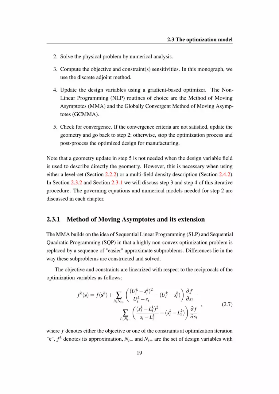
2.3 The optimization model
2. Solve the physical problem by numerical analysis.
3. Compute the objective and constraint(s) sensitivities. In this monograph, weuse the discrete adjoint method.
4. Update the design variables using a gradient-based optimizer. The Non-Linear Programming (NLP) routines of choice are the Method of MovingAsymptotes (MMA) and the Globally Convergent Method of Moving Asymp-totes (GCMMA).
5. Check for convergence. If the convergence criteria are not satisfied, update thegeometry and go back to step 2; otherwise, stop the optimization process andpost-process the optimized design for manufacturing.
Note that a geometry update in step 5 is not needed when the design variable fieldis used to describe directly the geometry. However, this is necessary when usingeither a level-set (Section 2.2.2) or a multi-field density description (Section 2.4.2).In Section 2.3.2 and Section 2.3.1 we will discuss step 3 and step 4 of this iterativeprocedure. The governing equations and numerical models needed for step 2 arediscussed in each chapter.
2.3.1 Method of Moving Asymptotes and its extension
The MMA builds on the idea of Sequential Linear Programming (SLP) and SequentialQuadratic Programming (SQP) in that a highly non-convex optimization problem isreplaced by a sequence of "easier" approximate subproblems. Differences lie in theway these subproblems are constructed and solved.
The objective and constraints are linearized with respect to the reciprocals of theoptimization variables as follows:
f k(s) = f (sk)+ ∑i∈Ns+
((Uk
i − ski )
2
Uki − si
− (Uki − sk
i )
)∂ f∂ si−
∑i∈Ns−
((sk
i −Lki )
2
si−Lki− (sk
i −Lki )
)∂ f∂ si
, (2.7)
where f denotes either the objective or one of the constraints at optimization iteration"k", f k denotes its approximation, Ns− and Ns+ are the set of design variables with
19

Topology optimization as a design tool
(a)
(b)
Fig. 2.5. MMA function approximation with positive (a) and negative (b) gradient.
respect to which the sensitivities are negative and strictly positive, respectively. Theapproximation (2.7) requires the functional gradients with respect to the designvariables, si, that can be computed using the adjoint method described in Section2.3.2 and the material interpolation and regularization laws presented in Section2.4. Using reciprocal sizing variables in structural optimization is motivated bythe fact that stresses and displacements are exact linear functions with respect tothese quantities for statically determinate structures [141]. The parameters Uk
i andLk
i represent local bounds of the approximated problem such that f k → ∞ whensi →Uk
i in increasing functions and when si → Lki in decreasing functions. The
values of Lki and Uk
i are different for each design variable and are dynamicallyupdated along the optimization process. For these reasons, Lk
i and Uki are referred
to as (lower and upper) "moving asymptotes". Moving the asymptotes allowsthe tuning of the curvature of the approximation: as Lk
i or Uki approach sk
i , thecurvature of f k increases, yielding a more conservative approximation. For Lk
i → ∞
or Uki → ∞, a linear function is recovered and the MMA approximations reduce
to SLP approximations. The CONvex LINearization (CONLIN) approximationof Fleury and Braibant [142] is recovered for Lk
i = 0 and Uki → ∞ [507]. Note
that (2.7) is an exact first-order approximation of the original function f such thatf k(sk) = f (sk) and ∇s f k(sk) = ∇s f (sk). A schematic representation of the MMAapproximation for a function f in a point sk
i with a positive and a negative gradient isdepicted in Figure 2.5. The function f k is strictly convex when the asymptotes arefinite and the sensitivities are non-zero. Furthermore, the approximation is separable,
20

2.3 The optimization model
allowing a reduced computational complexity in large-scale problems even when theHessians of the objective and constraints are dense [410].
Let us consider the all-inequality version of (2.6) where the state equations arenot listed as constraints due to the NAND solution approach. At iteration "k" theMMA subproblem reads [410]:
minimizes,y,r
zk +a0r+Nieq
∑i=1
(ciyi +
di
2y2
i
)subject to hk
j−a jr− y j ≤ 0, j = 1, . . . ,Nieq
y≥ 0, r ≥ 0
αααk ≤ s≤ βββ
k
, (2.8)
where r and y are artificial optimization variables, c, d, a and a0 are user-definedconstants and αααk and βββ
k are referred to as lower and upper move limits. Theseprevent the division by zero when solving the subproblem. They should be chosen insuch a way that Lk
i < αki < sk
i < β ki <Uk
i [409]. A popular possibility is [411]:
αki = max
(smin, Lk
i +0.1(ski −Lk
i ), ski −∆s(smax− smin)
)β
ki = min
(smax, Uk
i −0.1(Uki − sk
i ), ski +∆s(smax− smin)
), (2.9)
where ∆s is a user-defined relative step-size. The artificial variable, r, and theconstants d, a0 and a allows a simplified treatment of minimax and least squaresproblems. As this is not of interest in this dissertation, we consider a0 = 1, d = 0and a = 0 such that r = 0 for the optimal solution of (2.8). The elastic variables, y,enlarge the feasibility region of the original problem. Svanberg [410] proved thatthere exist at least one point satisfying the Karush-Kuhn-Tucker (KKT) conditionsof (2.8). It is customary to set c to large values such that the non-feasibility becomesexpensive. However, these constants may retain engineering interest when the boundson the inequality constraints are uncertain.
The update of the asymptotes position during the optimization process relies onthe following test:
tki =
(sk
i − sk−1i
)(sk−1
i − sk−2i
). (2.10)
Svanberg [410] proposed to:
21

Topology optimization as a design tool
• tighten the approximation when a design variable oscillation is detected, i.e.tki < 0. This can be done as following [409]:
Lk+1i = sk
i −α−(
ski −Lk
i
),
Uk+1i = sk
i +α−(
Uki − sk
i
),
(2.11)
where α− ∈ [0, 1] is a user-defined parameter, set to 0.7 in this thesis.
• relax the approximation when the convergence is monotone, i.e. tki > 0. This
can be done as following [409]:
Lk+1i = sk
i −α+
(sk
i −Lki
),
Uk+1i = sk
i +α+
(Uk
i − ski
),
(2.12)
where α+ > 1 is a user-defined parameter, set to 1.43 in this thesis.
• conserve the original approximation when the design variable did not changewithin the last two iterations, i.e. tk
i = 0
During the first two iterations the test tki cannot be computed. The asymptotes are
initialized as [411]:
Lki = sk
i −σMMA (smax− smin) ,
Uki = sk
i +σMMA (smax− smin) ,(2.13)
with k ∈ 1; 2 and σMMA is a user-defined parameter generally set to 0.5 [411].
Although the original MMA algorithm [409] worked well in practice, conver-gence cannot be guaranteed, leading to unsatisfactory results in a few practicalproblems [507]. This deficiency was cured by Zillober in [507] and later in [508]with a line-search procedure, ensuring that the search direction is a descent directionof an augmented Lagrangian merit function. On the other hand, Svanberg [410]extended his original MMA algorithm through the addition of an inner iteration loopthat does not require a line-search. The reworked version is referred to as GCMMAin literature. The curvatures of the objective and constraints approximations aremodified with inner iterations until specific stopping criteria are satisfied. A basicalgorithm of the inner iteration loop at the outer iteration "k" can be summarized asfollows [410]:
22

2.3 The optimization model
1. Let the inner iteration counter l← 0.
2. Assemble and solve the GCMMA approximate problem to obtain the solution(xlk, ylk,zlk)
3. Compute the objective and constraints in both the original and approximateproblem and check that:
zlk(xlk)≥ z(xlk) (2.14)
andhlk
i (xlk)≥ hi(xlk) i = 1, . . . , Nieq. (2.15)
If both criteria (2.14) and (2.15) are satisfied or the maximum number ofinner iterations, Nin, is reached, proceed to the next outer iteration and let(xk+1, yk+1,zk+1)← (xlk, ylk,zlk). Otherwise, modify the GCMMA approxi-mation, let l← l +1 and go to step 2.
The inner iterations do not require sensitivity analysis as the objective and constraintsgradients are updated at each outer iteration. However, the inner loop does requirethe objective and constraints values, meaning that the physical response needsto be re-computed. This slows down convergence as compared to the ordinaryMMA implementation. Criteria (2.14) and (2.15) imply that the solution of thesubproblem is a feasible point with a lower objective function than the previousiteration [410]. The author referred to this property as conservativeness. In GCMMA,the approximation described in (2.7) for MMA and hereafter denoted as f k
MMA ismodified through the addition of a function wc such that [410]:
f k(s) = f kMMA(s)+ ∑
i∈Ns
14
ρc
(Uk
i − ski
Uki − si
+sk
i −LKi
si−Lki−2)
︸ ︷︷ ︸wc
, (2.16)
where ρc is a conservative parameter that differs for the objective and each constraint.This is updated during the optimization procedure using the following rule [410]:
ρl+1,kc =
min(10ρ lk
c ,1.1(ρ lkc +δ lk
c ))
if δ lkc > 0
ρ lkc if δ lk
c ≤ 0, (2.17)
23

Topology optimization as a design tool
where the value of δ lkc is obtained through an extrapolation of the wc function as
follow [410]:
δlkc =
f (xlk)− f lk(xlk)
wc. (2.18)
At each inner iteration, ρc is initialized based on the converged solution of theprevious iterate [410]:
ρ0,k+1c = max
(0.1ρ
Nl ,kc ,ρmin
c
), (2.19)
where Nl is the number of inner iterations of the previous iterate and ρminc is a
user-defined minimum bound.
The GCMMA subproblems can be solved by either a dual approach or a primal-dual Interior Point (IP) approach. The latter is the method of choice in this thesis.The KKT conditions of each GCMMA subproblem are relaxed in two ways: first,the right-hand side of the complementary slackness equations is replaced by asmall parameter, εcs > 0; second, the inequality constraints are transformed intoequality constraints through the use of slack optimization variables. This removesthe combinatorial issue of determining which constraints are active. The relaxedKKT conditions are mathematically equivalent to those of a log-barrier problem,typical in IP methods [411]. A damped Newton method is adopted to solve the KKTsystem. Due to the separability of the approximation, the resulting system can besolved only with respect to λλλ ieq (the vector of Lagrange multipliers of the inequalityconstraints) and r. Hence, it has dimensions (Nieq +1) × (Nieq +1). The parameterεck is decreased during the Newton convergence through heuristic rules [411] in acentral-path fashion [313]. The iterative algorithm is stopped when both the norm ofthe KKT residuals and εck are sufficiently small.
2.3.2 Adjoint sensitivity analysis
The MMA, the GCMMA and any other gradient-based numerical optimizationalgorithm require the objective and constraints gradients to update the design variableset. In the following, let us denote by q j(s,u(s)) a generic optimization criterion andby Nq the total number of optimization criteria. The objective and constraints can beformulated as a function of these optimization criteria.
24

2.3 The optimization model
A possible and straightforward approach to obtain the objective and constraintsgradients is to evaluate the derivatives through finite differences. If a central differ-ence scheme is adopted, the design sensitivities are computed as [196]:
dq j
dsi=
q j(si + εsi)−q j(si− εsi)
2εsi
, (2.20)
where εsi is the perturbation size of the design variable i. To compute the optimizationcriterion, the physical problem R = 0 should be solved. Hence, the central finitedifference strategy requires at least 2×Ns system evaluations. The consequence is acomputational burden that makes impractical to solve high-dimensional problems(such as topology or shape optimization) using this route. Plus, the accuracy of afinite difference framework strongly depends on the degree of non-linearity of theproblem and on the choice of the perturbation size, εsi . Large values may lead toinaccuracies related to truncation errors [196]; the accuracy at small values getsaffected by cancellation error due to machine limits [196]. Despite these downsides,finite difference sensitivities are still used throughout this monograph to cross-checkthe accuracy of analytical sensitivities.
Analytical differentiation is an alternative to finite differences, allowing a reducedcomputational complexity. The direct differentiation of a generic optimizationcriterion through the chain rule leads to:
dq j
dsi=
∂q j
∂ si︸︷︷︸(i)
+
(∂q j
∂u
)T
︸ ︷︷ ︸(ii)
dudsi︸︷︷︸(iii)
. (2.21)
When dealing with smooth optimization criteria, terms (i) and (ii) in Eq. (2.21) aregenerally easy to compute. Evaluating term (iii) is much more involving. One mayrequire that the state sensitivities satisfy the linearized state equations as follows[164]:
dRdsi
=∂R∂ si
+∂R∂u︸︷︷︸
J
dudsi
= 0, (2.22)
where J indicates the Jacobian of the residual vector with respect to the state variables.Solving (2.22) for term (iii) we obtain [293]:
dudsi
=−(
∂R∂u
)−1∂R∂ si
. (2.23)
25

Topology optimization as a design tool
Solving (2.23) and substituting back into (2.21) yields the criterion sensitivities. Thisroute is known as direct method. Similarly to finite differencing, the computationalcomplexity of this approach is insensitive to the number of optimization criteria.However, it requires as many system solutions as the number of design variables:Eq. (2.23) should be solved for i = 1, 2, . . . , Ns. Hence, the direct method is stillimpractical for topology optimization problems. A much cheaper option is to use asymbolic substitution yielding:
dq j
dsi=
∂q j
∂ si−(
∂q j
∂u
)T (∂R∂u
)−1∂R∂ si
, (2.24)
which can be rearranged through transposition properties as:
dq j
dsi=
∂q j
∂ si−
(
∂R∂u
)−T∂q j
∂u︸ ︷︷ ︸Adjoint problem
T
∂R∂ si
. (2.25)
The term in bracket is referred to as adjoint problem. To simplify the computations,we introduce the adjoint equation [293]:(
∂R∂u
)T
λλλ =∂q j
∂u, (2.26)
where λλλ is the vector of adjoint variables or Lagrange multipliers. Now Eq. (2.25)can be restated as [293]:
dq j
dsi=
∂q j
∂ si︸︷︷︸(i)
−λλλT ∂R
∂ si︸︷︷︸(ii)
. (2.27)
The adjoint problem (2.26) is insensitive to the optimization problem dimensionas it does not depend on si. It requires as many systems solutions as the numberof optimization criteria, i.e. it should be solved for j = 1, 2, . . . , Nq. This is thepreferred method for sensitivity analysis in topology optimization problems sincegenerally Ns >> Nq. Note also that (2.26) is linear meaning that the sensitivityanalysis is consistently cheaper than forward analysis of nonlinear problems.
The computation of the adjoint sensitivities used in this thesis is done with thefollowing steps:
26

2.4 Mapping the design model on the analysis model
1. Recover the Jacobian, J, from the last Newton iteration of the forward analysisand compute the adjoint Right-Hand Side (RHS).
2. Solve the adjoint equation (2.26).
3. Compute terms (i) and (ii) of Eq. (2.27) for every design variable si.
4. Compute (2.27) by post-multiplication.
2.4 Mapping the design model on the analysis model
This section presents two fundamental features of any density-based topology opti-mization code used to map the density-based (and Ersatz material level-set) geometryrepresentation on the analysis model. First, we describe a few functions that arecommonly adopted in literature as artificial laws material property-density. Then,we discuss how to regularize the topology optimization problem to obtain a uniquesolution that is free of numerical instabilities.
2.4.1 Material interpolation
The continuous [0, 1] density setting requires a continuous and differentiable relationmaterial property-density such that both the physical response and design sensitivitiescan be computed. For instance, to solve our dissipator example using a steady-statediffusion model, the conductivity, k, within ΩD needs to be defined also for theintermediate "gray" material. Interpolating the material properties with an artificiallaw is referred to as material interpolation. Various techniques were developed overthe years. All the methods aim at "penalizing" the intermediate density values suchthat the optimization process converges to a manufacturable binary 0; 1 design.
The Simplified Isotropic Material with Penalization (SIMP) or power-law ap-proach introduced by Bendsoe [51] is arguably the most popular material interpo-lation model in the topology optimization community. Referring to the dissipatordesign problem, the conductivity k in ΩD is expressed as:
k(ρs) = kBM +(kHCM− kBM)ρ ps (2.28)
27

Topology optimization as a design tool
0 0.2 0.4 0.6 0.8 1
Design variable [-]
0
0.2
0.4
0.6
0.8
1
Conductivity [-]
p=1
p=2
p=3
p=4
p=5
(a)
0 0.2 0.4 0.6 0.8 1
Design variable [-]
0
0.2
0.4
0.6
0.8
1
Conductivity [-]
q=0
q=2
q=4
q=8
q=15
(b)
0 0.2 0.4 0.6 0.8 1
Design variable [-]
0
0.2
0.4
0.6
0.8
1
HC
M n
orm
aliz
ed d
ensity [-]
q=0
q=2
q=4
q=8
q=15
(c)
Fig. 2.6. Comparison of material interpolation models. (a): SIMP model; (b): RAMPmodel; (c): SINH model
where kHCM and kBM are the conductivities of the two materials and p is a penaliza-tion exponent. The latter defines the steepness of the interpolation: p = 1 allows alinear function (the Voigt bound) to be recovered while the interpolation convexityincreases for p > 1. Note that when Eq. (2.28) is used in material-void problems, aminimum value of kBM > 0 should be set in order to avoid singularities in the solutionof the physical problem. The SIMP interpolation function in the case kHCM = 1 andkBM = 1e−6 is represented in Figure 2.6(a). The conductivity interpolation doesnot provide penalization by itself. This effect is obtained only in the presence of a(linear) volume constraint of the type:∫
ΩD
ρs dx−V ∗ ≤ 0, (2.29)
where V ∗ is a maximum prescribed volume of HCM. When considering both Eq.(2.28) and (2.29), intermediate densities become inefficient: they provide smallconductivity per unit of material expense. The SIMP interpolation model originatedas artificial and somewhat heuristic strategy to obtain binary designs. However,Bendsoe and Sigmund [53] showed that it is possible to construct micro-structuresthat physically realize the SIMP interpolation model. This discovery can be ofinterest when interpreting premature designs along the optimization process, havinglarge regions with intermediate ρs material, or when searching for physical reasonsbehind non-convergence to binary 0; 1 designs.
An alternative to SIMP is the RAMP model, which was first introduced byStolpe and Svanberg [406]. The authors showed that SIMP does not in general lead
28

2.4 Mapping the design model on the analysis model
to a concave compliance with respect to the feasible set. Hence, it can be debatedwhether a solution to the "relaxed" continuous problem is also a solution to theoriginal discrete-valued problem. To cure this issue, they proposed to interpolate thegeneric material property as follows:
k(ρs) = kBM +(kHCM− kBM)ρs
1+q(1−ρs), (2.30)
where q is a penalization parameter that plays a role similar to the SIMP exponent,p. The RAMP interpolation function in the case kHCM = 1 and KBM = 1e− 6 isrepresented in Figure 2.6(b). Later experience showed that ensuring concavity withrespect to the feasible set does not hold relevance for practical problems [395].The most interesting feature of the RAMP approximation is that it preserves non-nil gradients at ρs = 0. This can increase convergence to binary designs and, inour experience, plays a significant role when dealing with large kHCM/kBM ratios.Furthermore, the RAMP model satisfies the Hasin-Shtrikman (HS) bounds for all0≤ ρs ≤ 1 in a certain range of q [54].
Instead of using a convex property-density relation coupled with the linearequality constraint (2.29), one could use a linear property-density relation coupledwith a concave volume constraint to achieve the penalization effect. For instance,Bruns [69] proposed the SINH (standing for hyperbolic sine) method, in which thematerial law and volume constraint take the form:
k(ρs) = kBM +(kHCM− kBM)ρs, (2.31)
∫ΩD
(1− sinh(p(1−ρs))
sinh(p)
)dx−V ∗ ≤ 0, (2.32)
where the term in brackets in (2.32) is a normalized HCM density, quantifying theHCM expense per unit volume. A graphical representation of the SINH materialinterpolation strategy is given in Figure 2.6(c). This approach did not encounterbroad acceptance for two main reasons. First, specifying V ∗ is tricky since the termin brackets in (2.32) may not represent the true volume. Second, the linear relation(2.31) does not satisfy the HS bounds.
Choosing suitable values of the penalization parameters can be a non-trivialtask. The best set-up, provided that it exists, strongly depends on the physics andobjective function considered. Since the (thermal) compliance minimization problem
29

Topology optimization as a design tool
is convex with p = 1 in (2.28), a popular approach is to slowly raise the penalizationparameters following a continuation scheme. A sequence of optimization problemswith increasing penalty values are solved. The solution of each continuation step isused as initial guess for the next continuation step. This method works well in manypractical problems where it avoids unsatisfactory local minima. However, thereis no theoretical proof that this approach leads to the global optimum. Stolpe andSvanberg [406] showed with some truss optimization examples that the trajectories ofthe optimal solutions of the penalized problems are in general discontinuous duringa continuation scheme. The interpolation and continuation strategies in complexmulti-physics problems are even more complicated to formulate. If the penalizationis not "balanced" among the material properties governing competitive physics, thereis a chance of favoring one physical phenomenon over the others at intermediateoptimization steps and obtain trivial local minima. More detailed discussions onthis issue are left for Section 5.4, where we investigate some possible continuationschemes in coupled problems involving heat transfer and fluid flow.
2.4.2 Regularization
The numerical instabilities arising in density-based topology optimization can bedivided in two categories: checkerboards and mesh-dependence. The first categoryindicates the formation of black-white checkerboard patterns in the optimized layouts.The second one refers to the issue of obtaining different solutions when the mesh isrefined.
Diaz and Sigmund [114] demonstrated that the reason for the creation of checker-boards is the numerical approximation of the FE discretization. Checkerboardpatterns were found to produce numerical stiffness that makes these artifacts locallystronger than any layered arrangement of the two material constituents. This instabil-ity can be mitigated by the use of higher order elements, patches and filtering [387].As the latter also solves mesh-dependence issues, it is the method of choice adoptedin this thesis. Mesh-dependence is related to the fact that some design optimizationproblems are ill-posed in nature. The creation of micro-structural holes with a fixedamount of structural volume is beneficial to the compliance of structures. Similarly,the creation of small HCM features in general improves the performance of heattransfer enhancers as heat can be distributed more efficiently. Figure 2.7 shows howthe numerical solution of the dissipator problem changes when the mesh is refined.
30

2.4 Mapping the design model on the analysis model
(a)
(b)
(c)
Fig. 2.7. Optimized dissipator geometries with different meshes. (a): 25 x 50elements; (b): 50 x 100 elements; (c): 100 x 200 elements
More and more HCM branches are created connecting the heat source in Γq with thecooled boundary, Γc. This means that the feasible set is not closed and a solutiondoes not exist [387]. Although this trend agrees with the intuition, obtaining a uniquemanufacturable structure is desirable for design engineers. Note that these numericalissues are highly problem and physics-dependent. For instance, the minimization ofpressure drop in flow problems is not ill-posed. The objective function worsens withsmall structural details and layouts with large channels are generally privileged.
The methods available to cure the non-existence issue are of two kinds: relaxationand restriction. Relaxation refers to the enlargement of the design space so that the"gray" material is allowed in the solution. This should be interpreted as a compositematerial, whose micro-structural topology is optimized. The homogenization methodfor topology optimization described in the seminal work of Bendsoe and Kicuchi[55] belongs to this category. The optimization variables parametrize the micro-structural layout determining macroscopic properties. These are then used to solvethe FE problem at the macro-scale. The homogenization theory was later used formaterial design [390] by topology optimization, where the microscopic layout ofperiodic structures with prescribed mechanical properties are sought. Followingthis flourishing line of development, relaxation based on homogenization was laterextended [355] to multi-scale topology optimization frameworks, where both thematerial and structure are optimized. An alternative to the homogenization methodto achieve the relaxation of the design space is to convert the problem into a VariableThickness Sheet (VTS) optimization [332]. Here, the density should be interpretedas a thickness function and can take intermediate values in the optimized design.
Restriction considers a smaller design set of the original problem in which rapidoscillations of the design field are limited. Ambrosio and Buttazzo [24] added a
31

Topology optimization as a design tool
penalization term, zp, to their objective function accounting for perimeter:
zp = αp
∫ΩD
||∇ρ||q dV, (2.33)
where q = 1 is the norm exponent and αp is the penalization weight. Selecting aproper αp value is not easy and requires some tuning. Other authors [62] defined amaximum design perimeter and augmented the optimization problem with a perime-ter constraint. However, choosing a maximum value for the constraint presentssimilar difficulties to the selection of a proper αp. Note that the generalization of thenotion of norm in Eq. (2.33) allows the computation of an approximate maximum lo-cal slope when q→∞. A much more popular alternative to these perimeter/variationstrategies is to employ filtering. Intuitively, filtering spreads the spatial influence ofeach design variable such that rapid oscillations of the design field are prevented.A straightforward but heuristic implementation of this idea was presented in [391],where a convolution operator is adopted to modify the sensitivity field:
˜∂q j
∂ρs=
∑i∈Ne
wiρsi∂q j∂ρsi
∑i∈Ne
ρsiwi, (2.34)
where wi is the filter weight and the index i spans the design variables, elemental ornodal, located in the neighborhood Ne of the element. This set is defined as:
i ∈ Ne if ||xi−xe||≤ r f , (2.35)
where r f is the filter radius and xi is the position of the design variable. The weightis defined as a linearly-decaying function:
wi = r f −||xi−xe||, (2.36)
which is a distance function centered in xe and locally supported within the filterradius. A schematic representation of the linear filter operator with nodal designvariables is represented in Figure 2.8(a). The nodal positions belonging to Ne aremarked in green. The filter weight function varies linearly between 0 and r f anddoes not depend upon the mesh size. Researchers often questioned the mathematicalrationale behind the sensitivity filter as it was not possible to identify which objectivefunction was being actually optimized. Lately, Sigmund and Maute [394] revealed
32

2.4 Mapping the design model on the analysis model
(a)
0 0.2 0.4 0.6 0.8 1
Filtered design variable [-]
0
0.2
0.4
0.6
0.8
1
Projected
designvariable
[-]
β = 1
β = 5
β = 10
β = 20
β = 40
(b)
Fig. 2.8. (a): Schematic representation of the linear filter operator; (b): generalizedtanh projection with η = 0.5
that using the sensitivity filter in structural optimization corresponds to minimizingthe compliance in non-local elasticity problems.
Taking inspiration from the sensitivity filter approach, Bruns and Tortorelli [70]proposed to filter the design variable field. In the original view of the authors, thismethod has the advantage that designers "know exactly what optimization problemis being solved". A new filtered design variable, s, is introduced in the optimizationproblem. For this reason, the authors of [393] refer to this method as "two-fieldSIMP". The additional design variable field is defined as:
s =∑
i∈Newisi
∑i∈Ne
wi. (2.37)
Note that this approach does not enlarge the design set. The filtered field can beobtained explicitly from s through (2.37). Now the density indicator is representedby this additional field such that ρs = s. For this reason, we will refer to s andρs as abstract and physical design variables throughout this monograph. As withthe homogenization method for topology optimization, this approach relies on theseparation of the design space, where the abstract design variables, s, live, and theFE space, where the physical design variables, ρs, live and the system response iscomputed.
33

Topology optimization as a design tool
Using the filter (2.37) blurs the boundary of the geometry representation, ρs, andgives at best regions with intermediate density values of thickness 2r f (sufficientlyfar from the design domain boundaries) even for well penalized problems. One mayreduce the related inaccuracies in the analysis by using a continuation approachwhere the filter radius is slowly decreased. As an alternative, Guest [176] proposed aprojection scheme, where a third field is introduced as:
s = 1− e−β s, (2.38)
where β corresponds to a projection steepness parameter. This method works withthree different design variable fields. The projected design variable field is used todescribe the geometry and interpolate the material properties, hence ρs = s. Equation(2.38) is a smoothed version of a Heaviside function. Using filtering followed byprojection with (2.38) guarantees a minimum length-scale on the optimized designs.To understand how this is possible consider the 1D example of Figure 2.9, where s isdefined at the nodes and s and s are defined at the elements and are element-wiseconstant. The geometry discretization consists of 7 equally spaced nodes and 6elements with characteristic size h = 1. The filter has radius r f = 2. Consider thesituation presented in Figure 2.9(a), where s = 1 in one node and s = 0 in neighbornodes. Filtering produces a smoothed layout with s > 0 in a region with width 2r f ,i.e. spanning 4 elements. This whole region is then projected to a structural memberof width 2r f when using (2.38). Hence, geometries with features smaller than 2r f arenot allowed for HCM elements sufficiently far from the design domain boundaries.Close to the boundaries, the region spanned by the filter operator is reduced. Forinstance, if the node with s = 1 belongs to a design domain boundary (Fig 2.9(b)),an r f wide smoothing is obtained. This shows that structural features with widthr f ≤ wHCM ≤ 2r f can appear close to the design domain boundaries.
Sigmund [392] later revisited the problem to obtain a minimum length-scale ofthe BM layout. This is achieved by simply modifying the Heaviside to be centeredat s = 1 as following:
s = 1− e−β (1−s). (2.39)
The effect of projection (2.39) is presented in Figure 2.9(c). A single s = 0 node po-sitioned sufficiently far from the boundaries is surrounded by an s = 1 neighborhood.After filtering and projection, the hole in the structure has width 2r f . Smaller holes
34

2.4 Mapping the design model on the analysis model
0 2 4 6
Length [-]
0
0.2
0.4
0.6
0.8
1
De
sig
n v
aria
ble
[-]
s
s
s
(a)
0 2 4 6
Length [-]
0
0.2
0.4
0.6
0.8
1
De
sig
n v
aria
ble
[-]
(b)
0 2 4 6
Length [-]
0
0.2
0.4
0.6
0.8
1
Desig
n v
ariable
[-]
(c)
Fig. 2.9. Filtering and projection 1D example. (a): Preservation of the minimumfeature size of HCM; (b): boundary effect on the minimum feature size of HCM; (c):preservation of the minimum feature size of BM
35

Topology optimization as a design tool
can appear close to the design domain boundaries for the same reasons discussed forFigure (2.9)(b).
Wang et al. [446] later generalized the previous approaches with a hyperbolictangent formulation where the projection thresholds, η , can be varied continuouslybetween 0 and 1.
s =tanh(βη)+ tanh(β (s−η))
tanh(βη)+ tanh(β (1−η))). (2.40)
This generalized projection with variable threshold and steepness is representedin Figure 2.8(b) for the case with η = 0.5. When η ∈ (0,1), Eq. (2.40) does notguarantee a minimum feature size on neither of the two phases but has shown toprovide mesh-independent and crisp results in practical cases [393]. Methods thatguarantee minimum length-scale on both phases involve the use of four designvariable fields. One example was demonstrated in [177]. Note that the projectiononly helps to obtain crisp boundaries when a filtering scheme is adopted. This shouldnot be used to improve the convergence to binary 0; 1 designs in poorly penalizedproblems [395]. In the best case, the abstract design variable field would morph suchthat the intermediate values of the physical design variable field are still present. Inmost cases, using high projection values and a small penalization parameter leads topremature convergence to poor local minima. Continuation schemes are generallyadopted to slowly raise the projection steepness parameter, β . This helps to avoidwiggling in the optimization history and premature convergence to local minima.However, in a recent paper [178], Guest showed that it is possible to avoid such acontinuation by tightening the initial asymptotes position in the MMA routine asfollows:
σMMA =0.5
β +1. (2.41)
Both asymptotes initialization strategies (2.13) and (2.41) are used throughout thismonograph. The choice will be clarified on a case-by-case basis.
When using the three-field density methods, all the computations described foradjoint sensitivity analysis in Section 2.3.2 are performed with respect to the physicaldesign variable, ρs = s. Then, the sensitivity field should be modified to ensureconsistent optimization criteria gradients with respect to the abstract design variable,s. In this monograph, we account for filtering and projection in the sensitivity
36

2.5 Steady-state diffusion example
analysis using the chain rule as follows:
dq j
dsi=
Ns
∑l=1
Ns
∑k=1
dq j
dsk
∂ sk
∂ sl
∂ sl
∂ si, (2.42)
where the first term on the RHS is the one computed through adjoint calculus.
2.5 Steady-state diffusion example
In this section, we investigate and discuss the effect of the most relevant topologyoptimization parameters introduced in this chapter. To this aim, we consider ourdissipator example. The design optimization problem can be stated as:
minimizes
∫Γq
T dx′
subject to∫
ΩD
ρs dx−V ∗ ≤ 0
s ∈ S =RNs | smin ≤ si ≤ smax, i = 1, ...,Ns
, (2.43)
where the maximum volume of HCM, V ∗, is set to 25 % of the total volume available.The design domain has width W = 2 and height H = 1. The heat source boundaryhas width wq = 0.2. The focus here is exclusively on the topology optimizationparameters; we are not interested in obtaining an optimized device for practical use.Hence, we limit the physics complexity. Heat transfer is governed by steady-statediffusion within ΩD:
− ∂
∂xi
(k(s)δi j
∂T∂x j
)= qv, (2.44)
where δi j is the Kronecker delta and k(s) is the design-dependent conductivityinterpolated with (2.28) between kBM = 1 and kHCM = 1000 and qv = 0 is thevolumetric heat generation. A constant heat flux is imposed through a Neumannboundary condition on Γq:
− k(s)δi j∂T∂x j
ni = qhs, (2.45)
37

Topology optimization as a design tool
Table 2.1. GCMMA parameters utilized in this monograph
Description Symbol Value
Relative step-size ∆s 0.03Maximum inner iterations Nin 2Initial asymptote position parameter σMMA 0.5Lower asymptote adaptivity α− 0.7Upper asymptote adaptivity α+ 1.43Constraint penalty ci 1000Parameters ai 0Parameter a0 1Parameters di 0Minimum conservativeness parameter ρmin
c 1e-5
where ni is the inward-pointing normal and qhs = 1 is the applied heat flux. The topboundary is cooled by convection, hence a mixed-type (Robin) condition is appliedon Γc:
− k(s)δi j∂T∂x j
ni = h(Text−T ), (2.46)
where Text = 0. The governing equations are discretized with 2e4 bilinear quadri-lateral elements and solved in COMSOL Multiphysics [101]. The optimizationproblems are solved using GCMMA in Matlab [292]. The most relevant GCMMAparameters are summarized in Table 2.1. Unless otherwise stated, these values areused to produce all the results presented in this thesis. Limiting the number ofmaximum inner iterations, Nin, to 2 does not guarantee the "globally convergent"feature of the GCMMA algorithm. However, a high Nin was often found to leadto slow convergence, requiring a large number of analyses. In specific numericalexamples, Nin is raised from this default value only to stabilize convergence andavoid dramatic oscillations along the optimization process. In this section, we willinvestigate the effect of the penalization exponent, p, filter radius, r f , projectionsteepness parameter, β , and projection threshold, η . The default values of theseparameters are listed in Table 2.2.
The COMSOL-Matlab design optimization framework used here was developedin cooperation with Dr. Reza Behrou and used to produce the results presentedin Chapter 8. The design studies presented in Chapters 3, 4, 5 and 6 are solvedusing the Finite Element Multi-disciplinary Design Optimization Code (FEMDOC),a C++ design optimization framework developed at University of Colorado (CU)
38
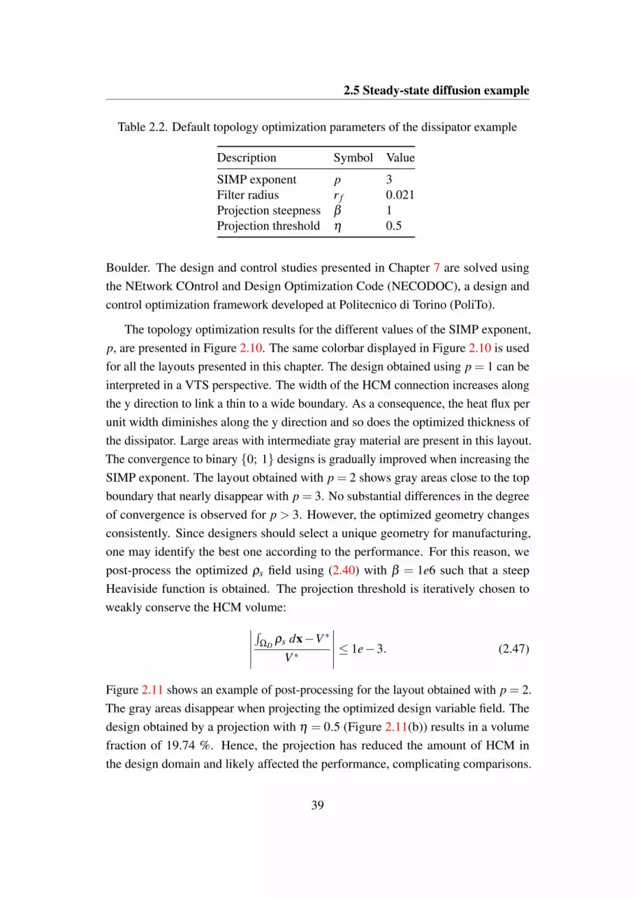
2.5 Steady-state diffusion example
Table 2.2. Default topology optimization parameters of the dissipator example
Description Symbol Value
SIMP exponent p 3Filter radius r f 0.021Projection steepness β 1Projection threshold η 0.5
Boulder. The design and control studies presented in Chapter 7 are solved usingthe NEtwork COntrol and Design Optimization Code (NECODOC), a design andcontrol optimization framework developed at Politecnico di Torino (PoliTo).
The topology optimization results for the different values of the SIMP exponent,p, are presented in Figure 2.10. The same colorbar displayed in Figure 2.10 is usedfor all the layouts presented in this chapter. The design obtained using p = 1 can beinterpreted in a VTS perspective. The width of the HCM connection increases alongthe y direction to link a thin to a wide boundary. As a consequence, the heat flux perunit width diminishes along the y direction and so does the optimized thickness ofthe dissipator. Large areas with intermediate gray material are present in this layout.The convergence to binary 0; 1 designs is gradually improved when increasing theSIMP exponent. The layout obtained with p = 2 shows gray areas close to the topboundary that nearly disappear with p = 3. No substantial differences in the degreeof convergence is observed for p > 3. However, the optimized geometry changesconsistently. Since designers should select a unique geometry for manufacturing,one may identify the best one according to the performance. For this reason, wepost-process the optimized ρs field using (2.40) with β = 1e6 such that a steepHeaviside function is obtained. The projection threshold is iteratively chosen toweakly conserve the HCM volume:∣∣∣∣∣
∫ΩD
ρs dx−V ∗
V ∗
∣∣∣∣∣≤ 1e−3. (2.47)
Figure 2.11 shows an example of post-processing for the layout obtained with p = 2.The gray areas disappear when projecting the optimized design variable field. Thedesign obtained by a projection with η = 0.5 (Figure 2.11(b)) results in a volumefraction of 19.74 %. Hence, the projection has reduced the amount of HCM inthe design domain and likely affected the performance, complicating comparisons.
39

Topology optimization as a design tool
(a) (b) (c)
(d) (e)
Fig. 2.10. The effect of the SIMP exponent, p, on the optimized designs. (a): p = 1,z = 7.108e−3; (b): p = 2, z = 5.103e−3; (c): p = 3, z = 5.033e−3; (d): p = 5,z = 5.043e−3; (e): p = 10, z = 5.429e−3;
(a) (b) (c)
Fig. 2.11. Post-processing for performance comparison. (a): optimized design forp = 2; (b): projected optimized design with η = 0.5; (c): projected optimized designwith η = 0.375
40

2.5 Steady-state diffusion example
(a) (b) (c)
(d) (e)
Fig. 2.12. The effect of the density filter radius, r f , on the optimized designs.(a): r f = 0.011, z = 5.032e− 3; (b): r f = 0.021, z = 5.033e− 3; (c): r f = 0.051,z = 5.041e−3; (d): r f = 0.101, z = 5.075e−3; (e): r f = 0.201, z = 5.147e−3
The projection threshold is iteratively changed to η = 0.375 such that the volumefraction of the layout displayed in Figure 2.11(b) is 25.01 %. All the objectivevalues reported in the figure captions are calculated on layouts obtained through thisprocedure. Using p = 3 allows the best performing layout to be obtained. Note thatthis value is generally recommended when using a SIMP interpolation [395]. Furtherincreasing the penalization exponent is not beneficial for performance. A largeperformance reduction is observed for p = 10. Although beneficial for convergenceto binary 0; 1 layouts, raising the SIMP exponent increases the non-convexityof the optimization problem. As a consequence, the chances to get stuck intounsatisfactory local minima are higher when using a gradient-based optimizer suchas GCMMA.
Figure 2.12 shows the optimized dissipator layouts obtained for different valuesof the filter radius, r f . The filter blurs the interface between HCM and BM yieldinga larger amount of "gray" material in the optimized layouts. This is an inherent effectof the filter operator and has nothing to do with penalization. Topology modificationsare observed when the filter radius is raised over the default value of r f = 0.021.The thin structural features connected to the top boundary disappear. This is aconsequence of both the penalization and filtering: the designs evolve in such a waythat the length of the "gray" interface is reduced. In this example, the filter radius has
41

Topology optimization as a design tool
(a) (b) (c)
(d) (e)
Fig. 2.13. The effect of the projection steepness parameter, β , on the optimizeddesigns. (a): β = 1, z = 5.033e− 3; (b): β = 5, z = 5.049e− 3; (c): β = 30,z = 5.055e−3; (d): β = 100, z = 5.072e−3; (e): β = 200, z = 5.621e−3
only a limited effect on the performance of the optimized layouts. However, in ourexperience, incautious combinations of r f and p may result in trivial heat transferstructures with a small heat transfer area.
The fuzziness introduced by the filter operator can be cured by raising theprojection parameter β such that the amount of "gray" material at the interface isreduced on the FE space. The optimized layouts obtained for different values of thesteepness parameters are collected in Figure 2.13. To avoid the use of a continuationscheme for β , we adopt the asymptotes initialization strategy (2.41). The inspectionof the design features close to the top boundary reveals that the amount of graymaterial is reduced when increasing β . This is desirable if the geometry needs to bemanufactured as it eliminates the need for post-processing procedures. However, forall cases considered, we obtained a better performance by simply post-processing thefinal optimized design obtained with β = 1. The optimized objective value increaseswith β indicating that the chances of convergence to unsatisfactory local minimaare higher. For β = 200 (Figure 2.13(e)), the optimization procedure leads to anunnatural layout responsible of large performance reductions as compared to ourβ = 1 reference design.
The effect of the projection threshold, η , on the optimized layouts is shown inFigure 2.14. Recall that for β → ∞, setting η = 0 and η = 1 allows the minimum
42

2.5 Steady-state diffusion example
(a) (b) (c)
(d) (e)
Fig. 2.14. The effect of the projection threshold, η , on the optimized designs. (a):η = 0.00, z = 5.035e− 3; the green and red circles have diameters of 2r f and r frespectively; (b): η = 0.25, z = 5.032e− 3; (c): η = 0.50, z = 5.034e− 3;; (d):η = 0.75, z = 5.036e−3; (e): η = 1.00, z = 5.133
feature size of HCM and BM to be prescribed. To facilitate the visualization of thisdesign capability, the optimized designs were obtained with β = 120 and r f = 0.075.Also in this case the asymptotes position is initialized according to (2.41). The redand green circles displayed Figure 2.14(a) have diameters r f and 2r f , respectively.In the layout optimized with η = 0.00, the thickness of the HCM connections isnearly constant within the design domain. A thinner horizontal HCM element is incontact with the top boundary. A closer analysis of the optimized layout suggeststhat the minimum feature size of HCM is 2r f far from the boundaries and r f closeto the boundaries. This was anticipated with the 1D study presented in Section2.4.2. In Figure 2.14(e) obtained with η = 1.00, we observe that the local curvatureradius of the holes is always larger than 2r f and that the shape of the smallest holesapproximates the green circle. In our experience, the appearance of circular holesin optimized structures is frequent when a minimum feature size is prescribed onthe BM. In designs optimized with η = 0.25, η = 0.50 and η = 0.75, we noticeno connection between the size of the design features and the one of the filter. Thelayout optimized for η = 0.25 yields the best performance. However, only slightobjective differences are predicted in the cases considered for η < 1. For η = 1, weobtain an optimized geometry that results in non-negligible performance reductionsas compared to the alternatives.
43

Topology optimization as a design tool
2.6 Conclusions
This chapter reviewed the fundamentals of topology optimization as a practicaldesign tool. After describing the design and optimization models that are used inthe remainder of this thesis, we investigated the effect of some selected topologyoptimization parameters using a simple design optimization example. The resultswill help to justify the choices and to predict the effects of these numerical parameterswhen solving the energy problems considered in this thesis.
44

Chapter 3
Design of fins with a simplified phasechange model
The utilization of PCMs for TES allows the construction of cheap and compactunits, ideally suited to domestic space heating applications [296]. A schematicrepresentation of the storage capacity for sensible and latent TES units is presentedin Figure 3.1. When the temperature difference between the source providing thermalenergy, Tsource, and the sink retrieving thermal energy, Tsink, is sufficiently small,the PCM yields a higher amount of heat stored. This allows a reduction of therequired storage volume and in turn decreases the cost of the installation. It is wellknown that the market uptake of LHTES units is hampered by the low thermalconductivity of the most popular PCMs, which slows the charge/discharge dynamicsand limit the achievable power density. For this reason, the search of optimal highconducting structures for heat transfer enhancement in LHTES is an active researchfield in the heat transfer community. Most of the state-of-art design proceduresstart with the formulation of a design concept, which is then improved throughmodifications of a few design parameters. Different starting layouts most often lead todifferent optimized layouts as the geometry parametrization does not allow to morphcontinuously across design concepts. As a result, uncountable geometries have beenproposed to answer a unique design question. This suggests that the literature lacksa thorough design optimization procedure for LHTES systems allowing dramaticdesign changes. This chapter demonstrates how topology optimization can beused to skip the design concept formulation step, to catch design trends usingmatchless design freedom and to answer practical design questions. We focus more
45

Design of fins with a simplified phase change model
Stored heat
PCM
Sensible m
ateria
l
Latent heat
Fig. 3.1. Stored heat in sensible and latent TES units as a function of the temperaturedifference between the source and the sink
on design freedom rather than physics complexity. For this reason, phase changeis accounted during the analysis through a simplified model that neglects naturalconvection. This assumption will be relaxed in Chapters 5 and 6. The plan ofthe chapter is as follows. In Section 3.1 we thoroughly review the most popularLHTES system configurations; Section 3.2 discusses the strategies for solving phasechange problems through nonlinear diffusion and Section 3.3 describes in detail ournumerical model and implementation and verifies the accuracy of the framework;Section 3.4 identifies alternative formulations of the design optimization problemand gives some algorithmic details regarding sensitivity analysis; finally, Section 3.5presents design examples of practical interest and discusses design trends useful fortechnology practitioners.
Some of the contents of this chapter were published in International Journal ofHeat and Mass Transfer [J2] and presented at the 4th International Conference onComputational Methods for Thermal Problems [C4].
46

3.1 Review of state-of-the-art LHTES systems
3.1 Review of state-of-the-art LHTES systems
In this section, we review the state-of-the-art LHTES system configurations, includ-ing the options for the container and the most popular heat transfer enhancementstrategies.
Agyenim and co-authors [7] argued that two types of containers are currently con-sidered for commercial LHTES installations, namely the rectangular and the cylin-drical one. The latter is no-doubt the most popular due to the faster charge/dischargedynamics [509], reduced heat losses per unit of storage material and compatibilitywith piping materials of general engineering use. Three different configurations wereinvestigated for the cylindrical layout including: (i) concentric tubes with Heat Trans-fer Fluid (HTF) in the internal pipe and PCM in the annulus, (ii) concentric tubeswith PCM in the internal pipe and HTF in the annulus, (iii) shell-and-tube systemswith HTF filling the pipes and PCM filling the shell. The study conducted by theauthors of [121] demonstrates that Option (i) allows an increased performance by re-ducing the process time as compared to Option (ii). Also, Agyenim et al. [7] pointedout that the losses are reduced during charge as the supplied thermal power is usedto melt the PCM. However, we observe that this does not hold true during discharge.Option (iii) is a convenient choice for medium-large installations. The experimentspresented in [6] revealed that the multi-tube single-shell configuration favors naturalconvection, reducing the time required for melting as compared to Option (i). Nosubstantial differences were reported concerning solidification because this processwas mostly ruled by diffusion. A separate note is required to discuss Triplex TubeHeat eXchanger (TTHX), that seems to create high scientific interest nowadays. Inhis seminal paper [221], Jian proposed to adopt three concentric tubes and circulateHTF in both the internal pipe and the most external annulus with PCM filling theintermediate ring. Lately, different configurations were considered to such a detailthat it is hard to identify differences between the published papers. Interestingly,most of this literature comes from the same research group. Only recently, otherresearches, e.g. [227, 21, 285], started considering this option. We believe that muchmore independent research is needed before TTHX can be considered as a reliablealternative to the ones discussed above.
Most of the PCMs of practical interest have low thermal conductivity. Thislimits the amount of energy that can be transferred between the HTF and PCMin time spans of interest for the applications. A notable exception is represented
47

Design of fins with a simplified phase change model
by the metallic PCMs but their high melting temperature limits their utilization toConcentrating Solar Power (CSP) systems. For a comprehensive discussion on PCMthermo-physical properties, we refer the reader of this monograph to Chapter 6. Inthe past three decades, many researchers dedicated to the search of heat transferenhancement techniques for LHTES systems. Research directions can be grouped inthree categories:
• Diffusion distance reduction, where HCM structures of various shapes andconfigurations are embedded in the PCM such that the average diffusiondistance within the PCM is reduced. This category includes extended surfaces,multiple and/or multi-pass HTF tubes, heat pipes and metal capsules.
A comprehensive overview of extended surfaces is presented later in thissection. The utilization of multiple HTF tubes is the most popular option forlarge installations as a unique shell needs to be fabricated. This yields costssavings as compared to multiple single-tube systems. Note that this layoutcorresponds to Option (iii) for cylindrical containers as discussed before.The enhancement effect is due to the increased heat transfer area betweenthe HTF and PCM and the reduced average diffusion distance within PCM.Although this approach was first adopted as an alternative to the use of fins [6],recent studies [107, 239] considered the combination of the two enhancementapproaches. We will deal with the design optimization for this combinedoption in Chapter 6 of this thesis. Multi-pass configurations such as the onereported by the authors of [222, 239] yield the same advantages listed formulti-tube systems. The difference is that a unique stream is circulated withinthe pipes. Hence, the effectiveness is reduced along the flow path due to adecreasing temperature difference between the HTF and PCM. Enhancementthrough heat pipes is a rather new concept for LHTESs and more researchshould be performed to assess the potential of this technology [215]. In themost popular configuration, heat pipes are positioned across the HTF tubesuch that the evaporator and condenser sections come in contact with eitherthe HTF or PCM [377]. By increasing the length of the adiabatic section,designers can "lump" heat sinks/sources far apart from the HTF tube. Theencapsulation of PCM within spherical metallic capsules reached maturity atthe industrial level [296]. Besides heat transfer enhancement, the reasons forchoosing encapsulation may also include chemical compatibility and thermal
48

3.1 Review of state-of-the-art LHTES systems
and mechanical stability [239]. Depending on the capsule size, Khan etal. [239] distinguished among nano-encapsulation, micro-encapsulation andmacro-encapsulation.
• Effective conductivity increase, where PCM is manipulated through multi-scale techniques such that its macroscopic thermal conductivity is improved.This category includes cellular metals, rings and brushes, Natural ExpandedGraphite (NEG) composites and dispersed nanoparticles. A discussion on thestate-of-the art solutions for cellular metals is left for Chapter 4.
Rings are pieces of tubes that are commonly used in chemical engineeringprocesses such as distillation due to their large surface area per volume. Theywere first adopted for LHTES enhancement by the authors of [430], showingcomparable performance to longitudinal fins. Brushes are ordered arrange-ments of high conductivity carbon fibers that were first used as enhancementdevices by Fukai et al. [151]. As shown by the same authors in [150], the fiberslayout can be engineered around the tubes such that the effective conductivityof the resulting composite is increased with a minimal penalty on the storagecapacity. A fast growing portion of the published literature concerns the useof high conducting nanoparticles dispersed in PCM. Most studies deal withpowders containing aluminum, copper or carbon [215]. Recent researchesfocus particularly on nanotubes and nanowires for which some authors [449]reported improvements to the thermal conductivity up to 40 %. The ease inmanufacturing and low cost [453] motivated the early interest in NEG-PCMcomposites for LHTES enhancement. A porosity of 10 % of the graphitematrix is recommended in [239] for best performances. From our review, itseems like the current manufacturing processes are able to control the obtainedporosity with precision but the topology of the micro-layout can hardly becustomized.
• Others, including the (few) methods that do not fit in any of the categoriesabove such as the utilization of multiple PCMs and intermediate HTFs.
Using multiple PCMs can alleviate the problem of heat transfer deteriorationalong the HTF path due to the reducing temperature difference between theHTF and PCM. For faster charge, PCMs should be arranged in a decreasingorder of melting temperature such that a nearly constant temperature differenceis maintained along the HTF pipe [329]. Since increasing melting temperatures
49

Design of fins with a simplified phase change model
are desired for discharge, the flow direction should be reversed during thisprocess [215]. Using an intermediate HTF was first proposed by Adinberg etal. [4] in their reflux storage for CSP applications. As with heat pipes, theoperational principle relies on evaporation and condensation. However, herethe region between the condenser and evaporator is non-adiabatic and filledwith tubes embedded in PCM. Heat is stored and retrieved by means of thegravity-assisted motion of the vapors along the tubes.
Figure 3.2 summarizes the proposed classification of enhancement techniques. Thestrategies considered within this monograph are highlighted in red. Since Chapters3, 5 and 6 deal with the design optimization of HCM fins, in the remainder ofthis section we present and discuss some of the most popular extended surfaceconfigurations. A similar description for cellular metals is left for Chapter 4. Thesearch for the optimal shape of fins attracted large attention within the heat transfercommunity. As a consequence, the literature on this topic spans several decades.The following discussion skips the earliest developments and focuses on the mostrecent findings. An extensive review of this vast body of literature revealed that theinvestigated fin layouts are of five types: longitudinal, circular, Y-shaped or tree, pinsand helical. A schematic representation of these layouts is shown in Figure 3.3.
Due to their easy design and fabrication, longitudinal fins represent the mostpopular extended surface geometry in the LHTES community, accounting for morethan 60 % of the installations [2]. Focusing on shell-and-tube systems, Khan etal. [239] observed that an accurate design of longitudinal fins is crucial for theperformance. Their study revealed that it is more convenient to increase the finlength rather than its thickness. The experiments presented in [347] reported thatthis fin configuration is more beneficial to solidification than to melting. Hosseiniet al. [209] investigated both numerically and experimentally the effect of the finsheight. They found that increasing the height leads to a more symmetric evolution ofthe melting front, yielding a better utilization of the stored energy. Solomon [401]observed that longitudinal fins suppress convection in the liquid PCM, thereforeslowing the charge of the unit. For their free cooling application, they recommendedto use fins occupying 60 % of the annular distance. Also Darzi et al. [108] foundthat longitudinal fins are highly effective for solidification but yield negligiblecontribution for melting in that natural convection is inhibited. For this reason,Beck et al. [45] recommended designs guaranteeing unrestricted natural convection
50

3.1 Review of state-of-the-art LHTES systems
LHTES enhancement
techniques
Diffusion length reduction
Effective conductivity
increase
Others
Multiple tubes
Multipass tubes
Heat pipes
Capsules
Fins
Matrices
Rings
Brushes
Nano particles
NEG
Multiple PCMs
Multiple HTFs
Fig. 3.2. Classification of heat transfer enhancement techniques for LHTES
51

Design of fins with a simplified phase change model
(a) (b) (c) (d) (e)
Fig. 3.3. Schematics of reviewed fin layouts. (a): longitudinal; (b): circular; (c):pins; (d): Y-shaped or tree; (e): helical
for improved melting rates. Building on these observations, Yuan et al. [483] andKazemy et al. [235] recently found an optimal tilt angle of longitudinal fins thatenhances convective transport. This research direction was anticipated by Liu andGroulx [271], who examined the effect of the fins orientation through experiments.They found that four diagonal fins yield reduced melting time as compared to twohorizontal and two vertical fins. Negligible differences in performance were observedfor solidification.
Circular fins were considered for heat transfer enhancement in LHTES units laterthan longitudinal fins. Back to 1992, Choi and Kim [88] observed that "Investigationsof circular fins in cylindrical geometry are very few in number". The simple layoutand consequent easy manufacturing motivated the development of this concept asdemonstrated by the large number of studies that are being published these days.The experiments described in [325] showed that increasing the density of fins alongthe pipe is by far more beneficial than increasing the velocity of the HTF. Wang etal. [452] investigated the effect of the fin pitch, height and thickness. When usingsmall inter-fin distances, they reported a larger effect of the fin height than thickness.The performance was found to be slightly sensitive to both the previous parameterswhen using high fin pitches. The authors of [480] studied how natural convection invertical units is affected by the circular fins design. Based on their parametric study,they recommended a specific fin number, thickness and inter-fin distance such thatthe melting time is minimized. A similar trend concerning natural convection wasnoticed by Jmal and Baccar [222] for solidification in air-PCM units. Kuboth et al.[253] recently showed numerically that varying the fin density distribution along the
52

3.1 Review of state-of-the-art LHTES systems
HTF pipe is beneficial for performance. They suggested to increase linearly the findensity from the inlet to the outlet using a growth factor of 10.
Pin fins geometries were first adopted as heat transfer enhancers in PCM forelectronics cooling applications. The interested reader can consult [362] for acomprehensive review of heat sink geometries. In a recent review [2] on heat transferenhancement in LHTES, this layout is only listed as a suitable alternative to platefins for maximum heat dissipation in heat sinks and no reference to studies in thefield of LHTES is given. This demonstrates that the investigations on this layout arein their early days. We found only two examples of applications to thermal storageunits. Bruno et al. [417] claimed to be the first research group that consideredexternal pins attached to the HTF pipes. Their work reported reduced performanceas compared to the circular fins. A similar conclusion was later drawn by theauthors of [48], where the pin fin effectiveness was calculated to be lower than thatof the annular fins. It is curious that this geometry attracted such little attentionamong researchers, despite the large interest in the field of electronics cooling. Wethink that more research should be conducted to assess the real potential of thisconfiguration. In both the studies analyzed, it is not clear whether the amount ofHCM is kept constant when comparing the alternative configurations. In our opinion,this is a fundamental prerequisite to draw meaningful conclusions. Furthermore, in[417] natural convection is neglected. This factor can modify the outcome of thecomparison since pins allows a nearly unrestricted motion of the buoyant eddies.
The need for performance improvement of longitudinal fins gave momentum tothe development of Y-shaped or tree fins. Sciacovelli et al. [374] adopted a responsesurface optimization method to optimize the fin length and bifurcation angle. Theauthors found that the discharge efficiency can be increased by 24 % if optimal finswith two bifurcations are chosen. In a more recent development [375], the authorswere able to obtain an optimized tilt angle along the longitudinal direction such thatthe solidification time is reduced. Lohrasbi et al. [278] adopted the same optimizationapproach of [374] to optimize V-shaped geometries where the bifurcation of the Ygeometry is in contact with the HTF pipe. Recently, more "exotic" geometries havestarted to appear. For instance, the authors of [383] parametrized a fin geometrymimicking the crystal structure of a snowflake and reported significant performanceimprovements as compared to the conventional longitudinal fins. Note that similarstructures were obtained by the Institute of Engineering Thermodynamics (DLR,
53

Design of fins with a simplified phase change model
Fig. 3.4. Schematic of a generic solid-liquid phase change process
Germany) [257] and patented by Le Commissariat a l’energie atomique et auxenergies alternatives (CEA, France) [320].
Another option that researchers have recently started to consider is represented byhelical fins. The layout proposed by Kozak et al. [360] yielded an increased meltingrate with respect to the conventional alternatives. Furthermore, it demonstratedpractical advantages such as the prevention of voids in solidification, preventionof large pressures in melting and ease of maintenance. The same geometry waspreviously considered by the authors of [45]. Their numerical results suggestedthat the helical configuration is responsible for a small performance reduction ascompared to the simple longitudinal fins.
3.2 Modeling diffusion-driven phase change
Here, we discuss the available computational strategies for computing the responseof phase change systems through nonlinear diffusion. In particular, we focus onfixed-grid approaches such as the enthalpy, the apparent heat capacity and the sourcemethods.
Melting or solidification of a pure material with a moving boundary separatingthe two phases is referred to as Stefan problem. A snapshot of a generic solid-liquid phase change process is presented in Figure 3.4. The liquid fills Ωl while thesolid fills Ωs. The two phases are separated by an interface, Γls. With negligible
54

3.2 Modeling diffusion-driven phase change
advective transport and constant density and specific heat, the thermal response canbe described by the following set of governing equations:
ρscps
∂T∂ t
=∂
∂xi
(ksi j
∂T∂x j
)in Ωs, (3.1)
ρlcpl
∂T∂ t
=∂
∂xi
(kli j
∂T∂x j
)in Ωl, (3.2)
T = Tm on Γls, (3.3)
ksi j
∂T∂x j
ni− kli j
∂T∂x j
ni = ρsL vΓlsni on Γls, (3.4)
where T is the temperature, ρs and ρl represent the solid and liquid densities, cps
and cpl represent the solid and liquid specific heats, ksi j and kli j are the conductivitytensors of the solid and of the liquid, L is the latent heat per unit mass of the solid,ni is the liquid-pointing normal of the interface and vΓls is its propagation velocity.Equations (3.1) and (3.2) prescribe the diffusion heat transfer in the solid and liquidregions, respectively. Eq. (3.3) identifies the melting (solidification) front as theisotherm with T = Tm, with Tm being the melting temperature. Eq. (3.4), broadlyreferred to as the Stefan condition [440], is a differential heat balance on the movinginterface.
Early interests in solving phase change problems date back to the end of the 19th
century, when Stefan found the analytical solution for a diffusive isothermal meltingin a semi-infinite 1D medium with constant thermo-physical properties and underthe "one-phase" assumption [211]. "One phase" refers to the fact that only a singlephase is present since the initial temperature of the slab corresponds to the meltingtemperature [211]. In dimensionless settings, the velocity of the interface is uniquelydetermined by the Stefan number Ste:
Ste =cp (T −Tm)
∆hsl, (3.5)
where cp is the solid or liquid specific heat and ∆hsl is the specific enthalpy changefor the phase transition. This original definition is clearly restricted to single-phaseproblems, but was later modified for more complicated processes. Stefan’s workwas extended by Neumann to two-phase melting problems [211], in which the initialtemperature field is lower than the melting temperature.
55

Design of fins with a simplified phase change model
The analytical solutions of the Stefan problem are limited to semi-infinite prob-lems, constant thermo-physical properties and homogeneous initial conditions. Ap-proximate analytical methods allowed a slight increase in the flexibility of theproblem formulation. A notable example in this class is the heat balance method ofGodman et al. [168]. In summary, it consists in choosing a suitable approximatingfunction of the temperature complying with the boundary conditions (e.g. polynomi-als or trigonometric series), integrating in space to obtain an Ordinary DifferentialEquation (ODE) referred to as the heat-balance integral, and then solving the ODE intime. The authors adopted a thermal layer approach similar to the boundary layer influid mechanics that allowed the integration domain to be restricted. The assumptionwas motivated by the fact that a sudden temperature variation at a boundary "isnot immediately felt through the slab" [168]. The approximate analytical methodsallow more complex boundary conditions to be considered. However, the selectionof the approximating function requires a special care and may be prohibitive inmulti-dimensional problems.
The need for solutions of practical interest gave momentum to the development ofnumerical methods for phase change problems. Those can be subdivided in two broadcategories, i.e. deforming grid and fixed grid methods. Fixed grid methods allow thesolution of the Stefan problem on a (structured) spatial grid that does not conformwith the solid-liquid interface. Enthalpy-based and immersed boundary techniquesbelong to this class. Since the numerical method adopted to produce the resultspresented in this monograph is a fixed grid method, further details are discussed inthe following sections. The fundamental idea behind the deforming grid methodsis to adapt the spatial or temporal grid dynamically in such a way that the meshconforms with the regions occupied by the two phases. A rather straightforward routewas followed by Gupta et al. [191], who kept a fixed spatial mesh and formulateda variable time-stepping strategy such that the boundary moves of one space meshelement during each time-step. However, it is hard to extend this method to multi-dimensional problems with complicated domains [211]. The alternative approachconsists of a dynamic adaptation of the space grid. This approach was used primarilyin the FEM community [440], see for instance [60, 283, 12, 485]. The node motionmodifies the FEM formulation in that the basis function, Nh, are time-dependent:
T h(x,T ) = Nhi (x, t)Ti(t), (3.6)
56

3.2 Modeling diffusion-driven phase change
where T h denotes the approximated temperature field and the index i runs over thenodes of the FEM mesh. A standard FEM assembly can be adopted for the diffusionterm in (3.1) and (3.2). However, the temporal accumulation term requires a specialcare. The time differentiation of (3.6) leads to [283]:
∂T h
∂ t=
∂Nhi
∂ tTi +Nh
idTi
dt= vm ·∇Nh
i Ti +Nhi
dTi
dt, (3.7)
where vm is the mesh deformation velocity defined as:
vm =−dxdt
, (3.8)
with x=Nhi xi being the position. Note that an additional convective term is present to
account for the mesh motion. The problem is now analyzed through a local coordinatesystem implicitly attached to the mesh, which moves and deforms simultaneouslywith it. The solution of the resulting FEM model can be obtained provided thatthe deformation velocity is specified at each mesh node. At the boundary, wecan make use of the Stefan condition (3.4). This (scalar) equation results in well-posed problem only in 1D. Multi-dimensionality demands for the specification of adeforming direction. Eq. (3.4) will then provide the magnitude of the deformation.There are a number of different ways to compute the deformation velocity of theinternal nodes. Most of them are based on solving pseudo-elasticity equations withboundary conditions of the first kind. These are given by the computed deformationat the interface and the zero deformation at the Dirichlet boundary. This option canbe fairly cheap since it is possible to partially re-utilize the diffusion matrix [440].
Although the deforming grid methods are generally regarded as the most accurateroute, they also demand for a high computational cost [440]. Furthermore, the choiceof the deformation direction is a crucial operation for the accuracy and stabilityof the method [440]. The analyst should select it according to the expected frontpropagation direction in such a way that grid distortions and highly skewed elementsare avoided. Finally, the utilization of variable-grid methods may be challenging inproblems with non-smooth solid-liquid interfaces or without a sharp phase changetemperature [333]. In the remainder of this section, we focus on three fixed gridapproaches: the enthalpy method, the apparent heat capacity method and the sourcemethod.
57

Design of fins with a simplified phase change model
3.2.1 Enthalpy method
Most of the fixed grid methods rely on a single governing equation:
∂h∂ t
=∂
∂xi
(ki j
∂T∂x j
), (3.9)
where h is the total enthalpy per unit volume defined as:
h = (1− f )∫ T
Tre f
ρcpsdτ + f(∫ T
Tre f
ρcpl dτ +ρL
), (3.10)
where Tre f is the reference temperature for the enthalpy calculation and f ∈ [0,1] isthe liquid fraction. When subcooling and phase separation are negligible, the liquidfraction is taken as a function of the temperature only [439]. However, it can begeneralized to include the dependence on phenomenological quantities, such as themelting, solidification and nucleation rate. Note that Voller et al. [439] showed thatit is possible to obtain (3.9) from the Stefan problem. Considering the presentedformulation instead of the original Stefan problem yields several advantages. Weconverted a two-region problem into a single-region problem with a unique governingequation. Solving for Eq. (3.9) does not require the tracking of the melting front andimplicitly satisfies the interface condition (3.4). The location of the interface is not adegree of freedom but it can be computed by post-processing the converged solution.This formulation can also naturally deal with phase change phenomena that do notresult in a sharp interface. Recall that this point is a major limitation of deforminggrid methods.
Eq. (3.9) can be readily solved using a fully explicit integration strategy if asuitable energy-enthalpy relation is defined. A popular approach [440] is to use has a primary state variable and to update T at each time step based on the currententhalpy field. The explicit marching can then be summarized in two recursive steps:
1. Compute the temperature field and diffusive term at the current time step basedon the current enthalpy field
2. Compute the enthalpy field at the next time iteration based on the diffusiveterm assembled in step (1)
58

3.2 Modeling diffusion-driven phase change
The advantage of choosing the enthalpy as the primary state variable lies in the factthat T (h) shows no jump discontinuities even in the case of isothermal phase change.The numerical experiments conducted by Voller [440] on a 1D example presentevidence that this scheme results in oscillations of the temperature in time, whosemagnitude increases for decreasing Stefan numbers. The author argued that themethod is stable meaning that the amplitude of the oscillations does not grow withtime. However, no formal proof was provided. Furthermore, the stability of numeri-cal time integration methods generally concerns perturbations of the approximatedset of data on which the differential problem depends. For parabolic problems, thetime marching through θ -methods with θ < 0.5 is conditionally stable, i.e. the timestep cannot be chosen arbitrarily but it is bounded by stability requirements [342].Implicit time-stepping techniques were adopted to obtain unconditional stability.In his review [439], Voller et al. discussed two implicit alternatives to the explicitmarching: Gauss-Seidel and Newton methods. He later argued that, due to the largenonlinearity, "developing an appropriate solution that outperforms an explicit schemeis a numerical challenge".
3.2.2 Apparent heat capacity method
With the apparent heat capacity technique, phase change is modeled by increasingthe specific heat of the PCM. With negligible convective transport, the governingequation reduces to a nonlinear Fourier equation:
ca∂T∂ t
=∂
xi
(ki j
∂T∂x j
), (3.11)
where ca is referred to as the apparent heat capacity. This term retains the nonlin-earity brought by the liquid fraction, f , on the enthalpy-temperature relation (3.10).Dividing Eq. (3.9) with (3.11) yields:
ca =∂h∂T
. (3.12)
Note that Eq. (3.11) is formulated as a function of a single state field (temperature)and does not require the computation of auxiliary variables. The apparent heatcapacity method can be easily incorporated into existing numerical codes. For thisreason, the method encountered a widespread popularity in literature [11].
59

Design of fins with a simplified phase change model
Obtaining the apparent heat capacity through analytical differentiation of theenthalpy-temperature relation can potentially yield numerical problems. First, h(T )may contain jump discontinuities, e.g. in isothermal phase change, that are non-differentiable. A common approach to deal with isothermal phase change is to smearthe discontinuity to allow for differentiability. For instance, considering a constantspecific heat in each phase, a piece-wise relaxation can be written as:
h(T ) =
cps
(T −Tre f
)T ≤ Tm− εT
T∫Tre f
cpsl(T )dτ + f (T )L Tm− εT < T ≤ Tm + εT
cpl
(T −Tre f
)T > Tm + εT
, (3.13)
where εT is the half-width of the phase transition temperature difference and cpsl(T )is an intermediate temperature-dependent specific heat. Equation (3.13) is shownin the schematic of Figure 3.5(a). Note that only for pure substances and eutecticmixtures a melting temperature, Tm, can be defined precisely. For non-eutectic mix-tures, there is no sharp melting temperature [296] and the formulation (3.13) retainsphysical significance. The intermediate specific heat, cpsl , is generally consideredas a constant and set to cpsl = 0.5(cps + cpl) [440] and the liquid fraction is taken aslinear in the smeared region, Tm− εT < T ≤ Tm + εT [296]. With these assumptions,differentiating (3.13) through (3.12) yields [211]:
ca =
cps T ≤ Tm− εT
cpsl +1
2εTL Tm− εT < T ≤ Tm + εT
cpl T > Tm + εT
, (3.14)
A schematic representation of Equation (3.14) is given in Figure 3.5(b). A small εT
results in large nonlinearities that may affect the convergence of the iterative solutionprocedure. More importantly, a too narrow ca spike may lead to large inaccuracies.If special care is not taken in the selection of the time-marching scheme, there is achance that a nodal position skips completely the capacity spike, meaning that thelatent heat effect gets lost completely. To alleviate this problem, Comini et al. [100]suggested to employ a spatial averaging of ca. Their formulation was later refined by
60

3.2 Modeling diffusion-driven phase change
Solid Liquid
(a)
Solid Liquid
(b)
Fig. 3.5. (a): Piece-wise relaxation of the enthalpy-temperature relation; (b): apparentspecific heat
61

Design of fins with a simplified phase change model
Lemmon et al. [259] to yield:
ca =∑i(∂h)/(∂xi)
2
∑i(∂T )/(∂xi)2 . (3.15)
In a finite element framework, h can be evaluated using the same shape functionsadopted to approximate the temperature [304]. A more physically-sound alternative[333] was proposed by Morgan et al. [304]. The authors adopted the followingtime-averaging:
ca =h(k+1)−h(k)
T (k+1)−T (k), (3.16)
where the subscript k indexes the time iterations. Here, ca is evaluated directly at theintegration points [99]. Pham [335] proposed to reduce the inaccuracies due to thenumerical integration by using a lumped capacitance. The masses are concentratedat the mesh nodes and the enthalpies are found directly from the nodal temperatures.This approach avoids the problem of numerical integration of the capacity term.Furthermore, evidence [333] was presented that the capacitance lumping extendsthe stability of linear time-dependent problems. However, Reference [333] reportedthat lumping can yield negative masses when using high order elements. Pham laterclaimed [334] that differences in the numerical results obtained with the consistentand lumped capacitance formulations are too small to be of practical importance.
3.2.3 Source method
The source method isolates the latent heat nonlinearity in a source term. Thisagrees with the intuition that a melting body behaves as a thermostat that retrievesenergy from the system (negative source term), while a solidification body behavesas a thermostat that releases energy (positive source term) to the system. In theFEM literature, this method is also referred to as "fictitious heat flow" or "budgetnode" method [439, 357, 358]. With negligible convective transport, the governingequations reduces to:
ρcp∂T∂ t
=∂
∂xi
(ki j
∂T∂x j
)−ρL
∂ f∂ t
, (3.17)
where cp = (1− f )cps + f cpl . Note that in most materials, the cp nonlinearity ismuch smaller than the one due to the phase transition. Hence, the former can be
62

3.2 Modeling diffusion-driven phase change
safely ignored in some cases. Differently from the apparent heat capacity technique,this method does not require the artificial smearing of the melting temperature range.However, the liquid fraction field, f , needs to be computed at every time instant.Iterative methods similar to those used for the enthalpy method were developedin literature. A general implicit approach to solve the isothermal phase change atnonlinear iteration "k" consists of the following two steps:
1. Solve for T k+1 using f k,
2. Update f k+1 such that the nodes undergoing phase change (identified by0 < f k < 1) have a temperature of Tm.
The efficiency of the method is clearly determined by Step 2, which distinguishesamong the approaches presented in [439, 357, 358]. The earliest source methodshad robust but slow convergence [439]. Voller and Swaminathan [438] presentedan improved iteration method with faster convergence in which the liquid fractionin step 1 is evaluated at iteration (k+ 1) using a linearization of the source termin temperature. Advances of the source method in the finite element communityconcerned the computation of a quasi-consistent or fully consistent Jacobian for theutilization of quasi-Newton [102] or Newton methods [130]. In [130], the weak formof the governing equations had the following source term:
qi =−ρL∫Ω
Ni∂ f∂ t
dx, (3.18)
where Ni is the shape function centered in node i and x∈RNdim with Ndim representingthe number of spatial dimensions. Using a two-level differentiation formula toapproximate the time derivative yields:
qi =
ρL
(∫Ω
Ni f (n+1)dx−∫Ω
Ni f (n)dx)
t(n+1)− t(n). (3.19)
It can be demonstrated that it is possible to recover a somewhat similar approximationto the time-averaged apparent heat capacity proposed by Morgan et al. [304] (Eq.(3.16)). Considering the capacity lumping described in [335] in deriving (3.16), we
63

Design of fins with a simplified phase change model
obtain:
cai = L∫Ω
Nif (n+1)− f (n)
T (n+1)−T (n)dx, (3.20)
where cai is a lumped capacity that fills the diagonal of the capacitance matrix atposition (i, i). One could argue that the spatial variation of the temperature is small ascompared to the one of the liquid fraction in elements undergoing phase change. Thisassumption allows considering the denominator as constant during the numericalintegration and obtain an approximate apparent lumped capacity, ˆcai . If a two-leveldifferentiation scheme is adopted for the temperature and neglecting the effect of thespecific heat, we recover the following contribution to the residual:
ρ ¯cai
T (n+1)−T (n)
t(n+1)− t(n)= ρL
∫Ω
Ni
(f (n+1)− f (n)
)dx
(((((((T (n+1)−T (n)
(((((((T (n+1)−T (n)
t(n+1)− t(n)= qi. (3.21)
In case of a sharp solid-liquid interface, the integration of (3.19) requires a discon-tinuous integration, whether Gauss quadrature with a large number of integrationpoints [102] or exact analytical integration [130]. However, when the mushy regionsspan several elements, the conventional Gauss quadrature is expected to yield anacceptable accuracy.
3.3 Numerical model
In this section, we present the governing equations as well as our numerical modeland solution strategy. As discussed in Section 3.1, the solidification dynamics isruled mostly by diffusion while melting is largely affected by convection. For thisreason, the simplified phase change model adopted here allows only discharge tobe predicted with acceptable accuracy. The charge of the unit will be considered inChapters 5 and 6.
Figure 3.6 presents a schematic of the physical problem considered on a quarterof the unit cross-section. The temperature, Td , is prescribed at the internal boundary,Γd , to represent the contact with the tube containing the HTF while a homogeneousNeumann boundary condition is prescribed on ΓN1 to describe an adiabatic boundary(external envelope) and on ΓN2 to account for the angular periodicity.
64

3.3 Numerical model
Fig. 3.6. Schematic of the ground domain considered with boundary conditions
We model diffusion phase change using the source method discussed in Section3.2.3. To allow for greater generality of the results presented, we cast the governingequation in a dimensionless form, computed with reference to the thermo-physicalproperties of the PCM. We adopt the following dimensionless variables:
• dimensionless time (Fourier number)
t∗ =αPCMt
L2 = Fo, (3.22)
• dimensionless coordinatex∗i =
xi
L, (3.23)
• dimensionless temperature
T ∗ =T −Tmin
Tmax−Tmin, (3.24)
• dimensionless latent heat (phase transition number)
L ∗ =L
cpPCM(Tmax−Tmin)=
1Ste
, (3.25)
65

Design of fins with a simplified phase change model
where L is the characteristic length, αPCM is the thermal diffusivity of the PCM, Fois the Fourier number, Tmax and Tmin are the maximum and minimum temperatureof the entire process. The dimensionless variables are marked with an asterisk todistinguish them from their dimensional counterpart.
We consider temperature-independent thermo-physical properties, constant den-sity, isotropic thermal conductivity and ignore the internal heat generation.
3.3.1 Governing equations
Substituting Eqs. (3.22) through (3.25) into Eq. (3.17) we obtain:
C(s)∂T ∗
∂ t∗=
∂
∂x∗i
(Ki j(s)
∂T ∗
∂x∗j
)− γ(s)L ∗∂ f ∗
∂ t∗, (3.26)
where C(s) is a design-dependent capacitance, Ki j(s) is a design-dependent con-ductivity and γ(s) is a design-dependent switch of the latent heat source term thatactivates it in the PCM portion of the domain and deactivates it in the HCM. Theliquid fraction is here defined directly as a function of the dimensionless temperaturef ∗ = f (T ∗). To allow for differentiability, the following logistic distribution functionis used rather than a piece-wise formulation:
f ∗ =1
1+ exp(−ξlog(T ∗−T ∗m)), (3.27)
where ξlog = 15 is a constant that controls the steepness of the logistic curve and isdependent on the temperature range of the mushy zone. The material interpolationstrategies should be formulated in such a way to recover consistent material propertiesin ΩHCM and ΩPCM, i.e.:
C =
(ρcp)HCM(ρcp)PCM
in ΩHCM
1 in ΩPCM
, (3.28)
Ki j =
kHCMkPCM
δi j in ΩHCM
δi j in ΩPCM
, (3.29)
66

3.3 Numerical model
γ =
0 in ΩHCM
1 in ΩPCM
, (3.30)
where δi j is the Kronecker delta. The time-independent Dirichlet and Neumannboundary conditions are given by:
T ∗ = T ∗d on Γd, ∀t∗, (3.31)
−Ki j∂T ∗
∂x∗jni = 0 on ΓN1 ∪ΓN2 , ∀t∗, (3.32)
where ni is the inward pointing normal on ΩD. The space-independent initialconditions are:
T ∗ = T ∗I in ΩHCM ∪ΩPCM, at t∗ = 0, (3.33)
with T ∗I being the initial dimensionless temperature field.
3.3.2 Finite Element model
The weighted residual statement of (3.26) over the computational domain Ω can bewritten as:
∫Ω
wh
(C(s)
∂T ∗
∂ t∗− ∂
∂x∗i
(Ki j(s)
∂T ∗
∂x∗j
)+ γ(s)L ∗∂ f ∗
∂ t∗
)dx = 0, (3.34)
where wh are admissible weighting functions defined later. Due to the presence ofthe second-order term, Eq. (3.34) can be further elaborated to obtain the weak form,with lower continuity requirements on the state field. The integration by parts ofhigher order derivatives (Green-Gauss theorem) leads to:
∫Ω
wh(
C(s)∂T ∗
∂ t∗+ γ(s)L ∗∂ f ∗
∂ t∗
)dx+
∫Ω
(∂wh
∂x∗i
(Ki j(s)
∂T ∗
∂x∗j
))dx+
∫ΓN1∪ΓN2
whq dx′ = 0,(3.35)
where x′ ∈ Rd−1 and q = 0 due to (3.32).
67

Design of fins with a simplified phase change model
The dimensionless temperature is approximated by a suitable trial function T h∗ ,which is selected from the following function space:
UT = T h∗ ∈H 1(Ω); T h∗ = T ∗d on Γd, (3.36)
where UT is a Hilbert space consisting of scalar functions with square integrablefirst derivatives. In a similar manner, the test function space is defined as:
V = wh ∈H 1(Ω); wh = 0 on Γd. (3.37)
Note that the only difference between the function spaces (3.37) and (3.36) is thatthe test functions should be zero on the boundary while the trial functions shouldsatisfy the Dirichlet condition. This asymmetry can be cured by modifying the trialfunctions through the addition of lifting functions of the boundary datum [342]. Theapproximate temperature field can be written as a product of time-dependent nodaltemperature values, T ∗i , and a set of spatially-varying shape functions, Ni. This splitbetween spatial and temporal dependencies leads to:
T ∗(x, t)≃ T h∗(x, t) =Nn
∑i=1
T ∗i (t)Ni(x), (3.38)
where Nn corresponds to the number of nodes of the finite element mesh. Eq. (3.38)can be casted more conveniently in vector form:
T h∗ = NT T∗, (3.39)
where N denotes the column vector of the shape functions and T∗ is the column vectorof the dimensionless nodal temperatures. The asterisk indicating the dimensionlessvariables is dropped for brevity hereafter. All the shape functions considered in thismonograph are Lagrange polynomials of order 1. As in the Galerkin method, weconsider the test function as being equal to the shape functions, i.e. wh = N. This is anatural choice when the test functions are seen as virtual variations of the dependentvariable as in the Ritz method [350]. The substitution of (3.39) into (3.35) leadsto the weak-form Galerkin model, which is conveniently given in matrix form asfollows:
Rus = CT+KT+ L(T) = 0, (3.40)
68

3.3 Numerical model
where Rus is the vector of unstabilized residuals, () indicates the time derivative,C is the capacitance matrix, K is the conductivity matrix and L is the latent heatsource term vector. Eq. (3.35) is referred to as semi-discrete weak form since thespatial components have been discretized but the temporal ones are still continuous.In the next section, we present methods for the time discretization that allows a fullydiscrete formulation to be obtained. The matrices and vectors appearing in (3.40)are defined as:
C =∫Ω
CNNT dx, (3.41)
K =∫Ω
∂N∂xi
Ki j∂NT
∂x jdx, (3.42)
L =∫Ω
NγL f (NT T)dx. (3.43)
For stability reasons, the vector of unstabilized residuals, Rus, is augmented with astabilization contribution as follows:
R = Rus +RGGLS = 0, (3.44)
where R is the vector of residuals and RGGLS is a stabilization term that is describedin the following section.
3.3.3 Stabilization
The finite element formulations based on the Galerkin method are known to producespurious oscillations in problems affected by thermal boundary layers thinner thanthe element size [216]. The discretization cannot reproduce the true solution andsatisfy the heat balance simultaneously. This situation generally occurs in problemswith low diffusivity materials and small time-steps [195], creating regions with steepgradients referred to as thermal shocks [129]. Modeling of PCM belongs to thiscategory. Small time-steps are required to resolve the fast transients at the beginningof the charge/discharge processes, especially when fluid flow is resolved in the liquidregion (see Chapter 5). However, the low conductivity of PCMs prevents the thermalsignal from traveling several elements. In purely diffusive problems, the thermalshocks have short-term effects that mildly affect the long-term predictions. However,
69
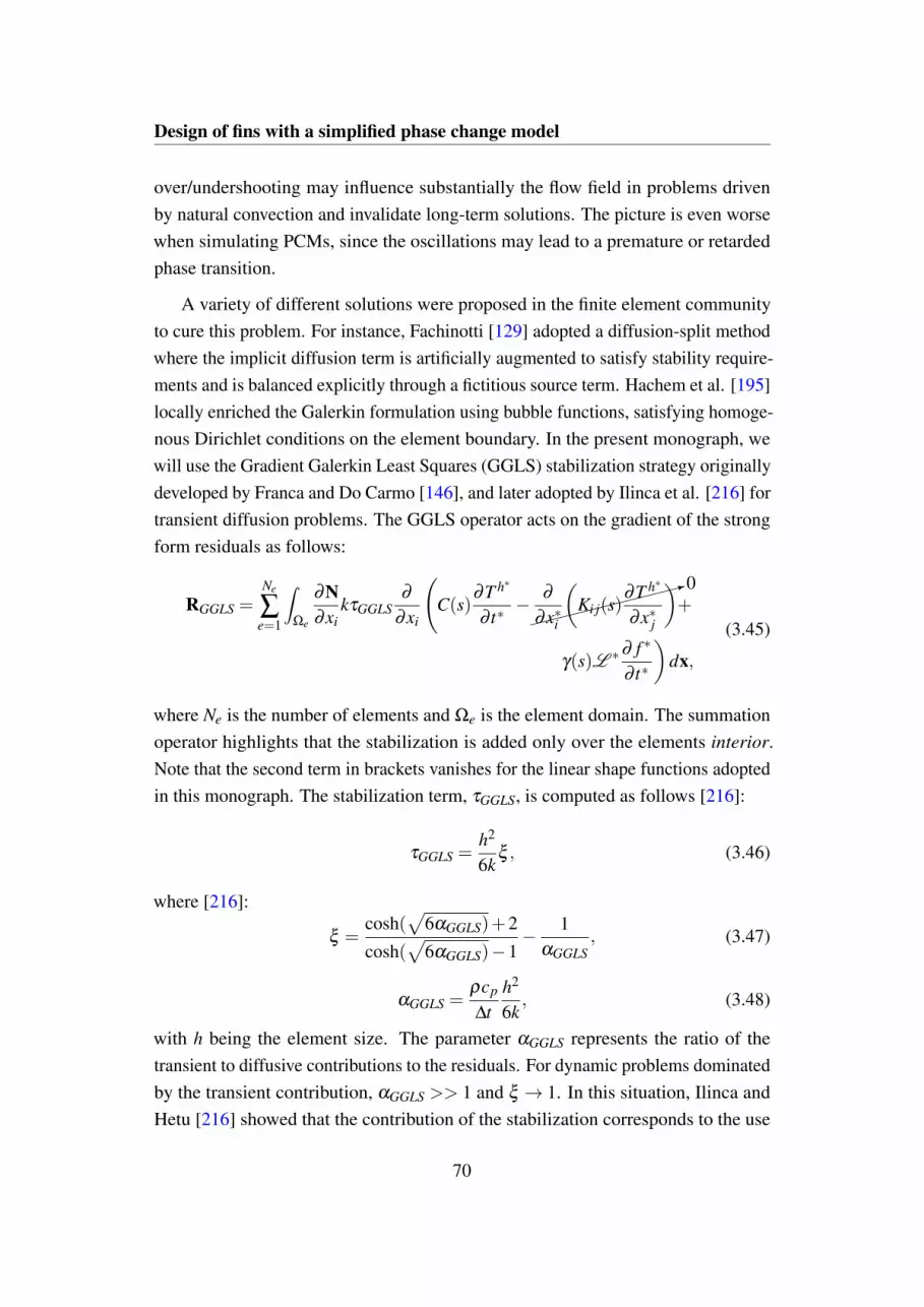
Design of fins with a simplified phase change model
over/undershooting may influence substantially the flow field in problems drivenby natural convection and invalidate long-term solutions. The picture is even worsewhen simulating PCMs, since the oscillations may lead to a premature or retardedphase transition.
A variety of different solutions were proposed in the finite element communityto cure this problem. For instance, Fachinotti [129] adopted a diffusion-split methodwhere the implicit diffusion term is artificially augmented to satisfy stability require-ments and is balanced explicitly through a fictitious source term. Hachem et al. [195]locally enriched the Galerkin formulation using bubble functions, satisfying homoge-nous Dirichlet conditions on the element boundary. In the present monograph, wewill use the Gradient Galerkin Least Squares (GGLS) stabilization strategy originallydeveloped by Franca and Do Carmo [146], and later adopted by Ilinca et al. [216] fortransient diffusion problems. The GGLS operator acts on the gradient of the strongform residuals as follows:
RGGLS =Ne
∑e=1
∫Ωe
∂N∂xi
kτGGLS∂
∂xi
(C(s)
∂T h∗
∂ t∗−:0
∂
∂x∗i
(Ki j(s)
∂T h∗
∂x∗j
)+
γ(s)L ∗∂ f ∗
∂ t∗
)dx,
(3.45)
where Ne is the number of elements and Ωe is the element domain. The summationoperator highlights that the stabilization is added only over the elements interior.Note that the second term in brackets vanishes for the linear shape functions adoptedin this monograph. The stabilization term, τGGLS, is computed as follows [216]:
τGGLS =h2
6kξ , (3.46)
where [216]:
ξ =cosh(
√6αGGLS)+2
cosh(√
6αGGLS)−1− 1
αGGLS, (3.47)
αGGLS =ρcp
∆th2
6k, (3.48)
with h being the element size. The parameter αGGLS represents the ratio of thetransient to diffusive contributions to the residuals. For dynamic problems dominatedby the transient contribution, αGGLS >> 1 and ξ → 1. In this situation, Ilinca andHetu [216] showed that the contribution of the stabilization corresponds to the use
70

3.3 Numerical model
of an artificial conductivity defined as:
ka = kαGGLS. (3.49)
The smoothing effect of the GGLS stabilization is demonstrated for a 1D phasechange problem similar to the one considered in the current chapter. We considera finite slab of length L = 1, initially at temperature T ∗I = 0.5 and connected to ahot thermostat on the right side at temperature T ∗r = 0.5. The slab is filled withPCM, with melting temperature T ∗m = 0 and Stefan number Ste = 0.1. At t∗ > 0, theleft boundary is suddenly connected to a cold thermostat at temperature T ∗l =−0.5.Figure 3.7 shows the slab temperature at different time instants with and without theGGLS stabilization. The numerical results obtained without stabilization suffer froman unbounded solution. At t∗ = 1e−5, the computed temperature at the third, fifthand sixth node is not bounded between the values of the adjacent nodes. On the otherhand, the GGLS stabilization allows a physical solution to obtained. Figures 3.7(b)and (c) show that the time advancement gradually smooths both the undershoots andovershoots.
3.3.4 Temporal discretization
With the aim of converting the ODE obtained in (3.40) to a set of algebraic equations,a suitable temporal approximation scheme should be selected. In principle, onecould treat time as an additional (spatial) coordinate and discretize it using the finiteelement procedure presented in the previous section. This requires the specificationof both initial and final time conditions [117]. The common finite element practiceadopts a finite difference approximation via the Θ-method. The time derivative ofthe unknown vector is approximated using a two-point finite difference as follows:
T =T(n+1)−T(n)
∆t(n). (3.50)
A similar approximation can be adopted for the latent heat source term yielding:
L =L(n+1)−L(n)
∆t(n). (3.51)
71

Design of fins with a simplified phase change model
0 0.02 0.04 0.06 0.08 0.1
Horizontal coordinate [-]
-0.5
0
0.5
1
1.5
Dim
en
sio
nle
ss t
em
pe
ratu
re [
-]
Without GGLS
With GGLS
(a)
0 0.02 0.04 0.06 0.08 0.1
Horizontal coordinate [-]
-0.5
0
0.5
1
1.5
Dim
en
sio
nle
ss t
em
pe
ratu
re [
-]
(b)
0 0.02 0.04 0.06 0.08 0.1
Horizontal coordinate [-]
-0.5
0
0.5
1
1.5
Dim
en
sio
nle
ss t
em
pe
ratu
re [
-]
(c)
Fig. 3.7. Effect of the GGLS stabilization on over and under-shooting when advanc-ing with small time steps. (a): t∗ = 1e−5; (b): t∗ = 5e−5; (c): t∗ = 1e−4;
72

3.3 Numerical model
The static portion of the residuals is constructed using an intermediate temperaturecomputed as:
T = ΘT(n+1)+(1−Θ)T (n). (3.52)
The parameter Θ is a weighted average coefficient that defines wether the intermedi-ate temperature is closer to T (n+1) or to T (n). Different values of Θ leads to differentwell-know time discretization schemes such as [350]:
• the explicit Euler scheme with Θ = 0,
• the Crank-Nicolson scheme with Θ = 0.5,
• the Galerkin scheme with Θ = 2/3,
• the implicit Euler scheme with Θ = 1.
For Θ≥ 0.5, the time-marching is unconditionally stable [350]. This means that timerestrictions are not required to make the integration stable, i.e. with an ultimatelybounded error. In this thesis, we choose the implicit Euler scheme for its inherentrobustness and stability properties [433]. This corresponds to a 1st order BackwardDifferentiation Formula (BDF) scheme.
Using (3.50) through (3.52) in (3.40) with Θ = 1 leads to the following (fullydiscrete) unstabilized residuals:
R(n+1)us = C
T(n+1)−T(n)
∆t(n)+KT(n+1)+
L(n+1)(
T(n+1))−L(n)
(T(n)
)∆t(n)
. (3.53)
Augmenting (3.53) with the fully discrete version of (3.45) gives the residuals at thetime iteration (n+1), R(n+1). At the time-step n = 0, these equations reduce to satisfythe initial conditions:
R(0) = T(0)−T. (3.54)
For every subsequent time-step when n> 0, we solve the nonlinear problem R(n+1)=
0 through the Newton method, as discussed in the following section.
To obtain the results presented in this chapter, we advance in time using a fixedtime-step. A refined time-stepping strategy is proposed in 5.2.3 and used to produceall the results presented in Chapters 5 and 6.
73

Design of fins with a simplified phase change model
3.3.5 Nonlinear solution
To solve the nonlinear systems of equations arising in (3.53), we adopt the Newtonmethod for two main reasons. First, this method allows superior convergenceproperties than the simpler Picard iteration method [350]. It can be shown that theconvergence is quadratic if the second and third derivatives of the residual have somespecific properties [224]. Second, the discrete adjoint method for sensitivity analysispresented in Chapter 2 requires the computation of the Jacobian matrix. As theneed for Jacobian assembling is a basic requirement of Netwon method, the samepiece of code can then be used for both the forward and sensitivity analyses. Despitethese advantages, the Newton method has a small radius of convergence, which maycomplicate the solution in case of strong nonlinearities and/or a bad initial guess ofthe solution vector. In transient problems, the time steps can be iteratively adapted toobtain Newton convergence. As a matter of fact, a pseudo-transient continuation (orpseudo time-stepping) [237] can be used with Newton method to obtain the solutionof numerically challenging steady-state problems where no good approximation ofthe root is available.
To illustrate the Newton method, let us consider a generic iteration "k". We lookfor an iterative procedure resulting in a recursive relation of the form:
Tk+1 = Tk +αr∆Tk, (3.55)
where ∆Tk represents the update step, while αr is referred to as under(over)-relaxation factor and will be discussed next. Expanding the residual vector (3.53) ina Taylor series leads to:
0 = R(Tk)+∂R∂T
∣∣∣∣Tk
∆Tk +O(∆T)2, (3.56)
where the partial derivative of the residuals with respect to the state variables is theJacobian matrix (or tangent matrix):
J =∂R∂T
∣∣∣∣Tk. (3.57)
74

3.3 Numerical model
Neglecting higher order terms, solving (3.56) for ∆Tk and substituting in (3.55) leadsto:
Tk+1 = Tk−αrJ(Tk)−1R(Tk). (3.58)
The iterative procedure is stopped when the following convergence criteria is satis-fied:
F (||R(T k)||)< εnl, (3.59)
where εnl is a user-specified tolerance and F (||R(T k)||) is some measure of theresiduals norm. In this thesis, we adopt the following:
F (||R(T k)||) = ||R(T k)||2||R(T 0)||2
, (3.60)
where || · ||2 denotes the L2 norm. Let us now consider the time iteration (n+ 1),for which the Newton method is applied to compute T (n+1) and the previous statevariables field T (n) is known. Considering the fully discrete residual formulationpresented in (3.53), we can split the Jacobian as following:
J(n+1) = J(n+1)s +J(n+1)
dyn , (3.61)
where J(n+1)s and J(n+1)
dyn are the static and dynamic Jacobians, respectively. Due tothe absence of boundary fluxes, the former only contains the diffusion term:
J(n+1)s = K. (3.62)
The dynamic Jacobian is defined as:
J(n+1)dyn =
C∆t(n)
+1
∆t(n)∂L(n+1)
∂T(n+1)+J(n+1)
GGLS, (3.63)
where JGGLS is the Jacobian of the stabilization contribution. The second termaccounts for the latent heat source. Recalling Eq. (3.43), using the Leibniz integrationrule and the chain rule, we obtain:
∂L(n+1)
∂T(n+1)=∫Ω
NNTγL
∂ f∂T
dx. (3.64)
75

Design of fins with a simplified phase change model
ΩHCM
ΩPCM
0.3
Fig. 3.8. Verification of accuracy of the computational model. (a): Schematicof the geometry considered; (b): comparison of the temperature profiles at t∗ =0.01; 0.05; 0.09; 0.13; 0.17
In a similar manner, we elaborate the GGLS stabilization contribution (3.45) toobtain:
J(n+1)GGLS =
Ne
∑e=1
∫Ω
∂N∂xi
kτGGLS∂NT
∂xi
(C(s)∆t
+ γ(s)L1∆t
∂ f∂T
)dx. (3.65)
3.3.6 Model verification
The analysis framework presented in this section is verified on a reference problemagainst the results obtained with the finite element commercial package COMSOLMultiphysics [101]. We simulate the discharge of a storage unit with the geometryshown in Figure 3.8(a). The computational mesh is composed of 11970 quadrilateralbilinear elements with angular size ∆θ = 1 and radial size ∆r = r∆θ . A represen-tation is given in Figure 3.9(a). We use the same materials adopted for the designoptimization study reported in [374]. The relevant thermo-physical properties rewrit-ten in non-dimensional form are presented in Table 3.1 while all the relevant analysisparameters are summarized in Table 3.2. Figure 3.8(b) shows the temperatureprofile along the red line highlighted in Figure 3.8(a) at different time instants, i.e.
76

3.3 Numerical model
(a) (b)
Fig. 3.9. (a): 2D computational mesh; (b): 3D computational mesh
Table 3.1. Thermo-physical properties of materials in dimensionless settings
Description Symbol Value
Conductivity ratio kHCMkPCM
600
Capacitance ratio (ρcp)HCM(ρcp)PCM
1.6Dimensionless Latent heat L ∗ 20Dimensionless melting temperature T ∗m 0.5
Table 3.2. Relevant analysis parameters
Description Symbol Value
Boundary heat flux qn 0Imposed temperature T ∗d 0Initial temperature T ∗I 1
77

Design of fins with a simplified phase change model
t∗ = 0.01; 0.05; 0.09; 0.13; 0.17. We observe that the thermal response predictedby the current framework agrees well with the results obtained with COMSOL.The relative error L2 norm is computed as 4.01×10⁻⁴ with a standard deviation of1.66×10−4. These results suggest that the presented model and its implementationare able to predict with sufficient accuracy the discharge of LHTES units in whichthe convective effects are negligible.
3.4 Design optimization problem
The design of efficient fins for solidification enhancement in LHTES requires thatthe geometry fulfills the following design criteria:
1. it allows the discharge of the maximum amount of energy in the least time, inorder to utilize the full energy density potential of the unit,
2. it allows the retrieval of the energy at a constant rate, providing a steady poweroutput.
In the following sections, we will present three alternative optimization problemformulations. The Energy Minization (EM) and the Time Minimization (TM) aretwo alternatives targeting design criterion (1). The Steadiness Maximization (SM)formulation is devised for the design criterion (2).
3.4.1 Energy Minimization
The EM problem formulation represents the following design question: what is theoptimal topology of HCM that allows discharging the maximum amount of energyfrom a given amount of PCM in a given time period?
In mathematical terms this corresponds to:
minimizes
z(T∗(s),s) = E at t∗ = t∗f
subject to∫
ΩD
ρs(s) dx−Φ
∫ΩD
dx≤ 0
s ∈ S =RNs | smin ≤ si ≤ smax, i = 1, ...,Ns
, (3.66)
78

3.4 Design optimization problem
Fig. 3.10. Optimization problem formulations. (a): EM vs TM update; (b): ideal vsreal energy history used for Steadiness Maximization
where E =∫
ΩD
(CT ∗+ γ f ∗L∗) dx is the dimensionless energy content of the unit,
ρs = s is the projected design variable field corresponding to the normalized densityof HCM, s is the vector of design variables, Φ the maximum volume fraction ofHCM and Ns the number of design variables with upper and lower bounds denotedby smax and smin, respectively. The inequality constraint prevents the trivial solutionof having the entire design domain filled with HCM.
Figure 3.10(a) shows the discharge at two generic design iterations, i and i+1.In the EM procedure, the final time t∗f is fixed and dE(t∗f ) represents the objectivereduction achieved with the optimization iteration.
3.4.2 Time Minimization
The TM optimization problem formulation considers the following design question:what is the optimal topology of HCM that allows discharging a given amount of
79

Design of fins with a simplified phase change model
energy from a given amount of PCM in the least time? This translates into:
minimizes
z(T∗(s),s) = t∗f
subject to E−ΨE f c = 0 at t∗ = t∗f∫ΩD
ρs(s) dx−Φ
∫ΩD
dx≤ 0
s ∈ S =RNs | smin ≤ si ≤ smax, i = 1, ...,Ns
, (3.67)
where Ψ is a specified target energy fraction and E f c is the total dimensionlessenergy in the tank in the fully charged condition. Note that the optimizer does not seethe final energy equality constraint. This is enforced implicitly during the analysis byiteratively halving the time-step until the constraint is satisfied within a user-specifiederror tolerance, εt . An improved strategy to control the time-stepping such that thecondition is satisfied is presented in Section 5.2.3. Problem (3.67) is quite similarto (3.66) but presents the complication that the objective to be minimized is anindependent variable. For this reason, we linearize the energy history around thefinal time, t∗f , to obtain:
E(t∗) = E(t∗f )+dEdt∗
∣∣∣∣t∗=t∗f
(t∗− t∗f
)+O
((t∗− t∗f )
2). (3.68)
Neglecting higher order terms, rearranging and differentiating leads to:
dt∗fds
=
(− dE
dt∗
∣∣∣∣t∗=t∗f
)−1 dE(t∗)ds
, (3.69)
where dE(t∗f )/ds = 0 because E(t∗f ) is a constant in the TM procedure. Note thatthe linearization allowed reformulating an independent variable as a function ofa dependent variable, with respect to which design sensitivities can be computed.The objective gradients differ from the ones computed with the EM approach by amultiplication factor. Solving for (3.67) requires minimal code modifications withrespect to (3.66).
A schematic representation of the TM procedure is also shown in Figure 3.10(b).Here the final energy E f is fixed and dt∗f represents the objective reduction achievedwith the optimization iteration.
80

3.4 Design optimization problem
3.4.3 Steadiness Maximization
The SM formulation considers the following design question: what is the optimaltopology of HCM fins that maximizes the steadiness of the TES discharge? Mathe-matically:
minimizes
z(T∗(s),s) =∫ max
(t∗f , t∗fid
)0
(E(t∗)−Eid(t∗)
)2
dt∗
subject to E−ΨE f c = 0 at t∗ = t∗f∫ΩD
ρs(s) dx−Φ
∫ΩD
dx≤ 0
ht f = t∗f − t∗fid ≤ 0
s ∈ S =RNs | smin ≤ si ≤ smax, i = 1, ...,Ns
, (3.70)
where Eid(t∗) is an ideal discharge history with the following form:
Eid(t∗) =
E f c− E f c(1−Ψ)t∗fid
t∗ if t∗ ≤ t∗fid
ΨE f c if t∗ > t∗fid
, (3.71)
where t∗fid is an ideal discharge time. A representative sketch of the ideal dischargehistory is given in in Fig. 3.10(b). For t∗ ≤ t∗f d the energy history is linear, hence thepower output is steady. This is the reason why we refer to this approach as SteadinessMaximization. The second inequality constraint, ht f , imposes a maximum limit onthe discharge time and has the aim of providing control over this important designcriterion to avoid undesirably lengthy discharge processes. The design sensitivitieswith respect to it are computed using the chain rule as follows:
dht f
ds=
∂ht f
∂ t∗f
dt∗fds
(3.72)
where the second multiplication term is obtained as detailed in (3.69). For thecomputation of z in the cases in which t∗f < t∗fid , the real discharge history is taken asa constant E(t∗) = ΨE f c in the range t∗f < t∗f ≤ t∗fid . For t∗f > t∗fid , the optimizationproblem is infeasible. However, the GCMMA or MMA routines do not guarantee asequence of feasible solutions. The objective still needs to be computed in case ofintermediate non-feasible steps. This is the reason for the second case of (3.71).
81

Design of fins with a simplified phase change model
3.4.4 Material interpolation and regularization
As discussed in Section 2.4.1, topology optimization with density methods requires asmart interpolation strategy, driving the optimization process to binary 0; 1 designs.A suitable interpolation function should be identified for each design-dependentterm in the governing equation (3.26). For the numerical studies presented in thischapter, we adopt the classical SIMP approach (2.28). The conductivity, K(s), isinterpolated using a power-law exponent of 2. The capacitance, C(s), and the latentheat switch, γ(s), are interpolated linearly, so that no unnecessary nonlinearity isadded to the problem. In preliminary numerical studies, we observed that penalizingthe conductivity was sufficient to achieve a fair convergence to binary designs.
The regularization of the problem is here achieved through the linear filterpresented in Eq. (2.37). To cure the fuzziness introduced by the filter operator weadopt the "tanh" projection operator (Eq. (2.40)). We set the projection threshold,η , to 0.5 and the projection steepness parameter, β , to 1. Note that this choice ofparameters results in a mild projection that does not provide any feature size control.
3.4.5 Sensitivity analysis
The adjoint method presented in Section 2.3.2 is used to compute the optimizationcriteria gradients necessary to drive our gradient-based optimizer. For the sensitivityanalysis of transient problems, Eq. (2.26) can be generalized as follows. Let us aconsider a total residual vector, Rtot , where the contributions of all the time stepstaken from the time-solver are stacked sequentially:
Rtot = [R(0)T, R(1)T
, ..., R(Nt)T]T , (3.73)
where Nt is the total number of time steps. Proceeding in a similar manner for thegeneric state variable field u:
utot = [u(0)T, u(1)T
, ..., u(Nt)T]T . (3.74)
82
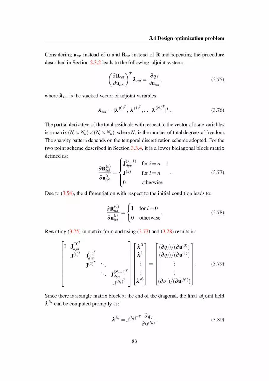
3.4 Design optimization problem
Considering utot instead of u and Rtot instead of R and repeating the proceduredescribed in Section 2.3.2 leads to the following adjoint system:(
∂Rtot
∂utot
)T
λλλ tot =∂q j
∂utot, (3.75)
where λλλ tot is the stacked vector of adjoint variables:
λλλ tot = [λλλ (0)T, λλλ
(1)T, ..., λλλ
(Nt)T]T . (3.76)
The partial derivative of the total residuals with respect to the vector of state variablesis a matrix (Nt×Nu)×(Nt×Nu), where Nu is the number of total degrees of freedom.The sparsity pattern depends on the temporal discretization scheme adopted. For thetwo point scheme described in Section 3.3.4, it is a lower bidiagonal block matrixdefined as:
∂R(n)tot
∂u(i)tot
=
J(n−1)
dyn for i = n−1
J(n) for i = n
0 otherwise
. (3.77)
Due to (3.54), the differentiation with respect to the initial condition leads to:
∂R(0)tot
∂u(i)tot
=
I for i = 0
0 otherwise. (3.78)
Rewriting (3.75) in matrix form and using (3.77) and (3.78) results in:
I J(0)T
dyn
J(1)T
J(1)T
dyn
J(2)T . . .
. . . J(Nt−1)T
dyn
J(Nt)T
λλλ0
λλλ1
...
...λλλ
Nt
=
(∂q j)/(∂u(0))
(∂q j)/(∂u(1))......
(∂q j)/(∂u(Nt))
. (3.79)
Since there is a single matrix block at the end of the diagonal, the final adjoint fieldλλλ
Nt can be computed promptly as:
λλλNt = J(Nt)
−T ∂q j
∂u(Nt). (3.80)
83

Design of fins with a simplified phase change model
Equation (3.79) can be then solved by backward substitution. This correspondsto the following backward time integration:(
J(n))T
λλλ(n) =
∂q j
∂u(n)−J(n)
T
dyn λλλ(n+1) (3.81)
for n = Nt − 1, ...,0. Finally, the discrete sensitivity field is calculated using thetime-dependent version of Eq. (2.27):
dq j
ds=
∂q j
∂ s−λλλ
Ttot
∂Rtot
∂ s. (3.82)
The assembly of Eqs. (3.82) and (3.81) requires the forward solution of the stateequations. For this reason, in this thesis the forward solutions are dumped on diskfor every time-step of the analysis. The backward time integration proceeds usingthe same time-steps adopted during the forward analysis.
3.4.6 Verification of accuracy of sensitivity analysis
The accuracy of the sensitivity analysis framework described in the previous sectionis checked against the sensitivities with respect to the TM objective obtained throughcentral finite differences:(
dzdsi
)f d=
z(si + εsi)− z(si− εsi))
2εsi
, (3.83)
where εsi is the perturbation size. The deviation is quantified on 30 design variablesthrough the L2 norm of the relative error. Figure 3.11 shows the results obtained fordifferent perturbation sizes on the initial design, corresponding to a homogeneousdesign variable field s = Φ, and on the optimized nominal design presented inSection 3.5.1. The minimum error is achieved for a perturbation size of εsi = 10−3
for both the initial and final design. Reducing the perturbation size from εsi =
10−1 to εsi = 10−4, yields a decrease of the error. As expected for central finitedifferences [196], the rate of convergence is quadratic (∼ O(ε2
si)) with respect to
the perturbation. For εsi < 10−4, the error increases again as cancellation dominates[196]. Overall, we observe an acceptable agreement between the analytical and finitedifference sensitivities. This suggests the correctness of our analytical derivationsand implementation.
84

3.5 Numerical results and design trends
-8 -6 -4 -2 0
Perturbation size (log10 scale) [-]
-8
-7.5
-7
-6.5
-6
-5.5
-5
-4.5
-4
-3.5
-3
Re
lative
err
or
no
rm (
log
10
sca
le)
[-]
Fig. 3.11. Finite difference check of adjoint sensitivities on the initial and finaloptimized designs
3.5 Numerical results and design trends
In this section, we describe the numerical studies and discuss the results obtained.For all the results presenter hereafter, the thermo-physical properties and analysisparameters are the same introduced for the verification study presented in the previoussection (see Tables 3.1 and 3.2). The design domain corresponds to the one depictedin Figure 3.6, which is discretized using the mesh adopted for the verification studyin Section 3.3.6 and shown in Figure 3.9(a). For the 3D design optimization studiespresented, the design domain corresponds to a linear out-of-plane extrusion of the 2Dgeometry, with adiabatic boundary conditions at the bottom and at the top. The heightZ of the quarter hollow cylinder is set to 3. The mesh has characteristic dimensions∆θ = 1.38, ∆r = 90 and ∆z = 0.025, yielding a total of 507000 hexahedral trilinearelements. A representation is shown in Figure 3.9(b). In all the numerical examples,the maximum volume fraction of HCM, Φ, is set to 10 %.
3.5.1 Nominal longitudinal design
Here, we illustrate how our topology optimization framework generates optimizedfin designs for a reference case with a target energy fraction, Ψ, of 5 %. This will bereferred to as nominal diffusion design.
85
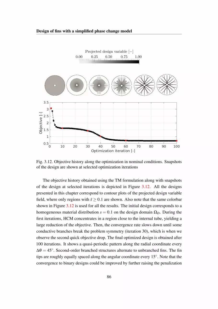
Design of fins with a simplified phase change model
Fig. 3.12. Objective history along the optimization in nominal conditions. Snapshotsof the design are shown at selected optimization iterations
The objective history obtained using the TM formulation along with snapshotsof the design at selected iterations is depicted in Figure 3.12. All the designspresented in this chapter correspond to contour plots of the projected design variablefield, where only regions with s≥ 0.1 are shown. Also note that the same colorbarshown in Figure 3.12 is used for all the results. The initial design corresponds to ahomogeneous material distribution s = 0.1 on the design domain ΩD. During thefirst iterations, HCM concentrates in a region close to the internal tube, yielding alarge reduction of the objective. Then, the convergence rate slows down until someconductive branches break the problem symmetry (iteration 30), which is when weobserve the second quick objective drop. The final optimized design is obtained after100 iterations. It shows a quasi-periodic pattern along the radial coordinate every∆θ = 45. Second-order branched structures alternate to unbranched fins. The fintips are roughly equally spaced along the angular coordinate every 15. Note that theconvergence to binary designs could be improved by further raising the penalization
86

3.5 Numerical results and design trends
Fig. 3.13. Optimized designs obtained by sweeping the energy constraint
exponent in the conductivity interpolation using a continuation scheme. However,this degree of convergence was considered satisfactory for diffusive structures. Amore aggressive penalization approach will be considered in Chapter 5, where theconvergence to binary designs is of crucial importance for the correct prediction ofthe flow dynamics.
3.5.2 The trade-off between time and discharged energy
In this section, we explore the inherent trade-off between the discharge time, t∗f , andthe target energy fraction, Ψ. We solve the optimization problem using both the TMand the EM approach.
First, we solve the TM problem (3.67) setting the target energy fraction, Ψ, to 2.5%, 5 %, 10 %, 25 %, 50 % and 80 %. The optimized designs obtained are depictedin Figure 3.13. Recall that the optimized design obtained for Ψ = 5 % correspondsto the nominal case that was presented in the previous section. As the target energyfraction, Ψ, increases, the characteristic length of the fins decreases to occupy asmaller region close to the internal tube leaving a hot external shell. Post-processingthe designs optimized for Ψ = 80 ;50 ;25 % reveals that the maximum length ofthe fins scales as lmax ∼
√1−Ψ. This trend is not visible at smaller energy fractions.
Once the fins achieve the length corresponding to the radius of the external envelope,the rate of the energy extraction is increased by moving HCM from the region closeto the internal pipe to the region close to the external shell. In the optimized designsfor Ψ = 10 % and Ψ = 2.5%, the internal tube is connected to fewer and thickerbranches, which ramify at a wider angle.
87

Design of fins with a simplified phase change model
Fig. 3.14. (a): Convergence to Pareto front with the TM and with the EM procedure;(b): converged Pareto front
Then, the optimized final time obtained is set as a constraint for 6 optimizationruns using the EM formulation (3.66). The initial and final performance curves inthe objective space are shown in Fig. 3.14(a). The TM performance curve movesalong the time axis (i.e. from right to left) during the optimization convergence.The EM performance curve moves along the energy axis (i.e. from top to bottom).The two approaches converge to the same Pareto front, that is presented in Figure3.14(b). A closer inspection reveals that the maximum relative deviation betweenthe two procedures is 2.75 %. This suggests that they can be used interchangeably toanswer two alternative design questions. However, in early studies we observed thatthe EM formulation gives a poorer performance when setting a high final time. Weconjecture that this behavior can arise as a result of badly scaled sensitivities due to atoo flat energy history but we did not investigated this further. Also, we noticed thatit might be challenging to set a reasonable final time as a constraint if the fin layout isunknown. The dynamics of the unit is largely influenced by the interpolation choiceand changes dramatically during the optimization convergence.
To exclude the possibility of convergence to poor local minima, we now cross-check the performance of the TM designs with different residual energy targetsΨ. Each design optimized for a certain Ψ is expected to perform better than theother designs in that particular Ψ condition. For each optimized design, Figure
88

3.5 Numerical results and design trends
Fig. 3.15. Performance cross-check on the optimized designs. (a): Entire Ψ spectrum;(b): zoom over the low Ψ spectrum
3.15(a) plots the discharge time increase as compared to the optimized design for thatparticular Ψ. It can be seen that the optimized designs perform as expected. We notethat either a badly designed or a badly utilized TES system can result in substantialperformance reductions, highlighting the importance of an accurate prediction ofthe discharge dynamics during the design optimization process. For instance, ifthe design optimized for Ψ = 80 % is used to discharge the tank up to Ψ = 10 %,nearly a 600 % time increase is obtained as compared to what required by the designoptimized for that situation. Taking a closer look at the low energy region (depictedin Fig. 3.15.(b)), which is the most meaningful for TES applications, we observe amuch more robust performance, i.e. the designs look slightly sensitive to changes inΨ. Our nominal design can be used for discharges down to Ψ = 10 % and Ψ = 2.5 %with less than 1 % performance reductions as compared to the structures optimizedfor those cases.
The results presented in this section demonstrate that topology optimizationallows the tracking of precise design trends along a Pareto front final time - final
89

Design of fins with a simplified phase change model
energy. The two design problem formulations give similar results but we reportedsuperior performance of the TM procedure in some specific cases. We also observedthat the proposed nominal design behaves robustly in the range of desired finalenergy values of interest for the development of practical LHTES systems.
3.5.3 Towards a constant power output
This numerical example aims at showing how topology optimization can addressmore complicated and interesting objectives for the design of LHTES units. Sensiblestorage systems where the same material is used as Heat Storage Medium (HSM)and HTF, e.g. domestic hot water storages, can deliver a high and constant thermalpower. This last feature is desirable in many applications in which the unit is directlylinked with downstream components such as refrigeration machines. In the LHTESsystems considered in this chapter, heat travels by diffusion from the internal pipe tothe PCM. As a result, the average temperature difference reduces exponentially intime, yielding a similar trend for the thermal power output. To manipulate the energyhistory and increase the steadiness of discharge, we adopt the optimization problemformulation (3.70).
To investigate how the ideal discharge time affects both the optimized designsand performance, we run four optimization cases with t∗fid = 1; 1.4; 1.8; 2.2. Theperformance of the optimized designs is shown in Figure 3.16. In the range of valuesconsidered, we observe a trade-off between discharge time and steadiness. Theobjective drops from the initial value of 6.1 when t∗fid = 1.0 to the final value of 2.6when when t∗fid = 2.2. On the right y-axis of Fig. 3.16, we plot an alternative metricto quantify steadiness: the dimensionless heat transfer drop. It is calculated as thedifference between the initial and the final heat transfer rate as follows:
∆q =∫
Γd
−ki j∂T ∗
∂x j
∣∣∣∣t∗=0
ni dx′−∫
Γd
−ki j∂T ∗
∂x j
∣∣∣∣t∗=t∗f
ni dx′. (3.84)
We observe that this second steadiness measure shows a trend comparable to the oneof the objective.
The optimized distribution of HCM for the four cases considered is shown inFigure 3.17. The "quick" design (i.e. t∗fid = 1.0) looks very similar to the optimizeddesigns of the previous section for the low Ψ region. As the discharge time increases,
90

3.5 Numerical results and design trends
Fig. 3.16. Trade-off between discharge time and steadiness of discharge
Fig. 3.17. Optimized designs obtained with the Steadiness Maximization approachfor different values of the ideal discharge time
91

Design of fins with a simplified phase change model
Fig. 3.18. Zoomed-in view of the region close to the internal tube.
more HCM is moved towards the external envelope through wide angle ramificationsand secondary branches. In the "slow" designs (i.e. with t∗fid = 1.8 and t∗fid = 2.2),the fin base is not in contact with the internal tube and leaves a small PCM gap. Forbetter visualization of the fin base disconnect, Figure 3.18 shows a zoomed-in viewinto the region close to the internal tube. This feature is effective in limiting the initialheat transfer rate but complicates the fabrication of the fin. Manufacturability is notconsidered in our optimization problem formulation and the practical realization ofthe device is beyond the scope of this chapter. However, the design trends obtainedthrough this numerical study can still be useful to identify possible manufacturingstrategies for steady power structures. For instance, a high porous metal matrixcould be installed in the PCM gap to provide mechanical support to the fins. Thedischarge histories of the four optimized designs is shown in Figure 3.19. To enhancethe readability, we plot on the x-axis the discharge time normalized with respect tothe ideal discharge time t∗fid . As the final time constraint is relaxed, the real energyhistory gets closer to the ideal one. A large performance improvement is achievableif the discharge time is increased from 1.0 to 1.4. Even the optimized design fort∗fid = 2.2 does not perfectly match the desired discharge history.
To show that the fin disconnect increases the performance, we manually alteredthe design optimized for t∗fid = 2.2 (referred to as disconnected design) and filledthe PCM gap with HCM to obtain the connected design shown in Figure 3.20(a),hereafter referred to as connected design 1. The energy histories for the two designsconsidered along with the ideal one are represented in Figure 3.20(b). The connecteddesign 1 yields a reduction of the total time needed for discharge. However, the
92

3.5 Numerical results and design trends
Fig. 3.19. Normalized energy history during the discharge for the 4 optimizeddesigns
Fig. 3.20. (a): Connected version of the disconnected optimized design obtained fort∗fid = 2.2; (b): comparison of the energy history during the discharge
93

Design of fins with a simplified phase change model
Table 3.3. Comparison of the connected and disconnected designs
Design
Performance Connected 1 Connected 2 Disconnected
Volume variation [%] + 1.710 - 0.001 0.000Discharge time [-] 1.77 1.81 2.20Objective [-] 14.63 14.21 2.68
disconnected design approximates better the ideal discharge curve. The area enclosedbetween the ideal discharge curve and the one of the disconnected design, i.e. A1, issmaller than the area enclosed between the ideal discharge curve and the one of theconnected design 1, i.e. A1 +A2. This demonstrates that a superior objective valueis obtained with the disconnected design. Our manipulation of the design field toclose the PCM gap resulted in a geometry for which the maximum volume fractionof HCM, Φ, is exceeded by 1.710 %. One may wonder whether this affects theoutcome of the previous analysis. For this reason, we iteratively raised the projectionthreshold, η , in (2.40) to produce a third layout for which the amount of HCMdiffers from the maximum allowed by only - 0.001 %. This geometry is referred toas connected design 2. The objective value and the discharge time registered for thethree cases are reported in Table 3.3. The results show that the connected designsresult in similar performance and the amount of HCM slightly affects the achievablesteadiness when all the fins are attached to the inner tube.
This example demonstrated that it is possible to manipulate the discharge historyof the LHTES unit to obtain a steadier power output. The steadiness measure isimproved through the use of a small PCM gap in contact with the HTF pipe thatcomplicates manufacturing.
3.5.4 The effect of melting temperature and conductivity ratio
This section studies the effect of the PCM thermo-physical properties on both theoptimized design and performance. To build physical intuition, we first consider aparametric analysis on the 1D problem presented in Figure 3.21. A bar composedof a matrix material, B, and an insert material, A, is initially at temperature T ∗I = 1,when suddenly comes in contact with a cold thermostat on the left boundary, Γd ,at a temperature of T ∗d = 0. The right boundary, Γn, is insulated. We monitor how
94

3.5 Numerical results and design trends
Fig. 3.21. Different setups used to investigate the effect of the melting temperatureon the discharge dynamics
Table 3.4. Parameters values used for the 4 cases considered in the 1D example
Parameter
Case KA CA L ∗A T ∗mA
KB CB L ∗B T ∗mB
1 sweeped 1 0 - 1 1 0 -2 1 sweeped 0 - 1 1 0 -3 1 0.66 0.66 sweeped 1 1 0 -4 1 1 60 sweeped 1 31 0 -
different topology choices, i.e. the placement of the insert in contact with either theleft or right boundary, and different material choices affect the discharge time. Asfor the nominal design, we consider Ψ = 5 %. The spatial discretization adoptedconsists of 500 linear Galerkin elements; the time integration is performed with a 1st
order BDF scheme with ∆t∗ = 0.001.
The material combinations investigated are summarized in Table 3.4. Cases 1and 2 consider A and B as two sensible materials, with no nonlinearity. The formeris intended to analyze the effect of the insert conductivity while the latter aims atinvestigating the effect of its specific heat. Cases 3 and 4 consider A as PCM andstudy the dynamics of nonlinear inserts embedded in a linear matrix for differentmelting temperatures. Case 3 analyzes a PCM with a small nonlinearity while Case4 considers a PCM with a large nonlinearity. To allow for meaningful comparisons,materials A and B are taken with the same integral capacitance in the temperature
95

Design of fins with a simplified phase change model
range 0≤ T ∗ ≤ 1 such that :
∫ 1
0
(C+
∂ f ∗
∂T ∗L ∗)
AdT ∗ =CB. (3.85)
The results of this parametric analysis are summarized in Figure 3.22. The ratiosreported on the x-axis correspond to the properties of material A divided by theproperties of material B. From the examination of Case 1 and Case 2, it can beconcluded that:
• The conductivity of the insert plays a relevant role on the discharge dynamicsonly when it is in contact with the Dirichlet boundary, i.e. in the regioncharacterized by high heat transfer.
• The specific heat of the insert influences remarkably the time required for thedischarge only when in contact with the Neumann boundary, i.e. in the regioncharacterized by low heat transfer.
• It is better to place high conductivity/high specific heat inserts close to theDirichlet boundary and low conductivity/low specific heat inserts close to theNeumann boundary.
For Cases 3 and, 4 we observe the following:
• The melting temperature has some effects on the discharge time only if theinsert is placed on the right boundary, i.e. the low heat transfer region.
• The melting temperature influences the optimal topology of the bar. Lowmelting temperature inserts are best placed close to the Neumann boundarywhile high melting temperature inserts should be positioned close to theDirichlet boundary. For high melting temperatures, the insert quickly gets ridof the latent heat during the high heat flux period (i.e. at the beginning of theprocess) and for the remaining part of the process behaves as a low capacitancematerial, that is best placed close to the Neumann boundary. On the otherhand, for low melting temperature inserts, the latent heat is withdrawn at theend of the process in a period characterized by low heat transfer regimes. Inthis latter case, it is better to choose the left boundary configuration, whichmakes the discharge time nearly insensitive to the insert capacitance.
96

3.5 Numerical results and design trends
Fig. 3.22. Results of the 1D parametric analysis
97

Design of fins with a simplified phase change model
Fig. 3.23. Effect of the melting temperature on the final design. The full linearmaterial is shown in black, the nonlinear material in white while intermediatedphases are in gray
• The magnitude of this effect increases with the nonlinearity of the insert: acloser look at the y scale shows that the effect is negligible for Case 3 andbecomes dominant for Case 4.
Now we use topology optimization to find the optimal topology of material A andB with the problem set-up considered in previous examples (Fig. 3.6). We choosethe materials considered for Case 4. Note that only for this example, the volumefraction Φ is set to 0.5. Figure 3.23 shows the final designs obtained for 3 differentmelting temperatures, i.e. 0.1, 0.5 and 0.9. The linear material is shown in black, thenonlinear material in white while intermediate phases are in gray. For low meltingtemperatures, the nonlinear material is aggregated towards the internal tube; for highmelting temperatures, it is confined on the external shell. The optimization withT ∗m = 0.1 and T ∗m = 0.9 converges well to 0; 1 designs. On the other hand, the onewith T ∗m = 0.5 has still a considerable amount of gray material. The results obtainedwith the 1D problem showed that at intermediate melting temperatures, T ∗m ∼ 0.5,the latent heat slightly influences the optimal placement of the insert. Despite thisdifferent degree of convergence, the layout obtained with T ∗m = 0.5 confirms thefindings of the 1D example: the optimized topology should be similar to the oneobtained with T ∗m = 0.9, i.e. internal linear material/external nonlinear material.
To exclude the eventuality of convergence to unsatisfactory local minima, weperform a cross-check optimization run in which the optimized design for T ∗m = 0.1 isused as a starting solution to the problem with T ∗m = 0.9. The objective history alongwith snapshots of the designs at selected iterations is shown in Figure 3.24. Here,
98

3.5 Numerical results and design trends
Fig. 3.24. Objective history along the optimization when the optimized design forT ∗m = 0.1 is used as initial guess in the optimization problem with T ∗m = 0.9
the layouts are not clipped at s = 0.1 to facilitate the visualization of the evolution.We notice that it takes roughly 20 iterations to reverse the optimized design to anearly homogeneous distribution. From this point onward, the topology evolvessimilarly to what we observed for the design at T ∗m = 0.9, where nonlinear materialis progressively concentrated towards the external insulated boundary.
In this section, we demonstrated that the melting temperature can be responsibleof topological changes for specific material choices. However, we noticed negligibleeffects for material properties in the range of interest for practical TES applications.This study also suggests that a topology optimization framework can be useful forthe design of multi-PCM systems.
3.5.5 3D designs
In this section, we consider the design optimization of three-dimensional structuresusing the TM formulation.
The objective history and the design evolution along the optimization processfor the 3D design with Ψ = 5 % is shown in Figure 3.25. The layouts showncorresponds to iso-surfaces of the design variable field at s = 0.1. The design is
99

Design of fins with a simplified phase change model
(a) (b) (c) (d) (e)
0 20 40 60 80 100 120 140 160
Optimization iteration [-]
0.5
1
1.5
2
2.5
3
3.5
Ob
jective
[-]
Fig. 3.25. Objective history and design evolution along the optimization processfor the 3D design example with Ψ = 5 %. (a): Initial guess; (b): iteration 20; (c):iteration 40; (d): iteration 60; (e): iteration 100. The layouts shown corresponds toiso-surfaces of the design variable field at s = 0.1
100
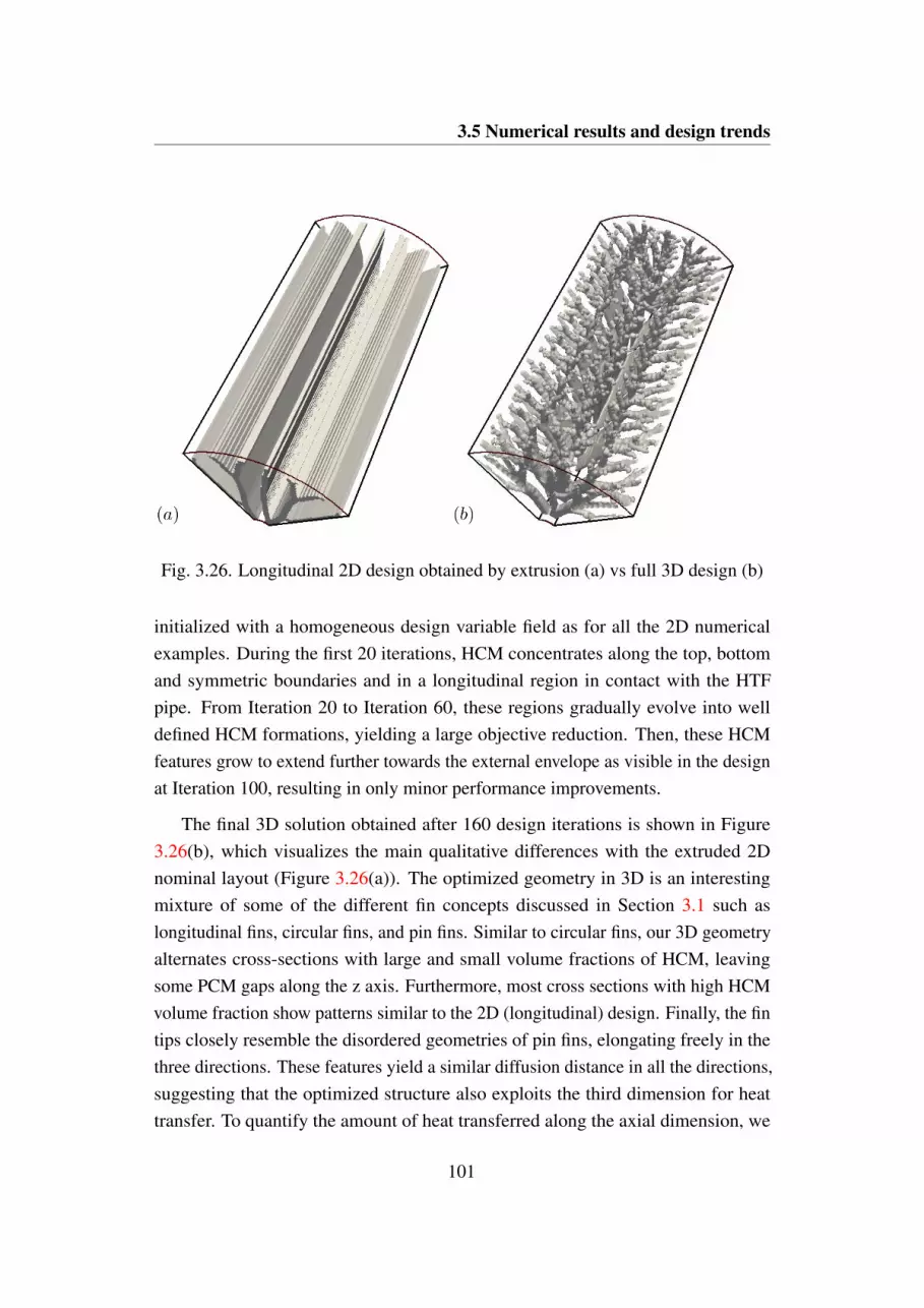
3.5 Numerical results and design trends
Fig. 3.26. Longitudinal 2D design obtained by extrusion (a) vs full 3D design (b)
initialized with a homogeneous design variable field as for all the 2D numericalexamples. During the first 20 iterations, HCM concentrates along the top, bottomand symmetric boundaries and in a longitudinal region in contact with the HTFpipe. From Iteration 20 to Iteration 60, these regions gradually evolve into welldefined HCM formations, yielding a large objective reduction. Then, these HCMfeatures grow to extend further towards the external envelope as visible in the designat Iteration 100, resulting in only minor performance improvements.
The final 3D solution obtained after 160 design iterations is shown in Figure3.26(b), which visualizes the main qualitative differences with the extruded 2Dnominal layout (Figure 3.26(a)). The optimized geometry in 3D is an interestingmixture of some of the different fin concepts discussed in Section 3.1 such aslongitudinal fins, circular fins, and pin fins. Similar to circular fins, our 3D geometryalternates cross-sections with large and small volume fractions of HCM, leavingsome PCM gaps along the z axis. Furthermore, most cross sections with high HCMvolume fraction show patterns similar to the 2D (longitudinal) design. Finally, the fintips closely resemble the disordered geometries of pin fins, elongating freely in thethree directions. These features yield a similar diffusion distance in all the directions,suggesting that the optimized structure also exploits the third dimension for heattransfer. To quantify the amount of heat transferred along the axial dimension, we
101

Design of fins with a simplified phase change model
Fig. 3.27. Visualization of the optimized 3D design. (a): Top view; (b): front view
adopted the following measure:
qz =||∇zT ∗||2||∇x,yT ∗||2
, (3.86)
where ∇ denotes the time-averaged gradient. Note that for every extruded 2D designwe have qz = 0 %. For the nominal 3D design, we obtain qz = 153 % meaning that alarge portion of heat is transferred along the axial direction. The front and top viewsvisible in Figure 3.27 display some additional details. As visible from the front view,the distribution of HCM concentrates more at the center than at the top and bottomboundaries. This agrees with the intuition that less HCM should be placed on theboundaries since less energy has to be extracted. Despite these boundary features,the design looks quasi-periodic along the z-axis. This suggests that structures withimproved performance can be expected to be obtained through optimization studiesthat consider a shorter portion of the shell with a higher design resolution.
We revisit the energy versus time trade-off in 3D with 3 different values of theenergy fraction, Ψ, i.e. 25 %, 10 % and 5 %. Figure 3.28(a) shows a comparisonbetween the Pareto fronts for the 3D and the 2D cases. Exploiting the third dimensionallows the Pareto front to be shifted towards smaller times. Figure 3.28(b) presents
102

3.6 Conclusions
Fig. 3.28. Performance improvement obtained by considering a full 3D optimization.(a): Shift of the Pareto front; (b): summary of absolute and percentage improvements
the absolute and relative improvements achieved. We report an average dischargetime reduction between 18.0 % and 22.6 % with respect to the corresponding 2Dcases. In the range of values considered, the advantages of accounting for the thirddimension in design studies increase for smaller desired energy fractions, Ψ.
This section highlighted the need for full 3D optimization strategies when de-signing TES systems with phase change. The optimized 3D designs not only showsome unexpected features but also outperform the 2D alternatives by roughly 20% due to the increased design freedom. We expect similar design trends in othervolume-to-line/volume-to-area maximum access problems such as those investigatedin [477].
3.6 Conclusions
In this chapter, we demonstrated the use of topology optimization for heat transferenhancement in LHTES units. A graphical summary of the main application-orientedadvances is presented in Figure 3.29. The design studies in two dimensions usingthe TM and the EM formulations converged on a smooth Pareto front residualenergy/process time. The trade-off among these design criteria manifests with highly
103

Design of fins with a simplified phase change model
Fin
al energ
y [%
]
Discharge time
80
25
2.5
2.5
Normalized discharge time
Fin
al energ
y [%
]
Fig. 3.29. Graphical summary of the main application-oriented advances of thechapter. (a): Design trend final energy/process time; (b): design features promotingthe power output steadiness; (c): 2D vs 3D geometries
104

3.6 Conclusions
different layouts and performance (Figure 3.29(a)). By including a measure of poweroutput steadiness in the objective, we obtained fin layouts that are disconnectedfrom the HTF pipe (Figure 3.29(b)). A PCM gap smooths the initial heat transferpeak but complicates the manufacturing process. Our investigations on the effectof PCM properties on the optimized layouts revealed that the melting temperaturecan be responsible of topological changes. However, those are expected to beof practical interests only for design of multi-PCM systems. Finally, moving toa 3D design domain yielded unintuitive features that were not not apparent inreduced dimensionality (Figure 3.29(c)). The optimized layouts freely span the threedimensions such that strong heat transfer is recorded along the direction parallel tothe HTF pipe. The increased design freedom led to an average 20 % reduction in thedischarge time.
The results presented were obtained using the assumption of negligible convectivetransport. This assumption is relaxed in Chapter 5 and Chapter 6, in which naturalconvection is considered in the analysis.
105

Chapter 4
Design of multi-scale conductingstructures
Engineered multi-scale structures offer exceptional design freedom. The materialproperties at the microscopic level can be finely controlled such that the the per-formance of devices is maximized for specific applications. Filling engineeredmulti-scale metal structures with PCMs leads to composites with spatially-varyingconductivity and capacitance that could be used for thermal storage, temperaturecontrol and thermal management applications. Recent advances in Additive Manufac-turing (AM) boosted a large research interest in multi-scale structures across variousfields of engineering. However, important technological flaws of AM still hamper thepractical applications. In this chapter, we propose a topology optimization frameworkto design assemblies of periodic cellular materials that can be fabricated by conven-tional manufacturing technologies. We demonstrate a multi-scale and multi-materialframework in which the structure, the layout of the material subdomains and theirmicro-structures are optimized concurrently. To limit the geometrical complexityat the macroscopic scale and comply with manufacturing requirements, our designmodel uses level-sets parametrized by geometric primitives.
The outline of the chapter is as following. In Section 4.1, we review the state-of-the-art multi-scale heat transfer structures with a focus on the manufacturingtechnologies and applications to LHTES units. Section 4.2 presents both the theoryand numerical model of our homogenization framework. The multi-scale and multi-material design methods are described in Section 4.3 and 4.4, respectively, while
106

4.1 Review of multi-scale heat transfer structures
the design models that use geometric primitives are discussed in 4.5. Section 4.6presents and discusses the numerical results obtained for both a steady-state heatsink and an LHTES unit. Finally, Section 4.7 summarizes the main findings andidentifies opportunities for future research.
Some of the contents of this chapter were presented at the 12th World Congressof Structural and Multidisciplinary Optimisation [C1] and are included in a paperdraft in preparation for submission to Computer Methods in Applied Mechanics andEngineering ([J6]).
4.1 Review of multi-scale heat transfer structures
Cellular solids can be classified according to the topology of the unit cell composingtheir reticular structure. Stochastic foams cannot be characterized by a single celland the topology cannot be controlled [443]. Due to the absent design possibilities,we refer to these geometries as non-engineered structures. Periodic structures arecharacterized by a unit cell that is repeated in either two directions (prismaticstructures or Linear Cellular Alloys (LCA) [204]) or three directions (truss or latticematerials) [443]. Although manufacturing constraints are present, in this latter casethe topology of the unit cell can be controlled to a certain extent. Recent advancesin manufacturing have led to a new class of cellular solids where the topologyof the reticular structure can be fully controlled with no need of periodicity. Thetopology of the cell can be tailored to location-specific requirements. These aregenerally referred to as architected cellular materials with ordered and location-specific structure [371]. Since the last two categories allow a precise design, werefer to both as engineered structures. Engineered and non-engineered multi-scalestructures can be further divided into open-cell and closed-cell. Open-cell structuresare composed of interconnected void regions, allowing a non-obstructed fluid flow[199]. Closed-cells structures are composed of separated enclosures.
The technologies available for impregnating PCM within open-cell structuresare mature. The direct infiltration is a viable route but potentially yields a largeamount of air bubbles trapped within the composites. According to the recent reviewof Zhang et al. [494], the most effective manufacturing method is the vacuumimpregnation. The fabrication of PCM-metal composites using cellular structureswith closed cells is also well-known. For instance, a possible approach is described
107
Design of multi-scale conducting structures
in [472], where the metal structure is slowly pressed into a mold occupied by theliquid PCM. A process similar to vacuum impregnation with no active mechanicalagents was described in [264]. In the following sections, we will briefly reviewthe manufacturing technologies and LHTES applications of multi-scale structures.Since the references mentioned above indicated that the fabrication methods of PCM-metal composites are well-established, we will focus only on the manufacturingtechnologies for empty cellular solids.
4.1.1 Non-engineered structures
Stochastic metal structures can be fabricated in a number of different ways. Banhart[40] divided the available processes in four categories depending on the state ofmatter of the metal during the fabrication. When using liquid metals, the most popularmanufacturing processes include foaming by direct gas injection or insertion of ablowing agent, solid-gas eutectic solidification and investment casting [40]. Sinteringis no doubt the most popular manufacturing process when using metals in the solidstate. A large control over the pore size and distribution [301] can be achieved ascompared to liquid-based metal processes and open-cell structures are generallyobtained [403]. Finally, stochastic foams can be obtained by electro-deposition andvapor deposition when the metal is in ionic and gaseous state [40]. Also in this lattercase, the manufacturing generally leads to open-cell structures [199]. Besides metals,another popular stochastic structure for heat transfer applications is CompressedExpanded Graphite (CEG). Natural graphite is first expanded by chemical andthermal treatment such that a 99.8 % porosity material is obtained [296]. Expandedgraphite can then be mechanically compressed as desired to obtain high conductingmatrices that are then impregnated with PCM. The large stochastic complexity ofgraphite matrix micro-structures in general leads to only moderate impregnationratios (∼ 80 % [296]).
Heat transfer enhancement in LHTES units using stochastic structures was anactive research field in the past decades. Cabeza et al. [72] compared the performanceof a commercial PCM-CEG composite to the one of stainless steel and copperpieces dispersions. Their experiments revealed the superiority of the CEG-PCMstructure due to the presence of uninterrupted heat transfer paths. Mills et al. [300]also focused on CEG-PCM composites and reported an increase in the thermalconductivity from 20 to 130 times as compared to the pure PCM. Their results
108

4.1 Review of multi-scale heat transfer structures
presented evidence that the typical uni-axial compression leads to large thermalconductivity anisotropies. The anisotropy issue is not observed in metal foamsdue to the different fabrication processes involved. This may be considered anadvantage with respect to CEG. Fleming et al. [140] investigated the use of acommercial aluminum foam for both melting and solidification of water. Theirexperimental results showed that the enhancement ranged from 100 % to 20 %for melting and solidification, respectively. This difference has to be attributedto the high thermal conductivity of the ice as compared to the liquid water. Tianand Cui [103] considered copper foams as a possible enhancement strategy. Theirexperiments revealed that the average heat transfer rate can be increased by 36 %during charge when compared to a case with pure PCM. The study of Zhou et al.[498] suggested that the utilization of metal foams may yield additional advantages.The authors observed a large reduction of the super-cooling effect in hydrate saltswhen embedded in metal stochastic structures. As early studies proved large benefitsof multi-scale structures for LHTES units, researchers are now investigating the effectof some grade parameters such as the pore density (given in Pores Per Inch (PPI))and porosity. The experiments performed by Atal et al. [36] had the aim of assessingthe effect of the porosity of aluminum foams on the performance of an LHTESunit. They concluded that a lower porosity leads to a faster discharge and charge.This trend is particularly noticeable at small heat transfer rates. Zhu and co-authors[504] investigated the effect of the pore density of an aluminum foam for meltingof PCM in a cavity. They found that a higher pore density leads to faster dischargedynamics due to the larger heat transfer area. The numerical results of Gao et al.[153] suggested that this trend can be questioned as natural convection is suppressedat high pore densities. The authors proposed an optimized structure with a porosityof 94 % and a pore density of 45 PPI. Recently, the trade-off between conductiveand convective transport suggested an interesting novel design concept. Metallicstructures can be placed only in areas interested by strong diffusion heat transfer insuch a way to leave undisturbed flow in areas interested by strong convective heattransfer. This reduces the costs by limiting the amount of HCM used. Xu et al. [475]investigated this simple idea on a shell-and-tube LHTES unit. The authors proposeda system in which the metal foam fills partially the shell and optimized the fillingheight. In a subsequent study [474], more advanced configurations of the porousinsert were investigated. A similar research [505] was conducted in the contextof thermal management of electronics. The authors found through experiments
109

Design of multi-scale conducting structures
that a partial fill may yield substantial costs savings at the expense of negligibleperformance drops.
4.1.2 Engineered structures
A growing interest in engineered cellular structures is arising in recent years [199].According to Tian et al. [420], periodic materials are superior to stochastic structuresfor heat transfer applications and there is a large room for design-related advances.Wadley [442] reviewed a wide range of fabrication processes for the mass productionof periodic cellular metals. The conventional hexagonal honeycomb structures canbe obtained by strip bonding of metal sheets and expansion [442]. The triangularand square honeycombs are easily fabricated by assembling slotted metal strips[442]. A wide variety of other topologies can be obtained by stacking corrugatedmetal sheets or by extrusion [442]. In this regard, a revolutionary manufacturingprocess was proposed in [91]. It consists of two steps. First, a metal oxide paste isextruded through a die. Then, the extruded medium is dried and reduced in hydrogenatmosphere so that the pure metal is recovered. A high flexibility in the distributionof the shapes and sizes of the unit cells is obtained. In the context of cellular metalswith 3D periodicity, lattice micro-structures can be fabricated through investmentcasting, folding of perforated metal sheets, weaving and braiding of metal wires[442]. As noted by Williams et al. [462], these fabrication strategies have limitedgeometrical freedom for shaping the macro-structure. Although in some specificcases it is possible to customize its shape to a certain extent (e.g. by smartly cuttingmetal panels and sheets in honeycomb and corrugated structures), in general thiscan be done only by conventional subtractive manufacturing. Furthermore, all themanufacturing processes mentioned so far yield a unique micro-structure within thematerial. Periodicity is a fabrication requirement. Recent advances in manufacturingled to a relaxation of this periodicity constraint. Thanks to a layer-by-layer buildingprocess, AM allows a matchless geometric freedom: the topology of the cell canbe varied at the macro-scale according to location-specific requirements. However,the adoption of metal-based AM is still hampered by its high costs, slow buildrates, residual thermal stresses and poor finishing of parts [462]. For these reasons,Williams et al. [462] proposed to use metal oxide as a printed agent and then sinterit in a reducing atmosphere to obtain a pure metal. This approach has similaritieswith the extrusion process described in [91]. Mun et al. [305] used AM to fabricate
110

4.1 Review of multi-scale heat transfer structures
a sacrificial pattern that was then used for molding and casting. This method allowsthe clustering of patterns for mass production at the cost of unavoidable periodicityof the 3D-printed parts. A similar method to combine AM and investment castingwas recently presented in [398]. In this case, the molds are directly printed withoutthe need for a sacrificial pattern.
One of the first studies considering engineered periodic structures for heat transferenhancement in LHTES units is the work of Hoogendoorn and Bart [208]. Moti-vated by the high cost of finned tubes, the authors tested conventional honeycomblayouts and aluminum thin strips. Their results revealed remarkable performanceimprovements as compared to pure PCM. A few years later, Bugaje [71] conductedsome experiments to assess the performance of a star matrix obtained from expandedaluminum. The authors observed that the enhancement effect is comparable butslightly lower than the one of fins, due to the thermal contact resistance. Followingthe advancements claimed by these seminal works, Tong et al. [422] conducted anumerical study to asses the effect of convection in LHTES units filled by metalmatrices. The authors obtained that convective effects modify the system dynamicsin a significant manner only during melting. No noticeable effect was observed forsolidification. An order of magnitude increase in thermal conductivity was laterreported by Nayak et al. [309] with an aluminum matrix submerged into Eicosane. Inboth the previous studies, the authors made no assumptions on the cellular topology:the conductivity and permeability were obtained by semi-empirical equations forporous media, similar to those adopted for the modeling of stochastic structures. Aspecific cellular layout was investigated by Mesalhy et al. [299], who consideredan orthogonal grid of circular fibers. The macroscopic conductivity was obtainedanalytically considering the micro-scale geometry. Their parametric study suggestedthat high porosities and high thermal conductivities are desirable features for largediffusion and convective transport in LHTES. Li and Wu [265] investigated a simi-lar structure but considered HCM connections with rectangular cross-section. Theauthors introduced no scale separation and the conductivity was obtained by directnumerical simulation. This approach allowed studying the influence of the poredensity on the performance. However, no analysis nor discussion on the effectof the cellular topology was presented. This topic was covered earlier by Fiedleret al. [139] and Tian et al. [420] in the context of heat transfer enhancement forelectronics cooling. The authors investigated various cellular layouts and found thatthe geometry plays a significant role for performance.
111

Design of multi-scale conducting structures
Fig. 4.1. Conceptual representation of the design model considered in this chapter.(a): Optimized periodic material; (b): optimized "machinable" assembly of periodicmaterials; (c): optimized "machinable" structure
4.1.3 Literature/technology gaps and design opportunities
From the literature and technology overview presented in the previous sections, wehighlight three important facts:
1. A matchless control over the mechanical properties of devices is possiblethrough architected materials with spatially-varying micro-structures [371].However, the current mass-scale manufacturing technologies for multi-scalemetal structures yield periodic cellular materials [91, 442, 305].
2. The macroscopic shape of the periodic structures fabricated by mass-productiontechnologies can be customized only by conventional machining [462], de-manding for design procedures with a tight control over their geometricalcomplexity.
3. The placement and macroscopic shape of multi-scale structures is crucial forsome applications, e.g. LHTES units [475, 474, 505].
In this chapter, we propose a design framework that creates optimized heat transferstructures building on the previous observations. A conceptual representation isgiven in Figure 4.1 for the dissipator geometry considered in Chapter 2. Inspiredby fact 1, we consider an assembly of a limited number of materials with localperiodicity. Given fact 2, we parametrize each material subdomain such that "well-behaved" "machinable" shapes are obtained. We optimize all the micro-structures
112

4.2 Homogenization
of the periodic materials as well as their aggregation layout. As the conventionalmanufacturing technologies were demonstrated for a large number of microscopiclayouts, we do not limit their geometrical complexity. Finally, considering facts 2and 3, we optimize also the "external" layout of the assembly, i.e. the structure, usingagain a "machinable" parametrization. To our knowledge, a unique paper [261] dealtwith multi-scale topology optimization with movable material subdomains. Theauthors of this recent valuable contribution used a discrete density-based descriptionat the macro-scale, which does not address fact 2. Furthermore, their heuristicdensity threshold demands the optimization of micro-structures with predefinedvolume fractions, which are free to evolve in our framework.
4.2 Homogenization
Computing system responses in highly heterogeneous media is of interest in manyfields of science and engineering. A direct numerical treatment is complicated bythe fact that the size of the period of the micro-structure, Y , is generally order ofmagnitudes smaller than the size of the medium filling the macroscopic domain, ΩD.Denoting by ε the ratio between the size of the period and the size of the medium, onecould identify the following scaling behavior for the number of degrees-of-freedomto be solved for [18]:
Ndo f ∼1
εNdim. (4.1)
Considering a typical multi-scale heat transfer structure (e.g. the 45 PPI foamproposed in [153]) filling a square cube with side length equal to 1 m, one obtainsa scale ratio of ε = 0.00085. According to (4.1), the direct numerical solution ofa multi-scale heat transfer problem in 3D involves a 1.6 × 10⁹ increase in degreesof freedom as compared to the analysis conducted in Chapter 3. To overcomethis difficulty, one can first consider a microscopic description of the problemand then formulate equivalent material models for the analysis at the macroscopicscale. There exist at least two approaches to achieve this goal. A typical route inengineering is the so-called Representative Volume Element (RVE) method. Theanalyst considers a microscopic problem on a period T of size ||Y || ≪ ||T || ≪ ||ΩD||.Then, a constitutive behavior is reconstructed by averaging the responses to a well-chosen set of loads. As noted by Allaire [18], the averaged property may dependon the sample size, load values and boundary conditions. The second method is
113

Design of multi-scale conducting structures
Fig. 4.2. Two-scale expansion in periodic medium
referred to as homogenization. Differently from the RVE approach, it has rigorousmathematical justifications. The homogenized properties are obtained from anasymptotic analysis on the characteristic inhomogeneity dimension, ε . This is themethod of choice for the analysis of the multi-scale heat transfer structures adoptedin this thesis. Figure 4.2 shows a representation of the scale separation for a periodicmedium in 2D. We assign a coordinate system x in R2 to the macro-scale problemin ΩD. The domain is composed by a set of periodic square cells with side lengthεY . Following standard conventions, we assign a local coordinate system y = x/ε inR2 to each of the cells. The factor 1/ε can be regarded as a "zoom" operator thatenlarges the size of the periodic cell such that it is comparable to the size of themedium at the macroscopic scale [202]. The periodicity assumption involves thatthe spatial variation of a generic physical property, e.g. the conductivity k, can bedescribed as follows [202]:
k(x+nY Y+y) = k(y), (4.2)
where nY is a diagonal translation matrix whose non-zero components, nii, arearbitrary integers.
In the following section, we will briefly present the fundamentals of the homoge-nization method. For the sake of brevity, we will not provide mathematical proofs.We refer the interested reader to the large body of literature on the topic, for instance[364, 118, 90, 18].
114

4.2 Homogenization
4.2.1 Two-scale asymptotic expansion
The two-scale representation inspires an intuitive reflection. Any physical responsewill present slow variations in x and fast variations in y. The key (heuristic) as-sumption of the homogenization method is to consider a response function of theform:
T (x)∼ T0(x,y)+ εT1(x,y)+ ε2T2(x,y)+ . . .+ ε
∞T∞(x,y), (4.3)
where each term Ti is a function of both scales x and y and Y-periodic in y. For thefollowing derivations, we can truncate the series at the second order. Eq. (4.3) isreferred to as two-scale asymptotic expansion or ansatz. Hassani and Hinton [202]noted that this technique was already used in the theory of vibrations. Using thechain rule, we obtain the following derivation rule:
dTi
dx=
∂Ti
∂x+
1ε
∂Ti
∂y. (4.4)
Now consider a steady-state diffusion problem such as the one described by Eq.(2.44). Here, we do not make any assumption on the boundary conditions and on theconductivity tensor which is in general anisotropic. We obtain:
− ∂
∂xi
(ki j(y)
∂T∂x j
)= qv. (4.5)
Since the medium is assumed as periodic, the conductivity depends only upon themicroscopic variable, y (Equation (4.2)). Casting the expansion (4.3) into (4.5) anddifferentiating using the rule (4.4) leads to the following cascade of equations [18]:
− ε−2[
∂
∂yi
(ki j(y)
∂T0(x,y)∂y j
)]− ε−1[
∂
∂yi
(ki j(y)
(∂T0(x,y)
∂x j+
∂T1(x,y)∂y j
))+
∂
∂xi
(ki j(y)
∂T0(x,y)∂y j
)]− ε
0[
∂
∂xi
(ki j(y)
(∂T0(x,y)
∂x j+
∂T1(x,y)∂y j
))+
∂
∂yi
(ki j(y)
(∂T1(x,y)
∂x j+
∂T2(x,y)∂y j
))]= qv.
(4.6)Noting that a power series in ε (such as Eq. (4.3)) is zero for all ε if the coefficientsare zero [18], we can solve (4.6) by considering separate equations for each power
115

Design of multi-scale conducting structures
of ε . Starting from ε−2, we obtain:
∂
∂yi
(ki j(y)
∂T0(x,y)∂y j
)= 0, (4.7)
that is a periodic problem in the microscopic domain, Y . It can be shown that allthe solutions to (4.7) differ by a lift function in x. Hence, the important conclusionbrought by (4.7) is that T0 is independent of y so that we can write:
T0(x,y) = T0(x). (4.8)
Using (4.8), the second ε−1 term in Eq. (4.6) disappears. We obtain the followingequation for ε−1:
∂
∂yi
(ki j(y)
(∂T0(x)
∂x j+
∂T1(x,y)∂y j
))= 0, (4.9)
which gives a relationship between T1 and T0. Since T1 is linear in the gradient of T0
with respect to x, without loss of generality it is possible to write:
T1(x,y) = ω(l)(y)
∂T0(x)∂xl
+ T1(x), (4.10)
which ω(l) is a y-dependent linearity weight and T1 is a constant in y. The substitutionof (4.10) into (4.9) leads to the following equation:
∂
∂yi
(ki j(y)
(e(l)j +
∂ω(l)(y)∂y j
))= 0, (4.11)
where e(l)j is a unit vector in the "l" direction. Here, ω(l) represents the "local
variation of temperature created by an average (or macroscopic) gradient", e(l)j [18].Augmenting the homogenization equation (4.11) with periodic boundary conditionsgives the so-called cell problem. The equation for ε0 reads:
− ∂
∂xi
(ki j(y)
(∂T0(x,y)
∂x j+
∂T1(x,y)∂y j
))− ∂
∂yi
(ki j(y)
(∂T1(x,y)
∂x j+
∂T2(x,y)∂y j
))= qv.
(4.12)
116

4.2 Homogenization
Integrating (4.12) over Y simplifies things a lot. This a consequence of a fact thatis easy to verify [202]: the integral over the period of the derivative of a periodicfunction is zero. Hence the second term in (4.12) disappears when taking the integral.The substitution of (4.10) into (4.12) and integration leads to:
1||Y ||
∫Y
[∂
∂xi
(ki j(y)
(∂ω(l)
∂y j
∂T0
∂xl+
∂T0
∂x j
))+qv
]dy = 0, (4.13)
which can be simplified by commuting the integral and differential operator and byrearranging the saturated indexes in the first term. These operations yield:
− ∂
∂xi
[1||Y ||
∫Y
(kil(y)
∂ω( j)
∂yl+ ki j(y)
)dy
]︸ ︷︷ ︸
kHi j
∂T0
∂x j= qv, (4.14)
where the term in bracket is the homogenized conductivity kHi j . Augmenting (4.14)
with the macroscopic boundary conditions gives the so-called homogenized problem.The state field T0 computed by solving (4.14) can be corrected using T1 and T2 torecover the oscillatory behavior. In this thesis, we neglect the correctors T1 and T2 inour homogenized solution. This approach is valid in the case of small ε values [18]as those of typical heat transfer structures. This assumption yields T = T0.
The homogenization framework can be easily adapted to the simplified phasechange model described in Chapter 3. One can modify the two-scale asymptoticexpansion (4.3) to allow for time-dependence:
T (t,x)∼ T0(t,x,y)+ εT1(t,x,y)+ ε2T2(t,x,y)+ . . .+ ε
∞T∞(t,x,y). (4.15)
The time dependence does not yield any contribution in Equations (4.7) and (4.9) asthe chain rule (4.4) only contributes to the spatial derivatives without affecting thetemporal derivatives. The cell problem is thus the same as the steady-state version(4.11). The homogenized macroscopic latent heat, L H , and specific heat, cH
p , canbe computed through a simple integral averaging [18]:
cHp =
1||Y ||
∫Y
cp(y) dy, (4.16)
117

Design of multi-scale conducting structures
L H =1||Y ||
∫YL (y) dy. (4.17)
A similar conclusion could have reached by intuition. The capacitance of the mediumis a bulk property: it is not affected by the topology of the micro-structure but onlyby the relative volume fractions of the material constituents.
4.2.2 Numerical solution of the cell problems
Solving the cell problems allows the components of the macroscopic conductivity tobe computed. A pseudo-algorithm is composed of two steps:
1. Solve (4.11) for all the Ndim independent unit gradients to obtain the periodicresponses, ω(i).
2. Post-process the periodic responses, ω(i), with the definition of the homoge-nized conductivity in (4.14) to compute all the components of the tensor. Dueto the symmetry of the conductivity tensor, only 3 components are neededwhen Ndim = 2.
Only in a few cases this procedure can be done analytically, e.g for rank laminatecomposites [201]. For general microscopic structures, the homogenized propertiescan be obtained by numerical means. In this thesis we follow the FE route. Detailedderivations of FE formulations for (4.11) in the context of linear elasticity arepresented in [173, 201] while a concise Matlab implementation is reported in [29].The weighted integral statement of the cell equation (4.11) over Y is written as:
∫Y
wh
(∂
∂yi
(ki j(y)
(e(l)j +
∂ω(l)(y)∂y j
)))dy = 0, (4.18)
where wh represents an admissible weighting function. Integrating by parts and ne-glecting the boundary integrals due to the periodicity condition leads to the followingweak form of the cell problem:
∫Y
∂wh
∂yiki j
∂ω(l)
∂y jdy+
∫Y
∂wh
∂yiki je
(l)j dy = 0. (4.19)
118

4.2 Homogenization
The periodic response, ω(l), is approximated by the trial function, ω(l)h. The weight-
ing and approximation functions are taken from the following function spaces:
UY = ω(l)h∈H 1(Y ); ω
(l)his Y-periodic on ∂Y,
VY = wh ∈H 1(Y ); wh = 0 on ∂Y,(4.20)
where UY and VY are Hilbert spaces consisting of scalar functions with squareintegrable first derivatives. We write the approximate periodic response as a productbetween nodal values and spatially-varying shape functions as following:
ω(l)(y)≃ ω
(l)h(y) =
Nn
∑i=1
Ni(y)ω(l)i = NT
ωωω(l), (4.21)
where ωωω(l) denotes a column vector with nodal values of ω(l). The test functionsare taken equal to the shape functions as in the Galerkin method, i.e. wh = N. Withthis assumption, the residuals, R(l)
m , of the weak-form Galerkin model for the cellequation read:
R(l)m = KY ωωω
(l)+ e(l) = 0, (4.22)
where KY has the same definition as in Eq. (3.42) but the integration is performed ofY rather than over Ω and the load vector e(l) is defined as:
e(l) =∫
Y
∂N∂yi
ki je(l)j dy. (4.23)
Solving (4.22) is simple as it is a linear system. The unique care in the solutionprocedure should be taken to deal with the periodic boundary conditions. In thisthesis, we adopt the method of Lagrange multipliers to enforce periodicity, usingmulti-freedom linear constraints. The vector of unknowns is augmented with thevector of Lagrange multipliers, one per each constraint. The microscopic conductivitymatrix, KY , is bordered to include the Lagrange multiplier contributions to the stateequations and the equations stating the connectivity between the degrees of freedom.This method was preferred over a master-slave elimination because of the easierimplementation within the presented numerical framework. However, this approachenlarges the dimensionality of the system matrix and its positive definiteness islost. For these reasons, elimination methods are generally preferred for numericalhomogenization as pointed out by the authors of [29].
119

Design of multi-scale conducting structures
4.2.3 Verification through forward homogenization
Here, we test the accuracy of the FE micro-scale analysis framework described inthe previous section.
Perrins et al. [331] investigated hexagonal and square arrays of high conductingcylinders embedded in a low conducting matrix material. They used a methoddevised by Rayleigh [348] to compute the effective conductivity of the compositematerial. Their analysis yielded analytical results in the form of a series expansion.For square arrays, the conductivity expression obtained from the truncation of theexpansion at the third order reads [331]:
kHii = kiiBM
1−2Φ
σ +Φ− 0.075422Φ6σ
σ2−1.060283Φ12 − 0.000076Φ12
σ
, (4.24)
where Φ is the volume fraction of the cylindrical inclusions and σ is a parameterdefined as:
σ =1+ k1− k
, (4.25)
where k is the conductivity ratio between the HCM cylinders and the BM matrix.The considered microscopic layout yields an isotropic medium, hence k11 = k22 andk12 = k21 = 0. We analyze a case with k = 10 and kiiBM = 1 and compare the resultsobtained for different volume fractions, Φ, of the HCM. For this choice of k, theanalytical expression (4.24) retains a precision of the predictions to the fourth digitup to a maximum volume fraction of Φ = 0.4 [331].
We solve the cell problem by FE analysis as described in the previous section.We consider a square microscopic domain, Y , with a side of length L = 1, which isdiscretized with quadrilateral bilinear elements. We use three alternative computa-tional grids: a coarse mesh with 20 × 20 elements with characteristic size hy = 0.05,an intermediate mesh with 50 × 50 elements with characteristic size hy = 0.02 and afine mesh with 100 × 100 elements with characteristic size hy = 0.01. The cylindersare represented in the analysis through a density approach. Verifying the geometryrepresentation model is also of interest here since this computational framework willbe used for the multi-scale analysis and design through topology optimization. Eachnode falling within the radius of the inclusions is assigned a microscopic designvariable of sm = 1, representing the HCM. A value of sm = 0 is assigned to the othernodes and represents the BM. The elemental densities are obtained by filtering the
120

4.2 Homogenization
0 0.1 0.2 0.3 0.4 0.5
Inclusion volume fraction [-]
1
1.5
2
2.5
Ho
mo
ge
niz
ed
co
nd
uctivity [
-]
Analytical: Perrins et al.
Numerical: 20 x 20
Numerical: 50 x 50
Numerical: 100 x 100
(a)
Reference geometry
Same geometry
Different geometry
(b)
Fig. 4.3. (a): Verification of the numerical homogenization framework throughcomparison with analytical predictions of Perrins et al. [331]; (b): discontinuity ofthe geometry representation with respect to the inclusion radius
nodal design variable field with (2.37) and projecting it using (2.40) with β = 1000.The filter radius is calculated such that elemental densities are simple average of thenodal design variable values. The steep projection applied helps to get rid of the"gray" material. In case it exists, the conductivity is interpolated linearly. Figure 4.3presents the homogenized conductivity obtained using the three meshes and the onepredicted using the analytical expression (4.24). The numerical curves approximatewell the analytical one. The absolute relative mean error and its standard deviationare 0.022 and 0.044 for the coarse mesh, 0.009 and 0.012 for the intermediate mesh,0.008 and 0.010 for the fine mesh. We notice that the accuracy of the predictionslightly deteriorates for high volume fractions. Furthermore a step-wise trend isvisible for the coarse mesh curve. This is a result of the density-based geometryrepresentation. As visible in Figure 4.3(b), the geometry changes are not continuouswith respect to the radius of the inclusion. When the radius is increased from thered circle to the blue circle, no geometry changes are observed. The same numberof nodes are contained within the circle. On the other hand, the geometry getsmodified when increasing the radius of the inclusion to create the green circle. Thisphenomenon yields only minimal effects as the mesh is refined.
121

Design of multi-scale conducting structures
4.3 Multi-scale analysis and design
In this section, we present multi-scale analysis and design approaches using topologyoptimization. First, we introduce material design through inverse homogenizationand verify the developed optimization capabilities using the array of cylindersconsidered in the previous section. Then, we present several multi-scale approacheswith particular focus on the one adopted in this thesis.
4.3.1 Material design
Homogenization allows the computation of effective macroscopic properties whenthe periodic micro-structure is known. From early days in topology optimization,researchers focused on inverse homogenization. This optimization problem addressesthe following design question: what is the microscopic layout required to obtain atarget macroscopic property? This branch of research is also referred to as materialdesign.
The first contribution to material design within the topology optimization com-munity can be traced back to Sigmund [389]. The author formulated the problemas a weight minimization with equality constraints prescribing the values of theelasticity tensor components. His results demonstrated that extremal macroscopicphysical properties can be obtained if the micro-structure is carefully controlled.In particular, materials with negative Poisson ratio were designed. This designframework was later used for bulk modulus maximization in three-phase composites[162] and for design of extremal (e.g. negative) thermal expansion [388] materials.In the field of heat transfer, several works dealt with the inverse homogenization ofconductivity-like properties. Hyun and Torquato [214] explored the micro-structuresfilling the gap between the HS bounds. Similarly, Zhou and Li [503, 501] usedtopology optimization to find the micro-structures realizing the Milton-Kohn (MK)bounds considering general three-phase anisotropic composites. Two-phase andthree-phase isotropic micro-structures lying on the theoretical bounds are found toconform to Vigdergauz-like [435] formations [74]. Following these early contri-butions, material design expanded rapidly to other fields such as the permeabilitymaximization in fluidic systems [181], design of functionally-graded materials [502],multi-functional materials [112], and metamaterials [115]. A thorough review onthe use of topology optimization for material design was recently published by
122

4.3 Multi-scale analysis and design
Cadman et al. [74]. According to the authors, two alternative optimization problemformulations gained popularity among researchers. The first formulation aims atobtaining extremal material properties. For instance, when seeking the compositewith minimal macroscopic conductivity the objective can be stated as:
z(sm) =Ndim
∑i=1
Ndim
∑j=1
kHi j (sm), (4.26)
The second formulation aims at obtaining a target value for each component ofthe conductivity tensor. In this case, the objective can be written using a quadraticmeasure of the deviation from the target:
z(sm) =Ndim
∑i=1
Ndim
∑j=1
(kH
i j (sm)− kH∗i j
)2, (4.27)
where kH∗i j denotes the target conductivity tensor. Since material design will be a
fundamental building block of our multi-scale framework, we perform a verificationexample. We consider the inverse version of the homogenization example of theprevious section. By imposing the target isotropic conductivity and the volumefraction of the inclusion, we aim at recovering a square array of cylindrical inclusionsas those investigated by Perrins et al. [331]. We consider the same design domain, Y ,adopted for the forward example and discretize it using the 100× 100 elements mesh.A design variable, sm, is assigned to each node of the mesh. The density filter (2.37)with r fm = 0.051 and the projection operator (2.40) with βm = 1 and ηm = 0.5 areused to obtain the microscopic physical design variables, ρsm , defined at the elementlevel. The objective is defined as in Eq. (4.27) using the conductivities calculatedwith Eq. (4.24) for a specified volume fraction, Φ, of HCM. The physical designvariable, ρsm , is used to interpolate the conductivity using a SIMP law (Equation(2.28)). The microscopic penalization exponent, pm, is raised every 200 designiterations using the following continuation scheme pm = 3; 5; 7. As we wish torecover a precise target volume fraction, the standard linear volume constraint (2.29)is modified as follows: (∫
Yρsmdy−Φ
∫Y
dy)2
− εΦ ≤ 0, (4.28)
123

Design of multi-scale conducting structures
(a) (b) (c)
Fig. 4.4. Verification of the current framework through inverse homogenization withdifferent volume fractions. (a): φ = 0.0804; (b): φ = 0.1256; (c): φ = 0.1809. Thered lines show the boundaries of the target HCM cylinders considered in Perrins etal. [331]
where εΦ is a small number here set to 1 × 10⁻⁴. The micro-structure layout isevolved using GCMMA with the same parameters listed in Table 2.1. The objec-tive and constraints sensitivities are calculated using the discrete adjoint methoddescribed in Section (2.3.2). Figure 4.4 presents the results obtained consideringinclusions or radius r = 0.16; 0.20; 0.24 corresponding to volume fractions ofΦ = 0.0804; 0.1256; 0.1809. The red lines represent the boundary of the targetcylindrical inclusions. The acceptable qualitative agreement suggests that our topol-ogy optimization framework for material design yields sufficiently accurate resultsto be integrated in a multi-scale design optimization framework.
4.3.2 Multi-scale design
Material design yields tailored micro-structures with desired macroscopic properties.However, their utilization in real macroscopic systems may be non-optimal due tothe complexity and variety of boundary conditions and performance metrics. Forthis reason, the idea of integrating the design at both scales arises naturally. The
124

4.3 Multi-scale analysis and design
designers can modify the micro-structure to tailor effective properties in such a waythat the performance of the macro-scale system is optimized.
The first contribution to multi-scale topology optimization is probably the hierar-chical method of Rodrigues et al. [355]. For each element of the macroscopic FEmesh a micro-structure is optimized. Hence, in general this multi-scale approachyields Ne different micro-structures. The flow of computations is organized in twonested loops. At the macro-scale (the outer loop), the optimal distribution of materialis sought to obtain maximum compliance under a volume constraint. At the micro-scale (the inner loop), the topology of the micro-structure is modified to yield localmaximum strain energy. The micro-scale problems are also subject to a maximumvolume constraint, fixed by the amount of material allocated in the macroscopicloop. This has clear similarities with the homogenization approach for topologyoptimization that was proposed by Bendsoe and Kikuchi [55] in the early days of themethod. However, in that seminal work [55], the authors limited the design freedomat the micro-scale to the angle and size of the rectangular holes. On the other hand,in [355] full design freedom is allowed at the micro-scale through the use of adensity-based geometry description. The hierarchical approach was later extendedto the optimization of 3D structures [93] and utilized for a variety of applicationssuch as bi-material laminated composite design [96] and bone remodelling [95]. Inan interesting recent development, Coelho et al. [94] modified the original approachconsidering a limited number of subdomains with a unique micro-structure. This isin contrast with the "point-wise varying micro-structure" of the original method andrepresents a step towards the practical manufacturing. The authors acknowledgedthat "the optimal solution obtained will depend on the designer experience to definea proper domain subdivision". For this reason, they first conducted some preliminarymulti-scale optimization runs using the original "point-wise" formulation; then, theyanalyzed the distribution of the composites and heuristically selected a suitabledomain subdivision. A nonlinear version of the hierarchical method was recently pre-sented in [308]. This paper introduced another modification to the original problemformulation. In this case, no macroscopic design variable enters the optimizationroutine. The material allocation at the macroscopic scale is entirely governed by themicroscopic design variables.
Although the hierarchical approach demonstrated to be effective in many cases,the inner iteration loop modifies the micro-structures and in turn affects the macro-scopic equilibrium. According to Xia and Breiktopf [469, 471], this "interface
125

Design of multi-scale conducting structures
nonlinearity" yields to divergence when used in BESO frameworks for topologyoptimization [212]. Hence, the authors adopted a FE2 strategy [138], where themicro-scale design is treated as a generalized nonlinear behavior. The advantages ofthis approach include an easy extension to problems with constitutive nonlinearitiesat the micro-scale and a possible utilization of reduced order models, see e.g. [470].Both the hierarchical and FE2 methods described so far are based on a clear decou-pling between the optimization processes at the microscopic and macroscopic scales.This allows a straightforward parallel implementation. However, the point-wisestrain energy maximization approach within the inner loop can hardly be extended toproblems beyond solid mechanics. Sivapuram et al. [397] recognized this difficultyand proposed a general decomposition strategy based on the objective and constraintslinearization that is applicable to any design problem.
An alternative and rather "exotic" approach for multi-scale design is Free MaterialOptimization (FMO), which dates back to the contributions [352, 52]. It consists ofsolving design optimization problems at the two scales in a sequential manner [372].The macro-scale problem is first solved using the constitutive properties as designvariables, e.g. the components of the conductivity tensor. Then, several materialdesign problems are solved to obtain the target properties. As noted by [397], astrong limitation of this approach is that it may be hard to set physics attainabilityconstraints on constitutive tensors and conservative assumptions are required in mostcases.
Instead of using homogenization to bridge the scales, Alexandersen and Lazarov[14, 15] used multi-scale FEM [119] for multi-scale design. Here, the structure iscompletely resolved and no scale separation is introduced. This approach yieldsthree advantages: it takes into consideration the finite size of microscopic structures,which is important when ε is not particularly small; it allows boundary effects tobe considered; it ensures the creation of fully connected microscopic structures.Following a similar research direction in which the structure is fully resolved, Wuand co-authors [468] recently considered the optimization of 3D-printed bone-likestructures. The micro-structures arise from the imposition of a p-norm aggregationof local volume constraints, computed with a filtering procedure similar to (2.37).Reticular structures were obtained also in the case of aligned principal stress di-rections through the use of an anisotropic filter. Resolving the full structure yieldsdiscrete problems, involving a large number of degrees of freedom. In [14], theauthors managed to limit the computational complexity by using the same spectral
126

4.3 Multi-scale analysis and design
preconditioner for several design iterations and by enforcing a periodicity conditionon the micro-structures. Despite these advances, the extensions of the method tocomplex multi-physics problems, requiring nonlinear and/or transient analysis, isstill considered a challenge.
Most of the multi-scale methods above can be seen as a "varying-gray" type ofoptimizations. A point-wise varying micro-structure is optimized. This questionsthe local periodicity assumption for homogenization and complicates manufacturing[94]. Motivated by this latter argument, Liu and Cheng [274] developed a multi-scaleoptimization procedure that considers a single periodic micro-structure within themacroscopic design domain, ΩD. The placement of the periodic composite at themacroscopic level is also optimized, yielding a concurrent material and structuredesign optimization framework. Note that optimizing a unique material and seekingits optimal placement does not fit within the hierarchical framework. When a uniquemicro-structure is considered, the design changes at the macro-scale would beprevented. The method is based on two sets of design variables:
• sm ∈ [0, 1] governing the micro-structure topology in such a way that ρsm(sm)=
1 denotes material and ρsm(sm) = 0 denotes BM or void in the microscopicdesign domain, Y . The microscopic physical design variables, ρsm , are used tointerpolate the material properties when solving the cell problem (4.11) usinga conventional SIMP procedure such as (Equation (2.28)):
kmi j(ρsm) = ki jBM +(ki jHCM − ki jBM)ρ
pmsm
, (4.29)
where kmi j is the value of conductivity adopted in the micro-scale problem. In
the original paper [274], the authors adopted neither filtering nor projection atthe micro-scale such that ρsm = sm.
• sM ∈ [0, 1] governing the macro-structure topology in such a way that ρsM0(sM)=
1 denotes composite and ρsM0(sM) = 0 denotes BM or void in the macroscopic
design domain, ΩD. The macroscopic physical design variables, ρsM0, are
used to interpolate the homogenized material properties when solving themacroscopic problem. Considering the conductivity, we have:
ki j(ρsM0,ρsm) = ki jBM +(kH
i j (ρsm)− ki jBM)ρpMsM0
, (4.30)
127

Design of multi-scale conducting structures
Fig. 4.5. Graphical representation of the PAMP multi-scale design model
where pM is the macroscopic SIMP exponent; the homogenized conductivity,kH
i j , depends on the microscopic design variables, ρsm , through the utilizationof (4.29) when solving the cell problem (4.11). The subscript "0" in ρsM0
denotes the density field of the structure and is used to distinguish it from othermacroscopic density fields arising in our multi-material design optimizationframework. In the original paper [274], the authors adopted neither filteringnor projection at the macro-scale such that ρsM0
= sM. Although Eq. (4.30)can be regarded as a SIMP procedure at the macro-scale, the homogenizedproperties are in general anisotropic. Hence, the authors [274] named thematerial law (4.30) as Porous Anisotropic Material with Penalization (PAMP)interpolation.
In contrast to the typical mono-scale topology optimization procedures where a"black-white" design is sought and to the previously described "varying-gray" multi-scale framework, this approach tries to obtain "gray-white" material configurations[274]. A graphical representation of the PAMP design model for the dissipator geom-etry considered in Chapter 2 is given in Figure 4.5. Both the set of design variablesare updated following a one-shot procedure without inner optimization loops. Theoptimization problem can then be formulated without particular modifications withrespect to the mono-scale case. A simple augmentation of the design variable setis required to include both sm and sM. In their seminal paper [274], Liu and Chengconstrained the local volume fraction of the composite to comply with practical
128

4.4 Multi-material analysis and design
fabrication techniques. We did not find this fabrication requirement in the successiveworks of their research group. The examples of application of this method spandifferent fields of engineering. For instance, Niu et al. [311] designed multi-scalestructures for maximized dynamic performance, Guo et al. [190] considered compli-ance maximization under load uncertainties while in [113] the authors applied thePAMP optimization procedure to thermoelastic problems.
The ability to optimize a single microscopic structure and to find the optimizedplacement of this composite in the macroscopic domain is a unique feature of thePAMP framework. Due to the manufacturing requirements highlighted in Section4.1, we build primarily on this approach to develop our multi-scale design framework.We extend the original method in two ways. First, instead of a unique micro-structure,we consider a fixed number of different micro-structures filling different subdomains.We control the geometry of the subdomains using a multi-material design framework(see Section 4.4). Second, we parametrize both the structure and the subdomainsusing geometric primitives to allow a higher control over the geometrical complexity(see Section 4.5). The layout of the structure is evolved using a structure level setfield, φ0(sM). This geometry description is then mapped to the elemental densityfield, ρsM0
, as described in Section 4.4.1
4.4 Multi-material analysis and design
The advances in topology optimization towards multi-material devices proceededin a number of different directions. Early developments along the density-basedroute can be found in [388], [162] and [386]. Using material design through inversehomogenization, the authors designed the micro-structure of a composite madeof two materials and void. Their approach requires two density fields. A genericmaterial property, (·), is interpolated as follows [388]:
(·) = ρpsM0
((1−ρ
psM1
)(·)1 +ρpsM1
(·)2
). (4.31)
In Eq. (4.31), ρsM0is used to define the transition between the structure and void
as done for single-material SIMP and is usually augmented with a (·)min to preventsingularities in the solution of the physical problem. The second density variablecan be seen as a mixture coefficient such that ρsM1
= 1 denotes pure material 2 while
129
Design of multi-scale conducting structures
ρs1 = 0 denotes pure material 1. The material interpolation law (4.31) was laterextended in [404] to allow an arbitrary number of material phases, Nm, through theintroduction of Nm−1 design variable fields. The generalization of (4.31) can bewritten as follows [404]:
(·) = ρpsM0
(Nm−1
∑j=1
j−1
∏i=1
ρpsMi
(1−ρ
psM j
)(·) j +
Nm−1
∏i=1
ρpsMi
(·)Nm
). (4.32)
The authors noted that premature convergence to unsatisfactory local minima waslikely with a high number of material phases. Hence, both a modified penalizationstrategy and an alternative weighting of the material properties were proposed.This framework is referred to as Discrete Material Optimization (DMO). Anotherapproach that is worth of mention in the density direction is the one followed by Yinet al. [481]. The authors used an exponential peak function model to describe thetransition between different materials. This allows the inclusion of any number ofmaterials if the "width" of the material peaks is sufficiently small. The advantageof this method is that it requires the introduction of a single design variable field.However, to our knowledge this approach encountered limited popularity.
The earliest level-set treatments of multiple material phases built on the partition-ing level-set scheme. This method was developed in [497] to simulate the behaviorof bubbles and droplets in complex multi-phase flows. Each material domain, Ωi, isparametrized by a unique level set field, φi, such that:
Ωi(x) = x ∈Ω : φi(x)> 0. (4.33)
The computational domain, Ω, is partitioned in a family of Nm material domainsΩ1; Ω2; . . . ; ΩNm such that:
Ω =Nm⋃i=1
Ωi, Ωi∩Ω j = /0 for i = j. (4.34)
Using this approach requires Nm− 1 level-set fields since the BM or void is notparametrized explicitly. In design optimization studies, the number of design vari-ables, Ns, scales linearly with the number of materials as in multi-material SIMP.Due to (4.33), this method requires no-overlap between the positive level-set regions.This should be enforced in the optimization process yielding Nm− 2 constraints
130

4.4 Multi-material analysis and design
that may impact the regularity of the optimization problem and the computationalcomplexity of its solution procedure. A similar drawback is shared by the piece-wiseconstant level-set model used in [266, 414, 282]. Although this approach has theadvantage of using a unique LSF, the material overlaps should be impeded explic-itly in the optimization process. Wang and Wang [451] presented a multi-materialtopology optimization method in which the level-sets do not directly represent thematerial domains. This decoupling strategy allows the overlap of the positive level-set regions, eliminating the need for non-overlap constraints. The interface betweenall the materials, Γm, is obtained from the union of all the level-set zero contours:
Γm =Nm⋃i=1
Γi, Γi(x′) = x′ : φi(x) = 0. (4.35)
The material domains are then identified by all the regions bordered by Γm. Thismeans that the intersections of the positive level-set regions now represent additionalmaterial domains. Collecting all the level-set functions in a unique vector φφφ =
[φ1, φ2, . . . , φNm−1]T , this material parametrization concept can be expressed in
vector form:Ωi(x) = x ∈Ω : H(φφφ) = vi, (4.36)
where vvvi is a constant vector with components vi j ∈ 0; 1 and H is a vectorHeaviside function. Since the authors took inspiration from a level-set framework[434] developed for image processing, this multi-material treatment is commonlyreferred to as "color" level-set. This approach yields Nm = 2Nφ material domainswith Nφ being the number of level-sets. The color level-set method was appliedsuccessfully to several optimization problems, ranging from stress-based design[189] to heat transfer [506] and metamaterial design [458].
Although this improved scaling behavior of Nφ with respect to Nm significantlydecreases the computational complexity, such a high number of material domainsmay be undesirable. For instance, if one wishes to optimize the configuration offive materials, three level-sets are needed and three redundant material phases arecreated. A suitable rule should be identified to treat them in the analysis. For thisreason, Wang et al. [457] reverted to a linear Nφ - Nm scaling. The material domains
131
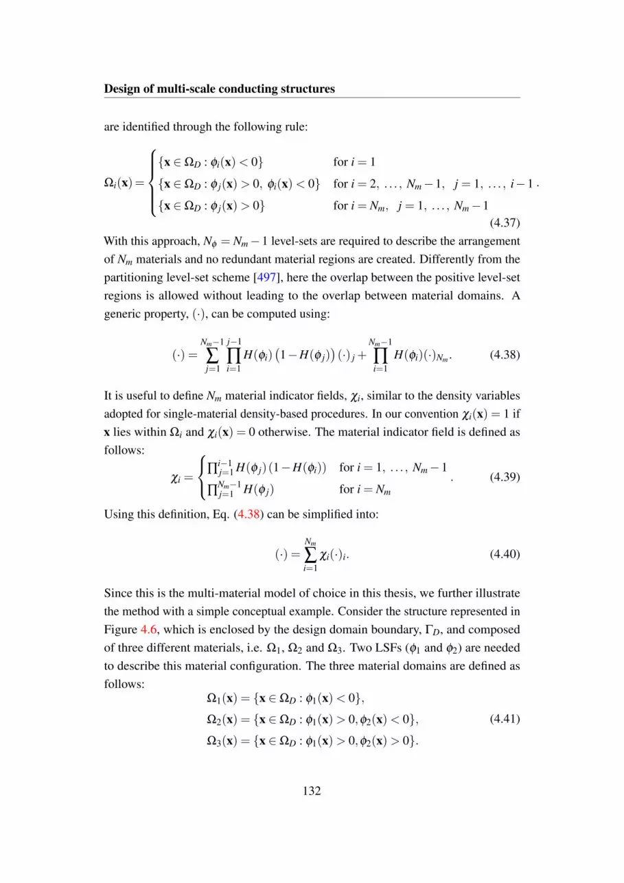
Design of multi-scale conducting structures
are identified through the following rule:
Ωi(x)=
x ∈ΩD : φi(x)< 0 for i = 1
x ∈ΩD : φ j(x)> 0, φi(x)< 0 for i = 2, . . . , Nm−1, j = 1, . . . , i−1
x ∈ΩD : φ j(x)> 0 for i = Nm, j = 1, . . . , Nm−1
.
(4.37)With this approach, Nφ = Nm−1 level-sets are required to describe the arrangementof Nm materials and no redundant material regions are created. Differently from thepartitioning level-set scheme [497], here the overlap between the positive level-setregions is allowed without leading to the overlap between material domains. Ageneric property, (·), can be computed using:
(·) =Nm−1
∑j=1
j−1
∏i=1
H(φi)(1−H(φ j)
)(·) j +
Nm−1
∏i=1
H(φi)(·)Nm. (4.38)
It is useful to define Nm material indicator fields, χi, similar to the density variablesadopted for single-material density-based procedures. In our convention χi(x) = 1 ifx lies within Ωi and χi(x) = 0 otherwise. The material indicator field is defined asfollows:
χi =
∏i−1j=1 H(φ j)(1−H(φi)) for i = 1, . . . , Nm−1
∏Nm−1j=1 H(φ j) for i = Nm
. (4.39)
Using this definition, Eq. (4.38) can be simplified into:
(·) =Nm
∑i=1
χi(·)i. (4.40)
Since this is the multi-material model of choice in this thesis, we further illustratethe method with a simple conceptual example. Consider the structure represented inFigure 4.6, which is enclosed by the design domain boundary, ΓD, and composedof three different materials, i.e. Ω1, Ω2 and Ω3. Two LSFs (φ1 and φ2) are neededto describe this material configuration. The three material domains are defined asfollows:
Ω1(x) = x ∈ΩD : φ1(x)< 0,Ω2(x) = x ∈ΩD : φ1(x)> 0,φ2(x)< 0,Ω3(x) = x ∈ΩD : φ1(x)> 0,φ2(x)> 0.
(4.41)
132

4.4 Multi-material analysis and design
z
Fig. 4.6. Schematic of the multi-material level-set model adopted in this thesis (Wanget al. [457])
Using (4.39), the material indicator functions for this case are computed as:
χ1 = 1−H(φ1),
χ2 = H(φ1)(1−H(φ2)) ,
χ3 = H(φ1)H(φ2).
(4.42)
As noted by the authors of [457], the explicit expression (4.38) facilitates the sen-sitivity analysis. We add that another key advantage of (4.38) is that it allows astraightforward integration with density-based analysis models. Although this ap-proach has several similarities with the multi-material density-based mixture model(4.31), a level-set description is here utilized. When using level-sets parametrized bygeometric primitives, we can benefit of an easier control on the geometrical com-plexity of the material domains. This allows obtaining "well-behaved" "machinable"shapes as those required by the conventional fabrication methods of multi-scale struc-tures (see Section 4.1). Further details on the geometric primitive design frameworkwill be given in the Section 4.5.
133
Design of multi-scale conducting structures
4.4.1 Density-based mapping of level-sets
In this chapter, we account for the level-set geometry description in the analysismodel by using a density-based procedure that allows an easy integration with themacroscopic analysis framework described in Chapter 3. LSFs are first mapped intothe [0, 1] interval through the use of a trigonometric smoothed Heaviside projectionH (Eq. (2.3)). Then, an elemental density is assigned to each FE of the mesh througha direct point-wise mapping based on the position of each element centroid (Eq.(2.4)). At the end of this procedure, the level-set field, φi, is converted to a densityfield:
ρsMi= H(φi) for i = 0, . . . , Nm−1, (4.43)
where for i = 0 we obtain the density-based mapping of the structural level-set fieldadopted in the PAMP interpolation (Eq. (4.30)). The density fields obtained fori > 0 cannot be used directly as material indicator functions to weight the materialproperties. Substituting (4.43) into (4.39) leads to the following relation between thematerial indicators and densities:
χi =
∏i−1j=1 ρsM j
(1−ρsMi
)for i = 1, . . . , Nm−1
∏Nm−1j=1 ρsM j
for i = Nm
. (4.44)
The comparison of Eq. (4.44) with Eq. (4.32) shows that the obtained analysis modelcorresponds to a generalized SIMP strategy with p = 1 and ρsM0
= 1. The utilizationof a smoothed Heaviside function yields regions with intermediate density withinthe design domain. This shares some similarities with the inherent fuzziness at theinterfaces when using the density filter (2.37). Note that by modifying the Heavisidesmoothing half-bandwidth, ξ , we do not have the direct control on the size of thesmearing on the design domain. This depends also on the local gradient of the LSF atthe interface. When the level-sets are parametrized by nodal design variables, someregularization techniques may be required to control the gradients near the interface[427]. Otherwise the blurred region may extend dramatically where the gradientsare flat, leading to an anisotropic bias during design optimization procedures. Usinglevel-sets parametrized by geometric primitives allows LSF gradients to be obtainedanalytically. A possible strategy is to rescale ξ based on local gradient information.Since the macro-shapes adopted in this chapter are reasonably "well-behaved" andξ is computed such that the intermediate densities span over a few elements, we
134

4.4 Multi-material analysis and design
used a fixed ξ and did not observe any anisotropic effect on both the analysis anddesign optimization. Furthermore, since intermediate density values are unavoidable,we do not adopt any SIMP-like penalization here. In preliminary optimization runs,we noted that penalizing the intermediate densities may yield the undesirable effectthat the length of the material interfaces is minimized, leading to poorly performingconfigurations. The inaccuracies in the analysis due to intermediate non-physicalmaterial may affect the outcome of the optimization. For this reason, some tuningwas necessary to select the value of the "smearing" parameter, ξ , in (2.3). Theoptimized designs are then analyzed using ξ = 0 to make sure the layouts performas expected. Alternatively, one could project the density fields using (2.40) andslowly raise the projection steepness parameter, β , along the optimization. Furtherdevelopments of this option are left for future studies.
As in Chapter 3, three material properties need to be interpolated at the macro-scale, i.e. the conductivity ratio, K, the capacitance ratio, C, and the latent heatswitch, γ . Due to the multi-scale optimization framework described in Section4.3, the conductivity at the macro-scale is in general anisotropic. Hence, eachcomponent of the conductivity tensor, Klm, should be interpolated separately. Weuse the multi-material formulation (4.38) to obtain the composite properties and thePAMP interpolation (4.30) to switch between the composite and the BM. With thisapproach, the conductivity ratio, Klm, is expressed as:
Klm(s) =(
1−ρsM0
)+ρsM0
Nm
∑i=1
χi(sM)KHlmi
(sm), (4.45)
where the vector of microscopic and macroscopic design variables are stacked ins = [sT
m sTM]T . In design studies in which we do not consider the design optimization
of the structure, we set φ0 > 0 so that we obtain ρsM0= 1 everywhere in ΩD. Note
that for ρsM0= 0 we obtain Klm(s) = 1 corresponding to the conductivity of pure
PCM in our dimensionless settings. For the purpose of computing the linear volumeconstraint (2.29), it is useful to introduce a normalized density of HCM at the macro-scale, corresponding to the ρs used in Chapter 3. To avoid confusion with the otherdensity-like variables, we will refer to this quantity as local volume fraction withΦloc. This can be obtained as a generic property through weighting of the material
135

Design of multi-scale conducting structures
indicator functions and the structural density field :
Φloc(s) = ρsM0
Nm
∑i=1
χi(sM)Φmi(sm), (4.46)
where Φmi denotes the microscopic volume fraction of the HCM for each material:
Φmi =
∫Y ρsmdy∫
Y dy. (4.47)
The first term in (4.45) is not considered in (4.46) since Φloc = 0 in pure PCMregions. As discussed in Section 4.2, the latent heat and capacity contributions donot depend upon the microscopic layout. We can formulate their interpolation byexploiting the definition (4.46). The latent heat switch is computed as:
γ(s) = 1−Φloc(s), (4.48)
while the capacitance contribution is computed as:
C(s) = 1+((ρcp)HCM
(ρcp)PCM−1)
Φloc(s). (4.49)
4.4.2 Superposition of interfaces
Here, we present and discuss a possible issue which may arise during the superposi-tion of the interfaces using a density-based mapping of the multi-material framework(4.37). With this goal, we consider a simple 1D example.
Figure 4.7(a) shows a schematic representation of the example. A bar with lengthL = 1 is composed of three materials, occupying Ω1, Ω2 and Ω3. The materialinterfaces are positioned such that there is no overlap and a minimum thicknessof the material patches is guaranteed. In this example, we consider lΓ23 = 0.3 andlΓ12 = 0.1. This geometry can be represented by using two level-set fields such asφ1 and φ2 depicted in Figure 4.7. After discretizing the bar with 100 equal-lengthFEs, we map the level-set fields on the piece-wise constant density fields, ρsM1
andρsM2
, based on the position of the element centroids. For this operation, we adoptthe smoothed Heaviside (2.3) using a smoothing half-bandwidth of ξ = 0.2. This isa rather large half-bandwidth but serves for the purpose of enlarging the interface
136

4.4 Multi-material analysis and design
(a)
0 0.2 0.4 0.6 0.8 1
Length [-]
-0.4
-0.2
0
0.2
0.4
0.6
0.8
1
Level-set &
density v
alu
es [-]
(b)
0 0.2 0.4 0.6 0.8 1
Length [-]
0
0.2
0.4
0.6
0.8
1
Mate
rial in
dic
ato
r valu
es [-]
(c)
Fig. 4.7. (a): Multi-material bar configuration yielding no particular accuracy issues;(b): level-set description and density-based mapping; (c): material indicator fields
137

Design of multi-scale conducting structures
(a)
0 0.2 0.4 0.6 0.8 1
Length [-]
-0.5
0
0.5
1
Level-set &
density v
alu
es [-]
(b)
0 0.2 0.4 0.6 0.8 1
Length [-]
0
0.2
0.4
0.6
0.8
1
Mate
rial in
dic
ato
r valu
es [-]
(c)
Fig. 4.8. (a): Multi-material bar configuration yielding accuracy problems at the in-terface; (b): level-set description and density-based mapping; (c): material indicatorfields
smearing and magnifying its effect. The material indicator fields are computed fromthe density fields according to (4.44). The results are shown in Fig. 4.7(c). Althoughthe smearing will affect the outcome of the prediction, this material configurationis not responsible for particular accuracy problems. Each material indicator, χi, ishigher then zero only in the regions close to each Ωi patch.
Let us now consider a different material placement such as the one presentedin Figure 4.8(a). The material domain Ω3 is now shifted along the x-axis such thatthe interfaces Γ12 and Γ23 are coincident and a material interface Γ13 is created. Apossible level-set multi-material description and the corresponding element-wiseconstant density-based mapping is represented in Figure 4.8(b). The material indi-cators obtained from the utilization of (4.44) are shown in Figure 4.8(c). Althoughthe material 2 is not connected to the interface Γ13, its material indicator field, χ2,
138

4.5 Geometric primitives design model
experiences a peak there. This may modify considerably the material property fieldsand consequently the numerical predictions. Furthermore, it is expected that theoptimization framework will try to leverage this flaw by creating and smartly placingthe unphysical overlapping interfaces within the design domain. It is possible toreduce the peak width by acting on ξ . However, since this problem is inherent in thedensity-based version of the multi-material description (4.37), it is not possible toreduce the peak magnitude. Due to the highlighted computational inaccuracy, thesmoothing half-bandwidth, ξ , should be chosen carefully in multi-material designstudies. Furthermore, we always analyze the optimized designs using ξ = 0 to makesure that layouts perform as expected.
4.5 Geometric primitives design model
In many cases of practical interest, it is desirable to obtain optimized layouts withspecific geometric requirements. According to the review on the manufacturingoptions presented in Section 4.1, designers often wish to obtain cellular periodicstructures and assemblies of structures featuring "well-behaved" "machinable" shapeswith a limited geometrical complexity. Another example is the case in which atruss-like structure should be manufactured by assembling a number of availablebars and one aims at obtaining optimized geometries with straight members. Theground structure approach adopted in truss optimization allows a straightforwardtreatment of this requirement. However, this capability is lost when moving to acontinuum setting. In typical nodal or elemental density-based topology optimizationprocedures, it is hard to accommodate the geometric constraints. This issue motivatedthe development of topology optimization using geometric primitives. The first workin this research direction was conducted by Norato et al. [315]. The authors usedfixed-width fixed-thickness rectangular bars parametrized by the bar end-points. Thegeometry in the design space, where the bars are defined, is mapped on the analysisspace through the concept of geometric projection [314]. The elemental density isdefined as a measure of the intersection between the structural member and the filterkernel:
ρsM0(x) =
||Ne∪Ωs||||Ne||
, (4.50)
where Ωs indicates the region occupied by the structure. Under the assumption thatthe structural member boundary is straight in the intersected region, the elemental
139

Design of multi-scale conducting structures
density can be obtained analytically using a signed distance function of the elementcentroid from the collection of bars. A Kreisselmeier Steinhauser (KS) function[251] was used to aggregate the distance functions computed with respect to multiplestructural members. This framework was later extended to 3D problems [494], whereoptimized plate structures are sought, and to stress-based topology optimization [493].In [494], the authors introduced an additional sizing variable for each plate to allowthe optimizer for removal of the structural members. This was penalized using aRAMP interpolation. Furthermore, an additional design variable field was introducedto allow arbitrary-shaped holes and non-rectangular boundaries. Differently fromthe initial idea presented in [315], in both [494] and [496] the authors smoothlyaggregated the density fields resulting from the different structural members ratherthan aggregating the distance functions. They used a KS function in [496] and ap-norm function in [494].
Other works using geometric primitives in topology optimization originated withthe primary aim of establishing a direct link between the geometry models used intopology optimization and in Computer Aided Design (CAD) systems. In [188], theauthors referred to this approach as Moving Morphable Component (MMC) anddescribed it as an "adaptive ground structure approach" for topology optimization.The layout was described using the level-set approach. The structural LSF, φ0, wasobtained as follows:
φ0(x) = maxi
(φpi(x)) , (4.51)
where φpi denotes the level-set field of each moving component. This correspondsto a union operator on the structural members. Note that the authors did not assigna sizing variable to each structural member as done in [494]. They noted thatthe removal of geometric primitives is possible through a complete overlap of themoving components. The LSF of each member, φpi , was defined using superellipsesparametrized by 5 design variables. This framework was later extended by the sameauthors [187] to components with variable thickness and curved skeletons using asimple coordinate transformation. This allows the parametrization of componentswith complex shapes. Both contributions [188] and [187] employed an XFEManalysis framework. Motivated by the need for increased computational efficiency,in [495] the authors demonstrated topology optimization with geometric primitivesusing the Ersatz material approach. A polynomially smoothed Heaviside functionwas used to map the level-set field on the [0, 1] interval. Then, the elemental density
140

4.5 Geometric primitives design model
was obtained as average of the structural LSF at the element nodes. Using theErsatz material approach, Zhang et al. [495] formulated an hybrid density/level-setapproach for the optimization of structures with embedded components. The latterwere described by geometric primitives. In a later development, the authors [493]showed that the MMC design model allows geometric complexity to be controlledwith ease through the use of a component indicator function that depends explicitlyon the design variables. More recently, Sharma [381] developed an XFEM-baseddesign framework using geometric primitives. The author extended the approachto 3D linear elastic problems and thermo-elasticity. Furthermore, he introduced ananisotropic filtering scheme that yields smooth boundaries with no undesirable masslosses.
4.5.1 Structure and materials parametrization
In this chapter, we adopt a geometric primitives design model based on level-setsas done in [188]. The structural components and material domains are described bycombinations of rectangles, squares, ellipses or circles. We will refer to any of theseas patch. The level-set field of a patch, φpi , is defined using the level-set function ofa superellipse in R≥0. In 2D, we have:
φpi(x⋆) = 1−
((x⋆1a
)pc
+
(x⋆2b
)pc) 1
pc, (4.52)
where the generalization of norm allows the degree of "cuboidness" of the componentto be tuned by modifying the norm exponent pc, a > 0 is the half-length, b > 0is the half-width and x⋆ denotes the local coordinate system of the patch. Thetransformation from the Cartesian coordinates to the local coordinates is obtainedusing: [
x⋆1x⋆2
]=
[cosθ sinθ
−sinθ cosθ
][x1− xc
1
x2− xc2
], (4.53)
where xc1 and xc
2 are the coordinates of the patch center. Note that the sign choice in(4.52) is motivated by the need to comply with the standard level-set parametrization(2.2), where the structure fills the positive level-set region. The level-set field can beevolved by acting on 5 design variables, i.e. a, b, θ , xc
1, xc2. Hence, the patch can
stretch, elongate, rotate and move within the design domain.
141
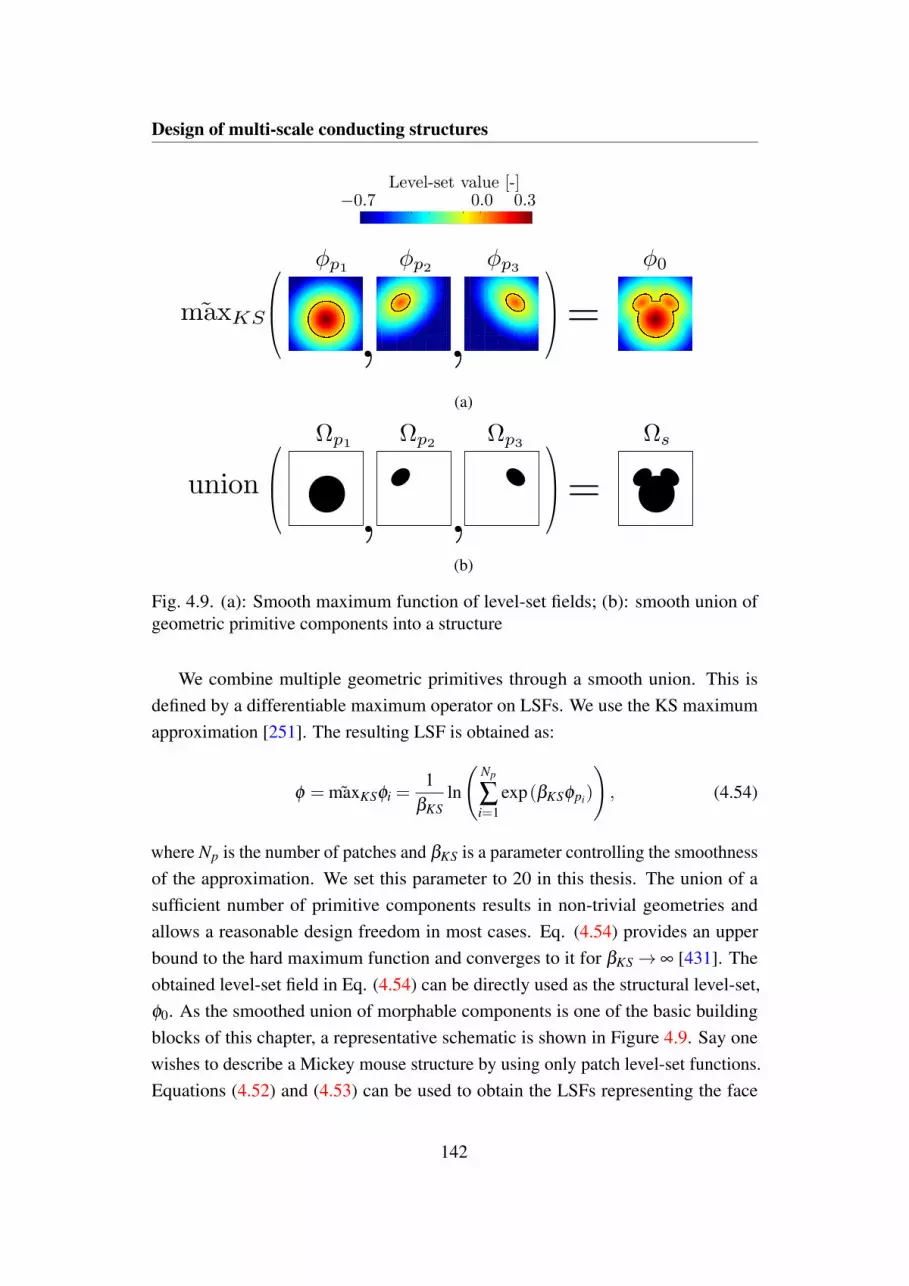
Design of multi-scale conducting structures
(a)
(b)
Fig. 4.9. (a): Smooth maximum function of level-set fields; (b): smooth union ofgeometric primitive components into a structure
We combine multiple geometric primitives through a smooth union. This isdefined by a differentiable maximum operator on LSFs. We use the KS maximumapproximation [251]. The resulting LSF is obtained as:
φ = ˜maxKSφi =1
βKSln
(Np
∑i=1
exp(βKSφpi)
), (4.54)
where Np is the number of patches and βKS is a parameter controlling the smoothnessof the approximation. We set this parameter to 20 in this thesis. The union of asufficient number of primitive components results in non-trivial geometries andallows a reasonable design freedom in most cases. Eq. (4.54) provides an upperbound to the hard maximum function and converges to it for βKS→ ∞ [431]. Theobtained level-set field in Eq. (4.54) can be directly used as the structural level-set,φ0. As the smoothed union of morphable components is one of the basic buildingblocks of this chapter, a representative schematic is shown in Figure 4.9. Say onewishes to describe a Mickey mouse structure by using only patch level-set functions.Equations (4.52) and (4.53) can be used to obtain the LSFs representing the face
142
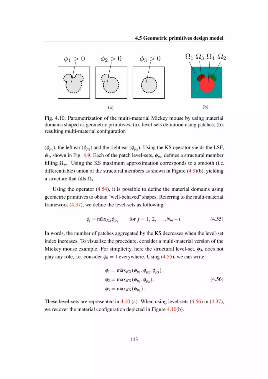
4.5 Geometric primitives design model
(a) (b)
Fig. 4.10. Parametrization of the multi-material Mickey mouse by using materialdomains shaped as geometric primitives. (a): level-sets definition using patches; (b):resulting multi-material configuration
(φp1), the left ear (φp2) and the right ear (φp3). Using the KS operator yields the LSF,φ0, shown in Fig. 4.9. Each of the patch level-sets, φpi , defines a structural memberfilling Ωpi . Using the KS maximum approximation corresponds to a smooth (i.e.differentiable) union of the structural members as shown in Figure (4.9)(b), yieldinga structure that fills Ωs.
Using the operator (4.54), it is possible to define the material domains usinggeometric primitives to obtain "well-behaved" shapes. Referring to the multi-materialframework (4.37), we define the level-sets as following:
φi = ˜maxKSφp j for j = 1, 2, . . . ,Nm− i. (4.55)
In words, the number of patches aggregated by the KS decreases when the level-setindex increases. To visualize the procedure, consider a multi-material version of theMickey mouse example. For simplicity, here the structural level-set, φ0, does notplay any role, i.e. consider φ0 = 1 everywhere. Using (4.55), we can write:
φ1 = ˜maxKS (φp1,φp2 ,φp3) ,
φ2 = ˜maxKS (φp1,φp2) ,
φ3 = ˜maxKS (φp1) .
(4.56)
These level-sets are represented in 4.10 (a). When using level-sets (4.56) in (4.37),we recover the material configuration depicted in Figure 4.10(b).
143

Design of multi-scale conducting structures
(a)
(b)
Fig. 4.11. Parametrization of the material domains with representation of the designvariables. (a): Floating patches; (b): finger agglomerate
4.5.2 Multi-material and structure configurations
In this chapter, we will consider a number of predefined configurations when opti-mizing the material domains and the macroscopic structure. The first one is obtainedby simply filling the design domain with a varying number of patches, between 3and 5, resulting in 4 and 6 materials, respectively. This configuration will be useduniquely for the material domains parametrization. Figure 4.11(a) highlights thedesign variables and shows a possible arrangement of the four materials obtained byconsidering three rectangular patches as geometric primitives. In the patches-type ofconfiguration, we have NsM = 5Nφ macroscopic design variables. For the sake of thematerial domains parametrization, we will also consider a particular agglomerateof patches that takes inspiration from the petal configuration of Coffin and Maute[97] . A circle (pc = 2) is centered at xc
1 = 0, xc2 = 0. Since the rotation does not
modify the layout, its unique design variable is the radius rs = a = b. Some patches
144

4.6 Numerical results and design trends
(a)
(b)
Fig. 4.12. Concurrent structure and material parametrization. (a): Structure fingerdesign; (b): structure finger design with patches background
are attached to the circle in such a way that their center coordinates are described by:
xc1 = rs cosθ ,
xc2 = rs sinθ .
(4.57)
Hence each of the attached patch is controlled by three design variables resulting ina total of NsM = 1+3(Nφ −1) macroscopic design variables. We will refer to thisparticular arrangement as "finger" design. Figure 4.11 (b) shows a multi-materialdescription obtained by using the finger-type of arrangement of geometric primitives.
Using both the PAMP-type interpolation (4.30) and the multi-material framework(4.37) allows the decoupling of the structure and material parameterizations. Indesign optimization studies considering also the optimization of the structure, we willconsider a finger-type of agglomerate for the φ0 definition. For the parametrizationof material domains, we will consider a patches-type of arrangement. This yieldsa finger-like structure with patches background such as the one depicted in Figure(4.12). The opaque regions in Fig (4.12)(b) indicate pure BM.
4.6 Numerical results and design trends
In this section, we present and discuss the numerical results obtained with ourmulti-scale and multi-material design optimization framework based on geometric
145

Design of multi-scale conducting structures
Fig. 4.13. Schematic of the steady-state diffusion heat sink design optimizationproblem
primitives. First, we test the design capabilities on a simple numerical example.Then, we provide the optimized multi-scale layouts for heat transfer enhancement inLHTES units.
4.6.1 Steady-state diffusion heat sink
For the sake of demonstrating the optimization framework described in this chapter,we consider an example with reduced physics complexity: a heat sink governed bysteady-state diffusion (Eq. (2.44)). A schematic of the design and computationaldomain, ΩD, is presented in Figure 4.13. A rectangle with dimensions W = 3.5 andH = 4 is loaded by a homogeneous heat generation qv = 400. A cold temperatureT = 0 is prescribed on the boundary Γc that is w = 0.1 wide. Symmetry is enforcedon Γsym. All the remaining boundaries are adiabatic. We aim at finding the optimalmulti-scale layout of HCM within ΩD such that the spatial integral of the temperature
146

4.6 Numerical results and design trends
is minimized. This corresponds to the following optimization problem:
minimizes
∫ΩD
T dx
subject to∫
ΩD
Φloc dx−V ∗ ≤ 0
s = [sTm, sT
M]T ∈ S =RNs | smini ≤ si ≤ smaxi, i = 1, ...,Ns
, (4.58)
where smini and smaxi denote the minimum and maximum values of the designvariable, si. The maximum volume of HCM is set to 20 % of the total. Themacroscopic design domain is discretized with 5600 bilinear quadrilateral elementswith characteristic size h = 0.05. The microscopic design and computational domainis the one considered in Sections 4.2.3 and 4.3.1 for the verification of the forwardand inverse homogenization frameworks. We use the 50 × 50 discretization with2500 bilinear quadrilateral elements. The thermal conductivity of HCM and BM isset to 600 and 1 respectively. The optimization problems are solved using GCMMA.As compared to the set-up summarized in Table 2.1, we modified the relative step-sizeand the upper asymptote adaptivity to ∆s = 0.01 and α+ = 1.1.
Smoothed union of geometric primitives
The ability of aggregating geometric primitives through a smooth union operator is abasic building block of our design framework. Here, we demonstrate this capabilityon a mono-scale design example. We optimize the structure (by evolving φ0) of asingle fully solid material, i.e. the micro-layout is described by sm = 1 everywherein Y .
We start by considering the finger parametrization introduced in Section 4.5.2for defining φ0. The complete list of design variable bounds and parameters forthis geometry description is presented in Table 4.1 The magnitude of the Heavisidesmearing largely affects the design sensitivities. The value reported in Table 4.1 wasselected after preliminary finite difference checks on the initial guess. Note that thischoice is problem-dependent and is not constant for all the problems consideredin this chapter. Furthermore, ξ modifies the amount of non-physical intermediatematerial in the design domain. To allow for meaningful performance comparisons,all the optimized objective values reported in this chapter are obtained using ξ = 0.
147

Design of multi-scale conducting structures
Table 4.1. Finger design parameterization bounds and parameters for the heat sinkexample
Description Symbol Value
Minimum circle radius rmin 1e-4Maximum circle radius rmax 4Minimum finger half-width amin 0.4Maximum finger half-width amax 4Minimum finger half-height bmin 0.4Maximum finger half-height bmax 4Minimum finger tilt θmin 0Maximum finger tilt θmax π/2"Cuboidness" parameter pc 2Heaviside half band-width ξ 0.1
The evolution of the design along the optimization process is shown in Figure 4.14for both a one-finger and a three-finger parametrization. The designs are evolvedusing 4 and 10 macroscopic design variables, respectively. The objective and volumeconstraint histories are shown in Figure 4.15. The objective is normalized with theinitial value of the one-finger example, z0 = 15933. This normalization parameterwill be adopted for all the objective values presented for the heat sink example. Theconstraint is normalized with respect to the maximum volume, V ∗. The startingguesses are shown in Figure 4.14(a). As visible from the constraint value presentedin Figure 4.15(b), the initial one-finger layout uses less HCM than V ∗. Instead, thethree-finger layout uses more HCM than allowed. In 7-8 optimization iterations, theamount of HCM in the design domain changes until it hits the maximum bound.This yields a constant decrease and increase of the objective for the one-finger andfor the three-finger design. No substantial layout modifications are observed in thisinitial part of the optimization process. In Figure 4.14(b), the designs look simplya "rescaled" version of the initial guess. From iteration 10 to iteration 60 (Figure4.14(d)), the geometries are modified substantially. The fingers rotate such that theirtips point towards the angles of the design domain. These modifications yield alarge performance increase: the objective is reduced by 43.1 % and 59.3 % in theone-finger and three-finger case. A further slight reduction is observed from iteration60 to iteration 100. In Figure 4.14(e), the fingers look stretched along the chosendirection and the internal circle looks moderately grown. We notice negligible layoutand performance changes in the last 20 iterations. The final normalized objectives
148
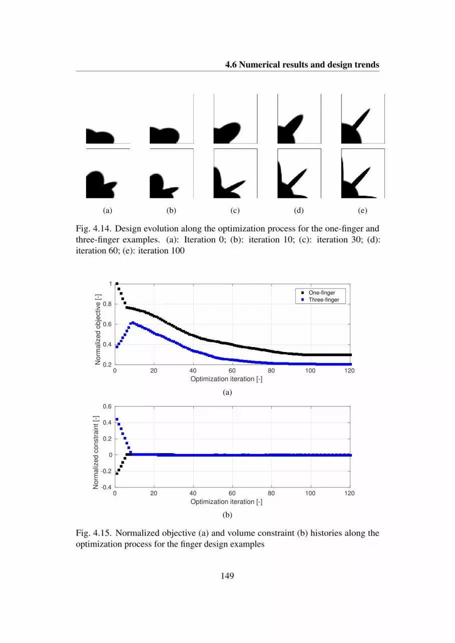
4.6 Numerical results and design trends
(a) (b) (c) (d) (e)
Fig. 4.14. Design evolution along the optimization process for the one-finger andthree-finger examples. (a): Iteration 0; (b): iteration 10; (c): iteration 30; (d):iteration 60; (e): iteration 100
0 20 40 60 80 100 120
Optimization iteration [-]
0.2
0.4
0.6
0.8
1
Norm
aliz
ed o
bje
ctive [-]
One-finger
Three-finger
(a)
0 20 40 60 80 100 120
Optimization iteration [-]
-0.4
-0.2
0
0.2
0.4
0.6
Norm
aliz
ed c
onstr
ain
t [-
]
(b)
Fig. 4.15. Normalized objective (a) and volume constraint (b) histories along theoptimization process for the finger design examples
149
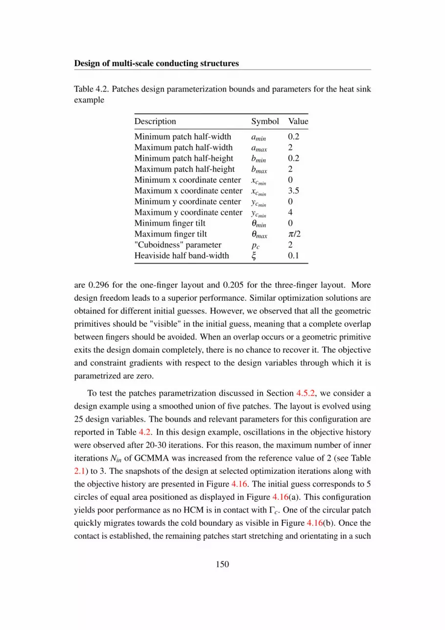
Design of multi-scale conducting structures
Table 4.2. Patches design parameterization bounds and parameters for the heat sinkexample
Description Symbol Value
Minimum patch half-width amin 0.2Maximum patch half-width amax 2Minimum patch half-height bmin 0.2Maximum patch half-height bmax 2Minimum x coordinate center xcmin 0Maximum x coordinate center xcmin 3.5Minimum y coordinate center ycmin 0Maximum y coordinate center ycmin 4Minimum finger tilt θmin 0Maximum finger tilt θmax π/2"Cuboidness" parameter pc 2Heaviside half band-width ξ 0.1
are 0.296 for the one-finger layout and 0.205 for the three-finger layout. Moredesign freedom leads to a superior performance. Similar optimization solutions areobtained for different initial guesses. However, we observed that all the geometricprimitives should be "visible" in the initial guess, meaning that a complete overlapbetween fingers should be avoided. When an overlap occurs or a geometric primitiveexits the design domain completely, there is no chance to recover it. The objectiveand constraint gradients with respect to the design variables through which it isparametrized are zero.
To test the patches parametrization discussed in Section 4.5.2, we consider adesign example using a smoothed union of five patches. The layout is evolved using25 design variables. The bounds and relevant parameters for this configuration arereported in Table 4.2. In this design example, oscillations in the objective historywere observed after 20-30 iterations. For this reason, the maximum number of inneriterations Nin of GCMMA was increased from the reference value of 2 (see Table2.1) to 3. The snapshots of the design at selected optimization iterations along withthe objective history are presented in Figure 4.16. The initial guess corresponds to 5circles of equal area positioned as displayed in Figure 4.16(a). This configurationyields poor performance as no HCM is in contact with Γc. One of the circular patchquickly migrates towards the cold boundary as visible in Figure 4.16(b). Once thecontact is established, the remaining patches start stretching and orientating in a such
150

4.6 Numerical results and design trends
(a) (b) (c) (d) (e)
0 20 40 60 80 100 120 140 160 180
Optimization iteration [-]
10 -2
10 -1
10 0
10 1
Norm
aliz
ed o
bj. (
log s
cale
) [-
]
(f)
Fig. 4.16. Patches design example. Snapshots of layout at iteration 0 (a), iteration10 (b), iteration 60 (c), iteration 100 (d) and iteration 193 (e). (f): Objective historyalong the optimization process
151

Design of multi-scale conducting structures
a way that a tree-like heat transfer structure is created (Figure 4.16(d)). Only minorlayout and performance modifications are observed from this point to convergence,which is reached after 193 design iterations. The optimized layout is shown in Figure4.16(e). Due to its larger design freedom, this geometry yields a higher performancethan the finger layouts. The calculated normalized objective is 0.0878.
This section demonstrated the use of the KS maximum function to aggregatestructural members defined using geometric primitives. The layouts converge to"machinable" structures that are controlled by a limited number of design variables.
Optimizing the micro-structure
Here, we describe the results obtained when optimizing the microscopic layout ofthe steady-state heat sink device. We consider a micro-scale problem with a singlematerial component, i.e. a unique topology of the microscopic layout is optimized.No design freedom at the macroscopic level on the shape of the material domains andstructure is considered, i.e. φ0 > 0 and φ1 < 0 everywhere in ΩD. The microscopicgeometry is parametrized using nodal design variables, sm, that are converted intoelemental densities, ρsm , using the filtering and projection approach presented inChapter 2. The filter radius is set to r fm = 0.051. The microscopic SIMP exponent,pm, and projection steepness parameter, βm, are slowly raised using the followingcontinuation scheme:
pm = 1; 2; 3; 3; 5,βm = 1; 1; 1; 4; 8.
(4.59)
The projection threshold is hold constant at ηm = 0.5. In our implementation, thefilter is non-periodic and truncated at the boundary. This ensures the evolution of themicro-scale geometry also when the layout is initialized with a homogeneous designvariable field, sm. In this case, the homogenized properties and volume constraintsensitivities with respect to the design variables located in the middle of the designdomain differ from those located close to the boundaries. This is not the case when aperiodic filter is adopted. For this reason, other authors initialized the micro-layoutswith either a random design variable field [28] or a specific initial configuration[82]. The first step does not yield penalization when considering the linear volumeconstraint of Eq. (4.58). Although in this design example a non-penalized stepcould be avoided, in our experience this is essential in the multi-material designexamples considered next. It serves for the purpose of redistributing HCM among
152

4.6 Numerical results and design trends
(a) (b) (c) (d)
0 100 200 300 400 500
Optimization iteration [-]
0.2
0.4
0.6
Norm
aliz
ed o
bje
ctive [-]
Fig. 4.17. Objective history with microscopic layout at selected iterations. (a):Iteration 0; (b): iteration 100; (c): iteration 200; (d): iteration 300
materials domains. A premature convergence to poor local minima micro-layoutswas observed otherwise. The transition between continuation steps is performedevery 100 iterations. The convergence of the optimization process is verified onlyafter the completion of the final step. The normalized objective history alongside withthe evolution of the microscopic layout is presented in figure 4.17. The initial guesscorresponds to a homogeneous microscopic design variable field sm = 0.1. Duringthe first continuation step, HCM is homogeneously aggregated within the periodicdomain to reach to maximum HCM volume. This is responsible for a moderateobjective reduction. We notice no progress towards a binary 0; 1 geometry. Alayout starts appearing during the second continuation step, since the intermediatedesign variables are penalized more strongly. A clear pattern is observed at iteration200 (Figure 4.17(c)). However, large areas with intermediate "gray" material arestill present. Those disappear nearly completely at the end of the third continuationstep as visible in Figure 4.17(d). However, the layout boundaries are still blurredby the filter. To improve the accuracy of the numerical homogenization predictions,the steepness of the projection is increased in the last two continuation steps. Thisyields negligible layout and performance modifications. The final optimized layout
153

Design of multi-scale conducting structures
Fig. 4.18. (a): Optimized microscopic layout; (b): composite visualization using agrid of 3 × 3 periods; (c): optimized fin layout
is shown in Figure 4.18(a). The normalized objective achievable with this geometryis 0.193. To test the effectiveness of the initialization, we conduct an optimizationexample with a pseudo-random initial distribution s = 0.2+10−3T , where T is arandom operator returning values in the range [−0.5, 0.5]. We obtain a layout thatperforms 2.898 % worse than the one represented in Figure 4.18(a). In the remainderof the chapter, we will always display a grid of 3 × 3 periods as the one depicted inFigure 4.18(b). This visualization allows the HCM connectivity between contiguousperiodic cells to be visualized.
Although this optimization required for multi-scale analysis, the design variablesare defined only at the microscopic level. When density-like design variables aredefined only at the macroscopic level with no freedom on the material layout, onerecovers a fin layout optimization framework similar to the one considered in Chapter3. To asses the advantage of switching to a multi-scale design optimization procedure,we compute a reference fin layout. Also in this case, we consider a three-field densitystrategy. The macroscopic SIMP exponent pM and projection steepness parameterβM are varied following the continuation strategy (4.59). The macroscopic densityfilter has radius r fM = 0.25. The final optimized design is shown in Figure 4.18(c).The computed normalized objective for this case is 0.061. This result suggests thatfins are more effective heat transfer enhancers than engineered cellular structureswith a periodic and unique micro-structure.
154
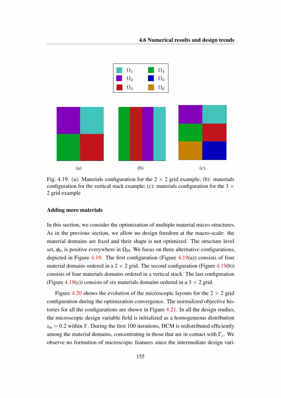
4.6 Numerical results and design trends
(a) (b) (c)
Fig. 4.19. (a): Materials configuration for the 2 × 2 grid example; (b): materialsconfiguration for the vertical stack example; (c): materials configuration for the 3 ×2 grid example
Adding more materials
In this section, we consider the optimization of multiple material micro-structures.As in the previous section, we allow no design freedom at the macro-scale: thematerial domains are fixed and their shape is not optimized. The structure levelset, φ0, is positive everywhere in ΩD. We focus on three alternative configurations,depicted in Figure 4.19. The first configuration (Figure 4.19(a)) consists of fourmaterial domains ordered in a 2 × 2 grid. The second configuration (Figure 4.19(b))consists of four materials domains ordered in a vertical stack. The last configuration(Figure 4.19(c)) consists of six materials domains ordered in a 3 × 2 grid.
Figure 4.20 shows the evolution of the microscopic layouts for the 2 × 2 gridconfiguration during the optimization convergence. The normalized objective his-tories for all the configurations are shown in Figure 4.21. In all the design studies,the microscopic design variable field is initialized as a homogeneous distributionsm = 0.2 within Y . During the first 100 iterations, HCM is redistributed efficientlyamong the material domains, concentrating in those that are in contact with Γc. Weobserve no formation of microscopic features since the intermediate design vari-
155

Design of multi-scale conducting structures
Ω1
Ω2
Ω3
Ω4
(a) (b) (c) (d)
Fig. 4.20. Microscopic layouts evolution of the 2 × 2 grid configuration at selectediterations. (a): Iteration 0; (b): iteration 100; (c): iteration 200; (d): iteration 300
0 100 200 300 400 500
Optimization iteration [-]
0.05
0.1
0.15
0.2
Norm
aliz
ed o
bje
ctive [-]
2 x 2 grid
Vertical stack
3 x 2 grid
Fig. 4.21. Normalized objective histories along the optimization process for the threematerial configurations
156

4.6 Numerical results and design trends
(a)
(b)
(c)
Ω1 Ω2 Ω3 Ω4 Ω5 Ω6
Fig. 4.22. Optimized microscopic layouts for the 2 × 2 grid configuration (a), forthe vertical stack configuration (b) and for the 3 × 2 grid configuration (b)
able values are non-penalized during the first continuation step. During the secondcontinuation step, a large objective reduction is achieved through the formation ofwell-defined micro-structures in Ω1, Ω2 and Ω3. At iteration 200, large regions with"gray" material are still present in the microscopic layout of the material occupyingΩ4. Those disappear nearly completely during the third continuation step due toa larger penalization effect. At the beginning of the fourth continuation step, theobjective of the 3 × 2 grid configuration grows. The increase of the projectionsteepness parameter results in a volume constraint violation and a few optimizationiterations are needed to recover a design set within the feasible region.
The optimized microscopic layouts for all the configurations are shown in Figure4.22. The microscopic layouts of the 2 × 2 grid configuration in Ω4 and Ω3 closelyresemble the ones of the 3 × 2 grid configuration in Ω6 and Ω5. However, somemicroscopic layout differences are noticeable in the top portion of the design domain.The utilization of more material domains allows a reduction of the normalizedobjective by 19.3 %, from 0.092 of the 2 × 2 grid configuration to 0.074 of the 3 ×2 grid configuration. Comparing the performance of the 2 × 2 grid configurationwith the one of the vertical stack configuration prompts additional reflections. Boththese designs use the same number of materials. However, arranging the materialsin a stack yields 8.0 % better performance than using a 2 × 2 grid. This suggeststhat assuming a priori the materials arrangement is crucial for the performance of
157

Design of multi-scale conducting structures
the optimized layouts. For this reason, in the next section we will avoid making thisassumption.
Note that all the optimized objective values obtained in this section are higherthan the one of the reference fins design. The best performing configuration (the3 × 2 grid of materials) results in a 21.3 % larger objective. This suggests that amulti-scale design optimization framework considering fixed material domains maynot yield any performance improvement as compared to a mono-scale analysis anddesign strategy.
Moving the material domains
In this section, we increase the design freedom of our framework by consideringthe optimization of material domains. The grid-like arrangements considered in theprevious section are now able to morph during the optimization. We consider themulti-material patches configuration described in Section 4.5.2 with three and fivefloating patches. The macroscopic design variable bounds and parameters are allequal to those presented in Table 4.2 except for the "cuboidness" parameter which ishere set to pc = 10 and the Heaviside smoothing bandwidth here set to ξ = 0.05. Areduction of ξ was necessary to limit the inaccuracies related to the superpositionof interfaces, as discussed in 4.4.2. This value was selected by trial-and-error onpreliminary optimization runs. No design freedom is considered as regards to thestructure, hence φ0 > 0 everywhere within ΩD.
Figure 4.23 presents the evolution of the material indicator fields and microscopicdesigns during the optimization process for the three patches configuration. Thematerial level-sets are evolved using 15 macroscopic design variables. The objectivehistory is displayed in Figure 4.24. Since the material domains are accounted for inthe analysis model through a density-based representation, the material boundariesare fuzzy in the analysis. Hence, we adopt a visualization in which the opacityvaries linearly with the magnitude of each material indicator field, χi. The samevisualization strategy will be used for all the movable material examples presentedin the remainder of the chapter. Recall that all the optimized objective values listedare obtained with ξ = 0 such that the fuzziness effect does not affect the finalperformance comparisons. The initial guess on the macroscopic design variablesis formulated such that a 2 × 2 grid of material domains is obtained, as in one ofthe fixed domain examples of the previous section. The initial microscopic layout
158

4.6 Numerical results and design trends
(a)
(b)
(c)
(d)
(e)
Fig. 4.23. Evolution of the microscopic and macroscopic layouts for the threemovable patches example at selected iterations. (a): Iteration 0; (b): iteration 100;(c): iteration 200; (d): iteration 300; (e): iteration 500
159

Design of multi-scale conducting structures
0 100 200 300 400 500
Optimization iteration [-]
0.05
0.1
0.15N
orm
aliz
ed o
bje
ctive [-]
Moving three patches
Moving five patches
Fig. 4.24. Normalized objective histories along the optimization process when usingmovable material domains
is a homogeneous sm = 0.2 field in Y . During the first continuation step, HCMis just redistributed among material domains with no formation of binary 0; 1design features. The green material detaches from Γc and starts floating. Thiscreates a thin Ω1 region in contact with the bottom and left boundaries of the designdomain. Here, HCM is rapidly concentrated such that a homogeneous ρsm = 1 fieldis obtained within Y . This yields a larger objective reduction as compared to thefirst continuation step of the fixed 2 × 2 grid configuration. From iteration 100 toiteration 200, noticeable design modifications are observed at both the macroscopicand microscopic level. The microscopic layouts evolve into black-and white patterns.The green floating domain grows and moves such that the shape of Ω1 changesslightly while Ω2 and Ω4 are confined at the top and right boundaries, respectively.Also during this step, the objective is reduced to a greater extent as compared tothe fixed material case. Only minor layout and performance variations are observedduring the last 300 iterations of the optimization process. The final optimized designshown in 4.24(e) consists of two thin fully solid regions (i.e. fins) elongating on thetop and left boundaries and three multi-scale structures with diagonal HCM stripes.The local volume fraction of the micro-structures, φloc, reduces when moving awayfrom Γc. The normalized objective value of the optimized configuration analyzedwith ξ = 0 is 0.055, corresponding to a 9.5 % objective reduction as comparedto the fins of Figure 4.18(c). This indicates that a multi-scale design optimizationframework may be convenient when the material domains are able to morph.
To analyze the effect of additional design freedom obtained through the intro-duction of more moving materials, we consider a morphable version of the 3 × 2
160

4.6 Numerical results and design trends
(a)
(b)
(c)
(d)
(e)
Fig. 4.25. Evolution of the microscopic and macroscopic layouts for the five movablepatches example at selected iterations. (a): Iteration 0; (b): iteration 100; (c):iteration 200; (d): iteration 300; (e): iteration 500
grid configuration discussed in the previous section. This is obtained by using 5patches that are evolved with 25 macroscopic design variables. Figure 4.25 presentsthe evolution of the macroscopic and microscopic layouts at selected optimizationiterations. The objective history is plotted in Figure 4.24 together with the threemoving patches example. The initial guess consists of a 3 × 2 grid of materialdomains with a homogeneous sm = 0.2 microscopic design variable field. Duringthe first continuation step, the redistribution of HCM largely relies on the motion ofthe material domains. Ω2, Ω3 and Ω5 migrate close to the right and top boundariesand a small φloc is attributed to these materials. More HCM is allocated in Ω4 andΩ6, which are positioned close to Γc. The central region is occupied by Ω1, withan intermediate ρsm layout. The material domains evolve rapidly also in the secondcontinuation step. Ω6 grows towards the center of ΩD to form a diagonal fin thatseparates the design domain in three well-distinct regions occupied by Ω2, Ω3 andΩ5. The remaining materials (Ω4 and Ω1) occupy a small portion of the designdomain and their microscopic layout is still homogeneous. Ω1 disappears from the
161

Design of multi-scale conducting structures
design domain during the third continuation step. The disappearance of materialsis allowed in our design optimization framework. To avoid this event, we alsoperformed some numerical experiments with a minimum material volume constraintbut we obtained nearly unaltered performance of the optimized configurations. Themicroscopic layout of Ω4 starts converging to a binary geometry during the last 200iterations, when this material domain evolves into a triangular region of pure HCM.The final layout (Figure 4.25) consists of a diagonal fin surrounded by laminateswith horizontal, vertical and diagonal HCM stripes. The optimized objective ofthis layout is 0.052, yielding only a 5.4 % improvement as compared to the threemorphable patches layout. Since Ω6 and Ω4 have the same micro-structure, weobserve that a similar layout could be obtained also in the previous experiment usingonly four materials. This suggests that the optimized configurations are at best localminima. Although we found that using a large number of materials helps to preventthe convergence to trivial solutions, we always rely on physical intuition to criticallyassess the optimized designs.
Optimizing the structure on the foreground
In this section, we analyze the effect of using a structure level-set, φ0, to controlexplicitly the external shape of the assembly of materials. The structure level-set isdefined as a finger-type of agglomerate of geometric primitives (see Section 4.5.2)with three fingers. The design variable bounds and parameters for this agglomerateare set as in Table 4.1 except for pc = 10 and ξ = 0.05. The material domainsare controlled using three patches with the same bounds and parameters as in theprevious section. The macroscopic layout is evolved using 25 design variables as forthe five movable patches example.
Figure 4.26 shows the evolution of both the microscopic and macroscopic layoutsalong the optimization process. The normalized objective history is displayed inFigure 4.27. To start from an unbiased layout, the initial material configuration ischosen in such a way that all the material domains lie within the finger-type structure.During the first continuation step, the external structure grows to occupy nearly theentire design domain. Also in this case, the material domains are arranged in regionsof increasing distance from Γc, such that the HCM can be efficiently redistributed.Only minor modifications (mainly at the macroscopic level) are observed during thesecond continuation step. Ω4 grows substantially during the third continuation step
162

4.6 Numerical results and design trends
(a)
(b)
(c)
(d)
(e)
Fig. 4.26. Optimized microscopic and macroscopic layouts at selected iterationswhen optimizing the structure on the foreground. (a): Iteration 0; (b): iteration 100;(c): iteration 200; (d): iteration 300; (e): iteration 500
0 100 200 300 400 500
Optimization iteration [-]
0.05
0.1
0.15
0.2
Norm
aliz
ed o
bje
ctive [-]
Fig. 4.27. Normalized objective histories along the optimization process whenoptimizing the structure on the foreground
163

Design of multi-scale conducting structures
Table 4.3. Comparison of the performance when using the wave-like and the rank-1laminate (straight) micro-structures
Micro-structure
Performance Wavy Straight
kH11 [-] 6.0728e+01 6.1661e+01
kH22 [-] 1.2354e+00 1.1124e+00
kH12 [-] -1.4648e-03 0.0000e+00
Normalized objective [-] 0.052636 0.053196
such that Ω2 is lost from the structure. The convergence to binary 0; 1microscopiclayouts is slower in this design example. A well-defined geometry for Ω3 is obtainedonly during the last 200 iterations. The material domain Ω2 reappears during theselast continuation steps with no HCM in its micro-structure such that the shape ofthe external assembly is further modified. The reappearance of material domainsis possible in our multi-material design optimization framework. The final layoutconsists of a triangular fin oriented along the design domain diagonal surroundedby two matrices with straight vertical and wave-like horizontal HCM stripes. In theoptimized configuration, the finger-like structure does not occupy the entire designdomain. The normalized objective value for this design case is 0.054, correspondingto an intermediate performance between the three and the five moving patches designexamples considered in the previous section.
Finally, to test the effectiveness of the wave-like micro-structure in Ω3, weconsider a possible alternative. This consists of a rank-1 laminate with the straightconducting paths aligned in the y1 direction and the same volume fraction of thewave-like material. The homogenized material properties of this micro-structure areobtained analytically following [477]. All the micro-structures are analyzed usingβ = 1000 to avoid the possibility of bias due to intermediate microscopic densityvalues. The homogenized properties and the performance of the two structures aresummarized in Table 4.3. The results show that there are minor but non-negligibledifferences between the two alternative materials. The wave-like material allows ahigher kH
22 to be achieved at the cost of a reduction in kH11. Overall, using a rank-1
laminate with horizontal HCM stripes leads to a 1.06 % worse performance of themacro-structure.
164

4.6 Numerical results and design trends
Table 4.4. Patches design parameterization bounds and parameters for the LHTESexample
Description Symbol Value
Minimum patch half-width amin 0.1Maximum patch half-width amax 1Minimum patch half-height bmin 0.1Maximum patch half-height bmax 1Minimum x coordinate center xcmin 0Maximum x coordinate center xcmin 1Minimum y coordinate center ycmin 0Maximum y coordinate center ycmin 1Minimum finger tilt θmin 0Maximum finger tilt θmax π/2"Cuboidness" parameter pc 10Heaviside half band-width ξ 0.05
4.6.2 Design of multi-scale structures for LHTES units
In this section, we use our multi-scale multi-material optimization framework todesign practical conducting structures for LHTES units. Phase change is modeledthrough the purely diffusive physical model introduced in Chapter 3 and describedby the governing PDE (3.26). We focus on the discharge of the unit, modeled bysetting T ∗I = 1 and T ∗d = 0. The time stepping is stopped when the energy in the tankdrops below 5 % of the total energy capacity. The macroscopic governing equationsare discretized in space and time using the FE framework adopted in Chapter 3. Themicroscopic homogenization equations are solved with the FE framework describedin Section 4.2 using the 20 × 20 elements mesh with 400 bilinear quadrilateralelements. We aim at minimizing the time required for the complete discharge of theunit. Hence, we adopt the optimization problem formulation (3.67). The thermo-physical properties of the material constituents were listed in Table 3.1. Differentlyfrom Chapter 3, here we consider a maximum volume fraction Φ of 20 %. Themacroscopic layouts are controlled using the parametrization options presented inSection 4.5.2. The design variable bounds and parameters for the patches and forthe finger agglomerate are given in Tables 4.4 and 4.5. The SIMP penalizationexponents, pm and pM, and the projection steepness parameter, βm, are slowly raisedduring the optimization process following the continuation scheme (4.59).
165

Design of multi-scale conducting structures
Table 4.5. Finger design parameterization bounds and parameters for the LHTESexample
Description Symbol Value
Minimum circle radius rmin 1e-4Maximum circle radius rmax 1Minimum finger half-width amin 0.1Maximum finger half-width amax 1Minimum finger half-height bmin 0.1Maximum finger half-height bmax 1Minimum finger tilt θmin 0Maximum finger tilt θmax π/2"Cuboidness" parameter pc 10Heaviside half band-width ξ 0.05
To assess the advantage of switching to a multi-scale multi-material designoptimization framework, we will compare the performance of the optimized layoutswith the two reference heat transfer structures depicted in Figure 4.28. The firstone (Figure 4.28(a)) is a fin layout obtained considering no design freedom at themicroscopic level. This geometry is computed using the optimization frameworkpresented in Chapter 3. All the black portions of the design domain denote pure HCMwhile the white portions denote pure PCM. The design differs with respect to thoseanalyzed in the previous chapter uniquely due to the modified maximum volumefraction and continuation scheme on the penalization and projection parameters.Using this geometry allows the unit to be discharged in t∗ = 0.272. Hereafter, wewill refer to this quantity as the reference discharge time, t∗re f . The second geometryis a single-material multi-scale structure filling the entire shell. Using this optimizedstructure yields the complete discharge of the tank in t∗ = 0.447, corresponding toa 64.3 % increase with respect to the fins. This result suggests that filling the unitwith a unique periodic cellular structure, although optimized at the microscopic level,may not be a convenient choice for heat transfer enhancement in LHTES units.
Adding more materials
Here, we relax the single material assumption and consider two alternative arrange-ments of periodic structures in the LHTES unit. The material domains are fixed andthe HCM structure fills the entire shell.
166
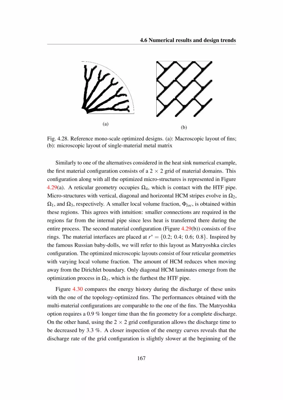
4.6 Numerical results and design trends
(a)(b)
Fig. 4.28. Reference mono-scale optimized designs. (a): Macroscopic layout of fins;(b): microscopic layout of single-material metal matrix
Similarly to one of the alternatives considered in the heat sink numerical example,the first material configuration consists of a 2 × 2 grid of material domains. Thisconfiguration along with all the optimized micro-structures is represented in Figure4.29(a). A reticular geometry occupies Ω4, which is contact with the HTF pipe.Micro-structures with vertical, diagonal and horizontal HCM stripes evolve in Ω2,Ω1, and Ω3, respectively. A smaller local volume fraction, Φloc, is obtained withinthese regions. This agrees with intuition: smaller connections are required in theregions far from the internal pipe since less heat is transferred there during theentire process. The second material configuration (Figure 4.29(b)) consists of fiverings. The material interfaces are placed at r∗ = 0.2; 0.4; 0.6; 0.8. Inspired bythe famous Russian baby-dolls, we will refer to this layout as Matryoshka circlesconfiguration. The optimized microscopic layouts consist of four reticular geometrieswith varying local volume fraction. The amount of HCM reduces when movingaway from the Dirichlet boundary. Only diagonal HCM laminates emerge from theoptimization process in Ω1, which is the furthest the HTF pipe.
Figure 4.30 compares the energy history during the discharge of these unitswith the one of the topology-optimized fins. The performances obtained with themulti-material configurations are comparable to the one of the fins. The Matryoshkaoption requires a 0.9 % longer time than the fin geometry for a complete discharge.On the other hand, using the 2 × 2 grid configuration allows the discharge time tobe decreased by 3.3 %. A closer inspection of the energy curves reveals that thedischarge rate of the grid configuration is slightly slower at the beginning of the
167

Design of multi-scale conducting structures
(a)
(b)
Fig. 4.29. Optimized microscopic layouts for two fixed materials configurations. (a):2 × 2 grid; (b): Matryoshka circles
20 40 60 80 100
Normalized dimensionless time [%]
0
20
40
60
80
100
Norm
aliz
ed d
imensio
nle
ss e
nerg
y [%
]
Fins
2 x 2 grid
Matryoshka circles
Fig. 4.30. Normalized energy histories of the optimized fins and multi-scale struc-tures with fixed material configurations
168

4.6 Numerical results and design trends
process. To gain further insights behind these performance differences, it is useful tostudy the liquid fraction evolution presented in Figure 4.31. The snapshots are takenat 20 %, 40 %, 60 % and 80 % of the reference discharge time. When using thetopology-optimized fins, the solidification front advances rapidly following the fingeometry. At t∗ = 0.4 t∗re f , the mushy PCM occupies uniquely the fins interstices anda thin region in contact with the external envelope. Since most of the heat propagatesradially, the solidification from at the end of the process approximates well theshell geometry. Different discharge dynamics are observed for the multi-materiallayouts. In the grid configuration, solidification proceeds slowly at the beginningof the process. At t∗ = 0.2 t∗re f , the amount of solidified material is less than thealternatives. However, when the solidification front reaches Ω2 and Ω3, it rapidlyexpands in the vertical and horizontal direction. This explains the limited heat transferdrop registered for this structure. At t∗ = 0.6 t∗re f , only the mushy region occupyingΩ1 needs to be cooled away. Solidification in the Matryoshka configuration evolvesin a different manner. Since at fixed r∗ the micro-structure cannot change with theangular position, the solidification front cannot evolve radially. Propagation alongthe θ = π/4 direction is faster than along the θ = 0 and θ = π/2 directions. Hence,the mushy PCM tends to be accumulated at the corners of the design domain. Thisexplains the limited heat transfer rate at the end of the discharge process.
Moving the material domains and the structure
The differences in performance between the alternative material configurationsconsidered in the previous section suggest that improvements of those layouts arepossible by adding design freedom at the macroscopic level. We consider threealternative options for the macroscopic parametrization. The first one consists ofthree floating patches (Section 4.5.2). The initial guess corresponds to a 2 × 2 gridas in the fixed layout of the previous Section. Figure 4.32(a) shows the optimizedmicroscopic and macroscopic layouts for this design case. Similarly to what obtainedin the heat sink design example, pure HCM concentrates close to the bottom andleft boundaries to form two thin fins. The material domain Ω4 floats within thedesign domain and is occupied by a metal matrix with thick diagonal HCM stripes.This material domain is bordered by low volume fraction structures with thin HCMstripes. The second parametrization of material domains consists of a finger-typeof agglomerate with three fingers (see Section 4.5.2). The optimized layout (Figure
169

Design of multi-scale conducting structures
t∗/t∗re f = 20 %
t∗/t∗re f = 40 %
t∗/t∗re f = 60 %
t∗/t∗re f = 80 %
(a) (b) (c)
Fig. 4.31. Liquid fraction evolution of the optimized fin design and fixed materialconfigurations. (a): Fins; (b): 2 × 2 grid; (c): Matryoshka circles
170

4.6 Numerical results and design trends
(a)
(b)
(c)
Fig. 4.32. Optimized macroscopic and microscopic layouts for three moving metalmatrices configurations. (a): Three patches; (b): three fingers; (c): finger structurewith patches background
171

Design of multi-scale conducting structures
20 40 60 80 100
Normalized dimensionless time [%]
0
10
20
30
40
50
60
70
80
90
100N
orm
aliz
ed
dim
en
sio
nle
ss e
ne
rgy [
%]
Fins
Three fingers
Three patches
Finger with patches
Fig. 4.33. Normalized energy histories of the optimized fin design and movingmaterial configurations
4.32(b)) is composed by an inner ring with a large volume fraction material. Thefingers are approximately equally spaced along the angular direction. The diagonalfinger is filled with a thick HCM reticular geometry. The materials occupying theother fingers are composed by wave-like vertical and horizontal HCM stripes. Thematerial domain Ω1 occupies a thin region close to the external envelope and ismade of full PCM. The last option we considered is obtained by adopting differentparameterizations for the structure and material domains. The structure level-set, φ0,is defined as the finger-type of agglomerate of geometric primitives. The materialdomains are controlled by three patches. Figure 4.32(c) shows the optimized layoutsfor this case. As for the moving patches configuration, two fins are created alignedalong the θ = 0 and θ = π/2 directions. The remainder of the structure is composedonly by two materials, as Ω2 disappears during the optimization process. Nearlythe same micro-structure is obtained in Ω3 and Ω4 such that this region can beconsidered as occupied by a unique material. The structure layout approximates acircle with a radius slightly smaller than the shell.
The energy histories during a complete discharge process for these three designsare compared to the one of the topology-optimized fins in Figure 4.33. All thealternatives yield performance improvements with respect to the fins. The dischargetime is reduced by 11.9 %, 23.7 % and 31.5 % when using the material finger layout,
172
4.7 Conclusions
the material patches layout and the finger structure with material patches layout. Asimilar trend would be obtained also for partial discharges. The gaps in performancebuild gradually in time. Differently from what obtained for the heat sink example,the choice on the macroscopic parametrization strongly affects the performance.
The liquid fraction evolution for all the layouts considered is presented in Figure4.34. Note that the snapshots at t∗ = 0.8 t∗re f for the patches and finger-plus-patchesconfigurations are not shown since the discharge is already completed. As comparedto what observed in the previous section, the solidification fronts propagate moreconcentrically with the internal pipe. This is well visible at t∗ = 0.6 t∗re f . For allthe designs, the mushy regions are well distributed close to the shell and cornersof the design domain. Different discharge dynamics are observed for t∗ < 0.6 t∗re f .In the three patches layout and in the finger-plus-patches layout, the solidificationpropagates rapidly following the two fins and resulting in a nearly triangular solidifiedregion at t∗ = 0.2 t∗re f . Then, in the patches design, solid PCM is rapidly created inΩ4 morphing the solidification front towards the center. In the fingers-plus-patchesconfiguration, the front advances along the diagonal direction until it reaches theborder of the structure. The gap between the structure and the shell is then cooledslowly due to the absence of HCM. In the finger configuration, the solidificationfront first advances towards the center of the design domain following the centralfinger Ω4. Then, the heat is transfered in the θ = 0 and θ = π/2 directions byexploiting the particular micro-structures of the side fingers. Also for this case, alarge portion of time at the end of the process is used to cool the pure PCM gap closeto the external shell.
4.7 Conclusions
In this chapter, we developed a multi-scale multi-material optimization frameworkto obtain "machinable" assemblies of periodic heat transfer structures. We firstdemonstrated the approach on a steady-state heat sink example. Then, we appliedthe method for the practical design of geometries for heat transfer enhancement inLHTES units. A graphical summary of the main application-oriented advances forLHTES units obtained in the chapter is presented in Figure 4.35. The optimizationresults suggest that optimizing a single periodic structure yields a reduced perfor-mance as compared to topology-optimized fin layouts. Improvements are possible
173

Design of multi-scale conducting structures
t∗/t∗re f = 20 %
t∗/t∗re f = 40 %
t∗/t∗re f = 60 %
t∗/t∗re f = 80 %
(a) (b) (c)
Fig. 4.34. Liquid fraction evolution of the optimized fin design and fixed materialconfigurations. (a): Three patches; (b): three fingers; (c): finger structure withpatches background
174

4.7 Conclusions
Topological fins
Dis
ch
arg
e tim
e
-24 %
+ 1 %
+ 64 %
-32 %
Design freedom
Single material Multiple materials Multiple moving
materials
Multiple moving
materials & structure
Fig. 4.35. Graphical summary of the main application-oriented advances of thechapter
by optimizing multiple structures within the design domain instead of a single one.Whether this strategy fills completely the gap in performance is problem-dependent.In the LHTES study, the discharge times of our fixed multi-material assemblies werecomparable to the one of fins. However, in the heat sink study, our best configu-ration resulted in a 21.3 % larger objective. The choice of the aggregation layoutof the structure relies on the designer experience. Different assumptions lead tolarge differences in performance. For this reason, we optimized both the micro-structures and the aggregation layout of the periodic materials. This was achievedby using geometric primitive level-sets so that reasonably "well-behaved" shapesof the material domains are obtained. The resulting optimized configurations aresuperior to the topology-optimized fins for both the design studies. We obtaineda maximum reduction of the objective of 14.8 % and 23.7 % for the heat sink andfor the LHTES unit, respectively. Inspired by the concurrent structure and materialPAMP design approach, we then extended the optimization framework to allow adecoupled parametrization of the material domains and structure, both controlled bygeometric primitive level-sets. Although this strategy did not yield benefits in theheat sink study, we obtained large gains in the LHTES unit. The optimized structurehas low geometrical complexity and allows the discharge time to be reduced by 31.5% as compared to the topology-optimized fins.
175

Chapter 5
Exploiting convective transport
Chapters 3 and 4 relied on a simplified phase change model. Considering onlydiffusion for design optimization studies is questionable. The convective effectsand fin layout are tightly connected and it is hard to assess whether convection canbe neglected if the design is unknown. Some recent design studies [46, 109, 436]investigated the effect of specific layout features on convective transport. Differentconclusions were drawn for melting and solidification, suggesting that differentlayouts may be required to enhance the two processes. In this chapter, we aimat exploring how the optimized layouts are affected by fluid flow and identifyingwhat makes the structures optimized for melting different from those optimized forsolidification. The remainder of this chapter is organized as follows: in Section5.1 we review possible methods for modeling convection in the liquid PCM; inSection 5.2, we present, verify and validate our finite element numerical modeland implementation; Section 5.3 introduces the material interpolation strategies forconjugate heat transfer and Section 5.4 discusses some issues that one may encounterwhen choosing suitable continuation strategies to design devices relying on naturalor forced convection; finally, in Section 5.5 we examine and compare the topology-optimized designs for melting and solidification and we present a possible approachto reduce the layout complexity in the spirit of an easier manufacturing.
Some of the contents of this chapter were published in Applied Energy [J1] andpresented at the 2017 ASME Summer Heat Transfer Conference [C2].
176

5.1 Modeling convection/diffusion phase change
5.1 Modeling convection/diffusion phase change
In most of the phase change phenomena of practical interest, the fluid motionyields a non-negligible contribution to the thermal response and has to be takeninto consideration in the analysis. Hence, the diffusive Stefan problem presented inSection 3.2 needs to be modified accordingly. Considering a laminar incompressibleviscous flow, the Stefan problem is augmented with the Navier-Stokes equations inthe liquid domain, Ωl , as follows:
∂vi
∂xi= 0 in Ωl, (5.1)
ρl∂vi
∂ t+ρlv j
∂vi
∂x j=
∂σi j
∂x j+Fi in Ωl, (5.2)
where vi is the velocity, Fi is a momentum source term, and σi j is the viscous stresstensor. Equation (5.1) acts as a kinematic constraint in prescribing a divergence-free flow. Equation (5.2) is the balance of momentum along the direction "i". Theconstitutive equation for viscous, isotropic, incompressible fluids allows the stresstensor to be written as [349]:
σi j =−pδi j +µl
(∂v j
∂xi+
∂vi
∂x j
), (5.3)
where µl is the dynamic viscosity of the liquid PCM. In isothermal melting orsolidification, the fluid-dynamic response can be computed considering a no-slipcondition vi = 0 at the (sharp) solid-liquid interface. The energy equation in the melt(Eq. (3.2)) needs to be modified to include a convective contribution:
ρcpl
∂T∂ t
+ρcpl vi∂T∂xi
=∂
∂xi
(kli j
∂T∂x j
)in Ωl. (5.4)
In Chapter 3, we discussed the numerical advantages of using a fixed gridmethod instead of solving the full Stefan problem using a variable grid that conformswith the interface. With a fixed grid approach, there is no need to satisfy theinterface conditions at the solid-liquid front [76]. Furthermore, the general fixedgrid formulation needs only minimal modifications for non-isothermal phase changewhere a mushy region is present, as in metal alloys and organic PCMs. The extensionof the fixed-grid approaches presented in Chapter 3 for the transient nonlinear
177

Exploiting convective transport
diffusion equation demands a proper modification of the momentum equation insuch a way that: (i) the velocities, and consequently the advective energy transport,are zero in the solid region, (ii) the full set of Navier-Stokes equations (Equations(5.1) and (5.2)) are recovered in liquid region, (iii) the dynamics in the mushy zoneis predicted accurately.
After the early developments of numerical methods for convection-diffusionphase change, Voller et al. [437] identified three possible ways to modify themomentum equation:
(1) switch-off techniques,
(2) variable viscosity,
(3) porosity.
The approach (1) as described by Morgan [303] is the most straightforward. Thenodal velocities are constrained to zero when the nodal temperature drops belowthe liquidus temperature. Instead of using the liquidus temperature to identify thenon-convective regions, Voller et al. [437] generalized the formulation by using athreshold liquid fraction. The author of [303] acknowledged that the approach is lessaccurate than the alternatives (2) or (3). However, he advocated that it is simpler toimplement in explicit schemes. The inaccuracies of simple switch-off techniqueswere later investigated by other authors, for instance Ma and Zhang [284]. It wasargued by these authors that the approach (1) is a simple numerical artifact and hasno physical significance. On the other hand, the approaches (2) and (3) are suitableto model phase change with specific melting and solidification dynamics. Those arediscussed in more details in the following sections.
5.1.1 Variable viscosity method
This modeling strategy can be adopted for amorphous materials such as waxes orglasses [441]. In this case, the solid is dispersed in melt pool such that both the solidand liquid move at the same velocity. The viscosity of the mixture increases fromsmall values (PCM behaving like a fluid) to large values (PCM behaving like a solid)during the transition from liquid to solid [321].
178

5.1 Modeling convection/diffusion phase change
The first work adopting this approach is the one of Gartling [155], who used atemperature-dependent viscosity interpolating an arbitrary large value (representingthe solid viscosity) and the liquid viscosity. Voller et al. [437] and then Cao andFaghri [76] later proposed:
µ = µl +B(1− f ), (5.5)
where µ is the effective viscosity and B→ ∞ is a large constant. The authors arguedthat using a latent heat (or liquid fraction) formulation such as (5.5) might be moreconvenient since isothermal phase change may be treated with equal ease. Anotherapproach is the one proposed in [56] where the effective viscosity is written usingthe harmonic mean:
µ =µl
f, (5.6)
whose denominator needs to be modified for practical implementation to allow for aminimum value such that the divisions by zero are avoided. The interpolations (5.5)and (5.6) were compared in [437]. The arithmetic formulation was found to lead tofaster solidification as compared to the harmonic one.
5.1.2 Porosity method
This model is applicable when the solid PCM is separated from the melt [441] andis not moving. Here, the mushy region is composed of columnar dendritic structureswith the base attached to solidified PCM and with the tip submerged in the melt pool.As noted by Mehrabian and co-authors [297], this is a multi-scale type of problem.The typical spacing of dendrite arms is three orders of magnitude lower than thewidth of the mushy zone. Reference [297] is one of the first works proposing a Darcyflow model to predict the interdendritic flow [43]. Ganesan and Porier [152] laterextended the porous media formulation by using a volume-averaging approach. Theyobtained [47, 57]:
ρl∂ vi
∂ t+ρl v j
∂ vi
∂x j=− ∂ p
∂xi+
1f
∂
∂x j
(µl f(
∂ vi
∂x j+
∂ v j
∂xi
))− f
µl
κvi︸ ︷︷ ︸
Fipm
, (5.7)
where κ is the permeability and vi is the interdendritic velocity which is relatedto the superficial (volume-averaged) velocity, vi, through the Dupuit-Forchheimer
179

Exploiting convective transport
relationship [310]:vi =
vi
εp, (5.8)
where εp is the porosity of the medium. Note that in the mushy zone we can writeεp = f . The inclusion of the advective transport in the momentum equation forflows in porous media led to some controversies in the engineering community.For instance, Nield and Bejan [310] observed that this term is generally small andcan be safely neglected in numerical computations. Also, the authors argued thatthe transient term can be dropped since it decays very rapidly [310]. However,Gartling advocated that this is a reasonable approximation when porosity patternswith evolutionary features are considered. The Darcy’s law allows the flow tobe reproduced faithfully at the dendrite base, where the porosity approaches zero.However, when moving to the dendrite tip, the full Navier-Stokes equations need tobe recovered [154]. It is customary to group the last term of Eq. (5.7) in a porousmedium momentum sink, Fipm , that can be formulated directly as a function ofthe liquid fraction, f . For (nearly) isothermal phase-change a linear relation wasproposed in [437] as:
Fipm =−Aml(1− f )vi, (5.9)
where Aml is a large constant. Eq. (5.9) has the advantage of yielding a limitednonlinearity as compared to various alternative formulations [64]. A more popu-lar approach consists in using a momentum sink inspired by the Kozeny-Carmanequation [64]:
Fipm =−AmKC
(1− f )2
f 3 + εmvi, (5.10)
where AmKC is referred to as the mushy constant whose value depends mainly on themorphology of the solid formations and εm is a small value to avoid the divisions byzero. Eq. (5.10) was derived for packed beds of solid particles invested by a Darcyflow [78]. In this case, the constant AmCK takes the form [310]:
AmKC =D2
h180
, (5.11)
where Dh is the average hydraulic diameter of the particles obtained by probabilisticsampling. The numerical value at the denominator was obtained through a best-fit on experimental results [310]. The experimental evidence presented in [339]recommended the Kozeny-Carman approach as the best choice for large liquid
180
5.2 Numerical model
fractions. Furthermore, this approach has the advantage of having a clear physicalrationale that motivates its formulation. For this reason, this is the most widespreadapproach in the literature nowadays, see for instance [473, 260, 220]. However, thechoice of the mushy constant, AmKC , introduces some arbitrariness that may invalidatethe advantage of using a physical-based model. Voller et al. [437], Shmueli et al.[385] and later Kumar and Krishna [255] observed that the value of the mushyconstant largely affects the thermal and fluid-dynamic response of PCM systems.
Substituting (5.8) into Eq. (5.7) leads to an equation for the superficial velocity:
ρl
f∂vi
∂ t+
ρl
f 2 v j∂vi
∂x j=− ∂ p
∂xi+
1f
∂
∂x j
(µl
(∂vi
∂x j+
∂v j
∂xi
))+Fipm . (5.12)
The comparison of (5.12) with (5.2) shows that the advective, the diffusive and thetransient term needs to be modified to account for the varying liquid fraction in themushy region. However, Voller et al. [64] argued that the porosity sink "will dominateover the transient, convective, and diffusive components" leading to the originalKozeny-Carman equation [78]. Hence, authors simply adopted [437, 64, 441]:
ρ∂vi
∂ t+ρv j
∂vi
∂x j=− ∂ p
∂xi+
∂
∂x j
(µ
(∂vi
∂x j+
∂v j
∂xi
))+Fipm , (5.13)
with the momentum sink defined as in (5.10). Although the validity of the previousassumption can be questioned (we found no quantitative assessment in this direction),Eq. (5.13) represents a standard formulation in the phase change literature of today.In most studies, see for instance [385, 30, 230, 3], a fitting of the mushy constant Am
with experimental results was done considering (5.13). For this reason, this is thereference momentum equation for PCMs used throughout this monograph.
5.2 Numerical model
In this chapter, the design and computational domains need to be modified from theones presented in Chapter 3. Due to the effect of natural convection, the symmetryalong the y = 0 axis of the cross-section no longer applies. Figure 5.1 shows aschematic of the design domain ΩD considered hereafter. It consists of a reflectionalong the y = 0 axis of the design domain considered for the diffusive designs (Figure3.6).
181

Exploiting convective transport
A
Fig. 5.1. Design and computational domain
182

5.2 Numerical model
Similarly to what we did in Section 3.3, here we rework the governing equationsto obtain a dimensionless setting. The dimensionless time, length and temperatureare equal to the ones adopted for the diffusion model (Eqs. (3.22) (3.23) and (3.24),respectively). Considering fluid flow requires the introduction of:
• the dimensionless velocityv∗i = vi/U, (5.14)
where U is a reference velocity,
• the dimensionless pressure
p∗ = p/(ρ0U2). (5.15)
where ρ0 is a reference density.
Recall that all the dimensionless quantities are marked with an asterisk. The referencevelocity is taken as the diffusion velocity, U , of the PCM calculated as:
U =αtPCM
L, (5.16)
where αtPCM is the thermal diffusivity of the PCM. The reference density, ρ0, istaken as the average PCM density. The governing equations presented in 3.3.1are augmented with the continuity and momentum equations formulated using thestandard porosity model (Eq. (5.13)). Under the assumption of constant fluidproperties, incompressible flow and negligible viscous dissipation we have:
∂v∗i∂x∗i
= 0, (5.17)
∂v∗i∂ t∗
+ v∗j∂v∗i∂x∗j
=−∂ p∗i∂x∗i
+Pr∂
∂x j
(∂v∗i∂x∗j
+∂v∗j∂x∗i
)+F∗nci
+F∗bi(s)+F∗pmi
, (5.18)
where Pr is the Prandtl number, F∗nciis a volumetric term accounting for temperature-
induced buoyancy forces and F∗bi(s) is a design-dependent momentum source term
that will be discussed later. For incompressible non-isothermal flows with smalldensity variations, ∆ρ , as compared to the reference density, ρ0, natural convectioncan be accounted by considering the density variations only in the buoyancy term as
183
Exploiting convective transport
follows [350]:
ρgi = ρ0gi +∆ρgi ∼ ρ0gi +ρ0βT (T −T0)gi, (5.19)
where βT is the coefficient of thermal expansion and T0 a reference temperature.Equation (5.19) is generally referred to as Boussinesq approximation and it is ofcommon use in the Computational Fluid-Dynamics (CFD) community. The con-stant term, ρ0gi, can be absorbed into the pressure term to obtain a total pressureaccounting for the gravitational head [13]. Hence, using the dimensionless variablespreviously introduced we obtain:
F∗nci=−Ra Pr eg
i T ∗, (5.20)
where egi is the unit vector in the direction of gravity and Ra is the Rayleigh number.
As discussed in the previous section, the porosity term, F∗pmi, ensures that the
velocities are zero in the solid PCM region and that accurate predictions are obtainedin the mushy region. The dimensionless version of (5.10) is written as:
F∗pmi=−
AmCK
ρ0U/L(1− f )2
f 3 + εmv∗i , (5.21)
where the constants are set as εm = 10−3 and Amushy = 108 kg/(m3 s) according to[385].
The energy equation (3.26) is modified through the addition of convective trans-port:
∂T ∗
∂ t∗+ v∗j
(1+ γ(s)L ∗ ∂ f
∂T ∗
)∂T ∗
∂x∗j=
∂
∂x∗j
(Ki j(s)
∂T ∗
∂x∗i
)− γ(s)L ∗∂ f ∗
∂ t∗. (5.22)
The term in brackets on the left-hand side accounts for the convective energy transportin the form of both sensible and latent heat. Note that the latter is modeled with anapparent heat capacity formulation (Section 3.2.2).
Moving to the boundary conditions, we prescribe an adiabatic boundary on theexternal shell ΓN1 and a symmetry boundary condition on ΓN2 such that:
−Ki j∂T ∗
∂x∗jni = 0 on ΓN1 ∪ΓN2 , ∀t∗. (5.23)
184

5.2 Numerical model
The temperature is fixed at the internal boundary, Γd , to represent the contact withthe tube containing the HTF. Mathematically:
T ∗ = T ∗d on Γd, ∀t∗, (5.24)
where T ∗d is the dimensionless temperature of the HTF pipe, which takes differentvalues for charge and discharge. The interaction with the external shell and pipeboundaries is modeled using a no-slip condition. Due to symmetry, only non-penetration is prescribed on the boundary running along the y-axis. Mathematically:
v∗i = 0 on Γd ∪ΓN1 , ∀t∗, (5.25)
v∗i ni = 0 on ΓN2, ∀t∗. (5.26)
To obtain a well-posed incompressible Navier-Stokes problem in the enclosure, thepressure p∗ = 0 is specified at point A (Fig. 5.1). This choice does not modify thethermal and fluid-dynamic responses. The initial conditions are:
T ∗ = T ∗I in ΩD, at t∗ = 0,
v∗i = 0 in ΩD, at t∗ = 0,
p∗ = 0 in ΩD, at t∗ = 0.
(5.27)
5.2.1 Finite Element model
Equations (5.17), (5.18) and (5.22) are discretized in space using a mixed finiteelement model. Denoting by Rc, Rm, Ren the residuals of the strong form of the con-tinuity, momentum and energy equation respectively, the weighted integral statementover the computational domain, Ω, is written as:∫
Ω
ηhRc dx = 0, (5.28)
∫Ω
ξhi Rmi dx = 0, (5.29)∫
Ω
whRen dx = 0, (5.30)
185

Exploiting convective transport
where ηh and ξ hi are the weight functions of the continuity and momentum equations.
Integration by parts of the viscous term in Eq. (5.29) and of the diffusive term in Eq.(5.30) allows the weak forms of the governing equations to be obtained.
The approximation and weighting functions for the temperature field were definedin (3.36) and (3.37). The pressure and velocity fields are approximated using ph andvh taken from the following function spaces:
Up = ph ∈H 1(Ω); ph = p∗d on Γdp,U = vh ∈H 1(Ω); vh = v∗d on Γdv,
(5.31)
where Γdp and Γdv denotes generic Dirichlet boundaries for the pressures and veloci-ties, respectively, and Up and U are Hilbert spaces consisting of scalar functions andvector functions with square integrable first derivatives. Through the modificationof the Dirichlet boundary restrictions in (5.31), we obtain the weighting functionspaces as:
Vp = ηh ∈H 1(Ω); ηh = 0 on Γdp,
V = ξξξ h ∈H 1(Ω); ξξξhhh= 0 on Γdv,
(5.32)
In Eq. (3.38), we showed how to write a spatial-temporal split to obtain theapproximate temperature field. Further, using the Galerkin method, the temperatureshape functions, N, were chosen equal to the weight functions, wh. Following asimilar route for the pressure and velocities leads to:
ph(x, t) =Nn
∑j=1
p∗j(t)η j(x) = ηηηhT
p∗, (5.33)
vhi (x, t) =
Nn
∑j=1
v∗i j(t)ξ j(x) = ξξξ
hTv∗i , (5.34)
where p∗j and v∗i jare time-dependent nodal pressure and velocity values and p∗
and v∗i represent their collection in column vectors. In (5.34), we took the sameapproximating function, ξ j, for all the velocity components. The asterisk indicatingthe dimensionless variables is dropped for brevity hereafter. Recalling (5.20), p∗j andp∗ represent the total pressure including the gravitational head. Substituting (3.38),(5.33) and (5.34) in the weak form of the governing equations leads to the following
186

5.2 Numerical model
unstabilized Galerkin model of the Navier-Stokes equations in matrix form [350]:
Rus,c = QTj v j = 0, (5.35)
Rus,mi = Mvi +Amvi +Di jv j−Qip−Fi = 0, (5.36)
where:
Q j =∫Ω
∂ξξξh
∂x jη
hdx, (5.37)
M j =∫Ω
ξξξhξξξ
hTdx, (5.38)
Am =∫Ω
ξξξh(ξξξ
hTv j)
∂ξξξhT
∂x jdx, (5.39)
Di j =
∫Ω
Pr(
2∂ξξξh
∂xi
∂ξξξhT
∂xi+ ∂ξξξ
h
∂xl
∂ξξξhT
∂xl
)dx for j = i, l = i
∫Ω
Pr(
∂ξξξh
∂xi
∂ξξξhT
∂x j
)dx for j = i
, (5.40)
Fi =∫Ω
ξξξh (Fnci +Fbi(s)+Fpmi
)dx+
∫ΓN
ξξξh fi dx′, (5.41)
with fi being the traction on ΓN . The energy equation presented in (3.40) is modifiedthrough the addition of a convective term as following:
Rus,e = CT+AT T+KT+ L+q = 0, (5.42)
where:
AT =∫Ω
N(
1+ γL∂ f∂T
)(ξξξ
hTv j)
∂N∂x j
dx. (5.43)
To avoid numerical instabilities, the discrete residuals are augmented with stabiliza-tion terms as follows:
Rc = Rus,c +RcPSPG , (5.44)
Rmi = Rus,mi +RmiSUPG, (5.45)
Re = Rus,e +ReSUPG +ReGGLS , (5.46)
187

Exploiting convective transport
where RcPSPG , RmiSUPGand ReSUPG are detailed in the following section, while ReGGLS
is the GGLS stabilization contribution to the residuals. A discussion on the GGLSstabilization was given in Section 3.3.3, which includes the main motivations forits use when modeling phase change systems and a numerical example showing itseffectiveness. The definition given in (3.45) for ReGGLS is here augmented with thefollowing advective contribution:
RGGLSA =Ne
∑e=1
∫Ωe
∂N∂xi
kτGGLS∂
∂xi
(vh
j
(1+ γL
∂ f∂T
)∂T h
∂x j
)dx. (5.47)
5.2.2 Stabilization
The treatment of incompressible flows with finite element results in two differenttypes of instabilities [419]. First, the advective transport of both momentum andenergy for a high Peclet number, Pe, leads to oscillations in the predicted velocity andtemperature fields. This situation occurs in convection-dominated transport whenthe downstream boundary conditions force rapid solution variations. Second, theequal order interpolation for the velocities and pressure fails to satisfy the Babuska-Brezzi condition, yielding instabilities in the pressure field. The pressure fieldsingularity exhibits as a checkerboard pattern with tight oscillations between positiveand negative values.
This first problem is well known also in the finite difference and finite volumecommunity [67]. The instabilities were observed to arise for Pe > 2 when the con-vective flux is approximated by central differences [433]. A simple upwinding alongwith more complicated hybrid schemes were proposed to solve the problem. Theunderlying idea is to substitute the downstream node contribution to the advectiveflux with the one of the current node. Intuitively, the convective fluxes are calculatedas if the transported field is shifted by one nodal position. This procedure lowers theaccuracy of the convection term approximation to the first order and the truncationerror to the second order. For this reason, the discretization error introduced by theupwinding procedures (but not only) is commonly referred to as numerical diffusion.It can be shown that the sum of a diffusion term with an artificial diffusivity k = vh/2and a convective term approximated by central differences results in the upwindscheme [67]. Since the 1D Galerkin finite element method with piece-wise linearshape functions yields the central difference approximation, the early developments
188

5.2 Numerical model
in the finite element community tried to leverage the finite difference advancements.According to Brooks and Hughes [67], three main paths were followed: artificial dif-fusion, smart quadrature and Petrov-Galerkin weighting. The latter has the advantageof yielding a consistent formulation. However, the extension to multi-dimensionalproblems revealed a cross-wind diffusion that affects the solution accuracy also inthe direction normal to the flow propagation. Following the anisotropic artificial dif-fusion idea developed in [238], Brooks and Hughes [67] proposed a Petrov-Galerkinformulation with the following weighting function:
N = N + N, (5.48)
where N is the Galerkin shape function and N is a perturbation defined as:
N =k||v||2
v j∂N∂x j
= τSUPGv j∂N∂x j
, (5.49)
where v j is a normalized velocity component and τSUPG is a stabilizing term laterintroduced by [418, 419]. Weighting the convective component with a perturbationof the type N is equal to a weak diffusion term with artificial diffusivity [67]:
ki j = kviv j. (5.50)
Using the weight function (5.49) for the energy equation and a similar ξ for themomentum equation, we obtain the following Streamline Upwind Petrov-Galerkin(SUPG) contribution to the residuals:
RmiSUPG=
Ne
∑e=1
∫Ωe
τSUPG(ξξξhT
v j)∂ξξξ
h
∂x jRh
midx, (5.51)
RenSUPG =Ne
∑e=1
∫Ωe
τSUPG(NT v j)∂N∂x j
Rhendx, (5.52)
where Rhmi
and Rhen represent the residual of the strong form of the momentum and
energy equation calculated using the trial functions presented in the previous section.
Adopting Petrov-Galerkin formulations to improve stability with no compromiseover consistency is the general idea that drove also the development of PressureStabilized Petrov-Galerkin (PSPG) method. In an original paper on incompressibleStokes flow [213], Hughes et al. developed a formulation able to circumvent the
189

Exploiting convective transport
Babuska-Brezzi condition, removing all the restrictions on the shape functions choice.Their error analysis led to the following perturbation function:
ξ = τPSPG1ρ
∂ηηηh
∂xi, (5.53)
which yields the following contribution to the residuals of the continuity equation:
RcPSPG =Ne
∑e=1
∫Ωe
τPSPG1ρ
∂ηηηh
∂xiRh
midx. (5.54)
5.2.3 Adaptive time-stepping
The residuals of the semi-discrete momentum and energy equations are discretizedin time adopting a backward Euler scheme as described in Section 3.3.4. Differentlyfrom what presented in Chapter 3, here the time-step size is changed using anadaptive scheme. Extremely small time-steps are required to resolve the flow atthe initial instants of the process. Using a fixed time-stepping strategy would resultin prohibitively slow analyses. Adaptive time-stepping allows to take bigger stepswhen the flow is developed. In addition, using adaptive time-stepping allows thelocal control of the truncation error introduced by (3.50). The numerical methodsfor time-step control developed in three main directions [425]:
• error estimates of the local truncation error based on a comparative erroranalysis of two integration methods with similar order [170, 156],
• heuristics based on the physical insights of the analyst on the problem [463,223],
• control theory methods such as the Proportional Integral Derivative (PID)control [192, 399].
In this monograph, we adopt the approach suggested in [156] for its ease of imple-mentation and proved accuracy for phase change problems. The adapted time-step(∆t∗)(n+1)
ad is controlled as follows:
(∆t∗)(n+1)ad = (∆t∗)(n)
(a
δt
d(n+1)
)b
, (5.55)
190

5.2 Numerical model
where a = 2 and b = 1/2 for first order-schemes [156]. The parameter δt is a user-specified error tolerance and d(n+1) is a local estimate of the truncation error definedas:
d(n+1) =
(1
Nd max(u)2
Nd
∑i=1
(u(n+1)i −u(n+1)
ip)2
)1/2
, (5.56)
where Nd is the number of degrees of freedom, u(n+1)i is the solution computed
through the implicit Euler scheme and u(n+1)ip
is the degree of freedom computedwith the following extrapolation:
u(n+1)p = u(n)+∆t∗
(n)u(n). (5.57)
Note that u collects all the degrees of freedom in a unique vector by stacking thedimensionless pressures, velocities and temperatures as follows:
u =
pvT
, (5.58)
where in two dimensions we have:
v =
[v1
v2
]. (5.59)
In our implementation, we prescribe a maximum ratio between the consecutivetime-steps as well as a minimum and a maximum absolute time-step. To enforce thefinal time constraint of (3.67), we refined the approach presented in Chapter 3. Ateach time step, we estimate the remaining process time (∆t∗)(n+1)
extr based on a linearextrapolation of the energy history:
(∆t∗)(n+1)extr = (∆t∗)(n)
ΨE f c−E(n+1)
E(n+1)−E(n). (5.60)
The fraction on the right-hand side is positive for both the charge and dischargeprocesses due to the monotonicity of the energy history. The time-step (n+ 1) isthen chosen as:
(∆t∗)(n+1) = min((∆t∗)(n+1)
ad ,(∆t∗)(n+1)extr
). (5.61)
191

Exploiting convective transport
The time solver is stopped when the the final time constraint of (3.67) is satisfiedwithin a specified relative tolerance, εt .
5.2.4 Nonlinear solution
The nonlinear system of equations arising from the spatial and temporal discretizationpresented above are solved with the Newton method as done for the diffusive systems.Following the procedure presented in 3.61, we split the Jacobian in a static and in adynamic contribution, Js and Jdyn. This operation simplifies the sensitivity analysisof the transient problems as presented in Section 3.4.5. After stacking the momentumresiduals as we did in 5.59 for the velocities:
Rm =
[Rm1
Rm2
], (5.62)
the static Jacobian of the mixed finite element model can be written in block form as:
Js =
Jcp,s Jcv,s 0Jmp,s Jmv,s JmT,s
0 Jev,s JeT,s
, (5.63)
where:Jcp,s =
∂Rc,PSPG
∂p, (5.64)
Jcv,s =[QT
1 QT2
]+
∂Rc,PSPG
∂v, (5.65)
Jmp,s =−[Q1 Q2
]T+
∂Rm,SUPG
∂p, (5.66)
Jmv,s = diag(Am,Am)+∂Am
∂vv+D+
∂Rm,SUPG
∂v, (5.67)
JmT,s =−[
∂Fnc1∂T
∂Fnc2∂T
]T+
∂Rm,SUPG
∂T, (5.68)
Jev,s =∂AT
∂vT+
∂Re,SUPG
∂v, (5.69)
JeT,s = AT +K+∂Re,SUPG
∂T. (5.70)
192

5.2 Numerical model
The dynamic contribution to Jacobian has the following form:
Jdyn =
0 Jcv,dyn 00 Jmv,dyn 00 0 JeT,dyn
, (5.71)
where:Jcp,dyn =
1∆t(n)
∂Rc,PSPG
∂ v, (5.72)
Jmv,dyn =1
∆t(n)
(diag(M,M)+
∂Rm,SUPG
∂ v
), (5.73)
JeT,dyn =1
∆t(n)
(C+
∂L∂T
+∂Re,SUPG
∂ T+
∂Re,SUPG
∂ L∂L∂T
+∂Re,GGLS
∂ T+
∂Re,GGLS
∂ L∂L∂T
).
(5.74)
Note that in this monograph we utilize a fully consistent Jacobian that includesthe derivative of the stabilization parameters τSUPG, τPSPG and τGGLS.
5.2.5 Verification and validation
To check the accuracy of the presented framework in predicting the response of theconvective systems, we proceed in three steps. First, we compare our predictionswith benchmark numerical solutions for steady-state natural convection in a squarecavity. Then, we demonstrate our model for phase change problems by comparingour predictions with experimental results for melting in a rectangular cavity. Last, wetest the accuracy in the shell-and-tube unit considered in this chapter. With this aim,we compare our results with those obtained with COMSOL Multiphysics [101] sinceno benchmark numerical solution nor experimental study is available considering asetup similar to the one that we adopt.
The thermally-driven cavity problem is a classical benchmark numerical examplefirst proposed by De Vahl Davis [110]. The results obtained by various researchgroups were collected in [111]. A square cavity with adiabatic top and bottomboundaries is differentially heated such that the left and right boundaries are keptat T ∗ = 1 and T ∗ = 0. No-slip and no-penetration are imposed at all the walls.Our predictions for Ra = 105; 106 are compared to those obtained by Mayne etal. [295], Wan et al. [104] and to the ones obtained with COMSOL Multiphysics.The results shown in Figure 5.2 indicate an acceptable qualitative agreement of our
193
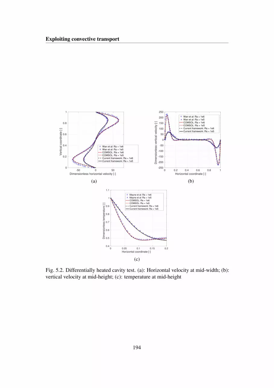
Exploiting convective transport
-50 0 50
Dimensionless horizontal velocity [-]
0
0.2
0.4
0.6
0.8
1
Vert
ical coord
inate
[-]
Wan et al: Ra = 1e6
Wan et al: Ra = 1e5
COMSOL: Ra = 1e6
COMSOL: Ra = 1e5
Current framework: Ra = 1e6
Current framework: Ra = 1e5
(a)
0 0.2 0.4 0.6 0.8 1
Horizontal coordinate [-]
-250
-200
-150
-100
-50
0
50
100
150
200
250
Dim
ensio
nle
ss v
ert
ical velo
city [-]
Wan et al: Ra = 1e6
Wan et al: Ra = 1e5
COMSOL: Ra = 1e6
COMSOL: Ra = 1e5
Current framework: Ra = 1e6
Current framework: Ra = 1e5
(b)
0 0.05 0.1 0.15 0.2
Horizontal coordinate [-]
0.4
0.5
0.6
0.7
0.8
0.9
1
1.1
Dim
ensio
nle
ss tem
pera
ture
[-]
Mayne et al: Ra = 1e6
Mayne et al: Ra = 1e5
COMSOL: Ra = 1e6
COMSOL: Ra = 1e5
Current framework: Ra = 1e6
Current framework: Ra = 1e5
(c)
Fig. 5.2. Differentially heated cavity test. (a): Horizontal velocity at mid-width; (b):vertical velocity at mid-height; (c): temperature at mid-height
194

5.2 Numerical model
0 0.02 0.04 0.06 0.08
Horizontal position [m]
-0.01
0
0.01
0.02
0.03
0.04
0.05
0.06
0.07
Ve
rtic
al p
ositio
n [
m]
Gau and Vishkanta
Pal and Joshi
Current framework
Fig. 5.3. Validation of the presented framework through comparisons with experi-mental results on melting of gallium in a square cavity
framework with the previous literature studies. Our predictions on the maximumhorizontal velocity at mid-width and maximum vertical velocity at mid-height havea maximum deviation of 0.7 % from the benchmarks. The horizontal velocity plotreported in Figure 5.2(a) highlights an increase of the boundary layer predicted byour framework. However, our results are in good agreement with those obtainedthrough COMSOL. The temperature profiles at mid-height also agree well with thosereported in [295]. The deviation of the maximum Nusselt number along the leftboundary is computed as 1.1 %. Note that the setup presented in [295] considersT ∗ = 0.5 and T ∗ =−0.5 for the hot and cold boundaries. Hence, the temperaturefield obtained by those authors was lifted for the sake of comparisons.
The melting of gallium in a rectangular cavity with vertical walls was investigatedexperimentally by Gau and Vishkanta [157]. The left and right wall are kept atT = 311.15 K and T = 301.3 K, respectively. The top and bottom boundaries areinsulated. The initial temperature of the enclosure is set to T = 301.3 K. Figure 5.3shows a comparison of the melting front evolution between the numerical predictionof our framework, the experimental results of Gau and Vishkanta [157] and thenumerical results of Pal and Joshi [324]. Visible discrepancies are observed onlyin the central part of the melting front as this is the region interested by the highest
195

Exploiting convective transport
Table 5.1. Comparison of the accuracy of the current framework with the one of Paland Joshy [324]
Numerical framework
Error Current Pal and Joshy [324]
Absolute mean [m] 0.0015 0.0017Absolute max [m] 0.0058 0.0053
Table 5.2. Properties of the PCM considered
Description Symbol Value
Dimensionless latent heat L ∗ 20Dimensionless melting temperature T ∗m 0.5Rayleigh number Ra 105
Prandtl number Pr 30
convective transport due to the moderate velocities and large enthalpy gradientsclose to the the interface. Small velocity and temperature differences can lead tolarge deviations. The error can be attributed to our artificial smearing of the liquidfraction (Eq. (3.27)) that has no physical rationale when modeling pure substanceswith isothermal phase change. The deviation could be reduced by calibrating ξlog
and AmCK to the experimental data [385, 240, 30]. Table 5.1 shows a comparisonof the accuracy of the current framework with the one of Pal and Joshy [324]. Theerror is computed in terms of the melt front position along the horizontal directionat a specified height. To compare points at different heights, both the numericalcurves are interpolated linearly. The results show that the accuracy of the presentednumerical framework is similar to the reference numerical study of Pal and Joshy[324]. For this reason, we consider our model reliable enough to predict the phasechange phenomenon.
We now verify our phase change model in the shell-and-tube geometry. Weconsider the same PCM used in Chapter 3. The thermo-physical properties aresummarized in Table 5.2. The outer and inner shell radius are set to r2 = 1 andr1 = 0.3 respectively. We perform a mesh convergence study, comparing threedifferent meshes with characteristic sizes ∆θ = π/45; π/90; π/180 to a referencemesh with ∆θ = π/360. The radial element size is calculated as ∆r = r∆θ . Thecharge time deviations computed with respect to the reference mesh are summarized
196

5.3 Design optimization problem
Table 5.3. Mesh convergence verification. The deviation is calculated with respect toa reference case with ∆θ = π/360
Mesh size ∆θ [-] Deviation [%]
π/45 5.24π/90 1.01
π/180 0.48
Table 5.4. Time-stepping verification. The deviation is calculated with respect to areference case with δt = 0.005
Integration tolerance δt [-] Deviation [%]
0.04 3.740.02 1.380.01 0.21
in Table 5.3. A mesh with characteristic size ∆θ = π/180 with 12851 quadrilateralelements is chosen to produce all the results presented in this chapter as it ensures alimited deviation from the reference mesh. To verify the independence of the resultsfrom the time-stepping strategy, we run four analyses with different values of theintegration tolerance, δt . The charge times obtained with δt = 0.04; 0.02; 0.01are compared to that of a reference case with δt = 0.005. Adopting an integrationtolerance of δt = 0.01 yields only a 0.21 % deviation from the reference case andis found sufficient to ensure the time-step independence of the results. A summaryof this verification analysis is presented in Table 5.4. The evolution of the iso-temperature contour at T ∗ = 0.5 obtained with δt = 0.01 and with ∆θ = π/180 isshown in Figure 5.4 alongside with the results obtained with COMSOL Multiphysics[101]. The qualitative agreement suggests that our modeling framework is ableto predict with fidelity the thermal and fluid-dynamic response in shell-and-tubeLHTES units.
5.3 Design optimization problem
In this chapter and in the next one, the optimization problem is formulated usingthe TM approach presented in Chapter 3. The flow of computations for the transientsensitivity analysis using the adjoint method are the same described in Section
197

Exploiting convective transport
COMSOL Multiphysics
Current framework
COMSOL Multiphysics
Current framework
(a) (b)
Fig. 5.4. Accuracy test of the current framework against COMSOL Multiphysics.Comparison of the T ∗ = 0.5 iso-temperature contour at t∗ = 1;2;3,4 for bothmelting (a) and solidification (b)
198

5.3 Design optimization problem
3.4. The material interpolation and regularization strategies require some additionaldiscussion, which is reported in the next sections.
5.3.1 Material interpolation
Although the concept of material interpolation is general in the field of topologyoptimization, fluid mechanics requires a specific interpolation strategy that differsfrom the one discussed in Section 3.4. The identification of the material property tointerpolate is non-trivial. The seminal paper of Borrvall and Petersson [63] borrowedsome concepts from lubrication theory. They considered a 3D flow confined betweenparallel plates where the characteristic size of the plates, L, was order of magnitudeslarger than the channel separation distance, h. Due to slowly varying h and laminarflow, the velocity field was assumed parallel to the plates with a Poiseuille velocityprofile in the direction orthogonal to the parallel plates. The analysis space wasthen reduced from 3D to 2D, considering the plane at half separation distance. Theout-of-plane viscous effects were taken into account in the momentum equationthrough an absorption term [322]:
Fpoisi =−12µ
h2 vi, (5.75)
that can be obtained from the integration of the Cauchy stress tensor along theout-of-plane direction. The plates distance, h, was used as piece-wise constantphysical design variable. This seminal study [63] focused on Stokes flow, i.e. withno advective momentum transport. Arguing that most flows of engineering interestresult in Reynolds numbers Re>> 1, Gersborg-Hansen et al. [158] later extended themethod to practical Navier-Stokes problems. The authors also noted that augmentingthe Stokes model through a sink term of the form (5.75) corresponds to a Brinkman-like model for flow in porous media with inverse permeability, αb, defined as:
αb = 12µ
h2 . (5.76)
This observation led to research directions that progressively abandoned the originalparallel plates idea. In the lubrication-derived approaches presented above, a mini-mum bound on the inverse permeability αb arises naturally from the definition of a
199

Exploiting convective transport
maximum channel depth, hmax:
αbmin = 12µ
h2max
. (5.77)
Olesen et al. [322] first considered the minimum inverse permeability as αbmin = 0.Evgragov [127] later rigorously proved that the inclusion of zero and infinite perme-ability results in a well-posed problem when considering dissipation minimizationwith Stokes flow. However, he argued that this does not hold in general for other flowconditions and/or objective functionals. In Ref. [126], the same author demonstratedthat ill-posed problems are generated when considering Navier-Stokes equations,since the design-to-flow mapping is not continuous. Evgragov [126] proposed tosolve this issue by filtering and using a slightly compressible formulation. Anotherstep towards the abandonment of the original lubrication approach was the opti-mization of 3D Stokes flow devices, first considered by Aage et al. [1]. Recall thatthe lubrication approximation leads to a reduced dimensionality of the analysis andoptimization. We notice that in principle augmenting the momentum equations witha Brinkman sink shares the criticalities listed in Section 5.1.2 for the porosity methodfor phase change. However, this approach works well in practice and encounteredbroad acceptance in the community. It was applied to Navier-Stokes equations inboth two [290, 13] and three dimensions [27, 16]. A complementary material interpo-lation approach was followed by Guest and Prevost [180], who improved the originalBrinkman sink formulation with a Stokes-Darcy interpolation. This is useful whenoptimizing devices with permeable solid materials. Furthermore, the analysis withintermediate design variable values retains a physical interpretation. Despite theseadvantages, the method did not encounter broad acceptance and applications weremostly limited to multi-scale design of porous structures, where the permeabilitytensor in the Darcy equation is obtained by homogenization procedures similar tothose described in Chapter 4, see for instance [179, 182].
The choice of the αb-s dependence was less debated. In [63], the authors notedthat a linear interpolation leads to a severe penalization of intermediate "gray" de-signs, yielding convergence to local minima. However, only a linear interpolationwas found to guarantee the convergence to binary 0,1 layouts [63]. Hence, mostresearchers adopted a continuation approach where a convex interpolation is slowlymorphed into a linear one. The choice of the continuation strategy is somewhatheuristic and highly problem-dependent. In our experience, defining a proper con-
200

5.3 Design optimization problem
tinuation strategy in conjugate heat transfer problems can be tricky. Some possibleissues are discussed in detail in Section 5.4.
In this monograph, we adopt the classical Brinkman sink approach. In ourdimensionless framework we have:
F∗bi(s) =−α
∗b (s)v
∗i , (5.78)
where the property α∗b physically corresponds to:
α∗b =
PrDa
, (5.79)
where Da is the Darcy number. Due to physics similarities, we adopt the interpolationstrategy proposed by Alexandersen et al. [13, 16] for natural convection problems:
α∗b (s) = α
∗max
1− s1+qα s
, (5.80)
where qα is a convexity factor used to control the shape of the interpolation functionat intermediate values of s, and α∗max is a large value approximating ∞. Note that anil Brinkman sink is obtained for s = 1. In our implementation, s = 1 denotes fullPCM while s = 0 denotes full HCM. This agrees with [13, 16] but is opposite tothe density parameterization adopted in Chapters 3 ad 4. To maintain consistencywith [13, 16], the design-dependent conductance K(s) is written using the followingRAMP-like interpolation:
K(s) =s(Ck(1+q f −1)+1)
Ck(1+q f s), (5.81)
where q f is a convexity factor and Ck = αtPCM/αtHCM is the diffusivity ratio betweenthe PCM and HCM. The latent heat factor, γ(s), is interpolated linearly, i.e. using aSIMP approach with exponent p = 1.
5.3.2 Regularization
Early contributions [63] in the field of fluid topology optimization already reportedthat regularization is non-necessary for minimum dissipation (or minimum pressuredrop) problems. This well agrees with the intuition that a minimum dissipation
201

Exploiting convective transport
problem can be thought as a compliance maximization [180]. In our experience,convective heat transfer problems for maximum thermal dissipation suffer from thesame lack-of-solution illness found for the compliance minimization of structures.Hence, we adopt the three-field regularization strategy presented in Section 3.4.
5.4 Continuation strategies in conjugate heat trans-fer
As discussed in Chapter 2 of this monograph, a popular (and heuristic) strategy toobtain convergence to binary 0; 1 designs whilst avoiding unsatisfactory localminima is to slowly ramp the penalization parameters and solve one optimizationproblem per each continuation step. The optimized layout at each step is used asinitial guess for the next step. Although this demonstrated to be effective in manyproblems of practical interest, selecting a proper continuation strategy in multi-physics problem can be a non-trivial task. The physical design variables shouldbe always penalized such that the physics complexity is maintained in its entirety.The results presented in this chapter and in Chapter 6 are obtained by raising theconvexity parameter, q f , (Eq. (5.81)) along with the projection parameter, β , in threesteps as follows:
β ∈ 1;2;4,q f ∈ 1;10;102.
(5.82)
The remaining material interpolation parameters of (5.80) are held constant at qα =
10 and αmax = 107. This strategy revealed to be able to avoid unsatisfactory localminima in preliminary numerical tests that we conducted for both solidification andmelting enhancement.
The remainder of this section aims at showing and investigating possible issuesthat may arise in coupled fluid-dynamic and heat transfer problems for an improperselection of the continuation strategy. We limit the physics complexity for an easierintuition. Hence, both the phase change and temporal dynamics are not considered.We focus on two design examples: a natural convection heat sink and a forcedconvection heat sink. Both the optimization problems are solved with the numericalimplementation framework presented in this chapter.
202

5.4 Continuation strategies in conjugate heat transfer
Fig. 5.5. Schematic of the natural convection heat sink design optimization problem
5.4.1 Natural convection heat sink
Topology optimization of heat sinks cooled by natural convection was first studiedby Alexandersen et al. [13, 16]. Here, we adopt design and computational domainssimilar to the ones described in their seminal 2D paper [13]. Figure 5.5 presents aschematic of the problem considered. Two rectangle with dimensions W = 7, w = 4,H = 4 and h = 2 are heated on Γhs having width whs = 0.2 with an inward heatflux, q∗ = 90. A cold temperature T ∗ = 0 is set on the three boundaries denotedwith Γc. The two bottom boundaries indicated with Γa are adiabatic. No-slip andnon-penetration are prescribed on all the boundaries. We aim at finding the optimallayout of HCM within the design domain, ΩD, such that the temperature on theheated boundary is minimized. Hence, the optimization problem can be written as:
minimizes
z =∫
Γhs
T ∗ dx′
subject to∫
ΩD
(1− s) dx−Φ
∫ΩD
dx≤ 0
s ∈ S =RNs | smin ≤ si ≤ smax, i = 1, ...,Ns
, (5.83)
where the design domain volume fraction, Φ, is set to 50 %. The portion of compu-tational domain outside the design domain Ω\ΩD is set to full fluid. The problemgoverning equations can be obtained through a slight modification of the more gen-
203

Exploiting convective transport
eral framework we considered for phase change problems with natural convection.The state-dependent Kozeny-Carman sink, F∗pmi
, appearing in the momentum equa-tion (Eq. (5.18)) is here set to 0. The phase transition contribution in (5.22) areneglected by setting L ∗ = 0. The Prandtl number is set to unity while the diffusivityratio between fluid and solid, Ck, is set to 1 %. We discretize the domain withquadrilateral bilinear element with characteristic size δx = 0.025 resulting in 180964degrees of freedom.
To understand how the physics at the initial optimization iteration is affectedby the choice of the penalization parameters we proceed as follows. First, we seta homogeneous design variable distribution s = 1−Φ everywhere in the designdomain, ΩD, that corresponds to our usual initial guess for topology optimization.Then, we run a set of 40 analysis considering all the combinations of the penalizationparameters varied as follows:
qα = 1e0; 1e1; 1e2; 1e3; 1e4; 1e5; 1e6; 1e7q f = 1e0; 1e1; 1e2; 1e3; 1e4
. (5.84)
Last, we compute an indicator function quantifying the amount of heat transferredby convection with respect to the total within the design domain:
qconv =
∫ΩD
||v∗i T ∗||2dx
∫ΩD
∣∣∣∣∣∣∣∣Ki j∂T ∗∂x∗j
∣∣∣∣∣∣∣∣2dx+
∫ΩD
||v∗i T ∗||2dx. (5.85)
The convection indicator qconv ∈ [0,1] so that 0 denotes a purely conductive contribu-tion and 1 denotes a purely convective contribution. The computed qconv distributionfor different Rayleigh numbers is presented in Figure 5.6. White iso-contours areplotted for qconv = 0.05; 0.95 such that is possible to identify three different re-gions. The red region is dominated by convection, the blue region is dominated byconduction. A balance between alternative heat transfer mechanisms is observed onlyfor the region enclosed by the iso-contours. When the Rayleigh number is increased,the iso-contours are shifted to the left such that the the size of the convection regiongrows while the one of the conduction region diminishes.
204

5.4 Continuation strategies in conjugate heat transfer
0 0.2 0.4 0.6 0.8 1
0
0.2
0.4
0.6
0.8
1
0 0.2 0.4 0.6 0.8 1
(a) (b)
Fig. 5.6. Convective transport indicator, qconv, distribution for different Rayleighnumbers. (a): Ra = 1280; (b): Ra = 6400. The white iso-contours are plotted forqconv = 0.05; 0.95
205

Exploiting convective transport
Fig. 5.7. Schematic of the forced convection heat sink design optimization problem
5.4.2 Forced convection heat sink
Topology optimization of heat sinks cooled by forced convection was consideredin a few more studies than those considering natural convection heat sinks, see forinstance [248, 290, 317]. A schematic of the design example considered here ispresented in Figure 5.7. We consider square design and computational domains withdimensions L = 0.11 and w = 0.02 and a volumetric heat generation q∗v = 5.56e4. Acooling fluid flows from the inlet, Γin, to the outlet, Γout . We prescribe vanishingnormal and tangential stresses at the outlet σi jn j = 0. At the inlet we set both avanishing tangential velocity v∗i ti = 0 with ti being the unit tangent vector and anormal stress niσi jn j = p∗in. No-slip and non-penetration are set on the remainingboundaries. A cold temperature T ∗= 0 is prescribed at the inlet and a fully developedcondition with vanishing temperature gradients in the normal direction is prescribedat the outlet. The remaining boundaries are adiabatic. We aim at finding the optimallayout of HCM such that the integral temperature is minimized. The optimization
206

5.4 Continuation strategies in conjugate heat transfer
(a) (b)
Fig. 5.8. Convective transport indicator qconv distribution for different inlet pressures.(a): p∗in = 0.1; (b): p∗in = 10. White iso-contours are plotted for qconv = 0.05; 0.95
problem reads:
minimizes
z =∫
ΩD
T ∗ dx
subject to
(∫ΩD
(1− s) dxΦ∫
ΩDdx
−1
)2
− ε2V ≤ 0
s ∈ S =RNs | smin ≤ si ≤ smax, i = 1, ...,Ns
, (5.86)
where the volume constraint is here written as a weak equality constraint such thatthe amount of HCM differs from the maximum allowed at worst by a small number,εV = 1e− 4. This was necessary to avoid trivial solutions with no HCM withinthe design domain, which we observed arising in few optimization cases. Naturalconvection is not considered in this study, hence we set Ra = 0. The computationaldomain is discretized using bilinear quadrilateral elements with characteristic sizeδx = 7.3e−4 yielding a total of 92412 degrees of freedom. Figure 5.8 displays thedistribution of the convection indicator, qconv, obtained by sweeping qα and q f asdescribed in the previous section. Also in this case, a negligible convective transportis observed at small values of q f - qα while heat transfer is dominated by convectionat high values. Raising the inlet pressure has similar effects to an increased Rayleighnumber for the natural convection example.
207

Exploiting convective transport
Fig. 5.9. Representation of alternative continuation trajectories
5.4.3 Possible continuation strategies
Through inductive reasoning, we can generalize the results described in the previoussections and obtain the simplified schematic presented in Figure 5.9. For intermediatedesign variable values, large qα and q f lead to an excessive penalization of conductiveheat transfer such that convection is the leading heat transfer mechanism. Onthe other hand, small qα and q f values penalize convective transport too stronglysuch that diffusion dominates. To understand what kind of physics is "felt" bythe "gray" regions during the optimization convergence, it is useful to plot thecontinuation trajectories on this qα -q f representative space. We consider threepossible continuation alternatives:
• Continuation strategy (i) (indicated in red) is obtained from [13]. It consistsof the following steps:
q f = 1e0; 1e1; 1e2; 1e3; 1e4,qα = 1e7; 1e7; 1e7; 1e7; 1e7.
(5.87)
As this trajectory lies in the convective region, this strategy is likely to privilegeconvective structures.
208

5.4 Continuation strategies in conjugate heat transfer
• Continuation strategy (ii) (indicated in blue) is a modified version of the onepresented in [16]. The penalization parameters are raised as follows:
q f = 0.881; 8.81; 88.1; 881; 881,qα = 8; 8; 8; 98; 998.
(5.88)
As the early continuation steps of this trajectory are positioned in the diffusiveregion, this strategy is likely to privilege diffusive structures.
• Continuation strategy (iii) (indicated in green) is an alternative to the previ-ous ones that aims at approximating the shape of the transition region such thatboth the heat transfer mechanisms are present along the optimization process.It consists of the following steps:
q f = 1e0; 1e1; 1e2; 1e3; 1e4,qα = 1e4; 1e3; 1e2; 1e1; 1e0.
(5.89)
For all the cases, we consider a fixed αmax = 1e7 as in [13]. Note that in [16],the authors ramp also this parameter along the optimization process. The effectof this parameter is considered separately in Section 5.4.5. Upon marching alongeach continuation trajectory, the amount of gray material reduces. Due to the strongnon-convexity of the optimization problem, the geometry evolves into a particularlocal minimum during the earliest continuation steps, and hardly escapes from itduring the following continuation steps. The radius of the circles in Figure 5.9represents qualitatively the ability of each continuation step to morph the design intoan effective structure.
5.4.4 Comparison of performance
Figure 5.10 collects the optimized designs obtained with the three continuationstrategies for the natural convection example. Continuation strategy (i) yields op-timized layouts that differ significantly from those obtained with the alternativetrajectories. The HCM aggregates in the center of the design domain in a branchedtriangular structure. For higher Rayleigh numbers, some solid material is left atthe top corners of the design domain. Although the suspended solid material is notphysically realistic, our density-based topology optimization framework allows this
209

Exploiting convective transport
(i)
(ii)
(iii)
(a) (b) (c)
Fig. 5.10. Optimized designs obtained with the three continuation strategies in thenatural convection example at different Rayleigh numbers. (a): Ra = 1280; (b):Ra = 3200; (c): Ra = 6400
type of solution. The disconnected HCM yields a negligible contribution to the heatdissipation through diffusion. This suggests that the floating features arise to manip-ulate the flow such that high velocity streams come in contact with the triangularstructure. Continuation strategies (ii) and (iii) result in similar optimized structures.Noticeable differences are visible at the intermediate Rayleigh number, for whichContinuation strategy (ii) presents diffusive-like branches at the top of the designdomain that are not observed in the optimized structure obtained with Continuationstrategy (iii). To cross-check the performance of the optimized structures presentedin Figure 5.10, the final design variable field is projected with a step Heavisidefunction centered in s = 0.5 such that pure HCM is obtained for s ≥ 0.5 and purefluid is recovered for s < 0.5. This ensures that the interpolation parameters haveno effect on the analysis. The performance of these modified layouts is reported inTable 5.5. Continuation strategy (iii) yields always a reduced objective as comparedto the alternatives. Continuation strategy (ii) results in similar performance at lowRayleigh numbers. Continuation strategy (i) is always the worst-performing choicein the range of values considered.
210

5.4 Continuation strategies in conjugate heat transfer
Table 5.5. Optimized objective in the natural convection example with the threedifferent continuation strategies
Rayleigh number
Continuation strategy 1280 3200 6400
(i) 6.48 6.11 5.55(ii) 5.75 5.61 5.33(iii) 5.72 5.37 4.39
Table 5.6. Optimized objective (x 102) in the forced convection example with thethree different continuation strategies
Inlet pressure
Continuation strategy 0.1 5 10
(i) 6.73 0.84 0.42(ii) 2.75 1.53 1.02(iii) 6.72 0.64 0.39
The optimized layouts obtained with the three continuation strategies in theforced convection example are reported in Figure 5.11. Continuation strategy (ii)leads to optimized designs that suppress fluid flow. The HCM is concentratedclose to the cold inlet so that the domain can be cooled by diffusion. At higherp∗in, similar solutions are observed but the convergence to binary 0; 1 designsis poor. This suggests that moving to a high qα at late continuation steps maybe unsatisfactory for some problems. Continuation strategies (i) and (iii) result insimilar layouts. A flow channel departing from the inlet bifurcates in a numberof different paths. With Continuation scheme (iii), the channels are concentratedtowards the outlet and the structure relies on HCM to cool the bottom corners of thedesign domain. At high pressures, Continuations strategy (i) leads to a geometrythat is nearly symmetric with respect to the x-axis. This suggests that the diffusivetransport is slightly exploited. The Heaviside projection is again adopted to post-process the optimized layouts before a cross-check analysis. The performance of theprojected layouts is summarized in Table 5.6. At p∗in = 0.1, Continuation strategy(ii) leads to the best-performing design. When the fluid motion driving force istoo small, a diffusive structure connected to the inlet is convenient even if the flowis completely suppressed. Continuation schemes (i) and (iii) did not reveal this
211

Exploiting convective transport
(i)
(ii)
(iii)
(a) (b) (c)
Fig. 5.11. Optimized designs obtained with the three continuation strategies in theforced convection example at different inlet pressures. (a): p∗in = 0.1; (b): p∗in = 5;(c): p∗in = 10
212

5.4 Continuation strategies in conjugate heat transfer
(a) (b)
Fig. 5.12. Effect of the maximum Brinkman constant on qconv. (a): αmax = 1e5; (b):αmax = 1e9
optimized solution as the convective transport contribution was overestimated atearly design iterations. At higher inlet pressures, exploiting the flow for coolingthe domain becomes important. At p∗in = 5 and p∗in = 10, Continuation scheme (iii)yields superior performance than the alternatives.
The results presented in this section demonstrate that the continuation trajectorieson the interpolation parameters are of primary importance in coupled flow and heattransfer problems. Improper choices may lead to unsatisfactory local minima that donot exploit sufficiently either convective or diffusive heat transfer.
5.4.5 On the effect of the maximum Brinkman constant
In this section, we investigate the effect of the maximum Brinkman constant, αmax.For brevity, the results are presented only for the natural convection example. Similartrends were observed for the forced convection example.
The computed maps of the convection indicator, qconv, at Ra = 100 for differentvalues of αmax = 1e5; 1e9 are presented in Figure 5.12. Recall that the resultsfor αmax = 1e7 were presented in Figure 5.6(b). Raising the maximum Brinkmanconstant shifts the iso-contours to the right and enlarges the size of the diffusion-
213
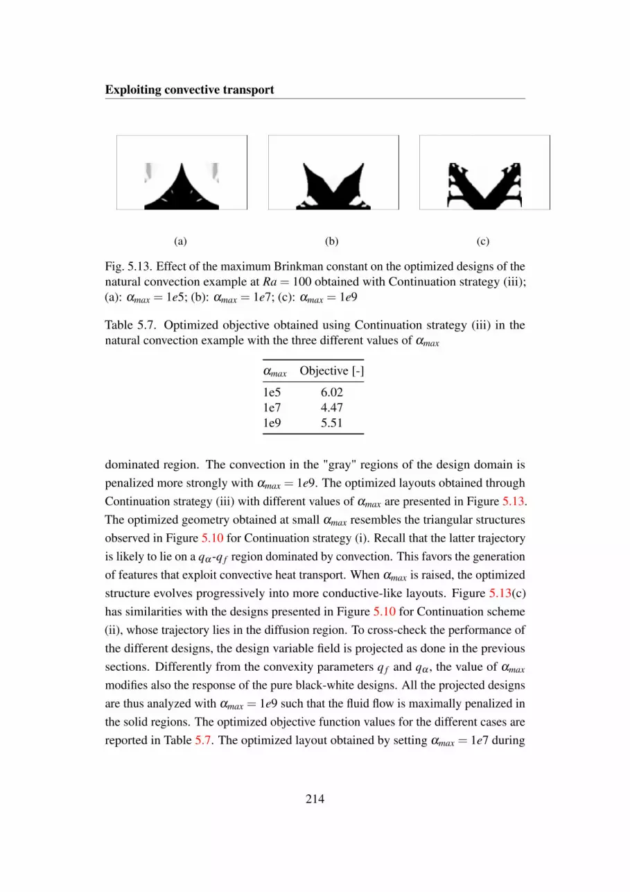
Exploiting convective transport
(a) (b) (c)
Fig. 5.13. Effect of the maximum Brinkman constant on the optimized designs of thenatural convection example at Ra = 100 obtained with Continuation strategy (iii);(a): αmax = 1e5; (b): αmax = 1e7; (c): αmax = 1e9
Table 5.7. Optimized objective obtained using Continuation strategy (iii) in thenatural convection example with the three different values of αmax
αmax Objective [-]
1e5 6.021e7 4.471e9 5.51
dominated region. The convection in the "gray" regions of the design domain ispenalized more strongly with αmax = 1e9. The optimized layouts obtained throughContinuation strategy (iii) with different values of αmax are presented in Figure 5.13.The optimized geometry obtained at small αmax resembles the triangular structuresobserved in Figure 5.10 for Continuation strategy (i). Recall that the latter trajectoryis likely to lie on a qα -q f region dominated by convection. This favors the generationof features that exploit convective heat transport. When αmax is raised, the optimizedstructure evolves progressively into more conductive-like layouts. Figure 5.13(c)has similarities with the designs presented in Figure 5.10 for Continuation scheme(ii), whose trajectory lies in the diffusion region. To cross-check the performance ofthe different designs, the design variable field is projected as done in the previoussections. Differently from the convexity parameters q f and qα , the value of αmax
modifies also the response of the pure black-white designs. All the projected designsare thus analyzed with αmax = 1e9 such that the fluid flow is maximally penalized inthe solid regions. The optimized objective function values for the different cases arereported in Table 5.7. The optimized layout obtained by setting αmax = 1e7 during
214

5.5 Numerical results and design trends
the optimization is largely superior to the alternatives. This suggests that the choiceof this parameter requires special care.
5.5 Numerical results and design trends
Here, we present and discuss the numerical studies conducted for both meltingand solidification enhancement in single-tube LHTES units. First, we compute areference design obtained neglecting fluid flow. This geometry is compared withthe convective layouts optimized for fastest melting and solidification. After theverification of the identified design trends with body-fitted analyses, we comparethe performance of the optimized geometries with a longitudinal layout; then, wepresent a method to reduce the complexity of the topology-optimized designs foreasier manufacturing and we test it on a real application.
The thermo-physical properties of PCM and the domain dimensions were intro-duced in Section 5.2.5. As in the forced and natural convection heat sink studies, weset the diffusivity ratio between PCM and HCM, Ck, to 1 %.
5.5.1 Diffusion design
In this section, we compute a reference solution where fluid flow is neglected. This isreferred to as diffusive design hereafter. Similar optimization studies were consideredin Chapter 3. However, the design interpolation strategies adopted here differ: ahigher penalization of the intermediate design variables is desirable to ensure theconvergence to binary 0; 1 designs. This is essential for the correct flow predictionwhen natural convection is considered. Furthermore, also the design domain wasmodified. We consider a charge process, which is reproduced with a hot Dirichletcondition T ∗d = 1 and a cold initial temperature field T ∗I = 0. The charge is consideredcomplete when the energy level in the tank reaches 95 % of the total capacity. Dueto the absence of convective effects, we obtained the same optimized design whenconsidering a discharge process from 100 % down to 5 % of the total capacity.
The objective history, normalized with respect to the initial value, along with thedesign at selected iterations is shown in Figure 5.14. The initial design correspondto a homogeneous distribution s = 0.9. In Figure 5.14, the designs corresponds
215

Exploiting convective transport
Fig. 5.14. Normalized objective history during the optimization of the diffusivedesign. The design evolution is shown at selected iterations. The jumps in theobjective correspond to the updates of the continuation scheme
216

5.5 Numerical results and design trends
to contour plots of the projected design variable field thresholded at s = 0.9. Theevolution of the objective shows three well-distinct stages, which correspond to thecontinuation scheme steps described in 5.4. In the first step, HCM concentrates ina region close to the internal tube and converges after 22 iterations. The secondcontinuation step, which penalizes the intermediate design variables more strongly,triggers a ramification (iteration 55) and converges to a structure with extremely thindesign features (iteration 120). During the third continuation step, those small designdetails characterized by intermediate design variables disappear so that shorter andthicker fins are created. Note the three continuation steps are necessary to achieve asatisfactory convergence to binary 0; 1 designs. Despite a lower objective function,the converged designs after the first and the second continuation step present largenon-physical "gray" regions. To quantify whether an optimized design convergedto a discrete solution, we adopt a measure of non-discreteness similar to the oneproposed by Sigmund [392]:
Mnd =
∫ΩD
4s(1− s)dV∫ΩD
dV, (5.90)
which intuitively represents the area fraction of the design domain in which theprojected design variable has not fully converged to either 0 or 1. When there areno regions with intermediate design variables, Mnd is 0 %. If s = 0.5 everywhere,we would obtain Mnd = 100 %. The final optimized design obtained thresholdingthe projected design variable field at s = 0.5 is shown in Figure 5.16(a). Thecalculated measure of non-discreteness Mnd for this layout is 1.44 %. Figure 5.15shows how the optimized geometry depends on the threshold choice. The layoutobtained thresholding the design variable field at s = 0.9 (Figure 5.15(a)) slightlydiffers from the one obtained with a threshold of s = 0.1 (Figure 5.15(b)). Thistest qualitatively confirms that the amount of intermediate gray material is limited.The optimized design is nearly symmetric with respect to the x-axis and showsquasi-periodicity along the angular direction with period ∆θ = π/2. The structureshows both longitudinal fins and Y-shaped (tree-like) fins around the HTF tube. Theformers are used extensively for heat transfer enhancement in LHTES, as discussedin Chapter 3 of this monograph. Similarly to what obtained in Chapter 3, thebranched fins are alternated to non-branched ones.
This section presented the optimization of a fin layout without considering naturalconvection during the analysis. This geometry will be used in the following sections
217

Exploiting convective transport
Fig. 5.15. (a): Final layout obtained for the diffusive design thresholded at s = 0.9;(b): final layout obtained for the diffusive design thresholded at s = 0.1
to benchmark the designs optimized considering fluid flow. Our diffusion geometrypresents similar features to those obtained in Chapter 3 of this monograph.
5.5.2 Melting design
In this section, we consider a melting process, i.e. the charge of a LHTES unit.In this study, natural convection is considered. Referring to the boundary andinitial conditions discussed in (5.24) and (5.27), to mimic melting we consider a hotDirichlet condition T ∗d = 1 and a cold initial temperature field T ∗I = 0. Similarly tothe diffusive design, the charge is considered complete when the energy level in thetank reaches 95 % of the total capacity. The optimized design obtained for meltingis shown in Figure 5.16(b). In this case, we obtain a measure of non-discretenessMnd of 1.19 %. The melting design is profoundly different from the one obtainedin Section 5.5.1: the HCM concentrates in the bottom part of the storage unit toform a conductive-like structure that occupies the shell sector parameterized by−π/3 < θ < π/3. The top portion of the shell is slightly occupied by HCM toleave room for fluid flow. To highlight the main layout differences between the twocases, Figure 5.16(c) presents a superposition of the optimized designs for diffusionand melting. The design here is represented by the contour of the projected designvariable at s = 0.5. We observe three main features:
(i) the top portion of the unit shows only two short fins which are slightly offsetfrom the radial direction;
218

5.5 Numerical results and design trends
Fig. 5.16. (a): Final layout obtained for the diffusive design; (b): final layout obtainedfor the melting design; (c) superposition of the two designs with zoom-in of themost relevant differences. The designs displayed were obtained by thresholding theprojected design variable field at s = 0.5
219

Exploiting convective transport
0 0.5 1 1.5 2 2.5Dimensionless time [-]
0
10
20
30
40
50
60
70
80
90
Norm
aliz
ed
dim
ensi
on
less
energ
y [
%]
20 50 80 100
Relative melting time [%]
126
Fig. 5.17. Energy histories of the melting and diffusive designs during a melting test
(ii) two large and thick branches are visible at θ = −π/3 and θ = π/3 withsecond-order bifurcations. These fins extend ∼ 37.8 % more in the radialdirection than those obtained in the diffusive design;
(iii) two thin branches elongates towards the bottom of the shell. These structuralcomponents are ∼ 19.6 % longer that the diffusive fins obtained at the sameangular position.
The radial position of the two thick branches described in (ii) recalls the results ob-tained in [452]. The authors observed that this particular configuration enhances heattransfer through convective transport. However, differently from our configuration,their design does not show any fin in the upper part of the unit and has a uniquelongitudinal fin elongating towards the bottom.
The normalized energy histories of the diffusive and melting designs are com-pared in a melting test. Here, both the layouts are analyzed for a charge of the unitincluding fluid flow. The results are plotted in Figure 5.17. Initially, the meltingdesign shows a slower charge rate than the diffusive design. This is due to the factthat diffusion is the dominant heat transfer mechanism during the initial portionof the process. However, the heat transfer rate of the diffusive design slows down
220

5.5 Numerical results and design trends
whereas the melting design maintains a fairly constant charge rate by exploiting theonset of natural convection. If the desired degree of charge of the storage units, Ψc,is above 80.2 %, the convective design is the best-performing choice. This limit isspecific to the particular design domain and material properties considered here. Forthe nominal charge case in which Ψc = 95 %, we obtain that the diffusive geometrydemands 25.9 % more time than the melting design to complete the charge process.Note that the particular choice of Ψc corresponds to an ideal utilization of the unit.Partial charge-discharge cycles may occur in real systems. Figure (5.18) shows theliquid fraction evolution at selected time instants of the melting test, correspondingto 20 %, 50 %, 80 % and 100 % of the total charge time of the melting design, t∗fm .At t∗ = 0.2 t∗fm , the liquid layer is thin and natural convection does not yield notice-able modifications of the melting front. During this initial stage of the process, thediffusive structure is more effective: thinner branches lead to more heat transfer areaas compared to the convective layout. As the fluid layer widens, natural convectionstarts to modify the shape of the melting front (t∗ = 0.5 t∗fm) and becomes dominantat t∗ = 0.8 t∗fm . The short fins of the melting design redirect the upward-movingfluid layer in such a way that the liquid PCM quickly fills the upper portion of thetank. The convective stream hardly reaches the region below the pipe, which isheated by long diffusive-like branches. The diffusive design can hardly get rid of themushy region at the bottom of the tank. To better visualize the main heat transfermechanisms, the magnitude of the average convective heat transfer rate, qvi, and ofthe conductive heat transfer rate, qki, are depicted in Figure 5.19. These quantitiesare calculated as:
qvi =
∫ t∗f0
(v∗i (T
∗+ γ f ∗L ∗))
dt∗
t∗f, (5.91)
qki =
∫ t∗f0
(−Ki j
∂T ∗∂x∗j
)dt∗
t∗f, (5.92)
where t∗f indicates the final time of the process of interest, set to t∗fm here as weare dealing with melting. The melting design largely utilizes the top fins and aportion of the pipe surface to enhance the convective heat transfer. This is confirmedby considering the conductive heat transfer plot which shows a large conductivecontribution in the same region. A wide eddy maintains a high temperature gradientat the interface: hot fluid is rapidly transported away leaving room for cold fluidcoming from the outer part of the shell. This mechanism can be better observed
221

Exploiting convective transport
0 0.25 0.5 0.75 1Liquid fraction [-]
t*=1.084
t*=1.734
t*=2.167
Fig. 5.18. Liquid fractions at selected time instants during melting. The left columnshows the diffusive design while the right column shows the melting design
222

5.5 Numerical results and design trends
Fig. 5.19. Average conductive and convective heat transfer rate during melting. Theleft column shows the diffusive design while the right column shows the meltingdesign
223

Exploiting convective transport
Fig. 5.20. Average velocity magnitude with streamlines during melting. The leftcolumn shows the diffusive design while the right column shows the melting design
in Figure 5.20, where we show the average velocity magnitude alongside withstreamlines. From a careful examination of the velocity plot, it is clear that thefins positioned above the pipe have the function of redirecting the flow towards theexternal shell. In the region below the pipe, convection is negligible and heat istransferred mainly by conduction. The ramification patterns of the diffusive designinhibit the formation of large convective eddies. The conductive heat transfer plot ofthe diffusive design shows a high average heat transfer rate at the fin tips indicatingthat conduction takes place mainly in the radial direction.
This numerical study presents evidence that melting can be enhanced remarkablythrough convective transport if the fins are designed with specific features, such asshort baffles in the top portion of the unit and a big diffusive structure at the bottom.
5.5.3 Solidification design
Here, we consider a solidification process corresponding to the discharge of theLHTES unit. Also in this numerical example, we account for fluid flow. Solidificationis modeled by considering a cold internal tube T ∗d = 0 (Eq. (5.24)) and a hot initialtemperature field T ∗I = 1 (Eq. (5.27)). The discharge is considered complete whenthe energy level in the tank reaches 5 % of the total capacity. The optimized designobtained for solidification is shown in Figure 5.21(b). The calculated measure ofnon-discreteness Mnd for this layout is 1.37 %. The optimized diffusive design isshown again in Figure 5.21(a) to facilitate the comparisons. To highlight the main
224

5.5 Numerical results and design trends
(i)
(ii)
(iii)
(iv)
Fig. 5.21. (a): Final layout obtained for the diffusive design; (b): final layout obtainedfor the solidification design; (c) superposition of the two designs with zoom-in ofthe most relevant differences. The designs displayed were obtained by thresholdingthe projected design variable field at s = 0.5
225
Exploiting convective transport
layout differences between the two cases, Figure 5.21(c) shows a superposition ofthe optimized designs represented by the projected design variable field contoured ats = 0.5. The solidification design closely resembles the one obtained consideringonly diffusion. However, accounting for natural convection in the analysis results infour small modifications:
(i) the branches elongating towards the top of the shell are ∼ 9.3 % longer thanthose of the diffusive design;
(ii) the bifurcations of the intermediate branches are not visible;
(iii) the horizontal branches are ∼ 43.7 % longer than than those of the diffusivedesign;
(iv) the branches elongating towards the bottom of the shell are ∼ 3.2 % shorterthan those of the diffusive design.
The aspects (i) and (iv) result in a higher concentration of HCM in the upper halfthe shell. This feature agrees with the intuition that a larger heat transfer areashould be utilized in the regions where the solidification front lags behind. Theobtained design is similar to the many longitudinal fin layouts utilized in literatureand presented in Chapter 3. However, to our best knowledge no previous study inliterature considered a varying fin length along the angular position in the shell, aswe obtained thanks to features (i), (iii), (iv). The normalized energy histories ofthe diffusive and solidification designs during the discharge of the unit are shownin Figure 5.22. The solidification design outperforms the diffusive design for anychoice of the discharge fraction, Ψd . The energy histories are very close to each otheruntil t∗ ∼ 0.45, when they start to diverge. From this point onward, the temporal gapbetween the two curves increases gradually in time. Overall, the diffusive designdemands 11.1 % more time than the solidification design to discharge the unit. Theliquid fraction evolution for the solidification test is shown in Figure 5.23 at 20 %, 50%, 80 % and 100 % of the discharge time of the solidification design, t∗fs . The shapeof the solidification front has negligible differences for t∗ = 0.2 t∗fs and t∗ = 0.5 t∗fs .The snapshots taken at t∗ = 0.8 t∗fs and t∗ = t∗fs show that the solidification designallows maintaining the solidus line nearly concentric with the internal tube thanksto the longer fins located above the pipe. In the meantime, the solidification frontof the diffusive design starts drifting downward. This asymmetry with respect to
226

5.5 Numerical results and design trends
20 50 80 100
Relative solidification time [%]
111
0 0.5 1 1.5 2 2.5 3Dimensionless time [-]
0
10
20
30
40
50
60
70
80
90
Norm
aliz
ed
dim
ensi
onle
ss e
nerg
y [
%]
Fig. 5.22. Energy histories of the solidification and diffusive designs during asolidification test
the x-axis is responsible for the increased discharge time: the "left-over" mushyregion at the top of the shell has to be cooled away for the discharge completion.Further insights can be gained by considering the average heat transfer rates in Figure5.24, obtained from Eqs. (5.91) and (5.92) with t∗f = t∗fs . The conductive portionin the diffusive design is concentrated at the fin tips similarly to what we observedfor the same geometry in the melting test. On the other hand, the solidificationdesign transports a non-negligible amount of conductive heat transfer along the finsides. This indicates that the solidification layout results in a more homogeneousheat transfer distribution and a better utilization of the fin material. In this case, theflow can penetrate close to the internal tube. The ramification patterns visible in thediffusive design inhibit this mechanism, suppressing natural convection. From theexamination of the streamlines shown in Figure 5.25, we notice that the diffusiongeometry confines the fluid outside of the finned region. This creates a tall and thineddy with a high downward velocity which contributes to the asymmetry of thesolidus line discussed before. Conversely, the downward velocity in the solidificationdesign is limited because of the presence of the small interstitial eddies and the longerhorizontal fins. Figure 5.25 also shows that the velocities involved in solidification
227

Exploiting convective transport
t*=1.084
t*=1.734
t*=2.167
0 0.25 0.5 0.75 1Liquid fraction [-]
Fig. 5.23. Liquid fractions at selected time instants during solidification. The leftcolumn shows the diffusive design while the right column shows the solidificationdesign
228

5.5 Numerical results and design trends
Fig. 5.24. Average conductive and convective heat transfer rate during solidifica-tion. The left column shows the diffusive design while the right column shows thesolidification design
Fig. 5.25. Average velocity magnitude with streamlines during solidification. Theleft column shows the diffusive design while the right column shows the solidificationdesign
229

Exploiting convective transport
Table 5.8. Charge time computed with a high-fidelity framework in COMSOLMultyphysics
Performance
Design Ch. time [-] TopOpt dev. [%] TopOpt dev. (β = 1000) [%]
Thresh. melting 1.72 + 25.58 + 7.76Thresh. diffusive 2.13 + 27.67 + 5.44
are significantly lower than those involved in melting (Fig. 5.20). This limits theaverage heat transfer rate and results in a long time required for the discharge ascompared to the charge of the LHTES unit.
5.5.4 Verification of density-based physical model
This section questions the accuracy of the density-based physical model in predictingthe thermal and flow responses of our optimized LHTES units. We compare thepredictions of a density-based description to those of a body-fitted grid that allows anexplicit tracking of the materials interface. This a-posteriori cross-check is importantfor two main reasons. First, the material interpolation strategy used in density-basedtopology optimization does not allow to enforce no-slip conditions at the walls andmay result in unphysical fluid-dynamic response that can alter both the optimizationresults and the identified design trends. Second, selecting a proper threshold forconverting a continuous density map to a sharp layout is crucial for manufacturingand needs to be verified.
For the body-fitted studies, we consider two computational domains separatedby an interface that conforms to the s = 0.5 iso-contour of the optimized designvariable field. These domains are then meshed using high resolution body-fittedgrids with 38976 and 32617 free quadrangular elements for the melting and diffusivedesigns, respectively. A graphical representation of the meshed PCM domain inthe melting design is reported in Figure 5.26 along with a zoomed-in view thatallows the resolution at the boundary to be appreciated. The charge times obtainedwith this high-fidelity framework are reported in Table 5.8. The results indicatethat the our density-based topology optimization framework predicts roughly a 26% higher charge time as compared to the high-fidelity framework. Figure 5.27reports the dimensionless diffusivity field along the red line depicted in Figure 5.26.
230
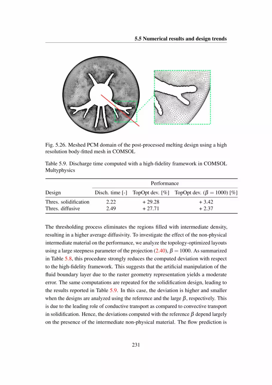
5.5 Numerical results and design trends
Fig. 5.26. Meshed PCM domain of the post-processed melting design using a highresolution body-fitted mesh in COMSOL
Table 5.9. Discharge time computed with a high-fidelity framework in COMSOLMultyphysics
Performance
Design Disch. time [-] TopOpt dev. [%] TopOpt dev. (β = 1000) [%]
Thres. solidification 2.22 + 29.28 + 3.42Thres. diffusive 2.49 + 27.71 + 2.37
The thresholding process eliminates the regions filled with intermediate density,resulting in a higher average diffusivity. To investigate the effect of the non-physicalintermediate material on the performance, we analyze the topology-optimized layoutsusing a large steepness parameter of the projection (2.40), β = 1000. As summarizedin Table 5.8, this procedure strongly reduces the computed deviation with respectto the high-fidelity framework. This suggests that the artificial manipulation of thefluid boundary layer due to the raster geometry representation yields a moderateerror. The same computations are repeated for the solidification design, leading tothe results reported in Table 5.9. In this case, the deviation is higher and smallerwhen the designs are analyzed using the reference and the large β , respectively. Thisis due to the leading role of conductive transport as compared to convective transportin solidification. Hence, the deviations computed with the reference β depend largelyon the presence of the intermediate non-physical material. The flow prediction is
231

Exploiting convective transport
0.4 0.6 0.8 1
Arc length [-]
0
10
20
30
40
50
60
70
80
90
100
Dim
en
sio
nle
ss t
he
rma
l d
iffu
siv
ity [
-]
COMSOL
TopOpt
Fig. 5.27. Dimensionless thermal diffusivity along the red line indicated in Figure5.26
slightly affected by the raster geometry representation due to the small velocitiesinvolved.
Instead of raising the projection steepness parameters, β , the performance differ-ences between the body-fitted and density-based analysis models could be decreasedalso by reducing the radius of the density filter (2.37). However, in our framework itis not possible to eliminate completely the fuzziness of the geometry representationby acting on r f . As we adopt nodal design variables, a minimum filter size is requiredto ensure that an element-wise constant filtered density, s, is assigned to each elementof the FE mesh.
From the analysis presented in this section, it can be concluded that our topologyoptimization framework is able to capture with sufficient accuracy the main physicalphenomena so that the design trends are preserved and the final manufactured finlayouts perform as expected.
5.5.5 Comparison with longitudinal fins
To further question the effectiveness of our optimized layouts, we use the body-fittedhigh-fidelity simulation framework discussed in the previous section to compare theperformance of our optimized geometries with a conventional longitudinal layout
232

5.5 Numerical results and design trends
0 0.5 1 1.5 2
Dimensionless time [-]
0
10
20
30
40
50
60
70
80
90
En
erg
y c
on
ten
t [%
]
Longitudinal design
Melting design
(a)
0 0.5 1 1.5 2
Dimensionless time [-]
10
20
30
40
50
60
70
80
90
100
En
erg
y c
on
ten
t [%
]
Longitudinal design
Solidification design
(b)
Fig. 5.28. High-fidelity comparison of energy histories between the topology-optimized and longitudinal geometries. (a): Charge; (b): discharge
(Figure 5.30(b)). The latter is composed of 10 fixed-length fins equally spaced alongthe angular direction. The fin length is computed as the average of those obtained fora solidification layout with reduced geometric complexity (Figure 5.30(a)), that willbe discussed in Section 5.5.6. The energy histories during melting and solidificationare shown in Figure 5.28. Our optimized layouts yield a reduction of 25.7 % and9.1 % of the charge and discharge time as compared to the conventional geometry.We observe trends similar to the ones discussed when analyzing and comparingthe performance of the convective geometries to the one of the diffusive geometry.In melting, the longitudinal fins yield a quick charge during the initial part of theprocess. When the energy content reaches roughly 80 % of the total capacity, the heattransfer rate drops dramatically. This is because the mushy region at the bottom of theshell is slowly melted away, similarly to what we observed for the diffusive designin Figure 5.18. The topology-optimized design allows a much steadier power outputto be maintained by exploiting the onset of convective transport. For this reason, ityields a quicker charge for Ψc > 88.7 %. On the other hand, the solidification designis superior to the longitudinal geometry for any choice of the target energy fraction,Ψd .
These results demonstrate that the topology-optimized designs yield substantialadvantages as compared to the popular longitudinal layout. One could argue that per-
233

Exploiting convective transport
formance gains are not enough to justify the increased manufacturing complexity. Inthe next section, we will show a possible method to reduce the geometric complexitywithout modifying the most relevant features of the optimized layouts.
5.5.6 Reduction of geometric complexity for a real application
In this section, we propose a method to reduce the geometric complexity of theoptimized designs in the spirit of easier manufacturing. We test the reduced ge-ometries in a real-world application: a small-scale storage unit for DHNs. Due tothe high compactness of the LHTES, the unit can be installed at each thermal userlocation in parallel to the building heat exchanger. We assume that the building isheated by a low-temperature system. This allows the placement of the unit and heatexchanger on the return line of the primary network, typically at 70 C. We considerthis value as the Dirichlet boundary condition during charge. On the other hand,the HTF temperature during discharge (and thus the Dirichlet boundary) is set to 20C, corresponding to the temperature of the secondary network at the startup. Thematerial properties and the shell dimensions are the same used for the design studypresented in [375]. The radius of the HTF tube is here set to r1 = 0.0165 m to keepconsistency with the dimensions adopted in this chapter. Three designs are analyzed:the optimized layout obtained with our topology optimization framework, a modifiedversion with reduced complexity that allows easier manufacturing and the classicaldesign with longitudinal fins. All the analyses are conducted using the high-fidelitybody-fitted framework adopted in the previous sections.
Figure 5.29 shows the procedure followed to reduce the complexity of thetopology-optimized layout. First, the optimized geometry (thresholded at s = 0.5)is interpolated over a 300 × 300 grid (Figure 5.29(a)). Then, a binary skeleton(Figure 5.29(b)) is obtained through sequential thinning [340, 353]. The branchjunctions, bifurcations and extrema are then manually identified and linked withline segments to obtain a straight skeleton (Fig. 5.29(c)). Finally, a uniform finthickness is calculated such that the HCM volume fraction is equal to the one ofthe original design. The computed reduced layout is depicted in Figure 5.29(d).The reduced layout obtained for the solidification case is depicted in Figure 5.30alongside with the benchmark longitudinal layout. Note that the designs shown in5.30(a) and 5.30(b) differ in terms of length and tilt angle of the fins. Figure 5.31shows the performance of the analyzed geometries over a full charge and discharge.
234

5.5 Numerical results and design trends
(a) (b) (c) (d)
Fig. 5.29. Reduction of complexity of the topological melting design for easiermanufacturing. (a): 300 × 300 pixelated geometry; (b): skeletonized geometry; (c):straight skeletonized geometry; (d): final reduced geometry
(a) (b)
Fig. 5.30. (a): Reduced topological solidification geometry; (b): reference longitudi-nal geometry
235

Exploiting convective transport
When using the topology-optimized design, the charge of the unit can be completedin 3076 s corresponding to a 37.3 % reduction of the discharge time as comparedto the unit equipped with the classical longitudinal fins. The simplification of thegeometry complexity presented in Figure 5.29 results in a layout that increasesthe discharge time by 256 s, corresponding to a 8.23 % performance reduction.However, the reduced geometry still yields a 32.3 % enhancement as compared to thelongitudinal one. Note that the use of longitudinal fins again yields a higher chargerate at the beginning of the process. When tested during a discharge case (Figure5.31(b)), the performance differences are less evident. The topology-optimizeddesign and its version with reduced complexity yield a 15.2 % and a 7.3 % reductionin the discharge time as compared to the classical geometry. Although limited inmagnitude, the improvement achieved through the utilization of the design withreduced geometric complexity highlights the importance of a variable length andangular distance of the fins.
This section demonstrated a possible approach to reduce the geometric complex-ity of topology-optimized results, facilitating manufacturing. This strategy allowsthe main topology features to be preserved and was found to yield remarkable advan-tages with respect to the classical longitudinal fins for both charge and discharge ofa real-world LHTES unit.
5.6 Conclusions
In this chapter, we extended the design and analysis framework developed in Chapter3 to account for natural convection in the liquid PCM. We first presented someissues that may arise in density-based topology optimization for conjugate heattransfer problems. Our simplified numerical examples demonstrated that an improperselection of the continuation trajectory on the penalization parameters may lead tounsatisfactory configurations, which do not exploit sufficiently either the convectiveor diffusive heat transfer. Then, we searched for heat transfer structures exploitingconvective transport for fastest melting and solidification in LHTES units.
A graphical summary of the main application-oriented advances is presented inFigure 5.32. The results suggest that neglecting fluid flow in design optimizationstudies leads to suboptimal configurations and proved that the heat transfer structuresoptimized for melting are in general different from those optimized for solidification.
236

5.6 Conclusions
0 500 1000 1500 2000 2500 3000 3500 4000 4500
Time [s]
0
10
20
30
40
50
60
70
80
90
En
erg
y c
on
ten
t [%
]
Longitudinal design
Reduced topological design
Topological design
(a)
0 500 1000 1500 2000 2500 3000 3500 4000 4500 5000
Time [s]
10
20
30
40
50
60
70
80
90
100
En
erg
y c
on
ten
t [%
]
(b)
Fig. 5.31. Energy histories during charge (a) and discharge (b) of a real-worldLHTES unit
237

Exploiting convective transport
Energ
y [%
]- 11 %
Time
- 26 %
Time
Energ
y [%
]
Topological
designReduced
topological designConventional
design
Melting
Solidification
Fig. 5.32. Graphical summary of the main application-oriented advances of the chap-ter. (a): Effect of natural convection on the optimized design and performance formelting enhancement; (b): effect of natural convection on the optimized design andperformance for solidification enhancement; (c): layout and performance comparisonof simplified topological geometries for easier manufacturing
238

5.6 Conclusions
A fast melting requires a nearly empty top of the shell such that sufficient room isleft for the upward fluid motion (Figure 5.32(a)). The diffusive fins concentrate inthe bottom portion of the unit. Using this layout allows the discharge time to bereduced by nearly 26 % as compared to a benchmark design obtained consideringonly diffusion. On the other hand, the geometry optimized for solidification presentsminor modifications with respect to the diffusive layout (Figure 5.32(b)). In thiscase, considering natural convection in the analysis yields a layout responsible of an11 % reduction in the discharge time. These design trends are not affected by ourdensity-based physical model, as verified through analyses with body-fitted gridsconforming to computational domains obtained from the thresholded optimizeddesign variable field. This high-fidelity framework was then used to compare thetopology-optimized geometries against a conventional longitudinal layout. Theresults indicate that large performance enhancements for both charge and dischargecan be obtained through topology optimization. Last, we presented a method forpost-processing the optimized layouts into easily manufacturable geometries thatconserve the main topology features (Figure 5.32(c)). As compared to the benchmarklongitudinal layout, the obtained geometries yield a considerable reduction in thetime required for the complete charge and discharge of a storage unit for districtheating applications.
In this chapter, we focused on single-tube configurations that are popular inlab-scale or small-scale facilities. However, most of the commercial installationsconsist of multiple tubes immersed in a unique shell. The extension of these resultsto multi-tube systems through a circular periodicity assumption is complicated bythe anisotropy of convective transport. For this reason, the design optimization ofmulti-tube units merits an ad-hoc treatment and will be discussed in Chapter 6.
239

Chapter 6
Design of practical multi-tube units
The shell-and-tube units with multiple tubes distinguish from the other LHTES con-figurations for their high compactness, large heat transfer area and easy integrationwith multiple hydraulic loops, preventing the mixing between HTFs. However, a lim-ited body of literature is devoted to the search of the optimal heat transfer structuresin this configuration. A popular approach to analyze and optimize multi-tube sys-tems consists in simulating a single tube under the assumption of periodicity, see forinstance [256, 219, 218, 250, 42, 480]. Representing multiple tubes by a collectionof many single tubes surrounded by PCM rings only approximates the shell area anddoes not account for boundary effects [50]. Natural convection further questions theperiodicity assumption. Agyenim et al. [7] found experimentally that the horizontalmulti-tube systems develop multiple convective cells with a complicated interaction.Similar observations were drawn by the authors of [186] and [120], who proposedspecific features to exploit convective transport in this configuration. Bridging thegap with the practical technology development of these units require more preciseinsights on specific design issues. Four fundamental questions remain unanswered:
(i) For which range of material properties do convective features matter?
(ii) How does the periodicity assumption affect the optimized layouts and perfor-mance?
(iii) Do systems with separate hydraulic loop require for ad-hoc geometries?
(iv) How are design and performance affected by the HCM and PCM choice?
240

6.1 Overview of materials in LHTES units
This chapter aims at shedding light on these practical design issues.
The outline of the chapter is as follows: in Section 6.1 we review the mostpopular materials used as HCMs and PCMs in LHTES units; Section 6.2 presentsand verifies numerically a heuristic approach able to answer question (i); finally,Section 6.3 answers questions (ii) through (iv) with specific numerical examples.
6.1 Overview of materials in LHTES units
When selecting a PCM for a particular application, a number of physical, technicaland economic requirements can be identified [296]. Physical criteria are used for aprimary selection. The ideal PCM features:
• a phase change temperature matching the application of interest;
• a high phase change enthalpy per unit volume, leading to a high energy density;
• a high thermal conductivity, allowing the charge and discharge of the unit intime spans matching the applications requirements;
• no phase separation, leading to reversible cycles with no performance degrada-tion;
• little subcooling, yielding charge/discharge cycles over a small temperaturerange.
Technical requirements mainly concern the chemical properties of the PCM [39],which should be chemically stable, compatible with the construction material toavoid corrosion, non-toxic and non-flammable. Economic requirements deal withthe availability of storage material at low cost.
A storage material satisfying all these requirements has yet to be found. It ispossible however to categorize PCMs in such a way that classes with similar physicaland technical properties are identified. A possible classification strategy is depictedin Figure 6.1. This option based on the chemical properties is rather popular in theliterature, see for instance [499, 402]. PCMs are subdivided into organic, inorganicand eutectic mixtures. Organic PCMs can be further classified into paraffins, fattyacids, alcohols and glycols. Inorganics include salts, salt hydrates and metallic
241

Design of practical multi-tube units
PCMs
Organic
Inorganic
Eutectics
Paraffins
Fatty acids
Sugar alcohols
Glycols
Salts
Salts hydrates
Metals (& alloys)
Organic-organic
Inorganic-organic
Inorganic-inorganic
Fig. 6.1. Classification of PCMs based on chemical properties
alloys. Eutectics are mixtures of different constituents and can be organic-organic,organic-inorganic and inorganic-inorganic. In the following sections, we review themost important organic and inorganic PCMs.
The melting temperature and the enthalpy of phase change are not independent.Richardson first observed that melting and solidification yield a fixed entropy changein conductor materials [296]. Considering an isothermal phase transition of a closedthermodynamic system with negligible volume changes and gravitational forces wecan write [131, 296]:
∆S =∆HTm
= constant, (6.1)
where S is the entropy, H is the enthalpy and Tm is the melting temperature. Richard-son’s rule is restricted to metallic materials and the validity for other substancesis often questioned. However, Figure 6.2 shows that a rough correlation betweenmelting temperature and specific enthalpy of phase change is present. The storagematerials with high melting temperature such as salts feature a high energy density.PCMs with low melting temperature are able to store a limited amount of latent heatduring the phase transition. Table 6.1 reports typical energy density ranges of PCMalong with those of popular sensible TES alternatives. For a reference temperature
242

6.1 Overview of materials in LHTES units
Fig. 6.2. Melting temperatures and enthalpies of different classes of PCMs [492]
difference of 20 C, exploiting phase change allows reducing the storage unit size ofa water tank by at least a factor of 2. Agyenim [7] proposed a classification of PCMsbased on their melting temperature, arguing that this criterion is directly linked tothe applications. The storage materials with low melting temperatures, i.e. Tm ≤ 65C, can be used for domestic heating and cooling, storage of off-peak electricity andintegration in building materials. This category includes water, water-salt solutions,and all the organic PCMs. Due to the wide variety of possible applications, thistemperature range is the one that was investigated the most [7]. The materials meltingat intermediate temperatures (80 C ≤ Tm ≤ 120 C), such as some paraffins, sugaralcohols and some salt hydrates are adopted for storage on the evaporator side ofLiBr-H2O absorption cooling systems or for storage in large district heating networks[98]. The materials with high melting temperature (Tm > 150 C) can be used instorage units connected to CSP plants or industrial waste-heat recovery systems [77].This temperature range includes salts, salt eutectics and metals.
6.1.1 Organic PCM
Organic PCMs include alcanes, fatty acids, glycols, alcohols and esters. To date,alcanes (i.e. paraffins) are by far the preferred option at the commercial level [7].This material class covers a wide melting temperature range. They are hydrocarbonswith general formula CnH(2n+2) with C being a carbon atom and H a hydrogen
243

Design of practical multi-tube units
Table 6.1. Energy density ranges of the most popular storage materials
Material Energy density [MJ/m3] Reference Notes
SensibleWater 84 [296] ∆T = 20 CRocks 50 [296] ∆T = 20 COrganic oils 30-33 [23] ∆T = 20 CSalts 39-75 [23] ∆T = 20 C
PCMParaffins 169-204 [23]Salt hydrates 263-548 [23]Salts 631-1584 [23]Water 360 [296]
atom. The melting temperature raises with increasing length of the molecular chainsuch that Tm ∼ ln(n). In practical applications, only materials with n > 14 are used.Paraffins have large enthalpy of fusion with respect to mass and can fully solidifywith practically no subcooling. They are also well resistant to phase separation.However, their thermal conductivity rarely exceeds 0.2 W/(m K). Furthermore, theirlow density results in small volumetric energy densities as compared to alternativePCMs with similar melting temperatures, such as salt hydrates. They are littlereactive at nominal operating temperatures and compatible with metallic materials.At high temperatures, i.e. T > 200 C, they become chemically unstable: the shortchain molecules break and evaporate yielding flammable mixtures.
Fatty acids respond to the general formula CH3CnH2nCOOH. As compared toalcanes, one end of the paraffinic chain is substituted by a carboxyl group. ThesePCMs have thermo-physical properties similar to those of paraffins [296]. Severaleutectic mixtures of fatty acids were experimented [484]. Eutetics generally decreasethe phase change temperature of pure acids with negligible modifications of theenthalpy of phase change. A similar effect can be obtained through the esterificationreaction. Researchers mainly chose stearic acid and palmitic acid to obtain esterswith low melting temperature and high enthalpy of phase change. Some scholars[368, 366, 367] reported only moderate thermal degradation after repeated cycling.However, the authors of [484] argued that thermal stability of these storage materialsis strongly affected by the presence of impurities.
244

6.1 Overview of materials in LHTES units
Sugar alcohols belong to a material class that has received little attention byresearchers so far [23]. They are hydrogenated carbohydrate with general formulaCH2OH[CH(OH)]nCH2OH [296]. Their melting temperature ranges from 90 Cto 200 C making them good candidates for intermediate temperature applications.Their high density and specific enthalpy of phase change results in high latent heatper unit volume as compared to alternative organic PCMs. However, they requiresubcooling for complete solidification. Furthermore, recent experimental results[400] demonstrated that some sugar alcohols, e.g. galacticol, feature a poor stabilityto thermal cycling. This suggests that much more research needs to be conductedbefore this class of material can be used in real-world thermal storage applications.
In the category of glycols, Polyethylene glycol (PEG) is the most popular materialfor thermal energy storage with phase change. It is a polymer composed of a longdymetyhil ether chain, resulting in the general formula C2nH4n+2On+1 [296]. PEGcomes in various grades, i.e. from PEG400 to PEG10000, depending on its molecularweight. Both the melting temperature and enthalpy increase with the length of themolecular chains. PEGs have high chemical and thermal stability as demonstrated inseveral experimental studies [336, 382].
6.1.2 Inorganic PCM
Inorganic PCMs include salt hydrates, salts, metals and metal alloys. They generallyhave higher volumetric energy density than organic materials due to their higherdensity [499]. However, they often require subcooling and some inorganic PCMsmay lead to severe corrosion of the container material [296].
Salt hydrates are inorganic salts containing a large amount of crystallized water.They have a highly stable crystal structure that results in higher melting temperaturesthan water [296]: they melt in the range 30 C < Tm < 50 C [23]. Some relevanttechnical impediments prevented their widespread adoption for storage purposes.First, phase separation is observed since all salt hydrates consist of several compo-nents. This in turn affects the cycling stability. For this reason, gelling or thickeningagents to hinder sedimentation were considered [336]. Subcooling can also be amajor problem. Mehling and Cabeza [296] reported subcoolings as large as 80 Cfor some materials. Furthermore, high corrosion rates were observed for a few salt
245

Design of practical multi-tube units
hydrates when in contact with metals such as copper, aluminum and brass [73, 307].This restricts the spectrum of usable HCMs for heat transfer enhancement purposes.
Salts melt at temperatures higher than 150 C. They are considered as suitablecandidates for high temperature applications such as CSP [275]. The thermo-physicalproperties vary substantially among nitrates, carbonates, hydroxides and clorides.Zalba et al. [486] observed that only a few pure inorganic salts posses a high latentheat of fusion. For this reason, double and ternary eutectic compositions werelargely investigated. In general, they feature a moderate thermal conductivity, limitedsubcooling and high chemical and thermal stabilities [296]. However compatibilityproblems of some salts with some common HCMs were reported [275, 384].
Metal and metal alloys were limited in applications for their high density, whichcomplicates the design of containers. However, their melting enthalpy per unit vol-ume is comparable to the one of salts [77] for similar ranges of melting temperatures.The high conductivity of metals yields fast charge and discharge kinetics with noneed for heat transfer enhancement systems. The authors of [486] reported that theselection of metallic materials for storage purposes is complicated by the lack of acomprehensive database able to solve some major discrepancies in thermo-physicaldata obtained in the previous researches.
6.1.3 High conducting materials
The most common HCM options for extended surfaces in LHTES are aluminum,graphite, copper and steel [405, 275, 77, 23]. The selection of the extended surfacematerial is a crucial step for obtaining cost-effective installations. However, it ishard to extract fundamental selection guidelines from the available LHTES literature.According to Ibrahim et al. [215], the relevant selection criteria are the thermalconductivity, density, corrosion potential and cost. Steel is often excluded as en-hancement material due to its high density and low thermal conductivity. However,finned steel tubes are standard components in heat transfer equipment [405] and thusthey can represent an option in practice. For instance, finned steel tubes were usedrecently in CSP [287] and refrigeration [163] applications. Copper is the secondmost conductive metal after silver [75]. Hence, it is commonly considered as oneof the most effective enhancers. Examples of recent studies considering copperfins are [306, 235]. However, we observe that its large density leads to bulky and
246

6.1 Overview of materials in LHTES units
Table 6.2. Thermo-physical properties and cost of most popular HCMs
Material
Property Graphite foil Aluminum Stainless steel Copper
Thermal conductivity [W/(m K)] 150 200 20 350Specific heat [kJ/(kg K)] 0.7 0.9 0.5 0.4Density [kg/m3] 1000 2700 7800 8880Diffusivity [m2/s] (x106) 214.29 82.31 5.13 99.43Cost per unit volume [k$/m3] 10 7 20 40Cost per unit mass [k$/kg] 10 2.59 2.56 4.54
expensive installations. Furthermore, compatibility issues with fatty acids werereported in [136]. Graphite and aluminum feature high conductivity, low density andcost. For these reasons, they represent the most widespread options for heat transferenhancement in LHTES as demonstrated by the large number of studies recentlypublished, e.g. [380, 132, 487, 23]. Both graphite and aluminum yield no galvaniccorrosion when in contact with galvanized steel [275], a common material choice forthe HTF pipes. Graphite is preferred for high temperature applications [77] as it doesnot get corroded by nitrates and nitrites. Below 330 C, also aluminum fins can beused since no long-term degradation was observed when in contact with those salts[405]. The thermo-physical properties of these materials along with their estimatedcost per unit volume as obtained from [405] are summarized in Table 6.2.
The volumetric cost carries large uncertainty. It depends on the vendor pricingscheme, on the quantity of the material purchased and on the specific industrialprocess with which it was treated. In most cases, the cost is not publicly availablebut it is a result of private trading. Since this parameter is of crucial importance forsome of the results presented in this chapter, we collected a number of alternativereferences. To allow meaningful comparisons over data corresponding to differentyears, all the values are normalized with respect to the volumetric price of aluminum.As motivated in [75], the price fluctuations in time are rapid but the price ratiosamong different materials tend to vary slowly. The work of Steinmann et al. [405]was the only one we found listing the cost values for graphite foils. Table 6.3summarizes the outcome of this literature review. The results suggest that we can setthe costs of HCM as those reported in [405] with sufficient confidence.
247

Design of practical multi-tube units
Table 6.3. Review on the volumetric cost of HCMs. The reported values arenormalized with respect to the cost of aluminum
Material
Reference Graphite foil Aluminum Stainless steel Copper
[44] - 1 3.61 4.88[35] - 1 - 3.84[226] - 1 3.14 10.81[75] - 1 1.96 3.55[405] 1.42 1 2.85 5.71
6.2 A heuristic method to anticipate design trends
In some recent studies [436, 109, 46], specific layout features of extended surfaceswere proposed to enhance convective transport. Given the large differences inmaterial properties highlighted in the previous section, it is hard to extrapolate somedesign guidelines valid for general LHTES units. It is desirable for designers toestimate in advance whether these details are important or negligible for performance.In the latter case, convection could be safely ignored during the design optimizationprocedure. In this section, we first propose and then verify a heuristic method able toprovide rule-of-thumb indications.
6.2.1 The method of intersection of asymptotes
We are interested in anticipating for which combinations of material properties theoptimized design transitions from conduction-dominated to convection-dominatedstructures. We found that the PCM-to-HCM diffusivity ratio, Ck, has the largesteffect on the optimized layouts. Some preliminary numerical studies showed that thetransition covers a small range of Ck values. To identify this range, we look for the in-tersection of two extrema conditions, as shown in the schematics presented in Figure6.3. For Ck→ 0, the extended surface has the potential for a dramatic enhancementthrough conductive transport. Hence, we conjecture that the optimal HCM structuresuppresses convective flows in order to create highly branched layouts, favoring diffu-sion. If this is true, convection yields such a limited contribution to performance thatfluid flow can be neglected. We call this condition the diffusion-dominant asymptote.For Ck→ ∞, the fins limit the conductive heat transfer rate due to the low diffusivity
248

6.2 A heuristic method to anticipate design trends
Complete process
time
Diffusivity ratio
Transition region
Diffusion-dominant
asymptote
Convection-dominant asymptote
Optimized designs
Fig. 6.3. Schematic of the intersection of asymptotes method used to identify thetransition region from conductive-like designs to convective-like designs
of the HCM and impede the creation of beneficial convective currents. Hence, wespeculate that no HCM is present in the optimal configuration such that convectivetransport is maximally exploited. We will refer to this condition as convection-dominant asymptote. The choice of the HCM affects only the performance of thediffusion-dominant asymptote: the time required for a complete charge/dischargevaries roughly as ∼
√Ck. The performance of the convection-dominant asymptote is
constant with respect to Ck and depends exclusively on the Rayleigh number, Ra, ofthe liquid PCM: a higher Ra yields a quicker process completion. The performancecurve of the optimal HCM structures lies always below the asymptotes because finscan exploit both conduction and convection. For Ck→ 0, the curve of the optimaldesigns tends to the diffusion-dominant asymptote, while it tends to the convection-dominant asymptote for Ck→ ∞. The optimal structure continuously evolves froma highly branched configuration to a virgin design domain (i.e. no HCM present).We believe that the most visible design changes can be expected for Ck ∼C∗k , whereC∗k indicates the abscissa corresponding to the intersection of the two asymptotes.We refer to the Ck range parametrized with C∗k − εk <Ck <C∗k + εk as the transitionregion.
249

Design of practical multi-tube units
A
Fig. 6.4. Schematic of the design domain considered in this chapter
6.2.2 Verification
Here, we verify numerically the method of intersection of asymptotes presented inthe previous section. We consider both charge (melting) and discharge (solidification)including fluid flow in the analysis. To mimic melting, we consider a hot Dirichletcondition T ∗d = 1 and a cold initial temperature field T ∗I = 0. On the other hand,solidification is reproduced with T ∗d = 0 and T ∗I = 1. The charge and discharge areconsidered complete when the energy level in the tank reaches 95 % and 5 % of thetotal capacity, respectively. A schematic of the multi-tube design and computationaldomains is given in Figure 6.4. We adopt the same governing equations, boundary
250

6.2 A heuristic method to anticipate design trends
(a) (b) (c)
Fig. 6.5. (a) Optimized diffusive design used to compute the diffusion asymptote;(b): melting design optimized for Ck = 0.2 %; (c): solidification design optimizedfor Ck = 0.2 %
conditions and numerical model presented for the single tube geometry in Chapter5. The design domain has dimensions r1 = 0.125, r2 = 1, d1 = 0.35 and d2 = 0.7.We use a free-quadrangular mesh with 15932 quadrilateral bilinear elements withcharacteristic size h = 0.01.
The calculated asymptotic graphs for melting and solidification are given inFigure 6.6. The diffusion-dominant asymptote was obtained by mapping the per-formance of a reference diffusive layout (Figure 6.5(a)) for different values of Ck
in the range 0.1 %≤Ck ≤ 20 %. This geometry was obtained considering Ck = 0.1% and without accounting for convection in the analysis. The convection-dominantasymptote corresponds to the charge/discharge time of a storage unit without fins.In the melting case, the two asymptotes intersect at C∗k ∼ 3.5 %. The performancecurve of the optimized designs is computed by running four optimization cases withCk = 0.2; 1.0; 2.0; 5.0 %. The transition region is investigated by studying thedesign differences between the layouts optimized for Ck = 2 % and Ck = 5 %. In thesolidification case, no intersection was observed in the range of values considered.Nevertheless, a similar analysis is performed to cross-check whether noticeabledesign features are created or destroyed far from the intersection of the asymptotes.From the examination of Figure 6.6, it is possible to obtain some preliminary in-sights into the design trends. We notice that the optimized designs curve in meltingmoves rapidly away from the diffusion-dominant asymptote. This indicates that theoptimized design is quickly morphing from a diffusive to a convective structure. Thistrend is less evident in solidification indicating that smaller design changes can beexpected. The performance of the designs optimized for Ck = 0.2 % in both melting
251

Design of practical multi-tube units
0 3.5 5 10 15 20
Ck [%]
0
0.5
1
1.5
2
2.5
3
3.5
4
Dim
en
sio
nle
ss d
isch
arg
e t
ime
[-]
(a)
0 5 10 15 20
Ck [%]
0
1
2
3
4
5
6
Dim
en
sio
nle
ss d
isch
arg
e t
ime
[-]
(b)
Fig. 6.6. Intersection of asymptotes for melting (a) and solidification (b) in multi-tubestorage units
and solidification is nearly coincident with the diffusion asymptote, anticipating largesimilarities in the layouts. This is confirmed by the optimized geometries shown inFigure 6.5(b) and 6.5(c).
Figure 6.7 shows three optimized designs obtained in the melting case for Ck ≥1 %. Design (b) closely resembles design (a) exception made for a few details. Thefins become thicker and shorter due to the decreased diffusivity of the HCM. Design(c) shows some fundamental design differences with respect to the previous cases.The HCM fins surrounding the top tubes are now short structures with a completelychanged orientation. No HCM element elongates towards the top region of theexternal shell. Large and thick fins stem from the bottom pipes towards the lowerportion of the unit. The optimized designs obtained in solidification are presentedin Figure 6.8. Designs (a) and (b) for solidification enhancement are qualitativelysimilar. Design (c) presents thicker finning elements but no substantial modificationsof the fins orientation are observed.
252

6.2 A heuristic method to anticipate design trends
(a) (b) (c)
Fig. 6.7. Optimized designs for melting in the multi-tube storage unit. (a): Optimizeddesign for Ck = 1 %, (b): optimized design for Ck = 2 %, (c): optimized design forCk = 5 %
(a) (b) (c)
Fig. 6.8. Optimized designs for solidification in the multi-tube storage unit. (a):Optimized design for Ck = 1 %, (b): optimized design for Ck = 2 %, (c): optimizeddesign for Ck = 5 %
253

Design of practical multi-tube units
2 5
Ck [%]
0
10
20
30
40
50
60
70
Melting
solidification
Fig. 6.9. Global of measure of design changes compared to the reference optimizeddesign with Ck = 1 %
To quantify the observed design changes, we consider the following globalcriterion:
||∆s||=∫
ΩDmax(s− sre f ,0) dx
Φ∫
ΩDdx
, (6.2)
which expresses how much HCM in the reference layout parametrized by sre f issubstituted by PCM in the optimized layout parametrized by s. Recall that s = 0denotes pure HCM and s = 1 denotes pure PCM as discussed in Section 5.3.1.We consider as reference designs the ones optimized for Ck = 1 %, i.e. design(a) in Figure 6.7 for melting and design (a) in Figure 6.8 for solidification. Thevalues of ||∆s|| calculated for the layouts optimized for Ck = 2 % and Ck = 5 %are shown in Figure 6.9. Both designs optimized for Ck = 2 % are very similar totheir reference layouts: the design changes amount to 18.63 % and 15.39 % formelting and solidification, respectively. The melting design, which is close to theasymptote intersection, morphs of an additional 49.12 % when moving to the casewith Ck = 5%. On the other hand, only an additional 14.79 % of design modificationsare calculated for the solidification case.
The liquid fraction evolution along the charge history is represented in Figure6.10. For a meaningful comparison, the snapshots are taken at 20 %, 50 % and 80% of their final charge time, t∗c . Note that t∗c is different for each of the geometriesanalyzed. The shape of the melting front highlights that the designs exploit different
254

6.2 A heuristic method to anticipate design trends
Fig. 6.10. Liquid fractions during melting at selected fraction of the final chargetime, t∗c , of each case. Referring to Figure 6.7, the left column shows design (a), theintermediate column shows the design (b), the right column shows design (c)
255

Design of practical multi-tube units
strategies to fill the storage unit with liquid PCM. At 20 % of the process, no relevantdifferences are visible. At 50 %, we notice that some liquid PCM starts drippingupward from the bottom tube and merges with the melted region surrounding the toptubes. Designs (a) and (b) are slower than (c) in this merging process. At 80 % ofthe charge process, the melting front surrounding the structures (a) and (b) is fairlyconcentric with the external shell. Design (c) shows a strongly advected liquidusprofile. The orientation of the fins relative to the position of the mushy PCM att∗ = 0.8 t∗c suggests the dominant heat transfer mechanism of the remaining part ofthe process. For all the mushy areas visible in designs (a) and (b), it is possible toidentify a fin elongating towards them. On the other hand, the mushy PCM locatedin the upper region of design (c) is not pointed by any fin. This indicates that thelatter structure relies on natural convection of the liquid PCM to complete the chargeprocess. The analysis of the liquid fraction evolution during solidification does notprovide meaningful insights. We observe negligible differences in the solidificationfront shape across the three designs.
This study demonstrated the utilization of the method of the intersection ofasymptotes to identify the transition region from conductive-like to convective-likedesigns. This approach helps to identify the ranges of material properties for whichneglecting fluid flow in the analysis would slightly impact on the outcome of theoptimization.
6.3 Numerical results and design trends
In this section, we describe the numerical examples and study the results obtainedfor the practical design of multi-tube LHTES units. First, we question the periodicityassumption and assess its impact on the outcome of design studies. Then, we optimizea HCM structure for units with separate hydraulic loops. Last, we solve the problemof choosing the best enhancer material under a fixed investment cost constraint. Thenumerical model, material properties and design optimization problem are equal tothose adopted in Chapter 5. The design domain and its dimensions were presentedin Section 6.2. The HTF pipe placement adopted in Section 6.2.2 is here slightlymodified to obtain four circular quasi-periodic regions, needed for the first numericalstudy. Hence, we set d1 = 0.414 and d2 = 0.828 such that the pipes are concentricwith the circles inscribed in each of the quarters of the cross-section.
256

6.3 Numerical results and design trends
(a) (b)
Fig. 6.11. Optimized designs obtained without (a) and with (b) the circular periodicityassumption. Each of the red circles in (b) indicate the periodic region considered
6.3.1 The effect of the periodicity assumption
In this section, we optimize and analyze both a multi-tube and a periodic single-tubegeometry to investigate the effectiveness of the periodicity assumption. Fluid flowis neglected such that the design differences are uniquely due to boundary effects.For this reason, the gravitational source term in Eq. (5.18) is ignored in the analysis.We focus on a discharge case, which is considered complete when the energy levelin the tank reaches 5 % of the total energy capacity. Solidification is reproduced byconsidering a cold internal tube T ∗d = 0 (Eq. (5.24)) and a hot initial temperaturefield T ∗I = 1 (Eq. (5.27)). Due to the absence of fluid flow, the same optimizedstructure would be obtained considering a charge process with a target energy levelof 95 %.
The optimized layout obtained considering the entire geometry is compared to theone obtained considering a circular periodicity assumption in Figure 6.11. The layoutoptimized without periodicity presents 3 large and 2 small fins around each tubewhich vary in length and tilt angle. The geometry is nearly symmetric with respectto the x-axis which is in agreement with the isotropy of the conductive heat transferand the symmetry of the domain and boundary conditions. The layout optimizedconsidering a circular quasi-periodic region presents significant differences. Each
257

Design of practical multi-tube units
0 0.5 1 1.5
Dimensionless time [-]
0
10
20
30
40
50
60
70
80
90
100
No
rma
lize
d d
ime
nsio
nle
ss e
ne
rgy [
%]
Multi-tube design
Single-tube design
Fig. 6.12. Energy histories during a discharge process for the full multi-tube and forthe periodic single-tube layouts
tube is surrounded by 12 fins without bifurcations elongating in the radial direction.The higher number of fins yields a higher heat transfer area than the multi-tube design.Figure 6.12 reports the energy history of the two designs during the discharge process.The design obtained considering the full multi-tube geometry reaches the desiredenergy level in 29.7 % less time than the layout obtained from the single-tubeperiodic geometry. However, the latter would yield a faster discharge for partialprocesses down to 18.8 % of the total energy capacity. The examination of theliquid fraction evolution reported in Figure 6.13 allows this trend to be interpreted.At the beginning of the process (t∗ = 0.24 and t∗ = 0.60), the solidification rateis higher for the single-tube design due to a higher concentration of HCM closeto the HTF pipes and a larger heat transfer area. The solidification fronts advancefollowing concentric circles that quickly reach the external shell and merge withthose of the other tubes. This results in a drop of the discharge rate: only sensibleheat can be transferred along the directions in which the solidification fronts mergeor hit the shell. At t∗ = 1.21, four residual mushy regions are visible close to theshell at θ = 0; π/2; π; 3π/2. The solidification fronts in the multi-tube designpropagates with shapes that well approximates a quarter of the shell. No merging
258

6.3 Numerical results and design trends
t∗ = 0.24
t∗ = 0.60
t∗ = 0.97
t∗ = 1.21
Fig. 6.13. Liquid fractions during the discharge at selected time instants. The leftcolumn shows the full multi-tube design, the right column shows the design obtainedexploiting the circular periodicity assumption
259

Design of practical multi-tube units
Cold streamHot stream
Inactive pipeStorage tank
Fig. 6.14. Schematic representation of a multi-tube system with separate loopsduring charge (left), discharge (center) and simultaneous charge and discharge (right)
between the solidification fronts of different tubes is observed for t∗ < 0.97 and ahigh heat transfer rate is maintained for the whole duration of the discharge process.
The results described in this section demonstrated that representing multi-tubeunits with a single periodic cell in general leads to suboptimal designs due toboundary effects.
6.3.2 Design of unit with separate hydraulic loops
This section deals with the optimization of multi-tubes units with two separateloops for the HTFs such as the system considered by Allouche et al. [20]. Theseparation of the HTFs yields various advantages such as the simpler mechanicalsystem design, operation without contact/contamination between the two HTFs[279, 467], possibility of simultaneous charge and discharge [312] and operationwith different operating pressures. The latter is a practical design requirement forthe integration of LHTES units in DH systems. A schematic representation of theseparate loops concept is given in Figure 6.14. We consider a charge followedby a discharge with target energy fractions of 95 % and 5 %, respectively. Theobjective is to minimize the total time, given as the sum of the duration of the twoprocesses. We constrain the design variable field in such a way that a HCM layerof thickness δ r = 0.02 covers the HTF pipes. This is necessary to correctly modelheat conduction in the pipe-covering material during the periods of inactivity. Theoptimized design is represented in Figure 6.15(a). This layout shows no ramification
260

6.3 Numerical results and design trends
(a) (b) (c)
Fig. 6.15. (a): Optimized design of a unit with separate hydraulic loops; (b):optimized design of a single-loop unit for fastest charge; (c): optimized design of asingle loop unit for fastest discharge
pattern on the surface of the pipes. A single thick HCM path is created to connectthe top pipes with the bottom pipes. This feature allows the effective utilization of allthe HCM in the tank: the links ensure that no isolated HCM regions are created andthat the pipe-covering material is utilized during both charge and discharge. A closerexamination reveals that additional HCM is aggregated around the bottom pipes,while the top ones have the prescribed minimum thickness value. This indicates thatthe bottom region of the unit is more critical for performance. The geometries shownin Figure 6.15(b) and 6.15(c) are single-loop designs optimized for fastest chargeand discharge, respectively. Figure 6.16 shows the energy histories obtained with thethree layouts. Design (b) and (c) require 171.3 % and 150.6 % more time than design(a) to complete the cycle. The most critical process is discharge, accounting for 71.4% and 72.0 % of the total delay accumulated. The charge of design (a) is slower thanthe ones of the other geometries for t∗ < 0.742. The heat transfer rate of designs (b)and (c) suddenly decreases when the unit has been charged up to roughly 70 % ofthe total capacity. A look at the liquid fraction evolution presented in Figure 6.17helps to interpret this event. The large heat transfer area of designs (b) and (c) allowsa quick melting of the bottom region of the shell. At t∗ = 0.74, the energy content ofthe tank is approximately 40 % of the fully charged condition. However, the liquidPCM is distributed unevenly and a large portion of the solid PCM is located far awayfrom the heated pipe. On the other hand, the melting front of design (a) is shiftedupward at the beginning of the process thanks to the HCM path linking the top andthe bottom pipes. From this point onward, the liquid is rapidly advected towards the
261

Design of practical multi-tube units
0 1 2 3 4 5 6
Dimensionless time [-]
0
10
20
30
40
50
60
70
80
90
100
No
rma
lize
d d
ime
nsio
nle
ss e
ne
rgy [
%]
single loop design: charge
single loop design: discharge
separate loops design
(a)
0 2 4 6 8 10 12
Dimensionless time [-]
0
10
20
30
40
50
60
70
80
90
100
No
rma
lize
d d
ime
nsio
nle
ss e
ne
rgy [
%]
(b)
Fig. 6.16. (a): Energy history during the charge process; (b): energy history duringthe discharge process
top so that at t∗ = 1.48 the energy level of the tank reaches 63 % of the fully chargedcondition. Roughly the same amount of time is required to feed the tank with theremaining 32 % of energy: the absence of conductive fins makes it hard to melt awaythe mushy area in the lower region of the tank.
The energy histories during the solidification process (Figure 6.16(b)) are verysimilar for the three designs when t∗ < 1.304. Also in this case, layouts (b) and(c) experience a sudden heat transfer drop. The reason for this behavior is visiblein Figure 6.18. By comparing the liquid fraction distribution of designs (b) and(c) at t∗ = 0.99 and t∗ = 1.99, we notice that a fast energy retrieval is achievableat the beginning of the process through the solidification of the upper part of theshell. When the top half is fully solidified, the fins attached to the top tube losetheir functionality and the solidification of the lower portion of the tank fully relieson diffusion through the solid PCM. The absence of branched structures in design(a) suggests that, also in this case, the process is ruled by diffusion through thePCM. However, at t∗ = 1.99, it is clear that the average diffusion length that hasto be traveled by the solidification front is shorter for design (a). The solidus linepropagates in a nearly concentric way with respect to the external shell. Note thatthe higher performance gap between single-loop and separate loop layouts during
262

6.3 Numerical results and design trends
t∗ = 0.74
t∗ = 1.48
t∗ = 2.22
t∗ = 2.96
Fig. 6.17. Liquid fractions at selected time instants during melting. The left columnshows design (a), the center column shows design (b) and the right column showsdesign (c)
263

Design of practical multi-tube units
t∗ = 0.99
t∗ = 1.99
t∗ = 2.98
t∗ = 3.98
Fig. 6.18. Liquid fractions at selected time instants during solidification. The leftcolumn shows design (a), the center column shows design (b) and the right columnshows design (c)
264

6.3 Numerical results and design trends
Fig. 6.19. Alternative geometry with double HCM connections between HTF pipes
Table 6.4. Performance of the alternative layout
Performance
Process Process time [-] Deviation from topological design [%]
Charge 3.31 + 12.99Discharge 3.91 - 1.38Charge-discharge 7.22 + 4.18
discharge is due to negligible convective transport. The upward fluid motion helps toheat the top portion of the shell during the charge of the unit.
The examination of the optimized layout raised some doubts over the validity ofthe numerical results: why a single and thick HCM connection? Why not increasingthe interface for higher heat transfer rate? To answer these questions and make surethe optimized layout is not a poorly performing local minimum, we benchmarkedit with the geometry presented in Figure 6.19, which consists of four curved HCMconnections between the top and the bottom pipes. The performance of this configu-ration is summarized in Table 6.4. The alternative layout yields a moderate increaseof the charge time, while discharge is slightly quicker. Overall, the completion ofthe charge-discharge cycle requires 4.18 % more time than the topology-optimizedlayout. To understand the physical reasons behind this performance gap, it is usefulto study the average velocity magnitude field shown in Figure 6.20. For both meltingand solidification, the topology-optimized design yields stronger convective currentsthat expedite energy transport in the shell. On the other hand, the layout of thealternative geometry suppresses fluid motion in the areas enclosed by HCM and
265

Design of practical multi-tube units
(a)
(b)
Fig. 6.20. Average velocity magnitude of the two geometries during melting (a) andsolidification (b)
266

6.3 Numerical results and design trends
prevents the formation of tall eddies. Weak convective streams concentrate in aregion close to the HCM structure. Velocity differences are large for charge: themaximum average velocity is 10.02 for the topology-optimized design and 4.76 forthe proposed alternative. This suggests that the reduction of convective transportis the main responsible for the longer charge time of the alternative geometry. Onthe other hand, we observe small velocity differences for discharge. As discussedin Chapter 5, convection contributes marginally to the discharge dynamics, whichis mostly ruled by diffusion. Hence, the reduction of convective transport of thealternative geometry is more than compensated by the increase of diffusion due tothe larger heat transfer area. This explains why the alternative geometry leads to aquicker discharge completion.
The numerical study described in this section presented the design optimizationof units with two separate hydraulic loops for the HTFs. The optimized structureis extremely different from those optimized for single-loop units. Finned tubesoptimized for enhanced melting and solidification in single-loop units are found tobe efficient only in the initial part of the charge and discharge processes.
6.3.3 The effect of the HCM-PCM couple choice
In this section, we investigate how the optimized layouts and performance areaffected by the choice of materials to be used as PCM and HCM. We test both thecharge and discharge of the multi-tube unit. For charge, we consider T ∗d = 1 andT ∗I = 0 while we set T ∗d = 0 and T ∗I = 1 for discharge. The time-stepping in the twoprocesses is stopped when 95 % of a reference energy capacity (discussed below) ischarged and discharged, respectively.
We consider three alternative PCMs targeting different applications. PCM-11is a salt hydrate with low melting temperature and moderate thermal conductivitywhich has been considered in [417] for refrigeration systems. The Solar Salt (SS) is abinary eutectic salt (NaNO3–KNO3 60–40 % wt.) with average melting temperatureof 230 C that is used in many CSP systems, see e.g. [145, 338]. RT100 is a paraffinwax that was considered in [98] for mid-temperature applications such as districtheating. The thermo-physical properties of these materials are summarized in Table6.5. The conductivity, density and specific heat have been averaged between those ofthe solid and liquid phase. For all the materials, we consider a mushy temperature
267
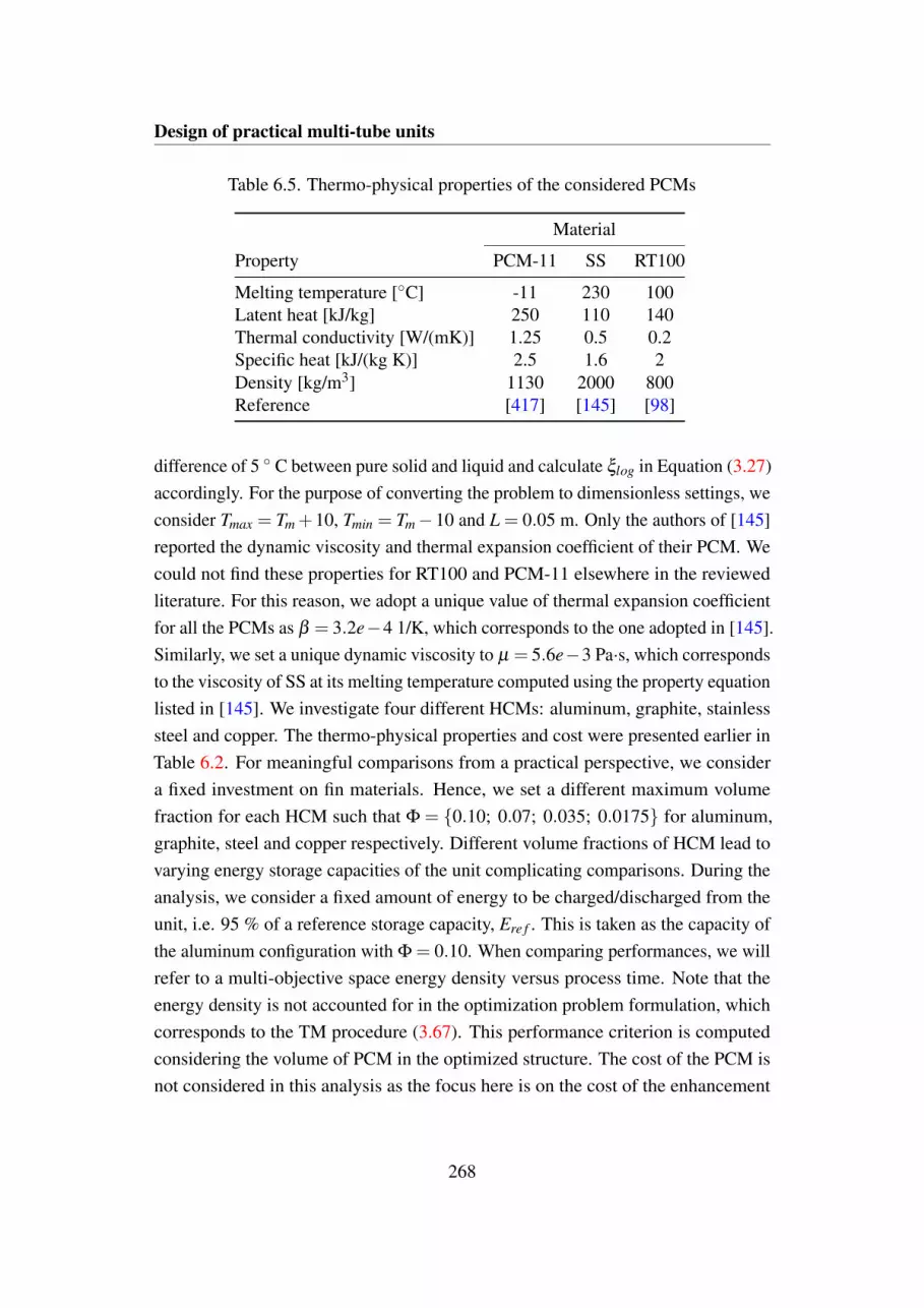
Design of practical multi-tube units
Table 6.5. Thermo-physical properties of the considered PCMs
Material
Property PCM-11 SS RT100
Melting temperature [C] -11 230 100Latent heat [kJ/kg] 250 110 140Thermal conductivity [W/(mK)] 1.25 0.5 0.2Specific heat [kJ/(kg K)] 2.5 1.6 2Density [kg/m3] 1130 2000 800Reference [417] [145] [98]
difference of 5 C between pure solid and liquid and calculate ξlog in Equation (3.27)accordingly. For the purpose of converting the problem to dimensionless settings, weconsider Tmax = Tm +10, Tmin = Tm−10 and L = 0.05 m. Only the authors of [145]reported the dynamic viscosity and thermal expansion coefficient of their PCM. Wecould not find these properties for RT100 and PCM-11 elsewhere in the reviewedliterature. For this reason, we adopt a unique value of thermal expansion coefficientfor all the PCMs as β = 3.2e−4 1/K, which corresponds to the one adopted in [145].Similarly, we set a unique dynamic viscosity to µ = 5.6e−3 Pa·s, which correspondsto the viscosity of SS at its melting temperature computed using the property equationlisted in [145]. We investigate four different HCMs: aluminum, graphite, stainlesssteel and copper. The thermo-physical properties and cost were presented earlier inTable 6.2. For meaningful comparisons from a practical perspective, we considera fixed investment on fin materials. Hence, we set a different maximum volumefraction for each HCM such that Φ = 0.10; 0.07; 0.035; 0.0175 for aluminum,graphite, steel and copper respectively. Different volume fractions of HCM lead tovarying energy storage capacities of the unit complicating comparisons. During theanalysis, we consider a fixed amount of energy to be charged/discharged from theunit, i.e. 95 % of a reference storage capacity, Ere f . This is taken as the capacity ofthe aluminum configuration with Φ = 0.10. When comparing performances, we willrefer to a multi-objective space energy density versus process time. Note that theenergy density is not accounted for in the optimization problem formulation, whichcorresponds to the TM procedure (3.67). This performance criterion is computedconsidering the volume of PCM in the optimized structure. The cost of the PCM isnot considered in this analysis as the focus here is on the cost of the enhancement
268

6.3 Numerical results and design trends
Charge: Aluminum
Charge: Copper
Charge: Graphite
Charge: Steel
(a) (b)
Fig. 6.21. Charge time of a RT100 unit with different HCMs. (a): Using unphysicalmaterial properties obtained through the rule of mixtures; (b): using optimized heattransfer structures obtained through topology optimization. The regions of dominatedmaterials are highlighted with gray boxes
device. However, for an average cost of PCM of 1 $/kg as indicated in [23], onlyminimal changes in the prescribed volume fractions would be needed.
Before extending the analysis to other PCMs, we focus on finding the best HCMsfor melting enhancement of a unit with RT100. As a rough preliminary step formaterial selection, we perform a set of 4 analyses considering volume-averagedmaterial properties between HCM and PCM using the rule of mixtures:
¯(·) = (·)HCMΦ+(·)PCM(1−Φ), (6.3)
where (·) denotes a generic material property and ¯(·) represents its volume-averagedvalue. All the analyses are performed with αmax = 0 such that the unpenalized mo-mentum equation is recovered. Although this correspond to an unphysical homoge-neous and liquid material, we are interested in testing the ability of this simplificationto provide material selection guidelines. The performance of our four HCM-RT100homogeneous mixtures in the energy density versus charge time space is reportedin Figure 6.21(a). Graphite and copper lie on a material Pareto front, meaning that
269

Design of practical multi-tube units
0.5 1 1.5 2 2.5Charge time [s] 10 4
100
120
140
160
180
200
220
240
260
280La
tent
ene
rgy
dens
ity [M
J/m
3 ]Dicharge: AluminumDicharge: CopperDicharge: GraphiteDicharge: SteelCharge: AluminumCharge: CopperCharge: GraphiteCharge: Steel
PCM-11
SS
RT100
Fig. 6.22. Charge and discharge times in the optimized configurations for differentHCM-PCM possible couplings
they are better than the alternatives with respect to at least one of the objectives.Aluminum and steel are dominated materials as the computed objective is worse thangraphite or copper with respect to both objectives. Hence, the results obtained withthis preliminary analysis lead to the conclusion that both aluminum and steel arenot cost-effective options for melting enhancement of RT100. To check the validityof assumption 6.3, we now optimize fin layouts using topology optimization. Theperformance of the optimized layouts is reported in Figure 6.21(b). The stainlesssteel geometry is dominated by the copper one in agreement with what we found inthe previous analysis. However, the optimized heat transfer structure using aluminumnow lies on the Pareto front with graphite and copper. This presents evidence that theHCM cannot be chosen a-priori using averaged material properties if the fin layoutis unknown.
The performance of the topology-optimized heat transfer structures with differentHCMs and PCMs for both charge and discharge is summarized in Figure 6.22. Foreach PCM and for each process, we draw the rectangle with minimum area thatencloses the computed values. This procedure highlights the ranges of energy densityand process time of the optimized configurations. Note that the charge and dischargeusing the same PCM-HCM couple have nearly coincident energy densities since the
270
6.3 Numerical results and design trends
same maximum volume fraction, Φ, is set when optimizing the two processes. Weobserve the same trend identified for the structures enhancing melting of RT100 forall the PCMs analyzed in both charge and discharge. Aluminum, copper and graphiteare cost-effective material choices while steel is a dominated material. Charge isalways faster than discharge due to the stronger convective motion. The benefitsdue to convection are larger for the structures of copper and steel, for which meltingis 17 % faster than solidification on average. An average of 9 % improvement forconvective motion is computed for aluminum and graphite. Choosing a suitableHCM seems to be more important for solidification than for melting. The dischargeusing the optimized aluminum structures yields an average of 66 % time reductionwith respect to the steel structures. On the other hand, when using aluminum insteadof steel for charge, an average process time reduction of 53 % is computed. The highlatent heat and thermal conductivity of PCM-11 leads to LHTES units with largerenergy density and faster process dynamics than those with SS and RT100. Forthis material, the trade-off between energy density and process dynamics can be ofinterest to designers: the energy density of the unit can be increased by 23.30 MJ/m3
if charge and discharge are allowed to be 0.95 and 1.19 hours longer. Consideringthis trade-off for RT100 is of minor importance: using copper instead of aluminumallows the energy density to be increased by only 9.24 MJ/m3 but requires 3.05 and4.22 hours more for the charge and discharge completion.
The layouts optimized for heat transfer enhancement in RT100, SS and PCM-11are shown in Figures 6.23, 6.24, 6.25 respectively. All the aluminum structuresare qualitatively similar. The HTF pipes are surrounded by four fins with varyinglength and tilt angle. We notice only minimal differences when comparing theselayouts to those we obtained in Section 6.3.1 without considering natural convectionin the analysis. This suggests that diffusion is the dominant heat transfer mechanism.The diffusivity ratio Ck ranges from 0.15 % to 0.54 % for the different PCMs andis far from the transition value of 3.5 % calculated in Section 6.2.2 for a case withthe same volume fraction of HCM. The absence of convective features makes thelayouts optimized for melting similar to those optimized for solidification. Analogoustrends are observed for the graphite geometries, which look like thinned versionsof the aluminum designs. The low volume fraction of the copper structures limitsthe complexity of the design evolution so that the resulting layouts consist of twoshort fins attached to the HTF pipes. The fins elongating towards the bottom ofthe shell are generally longer than those directed towards the top for discharge and
271

Design of practical multi-tube units
(a) (b) (c) (d)
Fig. 6.23. Optimized designs for charge (top) and discharge (bottom) with paraffinRT100 as PCM. (a): Aluminum; (b): graphite; (c): copper; (d): steel
(a) (b) (c) (d)
Fig. 6.24. Optimized designs for charge (top) and discharge (bottom) with SS asPCM. (a): Aluminum; (b): graphite; (c): copper; (d): steel
272

6.3 Numerical results and design trends
(a) (b) (c) (d)
Fig. 6.25. Optimized designs for charge (top) and discharge (bottom) with PCM-11as PCM. (a): Aluminum; (b): graphite; (c): copper; (d): steel
shorter for charge. The fins orientation around the top tubes is comparable in RT100(Ck = 0.12 %) and SS (Ck = 0.15 %) but changes completely when consideringPCM-11 (Ck = 0.44 %). A similar modification of the tilt angle of the fins wasobserved across the transition region identified in Section 6.2.2. This suggests thatthe volume fraction of HCM modifies the position of the transition region along theCk axis of Figure 6.3. Reducing the amount of conducting material yields limitedpossibilities of performance improvements through diffusion. Hence, exploitingconvective transport with ad-hoc design features can be convenient even at lowdiffusivity ratios. The optimized layouts using steel as HCM present short and thickstructures. For melting of all the PCMs considered, the fins orientation around thetop tubes is similar to the one of Figure 6.7(c). This indicates that convection plays amajor role here due the large diffusivity ratios (2.45 % ≤Ck ≤ 8.69 %).
To produce all the designs presented, we adopted a constant filter size, r f despitedifferent maximum volume fractions, Φ, are prescribed for different materials. Thismay overly penalize the designs with a small volume fraction, by preventing theformation of thin conducting members. A reduction of the filter size below thevalue adopted in this chapter requires the utilization of a FE mesh with a higherresolution. In fact, r f was selected such that all the elements span at least a nodaldesign variable and an element-wise constant filtered density, s, can be obtained. Onthe other hand, there exist reasons for using a constant filter size. For instance, if the
273

Design of practical multi-tube units
fins are fabricated through the same manufacturing process, it would be desirable toobtain designs with an equal minimum feature size. Recall that in Section 2.4.2 weshowed how it is possible to prescribe a minimum feature size (corresponding to 2r f
in regions sufficiently far from the boundaries of the design domain) by using theprojection (2.40) with η = 0.
The results presented in this section showed that choosing a-priori the HCMfor heat transfer enhancement in LHTES may be ineffective if the fins layout isunknown. Our forward analysis with volume-averaged material properties leads tothe conclusion that both aluminum and steel are not cost-effective materials. Whenconsidering optimized structures instead, aluminum lies on a energy density versusprocess time Pareto front along with graphite and copper. Furthermore, we foundthat the optimized layouts made of graphite and aluminum are slightly sensitive tothe choice of the PCM and process to be enhanced due to a high volume fraction ofHCM and a low diffusivity ratio as compared to copper and steel.
6.4 Conclusions
In this chapter, topology optimization was used to answer four practical designquestions that still hamper the large-scale technology development of multi-tubeLHTES units. A graphical summary of the main application-oriented advances ispresented in Figure 6.26. We proposed a heuristic approach able to give rule-of-thumb indications on the range of material properties for which convective featuresmatter for performance. The topology optimization results confirmed the anticipateddesign trends. The results of our first numerical study suggested that representingmulti-tube units with a collection of circular quasi-periodic cells generally leadsto suboptimal configurations (Figure 6.26(a)). A premature merging of the phasefront was observed along specific directions, yielding a quick heat transfer rate drop.The second study demonstrated that designing heat transfer structures for units withseparate hydraulic loops demands for ad-hoc optimization (Figure 5.32(b)). Theoptimized layout consists of a thick HCM path linking the top to the bottom pipes,which ensures a full utilization of the HCM during both the charge and discharge.This design yields a dramatic acceleration of the complete charge-discharge cyclewhen compared to geometries optimized for the operation with a unique hydraulicloop. Our design optimization study under cost constraints revealed that aluminum,
274

6.4 Conclusions
- 26 %
Time
Energ
y [%
]
Energ
y d
ensity
Process time
- 52 %
- 65 %
Fig. 6.26. Graphical summary of the main application-oriented advances of the chap-ter. (a): Effect of the periodicity assumption on optimized design and performance;(b): layout and performance comparison of geometries optimized for alternativehydraulic loop configurations; (c): design trend energy density/process time fordifferent HCM choices
275

Design of practical multi-tube units
graphite and copper lie on a Pareto front energy density versus process time butsteel was never found to be a cost-effective option (Figure 5.32(c)). The optimizedgeometries with graphite and aluminum look slightly affected by the type of PCM,suggesting that a modular fin layout may be efficient for practical installations.
276

Chapter 7
Design and control of resilientdistrict heating networks
The large scale utilization of the locally available heat sources makes DH a rationaland efficient domestic heating option. This technology was coupled successfully tohigh efficiency Combined Heat and Power (CHP) plants [447, 147], energy-intensiveindustries [263, 373] and renewable generation plants such as solar [464], biomass[426] and geothermal systems [476]. However, the fluid distribution networksare critical infrastructures. Small perturbations can rapidly propagate and lead toservice failures. In this chapter, we use numerical optimization to improve theresilience of a DHN. The resilience denotes the ability of a system to absorbperturbations and quickly recover its functionality with a limited impact on theservice quality. We demonstrate both a robust design and a centralized controloptimization framework. Although control problems hardly fit within the context ofthis thesis, our optimization model is constructed using mathematical tools of popularuse in topology optimization. The plan of the chapter is as follows. In Section 7.1,we introduce a quantitative notion of resilience and we review the state-of-the-artapproaches for resilience improvements through design and control. In Section7.2, we describe the governing equations and numerical model used to computethe fluid-dynamic and thermal responses of DHNs. In Section 7.3 and 7.4, we firstintroduce the optimization models adopted for robust design and centralized control;then, we present and discuss the results obtained for a real case-study. Finally, themain findings are summarized in Section 7.5.
277

Design and control of resilient district heating networks
Time
Quality of service
Resilience gain due to robust design
Robustness improvement
Resilience gain due to rapid control
Rapidity improvement
Event
Restoration
Resilience loss
Resilience
Fig. 7.1. (a): Resilience of infrastructures; (b): resilience gain through robust design;(c): resilience gain through rapid control
Some of the contents of this chapter were published in Energy [J3] and in Journalof Energy Resource Technology [J4] and presented at the ASME 2016 InternationalMechanical Engineering Congress and Exposition [C3] and at the 29th InternationalConference on Efficiency, Cost, Optimisation, Simulation and Environmental Impactof Energy Systems [C5].
7.1 Towards resilient district heating networks
In the civil engineering community, Bruneau et al. [68] proposed a clear quantitativemetric to assess the resilience of infrastructures to seismic events. Figure 7.1(a) showsa representative schematic of the authors idea. Let us represent the performanceof a system using a quality of service versus time plot. At time tp, the system issuddenly perturbed by an event that decreases its functionality from Qn to Qe. Then,efforts are taken to improve the level of service until the nominal conditions arere-established at time tr. The time period tr− tp is referred to as the restorationphase. Bruneau and co-authors [68] quantified the resilience as the blue area shownin Figure 7.1(a). The resilience loss indicated in gray is commonly named "resiliencetriangle "[37, 354, 210]. A resilient system shows three fundamental features:
278

7.1 Towards resilient district heating networks
(a) Reduced probability that its functionality drops below acceptable limits, e.g.Qmin in Figure 7.1(a). We will refer to this concept as reliability.
(b) Reduced impact of perturbation events, i.e. Qn−Qe in Figure 7.1(a). We willrefer to this concept as robustness.
(c) Reduced time span of the restoration phase, i.e. tr− tp in Figure 7.1(a). Wewill refer to this concept as rapidity.
Note that the previous definitions are not universal. The distinction between relia-bility, robustness and resilience is quite confused in the literature; often these termsare used interchangeably, see e.g. [169]. In this chapter, we will consider explicitlyaspects (b) and (c) of the resilience in DHNs. The robustness is improved throughdesign optimization, by modifying the topology of existing networks so that externalperturbations are maximally absorbed. The rapidity is improved through controloptimization, to quickly recover an acceptable level of service after disruptive events.The possible resilience improvements due to a robust design and rapid control areshown conceptually in Figure 7.1(b) and (c). In the next sections, we review the mostwidespread approaches and identify research opportunities for the resilient designand control of fluid distribution systems.
7.1.1 Improving resilience through design
Here, we consider the literature advancements for the resilient design of fluid dis-tribution infrastructures. From the previous definition, robustness and reliabilityimprovements are strictly connected. Although in this chapter we will focus onlyon the robustness aspect of resilience, the reliability design approaches are alsobriefly presented. In rare cases a Water Distribution Network (WDN) or a DHN canbe designed from scratch. For this reason, most of the scholars interest lies in theimprovement of the existing installations through the creation of loops. Accordingto Todini [421], looped topologies yield redundancy and allow local failures to beovercome.
Reliability refers to the probability that the system "remains functional" [183].In the context of WDNs and DHNs, the functionality includes both the demandsatisfaction in terms of flows to be supplied and the range of pressures and tempera-tures at which these flows are provided [423]. Due to the stochastic nature of this
279

Design and control of resilient district heating networks
metric, a direct quantification of reliability involves the probabilistic mapping andintegration of the failure region, which can be achieved with sampling approachessuch as Monte Carlo method [66] or using first and second-order approximations ofthe failure surface [423]. Alternatively, researchers considered a variety of differentdeterministic measures of reliability. For instance, Farmani et al. [133] proposeda reliability indicator based on the minimum surplus pressure head. Based on con-cepts borrowed by information theory, Tanyimboh et al. [415, 416] introduced thenotion of entropy for fluid networks. Although these ideas gained popularity in thecivil engineering community, whether these deterministic measures are capable ofaccounting properly for the reliability strongly relies on the designer experience; it ishard to extend the proposed methods and findings to a wide range of systems.
Robustness refers to the ability of the system to reduce the impact of "distur-bances, e.g. fluctuations of design parameters or noise" [166]. Gohler et al. [193]recently published an extensive review on the robustness metrics for engineeringdesign. The authors identified four different categories:
• sensitivity metrics, quantifying robustness as a measure of the performancecriteria gradients to noise factors;
• feasible space metrics, quantifying robustness as the size of the feasible set ofan optimization problem with a minimum performance constraint;
• expectancy and dispersion metrics, quantifying robustness as a combination ofstatistical moments on performance criteria;
• probability of functional compliance metrics, quantifying robustness as theprobability that the performance criteria are within acceptable limits.
The quantification of robustness using the last two categories was considered bymany authors in the field of WDNs. For instance, Kapelan [233] and Babayan [38]defined robustness as the probability to satisfy a minimum pressure constraint inevery node of the network. A hybrid approach between the two categories wasproposed by Giustolisi et al. [166], who introduced a robustness indicator based onthe distance between the expectancy of a performance criterion and a threshold value;the authors quantified this distance using the number of multiples of the standarddeviation. Inspired by the classical robustness idea of Taguchi [413], Jung et al.[228] quantified robustness using a coefficient of variation, computed as the ratio of
280
7.1 Towards resilient district heating networks
the nodal pressure standard deviation to its average value. Within these robustnesscategories, it is possible to include also the scenario-based approaches. For instance,Cunha et al. [105] and later Marques et al. [291] approximated the expectancyof their performance criterion using a weighted sum with addends calculated indifferent scenarios; the sum weights were set equal to the scenarios probabilities.This method was extended also to the calculation of the standard deviations in[232]. All the previous approaches share common features with the reliability-based optimization methods in that they require some form of characterization ofthe input uncertainty, whether stochastic variable bounds or Probability DensityFunctions (PDFs) or both. Gathering correct statistics for the noise factors of fluiddistribution networks is not trivial. As noted by Jung et al. [228], the probabilitydistributions of the most common noise factors are in general not known and theliterature lacks of an extensive database. Assumptions may have large impacton the optimization results. Under this perspective, the sensitivity metrics are ofgreat interest. The robustness quantification is fully deterministic, reducing therisk of an optimization bias due to the use of incorrect statistics. Despite its wideacceptance across various engineering fields ranging from Micro-Electro-MechanicalSystems (MEMSs) [198] to electromagnetics [243] and geotechnical design [167],we found no design optimization study using sensitivity metrics in the WDN andDHN communities.
Concerning the choice of the optimization algorithm, most of the reviewedliterature adopted heuristic or meta-heuristic global-search optimizers. GeneticAlgorithm (GA) in both its original form or in slightly modified versions is nodoubt the most popular choice [133, 233, 38, 166, 232, 228]. Other meta-heuristicalgorithms that were considered for the optimization of fluid networks include (butare not limited to) Simulated Annealing (SA) [105, 291, 341], Scatter Search (ScS)[269] and Particle Swarm (PS) [408]. If properly used, these techniques guaranteea thorough exploration of the design space but require many system solutions perdesign variable, leading to a critical curse of dimensionality [86]. The optimizationof large and complex DHNs with dynamic operation might be hardly tractable.Furthermore, using sampling approaches to compute statistics on the performancecriteria further increases the computational burden. Banos et al. [41] acknowledgedthat most of the researchers focused on small benchmark examples (e.g. the AnytownWDN) and only a few applications considered real-world installations. Among thereviewed papers, the one with largest design space [232] counts 85 design variables.
281

Design and control of resilient district heating networks
This gives little hope to the use of practical optimization algorithms able to accountfor both uncertainty and transient operation in real-world DHNs. For instance, theTurin DHN counts more than 50000 pipe segments. The optimal design throughmore efficient NLP algorithms was considered in the earliest developments of thedesign methods for WDNs, such as in [149] and [429]. To our knowledge, only tworesearches formulated the design of flow networks using a topology optimizationframework. Inspired by advances in truss structure optimization, Klarbring et al.[246] adopted the ground structure approach to design flow networks with minimaldissipation. The ground structure approach consists in selecting a large number ofpotential pipe connections, whose capacity is altered by the design variables duringthe optimization. Capacities hitting or approaching zero corresponds to topologychanges. Differently from the optimization problem in structural mechanics and evenfor a simple Hagen-Poiseulle flow model, the fluid-dynamic response is nonlinearwith respect to the capacity variables (e.g. cross-sectional area or diameter of thepipes) leading to non-convexity of the optimization problem. Arguing that in fluidnetworks "we cannot loose convexity any longer", Evgragov [128] later consideredalso the positions of the network nodes as design variables; the optimized layoutswere superior to those obtained using the classical ground structure approach withfixed nodes. The gradient-based route was quickly abandoned for WDN design dueto both its continuous nature (that requires a post-processing of the optimizationresults to obtain commercial diameters) and its convergence to local optima [125].However, these methods allow a convenient scalability. If design sensitivities can beobtained cheaply, e.g. through the adjoint method, the computational complexity isslightly affected by the dimensionality of the design space. Back to 2003, Klarbring[246] presented a flow network design example with 3206 design variables.
This literature review can be summarized with three facts:
1. The detailed probabilistic characterization of the uncertainties in fluid networksis cumbersome in most cases and may greatly affect the optimization results.
2. The robust design based on sensitivity metrics is accepted in various engineer-ing fields but was not considered for both WDNs and DHNs.
3. The heuristic and meta-heuristic optimization algorithms are popular for WDNdesign but their application to large real-world systems is hampered by theirpoor scaling properties.
282

7.1 Towards resilient district heating networks
In this chapter, we introduce a computational design approach for DHNs based onthe previous facts. Given the facts 1 and 2, we design robustness using a sensitivitymetric that does require the characterization of the noise uncertainty. Given fact 3, weformulate the design problem using topology optimization and update the networklayout with a gradient-based optimizer. The objective and constraint gradients arecomputed by the discrete adjoint approach, which is computationally cheap andnearly insensitive to the design space dimension.
7.1.2 Increasing resilience through control
Here, we discuss the advancements in WDNs and DHNs control and identify themost promising approaches for resilience improvements. Controlling DHNs basedon distributed meter readings and providing a customizable service in real-timeare considered primary requirements for the energy grids of the future [281, 424].Control can increase the rapidity of the infrastructures and is particularly importantin the case of accidents. In this situation, the service should be restored as quicklyas possible with a minimal impact on the customers comfort. Finding the optimaloperation strategy for these systems is a time-consuming and non-trivial problem.The real-world installations often count several thousand users and multiple gen-eration plants that are connected through complex fluid networks. The accurateprediction of the fluid-dynamic and thermal responses demands the utilization ofcomplex simulation tools. The non-convexity of the optimization problems requiresglobal-search algorithms. Furthermore, the large number of moving and dissipativecomponents (i.e. valves and pumps) results in optimization problems with a high-dimensional control space. The literature in the context of WDNs and DHNs controlcan be divided into scheduling and real-time control.
Scheduling involves the day-ahead planning of devices (e.g. pumps) operation tominimize specific performance criteria, e.g. the energy consumption or operationalcost [61]. Most frequently, the planning problems do not account for feedbacksfrom the data acquisition systems. Due to the "day-ahead" type of deadline, theexecution time is rarely a strict constraint. Nevertheless, for the reasons discussedpreviously, scholars developed methods to reduce the computational complexity ofthe hydraulic and thermal analyses. Artificial Neural Network (ANN) surrogatemodels met large acceptance among researchers. Broad et al. [65] demonstratedthe use of GA and ANN for pump scheduling in WDNs. A similar framework was
283

Design and control of resilient district heating networks
later considered by Behandish et al. [49], who optimized the operation of boththe pumps and storage tanks. Within the context of DHNs, Guelpa et al. [175]demonstrated the coupling of GA with Proper Orthogonal Decomposition (POD)analysis. Following a parallel research direction, other authors adopted meta-heuristictechniques with improved convergence rate in order to retain the full complexityof the analysis model. Examples include Ant Colony Optimization (ACO) [280],Limited Discrepancy Search (LDS) [159] and PS [407]. Other scholars proposed tocouple heuristic and deterministic algorithms. For instance, Giacomello et al. [161]developed a hybrid scheme for pump scheduling by combining the Greedy algorithmwith standard Linear Programming (LP) routines.
The execution time is a primary constraint in real-time applications. A controllaw needs to be obtained on-the-fly based on information gathered through the dataacquisition systems. The most typical real-time control strategies in WDNs andDHNs aims at reducing the pumping power [456], leakages [465], operational costs[165, 432] or emissions [365]. Due to the similarities in the nature of the optimiza-tion problem, the analysis and optimization approaches developed for schedulingwere considered also for real-time control. Rao et al. [346] used the ANN-GAapproach to optimize both the pumps statuses and valve openings using a 24 hourspredictive framework. Kang [231] tackled a similar problem by modifying GA witha "warm" initialization of the population that partially reuses the previous optimiza-tion solutions. Differently from the context of planning, the optimization runs areperformed after each sampling action of the metering facilities. As noted by theauthors of [286] and [465], despite efforts towards a greater computational efficiency,the previous approaches hardly meet the strict time requirements of real-time controland are limited to small-scale applications. For this reason, the deterministic ap-proaches are preferred. Examples of real-time control of WDNs using LP and NLPalgorithms can be traced back to [326] and [80]. After the seminal work of Sandouet al. [365], the number of studies focusing on real-time control of DHNs grew fastover the last years. For instance, Wang et al. [456] used the Generalized ReducedGradient (GRG) algorithm for optimization of both the pumps frequencies and valveopenings in a medium-size DHNs. Giraud et al. [165] adopted a Model PredictiveControl (MPC) framework based on Mixed Integer Linear Programming (MILP) tominimize the operational costs through the regulation of the heat generators, supplytemperatures and pressures. A similar route was followed by Verrilli et al. [432],who considered also the regulation of the thermal energy storages and user thermal
284

7.2 Modeling fluid distribution networks
loads. In rapidly-evolving systems, the utilization of standard MPC algorithms maylead to inaccuracies. The control law is optimized based on outdated information[171]. Hence it might be of more interest to obtain an approximate solution using themost up-to-date information [171]. Building on advances in control theory [116], arecent contribution [344] developed a method for real-time control using SequentialConvex Programming (SCP) and the Real Time Iteration (RTI) method. Instead ofsolving the optimization problem to full accuracy using fixed problem data, these areupdated at each optimization iteration using the feedback from the metering devices.This method allows the straight-forward integration with the data acquisition systemswith little limitations on the minimum sampling frequency. This possibility wasconsidered in [466] and [465] in the context of WDNs.
Despite these valuable contributions, most of the commercial DH infrastructuresare still controlled using a decentralized strategy. Each thermal user can regulatethe flow based on its degree of discomfort. As a consequence, the failure eventsmay yield a large reduction in the service quality for some users; the restorationrapidity is constrained by the time required to substitute the failed part. Hence,centralized control strategies for increased resilience are urgently needed. To ourknowledge, no research considered control optimization under this perspective. Inthis chapter, we propose a control strategy of DHNs after failure events that aimsat filling this literature gap. To cope with the strict execution time requirements,the optimization is conducted using MMA, which shares similarities with the SCProutines considered in [466]. The gradients of the objective and constraints withrespect to the control variables are computed using the discrete adjoint method,which permits the scalability to real-world problems. Although we conduct onlynumerical experiments, our approach is designed to fit within an RTI framework. RTIcan be of great interest for control during failure events, when the dynamics of thesystem is so fast that a full MPC procedure may be too slow to react to disturbances.
7.2 Modeling fluid distribution networks
In this section, we present a modeling framework for computing the fluid-dynamicand thermal responses of fluid distribution networks. We first simplify the governingequations to derive integral 1D formulations. Then, we construct a numerical modelusing a graph representation of the network.
285

Design and control of resilient district heating networks
7.2.1 Integral form of governing equations
We assume a steady-state and incompressible flow with isotropic and constantfluid properties and negligible viscous dissipation. The Navier-Stokes and energyequations can be written as in (5.1), (5.2) and (5.4). Assuming that the flow velocityand diffusion fluxes are aligned with the pipe direction, we can rework the governingequations in 1D considering:
vi = 0 for i = 2, 3,
∂
∂xi= 0 for i = 2, 3.
(7.1)
Using the simplifications (7.1) and writing the stress tensor following the constitutivelaw (5.3), the governing equations can be stated as:
ρ∂v1
∂x1+ mext = 0, (7.2)
ρ∂v1
∂ t︸︷︷︸(i)
+v1∂v1
∂x1︸ ︷︷ ︸(ii)
=− ∂P∂x1
+2µ∂v1
∂x1︸ ︷︷ ︸(iii)
−Floc−F⊥, (7.3)
ρcp∂T∂ t︸ ︷︷ ︸
(i)
+ρcpv1∂T∂x1
+ mextcpT = k∂ 2T∂x2
1︸ ︷︷ ︸(ii)
−q⊥, (7.4)
where mext and Floc are mass and momentum sinks and P denotes the total pressurethat includes the effect of gravity. The fluid-dynamic response in fluid networksgoverned by incompressible flow is in general much faster than the time frames ofinterest to the analyst. Hence, we neglect the transient term (i) in the momentumequation. We also consider two simplifications for the energy equation. First, as theconvective energy transport is dominant, we neglect term (ii). Second, we consideronly the steady-state version of (7.4) and neglect term (i). This assumption can bejustified in small distribution networks as small water volumes are involved. Wewill relax this assumption when considering large networks in future studies. Themomentum and energy sinks indicated with the subscript "⊥" account for the effectof the orthogonal contributions to the momentum and energy diffusion, which cannot
286

7.2 Modeling fluid distribution networks
(a)
(b)
(c)
Fig. 7.2. Control volumes considered to obtain the integral form of the governingequations. (a): Pipe; (b): junction or bifurcation; (c): building and heat exchanger
be written explicitly in a 1D setting:
F⊥ =−(1−δ1 j
) ∂σ1 j
∂x j, (7.5)
q⊥ =−(1−δ1 j
)k
∂ 2T∂x2
j. (7.6)
We now rework the simplified 1D governing equations in an integral form. Letus consider a pipe filling Ωp with constant cross-section and no mass sinks as theone depicted in Figure 7.2(a). Terms (ii) and (iii) in Eq. (7.3) disappear due to the
287

Design and control of resilient district heating networks
continuity constraint (7.2). The integration over Ωp leads to:
Po−Pi =−∆p⊥−∆ploc, (7.7)
where both the terms on the RHS are modeled using semi-empirical equations ofstandard engineering practice [25]:
∆p⊥ =12
f⊥LD
ρv21, (7.8)
∆ploc =12
βlocρv21, (7.9)
where f⊥ is the Darcy-Weisbach friction factor, D is the diameter of the pipe, L is thelength of the pipe and βloc is the local pressure drop coefficient accounting for theeffect of valves, bends and tees. Note that the phenomenological equations (7.8) and(7.9) allow both the laminar and turbulent flows in pipes to be considered with ease.The continuity equation (7.2) can be integrated over a control volume, Ω j, (Figure7.2(b)) enclosing a junction and half of the connected pipes. We obtain:
Np
∑i=1
Gini +Gext = 0, (7.10)
where Gext is an extracted mass flow rate at the junction, Np is the number of pipesof the junction, ni is the outward pointing normal of pipe "i" and Gi is its mass flowrate:
Gi = (ρvS)i , (7.11)
with S being the pipe cross section. Under this convention, the mass flow ratesexiting the control volume are positive and those entering the control volume arenegative. Integrating the energy equation (7.4) over Ω j leads to:
Np
∑i=1
cpGiTini + cpGextT =−Q⊥, (7.12)
where Ti is the temperature of pipe "i" at the boundary of the control volume, T isthe temperature of the junction where the mass flow rate extraction takes place, andQ⊥ is the total energy loss due to the orthogonal temperature gradients. The latter is
288

7.2 Modeling fluid distribution networks
formulated using the following heat transfer correlation:
Q⊥ =12
Np
∑i=1
πDiLiUdg (T −Tg) , (7.13)
where T is the mean integral temperature of the control volume that we set equal tothe one of the junction T , Udg is the global heat transfer coefficient between the pipeand the ground and Tg is the ground temperature.
The thermal response of each thermal user is computed using a steady-statelumped-parameter approach that accounts for heat transfer across the heat exchanger,heat transfer in the building delivery system and thermal losses. The static assumptionis valid for no external temperature variations and for fast control actions. Due to thelarge building capacitance, weak thermal transients would be observed during thecontrolled period. An integral energy balance across Ωu (Figure 7.2(c)) reads:
Gbcp(Ti−To) = KVV (Tb−Tamb), (7.14)
where Gb is the mass flow rate extracted at the building substation, Ti and To are thewater inlet and outlet temperatures of the heat exchanger, V is the building volume,KV is the volumetric heat loss coefficient, Tb is the building temperature and Tamb isthe external ambient temperature. Eq. (7.14) introduces two additional unknowns,To and Tb. The temperature Ti can be obtained from (7.12). As a closure equation,we consider the following thermal balance across a control volume enclosing theheat exchanger, Ωhe:
Gbcp(Ti−To) = (UA)(
Ti +To
2−Tb
), (7.15)
where (UA) is the global transmittance of the heat exchanger and of the heat deliverysystem of the building. Its value for each of the building of the network is obtainedthrough fitting on experimental data. Note that instead of using a standard logarithmicformulation, we linearize the characteristic temperature difference in (7.15) to benefitfrom linearity.
289

Design and control of resilient district heating networks
BranchesNodesUsers
Fig. 7.3. Schematics of the graph representation of the fluid network
7.2.2 Numerical model
The entire network is modeled using a graph representation [59], which is shownschematically in Figure 7.3(a). The branches correspond to the pipe sections enclosedby either junctions are bifurcations, represented as nodes. In the supply line ofDHNs, water is injected at the power plant and extracted at the user nodes. Thegreen branches (Figure 7.3(c)) are numerical artifacts that serve for the purpose ofcalculating the thermal response of the users, as described in the previous section.The degrees of freedom to be solved for include three state variables: the massflow rates, G, which are assigned to the branches, the total pressures, P, which areassigned to the nodes and the temperatures, T, which are assigned to the nodesand users. The network topology is uniquely represented by the incidence matrixA : RNb → RNn , with Nb being the number of branches and Nn being the number ofnodes. Denoting with ZZZ = ζ1,ζ2, ...,ζNb the set branches and ϒϒϒ = υ1,υ2, ...,υNnthe set of nodes, the incidence matrix, A, is defined as following:
Ai j =
+1 if υi is the inlet node of branch ζ j
−1 if υi is the outlet node of branch ζ j
0 otherwise
. (7.16)
290

7.2 Modeling fluid distribution networks
Using (7.16), the integral form of the continuity equation (7.10) can be casted in thefollowing form:
Rc = AG+Gext = 0, (7.17)
where Rc is the vector of residuals of the continuity equation and Gext is a vectorcollecting the nodal mass flow rate extractions. The integral form of the momentumequation (7.7) is written in matrix form as:
Rm = BG−AT P = 0, (7.18)
where Rm is the vector of residuals of the momentum equation and B is a diagonalnonlinear operator, containing the fluid-dynamic resistance of each branch of thenetwork formulated using (7.8) and (7.9):
Bii(Gi) =
G(
f⊥D L+βloc
)2ρS2
i
. (7.19)
The advective term of the integral form of the energy equations (7.12) contains thetemperatures of the cross-sections located at the branch half lengths. Due to ourgraph-based representation, these are not degrees of freedom. Hence, the advectivetransport needs to be reformulated as a function of the nodal temperature values. Asdiscussed in Section 5.2.2, instabilities arise in convection-dominated flows whenthe advective flux is approximated by central finite differences. For this reason,we use the upwind scheme [137] that guarantees unconditional boundedness [433].Considering the generic branch shown in Figure 7.3(b), the temperature Ti in (7.12)is written as:
Ti =1Gi
(max(Gi,0)Tj−min(Gi,0)Tj+1
). (7.20)
Using (7.13) and (7.20), the integral form of the energy equation (7.12) and thebuilding integral balances (7.14) and (7.15) can be written in matrix form as:
Re = CT−q = 0, (7.21)
where Re is the vector of residuals of the energy equation, C is the conductancematrix and q is the heat load vector, containing all the constant terms of the heat lossesin (7.13) and (7.14). The discretized governing equations are solved considering twosets of boundary conditions. For the design studies, the mass flow rates extracted
291

Design and control of resilient district heating networks
by the users are known. These values can be obtained from Eq. (7.14) by settingTb equal to the desired temperature level and Ti− To equal to a desired value oftemperature drop. With reference to Figure 7.3(a), we have:
Gexti = Gbi if xi ∈ Γ2,
Pi = Ppp if xi ∈ Γ1,(7.22)
where Gbi is the mass flow rate requested by building "i" and Ppp is the designpressure level at the power plant node highlighted in Figure 7.3(a). For the controlstudies, the outlet mass flow rate is unknown as it depends on the valve openings atthe users substations. Hence, we prescribe an outlet pressure condition and an inletflow rate condition. Mathematically:
Gexti =−Gpp if xi ∈ Γ1,
Pi = Pout if xi ∈ Γ2,(7.23)
where Gpp is the injected mass flow rate at the power plant and Pout is the outletpressure. To compute the thermal response, we prescribe the inlet temperature asfollows:
Ti = Tpp if xi ∈ Γ1, (7.24)
where Tpp is the water temperature at the power plant node.
The fluid-dynamic problem is solved through the SIMPLE algorithm [327] todeal with the pressure-velocity coupling. At each SIMPLE iteration, the momen-tum equation is solved through a damped fixed-point iteration method. Numericalexperiments showed that setting the damping parameter to 0.8 yields an acceptabletrade-off between convergence stability and computational cost. The outer iterationsare stopped when the L2 norm of the relative residuals drops below 1e− 9. Thepresented analysis framework was verified and then validated with the experimentalresults obtained from the Turin district heating network, see [175, 174].
7.3 Robust design
In this section, we present and demonstrate our robust design framework for im-proved resilience of fluid distribution networks. We first describe the adopted design
292

7.3 Robust design
and optimization models and introduce an alternative formulation for benchmarkpurposes. Then, we present the results obtained for several numerical examplesconducted on a portion of the Turin DHN. Here, we do not account for the thermalresponse of the system in our optimization problem. Hence, we do not solve (7.21)for T during the analysis.
7.3.1 Design and optimization models
Following [246, 128], the topology of the network is here parameterized using theground structure approach [54]. We start by populating the network with a largeset of additional connections between the nodes as potential or vanishing branches.These are identified by enumeration of all the possible looping paths on the availableroad-ways. The network layout is controlled by acting on the pipe diameters asfollows:
Di(si) = Dmin +(Dmax−Dmin)si, (7.25)
where 0≤ s≤ 1 is a vector of design variables, Dmax and Dmin represent the maximumand minimum diameters, respectively. To describe topological changes, it is essentialto allow for Dmin = 0. However, this leads to non-solvable state equations. Hence,we consider the so-called ε-perturbation of the original optimization problem bysetting a small and strictly positive bound on the pipe diameter, Dmin = ε . Here, weassume that the ε-perturbed problem converges to the original problem for ε → 0.Formal proofs of convergence for pressure loss minimization in networks governedby the Hagen-Poiseuille flow are discussed in [246] and [128].
In robust district heating networks, the level of service should be slightly affectedby random perturbations such as fouling, chemicals deposition or leakages. Wequantify the level of service with the minimum pressure in the supply network, minP.The random noise is modeled considering arbitrary variations of the local pressuredrop coefficient, βloc. We aim at maximizing the following measure of robustness:
z =Nb
∑i=1
zloci =Nb
∑i=1
Lid (min(P))
dβloci︸ ︷︷ ︸(I)
, (7.26)
where Li is the normalized branch length and zloci is the contribution of the branch"i" to the objective, hereafter referred to as local robustness. Multiplying the noise
293
Design and control of resilient district heating networks
sensitivities (term (I)) with Li accounts for the fact that the magnitude and probabilityof the fluid-dynamic noise are generally proportional to the branch length. Note thatour objective (7.26) is a fully deterministic sensitivity metric. Hence, it does not relyon statistical moments of the system response, as discussed in Section 7.1.1. Weexpect an agreement with conventional robust or reliability-based design approaches,dealing with uniformly-distributed and tightly-bounded stochastic variables witha linear objective-noise relation. To allow for differentiability, the hard minimumfunction in (7.26) is approximated using the generalized p-mean:
minP≃ minpmP =
(1
Nn
Nn
∑i=1
Ppri
) 1pr, (7.27)
where the exponent, pr, is set to −10. The approximation (7.27) provides an upperbound to the hard minimum function and converges to it for pr→−∞. The robust-ness measure (7.26) involves the sum over the gradient components of a criterioncomputed with respect to Nb variables. As Nb is in general high, we compute thenoise sensitivities (term (I) in (7.26)) using the discrete adjoint method presented inSection 2.3.2 for the computation of design sensitivities. Substituting the design vari-ables, s, with the noise variables, βββ loc, and stacking the continuity and momentumstate variables and residuals in the vectors u = [PT , GT ]T and R = [RT
c , RTm]
T , thenoise sensitivities can be written as follows:
d(minpm(P)
)dβββ loc
=∂(minpm(P)
)∂βββ loc
−λλλT111
∂R∂βββ loc
, (7.28)
where the first term on the RHS vanishes due to a nil explicit dependence and λλλ 1 isa vector of adjoint variables computed by solving the following adjoint equation:
Rλ =
(∂R∂u
)T
λλλ 1−∂(minpm(P)
)∂u
= 0, (7.29)
where Rλ is the vector of residuals of the adjoint equation.
Instead of the standard linear volume constraint adopted in topology optimization,we consider the following investment cost constraint:
Ns
∑i=1
ci(si)Li−C∗ ≤ 0, (7.30)
294
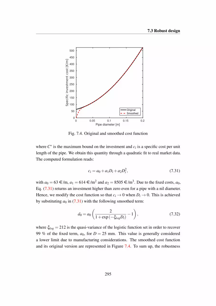
7.3 Robust design
0 0.05 0.1 0.15 0.2
Pipe diameter [m]
0
50
100
150
200
250
300
350
400
450
500
Original
Smoothed
Fig. 7.4. Original and smoothed cost function
where C∗ is the maximum bound on the investment and ci is a specific cost per unitlength of the pipe. We obtain this quantity through a quadratic fit to real market data.The computed formulation reads:
ci = a0 +a1Di +a2D2i , (7.31)
with a0 = 63 e /m, a1 = 614 e /m2 and a2 = 8505 e /m3. Due to the fixed costs, a0,Eq. (7.31) returns an investment higher than zero even for a pipe with a nil diameter.Hence, we modify the cost function so that ci→ 0 when Di→ 0. This is achievedby substituting a0 in (7.31) with the following smoothed term:
a0 = a0
(2
1+ exp(−ξlogDi)−1), (7.32)
where ξlog = 212 is the quasi-variance of the logistic function set in order to recover99 % of the fixed term, a0, for D = 25 mm. This value is generally considereda lower limit due to manufacturing considerations. The smoothed cost functionand its original version are represented in Figure 7.4. To sum up, the robustness
295

Design and control of resilient district heating networks
maximization problem is formulated as:
Prob :
maxs
Nb
∑i=1
d(minpmP)dβloci
Li
s.t.Ns
∑i=1
ci(si)Li−C∗ ≤ 0
s ∈ S =RNs | 0≤ si ≤ 1, i = 1, ...,Ns
. (7.33)
To test the effectiveness of our robustness measure (7.26), we consider also a non-robust design case. The objective to be maximized is the smooth minimum pressureof the supply line. The alternative optimization problem reads:
PPmin :
max
sminpmP
s.t.Ns
∑i=1
ci(si)Li−C∗ ≤ 0
s ∈ S =RNs | 0≤ si ≤ 1, i = 1, ...,Ns
. (7.34)
The problem (7.34) corresponds to a minimization of the fluid-dynamic resistance ofthe network.
The design sensitivities with respect to the investment constraint are readilyobtained since Eq. (7.30) is not state-dependent. Computing design sensitivitieswith respect to the objective (7.28) involves an additional adjoint equation. Wecan consider the standard formulation presented in Section 2.3.2 by constructingnew augmented vectors of the state variables and residuals u = [PT , GT , λλλ
T1 ]
T andR = [RT
c , RTm, RT
λ]T . The objective sensitivities can then be obtained from:
dzds
=∂ z∂ s−λλλ
T2
∂ R∂ s
, (7.35)
where the vector of adjoint variables λλλ 2 is computed by solving the linear system:
∂ R∂ u
λλλ 2 =∂ z∂ u
. (7.36)
The design sensitivities with respect to the alternative objective adopted in Prob-lem (7.34) are obtained using the formulation discussed in Section 2.3.2 with
296

7.3 Robust design
u = [PT , GT ]T and R = [RTc , RT
m]T , as done to compute the robustness measure
(7.26).
7.3.2 Numerical results and design trends
In this section, we present the optimized layouts and discuss the performance anddesign trends obtained through our robust design framework. First, we analyze theconvergence of a reference design case. Then, we study how the optimized layoutsand performance are affected by the allocated investment. Last, we benchmarkthe results of our framework with those obtained by solving the non-robust designoptimization problem (7.34). The optimization problems are solved using MMA.As compared to Table 2.1, we modify the upper asymptote adaptivity α+ = 1.2 andthe step-size ∆s = 0.01. Nin and ρmin
c are GCMMA-specific parameters and are notneeded here.
The Turin DHN counts around 6500 buildings connected for a total thermalrequest of 1.3 GW in design conditions. The system is composed of a transportationand 182 distribution networks. The transportation network connects the thermalplants to each distribution network, which in turn supplies the heat to the users locatedin the vicinity of the connecting node. In this chapter, we focus on a medium-sizedistribution network that delivers thermal energy to 110 buildings. A representationis given in Figure 7.5. This subnetwork consists of 231 branches and is designed tosatisfy a total thermal request of 17.6 MW. It is connected to the main transportationnetwork in two points, which are labeled as "Inlet 1" and "Inlet 2" in Figure 7.5(b).In this design example, we consider the system as being alimented from Inlet 2.This configuration yields the most severe pressure drops and the effect of randomnoise can largely affect the level of service of the most remote users. The branchespresent in the current configuration and the potential looping paths of the groundstructure are highlighted in Figure 7.5(b). The failure branches are considered onlyfor control optimization and are treated as normal connections in this section. All theusers are connected simultaneously and retrieve the thermal power corresponding totheir design thermal load. The extracted mass flow rate at each building substation,Gexti = Gbi , is computed from Eq. (7.14), considering constant values for the designoutdoor temperature, Tamb, the design indoor temperature, Tb, and the temperaturedrop across the heat exchanger, Ti−To. The values of the most relevant parametersand properties are summarized in Table 7.1.
297

Design and control of resilient district heating networks
(a)
Looping branchesCurrent branches
Inlet 2Inlet
Inlet 1
Failure 1Failure 2Failure 3
(b)
Fig. 7.5. Overview of the subnetwork considered. (a): Representation on the Turincity map; (b): looping branches and failures considered in this chapter
Table 7.1. Parameters and properties for robust design
Description Symbol Value Unit
Inlet total pressure Ppp 6.5 barDesign outdoor temperature Tamb 265.15 KDesign indoor temperature Tb 293.15 KTemperature drop across heat exchanger Ti−To 50 KDacy-Weisbach friction factor f 0.014 -Water density ρ 1000 kg/m3
Maximum diameter Dmax 0.25 mMinimum diameter Dmin 0.001 m
298

7.3 Robust design
10
20
30
40
50
60
70
80
Flo
w r
ate
[kg/s
]
A
5.4
5.6
5.8
6
6.2
6.4
Pre
ssure
[bar]
Fig. 7.6. Fluid-dynamic response in design conditions. (a): Mass flow rates; (b):pressures
Figure 7.6 shows the system response of the current network, in which no loopingbranches are present. A total mass flow rate of 84.3 kg/s at 6.5 bar is injected frominlet 2. In the northern portion of the network, the flow propagates mainly along aunique path since no loops are present. This yields large pressure drops. A total massflow rate of 51.8 kg/s at 5.87 bar reaches node A (Figure 7.6(a)), where it is dividedin two roughly equal streams. Due to the presence of loops, the pressure drops arelimited in the southern portion of the network. Local minima of the pressure field areobserved in correspondence of some users, due to a bad sizing of the pipes in theirsubstations. This suggests that the maximum fluid-dynamic resistance can hardly bereduced by the construction of looping branches. The computed minimum pressurefor this design case is 5.182 bar, corresponding to a maximum pressure drop fromthe power plant node of 1.318 bar along the supply line. The computed robustnessmeasure amounts to -0.089 bar. To gain a physical understanding behind this value,consider the following βloci perturbation field:
δβloci = fβlocLi, (7.37)
where fβlocis a constant multiplication factor. If the minimum pressure is linear in
δβloci , for every unit increase of fβlocthe minimum pressure is reduced by 0.096 bar.
Hence, the pressure drop along the supply line is doubled for fβloc≥ 1.318/0.089 =
14.809.
299

Design and control of resilient district heating networks
0.02 0.04 0.06 0.08 0.1
Diameter [m]
(a) (b) (c)
1
23
(d)
0 10 20 30 40 50 60 70 80 90 100
Optimization iteration [-]
0.65
0.7
0.75
0.8
0.85
0.9
0.95
1
Norm
aliz
ed O
bje
ctive [-]
Fig. 7.7. Normalized objective history during the optimization of the nominal case.The design evolution is shown at selected optimization iterations. (a): Iteration 0;(b): iteration 30; (c): iteration 60; (d): iteration 100
Let us now consider a nominal robust design case with a reference investmentof 200 ke . Figure 7.7 shows the objective history alongside with snapshots of thenetwork layout at selected design iterations. The objective is normalized with respectto its initial value. The design is initialized by setting a constant diameter to all thebranches of the ground structure, calculated in such a way that the investment cost(7.30) hits the maximum bound C∗. In this case, we computed an initial diameter ofD = 0.0122 m. This initialization strategy is adopted for all the results presented inthis section. During the first 30 iterations, large robustness improvements (∼- 30 %)are obtained by increasing the size of most of the branches in the northern portion
300

7.3 Robust design
of the network. Two pipes in the central region hit the minimum diameter bound.Most of the grown connections in the top region feature a similar diameter value atiteration 30. Differences start to emerge during the following 30 iterations. Thesechanges are responsible for another 7.1 % reduction in the objective. At iteration 60,few preferred flow paths can be identified. Only minor objective improvements (-1.2%) are registered during the last 40 iterations. However, we notice significant layoutmodifications as the diameters of Branches 1, 2 and 3 (Figure 7.7(d)) are reducedto the minimum value. The saved investment is reallocated nearly homogeneouslyamong the looping branches of the northern portion of the network. Negligibleobjective improvements and layout modifications are observed after 100 iterations.If the optimized design is thresholded at Dth = Dmin + 0.0001 m, the final layoutcounts 15 branches out of the possible 24.
Now we investigate the trade-off between investment and robustness. The maxi-mum investment bound, C∗, is increased in 16 steps from 20 ke to 1000 ke . Foreach case, an optimization run is performed. To analyze how the topology of thenetwork evolves during the sweep, for each branch of the ground structure we com-pute the minimum investment at which it is visible in the optimized configuration.Formally, we define this quantity as follows:
C∗mini= minC∗ ∈ R>0 : D∗i (C
∗)≥ Dth, (7.38)
where D∗i is the optimized value of diameter "i". This figure of merit is shown in 7.8.At low investments (C∗ ≤ 60 ke ), four looping branches (4, 5, 6 and 7) are createdclose to the inlet. A long additional path composed of Branches 8, 9 and 10 appearson the optimized layouts for 60 ke <C∗ ≤ 100 ke . Then, the connectivity on theeastern side is modified through the addition of three alternative paths (11, 12 and13) in the range of investments 100 ke <C∗ ≤ 200 ke . For 200 ke <C∗ ≤ 400ke , few other connections are created. No topology modifications are observed forC∗ > 400 ke . Branch 14 is never convenient for C∗ ≤ 1000 ke . The robustnessand cost are antagonist in the range of values considered. The optimized objectiveand the maximum investment lie on the Pareto front shown in Figure 7.9. Accordingto the previous observations, we can divide the front in two regions:
(i) The region of topology modifications (C∗ ≤ 400 ke ), where the Pareto frontis steep and large robustness improvements are achievable at limited costs: a400 ke investment yields a 38.8 % increase in the objective.
301
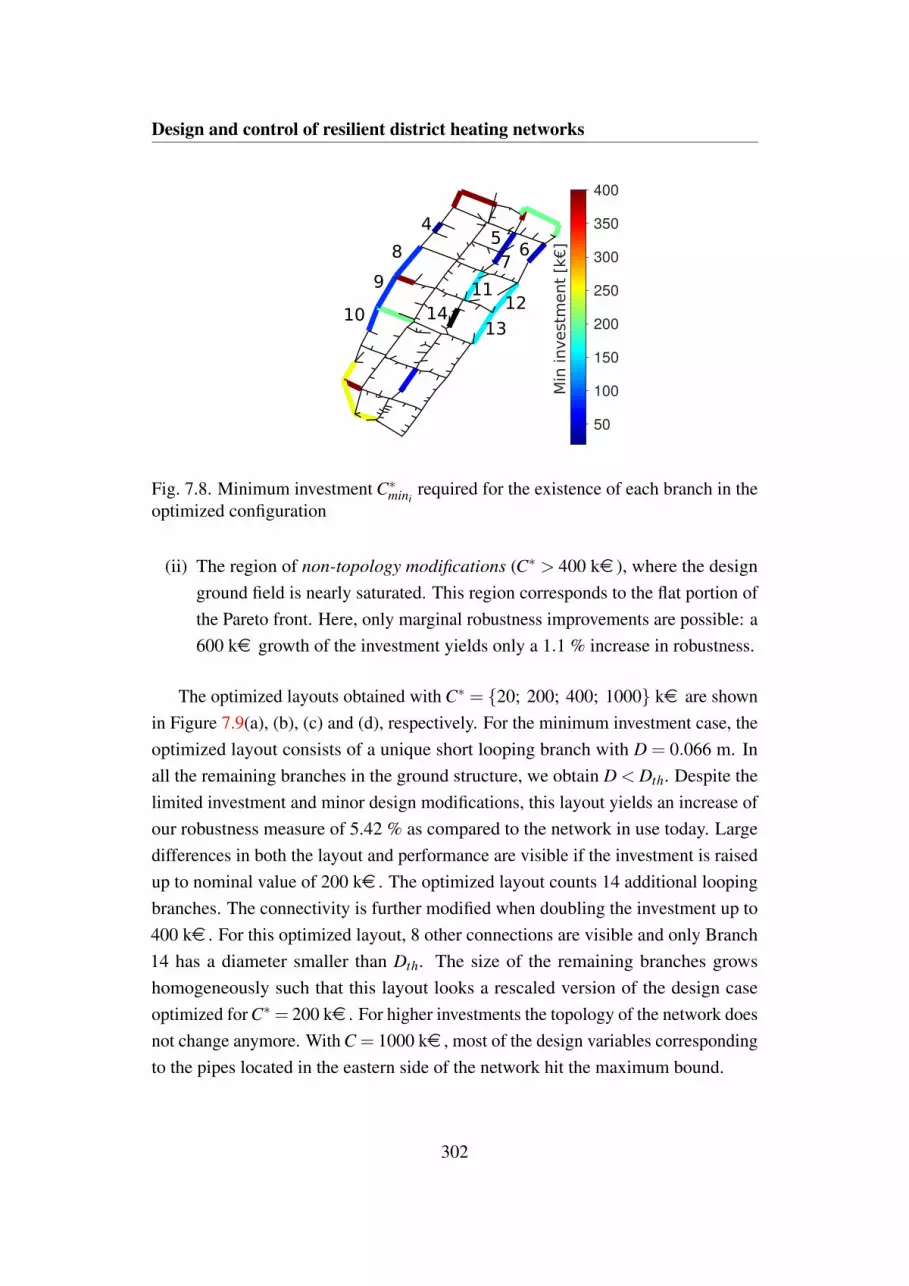
Design and control of resilient district heating networks
50
100
150
200
250
300
350
400
45
67
8
9
10
1112
1314
Fig. 7.8. Minimum investment C∗minirequired for the existence of each branch in the
optimized configuration
(ii) The region of non-topology modifications (C∗ > 400 ke ), where the designground field is nearly saturated. This region corresponds to the flat portion ofthe Pareto front. Here, only marginal robustness improvements are possible: a600 ke growth of the investment yields only a 1.1 % increase in robustness.
The optimized layouts obtained with C∗ = 20; 200; 400; 1000 ke are shownin Figure 7.9(a), (b), (c) and (d), respectively. For the minimum investment case, theoptimized layout consists of a unique short looping branch with D = 0.066 m. Inall the remaining branches in the ground structure, we obtain D < Dth. Despite thelimited investment and minor design modifications, this layout yields an increase ofour robustness measure of 5.42 % as compared to the network in use today. Largedifferences in both the layout and performance are visible if the investment is raisedup to nominal value of 200 ke . The optimized layout counts 14 additional loopingbranches. The connectivity is further modified when doubling the investment up to400 ke . For this optimized layout, 8 other connections are visible and only Branch14 has a diameter smaller than Dth. The size of the remaining branches growshomogeneously such that this layout looks a rescaled version of the design caseoptimized for C∗= 200 ke . For higher investments the topology of the network doesnot change anymore. With C = 1000 ke , most of the design variables correspondingto the pipes located in the eastern side of the network hit the maximum bound.
302

7.3 Robust design
0.01
0.02
0.03
0.04
0.05
0.06
Dia
mete
r [m
]
(a)
0.02
0.04
0.06
0.08
0.1
Dia
mete
r [m
]
(b)
0.05
0.1
0.15
Dia
mete
r [m
]
(c)
0.05
0.1
0.15
0.2
Dia
mete
r [m
](d)
0 100 200 300 400 500 600 700 800 900 1000-0.095
-0.09
-0.085
-0.08
-0.075
-0.07
-0.065
-0.06
-0.055
-0.05
Ro
bu
stn
ess [
ba
r]
Fig. 7.9. Pareto front with selected optimized layouts. (a): 20 ke ; (b): 200 ke ; (c):400 ke ; (d): 1000 ke
303

Design and control of resilient district heating networks
0.02
0.04
0.06
0.08
0.1
0.12
Dia
mete
r [m
]
(a)
-0.04
-0.02
0
0.02
0.04
Dia
m d
iffe
rence [m
]
1
1015
5
11
13
(b)
Fig. 7.10. (a): Optimized layout when solving PPmin with C∗ = 200 ke ; (b):difference between the solutions to PPmin and Prob
Now we benchmark our robust design framework with both the optimized layoutand performance obtained from a minimum pressure maximization design example.The optimization problem is formulated as in (7.34). The maximum investment isset to C∗ = 200 ke as for the nominal case. Figure 7.10(a) shows the optimizedlayout for this case. Figure 7.10(b) highlights the difference between the solutionsto the problems PPmin and Prob. The optimized network topologies are different.When maximizing the minimum pressure, Branch 1 has an optimized diameter ofD1 = 0.048 m. However, the diameter of this pipe degenerated to the minimumbound in our robust design framework. Furthermore, the diameters of Branches10, 15 and 5 are increased by 0.017 m, 0.034 m and 0.018 m as compared to thesolution of Prob. The cost of these modifications is covered by reducing the sizeof Branches 11 and 13. Slight modifications are observed for the remaining pipes.The smooth minimum pressures, minpmP, strict minimum pressures, minP, androbustness measures calculated for both the solutions are compared in Table 7.2.Although solving PPmin yields an increase of the smooth minimum pressure withrespect to the robust design, the strict minimum pressure is lower. The overalldifferences are below 0.5 % for both the strict minimum pressure and its smoothapproximation. The performance differences are non-negligible as regards to ourrobustness measure: the solution of Prob allows an increase of 4.8 % as comparedto the solution of PPmin .
304

7.3 Robust design
Table 7.2. Performance of the solutions to Prob and PPmin
Design
Performance Robust Min pressure
Smooth minimum pressure [bar] 5.9718 5.9936Strict minimum pressure [bar] 5.4381 5.4365Robustness [bar] -0.0592 - 0.0622
0 20 40 60 80
loc factor [-]
0.5
1
1.5
2
2.5
3
3.5
4
4.5
5
5.5
6
Sm
oo
th m
inim
um
pre
ssu
re [
ba
r]
Current network
Robust design
Min pressure design
(a)
0 20 40 60 80
loc factor
0.5
1
1.5
2
2.5
3
3.5
4
4.5
5
5.5
6
Str
ict
min
imu
m p
ressu
re [
ba
r]
(b)
Fig. 7.11. Response of the solutions to Prob, PPmin and current network to fluid-dynamic disturbances. (a): Smooth minimum pressure, minpmP; (b): strict minimumpressure, minP
To investigate how these solutions respond to fluid-dynamic noise, we analyzethe optimized designs in perturbed conditions. The local loss coefficients of the pipesare increased as follows:
βloci = βloci +δβloci, (7.39)
where βloci is the perturbed local loss coefficient of pipe "i" and δβloci is the pertur-bation defined according to (7.37). The multiplication factor, fβloc
, is raised in 15steps from 0 to 70. The results of this study are summarized in Figure (7.11), wherewe show also the performance of the network in use nowadays. Both the designformulations yields consistent improvements to the current situation. The differencesbetween the solutions to Prob and PPmin are limited for small disturbances. How-
305
Design and control of resilient district heating networks
ever, the gap between the two pressure curves increases gradually with fβloc. For a
multiplication factor of 70, considering our robustness measure yields an increasein the smooth and strict minimum pressures of 164 % and 195 %, respectively.Note that in all cases, the strict minimum pressure scales roughly linearly with fβloc
.This suggests that a probabilistic characterization of noise, e.g. obtaining stochasticbounds to maximize the feasible set or obtaining PDFs to minimize variance [193],may yield limited differences in this design example.
7.4 Centralized control
This section focuses on resilience improvements of DHNs through a centralizedcontrol during failure events. We first define the control variables, objective functionand constraints of our framework. Then, we present a benchmark control strategyinspired by the typical habits in use nowadays. Last, we present the results obtainedfor several numerical experiments conducted on the same portion of the Turin DHNconsidered in the previous section.
7.4.1 Control and optimization models
Most of the control actions in a DHN are taken at each user location. The flow withinthe building heat exchanger can be adjusted through the manipulation of a valve.Our centralized control strategy aims at optimizing the set-up of all the user valvesin the network. The vector of control variables, s, is used to interpolate the local losscoefficient of the user control valves as follows:
βloci(si) = βlocmin +(βlocmax−βlocmin)si i = 1, . . . ,Ns−1, (7.40)
where βlocmin and βlocmax are the minimum and maximum local pressure drop co-efficients and Ns is the number of control variables. The flow can be preventedonly for βloc→ ∞ which leads to ill-conditioning of the state equations. Due to oursteady-state assumption, valve closures are not of interest here as a nil flow wouldresult in a nil thermal power transferred to the building connected. The modificationof the control valves affects the equivalent fluid-dynamic resistance of the network.Setting a fixed inlet mass flow rate may yield a head drop higher than the one that
306

7.4 Centralized control
can be sustained by the circulation pump. The fluid-dynamic equilibrium betweenthe network and the pump is obtained by modifying the inlet mass flow rate, Gin,during the optimization process, in such a way to meet a pumping constraint. Thephysical design variables set (7.40) is augmented with:
Gin(sNs) = G(0)in (χmax−χmin)sNs, (7.41)
where χmin and χmax are the minimum and maximum mass flow rates normalizedwith respect to the design value, G(0)
in .
When controlling DHNs after a mechanical failure event, the primary concernis to guarantee the thermal comfort to all the connected users, so that the qualityof service is maintained above acceptable limits. We formulate the optimizationproblem as a minimization of the discomfort of the most critical users. We quantifythe thermal discomfort, γi, of user "i" as follows:
γi =
(Φi−Φspi
Φspi
)2
, (7.42)
where Φi is the real thermal power delivered to the user and Φspi is the ideal value,which would be required to obtain the internal set-point temperature, Tsp. Thisquantity is calculated as:
Φspi = KVVi(Tsp−Tamb). (7.43)
The term in brackets in Equation (7.42) represents the thermal power deficitor surplus in relative terms. We will refer to this quantity as thermal mismatch,∥∆Φi∥, hereafter. The quadratic formulation (7.42) equally accounts for both theover-heating and under-heating. The thermal discomfort of the most critical users isobtained through a smooth maximum approximation using the p-mean formulationas in (7.27). The objective is written as:
z = ˜maxpmγγγ =
(1
Nbg
Nbg
∑i=1
γpγ
i
) 1pγ
, (7.44)
where Nbg is the number of buildings and pγ is the p-mean exponent. Eq. (7.44)provides a lower bound to the hard maximum function and converges to it in the
307

Design and control of resilient district heating networks
limit of pγ → ∞ [431]. The optimization problem is augmented with a pressurehead constraint to enforce the fluid-dynamic equilibrium with the circulation pump.Mathematically:
(∆PPH−∆Pmax)2− ε
2p ≤ 0. (7.45)
Using the constraint (7.45) results in a weakly-imposed fluid-dynamic equilibrium,such that in the worst case the maximum pressure drop registered in the network∆Pmax = max(P)−min(P) differs from the pump pressure head, ∆PPH , by a smallnumber, εp. To sum up, the optimization problem is formulated as:
PLMD :
min
s˜maxpmγγγ
s.t. (∆PPH−∆Pmax)2− ε
2p ≤ 0
s ∈ S =RNs | 0≤ si ≤ 1, i = 1, ...,Ns
. (7.46)
As solving Problem (7.46) corresponds to minimizing the maximum discomfort, wewill refer to this control strategy as Least Maximum Discomfort (LMD) Control.The objective and constraint gradients with respect to the control variables, s, arecomputed with the discrete adjoint method described in Section 2.3.2. To this aim,the continuity, momentum and energy state variables and residuals are stacked in thevectors u = [PT , GT , TT ]T and R = [RT
c , RTm, RT
e ]T .
In order to permit useful comparisons, we benchmark our centralized controlstrategy with an alternative approach inspired by the current habits. This is labeledas Conventional Control or C-Control in short. The decisions are taken from eachindividual user based on the local degree of discomfort. There is an intrinsic hierarchyin the control possibilities. The control actions of the over-heated buildings aregenerally successful (a valve can always be closed more as long as βloc ≤ βlocmax).The control actions of the under-heated buildings are limited by fluid-dynamicconstraints: even if the user valves are completely open, the incoming mass flow ratemay be inadequate to meet the thermal requirements. For this reason, we handle theover-heated and under-heated buildings separately. For over-heated buildings, weconsider a criterion similar to (7.44):
˜maxpmγk, (7.47)
308
7.4 Centralized control
but here the index "k" spans only those buildings in which:
Φk−Φspk ≥ 0. (7.48)
The corresponding control variables are updated with MMA, using the gradientswith respect to the criterion (7.47) and to the constraint (7.45). The control variablescorresponding to the under-heated buildings are updated using a heuristic recursiverelation of the form:
s(i+1)l = max
(smin, s(i)l − fss
(0)l
), (7.49)
where s(0)l is the control variable value at iteration 0, s(i)l is its value at the optimizationiteration "i" and fs is a constant multiplication factor here set to 0.2. The index lruns over those buildings in which:
Φl−Φspl < 0. (7.50)
We stop the iterative procedure when the norm of the control variables change dropsbelow 1e−5 and the pumping constraint (7.45) is satisfied. This scheme revealed tobe effective in the numerical examples described in the next section. Oscillations ofthe criterion (7.47) and pumping constraint (7.45) are severe only during the initialiterations, when the heuristic update (7.49) is dominant.
7.4.2 Numerical results and control trends
This section presents and discusses the performance of our centralized controlframework in handling failure events. We focus on the same subnetwork consideredfor the robust design (Figure 7.5). The values of the most relevant parametersand properties are listed in Table 7.3. The failures are simulated by prescribingthe maximum local loss coefficient, βlocmax , to three selected branches, highlightedin Figure 7.5(b). We first shed light on the LMD-Control procedure focusing ona reference case with Inlet 1 and Failure 1, which is the combination with thelargest influence on the system performance. Then, we assess the effect of theavailable pressure head for different failures and inlet positions. Last, we studyhow the malfunctions in the main transportation network can be managed througha centralized control of the considered distribution network. All the optimization
309

Design and control of resilient district heating networks
Table 7.3. Parameters and properties for the centralized control
Description Symbol Value Unit
Relative outlet total pressure Pout 0 PaInlet temperature Tpp 363.15 KDacy-Weisbach friction factor f 0.014 -Water density ρ 1000 kg/m3
Water specific heat cp 4186 J/(kg K)Volumetric heat transfer coefficient K 0.9 W/(m3 K)Set-point internal temperature Tsp 293.15 KDesign outdoor temperature Tamb 265.15 KMinimum local pressure drop coefficient βlocmin 0 -Maximum local pressure drop coefficient βlocmax 1e7 -Minimum relative inlet mass flow rate χmin 0.5 -Maximum relative inlet mass flow rate χmax 1.5 -
problems are solved using MMA. Compared to the parameters set-up discussed in theprevious section, to produce the following results we set the constraint penalty as c1 =
10000. Recall that PLMD (7.46) includes an inequality constraint (7.45) that weaklyenforces the fluid-dynamic equilibrium between the network and the circulationpump. Since we devised our control framework to fit within an RTI system, wewould like to obtain a sequence of feasible solutions along the optimization process.In preliminary numerical studies, we observed that using the reference constraintpenalty, c1 = 1000, was leading to constraint violations of unacceptable magnitudealong the optimization history. Raising c1 to 10000 fixed the issue.
The objective history for the reference failure case is shown in Figure 7.12. Theobjective values are normalized with respect to the initial value, z(0). Convergenceis reached in 134 control iterations and required a total computational time of only246.89 s on an old machine equipped with two Intel i7-870 Quad-Core processors.This suggests that the developed framework is ideal for the integration within anRTI control system. We study only the first 100 iterations as minimal objective andthermal mismatch changes are observed after. The objective history is smooth andthe improvements are quick. The maximum discomfort measure drops by more than60 % in the first 20 iterations and it takes 80 more iterations to obtain an additional20 % reduction. The initial discomfort field peaks in those regions that are locatedright downstream the malfunction. The thermal mismatch of this group of users israpidly increased by redirecting some of the mass flow rate of the neighbors. This
310

7.4 Centralized control
Thermal mismatch [%]
3.6-3.6-14.3-21.4
(a) (b) (c) (d)
0 10 20 30 40 50 60 70 80 90 100
Optimization iteration [-]
0.2
0.3
0.4
0.5
0.6
0.7
0.8
0.9
1.0
Norm
aliz
ed o
bje
ctive [-]
Fig. 7.12. Normalized objective history during the optimization of the referencefailure case. The thermal mismatch field is shown at selected optimization iterations.(a): Iteration 0; (b): iteration 20; (c): iteration 50; (d): iteration 100
311

Design and control of resilient district heating networks
(a)
-53.6
-35.7
-17.9
0.0
Therm
al m
ism
atc
h [%
]
(b)
-53.6
-35.7
-17.9
0.0
The
rmal m
ism
atc
h [
%]
Fig. 7.13. Final thermal mismatch field. (a): LMD-Control; (b): C-Control
smoothing process progressively enlarges the area with a negative thermal mismatch,which reaches the northern portion of the network after 20 iterations. At this point, itis still possible to clearly distinguish among three different zones: a cold zone (blue),an intermediate zone (green) and a warm zone (orange). The former two appearmixed together after 50 and 100 iterations. Figure 7.13 shows a comparison of thefinal thermal mismatch distributions obtained with the LMD-Control and C-Control.Our centralized control strategy results in a nearly homogeneous thermal mismatchfield. On the other hand, the conventional operation strategy yields strong discomfortpeaks. The users located right downstream the broken pipe feel the highest thermaldiscomfort. The head availabilities for these buildings are too low to provide massflow rates able to satisfy their thermal requirements. Overall, the utilization of theLMD-Control yields a reduction in the global measure of discomfort of 96 % ascompared to C-Control.
Now we investigate how the inlet pressure head affects the performance ofboth the control strategies. The pumping head, ∆PPH , in (7.45) is increased in6 steps of 14 % over the design value. For each case, an optimization run isperformed. Figure 7.14 shows the evolution of the thermal mismatch distributionfor ∆PPH = 100; 142; 184 %. The snapshots are taken after 20, 50 and 100iterations. Similar improvements are achieved within the first 20 iterations: thethermal mismatch peaks are smoothed over the whole south-east portion of thenetwork. From iteration 20 to iteration 50, this "cold wave" expands to occupy
312

7.4 Centralized control
Thermal mismatch [%]
3.6-3.6-14.3-21.4
(a)
(b)
(c)
Fig. 7.14. Evolution of the thermal mismatch distribution for ∆PPH = 100 % (a),∆PPH = 142 % (b), ∆PPH = 184 % (c). The snapshots are taken at iteration 20,iteration 50 and iteration 100
313

Design and control of resilient district heating networks
0 20 40 60 80
Pumping head increase [%]
0
2
4
6
8
10
12
14
16
18
Norm
aliz
ed m
axim
um
dis
com
fort
[%
]
(a)
0 20 40 60 80
Pumping head increase [%]
0
50
100
150
200
250
300
350
400
450
Norm
aliz
ed m
axim
um
dis
com
fort
[%
](b)
Fig. 7.15. Effect of the inlet pressure head on the control strategy performance. (a):LMD-Control. (b): C-Control
the whole southern portion, while the northern one looks still warm. Substantialdifferences among the three cases are visible after iteration 50. At this stage, theover-heated buildings contribute meaningfully to the objective and the optimizer triesto blend the hot and the cold regions in a unique homogeneous field. The successof this last step largely depends upon the value of ∆PPH . The final normalizedobjective values obtained for the LMD-Control and the C-Control are reported inFigure 7.15. Increasing ∆PPH yields moderate effects on the performance of ourcentralized control strategy. It is possible to decrease the normalized objective from18.0 % to 0.2 % with an 84 % increase in the pressure head. On the other hand,Figure 7.15(b) indicates that a growth of the inlet pressure head is crucial whenusing the conventional operation strategy. For all the values of ∆PPH considered,the conventional strategy yields inferior performance with respect to the worst-performing case of our centralized strategy. This suggests that a centralized controlstrategy may be a valid alternative to the installation of a backup pumping system atthe inlet of the distribution networks.
To generalize the previous observations, we study the influence of the location ofthe inlet and failure. With reference to Figure 7.5(b), the numerical experiments arefirst repeated considering Failure 2 and Failure 3. We study the subnetwork whenalimented from Inlet 1. Figure 7.16(a) shows the outcome of this analysis. The trend
314

7.4 Centralized control
0 20 40 60 80
Pumping head increase [%]
0
2
4
6
8
10
12
14
16
18
Norm
aliz
ed m
axim
um
dis
com
fort
[%
]
Failure 2
Failure 3
Failure 1
(a)
0 42 84Pumping head increase [%]
0
7
14
21
29
36
43
50
57
Min
imum
pow
er
mis
matc
h im
pro
vem
ent [%
](b)
Fig. 7.16. (a): Effect of the inlet pressure head on the control strategy performancefor different failure locations; (b): summary of the performance improvementsachievable with the LMD-Control compared to the C-Control for different failurelocations
for Failure 1 was already presented in Figure 7.15 and is reported here to facilitate thecomparisons. The three curves drop at different rates, indicating that the location ofthe failure modifies the effect of the available pressure head on the discomfort peaks.With no additional pressure head, Failure 1 yields the highest maximum thermaldiscomfort. However, this case results in the best performance for ∆PPH = 184 %.Figure 7.16(b) summarizes the improvements in the minimum thermal mismatch (i.e.the discomfort of the most under-heated user) obtained with respect to the C-Control.In all the cases considered, the performance gap between the control strategies dropsquadratically when the pressure head is increased. The effect of the inlet locationis shown in Figure 7.17. To obtain these results, we considered Failure 1 as in thereference configuration. The two curves exhibit a nearly constant spacing along the yaxis and drop at the same rate. This suggests that the inlet position does not modifythe effect of the available pressure head on the discomfort peaks. The improvementsobtained with the LMD-Control with respect to the C-Control are summarized inFigure 7.17(b). With no additional pressure head, the gains are higher with Inlet 1than with Inlet 2. The improvements obtained with Inlet 1 and Inlet 2 scale linearlyand quadratically with ∆PPH , respectively. As a consequence, for ∆PPH = 184 %, theLMD-Control yields larger benefits when water is injected at Inlet 2. These results
315

Design and control of resilient district heating networks
0 20 40 60 80
Pumping head increase [%]
0
5
10
15
20
25
Norm
aliz
ed m
axim
um
dis
com
fort
[%
]
Inlet 1
Inlet 2
(a)
0 42 840
7
14
21
29
36
43
50
57
Min
imu
m p
ow
er
mis
ma
tch
im
pro
ve
me
nt
[%]
Pressure head increase [%]
(b)
Fig. 7.17. (a): Effect of the inlet pressure head on the control strategy performance fordifferent inlet locations; (b): summary of the performance improvements achievablewith the LMD-Control compared to the C-Control for different inlet locations
present evidence that the benefits of a backup pumping system depends largely on thelocation of the failures and slightly on the inlet position. However, the improvementsof our control strategy with respect to the one in use today are observed to be moreaffected by the position of the inlet than by the location of the failure.
Here, we test the ability of our centralized control strategy to handle failures in themain supply line (transportation network) rather than in the controlled subnetwork.The mainly supply line of the Turin DHN is represented in Figure 7.18(a). Thegraph representation of this system counts 1373 nodes and 1389 branches. Hotwater is injected in six different positions highlighted with green indicators. Thosecorrespond to the location of the CHP plants, boilers and storage tanks. We considertwo malfunctions, labeled as Failure 4 and Failure 5. In both cases, the location of themost critical distribution network, i.e. the one with the lowest available pressure head,corresponds to the one indicated in Figure 7.18(a). For simplicity, we assume thatthis critical subnetwork has the same topology and design specifications of the oneconsidered for the previous analyses. Water is injected in this distribution networkthrough Inlet 1, as in the reference case. The fluid-dynamic equilibrium lies at theintersection between the characteristic curves of the transportation and distributionnetworks. These curves are shown in Figure 7.18(b). All the values are normalized
316

7.4 Centralized control
Failure 4Failure 5
Critical subnetwork
Inlet
(a)
A
B
B’
A’
(b)
Fig. 7.18. (a): Overview of the transportation network; (b): intersection of the mainnetwork characteristic curves with the subnetwork characteristic curves
with respect to the nominal operating conditions. The subnetwork control curvesare obtained by sweeping the pressure head, ∆PPH , in the nonlinear constraint (7.45)from 40 % to 90 % of the design value in steps of 10 %. The LMD-Control curve ofthe subnetwork intersects the main network characteristic curves in Point A and B.Failure 4 has larger impact than Failure 5 on the fluid-dynamic response. In this case,the system can be operated with 65.1 % of the design pressure head and 82.5 % ofthe design inlet mass flow rate. Point B locates at 78.3 % and 90.0 % of the designpressure head and inlet mass flow rate, respectively. When the subnetwork is operatedthrough the C-Control, the fluid dynamic equilibrium moves to Point A’ and B’, withhigher inlet mass flow rate and lower available pressure head with respect to A andB. Figure 7.19 shows the thermal mismatch field ∥∆Φ∥ in Points A, B, A’ and B’. Toobtain these results, we performed four additional optimization runs in which themaximum pressure head, ∆PPH , was set according to the interpolated pressure headof the four points. The optimized inlet mass flow rates present negligible differencesfrom the ones predicted through the piece-wise linear trend shown in Figure 7.18(b).For both Failure 4 and Failure 5, the LMD-Control yields a nearly "flat" thermalmismatch field. In Points A and B, all the network users are equally under-heated
317

Design and control of resilient district heating networks
-8.9-13.8 -4.1 0.7
Point A Point B Point A’ Point B’
Fig. 7.19. Final thermal mismatch field ∥∆Φ∥ for failures in the main network
Table 7.4. Smooth maximum discomfort z (×102) [-] obtained for failures in themain network
Control strategy
Failure LMD Conventional4 0.49 1.285 0.16 0.57
by roughly 7 % and 4 % so that the discomfort peaks are avoided. Operating thenetwork with the C-Control (Points A’ and B’) results in a strong thermal imbalance.The users located in the northern portion of the system are more under-heated ascompared to those located in the southern portion. This can be explained by theabsence of loops in the northern portion, yielding a higher fluid-dynamic resistance.Despite this general trend, the thermal mismatch distribution is highly oscillatingand presents multiple local minima and maxima. Whether a building thermal requestis satisfied depends on both the available and nominal pressure heads at each usersubstation. The latter can vary substantially due to practical installation requirements.Table 7.4 summarizes the normalized maximum discomfort in the 4 points analyzed.Compared to the conventional operation strategy is use today, the LMD-Controlallows our global discomfort measure to be reduced by roughly 62 % and 72 % inthe two failure cases considered. These results suggest that a partial centralization ofthe control system may yield benefits also when mechanical failures are not locatedin the controlled area.
318

7.5 Conclusions
7.5 Conclusions
In this chapter, we demonstrated a robust design and a centralized control frameworkfor increased resilience of DHNs. Robustness was defined using a sensitivity metricthat does not require any probabilistic characterization of the noise uncertainty. Thedesign problem was formulated using the ground structure approach for topologyoptimization where realistic looping paths are selected as potential or vanishingconnections. Control aimed at minimizing a differentiable global measure of dis-comfort after a pipe breakage event. The optimization problem was solved usingpopular mathematical tools for topology optimization: MMA and discrete adjointsensitivities. Both the design and control frameworks were tested on a limited portionof the Turin district heating network.
The most relevant application-oriented advances of this chapter are presented inFigure 7.20. The robust design results (Figure 7.20(a)) indicate that our sensitivitymetric for robustness quantification well measures the ability to absorb fluid-dynamicperturbations. When analyzed considering a distributed fluid-dynamic noise, the lay-out optimized with our framework is superior to the one computed using a minimumpressure maximization formulation. Robustness and investment were found to beantagonist in the range of values considered. Large robustness improvements (+ 38.8%) with a limited investment (400 ke ) are possible through topology modificationsof the network. Oversizing the pipes with no change of the connectivity leads to onlyminor benefits. The outcomes of our control numerical examples (Figure 7.20(b))show that the proposed framework allow mechanical failures to be quickly handledwith little impact on the level of service. The steep discomfort peaks that naturallyarise when taking non-centralized control actions are eliminated. In the nominalconditions, the utilization of our centralized control framework yields a reductionin the global measure of discomfort of 96 % as compared to the control strategyin use today. Furthermore, we obtained improvements to the thermal deficit of themost critical user between 5.89 % and 56.38 % in all the failure cases analyzed. Theinlet pressure head weakly affects the achievable performance. This suggests thatadopting a centralized real-time control system may yield considerable investmentsavings on pumping equipment. Furthermore, a partially centralized system wasfound to be beneficial also when failures are not located in the controlled portion ofthe network.
319

Design and control of resilient district heating networks
Investment
Diameter
Thermal mismatch
Optimization iteration
Maxim
um
Dis
com
fort
100
Our framework Conventional
Ro
bustn
ess
Topology
modificationsNon-topology
modificationsM
inim
um
pre
ssure
Fluid-dynamic perturbation
Fig. 7.20. Graphical summary of the main application-oriented advances obtainedin this chapter using: (a) our robust design framework; (b) our centralized controlframework
320

Chapter 8
Design of flow fields in PEM fuel cells
PEMFCs are electrochemical devices used to directly convert the chemical energy ofhydrogen into electricity [79]. They represent an efficient power generation solutionfor both stationary and moving power systems such as automotive, aerospace andmarine vehicles [461, 87, 9] because of their high power density, low operating tem-perature, low weight and fast startups [254, 461]. However, their limited durabilityand high cost are major obstacles to achieve a large scale commercialization [460].The search for improved flow field geometries, yielding enhanced performance atreduced costs, is a long-standing problem in the fuel cell community. However, asobserved for fins geometries in Chapter 3, most of the current literature deals withimprovements to specific design concepts that are heuristically proposed followingpersonal insights or intuition. The presence of a multitude of different solutionssuggests that the choice of the design concept is crucial for the final geometry.Hence, also in this field, there is a urgent need for a thorough and affordable designoptimization route, allowing dramatic design changes. In this chapter, we developand demonstrate a topology optimization framework for the design of flow fieldsin PEMFCs. To our best knowledge, a unique study [242] dealt with topologyoptimization of fuel cells. This valuable contribution relies on overly simplifiedelectrochemical and mass transport models and does not consider all the optimizationcriteria of practical interest for the development of these energy devices. Further-more, the paper suffers from a limited resolution and convergence to well-definedmanufacturable layouts. These shortcomings motivate the work presented hereafter.
321

Design of flow fields in PEM fuel cells
Fig. 8.1. Representative exploded view of the cathodic section of a PEM fuel cell
The plan of the chapter is as follows. In Section 8.1, we review the most populartechnological solutions and identify room for improvements to the geometric designof PEMFCs. In Section 8.2, we describe a method capable of reducing the problemdimensionality and present the governing equations and numerical model used topredict gas dynamics, transport of chemical species and electrochemistry. Section8.3 introduces the optimization framework focusing on the objective, constraintsand material interpolation strategies. In Section 8.4, we calibrate and verify our 2Danalysis framework and present numerical results and design trends. Finally, Section8.5 summarizes the main contributions of the chapter.
Some of the contents of this chapter were presented at the 18th U.S. NationalCongress for Theoretical and Applied Mechanics ([C6]) and included in a paperdraft that was submitted for publication in Applied Energy ([J5]).
8.1 Overview of geometric design in PEMFCs
A schematic exploded view of the cathode of a typical PEMFC is shown in Figure8.1. It is composed of three stacked layers: a BPP, a Gas Diffusion Layer (GDL), anda Catalyst Layer (CL). The CL is positioned at the interface between the membraneand the GDL and is responsible for the recombination of oxygen with protons
322

8.1 Overview of geometric design in PEMFCs
through electrochemical reactions and mass transfer phenomena. The delicatecatalyst structure is protected by the porous GDL, which provides a path for thereactants from the BPP to the CL and allows the transport of the electrons neededfor the electrochemical reactions. The BPP serves as an electronic interconnectionbetween adjacent cells and feeds the reactants to the electrode. A cross-section ona horizontal plane, e.g. π1, reveals the presence of both solid and empty regions.The former are referred to as ribs and are generally made of graphite. The lattercorrespond to the channels in which the reactants flow. If a sufficient pressuredifferential is available, the gas is allowed to flow under the ribs (moving on avertical plane, e.g. π2) and reach the contiguous channel. The BPP is a crucialcomponent, playing four major roles [32]:
(i) It should distribute the reactants homogeneously over the active sites. Thepoor distribution of the reactants may be a consequence of an uneven flowresistance of the channels caused by either a bad mechanical design or wateraccumulation and fouling [289]. Nonuniform electrochemical reactions affectwater management [450] and yield water content and temperature inhomo-geneities, leading to hygro-thermal stresses [10]. Delamination between theGDL and the membrane [318] may occur at early stages of the operating life,impacting on the durability.
(ii) It should guarantee a high power generation at minimal pressure dropfrom the inlet to the outlet. Large pressure drops may require a non-negligibleparasitic power to drive external blowers. Furthermore, cross-leakages ofreactants, mechanical stresses and reversible voltage losses may also arise as aconsequence of excessive pressure drops [450, 268].
(iii) It should guarantee an effective water management; performance drops areobserved due to both dehydration and flooding. Dehydration refers to thewater depletion in the membrane and yields a reduced ionic conductivity andrisk of de-adhesion [84]. Flooding refers to the liquid water accumulation inboth the channels and GDL, which is manly due to a high rate of condensation[289, 207]. In PEMFC, the phenomenon is critical at the cathode, where vaporis produced due to the Oxygen Reduction Reaction (ORR) [9]. This leads tothe deterioration of the oxygen transport over the reactive sites and in turnaffects the performance. Flooding is seldom an issue in high temperature
323

Design of flow fields in PEM fuel cells
PEMFCs due to the increased vapor saturation pressure [83]. However, inthese systems different membranes are required to avoid dehydration [83].
(iv) It should provide a low electrical resistance and high mechanical stabilityby creating a sufficient contact area between the BPP and GDL [258].
In summary, the geometry of the BPP grooves affects the transport of both thereactants and electrons, reaction rate, pressure drop and water management [9].These factors greatly influence the fuel cell performance [249]. Kahraman andOrhan [229] estimated that crafted designs can yield improvements to the powerdensity as high as 50 %. For this reason, a vast body of literature investigated theeffect of various geometrical features of the BPP. Researches towards enhancementtechniques can be grouped in three categories: design of the channels and ribs,utilization of obstacles and design of the flow fields.
The design of the channels and ribs was tackled at different levels of complexity,ranging from the definition of the widths and depths to the shape optimization of thechannel cross sections and utilization of tapered conduits. The former was generallyconsidered using a channel-to-rib width ratio:
W =Wch
Wrib, (8.1)
where Wch and Wrib represent the widths of the channels and ribs, respectively. Kumarand Reddy [254] were among the first to investigate systematically the effect of W onperformance. Their results indicate that there might be an optimum value of W closeto 3. The authors did not model the transport of electrons and their layout may resultin a high electrical contact resistance. In this regard, the experiments conducted byYoon et al. [482] suggest that mass transport has larger impact on performance thanelectric conduction. The authors considered layouts with 0.33≤ W ≤ 2 and foundthat thinner ribs always lead to a higher power generation. Later, the numerical studyby Ahmed and Sung [8] led to different conclusions. Their results indicate that athigh current densities, large performance degradations can be expected for W ≥ 1.4due to the increased ohmic losses. Many other studies were later conducted to assessthe effect of this parameter on performance, see e.g. [241, 445, 488]. Althoughthe specific "optimized "values are of little interest due to the high variability ofthe test conditions, most of the findings suggest that increasing W in general leadsto a higher ohmic resistance and pressure drop, enhanced reactant distribution and
324

8.1 Overview of geometric design in PEMFCs
improved water management. As observed by Manso et al. [289], only a limitednumber of studies focused on the effect of the channel depth, Hch. Afshari et al. [5]reported increased current densities for smaller depths and suggested to adopt 1 mmdeep channels. The authors noted that a moderate increase of the pressure drop atreduced depths is unavoidable but slightly affects the net performance of the system.A recent numerical and experimental study reported in [445] revealed that reducedchannel depths and thinner ribs are always beneficial for water management. Atlow operating voltages, these features prevent the accumulation of water in the GDLthrough strong under-rib convection. At high operating voltages, water plugs in thechannels are eliminated thanks to large streamwise pressure gradients. All the studiesdiscussed so far considered channels with rectangular cross-sections. Many scholarsdedicated to the search of alternative channel configurations such as hemispherical,triangular, trapezoidal and stepped cross sections. Ferng and Su [135] observedthat designing a proper channel cross-section is crucial for parallel flow fields butyields minor effects in serpentine layouts. The authors of [254] suggested to usetriangular and hemispherical channels to obtain the most effective mass distributionover the active sites but did not discuss any issue related to water management. Later,the experiments conducted by Owejan et al. [323] revealed that the shape of thechannel cross-section has large effects on the two-phase flow dynamics. Differentlyfrom rectangular channels, triangular ones were found to confine the accumulationof water at the channel angles in contact with GDL, yielding a little impact on thereactant distribution. Similar effects were reported in [148] for highly humidifiedstreams in trapezoidal channels. However, the authors noted that some issues relatedto the membrane dehydration may arise when using dry streams due to an excessivewater removal. Zeng et al. [489] used GA to conduct a formal shape optimizationof trapezoidal channels by varying the width of the bottom and top edges. Theiroptimized layout features a edge ratio of 1.45 and yields an increase of 8.09 %in the output power compared to rectangular channels. Recently, Paulino et al.[328] compared numerically rectangular, trapezoidal and stepped channels. Theauthors confirmed the findings of Freire et al. [148] in regard to water management.However, they pointed out that rectangular cross-sections guarantee an improvedelectric performance and might be beneficial to intermittent applications, for whichwater management issues do not appear. The findings of the previous researcheshighlighted that water management and in turn reactant distribution are critical in theregions of the cell located close to the outlet section. There, the high water content
325

Design of flow fields in PEM fuel cells
due to the upstream electrochemical reactions may quickly lead to flooding. Theregions connected to the inlet are rarely responsible for performance drops. Buildingon these observations, many authors in the last decade focused on the design oftapered channels, i.e. with a varying cross-section along the path from the inlet to theoutlet. The concept was first investigated numerically by Yan et al. [478] and Liu etal. [272]. The authors reported performance improvements for both width tapering,i.e. channel width increasing along the streamline direction, and height tapering, i.e.channel height decreasing along the streamline direction. Liu et al [272] pointedout that the advantages due to tapering are most visible at high current densitiesand that the pressure losses are in generally negligible as compared to the gains inpower generation. Similar conclusions can be drawn from the experiments reportedrecently in [444]. The tests conducted at low air humidity revealed a negligibleinfluence of tapering, suggesting that water management is the primary performancebenefit of this enhancement technique. Wang et al. [454] optimized the height ofthe channels of a serpentine configuration using 5 design variables. Their optimizedgeometry is composed of 3 tapered channels and a divergent channel connectedto the outlet. According to the authors, the convergent portions of the flow fieldimprove the advective transport of the reactants within the GDL. The divergentportion serves for the purpose of minimizing the reactant cross-leakages to the outlet.The authors reported an 11.9 % increase to the power generation as compared toa conventional non-tapered configuration. Fontana et al. [144] later considereda single convergent channel with constant inclination. Their results show that aninclination of 0.75 leads to a 9.5 % increase in the power generation but requiresa 350 % higher pressure at the inlet. More recently, Mancusi et al. [288] reportedinteresting insights on two-phase flow in tapered channels. The authors observeda transition from a slug flow regime to a film flow regime at large tapering angles,which may lead to a performance degradation due to the reduced oxygen transport.This suggests that in general it is possible to identify an optimal tapering angle. Themain findings of the reviewed literature dealing with the design of the channels andribs in PEMFCs are summarized in Table 8.1.
Differently from tapering, blockages (also referred to as baffles or indentations)are sudden variations of the channel cross-section, leading to partial or complete flowobstructions. The proposal of these geometrical features for PEMFC performanceenhancement builds on advancements in the field of convective heat transfer [206].The increased advective transport along the x direction (Figure 8.1) improves water
326
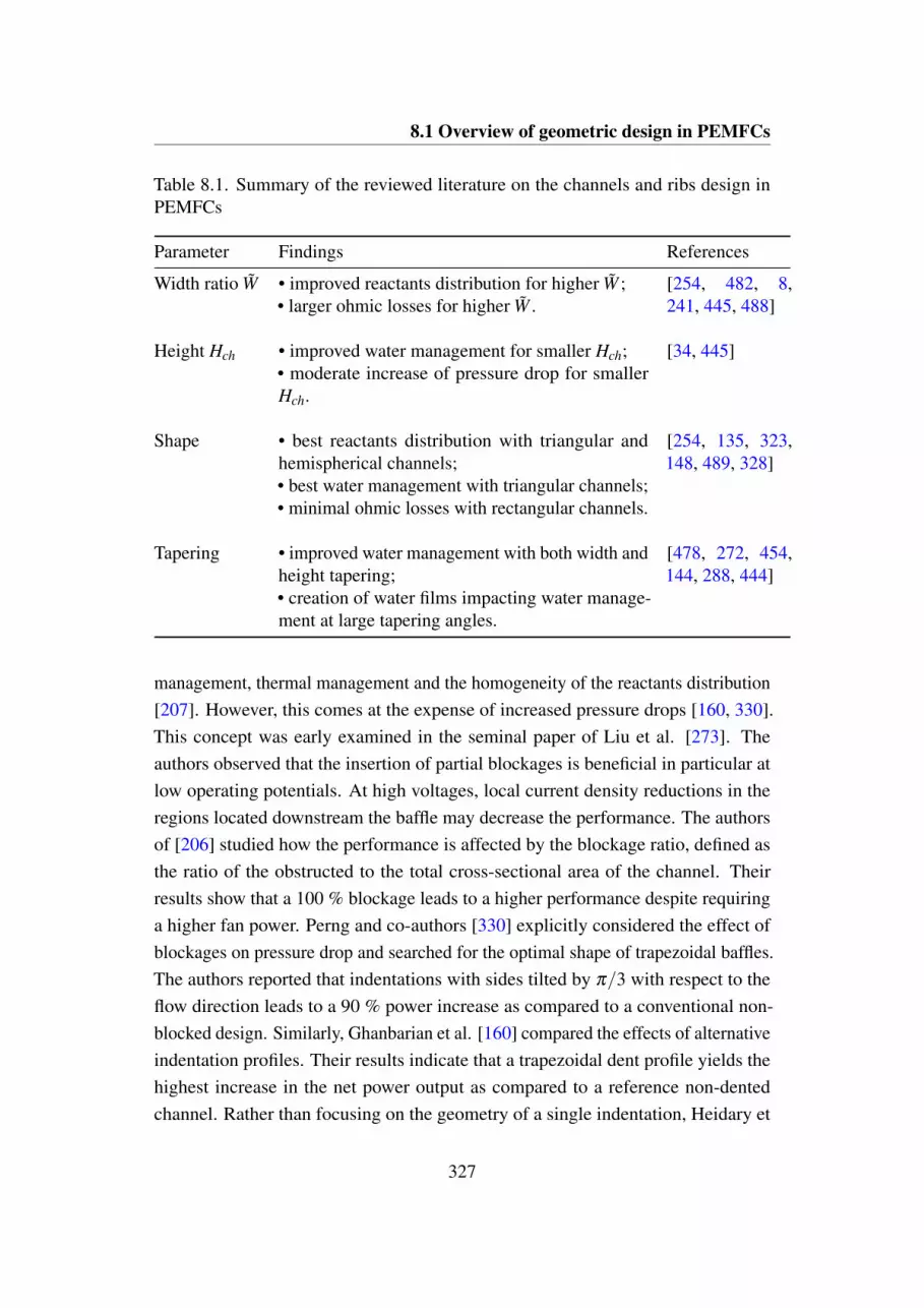
8.1 Overview of geometric design in PEMFCs
Table 8.1. Summary of the reviewed literature on the channels and ribs design inPEMFCs
Parameter Findings References
Width ratio W • improved reactants distribution for higher W ;• larger ohmic losses for higher W .
[254, 482, 8,241, 445, 488]
Height Hch • improved water management for smaller Hch;• moderate increase of pressure drop for smallerHch.
[34, 445]
Shape • best reactants distribution with triangular andhemispherical channels;• best water management with triangular channels;• minimal ohmic losses with rectangular channels.
[254, 135, 323,148, 489, 328]
Tapering • improved water management with both width andheight tapering;• creation of water films impacting water manage-ment at large tapering angles.
[478, 272, 454,144, 288, 444]
management, thermal management and the homogeneity of the reactants distribution[207]. However, this comes at the expense of increased pressure drops [160, 330].This concept was early examined in the seminal paper of Liu et al. [273]. Theauthors observed that the insertion of partial blockages is beneficial in particular atlow operating potentials. At high voltages, local current density reductions in theregions located downstream the baffle may decrease the performance. The authorsof [206] studied how the performance is affected by the blockage ratio, defined asthe ratio of the obstructed to the total cross-sectional area of the channel. Theirresults show that a 100 % blockage leads to a higher performance despite requiringa higher fan power. Perng and co-authors [330] explicitly considered the effect ofblockages on pressure drop and searched for the optimal shape of trapezoidal baffles.The authors reported that indentations with sides tilted by π/3 with respect to theflow direction leads to a 90 % power increase as compared to a conventional non-blocked design. Similarly, Ghanbarian et al. [160] compared the effects of alternativeindentation profiles. Their results indicate that a trapezoidal dent profile yields thehighest increase in the net power output as compared to a reference non-dentedchannel. Rather than focusing on the geometry of a single indentation, Heidary et
327

Design of flow fields in PEM fuel cells
Table 8.2. Summary of the reviewed literature on the blockages design in PEMFCs
Parameter Findings References
Blockage ratio complete blockage is always superior to partial. [206]
Shape highest increase in power output with trapezoidal pro-files.
[330, 160]
Distribution under-rib transport enhanced with staggered arrange-ment
[206, 207]
al. [206, 207] studied how to distribute blockages in the flow field. Their numericaland experimental results suggest that a staggered arrangement may be superior tothe most popular inline arrangement as both under-rib and under-block convectionare exploited. The inline arrangement of blockages leads to a negligible under-ribtransport due to the small pressure differentials among parallel channels. The mainfindings of the reviewed literature dealing with the design of blockages in PEMFCsare summarized in Table 8.2.
The search for the optimal flow field layout for PEMFCs is a long-standingengineering challenge. The topology of the channels mainly affects the reactantdistribution, pressure drop and water management. The reviewed works presented inthe remainder of this section did not reveal a substantial influence on the electricalresistance and mechanical stability as a minimum rib width is generally ensured. Forhigh temperature systems, the minimization of the pressure drop and the homoge-neous mass transfer to the active sites are the primary design criteria since watermanagement is rarely an issue [491]. The variety of the heuristic solutions availableand the amount of seemingly unconnected published literature on the topic makesthis field quite similar to the design of heat transfer surfaces in the LHTES unitsdiscussed in Section 3.1. The reviewed geometries can be roughly grouped in fivecategories: serpentine, parallel, interdigitated, mesh and bio-inspired. Some repre-sentative schematics are shown in Figure 8.2. The serpentine layout (Figure 8.2(a))is no doubt the most popular solution among practitioners [268]. In this design,water is forced through a unique channel that connects the inlet to the outlet, using atortuous path that covers the entire active surface. Water clogging is rarely a problemand occurs mainly in U-bends at high current densities. The results presented byWang et al. [455] indicate that this layout is particularly convenient for scale-up to
328

8.1 Overview of geometric design in PEMFCs
(a)
(b)
(c)
(d)
(e)
Fig. 8.2. Schematics of the most popular flow field geometries. The channels areindicated in white, the ribs are indicated in black; (a): serpentine; (b): parallel; (c):interdigitated; (d): mesh; (e): bio-inspired
commercial installations. An increase of the active area leads to a larger under-ribtransport as a result of the higher pressure differential among contiguous channels.However, the recent experimental results of Chen et al. [85] suggests that this trendcannot be extrapolated in general as there should be an optimal pressure differenceamong contiguous channels for maximal power generation. The advantages of thisconfiguration come at the expense of large pressure drops. Furthermore, Kahramanand Orhan [229] observed that the current density distribution may be critical due toa premature reactant depletion. To cure the issues of the reference design concept,research and technology developed in a number of different directions. A ratherpopular option is to use a multi-serpentine configuration in which the gas flows ina number of parallel serpentine-like paths [229]. An interesting alternative is theone proposed by Monsaf et al. [302], who used a concentric spiral layout, yieldingincreased mass transfer at reduced pressure drops. Alizadeh et al. [17] proposed acascade layout, where three serpentine channels with different geometrical parame-ters are concatenated from the inlet to the outlet. In [234], an improved water removalwas observed with the addition of porous carbon pins attached to the rib surfaces.Singdeo et al. [396] adopted a "compensated" arrangement, yielding a more uniform
329
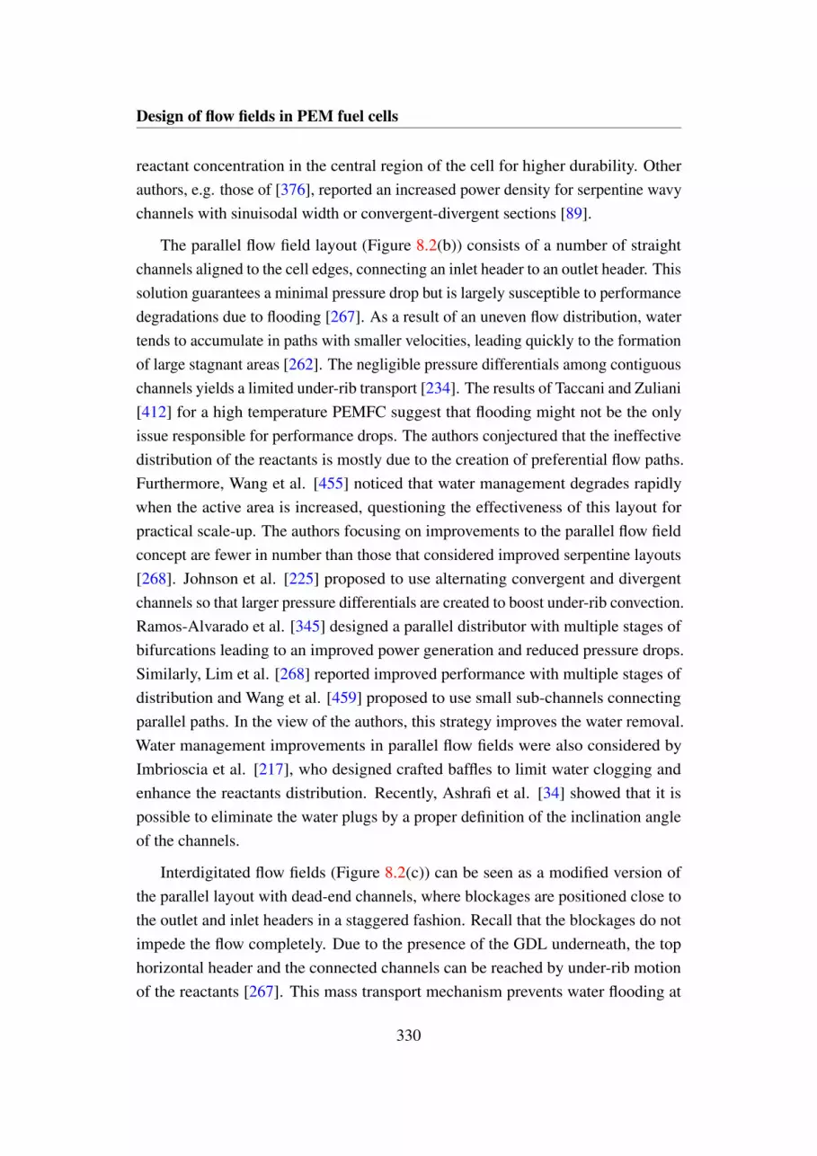
Design of flow fields in PEM fuel cells
reactant concentration in the central region of the cell for higher durability. Otherauthors, e.g. those of [376], reported an increased power density for serpentine wavychannels with sinuisodal width or convergent-divergent sections [89].
The parallel flow field layout (Figure 8.2(b)) consists of a number of straightchannels aligned to the cell edges, connecting an inlet header to an outlet header. Thissolution guarantees a minimal pressure drop but is largely susceptible to performancedegradations due to flooding [267]. As a result of an uneven flow distribution, watertends to accumulate in paths with smaller velocities, leading quickly to the formationof large stagnant areas [262]. The negligible pressure differentials among contiguouschannels yields a limited under-rib transport [234]. The results of Taccani and Zuliani[412] for a high temperature PEMFC suggest that flooding might not be the onlyissue responsible for performance drops. The authors conjectured that the ineffectivedistribution of the reactants is mostly due to the creation of preferential flow paths.Furthermore, Wang et al. [455] noticed that water management degrades rapidlywhen the active area is increased, questioning the effectiveness of this layout forpractical scale-up. The authors focusing on improvements to the parallel flow fieldconcept are fewer in number than those that considered improved serpentine layouts[268]. Johnson et al. [225] proposed to use alternating convergent and divergentchannels so that larger pressure differentials are created to boost under-rib convection.Ramos-Alvarado et al. [345] designed a parallel distributor with multiple stages ofbifurcations leading to an improved power generation and reduced pressure drops.Similarly, Lim et al. [268] reported improved performance with multiple stages ofdistribution and Wang et al. [459] proposed to use small sub-channels connectingparallel paths. In the view of the authors, this strategy improves the water removal.Water management improvements in parallel flow fields were also considered byImbrioscia et al. [217], who designed crafted baffles to limit water clogging andenhance the reactants distribution. Recently, Ashrafi et al. [34] showed that it ispossible to eliminate the water plugs by a proper definition of the inclination angleof the channels.
Interdigitated flow fields (Figure 8.2(c)) can be seen as a modified version ofthe parallel layout with dead-end channels, where blockages are positioned close tothe outlet and inlet headers in a staggered fashion. Recall that the blockages do notimpede the flow completely. Due to the presence of the GDL underneath, the tophorizontal header and the connected channels can be reached by under-rib motionof the reactants [267]. This mass transport mechanism prevents water flooding at
330

8.1 Overview of geometric design in PEMFCs
high current densities and yields a homogeneous reactants distribution [229]. Thelinear region of the polarization curve is extended so that mass transfer deteriorationoccurs at high current densities as compared to parallel and serpentine layouts [262].However, a price should be paid in terms of large pressure drops and possible long-term damage of the GDL [229]. The research and technology improvements forinterdigitated flow fields deal mainly with positioning and sizing of the blocking ribs.The most relevant strategies were already reviewed in this section when discussingthe use of blockages for performance enhancement in PEMFC, see for instance[206, 207]. Note that due to layout similarities, these novel geometries are referredto as "modified parallel" or "modified interdigitated" with seemingly no distinctionin literature.
The mesh flow field layouts (also referred to as grid or pin flow fields) (Figure8.2(d)) consists of a regular grid of pins protruding from the BPP that creates anintricate groove of flow patterns when in contact with the GDL. Arvay et al. [32]argued that mesh layouts can be considered as a special case of parallel layouts inwhich the effect of water clogging is reduced without creating additional pressuredrops. However, the creation of preferential flow paths quickly leads to a poorreactant distribution and water removal [229]. Furthermore, since in most casesPEMFCs are operated in laminar flow regimes, stable recirculation zones appeardownstream each pin, creating regions with large reactant depletion [262]. Wang[450] observed that the ineffective distribution of the reactants "is not inherent butis a poor design." The authors [448] suggested to use different channel widths inthe streamline and crosswind directions so that the flooded regions can be easilybypassed and large pressure differentials are created to remove the water plugs. Guoet al. [184] optimized the channel widths in a pin-type flow field adopting a networkmodel similar to the one presented in Chapter 7. Their optimized design solvedissues related to the poor distribution of the reactants and dramatically improvedthe performance of the reference mesh geometry. Lobato et al. [276, 277] pointedout that pin-type flow fields may be convenient for a high temperature PEMFC,where water management is not an issue. Their numerical and experimental analysisrevealed that the polarization performance of pin-type flow fields is close to that of aserpentine flow field with slight drops at high current densities. The authors notedthat current density and temperature inhomogeneities are diminished, promoting thedurability of the cell [277].
331
Design of flow fields in PEM fuel cells
Recently, nature-inspired flow field designs started mimicking some flow distri-bution systems that are found in nature such as lungs [247] and leaves [359, 106].Roshandel et al. [359] were among the first to investigate the nature-inspired routefor the design of BPPs in PEMFCs. The authors compared a leaf-like design to alung-like design, reporting a higher performance for the first option. Later, Roshan-del et al. [359] conducted a numerical study on a similar leaf geometry and revealedan increase to the power density of 56 % and 26 % with respect to parallel andserpentine layouts. Also Ruan et al. [361] proposed a "bio-mimetic" flow fieldthat builds on observations of leaves flow patterns. A simplified version of theirlayout is presented in Figure 8.2(e). The diameters of the channels were selectedaccording to the Murray’s law. Their numerical experiments predicted an improvedcurrent density, pressure drop and thermal and water management as compared toserpentine and parallel layouts. The authors of [106] adopted a formal statisticalframework to analyze the flow distribution patterns in leaves and compared a single-bifurcation layout with a double-bifurcation layout. Their results indicate that usingtwo bifurcations yields a more uniform reactants distribution and in turn improvesperformance. However, the authors gave no indication on water management orpressure drop issues. A different bio-inspired configuration mimicking leaf veins wastested in [185] through numerical and experimental means. The results revealed a 25% improvement to the power density with respect to a parallel layout. However, thepressure drop was increased by a factor of 20. The authors compared a fixed-widthchannel layout with a varying-width alternative obtained from the Murray’s lawand found that thickness plays only a minor role. Another leaf-like geometry wasrecently tested experimentally by Saripella et al. [369]. The authors reported that theinterdigitated nature of their option leads to an effective water removal and a highunder-rib transport as compared to a conventional single serpentine design. Arvay etal. [33] considered several pitchfork-like designs with branching patterns derivedfrom the Murray’s law. Their numerical results show that an increase of the numberof branches leads to smaller pressure drops with little influence on the generatedpower. All their designs were found superior to conventional parallel and serpentinealternatives.
To sum up, the main features of the flow fields reviewed in this section arecollected in Table 8.3.
332

8.1 Overview of geometric design in PEMFCs
Table 8.3. Summary of the main features of the reviewed flow fields for PEMFCs
Geometry Features
Serpentine • reduced formation of water clogs;• chance of premature reactant depletion;• large pressure drop.
Parallel • performance degradation due to flooding;• uneven reactants distribution;• small pressure drop.
Interdigitated • flooding prevented;• homogeneous reactants distribution;• highest pressure drop.
Mesh • reduced consequences of flooding;• poorest reactants distribution;• minimal pressure drop.
Bio-inspired • many heuristic alternatives;• generally improved water management and reactants distribution;• leaf-like options superior to lungs-like ones.
333

Design of flow fields in PEM fuel cells
8.2 Physical model
Here, we give an overview of the theoretical and computational tools developedto compute the fluid-dynamic and electrochemical response of the system. First,we introduce the approach we used to reduce the analysis of a three-dimensionalproblem in 2D. Then, we present the governing equations that rule mass transportand electrochemistry along with the suitable boundary conditions. Last, we introducethe spatial discretization and numerical solution methods that we adopted.
8.2.1 Depth-averaging
In this chapter, we consider only the cathodic portion of the cell, which is the oneshowing the highest performance limitations [81]. We aim at finding an optimizedlayout of rectangular gas channels of height Hbpp in the BPP. Due to its computa-tional complexity, topology optimization greatly benefits from analyses in reduceddimensionality. However, choosing a representative plane is not a trivial problemsince the 3D transport effects are non-negligible. Considering a plane that crosses theGDL (such as π3 in Figure 8.1) does not allow the effect of the flow field geometry tobe considered. Choosing plane π1 (Figure 8.1) would result in an inaccurate fluid re-sponse, as visible in Figure 8.3(a). The impermeable graphite ribs filling Ωrib wouldsuppress the flow across contiguous channels. However, as shown in Figure 8.3(c),mass transport across contiguous channels in 3D is possible thanks to the under-ribflow. For this reason, we use an averaging procedure that is inspired by [205]. Figure8.3(c) shows a schematic representation of the process. We consider two RVEsstretched along the z direction so that they span the entire depth of the GDL and BPP.One comprises the channel and GDL, the other comprises the rib and GDL. Weaim at obtaining two equivalent two-dimensional porous media, yielding the sametransport response of the 3D system. This reduces to the calculation of the equivalentporosity εp, permeability κ and species diffusivity D. Similarly to homogenization(see Section 4.2), a formal averaging requires that the size of the RVE, T , is muchsmaller than the size of the macroscopic domain, ΩD. This condition does not holdhere as the depth of our RVEs corresponds to the macroscopic dimension. For thisreason, in this chapter we follow a heuristic and simplified treatment following theconventional engineering practices. This approach will be verified in Section 8.4.1.For stratified media with the main transport direction aligned with the strata, we can
334

8.2 Physical model
.(a) (b)
Averagedporous channel
Averagedporous rib
Channel + GDL
Rib + GDL
Averaging
Averaging
(c)
Fig. 8.3. (a): 2D plane leading to incorrect transport predictions; (b): final analysisand design domain; (c): averaging procedure
335

Design of flow fields in PEM fuel cells
consider a simple depth-weighted mean of the transport properties [351] κ and D. Asthe porosity is a bulk property (recall the discussion for cp and L homogenizationin Section 4.2), the same approach can be followed for the calculation of εp. Hence,for all the properties we write:
¯(·) =(·)gdl Hgdl +(·)bpp Hbpp
Hbpp +Hgdl, (8.2)
where ¯(·) indicates a generic averaged property for each of the equivalent porousmedia, H denotes the depth along the x direction and the subscripts "bpp" and "gdl"denote the BPP and the GDL, respectively. The property of the BPP, (·)bpp, cancorrespond to the one of the channels, (·)ch, or the one of the rib, (·)rib. In the formercase we obtain an averaged property corresponding to a "porous channel", ¯(·)pc; inthe latter case, we obtain an averaged property corresponding to a "porous rib", ¯(·)pr.This procedure leads to the computational and design domain depicted in Figure8.3(b). It is subdivided into two non-overlapping sub-domains, Ωpc and Ωpr, suchthat ΩD = Ωpc∪Ωpr, where Ωpc and Ωpr refer to the portions of the design domainoccupied by the "porous channel" and the "porous rib", respectively.
8.2.2 Governing equations
The governing equations for the flow and transport in porous media can be derivedfrom a formal averaging of the conservation laws over a RVE, with size much largerthan the pore scale and much smaller than the characteristic dimensions of theflow. Due to the presence of the solid phase, a distinction should be made betweentwo types of flow velocities. Averaging over a RVE that includes only the fluidphase leads to the intrinsic velocity vi. Averaging over a RVE that includes both thefluid and solid phases leads to the superficial velocity vi. The ratio between thesequantities is given by the porosity of the medium εp using the Dupuit-Forchheimerequation (5.8). Considering a constant porosity and a steady-state incompressibleflow, the continuity equation in porous media can be written directly as a function ofthe superficial velocity:
∂vi
∂xi= 0, (8.3)
336

8.2 Physical model
The momentum equation considered for the liquid PCM (5.7) can be reworked into:
1εp(s)2
(ρv j
∂vi
∂x j
)=− ∂ p
∂xi+
1εp(s)
(∂
∂x j
(µ
(∂vi
∂x j+
∂v j
∂xi
)))+Fpoisi +Fbi(s) = 0,
(8.4)
where Fpois is a momentum sink accounting for the out-of-plane velocity gradients(Equation (5.75)) and Fbi(s) is the design-dependent portion of the Brinkmann sink(Equation (5.78)). Both terms were introduced in Section 5.3.1 when presentingalternative material interpolation strategies for fluid topology optimization. Equation(8.4) can be derived by restricting the averaging over the fluid portion of the RVE.Note that the porosity of the medium εp(s) is a design-dependent property. Thematerial interpolation strategies are discussed in Section 8.3.2. The transport ofthe chemical species in the cell is modeled through an advection-diffusion-reactionequation:
Htotρvi∂ωk
∂xi= Htot
∂ jki(s)∂xi
+Rk, (8.5)
where ωk is the mass fraction of the kth chemical species, jki(s) is a design-dependentdiffusive flux, Htot = Hch+Hbpp is the depth of the electrode and Rk is the rate of thespecies generation due to electrochemical reactions. Eq. (8.5) is obtained consideringa RVE that includes both the solid and fluid phase. Diffusion is modeled through amixture-averaged formulation:
jki(s) = ρ fD(s)Dmk
∂ωk
∂xi+ρωk fD(s)Dm
k1
Mm∂Mm
∂xi, (8.6)
where fD(s) is a design-dependent diffusivity correction, Mm is the average molarmass, and Dm
k is calculated using the mixture-averaged diffusion model given by theWilke relation [236]:
Dmk =
1−ωkns∑
k=1k = j
ωkDk j
, (8.7)
where ns is the number of chemical species involved and Dk j represents the Maxwell-Stefan diffusivity tensor. The mixture-averaged diffusion model yields computationalsavings as compared to the full Maxwell-Stefan formulation in that the diffusionfluxes are explicitly dependent on the species gradients. Although Krishna andWesselingh [252] pointed out that Eq. (8.7) can be used only in case of stagnant
337
Design of flow fields in PEM fuel cells
non-transferring mixtures, it is rather popular in the fuel cell community [143].The results presented in [270] suggest that the choice of the diffusion model forthe analysis of the PEMFC cathode yields negligible perturbations to the responsepredictions. Anyway, we will test the validity of this assumption in Section 8.4.1.We solve Eq. (8.6) for ns−1 species. The mass fraction of the remaining chemicalspecies is obtained using:
ωns = 1−ns−1
∑i=1
ωi. (8.8)
The reaction term in Eq. (8.5) is written as:
Rk =Mkνkiloc
neF, (8.9)
where Mk is the molar mass, νk is the stoichiometric coefficient of the reaction, ne
is the number of participating electrons, and F is the Faraday constant. The localcurrent density, iloc, is calculated through the Butler-Volmer equation [81]:
iloc = i0CO2
CO2ref
(exp(
αC
RgTFηc
)− exp
(−1−αC
RgTFηc
)), (8.10)
where αC is the cathodic charge transfer coefficients, T is the temperature, Rg is theideal gas constant, CO2 is the oxygen molar concentration and CO2ref
its referencevalue, i0 is the exchange current density referred to the area of the PEM, and ηc isthe cathode overpotential. Predicting the electrochemical response by (8.10) carriesthe assumption that the concentration of protons, electrons and water does not limitthe reaction rate [319]. The cathode overpotential is calculated as follows [258]:
ηc =VOC−Vcell−Roiloc, (8.11)
where Vcell is the prescribed operating voltage of the cell, VOC is the open-circuitvoltage and Ro is the Ohmic resistance accounting for charge transport through themembrane and both the electrodes. The relevant physical parameters and propertiesare listed in Table 8.4. The boundary conditions and characteristic dimensions of theconsidered domain are summarized in Figure 8.4. We prescribe a fully developedflow at Γout and a symmetry boundary condition along Γsym such that:
− ∂ωk
∂xini = 0 on Γout ∪Γsym, (8.12)
338
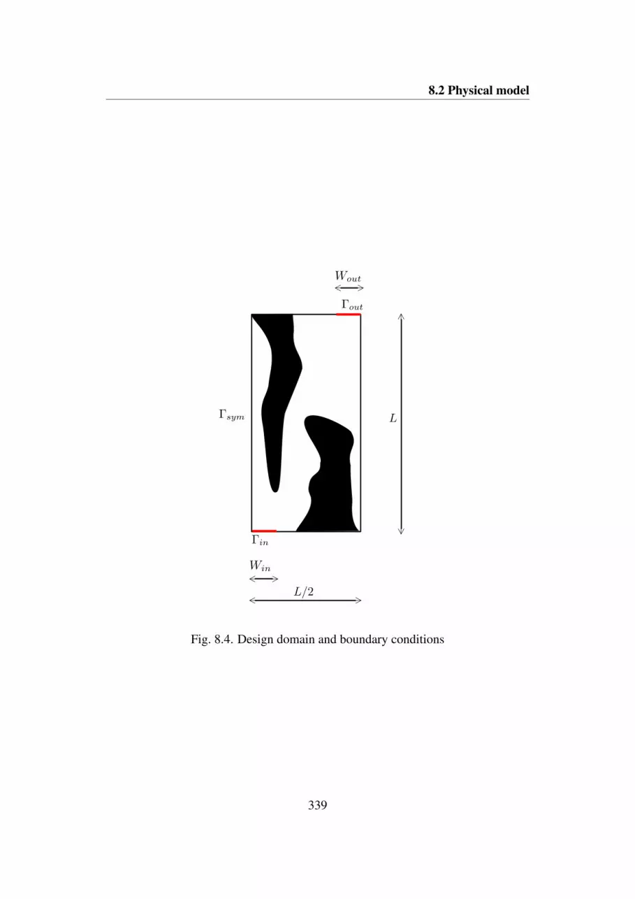
8.2 Physical model
Fig. 8.4. Design domain and boundary conditions
339

Design of flow fields in PEM fuel cells
Table 8.4. Relevant physical parameters and properties
Description Symbol Value Unit
number of chemical species ns 3 −number of participating electrons ne 4 −molar mass H2O MH2O 18 g/molmolar mass N2 MN2 28 g/molmolar mass O2 MO2 32 g/molstoichiometric coefficient H2O νH2O 2 −stoichiometric coefficient N2 νN2 0 −stoichiometric coefficient O2 νO2 −1 −universal gas constant Rg 8.3144 J/mol KFaraday constant F 96485.3 C/mol
where n is the outward-pointing normal. The chemical composition of the mixture atthe inlet section is known such that:
ωk = ωkin on Γin, (8.13)
where ωkin is the prescribed mass fraction at the inlet. A no-slip condition is pre-scribed on the sealing gasket wall. Due to symmetry, only non-penetration isprescribed along the symmetry axis such that:
vi = 0 on Γsg, (8.14)
vini = 0 on Γsym, (8.15)
where Γsg = Γtot/(Γsym∪Γin∪Γout) with Γtot representing all the boundaries ofthe design domain. For our design optimization studies, a normal stress conditionaugmented with a nil tangential velocity condition is prescribed at the inlet as follows:
niσi jn j = Fin on Γin, (8.16)
viti = 0 on Γin, (8.17)
where ti is a unit vector tangent to the boundary. Note that Eq. (8.16) well approxi-mates an inlet pressure condition for low-viscosity fluids. For our calibration andverification studies, we consider also an alternative inlet condition with fixed flow
340

8.2 Physical model
rate:vini =
Vin
HtotWchon Γin, (8.18)
where Vin is the inlet volumetric flow rate. The condition (8.18) is augmented withthe nil tangential velocity constraint (8.17). Vanishing normal and tangential stressesare prescribed at the outlet such that:
σi jn j = 0 on Γout . (8.19)
8.2.3 Finite element model
Equations (8.3), (8.4) and (8.6) are discretized in space using a mixed finite elementmodel. Following the procedure described in Sections 3.3.2 and 5.2.1, the weakform of the governing equations is obtained by multiplying the residual of the strongform with a set of admissible test functions and integrating over the domain. Theapproximation and weighting functions for pressure and velocities were definedin (5.31) and (5.32). The approximation and weighting functions for transport ofchemical species, ωk, are defined in a similar way to what we have done for energytransport in (3.36) and (3.37):
Uω = ωhk ∈H 1(Ω); ω
hk = ω
hkin
on Γin, (8.20)
V = wh ∈H 1(Ω); wh = 0 on Γin, (8.21)
where ωhk represents the approximate mass fraction field, and wh is the weighting
function of the advection-diffusion-reaction equation (8.6). The function spaces Uω
and V are Hilbert spaces consisting of scalar functions with square integrable firstderivatives. We write all the unknown fields as a product of spatially varying shapefunctions and nodal values. For pressure and velocities we use (5.33) and (5.34) andneglect time-dependence. For the mass fractions, we write:
ωhk (x) =
Nn
∑i=1
ωkiNi(x) = NTωωωk, (8.22)
where ωωωk is the column vector of nodal mass fraction values of the chemical species"k". The weight functions are chosen equal to the shape functions as in the Galerkinmethod. With these assumptions, we recover the unstabilized Galerkin model of
341

Design of flow fields in PEM fuel cells
the Navier-Stokes equations presented in (5.35) and (5.36) with M j = 0 and wherethe definition of Am, Di j and Fi is modified as follows to account for flow in porousmedia:
Am =∫Ω
ρ
ε2p
ξξξh(ξξξ
hTv j)
∂ξξξhT
∂x jdx, (8.23)
Di j =
∫Ω
µ
εp
(2∂ξξξ
h
∂xi
∂ξξξhT
∂xi+ ∂ξξξ
h
∂xl
∂ξξξhT
∂xl
)dx for j = i, l = i
∫Ω
µ
εp
(∂ξξξ
h
∂xi
∂ξξξhT
∂x j
)dx for j = i
, (8.24)
Fi =∫Ω
ξξξh(Fpoisi +Fbi)dx+
∫ΓN
ξξξh fidx′. (8.25)
Considering nil boundary diffusion fluxes as motivated in the previous section, theresidual vector of the unstabilized Galerkin model of the advection-diffusion-reactionequation (8.6) is written as following:
Rωus = Aωωωωk +Kklωωω l−Rk = 0, (8.26)
where:Aω =
∫Ω
HtotρN(ξξξhT
v j)∂N∂x j
dx, (8.27)
Kkl =
∫Ω
Htotρ fDDmk
(1+ 1
Mn∂Mn
∂ωl
)∂N∂xi
∂NT
∂xidx for l = k∫
Ω
Htotρ fDDmk
1Mn
∂Mn
∂ωl
∂N∂xi
∂NT
∂xidx for l = k
, (8.28)
Rk =∫Ω
NRk dx. (8.29)
We use four-node quadrilateral finite elements to discretize the computationaldomain. The velocity, pressure and mass fractions are approximated by bilinear equal-order interpolations. As discussed in Section 5.2.2, using equal-order approximationfunctions for the velocity and pressure does not satisfy the Babuska-Brezzi conditionand leads to spurious oscillations in the pressure field [213]. Furthermore, high Pecletnumbers and sharp crosswind gradients may result in overshoots and undershoots inthe concentration field, leading to an non-physical response [419]. To prevent thesenumerical instabilities, the residuals of the weak form of the governing equations
342

8.3 Design optimization problem
are augmented with consistent stabilization terms corresponding to Galerkin LeastSquares (GLS) [203] and Cross-Wind Diffusion (CWD) [92]. Since in this chapterwe adopt a commercial code [101] for the analyses, we will not discuss furtherdetails about the stabilization approaches. The nonlinear system of equations aresolved with a damped Newton’s method with damping coefficient set to 0.7. Thediscretized nonlinear problem is considered converged if the absolute residual normdrops below 10−7. The linear systems of equations arising at each Newton’s iterationare solved with the MUltifrontal Massively Parallel sparse direct Solver (MUMPS)[26].
8.3 Design optimization problem
In this section, we introduce the optimization problem formulation adopted for thedesign of the PEMFC flow fields. First, we define and discuss the objective andconstraints. Then, we present our strategy to interpolate the material propertiesbetween the values obtained through our depth-averaging procedure (8.2). Last, wegive details related to the numerical solution.
8.3.1 Objectives and constraints
We aim at distributing the reactant over the active sites in such a way that the mosthomogeneous current density field is created and the highest power generation isobtained at limited pressure drop. As discussed in Section 8.1, a non-uniform currentdensity distribution is responsible for thermal stresses of the membrane, leading toboth performance and material degradation [289, 32]. We consider two optimizationcriteria: the standard deviation, θiloc , of the current density distribution and the poweroutput of the cell. We formulate the multi-objective optimization problem using apenalty method as follows:
minimizes
wθ
θ 0iloc
θiloc−wW
W 0
∫ΩD
Vcelliloc dx
subject to∫
ΩD
ρs dx≤V ∗
s ∈ S =RNs | smin ≤ si ≤ smax, i = 1, ...,Ns
, (8.30)
343
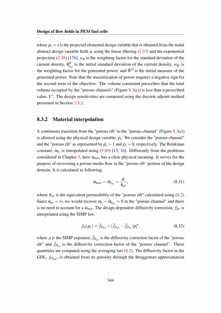
Design of flow fields in PEM fuel cells
where ρs = s is the projected elemental design variable that is obtained from the nodalabstract design variable field, s, using the linear filtering (2.37) and the exponentialprojection (2.38) [176], wθ is the weighting factor for the standard deviation of thecurrent density, θ 0
ilocis the initial standard deviation of the current density, wW is
the weighting factor for the generated power, and W 0 is the initial measure of thegenerated power. Note that the maximization of power requires a negative sign forthe second term of the objective. The volume constraint prescribes that the totalvolume occupied by the "porous channels" (Figure 8.3(c)) is less than a prescribedvalue, V ∗. The design sensitivities are computed using the discrete adjoint methodpresented in Section 2.3.2.
8.3.2 Material interpolation
A continuous transition from the "porous rib" to the "porous channel" (Figure 8.3(c))is allowed using the physical design variable, ρs. We consider the "porous channel"and the "porous rib" as represented by ρs = 1 and ρs = 0, respectively. The Brinkmanconstant, αb, is interpolated using (5.80) [13, 16]. Differently from the problemsconsidered in Chapter 5, here αmax has a clear physical meaning. It serves for thepurpose of recovering a porous media flow in the "porous rib" portion of the designdomain. It is calculated as following:
αmax = αbpr =µ
κpr, (8.31)
where κpr is the equivalent permeability of the "porous rib" calculated using (8.2).Since κpc = ∞, we would recover αb = αbpc = 0 in the "porous channel" and thereis no need to account for a αmin. The design-dependent diffusivity correction, fD, isinterpolated using the SIMP law:
fD(ρs) = fDpr +( fDpc− fDpr)ρps , (8.32)
where p is the SIMP exponent, fDpr is the diffusivity correction factor of the "porousrib" and fDpc is the diffusivity correction factor of the "porous channel". Thesequantities are computed using the averaging law (8.2). The diffusivity factor in theGDL, fDgdl , is obtained from its porosity through the Bruggeman approximation
344

8.3 Design optimization problem
[81]:fDgdl = ε
3/2pgdl . (8.33)
The porosity is interpolated linearly as follows:
εp(ρs) = εppr +(εppc− εppr)ρs, (8.34)
where εppr and εppc are the equivalent porosities of the "porous rib" and of the"porous channel" calculated using (8.2).
8.3.3 Numerical implementation
The optimization problems presented in this chapter are solved using GCMMA. Ascompared to Table 2.1, we modify the relative step-size to ∆s = 0.01. To discourageoscillatory behaviors for a large curvature of the regularization, β , the positionof the initial asymptotes is modified using the formulation proposed by [178]. Acontinuation on the convexity factors, qα and p, is used to ensure a smooth evolutionof the design and a stable convergence to satisfactory solutions. These parametersare modified during the optimization convergence as follows:
p = 1; 2; 3; 5,qα = 104;103;102;101.
(8.35)
The projection steepness parameter is kept constant at β = 50. The transition to thenext continuation step is performed every 60 iterations. The optimization procedureends when all the continuation steps are completed. The convergence of the optimiza-tion process is verified after the final step. The optimization problem investigated inthis chapter has similarities with the forced convection design example described inSection 5.4.2. The continuation trajectories should be chosen carefully to avoid astrong imbalance between convective and diffusive transport at all continuation steps.For inlet pressures higher than Fin > 4 Pa, we observed that strategy (8.35) leads tooscillations in the objective history; for Fin > 20 Pa we also obtained unsatisfactorylocal minima. Skipping the first continuation step fixed the issue, yielding both astable convergence and solutions with superior performance. For this reason, for alldesign studies with Fin > 4 Pa, only the last three continuation steps are considered.
345

Design of flow fields in PEM fuel cells
Table 8.5. Material properties and model parameters adopted from [197]
Description Symbol Value Unit
membrane length L 2.236×10⁻² mchannel width Wch 1.8×10⁻³ mchannel depth Hch 1.8×10⁻³ mGDL depth Hgdl 0.2×10⁻³ mopen-circuit voltage VOC 1.22 Vohmic resistance Ro 7×10⁻⁵ Ω ·m2
cell temperature T 343.15 Koxygen reference concentration CO2ref
30 mol/m3
inlet flow rate Vin 2×10⁻⁶ m3/scathodic transfer coefficient αc 0.5 −porosity of the GDL εGDL 0.8 −inlet water mass fraction ωH2O 0.1 −inlet oxygen mass fraction ωO2 0.9 −dynamic viscosity µ 2.07×10⁻⁵ Pa · soxygen diffusivity in water DO2,H2O 5.88×10⁻⁵ m2/s
8.4 Numerical results and design trends
In this section, we present and discuss the numerical results and design trends ob-tained. First, we calibrate a 3D physical model to a real system and verify theaccuracy of our depth-averaging procedure by comparing 2D and 3D predictions.Then, we consider a reference design case with Fin = 5 Pa and compare its perfor-mance with conventional flow field layouts. Last, we investigate the effect of theinlet pressure and current standard deviation weight on the optimized designs andperformance.
8.4.1 Calibration and verification of the analysis model
For calibration and verification purposes, we consider the high temperature PEMFCsystem investigated by [197]. It consists of the serpentine flow field with seven chan-nels schematically shown in Figure 8.5. The relevant parameters and properties aresummarized in Table 8.5. The system is alimented by a mixture of oxygen and waterusing a fixed flow rate. Hence, we set ns = 2 and the velocity inlet boundary condi-tion according to (8.18). Also, it is not possible to exploit symmetry in this numerical
346

8.4 Numerical results and design trends
GDL
Channels
(a)
GDL
Channels
(b)
(c)
Fig. 8.5. Schematic representation of the 3D numerical study conducted for calibra-tion and verification purposes. (a): 3D view; (b): top view; (c): side view
347

Design of flow fields in PEM fuel cells
Table 8.6. Mesh convergence verification. The deviation is calculated with respect toa reference case with ∆h = 1.8 mm
Mesh size ∆h [mm] 2D deviation [%] 3D deviation [%]
7.2 5.68 4.504.5 1.97 0.742.7 0.64 0.27
example, i.e. Γsym = /0. We developed both a full 3D model and a reduced 2D modelwith properties computed through the averaging procedure described in Section 8.2.1.The 3D and 2D computational domains are meshed using free tetrahedral and freequadrilateral elements with characteristic size ∆h = 2.7 mm. This value is selectedafter a convergence study on the outlet oxygen flow rate obtained with Vcell = 0.4V by comparing the predictions against those computed on a reference mesh with∆h = 1.8 mm. The results are summarized in Table 8.6. For the 3D numerical study,the mesh characteristic size in the GDL is computed as ∆hgdl = max
(∆h/25, Hgdl
).
In [197], the electrochemistry at the anode was modeled using the Butler-Volmerequation and at cathode using a simplified Tafel equation [319]. To calibrate themodel, the authors fitted the exchange current density to their experimental results.As our framework does not consider electrochemistry at the anode, we re-calibratethe exchange current density to their numerical results using a least-square fitting.For this process, we neglect the effect of the reactants concentration in (8.10). Thecomputed value is i0 = 0.17 A/m2. The polarization curves obtained using a full3D and our reduced 2D analysis frameworks are compared to the numerical andexperimental results of [197] in Figure 8.6. This trend is obtained by sweeping theoperating voltage of the cell, Vcell , in 10 steps from 0.2 V to 0.9 V and computingthe average current density over the active area. Our 3D framework yields a meanrelative deviation from the experimental and numerical results of 11.53 % and 3.03%, respectively. Most of the error is computed for Vcell ≥ 0.7 V, which is far from thepractical operating conditions of the cell targeting a peak power generation (Vcell ∼0.4 V). For 0.3 V ≤Vcell ≤ 0.5 V , we observe a satisfactory match between our 3Dmodel and the numerical and experimental results of [197]. This indicates that ourcalibrated model is able to predict the electrochemical response of a real cell withsufficient accuracy in practical operating conditions. The polarization curve obtainedusing the 2D model closely approximates the one obtained in 3D. Although at lowoperating voltages we observe a slight overestimation of the generated current, we
348

8.4 Numerical results and design trends
Fig. 8.6. Polarization curves obtained with the 2D and 3D models versus theexperimental and numerical results of [197]
report a mean relative deviation of 0.65 %. This suggests that the oxygen distributionfields computed through the 2D and the 3D frameworks are comparable.
The most relevant state variable fields obtained using the 2D and 3D frameworksare qualitatively compared in Figure 8.7, for Vcell = 0.4 V. In 3D, we show theresponse distribution over two planes. In the portion of the domain occupied bythe ribs, we consider plane π3 (Figure 8.1) located at half-depth of the GDL. In theportion of the domain occupied by the channels, we consider plane π1 located athalf-depth of the BPP (Figure 8.1). The oxygen mass fraction field (Figure 8.7(a))computed with the two frameworks is qualitatively similar. The oxygen concentratesmainly along the channels. Local minima are observed in correspondence of theribs since the limited convection and diffusion leads to a higher reactant depletion.The 3D model predicts a minimum oxygen fraction on π3 of 0.72 in a GDL regionclose to the outlet. Due to our depth-averaging procedure, this value is overestimatedin the 2D model, leading to a higher current density generation. This mild trend isobservable also in the polarization curve presented in Figure 8.6. The velocity fieldsare compared in Figure 8.7(b). The predictions of our 2D framework qualitativelymatch those of the 3D model. The ratio between maximum velocities in 2D and3D is 67.9 %, approximating the theoretical ratio of average-to-maximum velocityin plane Poiseuille flow of 66.6 %. Note that the 3D framework predicts velocity
349

Design of flow fields in PEM fuel cells
2D 2D (colorbar rescaled) 3D
(a)
(b)
(c)
Fig. 8.7. Comparison of 2D and 3D responses. (a): Oxygen mass fraction field; (b):velocity field; (c): pressure field
350

8.4 Numerical results and design trends
reductions after U-bends that are not captured in 2D. Similar trends in 2D and 3D areobserved also for the pressure field shown in Figure 8.7(c). The pressure diminishesgradually along the path from the inlet to the outlet. However, our 2D frameworkunderestimates the pressure drop by 16.5 %. To assess how this difference can affectour fluid-dynamic predictions, we compute the characteristic curve of the cell bysweeping the inlet flow rate Vin from 10 % to 150 % of the reference case. The resultsare shown in Figure 8.8. The 3D model returns a super-linear pressure drop to flowrate relation. This trend is not reproducible in 2D under plane Poiseuille assumptions.We obtain a nearly linear relation using our 2D model. As the flow is laminar inthe range of values considered (8.7 ≤ Re ≤ 130.5), we conjecture that the super-linear drag is connected to geometry features that invalidate the fully-developed flowassumption, such as U-bends. Recall that we observed sudden velocity reductionsin Figure 8.7(c). To confirm this speculation, we compute the pressure drop over asingle channel (the one connected to the inlet) and multiply the result by the numberof channels to allow for comparisons. The 3D single-channel pressure drops closelymatch the 2D predictions. A high-fidelity 2D modeling of the 3D dynamics inserpentine flow fields would require the introduction of a quadratic Forchheimerdrag term in correspondence of U-bends, e.g. in the regions highlighted in Figure8.8(c). There, the momentum equation (8.4) can be augmented with the followingsink [310]:
Ff ci =−ρα f c|vi|vi, (8.36)
where α f c is a multiplicative constant that can be calibrated by trial and error.Figure 8.8(b) shows that the 2D predictions approximate better the 3D ones as α f ci isincreased. A value of α f c = 500 allows the super-linear drag effects to be reproducedwith a high degree of accuracy. However, this value is highly geometry-dependentand hardly fits within an inverse design framework. For this reason, we neglectsuper-linear drag in our analysis model. We observe that a similar issue may arise inother 2D fluid topology optimization frameworks.
Figure 8.9 presents a comparison between the results obtained using a mixture-averaged and a full Maxwell-Stefan diffusion model. For this study, we adopt our2D framework and we consider the cathode as alimented by air such that multi-component diffusion effects arise. The inlet mass fraction of the chemical species areset as ωH2O = 0.023, ωO2 = 0.228 and ωN2 = 0.749 in agreement with [363]. Thepolarization curves (Figure 8.9(a)) match well. The mixture-averaged frameworkgives a mean relative deviation of 0.02 %. This indicates that the oxygen distribution
351

Design of flow fields in PEM fuel cells
0 50 100 150
Normalized flow rate [%]
0
5
10
15
20
25
30
35
Pre
ssu
re d
rop
[P
a]
2D
3D
3D single channel
(a)
0 50 100 150
Normalized flow rate [%]
0
5
10
15
20
25
30
35
Pre
ssu
re d
rop
[P
a]
2D: fc
= 0
2D: fc
= 100
2D: fc
= 300
2D: fc
= 500
3D
(b)
Quadratic drag regions
Channels
(c)
Fig. 8.8. Comparison of pressure drop using the 2D and 3D models. (a): reduction of3D effects by the analysis of a single channel in 3D; (b): introduction of a quadraticForchheimer drag term in 2D to account for 3D effects; (c): regions of the 2Dgeometry interested by quadratic drag
352

8.4 Numerical results and design trends
(a) (b)
Fig. 8.9. Comparison of responses using the mixture-averaged and Maxwell-Stefandiffusion models. (a): Polarization curve; (b): outlet oxygen mass flow rate
is slightly affected by the choice of the diffusion model. Kee et al. [236] observedthat the mixture-averaged route may lead to species non-conservation. Figure 8.9(b)shows the outlet oxygen flow rate as a function of the current density generation forthe two diffusion models. The results suggest that mass non-conservation is not anissue when modeling the cathode of a PEM fuel cell through a mixture-averageddiffusion model. The mean relative deviation is below 0.01 %.
8.4.2 Reference design
In this section, we present the design optimization results obtained for a referencecase with Fin = 5 Pa and compare its performance with conventional flow fieldlayouts. Here, we aim at maximizing only the generated power. Hence, we setwθ = 0.00 and wW = 1.00 in Eq. (8.30). The design and computational domaincorresponds to the one shown in Figure 8.4 with Win = Wout = 1.20 mm and L =
22.36 mm as in the previous section. The maximum volume of "porous channel"material, V ∗, is set to 50 % of the total. The filtered elemental design variablefield, s, is computed from the nodal design variable field, s, using a filter radius ofr f = 0.35 mm. The material properties are the same adopted for the verificationstudy presented in Section 8.4.1. However, the channel and GDL depths are modified
353

Design of flow fields in PEM fuel cells
to produce all the topology optimization results. Since our analysis framework doesnot account for either flooding or dehydration, there is a chance that the optimizeddesigns will not perform as expected. As highlighted in Section 8.1, there is evidencethat adopting small channel depths simplifies water management regardless of theflow field layout [5, 445]. For this reason, we choose the configuration adopted in[363], where Hgdl = 0.38 mm and Hch = 1.00 mm. Note that water management isseldom an issue at higher temperatures [83]. Hence, the design results and trendspresented hereafter apply to high temperature PEMFCs with little risk of bias due toour physics reduction.
The objective history along with snapshots of the projected design variable fieldat selected iterations is shown in Figure 8.10. For all the designs presented inthis chapter, we will adopt the colorbar presented in Figure 8.10. The jumps inthe objective history correspond to the transitions between the continuation steps.The initial design (Figure 8.10(a)) corresponds to a homogeneous projected designvariable field at ρs = 0.5. Within the first continuation step, the "porous rib" materialis retrieved from the regions close to the inlet and outlets and aggregated in twocentral areas. Four wide "porous channels" start to appear at iteration 20 (Figure8.10(b)), which then evolve into Y-shaped connections at iteration 60 (Figure 8.10(c)).Some regions with intermediate ρs values are still present at the end of the firstcontinuation step due to the moderate penalization of both the diffusive and advectivetransport. At iteration 100, as shown in Figure 8.10(d), the design converges to abinary 0; 1 layout since a stronger penalization is applied on the intermediateρs values. From this point onward, limited objective and layout modificationsare observed. The final optimized design after 180 iterations is shown in Figure8.11(a). This geometry shows features pertaining to different design conceptspresented in Section 8.1. As in the parallel configuration, our optimized layoutpresents inlet and outlet headers that are connected by a number of alternative paths.The intricate groove of the flow channels somehow recalls the layout of the meshflow fields. Furthermore, the width tapering of the main vertical channels and theinclination angle of the diagonal connections make it similar to the bio-inspiredgeometry proposed by [361] and schematically shown in Figure 8.2(e). For thisdesign optimization case, the need for the last continuation step could be questioned.However, this last step is essential to ensure convergence to binary 0; 1 designs athigher Fin values, as considered in the next section.
354

8.4 Numerical results and design trends
(a) (b) (c) (d)
0 20 40 60 80 100 120 140 160 180
Optimization iteration [-]
1
1.05
1.1
1.15
1.2
1.25
1.3
1.35
Norm
aliz
ed o
bje
ctive [-]
Fig. 8.10. Objective history during the optimization process with design snapshotstaken at selected iterations. (a): initial guess; (b): iteration 20; (c): iteration 60; (d):iteration 100
355
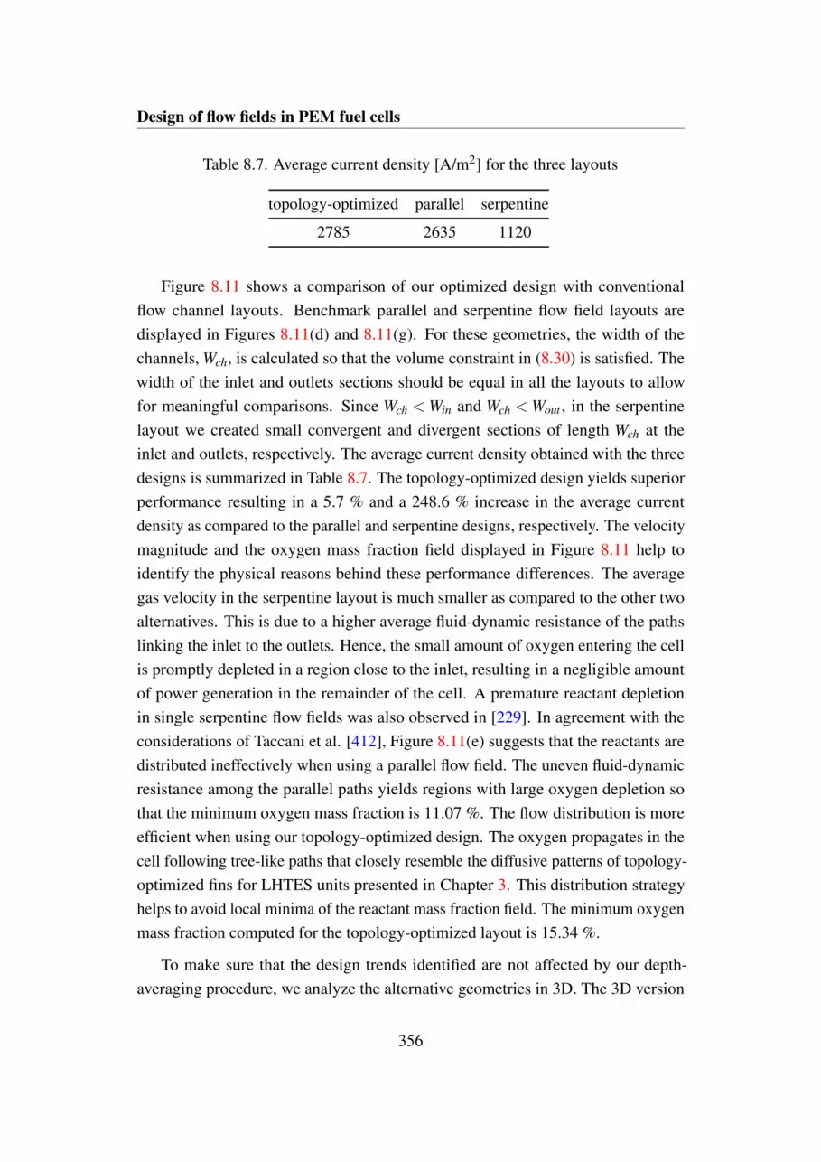
Design of flow fields in PEM fuel cells
Table 8.7. Average current density [A/m2] for the three layouts
topology-optimized parallel serpentine
2785 2635 1120
Figure 8.11 shows a comparison of our optimized design with conventionalflow channel layouts. Benchmark parallel and serpentine flow field layouts aredisplayed in Figures 8.11(d) and 8.11(g). For these geometries, the width of thechannels, Wch, is calculated so that the volume constraint in (8.30) is satisfied. Thewidth of the inlet and outlets sections should be equal in all the layouts to allowfor meaningful comparisons. Since Wch < Win and Wch < Wout , in the serpentinelayout we created small convergent and divergent sections of length Wch at theinlet and outlets, respectively. The average current density obtained with the threedesigns is summarized in Table 8.7. The topology-optimized design yields superiorperformance resulting in a 5.7 % and a 248.6 % increase in the average currentdensity as compared to the parallel and serpentine designs, respectively. The velocitymagnitude and the oxygen mass fraction field displayed in Figure 8.11 help toidentify the physical reasons behind these performance differences. The averagegas velocity in the serpentine layout is much smaller as compared to the other twoalternatives. This is due to a higher average fluid-dynamic resistance of the pathslinking the inlet to the outlets. Hence, the small amount of oxygen entering the cellis promptly depleted in a region close to the inlet, resulting in a negligible amountof power generation in the remainder of the cell. A premature reactant depletionin single serpentine flow fields was also observed in [229]. In agreement with theconsiderations of Taccani et al. [412], Figure 8.11(e) suggests that the reactants aredistributed ineffectively when using a parallel flow field. The uneven fluid-dynamicresistance among the parallel paths yields regions with large oxygen depletion sothat the minimum oxygen mass fraction is 11.07 %. The flow distribution is moreefficient when using our topology-optimized design. The oxygen propagates in thecell following tree-like paths that closely resemble the diffusive patterns of topology-optimized fins for LHTES units presented in Chapter 3. This distribution strategyhelps to avoid local minima of the reactant mass fraction field. The minimum oxygenmass fraction computed for the topology-optimized layout is 15.34 %.
To make sure that the design trends identified are not affected by our depth-averaging procedure, we analyze the alternative geometries in 3D. The 3D version
356

8.4 Numerical results and design trends
(a) (b) (c)
(d) (e) (f)
(g) (h) (i)
Fig. 8.11. Performance comparison with conventional flow field layouts for Fin = 5Pa. Topology-optimized design (a) with its velocity field (b) and oxygen massfraction (c). Parallel layout (d) with its velocity field (e) and oxygen mass fraction(f). Serpentine layout (g) with its velocity field (h) and oxygen mass fraction (i)
357

Design of flow fields in PEM fuel cells
(a)
(b)
(c)
Fig. 8.12. 3D versions of the topology-optimized (a), parallel (b) and serpentine (c)designs
Table 8.8. Performance of the the 3D versions of the three layouts
Design
Performance topology-optimized parallel serpentine
Average current density [A/m2] 2770 2661 10342D deviation [%] - 0.54 + 0.97 - 7.68
of the topology-optimized layout is obtained using channel walls described by theρs = 0.5 iso-countour. Views of the computed geometry and the 3D versions of theparallel and serpentine layouts are shown in Figure 8.12. The three geometries areanalyzed using high-resolution body-fitted meshes with 444113, 431012, 468174tetrahedral elements, respectively. The average current densities computed in 3D aresummarized in Table 8.8. The results show a satisfactory match between the 2D and3D predictions for the topology-optimized and parallel design. A larger discrepancyis computed for the serpentine layout due to the presence of quadratic drag effects incorrespondence of U-bends that are not captured in 2D (see Section 8.4.1).
The results obtained in the presented numerical example showed that topologyoptimization allows optimized flow paths in PEMFC to be obtained without the needfor a close-to-optimal design to start with. The layout computed for a referencepressure drop of Fin = 5 Pa is superior in terms of power generation to conventionalalternatives like the serpentine and parallel configurations. Furthermore, the 3Dresults confirmed the design trends identified in 2D, suggesting that the depth-averaging procedure described in Section 8.2.1 is a reliable approach for topologyoptimization of electrochemical devices.
358

8.4 Numerical results and design trends
5 10 15 20 25 30 35 40
Pressure drop [Pa]
0
500
1000
1500
2000
2500
3000A
vera
ge c
urr
ent density [A
/m2]
Pareto TopOpt
Parallel
Serpentine
Fig. 8.13. Pareto front current density versus pressure drop
8.4.3 The trade-off between pressure drop and power genera-tion
In this section, we analyze how the optimized designs and power output are affectedby the choice of the inlet pressure, Fin. The model parameters and physical propertiesare unchanged with respect to the reference design.
We consider 14 different values of the inlet pressure in the range 0.1 Pa ≤Fin ≤ 40 Pa. Only minor design and performance differences are observed forFin > 40 Pa. For each case, a topology optimization run is performed. To benchmarkthe effectiveness of our topology optimization framework, the serpentine and parallelgeometries are analyzed in the same conditions. The computed average currentdensity is shown in Figure 8.13. In the range of values considered, a reduction inpressure drop can be obtained only at the expense of less power generation. Hence,these two performance criteria are antagonist and the curve of the optimized valuesin Figure 8.13 is an approximation of the multi-objective Pareto front. The layoutsobtained with our optimization framework are always superior to the conventionalalternatives. Improvements are large at low inlet pressures. The average currentdensity of the topology-optimized layout at Fin = 1 Pa is 83.21 % and 574.8 % higherthan the one obtained using the parallel and the serpentine flow fields, respectively.This gap reduces for higher Fin so that the performance enhancement of the topology-
359

Design of flow fields in PEM fuel cells
optimized layout is only 0.89 % and 4.55 % at Fin = 40 Pa. This suggests thatthe topology of the flow distributor slightly affects the performance at high inletpressures. The optimized layouts obtained at selected Pareto points are displayed inFigure 8.14. When a higher inlet pressure is available, the geometry evolves morefreely resulting in unintuitive layouts. The number of connections increases and thewidth of the channels decreases creating more and more complicated geometries. Thedesign optimized for Fin = 40 Pa shows similarities with the mesh design concept(Figure 8.2)(d). To quantify the design modifications along the Pareto front, we studythe evolution of two performance metrics. The first one is the number of internalholes, Nh, in the layout (filled by "porous rib" material) representing the complexityof the flow channel topology. The values obtained for the different inlet pressuresare presented in the bar chart of Figure 8.15(a). The number of internal holes, Nh,increases fast at low inlet pressures and levels-off at Fin = 25 Pa. From this pointonward, no topology modifications are observed. The second performance metric isa perimeter measure, Γp, based on the total variation of the projected design variablefield [395]:
Γp =∫
Ω
||∇ρs||2 dx, (8.37)
where || · ||2 indicates the L2 norm. The influence of the inlet pressure on the perimetermeasure of the optimized designs is shown in Figure 8.15(b). The perimeter lengthincreases monotonically in the range of values considered. At low inlet pressures,i.e. Fin≪ 25 Pa corresponding to the region of topological changes, a fast growth ofthe perimeter measure is observed. For higher inlet pressure values, i.e. Fin > 25 Pa,Γp is increased moderately as the perimeter modifications are obtained exclusivelythrough a higher arc-to-chord ratio of the connections, resulting in a higher tortuosityof the channels.
To investigate how the optimized layouts perform when operated far fromtheir reference pressure drop conditions, we consider the designs optimized forFin = 0.1; 2.0; 5.0; 10.0; 40.0 Pa. For each geometry, we run five analyses corre-sponding to different pressure drops, i.e. Fin = 0.1; 2.0; 5.0; 10.0; 40.0 Pa. Thiscross-check also helps to exclude the possibility of convergence to unsatisfactorylocal minima. The outcome of this investigation is summarized in Figure 8.16. Theresults show that each layout performs better than the alternatives in the condition inwhich it is optimized for. Furthermore, it shows that the geometries optimized forFin = 2.0 Pa and Fin = 5.0 Pa are slightly sensitive to changes in the operating inlet
360

8.4 Numerical results and design trends
0.1 Pa 1.0 Pa 2.0 Pa
5.0 Pa 7.5 Pa 10 Pa
15 Pa 20 Pa 40 Pa
Fig. 8.14. Optimized designs obtained for different values of the imposed pressuredrop, Fin
361

Design of flow fields in PEM fuel cells
0.1
0.5 1
2
4
5
6
7.5
10
15
20
25
30
40
Pressure drop [Pa]
0
5
10
15
20
25
30
35
40
Nu
mb
er
of
ho
les [
-]
(a)
0 10 20 30 40
Pressure drop [Pa]
0.05
0.1
0.15
0.2
0.25
0.3
0.35
0.4
0.45
0.5
Pe
rim
ete
r m
ea
su
re [
m]
(b)
Fig. 8.15. (a): Effect of the inlet pressure on the number of internal holes of theoptimized layouts; (b): effect of the inlet pressure on the perimeter measure, Γp, ofthe optimized layouts
0.1 2.0 5.0 10.0 40.0
Pressure drop [Pa]
70
75
80
85
90
95
100
Av. curr
ent w
ith r
espect to
best [%
]
Optimized for 0.1 Pa
Optimized for 2.0 Pa
Optimized for 5.0 Pa
Optimized for 10.0 Pa
Optimized for 40.0 Pa
Fig. 8.16. Performance of the optimized layouts when operated far from theirreference pressure drop conditions
362

8.4 Numerical results and design trends
pressure. The average current density drop in the cases analyzed is only 3.15 % and3.34 %, respectively. On the other hand, the geometries optimized for Fin = 0.1 Paand Fin = 5.0 Pa yield large performance reductions when operated far from theirreference pressure drop condition.
This design study showed that the inlet pressure modifies consistently both theoptimized designs and performance. At low inlet pressures, the topology complexityand power generation of the optimized designs increase fast. In this case, topologyoptimization yields layouts responsible of large improvements as compared to con-ventional flow fields. At high inlet pressures, the performance is slightly affected bythe layout of the gas distributors. The geometry changes are only due to tortuositymodifications of the channels, yielding minor power generation enhancements.
8.4.4 Increasing the homogeneity of the current density distribu-tion
In this section, we study the design trends obtained using the full penalty method,i.e. wθ = 0.00 and wW = 0.00. The optimization problem (8.30) is solved for fivevalues of the current standard deviation weight in the range 0.25≤wθ ≤ 7.50. Minordesign and performance differences are observed for wθ > 7.50. We consider thereference inlet pressure case, i.e. Fin = 5 Pa and a fixed value of the power generationweight wW = 1.00. The model parameters and material properties are unchangedwith respect to the reference design. The optimized designs are shown in Figure8.17 along with the reference design case obtained by setting wθ = 0.00. The resultsshow that there is a significant influence of the weighting factor wθ on the optimizedlayouts. As wθ is increased, the geometries feature a higher concentration of "porousrib" material close to the inlets while the "porous channels" migrate towards theexternal edges and outlets. The vertical channel at the center of the cell get thinnerwhile two diagonal long and wide channels are created for wθ ≥ 5.00, linking theinlet to the outlets. This suggests that more reactants are able to reach the regionsclose to the outlets through convective transport. To demonstrate these design trends,we consider the following performance metric:
V =
∫Ω2
ρs dx∫Ω1
ρs dx, (8.38)
363

Design of flow fields in PEM fuel cells
wθ = 0.00 wθ = 0.25 wθ = 0.50
wθ = 2.00 wθ = 5.00 wθ = 7.50
Fig. 8.17. Optimized designs obtained for different values of the current standarddeviation weight, wθ , with Fin = 5 Pa and wW = 1.00
364

8.4 Numerical results and design trends
(a)
0 2 4 6
Deviation weight [-]
100
105
110
115
120
125
130
135
Vo
lum
e r
atio
[%
]
(b)
Fig. 8.18. (a): Domain splitting in close-to-inlet region (Ω1) and close-to-outletsregion (Ω2); (b): effect of wθ on volume ratio V
where Ω1 and Ω2 are the portions of the design domain shown in Figure 8.18(a). Theparameter V quantifies the "density" of channels in the regions close to the outletsas compared to its value in the region connected to the inlet. We will refer to V asvolume ratio hereafter. The influence of wθ on the volume ratio of the optimizedlayouts is shown in Figure 8.18(b). In the range of values considered, V increasesmonotonically. When the power is the unique optimization criteria (wθ = 0.00),the flow field complexity in Ω2 is comparable to that of Ω1 such that V = 103.5 %.Obtaining a more homogeneous current density distribution requires more channelsto be located close to the outlets. Setting wθ = 7.50 yields a layout in which thetotal volume of the channels in Ω2 is 31.5 % higher than the one measured in Ω1.Figure 8.19(a) shows that these design modifications are effective in lowering ourcriterion of current density dispersion: θiCL is decreased from 86.87 A/m2 to 79.78A/m2, corresponding to a 8.16 % reduction. The amount of power generated by theoptimized layouts reveals to be slightly sensitive to the choice of wθ (Figure 8.19(b)).We obtain a reduction of only 0.28 % when raising wθ from 0.00 to 7.50, suggestingthat the power generation is marginally affected by the design features promotinghomogeneity. This indicates that the inclusion of current density dispersion measuresin flow field design optimization frameworks has the potential to indicate promisingroutes for practical technological development.
365

Design of flow fields in PEM fuel cells
(a) (b)
Fig. 8.19. (a): Effect of wθ on the standard deviation of current density; (b): effectof wθ on the average current density
8.5 Conclusions
This chapter demonstrated the use of density-based topology optimization for thepractical design of flow fields in PEMFCs. The objective function was formulated tomaximize both the power output and homogeneity of the current density distribution,permitting reduced costs and higher durability. The gas dynamics, transport of chem-ical species, and electrochemical interactions in the cathodic portion of the PEMFCwere computed using a 2D finite element model. The 3D transport effects wereaccounted for in the 2D model through an original depth-averaging procedure, whichwas verified against the predictions of a full 3D model calibrated using experimentaland numerical results available in literature. Our analysis model framework didnot account for liquid water transport. For this reason, the optimization results areconsidered realistic mostly for high temperature systems, in which flooding is seldoman issue [83].
A graphical summary of the main application-oriented advances is presentedin Figure 8.20. Topology optimization yielded layouts with unintuitive and non-trivial features. Our reference flow field obtained considering an inlet pressureof 5 Pa has similarities with various design concepts such as parallel, mesh andbio-inspired geometries. Its performance was found to be superior to the one of
366
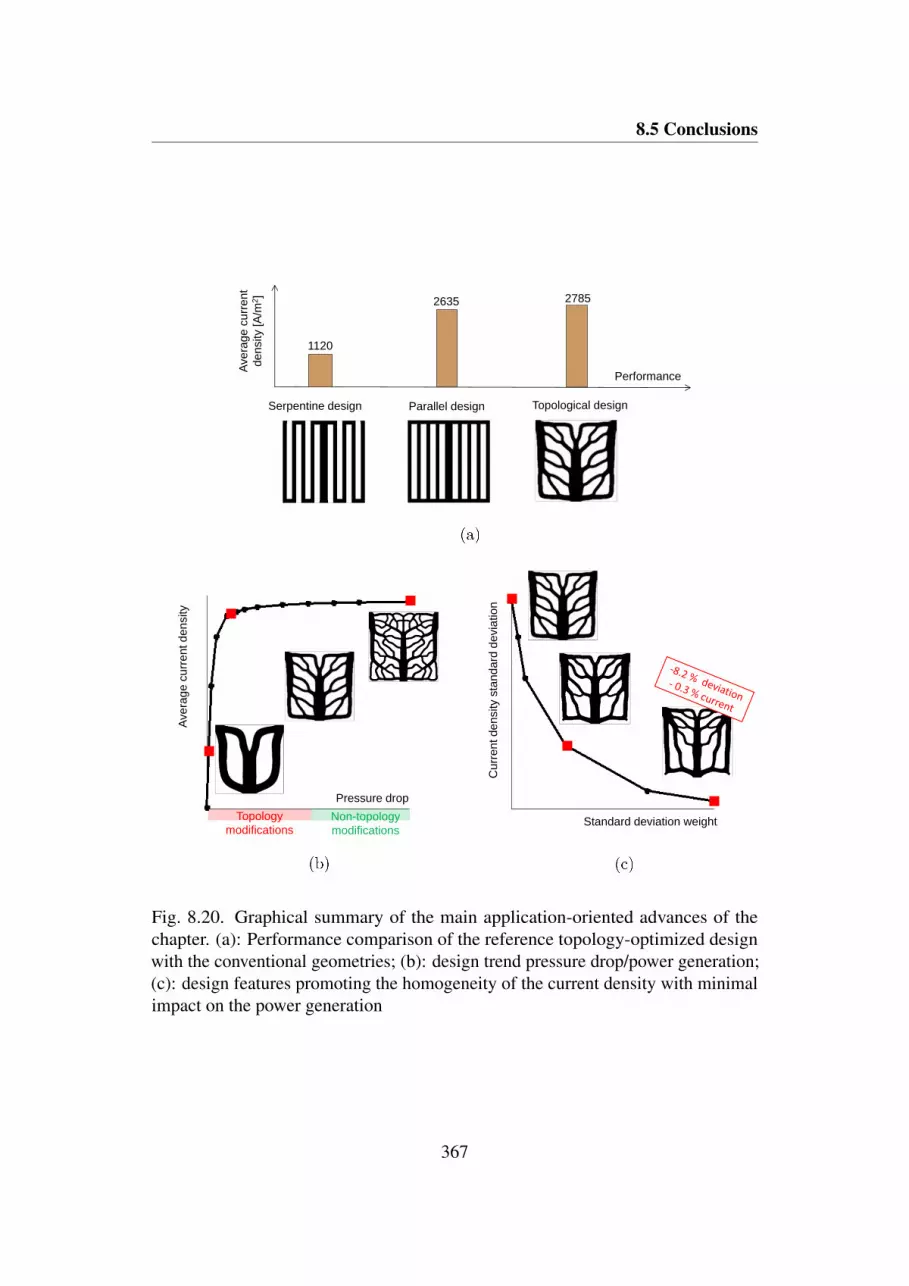
8.5 Conclusions
Avera
ge
cu
rrent
density
[A/m
2]
2635
1120
Serpentine design Parallel design Topological design
Performance
2785
Avera
ge
cu
rrentdensity
Pressure drop
Topology
modificationsNon-topology
modifications
Cu
rrentdensity
sta
nd
ard
devia
tion
Standard deviation weight
Fig. 8.20. Graphical summary of the main application-oriented advances of thechapter. (a): Performance comparison of the reference topology-optimized designwith the conventional geometries; (b): design trend pressure drop/power generation;(c): design features promoting the homogeneity of the current density with minimalimpact on the power generation
367

Design of flow fields in PEM fuel cells
both parallel and serpentine flow fields, yielding a 5.7 % and a 248.6 % increase inthe average current density (Figure 8.20(a)). The smaller fluid-dynamic resistanceof our layout allows a much higher air flow rate as compared to the serpentinegeometry. Furthermore, its effective reactants distribution avoids the creation ofregions with a large oxygen depletion, which arise in the parallel geometry dueto the uneven fluid-dynamic resistance of the flow paths. The trade-off betweenpressure drop and power generation was then explored to study the influence of theinlet pressure on both the optimized designs and performance (Figure 8.20(b)). Theresults showed that, at low inlet pressures, substantial power output improvementsare achievable through topological modifications of the flow distributor. In this case,the optimization process yielded large enhancements with respect to the conventionalflow fields. At higher inlet pressures, no topology modifications were observedand only moderate enhancements could be obtained through the increase of thetortuosity of the channels. In this case, the performance was found to be slightlysensitive to the flow field layout and the topology-optimized designs performedsimilarly to the serpentine and parallel flow fields. Adding a measure of the currentdensity dispersion to the optimization objective led to design features capable ofdecreasing the current density standard deviation by 8.16 % with negligible impacton the amount of power generated (Figure 8.20(c)). This finding suggests a viableroute for the future development of these systems with the aim of increasing thedurability.
368

Chapter 9
Conclusions
In this chapter, we summarize the work presented in this thesis, highlighting the mainresearch contributions. Finally, we give recommendations and identify directions forfuture developments.
9.1 Contributions
This dissertation developed a systematic framework for the optimal design of energysystems via topology optimization, yielding both method-related and application-oriented advances. The method-related advances stem from the modification oftopology optimization approaches to allow practical improvements to LHTES, DHNsand PEMFCs. The application-oriented advances comprise the identification ofgeometries that greatly outperform the current industrial solutions and of designtrends and guidelines that could be of interest to design engineers. The researchobjectives of this thesis were formulated according to the four fundamental researchquestions discussed in Chapter 1. Here, we present how it is possible to addressthem through the main contributions of our work.
Q1 How and how much can we improve the performance of LHTES units throughthe design of high conducting structures?
We first developed a density-based topology optimization framework for the optimaldesign of fins in shell-and-tube systems. We formulated the design optimization
369

Conclusions
problem in order to respond to three design criteria of practical interest. The unitdynamics was predicted using a simplified phase change model based on transientnonlinear diffusion. Then, we proposed a multi-scale multi-material design frame-work based on geometric primitive level-sets to obtain assemblies of periodic cellularmaterials that can be manufactured using conventional machining techniques, permit-ting reduced costs and mass production. To achieve this goal, the analysis and designcapabilities were extended using forward and inverse computational homogenization.The topology optimization results demonstrated that the optimized layouts stronglydepend on the desired level of discharge of the unit and that there is room for ma-nipulation of the energy history towards a steadier power output. Hence, powerfuldesign approaches are crucial in order to reduce costs and increase the efficiency ofthis technology. Considering a reduced dimensionality led to suboptimal configu-rations. The geometries optimized in three dimensions presented unique featuresthat were not apparent in 2D, yielding an average performance improvement of 20 %with respect to the 2D layouts. The multi-scale optimization results indicated thatthe performance of a limited number of cellular materials with optimized micro-structure strongly depends on the designer assumptions on the materials aggregationlayout. Our tentative configurations yielded inferior performance with respect to thetopology-optimized fins. However, when the aggregation layout was also controlledduring the optimization, we obtained "machinable" structures responsible for sub-stantial enhancements, ranging from a 12 % to a 31 % reduction in the dischargetime as compared to the topology-optimized fins.
Q2 How are optimized fin layouts and performance affected by natural convection,storage unit configuration and materials choice?
To understand the effect of physics reductions in the analysis, we augmented thefinite element model to include the effect of natural convection in the liquid PCM.Both the phase transition and geometry variations were accounted for in the flowanalysis using a porosity approach. The effect of the material interpolation strategiesand continuation trajectories on the penalization parameters was assessed by meansof simplified conjugate heat transfer examples, revealing that incorrect choicesmay easily lead to unsatisfactory local minima. In the effort to produce results ofgreater interest for practical installations, we then considered the design of units withmultiple tubes immersed in the shell. In this realistic setup, we investigated the effectof the unit configuration (by analyzing systems with unique or separate hydraulic
370

9.1 Contributions
loops for the hot and cold HTFs) and of the materials choice (by considering differentpopular combinations of PCMs and HCMs). The numerical results demonstratethat accounting for fluid flow in the analysis is crucial for melting. The topology-optimized layout allows unobstructed liquid motion in the regions subject to strongconvective currents. Diffusive-like geometries evolved in those regions that cannotbe reached by the fluid. This layout led to a 26 % reduction in the charge time ascompared to a benchmark diffusive geometry. For solidification, both the design andperformance differences with respect to the diffusive structure were moderate. Thestructure optimized for solidification yielded only an 11 % reduction in the dischargetime. This indicates that a simplified phase change model may be a viable routefor the preliminary design of geometries enhancing solidification. When tested ona real-world single-tube storage unit for DHNs, topological geometries, as well astheir post-processed versions for easier manufacturing, were found to be superior tothe conventional longitudinal fins, yielding enhancements between 7.3 % and 32.3%. Multi-tube units with unique or separate hydraulic loops for the hot and coldHTFs required ad-hoc designs. Using finned tubes optimized by considering circularperiodicity or a different loop configuration was found to lead to sudden degradationsof the heat transfer rate. The cost-constrained design studies conducted with differentHCM-PCM combinations revealed that using steel is never convenient in terms ofboth the energy and power density of the unit. Furthermore, the optimized layoutswere found to be slightly sensitive to the choice of PCM, suggesting that a modularfin configuration can be adopted for both low, intermediate and high temperatureinstallations.
Q3 How can we enhance the resilience of district heating infrastructures throughthe design of the network layout and the control of user valves?
We considered improvements to the robustness and rapidity aspects of the resilienceof the infrastructure. We developed a topology optimization framework for the robustdesign of looping paths in existing DHNs for maximized absorption of external per-turbations. The robustness was quantified with a sensitivity metric computed throughadjoint calculus. This fully deterministic route did not require the characterizationof the input uncertainty, which may be hard to achieve in real-world installations.The rapidity was improved using a centralized control framework of user valvesconstructed with the MMA and discrete adjoint sensitivities. This was devised toquickly restore acceptable levels of service after a disruptive mechanical failure
371

Conclusions
event. The fluid-dynamic and thermal analyses at each optimization iteration wereconducted using a validated computational model based on a graph representation ofthe network. The robust design results suggest that our sensitivity metric leads to lay-outs that are more capable of withstanding fluid-dynamic noise than those obtainedusing a minimum power dissipation formulation. Robustness and investment cost lieon a Pareto front, where large resilience improvements (+ 38.8 %) are obtained at alimited cost (400 ke ) by modifying the connectivity of the network. Our controloptimization studies reveal that a centralized management represents a substantialprogress with respect to the approach in use today. Among the different failurecases analyzed, we obtained improvements to the thermal deficit of the most criticaluser between 5.89 % and 56.38 %. All the mechanical failures simulated could behandled to limit the impact on service with minimal backup pumping power. Thisstrategy is suitable for integration within an RTI framework, where a continuousfeedback from metering devices can be used to improve the accuracy of both theforward and sensitivity analyses.
Q4 How and how much can we improve the efficiency and durability of PEMFCsthrough the design of reactants flow paths?
We developed a density-based topology optimization framework for the design offlow fields in PEMFCs to obtain efficient and durable devices. The physical responseof the system was predicted using a 2D finite element model, accounting for the fluiddynamics, transport of chemical species and electrochemistry at the cathode. Thethree-dimensional effects were reproduced in 2D using a depth-averaging procedure,whose accuracy was verified against the 3D predictions. The efficiency was im-proved by maximizing the power generation at a fixed pressure drop. The durabilitywas improved by minimizing a measure of dispersion of the current density so thatsteep thermal gradients and stresses are avoided. The power maximization resultsdemonstrate that the topology-optimized layouts are superior to conventional flowfields due to an increased reactants flow rate and improved distribution effectiveness.For a reference design case with a pressure drop of 5 Pa, the topology-optimizeddesign led to a 5.7 % and a 248.6 % increase in the average current density com-pared to the parallel and serpentine flow fields, respectively. When our measure ofhomogeneity was included in the objective, we obtained design features that slightlyinfluence power generation. The optimization process led to a layout yielding a 8.16
372

9.2 Perspectives
% reduction of the current density standard deviation with only a 0.28 % degradationof the power generated.
9.2 Perspectives
This thesis answered a few research questions but raised many others. We foreseeand recommend future research in the following five areas.
Experimental validation of the optimization resultsVarious discussions with scholars within the applied heat transfer community re-vealed that most practitioners are impressed by the topology optimization results butseldom believe in the method for real-world problems. In our view, experimentaltesting to validate the topology optimization results is essential to win over skepti-cism and make a real step forward in innovating the outdated design methodologies.Future researches should focus on assessing whether the optimized designs presentedin this thesis perform as expected and improving both the analysis and design mod-els using feedbacks from experiments. In all the applications considered in thisthesis, we observed some basic principles and formulated preliminary technologyconcepts. This collocates the proposed enhancement techniques to a TechnologyReadiness Level (TRL) of 2 according the classification adopted by the EuropeanUnion [123]. Experimental testing and technology validation at the laboratory scalehas the potential to raise the optimized layouts to a TRL of 4.
Advances using the presented analysis and design frameworkHere, we include the researches that can be conducted in the field of LHTES andDHNs using the computational tools developed in this thesis. First, some recentnumerical results [477] show that needle-like HCM formations are superior to treestructures for both thermal compliance and maximum temperature minimization.Future researches should assess whether this trend is valid also for heat transferenhancement in LHTES systems by repeating our optimization studies with dif-ferent initial guesses and periodicity assumptions. Second, the design studies thatconsidered natural convection in the liquid PCM were limited to two dimensionsand to the macroscopic scale. Combining heat transfer enhancements due to the3D and convective design features with the developed multi-scale capabilities hasthe potential for dramatic improvements to the structures in use today. We arecurrently working in this direction. Furthermore, we speculate that the utilization of
373

Conclusions
multi-scale structures allows a finer manipulation of the process dynamics. Hence,the design of multi-scale structures may merit further investigations in view of theapplications that are particularly sensitive to the power level. Last, it may be ofinterest to obtain optimized layouts and provide guidelines for mechanical designunder different conditions and configurations such as the melting of units with highRayleigh number, the simultaneous charge and discharge in multi-tube systems andthe enhancement of shell-and-tube units with a large number of immersed pipes.The presented work in the field of district heating revealed that our demonstrativerobust design and centralized control framework may have interesting capabilitieson the small subnetwork considered. However, the method is better suited to largerand more complex transportation networks due to it its scalability properties. Futurestudies should consider this possibility.
Extensions of the analysis and optimization capabilitiesHere, we include some possible extensions of the analysis and design tools developedin this thesis that can greatly contribute to advances in the field of LHTES, DHNsand PEMFCs. LHTES units are often operated with variable operating conditionsof the HTF and using a sequence of partial charge/discharge cycles. The design ofhigh conducting structures for stable performance with respect to different utilizationstrategies and conditions is certainly of interest to commercial installations. Forthis purpose, we plan on augmenting our design framework with computationallyefficient ways for analysis and design under uncertainty such as the PolynomialChaos Expansion (PCE) or perturbation methods. Advances in the topology opti-mization of shape memory alloys with programmed dynamics [294] and some recentexperiments [200] for pool boiling enhancement are paving the way to the field ofdeformable smart structures. Our numerical experiments suggested that the length ofthe optimized fins increases with the amount of energy to be charged and dischargedinto and from the unit. Designing fins with prescribed dynamics that open and closelike flowers by motion in the liquid PCM is a challenging but exciting possiblefuture development. Also advances in the field of DHNs and PEMFCs require thedevelopment of additional analysis and optimization capabilities. First, the networkmodel for control applications should be augmented to account for dynamics. Thiswill allow to develop control algorithms based on formal MPC frameworks that aresuited to both daily planning and on-line control in ordinary operating conditions.Second, neglecting water management in PEMFC may yield non-realistic results inlow temperature systems. For this reason, the model should be improved to account
374

9.2 Perspectives
for multi-phase flow. Last, preliminary studies that were not presented in this thesissuggest that the optimized 3D flow field layouts present unintuitive features able tofurther boost performance. However, the physical model should also consider elec-trical conduction since ohmic losses may become predominant in some geometricconfigurations.
Advances in topology optimization for energy applicationsHere, we discuss recommendations for future research in the field of topologyoptimization that can increase its employability to solve energy problems. Most of theoptimization experiments presented in this thesis involved coupled flow and transportphenomena. For these multi-physics problems, the selection of proper continuationtrajectories on the penalization parameters is by no mean a trivial task. Our analysisdemonstrated that improper choices may lead to poorly-performing local minimadue to an imbalance between transport mechanisms at early continuation steps. Thisissue is generally solved by an endless and frustrating parameters tuning. Our studyprovided insights into the methodological problem but did not identify any suitablesolution. We are convinced that future researches should look at rigorous methodsfor the proper selection of the continuation schemes in coupled problems. Theaccuracy of our novel multi-scale multi-material topology optimization frameworkbased on geometric primitive level-sets was found to be affected by the issue ofthe interface superposition, which is inherent in the Ersatz material approach forthe geometry representation. Although this created limited problems in the designexamples considered in this thesis, we welcome future developments using designmodels that retain a crisp definition of the interfaces, such as the XFEM level-setapproach. Last, we observed a wide acceptance among practitioners of our topologyoptimization framework based on geometric primitives. Well-behaved shapes ofstructures are easy to understand, fabricate and verify. Since the method is still inits infancy, large efforts should be taken in the future to explore and improve thispromising route.
Broadening the range of energy problemsThis thesis focused only on three representative energy applications. There is a largenumber of high potential technologies in the energy field that demand advanceddesign methodologies to reduce costs, improve the efficiency and increase the re-silience. We plan on broadening the spectrum of energy applications to: the designof 3D printed plastic blades for small hydro turbines; the design of flow fields in
375

Conclusions
redox flow batteries; the design of ceramic multi-scale absorbers for volumetric CSPreceivers; the design and control of large electricity and gas distribution networks.
376

References
[1] Niels Aage, Thomas H. Poulsen, Allan Gersborg-Hansen, and Ole Sigmund.Topology optimization of large scale stokes flow problems. Structural andMultidisciplinary Optimization, 35(2):175–180, jun 2007. doi:10.1007/s00158-007-0128-0. [Cited on page 200]
[2] Ammar M. Abdulateef, Sohif Mat, Jasim Abdulateef, Kamaruzzaman Sopian,and Abduljalil A. Al-Abidi. Geometric and design parameters of finsemployed for enhancing thermal energy storage systems: a review. Re-newable and Sustainable Energy Reviews, 82:1620–1635, feb 2018. doi:10.1016/j.rser.2017.07.009. [Cited on pages 50 and 53]
[3] Ammar M. Abdulateef, Sohif Mat, Kamaruzzaman Sopian, Jasim Abdulateef,and Ali A. Gitan. Experimental and computational study of melting phase-change material in a triplex tube heat exchanger with longitudinal/triangularfins. Solar Energy, 155:142–153, oct 2017. doi:10.1016/j.solener.2017.06.024. [Cited on page 181]
[4] R. Adinberg, D. Zvegilsky, and M. Epstein. Heat transfer efficient thermalenergy storage for steam generation. Energy Conversion and Management,51(1):9–15, jan 2010. doi:10.1016/j.enconman.2009.08.006. [Cited onpage 50]
[5] E. Afshari, M. Mosharaf-Dehkordi, and H. Rajabian. An investigation of thePEM fuel cells performance with partially restricted cathode flow channelsand metal foam as a flow distributor. Energy, 118:705–715, jan 2017. doi:10.1016/j.energy.2016.10.101. [Cited on pages 325 and 354]
[6] Francis Agyenim, Philip Eames, and Mervyn Smyth. Heat transfer en-hancement in medium temperature thermal energy storage system using amultitube heat transfer array. Renewable Energy, 35(1):198–207, jan 2010.doi:10.1016/j.renene.2009.03.010. [Cited on pages 47 and 48]
[7] Francis Agyenim, Neil Hewitt, Philip Eames, and Mervyn Smyth. A reviewof materials, heat transfer and phase change problem formulation for latentheat thermal energy storage systems (LHTESS). Renewable and SustainableEnergy Reviews, 14(2):615–628, feb 2010. doi:10.1016/j.rser.2009.10.015. [Cited on pages 47, 240, and 243]
377

References
[8] Dewan Hasan Ahmed and Hyung Jin Sung. Effects of channel geometricalconfiguration and shoulder width on PEMFC performance at high currentdensity. Journal of Power Sources, 162(1):327–339, nov 2006. doi:10.1016/j.jpowsour.2006.06.083. [Cited on pages 324 and 327]
[9] Ararimeh Aiyejina and M. K. S. Sastry. PEMFC flow channel geometryoptimization: A review. Journal of Fuel Cell Science and Technology,9(1):011011, 2012. doi:10.1115/1.4005393. [Cited on pages 321, 323, and 324]
[10] Maher A. R. Sadiq Al-Baghdadi and Haroun A. K. Shahad Al-Janabi. Effectof design parameters on the hygro-thermal stresses in proton exchange mem-branes of the fuel cells. Engineering Applications of Computational Fluid Me-chanics, 1(2):71–87, jan 2007. doi:10.1080/19942060.2007.11015183.[Cited on page 323]
[11] Saleh Nasser AL-Saadi and Zhiqiang (John) Zhai. Modeling phase changematerials embedded in building enclosure: A review. Renewable and Sustain-able Energy Reviews, 21:659–673, may 2013. doi:10.1016/j.rser.2013.01.024. [Cited on page 59]
[12] M. R. Albert and K. O'Neill. Moving boundary-moving mesh analysis ofphase change using finite elements with transfinite mappings. InternationalJournal for Numerical Methods in Engineering, 23(4):591–607, apr 1986.doi:10.1002/nme.1620230406. [Cited on page 56]
[13] Joe Alexandersen, Niels Aage, Casper Schousboe Andreasen, and Ole Sig-mund. Topology optimisation for natural convection problems. Interna-tional Journal for Numerical Methods in Fluids, 76(10):699–721, sep 2014.doi:10.1002/fld.3954. [Cited on pages v, 184, 200, 201, 203, 208, 209, and 344]
[14] Joe Alexandersen and Boyan S. Lazarov. Topology optimisation of manufac-turable microstructural details without length scale separation using a spectralcoarse basis preconditioner. Computer Methods in Applied Mechanics andEngineering, 290:156–182, jun 2015. doi:10.1016/j.cma.2015.02.028.[Cited on page 126]
[15] Joe Alexandersen and Boyan Stefanov Lazarov. Tailoring macroscale re-sponse of mechanical and heat transfer systems by topology optimizationof microstructural details. In Computational Methods in Applied Sciences,pages 267–288. Springer International Publishing, 2015. doi:10.1007/978-3-319-18320-6_15. [Cited on page 126]
[16] Joe Alexandersen, Ole Sigmund, and Niels Aage. Large scale three-dimensional topology optimisation of heat sinks cooled by natural convection.International Journal of Heat and Mass Transfer, 100:876–891, sep 2016.doi:10.1016/j.ijheatmasstransfer.2016.05.013. [Cited on pages 200,201, 203, 209, and 344]
378

References
[17] E. Alizadeh, M. Rahimi-Esbo, S.M. Rahgoshay, S.H.M. Saadat, and M. Khor-shidian. Numerical and experimental investigation of cascade type serpentineflow field of reactant gases for improving performance of PEM fuel cell. In-ternational Journal of Hydrogen Energy, 42(21):14708–14724, may 2017.doi:10.1016/j.ijhydene.2017.04.212. [Cited on page 329]
[18] Grégoire Allaire. A brief introduction to homogenization and miscellaneousapplications. ESAIM: Proceedings, 37:1–49, sep 2012. doi:10.1051/proc/201237001. [Cited on pages 113, 114, 115, 116, and 117]
[19] Grégoire Allaire, François Jouve, and Anca-Maria Toader. Structural opti-mization using sensitivity analysis and a level-set method. Journal of Com-putational Physics, 194(1):363–393, feb 2004. doi:10.1016/j.jcp.2003.09.032. [Cited on page 15]
[20] Yosr Allouche, Szabolcs Varga, Chiheb Bouden, and Armando C. Oliveira.Validation of a CFD model for the simulation of heat transfer in a tubes-in-tank PCM storage unit. Renewable Energy, 89:371–379, apr 2016. doi:10.1016/j.renene.2015.12.038. [Cited on page 260]
[21] Saleh Almsater, Alemu Alemu, Wasim Saman, and Frank Bruno. Devel-opment and experimental validation of a CFD model for PCM in a verticaltriplex tube heat exchanger. Applied Thermal Engineering, 116:344–354, apr2017. doi:10.1016/j.applthermaleng.2017.01.104. [Cited on page 47]
[22] Guruprasad Alva, Yaxue Lin, and Guiyin Fang. An overview of thermalenergy storage systems. Energy, 144:341–378, feb 2018. doi:10.1016/j.energy.2017.12.037. [Cited on page 1]
[23] Guruprasad Alva, Lingkun Liu, Xiang Huang, and Guiyin Fang. Thermalenergy storage materials and systems for solar energy applications. Renewableand Sustainable Energy Reviews, 68:693–706, 2017. doi:10.1016/J.RSER.2016.10.021. [Cited on pages 244, 245, 246, 247, and 269]
[24] Luigi Ambrosio and Giuseppe Buttazzo. An optimal design problem withperimeter penalization. Calculus of Variations and Partial Differential Equa-tions, 1(1):55–69, mar 1993. doi:10.1007/bf02163264. [Cited on page 31]
[25] Refrigerating American Society of Heating, Air-Conditioning Engineers, andAshrae. 2013 ASHRAE Handbook: Fundamentals. ASHRAE HandbookFundamentals Systems-International Metric System. ASHRAE, 2013. [Citedon page 288]
[26] Patrick R. Amestoy, Iain S. Duff, Jean-Yves L'Excellent, and Jacko Koster. Afully asynchronous multifrontal solver using distributed dynamic scheduling.SIAM Journal on Matrix Analysis and Applications, 23(1):15–41, jan 2001.doi:10.1137/s0895479899358194. [Cited on page 343]
379

References
[27] Casper Schousboe Andreasen, Allan Roulund Gersborg, and Ole Sigmund.Topology optimization of microfluidic mixers. International Journal forNumerical Methods in Fluids, 61(5):498–513, oct 2009. doi:10.1002/fld.1964. [Cited on page 200]
[28] Casper Schousboe Andreasen and Ole Sigmund. Saturated poroelastic actua-tors generated by topology optimization. Structural and Multidisciplinary Op-timization, 43(5):693–706, dec 2010. doi:10.1007/s00158-010-0597-4.[Cited on page 152]
[29] Erik Andreassen and Casper Schousboe Andreasen. How to determine com-posite material properties using numerical homogenization. ComputationalMaterials Science, 83:488–495, feb 2014. doi:10.1016/j.commatsci.2013.09.006. [Cited on pages 118 and 119]
[30] Simone Arena, Efisio Casti, Jaume Gasia, Luisa F. Cabeza, and Giorgio Cau.Numerical simulation of a finned-tube LHTES system: influence of the mushyzone constant on the phase change behaviour. Energy Procedia, 126:517–524,sep 2017. doi:10.1016/j.egypro.2017.08.237. [Cited on pages 181 and 196]
[31] J.S. Arora and Q. Wang. Review of formulations for structural and mechan-ical system optimization. Structural and Multidisciplinary Optimization,30(4):251–272, jun 2005. doi:10.1007/s00158-004-0509-6. [Cited onpage 17]
[32] A. Arvay, J. French, J.-C. Wang, X.-H. Peng, and A.M. Kannan. Na-ture inspired flow field designs for proton exchange membrane fuel cell.International Journal of Hydrogen Energy, 38(9):3717–3726, mar 2013.doi:10.1016/j.ijhydene.2012.12.149. [Cited on pages 323, 331, and 343]
[33] A Arvay, J French, J-C Wang, X-H Peng, and A M Kannan. Modeling andsimulation of biologically inspired flow field designs for proton exchangemembrane fuel cells. The Open Electrochemistry Journal, 6(1), 2015. [Citedon page 332]
[34] Moosa Ashrafi, Homayoon Kanani, and Mehrzad Shams. Numerical andexperimental study of two-phase flow uniformity in channels of parallel PEMfuel cells with modified z-type flow-fields. Energy, 147:317–328, mar 2018.doi:10.1016/j.energy.2018.01.064. [Cited on pages 327 and 330]
[35] Donald R Askeland and Pradeep Prabhakar Phulé. The science and engineer-ing of materials. Springer, 2006. [Cited on page 248]
[36] Aditya Atal, Yuping Wang, Mayur Harsha, and Subrata Sengupta. Effectof porosity of conducting matrix on a phase change energy storage device.International Journal of Heat and Mass Transfer, 93:9–16, feb 2016. doi:10.1016/j.ijheatmasstransfer.2015.09.033. [Cited on page 109]
380

References
[37] Bilal M. Ayyub. Systems resilience for multihazard environments: Definition,metrics, and valuation for decision making. Risk Analysis, 34(2):340–355, jul2013. doi:10.1111/risa.12093. [Cited on page 278]
[38] Artem V. Babayan, Dragan A. Savic, Godfrey A. Walters, and Zoran S.Kapelan. Robust least-cost design of water distribution networks using re-dundancy and integration-based methodologies. Journal of Water ResourcesPlanning and Management, 133(1):67–77, jan 2007. doi:10.1061/(asce)0733-9496(2007)133:1(67). [Cited on pages 280 and 281]
[39] Ruben Baetens, Bjørn Petter Jelle, and Arild Gustavsen. Phase change mate-rials for building applications: A state-of-the-art review. Energy and Build-ings, 42(9):1361–1368, sep 2010. doi:10.1016/j.enbuild.2010.03.026.[Cited on page 241]
[40] John Banhart. Manufacture, characterisation and application of cellular metalsand metal foams. Progress in Materials Science, 46(6):559–632, jan 2001.doi:10.1016/s0079-6425(00)00002-5. [Cited on page 108]
[41] R. Baños, C. Gil, J. Reca, and F.G. Montoya. A memetic algorithm applied tothe design of water distribution networks. Applied Soft Computing, 10(1):261–266, jan 2010. doi:10.1016/j.asoc.2009.07.010. [Cited on page 281]
[42] Tilman Barz, Christoph Zauner, Daniel Lager, Diana C. López Cárdenas,Florian Hengstberger, Mariano Nicolás Cruz Bournazou, and Klemens Marx.Experimental analysis and numerical modeling of a shell and tube heat stor-age unit with phase change materials. Industrial & Engineering ChemistryResearch, 55(29):8154–8164, jul 2016. doi:10.1021/acs.iecr.6b01080.[Cited on page 240]
[43] Biswajit Basu and A W Date. Numerical modelling of melting and solid-ification problems—a review. Sadhana, 13(3):169–213, nov 1988. doi:10.1007/bf02812200. [Cited on page 179]
[44] Michael Bauccio et al. ASM metals reference book. ASM international, 1993.[Cited on page 248]
[45] Anton Beck, Martin Koller, Heimo Walter, and Michael Hameter. Transientnumerical analysis of different finned tube designs for the use in latent heatthermal energy storage devices. In Proceedings of the ASME, 2015. doi:10.1115/es2015-49145. [Cited on pages 50 and 54]
[46] Anton Beck, Martin Koller, Heimo Walter, and Michael Hameter. Transientnumerical analysis of different finned tube designs for use in latent heatthermal energy storage devices. In Proceedings of the ASME 2015 9th Inter-national Conference on Energy Sustainability. ASME International, jun 2015.doi:10.1115/es2015-49145. [Cited on pages 176 and 248]
381

References
[47] C Beckermann and R Viskanta. Double-diffusive convection during den-dritic solidification of a binary mixture. PhysicoChemical Hydrodynamics,10(2):195–213, 1988. [Cited on page 179]
[48] N. Beemkumar, A. Karthikeyan, D. Yuvarajan, and S. Lakshmi Sankar. Ex-perimental investigation on improving the heat transfer of cascaded thermalstorage system using different fins. Arabian Journal for Science and Engi-neering, 42(5):2055–2065, mar 2017. doi:10.1007/s13369-017-2455-9.[Cited on page 53]
[49] M. Behandish and Z.Y. Wu. Concurrent pump scheduling and storage leveloptimization using meta-models and evolutionary algorithms. Procedia Engi-neering, 70:103–112, 2014. doi:10.1016/j.proeng.2014.02.013. [Citedon page 284]
[50] M. Belusko, N.H.S. Tay, M. Liu, and F. Bruno. Effective tube-in-tank PCMthermal storage for CSP applications, part 2: Parametric assessment andimpact of latent fraction. Solar Energy, 139:744–756, dec 2016. doi:10.1016/j.solener.2015.09.034. [Cited on page 240]
[51] M. P. Bendsøe. Optimal shape design as a material distribution problem. Struc-tural Optimization, 1(4):193–202, dec 1989. doi:10.1007/bf01650949.[Cited on pages 12 and 27]
[52] M. P. Bendsøe and A. R. Díaz. Optimization of material properties formindlin plate design. Structural Optimization, 6(4):268–270, dec 1993. doi:10.1007/bf01743387. [Cited on page 126]
[53] M. P. Bendsøe and O. Sigmund. Material interpolation schemes in topologyoptimization. Archive of Applied Mechanics (Ingenieur Archiv), 69(9-10):635–654, nov 1999. doi:10.1007/s004190050248. [Cited on page 28]
[54] Martin P. Bendsøe and Ole Sigmund. Topology Optimization: theory, meth-ods and applications. Springer Berlin Heidelberg, 2004. doi:10.1007/978-3-662-05086-6. [Cited on pages 17, 29, and 293]
[55] Martin Philip Bendsøe and Noboru Kikuchi. Generating optimal topologiesin structural design using a homogenization method. Computer Methodsin Applied Mechanics and Engineering, 71(2):197–224, nov 1988. doi:10.1016/0045-7825(88)90086-2. [Cited on pages 12, 31, and 125]
[56] W.D. Bennon and F.P. Incropera. A continuum model for momentum, heatand species transport in binary solid-liquid phase change systems i. modelformulation. International Journal of Heat and Mass Transfer, 30(10):2161–2170, oct 1987. doi:10.1016/0017-9310(87)90094-9. [Cited on page 179]
[57] M. S. Bhat, D. R. Poirier, and J. C. Heinrich. Permeability for cross flowthrough columnar-dendritic alloys. Metallurgical and Materials TransactionsB, 26(5):1049–1056, oct 1995. doi:10.1007/bf02654107. [Cited on page 179]
382

References
[58] Lorenz T. Biegler, Omar Ghattas, Matthias Heinkenschloss, and Bart vanBloemen Waanders. Large-scale PDE-constrained optimization: An introduc-tion. In Large-Scale PDE-Constrained Optimization, pages 3–13. SpringerBerlin Heidelberg, 2003. doi:10.1007/978-3-642-55508-4_1. [Cited onpage 17]
[59] John Adrian Bondy and Uppaluri Siva Ramachandra Murty. Graph the-ory with applications, volume 290. Citeseer, 1976. doi:10.1007/978-1-349-03521-2. [Cited on page 290]
[60] R Bonnerot and P Jamet. Numerical computation of the free boundary forthe two-dimensional stefan problem by space-time finite elements. Jour-nal of Computational Physics, 25(2):163–181, oct 1977. doi:10.1016/0021-9991(77)90019-5. [Cited on page 56]
[61] Gratien Bonvin, Sophie Demassey, Claude Le Pape, Nadia Maïzi, VincentMazauric, and Alfredo Samperio. A convex mathematical program forpump scheduling in a class of branched water networks. Applied Energy,185:1702–1711, jan 2017. doi:10.1016/j.apenergy.2015.12.090. [Citedon page 283]
[62] T. Borrvall. Topology optimization of elastic continua using restriction.Archives of Computational Methods in Engineering, 8(4):351–385, dec 2001.doi:10.1007/bf02743737. [Cited on page 32]
[63] Thomas Borrvall and Joakim Petersson. Topology optimization of fluids instokes flow. International Journal for Numerical Methods in Fluids, 41(1):77–107, 2002. doi:10.1002/fld.426. [Cited on pages 199, 200, and 201]
[64] A. D. Brent, V. R. Voller, and K. J. Reid. Enthalpy-porosity technique formodeling convection-diffusion phase change: Application to the melting of apure metal. Numerical Heat Transfer, Part B: Fundamentals, 13(3):297–318,1988. doi:10.1080/10407798808551388. [Cited on pages 180 and 181]
[65] D. R. Broad, H. R. Maier, and G. C. Dandy. Optimal operation of complexwater distribution systems using metamodels. Journal of Water ResourcesPlanning and Management, 136(4):433–443, jul 2010. doi:10.1061/(asce)wr.1943-5452.0000052. [Cited on page 283]
[66] Darren R. Broad, Graeme C. Dandy, and Holger R. Maier. A systematicapproach to determining metamodel scope for risk-based optimization and itsapplication to water distribution system design. Environmental Modelling &Software, 69:382–395, jul 2015. doi:10.1016/j.envsoft.2014.11.015.[Cited on page 280]
[67] Alexander N. Brooks and Thomas J.R. Hughes. Streamline upwind/petrov-galerkin formulations for convection dominated flows with particular emphasison the incompressible navier-stokes equations. Computer Methods in AppliedMechanics and Engineering, 32(1-3):199–259, sep 1982. doi:10.1016/0045-7825(82)90071-8. [Cited on pages 188 and 189]
383

References
[68] Michel Bruneau, Stephanie E. Chang, Ronald T. Eguchi, George C. Lee,Thomas D. O’Rourke, Andrei M. Reinhorn, Masanobu Shinozuka, KathleenTierney, William A. Wallace, and Detlof von Winterfeldt. A frameworkto quantitatively assess and enhance the seismic resilience of communities.Earthquake Spectra, 19(4):733–752, nov 2003. doi:10.1193/1.1623497.[Cited on page 278]
[69] T.E. Bruns. A reevaluation of the SIMP method with filtering and an al-ternative formulation for solid–void topology optimization. Structural andMultidisciplinary Optimization, 30(6):428–436, aug 2005. doi:10.1007/s00158-005-0537-x. [Cited on page 29]
[70] Tyler E. Bruns and Daniel A. Tortorelli. Topology optimization of non-linear elastic structures and compliant mechanisms. Computer Methodsin Applied Mechanics and Engineering, 190(26-27):3443–3459, mar 2001.doi:10.1016/s0045-7825(00)00278-4. [Cited on page 33]
[71] I. M. Bugaje. Enhancing the thermal response of latent heat stor-age systems. International Journal of Energy Research, 21(9):759–766, 1997. doi:10.1002/(SICI)1099-114X(199707)21:9<759::AID-ER254>3.0.CO;2-7. [Cited on page 111]
[72] L.F. Cabeza, H. Mehling, S. Hiebler, and F. Ziegler. Heat transfer enhancementin water when used as PCM in thermal energy storage. Applied ThermalEngineering, 22(10):1141–1151, jul 2002. doi:10.1016/s1359-4311(02)00035-2. [Cited on page 108]
[73] L.F. Cabeza, J. Roca, M. Nogués, H. Mehling, and S. Hiebler. Immersioncorrosion tests on metal-salt hydrate pairs used for latent heat storage in the48 to 58°c temperature range. Materials and Corrosion, 53(12):902–907, dec2002. doi:10.1002/maco.200290004. [Cited on page 246]
[74] Joseph E. Cadman, Shiwei Zhou, Yuhang Chen, and Qing Li. On designof multi-functional microstructural materials. Journal of Materials Science,48(1):51–66, jul 2012. doi:10.1007/s10853-012-6643-4. [Cited on pages122 and 123]
[75] William D Callister and David G Rethwisch. Materials science and engi-neering, volume 5. John Wiley & Sons NY, 2011. [Cited on pages 246, 247,and 248]
[76] Y. Cao and A. Faghri. A numerical analysis of phase-change problemsincluding natural convection. Journal of Heat Transfer, 112(3):812, 1990.doi:10.1115/1.2910466. [Cited on pages 177 and 179]
[77] Bruno Cárdenas and Noel León. High temperature latent heat thermal energystorage: Phase change materials, design considerations and performanceenhancement techniques. Renewable and Sustainable Energy Reviews, 27:724–737, nov 2013. doi:10.1016/j.rser.2013.07.028. [Cited on pages 243, 246,and 247]
384

References
[78] Philip Crosbie Carman. Fluid flow through granular beds. Transactions-Institution of Chemical Engineeres, 15:150–166, 1937. [Cited on pages 180and 181]
[79] L. Carrette, K. A. Friedrich, and U. Stimming. Fuel cells - fundamen-tals and applications. Fuel Cells, 1(1):5–39, may 2001. doi:10.1002/1615-6854(200105)1:1<5::aid-fuce5>3.0.co;2-g. [Cited on page 321]
[80] G Cembrano, G Wells, J Quevedo, R Pérez, and R Argelaguet. Opti-mal control of a water distribution network in a supervisory control sys-tem. Control Engineering Practice, 8(10):1177–1188, oct 2000. doi:10.1016/s0967-0661(00)00058-7. [Cited on page 284]
[81] Firat C. Cetinbas, Suresh G. Advani, and Ajay K. Prasad. Three dimensionalproton exchange membrane fuel cell cathode model using a modified agglom-erate approach based on discrete catalyst particles. Journal of Power Sources,250:110–119, mar 2014. doi:10.1016/j.jpowsour.2013.10.138. [Citedon pages 334, 338, and 345]
[82] Vivien J. Challis, James K. Guest, Joseph F. Grotowski, and Anthony P.Roberts. Computationally generated cross-property bounds for stiffness andfluid permeability using topology optimization. International Journal ofSolids and Structures, 49(23-24):3397–3408, nov 2012. doi:10.1016/j.ijsolstr.2012.07.019. [Cited on page 152]
[83] Amrit Chandan, Mariska Hattenberger, Ahmad El-kharouf, Shangfeng Du,Aman Dhir, Valerie Self, Bruno G. Pollet, Andrew Ingram, and WaldemarBujalski. High temperature (HT) polymer electrolyte membrane fuel cells(PEMFC) – a review. Journal of Power Sources, 231:264–278, jun 2013.doi:10.1016/j.jpowsour.2012.11.126. [Cited on pages 324, 354, and 366]
[84] Denver Cheddie and Norman Munroe. Review and comparison of approachesto proton exchange membrane fuel cell modeling. Journal of Power Sources,147(1-2):72–84, sep 2005. doi:10.1016/j.jpowsour.2005.01.003. [Citedon page 323]
[85] Shizhong Chen, Xuyang Zhang, and Hongtan Liu. Effect of pressure dif-ference between adjacent channels in an adjustable flow field in PEM fuelcells. International Journal of Hydrogen Energy, 42(7):4667–4672, feb 2017.doi:10.1016/j.ijhydene.2016.10.164. [Cited on page 329]
[86] Stephen Chen, James Montgomery, and Antonio Bolufé-Röhler. Measuringthe curse of dimensionality and its effects on particle swarm optimizationand differential evolution. Applied Intelligence, 42(3):514–526, nov 2014.doi:10.1007/s10489-014-0613-2. [Cited on page 281]
[87] Shan-Jen Cheng, Jr-Ming Miao, and Sheng-Ju Wu. Use of metamodelingoptimal approach promotes the performance of proton exchange membranefuel cell (PEMFC). Applied Energy, 105:161–169, may 2013. doi:10.1016/j.apenergy.2013.01.001. [Cited on page 321]
385

References
[88] Jong Chan Choi and Sang Done Kim. Heat-transfer characteristics of a latentheat storage system using MgCl2 · 6h2o. Energy, 17(12):1153–1164, dec1992. doi:10.1016/0360-5442(92)90004-j. [Cited on page 52]
[89] Mohammad Ziauddin Chowdhury and Yahya Erkan Akansu. Novelconvergent-divergent serpentine flow fields effect on PEM fuel cell perfor-mance. International Journal of Hydrogen Energy, 42(40):25686–25694, oct2017. doi:10.1016/j.ijhydene.2017.04.079. [Cited on page 330]
[90] Doina Cioranescu and Patrizia Donato. An introduction to homogenization,volume 17 of oxford lecture series in mathematics and its applications. TheClarendon Press Oxford University Press, New York, 4:118, 1999. [Cited onpage 114]
[91] Joe K. Cochran, Kevin Hurysz, Kon Juin Lee, and Thomas H. Jr. Sanders.Extrusion and thermo-chemical processing of layered linear cellular alloys.Materials Science Forum, 426-432:4295–4300, 2003. doi:10.4028/www.scientific.net/msf.426-432.4295. [Cited on pages 110 and 112]
[92] Ramon Codina. A discontinuity-capturing crosswind-dissipation for the finiteelement solution of the convection-diffusion equation. Computer Methodsin Applied Mechanics and Engineering, 110(3-4):325–342, dec 1993. doi:10.1016/0045-7825(93)90213-h. [Cited on page 343]
[93] P. G. Coelho, P. R. Fernandes, J. M. Guedes, and H. C. Rodrigues. Ahierarchical model for concurrent material and topology optimisation ofthree-dimensional structures. Structural and Multidisciplinary Optimiza-tion, 35(2):107–115, jun 2007. doi:10.1007/s00158-007-0141-3. [Citedon page 125]
[94] P. G. Coelho and H. C. Rodrigues. Hierarchical topology optimization ad-dressing material design constraints and application to sandwich-type struc-tures. Structural and Multidisciplinary Optimization, 52(1):91–104, jan 2015.doi:10.1007/s00158-014-1220-x. [Cited on pages 125 and 127]
[95] P.G. Coelho, P.R. Fernandes, H.C. Rodrigues, J.B. Cardoso, and J.M. Guedes.Numerical modeling of bone tissue adaptation—a hierarchical approachfor bone apparent density and trabecular structure. Journal of Biomechan-ics, 42(7):830–837, may 2009. doi:10.1016/j.jbiomech.2009.01.020.[Cited on page 125]
[96] P.G. Coelho, J.M. Guedes, and H.C. Rodrigues. Multiscale topology opti-mization of bi-material laminated composite structures. Composite Struc-tures, 132:495–505, nov 2015. doi:10.1016/j.compstruct.2015.05.059. [Cited on page 125]
[97] Peter Coffin and Kurt Maute. A level-set method for steady-state and transientnatural convection problems. Structural and Multidisciplinary Optimization,53(5):1047–1067, dec 2015. doi:10.1007/s00158-015-1377-y. [Cited onpage 144]
386
References
[98] Francesco Colella, Adriano Sciacovelli, and Vittorio Verda. Numerical analy-sis of a medium scale latent energy storage unit for district heating systems.Energy, 45(1):397–406, sep 2012. doi:10.1016/j.energy.2012.03.043.[Cited on pages 243, 267, and 268]
[99] G. Comini, S. Del Giudice, and O. Saro. A conservative algorithm formultidimensional conduction phase change. International Journal for Numer-ical Methods in Engineering, 30(4):697–709, sep 1990. doi:10.1002/nme.1620300410. [Cited on page 62]
[100] G. Comini, S. Del Guidice, R. W. Lewis, and O. C. Zienkiewicz. Finite ele-ment solution of non-linear heat conduction problems with special referenceto phase change. International Journal for Numerical Methods in Engineering,8(3):613–624, 1974. doi:10.1002/nme.1620080314. [Cited on page 60]
[101] COMSOL. version 5.0. COMSOL Inc., Burlington, MA, USA, 2014. [Citedon pages 38, 76, 193, 197, and 343]
[102] Luis A. Crivelli and Sergio R. Idelsohn. A temperature-based finite ele-ment solution for phase-change problems. International Journal for Numer-ical Methods in Engineering, 23(1):99–119, jan 1986. doi:10.1002/nme.1620230109. [Cited on pages 63 and 64]
[103] H.T. Cui. Experimental investigation on the heat charging process by paraffinfilled with high porosity copper foam. Applied Thermal Engineering, 39:26–28, jun 2012. doi:10.1016/j.applthermaleng.2012.01.037. [Cited onpage 109]
[104] G. W. Wei D. C. Wan, B. S. V. Patnaik. A new benchmark quality solution forthe buoyancy-driven cavity by discrete singular convulution. Numerical HeatTransfer, Part B: Fundamentals, 40(3):199–228, sep 2001. doi:10.1080/104077901752379620. [Cited on page 193]
[105] Maria da Conceição Cunha and Joaquim José de Oliveira Sousa. Robust designof water distribution networks for a proactive risk management. Journal ofWater Resources Planning and Management, 136(2):227–236, mar 2010.doi:10.1061/(asce)wr.1943-5452.0000029. [Cited on page 281]
[106] Cesar E. Damian-Ascencio, Adriana Saldaña-Robles, Abel Hernandez-Guerrero, and Sergio Cano-Andrade. Numerical modeling of a protonexchange membrane fuel cell with tree-like flow field channels based onan entropy generation analysis. Energy, 133:306–316, aug 2017. doi:10.1016/j.energy.2017.05.139. [Cited on page 332]
[107] Devendra Dandotiya and N. D. Banker. Numerical investigation of heattransfer enhancement in a multitube thermal energy storage heat exchangerusing fins. Numerical Heat Transfer, Part A: Applications, 72(5):389–400,sep 2017. doi:10.1080/10407782.2017.1376976. [Cited on page 48]
387

References
[108] A. Ali Rabienataj Darzi, Mahmoud Jourabian, and Mousa Farhadi. Meltingand solidification of PCM enhanced by radial conductive fins and nanoparti-cles in cylindrical annulus. Energy Conversion and Management, 118:253–263, jun 2016. doi:10.1016/j.enconman.2016.04.016. [Cited on page 50]
[109] A. Ali Rabienataj Darzi, Mahmoud Jourabian, and Mousa Farhadi. Meltingand solidification of PCM enhanced by radial conductive fins and nanoparti-cles in cylindrical annulus. Energy Conversion and Management, 118:253–263, jun 2016. doi:10.1016/j.enconman.2016.04.016. [Cited on pages 176and 248]
[110] G. De Vahl Davis. Natural convection of air in a square cavity: A benchmark numerical solution. International Journal for Numerical Methods inFluids, 3(3):249–264, may 1983. doi:10.1002/fld.1650030305. [Cited onpage 193]
[111] G. De Vahl Davis and I. P. Jones. Natural convection in a square cavity:A comparison exercise. International Journal for Numerical Methods inFluids, 3(3):227–248, may 1983. doi:10.1002/fld.1650030304. [Cited onpage 193]
[112] Niek de Kruijf, Shiwei Zhou, Qing Li, and Yiu-Wing Mai. Topological designof structures and composite materials with multiobjectives. InternationalJournal of Solids and Structures, 44(22-23):7092–7109, nov 2007. doi:10.1016/j.ijsolstr.2007.03.028. [Cited on page 122]
[113] Jiadong Deng, Jun Yan, and Gengdong Cheng. Multi-objective concurrenttopology optimization of thermoelastic structures composed of homogeneousporous material. Structural and Multidisciplinary Optimization, 47(4):583–597, nov 2012. doi:10.1007/s00158-012-0849-6. [Cited on page 129]
[114] A. Díaz and O. Sigmund. Checkerboard patterns in layout optimization.Structural Optimization, 10(1):40–45, aug 1995. doi:10.1007/bf01743693.[Cited on page 30]
[115] Alejandro R. Diaz and Ole Sigmund. A topology optimization methodfor design of negative permeability metamaterials. Structural and Mul-tidisciplinary Optimization, 41(2):163–177, jul 2009. doi:10.1007/s00158-009-0416-y. [Cited on page 122]
[116] Moritz Diehl, H.Georg Bock, Johannes P. Schlöder, Rolf Findeisen, ZoltanNagy, and Frank Allgöwer. Real-time optimization and nonlinear modelpredictive control of processes governed by differential-algebraic equations.Journal of Process Control, 12(4):577–585, jun 2002. doi:10.1016/s0959-1524(01)00023-3. [Cited on page 285]
[117] J N Reddy Dr. An Introduction to the Finite Element Method. McGraw-HillEducation, 2005. [Cited on page 71]
388

References
[118] Oleinik O. A. E., Shamaev A. S., and Yosifian G. A. Mathematical Prob-lems in Elasticity and Homogenization. Elsevier, 1992. doi:10.1016/s0168-2024(08)x7009-2. [Cited on page 114]
[119] Yalchin Efendiev and Tom Hou. Multiscale Finite Element Methods. SpringerNew York, 2009. doi:10.1007/978-0-387-09496-0. [Cited on page 126]
[120] M. Esapour, M.J. Hosseini, A.A. Ranjbar, Y. Pahamli, and R. Bahrampoury.Phase change in multi-tube heat exchangers. Renewable Energy, 85:1017–1025, jan 2016. doi:10.1016/j.renene.2015.07.063. [Cited on page 240]
[121] Mehmet Esen, Aydin Durmus, and Ayla Durmus. Geometric design ofsolar-aided latent heat store depending on various parameters and phasechange materials. Solar Energy, 62(1):19–28, jan 1998. doi:10.1016/s0038-092x(97)00104-7. [Cited on page 47]
[122] EUCO (European Council). Council decision establishing the specific pro-gramme implementing horizon 2020—the framework programme for researchand innovation (2014–2020), 2013. [Cited on page 1]
[123] EUCO (European Council). Horizon 2020: Work programme 2016-2017,2016. [Cited on page 373]
[124] EUCO (European Council). The strategic energy technology (set) plan, 2017.[Cited on page 3]
[125] Muzaffar M. Eusuff and Kevin E. Lansey. Optimization of water distributionnetwork design using the shuffled frog leaping algorithm. Journal of WaterResources Planning and Management, 129(3):210–225, may 2003. doi:10.1061/(asce)0733-9496(2003)129:3(210). [Cited on page 282]
[126] A. Evgrafov. Topology optimization of slightly compressible fluids. ZAMM,86(1):46–62, jan 2006. doi:10.1002/zamm.200410223. [Cited on page 200]
[127] Anton Evgrafov. The limits of porous materials in the topology optimizationof stokes flows. Applied Mathematics and Optimization, 52(3):263–277, oct2005. doi:10.1007/s00245-005-0828-z. [Cited on page 200]
[128] Anton Evgrafov. Simultaneous optimization of topology and geometry offlow networks. Structural and Multidisciplinary Optimization, 32(2):99–109,may 2006. doi:10.1007/s00158-005-0590-5. [Cited on pages 282 and 293]
[129] Víctor D. Fachinotti and Michel Bellet. Linear tetrahedral finite elementsfor thermal shock problems. International Journal of Numerical Meth-ods for Heat & Fluid Flow, 16(5):590–601, jul 2006. doi:10.1108/09615530610669120. [Cited on pages 69 and 70]
[130] Víctor D Fachinotti, Alberto Cardona, and Alfredo E Huespe. A fast con-vergent and accurate temperature model for phase-change heat conduction.International Journal for Numerical Methods in Engineering, 44(12):1863–1884, 1999. [Cited on pages 63 and 64]
389
References
[131] Amir Faghri and Yuwen Zhang. Transport phenomena in multiphase systems.Academic Press, 2006. [Cited on page 242]
[132] Li-Wu Fan, Zi-Qin Zhu, Sheng-Lan Xiao, Min-Jie Liu, Hai Lu, Yi Zeng, Zi-Tao Yu, and Ke-Fa Cen. An experimental and numerical investigation of con-strained melting heat transfer of a phase change material in a circumferentiallyfinned spherical capsule for thermal energy storage. Applied Thermal En-gineering, 100:1063–1075, may 2016. doi:10.1016/j.applthermaleng.2016.02.125. [Cited on page 247]
[133] Raziyeh Farmani, Godfrey A. Walters, and Dragan A. Savic. Trade-offbetween total cost and reliability for anytown water distribution network.Journal of Water Resources Planning and Management, 131(3):161–171, may2005. doi:10.1061/(asce)0733-9496(2005)131:3(161). [Cited on pages280 and 281]
[134] D. Fernandes, F. Pitié, G. Cáceres, and J. Baeyens. Thermal energy stor-age: “how previous findings determine current research priorities”. Energy,39(1):246–257, mar 2012. doi:10.1016/j.energy.2012.01.024. [Citedon page 2]
[135] Y FERNG and A SU. A three-dimensional full-cell CFD model used toinvestigate the effects of different flow channel designs on PEMFC perfor-mance. International Journal of Hydrogen Energy, 32(17):4466–4476, dec2007. doi:10.1016/j.ijhydene.2007.05.012. [Cited on pages 325 and 327]
[136] Gerard Ferrer, Aran Solé, Camila Barreneche, Ingrid Martorell, and Luisa F.Cabeza. Corrosion of metal containers for use in PCM energy storage. Re-newable Energy, 76:465–469, apr 2015. doi:10.1016/j.renene.2014.11.036. [Cited on page 247]
[137] Joel H. Ferziger and Milovan Peric. Computational Methods for Fluid Dynam-ics. Springer Berlin Heidelberg, 1996. doi:10.1007/978-3-642-97651-3.[Cited on page 291]
[138] Frédéric Feyel and Jean-Louis Chaboche. FE2 multiscale approach for mod-elling the elastoviscoplastic behaviour of long fibre SiC/ti composite materials.Computer Methods in Applied Mechanics and Engineering, 183(3-4):309–330,mar 2000. doi:10.1016/s0045-7825(99)00224-8. [Cited on page 126]
[139] Thomas Fiedler, Andreas Öchsner, Irina V. Belova, and Graeme E. Murch.Thermal conductivity enhancement of compact heat sinks using cellular metals.In Diffusion in Solids and Liquids III, pages 222–226. Trans Tech PublicationsLtd., feb 2008. doi:10.4028/3-908451-51-5.222. [Cited on page 111]
[140] Evan Fleming, Shaoyi Wen, Li Shi, and Alexandre K. da Silva. Experimentaland theoretical analysis of an aluminum foam enhanced phase change thermalstorage unit. International Journal of Heat and Mass Transfer, 82:273–281,mar 2015. doi:10.1016/j.ijheatmasstransfer.2014.11.022. [Cited onpage 109]
390

References
[141] C. Fleury. CONLIN: An efficient dual optimizer based on convex approx-imation concepts. Structural Optimization, 1(2):81–89, jun 1989. doi:10.1007/bf01637664. [Cited on page 20]
[142] Claude Fleury and Vincent Braibant. Structural optimization: A new dualmethod using mixed variables. International Journal for Numerical Methodsin Engineering, 23(3):409–428, mar 1986. doi:10.1002/nme.1620230307.[Cited on page 20]
[143] Victor Fontalvo, Danny Illera, Humberto Gómez, and Marco Sanjuan. CFDmultiphysics modeling and performance evaluation of PEM fuel cells. InVolume 6: Energy. ASME, nov 2017. doi:10.1115/imece2017-72160.[Cited on page 338]
[144] Éliton Fontana, Erasmo Mancusi, Adriano da Silva, Viviana Cocco Mar-iani, Antônio Augusto Ulson de Souza, and Selene M.A. Guelli Ulsonde Souza. Study of the effects of flow channel with non-uniform cross-sectional area on PEMFC species and heat transfer. International Journal ofHeat and Mass Transfer, 54(21-22):4462–4472, oct 2011. doi:10.1016/j.ijheatmasstransfer.2011.06.037. [Cited on pages 326 and 327]
[145] F. Fornarelli, S.M. Camporeale, B. Fortunato, M. Torresi, P. Oresta,L. Magliocchetti, A. Miliozzi, and G. Santo. CFD analysis of melting processin a shell-and-tube latent heat storage for concentrated solar power plants.Applied Energy, 164:711–722, feb 2016. doi:10.1016/j.apenergy.2015.11.106. [Cited on pages 267 and 268]
[146] Leopoldo Penna Franca and Eduardo Gomes Dutra Do Carmo. The galerkingradient least-squares method. Computer Methods in Applied Mechanicsand Engineering, 74(1):41–54, sep 1989. doi:10.1016/0045-7825(89)90085-6. [Cited on page 70]
[147] Alessandro Franco and Michele Versace. Optimum sizing and operationalstrategy of CHP plant for district heating based on the use of compositeindicators. Energy, 124:258–271, apr 2017. doi:10.1016/j.energy.2017.02.062. [Cited on page 277]
[148] Luciana S. Freire, Ermete Antolini, Marcelo Linardi, Elisabete I. Santiago, andRaimundo R. Passos. Influence of operational parameters on the performanceof PEMFCs with serpentine flow field channels having different (rectangularand trapezoidal) cross-section shape. International Journal of HydrogenEnergy, 39(23):12052–12060, aug 2014. doi:10.1016/j.ijhydene.2014.06.041. [Cited on pages 325 and 327]
[149] Okitsugu Fujiwara and Do Ba Khang. A two-phase decomposition methodfor optimal design of looped water distribution networks. Water Resources Re-search, 26(4):539–549, apr 1990. doi:10.1029/wr026i004p00539. [Citedon page 282]
391

References
[150] Jun Fukai, Yuichi Hamada, Yoshio Morozumi, and Osamu Miyatake. Effectof carbon-fiber brushes on conductive heat transfer in phase change materials.International Journal of Heat and Mass Transfer, 45(24):4781–4792, nov2002. doi:10.1016/s0017-9310(02)00179-5. [Cited on page 49]
[151] Jun Fukai, Makoto Kanou, Yoshikazu Kodama, and Osamu Miyatake.Thermal conductivity enhancement of energy storage media using carbonfibers. Energy Conversion and Management, 41(14):1543–1556, sep 2000.doi:10.1016/s0196-8904(99)00166-1. [Cited on page 49]
[152] S. Ganesan and D. R. Poirier. Conservation of mass and momentum for theflow of interdendritic liquid during solidification. Metallurgical TransactionsB, 21(1):173–181, feb 1990. doi:10.1007/bf02658128. [Cited on page 179]
[153] Dongyan Gao, Zhenqian Chen, Dongliang Zhang, and Linghai Chen. Latticeboltzmann modeling of melting of phase change materials in porous mediawith conducting fins. Applied Thermal Engineering, 118:315–327, may2017. doi:10.1016/j.applthermaleng.2017.03.002. [Cited on pages 109and 113]
[154] D. K. Gartling, C. E. Hickox, and R. C. Givler. Simulation of coupled viscousand porous flow problems. International Journal of Computational Fluid Dy-namics, 7(1-2):23–48, jul 1996. doi:10.1080/10618569608940751. [Citedon page 180]
[155] DK Gartling. Finite element analysis of convective heat transfer problemswith change of phase. Technical report, Sandia Labs, 1978. [Cited on page 179]
[156] DK Gartling and RE Hogan. Coyote ii-a finite element computer program fornonlinear heat conduction problems. part i-theoretical background. Technicalreport, Sandia National Labs., Albuquerque, NM (United States), 1994. doi:10.2172/6590258. [Cited on pages 190 and 191]
[157] C. Gau and R. Viskanta. Melting and solidification of a pure metal on a verticalwall. Journal of Heat Transfer, 108(1):174, 1986. doi:10.1115/1.3246884.[Cited on page 195]
[158] A. Gersborg-Hansen, O. Sigmund, and R.B. Haber. Topology optimizationof channel flow problems. Structural and Multidisciplinary Optimization,30(3):181–192, jun 2005. doi:10.1007/s00158-004-0508-7. [Cited onpage 199]
[159] Bissan Ghaddar, Joe Naoum-Sawaya, Akihiro Kishimoto, Nicole Taheri, andBradley Eck. A lagrangian decomposition approach for the pump schedulingproblem in water networks. European Journal of Operational Research,241(2):490–501, mar 2015. doi:10.1016/j.ejor.2014.08.033. [Cited onpage 284]
392

References
[160] A. Ghanbarian and M.J. Kermani. Enhancement of PEM fuel cell performanceby flow channel indentation. Energy Conversion and Management, 110:356–366, feb 2016. doi:10.1016/j.enconman.2015.12.036. [Cited on pages 327and 328]
[161] Carlo Giacomello, Zoran Kapelan, and Matteo Nicolini. Fast hybrid op-timization method for effective pump scheduling. Journal of Water Re-sources Planning and Management, 139(2):175–183, mar 2013. doi:10.1061/(axes)wr.1943-5452.0000239. [Cited on page 284]
[162] Leonid V. Gibiansky and Ole Sigmund. Multiphase composites with extremalbulk modulus. Journal of the Mechanics and Physics of Solids, 48(3):461–498, mar 2000. doi:10.1016/s0022-5096(99)00043-5. [Cited on pages 122and 129]
[163] Antoni Gil, Eduard Oró, Laia Miró, Gerard Peiró, Álvaro Ruiz, José ManuelSalmerón, and Luisa F. Cabeza. Experimental analysis of hydroquinone usedas phase change material (PCM) to be applied in solar cooling refrigeration.International Journal of Refrigeration, 39:95–103, mar 2014. doi:10.1016/j.ijrefrig.2013.05.013. [Cited on page 246]
[164] Michael B Giles and Niles A Pierce. An introduction to the adjoint approachto design. Flow, turbulence and combustion, 65(3-4):393–415, 2000. [Cited onpage 25]
[165] Loïc Giraud, Massinissa Merabet, Roland Baviere, and Mathieu Vallée. Opti-mal control of district heating systems using dynamic simulation and mixedinteger linear programming. In Proceedings of the 12th International Mod-elica Conference, Prague, Czech Republic, May 15-17, 2017. LinköpingUniversity Electronic Press, jul 2017. doi:10.3384/ecp17132141. [Cited onpage 284]
[166] Orazio Giustolisi, Daniele Laucelli, and Andrew F. Colombo. Deterministicversus stochastic design of water distribution networks. Journal of WaterResources Planning and Management, 135(2):117–127, mar 2009. doi:10.1061/(asce)0733-9496(2009)135:2(117). [Cited on pages 280 and 281]
[167] Wenping Gong, Sara Khoshnevisan, and C. Hsein Juang. Gradient-baseddesign robustness measure for robust geotechnical design. Canadian Geotech-nical Journal, 51(11):1331–1342, nov 2014. doi:10.1139/cgj-2013-0428.[Cited on page 281]
[168] Theodore R. Goodman and John J. Shea. The melting of finite slabs. Journalof Applied Mechanics, 27(1):16, 1960. doi:10.1115/1.3643893. [Cited onpage 56]
[169] R. Greco, A. Di Nardo, and G. Santonastaso. Resilience and entropy as indicesof robustness of water distribution networks. Journal of Hydroinformatics,14(3):761, jul 2012. doi:10.2166/hydro.2012.037. [Cited on page 279]
393

References
[170] P. M. Gresho and R. L. Sani. Incompressible Flow and the Finite ElementMethod, Volume 1, Advection-Diffusion and Isothermal Laminar Flow. Wiley,2000. [Cited on page 190]
[171] Sébastien Gros, Mario Zanon, Rien Quirynen, Alberto Bemporad, and MoritzDiehl. From linear to nonlinear MPC: bridging the gap via the real-timeiteration. International Journal of Control, pages 1–19, sep 2016. doi:10.1080/00207179.2016.1222553. [Cited on page 285]
[172] Oliver Gröger, Hubert A. Gasteiger, and Jens-Peter Suchsland. Re-view—electromobility: Batteries or fuel cells? Journal of The ElectrochemicalSociety, 162(14):A2605–A2622, 2015. doi:10.1149/2.0211514jes. [Citedon page 2]
[173] JoséMiranda Guedes and Noboru Kikuchi. Preprocessing and postprocessingfor materials based on the homogenization method with adaptive finite ele-ment methods. Computer Methods in Applied Mechanics and Engineering,83(2):143–198, oct 1990. doi:10.1016/0045-7825(90)90148-f. [Cited onpage 118]
[174] Elisa Guelpa, Adriano Sciacovelli, and Vittorio Verda. Thermo-fluid dynamicmodel of large district heating networks for the analysis of primary energysavings. Energy, aug 2017. doi:10.1016/j.energy.2017.07.177. [Citedon page 292]
[175] Elisa Guelpa, Claudia Toro, Adriano Sciacovelli, Roberto Melli, Enrico Sci-ubba, and Vittorio Verda. Optimal operation of large district heating networksthrough fast fluid-dynamic simulation. Energy, 102:586–595, may 2016.doi:10.1016/j.energy.2016.02.058. [Cited on pages 284 and 292]
[176] J. K. Guest, J. H. Prévost, and T. Belytschko. Achieving minimum length scalein topology optimization using nodal design variables and projection functions.International Journal for Numerical Methods in Engineering, 61(2):238–254,aug 2004. doi:10.1002/nme.1064. [Cited on pages 34 and 344]
[177] James K. Guest. Topology optimization with multiple phase projection.Computer Methods in Applied Mechanics and Engineering, 199(1-4):123–135, dec 2009. doi:10.1016/j.cma.2009.09.023. [Cited on page 36]
[178] James K. Guest, Alireza Asadpoure, and Seung-Hyun Ha. Eliminating beta-continuation from heaviside projection and density filter algorithms. Structuraland Multidisciplinary Optimization, 44(4):443–453, jul 2011. doi:10.1007/s00158-011-0676-1. [Cited on pages 36 and 345]
[179] James K. Guest and Jean H. Prévost. Optimizing multifunctional materials:Design of microstructures for maximized stiffness and fluid permeability.International Journal of Solids and Structures, 43(22-23):7028–7047, nov2006. doi:10.1016/j.ijsolstr.2006.03.001. [Cited on page 200]
394

References
[180] James K. Guest and Jean H. Prévost. Topology optimization of creeping fluidflows using a darcy–stokes finite element. International Journal for NumericalMethods in Engineering, 66(3):461–484, 2006. doi:10.1002/nme.1560.[Cited on pages 200 and 202]
[181] James K. Guest and Jean H. Prevost. Design of maximum permeability mate-rial structures. Computer Methods in Applied Mechanics and Engineering,196(4-6):1006–1017, jan 2007. doi:10.1016/j.cma.2006.08.006. [Citedon page 122]
[182] James K. Guest and Jean H. Prévost. Design of maximum permeability mate-rial structures. Computer Methods in Applied Mechanics and Engineering,196(4-6):1006–1017, jan 2007. doi:10.1016/j.cma.2006.08.006. [Citedon page 200]
[183] Indra Gunawan, Frank Schultmann, and Seyed Ashkan Zarghami. The four rsperformance indicators of water distribution networks. International Journalof Quality & Reliability Management, 34(5):720–732, may 2017. doi:10.1108/ijqrm-11-2016-0203. [Cited on page 279]
[184] Nannan Guo, Ming C. Leu, and Umit O. Koylu. Network based optimizationmodel for pin-type flow field of polymer electrolyte membrane fuel cell.International Journal of Hydrogen Energy, 38(16):6750–6761, may 2013.doi:10.1016/j.ijhydene.2013.03.066. [Cited on page 331]
[185] Nannan Guo, Ming C. Leu, and Umit O. Koylu. Bio-inspired flow fielddesigns for polymer electrolyte membrane fuel cells. International Jour-nal of Hydrogen Energy, 39(36):21185–21195, dec 2014. doi:10.1016/j.ijhydene.2014.10.069. [Cited on page 332]
[186] Shaopeng Guo, Jun Zhao, Weilong Wang, Jinyue Yan, Guang Jin, ZhiyuZhang, Jie Gu, and Yonghong Niu. Numerical study of the improvement of anindirect contact mobilized thermal energy storage container. Applied Energy,161:476–486, jan 2016. doi:10.1016/j.apenergy.2015.10.032. [Citedon page 240]
[187] Xu Guo, Weisheng Zhang, Jian Zhang, and Jie Yuan. Explicit structuraltopology optimization based on moving morphable components (MMC) withcurved skeletons. Computer Methods in Applied Mechanics and Engineer-ing, 310:711–748, oct 2016. doi:10.1016/j.cma.2016.07.018. [Cited onpage 140]
[188] Xu Guo, Weisheng Zhang, and Wenliang Zhong. Doing topology optimizationexplicitly and geometrically—a new moving morphable components basedframework. Journal of Applied Mechanics, 81(8):081009, may 2014. doi:10.1115/1.4027609. [Cited on pages 15, 140, and 141]
[189] Xu Guo, Weisheng Zhang, and Wenliang Zhong. Stress-related topology opti-mization of continuum structures involving multi-phase materials. Computer
395

References
Methods in Applied Mechanics and Engineering, 268:632–655, jan 2014.doi:10.1016/j.cma.2013.10.003. [Cited on page 131]
[190] Xu Guo, Xiaofang Zhao, Weisheng Zhang, Jun Yan, and Guomin Sun. Multi-scale robust design and optimization considering load uncertainties. ComputerMethods in Applied Mechanics and Engineering, 283:994–1009, jan 2015.doi:10.1016/j.cma.2014.10.014. [Cited on page 129]
[191] R.S. Gupta and Dhirendra Kumar. A modified variable time step method forthe one-dimensional stefan problem. Computer Methods in Applied Mechanicsand Engineering, 23(1):101–109, jul 1980. doi:10.1016/0045-7825(80)90081-x. [Cited on page 56]
[192] Kjell Gustafsson. Control-theoretic techniques for stepsize selection in im-plicit runge-kutta methods. ACM Transactions on Mathematical Software,20(4):496–517, dec 1994. doi:10.1145/198429.198437. [Cited on page 190]
[193] Simon Moritz Göhler, Tobias Eifler, and Thomas J. Howard. Robustness met-rics: Consolidating the multiple approaches to quantify robustness. Journal ofMechanical Design, 138(11):111407, sep 2016. doi:10.1115/1.4034112.[Cited on pages 280 and 306]
[194] E Haber. A multilevel, level-set method for optimizing eigenvalues in shapedesign problems. Journal of Computational Physics, 198(2):518–534, aug2004. doi:10.1016/j.jcp.2004.01.031. [Cited on page 14]
[195] E. Hachem, H. Digonnet, N. Kosseifi, E. Massoni, and T. Coupez. En-riched finite element spaces for transient conduction heat transfer. Ap-plied Mathematics and Computation, 217(8):3929–3943, dec 2010. doi:10.1016/j.amc.2010.09.057. [Cited on pages 69 and 70]
[196] Raphael T. Haftka and Zafer Gürdal. Elements of Structural Optimization.Springer Netherlands, 1992. doi:10.1007/978-94-011-2550-5. [Cited onpages 16, 25, and 84]
[197] Marjan Haghayegh, Mohammad H. Eikani, and Soosan Rowshanzamir.Modeling and simulation of a proton exchange membrane fuel cell usingcomputational fluid dynamics. International Journal of Hydrogen Energy,42(34):21944–21954, aug 2017. doi:10.1016/j.ijhydene.2017.07.098.[Cited on pages xxxii, xxxvi, 346, 348, and 349]
[198] J.S. Han and B.M. Kwak. Robust optimization using a gradient index: MEMSapplications. Structural and Multidisciplinary Optimization, 27(6), may 2004.doi:10.1007/s00158-004-0410-3. [Cited on page 281]
[199] Xiao-Hong Han, Qin Wang, Young-Gil Park, Christophe T’Joen, AndrewSommers, and Anthony Jacobi. A review of metal foam and metal matrixcomposites for heat exchangers and heat sinks. Heat Transfer Engineering,33(12):991–1009, sep 2012. doi:10.1080/01457632.2012.659613. [Citedon pages 107, 108, and 110]
396

References
[200] Wei Hao, Tao Wang, Yu yan Jiang, Cong Guo, and Chao hong Guo. Poolboiling heat transfer on deformable structures made of shape-memory-alloys.International Journal of Heat and Mass Transfer, 112:236–247, sep 2017.doi:10.1016/j.ijheatmasstransfer.2017.04.113. [Cited on page 374]
[201] B. Hassani and E. Hinton. A review of homogenization and topologyopimization II—analytical and numerical solution of homogenization equa-tions. Computers & Structures, 69(6):719–738, dec 1998. doi:10.1016/s0045-7949(98)00132-1. [Cited on page 118]
[202] B. Hassani and E. Hinton. A review of homogenization and topology optimiza-tion i—homogenization theory for media with periodic structure. Computers& Structures, 69(6):707–717, dec 1998. doi:10.1016/s0045-7949(98)00131-x. [Cited on pages 114, 115, and 117]
[203] G. Hauke and T.J.R. Hughes. A unified approach to compressible and in-compressible flows. Computer Methods in Applied Mechanics and Engineer-ing, 113(3-4):389–395, mar 1994. doi:10.1016/0045-7825(94)90055-8.[Cited on page 343]
[204] Alethea M. Hayes, Aijun Wang, Benjamin M. Dempsey, and David L. McDow-ell. Mechanics of linear cellular alloys. Mechanics of Materials, 36(8):691–713, aug 2004. doi:10.1016/j.mechmat.2003.06.001. [Cited on page 107]
[205] Zhongjie He, Hua Li, and Karl Erik Birgersson. Reduced Modelling ofPlanar Fuel Cells. Springer International Publishing, 2017. doi:10.1007/978-3-319-42646-4. [Cited on page 334]
[206] Hadi Heidary, Mohammad J. Kermani, and Bahram Dabir. Influences ofbipolar plate channel blockages on PEM fuel cell performances. Energy Con-version and Management, 124:51–60, sep 2016. doi:10.1016/j.enconman.2016.06.043. [Cited on pages 326, 327, 328, and 331]
[207] Hadi Heidary, Mohammad J. Kermani, Ajay K. Prasad, Suresh G. Advani,and Bahram Dabir. Numerical modelling of in-line and staggered blockagesin parallel flowfield channels of PEM fuel cells. International Journal ofHydrogen Energy, 42(4):2265–2277, jan 2017. doi:10.1016/j.ijhydene.2016.10.076. [Cited on pages 323, 327, 328, and 331]
[208] C.J. Hoogendoorn and G.C.J. Bart. Performance and modelling of latent heatstores. Solar Energy, 48(1):53–58, 1992. doi:10.1016/0038-092x(92)90176-b. [Cited on page 111]
[209] M.J. Hosseini, A.A. Ranjbar, M. Rahimi, and R. Bahrampoury. Experimentaland numerical evaluation of longitudinally finned latent heat thermal storagesystems. Energy and Buildings, 99:263–272, jul 2015. doi:10.1016/j.enbuild.2015.04.045. [Cited on page 50]
397

References
[210] Seyedmohsen Hosseini, Kash Barker, and Jose E. Ramirez-Marquez. A reviewof definitions and measures of system resilience. Reliability Engineering &System Safety, 145:47–61, jan 2016. doi:10.1016/j.ress.2015.08.006.[Cited on page 278]
[211] Henry Hu and Stavros A Argyropoulos. Mathematical modelling of solidifica-tion and melting: a review. Modelling and Simulation in Materials Science andEngineering, 4(4):371–396, jul 1996. doi:10.1088/0965-0393/4/4/004.[Cited on pages 55, 56, and 60]
[212] X. Huang and Y. M. Xie. Bi-directional evolutionary topology optimization ofcontinuum structures with one or multiple materials. Computational Mechan-ics, 43(3):393–401, jul 2008. doi:10.1007/s00466-008-0312-0. [Cited onpage 126]
[213] Thomas J.R. Hughes, Leopoldo P. Franca, and Marc Balestra. A new finiteelement formulation for computational fluid dynamics: V. circumventing thebabuška-brezzi condition: a stable petrov-galerkin formulation of the stokesproblem accommodating equal-order interpolations. Computer Methods inApplied Mechanics and Engineering, 59(1):85–99, nov 1986. doi:10.1016/0045-7825(86)90025-3. [Cited on pages 189 and 342]
[214] S. Hyun and S. Torquato. Designing composite microstructures with targetedproperties. Journal of Materials Research, 16(01):280–285, jan 2001. doi:10.1557/jmr.2001.0042. [Cited on page 122]
[215] Nasiru I. Ibrahim, Fahad A. Al-Sulaiman, Saidur Rahman, Bekir S. Yilbas,and Ahmet Z. Sahin. Heat transfer enhancement of phase change materialsfor thermal energy storage applications: A critical review. Renewable andSustainable Energy Reviews, 74:26–50, jul 2017. doi:10.1016/j.rser.2017.01.169. [Cited on pages 48, 49, 50, and 246]
[216] F. Ilinca and J.-F. Hétu. Galerkin gradient least-squares formulations fortransient conduction heat transfer. Computer Methods in Applied Mechan-ics and Engineering, 191(27-28):3073–3097, apr 2002. doi:10.1016/s0045-7825(02)00242-6. [Cited on pages 69 and 70]
[217] Gerardo Martín Imbrioscia and Héctor José Fasoli. Simulation and study ofproposed modifications over straight-parallel flow field design. InternationalJournal of Hydrogen Energy, 39(16):8861–8867, may 2014. doi:10.1016/j.ijhydene.2013.11.079. [Cited on page 330]
[218] Kamal A.R. Ismail, Fátima A.M. Lino, Raquel C.R. da Silva, Antonio B.de Jesus, and Louryval C. Paixão. Experimentally validated two dimensionalnumerical model for the solidification of PCM along a horizontal long tube.International Journal of Thermal Sciences, 75:184–193, jan 2014. doi:10.1016/j.ijthermalsci.2013.08.008. [Cited on page 240]
398

References
[219] K.A.R Ismail, C.L.F Alves, and M.S. Modesto. Numerical and experimentalstudy on the solidification of PCM around a vertical axially finned isothermalcylinder. Applied Thermal Engineering, 21(1):53–77, jan 2001. doi:10.1016/s1359-4311(00)00002-8. [Cited on page 240]
[220] Hamid Jannesari and Naeim Abdollahi. Experimental and numerical studyof thin ring and annular fin effects on improving the ice formation in ice-on-coil thermal storage systems. Applied Energy, 189:369–384, mar 2017.doi:10.1016/j.apenergy.2016.12.064. [Cited on page 181]
[221] Long Jian-you. Numerical and experimental investigation for heat transfer intriplex concentric tube with phase change material for thermal energy storage.Solar Energy, 82(11):977–985, nov 2008. doi:10.1016/j.solener.2008.05.006. [Cited on page 47]
[222] Imen Jmal and Mounir Baccar. Numerical study of PCM solidification in afinned tube thermal storage including natural convection. Applied ThermalEngineering, 84:320–330, jun 2015. doi:10.1016/j.applthermaleng.2015.03.065. [Cited on pages 48 and 52]
[223] Zdenek Johan and Thomas JR Hughes. A globally convergent matrix-freealgorithm for implicit time-marching schemes arising in finite element anal-ysis in fluids. Computer Methods in Applied Mechanics and Engineering,87(2-3):281–304, 1991. doi:10.1016/0045-7825(91)90009-u. [Cited onpage 190]
[224] Claes Johnson. Numerical solution of partial differential equations by thefinite element method. Courier Corporation, 2012. [Cited on page 74]
[225] Mark C Johnson, David P Wilkinson, John Kenna, Olen R Vanderleeden,Joerg Zimmerman, and Mehrzad Tabatabaian. Differential pressure fluid flowfields for fuel cells, July 1 2003. US Patent 6,586,128. [Cited on page 330]
[226] David Rayner Hunkin Jones and Michael F Ashby. Engineering materials2: an introduction to microstructures, processing and design. Butterworth-Heinemann, 2005. [Cited on page 248]
[227] Mahmood Mastani Joybari, Fariborz Haghighat, and Saeid Seddegh. Numeri-cal investigation of a triplex tube heat exchanger with phase change material:Simultaneous charging and discharging. Energy and Buildings, 139:426–438,mar 2017. doi:10.1016/j.enbuild.2017.01.034. [Cited on page 47]
[228] Donghwi Jung, Kevin E. Lansey, Younghwan Choi, and Joong Hoon Kim.Robustness-based optimal pump design and scheduling for water distributionsystems. Journal of Hydroinformatics, page jh2015091, nov 2015. doi:10.2166/hydro.2015.091. [Cited on pages 280 and 281]
[229] Huseyin Kahraman and Mehmet F. Orhan. Flow field bipolar plates in a protonexchange membrane fuel cell: Analysis & modeling. Energy Conversion and
399

References
Management, 133:363–384, feb 2017. doi:10.1016/j.enconman.2016.10.053. [Cited on pages 324, 329, 331, and 356]
[230] Babak Kamkari and Hamid Jahedi Amlashi. Numerical simulation and experi-mental verification of constrained melting of phase change material in inclinedrectangular enclosures. International Communications in Heat and MassTransfer, 88:211–219, nov 2017. doi:10.1016/j.icheatmasstransfer.2017.07.023. [Cited on page 181]
[231] D. Kang. Real-time optimal control of water distribution systems. ProcediaEngineering, 70:917–923, 2014. doi:10.1016/j.proeng.2014.02.102.[Cited on page 284]
[232] Doosun Kang and Kevin Lansey. Scenario-based robust optimization ofregional water and wastewater infrastructure. Journal of Water ResourcesPlanning and Management, 139(3):325–338, may 2013. doi:10.1061/(asce)wr.1943-5452.0000236. [Cited on page 281]
[233] Zoran S. Kapelan, Dragan A. Savic, and Godfrey A. Walters. Multiobjectivedesign of water distribution systems under uncertainty. Water ResourcesResearch, 41(11), nov 2005. doi:10.1029/2004wr003787. [Cited on pages280 and 281]
[234] P. Karthikeyan, R.J. Vasanth, and M. Muthukumar. Experimental inves-tigation on uniform and zigzag positioned porous inserts on the rib sur-face of cathode flow channel for performance enhancement in PEMFC.International Journal of Hydrogen Energy, 40(13):4641–4648, apr 2015.doi:10.1016/j.ijhydene.2015.01.175. [Cited on pages 329 and 330]
[235] M. Kazemi, M.J. Hosseini, A.A. Ranjbar, and R. Bahrampoury. Improvementof longitudinal fins configuration in latent heat storage systems. RenewableEnergy, 116:447–457, feb 2018. doi:10.1016/j.renene.2017.10.006.[Cited on pages 52 and 246]
[236] Robert J. Kee, Michael E. Coltrin, and Peter Glarborg. Chemically ReactingFlow. John Wiley & Sons, Inc., feb 2003. doi:10.1002/0471461296. [Citedon pages 337 and 353]
[237] C. T. Kelley and David E. Keyes. Convergence analysis of pseudo-transientcontinuation. SIAM Journal on Numerical Analysis, 35(2):508–523, apr 1998.doi:10.1137/s0036142996304796. [Cited on page 74]
[238] D. W. Kelly, S. Nakazawa, O. C. Zienkiewicz, and J. C. Heinrich. A noteon upwinding and anisotropic balancing dissipation in finite element ap-proximations to convective diffusion problems. International Journal forNumerical Methods in Engineering, 15(11):1705–1711, nov 1980. doi:10.1002/nme.1620151111. [Cited on page 189]
400

References
[239] Zakir Khan, Zulfiqar Khan, and Abdul Ghafoor. A review of performanceenhancement of PCM based latent heat storage system within the contextof materials, thermal stability and compatibility. Energy Conversion andManagement, 115:132–158, may 2016. doi:10.1016/j.enconman.2016.02.045. [Cited on pages 48, 49, and 50]
[240] Ali C. Kheirabadi and Dominic Groulx. Simulating phase change heat transferusing comsol and fluent: effect of the mushy-zone constant. ComputationalThermal Sciences: An International Journal, 7(5-6):427–440, 2015. doi:10.1615/computthermalscien.2016014279. [Cited on page 196]
[241] Ah-Reum Kim, Seungho Shin, and Sukkee Um. Multidisciplinary approachesto metallic bipolar plate design with bypass flow fields through deformablegas diffusion media of polymer electrolyte fuel cells. Energy, 106:378–389,jul 2016. doi:10.1016/j.energy.2016.03.073. [Cited on pages 324 and 327]
[242] C. Kim and H. Sun. Topology optimization of gas flow channel routes inan automotive fuel cell. International Journal of Automotive Technology,13(5):783–789, jul 2012. doi:10.1007/s12239-012-0078-4. [Cited onpage 321]
[243] Nam-Kyung Kim, Dong-Hun Kim, Dong-Wook Kim, Heung-Geun Kim,David A. Lowther, and Jan K. Sykulski. Robust optimization utilizing thesecond-order design sensitivity information. IEEE Transactions on Magnetics,46(8):3117–3120, aug 2010. doi:10.1109/tmag.2010.2043719. [Cited onpage 281]
[244] Yong-Sang Kim and Jung-Gu Kim. Failure analysis of a thermally insulatedpipeline in a district heating system. Engineering Failure Analysis, 83:193–206, jan 2018. doi:10.1016/j.engfailanal.2017.09.014. [Cited onpage 2]
[245] Uri Kirsch. Structural Optimization. Springer Berlin Heidelberg, 1993.doi:10.1007/978-3-642-84845-2. [Cited on pages 16 and 17]
[246] Anders Klarbring, Joakim Petersson, Bo Torstenfelt, and Matts Karlsson.Topology optimization of flow networks. Computer Methods in AppliedMechanics and Engineering, 192(35-36):3909–3932, aug 2003. doi:10.1016/s0045-7825(03)00393-1. [Cited on pages 282 and 293]
[247] Jason P. Kloess, Xia Wang, Joan Liu, Zhongying Shi, and Laila Guessous.Investigation of bio-inspired flow channel designs for bipolar plates in protonexchange membrane fuel cells. Journal of Power Sources, 188(1):132–140,mar 2009. doi:10.1016/j.jpowsour.2008.11.123. [Cited on page 332]
[248] Adriano A. Koga, Edson Comini C. Lopes, Helcio F. Villa Nova, Cícero R.de Lima, and Emílio Carlos Nelli Silva. Development of heat sink deviceby using topology optimization. International Journal of Heat and MassTransfer, 64:759–772, sep 2013. doi:10.1016/j.ijheatmasstransfer.2013.05.007. [Cited on page 206]
401

References
[249] A. Kopanidis, A. Theodorakakos, M. Gavaises, and D. Bouris. Pore scale 3dmodelling of heat and mass transfer in the gas diffusion layer and cathodechannel of a PEM fuel cell. International Journal of Thermal Sciences,50(4):456–467, apr 2011. doi:10.1016/j.ijthermalsci.2010.11.014.[Cited on page 324]
[250] J.P. Kotzé, T.W. von Backström, and P.J. Erens. Simulation and testing of alatent heat thermal energy storage unit with metallic phase change material.Energy Procedia, 49:860–869, 2014. doi:10.1016/j.egypro.2014.03.093. [Cited on page 240]
[251] Gerhard Kreisselmeier and Reinhold Steinhauser. Application of vectorperformance optimization to a robust control loop design for a fighter aircraft.International Journal of Control, 37(2):251–284, feb 1983. doi:10.1080/00207179.1983.9753066. [Cited on pages 140 and 142]
[252] R. Krishna and J.A. Wesselingh. The maxwell-stefan approach to masstransfer. Chemical Engineering Science, 52(6):861–911, mar 1997. doi:10.1016/s0009-2509(96)00458-7. [Cited on page 337]
[253] Sebastian Kuboth, Andreas König-Haagen, and Dieter Brüggemann. Numeri-cal analysis of shell-and-tube type latent thermal energy storage performancewith different arrangements of circular fins. Energies, 10(3):274, feb 2017.doi:10.3390/en10030274. [Cited on page 52]
[254] Atul Kumar and Ramana G Reddy. Effect of channel dimensions and shape inthe flow-field distributor on the performance of polymer electrolyte membranefuel cells. Journal of Power Sources, 113(1):11–18, jan 2003. doi:10.1016/s0378-7753(02)00475-5. [Cited on pages 321, 324, 325, and 327]
[255] Mathura Kumar and D. Jaya Krishna. Influence of mushy zone constanton thermohydraulics of a PCM. Energy Procedia, 109:314–321, mar 2017.doi:10.1016/j.egypro.2017.03.074. [Cited on page 181]
[256] Marcel Lacroix. Study of the heat transfer behavior of a latent heat thermalenergy storage unit with a finned tube. International Journal of Heat andMass Transfer, 36(8):2083–2092, jan 1993. doi:10.1016/s0017-9310(05)80139-5. [Cited on page 240]
[257] Doerte Laing, Thomas Bauer, Nils Breidenbach, Bernd Hachmann, and MaikeJohnson. Development of high temperature phase-change-material storages.Applied Energy, 109:497–504, sep 2013. doi:10.1016/j.apenergy.2012.11.063. [Cited on page 54]
[258] James Larminie and Andrew Dicks. Fuel cell systems analysed. In FuelCell Systems Explained, pages 369–389. John Wiley & Sons, Ltd,., dec 2013.doi:10.1002/9781118878330.ch11. [Cited on pages 324 and 338]
402

References
[259] E. C. Lemmon. Phase-change techniques for finite element conduction codes.In R. W. Lewis and K. Morgan, editors, Numerical Methods in ThermalProblems, pages 149–158, 1979. [Cited on page 62]
[260] Bin Li and Xiaoqiang Zhai. Experimental investigation and theoreticalanalysis on a mid-temperature solar collector/storage system with com-posite PCM. Applied Thermal Engineering, 124:34–43, sep 2017. doi:10.1016/j.applthermaleng.2017.06.002. [Cited on page 181]
[261] Hao Li, Zhen Luo, Liang Gao, and Qinghua Qin. Topology optimization forconcurrent design of structures with multi-patch microstructures by level sets.Computer Methods in Applied Mechanics and Engineering, 331:536–561, apr2018. doi:10.1016/j.cma.2017.11.033. [Cited on page 113]
[262] X LI and I SABIR. Review of bipolar plates in PEM fuel cells: Flow-fielddesigns. International Journal of Hydrogen Energy, 30(4):359–371, mar 2005.doi:10.1016/j.ijhydene.2004.09.019. [Cited on pages 330 and 331]
[263] Yemao Li, Jianjun Xia, Hao Fang, Yingbo Su, and Yi Jiang. Case study onindustrial surplus heat of steel plants for district heating in northern china.Energy, 102:397–405, may 2016. doi:10.1016/j.energy.2016.02.105.[Cited on page 277]
[264] Yong Li, Bei Guo, Guanfei Huang, Shuichi Kubo, and Pengcheng Shu. Charac-terization and thermal performance of nitrate mixture/SiC ceramic honeycombcomposite phase change materials for thermal energy storage. Applied Ther-mal Engineering, 81:193–197, apr 2015. doi:10.1016/j.applthermaleng.2015.02.008. [Cited on page 108]
[265] Zhuo Li and Zhi-Gen Wu. Numerical study on the thermal behavior of phasechange materials (PCMs) embedded in porous metal matrix. Solar Energy,99:172–184, jan 2014. doi:10.1016/j.solener.2013.11.017. [Cited onpage 111]
[266] Johan Lie, Marius Lysaker, and Xue-Cheng Tai. Piecewise constant level setmethods and image segmentation. In Lecture Notes in Computer Science,pages 573–584. Springer Berlin Heidelberg, 2005. doi:10.1007/11408031_49. [Cited on page 131]
[267] B. H. Lim, E. H. Majlan, W. R. W. Daud, T. Husaini, and M. I. Rosli. Ef-fects of flow field design on water management and reactant distributionin PEMFC: a review. Ionics, 22(3):301–316, feb 2016. doi:10.1007/s11581-016-1644-y. [Cited on page 330]
[268] B.H. Lim, E.H. Majlan, W.R.W. Daud, M.I. Rosli, and T. Husaini. Numericalanalysis of modified parallel flow field designs for fuel cells. InternationalJournal of Hydrogen Energy, 42(14):9210–9218, apr 2017. doi:10.1016/j.ijhydene.2016.03.189. [Cited on pages 323, 328, and 330]
403

References
[269] Min-Der Lin, Yu-Hsin Liu, Gee-Fon Liu, and Chien-Wei Chu. Scatter searchheuristic for least-cost design of water distribution networks. Engineering Op-timization, 39(7):857–876, oct 2007. doi:10.1080/03052150701503611.[Cited on page 281]
[270] Michael Lindstrom and Brian Wetton. A comparison of fick andmaxwell–stefan diffusion formulations in PEMFC gas diffusion layers.Heat and Mass Transfer, 53(1):205–212, apr 2016. doi:10.1007/s00231-016-1812-7. [Cited on page 338]
[271] Chang Liu and Dominic Groulx. Experimental study of the phase changeheat transfer inside a horizontal cylindrical latent heat energy storage system.International Journal of Thermal Sciences, 82:100–110, aug 2014. doi:10.1016/j.ijthermalsci.2014.03.014. [Cited on page 52]
[272] H.C. Liu, W.M. Yan, C.Y. Soong, Falin Chen, and H.S. Chu. Reactant gastransport and cell performance of proton exchange membrane fuel cells withtapered flow field design. Journal of Power Sources, 158(1):78–87, jul 2006.doi:10.1016/j.jpowsour.2005.09.017. [Cited on pages 326 and 327]
[273] Hui-Chung Liu, Wei-Mon Yan, Chyi-Yeou Soong, and Falin Chen. Effectsof baffle-blocked flow channel on reactant transport and cell performance ofa proton exchange membrane fuel cell. Journal of Power Sources, 142(1-2):125–133, mar 2005. doi:10.1016/j.jpowsour.2004.09.037. [Cited onpage 327]
[274] Ling Liu, Jun Yan, and Gengdong Cheng. Optimum structure with homoge-neous optimum truss-like material. Computers & Structures, 86(13-14):1417–1425, jul 2008. doi:10.1016/j.compstruc.2007.04.030. [Cited on pages127 and 128]
[275] Ming Liu, Wasim Saman, and Frank Bruno. Review on storage materialsand thermal performance enhancement techniques for high temperature phasechange thermal storage systems. Renewable and Sustainable Energy Reviews,16(4):2118–2132, may 2012. doi:10.1016/j.rser.2012.01.020. [Citedon pages 246 and 247]
[276] Justo Lobato, Pablo Cañizares, Manuel A. Rodrigo, F. Javier Pinar, Esper-anza Mena, and Diego Úbeda. Three-dimensional model of a 50 cm2 hightemperature PEM fuel cell. study of the flow channel geometry influence.International Journal of Hydrogen Energy, 35(11):5510–5520, jun 2010.doi:10.1016/j.ijhydene.2010.02.089. [Cited on page 331]
[277] Justo Lobato, Pablo Cañizares, Manuel A. Rodrigo, F. Javier Pinar, andDiego Úbeda. Study of flow channel geometry using current distributionmeasurement in a high temperature polymer electrolyte membrane fuel cell.Journal of Power Sources, 196(9):4209–4217, may 2011. doi:10.1016/j.jpowsour.2010.10.017. [Cited on page 331]
404

References
[278] Sina Lohrasbi, Mofid Gorji-Bandpy, and Davood Domiri Ganji. Thermalpenetration depth enhancement in latent heat thermal energy storage systemin the presence of heat pipe based on both charging and discharging processes.Energy Conversion and Management, 148:646–667, sep 2017. doi:10.1016/j.enconman.2017.06.034. [Cited on page 53]
[279] Jian-You Long and Dong-Sheng Zhu. Numerical and experimental study onheat pump water heater with PCM for thermal storage. Energy and Buildings,40(4):666–672, jan 2008. doi:10.1016/j.enbuild.2007.05.001. [Citedon page 260]
[280] Manuel López-Ibáñez, T. Devi Prasad, and Ben Paechter. Ant colony opti-mization for optimal control of pumps in water distribution networks. Journalof Water Resources Planning and Management, 134(4):337–346, jul 2008.doi:10.1061/(asce)0733-9496(2008)134:4(337). [Cited on page 284]
[281] Henrik Lund, Sven Werner, Robin Wiltshire, Svend Svendsen, Jan EricThorsen, Frede Hvelplund, and Brian Vad Mathiesen. 4th generation dis-trict heating (4gdh). Energy, 68:1–11, apr 2014. doi:10.1016/j.energy.2014.02.089. [Cited on pages 2 and 283]
[282] Zhen Luo, Liyong Tong, Junzhao Luo, Peng Wei, and Michael Yu Wang.Design of piezoelectric actuators using a multiphase level set method ofpiecewise constants. Journal of Computational Physics, 228(7):2643–2659,apr 2009. doi:10.1016/j.jcp.2008.12.019. [Cited on page 131]
[283] Daniel R. Lynch and Kevin O'Neill. Continuously deforming finite elementsfor the solution of parabolic problems, with and without phase change. In-ternational Journal for Numerical Methods in Engineering, 17(1):81–96, jan1981. doi:10.1002/nme.1620170107. [Cited on pages 56 and 57]
[284] Zhanhua Ma and Yuwen Zhang. Solid velocity correction schemes for atemperature transforming model for convection phase change. InternationalJournal of Numerical Methods for Heat & Fluid Flow, 16(2):204–225, feb2006. doi:10.1108/09615530610644271. [Cited on page 178]
[285] Jasim M. Mahdi and Emmanuel C. Nsofor. Melting enhancement in triplex-tube latent heat energy storage system using nanoparticles-metal foam combi-nation. Applied Energy, 191:22–34, apr 2017. doi:10.1016/j.apenergy.2016.11.036. [Cited on page 47]
[286] Helena Mala-Jetmarova, Nargiz Sultanova, and Dragan Savic. Lost inoptimisation of water distribution systems? a literature review of systemoperation. Environmental Modelling & Software, 93:209–254, jul 2017.doi:10.1016/j.envsoft.2017.02.009. [Cited on page 284]
[287] D.J. Malan, R.T. Dobson, and F. Dinter. Solar thermal energy storage in powergeneration using phase change material with heat pipes and fins to enhanceheat transfer. Energy Procedia, 69:925–936, may 2015. doi:10.1016/j.egypro.2015.03.176. [Cited on page 246]
405

References
[288] Erasmo Mancusi, Éliton Fontana, Antônio Augusto Ulson de Souza, andSelene M.A. Guelli Ulson de Souza. Numerical study of two-phase flowpatterns in the gas channel of PEM fuel cells with tapered flow field design.International Journal of Hydrogen Energy, 39(5):2261–2273, feb 2014. doi:10.1016/j.ijhydene.2013.11.106. [Cited on pages 326 and 327]
[289] A.P. Manso, F.F. Marzo, J. Barranco, X. Garikano, and M. Garmendia Mujika.Influence of geometric parameters of the flow fields on the performanceof a PEM fuel cell. a review. International Journal of Hydrogen Energy,37(20):15256–15287, oct 2012. doi:10.1016/j.ijhydene.2012.07.076.[Cited on pages 323, 325, and 343]
[290] Gilles Marck, Maroun Nemer, and Jean-Luc Harion. Topology optimizationof heat and mass transfer problems: Laminar flow. Numerical Heat Transfer,Part B: Fundamentals, 63(6):508–539, jun 2013. doi:10.1080/10407790.2013.772001. [Cited on pages 200 and 206]
[291] J. Marques, M. C. Cunha, J. Sousa, and D. Savic. Robust optimizationmethodologies for water supply systems design. Drinking Water Engi-neering and Science Discussions, 5(1):173–192, apr 2012. doi:10.5194/dwesd-5-173-2012. [Cited on page 281]
[292] MATLAB. version R2017a. The MathWorks Inc., Natick, Massachusetts,2017. [Cited on page 38]
[293] K. Maute, M. Nikbay, and C. Farhat. Sensitivity analysis and design optimiza-tion of three-dimensional non-linear aeroelastic systems by the adjoint method.International Journal for Numerical Methods in Engineering, 56(6):911–933,2003. doi:10.1002/nme.599. [Cited on pages 25 and 26]
[294] Kurt Maute, Anton Tkachuk, Jiangtao Wu, H. Jerry Qi, Zhen Ding, andMartin L. Dunn. Level set topology optimization of printed active composites.Journal of Mechanical Design, 137(11):111402, oct 2015. doi:10.1115/1.4030994. [Cited on page 374]
[295] David A. Mayne, Asif S. Usmani, and Martin Crapper. h-adaptive finiteelement solution of high rayleigh number thermally driven cavity prob-lem. International Journal of Numerical Methods for Heat & Fluid Flow,10(6):598–615, sep 2000. doi:10.1108/09615530010347187. [Cited onpages 193 and 195]
[296] Harald Mehling and Luisa F Cabeza. Heat and cold storage with PCM.Springer, 2008. [Cited on pages 45, 48, 60, 108, 241, 242, 244, 245, and 246]
[297] R. Mehrabian, M. Keane, and M. C. Flemings. Interdendritic fluid flowand macrosegregation influence of gravity. Metallurgical and MaterialsTransactions B, 1(5):1209–1220, may 1970. doi:10.1007/bf02900233.[Cited on page 179]
406

References
[298] Kevin Merlin, Didier Delaunay, Jérôme Soto, and Luc Traonvouez. Heattransfer enhancement in latent heat thermal storage systems: Comparativestudy of different solutions and thermal contact investigation between theexchanger and the PCM. Applied Energy, 166:107–116, mar 2016. doi:10.1016/j.apenergy.2016.01.012. [Cited on page 2]
[299] Osama Mesalhy, Khalid Lafdi, Ahmed Elgafy, and Keith Bowman. Numericalstudy for enhancing the thermal conductivity of phase change material (PCM)storage using high thermal conductivity porous matrix. Energy Conversionand Management, 46(6):847–867, apr 2005. doi:10.1016/j.enconman.2004.06.010. [Cited on page 111]
[300] Andrew Mills, Mohammed Farid, J.R. Selman, and Said Al-Hallaj. Thermalconductivity enhancement of phase change materials using a graphite matrix.Applied Thermal Engineering, 26(14-15):1652–1661, oct 2006. doi:10.1016/j.applthermaleng.2005.11.022. [Cited on page 108]
[301] M. Mirzaei and M.H. Paydar. A novel process for manufacturing porous316 l stainless steel with uniform pore distribution. Materials & Design,121:442–449, may 2017. doi:10.1016/j.matdes.2017.02.069. [Cited onpage 108]
[302] Tamerabet Monsaf, Ben Moussa Hocine, Sahli Youcef, and MohammediAbdallah. Unsteady three-dimensional numerical study of mass transfer inPEM fuel cell with spiral flow field. International Journal of HydrogenEnergy, 42(2):1237–1251, jan 2017. doi:10.1016/j.ijhydene.2016.12.084. [Cited on page 329]
[303] K. Morgan. A numerical analysis of freezing and melting with convection.Computer Methods in Applied Mechanics and Engineering, 28(3):275–284,sep 1981. doi:10.1016/0045-7825(81)90002-5. [Cited on page 178]
[304] K. Morgan, R. W. Lewis, and O. C. Zienkiewicz. An improved algrorithmfor heat conduction problems with phase change. International Journal forNumerical Methods in Engineering, 12(7):1191–1195, 1978. doi:10.1002/nme.1620120710. [Cited on pages 62 and 63]
[305] Jiwon Mun, Byoung-Gwan Yun, Jaehyung Ju, and Byung-Moon Chang.Indirect additive manufacturing based casting of a periodic 3d cellular metal– flow simulation of molten aluminum alloy. Journal of ManufacturingProcesses, 17:28–40, jan 2015. doi:10.1016/j.jmapro.2014.11.001.[Cited on pages 110 and 112]
[306] Robynne E. Murray and Dominic Groulx. Experimental study of the phasechange and energy characteristics inside a cylindrical latent heat energy stor-age system: Part 1 consecutive charging and discharging. Renewable Energy,62:571–581, feb 2014. doi:10.1016/j.renene.2013.08.007. [Cited onpage 246]
407

References
[307] K Nagano, K Ogawa, T Mochida, K Hayashi, and H Ogoshi. Performanceof heat charge/discharge of magnesium nitrate hexahydrate and magnesiumchloride hexahydrate mixture to a single vertical tube for a latent heat storagesystem. Applied Thermal Engineering, 24(2-3):209–220, feb 2004. doi:10.1016/j.applthermaleng.2003.09.002. [Cited on page 246]
[308] P.B. Nakshatrala, D.A. Tortorelli, and K.B. Nakshatrala. Nonlinear structuraldesign using multiscale topology optimization. part i: Static formulation.Computer Methods in Applied Mechanics and Engineering, 261-262:167–176,jul 2013. doi:10.1016/j.cma.2012.12.018. [Cited on page 125]
[309] K.C. Nayak, S.K. Saha, K. Srinivasan, and P. Dutta. A numerical model forheat sinks with phase change materials and thermal conductivity enhancers.International Journal of Heat and Mass Transfer, 49(11-12):1833–1844,jun 2006. doi:10.1016/j.ijheatmasstransfer.2005.10.039. [Cited onpage 111]
[310] Donald Nield and Adrian Bejan. Convection in porous media. In ConvectionHeat Transfer, pages 537–605. John Wiley & Sons, Inc., mar 2013. doi:10.1002/9781118671627.ch12. [Cited on pages 180 and 351]
[311] Bin Niu, Jun Yan, and Gengdong Cheng. Optimum structure with homo-geneous optimum cellular material for maximum fundamental frequency.Structural and Multidisciplinary Optimization, 39(2):115–132, nov 2008.doi:10.1007/s00158-008-0334-4. [Cited on page 129]
[312] Fuxin Niu, Long Ni, Yang Yao, Yuebin Yu, and Haorong Li. Performance andthermal charging/discharging features of a phase change material assisted heatpump system in heating mode. Applied Thermal Engineering, 58(1-2):536–541, sep 2013. doi:10.1016/j.applthermaleng.2013.04.042. [Cited onpage 260]
[313] Jorge Nocedal and S. Wright. Numerical Optimization. Springer New York,2006. doi:10.1007/978-0-387-40065-5. [Cited on page 24]
[314] J. Norato, R. Haber, D. Tortorelli, and M. P. Bendsøe. A geometry projectionmethod for shape optimization. International Journal for Numerical Methodsin Engineering, 60(14):2289–2312, jul 2004. doi:10.1002/nme.1044. [Citedon page 139]
[315] J.A. Norato, B.K. Bell, and D.A. Tortorelli. A geometry projection methodfor continuum-based topology optimization with discrete elements. ComputerMethods in Applied Mechanics and Engineering, 293:306–327, aug 2015.doi:10.1016/j.cma.2015.05.005. [Cited on pages 139 and 140]
[316] Donald A. Norman and Roberto Verganti. Incremental and radical innovation:Design research vs. technology and meaning change. Design Issues, 30(1):78–96, jan 2014. doi:10.1162/desi_a_00250. [Cited on page 3]
408

References
[317] Tijs Van Oevelen and Martine Baelmans. Numerical topology optimization ofheat sinks. In Proceedings of the 15th International Heat Transfer Conference.Begellhouse, 2014. doi:10.1615/ihtc15.opt.009168. [Cited on page 206]
[318] Kyeongmin Oh, Purushothama Chippar, and Hyunchul Ju. Numerical studyof thermal stresses in high-temperature proton exchange membrane fuel cell(HT-PEMFC). International Journal of Hydrogen Energy, 39(6):2785–2794,feb 2014. doi:10.1016/j.ijhydene.2013.01.201. [Cited on page 323]
[319] Ryan O’Hayre, Suk-Won Cha, Whitney Colella, and Fritz B. Prinz. FuelCell Fundamentals. John Wiley & Sons, Inc, may 2016. doi:10.1002/9781119191766. [Cited on pages 338 and 348]
[320] M. Olcese. Echangeur thermique pour systeme de stockage thermique,April 17 2014. WO Patent App. PCT/EP2013/070,849. [Cited on page 54]
[321] Curtis M. Oldenburg and Frank J. Spera. Hybrid model for solification andconvection. Numerical Heat Transfer, Part B: Fundamentals, 21(2):217–229,mar 1992. doi:10.1080/10407799208944917. [Cited on page 178]
[322] Laurits Højgaard Olesen, Fridolin Okkels, and Henrik Bruus. A high-levelprogramming-language implementation of topology optimization applied tosteady-state navier-stokes flow. International Journal for Numerical Methodsin Engineering, 65(7):975–1001, 2006. doi:10.1002/nme.1468. [Cited onpages 199 and 200]
[323] J OWEJAN, T TRABOLD, D JACOBSON, M ARIF, and S KANDLIKAR.Effects of flow field and diffusion layer properties on water accumulation ina PEM fuel cell. International Journal of Hydrogen Energy, 32(17):4489–4502, dec 2007. doi:10.1016/j.ijhydene.2007.05.044. [Cited on pages325 and 327]
[324] Debabrata Pal and Yogendra K Joshi. Melting in a side heated tall enclosureby a uniformly dissipating heat source. International Journal of Heat andMass Transfer, 44(2):375–387, aug 2001. doi:10.1016/s0017-9310(00)00116-2. [Cited on pages xxxiv, 195, and 196]
[325] S. Paria, S. Baradaran, Ahmad Amiri, A. A. D. Sarhan, and S. N. Kazi.Performance evaluation of latent heat energy storage in horizontal shell-and-finned tube for solar application. Journal of Thermal Analysis and Calorimetry,123(2):1371–1381, sep 2015. doi:10.1007/s10973-015-5006-1. [Cited onpage 52]
[326] M. F. K. Pasha and K. Lansey. Optimal pump scheduling by linear program-ming. In World Environmental and Water Resources Congress 2009. AmericanSociety of Civil Engineers, may 2009. doi:10.1061/41036(342)38. [Citedon page 284]
409

References
[327] S.V Patankar and D.B Spalding. A calculation procedure for heat, massand momentum transfer in three-dimensional parabolic flows. InternationalJournal of Heat and Mass Transfer, 15(10):1787–1806, oct 1972. doi:10.1016/0017-9310(72)90054-3. [Cited on page 292]
[328] A. L. R. Paulino, E. F. Cunha, E. Robalinho, M. Linardi, I. Korkischko, andE. I. Santiago. CFD analysis of PEMFC flow channel cross sections. FuelCells, 17(1):27–36, feb 2017. doi:10.1002/fuce.201600141. [Cited onpages 325 and 327]
[329] Gerard Peiró, Jaume Gasia, Laia Miró, and Luisa F. Cabeza. Experimentalevaluation at pilot plant scale of multiple PCMs (cascaded) vs. single PCMconfiguration for thermal energy storage. Renewable Energy, 83:729–736,nov 2015. doi:10.1016/j.renene.2015.05.029. [Cited on page 49]
[330] Shiang-Wuu Perng and Horng-Wen Wu. A three-dimensional numericalinvestigation of trapezoid baffles effect on non-isothermal reactant transportand cell net power in a PEMFC. Applied Energy, 143:81–95, apr 2015.doi:10.1016/j.apenergy.2014.12.059. [Cited on pages 327 and 328]
[331] W. T. Perrins, D. R. McKenzie, and R. C. McPhedran. Transport properties ofregular arrays of cylinders. Proceedings of the Royal Society A: Mathematical,Physical and Engineering Sciences, 369(1737):207–225, dec 1979. doi:10.1098/rspa.1979.0160. [Cited on pages xxii, 120, 121, 123, and 124]
[332] Joakim Petersson. A finite element analysis of optimal variable thicknesssheets. SIAM Journal on Numerical Analysis, 36(6):1759–1778, jan 1999.doi:10.1137/s0036142996313968. [Cited on page 31]
[333] Q. T. Pham. Comparison of general-purpose finite element methods for thestefan problem. Numerical Heat Transfer, Part B: Fundamentals, 27(4):417–435, jun 1995. doi:10.1080/10407799508914965. [Cited on pages 57 and 62]
[334] Q. T. Pham. Finite element procedure for heat conduction problems withinternal heating. Numerical Heat Transfer, Part A: Applications, 27(5):611–619, may 1995. doi:10.1080/10407789508913721. [Cited on page 62]
[335] Q.T. Pham. The use of lumped capacitance in the finite-element solu-tion of heat conduction problems with phase change. International Jour-nal of Heat and Mass Transfer, 29(2):285–291, feb 1986. doi:10.1016/0017-9310(86)90235-8. [Cited on pages 62 and 63]
[336] Kinga Pielichowska and Krzysztof Pielichowski. Phase change materials forthermal energy storage. Progress in Materials Science, 65:67–123, aug 2014.doi:10.1016/j.pmatsci.2014.03.005. [Cited on page 245]
[337] Georg Pingen, Matthias Waidmann, Anton Evgrafov, and Kurt Maute. Aparametric level-set approach for topology optimization of flow domains.Structural and Multidisciplinary Optimization, 41(1):117–131, jun 2009. doi:10.1007/s00158-009-0405-1. [Cited on pages 14 and 15]
410
References
[338] A. Pizzolato, F. Donato, V. Verda, M. Santarelli, and A. Sciacovelli. CSPplants with thermocline thermal energy storage and integrated steam generator– techno-economic modeling and design optimization. Energy, 139:231–246,nov 2017. doi:10.1016/j.energy.2017.07.160. [Cited on page 267]
[339] D. R. Poirier. Permeability for flow of interdendritic liquid in columnar-dendritic alloys. Metallurgical Transactions B, 18(1):245–255, mar 1987.doi:10.1007/bf02658450. [Cited on page 180]
[340] William K. Pratt. Digital Image Processing. John Wiley & Sons, Inc., jan2007. doi:10.1002/0470097434. [Cited on page 234]
[341] GD Puccini, LE Blaser, CA Bonetti, and A Butarelli. Robustness-based designof water distribution networks. Water Utility Journal, 13:13–28, 2016. [Citedon page 281]
[342] Alfio Quarteroni. Numerical Models for Differential Problems. SpringerMilan, 2009. doi:10.1007/978-88-470-1071-0. [Cited on pages 59 and 68]
[343] Daniel Quiggin and Richard Buswell. The implications of heat electrificationon national electrical supply-demand balance under published 2050 energyscenarios. Energy, 98:253–270, mar 2016. doi:10.1016/j.energy.2015.11.060. [Cited on page 1]
[344] Tran Dinh Quoc, Carlo Savorgnan, and Moritz Diehl. Real-time sequentialconvex programming for optimal control applications. In Modeling, Simula-tion and Optimization of Complex Processes, pages 91–102. Springer BerlinHeidelberg, 2012. doi:10.1007/978-3-642-25707-0_8. [Cited on page 285]
[345] Bladimir Ramos-Alvarado, Abel Hernandez-Guerrero, Daniel Juarez-Robles,and Peiwen Li. Numerical investigation of the performance of symmetricflow distributors as flow channels for PEM fuel cells. International Journalof Hydrogen Energy, 37(1):436–448, jan 2012. doi:10.1016/j.ijhydene.2011.09.080. [Cited on page 330]
[346] Zhengfu Rao and Elad Salomons. Development of a real-time, near-optimalcontrol process for water-distribution networks. Journal of Hydroinformatics,9(1):25, jan 2007. doi:10.2166/hydro.2006.015. [Cited on page 284]
[347] Manish K. Rathod and Jyotirmay Banerjee. Thermal performance enhance-ment of shell and tube latent heat storage unit using longitudinal fins. Ap-plied Thermal Engineering, 75:1084–1092, jan 2015. doi:10.1016/j.applthermaleng.2014.10.074. [Cited on page 50]
[348] Lord Rayleigh. LVI.on the influence of obstacles arranged in rectangularorder upon the properties of a medium. Philosophical Magazine Series 5,34(211):481–502, dec 1892. doi:10.1080/14786449208620364. [Cited onpage 120]
411

References
[349] J. N. Reddy. An Introduction to Continuum Mechanics. Cambridge UniversityPress, 2007. doi:10.1017/cbo9780511800894. [Cited on page 177]
[350] Junuthula Narasimha Reddy and David K Gartling. The finite element methodin heat transfer and fluid dynamics. CRC press, 2010. [Cited on pages 68, 73, 74,184, and 187]
[351] Ph. Renard and G. de Marsily. Calculating equivalent permeability: a review.Advances in Water Resources, 20(5-6):253–278, oct 1997. doi:10.1016/s0309-1708(96)00050-4. [Cited on page 336]
[352] U. T. Ringertz. On finding the optimal distribution of material proper-ties. Structural Optimization, 5(4):265–267, dec 1993. doi:10.1007/bf01743590. [Cited on page 126]
[353] M Haralick Robert and G SHAPIRO Linda. Computer and robot vision. Vol.I, Addison-Wesley, pages 28–48, 1992. [Cited on page 234]
[354] Claudio Rochas, Tatjana Kuzn, ecova, and Francesco Romagnoli. The conceptof the system resilience within the infrastructure dimension: applicationto a latvian case. Journal of Cleaner Production, 88:358–368, feb 2015.doi:10.1016/j.jclepro.2014.04.081. [Cited on page 278]
[355] H. Rodrigues, J.M. Guedes, and M.P. Bendsoe. Hierarchical optimizationof material and structure. Structural and Multidisciplinary Optimization,24(1):1–10, aug 2002. doi:10.1007/s00158-002-0209-z. [Cited on pages31 and 125]
[356] Susana Rojas-Labanda and Mathias Stolpe. Benchmarking optimiza-tion solvers for structural topology optimization. Structural and Mul-tidisciplinary Optimization, 52(3):527–547, may 2015. doi:10.1007/s00158-015-1250-z. [Cited on page 17]
[357] W. Donald Rolph and Klaus-JÜRgen Bathe. An efficient algorithm for analysisof nonlinear heat transfer with phase changes. International Journal forNumerical Methods in Engineering, 18(1):119–134, jan 1982. doi:10.1002/nme.1620180111. [Cited on pages 62 and 63]
[358] J. Roose and O. Storrer. Modelization of phase changes by fictitious-heat flow.International Journal for Numerical Methods in Engineering, 20(2):217–225,feb 1984. doi:10.1002/nme.1620200203. [Cited on pages 62 and 63]
[359] R. Roshandel, F. Arbabi, and G. Karimi Moghaddam. Simulation of aninnovative flow-field design based on a bio inspired pattern for PEM fuel cells.Renewable Energy, 41:86–95, may 2012. doi:10.1016/j.renene.2011.10.008. [Cited on page 332]
[360] A. Rozenfeld, Y. Kozak, T. Rozenfeld, and G. Ziskind. Experimental demon-stration, modeling and analysis of a novel latent-heat thermal energy storageunit with a helical fin. International Journal of Heat and Mass Transfer,
412

References
110:692–709, jul 2017. doi:10.1016/j.ijheatmasstransfer.2017.03.020. [Cited on page 54]
[361] Hanxia Ruan, Chaoqun Wu, Shuliang Liu, and Tao Chen. Design andsimulation of novel flow field plate geometry for proton exchange mem-brane fuel cells. Heat and Mass Transfer, 52(10):2167–2176, dec 2015.doi:10.1007/s00231-015-1737-6. [Cited on pages 332 and 354]
[362] Santosh Kumar Sahoo, Mihir Kumar Das, and Prasenjit Rath. Applicationof TCE-PCM based heat sinks for cooling of electronic components: Areview. Renewable and Sustainable Energy Reviews, 59:550–582, jun 2016.doi:10.1016/j.rser.2015.12.238. [Cited on page 53]
[363] Uktam R. Salomov, Eliodoro Chiavazzo, and Pietro Asinari. Gas-dynamic andelectro-chemical optimization of catalyst layers in high temperature polymericelectrolyte membrane fuel cells. International Journal of Hydrogen Energy,40(15):5425–5431, apr 2015. doi:10.1016/j.ijhydene.2015.01.059.[Cited on pages 351 and 354]
[364] Enrique Sanchez-Palencia and André Zaoui, editors. Homogenization Tech-niques for Composite Media. Springer Berlin Heidelberg, 1987. doi:10.1007/3-540-17616-0. [Cited on pages 12 and 114]
[365] G. Sandou, S. Font, S. Tebbani, A. Hiret, C. Mondon, S. Tebbani, A. Hiret,and C. Mondon. Predictive control of a complex district heating network. InProceedings of the 44th IEEE Conference on Decision and Control. IEEE,2005. doi:10.1109/cdc.2005.1583351. [Cited on page 284]
[366] Ahmet Sarı. Eutectic mixtures of some fatty acids for low temperature solarheating applications: Thermal properties and thermal reliability. AppliedThermal Engineering, 25(14-15):2100–2107, oct 2005. doi:10.1016/j.applthermaleng.2005.01.010. [Cited on page 244]
[367] Ahmet Sarı, Alper Biçer, and Ali Karaipekli. Synthesis, characterization,thermal properties of a series of stearic acid esters as novel solid–liquidphase change materials. Materials Letters, 63(13-14):1213–1216, may 2009.doi:10.1016/j.matlet.2009.02.045. [Cited on page 244]
[368] Ahmet Sarı, Hayati Sarı, and Adem Önal. Thermal properties and thermalreliability of eutectic mixtures of some fatty acids as latent heat storagematerials. Energy Conversion and Management, 45(3):365–376, feb 2004.doi:10.1016/s0196-8904(03)00154-7. [Cited on page 244]
[369] Bhaskar P. Saripella, Umit O. Koylu, and Ming C. Leu. Comparisons ofperformances and liquid water distributions within bio-inspired and single-serpentine PEM fuel cell channels. In ASME 2015 13th International Confer-ence on Fuel Cell Science, Engineering and Technology. ASME, jun 2015.doi:10.1115/fuelcell2015-49099. [Cited on page 332]
413

References
[370] M.A. Sayegh, J. Danielewicz, T. Nannou, M. Miniewicz, P. Jadwiszczak,K. Piekarska, and H. Jouhara. Trends of european research and developmentin district heating technologies. Renewable and Sustainable Energy Reviews,68:1183–1192, feb 2017. doi:10.1016/j.rser.2016.02.023. [Cited onpage 2]
[371] Tobias A. Schaedler and William B. Carter. Architected cellular materials.Annual Review of Materials Research, 46(1):187–210, jul 2016. doi:10.1146/annurev-matsci-070115-031624. [Cited on pages 107 and 112]
[372] Fabian Schury, Michael Stingl, and Fabian Wein. Efficient two-scale opti-mization of manufacturable graded structures. SIAM Journal on ScientificComputing, 34(6):B711–B733, jan 2012. doi:10.1137/110850335. [Citedon page 126]
[373] Gerald Schweiger, Jonatan Rantzer, Karin Ericsson, and Patrick Lauenburg.The potential of power-to-heat in swedish district heating systems. Energy,feb 2017. doi:10.1016/j.energy.2017.02.075. [Cited on page 277]
[374] A. Sciacovelli, F. Gagliardi, and V. Verda. Maximization of performanceof a PCM latent heat storage system with innovative fins. Applied Energy,137:707–715, jan 2015. doi:10.1016/j.apenergy.2014.07.015. [Citedon pages 53 and 76]
[375] Adriano Sciacovelli and Vittorio Verda. Second-law design of a latent heatthermal energy storage with branched fins. International Journal of NumericalMethods for Heat & Fluid Flow, 26(2):489–503, mar 2016. doi:10.1108/hff-01-2015-0040. [Cited on pages 53 and 234]
[376] Mehmet Seyhan, Yahya Erkan Akansu, Miraç Murat, Yusuf Korkmaz, andSelahaddin Orhan Akansu. Performance prediction of PEM fuel cell withwavy serpentine flow channel by using artificial neural network. InternationalJournal of Hydrogen Energy, 42(40):25619–25629, oct 2017. doi:10.1016/j.ijhydene.2017.04.001. [Cited on page 330]
[377] H. Shabgard, T.L. Bergman, N. Sharifi, and A. Faghri. High temperaturelatent heat thermal energy storage using heat pipes. International Journal ofHeat and Mass Transfer, 53(15-16):2979–2988, jul 2010. doi:10.1016/j.ijheatmasstransfer.2010.03.035. [Cited on page 48]
[378] Xiaofang Shan, Peng Wang, and Weizhen Lu. The reliability and avail-ability evaluation of repairable district heating networks under change-able external conditions. Applied Energy, 203:686–695, oct 2017. doi:10.1016/j.apenergy.2017.06.081. [Cited on page 2]
[379] Omar Z. Sharaf and Mehmet F. Orhan. An overview of fuel cell technol-ogy: Fundamentals and applications. Renewable and Sustainable Energy Re-views, 32:810–853, apr 2014. doi:10.1016/j.rser.2014.01.012. [Citedon page 2]
414

References
[380] Nourouddin Sharifi, Theodore L. Bergman, Michael J. Allen, and Amir Faghri.Melting and solidification enhancement using a combined heat pipe, foilapproach. International Journal of Heat and Mass Transfer, 78:930–941,nov 2014. doi:10.1016/j.ijheatmasstransfer.2014.07.054. [Cited onpage 247]
[381] Ashesh Sharma. Advances in Design and Optimization using ImmersedBoundary Methods. PhD thesis, Colorado University, 11 2017. [Cited on pages16 and 141]
[382] R.K. Sharma, P. Ganesan, V.V. Tyagi, and T.M.I. Mahlia. Accelerated ther-mal cycle and chemical stability testing of polyethylene glycol (PEG) 6000for solar thermal energy storage. Solar Energy Materials and Solar Cells,147:235–239, apr 2016. doi:10.1016/j.solmat.2015.12.023. [Cited onpage 245]
[383] Mohsen Sheikholeslami, Sina Lohrasbi, and Davood Domairry Ganji. Re-sponse surface method optimization of innovative fin structure for expeditingdischarging process in latent heat thermal energy storage system containingnano-enhanced phase change material. Journal of the Taiwan Institute ofChemical Engineers, 67:115–125, oct 2016. doi:10.1016/j.jtice.2016.08.019. [Cited on page 53]
[384] Byung Chul Shin, Sang Done Kim, and Won-Hoon Park. Ternary carbonateeutectic (lithium, sodium and potassium carbonates) for latent heat storagemedium. Solar Energy Materials, 21(1):81–90, nov 1990. doi:10.1016/0165-1633(90)90044-2. [Cited on page 246]
[385] H. Shmueli, G. Ziskind, and R. Letan. Melting in a vertical cylindrical tube:Numerical investigation and comparison with experiments. InternationalJournal of Heat and Mass Transfer, 53(19-20):4082–4091, sep 2010. doi:10.1016/j.ijheatmasstransfer.2010.05.028. [Cited on pages 181, 184,and 196]
[386] O. Sigmund. Design of multiphysics actuators using topology optimiza-tion – part II: Two-material structures. Computer Methods in Applied Me-chanics and Engineering, 190(49-50):6605–6627, oct 2001. doi:10.1016/s0045-7825(01)00252-3. [Cited on page 129]
[387] O. Sigmund and J. Petersson. Numerical instabilities in topology optimization:A survey on procedures dealing with checkerboards, mesh-dependenciesand local minima. Structural Optimization, 16(1):68–75, aug 1998. doi:10.1007/bf01214002. [Cited on pages 30 and 31]
[388] O. Sigmund and S. Torquato. Design of materials with extreme thermalexpansion using a three-phase topology optimization method. Journal ofthe Mechanics and Physics of Solids, 45(6):1037–1067, jun 1997. doi:10.1016/s0022-5096(96)00114-7. [Cited on pages 122 and 129]
415

References
[389] Ole Sigmund. Materials with prescribed constitutive parameters: An inversehomogenization problem. International Journal of Solids and Structures,31(17):2313–2329, sep 1994. doi:10.1016/0020-7683(94)90154-6.[Cited on page 122]
[390] Ole Sigmund. Tailoring materials with prescribed elastic properties. Mechan-ics of Materials, 20(4):351–368, jun 1995. doi:10.1016/0167-6636(94)00069-7. [Cited on page 31]
[391] Ole Sigmund. On the design of compliant mechanisms using topology opti-mization. Mechanics of Structures and Machines, 25(4):493–524, jan 1997.doi:10.1080/08905459708945415. [Cited on page 32]
[392] Ole Sigmund. Morphology-based black and white filters for topology opti-mization. Structural and Multidisciplinary Optimization, 33(4-5):401–424,jan 2007. doi:10.1007/s00158-006-0087-x. [Cited on pages 34 and 217]
[393] Ole Sigmund. On the usefulness of non-gradient approaches in topologyoptimization. Structural and Multidisciplinary Optimization, 43(5):589–596,mar 2011. doi:10.1007/s00158-011-0638-7. [Cited on pages 16, 33, and 36]
[394] Ole Sigmund and Kurt Maute. Sensitivity filtering from a continuum mechan-ics perspective. Structural and Multidisciplinary Optimization, 46(4):471–475,jun 2012. doi:10.1007/s00158-012-0814-4. [Cited on page 32]
[395] Ole Sigmund and Kurt Maute. Topology optimization approaches. Structuraland Multidisciplinary Optimization, 48(6):1031–1055, aug 2013. doi:10.1007/s00158-013-0978-6. [Cited on pages 12, 13, 16, 29, 36, 41, and 360]
[396] Debanand Singdeo, Tapobrata Dey, Shrihari Gaikwad, Søren Juhl Andreasen,and Prakash C. Ghosh. A new modified-serpentine flow field for applicationin high temperature polymer electrolyte fuel cell. Applied Energy, 195:13–22,jun 2017. doi:10.1016/j.apenergy.2017.03.022. [Cited on page 329]
[397] Raghavendra Sivapuram, Peter D. Dunning, and H. Alicia Kim. Simultaneousmaterial and structural optimization by multiscale topology optimization.Structural and Multidisciplinary Optimization, 54(5):1267–1281, jul 2016.doi:10.1007/s00158-016-1519-x. [Cited on page 126]
[398] Dean Snelling, Qian Li, Nicolas Meisel, Christopher B. Williams, Romesh C.Batra, and Alan P. Druschitz. Lightweight metal cellular structures fabri-cated via 3d printing of sand cast molds. Advanced Engineering Materi-als, 17(7):923–932, mar 2015. doi:10.1002/adem.201400524. [Cited onpage 111]
[399] Gustaf Söderlind. Automatic control and adaptive time-stepping. NumericalAlgorithms, 31(1-4):281–310, 2002. [Cited on page 190]
416

References
[400] Aran Solé, Hannah Neumann, Sophia Niedermaier, Luisa F. Cabeza, and ElenaPalomo. Thermal stability test of sugar alcohols as phase change materials formedium temperature energy storage application. Energy Procedia, 48:436–439, 2014. doi:10.1016/j.egypro.2014.02.051. [Cited on page 245]
[401] Gnanadurai Ravikumar Solomon and Ramalingam Velraj. Analysis of the heattransfer mechanisms during energy storage in a phase change material filledvertical finned cylindrical unit for free cooling application. Energy Conversionand Management, 75:466–473, nov 2013. doi:10.1016/j.enconman.2013.06.044. [Cited on page 50]
[402] Farah Souayfane, Farouk Fardoun, and Pascal-Henry Biwole. Phase changematerials (PCM) for cooling applications in buildings: A review. Energyand Buildings, 129:396–431, oct 2016. doi:10.1016/j.enbuild.2016.04.006. [Cited on page 241]
[403] Lenko Stanev, Mihail Kolev, Boris Drenchev, and Ludmil Drenchev. Open-cellmetallic porous materials obtained through space holders—part i: Productionmethods. a review. Journal of Manufacturing Science and Engineering,139(5):050801, nov 2016. doi:10.1115/1.4034439. [Cited on page 108]
[404] J. Stegmann and E. Lund. Discrete material optimization of general compositeshell structures. International Journal for Numerical Methods in Engineering,62(14):2009–2027, 2005. doi:10.1002/nme.1259. [Cited on page 130]
[405] Wolf-Dieter Steinmann, Doerte Laing, and Rainer Tamme. Development ofPCM storage for process heat and power generation. Journal of Solar EnergyEngineering, 131(4):041009, 2009. doi:10.1115/1.3197834. [Cited on pages246, 247, and 248]
[406] M. Stolpe and K. Svanberg. An alternative interpolation scheme for minimumcompliance topology optimization. Structural and Multidisciplinary Opti-mization, 22(2):116–124, sep 2001. doi:10.1007/s001580100129. [Citedon pages 28 and 30]
[407] Douglas F. Surco, Thelma P. B. Vecchi, and Mauro A. S. S. Ravagnani.Optimization of water distribution networks using a modified particle swarmoptimization algorithm. Water Science and Technology: Water Supply, pagews2017148, jul 2017. doi:10.2166/ws.2017.148. [Cited on page 284]
[408] C. R. Suribabu and T. R. Neelakantan. Design of water distribution networksusing particle swarm optimization. Urban Water Journal, 3(2):111–120, jun2006. doi:10.1080/15730620600855928. [Cited on page 281]
[409] Krister Svanberg. The method of moving asymptotes—a new method forstructural optimization. International Journal for Numerical Methods inEngineering, 24(2):359–373, feb 1987. doi:10.1002/nme.1620240207.[Cited on pages 21 and 22]
417

References
[410] Krister Svanberg. A class of globally convergent optimization methods basedon conservative convex separable approximations. SIAM Journal on Optimiza-tion, 12(2):555–573, jan 2002. doi:10.1137/s1052623499362822. [Citedon pages 21, 22, 23, and 24]
[411] Krister Svanberg. Mma and gcmma-two methods for nonlinear optimization.Technical report, KTH, Stockholm, 2007. [Cited on pages 21, 22, and 24]
[412] Rodolfo Taccani and Nicola Zuliani. Effect of flow field design on per-formances of high temperature PEM fuel cells: Experimental analysis. In-ternational Journal of Hydrogen Energy, 36(16):10282–10287, aug 2011.doi:10.1016/j.ijhydene.2010.10.026. [Cited on pages 330 and 356]
[413] Genichi Taguchi, Subir Chowdhury, Yuin Wu, et al. Taguchi’s quality en-gineering handbook, volume 1736. Wiley Online Library, 2005. [Cited onpage 280]
[414] Xue-Cheng Tai and Hongwei Li. A piecewise constant level set method forelliptic inverse problems. Applied Numerical Mathematics, 57(5-7):686–696,may 2007. doi:10.1016/j.apnum.2006.07.010. [Cited on page 131]
[415] T. T. Tanyimboh and A. B. Templeman. Calculating maximum entropy flowsin networks. Journal of the Operational Research Society, 44(4):383–396,apr 1993. doi:10.1057/jors.1993.68. [Cited on page 280]
[416] Tiku T. Tanyimboh. Informational entropy: a failure tolerance and reliabilitysurrogate for water distribution networks. Water Resources Management,31(10):3189–3204, may 2017. doi:10.1007/s11269-017-1684-8. [Citedon page 280]
[417] N.H.S. Tay, F. Bruno, and M. Belusko. Comparison of pinned and finnedtubes in a phase change thermal energy storage system using CFD. AppliedEnergy, 104:79–86, apr 2013. doi:10.1016/j.apenergy.2012.10.040.[Cited on pages 53, 267, and 268]
[418] T. Texduyar and T. Hughes. Finite element formulations for convectiondominated flows with particular emphasis on the compressible euler equations.In 21st Aerospace Sciences Meeting. American Institute of Aeronautics andAstronautics, jan 1983. doi:10.2514/6.1983-125. [Cited on page 189]
[419] T.E. Tezduyar, S. Mittal, S.E. Ray, and R. Shih. Incompressible flow compu-tations with stabilized bilinear and linear equal-order-interpolation velocity-pressure elements. Computer Methods in Applied Mechanics and Engineering,95(2):221–242, mar 1992. doi:10.1016/0045-7825(92)90141-6. [Citedon pages 188, 189, and 342]
[420] J. Tian, T. Kim, T.J. Lu, H.P. Hodson, D.T. Queheillalt, D.J. Sypeck,and H.N.G. Wadley. The effects of topology upon fluid-flow and heat-transfer within cellular copper structures. International Journal of Heat
418

References
and Mass Transfer, 47(14-16):3171–3186, jul 2004. doi:10.1016/j.ijheatmasstransfer.2004.02.010. [Cited on pages 110 and 111]
[421] Ezio Todini. Looped water distribution networks design using a resilienceindex based heuristic approach. Urban Water, 2(2):115–122, jun 2000. doi:10.1016/s1462-0758(00)00049-2. [Cited on page 279]
[422] Xinglin Tong, Jamil A. Khan, and M. RuhulAmin. Enhancement oh heattransfer by inserting a metal matrix into a phase change material. NumericalHeat Transfer, Part A: Applications, 30(2):125–141, aug 1996. doi:10.1080/10407789608913832. [Cited on page 111]
[423] André Jacomel Torii and Rafael Holdorf Lopez. Reliability analysis of waterdistribution networks using the adaptive response surface approach. Journal ofHydraulic Engineering, 138(3):227–236, mar 2012. doi:10.1061/(asce)hy.1943-7900.0000504. [Cited on pages 279 and 280]
[424] Mindaugas Valincius, Mindaugas Vaišnoras, and Algirdas Kaliatka. Studyand demonstration of pressure wave-based leak detection in a district heatingnetwork. Structure and Infrastructure Engineering, 14(2):151–162, may 2017.doi:10.1080/15732479.2017.1330892. [Cited on page 283]
[425] AMP Valli, GF Carey, and ALGA Coutinho. Control strategies for timestepselection in finite element simulation of incompressible flows and coupledreaction–convection–diffusion processes. International Journal for numericalmethods in fluids, 47(3):201–231, 2005. doi:10.1002/fld.805. [Cited onpage 190]
[426] Ioannis Vallios, Theocharis Tsoutsos, and George Papadakis. An appliedmethodology for assessment of the sustainability of biomass district heatingsystems. International Journal of Sustainable Energy, 35(3):267–294, mar2014. doi:10.1080/14786451.2014.895005. [Cited on page 277]
[427] N. P. van Dijk, K. Maute, M. Langelaar, and F. van Keulen. Level-setmethods for structural topology optimization: a review. Structural andMultidisciplinary Optimization, 48(3):437–472, mar 2013. doi:10.1007/s00158-013-0912-y. [Cited on pages 14, 15, and 134]
[428] N. P. van Dijk, G. H. Yoon, F. van Keulen, and M. Langelaar. A level-setbased topology optimization using the element connectivity parameterizationmethod. Structural and Multidisciplinary Optimization, 42(2):269–282, feb2010. doi:10.1007/s00158-010-0485-y. [Cited on page 14]
[429] K. Vasant Kumar Varma, Shankar Narasimhan, and S. Murty Bhallamudi.Optimal design of water distribution systems using an NLP method. Journalof Environmental Engineering, 123(4):381–388, apr 1997. doi:10.1061/(asce)0733-9372(1997)123:4(381). [Cited on page 282]
419

References
[430] R. Velraj, R.V. Seeniraj, B. Hafner, C. Faber, and K. Schwarzer. Heat transferenhancement in a latent heat storage system. Solar Energy, 65(3):171–180,feb 1999. doi:10.1016/s0038-092x(98)00128-5. [Cited on page 49]
[431] Alexander Verbart, Matthijs Langelaar, and Fred van Keulen. A unifiedaggregation and relaxation approach for stress-constrained topology optimiza-tion. Structural and Multidisciplinary Optimization, 55(2):663–679, jul 2016.doi:10.1007/s00158-016-1524-0. [Cited on pages 142 and 308]
[432] Francesca Verrilli, Seshadhri Srinivasan, Giovanni Gambino, Michele Canelli,Mikko Himanka, Carmen Del Vecchio, Maurizio Sasso, and Luigi Glielmo.Model predictive control-based optimal operations of district heating sys-tem with thermal energy storage and flexible loads. IEEE Transactionson Automation Science and Engineering, 14(2):547–557, apr 2017. doi:10.1109/tase.2016.2618948. [Cited on page 284]
[433] Henk Kaarle Versteeg and Weeratunge Malalasekera. An introduction tocomputational fluid dynamics: the finite volume method. Pearson Education,2007. [Cited on pages 73, 188, and 291]
[434] Luminita A. Vese and Tony F. Chan. A multiphase level set framework for im-age segmentation using the mumford and shah model. International Journal ofComputer Vision, 50(3):271–293, 2002. doi:10.1023/a:1020874308076.[Cited on page 131]
[435] S. Vigdergauz. Two-dimensional grained composites of extreme rigidity.Journal of Applied Mechanics, 61(2):390, 1994. doi:10.1115/1.2901456.[Cited on page 122]
[436] J. Vogel, J. Felbinger, and M. Johnson. Natural convection in high temperatureflat plate latent heat thermal energy storage systems. Applied Energy, 184:184–196, dec 2016. doi:10.1016/j.apenergy.2016.10.001. [Cited on pages 176and 248]
[437] V. R. Voller, M. Cross, and N. C. Markatos. An enthalpy method for convec-tion/diffusion phase change. International Journal for Numerical Methodsin Engineering, 24(1):271–284, jan 1987. doi:10.1002/nme.1620240119.[Cited on pages 178, 179, 180, and 181]
[438] V. R. Voller and C. R. Swaminathan. ERAL source-based method for so-lidification phase change. Numerical Heat Transfer, Part B: Fundamentals,19(2):175–189, jan 1991. doi:10.1080/10407799108944962. [Cited onpage 63]
[439] V. R. Voller, C. R. Swaminathan, and B. G. Thomas. Fixed grid techniquesfor phase change problems: A review. International Journal for Numeri-cal Methods in Engineering, 30(4):875–898, sep 1990. doi:10.1002/nme.1620300419. [Cited on pages 58, 59, 62, and 63]
420

References
[440] VR Voller. An overview of numerical methods for solving phase changeproblems. Advances in numerical heat transfer, 1(9):341–380, 1997. [Cited onpages 55, 56, 57, 58, 59, and 60]
[441] V.R. Voller, A.D. Brent, and C. Prakash. The modelling of heat, mass andsolute transport in solidification systems. International Journal of Heat andMass Transfer, 32(9):1719–1731, sep 1989. doi:10.1016/0017-9310(89)90054-9. [Cited on pages 178, 179, and 181]
[442] H. N.G Wadley. Multifunctional periodic cellular metals. PhilosophicalTransactions of the Royal Society A: Mathematical, Physical and Engineer-ing Sciences, 364(1838):31–68, jan 2006. doi:10.1098/rsta.2005.1697.[Cited on pages 110 and 112]
[443] H.N.G. Wadley. Cellular metals manufacturing. Advanced EngineeringMaterials, 4(10):726–733, oct 2002. doi:10.1002/1527-2648(20021014)4:10<726::aid-adem726>3.0.co;2-y. [Cited on page 107]
[444] Chao Wang, Qinglei Zhang, Jiabin Lu, Shuiyun Shen, Xiaohui Yan, FengjuanZhu, Xiaojing Cheng, and Junliang Zhang. Effect of height/width-taperedflow fields on the cell performance of polymer electrolyte membrane fuelcells. International Journal of Hydrogen Energy, 42(36):23107–23117, sep2017. doi:10.1016/j.ijhydene.2017.07.136. [Cited on pages 326 and 327]
[445] Chao Wang, Qinglei Zhang, Shuiyun Shen, Xiaohui Yan, Fengjuan Zhu,Xiaojing Cheng, and Junliang Zhang. The respective effect of under-ribconvection and pressure drop of flow fields on the performance of PEM fuelcells. Scientific Reports, 7:43447, mar 2017. doi:10.1038/srep43447.[Cited on pages 324, 325, 327, and 354]
[446] Fengwen Wang, Boyan Stefanov Lazarov, and Ole Sigmund. On projec-tion methods, convergence and robust formulations in topology optimization.Structural and Multidisciplinary Optimization, 43(6):767–784, dec 2010.doi:10.1007/s00158-010-0602-y. [Cited on page 36]
[447] Haichao Wang, Elnaz Abdollahi, Risto Lahdelma, Wenling Jiao, and ZhigangZhou. Modelling and optimization of the smart hybrid renewable energyfor communities (SHREC). Renewable Energy, 84:114–123, dec 2015. doi:10.1016/j.renene.2015.05.036. [Cited on page 277]
[448] J. Wang and H. Wang. Flow-field designs of bipolar plates in PEM fuelcells: Theory and applications. Fuel Cells, 12(6):989–1003, nov 2012. doi:10.1002/fuce.201200074. [Cited on page 331]
[449] Jifen Wang, Huaqing Xie, and Zhong Xin. Thermal properties of paraffinbased composites containing multi-walled carbon nanotubes. Thermochim-ica Acta, 488(1-2):39–42, may 2009. doi:10.1016/j.tca.2009.01.022.[Cited on page 49]
421

References
[450] Junye Wang. Theory and practice of flow field designs for fuel cell scaling-up:A critical review. Applied Energy, 157:640–663, nov 2015. doi:10.1016/j.apenergy.2015.01.032. [Cited on pages 323 and 331]
[451] Michael Yu Wang and Xiaoming Wang. Color level sets: a multi-phasemethod for structural topology optimization with multiple materials. Com-puter Methods in Applied Mechanics and Engineering, 193(6-8):469–496, feb2004. doi:10.1016/j.cma.2003.10.008. [Cited on page 131]
[452] Wei-Wei Wang, Liang-Bi Wang, and Ya-Ling He. Parameter effect of aphase change thermal energy storage unit with one shell and one finnedtube on its energy efficiency ratio and heat storage rate. Applied ThermalEngineering, 93:50–60, jan 2016. doi:10.1016/j.applthermaleng.2015.08.108. [Cited on pages 52 and 220]
[453] Xianglei Wang, Quangui Guo, Yajuan Zhong, Xinghai Wei, and Lang Liu.Heat transfer enhancement of neopentyl glycol using compressed expandednatural graphite for thermal energy storage. Renewable Energy, 51:241–246,mar 2013. doi:10.1016/j.renene.2012.09.029. [Cited on page 49]
[454] Xiao-Dong Wang, Yu-Xian Huang, Chin-Hsiang Cheng, Jiin-Yuh Jang, Duu-Jong Lee, Wei-Mon Yan, and Ay Su. An inverse geometry design problem foroptimization of single serpentine flow field of PEM fuel cell. InternationalJournal of Hydrogen Energy, 35(9):4247–4257, may 2010. doi:10.1016/j.ijhydene.2010.02.059. [Cited on pages 326 and 327]
[455] Xiao-Dong Wang, Xin-Xin Zhang, Wei-Mon Yan, Duu-Jong Lee, and Ay Su.Determination of the optimal active area for proton exchange membranefuel cells with parallel, interdigitated or serpentine designs. InternationalJournal of Hydrogen Energy, 34(9):3823–3832, may 2009. doi:10.1016/j.ijhydene.2008.12.049. [Cited on pages 328 and 330]
[456] Yaran Wang, Shijun You, Huan Zhang, Wandong Zheng, Xuejing Zheng,and Qingwei Miao. Hydraulic performance optimization of meshed districtheating network with multiple heat sources. Energy, 126:603–621, may 2017.doi:10.1016/j.energy.2017.03.044. [Cited on page 284]
[457] Yiqiang Wang, Zhen Luo, Zhan Kang, and Nong Zhang. A multi-materiallevel set-based topology and shape optimization method. Computer Methodsin Applied Mechanics and Engineering, 283:1570–1586, jan 2015. doi:10.1016/j.cma.2014.11.002. [Cited on pages xxii, 131, and 133]
[458] Yu Wang, Jie Gao, Zhen Luo, Terry Brown, and Nong Zhang. Level-set topology optimization for multimaterial and multifunctional mechan-ical metamaterials. Engineering Optimization, 49(1):22–42, apr 2016.doi:10.1080/0305215x.2016.1164853. [Cited on page 131]
[459] Yulin Wang, Like Yue, and Shixue Wang. New design of a cathode flow-field with a sub-channel to improve the polymer electrolyte membrane fuel
422

References
cell performance. Journal of Power Sources, 344:32–38, mar 2017. doi:10.1016/j.jpowsour.2017.01.075. [Cited on page 330]
[460] Yun Wang, Ken S. Chen, Jeffrey Mishler, Sung Chan Cho, and Xavier Cor-dobes Adroher. A review of polymer electrolyte membrane fuel cells:Technology, applications, and needs on fundamental research. Applied En-ergy, 88(4):981–1007, apr 2011. doi:10.1016/j.apenergy.2010.09.030.[Cited on page 321]
[461] Jung-Ho Wee. Applications of proton exchange membrane fuel cell systems.Renewable and Sustainable Energy Reviews, 11(8):1720–1738, oct 2007.doi:10.1016/j.rser.2006.01.005. [Cited on page 321]
[462] Christopher B. Williams, Joe K. Cochran, and David W. Rosen. Additivemanufacturing of metallic cellular materials via three-dimensional printing.The International Journal of Advanced Manufacturing Technology, 53(1-4):231–239, jul 2010. doi:10.1007/s00170-010-2812-2. [Cited on pages110 and 112]
[463] James M Winget and Thomas JR Hughes. Solution algorithms for nonlin-ear transient heat conduction analysis employing element-by-element itera-tive strategies. Computer Methods in Applied Mechanics and Engineering,52(1-3):711–815, 1985. doi:10.1016/0045-7825(85)90015-5. [Cited onpage 190]
[464] Carlo Winterscheid, Jan-Olof Dalenbäck, and Stefan Holler. Integration ofsolar thermal systems in existing district heating systems. Energy, may 2017.doi:10.1016/j.energy.2017.04.159. [Cited on page 277]
[465] Robert Wright, Edo Abraham, Panos Parpas, and Ivan Stoianov. Control of wa-ter distribution networks with dynamic DMA topology using strictly feasiblesequential convex programming. Water Resources Research, 51(12):9925–9941, dec 2015. doi:10.1002/2015wr017466. [Cited on pages 284 and 285]
[466] Robert Wright, Ivan Stoianov, Panos Parpas, Kevin Henderson, and JohnKing. Adaptive water distribution networks with dynamically reconfigurabletopology. Journal of Hydroinformatics, 16(6):1280, nov 2014. doi:10.2166/hydro.2014.086. [Cited on page 285]
[467] Dawei Wu, Junlong Chen, and Anthony P. Roskilly. Phase change materialthermal storage for biofuel preheating in micro trigeneration application: Anumerical study. Applied Energy, 137:832–844, jan 2015. doi:10.1016/j.apenergy.2014.09.087. [Cited on page 260]
[468] Jun Wu, Niels Aage, Rudiger Westermann, and Ole Sigmund. Infill optimiza-tion for additive manufacturing—approaching bone-like porous structures.IEEE Transactions on Visualization and Computer Graphics, 24(2):1127–1140, feb 2018. doi:10.1109/tvcg.2017.2655523. [Cited on page 126]
423

References
[469] Liang Xia and Piotr Breitkopf. Concurrent topology optimization design ofmaterial and structure within fe2 nonlinear multiscale analysis framework.Computer Methods in Applied Mechanics and Engineering, 278:524–542, aug2014. doi:10.1016/j.cma.2014.05.022. [Cited on page 125]
[470] Liang Xia and Piotr Breitkopf. A reduced multiscale model for nonlinearstructural topology optimization. Computer Methods in Applied Mechanicsand Engineering, 280:117–134, oct 2014. doi:10.1016/j.cma.2014.07.024. [Cited on page 126]
[471] Liang Xia and Piotr Breitkopf. Recent advances on topology optimizationof multiscale nonlinear structures. Archives of Computational Methods inEngineering, 24(2):227–249, jan 2016. doi:10.1007/s11831-016-9170-7.[Cited on page 125]
[472] Biao Xie, Wen long Cheng, and Zhi ming Xu. Studies on the effect ofshape-stabilized PCM filled aluminum honeycomb composite material onthermal control. International Journal of Heat and Mass Transfer, 91:135–143,dec 2015. doi:10.1016/j.ijheatmasstransfer.2015.07.108. [Cited onpage 108]
[473] Junling Xie and Chris Yuan. Parametric study of ice thermal storage systemwith thin layer ring by taguchi method. Applied Thermal Engineering, 98:246–255, apr 2016. doi:10.1016/j.applthermaleng.2015.12.038. [Cited onpage 181]
[474] Yang Xu, Ming-Jia Li, Zhang-Jing Zheng, and Xiao-Dai Xue. Meltingperformance enhancement of phase change material by a limited amount ofmetal foam: Configurational optimization and economic assessment. AppliedEnergy, 212:868–880, feb 2018. doi:10.1016/j.apenergy.2017.12.082.[Cited on pages 109 and 112]
[475] Yang Xu, Qinlong Ren, Zhang-Jing Zheng, and Ya-Ling He. Evaluation andoptimization of melting performance for a latent heat thermal energy storageunit partially filled with porous media. Applied Energy, 193:84–95, may 2017.doi:10.1016/j.apenergy.2017.02.019. [Cited on pages 109 and 112]
[476] Nurettin Yamankaradeniz. Thermodynamic performance assessments of adistrict heating system with geothermal by using advanced exergy analysis.Renewable Energy, 85:965–972, jan 2016. doi:10.1016/j.renene.2015.07.035. [Cited on page 277]
[477] Suna Yan, Fengwen Wang, and Ole Sigmund. On the non-optimality oftree structures for heat conduction. International Journal of Heat and MassTransfer, 122:660–680, jul 2018. doi:10.1016/j.ijheatmasstransfer.2018.01.114. [Cited on pages 103, 164, and 373]
[478] Wei-Mon Yan, Hui-Chung Liu, Chyi-Yeou Soong, Falin Chen, and C.H.Cheng. Numerical study on cell performance and local transport phenom-ena of PEM fuel cells with novel flow field designs. Journal of Power
424

References
Sources, 161(2):907–919, oct 2006. doi:10.1016/j.jpowsour.2006.05.007. [Cited on pages 326 and 327]
[479] Libing Yang, Evgueniy Entchev, Antonio Rosato, and Sergio Sibilio. Smartthermal grid with integration of distributed and centralized solar energy sys-tems. Energy, 122:471–481, mar 2017. doi:10.1016/j.energy.2017.01.114. [Cited on page 2]
[480] Xiaohu Yang, Zhao Lu, Qingsong Bai, Qunli Zhang, Liwen Jin, and JinyueYan. Thermal performance of a shell-and-tube latent heat thermal energystorage unit: Role of annular fins. Applied Energy, 202:558–570, sep 2017.doi:10.1016/j.apenergy.2017.05.007. [Cited on pages 52 and 240]
[481] L. Yin and G.K. Ananthasuresh. Topology optimization of compliant mech-anisms with multiple materials using a peak function material interpolationscheme. Structural and Multidisciplinary Optimization, 23(1):49–62, dec2001. doi:10.1007/s00158-001-0165-z. [Cited on page 130]
[482] Y YOON, W LEE, G PARK, T YANG, and C KIM. Effects of channel andrib widths of flow field plates on the performance of a PEMFC. InternationalJournal of Hydrogen Energy, 30(12):1363–1366, sep 2005. doi:10.1016/j.ijhydene.2005.04.008. [Cited on pages 324 and 327]
[483] Yanping Yuan, Xiaoling Cao, Bo Xiang, and Yanxia Du. Effect of installationangle of fins on melting characteristics of annular unit for latent heat thermalenergy storage. Solar Energy, 136:365–378, oct 2016. doi:10.1016/j.solener.2016.07.014. [Cited on page 52]
[484] Yanping Yuan, Nan Zhang, Wenquan Tao, Xiaoling Cao, and Yaling He.Fatty acids as phase change materials: A review. Renewable and SustainableEnergy Reviews, 29:482–498, jan 2014. doi:10.1016/j.rser.2013.08.107. [Cited on page 244]
[485] Nicholas Zabaras and Yimin Ruan. Moving and deforming finite-element sim-ulation of two-dimensional stefan problems. Communications in Applied Nu-merical Methods, 6(7):495–506, oct 1990. doi:10.1002/cnm.1630060702.[Cited on page 56]
[486] Belen Zalba, Jose Ma Marin, Luisa F. Cabeza, and Harald Mehling. Reviewon thermal energy storage with phase change: materials, heat transfer analysisand applications. Applied Thermal Engineering, 23(3):251–283, feb 2003.doi:10.1016/s1359-4311(02)00192-8. [Cited on page 246]
[487] Christoph Zauner, Florian Hengstberger, Mark Etzel, Daniel Lager, ReneHofmann, and Heimo Walter. Experimental characterization and simulation ofa fin-tube latent heat storage using high density polyethylene as PCM. AppliedEnergy, 179:237–246, oct 2016. doi:10.1016/j.apenergy.2016.06.138.[Cited on page 247]
425

References
[488] Navid Zehtabiyan-Rezaie, Amir Arefian, Mohammad J. Kermani,Amir Karimi Noughabi, and M. Abdollahzadeh. Effect of flow field withconverging and diverging channels on proton exchange membrane fuel cellperformance. Energy Conversion and Management, 152:31–44, nov 2017.doi:10.1016/j.enconman.2017.09.009. [Cited on pages 324 and 327]
[489] Xiangbing Zeng, Ya Ge, Jun Shen, Lingping Zeng, Zhichun Liu, and WeiLiu. The optimization of channels for a proton exchange membrane fuelcell applying genetic algorithm. International Journal of Heat and MassTransfer, 105:81–89, feb 2017. doi:10.1016/j.ijheatmasstransfer.2016.09.068. [Cited on pages 325 and 327]
[490] Huili Zhang, Jan Baeyens, Gustavo Cáceres, Jan Degrève, and Yongqin Lv.Thermal energy storage: Recent developments and practical aspects. Progressin Energy and Combustion Science, 53:1–40, mar 2016. doi:10.1016/j.pecs.2015.10.003. [Cited on pages 1 and 2]
[491] Jianlu Zhang, Zhong Xie, Jiujun Zhang, Yanghua Tang, Chaojie Song,Titichai Navessin, Zhiqing Shi, Datong Song, Haijiang Wang, David P.Wilkinson, Zhong-Sheng Liu, and Steven Holdcroft. High temperaturePEM fuel cells. Journal of Power Sources, 160(2):872–891, oct 2006.doi:10.1016/j.jpowsour.2006.05.034. [Cited on page 328]
[492] P. Zhang, X. Xiao, and Z.W. Ma. A review of the composite phase changematerials: Fabrication, characterization, mathematical modeling and applica-tion to performance enhancement. Applied Energy, 165:472–510, mar 2016.doi:10.1016/j.apenergy.2015.12.043. [Cited on pages xxvii and 243]
[493] Shanglong Zhang, Arun L. Gain, and Julián A. Norato. Stress-based topologyoptimization with discrete geometric components. Computer Methods inApplied Mechanics and Engineering, 325:1–21, oct 2017. doi:10.1016/j.cma.2017.06.025. [Cited on pages 140 and 141]
[494] Shanglong Zhang, Julián A. Norato, Arun L. Gain, and Naesung Lyu. Ageometry projection method for the topology optimization of plate structures.Structural and Multidisciplinary Optimization, 54(5):1173–1190, may 2016.doi:10.1007/s00158-016-1466-6. [Cited on pages 107 and 140]
[495] Weisheng Zhang, Wenliang Zhong, and Xu Guo. Explicit layout control inoptimal design of structural systems with multiple embedding components.Computer Methods in Applied Mechanics and Engineering, 290:290–313, jun2015. doi:10.1016/j.cma.2015.03.007. [Cited on pages 140 and 141]
[496] Weisheng Zhang, Jianhua Zhou, Yichao Zhu, and Xu Guo. Structural complex-ity control in topology optimization via moving morphable component (MMC)approach. Structural and Multidisciplinary Optimization, 56(3):535–552, jun2017. doi:10.1007/s00158-017-1736-y. [Cited on page 140]
426

References
[497] Hong-Kai Zhao, Barry Merriman, Stanley Osher, and Lihe Wang. Capturingthe behavior of bubbles and drops using the variational level set approach.Journal of Computational Physics, 143(2):495–518, jul 1998. doi:10.1006/jcph.1997.5810. [Cited on pages 130 and 132]
[498] D. Zhou and C.Y. Zhao. Experimental investigations on heat transfer in phasechange materials (PCMs) embedded in porous materials. Applied ThermalEngineering, 31(5):970–977, apr 2011. doi:10.1016/j.applthermaleng.2010.11.022. [Cited on page 109]
[499] D. Zhou, C.Y. Zhao, and Y. Tian. Review on thermal energy storage withphase change materials (PCMs) in building applications. Applied Energy,92:593–605, apr 2012. doi:10.1016/j.apenergy.2011.08.025. [Cited onpages 241 and 245]
[500] M. Zhou and G.I.N. Rozvany. The COC algorithm, part II: Topolog-ical, geometrical and generalized shape optimization. Computer Meth-ods in Applied Mechanics and Engineering, 89(1-3):309–336, aug 1991.doi:10.1016/0045-7825(91)90046-9. [Cited on page 12]
[501] Shiwei Zhou and Qing Li. Computational design of multi-phase microstruc-tural materials for extremal conductivity. Computational Materials Sci-ence, 43(3):549–564, sep 2008. doi:10.1016/j.commatsci.2007.12.021.[Cited on page 122]
[502] Shiwei Zhou and Qing Li. Design of graded two-phase microstructures fortailored elasticity gradients. Journal of Materials Science, 43(15):5157–5167,jun 2008. doi:10.1007/s10853-008-2722-y. [Cited on page 122]
[503] Shiwei Zhou and Qing Li. A microstructure diagram for known bounds inconductivity. Journal of Materials Research, 23(03):798–811, mar 2008.doi:10.1557/jmr.2008.0101. [Cited on page 122]
[504] Feng Zhu, Chuan Zhang, and Xiaolu Gong. Numerical analysis and compari-son of the thermal performance enhancement methods for metal foam/phasechange material composite. Applied Thermal Engineering, 109:373–383, oct2016. doi:10.1016/j.applthermaleng.2016.08.088. [Cited on page 109]
[505] Zi-Qin Zhu, Yuan-Kai Huang, Nan Hu, Yi Zeng, and Li-Wu Fan. Transientperformance of a PCM-based heat sink with a partially filled metal foam:Effects of the filling height ratio. Applied Thermal Engineering, 128:966–972,jan 2018. doi:10.1016/j.applthermaleng.2017.09.047. [Cited on pages109 and 112]
[506] Chungang Zhuang, Zhenhua Xiong, and Han Ding. Topology optimizationof multi-material for the heat conduction problem based on the level setmethod. Engineering Optimization, 42(9):811–831, sep 2010. doi:10.1080/03052150903443780. [Cited on page 131]
427

References
[507] C. Zillober. A globally convergent version of the method of moving asymp-totes. Structural Optimization, 6(3):166–174, sep 1993. doi:10.1007/bf01743509. [Cited on pages 20 and 22]
[508] Christian Zillober. Global convergence of a nonlinear programming methodusing convex approximations. Numerical Algorithms, 27(3):265–289, 2001.doi:10.1023/a:1011841821203. [Cited on page 22]
[509] B. Zivkovic and I. Fujii. An analysis of isothermal phase change of phasechange material within rectangular and cylindrical containers. Solar En-ergy, 70(1):51–61, 2001. doi:10.1016/s0038-092x(00)00112-2. [Citedon page 47]
428


