arX

iv:c

ond-

mat

/990

8477

v2 [

cond

-mat

.str

-el]

23

Nov

199

9

A reliable Pade analytical continuation method

based on a high accuracy symbolic computation algorithm

K. S. D. Beach†, R. J. Gooding

Dept. of Physics, Queen’s University, Kingston, Ontario, Canada K7L 3N6

F. Marsiglio

Dept. of Physics, University of Alberta, Edmonton, Alberta, Canada T6G 2J1

(February 1, 2008)

Abstract

We critique a Pade analytic continuation method whereby a rational poly-

nomial function is fit to a set of input points by means of a single matrix

inversion. This procedure is accomplished to an extremely high accuracy us-

ing a novel symbolic computation algorithm. As an example of this method

in action, it is applied to the problem of determining the spectral function

of a single-particle thermal Green’s function known only at a finite number

of Matsubara frequencies with two example self energies drawn from the T-

matrix theory of the Hubbard model. We present a systematic analysis of the

effects of error in the input points on the analytic continuation, and this leads

us to propose a procedure to test quantitatively the reliability of the resulting

continuation, thus eliminating the black magic label frequently attached to

this procedure.

Typeset using REVTEX

1

I. INTRODUCTION

Analytic continuation arises in the many-body problem whenever real time dynamics

are to be recovered from a response function calculated at non-zero temperatures in the

Matsubara formalism. In that case, the function whose value is known only at a discrete set

of points on the imaginary axis must be continued to the real axis.

A general statement of the problem of interest in this paper is as follows: An analytic

continuation of a function f defined on a subset A ⊂ C is a function that coincides with f

on A and is analytic on a domain containing A. Usually, we are interested in the analytic

continuation f with the largest such domain, for then f is the greatest analytic extension of

f to the complex plane. Since there exists no general prescription for finding f from f , there

is no choice but to resort to approximate techniques. Currently, the state of the “art” is to

interpolate between known points using fitting functions capable of reproducing the analytic

structure of f in the complex plane1. A serious difficulty is that the analytic structure of f

is not usually known a priori.

A widely used technique is the Pade approximant method in which ratios of polynomials

(or terminating continued fractions) are used as fitting functions. Several Pade schemes

exist. The most common scheme, a recursive algorithm called Thiele’s Reciprocal Difference

Method2, was used by Vidberg and Serene3 in the context of the Eliashberg equations. Yet,

despite twenty years of widespread use, the Pade approximant method remains somewhat

of an untested approach in that there is still no reliable, quantitative measure of the quality

of a Pade result. The prevailing wisdom is that a Pade fit can be considered ‘good’ when

the output function is stable with respect to the addition of more input points. The results

of this work make it clear that such a criterion is insufficient.

The various Pade schemes can be divided into two broad classes: (I) those which return

the value of the continued function point by point in the complex plane (f(A), z) 7→ f(z)

and (II) those which yield the function itself f(A) 7→ f by returning the polynomial (or

continued fraction) coefficients. Thiele’s method is class I, as are most numerical methods.

2

In this work we present a robust Pade scheme that is class II and propose a goodness-of-fit

criterion based on the convergence of the polynomial coefficients to allowed values. One

advantage of our approach is that we formulate the problem as a matrix equation, allowing

us to make use of existing, highly efficient routines for matrix inversion. In contrast, a

naıvely implemented recursion algorithm can lead to a severe propagation of error since

repeated operations are performed on terms of very different orders of magnitude.

Our paper is organized as follows. In the next section we review the formal aspects of

thermal Green’s functions to establish the definitions of the various functions that enter into

this problem. In §III we present the details of the Pade form that we will use, and state the

algorithm that we use to solve for the Pade coefficients. This leads to the consideration of

the accuracy required for such a calculation, thus necessitating the use of a high accuracy

symbolic computation algorithm. This is presented in §IV, and then we display our numerical

results for relevant test functions, including the statistical test that allows us to conclude

whether or not a given analytic continuation is accurate. Finally, in §V we present our

conclusions.

II. GREEN’S FUNCTION FORMALISM

First, we introduce the components of theories based on thermal Green’s functions to

establish the definitions of the various functions that enter into this problem.

The one-particle propagator or Green’s function can be formulated using real or imagi-

nary time operators. In real time, the retarded Green’s function

GR(t) = −i〈{c(it), c†(0)}〉θ(t) (1)

describes how the system responds when a particle is added at time zero and removed at

time t. Its imaginary time counterpart, the thermal Green’s function

G(τ) = −〈T[c(τ)c†(0)]〉 , (2)

3

is not so clearly physically motivated. Its main advantages are its mathematical elegance

and computational ease. Further, since it is defined in terms of the time ordering operator

T, G(τ) admits a diagrammatic expansion via Wick’s theorem. Moreover, whereas the

retarded Green’s function GR(t) is aperiodic in t (it has a lone discontinuity at t = 0), the

temperature Green’s function is periodic in τ with period 2β.

The two Green’s functions have Fourier representations: the first a Fourier transform

GR(t) =1

2π

∫ ∞

−∞

dω e−iωtGR(ω) (3)

and the second, as a consequence of its periodicity, a Fourier series

G(τ) =1

β

∑

odd m

e−imπτ/βGm (4)

=1

β

∑

ωn

e−iωnτG(ωn) (5)

which, in Eq. (5), we have recast as a sum over the Matsubara frequencies {ωn = (2n−1)π/β :

n ∈ Z} of some new Fourier component G(ωn).

The formal connection between the real and imaginary time formalisms is the following:

There exists a unique function G : C 7→ C with asymptotic form

G(z) = (1/z)(1 + O(1)/Im z) (6)

which takes on the values of the Fourier components of the temperature Green’s function at

Matsubara points on the imaginary axis G(iωn) = G(ωn) and gives the Fourier transform

of the retarded Green’s function just above the real axis G(ω + i0+) = GR(ω). That is,

Eqs. (3) and (5) can be written as

GR(t) =1

2π

∫ ∞

−∞

dω e−iωtG(ω + i0+) (7)

and

G(τ) =1

β

∑

ωn

e−iωnτ G(iωn) . (8)

4

Clearly, all the information one can potentially extract from these functions is contained in

G.

The function G has several interesting properties. First, it is analytic everywhere in the

complex plane with the exception of the real axis; this is a causality requirement. Second,

the value of G in the upper and lower half planes is related by G(z∗) = G(z)∗, which is

a statement of the time reversal symmetry between the retarded and advanced Green’s

functions. Its immediate consequence is that the imaginary part of G may be discontinuous

across the real axis. It also implies that we need only know the function in either the upper

or the lower half plane since the other is a conjugated reflection of the first. Third, G can

be written as a Stieltjes/Hilbert transform

G(z) =

∫ ∞

−∞

dωA(ω)

z − ω(9)

where the spectral function, given by the magnitude of the discontinuity in G across the real

axis, viz.

A(ω) = −1

πImGR(ω)

= −1

2πi(G(ω + i0+) − G(ω − i0+)) , (10)

is non-negative and normalized to unity

A(ω) ≥ 0 ,

∫ ∞

−∞

dωA(ω) = 1 . (11)

Typically, we are working in the Matsubara formalism and we calculate G(ωn) from its

self-energy (via G(ωn)−1 = iωn−ξ−Σ(ωn)) which is in turn calculated from an approximate

theory based on, e.g., a diagrammatic expansion of the propagator. From here the route to

real time dynamics is somewhat circuitous:

G(ωn)1; G(z)

2; GR(ω)

3; GR(t) . (12)

(1) The first step is to analytically continue from the Fourier components of the temperature

Green’s function to construct G. That this is possible, in principle, provided we know

5

G(ωn) = G(iωn) for an infinite set of points including the point at infinity, was proved by

Baym and Mermin4. (2) Supposing that the analytic continuation to the upper half plane

can be found, we merely evaluate it along the real axis (setting z = ω + i0+) to get GR(ω).

(3) A Fourier transform then recovers the real time response function.

In practice, however, we do not know the values of G(ωn) at an infinite number of points.

Moreover, even if we did, the theorem of Baym and Mermin shows only the existence of a

function G. There is no general method to perform the analytic continuation — hence the

need for a procedure such as the Pade.

III. PADE APPROXIMANTS

The Pade method is based on the assumption that G can be written as a rational poly-

nomial or terminating continued fraction. Since theories are most commonly specified by a

choice of self-energy, the continued fraction form turns out to be the more useful, at least

for investigating questions of a mathematical nature (e.g. analytic structure). In particular,

we shall find it helpful to consider G (in the upper half plane) a continued fraction of Jacobi

form5,6 (J-frac). That is,

G(z) = G(r+1)(z) =λ2

0

z − e0−

λ21

z − e1−· · ·

λ2r

z − er(13)

=1

z − ξ − Σ(r)(z)(14)

where the λn and en are complex constants. By comparison with Dyson’s equation, Eq. (14),

we make the identification λ20 = 1 and e0 = ξ, where ξ is just the free particle energy

measured with respect to the chemical potential7. Then, we find that Σ(r)(z) is itself a

continued fraction

Σ(r)(z) =λ2

1

z − e1−

λ22

z − e2−· · ·

λ2r

z − er

. (15)

The justification for this continued fraction form is a theorem due to Wall and Wetzel8

which assures us that a positive definite J-frac has a spectral representation with non-

negative, integrable spectral weight and that it is analytic in the upper half complex plane

6

— all the properties we know G must have to be physically reasonable. By positive definite

J-frac we mean a continued fraction in the form of Eq. (13) satisfying Im en ≤ 0 and for

which there exists a sequence of real numbers g0, g1, . . . (0 ≤ gn ≤ 1) such that

(Imλn)2 = (Im en−1)(Im en)(1 − gn−1)gn . (16)

There are two special cases worth mentioning. If the λn and en are all real then the

J-frac is positive definite and can be cast as a sum of simple poles5

r∑

n=1

Rn

z − En

(17)

with real, distinct energies En and positive residues Rn > 0. The J-frac is also positive

definite if the λn are real and none of the en sits in the upper half complex plane (Eq. (16) is

satisfied by setting all gn = 0 or 1), in which case the function is characterized by simple poles

resting on or below the real axis. In the general case, all the continued fraction coefficients

have the potential to be complex, with the exception of λ20 = 1, e0 = ξ, and λ2

1. Since

e0 = ξ has no imaginary part, Eq. (16) implies that the coefficient λ21 must always be real

and positive.

It is clear that by observing the values of the λn, en coefficients, one can learn a great deal

about the analytic properties of G(r+1). For example, if some en has a positive imaginary

part (and no λm = 0 for m < n) then G(r+1) may have a pole in the upper half plane — such

a function would be noncausal and have negative spectral weight. (In fact, it is through

such considerations that we are led to propose a method for testing the accuracy of a given

analytic continuation via a Pade.)

Nonetheless, despite the usefulness of the continued fraction form, for computational

purposes it is actually much easier to work with rational polynomials. Conveniently, every

terminating continued fraction is equivalent to a rational polynomial. For instance, a J-frac

with r stories, Eq. (15) say, can be written as the ratio

Σ(r)(z) =P(r)(z)

Q(r)(z)(18)

7

of two polynomials P,Q defined recursively by the formulas

P(n+1) = (z − en)P(n)(z) − λ2nP(n−1)(z) (19a)

Q(n+1) = (z − en)Q(n)(z) − λ2nQ(n−1)(z) (19b)

(for n = 1, 2, 3, . . .) with base cases

P(0) = 0, P(1) = λ21 (20a)

Q(0) = 1, Q(1) = z − e1 . (20b)

Writing out the leading order terms of P and Q

P(r)(z) = λ21z

r−1 − λ21(e2 + e3 + · · ·+ er)z

r−2 + · · · (21a)

Q(r)(z) = zr − (e1 + e2 + · · ·+ er)zr−1 + · · · (21b)

makes it clear that the polynomial P is of order r−1 in z while the polynomial Q is of order

r. (Accordingly, one refers to Σ(r) in Eq. (18) as a [r− 1/r] rational polynomial.) Moreover,

it suggests that we write the self energy explicitly as a rational polynomial of the form

Σ(r)(z) =p1 + p2z + · · · + prz

r−1

q1 + q2z + · · ·+ qrzr−1 + zr. (22)

It is straightforward to relate the old and new coefficients to one another via Eqs. (19) and

(20): e.g. λ21 = pr, e1 = pr−1/pr − qr, etc.

The coefficients pn, qn can be determined by specifying the value of Σ(r) at 2r points,

viz., by solving the set of 2r linear equations9

{Σ(r)(iωn) = Σ(ωn)} . (23)

If we define the column vectors

8

p

q

=

p1

...

pr

q1...

qr

and σ =

σ1(iω1)r

σ2(iω2)r

...

σ2r(iω2r)r

, (24)

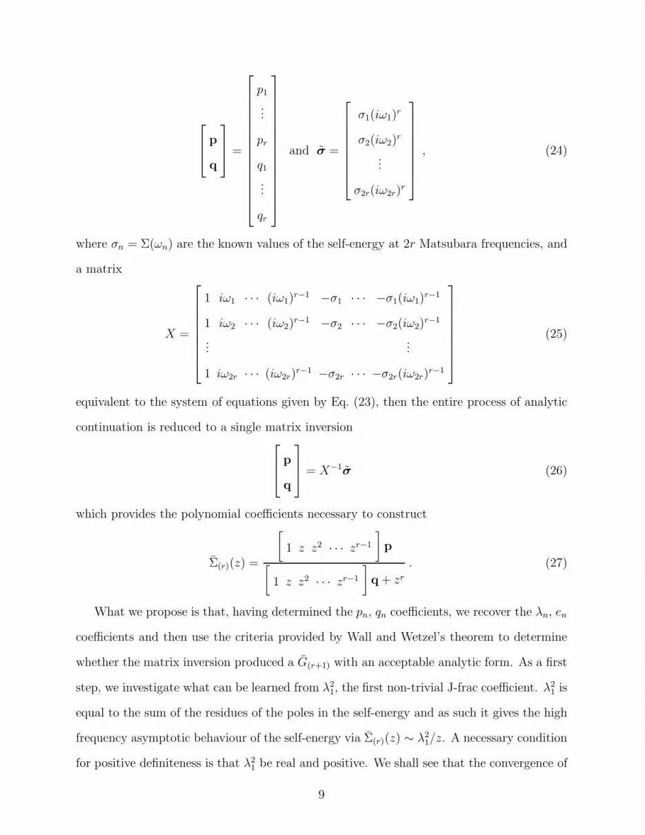
where σn = Σ(ωn) are the known values of the self-energy at 2r Matsubara frequencies, and

a matrix

X =

1 iω1 · · · (iω1)r−1 −σ1 · · · −σ1(iω1)

r−1

1 iω2 · · · (iω2)r−1 −σ2 · · · −σ2(iω2)

r−1

......

1 iω2r · · · (iω2r)r−1 −σ2r · · · −σ2r(iω2r)

r−1

(25)

equivalent to the system of equations given by Eq. (23), then the entire process of analytic

continuation is reduced to a single matrix inversion

p

q

= X−1

σ (26)

which provides the polynomial coefficients necessary to construct

Σ(r)(z) =

[

1 z z2 · · · zr−1

]

p

[

1 z z2 · · · zr−1

]

q + zr

. (27)

What we propose is that, having determined the pn, qn coefficients, we recover the λn, en

coefficients and then use the criteria provided by Wall and Wetzel’s theorem to determine

whether the matrix inversion produced a G(r+1) with an acceptable analytic form. As a first

step, we investigate what can be learned from λ21, the first non-trivial J-frac coefficient. λ2

1 is

equal to the sum of the residues of the poles in the self-energy and as such it gives the high

frequency asymptotic behaviour of the self-energy via Σ(r)(z) ∼ λ21/z. A necessary condition

for positive definiteness is that λ21 be real and positive. We shall see that the convergence of

9

Imλ21 to zero as a function of the number r of poles in the Pade fitting function can provide

information on the quality of the fit and on the analytic structure of the true continuation

G.

IV. NUMERICAL RESULTS

The procedure we have outlined in Sect. III is a specialization of the following general

Pade procedure — such considerations are central to our statistical analysis of the quality

of the fits provided by this method.

Given a function f and a set A of 2r input points, we suppose that we can approximate

the analytic continuation f by a [r− 1/r] rational polynomial f(r), the coefficients of which

are determined by solving the linear system of equations {f(r)(a) = f(a) : a ∈ A}. This

problem can be cast as a matrix inversion in which the kernel X has elements with ratios

as large as

ζ = |(maxA ∪ f(A))r−1/minA ∪ f(A)| . (28)

Thus to reliably perform the inversion we need a numerical range ∼ ζ2, i.e. 2 log10 ζ decimal

digits of numerical precision. This analysis is general in that no other Pade algorithm can

have less stringent precision requirements.

For the case of a self-energy Σ, known at the first 2r Matsubara frequencies above the

real line on the imaginary axis, we have shown that the matrix X is given by Eq. (25). Since

Σ(ωn) ∼ 1/ωn, the ratio of the largest to smallest terms in X is ζ = (ω2r)r = ((4r− 1)πT )r,

the square of which gives an estimate of the amount of precision needed to invert X. Here,

that corresponds to

2r log10(4r − 1)πT (29)

decimal digits.

To achieve a sufficient level of precision for our numerical work, we implement the Pade

algorithm using the symbolic computation package MAPLE. Under MAPLE, expression

10

evaluation takes place in software and thereby transcends the limits imposed by hardware

floating-point. All computations are performed in base ten to any desired level of precision

(we specified Digits := 250;10). Moreover, MAPLE is an ideal environment for rapid

prototyping since high level matrix data types and routines are available as primitives.

We begin by considering a test function of known analytic structure. The self-energy11

Σ(~k, ωn) = −U2

βM

∑

~Q

∑

νn′

χ0( ~Q, νn′)G0( ~Q− ~k, νn′ − ωn) (30)

corresponds to the first ‘rung’ of the ladder diagrams in the T-matrix12 approximation of

the single-band Hubbard model13 (characterized by a near-neighbour hopping integral t and

an on-site repulsion energy U). Here, G0 is the free propagator

G0(~k, ωn) =1

iωn − ξ~k(31)

and χ0 is the free pair susceptibility

χ0( ~Q, νn) =1

βM

∑

~k

∑

ωn′

G0(~k, ωn′)G0( ~Q− ~k, νn − ωn′) . (32)

The frequency sums in Eqs. (30) and (32) can be performed analytically, giving14

χ0( ~Q, νn) =1

M

∑

~k

f [ξ~k] + f [ξ ~Q−~k] − 1

iνn − ξ~k − ξ ~Q−~k

(33)

and

Σ(~k, ωn) =U2

M2

∑

~Q,~k′

(f [ξ~k′] + f [ξ ~Q−~k′] − 1)f [ξ ~Q−~k] − f [ξ~k′]f [ξ ~Q−~k′]

iωn + ξ ~Q−~k − ξ~k′ − ξ ~Q−~k′

. (34)

Since the ξ~k are real, the analytic continuation of the self-energy is a meromorphic function

with a finite number of simple poles, all situated along the real axis. Calculated in two

dimensions on an 8 × 8 (M = 64) lattice, its ~k = 0 component possesses r0 = 26 poles.

(The number of poles is determined by counting the number of distinct elements in the set

{ξ ~Q − ξ~k′ − ξ ~Q−~k′ : ∀~k′, ~Q}.)

For a particular set of parameters15 — we use an interaction strength |U |/t = 4, chemical

potential µ/t = −2, and temperature T/t = 0.7 — the test function, Eq. (30), is calculated

11

in two different ways for the Matsubara frequencies {ω1, ω2, . . . , ω2r}. First, it is calculated

exactly, as prescribed by Eq. (34), but with a small, random error, viz., each value is mul-

tiplied by 1 + ǫ with −1 ≤ ǫ ≤ 1. Second, it is calculated by truncating the Matsubara

sum at an arbitrary cutoff frequency νp ≫ 1 (much larger than the relevant energy scale of

the problem) and then systematically adding back the high frequency contributions up to a

given order. That is,

−1

β

∑

νn′

χ0( ~Q, νn′)G0( ~Q− ~k, νn′ − ωn) = −1

β

∑

|νn′ |≤νp

χ0( ~Q, νn′)G0( ~Q− ~k, νn′ − ωn)

+

m−1∑

l=1

χ0(l)(

~Q)Θ(l+1)[iωn + ξ ~Q−~k] + O(1/(νp)m) (35)

where

χ0(l)(

~Q) =1

M

∑

~k

(f [ξ~k] + f [ξ ~Q−~k] − 1)(ξ~k + ξ ~Q−~k)l−1 (36)

are the coefficients of a Laurent expansion of χ0( ~Q, νn) and the Θ(l) functions (defined in

the Appendix) are constructed using the symbolic manipulation capabilities of MAPLE.

Now, we let the self-energy, evaluated at the first 2r Matsubara frequencies according to

the two schemes described above, serve as the input to the Pade procedure. The resulting

approximant Σ(r) yields a propagator G(r+1)(~k, z) = (z − ξ~k − Σ(r)(~k, z))−1 with spectral

function A(r+1)(~k, ω) = −(1/π)Im G(r+1)(~k, ω+ i0+). The spectral function derived from the

Pade approximant is compared to that of the exact function using the logarithmic measure

10−F ≡

∫ ∞

−∞

dx (A(~k, x) − A(r+1)(~k, x))2

=1

π2

∫ ∞

−∞

dx∣∣∣Im

(

G(~k, x+ iη) − G(r+1)(~k, x+ iη))∣∣∣

2

. (37)

In practice we choose η to be a small, but noninfinitesimal positive real quantity (we use

η/t = 0.064), which has the effect of introducing a slight artificial broadening to the δ-

function peaks of the spectral function.

The results of this comparison (for the ~k = 0 component of the spectral function) are

presented in Figs. 1(a) and 1(b), where F is plotted as a function of r for different values of

12

the random error E = − log10 ǫ and the systematic error E = − log10 1/(νp)m = m log10 νp

(and thus a larger E corresponds to a smaller error). In each graph, a vertical dashed line

marks the exact number of poles (r0 = 26) in the true self-energy. The most distinctive

feature of both graphs is that, at high accuracy (large E), the F curves exhibit a large step

at the point r = r0. In the random error case, the E = 120 curve jumps by four decades,

and this represents an improvement in the Pade fit of nearly 40 orders of magnitude. In the

systematic error case, the result is even more dramatic: the E = 100 and E = 120 curves

jump by roughly four and seven decades, respectively.

At these large accuracies, the only factor inhibiting the success of the Pade approximants

is the lack of a sufficient number of poles to reproduce the analytic structure of the true

function. The large jump observed in the large E curves marks the point, r = r0, at which

the number of poles in the Pade approximant exactly matches the required number, and

for this and larger r there is no difficulty in finding an excellent fit of the test function.

In contrast, when the input points are known to relatively low accuracy, no such feature is

observed, and instead the F curves pass smoothly through r0. This makes clear that for

self-energies calculated to 20, 40, or even 60 decimal digits of accuracy, the level of error in

the input points is still the main obstacle to a successful Pade fit.

The usual response to this situation is to increase the number of Pade points in an

attempt to overcome the intrinsic error limitations (by making the system of equations more

and more overcomplete). However, whatever advantage this additional information brings

to the Pade approximant is soon outweighed by the accompanying complications: When a

rational polynomial of degree [r−1/r] is used to fit a function with r0 < r poles, r−r0 zeros

of the numerator must coincide with an equal number of zeros in the denominator in order to

cancel the extraneous poles. As r − r0 grows, it is less and less likely that this cancellation

will be complete. A slight misplacement of zeros leads to ‘defects’ in which the function

moves between 0 and ∞ in a small neighbourhood. Moreover, it cannot be predicted where

these zero-zero pairs will appear17. For the purposes of calculating a spectral function, they

are of little consequence provided that they lie deep in the complex plane. However, when

13

they are not so far removed from the real axis, they can distort the spectral function away

from its proper shape. When they lie on or near the real axis, they can give rise to deep

troughs of negative spectral weight and other spurious, non-physical features.

The deterioration of the Pade fit, as described above, is evident in Figs. 1(a) and 1(b)

in which many of the F curves reach maxima at points rbest > r0 and then quickly begin to

fall off for larger r. Interestingly, this behaviour is much more pronounced in the systematic

error case where such maxima occur for each curve. In the random error case, the curves

below some error threshold are essentially flat for all r.

The primary lesson that one should draw from these results is that the addition of Pade

points well beyond the required number is not a useful strategy for improving the Pade fit.

Unless the exact analytic continuation is already known, there is no way to predict the value

of rbest. We believe that better results are achieved by fixing the number of Pade points

at 2r0 (giving rise to a [r0 − 1/r0] rational polynomial) and working towards increasing the

accuracy with which those input points are calculated. Even a small effort there can result

in an improvement of several orders of magnitude in the fit. What to try when one does not

know a priori what r0 is discussed later in this paper.

Now consider Figs. 2(a) through 2(d) in which the spectral function of a Pade approx-

imant with 26 poles (calculated by specifying the value of the self-energy at 52 Matsubara

frequencies) is compared to the exact spectral function. In Fig. 2(a), the accuracy of the

input points is given by E = 16 (random error), roughly the number of digits in a double

precision Fortran variable. Despite the fact that the overall energy scale is correct, the

details of the fit are quite poor. Here, the effect of insufficient accuracy is to produce a

washed out version of the spectral function which completely lacks fine structure. Even at

E = 30 (Fig. 2(b)), corresponding to the number of digits available in the largest Fortran

data type, the Pade inversion is only just beginning to distinguish the main peaks of the

spectral function. Figure 2(c) shows the result for E = 80 and Fig. 2(d) the result for

E = 120. Notice that in Fig. 2(d), the fit is near perfect: even the smallest peaks have been

reproduced faithfully.

14

In this example, with r = r0, the Pade approximant provides a remarkable fit to the

true function whenever the accuracy of the input points is better than E ∼ 110. The

difficulty in translating our success in this specific case to the general problem is that, in

real applications, one has no way to judge when sufficient accuracy has been achieved. Also,

in most instances, the number of poles in the self-energy is unknown.

In what follows, we hope to address these deficiencies. We begin by defining a logarithmic

measure of the imaginary part of the J-frac coefficient λ21:

10−Λ ≡ |Imλ21| . (38)

We argued in Sect. III that λ21 ought to be real and positive. In a Pade calculation, however, it

is real-valued only to within some small fraction which characterizes the numerical sensitivity

of the matrix inversion. As we shall soon discover, the convergence of the imaginary part

of λ21 to zero (Λ → ∞) can be used (1) to determine when the threshold of accuracy for an

exact fit has been reached and (2) to infer the value of r0 if it is unknown.

In Figs. 3(a) and 3(b), we plot Λ as a function of r for the random and systematic error

cases. Over each plot is superimposed a reference line given by Eq. (29). What we observe

is a set of Λ curves that initially follow the reference line but later fan out, spaced according

to their E values. Our claim is that these curves provide the quantitative measure of success

of the Pade approximant that has heretofore been lacking, the essential point being that

the shape of the curves reveals the performance characteristics of the Pade inversion in the

various r regimes.

When 0 < r < r0, the accuracy of the Pade approximant is matrix inversion dominated

and the behaviour of Λ is governed by Λ ∼ 2r log10(4r − 1)πT . In this regime, the Pade

approximant has too few poles to fit the true function and thus the matrix inversion must

judiciously arrange the available poles (sometimes apportioning one pole to a region where

there should be two or three) to give the best possible fit. In the opposite limit, r ≫ r0, the

accuracy of the Pade approximant is input-point error dominated. In this regime, there are

more than enough poles to perform an exact fit, but the proper placement of those poles and

15

the determination of their residues is hampered by the finite accuracy to which the input

points are known. We find this reflected in the Λ curves which, for large r, saturate at a

value Λ ∼ E (roughly).

Most interesting, though, is the behaviour of Λ in the vicinity of r = r0 where the Λ

curves in Figs. 3(a) and 3(b) first cross the reference line. In those plots, we see that the Λ

curves corresponding to small values of E closely follow the reference line (Eq. (29)) until

finite accuracy becomes a limiting factor. The curves then fall below the reference line and

become more or less flat. As E is increased, the r coordinate at which a given Λ curve

first deviates from the reference line moves to the right until (for some accuracy, E0 say) it

coincides with r0. Here, there is a sudden change in behaviour: all Λ curves corresponding

to accuracies E > E0 cross the reference line at r = r0. Such a crossing signals that there

are now both sufficient poles in the approximant and sufficient accuracy on the input points

to fit Σ more or less exactly. We can verify this interpretation by appealing to Figs. 1 and

2 which clearly show a large jump at r0 for precisely the same curves that demonstrate a

crossing in Figs. 3(a) and 3(b).

The results we have described are extremely general and do not dependent on the choice

of test function. For example, we may replace Eq. (30) with the full non-self-consistent

T-matrix self-energy

Σ(~k, ωn) = −U2

βM

∑

~Q

∑

νn′

χ0( ~Q, νn′)G0( ~Q− ~k, νn′ − ωn)

1 + Uχ0( ~Q, νn′). (39)

Here, the frequency sums cannot be performed analytically16 and thus we do not have a

closed form analytical expression for the self-energy. (Thus, this is more representative of

the usual situation in which the Pade method might be applied.) In this case, we know only

that its analytic continuation has a finite number of poles along the real axis (although we

are able to predict analytically an upper bound for the number of poles).

This self-energy can be calculated to high accuracy using the method of Eq. (35) with the

χ0(l)(

~Q) replaced by the coefficients of the Laurent expansion of χ0( ~Q, νn)/(1 +Uχ0( ~Q, νn)).

That is, χ0(1)(

~Q) 7→ χ0(1)(

~Q), χ0(2)(

~Q) 7→ χ0(2)(

~Q) − Uχ0(1)(

~Q)2 and so on according to18

16

χ(1)

iνn

+χ(2)

(iνn)2+

χ(3)

(iνn)3+ · · ·

1 + U(

χ(1)

iνn

+χ(2)

(iνn)2+

χ(3)

(iνn)3+ · · ·

) =χ(1)

iνn

+χ(2) − Uχ2

(1)

(iνn)2+χ(3) − 2Uχ(2)χ(1) + U2χ3

(1)

(iνn)3+ · · ·

(40)

The Pade approximant method can then be applied to Eq. (39) calculated in this way.

We find that the resulting plot of Λ vs. r is identical to that of Fig. 3(b) except that the

crossing of the reference line at high accuracy now occurs at r = 156. This allows us to

deduce that the function has r0 = 156 poles, significantly more than the 26 poles of Eq. (34).

(This is a consequence of the lifting of degeneracy in each ~Q component brought about by

the renormalization 1/(1 +U( ~Q, νn)).) We also find that the approximant spectral function

compares well with increasing accuracy of the input points to the numerically exact spectral

functions as calculated (i) by a non-Pade method due to Marsiglio et al.19 (this non-Pade

method is of limited application since it requires the self-energy to have a very specific form,

but for those cases where it is applicable, it can outperform the Pade method), and (ii) by

an exact partial fraction decomposition of the self energy20 that can be done to a very high

accuracy (say 10−40 on all poles and residues).

Finally, one interesting feature that could potentially be exploited is that for self-energy

values calculated using the Θ function expansion, the value of r which gives the maximum

value of Λ roughly tracks rbest (cf. Figs. 1(b) and 3(b)).

V. CONCLUSIONS

The Pade procedure is very sensitive to the numerical precision with which the matrix

inversion is performed and to the intrinsic error on the input points. Sufficient precision

is difficult to achieve in traditional computer languages (e.g. C, Fortran) and so, in many

instances, it may be necessary to make use of a symbolic computation package capable

of supporting very large precision data types. Likewise, sufficient accuracy is difficult to

achieve without a sophisticated computational scheme (e.g. the Θ function expansion) that

goes beyond a simple truncation of the Matsubara frequency sums in the self-energy. The

17

required level of precision and accuracy depends on the temperature T , which controls the

spacing of the Matsubara points, and on the pole count r0.

An insufficient level of accuracy leads to an approximant spectral function that lacks fine

structural detail or, worse, one that exhibits spurious spikes or troughs of spectral weight.

This poses a problem whenever we are interested in the presence of a specific feature in the

spectral function (e.g. the onset of a normal state pseudogap). In that case, it is essential to

have confidence in the quality of the Pade result. We must be convinced that the observed

feature is robust and not merely a by-product of insufficient accuracy.

We have argued that simply adding more Pade points cannot compensate for too large

an error on the input points. While there is a small set of r values for which an increase in

r improves the fit, there is no known criterion that indicates when to stop adding points.

Without already knowing the exact result, one cannot distinguish between the regime where

additional points improve the fit (r < rbest) and the regime where such points degrade it

(r ≥ rbest). Instead, we recommend the use of a Pade approximant function having the same

number of poles as the function to be fit. The exact number of poles, when it is not known,

can be determined from the crossing point in a Λ vs. r plot. The crossing also indicates that

a sufficient level of numerical accuracy in the input points has been acheived.

There are several caveats to the procedure we have outlined. (1) If the true Green’s

function has a branch cut along the real axis arising from trancendental functions then no

Λ crossing will ever be observed, since a branch cut of that kind can only be represented by

an infinity of poles (r0 = ∞). (2) The self-energy of the Green’s function we are trying to

reproduce must have the correct asymptotic form and must be analytic in, say, the upper

half of the complex plane; otherwise, the rational polynomial (or continued fraction) form

of the approximant cannot reproduce its analytic structure. (3) The Pade method is often

used to model a function that is smooth in some region of interest (well away from its

poles) and such calculations are rarely performed with more than machine accuracy. Our

numerical analysis of the Pade inversion, with its prediction of extremely high accuracy

requirements, is not meant to invalidate these results. We have applied the Pade method

18

to the particularly difficult problem of reproducing the sharp peak structures characteristic

of a spectral function whose Green’s function has its poles along the real axis. In that case,

the poles lie in the region of interest. The precision and accuracy requirements of the Pade

inversion are greatly reduced if the poles of the Green’s function lie deep in the complex

plane.

Finally, let us remember that the starting point for our new Pade approach was the

realization that the convergence of the continued fraction coefficients to ‘allowed’ values

can provide a criterion for judging the quality of a Pade approximant, even if the analytic

structure of the function we are trying to fit is unknown. In Sect. IV, we demonstrated the

utility of this idea using the λ1 coefficient. However, we know that there is much addtional

information that can be extracted from the remaining continued fraction coefficients. In

future, perhaps our analysis can be extended to include e1, λ2, e2, etc.

ACKNOWLEDGMENTS

One of us (RJG) wishes to thank George Baker for directing him to a variety of valuable

references, and we thank David Senechal and Andre-Marie Tremblay for helpful comments

on their recent paper6. This work was supported by the NSERC of Canada, and the Institute

of Theoretical Physics of the University of Alberta.

19

APPENDIX:

In addition to the usual occupation functions

f [x] =1

β

∑

ωn

eiωn0+

iωn − x=

1

eβx + 1(A1a)

b[x] = −1

β

∑

νn

eiνn0+

iνn − x=

1

eβx − 1(A1b)

it is often convenient to define partial occupation functions. For example, the bose version

of such a function looks like

b[x] = −1

β

∑

νn>νp

eiνn0+

iνn − x=

1

2πiψ

( β

2πi(iνp+1 − x)

)

(A2)

where ψ(z) = d ln Γ(z)/dz is the digamma function21. This can be generalized to a m-order

function (symmetric in its arguments)

b[x1, x2, . . . , xm] = −1

β

∑

νn>νp

1

iνn − x1

1

iνn − x2· · ·

1

iνn − xm(A3)

which has the interesting property that it can be expressed (via partial fraction decomposi-

tion) in terms of the (m− 1)-order partial occupation function

b[x1, x2, . . . , xm] =

b[x1,x2,...,xm−2,xm−1]−b[x1,x2,...,xm−2,xm]xm−1−xm

if xm−1 6= xm

∂∂yb[x1, x2, . . . , xm−2, y]|y=xm

otherwise.(A4)

Equation (A2) serves to terminate the recursion.

Furthermore, it is straightforward to show that for all l ≥ 0

Θ(l+2)[x] ≡ −1

β

∑

|νn|>νp

1

(iνn)l+1

1

iνn − x

= −1

β

∑

νn>νp

(1

(iνn)l+1

1

iνn − x+

1

(−iνn)l+1

1

−iνn − x

)

= b[0, 0, . . . , 0︸ ︷︷ ︸

l+1

, x] + (−1)lb[0, 0, . . . , 0︸ ︷︷ ︸

l+1

,−x]

=1

l!

∂l

∂yl

{

b[x, y] + (−1)lb[−x, y]}∣

∣∣y=0

(A5)

20

where, according to Eq. (A4), the two-argument function b[x, y] is related to b[x] by

b[x, y] =b[x] − b[y]

x− y(A6)

provided x 6= y. The Θ functions provide a closed-form representation of the high-frequency

asymptotics of a broad class of Matsubara sums. In particular, the sum

−1

β

∑

νn′

χ0( ~Q, νn′)G0( ~Q− ~k, νn′ − ωn) (A7)

can be separated into a finite sum over all low frequencies

1

β

∑

|νn′ |≤νp

χ0( ~Q, νn′)G0( ~Q− ~k, νn′ − ωn) (A8)

and an infinite sum over the remaining frequencies

−1

β

∑

|νn′ |>νp

χ0( ~Q, νn′)G0( ~Q− ~k, νn′ − ωn) = −1

β

∑

|νn′ |>νp

( ∞∑

l=1

χ0(l)(

~Q)

(iνn′)l

)1

i(νn′ − ωn) − ξ ~Q−~k

= −∞∑

l=1

χ0(l)(

~Q)1

β

∑

|νn′ |>νp

1

(iνn′)l

1

iνn′ − (iωn + ξ ~Q−~k)

= +

∞∑

l=1

χ0(l)(

~Q)Θ(l+1)[iωn + ξ ~Q−~k] (A9)

where, in Eq. (A9), we have used the fact that the free susceptibility χ0 admits a Laurent

expansion in the frequency variable

χ0( ~Q, νn) =1

iνn

1

M

∑

~k

f [ξ~k] + f [ξ ~Q−~k] − 1

1 − (ξ~k + ξ ~Q−~k)/iνn

=χ0

(1)(~Q)

iνn

+χ0

(2)(~Q)

(iνn)2+χ0

(3)(~Q)

(iνn)3+ · · · (A10)

with ~Q-dependent coefficients

χ0(l)(

~Q) =1

M

∑

~k

(f [ξ~k] + f [ξ ~Q−~k] − 1)(ξ~k + ξ ~Q−~k)l−1 . (A11)

21

REFERENCES

† Address as of Sept. 1, 1999: Dept. of Physics, Massachusetts Institute of Technology,

Cambridge MA 02139.

1 Of course, other methods are available for certain formulations of the many-body thermal

Green’s function problem. A number of these are discussed in a recent paper: see J.

Schmalian, M. Langer, S. Grabowski and K.H. Bennemann, Comp. Phys. Comm. 93, 141

(1996), and references therein.

2 G. A. Baker, Essentials of Pade Approximants, Academic Press, New York (1975).

3 H. J. Vidberg and J. Serene, J. Low Temp. Phys. 29, 179 (1977).

4 G. Baym and D. Mermin, J. Math. Phys. 2, 232 (1961).

5 H. S. Wall, Analytic theory of continued fractions, Chelsea Publishing Co., New York

(1948).

6 The implementation of such a form was made recently in S. Pairault, D. Senechal, and

A.-M. S. Tremblay, Phys. Rev. Lett. 80, 5389 (1998); also see cond-mat/9905242.

7 We have chosen to absorb all frequency independent terms of the self-energy into ξ.

8 H. S. Wall and M. Wetzel, Trans. Amer. Math. Soc. 55, 373 (1944).

9 The system of equations is linear in the (p, q) basis, but not in the (λ, e) basis.

10 There is no reason to choose this specific value. Any Digits which is in excess of what

is required by the statistical test discussed in this section is adequate. It is important to

note that there is virtually no extra time required to make such high accuracy calculations,

and thus there is no reason to not implement algorithms such as this with a very high

accuracy.

11 We use the convention that ωn = (2n−1)π/β represents a fermionic Matsubara frequency

and νn = 2nπ/β a bosonic one.

22

12 See, e.g., A.L. Fetter and J.D. Walecka, “Quantum Theory of Many-Particle Systems”

(McGraw Hill, New York, 1971).

13 For those readers not familiar with the Hubbard model, an excellent discussion may be

found in A. Auerbach, “Interacting Electrons and Quantum Magnetism” (Springer-Verlag,

New York, 1994).

14 These relations can be derived most easily using the identity (1−f(x)−f(y))∗N(x+y) =

f(x) ∗ f(y), where f/N is the fermi/bose distribution function.

15 As viewed in the µ–T phase diagram, this choice of parameters places the system well

inside the band (−4 < µ/t < 4) and just above the superconducting instability (T > Tc),

the so-called Thouless criterion line. This region is of interest in that one expects to see

a suppression of the spectral weight around the chemical potential, the so-called normal

state pseudo-gap.

16 In fact, the frequency sum can be performed formally to yield an infinite sum of generalized

occupation functions. However, this is of no computational value since it only trades a

difficult frequency sum for an infinite series of increasingly more difficult (at each order)

~k sums.

17 Theorems do exist concerning their overall distribution in the complex plane; see

Chapts. 11 and 13 of Ref.2.

18 This expansion is easy to implement in MAPLE using the series() command, although

the computational resources required to execute it are significant due to the combinatorial

explosion of terms at high order.

19 F. Marsiglio, M. Schossmann, and J. P. Carbotte, Phys. Rev. B 39, 4965 (1988).

20 The details of these calculations will be presented in a separate publication.

21 L. V. Ahlfors, Complex Analysis, McGraw-Hill Book Co., New York (1953).

23

FIGURES

FIG. 1. For various levels of (a) random and (b) systematic error, characterized roughly as

10−E (see the text for more details), the quality of the Pade fit as measured by F (see Eq. (37)) is

plotted with respect to the number of poles in the Pade approximant (the solid lines are a guide

to the eye). The ~k = 0 self energy being studied is that of Eq. (30) where the parameters of the

attractive Hubbard model (with t being the hopping energy), for an 8 × 8 square lattice, are a

repulsive energy |U |/t = 4, a chemical potential µ/t = −2, and a temperature T/t = 0.7. The

vertical dashed line indicates the number of poles (r0 = 26) in the true Green’s function. In plot

(a), error bars (representing the standard deviation of the data points over a set of initial random

seeds) are smaller than the symbols marking the data points and are not shown. In plot (b), the

dotted line is the best linear fit through the maximum values of F .

FIG. 2. The ~k = 0 spectral function of the Pade approximant is compared to the exact spectral

function for different levels of random error (10−E) on the initial input points. The parameters of

the Hamiltonian and the self-energy being studied are the same as those of Fig. 1.

FIG. 3. For various levels of (a) random and (b) systematic error (10−E), the parameter Λ is

plotted with respect to the number of poles in the Pade approximant. The parameters are the same

as those of Fig. 1. The vertical dashed line indicates the number of poles (r0 = 26) in the true

Green’s function. The solid line originating in the lower left corner is given by 2r log 10(4r− 1)πT .

In plot (b), the dotted line is the best linear fit through the maximum values of Λ. The parameters

of the Hamiltonian and the self-energy being studied are the same as those of Fig. 1.

24

0

F

100

80

60

40

20

0

r10 20 504030 7060 80

r

E=120E=100E=80E=60E=40E=20

(a)

0

F

100

80

60

40

20

0

r10 20 504030 7060 80

r

E=120E=100E=80E=60E=40E=20

(b)

E=16

A(0,·)

0

1

2

3

4

5

-1 0·

1

ApproximantExact

(a)

E=30

A(0,·)

0

1

2

3

4

5

-1 0·

1

ApproximantExact

(b)

E=80

A(0,·)

0

1

2

3

4

5

-1 0·

1

ApproximantExact

(c)

E=120

A(0,·)

0

1

2

3

4

5

-1 0·

1

ApproximantExact

(d)

0

20

40

60

80

100

120

140

ñ

r10 20 504030 7060 80

r

E=120E=100E=80E=60E=40E=20

(a)

0

20

40

60

80

100

120

140

ñ

r10 20 504030 7060 80

r

E=120E=100E=80E=60E=40E=20

(b)