Embed Size (px)
Citation preview

i
Simulation with ArenaFifth Edition
W. David KeltonProfessor
Department of Quantitative Analysis and Operations ManagementUniversity of Cincinnati
Randall P. SadowskiRetired
Nancy B. SwetsRequirements Analyst
SimulationRockwell Automation
Boston Burr Ridge, IL Dubuque, IA New York San Francisco St. LouisBangkok Bogotá Caracas Kuala Lumpur Lisbon London Madrid Mexico City
Milan Montreal New Delhi Santiago Seoul Singapore Sydney Taipei Toronto

ii
SIMULATION WITH ARENA, FIFTH EDITION
Published by McGraw-Hill, a business unit of The McGraw-Hill Companies, Inc., 1221 Avenue of theAmericas, New York, NY 10020. Copyright © 2010 by The McGraw-Hill Companies, Inc. All rightsreserved. Previous editions © 2007, 2004, 2002, and 1998. No part of this publication may be reproducedor distributed in any form or by any means, or stored in a database or retrieval system, without the priorwritten consent of The McGraw-Hill Companies, Inc., including, but not limited to, in any network orother electronic storage or transmission, or broadcast for distance learning.
Some ancillaries, including electronic and print components, may not be available to customers outsidethe United States.
This book is printed on acid-free paper.
1 2 3 4 5 6 7 8 9 0 DOC/DOC 0 9
ISBN 978–0–07–337628–8MHID 0–07–337628–0
Global Publisher: Raghothaman SrinivasanSponsoring Editor: Debra B. HashDirector of Development: Kristine TibbettsDevelopmental Editor: Lorraine K. BuczekSenior Marketing Manager: Curt ReynoldsProject Manager: Melissa M. LeickSenior Production Supervisor: Sherry L. KaneAssociate Design Coordinator: Brenda A. RolwesCover Designer: Peter KauffmanTypeface: 10/12 Times New Roman PSPrinter: R. R. Donnelley Crawfordsville, IN
All credits appearing on page or at the end of the book are considered to be an extension of the copyrightpage.
Library of Congress Cataloging-in-Publication Data
Kelton, W. David. Simulation with Arena / W. David Kelton, Randall P. Sadowski, Nancy B. Swets. — 5th ed. p. cm. Includes index. ISBN 978–0–07–337628–8 — ISBN 0–07–337628–0 (hard copy : alk. paper) 1. Computer simulation.2. Arena (Computer file). I. Sadowski, Randall P. II. Swets, Nancy B. III. Title.QA76.9.C65K45 2010003'.3--dc22
2009019022
www.mhhe.com

iii
About the Authors
W. DAVID KELTON is Professor in the Department of Quantitative Analysis andOperations Management at the University of Cincinnati, where he has also served as MSprogram director and acting department head. He received a B.A. in mathematics fromthe University of Wisconsin-Madison, an M.S. in mathematics from Ohio University,and M.S. and Ph.D. degrees in industrial engineering from Wisconsin. He has also been afaculty member at Kent State, The University of Michigan, the University of Minnesota,and Penn State. Visiting posts have included the Naval Postgraduate School, theUniversity of Wisconsin-Madison, the Institute for Advanced Studies in Vienna, and theWarsaw School of Economics. He is a Fellow of both INFORMS and IIE.
His research interests and publications are in the probabilistic and statisticalaspects of simulation, applications of simulation, and stochastic models. His papers haveappeared in Operations Research, Management Science, the INFORMS Journal onComputing, IIE Transactions, Naval Research Logistics, Military Operations Research,the European Journal of Operational Research, Simulation, Socio-Economic PlanningSciences, the Journal of Statistical Computation and Simulation, and the Journal of theAmerican Statistical Association, among others. In addition to the United States andCanada, he has spoken on simulation in Austria, Germany, Switzerland, The Nether-lands, Belgium, Spain, Poland, Turkey, Chile, and South Korea.
He was Editor-in-Chief for the INFORMS Journal on Computing from 2000to mid-2007, during which time the journal rose from unranked on the ISI Impact Factorto first out of 56 journals in the operations-research/management-science category. Inaddition, he has served as Simulation Area Editor for Operations Research, theINFORMS Journal on Computing, and IIE Transactions; Associate Editor of OperationsResearch, the Journal of Manufacturing Systems, and Simulation; and was Guest Co-Editor for a special simulation issue of IIE Transactions. Awards include the TIMSCollege on Simulation award for best simulation paper in Management Science, the IIEOperations Research Division Award, a Meritorious Service Award from OperationsResearch, the INFORMS College on Simulation Distinguished Service Award, and theINFORMS College on Simulation Outstanding Simulation Publication Award. He wasPresident of the TIMS College on Simulation, and was the INFORMS co-representativeto the Winter Simulation Conference Board of Directors from 1991 through 1999,serving as Board Chair for 1998. In 1987 he was Program Chair for the WSC, and in1991 was General Chair; he is a founding Trustee of the WSC Foundation. He hasworked on grants and consulting contracts from a number of corporations, foundations,and agencies. He once made it down a black-diamond run in the back bowls, this timeupright on his skis.

iv
RANDALL P. SADOWSKI is currently enjoying retirement and plans to continue this newcareer. In his previous life, he was Product Manager for scheduling and data-trackingapplications for Rockwell Automation. Prior to that, he was director of university relations,chief applications officer, vice president of consulting services and user education atSystems Modeling Corporation.
Before joining Systems Modeling, he was on the faculty at Purdue Universityin the School of Industrial Engineering and at the University of Massachusetts. Hereceived his bachelor’s and master’s degrees in industrial engineering from OhioUniversity and his Ph.D. in industrial engineering from Purdue.
He has authored over 50 technical articles and papers, served as chair of theThird International Conference on Production Research and was the general chair of the1990 Winter Simulation Conference. He is on the visiting committee for the IEdepartments at Lehigh University, the University of Pittsburgh, and Ohio University. Heis co-author, with C. Dennis Pegden and Robert E. Shannon, of Introduction toSimulation Using SIMAN.
He is a Fellow of the Institute of Industrial Engineers and served as editor of atwo-year series on Computer Integrated Manufacturing Systems for IE Magazine thatreceived the 1987 IIE Outstanding Publication award. He has served in several positionsat IIE, including president at the chapter and division levels, and vice president ofSystems Integration at the international level. He founded the annual IIE/RA StudentSimulation Contest. He collects tools and is the proud owner of a tractor named Dutch, astocked farm pond, a monster mower, and an ATV used to inspect the farm and haulfirewood.
NANCY B. SWETS (nee Zupick) is the Requirements Analyst for the Arena simulationproduct at Rockwell Automation. She works with product management, developmentand Arena customers to research and write out the software requirements for future re-leases of the software. In addition to this role, she helps manage the IIE/RA StudentSimulation Contest and participates in marketing and sales activities.
Nancy received her bachelor’s degree in industrial engineering from theUniversity of Pittsburgh. It was at Pitt that she became hooked on simulation inDr. Byron Gottfried’s class and where she first became familiar with the SIMANsimulation language. In 1997 she joined Systems Modeling in the technical supportgroup where she worked for over a decade assisting clients with their simulations in awide array of industries.
When not immersed in the world of simulation, Nancy spends her time hangingout with her family. She enjoys gardening, cooking, traveling, and occasionally dabblesin politics to reduce stress.

v
To those in the truly important arena of our lives:
Albert, Anna, Anne, Christie and Molly;
Aidan, Charity, Emma, Jenny, Michael, Mya, Noah, Sammy,Sean, Shelley and Tierney;
Anna Jurgaitis Zupick, Anna, Ian and Rod.

vi
Arena, Arena Factory Analyzer, and SIMAN are either registered trademarks or trademarks of RockwellAutomation, Inc. AutoCAD is a registered trademark of Autodesk. Microsoft, ActiveX, Outlook, PowerPoint,Windows, Windows NT, Visio, and Visual Basic are either registered trademarks or trademarks of MicrosoftCorporation in the United States and/or other countries. OptQuest is a registered trademark of OptTekSystems, Inc. Oracle is a registered trademark of Oracle Corporation. Crystal Reports is a registered trademarkof SAP BusinessObjects. All other trademarks and registered trademarks are acknowledged as being theproperty of their respective owners.
This Rockwell Automation product is warranted in accord with the product license. The product’s performancewill be affected by system configuration, the application being performed, operator control, and other relatedfactors.
This product’s implementation may vary among users.
This textbook is as up-to-date as possible at the time of printing. Rockwell Automation reserves the right tochange any information contained in this book or the software at any time without prior notice.
The instructions in this book do not claim to cover all the details or variations in the equipment, procedure, orprocess described, nor to provide directions for meeting every possible contingency during installation,operation, or maintenance.
vii
Contents
Chapter 1: What Is Simulation? ..........................................................................................1
1.1 Modeling .......................................................................................................................... 11.1.1 What’s Being Modeled? .............................................................................. 21.1.2 How About Just Playing with the System? ................................................. 31.1.3 Sometimes You Can’t (or Shouldn’t) Play with the System ........................ 31.1.4 Physical Models .......................................................................................... 41.1.5 Logical (or Mathematical) Models ............................................................. 41.1.6 What Do You Do with a Logical Model? .................................................... 4
1.2 Computer Simulation ....................................................................................................... 51.2.1 Popularity and Advantages .......................................................................... 51.2.2 The Bad News ............................................................................................. 61.2.3 Different Kinds of Simulations ................................................................... 7
1.3 How Simulations Get Done .............................................................................................. 81.3.1 By Hand ...................................................................................................... 81.3.2 Programming in General-Purpose Languages .......................................... 101.3.3 Simulation Languages .............................................................................. 101.3.4 High-Level Simulators .............................................................................. 101.3.5 Where Arena Fits In .................................................................................. 10
1.4 When Simulations Are Used .............................................................................................. 121.4.1 The Early Years ......................................................................................... 121.4.2 The Formative Years .................................................................................. 121.4.3 The Recent Past ........................................................................................ 131.4.4 The Present ............................................................................................... 131.4.5 The Future ................................................................................................. 13
Chapter 2: Fundamental Simulation Concepts ...............................................................15
2.1 An Example .................................................................................................................... 152.1.1 The System ............................................................................................... 152.1.2 Goals of the Study .................................................................................... 17
2.2 Analysis Options ............................................................................................................ 182.2.1 Educated Guessing .................................................................................... 182.2.2 Queueing Theory ...................................................................................... 192.2.3 Mechanistic Simulation ............................................................................ 20
2.3 Pieces of a Simulation Model ......................................................................................... 202.3.1 Entities ...................................................................................................... 202.3.2 Attributes .................................................................................................. 212.3.3 (Global) Variables ..................................................................................... 212.3.4 Resources .................................................................................................. 222.3.5 Queues ...................................................................................................... 222.3.6 Statistical Accumulators ........................................................................... 232.3.7 Events ........................................................................................................ 232.3.8 Simulation Clock ...................................................................................... 242.3.9 Starting and Stopping ............................................................................... 24
viii
2.4 Event-Driven Hand Simulation ...................................................................................... 252.4.1 Outline of the Action ................................................................................ 252.4.2 Keeping Track of Things ........................................................................... 262.4.3 Carrying It Out .......................................................................................... 282.4.4 Finishing Up ............................................................................................. 32
2.5 Event- and Process-Oriented Simulation ........................................................................ 322.6 Randomness in Simulation ............................................................................................. 34
2.6.1 Random Input, Random Output ................................................................ 342.6.2 Replicating the Example ........................................................................... 352.6.3 Comparing Alternatives ............................................................................ 36
2.7 Simulating with Spreadsheets ........................................................................................ 372.7.1 A News Vendor Problem ........................................................................... 372.7.2 A Single-Server Queue ............................................................................. 432.7.3 Extensions and Limitations ....................................................................... 47
2.8 Overview of a Simulation Study .................................................................................... 472.9 Exercises ......................................................................................................................... 48
Chapter 3: A Guided Tour Through Arena .......................................................................53
3.1 Starting Up ..................................................................................................................... 533.2 Exploring the Arena Window ......................................................................................... 55
3.2.1 Opening a Model ...................................................................................... 553.2.2 Basic Interaction and Pieces of the Arena Window .................................. 563.2.3 Panning, Zooming, Viewing, and Aligning in the Flowchart View .......... 583.2.4 Modules .................................................................................................... 603.2.5 Internal Model Documentation ................................................................. 61
3.3 Browsing Through an Existing Model: Model 3-1 ......................................................... 623.3.1 The Create Flowchart Module .................................................................. 623.3.2 The Entity Data Module ........................................................................... 633.3.3 The Process Flowchart Module ................................................................ 643.3.4 The Resource Data Module ...................................................................... 663.3.5 The Queue Data Module ........................................................................... 673.3.6 Animating Resources and Queues ............................................................ 673.3.7 The Dispose Flowchart Module ................................................................ 673.3.8 Connecting Flowchart Modules ................................................................ 683.3.9 Dynamic Plots ........................................................................................... 693.3.10 Dressing Things Up .................................................................................. 713.3.11 Setting the Run Conditions ....................................................................... 723.3.12 Running It ................................................................................................. 733.3.13 Viewing the Reports ................................................................................. 74
3.4 Building Model 3-1 Yourself .......................................................................................... 793.4.1 New Model Window and Basic Process Panel ......................................... 803.4.2 Place and Connect the Flowchart Modules ............................................... 813.4.3 The Create Flowchart Module .................................................................. 813.4.4 Displays ..................................................................................................... 823.4.5 The Entity Data Module ........................................................................... 833.4.6 The Process Flowchart Module ................................................................ 833.4.7 The Resource and Queue Data Modules .................................................. 843.4.8 Resource Animation .................................................................................. 843.4.9 The Dispose Flowchart Module ................................................................ 853.4.10 Dynamic Plots ........................................................................................... 85
ix
3.4.11 Window Dressing ...................................................................................... 883.4.12 The Run > Setup Dialog Boxes ................................................................. 893.4.13 Establishing Named Views ....................................................................... 89
3.5 Case Study: Specialized Serial Processing vs. Generalized Parallel Processing ........... 903.5.1 Model 3-2: Serial Processing – Specialized Separated Work ................... 903.5.2 Model 3-3: Parallel Processing – Generalized Integrated Work ............... 933.5.3 Models 3-4 and 3-5: The Effect of Task-Time Variability ........................ 95
3.6 More on Menus, Toolbars, Drawing, and Printing ......................................................... 983.6.1 Menus ....................................................................................................... 983.6.2 Toolbars .................................................................................................. 1033.6.3 Drawing ................................................................................................... 1063.6.4 Printing ................................................................................................... 107
3.7 Help! ............................................................................................................................. 1083.8 More on Running Models ............................................................................................. 1093.9 Summary and Forecast ................................................................................................. 1103.10 Exercises ....................................................................................................................... 110
Chapter 4: Modeling Basic Operations and Inputs....................................................... 117
4.1 Model 4-1: An Electronic Assembly and Test System .................................................. 1174.1.1 Developing a Modeling Approach .......................................................... 1184.1.2 Building the Model ................................................................................. 1194.1.3 Running the Model ................................................................................. 1304.1.4 Viewing the Results ................................................................................ 132
4.2 Model 4-2: The Enhanced Electronic Assembly and Test System ............................... 1344.2.1 Expanding Resource Representation: Schedules and States .................. 1354.2.2 Resource Schedules ................................................................................ 1364.2.3 Resource Failures .................................................................................... 1404.2.4 Frequencies ............................................................................................. 1424.2.5 Results of Model 4-2 .............................................................................. 145
4.3 Model 4-3: Enhancing the Animation .......................................................................... 1494.3.1 Changing Animation Queues .................................................................. 1504.3.2 Changing Entity Pictures ........................................................................ 1524.3.3 Adding Resource Pictures ....................................................................... 1544.3.4 Adding Variables and Plots ..................................................................... 156
4.4 Model 4-4: The Electronic Assembly and Test System with Part Transfers ................. 1584.4.1 Some New Arena Concepts: Stations and Transfers ............................... 1584.4.2 Adding the Route Logic .......................................................................... 1604.4.3 Altering the Animation ........................................................................... 163
4.5 Finding and Fixing Errors ............................................................................................ 1674.6 Input Analysis: Specifying Model Parameters and Distributions ................................. 174
4.6.1 Deterministic vs. Random Inputs ........................................................... 1754.6.2 Collecting Data ....................................................................................... 1764.6.3 Using Data .............................................................................................. 1774.6.4 Fitting Input Distributions via the Input Analyzer .................................. 1784.6.5 No Data? ................................................................................................. 1854.6.6 Nonstationary Arrival Processes ............................................................. 1884.6.7 Multivariate and Correlated Input Data .................................................. 189
4.7 Summary and Forecast ................................................................................................. 1894.8 Exercises ....................................................................................................................... 190
x
Chapter 5: Modeling Detailed Operations ..................................................................... 201
5.1 Model 5-1: A Simple Call Center System .................................................................... 2025.2 New Modeling Issues ................................................................................................... 203
5.2.1 Customer Rejections and Balking .......................................................... 2035.2.2 Three-Way Decisions .............................................................................. 2045.2.3 Variables and Expressions ...................................................................... 2045.2.4 Storages ................................................................................................... 2055.2.5 Terminating or Steady-State ................................................................... 205
5.3 Modeling Approach ...................................................................................................... 2065.4 Building the Model ....................................................................................................... 208
5.4.1 Create Arrivals and Direct to Service ..................................................... 2085.4.2 Arrival Cutoff Logic ............................................................................... 2145.4.3 Technical Support Calls .......................................................................... 2165.4.4 Sales Calls ............................................................................................... 2195.4.5 Order-Status Calls ................................................................................... 2205.4.6 System Exit and Run Setup .................................................................... 2265.4.7 Animation ............................................................................................... 228
5.5 Model 5-2: The Enhanced Call Center System ............................................................ 2315.5.1 The New Problem Description ................................................................ 2315.5.2 New Concepts ......................................................................................... 2335.5.3 Defining the Data ................................................................................... 2355.5.4 Modifying the Model .............................................................................. 239
5.6 Model 5-3: The Enhanced Call Center with More Output Performance Measures ..... 2445.7 Model 5-4: An (s, S) Inventory Simulation .................................................................. 251
5.7.1 System Description ................................................................................. 2515.7.2 Simulation Model ................................................................................... 253
5.8 Summary and Forecast ................................................................................................. 2645.9 Exercises ....................................................................................................................... 265
Chapter 6: Statistical Analysis of Output from Terminating Simulations ...................273
6.1 Time Frame of Simulations .......................................................................................... 2746.2 Strategy for Data Collection and Analysis ................................................................... 2746.3 Confidence Intervals for Terminating Systems ............................................................ 2766.4 Comparing Two Scenarios ............................................................................................ 2816.5 Evaluating Many Scenarios with the Process Analyzer (PAN) .................................... 2856.6 Searching for an Optimal Scenario with OptQuest ...................................................... 2906.7 Summary and Forecast ................................................................................................. 2956.8 Exercises ....................................................................................................................... 296
Chapter 7: Intermediate Modeling and Steady-State Statistical Analysis ..................301
7.1 Model 7-1: A Small Manufacturing System ................................................................. 3017.1.1 New Arena Concepts .............................................................................. 3027.1.2 The Modeling Approach ......................................................................... 3047.1.3 The Data Modules ................................................................................... 3057.1.4 The Logic Modules ................................................................................. 3077.1.5 Animation ............................................................................................... 3147.1.6 Verification ............................................................................................. 316
xi
7.2 Statistical Analysis of Output from Steady-State Simulations ..................................... 3207.2.1 Warm-Up and Run Length ...................................................................... 3207.2.2 Truncated Replications ........................................................................... 3247.2.3 Batching in a Single Run ........................................................................ 3257.2.4 What To Do? ........................................................................................... 3287.2.5 Other Methods and Goals for Steady-State Statistical Analysis ............. 329
7.3 Summary and Forecast ................................................................................................. 3297.4 Exercises ....................................................................................................................... 329
Chapter 8: Entity Transfer ...............................................................................................335
8.1 Types of Entity Transfers .............................................................................................. 3358.2 Model 8-1: The Small Manufacturing System with Resource-Constrained Transfers . 3378.3 The Small Manufacturing System with Transporters ................................................... 341
8.3.1 Model 8-2: The Modified Model 8-1 for Transporters ........................... 3428.3.2 Model 8-3: Refining the Animation for Transporters ............................. 349
8.4 Conveyors ..................................................................................................................... 3558.4.1 Model 8-4: The Small Manufacturing System with Nonaccumulating
Conveyors .......................................................................................... 3588.4.2 Model 8-5: The Small Manufacturing System with Accumulating
Conveyors .......................................................................................... 3638.5 Summary and Forecast ................................................................................................. 3648.6 Exercises ....................................................................................................................... 364
Chapter 9: A Sampler of Further Modeling Issues and Techniques ............................369
9.1 Modeling Conveyors Using the Advanced Transfer Panel ........................................... 3699.1.1 Model 9-1: Finite Buffers at Stations ...................................................... 3709.1.2 Model 9-2: Parts Stay on Conveyor During Processing ......................... 374
9.2 More on Transporters ................................................................................................... 3759.3 Entity Reneging ............................................................................................................ 376
9.3.1 Entity Balking and Reneging .................................................................. 3769.3.2 Model 9-3: A Service Model with Balking and Reneging ..................... 377
9.4 Holding and Batching Entities ..................................................................................... 3859.4.1 Modeling Options ................................................................................... 3859.4.2 Model 9-4: A Batching Process Example ............................................... 386
9.5 Overlapping Resources ................................................................................................. 3929.5.1 System Description ................................................................................. 3929.5.2 Model 9-5: A Tightly Coupled Production System ................................. 3949.5.3 Model 9-6: Adding Part-Status Statistics ................................................ 400
9.6 A Few Miscellaneous Modeling Issues ........................................................................ 4039.6.1 Guided Transporters ................................................................................ 4049.6.2 Parallel Queues ....................................................................................... 4049.6.3 Decision Logic ........................................................................................ 405
9.7 Exercises ....................................................................................................................... 406
Chapter 10: Arena Integration and Customization ....................................................... 413
10.1 Model 10-1: Reading and Writing Data Files .............................................................. 41310.1.1 Model 10-2: Reading Entity Arrivals from a Text File ........................... 41510.1.2 Model 10-3 and Model 10-4: Reading and Writing Access and
Excel Files .......................................................................................... 419
xii
10.1.3 Advanced Reading and Writing .............................................................. 42610.1.4 Model 10-5: Reading in String Data ....................................................... 430
10.2 VBA in Arena ............................................................................................................... 43210.2.1 Overview of ActiveX Automation and VBA .......................................... 43210.2.2 Built-in Arena VBA Events .................................................................... 43410.2.3 Arena’s Object Model ............................................................................. 43810.2.4 Arena’s Macro Recorder ......................................................................... 441
10.3 Model 10-6: Presenting Arrival Choices to the User .................................................... 44410.3.1 Modifying the Creation Logic ................................................................ 44410.3.2 Designing the VBA UserForm ................................................................ 44610.3.3 Displaying the Form and Setting Model Data ........................................ 448
10.4 Model 10-7: Recording and Charting Model Results in Microsoft Excel ................... 45510.4.1 Setting Up Excel at the Beginning of the Run ........................................ 45610.4.2 Storing Individual Call Data Using the VBA Module ............................ 45910.4.3 Charting the Results and Cleaning Up at the End of the Run ................ 461
10.5 Creating Modules Using the Arena Professional Edition: Template 10-1 .................... 46210.5.1 The Create from File Module ................................................................. 46310.5.2 The Template Source File: Template 10-01.tpl ....................................... 46410.5.3 The Panel Icon and User View ................................................................ 46410.5.4 The Module Logic and Operands ........................................................... 46510.5.5 Uses of Templates ................................................................................... 470
10.6 Summary and Forecast ................................................................................................. 47110.7 Exercises ....................................................................................................................... 471
Chapter 11: Continuous and Combined Discrete/Continuous Models .......................473
11.1 Modeling Simple Discrete/Continuous Systems .......................................................... 47411.1.1 Model 11-1: A Simple Continuous System ............................................ 47411.1.2 Model 11-2: Interfacing Continuous and Discrete Logic ....................... 477
11.2 A Coal-Loading Operation ........................................................................................... 48111.2.1 System Description ................................................................................. 48211.2.2 Modeling Approach ................................................................................ 48311.2.3 Model 11-3: Coal Loading with Continuous Approach ......................... 48511.2.4 Model 11-4: Coal Loading with Flow Process ....................................... 495
11.3 Continuous State-Change Systems ............................................................................... 49911.3.1 Model 11-5: A Soaking-Pit Furnace ....................................................... 49911.3.2 Modeling Continuously Changing Rates ................................................ 50011.3.3 Arena’s Approach for Solving Differential Equations ............................ 50111.3.4 Building the Model ................................................................................. 50211.3.5 Defining the Differential Equations Using VBA .................................... 506
11.4 Summary and Forecast ................................................................................................. 50811.5 Exercises ....................................................................................................................... 508
Chapter 12: Further Statistical Issues ........................................................................... 513
12.1 Random-Number Generation ....................................................................................... 51312.2 Generating Random Variates ........................................................................................ 519
12.2.1 Discrete ................................................................................................... 51912.2.2 Continuous .............................................................................................. 521
12.3 Nonstationary Poisson Processes ................................................................................. 523
xiii
12.4 Variance Reduction ....................................................................................................... 52412.4.1 Common Random Numbers ................................................................... 52512.4.2 Other Methods ........................................................................................ 531
12.5 Sequential Sampling ..................................................................................................... 53212.5.1 Terminating Models ................................................................................ 53312.5.2 Steady-State Models ............................................................................... 537
12.6 Designing and Executing Simulation Experiments ...................................................... 53912.7 Exercises ....................................................................................................................... 540
Chapter 13: Conducting Simulation Studies .................................................................543
13.1 A Successful Simulation Study .................................................................................... 54313.2 Problem Formulation .................................................................................................... 54613.3 Solution Methodology .................................................................................................. 54713.4 System and Simulation Specification ........................................................................... 54813.5 Model Formulation and Construction .......................................................................... 55213.6 Verification and Validation ........................................................................................... 55413.7 Experimentation and Analysis ...................................................................................... 55713.8 Presenting and Preserving the Results .......................................................................... 55813.9 Disseminating the Model .............................................................................................. 559
Appendix A: A Functional Specification for The Washington Post .............................561
A.1 Introduction ..................................................................................................................... 561A.1.1 Document Organization ............................................................................ 561A.1.2 Simulation Objectives ............................................................................... 561A.1.3 Purpose of the Functional Specification ................................................... 562A.1.4 Use of the Model ....................................................................................... 562A.1.5 Hardware and Software Requirements ...................................................... 563
A.2 System Description and Modeling Approach ................................................................. 563A.2.1 Model Timeline ......................................................................................... 563A.2.2 Presses ....................................................................................................... 563A.2.3 Product Types ............................................................................................ 565A.2.4 Press Packaging Lines ............................................................................... 565A.2.5 Tray System ............................................................................................... 565A.2.6 Truck Arrivals ........................................................................................... 566A.2.7 Docks ......................................................................................................... 567A.2.8 Palletizers .................................................................................................. 567A.2.9 Manual Insertion Process .......................................................................... 568
A.3 Animation ....................................................................................................................... 569A.4 Summary of Input and Output ........................................................................................ 569
A.4.1 Model Input ............................................................................................... 569A.4.2 Model Output ............................................................................................ 570
A.5 Project Deliverables ........................................................................................................ 572A.5.1 Simulation Model Documentation ............................................................ 572A.5.2 User’s Manual ............................................................................................ 572A.5.3 Model Validation ....................................................................................... 572A.5.4 Animation .................................................................................................. 572
A.6 Acceptance ...................................................................................................................... 572
xiv
Appendix B: A Refresher on Probability and Statistics ...............................................575
B.1 Probability Basics ......................................................................................................... 575B.2 Random Variables ......................................................................................................... 577
B.2.1 Basics ......................................................................................................... 577B.2.2 Discrete ...................................................................................................... 578B.2.3 Continuous ................................................................................................. 580B.2.4 Joint Distributions, Covariance, Correlation, and Independence .............. 582
B.3 Sampling and Sampling Distributions .......................................................................... 585B.4 Point Estimation ........................................................................................................... 587B.5 Confidence Intervals .................................................................................................... 587B.6 Hypothesis Tests ........................................................................................................... 589B.7 Exercises ....................................................................................................................... 591
Appendix C: Arena’s Probability Distributions .............................................................593
Arena’s Probability Distributions ............................................................................................. 593Beta ............................................................................................................................... 595Continuous .................................................................................................................... 596Discrete ......................................................................................................................... 598Erlang ........................................................................................................................... 599Exponential ................................................................................................................... 600Gamma ......................................................................................................................... 601Johnson ......................................................................................................................... 602Lognormal .................................................................................................................... 603Normal .......................................................................................................................... 604Poisson .......................................................................................................................... 605Triangular ..................................................................................................................... 606Uniform ........................................................................................................................ 607Weibull .......................................................................................................................... 608
Appendix D: Academic Software Installation Instructions ..........................................609
D.1 Authorization to Copy Software ................................................................................... 609D.2 Installing the Arena Software ....................................................................................... 609D.3 System Requirements ................................................................................................... 610
References .................................................................................................................... 611
Index .................................................................................................................... 615
xv
Preface
This fifth edition of Simulation with Arena has the same goal as the firstfour editions: to provide an introduction to simulation using Arena. It is
intended to be used as an entry-level simulation text, most likely in a first course onsimulation at the undergraduate or beginning graduate level. However, material from thelater chapters could be incorporated into a second, graduate-level course. The book canalso be used to learn simulation independent of a formal course (more specifically, byArena users). The objective is to present the concepts and methods of simulation usingArena as a vehicle to help the reader reach the point of being able to carry out effectivesimulation modeling, analysis, and projects using the Arena simulation system. Whilewe’ll cover most of the capabilities of Arena, the book is not meant to be an exhaustivereference on the software, which is fully documented in its extensive online referenceand help system.
Included in Appendix D are instructions on how to download the latest studentversion of Arena and all the examples in the text. The Web site for this download and forthe book in general is www.mhhe.com/kelton. There is no longer a CD supplied with thebook; everything (including the Arena student software and example files discussed inthe book) is available from this site. We encourage all readers to visit this site to learn ofany updates or errata for the book or example files, possible additional exercises, andother items of interest. At the time of this book writing, the current version of Arena was12.0, so the book is based on that. However, the book will continue to be useful forlearning about later versions of Arena, the student versions of which may be posted onthe book’s Web site as well for downloading. The site also contains material to supportinstructors who have adopted the book for use in class, including downloadable lectureslides and solutions to exercises; university instructors who have adopted the bookshould contact their local McGraw-Hill representative for authorization (seewww.mhhe.com to locate local representatives). Software support is supplied only to theregistered instructor via the instructions provided at the textbook Web site:www.mhhe.com/kelton. Those professors adopting this book for classroom instructionwill receive a free lab license from Rockwell Automation; please send an email [email protected] for more information.
We’ve adopted an informal, tutorial writing style centered around carefullycrafted examples to aid the beginner in understanding the ideas and topics presented.Ideally, readers would build simulation models as they read through the chapters. Westart by having the reader develop simple, well-animated, high-level models, and thenprogress to advanced modeling and analysis. Statistical analysis is not treated as aseparate topic, but is integrated into many of the modeling chapters, reflecting the jointnature of these activities in good simulation studies. We’ve also devoted more advancedchapters to statistical issues and project planning to cover more advanced issues nottreated in our modeling chapters. We believe that this approach greatly enhances thelearning process by placing it in a more realistic and (frankly) less boring setting.

xvi
We assume neither prior knowledge of simulation nor computer-programmingexperience. We do assume basic familiarity with computing in general (files, folders,basic editing operations, etc.), but nothing advanced. A fundamental understanding ofprobability and statistics is needed, though we provide a self-contained refresher of thesesubjects in Appendices B and C.
Here’s a quick overview of the topics and organization. We start in Chapter 1with a general introduction, a brief history of simulation, and modeling concepts.Chapter 2 addresses the simulation process using a simple simulation executed by handand briefly discusses using spreadsheets to simulate very simple models. In Chapter 3,we acquaint readers with Arena by examining a completed simulation model of theproblem simulated by hand in Chapter 2, rebuilding it from scratch, going over the Arenauser interface, and providing an overview of Arena’s capabilities; we also provide a smallcase study illustrating how knowledge of just these basic building blocks of Arena allowsone to address interesting and realistic issues.
Chapters 4 and 5 advance the reader’s modeling skills by considering one“core” example per chapter, in increasingly complex versions to illustrate a variety ofmodeling and animation features; the statistical issue of selecting input probability distri-butions is also covered in Chapter 4 using the Arena Input Analyzer.
Chapter 6 uses one of the models in Chapter 5 to illustrate the basic Arenacapabilities of statistical analysis of output, including single-system analysis, comparingmultiple scenarios (configurations of a model), and searching for an optimal scenario;this material uses the Arena Output and Process Analyzers, as well as OptQuest forArena (OptQuest is currently not included with the student version of Arena).
In Chapter 7, we introduce another “core” model, again in increasinglycomplex versions, and then use it to illustrate statistical analysis of long-run (steady-state) simulations. Alternate ways in which simulated entities can move around is thesubject of Chapter 8, including material-handling capabilities, building on the models inChapter 7. Chapter 9 digs deeper into Arena’s extensive modeling constructs, using asequence of small, focused models to present a wide variety of special-purposecapabilities; this is for more advanced simulation users and would probably not becovered in a beginning course.
In Chapter 10, we describe a number of topics in the area of customizing Arenaand integrating it with other applications like spreadsheets and databases; this includesusing Visual Basic for Applications (VBA) with Arena. Also included in this chapter isan introduction to Arena’s string functionality. Chapter 11 shows how Arena can handlecontinuous and combined discrete/continuous models, such as fluid flow. Chapter 12covers more advanced statistical concepts underlying and applied to simulation analysis,including random-number generators, variate and process generation, variance-reduction techniques, sequential sampling, and designing simulation experiments.Chapter 13 provides a broad overview of the simulation process and discusses morespecifically the issues of managing and disseminating a simulation project.
Appendix A describes a complete modeling specification from a project for TheWashington Post newspaper. Appendix B gives a complete but concise review of the
xvii
basics of probability and statistics couched in the framework of their role in simulationmodeling and analysis. The probability distributions supported by Arena are detailed inAppendix C. Installation instructions for the Arena student software can be found inAppendix D. All references are collected in a single References section at the end of thebook. The index is extensive, to aid readers in locating topics and seeing how they relateto each other; the index includes authors cited.
As mentioned above, the presentation is in “tutorial style,” built around asequence of carefully crafted examples illustrating concepts and applications, rather thanin the conventional style of stating concepts first and then citing examples as anafterthought. So it probably makes sense to read (or teach) the material essentially in theorder presented. A one-semester or one-quarter first course in simulation could cover allthe material in Chapters 1–8, including the statistical material. Time permitting, selectedmodeling and computing topics from Chapters 9–11 could be included, or some of themore advanced statistical issues from Chapter 12, or the project-management materialfrom Chapter 13, according to the instructor’s tastes. A second course in simulationcould assume most of the material in Chapters 1–8, then cover the more advancedmodeling ideas in Chapters 9–11, followed by topics from Chapters 12 and 13. For self-study, we’d suggest going through Chapters 1–6 to understand the basics, getting at leastfamiliar with Chapters 7 and 8, then regarding the rest of the book as a source for moreadvanced topics and reference. Regardless of what’s covered, and whether the book isused in a course or independently, it will be helpful to follow along in Arena on acomputer while reading this book.
The student version of Arena (see Appendix D for instructions on downloadingand installing the software), has all the modeling and analysis capabilities of thecomplete commercial version, but limits model size. All the examples in the book, aswell as all the exercises at the ends of the chapters, will run with this student version ofArena. The download also contains files for all the example models in the book, as wellas other support materials. This software can be installed on any university computer aswell as on students’ computers. It is intended for use in conjunction with this book for thepurpose of learning simulation and Arena. It is not authorized for use in commercialenvironments.
If you were familiar with the fourth edition, here are the main changes:
� The CD has been replaced by a download site available via www.mhhe.com/kelton.
� All the examples have been updated to conform to the current Arenaversion. The software is largely consistent with what was discussed in thefourth edition, but there are several new features and capabilities that weillustrate, including improved animated plots and string variables andattributes.
� New homework exercises have been added in most chapters and many ofthe existing exercises have been modified.

xviii
� Among the new exercises are health-care applications in Chapters 4 and 6and military models in Chapters 8 and 11.
� Updates for a number of Arena modules that have been modified in thecurrent version of the software.
� Other than Chapter 10, all chapters cover the same material as in the fourthedition, except for updates.
� Chapter 10 has a new Section 10.6 on strings and their use in reading incharacter data from other sources.
� The support materials on the Web site (slides and solutions) have all beenupdated.
As with any labor like this, there are a lot of people and institutions thatsupported us in a lot of different ways. First and foremost, Lynn Barrett at RockwellAutomation really made this all happen by reading and then fixing our semi-literatedrafts, orchestrating the composing and production, reminding us of what month (andyear) it was, and tolerating our tardiness and fussiness and quirky personal-hyphenationhabits; her husband Doug also deserves our thanks for putting up with her putting upwith us. Rockwell Automation provided resources in the form of time, software,hardware, technical assistance, and moral encouragement; we’d particularly like to thankthe Arena development team—Mark Glavach, Cynthia Kasales, Ivo Peterka, ZdenekKodejs, Jon Qualey, Martin Skalnik, Martin Paulicek, Hynek Frauenberg, and KarenRempel—as well as Judy Jordan, Jonathan C. Phillips, Nathan Ivey, Darryl Starks, RobSchwieters, Gail Kenny, Tom Hayson, Carley Jurishica, and Ted Matwijec. Thanks alsoto previous development members, including David Sturrock, Norene Collins, CoryCrooks, Glenn Drake, Tim Haston, Judy Kirby, Frank Palmieri, David Takus, ChristineWatson, Vytas Urbonavicius, Steven Frank, Gavan Hood, Scott Miller, and DennisPegden. And a special note of thanks goes to David Sturrock for his writing andinfluence as a co-author of the third and fourth editions. The Department ofQuantitative Analysis and Operations Management at the University of Cincinnati wasalso quite supportive.
We are also grateful to Gary Lucke and Olivier Girod of The Washington Postfor allowing us to include a simulation specification that was developed for them byRockwell Automation as part of a larger project. Special thanks go to Peter Kauffman forhis cover design and production assistance, and to Jim McClure for his cartoon andillustration design. And we appreciate the skillful motivation and gentle nudging by oureditor at McGraw-Hill, Debra Hash. Reviewers of earlier editions, including Bill Harper;Mansooreh Mollaghasemi; Barry Nelson; Ed Watson; and King Preston White, Jr.,provided extremely valuable input and help, ranging from overall organization andcontent all the way to the downright subatomic. Thanks are also due to the manyindividuals who have used part or all of the early material in classes (as well as to theirstudents who were subjected to early drafts), as well as a host of other folks who providedall kinds of input, feedback and help: Christos Alexopoulos; Ken Bauer; Diane Bischak;

xix
Sherri Blaszkiewicz; Eberhard Blümel; Mike Branson; Jeff Camm; Colin Campbell;John Charnes; Chun-Hung Chen; Hong Chen; Jack Chen; Russell Cheng; ChristopherChung; Frank Ciarallo; John J. Clifford; Mary Court; Tom Crowe; Halim Damerdji; PatDelaney; Mike Dellinger; Darrell Donahue; Ken Ebeling; Neil Eisner; Gerald Evans;Steve Fisk; Michael Fu; Shannon Funk; Fred Glover; Dave Goldsman; Byron Gottfried;Frank Grange; Don Gross; John Gum; Nancy Markovitch Gurgiolo;Tom Gurgiolo; JorgeHaddock; Bill Harper; Joe Heim; Michael Howard; Arthur Hsu; Eric Johnson; ElenaJoshi; Keebom Kang; Elena Katok; Jim Kelly; Teri King; Gary Kochenberger; PatrickKoelling; David Kohler; Wendy Krah; Bradley Kramer; Michael Kwinn, Jr.; Averill Law;Larry Leemis; Marty Levy; Vladimir Leytus; Bob Lipset; Tom Lucas; Gerald Mackulak;Deb Mederios; Brian Melloy; Mansooreh Mollaghasemi; Ed Mooney; Jack Morris; JimMorris; Charles Mosier; Marvin Nakayama; Dick Nance; Barry Nelson; James Patell;Cecil Peterson; Dave Pratt; Mike Proctor; Madhu Rao; James Reeve; Steve Roberts; PaulRogers; Ralph Rogers; Tom Rohleder; Jerzy Rozenblit; Salim Salloum; G.Sathyanarayanan; Bruce Schmeiser; Carl Schultz; Thomas Schulze; Marv Seppanen;Michael Setzer; David Sieger; Robert Signorile; Julie Ann Stuart; Jim Swain; MikeTaaffe; Laurie Travis; Reha Tutuncu; Wayne Wakeland; Ed Watson; Michael Weng; KingPreston White, Jr.; Jim Wilson; Irv Winters; Chih-Hang (John) Wu; James Wynne; andStefanos Zenios.
W. DAVID KELTON
University of [email protected]
RANDALL P. SADOWSKI
Happily Retired, [email protected]
NANCY B. SWETS
Rockwell [email protected]

1WHAT IS SIMULATION?
CHAPTER 1
What Is Simulation?
Simulation refers to a broad collection of methods and applications to mimic thebehavior of real systems, usually on a computer with appropriate software. In fact,“simulation” can be an extremely general term since the idea applies across many fields,industries, and applications. These days, simulation is more popular and powerful thanever since computers and software are better than ever.
This book gives you a comprehensive treatment of simulation in general and theArena simulation software in particular. We cover the general idea of simulation and itslogic in Chapters 1 and 2 (including a bit about using spreadsheets to simulate) andArena in Chapters 3–9. We don’t, however, intend for this book to be a complete refer-ence on everything in Arena (that’s what the help systems in the software are for). InChapter 10, we show you how to integrate Arena with external files and other applica-tions and give an overview of some advanced Arena capabilities. In Chapter 11, weintroduce you to continuous and combined discrete/continuous modeling with Arena.Chapters 12-13 cover issues related to planning and interpreting the results of simulationexperiments, as well as managing a simulation project. Appendix A is a detailed accountof a simulation project carried out for The Washington Post newspaper. Appendix B pro-vides a quick review of probability and statistics necessary for simulation. Appendix Cdescribes Arena’s probability distributions, and Appendix D provides software installa-tion instructions. After reading this book, you should be able to model systems withArena and carry out effective and successful simulation studies.
This chapter touches on the general notion of simulation. In Section 1.1, we describesome general ideas about how you might study models of systems and give someexamples of where simulation has been useful. Section 1.2 contains more specificinformation about simulation and its popularity, mentions some good things (and onebad thing) about simulation, and attempts to classify the many different kinds ofsimulations that people do. In Section 1.3, we talk a little bit about software options.Finally, Section 1.4 traces changes over time in how and when simulation is used. Afterreading this chapter, you should have an appreciation for where simulation fits in, thekinds of things it can do, and how Arena might be able to help you do them.
1.1 Modeling
Simulation, like most analysis methods, involves systems and models of them. So in thissection, we give you some examples of models and describe options for studying them tolearn about the corresponding system.
2 CHAPTER 1
1.1.1 What’s Being Modeled?Computer simulation deals with models of systems. A system is a facility or process,either actual or planned, such as:
� A manufacturing plant with machines, people, transport devices, conveyor belts,and storage space.
� A bank with different kinds of customers, servers, and facilities like tellerwindows, automated teller machines (ATMs), loan desks, and safety deposit boxes.
� An airport with departing passengers checking in, going through security, goingto the departure gate, and boarding; departing flights contending for push-backtugs and runway slots; arriving flights contending for runways, gates, and arrivalcrew; arriving passengers moving to baggage claim and waiting for their bags;and the baggage-handling system dealing with delays, security issues, and equip-ment failure.
� A distribution network of plants, warehouses, and transportation links.� An emergency facility in a hospital, including personnel, rooms, equipment,
supplies, and patient transport.� A field-service operation for appliances or office equipment, with potential
customers scattered across a geographic area, service technicians with differentqualifications, trucks with different parts and tools, and a central depot anddispatch center.
� A computer network with servers, clients, disk drives, tape drives, printers,networking capabilities, and operators.
� A freeway system of road segments, interchanges, controls, and traffic.� A central insurance claims office where a lot of paperwork is received, reviewed,
copied, filed, and mailed by people and machines.� A criminal-justice system of courts, judges, support staff, probation officers,
parole agents, defendants, plaintiffs, convicted offenders, and schedules.� A chemical-products plant with storage tanks, pipelines, reactor vessels, and rail-
way tanker cars in which to ship the finished product.� A fast-food restaurant with different types of staff, customers, and equipment.� A supermarket with inventory control, checkout, and customer service.� A theme park with rides, stores, restaurants, workers, guests, and parking lots.� The response of emergency personnel to the occurrence of a catastrophic event.� A network of shipping ports including ships, containers, cranes, and landside
transport.� A military operation including supplies, logistics, and combat engagement.
People often study a system to measure its performance, improve its operation, ordesign it if it doesn’t exist. Managers or controllers of a system might also like to have areadily available aid for day-to-day operations, like help in deciding what to do in afactory if an important machine goes down.
We’re even aware of managers who requested that simulations be constructed butdidn’t really care about the final results. Their primary goal was to focus attention onunderstanding how their system worked. Often simulation analysts find that the process of
3WHAT IS SIMULATION?
defining how the system works, which must be done before you can start developing thesimulation model, provides great insight into what changes need to be made. Part of this isdue to the fact that rarely is there one individual responsible for understanding how anentire system works. There are experts in machine design, material handling, processes,and so on, but not in the day-to-day operation of the system. So as you read on, be awarethat simulation is much more than just building a model and conducting a statisticalexperiment. There is much to be learned at each step of a simulation project, and thedecisions you make along the way can greatly affect the significance of your findings.
1.1.2 How About Just Playing with the System?It might be possible to experiment with the actual physical system. For instance:
� Some cities have installed entrance-ramp traffic lights on their freeway systemsto experiment with different sequencing to find settings that make rush hour assmooth and safe as possible.
� A supermarket manager might try different policies for inventory control andcheckout-personnel assignment to see what combinations seem to be most profit-able and provide the best service.
� An airline could test the expanded use of automated check-in kiosks (andemployees to urge passengers to use them) to see if this speeds check-in.
� A computer facility can experiment with different network layouts and job priori-ties to see how they affect machine utilization and turnaround.
This approach certainly has its advantages. If you can experiment directly with thesystem and know that nothing else about it will change significantly, then you’re unques-tionably looking at the right thing and needn’t worry about whether a model or proxy forthe system faithfully mimics it for your purposes.
1.1.3 Sometimes You Can’t (or Shouldn’t) Play with the SystemIn many cases, it’s just too difficult, costly, or downright impossible to do physical studieson the system itself.
� Obviously, you can’t experiment with alternative layouts of a factory if it’s not yetbuilt.
� Even in an existing factory, it might be very costly to change to an experimentallayout that might not work out anyway.
� It would be hard to run twice as many customers through a bank to see the effectof closing a nearby branch.
� Trying a new check-in procedure at an airport might initially cause a lot of peopleto miss their flights if there are unforeseen problems with the new procedure.
� Fiddling around with emergency room staffing in a hospital clearly won’t do.
In these situations, you might build a model to serve as a stand-in for studying thesystem and ask pertinent questions about what would happen in the system if you did thisor that, or if some situation beyond your control were to develop. Nobody gets hurt, andyour freedom to try wide-ranging ideas with the model could uncover attractive alterna-tives that you might not have been able to try with the real system.
4 CHAPTER 1
However, you have to build models carefully and with enough detail so that what youlearn about the model will never1 be different from what you would have learned aboutthe system by playing with it directly. This is called model validity, and we’ll have moreto say about it later, in Chapter 13.
1.1.4 Physical ModelsThere are lots of different kinds of models. Maybe the first thing the word evokes is aphysical replica or scale model of the system, sometimes called an iconic model.For instance:
� People have built tabletop models of material handling systems that are miniatureversions of the facility, not unlike electric train sets, to consider the effect onperformance of alternative layouts, vehicle routes, and transport equipment.
� A full-scale version of a fast-food restaurant placed inside a warehouse toexperiment with different service procedures was described by Swart and Donno(1981). In fact, most large fast-food chains now have full-scale restaurants in theircorporate office buildings for experimentation with new products and services.
� Simulated control rooms have been developed to train operators for nuclearpower plants.
� Physical flight simulators are widely used to train pilots. There are also flight-simulation computer programs, with which you may be familiar in game form,that represent purely logical models executing inside a computer. Further, physi-cal flight simulators might have computer screens to simulate airport approaches,so they have elements of both physical and computer-simulation models.
Although iconic models have proven useful in many areas, we won’t consider them.
1.1.5 Logical (or Mathematical) ModelsInstead, we’ll consider logical (or mathematical) models of systems. Such a model is justa set of approximations and assumptions, both structural and quantitative, about the waythe system does or will work.
A logical model is usually represented in a computer program that’s exercised toaddress questions about the model’s behavior; if your model is a valid representation ofyour system, you hope to learn about the system’s behavior too. And since you’re dealingwith a mere computer program rather than the actual system, it’s usually easy, cheap, andfast to get answers to a lot of questions about the model and system by simplymanipulating the program’s inputs and form. Thus, you can make your mistakes on thecomputer where they don’t count, rather than for real where they do. As in many otherfields, recent dramatic increases in computing power (and decreases in computing costs)have impressively advanced your ability to carry out computer analyses of logical models.
1.1.6 What Do You Do with a Logical Model?After making the approximations and stating the assumptions for a valid logical model ofthe target system, you need to find a way to deal with the model and analyze its behavior.
1 Well, hardly ever.
5WHAT IS SIMULATION?
If the model is simple enough, you might be able to use traditional mathematicaltools like queueing theory, differential-equation methods, or something like linearprogramming to get the answers you need. This is a nice situation since you might getfairly simple formulas to answer your questions, which can easily be evaluatednumerically; working with the formula (for instance, taking partial derivatives of it withrespect to controllable input parameters) might provide insight itself. Even if you don’tget a simple closed-form formula, but rather an algorithm to generate numerical answers,you’ll still have exact answers (up to roundoff, anyway) rather than estimates that aresubject to uncertainty.
However, most systems that people model and study are pretty complicated, so thatvalid models2 of them are pretty complicated too. For such models, there may not beexact mathematical solutions worked out, which is where simulation comes in.
1.2 Computer Simulation
Computer simulation refers to methods for studying a wide variety of models of real-world systems by numerical evaluation using software designed to imitate the system’soperations or characteristics, often over time. From a practical viewpoint, simulation isthe process of designing and creating a computerized model of a real or proposed systemfor the purpose of conducting numerical experiments to give us a better understanding ofthe behavior of that system for a given set of conditions. Although it can be used to studysimple systems, the real power of this technique is fully realized when we use it to studycomplex systems.
While simulation may not be the only tool you could use to study the model, it’sfrequently the method of choice. The reason for this is that the simulation model can beallowed to become quite complex, if needed to represent the system faithfully, and youcan still do a simulation analysis. Other methods may require stronger simplifyingassumptions about the system to enable an analysis, which might bring the validity of themodel into question.
1.2.1 Popularity and AdvantagesOver the last two or three decades, simulation has been consistently reported as the mostpopular operations research tool:
� Rasmussen and George (1978) asked M.S. graduates from the OperationsResearch Department at Case Western Reserve University (of which there aremany since that department was founded a long time ago) about the value ofmethods after graduation. The first four methods were statistical analysis,forecasting, systems analysis, and information systems, all of which are very broadand general categories. Simulation was next, and ranked higher than other moretraditional operations research tools like linear programming and queueing theory.
2 You can always build a simple (maybe simplistic) model of a complicated system, but there’s a goodchance that it won’t be valid. If you go ahead and analyze such a model, you may be getting nice, clean, simpleanswers to the wrong questions. This is sometimes called a Type III Error—working on the wrong problem(statisticians have already claimed Type I and Type II Errors).
6 CHAPTER 1
� Thomas and DaCosta (1979) gave analysts in 137 large firms a list of tools andasked them to check off which ones they used. Statistical analysis came in first,with 93% of the firms reporting that they use it (it’s hard to imagine a large firmthat wouldn’t), followed by simulation (84%). Again, simulation came in higherthan tools like linear programming, PERT/CPM, inventory theory, and nonlinearprogramming.
� Shannon, Long, and Buckles (1980) surveyed members of the OperationsResearch Division of the American Institute of Industrial Engineers (now theInstitute of Industrial Engineers) and found that among the tools listed, simulationranked first in utility and interest. Simulation was second in familiarity, behindlinear programming, which might suggest that simulation should be givenstronger emphasis in academic curricula.
� Forgionne (1983); Harpell, Lane, and Mansour (1989); and Lane, Mansour, andHarpell (1993) all report that, in terms of utilization of methods by practitionersin large corporations, statistical analysis was first and simulation was second.Again, though, academic curricula seem to be behind since linear programmingwas more frequently taught, as opposed to being used by practitioners, than wassimulation.
� Morgan (1989) reviewed many surveys of the above type and reported that“heavy” use of simulation was consistently found. Even in an industry with thelowest reported use of operations research tools (motor carriers), simulationranked first in usage.
The main reason for simulation’s popularity is its ability to deal with verycomplicated models of correspondingly complicated systems. This makes it a versatileand powerful tool. Another reason for simulation’s increasing popularity is the obviousimprovement in performance/price ratios of computer hardware, making it ever morecost effective to do what was prohibitively expensive computing just a few years ago.Finally, advances in simulation software power, flexibility, and ease of use have movedthe approach from the realm of tedious and error-prone, low-level programming to thearena of quick and valid decision making.
Our guess is that simulation’s popularity and effectiveness are now even greater thanreported in the surveys described above, precisely due to these advances in computerhardware and software.
1.2.2 The Bad NewsHowever, simulation isn’t quite paradise, either.
Because many real systems are affected by uncontrollable and random inputs, manysimulation models involve random, or stochastic, input components, causing their outputto be random too. For example, a model of a distribution center would have arrivals,departures, and lot sizes arising randomly according to particular probabilitydistributions, which will propagate through the model’s logic to cause outputperformance measures like throughput and cycle times to be random as well. So runninga stochastic simulation once is like performing a random physical experiment once, orwatching the distribution center for one day—you’ll probably see something different
7WHAT IS SIMULATION?
next time, even if you don’t change anything yourself. In many simulations, as the timeframe becomes longer (like months instead of a day), most results averaged over the runwill tend to settle down and become less variable, but it can be hard to determine howlong is “long enough” for this to happen. Moreover, the model or study might dictate thatthe simulation stop at a particular point (for instance, a bank is open from 9 to 5), sorunning it longer to calm the output is inappropriate.
Thus, you have to think carefully about designing and analyzing simulation experi-ments to take account of this uncertainty in the results, especially if the appropriate timeframe for your model is relatively short. We’ll return to this idea repeatedly in the bookand illustrate proper statistical design and analysis tools, some of which are built intoArena, but others you have to worry about yourself.
Even though simulation output may be uncertain, we can deal with, quantify, andreduce this uncertainty. You might be able to get rid of the uncertainty completely bymaking a lot of over-simplifying assumptions about the system; this would get you anice, simple model that will produce nice, non-random results. Unfortunately, though,such an over-simplified model will probably not be a valid representation of the system,and the error due to such model invalidity is impossible to measure or reliably reduce.For our money, we’d prefer an approximate answer to the right problem rather than anexact answer to the wrong problem (remember the Type III Error?).
1.2.3 Different Kinds of SimulationsThere are a lot of ways to classify simulation models, but one useful way is along thesethree dimensions:
� Static vs. Dynamic: Time doesn’t play a natural role in static models but does indynamic models. The Buffon needle problem, described at the beginning ofSection 1.3.1, is a static simulation. The small manufacturing model described inChapters 2 and 3 is a dynamic model. Most operational models are dynamic;Arena was designed with them in mind, so our primary focus will be on suchmodels (except for Section 2.7.1, which develops a static model).
� Continuous vs. Discrete: In a continuous model, the state of the system canchange continuously over time; an example would be the level of a reservoir aswater flows in and is let out, and as precipitation and evaporation occur. In adiscrete model, though, change can occur only at separated points in time, such asa manufacturing system with parts arriving and leaving at specific times,machines going down and coming back up at specific times, and breaks forworkers. You can have elements of both continuous and discrete change in thesame model, which are called mixed continuous-discrete models; an examplemight be a refinery with continuously changing pressure inside vessels anddiscretely occurring shutdowns. Arena can handle continuous, discrete, andmixed models; our focus will be on discrete models for most of the book, thoughChapter 11 discusses continuous and mixed models.
� Deterministic vs. Stochastic: Models that have no random input are deterministic;a strict appointment-book operation with fixed service times is an example.Stochastic models, on the other hand, operate with at least some inputs being
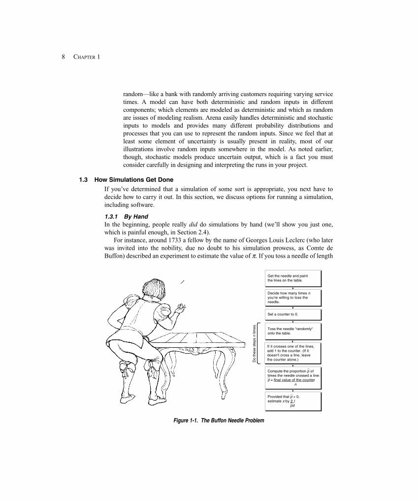
8 CHAPTER 1
random—like a bank with randomly arriving customers requiring varying servicetimes. A model can have both deterministic and random inputs in differentcomponents; which elements are modeled as deterministic and which as randomare issues of modeling realism. Arena easily handles deterministic and stochasticinputs to models and provides many different probability distributions andprocesses that you can use to represent the random inputs. Since we feel that atleast some element of uncertainty is usually present in reality, most of ourillustrations involve random inputs somewhere in the model. As noted earlier,though, stochastic models produce uncertain output, which is a fact you mustconsider carefully in designing and interpreting the runs in your project.
1.3 How Simulations Get Done
If you’ve determined that a simulation of some sort is appropriate, you next have todecide how to carry it out. In this section, we discuss options for running a simulation,including software.
1.3.1 By HandIn the beginning, people really did do simulations by hand (we’ll show you just one,which is painful enough, in Section 2.4).
For instance, around 1733 a fellow by the name of Georges Louis Leclerc (who laterwas invited into the nobility, due no doubt to his simulation prowess, as Comte deBuffon) described an experiment to estimate the value of π. If you toss a needle of length
Provided that p > 0,estimate π by 2 l
pd
Provided that p > 0,estimate π by 2 l
pd
If it crosses one of the lines,add 1 to the counter. (If itdoesn't cross a line, leavethe counter alone.)
If it crosses one of the lines,add 1 to the counter. (If itdoesn't cross a line, leavethe counter alone.)
Get the needle and paintthe lines on the table.Get the needle and paintthe lines on the table.
Decide how many times nyou're willing to toss theneedle.
Decide how many times nyou're willing to toss theneedle.
Set a counter to 0.Set a counter to 0.
Toss the needle "randomly"onto the table.Toss the needle "randomly"onto the table.
Compute the proportion p oftimes the needle crossed a line:p = final value of the counter n
Compute the proportion p oftimes the needle crossed a line:p = final value of the counter n
Do
thes
e st
eps
n tim
es.
Figure 1-1. The Buffon Needle Problem
9WHAT IS SIMULATION?
l onto a table painted with parallel lines spaced d apart (d must be ≥ l), it turns out that theneedle will cross a line with probability p l d= 2 ( )π . So Figure 1-1 shows a simulationexperiment to estimate the value of π . (Don’t try this at home, or at least not with a bigneedle.)
Though this experiment may seem pretty simple (probably even silly) to you, thereare some aspects of it that are common to most simulations:
� The purpose is to estimate something (in this case, π) whose value would be hardto compute exactly (okay, maybe in 1733 that was true).
� The estimate we get at the end is not going to be exactly right; that is, it has someerror associated with it, and it might be nice to get an idea of how large that error islikely to be.
� It seems intuitive that the more tosses we make (that is, the bigger n is), thesmaller the error is likely to be and thus the better the estimate is likely to be.
� In fact, you could do a sequential experiment and just keep tossing until theprobable error is small enough for you to live with, instead of deciding on thenumber n of tosses beforehand.
� You might be able to reduce the error without increasing the number of tosses ifyou invest a little up-front work. Weld a second needle to the first so they cross atright angles at their midpoints; such a weapon is called a Buffon cross. Leave thelines on the table alone. On each toss, record separately whether each needlecrosses a line (it could be that they both cross, neither crosses, or just one but notthe other crosses), and get two different estimates of π. It’s intuitive (and, happily,true) that whether one needle crosses a line is negatively correlated with whetherthe other one does, so the two estimates of π will be negatively correlated witheach other. The average of the two estimates is also an unbiased estimate of π, butwill have less variance than a single-needle estimate from the same number oftosses since it’s likely that if one estimate is high, the other one will be low. (Thisis a physical analog of what’s called a variance-reduction technique, specificallyantithetic variates, and is discussed in Section 12.4.2. It seems like some kind ofcheat or swindle, but it’s really a fair game.)
We’ll come back to these kinds of issues as we talk about more interesting and helpfulsimulations. (For more on the Buffon needle problem, as well as other such interestinghistorical curiosities, see Morgan, 1984.)
In the 1920s and 1930s, statisticians began using random-number machines and tablesin numerical experiments to help them develop and understand statistical theory. Forinstance, Walter A. Shewhart (the quality control pioneer) did numerical experiments bydrawing numbered chips from a bowl to study the first control charts. Guinness Breweryemployee W. S. Gossett did similar numerical sampling experiments to help him gain in-sight into what was going on in mathematical statistics. (To protect his job at Guinness, hepublished his research under the pseudonym “Student” and also developed the t distribu-tion used widely in statistical inference.) Engineers, physicists, and mathematicians haveused various kinds of hand-simulation ideas for many years on a wide variety of problems.
10 CHAPTER 1
1.3.2 Programming in General-Purpose LanguagesAs digital computers appeared in the 1950s and 1960s, people began writing computerprograms in general-purpose procedural languages like FORTRAN to do simulations ofmore complicated systems. Support packages were written to help out with routine choreslike list processing, keeping track of simulated events, and statistical bookkeeping.
This approach was highly customizable and flexible (in terms of the kinds of modelsand manipulations possible), but also painfully tedious and error prone since models hadto be coded pretty much from scratch every time. (Plus, if you dropped your deck ofcards, it could take quite a while to reconstruct your “model.”) For a more detailed historyof discrete-event simulation languages, see Nance (1996) and Nance and Sargent (2003).
As a kind of descendant of simulating with general-purpose programming languag-es, people sometimes use spreadsheet software for some kinds of simulation. This hasproven popular for static models, perhaps with add-ins to facilitate common operationsand to provide higher-quality tools (like random-number generators) than what comesstandard with spreadsheets. But for all but the very simplest dynamic models, the inher-ent limitations of spreadsheets make it at best awkward, and usually practicallyimpossible, to use them for simulations of large, realistic, dynamic models. Section 2.7briefly illustrates two examples of simulating with spreadsheets.
1.3.3 Simulation LanguagesSpecial-purpose simulation languages like GPSS, Simscript, SLAM, and SIMANappeared on the scene some time later and provided a much better framework for thekinds of simulations many people do. Simulation languages became very popular andare still in use.
Nonetheless, you still have to invest quite a bit of time to learn about their featuresand how to use them effectively. And, depending on the user interface provided, there canbe picky, apparently arbitrary, and certainly frustrating syntactical idiosyncrasies thatbedevil even old hands.
1.3.4 High-Level SimulatorsThus, several high-level “simulator” products emerged that are indeed very easy to use.They typically operate by intuitive graphical user interfaces, menus, and dialogs. Youselect from available simulation-modeling constructs, connect them, and run the modelalong with a dynamic graphical animation of system components as they move aroundand change.
However, the domains of many simulators are also rather restricted (like manufactur-ing or communications) and are generally not as flexible as you might like in order tobuild valid models of your systems. Some people feel that these packages may have gonetoo far up the software-hierarchy food chain and have traded away too much flexibility toachieve the ease-of-use goal.
1.3.5 Where Arena Fits InArena combines the ease of use found in high-level simulators with the flexibility ofsimulation languages and even all the way down to general-purpose procedurallanguages like the Microsoft® Visual Basic® programming system or C if you reallywant. It does this by providing alternative and interchangeable templates of graphical

11WHAT IS SIMULATION?
simulation modeling and analysis modules that you can combine to build a fairly widevariety of simulation models. For ease of display and organization, modules are typicallygrouped into panels to compose a template. By switching panels, you gain access to awhole different set of simulation modeling constructs and capabilities. In most cases,modules from different panels can be mixed together in the same model.
Arena maintains its modeling flexibility by being fully hierarchical, as depicted inFigure 1-2. At any time, you can pull in low-level modules from the Blocks and Elementspanel and gain access to simulation-language flexibility if you need to and mix inSIMAN constructs together with the higher-level modules from other templates (Arenais based on, and actually includes, the SIMAN simulation language; see Pedgen,Shannon, and Sadowski 1995 for a complete discussion of SIMAN). For specializedneeds, like complex decision algorithms or accessing data from an external application,you can write pieces of your model in a procedural language like Visual Basic or C/C++.All of this, regardless of how high or low you want to go in the hierarchy, takes place inthe same consistent graphical user interface.
A singlegraphical userinterfaceconsistent atany level ofmodeling
Advanced Process, Advanced TransferPanels Access to more detailed modeling for greater
flexibility
User-Created TemplatesCommonly used constructsCompany-specific processesCompany-specific templatesetc.
Basic Process PanelMany common modeling constructsVery accessible, easy to useReasonable flexibility
Blocks, Elements Panels All the flexibility of the SIMAN simulation
language
Higher
Level ofModeling
Lower
User-Written Visual Basic, C/C++ CodeThe ultimate in flexibilityVBA is built inC/C++ requires compiler
Application Solution TemplatesContact centersPackaging linesHealth careAirports
etc.
Figure 1-2. Arena’s Hierarchical Structure
12 CHAPTER 1
In fact, the modules in Arena are composed of SIMAN components; you can createyour own modules and collect them into your own templates for various classes ofsystems. For instance, Rockwell Automation (formerly Systems Modeling) has builttemplates for general modeling (the Arena template, which is the primary focus of thisbook), high-speed packaging, contact centers, and other industries. Other people havebuilt templates for their company in industries as diverse as mining, auto manufacturing,fast-food, and forest-resource management. In this way, you don’t have to compromisebetween modeling flexibility and ease of use. While this textbook focuses on modelingwith the Arena template, you can get a taste of creating your own modules in Chapter 10.
Further, Arena includes dynamic animation in the same work environment. It alsoprovides integrated support, including graphics, for some of the statistical design andanalysis issues that are part and parcel of a good simulation study.
1.4 When Simulations Are Used
Just as the capabilities and sophistication of simulation languages and packages haveincreased dramatically over the last 40 or 50 years, the concept of how and when to usesimulation has changed. For a thorough account of the development of computer simula-tion in general since the earliest days, see Nance and Sargent (2003).
1.4.1 The Early YearsIn the late 1950s and 1960s, simulation was a very expensive and specialized tool that wasgenerally used only by large corporations that required substantial capital investments.Typical simulation users were found in steel and aerospace corporations. Theseorganizations would form groups of people, mostly Ph.D.s, who would develop large,complex simulation models using available languages, such as FORTRAN. These modelswould then be run on large mainframes charging from $600 to $1,000 per hour.Interestingly, the personal computers that reside on most engineers’ desks today are muchmore powerful and faster than the mainframes of the 1960s.
1.4.2 The Formative YearsThe use of simulation as we know it today began during the 1970s and early 1980s.Computers were becoming faster and cheaper, and the value of simulation was beingdiscovered by other industries, although most of the companies were still quite large.However, simulation was seldom considered until there was a disaster. It became the toolof choice for many companies, notably in the automotive and heavy industries, fordetermining why the disaster occurred and, sometimes, where to point the finger of blame.
We recall the startup of an automotive assembly line, an investment of over $100million, that was not achieving much of its potential. The line was producing a newlyreleased vehicle that was in great demand—far greater than could be satisfied by theexisting output of the line. Management appointed a S.W.A.T. team to analyze theproblem, and that team quickly estimated the lost potential profit to be in excess of$500,000 per day. The team was told, “Find the problem and fix it.” In about three weeks,a simulation was developed and used to identify the problem, which turned out not tohave been on the initial suspect list. The line was ultimately modified and did produce
13WHAT IS SIMULATION?
according to specifications; unfortunately, by that time the competition was producingsimilar vehicles, and the additional output was no longer needed. Ironically, a simulationmodel had been used during the design of the assembly line to determine its feasibility.Unfortunately, many of the processes were new, and engineering had relied onequipment vendors to provide estimates of failures and throughputs. As is often the case,the vendors were extremely optimistic in their estimates. If the original design team hadused the simulation to perform a good sensitivity analysis on these questionable data, theproblem might have been uncovered and resolved well before implementation.
During this time, simulation also found a home in academia as a standard part ofindustrial engineering and operations research curricula. Its growing use in industrycompelled universities to teach it more widely. At the same time, simulation began toreach into quantitative business programs, broadening the number and type of studentsand researchers exposed to its potential.
1.4.3 The Recent PastDuring the late 1980s, simulation began to establish its real roots in business. A largepart of this was due to the introduction of the personal computer and animation.Although simulation was still being used to analyze failed systems, many people wererequesting simulations before production was to begin. (However, in most cases, it wasreally too late to affect the system design, but it did offer the plant manager and systemdesigner the opportunity to spruce up their resumes.) By the end of the 1980s, the valueof simulation was being recognized by many larger firms, several of which actually madesimulation a requirement before approval of any major capital investment. However,simulation was still not in widespread use and was rarely used by smaller firms.
1.4.4 The PresentSimulation really began to mature during the 1990s. Many smaller firms embraced thetool, and it began to see use at the very early stages of projects—where it could have thegreatest impact. Better animation, greater ease of use, faster computers, easy integrationwith other packages, and the emergence of simulators have all helped simulation becomea standard tool in many companies. Although most managers will readily admit thatsimulation can add value to their enterprise, it has yet to become a standard tool thatresides on everyone’s computers. The manner in which simulation is used is alsochanging; it is being employed earlier in the design phase and is often being updated aschanges are made to operating systems. This provides a living simulation model that canbe used for systems analysis on very short notice. Simulation has also invaded the serviceindustry where it is being applied in many non-traditional areas.
The major impediments preventing simulation from becoming a universally acceptedand well-utilized tool are model-development time and the modeling skills required forthe development of a successful simulation. Those are probably the reasons why you’rereading this book!
1.4.5 The FutureThe rate of change in simulation has accelerated in recent years, and there is every reasonto believe that it will continue its rapid growth and cross the bridges to mainstream
14 CHAPTER 1
acceptance. Simulation software has taken advantage of advancements in technology,enabling quicker model runs, higher-fidelity animations, and comprehensive dataanalysis. This trend must continue if simulation is to become a state-of-the-art and yeteasy-to-use tool, required for effective decision-making. This evolution of simulationsoftware has allowed for greater integration of simulation with other packages (likespreadsheets, databases, and word processors). It is now becoming possible to foreseethe complete integration of simulation with other software packages that collect, store,and analyze system data at the front end along with software that helps control thesystem at the back end.
The Internet and intranets have had a tremendous impact on the way organizationsconduct their business. Information sharing in real time is not only possible, but isbecoming mandatory. Simulation tools are being developed to support distributed modelbuilding, distributed processing, and remote analysis of results. Soon, a set of enterprise-wide tools will be available to provide the ability for employees throughout anorganization to obtain answers to critical and even routine questions.
In order to make simulation easier to use by more people, we will see more verticalproducts aimed at very specific markets. This will allow analysts to constructsimulations easily, using modeling constructs designed for their industry or companywith terminology that directly relates to their environment. These may be veryspecialized tools designed for very specific environments, but they should still have thecapability to model any system activities that are unique to each simulation project.Some of these types of products are on the market today in application areas such ashigh-speed packaging, contact centers, communications, and business-process re-engineering.
Today's simulation projects concentrate on strategic decision making, typicallyaround the design or redesign of complex systems. The next logical step is to use andevolve the same simulation to assist in operational decision making. This approachrequires that the simulation model be kept current, but it also allows for examining andtesting systems as market conditions, demands, and system processes change. As weprogress to this next logical step, simulations will no longer be disposable or used onlyonce, but will become a critical part of the operation of the ongoing system.
With the rapid advances being made in computers and software, it is very difficult topredict much about the simulations of the distant future, but even now we are seeing thedevelopment and implementation of features such as automatic statistical analysis,software that recommends system changes, simulations totally integrated with systemoperating software, and yes, even virtual reality.
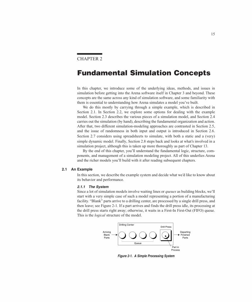
15FUNDAMENTAL SIMULATION CONCEPTS
CHAPTER 2
Fundamental Simulation Concepts
In this chapter, we introduce some of the underlying ideas, methods, and issues insimulation before getting into the Arena software itself in Chapter 3 and beyond. Theseconcepts are the same across any kind of simulation software, and some familiarity withthem is essential to understanding how Arena simulates a model you’ve built.
We do this mostly by carrying through a simple example, which is described inSection 2.1. In Section 2.2, we explore some options for dealing with the examplemodel. Section 2.3 describes the various pieces of a simulation model, and Section 2.4carries out the simulation (by hand), describing the fundamental organization and action.After that, two different simulation-modeling approaches are contrasted in Section 2.5,and the issue of randomness in both input and output is introduced in Section 2.6.Section 2.7 considers using spreadsheets to simulate, with both a static and a (very)simple dynamic model. Finally, Section 2.8 steps back and looks at what’s involved in asimulation project, although this is taken up more thoroughly as part of Chapter 13.
By the end of this chapter, you’ll understand the fundamental logic, structure, com-ponents, and management of a simulation modeling project. All of this underlies Arenaand the richer models you’ll build with it after reading subsequent chapters.
2.1 An Example
In this section, we describe the example system and decide what we’d like to know aboutits behavior and performance.
2.1.1 The SystemSince a lot of simulation models involve waiting lines or queues as building blocks, we’llstart with a very simple case of such a model representing a portion of a manufacturingfacility. “Blank” parts arrive to a drilling center, are processed by a single drill press, andthen leave; see Figure 2-1. If a part arrives and finds the drill press idle, its processing atthe drill press starts right away; otherwise, it waits in a First-In First-Out (FIFO) queue.This is the logical structure of the model.
Drill Press
Queue
ArrivingBlankParts
DepartingFinished
Parts
Part inProcess
Drilling Center
Figure 2-1. A Simple Processing System
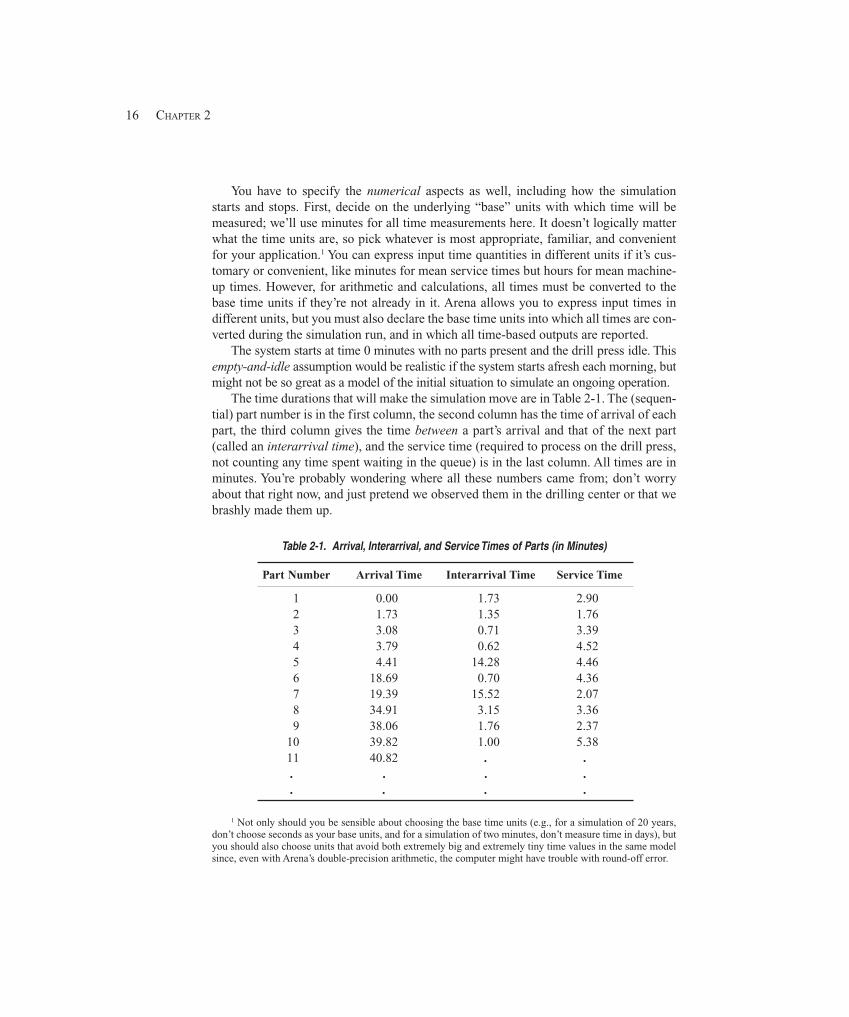
16 CHAPTER 2
You have to specify the numerical aspects as well, including how the simulationstarts and stops. First, decide on the underlying “base” units with which time will bemeasured; we’ll use minutes for all time measurements here. It doesn’t logically matterwhat the time units are, so pick whatever is most appropriate, familiar, and convenientfor your application.1 You can express input time quantities in different units if it’s cus-tomary or convenient, like minutes for mean service times but hours for mean machine-up times. However, for arithmetic and calculations, all times must be converted to thebase time units if they’re not already in it. Arena allows you to express input times indifferent units, but you must also declare the base time units into which all times are con-verted during the simulation run, and in which all time-based outputs are reported.
The system starts at time 0 minutes with no parts present and the drill press idle. Thisempty-and-idle assumption would be realistic if the system starts afresh each morning, butmight not be so great as a model of the initial situation to simulate an ongoing operation.
The time durations that will make the simulation move are in Table 2-1. The (sequen-tial) part number is in the first column, the second column has the time of arrival of eachpart, the third column gives the time between a part’s arrival and that of the next part(called an interarrival time), and the service time (required to process on the drill press,not counting any time spent waiting in the queue) is in the last column. All times are inminutes. You’re probably wondering where all these numbers came from; don’t worryabout that right now, and just pretend we observed them in the drilling center or that webrashly made them up.
Table 2-1. Arrival, Interarrival, and Service Times of Parts (in Minutes)
Part Number Arrival Time Interarrival Time Service Time
1 0.00 1.73 2.902 1.73 1.35 1.763 3.08 0.71 3.394 3.79 0.62 4.525 4.41 14.28 4.466 18.69 0.70 4.367 19.39 15.52 2.078 34.91 3.15 3.369 38.06 1.76 2.37
10 39.82 1.00 5.3811 40.82 . ... . ...... . ... . ... . .... . . ... . ... . ...
1 Not only should you be sensible about choosing the base time units (e.g., for a simulation of 20 years,don’t choose seconds as your base units, and for a simulation of two minutes, don’t measure time in days), butyou should also choose units that avoid both extremely big and extremely tiny time values in the same modelsince, even with Arena’s double-precision arithmetic, the computer might have trouble with round-off error.
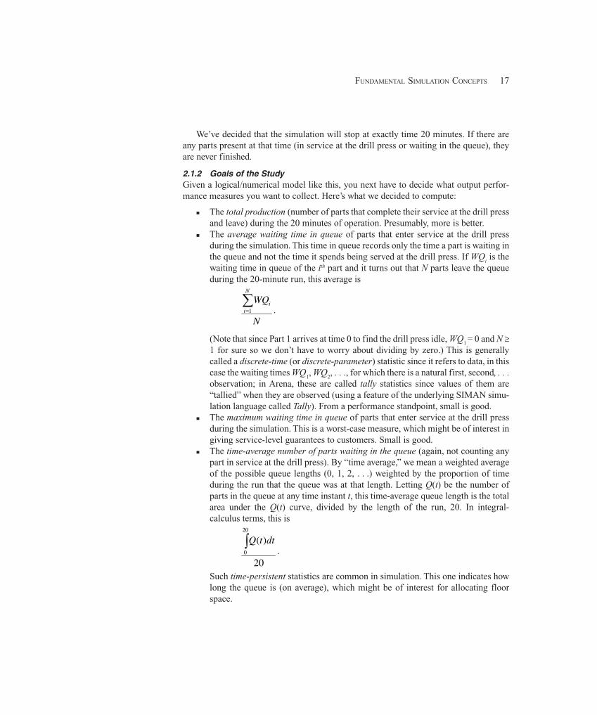
17FUNDAMENTAL SIMULATION CONCEPTS
We’ve decided that the simulation will stop at exactly time 20 minutes. If there areany parts present at that time (in service at the drill press or waiting in the queue), theyare never finished.
2.1.2 Goals of the StudyGiven a logical/numerical model like this, you next have to decide what output perfor-mance measures you want to collect. Here’s what we decided to compute:
� The total production (number of parts that complete their service at the drill pressand leave) during the 20 minutes of operation. Presumably, more is better.
� The average waiting time in queue of parts that enter service at the drill pressduring the simulation. This time in queue records only the time a part is waiting inthe queue and not the time it spends being served at the drill press. If WQ
i is the
waiting time in queue of the ith part and it turns out that N parts leave the queueduring the 20-minute run, this average is
N
WQN
ii∑
=1 .
(Note that since Part 1 arrives at time 0 to find the drill press idle, WQ1 = 0 and N ≥
1 for sure so we don’t have to worry about dividing by zero.) This is generallycalled a discrete-time (or discrete-parameter) statistic since it refers to data, in thiscase the waiting times WQ
1, WQ
2, . . ., for which there is a natural first, second, . . .
observation; in Arena, these are called tally statistics since values of them are“tallied” when they are observed (using a feature of the underlying SIMAN simu-lation language called Tally). From a performance standpoint, small is good.
� The maximum waiting time in queue of parts that enter service at the drill pressduring the simulation. This is a worst-case measure, which might be of interest ingiving service-level guarantees to customers. Small is good.
� The time-average number of parts waiting in the queue (again, not counting anypart in service at the drill press). By “time average,” we mean a weighted averageof the possible queue lengths (0, 1, 2, . . .) weighted by the proportion of timeduring the run that the queue was at that length. Letting Q(t) be the number ofparts in the queue at any time instant t, this time-average queue length is the totalarea under the Q(t) curve, divided by the length of the run, 20. In integral-calculus terms, this is
20
)(20
0∫ dttQ
.
Such time-persistent statistics are common in simulation. This one indicates howlong the queue is (on average), which might be of interest for allocating floorspace.
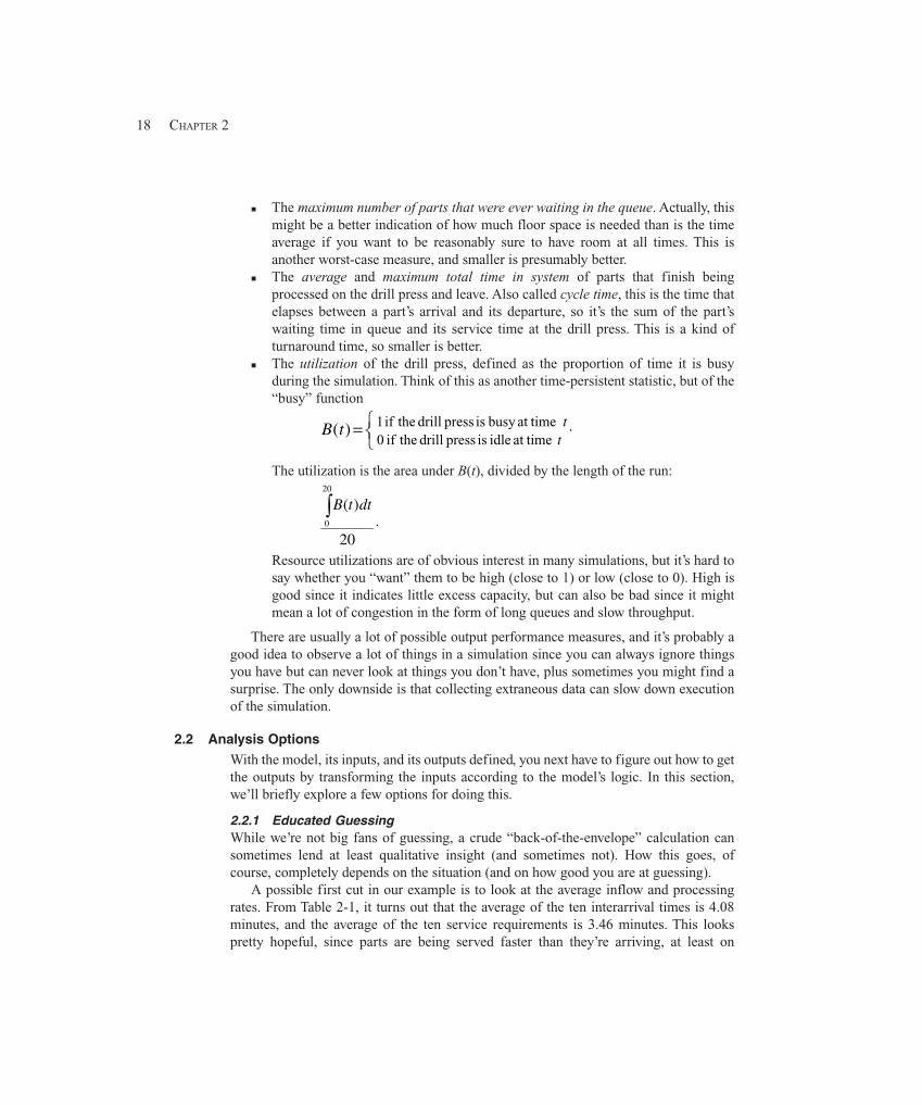
18 CHAPTER 2
� The maximum number of parts that were ever waiting in the queue. Actually, thismight be a better indication of how much floor space is needed than is the timeaverage if you want to be reasonably sure to have room at all times. This isanother worst-case measure, and smaller is presumably better.
� The average and maximum total time in system of parts that finish beingprocessed on the drill press and leave. Also called cycle time, this is the time thatelapses between a part’s arrival and its departure, so it’s the sum of the part’swaiting time in queue and its service time at the drill press. This is a kind ofturnaround time, so smaller is better.
� The utilization of the drill press, defined as the proportion of time it is busyduring the simulation. Think of this as another time-persistent statistic, but of the“busy” function
⎩⎨⎧ ⋅= t
ttB
time at busyis pressdrill the if 1
time at idle is pressdrill the if 0)(
The utilization is the area under B(t), divided by the length of the run:
20
)(20
0∫ dttB
.
Resource utilizations are of obvious interest in many simulations, but it’s hard tosay whether you “want” them to be high (close to 1) or low (close to 0). High isgood since it indicates little excess capacity, but can also be bad since it mightmean a lot of congestion in the form of long queues and slow throughput.
There are usually a lot of possible output performance measures, and it’s probably agood idea to observe a lot of things in a simulation since you can always ignore thingsyou have but can never look at things you don’t have, plus sometimes you might find asurprise. The only downside is that collecting extraneous data can slow down executionof the simulation.
2.2 Analysis Options
With the model, its inputs, and its outputs defined, you next have to figure out how to getthe outputs by transforming the inputs according to the model’s logic. In this section,we’ll briefly explore a few options for doing this.
2.2.1 Educated GuessingWhile we’re not big fans of guessing, a crude “back-of-the-envelope” calculation cansometimes lend at least qualitative insight (and sometimes not). How this goes, ofcourse, completely depends on the situation (and on how good you are at guessing).
A possible first cut in our example is to look at the average inflow and processingrates. From Table 2-1, it turns out that the average of the ten interarrival times is 4.08minutes, and the average of the ten service requirements is 3.46 minutes. This lookspretty hopeful, since parts are being served faster than they’re arriving, at least on
19FUNDAMENTAL SIMULATION CONCEPTS
average, meaning that the system has a chance of operating in a stable way over the longterm and not “exploding.” If these averages were exactly what happened for each part—no variation either way—then there would never be a queue and all waiting times inqueue would be zero, a happy thought indeed. No matter how happy this thought mightbe, though, it’s probably wrong since the data clearly show that there is variation in theinterarrival and service times, which could create a queue sometimes; for example, ifthere happened to be some small interarrival times during a period when there alsohappened to be some large service times.
Suppose, on the other hand, that the averages in the input data in Table 2-1 had comeout the other way, with the average interarrival time being smaller than the averageservice time. If this situation persisted, parts would, on average, be arriving faster thanthey could be served, implying heavy congestion (at least after a while, probably longerthan the 20-minute run we have planned). Indeed, the system will explode over the longrun— not a happy thought.
The truth, as usual, will probably be between the extremes. Clearly, guessing has itslimits.
2.2.2 Queueing TheorySince this is a queue, why not use queueing theory? It’s been around for almost a century,and a lot of very bright people have worked very hard to develop it. In some situations, itcan result in simple formulas from which you can get a lot of insight.
Probably the simplest and most popular object of queueing theory is the M/M/1queue. The first “M” states that the arrival process is Markovian; that is, the interarrivaltimes are independent and identically distributed “draws” from an exponential probabil-ity distribution (see Appendices B and C for a brief refresher on probability and distribu-tions). The second “M” stands for the service-time distribution, and here it’s alsoexponential. The “1” indicates that there’s just a single server. So at least on the surfacethis looks pretty good for our model.
Better yet, most of our output performance measures can be expressed as simpleformulas. For instance, the average waiting time in queue (expected from a long run) is
μμ μ
S
A S
2
−
where μA
is the expected value of the interarrival-time distribution and μS is the expected
value of the service-time distribution (assuming that μA > μ
S so the queue doesn’t
explode). So one immediate idea is to use the data to estimate μA and μ
S , then plug these
estimates into the formula; for our data, we get 3.462/(4.08 – 3.46) = 19.31 minutes.Such an approach can sometimes give a reasonable order-of-magnitude approxima-
tion that might facilitate crude comparisons. But there are problems too (see Exercise2-6):
� The estimates of μA and μ
S aren’t exact, so there will be error in the result as well.
� The assumptions of exponential interarrival-time and service-time distributions areessential to deriving the formula above, and we probably don’t satisfy these
20 CHAPTER 2
assumptions. This calls into question the validity of the formula. While there aremore sophisticated versions for more general queueing models, there will always beassumptions to worry about.
� The formula is for long-run performance, not the 20-minute period we want. Thisis typical of most (but not all) queueing theory.
� The formula doesn’t provide any information on the natural variability in thesystem. This is not only a difficulty in analysis but might also be of inherentinterest itself, as in the variability of production. (It’s sometimes possible, though,to find other formulas that measure variability.)
Many people feel that queueing theory can prove valuable as a first-cut approxima-tion to get an idea of where things stand and to provide guidance about what kinds ofsimulations might be appropriate at the next step in the project. We agree, but urge you tokeep in mind the problems listed above and temper your interpretations accordingly.
2.2.3 Mechanistic SimulationSo all of this brings us back to simulation. By “mechanistic” we mean that the individualoperations (arrivals, service by the drill press, etc.) will occur as they would in reality.The movements and changes of things in the simulation model occur at the right “time,”in the right order, and have the right effects on each other and the statistical-accumulatorvariables.
In this way, simulation provides a completely concrete, “brute-force” way of dealingdirectly with the model. There’s nothing mysterious about how it works—just a few basicideas and then a whole lot of details and bookkeeping that software like Arena handlesfor you.
2.3 Pieces of a Simulation Model
We’ll talk about the various parts of a simulation model in this section, all in reference toour example.
2.3.1 EntitiesMost simulations involve “players” called entities that move around, change status, affectand are affected by other entities and the state of the system, and affect the outputperformance measures. Entities are the dynamic objects in the simulation—they usuallyare created, move around for a while, and then are disposed of as they leave. It’s possible,though, to have entities that never leave but just keep circulating in the system. However,all entities have to be created, either by you or automatically by the software.
The entities for our example are the parts to be processed. They’re created when theyarrive, move through the queue (if necessary), are served by the drill press, and are thendisposed of as they leave. Even though there’s only one kind of entity in our example,there can be many independent “copies,” or realizations of it in existence at a time, justas there can be many different individual parts of this type in the real system at a time.
Most entities represent “real” things in a simulation. You can have lots of differentkinds of entities and many realizations of each kind of entity existing in the model at atime. For instance, you could have several different kinds of parts, perhaps requiring
21FUNDAMENTAL SIMULATION CONCEPTS
Figure 2-2. A Victorious Breakdown Demon
different processing and routing and having different priority; moreover, there could beseveral realizations of each kind of part floating around in the model at a time.
There are situations, though, where “fake” (or “logic”) entities not corresponding toanything tangible can be conjured up to take care of certain modeling operations. Forinstance, one way to model machine failures is to create a “breakdown demon” (seeFigure 2-2) that lurks in the shadows during the machine’s up time, runs out and kicks themachine when it’s supposed to break down, stands triumphantly over it until it getsrepaired, then scurries back to the shadows and begins another lurking period rep-resenting the machine’s next up time. A similar example is a “break angel” that arrivesperiodically and takes a server off duty. (For both of these examples, however, Arena haseasier built-in modeling constructs that don’t require creation of such fake entities.)
Figuring out what the entities are is probably the first thing you need to do inmodeling a system.
2.3.2 AttributesTo individualize entities, you attach attributes to them. An attribute is a commoncharacteristic of all entities, but with a specific value that can differ from one entity toanother. For instance, our part entities could have attributes called Due Date,Priority, and Color to indicate these characteristics for each individual entity. It’s upto you to figure out what attributes your entities need, name them, assign values to them,change them as appropriate, and then use them when it’s time (that’s all part of modeling).
The most important thing to remember about attributes is that their values are tied tospecific entities. The same attribute will generally have different values for different enti-ties, just as different parts have different due dates, priorities, and color codes. Think ofan attribute as a tag attached to each entity, but what’s written on this tag can differ acrossentities to characterize them individually. An analogy to traditional computer program-ming is that attributes are local variables—in this case, local to each individual entity.
Arena keeps track of some attributes automatically, but you may need to define,assign values to, change, and use attributes of your own.
2.3.3 (Global) VariablesA variable (or a global variable) is a piece of information that reflects somecharacteristic of your system, regardless of how many or what kinds of entities might be
22 CHAPTER 2
around. You can have many different variables in a model, but each one is unique. Thereare two types of variables: Arena built-in variables (number in queue, number of busyservers, current simulation clock time, and so on) and user-defined variables (meanservice time, travel time, current shift, and so on). In contrast to attributes, variables arenot tied to any specific entity, but rather pertain to the system at large. They’re accessibleby all entities, and many can be changed by any entity. If you think of attributes as tagsattached to the entities currently floating around in the room, then think of variables as(rewriteable) writing on the wall.
Variables are used for lots of different purposes. For instance, the time to movebetween any two stations in a model might be the same throughout the model, and avariable called Transfer Time could be defined and set to the appropriate value andthen used wherever this constant is needed; in a modified model where this time is set toa different constant, you’d only need to change the definition of Transfer Time tochange its value throughout the model. Variables can also represent something thatchanges during the simulation, like the number of parts in a certain subassembly area ofthe larger model, which is incremented by a part entity when it enters the area anddecremented by a part when it leaves the area. Arena Variables can be vectors or matricesif it is convenient to organize the information as lists or two-dimensional tables ofindividual values.
Some built-in Arena variables for our model include the status of the drill press(busy or idle), the time (simulation clock), and the current length of the queue.
2.3.4 ResourcesEntities often compete with each other for service from resources that represent thingslike personnel, equipment, or space in a storage area of limited size. An entity seizes(units of) a resource when available and releases it (or them) when finished. It’s better tothink of the resource as being given to the entity rather than the entity being assigned tothe resource since an entity (like a part) could need simultaneous service from multipleresources (such as a machine and a person).
A resource can represent a group of several individual servers, each of which iscalled a unit of that resource. This is useful to model, for instance, several identical“parallel” agents at an airline ticketing counter. The number of available units of aresource can be changed during the simulation run to represent agents going on break oropening up their stations if things get busy. If a resource has multiple units, or a variablenumber of units, we have to generalize our definition in Section 2.1.2 of resourceutilization to be the time-average number of units of the resource that are busy, dividedby the time-average number of units of the resource that are available. In our example,there is just a single drill press, so this resource has a single unit available at all times.
2.3.5 QueuesWhen an entity can’t move on, perhaps because it needs to seize a unit of a resource that’stied up by another entity, it needs a place to wait, which is the purpose of a queue. InArena, queues have names and can also have capacities to represent, for instance, limitedfloor space for a buffer. You’d have to decide as part of your modeling how to handle anentity arriving at a queue that’s already full.
23FUNDAMENTAL SIMULATION CONCEPTS
2.3.6 Statistical AccumulatorsTo get your output performance measures, you have to keep track of various intermediatestatistical-accumulator variables as the simulation progresses. In our example, we’llwatch:
� The number of parts produced so far� The total of the waiting times in queue so far� The number of parts that have passed through the queue so far (since we’ll need
this as the denominator in the average waiting-time output measure)� The longest time spent in queue we’ve seen so far� The total of the time spent in the system by all parts that have departed so far� The longest time in system we’ve seen so far� The area so far under the queue-length curve Q(t)� The highest level that Q(t) has so far attained� The area so far under the server-busy function B(t)
All of these accumulators should be initialized to 0. When something happens in thesimulation, you have to update the affected accumulators in the appropriate way.
Arena takes care of most (but sometimes not all) of the statistical accumulationyou’re likely to want, so most of this will be invisible to you except for asking for it insome situations. But in our hand simulation, we’ll do it all manually so you can see howit goes and will understand how to do it yourself in Arena if you need to.
2.3.7 EventsNow let’s turn to how things work when we run our model. Basically, everything’scentered around events. An event is something that happens at an instant of (simulated)time that might change attributes, variables, or statistical accumulators. In our example,there are three kinds of events:
� Arrival: A new part enters the system.� Departure: A part finishes its service at the drill press and leaves the system.� The End: The simulation is stopped at time 20 minutes. (It might seem rather
artificial to anoint this as an event, but it certainly changes things, and this is oneway to stop a simulation.)
In addition to the above events, there of course must be an initialization to set thingsup. We’ll explain the logic of each event in more detail later.
Other things happen in our example model, but needn’t be separate events. Forinstance, parts leave the queue and begin service at the drill press, which changes thesystem, but this only happens because of some other entity’s departure, which is alreadyan event.
To execute, a simulation has to keep track of the events that are supposed to happen inthe (simulated) future. In Arena, this information is stored in an event calendar. We won’tget into the details of the event calendar’s data structure, but here’s the idea: When thelogic of the simulation calls for it, a record of information for a future event is placed onthe event calendar. This event record contains identification of the entity involved, theevent time, and the kind of event it will be. Arena places each newly scheduled event on
24 CHAPTER 2
the calendar so that the next (soonest) event is always at the top of the calendar (that is,the new event record is sorted onto the calendar in increasing order of event times).When it’s time to execute the next event, the top record is removed from the calendar andthe information in this record is used to execute the appropriate logic; part of this logicmight be to place one or more new event records onto the calendar. It’s possible that, at acertain time, it doesn’t make sense to have a certain event type scheduled (in our model,if the drill press is idle, you don’t want a departure event to be scheduled), in which casethere’s just no record for that kind of event on the calendar, so it obviously can’t happennext. Though this model doesn’t require it, it’s also possible to have several events of thesame kind scheduled on the calendar at once, for different times and for different entities.
In a discrete-event model, the variables that describe the system don’t changebetween successive events. Most of the work in event-driven simulation involves gettingthe logic right for what happens with each kind of event. As you’ll see later, though,modeling with Arena usually gets you out of having to define this detailed event logicexplicitly, although you can do so if you want in order to represent something verypeculiar to your model that Arena isn’t set up to handle directly.
2.3.8 Simulation ClockThe current value of time in the simulation is simply held in a variable called the simula-tion clock. Unlike real time, the simulation clock does not take on all values and flowcontinuously; rather, it lurches from the time of one event to the time of the next eventscheduled to happen. Since nothing changes between events, there is no need to waste(real) time looking at (simulated) times that don’t matter.
The simulation clock interacts closely with the event calendar. At initialization of thesimulation, and then after executing each event, the event calendar’s top record (alwaysthe one for the next event) is taken off the calendar. The simulation clock lurches forwardto the time of that event (one of the data fields in the event record), and the information inthe removed event record (entity identification, event time, and event type) is used toexecute the event at that instant of simulated time. How the event is executed clearlydepends on what kind of event it is as well as on the model state at that time, but ingeneral could include updating variables and statistical accumulators, altering entityattributes, and placing new event records onto the calendar.
While we’ll keep track of the simulation clock and event calendar ourselves in thehand simulation, these are clearly important pieces of any dynamic simulation, so Arenakeeps track of them (the clock is a variable called TNOW in Arena).
2.3.9 Starting and StoppingImportant, but sometimes-overlooked, issues in a simulation are how it will start andstop. For our example, we’ve made specific assumptions about this, so it’ll be easy tofigure out how to translate them into values for attributes, variables, accumulators, theevent calendar, and the clock.
Arena does a lot of things for you automatically, but it can’t decide modeling issueslike starting and stopping rules. You have to determine the appropriate startingconditions, how long a run should last, and whether it should stop at a particular time (as
25FUNDAMENTAL SIMULATION CONCEPTS
we’ll do at time 20 minutes) or whether it should stop when something specific happens(like as soon as 100 finished parts are produced). It’s important to think about this andmake assumptions consistent with what you’re modeling; these decisions can have just asgreat an effect on your results as can more obvious things like values of input parameters(such as interarrival-time means, service-time variances, and the number of machines).
You should do something specific (and conscious) to stop the simulation with Arena,since it turns out that, in many situations, taking all the defaults will cause your simula-tion to run forever (or until you get sick of waiting and kill it, whichever comes first).
2.4 Event-Driven Hand Simulation
We’ll let you have the gory details of the hand simulation in this section, after outliningthe action and defining how to keep track of things.
2.4.1 Outline of the ActionHere’s roughly how things go for each event:
� Arrival: A new part shows up.� Schedule the next new part to arrive later, at the next arrival time, by placing a
new event record for it onto the event calendar.� Update the time-persistent statistics (between the last event and now).� Store the arriving part’s time of arrival (the current value of the clock) in an
attribute, which will be needed later to compute its total time in system andpossibly the time it spends waiting in the queue.
� If the drill press is idle, the arriving part goes right into service (experiencinga time in queue of zero), so the drill press is made busy and the end of thispart’s service is scheduled. Tally this part’s time in queue (zero).
� On the other hand, if the drill press is already busy with another part, thearriving part is put at the end of the queue and the queue-length variable isincremented.
� Departure: The part being served by the drill press is done and ready to leave.� Increment the number-produced statistical accumulator.� Compute and tally the total time in system of the departing part by taking the
current value of the clock minus the part’s arrival time (stored in an attributeduring the Arrival event).
� Update the time-persistent statistics.� If there are any parts in queue, take the first one out, compute and tally its
time in queue (which is now ending), and begin its service at the drill press byscheduling its departure event (that is, place it on the event calendar).
� On the other hand, if the queue is empty, then make the drill press idle. Notethat in this case, there’s no departure event scheduled on the event calendar.
� The End: The simulation is over.� Update the time-persistent statistics to the end of the simulation.� Compute and report the final summary output performance measures.
26 CHAPTER 2
After each event (except the end event), the event calendar’s top record is removed,indicating what event will happen next and at what time. The simulation clock isadvanced to that time, and the appropriate logic is carried out.
2.4.2 Keeping Track of ThingsAll the calculations for the hand simulation are detailed in Table 2-2. Traces of Q(t) andB(t) over the whole simulation are in Figure 2-3. Each row in Table 2-2 represents anevent concerning a particular part (in the first column) at time t (second column), and thesituation after completion of the logic for that event (in the other columns). The othercolumn groups are:
� Event: This describes what just happened; Arr and Dep refer respectively to anarrival and a departure.
� Variables: These are the values of the number Q(t) of parts in queue and theserver-busy function B(t).
� Attributes: Each arriving entity’s arrival time is assigned when it arrives and iscarried along with it throughout. If a part is in service at the drill press, its arrivaltime is at the right edge of the column and is not enclosed in parentheses. Thearrival times of any parts in the queue, in right-to-left order (to agree with Figure2-1), extend back toward the left and are in parentheses. For instance, at the end ofthe run, the part in service arrived at time 18.69, and the part that’s first (and only)in the queue arrived at time 19.39. We have to keep track of these to compute thetime in queue of a part when it enters service at the drill press after having waitedin the queue as well as the total time in system of a part when it leaves.
� Statistical Accumulators: We have to initialize and then update these as we goalong to watch what happens. They are:
P = the total number of parts produced so farN = the number of entities that have passed through the queue so farΣWQ = the sum of the queue times that have been observed so farWQ* = the maximum time in queue observed so farΣTS = the sum of the total times in system that have been observed so farTS* = the maximum total time in system observed so far∫ Q = the area under the Q(t) curve so farQ* = the maximum value of Q(t) so far∫ B = the area under the B(t) curve so far
� Event Calendar: These are the event records as described earlier. Note that, ateach event time, the top record on the event calendar becomes the first threeentries under “Just-Finished Event” at the left edge of the entire table in the nextrow, at the next event time.
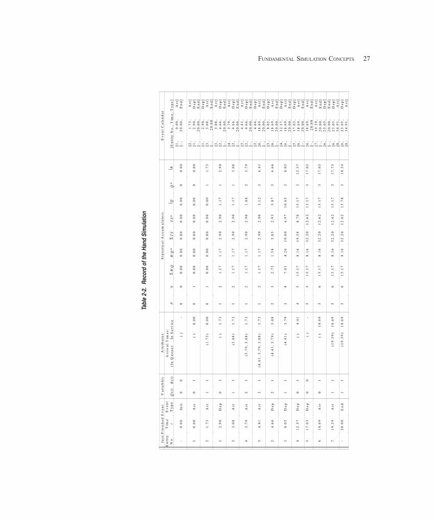
27FUNDAMENTAL SIMULATION CONCEPTS
Tabl
e 2-
2.Re
cord
of t
he H
and
Sim
ulat
ion
Just
-Fin
ish
ed
Ev
en
tV
ari
ab
les
Att
rib
ute
sS
tati
stic
al
Ac
cu
mu
lato
rsE
ve
nt
Ca
len
da
rE
nti
tyN
o.
Tim
et
Ev
en
tT
yp
eQ
( t)
B( t
)A
rriv
al
Tim
es:
(In
Qu
eu
e)
In S
erv
ice
PN
ΣW
QW
Q*
ΣT
ST
S*
*∫ B
[
En
tity
No
., T
ime
, T
yp
e]
–0
.00
Init
00
( )
–0
00
.00
0.0
00
.00
0.0
00
.00
00
.00
[1,
[–,
0.0
0,
20
.00
,A
rr]
En
d]
10
.00
Arr
01
( )
0.0
00
10
.00
0.0
00
.00
0.0
00
.00
00
.00
[2,
[1,
[–,
1.7
3,
2.9
0,
20
.00
,
Arr
]D
ep
]E
nd
]
21
.73
Arr
11
(1.7
3)
0.0
00
10
.00
0.0
00
.00
0.0
00
.00
11
.73
[1,
[3,
[–,
2.9
0,
3.0
8,
20
.00
De
p]
Arr
]E
nd
]
12
.90
De
p0
1(
)1
.73
12
1.1
71
.17
2.9
02
.90
1.1
71
2.9
0[3
,[2
,[–
,
3.0
8,
4.6
6,
20
.00
,
Arr
]D
ep
]E
nd
]
33
.08
Arr
11
(3.0
8)
1.7
31
21
.17
1.1
72
.90
2.9
01
.17
13
.08
[4,
[2,
[–,
3.7
9,
4.6
6,
20
.00
,
Arr
]D
ep
]E
nd
]
43
.79
Arr
21
(3.7
9,
3.0
8)
1.7
31
21
.17
1.1
72
.90
2.9
01
.88
23
.79
[5,
[2,
[–,
4.4
1,
4.6
6,
20
.00
,
Arr
]D
ep
]E
nd
]
54
.41
Arr
31
(4.4
1,
3.7
9,
3.0
8)
1.7
31
21
.17
1.1
72
.90
2.9
03
.12
34
.41
[2,
[6,
[–,
4.6
6,
18
.69
,2
0.0
0,
De
p]
Arr
]E
nd
]
24
.66
De
p2
1(4
.41
, 3
.79
)3
.08
23
2.7
51
.58
5.8
32
.93
3.8
73
4.6
6[3
,[6
,[–
,
8.0
5,
18
.69
,2
0.0
0,
De
p]
Arr
]E
nd
]
38
.05
De
p1
1(4
.41
)3
.79
34
7.0
14
.26
10
.80
4.9
71
0.6
53
8.0
5[4
,[6
,[–
,
12
.57
,1
8.6
9,
20
.00
,
De
p]
Arr
]E
nd
]
41
2.5
7D
ep
01
( )
4.4
14
51
5.1
78
.16
19
.58
8.7
81
5.1
73
12
.57
[5,
[6,
[–,
17
.03
,1
8.6
9,
20
.00
,
De
p]
Arr
]E
nd
]5
17
.03
De
p0
0(
)–
55
15
.17
8.1
63
2.2
01
2.6
21
5.1
73
17
.03
[6,
[–,
18
.69
,2
0.0
0A
rr]
En
d]
61
8.6
9A
rr0
1(
)1
8.6
95
61
5.1
78
.16
32
.20
12
.62
15
.17
31
7.0
3[7
,[–
,[6
,
19
.39
,2
0.0
0,
23
.05
,
Arr
]E
nd
]D
ep
]
71
9.3
9A
rr1
1(1
9.3
9)
18
.69
56
15
.17
8.1
63
2.2
01
2.6
21
5.1
73
17
.73
[–,
[6,
[8,
20
.00
,2
3.0
5,
34
.91
,
En
d]
De
p]
Arr
]–
20
.00
En
d1
1(1
9.3
9)
18
.69
56
15
.17
8.1
63
2.2
01
2.6
21
5.7
83
18
.34
[6,
[8,
23
.05
,3
4.9
1,
De
p]
Arr
]
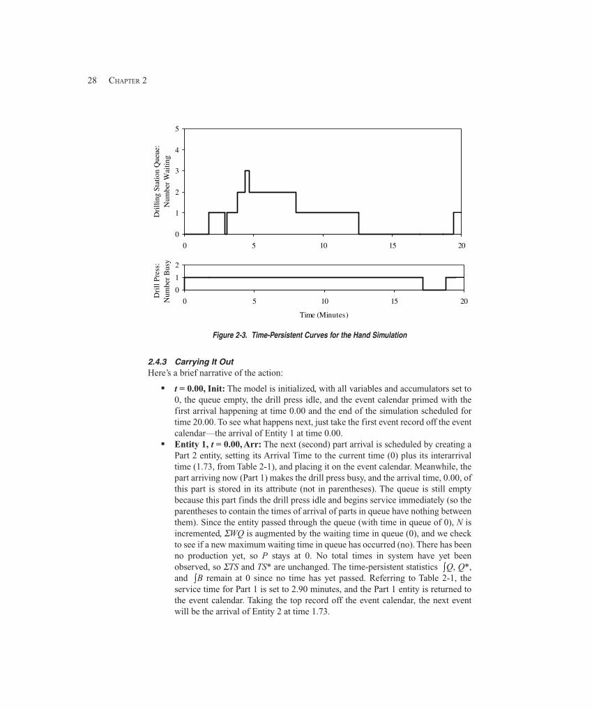
28 CHAPTER 2
0
1
2
3
4
5
0 5 10 15 20
Dri
lling
Sta
tion
Que
ue:
Num
ber
Wai
ting
0
1
2
0 5 10 15 20
Time (Minutes)
Dri
ll Pr
ess:
Num
ber
Bus
y
Figure 2-3. Time-Persistent Curves for the Hand Simulation
2.4.3 Carrying It OutHere’s a brief narrative of the action:
� t = 0.00, Init: The model is initialized, with all variables and accumulators set to0, the queue empty, the drill press idle, and the event calendar primed with thefirst arrival happening at time 0.00 and the end of the simulation scheduled fortime 20.00. To see what happens next, just take the first event record off the eventcalendar—the arrival of Entity 1 at time 0.00.
� Entity 1, t = 0.00, Arr: The next (second) part arrival is scheduled by creating aPart 2 entity, setting its Arrival Time to the current time (0) plus its interarrivaltime (1.73, from Table 2-1), and placing it on the event calendar. Meanwhile, thepart arriving now (Part 1) makes the drill press busy, and the arrival time, 0.00, ofthis part is stored in its attribute (not in parentheses). The queue is still emptybecause this part finds the drill press idle and begins service immediately (so theparentheses to contain the times of arrival of parts in queue have nothing betweenthem). Since the entity passed through the queue (with time in queue of 0), N isincremented, ΣWQ is augmented by the waiting time in queue (0), and we checkto see if a new maximum waiting time in queue has occurred (no). There has beenno production yet, so P stays at 0. No total times in system have yet beenobserved, so ΣTS and TS* are unchanged. The time-persistent statistics ∫Q, Q*,and ∫B remain at 0 since no time has yet passed. Referring to Table 2-1, theservice time for Part 1 is set to 2.90 minutes, and the Part 1 entity is returned tothe event calendar. Taking the top record off the event calendar, the next eventwill be the arrival of Entity 2 at time 1.73.
29FUNDAMENTAL SIMULATION CONCEPTS
� Entity 2, t = 1.73, Arr: The next (third) part arrival is scheduled by creating a Part3 entity, setting its Arrival Time to the current time (1.73) plus its interarrival time(1.35, from Table 2-1), and placing it on the event calendar, which schedules thearrival of this part at time 1.73 + 1.35 = 3.08. Meanwhile, the part arriving now(Part 2) finds the drill press already busy (with Part 1), so it must queue up. Thedrill press is still busy, so B(t) stays at 1, but the queue length Q(t) is incrementedfrom 0 to 1. Now there is a queue, and the arrival time (the time now, which is1.73) of the part in the queue (the currently arriving Part 2) is stored as anattribute of that part in the queue (in parentheses); Part 1, which arrived at time0.00, is still in service. This event has resulted in no new production and no newtime-in-queue observations, so P, N, ΣWQ, WQ*, ΣTS, and TS* are unchanged.∫Q is augmented by 0×(1.73 – 0.00) = 0 and ∫B is augmented by 1×(1.73 –0.00) = 1.73. Since the new value of Q(t) is 1, which is greater than the former Q*= 0, we set Q* = 1 as the new maximum queue length observed so far. We don’tupdate the time of the next departure, since it’s still (correctly) scheduled as thedeparture time of Part 1, which arrived earlier and is now partially processed. Thenext event will be the departure of Part 1 at time 2.90.
� Entity 1, t = 2.90, Dep: Since this is a departure event, we don’t need to schedulethe next arrival—it’s already on its way, with the (correct) arrival event [3, 3.08,Arr] already on the event calendar. Part 1 is now done being processed by the drillpress and ready to depart. Since there is a queue, the drill press will stay busy, soB(t) remains at 1, but Q(t) is decremented (from 1 to 0) and the queue becomesempty (as Part 2, which arrived at time 1.73, leaves it to enter service). Part 2’swaiting time in queue of duration 2.90 – 1.73 = 1.17 has now been completed,which is added into ΣWQ, and N is incremented; this is a new maximum waitingtime in queue, so WQ* is redefined to 1.17. A finished part (Part 1) has been pro-duced so P is incremented and the total time in system for Part 1 is computed as2.90 – 0.00 = 2.90, which is added into ΣTS; this is a new maximum total time insystem, so TS* is updated to 2.90. We augment ∫Q by 1×(2.90 – 1.73) = 1.17,and ∫B is augmented by the same amount. No new maximum for Q(t) has beenrealized, so Q* is unchanged at 1. From Table 2-1, the next service time is 1.76, sothe next departure (of Part 2, which is now entering service) will be at time 2.90 +1.76 = 4.66. The next event is the arrival of Part 3 at time 3.08.
� Entity 3, t = 3.08, Arr: The next (fourth) part arrival is scheduled by creating aPart 4 entity, setting its Arrival Time to 3.08 + 0.71 = 3.79 (0.71 is the nextinterarrival time in Table 2-1), and placing it on the event calendar. Meanwhile,the part arriving now (Part 3) finds the drill press already busy (with Part 2), soPart 3 queues up. The drill press is still busy, so B(t) stays at 1, but the queuelength Q(t) is incremented from 0 to 1. The arrival time (3.08) of the part in queue(the currently arriving Part 3) is stored as an attribute of that part; Part 2, whicharrived at time 1.73, is still in service. With this event, we’re not experiencing anynew production or time-in-queue observations, so P, N, ΣWQ, WQ*, ΣTS, and TS*are unchanged. ∫Q is augmented by 0×(3.08 – 2.90) = 0 and ∫B is augmented by1×(3.08 – 2.90) = 0.18. The new value of Q(t) is 1, which is no more than the
30 CHAPTER 2
former Q* = 1, so we leave Q* = 1 unchanged. We don’t update the time of thenext departure, since it’s still (correctly) scheduled as the departure time of Part 2,which arrived earlier and is now partially processed. The next event will be thearrival of Part 4 at time 3.79.
� Entity 4, t = 3.79, Arr: The next (fifth) part arrival is scheduled for time 3.79 +0.62 = 4.41. The part arriving now (Part 4) queues up since the drill press is nowbusy; B(t) stays at 1, and the queue length Q(t) is incremented to 2. The arrivaltime (3.79) of Part 4, now arriving, is stored as an attribute of that part, and placedat the end of the queue (the queue is FIFO); Part 2, which arrived at time 1.73, isstill in service. We’re not experiencing any new production or time-in-queueobservations, so P, N, ΣWQ, WQ*, ΣTS, and TS* are unchanged. ∫Q is augmentedby 1×(3.79 – 3.08) = 0.71 and ∫B is augmented by 1×(3.79 – 3.08) = 0.71. Thenew value of Q(t) is 2, which exceeds the former Q* = 1, so we now set Q* = 2. Wedon’t update the time of the next departure, since it’s still (correctly) scheduled asthe departure time of Part 2. The next event will be the arrival of Part 5 at time4.41.
� Entity 5, t = 4.41, Arr: The next (sixth) part arrival is scheduled for time 4.41 +14.28 = 18.69. The part arriving now (Part 5) joins the end of the queue, B(t) staysat 1, the queue length Q(t) is incremented to 3, and Part 2 continues in service. Asin the preceding event, P, N, ΣWQ, WQ*, ΣTS, and TS* are unchanged. ∫Q is aug-mented by 2×(4.41 – 3.79) = 1.24 and ∫B is augmented by 1×(4.41 – 3.79) =0.62. Q(t) has now risen to 3, a new maximum, so we set Q* = 3. The time of thenext departure is still (correctly) scheduled as the departure time of Part 2 at time4.66, which now floats to the top of the event calendar and will be the next eventto occur.
� Entity 2, t = 4.66, Dep: Part 2 now is done and is ready to depart. Since there is aqueue, the drill press will stay busy so B(t) remains at 1, but Q(t) is decrementedto 2. The queue advances, and the first part in it (Part 3, which arrived at time3.08) will enter service. A waiting time in queue of duration 4.66 – 3.08 = 1.58for Part 3 has now been completed, which is added into ΣWQ, and N isincremented; this is a new maximum waiting time in queue, so WQ* is changed to1.58. A new part has been produced so P is incremented to 2 and the total time insystem of Part 2 is computed as 4.66 – 1.73 = 2.93, which is added into ΣTS; thisis a new maximum total time in system, so TS* is changed to 2.93. ∫Q is aug-mented by 3×(4.66 – 4.41) = 0.75 and ∫B is augmented by 1×(4.66 – 4.41) =0.25. No new maximum for Q(t) has been realized, so Q* is unchanged. The nextdeparture (of Part 3, which is now entering service) is scheduled for time 4.66 +3.39 = 8.05; no update to the time of the next arrival is needed. The next event isthe departure of Entity 3 at time 8.05.
� Entity 3, t = 8.05, Dep: Part 3 departs. Part 4, first in queue, enters service, addsits waiting time in queue 8.05 – 3.79 = 4.26 (a new maximum) into ΣWQ, and Nis incremented; B(t) stays at 1 and Q(t) is decremented to 1. Part 3’s total time insystem is 8.05 – 3.08 = 4.97 (a new maximum), which is added into ΣTS, and P isincremented. ∫Q is augmented by 2×(8.05 – 4.66) = 6.78 and ∫B is augmented by
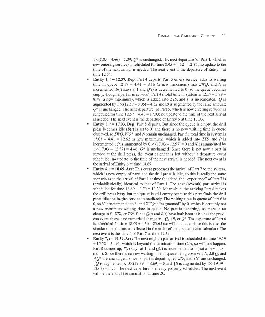
31FUNDAMENTAL SIMULATION CONCEPTS
1×(8.05 – 4.66) = 3.39; Q* is unchanged. The next departure (of Part 4, which isnow entering service) is scheduled for time 8.05 + 4.52 = 12.57; no update to thetime of the next arrival is needed. The next event is the departure of Entity 4 attime 12.57.
� Entity 4, t = 12.57, Dep: Part 4 departs. Part 5 enters service, adds its waitingtime in queue 12.57 – 4.41 = 8.16 (a new maximum) into ΣWQ, and N isincremented; B(t) stays at 1 and Q(t) is decremented to 0 (so the queue becomesempty, though a part is in service). Part 4’s total time in system is 12.57 – 3.79 =8.78 (a new maximum), which is added into ΣTS, and P is incremented. ∫Q isaugmented by 1 ×(12.57 – 8.05) = 4.52 and ∫B is augmented by the same amount;Q* is unchanged. The next departure (of Part 5, which is now entering service) isscheduled for time 12.57 + 4.46 = 17.03; no update to the time of the next arrivalis needed. The next event is the departure of Entity 5 at time 17.03.
� Entity 5, t = 17.03, Dep: Part 5 departs. But since the queue is empty, the drillpress becomes idle (B(t) is set to 0) and there is no new waiting time in queueobserved, so ΣWQ, WQ*, and N remain unchanged. Part 5’s total time in system is17.03 – 4.41 = 12.62 (a new maximum), which is added into ΣTS, and P isincremented. ∫Q is augmented by 0 × (17.03 – 12.57) = 0 and ∫B is augmented by1×(17.03 – 12.57) = 4.46; Q* is unchanged. Since there is not now a part inservice at the drill press, the event calendar is left without a departure eventscheduled; no update to the time of the next arrival is needed. The next event isthe arrival of Entity 6 at time 18.69.
� Entity 6, t = 18.69, Arr: This event processes the arrival of Part 7 to the system,which is now empty of parts and the drill press is idle, so this is really the samescenario as in the arrival of Part 1 at time 0; indeed, the “experience” of Part 7 is(probabilistically) identical to that of Part 1. The next (seventh) part arrival isscheduled for time 18.69 + 0.70 = 19.39. Meanwhile, the arriving Part 6 makesthe drill press busy, but the queue is still empty because this part finds the drillpress idle and begins service immediately. The waiting time in queue of Part 6 is0, so N is incremented to 6, and ΣWQ is “augmented” by 0, which is certainly nota new maximum waiting time in queue. No part is departing, so there is nochange in P, ΣTS, or TS*. Since Q(t) and B(t) have both been at 0 since the previ-ous event, there is no numerical change in ∫Q, ∫B, or Q*. The departure of Part 6is scheduled for time 18.69 + 4.36 = 23.05 (so will not occur since this is after thesimulation end time, as reflected in the order of the updated event calendar). Thenext event is the arrival of Part 7 at time 19.39.
� Entity 7, t = 19.39, Arr: The next (eighth) part arrival is scheduled for time 19.39+ 15.52 = 34.91, which is beyond the termination time (20), so will not happen.Part 8 queues up, B(t) stays at 1, and Q(t) is incremented to 1 (not a new maxi-mum). Since there is no new waiting time in queue being observed, N, ΣWQ, andWQ* are unchanged; since no part is departing, P, ΣTS, and TS* are unchanged.∫Q is augmented by 0×(19.39 – 18.69) = 0 and ∫B is augmented by 1×(19.39 –18.69) = 0.70. The next departure is already properly scheduled. The next eventwill be the end of the simulation at time 20.
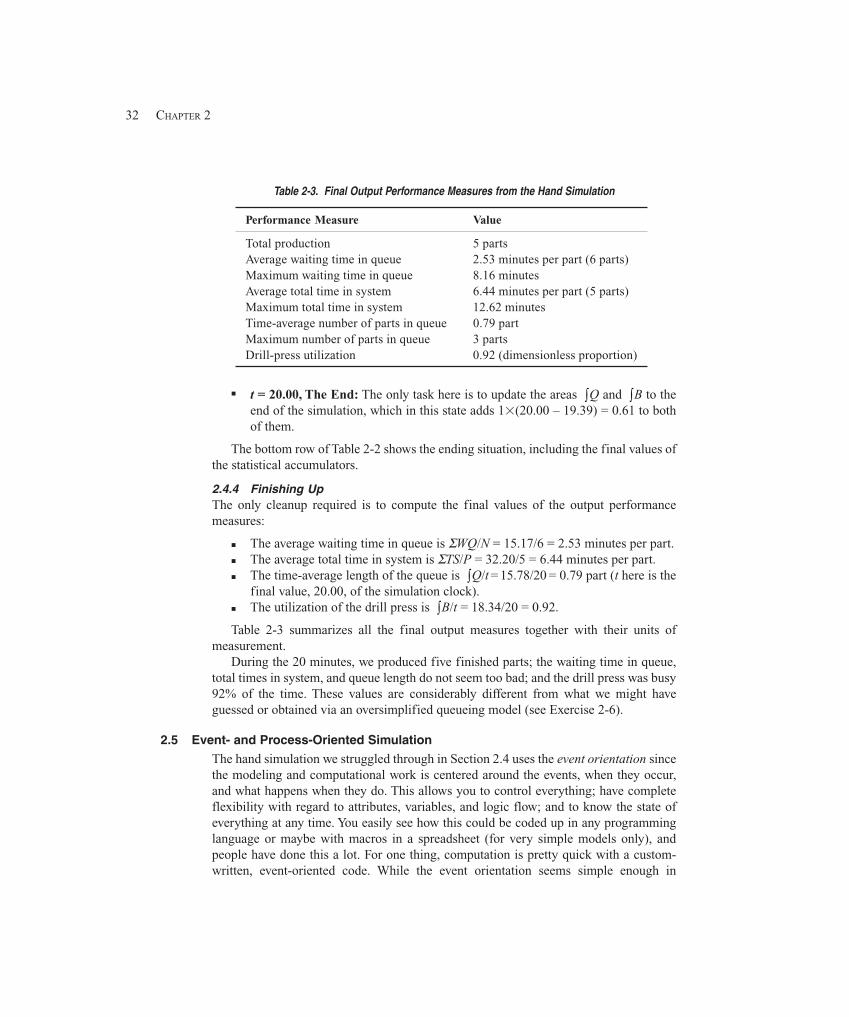
32 CHAPTER 2
Table 2-3. Final Output Performance Measures from the Hand Simulation
Performance Measure Value
Total production 5 partsAverage waiting time in queue 2.53 minutes per part (6 parts)Maximum waiting time in queue 8.16 minutesAverage total time in system 6.44 minutes per part (5 parts)Maximum total time in system 12.62 minutesTime-average number of parts in queue 0.79 partMaximum number of parts in queue 3 partsDrill-press utilization 0.92 (dimensionless proportion)
� t = 20.00, The End: The only task here is to update the areas ∫Q and ∫B to theend of the simulation, which in this state adds 1×(20.00 – 19.39) = 0.61 to bothof them.
The bottom row of Table 2-2 shows the ending situation, including the final values ofthe statistical accumulators.
2.4.4 Finishing UpThe only cleanup required is to compute the final values of the output performancemeasures:
� The average waiting time in queue is ΣWQ/N = 15.17/6 = 2.53 minutes per part.� The average total time in system is ΣTS/P = 32.20/5 = 6.44 minutes per part.� The time-average length of the queue is ∫Q/t = 15.78/20 = 0.79 part (t here is the
final value, 20.00, of the simulation clock).� The utilization of the drill press is ∫B/t = 18.34/20 = 0.92.
Table 2-3 summarizes all the final output measures together with their units ofmeasurement.
During the 20 minutes, we produced five finished parts; the waiting time in queue,total times in system, and queue length do not seem too bad; and the drill press was busy92% of the time. These values are considerably different from what we might haveguessed or obtained via an oversimplified queueing model (see Exercise 2-6).
2.5 Event- and Process-Oriented Simulation
The hand simulation we struggled through in Section 2.4 uses the event orientation sincethe modeling and computational work is centered around the events, when they occur,and what happens when they do. This allows you to control everything; have completeflexibility with regard to attributes, variables, and logic flow; and to know the state ofeverything at any time. You easily see how this could be coded up in any programminglanguage or maybe with macros in a spreadsheet (for very simple models only), andpeople have done this a lot. For one thing, computation is pretty quick with a custom-written, event-oriented code. While the event orientation seems simple enough in
33FUNDAMENTAL SIMULATION CONCEPTS
principle (although not much fun by hand) and has some advantages, you can imaginethat it becomes very complicated for large models with lots of different kinds of events,entities, and resources.
A more natural way to think about many dynamic simulations is to take the viewpointof a “typical” entity as it works its way through the model, rather than the omniscientorientation of the master controller keeping track of all events, entities, attributes,variables, and statistical accumulators as we did in the event-oriented hand simulation.This alternative view centers on the processes that entities undergo, so is called theprocess orientation. As you’ll see, this is strongly analogous to another commonmodeling tool—namely, flowcharting. In this view, we might model the hand-simulatedexample in steps like this (put yourself in the position of a typical part entity):
� Create yourself (a new entity arrives).� Write down what time it is now on one of your attributes so you’ll know your
arrival time later for the waiting-time-in-queue and total-time-in-systemcomputations.
� Put yourself at the end of the queue.� Wait in the queue until the drill press becomes free (this wait could be of 0
duration, if you’re lucky enough to find the drill press idle when you arrive).� Seize the drill press (and take yourself out of the queue).� Compute and tally your waiting time in queue.� Stay put, or delay yourself, for an amount of time equal to your service
requirement.� Release the drill press (so other entities can seize it).� Increment the production-counter accumulator on the wall and tally your total
time in system.� Dispose of yourself and go away.
This is the sort of “program” you write with a process-oriented simulation languagelike SIMAN and is also the view of things normally taken by Arena (which actuallytranslates your flowchart-like description into a SIMAN model to be run, though youdon’t need to get into that unless you want to; see Section 7.1.6). It’s a much more naturalway to think about modeling, and (importantly) big models can be built without theextreme complexity they’d require in an event-oriented program. It does, though,require more behind-the-scenes support for chores like time advance, keeping track oftime-persistent statistics (which didn’t show up in the process-oriented logic), andoutput-report generation. Simulation software like Arena provides this support as well asa rich variety of powerful modeling constructs that enable you to build complicatedmodels relatively quickly and reliably.
Most discrete-event simulations are actually executed in the event orientation, eventhough you may never see it if you do your modeling in the process orientation. Arena’shierarchical nature allows you to get down into the event orientation if you need to inorder to regain the control to model something peculiar, and in that case you have tothink (and code) with event-oriented logic as we did in the hand simulation.
34 CHAPTER 2
Because of its ease and power, process-oriented logic has become very popular and isthe approach we’ll take from now on. However, it’s good to have some understanding ofwhat’s going on under the hood, so we first made you suffer through the laborious eventsimulation.
2.6 Randomness in Simulation
In this section, we’ll discuss how (and why) you model randomness in a simulationmodel’s input and the effect this can have on your output. We’ll need some probabilityand statistics here, so this might be a good time to take a quick glance at (or a painstakingreview of) Appendix B to review some basic ideas, terminology, and notation.
2.6.1 Random Input, Random OutputThe simulation in Section 2.4 used the input data in Table 2-1 to drive the simulationrecorded in Table 2-2, resulting in the numerical output performance measures reportedin Table 2-3. This might be what happened from 8:00 to 8:20 on some particular Mondaymorning, and if that’s all you’re interested in, you’re done.
But you’re probably interested in more, like what you’d expect to see on a “typical”morning and how the results might differ from day to day. And since the arrival andservice times of parts on other days would probably differ from those in Table 2-1, thetrace of the action in Table 2-2 will likely be changed, so the numerical outputperformance measures will probably be different from what we got in Table 2-3.Therefore, a single run of the example just won’t do since we really have no idea how“typical” our results are or how much variability might be associated with them. Instatistical terms, what you get from a single run of a simulation is a sample of size one,which just isn’t worth much. It would be pretty unwise to put much faith in it, much lessmake important decisions based on it alone. If you rolled a die once and it came up afour, would you be willing to conclude that all the other faces were four as well?
So random input looks like a curse. But you must often allow for it to make yourmodel a valid representation of reality, where there may also be considerable uncertainty.The way people usually model this, instead of using a table of numerical input values, isto specify probability distributions from which observations are generated (or drawn orsampled) and drive the simulation with them. We’ll talk in Section 4.4 about how you candetermine these input probability distributions using the Arena Input Analyzer. Arenainternally handles generation of observations from distributions you specify. Not onlydoes this make your model more realistic, but it also sets you free to do more simulationthan you might have observed data for and to explore situations that you didn’t actuallyobserve. As for the tedium of generating the input observations and doing the simulationlogic, that’s exactly what Arena (and computers) like to do for you.
But random input induces randomness in the output too. We’ll explore this a little bitin the remainder of this section, but will take it up more fully in Chapter 6, Section 7.2,and Chapter 12 and show you how to use the Arena Output Analyzer, Process Analyzer,and OptQuest®, from OptTek Systems, Inc., to help interpret and appropriately cope withrandomness in the output.
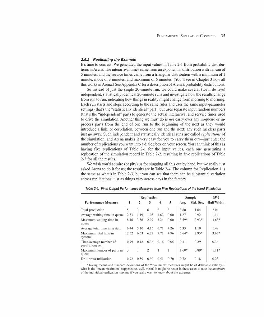
35FUNDAMENTAL SIMULATION CONCEPTS
2.6.2 Replicating the ExampleIt’s time to confess: We generated the input values in Table 2-1 from probability distribu-tions in Arena. The interarrival times came from an exponential distribution with a mean of5 minutes, and the service times came from a triangular distribution with a minimum of 1minute, mode of 3 minutes, and maximum of 6 minutes. (You’ll see in Chapter 3 how allthis works in Arena.) See Appendix C for a description of Arena’s probability distributions.
So instead of just the single 20-minute run, we could make several (we’ll do five)independent, statistically identical 20-minute runs and investigate how the results changefrom run to run, indicating how things in reality might change from morning to morning.Each run starts and stops according to the same rules and uses the same input-parametersettings (that’s the “statistically identical” part), but uses separate input random numbers(that’s the “independent” part) to generate the actual interarrival and service times usedto drive the simulation. Another thing we must do is not carry over any in-queue or in-process parts from the end of one run to the beginning of the next as they wouldintroduce a link, or correlation, between one run and the next; any such luckless partsjust go away. Such independent and statistically identical runs are called replications ofthe simulation, and Arena makes it very easy for you to carry them out—just enter thenumber of replications you want into a dialog box on your screen. You can think of this ashaving five replications of Table 2-1 for the input values, each one generating areplication of the simulation record in Table 2-2, resulting in five replications of Table2-3 for all the results.
We wish you’d admire (or pity) us for slugging all this out by hand, but we really justasked Arena to do it for us; the results are in Table 2-4. The column for Replication 1 isthe same as what’s in Table 2-3, but you can see that there can be substantial variationacross replications, just as things vary across days in the factory.
Table 2-4. Final Output Performance Measures from Five Replications of the Hand Simulation
Replication Sample 95%
Performance Measure 1 2 3 4 5 Avg. Std. Dev. Half Width
Total production 5 3 6 2 3 3.80 1.64 2.04
Average waiting time in queue 2.53 1.19 1.03 1.62 0.00 1.27 0.92 1.14
Maximum waiting time in 8.16 3.56 2.97 3.24 0.00 3.59* 2.93* 3.63*queue
Average total time in system 6.44 5.10 4.16 6.71 4.26 5.33 1.19 1.48
Maximum total time in 12.62 6.63 6.27 7.71 4.96 7.64* 2.95* 3.67*system
Time-average number of 0.79 0.18 0.36 0.16 0.05 0.31 0.29 0.36parts in queue
Maximum number of parts in 3 1 2 1 1 1.60* 0.89* 1.11*queue
Drill-press utilization 0.92 0.59 0.90 0.51 0.70 0.72 0.18 0.23
*Taking means and standard deviations of the “maximum” measures might be of debatable validity—what is the “mean maximum” supposed to, well, mean? It might be better in these cases to take the maximumof the individual-replication maxima if you really want to know about the extremes.
36 CHAPTER 2
The columns in Table 2-4 give the sample mean and sample standard deviation (seeAppendix B) across the individual-replication results for the output performancemeasure in each row. The sample mean provides a more stable indication of what toexpect from each performance measure than what happens on an individual replication,and the sample standard deviation measures cross-replication variation.
Since the individual replication results are independent and identically distributed,you could form a confidence interval for the true expected performance measure μ(think of μ as the sample mean across an infinite number of replications) as
X ts
nn± − −1 1 2, /α
where X is the sample mean, s is the sample standard deviation, n is the number ofreplications (n = 5 here), and tn− −1 1 2, /α is the upper 1 – �/2 critical point from Student’s tdistribution with n – 1 degrees of freedom. Using the total-production measure, forexample, this works out for a 95% confidence interval (� = 0.05) to
5
64.1776.280.3 ±
or 3.80 ± 2.04; the half widths for 95% confidence intervals on the expectations of allperformance measures are in the last column of Table 2-4. The correct interpretation hereis that in about 95% of the cases of making five simulation replications as we did, theinterval formed like this will contain or “cover” the true (but unknown) expected value oftotal production. This confidence interval assumes that the total-production results fromthe replications are normally distributed, which is not really justified here, but we usethis form anyway; see Section 6.3 for more on this issue of statistical robustness. Youmight notice that the half width of this interval (2.04) is pretty big compared to the valueat its center (3.80); that is, the precision is not too good. This could be remedied by sim-ply making more than the five replications we made, which looks like it was not enoughto learn anything precise about the expected value of this output performance measure.The great thing about collecting your data by simulation is that you can always2 go getmore by simply calling for more replications.
2.6.3 Comparing AlternativesMost simulation studies involve more than just a single setup or configuration of thesystem. People often want to see how changes in design, parameters (controllable inreality or not), or operation might affect performance. To see how randomness insimulation plays a role in these comparisons, we made a simple change to the examplemodel and re-simulated (five replications).
The change we made was just to double the arrival rate—in other words, the meaninterarrival time is now 2.5 minutes instead of 5 minutes. The exponential distribution isstill used to generate interarrival times, and everything else in the simulation stays thesame. This could represent, for instance, acquiring another customer for the facility,whose part-processing demands would be intermingled with the existing customer base.
2 Well, almost always.
37FUNDAMENTAL SIMULATION CONCEPTS
Figure 2-4 indicates what happened to the five “non-extreme” performance mea-sures; the upper row (circles) of each plot indicates the original configuration (and istaken right out of Table 2-4), and the lower row (triangles) is for the new configuration.For each performance measure, the results of the five replications of each model are indi-cated, and the result from the first replication in each case is filled in (replications 2-5 arehollow).
It’s not clear that total production really increases much with the double-time arrivals,due to limited processing capacity. It does appear, though, that the time in queue and insystem, as well as the utilization, tend to increase, although not in every case (due to vari-ability). And despite some overlap, the average queue lengths seem to grow somewhatwhen the arrival rate is doubled. While formal statistical analyses would be possible hereto help sort things out (see Section 6.4), simple plots like these can sometimes be prettyilluminating (though you’d probably want substantially more than just five replicationsof each scenario).
Moreover, note that relying on just one replication (the first, indicated by the filled-insymbols) could be misleading. For instance, the average waiting time in queue in the firstreplications of each model variant would have suggested that it is far greater for thedouble-time arrivals, but looking at the spread across replications indicates that the dif-ference isn’t so clear-cut or dramatic. This is exactly the danger in relying on only asingle run to make important decisions.
2.7 Simulating with Spreadsheets
You’ll agree that simulating by hand doesn’t have much of a future. People use spread-sheets for a lot of things, so how about simulation? Well, maybe, depending on the typeand complexity of the model, and on what add-in software you might have. In this sec-tion, we’ll discuss two examples, first a static model and then a dynamic model (recallSection 1.2.3); both, however, are very simple.
2.7.1 A News Vendor ProblemRupert sells daily newspapers on a street corner. Each morning he must buy the same,fixed number q of copies from the printer at c = 55 cents each, and sells them for r =$1.00 each through the day. He’s noticed that demand D during a day is close to being arandom variable X that’s normally distributed with mean μ = 135.7 and standard devia-tion σ = 27.1, except that D must be a nonnegative integer to make sense, so D = max(⎣X⎤, 0) where ⎣⋅⎤ rounds to the nearest integer (Rupert’s not your average news vendor).Further, demands from day to day are independent of each other. Now if demand D in aday is no more than q, he can satisfy all customers and will have q – D ≥ 0 papers leftover, which he sells as scrap to the recycler on the next corner at the end of the day for s =3 cents each (after all, it’s old news at that point). But if D > q, he sells out all of his supplyof q and just misses those other D – q > 0 sales. Each day starts afresh, independent of anyother day, so this is a single-period (single-day) problem, and for a given day is a staticmodel since it doesn’t matter when individual customers show up through the day.
How many papers q should Rupert buy each morning to maximize his expectedprofit? If he buys too few, he’ll sell out and miss out on the 45 cents profit on each lost
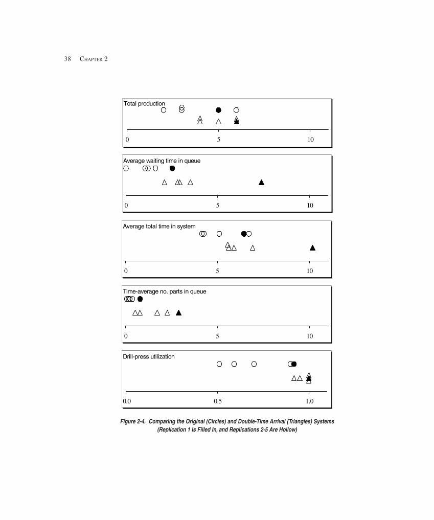
38 CHAPTER 2
0 5 10
Average total time in system
0 5 10
Time-average no. parts in queue
0.0 0.5 1.0
Drill-press utilization
0 5 10
Average waiting time in queue
0 5 10
Total production
Figure 2-4. Comparing the Original (Circles) and Double-Time Arrival (Triangles) Systems(Replication 1 Is Filled In, and Replications 2-5 Are Hollow)
39FUNDAMENTAL SIMULATION CONCEPTS
sale, but if he buys too many he will have some left over to scrap at a loss of 52 centseach. If he had a crystal ball and knew in the morning what demand was going to be thatday, he’d of course buy just that many; Rupert’s good, but he’s not that good, so he needsto decide on a fixed value of q that will apply to every day.
This is a genuine classic in operations research, a single-period, perishable-inventoryproblem, with more serious applications like food stocks and blood banks. It has manyversions, variants, and extensions, and a lot of attention has been paid to getting exactanalytical solutions. But it’s simple to simulate it; so simple, in fact, that it can be done ina spreadsheet.
First, let’s figure out an expression for Rupert’s profit on a typical day. Clearly, hisdaily cost is cq (we won’t impose some enigmatic negative-good-will cost for lost sales ifD > q and he sells out). If it turns out that D < q then he sells D and meets all customerdemand, gets revenue rD from customers, and has q – D left over as scrap so gets s(q – D)more revenue, such as it is, from the recycler. On the other hand, if D > q he sells q, getsrevenue rq from customers, but gets no scrap revenue. Thus, Rupert’s total daily revenueis r min (D, q) + s max (q – D, 0); to see this, just play out the two cases D < q and D > q.So his daily profit, in dollars, is
W(q) = r min (D, q) + s max (q – D, 0) – cq.
We’ve written this as a function of q since it clearly depends on Rupert’s choice of q.In mathematical-programming or optimization parlance, q is Rupert’s decision variableto try to maximize his objective function of expected daily profit, E(W(q)). Since D is arandom variable, so too is W(q), and we need to take its expectation (see Appendix B fora refresher on probability and statistics) to get a deterministic objective function to try tomaximize. Since expected values are long-run averages, in this case, over many days,Rupert is maximizing his long-run average daily profit by finding the best set-it-and-for-get-it constant value of q. He’s not trying to adjust q each day depending on demand,which is impossible since he has to commit to buying a fixed number q papers in themorning, before that day’s demand is realized. Depending on the form of the probabilitydistribution of D, it might be possible in some cases to derive an exact expression forE(W(q)) that we could try to maximize with respect to q. But we can always build asimple simulation model and heed the lessons from Section 2.6 about statistical analysisof simulation output to get a valid and precise estimate of the optimal q, without makingstrong and maybe unrealistic assumptions about the distribution of D just to enable ananalytical result.
To simulate this, we need to generate numerical values on the demand randomvariable D = max (⎣X⎤, 0); such are called random variates on D. Thus, we first need togenerate random variates on X, which has a normal distribution with mean μ = 135.7 andstandard deviation σ = 27.1. Section 12.2 discusses random-variate generation ingeneral, so we’ll trust you to look ahead if you’re interested at this point. In this case wecan generate a normally distributed random variate as X =
1,
−Φ σμ (U) where U is arandom number (continuous random variate distributed uniformly between 0 and 1,discussed in Section 12.1), σμ ,Φ is the cumulative distribution of the normal
40 CHAPTER 2
distribution with mean μ and standard deviation σ, and 1,
−Φ σμ is the functional inverse of
σμ ,Φ , i.e.,
1,
−Φ σμ
“undoes” whatever σμ ,Φ does. Another way of looking at thefunctional inverse is that we need to solve U =
σμ ,Φ
(X) for X, where U would be aspecific number between 0 and 1 from the random-number generator. As you may know,neither
σμ ,Φ
nor for the normal distribution can be written as an explicit closed-form formula, so evaluation of
1,
−Φ σμ
(U) must be by numerical approximation, but thisis built into spreadsheet software, and certainly into simulation software as well.
We used the Microsoft® Excel spreadsheet to create the file Newsvendor.xls inFigure 2-5. You’ll find this file in the Book Examples folder, which is in turn in the Arenafolder if you followed the instructions in Appendix D for Arena installation from the CDsupplied with this book; a typical complete path to this folder would be C:\ProgramFiles\Rockwell Software\Arena\Book Examples. In cells B4 – B8 (shadedblue in the file) are the input parameters, and in row 2 (pink) are some trial values for thedecision variable q (cells H2, K2, N2, Q2, and T2). Column D just gives the day numberfor reference. We simulated 30 days, though as mentioned earlier, each day is indepen-dent so is really an independent, static simulation.
Column E has the demand on each day, via the Excel formula
MAX(ROUND(NORMINV(RAND(), $B$7, $B$8), 0),0)
that is the same all the way down the column. Let’s dissect this formula from the insideout:
� RAND() is Excel’s built-in random-number generator, which returns a numberbetween 0 and 1 that’s supposed to be uniformly distributed and independentacross draws. See Section 12.1 for a discussion of random-number generators,which are more subtle than you might think, but are clearly essential to good sto-chastic simulation. Unfortunately, not all random-number generators suppliedwith various software packages are of high quality (however, the one built intoArena is excellent). Excel’s RAND()function is “volatile” by default, meaningthat every instance of it re-draws a “fresh” random number upon any recalculationof the spreadsheet, which you can force by hitting the F9 key, by saving the file, orby editing just about anything anywhere in the sheet.
� NORMINV(u, μ, σ) is Excel’s built-in numerical approximation to 1,
−Φ σμ , so whenused with u = RAND() returns a random variate distributed normally with meanμ and standard deviation σ. We have μ in cell B7 and σ in cell B8; the $ in Excel-formula cell references forces what immediately follows it (column letter or rownumber) not to change when the formula is copied into other cells, and here wewant both the column and row to stay the same when this formula is copied intoother cells since μ and σ are in these fixed cells.
� ROUND(x, 0) in Excel returns x rounded to the nearest integer. The secondargument’s being 0 ensures that the rounding is to the nearest integer as opposedto other kinds of rounding (see Excel’s Help).
� MAX(a, b, ...), as you might guess, returns the maximum of its arguments.
1,
−Φ σμ
1,
−Φ σμσμ ,Φ
1,
−Φ σμ
1,
−Φ σμ
σμ ,Φ
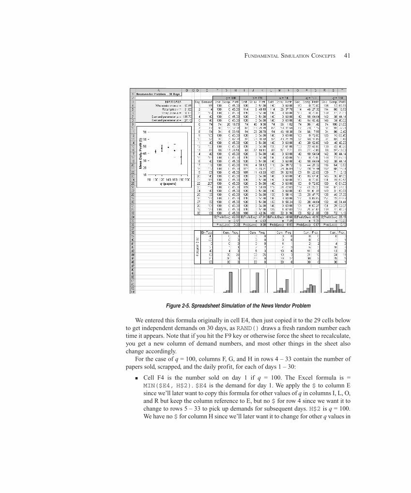
41FUNDAMENTAL SIMULATION CONCEPTS
Figure 2-5. Spreadsheet Simulation of the News Vendor Problem
We entered this formula originally in cell E4, then just copied it to the 29 cells belowto get independent demands on 30 days, as RAND() draws a fresh random number eachtime it appears. Note that if you hit the F9 key or otherwise force the sheet to recalculate,you get a new column of demand numbers, and most other things in the sheet alsochange accordingly.
For the case of q = 100, columns F, G, and H in rows 4 – 33 contain the number ofpapers sold, scrapped, and the daily profit, for each of days 1 – 30:
� Cell F4 is the number sold on day 1 if q = 100. The Excel formula is =MIN($E4, H$2). $E4 is the demand for day 1. We apply the $ to column Esince we’ll later want to copy this formula for other values of q in columns I, L, O,and R but keep the column reference to E, but no $ for row 4 since we want it tochange to rows 5 – 33 to pick up demands for subsequent days. H$2 is q = 100.We have no $ for column H since we’ll later want it to change for other q values in
42 CHAPTER 2
columns I, L, O, and R, but we apply a $ to row 2 to keep the reference to it forrows below. Thus, this is min(D, q), as desired.
� Cell G4 is the number of papers scrapped at the end of day 1 if q = 100. The Excelformula is = MAX(H$2 - $E4, 0), with $ usage the same as for Cell F4 and forthe same reasons. This is max(q – D, 0).
� Cell H4 is the profit, in dollars, on day 1 if q = 100. The Excel formula is= $B$5∗F4 + $B$6∗G4 - $B$4∗H$2, which is r min(D, q) + s max(q – D, 0) –cq. We’ll let you figure out why the $ signs are present and absent where they are.
We then simply copied cells F4, G4, and H4 into the 29 rows below, allowing the columnletters and row numbers to run as appropriate and controlled by the $ placement in theformulas, to get the simulation table, as this is sometimes called, for the case q = 100.
At the bottom of these columns, shaded green in the file, we added the average profit(cell H34) and the half width of a 95% confidence interval on the expected average profit(cell H35) over the 30 days, with formulae just like those toward the end of Section 2.6.2;the value 2.045 is the upper 0.975 critical point from the t table with 29 degrees of free-dom3. Note that, as in Section 2.6.2, the form of this confidence interval assumes thatthe individual profits in a column are normally distributed, which is not quite true, espe-cially for small values of q where there’s little variability in profit, but we do so anyway;again, see the end of Section 6.3 for more on statistical robustness.
We also added in row 36 the proportion of days in which a loss was incurred, which isan estimate of the probability of incurring a loss in a day, using the Excel COUNTIFfunction. With this low value of q a loss is quite unlikely since demand will be at least qon nearly all days, but that will change for higher values of q. And in rows 38 – 46 wecollect frequency-distribution data (again using COUNTIF) to construct a histogram ofprofits directly below; the vertical line in the histograms, which is red in the file, is atzero, so we have an indication to its left of the probability of incurring a loss, as well asthe general distribution of the profit data.
To complete the simulation study, we took columns F, G, and H and replicated theminto four more blocks of three columns each out to the right, but with q taking the values120, 140, 160, and 180, and added histograms at the bottom for each value of q. Tovisualize the mean results, we added the plot on the left edge to show the average profitas a dot, with vertical I-beams showing the confidence intervals, for different values of qon the horizontal axis.
Notice that, for a given day, we chose to use the same realized numerical demandvariate (column E) for all trial values of q, rather than generate fresh independentdemands for each value of q, which would have been valid as well. We’re not lazy (atleast about this) and filling more Excel columns with fresh demands wouldn’t cost much,but we did it this way deliberately. Our interest is really in comparing profit for differentvalues of q, and by using the same realized numerical demands on a given day for all q,the differences we see in profit will be attributable to differences in q (which is the effectwe’re trying to measure) rather than to chance differences in demand. This is an exampleof a variance-reduction technique, in particular of common random numbers, discussed
3 More generally, we could use TINV(0.05, COUNT(H4:H33) - 1) instead of hard-wiring in 2.045.
43FUNDAMENTAL SIMULATION CONCEPTS
more fully in Section 12.4. Such strategies in stochastic simulation can help you getmore precise answers, often with little or no more work (in this case, with less work) andare worth thinking about.
If you open the spreadsheet file yourself, you won’t see the same numbers as inFigure 2-5 due to the volatility of Excel’s RAND(). And as you recalculate (tap the F9key a few times) you’ll see all the numbers change, the objects in the mean plot on theleft will jump up and down, and the histograms at the bottom will undulate left and right,all reflecting this volatility and the underlying truth that such a stochastic simulation isan experiment with random outcomes; indeed the jumping up and down of the I-beamsin the mean plot at the left is a reminder that confidence intervals themselves are randomintervals and depend on the particular sample you happened to get. Notice that all five ofthe dots and I-beams tend to jump up or down together, reflecting the common-random-numbers variance reduction mentioned in the preceding paragraph; see Exercise 2-10.
Despite this randomness, it looks like Rupert should probably set q to be around 140,maybe a bit less, to maximize his expected daily profit. From the confidence-intervalI-beams, it also looks like we might want to increase the sample size to considerablymore than 30 days to pin this down better (Exercise 2-11). And clearly it would help toconsider more values of q in a finer mesh (Exercise 2-12), but this study at least tells usthat Rupert should probably buy at least 120 papers each morning, but no more than 160,since otherwise he loses too much profit due to lost sales or scrapping too much at a loss.
But looking beyond averages via the histograms at the bottom, the higher the q, themore variability (risk) there is in the profit, seen by the histograms’ broadening out. Thisis good and bad news. With high q, Rupert has the large inventory to reap a lot of profit onhigh-demand days, but you also see more negative profits when demand is low, on boringslow-news days when he gets stuck with a lot to scrap at a loss. If Rupert is a risk-taker, hemight go for a high value of q (sometimes you eat the bear, sometimes the bear eats you).At the other end, very low q values entail little risk since demand seldom falls short ofsuch small q’s, but the downside is that average profit is also low as Rupert cannot cash inon high-demand days since he sells out. Such risk/return tradeoffs in business decisionsare commonly quantified via spreadsheet simulations of static models like this.
It’s quite easy to simulate the news vendor problem in Arena; see Exercises 6.22 and6.23.
2.7.2 A Single-Server QueueSpreadsheets might also be used to simulate some dynamic models, but only very simpleones. Consider a single-server queue that’s logically the same as what we ploddedthrough by hand in Section 2.4, but different on some specifics. As before, customersarrive one at a time (the first customer arrives at time 0 to find the system empty andidle), may have to wait in a FIFO queue, are served one at a time by a single server, andthen depart. But we’ll make the following changes from the hand-simulated model:
� Interarrival times have an exponential probability distribution with mean 1/λ =1.6 minutes, and are independent of each other (see Appendices B and C). Theparameter λ = 1/1.6 = 0.625 is the arrival rate (per minute here).
44 CHAPTER 2
� Service times have a continuous uniform distribution between a = 0.27 minuteand b = 2.29 minutes, are independent of each other, and are independent of thearrival times.
This is called the M/U/1 queue, where the U refers to the uniformly distributed servicetimes.
Instead of observing all the outputs in the hand simulation, we’ll just watch the wait-ing times in queue, WQ
1, WQ
2, ..., WQ
50 of the first 50 customers to complete their queue
waits (not including their service times). In the hand simulation, we set up a clock, statevariables, an event calendar, and statistical accumulators to simulate this, but for asingle-server FIFO queue there is a simple recursion for the WQ
i values (if that’s all
we’re interested in by way of output), Lindley’s (1952) formula. Let Si be the time in ser-
vice for customer i, and let Ai be the interarrival time between customers i – 1 and i. Then
WQi = max (WQ
i–1 + S
i–1 – A
i, 0) for i = 2, 3, ...
and we initialize by setting WQ1 = 0 since the first customer arrives to an empty and idle
system.To simulate this, we need to generate random variates from the exponential and
continuous uniform distributions. Again referring ahead to Section 12.2, there are simpleformulas for both (as before, U denotes a random number distributed continuouslyuniformly between 0 and 1):
� Exponential interarrival times with mean 1/λ: Ai = – (1/λ) ln (1 – U) where ln is
the natural (base e) logarithm.� Continuously uniformly distributed service times between a and b: S
i = a + (b –
a) U.
Figure 2-6 shows the Excel file MU1.xls in the Book Examples folder. Cells B4,B5, and B6 are the parameters, and column D just gives the customer number i = 1, 2, ...,50 for a run of the model. Interarrival times are in column E, using the Excel formula−$B$4∗LN(1 - RAND()), and service times are in column F, generated by the formula$B$5 + ($B$6 - $B$5)∗RAND().
Lindley’s recursion is in column G, initialized by the 0 in cell G4. A typical entry is incell G9, MAX(G8 + F8 - E9, 0), which generates WQ
6 from WQ
5 (in cell G8), S
5 (cell
F8), and A6 (cell E9). In this way, each queue wait in column G is linked to the one above
it, establishing a correlation between them. Since this is correlation of entries in asequence with each other, it’s called autocorrelation. In this case, it’s positiveautocorrelation since a large wait probably means that the next wait will be large too, andvice-versa, which you can understand from looking at Lindley’s recursion or just fromyour own painful experiences standing in line. So, unlike the news vendor’s profit rowsin Section 2.7.1, the waiting times in queue here are not independent from row to row incolumn G, which is typical of the output sequence within a run of a dynamic simulation.
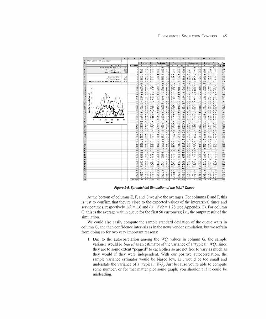
45FUNDAMENTAL SIMULATION CONCEPTS
Figure 2-6. Spreadsheet Simulation of the M/U/1 Queue
At the bottom of columns E, F, and G we give the averages. For columns E and F, thisis just to confirm that they’re close to the expected values of the interarrival times andservice times, respectively 1/λ = 1.6 and (a + b)/2 = 1.28 (see Appendix C). For columnG, this is the average wait in queue for the first 50 customers; i.e., the output result of thesimulation.
We could also easily compute the sample standard deviation of the queue waits incolumn G, and then confidence intervals as in the news vendor simulation, but we refrainfrom doing so for two very important reasons:
1. Due to the autocorrelation among the WQi values in column G, the sample
variance would be biased as an estimator of the variance of a “typical” WQi, since
they are to some extent “pegged” to each other so are not free to vary as much asthey would if they were independent. With our positive autocorrelation, thesample variance estimator would be biased low, i.e., would be too small andunderstate the variance of a “typical” WQ
i. Just because you’re able to compute
some number, or for that matter plot some graph, you shouldn’t if it could bemisleading.
46 CHAPTER 2
2. It’s not clear what a “typical” WQi even means here, since the initialization WQ
1 =
0 makes the early part of the output sequence smaller than later on, so the distribu-tion (and thus variance) of the WQ
i values is changing as i grows. Thus, it’s not
even clear what it is we’d be estimating by a sample-variance estimate.
We copied columns E, F, and G into five more blocks of three columns each out to theright, creating five independent replications of this run of 50 queue waits. All randomnumbers, and thus results, are independent across these five sets of three columns each.This is the same model all the way across, just replicated five independent times.
The plot on the left traces the WQi sequence in each of the five replications using
different dash patterns, and also plots the average of the five values of WQi, for a fixed i,
across the replications (in column T) as the thicker solid curve. Note the variation withina run, and the average thick curve calms things down a bit. All curves start off at 0 on theleft, reflecting the deterministic initialization WQ
1 = 0, and rise from there, subject to a
lot of wiggling that reflects output variability. The positive autocorrelation is in evidencesince the curves, while wiggly, do not break off from themselves abruptly as theyprogress to the right, and points on them tend to be close to their neighboring points for alittle while left and right.
The thick gray horizontal line plots the value in cell B10, which is the steady-stateexpected wait in queue, E(WQ∞). This can be computed exactly, from queueing theory(see, for example Gross and Harris, 1998), for single-server FIFO queues with exponen-tial interarrival times and service times S
i with any distribution, as
E(WQ∞) = ))(E1(2
))(E()(Var 2
i
ii
S
SS
λλ
−+
.
In our case, λ = 0.625 (the reciprocal of cell B4), E(Si) = (a + b)/2 = 1.28 in cell B8, and
Var(Si) = (b – a)2/12 = 0.34 in cell B9 (see Appendix C). Though the variation in the plot
obscures it, a little imagination might suggest that the thick solid average curve isconverging to the gray horizontal line; see Exercise 2-13.
Why no histograms like those at the bottom in news vendor problem spreadsheet?They could have been constructed in the same way, and could provide useful informationabout the distribution of the queue waits, beyond just their means. The potential problemwith this is the autocorrelation in the queue-wait sequence, so a histogram, like a vari-ance estimate, could be biased if our run were not long enough to ensure that the waitingtimes in queue eventually visit all possible regions and in the right proportions; theautocorrelation links together nearby observations, which would impede such visitationif the run were too short. However, a very long run could indeed produce a nearly unbi-ased histogram, which could be useful; in practice, it might be hard to determine howlong is long enough. The question is whether to present something that’s accurate anduseful most of the time, at the risk of its being occasionally biased and misleading.
Simulating a single-server queue in Arena is quite simple, and is basically the centralexample we use in Chapter 3 to introduce Arena.
47FUNDAMENTAL SIMULATION CONCEPTS
2.7.3 Extensions and LimitationsSpreadsheet simulation is popular for static models, many involving financial or riskanalysis. Commercial add-in packages to Excel, like @RISK (Palisade Corporation,2009) and Crystal Ball® (Oracle Corporation, 2009), facilitate common operations,provide better random-number generators, make it easy to generate variates from manydistributions, and include tools for analysis of the results.
However, spreadsheets are not very well suited for simulation of dynamic models.Absent something like Lindley’s recursion for very special and simple cases like thesingle-server FIFO queue in Section 2.7.2, spreadsheets are not very good tools fordynamic models. Our focus in the rest of the book is on dynamic models, for whichArena is specifically designed.
2.8 Overview of a Simulation Study
In deciding how to model a system, you’ll find that issues related to design and analysisand representing the model in the software certainly are essential to a successful simula-tion study, but they’re not the only ingredients. We’ll take all this up in Chapter 13 insome detail, but we want to mention briefly at this early point what’s involved.
No simulation study will follow a cut-and-dried “formula,” but there are severalaspects that do tend to come up frequently:
� Understand the system. Whether the system exists or not, you must have anintuitive, down-to-earth feel for what’s going on. This will entail site visits andinvolvement of people who work in the system on a day-to-day basis.
� Be clear about your goals. Realism is the watchword here; don’t promise the sun,moon, and stars. Understand what can be learned from the study, and expect nomore. Specificity about what is to be observed, manipulated, changed, anddelivered is essential. And return to these goals throughout the simulation study tokeep your attention focused on what’s important, namely, making decisions abouthow best (or at least better) to operate the system.
� Formulate the model representation. What level of detail is appropriate? Whatneeds to be modeled carefully and what can be dealt with in a fairly crude, high-level manner? Get buy-ins to the modeling assumptions from management andthose in decision-making positions.
� Translate into modeling software. Once the modeling assumptions are agreedupon, represent them faithfully in the simulation software. If there are difficul-ties, be sure to iron them out in an open and honest way rather than burying them.Involve those who really know what’s going on (animation can be a big helphere).
� Verify that your computer representation represents the conceptual modelfaithfully. Probe the extreme regions of the input parameters, verify that the rightthings happen with “obvious” input, and walk through the logic with thosefamiliar with the system.
� Validate the model. Do the input distributions match what you’ve observed in thefield? Do the output performance measures from the model match up with those
48 CHAPTER 2
from reality? While statistical tests can be carried out here, a good dose ofcommon sense is also valuable.
� Design the experiments. Plan out what it is you want to know and how yoursimulation experiments will get you to the answers in a precise and efficientway. Often, principles of classical statistical experimental design can be of greathelp here.
� Run the experiments. This is where you go to lunch while the computer isgrinding merrily away, or maybe go home for the night or the weekend, or go onvacation. The need for careful experimental design here is clear. But don’tpanic—your computer probably spends most of its time doing nothing, socarrying out your erroneous instructions doesn’t constitute the end of the world(remember, you’re going to make your mistakes on the computer where theydon’t count rather than for real where they do).
� Analyze your results. Carry out the right kinds of statistical analyses to be able tomake accurate and precise statements. This is clearly tied up intimately with thedesign of the simulation experiments.
� Get insight. This is far more easily said than done. What do the results mean at thegut level? Does it all make sense? What are the implications? What furtherquestions (and maybe simulations) are suggested by the results? Are you lookingat the right set of performance measures?
� Document what you’ve done. You’re not going to be around forever, so make iteasier on the next person to understand what you’ve done and to carry thingsfurther. Documentation is also critical for getting management buy-in andimplementation of the recommendations you’ve worked so hard to be able to makewith precision and confidence.
By paying attention to these and similar issues, your shot at a successful simulationproject will be greatly improved.
2.9 Exercises
2-1 For the hand simulation of the simple processing system, define another time-persistent statistic as the total number of parts in the system, including any parts inqueue and in service. Augment Table 2-2 to track this as a new global variable, add newstatistical accumulators to get its time average and maximum, and compute these valuesat the end.
2-2 In the preceding exercise, did you really need to add state variables and keep trackof new accumulators to get the time-average number of parts in the system? If not, whynot? How about the maximum number of parts in the system?
2-3 In the hand simulation of the simple processing system, suppose that the queuediscipline were changed so that when the drill press becomes idle and finds parts waitingin queue, instead of taking the first one, it instead takes the one that will require theshortest processing time (this is sometimes called an SPT queue discipline). To make thiswork, you’ll need to assign a second attribute to parts in the system when they arrive,
49FUNDAMENTAL SIMULATION CONCEPTS
representing what their service time at the drill press will be. Re-do the hand simulation.Is this a better rule? From what perspective?
2-4 In the hand simulation of the simple processing system, suppose that a constantsetup time of 3 minutes was required once a part entered the drill press but before itsservice could actually begin. When a setup is going on, regard the drill press as beingbusy. Plot the total number of parts in system as a function of simulated time. Re-do thehand simulation and discuss the results.
2-5 In the hand simulation of the simple processing system, suppose the drill press canwork on two parts simultaneously (and they enter, are processed, and leave the drill pressindependently). There’s no difference in processing speed if there are two parts in thedrill press instead of one. Redefine B(t) to be the number of parts in service at the drillpress at time (so 0 � B(t) � 2), and the drill press utilization is redefined as
.2
)(0
T
dttBT
∫
where T = 20. Re-run the original simulation to measure the effect of this change.
2-6 In Section 2.2.2, we used the M/M/1 queueing formula with the mean interarrivaltime μ
A and the mean service time μ
S estimated from the data in Table 2-1 as 4.08 and
3.46, respectively. This produced a “predicted” value of 19.31 minutes for the averagewaiting time in queue. However, the hand-simulation results in Section 2.4.4 produced avalue of 2.53 minutes for this measure.
(a) If these two (very different) numbers are supposed to estimate or approximatethe same thing (average waiting time in queue), why are they so apparentlydifferent? Give at least three reasons.
(b) We carried out the simulation for a million minutes (rather than 20 minutes),using the same sources of interarrival and service times as in Table 2-1, and gota value of 3.60 for the average waiting time in queue (as you can imagine, itreally took us a long time to do this by hand, but we enjoyed it). Why is this yetdifferent from the values 19.31 and 2.53 being compared in part (a)?
(c) We consulted an oracle, who sold us the information that the interarrival timesare actually “draws” from an exponential distribution with mean 5 minutes, andthe service times are actually draws from a triangular distribution withminimum 1 minute, mode 3 minutes, and maximum 6 minutes (see Appendix Cfor more information on these distributions, and Appendix B to brush up onyour probability). With this (exact) information, the mean interarrival time isactually μ
A = 5 minutes, and the mean service time is actually μ
S = (1 + 3 + 6)/3
= 3.33 minutes. Using these values, use the M/M/1 formula in Section 2.2.2 topredict a value for the average waiting time in queue. Why is it yet differentfrom the previous three values (19.31, 2.53, and 3.60) for this same quantitydiscussed previously in this exercise?
50 CHAPTER 2
(d) Using the information from the oracle in part (c), we treated ourselves toanother million-minute hand simulation (just as enjoyable), but this time drewthe service times from an exponential (not triangular) distribution with mean3.33 minutes, and got a result of 6.61 for the mean waiting time in queue.Compare and contrast this with the previous four values for this quantitydiscussed previously in this exercise.
2-7 Here are the actual numbers used to plot the triangles for the double-time-arrivalmodel in Figure 2-4:
ReplicationPerformance Measure 1 2 3 4 5
Total production 6 4 6 4 5Average waiting time in queue 7.38 2.10 3.52 2.81 2.93Average total time in system 10.19 5.61 5.90 6.93 5.57Time-average no. parts in queue 2.88 0.52 1.71 0.77 2.25Drill-press utilization 1.00 0.92 1.00 0.95 1.00
For each of these five performance measures, compute the sample mean, samplestandard deviation, and half widths of 95% confidence intervals on the expectedperformance measures, as done in Table 2-4. Comparing these confidence intervals tothose in Table 2-4, can you clarify any differences beyond the discussion in Section 2.6.3(which was based on looking at Figure 2-4)?
2-8 In the hand simulation of the simple processing system, suppose the drill press istaken down for burn-in maintenance at time 4 minutes, and it takes 4 minutes to do thiswork and bring it back up; it then stays up for the rest of the 20-minute simulation length.If there’s a part in service when the drill press goes down, it just sits there, its processingsuspended until the drill press comes back up, when it’s resumed and needs just itsremaining processing time (its processing does not have to start over from scratch).During the down time, the arrival process of new parts continues without regard to downtime. Regard the drill press as being busy when it’s down, and define the time in systemof a part to include the time it sits in the drill press but not being worked on if it’s unluckyenough to be in service when the drill press is taken down. Using the same input data asin Table 2-1, carry out this simulation by hand and note any differences in the outputperformance measures from the original model. (See Exercise 6-18 for the question ofwhether this model change induces statistically significant changes in the outputperformance measures.)
2-9 In Exercise 2-8, refine the output performance measure on the status of the drillpress from just the two states (busy vs. idle, where in Exercise 2-8 the drill press was tobe regarded as “busy” during its down time) to three states:
51FUNDAMENTAL SIMULATION CONCEPTS
1. busy working on a part and not down,2. idle and not down, and3. down, with or without a part being stuck in the machine for the down time.
Give the output performance measures from this simulation under this refined definitionof the drill-press state.
2-10 Modify the news vendor problem in Section 2.7.1 to use independent demands foreach trial value of q, and note the difference in the behavior of the output, particularly inthe mean plot on the left.
2-11 Increase the sample size on the news vendor problem in Section 2.7.1 from 30 daysto 150. As in the original problem, use the same realized demands in column E for allvalues of q. Don’t forget to change the statistical-summary and histogram cells appropri-ately at the bottom of the columns, as well as the cells referred to in the various graphics.What is the effect on the results? Based on your results, about what sample size (in days)would be needed to bring the maximum half-width of all five confidence intervals downto under ± $1.50? Don’t actually carry this out, but just get an estimate; see Section 6.3.
2-12 Based on your results from Exercise 2-11, try a different set of trial values of q totry to home in more precisely on the optimal q. Keep the sample size at 150 days.Depending on what you choose to try, you may need to rescale the axes on the mean ploton the left.
2-13 Modify the M/U/1 queue spreadsheet simulation from Section 2.7.2 to have expo-nential service times with mean 1.28 minutes, rather than the original uniform servicetimes, resulting in the M/M/1 queue. Change the steady-state expected wait in queue ap-propriately; see the exponential-distribution entry in Appendix C.
2-14 Modify the M/U/1 queue spreadsheet simulation from Section 2.7.2 to make tenreplications rather than 5, and to run for 100 customers rather than 50. To avoid clutter,plot only the cross-replication average queue-wait curve. Compare with the original inSection 2.7.2.
2-15 Supermarket customers load their carts with goods totaling between $5 and $200,uniformly (and continuously) distributed; call this the raw order amount. Assume thatcustomers purchase independently of each other. At checkout, 63% of customers have aloyalty card that gives them 4% off their raw order amount. Also at checkout, 18% ofcustomers have coupons that give them 7% off their raw order amount. These twodiscounts occur independently of each other, and a given customer could have one or theother of them, both of them, or neither of them, to get to their net order amount (whatthey actually pay). Construct a spreadsheet simulation to simulate 100 customers andcollect statistics on the net order amount; these statistics should include the average,standard deviation, minimum, maximum, and a histogram to describe the distribution ofthe net order amounts between $0 and $200. (HINT: to decide whether a customer gets aloyalty discount, explore the Excel IF function with the first argument’s being a randomnumber RAND() distributed uniformly between 0 and 1; do similarly to decide on acoupon discount.)

53A GUIDED TOUR THROUGH ARENA
CHAPTER 3
A Guided Tour Through Arena
As we were honest enough to admit in Chapter 2, we really used Arena to carry out the“hand” simulation in Section 2.4, as well as the multiple replications and the modifiedmodel with the double-time arrivals in Section 2.6. In this chapter, we’ll lead you on atour through Arena by having you start up Arena, browse through the existing model webuilt for the hand simulation, run it, and then build it from scratch. Then we’ll use justthese basic building blocks in a case study exploring a question of real interest, whetherit’s better to have specialized serial processing or generalized parallel processing, andthe effect of variability on such a decision. We’ll also explore the Arena user interface,get you into the help and documentation systems, discuss different ways to run yoursimulation, and illustrate some of the drawing and graphics tools.
Section 3.1 gets you to start Arena on your computer, and in Section 3.2, you’ll openan existing model and look around. In Section 3.3, you’ll go through the model in somedetail, browsing the dialog boxes and animation, running the model, and taking a look atthe results; in Section 3.4, you’ll construct this model from scratch. Section 3.5 containsthe case study mentioned above. In Section 3.6, we’ll briefly go over many of Arena’spieces and capabilities, including what’s available in the menus and toolbars and thedrawing and printing capabilities. There’s a broad and deep help system in Arena, with allof the detailed technical documentation, which is the subject of Section 3.7. There are alot of options for running and controlling simulations, which are discussed in Section 3.8.
By the end of this chapter, you’ll have a good feel for how Arena works and have anidea of the things you can do with it. You’ll be able to work effectively with Arena tobuild simple models and maybe take a stab at doing some not-so-simple things as well bycruising the menus and dialogs on your own, with the aid of the help and documentationsystems. While you can probably make some sense out of things by just reading thischapter, you’ll be a lot better off if you follow along in Arena on your computer. Moreinformation on building your own models with Arena is discussed in Chapter 4 andbeyond.
3.1 Starting Up
Arena is a true Microsoft® Windows® operating system application, so its look and feelwill already be familiar to you, and all the usual features and operations are there. Inaddition, Arena is fully compatible with other Windows software, like word processors,spreadsheets, and CAD packages, so you can easily move things back and forth (Chapter10 goes into detail about Arena’s interaction and communication with other software).
By the way, we’re assuming you’re already comfortable with the basics of workingwith Windows, such as:
54 CHAPTER 3
� Disks, files, folders, and paths.� Using the mouse and keyboard, including clicking, double-clicking, and right-
clicking.� Operating on windows, like moving, resizing, maximizing, minimizing, and
closing.� Accessing things from menus. We’ll use notation like “M > C > S > T” to mean
open the M menu, choose C from it, then choose S from the submenu menu (ifany), then choose the tabbed page labeled T (if any), etc.
� Using the Control, Alt, and Shift keys. By “Ctrl+whatever,” we’ll mean to holddown the Ctrl key and press “whatever” (this will also apply for Alt+whatever andShift+whatever). If “whatever” is a keyboard key, it’s not case-sensitive. “What-ever” could also be a mouse click, like Ctrl+Click to extend a selection to includeadditional items.
� Cut (or the menu command Edit > Cut or the shortcut key combination Ctrl+X),Copy (or Edit > Copy or Ctrl+C), and Paste (or Edit > Paste or Ctrl+V) of text andother items.
� Filling out dialog boxes by entering and editing text entries, pressing buttons,selecting and clearing (that is, unchecking) check boxes, clicking exactly onefrom a list of option buttons (also called radio buttons), and selecting items fromdrop-down list boxes.
If any of these things are unfamiliar to you, it would probably be a good idea for youto go through a tutorial on Windows before moving on.
Go to your computer, on which Arena is already installed per the instructions thatcame with it (see Appendix D for instructions on installing the student version of Arena,which is what’s available for download from the web site accompanying this book, asdescribed in the Preface and Appendix D). Approach the computer cautiously but withconfidence—if it senses you’re afraid, it could attack. Locate the Arena icon, or ashortcut to it, and double-click on it (or launch Arena by starting Windows and clickingthe Start button, then Programs > Rockwell Software > Arena, and finally the Arenaicon). In a moment, the Arena copyright window will come up; if you’re running aTraining/Evaluation or Student version (which is what’s available for downloading on theweb site accompanying this book, as described in the Preface and Appendix D), you’llget a message box to this effect, which you should read and then click OK (or just pressthe Enter key on your keyboard since the OK button is already selected by default).
At the top left of the Arena window are the File, View, Tools, and Help menus (inaddition to several other menus if a blank model file was automatically opened whenArena started up). You’ll also see toolbars with various buttons, only a few of which areavailable unless you have a model file open:
Create a New blank model file. This is equivalent to the menu command File >New and to the keyboard operation Ctrl+N.
Display a dialog box to open a previously saved model; equivalently File > Openor Ctrl+O. You may need to navigate around to other folders or disks to find whatyou want.
55A GUIDED TOUR THROUGH ARENA
Template Attach (Templates, of which there are several, contain the modelingelements); equivalently File > Template Panel > Attach. The template files (withfile name extension.tpo) are in the Template folder, which in turn is in the Arenafolder. You can also right-click in the Project Bar on the left (see Figure 3-1),then Template Panel > Attach from the pop-up that appears.
Template Detach (when you don’t need the modeling elements in the active panelany more); equivalently File > Template Panel > Detach or right-click in theactive panel (which you want to detach) the Project Bar on the left, thenTemplate Panel > Detach in the pop-up.
Context Help to provide help on a menu or toolbar command. Click on it to addthe question mark to your mouse arrow and then click on a toolbar button ormenu command to get help on it; closing that help window returns the mousepointer to arrow-only.
Tooltips provide another source of quick and brief help (even quicker and briefer) ontoolbar buttons. If your mouse remains motionless over a button for a second or two, alittle box shows up with the name of the button. If you want to know more about thatbutton, you could use as just described, or maybe look it up (now that you at leastknow its name) in Arena’s help system; more on that in Section 3.7. If you get tired ofbeing pestered by tooltips at every turn, you can turn them off via View > Toolbars >Toolbars and clear (uncheck) the Show Tooltips option.
When you’re done with your Arena session and want to get out, click at the upper-right corner of the Arena window, or File > Exit, or Alt+F4, or right-click in the Arenawindow bar at the very top and select Close from the pop-up.
3.2 Exploring the Arena Window
In this section, we’ll open an existing model, use it to look around the Arena window soyou can get familiar with where things are, and introduce some basic Arena terminology.
3.2.1 Opening a ModelThe ready-made model for the hand simulation can be found via File > Open (or justclick to bring up the Open dialog box). File names appear in a scrolling box, and youcan also navigate to other folders or drives. Find the file named Model 03-01.doe;the file name extension .doe1 is the default for Arena files. In a typical installation usingthe CD that came with this book, it will be in the Book Examples folder, which is in turnin the Arena folder. Click on this file name (highlighting it), and then click the Open but-ton (or just double-click the file name).
You should get an Arena window that looks something like Figure 3-1 (you might seedifferent toolbars and buttons on your computer or see some things in different places).We’ll call this Model 3-1.
1 In its early development, Arena was code-named “Bambi.” We’re not making this up.
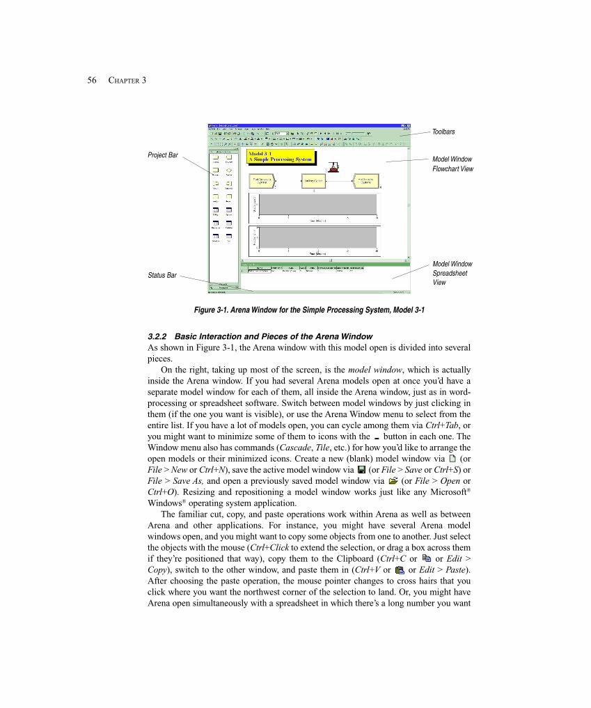
56 CHAPTER 3
Figure 3-1. Arena Window for the Simple Processing System, Model 3-1
3.2.2 Basic Interaction and Pieces of the Arena WindowAs shown in Figure 3-1, the Arena window with this model open is divided into severalpieces.
On the right, taking up most of the screen, is the model window, which is actuallyinside the Arena window. If you had several Arena models open at once you’d have aseparate model window for each of them, all inside the Arena window, just as in word-processing or spreadsheet software. Switch between model windows by just clicking inthem (if the one you want is visible), or use the Arena Window menu to select from theentire list. If you have a lot of models open, you can cycle among them via Ctrl+Tab, oryou might want to minimize some of them to icons with the button in each one. TheWindow menu also has commands (Cascade, Tile, etc.) for how you’d like to arrange theopen models or their minimized icons. Create a new (blank) model window via (orFile > New or Ctrl+N), save the active model window via (or File > Save or Ctrl+S) orFile > Save As, and open a previously saved model window via (or File > Open orCtrl+O). Resizing and repositioning a model window works just like any Microsoft®
Windows® operating system application.The familiar cut, copy, and paste operations work within Arena as well as between
Arena and other applications. For instance, you might have several Arena modelwindows open, and you might want to copy some objects from one to another. Just selectthe objects with the mouse (Ctrl+Click to extend the selection, or drag a box across themif they’re positioned that way), copy them to the Clipboard (Ctrl+C or or Edit >Copy), switch to the other window, and paste them in (Ctrl+V or or Edit > Paste).After choosing the paste operation, the mouse pointer changes to cross hairs that youclick where you want the northwest corner of the selection to land. Or, you might haveArena open simultaneously with a spreadsheet in which there’s a long number you want
Project Bar
Status Bar
Model WindowSpreadsheetView
Model WindowFlowchart View
Toolbars
57A GUIDED TOUR THROUGH ARENA
to put into an Arena dialog text box. Copy the number from the spreadsheet cell, switchto Arena (either via the Windows® Taskbar or by using Alt+Tab to cycle through the openapplications), position the insertion pointer in the Arena dialog box where you want thenumber, and paste it in. If you’re writing a report in a word processor and want to paste ina “snapshot” of an Arena screen, go to Arena and get it into the state you want tophotograph, press the Prnt Scrn (Print Screen) key, switch over to your word-processingdocument, and paste the shot where you want it; if you want just the active window (likea dialog box you want to document), press Alt+Prnt Scrn instead, then paste it into theword-processing document.
The model window can be split into two regions, or views: the flowchart view and thespreadsheet view. Often it’s helpful to see both the flowchart and spreadsheet views ofthe model window at the same time. But you can choose to see only one of the views andthus devote all of the real estate in the model window to it by clearing the menucommand View > Split Screen or clicking so that it does not appear to be pushed in; inthis case, to see one or the other view, just single-click on either a flowchart ( ) orspreadsheet ( ) module in the Project Bar on the left of your screen. The flowchart viewcontains the model’s graphics, including the process flowchart, animation, and otherdrawing elements. The spreadsheet view can display model data such as times and otherparameters, and allows you to enter or edit them (right now it happens to be showingdetails about something called “Create – Basic Process”). Many model parameters canbe viewed and edited in either the flowchart view or the spreadsheet view, but thespreadsheet view gives you access to lots of parameters at once, arranged in compactgroups of similar parameters convenient for editing, especially in large models. Thehorizontal line splitting the flowchart and spreadsheet views (if both views are visible)can be dragged up or down to change the proportion of the model window allocated tothe two views.
Down the left edge of the Arena window in Figure 3-1 is the Project Bar, which hostspanels containing the objects with which you’ll be working, displaying one panel at atime. Right now the Project Bar is displaying the Basic Process panel, which containsfundamental building blocks, called modules, that are useful in a wide variety ofsimulation models.
Below the Basic Process panel on the Project Bar is a horizontal button labeled“Reports,” which will display another panel containing a road map to the results of asimulation after it’s run; click on this button to make this panel visible, and then click onthe Basic Process button to make that panel visible again.
The Navigate panel allows you to display different views of a model, includingdifferent submodels in a hierarchical model (Model 3-1 doesn’t have submodels so theonly view in the Navigate panel is Top-Level, though if you click on the + to its left, youopen a tree that has three entries for our model, which we’ll discuss in Section 3.2.3below). If the small button ( ) on the right of the horizontal Navigate button is pressed,you’ll also get a “thumbnail” of the model window in the top of the Navigate panel, witha translucent blue box showing the location and zoom size of the active window’s currentview. Clicking anywhere in the thumbnail changes the current view to that spot. Drag the
58 CHAPTER 3
blue box around to pan to other regions of the window, or resize the blue box (hover thepointer over an edge and then click-drag) to change the “altitude” of the zoom. The +/–toggle in the circle in the thumbnail’s upper right determines whether the blue box isshown relative to the entire window’s capacity (the “+” choice), or takes into accountwhat region in the window actually has content (the “–” choice).
The Project Bar is usually docked to the left edge of the Arena window, but it can betorn off and “floated” anywhere on your screen, or it can be docked to the right edge of themodel window if you prefer. You’ll usually need the Project Bar to be visible whileworking on a model, but if you’d like more room just to look through things, you can pushthe small button at the upper right of the Project Bar, or clear View > Project Bar to hideit (re-check View > Project Bar to display it again).
There are several other panels that come with Arena, perhaps depending on what youlicensed. These include Advanced Process (with different and “smaller” building blocksfor more detailed modeling), Advanced Transfer (containing many options for movingentities around), and Blocks and Elements (which together give you full access to theSIMAN simulation language that underlies Arena; see Pegden, Shannon, and Sadowski,1995). Yet more panels contain constructs for specialized applications, like modelingcontact centers and high-speed packaging lines. As mentioned earlier, to make theelements in a panel available for use in your model, you need to Attach the panel to yourmodel via File > Template Panel > Attach or the Template Attach button ( ), or by right-clicking in a panel and selecting Template Panel > Attach in the pop-up. Panel files havethe file name extension .tpo and are typically in the Template folder inside the Arenafolder. If you want Arena to attach certain panels to each new model you start, do Tools >Options > Settings and type the file names of those .tpo panel files into the Auto AttachPanels box there.
At the very bottom of the Arena window is the Status Bar, which displays variouskinds of information on the status of the simulation, depending on what’s going on at themoment. Right now the only thing it shows are the (x, y) coordinates in the world space(see Section 3.2.3) of the location of the mouse pointer. While the simulation runs, theStatus Bar will display, for instance, the simulation clock value, the replication numberbeing executed, and the number of replications to be run. You can hide the Status Bar byclearing (unchecking) View > Status Bar.
3.2.3 Panning, Zooming, Viewing, and Aligning in the Flowchart ViewThe particular flowchart view of the model window you see in Figure 3-1 is just one ofmany possible views of the model and the big world space in which the flowchartdepiction of a model lives. The world space’s center has (x, y) coordinates (0, 0), and itextends for thousands of units in all four directions from there; these units are justpositional and don’t have any particular physical meaning (call them furlongs or youdels2
if you like). To maximize the size of the model window within the Arena window, click if it’s visible in the upper right corner of the model window. Likewise, to maximize the
Arena window itself to consume your entire screen, click its button.
2 Apologies to Gene Woolsey.
59A GUIDED TOUR THROUGH ARENA
To see different parts of the flowchart view, you can pan around using the scroll barson the lower and right edges, or the arrow keys (try it; to navigate via the keyboard, youmust first make the model window active by clicking in it). You can also zoom in (withthe button or the + key or View > Zoom In), or zoom out (with the button or the –key or View > Zoom Out) to see parts of the model from different “altitudes.” To pan/zoom automatically to see all the model at the closest possible zoom, click (or View >Views > All, or the * key). If you want to go back to the preceding view (maybe youmessed up), click (or View > Views >Previous). If you’re at a relatively high altitudebut spy a region that you’d like to view up close, select View > Views > Region (or hit the“[” key) to change the mouse pointer to cross hairs, click on one corner of the rectangularregion you want to see, then again on the opposite corner—Arena will pan and zoom tosee all of that region at the closest possible zoom (that is, lowest possible altitude).Another way to pan and zoom is via the thumbnail option in the Navigate toolbar,described in Section 3.2.2.
If you get to a view you like (and to which you’d like to be able to return instantly),you can save it as a Named View and assign a hot key to it. Pan and zoom to the view youwant to save, then select View > Named Views (or hit the the ? key or the button), andthen click Add. You must give the view a descriptive Name, and you can optionally assigna hot key to it as well. To jump back to this view at any time, select View > Named Views(or hit the ? key or the button), click on the view you want, and press the Show button.You can also access your Named Views in the Navigate panel of the Project Bar by click-ing the + to the left (in this case of Top-Level) to open up a tree of the Named Views; justclick on an entry to go to that view. Yet another way (probably the fastest way) to get to aNamed View is to hit the hot key assigned to it; you’ll have to remember what the hotkeys are, or maybe document them in the model with some text, as described in Section3.6.3. Hot keys for Named Views are one of the few places in Arena where characters arecase-sensitive (for example, “a” and “A” are different). Named Views can be accessed atany time, even while the simulation is running. We’ve set up three Named Views forModel 3-1: all (hot key a), logic (hot key l), and plots (hot key p). Try them out.
New Arena models start out in a specific “Home” pan/zoom configuration, just to thesoutheast of the (0, 0) position in the world space, to which you can return by pressingthe Home key on your keyboard (or View > Views > Home). To see the largest possiblearea of the world space (from the maximum altitude), select View > Views > Max.
To get your visual bearings, you can display a background grid of little dots bychecking View > Grid (or by clicking ). If you further want to cause newly placed
items to snap to this grid, check View > Snap to Grid (or click ). Both of these actions
are toggle keys; that is, you just repeat the action to undo it. To snap existing items to thegrid, first select them (maybe using Ctrl+Click to keep extending your selection, ordragging a rectangle across them if they’re arranged that way) and then Arrange > SnapObject to Grid to adjust their positions to align with the grid points. To customize thespacing of the grid points, select View > Grid & Snap Settings; the units are (x, y) valuesin the measurement units of the world space. You can also display Rulers on the top andleft edges, with units’ being Arena world units, by pushing the button or checking
View > Rulers.
60 CHAPTER 3
You might want to align objects in the flowchart view precisely, either horizontally orvertically, with respect to their edges or centers, and there are several options for doingthis. One option is to establish horizontal and vertical Guides in the flowchart view;make sure Rulers are displayed, then click the Guides button ( ) or select View >Guides, and then drag down from the horizontal ruler on the top or drag to the right fromthe vertical ruler on the left to place a dashed blue Guide line (you can have several ofeach). Then, click the Glue to Guides button ( ) or select View > Glue to Guides, andthen drag objects toward the guides until a red positional square lights up for edge orcenter positioning. Once objects are glued to a guide, you can drag the guide, and allobjects glued to it will move together and stick with their alignment to the guide. Todelete a guide, select it by clicking on it (it will be highlighted green) and hit the Deletekey. Another option is to select the objects you want to align and then use the Arrangemenu; select Align to line the selected objects up on their Top, Bottom, Left, or Rightedges; select Distribute to space them evenly horizontally or vertically with spacingspecified in Settings. Arrange > Flowchart Alignment lines up flowchart modules (seeSection 3.2.4 next) in the current set of selected objects.
3.2.4 ModulesThe basic building blocks for Arena models are called modules. These are the flowchartand data objects that define the process to be simulated and are chosen from panels in theProject Bar. Modules come in two basic flavors: flowchart and data.
Flowchart modules describe the dynamic processes in the model. You can think offlowchart modules as being nodes or places through which entities flow, or where entitiesoriginate or leave the model. To put an instance of a flowchart module of a particular typeinto your model, drag it from the Project Bar into the flowchart view of the modelwindow (you can drag it around later to reposition it). Flowchart modules are typicallyconnected to each other in some way. In the Basic Process panel, the kinds of flowchartmodules available are Create, Dispose, Process, Decide, Batch, Separate, Assign, andRecord; other panels have many additional kinds of flowchart modules. Each type offlowchart module in the Basic Process panel has a distinctive shape, similar to classicalflowcharting (see Schriber, 1969) and suggestive of what it does. But in other panels(such as the Advanced Process panel), there are many more flowchart-module types thanthere are reasonable shapes, so they’re all represented by simple rectangles. Some panels(like Advanced Transfer) use colors in the rectangles to distinguish different types offlowchart modules, and some panels (like the specialized ones for contact centers andpackaging) use more elaborate graphics for them. One way to edit a flowchart module isto double-click on it once it’s been placed in the flowchart view of the model window, tobring up a dialog box pertaining to it. Another way to edit flowchart modules is to selecta module type (for example, click on a Create or a Process module), either in the ProjectBar or in the flowchart view of the model window, and a line for each flowchart moduleof that type in the model shows up in the spreadsheet view of the model window (if it’svisible), where you can edit the entries. This gives you a compact view of all theinstances of flowchart modules of that type in your model, which is useful in largemodels where you might have many such instances.
61A GUIDED TOUR THROUGH ARENA
Data modules define the characteristics of various process elements, like entities,resources, and queues. They can also set up variables and other types of numerical valuesand expressions that pertain to the whole model. Icons for data modules in the Project Barlook like little spreadsheets. The Basic Process panel’s data modules are Entity, Queue,Resource, Variable, Schedule, and Set (other panels contain additional kinds of datamodules). Entities don’t flow through data modules, and data modules aren’t dragged intothe model window; rather, data modules exist “behind the scenes” in a model to definedifferent kinds of values, expressions, and conditions. You don’t double-click on a datamodule to edit it, but just single-click it in the Project Bar and a spreadsheet for that typeof module will appear in the spreadsheet view of the model window (which must bevisible), which you can then edit or extend by double-clicking where indicated to addadditional rows. While the default is to edit modules from the spreadsheet view, if youdouble-click on the number in the left-hand column (or right-click and select Edit viaDialog), you can also edit in the dialog mode. Unlike flowchart modules, you don’t havemore than one instance of a data module in a model; however, there could be many rowsin the spreadsheet for a data module, each typically representing a separate object of thattype (for instance, if your model has three different queues, the Queue data module willdisplay three rows, one for each queue, in its spreadsheet).
Flowchart and data modules in a model are related to each other by the names forobjects (like queues, resources, entity types, and variables) that they have in common.Arena keeps internal lists of the names you give to these kinds of objects as you definethem, and then presents these names to you in drop-down lists in the appropriate placesin both flowchart and data modules, which helps you remember what you’ve namedthings (and protects you from your own inevitable typos...or, at least, keeps you consis-tent in your lousy typing so your model will still run).
3.2.5 Internal Model DocumentationIf you rest your mouse pointer on a module symbol or other object, you’ll see a Data Tip.Data Tips have two parts, a default description and a user-defined description. Thedefault tip will describe some generic information about the object, such as its name andtype. The user-defined part will display exactly what is entered in the Object PropertiesDescription field. You can enter text in this field by right-clicking on an object andselecting Properties. Display of these Data Tips can be toggled via View > Data Tips. Bydefault, both are enabled, but either the default or the user-defined Data Tips may bedisabled.
In addition to the module descriptions, you can also enter a Project Description thatprovides some context to the entire model. This is a good place to document what themodel does, why it was created, assumptions you have made, and similar information.This is entered in Run > Setup > Project Parameters (see Figure 3-15 later in this chapter).
While Data Tips are a useful feature, particularly when your models get large, youmight wonder if there is another way to make use of this information. There is. Tools >Model Documentation Report creates a custom report summarizing all your model data. Itprovides some options about what information to include, then generates an HTML report.
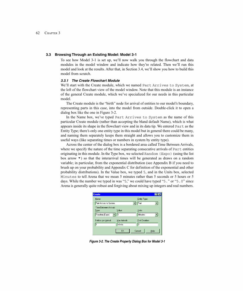
62 CHAPTER 3
3.3 Browsing Through an Existing Model: Model 3-1
To see how Model 3-1 is set up, we’ll now walk you through the flowchart and datamodules in the model window and indicate how they’re related. Then we’ll run thismodel and look at the results. After that, in Section 3.4, we’ll show you how to build thismodel from scratch.
3.3.1 The Create Flowchart ModuleWe’ll start with the Create module, which we named Part Arrives to System, atthe left of the flowchart view of the model window. Note that this module is an instanceof the general Create module, which we’ve specialized for our needs in this particularmodel.
The Create module is the “birth” node for arrival of entities to our model’s boundary,representing parts in this case, into the model from outside. Double-click it to open adialog box like the one in Figure 3-2.
In the Name box, we’ve typed Part Arrives to System as the name of thisparticular Create module (rather than accepting the bland default Name), which is whatappears inside its shape in the flowchart view and in its data tip. We entered Part as theEntity Type; there’s only one entity type in this model but in general there could be many,and naming them separately keeps them straight and allows you to customize them inuseful ways (like separating times or numbers in system by entity type).
Across the center of the dialog box is a bordered area called Time Between Arrivals,where we specify the nature of the time separating consecutive arrivals of Part entitiesoriginating in this module. In the Type box, we selected Random (Expo) (using the listbox arrow ) so that the interarrival times will be generated as draws on a randomvariable; in particular, from the exponential distribution (see Appendix B if you need tobrush up on your probability and Appendix C for definition of the exponential and otherprobability distributions). In the Value box, we typed 5, and in the Units box, selectedMinutes to tell Arena that we mean 5 minutes rather than 5 seconds or 5 hours or 5days. While the number we typed in was “5,” we could have typed “5.” or “5.0” sinceArena is generally quite robust and forgiving about mixing up integers and real numbers.
Figure 3-2. The Create Property Dialog Box for Model 3-1
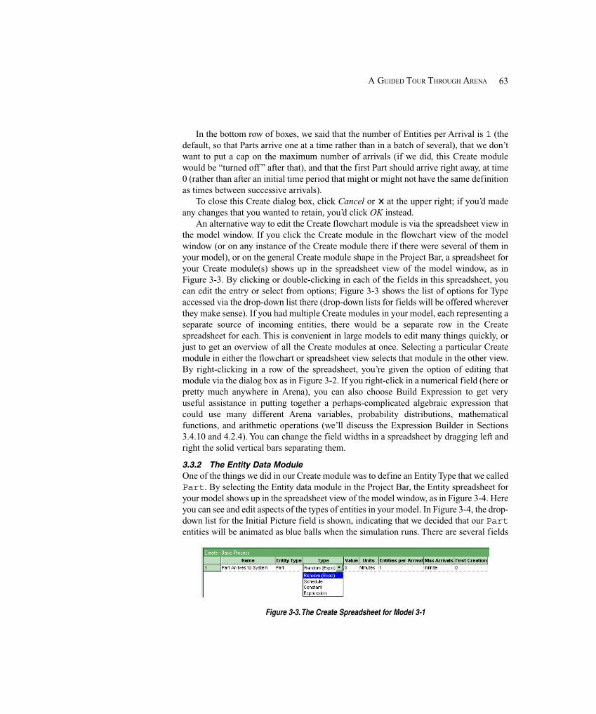
63A GUIDED TOUR THROUGH ARENA
In the bottom row of boxes, we said that the number of Entities per Arrival is 1 (thedefault, so that Parts arrive one at a time rather than in a batch of several), that we don’twant to put a cap on the maximum number of arrivals (if we did, this Create modulewould be “turned off ” after that), and that the first Part should arrive right away, at time0 (rather than after an initial time period that might or might not have the same definitionas times between successive arrivals).
To close this Create dialog box, click Cancel or at the upper right; if you’d madeany changes that you wanted to retain, you’d click OK instead.
An alternative way to edit the Create flowchart module is via the spreadsheet view inthe model window. If you click the Create module in the flowchart view of the modelwindow (or on any instance of the Create module there if there were several of them inyour model), or on the general Create module shape in the Project Bar, a spreadsheet foryour Create module(s) shows up in the spreadsheet view of the model window, as inFigure 3-3. By clicking or double-clicking in each of the fields in this spreadsheet, youcan edit the entry or select from options; Figure 3-3 shows the list of options for Typeaccessed via the drop-down list there (drop-down lists for fields will be offered whereverthey make sense). If you had multiple Create modules in your model, each representing aseparate source of incoming entities, there would be a separate row in the Createspreadsheet for each. This is convenient in large models to edit many things quickly, orjust to get an overview of all the Create modules at once. Selecting a particular Createmodule in either the flowchart or spreadsheet view selects that module in the other view.By right-clicking in a row of the spreadsheet, you’re given the option of editing thatmodule via the dialog box as in Figure 3-2. If you right-click in a numerical field (here orpretty much anywhere in Arena), you can also choose Build Expression to get veryuseful assistance in putting together a perhaps-complicated algebraic expression thatcould use many different Arena variables, probability distributions, mathematicalfunctions, and arithmetic operations (we’ll discuss the Expression Builder in Sections3.4.10 and 4.2.4). You can change the field widths in a spreadsheet by dragging left andright the solid vertical bars separating them.
3.3.2 The Entity Data ModuleOne of the things we did in our Create module was to define an Entity Type that we calledPart. By selecting the Entity data module in the Project Bar, the Entity spreadsheet foryour model shows up in the spreadsheet view of the model window, as in Figure 3-4. Hereyou can see and edit aspects of the types of entities in your model. In Figure 3-4, the drop-down list for the Initial Picture field is shown, indicating that we decided that our Partentities will be animated as blue balls when the simulation runs. There are several fields
Figure 3-3. The Create Spreadsheet for Model 3-1
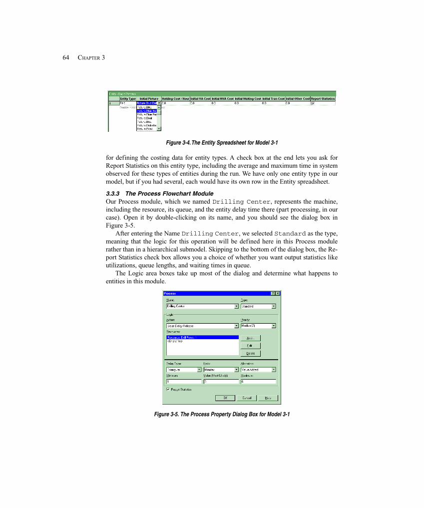
64 CHAPTER 3
Figure 3-4. The Entity Spreadsheet for Model 3-1
for defining the costing data for entity types. A check box at the end lets you ask forReport Statistics on this entity type, including the average and maximum time in systemobserved for these types of entities during the run. We have only one entity type in ourmodel, but if you had several, each would have its own row in the Entity spreadsheet.
3.3.3 The Process Flowchart ModuleOur Process module, which we named Drilling Center, represents the machine,including the resource, its queue, and the entity delay time there (part processing, in ourcase). Open it by double-clicking on its name, and you should see the dialog box inFigure 3-5.
After entering the Name Drilling Center, we selected Standard as the type,meaning that the logic for this operation will be defined here in this Process modulerather than in a hierarchical submodel. Skipping to the bottom of the dialog box, the Re-port Statistics check box allows you a choice of whether you want output statistics likeutilizations, queue lengths, and waiting times in queue.
The Logic area boxes take up most of the dialog and determine what happens toentities in this module.
Figure 3-5. The Process Property Dialog Box for Model 3-1
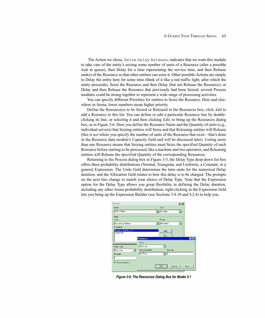
65A GUIDED TOUR THROUGH ARENA
The Action we chose, Seize Delay Release, indicates that we want this moduleto take care of the entity’s seizing some number of units of a Resource (after a possiblewait in queue), then Delay for a time representing the service time, and then Releaseunit(s) of the Resource so that other entities can seize it. Other possible Actions are simplyto Delay the entity here for some time (think of it like a red traffic light, after which theentity proceeds), Seize the Resource and then Delay (but not Release the Resource), orDelay and then Release the Resource that previously had been Seized; several Processmodules could be strung together to represent a wide range of processing activities.
You can specify different Priorities for entities to Seize the Resource. Here and else-where in Arena, lower numbers mean higher priority.
Define the Resource(s) to be Seized or Released in the Resources box; click Add toadd a Resource to this list. You can define or edit a particular Resource line by double-clicking its line, or selecting it and then clicking Edit, to bring up the Resources dialogbox, as in Figure 3-6. Here you define the Resource Name and the Quantity of units (e.g.,individual servers) that Seizing entities will Seize and that Releasing entities will Release(this is not where you specify the number of units of the Resource that exist—that’s donein the Resource data module’s Capacity field and will be discussed later). Listing morethan one Resource means that Seizing entities must Seize the specified Quantity of eachResource before starting to be processed, like a machine and two operators, and Releasingentities will Release the specified Quantity of the corresponding Resources.
Returning to the Process dialog box in Figure 3-5, the Delay Type drop-down list boxoffers three probability distributions (Normal, Triangular, and Uniform), a Constant, or ageneral Expression. The Units field determines the time units for the numerical Delayduration, and the Allocation field relates to how this delay is to be charged. The promptson the next line change to match your choice of Delay Type. Note that the Expressionoption for the Delay Type allows you great flexibility in defining the Delay duration,including any other Arena probability distribution; right-clicking in the Expression fieldlets you bring up the Expression Builder (see Sections 3.4.10 and 4.2.4) to help you.
Figure 3-6. The Resources Dialog Box for Model 3-1
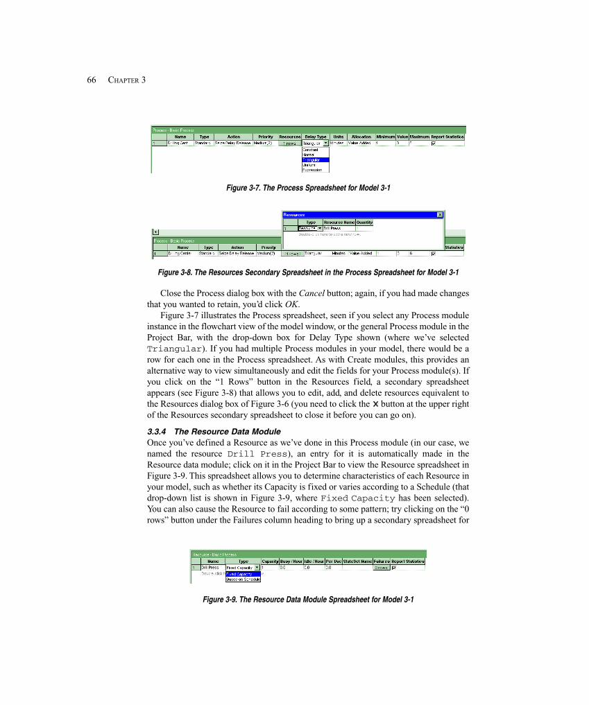
66 CHAPTER 3
Figure 3-7. The Process Spreadsheet for Model 3-1
Figure 3-8. The Resources Secondary Spreadsheet in the Process Spreadsheet for Model 3-1
Close the Process dialog box with the Cancel button; again, if you had made changesthat you wanted to retain, you’d click OK.
Figure 3-7 illustrates the Process spreadsheet, seen if you select any Process moduleinstance in the flowchart view of the model window, or the general Process module in theProject Bar, with the drop-down box for Delay Type shown (where we’ve selectedTriangular). If you had multiple Process modules in your model, there would be arow for each one in the Process spreadsheet. As with Create modules, this provides analternative way to view simultaneously and edit the fields for your Process module(s). Ifyou click on the “1 Rows” button in the Resources field, a secondary spreadsheetappears (see Figure 3-8) that allows you to edit, add, and delete resources equivalent tothe Resources dialog box of Figure 3-6 (you need to click the button at the upper rightof the Resources secondary spreadsheet to close it before you can go on).
3.3.4 The Resource Data ModuleOnce you’ve defined a Resource as we’ve done in this Process module (in our case, wenamed the resource Drill Press), an entry for it is automatically made in theResource data module; click on it in the Project Bar to view the Resource spreadsheet inFigure 3-9. This spreadsheet allows you to determine characteristics of each Resource inyour model, such as whether its Capacity is fixed or varies according to a Schedule (thatdrop-down list is shown in Figure 3-9, where Fixed Capacity has been selected).You can also cause the Resource to fail according to some pattern; try clicking on the “0rows” button under the Failures column heading to bring up a secondary spreadsheet for
Figure 3-9. The Resource Data Module Spreadsheet for Model 3-1

67A GUIDED TOUR THROUGH ARENA
Figure 3-10. The Queue Data Module Spreadsheet for Model 3-1
this (the failure pattern is defined in the Failure data module in the Advanced Processpanel, which you might have to attach to the Project Bar for your model).
3.3.5 The Queue Data ModuleIf the Drill Press resource is busy when an entity gets to the Process module, theentity will have to queue up. The Queue spreadsheet, seen in Figure 3-10, appears in thespreadsheet view if you select the Queue data module in the Project Bar. Here you cancontrol aspects of the queues in your model (we have only one, named DrillingCenter.Queue), such as the discipline used to operate it, as shown in the Type list inFigure 3-10 (First In First Out is the default and is selected). You could, forinstance, rank the queue according to some attribute of entities that reside in it; if youchose Lowest Attribute Value, the queue would be ranked in increasing order of someattribute, and an additional field would show up in the line for this Queue in which youwould have to specify the Attribute to be used for ranking.
3.3.6 Animating Resources and QueuesSpeaking of queues, you might have noticed the just above the Processmodule in the flowchart view. This is where the queue will be animated, and the Processmodule acquired this graphic when we specified that we wanted entities to Seize aResource there.
And while we’re on the subject of animation, you’ve no doubt noticed the aboveand to the right of the Process module and positioned at what will be the head of thequeue animation. This is a Resource animation and will change appearance during thesimulation depending on whether the Drill Press Resource is Idle or Busy. This didnot come “free” with the Resource specified in the Process module; rather, we added it toour model via the Resource button ( ) in the Animate toolbar. Double-click on the icon to get the Resource Picture Placement dialog, as in Figure 3-11. This allows us topick pictures from libraries (files with extension .plb to their name, usually found in theArena folder) to cause the Resource to be animated differently depending on the state it’sin. While you can get an idea of how this works at this point, we’ll discuss Resourceanimation in Sections 3.4.8 and 4.3.3.
3.3.7 The Dispose Flowchart ModuleThe Dispose module represents entities leaving the model boundaries; double-click itsname to bring up the dialog box in Figure 3-12; the Dispose spreadsheet is in Figure3-13. There’s not much to do here—just give the module a descriptive Name and decideif you want output on the Entity Statistics, which include things like average and maxi-mum time in system of entities that go out through this module and costing informationon these entities.
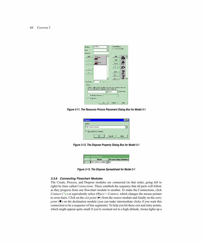
68 CHAPTER 3
Figure 3-11. The Resource Picture Placement Dialog Box for Model 3-1
Figure 3-12. The Dispose Property Dialog Box for Model 3-1
Figure 3-13. The Dispose Spreadsheet for Model 3-1
3.3.8 Connecting Flowchart ModulesThe Create, Process, and Dispose modules are connected (in that order, going left toright) by lines called Connections. These establish the sequence that all parts will followas they progress from one flowchart module to another. To make the Connections, clickConnect ( ) or equivalently select Object > Connect, which changes the mouse pointerto cross hairs. Click on the exit point ( ) from the source module and finally on the entrypoint ( ) on the destination module (you can make intermediate clicks if you want thisconnection to be a sequence of line segments). To help you hit these exit and entry points,which might appear quite small if you’re zoomed out to a high altitude, Arena lights up a
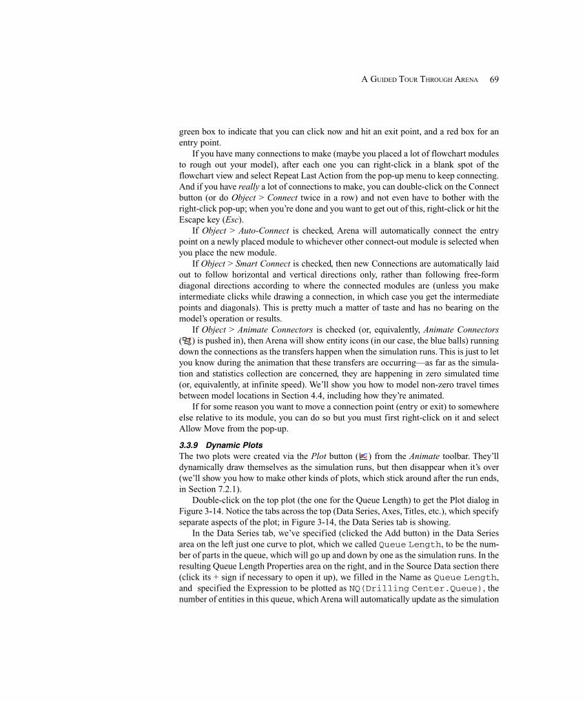
69A GUIDED TOUR THROUGH ARENA
green box to indicate that you can click now and hit an exit point, and a red box for anentry point.
If you have many connections to make (maybe you placed a lot of flowchart modulesto rough out your model), after each one you can right-click in a blank spot of theflowchart view and select Repeat Last Action from the pop-up menu to keep connecting.And if you have really a lot of connections to make, you can double-click on the Connectbutton (or do Object > Connect twice in a row) and not even have to bother with theright-click pop-up; when you’re done and you want to get out of this, right-click or hit theEscape key (Esc).
If Object > Auto-Connect is checked, Arena will automatically connect the entrypoint on a newly placed module to whichever other connect-out module is selected whenyou place the new module.
If Object > Smart Connect is checked, then new Connections are automatically laidout to follow horizontal and vertical directions only, rather than following free-formdiagonal directions according to where the connected modules are (unless you makeintermediate clicks while drawing a connection, in which case you get the intermediatepoints and diagonals). This is pretty much a matter of taste and has no bearing on themodel’s operation or results.
If Object > Animate Connectors is checked (or, equivalently, Animate Connectors( ) is pushed in), then Arena will show entity icons (in our case, the blue balls) runningdown the connections as the transfers happen when the simulation runs. This is just to letyou know during the animation that these transfers are occurring—as far as the simula-tion and statistics collection are concerned, they are happening in zero simulated time(or, equivalently, at infinite speed). We’ll show you how to model non-zero travel timesbetween model locations in Section 4.4, including how they’re animated.
If for some reason you want to move a connection point (entry or exit) to somewhereelse relative to its module, you can do so but you must first right-click on it and selectAllow Move from the pop-up.
3.3.9 Dynamic PlotsThe two plots were created via the Plot button ( ) from the Animate toolbar. They’lldynamically draw themselves as the simulation runs, but then disappear when it’s over(we’ll show you how to make other kinds of plots, which stick around after the run ends,in Section 7.2.1).
Double-click on the top plot (the one for the Queue Length) to get the Plot dialog inFigure 3-14. Notice the tabs across the top (Data Series, Axes, Titles, etc.), which specifyseparate aspects of the plot; in Figure 3-14, the Data Series tab is showing.
In the Data Series tab, we’ve specified (clicked the Add button) in the Data Seriesarea on the left just one curve to plot, which we called Queue Length, to be the num-ber of parts in the queue, which will go up and down by one as the simulation runs. In theresulting Queue Length Properties area on the right, and in the Source Data section there(click its + sign if necessary to open it up), we filled in the Name as Queue Length,and specified the Expression to be plotted as NQ(Drilling Center.Queue), thenumber of entities in this queue, which Arena will automatically update as the simulation
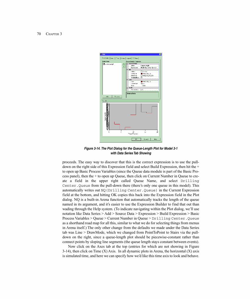
70 CHAPTER 3
Figure 3-14. The Plot Dialog for the Queue-Length Plot for Model 3-1with Data Series Tab Showing
proceeds. The easy way to discover that this is the correct expression is to use the pull-down on the right side of this Expression field and select Build Expression, then hit the +to open up Basic Process Variables (since the Queue data module is part of the Basic Pro-cess panel), then the + to open up Queue, then click on Current Number in Queue to cre-ate a field in the upper right called Queue Name, and select DrillingCenter.Queue from the pull-down there (there’s only one queue in this model). Thisautomatically writes out NQ(Drilling Center.Queue) in the Current Expressionfield at the bottom, and hitting OK copies this back into the Expression field in the Plotdialog. NQ is a built-in Arena function that automatically tracks the length of the queuenamed in its argument, and it’s easier to use the Expression Builder to find that out thanwading through the Help system. (To indicate navigating within the Plot dialog, we’ll usenotation like Data Series > Add > Source Data > Expression > Build Expression > BasicProcess Variables > Queue > Current Number in Queue > Drilling Center.Queueas a shorthand road map for all this, similar to what we do for selecting things from menusin Arena itself.) The only other change from the defaults we made under the Data Seriestab was Line > DrawMode, which we changed from PointToPoint to Stairs via the pull-down on the right, since a queue-length plot should be piecewise-constant rather thanconnect points by sloping line segments (the queue length stays constant between events).
Now click on the Axes tab at the top (entries for which are not showing in Figure3-14), then click on Time (X) Axis. In all dynamic plots in Arena, the horizontal (X) axisis simulated time, and here we can specify how we’d like this time axis to look and behave.

71A GUIDED TOUR THROUGH ARENA
On the right under Scale (you may need to scroll down to it), we specified Maximum to be20, to show the whole plot for our 20-minute run (the time units here are in the Base TimeUnits for the model). We also set MajorIncrement to 5 for tic marks on the time axis every5 minutes. Under Title, we typed in the Text we wanted for the horizontal axis, andchanged Visible to True via the pull-down to make it show up. Next, click on Left Value(Y) Axis and note our entry under Scale (MajorIncrement = 1); we left Maximum at itsdefault value of 100, and left AutoScaleMaximum at its default value of True, which willautomatically adjust the Y-axis scale as needed since we don’t know up front how long thequeue will get. Under Title, we typed the Text we wanted, and set Visible to True.
Finally, in the Legend tab we merely cleared (unchecked) the Show Legend box. Wehave only one curve in this plot, and our Y-axis Title adequately describes it.
There are many, many other options in Plot, which you can easily explore on yourown (or hit the Help button on the bottom right of the Plot dialog), and we left those attheir defaults. Note that in the Sample area at the bottom of the Plot dialog is a “dummy”schematic showing how all these specifications will look once the actual plot is drawnduring the simulation (depending on your Axes settings there could be a smashed-to-gether jumble of axis numbers in this Sample, but these should straighten themselves outin the actual plot if you’ve specified things right).
The size of the plot is determined by dragging the handles on its borders. Click(once) on the plot and try this (don’t worry, there’s an Undo). Actually, you have tospecify an initial size of the plot after you fill out the dialogs, but you can change thislater, as well as drag it around to relocate it.
The Plot dialog for the Number Busy plot is similar, so we won’t go through it indetail (but go ahead and open it to look at it). The only really different thing is that theExpression whose value we want to plot on the y-axis is NR(Drill Press), which weknow will always be either 0 or 1, so we specified Axes > Left Value (Y) Axis > Scale >Maximum to be 2, and AutoScaleMaximum there to be False to make for an attractiveand tasteful graph. As before, we used the Expression Builder in Data Series > SourceData > Expression to figure out that this is the right name and syntax.
3.3.10 Dressing Things UpText labels in the model window, like the title at the upper left, can be done via the Textbutton ( ) on the Draw toolbar. You can control the usual things like font, size, and stylefrom there. To go to a new line in the text use Ctrl+Enter. To change the text color, selectthe text (single-click on it), and use the Text Color button ( ) to select either the coloron the underline there (click on the in this case) or to choose a different color (click onthe in this case) that will become the new underline color for future text. You can alsoresize or rotate text by selecting it and dragging the underline bar.
The Draw toolbar also has things like boxes, ellipses, polygons, and lines, as well asthe means to control their colors and styles, which you can use to decorate your modelwindow, depending on your artistic creativity and talent (as you can see, ours is severelylimited). This is how we made the simple shadow box behind the model title in the upperleft of the model window. The Arrange toolbar and menu have buttons and commandsthat allow you to manipulate objects, such as grouping, flipping, sending a draw object to
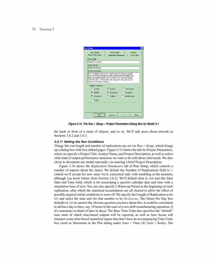
72 CHAPTER 3
Figure 3-15. The Run > Setup > Project Parameters Dialog Box for Model 3-1
the back or front of a stack of objects, and so on. We’ll talk more about artwork inSections 3.6.2 and 3.6.3.
3.3.11 Setting the Run ConditionsThings like run length and number of replications are set via Run > Setup, which bringsup a dialog box with five tabbed pages. Figure 3-15 shows the tab for Project Parameters,where we specify a Project Title, Analyst Name, and Project Description, as well as selectwhat kind of output performance measures we want to be told about afterwards. We alsochose to document our model internally via entering a brief Project Description.
Figure 3-16 shows the Replication Parameters tab of Run Setup, which controls anumber of aspects about the run(s). We default the Number of Replications field to 1(which we’ll accept for now since we’re concerned only with modeling at the moment,although you know better, from Section 2.6.2). We’ll default (that is, not use) the StartDate and Time field, which is for associating a specific calendar date and time with asimulation time of zero. You can also specify a Warm-up Period at the beginning of eachreplication, after which the statistical accumulators are all cleared to allow the effect ofpossibly atypical initial conditions to wear off. We specify the Length of Replication to be20 and select the time unit for that number to be Minutes. The Hours Per Day boxdefaults to 24 (to answer the obvious question you have about this, it could be convenientto define a day to have, say, 16 hours in the case of a two-shift manufacturing operation, ifit’s customary to think of time in days). The Base Time Units box specifies the “default”time units in which time-based outputs will be reported, as well as how Arena willinterpret some time-based numerical inputs that don’t have an accompanying Time Unitsbox (such as Maximum in the Plot dialog under Axes > Time (X) Axis > Scale). The
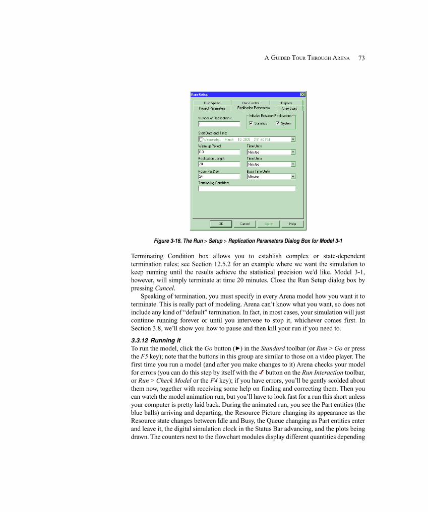
73A GUIDED TOUR THROUGH ARENA
Figure 3-16. The Run > Setup > Replication Parameters Dialog Box for Model 3-1
Terminating Condition box allows you to establish complex or state-dependenttermination rules; see Section 12.5.2 for an example where we want the simulation tokeep running until the results achieve the statistical precision we’d like. Model 3-1,however, will simply terminate at time 20 minutes. Close the Run Setup dialog box bypressing Cancel.
Speaking of termination, you must specify in every Arena model how you want it toterminate. This is really part of modeling. Arena can’t know what you want, so does notinclude any kind of “default” termination. In fact, in most cases, your simulation will justcontinue running forever or until you intervene to stop it, whichever comes first. InSection 3.8, we’ll show you how to pause and then kill your run if you need to.
3.3.12 Running ItTo run the model, click the Go button ( ) in the Standard toolbar (or Run > Go or pressthe F5 key); note that the buttons in this group are similar to those on a video player. Thefirst time you run a model (and after you make changes to it) Arena checks your modelfor errors (you can do this step by itself with the button on the Run Interaction toolbar,or Run > Check Model or the F4 key); if you have errors, you’ll be gently scolded aboutthem now, together with receiving some help on finding and correcting them. Then youcan watch the model animation run, but you’ll have to look fast for a run this short unlessyour computer is pretty laid back. During the animated run, you see the Part entities (theblue balls) arriving and departing, the Resource Picture changing its appearance as theResource state changes between Idle and Busy, the Queue changing as Part entities enterand leave it, the digital simulation clock in the Status Bar advancing, and the plots beingdrawn. The counters next to the flowchart modules display different quantities depending
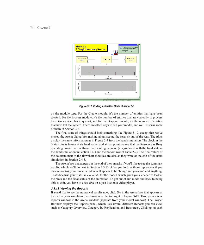
74 CHAPTER 3
Figure 3-17. Ending Animation State of Model 3-1
on the module type. For the Create module, it’s the number of entities that have beencreated. For the Process module, it’s the number of entities that are currently in processthere (in service plus in queue), and for the Dispose module, it’s the number of entitiesthat have left the system. There are other ways to run your model, and we’ll discuss someof them in Section 3.8.
The final state of things should look something like Figure 3-17, except that we’vemoved the Arena dialog box (asking about seeing the results) out of the way. The plotsdisplay the same information as in Figure 2-3 from the hand simulation. The clock in theStatus Bar is frozen at its final value, and at that point we see that the Resource is Busyoperating on one part, with one part waiting in queue (in agreement with the final state inthe hand simulation in Section 2.4.3 and the bottom row of Table 2-2). The final values ofthe counters next to the flowchart modules are also as they were at the end of the handsimulation in Section 2.4.3.
The Arena box that appears at the end of the run asks if you’d like to see the summaryresults, which we’ll do next in Section 3.3.13. After you look at those reports (or if youchoose not to), your model window will appear to be “hung” and you can’t edit anything.That’s because you’re still in run mode for the model, which gives you a chance to look atthe plots and the final status of the animation. To get out of run mode and back to beingable to edit, you have to click End ( ), just like on a video player.
3.3.13 Viewing the ReportsIf you’d like to see the numerical results now, click Yes in the Arena box that appears atthe end of your simulation, as shown near the top right of Figure 3-17. This opens a newreports window in the Arena window (separate from your model window). The ProjectBar now displays the Reports panel, which lists several different Reports you can view,such as Category Overview, Category by Replication, and Resources. Clicking on each
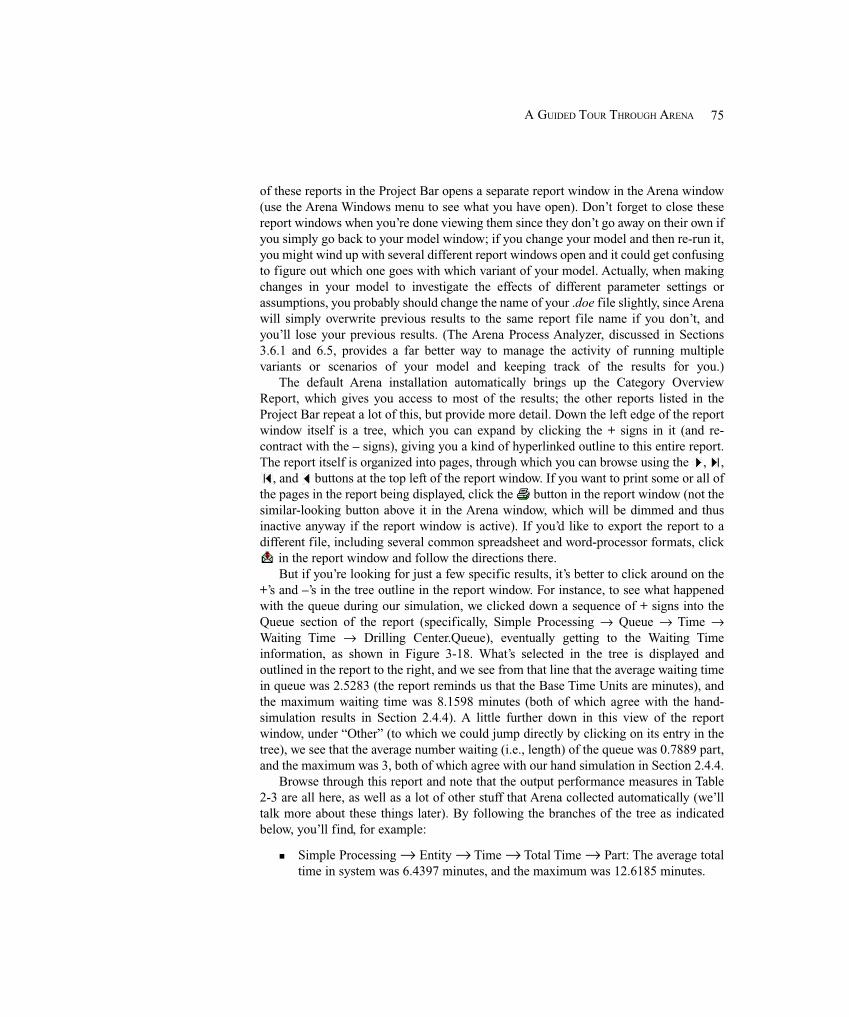
75A GUIDED TOUR THROUGH ARENA
of these reports in the Project Bar opens a separate report window in the Arena window(use the Arena Windows menu to see what you have open). Don’t forget to close thesereport windows when you’re done viewing them since they don’t go away on their own ifyou simply go back to your model window; if you change your model and then re-run it,you might wind up with several different report windows open and it could get confusingto figure out which one goes with which variant of your model. Actually, when makingchanges in your model to investigate the effects of different parameter settings orassumptions, you probably should change the name of your .doe file slightly, since Arenawill simply overwrite previous results to the same report file name if you don’t, andyou’ll lose your previous results. (The Arena Process Analyzer, discussed in Sections3.6.1 and 6.5, provides a far better way to manage the activity of running multiplevariants or scenarios of your model and keeping track of the results for you.)
The default Arena installation automatically brings up the Category OverviewReport, which gives you access to most of the results; the other reports listed in theProject Bar repeat a lot of this, but provide more detail. Down the left edge of the reportwindow itself is a tree, which you can expand by clicking the + signs in it (and re-contract with the – signs), giving you a kind of hyperlinked outline to this entire report.The report itself is organized into pages, through which you can browse using the , ,
, and buttons at the top left of the report window. If you want to print some or all ofthe pages in the report being displayed, click the button in the report window (not thesimilar-looking button above it in the Arena window, which will be dimmed and thusinactive anyway if the report window is active). If you’d like to export the report to adifferent file, including several common spreadsheet and word-processor formats, click
in the report window and follow the directions there.But if you’re looking for just a few specific results, it’s better to click around on the
+’s and –’s in the tree outline in the report window. For instance, to see what happenedwith the queue during our simulation, we clicked down a sequence of + signs into theQueue section of the report (specifically, Simple Processing → Queue → Time →Waiting Time → Drilling Center.Queue), eventually getting to the Waiting Timeinformation, as shown in Figure 3-18. What’s selected in the tree is displayed andoutlined in the report to the right, and we see from that line that the average waiting timein queue was 2.5283 (the report reminds us that the Base Time Units are minutes), andthe maximum waiting time was 8.1598 minutes (both of which agree with the hand-simulation results in Section 2.4.4). A little further down in this view of the reportwindow, under “Other” (to which we could jump directly by clicking on its entry in thetree), we see that the average number waiting (i.e., length) of the queue was 0.7889 part,and the maximum was 3, both of which agree with our hand simulation in Section 2.4.4.
Browse through this report and note that the output performance measures in Table2-3 are all here, as well as a lot of other stuff that Arena collected automatically (we’lltalk more about these things later). By following the branches of the tree as indicatedbelow, you’ll find, for example:
� Simple Processing → Entity → Time → Total Time → Part: The average totaltime in system was 6.4397 minutes, and the maximum was 12.6185 minutes.
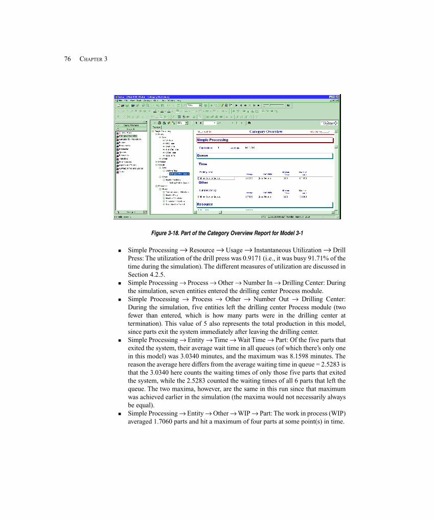
76 CHAPTER 3
Figure 3-18. Part of the Category Overview Report for Model 3-1
� Simple Processing → Resource → Usage → Instantaneous Utilization → DrillPress: The utilization of the drill press was 0.9171 (i.e., it was busy 91.71% of thetime during the simulation). The different measures of utilization are discussed inSection 4.2.5.
� Simple Processing → Process → Other → Number In → Drilling Center: Duringthe simulation, seven entities entered the drilling center Process module.
� Simple Processing → Process → Other → Number Out → Drilling Center:During the simulation, five entities left the drilling center Process module (twofewer than entered, which is how many parts were in the drilling center attermination). This value of 5 also represents the total production in this model,since parts exit the system immediately after leaving the drilling center.
� Simple Processing → Entity → Time → Wait Time → Part: Of the five parts thatexited the system, their average wait time in all queues (of which there’s only onein this model) was 3.0340 minutes, and the maximum was 8.1598 minutes. Thereason the average here differs from the average waiting time in queue = 2.5283 isthat the 3.0340 here counts the waiting times of only those five parts that exitedthe system, while the 2.5283 counted the waiting times of all 6 parts that left thequeue. The two maxima, however, are the same in this run since that maximumwas achieved earlier in the simulation (the maxima would not necessarily alwaysbe equal).
� Simple Processing → Entity → Other → WIP → Part: The work in process (WIP)averaged 1.7060 parts and hit a maximum of four parts at some point(s) in time.
77A GUIDED TOUR THROUGH ARENA
Many of the numbers in the reports (as in our hand simulation in Chapter 2) can beclassified as tally, time-persistent, or counter statistics:
� Tally statistics are those that result from taking the average, minimum, or maxi-mum of a list of numbers. For example, the average and maximum total time insystem (6.4397 and 12.6185 minutes, respectively) are tally statistics sincethey’re respectively the average and maximum of the total times in system of thefive parts that left the system during the simulation. Tally statistics are sometimescalled discrete-time statistics since their “time” index (1, 2, 3, ...) is a discreteindexing of the time order in which the observations were made.
� Time-persistent statistics are those that result from taking the (time) average,minimum, or maximum of a plot of something during the simulation, where thex-axis is continuous time. Time-persistent averages involve the accumulated areaunder the plotted curve (i.e., an integral). The average and maximum of thenumber of parts in queue (0.7889 and 3 parts, respectively) are time-persistentstatistics, as is the instantaneous utilization of the drill press (0.9171). Time-persistent statistics are also known as continuous-time statistics.
� Counter statistics, as the name suggests, are accumulated sums of something.Often, they are simply nose counts of how many times something happened, likethe number of parts that left the drilling center (five in our simulation) or thatentered the drilling center (seven). But they could be accumulations of numbersthat are not all equal to 1; for instance, the accumulated waiting time at thedrilling center was 15.1700 minutes, representing the sum (not average) of thewaiting times observed in queue there. In the Category Overview report, thisnumber can be found via Simple Processing → Process → Accumulated Time →Accum Wait Time → Drilling Center. Another counter statistic is at SimpleProcessing → Resource → Usage → Total Number Seized → Drill Press, wherewe see that the drill press resource was used (either to completion for the part orjust started) six times.
If you close a report window, you can view it later as long as you don’t delete (oroverwrite) the Microsoft® Access database file that Arena creates as it runs. This Accessfile is named model_filename.mdb, where model_filename is what younamed your .doe model file (so in our case, the Access file is named Model03-01.mdb). On the Project Bar, select Reports and then click on the report you want(such as Category Overview) to view it again. The way this works is that Arena usesthird-party software called Crystal Reports® from SAP (http://www.sap.com/solutions/sapbusinessobjects/sme/reporting/index.epx) to read the Access database file, extractthe useful stuff from it, and then display it to you in the report-window format we’vedescribed above.
Right now you might be thinking that this report structure is pretty serious overkilljust to get a handful of numbers out of this small model, and it probably is. However, inlarge, complicated models it’s quite helpful to have this structure to organize the myriadsof different output numbers and to help you find things and make some quickcomparisons and conclusions.
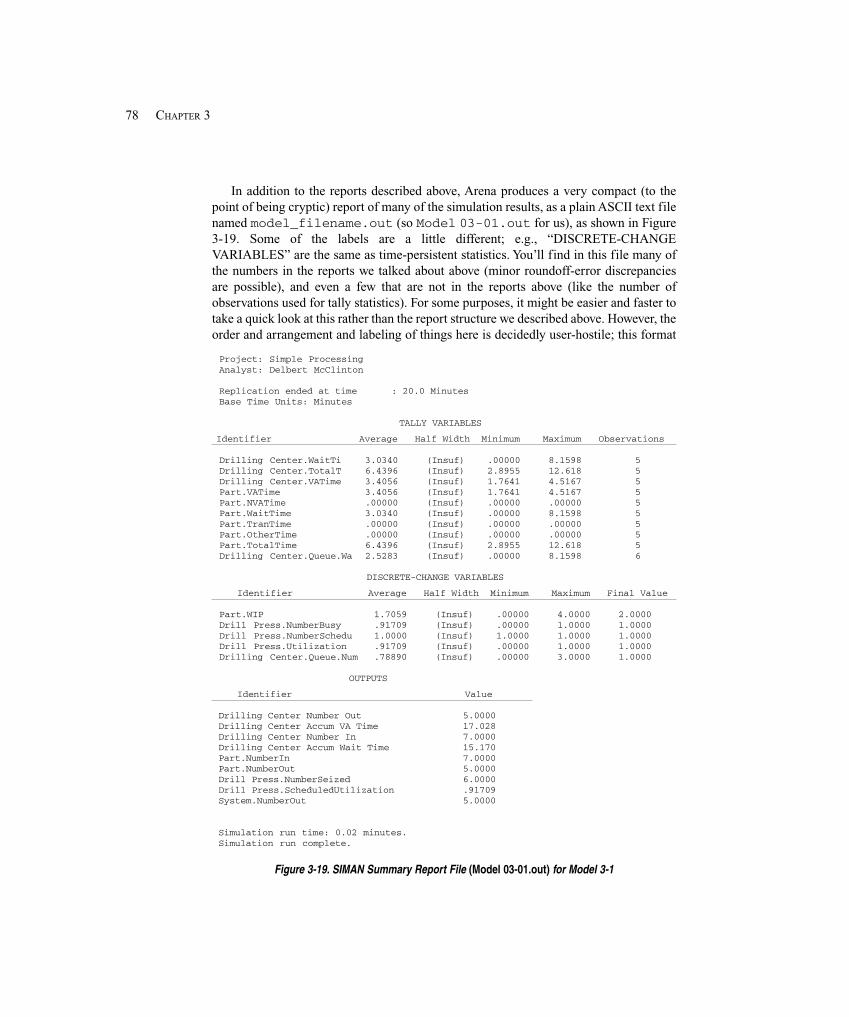
78 CHAPTER 3
In addition to the reports described above, Arena produces a very compact (to thepoint of being cryptic) report of many of the simulation results, as a plain ASCII text filenamed model_filename.out (so Model 03-01.out for us), as shown in Figure3-19. Some of the labels are a little different; e.g., “DISCRETE-CHANGEVARIABLES” are the same as time-persistent statistics. You’ll find in this file many ofthe numbers in the reports we talked about above (minor roundoff-error discrepanciesare possible), and even a few that are not in the reports above (like the number ofobservations used for tally statistics). For some purposes, it might be easier and faster totake a quick look at this rather than the report structure we described above. However, theorder and arrangement and labeling of things here is decidedly user-hostile; this format
Project: Simple ProcessingAnalyst: Delbert McClinton
Replication ended at time : 20.0 MinutesBase Time Units: Minutes
TALLY VARIABLES
Identifier Average Half Width Minimum Maximum Observations
Drilling Center.WaitTi 3.0340 (Insuf) .00000 8.1598 5Drilling Center.TotalT 6.4396 (Insuf) 2.8955 12.618 5Drilling Center.VATime 3.4056 (Insuf) 1.7641 4.5167 5Part.VATime 3.4056 (Insuf) 1.7641 4.5167 5Part.NVATime .00000 (Insuf) .00000 .00000 5Part.WaitTime 3.0340 (Insuf) .00000 8.1598 5Part.TranTime .00000 (Insuf) .00000 .00000 5Part.OtherTime .00000 (Insuf) .00000 .00000 5Part.TotalTime 6.4396 (Insuf) 2.8955 12.618 5Drilling Center.Queue.Wa 2.5283 (Insuf) .00000 8.1598 6
DISCRETE-CHANGE VARIABLES
Identifier Average Half Width Minimum Maximum Final Value
Part.WIP 1.7059 (Insuf) .00000 4.0000 2.0000Drill Press.NumberBusy .91709 (Insuf) .00000 1.0000 1.0000Drill Press.NumberSchedu 1.0000 (Insuf) 1.0000 1.0000 1.0000Drill Press.Utilization .91709 (Insuf) .00000 1.0000 1.0000Drilling Center.Queue.Num .78890 (Insuf) .00000 3.0000 1.0000
OUTPUTS
Identifier Value
Drilling Center Number Out 5.0000Drilling Center Accum VA Time 17.028Drilling Center Number In 7.0000Drilling Center Accum Wait Time 15.170Part.NumberIn 7.0000Part.NumberOut 5.0000Drill Press.NumberSeized 6.0000Drill Press.ScheduledUtilization .91709System.NumberOut 5.0000
Simulation run time: 0.02 minutes.Simulation run complete.
Figure 3-19. SIMAN Summary Report File (Model 03-01.out) for Model 3-1
79A GUIDED TOUR THROUGH ARENA
is actually a leftover from earlier versions of Arena and in fact goes back to the early1980s and the underlying SIMAN simulation language. However, if, out of nostalgia or amania for compactness, you want this to be the default report that Arena gives you if youask for one after the run ends, select Run > Setup > Reports and in the Default Report listscroll down and pick SIMAN Summary Report (.out file).
The exact meaning of report labels like Average, Minimum, Maximum, and Time-Average should be clear to you by now. But the reports also refer here and there to HalfWidths (though we never get numbers for them in this model and are just scolded thatwe’re somehow Insufficient). As you might guess, these will be half widths of confidenceintervals (they’ll be at level 95%) on the expected value of the correspondingperformance measure, provided that our simulation produces adequate data to form them.
If we were doing more than one replication (which we’re not in this case), Arenawould take the summary results for an output performance measure from each replica-tion, average them over the replications, compute the sample standard deviation fromthem, and finally compute the half width of a 95% confidence interval on the expectedvalue of this performance measure. This is exactly what we did by hand in Section 2.6.2for several of the output performance measures there, as given in Table 2-4. Exercise 3-1asks you to do this with Arena to reproduce (except maybe for round-off) the results inTable 2-4.
If we’re interested in the long-run (or steady-state) behavior of the system after anyinitialization effects have worn off, we might choose to make just one (really) long repli-cation or run; this issue is taken up in Section 7.2.3. If we do so, we might see half-widthnumbers in the reports if our run is long enough, even though we’re doing only onereplication. Arena tries to compute these half widths by breaking the single long run intobatches whose means serve as stand-ins for truly independent summary results over rep-lications for making confidence intervals. We’ll talk about this more in Section 7.2.3,including a discussion of exactly how these half widths are computed from the simula-tion output data. The reason you might get “Insufficient” (or, sometimes, “Correlated”)instead of a numerical value for the half width is that the run must be long enough toprovide data in sufficient quantity and of adequate quality to justify the validity of thehalf widths; if your run is not long enough for this, Arena simply declines to deliver avalue on the theory that a wrong answer is worse than no answer at all.
3.4 Building Model 3-1 Yourself
In this section, we’ll lead you through the construction of Model 3-1 from scratch. Whatyou end up with might not look exactly like our Model 3-1 cosmetically, but it should befunctionally equivalent and give you the same results.
Before embarking on this, we might mention a couple of little user-interfacefunctions that often come in handy:
� Right-clicking in an empty spot in the flowchart view of the model windowbrings up a small pop-up box of options, one of which is to repeat the last action(like placing a module in your model, of which you may need multiple instances).This can obviously save you time when you have repetitive actions (though it
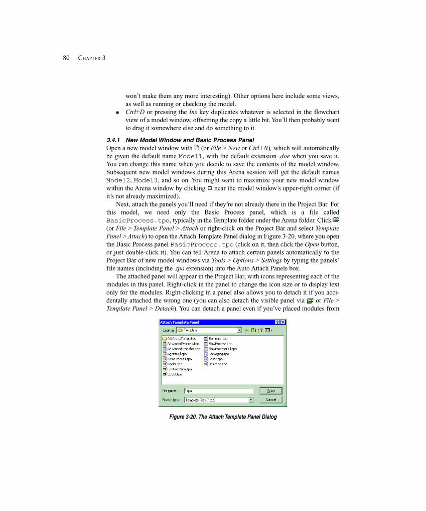
80 CHAPTER 3
won’t make them any more interesting). Other options here include some views,as well as running or checking the model.
� Ctrl+D or pressing the Ins key duplicates whatever is selected in the flowchartview of a model window, offsetting the copy a little bit. You’ll then probably wantto drag it somewhere else and do something to it.
3.4.1 New Model Window and Basic Process PanelOpen a new model window with (or File > New or Ctrl+N), which will automaticallybe given the default name Model1, with the default extension .doe when you save it.You can change this name when you decide to save the contents of the model window.Subsequent new model windows during this Arena session will get the default namesModel2, Model3, and so on. You might want to maximize your new model windowwithin the Arena window by clicking near the model window’s upper-right corner (ifit’s not already maximized).
Next, attach the panels you’ll need if they’re not already there in the Project Bar. Forthis model, we need only the Basic Process panel, which is a file calledBasicProcess.tpo, typically in the Template folder under the Arena folder. Click (or File > Template Panel > Attach or right-click on the Project Bar and select TemplatePanel > Attach) to open the Attach Template Panel dialog in Figure 3-20, where you openthe Basic Process panel BasicProcess.tpo (click on it, then click the Open button,or just double-click it). You can tell Arena to attach certain panels automatically to theProject Bar of new model windows via Tools > Options > Settings by typing the panels’file names (including the .tpo extension) into the Auto Attach Panels box.
The attached panel will appear in the Project Bar, with icons representing each of themodules in this panel. Right-click in the panel to change the icon size or to display textonly for the modules. Right-clicking in a panel also allows you to detach it if you acci-dentally attached the wrong one (you can also detach the visible panel via or File >Template Panel > Detach). You can detach a panel even if you’ve placed modules from
Figure 3-20. The Attach Template Panel Dialog
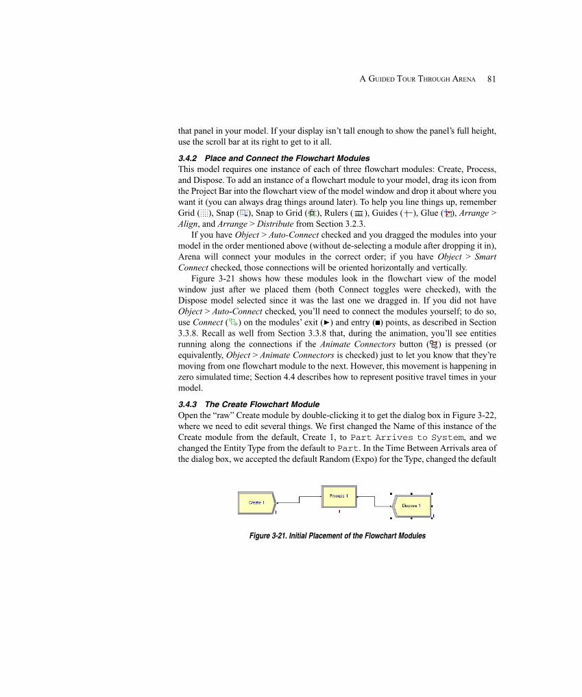
81A GUIDED TOUR THROUGH ARENA
that panel in your model. If your display isn’t tall enough to show the panel’s full height,use the scroll bar at its right to get to it all.
3.4.2 Place and Connect the Flowchart ModulesThis model requires one instance of each of three flowchart modules: Create, Process,and Dispose. To add an instance of a flowchart module to your model, drag its icon fromthe Project Bar into the flowchart view of the model window and drop it about where youwant it (you can always drag things around later). To help you line things up, rememberGrid ( ), Snap ( ), Snap to Grid ( ), Rulers ( ), Guides ( ), Glue ( ), Arrange >Align, and Arrange > Distribute from Section 3.2.3.
If you have Object > Auto-Connect checked and you dragged the modules into yourmodel in the order mentioned above (without de-selecting a module after dropping it in),Arena will connect your modules in the correct order; if you have Object > SmartConnect checked, those connections will be oriented horizontally and vertically.
Figure 3-21 shows how these modules look in the flowchart view of the modelwindow just after we placed them (both Connect toggles were checked), with theDispose model selected since it was the last one we dragged in. If you did not haveObject > Auto-Connect checked, you’ll need to connect the modules yourself; to do so,use Connect ( ) on the modules’ exit ( ) and entry ( ) points, as described in Section3.3.8. Recall as well from Section 3.3.8 that, during the animation, you’ll see entitiesrunning along the connections if the Animate Connectors button ( ) is pressed (orequivalently, Object > Animate Connectors is checked) just to let you know that they’removing from one flowchart module to the next. However, this movement is happening inzero simulated time; Section 4.4 describes how to represent positive travel times in yourmodel.
3.4.3 The Create Flowchart ModuleOpen the “raw” Create module by double-clicking it to get the dialog box in Figure 3-22,where we need to edit several things. We first changed the Name of this instance of theCreate module from the default, Create 1, to Part Arrives to System, and wechanged the Entity Type from the default to Part. In the Time Between Arrivals area ofthe dialog box, we accepted the default Random (Expo) for the Type, changed the default
Figure 3-21. Initial Placement of the Flowchart Modules
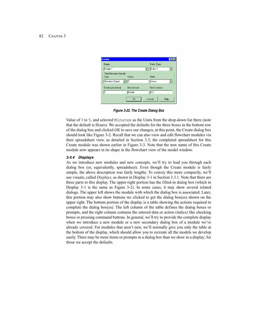
82 CHAPTER 3
Figure 3-22. The Create Dialog Box
Value of 1 to 5, and selected Minutes as the Units from the drop-down list there (notethat the default is Hours). We accepted the defaults for the three boxes in the bottom rowof the dialog box and clicked OK to save our changes; at this point, the Create dialog boxshould look like Figure 3-2. Recall that we can also view and edit flowchart modules viatheir spreadsheet view, as detailed in Section 3.3; the completed spreadsheet for thisCreate module was shown earlier in Figure 3-3. Note that the new name of this Createmodule now appears in its shape in the flowchart view of the model window.
3.4.4 DisplaysAs we introduce new modules and new concepts, we’ll try to lead you through eachdialog box (or, equivalently, spreadsheet). Even though the Create module is fairlysimple, the above description was fairly lengthy. To convey this more compactly, we’lluse visuals, called Displays, as shown in Display 3-1 in Section 3.3.1. Note that there arethree parts to this display. The upper-right portion has the filled-in dialog box (which inDisplay 3-1 is the same as Figure 3-2). In some cases, it may show several relateddialogs. The upper left shows the module with which the dialog box is associated. Later,this portion may also show buttons we clicked to get the dialog box(es) shown on theupper right. The bottom portion of the display is a table showing the actions required tocomplete the dialog box(es). The left column of the table defines the dialog boxes orprompts, and the right column contains the entered data or action (italics) like checkingboxes or pressing command buttons. In general, we’ll try to provide the complete displaywhen we introduce a new module or a new secondary dialog box of a module we’vealready covered. For modules that aren’t new, we’ll normally give you only the table atthe bottom of the display, which should allow you to recreate all the models we developeasily. There may be more items or prompts in a dialog box than we show in a display; forthose we accept the defaults.
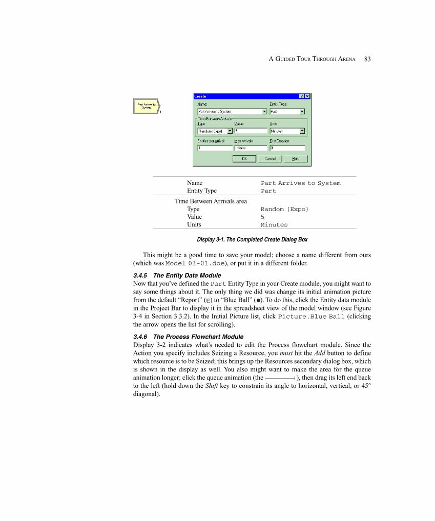
83A GUIDED TOUR THROUGH ARENA
Name Part Arrives to SystemEntity Type Part
Time Between Arrivals areaType Random (Expo)Value 5Units Minutes
Display 3-1. The Completed Create Dialog Box
This might be a good time to save your model; choose a name different from ours(which was Model 03-01.doe), or put it in a different folder.
3.4.5 The Entity Data ModuleNow that you’ve defined the Part Entity Type in your Create module, you might want tosay some things about it. The only thing we did was change its initial animation picturefrom the default “Report” ( ) to “Blue Ball” ( ). To do this, click the Entity data modulein the Project Bar to display it in the spreadsheet view of the model window (see Figure3-4 in Section 3.3.2). In the Initial Picture list, click Picture.Blue Ball (clickingthe arrow opens the list for scrolling).
3.4.6 The Process Flowchart ModuleDisplay 3-2 indicates what’s needed to edit the Process flowchart module. Since theAction you specify includes Seizing a Resource, you must hit the Add button to definewhich resource is to be Seized; this brings up the Resources secondary dialog box, whichis shown in the display as well. You also might want to make the area for the queueanimation longer; click the queue animation (the ), then drag its left end backto the left (hold down the Shift key to constrain its angle to horizontal, vertical, or 45°diagonal).
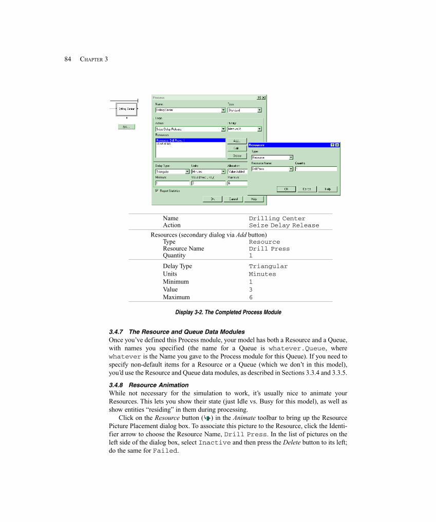
84 CHAPTER 3
Name Drilling CenterAction Seize Delay Release
Resources (secondary dialog via Add button)Type ResourceResource Name Drill PressQuantity 1
Delay Type TriangularUnits MinutesMinimum 1Value 3Maximum 6
Display 3-2. The Completed Process Module
3.4.7 The Resource and Queue Data ModulesOnce you’ve defined this Process module, your model has both a Resource and a Queue,with names you specified (the name for a Queue is whatever.Queue, wherewhatever is the Name you gave to the Process module for this Queue). If you need tospecify non-default items for a Resource or a Queue (which we don’t in this model),you’d use the Resource and Queue data modules, as described in Sections 3.3.4 and 3.3.5.
3.4.8 Resource AnimationWhile not necessary for the simulation to work, it’s usually nice to animate yourResources. This lets you show their state (just Idle vs. Busy for this model), as well asshow entities “residing” in them during processing.
Click on the Resource button ( ) in the Animate toolbar to bring up the ResourcePicture Placement dialog box. To associate this picture to the Resource, click the Identi-fier arrow to choose the Resource Name, Drill Press. In the list of pictures on theleft side of the dialog box, select Inactive and then press the Delete button to its left;do the same for Failed.
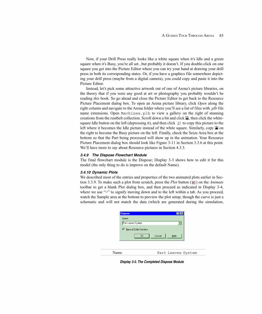
85A GUIDED TOUR THROUGH ARENA
Now, if your Drill Press really looks like a white square when it’s Idle and a greensquare when it’s Busy, you’re all set...but probably it doesn’t. If you double-click on onesquare you get into the Picture Editor where you can try your hand at drawing your drillpress in both its corresponding states. Or, if you have a graphics file somewhere depict-ing your drill press (maybe from a digital camera), you could copy and paste it into thePicture Editor.
Instead, let’s pick some attractive artwork out of one of Arena’s picture libraries, onthe theory that if you were any good at art or photography you probably wouldn’t bereading this book. So go ahead and close the Picture Editor to get back to the ResourcePicture Placement dialog box. To open an Arena picture library, click Open along theright column and navigate to the Arena folder where you’ll see a list of files with .plb filename extensions. Open Machines.plb to view a gallery on the right of stunningcreations from the rustbelt collection. Scroll down a bit and click , then click the white-square Idle button on the left (depressing it), and then click to copy this picture to theleft where it becomes the Idle picture instead of the white square. Similarly, copy onthe right to become the Busy picture on the left. Finally, check the Seize Area box at thebottom so that the Part being processed will show up in the animation. Your ResourcePicture Placement dialog box should look like Figure 3-11 in Section 3.3.6 at this point.We’ll have more to say about Resource pictures in Section 4.3.3.
3.4.9 The Dispose Flowchart ModuleThe final flowchart module is the Dispose; Display 3-3 shows how to edit it for thismodel (the only thing to do is improve on the default Name).
3.4.10 Dynamic PlotsWe described most of the entries and properties of the two animated plots earlier in Sec-tion 3.3.9. To make such a plot from scratch, press the Plot button ( ) on the Animatetoolbar to get a blank Plot dialog box, and then proceed as indicated in Display 3-4,where we use “>” to signify moving down and to the left within a tab. As you proceed,watch the Sample area at the bottom to preview the plot setup, though the curve is just aschematic and will not match the data (which are generated during the simulation,
Name Part Leaves System
Display 3-3. The Completed Dispose Module
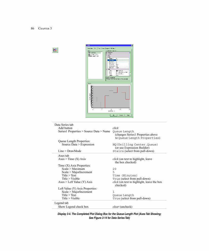
86 CHAPTER 3
Data Series tabAdd button clickSeries1 Properties > Source Data > Name Queue Length
(changes Series1 Properties above to Queue Length Properties)
Queue Length Properties:Source Data > Expression NQ(Drilling Center.Queue)
(or use Expression Builder)Line > DrawMode Stairs (select from pull-down)
Axes tabAxes > Time (X) Axis click (on text to highlight, leave
the box checked)Time (X) Axis Properties:
Scale > Maximum 20Scale > MajorIncrement 5Title > Text Time (Minutes)Title > Visible True (select from pull-down)
Axes > Left Value (Y) Axis click (on text to highlight, leave the box checked)
Left Value (Y) Axis Properties:Scale > MajorIncrement 1Title > Text Queue LengthTitle > Visible True (select from pull-down)
Legend tabShow Legend check box clear (uncheck)
Display 3-4. The Completed Plot Dialog Box for the Queue-Length Plot (Axes Tab Showing;See Figure 3-14 for Data Series Tab)
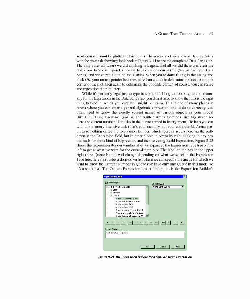
87A GUIDED TOUR THROUGH ARENA
so of course cannot be plotted at this point). The screen shot we show in Display 3-4 iswith the Axes tab showing; look back at Figure 3-14 to see the completed Data Series tab.The only other tab where we did anything is Legend, and all we did there was clear thecheck box to Show Legend, since we have only one curve (the Queue Length DataSeries) and we’ve put a title on the Y axis). When you’re done filling in the dialog andclick OK, your mouse pointer becomes cross hairs; click to determine the location of onecorner of the plot, then again to determine the opposite corner (of course, you can resizeand reposition the plot later).
While it’s perfectly legal just to type in NQ(Drilling Center.Queue) manu-ally for the Expression in the Data Series tab, you’d first have to know that this is the rightthing to type in, which you very well might not know. This is one of many places inArena where you can enter a general algebraic expression, and to do so correctly, youoften need to know the exactly correct names of various objects in your model(like Drilling Center.Queue) and built-in Arena functions (like NQ, which re-turns the current number of entities in the queue named in its argument). To help you outwith this memory-intensive task (that’s your memory, not your computer’s), Arena pro-vides something called the Expression Builder, which you can access here via the pull-down in the Expression field, but in other places in Arena by right-clicking in any boxthat calls for some kind of Expression, and then selecting Build Expression. Figure 3-23shows the Expression Builder window after we expanded the Expression Type tree on theleft to get at what we want for the queue-length plot. The label on the box in the upperright (now Queue Name) will change depending on what we select in the ExpressionType tree; here it provides a drop-down list where we can specify the queue for which wewant to know the Current Number in Queue (we have only one Queue in this model soit’s a short list). The Current Expression box at the bottom is the Expression Builder’s
Figure 3-23. The Expression Builder for a Queue-Length Expression
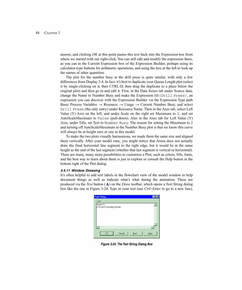
88 CHAPTER 3
answer, and clicking OK at this point pastes this text back into the Expression box fromwhere we started with our right-click. You can still edit and modify the expression there,as you can in the Current Expression box of the Expression Builder, perhaps using itscalculator-type buttons for arithmetic operations, and using the tree at the left to look upthe names of other quantities.
The plot for the number busy at the drill press is quite similar, with only a fewdifferences from Display 3-4. In fact, it’s best to duplicate your Queue Length plot (selectit by single-clicking on it, then CTRL-D, then drag the duplicate to a place below theoriginal plot) and then go in and edit it. First, in the Data Series tab under Source data,change the Name to Number Busy and make the Expression NR(Drill Press), anexpression you can discover with the Expression Builder via the Expression Type pathBasic Process Variables → Resource → Usage → Current Number Busy, and selectDrill Press (the only entry) under Resource Name. Then in the Axes tab, select LeftValue (Y) Axis on the left, and under Scale on the right set Maximum to 2, and setAutoScaleMaximum to False (pull-down). Also in the Axes tab for Left Value (Y)Axis, under Title, set Text to Number Busy. The reason for setting the Maximum to 2and turning off AutoScaleMaximum in the Number Busy plot is that we know this curvewill always be at height zero or one in this model.
To make the two plots visually harmonious, we made them the same size and alignedthem vertically. After your model runs, you might notice that Arena does not actuallydraw the final horizontal line segment to the right edge, but it would be at the sameheight as the end of the last segment (whether that last segment is vertical or horizontal).There are many, many more possibilities to customize a Plot, such as colors, fills, fonts,and the best way to learn about them is just to explore or consult the Help button in thebottom right of the Plot dialog.
3.4.11 Window DressingIt’s often helpful to add text labels in the flowchart view of the model window to helpdocument things as well as indicate what’s what during the animation. These areproduced via the Text button ( ) on the Draw toolbar, which opens a Text String dialogbox like the one in Figure 3-24. Type in your text (use Ctrl+Enter to go to a new line),
Figure 3-24. The Text String Dialog Box
89A GUIDED TOUR THROUGH ARENA
perhaps change its font (Times Roman, Arial, etc.), font style (Italics, Bold, etc.), andsize via the Font button, and then click OK. Your mouse pointer becomes cross hairs,which you click to place the northwest corner of the text entry in the flowchart view ofyour model window. You can drag it around later, as well as resize and reorient it usingthe underline below it that appears when you select it (hold down the shift key whilereorienting it to constrain it to be horizontal or vertical or on a 45º line). To change thetext color, select the text and use the Text Color button ( ) to select either the color ofthe underline there (click on the in this case) or to choose a different color (click on the
in this case and select a color from the palette), which will also become the newunderline color.
The yellow backdrop box behind the model label in Model 3-1 and its shadow weremade with the Box button ( ) on the Draw toolbar; clicking this button turns yourmouse pointer to cross hairs, after which you click once to determine one corner of thebox and again to determine the opposite corner. You can change the fill color by firstselecting the box and then clicking the Fill Color button ( ); change the border colorwith the Line Color button ( ). To create faux three-dimensional effects like shadows,you can cleverly “stack” and offset objects (like a yellow box on top of a slightly shiftedblack box) using options like Send to Back from the Arrange toolbar and menu.
If you’d like to drop a graphics file (.gif, .jpg, etc.) into the flowchart view of yourmodel window, use Edit > Insert New Object, select Create from File, next Browse tochoose the file you want, press Open, then OK, and finally drop it in with the cross hairs.
Clearly, you could spend a ruinous amount of time on this kind of stuff. Withoutimplying anything about anybody, we offer it as a simple empirical observation that thehigher up in an organization you go to present your simulation, the more effort isprobably justified on graphics.
3.4.12 The Run > Setup Dialog BoxesTo establish the run conditions, use the Run > Setup menu command, where you’ll findtabbed pages that control various aspects of how your simulation will execute. You’llneed to edit just two of these pages.
The first one is the Project Parameters tab, where you should enter a Project Title,Analyst Name (that’s you), and Project Description. You might also need to modify theselection of which statistics will be collected and reported, depending on how you haveyour defaults set in Tools > Options > Project Parameters (we want Entities, Resources,Queues, and Processes). The completed dialog was shown in Figure 3-15 in Section3.3.11.
The other tab that you need to edit is Replication Parameters. These edits were alsodiscussed in Section 3.3.11, and were shown in Figure 3-16 there.
3.4.13 Establishing Named ViewsTo set up a Named View for your model, first pan and zoom to the scene you want toremember, then View > Named Views (the button or or type ?), press Add, then pick aname and maybe a hot key (case-sensitive). If you want to change this view’s definitionlater, press Edit instead once you’ve panned and zoomed to the new view you want to
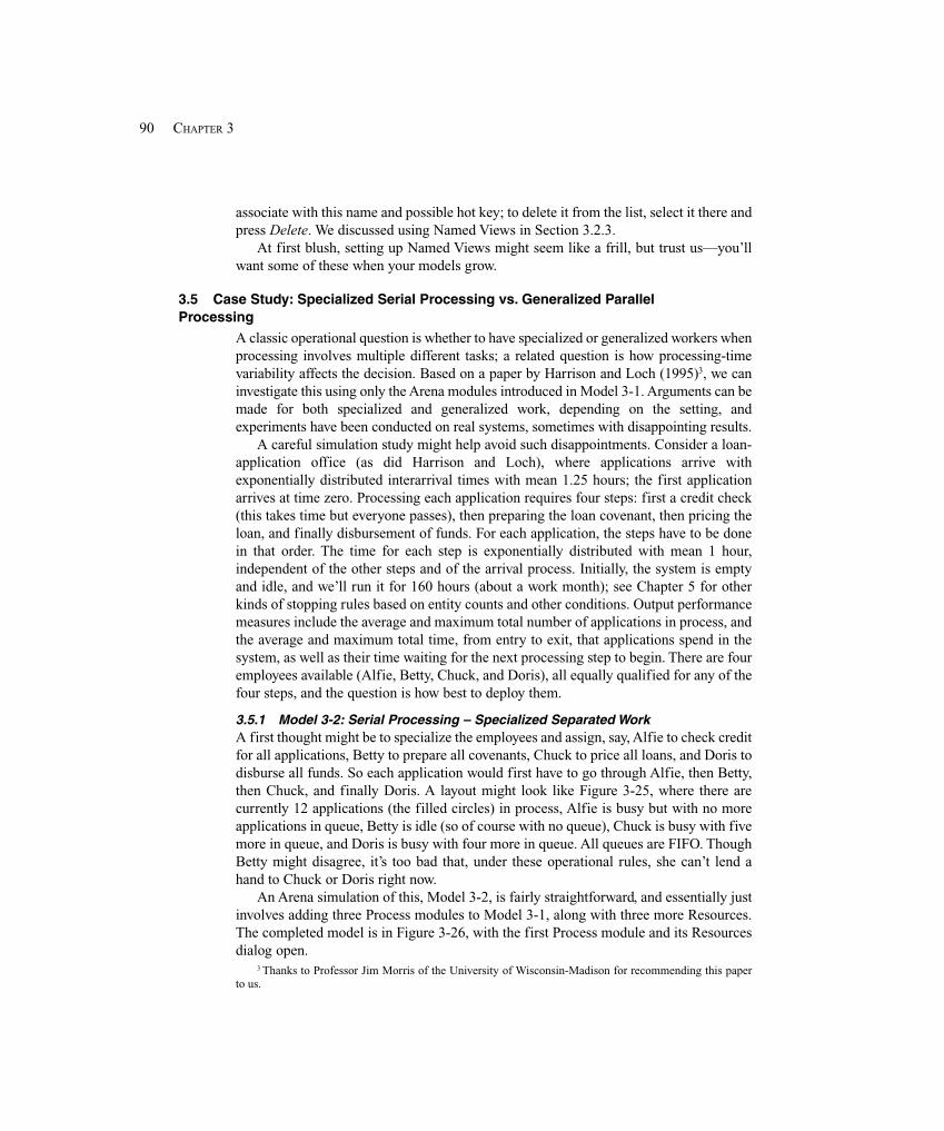
90 CHAPTER 3
associate with this name and possible hot key; to delete it from the list, select it there andpress Delete. We discussed using Named Views in Section 3.2.3.
At first blush, setting up Named Views might seem like a frill, but trust us—you’llwant some of these when your models grow.
3.5 Case Study: Specialized Serial Processing vs. Generalized ParallelProcessing
A classic operational question is whether to have specialized or generalized workers whenprocessing involves multiple different tasks; a related question is how processing-timevariability affects the decision. Based on a paper by Harrison and Loch (1995)3, we caninvestigate this using only the Arena modules introduced in Model 3-1. Arguments can bemade for both specialized and generalized work, depending on the setting, andexperiments have been conducted on real systems, sometimes with disappointing results.
A careful simulation study might help avoid such disappointments. Consider a loan-application office (as did Harrison and Loch), where applications arrive withexponentially distributed interarrival times with mean 1.25 hours; the first applicationarrives at time zero. Processing each application requires four steps: first a credit check(this takes time but everyone passes), then preparing the loan covenant, then pricing theloan, and finally disbursement of funds. For each application, the steps have to be donein that order. The time for each step is exponentially distributed with mean 1 hour,independent of the other steps and of the arrival process. Initially, the system is emptyand idle, and we’ll run it for 160 hours (about a work month); see Chapter 5 for otherkinds of stopping rules based on entity counts and other conditions. Output performancemeasures include the average and maximum total number of applications in process, andthe average and maximum total time, from entry to exit, that applications spend in thesystem, as well as their time waiting for the next processing step to begin. There are fouremployees available (Alfie, Betty, Chuck, and Doris), all equally qualified for any of thefour steps, and the question is how best to deploy them.
3.5.1 Model 3-2: Serial Processing – Specialized Separated WorkA first thought might be to specialize the employees and assign, say, Alfie to check creditfor all applications, Betty to prepare all covenants, Chuck to price all loans, and Doris todisburse all funds. So each application would first have to go through Alfie, then Betty,then Chuck, and finally Doris. A layout might look like Figure 3-25, where there arecurrently 12 applications (the filled circles) in process, Alfie is busy but with no moreapplications in queue, Betty is idle (so of course with no queue), Chuck is busy with fivemore in queue, and Doris is busy with four more in queue. All queues are FIFO. ThoughBetty might disagree, it’s too bad that, under these operational rules, she can’t lend ahand to Chuck or Doris right now.
An Arena simulation of this, Model 3-2, is fairly straightforward, and essentially justinvolves adding three Process modules to Model 3-1, along with three more Resources.The completed model is in Figure 3-26, with the first Process module and its Resourcesdialog open.
3 Thanks to Professor Jim Morris of the University of Wisconsin-Madison for recommending this paperto us.
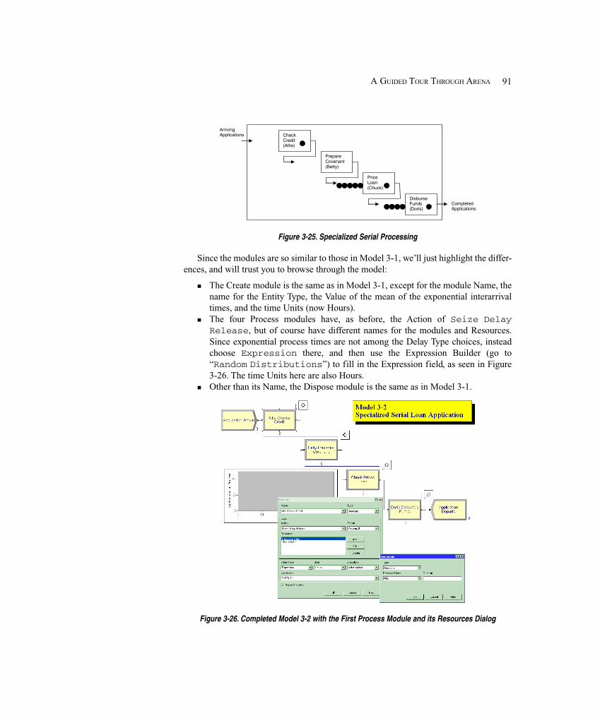
91A GUIDED TOUR THROUGH ARENA
Check Credit (Alfie)
Disburse Funds (Doris)
Price Loan (Chuck)
Prepare Covenant (Betty)
Completed Applications
Arriving Applications
Figure 3-25. Specialized Serial Processing
Since the modules are so similar to those in Model 3-1, we’ll just highlight the differ-ences, and will trust you to browse through the model:
� The Create module is the same as in Model 3-1, except for the module Name, thename for the Entity Type, the Value of the mean of the exponential interarrivaltimes, and the time Units (now Hours).
� The four Process modules have, as before, the Action of Seize DelayRelease, but of course have different names for the modules and Resources.Since exponential process times are not among the Delay Type choices, insteadchoose Expression there, and then use the Expression Builder (go to“Random Distributions”) to fill in the Expression field, as seen in Figure3-26. The time Units here are also Hours.
� Other than its Name, the Dispose module is the same as in Model 3-1.
Figure 3-26. Completed Model 3-2 with the First Process Module and its Resources Dialog
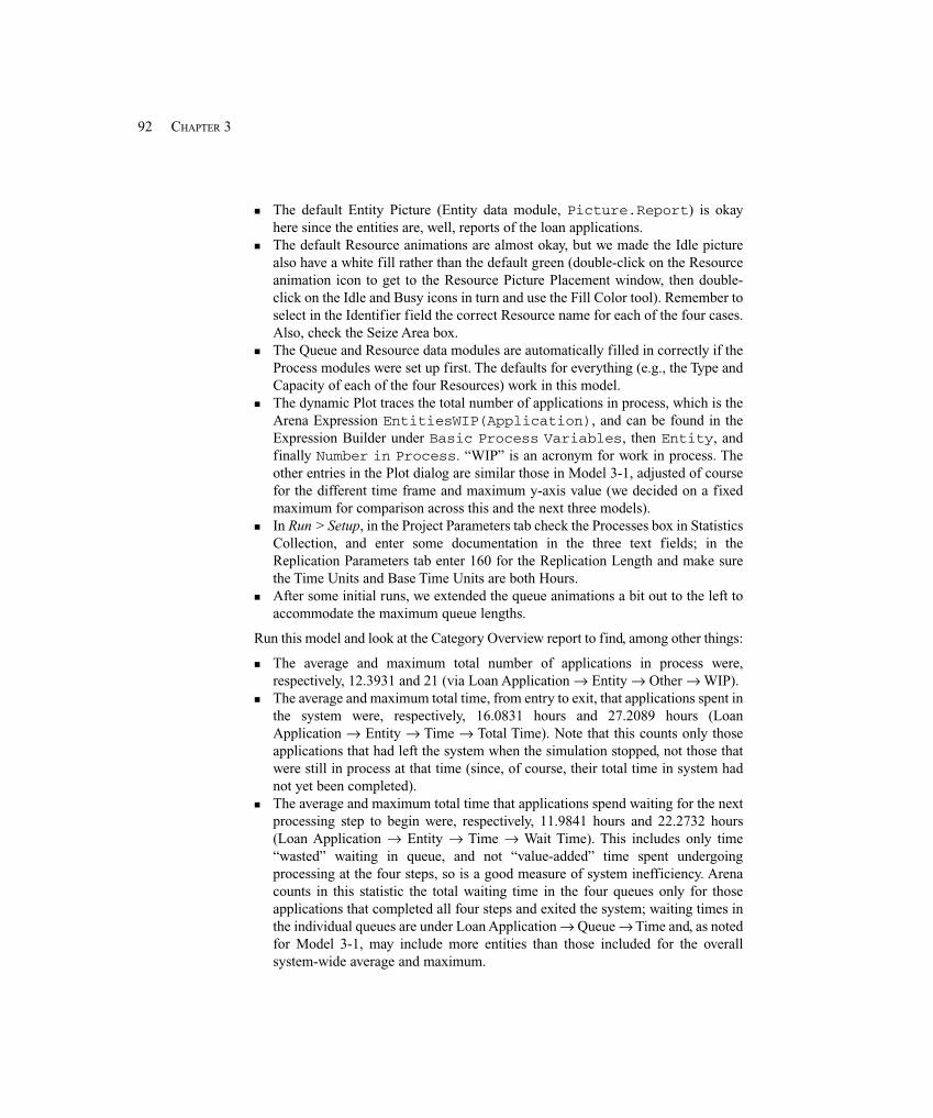
92 CHAPTER 3
� The default Entity Picture (Entity data module, Picture.Report) is okayhere since the entities are, well, reports of the loan applications.
� The default Resource animations are almost okay, but we made the Idle picturealso have a white fill rather than the default green (double-click on the Resourceanimation icon to get to the Resource Picture Placement window, then double-click on the Idle and Busy icons in turn and use the Fill Color tool). Remember toselect in the Identifier field the correct Resource name for each of the four cases.Also, check the Seize Area box.
� The Queue and Resource data modules are automatically filled in correctly if theProcess modules were set up first. The defaults for everything (e.g., the Type andCapacity of each of the four Resources) work in this model.
� The dynamic Plot traces the total number of applications in process, which is theArena Expression EntitiesWIP(Application), and can be found in theExpression Builder under Basic Process Variables, then Entity, andfinally Number in Process. “WIP” is an acronym for work in process. Theother entries in the Plot dialog are similar those in Model 3-1, adjusted of coursefor the different time frame and maximum y-axis value (we decided on a fixedmaximum for comparison across this and the next three models).
� In Run > Setup, in the Project Parameters tab check the Processes box in StatisticsCollection, and enter some documentation in the three text fields; in theReplication Parameters tab enter 160 for the Replication Length and make surethe Time Units and Base Time Units are both Hours.
� After some initial runs, we extended the queue animations a bit out to the left toaccommodate the maximum queue lengths.
Run this model and look at the Category Overview report to find, among other things:
� The average and maximum total number of applications in process were,respectively, 12.3931 and 21 (via Loan Application → Entity → Other → WIP).
� The average and maximum total time, from entry to exit, that applications spent inthe system were, respectively, 16.0831 hours and 27.2089 hours (LoanApplication → Entity → Time → Total Time). Note that this counts only thoseapplications that had left the system when the simulation stopped, not those thatwere still in process at that time (since, of course, their total time in system hadnot yet been completed).
� The average and maximum total time that applications spend waiting for the nextprocessing step to begin were, respectively, 11.9841 hours and 22.2732 hours(Loan Application → Entity → Time → Wait Time). This includes only time“wasted” waiting in queue, and not “value-added” time spent undergoingprocessing at the four steps, so is a good measure of system inefficiency. Arenacounts in this statistic the total waiting time in the four queues only for thoseapplications that completed all four steps and exited the system; waiting times inthe individual queues are under Loan Application → Queue → Time and, as notedfor Model 3-1, may include more entities than those included for the overallsystem-wide average and maximum.
93A GUIDED TOUR THROUGH ARENA
� During the 160 hours, 117 applications were completed (Loan Application →Entity → Other → Number Out), a measure of productivity.
� Alfie, Betty, Chuck, and Doris were busy, respectively, 82.33%, 70.34%, 80.44%,and 80.80% of the time.
� Alfie, Betty, Chuck, and Doris processed, respectively, 128, 128, 122, and 117applications (Loan Application → Process → Other → Number Out). In thismodel, all applications visit these people in this order, so these numbers in thisorder must decrease or stay the same. (Under what conditions would they all bethe same? Is that possible in this model?)
The main inefficiency in this system is the waiting in queue that the applicationsmust endure, and there are four different places where that could happen. Also, there isthe possibility, as in Figure 3-25, that applications could be queued at some stationswhile other employees are idle, which seems like a waste of resources.
3.5.2 Model 3-3: Parallel Processing – Generalized Integrated WorkWould it be better to “generalize” or “integrate” the work so that each employee com-pletely processes all four steps of one application at a time, and with a single queue ofapplications “feeding” the group? From the applications’ viewpoint, this would presentjust one opportunity for wasting time waiting in queue, but then again the processingwould be longer. Figure 3-27 shows how this would work, where each employee pro-cesses all four steps before moving on to the next application in queue. Like the special-ized serial processing snapshot in Figure 3-25, there are currently 12 applications inprocess, but note that the total number in queue is now eight rather than nine, since Bettyis now busy (we don’t know how she feels about that, but this looks like better service).
The Arena model for this, Model 3-3, is actually simpler than Model 3-2, and isshown in its completed form in Figure 3-28 with the (sole) Process module and itsResources dialog showing. The Create and Dispose modules are identical to Model 3-2,as is the dynamic Plot and the Run > Setup dialog (except for labeling).
Alfie (all 4 steps)
Doris (all 4 steps)
Chuck (all 4 steps)
Betty (all 4 steps)
Completed Applications
Arriving Applications
Figure 3-27. Generalized Parallel Processing
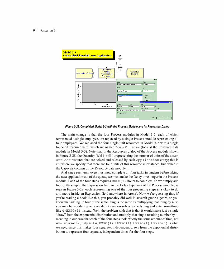
94 CHAPTER 3
Figure 3-28. Completed Model 3-3 with the Process Module and its Resources Dialog
The main change is that the four Process modules in Model 3-2, each of whichrepresented a single employee, are replaced by a single Process module representing allfour employees. We replaced the four single-unit resources in Model 3-2 with a singlefour-unit resource here, which we named Loan Officer (look at the Resource datamodule in Model 3-3). Note that, in the Resources dialog of the Process module shownin Figure 3-28, the Quantity field is still 1, representing the number of units of the LoanOfficer resource that are seized and released by each Application entity; this isnot where we specify that there are four units of this resource in existence, but rather inthe Capacity column of the Resource data module.
And since each employee must now complete all four tasks in tandem before takingthe next application out of the queue, we must make the Delay time longer in the Processmodule. Each of the four steps requires EXPO(1) hours to complete, so we simply addfour of these up in the Expression field in the Delay Type area of the Process module, asseen in Figure 3-28, each representing one of the four processing steps (it’s okay to doarithmetic inside an Expression field anywhere in Arena). Now we’re guessing that, ifyou’re reading a book like this, you probably did well in seventh-grade algebra, so youknow that adding up four of the same thing is the same as multiplying that thing by 4, soyou may be wondering why we didn’t save ourselves some typing and enter somethinglike 4*EXPO(1) instead. Well, the problem with that is that it would make just a single“draw” from the exponential distribution and multiply that single resulting number by 4,meaning in our case that each of the four steps took exactly the same amount of time, notwhat we want. So, ugly as it is, EXPO(1) + EXPO(1) + EXPO(1) + EXPO(1) is whatwe need since this makes four separate, independent draws from the exponential distri-bution to represent four separate, independent times for the four steps.
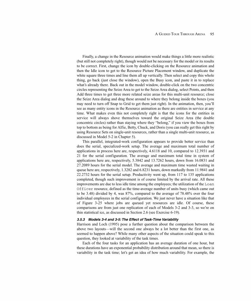
95A GUIDED TOUR THROUGH ARENA
Finally, a change in the Resource animation would make things a little more realistic(but still not completely right), though would not be necessary for the model or its resultsto be correct. First, change the icon by double-clicking on the Resource animation andthen the Idle icon to get to the Resource Picture Placement window, and duplicate thewhite square three times and line them all up vertically. Then select and copy this wholething, go back (just close the window), open the Busy icon, and paste it in to replacewhat’s already there. Back out in the model window, double-click on the two concentriccircles representing the Seize Area to get to the Seize Area dialog, select Points, and thenAdd three times to get three more related seize areas for this multi-unit resource; closethe Seize Area dialog and drag these around to where they belong inside the boxes (youmay need to turn off Snap to Grid to get them just right). In the animation, then, you’llsee as many entity icons in the Resource animation as there are entities in service at anytime. What makes even this not completely right is that the icons for the entities inservice will always shove themselves toward the original Seize Area (the doubleconcentric circles) rather than staying where they “belong,” if you view the boxes fromtop to bottom as being for Alfie, Betty, Chuck, and Doris (you can really get this right byusing Resource Sets on single-unit resources, rather than a single multi-unit resource, asdiscussed in Model 5-2 in Chapter 5).
This parallel, integrated-work configuration appears to provide better service thandoes the serial, specialized-work setup. The average and maximum total number ofapplications in process here are, respectively, 4.6118 and 10, compared to 12.3931 and21 for the serial configuration. The average and maximum total time in system ofapplications here are, respectively, 5.3842 and 13.7262 hours, down from 16.0831 and27.2089 hours for the serial model. The average and maximum time wasted waiting inqueue here are, respectively, 1.3282 and 6.8231 hours, down markedly from 11.9841 and22.2732 hours for the serial setup. Productivity went up, from 117 to 135 applicationscompleted, though such improvement is of course limited by the arrival rate. All theseimprovements are due to less idle time among the employees; the utilization of the LoanOfficer resource, defined as the time-average number of units busy (which came outto be 3.48) divided by 4, was 87%, compared to the average of 78.48% over the fourindividual employees in the serial configuration. We just never have a situation like thatof Figure 3-25 where jobs are queued yet resources are idle. Of course, thesecomparisons are from just one replication of each of Models 3-2 and 3-3, so we’re onthin statistical ice, as discussed in Section 2.6 (see Exercise 6-19).
3.5.3 Models 3-4 and 3-5: The Effect of Task-Time VariabilityHarrison and Loch (1995) pose a further question about the comparison between theabove two layouts—will the second one always be a lot better than the first one, asseemed to happen above? While many other aspects of the situation could speak to thisquestion, they looked at variability of the task times.
Each of the four tasks for an application has an average duration of one hour, butthese durations have an exponential probability distribution around that mean, so there isvariability in the task time; let’s get an idea of how much variability. For example, the
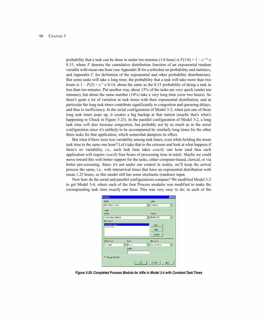
96 CHAPTER 3
probability that a task can be done in under ten minutes (1/6 hour) is F(1/6) = 1 – e–1/6 ≅0.15, where F denotes the cumulative distribution function of an exponential randomvariable with mean one hour (see Appendix B for a refresher on probability and statistics,and Appendix C for definition of the exponential and other probability distributions).But some tasks will take a long time; the probability that a task will take more than twohours is 1 – F(2) = e–2 ≅ 0.14, about the same as the 0.15 probability of doing a task inless than ten minutes. Put another way, about 15% of the tasks are very quick (under tenminutes), but about the same number (14%) take a very long time (over two hours). Sothere’s quite a lot of variation in task times with their exponential distribution, and inparticular the long task times contribute significantly to congestion and queueing delays,and thus to inefficiency. In the serial configuration of Model 3-2, when just one of theselong task times pops up, it creates a big backup at that station (maybe that’s what’shappening to Chuck in Figure 3-25). In the parallel configuration of Model 3-2, a longtask time will also increase congestion, but probably not by as much as in the serialconfiguration since it’s unlikely to be accompanied by similarly long times for the otherthree tasks for that application, which somewhat dampens its effect.
But what if there were less variability among task times, even while holding the meantask time to the same one hour? Let’s take that to the extreme and look at what happens ifthere’s no variability, i.e., each task time takes exactly one hour (and thus eachapplication will require exactly four hours of processing time in total). Maybe we couldmove toward this with better support for the tasks, either computer-based, clerical, or viabetter pre-screening. Since it’s not under our control in reality, we’ll keep the arrivalprocess the same; i.e., with interarrival times that have an exponential distribution withmean 1.25 hours, so this model still has some stochastic (random) input.
Now how do the serial and parallel configurations compare? We modified Model 3-2to get Model 3-4, where each of the four Process modules was modified to make thecorresponding task time exactly one hour. This was very easy to do; in each of the
Figure 3-29. Completed Process Module for Alfie in Model 3-4 with Constant Task Times
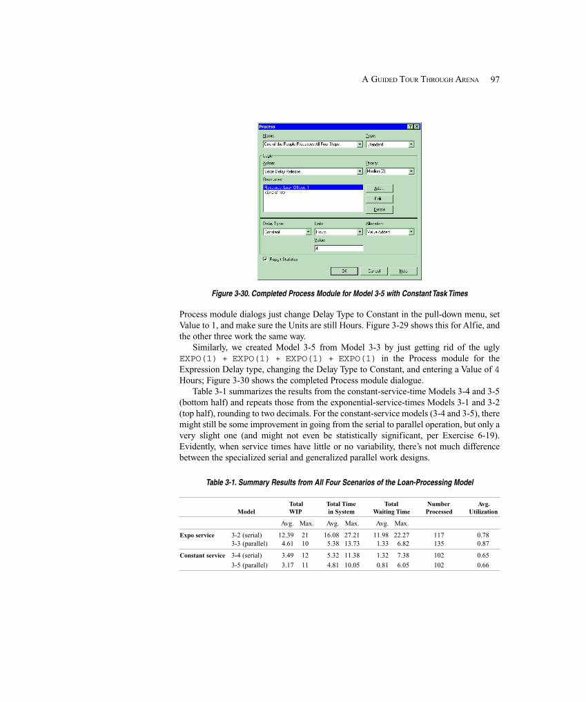
97A GUIDED TOUR THROUGH ARENA
Figure 3-30. Completed Process Module for Model 3-5 with Constant Task Times
Process module dialogs just change Delay Type to Constant in the pull-down menu, setValue to 1, and make sure the Units are still Hours. Figure 3-29 shows this for Alfie, andthe other three work the same way.
Similarly, we created Model 3-5 from Model 3-3 by just getting rid of the uglyEXPO(1) + EXPO(1) + EXPO(1) + EXPO(1) in the Process module for theExpression Delay type, changing the Delay Type to Constant, and entering a Value of 4Hours; Figure 3-30 shows the completed Process module dialogue.
Table 3-1 summarizes the results from the constant-service-time Models 3-4 and 3-5(bottom half) and repeats those from the exponential-service-times Models 3-1 and 3-2(top half), rounding to two decimals. For the constant-service models (3-4 and 3-5), theremight still be some improvement in going from the serial to parallel operation, but only avery slight one (and might not even be statistically significant, per Exercise 6-19).Evidently, when service times have little or no variability, there’s not much differencebetween the specialized serial and generalized parallel work designs.
Table 3-1. Summary Results from All Four Scenarios of the Loan-Processing Model
Total Total Time Total Number Avg.Model WIP in System Waiting Time Processed Utilization
Avg. Max. Avg. Max. Avg. Max.
Expo service 3-2 (serial) 12.39 21 16.08 27.21 11.98 22.27 117 0.783-3 (parallel) 4.61 10 5.38 13.73 1.33 6.82 135 0.87
Constant service 3-4 (serial) 3.49 12 5.32 11.38 1.32 7.38 102 0.65
3-5 (parallel) 3.17 11 4.81 10.05 0.81 6.05 102 0.66
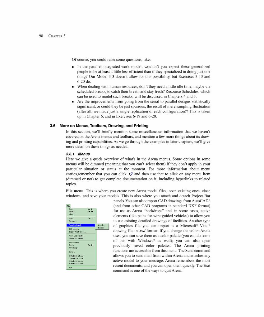
98 CHAPTER 3
Of course, you could raise some questions, like:
� In the parallel integrated-work model, wouldn’t you expect these generalizedpeople to be at least a little less efficient than if they specialized in doing just onething? Our Model 3-3 doesn’t allow for this possibility, but Exercises 3-13 and6-20 do.
� When dealing with human resources, don’t they need a little idle time, maybe viascheduled breaks, to catch their breath and stay fresh? Resource Schedules, whichcan be used to model such breaks, will be discussed in Chapters 4 and 5.
� Are the improvements from going from the serial to parallel designs statisticallysignificant, or could they be just spurious, the result of mere sampling fluctuation(after all, we made just a single replication of each configuration)? This is takenup in Chapter 6, and in Exercises 6-19 and 6-20.
3.6 More on Menus, Toolbars, Drawing, and Printing
In this section, we’ll briefly mention some miscellaneous information that we haven’tcovered on the Arena menus and toolbars, and mention a few more things about its draw-ing and printing capabilities. As we go through the examples in later chapters, we’ll givemore detail on these things as needed.
3.6.1 MenusHere we give a quick overview of what’s in the Arena menus. Some options in somemenus will be dimmed (meaning that you can’t select them) if they don’t apply in yourparticular situation or status at the moment. For more information about menuentries,remember that you can click and then use that to click on any menu item(dimmed or not) to get complete documentation on it, including hyperlinks to relatedtopics.
File menu. This is where you create new Arena model files, open existing ones, closewindows, and save your models. This is also where you attach and detach Project Bar
panels. You can also import CAD drawings from AutoCAD®
(and from other CAD programs in standard DXF format)for use as Arena “backdrops” and, in some cases, activeelements (like paths for wire-guided vehicles) to allow youto use existing detailed drawings of facilities. Another typeof graphics file you can import is a Microsoft® Visio®
drawing file in .vsd format. If you change the colors Arenauses, you can save them as a color palette (you can do someof this with Windows® as well); you can also openpreviously saved color palettes. The Arena printingfunctions are accessible from this menu. The Send commandallows you to send mail from within Arena and attaches anyactive model to your message. Arena remembers the mostrecent documents, and you can open them quickly. The Exitcommand is one of the ways to quit Arena.
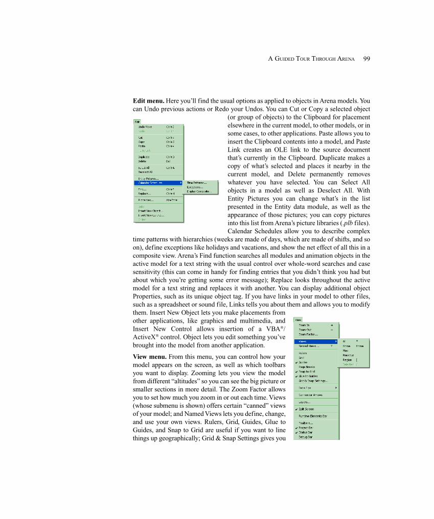
99A GUIDED TOUR THROUGH ARENA
Edit menu. Here you’ll find the usual options as applied to objects in Arena models. Youcan Undo previous actions or Redo your Undos. You can Cut or Copy a selected object
(or group of objects) to the Clipboard for placementelsewhere in the current model, to other models, or insome cases, to other applications. Paste allows you toinsert the Clipboard contents into a model, and PasteLink creates an OLE link to the source documentthat’s currently in the Clipboard. Duplicate makes acopy of what’s selected and places it nearby in thecurrent model, and Delete permanently removeswhatever you have selected. You can Select Allobjects in a model as well as Deselect All. WithEntity Pictures you can change what’s in the listpresented in the Entity data module, as well as theappearance of those pictures; you can copy picturesinto this list from Arena’s picture libraries (.plb files).Calendar Schedules allow you to describe complex
time patterns with hierarchies (weeks are made of days, which are made of shifts, and soon), define exceptions like holidays and vacations, and show the net effect of all this in acomposite view. Arena’s Find function searches all modules and animation objects in theactive model for a text string with the usual control over whole-word searches and casesensitivity (this can come in handy for finding entries that you didn’t think you had butabout which you’re getting some error message); Replace looks throughout the activemodel for a text string and replaces it with another. You can display additional objectProperties, such as its unique object tag. If you have links in your model to other files,such as a spreadsheet or sound file, Links tells you about them and allows you to modifythem. Insert New Object lets you make placements fromother applications, like graphics and multimedia, andInsert New Control allows insertion of a VBA®/ActiveX® control. Object lets you edit something you’vebrought into the model from another application.
View menu. From this menu, you can control how yourmodel appears on the screen, as well as which toolbarsyou want to display. Zooming lets you view the modelfrom different “altitudes” so you can see the big picture orsmaller sections in more detail. The Zoom Factor allowsyou to set how much you zoom in or out each time. Views(whose submenu is shown) offers certain “canned” viewsof your model; and Named Views lets you define, change,and use your own views. Rulers, Grid, Guides, Glue toGuides, and Snap to Grid are useful if you want to linethings up geographically; Grid & Snap Settings gives you
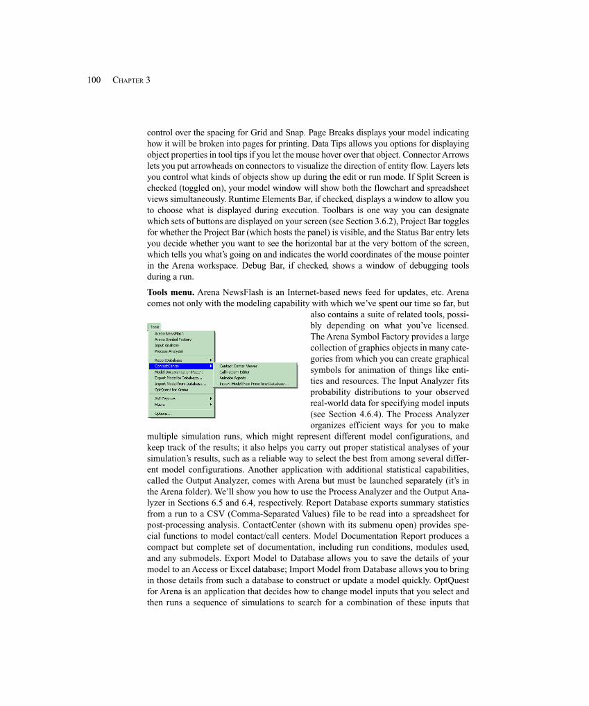
100 CHAPTER 3
control over the spacing for Grid and Snap. Page Breaks displays your model indicatinghow it will be broken into pages for printing. Data Tips allows you options for displayingobject properties in tool tips if you let the mouse hover over that object. Connector Arrowslets you put arrowheads on connectors to visualize the direction of entity flow. Layers letsyou control what kinds of objects show up during the edit or run mode. If Split Screen ischecked (toggled on), your model window will show both the flowchart and spreadsheetviews simultaneously. Runtime Elements Bar, if checked, displays a window to allow youto choose what is displayed during execution. Toolbars is one way you can designatewhich sets of buttons are displayed on your screen (see Section 3.6.2), Project Bar togglesfor whether the Project Bar (which hosts the panel) is visible, and the Status Bar entry letsyou decide whether you want to see the horizontal bar at the very bottom of the screen,which tells you what’s going on and indicates the world coordinates of the mouse pointerin the Arena workspace. Debug Bar, if checked, shows a window of debugging toolsduring a run.
Tools menu. Arena NewsFlash is an Internet-based news feed for updates, etc. Arenacomes not only with the modeling capability with which we’ve spent our time so far, but
also contains a suite of related tools, possi-bly depending on what you’ve licensed.The Arena Symbol Factory provides a largecollection of graphics objects in many cate-gories from which you can create graphicalsymbols for animation of things like enti-ties and resources. The Input Analyzer fitsprobability distributions to your observedreal-world data for specifying model inputs(see Section 4.6.4). The Process Analyzerorganizes efficient ways for you to make
multiple simulation runs, which might represent different model configurations, andkeep track of the results; it also helps you carry out proper statistical analyses of yoursimulation’s results, such as a reliable way to select the best from among several differ-ent model configurations. Another application with additional statistical capabilities,called the Output Analyzer, comes with Arena but must be launched separately (it’s inthe Arena folder). We’ll show you how to use the Process Analyzer and the Output Ana-lyzer in Sections 6.5 and 6.4, respectively. Report Database exports summary statisticsfrom a run to a CSV (Comma-Separated Values) file to be read into a spreadsheet forpost-processing analysis. ContactCenter (shown with its submenu open) provides spe-cial functions to model contact/call centers. Model Documentation Report produces acompact but complete set of documentation, including run conditions, modules used,and any submodels. Export Model to Database allows you to save the details of yourmodel to an Access or Excel database; Import Model from Database allows you to bringin those details from such a database to construct or update a model quickly. OptQuestfor Arena is an application that decides how to change model inputs that you select andthen runs a sequence of simulations to search for a combination of these inputs that
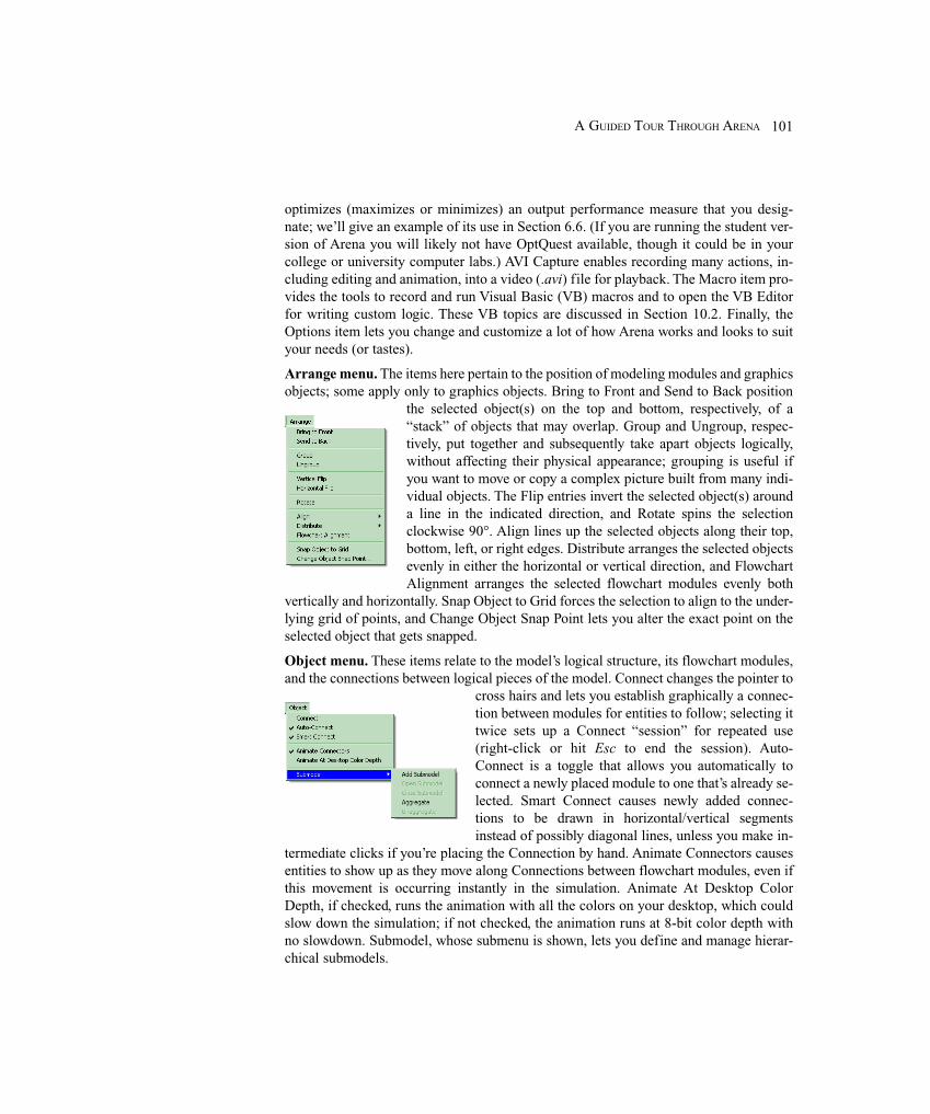
101A GUIDED TOUR THROUGH ARENA
optimizes (maximizes or minimizes) an output performance measure that you desig-nate; we’ll give an example of its use in Section 6.6. (If you are running the student ver-sion of Arena you will likely not have OptQuest available, though it could be in yourcollege or university computer labs.) AVI Capture enables recording many actions, in-cluding editing and animation, into a video (.avi) file for playback. The Macro item pro-vides the tools to record and run Visual Basic (VB) macros and to open the VB Editorfor writing custom logic. These VB topics are discussed in Section 10.2. Finally, theOptions item lets you change and customize a lot of how Arena works and looks to suityour needs (or tastes).
Arrange menu. The items here pertain to the position of modeling modules and graphicsobjects; some apply only to graphics objects. Bring to Front and Send to Back position
the selected object(s) on the top and bottom, respectively, of a“stack” of objects that may overlap. Group and Ungroup, respec-tively, put together and subsequently take apart objects logically,without affecting their physical appearance; grouping is useful ifyou want to move or copy a complex picture built from many indi-vidual objects. The Flip entries invert the selected object(s) arounda line in the indicated direction, and Rotate spins the selectionclockwise 90°. Align lines up the selected objects along their top,bottom, left, or right edges. Distribute arranges the selected objectsevenly in either the horizontal or vertical direction, and FlowchartAlignment arranges the selected flowchart modules evenly both
vertically and horizontally. Snap Object to Grid forces the selection to align to the under-lying grid of points, and Change Object Snap Point lets you alter the exact point on theselected object that gets snapped.
Object menu. These items relate to the model’s logical structure, its flowchart modules,and the connections between logical pieces of the model. Connect changes the pointer to
cross hairs and lets you establish graphically a connec-tion between modules for entities to follow; selecting ittwice sets up a Connect “session” for repeated use(right-click or hit Esc to end the session). Auto-Connect is a toggle that allows you automatically toconnect a newly placed module to one that’s already se-lected. Smart Connect causes newly added connec-tions to be drawn in horizontal/vertical segmentsinstead of possibly diagonal lines, unless you make in-
termediate clicks if you’re placing the Connection by hand. Animate Connectors causesentities to show up as they move along Connections between flowchart modules, even ifthis movement is occurring instantly in the simulation. Animate At Desktop ColorDepth, if checked, runs the animation with all the colors on your desktop, which couldslow down the simulation; if not checked, the animation runs at 8-bit color depth withno slowdown. Submodel, whose submenu is shown, lets you define and manage hierar-chical submodels.
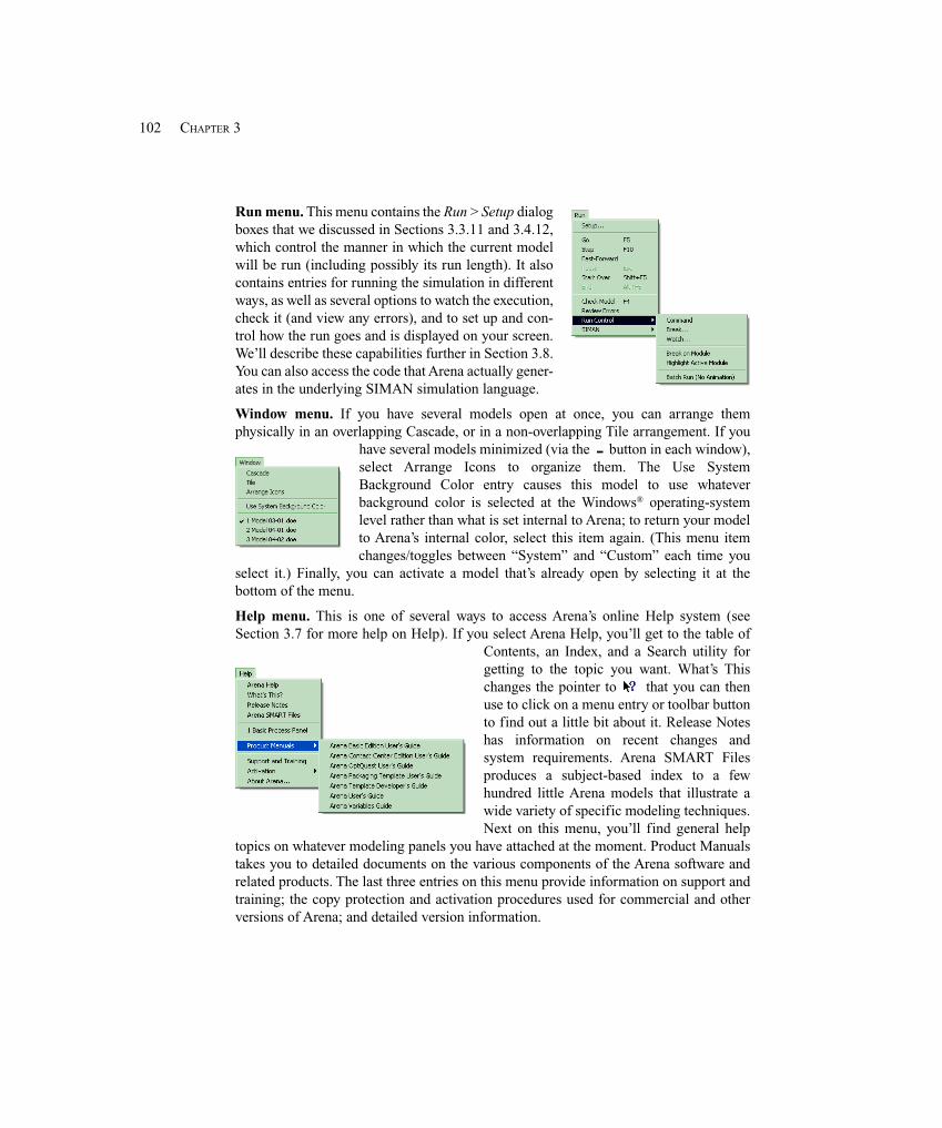
102 CHAPTER 3
Run menu. This menu contains the Run > Setup dialogboxes that we discussed in Sections 3.3.11 and 3.4.12,which control the manner in which the current modelwill be run (including possibly its run length). It alsocontains entries for running the simulation in differentways, as well as several options to watch the execution,check it (and view any errors), and to set up and con-trol how the run goes and is displayed on your screen.We’ll describe these capabilities further in Section 3.8.You can also access the code that Arena actually gener-ates in the underlying SIMAN simulation language.
Window menu. If you have several models open at once, you can arrange themphysically in an overlapping Cascade, or in a non-overlapping Tile arrangement. If you
have several models minimized (via the button in each window),select Arrange Icons to organize them. The Use SystemBackground Color entry causes this model to use whateverbackground color is selected at the Windows® operating-systemlevel rather than what is set internal to Arena; to return your modelto Arena’s internal color, select this item again. (This menu itemchanges/toggles between “System” and “Custom” each time you
select it.) Finally, you can activate a model that’s already open by selecting it at thebottom of the menu.
Help menu. This is one of several ways to access Arena’s online Help system (seeSection 3.7 for more help on Help). If you select Arena Help, you’ll get to the table of
Contents, an Index, and a Search utility forgetting to the topic you want. What’s Thischanges the pointer to that you can thenuse to click on a menu entry or toolbar buttonto find out a little bit about it. Release Noteshas information on recent changes andsystem requirements. Arena SMART Filesproduces a subject-based index to a fewhundred little Arena models that illustrate awide variety of specific modeling techniques.Next on this menu, you’ll find general help
topics on whatever modeling panels you have attached at the moment. Product Manualstakes you to detailed documents on the various components of the Arena software andrelated products. The last three entries on this menu provide information on support andtraining; the copy protection and activation procedures used for commercial and otherversions of Arena; and detailed version information.
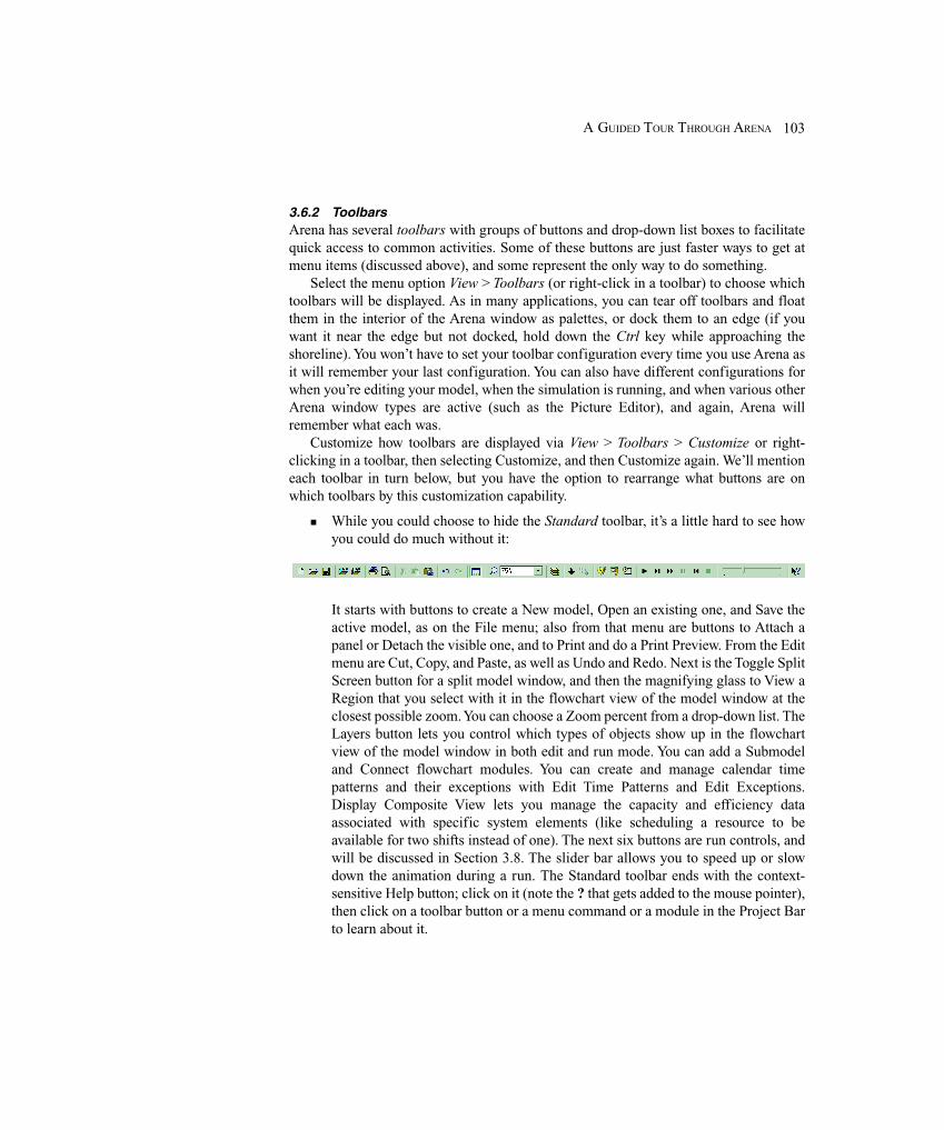
103A GUIDED TOUR THROUGH ARENA
3.6.2 ToolbarsArena has several toolbars with groups of buttons and drop-down list boxes to facilitatequick access to common activities. Some of these buttons are just faster ways to get atmenu items (discussed above), and some represent the only way to do something.
Select the menu option View > Toolbars (or right-click in a toolbar) to choose whichtoolbars will be displayed. As in many applications, you can tear off toolbars and floatthem in the interior of the Arena window as palettes, or dock them to an edge (if youwant it near the edge but not docked, hold down the Ctrl key while approaching theshoreline). You won’t have to set your toolbar configuration every time you use Arena asit will remember your last configuration. You can also have different configurations forwhen you’re editing your model, when the simulation is running, and when various otherArena window types are active (such as the Picture Editor), and again, Arena willremember what each was.
Customize how toolbars are displayed via View > Toolbars > Customize or right-clicking in a toolbar, then selecting Customize, and then Customize again. We’ll mentioneach toolbar in turn below, but you have the option to rearrange what buttons are onwhich toolbars by this customization capability.
� While you could choose to hide the Standard toolbar, it’s a little hard to see howyou could do much without it:
It starts with buttons to create a New model, Open an existing one, and Save theactive model, as on the File menu; also from that menu are buttons to Attach apanel or Detach the visible one, and to Print and do a Print Preview. From the Editmenu are Cut, Copy, and Paste, as well as Undo and Redo. Next is the Toggle SplitScreen button for a split model window, and then the magnifying glass to View aRegion that you select with it in the flowchart view of the model window at theclosest possible zoom. You can choose a Zoom percent from a drop-down list. TheLayers button lets you control which types of objects show up in the flowchartview of the model window in both edit and run mode. You can add a Submodeland Connect flowchart modules. You can create and manage calendar timepatterns and their exceptions with Edit Time Patterns and Edit Exceptions.Display Composite View lets you manage the capacity and efficiency dataassociated with specific system elements (like scheduling a resource to beavailable for two shifts instead of one). The next six buttons are run controls, andwill be discussed in Section 3.8. The slider bar allows you to speed up or slowdown the animation during a run. The Standard toolbar ends with the context-sensitive Help button; click on it (note the ? that gets added to the mouse pointer),then click on a toolbar button or a menu command or a module in the Project Barto learn about it.
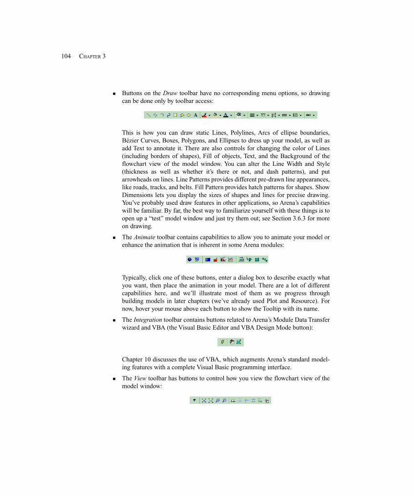
104 CHAPTER 3
� Buttons on the Draw toolbar have no corresponding menu options, so drawingcan be done only by toolbar access:
This is how you can draw static Lines, Polylines, Arcs of ellipse boundaries,Bézier Curves, Boxes, Polygons, and Ellipses to dress up your model, as well asadd Text to annotate it. There are also controls for changing the color of Lines(including borders of shapes), Fill of objects, Text, and the Background of theflowchart view of the model window. You can alter the Line Width and Style(thickness as well as whether it’s there or not, and dash patterns), and putarrowheads on lines. Line Patterns provides different pre-drawn line appearances,like roads, tracks, and belts. Fill Pattern provides hatch patterns for shapes. ShowDimensions lets you display the sizes of shapes and lines for precise drawing.You’ve probably used draw features in other applications, so Arena’s capabilitieswill be familiar. By far, the best way to familiarize yourself with these things is toopen up a “test” model window and just try them out; see Section 3.6.3 for moreon drawing.
� The Animate toolbar contains capabilities to allow you to animate your model orenhance the animation that is inherent in some Arena modules:
Typically, click one of these buttons, enter a dialog box to describe exactly whatyou want, then place the animation in your model. There are a lot of differentcapabilities here, and we’ll illustrate most of them as we progress throughbuilding models in later chapters (we’ve already used Plot and Resource). Fornow, hover your mouse above each button to show the Tooltip with its name.
� The Integration toolbar contains buttons related to Arena’s Module Data Transferwizard and VBA (the Visual Basic Editor and VBA Design Mode button):
Chapter 10 discusses the use of VBA, which augments Arena’s standard model-ing features with a complete Visual Basic programming interface.
� The View toolbar has buttons to control how you view the flowchart view of themodel window:

105A GUIDED TOUR THROUGH ARENA
From here you can Manage Named Views, Zoom In and Out, or choose to ViewAll the model or View Previous. You can also reveal the Rulers and Grid, createGuides, show page breaks for printing, and Snap new objects to the Grid, as wellas Glue objects to Guides.
� The Arrange toolbar corresponds closely to the Arrange menu:
You can Bring a selected object to the Front or Send it to the Back. A selection ofmultiple drawing objects can be made into a logical Group and Ungrouped later.Drawing objects can also be Flipped around a Vertical or Horizontal line on theirmidpoint or Rotated clockwise 90°. You can also Align the selected objects ontheir Top, Bottom, Left, or Right edges, as well as Space them evenly eitherhorizontally or vertically. Finally, you can Snap selected objects to the Grid.
� The Run Interaction toolbar has buttons corresponding to the Check Model,Command, Break, Watch, and Break on Module entries from the Run menu (seeSection 3.8 for more). The last button corresponds to Animate Connectors fromthe Object menu:
� The Record Macro toolbar has buttons to Start/Pause/Resume as well as Stop re-cording a VB macro. A macro is a series of Visual Basic statements stored in asubroutine in a Visual Basic module (macros are discussed in Chapter 10):
� The AVI Capture toolbar has buttons to start and stop capturing everything goingon in the Arena model window, including editing and animation during a run:
This results in a .avi file that can later be played by any of a variety of video-player software products. Explore the Help button in this dialog and try it out.
� The Animate Transfer toolbar gives you tools to add animation objects to yourmodel:
These include Storage, Seize, Parking, Transporter, Station, Intersection, Route,Segment, Distance, Network, and Promote Path. We’ll discuss these capabilitiesin subsequent chapters as we develop models whose animations can benefit fromthem.
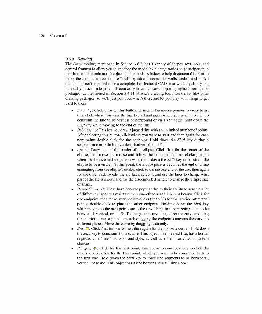
106 CHAPTER 3
3.6.3 DrawingThe Draw toolbar, mentioned in Section 3.6.2, has a variety of shapes, text tools, andcontrol features to allow you to enhance the model by placing static (no participation inthe simulation or animation) objects in the model window to help document things or tomake the animation seem more “real” by adding items like walls, aisles, and pottedplants. This isn’t intended to be a complete, full-featured CAD or artwork capability, butit usually proves adequate; of course, you can always import graphics from otherpackages, as mentioned in Section 3.4.11. Arena’s drawing tools work a lot like otherdrawing packages, so we’ll just point out what’s there and let you play with things to getused to them:
� Line, : Click once on this button, changing the mouse pointer to cross hairs,then click where you want the line to start and again where you want it to end. Toconstrain the line to be vertical or horizontal or on a 45° angle, hold down theShift key while moving to the end of the line.
� Polyline, : This lets you draw a jagged line with an unlimited number of points.After selecting this button, click where you want to start and then again for eachnew point; double-click for the endpoint. Hold down the Shift key during asegment to constrain it to vertical, horizontal, or 45°.
� Arc, : Draw part of the border of an ellipse. Click first for the center of theellipse, then move the mouse and follow the bounding outline, clicking againwhen it’s the size and shape you want (hold down the Shift key to constrain theellipse to be a circle). At this point, the mouse pointer becomes the end of a lineemanating from the ellipse’s center; click to define one end of the arc, then againfor the other end. To edit the arc later, select it and use the lines to change whatpart of the arc is shown and use the disconnected handle to change the ellipse sizeor shape.
� Bézier Curve, : These have become popular due to their ability to assume a lotof different shapes yet maintain their smoothness and inherent beauty. Click forone endpoint, then make intermediate clicks (up to 30) for the interior “attractor”points; double-click to place the other endpoint. Holding down the Shift keywhile moving to the next point causes the (invisible) lines connecting them to behorizontal, vertical, or at 45°. To change the curvature, select the curve and dragthe interior attractor points around; dragging the endpoints anchors the curve todifferent places. Move the curve by dragging it directly.
� Box, : Click first for one corner, then again for the opposite corner. Hold downthe Shift key to constrain it to a square. This object, like the next two, has a borderregarded as a “line” for color and style, as well as a “fill” for color or patternchoices.
� Polygon, : Click for the first point, then move to new locations to click theothers; double-click for the final point, which you want to be connected back tothe first one. Hold down the Shift key to force line segments to be horizontal,vertical, or at 45°. This object has a line border and a fill like a box.

107A GUIDED TOUR THROUGH ARENA
� Ellipse, : First click for the center, move the mouse and follow the boundingoutline to the size and shape you want, and finally click again. Hold the Shift keyto force it to a circle. This object has a line border and a fill like a box.
� Text, : This is how you add annotation to your model to label things or providedocumentation. Clicking the button brings up a dialog box where you type inyour text; use Ctrl+Enter to go to a new line and Ctrl+Tab for a tab. The Fontbutton lets you change the font, style, and size. Closing this dialog box changesthe mouse pointer to cross hairs, which you click where you want to position thenorthwest corner of your text. Use the underline to move, resize, or reorient thetext to a different angle (hold the Shift key to constrain the angle to horizontal,vertical, or 45°).
� Line Color, : If a line object (a line, polyline, arc, Bézier curve, or the borderof a shape) is selected, clicking the paintbrush part of the button changes thatobject to the color underlining the paintbrush. Clicking the drop-down arrowchanges the selected line object to the color you then select from the palette, andchanges the underline color to this as well. New line objects will be in theunderline color. Arena will remember this line color not only for future lineobjects in this window, but also for new windows and future Arena sessions, untilyou change it again.
� Fill Color, : This operates on the interior of a shape (box, polygon, or ellipse)just as Line Color operates on line objects.
� Text Color, : This operates on Text drawing objects just as Line Coloroperates on line objects.
� Window Background Color, : This sets the background color of the flowchartview of the model window to the color you select from the palette.
� Line Width, : Operates on the width of line objects just as Line Coloroperates on their color.
� Line Style, : Provides dash patterns for lines. The No Line option makes theline invisible but it is still logically there (this might make sense for a border of ashape).
� Arrow Style, : Provides various arrowheads for lines.� Line Pattern, : Provides different pre-drawn line appearances, like roads,
tracks, and belts.� Fill Pattern, : Operates on the pattern for the interior of a shape just as Fill
Color operates on its color.� Show Dimensions, : Shows sizes of shapes and lengths of lines and line
segments, for precise drawing.
3.6.4 PrintingAll or parts of the flowchart view of the active model window can be printed directlyfrom Arena (in color, if you have it). File > Print Preview (or ) lets you preview what’scoming, File > Print (or or Ctrl+P) lets you print it, and File > Print Setup lets youselect a print driver or do a setup of your printer.
108 CHAPTER 3
If your model is big, the print will extend across several pages. And if you haveNamed Views, you’ll get a print of the current view, followed by a separate print of eachnamed view. If you don’t want all this, use Print Preview to see what’s on which page,then selectively print only the pages you want. The menu option View > Page Breaks willshow in the flowchart view where the pages will end if the model is printed.
As an alternative to printing directly from Arena, remember that you can get to a viewyou like (maybe even during a pause in the animation), press the Prnt Scrn (Print Screen)key, switch over to your word-processing document, and paste the shot in where youwant it. Then you can print this document when you’d like. You could also paste the PrntScrn image into a paint program and perhaps crop it or otherwise clean it up (in fact,that’s exactly how we got all the pieces of the Arena window into this book).
3.7 Help!
Arena has an extensive and comprehensive Help system to serve as a reference, guideyou through various operations, and supply examples of modeling facets as well ascomplete projects. The help system is carefully integrated and provides extensivehyperlinks to other areas to aid in getting the information you need quickly and easily.There are several different ways to access the help system, which we’ll describe briefly inthis section. However, you may find that the best way to learn about help is just to get inand start exploring.
At any time, you can access the full help system from the Help menu. The contents ofthis menu were described above, at the end of Section 3.6.1.
The button invokes context-sensitive help. To use it, just click the button, thenclick on whatever you’re curious about—a toolbar button, a command from a menu, amodule in the Project Bar—and you can get to the information you need via a visual path.
Most Arena dialog boxes have a Help button that you can press. This is a good way toget direct information on what that part of the software is about, what your options are,how relevant things are defined, related concepts (via hyperlinks to other parts of theHelp system), and examples. You can also use the ? button at the top of the dialog box toaccess What’s This? help information on individual items in a dialog box. Simply clickthe ? and then click on the selected item.
In case you forget what a particular button does, you can let your pointer staymotionless on it for a second or two; a little boxed Tooltip will appear to remind you whatit is.
SMART files, via the Help menu, are subject-categorized Arena models (a fewhundred) that illustrate, via small working models, a wide variety of Arena modelingcapabilities.
Online help is available in the form of technical notes and updates, at http://www.rockwellautomation.com/support/.
In the Examples folder inside the Arena folder are several detailed Example modelsthat you can open, browse, copy, edit (to be safe, edit a copy), and run. If you have astudent or other limited version of Arena, you may not be able to run these models tocompletion due to the limit on the number of concurrent entities. If you open a large
109A GUIDED TOUR THROUGH ARENA
model (one that exceeds the student version limits), Arena will enter a runtime mode.Runtime mode allows you to make minor changes and run the model, but does not allowsignificant changes like adding and deleting modules. The Example models illustratedifferent aspects of building and studying models. The Help topic4 “Example Models”has a description of what’s in each one.
3.8 More on Running Models
Usually you’ll just want to run your model to completion as you have it set up, but thereare times when you might like to control how the run is done. Entries from the Run menu,as well as corresponding buttons from the Standard and Run Interaction toolbars, let youdo this. (See Section 4.5 for details and examples of using these capabilities.)
� Run > Setup gives you access to many options for how runs are made for thecurrent model, like deciding whether to see the animation and perhaps running infull-screen mode. These selections and specifications are saved with the currentmodel rather than going into global effect. Click the Help button inside any Run >Setup dialog box and browse through the hyperlinked topics to get familiar withwhat the (numerous) possibilities are.
� Run > Go (or from the Standard toolbar or the F5 function key) just does it (orresumes it after a pause). If you’ve made changes to the model since the lastcheck (see below), it gets checked before it’s run.
� Run > Step (or or F10) executes the model one action at a time so you can seein detail what’s going on. This gets really boring so is useful primarily as a debug-ging or demonstration tool. As with the Go button, use of Step causes the modelto be checked if Arena detects changes since the last check was performed.
� Run > Fast-Forward (or ) disables the animation and executes the run at a muchfaster rate. You can pause at any time during the run to view the animation. Fast-Forward causes the model to be checked if Arena detects changes since the lastcheck was performed.
� Run > Pause (or or Esc) interrupts the run so you can look at something. Press, , or to resume it.
� Run > Start Over (or or Shift+F5) goes back to the beginning of the simulationand reruns the model. Start Over causes the model to be checked if Arena detectschanges since the last check was performed.
� While Arena is running your model, it’s in what’s called run mode, and most ofthe model-building tools are disabled. So when the run is over, you need to selectRun > End (or or Alt+F5) to get out of run mode and enable the modeling toolsagain. If you’ve paused your run before it terminated, this will kill it at that point.
� Use Run > Check Model (or or F4) to “compile” your model without runningit. If Arena detects errors at this stage, you’re told about them (gently, of course)in an Errors/Warnings window; the buttons at the bottom of this window help you
4 To go to a specific Help topic, select Help > Arena Help > Index, type the topic name into the first region,and then open (double-click, or single-click and then click Display) the index topic in the second region below.
110 CHAPTER 3
find the problem (for example, by selecting the offending module in the flow-chart view of the model window).
� Run > Review Errors recalls the most recent Errors/Warnings window containingwhatever Arena found wrong during that check.
� Run > Run Control > Command (or ) gets you to an interactive command-linewindow that allows control over a lot of how the run is done—like interrupts andaltering values. This also checks the model, if required, and starts the run if it’s notyet started.
� Run > Run Control > Breakpoints (or ) lets you set times or conditions to inter-rupt the model in order to check on or illustrate something.
� Run > Run Control > Watch (or ) establishes a window in which you canobserve the value of a variable or expression as the run progresses. Run > Setup >Run Control lets you determine whether this is concurrent with the run or onlywhen the Watch window is the active window (the latter will speed things up).
� Run > Run Control > Break on Module (or ) either sets or clears a break put onthe selected module. A break on a module halts execution when an entity starts orresumes execution of the logic for the module.
� Run > Run Control > Highlight Active Module causes a flowchart module to behighlighted when it is being executed, which provides a visual indication of theaction during the animation.
� If Run > Run Control > Batch Run (No Animation) is checked, the model will berun without any animation. This is even faster than Fast-Forward, and is usuallyused when the project is in production mode to produce adequate statistics forprecise analysis.
� Run > SIMAN allows you to view or write to a file the model file (.mod) andexperiment file (.exp) for the code in the underlying SIMAN simulation languagethat your Arena model generates. To understand this, you’ll of course need toknow something about SIMAN (see Pegden, Shannon, and Sadowski, 1995).
3.9 Summary and Forecast
After this guided tour through Arena, you should be a pretty knowledgeable (and tired)tourist. In Chapters 4 through 9, we’ll set you out to explore on your own, but with apretty detailed road map from us. In those chapters, you’ll build a sequence ofprogressively more complex models that illustrate many of Arena’s modeling capabilitiesand sometimes require you to perform a few creative modeling stunts. We’ll alsointegrate at the end of Chapter 4, throughout Chapter 6, at the end of Chapter 7, and inChapter 12 some information on the statistical aspects of doing simulation studies withArena, on both the input and output sides.
3.10 Exercises
3-1 Make five replications of Model 3-1 by just asking for them in Run > Setup >Replication Parameters. Look at the output and note how the performance measures varyacross replications, confirming Table 2-4. To see the results for each of the five
111A GUIDED TOUR THROUGH ARENA
replications individually, you’ll need to open the Category by Replication report; theconfidence-interval half-widths can be seen in the Category Overview report, however.
3-2 Implement the double-time arrival modification to Model 3-1 discussed in Section2.6.3 by opening the Create module and changing the Value 5 to 2.5 for the mean of theexponential distribution for Time Between Arrivals (don’t forget to click OK, rather thanCancel, if you want this change to happen). Make five replications and compare theresults to what we got in the hand simulation (see Figure 2-4). To see the results for each ofthe five replications individually, you’ll need to open the Category by Replication report.
3-3 Lengthen the run in Model 3-1 to 8 hours for a more interesting show. If you wantthe plots to be complete, you’ll have to open them and extend the Maximum in the Scalefor the Time (X) Axes (mind the units!), as well as possibly adjust the Major Incrementthere. Make just one replication.
3-4 Implement the change to Model 3-1 described in Exercise 2-4 from Chapter 2.Open the Process module, change the Delay Type to Expression, and enter theappropriate Expression (use the Expression Builder if you like). Run the model for 20minutes and check against your hand-simulation results. If they’re different, what mightbe the explanation (assuming you did everything right)?
Next, try running this for 48 hours and watch the queue-length plot (for both plots,change the Scale Maximum for the Time (X) Axis to 2880 and increase theMajorIncrement to 240). To allow more room in the queue animation, click on the linefor the queue and drag its left end to the left. What’s happening? Why?
3-5 Implement the additional statistic-collection function described in Exercise 2-1,and add a plot that tracks the total number of parts in the system (also called work inprocess, abbreviated as WIP) over time. Note that at any given point in simulated time,WIP is the number in queue plus the number in service; you might also use the ExpressionBuilder and check the Help topic EntitiesWIP Variable.
3-6 Modify Model 3-1 with all of the following changes:
� Add a second machine to which all parts go immediately after exiting the firstmachine for a separate kind of processing (for example, the first machine isdrilling and the second machine is washing). Processing times at the secondmachine are independent of those from the first machine but drawn from thesame distribution as for the first machine. Gather all the statistics as before, plusthe time in queue, queue length, and utilization at the second machine.
� Immediately after the second machine, there’s a pass/fail inspection that takes aconstant 4.5 minutes to carry out and has an 75% chance of a passing result;queueing is possible for the single inspector, and the queue is first-in, first-out.All parts exit the system regardless of whether they pass the test. Count the num-ber that fail and the number that pass, and gather statistics on the time in queue,queue length, and utilization at the inspection center. (HINT: Try the Decideflowchart module.)
112 CHAPTER 3
� Include plots to track the queue length and number busy at all three stations; putall queue lengths together in the same plot, and put all numbers busy in the sameplot (you’ll need to turn on the plot Legends to identify the three curves).Configure them as needed.
� Run the simulation for 480 minutes instead of 20 minutes.
3-7 In Exercise 3-6, suppose that parts that fail inspection after being washed are sentback and re-washed, instead of leaving; such re-washed parts must then undergo thesame inspection, and have the same probability of failing (as improbable as that mightseem). There’s no limit on how many times a given part might have to loop back throughthe washer and inspector. Run this model under the same conditions as Exercise 3-6, andcompare the results for the time in queue, queue length, and utilization at the inspectioncenter (add a brief Text box to your .doe file for this comparison). Of course, this timethere’s no need to count the number of parts that fail and pass, since they all eventuallypass (or do they?). You may have to allow for more room in some of the queueanimations.
3-8 In Exercise 3-7, suppose the inspection can result in one of three outcomes: pass(probability 0.75, as before), fail (probability 0.11), and re-wash (probability 0.14).Failures leave immediately, and re-washes loop back to the washer. The aboveprobabilities hold for each part undergoing inspection, regardless of its past history.Count the number that eventually fail and the number that eventually pass, and gatherstatistics (in a Text box in your model) on the time in queue, queue length, and utilizationat the inspection center. (HINT: Explore the Decide flowchart module and contemplate ahigher-dimensional coin to flip.)
3-9 In Model 3-1, suppose that instead of having a single source of parts, there arethree sources of arrival, one for each of three different kinds of parts that arrive: Blue (asbefore), Green, and Red. For each color of arriving part, interarrival times areexponentially distributed with a mean of 16 minutes. Run the simulation for 480minutes, and compute the same performance measures as for Model 3-1. Once the partsare in the system, they retain their correct color (for the animation) but are notdifferentiated for collection of statistics on time in queue, queue length, or utilization(that is, they’re lumped together for purposes of processing and statistics collection onthese output performance measures); however, collect statistics separately by part colorfor total time in system. Processing times at the drilling center are the same as in Model3-1 and are the same regardless of the color of the part.
3-10 In science museums, you’ll often find what’s called a probability board (alsoknown as a quincunx):
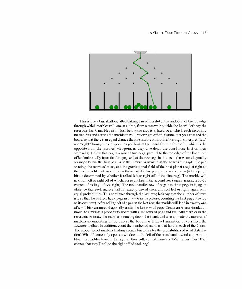
113A GUIDED TOUR THROUGH ARENA
This is like a big, shallow, tilted baking pan with a slot at the midpoint of the top edgethrough which marbles roll, one at a time, from a reservoir outside the board; let’s say thereservoir has k marbles in it. Just below the slot is a fixed peg, which each incomingmarble hits and causes the marble to roll left or right off of; assume that you’ve tilted theboard so that there’s an equal chance that the marble will roll left vs. right (interpret “left”and “right” from your viewpoint as you look at the board from in front of it, which is theopposite from the marbles’ viewpoint as they dive down the board nose first on theirstomachs). Below this peg is a row of two pegs, parallel to the top edge of the board butoffset horizontally from the first peg so that the two pegs in this second row are diagonallyarranged below the first peg, as in the picture. Assume that the board’s tilt angle, the pegspacing, the marbles’ mass, and the gravitational field of the host planet are just right sothat each marble will next hit exactly one of the two pegs in the second row (which peg ithits is determined by whether it rolled left or right off of the first peg). The marble willnext roll left or right off of whichever peg it hits in the second row (again, assume a 50-50chance of rolling left vs. right). The next parallel row of pegs has three pegs in it, againoffset so that each marble will hit exactly one of them and roll left or right, again withequal probabilities. This continues through the last row; let’s say that the number of rowsis n so that the last row has n pegs in it (n = 6 in the picture, counting the first peg at the topas its own row). After rolling off of a peg in the last row, the marble will land in exactly oneof n + 1 bins arranged diagonally under the last row of pegs. Create an Arena simulationmodel to simulate a probability board with n = 6 rows of pegs and k = 1500 marbles in thereservoir. Animate the marbles bouncing down the board, and also animate the number ofmarbles accumulating in the bins at the bottom with Level animation objects from theAnimate toolbar. In addition, count the number of marbles that land in each of the 7 bins.The proportion of marbles landing in each bin estimates the probabilities of what distribu-tion? What if somebody opens a window to the left of the board and a wind comes in toblow the marbles toward the right as they roll, so that there’s a 75% (rather than 50%)chance that they’ll roll to the right off of each peg?
114 CHAPTER 3
3-11 In Exercise 3-9, as part of the processing of parts, an inspection is included (there’sno extra processing time required for the inspection, and during the inspection, the partentity continues to occupy the resource). Each part passes this inspection with probability0.85, regardless of its color. If it passes, it just leaves the system, as before. If it fails, itmust loop back and be re-processed, going to the end of the queue if there is one andtaking an amount of time for re-processing that is an independent draw from the sameprocessing-time distribution; parts undergoing re-processing must still be inspected (withthe same pass probability) and can fail multiple times (there’s no limit on the number offailures for a given part) before finally passing and leaving. Adjust the plots if needed sothey show the entire curve. Compare the average time of parts in the processing queue,the average length of the queue, the resource utilization, and the average time in systemby part color with what you got from Exercise 3-9 ... does it make sense? (HINT: Explorethe Decide module, with “Type” chosen to be “2-way by Chance.”)
3-12 In Exercise 3-11, after (finally) passing inspection, parts’ paint need to be touchedup, so they are sent to one of three separate touch-up-paint booths, one for each color,with each part being directed to the booth for its color (of course); each touch-up boothhas its own FIFO queue and its own (single) server. Touch-up times are TRIA(3, 10, 18)minutes, regardless of color. Add a plot that tracks, on a single set of axes, the queuelengths of each of the touch-up booths (with appropriate colors for each of the threecurves). In a Text box in your model, collect the same output statistics as for Exercise3-9, in addition to the average time in queue, number in queue, and utilization for eachtouch-up booth. (HINT: Explore the Decide module some more, this time with “Type”chosen to be “N-way by Condition” and then “Add” conditions based on Entity Type.)
3-13 In Model 3-3, time studies showed that moving to this integrated work entailed anaverage increase of 18% in the time it takes to complete each of the four tasks to processan application since employees are no longer specialized in just one task, as they were inModel 3-2. Model this as increasing each service time by 18% from what it was in Model3-3. If this happens, is the generalized parallel integrated-work scheme still advisable, incomparison with the specialized serial organization of Model 3-2? In a Text box in yourmodel, give pertinent results and comparisons.
3-14 Five identical machines operate independently in a small shop. Each machine is up(i.e., works) for between 7 and 10 hours (uniformly distributed) and then breaks down.There are two repair technicians available, and it takes one technician between 1 and 4hours (uniformly distributed) to fix a machine; only one technician can be assigned towork on a broken machine even if the other technician is idle. If more than two machinesare broken down at a given time, they form a (virtual) FIFO “repair” queue and wait forthe first available technician. A technician works on a broken machine until it is fixed,regardless of what else is happening in the system. All uptimes and downtimes are inde-pendent of each other. Starting with all machines at the beginning of an “up” time, simu-late this for 160 hours and observe the time-average number of machines that are down(in repair or in queue for repair), as well as the utilization of the repair technicians as a
115A GUIDED TOUR THROUGH ARENA
group; put your results in a Text box in your model. Animate the machines when they’reeither undergoing repair or in queue for a repair technician, and plot the total number ofmachines down (in repair plus in queue) over time. (HINT: Think of the machines as“customers” and the repair technicians as “servers” and note that there are always fivemachines floating around in the model and they never leave.)
3-15 A compromise between complete specialization (Model 3-2) and complete gener-alization (Model 3-3) of work might be for Alfie and Betty to form a two-unit resource,each unit of which would check credit and prepare the covenant for a loan application.The application would then move on to a second two-unit resource (Chuck and Doris),each unit of which would price the loan and disburse the funds. This would require lessinvestment in cross-training all four employees for all four tasks (each employee wouldhave to do two tasks for each loan). Run this compromise model under the same condi-tions as for Models 3-2 and 3-3 and compare (in a Text box in your model) the pertinentresults with those from Models 3-2 and 3-3.
3-16 In Exercise 3-15, increase each service time by 9%, similar to the 18% increase inExercise 3-13 but not as big an increase since there’s still some specialization here.Compare (in a Text box in your model) your results to those of Models 3-2 and 3-3, aswell as to Exercise 3-15.
3-17 In Model 3-2, the long-run (a.k.a. steady-state) expected total time in system of aloan application is 20 hours, which can be derived from queueing theory, namely, expo-nential queues in series. This means that in a mythical simulation of infinite length(rather than the 160 hours we ran), loan applications would average 20 hours from entryto exit; there’s no uncertainty associated with this 20, since this mythical run is infinitelylong. Another way of looking at it is that a loan application arriving after the system hasalready been in operation for a long (infinite) time would have an expected total time insystem of 20 hours. In Section 3.5.1, we saw that Model 3-2 produced an average totaltime in system of 16.0831 hours, well under the steady-state mean of 20. Why is our re-sult so much lower than the 20?
(a) Maybe it’s just because of random fluctuation, as we’ve discussed, and we madeonly one replication that might have just bounced low? Instead, make 50 repli-cations to dampen the randomness, and investigate. (Throughout this exerciseyou might want to select Run > Run Control > Batch Run (No Animation) toturn off the animation and speed things up.) Since you’re making more thanone replication, the Average column in the Category Overview report for TotalTime is the average of 50 independent and identically distributed average(within-run) total times, the first of which is our 16.0831, and then there are 49more. The “Half Width” column you’ll see is the “ ± ” part of a 95% confidenceinterval on the expected average total time in system, found by taking the stan-dard deviation of the 50 within-run average total times, dividing by the squareroot of 50, and multiplying by the student t critical value for a 95% confidenceinterval with 49 degrees of freedom (this t critical value is 2.010, as you can
116 CHAPTER 3
confirm by consulting your favorite t table...remember, you want to divide thatother 5% equally in the two tails, so you want 2.5% out in each tail). So is it justrandom fluctuation that caused us to be unlucky and have our first replicationbounce low, down to 16.0831?
(b) Or maybe it’s because our 160-hour run is not long enough? Lengthen it to16,000 hours (100 times as long) and go back to just one replication. The HalfWidth you see here is again that of a 95% confidence interval, but it’s formed ina different way, discussed in Section 7.2.3. So is it run length?
(c) To see if your result from part (b) might be subject to random fluctuation aswell (HINT: it is, but not as much as in the original short run), replicate the16,000-hour run in part (b) 50 times.
(d) Or maybe it’s because of the way we initialized our simulation? Like mostsimulations, Model 3-2 starts out empty and idle, i.e., it’s empty of entities andall resources are idle. So for a while at the beginning, the model could beuncharacteristically uncongested (in comparison to long-run steady-stateconditions) until it starts filling up with application entities. As you’ve no doubtnoticed, there’s a field called Warm-up Period in Run > Setup > ReplicationParameters and, as its name suggests, Arena “warms up” your model this longbefore starting to collect output statistics (this Warm-up Period is taken out ofthe beginning of your Replication Length, so statistics are collected for the lastReplication Length - Warm-up Period time units). The Warm-up Period defaultsto zero, in which case statistics are collected from the very beginning of the run,but you could fill in a positive value. Try warming up for 40 hours, and repeatthe original Model 3-2 (one replication of length 160 hours, of which only thelast 160 - 40 = 120 hours will be counted in the output), as well as each of parts(a) - (c) above, to see what difference this warm-up period makes in thesedifferent cases.
Other than changing entries in Run > Setup > Replication Parameters and turning off theanimation, there’s no modeling to do here, so just make a table of your results and discusswhat you see, as a result of changing only the run conditions, not anything in the model.Do you necessarily “want” to estimate steady-state, long-run performance measures?Later, have a look at Section 7.2. (Thanks to Professor Jim Morris of the University ofWisconsin-Madison for conceiving this exercise.)
117MODELING BASIC OPERATIONS AND INPUTS
CHAPTER 4
Modeling Basic Operations andInputs
In Chapters 2 and 3, we introduced you to a simple processing system (Model 3-1),conducted a hand simulation (Chapter 2), and examined an Arena model (Chapter 3). Wealso considered a couple of other models, in Sections 2.7 and 3.5, but all were quitesimple and stylized. In this chapter, we’ll work with a more realistic system and developcomplete models of several versions of that system, with each version adding complexityand new modeling concepts. We’ll also talk about how you can realistically specify inputprobability distributions that represent the actual system under study.
Section 4.1 describes this more complicated system—a sealed electronic assemblyand test system. We then discuss how to develop a modeling approach, introduce severalnew Arena concepts, build the model, and show you how to run it and view the results.By this time, you should start to become dangerous in your modeling skills. In Section4.2, we’ll enhance the model by enriching the scheduling, failure, and states of resources,and give you alternate methods for studying the results. Section 4.3 shows you how todress up the animation a little bit. In Section 4.4, we’ll generalize how entities movearound, introducing the notions of Stations, Routes for non-zero travel times, and anima-tion of transfers. Section 4.5 addresses how to find and correct errors in your models.Finally, in Section 4.6, we take up the issue of how you specify quantitative inputs, in-cluding probability distributions from which observations on random variables are“generated” to drive your simulation. When you finish this chapter, you should be able tobuild some reasonably elaborate models of your own, as well as specify appropriate andrealistic distributions as input to your models.
4.1 Model 4-1: An Electronic Assembly and Test System
This system represents the final operations of the production of two different sealedelectronic units, shown in Figure 4-1. The arriving parts are cast metal cases that havealready been machined to accept the electronic parts.
The first units, called Part A, are produced in an adjacent department, outside thebounds of this model, with interarrival times to our model being exponentially distribut-ed with a mean of 5 (all times are in minutes). Upon arrival, they’re transferred(instantly) to the Part A Prep area, where the mating faces of the cases are machined toassure a good seal, and the part is then deburred and cleaned; the process time for thecombined operation at the Part A Prep area follows a TRIA(1, 4, 8) distribution. The partis then transferred (instantly, again) to the sealer.
The second units, called Part B, are produced in a different building, also outside thismodel’s bounds, where they are held until a batch of four units is available; the batch is
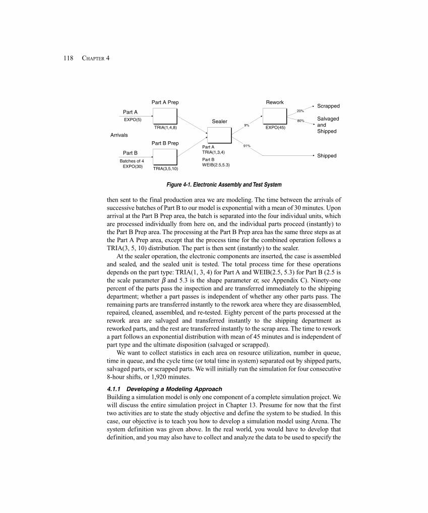
118 CHAPTER 4
Part A Prep
Part B Prep
Rework
Sealer9%
91%
Part A
Part B
Batches of 4
Arrivals
EXPO(5)
TRIA(1,4,8)
TRIA(3,5,10)
Part ATRIA(1,3,4)
EXPO(30)
Part BWEIB(2.5,5.3)
EXPO(45)
20%
80%
Shipped
SalvagedandShipped
Scrapped
Figure 4-1. Electronic Assembly and Test System
then sent to the final production area we are modeling. The time between the arrivals ofsuccessive batches of Part B to our model is exponential with a mean of 30 minutes. Uponarrival at the Part B Prep area, the batch is separated into the four individual units, whichare processed individually from here on, and the individual parts proceed (instantly) tothe Part B Prep area. The processing at the Part B Prep area has the same three steps as atthe Part A Prep area, except that the process time for the combined operation follows aTRIA(3, 5, 10) distribution. The part is then sent (instantly) to the sealer.
At the sealer operation, the electronic components are inserted, the case is assembledand sealed, and the sealed unit is tested. The total process time for these operationsdepends on the part type: TRIA(1, 3, 4) for Part A and WEIB(2.5, 5.3) for Part B (2.5 isthe scale parameter β and 5.3 is the shape parameter α; see Appendix C). Ninety-onepercent of the parts pass the inspection and are transferred immediately to the shippingdepartment; whether a part passes is independent of whether any other parts pass. Theremaining parts are transferred instantly to the rework area where they are disassembled,repaired, cleaned, assembled, and re-tested. Eighty percent of the parts processed at therework area are salvaged and transferred instantly to the shipping department asreworked parts, and the rest are transferred instantly to the scrap area. The time to reworka part follows an exponential distribution with mean of 45 minutes and is independent ofpart type and the ultimate disposition (salvaged or scrapped).
We want to collect statistics in each area on resource utilization, number in queue,time in queue, and the cycle time (or total time in system) separated out by shipped parts,salvaged parts, or scrapped parts. We will initially run the simulation for four consecutive8-hour shifts, or 1,920 minutes.
4.1.1 Developing a Modeling ApproachBuilding a simulation model is only one component of a complete simulation project. Wewill discuss the entire simulation project in Chapter 13. Presume for now that the firsttwo activities are to state the study objective and define the system to be studied. In thiscase, our objective is to teach you how to develop a simulation model using Arena. Thesystem definition was given above. In the real world, you would have to develop thatdefinition, and you may also have to collect and analyze the data to be used to specify the

119MODELING BASIC OPERATIONS AND INPUTS
input parameters and distributions (see Section 4.5). We recommend that the nextactivity be the development of a modeling approach. For a real problem, this may requirethe definition of a data structure, the segmentation of the system into submodels, or thedevelopment of control logic. For this problem, it requires only that we decide whichArena modules will provide the capabilities we need in order to capture the operation ofthe system at an appropriate level of detail. In addition, we must decide how we’re goingto model the different processing times at the sealer operation. To simplify this task, let’sseparate the model into the following components: part arrival, prep areas, sealeroperation, rework, part departure, and part animation. Also, we’ll assume that all entitiesin the system represent individual parts that are being processed.
Because we have two distinct streams of arriving entities to our model, each with itsown timing pattern, we will use two separate Create modules (one for each part type) togenerate the arriving parts.
We also have different processing times by part type at the sealer operation, so we’lluse two Assign modules to define an attribute called Sealer Time that will beassigned the appropriate sealer processing time after the parts are generated by theCreate modules. When the parts are processed at the sealer operation, we’ll use the timecontained in the Sealer Time attribute for the processing time there, rather thangenerating it on the spot as we did in the models in Chapter 3.
Each of the two prep areas and the sealer operation will be modeled with its ownProcess module, very much like the Process module used in the models in Chapter 3. Aninspection is performed after the sealer operation has been completed, which results inparts going to different places based on a “coin flip” (with just the right bias in the coin).We’ll use a Decide module with the pass or fail result being based on the coin flip. Therework area will be modeled with Process and Decide modules, as it also has a pass orfail option. The part departures will be modeled with three separate Record and Disposemodules (shipped, salvaged, and scrapped) so we can keep corresponding cycle-timestatistics sorted out by shipped vs. salvaged vs. scrapped. All of these modules can befound on the Basic Process panel.
4.1.2 Building the ModelTo build the model, you need to open a new model window and place the requiredmodules on the screen: two Create, two Assign, four Process, two Decide, three Record,and three Dispose modules.
Your model window should now look something like Figure 4-2, assuming you’vemade the Connections or used the Auto-Connect feature (Object menu) while placing themodules in the appropriate sequence (the numbers inside your module shapes might bedifferent if you placed your modules in a different order, but that doesn’t matter sincethey’re all “blanks” at this point). You might want to use the File > Save function now tosave your model under a name of your choosing.
Now let’s open each module and enter the information required to complete themodel. Start with the Create 1 module that will create the arriving Part A entities.Display 4-1 (the “Display” device was described in Section 3.4.4) provides theinformation required to complete this module. Note that this is very similar to the Create
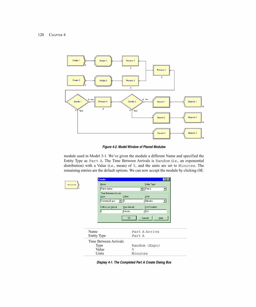
120 CHAPTER 4
Figure 4-2. Model Window of Placed Modules
module used in Model 3-1. We’ve given the module a different Name and specified theEntity Type as Part A. The Time Between Arrivals is Random (i.e., an exponentialdistribution) with a Value (i.e., mean) of 5, and the units are set to Minutes. Theremaining entries are the default options. We can now accept the module by clicking OK.
Name Part A ArriveEntity Type Part ATime Between Arrivals
Type Random (Expo)Value 5Units Minutes
Display 4-1. The Completed Part A Create Dialog Box
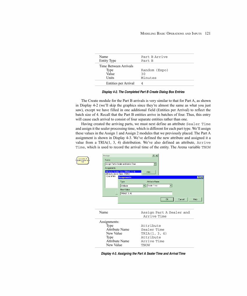
121MODELING BASIC OPERATIONS AND INPUTS
Name Part B ArriveEntity Type Part BTime Between Arrivals
Type Random (Expo)Value 30Units Minutes
Entities per Arrival 4
Display 4-2. The Completed Part B Create Dialog Box Entries
The Create module for the Part B arrivals is very similar to that for Part A, as shownin Display 4-2 (we’ll skip the graphics since they’re almost the same as what you justsaw), except we have filled in one additional field (Entities per Arrival) to reflect thebatch size of 4. Recall that the Part B entities arrive in batches of four. Thus, this entrywill cause each arrival to consist of four separate entities rather than one.
Having created the arriving parts, we must next define an attribute Sealer Timeand assign it the sealer processing time, which is different for each part type. We’ll assignthese values in the Assign 1 and Assign 2 modules that we previously placed. The Part Aassignment is shown in Display 4-3. We’ve defined the new attribute and assigned it avalue from a TRIA(1, 3, 4) distribution. We’ve also defined an attribute, ArriveTime, which is used to record the arrival time of the entity. The Arena variable TNOW
Name Assign Part A Sealer and Arrive Time
Assignments:Type AttributeAttribute Name Sealer TimeNew Value TRIA(1, 3, 4)Type AttributeAttribute Name Arrive TimeNew Value TNOW
Display 4-3. Assigning the Part A Sealer Time and Arrival Time
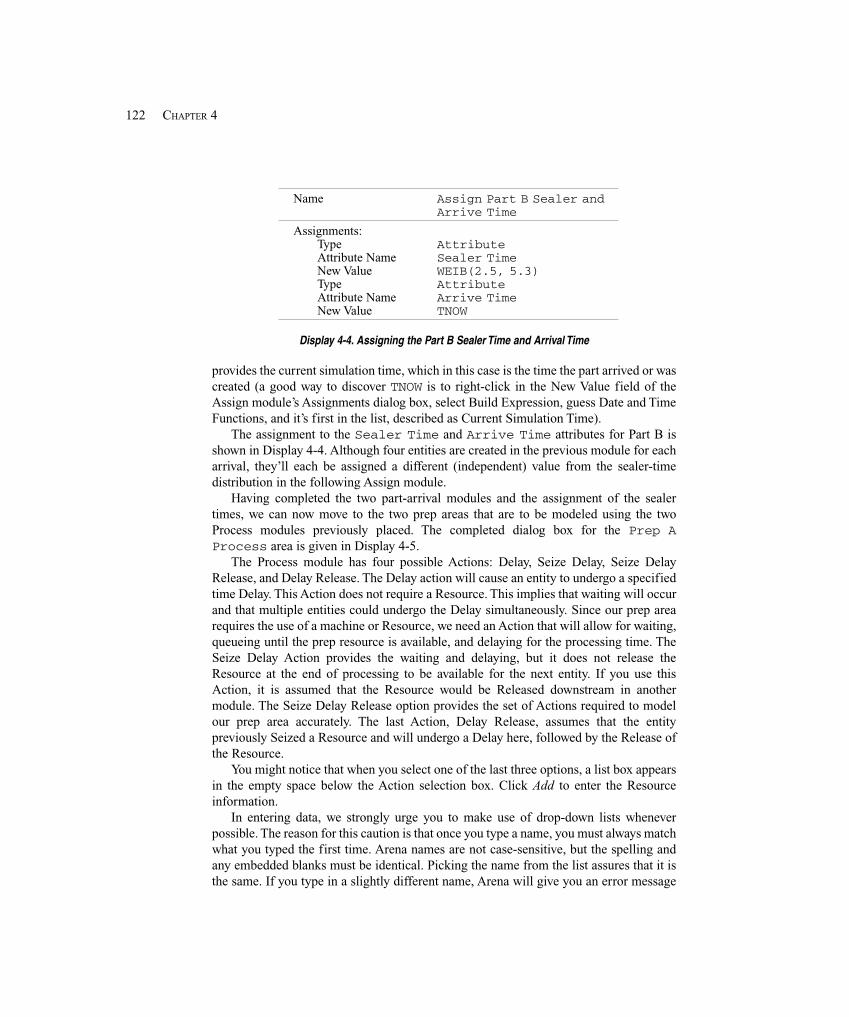
122 CHAPTER 4
Name Assign Part B Sealer andArrive Time
Assignments:Type AttributeAttribute Name Sealer TimeNew Value WEIB(2.5, 5.3)Type AttributeAttribute Name Arrive TimeNew Value TNOW
Display 4-4. Assigning the Part B Sealer Time and Arrival Time
provides the current simulation time, which in this case is the time the part arrived or wascreated (a good way to discover TNOW is to right-click in the New Value field of theAssign module’s Assignments dialog box, select Build Expression, guess Date and TimeFunctions, and it’s first in the list, described as Current Simulation Time).
The assignment to the Sealer Time and Arrive Time attributes for Part B isshown in Display 4-4. Although four entities are created in the previous module for eacharrival, they’ll each be assigned a different (independent) value from the sealer-timedistribution in the following Assign module.
Having completed the two part-arrival modules and the assignment of the sealertimes, we can now move to the two prep areas that are to be modeled using the twoProcess modules previously placed. The completed dialog box for the Prep AProcess area is given in Display 4-5.
The Process module has four possible Actions: Delay, Seize Delay, Seize DelayRelease, and Delay Release. The Delay action will cause an entity to undergo a specifiedtime Delay. This Action does not require a Resource. This implies that waiting will occurand that multiple entities could undergo the Delay simultaneously. Since our prep arearequires the use of a machine or Resource, we need an Action that will allow for waiting,queueing until the prep resource is available, and delaying for the processing time. TheSeize Delay Action provides the waiting and delaying, but it does not release theResource at the end of processing to be available for the next entity. If you use thisAction, it is assumed that the Resource would be Released downstream in anothermodule. The Seize Delay Release option provides the set of Actions required to modelour prep area accurately. The last Action, Delay Release, assumes that the entitypreviously Seized a Resource and will undergo a Delay here, followed by the Release ofthe Resource.
You might notice that when you select one of the last three options, a list box appearsin the empty space below the Action selection box. Click Add to enter the Resourceinformation.
In entering data, we strongly urge you to make use of drop-down lists wheneverpossible. The reason for this caution is that once you type a name, you must always matchwhat you typed the first time. Arena names are not case-sensitive, but the spelling andany embedded blanks must be identical. Picking the name from the list assures that it isthe same. If you type in a slightly different name, Arena will give you an error message
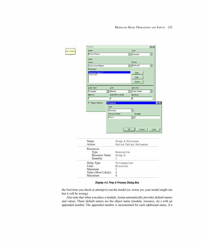
123MODELING BASIC OPERATIONS AND INPUTS
Name Prep A ProcessAction Seize Delay ReleaseResources
Type ResourceResource Name Prep AQuantity 1
Delay Type TriangularUnits MinutesMinimum 1Value (Most Likely) 4Maximum 8
Display 4-5. Prep A Process Dialog Box
the first time you check or attempt to run the model (or, worse yet, your model might runbut it will be wrong).
Also note that when you place a module, Arena automatically provides default namesand values. These default names are the object name (module, resource, etc.) with anappended number. The appended number is incremented for each additional name, if a
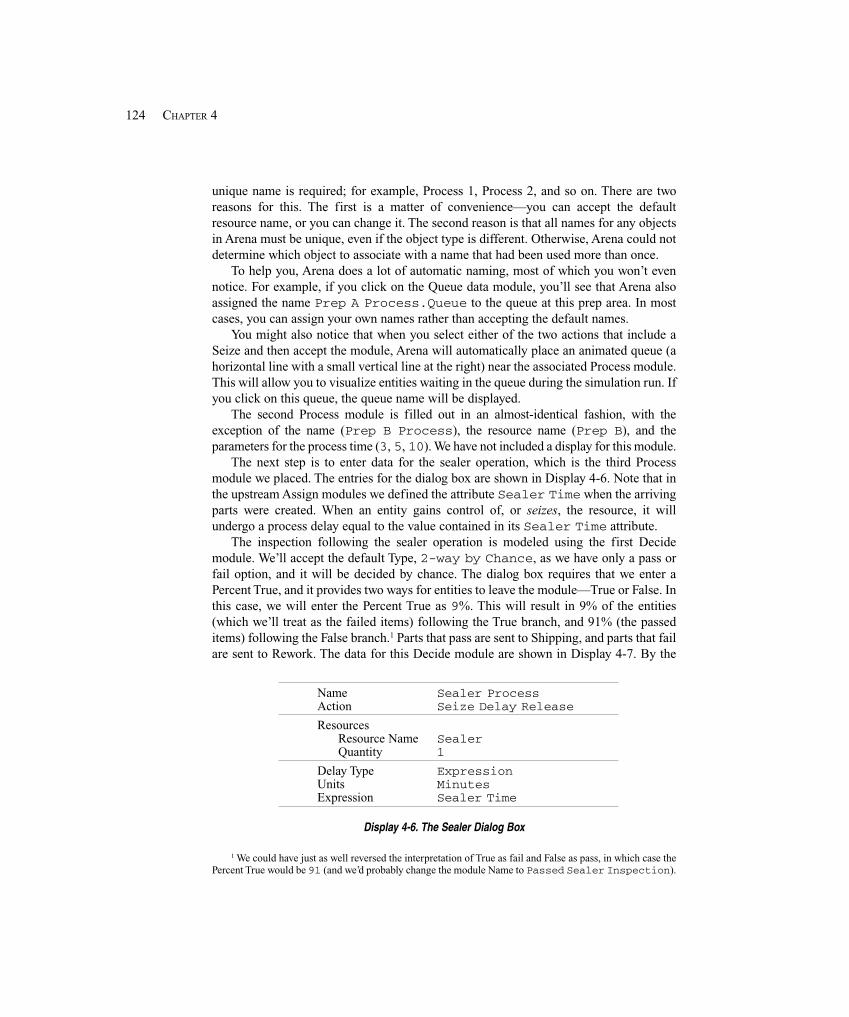
124 CHAPTER 4
unique name is required; for example, Process 1, Process 2, and so on. There are tworeasons for this. The first is a matter of convenience—you can accept the defaultresource name, or you can change it. The second reason is that all names for any objectsin Arena must be unique, even if the object type is different. Otherwise, Arena could notdetermine which object to associate with a name that had been used more than once.
To help you, Arena does a lot of automatic naming, most of which you won’t evennotice. For example, if you click on the Queue data module, you’ll see that Arena alsoassigned the name Prep A Process.Queue to the queue at this prep area. In mostcases, you can assign your own names rather than accepting the default names.
You might also notice that when you select either of the two actions that include aSeize and then accept the module, Arena will automatically place an animated queue (ahorizontal line with a small vertical line at the right) near the associated Process module.This will allow you to visualize entities waiting in the queue during the simulation run. Ifyou click on this queue, the queue name will be displayed.
The second Process module is filled out in an almost-identical fashion, with theexception of the name (Prep B Process), the resource name (Prep B), and theparameters for the process time (3, 5, 10). We have not included a display for this module.
The next step is to enter data for the sealer operation, which is the third Processmodule we placed. The entries for the dialog box are shown in Display 4-6. Note that inthe upstream Assign modules we defined the attribute Sealer Time when the arrivingparts were created. When an entity gains control of, or seizes, the resource, it willundergo a process delay equal to the value contained in its Sealer Time attribute.
The inspection following the sealer operation is modeled using the first Decidemodule. We’ll accept the default Type, 2-way by Chance, as we have only a pass orfail option, and it will be decided by chance. The dialog box requires that we enter aPercent True, and it provides two ways for entities to leave the module—True or False. Inthis case, we will enter the Percent True as 9%. This will result in 9% of the entities(which we’ll treat as the failed items) following the True branch, and 91% (the passeditems) following the False branch.1 Parts that pass are sent to Shipping, and parts that failare sent to Rework. The data for this Decide module are shown in Display 4-7. By the
Name Sealer ProcessAction Seize Delay ReleaseResources
Resource Name SealerQuantity 1
Delay Type ExpressionUnits MinutesExpression Sealer Time
Display 4-6. The Sealer Dialog Box
1 We could have just as well reversed the interpretation of True as fail and False as pass, in which case thePercent True would be 91 (and we’d probably change the module Name to Passed Sealer Inspection).
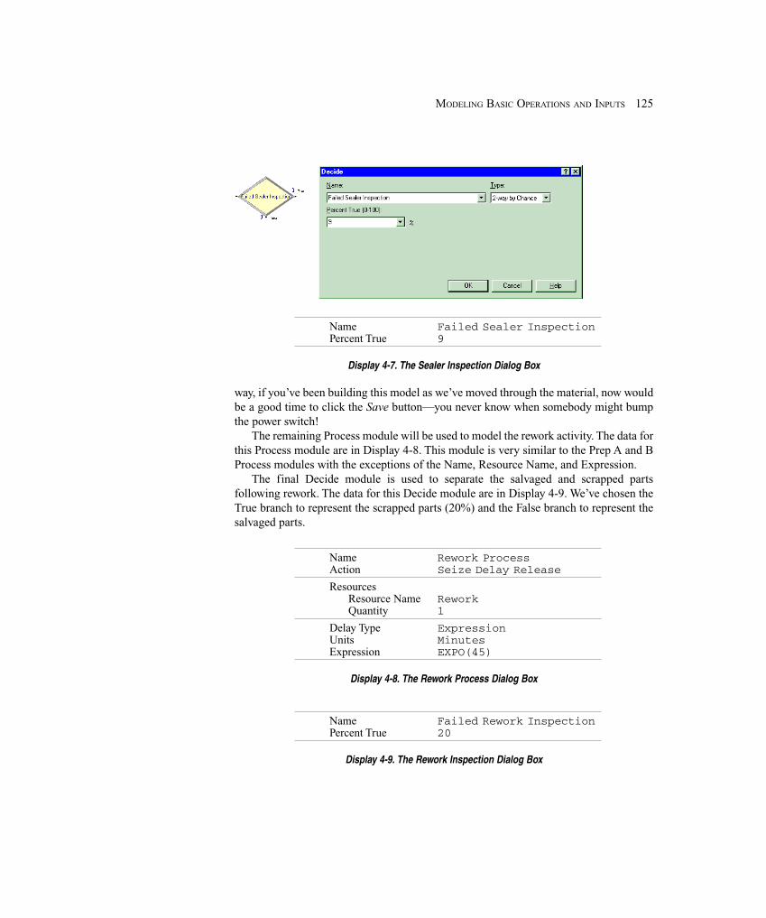
125MODELING BASIC OPERATIONS AND INPUTS
Name Failed Sealer InspectionPercent True 9
Display 4-7. The Sealer Inspection Dialog Box
way, if you’ve been building this model as we’ve moved through the material, now wouldbe a good time to click the Save button—you never know when somebody might bumpthe power switch!
The remaining Process module will be used to model the rework activity. The data forthis Process module are in Display 4-8. This module is very similar to the Prep A and BProcess modules with the exceptions of the Name, Resource Name, and Expression.
The final Decide module is used to separate the salvaged and scrapped partsfollowing rework. The data for this Decide module are in Display 4-9. We’ve chosen theTrue branch to represent the scrapped parts (20%) and the False branch to represent thesalvaged parts.
Name Rework ProcessAction Seize Delay ReleaseResources
Resource Name ReworkQuantity 1
Delay Type ExpressionUnits MinutesExpression EXPO(45)
Display 4-8. The Rework Process Dialog Box
Name Failed Rework InspectionPercent True 20
Display 4-9. The Rework Inspection Dialog Box
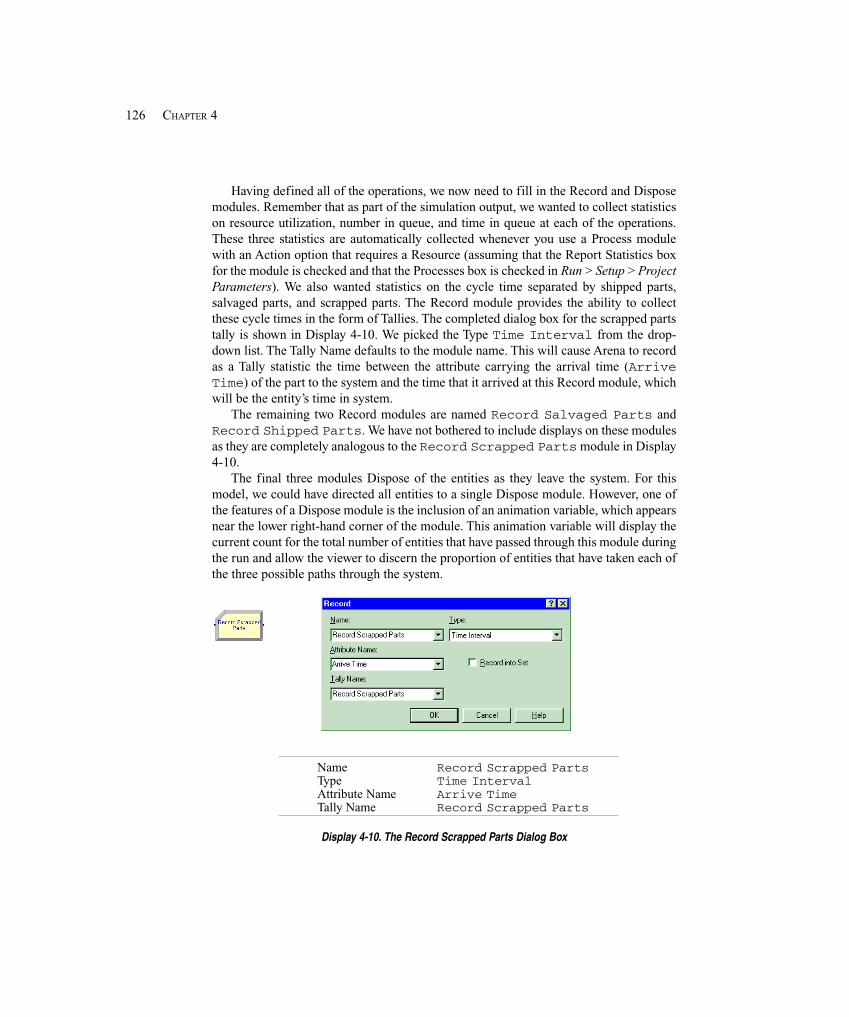
126 CHAPTER 4
Having defined all of the operations, we now need to fill in the Record and Disposemodules. Remember that as part of the simulation output, we wanted to collect statisticson resource utilization, number in queue, and time in queue at each of the operations.These three statistics are automatically collected whenever you use a Process modulewith an Action option that requires a Resource (assuming that the Report Statistics boxfor the module is checked and that the Processes box is checked in Run > Setup > ProjectParameters). We also wanted statistics on the cycle time separated by shipped parts,salvaged parts, and scrapped parts. The Record module provides the ability to collectthese cycle times in the form of Tallies. The completed dialog box for the scrapped partstally is shown in Display 4-10. We picked the Type Time Interval from the drop-down list. The Tally Name defaults to the module name. This will cause Arena to recordas a Tally statistic the time between the attribute carrying the arrival time (ArriveTime) of the part to the system and the time that it arrived at this Record module, whichwill be the entity’s time in system.
The remaining two Record modules are named Record Salvaged Parts andRecord Shipped Parts. We have not bothered to include displays on these modulesas they are completely analogous to the Record Scrapped Parts module in Display4-10.
The final three modules Dispose of the entities as they leave the system. For thismodel, we could have directed all entities to a single Dispose module. However, one ofthe features of a Dispose module is the inclusion of an animation variable, which appearsnear the lower right-hand corner of the module. This animation variable will display thecurrent count for the total number of entities that have passed through this module duringthe run and allow the viewer to discern the proportion of entities that have taken each ofthe three possible paths through the system.
Name Record Scrapped PartsType Time IntervalAttribute Name Arrive TimeTally Name Record Scrapped Parts
Display 4-10. The Record Scrapped Parts Dialog Box
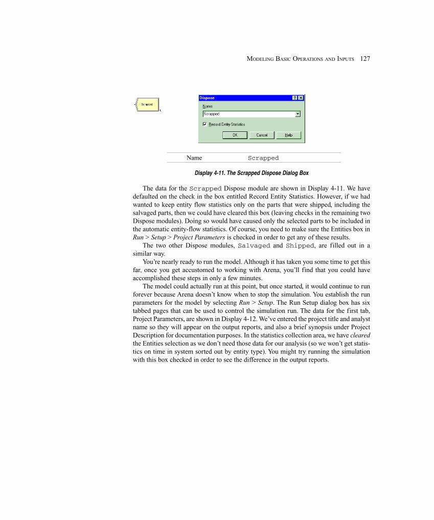
127MODELING BASIC OPERATIONS AND INPUTS
Name Scrapped
Display 4-11. The Scrapped Dispose Dialog Box
The data for the Scrapped Dispose module are shown in Display 4-11. We havedefaulted on the check in the box entitled Record Entity Statistics. However, if we hadwanted to keep entity flow statistics only on the parts that were shipped, including thesalvaged parts, then we could have cleared this box (leaving checks in the remaining twoDispose modules). Doing so would have caused only the selected parts to be included inthe automatic entity-flow statistics. Of course, you need to make sure the Entities box inRun > Setup > Project Parameters is checked in order to get any of these results.
The two other Dispose modules, Salvaged and Shipped, are filled out in asimilar way.
You’re nearly ready to run the model. Although it has taken you some time to get thisfar, once you get accustomed to working with Arena, you’ll find that you could haveaccomplished these steps in only a few minutes.
The model could actually run at this point, but once started, it would continue to runforever because Arena doesn’t know when to stop the simulation. You establish the runparameters for the model by selecting Run > Setup. The Run Setup dialog box has sixtabbed pages that can be used to control the simulation run. The data for the first tab,Project Parameters, are shown in Display 4-12. We’ve entered the project title and analystname so they will appear on the output reports, and also a brief synopsis under ProjectDescription for documentation purposes. In the statistics collection area, we have clearedthe Entities selection as we don’t need those data for our analysis (so we won’t get statis-tics on time in system sorted out by entity type). You might try running the simulationwith this box checked in order to see the difference in the output reports.
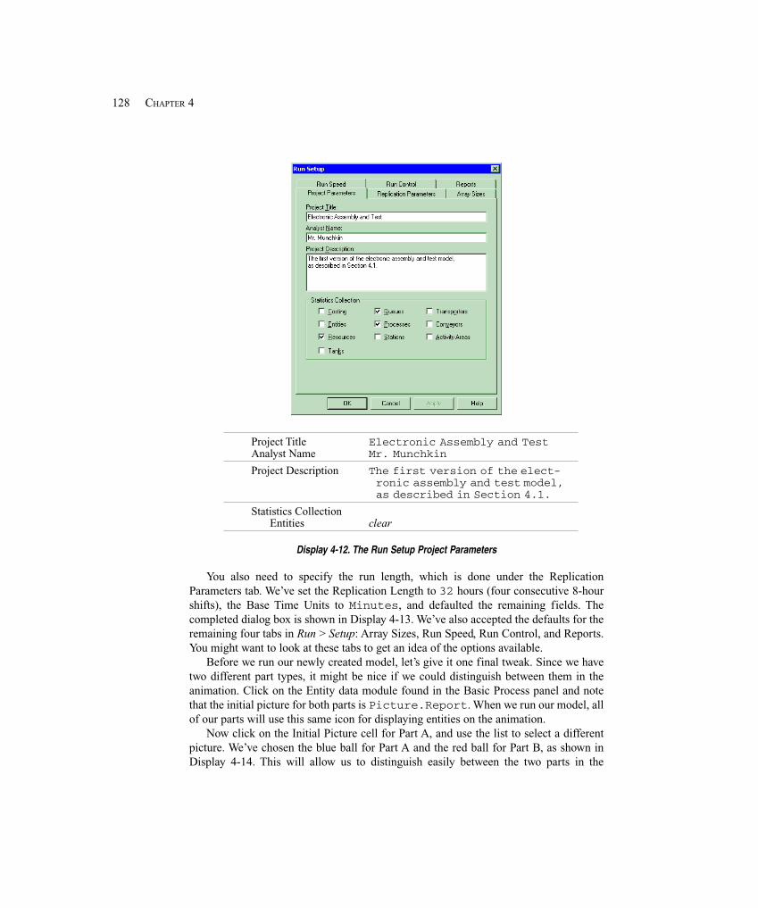
128 CHAPTER 4
Project Title Electronic Assembly and TestAnalyst Name Mr. MunchkinProject Description The first version of the elect-
ronic assembly and test model, as described in Section 4.1.
Statistics CollectionEntities clear
Display 4-12. The Run Setup Project Parameters
You also need to specify the run length, which is done under the ReplicationParameters tab. We’ve set the Replication Length to 32 hours (four consecutive 8-hourshifts), the Base Time Units to Minutes, and defaulted the remaining fields. Thecompleted dialog box is shown in Display 4-13. We’ve also accepted the defaults for theremaining four tabs in Run > Setup: Array Sizes, Run Speed, Run Control, and Reports.You might want to look at these tabs to get an idea of the options available.
Before we run our newly created model, let’s give it one final tweak. Since we havetwo different part types, it might be nice if we could distinguish between them in theanimation. Click on the Entity data module found in the Basic Process panel and notethat the initial picture for both parts is Picture.Report. When we run our model, allof our parts will use this same icon for displaying entities on the animation.
Now click on the Initial Picture cell for Part A, and use the list to select a differentpicture. We’ve chosen the blue ball for Part A and the red ball for Part B, as shown inDisplay 4-14. This will allow us to distinguish easily between the two parts in the
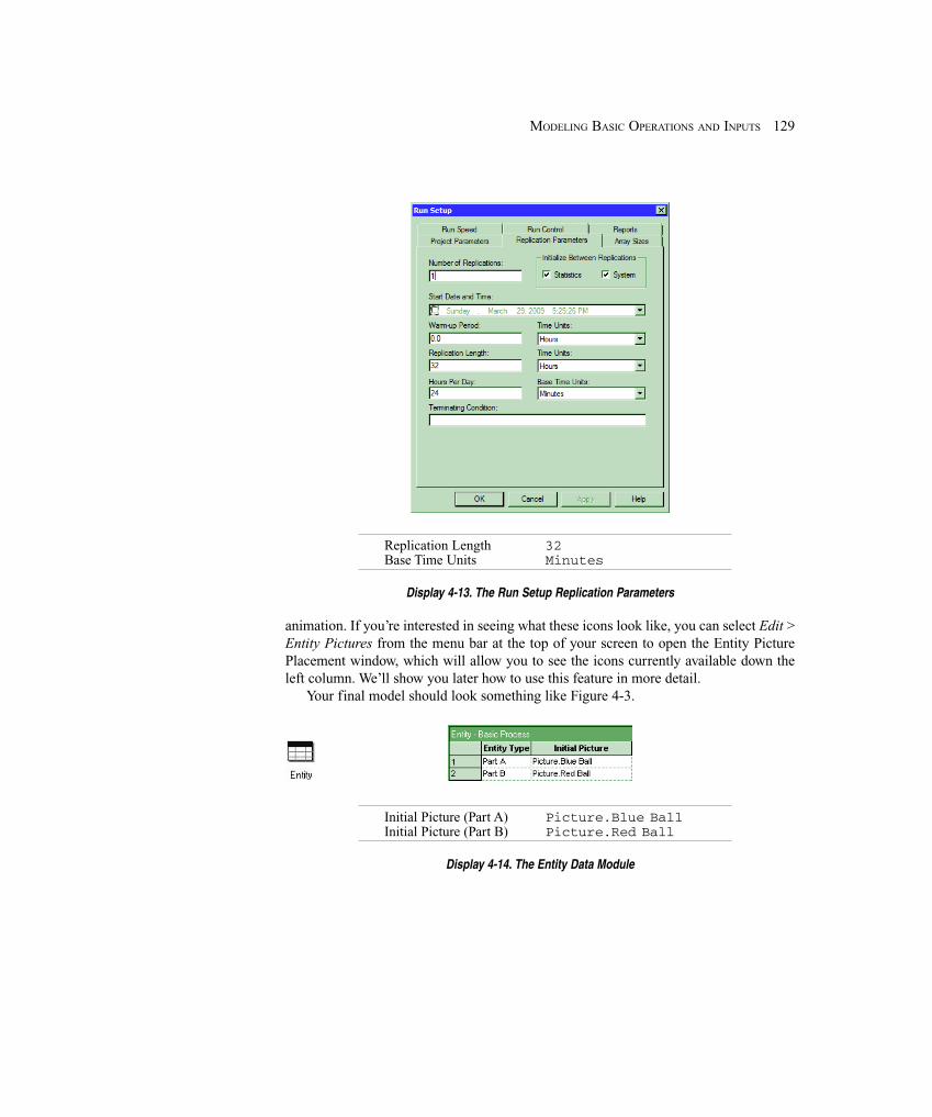
129MODELING BASIC OPERATIONS AND INPUTS
Replication Length 32Base Time Units Minutes
Display 4-13. The Run Setup Replication Parameters
animation. If you’re interested in seeing what these icons look like, you can select Edit >Entity Pictures from the menu bar at the top of your screen to open the Entity PicturePlacement window, which will allow you to see the icons currently available down theleft column. We’ll show you later how to use this feature in more detail.
Your final model should look something like Figure 4-3.
Initial Picture (Part A) Picture.Blue BallInitial Picture (Part B) Picture.Red Ball
Display 4-14. The Entity Data Module
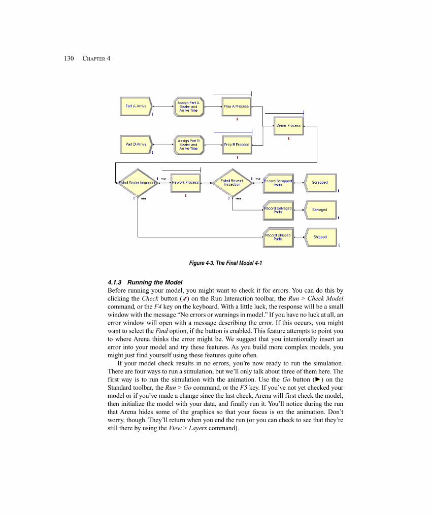
130 CHAPTER 4
Figure 4-3. The Final Model 4-1
4.1.3 Running the ModelBefore running your model, you might want to check it for errors. You can do this byclicking the Check button ( ) on the Run Interaction toolbar, the Run > Check Modelcommand, or the F4 key on the keyboard. With a little luck, the response will be a smallwindow with the message “No errors or warnings in model.” If you have no luck at all, anerror window will open with a message describing the error. If this occurs, you mightwant to select the Find option, if the button is enabled. This feature attempts to point youto where Arena thinks the error might be. We suggest that you intentionally insert anerror into your model and try these features. As you build more complex models, youmight just find yourself using these features quite often.
If your model check results in no errors, you’re now ready to run the simulation.There are four ways to run a simulation, but we’ll only talk about three of them here. Thefirst way is to run the simulation with the animation. Use the Go button ( ) on theStandard toolbar, the Run > Go command, or the F5 key. If you’ve not yet checked yourmodel or if you’ve made a change since the last check, Arena will first check the model,then initialize the model with your data, and finally run it. You’ll notice during the runthat Arena hides some of the graphics so that your focus is on the animation. Don’tworry, though. They’ll return when you end the run (or you can check to see that they’restill there by using the View > Layers command).
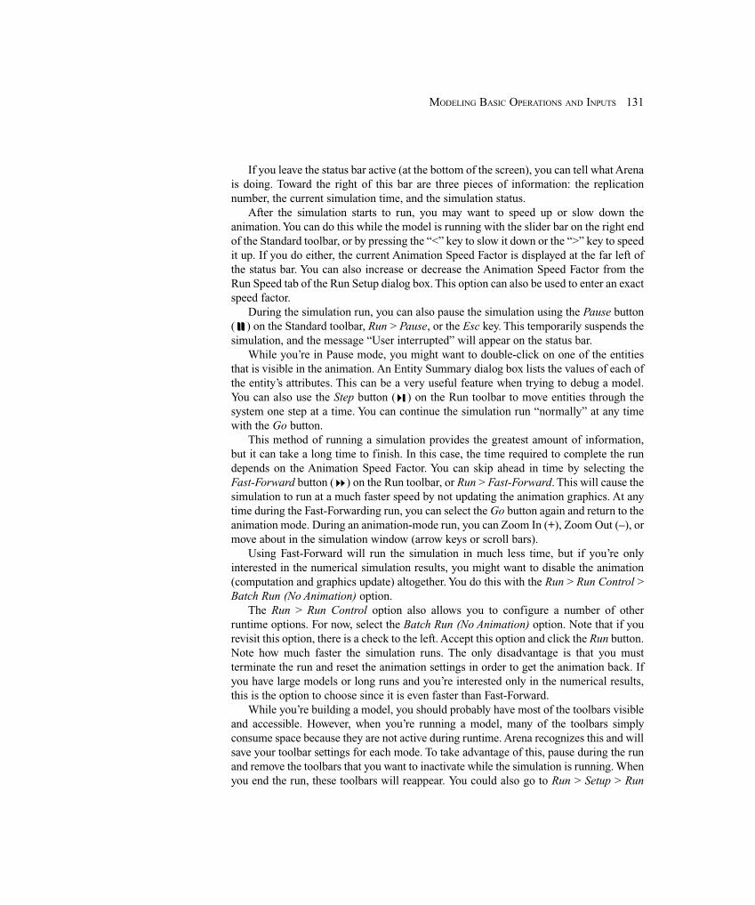
131MODELING BASIC OPERATIONS AND INPUTS
If you leave the status bar active (at the bottom of the screen), you can tell what Arenais doing. Toward the right of this bar are three pieces of information: the replicationnumber, the current simulation time, and the simulation status.
After the simulation starts to run, you may want to speed up or slow down theanimation. You can do this while the model is running with the slider bar on the right endof the Standard toolbar, or by pressing the “<” key to slow it down or the “>” key to speedit up. If you do either, the current Animation Speed Factor is displayed at the far left ofthe status bar. You can also increase or decrease the Animation Speed Factor from theRun Speed tab of the Run Setup dialog box. This option can also be used to enter an exactspeed factor.
During the simulation run, you can also pause the simulation using the Pause button( ) on the Standard toolbar, Run > Pause, or the Esc key. This temporarily suspends thesimulation, and the message “User interrupted” will appear on the status bar.
While you’re in Pause mode, you might want to double-click on one of the entitiesthat is visible in the animation. An Entity Summary dialog box lists the values of each ofthe entity’s attributes. This can be a very useful feature when trying to debug a model.You can also use the Step button ( ) on the Run toolbar to move entities through thesystem one step at a time. You can continue the simulation run “normally” at any timewith the Go button.
This method of running a simulation provides the greatest amount of information,but it can take a long time to finish. In this case, the time required to complete the rundepends on the Animation Speed Factor. You can skip ahead in time by selecting theFast-Forward button ( ) on the Run toolbar, or Run > Fast-Forward. This will cause thesimulation to run at a much faster speed by not updating the animation graphics. At anytime during the Fast-Forwarding run, you can select the Go button again and return to theanimation mode. During an animation-mode run, you can Zoom In (+), Zoom Out (–), ormove about in the simulation window (arrow keys or scroll bars).
Using Fast-Forward will run the simulation in much less time, but if you’re onlyinterested in the numerical simulation results, you might want to disable the animation(computation and graphics update) altogether. You do this with the Run > Run Control >Batch Run (No Animation) option.
The Run > Run Control option also allows you to configure a number of otherruntime options. For now, select the Batch Run (No Animation) option. Note that if yourevisit this option, there is a check to the left. Accept this option and click the Run button.Note how much faster the simulation runs. The only disadvantage is that you mustterminate the run and reset the animation settings in order to get the animation back. Ifyou have large models or long runs and you’re interested only in the numerical results,this is the option to choose since it is even faster than Fast-Forward.
While you’re building a model, you should probably have most of the toolbars visibleand accessible. However, when you’re running a model, many of the toolbars simplyconsume space because they are not active during runtime. Arena recognizes this and willsave your toolbar settings for each mode. To take advantage of this, pause during the runand remove the toolbars that you want to inactivate while the simulation is running. Whenyou end the run, these toolbars will reappear. You could also go to Run > Setup > Run
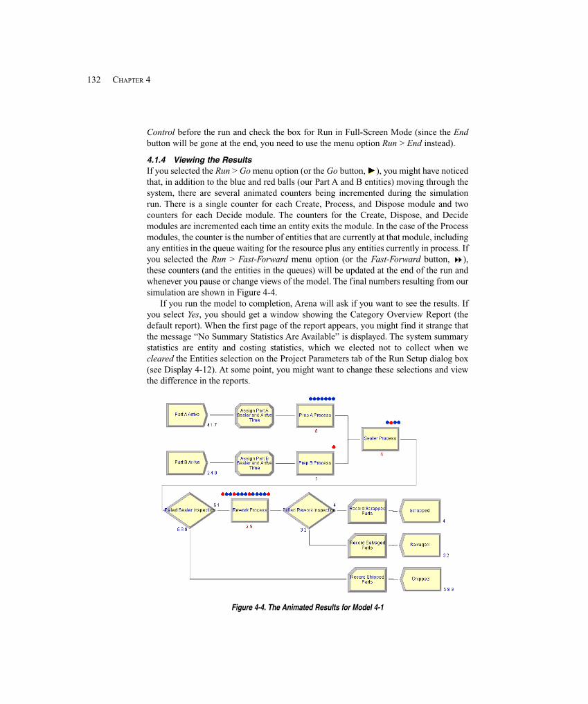
132 CHAPTER 4
Control before the run and check the box for Run in Full-Screen Mode (since the Endbutton will be gone at the end, you need to use the menu option Run > End instead).
4.1.4 Viewing the ResultsIf you selected the Run > Go menu option (or the Go button, ), you might have noticedthat, in addition to the blue and red balls (our Part A and B entities) moving through thesystem, there are several animated counters being incremented during the simulationrun. There is a single counter for each Create, Process, and Dispose module and twocounters for each Decide module. The counters for the Create, Dispose, and Decidemodules are incremented each time an entity exits the module. In the case of the Processmodules, the counter is the number of entities that are currently at that module, includingany entities in the queue waiting for the resource plus any entities currently in process. Ifyou selected the Run > Fast-Forward menu option (or the Fast-Forward button, ),these counters (and the entities in the queues) will be updated at the end of the run andwhenever you pause or change views of the model. The final numbers resulting from oursimulation are shown in Figure 4-4.
If you run the model to completion, Arena will ask if you want to see the results. Ifyou select Yes, you should get a window showing the Category Overview Report (thedefault report). When the first page of the report appears, you might find it strange thatthe message “No Summary Statistics Are Available” is displayed. The system summarystatistics are entity and costing statistics, which we elected not to collect when wecleared the Entities selection on the Project Parameters tab of the Run Setup dialog box(see Display 4-12). At some point, you might want to change these selections and viewthe difference in the reports.
Figure 4-4. The Animated Results for Model 4-1
133MODELING BASIC OPERATIONS AND INPUTS
Recall that you can navigate through the report using the tree listing under thePreview tab at the left side of the report window or by using the arrow buttons in theupper-left corner of the report window. This report will provide statistics by thecategories selected in the Run Setup dialog box (Project Parameters tab, StatisticsCollection area). For our model, you will find sections on Process, Queue, Resource, andUser Specified. The User Specified section is there because we included Recordmodules in our model to collect statistics on the cycle times sorted by departure type.
As in Chapter 3, you will find three types of statistics in our report: tally, time-persistent, and counter. A fourth statistic (outputs) is available when multiple replica-tions are made (we’ll talk about them in Chapter 6, when we do multiple replications).The tally statistics here include several process times, queue times, and the interval timescollected by our Record modules. The time-persistent statistics include number waitingin queue, resource usage, and resource utilization. Counters include accumulated time,number in, number out, and total number seized.
The tally and time-persistent statistics provide the average, 95% confidence-intervalhalf width, and the minimum and maximum observed values. With the exception of thehalf-width column, these entries are as described in Chapters 2 and 3, and should be selfexplanatory.
At the end of a single-replication simulation run, Arena attempts to calculate a 95%confidence-interval half width for the steady-state (long-run) expected value of eachobserved statistic, using a method called batch means (see Section 7.2.3). Arena firstchecks to see if sufficient data have been collected to test the critical statisticalassumption (uncorrelated batches) required for the batch-means method. If not, theannotation “Insufficient” appears in the report and no confidence-interval half width isproduced, as can be seen for several of the results. If there are enough data to test foruncorrelated batches, but the test is failed, the annotation “Correlated” appears and onceagain there’s no half width, which is the case for several of the results. If there wasenough data to perform the test for uncorrelated batches and the test were passed, thehalf width (the “plus-or-minus” amount) of a 95% confidence interval on the long-run(steady-state) expected value of the statistic would be given (this happens for a few of theresults in this run). In this way, Arena refuses to report unreliable half-width values eventhough it could do so from a purely computational viewpoint. The details and importanceof these tests are further discussed in Section 7.2.3.
Trying to draw conclusions from this single short run could be misleading because wehaven’t yet addressed issues like run length, number of replications, or even whether long-run steady-state results are appropriate (but we will, in Section 7.2). However, if you lookat the results for the waiting time in queue and number waiting in queue (Figure 4-5), yousee that the rework station is plagued by waiting times and queue lengths that are muchlonger than for the other stations (you can corroborate this imbalance in congestion bylooking at the Process and Resources sections of the Category Overview report as well).This implies either that the rework area doesn’t have enough capacity to handle its work,or there is a great deal of variability at this station. We’ll address this issue in a minute inSection 4.2. (By the way, note that in some places in the Category Overview Report, youget a color-coded graphic for some of the results.)
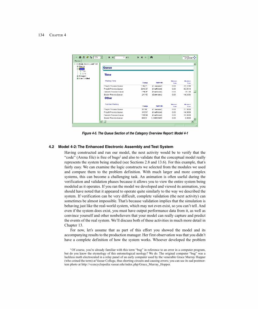
134 CHAPTER 4
Figure 4-5. The Queue Section of the Category Overview Report: Model 4-1
4.2 Model 4-2: The Enhanced Electronic Assembly and Test SystemHaving constructed and run our model, the next activity would be to verify that the“code” (Arena file) is free of bugs2 and also to validate that the conceptual model reallyrepresents the system being studied (see Sections 2.8 and 13.6). For this example, that’sfairly easy. We can examine the logic constructs we selected from the modules we usedand compare them to the problem definition. With much larger and more complexsystems, this can become a challenging task. An animation is often useful during theverification and validation phases because it allows you to view the entire system beingmodeled as it operates. If you ran the model we developed and viewed its animation, youshould have noted that it appeared to operate quite similarly to the way we described thesystem. If verification can be very difficult, complete validation (the next activity) cansometimes be almost impossible. That’s because validation implies that the simulation isbehaving just like the real-world system, which may not even exist, so you can’t tell. Andeven if the system does exist, you must have output performance data from it, as well asconvince yourself and other nonbelievers that your model can really capture and predictthe events of the real system. We’ll discuss both of these activities in much more detail inChapter 13.
For now, let’s assume that as part of this effort you showed the model and itsaccompanying results to the production manager. Her first observation was that you didn’thave a complete definition of how the system works. Whoever developed the problem
2 Of course, you’re already familiar with this term “bug” in reference to an error in a computer program,but do you know the etymology of this entomological neology? We do. The original computer “bug” was aluckless moth electrocuted in a relay panel of an early computer used by the venerable Grace Murray Hopper(who coined the term) at Vassar College, thus shorting circuits and causing errors; you can see its sad postmor-tem photo at http://vcencyclopedia.vassar.edu/index.php/Grace_Murray_Hopper.
.
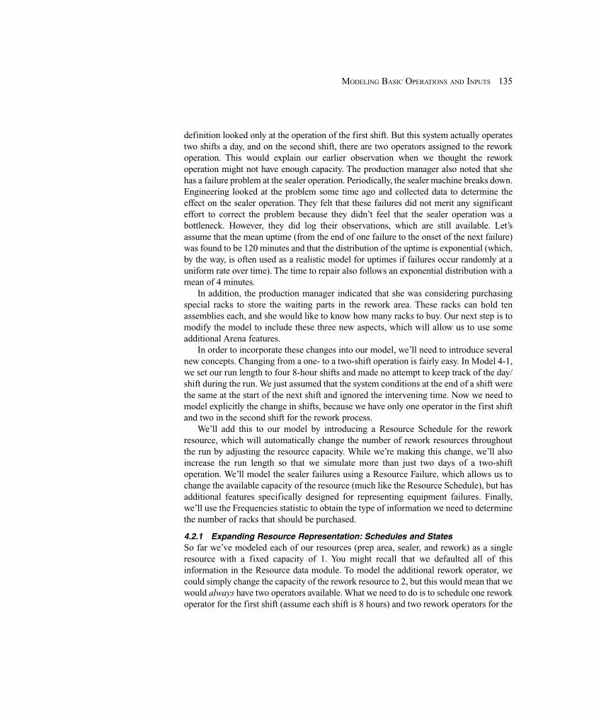
135MODELING BASIC OPERATIONS AND INPUTS
definition looked only at the operation of the first shift. But this system actually operatestwo shifts a day, and on the second shift, there are two operators assigned to the reworkoperation. This would explain our earlier observation when we thought the reworkoperation might not have enough capacity. The production manager also noted that shehas a failure problem at the sealer operation. Periodically, the sealer machine breaks down.Engineering looked at the problem some time ago and collected data to determine theeffect on the sealer operation. They felt that these failures did not merit any significanteffort to correct the problem because they didn’t feel that the sealer operation was abottleneck. However, they did log their observations, which are still available. Let’sassume that the mean uptime (from the end of one failure to the onset of the next failure)was found to be 120 minutes and that the distribution of the uptime is exponential (which,by the way, is often used as a realistic model for uptimes if failures occur randomly at auniform rate over time). The time to repair also follows an exponential distribution with amean of 4 minutes.
In addition, the production manager indicated that she was considering purchasingspecial racks to store the waiting parts in the rework area. These racks can hold tenassemblies each, and she would like to know how many racks to buy. Our next step is tomodify the model to include these three new aspects, which will allow us to use someadditional Arena features.
In order to incorporate these changes into our model, we’ll need to introduce severalnew concepts. Changing from a one- to a two-shift operation is fairly easy. In Model 4-1,we set our run length to four 8-hour shifts and made no attempt to keep track of the day/shift during the run. We just assumed that the system conditions at the end of a shift werethe same at the start of the next shift and ignored the intervening time. Now we need tomodel explicitly the change in shifts, because we have only one operator in the first shiftand two in the second shift for the rework process.
We’ll add this to our model by introducing a Resource Schedule for the reworkresource, which will automatically change the number of rework resources throughoutthe run by adjusting the resource capacity. While we’re making this change, we’ll alsoincrease the run length so that we simulate more than just two days of a two-shiftoperation. We’ll model the sealer failures using a Resource Failure, which allows us tochange the available capacity of the resource (much like the Resource Schedule), but hasadditional features specifically designed for representing equipment failures. Finally,we’ll use the Frequencies statistic to obtain the type of information we need to determinethe number of racks that should be purchased.
4.2.1 Expanding Resource Representation: Schedules and StatesSo far we’ve modeled each of our resources (prep area, sealer, and rework) as a singleresource with a fixed capacity of 1. You might recall that we defaulted all of thisinformation in the Resource data module. To model the additional rework operator, wecould simply change the capacity of the rework resource to 2, but this would mean that wewould always have two operators available. What we need to do is to schedule one reworkoperator for the first shift (assume each shift is 8 hours) and two rework operators for the

136 CHAPTER 4
second shift. Arena has a built-in construct to model this, called a Schedule, that allowsyou to vary the capacity of a resource over time according to a fixed pattern. A resourceSchedule is defined by a sequence of time-dependent resource capacity changes.
We also need to capture in our model the periodic random breakdowns (or failures)of the sealer machine. This could be modeled using a Schedule, which would define anavailable resource capacity of 1 for the uptimes and a capacity of 0 for the time to repair.However, there is a built-in construct designed specifically to model failures. First, let’sintroduce the concept of Resource States.
Arena automatically has four Resource States: Idle, Busy, Inactive, and Failed. Forstatistical reporting, Arena keeps track of the time the resource was in each of the fourstates. The resource is said to be Idle if no entity has seized it. As soon as an entity seizesthe resource, the state is changed to Busy. The state will be changed to Inactive if Arena hasmade the resource unavailable for allocation; this could be accomplished with a Schedule’schanging the capacity to 0. The state will be changed to Failed if Arena has placed theresource in the Failed state, which also implies that it’s unavailable for allocation.
When a failure occurs, Arena causes the entire resource to become unavailable. If thecapacity is 2, for example, both units of the resource will be placed in the Failed stateduring the repair time.
4.2.2 Resource SchedulesBefore we add our resource schedule for the rework operation, let’s first define our new16-hour day. We do this in the Replication Parameters tab of the Run > Setup option, bychanging the Hours Per Day from 24 to 16 (ignore the warning about Calendars that youmight get here). While we’re in this dialog box, let’s also change our Time Units for theReplication Length to Days and the Replication Length itself to 10 days.
You can start the definition of a resource schedule in either the Resource or Scheduledata module. We’ll start with the Resource data module. When you click on this modulefrom the Basic Process panel, the information on the current resources in the model willbe displayed in the spreadsheet view of the model window along the bottom of yourscreen. Now click in the Type column for the Rework resource row and select Based onSchedule from the list. When you select this option, Arena will add two new columnsto the spreadsheet view—Schedule Name and Schedule Rule. Note that the Capacity cellfor the Rework resource has been dimmed because the capacity will instead be based ona schedule. In addition, the cells for two new columns are also dimmed for the other threeresources because they still have a fixed capacity. Next you should enter the schedulename (e.g., Rework Schedule) in the Schedule Name cell for the Rework resource.
Finally, you need to select the Schedule Rule, which can affect the specific timing ofwhen the capacity defined by the schedule will actually change. There are three optionsfor the Schedule Rule: Wait (the default), Ignore, and Preempt. If a capacity decrease ofx units is scheduled to occur and at least x units of the resource are idle, all three optionsimmediately cause x units of the resource unit(s) to become Inactive. But if fewer than xunits of the resource are idle, each Schedule Rule responds differently: (The threeoptions are illustrated in Figure 4-6.)
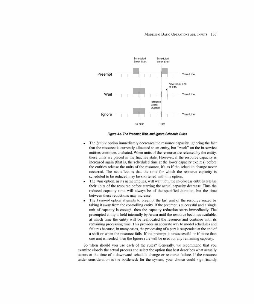
137MODELING BASIC OPERATIONS AND INPUTS
Time LinePreempt
ScheduledBreak Start
ScheduledBreak End
Time LineWait
New Break Endat 1:15
Time LineIgnore
ReducedBreakDuration
12 noon 1 pm
Figure 4-6. The Preempt, Wait, and Ignore Schedule Rules
� The Ignore option immediately decreases the resource capacity, ignoring the factthat the resource is currently allocated to an entity, but “work” on the in-serviceentities continues unabated. When units of the resource are released by the entity,these units are placed in the Inactive state. However, if the resource capacity isincreased again (that is, the scheduled time at the lower capacity expires) beforethe entities release the units of the resource, it’s as if the schedule change neveroccurred. The net effect is that the time for which the resource capacity isscheduled to be reduced may be shortened with this option.
� The Wait option, as its name implies, will wait until the in-process entities releasetheir units of the resource before starting the actual capacity decrease. Thus thereduced capacity time will always be of the specified duration, but the timebetween these reductions may increase.
� The Preempt option attempts to preempt the last unit of the resource seized bytaking it away from the controlling entity. If the preempt is successful and a singleunit of capacity is enough, then the capacity reduction starts immediately. Thepreempted entity is held internally by Arena until the resource becomes available,at which time the entity will be reallocated the resource and continue with itsremaining processing time. This provides an accurate way to model schedules andfailures because, in many cases, the processing of a part is suspended at the end ofa shift or when the resource fails. If the preempt is unsuccessful or if more thanone unit is needed, then the Ignore rule will be used for any remaining capacity.
So when should you use each of the rules? Generally, we recommend that youexamine closely the actual process and select the option that best describes what actuallyoccurs at the time of a downward schedule change or resource failure. If the resourceunder consideration is the bottleneck for the system, your choice could significantly

138 CHAPTER 4
Rework ResourceType Based on ScheduleSchedule Name Rework ScheduleSchedule Rule Ignore
Display 4-15. The Resource Data Module: Selecting a Resource Schedule
affect the results obtained. But sometimes it isn’t clear what to do, and, while there are nostrict guidelines, a few rules of thumb may be of help. First, if the duration of thescheduled decrease in capacity is very large compared to the processing time, the Ignoreoption may be an adequate representation. If the time between capacity decreases is largecompared to the duration of the decrease, the Wait option could be considered. For thismodel, we’ve selected the Ignore option because, in most cases, an operator will finishhis task before leaving and that additional work time is seldom considered.
The final spreadsheet view of the first four columns is shown in Display 4-15 (thereare actually additional columns to the right, which we don’t show here). There is also adialog form for entering these data, which can be opened by right-clicking on the reworkcell in the Name column and selecting Edit via Dialog.
Now that you’ve named the schedule and indicated the schedule rule, you mustdefine the actual schedule the resource should follow. One way to do this is by clickingon the Schedule data module and entering the schedule information in the spreadsheetview. A row has already been added that contains our newly defined Rework Schedule.Clicking in the Durations column will open the Graphical Schedule Editor, a graphicalinterface for entering the schedule data. The horizontal axis is the calendar or simulationtime. (Note that a day is defined as 16 hours based on our day definition in the Run Setupdialog box.) The vertical axis is the capacity of the resource. You enter data by clickingon the x-y location that represents day one, hour one, and a capacity value of one. Thiswill cause a solid blue bar to appear that represents the desired capacity during this hour;in this case, one. You can complete the data entry by repeatedly clicking or by clicking,holding, and then dragging the bar over the first eight hours. Complete the data scheduleby entering a capacity of 2 for hours nine through 16. It’s not necessary to add the datafor Day 2, as the data entered for Day 1 will be repeated automatically for the rest of thesimulation run. The complete schedule is shown in Figure 4-7. You might note that weused the Options button to reduce our maximum vertical axis (capacity) value from tento four; other things can be changed in the Options dialog box, like how long a time slotlasts, the number of time slots, and whether the schedule repeats from the beginning orremains forevermore at a fixed-capacity level.
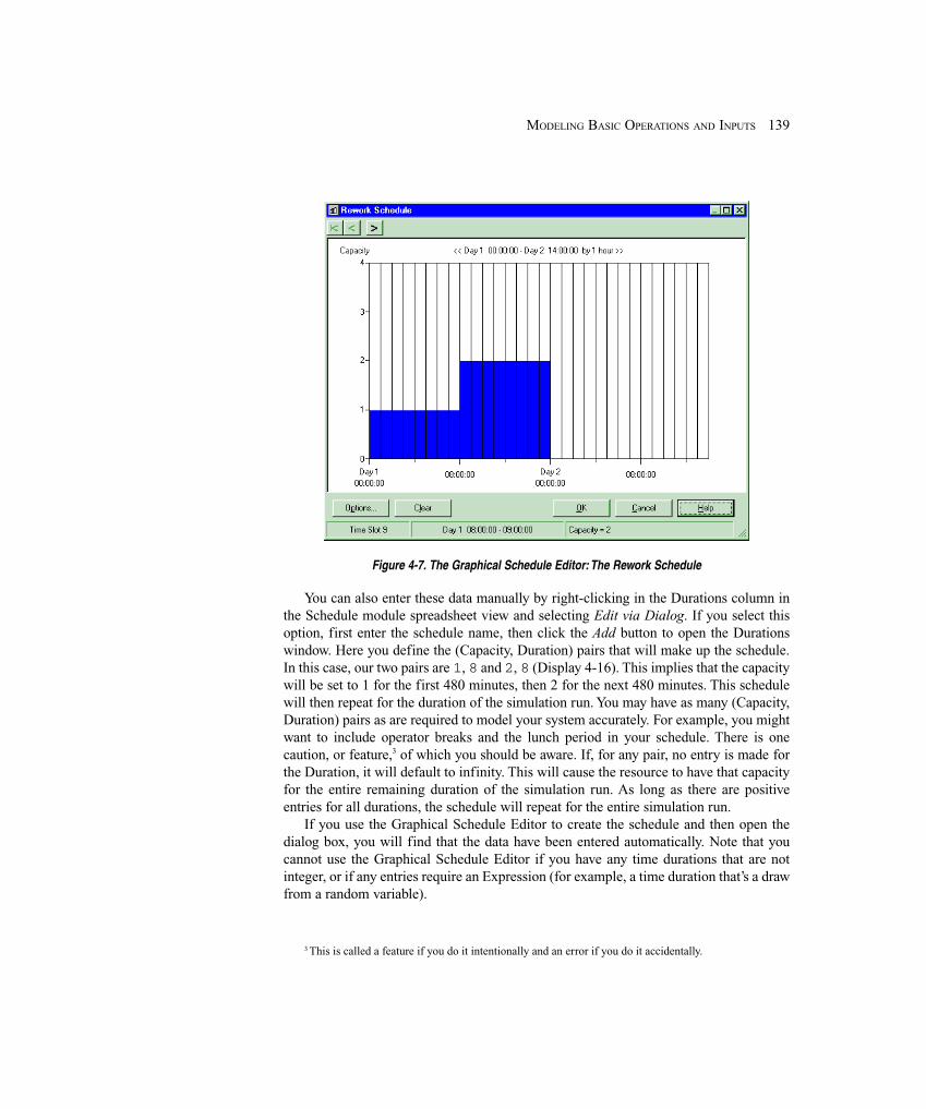
139MODELING BASIC OPERATIONS AND INPUTS
Figure 4-7. The Graphical Schedule Editor: The Rework Schedule
You can also enter these data manually by right-clicking in the Durations column inthe Schedule module spreadsheet view and selecting Edit via Dialog. If you select thisoption, first enter the schedule name, then click the Add button to open the Durationswindow. Here you define the (Capacity, Duration) pairs that will make up the schedule.In this case, our two pairs are 1, 8 and 2, 8 (Display 4-16). This implies that the capacitywill be set to 1 for the first 480 minutes, then 2 for the next 480 minutes. This schedulewill then repeat for the duration of the simulation run. You may have as many (Capacity,Duration) pairs as are required to model your system accurately. For example, you mightwant to include operator breaks and the lunch period in your schedule. There is onecaution, or feature,3 of which you should be aware. If, for any pair, no entry is made forthe Duration, it will default to infinity. This will cause the resource to have that capacityfor the entire remaining duration of the simulation run. As long as there are positiveentries for all durations, the schedule will repeat for the entire simulation run.
If you use the Graphical Schedule Editor to create the schedule and then open thedialog box, you will find that the data have been entered automatically. Note that youcannot use the Graphical Schedule Editor if you have any time durations that are notinteger, or if any entries require an Expression (for example, a time duration that’s a drawfrom a random variable).
3 This is called a feature if you do it intentionally and an error if you do it accidentally.
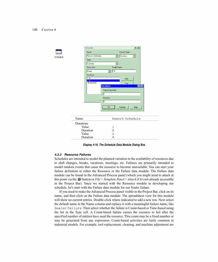
140 CHAPTER 4
Name Rework ScheduleDurations
Value 1Duration 8Value 2Duration 8
Display 4-16. The Schedule Data Module Dialog Box
4.2.3 Resource FailuresSchedules are intended to model the planned variation in the availability of resources dueto shift changes, breaks, vacations, meetings, etc. Failures are primarily intended tomodel random events that cause the resource to become unavailable. You can start yourfailure definition in either the Resource or the Failure data module. The Failure datamodule can be found in the Advanced Process panel (which you might need to attach atthis point via the button or File > Template Panel > Attach if it’s not already accessiblein the Project Bar). Since we started with the Resource module in developing ourschedule, let’s start with the Failure data module for our Sealer failure.
If you need to make the Advanced Process panel visible in the Project Bar, click on itsname, and then click on the Failure data module. The spreadsheet view for this modulewill show no current entries. Double-click where indicated to add a new row. Next selectthe default name in the Name column and replace it with a meaningful failure name, likeSealer Failure. Then select whether the failure is Count-based or Time-based usingthe list in the Type cell. A Count-based failure causes the resource to fail after thespecified number of entities have used the resource. This count may be a fixed number ormay be generated from any expression. Count-based activities are fairly common inindustrial models. For example, tool replacement, cleaning, and machine adjustment are

141MODELING BASIC OPERATIONS AND INPUTS
Name Sealer FailureType TimeUp Time EXPO(120)Up Time Units MinutesDown Time EXPO(4)Down Time Units Minutes
Display 4-17. The Sealer Failure Spreadsheet View
typically based on the number of parts that have been processed rather than on elapsedtime. Although these may not normally be viewed as “failures,” they do occur on aperiodic basis and prevent the resource from producing parts. On the other hand, wefrequently model failures as Time-based because that’s the way we’ve collected thefailure data. In our model, the problem calls for a Time-based failure. So click on theType cell and select the Time option. When you do this, the column further to the rightin the spreadsheet will change to reflect the different data requirements between the twooptions. Our Up Time and Down Time entries are exponential distributions with meansof 120 minutes and 4 minutes, respectively. We also need to change the Up Time Unitsand Down Time Units from Hours to Minutes.
The last field, Uptime in this State only, allows us to define the state of the resourcethat should be considered as “counting” for the uptimes. If this field is defaulted, then allstates are considered. Use of this feature is very dependent on how your data werecollected and the calendar timing of your model. Most failure data are simply loggeddata; for example, only the time of the failure is logged. If this is the case, then holidays,lunch breaks, and idle time are included in the time between failures, and you shoulddefault this field. Only if your time between failures can be linked directly to a specificstate should this option be chosen. Many times equipment vendors will supply failuredata based on actual operating hours; in this case, you would want to select this optionand specify the Busy state. Note that if you select this option you must also define theBusy state using the StateSet data module found in the Advanced Process panel. Thefinal spreadsheet view for our Sealer Failure is shown in Display 4-17.
Having completed the definition of our Sealer Failure, we now need to attach it to theSealer resource. Open the Resource data module (back in the Basic Process panel) andclick in the Failures column for the Sealer resource row. This will open another windowwith the Failures spreadsheet view. Double-click to add a new row and, in the FailureName cell, select Sealer Failure from the list. We must also select the FailureRule—Ignore, Wait, or Preempt. These options are the same as for schedules, and yourespond in an identical manner. Returning to our rules of thumb for choosing the FailureRule option, because our expected uptime (120 minutes) is large compared to our failureduration (4 minutes), we’ll use the Wait option. The final spreadsheet view is shown in
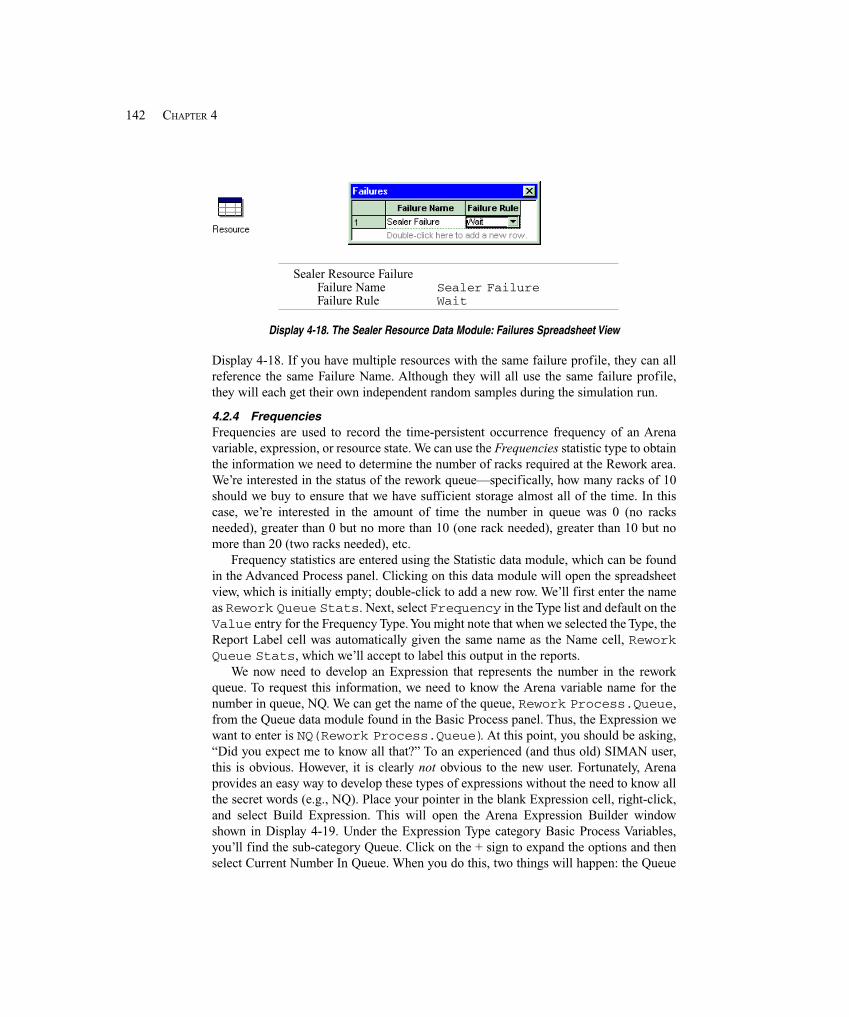
142 CHAPTER 4
Sealer Resource FailureFailure Name Sealer FailureFailure Rule Wait
Display 4-18. The Sealer Resource Data Module: Failures Spreadsheet View
Display 4-18. If you have multiple resources with the same failure profile, they can allreference the same Failure Name. Although they will all use the same failure profile,they will each get their own independent random samples during the simulation run.
4.2.4 FrequenciesFrequencies are used to record the time-persistent occurrence frequency of an Arenavariable, expression, or resource state. We can use the Frequencies statistic type to obtainthe information we need to determine the number of racks required at the Rework area.We’re interested in the status of the rework queue—specifically, how many racks of 10should we buy to ensure that we have sufficient storage almost all of the time. In thiscase, we’re interested in the amount of time the number in queue was 0 (no racksneeded), greater than 0 but no more than 10 (one rack needed), greater than 10 but nomore than 20 (two racks needed), etc.
Frequency statistics are entered using the Statistic data module, which can be foundin the Advanced Process panel. Clicking on this data module will open the spreadsheetview, which is initially empty; double-click to add a new row. We’ll first enter the nameas Rework Queue Stats. Next, select Frequency in the Type list and default on theValue entry for the Frequency Type. You might note that when we selected the Type, theReport Label cell was automatically given the same name as the Name cell, ReworkQueue Stats, which we’ll accept to label this output in the reports.
We now need to develop an Expression that represents the number in the reworkqueue. To request this information, we need to know the Arena variable name for thenumber in queue, NQ. We can get the name of the queue, Rework Process.Queue,from the Queue data module found in the Basic Process panel. Thus, the Expression wewant to enter is NQ(Rework Process.Queue). At this point, you should be asking,“Did you expect me to know all that?” To an experienced (and thus old) SIMAN user,this is obvious. However, it is clearly not obvious to the new user. Fortunately, Arenaprovides an easy way to develop these types of expressions without the need to know allthe secret words (e.g., NQ). Place your pointer in the blank Expression cell, right-click,and select Build Expression. This will open the Arena Expression Builder windowshown in Display 4-19. Under the Expression Type category Basic Process Variables,you’ll find the sub-category Queue. Click on the + sign to expand the options and thenselect Current Number In Queue. When you do this, two things will happen: the Queue
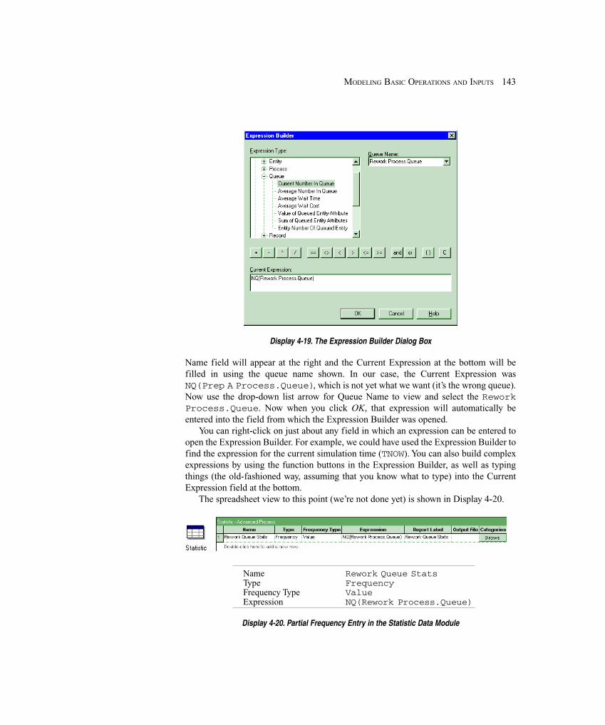
143MODELING BASIC OPERATIONS AND INPUTS
Display 4-19. The Expression Builder Dialog Box
Name field will appear at the right and the Current Expression at the bottom will befilled in using the queue name shown. In our case, the Current Expression wasNQ(Prep A Process.Queue), which is not yet what we want (it’s the wrong queue).Now use the drop-down list arrow for Queue Name to view and select the ReworkProcess.Queue. Now when you click OK, that expression will automatically beentered into the field from which the Expression Builder was opened.
You can right-click on just about any field in which an expression can be entered toopen the Expression Builder. For example, we could have used the Expression Builder tofind the expression for the current simulation time (TNOW). You can also build complexexpressions by using the function buttons in the Expression Builder, as well as typingthings (the old-fashioned way, assuming that you know what to type) into the CurrentExpression field at the bottom.
The spreadsheet view to this point (we’re not done yet) is shown in Display 4-20.
Name Rework Queue StatsType FrequencyFrequency Type ValueExpression NQ(Rework Process.Queue)
Display 4-20. Partial Frequency Entry in the Statistic Data Module
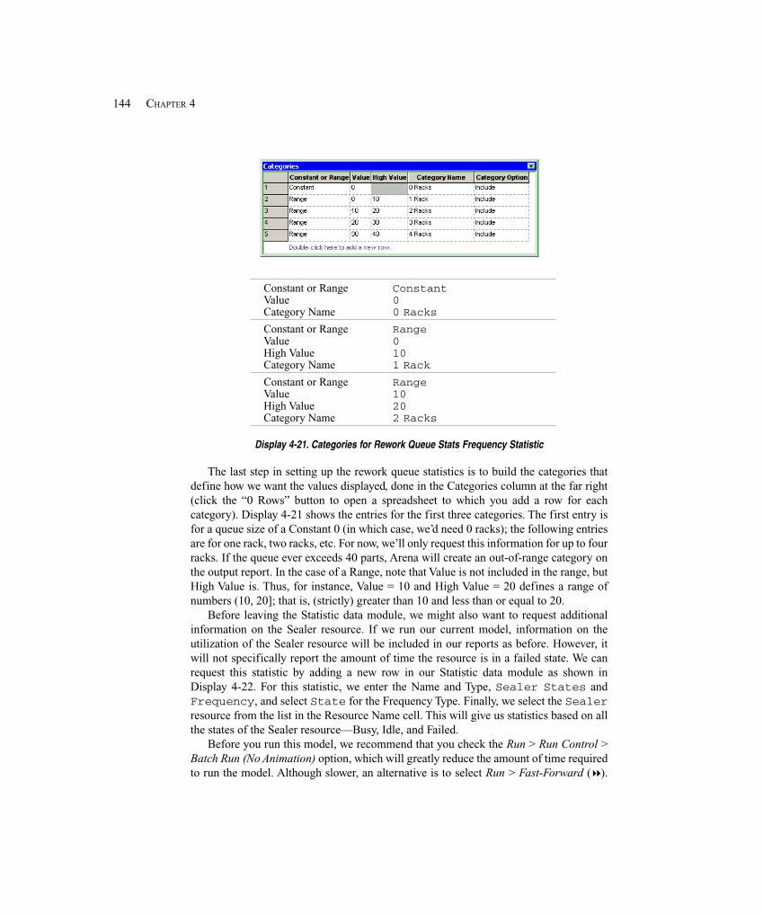
144 CHAPTER 4
Constant or Range ConstantValue 0Category Name 0 RacksConstant or Range RangeValue 0High Value 10Category Name 1 RackConstant or Range RangeValue 10High Value 20Category Name 2 Racks
Display 4-21. Categories for Rework Queue Stats Frequency Statistic
The last step in setting up the rework queue statistics is to build the categories thatdefine how we want the values displayed, done in the Categories column at the far right(click the “0 Rows” button to open a spreadsheet to which you add a row for eachcategory). Display 4-21 shows the entries for the first three categories. The first entry isfor a queue size of a Constant 0 (in which case, we’d need 0 racks); the following entriesare for one rack, two racks, etc. For now, we’ll only request this information for up to fourracks. If the queue ever exceeds 40 parts, Arena will create an out-of-range category onthe output report. In the case of a Range, note that Value is not included in the range, butHigh Value is. Thus, for instance, Value = 10 and High Value = 20 defines a range ofnumbers (10, 20]; that is, (strictly) greater than 10 and less than or equal to 20.
Before leaving the Statistic data module, we might also want to request additionalinformation on the Sealer resource. If we run our current model, information on theutilization of the Sealer resource will be included in our reports as before. However, itwill not specifically report the amount of time the resource is in a failed state. We canrequest this statistic by adding a new row in our Statistic data module as shown inDisplay 4-22. For this statistic, we enter the Name and Type, Sealer States andFrequency, and select State for the Frequency Type. Finally, we select the Sealerresource from the list in the Resource Name cell. This will give us statistics based on allthe states of the Sealer resource—Busy, Idle, and Failed.
Before you run this model, we recommend that you check the Run > Run Control >Batch Run (No Animation) option, which will greatly reduce the amount of time requiredto run the model. Although slower, an alternative is to select Run > Fast-Forward ( ).
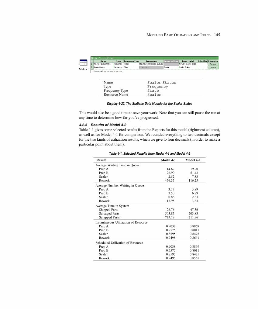
145MODELING BASIC OPERATIONS AND INPUTS
Name Sealer StatesType FrequencyFrequency Type StateResource Name Sealer
Display 4-22. The Statistic Data Module for the Sealer States
This would also be a good time to save your work. Note that you can still pause the run atany time to determine how far you’ve progressed.
4.2.5 Results of Model 4-2Table 4-1 gives some selected results from the Reports for this model (rightmost column),as well as for Model 4-1 for comparison. We rounded everything to two decimals exceptfor the two kinds of utilization results, which we give to four decimals (in order to make aparticular point about them).
Table 4-1. Selected Results from Model 4-1 and Model 4-2
Result Model 4-1 Model 4-2
Average Waiting Time in Queue Prep A 14.62 19.20 Prep B 26.90 51.42 Sealer 2.52 7.83 Rework 456.35 116.25
Average Number Waiting in Queue Prep A 3.17 3.89 Prep B 3.50 6.89 Sealer 0.86 2.63 Rework 12.95 3.63
Average Time in System Shipped Parts 28.76 47.36 Salvaged Parts 503.85 203.83 Scrapped Parts 737.19 211.96
Instantaneous Utilization of Resource Prep A 0.9038 0.8869 Prep B 0.7575 0.8011 Sealer 0.8595 0.8425 Rework 0.9495 0.8641
Scheduled Utilization of Resource Prep A 0.9038 0.8869 Prep B 0.7575 0.8011 Sealer 0.8595 0.8425 Rework 0.9495 0.8567
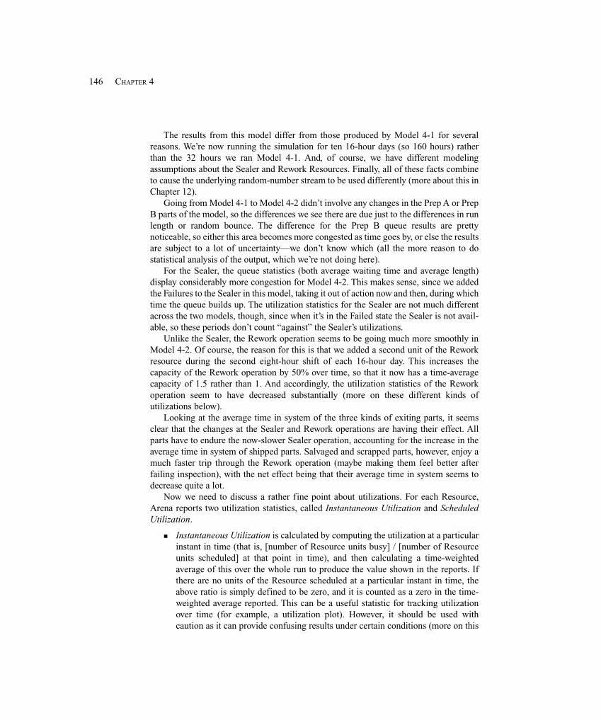
146 CHAPTER 4
The results from this model differ from those produced by Model 4-1 for severalreasons. We’re now running the simulation for ten 16-hour days (so 160 hours) ratherthan the 32 hours we ran Model 4-1. And, of course, we have different modelingassumptions about the Sealer and Rework Resources. Finally, all of these facts combineto cause the underlying random-number stream to be used differently (more about this inChapter 12).
Going from Model 4-1 to Model 4-2 didn’t involve any changes in the Prep A or PrepB parts of the model, so the differences we see there are due just to the differences in runlength or random bounce. The difference for the Prep B queue results are prettynoticeable, so either this area becomes more congested as time goes by, or else the resultsare subject to a lot of uncertainty—we don’t know which (all the more reason to dostatistical analysis of the output, which we’re not doing here).
For the Sealer, the queue statistics (both average waiting time and average length)display considerably more congestion for Model 4-2. This makes sense, since we addedthe Failures to the Sealer in this model, taking it out of action now and then, during whichtime the queue builds up. The utilization statistics for the Sealer are not much differentacross the two models, though, since when it’s in the Failed state the Sealer is not avail-able, so these periods don’t count “against” the Sealer’s utilizations.
Unlike the Sealer, the Rework operation seems to be going much more smoothly inModel 4-2. Of course, the reason for this is that we added a second unit of the Reworkresource during the second eight-hour shift of each 16-hour day. This increases thecapacity of the Rework operation by 50% over time, so that it now has a time-averagecapacity of 1.5 rather than 1. And accordingly, the utilization statistics of the Reworkoperation seem to have decreased substantially (more on these different kinds ofutilizations below).
Looking at the average time in system of the three kinds of exiting parts, it seemsclear that the changes at the Sealer and Rework operations are having their effect. Allparts have to endure the now-slower Sealer operation, accounting for the increase in theaverage time in system of shipped parts. Salvaged and scrapped parts, however, enjoy amuch faster trip through the Rework operation (maybe making them feel better afterfailing inspection), with the net effect being that their average time in system seems todecrease quite a lot.
Now we need to discuss a rather fine point about utilizations. For each Resource,Arena reports two utilization statistics, called Instantaneous Utilization and ScheduledUtilization.
� Instantaneous Utilization is calculated by computing the utilization at a particularinstant in time (that is, [number of Resource units busy] / [number of Resourceunits scheduled] at that point in time), and then calculating a time-weightedaverage of this over the whole run to produce the value shown in the reports. Ifthere are no units of the Resource scheduled at a particular instant in time, theabove ratio is simply defined to be zero, and it is counted as a zero in the time-weighted average reported. This can be a useful statistic for tracking utilizationover time (for example, a utilization plot). However, it should be used withcaution as it can provide confusing results under certain conditions (more on this
147MODELING BASIC OPERATIONS AND INPUTS
shortly). If you like math (and even if you don’t), we can express all this asfollows. Let B(t) be the number of units of the Resource that are busy at time t,and let M(t) be the number of units of that Resource that are scheduled (busy ornot) at time t. Let U(t) = B(t)/M(t) whenever M(t) > 0, and simply define U(t) to be0 if M(t) = 0. If the run is from time 0 to time T, then the reported InstantaneousUtilization is
,)(0∫T
TdttU
which is just the time average of the U(t) function as defined above. It’s importantto note that in reporting this, Arena accounts for time periods when there’s nocapacity scheduled as time periods with a utilization of zero.
� Scheduled Utilization is the time-average number of units of the Resource that arebusy (taken over the whole run), divided by the time-average number of units ofthe Resource that are scheduled (over the whole run). In the above notation, thereported Scheduled Utilization is
.)(
)(
)(
)(
0
0
0
0
∫
∫
∫
∫=
T
T
T
T
dttM
dttB
TdttM
TdttB
There’s no problem with dividing by zero here as long as the Resource was everscheduled at all to have units available (the only situation that makes sense if theResource is even present in the model).
Under different conditions, each of these reported utilizations can provide usefulinformation. If the capacity of a Resource stays constant over the entire simulation run(the Resource is never in an Inactive or Failed state), the two reported utilizations will bethe same (you’re asked to prove this in Exercise 4-19, and you can verify from Table 4-1that this is so in Model 4-2 for the Resources that have fixed capacity). If a Schedule isattached to the Resource and the scheduled capacities are either zero or a single positiveconstant (for example, 1), the reported Instantaneous Utilization tells you how busy theResource was over the entire run (counting zero-capacity periods as zero-utilizationperiods); a plot of U(t) as defined above would tell you how closely your Schedule trackswhat’s being asked of the Resource, so it could be useful to investigate staffing plans.The reported Scheduled Utilization tells you how busy the Resource was over the timethat it was available at all (in other words, capacity was non-zero).
For example, consider the case where a Resource is scheduled to be available 2/3 ofthe time with a capacity of 1, and unavailable the other 1/3 of the time (capacity of 0).Suppose further that during the time the Resource was available, it was busy half thetime. For this example, the reported Instantaneous Utilization would be 0.3333 and thereported Scheduled Utilization would be 0.5000. This tells you that over the entire runthe Resource was utilized 1/3 of the time, but during the time that it was scheduled to beavailable, it was utilized 1/2 the time. In this case, the reported Instantaneous Utilizationis less than or equal to the reported Scheduled Utilization.
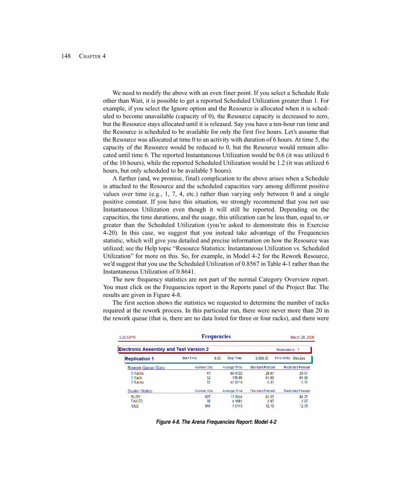
148 CHAPTER 4
We need to modify the above with an even finer point. If you select a Schedule Ruleother than Wait, it is possible to get a reported Scheduled Utilization greater than 1. Forexample, if you select the Ignore option and the Resource is allocated when it is sched-uled to become unavailable (capacity of 0), the Resource capacity is decreased to zero,but the Resource stays allocated until it is released. Say you have a ten-hour run time andthe Resource is scheduled to be available for only the first five hours. Let’s assume thatthe Resource was allocated at time 0 to an activity with duration of 6 hours. At time 5, thecapacity of the Resource would be reduced to 0, but the Resource would remain allo-cated until time 6. The reported Instantaneous Utilization would be 0.6 (it was utilized 6of the 10 hours), while the reported Scheduled Utilization would be 1.2 (it was utilized 6hours, but only scheduled to be available 5 hours).
A further (and, we promise, final) complication to the above arises when a Scheduleis attached to the Resource and the scheduled capacities vary among different positivevalues over time (e.g., 1, 7, 4, etc.) rather than varying only between 0 and a singlepositive constant. If you have this situation, we strongly recommend that you not useInstantaneous Utilization even though it will still be reported. Depending on thecapacities, the time durations, and the usage, this utilization can be less than, equal to, orgreater than the Scheduled Utilization (you’re asked to demonstrate this in Exercise4-20). In this case, we suggest that you instead take advantage of the Frequenciesstatistic, which will give you detailed and precise information on how the Resource wasutilized; see the Help topic “Resource Statistics: Instantaneous Utilization vs. ScheduledUtilization” for more on this. So, for example, in Model 4-2 for the Rework Resource,we’d suggest that you use the Scheduled Utilization of 0.8567 in Table 4-1 rather than theInstantaneous Utilization of 0.8641.
The new frequency statistics are not part of the normal Category Overview report.You must click on the Frequencies report in the Reports panel of the Project Bar. Theresults are given in Figure 4-8.
The first section shows the statistics we requested to determine the number of racksrequired at the rework process. In this particular run, there were never more than 20 inthe rework queue (that is, there are no data listed for three or four racks), and there were
Figure 4-8. The Arena Frequencies Report: Model 4-2
149MODELING BASIC OPERATIONS AND INPUTS
more than ten only 5.35% of the time. This might imply that you could get by with onlyone rack, or at most, two. The Sealer States statistics give the percentage of times theSealer spent in the Busy, Failed, and Idle states.
One last note is worth mentioning about frequency statistics. For our results, the lasttwo columns, Standard and Restricted Percent, have the same values. It is possible toexclude selective data resulting in differences between these columns. For example, ifyou exclude the Failed state for the sealer Frequency, the Standard Percent would remainthe same, but the Restricted Percent column would have values only for Busy and Idle,which would sum to 100%.
4.3 Model 4-3: Enhancing the Animation
So far in this chapter we’ve simply accepted the default animation provided with themodules we used. Although this base animation is often sufficient for determiningwhether your model is working correctly, you might want the animation to look morelike the real system before allowing decision makers to view the model. Making theanimation more realistic is really very easy and seldom requires a lot of time. To a largeextent, the amount of time you decide to invest depends on the level of detail you decideto add and the nature of the audience for your efforts. A general observation is that, forpresentation purposes, the higher you go in an organization, the more time you shouldprobably spend on the animation. You will also find that making the animation beautifulcan be a lot of fun and can even become an obsession. So with that thought in mind, let’sexplore some of what can be done.
We’ll modify Model 4-2 into what we’ll call Model 4-3, and we’ll start by looking atthe existing animation. The current animation has three components: entities, queues,and variables. The entities we selected using the Entity data module can be seen whenthey travel from one module to another or when they’re waiting in a queue. For eachProcess module we placed, Arena automatically added an animation queue, whichdisplays waiting entities during the run. Variables were also placed automatically byArena to represent the number of entities resident in or that have exited a module.
As suggested by how they came to exist in the model—added when you placed themodule—the animation constructs are “attached” to the module in two respects. First,their names, or Identifiers, come from values in the module dialog box; you can’t changethem directly in the animation construct’s dialog box. Second, if you move the module,the animation objects that were automatically supplied move with it; however, if youwant the animation to stay where it is, just hold the Shift key when you move the module.On the second point, if for some reason you replace the animation objects (e.g., queues,counters) that automatically came with the module, they do not move with the module.
Sometimes it’s helpful to “pull apart” the animation to a completely different area inthe model window, away from the logic. If you do so, you might consider setting up someNamed Views (see Section 3.4.13) to facilitate going back and forth. If you want todisconnect an animation construct completely from the module it originallyaccompanied, Cut it to the Clipboard and Paste it back into the model. It will retain all ofits characteristics, but no longer will have any association with the module. An
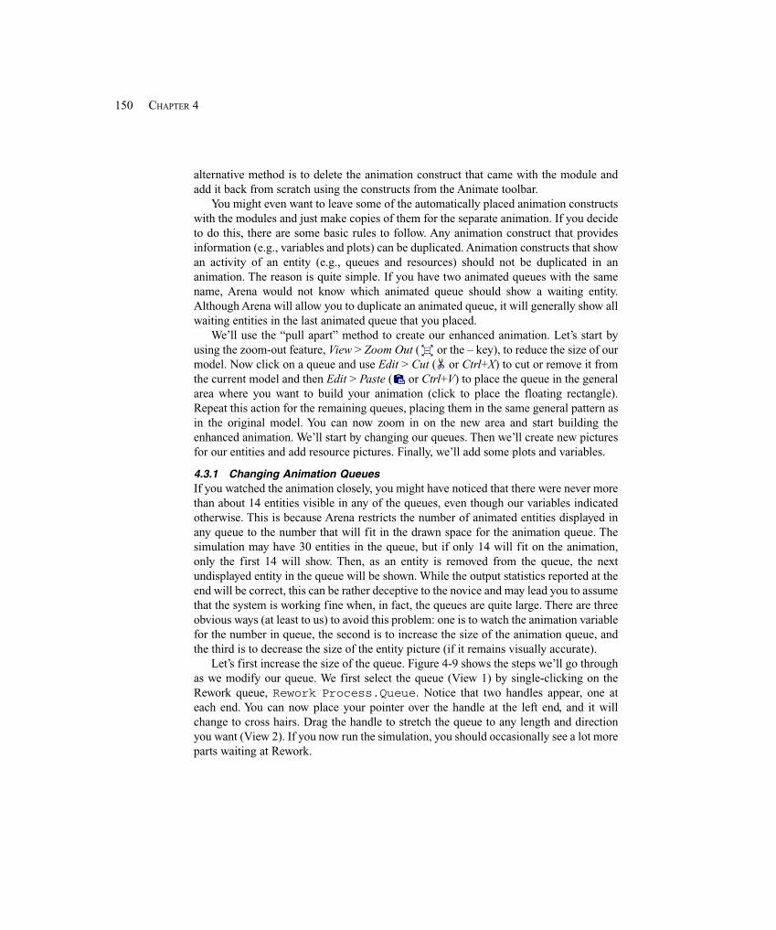
150 CHAPTER 4
alternative method is to delete the animation construct that came with the module andadd it back from scratch using the constructs from the Animate toolbar.
You might even want to leave some of the automatically placed animation constructswith the modules and just make copies of them for the separate animation. If you decideto do this, there are some basic rules to follow. Any animation construct that providesinformation (e.g., variables and plots) can be duplicated. Animation constructs that showan activity of an entity (e.g., queues and resources) should not be duplicated in ananimation. The reason is quite simple. If you have two animated queues with the samename, Arena would not know which animated queue should show a waiting entity.Although Arena will allow you to duplicate an animated queue, it will generally show allwaiting entities in the last animated queue that you placed.
We’ll use the “pull apart” method to create our enhanced animation. Let’s start byusing the zoom-out feature, View > Zoom Out ( or the – key), to reduce the size of ourmodel. Now click on a queue and use Edit > Cut ( or Ctrl+X) to cut or remove it fromthe current model and then Edit > Paste ( or Ctrl+V) to place the queue in the generalarea where you want to build your animation (click to place the floating rectangle).Repeat this action for the remaining queues, placing them in the same general pattern asin the original model. You can now zoom in on the new area and start building theenhanced animation. We’ll start by changing our queues. Then we’ll create new picturesfor our entities and add resource pictures. Finally, we’ll add some plots and variables.
4.3.1 Changing Animation QueuesIf you watched the animation closely, you might have noticed that there were never morethan about 14 entities visible in any of the queues, even though our variables indicatedotherwise. This is because Arena restricts the number of animated entities displayed inany queue to the number that will fit in the drawn space for the animation queue. Thesimulation may have 30 entities in the queue, but if only 14 will fit on the animation,only the first 14 will show. Then, as an entity is removed from the queue, the nextundisplayed entity in the queue will be shown. While the output statistics reported at theend will be correct, this can be rather deceptive to the novice and may lead you to assumethat the system is working fine when, in fact, the queues are quite large. There are threeobvious ways (at least to us) to avoid this problem: one is to watch the animation variablefor the number in queue, the second is to increase the size of the animation queue, andthe third is to decrease the size of the entity picture (if it remains visually accurate).
Let’s first increase the size of the queue. Figure 4-9 shows the steps we’ll go throughas we modify our queue. We first select the queue (View 1) by single-clicking on theRework queue, Rework Process.Queue. Notice that two handles appear, one ateach end. You can now place your pointer over the handle at the left end, and it willchange to cross hairs. Drag the handle to stretch the queue to any length and directionyou want (View 2). If you now run the simulation, you should occasionally see a lot moreparts waiting at Rework.
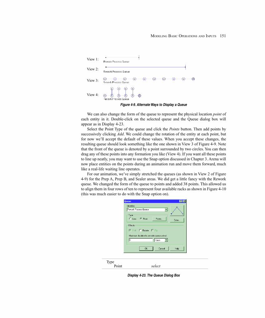
151MODELING BASIC OPERATIONS AND INPUTS
View 1:
View 2:
View 3:
View 4:
Figure 4-9. Alternate Ways to Display a Queue
We can also change the form of the queue to represent the physical location point ofeach entity in it. Double-click on the selected queue and the Queue dialog box willappear as in Display 4-23.
Select the Point Type of the queue and click the Points button. Then add points bysuccessively clicking Add. We could change the rotation of the entity at each point, butfor now we’ll accept the default of these values. When you accept these changes, theresulting queue should look something like the one shown in View 3 of Figure 4-9. Notethat the front of the queue is denoted by a point surrounded by two circles. You can thendrag any of these points into any formation you like (View 4). If you want all these pointsto line up neatly, you may want to use the Snap option discussed in Chapter 3. Arena willnow place entities on the points during an animation run and move them forward, muchlike a real-life waiting line operates.
For our animation, we’ve simply stretched the queues (as shown in View 2 of Figure4-9) for the Prep A, Prep B, and Sealer areas. We did get a little fancy with the Reworkqueue. We changed the form of the queue to points and added 38 points. This allowed usto align them in four rows of ten to represent four available racks as shown in Figure 4-10(this was much easier to do with the Snap option on).
TypePoint select
Display 4-23. The Queue Dialog Box

152 CHAPTER 4
Figure 4-10. The Rework Queue with 40 Points
4.3.2 Changing Entity PicturesNow let’s focus our attention on our animation entities. In our current animation, wearbitrarily selected blue and red balls for the two kinds of entities. Let’s say we want ourentities to be similar to the balls but have the letter “A” or “B” displayed inside the ball.You create new pictures in the Entity Picture Placement window, as shown in Figure4-11, which is opened using Edit > Entity Pictures. The left side of this window containsentity pictures currently available in your model, displayed as a list of buttons withpictures and associated names. The right side of this window is used for accessingpicture libraries, which are simply collections of pictures stored in a file. Arena providesseveral of these libraries with a starting selection of icons; you might want to open andexamine them before you animate your next model (their file names end with .plb).
There are several ways to add a new picture to your animation. You can use the Addbutton (on the left) to draw a new picture for the current list, or you can use the Copybutton (on the left) to copy a picture already on the current list. If you use the Addfunction, your new entry will not have a picture or a name associated with it until youdraw it and give it a name in the Value field above the list. If you use the Copy function,the new picture and name will be the same as the picture selected when you copied.
To add a picture from a library to your current entity picture list, highlight the pictureyou want to replace on the left, highlight the new selection from a library on the right,and click on the left arrow button ( ) to copy the picture to your picture list. You can alsobuild and maintain your own picture libraries by choosing the New button, creating yourown pictures, and saving the file for future use. Or you can use clip art by using thestandard copy and paste commands.
For this example, as for most of our examples, we’ll keep our pictures fairly simple,but you can make your entity and resource pictures as fancy as you want. Since the blueand red balls were about the right size, let’s use them as our starting point. Click on thePicture.Blue Ball icon in the current list on the left and then click Copy. Nowselect one of these two identical pictures and change the name (in the Value dialog box) toPicture.Part A (now wasn’t that obvious?). Note that as you type in the new name itwill also change on the selected icon. To change the picture, double-click on the pictureicon. This opens the Picture Editor window that will allow you to modify the picturedrawing. Before you change this picture, notice the small gray circle in the center of thesquare; this is the entity reference point, which determines the entity’s relation with theother animation objects. Basically, this point will follow the paths when the entity ismoving, will reside on the seize point when the entity has control of a resource, and so on.
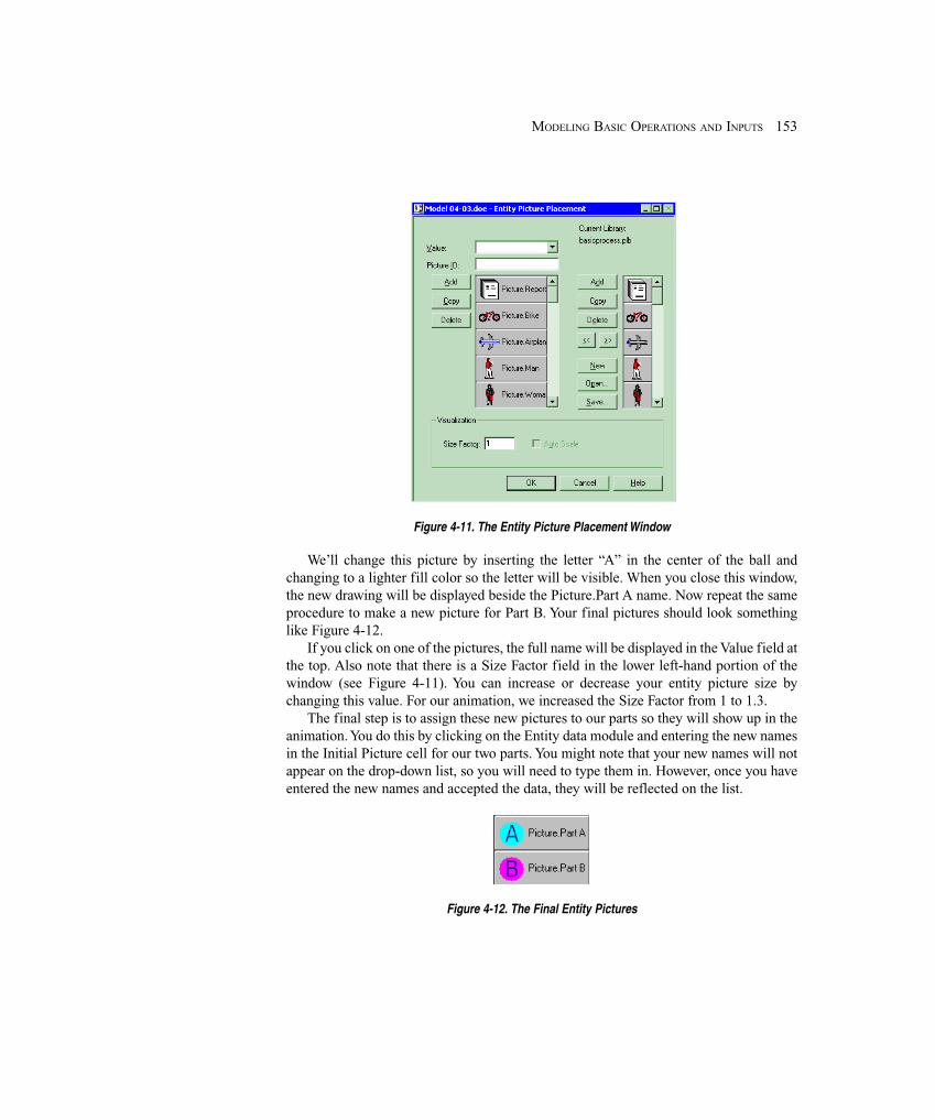
153MODELING BASIC OPERATIONS AND INPUTS
Figure 4-11. The Entity Picture Placement Window
We’ll change this picture by inserting the letter “A” in the center of the ball andchanging to a lighter fill color so the letter will be visible. When you close this window,the new drawing will be displayed beside the Picture.Part A name. Now repeat the sameprocedure to make a new picture for Part B. Your final pictures should look somethinglike Figure 4-12.
If you click on one of the pictures, the full name will be displayed in the Value field atthe top. Also note that there is a Size Factor field in the lower left-hand portion of thewindow (see Figure 4-11). You can increase or decrease your entity picture size bychanging this value. For our animation, we increased the Size Factor from 1 to 1.3.
The final step is to assign these new pictures to our parts so they will show up in theanimation. You do this by clicking on the Entity data module and entering the new namesin the Initial Picture cell for our two parts. You might note that your new names will notappear on the drop-down list, so you will need to type them in. However, once you haveentered the new names and accepted the data, they will be reflected on the list.
Figure 4-12. The Final Entity Pictures

154 CHAPTER 4
4.3.3 Adding Resource PicturesNow that we’ve completed our animated queues and entities, let’s add resource picturesto our animation. You add a resource picture by clicking the Resource button ( ) foundin the Animate toolbar. This will open the Resource Picture Placement window, whichlooks very similar to the Entity Picture Placement window. There’s very little differencebetween an entity picture and a resource picture other than the way we refer to them.Entities acquire pictures by assigning a picture name somewhere in the model.Resources acquire pictures depending on their state. In Section 4.2.1, we discussed thefour automatic resource states (Idle, Busy, Failed, and Inactive). When you open aResource Picture Placement window, you might notice that there is a default picture foreach of the four default states. You can, however, change the drawings used to depict theresource in its various states, just like we changed our entity pictures.
First we need to identify which resource picture we are creating. You do this by usingthe drop-down list in the Identifier box to select one of our resources (e.g., Prep A). Nowlet’s replace these pictures as we did for the entity pictures. Double-click on the Idlepicture to open the Picture Editor window. Use the background color for the fill, makethe line thickness 3 points (from the Draw toolbar), and change the line color. Note thatthe box must be highlighted in order to make these changes. The small circle with thecross is the reference point for the resource, indicating how other objects (like entitypictures) align to its picture; drag this into the middle of your box. Accept this icon (byclosing the Picture Editor window) and return to the Resource Picture Placementwindow. Now let’s develop our own picture library. Choosing the New button from theResource Picture Placement window opens a new, empty library file. Now select yournewly created icon, click Add under the current library area, and then click the rightarrow button. Click the Save button to name and save your new library file (e.g.,Book.plb).
We’ll now use this picture to create the rest of our resource pictures. Highlight theBusy picture on the left and the new library picture on the right and use the left arrowbutton to make your busy picture look just like your idle picture. When the animation isrunning, the entity picture will sit in the center of this box, so we’ll know it’s busy.However, you do need to check the Seize Area toggle at the bottom of the window for thisto happen. Now copy the same library picture to the inactive and failed states. Open eachof these pictures and fill the box with a color that will denote whether the resource is inthe failed or inactive state (e.g., red for failed and gray for inactive). Now copy these twonew pictures to your library and save it. Your final resource pictures should looksomething like those shown in Figure 4-13. We also increased our Size Factor to 1.3 sothe resource size will be consistent with our entity size.
When you accept the resource pictures and return to the main model window, yourpointer will be a cross hair. Position this pointer in the approximate area where you wantto place the resource and click. This places the new resource on your animation. (By theway, have you remembered to save your model recently?) Your new resource icon may belarger than you want, so adjust it appropriately by dragging one of its corner handles. Theresource picture also contains an object that appears as a double circle with a dashed lineconnected to the lower left portion of the resource picture—the Seize Area. This Seize
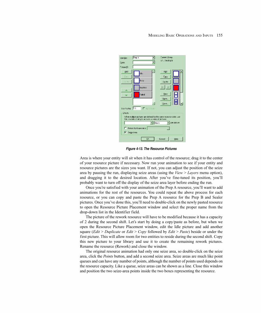
155MODELING BASIC OPERATIONS AND INPUTS
Figure 4-13. The Resource Pictures
Area is where your entity will sit when it has control of the resource; drag it to the centerof your resource picture if necessary. Now run your animation to see if your entity andresource pictures are the sizes you want. If not, you can adjust the position of the seizearea by pausing the run, displaying seize areas (using the View > Layers menu option),and dragging it to the desired location. After you’ve fine-tuned its position, you’llprobably want to turn off the display of the seize area layer before ending the run.
Once you’re satisfied with your animation of the Prep A resource, you’ll want to addanimations for the rest of the resources. You could repeat the above process for eachresource, or you can copy and paste the Prep A resource for the Prep B and Sealerpictures. Once you’ve done this, you’ll need to double-click on the newly pasted resourceto open the Resource Picture Placement window and select the proper name from thedrop-down list in the Identifier field.
The picture of the rework resource will have to be modified because it has a capacityof 2 during the second shift. Let’s start by doing a copy/paste as before, but when weopen the Resource Picture Placement window, edit the Idle picture and add anothersquare (Edit > Duplicate or Edit > Copy followed by Edit > Paste) beside or under thefirst picture. This will allow room for two entities to reside during the second shift. Copythis new picture to your library and use it to create the remaining rework pictures.Rename the resource (Rework) and close the window.
The original resource animation had only one seize area, so double-click on the seizearea, click the Points button, and add a second seize area. Seize areas are much like pointqueues and can have any number of points, although the number of points used depends onthe resource capacity. Like a queue, seize areas can be shown as a line. Close this windowand position the two seize-area points inside the two boxes representing the resource.
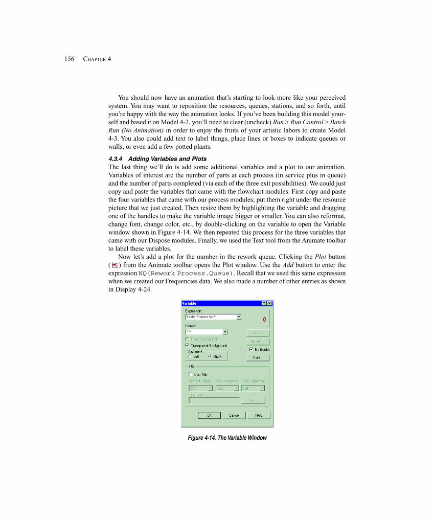
156 CHAPTER 4
You should now have an animation that’s starting to look more like your perceivedsystem. You may want to reposition the resources, queues, stations, and so forth, untilyou’re happy with the way the animation looks. If you’ve been building this model your-self and based it on Model 4-2, you’ll need to clear (uncheck) Run > Run Control > BatchRun (No Animation) in order to enjoy the fruits of your artistic labors to create Model4-3. You also could add text to label things, place lines or boxes to indicate queues orwalls, or even add a few potted plants.
4.3.4 Adding Variables and PlotsThe last thing we’ll do is add some additional variables and a plot to our animation.Variables of interest are the number of parts at each process (in service plus in queue)and the number of parts completed (via each of the three exit possibilities). We could justcopy and paste the variables that came with the flowchart modules. First copy and pastethe four variables that came with our process modules; put them right under the resourcepicture that we just created. Then resize them by highlighting the variable and draggingone of the handles to make the variable image bigger or smaller. You can also reformat,change font, change color, etc., by double-clicking on the variable to open the Variablewindow shown in Figure 4-14. We then repeated this process for the three variables thatcame with our Dispose modules. Finally, we used the Text tool from the Animate toolbarto label these variables.
Now let’s add a plot for the number in the rework queue. Clicking the Plot button( ) from the Animate toolbar opens the Plot window. Use the Add button to enter theexpression NQ(Rework Process.Queue). Recall that we used this same expressionwhen we created our Frequencies data. We also made a number of other entries as shownin Display 4-24.
Figure 4-14. The Variable Window
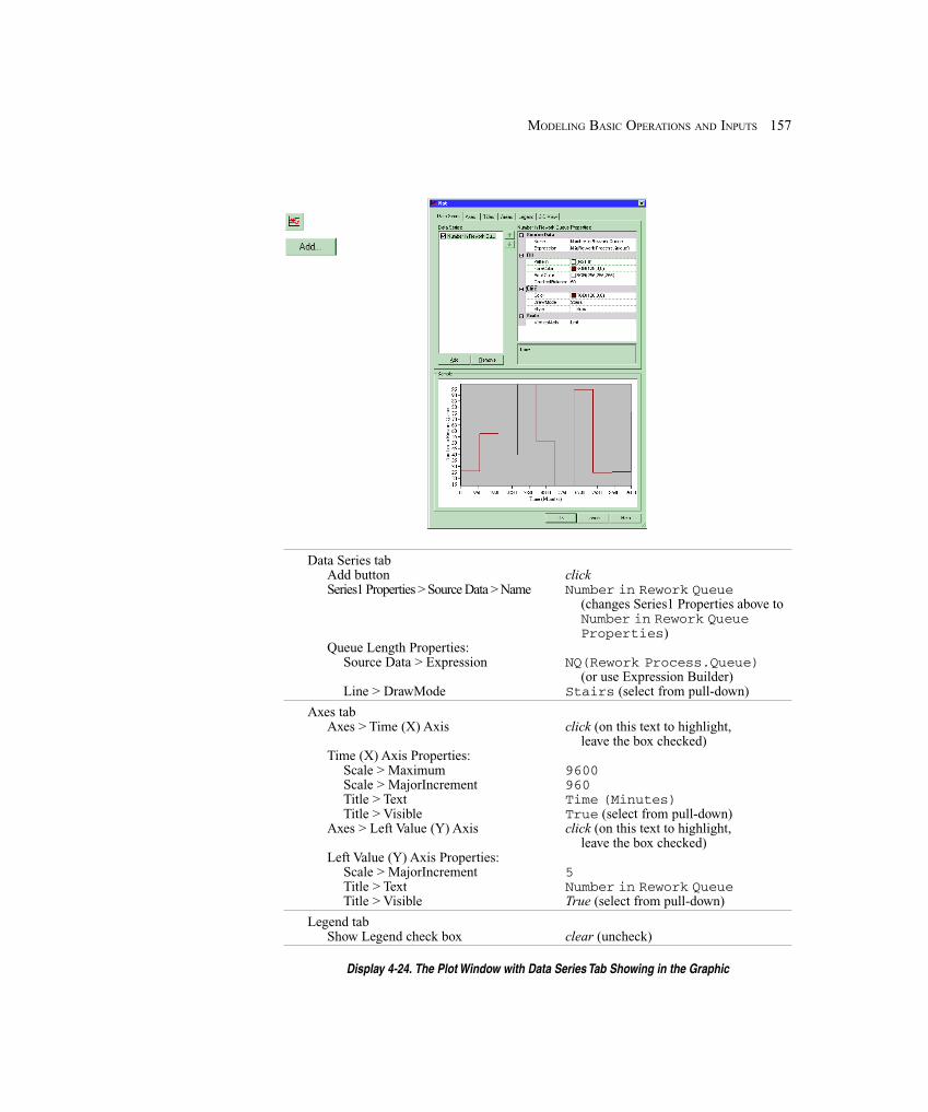
157MODELING BASIC OPERATIONS AND INPUTS
Data Series tabAdd button clickSeries1 Properties > Source Data > Name Number in Rework Queue
(changes Series1 Properties above toNumber in Rework QueueProperties)
Queue Length Properties:Source Data > Expression NQ(Rework Process.Queue)
(or use Expression Builder)Line > DrawMode Stairs (select from pull-down)
Axes tabAxes > Time (X) Axis click (on this text to highlight,
leave the box checked)Time (X) Axis Properties:
Scale > Maximum 9600Scale > MajorIncrement 960Title > Text Time (Minutes)Title > Visible True (select from pull-down)
Axes > Left Value (Y) Axis click (on this text to highlight,leave the box checked)
Left Value (Y) Axis Properties:Scale > MajorIncrement 5Title > Text Number in Rework QueueTitle > Visible True (select from pull-down)
Legend tabShow Legend check box clear (uncheck)
Display 4-24. The Plot Window with Data Series Tab Showing in the Graphic
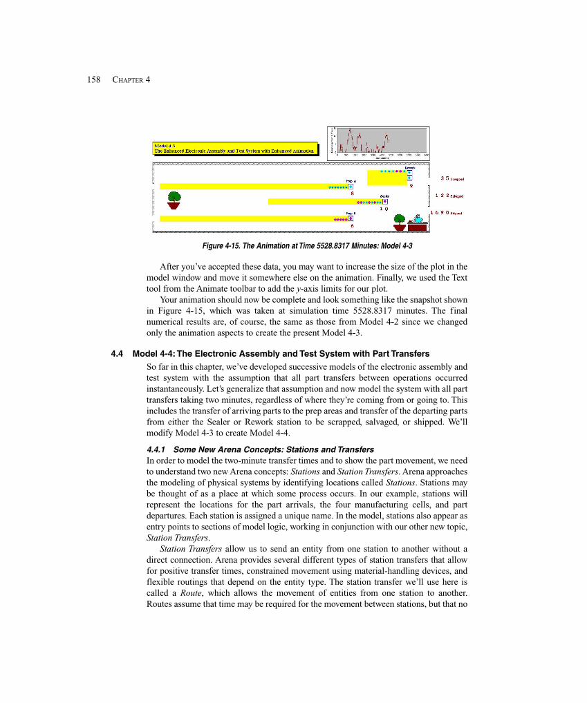
158 CHAPTER 4
Figure 4-15. The Animation at Time 5528.8317 Minutes: Model 4-3
After you’ve accepted these data, you may want to increase the size of the plot in themodel window and move it somewhere else on the animation. Finally, we used the Texttool from the Animate toolbar to add the y-axis limits for our plot.
Your animation should now be complete and look something like the snapshot shownin Figure 4-15, which was taken at simulation time 5528.8317 minutes. The finalnumerical results are, of course, the same as those from Model 4-2 since we changedonly the animation aspects to create the present Model 4-3.
4.4 Model 4-4: The Electronic Assembly and Test System with Part TransfersSo far in this chapter, we’ve developed successive models of the electronic assembly andtest system with the assumption that all part transfers between operations occurredinstantaneously. Let’s generalize that assumption and now model the system with all parttransfers taking two minutes, regardless of where they’re coming from or going to. Thisincludes the transfer of arriving parts to the prep areas and transfer of the departing partsfrom either the Sealer or Rework station to be scrapped, salvaged, or shipped. We’llmodify Model 4-3 to create Model 4-4.
4.4.1 Some New Arena Concepts: Stations and TransfersIn order to model the two-minute transfer times and to show the part movement, we needto understand two new Arena concepts: Stations and Station Transfers. Arena approachesthe modeling of physical systems by identifying locations called Stations. Stations maybe thought of as a place at which some process occurs. In our example, stations willrepresent the locations for the part arrivals, the four manufacturing cells, and partdepartures. Each station is assigned a unique name. In the model, stations also appear asentry points to sections of model logic, working in conjunction with our other new topic,Station Transfers.
Station Transfers allow us to send an entity from one station to another without adirect connection. Arena provides several different types of station transfers that allowfor positive transfer times, constrained movement using material-handling devices, andflexible routings that depend on the entity type. The station transfer we’ll use here iscalled a Route, which allows the movement of entities from one station to another.Routes assume that time may be required for the movement between stations, but that no
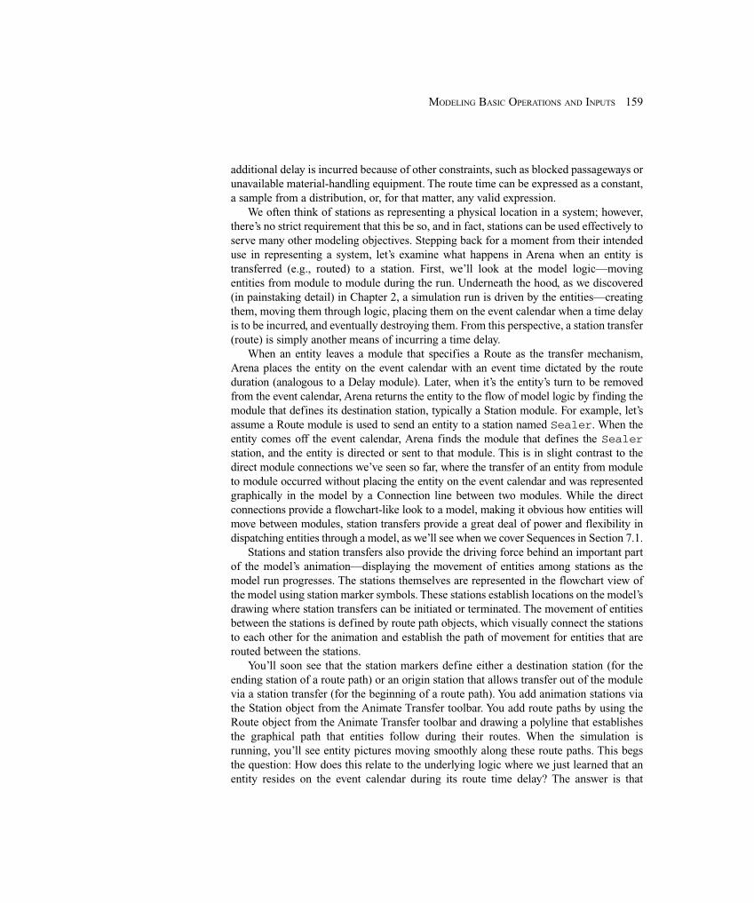
159MODELING BASIC OPERATIONS AND INPUTS
additional delay is incurred because of other constraints, such as blocked passageways orunavailable material-handling equipment. The route time can be expressed as a constant,a sample from a distribution, or, for that matter, any valid expression.
We often think of stations as representing a physical location in a system; however,there’s no strict requirement that this be so, and in fact, stations can be used effectively toserve many other modeling objectives. Stepping back for a moment from their intendeduse in representing a system, let’s examine what happens in Arena when an entity istransferred (e.g., routed) to a station. First, we’ll look at the model logic—movingentities from module to module during the run. Underneath the hood, as we discovered(in painstaking detail) in Chapter 2, a simulation run is driven by the entities—creatingthem, moving them through logic, placing them on the event calendar when a time delayis to be incurred, and eventually destroying them. From this perspective, a station transfer(route) is simply another means of incurring a time delay.
When an entity leaves a module that specifies a Route as the transfer mechanism,Arena places the entity on the event calendar with an event time dictated by the routeduration (analogous to a Delay module). Later, when it’s the entity’s turn to be removedfrom the event calendar, Arena returns the entity to the flow of model logic by finding themodule that defines its destination station, typically a Station module. For example, let’sassume a Route module is used to send an entity to a station named Sealer. When theentity comes off the event calendar, Arena finds the module that defines the Sealerstation, and the entity is directed or sent to that module. This is in slight contrast to thedirect module connections we’ve seen so far, where the transfer of an entity from moduleto module occurred without placing the entity on the event calendar and was representedgraphically in the model by a Connection line between two modules. While the directconnections provide a flowchart-like look to a model, making it obvious how entities willmove between modules, station transfers provide a great deal of power and flexibility indispatching entities through a model, as we’ll see when we cover Sequences in Section 7.1.
Stations and station transfers also provide the driving force behind an important partof the model’s animation—displaying the movement of entities among stations as themodel run progresses. The stations themselves are represented in the flowchart view ofthe model using station marker symbols. These stations establish locations on the model’sdrawing where station transfers can be initiated or terminated. The movement of entitiesbetween the stations is defined by route path objects, which visually connect the stationsto each other for the animation and establish the path of movement for entities that arerouted between the stations.
You’ll soon see that the station markers define either a destination station (for theending station of a route path) or an origin station that allows transfer out of the modulevia a station transfer (for the beginning of a route path). You add animation stations viathe Station object from the Animate Transfer toolbar. You add route paths by using theRoute object from the Animate Transfer toolbar and drawing a polyline that establishesthe graphical path that entities follow during their routes. When the simulation isrunning, you’ll see entity pictures moving smoothly along these route paths. This begsthe question: How does this relate to the underlying logic where we just learned that anentity resides on the event calendar during its route time delay? The answer is that
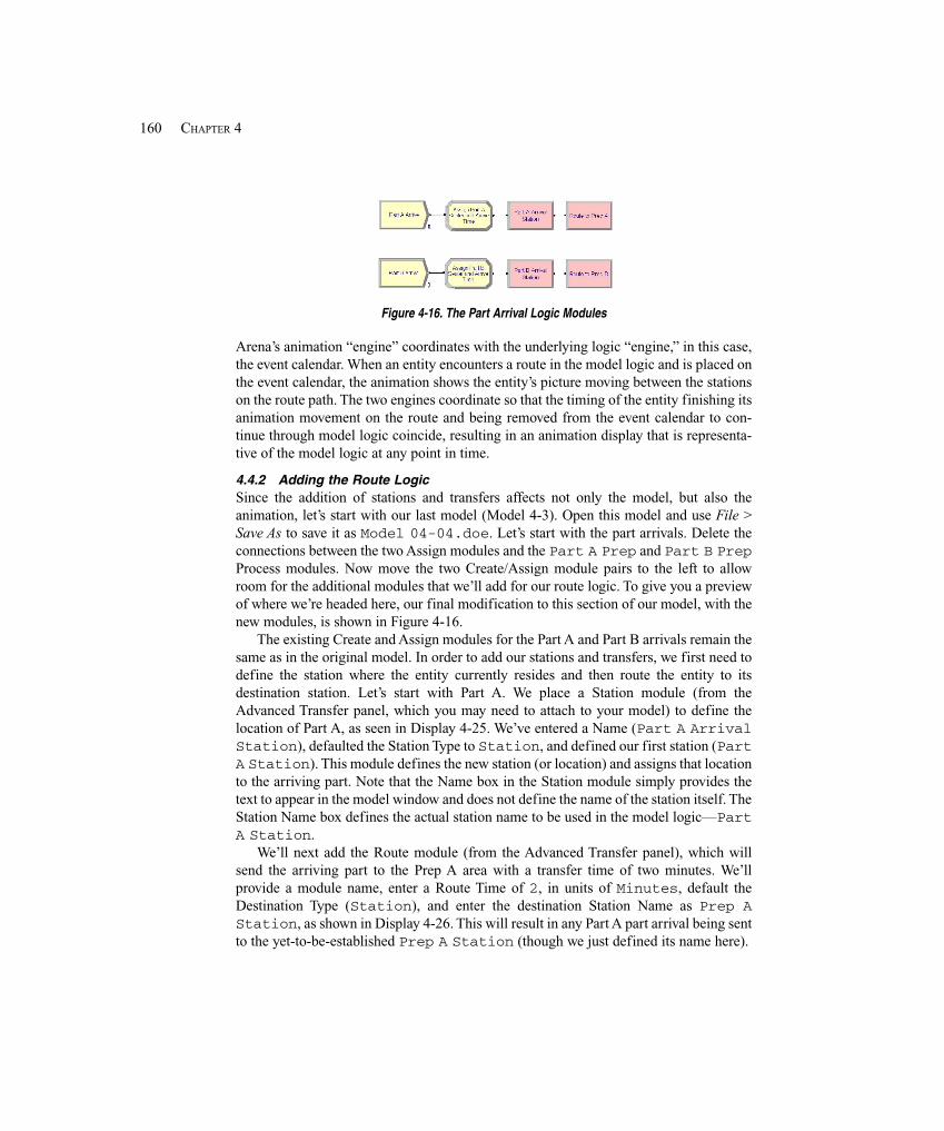
160 CHAPTER 4
Figure 4-16. The Part Arrival Logic Modules
Arena’s animation “engine” coordinates with the underlying logic “engine,” in this case,the event calendar. When an entity encounters a route in the model logic and is placed onthe event calendar, the animation shows the entity’s picture moving between the stationson the route path. The two engines coordinate so that the timing of the entity finishing itsanimation movement on the route and being removed from the event calendar to con-tinue through model logic coincide, resulting in an animation display that is representa-tive of the model logic at any point in time.
4.4.2 Adding the Route LogicSince the addition of stations and transfers affects not only the model, but also theanimation, let’s start with our last model (Model 4-3). Open this model and use File >Save As to save it as Model 04-04.doe. Let’s start with the part arrivals. Delete theconnections between the two Assign modules and the Part A Prep and Part B PrepProcess modules. Now move the two Create/Assign module pairs to the left to allowroom for the additional modules that we’ll add for our route logic. To give you a previewof where we’re headed here, our final modification to this section of our model, with thenew modules, is shown in Figure 4-16.
The existing Create and Assign modules for the Part A and Part B arrivals remain thesame as in the original model. In order to add our stations and transfers, we first need todefine the station where the entity currently resides and then route the entity to itsdestination station. Let’s start with Part A. We place a Station module (from theAdvanced Transfer panel, which you may need to attach to your model) to define thelocation of Part A, as seen in Display 4-25. We’ve entered a Name (Part A ArrivalStation), defaulted the Station Type to Station, and defined our first station (PartA Station). This module defines the new station (or location) and assigns that locationto the arriving part. Note that the Name box in the Station module simply provides thetext to appear in the model window and does not define the name of the station itself. TheStation Name box defines the actual station name to be used in the model logic—PartA Station.
We’ll next add the Route module (from the Advanced Transfer panel), which willsend the arriving part to the Prep A area with a transfer time of two minutes. We’llprovide a module name, enter a Route Time of 2, in units of Minutes, default theDestination Type (Station), and enter the destination Station Name as Prep AStation, as shown in Display 4-26. This will result in any Part A part arrival being sentto the yet-to-be-established Prep A Station (though we just defined its name here).
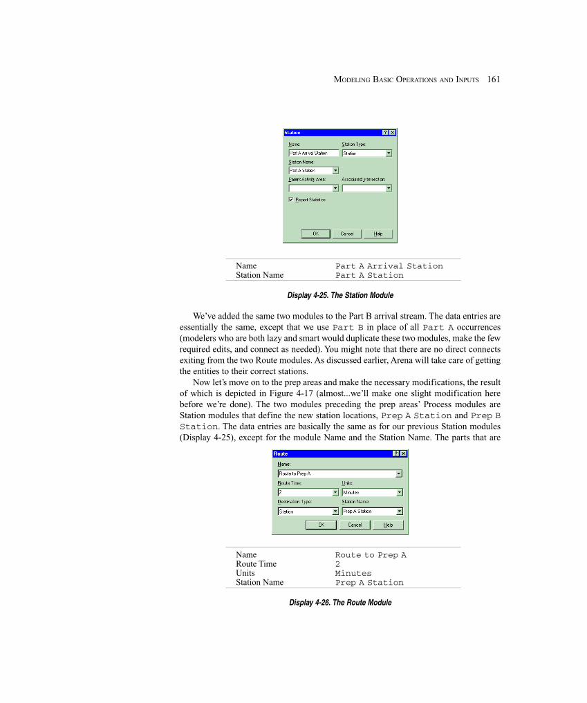
161MODELING BASIC OPERATIONS AND INPUTS
Name Part A Arrival StationStation Name Part A Station
Display 4-25. The Station Module
We’ve added the same two modules to the Part B arrival stream. The data entries areessentially the same, except that we use Part B in place of all Part A occurrences(modelers who are both lazy and smart would duplicate these two modules, make the fewrequired edits, and connect as needed). You might note that there are no direct connectsexiting from the two Route modules. As discussed earlier, Arena will take care of gettingthe entities to their correct stations.
Now let’s move on to the prep areas and make the necessary modifications, the resultof which is depicted in Figure 4-17 (almost...we’ll make one slight modification herebefore we’re done). The two modules preceding the prep areas’ Process modules areStation modules that define the new station locations, Prep A Station and Prep BStation. The data entries are basically the same as for our previous Station modules(Display 4-25), except for the module Name and the Station Name. The parts that are
Name Route to Prep ARoute Time 2Units MinutesStation Name Prep A Station
Display 4-26. The Route Module
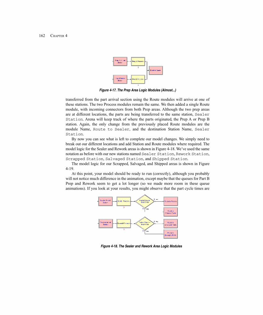
162 CHAPTER 4
Figure 4-17. The Prep Area Logic Modules (Almost...)
transferred from the part arrival section using the Route modules will arrive at one ofthese stations. The two Process modules remain the same. We then added a single Routemodule, with incoming connectors from both Prep areas. Although the two prep areasare at different locations, the parts are being transferred to the same station, SealerStation. Arena will keep track of where the parts originated, the Prep A or Prep Bstation. Again, the only change from the previously placed Route modules are themodule Name, Route to Sealer, and the destination Station Name, SealerStation.
By now you can see what is left to complete our model changes. We simply need tobreak out our different locations and add Station and Route modules where required. Themodel logic for the Sealer and Rework areas is shown in Figure 4-18. We’ve used the samenotation as before with our new stations named Sealer Station, Rework Station,Scrapped Station, Salvaged Station, and Shipped Station.
The model logic for our Scrapped, Salvaged, and Shipped areas is shown in Figure4-19.
At this point, your model should be ready to run (correctly), although you probablywill not notice much difference in the animation, except maybe that the queues for Part BPrep and Rework seem to get a lot longer (so we made more room in these queueanimations). If you look at your results, you might observe that the part cycle times are
Figure 4-18. The Sealer and Rework Area Logic Modules
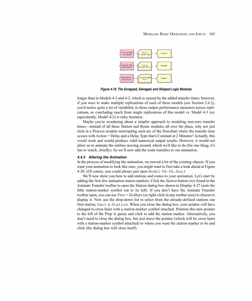
163MODELING BASIC OPERATIONS AND INPUTS
Figure 4-19. The Scrapped, Salvaged, and Shipped Logic Modules
longer than in Models 4-3 and 4-2, which is caused by the added transfer times; however,if you were to make multiple replications of each of these models (see Section 2.6.2),you’d notice quite a lot of variability in these output performance measures across repli-cations, so concluding much from single replications of this model vs. Model 4-3 (or,equivalently, Model 4-2) is risky business.
Maybe you’re wondering about a simpler approach to modeling non-zero transfertimes—instead of all these Station and Route modules all over the place, why not juststick in a Process module interrupting each arc of the flowchart where the transfer timeoccurs with Action = Delay and a Delay Type that’s Constant at 2 Minutes? Actually, thiswould work and would produce valid numerical output results. However, it would notallow us to animate the entities moving around, which we’d like to do (for one thing, it’sfun to watch...briefly). So we’ll now add the route transfers to our animation.
4.4.3 Altering the AnimationIn the process of modifying the animation, we moved a lot of the existing objects. If youwant your animation to look like ours, you might want to first take a look ahead at Figure4-20. (Of course, you could always just open Model 04-04.doe.)
We’ll now show you how to add stations and routes to your animation. Let’s start byadding the first few animation station markers. Click the Station button ( ) found in theAnimate Transfer toolbar to open the Station dialog box shown in Display 4-27 (note thelittle station-marker symbol out to its left). If you don’t have the Animate Transfertoolbar open, you can use View > Toolbars (or right-click in any toolbar area) to choose todisplay it. Now use the drop-down list to select from the already-defined stations ourfirst station, Part A Station. When you close the dialog box, your pointer will havechanged to cross hairs with a station-marker symbol attached. Position this new pointerto the left of the Prep A queue and click to add the station marker. Alternatively, youdon’t need to close the dialog box, but just move the pointer (which will be cross hairswith a station-marker symbol attached) to where you want the station marker to be andclick (the dialog box will close itself).
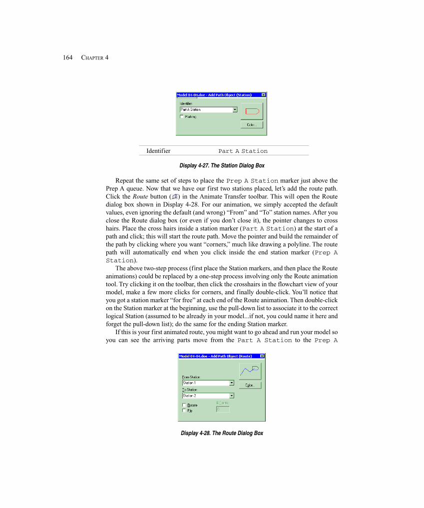
164 CHAPTER 4
Identifier Part A Station
Display 4-27. The Station Dialog Box
Repeat the same set of steps to place the Prep A Station marker just above thePrep A queue. Now that we have our first two stations placed, let’s add the route path.Click the Route button ( ) in the Animate Transfer toolbar. This will open the Routedialog box shown in Display 4-28. For our animation, we simply accepted the defaultvalues, even ignoring the default (and wrong) “From” and “To” station names. After youclose the Route dialog box (or even if you don’t close it), the pointer changes to crosshairs. Place the cross hairs inside a station marker (Part A Station) at the start of apath and click; this will start the route path. Move the pointer and build the remainder ofthe path by clicking where you want “corners,” much like drawing a polyline. The routepath will automatically end when you click inside the end station marker (Prep AStation).
The above two-step process (first place the Station markers, and then place the Routeanimations) could be replaced by a one-step process involving only the Route animationtool. Try clicking it on the toolbar, then click the crosshairs in the flowchart view of yourmodel, make a few more clicks for corners, and finally double-click. You’ll notice thatyou got a station marker “for free” at each end of the Route animation. Then double-clickon the Station marker at the beginning, use the pull-down list to associate it to the correctlogical Station (assumed to be already in your model...if not, you could name it here andforget the pull-down list); do the same for the ending Station marker.
If this is your first animated route, you might want to go ahead and run your model soyou can see the arriving parts move from the Part A Station to the Prep A
Display 4-28. The Route Dialog Box
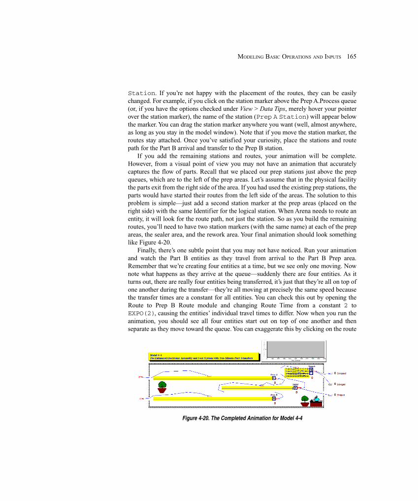
165MODELING BASIC OPERATIONS AND INPUTS
Station. If you’re not happy with the placement of the routes, they can be easilychanged. For example, if you click on the station marker above the Prep A.Process queue(or, if you have the options checked under View > Data Tips, merely hover your pointerover the station marker), the name of the station (Prep A Station) will appear belowthe marker. You can drag the station marker anywhere you want (well, almost anywhere,as long as you stay in the model window). Note that if you move the station marker, theroutes stay attached. Once you’ve satisfied your curiosity, place the stations and routepath for the Part B arrival and transfer to the Prep B station.
If you add the remaining stations and routes, your animation will be complete.However, from a visual point of view you may not have an animation that accuratelycaptures the flow of parts. Recall that we placed our prep stations just above the prepqueues, which are to the left of the prep areas. Let’s assume that in the physical facilitythe parts exit from the right side of the area. If you had used the existing prep stations, theparts would have started their routes from the left side of the areas. The solution to thisproblem is simple—just add a second station marker at the prep areas (placed on theright side) with the same Identifier for the logical station. When Arena needs to route anentity, it will look for the route path, not just the station. So as you build the remainingroutes, you’ll need to have two station markers (with the same name) at each of the prepareas, the sealer area, and the rework area. Your final animation should look somethinglike Figure 4-20.
Finally, there’s one subtle point that you may not have noticed. Run your animationand watch the Part B entities as they travel from arrival to the Part B Prep area.Remember that we’re creating four entities at a time, but we see only one moving. Nownote what happens as they arrive at the queue—suddenly there are four entities. As itturns out, there are really four entities being transferred, it’s just that they’re all on top ofone another during the transfer—they’re all moving at precisely the same speed becausethe transfer times are a constant for all entities. You can check this out by opening theRoute to Prep B Route module and changing Route Time from a constant 2 toEXPO(2), causing the entities’ individual travel times to differ. Now when you run theanimation, you should see all four entities start out on top of one another and thenseparate as they move toward the queue. You can exaggerate this by clicking on the route
Figure 4-20. The Completed Animation for Model 4-4

166 CHAPTER 4
Figure 4-21. The Batch B Entity Picture
path and making it much longer. Although this will show four entities moving, it may notrepresent reality since, if you believe the modeling assumptions, this travel time was sup-posed to be a constant 2 minutes (but your boss will probably never know).
Here’s a blatant sleight of hand to keep the model assumptions yet make the anima-tion look right. If we show the B parts arriving, with each part animated as a “big batch”picture, we’ll get the desired visual results. There will still be four moving across to thePrep B Station, but only the top one will show. We need only convert the picture back toa single entity when they enter the queue at the prep area. In order to implement this con-cept, we’ll need to create a new “big batch” picture and make two changes to the model.
First use Edit > Entity Pictures to open the Entity Picture Placement window. Nextmake a copy of the Picture.Part B picture and rename it Picture.Batch B inthe Value field above it. Edit this new picture’s drawing by double-clicking on its buttonin the list. In the Picture Editor, use Copy and Paste to get four Part B circles as shown inFigure 4-21; move the entity reference point to be near the center of your four-pack. Thenclose the Picture Edit window and click OK to return to the model window.
Now that we have a batch picture, we need to tell Arena when it should be used. Openthe Assign Part B Sealer and Arrive Time Assign module and Add anotherassignment (in this case, it doesn’t matter where in the list of assignments it’s added sincethere’s no dependency in these assignments of one on another). This new assignment willbe of Type Entity Picture, with the Entity Picture being Picture.Batch B(which you’ll need to type in here for the first time). This will cause Arena to show thebatch picture when it routes the Part B arrivals to the Prep B station. Now we need toconvert the picture back to a single entity when it arrives at the Prep B area. You’ll needto insert a new Assign module (Assign Picture) between the Prep B station, PrepB Arrival Station, and the Prep B Process Process module. This assignmentwill have Entity Picture Type, with the Entity Picture being Picture.Part B(which will be on the drop-down list for Entity Picture). Thus, when the entities enter thequeue or service at Prep B Process, they will be displayed as individual parts.
Now if you run the simulation (with the animation turned on), you’ll see an arrivingbatch being routed to the Prep B area and individual parts when the batch enters thequeue. Defining different entity pictures allows you to see the different types of partsmove through the system. Note the batch of four B parts when they enter the system.Although there are still four of these pictures, each on top of the other, the new Batch Bpicture gives the illusion of a single batch of four parts entering.
Now that you understand the concept of routes, we’ll use them in Chapter 7 in a morecomplex system.
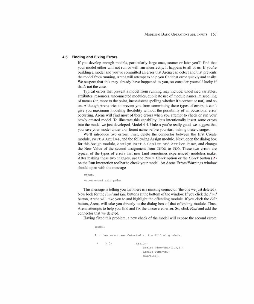
167MODELING BASIC OPERATIONS AND INPUTS
4.5 Finding and Fixing Errors
If you develop enough models, particularly large ones, sooner or later you’ll find thatyour model either will not run or will run incorrectly. It happens to all of us. If you’rebuilding a model and you’ve committed an error that Arena can detect and that preventsthe model from running, Arena will attempt to help you find that error quickly and easily.We suspect that this may already have happened to you, so consider yourself lucky ifthat’s not the case.
Typical errors that prevent a model from running may include: undefined variables,attributes, resources, unconnected modules, duplicate use of module names, misspellingof names (or, more to the point, inconsistent spelling whether it’s correct or not), and soon. Although Arena tries to prevent you from committing these types of errors, it can’tgive you maximum modeling flexibility without the possibility of an occasional erroroccurring. Arena will find most of these errors when you attempt to check or run yournewly created model. To illustrate this capability, let’s intentionally insert some errorsinto the model we just developed, Model 4-4. Unless you’re really good, we suggest thatyou save your model under a different name before you start making these changes.
We’ll introduce two errors. First, delete the connector between the first Createmodule, Part A Arrive, and the following Assign module. Next, open the dialog boxfor this Assign module, Assign Part A Sealer and Arrive Time, and changethe New Value of the second assignment from TNOW to TNO. These two errors aretypical of the types of errors that new (and sometimes experienced) modelers make.After making these two changes, use the Run > Check option or the Check button ( )on the Run Interaction toolbar to check your model. An Arena Errors/Warnings windowshould open with the message
ERROR:
Unconnected exit point
This message is telling you that there is a missing connector (the one we just deleted).Now look for the Find and Edit buttons at the bottom of the window. If you click the Findbutton, Arena will take you to and highlight the offending module. If you click the Editbutton, Arena will take you directly to the dialog box of that offending module. Thus,Arena attempts to help you find and fix the discovered error. So, click Find and add theconnector that we deleted.
Having fixed this problem, a new check of the model will expose the second error:
ERROR:
A linker error was detected at the following block:
* 3 0$ ASSIGN:
Sealer Time=TRIA(1,3,4):
Arrive Time=TNO:
NEXT(14$);
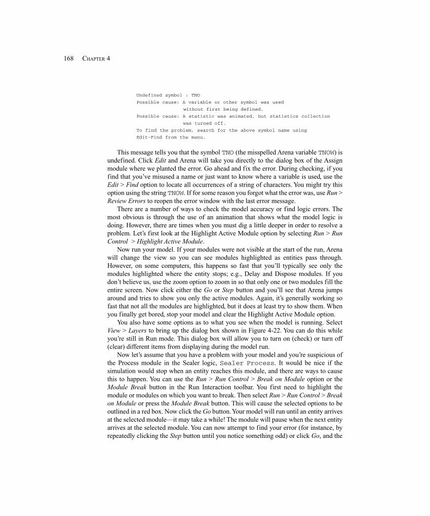
168 CHAPTER 4
Undefined symbol : TNO
Possible cause: A variable or other symbol was used
without first being defined.
Possible cause: A statistic was animated, but statistics collection
was turned off.
To find the problem, search for the above symbol name using
Edit-Find from the menu.
This message tells you that the symbol TNO (the misspelled Arena variable TNOW) isundefined. Click Edit and Arena will take you directly to the dialog box of the Assignmodule where we planted the error. Go ahead and fix the error. During checking, if youfind that you’ve misused a name or just want to know where a variable is used, use theEdit > Find option to locate all occurrences of a string of characters. You might try thisoption using the string TNOW. If for some reason you forgot what the error was, use Run >Review Errors to reopen the error window with the last error message.
There are a number of ways to check the model accuracy or find logic errors. Themost obvious is through the use of an animation that shows what the model logic isdoing. However, there are times when you must dig a little deeper in order to resolve aproblem. Let’s first look at the Highlight Active Module option by selecting Run > RunControl > Highlight Active Module.
Now run your model. If your modules were not visible at the start of the run, Arenawill change the view so you can see modules highlighted as entities pass through.However, on some computers, this happens so fast that you’ll typically see only themodules highlighted where the entity stops; e.g., Delay and Dispose modules. If youdon’t believe us, use the zoom option to zoom in so that only one or two modules fill theentire screen. Now click either the Go or Step button and you’ll see that Arena jumpsaround and tries to show you only the active modules. Again, it’s generally working sofast that not all the modules are highlighted, but it does at least try to show them. Whenyou finally get bored, stop your model and clear the Highlight Active Module option.
You also have some options as to what you see when the model is running. SelectView > Layers to bring up the dialog box shown in Figure 4-22. You can do this whileyou’re still in Run mode. This dialog box will allow you to turn on (check) or turn off(clear) different items from displaying during the model run.
Now let’s assume that you have a problem with your model and you’re suspicious ofthe Process module in the Sealer logic, Sealer Process. It would be nice if thesimulation would stop when an entity reaches this module, and there are ways to causethis to happen. You can use the Run > Run Control > Break on Module option or theModule Break button in the Run Interaction toolbar. You first need to highlight themodule or modules on which you want to break. Then select Run > Run Control > Breakon Module or press the Module Break button. This will cause the selected options to beoutlined in a red box. Now click the Go button. Your model will run until an entity arrivesat the selected module—it may take a while! The module will pause when the next entityarrives at the selected module. You can now attempt to find your error (for instance, byrepeatedly clicking the Step button until you notice something odd) or click Go, and the
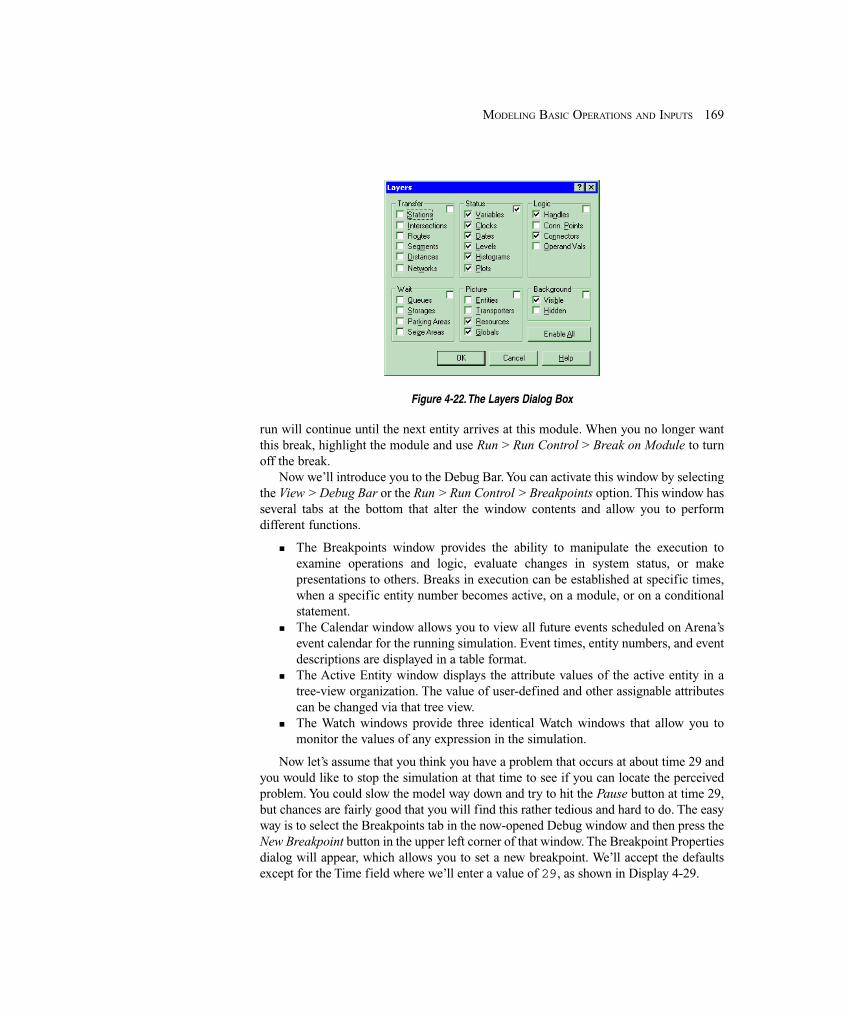
169MODELING BASIC OPERATIONS AND INPUTS
Figure 4-22. The Layers Dialog Box
run will continue until the next entity arrives at this module. When you no longer wantthis break, highlight the module and use Run > Run Control > Break on Module to turnoff the break.
Now we’ll introduce you to the Debug Bar. You can activate this window by selectingthe View > Debug Bar or the Run > Run Control > Breakpoints option. This window hasseveral tabs at the bottom that alter the window contents and allow you to performdifferent functions.
� The Breakpoints window provides the ability to manipulate the execution toexamine operations and logic, evaluate changes in system status, or makepresentations to others. Breaks in execution can be established at specific times,when a specific entity number becomes active, on a module, or on a conditionalstatement.
� The Calendar window allows you to view all future events scheduled on Arena’sevent calendar for the running simulation. Event times, entity numbers, and eventdescriptions are displayed in a table format.
� The Active Entity window displays the attribute values of the active entity in atree-view organization. The value of user-defined and other assignable attributescan be changed via that tree view.
� The Watch windows provide three identical Watch windows that allow you tomonitor the values of any expression in the simulation.
Now let’s assume that you think you have a problem that occurs at about time 29 andyou would like to stop the simulation at that time to see if you can locate the perceivedproblem. You could slow the model way down and try to hit the Pause button at time 29,but chances are fairly good that you will find this rather tedious and hard to do. The easyway is to select the Breakpoints tab in the now-opened Debug window and then press theNew Breakpoint button in the upper left corner of that window. The Breakpoint Propertiesdialog will appear, which allows you to set a new breakpoint. We’ll accept the defaultsexcept for the Time field where we’ll enter a value of 29, as shown in Display 4-29.
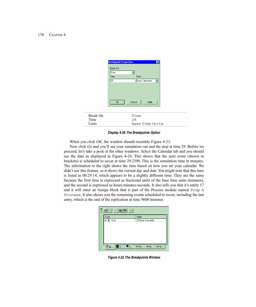
170 CHAPTER 4
Break On TimeTime 29Units Base Time Units
Display 4-29. The Breakpoints Option
When you click OK, the window should resemble Figure 4-23.Now click Go and you’ll see your simulation run and the stop at time 29. Before we
proceed, let’s take a peek at the other windows. Select the Calendar tab and you shouldsee the data as displayed in Figure 4-24. This shows that the next event (shown inbrackets) is scheduled to occur at time 29.2390. This is the simulation time in minutes.The information to the right shows the time based on how you set your calendar. Wedidn’t use this feature, so it shows the current day and date. You might note that this timeis listed as 00:29:14, which appears to be a slightly different time. They are the samebecause the first time is expressed as fractional units of the base time units (minutes),and the second is expressed as hours:minutes:seconds. It also tells you that it’s entity 17and it will enter an Assign block that is part of the Process module named Prep AProcess. It also shows you the remaining events scheduled to occur, including the lastentry, which is the end of the replication at time 9600 minutes.
Figure 4-23. The Breakpoints Window
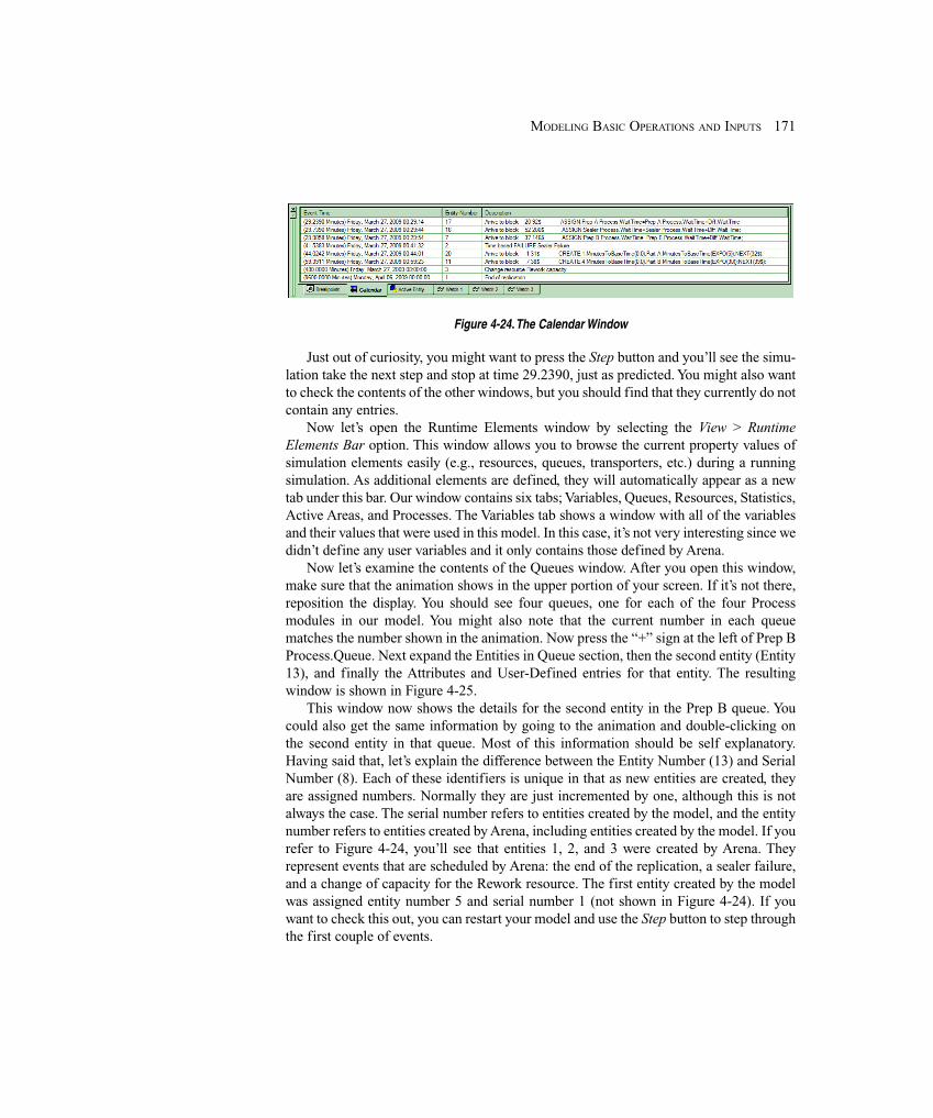
171MODELING BASIC OPERATIONS AND INPUTS
Figure 4-24. The Calendar Window
Just out of curiosity, you might want to press the Step button and you’ll see the simu-lation take the next step and stop at time 29.2390, just as predicted. You might also wantto check the contents of the other windows, but you should find that they currently do notcontain any entries.
Now let’s open the Runtime Elements window by selecting the View > RuntimeElements Bar option. This window allows you to browse the current property values ofsimulation elements easily (e.g., resources, queues, transporters, etc.) during a runningsimulation. As additional elements are defined, they will automatically appear as a newtab under this bar. Our window contains six tabs; Variables, Queues, Resources, Statistics,Active Areas, and Processes. The Variables tab shows a window with all of the variablesand their values that were used in this model. In this case, it’s not very interesting since wedidn’t define any user variables and it only contains those defined by Arena.
Now let’s examine the contents of the Queues window. After you open this window,make sure that the animation shows in the upper portion of your screen. If it’s not there,reposition the display. You should see four queues, one for each of the four Processmodules in our model. You might also note that the current number in each queuematches the number shown in the animation. Now press the “+” sign at the left of Prep BProcess.Queue. Next expand the Entities in Queue section, then the second entity (Entity13), and finally the Attributes and User-Defined entries for that entity. The resultingwindow is shown in Figure 4-25.
This window now shows the details for the second entity in the Prep B queue. Youcould also get the same information by going to the animation and double-clicking onthe second entity in that queue. Most of this information should be self explanatory.Having said that, let’s explain the difference between the Entity Number (13) and SerialNumber (8). Each of these identifiers is unique in that as new entities are created, theyare assigned numbers. Normally they are just incremented by one, although this is notalways the case. The serial number refers to entities created by the model, and the entitynumber refers to entities created by Arena, including entities created by the model. If yourefer to Figure 4-24, you’ll see that entities 1, 2, and 3 were created by Arena. Theyrepresent events that are scheduled by Arena: the end of the replication, a sealer failure,and a change of capacity for the Rework resource. The first entity created by the modelwas assigned entity number 5 and serial number 1 (not shown in Figure 4-24). If youwant to check this out, you can restart your model and use the Step button to step throughthe first couple of events.
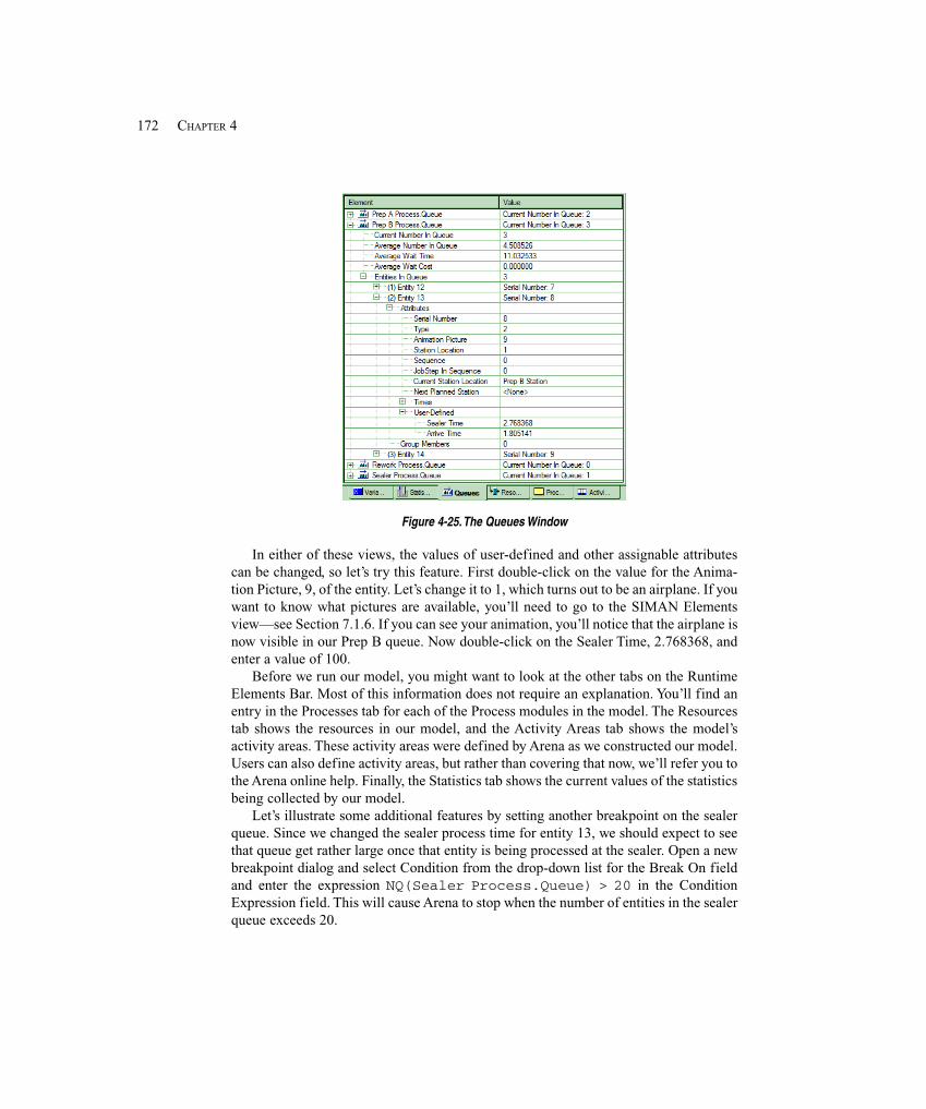
172 CHAPTER 4
Figure 4-25. The Queues Window
In either of these views, the values of user-defined and other assignable attributescan be changed, so let’s try this feature. First double-click on the value for the Anima-tion Picture, 9, of the entity. Let’s change it to 1, which turns out to be an airplane. If youwant to know what pictures are available, you’ll need to go to the SIMAN Elementsview—see Section 7.1.6. If you can see your animation, you’ll notice that the airplane isnow visible in our Prep B queue. Now double-click on the Sealer Time, 2.768368, andenter a value of 100.
Before we run our model, you might want to look at the other tabs on the RuntimeElements Bar. Most of this information does not require an explanation. You’ll find anentry in the Processes tab for each of the Process modules in the model. The Resourcestab shows the resources in our model, and the Activity Areas tab shows the model’sactivity areas. These activity areas were defined by Arena as we constructed our model.Users can also define activity areas, but rather than covering that now, we’ll refer you tothe Arena online help. Finally, the Statistics tab shows the current values of the statisticsbeing collected by our model.
Let’s illustrate some additional features by setting another breakpoint on the sealerqueue. Since we changed the sealer process time for entity 13, we should expect to seethat queue get rather large once that entity is being processed at the sealer. Open a newbreakpoint dialog and select Condition from the drop-down list for the Break On fieldand enter the expression NQ(Sealer Process.Queue) > 20 in the ConditionExpression field. This will cause Arena to stop when the number of entities in the sealerqueue exceeds 20.
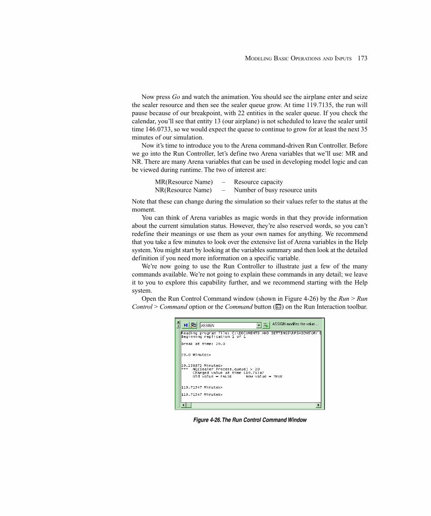
173MODELING BASIC OPERATIONS AND INPUTS
Now press Go and watch the animation. You should see the airplane enter and seizethe sealer resource and then see the sealer queue grow. At time 119.7135, the run willpause because of our breakpoint, with 22 entities in the sealer queue. If you check thecalendar, you’ll see that entity 13 (our airplane) is not scheduled to leave the sealer untiltime 146.0733, so we would expect the queue to continue to grow for at least the next 35minutes of our simulation.
Now it’s time to introduce you to the Arena command-driven Run Controller. Beforewe go into the Run Controller, let’s define two Arena variables that we’ll use: MR andNR. There are many Arena variables that can be used in developing model logic and canbe viewed during runtime. The two of interest are:
MR(Resource Name) – Resource capacityNR(Resource Name) – Number of busy resource units
Note that these can change during the simulation so their values refer to the status at themoment.
You can think of Arena variables as magic words in that they provide informationabout the current simulation status. However, they’re also reserved words, so you can’tredefine their meanings or use them as your own names for anything. We recommendthat you take a few minutes to look over the extensive list of Arena variables in the Helpsystem. You might start by looking at the variables summary and then look at the detaileddefinition if you need more information on a specific variable.
We’re now going to use the Run Controller to illustrate just a few of the manycommands available. We’re not going to explain these commands in any detail; we leaveit to you to explore this capability further, and we recommend starting with the Helpsystem.
Open the Run Control Command window (shown in Figure 4-26) by the Run > RunControl > Command option or the Command button ( ) on the Run Interaction toolbar.
Figure 4-26. The Run Control Command Window
174 CHAPTER 4
Now let’s use the features in the Run Control Command window to increase thecapacity of the sealer resource. First we’ll check the current values of NR and MR for theSealer resource. To do this, use the drop-down feature to select the command SHOW(that field currently has the command ASSIGN showing). Then press the InsertCommand button ( ) to insert the SHOW command into the window. Now typeMR(Sealer) and press the Enter key. The response will be
MR(Sealer) = 1.
This tells you that the Sealer resource currently has a capacity of one. Now repeat theprocess for NR(Sealer). The response will be
NR(Sealer) = 1.
This tells you that one unit of the Sealer resource is currently busy, which should beobvious from the animation since it shows the airplane parked on that resource. Now let’sincrease the Sealer resource capacity to 3. Use the ASSIGN command to make thefollowing entry
ASSIGN MR(Sealer) = 3
and press the Enter key. The Sealer resource now has a capacity of 3. Now press Go andwatch the animation to see the sealer queue shrink to zero in about 20 minutes ofsimulation time.
Finally, during a run, you might want to view reports on the status of the model. Youcan view reports at any time during a run. Simply go to the Project Bar and click on theReports panel. You can request a report when the model is running or when the model isin Pause mode. Just like the Watch window, you could have an animation running andperiodically request a report and never stop the run. Just remember to close the reportwindows when you’re done viewing them.
Even if you don’t use the Run Controller, the options available on the Run Interactiontoolbar provide the capability to detect model logic errors without your needing tobecome a SIMAN expert. So that you’ll understand how they work, we recommend thatyou take a simple animated model and practice using these tools. You could wait untilyou need them, but then not only would you be trying to find an error, but you’d also betrying to learn several new tools!
4.6 Input Analysis: Specifying Model Parameters and Distributions
As you’ve no doubt noticed, there are a lot of details that you have to specify completelyin order to define a working simulation model. Probably you think first of the logicalaspects of the model, like what the entities and resources are, how entities enter andmaybe leave the model, the resources they need, the paths they follow, and so on. Thesekinds of activities might be called structural modeling since they lay out the fundamentallogic of what you want your model to look like and do.
You’ve also noticed that there are other things in specifying a model that are morenumerical or mathematical in nature (and maybe therefore more mundane). For example,in specifying Model 4-2, we declared that interarrival times for Part A were distributed
175MODELING BASIC OPERATIONS AND INPUTS
exponentially with a mean of 5 minutes, total processing times for Part B Prep followed atriangular (3, 5, 10) distribution, the “up” times for the sealer were draws from anexponential (120) distribution, and we set up a schedule for the number of reworkoperators at different times. You also have to make these kinds of specifications, whichmight be called quantitative modeling, and are potentially just as important to the resultsas are the structural-modeling assumptions.
So where did we get all these numbers and distributions for Model 4-2 (as well as forpractically all the other models in this book)? Okay, we admit that we just made them up,after playing around for a while, to get the kinds of results we wanted in order to illustratevarious points. We get to do this since we’re just writing a book rather than doing any realwork, but unfortunately, you won’t have this luxury. Rather, you need to observe the realsystem (if it exists) or use specifications for it (if it doesn’t exist), collect data on whatcorresponds to your input quantitative modeling, and analyze these data to come up withreasonable “models,” or representations of how they’ll be specified or generated in thesimulation. For Model 4-2, this would entail collecting data on actual interarrival timesfor Part A, processing times for Part B Prep, up times for the sealer, and actual staffing atthe rework station (as well as all the other quantitative inputs required to specify themodel). You’d then need to take a look at these data and do some kind of analysis on themto specify the corresponding inputs to your model in an accurate, realistic, and valid way.
In this section, we’ll describe this process and show you how to use the Arena InputAnalyzer (which is a separate application that accompanies and works with Arena) tohelp you fit probability distributions to data observed on quantities subject to variation.
4.6.1 Deterministic vs. Random InputsOne fundamental issue in quantitative modeling is whether you’re going to model an inputquantity as a deterministic (non-random) quantity, or whether you’re going to model it as arandom variable following some probability distribution. Sometimes it’s clear thatsomething should be deterministic, like the number of rework operators, though you mightwant to vary the values from run to run to see what effect they have on performance.
But sometimes it’s not so clear, and we can offer only the (obvious) advice that youshould do what appears most realistic and valid so far as possible. In Section 4.6.2, we’lltalk a little about using your model for what’s called sensitivity analysis to measure howimportant a particular input is to your output, which might indicate how much you needto worry about whether it should be modeled as deterministic or random.
You might be tempted to assume away your input’s randomness, since this seemssimpler and has the advantage that the model’s outputs will be non-random. This can bepretty dangerous, though, from the model-validity viewpoint because it’s often therandomness itself that leads to important system behavior that you’d certainly want tocapture in your simulation model. For instance, in a simple single-server queue, wemight assume that all interarrival times are exactly 1 minute and that all processing timesare exactly 59 seconds; both of these figures might agree with average values fromobserved data on arrivals and service. If the model starts empty with the server idle andthe first arrival is at time 0, then there will never be a queue since each customer willfinish service and leave 1 second before the next customer arrives. However, if the reality
176 CHAPTER 4
is that the interarrival and service times are exponential random variables with respectivemeans of 1 minute and 59 seconds (rather than constant at these values), you get a verydifferent story in terms of queue length (go ahead and build a little Arena model for this,and run it for a long time); in fact, in the long run, it turns out that the average number ofcustomers in the queue is 58.0167, a far cry from 0. Intuitively, what’s going on here isthat, with the (correct) random model, it sometimes happens that some obnoxiouscustomer has a long service demand, or that several customers arrive at almost the sametime; it’s precisely these kinds of random occurrences that cause the queue to build up,which never happen in the (incorrect) deterministic model.
4.6.2 Collecting DataOne of the very early steps in planning your simulation project should be to identify whatdata you’ll need to support the model. Finding the data and preparing them for use inyour model can be time-consuming, expensive, and often frustrating; and the availabilityand quality of data can influence the modeling approach you take and the level of detailyou capture in the model.
There are many types of data that you might need to collect. Most models require agood bit of information involving time delays: interarrival times, processing times, traveltimes, operator work schedules, etc. In many cases, you’ll also need to estimateprobabilities, such as the percentage yield from an operation, the proportions of eachtype of customer, or the probability that a caller has a touch-tone phone. If you’remodeling a system where the physical movement of entities among stations will berepresented in the model, the operating parameters and physical layout of the material-handling system will also be needed.
You can go to many sources for data, ranging from electronic databases to interviewsof people working in the system to be studied. It seems that when it comes to finding datafor a simulation study, it’s either “feast or famine,” with each presenting its own uniquechallenges.
If the system you’re modeling exists (or is similar to an actual system somewhereelse), you may think that your job’s easier, since there should be a lot of data available.However, what you’re likely to find is that the data you get are not the data you need. Forexample, it’s common to collect processing-time data on machines (that is, a part’s timespan from arriving at the machine to completing the process), which at first glance mightlook like a good source for processing times in the simulation model. But, if theobserved processing-time data included the queue time or included machine failuretimes, they might not fit into the model’s logic, which explicitly models the queueinglogic and the machine failures separately from the machining time.
On the other hand, if you’re about to model a brand new system or a significantmodification to an existing one, you may find yourself at the other end of the spectrum,with little or no data. In this case, your model is at the mercy of rough approximationsfrom designers, equipment vendors, etc. We’ll have a few suggestions (as opposed tosolutions) for you in Section 4.6.5.
In either case, as you decide what and how much data to collect, it’s important to keepthe following helpful hints in mind:
177MODELING BASIC OPERATIONS AND INPUTS
� Sensitivity analysis: One often-ignored aspect of performing simulation studiesis developing an understanding of what’s important and what’s not. Sensitivityanalysis can be used even very early in a project to assess the impact of changes indata on the model results. If you can’t easily obtain good data about some aspectof your system, run the model with a range of values to see if the system’sperformance changes significantly. If it doesn’t, you may not need to invest incollecting data and still can have good confidence in your conclusions. If it does,then you’ll either need to find a way to obtain reliable data or your results andrecommendations will be coarser.
� Match model detail with quality of data: A benefit of developing an earlyunderstanding of the quality of your input data is that it can help you to decidehow much detail to incorporate in the model logic. Typically, it doesn’t make anysense to model carefully the detailed logic of a part of your system for which youhave unreliable values of the associated data, unless you think that, at a later time,you’ll be able to obtain better data.
� Cost: Because it can be expensive to collect and prepare data for use in a model,you may decide to use looser estimates for some data. In making this assessment,sensitivity analysis can be helpful so that you have an idea of the value of the datain affecting your recommendations.
� Garbage in, garbage out: Remember that the results and recommendations youpresent from your simulation study are only as reliable as the model and itsinputs. If you can’t locate accurate data concerning critical elements of the model,you can’t place a great deal of confidence in the accuracy of your conclusions.This doesn’t mean that there’s no value in performing a simulation study if youcan’t obtain “good” data. You still can develop tremendous insight into theoperation of a complex system, the interactions among its elements, and somelevel of prediction regarding how it will perform. But take care to articulate thereliability of your predictions based on the quality of the input data.
A final hint that we might offer is that data collection (and some of their analysis) isoften identified as the most difficult, costly, time-consuming, and tedious part of asimulation study. This is due in part to various problems you might encounter incollecting and analyzing data, and in part due to the undeniable fact that it’s just not asmuch fun as building the logical model and playing around with it. So, be of good cheerin this activity, and keep reminding yourself that it’s an important (if not pleasant orexciting) part of why you’re using simulation.
4.6.3 Using DataIf you have historical data (e.g., a record of breakdowns and repair times for a machine),or if you know how part of a system will work (e.g., planned operator schedules), youstill face decisions concerning how to incorporate the data into your model. The funda-mental choice is whether to use the data directly or whether to fit a probability distribu-tion to the existing data. Which approach you decide to use can be chosen based on boththeoretical issues and practical considerations.
178 CHAPTER 4
From a theoretical standpoint, your collected data represent what’s happened in thepast, which may or may not be an unbiased prediction of what will happen in the future.If the conditions surrounding the generation of these historical data no longer apply (or ifthey changed during the time span in which the data were recorded), then the historicaldata may be biased or may simply be missing some important aspects of the process. Forexample, if the historical data are from a database of product orders placed over the last12 months, but four months ago a new product option was introduced, then the order datastored in the preceding eight months are no longer directly useful since they don’tcontain the new option. The tradeoffs are that if you use the historical data directly, novalues other than those recorded can be experienced; but if you sample from a fittedprobability distribution, it’s possible to get values that aren’t possible (e.g., from the tailsof unbounded distributions) or to lose important characteristics (e.g., bimodal data,sequential patterns).
Practical considerations can come into play too. You may not have enough historicaldata to drive a simulation run that’s long enough to support your analysis. You may verywell need to consider the effect of file access on the speed of your simulation runs as well.Reading a lot of data from a file is typically slower than sampling from a probability dis-tribution, so driving the model with the historical data during a run can slow you down.
Regardless of your choice, Arena supplies built-in tools to take care of the mechanicsof using the historical data in your model. If you decide to fit a probability distribution tothe data, the Input Analyzer facilitates this process, providing an expression that you canuse directly in your model; we’ll go into this in Section 4.6.4. If you want to drive themodel directly from the historical data, you can bring the values in once to become partof the model’s data structure, or you can read the data dynamically during the simulationrun, which will be discussed in Section 10.1.
4.6.4 Fitting Input Distributions via the Input AnalyzerIf you decide to incorporate your existing data values by fitting a probability distributionto them, you can either select the distribution yourself and use the Input Analyzer toprovide numerical estimates of the appropriate parameters, or you can fit a number ofdistributions to the data and select the most appropriate one. In either case, the InputAnalyzer provides you with estimates of the parameter values (based on the data yousupply) and a ready-made expression that you can just copy and paste into your model.
When the Input Analyzer fits a distribution to your data, it estimates the distribution’sparameters (including any shift or offset that’s required to formulate a valid expression)and calculates a number of measures of how good the distribution fits your data. You canuse this information to select which distribution you want to use in your model, which wediscuss below.
Probability distributions can be thought of as falling into two main types: theoreticaland empirical. Theoretical distributions, such as the exponential and gamma, generatesamples based on a mathematical formulation. Empirical distributions simply divide theactual data into groupings and calculate the proportion of values in each group, possiblyinterpolating between points for more accuracy.
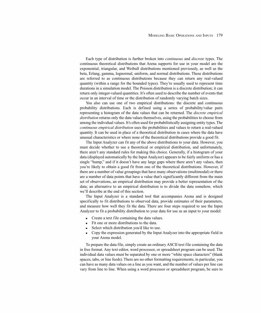
179MODELING BASIC OPERATIONS AND INPUTS
Each type of distribution is further broken into continuous and discrete types. Thecontinuous theoretical distributions that Arena supports for use in your model are theexponential, triangular, and Weibull distributions mentioned previously, as well as thebeta, Erlang, gamma, lognormal, uniform, and normal distributions. These distributionsare referred to as continuous distributions because they can return any real-valuedquantity (within a range for the bounded types). They’re usually used to represent timedurations in a simulation model. The Poisson distribution is a discrete distribution; it canreturn only integer-valued quantities. It’s often used to describe the number of events thatoccur in an interval of time or the distribution of randomly varying batch sizes.
You also can use one of two empirical distributions: the discrete and continuousprobability distributions. Each is defined using a series of probability/value pairsrepresenting a histogram of the data values that can be returned. The discrete empiricaldistribution returns only the data values themselves, using the probabilities to choose fromamong the individual values. It’s often used for probabilistically assigning entity types. Thecontinuous empirical distribution uses the probabilities and values to return a real-valuedquantity. It can be used in place of a theoretical distribution in cases where the data haveunusual characteristics or where none of the theoretical distributions provide a good fit.
The Input Analyzer can fit any of the above distributions to your data. However, youmust decide whether to use a theoretical or empirical distribution, and unfortunately,there aren’t any standard rules for making this choice. Generally, if a histogram of yourdata (displayed automatically by the Input Analyzer) appears to be fairly uniform or has asingle “hump,” and if it doesn’t have any large gaps where there aren’t any values, thenyou’re likely to obtain a good fit from one of the theoretical distributions. However, ifthere are a number of value groupings that have many observations (multimodal) or thereare a number of data points that have a value that’s significantly different from the mainset of observations, an empirical distribution may provide a better representation of thedata; an alternative to an empirical distribution is to divide the data somehow, whichwe’ll describe at the end of this section.
The Input Analyzer is a standard tool that accompanies Arena and is designedspecifically to fit distributions to observed data, provide estimates of their parameters,and measure how well they fit the data. There are four steps required to use the InputAnalyzer to fit a probability distribution to your data for use as an input to your model:
� Create a text file containing the data values.� Fit one or more distributions to the data.� Select which distribution you’d like to use.� Copy the expression generated by the Input Analyzer into the appropriate field in
your Arena model.
To prepare the data file, simply create an ordinary ASCII text file containing the datain free format. Any text editor, word processor, or spreadsheet program can be used. Theindividual data values must be separated by one or more “white space characters” (blankspaces, tabs, or line feeds). There are no other formatting requirements; in particular, youcan have as many data values on a line as you want, and the number of values per line canvary from line to line. When using a word processor or spreadsheet program, be sure to
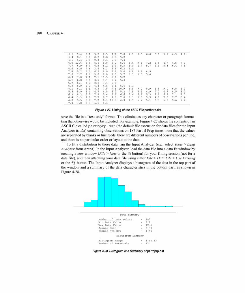
180 CHAPTER 4
6.1 9.4 8.1 3.2 6.5 7.2 7.8 4.9 3.5 6.6 6.1 5.1 4.9 4.26.4 8.1 6.0 8.2 6.8 5.9 5.26.5 5.4 5.9 9.3 5.4 6.5 7.46.0 12.6 6.8 5.6 5.8 6.2 5.6 6.4 9.5 7.2 5.6 4.7 4.5 7.07.7 6.9 5.4 6.3 8.1 4.9 5.3 5.0 4.7 5.7 4.9 5.3 6.4 7.54.4 4.9 7.6 3.6 8.3 5.6 6.2 5.07.4 5.2 5.0 6.5 8.0 6.2 5.0 4.8 6.2 4.97.0 7.7 4.7 5.0 6.0 9.0 5.7 7.1 5.0 5.64.9 7.8 7.1 7.1 11.5 5.4 5.26.1 6.8 5.4 3.5 7.1 5.7 5.45.7 6.1 4.2 8.8 7.4 5.55.3 5.9 5.2 6.4 4.5 5.1 5.6 6.18.1 8.1 5.1 8.3 7.5 7.6 10.9 6.5 9.0 5.9 6.8 9.0 6.5 6.05.8 5.0 6.4 4.7 4.5 6.2 5.2 7.9 5.5 4.9 7.2 4.9 4.5 6.06.3 8.3 5.5 7.8 5.4 5.3 6.6 3.6 7.3 5.3 8.9 6.8 7.1 8.76.4 3.3 7.0 7.7 6.7 7.6 7.6 7.1 5.6 5.9 4.1 7.5 7.7 5.44.8 5.5 8.8 7.2 6.3 10.0 4.3 4.9 5.7 5.1 6.7 6.0 5.6 7.27.0 7.8 6.3 6.1 8.4
Figure 4-27. Listing of the ASCII File partbprp.dst
save the file in a “text only” format. This eliminates any character or paragraph format-ting that otherwise would be included. For example, Figure 4-27 shows the contents of anASCII file called partbprp.dst (the default file extension for data files for the InputAnalyzer is .dst) containing observations on 187 Part B Prep times; note that the valuesare separated by blanks or line feeds, there are different numbers of observations per line,and there is no particular order or layout to the data.
To fit a distribution to these data, run the Input Analyzer (e.g., select Tools > InputAnalyzer from Arena). In the Input Analyzer, load the data file into a data fit window bycreating a new window (File > New or the button) for your fitting session (not for adata file), and then attaching your data file using either File > Data File > Use Existingor the button. The Input Analyzer displays a histogram of the data in the top part ofthe window and a summary of the data characteristics in the bottom part, as shown inFigure 4-28.
Data Summary
Number of Data Points = 187Min Data Value = 3.2Max Data Value = 12.6Sample Mean = 6.33Sample Std Dev = 1.51
Histogram Summary
Histogram Range = 3 to 13Number of Intervals = 13
Figure 4-28. Histogram and Summary of partbprp.dst
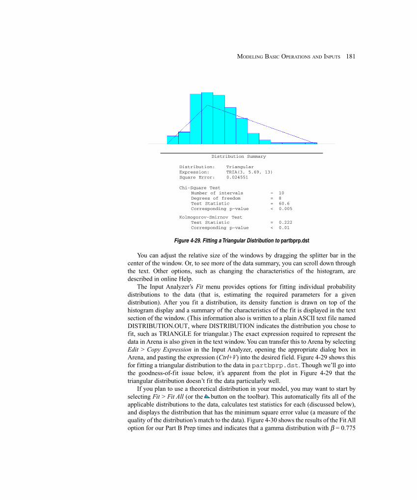
181MODELING BASIC OPERATIONS AND INPUTS
Distribution Summary
Distribution: TriangularExpression: TRIA(3, 5.69, 13)Square Error: 0.024551
Chi-Square TestNumber of intervals = 10Degrees of freedom = 8Test Statistic = 60.6Corresponding p-value < 0.005
Kolmogorov-Smirnov TestTest Statistic = 0.222Corresponding p-value < 0.01
Figure 4-29. Fitting a Triangular Distribution to partbprp.dst
You can adjust the relative size of the windows by dragging the splitter bar in thecenter of the window. Or, to see more of the data summary, you can scroll down throughthe text. Other options, such as changing the characteristics of the histogram, aredescribed in online Help.
The Input Analyzer’s Fit menu provides options for fitting individual probabilitydistributions to the data (that is, estimating the required parameters for a givendistribution). After you fit a distribution, its density function is drawn on top of thehistogram display and a summary of the characteristics of the fit is displayed in the textsection of the window. (This information also is written to a plain ASCII text file namedDISTRIBUTION.OUT, where DISTRIBUTION indicates the distribution you chose tofit, such as TRIANGLE for triangular.) The exact expression required to represent thedata in Arena is also given in the text window. You can transfer this to Arena by selectingEdit > Copy Expression in the Input Analyzer, opening the appropriate dialog box inArena, and pasting the expression (Ctrl+V) into the desired field. Figure 4-29 shows thisfor fitting a triangular distribution to the data in partbprp.dst. Though we’ll go intothe goodness-of-fit issue below, it’s apparent from the plot in Figure 4-29 that thetriangular distribution doesn’t fit the data particularly well.
If you plan to use a theoretical distribution in your model, you may want to start byselecting Fit > Fit All (or the button on the toolbar). This automatically fits all of theapplicable distributions to the data, calculates test statistics for each (discussed below),and displays the distribution that has the minimum square error value (a measure of thequality of the distribution’s match to the data). Figure 4-30 shows the results of the Fit Alloption for our Part B Prep times and indicates that a gamma distribution with β = 0.775
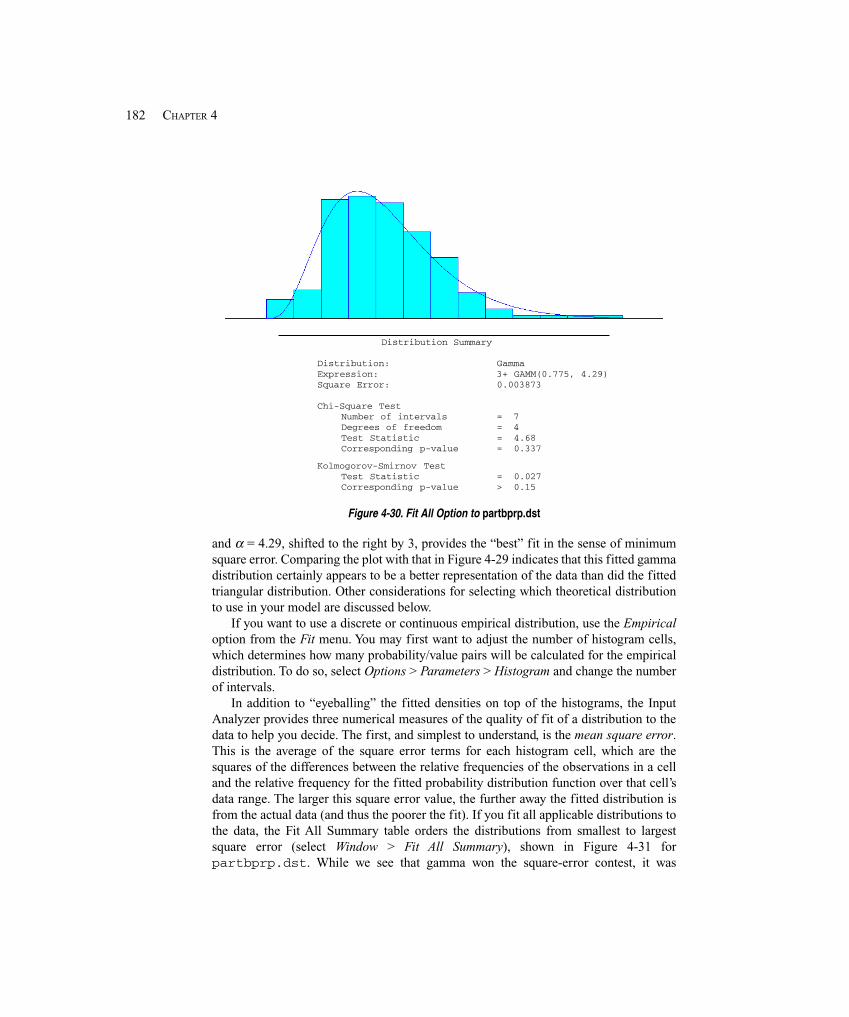
182 CHAPTER 4
Distribution Summary
Distribution: GammaExpression: 3+ GAMM(0.775, 4.29)Square Error: 0.003873
Chi-Square TestNumber of intervals = 7Degrees of freedom = 4Test Statistic = 4.68Corresponding p-value = 0.337
Kolmogorov-Smirnov TestTest Statistic = 0.027Corresponding p-value > 0.15
Figure 4-30. Fit All Option to partbprp.dst
and α = 4.29, shifted to the right by 3, provides the “best” fit in the sense of minimumsquare error. Comparing the plot with that in Figure 4-29 indicates that this fitted gammadistribution certainly appears to be a better representation of the data than did the fittedtriangular distribution. Other considerations for selecting which theoretical distributionto use in your model are discussed below.
If you want to use a discrete or continuous empirical distribution, use the Empiricaloption from the Fit menu. You may first want to adjust the number of histogram cells,which determines how many probability/value pairs will be calculated for the empiricaldistribution. To do so, select Options > Parameters > Histogram and change the numberof intervals.
In addition to “eyeballing” the fitted densities on top of the histograms, the InputAnalyzer provides three numerical measures of the quality of fit of a distribution to thedata to help you decide. The first, and simplest to understand, is the mean square error.This is the average of the square error terms for each histogram cell, which are thesquares of the differences between the relative frequencies of the observations in a celland the relative frequency for the fitted probability distribution function over that cell’sdata range. The larger this square error value, the further away the fitted distribution isfrom the actual data (and thus the poorer the fit). If you fit all applicable distributions tothe data, the Fit All Summary table orders the distributions from smallest to largestsquare error (select Window > Fit All Summary), shown in Figure 4-31 forpartbprp.dst. While we see that gamma won the square-error contest, it was

183MODELING BASIC OPERATIONS AND INPUTS
Function Sq ErrorGamma 0.00387Weibull 0.00443Beta 0.00444Erlang 0.00487Normal 0.00633Lognormal 0.00871Triangular 0.0246Uniform 0.0773Exponential 0.0806
Figure 4-31. Fit All Summary for partbprp.dst
followed closely by Weibull, beta, and Erlang, any of which would probably be just asaccurate as gamma to use as input to the model.
The other two measures of a distribution’s fit to the data are the chi-square andKolmogorov-Smirnov (K-S) goodness-of-fit hypothesis tests. These are standardstatistical hypothesis tests that can be used to assess whether a fitted theoreticaldistribution is a good fit to the data. The Input Analyzer reports information about thetests in the text window (see the bottoms of Figures 4-29 and 4-30). Of particular interestis the Corresponding p-value, which will always fall between 0 and 1.4 To interpret this,larger p-values indicate better fits. Corresponding p-values less than about 0.05 indicatethat the distribution’s not a very good fit. Of course, as with any statistical hypothesistest, a high p-value doesn’t constitute “proof ” of a good fit—just a lack of evidenceagainst the fit.
When it comes down to fitting or choosing a distribution to use, there’s no rigorous,universally agreed-upon approach that you can employ to pick the “best” distribution.Different statistical tests (such as the K-S and chi-square) might rank distributions differ-ently, or changes in the preparation of the data (e.g., the number of histogram cells)might reorder how well the distributions fit.
Your first critical decision is whether to use a theoretical distribution or an empiricalone. Examining the results of the K-S and chi-square tests can be helpful. If the p-valuesfor one or more distributions are fairly high (e.g., 0.10 or greater), then you can use atheoretical distribution and have a fair degree of confidence that you’re getting a goodrepresentation of the data (unless your sample is quite small, in which case the discrimina-tory power of goodness-of-fit tests is quite weak). If the p-values are low, you may want touse an empirical distribution to do a better job capturing the characteristics of the data.
If you’ve decided to use a theoretical distribution, there often will be a number ofthem with very close goodness-of-fit statistics. In this case, other issues may be worthconsidering for selecting among them:
� First of all, you may want to limit yourself to considering only bounded orunbounded distributions, based on your understanding of how the data will beused in your model. For instance, often the triangular (bounded) and normal
4 More precisely, the p-value is the probability of getting a data set that’s more inconsistent with the fitteddistribution than the data set you actually got, if the fitted distribution is truly “the truth.”
184 CHAPTER 4
(unbounded) distributions will be good fits to data such as process times. Over along simulation run, they each might provide similar results, but during the run,the normal distribution might periodically return fairly large values that might notpractically occur in the real system. A normal distribution with a mean that’sclose to zero may return an artificially large number of zero-valued samples if thedistribution’s being used for something that can’t be negative, such as a time(Arena will change all negative input values to zero if they occur in a contextwhere negative values don’t make sense, like an interarrival or process time); thismight be a compelling reason to avoid the normal distribution to representquantities like process times that cannot be negative. On the other hand, boundingthe triangular to obtain a faithful overall representation of the data might excludea few outlying values that should be captured in the simulation model.
� Another consideration is of a more practical nature; namely, that it’s easier toadjust parameters of some distributions than of others. If you’re planning to makeany changes to your model that include adjusting the parameters of thedistribution (e.g., for sensitivity analysis or to analyze different scenarios), youmight favor those with more easily understood parameters. For example, inrepresenting interarrival times, Weibull and exponential distributions mightprovide fits of similar quality, but it’s much easier to change an interarrival-timemean by adjusting an exponential mean than by changing the parameters of aWeibull distribution since the mean in the latter case is a complicated function ofthe parameters.
� If you’re concerned about whether you’re making the correct choice, run themodel with each of your options to see if there’s a significant difference in theresults (you may have to wait until the model’s nearly complete to be able to drawa good conclusion). You can further investigate the factors affecting distributionfits (such as the goodness-of-fit tests) by consulting Arena’s online Help or othersources, such as Pegden, Shannon, and Sadowski (1995) or Law and Kelton(2000). Otherwise, select a distribution based on the qualitative and practicalissues discussed above.
Before leaving our discussion of the Input Analyzer, we’d like to revisit an issue wementioned earlier, namely, what to do if your data appear to have multiple peaks orperhaps a few extreme values, sometimes called outliers. Either of these situations usuallymakes it impossible to get a decent fit from any standard theoretical distribution. As wementioned before, one option is to use an empirical distribution, which is probably the bestroute unless your sample size is quite small. In the case of outliers, you should certainly goback to your data set and make sure that they’re actually correct rather than just beingsome kind of error, perhaps just a typo; if data values appear to be in error and you can’tbacktrack to confirm or correct them, then you should probably just remove them.
In the case of either multiple peaks or (correct) outliers, you might want to considerdividing your data set into two (maybe more) subsets before reading them into the InputAnalyzer. For example, suppose you have data on machine downtimes and notice fromthe histogram that there are two distinct peaks; i.e., the data are bimodal. Reviewing the
185MODELING BASIC OPERATIONS AND INPUTS
original records, you discover that these downtimes resulted from two different situa-tions—breakdowns and scheduled maintenance. Separating the data into two subsetsreveals that downtimes resulting from breakdowns tend to be longer than downtimes dueto scheduled maintenance, explaining the two peaks. You could then separate the data(before going into the Input Analyzer), fit separate distributions to these data sets, andthen modify your model logic to account for both kinds of downtimes.
You can also do a different kind of separation of the data directly in the InputAnalyzer, based purely on their range. After loading the data file, select Options >Parameters > Histogram to specify cutoffs for the Low Value and High Value, and thesecutoffs will then define the bounds of a subset of your entire data set. For bimodal data,you’d focus on the left peak by leaving the Low Value alone and specifying the HighValue as the point where the histogram bottoms out between the two peaks, and laterfocus on the right peak by using this cutpoint as the Low Value and using the originalHigh Value for the entire data set; getting the right cutpoint could require some trial anderror. Then fit whatever distribution seems promising to each subset (or use the Fit Alloption) to represent that range of the data. If you’ve already fit a distribution (or used FitAll) before making Low/High Value cut, the Input Analyzer will immediately re-do thefit(s) and give you the new results for the data subset included in your cut; if you’ve doneFit All, a different distribution form altogether might come up as “the best.” You’d need torepeat this process for each subset of the data. As a practical matter, you probably shouldlimit the number of subsets to two or three since this process can become cumbersome,and it’s probably not obvious where the best cutpoints are. To generate draws in yoursimulation model representing the original entire data set, the idea is to select one of yourdata subsets randomly, with the selection probabilities corresponding to the relative sizesof the subsets, then generate a value from the distribution you decided on for that subset.For instance, if you started out with a bimodal data set of size 200 and set your cutpointso that the smallest 120 points represented the left peak and the largest 80 pointsrepresented the right peak, you’d generate from the distribution fitted to the left part ofthe data with probability 0.6 and generate from the distribution fitted to the right part ofthe data with probability 0.4. This kind of operation isn’t exactly provided automaticallyin a single Arena module, so you’d have to put something together yourself. If the valueinvolved is an activity time like a time delay an entity incurs, one possibility would be touse the Decide module with a Type of 2-way by Chance or N-way by Chance, dependingon whether you have two versus more than two subsets to do a “coin flip” to decide fromwhich subset to generate, then Connect to one of several Assign modules to Assign avalue to an entity attribute as a draw from the appropriate distribution, and use thisattribute downstream for whatever it’s supposed to do. A different approach would be toset up an Arena Expression for the entire thing; Expressions are covered in Section 5.2.3.
4.6.5 No Data?Whether you like it or not, there are times when you just can’t get reliable data on whatyou need for input modeling. This can arise from several situations, like (obviously) thesystem doesn’t exist, data collection is too expensive or disruptive, or maybe you don’thave the cooperation or clearance you need. In this case, you’ll have to rely on some
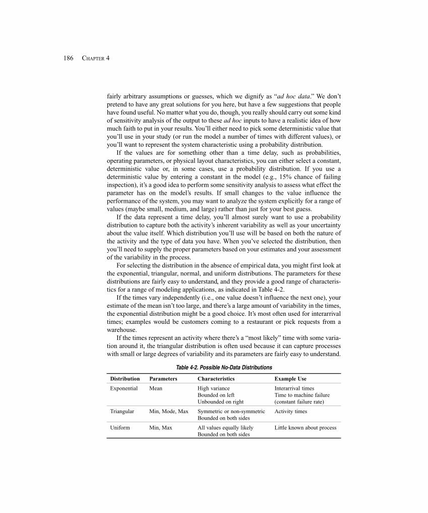
186 CHAPTER 4
fairly arbitrary assumptions or guesses, which we dignify as “ad hoc data.” We don’tpretend to have any great solutions for you here, but have a few suggestions that peoplehave found useful. No matter what you do, though, you really should carry out some kindof sensitivity analysis of the output to these ad hoc inputs to have a realistic idea of howmuch faith to put in your results. You’ll either need to pick some deterministic value thatyou’ll use in your study (or run the model a number of times with different values), oryou’ll want to represent the system characteristic using a probability distribution.
If the values are for something other than a time delay, such as probabilities,operating parameters, or physical layout characteristics, you can either select a constant,deterministic value or, in some cases, use a probability distribution. If you use adeterministic value by entering a constant in the model (e.g., 15% chance of failinginspection), it’s a good idea to perform some sensitivity analysis to assess what effect theparameter has on the model’s results. If small changes to the value influence theperformance of the system, you may want to analyze the system explicitly for a range ofvalues (maybe small, medium, and large) rather than just for your best guess.
If the data represent a time delay, you’ll almost surely want to use a probabilitydistribution to capture both the activity’s inherent variability as well as your uncertaintyabout the value itself. Which distribution you’ll use will be based on both the nature ofthe activity and the type of data you have. When you’ve selected the distribution, thenyou’ll need to supply the proper parameters based on your estimates and your assessmentof the variability in the process.
For selecting the distribution in the absence of empirical data, you might first look atthe exponential, triangular, normal, and uniform distributions. The parameters for thesedistributions are fairly easy to understand, and they provide a good range of characteris-tics for a range of modeling applications, as indicated in Table 4-2.
If the times vary independently (i.e., one value doesn’t influence the next one), yourestimate of the mean isn’t too large, and there’s a large amount of variability in the times,the exponential distribution might be a good choice. It’s most often used for interarrivaltimes; examples would be customers coming to a restaurant or pick requests from awarehouse.
If the times represent an activity where there’s a “most likely” time with some varia-tion around it, the triangular distribution is often used because it can capture processeswith small or large degrees of variability and its parameters are fairly easy to understand.
Table 4-2. Possible No-Data Distributions
Distribution Parameters Characteristics Example Use
Exponential Mean High variance Interarrival timesBounded on left Time to machine failureUnbounded on right (constant failure rate)
Triangular Min, Mode, Max Symmetric or non-symmetric Activity timesBounded on both sides
Uniform Min, Max All values equally likely Little known about processBounded on both sides
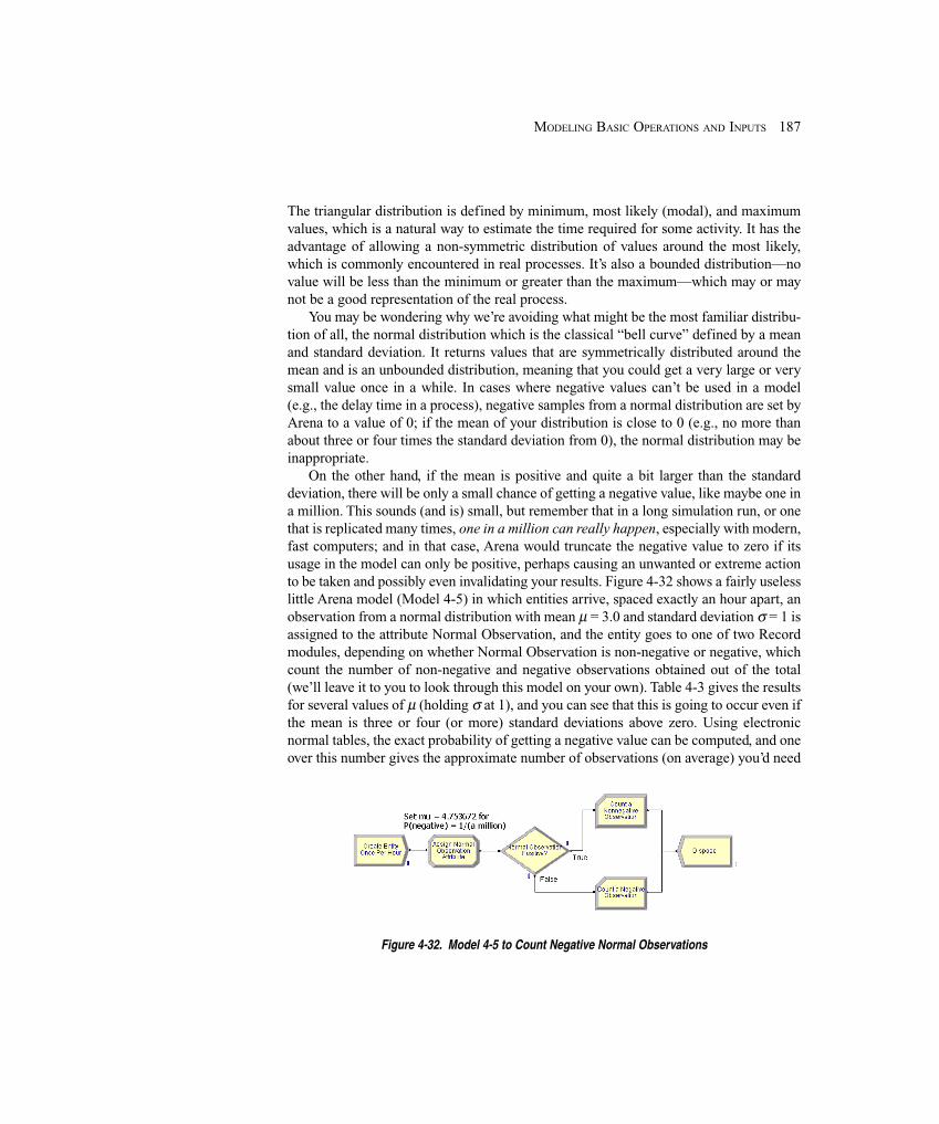
187MODELING BASIC OPERATIONS AND INPUTS
The triangular distribution is defined by minimum, most likely (modal), and maximumvalues, which is a natural way to estimate the time required for some activity. It has theadvantage of allowing a non-symmetric distribution of values around the most likely,which is commonly encountered in real processes. It’s also a bounded distribution—novalue will be less than the minimum or greater than the maximum—which may or maynot be a good representation of the real process.
You may be wondering why we’re avoiding what might be the most familiar distribu-tion of all, the normal distribution which is the classical “bell curve” defined by a meanand standard deviation. It returns values that are symmetrically distributed around themean and is an unbounded distribution, meaning that you could get a very large or verysmall value once in a while. In cases where negative values can’t be used in a model(e.g., the delay time in a process), negative samples from a normal distribution are set byArena to a value of 0; if the mean of your distribution is close to 0 (e.g., no more thanabout three or four times the standard deviation from 0), the normal distribution may beinappropriate.
On the other hand, if the mean is positive and quite a bit larger than the standarddeviation, there will be only a small chance of getting a negative value, like maybe one ina million. This sounds (and is) small, but remember that in a long simulation run, or onethat is replicated many times, one in a million can really happen, especially with modern,fast computers; and in that case, Arena would truncate the negative value to zero if itsusage in the model can only be positive, perhaps causing an unwanted or extreme actionto be taken and possibly even invalidating your results. Figure 4-32 shows a fairly uselesslittle Arena model (Model 4-5) in which entities arrive, spaced exactly an hour apart, anobservation from a normal distribution with mean μ = 3.0 and standard deviation σ = 1 isassigned to the attribute Normal Observation, and the entity goes to one of two Recordmodules, depending on whether Normal Observation is non-negative or negative, whichcount the number of non-negative and negative observations obtained out of the total(we’ll leave it to you to look through this model on your own). Table 4-3 gives the resultsfor several values of μ (holding σ at 1), and you can see that this is going to occur even ifthe mean is three or four (or more) standard deviations above zero. Using electronicnormal tables, the exact probability of getting a negative value can be computed, and oneover this number gives the approximate number of observations (on average) you’d need
Figure 4-32. Model 4-5 to Count Negative Normal Observations
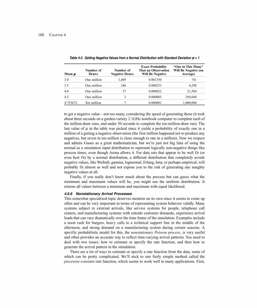
188 CHAPTER 4
Table 4-3. Getting Negative Values from a Normal Distribution with Standard Deviation σσσσσ = 1
Exact Probability “One in This Many”Number of Number of That an Observation Will Be Negative (on
Mean μμμμμ Draws Negative Draws Will Be Negative Average)
3.0 One million 1,409 0.001350 741
3.5 One million 246 0.000233 4,298
4.0 One million 37 0.000032 31,560
4.5 One million 3 0.000003 294,048
4.753672 Ten million 7 0.000001 1,000,000
to get a negative value—not too many, considering the speed of generating these (it tookabout three seconds on a garden-variety 2.1GHz notebook computer to complete each ofthe million-draw runs, and under 30 seconds to complete the ten-million-draw run). Thelast value of μ in the table was picked since it yields a probability of exactly one in amillion of a getting a negative observation (the first million happened not to produce anynegatives, but seven in ten million is close enough to one in a million). Now we respectand admire Gauss as a great mathematician, but we’re just not big fans of using thenormal as a simulation input distribution to represent logically non-negative things likeprocess times, even though Arena allows it. For data sets that appear to be well fit (oreven best fit) by a normal distribution, a different distribution that completely avoidsnegative values, like Weibull, gamma, lognormal, Erlang, beta, or perhaps empirical, willprobably fit almost as well and not expose you to the risk of generating any naughtynegative values at all.
Finally, if you really don’t know much about the process but can guess what theminimum and maximum values will be, you might use the uniform distribution. Itreturns all values between a minimum and maximum with equal likelihood.
4.6.6 Nonstationary Arrival ProcessesThis somewhat specialized topic deserves mention on its own since it seems to come upoften and can be very important in terms of representing system behavior validly. Manysystems subject to external arrivals, like service systems for people, telephone callcenters, and manufacturing systems with outside customer demands, experience arrivalloads that can vary dramatically over the time frame of the simulation. Examples includea noon rush for burgers, heavy calls to a technical support line in the middle of theafternoon, and strong demand on a manufacturing system during certain seasons. Aspecific probabilistic model for this, the nonstationary Poisson process, is very usefuland often provides an accurate way to reflect time-varying arrival patterns. You need todeal with two issues: how to estimate or specify the rate function, and then how togenerate the arrival pattern in the simulation.
There are a lot of ways to estimate or specify a rate function from the data, some ofwhich can be pretty complicated. We’ll stick to one fairly simple method called thepiecewise-constant rate function, which seems to work well in many applications. First,
189MODELING BASIC OPERATIONS AND INPUTS
identify lengths of time within which the arrival rate appears to be fairly flat; forinstance, a call center’s arrivals might be fairly constant over half-hour periods but couldbe quite different in different periods. Count up the numbers of arrivals in each period,and then compute a different rate for each period. For instance, suppose the call centerexperiences the following numbers of incoming calls for the four 30-minute periodsbetween 8:00 AM and 10:00 AM: 20, 35, 45, and 50. Then the rates, in units of calls perminute, for the first four 30-minute periods would be 0.67, 1.17, 1.50, and 1.67.
Once you’ve estimated the rate function in this way, you need to make sure that Arenafollows this pattern in generating the arrivals to your model. The Create module will dothis if you select Schedule as the Type for Time Between Arrivals. You then must specifythe rate function via the Schedule data module, similarly to what we did in Section 4.2.2for a Resource Schedule. One caution here: Arena allows you to mix and match whatevertime units you want, but you must be careful that the numbers and time units are definedproperly. We’ll do this in Model 5-2 in Chapter 5. In Chapter 12, we’ll have more to sayabout estimating the rate function, as well as what underlies Arena’s generation methodfor nonstationary arrivals.
4.6.7 Multivariate and Correlated Input DataMost of the time we assume that all random variables driving a simulation are generatedindependently of each other from whatever distribution we decide on to represent them.Sometimes, though, this may not be the best assumption, for purely physical reasons. Forinstance, in Model 4-2 you could imagine that certain parts are “difficult”; maybe you’ddetect this by noticing that a large prep time for a specific part tends to be followed by alarge sealer time for that part; that is, these two times are positively correlated. Ignoringthis correlation could lead to an invalid model and biased results.
There are a number of ways to model situations like this, to estimate the requiredparameters (including the strength of the correlations), and to generate the requiredobservations on the random variables during the simulation. Some of these methodsentail viewing the associated random variables as coordinates of a random vector havingsome joint multivariate distribution to be fitted and generated from. You might also beable to specify some kind of formula-based association between related input quantities.Frankly, though, this is a pretty difficult issue in terms of both estimating the behaviorand generating it during the simulation. For more on these and related issues, see Lawand Kelton (2000) or Devroye (1986).
4.7 Summary and Forecast
If you’ve read and understood the material in this chapter, you should be gettingdangerous in the use of Arena. We encourage you to press other buttons in the moduleswe’ve used and even try modules that we’ve not used. If you get stuck, try the onlineHelp feature, which may not answer your question, but will answer the questions youshould be asking. You might also want to try other animation features or provide nicerpictures. At this point, the best advice we can give you is to use Arena. Chapters 5-12 willcover most of the modeling capabilities (and some of the statistical-analysis capabilities)of Arena in more depth.
190 CHAPTER 4
4.8 Exercises
4-1 Travelers arrive at the main entrance door of an airline terminal according to anexponential interarrival-time distribution with mean 1.6 minutes, with the first arrival attime 0. The travel time from the entrance to the check-in is distributed uniformlybetween 2 and 3 minutes. At the check-in counter, travelers wait in a single line until oneof five agents is available to serve them. The check-in time (in minutes) follows aWeibull distribution with parameters β = 7.78 and α = 3.91. Upon completion of theircheck-in, they are free to travel to their gates. Create a simulation model, with animation(including the travel time from entrance to check-in), of this system. Run the simulationfor 16 hours to determine the average time in system, number of passengers completingcheck-in, and the average length of the check-in queue.
4-2 Develop a model of a simple serial two-process system. Items arrive at the systemwith a mean time between arrivals of 10 minutes, with the first arrival at time 0. They areimmediately sent to Process 1, which has a single resource with a mean service time of9.1 minutes. Upon completion, they are sent to Process 2, which is identical to (but inde-pendent of) Process 1. Items depart the system upon completion of Process 2. Perfor-mance measures of interest are the average numbers in queue at each process and thetotal time in system of items. Using a replication length of 10,000 minutes, make thefollowing four runs and compare the results (noting that the structure of the model isunchanged, and it’s only the input distributions that are changing):
Run 1: exponential interarrival times and exponential service timesRun 2: constant interarrival times and exponential service timesRun 3: exponential interarrival times and constant service timesRun 4: constant interarrival times and constant service times
4-3 Modify the Exercise 4-1 check-in problem by adding agent breaks. The 16 hoursare divided into two 8-hour shifts. Agent breaks are staggered (i.e., one agent goes onbreak, and immediately upon return, the next agent goes on break, until all agents havehad their breaks), starting at 90 minutes into each shift. Each agent is given one 15-minute break. Agent lunch breaks (30 minutes) are also staggered, starting 3.5 hours intoeach shift. The agents are rude and, if they’re busy when break time comes around, theyjust leave anyway and make the passenger wait until break time is over before finishingup that passenger (since all agents are identical, it’s not necessary for the same agent tofinish up that passenger). Compare the results of this model to those of the model with-out agent breaks.
4-4 Two different part types arrive at a facility for processing. Parts of Type 1 arrivewith interarrival times following a lognormal distribution with a log mean of 11.5 hoursand log standard deviation of 2.0 hours (note that these values are the mean and standarddeviation of this lognormal random variable itself); the first arrival is at time 0. Thesearriving parts wait in a queue designated for only Part Type 1’s until a (human) operatoris available to process them (there’s only one such human operator in the facility) and theprocessing times follow a triangular distribution with parameters 5, 6, and 8 hours. Parts
191MODELING BASIC OPERATIONS AND INPUTS
of Type 2 arrive with interarrival times following an exponential distribution with meanof 15.1 hours; the first arrival is at time 0. These parts wait in a second queue (designatedfor Part Type 2’s only) until the same lonely (human) operator is available to processthem; processing times follow a triangular distribution with parameters 3, 7, and 8 hours.After being processed by the human operator, all parts are sent for processing to anautomatic machine not requiring a human operator, which has processing timesdistributed as triangular with parameters of 4, 6, and 8 hours for both part types; all partsshare the same first-come, first-served queue for this automatic machine. Completedparts exit the system. Assume that the times for all part transfers are negligible. Run thesimulation for 5,000 hours to determine the average total time in system (sometimescalled cycle time) for all parts (lumped together regardless of type), and the averagenumber of items in the queues designated for the arriving parts. Animate your model,including use of different pictures for the different part types, and use resources that lookdifferent for busy vs. idle.
4-5 During the verification process of the airline check-in system from Exercise 4-3, itwas discovered that there were really two types of passengers. The first passenger typearrives according to an exponential interarrival distribution with mean 2.41 minutes andhas a service time (in minutes) following a gamma distribution with parameters β = 0.42and α = 14.4. The second type of passenger arrives according to an exponential distribu-tion with mean 4.4 minutes and has a service time (in minutes) following 3 plus an Erlangdistribution with parameters ExpMean = 0.54 and k = 15 (i.e., the Expression for the ser-vice time is 3 + ERLA(0.54, 15 )). A passenger of each type arrives at time 0. Modify themodel from Exercise 4-3 to include this new information. Compare the results.
4-6 Parts arrive at a single workstation system according to an exponential interarrivaldistribution with mean 21.5 seconds; the first arrival is at time 0. Upon arrival, the partsare initially processed. The processing-time distribution is TRIA(16, 19, 22) seconds.There are several easily identifiable visual characteristics that determine whether a parthas a potential quality problem. These parts, about 10% (determined after the initial pro-cessing), are sent to a station where they undergo a thorough inspection. The remainingparts are considered good and are sent out of the system. The inspection-time distributionis 95 plus a WEIB(48.5, 4.04) random variable, in seconds. About 14% of these parts failthe inspection and are sent to scrap. The parts that pass the inspection are classified asgood and are sent out of the system (so these parts didn’t need the thorough inspection,but you know what they say about hindsight). Run the simulation for 10,000 seconds toobserve the number of good parts that exit the system, the number of scrapped parts, andthe number of parts that received the thorough inspection. Animate your model.
4-7 A proposed production system consists of five serial automatic workstations. Theprocessing times at each workstation are constant: 11, 10, 11, 11, and 12 (all times givenin this problem are in minutes). The part interarrival times are UNIF(13.0, 15.1). There isan unlimited buffer in front of all workstations, and we will assume that all transfer timesare negligible or zero. The unique aspect of this system is that at Workstations 2 through5 there is a chance that the part will need to be reprocessed by the workstation that
192 CHAPTER 4
precedes it. For example, after completion at Workstation 2, the part can be sent back tothe queue in front of Workstation 1. The probability of revisiting a workstation is inde-pendent in that the same part could be sent back many times with no change in theprobability. At present, it is estimated that this probability, the same for all four worksta-tions, will be between 5% and 10%. Develop the simulation model and make six runs of10,000 minutes each for probabilities of 5, 6, 7, 8, 9, and 10%. Using the results, con-struct a table (put this table inside your .doe file using an Arena Text box) of the averagecycle time (system time) against the probability of a revisit. Also include the maximumcycle time for each run in your table.
4-8 A production system consists of four serial automatic workstations. The first partarrives at time zero, and then (exactly) every 9.8 minutes thereafter. All transfer times areassumed to be zero and all processing times are constant. There are two types of failures:major and jams. The data for this system are given in the table below (all times are inminutes). Use exponential distributions for the uptimes and uniform distributions for re-pair times (for instance, repairing jams at Workstation 3 is UNIF(2.8, 4.2)). Run yoursimulation for 10,000 minutes to determine the percent of time each resource spends inthe failure state and the ending status of each workstation queue.
Workstation Major Failure Means Jam MeansNumber Process Time Uptimes Repair Uptimes Repair
1 8.5 475 20, 30 47.6 2, 32 8.3 570 24, 36 57 2.4, 3.63 8.6 665 28, 42 66.5 2.8, 4.24 8.6 475 20, 30 47.5 2, 3
4-9 An office that dispenses automotive license plates has divided its customers intocategories to level the office workload. Customers arrive and enter one of three linesbased on their residence location. Model this arrival activity as three independent arrivalstreams using an exponential interarrival distribution with mean 10 minutes for eachstream, and an arrival at time 0 for each stream. Each customer type is assigned a single,separate clerk to process the application forms and accept payment, with a separatequeue for each. The service time is UNIF(8, 10) minutes for all customer types. Aftercompletion of this step, all customers are sent to a single, second clerk who checks theforms and issues the plates (this clerk serves all three customer types, who merge into asingle first-come, first-served queue for this clerk). The service time for this activity isUNIF(2.65, 3.33) minutes for all customer types. Develop a model of this system andrun it for 5,000 minutes; observe the average and maximum time in system for allcustomer types combined.
A consultant has recommended that the office not differentiate between customers atthe first stage and use a single line with three clerks who can process any customer type.Develop a model of this system, run it for 5,000 minutes, and compare the results withthose from the first system.
193MODELING BASIC OPERATIONS AND INPUTS
4-10 Customers arrive at an order counter with exponential interarrivals with a mean of10 minutes; the first customer arrives at time 0. A single clerk accepts and checks theirorders and processes payments, taking UNIF(7.9, 10) minutes. Upon completion of thisactivity, orders are randomly assigned to one of two available stock persons (each stockperson has a 50% chance of getting any individual assignment) who retrieve the ordersfor the customers, taking UNIF(16, 20) minutes. These stock persons only retrieve ordersfor customers who have been assigned specifically to them. Upon receiving their orders,the customers depart the system. Develop a model of this system and run the simulationfor 5,000 minutes, observing the average and maximum customer time in system.
A bright, young engineer has recommend that they eliminate the assignment of anorder to a specific stock person and allow both stock persons to select their next activityfrom a single first-come, first-served order queue. Develop a model of this system, run itfor 5,000 minutes, and compare the results to the first system.
4-11 Using the model from Exercise 4-2, set the interarrival-time distribution toexponential and the process-time distribution for each Process to uniform on theinterval [9 – h, 9 + h]. Setting the value of h to 1.732, 3.464, and 5.196, compute the(exact) variance of this distribution and make three different runs of 100,000 minuteseach and compare the results. Note that the mean of the process time is always 9 and thedistribution form is always the same (uniform); the standard deviation (and thus thevariance) is the only thing that’s changing.
4-12 Using the model from Exercise 4-11, assume the process time has a mean of 9 anda variance of 4. Calculate the parameters for the gamma distribution that will give thesevalues. Make a 100,000-minute run and compare the results with those from the h =3.464 case of Exercise 4-11. Note that here both the mean and the variance are thesame—it’s only the shape of the distribution that differs.
4-13 Parts arrive at a single machine system according to an exponential interarrivaldistribution with mean 20 minutes; the first part arrives at time 0. Upon arrival, the partsare processed at a machine. The processing-time distribution is TRIA(11, 16, 18)minutes. The parts are inspected and about 24% are sent back to the same machine to bereprocessed (same processing time). Run the simulation for 20,000 minutes to observethe average and maximum number of times a part is processed, the average number ofparts in the machine queue, and the average part cycle time (time from a part’s entry tothe system to its exit after however many passes through the machine system arerequired).
4-14 Using the model from Exercise 4-13, make two additional runs with run times of60,000 minutes and 100,000 minutes and compare the results with those of Exercise 4-13.
4-15 Items arrive from an inventory-picking system according to an exponentialinterarrival distribution with mean 1.1 (all times are in minutes), with the first arrival attime 0. Upon arrival, the items are packed by one of four identical packers, with a singlequeue “feeding” all four packers. The packing time is TRIA(2.75, 3.3, 4.0). Packedboxes are then separated by type (20%, international and 80%, domestic), and sent to
194 CHAPTER 4
shipping. There is a single shipper for international packages and two shippers fordomestic packages with a single queue feeding the two domestic shippers. The interna-tional shipping time is TRIA(2.2, 3.3, 4.8), and the domestic shipping time is TRIA(1.7,2.0, 2.7). This packing system works three 8-hour shifts, five days a week. All the pack-ers and shippers are given a 15-minute break two hours into their shift, a 30-minute lunchbreak four hours into their shift, and a second 15-minute break six hours into their shift;use the Wait Schedule Rule. Run the simulation for two weeks (ten working days) todetermine the average and maximum number of items or boxes in each of the threequeues. Animate your model, including a change in the appearance of entities afterthey’re packed into a box.
4-16 Using the model from Exercise 4-15, change the packer and domestic shipperschedules to stagger the breaks so there are always at least three packers and one domesticshipper working. Start the first 15-minute packer break one hour into the shift, the30-minute lunch break three hours into the shift, and the second 15-minute break sixhours into the shift. Start the first domestic shipper 15-minute break 90 minutes into theshift, the 30-minute lunch break 3.5 hours into the shift, and the second 15-minute breaksix hours into the shift. Compare the new results to those from Exercise 4-15.
4-17 Using the Input Analyzer, open a new window and generate a new data file (useFile > Data File > Generate New) containing 50 points for an Erlang distribution withparameters: ExpMean equal to 12, k equal to 3, and Offset equal to 5. Once you have thedata file, perform a Fit All to find the “best” fit from among the available distributions.Repeat this process for 500, 5,000, and 25,000 data points, using the same Erlang param-eters. Compare the results of the Fit All for the four different sample sizes.
4-18 Hungry’s Fine Fast Foods is interested in looking at their staffing for the lunchrush, running from 10 AM to 2 PM. People arrive as walk-ins, by car, or on a (roughly)scheduled bus, as follows:
� Walk-ins—one at a time, interarrivals are exponential with mean 3 minutes; thefirst walk-in occurs EXPO(3) minutes past 10 AM.
� By car—with 1, 2, 3, or 4 people to a car with respective probabilities 0.2, 0.3,0.3, and 0.2; interarrivals distributed as exponential with mean 5 minutes; thefirst car arrives EXPO(5) minutes past 10 AM.
� A single bus arrives every day sometime between 11 AM and 1 PM (arrival timedistributed uniformly over this period). The number of people on the bus variesfrom day to day, but it appears to follow a Poisson distribution with a mean of 30people.
Once people arrive, either alone or in a group from any source, they operateindependently regardless of their source. The first stop is with one of the servers at theorder/payment counter, where ordering takes TRIA(1, 2, 4) minutes and payment thentakes TRIA(1, 2, 3) minutes; these two operations are sequential, first order-taking thenpayment, by the same server for a given customer. The next stop is to pick up the foodordered, which takes an amount of time distributed uniformly between 30 seconds and
195MODELING BASIC OPERATIONS AND INPUTS
2 minutes. Then each customer goes to the dining room, which has 30 seats (people arewilling to sit anywhere, not necessarily with their group), and partakes of the sublimevictuals, taking an enjoyable TRIA(11, 20, 31) minutes. After that, the customer walksfulfilled to the door and leaves. Queueing at each of the three “service” stations (order/pay, pickup food, and dining room) is allowed, with FIFO discipline. There is a traveltime of EXPO(30) seconds from each station to all but the exit door—entry to order/pay,order/pay to pickup food, and pickup food to dining. After eating, people move moreslowly, so the travel time from the dining room to the exit is EXPO(1) minute.
The servers at both order/pay and pickup food have a single break that they “share”on a rotating basis. More specifically, at 10:50, 11:50, 12:50, and 1:50, one server fromeach station goes on a 10-minute break; if the person due to go on break at a station isbusy at break time, he or she finishes serving the customer but still has to be back at thetop of the hour (so the break could be a little shorter than 10 minutes).
Staffing is the main issue facing Hungry’s. Currently, there are six servers at theorder/pay station and two at the pickup food station throughout the 4-hour period. Sincethey know that the bus arrives sometime during the middle two hours, they’re consider-ing a variable staffing plan that, for the first and last hour would have three at order/payand one at pickup food, and for the middle two hours would have nine at order/pay andthree at pickup food (note that the total number of person-hours on the payroll is thesame, 32, under either the current staffing plan or the alternate plan, so the payroll cost isthe same). What’s your advice?
In terms of output, observe the average and maximum length of each queue, theaverage and maximum time in each queue, and the total number of customers completelyserved and out the door. Make plots of the queues to get into order/pay, pickup food, andthe dining room. Animate all queues, resources, and movements between stations. Pickfrom a .plb picture library a humanoid picture for the entities (different for each arrivalsource), and make an appropriate change to their appearance after they’ve finishedeating and leave the dining room. Also, while you won’t be able to animate the individualservers or seats in the dining room, pick reasonable pictures for them as well.
4-19 In the discussion in Section 4.2.5 of Arena’s Instantaneous Utilization vs. Sched-uled Utilization output values, we stated that if the Resource has a fixed Capacity (say,M(t) = c > 0 for all times t), then Instantaneous Utilization and Scheduled Utilization willbe the same. Prove this.
4-20 In the discussion in Section 4.2.5 of Arena’s Instantaneous Utilization vs.Scheduled Utilization output values, we stated that neither of the two measures is alwayslarger. Prove this; recall that to prove that a general statement is not true you only have tocome up with a single example (called a counterexample) for which it’s not true.
4-21 Modify your solution for Exercise 4-7 to include transfer times between partarrival and the first workstation, between workstations (both going forward and forreprocessing), and between the last workstation and the system exit. Assume all parttransfer times are UNIF(2,5). Animate your model to show entity movement and run for10,000 minutes using a reprocess probability of 8%.

196 CHAPTER 4
4-22 Management wants to study Terminal 3 at a hub airport with an eventual eyetoward improvement. The first step is to model it as it is during the eight hours throughthe busiest part of a typical weekday. We’ll model the check-in and security operationsonly, i.e., once passengers get through security they’re on their way to their gate and outof our model. Passengers arrive one at a time through the front door from curbsideground transportation with interarrival times distributed exponentially with mean 0.5minute (all times are in minutes unless otherwise noted). Of these passengers, 35% goleft to an old-fashioned manual check-in counter, 50% go right to a newfangledautomated check-in counter, and the remaining 15% don’t need to check in at all andproceed directly from the front door to security (it takes these latter types of passengersbetween 3 and 5 minutes, uniformly distributed, to make the walk from the front door tothe entrance to the security area; the other two passenger types move instantly fromtheir arrival to the manual or automated check-in counter as the case may be). There aretwo agents at the manual check-in station, fed by a single FIFO queue; manual check-intimes follow a triangular distribution between 1 and 5 minutes with a mode of 2minutes. After manual check-in, passengers walk to the security area, a stroll that takesthem between 2 and 5.8 minutes, uniformly distributed. The automated check-in hastwo stations (a station consists of a touch-screen kiosk and an employee to take checkedbags; view a kiosk-employee pair as a single unified unit, i.e., the kiosk and itsemployee cannot be separated), fed by a single FIFO queue, and check-in times aretriangularly distributed between 0.5 and 1.5 with a mode of 1. After automated check-in, passengers walk to the security area, taking between 1 and 3 minutes, uniformlydistributed, to get there (automated check-in passengers are just quicker than manualcheck-in passengers at everything). All passengers eventually get to the security area,where there are six stations fed by a single FIFO queue; security-check times aretriangularly distributed between 1 and 6 with a mode of 2 (this distribution captures allthe possibilities there, like x-ray of carry-ons, walking through the metal detector, bagsearch, body wanding, shoes off, laptop checking, etc.). Once through the securitycheck (everybody passes, though it takes some longer than others to do so), passengershead to their gates and are no longer in our model. Simulate this system for an 8-hourperiod and look at the average queue lengths, average times in queue, resourceutilizations, and average total time in system of passengers (for all passenger typescombined). Animate your model, including queues, resources, and passengers walkingto security. Put in plots that track the length of each of the three queues over the eight-hour simulation (either three separate plots or three curves in a single plot).
4-23 Modify Model 4-1 to include a packing operation for “shipped” parts (those thatpass the initial inspection and don’t need rework) before they exit the system; don’t countparts as having left the system until they’re packed. Packing takes between 2 and 4 min-utes, distributed (continuously) uniformly, and there’s a single packer named Brett to dothis. Also, add a similar but separate packing operation for “salvaged” parts, where thepacking-time distribution is the same and there’s a separate packer named AJ for these.Leave the run conditions the same as for Model 4-1. In addition, collect statistics on en-tities and compare the total system time (for both part types) between the two models.

197MODELING BASIC OPERATIONS AND INPUTS
4-24 In the results from Exercise 4-23, you might have noticed that AJ doesn’t havemuch to do. So say goodbye to him, and send salvaged parts to Brett for packing, alongwith the shipped parts. Both types of parts have the same priority for Brett, but they re-side in separate queues. (HINT: It’s okay in Arena to have multiple places where entitiesare trying to seize on the same resource.) Compare the results to those obtained fromExercise 4-23.
4-25 Compare the results for Model 4-1, Exercise 4-23, and Exercise 4-24, looking atthe total times in system of the three different exit possibilities (shipped, salvaged, andscrapped). In an attempt to make the comparison more statistically meaningful, make100 replications of each. Make a table or graph summarizing your results, and discusswith respect to the relative structures of these three models. What suggestions would youhave for further investigation of these differences?
4-26 Modify Model 4-1 so that, in both inspections, only half of what had failed beforenow really fail, and the others have returned for a re-do and the preceding operation (i.e.,to the Sealer and Rework for the first and second inspections, respectively). The re-doneparts still have to be re-inspected with the same probabilities for what happens to themthere as for parts arriving there for the first time. There’s no limit on the number of re-dosin either place. (HINT: Explore the Help topic in the Decide modules and think about athree-sided coin.) Compare the results (making 100 replications) to Model 4-1, lookingat the total times in system of the three different exit possibilities (shipped, salvaged, andscrapped).
4-27 An acute-care facility treats non-emergency patients (cuts, colds, etc.). Patients ar-rive according to an exponential interarrival-time distribution with a mean of 11 (alltimes are in minutes). Upon arrival they check in at a registration desk staffed by a singlenurse. Registration times follow a triangular distribution with parameters 6, 10, and 19.After completing registration, they wait for an available examination room; there arethree identical rooms. Data show that patients can be divided into two groups with regardto different examination times. The first group (55% of patients) has service times thatfollow a triangular distribution with parameters 14, 22, and 39. The second group (45%)has triangular service times with parameters 24, 36, and 59. Upon completion, patientsare sent home. The facility is open 16 hours each day. Make 200 replications of one dayeach and observe the average total time patients spend in the system.
4-28 Modify your solution from Exercise 4-27 to include lunch breaks for the doctorswho staff the examination rooms. There are three doctors on duty for the first 3.5 hoursof each eight-hour shift. For the next 90 minutes, the doctors take rotating 30-minutelunch breaks, resulting in only two doctors being available at any point during these 90minutes. If all three doctors are busy with patients when the 90-minute lunch periodbegins, they wait until the first patient among the three is done, and that doctor takes thefirst 30-minute lunch break; each doctor gets a full 30-minute lunch, so if the 90-minutelunch period starts a little late, it also ends that much late. After all the lunch breaks end,all three doctors are available until the end of their eight-hour shift, at which point thesecond eight-hour shift begins with the same staffing and lunch (maybe call it dinner)
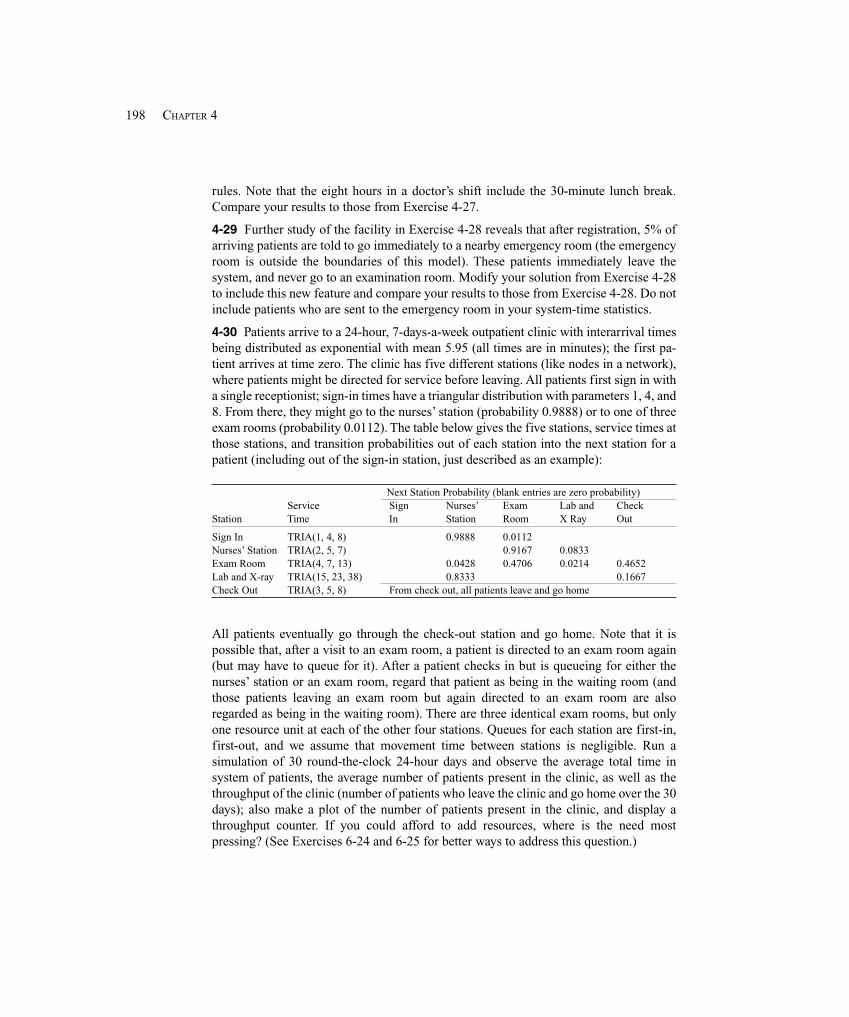
198 CHAPTER 4
rules. Note that the eight hours in a doctor’s shift include the 30-minute lunch break.Compare your results to those from Exercise 4-27.
4-29 Further study of the facility in Exercise 4-28 reveals that after registration, 5% ofarriving patients are told to go immediately to a nearby emergency room (the emergencyroom is outside the boundaries of this model). These patients immediately leave thesystem, and never go to an examination room. Modify your solution from Exercise 4-28to include this new feature and compare your results to those from Exercise 4-28. Do notinclude patients who are sent to the emergency room in your system-time statistics.
4-30 Patients arrive to a 24-hour, 7-days-a-week outpatient clinic with interarrival timesbeing distributed as exponential with mean 5.95 (all times are in minutes); the first pa-tient arrives at time zero. The clinic has five different stations (like nodes in a network),where patients might be directed for service before leaving. All patients first sign in witha single receptionist; sign-in times have a triangular distribution with parameters 1, 4, and8. From there, they might go to the nurses’ station (probability 0.9888) or to one of threeexam rooms (probability 0.0112). The table below gives the five stations, service times atthose stations, and transition probabilities out of each station into the next station for apatient (including out of the sign-in station, just described as an example):
Next Station Probability (blank entries are zero probability)Service Sign Nurses’ Exam Lab and Check
Station Time In Station Room X Ray Out
Sign In TRIA(1, 4, 8) 0.9888 0.0112Nurses’ Station TRIA(2, 5, 7) 0.9167 0.0833Exam Room TRIA(4, 7, 13) 0.0428 0.4706 0.0214 0.4652Lab and X-ray TRIA(15, 23, 38) 0.8333 0.1667Check Out TRIA(3, 5, 8) From check out, all patients leave and go home
All patients eventually go through the check-out station and go home. Note that it ispossible that, after a visit to an exam room, a patient is directed to an exam room again(but may have to queue for it). After a patient checks in but is queueing for either thenurses’ station or an exam room, regard that patient as being in the waiting room (andthose patients leaving an exam room but again directed to an exam room are alsoregarded as being in the waiting room). There are three identical exam rooms, but onlyone resource unit at each of the other four stations. Queues for each station are first-in,first-out, and we assume that movement time between stations is negligible. Run asimulation of 30 round-the-clock 24-hour days and observe the average total time insystem of patients, the average number of patients present in the clinic, as well as thethroughput of the clinic (number of patients who leave the clinic and go home over the 30days); also make a plot of the number of patients present in the clinic, and display athroughput counter. If you could afford to add resources, where is the need mostpressing? (See Exercises 6-24 and 6-25 for better ways to address this question.)

199MODELING BASIC OPERATIONS AND INPUTS
This is a modification of a model developed by Bretthauer and Côté (1998) andBretthauer (2000). The latter does an analytical evaluation and optimization under theassumption that this is a Jackson network of queues, where service times also haveexponential distributions (not triangular or other kinds of distributions). The advantageof simulating instead is that the model can be more general and thus possibly more valid;for instance, we do not have to assume exponential service times if the data suggestotherwise. The disadvantage of simulation is that we do not get exact answers, so wemust do proper statistical analysis of the output (see Chapter 6). (Thanks to ProfessorJim Morris of the University of Wisconsin-Madison for suggesting these papers and thisexercise.)

201MODELING DETAILED OPERATIONS
CHAPTER 5
Modeling Detailed Operations
In Chapter 4, we showed you the kinds of modeling you could do with modules mostlyfrom the Basic Process panel. They are relatively high-level, easy-to-use modules thatwill usually take you a long way toward building a model at a sufficient level of detail.Sometimes it’s all you’ll need.
But sometimes it isn’t. As you gain experience in modeling, and as your modelsbecome bigger, more complex, and more detailed, you might find that you’d like to beable to control or model things at a lower level, in more detail, or just differently fromwhat the modules of the Basic Process panel offer. Arena doesn’t strand you at this levelor force you to accept a limited number of “canned” modeling constructs, nor does itforce you to learn a programming language or some pseudo-programming syntax tocapture complicated system aspects. Rather, it offers a rich and deep hierarchy of severaldifferent modeling levels to get the flexibility you might need to model some specificlogic appropriately. It’s probably a good idea to start with the high-level modules, takethem as far as they’ll go (maybe that’s all the way), and when you need greater flexibilitythan they provide, go to a lower, more detailed level. This structure allows you to exploitthe easy, high-level modeling constructs to the extent possible, yet allows you to drilldown when you need to. And because standard Arena modules provide all of thismodeling power, you’ll be familiar with how to use them. To put them to work, you’llsimply need to become familiar with what they do.
This chapter explores some (certainly not all) of the detailed, lower-level modelingconstructs available in the Advanced Process and Blocks panels; the latter panel providesthe lowest-level model logic where modules correspond to the blocks in the SIMANsimulation language that underlies Arena.
The example we’ll use for this is a telephone call center, including technical support,sales, and order-status checking. Section 5.1 describes the initial system and Section 5.2talks about how to model it using some new Arena modeling concepts. Section 5.3describes our basic modeling strategy. The model logic and animation are developed inSection 5.4. In Section 5.5, we embellish our model and present several new Arenamodeling concepts. We’ll then show you how to modify the original model to create theembellished model. We’ll also touch on the important topics of nonstationary (time-dependent) arrival processes and a greater level of customization in animation. InSection 5.6, we add more output measures to our enhanced model. We close the chapterin Section 5.7 with an altogether different kind of model, an inventory system, and takethe opportunity to illustrate the use of one of Arena’s lowest and most detailed modelinglevels, the Blocks panel that composes the underlying SIMAN simulation language.
After reading this chapter, you should be able to build very detailed and complexmodels and be able to exploit Arena’s rich and deep hierarchy of modeling levels.
202 CHAPTER 5
5.1 Model 5-1: A Simple Call Center System
Our generic call center system provides a central number in an organization thatcustomers call for technical support, sales information, and order status. Incoming callsarrive with interarrival times being exponentially distributed with a mean of 0.857minute. This central number feeds 26 trunk lines. If all 26 lines are in use, a caller gets abusy signal; hopefully, the caller will try again later, but for our model, he just goes away.An answered caller hears a recording describing three options: transfer to technicalsupport, sales information, or order-status inquiry (76%, 16%, and 8%, respectively).The estimated time for this activity is UNIF(0.1, 0.6); all times are in minutes.
If the caller chooses technical support, a second recording requests which of threeproduct types the caller is using, which requires UNIF(0.1, 0.5) minutes. The percentageof requests for product types 1, 2, and 3 are 25%, 34%, and 41%, respectively. If a quali-fied technical support person is available for the selected product type, the call is auto-matically routed to that person. If none are currently available, the customer is placed in anelectronic queue where he is subjected to annoying rock music until a support person isavailable. The time for all technical support calls is estimated to be TRIA(3, 6, 18) minutesregardless of the product type. Upon completion of the call, the customer exits the system.
Sales calls are automatically routed to the sales staff. If a salesperson is not available,the caller is treated to soothing new-age space music (after all, we’re hoping for a sale).Sales calls are estimated to be TRIA(4, 15, 45)—sales people tend to talk a lot more thantechnical support people! Upon completion of the call, the happy customer exits thesystem.
Callers requesting order-status information are automatically handled by the phonesystem, and there is no limit on the number the system can handle (except that there areonly 26 trunk lines, which is itself a limit, since an ongoing order-status call occupies oneof these lines). The estimated time for these transactions is TRIA(2, 3, 4) minutes, with15% of these callers opting to speak to a real person after they have received their orderstatus.
These calls are routed to the sales staff where they wait with a lower priority thansales calls. This means that if an order-status call is in a queue waiting for a salespersonand a new arriving sales call enters, the sales call will be given priority over the order-status call and answered first. These follow-up order-status calls are estimated to lastTRIA(2, 3, 4) minutes. These callers then exit the system.
The call center hours are from 8 AM until 6 PM, with a small proportion of the staff onduty until 7 PM. Although the system closes to new calls at 6 PM, all calls that enter thesystem by that time are answered and served.
Over the course of a day there are eight technical support employees to answertechnical support calls. Two are devoted to product type 1 calls; three, to product type 2calls; and three, to product type 3 calls. There are four sales employees to answer thesales calls and those order-status calls that opt to speak to a real person.
As a point of interest, we’ll count the number of customer calls that are not able to geta trunk line and are thus rejected from entering the system (similar to balking inqueueing systems, though balking usually means a decision on the customer’s part not toenter, rather than being rejected as in our model). However, we won’t consider
203MODELING DETAILED OPERATIONS
reneging—customers who get a trunk line initially but later hang up the phone beforebeing served (see Section 9.3 for a discussion of how to model reneging).
Some statistics of interest for these types of systems are: number of customerrejections (busy signals), total time on the line by customer type, time waiting for a realperson by customer type, number of calls waiting for service by customer type, andpersonnel utilization.
5.2 New Modeling Issues
From a simulation viewpoint, this problem is quite different from the ones we covered inChapters 3 and 4. The most obvious difference is that the previous systems weremanufacturing oriented, and this system is of a service nature. Although the originalversion of SIMAN (the simulation language on which Arena is based) was developed formanufacturing applications, the current Arena capabilities also allow for accuratemodeling of service systems. Applications in this area include fast-food restaurants,banks, insurance companies, service centers, and many others. Although these systemshave some special characteristics, the basic modeling requirements are largely the sameas for manufacturing systems.
Now let’s take a look at our call center and explore the new requirements.
5.2.1 Customer Rejections and BalkingA call generated by our arrival process is really a customer trying to access one of the 26trunk lines. If all 26 lines are currently in use, a busy signal is received and the customeris rejected and departs the system. The term for this is balking if done voluntarily by thecustomer, though in our call center it is involuntary, so we’ll call it a rejection; modelingand handling balking and rejection are similar to each other, however.
Consider a drive-through at a fast-food restaurant that has a single window with roomfor only five cars to wait for service. The arriving entities would be cars entering a queueto wait to seize a resource called “Window Service.” We’d need to set the queue capacityto 5. This would allow one car to be in service and a maximum of five cars to be waiting.If a sixth car attempted to enter the queue, it would balk (or be rejected). You decide aspart of your modeling assumptions what happens to these balked/rejected cars or entities.They might be disposed of or we might assume that they would drive around the blockand try to re-enter the queue a little later.
There are two methods to model balking/rejection in Arena. The first method is toemploy a Queue module from the Blocks panel and define the queue capacity as 0. Anarriving entity (an incoming call in our model) enters the zero-capacity queue and imme-diately attempts to seize one unit of a resource called “Trunk Line.” If a unit is available,it’s allocated to the call and the call enters the system. If a unit of the resource is not avail-able, the entity attempts to stay in the queue. But since the queue has a capacity of 0, thecall would be balked from the queue and disposed. The second method would have thearriving entity use a Decide module to check whether a unit of the “Trunk Line” resourceis available. If a unit is available, the entity is allowed to proceed and seize the resource.If no unit is available, the entity is sent to the balking section of the model. We’ll use thissecond method in our model.
204 CHAPTER 5
Balking and rejection clearly represent a kind of failure of the system to meetcustomer needs, so we’ll count the number of times this happens in the simulation;smaller is better.
5.2.2 Three-Way DecisionsOnce a call is allocated a trunk line and enters the system, we must then determine thecall type so we can direct it to the proper part of the system for service. To do this, weneed the ability to send entities or calls to three different parts of the system based on thegiven probabilities. The same requirement is true for technical calls since there are threedifferent product types.
We could get out our calculator and dust off our probability concepts and computethe probability of each call type—there are a total of five. We could then defineSequences (see Section 7.1) for each of these call types and route them through thesystem. Although this might work, you would have to re-compute the probabilities eachtime you change the distribution of call types, which you might want to do to test theflexibility or robustness of the system.
You may not have been aware of it, but the capability is provided to branch in three ormore directions in the same Decide module that we used in the models of Chapter 4.
5.2.3 Variables and ExpressionsIn many models, we might want to reuse data in several different places. For example, inour call center, there will be several places where we will need to enter the distributionsfor the time to handle the technical support calls. If we decide to change this value duringour experimentation, we’ll have to open each dialog that included a call time and changethe value. There are other situations where we might want to keep track of the totalnumber of entities in a system or in a portion of the system. In other cases, we may wantto use complex expressions throughout the model. For example, we might want to base aprocessing time on the part type. Arena Variables and Expressions allow us to fulfillthese kinds of needs easily.
The Variable module allows you to define your own global variables and their initialvalues. Variables can then be referenced in the model by their names. They can also bespecified as one- or two-dimensional arrays. The Expression module allows you todefine expressions and their associated values. Similar to variables, expressions arereferenced in the model by their names and can also be specified as one- or two-dimensional arrays. Although variables and expressions may appear to be quite similar,they serve distinctly different functions.
User-defined Variables store some real-valued quantity that can be reassigned duringthe simulation run. For example, we could define a Variable called Wait Time with aninitial value of 2 and enter the Variable name wherever a wait time was required. Wecould also define a Variable called Number in System with an initial value of 0, add 1to this variable every time a new part entered the system, and subtract 1 from it everytime a part exited the system. For our call center, we’ll use three variables. The first willkeep track of the number of calls in the system, and the last two will be used to terminatethe generation of incoming calls after ten hours.
205MODELING DETAILED OPERATIONS
User-defined Expressions, on the other hand, don’t store a value. Instead, theyprovide a way of associating a name with some mathematical expression. Whenever thename is referenced in the model, the associated expression is evaluated and its numericalvalue is returned. Typically, expressions are used to compute values from a distributionor from a complex equation based on the entity’s attribute values or even current systemvariable values. If the mathematical expression is used in only one place in the model, itmight be easier to enter it directly where it is required. However, if the expression is usedin several places or the form of the expression to be used depends on an entity attribute, auser-defined expression is often better. For our call center, we’ll use the Expressionmodule to define an expression to generate the technical support times.
Variables and Expressions have many other uses that we hope will become obviousas you become more familiar with Arena.
5.2.4 StoragesStorages are an Arena concept that allow the user to animate the presence of entities thatfall outside the normal animation features that you have seen to this point. Our previousmodels all showed an animated entity in a Queue, on a Resource, or moving along aRoute. Consider an example where you have an entity arrival that initially enters a delaybefore it is allowed to proceed to the next module. If the delay represents a travel timefrom one area of the system to another, you might use the concept of Stations andRoutes. This would allow you to animate the movement of an entity through the system,as we did in Model 4-4. But if during the delay the entity is not moving, we need theStorages concept to animate it.
A Storage holds a non-ordered set of entities that are waiting for an event to occur;e.g., the conclusion of a predefined delay time, the arrival of a requested transporter thatis en route, etc. You might think of a Storage as a variable that we can increment anddecrement with the added feature that we can animate the entities that are in a Storage.Placing an entity in a Storage does not prevent the entity from progressing throughmodel logic. For example, we could place an entity in a Storage, and then show it on theanimation, as it entered a delay, and then continued through the model logic until wedecided to remove it from the Storage at a later point in the model. During the entiretime, the entity would be displayed on the animated Storage.
There are two ways to place an entity in a Storage and then remove it. The first usesthe Store and Unstore modules found in the Advanced Process panel. The second way isto use a module that has a field to enter a Storage ID. An example is the Delay modulefrom the Blocks panel. We’ll show you how to use both methods during our modeldevelopment.
5.2.5 Terminating or Steady-StateMost (not all) simulations can be classified as either terminating or steady-state. This isprimarily an issue of intent or the goal of the study rather than having much to do withinternal model logic or construction.
A terminating simulation is one in which the model dictates specific starting andstopping conditions as a natural reflection of how the target system actually operates. Asthe name suggests, the simulation will terminate according to some model-specified rule
206 CHAPTER 5
or condition. For instance, a store opens at 9 AM with no customers present, closes itsdoors at 9 PM, and then continues operation until all customers are “flushed” out. Anotherexample is a job shop that operates for as long as it takes to produce a “run” of 500completed assemblies specified by the order. The key notion is that the time frame of thesimulation has a well-defined (though possibly unknown at the outset) and natural end,as well as a clearly defined way to start up.
A steady-state simulation, on the other hand, is one in which the quantities to beestimated are defined in the long run; that is, over a theoretically infinite time frame. Inprinciple (though usually not in practice), the initial conditions for the simulation don’tmatter. Of course, a steady-state simulation has to stop at some point, and as you mightguess, these runs can get pretty long, so you need to do something to make sure thatyou’re running it long enough. This is an issue we’ll take up in Section 7.2. For example,a pediatric emergency room never really stops or restarts, so a steady-state simulationmight be appropriate. Sometimes people do a steady-state simulation of a system thatactually terminates in order to design for some kind of worst-case or peak-load situation.
We now have to decide which to do for this call center model. Although we’ll lead youto believe that the distinction between terminating or non-terminating systems is veryclear, that’s seldom the case. Some systems appear at first to be one type, but on closerexamination, they turn out to be the other. This issue is further complicated by the fact thatsome systems have elements of both types, and system classification may depend on thetypes of questions that the analyst needs to address. For example, consider a fast-foodrestaurant that opens at 11 AM and closes at 11 PM. If we were interested in the dailyoperational issues of this restaurant, we’d analyze the system as a terminating system. Ifwe were interested only in the operation during the rush that occurs for two hours overlunch, we might assume a stationary arrival process at the peak arrival rate and analyzethe system as a steady-state system.
Our call center definitely appears to be a terminating system. The system wouldappear to start and end empty and idle, so we’re going to proceed to analyze our callcenter system as a terminating system.
5.3 Modeling Approach
In Figure 1-2 of Chapter 1, we briefly discussed the Arena hierarchical structure. Thisstructure freely allows you to combine the modeling constructs from any level into asingle simulation model. In Chapters 3 and 4, we were able to develop our models usingmostly only the constructs found in the Basic Process panel (yes, we planned it that way),although we did require the Advanced Process panel for our failure and special statistics,and the Advanced Transfer panel for some entity movement.
The general approach that we recommend when you are creating your models is tostay at the highest level possible for as long as you can. However, as soon as you find thatthese high-level constructs don’t allow you to capture the necessary detail, we suggestthat you drop down to the next level for some parts of your model rather than sacrificethe accuracy of the simulation model (of course, there are elements of judgment in thiskind of decision). You can mix modeling constructs from different levels and panels in
207MODELING DETAILED OPERATIONS
the same model. As you become more familiar with the various panels (and modelinglevels), you should find that you’ll do this naturally. Before we proceed, let’s brieflydiscuss the available panels.
The Basic Process panel provides the highest level of modeling. It’s designed to allowyou to create high-level models of most systems quickly and easily. Using a combinationof the Create, Process, Decide, Assign, Record, Batch, Separate, and Dispose modulesallows a great deal of flexibility. In fact, if you look around in these modules, you’ll findmany additional features we haven’t yet discussed. In many cases, these modules alonewill provide all the detail required for a simulation project. These modules providecommon functions required by almost all models, so it’s likely that you’ll use themregardless of your intended level of detail.
The Advanced Process panel augments the Basic Process panel by providingadditional and more detailed modeling capabilities. For example, the sequence ofmodules Seize – Delay – Release provides basically the same fundamental modelinglogic as a Process module, but could afford more flexibility than the Process module. Thehandy feature of the Advanced Process panel modules is that you can put them togetherin almost any combination required for your model. In fact, many experienced modelersstart at this level because they feel that the resulting model is more transparent to theuser, who may or may not be the modeler.
The Advanced Transfer panel provides the modeling constructs for material-handlingactivities (like transporters and conveyors) and entity movement in general. Similar tothe general modeling capabilities provided by the Advanced Process panel, the AdvancedTransfer panel modules give you more flexibility.
The Blocks panel (part of the SIMAN template) provides an even lower level ofmodeling capability. In fact, it provides the basic functionality that was used to create allof the modules found in the Basic Process, Advanced Process, and Advanced Transferpanels. In addition, it provides many other special-purpose modeling constructs notavailable in the higher-level modules. Examples would include “while” loops, combinedprobabilistic and logic branching, and automatic search features. You might note thatseveral of the modules have the same names as those found in the higher-level panels.Although the names are the same, the modules are not. You can distinguish between thetwo by the color and shape.
The difference between the Blocks panel on the one hand and the Basic Process,Advanced Process, and Advanced Transfer panels on the other hand is easy to explain ifyou’ve used SIMAN previously, where you define the model and experiment framesseparately, even though you may do this all in Arena. The difference is perhaps bestillustrated between the Assign modules on the two panels. When you use the BasicProcess panel Assign module, you’re given the option of the type of assignment you wantto make. If you make an assignment to a new attribute, Arena will automatically definethat new attribute and add it to the drop-down lists for attributes everywhere in yourmodel. One reason for staying at the highest level possible is that the Blocks Assignmodule only allows you to make the assignment—it doesn’t define the new attribute.Even with this shortcoming, there are numerous powerful and useful features availableonly in the Blocks panel.
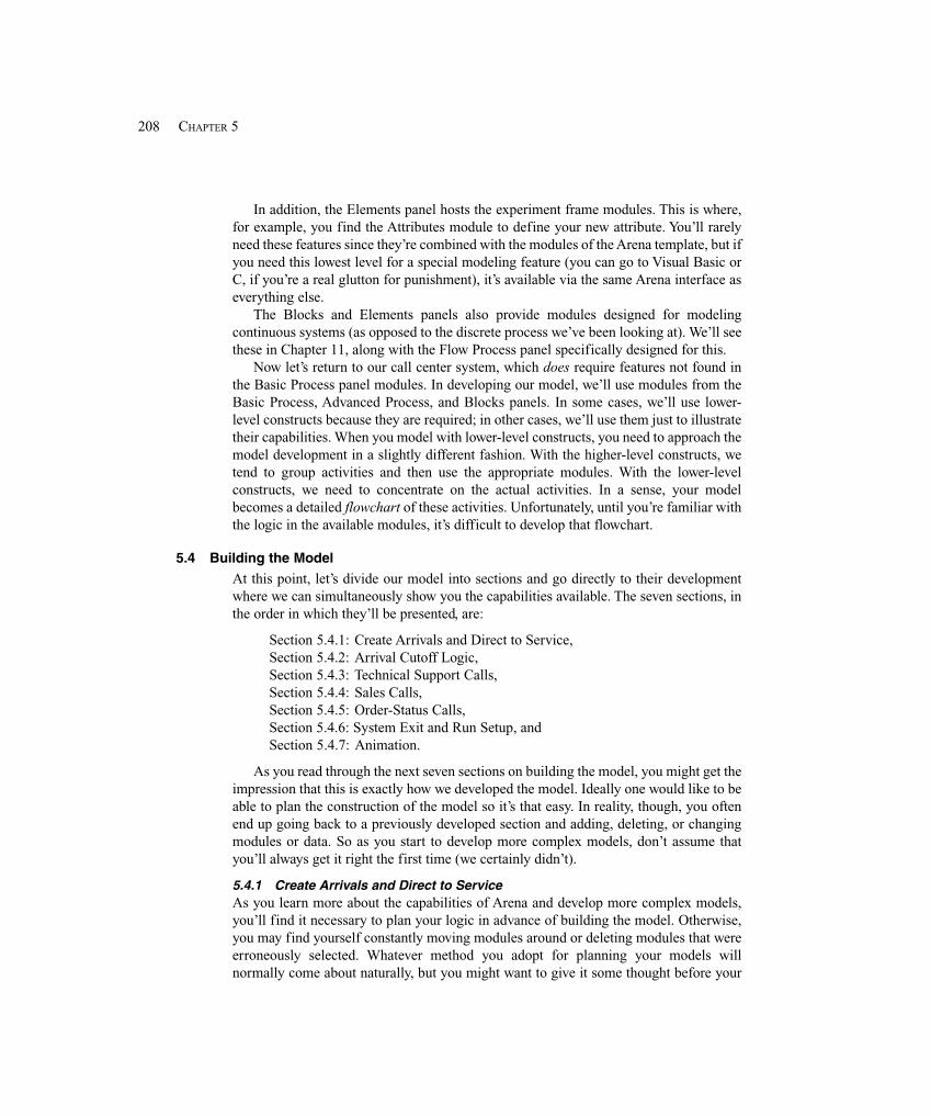
208 CHAPTER 5
In addition, the Elements panel hosts the experiment frame modules. This is where,for example, you find the Attributes module to define your new attribute. You’ll rarelyneed these features since they’re combined with the modules of the Arena template, but ifyou need this lowest level for a special modeling feature (you can go to Visual Basic orC, if you’re a real glutton for punishment), it’s available via the same Arena interface aseverything else.
The Blocks and Elements panels also provide modules designed for modelingcontinuous systems (as opposed to the discrete process we’ve been looking at). We’ll seethese in Chapter 11, along with the Flow Process panel specifically designed for this.
Now let’s return to our call center system, which does require features not found inthe Basic Process panel modules. In developing our model, we’ll use modules from theBasic Process, Advanced Process, and Blocks panels. In some cases, we’ll use lower-level constructs because they are required; in other cases, we’ll use them just to illustratetheir capabilities. When you model with lower-level constructs, you need to approach themodel development in a slightly different fashion. With the higher-level constructs, wetend to group activities and then use the appropriate modules. With the lower-levelconstructs, we need to concentrate on the actual activities. In a sense, your modelbecomes a detailed flowchart of these activities. Unfortunately, until you’re familiar withthe logic in the available modules, it’s difficult to develop that flowchart.
5.4 Building the Model
At this point, let’s divide our model into sections and go directly to their developmentwhere we can simultaneously show you the capabilities available. The seven sections, inthe order in which they’ll be presented, are:
Section 5.4.1: Create Arrivals and Direct to Service,Section 5.4.2: Arrival Cutoff Logic,Section 5.4.3: Technical Support Calls,Section 5.4.4: Sales Calls,Section 5.4.5: Order-Status Calls,Section 5.4.6: System Exit and Run Setup, andSection 5.4.7: Animation.
As you read through the next seven sections on building the model, you might get theimpression that this is exactly how we developed the model. Ideally one would like to beable to plan the construction of the model so it’s that easy. In reality, though, you oftenend up going back to a previously developed section and adding, deleting, or changingmodules or data. So as you start to develop more complex models, don’t assume thatyou’ll always get it right the first time (we certainly didn’t).
5.4.1 Create Arrivals and Direct to ServiceAs you learn more about the capabilities of Arena and develop more complex models,you’ll find it necessary to plan your logic in advance of building the model. Otherwise,you may find yourself constantly moving modules around or deleting modules that wereerroneously selected. Whatever method you adopt for planning your models willnormally come about naturally, but you might want to give it some thought before your
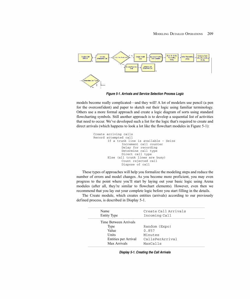
209MODELING DETAILED OPERATIONS
Figure 5-1. Arrivals and Service Selection Process Logic
models become really complicated—and they will! A lot of modelers use pencil (a penfor the overconfident) and paper to sketch out their logic using familiar terminology.Others use a more formal approach and create a logic diagram of sorts using standardflowcharting symbols. Still another approach is to develop a sequential list of activitiesthat need to occur. We’ve developed such a list for the logic that’s required to create anddirect arrivals (which happens to look a lot like the flowchart modules in Figure 5-1):
Create arriving callsRecord attempted call
If a trunk line is available - SeizeIncrement call counterDelay for recordingDetermine call typeDirect call type
Else (all trunk lines are busy)Count rejected callDispose of call
These types of approaches will help you formalize the modeling steps and reduce thenumber of errors and model changes. As you become more proficient, you may evenprogress to the point where you’ll start by laying out your basic logic using Arenamodules (after all, they’re similar to flowchart elements). However, even then werecommend that you lay out your complete logic before you start filling in the details.
The Create module, which creates entities (arrivals) according to our previouslydefined process, is described in Display 5-1.
Name Create Call ArrivalsEntity Type Incoming Call
Time Between ArrivalsType Random (Expo)Value 0.857Units MinutesEntities per Arrival CallsPerArrivalMax Arrivals MaxCalls
Display 5-1. Creating the Call Arrivals

210 CHAPTER 5
Figure 5-2. The Variable Data Module
We used a very similar Create module in the models in Chapters 3 and 4, with theexception of the entries in the Entities per Arrival and Max Arrivals fields. Rememberthat the system closes to new calls after 6 PM. We’ll show you how to use the variableMaxCalls to terminate the call arrivals in the next section.
In most cases where you define a new object (variable, attribute, etc.) in the modulesfrom the Basic Process and Advanced Process panels, Arena will automatically make anentry in the appropriate data module. This always happens when you specify the Type;e.g., variable, attribute, etc. However, in this case, we simply enter MaxCalls withoutspecifying the type. Therefore, we need to define our variable MaxCalls. We do this inthe Variable data module found in the Basic Process panel, seen in Figure 5-2. Open thisdata module by clicking on it and double-clicking to add a new row. Next type in theName of our new variable, MaxCalls. Then click on the Initial Values cell toopen the spreadsheet window where you can enter the initial value. We entered a value of999999, which means that the arrival process will be terminated after 999999 arrivingcalls (clearly a ruse that we’ll explain below). We also define the variable CallsPerArrivaland initialize it to a value of 1 (this initialization is not visible in Figure 5-2); again, we’llexplain this a bit later.
As we continue to develop this model, we’ll sometimes be thinking ahead to how wewould like to animate our model. Let’s assume that we want our arriving call to beanimated as a black ball. We could assign a picture using an Assign module, but wespecified in our Create module that the entity type was Incoming Call so at this pointwe should click on our Entity data module and select Picture.Black Ball from thedrop-down list in the Initial Picture cell.
At this point in the model, we want to record the number of attempted calls using aRecord module, as shown in Display 5-2.
We next need to check for an available trunk line. If a line is available, we seize thatline; otherwise, the call is rejected from the system. In Section 5.2.1, we discussed twoobvious ways (at least to us) to accomplish this. For this model, we’ll use a Decidemodule followed by a Seize module (in the Advanced Process panel) if a line is available.
Name Record Attempted CallType CountValue 1Counter Name Attempted Calls
Display 5-2. Counting the Attempting Calls
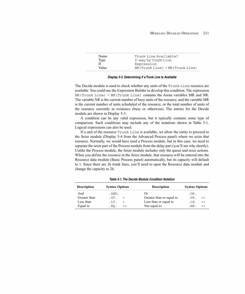
211MODELING DETAILED OPERATIONS
Name Trunk Line Available?Type 2-way by ConditionIf ExpressionValue NR(Trunk Line) < MR(Trunk Line)
Display 5-3. Determining if a Trunk Line Is Available
The Decide module is used to check whether any units of the Trunk Line resource areavailable. You could use the Expression Builder to develop this condition. The expressionNR(Trunk Line) < MR(Trunk Line) contains the Arena variables MR and NR.The variable NR is the current number of busy units of the resource, and the variable MRis the current number of units scheduled of the resource, or the total number of units ofthe resource currently in existence (busy or otherwise). The entries for the Decidemodule are shown in Display 5-3.
A condition can be any valid expression, but it typically contains some type ofcomparison. Such conditions may include any of the notations shown in Table 5-1.Logical expressions can also be used.
If a unit of the resource Trunk Line is available, we allow the entity to proceed tothe Seize module (Display 5-4 from the Advanced Process panel) where we seize thatresource. Normally, we would have used a Process module, but in this case, we need toseparate the seize part of the Process module from the delay part (you’ll see why shortly).Unlike the Process module, the Seize module includes only the queue and seize actions.When you define the resource in the Seize module, that resource will be entered into theResource data module (Basic Process panel) automatically, but its capacity will defaultto 1. Since there are 26 trunk lines, you’ll need to open the Resource data module andchange the capacity to 26.
Table 5-1. The Decide Module Condition Notation
Description Syntax Options Description Syntax Options
And .AND. Or .OR.Greater than .GT. > Greater than or equal to .GE. >=Less than .LT. < Less than or equal to .LE. <=Equal to .EQ. == Not equal to .NE. <>
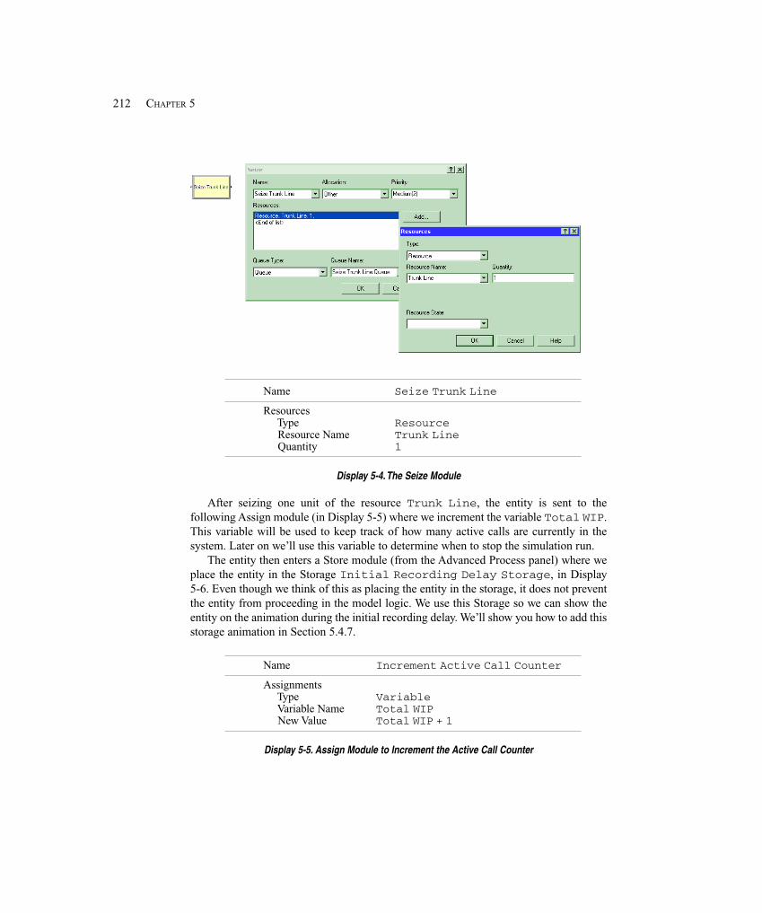
212 CHAPTER 5
Name Seize Trunk Line
Resources Type Resource Resource Name Trunk Line Quantity 1
Display 5-4. The Seize Module
After seizing one unit of the resource Trunk Line, the entity is sent to thefollowing Assign module (in Display 5-5) where we increment the variable Total WIP.This variable will be used to keep track of how many active calls are currently in thesystem. Later on we’ll use this variable to determine when to stop the simulation run.
The entity then enters a Store module (from the Advanced Process panel) where weplace the entity in the Storage Initial Recording Delay Storage, in Display5-6. Even though we think of this as placing the entity in the storage, it does not preventthe entity from proceeding in the model logic. We use this Storage so we can show theentity on the animation during the initial recording delay. We’ll show you how to add thisstorage animation in Section 5.4.7.
Name Increment Active Call Counter
Assignments Type Variable Variable Name Total WIP New Value Total WIP + 1
Display 5-5. Assign Module to Increment the Active Call Counter
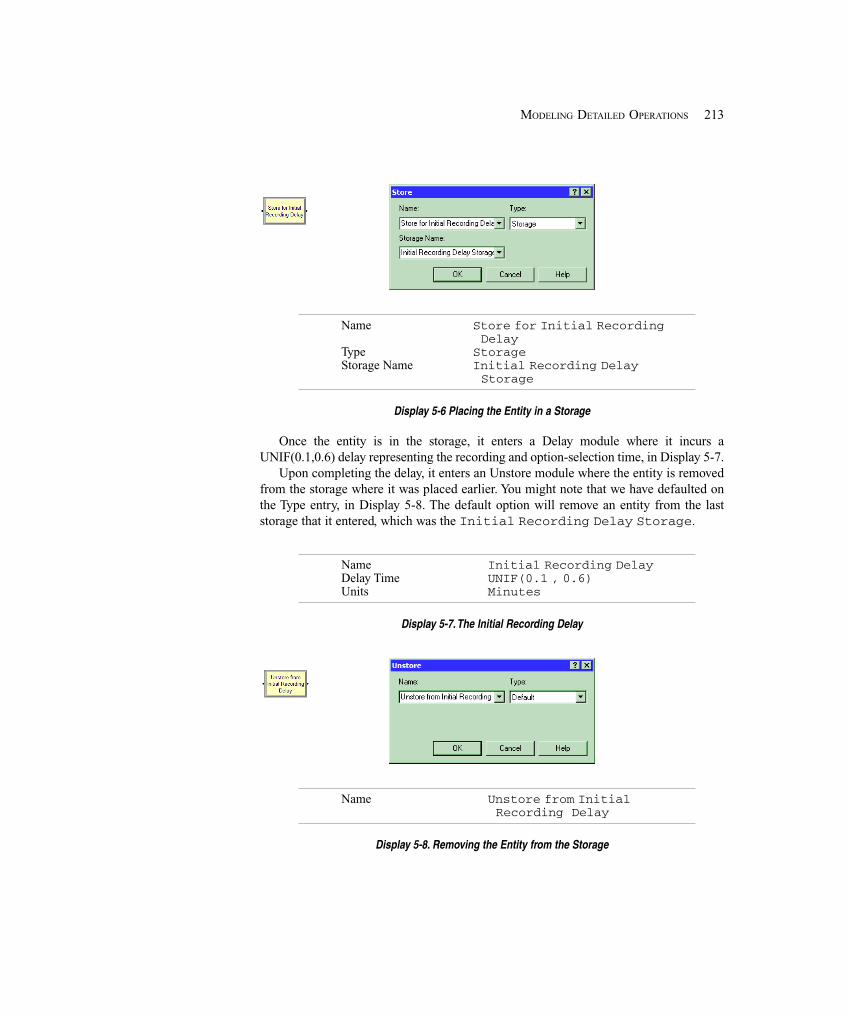
213MODELING DETAILED OPERATIONS
Name Store for Initial Recording Delay
Type StorageStorage Name Initial Recording Delay
Storage
Display 5-6 Placing the Entity in a Storage
Once the entity is in the storage, it enters a Delay module where it incurs aUNIF(0.1,0.6) delay representing the recording and option-selection time, in Display 5-7.
Upon completing the delay, it enters an Unstore module where the entity is removedfrom the storage where it was placed earlier. You might note that we have defaulted onthe Type entry, in Display 5-8. The default option will remove an entity from the laststorage that it entered, which was the Initial Recording Delay Storage.
Name Initial Recording DelayDelay Time UNIF(0.1 , 0.6)Units Minutes
Display 5-7. The Initial Recording Delay
Name Unstore from Initial Recording Delay
Display 5-8. Removing the Entity from the Storage
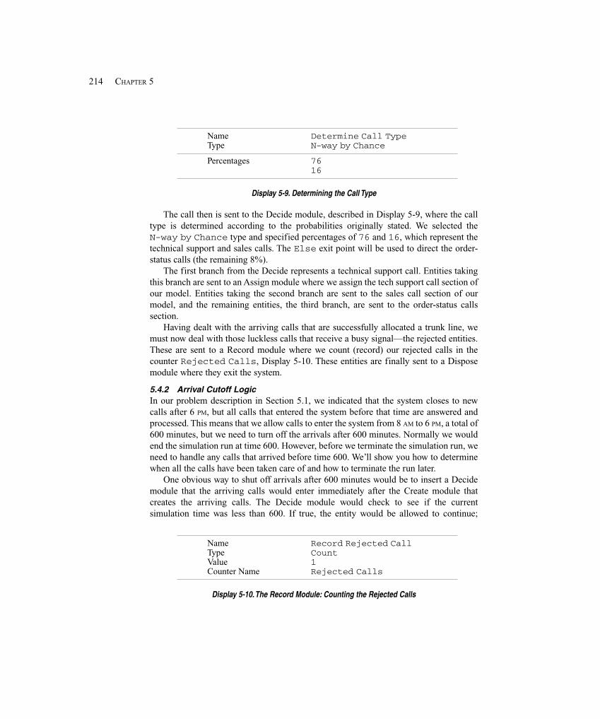
214 CHAPTER 5
Name Determine Call TypeType N-way by Chance
Percentages 7616
Display 5-9. Determining the Call Type
The call then is sent to the Decide module, described in Display 5-9, where the calltype is determined according to the probabilities originally stated. We selected theN-way by Chance type and specified percentages of 76 and 16, which represent thetechnical support and sales calls. The Else exit point will be used to direct the order-status calls (the remaining 8%).
The first branch from the Decide represents a technical support call. Entities takingthis branch are sent to an Assign module where we assign the tech support call section ofour model. Entities taking the second branch are sent to the sales call section of ourmodel, and the remaining entities, the third branch, are sent to the order-status callssection.
Having dealt with the arriving calls that are successfully allocated a trunk line, wemust now deal with those luckless calls that receive a busy signal—the rejected entities.These are sent to a Record module where we count (record) our rejected calls in thecounter Rejected Calls, Display 5-10. These entities are finally sent to a Disposemodule where they exit the system.
5.4.2 Arrival Cutoff LogicIn our problem description in Section 5.1, we indicated that the system closes to newcalls after 6 PM, but all calls that entered the system before that time are answered andprocessed. This means that we allow calls to enter the system from 8 AM to 6 PM, a total of600 minutes, but we need to turn off the arrivals after 600 minutes. Normally we wouldend the simulation run at time 600. However, before we terminate the simulation run, weneed to handle any calls that arrived before time 600. We’ll show you how to determinewhen all the calls have been taken care of and how to terminate the run later.
One obvious way to shut off arrivals after 600 minutes would be to insert a Decidemodule that the arriving calls would enter immediately after the Create module thatcreates the arriving calls. The Decide module would check to see if the currentsimulation time was less than 600. If true, the entity would be allowed to continue;
Name Record Rejected CallType CountValue 1Counter Name Rejected Calls
Display 5-10. The Record Module: Counting the Rejected Calls
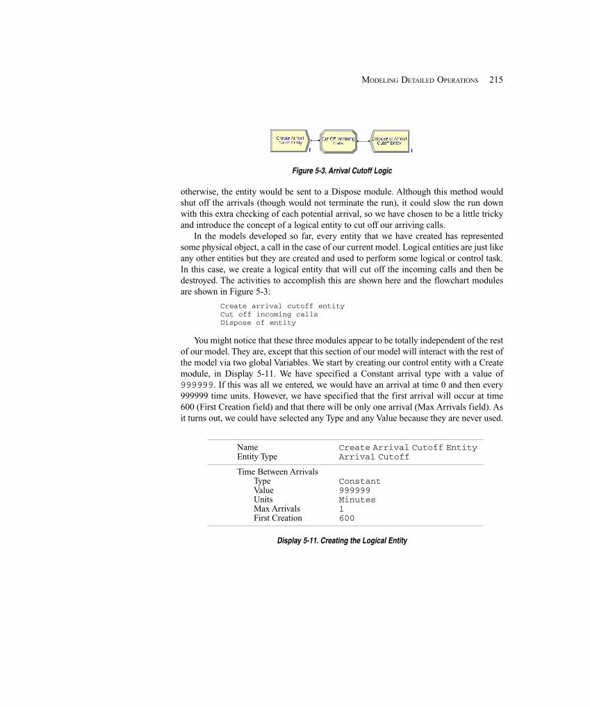
215MODELING DETAILED OPERATIONS
Figure 5-3. Arrival Cutoff Logic
otherwise, the entity would be sent to a Dispose module. Although this method wouldshut off the arrivals (though would not terminate the run), it could slow the run downwith this extra checking of each potential arrival, so we have chosen to be a little trickyand introduce the concept of a logical entity to cut off our arriving calls.
In the models developed so far, every entity that we have created has representedsome physical object, a call in the case of our current model. Logical entities are just likeany other entities but they are created and used to perform some logical or control task.In this case, we create a logical entity that will cut off the incoming calls and then bedestroyed. The activities to accomplish this are shown here and the flowchart modulesare shown in Figure 5-3:
Create arrival cutoff entityCut off incoming callsDispose of entity
You might notice that these three modules appear to be totally independent of the restof our model. They are, except that this section of our model will interact with the rest ofthe model via two global Variables. We start by creating our control entity with a Createmodule, in Display 5-11. We have specified a Constant arrival type with a value of999999. If this was all we entered, we would have an arrival at time 0 and then every999999 time units. However, we have specified that the first arrival will occur at time600 (First Creation field) and that there will be only one arrival (Max Arrivals field). Asit turns out, we could have selected any Type and any Value because they are never used.
Name Create Arrival Cutoff EntityEntity Type Arrival Cutoff
Time Between ArrivalsType ConstantValue 999999Units MinutesMax Arrivals 1First Creation 600
Display 5-11. Creating the Logical Entity
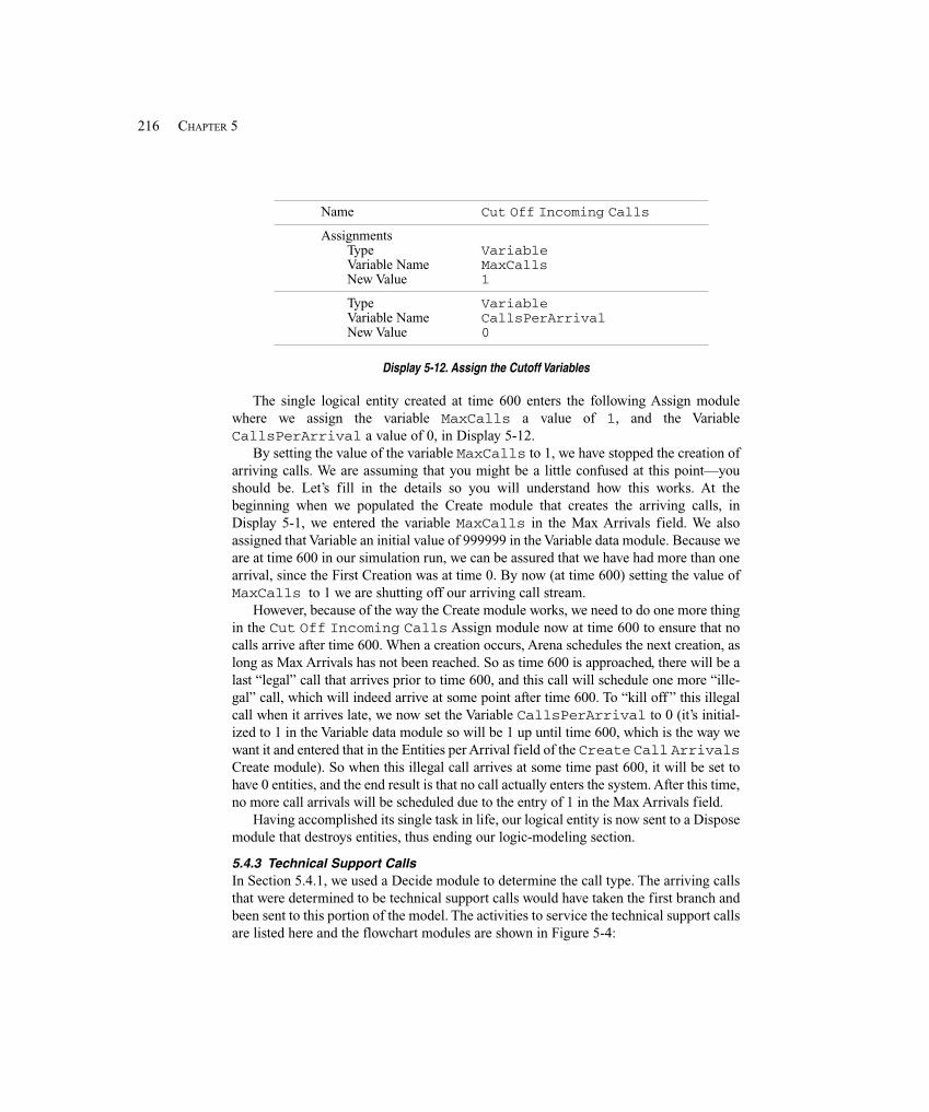
216 CHAPTER 5
Name Cut Off Incoming Calls
AssignmentsType VariableVariable Name MaxCallsNew Value 1
Type VariableVariable Name CallsPerArrivalNew Value 0
Display 5-12. Assign the Cutoff Variables
The single logical entity created at time 600 enters the following Assign modulewhere we assign the variable MaxCalls a value of 1, and the VariableCallsPerArrival a value of 0, in Display 5-12.
By setting the value of the variable MaxCalls to 1, we have stopped the creation ofarriving calls. We are assuming that you might be a little confused at this point—youshould be. Let’s fill in the details so you will understand how this works. At thebeginning when we populated the Create module that creates the arriving calls, inDisplay 5-1, we entered the variable MaxCalls in the Max Arrivals field. We alsoassigned that Variable an initial value of 999999 in the Variable data module. Because weare at time 600 in our simulation run, we can be assured that we have had more than onearrival, since the First Creation was at time 0. By now (at time 600) setting the value ofMaxCalls to 1 we are shutting off our arriving call stream.
However, because of the way the Create module works, we need to do one more thingin the Cut Off Incoming Calls Assign module now at time 600 to ensure that nocalls arrive after time 600. When a creation occurs, Arena schedules the next creation, aslong as Max Arrivals has not been reached. So as time 600 is approached, there will be alast “legal” call that arrives prior to time 600, and this call will schedule one more “ille-gal” call, which will indeed arrive at some point after time 600. To “kill off ” this illegalcall when it arrives late, we now set the Variable CallsPerArrival to 0 (it’s initial-ized to 1 in the Variable data module so will be 1 up until time 600, which is the way wewant it and entered that in the Entities per Arrival field of the Create Call ArrivalsCreate module). So when this illegal call arrives at some time past 600, it will be set tohave 0 entities, and the end result is that no call actually enters the system. After this time,no more call arrivals will be scheduled due to the entry of 1 in the Max Arrivals field.
Having accomplished its single task in life, our logical entity is now sent to a Disposemodule that destroys entities, thus ending our logic-modeling section.
5.4.3 Technical Support CallsIn Section 5.4.1, we used a Decide module to determine the call type. The arriving callsthat were determined to be technical support calls would have taken the first branch andbeen sent to this portion of the model. The activities to service the technical support callsare listed here and the flowchart modules are shown in Figure 5-4:
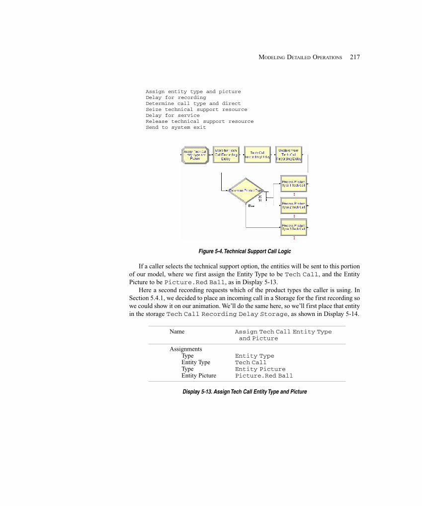
217MODELING DETAILED OPERATIONS
Assign entity type and pictureDelay for recordingDetermine call type and directSeize technical support resourceDelay for serviceRelease technical support resourceSend to system exit
Figure 5-4. Technical Support Call Logic
If a caller selects the technical support option, the entities will be sent to this portionof our model, where we first assign the Entity Type to be Tech Call, and the EntityPicture to be Picture.Red Ball, as in Display 5-13.
Here a second recording requests which of the product types the caller is using. InSection 5.4.1, we decided to place an incoming call in a Storage for the first recording sowe could show it on our animation. We’ll do the same here, so we’ll first place that entityin the storage Tech Call Recording Delay Storage, as shown in Display 5-14.
Name Assign Tech Call Entity Type and Picture
AssignmentsType Entity TypeEntity Type Tech CallType Entity PictureEntity Picture Picture.Red Ball
Display 5-13. Assign Tech Call Entity Type and Picture

218 CHAPTER 5
Name Store for Tech Call Recording Delay
Type StorageStorage Name Tech Call Recording Delay
Storage
Display 5-14. Technical Support Call Storage
Name Tech Call Recording DelayDelay Time UNIF( 0.1 , 0.5 )Units Minutes
Display 5-15. The Technical Support Recording Delay
Once the entity has been placed in the storage, it enters the following Delay modulewhere it incurs a UNIF(0.1,0.5) delay representing the recording and option-selectiontime, as shown in Display 5-15.
Upon completing the delay, it enters an Unstore module where the entity is removedfrom the storage where it had been placed, as shown in Display 5-16. Again, the defaultoption will remove the entity from the last storage that it entered.
The call is sent to the Decide module next, as described in Display 5-17, where theproduct type is determined according to the probabilities originally stated. We selectedthe N-way by Chance type and specified percentages of 25 and 34, which representthe Type 1 and Type 2 technical support calls. The Else exit point will be used to directthe product Type 3 calls (the remaining 41%).
Each of the three branches from this Decide module connects to a Process module toservice that type of technical support call. The entries for each of these three modules arevery similar, so we’ll only walk you through the first, for product Type 1 technicalsupport, in Display 5-18. We’ve selected the Seize Delay Release Action and haverequested to seize one unit of resource Tech 1. As with the Trunk Line resource, youalso need to open the Resource data module and change the Capacity from the default (1)to 2. We then delay for a time found in the expression Tech Time, which we have notyet defined. After the delay, the Tech 1 resource is released and the completed call issent to the exit portion of our model.
Name Unstore from Tech Call Recording Delay
Display 5-16. Removing the Entity from the Storage
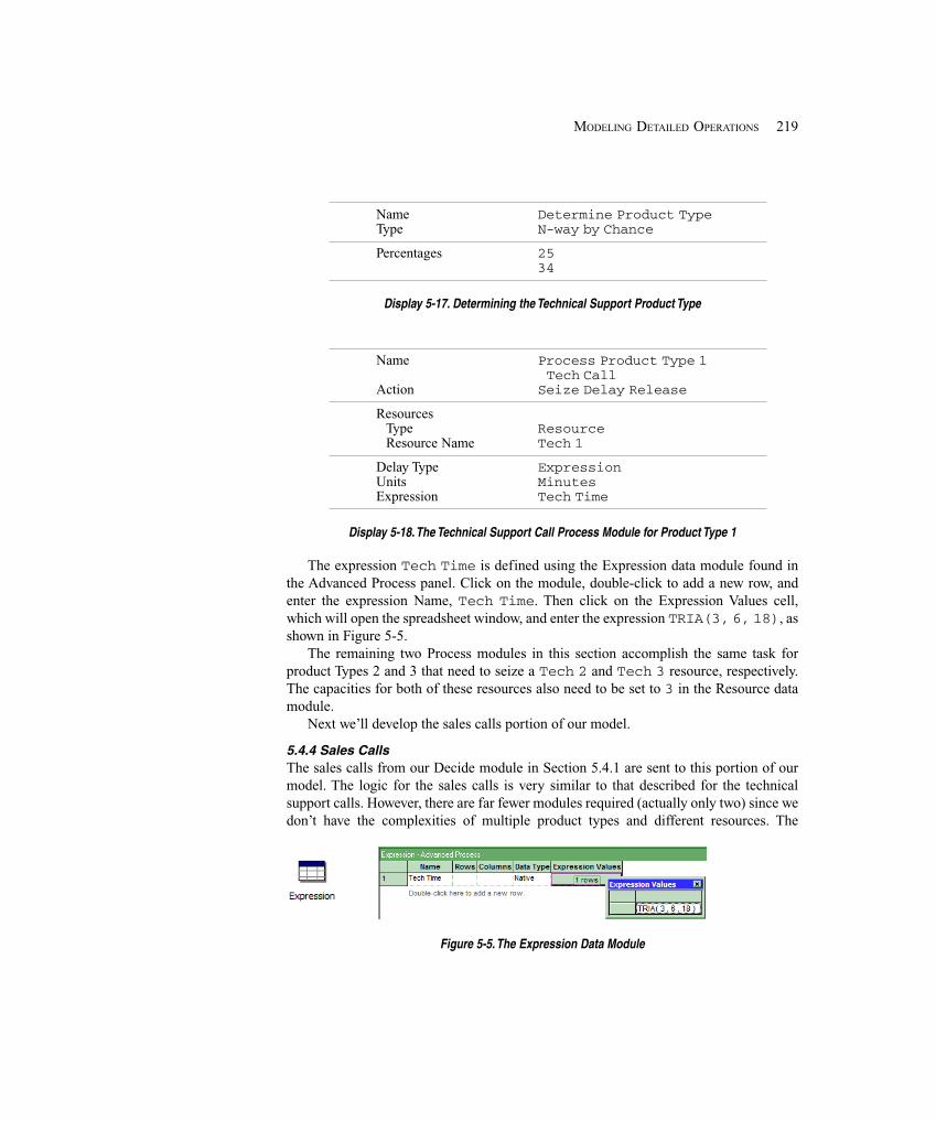
219MODELING DETAILED OPERATIONS
Name Determine Product TypeType N-way by Chance
Percentages 2534
Display 5-17. Determining the Technical Support Product Type
Name Process Product Type 1 Tech Call
Action Seize Delay Release
ResourcesType ResourceResource Name Tech 1
Delay Type ExpressionUnits MinutesExpression Tech Time
Display 5-18. The Technical Support Call Process Module for Product Type 1
The expression Tech Time is defined using the Expression data module found inthe Advanced Process panel. Click on the module, double-click to add a new row, andenter the expression Name, Tech Time. Then click on the Expression Values cell,which will open the spreadsheet window, and enter the expression TRIA(3, 6, 18), asshown in Figure 5-5.
The remaining two Process modules in this section accomplish the same task forproduct Types 2 and 3 that need to seize a Tech 2 and Tech 3 resource, respectively.The capacities for both of these resources also need to be set to 3 in the Resource datamodule.
Next we’ll develop the sales calls portion of our model.
5.4.4 Sales CallsThe sales calls from our Decide module in Section 5.4.1 are sent to this portion of ourmodel. The logic for the sales calls is very similar to that described for the technicalsupport calls. However, there are far fewer modules required (actually only two) since wedon’t have the complexities of multiple product types and different resources. The
Figure 5-5. The Expression Data Module
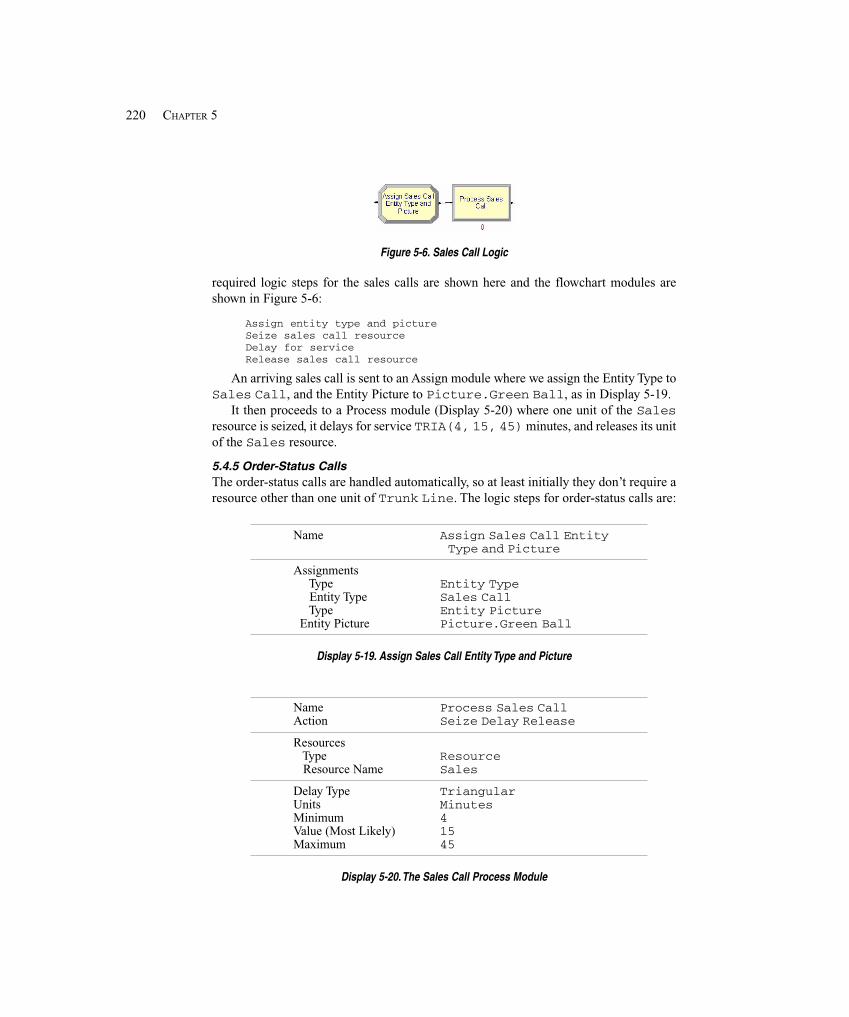
220 CHAPTER 5
Figure 5-6. Sales Call Logic
required logic steps for the sales calls are shown here and the flowchart modules areshown in Figure 5-6:
Assign entity type and pictureSeize sales call resourceDelay for serviceRelease sales call resource
An arriving sales call is sent to an Assign module where we assign the Entity Type toSales Call, and the Entity Picture to Picture.Green Ball, as in Display 5-19.
It then proceeds to a Process module (Display 5-20) where one unit of the Salesresource is seized, it delays for service TRIA(4, 15, 45) minutes, and releases its unitof the Sales resource.
5.4.5 Order-Status CallsThe order-status calls are handled automatically, so at least initially they don’t require aresource other than one unit of Trunk Line. The logic steps for order-status calls are:
Name Assign Sales Call Entity Type and Picture
Assignments Type Entity Type Entity Type Sales Call Type Entity Picture Entity Picture Picture.Green Ball
Display 5-19. Assign Sales Call Entity Type and Picture
Name Process Sales CallAction Seize Delay Release
Resources Type Resource Resource Name Sales
Delay Type TriangularUnits MinutesMinimum 4Value (Most Likely) 15Maximum 45
Display 5-20. The Sales Call Process Module
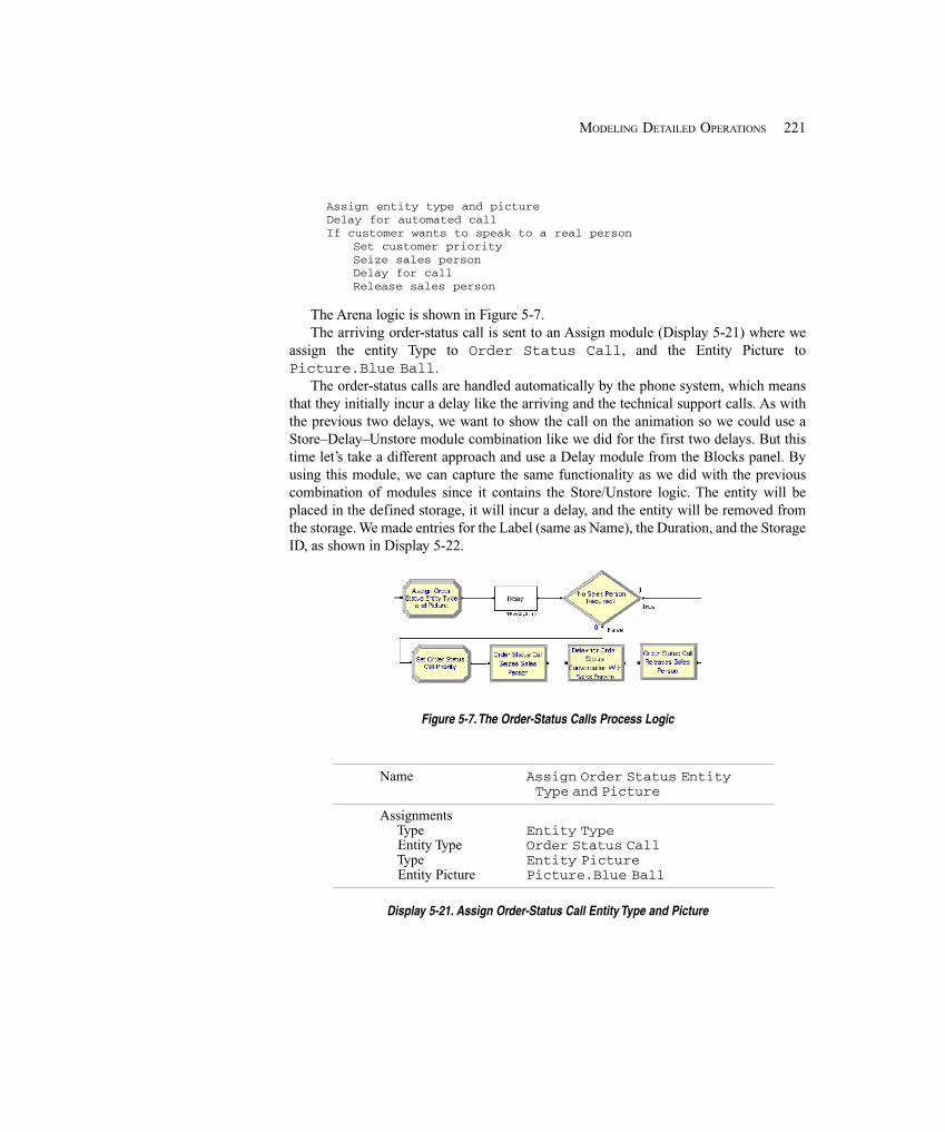
221MODELING DETAILED OPERATIONS
Assign entity type and pictureDelay for automated callIf customer wants to speak to a real person
Set customer prioritySeize sales personDelay for callRelease sales person
The Arena logic is shown in Figure 5-7.The arriving order-status call is sent to an Assign module (Display 5-21) where we
assign the entity Type to Order Status Call, and the Entity Picture toPicture.Blue Ball.
The order-status calls are handled automatically by the phone system, which meansthat they initially incur a delay like the arriving and the technical support calls. As withthe previous two delays, we want to show the call on the animation so we could use aStore–Delay–Unstore module combination like we did for the first two delays. But thistime let’s take a different approach and use a Delay module from the Blocks panel. Byusing this module, we can capture the same functionality as we did with the previouscombination of modules since it contains the Store/Unstore logic. The entity will beplaced in the defined storage, it will incur a delay, and the entity will be removed fromthe storage. We made entries for the Label (same as Name), the Duration, and the StorageID, as shown in Display 5-22.
Figure 5-7. The Order-Status Calls Process Logic
Name Assign Order Status Entity Type and Picture
Assignments Type Entity Type Entity Type Order Status Call Type Entity Picture Entity Picture Picture.Blue Ball
Display 5-21. Assign Order-Status Call Entity Type and Picture
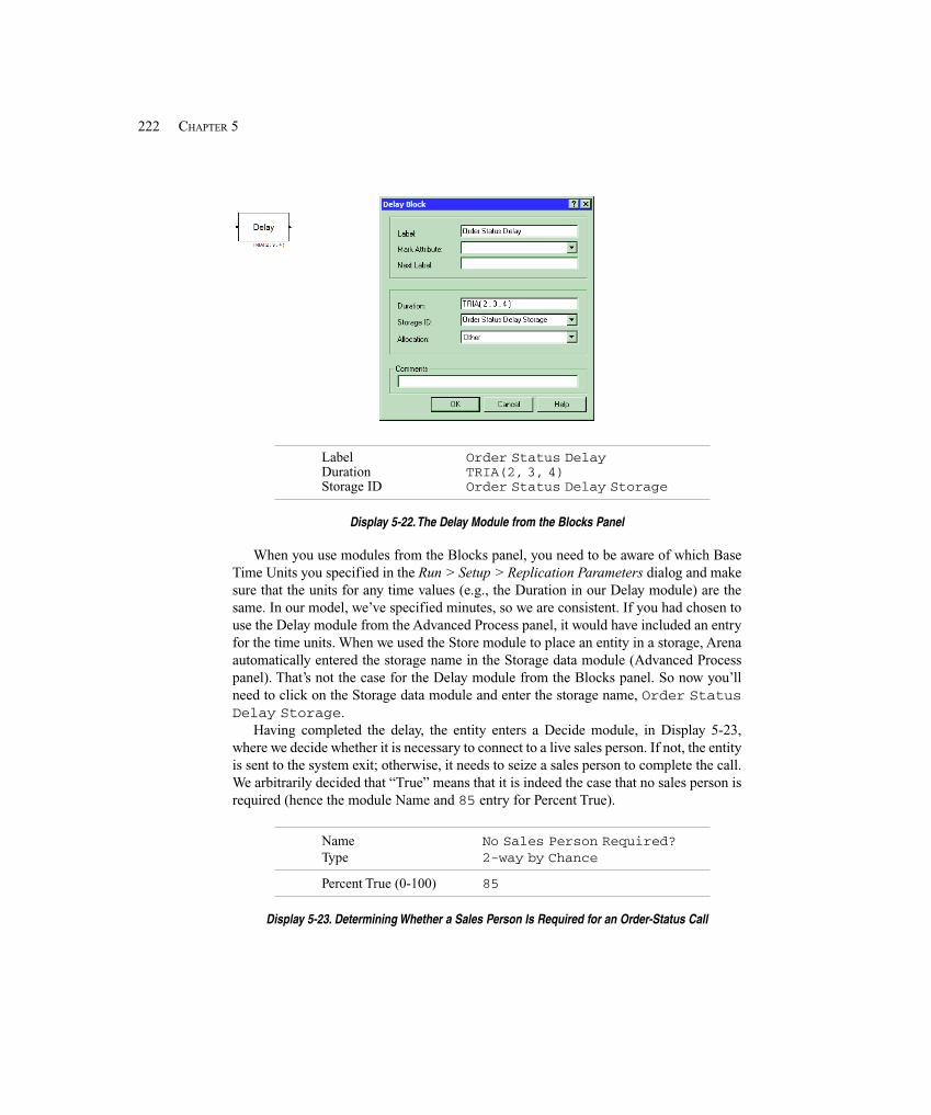
222 CHAPTER 5
Label Order Status DelayDuration TRIA(2, 3, 4)Storage ID Order Status Delay Storage
Display 5-22. The Delay Module from the Blocks Panel
When you use modules from the Blocks panel, you need to be aware of which BaseTime Units you specified in the Run > Setup > Replication Parameters dialog and makesure that the units for any time values (e.g., the Duration in our Delay module) are thesame. In our model, we’ve specified minutes, so we are consistent. If you had chosen touse the Delay module from the Advanced Process panel, it would have included an entryfor the time units. When we used the Store module to place an entity in a storage, Arenaautomatically entered the storage name in the Storage data module (Advanced Processpanel). That’s not the case for the Delay module from the Blocks panel. So now you’llneed to click on the Storage data module and enter the storage name, Order StatusDelay Storage.
Having completed the delay, the entity enters a Decide module, in Display 5-23,where we decide whether it is necessary to connect to a live sales person. If not, the entityis sent to the system exit; otherwise, it needs to seize a sales person to complete the call.We arbitrarily decided that “True” means that it is indeed the case that no sales person isrequired (hence the module Name and 85 entry for Percent True).
Name No Sales Person Required?Type 2-way by Chance
Percent True (0-100) 85
Display 5-23. Determining Whether a Sales Person Is Required for an Order-Status Call
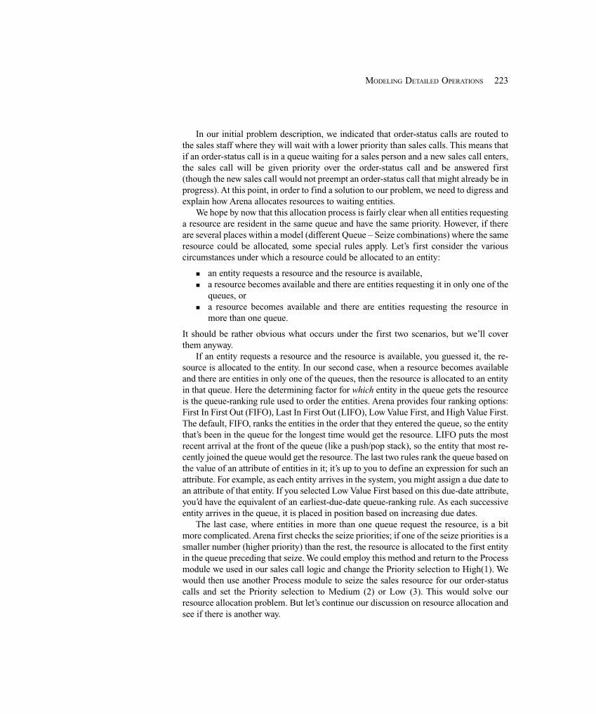
223MODELING DETAILED OPERATIONS
In our initial problem description, we indicated that order-status calls are routed tothe sales staff where they will wait with a lower priority than sales calls. This means thatif an order-status call is in a queue waiting for a sales person and a new sales call enters,the sales call will be given priority over the order-status call and be answered first(though the new sales call would not preempt an order-status call that might already be inprogress). At this point, in order to find a solution to our problem, we need to digress andexplain how Arena allocates resources to waiting entities.
We hope by now that this allocation process is fairly clear when all entities requestinga resource are resident in the same queue and have the same priority. However, if thereare several places within a model (different Queue – Seize combinations) where the sameresource could be allocated, some special rules apply. Let’s first consider the variouscircumstances under which a resource could be allocated to an entity:
� an entity requests a resource and the resource is available,� a resource becomes available and there are entities requesting it in only one of the
queues, or� a resource becomes available and there are entities requesting the resource in
more than one queue.
It should be rather obvious what occurs under the first two scenarios, but we’ll coverthem anyway.
If an entity requests a resource and the resource is available, you guessed it, the re-source is allocated to the entity. In our second case, when a resource becomes availableand there are entities in only one of the queues, then the resource is allocated to an entityin that queue. Here the determining factor for which entity in the queue gets the resourceis the queue-ranking rule used to order the entities. Arena provides four ranking options:First In First Out (FIFO), Last In First Out (LIFO), Low Value First, and High Value First.The default, FIFO, ranks the entities in the order that they entered the queue, so the entitythat’s been in the queue for the longest time would get the resource. LIFO puts the mostrecent arrival at the front of the queue (like a push/pop stack), so the entity that most re-cently joined the queue would get the resource. The last two rules rank the queue based onthe value of an attribute of entities in it; it’s up to you to define an expression for such anattribute. For example, as each entity arrives in the system, you might assign a due date toan attribute of that entity. If you selected Low Value First based on this due-date attribute,you’d have the equivalent of an earliest-due-date queue-ranking rule. As each successiveentity arrives in the queue, it is placed in position based on increasing due dates.
The last case, where entities in more than one queue request the resource, is a bitmore complicated. Arena first checks the seize priorities; if one of the seize priorities is asmaller number (higher priority) than the rest, the resource is allocated to the first entityin the queue preceding that seize. We could employ this method and return to the Processmodule we used in our sales call logic and change the Priority selection to High(1). Wewould then use another Process module to seize the sales resource for our order-statuscalls and set the Priority selection to Medium (2) or Low (3). This would solve ourresource allocation problem. But let’s continue our discussion on resource allocation andsee if there is another way.

224 CHAPTER 5
If all priorities are equal, Arena applies a default tie-breaking rule, and the resource isallocated based on the entity that has waited the longest regardless of the queue it’s in.Thus, it’s essentially a FIFO tie-breaking rule among a merger of the queues involved.This means that if your queues were ranked according to earliest due date, then the entitythat met that criterion might not always be allocated the resource. For example, a late jobmight have just entered a queue, whereas an early job may be at the front of anotherqueue and has been waiting longer.
Arena provides a solution to this potential problem in the form of a shared queue. Ashared queue is just what its name implies—a single queue that can be shared by two ormore seize activities. This allows you to define a single queue where all entitiesrequesting the resource will be placed regardless of where their seize activities are withinyour model. Arena performs the bookkeeping to ensure that an entity in a shared queuecontinues in the proper place in the model logic when it’s allocated a resource.
In our model, each sales call and a small percentage (15%) of the order-status callswill require a unit of the Sales resource. Since these activities are modeled separately,we’ll use a shared queue when we attempt to seize a unit of the Sales resource. Bothtypes of calls are allocated a unit of the Sales resource based on a FIFO rule, or thelongest waiting time, so a shared queue is not required in our model to assure that theproper call is allocated the resource. However, a shared queue also allows us to collectcomposite statistics easily on the total number of calls waiting for a Sales resource andprovides the ability to show all of these waiting calls in the same queue—if we decide toanimate that queue.
Since we did not assign the sales calls a priority, we’ll take advantage of the fact thatfor an entity with an unassigned value for an attribute, that value will default to zero.Now we’ll use an Assign module to define a new attribute, Sales Call Priority, tothose order-status calls requiring a unit of the Sales resource and set its value to 1, as inDisplay 5-24.
The result is that sales calls will have a Sales Call Priority with a value of 0and order-status calls will have a Sales Call Priority with a value of 1. Next we’llsend the entity to a Seize module. You might ask why we are using a Seize module ratherthan a Process module. It turns out that if we use a Process module, the queue namedefaults to “module name” with a “.queue” extension, which can’t be changed. Since wewant to use the same queue that was defined for the sales calls seize, we need to use aSeize module instead, which allows us to change the default queue name.
Label Set Order Status Call Priority
Type AttributeAssignments
Attribute Name Sales Call PriorityNew Value 1
Display 5-24. Assigning the Call Priority
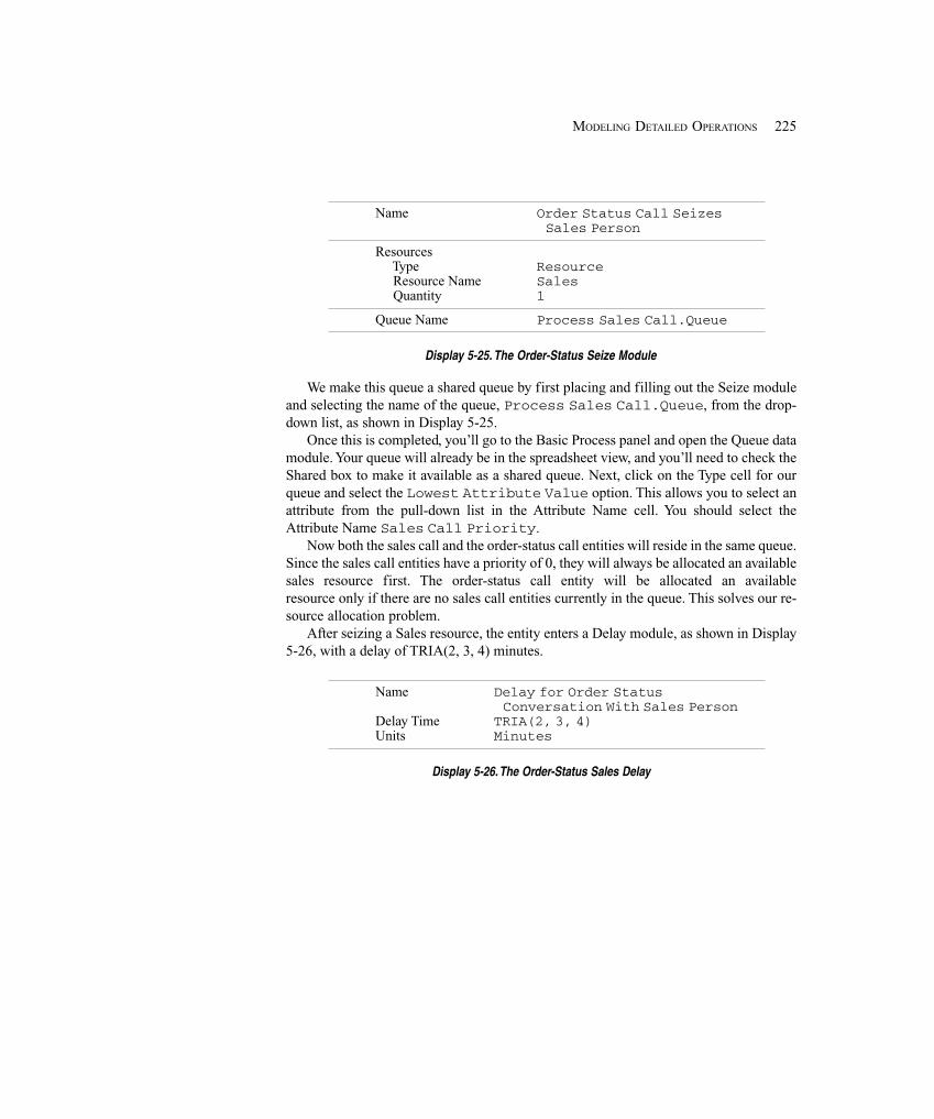
225MODELING DETAILED OPERATIONS
Name Order Status Call Seizes Sales Person
Resources Type Resource Resource Name Sales Quantity 1
Queue Name Process Sales Call.Queue
Display 5-25. The Order-Status Seize Module
We make this queue a shared queue by first placing and filling out the Seize moduleand selecting the name of the queue, Process Sales Call.Queue, from the drop-down list, as shown in Display 5-25.
Once this is completed, you’ll go to the Basic Process panel and open the Queue datamodule. Your queue will already be in the spreadsheet view, and you’ll need to check theShared box to make it available as a shared queue. Next, click on the Type cell for ourqueue and select the Lowest Attribute Value option. This allows you to select anattribute from the pull-down list in the Attribute Name cell. You should select theAttribute Name Sales Call Priority.
Now both the sales call and the order-status call entities will reside in the same queue.Since the sales call entities have a priority of 0, they will always be allocated an availablesales resource first. The order-status call entity will be allocated an availableresource only if there are no sales call entities currently in the queue. This solves our re-source allocation problem.
After seizing a Sales resource, the entity enters a Delay module, as shown in Display5-26, with a delay of TRIA(2, 3, 4) minutes.
Name Delay for Order Status Conversation With Sales Person
Delay Time TRIA(2, 3, 4)Units Minutes
Display 5-26. The Order-Status Sales Delay
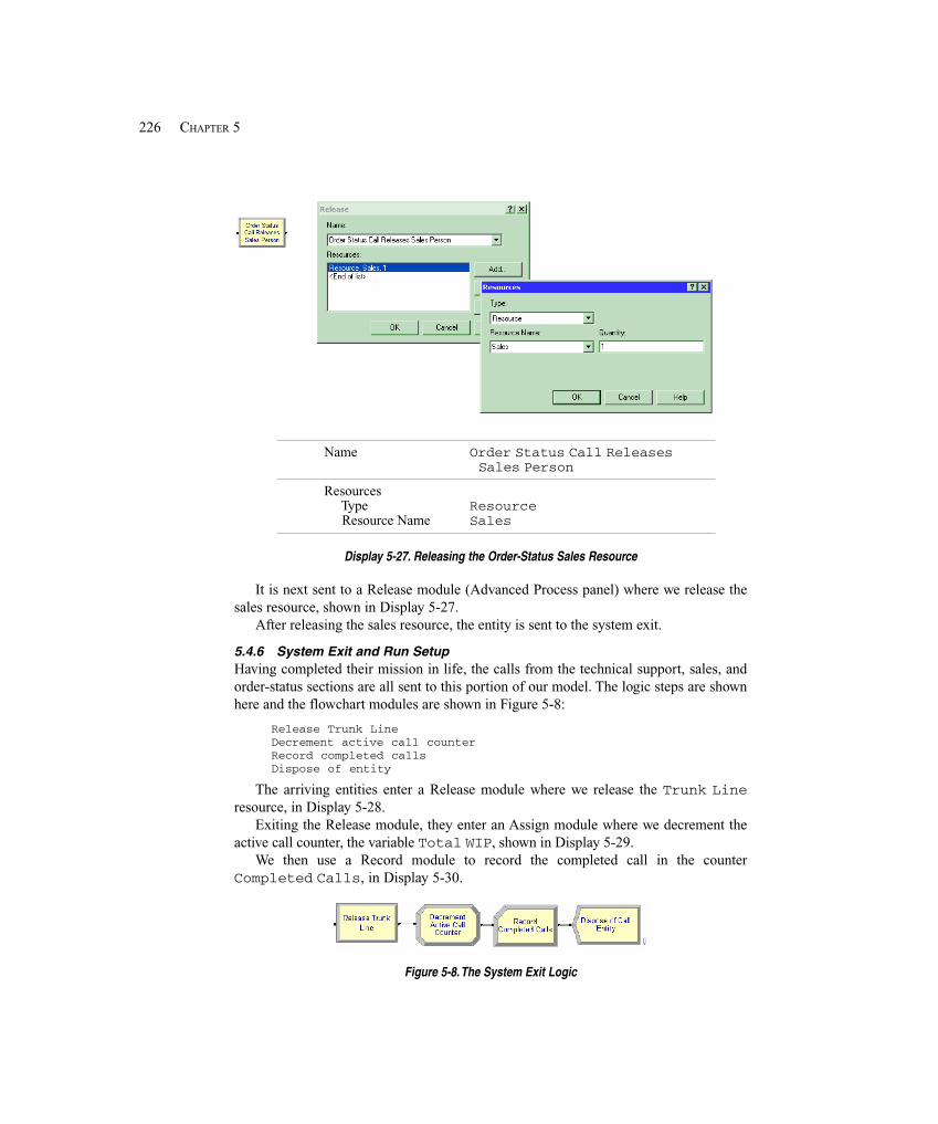
226 CHAPTER 5
Name Order Status Call Releases Sales Person
Resources Type Resource Resource Name Sales
Display 5-27. Releasing the Order-Status Sales Resource
It is next sent to a Release module (Advanced Process panel) where we release thesales resource, shown in Display 5-27.
After releasing the sales resource, the entity is sent to the system exit.
5.4.6 System Exit and Run SetupHaving completed their mission in life, the calls from the technical support, sales, andorder-status sections are all sent to this portion of our model. The logic steps are shownhere and the flowchart modules are shown in Figure 5-8:
Release Trunk LineDecrement active call counterRecord completed callsDispose of entity
The arriving entities enter a Release module where we release the Trunk Lineresource, in Display 5-28.
Exiting the Release module, they enter an Assign module where we decrement theactive call counter, the variable Total WIP, shown in Display 5-29.
We then use a Record module to record the completed call in the counterCompleted Calls, in Display 5-30.
Figure 5-8. The System Exit Logic
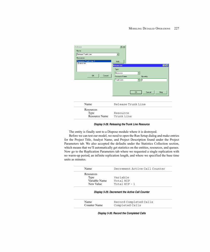
227MODELING DETAILED OPERATIONS
Name Release Trunk Line
Resources Type Resource Resource Name Trunk Line
Display 5-28. Releasing the Trunk Line Resource
The entity is finally sent to a Dispose module where it is destroyed.Before we can test our model, we need to open the Run Setup dialog and make entries
for the Project Title, Analyst Name, and Project Description found under the ProjectParameters tab. We also accepted the defaults under the Statistics Collection section,which means that we’ll automatically get statistics on the entities, resources, and queues.Now go to the Replication Parameters tab where we requested a single replication withno warm-up period, an infinite replication length, and where we specified the base timeunits as minutes.
Name Decrement Active Call Counter
Resources Type Variable Variable Name Total WIP New Value Total WIP - 1
Display 5-29. Decrement the Active Call Counter
Name Record Completed CallsCounter Name Completed Calls
Display 5-30. Record the Completed Calls
228 CHAPTER 5
At this point, you might remember (we are guessing you forgot by this time) that wayback in the early part of Section 5.4.1 we told you that we were going to use the variableTotal WIP to help determine when to stop the simulation. The call center acceptsincoming calls only from 8 AM to 6 PM (600 minutes), but any calls that are in the systemat 6 PM must be completed. We could have just set an arbitrarily long replication time, butthis would have resulted in inaccurate results, specifically on resource utilizations andother time-persistent statistics. There are two conditions that must be true before we canshut down the system and end the simulation run. The first is that the simulation timemust be at least 600 minutes. The second condition is that we must have completed allcalls. Since the variable Total WIP is used to keep track of how many calls arecurrently in the system, we only need to check whether it is zero, which implies that allcalls have been completed. So we’ll enter the expression
TNOW >= 600.0 && Total WIP == 0
into the Terminating Condition field; && means “and.” Actually, we used the ExpressionBuilder to construct the expression.
We defined this variable specifically for our purposes, although we also could haveused the Arena variable NR(Trunk Line). This variable tells us how many trunk linesare currently busy, so when its value is zero, there are no active calls in the system.
By now you should have a fairly good understanding of how to use the modules fromthe Advanced Process panel, and hopefully, have a better grasp of what the majormodules in the Basic Process panel provide. You might have noticed that the logic for thelast two sections, sales and order-status calls, have several common components. Bydefining and assigning a call type and expressions for the time delays, we could havedeveloped one general section of logic that would have handled both call types. (We didconsider doing that.) However, this approach can sometimes become quite complicated,and this type of logic is seldom obvious to another modeler (or client) if someone elsehas to use or modify your model. Unless you can combine significant amounts of modellogic and make it relatively transparent, we recommend that you lay out each section oflogic separately, even if doing so might be a bit redundant at times. Basically, this is amatter of taste.
That completes our model development, but before we attempt to run our model, let’sdevelop our animation.
5.4.7 AnimationWe’re not going to get fancy with the animation for our model, but we do want torepresent the model activities. We’ll animate our recording delays (Storages), resources,resource queues, the number of active calls in each section of the model, and the totalnumber of trunk lines in use. Our final animation is shown in Figure 5-9. This shows thestatus at approximately 281.6 minutes into the simulation run.
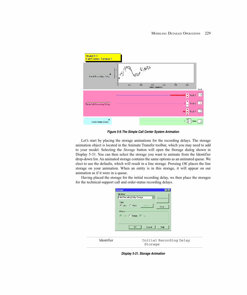
229MODELING DETAILED OPERATIONS
Figure 5-9. The Simple Call Center System Animation
Let’s start by placing the storage animations for the recording delays. The storageanimation object is located in the Animate Transfer toolbar, which you may need to addto your model. Selecting the Storage button will open the Storage dialog shown inDisplay 5-31. You can then select the storage you want to animate from the Identifierdrop-down list. An animated storage contains the same options as an animated queue. Weelect to use the defaults, which will result in a line storage. Pressing OK places the linestorage on your animation. When an entity is in this storage, it will appear on ouranimation as if it were in a queue.
Having placed the storage for the initial recording delay, we then place the storagesfor the technical-support call and order-status recording delays.
Identifier Initial Recording Delay Storage
Display 5-31. Storage Animation
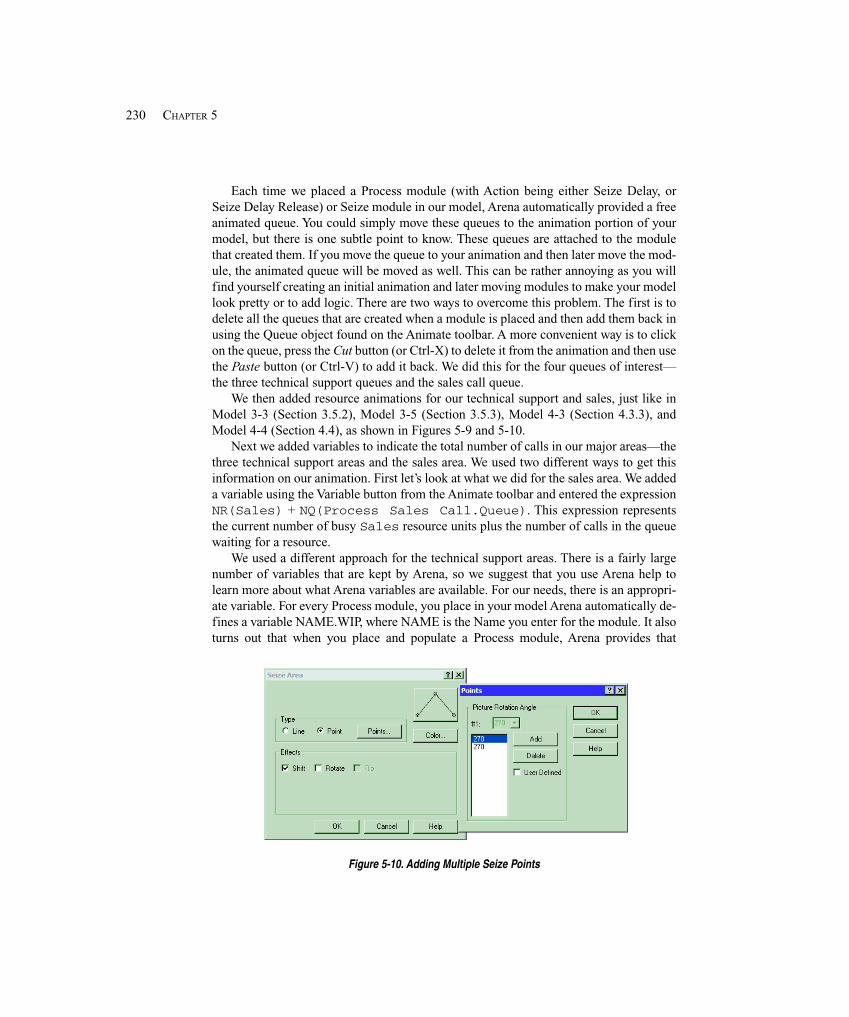
230 CHAPTER 5
Each time we placed a Process module (with Action being either Seize Delay, orSeize Delay Release) or Seize module in our model, Arena automatically provided a freeanimated queue. You could simply move these queues to the animation portion of yourmodel, but there is one subtle point to know. These queues are attached to the modulethat created them. If you move the queue to your animation and then later move the mod-ule, the animated queue will be moved as well. This can be rather annoying as you willfind yourself creating an initial animation and later moving modules to make your modellook pretty or to add logic. There are two ways to overcome this problem. The first is todelete all the queues that are created when a module is placed and then add them back inusing the Queue object found on the Animate toolbar. A more convenient way is to clickon the queue, press the Cut button (or Ctrl-X) to delete it from the animation and then usethe Paste button (or Ctrl-V) to add it back. We did this for the four queues of interest—the three technical support queues and the sales call queue.
We then added resource animations for our technical support and sales, just like inModel 3-3 (Section 3.5.2), Model 3-5 (Section 3.5.3), Model 4-3 (Section 4.3.3), andModel 4-4 (Section 4.4), as shown in Figures 5-9 and 5-10.
Next we added variables to indicate the total number of calls in our major areas—thethree technical support areas and the sales area. We used two different ways to get thisinformation on our animation. First let’s look at what we did for the sales area. We addeda variable using the Variable button from the Animate toolbar and entered the expressionNR(Sales) + NQ(Process Sales Call.Queue). This expression representsthe current number of busy Sales resource units plus the number of calls in the queuewaiting for a resource.
We used a different approach for the technical support areas. There is a fairly largenumber of variables that are kept by Arena, so we suggest that you use Arena help tolearn more about what Arena variables are available. For our needs, there is an appropri-ate variable. For every Process module, you place in your model Arena automatically de-fines a variable NAME.WIP, where NAME is the Name you enter for the module. It alsoturns out that when you place and populate a Process module, Arena provides that
Figure 5-10. Adding Multiple Seize Points
231MODELING DETAILED OPERATIONS
variable as part of the standard animation for that module, along with the queue. If youlook closely at your model when it’s not running, you’ll see a red 0 centered directlyunder each Process module. For our technical support for product Type 1, that turns outto be the variable Process Product Type 1 Tech Call.WIP. You can place a newvariable using the Variable button and enter the name—it’s not on the drop-down list—oryou can cut and paste the variable supplied by the Process module. We actually used thecopy and paste functions in creating our animation. Arena will not let you animatemultiple queues or resources with the same name, but it will allow it for variables. Weused this approach to add the three WIP variables to our technical support portion of theanimation.
The last thing that we added to our animation was the total number of trunk lines inuse. We could have used the Arena variable NR(Trunk Lines), which would havegiven us the current number of calls in the system. Instead, we decided to add a plot, ofthe same variable, which gives us a good view of how the demand on our system changesover the simulation run. To complete our animation, we added some labels and back-ground color.
If you run your model, you might notice by looking at our plot of the number of busytrunk lines that the system is either full or close to full most of the time; the “flat top” onthe plot at height 26 confirms our arrival logic that refuses incoming calls when all 26trunk lines are already taken. Looking at the output from the run, we see that there were734 attempted calls with 643 of them completed and 91 rejected or balked. You mightalso notice that the simulation run length was just over 637 minutes. The last 37 minuteswere the time it took to complete the calls that were in the system at 6 PM; note that thetrunk-lines plot declines to zero at the end of the simulation, confirming our terminationlogic described above.
That completes Model 5-1.
5.5 Model 5-2: The Enhanced Call Center System
In developing models for real systems, you want to keep your model as simple aspossible and yet you want that model to capture the system’s behavior accurately. Ourultimate goal is to use our model to find the most cost effective way to increase ourservice level or customer satisfaction. We would like to consider the impact of suchchanges as increasing the number of trunk lines or changing our staffing levels. Althoughour current model would allow us to capture these changes, it’s lacking in detail. So let’srevisit our problem description and determine where we need to add more detail.
5.5.1 The New Problem DescriptionLet’s start with a more detailed examination of call arrivals. The call-arrival rate to thissystem actually varies over the course of the day according to a nonstationary Poissonprocess (see Section 12.3), which is typical of these types of systems. So we mightcollect data expressed in calls per hour for each 30-minute period during which thesystem is open. These call-arrival rates are given in Table 5-2.
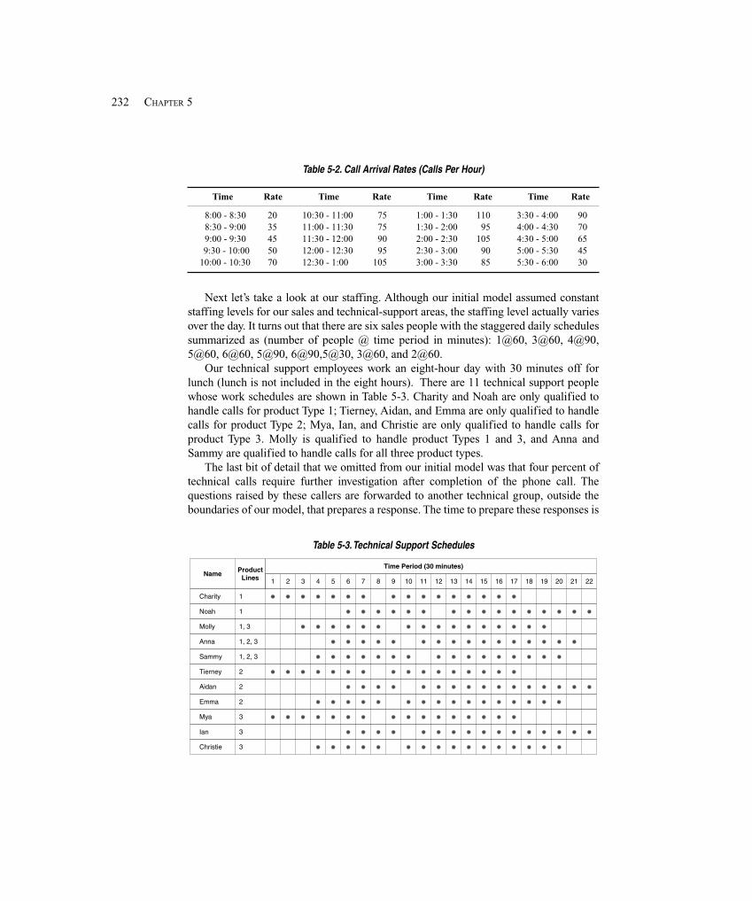
232 CHAPTER 5
Table 5-2. Call Arrival Rates (Calls Per Hour)
Time Rate Time Rate Time Rate Time Rate
8:00 - 8:30 20 10:30 - 11:00 75 1:00 - 1:30 110 3:30 - 4:00 908:30 - 9:00 35 11:00 - 11:30 75 1:30 - 2:00 95 4:00 - 4:30 709:00 - 9:30 45 11:30 - 12:00 90 2:00 - 2:30 105 4:30 - 5:00 65
9:30 - 10:00 50 12:00 - 12:30 95 2:30 - 3:00 90 5:00 - 5:30 4510:00 - 10:30 70 12:30 - 1:00 105 3:00 - 3:30 85 5:30 - 6:00 30
Next let’s take a look at our staffing. Although our initial model assumed constantstaffing levels for our sales and technical-support areas, the staffing level actually variesover the day. It turns out that there are six sales people with the staggered daily schedulessummarized as (number of people @ time period in minutes): 1@60, 3@60, 4@90,5@60, 6@60, 5@90, 6@90,5@30, 3@60, and 2@60.
Our technical support employees work an eight-hour day with 30 minutes off forlunch (lunch is not included in the eight hours). There are 11 technical support peoplewhose work schedules are shown in Table 5-3. Charity and Noah are only qualified tohandle calls for product Type 1; Tierney, Aidan, and Emma are only qualified to handlecalls for product Type 2; Mya, Ian, and Christie are only qualified to handle calls forproduct Type 3. Molly is qualified to handle product Types 1 and 3, and Anna andSammy are qualified to handle calls for all three product types.
The last bit of detail that we omitted from our initial model was that four percent oftechnical calls require further investigation after completion of the phone call. Thequestions raised by these callers are forwarded to another technical group, outside theboundaries of our model, that prepares a response. The time to prepare these responses is
Table 5-3. Technical Support Schedules
22212019181716151413121110987654321
ProductLines
Name
Charity
Noah
Molly
Anna
Sammy
Tierney
Aidan
Mya
Ian
Emma
Christie
1
1
1, 3
1, 2, 3
1, 2, 3
2
2
2
3
3
3
Time Period (30 minutes)
233MODELING DETAILED OPERATIONS
estimated to be EXPO(60) minutes. The resulting response is sent back to the sametechnical support person who answered the original call. This person then calls thecustomer, which takes TRIA(2, 4, 9) minutes. These returned calls require one of the 26trunk lines and receive priority over incoming calls. If a returned call is not completed onthe same day the original call was received, it’s carried over to the next day.
If we are going to consider changing our staffing levels to increase customer satisfac-tion, we might also want more detail on when the system is congested. So let’s addcounters to our model that we’ll use to count the number of rejected calls during eachhour of operation.
5.5.2 New ConceptsOur enhanced model requires two new concepts. The first is the arrival process whoserate varies over time. The second concept shows that when a call attempts to seize a unitof a technical staff resource, it is really trying to seize a resource from a pool or set ofresources qualified to handle the call. Let’s discuss each of these new concepts before webuild our model.
We’ll start with the arrival process, which has a rate that varies over time. This type ofarrival process is fairly typical of service systems and requires a different approach.Arrivals at many systems are modeled as a stationary Poisson process in which arrivalsoccur one at a time, are independent of one another, and the average rate is constant overtime. For those of you who are not big fans of probability, this implies that we haveexponential interarrival times with a fixed mean. You may not have realized it, but this isthe process we used to model arrivals in our previous models (with the exception ofModel 4-5, which was contrived to illustrate a particular point). There was a slightvariation of this used for the Part B arrivals in Models 4-1 through 4-4, where weassumed that an arrival was a batch of four; therefore, our arrivals still occurred onebatch at a time according to a stationary Poisson process.
For this model, the mean arrival rate is a function of time. These types of arrivals areusually modeled as a nonstationary Poisson process. An obvious, but incorrect, modelingapproach would be to enter for the Time Between Arrivals in a Create module anexponential distribution with a user-defined variable as a mean Value, then change thisValue based on the rate for the current time period. For our example, we’d change thisValue every 30 minutes. This would provide an approximate solution if the rate changebetween the periods was rather small. But if the rate change is large, this method can givevery misleading (and wrong) results. The easiest way to illustrate the potential problem isto consider an extreme example. Let’s say we have only two periods, each 30 minuteslong. The rate for the first period is 3 (average arrivals per hour), or an interarrival-timemean of 20 minutes, and the rate for the second period is 60, or an interarrival-time meanof 1 minute. Let’s suppose that the last arrival in the first time period occurred at time 29
234 CHAPTER 5
minutes. We’d generate the next arrival using an interarrival-time mean Value of 20minutes. Using an exponential distribution with a mean of 20 could easily1 return a valuemore than 31 for the time to the next arrival. This would result in no arrivals during thesecond period, when in fact there should be an expected value of 30 arrivals2. In general,using this simplistic method causes an incorrect decrease in the number of arrivals whengoing from one period to the next with an increase in the rate, or a decrease in theinterarrival time. Going from one period to the next with a decrease in the rate willincorrectly increase the number of arrivals in the second period.
Nevertheless, it’s important to be able to model and generate such arrival processescorrectly since they seem to arise all the time, and ignoring the nonstationarity can createserious model-validity errors since the peaks and troughs can have significant impact onsystem performance. Fortunately, Arena has a built-in ability to generate nonstationaryPoisson arrivals (and to do so correctly) in the Create module. The underlying methodused is described in Section 12.3.
The second new concept is the need to model an entity arriving at a location orstation and selecting from one of several similar (but not quite identical) objects. Themost common situation is the selection of an available resource from a pool of resources.Let’s assume you have three operators: Sean, Lynn, and Michael. Any one of theseoperators can perform the required task, and you would like to select any of the three, aslong as one is currently available. The Sets data module in the Basic Process panelprovides the basis for this functionality. Arena sets are groups of objects of the same typethat can be referenced by a common name (the set name) and a set index. The objects thatmake up the set are referred to as members of the set. Members of a particular set mustall be the same type of object, such as resources, queues, pictures, etc. You can collectalmost any type of Arena objects into a set, depending on your modeling requirements.An object can also reside in more than one set. Let’s assume in our Operators set thatLynn is also qualified as a setup person. Therefore, we might define a second resourceset called Setup as Lynn and Doug (Doug’s not an operator). Now, if an operator isrequired, we’d select from the set called Operators; if a setup person is required, wewould select from the set called Setup. Lynn might be chosen via either case becauseshe’s a member of both sets. You can have as many sets as you want with as much or aslittle overlap as required.
For our call center, we’ll need to use sets to model the technical support staff correctly.We also need to consider how to model the returned technical support calls. These areunique in that they must be returned by the same tech-support person who handled the
2 The probability of no arrivals in the second period should be e-60(1/2) = 0.000000000000093576.
1 With probability e-31/20 = 0.21, to be (almost) exact. Actually this figure is the conditional probability ofno arrivals in the second period, given that there were arrivals in the first period and that the last of these was attime 29. This is not quite what we want, though; we want the unconditional probability of seeing no arrivals inthe second period. It’s possible to work this out, but it’s complicated. However, it’s easy to see that a lowerbound on this probability is given by the probability that the first arrival after time 0, generated as exponentialwith mean 20 minutes, occurs after time 60—this is one way (not the only way) to have no arrivals in the sec-ond period, and has probability e-60/20 = e-3 = 0.0498. Thus, the incorrect method would give us at least a 5%chance of having no arrivals in the second period. Now, go back to the text, read the next sentence, and see thenext footnote.
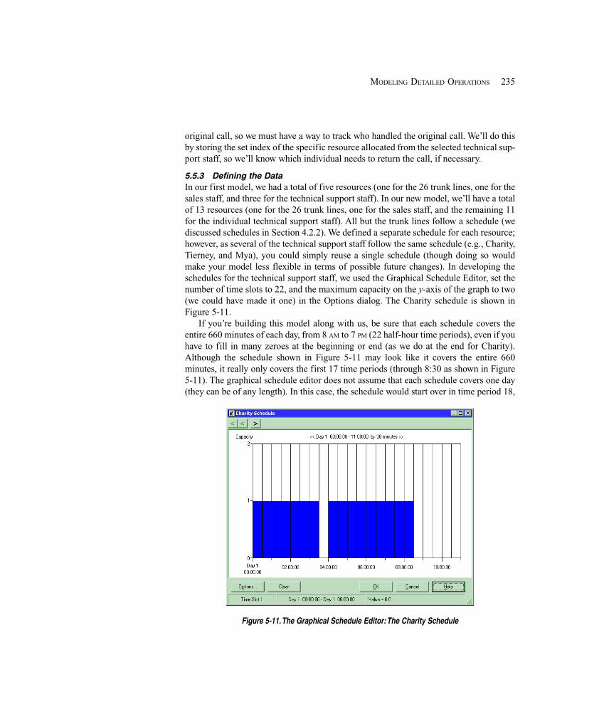
235MODELING DETAILED OPERATIONS
original call, so we must have a way to track who handled the original call. We’ll do thisby storing the set index of the specific resource allocated from the selected technical sup-port staff, so we’ll know which individual needs to return the call, if necessary.
5.5.3 Defining the DataIn our first model, we had a total of five resources (one for the 26 trunk lines, one for thesales staff, and three for the technical support staff). In our new model, we’ll have a totalof 13 resources (one for the 26 trunk lines, one for the sales staff, and the remaining 11for the individual technical support staff). All but the trunk lines follow a schedule (wediscussed schedules in Section 4.2.2). We defined a separate schedule for each resource;however, as several of the technical support staff follow the same schedule (e.g., Charity,Tierney, and Mya), you could simply reuse a single schedule (though doing so wouldmake your model less flexible in terms of possible future changes). In developing theschedules for the technical support staff, we used the Graphical Schedule Editor, set thenumber of time slots to 22, and the maximum capacity on the y-axis of the graph to two(we could have made it one) in the Options dialog. The Charity schedule is shown inFigure 5-11.
If you’re building this model along with us, be sure that each schedule covers theentire 660 minutes of each day, from 8 AM to 7 PM (22 half-hour time periods), even if youhave to fill in many zeroes at the beginning or end (as we do at the end for Charity).Although the schedule shown in Figure 5-11 may look like it covers the entire 660minutes, it really only covers the first 17 time periods (through 8:30 as shown in Figure5-11). The graphical schedule editor does not assume that each schedule covers one day(they can be of any length). In this case, the schedule would start over in time period 18,
Figure 5-11. The Graphical Schedule Editor: The Charity Schedule
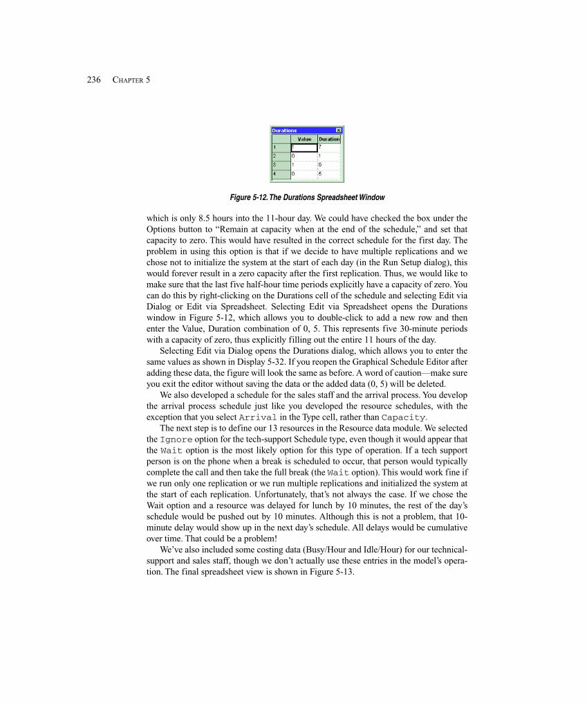
236 CHAPTER 5
Figure 5-12. The Durations Spreadsheet Window
which is only 8.5 hours into the 11-hour day. We could have checked the box under theOptions button to “Remain at capacity when at the end of the schedule,” and set thatcapacity to zero. This would have resulted in the correct schedule for the first day. Theproblem in using this option is that if we decide to have multiple replications and wechose not to initialize the system at the start of each day (in the Run Setup dialog), thiswould forever result in a zero capacity after the first replication. Thus, we would like tomake sure that the last five half-hour time periods explicitly have a capacity of zero. Youcan do this by right-clicking on the Durations cell of the schedule and selecting Edit viaDialog or Edit via Spreadsheet. Selecting Edit via Spreadsheet opens the Durationswindow in Figure 5-12, which allows you to double-click to add a new row and thenenter the Value, Duration combination of 0, 5. This represents five 30-minute periodswith a capacity of zero, thus explicitly filling out the entire 11 hours of the day.
Selecting Edit via Dialog opens the Durations dialog, which allows you to enter thesame values as shown in Display 5-32. If you reopen the Graphical Schedule Editor afteradding these data, the figure will look the same as before. A word of caution—make sureyou exit the editor without saving the data or the added data (0, 5) will be deleted.
We also developed a schedule for the sales staff and the arrival process. You developthe arrival process schedule just like you developed the resource schedules, with theexception that you select Arrival in the Type cell, rather than Capacity.
The next step is to define our 13 resources in the Resource data module. We selectedthe Ignore option for the tech-support Schedule type, even though it would appear thatthe Wait option is the most likely option for this type of operation. If a tech supportperson is on the phone when a break is scheduled to occur, that person would typicallycomplete the call and then take the full break (the Wait option). This would work fine ifwe run only one replication or we run multiple replications and initialized the system atthe start of each replication. Unfortunately, that’s not always the case. If we chose theWait option and a resource was delayed for lunch by 10 minutes, the rest of the day’sschedule would be pushed out by 10 minutes. Although this is not a problem, that 10-minute delay would show up in the next day’s schedule. All delays would be cumulativeover time. That could be a problem!
We’ve also included some costing data (Busy/Hour and Idle/Hour) for our technical-support and sales staff, though we don’t actually use these entries in the model’s opera-tion. The final spreadsheet view is shown in Figure 5-13.
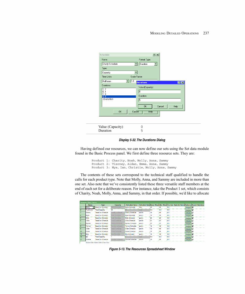
237MODELING DETAILED OPERATIONS
Value (Capacity) 0Duration 5
Display 5-32. The Durations Dialog
Having defined our resources, we can now define our sets using the Set data modulefound in the Basic Process panel. We first define three resource sets. They are:
Product 1: Charity, Noah, Molly, Anna, SammyProduct 2: Tierney, Aidan, Emma, Anna, SammyProduct 3: Mya, Ian, Christie, Molly, Anna, Sammy
The contents of these sets correspond to the technical staff qualified to handle thecalls for each product type. Note that Molly, Anna, and Sammy are included in more thanone set. Also note that we’ve consistently listed these three versatile staff members at theend of each set for a deliberate reason. For instance, take the Product 1 set, which consistsof Charity, Noah, Molly, Anna, and Sammy, in that order. If possible, we’d like to allocate
Figure 5-13. The Resources Spreadsheet Window

238 CHAPTER 5
Figure 5-14. The Members Spreadsheet Window for the Product 1 Set
Charity or Noah to an incoming call first because they can only handle product Type 1calls. We’ll use the Preferred Order selection rule, which allocates resources based ontheir order in the set, starting with the first (Charity). In our model, this will try to keepMolly, Anna, and Sammy available since they can handle other product types as well.
The Set module allows us to form sets of resources, counters, tallies, entity types, andentity pictures. You can also form sets of any other Arena objects by using the AdvancedSet data module found in the Advanced Process panel. Form a set by clicking on the Setmodule and then double-clicking in the spreadsheet view to add a new entry. We’ll walkyou through the details for creating the first resource set. Enter Product 1 in the Namecell, and select Resource from the pull-down in the Type cell. To define the membersof the set, click on “0 Rows” in the Members column to open a spreadsheet for listing themembers, and then double-click to open a new blank row. Since we have already definedour resources, you can use the pull-down option to select the Resource Name for eachmember. To add additional members to the set, just double-click where indicated to addmore new rows. The completed member spreadsheet view for the Product 1 set is shownin Figure 5-14. You’ll need to repeat this for the Product 2 and Product 3 sets.
We also defined a Counter set (called Rejected Calls) with ten members, whichwe’ll use to keep track of the number of rejected calls (busy signals) for each hour timeperiod. For this set, we first defined the ten counters using the Statistic data module (inthe Advanced Process panel). We assigned the statistic names as Period 01 throughPeriod 10 and the corresponding Counter Names as Period 01 Rejected Callsthrough Period 10 Rejected Calls (the leading 0s for periods 1 through 9 are sothings will be alphabetized properly in the output reports). We also selectedReplicate for the Initialize Option cell, which will cause the counters to be clearedwhenever the other statistics are cleared, as specified in the Run > Setup dialog. We couldhave also selected the Yes option; if the No option is specified and multiple replicationsare performed, then the value of the counter at the end of a replication will be retained asthe initial value at the beginning of the next replication so that the reported values will becumulative as the replications are made. The first five counter entries are shown inFigure 5-15.
The completed Set data module is shown in Figure 5-16, which includes threeResource sets and one Counter set.
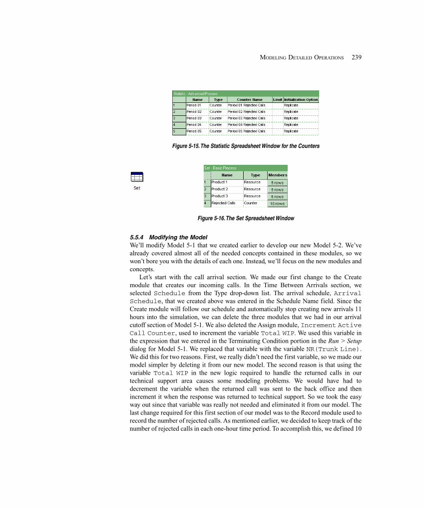
239MODELING DETAILED OPERATIONS
Figure 5-15. The Statistic Spreadsheet Window for the Counters
Figure 5-16. The Set Spreadsheet Window
5.5.4 Modifying the ModelWe’ll modify Model 5-1 that we created earlier to develop our new Model 5-2. We’vealready covered almost all of the needed concepts contained in these modules, so wewon’t bore you with the details of each one. Instead, we’ll focus on the new modules andconcepts.
Let’s start with the call arrival section. We made our first change to the Createmodule that creates our incoming calls. In the Time Between Arrivals section, weselected Schedule from the Type drop-down list. The arrival schedule, ArrivalSchedule, that we created above was entered in the Schedule Name field. Since theCreate module will follow our schedule and automatically stop creating new arrivals 11hours into the simulation, we can delete the three modules that we had in our arrivalcutoff section of Model 5-1. We also deleted the Assign module, Increment ActiveCall Counter, used to increment the variable Total WIP. We used this variable inthe expression that we entered in the Terminating Condition portion in the Run > Setupdialog for Model 5-1. We replaced that variable with the variable NR(Trunk Line).We did this for two reasons. First, we really didn’t need the first variable, so we made ourmodel simpler by deleting it from our new model. The second reason is that using thevariable Total WIP in the new logic required to handle the returned calls in ourtechnical support area causes some modeling problems. We would have had todecrement the variable when the returned call was sent to the back office and thenincrement it when the response was returned to technical support. So we took the easyway out since that variable was really not needed and eliminated it from our model. Thelast change required for this first section of our model was to the Record module used torecord the number of rejected calls. As mentioned earlier, we decided to keep track of thenumber of rejected calls in each one-hour time period. To accomplish this, we defined 10

240 CHAPTER 5
Name Record Rejected Call for Current Hour Period
Type CountValue 1Record into Set CheckCounter Set Name Rejected CallsSet Index AINT((TNOW/60) + 1)
Display 5-33. Counting the Rejected Calls by One-Hour Period
counters in the Statistic data module and formed a set called Rejected Callscontaining these counters. We altered the Record module by checking the Record intoSet box and entered the set name. We then developed an expression AINT((TNOW/60)+1) that would yield an integer value that represents the current period based on thesimulation run time, in Display 5-33; to understand how this expression works, note thatTNOW is the internal Arena simulation-clock value (in minutes, our Base Time Units),AINT is a built-in Arena function that truncates its real-number argument toward zero,and then “play computer” for some minute values of TNOW.
Now let’s proceed to the changes we made to the Tech Support Calls section of ourmodel. The first five modules (up to and including the Determine Product TypeDecide module) remain the same as in Model 5-1. We’ll walk you through the changesrequired for the product Type 1 technical support and refer you to the file Model05-02.doe for the differences for the other two types of technical support calls.
Directly following the Determine Product Type Decide module, we insertedan Assign module where we made three assignments. We first assigned a new entity typeand entity picture so we could tell the difference between the calls for different producttypes in both the animation and the reports. We also defined a new attribute called TechCall Type, which is assigned an integer value of 1, 2 or 3, depending on the producttype. Soon you’ll see why we need this new attribute.
The following Process module is the same except for the information in theResources section. Since we replaced the single resource, Tech 1, in Model 5-1 withresource set Product 1, we needed to modify this section. We changed the Type to Setand entered Product 1 for the Set Name. We selected Preferred Order for theSelection Rule and defined a new attribute, Tech Agent Index, for the Save Attributefield. When we defined our resource sets, we consistently listed the most versatile staffmembers at the end of each set. Recall that this set consists of Charity, Noah, Molly,Anna, and Sammy, in that order; notice that we placed Molly, Anna, and Sammy as thelast resources in the set. Thus, if possible, we’d like to allocate Charity or Noah to anincoming call first because they can only handle product Type 1 calls. The PreferredOrder selection rule allocates resources based on their order in the set, if there is a choiceamong multiple idle resources, starting with the first (Charity). In our model, this will tryto keep Molly, Anna, and Sammy available; remember that they can handle other calltypes as well. We’ve also stored the index of the resource allocated in the Save AttributeTech Agent Index because we’ll need to know which person took the call if further
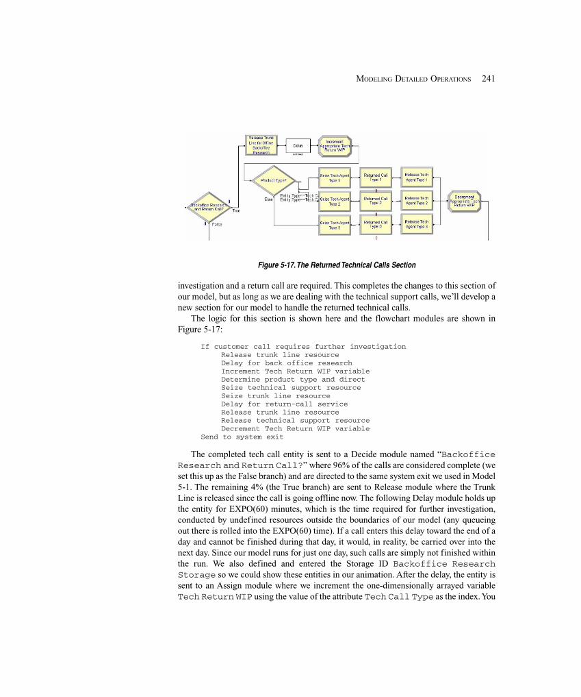
241MODELING DETAILED OPERATIONS
Figure 5-17. The Returned Technical Calls Section
investigation and a return call are required. This completes the changes to this section ofour model, but as long as we are dealing with the technical support calls, we’ll develop anew section for our model to handle the returned technical calls.
The logic for this section is shown here and the flowchart modules are shown inFigure 5-17:
If customer call requires further investigationRelease trunk line resourceDelay for back office researchIncrement Tech Return WIP variableDetermine product type and directSeize technical support resourceSeize trunk line resourceDelay for return-call serviceRelease trunk line resourceRelease technical support resourceDecrement Tech Return WIP variable
Send to system exit
The completed tech call entity is sent to a Decide module named “BackofficeResearch and Return Call?” where 96% of the calls are considered complete (weset this up as the False branch) and are directed to the same system exit we used in Model5-1. The remaining 4% (the True branch) are sent to Release module where the TrunkLine is released since the call is going offline now. The following Delay module holds upthe entity for EXPO(60) minutes, which is the time required for further investigation,conducted by undefined resources outside the boundaries of our model (any queueingout there is rolled into the EXPO(60) time). If a call enters this delay toward the end of aday and cannot be finished during that day, it would, in reality, be carried over into thenext day. Since our model runs for just one day, such calls are simply not finished withinthe run. We also defined and entered the Storage ID Backoffice ResearchStorage so we could show these entities in our animation. After the delay, the entity issent to an Assign module where we increment the one-dimensionally arrayed variableTech Return WIP using the value of the attribute Tech Call Type as the index. You
242 CHAPTER 5
can define this variable in the Assign module, but you first need to open the Variable datamodule and enter a value of 3 in the Rows cell, which defines the array size. We nextsense the product type with an N-way by Condition test in the “Product Type?”Decide module and direct the return call to the proper branch.
The return-call entity must seize both a trunk line (outgoing calls need a trunk line asdo incoming calls), and the appropriate tech support person, being the one who took theoriginal incoming call. We’ll describe things for product Type 1; the other two aresimilar. In the following Seize module, the return tech support call for product Type 1seizes from the appropriate Resource Set of tech support people. Queueing is possible,and we use a separate queue (and animation) for this, and specify the seize Priority asHigh (1), as outgoing return calls take priority over incoming calls. Here we seize onlythe tech support person and not the trunk line (we’ll do that in the following module).This return call must go to the same tech support person who took the original customercall, so we use the Specific Member Selection Rule and specify the Attribute TechAgent Index in the Set Index field to ensure this.
Having already seized the right Tech 1 agent, the return Tech 1 call now seizes aTrunk Line in the following Process module, with High Priority over Medium-priorityincoming calls. The processing delay is based on the expression Returned TechTime and when completed, the trunk line is released. Queueing could occur in thismodule, if no trunk line is immediately available. During that time, the animation is stillaccurate since the entity picture shows in the Resource animation’s Seize Area, so there isno separate queue animation for this. When the call is completed, the specified techsupport person is released in the following Release module.
In our first attempt at developing this section, we used a single Process module witha high priority to seize both the tech support person and the trunk line at the same time.When we ran our simulation and watched the animation, we realized that these returncalls were waiting a long time before they were processed. It turns out that when you takethis modeling approach both resources must be available at the same time for the entityto proceed. If only one of the specified resources is available and the system is busy, itwould most likely be allocated to another waiting entity. Since these return calls have ahigh priority, we decided to seize the resources separately. We realized that in the realsystem the returned call would most likely be given to the specified tech support person,who would try to return the call as soon as he or she was available. Of course in doing so,he or she would have to first seize an available trunk line. So we modified our modellogic by separating the two seize actions as previously described.
Upon completion of the return call, the entity enters an Assign module where thearrayed variable Tech Return WIP is decremented. The completed call is now readyto be sent to the system exit. In every other case where a completed call was sent to thesystem exit, it still had the trunk line resource, so the first module was a Release moduleto release that resource. These entities have already released the trunk line resource so weneed to send the entities to the Record module following that Release module.
If you look in the Statistic data module (Advanced Process panel), you’ll see the tenCounter-type entries we described earlier. We also set up four statistics of the Time-Persistent type to request results (time average, minimum, and maximum) on the total

243MODELING DETAILED OPERATIONS
number of calls in backoffice research for a callback (tracking variableNSTO(Backoffice Research Storage)) and for the total numbers of each tech-support product type in the system (tracking expressions Tech 1 Total Online WIP,Tech 2 Total Online WIP, and Tech 3 Total Online WIP).
Our new model does not require any changes to the Sales Calls or Order-Status Callsof Model 5-1.
Now let’s review the modifications to our animation. The three animated storages forthe recording delays, the Trunk Lines Busy plot, the variable for the Sales WIP, and thequeues for the calls waiting for tech support and sales remain the same. We first deletedthe Tech 1, Tech 2, and Tech 3 resources from our animation. Then we changed thevariable names for the three WIP displays to match our new model. For example, wechanged the WIP variable for product Type 1 from Process Product Type 1 TechCall.WIP to Tech 1 Total Online WIP, which is an expression we defined in theExpression data module to be Process Product Type 1 Tech Call.WIP + TechReturn WIP(1) so it is at all times the total number of tech calls for product Type 1that are “open,” either as an incoming call or in the back office for a return call. We alsorearranged our new animation to allow for a Back Office Research area and added a WIPvariable, NSTO(Backoffice Research Storage); NSTO is a built-in Arenafunction that returns the number of entities in the Storage given in its argument.
We also added three new queues to the tech support area to shown the return calls wait-ing for service. This queue for the Tech 1 area is Seize Tech Agent Type 1.Queue.We then added a storage animation to show the return calls that we had under investigationfor the new back office research area, Backoffice Research Storage.
The final change was to add the resources for our new tech support personnel. Weselected Charity from the resource list and opened the Arena office picture library,Office.plb. There we found a picture of a person sitting at a desk with an idle phoneand a second picture with the person talking on the phone. We copied the first picture torepresent our Idle picture and the second to be the Busy picture. For our Inactive state, wealtered the first picture to remove the person so the desk was unattended. We then closedthe window and placed our resource. After sizing our resource, we used the Text option tolabel it. Then we made a copy of these two objects and changed the identifiers torepresent Noah. We repeated this for Tierney, but changed the color of the shirt in the Idleand Busy pictures. Our plan was to use different shirt colors to represent the differentcapabilities of the support staff.
The final animated simulation is similar to Figure 5-18, which was taken at approxi-mately time 341.1. In the Category Overview report, we see from the User Specifiedsection’s Counters that most rejected calls occur in hours 5-8 (corresponding to noon to4:00 PM), so this might be a time period to look at adding staff (though we’ve made onlyone replication here so such a conclusion is statistically suspect); we’ll take this up in amore organized and statistically reliable way in Chapter 6.
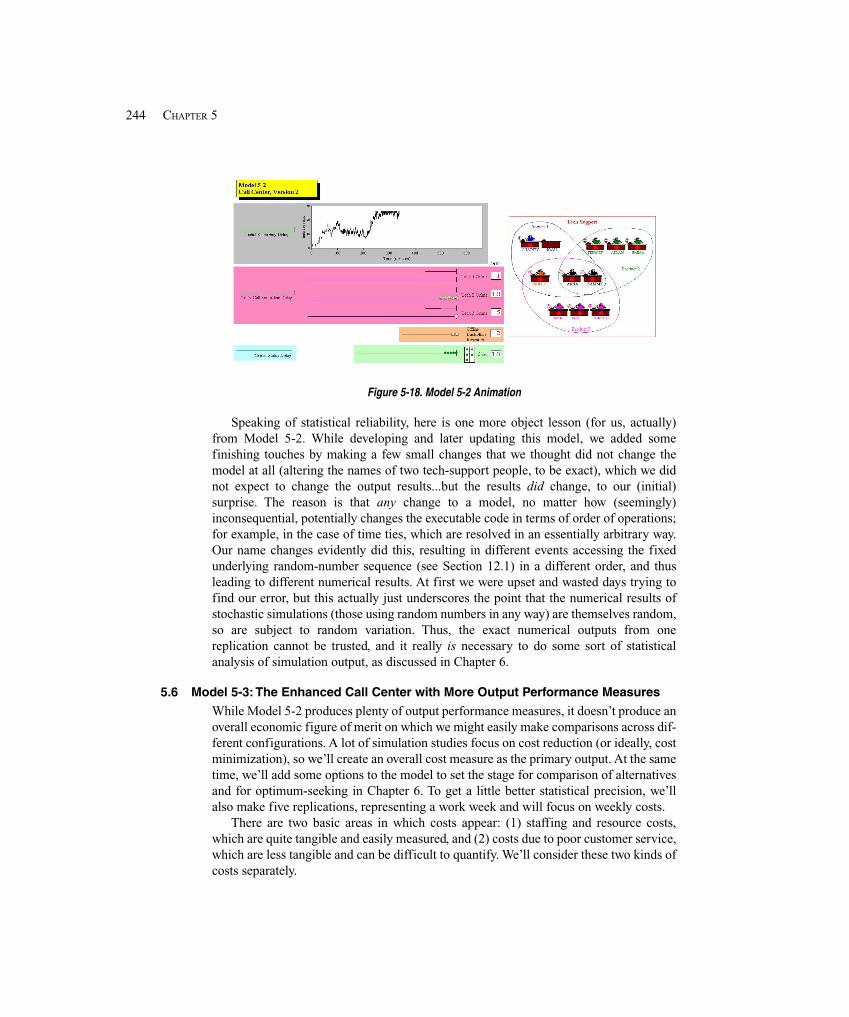
244 CHAPTER 5
Figure 5-18. Model 5-2 Animation
Speaking of statistical reliability, here is one more object lesson (for us, actually)from Model 5-2. While developing and later updating this model, we added somefinishing touches by making a few small changes that we thought did not change themodel at all (altering the names of two tech-support people, to be exact), which we didnot expect to change the output results...but the results did change, to our (initial)surprise. The reason is that any change to a model, no matter how (seemingly)inconsequential, potentially changes the executable code in terms of order of operations;for example, in the case of time ties, which are resolved in an essentially arbitrary way.Our name changes evidently did this, resulting in different events accessing the fixedunderlying random-number sequence (see Section 12.1) in a different order, and thusleading to different numerical results. At first we were upset and wasted days trying tofind our error, but this actually just underscores the point that the numerical results ofstochastic simulations (those using random numbers in any way) are themselves random,so are subject to random variation. Thus, the exact numerical outputs from onereplication cannot be trusted, and it really is necessary to do some sort of statisticalanalysis of simulation output, as discussed in Chapter 6.
5.6 Model 5-3: The Enhanced Call Center with More Output Performance MeasuresWhile Model 5-2 produces plenty of output performance measures, it doesn’t produce anoverall economic figure of merit on which we might easily make comparisons across dif-ferent configurations. A lot of simulation studies focus on cost reduction (or ideally, costminimization), so we’ll create an overall cost measure as the primary output. At the sametime, we’ll add some options to the model to set the stage for comparison of alternativesand for optimum-seeking in Chapter 6. To get a little better statistical precision, we’llalso make five replications, representing a work week and will focus on weekly costs.
There are two basic areas in which costs appear: (1) staffing and resource costs,which are quite tangible and easily measured, and (2) costs due to poor customer service,which are less tangible and can be difficult to quantify. We’ll consider these two kinds ofcosts separately.

245MODELING DETAILED OPERATIONS
First, let’s look at staffing and resource costs, some of which we defined in Model 5-2but didn’t use. In the Resource module of Model 5-2, we defined a cost of $20/hour forsales staff and $18-$22/hour for tech support staff, depending on their level of trainingand flexibility; these costs were incurred whenever the staff were present according totheir schedules, regardless of whether they were busy or idle. Using the staffing informa-tion described in Section 5.5 (and defined in the Schedule data module of Model 5-2),the weekly cost for the current staff is:
Sales staff altogether: 45 hours/day × $20/hour × 5 days/week = $4,500/weekTech support staff:
8 people × (8 hours/day)/person × $18/hour × 5 days/week = $5,760/week1 person × (8 hours/day)/person × $20/hour × 5 days/week = $800/week2 people × (8 hours/day)/person × $22/hour × 5 days/week = $1,760/week
Adding, we get a current weekly payroll cost of $12,820.To try to improve service, we now generalize the model to allow for additional staff.
Looking at the hourly counts of the busy-signal balks from Model 5-2, it seems that themost severe staffing shortfalls are between noon and 4:00 PM, so we’ll create the abilityin the model to add both sales and tech support during that four-hour period, whichcorresponds to the four hour-long time periods 5 through 8.
To add an easily controlled variable number of sales staff, we define a variable NewSales to be the number of additional sales staff we hire for this four-hour period eachday, at a cost of $17/hour. Each additional sales staff person will thus work 20 hours/week, so the additional cost is $17/hour × 20 hours/week = $340/week for each new salesstaff person. To place the new sales staff in the model, we edit the Sales Scheduleline in the Schedule data module. Since we’ll use a Variable (New Sales) as part of theschedule, we cannot use the Graphical Schedule Editor and must access this schedule viaits dialog (or spreadsheet); right-click in the Sales Schedule line and then select Editvia Dialog. Display 5-34 illustrates where the edits are made. Of course, if we set NewSales to 0, we have the same sales-staff configuration as in the base model.
We follow a similar strategy to add tech support people during this 12:00 PM to4:00 PM period. We defined new Variables New Tech 1, New Tech 2, and New Tech 3to be the number of additional tech support staff added who are qualified only onProduct Types 1, 2, and 3, respectively, and New Tech All to be the number of techsupport people added who are qualified on all three product types. Naturally, the newType 1 techs are all named Larry, the new Type 2 techs are all named Moe, the new Type3 techs are all named Curly, and the new All-type techs are all named Hermann. Fournew entries in the Resource data module are added to create these resources and definehourly rates for them ($16 for each Larry, Moe, and Curly, and $18 for each Hermann).To express their qualifications, we add Larry to the Product 1 set in the Set module,Moe to the Product 2 set, Curly to the Product 3 set, and Hermann to all three ofthese sets. We created schedule entries for all four of these new resources. The Larryschedule is in Display 5-35 and the other three are similar; like the sales schedule, thesecan be edited only via the dialog (or spreadsheet) and not by the Graphical Schedule
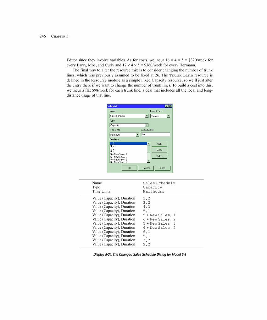
246 CHAPTER 5
Editor since they involve variables. As for costs, we incur 16 × 4 × 5 = $320/week forevery Larry, Moe, and Curly and 17 × 4 × 5 = $360/week for every Hermann.
The final way to alter the resource mix is to consider changing the number of trunklines, which was previously assumed to be fixed at 26. The Trunk Line resource isdefined in the Resource module as a simple Fixed Capacity resource, so we’ll just alterthe entry there if we want to change the number of trunk lines. To build a cost into this,we incur a flat $98/week for each trunk line, a deal that includes all the local and long-distance usage of that line.
Name Sales ScheduleType CapacityTime Units Halfhours
Value (Capacity), Duration 1,2Value (Capacity), Duration 3,2Value (Capacity), Duration 4,3Value (Capacity), Duration 5,1Value (Capacity), Duration 5 + New Sales, 1Value (Capacity), Duration 6 + New Sales, 2Value (Capacity), Duration 5 + New Sales, 3Value (Capacity), Duration 6 + New Sales, 2Value (Capacity), Duration 6,1Value (Capacity), Duration 5,1Value (Capacity), Duration 3,2Value (Capacity), Duration 2,2
Display 5-34. The Changed Sales Schedule Dialog for Model 5-3
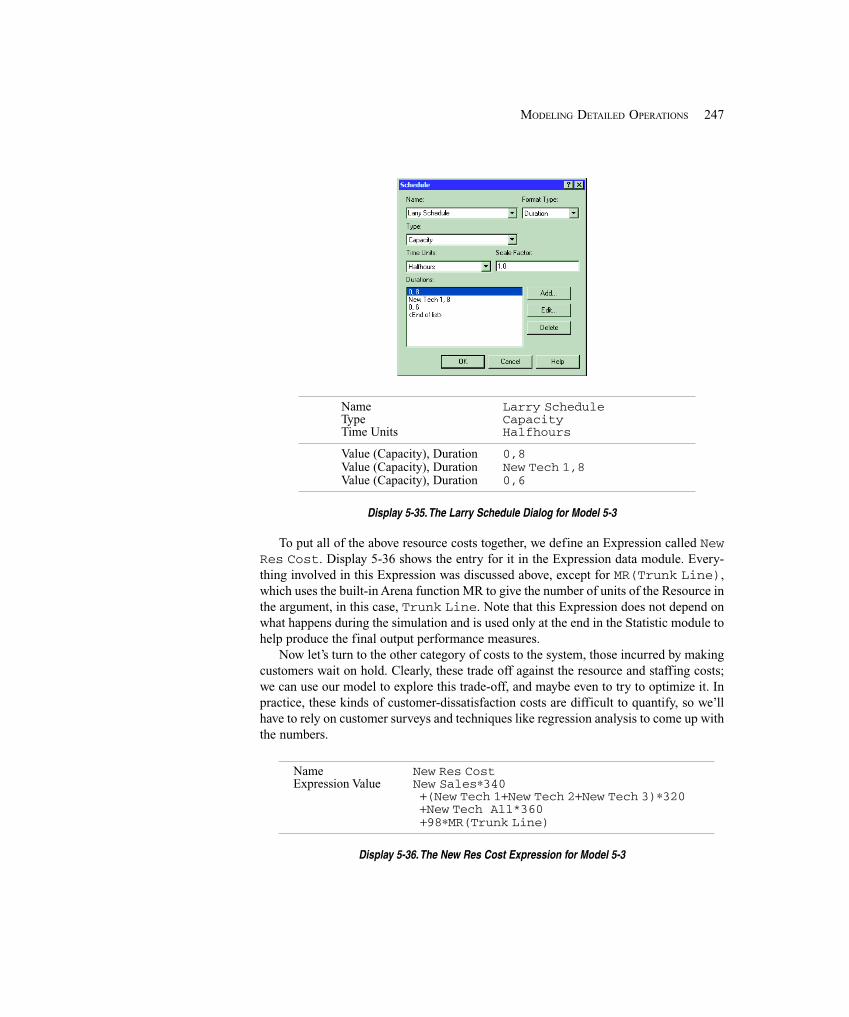
247MODELING DETAILED OPERATIONS
Name Larry ScheduleType CapacityTime Units Halfhours
Value (Capacity), Duration 0,8Value (Capacity), Duration New Tech 1,8Value (Capacity), Duration 0,6
Display 5-35. The Larry Schedule Dialog for Model 5-3
To put all of the above resource costs together, we define an Expression called NewRes Cost. Display 5-36 shows the entry for it in the Expression data module. Every-thing involved in this Expression was discussed above, except for MR(Trunk Line),which uses the built-in Arena function MR to give the number of units of the Resource inthe argument, in this case, Trunk Line. Note that this Expression does not depend onwhat happens during the simulation and is used only at the end in the Statistic module tohelp produce the final output performance measures.
Now let’s turn to the other category of costs to the system, those incurred by makingcustomers wait on hold. Clearly, these trade off against the resource and staffing costs;we can use our model to explore this trade-off, and maybe even to try to optimize it. Inpractice, these kinds of customer-dissatisfaction costs are difficult to quantify, so we’llhave to rely on customer surveys and techniques like regression analysis to come up withthe numbers.
Name New Res CostExpression Value New Sales∗340
+(New Tech 1+New Tech 2+New Tech 3)∗320 +New Tech All*360 +98∗MR(Trunk Line)
Display 5-36. The New Res Cost Expression for Model 5-3

248 CHAPTER 5
Name Assign Excess Tech Wait TimeAssignments
Type VariableVariable Name Excess Tech Wait TimeNew Value Excess Tech Wait Time
+ MAX(ENTITY.WAITTIME − 3, 0)
Display 5-37. The New Assign Module to Accumulate Excess Tech Waiting Times for Model 5-3
We assume that most people are by now hardened enough to expect some waitingtime on hold when dealing with a call center, but at some point, people will start gettingmad and the system will start incurring a cost. For tech calls, this point is 3 minutes; forsales calls, it’s 1 minute; and for order-status calls, it’s 2 minutes. Beyond this tolerancepoint for each call type, the system will incur a cost of 36.8 cents/minute for tech callsthat continue on hold, 81.8 cents/minute for sales calls, and 34.6 cents/minute for order-status calls. For each call type, we accumulate in a variable the “excess” waiting times inqueue (i.e., the waiting time in queue beyond the tolerance cutoff) of all completed callsvia a new Assign module through which entities pass after their calls are done.
Display 5-37 shows this new Assign module for tech support calls, and the other twoare similar (we put bright orange boxes behind these new Assign modules so you caneasily spot them in the model). Note that ENTITY.WAITTIME is a built-in Arenaattribute that automatically accumulates the total of all times in queue for an entity as itgoes along, as well as any other delay times that are allocated to “Wait.” In our model,there are no such delay allocations, and there are no upstream queue delays other thanthat on hold while waiting for the call to be answered, so this value indeed contains whatwe want in this case. (Computation of ENTITY.WAITTIME happens only if the Costingbox is checked in the Run > Setup > Project Parameters dialog, so we need to make sureit is checked.) At the end of the simulation, the variable Excess Tech Wait Time willbe the total number of minutes beyond the 3-minute tolerance that completed tech callsendured during the one-day run, and over the five replications, these will be averaged toproduce, in the final output, an average daily excess tech wait time. If we multiply this bythe per-minute cost of 36.8 cents, we would get the cost for the excess tech wait time fora day, but we’re costing things out on a weekly basis, so we need to multiply instead by36.8 cents × 5 = $1.84 to get the weekly cost. The costs for the other two types of calls arecomputed similarly (the factors by which we need to multiply the excess wait times to getweekly costs are 81.8 cents × 5 = $4.09 for sales calls, and 34.6 cents × 5 = $1.73 fororder-status calls). While we are making five one-day replications, so it could bethought of as a work week, the model constructed in this way will produce weekly costestimates regardless of the number of replications made (we’ll use this model inChapter 6 with far more than five replications, to improve output precision).
Putting all these various costs together into a single overall cost measure is fairlysimple. Given all the above discussion and setup, the overall Total Cost outputperformance measure is

249MODELING DETAILED OPERATIONS
New Res Cost+ Excess Sales Wait Time ∗ 4.09+ Excess Status Wait Time ∗ 1.73+ Excess Tech Wait Time ∗ 1.84+ 12820,
which we enter in the Statistic data module (in the Advanced Process panel); the Type ofthis Statistic is chosen to be Output, meaning that it is a quantity that’s computed onlyat the end of the simulation and we just want to see its value in the reports. Since we’redefining this output ourselves, rather than having Arena compute it internally, it willappear under User Specified → Output in the Category Overview report.
At this point, you’re probably wondering about those poor unfortunate rejected soulswho called only to get immediately brushed off by a busy signal. They didn’t even havethe opportunity to get mad after their tolerance time on hold and start charging costagainst the system (even though they’re really mad). We could have estimated a (big) costfor each busy signal and built that into our cost structure, but instead we decided just tocompute the percent of incoming calls that receive a busy signal and produce that as aseparate output. Instead of viewing this as part of the performance-measure objective ofthe model, we’ll view it later as a requirement (kind of like a constraint, except it’s on anoutput rather than on an input) that no more than 5% of incoming calls get a busy signal;any model configuration not meeting this requirement will be regarded as unacceptableno matter how low its Total Cost output might be.
To compute the percent of incoming calls that get busy signals, we need to know thetotal number of attempted calls and rejected calls. We already have a Record module thatcounts the number of attempted calls (the counter Attempted Calls). We also countthe number of rejected calls, but we are currently recording these rejected calls on a per-hour basis. We could just add up the values from these ten counters, but we took the easyway out and added another Record module in the call-arrival section of the model logic(with a bright orange box behind it) that will give us that total (counter TotalRejected Calls). To compute the output value Percent Rejected, we added aline to the Statistic module with that name and the expression 100*NC(TotalRejected Calls)/NC(Attempted Calls); NC is the built-in Arena functionthat returns the value of the counter named in its argument.
Because we’ve requested multiple (five) replications, we need to tell Arena what todo between replications. There are four possible options.
Option 1: Initialize System (yes), Initialize Statistics (yes)This will result in five statistically independent and identical replications and reports,each starting with an empty system at time 0 and each running for up to 660 minutes.The random-number generator (see Section 12.1) just keeps on going betweenreplications, making them independent and identically distributed (IID). Possiblereturned technical support calls that are carried over to the next day are lost.
Option 2: Initialize System (yes), Initialize Statistics (no)This will result in five independent replications, each starting with an empty systemat time 0 and each running for up to 660 minutes, with the reports being cumulative.

250 CHAPTER 5
Thus, Report 2 would include the statistics for the first two replications, Report 3would contain the statistics for the first three replications, etc. The random-numbergenerator behaves as in Option 1.
Option 3: Initialize System (no), Initialize Statistics (yes)This will result in five runs, the first starting at time 0, the second at the time the firstcompleted (remember that we are using a stopping rule to terminate a replication), thethird at the time the second completed, etc. Since the system is not initialized betweenreplications, the time continues to advance, and any technical support calls that werenot returned will be carried over to the next day. The reports will contain only thestatistics for a single replication or day, rather than being cumulative.
Option 4: Initialize System (no), Initialize Statistics (no) This will result in five runs, the first starting at time 0, the second at the time the firstcompleted, the third at the time the second completed, etc. Since the system is notinitialized between replications, the time continues to advance, and any technical sup-port calls that were not returned will be carried over to the next day. The reports willbe cumulative.
Ideally we would like to select either Option 3 or 4 since we’d like to carry all non-returned technical calls into the next day. However, this would require us to change ourstopping rule and let each replication run for 660 minutes. So for now let’s just accept thedefaults—Option 1.
As you’ve gone through the discussion in this section, you’ve probably thought ofother ways we could have accomplished many of the things we did. It would have beenpossible, for instance, to exploit Arena’s built-in costing capabilities more fully rather thandoing a lot of it on our own and to have parameterized the model differently with only the“primitive” input values like wage rates and number of employees. Or we could have letArena do some of the calculations internally that we did externally on our own littlecalculators. That’s all true, but it also would have taken more time and effort for us to doso. This is a typical kind of judgment call you’ll have to make when building a model—trading off your model-building time against model generality (and maybe elegance),usually being guided by who’s going to use the model, and for what. The configuration ofthis model will be useful in the next chapter, where we show you several of Arena’scapabilities in the important activity of statistical analysis of simulation output data.
We ran the model in what might be called the “base case,” with no additionalemployees or trunk lines (i.e., New Sales, New Tech 1, New Tech 2, New Tech 3,and New Tech All were all set to 0, and the number of trunk lines was set to 26). TheTotal Cost came out to be $22,242.55 for the week, and 11.96% of incoming calls gota busy signal. Since this percent of rejected calls is above our 5% target, we madeanother run where we increased each of the six input resource “control” variables by 3(i.e., New Sales, New Tech 1, New Tech 2, New Tech 3, and New Tech All wereall set to 3, and the number of trunk lines was set to 29); this produced a Total Cost of$23,683.35 with only 1.61% of incoming calls getting a busy signal; evidently, the costof hiring the extra staff and adding three trunk lines is not a wise investment looking
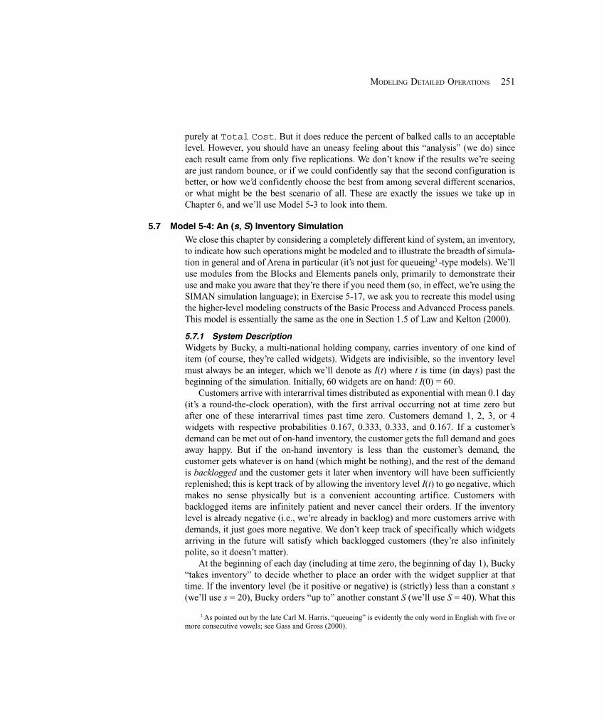
251MODELING DETAILED OPERATIONS
purely at Total Cost. But it does reduce the percent of balked calls to an acceptablelevel. However, you should have an uneasy feeling about this “analysis” (we do) sinceeach result came from only five replications. We don’t know if the results we’re seeingare just random bounce, or if we could confidently say that the second configuration isbetter, or how we’d confidently choose the best from among several different scenarios,or what might be the best scenario of all. These are exactly the issues we take up inChapter 6, and we’ll use Model 5-3 to look into them.
5.7 Model 5-4: An (s, S) Inventory Simulation
We close this chapter by considering a completely different kind of system, an inventory,to indicate how such operations might be modeled and to illustrate the breadth of simula-tion in general and of Arena in particular (it’s not just for queueing3 -type models). We’lluse modules from the Blocks and Elements panels only, primarily to demonstrate theiruse and make you aware that they’re there if you need them (so, in effect, we’re using theSIMAN simulation language); in Exercise 5-17, we ask you to recreate this model usingthe higher-level modeling constructs of the Basic Process and Advanced Process panels.This model is essentially the same as the one in Section 1.5 of Law and Kelton (2000).
5.7.1 System DescriptionWidgets by Bucky, a multi-national holding company, carries inventory of one kind ofitem (of course, they’re called widgets). Widgets are indivisible, so the inventory levelmust always be an integer, which we’ll denote as I(t) where t is time (in days) past thebeginning of the simulation. Initially, 60 widgets are on hand: I(0) = 60.
Customers arrive with interarrival times distributed as exponential with mean 0.1 day(it’s a round-the-clock operation), with the first arrival occurring not at time zero butafter one of these interarrival times past time zero. Customers demand 1, 2, 3, or 4widgets with respective probabilities 0.167, 0.333, 0.333, and 0.167. If a customer’sdemand can be met out of on-hand inventory, the customer gets the full demand and goesaway happy. But if the on-hand inventory is less than the customer’s demand, thecustomer gets whatever is on hand (which might be nothing), and the rest of the demandis backlogged and the customer gets it later when inventory will have been sufficientlyreplenished; this is kept track of by allowing the inventory level I(t) to go negative, whichmakes no sense physically but is a convenient accounting artifice. Customers withbacklogged items are infinitely patient and never cancel their orders. If the inventorylevel is already negative (i.e., we’re already in backlog) and more customers arrive withdemands, it just goes more negative. We don’t keep track of specifically which widgetsarriving in the future will satisfy which backlogged customers (they’re also infinitelypolite, so it doesn’t matter).
At the beginning of each day (including at time zero, the beginning of day 1), Bucky“takes inventory” to decide whether to place an order with the widget supplier at thattime. If the inventory level (be it positive or negative) is (strictly) less than a constant s(we’ll use s = 20), Bucky orders “up to” another constant S (we’ll use S = 40). What this
3 As pointed out by the late Carl M. Harris, “queueing” is evidently the only word in English with five ormore consecutive vowels; see Gass and Gross (2000).
252 CHAPTER 5
means is that he orders a quantity of widgets so that, if they were to arrive instantly, theinventory level would pop up to exactly S. So if t is an integer and thus I(t) is theinventory level at the beginning of a day (could be positive, negative, or zero) and I(t) < s,Bucky orders S - I(t) items; if I(t) > s, Bucky does nothing, lets the day go by, and checksagain at the beginning of the next day, that is, at time t + 1. Due to the form of this review/replenishment policy, systems like this are often called (s, S) inventory models.
However, an order placed at the beginning of a day does not arrive instantly, butrather sometime during the last half of that day, after a delivery lag (a.k.a. lead time)distributed uniformly between 0.5 and 1 day. So when the order arrives, the inventorylevel will pop up by an amount equal to the original order quantity but, if there were anydemands since the order was placed, it will pop up to something less than S when theorder is finally delivered. Note that the relative timings of the inventory evaluations anddelivery lags are such that there can never be more than one order on the way, since anorder placed at the beginning of a day will arrive, at the very latest, just before the end ofthat day, which is the beginning of the next day, the first opportunity to place anotherorder; see Exercise 5-18 for modeling implications of this particular numerical situation.
Bucky is interested in the average total operating cost per day of this system over 120days, which will be the sum of three components:
� Average ordering cost per day. Every time an order is placed, there’s a costincurred of $32 regardless of the order quantity, plus $3 per item ordered; if noorder is placed there’s no ordering cost, not even the fixed cost of $32. The $3 isnot the (wholesale) price of a widget, but rather the administrative operationalcost to Bucky of ordering a widget (we’re not considering prices at all in thismodel). At the end of the 120-day simulation, the total of all the ordering costsaccrued is divided by 120 to get the average ordering cost per day.
� Average holding cost per day. Whenever there are items actually physically ininventory (i.e., I(t) > 0), a holding cost is incurred of $1 per widget per day. Thetotal holding cost is thus
∫ ×120
0)0),((max1 dttI
(think about it), and the average holding cost per day is this total divided by thelength of the simulation, 120 days.
� Average shortage cost per day. Whenever we’re in backlog (i.e., I(t) < 0), ashortage cost of $5 per widget per day is incurred, a harsher penalty than holdingpositive inventory. The total shortage cost is thus
∫ −×120
0)0),((max5 dttI
(think about it a little harder), and the average shortage cost per day is this totaldivided by the simulation length.
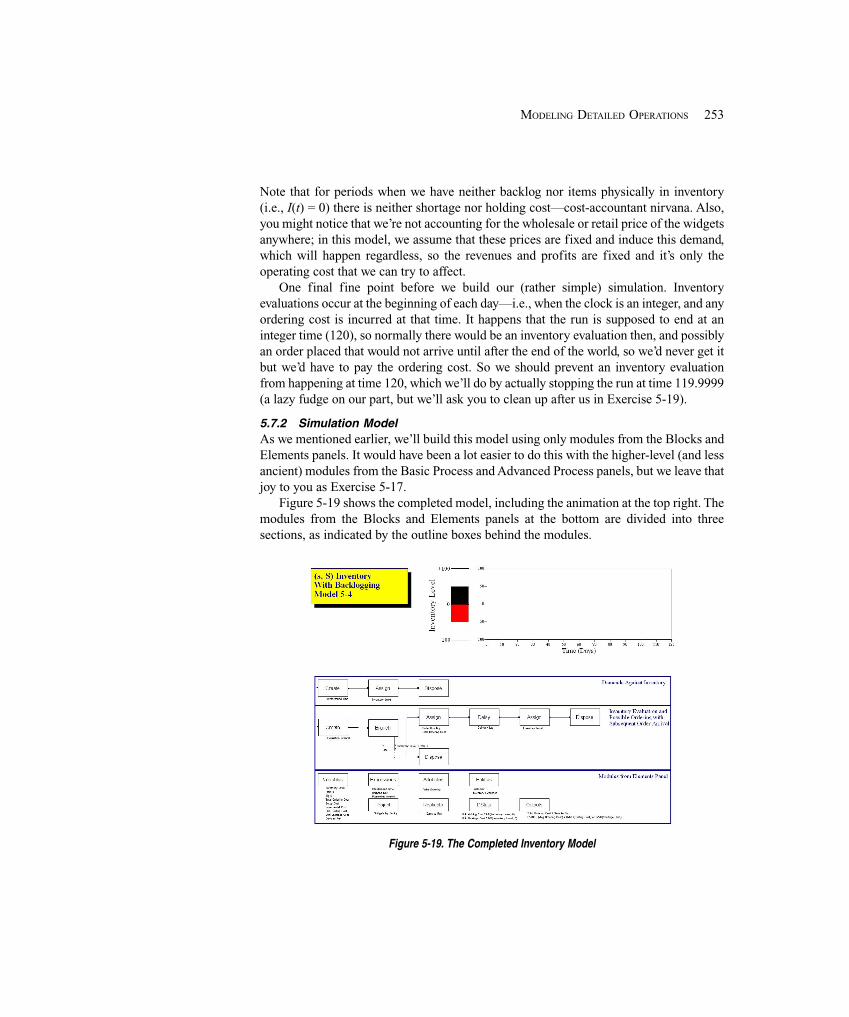
253MODELING DETAILED OPERATIONS
Note that for periods when we have neither backlog nor items physically in inventory(i.e., I(t) = 0) there is neither shortage nor holding cost—cost-accountant nirvana. Also,you might notice that we’re not accounting for the wholesale or retail price of the widgetsanywhere; in this model, we assume that these prices are fixed and induce this demand,which will happen regardless, so the revenues and profits are fixed and it’s only theoperating cost that we can try to affect.
One final fine point before we build our (rather simple) simulation. Inventoryevaluations occur at the beginning of each day—i.e., when the clock is an integer, and anyordering cost is incurred at that time. It happens that the run is supposed to end at aninteger time (120), so normally there would be an inventory evaluation then, and possiblyan order placed that would not arrive until after the end of the world, so we’d never get itbut we’d have to pay the ordering cost. So we should prevent an inventory evaluationfrom happening at time 120, which we’ll do by actually stopping the run at time 119.9999(a lazy fudge on our part, but we’ll ask you to clean up after us in Exercise 5-19).
5.7.2 Simulation ModelAs we mentioned earlier, we’ll build this model using only modules from the Blocks andElements panels. It would have been a lot easier to do this with the higher-level (and lessancient) modules from the Basic Process and Advanced Process panels, but we leave thatjoy to you as Exercise 5-17.
Figure 5-19 shows the completed model, including the animation at the top right. Themodules from the Blocks and Elements panels at the bottom are divided into threesections, as indicated by the outline boxes behind the modules.
Figure 5-19. The Completed Inventory Model
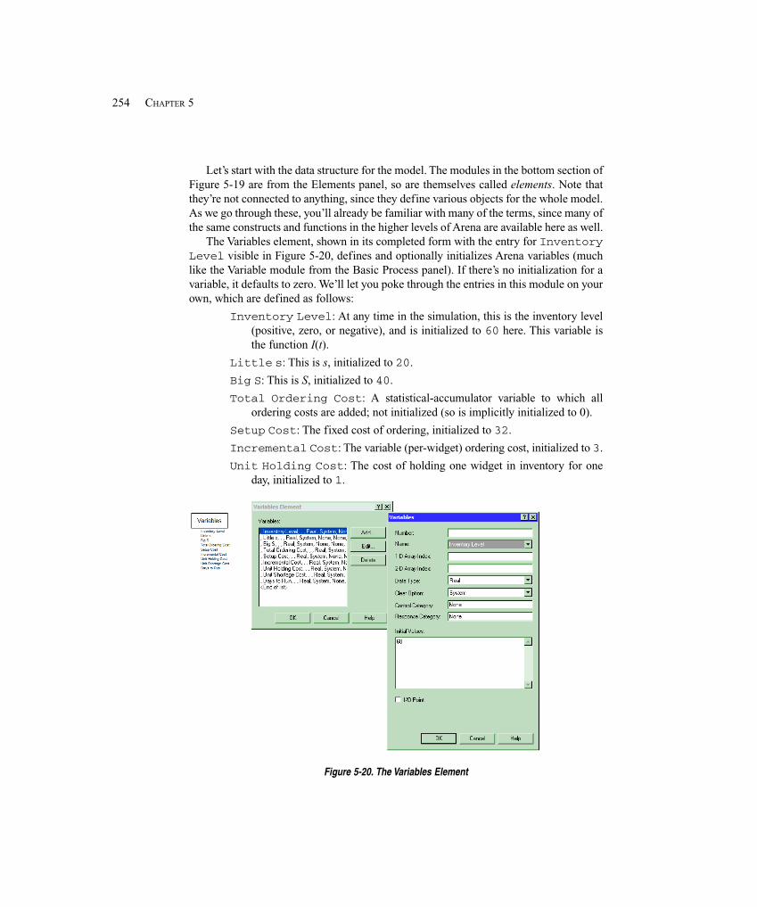
254 CHAPTER 5
Let’s start with the data structure for the model. The modules in the bottom section ofFigure 5-19 are from the Elements panel, so are themselves called elements. Note thatthey’re not connected to anything, since they define various objects for the whole model.As we go through these, you’ll already be familiar with many of the terms, since many ofthe same constructs and functions in the higher levels of Arena are available here as well.
The Variables element, shown in its completed form with the entry for InventoryLevel visible in Figure 5-20, defines and optionally initializes Arena variables (muchlike the Variable module from the Basic Process panel). If there’s no initialization for avariable, it defaults to zero. We’ll let you poke through the entries in this module on yourown, which are defined as follows:
Inventory Level: At any time in the simulation, this is the inventory level(positive, zero, or negative), and is initialized to 60 here. This variable isthe function I(t).
Little s: This is s, initialized to 20.
Big S: This is S, initialized to 40.
Total Ordering Cost: A statistical-accumulator variable to which allordering costs are added; not initialized (so is implicitly initialized to 0).
Setup Cost: The fixed cost of ordering, initialized to 32.
Incremental Cost: The variable (per-widget) ordering cost, initialized to 3.
Unit Holding Cost: The cost of holding one widget in inventory for oneday, initialized to 1.
Figure 5-20. The Variables Element
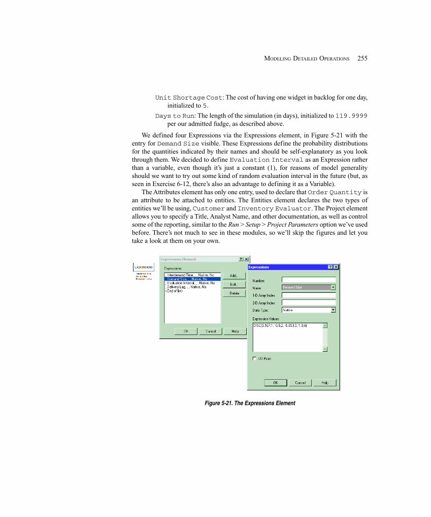
255MODELING DETAILED OPERATIONS
Unit Shortage Cost: The cost of having one widget in backlog for one day,initialized to 5.
Days to Run: The length of the simulation (in days), initialized to 119.9999per our admitted fudge, as described above.
We defined four Expressions via the Expressions element, in Figure 5-21 with theentry for Demand Size visible. These Expressions define the probability distributionsfor the quantities indicated by their names and should be self-explanatory as you lookthrough them. We decided to define Evaluation Interval as an Expression ratherthan a variable, even though it’s just a constant (1), for reasons of model generalityshould we want to try out some kind of random evaluation interval in the future (but, asseen in Exercise 6-12, there’s also an advantage to defining it as a Variable).
The Attributes element has only one entry, used to declare that Order Quantity isan attribute to be attached to entities. The Entities element declares the two types ofentities we’ll be using, Customer and Inventory Evaluator. The Project elementallows you to specify a Title, Analyst Name, and other documentation, as well as controlsome of the reporting, similar to the Run > Setup > Project Parameters option we’ve usedbefore. There’s not much to see in these modules, so we’ll skip the figures and let youtake a look at them on your own.
Figure 5-21. The Expressions Element
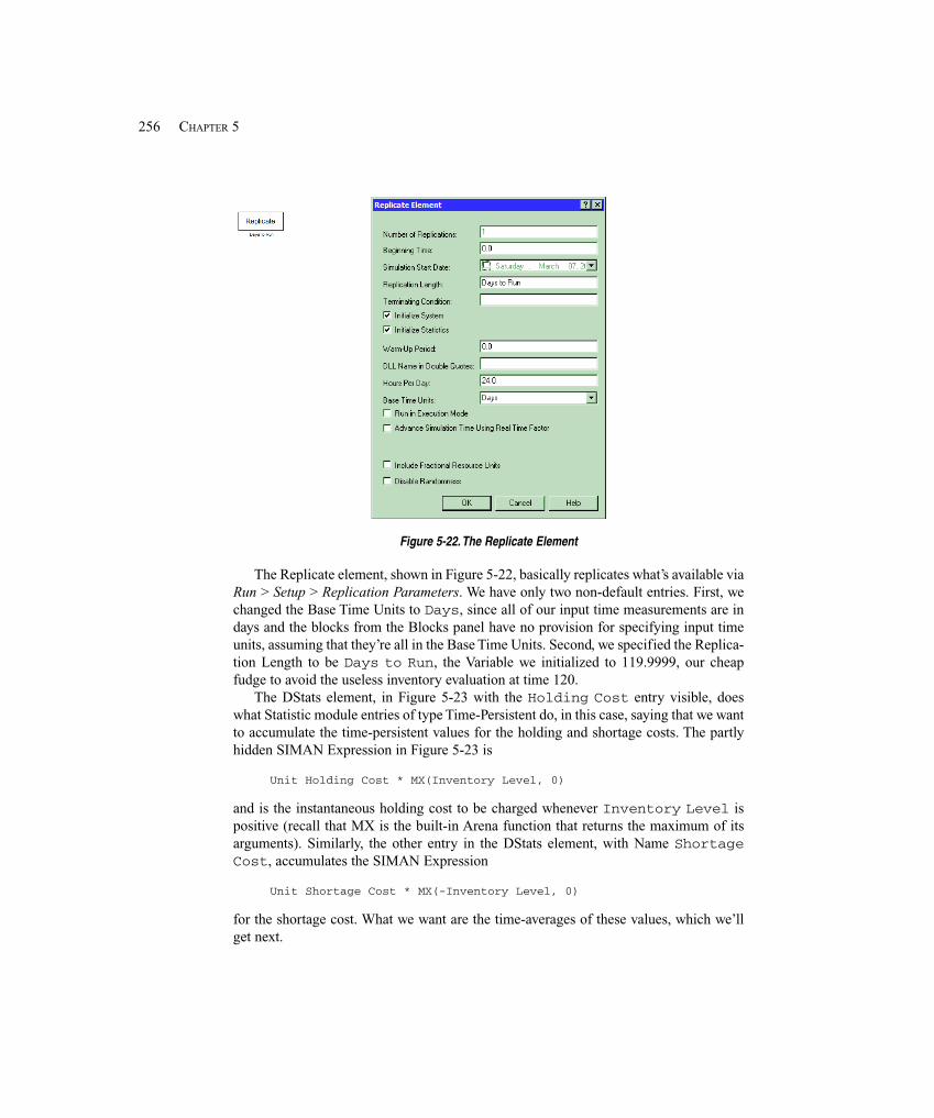
256 CHAPTER 5
Figure 5-22. The Replicate Element
The Replicate element, shown in Figure 5-22, basically replicates what’s available viaRun > Setup > Replication Parameters. We have only two non-default entries. First, wechanged the Base Time Units to Days, since all of our input time measurements are indays and the blocks from the Blocks panel have no provision for specifying input timeunits, assuming that they’re all in the Base Time Units. Second, we specified the Replica-tion Length to be Days to Run, the Variable we initialized to 119.9999, our cheapfudge to avoid the useless inventory evaluation at time 120.
The DStats element, in Figure 5-23 with the Holding Cost entry visible, doeswhat Statistic module entries of type Time-Persistent do, in this case, saying that we wantto accumulate the time-persistent values for the holding and shortage costs. The partlyhidden SIMAN Expression in Figure 5-23 is
Unit Holding Cost * MX(Inventory Level, 0)
and is the instantaneous holding cost to be charged whenever Inventory Level ispositive (recall that MX is the built-in Arena function that returns the maximum of itsarguments). Similarly, the other entry in the DStats element, with Name ShortageCost, accumulates the SIMAN Expression
Unit Shortage Cost * MX(-Inventory Level, 0)
for the shortage cost. What we want are the time-averages of these values, which we’llget next.
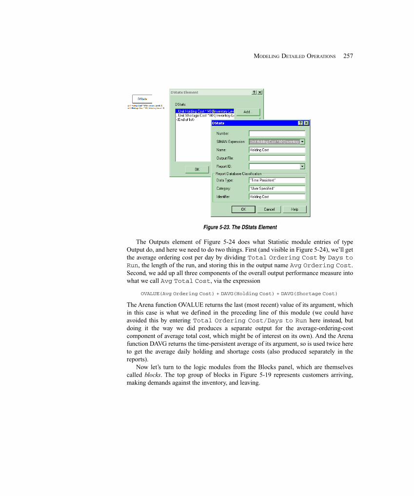
257MODELING DETAILED OPERATIONS
Figure 5-23. The DStats Element
The Outputs element of Figure 5-24 does what Statistic module entries of typeOutput do, and here we need to do two things. First (and visible in Figure 5-24), we’ll getthe average ordering cost per day by dividing Total Ordering Cost by Days toRun, the length of the run, and storing this in the output name Avg Ordering Cost.Second, we add up all three components of the overall output performance measure intowhat we call Avg Total Cost, via the expression
OVALUE(Avg Ordering Cost) + DAVG(Holding Cost) + DAVG(Shortage Cost)
The Arena function OVALUE returns the last (most recent) value of its argument, whichin this case is what we defined in the preceding line of this module (we could haveavoided this by entering Total Ordering Cost/Days to Run here instead, butdoing it the way we did produces a separate output for the average-ordering-costcomponent of average total cost, which might be of interest on its own). And the Arenafunction DAVG returns the time-persistent average of its argument, so is used twice hereto get the average daily holding and shortage costs (also produced separately in thereports).
Now let’s turn to the logic modules from the Blocks panel, which are themselvescalled blocks. The top group of blocks in Figure 5-19 represents customers arriving,making demands against the inventory, and leaving.
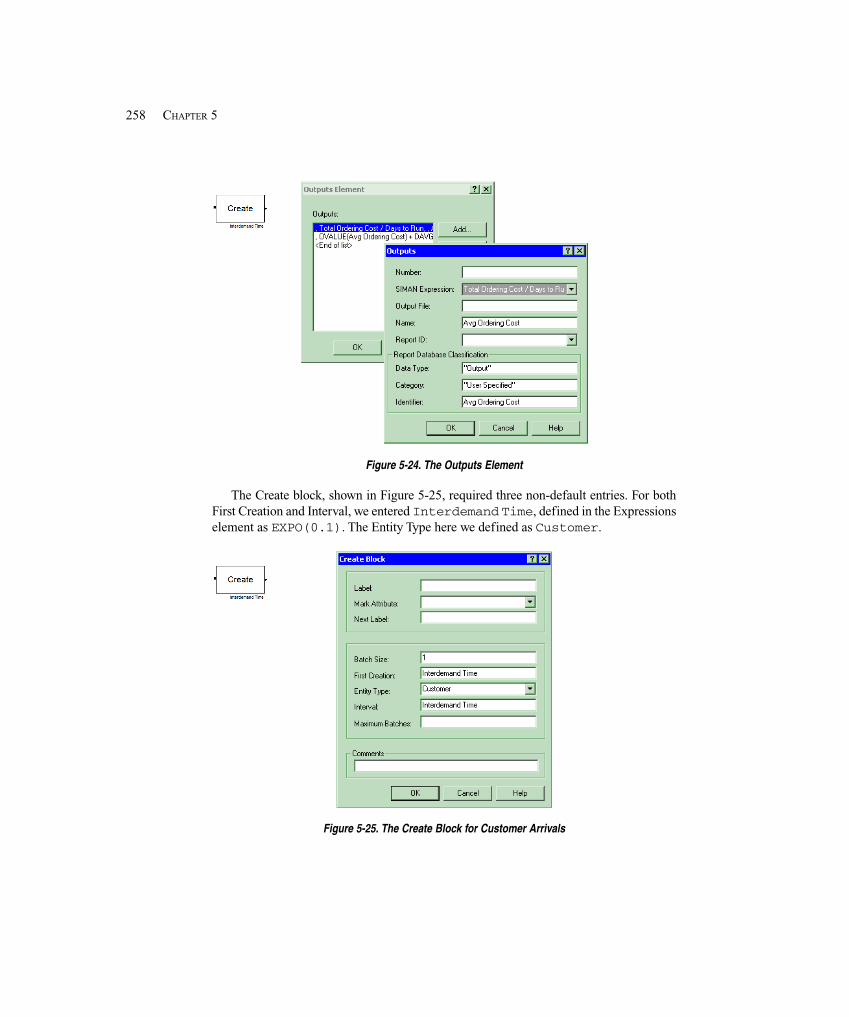
258 CHAPTER 5
Figure 5-24. The Outputs Element
The Create block, shown in Figure 5-25, required three non-default entries. For bothFirst Creation and Interval, we entered Interdemand Time, defined in the Expressionselement as EXPO(0.1). The Entity Type here we defined as Customer.
Figure 5-25. The Create Block for Customer Arrivals
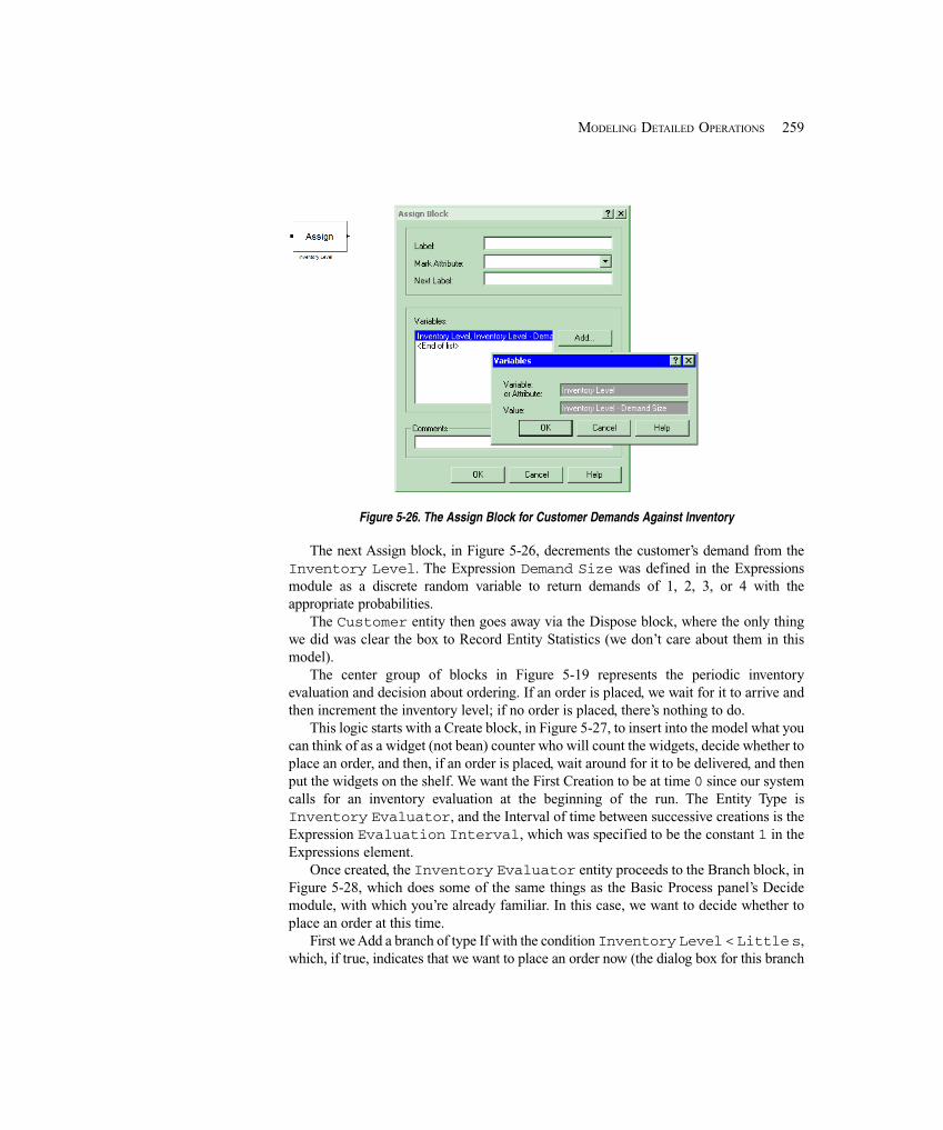
259MODELING DETAILED OPERATIONS
Figure 5-26. The Assign Block for Customer Demands Against Inventory
The next Assign block, in Figure 5-26, decrements the customer’s demand from theInventory Level. The Expression Demand Size was defined in the Expressionsmodule as a discrete random variable to return demands of 1, 2, 3, or 4 with theappropriate probabilities.
The Customer entity then goes away via the Dispose block, where the only thingwe did was clear the box to Record Entity Statistics (we don’t care about them in thismodel).
The center group of blocks in Figure 5-19 represents the periodic inventoryevaluation and decision about ordering. If an order is placed, we wait for it to arrive andthen increment the inventory level; if no order is placed, there’s nothing to do.
This logic starts with a Create block, in Figure 5-27, to insert into the model what youcan think of as a widget (not bean) counter who will count the widgets, decide whether toplace an order, and then, if an order is placed, wait around for it to be delivered, and thenput the widgets on the shelf. We want the First Creation to be at time 0 since our systemcalls for an inventory evaluation at the beginning of the run. The Entity Type isInventory Evaluator, and the Interval of time between successive creations is theExpression Evaluation Interval, which was specified to be the constant 1 in theExpressions element.
Once created, the Inventory Evaluator entity proceeds to the Branch block, inFigure 5-28, which does some of the same things as the Basic Process panel’s Decidemodule, with which you’re already familiar. In this case, we want to decide whether toplace an order at this time.
First we Add a branch of type If with the condition Inventory Level < Little s,which, if true, indicates that we want to place an order now (the dialog box for this branch
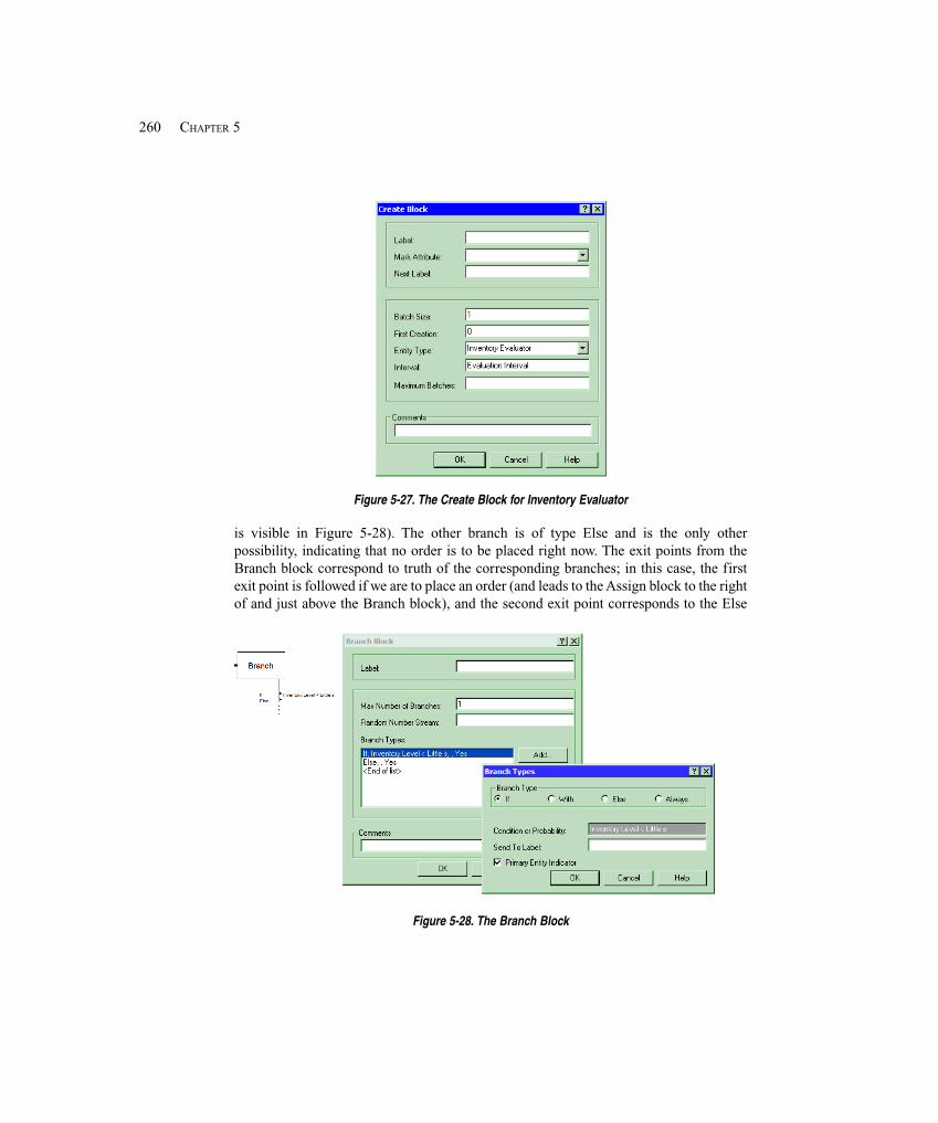
260 CHAPTER 5
Figure 5-27. The Create Block for Inventory Evaluator
is visible in Figure 5-28). The other branch is of type Else and is the only otherpossibility, indicating that no order is to be placed right now. The exit points from theBranch block correspond to truth of the corresponding branches; in this case, the firstexit point is followed if we are to place an order (and leads to the Assign block to the rightof and just above the Branch block), and the second exit point corresponds to the Else
Figure 5-28. The Branch Block
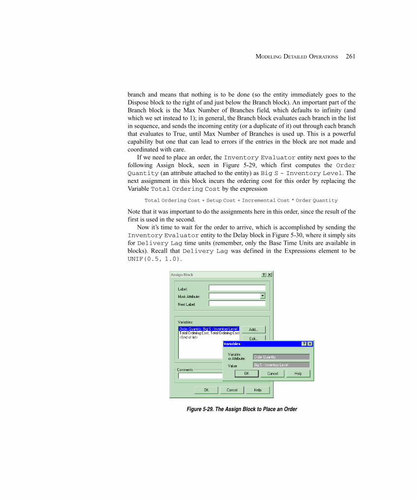
261MODELING DETAILED OPERATIONS
branch and means that nothing is to be done (so the entity immediately goes to theDispose block to the right of and just below the Branch block). An important part of theBranch block is the Max Number of Branches field, which defaults to infinity (andwhich we set instead to 1); in general, the Branch block evaluates each branch in the listin sequence, and sends the incoming entity (or a duplicate of it) out through each branchthat evaluates to True, until Max Number of Branches is used up. This is a powerfulcapability but one that can lead to errors if the entries in the block are not made andcoordinated with care.
If we need to place an order, the Inventory Evaluator entity next goes to thefollowing Assign block, seen in Figure 5-29, which first computes the OrderQuantity (an attribute attached to the entity) as Big S - Inventory Level. Thenext assignment in this block incurs the ordering cost for this order by replacing theVariable Total Ordering Cost by the expression
Total Ordering Cost + Setup Cost + Incremental Cost * Order Quantity
Note that it was important to do the assignments here in this order, since the result of thefirst is used in the second.
Now it’s time to wait for the order to arrive, which is accomplished by sending theInventory Evaluator entity to the Delay block in Figure 5-30, where it simply sitsfor Delivery Lag time units (remember, only the Base Time Units are available inblocks). Recall that Delivery Lag was defined in the Expressions element to beUNIF(0.5, 1.0).
Figure 5-29. The Assign Block to Place an Order
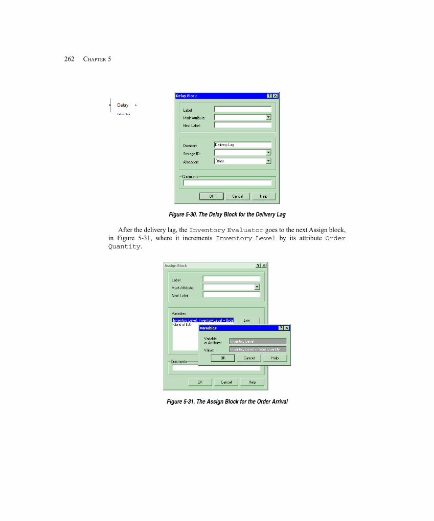
262 CHAPTER 5
Figure 5-30. The Delay Block for the Delivery Lag
After the delivery lag, the Inventory Evaluator goes to the next Assign block,in Figure 5-31, where it increments Inventory Level by its attribute OrderQuantity.
Figure 5-31. The Assign Block for the Order Arrival
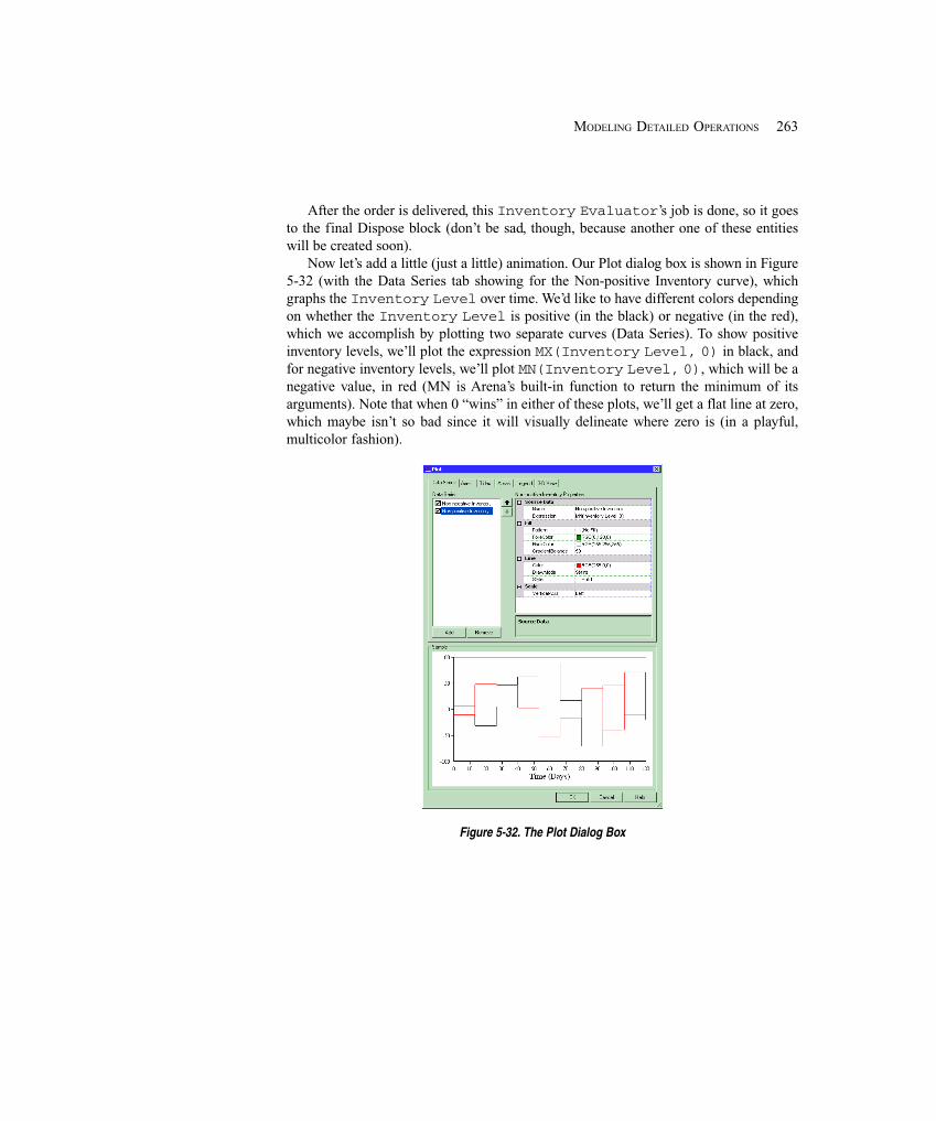
263MODELING DETAILED OPERATIONS
After the order is delivered, this Inventory Evaluator’s job is done, so it goesto the final Dispose block (don’t be sad, though, because another one of these entitieswill be created soon).
Now let’s add a little (just a little) animation. Our Plot dialog box is shown in Figure5-32 (with the Data Series tab showing for the Non-positive Inventory curve), whichgraphs the Inventory Level over time. We’d like to have different colors dependingon whether the Inventory Level is positive (in the black) or negative (in the red),which we accomplish by plotting two separate curves (Data Series). To show positiveinventory levels, we’ll plot the expression MX(Inventory Level, 0) in black, andfor negative inventory levels, we’ll plot MN(Inventory Level, 0), which will be anegative value, in red (MN is Arena’s built-in function to return the minimum of itsarguments). Note that when 0 “wins” in either of these plots, we’ll get a flat line at zero,which maybe isn’t so bad since it will visually delineate where zero is (in a playful,multicolor fashion).
Figure 5-32. The Plot Dialog Box
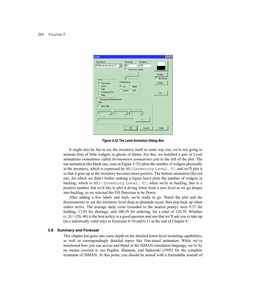
264 CHAPTER 5
Figure 5-33. The Level Animation Dialog Box
It might also be fun to see the inventory itself in some way (no, we’re not going toanimate bins of little widgets or ghosts of them). For this, we installed a pair of Levelanimations (sometimes called thermometer animations) just to the left of the plot. Thetop animation (the black one, seen in Figure 5-33) plots the number of widgets physicallyin the inventory, which is expressed by MX(Inventory Level, 0), and we’ll plot itso that it goes up as the inventory becomes more positive. The bottom animation (the redone, for which we didn’t bother making a figure here) plots the number of widgets inbacklog, which is MX(-Inventory Level, 0); when we’re in backlog, this is apositive number, but we’d like to plot it diving lower from a zero level as we go deeperinto backlog, so we selected the Fill Direction to be Down.
After adding a few labels and such, we’re ready to go. Watch the plot and thethermometers to see the inventory level drop as demands occur, then pop back up whenorders arrive. The average daily costs (rounded to the nearest penny) were 9.37 forholding, 17.03 for shortage, and 100.39 for ordering, for a total of 126.79. Whether(s, S) = (20, 40) is the best policy is a good question and one that we’ll ask you to take up(in a statistically valid way) in Exercises 6-10 and 6-11 at the end of Chapter 6.
5.8 Summary and ForecastThis chapter has gone into some depth on the detailed lower-level modeling capabilities,as well as correspondingly detailed topics like fine-tuned animation. While we’vementioned how you can access and blend in the SIMAN simulation language, we’ve byno means covered it; see Pegden, Shannon, and Sadowski (1995) for the completetreatment of SIMAN. At this point, you should be armed with a formidable arsenal of
265MODELING DETAILED OPERATIONS
modeling tools to allow you to attack many systems, choosing constructs from variouslevels as appropriate. In several of the following chapters, we’ll continue to expand onArena’s modeling capabilities.
5.9 Exercises
5-1 Develop a model of the problem we described in Chapter 2 and modeled as Model3-1, but this time only using modules from the Advanced Process panel to replace theProcess module. Use the Plot and Variable features from the Animate toolbar to completeyour model. Run it for 20 minutes and compare your results to what we got earlier.
5-2 Parts arrive at a two-machine system according to an exponential interarrivaldistribution with mean 20 minutes. Upon arrival, the parts are sent to Machine 1 andprocessed. The processing-time distribution is TRIA(4.5, 9.3, 11) minutes. The parts arethen processed at Machine 2 with a processing-time distribution as TRIA(16.4, 19.1,20.8) minutes. The parts from Machine 2 are directed back to Machine 1 to be processeda second time (same processing-time distribution but an independent draw from it). Thecompleted parts then exit the system. Run the simulation for a single replication of20,000 minutes to observe the average number in the machine queues and the averagepart cycle time.
5-3 Stacks of paper arrive at a trimming process with interarrival times of EXPO(10);all times are in minutes. There are two trimmers, a primary and a secondary. All arrivalsare sent to the primary trimmer. If the queue in front of the primary trimmer is shorterthan five, the stack of paper enters that queue to wait to be trimmed by the primarytrimmer, an operation of duration TRIA(9, 12, 15). If there are already five stacks in theprimary queue, the stack is balked to the secondary trimmer (which has an infinite queuecapacity) for trimming, of duration TRIA(17, 19, 22). After the primary trimmer hastrimmed 25 stacks, it must be shut down for cleaning, which lasts EXPO(30). During thistime, the stacks in the queue for the primary trimmer wait for it to become available.Animate and run your simulation for 5,000 minutes. Collect statistics, by trimmer, forcycle time, resource utilization, number in queue, and time in queue. Whenever possible,use modules from the Advanced Process panel.
5-4 Trucks arrive with EXPO(9.1) interarrival times (all times are in minutes) to anunload area that has three docks. The unload times are TRIA(25, 28, 30), TRIA(23, 26,28), and TRIA(22, 25, 27) for docks 1, 2, and 3, respectively. If there is an empty dock,the truck proceeds immediately to that dock. Assume zero travel times to all docks. Ifthere is more than one empty dock, the truck places preference on the higher-numbereddock (3, 2, 1). If all the docks are busy, it chooses the dock with the minimum number oftrucks waiting. If there is a tie, it places preference on the lowest numbered dock (1, 2, 3).Develop a simulation model with modules from the Advanced Process panel, usingrequired modules from the Basic Process panel to implement the selection logic. Runyour model for 20,000 minutes and collect statistics on dock utilization, number inqueue, time in queue, and the time in system.
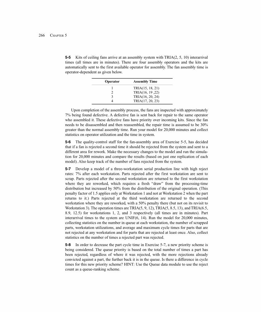
266 CHAPTER 5
5-5 Kits of ceiling fans arrive at an assembly system with TRIA(2, 5, 10) interarrivaltimes (all times are in minutes). There are four assembly operators and the kits areautomatically sent to the first available operator for assembly. The fan assembly time isoperator-dependent as given below.
Operator Assembly Time
1 TRIA(15, 18, 21)2 TRIA(16, 19 ,22)3 TRIA(16, 20, 24)4 TRIA(17, 20, 23)
Upon completion of the assembly process, the fans are inspected with approximately7% being found defective. A defective fan is sent back for repair to the same operatorwho assembled it. These defective fans have priority over incoming kits. Since the fanneeds to be disassembled and then reassembled, the repair time is assumed to be 30%greater than the normal assembly time. Run your model for 20,000 minutes and collectstatistics on operator utilization and the time in system.
5-6 The quality-control staff for the fan-assembly area of Exercise 5-5, has decidedthat if a fan is rejected a second time it should be rejected from the system and sent to adifferent area for rework. Make the necessary changes to the model and run the simula-tion for 20,000 minutes and compare the results (based on just one replication of eachmodel). Also keep track of the number of fans rejected from the system.
5-7 Develop a model of a three-workstation serial production line with high rejectrates: 7% after each workstation. Parts rejected after the first workstation are sent toscrap. Parts rejected after the second workstation are returned to the first workstationwhere they are reworked, which requires a fresh “draw” from the processing-timedistribution but increased by 50% from the distribution of the original operation. (Thispenalty factor of 1.5 applies only at Workstation 1 and not at Workstation 2 when the partreturns to it.) Parts rejected at the third workstation are returned to the secondworkstation where they are reworked, with a 50% penalty there (but not on its revisit toWorkstation 3). The operation times are TRIA(5, 9, 12), TRIA(5, 8.5, 13), and TRIA(6.5,8.9, 12.5) for workstations 1, 2, and 3 respectively (all times are in minutes). Partinterarrival times to the system are UNIF(6, 14). Run the model for 20,000 minutes,collecting statistics on the number in queue at each workstation, the number of scrappedparts, workstation utilizations, and average and maximum cycle times for parts that arenot rejected at any workstation and for parts that are rejected at least once. Also, collectstatistics on the number of times a rejected part was rejected.
5-8 In order to decrease the part cycle time in Exercise 5-7, a new priority scheme isbeing considered. The queue priority is based on the total number of times a part hasbeen rejected, regardless of where it was rejected, with the more rejections alreadyconvicted against a part, the further back it is in the queue. Is there a difference in cycletimes for this new priority scheme? HINT: Use the Queue data module to use the rejectcount as a queue-ranking scheme.
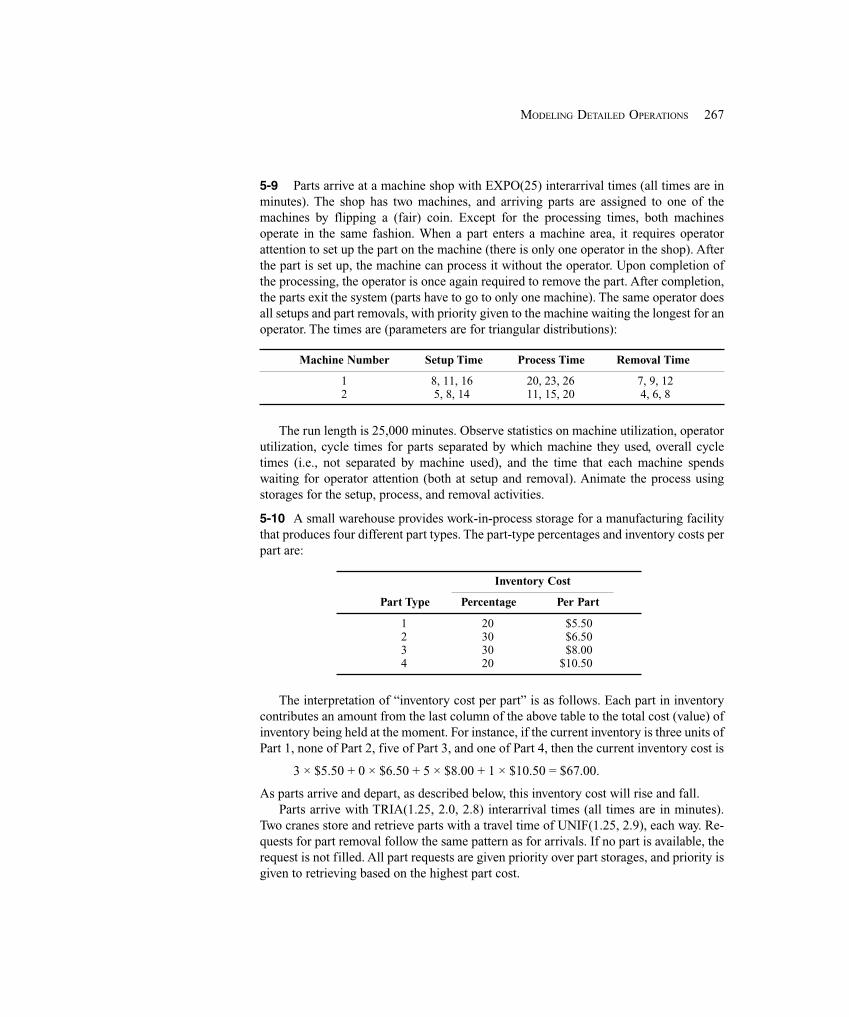
267MODELING DETAILED OPERATIONS
5-9 Parts arrive at a machine shop with EXPO(25) interarrival times (all times are inminutes). The shop has two machines, and arriving parts are assigned to one of themachines by flipping a (fair) coin. Except for the processing times, both machinesoperate in the same fashion. When a part enters a machine area, it requires operatorattention to set up the part on the machine (there is only one operator in the shop). Afterthe part is set up, the machine can process it without the operator. Upon completion ofthe processing, the operator is once again required to remove the part. After completion,the parts exit the system (parts have to go to only one machine). The same operator doesall setups and part removals, with priority given to the machine waiting the longest for anoperator. The times are (parameters are for triangular distributions):
Machine Number Setup Time Process Time Removal Time
1 8, 11, 16 20, 23, 26 7, 9, 122 5, 8, 14 11, 15, 20 4, 6, 8
The run length is 25,000 minutes. Observe statistics on machine utilization, operatorutilization, cycle times for parts separated by which machine they used, overall cycletimes (i.e., not separated by machine used), and the time that each machine spendswaiting for operator attention (both at setup and removal). Animate the process usingstorages for the setup, process, and removal activities.
5-10 A small warehouse provides work-in-process storage for a manufacturing facilitythat produces four different part types. The part-type percentages and inventory costs perpart are:
Inventory Cost
Part Type Percentage Per Part
1 20 $5.502 30 $6.503 30 $8.004 20 $10.50
The interpretation of “inventory cost per part” is as follows. Each part in inventorycontributes an amount from the last column of the above table to the total cost (value) ofinventory being held at the moment. For instance, if the current inventory is three units ofPart 1, none of Part 2, five of Part 3, and one of Part 4, then the current inventory cost is
3 × $5.50 + 0 × $6.50 + 5 × $8.00 + 1 × $10.50 = $67.00.
As parts arrive and depart, as described below, this inventory cost will rise and fall.Parts arrive with TRIA(1.25, 2.0, 2.8) interarrival times (all times are in minutes).
Two cranes store and retrieve parts with a travel time of UNIF(1.25, 2.9), each way. Re-quests for part removal follow the same pattern as for arrivals. If no part is available, therequest is not filled. All part requests are given priority over part storages, and priority isgiven to retrieving based on the highest part cost.
268 CHAPTER 5
For part arrivals, increment the inventory cost upon arrival, and increment the totalnumber of parts in inventory after the part is stored. For part requests, decrement the totalnumber of parts in inventory as soon as you know there is a part to retrieve, and decre-ment the inventory cost after the part is retrieved.
Run your model for 5,000 minutes starting with four of each part type in the ware-house. Collect statistics on the crane utilization, the average inventory cost, the averagenumber of each part type in the warehouse, and the number of unfilled requests due tohaving no parts of the requested type.
HINTS: Use index variables for part inventory and per-part cost. (Note that you canuse the “Other” option in the Assign module when assigning to index variables.) Use theDiscrete distribution to determine the part type and the Statistic data module to collectsome of the required statistics.
5-11 A medium-sized airport has a limited number of international flights that arriveand require immigration and customs. The airport would like to examine the customsstaffing and establish a policy on the number of passengers who should have bagssearched and the staffing of the customs facility. The number of passengers who arriveon these large planes is uniformly distributed between 240 and 350, and the simulation isto run until all passengers on the plane have been completely processed (i.e., the numberof passengers on the plane determines the replication length). Arriving passengers mustfirst pass through immigration (immigration is outside the boundaries of this model).They then claim their bags and proceed to customs. The interarrival times to customs aredistributed as EXPO(0.2), with the first passenger arriving at (or just barely after) timezero; all times are in minutes. The current plan is to have two customs agents dedicated topassengers who will not have their bags searched, with service times distributed asEXPO(0.56). A new airport systems analyst has developed a probabilistic method todecide which customers will have their bags searched. The decision is made when thepassengers are about to enter the normal customs queue. The decision process is asfollows: a number is first generated from a Poisson distribution with a mean of 7.0. Thisnumber is increased by 1, to avoid getting a zero, and a count is started. When the countreaches the generated number, that unlucky passenger is sent to a second line to have hisor her bags searched. A new search number is generated and the process starts over. Asingle agent is dedicated to these passengers, with service times distributed as EXPO(3).Develop a simulation of the proposed system and make 20 replications (i.e., process 20planes, since a replication ends when the last customer from a plane clears customs),observing statistics on the system time by passenger type (searched vs. not searched), thenumber of passengers, and agent utilizations.
5-12 A state driver’s license exam center would like to examine its operation forpotential improvement. Arriving customers enter the building and take a number todetermine their place in line for the written exam, which is self administered by one offive electronic testers. The testing times are distributed as EXPO(8); all times are inminutes. Thirteen percent of the customers fail the test (it’s a hard test with lots ofquestions). These customers are given a booklet on the state driving rules for further
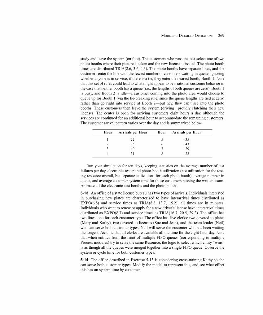
269MODELING DETAILED OPERATIONS
study and leave the system (on foot). The customers who pass the test select one of twophoto booths where their picture is taken and the new license is issued. The photo boothtimes are distributed TRIA(2.6, 3.6, 4.3). The photo booths have separate lines, and thecustomers enter the line with the fewest number of customers waiting in queue, ignoringwhether anyone is in service; if there is a tie, they enter the nearest booth, Booth 1. Notethat this set of rules could lead to what might appear to be irrational customer behavior inthe case that neither booth has a queue (i.e., the lengths of both queues are zero), Booth 1is busy, and Booth 2 is idle—a customer coming into the photo area would choose toqueue up for Booth 1 (via the tie-breaking rule, since the queue lengths are tied at zero)rather than go right into service at Booth 2—but hey, they can’t see into the photobooths! These customers then leave the system (driving), proudly clutching their newlicenses. The center is open for arriving customers eight hours a day, although theservices are continued for an additional hour to accommodate the remaining customers.The customer arrival pattern varies over the day and is summarized below:
Hour Arrivals per Hour Hour Arrivals per Hour
1 22 5 35 2 35 6 43 3 40 7 29 4 31 8 22
Run your simulation for ten days, keeping statistics on the average number of testfailures per day, electronic-tester and photo-booth utilization (not utilization for the test-ing resource overall, but separate utilizations for each photo booth), average number inqueue, and average customer system time for those customers passing the written exam.Animate all the electronic-test booths and the photo booths.
5-13 An office of a state license bureau has two types of arrivals. Individuals interestedin purchasing new plates are characterized to have interarrival times distributed asEXPO(6.8) and service times as TRIA(8.8, 13.7, 15.2); all times are in minutes.Individuals who want to renew or apply for a new driver’s license have interarrival timesdistributed as EXPO(8.7) and service times as TRIA(16.7, 20.5, 29.2). The office hastwo lines, one for each customer type. The office has five clerks: two devoted to plates(Mary and Kathy), two devoted to licenses (Sue and Jean), and the team leader (Neil)who can serve both customer types. Neil will serve the customer who has been waitingthe longest. Assume that all clerks are available all the time for the eight-hour day. Notethat when entities from the front of multiple FIFO queues (corresponding to multipleProcess modules) try to seize the same Resource, the logic to select which entity “wins”is as though all the queues were merged together into a single FIFO queue. Observe thesystem or cycle time for both customer types.
5-14 The office described in Exercise 5-13 is considering cross-training Kathy so shecan serve both customer types. Modify the model to represent this, and see what effectthis has on system time by customer.

270 CHAPTER 5
5-15 Modify the model from Exercise 5-14 to include 30-minute lunch breaks for eachclerk. Start the first lunch break 180 minutes into the day. Lunch breaks should followone after the other covering a 150-minute time span during the middle of the day. Thebreaks should be given in the following order: Mary, Sue, Neil, Kathy, and Jean. Whatimpact does this have on system time by customer?
5-16 Modify the probability-board model from Exercise 3-10 so that the bounce-rightprobabilities for all the pegs can be changed at once by changing the value of just a singlevariable. Run it with the bounce-right probabilities set to 0.25 and compare with theresults of the wind-blown version of the model from Exercise 3-10.
5-17 Recreate Model 5-4 (the inventory model) without using anything from the Blocksor Elements panels, and using only modules from the Basic Process and AdvancedProcess panels.
5-18 In Model 5-4, the relative timings of the inventory-evaluation interval and thedelivery lag were such that at no time could there be more than one order outstanding.What if the numbers were different so that there could be multiple orders on the way at agiven time? Would Model 5-4 still work? (Note that in Model 5-4 we represented theorder quantity, if any, by an attribute of the inventory-evaluator entity; what if that orderquantity had been represented instead by a variable?) Model 5-4 would still work in thecase of multiple outstanding orders, precisely because the order quantity is an Attributeattached to the inventory-evaluation entity. If the delivery lags were longer, then therecould be multiple entities of this type in existence at once, each with its own order-quantity attribute attached. If the order quantity were represented by a single globalvariable, though, we’d be limited to a model that has capacity for keeping track of nomore than one outstanding order at a time.
5-19 In Model 5-4, remove the “fudge factor” of ending at time 119.9999 rather thanthe correct 120. Run the simulation to exactly time 120, but add logic to prevent a uselessinventory evaluation at time 120. What is the effect on the output?
5-20 Generalize Model 5-4 to have two additional types of items (doodads andkontraptions), as well as widgets; initially, there are 60 widgets, 50 doodads, and 70kontraptions. The customers arrive in the same pattern as before, but now each customerwill have a demand for doodads and kontraptions, as well as for widgets. Widgetdemands are as before, doodad demands are POIS(1.9), and kontraption demands arePOIS(2.3); assume that a customer’s demand for an item is independent of his or herdemands for the other two items. There’s still one inventory evaluator, who still arrives atthe beginning of each day, but now has to look at all three inventories and order accordingto separate (s, S) policies for each of the three inventories; you may “clone” this inventoryevaluator for this triple duty. For widgets, (s, S) = (20, 40) as before; for doodads, (s, S) =(15, 35); and for kontraptions, (s, S) = (25, 45). Delivery lags for widgets are UNIF(0.5,1.0) as before; for doodads, it’s UNIF(0.4, 0.8); and for kontraptions, it’s UNIF(0.8, 1.7);note that for kontraptions, it’s possible for a delivery lag to extend beyond the time of thenext inventory evaluation, but make the order decision based on only the inventory on
271MODELING DETAILED OPERATIONS
hand, rather than based on the inventory on hand plus on order (even though the lattermight make more sense; see Exercise 5-25). Ordering costs (both setup and incremental),holding, and shortage costs for doodads and kontraptions are the same as for widgets.Run the simulation for the same length of time as Model 5-4 (i.e., it’s okay to fudge theending point to avoid useless inventory evaluations at time 120), and get the total dailycost, as well as separate holding and shortage costs for each type of item.
5-21 In Exercise 5-20, suppose that the suppliers for the three items merge and offer adeal to eliminate multiple setup costs on a given day’s orders—that is, if Bucky ordersany items of any type at the beginning of a day, he only has to pay the $32 setup cost oncefor that day, not a separate $32 for each type of item he orders. (If no order is placed foranything, there’s still no setup cost.) Modify your model for Exercise 5-20 to do this.What kind of incentives do you think this alternate cost structure might place on Buckyin terms of picking better values of s and S for each item (see Exercises 6-13 and 6-14)?
5-22 In the machine-repair model of Exercise 3-14, suppose it costs $80 in lostproductivity for each hour that each machine is broken down and $19/hour to employeach repair technician (the technicians are paid this hourly wage regardless of whetherthey are busy or idle). Modify the model to collect these cost data, and report the averagetotal cost per hour. Also, show the machines in the “up” state in a separate area of theanimation, make separate animation pictures for up vs. down machines, and keep trackof the number of machines up (and plot it). Make the number of machines in the shop aVariable. If you want to minimize total average cost, is two the right number of repairtechnicians? Experiment (though see Exercise 6-21 for a statistically valid way toexperiment).
5-23 Modify Model 3-3 so that the Resource animations are really accurate, i.e., so thateach of Alfie, Betty, Chuck, and Doris is individually animated. If a loan applicationarrives to find more than one of them idle, assume that a random choice is made.Produce output statistics on the utilization of each individual resource, as well as theoverall utilization of the four resources combined. Relate the overall utilization to theindividual utilizations.
5-24 Modify Model 3-5 so that the Resource animations are really accurate, i.e., so thateach of Alfie, Betty, Chuck, and Doris is individually animated. If a loan applicationarrives to find more than one of them idle, assume that a random choice is made.Produce output statistics on the utilization of each individual resource, as well as theoverall utilization of the four resources combined. Relate the overall utilization to theindividual utilizations.
5-25 In Exercise 5-20, base the reorder decision (for widgets, doodads, and kon-traptions) not on just the inventory level on hand, but rather on the inventory level on handPLUS the total inventory on order (i.e., en route from the supplier based on prior orders).Use the same vales of s and S for each of the three types of items as in Exercise 5-20.

272 CHAPTER 5
5-26 Modify Model 5-1 to use a nonstationary Poisson process (as used in Models 5-2and 5-3) to implement the stopping rule for this model differently. Get rid of the secondtwo Variables and the non-default entries in the Entities per Arrival field and the Max Ar-rivals field in the “Create Call Arrivals” create module. Also get rid of the three modulesin the “Arrival Cutoff Logical Entity” area. Put a Text box in your model to explain brieflywhat you’ve done to implement this. Explain in a second Text box in your model why theresults are a little different from those produced by Model 5-1, and why this is okay.
273STATISTICAL ANALYSIS OF OUTPUT FROM TERMINATING SIMULATIONS
CHAPTER 6
Statistical Analysis of Output fromTerminating Simulations
As we warned you back in Section 2.6 with the hand simulation, there’s an issue ofrandomness and thus statistical analysis when you build a model with any random (i.e.,distribution- or probability-driven) inputs, as has been the case with all our models so far.In this section, we’ll show you how to collect the appropriate data from the simulationand then statistically analyze them from the reports you’re already getting, using the thirdversion of the call center model as created in Chapter 5, Model 5-3. We’ll also show youhow to do more sophisticated statistical analyses with the help of the Output Analyzer (tocompare two alternative versions of your model, called scenarios), the Process Analyzer(to run several scenarios conveniently and perhaps select the best or gauge the effects ofinputs on outputs), and OptQuest for Arena (which “takes over” running your model in aquest for a configuration of input controls that optimizes a selected output response).
In Section 6.1, we’ll talk about the time frame of simulations, which affects the kindof analysis you do. Then in Sections 6.2 and 6.3 we’ll describe the basic strategy for datacollection and statistical analysis in the context of just a single variant (the base case ofModel 5-3, with the number of trunk lines still at 26 and no additional people hired forhours 5 through 8). We’ll make some simple changes to the model’s input parameters inSection 6.4 and use the Arena Output Analyzer to see if it makes a (statisticallysignificant) difference. In Section 6.5, we’ll introduce several more model variants anduse the Arena Process Analyzer to run them in an efficient and organized way, as well assort out which of them is probably best. Finally, in Section 6.6, we’ll use OptQuest forArena to search intelligently and efficiently among the bewildering number of possibleinput-parameter combinations for a model configuration that appears to be optimal insome sense (if you are running the student version of Arena, you will likely not haveOptQuest available, though it could be in your college or university computer labs if aresearch lab license is present). Throughout, we’ll be illustrating methods that result inreliable and precise statistical analyses, which promote informed and sound decisions.
In the past, which is fortunately now gone, a lot of people pretty much ignored thesekinds of issues, and that’s a real shame. By just running your model once, and then tryingout a few haphazardly chosen scenarios (and running them only once), you just have noidea how valid or precise or general your results or conclusions might be. Sometimes thetruth about validity and precision and generality can be ugly, and thus dangerous if it’sunknown, since you’d run a real risk of getting poor estimates and making bad decisions.As you’ll see, it doesn’t take much work at all on your part to do these things right; yourcomputer might have to work hard, but it spends most of its time loafing anyway andbesides, unlike you, it’s cheap (compared to the importance of the decisions you’ll make
274 CHAPTER 6
based on your simulation’s results). You’ve worked hard to build your model, so now it’stime to let the model (and your computer) work hard for you to find out how it reallybehaves, and then you can confidently transport that knowledge into solid decisions.
6.1 Time Frame of Simulations
As in Section 5.2.5, most (not all) simulations can be classified as either terminating orsteady state. For many models, this is primarily an issue of intent or the goal of the studyrather than having much to do with internal model logic or construction.
A terminating simulation is one in which the model dictates specific starting andstopping conditions as a natural reflection of how the target system actually operates. Asthe name suggests, the simulation will terminate according to some model-specified ruleor condition. For instance, a store opens at 9 AM with no customers present, closes itsdoors at 9 PM, but continues operation for a little while longer until all customers are“flushed” out. Another example is a job shop that operates for as long as it takes toproduce a “run” of 500 completed assemblies specified by the order. The key notion isthat the time frame of the simulation has a well-defined (though possibly unknown-at-the-outset) and natural end, as well as a clearly defined way to start up.
A steady-state simulation, on the other hand, is one in which the quantities to beestimated are defined in the long run; i.e., over a theoretically infinite time frame. Inprinciple (though usually not in practice), the initial conditions for the simulation don’tmatter. Of course, a steady-state simulation has to stop at some point, and as you mightguess, these runs can get pretty long; you need to do something to make sure that you’rerunning it long enough, an issue we’ll take up in Section 7.2. For example, an emergencyroom never really stops or restarts, so a steady-state simulation might be appropriate.Sometimes people do a steady-state simulation of a system that actually terminates inorder to design for some kind of worst-case or peak-load situation.
In this chapter, we’ll stick to a terminating statistical analysis of the third version ofthe call center model from Chapter 5 in its Model 5-3 incarnation, viewing it as a termi-nating simulation starting and stopping as described in Chapter 5. Steady-state analyseshave to be done differently (we’ll do this in Section 7.2 using the model we’ll develop inSection 7.1).
6.2 Strategy for Data Collection and Analysis
With a terminating simulation, it’s conceptually simple to collect the appropriate data forstatistical analysis—just make some number n of independent replications.1
To do this, just open the Run > Setup > Replication Parameters dialog box and enterthe value of n you want for the Number of Replications. Be sure that the boxes underInitialize Between Replications are both checked (the default) to cause both the system-state variables and the statistical accumulators to be cleared at the end of each replica-tion. There are reasons to leave one or both of these boxes unchecked, but to get true,statistically independent and identically distributed (IID) replications for terminatinganalysis, you need to make sure that both boxes are checked. These changes will cause
1 While conceptually simple, this could still imply a lot of run time for big or highly variable models.
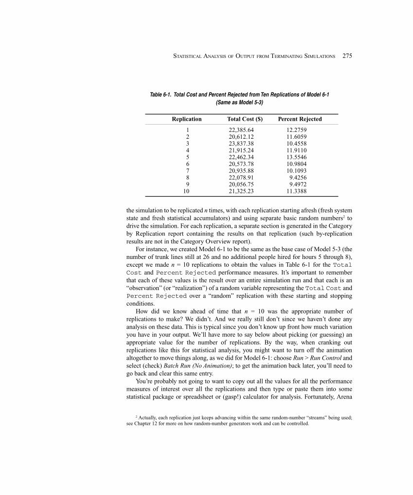
275STATISTICAL ANALYSIS OF OUTPUT FROM TERMINATING SIMULATIONS
Table 6-1. Total Cost and Percent Rejected from Ten Replications of Model 6-1(Same as Model 5-3)
Replication Total Cost ($) Percent Rejected
1 22,385.64 12.27592 20,612.12 11.60593 23,837.38 10.45584 21,915.24 11.91105 22,462.34 13.55466 20,573.78 10.98047 20,935.88 10.10938 22,078.91 9.42569 20,056.75 9.4972
10 21,325.23 11.3388
the simulation to be replicated n times, with each replication starting afresh (fresh systemstate and fresh statistical accumulators) and using separate basic random numbers2 todrive the simulation. For each replication, a separate section is generated in the Categoryby Replication report containing the results on that replication (such by-replicationresults are not in the Category Overview report).
For instance, we created Model 6-1 to be the same as the base case of Model 5-3 (thenumber of trunk lines still at 26 and no additional people hired for hours 5 through 8),except we made n = 10 replications to obtain the values in Table 6-1 for the TotalCost and Percent Rejected performance measures. It’s important to rememberthat each of these values is the result over an entire simulation run and that each is an“observation” (or “realization”) of a random variable representing the Total Cost andPercent Rejected over a “random” replication with these starting and stoppingconditions.
How did we know ahead of time that n = 10 was the appropriate number ofreplications to make? We didn’t. And we really still don’t since we haven’t done anyanalysis on these data. This is typical since you don’t know up front how much variationyou have in your output. We’ll have more to say below about picking (or guessing) anappropriate value for the number of replications. By the way, when cranking outreplications like this for statistical analysis, you might want to turn off the animationaltogether to move things along, as we did for Model 6-1: choose Run > Run Control andselect (check) Batch Run (No Animation); to get the animation back later, you’ll need togo back and clear this same entry.
You’re probably not going to want to copy out all the values for all the performancemeasures of interest over all the replications and then type or paste them into somestatistical package or spreadsheet or (gasp!) calculator for analysis. Fortunately, Arena
2 Actually, each replication just keeps advancing within the same random-number “streams” being used;see Chapter 12 for more on how random-number generators work and can be controlled.
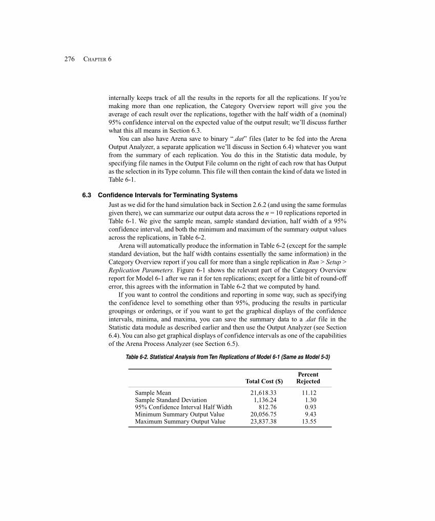
276 CHAPTER 6
internally keeps track of all the results in the reports for all the replications. If you’remaking more than one replication, the Category Overview report will give you theaverage of each result over the replications, together with the half width of a (nominal)95% confidence interval on the expected value of the output result; we’ll discuss furtherwhat this all means in Section 6.3.
You can also have Arena save to binary “.dat” files (later to be fed into the ArenaOutput Analyzer, a separate application we’ll discuss in Section 6.4) whatever you wantfrom the summary of each replication. You do this in the Statistic data module, byspecifying file names in the Output File column on the right of each row that has Outputas the selection in its Type column. This file will then contain the kind of data we listed inTable 6-1.
6.3 Confidence Intervals for Terminating Systems
Just as we did for the hand simulation back in Section 2.6.2 (and using the same formulasgiven there), we can summarize our output data across the n = 10 replications reported inTable 6-1. We give the sample mean, sample standard deviation, half width of a 95%confidence interval, and both the minimum and maximum of the summary output valuesacross the replications, in Table 6-2.
Arena will automatically produce the information in Table 6-2 (except for the samplestandard deviation, but the half width contains essentially the same information) in theCategory Overview report if you call for more than a single replication in Run > Setup >Replication Parameters. Figure 6-1 shows the relevant part of the Category Overviewreport for Model 6-1 after we ran it for ten replications; except for a little bit of round-offerror, this agrees with the information in Table 6-2 that we computed by hand.
If you want to control the conditions and reporting in some way, such as specifyingthe confidence level to something other than 95%, producing the results in particulargroupings or orderings, or if you want to get the graphical displays of the confidenceintervals, minima, and maxima, you can save the summary data to a .dat file in theStatistic data module as described earlier and then use the Output Analyzer (see Section6.4). You can also get graphical displays of confidence intervals as one of the capabilitiesof the Arena Process Analyzer (see Section 6.5).
Table 6-2. Statistical Analysis from Ten Replications of Model 6-1 (Same as Model 5-3)
PercentTotal Cost ($) Rejected
Sample Mean 21,618.33 11.12Sample Standard Deviation 1,136.24 1.3095% Confidence Interval Half Width 812.76 0.93Minimum Summary Output Value 20,056.75 9.43Maximum Summary Output Value 23,837.38 13.55
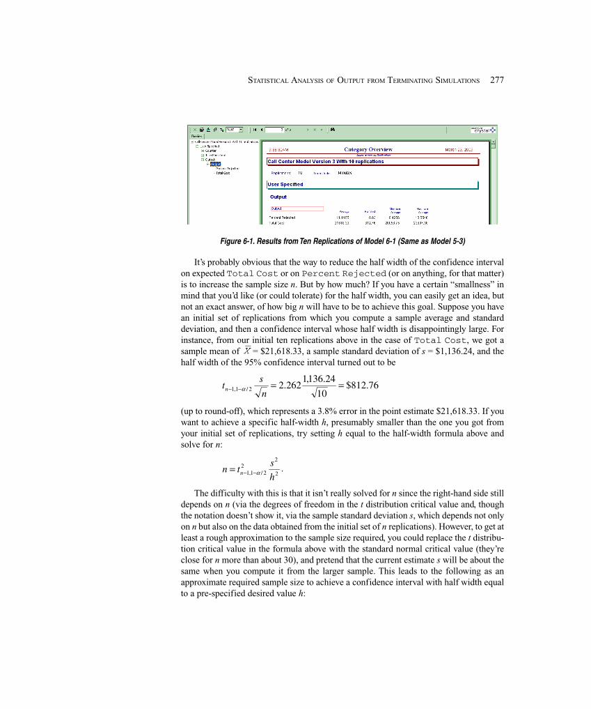
277STATISTICAL ANALYSIS OF OUTPUT FROM TERMINATING SIMULATIONS
Figure 6-1. Results from Ten Replications of Model 6-1 (Same as Model 5-3)
It’s probably obvious that the way to reduce the half width of the confidence intervalon expected Total Cost or on Percent Rejected (or on anything, for that matter)is to increase the sample size n. But by how much? If you have a certain “smallness” inmind that you’d like (or could tolerate) for the half width, you can easily get an idea, butnot an exact answer, of how big n will have to be to achieve this goal. Suppose you havean initial set of replications from which you compute a sample average and standarddeviation, and then a confidence interval whose half width is disappointingly large. Forinstance, from our initial ten replications above in the case of Total Cost, we got asample mean of = $21,618.33, a sample standard deviation of s = $1,136.24, and thehalf width of the 95% confidence interval turned out to be
76.812$10
24.136,1262.22/1,1 ==−−
n
stn α
(up to round-off), which represents a 3.8% error in the point estimate $21,618.33. If youwant to achieve a specific half-width h, presumably smaller than the one you got fromyour initial set of replications, try setting h equal to the half-width formula above andsolve for n:
2
22
2/1,1 h
stn n α−−= .
The difficulty with this is that it isn’t really solved for n since the right-hand side stilldepends on n (via the degrees of freedom in the t distribution critical value and, thoughthe notation doesn’t show it, via the sample standard deviation s, which depends not onlyon n but also on the data obtained from the initial set of n replications). However, to get atleast a rough approximation to the sample size required, you could replace the t distribu-tion critical value in the formula above with the standard normal critical value (they’reclose for n more than about 30), and pretend that the current estimate s will be about thesame when you compute it from the larger sample. This leads to the following as anapproximate required sample size to achieve a confidence interval with half width equalto a pre-specified desired value h:
278 CHAPTER 6
2
22
2/1 h
szn α−≅
where s is the sample standard deviation from an initial set of n replications (which you’dhave to make before doing this). An easier but slightly different approximation is (we’llleave the algebra to you)
2
20
0 h
hnn ≅
where n0 is the number of initial replications you have and h
0 is the half width you got
from them. In the Total Cost example above, to reduce the half width fromh
0 = $812.76 to, say, h = $250.00, we’d thus need a total of something like
4.79250
24.136,196.1 2
22 =≅n (first approximation)
or
7.105250
76.81210 2
2
=≅n (second approximation)
(round up) replications instead of the ten we originally made. The second approximationwill always be bigger since it uses 2/1,10 α−−nt rather than z
1–a/2. Note the depressing qua-
dratic growth of the number of replications as h shrinks (i.e., we demand more preci-sion)—to reduce the half width to half its initial value, you need about four times asmany replications. While this might seem unfair (to do twice as well you have to workfour times as hard), the intuition is that as you add more and more replications, each ad-ditional replication carries less and less percentage increase in your accumulating store-house of knowledge.
Since this model runs very quickly without the animation, we decided to be conser-vative (statistically, not necessarily politically) and make 110 replications. The onlychange required to Model 6-1 was in Run > Setup > Replication Parameters where wechanged the 10 in Number of Replications to 110; we’ll call the result Model 6-2. Thisproduced a 95% confidence interval of
22175.19 ± 369.54,
or in other words, [21805.65, 22544.73] (we’ll drop the “$” units from here on). Notethat this does not quite meet our goal of getting the half width down to 250 or less, soevidently our initial ten replications were a little less variable than “usual” so we under-shot a little on the required number of replications; on the other hand, it could have hap-pened that the half width would be below 250, since these are indeed onlyapproximations and are not exact. In Section 12.5, we’ll discuss sequential sampling,which for us will be ways to trick Arena into continuing to run until it produces confi-dence intervals that really are of the desired precision.
279STATISTICAL ANALYSIS OF OUTPUT FROM TERMINATING SIMULATIONS
By the way, from this 110-replication run of Model 6-2, the approximate 95%confidence interval on the expected percentage of incoming calls that are rejected was11.7396 ± 0.51. This seems like a pretty tight confidence interval, with half width ofabout half a percentage point (on a dimensionless scale that’s always between 0 and 100for a percent). However, if you wanted even tighter precision, you could repeat theabove approximations for the required number of replications and then use themaximum of this and the 110 we got for the Total Cost output performance measureso that you would meet your precision needs on both outputs.
It’s important to understand just what a confidence interval is (and what it isn’t). Takethe Total Cost output measure as an example. Each replication produces a TotalCost value for that replication, and due to random inputs, these values vary acrossreplications. The average of the 110 values, you’ll agree, is probably a “better” indicatorof what to expect from a “typical” run than is any one of the individual values. Also, it’sintuitive that the more replications you make, the “better” this average will be. Theexpected average, which is usually denoted by some kind of notation like μ, can bethought of as the Total Cost averaged over an infinite number of replications; assuch, μ will have no uncertainty associated with it.
Unfortunately, mere mortals like us can’t wait for an infinite number of replications,so we have to make do with a finite-sample estimate like the 22,175.19 from our 110replications. The confidence interval centered around 22,175.19 can be thought of as a“random” interval (the next set of 110 replications will give you a different interval) thathas approximately a 95% (in this case) chance of containing or “covering” μ in the sensethat if we made a lot of sets of 110 replications and made such an interval from each set,about 95% of these intervals would cover μ. Thus, a confidence interval gives you both a“point” estimate (22,175.19) of μ, as well as an idea of how precise this estimate is.
A confidence interval is not an interval in which, for example, 95% of the TotalCost measures from replications will fall. Such an interval, called a prediction interval,is useful as well and can basically be derived from the same data. One clear differencebetween these two types of intervals is that a confidence interval will shrink to a singlepoint as n increases, but a prediction interval won’t since it needs to allow for variation in(future) replications.
A final word about confidence intervals concerns our hedging the confidence-levelstatement (“approximately” 95%, etc.). The standard methods for doing this, whichArena uses, assumes that the basic data, such as the 110 observations on Total Costacross the replications, are IID (that’s satisfied for us) and normally distributed (that’s notsatisfied). Basically, use of the t distribution in the confidence-interval formula requiresnormality of the data. So what’s the effect on the actual (as opposed to stated) confidencelevel of violation of this normality assumption? We can firmly and absolutely state that itdepends on several things, including the “true” distribution as well as the number, n, ofreplications. The central limit theorem, one of the cornerstones of statistical theory,reassures us that we’ll be pretty much okay (in terms of actual confidence being close tostated confidence) if n is “large.” But how large? The answer to this is fairlyimponderable and depends on how closely the distribution of the data resembles a normal
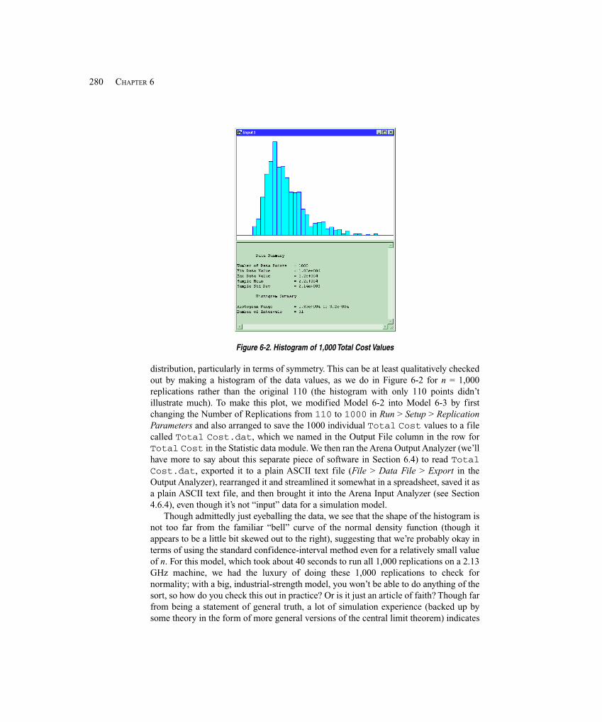
280 CHAPTER 6
Figure 6-2. Histogram of 1,000 Total Cost Values
distribution, particularly in terms of symmetry. This can be at least qualitatively checkedout by making a histogram of the data values, as we do in Figure 6-2 for n = 1,000replications rather than the original 110 (the histogram with only 110 points didn’tillustrate much). To make this plot, we modified Model 6-2 into Model 6-3 by firstchanging the Number of Replications from 110 to 1000 in Run > Setup > ReplicationParameters and also arranged to save the 1000 individual Total Cost values to a filecalled Total Cost.dat, which we named in the Output File column in the row forTotal Cost in the Statistic data module. We then ran the Arena Output Analyzer (we’llhave more to say about this separate piece of software in Section 6.4) to read TotalCost.dat, exported it to a plain ASCII text file (File > Data File > Export in theOutput Analyzer), rearranged it and streamlined it somewhat in a spreadsheet, saved it asa plain ASCII text file, and then brought it into the Arena Input Analyzer (see Section4.6.4), even though it’s not “input” data for a simulation model.
Though admittedly just eyeballing the data, we see that the shape of the histogram isnot too far from the familiar “bell” curve of the normal density function (though itappears to be a little bit skewed out to the right), suggesting that we’re probably okay interms of using the standard confidence-interval method even for a relatively small valueof n. For this model, which took about 40 seconds to run all 1,000 replications on a 2.13GHz machine, we had the luxury of doing these 1,000 replications to check fornormality; with a big, industrial-strength model, you won’t be able to do anything of thesort, so how do you check this out in practice? Or is it just an article of faith? Though farfrom being a statement of general truth, a lot of simulation experience (backed up bysome theory in the form of more general versions of the central limit theorem) indicates
281STATISTICAL ANALYSIS OF OUTPUT FROM TERMINATING SIMULATIONS
that if the value you’re getting out of each individual replication is a sum or average ofsomething, as opposed to an extreme value (maximum or minimum of something), useof standard normal-theory statistical-inference methods is fairly safe. Our Total Costmeasure is of the “sum” form, perhaps explaining its approximate normality in Figure6-2, and justifying use of Arena’s normal-theory-based statistical methods.
6.4 Comparing Two Scenarios
In most simulation studies, people eventually become interested in comparing differentversions, or alternatives, or scenarios, of some general model. What makes the scenariosdiffer from each other could be anything from a simple parameter change to fundamen-tally different logic. In any case, you need to take care to apply the appropriate statisticalmethods to the output from the scenarios to ensure that valid conclusions are drawn. Inthis section, we’ll restrict ourselves to the case of just two scenarios; in Section 6.5, we’llallow for more.
We’ll begin by modifying Model 6-3 into what we’ll call Model 6-4, by simplyknocking the Number of Replications in Run > Setup > Replication Parameters backdown to 110; we left in the entry in the Statistic data module, Output File Column,Total Cost row to save the Total Costs from each replication to the file TotalCost.dat (more on this below). Let’s consider two versions. The first, which we’ll callthe base case, is the same as Model 5-3 in Chapter 5, with exactly the same inputparameters and run conditions (except that we’re doing 110 rather than five replications),i.e., we still have 26 trunk lines and have added no Larrys (Variable New Tech 1 is 0),no Moes (New Tech 2 is 0), no Curlys (New Tech 3 is 0), no Hermanns (New TechAll is 0), or sales staff (New Sales is 0) during hours 5-8. The alternative scenario,what we’ll call the more-resource scenario is just the base case except that we’ll addthree trunk lines (in the Trunk Line row of the Resource data module change theCapacity from 26 to 29), and hire three each of Larry, Moe, Curly, Hermann, and salesstaff (in the Variable data module initialize each of New Tech 1, New Tech 2, NewTech 3, New Tech All, and New Sales to 3 rather than 0). By adding resources inthis way, we’ll certainly increase salary cost, but will also reduce waiting and thusexcess-wait costs. So it’s not clear whether this change will drive Total Cost down or up,much less by how much. And while these changes should reduce the percent of incomingcalls that are rejected, it’s hard to say by how much. Sounds like a job for (you guessed it)simulation.
We made a run (just one replication) of both the base case and the more-resourcescase, and got Total Cost outputs of $22,385.64 and $23,306.75, respectively;Percent Rejected was 12.2759 and 0.2833, respectively. On the surface, this looksmixed for the more-resources scenario since Total Cost seems to have increasedsomewhat while Percent Rejected decreased, apparently substantially. But if youwere conscious when you read Section 6.3 (or Section 2.6.3), you’ll know better than tofall into this trap of concluding much of anything from just one run with no statisticalanalysis of the output. So we’ll do this comparison in a way that will allow us to make astatistically valid conclusion.
282 CHAPTER 6
Before doing the comparison the right way, we’ll do it in a reasonable-but-not-quite-right way. Focusing on the Total Cost output measure, we saw in Section 6.3 that,from 110 replications of the base-case scenario, a 95% confidence interval on theexpected Total Cost is
22175.19 ± 369.54 or [21805.65, 22544.73].
Rerunning the model in the more-resources configuration, also with 110 replications,the confidence interval becomes
24542.82 ± 329.11, or [24213.71, 24871.93].
These two intervals do not overlap at all, suggesting that the expected Total Costs aresignificantly different. Turning to the Percent Rejected output measure, the base-case confidence interval was 11.7396 ± 0.51, while the more-resources interval was1.7276 ± 0.31; these two intervals do not overlap, suggesting a statistically significantdifference on this measure. However, looking at whether confidence intervals do or don’toverlap is not quite the right procedure; to do the comparison the right way, we’ll use theArena Output Analyzer discussed next.
As we’ve mentioned before, the Output Analyzer is a separate application that runsapart from Arena itself, but operates on output files created by Arena through the Statis-tic data module (the .dat files we’ve mentioned before). While some of the things theOutput Analyzer does are also done by Arena itself (like forming confidence intervals onexpected output performance measures), the Output Analyzer has additional capabilities,and statistical comparison of two scenarios is among them.
To save the values of Total Cost for each replication to a .dat file for the OutputAnalyzer, we entered Total Cost.dat in the Output File column for the TotalCost row in the Statistic data module, and similarly for Percent Rejected. Afterthe simulation has been run, these files will contain the 110 values of these outputperformance measures over the 110 replications; the file format is binary, however, and itcan be read only by the Output Analyzer so will not be readable from applications likeword processors or spreadsheets. Since we’ll want to save the Total Cost andPercent Rejected values over our 110 replications of both the base-case and more-resource scenarios, and since we’ll have two such files for each output performancemeasure, we either need to change their file names in the Arena model before each run,or rename them out in the operating system after each run to avoid overwriting them onsubsequent runs; we took the latter route and appended “- Base Case” or “- MoreResources” to the file names. Once you’ve made your runs of 110 replications eachof the two scenarios, start the Output Analyzer (it’s probably in the same folder thatcontains Arena, unless you did something weird during your installation).
In the Output Analyzer, select File > New (or Ctrl+N or ) to open a new data group.This is not a .dat file containing data, but is rather a list of .dat files that you select as theones in which you have current interest; this basically screens out the possibly many other.dat files present and, while not required, simplifies things. You can save this data groupfile (the default file name extension is .dgr) after you populate it with .dat file names sothat next time you can just open it rather than selecting the .dat files all over again; wesaved this data group as Model 06-04.dgr.
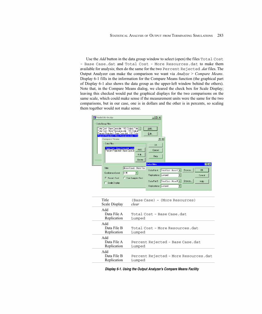
283STATISTICAL ANALYSIS OF OUTPUT FROM TERMINATING SIMULATIONS
Use the Add button in the data group window to select (open) the files Total Cost- Base Case.dat and Total Cost - More Resources.dat to make themavailable for analysis; then do the same for the two Percent Rejected .dat files. TheOutput Analyzer can make the comparison we want via Analyze > Compare Means.Display 6-1 fills in the information for the Compare Means function (the graphical partof Display 6-1 also shows the data group as the upper-left window behind the others).Note that, in the Compare Means dialog, we cleared the check box for Scale Display;leaving this checked would put the graphical displays for the two comparisons on thesame scale, which could make sense if the measurement units were the same for the twocomparisons, but in our case, one is in dollars and the other is in percents, so scalingthem together would not make sense.
Title (Base Case) - (More Resources)Scale Display clear
AddData File A Total Cost - Base Case.datReplication Lumped
AddData File B Total Cost - More Resources.datReplication Lumped
AddData File A Percent Rejected - Base Case.datReplication Lumped
AddData File B Percent Rejected - More Resources.datReplication Lumped
Display 6-1. Using the Output Analyzer’s Compare Means Facility
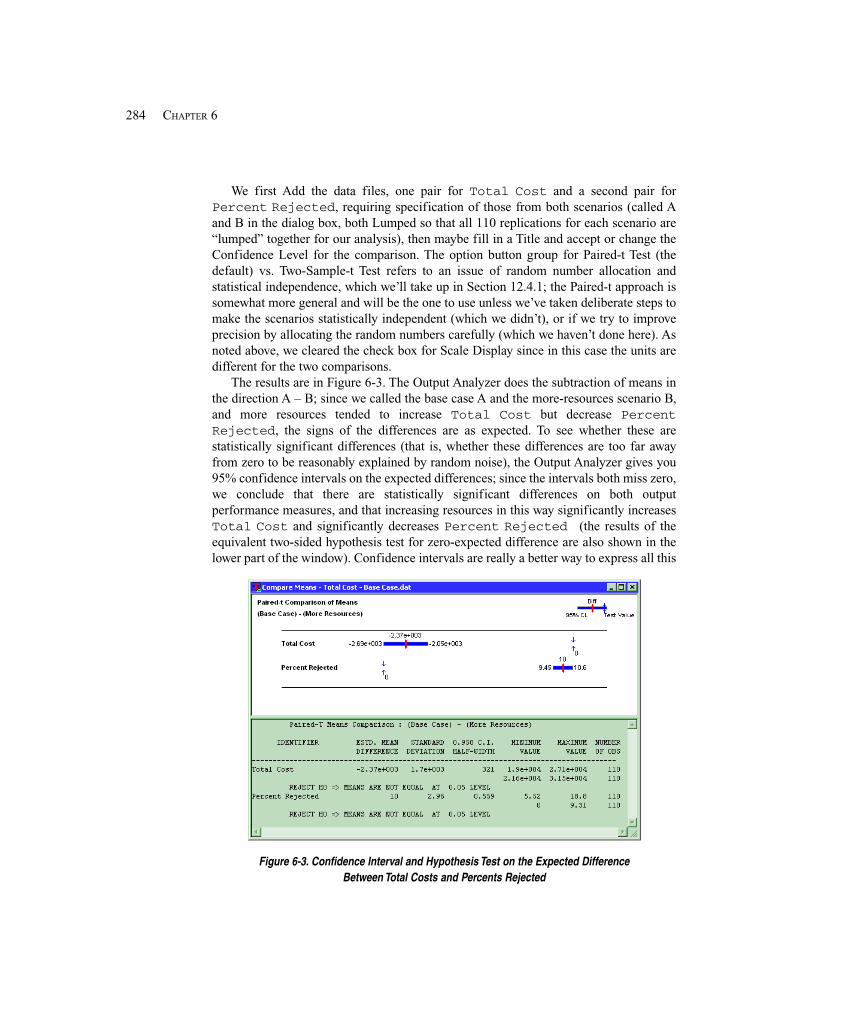
284 CHAPTER 6
We first Add the data files, one pair for Total Cost and a second pair forPercent Rejected, requiring specification of those from both scenarios (called Aand B in the dialog box, both Lumped so that all 110 replications for each scenario are“lumped” together for our analysis), then maybe fill in a Title and accept or change theConfidence Level for the comparison. The option button group for Paired-t Test (thedefault) vs. Two-Sample-t Test refers to an issue of random number allocation andstatistical independence, which we’ll take up in Section 12.4.1; the Paired-t approach issomewhat more general and will be the one to use unless we’ve taken deliberate steps tomake the scenarios statistically independent (which we didn’t), or if we try to improveprecision by allocating the random numbers carefully (which we haven’t done here). Asnoted above, we cleared the check box for Scale Display since in this case the units aredifferent for the two comparisons.
The results are in Figure 6-3. The Output Analyzer does the subtraction of means inthe direction A – B; since we called the base case A and the more-resources scenario B,and more resources tended to increase Total Cost but decrease PercentRejected, the signs of the differences are as expected. To see whether these arestatistically significant differences (that is, whether these differences are too far awayfrom zero to be reasonably explained by random noise), the Output Analyzer gives you95% confidence intervals on the expected differences; since the intervals both miss zero,we conclude that there are statistically significant differences on both outputperformance measures, and that increasing resources in this way significantly increasesTotal Cost and significantly decreases Percent Rejected (the results of theequivalent two-sided hypothesis test for zero-expected difference are also shown in thelower part of the window). Confidence intervals are really a better way to express all this
Figure 6-3. Confidence Interval and Hypothesis Test on the Expected DifferenceBetween Total Costs and Percents Rejected
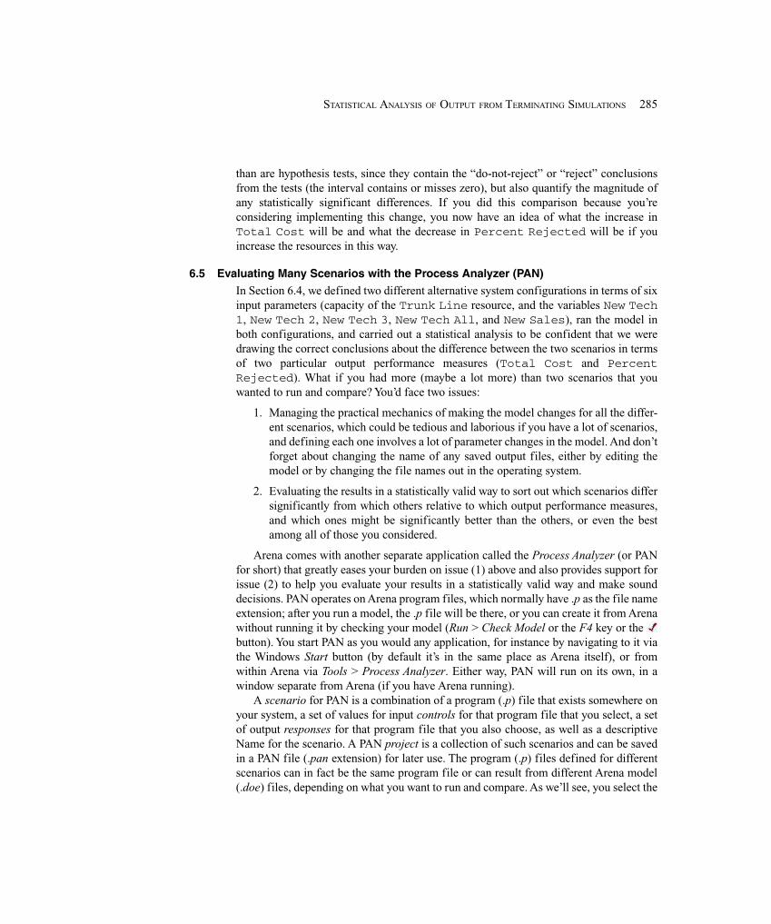
285STATISTICAL ANALYSIS OF OUTPUT FROM TERMINATING SIMULATIONS
than are hypothesis tests, since they contain the “do-not-reject” or “reject” conclusionsfrom the tests (the interval contains or misses zero), but also quantify the magnitude ofany statistically significant differences. If you did this comparison because you’reconsidering implementing this change, you now have an idea of what the increase inTotal Cost will be and what the decrease in Percent Rejected will be if youincrease the resources in this way.
6.5 Evaluating Many Scenarios with the Process Analyzer (PAN)
In Section 6.4, we defined two different alternative system configurations in terms of sixinput parameters (capacity of the Trunk Line resource, and the variables New Tech1, New Tech 2, New Tech 3, New Tech All, and New Sales), ran the model inboth configurations, and carried out a statistical analysis to be confident that we weredrawing the correct conclusions about the difference between the two scenarios in termsof two particular output performance measures (Total Cost and PercentRejected). What if you had more (maybe a lot more) than two scenarios that youwanted to run and compare? You’d face two issues:
1. Managing the practical mechanics of making the model changes for all the differ-ent scenarios, which could be tedious and laborious if you have a lot of scenarios,and defining each one involves a lot of parameter changes in the model. And don’tforget about changing the name of any saved output files, either by editing themodel or by changing the file names out in the operating system.
2. Evaluating the results in a statistically valid way to sort out which scenarios differsignificantly from which others relative to which output performance measures,and which ones might be significantly better than the others, or even the bestamong all of those you considered.
Arena comes with another separate application called the Process Analyzer (or PANfor short) that greatly eases your burden on issue (1) above and also provides support forissue (2) to help you evaluate your results in a statistically valid way and make sounddecisions. PAN operates on Arena program files, which normally have .p as the file nameextension; after you run a model, the .p file will be there, or you can create it from Arenawithout running it by checking your model (Run > Check Model or the F4 key or the button). You start PAN as you would any application, for instance by navigating to it viathe Windows Start button (by default it’s in the same place as Arena itself), or fromwithin Arena via Tools > Process Analyzer. Either way, PAN will run on its own, in awindow separate from Arena (if you have Arena running).
A scenario for PAN is a combination of a program (.p) file that exists somewhere onyour system, a set of values for input controls for that program file that you select, a setof output responses for that program file that you also choose, as well as a descriptiveName for the scenario. A PAN project is a collection of such scenarios and can be savedin a PAN file (.pan extension) for later use. The program (.p) files defined for differentscenarios can in fact be the same program file or can result from different Arena model(.doe) files, depending on what you want to run and compare. As we’ll see, you select the
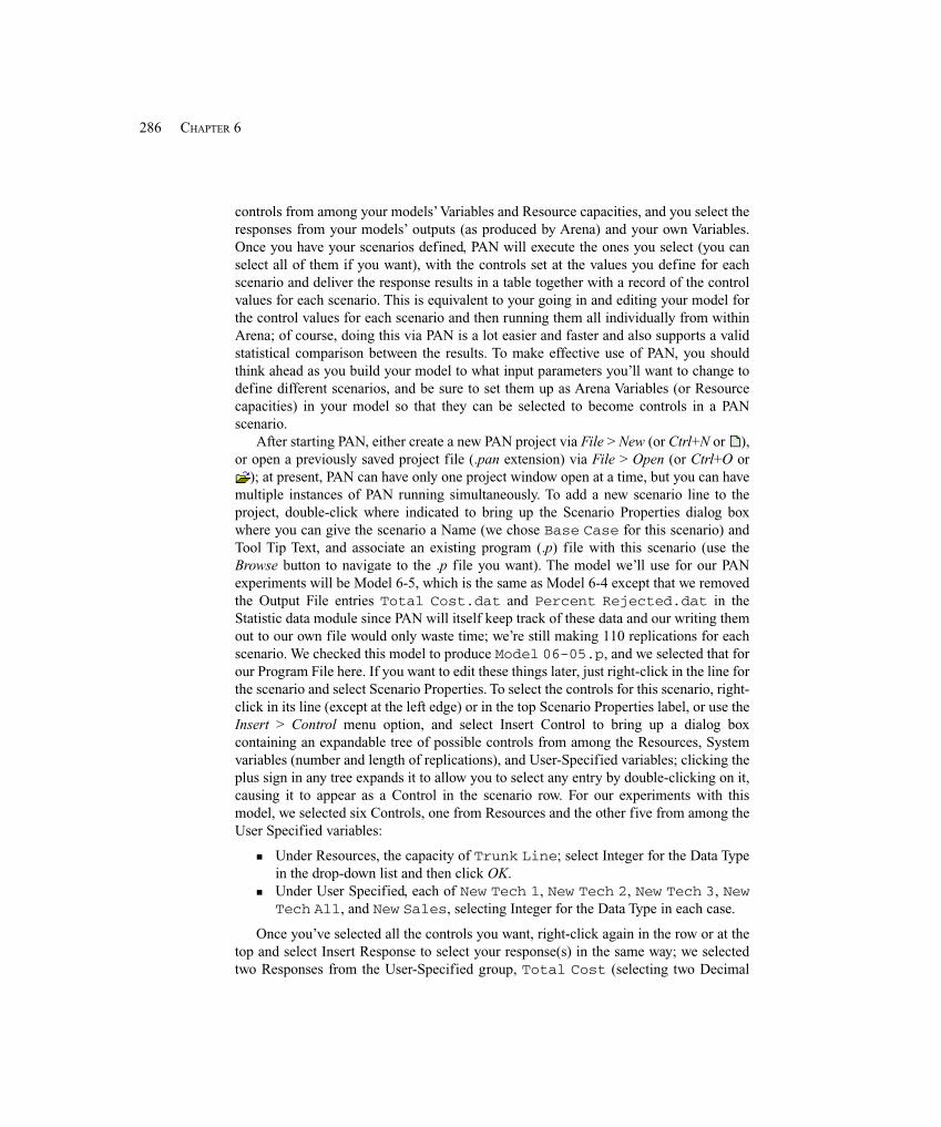
286 CHAPTER 6
controls from among your models’ Variables and Resource capacities, and you select theresponses from your models’ outputs (as produced by Arena) and your own Variables.Once you have your scenarios defined, PAN will execute the ones you select (you canselect all of them if you want), with the controls set at the values you define for eachscenario and deliver the response results in a table together with a record of the controlvalues for each scenario. This is equivalent to your going in and editing your model forthe control values for each scenario and then running them all individually from withinArena; of course, doing this via PAN is a lot easier and faster and also supports a validstatistical comparison between the results. To make effective use of PAN, you shouldthink ahead as you build your model to what input parameters you’ll want to change todefine different scenarios, and be sure to set them up as Arena Variables (or Resourcecapacities) in your model so that they can be selected to become controls in a PANscenario.
After starting PAN, either create a new PAN project via File > New (or Ctrl+N or ),or open a previously saved project file (.pan extension) via File > Open (or Ctrl+O or
); at present, PAN can have only one project window open at a time, but you can havemultiple instances of PAN running simultaneously. To add a new scenario line to theproject, double-click where indicated to bring up the Scenario Properties dialog boxwhere you can give the scenario a Name (we chose Base Case for this scenario) andTool Tip Text, and associate an existing program (.p) file with this scenario (use theBrowse button to navigate to the .p file you want). The model we’ll use for our PANexperiments will be Model 6-5, which is the same as Model 6-4 except that we removedthe Output File entries Total Cost.dat and Percent Rejected.dat in theStatistic data module since PAN will itself keep track of these data and our writing themout to our own file would only waste time; we’re still making 110 replications for eachscenario. We checked this model to produce Model 06-05.p, and we selected that forour Program File here. If you want to edit these things later, just right-click in the line forthe scenario and select Scenario Properties. To select the controls for this scenario, right-click in its line (except at the left edge) or in the top Scenario Properties label, or use theInsert > Control menu option, and select Insert Control to bring up a dialog boxcontaining an expandable tree of possible controls from among the Resources, Systemvariables (number and length of replications), and User-Specified variables; clicking theplus sign in any tree expands it to allow you to select any entry by double-clicking on it,causing it to appear as a Control in the scenario row. For our experiments with thismodel, we selected six Controls, one from Resources and the other five from among theUser Specified variables:
� Under Resources, the capacity of Trunk Line; select Integer for the Data Typein the drop-down list and then click OK.
� Under User Specified, each of New Tech 1, New Tech 2, New Tech 3, NewTech All, and New Sales, selecting Integer for the Data Type in each case.
Once you’ve selected all the controls you want, right-click again in the row or at thetop and select Insert Response to select your response(s) in the same way; we selectedtwo Responses from the User-Specified group, Total Cost (selecting two Decimal
287STATISTICAL ANALYSIS OF OUTPUT FROM TERMINATING SIMULATIONS
Figure 6-4. The PAN Project Experiment 06-05.pan After Definingthe First (Base-Case) Scenario
Places) and Percent Rejected (one Decimal Place). The values of the controlsshow up as the ones they have in the model as it was defined, but (here’s the power ofPAN) you can change them for execution of this scenario by simply editing their valuesin this scenario row in the PAN project window; for the base-case scenario, we left thecontrol values as they were in the original model (26 and the five 0s). The values for theresponses are blank since we haven’t run the scenario yet. Figure 6-4 shows the status ofpart of the PAN project window after we defined this scenario and saved the project asExperiment 06-05.pan (we chose “Experiment” since this really is a wholeexperiment going on, which could even be a statistically designed one though it isn’there—see Section 12.6).
You could repeat the above process for additional scenarios. However, if they aresimilar to one that you’ve already defined, you can duplicate it (right-click in its scenarionumber on the left and select Duplicate Scenario(s)), and then just make edits in theduplicated scenario.
To define a sensible set of scenarios for this model, suppose that you received anorder from above giving you $1360/week more to spend on additional resources, but thatyou have to devote the entire $1360 to just a single kind of resource. To which of the six“expandable” resources should you allocate the new money? Given the weekly costs ofthe resources, you could get 13 more trunk lines ($98 each), or 4 more of any one of theadditional single-product tech-support people ($320 each), or 3 of the additional all-product tech-support people ($360 each), or 4 additional sales people ($340 each).Figure 6-5 shows the PAN project filled out with the six possible scenarios, plus thebase-case scenario at the top.
To run some or all of the scenarios, select their rows by clicking in the left-mostcolumn of each row (Ctrl+Click to extend the selection or Shift+Click to select acontiguous set of lines). Then select Run > Go (or the F5 function key or the button)...and then, you may have to wait a little while and watch the Reps column count up andthe Responses columns get populated. Figure 6-6 shows the results of running all sevenscenarios; the Responses column gives the average over the 110 replications of eachscenario. Looking at the Total Cost column, it appears that beefing up the sales-callstaff would be best; looking at the Percent Rejected column, it appears that addingNew Tech Alls would be best.
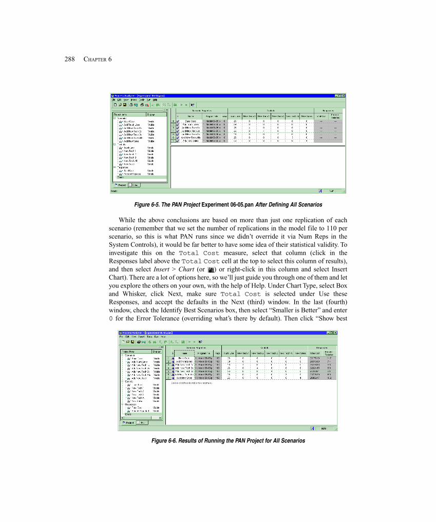
288 CHAPTER 6
Figure 6-5. The PAN Project Experiment 06-05.pan After Defining All Scenarios
While the above conclusions are based on more than just one replication of eachscenario (remember that we set the number of replications in the model file to 110 perscenario, so this is what PAN runs since we didn’t override it via Num Reps in theSystem Controls), it would be far better to have some idea of their statistical validity. Toinvestigate this on the Total Cost measure, select that column (click in theResponses label above the Total Cost cell at the top to select this column of results),and then select Insert > Chart (or ) or right-click in this column and select InsertChart). There are a lot of options here, so we’ll just guide you through one of them and letyou explore the others on your own, with the help of Help. Under Chart Type, select Boxand Whisker, click Next, make sure Total Cost is selected under Use theseResponses, and accept the defaults in the Next (third) window. In the last (fourth)window, check the Identify Best Scenarios box, then select “Smaller is Better” and enter0 for the Error Tolerance (overriding what’s there by default). Then click “Show best
Figure 6-6. Results of Running the PAN Project for All Scenarios
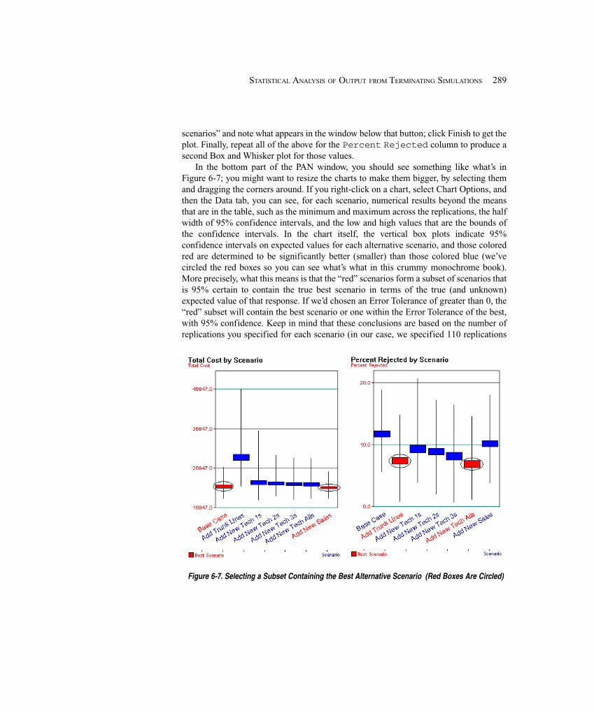
289STATISTICAL ANALYSIS OF OUTPUT FROM TERMINATING SIMULATIONS
scenarios” and note what appears in the window below that button; click Finish to get theplot. Finally, repeat all of the above for the Percent Rejected column to produce asecond Box and Whisker plot for those values.
In the bottom part of the PAN window, you should see something like what’s inFigure 6-7; you might want to resize the charts to make them bigger, by selecting themand dragging the corners around. If you right-click on a chart, select Chart Options, andthen the Data tab, you can see, for each scenario, numerical results beyond the meansthat are in the table, such as the minimum and maximum across the replications, the halfwidth of 95% confidence intervals, and the low and high values that are the bounds ofthe confidence intervals. In the chart itself, the vertical box plots indicate 95%confidence intervals on expected values for each alternative scenario, and those coloredred are determined to be significantly better (smaller) than those colored blue (we’vecircled the red boxes so you can see what’s what in this crummy monochrome book).More precisely, what this means is that the “red” scenarios form a subset of scenarios thatis 95% certain to contain the true best scenario in terms of the true (and unknown)expected value of that response. If we’d chosen an Error Tolerance of greater than 0, the“red” subset will contain the best scenario or one within the Error Tolerance of the best,with 95% confidence. Keep in mind that these conclusions are based on the number ofreplications you specified for each scenario (in our case, we specified 110 replications
Figure 6-7. Selecting a Subset Containing the Best Alternative Scenario (Red Boxes Are Circled)
290 CHAPTER 6
for each scenario, but we could have specified different numbers of replications fordifferent scenarios); if you want to narrow the selected (red) subset, you could increasethe number of replications for the scenarios. You could also narrow the selected (red)subset by specifying the Error Tolerance to be a positive number that represents anamount small enough that you don’t care if the selected scenario(s) are actually inferiorto the true best one by at most this amount; so a positive Error Tolerance may reduce thenumber of selected scenarios at the risk of being off by a little bit. This selectionprocedure is firmly based on sound statistical theory developed by Nelson, Swann,Goldsman, and Song (2001).
So depending on whether you regard Total Cost or Percent Rejected as themore important response, you now have an indication of which among these six (seven,if you include the base case) scenarios would likely be best. It’s hard to think of a sensibleway to combine these two responses into one on which to optimize. Wouldn’t it be niceif, for instance, we could seek to minimize Total Cost while holding PercentRejected to no more than something like five? Press on (to Section 6.6), gentle reader.
6.6 Searching for an Optimal Scenario with OptQuest3
The scenarios evaluated in Section 6.5 were just a few of the myriad of possibilities thatwe might explore in a quest to minimize Total Cost, subject to the requirement thatthe Percent Rejected response turn out to be no more than five. Suppose you’renow set free to explore all the possibilities you’d like in terms of the Trunk Linecapacity (but you’re contractually obligated to keep at least the 26 you already have, andthe wiring closet has room for at most 50), as well as New Tech 1, New Tech 2, NewTech 3, New Tech All, and New Sales (but you have room for at most 15 newpeople in all of the tech-support and sales categories combined). Since you have six inputcontrol variables to play with, you can think of this as wandering around in part of six-dimensional space looking for a six-vector (of non-negative integers) that minimizesTotal Cost while holding Percent Rejected to five or less. This is a lot ofpossibilities (1,356,600, actually), and considering them all exhaustively is not practical(with the 110 replications per scenario that we’ve been using, it would run around theclock for over two months on a 2.13 GHz machine).
Where do you start? This is a hard question, but a reasonable idea would be the bestpoint you know about so far. None of the scenarios in the PAN experiment of Figure 6-6meets the requirement that Percent Rejected < 5 (though a couple are close, andwe could start with such an infeasible point though we’d need to move away from iteventually, of course). However, the more-resources case from Section 6.4 (the TrunkLine resource has a capacity of 29, and New Tech 1, New Tech 2, New Tech 3, NewTech All, and New Sales are all set to 3) does meet the Percent Rejected < 5
3 If you are running the student version of Arena, you will likely not have OptQuest available, though itcould be in your college or university computer labs. Instructors can request a research license from RockwellAutomation, which will enable OptQuest as well as the full commercial version of Arena. However, this li-cense is for academic use only; commercial use of a research license is strictly prohibited.
291STATISTICAL ANALYSIS OF OUTPUT FROM TERMINATING SIMULATIONS
requirement, so we’ll start there, even though its Total Cost is on the high sidecompared to other scenarios with which we’ve experimented, and we’ll seek to reduce itwhile obeying the Percent Rejected < 5 requirement.
But where do you go from here? This is not an easy question to answer either, to saythe least. A lot of people have been doing research into such topics for many years andhave developed a variety of methods to address this problem. Arena comes with apackage called OptQuest®, from OptTek Systems Inc., that uses heuristics known as tabusearch and scatter search (and other methods) to move around intelligently in the input-control space and try to converge quickly and reliably to an optimal point. OptQuest is, ina way, similar to PAN in that it “takes over” the execution of your Arena model; thedifference is that rather than relying on you to specify which specific scenarios tosimulate, OptQuest decides on its own which ones to consider in an iterative fashion thathopefully leads to something close to an optimal combination of input control values.For detailed documentation on how OptQuest works with Arena, see Help > ProductManuals > Arena OptQuest User’s Guide.
To run OptQuest for Arena, first make active the Arena window for the model ofinterest. We’ll basically use Model 6-5, except that OptQuest requires that a finite RunLength be specified in Run > Setup > Replication Parameters, so we entered 1000 hours,which will never be reached since we retain our model-sensitive stopping rule that willalmost certainly stop the replication well before time 1000 hours. We called the resultModel 6-6. Then select Tools > OptQuest for Arena to bring up the OptQuest applicationwindow, then New Optimization.
OptQuest takes a moment to look through your model for potential Controls(including capacities of resources and Arena Variables you’ve defined) and Responses(including the built-in Arena costing outputs, and all outputs you’ve defined), andpresents them in an expandable/contractible tree on the left. The Controls are the inputparameters that you can choose to allow OptQuest to vary as it searches; in mathematical-programming or optimization parlance, these are the choice variables or decisionvariables, and we seek a combination that will optimize (minimize or maximize) anobjective that will be chosen below from the simulation’s outputs. Start by clicking on theword Controls in the tree on the left (or the menu option View > Controls), to bring up alist of all Resources and User Specified variables, and check the boxes in the Includedcolumn for Trunk Line, New Sales, New Tech 1, New Tech 2, New Tech 3, andNew Tech All. In each of these Included Control lines, double-click to open a windowwhere you specify the appropriate Lower Bound, Suggested Value (i.e., starting values asdiscussed above), Upper Bound, and maybe a brief Description; also check the Type asappropriate, which will be Integer for all of our controls. You can then click on theIncluded column heading and its arrow to collect the controls you’ve selected at the top orbottom. Note that, since the total of all new staff hired must be no more than 15, certainlyeach one must be no more than 15, establishing those Upper (High) Bounds. Figure 6-8shows the OptQuest window with the completed Controls section visible.
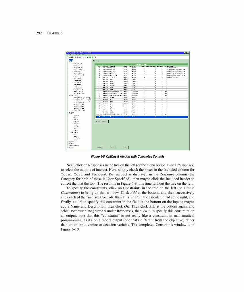
292 CHAPTER 6
Figure 6-8. OptQuest Window with Completed Controls
Next, click on Responses in the tree on the left (or the menu option View > Responses)to select the outputs of interest. Here, simply check the boxes in the Included column forTotal Cost and Percent Rejected as displayed in the Response column (theCategory for both of these is User Specified), then maybe click the Included header tocollect them at the top. The result is in Figure 6-9, this time without the tree on the left.
To specify the constraints, click on Constraints in the tree on the left (or View >Constraints) to bring up that window. Click Add at the bottom, and then successivelyclick each of the first five Controls, then a + sign from the calculator pad at the right, andfinally <= 15 to specify this constraint in the field at the bottom on the inputs; maybeadd a Name and Description, then click OK. Then click Add at the bottom again, andselect Percent Rejected under Responses, then <= 5 to specify this constraint onan output; note that this “constraint” is not really like a constraint in mathematicalprogramming, as it’s on a model output (one that’s different from the objective) ratherthan on an input choice or decision variable. The completed Constraints window is inFigure 6-10.
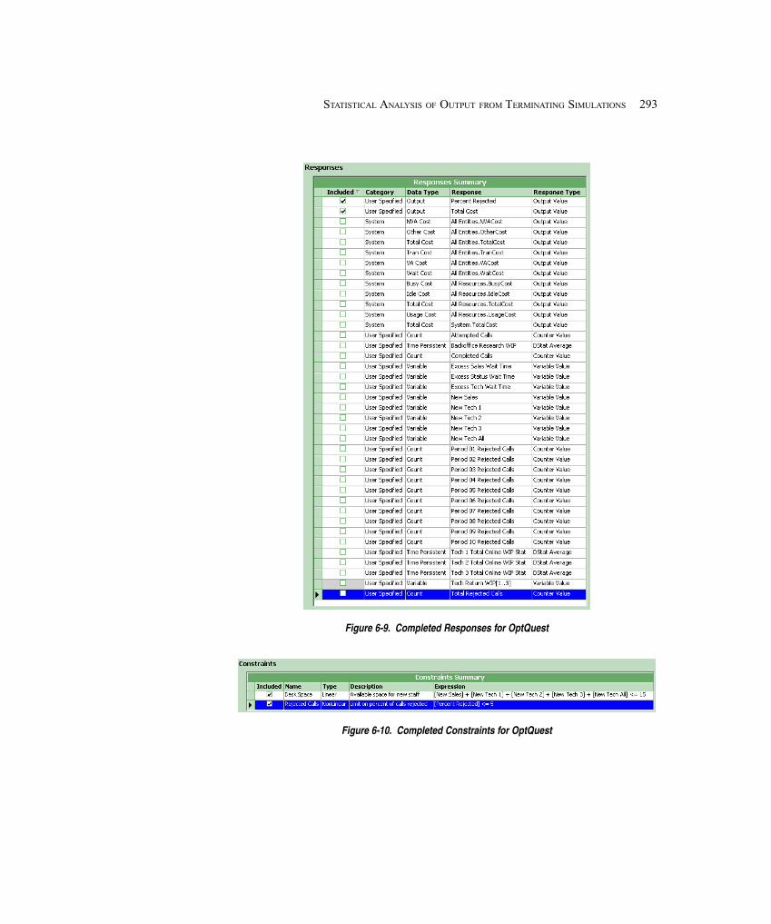
293STATISTICAL ANALYSIS OF OUTPUT FROM TERMINATING SIMULATIONS
Figure 6-9. Completed Responses for OptQuest
Figure 6-10. Completed Constraints for OptQuest

294 CHAPTER 6
Figure 6-11. Completed Objectives for OptQuest
To tell OptQuest what it is you want to optimize, click Objectives in the tree on theleft (or View > Objectives), then Add, then click Total Cost under the Responses,then the Minimize radio button (and a Name and Description if you like). The result isin Figure 6-11.
The Options entry on the tree to the left (or View > Options) provides several ways tocontrol how OptQuest decides to stop searching, a tolerance for regarding two objectivevalues as equal, control on the replications per scenario, and a file for a complete log ofwhat OptQuest considers during its run. After some experimentation on our model’s runspeed, we decided to allow OptQuest to search through 500 different scenarios (whatOptQuest calls “simulations”), and then stop, rather than allow OptQuest to decide itselfwhen to stop. Since we know that this model has considerable variation across replica-tions, under Replications per simulation, push the radio button for “Vary the number ofreplications” and specify a minimum of 5 and a maximum of 110 replications. Elsewherewe’ll accept the default options.
From the Options window, you could click the Optimize button to start OptQuest, oralternatively click the Start Optimization ( ) button on the toolbar, or select Run > StartOptimization (or the F5 key). This causes OptQuest to simulate your model at thestarting point you chose, and then decide on its own how best to search through thefeasible region of six-dimensional space for a combination of input controls thatminimizes Total Cost while satisfying both constraints. As it does so, you can see itsprogress by selecting Optimization in the tree on the left, to see the best objective valueso far, the current objective value, and how many “simulations” (scenarios) have beenrun. You can also see the best and current controls, and that the constraints are beingsatisfied during the search (or occasionally violated). The graph at the bottom plots thebest (smallest for us) objective found so far, as a function of how many “simulations”have thus far been tried. The final view of this information is in Figure 6-12, whichdisplays the best set of controls found and the associated objective function. This graph istypical, with large improvements (reductions) realized early (the low-hanging-fruitphenomenon), followed by harder-fought improvements and eventually a tapering off.As we asked, OptQuest evaluated 500 scenarios (0.04% of the 1,356,600 possible),finding the best one among them as the 306th scenario it considered (and then noimprovement for the rest of the 500 scenarios). The best Total Cost was 20691.92,some 16% lower than the starting point of 24542.82 we got in Section 6.4; the way toachieve that would be to add one trunk line (up to 27), hire three new sales staffers, andhire one each of type 2, type 3, and all-type tech support people (so six new people inall—well below the limit of 15). This run took a little under six minutes on a 2.13GHzmachine; another run of about two hours and nearly 10,000 scenarios found a slightlybetter solution producing a cost of 20447.59 (1.2% lower). You can check the log file
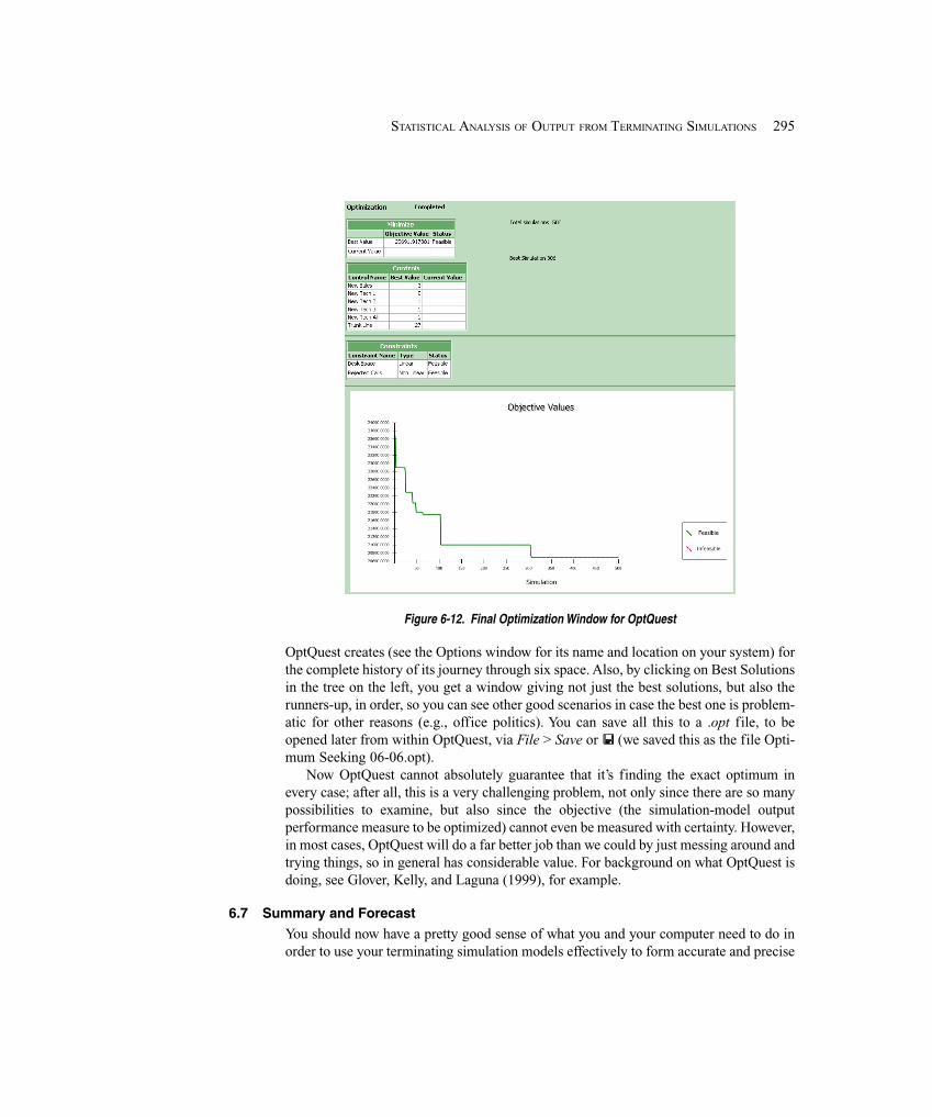
295STATISTICAL ANALYSIS OF OUTPUT FROM TERMINATING SIMULATIONS
Figure 6-12. Final Optimization Window for OptQuest
OptQuest creates (see the Options window for its name and location on your system) forthe complete history of its journey through six space. Also, by clicking on Best Solutionsin the tree on the left, you get a window giving not just the best solutions, but also therunners-up, in order, so you can see other good scenarios in case the best one is problem-atic for other reasons (e.g., office politics). You can save all this to a .opt file, to beopened later from within OptQuest, via File > Save or (we saved this as the file Opti-mum Seeking 06-06.opt).
Now OptQuest cannot absolutely guarantee that it’s finding the exact optimum inevery case; after all, this is a very challenging problem, not only since there are so manypossibilities to examine, but also since the objective (the simulation-model outputperformance measure to be optimized) cannot even be measured with certainty. However,in most cases, OptQuest will do a far better job than we could by just messing around andtrying things, so in general has considerable value. For background on what OptQuest isdoing, see Glover, Kelly, and Laguna (1999), for example.
6.7 Summary and ForecastYou should now have a pretty good sense of what you and your computer need to do inorder to use your terminating simulation models effectively to form accurate and precise
296 CHAPTER 6
estimates of expected results, draw valid conclusions about how different alternatives (orscenarios) of your model might differ in terms of key output performance measures, andto search efficiently for a model configuration that’s optimal in some sense. This takesyou a long way toward becoming an effective user of your models (not just an effectivemodeler, though that’s certainly important too). In Chapter 7, we’ll go through somemore modeling ideas and then at the end revisit output analysis if your interest is in long-run (or steady-state) results, in which case you have to do things a little differently fromwhat we’ve described in this chapter. Chapter 12 discusses further statistical issues insimulation, including how the underlying randomness is generated, how to reduce outputvariability (without just more computing), getting Arena to decide itself how much to runto give you acceptably precise results, and a little more on designing simulationexperiments.
6.8 Exercises
6-1 In Exercise 5-1, statistically compare your results to what we got earlier; do thiscomparison informally by making 95% confidence intervals based on 50 replicationsfrom both models and see if they overlap. As performance measures, use the averagewaiting time in queue, average queue length, and server utilization.
6-2 Using the model from Exercise 5-2, change the processing time for the secondpass on Machine 1 to TRIA(6.7, 9.1, 13.6). Run the simulation for 20,000 minutes andcompare the results with respect to the same three output performance measures. Do an“informal” statistical comparison by making 20 replications of both versions of themodel, forming 95% confidence intervals, and looking at the relation between theconfidence intervals.
6-3 In Exercise 5-3, about how many replications would be required to bring the halfwidth of a 95% confidence interval for the expected average cycle time for bothtrimmers down to one minute? (You don’t need to do this, just do something to estimatethe approximate number of replications that would be required.)
6-4 The facility of Exercise 5-4 is in a congested urban area where land is expensiveand you’ve been asked to decide how much space should be planned for the trucks inqueue to unload; address this question (being mindful of statistical issues).
6-5 In Exercise 5-5, suppose you could hire one more person and that person could bea second (identical) operator at any of the four locations. Which one should it be? UsePAN with 50 replications per scenario and select the best in terms of lowest average timein system. In retrospect, is your choice surprising? How critical is it to get this choiceright?
Now suppose you could hire up to three more people and allocate them any way youwant to the four existing operators, including allocating all three of the new people to asingle operator. What’s the best thing to do? Use OptQuest to search for the optimalallocation of this maximum of three more people, with the objective of minimizing theaverage time in system.
297STATISTICAL ANALYSIS OF OUTPUT FROM TERMINATING SIMULATIONS
6-6 In Exercise 4-1, suppose that 7% of arriving customers are classified just aftertheir arrival as being frequent fliers. Run your simulation for five replications (fivedays). Assume all times are the same as before, and observe statistics on the average timein system by customer type (frequent fliers and non-frequent fliers) under each of thefollowing scenarios:
(a) Assign four of the current agents to serve non-frequent fliers only and the fifthto serve frequent fliers only.
(b) Change your model from part (a) so that the frequent-flier agent can serveregular customers when there are no frequent fliers waiting in queue.
(c) Change your model so that any agent can serve any customer, but priority isalways given to frequent fliers.
Which of the three scenarios above do you think is “best” for the frequent fliers? Howabout for the 93% of customers who are non-frequent fliers? Viewing this as aterminating simulation, address these comparison questions in a statistically valid way.
6-7 In Exercise 5-13, make 30 replications and compute a 95% confidence interval onthe expected system or cycle time for both customer types.
6-8 In Exercise 5-14, make 30 replications, and estimate the expected differencebetween this and the model of Exercise 5-13 (based on system time by customer). Besure to use an appropriate formal statistical technique.
6-9 In Exercise 5-15, make 30 replications and estimate the expected differencebetween this model and the one in Exercise 5-14 (based on system time by customer),using an appropriate formal statistical technique.
6-10 For the inventory system of Model 5-4, set up a PAN comparison to investigate theaverage total cost resulting from each of the following (s, S) pairs:
(20, 40) (20, 60) (20, 80) (20, 100)(40, 60) (40, 80) (40, 100)
(60, 80) (60, 100)(80, 100)
Run 100 replications of each case, and pick the best (lowest-cost) among these in a statis-tically valid way. This comparison is from Section 1.5.5 of Law and Kelton (2000).
6-11 For the inventory system of Model 5-4, use OptQuest to look for the best (total-cost-minimizing) setting for (s, S). Let s run between 1 and 99 (by ones) and let S runbetween 2 and 100 (by ones); remember that s and S must be integers and that we musthave s < S. Make your own judgments about stopping criterion, number of replications,etc.
6-12 In Exercise 6-11, investigate whether taking inventory at the beginning of each dayis necessarily the best policy by adding the inventory-evaluation interval (currently set atone day) to the optimum-seeking variable mix, and allow OptQuest to vary it

298 CHAPTER 6
(continuously) between a half day and five days, as well as simultaneously allowing sand S to vary as in Exercise 6-11. If you use Model 05-04.doe as a base, you’ll needto change Evaluation Interval from an Expression to a Variable so OptQuest canget at it.
6-13 Apply OptQuest on all six values of (s, S) in Exercise 5-20. Let each s rangebetween 1 and 99 (by ones), and let each S range between 2 and 100 (by ones); of course,s and S must be integers and for each of the three items in inventory we must have s < S.
6-14 Apply OptQuest on all six values of (s, S) in Exercise 5-21, with the same rangesas in Exercise 6-13. Compare your results with those from Exercise 6-13 and explain thisin terms of the incentives offered by the supplier in this different cost structure.
6-15 In Exercise 4-22, suppose you could hire one more person, and that person couldbe assigned either to manual check-in, automated check-in, or security. Where would thisadditional person be best used? As an overall criterion of “goodness” of a system, use theaverage total time in system of all types of passengers combined. Set up a PAN run anddecide about the number of replications needed to arrive at a reliable conclusion.
6-16 In Exercise 6-15, suppose you could hire a total of five more people (rather thanjust one more) to be allocated in any way to the existing staff at manual check-in,automated check-in, or security. You can’t reduce staffing anywhere from the levels inExercise 4-22. Using average total time in system of all types of passengers combined,what would be the best deployment of these five additional people? Should you even useall five of them? Set up an OptQuest run and decide about the stopping criterion andnumbers of replications.
6-17 In Exercise 4-22 (with staffing fixed at the original levels), the airline noticed thata lot of the people who opt for the manual check-in really don’t need the extra servicesthere and could have used the automated check-in. Instead of the original 35% and 50%that go to manual and automated, respectively, suppose that through more effective“encouragement” from people with red blazers and loud voices, it could be made 10%and 75% instead. (There probably are 10% of passengers who genuinely need the extraservices of manual check-in.) How would this shift in passenger attitudes (or maybebravery) affect average total time in system of passengers? Base your comparison on 200replications of the model in each configuration.
6-18 Exercise 2-8 described a change in Model 3-1. Carry out a statistically valid studyto measure the effect of this change on the average waiting time in queue and on theserver utilization. Make your own decisions about numbers of replications in order toarrive at meaningful and reasonably precise conclusions.
6-19 Recall Models 3-2, 3-3, 3-4, and 3-5 from Chapter 3, comparing specialized serialvs. generalized parallel operations in environments of both high-variance and low-variance (no-variance, actually) service times. It appeared in Table 3-1 that thegeneralized parallel arrangement provided better service, though the improvement was
299STATISTICAL ANALYSIS OF OUTPUT FROM TERMINATING SIMULATIONS
much stronger in the high-variance service-time environment. Choose relevant outputperformance measures and make valid statistical comparisons to see if what appears tobe true in Table 3-1 (from just a single run) is statistically valid.
6-20 Recall Exercise 3-13, which modified Model 3-3 to add 18% onto the individual-task times in the generalized integrated-work parallel configuration of Model 3-3.Choose relevant output performance measures and make a valid statistical comparison tosee if the model of Exercise 3-13 differs significantly from the original specialized serialconfiguration of Model 3-2. In other words, if you had to endure this 18% increase intask-processing times, should you still move from the specialized-work serial setup tothe generalized-work parallel setup?
6-21 For the enhanced machine-repair model of Exercise 5-22, do a valid statisticalanalysis to defend your choice of the number of repair technicians to hire in order tominimize total average cost. Make your own decision on number of replications, andmodify it if necessary.
6-22 Use Arena to simulate the news vendor problem of Section 2.7.1. Consider just thecase q = 160, and run for 30 days to get an average daily profit and 95% confidenceinterval, as well as the proportion of days in which a loss is incurred.
6-23 Generalize your Arena model from Exercise 6-22 to consider all five values of q inSection 2.7.1, in a single Arena run, using the same daily demand realization for eachvalue of q.
6-24 In the outpatient clinic of Exercise 4-30, suppose you could add one unit ofresource to any one of the five stations (receptionist, nurse, exam room, check-outadministrator, or lab technician). Where would be the most useful addition? Look at bothaverage patient total time in system, as well as patient throughput. Set up a PAN run andmake your own decision about the number of replications per scenario.
6-25 The outpatient clinic of Exercise 4-30 has received an economic-stimulus capitalgrant of $400,000 to expand service and reduce patients’ average total time in system.They can allocate these funds in any way they like in order to add any number ofresources to any of the five stations, though they cannot reduce any resources belowcurrent levels (one at each station, except three exam rooms). The clinic has thefollowing capital-costs estimates for an additional unit of resource at each station; alsogiven are the maximum number additional resources to each station if the entire$400,000 were allocated to that station:
Receptionist $40,000 could add max of 10Nurse $80,000 could add max of 5Exam Room $200,000 could add max of 2Lab/X-Ray $100,000 could add max of 4Check Out $50,000 could add max of 8

300 CHAPTER 6
Remember, the $400,000 is additional funding, so should be spent on additionalresources; funding of the existing resource levels is already budgeted. Physicians are themain users of the exam rooms, so they are looking at the fact (results from Exercise 4-30)that the exam rooms are apparently the most heavily utilized and are arguing to spend theentire $400,000 on adding two exam rooms. Do you agree? Set up an OptQuest run toinvestigate this, and make your recommendations.
301INTERMEDIATE MODELING AND STEADY-STATE STATISTICAL ANALYSIS
CHAPTER 7
Intermediate Modeling andSteady-State Statistical Analysis
Many of the essential elements of modeling with Arena were covered in Chapters 3, 4,and 5, including the basic use of some of the Basic Process and Advanced Process panelmodules, controlling the flow of entities, Resource Schedules and States, Sets, Variables,Expressions, Stations, Transfers, and enhancing the animation. In this chapter, we’llexpand on several concepts that allow you to do more detailed modeling. As before, we’llillustrate things concretely by means of a fairly elaborate example. We’ll first start byintroducing a new example as described in Section 7.1; expressing it in Arena requiresthe concept of entity-dependent Sequences, discussed in Section 7.1.1. Then in Section7.1.2, we take up the general issue of how to go about modeling a system, the level ofdetail appropriate for a project, and the need to pay attention to data requirements andavailability. The data portion required for the model is built in Section 7.1.3 and thelogical model in Section 7.1.4. In Section 7.1.5, we develop an animation, includingdiscussion of importing existing CAD drawings for the layout. We conclude this portionwith a discussion on verifying that the representation of a model in Arena really doeswhat you want, in Section 7.1.6.
Continuing our theme of viewing all aspects of simulation projects throughout astudy, we resume the topic of statistical analysis of the output data in Section 7.2, but thistime it’s for steady-state simulations, using the model from Section 7.1.
By the time you read and digest the material in this chapter, you’ll have a pretty goodidea of how to model things in considerable detail. You’ll also be in a position to drawstatistically valid conclusions about the performance of systems as they operate in thelong run.
7.1 Model 7-1: A Small Manufacturing SystemA layout for our small manufacturing system is shown in Figure 7-1. The system to bemodeled consists of part arrivals, four manufacturing cells, and part departures. Cells 1,2, and 4 each have a single machine; Cell 3 has two machines. The two machines at Cell3 are not identical; one of these machines is a newer model that can process parts in 80%of the time required by the older machine. The system produces three part types, eachvisiting a different sequence of stations. The part steps and process times (in minutes) aregiven in Table 7-1. All process times are triangularly distributed; the process times givenin Table 7-1 at Cell 3 are for the older (slower) machine.
The interarrival times between successive part arrivals (all types combined) areexponentially distributed with a mean of 13 minutes; the first part arrives at time 0. Thedistribution by type is 26%, Part 1; 48%, Part 2; and 26%, Part 3. Parts enter from the
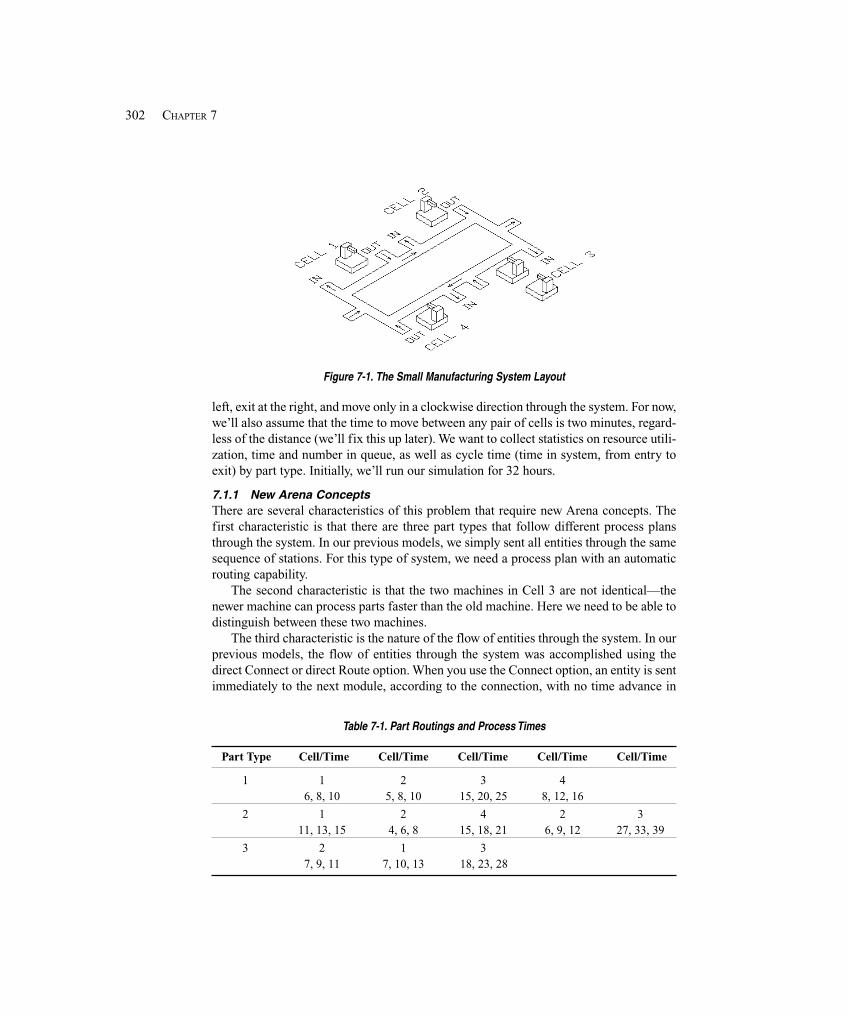
302 CHAPTER 7
Figure 7-1. The Small Manufacturing System Layout
left, exit at the right, and move only in a clockwise direction through the system. For now,we’ll also assume that the time to move between any pair of cells is two minutes, regard-less of the distance (we’ll fix this up later). We want to collect statistics on resource utili-zation, time and number in queue, as well as cycle time (time in system, from entry toexit) by part type. Initially, we’ll run our simulation for 32 hours.
7.1.1 New Arena ConceptsThere are several characteristics of this problem that require new Arena concepts. Thefirst characteristic is that there are three part types that follow different process plansthrough the system. In our previous models, we simply sent all entities through the samesequence of stations. For this type of system, we need a process plan with an automaticrouting capability.
The second characteristic is that the two machines in Cell 3 are not identical—thenewer machine can process parts faster than the old machine. Here we need to be able todistinguish between these two machines.
The third characteristic is the nature of the flow of entities through the system. In ourprevious models, the flow of entities through the system was accomplished using thedirect Connect or direct Route option. When you use the Connect option, an entity is sentimmediately to the next module, according to the connection, with no time advance in
Table 7-1. Part Routings and Process Times
Part Type Cell/Time Cell/Time Cell/Time Cell/Time Cell/Time
1 1 2 3 46, 8, 10 5, 8, 10 15, 20, 25 8, 12, 16
2 1 2 4 2 311, 13, 15 4, 6, 8 15, 18, 21 6, 9, 12 27, 33, 39
3 2 1 37, 9, 11 7, 10, 13 18, 23, 28
303INTERMEDIATE MODELING AND STEADY-STATE STATISTICAL ANALYSIS
the simulation. If we used the Connect option in this new model, we would have toinclude a number of Decide modules to direct the parts to the correct next station in thesequence followed by Route modules both to model the two-minute transfer time and toenable animation of the part movements. As you might expect, there is an Arena concept,sequences, that allows easy modeling of the flow of entities through the system whileallowing for the part transfer time and enabling its animation.
Many systems are characterized by entities that follow predefined, but different pathsthrough the system. Most manufacturing systems have part or process plans that specifya list of operations each part type must complete before exiting the system. Many servicesystems have similar types of requirements. For example, a model of passenger traffic inan airport may require different paths through the airport depending on whether thepassengers check baggage or have only carry-on pieces, as well as whether thepassengers have domestic or international flights.
Arena can send entities through a system automatically according to a predefinedsequence of station visitations. The Sequence data module, on the Advanced Transferpanel, allows us to define an ordered list of Stations that can include assignments ofattributes or variables at each station. To direct an entity to follow this pattern of stationvisitations, we assign the sequence to the entity (using a built-in sequence attribute,described below) and use the “By Sequence” option in the Route module when wetransfer the entity to its next destination.
As the entity makes its way along its sequence, Arena will do all the necessary book-keeping to keep track of where the entity is and where it will go next. This is accom-plished through the use of three special, automatically defined Arena attributes:Entity.Station (or M), Entity.Sequence (or NS), and Entity.JobStep (or IS). Each entityhas these three attributes, with the default values for newly created entities being 0 foreach. The Entity.Station attribute contains the current station location of the entity or thestation to which the entity is currently being transferred. The Entity.Sequence attributecontains the sequence the entity will follow, if any; you need to assign this to each entitythat will be transferring via a sequence. The Entity.Jobstep attribute specifies the entity’sposition within the sequence, so normally starts at 0 and then is incremented by 1 as theentity moves to each new station in its sequence.
We first define and name the list of stations to be visited for each type of entity (bypart type, in our example) using the Sequence data module in the Advanced Transferpanel. Then, when we cause a new part to arrive into the system, we associate a specificSequence with that entity by assigning the name of the sequence to the entity’sEntity.Sequence attribute, NS.1 When the entity is ready to transfer to the next station inits sequence, we select the By Sequence option in the Destination Type field of themodule we’re using to transfer the entity to the next station. At this point during the run,Arena first increments the Entity.Jobstep attribute (IS) by 1. Then it retrieves thedestination station from the Sequence based on the current values for the Entity.Sequence
1 Arena uses M, NS, and IS internally as names for these attributes, but provides the aliasesEntity.Station, Entity.Sequence, and Entity.Jobstep in the pull-down list.
304 CHAPTER 7
and Entity.Jobstep attributes. Any optional assignments are made (as defined in theSequence) and the entity’s Station attribute (Entity.Station) is set to the destinationstation. Finally, Arena transfers the entity to that station.
Typically, an entity will follow a sequence through to completion and will then exitthe model. However, this is not a requirement. The Entity.Jobstep attribute is incrementedonly when the entity is transferred using the By Sequence option. You can temporarilysuspend transfer via the sequence, transfer the entity directly to another station, and thenre-enter the sequence later. This might be useful if some of the parts are required to bereworked at some point in the process. Upon completion of the rework, they might re-enter the normal sequence.
You can also reassign the sequence attributes at any time. For example, you mighthandle a part failure by assigning a new Entity.Sequence attribute and resetting theEntity.Jobstep attribute to 0. This new Sequence could transfer the part through a seriesof stations in a rework area. You can also back up or jump forward in the sequence bydecreasing or increasing the Entity.Jobstep attribute. However, caution is advised as youmust be sure to reset the Entity.Jobstep attribute correctly, remembering that Arena willfirst increment it, then look up the destination station in the sequence.
As indicated earlier, attribute and variable assignments can also be made at each stepin a sequence. For example, you could change the entity picture or assign a process timeto a user-defined attribute. For our small manufacturing model, we’ll use this option todefine some of our processing times that are part- and station-specific.
7.1.2 The Modeling ApproachThe modeling approach to use for a specific simulation model will often depend on thesystem’s complexity and the nature of the available data. In simple models, it’s usuallyobvious what modules you’ll require and the order in which you’ll place them. But inmore complex models, you’ll often need to take a considerable amount of care develop-ing the proper approach. As you learn more about Arena, you’ll find that there are often anumber of ways to model a system or a portion of a system. You will often hear experi-enced modelers say that there’s not just a single, correct way to model a system. Thereare, however, plenty of wrong ways if they fail to capture the required system detailcorrectly.
The design of complex models is often driven by the data requirements of the modeland what real data are available. Experienced modelers will often spend a great deal oftime determining how they’ll enter, store, and use their data, and then let this designdetermine which modeling constructs are required. As the data requirements becomemore demanding, this approach is often the only one that will allow the development ofan accurate model in a short period of time. This is particularly true of simulation modelsof supply-chain systems, warehousing, distribution networks, and service networks. Forexample, a typical warehouse can have hundreds of thousands of uniquely differentitems, called SKUs (Stock-Keeping Units). Each SKU may require data characterizingits location in the warehouse, its size, and its weight, as well as reorder or restocking datafor this SKU. In addition to specifying data for the contents of the warehouse, you alsohave customer order data and information on the types of storage devices or equipment
305INTERMEDIATE MODELING AND STEADY-STATE STATISTICAL ANALYSIS
that hold the SKUs. If your model requires the ability to change SKU locations, storagedevices, restocking options, and so forth, during your experimentation, the data structureyou use is critical. Although the models we’ll develop in this book are not thatcomplicated, it’s always advisable to consider your data requirements before you startyour modeling.
For our small manufacturing system, the data structure will, to a limited extent, affectour model design. We will use Sequences to control the flow of parts through the system,and the optional assignment feature in the Sequence data module to enter attributes forpart process times for all but Cell 1. We’ll use an Expression to define part process timesfor Cell 1. The part transfer time and the 80% factor for the time required by the newmachine in Cell 3 will exploit the Variables concept. Although we don’t normally thinkof Sets as part of our data design, their use can affect the modeling method. In thismodel, we’ll use Sets, combined with a user-defined index, to ensure that we associatethe correct sequence and picture with each part type.
First, we’ll enter the data modules as discussed earlier. We’ll then enter the mainmodel portion, which will require several new modules. Next, we’ll animate the modelusing a CAD or other drawing as a starting point. Finally, we’ll discuss briefly theconcept of model verification. By now you should be fairly familiar with opening andfilling Arena dialog boxes, so we will not dwell on the mundane details of how to enterthe information in Arena. In the case of modules and concepts that were introduced inprevious chapters, we’ll only indicate the data that must be entered. To see the “bigpicture” of where we’re heading, you may want to peek ahead at Figure 7-5, which showsthe complete model.
7.1.3 The Data ModulesWe start by editing the Sequence data module from the Advanced Transfer panel.Double-click to add a new row and enter the name of the first sequence, Part 1Process Plan. Having entered the sequence name, you next need to enter the processSteps, which are lists of Arena stations. For example, the Part 1 Process Planrequires you to enter the following Arena stations: Cell 1, Cell 2, Cell 3, Cell 4,and Exit System. We have given the Step Names as Part 1 Step 1 through Part1 Step 5. The most common error in entering sequences is to forget to enter the laststep, which is typically where the entity exits the system. If you forget this step, you’ll getan Arena run-time error when the first entity completes its process route and Arena is nottold where to send it next. As you define the Sequences, remember that after you’veentered a station name once, you can subsequently pick it from station drop-down listselsewhere in your model. You’ll also need to assign attribute values for the part processtimes for Cells 2, 3, and 4. Recall that we’ll define an Expression for the part processtimes at Cell 1, so we won’t need to make an attribute assignment for process times there.
Display 7-1 shows the procedure for Sequence Part 1 Process Plan, StepPart 1 Step 2, and Assignment of Process Time. Using the data in Table 7-1, itshould be fairly straightforward to enter the remaining sequence steps. Soon we’ll showyou how to reference these sequences in the model logic.
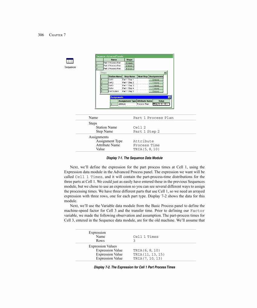
306 CHAPTER 7
Name Part 1 Process PlanSteps
Station Name Cell 2Step Name Part 1 Step 2
AssignmentsAssignment Type AttributeAttribute Name Process TimeValue TRIA(5, 8, 10)
Display 7-1. The Sequence Data Module
Next, we’ll define the expression for the part process times at Cell 1, using theExpression data module in the Advanced Process panel. The expression we want will becalled Cell 1 Times, and it will contain the part-process-time distributions for thethree parts at Cell 1. We could just as easily have entered these in the previous Sequencesmodule, but we chose to use an expression so you can see several different ways to assignthe processing times. We have three different parts that use Cell 1, so we need an arrayedexpression with three rows, one for each part type. Display 7-2 shows the data for thismodule.
Next, we’ll use the Variable data module from the Basic Process panel to define themachine-speed factor for Cell 3 and the transfer time. Prior to defining our Factorvariable, we made the following observation and assumption. The part-process times forCell 3, entered in the Sequence data module, are for the old machine. We’ll assume that
ExpressionName Cell 1 TimesRows 3
Expression ValuesExpression Value TRIA(6, 8, 10)Expression Value TRIA(11, 13, 15)Expression Value TRIA(7, 10, 13)
Display 7-2. The Expression for Cell 1 Part Process Times
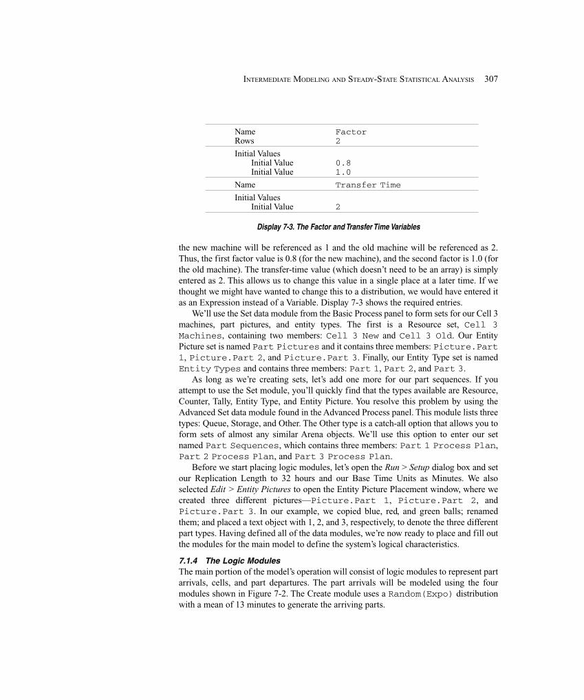
307INTERMEDIATE MODELING AND STEADY-STATE STATISTICAL ANALYSIS
Name FactorRows 2
Initial ValuesInitial Value 0.8Initial Value 1.0
Name Transfer TimeInitial Values
Initial Value 2
Display 7-3. The Factor and Transfer Time Variables
the new machine will be referenced as 1 and the old machine will be referenced as 2.Thus, the first factor value is 0.8 (for the new machine), and the second factor is 1.0 (forthe old machine). The transfer-time value (which doesn’t need to be an array) is simplyentered as 2. This allows us to change this value in a single place at a later time. If wethought we might have wanted to change this to a distribution, we would have entered itas an Expression instead of a Variable. Display 7-3 shows the required entries.
We’ll use the Set data module from the Basic Process panel to form sets for our Cell 3machines, part pictures, and entity types. The first is a Resource set, Cell 3Machines, containing two members: Cell 3 New and Cell 3 Old. Our EntityPicture set is named Part Pictures and it contains three members: Picture.Part1, Picture.Part 2, and Picture.Part 3. Finally, our Entity Type set is namedEntity Types and contains three members: Part 1, Part 2, and Part 3.
As long as we’re creating sets, let’s add one more for our part sequences. If youattempt to use the Set module, you’ll quickly find that the types available are Resource,Counter, Tally, Entity Type, and Entity Picture. You resolve this problem by using theAdvanced Set data module found in the Advanced Process panel. This module lists threetypes: Queue, Storage, and Other. The Other type is a catch-all option that allows you toform sets of almost any similar Arena objects. We’ll use this option to enter our setnamed Part Sequences, which contains three members: Part 1 Process Plan,Part 2 Process Plan, and Part 3 Process Plan.
Before we start placing logic modules, let’s open the Run > Setup dialog box and setour Replication Length to 32 hours and our Base Time Units as Minutes. We alsoselected Edit > Entity Pictures to open the Entity Picture Placement window, where wecreated three different pictures—Picture.Part 1, Picture.Part 2, andPicture.Part 3. In our example, we copied blue, red, and green balls; renamedthem; and placed a text object with 1, 2, and 3, respectively, to denote the three differentpart types. Having defined all of the data modules, we’re now ready to place and fill outthe modules for the main model to define the system’s logical characteristics.
7.1.4 The Logic ModulesThe main portion of the model’s operation will consist of logic modules to represent partarrivals, cells, and part departures. The part arrivals will be modeled using the fourmodules shown in Figure 7-2. The Create module uses a Random(Expo) distributionwith a mean of 13 minutes to generate the arriving parts.
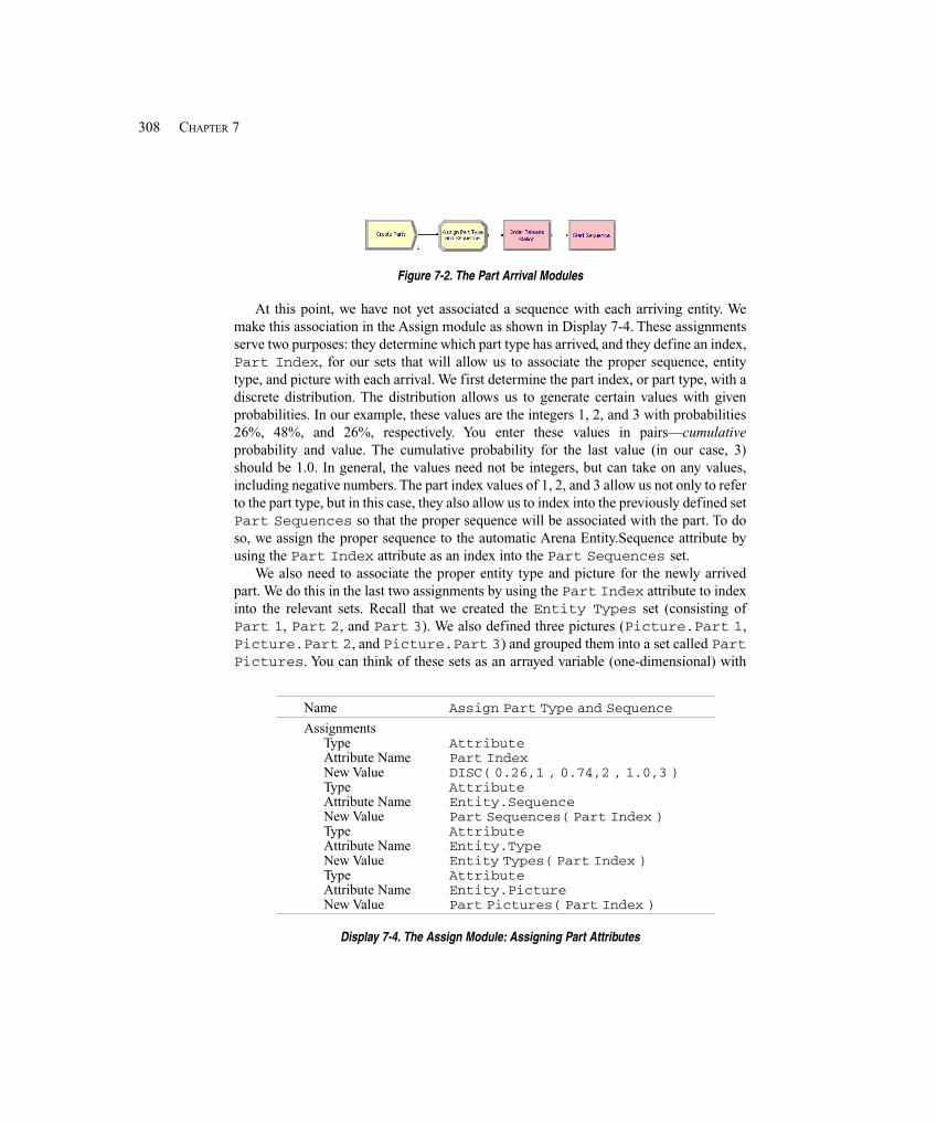
308 CHAPTER 7
Figure 7-2. The Part Arrival Modules
At this point, we have not yet associated a sequence with each arriving entity. Wemake this association in the Assign module as shown in Display 7-4. These assignmentsserve two purposes: they determine which part type has arrived, and they define an index,Part Index, for our sets that will allow us to associate the proper sequence, entitytype, and picture with each arrival. We first determine the part index, or part type, with adiscrete distribution. The distribution allows us to generate certain values with givenprobabilities. In our example, these values are the integers 1, 2, and 3 with probabilities26%, 48%, and 26%, respectively. You enter these values in pairs—cumulativeprobability and value. The cumulative probability for the last value (in our case, 3)should be 1.0. In general, the values need not be integers, but can take on any values,including negative numbers. The part index values of 1, 2, and 3 allow us not only to referto the part type, but in this case, they also allow us to index into the previously defined setPart Sequences so that the proper sequence will be associated with the part. To doso, we assign the proper sequence to the automatic Arena Entity.Sequence attribute byusing the Part Index attribute as an index into the Part Sequences set.
We also need to associate the proper entity type and picture for the newly arrivedpart. We do this in the last two assignments by using the Part Index attribute to indexinto the relevant sets. Recall that we created the Entity Types set (consisting ofPart 1, Part 2, and Part 3). We also defined three pictures (Picture.Part 1,Picture.Part 2, and Picture.Part 3) and grouped them into a set called PartPictures. You can think of these sets as an arrayed variable (one-dimensional) with
Name Assign Part Type and Sequence
AssignmentsType AttributeAttribute Name Part IndexNew Value DISC( 0.26,1 , 0.74,2 , 1.0,3 )Type AttributeAttribute Name Entity.SequenceNew Value Part Sequences( Part Index )Type AttributeAttribute Name Entity.TypeNew Value Entity Types( Part Index )Type AttributeAttribute Name Entity.PictureNew Value Part Pictures( Part Index )
Display 7-4. The Assign Module: Assigning Part Attributes

309INTERMEDIATE MODELING AND STEADY-STATE STATISTICAL ANALYSIS
the index being the Part Index attribute we just assigned. This is true in this casebecause we have a one-to-one relationship between the part type (Part Index ) and thesequence, picture, and entity type. An index of 1 implies Part 1 follows the firstsequence, etc. (Be careful in future models because this may not always be true. It is onlytrue in this case because we defined our data structure so we would have this one-to-onerelationship.)
In this case, the completed Assign module determines the part type, and then assignsthe proper sequence, entity type, and picture. Note that it was essential to define thevalue of Part Index first in this Assign module, which performs multiple assignmentsin the order listed, since the value of Part Index determined in the first step is used inthe later assignments. We’re now ready to send our part on its way to the first station in itssequence.
We’ll accomplish this with the Route module from the Advanced Transfer panel.Before we do this, we need to tell Arena where our entity, or part, currently resides (itscurrent station location). If you’ve been building your own model along with us (andpaying attention), you might have noticed the attribute named Entity.Station onthe drop-down list in the Assign module that we just completed. (You can go back andlook now if you like.) You might be tempted to add an assignment that would define thecurrent location of our part. Unfortunately if you use this approach, Arena will return anerror when you try to run your model; instead, we use a Station module as described next.
Our completed model will have six stations: Order Release, Cell 1, Cell 2,Cell 3, Cell 4, and Exit System. The last five stations were defined when wefilled in the information for our part sequences. The first station, Order Release, willbe defined when we send the entity through a Station module (Advanced Transfer panel),which will define the station and tell Arena that the current entity is at that location. Ourcompleted Station module is shown in Display 7-5.
We’re finally ready to send our part to the first station in its sequence with the Routemodule (Advanced Transfer panel). The Route module transfers an entity to a specifiedstation, or the next station in the station visitation sequence defined for the entity. ARoute Time to transfer to the next station may be defined. In our model, the previouslydefined variable Transfer Time is entered for the Route Time; see Display 7-6. Weselected the By Sequence option as the Destination Type. This causes the StationName field to disappear, and when we run the model, Arena will route the arrivingentities according to the sequences we defined and attached to entities after they werecreated.
Name Order Release StationStation Type StationStation Name Order Release
Display 7-5. The Station Module
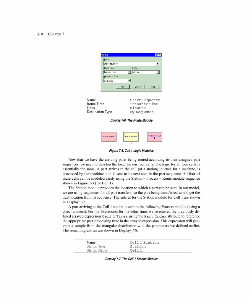
310 CHAPTER 7
Name Start SequenceRoute Time Transfer TimeUnits MinutesDestination Type By Sequence
Display 7-6. The Route Module
Figure 7-3. Cell 1 Logic Modules
Now that we have the arriving parts being routed according to their assigned partsequences, we need to develop the logic for our four cells. The logic for all four cells isessentially the same. A part arrives to the cell (at a station), queues for a machine, isprocessed by the machine, and is sent to its next step in the part sequence. All four ofthese cells can be modeled easily using the Station – Process – Route module sequenceshown in Figure 7-3 (for Cell 1).
The Station module provides the location to which a part can be sent. In our model,we are using sequences for all part transfers, so the part being transferred would get thenext location from its sequence. The entries for the Station module for Cell 1 are shownin Display 7-7.
A part arriving at the Cell 1 station is sent to the following Process module (using adirect connect). For the Expression for the delay time, we’ve entered the previously de-fined arrayed expression Cell 1 Times using the Part Index attribute to referencethe appropriate part-processing time in the arrayed expression. This expression will gen-erate a sample from the triangular distribution with the parameters we defined earlier.The remaining entries are shown in Display 7-8.
Name Cell 1 StationStation Type StationStation Name Cell 1
Display 7-7. The Cell 1 Station Module
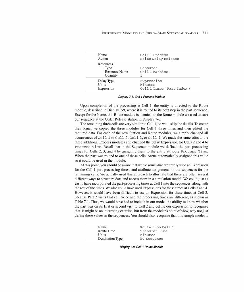
311INTERMEDIATE MODELING AND STEADY-STATE STATISTICAL ANALYSIS
Name Cell 1 ProcessAction Seize Delay Release
ResourcesType ResourceResource Name Cell 1 MachineQuantity 1
Delay Type ExpressionUnits MinutesExpression Cell 1 Times( Part Index )
Display 7-8. Cell 1 Process Module
Upon completion of the processing at Cell 1, the entity is directed to the Routemodule, described in Display 7-9, where it is routed to its next step in the part sequence.Except for the Name, this Route module is identical to the Route module we used to startour sequence at the Order Release station in Display 7-6.
The remaining three cells are very similar to Cell 1, so we’ll skip the details. To createtheir logic, we copied the three modules for Cell 1 three times and then edited therequired data. For each of the new Station and Route modules, we simply changed alloccurrences of Cell 1 to Cell 2, Cell 3, or Cell 4. We made the same edits to thethree additional Process modules and changed the delay Expression for Cells 2 and 4 toProcess Time. Recall that in the Sequence module we defined the part-processingtimes for Cells 2, 3, and 4 by assigning them to the entity attribute Process Time.When the part was routed to one of these cells, Arena automatically assigned this valueso it could be used in the module.
At this point, you should be aware that we’ve somewhat arbitrarily used an Expressionfor the Cell 1 part-processing times, and attribute assignments in the sequences for theremaining cells. We actually used this approach to illustrate that there are often severaldifferent ways to structure data and access them in a simulation model. We could just aseasily have incorporated the part-processing times at Cell 1 into the sequences, along withthe rest of the times. We also could have used Expressions for these times at Cells 3 and 4.However, it would have been difficult to use an Expression for these times at Cell 2,because Part 2 visits that cell twice and the processing times are different, as shown inTable 7-1. Thus, we would have had to include in our model the ability to know whetherthe part was on its first or second visit to Cell 2 and define our expression to recognizethat. It might be an interesting exercise, but from the modeler’s point of view, why not justdefine these values in the sequences? You should also recognize that this sample model is
Name Route from Cell 1Route Time Transfer TimeUnits MinutesDestination Type By Sequence
Display 7-9. Cell 1 Route Module

312 CHAPTER 7
Name Cell 3 ProcessAction Seize Delay ReleaseResources
Type SetSet Name Cell 3 MachinesQuantity 1Save Attribute Machine Index
Delay Type ExpressionUnits MinutesExpression Process Time * Factor(Machine Index)
Display 7-10. Cell 3 Process Module
relatively small in terms of the number of cells and parts. In practice, it would not beuncommon to have 30 to 50 machines with hundreds of different part types. If youundertake a problem of that size, we strongly recommend that you take great care indesigning the data structure since it may make the difference between a success or failureof the simulation project.
The Process module for Cell 3 is slightly different because we have two differentmachines, a new one and an old one, that process parts at different rates. If the machineswere identical, we could have used a single resource and entered a capacity of 2. Wemade note of this earlier and grouped these two machines into a Set called Cell 3Machines. Now we need to use this set at Cell 3. Display 7-10 shows the data entriesrequired to complete the Process module for this cell.
In the Resource section, we select Set from the drop-down list for our ResourceType. This allows us to select from our specified Cell 3 Machines set for the SetName field. You can also Seize a Specific Member of a set; that member can be specifiedas an entity attribute. For our selection of Resource Set, we’ve accepted the defaultselection rule, Cyclical, which causes the entity to attempt to select the first availableresource beginning with the successor of the last resource selected. In our case, Arenawill try to select our two resources alternately; however, if only one resource is currentlyavailable, it will be selected. Obviously, these rules are used only if more than oneresource is available for selection. The Random rule would cause a random(equiprobable) selection from among those available, and the Preferred Order rule wouldselect the first (lowest-numbered) available resource in the set. Had we selected thisoption, Arena would have always used the new machine, if available, because it’s the firstresource in the set. The remaining rules would apply only if one or more of our resourceshad a capacity greater than 1.
The Save Attribute option allows us to save the index, which is a reference to theselected set member, in a user-specified attribute. In our case, we will save this value inthe Attribute Machine Index. If the new machine is selected, this attribute will beassigned a value of 1, and if the old machine is selected, the attribute will be assigned avalue of 2. This numbering is based on the order in which we entered our resources whenwe defined the set. The Expression for the delay time uses our attribute Process
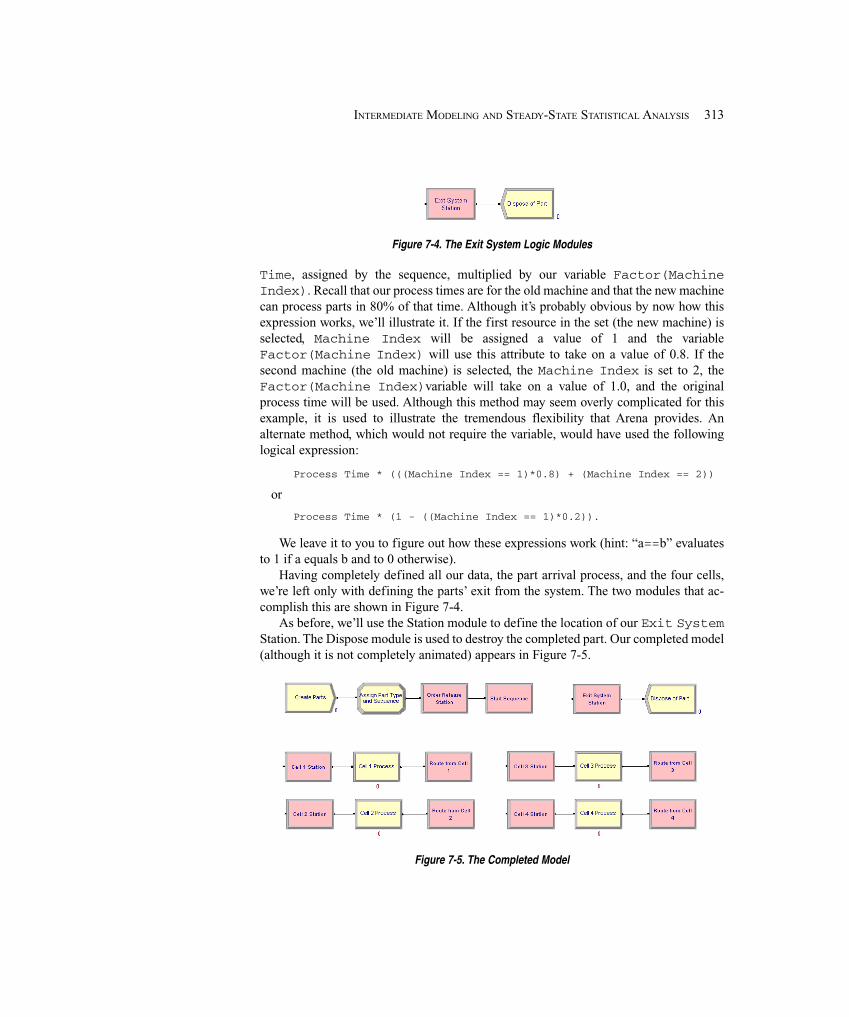
313INTERMEDIATE MODELING AND STEADY-STATE STATISTICAL ANALYSIS
Figure 7-4. The Exit System Logic Modules
Time, assigned by the sequence, multiplied by our variable Factor(MachineIndex). Recall that our process times are for the old machine and that the new machinecan process parts in 80% of that time. Although it’s probably obvious by now how thisexpression works, we’ll illustrate it. If the first resource in the set (the new machine) isselected, Machine Index will be assigned a value of 1 and the variableFactor(Machine Index) will use this attribute to take on a value of 0.8. If thesecond machine (the old machine) is selected, the Machine Index is set to 2, theFactor(Machine Index)variable will take on a value of 1.0, and the originalprocess time will be used. Although this method may seem overly complicated for thisexample, it is used to illustrate the tremendous flexibility that Arena provides. Analternate method, which would not require the variable, would have used the followinglogical expression:
Process Time * (((Machine Index == 1)*0.8) + (Machine Index == 2))
or
Process Time * (1 - ((Machine Index == 1)*0.2)).
We leave it to you to figure out how these expressions work (hint: “a==b” evaluatesto 1 if a equals b and to 0 otherwise).
Having completely defined all our data, the part arrival process, and the four cells,we’re left only with defining the parts’ exit from the system. The two modules that ac-complish this are shown in Figure 7-4.
As before, we’ll use the Station module to define the location of our Exit SystemStation. The Dispose module is used to destroy the completed part. Our completed model(although it is not completely animated) appears in Figure 7-5.
Figure 7-5. The Completed Model
314 CHAPTER 7
At this point, we could run our model, but it would be difficult to tell if our sequencesare working properly. So before we start any analysis, we’ll first develop our animationto help us determine whether the model is working correctly. Let’s also assume that we’llhave to present this model to higher-level management, so we want to develop a some-what fancier animation.
7.1.5 AnimationWe could develop our animation in the same manner as we did in Chapter 5—create ourown entity pictures, resource symbols, and background based on the picture that waspresented in Figure 7-1. However, a picture might already exist that reflects an accuraterepresentation of the system. In fact, it might even exist as a CAD file somewhere in yourorganization. For instance, the drawing presented in Figure 7-1 was developed using theAutoCAD® package from AutoDesk. Arena supports integration of files from CADprograms into its workspaces. Files saved in the DXF format defined by AutoCAD canbe imported directly into Arena. Files generated from other CAD or drawing programs(e.g., Microsoft® Visio®) should transfer into Arena as long as they adhere to theAutoCAD standard DXF format.
If the original CAD drawing is 2-D, you only need to save it in the DXF format andthen import that file directly into Arena. Most CAD objects (polygons, etc.) will berepresented as the same or similar objects in Arena. If the drawing is 3-D, you must firstconvert the file to 2-D. Colors are lost during this conversion to 2-D, but they may beadded again in AutoCAD or in Arena. This conversion also transforms all objects tolines, so the imported drawing can only be manipulated in Arena as individual lines, orthe lines may be grouped as objects. We’ll assume that you have a DXF file and refer youto online help (the Importing DXF Files topic) for details on creating the DXF file orconverting a 3-D drawing. One word of advice: a converted file is imported into Arena aswhite lines so if your current background is white, it may appear that the file was notimported. Simply change the Window Background Color ( on the Draw toolbar) orselect all the lines and change the line color ( ).
For our small manufacturing system, we started with a 3-D drawing and converted itto 2-D. We then saved the 2-D file in the DXF format (Model 07-01.dxf). A DXFfile is imported into your current model file by selecting File > DXF Import. Select thefile, and when you move your pointer to the model window, it will appear as cross hairs.Using the pointer, draw a box to contain the entire drawing to be imported. If theimported drawing is not the correct size, you can select the entire drawing and resize it asrequired. You can now use this drawing as the start of your animation.
For our animation, you should delete all the lettering and arrows. Then we’ll move theCell 1 queue animation object from the Process module (Cell 1 Process) to itsapproximate position on the drawing.
Now position your pointer near the upper-left corner of a machine and drag yourpointer so the resulting bounding outline encloses the entire drawing. Use the Copybutton to copy the drawing of the machine to the clipboard. Now we’ll open the ResourcePicture Placement window by clicking the Resource button ( ) from the Animatetoolbar. Double-click the idle resource symbol and replace the current picture with a
315INTERMEDIATE MODELING AND STEADY-STATE STATISTICAL ANALYSIS
copy of the contents of the clipboard. Delete the base of the machine and draw two boxeson top of the representation for the top part of the machine. This is necessary as ourdrawing consists of all lines, and we want to add a fill color to the machine. Now deleteall the lines from the original copy and fill the boxes with your favorite color. Copy thisnew symbol to your library and then copy that symbol to the Busy picture. Save yourlibrary, exit the resource window, and finally place the resource. You now have a resourcepicture that will not change, but we could go back later and add more animation effects.
For the next step, draw a box the same size as the base of the machine and then deletethe entire drawing of the machine. Fill this new box with a different color and then placethe resource symbol on top of this box (you may have to resize the resource symbol to bethe correct size). Now move the seize point so that it is positioned at about the center ofour new machine. Now make successive copies of our new resource and the machinebase, and then change the names. If you follow this procedure, note that you will need toflip the resources for Cells 3 and 4.
To complete this phase of the animation, you need to move and resize the remainingqueues. Once this is complete, you can run your animation and see your handiwork. Youwon’t see parts moving about the system (there are no routes yet), but you will see theparts in the queues and at the machines. If you look closely at one of the machines whilethe animation is running, you’ll notice that the parts sit right on top of the entire machine.This display is not what we want. Ideally, the part should sit on top of the base, but underthe top part of our machine (the resource). Representing this is not a problem. Select aresource (you can do this in edit mode or by temporarily pausing the run) and use theBring to Front feature with Arrange > Bring to Front or the button on the Arrange toolbar( ). Now when you run the animation, you’ll get the desired effect. We’re now ready toanimate our part movement.
In our previous animations, we basically had only one path through the system soadding the routes was fairly straightforward. In our small manufacturing system, thereare multiple paths through the system, so you must be careful to add routes for eachtravel possibility. For example, a part leaving Cell 2 can go to Cell 1, 3, or 4. The stationsneed to be positioned first; add station animation objects using the Station button on theAnimate Transfer toolbar. Next, place the routes. If you somehow neglect to place aroute, the simulation will still (correctly) send the entity to the correct station with atransfer time of 2; however, that entity movement will not appear in your animation. Alsobe aware that routes can be used in both directions. For example, let’s assume that youadded the route from Cell 1 to Cell 2, but missed the route from 2 to 1. When a Part 2completes its processing at Cell 2, Arena looks to route that part to Cell 1, routing from 2to 1. If the route were missing, it would look for the route from 1 to 2 and use that. Thus,you would see that part moving from the entrance of Cell 2 to the Exit of Cell 1 in acounterclockwise direction (an animation mistake for this model).
If you run and watch your newly animated model, you should notice thatoccasionally parts will run over or pass each other. This is due to a combination of thedata supplied and the manner in which we animated the model. Remember that all parttransfers were assumed to be two minutes regardless of the distance to be traveled. Arena
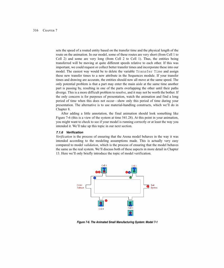
316 CHAPTER 7
sets the speed of a routed entity based on the transfer time and the physical length of theroute on the animation. In our model, some of these routes are very short (from Cell 1 toCell 2) and some are very long (from Cell 2 to Cell 1). Thus, the entities beingtransferred will be moving at quite different speeds relative to each other. If this wasimportant, we could request or collect better transfer times and incorporate these into ourmodel. The easiest way would be to delete the variable Transfer Time and assignthese new transfer times to a new attribute in the Sequences module. If your transfertimes and drawing are accurate, the entities should now all move at the same speed. Theonly potential problem is that a part may enter the main aisle at the same time anotherpart is passing by, resulting in one of the parts overlapping the other until their pathsdiverge. This is a more difficult problem to resolve, and it may not be worth the bother. Ifthe only concern is for purposes of presentation, watch the animation and find a longperiod of time when this does not occur—show only this period of time during yourpresentation. The alternative is to use material-handling constructs, which we’ll do inChapter 8.
After adding a little annotation, the final animation should look something likeFigure 7-6 (this is a view of the system at time 541.28). At this point in your animation,you might want to check to see if your model is running correctly or at least the way youintended it. We’ll take up this topic in our next section.
7.1.6 VerificationVerification is the process of ensuring that the Arena model behaves in the way it wasintended according to the modeling assumptions made. This is actually very easycompared to model validation, which is the process of ensuring that the model behavesthe same as the real system. We’ll discuss both of these aspects in more detail in Chapter13. Here we’ll only briefly introduce the topic of model verification.
Figure 7-6. The Animated Small Manufacturing System: Model 7-1
317INTERMEDIATE MODELING AND STEADY-STATE STATISTICAL ANALYSIS
Verification deals with both obvious problems as well as the not-so-obvious. Forexample, if you had tried to run your model and Arena returned an error message thatindicated that you had neglected to define one of the machine resources at Cell 3, themodel is obviously not working the way you intended. Actually, we would normally callthis the process of debugging! However, since we assume that you’ll not make thesekinds of errors (or, if you do, you can figure out yourself how to fix them), we’ll dealwith the not-so-obvious problems.
Verification is fairly easy when you’re developing small classroom-size problemslike the ones in this book. When you start developing more realistically sized models,you’ll find that it’s a much more difficult process, and you may never be 100% sure onvery, very large models.
One easy verification method is to allow only a single entity to enter the system andfollow that entity to be sure that the model logic and data are correct. You could use theStep button ( ) found on the Standard toolbar to control the model execution and stepthe entity through the system. For this model, you could set the Max Arrivals field in theCreate module to 1. To control the entity type, you could replace the discrete distributionin the Assign module that determines the part type with the specific part type you want toobserve. This would allow you to check each of the part sequences. Another commonmethod is to replace some or all model data with constants. Using deterministic dataallows you to predict system behavior exactly.
If you’re going to use your model to make real decisions, you should also check tosee how the model behaves under extreme conditions. For example, introduce only onepart type or increase/decrease the part interarrival or service times. If your model is go-ing to have problems, they will most likely show up during these kinds of stressed-outruns. Also, try to make effective use of your animation—it can often reveal problemswhen viewed by a person familiar with the operation of the system being modeled.
It’s often a good idea, and a good test, to make long runs for different data and observethe summary results for potential problems. One skill that can be of great use during thisprocess is that of performance estimation. A long, long time ago, before the invention ofcalculators and certainly before personal computers, engineers carried around stickscalled slide rules (often protected by leather cases and proudly attached to engineers’belts). These were used to calculate the answers to the complicated problems given tothem by their professors or bosses. These devices achieved this magic feat by adding orsubtracting logs (not tree logs, but logarithms). Although they worked rather well (but notas well, as easily, or as fast as a calculator), they only returned (actually you read it off thestick) a sequence of digits, say 3642. It was up to the engineer to figure out where to putthe decimal point. Therefore, engineers had to become very good at developing roughestimates of the answers to problems before they used the sticks. For example, if theengineer estimated the answer to be about 400, then the answer was 364.2. However, ifthe estimate was about 900, there was a problem. At that point, it was necessary todetermine if the problem was in the estimation process or the slide-rule process. Wesuspect that at this point you’re asking two questions: 1) why the long irrelevant story, and2) did we really ever use such sticks? Well, the answers are: 1) to illustrate a point, and 2)two of the authors did!
318 CHAPTER 7
So how do you use this great performance-estimation skill? You define a set of condi-tions for the simulation, estimate what will result, make a run, and look at the summarydata to see if you were correct. If you were, feel good and try it for a different set of con-ditions. If you weren’t correct (or at least in the ballpark), find out why not. It may be dueto bad estimation, a lack of understanding of the system, or a faulty model. Sometimesnot-so-obvious (but real) results are created by surprising interactions in the model. Ingeneral, you should thoroughly exercise your simulation models and be comfortablewith the results before you use them to make decisions. And it’s best to do this early inyour project—and often.
Back in Section 2.8 when we mentioned verification, we suggested that you verifyyour code. Your response could have been, “What code?” Well, there is code, and we’llshow you a little in Figures 7-7 and 7-8. But you still might be asking, “Why code?” Toexplain the reason for this code requires a little bit of background (yes, another historylesson). The formation of Systems Modeling (the company that originally developedArena) and the initial release of the simulation language SIMAN® (on which Arena isbased and to which you can gain access through Arena) occurred in 1982. Personalcomputers were just starting to hit the market, and SIMAN was designed to run on thesenew types of machines. In fact, SIMAN required only 64 Kbytes of memory, which wasa lot in those days. There was no animation capability (Cinema, the accompanyinganimation tool, was released in 1985), and you created models using a text editor, justlike using a programming language. A complete model required the development of twofiles, a model file and an experiment file. The model file, often referred to as the .modfile, contained the model logic. The experiment file, referred to as the .exp file, definedthe experimental conditions. It required the user to list all stations, attributes, resources,etc., that were used in the model. The creation of these files required that the user followa rather exacting syntax for each type of model or experiment construct. In other words,you had to start certain statements only in column 10; you had to follow certain entrieswith the required comma, semicolon, or colon; all resources and attributes werereferenced only by number; and only a limited set of key words could be used. (Many ofyour professors, or maybe their professors, learned simulation this way.)
Since 1982, SIMAN has been enhanced continually and still provides the basis for anArena simulation model. When you run an Arena simulation, Arena examines eachoption you selected in your modules and the data that you supplied and then createsSIMAN .mod and .exp files. These are the files that are used to run your simulations. Theimplication is that all the modules found in the Basic Process, Advanced Process, andAdvanced Transfer panels are based on the constructs found in the SIMAN simulationlanguage. The idea is to provide a simulation tool (Arena) that is easy to use, yet one thatis still based on the powerful and flexible SIMAN language. So you see, it is stillpossible, and sometimes even desirable, to look at the SIMAN code. In fact, you caneven write out and edit these files. However, it is only possible to go down (from Arena toSIMAN code) and not possible to go back up (from SIMAN code to Arena). As youbecome more proficient with Arena, you might occasionally want to look at this code tobe assured that the model is doing exactly what you want it to—verification.

319INTERMEDIATE MODELING AND STEADY-STATE STATISTICAL ANALYSIS
;; Model statements for module: BasicProcess.Process 3 (Cell 3 Process);10$ ASSIGN: Cell 3 Process.NumberIn=Cell 3 Process.NumberIn + 1:
Cell 3 Process.WIP=Cell 3 Process.WIP+1;138$ QUEUE, Cell 3 Process.Queue;137$ SEIZE, 2,VA:
SELECT(Cell 3 Machines,CYC,Machine Index),1:NEXT(136$);136$ DELAY: Process Time * Factor( Machine Index ),,VA;135$ RELEASE: Cell 3 Machines(Machine Index),1;183$ ASSIGN: Cell 3 Process.NumberOut=Cell 3 Process.NumberOut + 1:
Cell 3 Process.WIP=Cell 3 Process.WIP-1:NEXT(11$);
Figure 7-7. SIMAN Model File for the Process Module
We should point out that you can still create your models in Arena using the baseSIMAN language. If you build a model using only the modules found in the Blocks andElements panels, you are basically using the SIMAN language. Recall that we usedseveral modules from the Blocks panel when we constructed our inventory model inSection 5.7.
You can view the SIMAN code for our small manufacturing model by using the Run >SIMAN > View option. Selecting this option will generate both files, each in a separatewindow. Figure 7-7 shows a small portion of the .mod file, the code written out for theProcess module used at Cell 3. The SIMAN language is rather descriptive, so it is possibleto follow the general logic. An entity that arrives at this module increments some internalcounters, enters a queue, Cell 3 Process.Queue, waits to seize a resource from theset Cell 3 Machines, delays for the process time (adjusted by our factor), releases theresource, decrements the internal counters, and exits the module.
Figure 7-8 shows a portion of the .exp file that defines our three attributes and thequeues and resources used in our model.
We won’t go into a detailed explanation of the statements in these files; the purposeof this exercise is merely to make you aware of their existence. For a more comprehen-sive explanation, refer to Pegden, Shannon, and Sadowski (1995).
ATTRIBUTES: Machine Index:Part Index:Process Time;
QUEUES: Cell 1 Process.Queue,FIFO,,AUTOSTATS(Yes,,):Cell 2 Process.Queue,FIFO,,AUTOSTATS(Yes,,):Cell 3 Process.Queue,FIFO,,AUTOSTATS(Yes,,):Cell 4 Process.Queue,FIFO,,AUTOSTATS(Yes,,);
RESOURCES: Cell 2 Machine,Capacity(1),,,COST(0.0,0.0,0.0),CATEGORY(Resources),,AUTOSTATS(Yes,,):
Cell 1 Machine,Capacity(1),,,COST(0.0,0.0,0.0),CATEGORY(Resources),,AUTOSTATS(Yes,,):
Cell 3 Old,Capacity(1),,,COST(0.0,0.0,0.0),CATEGORY(Resources),,AUTOSTATS(Yes,,):
Cell 3 New,Capacity(1),,,COST(0.0,0.0,0.0),CATEGORY(Resources),,AUTOSTATS(Yes,,):
Cell 4 Machine,Capacity(1),,,COST(0.0,0.0,0.0),CATEGORY(Resources),,AUTOSTATS(Yes,,);
Figure 7-8. SIMAN Experiment File for the Process Module
320 CHAPTER 7
If you’re familiar with SIMAN or you would just like to learn more about how thisprocess works, we might suggest that you place a few modules, enter some data, andwrite out the .mod and .exp files. Then edit the modules by selecting different optionsand write out the new files. Look for the differences between the two .mod files. Doingso should give you a fair amount of insight as to how this process works.
7.2 Statistical Analysis of Output from Steady-State Simulations
In Chapter 6, we described the difference between terminating and steady-statesimulations and indicated how you can use Arena’s reports, PAN, and the OutputAnalyzer to do statistical analyses in the terminating case. In this section, we’ll show youhow to do statistical inference on steady-state simulations.
Before proceeding, we should encourage you to be sure that a steady-state simulationis appropriate for what you want to do. Often people simply assume that a long-run,steady-state simulation is the thing to do, which might in fact be true. But if the startingand stopping conditions are part of the essence of your model, a terminating analysis isprobably more appropriate; if so, you should just proceed as in Chapter 6. The reason foravoiding steady-state simulation is that, as you’re about to see, it’s a lot harder to carryout anything approaching a valid statistical analysis than in the terminating case if youwant anything beyond Arena’s standard 95% confidence intervals on mean performancemeasures; so if you don’t need to get into this, you shouldn’t.
One more caution before we wade into this material: As you can imagine, the runlengths for steady-state simulations need to be pretty long. Because of this, there are moreopportunities for Arena to sequence its internal operations a little differently, causing therandom-number stream (see Chapter 12) to be used differently. This doesn’t make yourmodel in any sense “wrong” or inaccurate, but it can affect the numerical results,especially for models that have a lot of statistical variability inherent in them. So if youfollow along on your computer and run our models, there’s a chance that you’re going toget numerical answers that differ from what we report here. Don’t panic over this since itis, in a sense, to be expected. If anything, this just amplifies the need for some kind ofstatistical analysis of simulation output data since variability can come not only from“nature” in the model’s properties, but also from internal computational issues.
In Section 7.2.1, we’ll discuss determination of model warm-up and run length.Section 7.2.2 describes the truncated-replication strategy for analysis, which is by far thesimplest approach (and, in some ways, the best). A different approach called batching isdescribed in Section 7.2.3. A brief summary is given in Section 7.2.4, and Section 7.2.5mentions some other issues in steady-state analysis.
7.2.1 Warm-Up and Run LengthAs you might have noticed, our examples have been characterized by a model that’sinitially in an empty-and-idle state. This means that the model starts out empty of entitiesand all resources are idle. In a terminating system, this might be the way things actuallystart out, so everything is fine. But in a steady-state simulation, initial conditions aren’tsupposed to matter, and the run is supposed to go on forever.
321INTERMEDIATE MODELING AND STEADY-STATE STATISTICAL ANALYSIS
Actually, though, even in a steady-state simulation, you have to initialize and stop therun somehow. And since you’re doing a simulation in the first place, it’s a pretty safe betthat you don’t know much about the “typical” system state in steady state or how “long” arun is long enough. So you’re probably going to wind up initializing in a state that’s prettyweird from the viewpoint of steady state and just trying some (long) run lengths. If you’reinitializing empty and idle in a simulation where things eventually become congested,your output data for some period of time after initialization will tend to understate theeventual congestion; that is, your data will be biased low.
To remedy this, you might try to initialize in a state that’s “better” than empty and idle.This would mean placing, at time 0, some number of entities around the model and start-ing things out that way. While it’s possible to do this in your model, it’s pretty inconvenient.More problematic is that you’d generally have no idea how many entities to place around attime 0; this is, after all, one of the questions the simulation is supposed to answer.
Another way of dealing with initialization bias is just to run the model for so long thatwhatever bias may have been there at the beginning is overwhelmed by the amount oflater data. This can work in some models if the biasing effects of the initial conditionswear off quickly.
However, what people usually do is initialize empty and idle, realizing that this isunrepresentative of steady state, but then let the model warm up for a while until itappears that the effects of the artificial initial conditions have worn off. At that time, youcan clear the statistical accumulators (but not the system state) and start afresh, gatheringstatistics for analysis from then on. In effect, this is initializing in a state other than emptyand idle, but you let the model decide how many entities to have around when you start(afresh) to watch your performance measures. The run length should still be long, butmaybe not as long as you’d need to overwhelm the initial bias by sheer arithmetic.
It’s very easy to specify an initial Warm-up Period in Arena. Just open the Run >Setup > Replication Parameters dialog box and fill in a value (be sure to verify the TimeUnits). Every replication of your model still runs starting as it did before, but at the endof the Warm-up Period, all statistical accumulators are cleared and your reports (andany Outputs-type saved data from the Statistic module of results across the replications)reflect only what happened after the warm-up period ends. In this way, you can “decon-taminate” your data from the biasing initial conditions.
The hard part is knowing how long the warm-up period should be. Probably the mostpractical idea is just to make some plots of key outputs from within a run, and eyeballwhen they appear to stabilize. To illustrate this, we took Model 7-1 from Section 7.1 andmade the following modifications, calling the result Model 7-2:
� To establish a single overall output performance measure, we made an entry inthe Statistic module to compute the total work in process (WIP) of all threeparts combined. The Name and Report Label are both Total WIP, and theType is Time-Persistent. To enter the Expression we want to track overtime, we right-clicked in that field and selected Build Expression, clicked downthe tree via Basic Process Variables → Entity → Number in Process, selectedPart 1 as the Entity Type, and got EntitiesWIP(Part 1) for the Current
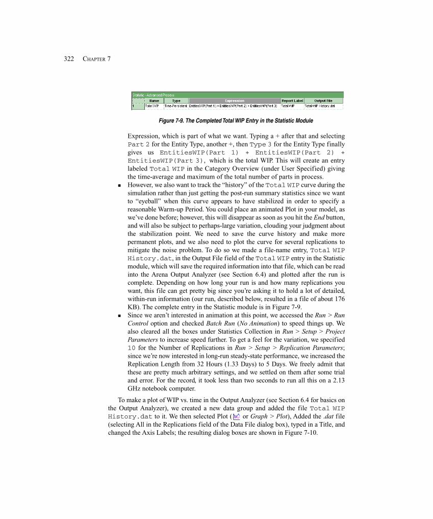
322 CHAPTER 7
Figure 7-9. The Completed Total WIP Entry in the Statistic Module
Expression, which is part of what we want. Typing a + after that and selectingPart 2 for the Entity Type, another +, then Type 3 for the Entity Type finallygives us EntitiesWIP(Part 1) + EntitiesWIP(Part 2) +EntitiesWIP(Part 3), which is the total WIP. This will create an entrylabeled Total WIP in the Category Overview (under User Specified) givingthe time-average and maximum of the total number of parts in process.
� However, we also want to track the “history” of the Total WIP curve during thesimulation rather than just getting the post-run summary statistics since we wantto “eyeball” when this curve appears to have stabilized in order to specify areasonable Warm-up Period. You could place an animated Plot in your model, aswe’ve done before; however, this will disappear as soon as you hit the End button,and will also be subject to perhaps-large variation, clouding your judgment aboutthe stabilization point. We need to save the curve history and make morepermanent plots, and we also need to plot the curve for several replications tomitigate the noise problem. To do so we made a file-name entry, Total WIPHistory.dat, in the Output File field of the Total WIP entry in the Statisticmodule, which will save the required information into that file, which can be readinto the Arena Output Analyzer (see Section 6.4) and plotted after the run iscomplete. Depending on how long your run is and how many replications youwant, this file can get pretty big since you’re asking it to hold a lot of detailed,within-run information (our run, described below, resulted in a file of about 176KB). The complete entry in the Statistic module is in Figure 7-9.
� Since we aren’t interested in animation at this point, we accessed the Run > RunControl option and checked Batch Run (No Animation) to speed things up. Wealso cleared all the boxes under Statistics Collection in Run > Setup > ProjectParameters to increase speed further. To get a feel for the variation, we specified10 for the Number of Replications in Run > Setup > Replication Parameters;since we’re now interested in long-run steady-state performance, we increased theReplication Length from 32 Hours (1.33 Days) to 5 Days. We freely admit thatthese are pretty much arbitrary settings, and we settled on them after some trialand error. For the record, it took less than two seconds to run all this on a 2.13GHz notebook computer.
To make a plot of WIP vs. time in the Output Analyzer (see Section 6.4 for basics onthe Output Analyzer), we created a new data group and added the file Total WIPHistory.dat to it. We then selected Plot ( or Graph > Plot), Added the .dat file(selecting All in the Replications field of the Data File dialog box), typed in a Title, andchanged the Axis Labels; the resulting dialog boxes are shown in Figure 7-10.
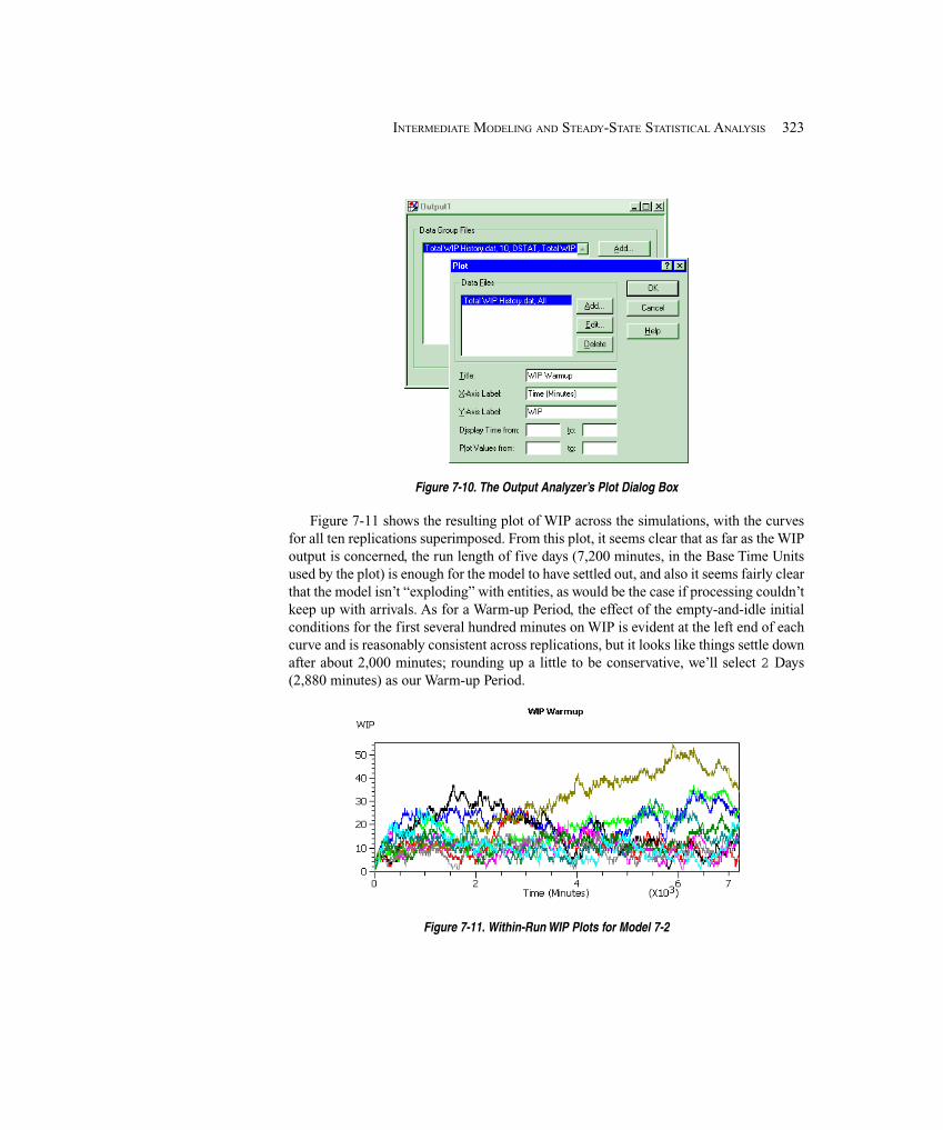
323INTERMEDIATE MODELING AND STEADY-STATE STATISTICAL ANALYSIS
Figure 7-10. The Output Analyzer’s Plot Dialog Box
Figure 7-11 shows the resulting plot of WIP across the simulations, with the curvesfor all ten replications superimposed. From this plot, it seems clear that as far as the WIPoutput is concerned, the run length of five days (7,200 minutes, in the Base Time Unitsused by the plot) is enough for the model to have settled out, and also it seems fairly clearthat the model isn’t “exploding” with entities, as would be the case if processing couldn’tkeep up with arrivals. As for a Warm-up Period, the effect of the empty-and-idle initialconditions for the first several hundred minutes on WIP is evident at the left end of eachcurve and is reasonably consistent across replications, but it looks like things settle downafter about 2,000 minutes; rounding up a little to be conservative, we’ll select 2 Days(2,880 minutes) as our Warm-up Period.
Figure 7-11. Within-Run WIP Plots for Model 7-2
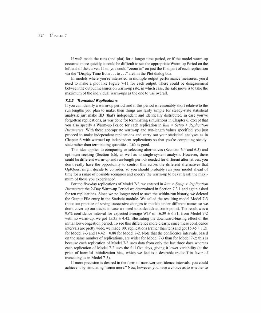
324 CHAPTER 7
If we’d made the runs (and plot) for a longer time period, or if the model warm-upoccurred more quickly, it could be difficult to see the appropriate Warm-up Period on theleft end of the curves. If so, you could “zoom in” on just the first part of each replicationvia the “Display Time from . . . to . . .” area in the Plot dialog box.
In models where you’re interested in multiple output performance measures, you’dneed to make a plot like Figure 7-11 for each output. There could be disagreementbetween the output measures on warm-up rate, in which case, the safe move is to take themaximum of the individual warm-ups as the one to use overall.
7.2.2 Truncated ReplicationsIf you can identify a warm-up period, and if this period is reasonably short relative to therun lengths you plan to make, then things are fairly simple for steady-state statisticalanalysis: just make IID (that’s independent and identically distributed, in case you’veforgotten) replications, as was done for terminating simulations in Chapter 6, except thatyou also specify a Warm-up Period for each replication in Run > Setup > ReplicationParameters. With these appropriate warm-up and run-length values specified, you justproceed to make independent replications and carry out your statistical analyses as inChapter 6 with warmed-up independent replications so that you’re computing steady-state rather than terminating quantities. Life is good.
This idea applies to comparing or selecting alternatives (Sections 6.4 and 6.5) andoptimum seeking (Section 6.6), as well as to single-system analysis. However, therecould be different warm-up and run-length periods needed for different alternatives; youdon’t really have the opportunity to control this across the different alternatives thatOptQuest might decide to consider, so you should probably run your model ahead oftime for a range of possible scenarios and specify the warm-up to be (at least) the maxi-mum of those you experienced.
For the five-day replications of Model 7-2, we entered in Run > Setup > ReplicationParameters the 2-Day Warm-up Period we determined in Section 7.3.1 and again askedfor ten replications. Since we no longer need to save the within-run history, we deletedthe Output File entry in the Statistic module. We called the resulting model Model 7-3(note our practice of saving successive changes to models under different names so wedon’t cover up our tracks in case we need to backtrack at some point). The result was a95% confidence interval for expected average WIP of 16.39 ± 6.51; from Model 7-2with no warm-up, we got 15.35 ± 4.42, illustrating the downward-biasing effect of theinitial low-congestion period. To see this difference more clearly, since these confidenceintervals are pretty wide, we made 100 replications (rather than ten) and got 15.45 ± 1.21for Model 7-3 and 14.42 ± 0.88 for Model 7-2. Note that the confidence intervals, basedon the same number of replications, are wider for Model 7-3 than for Model 7-2; this isbecause each replication of Model 7-3 uses data from only the last three days whereaseach replication of Model 7-2 uses the full five days, giving it lower variability (at theprice of harmful initialization bias, which we feel is a desirable tradeoff in favor oftruncating as in Model 7-3).
If more precision is desired in the form of narrower confidence intervals, you couldachieve it by simulating “some more.” Now, however, you have a choice as to whether to
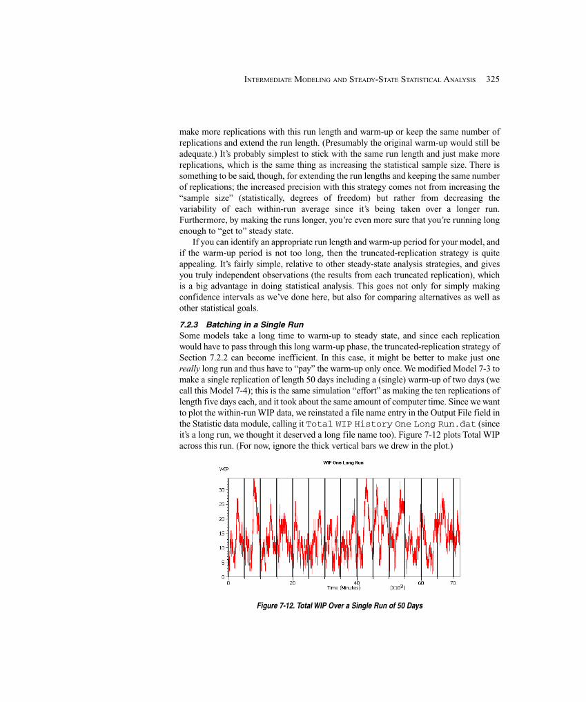
325INTERMEDIATE MODELING AND STEADY-STATE STATISTICAL ANALYSIS
make more replications with this run length and warm-up or keep the same number ofreplications and extend the run length. (Presumably the original warm-up would still beadequate.) It’s probably simplest to stick with the same run length and just make morereplications, which is the same thing as increasing the statistical sample size. There issomething to be said, though, for extending the run lengths and keeping the same numberof replications; the increased precision with this strategy comes not from increasing the“sample size” (statistically, degrees of freedom) but rather from decreasing thevariability of each within-run average since it’s being taken over a longer run.Furthermore, by making the runs longer, you’re even more sure that you’re running longenough to “get to” steady state.
If you can identify an appropriate run length and warm-up period for your model, andif the warm-up period is not too long, then the truncated-replication strategy is quiteappealing. It’s fairly simple, relative to other steady-state analysis strategies, and givesyou truly independent observations (the results from each truncated replication), whichis a big advantage in doing statistical analysis. This goes not only for simply makingconfidence intervals as we’ve done here, but also for comparing alternatives as well asother statistical goals.
7.2.3 Batching in a Single RunSome models take a long time to warm-up to steady state, and since each replicationwould have to pass through this long warm-up phase, the truncated-replication strategy ofSection 7.2.2 can become inefficient. In this case, it might be better to make just onereally long run and thus have to “pay” the warm-up only once. We modified Model 7-3 tomake a single replication of length 50 days including a (single) warm-up of two days (wecall this Model 7-4); this is the same simulation “effort” as making the ten replications oflength five days each, and it took about the same amount of computer time. Since we wantto plot the within-run WIP data, we reinstated a file name entry in the Output File field inthe Statistic data module, calling it Total WIP History One Long Run.dat (sinceit’s a long run, we thought it deserved a long file name too). Figure 7-12 plots Total WIPacross this run. (For now, ignore the thick vertical bars we drew in the plot.)
Figure 7-12. Total WIP Over a Single Run of 50 Days
326 CHAPTER 7
The difficulty now is that we have only one “replication” on each performancemeasure from which to do our analysis, and it’s not clear how we’re going to compute avariance estimate, which is the basic quantity needed to do statistical inference. Viewingeach individual observation or time-persistent value within a run as a separate “datapoint” would allow us to do the arithmetic to compute a within-run sample variance, butdoing so is extremely dangerous since the possibly heavy correlation (see Section B.2.4in Appendix B) of points within a run will cause this estimate to be severely biased withrespect to the true variance of an observation. Somehow, we need to take this correlationinto account or else “manufacture” some kind of “independent observations” from thissingle long run in order to get a decent estimate of the variance.
There are several different ways to proceed with statistical analysis from a single longrun. One relatively simple idea (that also appears to work about as well as other morecomplicated methods) is to try to manufacture almost-uncorrelated “observations” bybreaking the run into a few large batches of many individual points, compute theaverages of the points within each batch, and treat them as the basic IID observations onwhich to do statistical analysis (starting with variance estimation). These batch meansthen take the place of the means from within the multiple replications in the truncated-replication approach—we’ve replaced the replications by batches. In the WIP plot ofFigure 7-12, the thick vertical dividing lines illustrate the idea; we’d take the time-average WIP level between the lines as the basic “data” for statistical analysis. In order toobtain an unbiased variance estimate, we need the batch means to be nearly uncorrelated,which is why we need to make the batches big; there will still be some heavy correlationof individual points near either side of a batch boundary, but these points will be a smallminority within their own large batches, which we hope will render the batch meansnearly uncorrelated. In any case, Arena will try to make the batches big enough to lookuncorrelated, and will let you know if your run was too short for it to manufacture batchmeans that “look” (in the sense of a statistical test) nearly uncorrelated, in which case,you’d have to make your run longer.
As we just hinted, Arena automatically attempts to compute 95% confidence intervalsvia batch means for the means of all output statistics and gives you the results in the HalfWidth column next to the Average column in the report for each replication. If you’remaking just one replication, as we’ve been discussing, this is your batch-meansconfidence interval. On the other hand, if you’ve made more than one replication, you seethis in the Category by Replication report from a multi-replication run for eachreplication; the Half Width in the Category Overview report is from a multi-replicationrun across replications, as discussed in Sections 6.3 and 7.2.2. We say “attempts tocompute” since internal checks are done to see if your replication is long enough toproduce enough data for a valid batch-means confidence interval on an output statistic; ifnot, you get only a message to this effect, without a half-width value (on the theory that awrong answer is worse than no answer at all) for this statistic. If you’ve specified a Warm-up Period, data collected during this period are not used in the confidence-intervalcalculation. To understand how this procedure works, think of Arena as batching “on thefly” (that is, observing the output data during your run and throwing them into batches asyour simulation goes along).
327INTERMEDIATE MODELING AND STEADY-STATE STATISTICAL ANALYSIS
So what does “enough data” mean? There are two levels of checks to be passed, thefirst of which is just to get started. For a Tally statistic, Arena demands a minimum of 320observations. For a time-persistent statistic, you must have had at least five units of simu-lated time during which there were at least 320 changes in the level of the discrete-change variable. Admittedly, these are somewhat arbitrary values and conditions, but weneed to get started somehow, and the more definitive statistical test, which must also bepassed, is done at the end of this procedure. If your run is not long enough to meet thisfirst check, Arena reports “(Insufficient)” in the Half-Width column for this variable.Just making your replication longer should eventually produce enough data to meet thesegetting-started requirements.
If you have enough data to get started, Arena then begins batching by forming 20batch means for each Tally and time-persistent statistic. For Tally statistics, each batchmean will be the average of 16 consecutive observations; for time-persistent statistics,each will be the time average over 0.25 base time unit. As your run progresses, you willeventually accumulate enough data for another batch of these same “sizes,” which is thenformed as batch number 21. If you continue your simulation, you’ll get batches 22, 23,and so on, until you reach 40 batches. At this point, Arena will re-batch these 40 batchesby averaging batches one and two into a new (and bigger) batch one, batches three andfour into a new (bigger) batch two, etc., so that you’ll then be back to 20 batches, buteach will be twice as “big.” As your simulation proceeds, Arena will continue to formnew batches (21, 22, and so on), each of this larger size, until again 40 batches areformed, when re-batching back down to 20 is once again performed. Thus, when you’redone, you’ll have between 20 and 39 complete batches of some size. Unless you’re reallylucky, you’ll also have some data left over at the end in a partial batch that won’t be usedin the confidence-interval computation. The reason for this re-batching into largerbatches stems from an analysis by Schmeiser (1982), who demonstrated that there’s noadvantage to the other option, of continuing to gather more and more batches of a fixedsize to reduce the half width, since the larger batches will have inherently lower variance,compensating for having fewer of them. On the other hand, having batches that are toosmall, even if you have a lot of them, is dangerous since they’re more likely to producecorrelated batch means, and thus an invalid confidence interval.
The final check is to see if the batches are big enough to support the assumption ofindependence between the batch means. Arena tests for this using a statistical hypothesistest due to Fishman (1978). If this test is passed, you’ll get the Half Width for this outputvariable in your report. If not, you’ll get “(Correlated)” indicating that your process isevidently too heavily autocorrelated for your run length to produce nearly uncorrelatedbatches; again, lengthening your run should resolve this problem, though—dependingon the situation, you may have to lengthen it a lot.
Returning to Model 7-4, after making the one 50-day run and deleting the first twodays as a warm-up period, Arena produced in the Category Overview report a 95%batch-means confidence interval of 13.6394 ± 1.38366 on expected average WIP. Thereason this batch-means confidence interval shows up here in the Category Overviewreport is that we’ve made only a single replication.
328 CHAPTER 7
In most cases, these automatic batch-means confidence intervals will be enough foryou to understand how precise your averages are, and they’re certainly easy (requiring nowork at all on your part). But there are a few considerations to bear in mind. First, don’tforget that these are relevant only for steady-state simulations; if you have a terminatingsimulation (Chapter 6), you should be making independent replications and doing youranalysis on them, in which case Arena reports cross-replication confidence-interval half-widths as in Chapter 6, and does no within-run batching. Secondly, you still ought to takea look at the Warm-up Period for your model, as in Section 7.2.1, since the automaticbatch-means confidence intervals don’t do anything to correct for initialization bias ifyou don’t specify a Warm-up Period. Finally, you can check the value of the automaticbatch-means half width as it is computed during your run, via the Arena variablesTHALF(Tally ID) for Tally statistics and DHALF(Dstat ID) for time-persistent (a.k.a.Dstat) statistics; one reason to be interested in this is that you could use one of these for acritical output measure in the Terminating Condition field of Run > Setup > ReplicationParameters to run your model long enough for it to become small (i.e., precise) enoughto suit you; see Section 12.5 for more on this and related ideas.
We should mention that, if you really want, you can decide on your own batch sizes,compute and save the batch means, then use them in statistical procedures likeconfidence-interval formation and comparison of two alternatives (see Sections 6.3 and6.4). Briefly, the way this works is that you save your within-run history of observationsjust as we did to make our warm-up-determination plots, read this file into the OutputAnalyzer, and use its Analyze > Batch/Truncate Obs’ns capability to do the batching andaveraging, saving the batch means that you then treat as we did the cross-replicationmeans in Sections 6.3 and 6.4. When batching, the Output Analyzer performs the samestatistical test for uncorrelated batches, and will let you know if the batch size you selectedis too small. Some reasons to go through this are if you want something other than a 95%confidence level, if you want to make the most efficient use of your data and minimizewaste at the end, or if you want to do a statistical comparison between two alternativesbased on their steady-state performance. However, it’s certainly a lot more work.
7.2.4 What To Do?We’ve shown you how to attack the same problem by a couple of different methods andhinted that there are a lot more methods out there. So which one should you use? Asusual, the answer isn’t obvious (we warned you that steady-state output analysis isdifficult). Sometimes there are tradeoffs between scientific results and conceptual (andpractical) simplicity, and that’s certainly the case here.
In our opinion (and we don’t want to peddle this as anything more than opinion), wemight suggest the following list, in decreasing order of appeal:
1. Try to get out of doing a steady-state simulation altogether by convincingyourself (or your patron) that the appropriate modeling assumptions really entailspecific starting and stopping conditions. Go to Chapter 6 (and don’t come backhere).
2. If your model is such that the warm-up is relatively short, probably the simplestand most direct approach is truncated replications. This has obvious intuitive
329INTERMEDIATE MODELING AND STEADY-STATE STATISTICAL ANALYSIS
appeal, is easy to do (once you’ve made some plots and identified a reasonableWarm-up Period), and basically winds up proceeding just like statistical analysisfor terminating simulations, except for the warm-up. It also allows you to takeadvantage of the more sophisticated analysis capabilities in PAN and OptQuest.
3. If you find that your model warms up slowly, then you might consider batchmeans, with a single warm-up at the beginning of your single really long run. Youcould either accept Arena’s automatic batch-means confidence intervals orhandcraft your own. You cannot use the statistical methods in PAN or OptQuestwith the batch-means approach, however (part of the reason this is last in ourpreference list).
7.2.5 Other Methods and Goals for Steady-State Statistical AnalysisWe’ve described two different strategies (truncated replications and batch means) fordoing steady-state statistical analysis; both of these methods are available in Arena. Thishas been an area that’s received a lot of attention among researchers, so there are anumber of other strategies for this difficult problem: econometric time-series modeling,spectral analysis from electrical engineering, regenerative models from stochasticprocesses, standardized time series, as well as variations on batch means like separatingor weighting the batches. If you’re interested in exploring these ideas, you might consultChapter 9 of Law and Kelton (2000), a survey paper like Sargent, Kang, and Goldsman(1992), or peruse a recent volume of the annual Proceedings of the Winter SimulationConference, where there are usually tutorials, surveys, and papers covering the latestdevelopments on these subjects.
7.3 Summary and Forecast
Now you should have a very good set of skills for carrying out fairly detailed modelingand have an understanding of (and know what to do about) issues like verification andsteady-state statistical analysis. In the following chapter, we’ll expand on this to showyou how to model complicated and realistic material-handling operations. In the chaptersbeyond, you’ll drill down deeper into Arena’s modeling and analysis capabilities toexploit its powerful and flexible hierarchical structure.
7.4 Exercises
7-1 In Exercise 4-7 (with a reprocess probability of 8%), is the run long enough togenerate a batch-means-based confidence interval for the steady-state expected averagecycle time? Why or why not? If not, about how long would the run need to be to producesuch a confidence interval?
7-2 Modify your solution for Exercise 5-2 to include transfer times between partarrival and the first machine, between machines, and between the last Machine 1 and thesystem exit. Assume all part transfer times are UNIF(1.5,3.2). Animate your model toshow part transfers with the part entity picture changing when it departs from Machine 2.Run for 20,000 minutes. To the extent possible, indicate the batch-means-basedconfidence intervals on expected steady-state performance measures from this run.
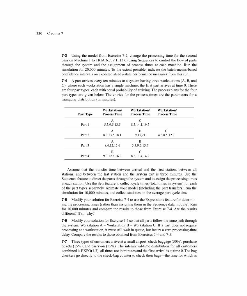
330 CHAPTER 7
7-3 Using the model from Exercise 7-2, change the processing time for the secondpass on Machine 1 to TRIA(6.7, 9.1, 13.6) using Sequences to control the flow of partsthrough the system and the assignment of process times at each machine. Run thesimulation for 20,000 minutes. To the extent possible, indicate the batch-means-basedconfidence intervals on expected steady-state performance measures from this run.
7-4 A part arrives every ten minutes to a system having three workstations (A, B, andC), where each workstation has a single machine; the first part arrives at time 0. Thereare four part types, each with equal probability of arriving. The process plans for the fourpart types are given below. The entries for the process times are the parameters for atriangular distribution (in minutes).
Workstation/ Workstation/ Workstation/Part Type Process Time Process Time Process Time
A CPart 1 5.5,9.5,13.5 8.5,14.1,19.7
A B CPart 2 8.9,13.5,18.1 9,15,21 4.3,8.5,12.7
A BPart 3 8.4,12,15.6 5.3,9.5,13.7
B CPart 4 9.3,12.6,16.0 8.6,11.4,14.2
Assume that the transfer time between arrival and the first station, between allstations, and between the last station and the system exit is three minutes. Use theSequence feature to direct the parts through the system and to assign the processing timesat each station. Use the Sets feature to collect cycle times (total times in system) for eachof the part types separately. Animate your model (including the part transfers), run thesimulation for 10,000 minutes, and collect statistics on the average part cycle time.
7-5 Modify your solution for Exercise 7-4 to use the Expressions feature for determin-ing the processing times (rather than assigning them in the Sequence data module). Runfor 10,000 minutes and compare the results to those from Exercise 7-4. Are the resultsdifferent? If so, why?
7-6 Modify your solution for Exercise 7-5 so that all parts follow the same path throughthe system: Workstation A – Workstation B – Workstation C. If a part does not requireprocessing at a workstation, it must still wait in queue, but incurs a zero processing-timedelay. Compare the results to those obtained from Exercises 7-4 and 7-5.
7-7 Three types of customers arrive at a small airport: check baggage (30%), purchasetickets (15%), and carry-on (55%). The interarrival-time distribution for all customerscombined is EXPO(1.3); all times are in minutes and the first arrival is at time 0. The bagcheckers go directly to the check-bag counter to check their bags—the time for which is
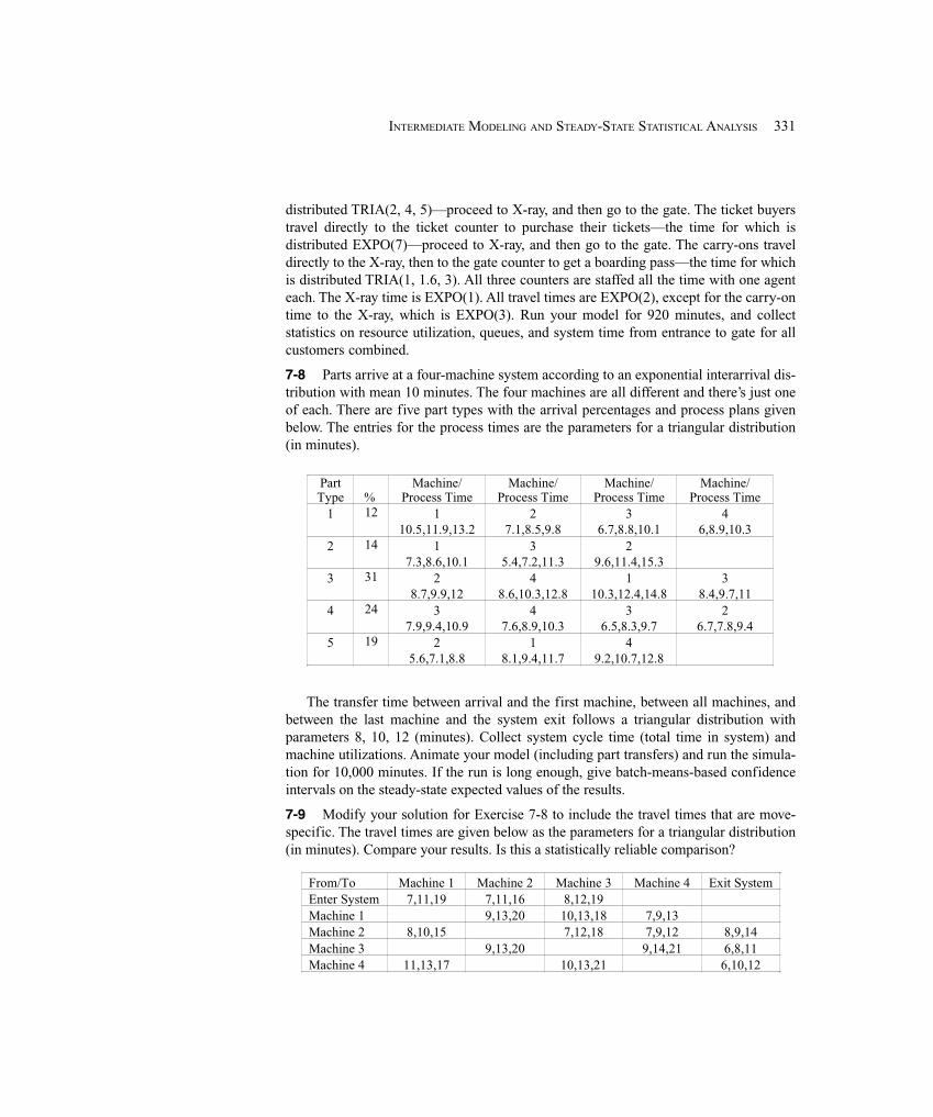
331INTERMEDIATE MODELING AND STEADY-STATE STATISTICAL ANALYSIS
distributed TRIA(2, 4, 5)—proceed to X-ray, and then go to the gate. The ticket buyerstravel directly to the ticket counter to purchase their tickets—the time for which isdistributed EXPO(7)—proceed to X-ray, and then go to the gate. The carry-ons traveldirectly to the X-ray, then to the gate counter to get a boarding pass—the time for whichis distributed TRIA(1, 1.6, 3). All three counters are staffed all the time with one agenteach. The X-ray time is EXPO(1). All travel times are EXPO(2), except for the carry-ontime to the X-ray, which is EXPO(3). Run your model for 920 minutes, and collectstatistics on resource utilization, queues, and system time from entrance to gate for allcustomers combined.
7-8 Parts arrive at a four-machine system according to an exponential interarrival dis-tribution with mean 10 minutes. The four machines are all different and there’s just oneof each. There are five part types with the arrival percentages and process plans givenbelow. The entries for the process times are the parameters for a triangular distribution(in minutes).
PartType %
Machine/Process Time
Machine/Process Time
Machine/Process Time
Machine/Process Time
1 12 110.5,11.9,13.2
27.1,8.5,9.8
36.7,8.8,10.1
46,8.9,10.3
2 14 17.3,8.6,10.1
35.4,7.2,11.3
29.6,11.4,15.3
3 31 28.7,9.9,12
48.6,10.3,12.8
110.3,12.4,14.8
38.4,9.7,11
4 24 37.9,9.4,10.9
47.6,8.9,10.3
36.5,8.3,9.7
26.7,7.8,9.4
5 19 25.6,7.1,8.8
18.1,9.4,11.7
49.2,10.7,12.8
The transfer time between arrival and the first machine, between all machines, andbetween the last machine and the system exit follows a triangular distribution withparameters 8, 10, 12 (minutes). Collect system cycle time (total time in system) andmachine utilizations. Animate your model (including part transfers) and run the simula-tion for 10,000 minutes. If the run is long enough, give batch-means-based confidenceintervals on the steady-state expected values of the results.
7-9 Modify your solution for Exercise 7-8 to include the travel times that are move-specific. The travel times are given below as the parameters for a triangular distribution(in minutes). Compare your results. Is this a statistically reliable comparison?
From/To Machine 1 Machine 2 Machine 3 Machine 4 Exit SystemEnter System 7,11,19 7,11,16 8,12,19Machine 1 9,13,20 10,13,18 7,9,13Machine 2 8,10,15 7,12,18 7,9,12 8,9,14Machine 3 9,13,20 9,14,21 6,8,11Machine 4 11,13,17 10,13,21 6,10,12
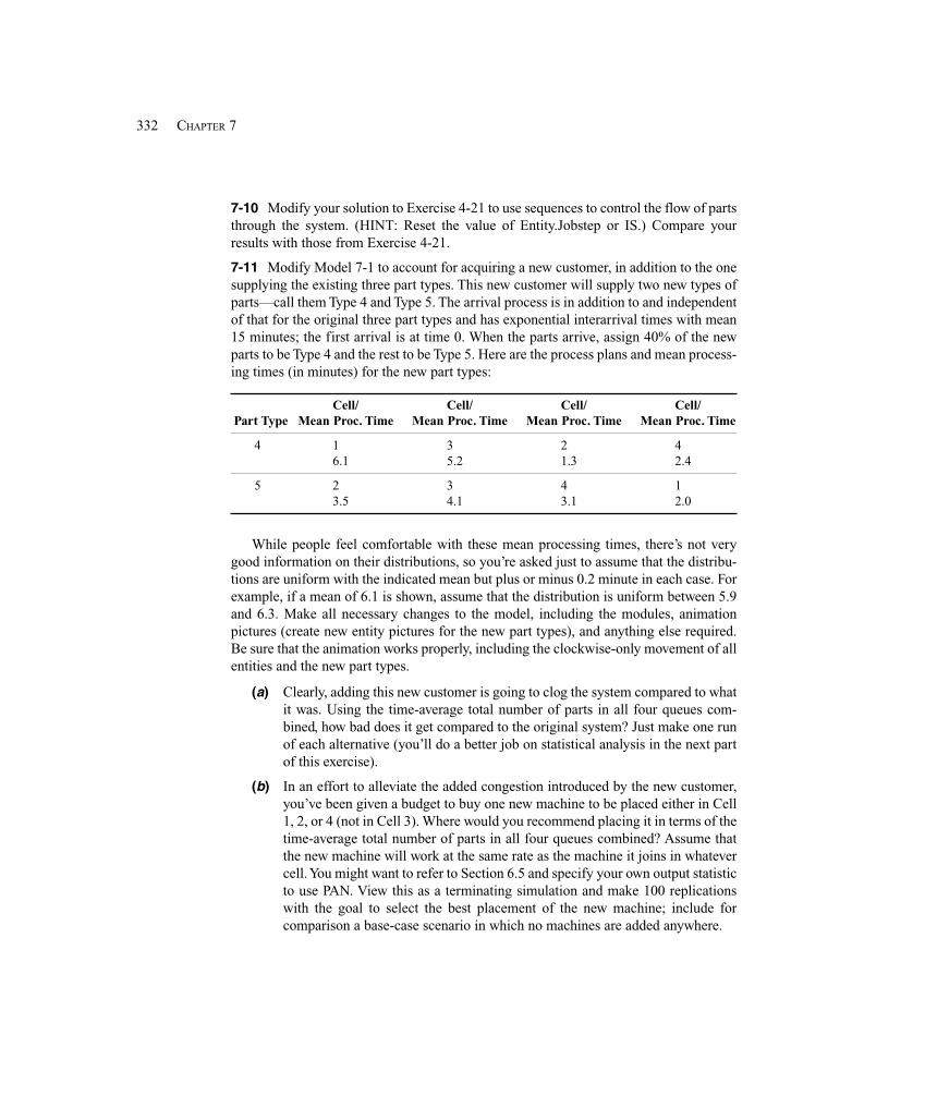
332 CHAPTER 7
7-10 Modify your solution to Exercise 4-21 to use sequences to control the flow of partsthrough the system. (HINT: Reset the value of Entity.Jobstep or IS.) Compare yourresults with those from Exercise 4-21.
7-11 Modify Model 7-1 to account for acquiring a new customer, in addition to the onesupplying the existing three part types. This new customer will supply two new types ofparts—call them Type 4 and Type 5. The arrival process is in addition to and independentof that for the original three part types and has exponential interarrival times with mean15 minutes; the first arrival is at time 0. When the parts arrive, assign 40% of the newparts to be Type 4 and the rest to be Type 5. Here are the process plans and mean process-ing times (in minutes) for the new part types:
Cell/ Cell/ Cell/ Cell/Part Type Mean Proc. Time Mean Proc. Time Mean Proc. Time Mean Proc. Time
4 1 3 2 46.1 5.2 1.3 2.4
5 2 3 4 13.5 4.1 3.1 2.0
While people feel comfortable with these mean processing times, there’s not verygood information on their distributions, so you’re asked just to assume that the distribu-tions are uniform with the indicated mean but plus or minus 0.2 minute in each case. Forexample, if a mean of 6.1 is shown, assume that the distribution is uniform between 5.9and 6.3. Make all necessary changes to the model, including the modules, animationpictures (create new entity pictures for the new part types), and anything else required.Be sure that the animation works properly, including the clockwise-only movement of allentities and the new part types.
(a) Clearly, adding this new customer is going to clog the system compared to whatit was. Using the time-average total number of parts in all four queues com-bined, how bad does it get compared to the original system? Just make one runof each alternative (you’ll do a better job on statistical analysis in the next partof this exercise).
(b) In an effort to alleviate the added congestion introduced by the new customer,you’ve been given a budget to buy one new machine to be placed either in Cell1, 2, or 4 (not in Cell 3). Where would you recommend placing it in terms of thetime-average total number of parts in all four queues combined? Assume thatthe new machine will work at the same rate as the machine it joins in whatevercell. You might want to refer to Section 6.5 and specify your own output statisticto use PAN. View this as a terminating simulation and make 100 replicationswith the goal to select the best placement of the new machine; include forcomparison a base-case scenario in which no machines are added anywhere.

333INTERMEDIATE MODELING AND STEADY-STATE STATISTICAL ANALYSIS
7-12 Modify your solution to Exercise 5-2 to use Sequences to control the flow of partsthrough the system. Also add a transfer time between arrival and the first machine,between both machines, and between the last machine and the system exit that follows atriangular distribution with parameters 7, 9, 14 (minutes). View this as a terminatingsimulation, and make 100 replications of this model as well as the one from Exercise5-2, using PAN to compare the results for average total time in system and the averagelengths of each queue.
7-13 Modify your solution to Exercise 7-12 to account for a 20% increase in processingtime when the part returns to the first machine for its last operation. View this as a termi-nating simulation, and make 100 replications of this model as well as the one from Exer-cise 7-12, using PAN to compare the results for the same output performance measuresas in Exercise 7-12.

334 CHAPTER 7
335ENTITY TRANSFER
CHAPTER 8
Entity Transfer
Up to now, we’ve considered two different cases with regard to how long it takes entitiesto move from one place to another. We’ve had them move from module to module with notravel time via Connections. In other models, we’ve moved them by Routing betweenstations with some transit-time delay. In both cases, the entities proceed uninhibited, asthough they all had their own feet and there was enough room in the transitways for asmany of them at a time as wanted to be moving.
Of course, things aren’t always so nice. There could be a limit on the concurrentnumber of entities in transit, such as a communications system where the entities arepackets of information and the bandwidth is limited to a certain number of packets intransmission at a time. There could also be situations in which something like a forkliftor a person needs to come pick up an entity and then transport it. There are also differentkinds of conveyors where entities can be viewed as competing for space on the belt orline. We’ll explore some of these modeling ideas and capabilities in this chapter. It isoften important to model such entity transfer accurately since studies have shown thatdelays and inefficiencies in operations might be caused more by the need just to movethings around rather than in actually doing the work.
Section 8.1 discusses in more detail the different kinds of entity movement andtransfers and how they can be modeled. In Section 8.2, we’ll indicate how you can usethe Arena modeling tools you already have to represent a constraint on the number ofentities that can be in motion at a time (though all entities still have their own feet).Transport devices like forklifts, pushcarts, and (of course) people are taken up in Section8.3. Modeling conveyors of different types is described in Section 8.4.
After reading this chapter and considering the examples, you’ll be able to model arich variety of entity movement and transfer that can add validity to your model andrealism to your animations.
8.1 Types of Entity Transfers
To transfer entities between modules, we initially used the Connect option (Chapter 3) totransfer entities directly between modules with no time delay. In Chapter 4, weintroduced the concept of a Route that allows you to transfer entities between stationswith a time delay in the transfer. We first showed how to use Routes for entity transfer toa specific station; then we generalized this concept in Chapter 7 by using Sequences.
Although this gives us the ability to model most situations, we sometimes find itnecessary to limit or constrain the number of transfers occurring at any point in time. Forexample, in modeling a communications network, the links have a limited capacity. Thus,we must have a method to limit the number of simultaneous messages that are beingtransferred by each network link or for the entire network. The solution is rather simple;
336 CHAPTER 8
we think of the network links as resources with a capacity equal to the maximum numberof simultaneous messages allowed. If the capacity depends on the size of the messages,then we define the resource capacity in terms of this size and require each message toseize the required number of units of this resource, determined by its size, before it canbe transferred. Let’s call this type of entity transfer resource constrained, and we’lldiscuss it in more detail in Section 8.2.
Using a resource to constrain the number of simultaneous transfers may work fine fora communications network, but it doesn’t allow us to model accurately an entire class orcategory of entity transfers generally referred to as material handling. The modelingrequirements for different material-handling systems can vary greatly, and the number ofdifferent types of material-handling devices is enormous. In fact, there is an entirehandbook devoted to this subject (see Kulwiec, 1985). However, it’s possible to dividethese devices into two general categories based on their modeling requirements.
� The first category constrains the number of simultaneous transfers based on thenumber of individual material-handling devices available. Material-handlingdevices that fall into this category are carts, hand trucks, fork trucks, AGVs,people, and so on. However, there is an additional requirement in that each ofthese devices has a physical location. If a transfer is required, we may first have tomove the device to the location where the requesting entity resides before we canperform the actual transfer. From a modeling standpoint, you might think of theseas moveable resources, referred to in Arena as Transporters.
� The second category constrains the ability to start a transfer based on spaceavailability. It also requires that we limit the total number of simultaneoustransfers between two locations, but this limit is typically based on the spacerequirement. Material-handling devices that fall into this category includeconveyors, overhead trolleys, power-and-free systems, tow lines, and more. Anescalator is a familiar example of this type of material-handling device. If atransfer is required, we first have to obtain the required amount of available orunoccupied space on the device, at the location where we are waiting, before wecan initiate our transfer. These devices require a significantly different modelingcapability, referred to in Arena as Conveyors.
The Arena Transporter and Conveyor constructs allow us to model almost any type ofmaterial-handling system easily. However, there are a few material-handling devices thathave very unique requirements that can create a modeling challenge. Gantry or bridgecranes are classic examples of such devices. A single crane is easily modeled with thetransporter constructs. If you have more than one crane on a single track, the methodused to control how the cranes move is critical to modeling these devices accurately.Unfortunately, almost all systems that have multiple cranes are controlled by the craneoperators who generally reside in the cabs located on the cranes. These operators can seeand talk to one another, and their decisions are not necessarily predictable. In this case, itis easy to model the cranes; the difficult part is how to incorporate the human logic thatprevents the cranes from colliding or gridlocking.
337ENTITY TRANSFER
Thus, we’ve defined three types of constrained entity transfers: resource constrained,transporters, and conveyors. We’ll first briefly discuss resource-constrained transfers inSection 8.2, then introduce transporters and conveyors by using them in our small manu-facturing system from Chapter 7 (Model 7-1) in Sections 8.3 and 8.4.
8.2 Model 8-1: The Small Manufacturing System with Resource-ConstrainedTransfers
In our initial model (Model 7-1) of the small manufacturing system, we assumed that alltransfer times were two minutes. If these transfer times depend on the availability ofmaterial-handling devices, the actual times may be quite different from each other duringoperation of the system. Because of this, the earlier model might give us reasonableestimates of the maximum potential system capacity; however, it would most likely notprovide very accurate estimates on the part cycle times. The simplest method is toinclude resource-constrained transfers. So let’s assume that our transfer capacity is two,with the same two-minute transfer time in every case. This means that a maximum of twotransfers can occur at the same time. If other entities are ready for transfer, they will haveto wait until one of the ongoing transfers is complete.
Using a resource to constrain the number of simultaneous entity transfers is arelatively easy addition to a model. We need to define what we think of as a new kind oftransferring resource, seize one unit of that resource before we initiate our route to leavea location, and release the resource when we arrive at the next station or location. This isan ordinary Arena resource, but we’re thinking of it differently to model the transfers.
There are two different ways we could add this logic to our existing model. The mostobvious (at least to us) is to insert a Seize module from the Advanced Process panel justprior to each of the existing Route modules (there are five in the current model). EachSeize module would request one unit of the transfer resource; e.g., Transfer. Wewould also need to change the capacity of this new resource to 2 in the Resource datamodule. There is one additional concept that you should consider while making thesemodifications: “Should each Seize module have a separate queue?” If you use a singleshared queue (see Section 5.4.5 and Model 5-1) for all of our newly inserted Seizemodules, then the resource would be allocated based on a FIFO rule. If you specified adifferent queue at each Seize module, you would be able to apply priorities to theselection process. For example, you might want to give the new arriving entities toppriority. This would allow the newly arriving parts to be sent to their first operation assoon as possible, in the hope that it would allow the processing of the part to start with aresulting reduction in the part cycle time. (If you spend much time thinking about this,you might conclude that this is faulty logic.) If all priorities are the same, you end upwith the same FIFO rule as with the shared-queue approach. So it would appear that thetwo approaches are the same. This is not quite true if you plan to show the waiting partsin your animation (which we do). By using separate queues (the default) prior to eachroute, we can show the waiting parts easily on our animation.
Having seized the transfer resource prior to each part transfer via a route, we nowneed to release that resource once the part arrives at its destination. We accomplish this

338 CHAPTER 8
by inserting a Release module after each Station module in the model. (The single excep-tion is Order Release Station, which is used only to tell Arena the location of thenewly arrived parts.) In each of these modules, we simply release the Transferresource.
The second method is to replace the Route modules with Leave modules (from theAdvanced Transfer panel) and the Station modules with Enter modules (also from theAdvanced Transfer panel). The Leave module allows us to seize the resource and also toroute the part in the same module. Similarly, the Enter module allows us to combine thefeatures of the Station and Release modules. We’ll choose this second method because itallows us to introduce two new modules, and it facilitates the conversion of the model toinclude other transfer features.
The Leave module allows you to seize a transferring resource before leaving thestation. Which resource to seize can be defined as a particular resource, a resource set, aspecific member of a set, or a resource based on the evaluation of an expression. You canalso specify a Priority in the Transfer Out logic that would allow you to control whichentity would be given the transferring resource if more than one entity was waiting. Thesmaller the number, the higher the priority. For our system, you will only have to selectthe Seize Resource option and enter a transferring resource name. We’ll also have toenter the additional routing information.
Let’s start by replacing the Start Sequence Route module with the Leavemodule shown in Display 8-1. We’ll use the same module name, Start Sequence,select the Transfer Out logic as Seize Resource, and enter the Resource Name asTransfer. Finally, we select Route as the Connect Type, enter Transfer Time forthe Move Time, select Minutes, and select By Sequence as the Station Type. We’vedefaulted on the remaining boxes. Note that this gives us our individual queues for partswaiting for the Transfer resource. Notice also that with the selection of the TransferOut resource logic, a queue (Start Sequence.Queue) was added to the modulewhen the dialog box was accepted. At this point, you might want to move this queue tothe proper position on your animation.
Now you can replace the remaining four Route modules with Leave modules. Withthe exception of the Name (we used the same name that was on the replaced Route mod-ule), the data entries are the same as shown in Display 8-1.
The Enter module allows you to release the transferring resource and provides theoption of including an unload delay time. Let’s start with the replacement of the Cell 1Station Station module with an Enter module, as in Display 8-2. Delete the existingStation module and add the new Enter module. We’ll use the same Name, Cell 1Station, and select Cell 1 from the drop-down list for the station Name. In the logicsection, you need only select Release Resource for the Transfer In entry and selectthe Transfer resource for the Resource Name to be released.
Replace the remaining four Station modules with Enter modules (but not the OrderRelease Station). As before, the data entries are the same as shown in Display 8-2,with the exception of the Name (we used the same name that was in the replaced Stationmodule).
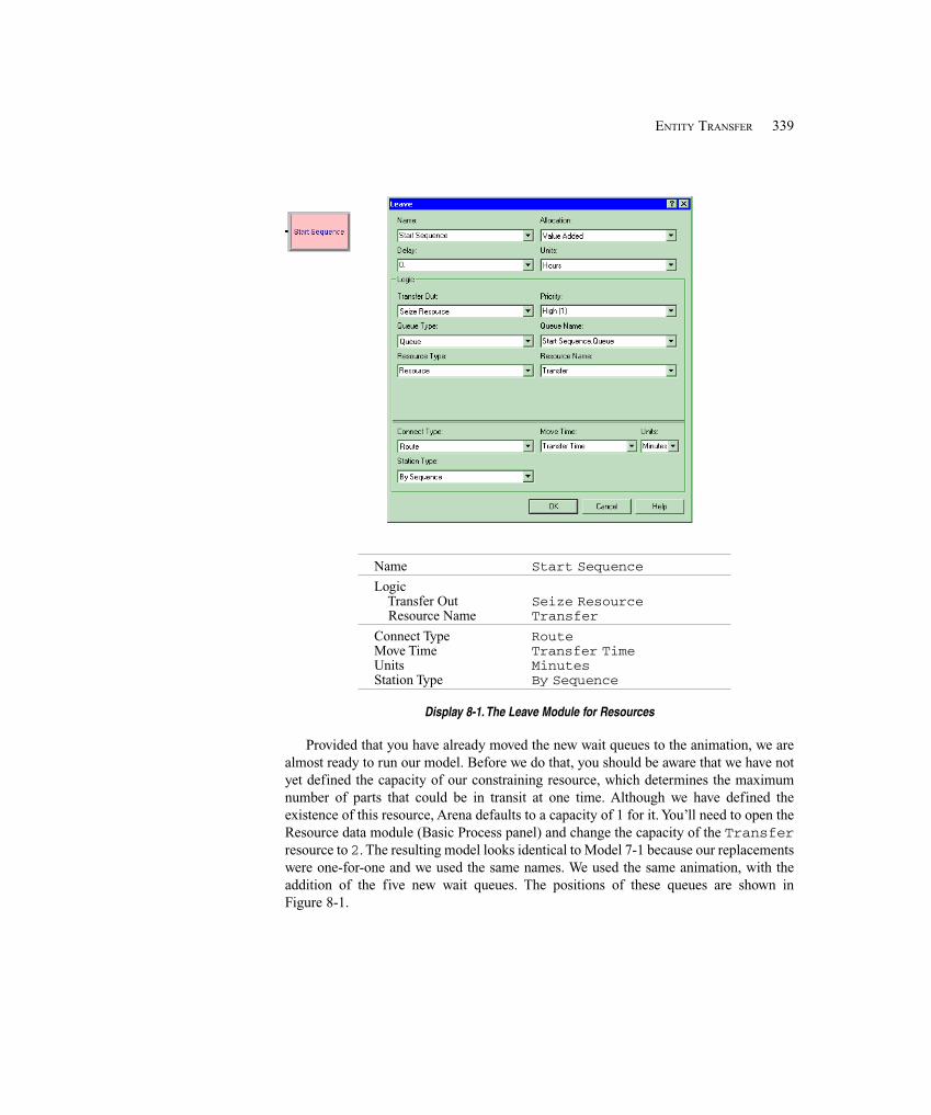
339ENTITY TRANSFER
Name Start Sequence
Logic Transfer Out Seize Resource Resource Name Transfer
Connect Type RouteMove Time Transfer TimeUnits MinutesStation Type By Sequence
Display 8-1. The Leave Module for Resources
Provided that you have already moved the new wait queues to the animation, we arealmost ready to run our model. Before we do that, you should be aware that we have notyet defined the capacity of our constraining resource, which determines the maximumnumber of parts that could be in transit at one time. Although we have defined theexistence of this resource, Arena defaults to a capacity of 1 for it. You’ll need to open theResource data module (Basic Process panel) and change the capacity of the Transferresource to 2. The resulting model looks identical to Model 7-1 because our replacementswere one-for-one and we used the same names. We used the same animation, with theaddition of the five new wait queues. The positions of these queues are shown inFigure 8-1.
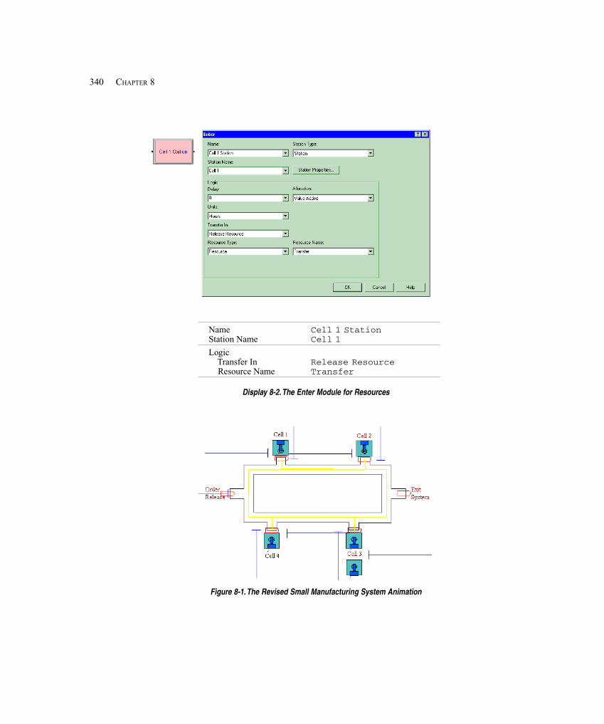
340 CHAPTER 8
Name Cell 1 StationStation Name Cell 1Logic Transfer In Release Resource Resource Name Transfer
Display 8-2. The Enter Module for Resources
Figure 8-1. The Revised Small Manufacturing System Animation
341ENTITY TRANSFER
If you run this model and watch the animation, you’ll quickly observe that there isseldom a part waiting for transfer. If you have doubts about the correctness of yourmodel, change the capacity of the Transfer resource to 1 and watch the animation. Ifyou compare the results of this model (with one Transfer resource unit) to the resultsof Model 7-1, you’ll see a slight increase in the part total time in system due to time spentwaiting in a queue for the Transfer resource. The difference is between 2 and 5minutes, depending on part type.
8.3 The Small Manufacturing System with Transporters
Let’s now assume that all material transfers are accomplished with some type ofTransporter such as carts, hand trucks, or fork trucks (we’ll call them carts). Let’s furtherassume that there are two of these carts, each moving at 50 feet per minute, whetherloaded or empty. Each cart can transport only one part at a time, and there are 0.25-minute load and unload times at the start and end of each transport. We’ll provide thedistances between stations after we’ve added the carts to our model.
There are two types of Arena transporters: free-path and guided. Free-pathtransporters can move freely through the system without encountering delays due tocongestion. The time to travel from one point to another depends only on the transportervelocity and the distance to be traveled. Guided transporters are restricted to movingwithin a predefined network. Their travel times depend on the vehicles’ speeds, thenetwork paths they follow, and potential congestion along those paths. The mostcommon type of guided vehicle is an automated guided vehicle (AGV). The carts for oursystem fall into the free-path category.
The transfer of a part with a transporter requires three activities: Request a transporter,Transport the part, and Free the transporter. The key words are Request Transporter,Transport, and Free Transporter. The Request Transporter activity, which is analogous toseizing a resource, allocates an available transporter to the requesting entity and movesthe allocated transporter to the location of the entity, if it’s not already there. The Transportactivity causes the transporter to move the entity to the destination station. This isanalogous to a route, but in the case of a Transport, the transporter and entity movetogether. The Free Transporter activity frees the transporter for the next request, muchlike the action of releasing a resource.
If there are multiple transporters in the system, we face two issues regarding theirassignment to entities. First, we might have the situation during the run where an entityrequests a transporter and more than one is available. In this case, a Transporter SelectionRule dictates which one of the transporter units will fulfill the request. In most modeledsystems, the Smallest Distance rule makes sense—allocate the transporter unit that’sclosest to the requesting entity. Other rules include Preferred Order, Cyclical, Random,Specific Member, and Largest Distance (though it takes a creative mind to imagine acase where it would be sensible). The second issue concerning transporter allocationarises when a transporter is freed and there are multiple entities waiting that haverequested one. In this case, Arena applies a priority, allocating the transporter to thewaiting entity that has the highest priority (lowest priority number). If there’s a prioritytie among entities, the transporter will be allocated to the closest waiting entity.

342 CHAPTER 8
8.3.1 Model 8-2: The Modified Model 8-1 for TransportersTo represent the carts in our small manufacturing system model, let’s start by defining thecarts. We do this with the Transporter data module found on the Advanced Transfer panel.If you’re building the model along with us, we suggest that you start with a copy of Model8-1, which we just completed. In this case, we need only enter the transporter Name,Number of Units, Type (Free Path vs. Guided), the Distance Set to which the transporterwill refer when moving and calculating time to move (discussed below), Velocity andtime Units for this velocity, and information on the transporters’ Initial Position Status(Display 8-3). We’ll accept the default for the Distance Set name (we’ll return to thisconcept later), time Units, Initial Position of the carts, and the Report Statistics.
We need to take care when defining the Velocity that we enter a quantity that’s appro-priate for the time and distance units we’re using in the model. We defaulted our timeUnits to Per Minute, the same units as for our stated velocity, but we’ll need to make surethat our distances are specified in feet.
Having defined the transporter, we can now develop the picture that represents thecart. This is done in almost the same way as it was for an entity or resource. Clicking onthe Transporter button ( ), found on the Animate Transfer toolbar, opens theTransporter Picture Placement window. Let’s replace the default picture with a box (weused a five-pixel line width) that is white, with a green line when the cart is idle and blueline when it’s busy. When the cart is carrying a part, Arena also needs to know where onthe cart’s busy picture to position the part. This placement is similar to a seize point for aresource. In this case, it’s called a Ride Point and can be found under the Object menu ofthe Arena Picture Editor window when you’re editing the busy picture. Selecting Object> Ride Point changes your pointer to cross hairs. Move this pointer to the center of thecart and click. The ride point, which appears as ⊗ on the busy cart, results in the entitybeing positioned so its reference point is aligned with this ride point. When you’vefinished creating your pictures, accept the changes to close the Transporter PicturePlacement window. Your pointer becomes cross hairs that you should positionsomewhere near your animation and click. This action places the picture of your idle cartin the model window. You needn’t worry about where you place the transporter as it isonly placed in the model window in case you need to re-edit it later. During a run, thispicture will be hidden, and replicas of it will move across the animation for eachindividual transporter unit.
Name CartNumber of Units 2Velocity 50
Display 8-3. The Transporter Data Module
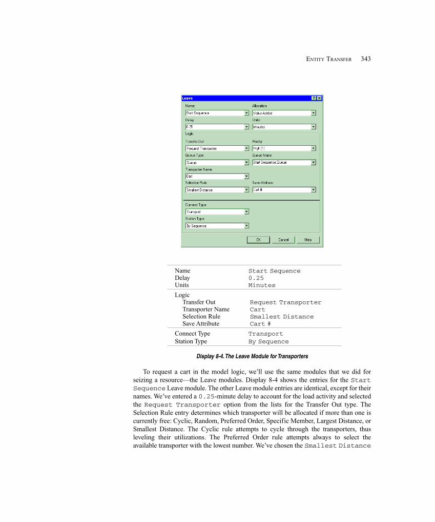
343ENTITY TRANSFER
Name Start SequenceDelay 0.25Units Minutes
LogicTransfer Out Request TransporterTransporter Name CartSelection Rule Smallest DistanceSave Attribute Cart #
Connect Type TransportStation Type By Sequence
Display 8-4. The Leave Module for Transporters
To request a cart in the model logic, we’ll use the same modules that we did forseizing a resource—the Leave modules. Display 8-4 shows the entries for the StartSequence Leave module. The other Leave module entries are identical, except for theirnames. We’ve entered a 0.25-minute delay to account for the load activity and selectedthe Request Transporter option from the lists for the Transfer Out type. TheSelection Rule entry determines which transporter will be allocated if more than one iscurrently free: Cyclic, Random, Preferred Order, Specific Member, Largest Distance, orSmallest Distance. The Cyclic rule attempts to cycle through the transporters, thusleveling their utilizations. The Preferred Order rule attempts always to select theavailable transporter with the lowest number. We’ve chosen the Smallest Distance
344 CHAPTER 8
rule, which results in an allocation of the cart closest to the requesting entity. A newAttribute, Cart #, is defined and used to save the number of the cart that was allocated(more on this later). We also select the Transport option for the Connect Type. Notethat when you make this selection, the Move Time field disappears. The actual move timewill be calculated from the distance traveled and the transporter velocity.
The Leave module performs four activities: allocate a transporter, move the emptytransporter to the location of the requesting part, delay for the load time, and transport thepart to its destination. There are alternate ways to model these activities. For example, wecould have used a Request – Delay – Transport module combination to perform the sameactivities. The Request module (Advanced Transfer panel) performs the first two; theDelay module, the load activity; and the Transport module (Advanced Transfer panel), thelast activity. Although this requires three modules, it does provide you with some additionalmodeling flexibility. You can specify different travel velocities for both moving the emptytransporter and transporting the part to its destination location. In fact, you could specifythe transporting velocity as an expression of an attribute of the part; for example, partweight. You could also replace the Delay module with a Process module, which couldrequire the availability of an operator or material handler (modeled as a resource) to loadthe part. Finally, you could replace the Request module with an Allocate – Move modulecombination. The Allocate module (Advanced Transfer panel) allocates a transporter,while the Move module (Advanced Transfer panel) moves the empty transporter to therequesting part location. Again, this would allow you to insert additional logic betweenthese two activities if such logic were required to model your system accurately.
When the part arrives at its next location, it needs to free the cart so it can be used byother parts. To free the cart, we’ll use the same modules that we did for releasing theresource in the previous model—the Enter modules. Display 8-5 shows the entries for theEnter Cell 1 Station module. The other Enter module entries are identical, except fortheir names. We’ve entered the unload Delay in minutes and selected the FreeTransporter option for Transfer In. In our model, we also entered the TransporterName, Cart, and name of the attribute where we saved the transporter Unit Number,Cart #. We could have left both of these last two fields empty. Arena keeps track ofwhich cart was allocated to the entity and frees that cart. However, if you enter theTransporter Name and there is more than one transporter, you also need to enter the UnitNumber. If you only entered the Transporter Name, Arena would always try to free thefirst transporter.
As with the Leave module, the Enter module performs multiple activities: definingthe station, delaying for the unload time, and freeing the transporter. Again there arealternate ways to model these functions. We could have used a Station – Delay – Freemodule combination to perform the same activities. The Station module defines thestation; the Delay module, the unload activity; and the Free module (Advanced Transferpanel) frees the transporter. Separating these three activities would allow you to insertadditional model logic, if required for your system. For example, you could replace theDelay module with a Process module, which could require the availability of an operatoror material handler (modeled as a resource) to unload the part.
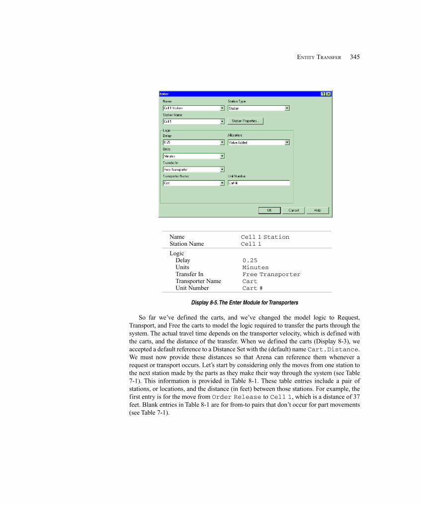
345ENTITY TRANSFER
Name Cell 1 StationStation Name Cell 1
LogicDelay 0.25Units MinutesTransfer In Free TransporterTransporter Name CartUnit Number Cart #
Display 8-5. The Enter Module for Transporters
So far we’ve defined the carts, and we’ve changed the model logic to Request,Transport, and Free the carts to model the logic required to transfer the parts through thesystem. The actual travel time depends on the transporter velocity, which is defined withthe carts, and the distance of the transfer. When we defined the carts (Display 8-3), weaccepted a default reference to a Distance Set with the (default) name Cart.Distance.We must now provide these distances so that Arena can reference them whenever arequest or transport occurs. Let’s start by considering only the moves from one station tothe next station made by the parts as they make their way through the system (see Table7-1). This information is provided in Table 8-1. These table entries include a pair ofstations, or locations, and the distance (in feet) between those stations. For example, thefirst entry is for the move from Order Release to Cell 1, which is a distance of 37feet. Blank entries in Table 8-1 are for from-to pairs that don’t occur for part movements(see Table 7-1).
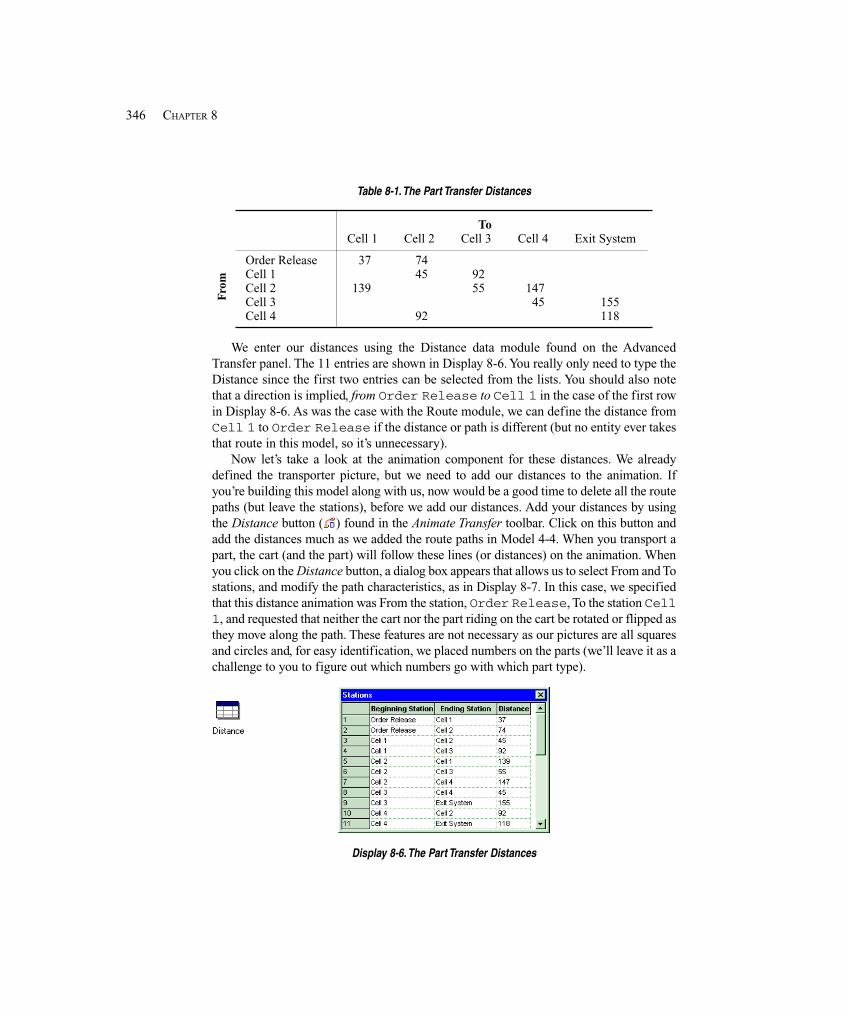
346 CHAPTER 8
Table 8-1. The Part Transfer Distances
ToCell 1 Cell 2 Cell 3 Cell 4 Exit System
Order Release 37 74Cell 1 45 92Cell 2 139 55 147Cell 3 45 155Cell 4 92 118
We enter our distances using the Distance data module found on the AdvancedTransfer panel. The 11 entries are shown in Display 8-6. You really only need to type theDistance since the first two entries can be selected from the lists. You should also notethat a direction is implied, from Order Release to Cell 1 in the case of the first rowin Display 8-6. As was the case with the Route module, we can define the distance fromCell 1 to Order Release if the distance or path is different (but no entity ever takesthat route in this model, so it’s unnecessary).
Now let’s take a look at the animation component for these distances. We alreadydefined the transporter picture, but we need to add our distances to the animation. Ifyou’re building this model along with us, now would be a good time to delete all the routepaths (but leave the stations), before we add our distances. Add your distances by usingthe Distance button ( ) found in the Animate Transfer toolbar. Click on this button andadd the distances much as we added the route paths in Model 4-4. When you transport apart, the cart (and the part) will follow these lines (or distances) on the animation. Whenyou click on the Distance button, a dialog box appears that allows us to select From and Tostations, and modify the path characteristics, as in Display 8-7. In this case, we specifiedthat this distance animation was From the station, Order Release, To the station Cell1, and requested that neither the cart nor the part riding on the cart be rotated or flipped asthey move along the path. These features are not necessary as our pictures are all squaresand circles and, for easy identification, we placed numbers on the parts (we’ll leave it as achallenge to you to figure out which numbers go with which part type).
Display 8-6. The Part Transfer Distances
Fro
m
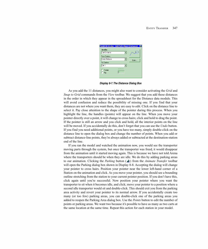
347ENTITY TRANSFER
Display 8-7. The Distance Dialog Box
As you add the 11 distances, you might also want to consider activating the Grid andSnap to Grid commands from the View toolbar. We suggest that you add these distancesin the order in which they appear in the spreadsheet for the Distance data module. Thiswill avoid confusion and reduce the possibility of missing one. If you find that yourdistances are not where you want them, they are easy to edit. Click on the distance line toselect it. Pay close attention to the shape of the pointer during this process. When youhighlight the line, the handles (points) will appear on the line. When you move yourpointer directly over a point, it will change to cross hairs; click and hold to drag the point.If the pointer is still an arrow and you click and hold, all the interior points on the linewill be moved. If you accidentally do this, don’t forget that you can use the Undo button.If you find you need additional points, or you have too many, simply double-click on thedistance line to open the dialog box and change the number of points. When you add orsubtract distance-line points, they’re always added or subtracted at the destination-stationend of the line.
If you ran the model and watched the animation now, you would see the transportermoving parts through the system, but once the transporter was freed, it would disappearfrom the animation until it started moving again. This is because we have not told Arenawhere the transporters should be when they are idle. We do this by adding parking areasto our animation. Clicking the Parking button ( ) from the Animate Transfer toolbarwill open the Parking dialog box shown in Display 8-8. Accepting the dialog will changeyour pointer to cross hairs. Position your pointer near the lower left-hand corner of aStation on the animation and click. As you move your pointer, you should see a boundingoutline stretching from the station to your current pointer position. If you don’t have this,click again until you’re successful. Now position your pointer where you want thetransporter to sit when it becomes idle, and click; move your pointer to a position where asecond idle transporter would sit and double-click. This should exit you from the parkingarea activity and revert your pointer to its normal arrow. If you accidentally create toomany (or too few) parking areas, you can double-click one of the parking areas youadded to reopen the Parking Area dialog box. Use the Points button to edit the number ofpoints or parking areas. We want two because it’s possible to have as many as two carts atthe same location at the same time. Repeat this action for each station in your model.
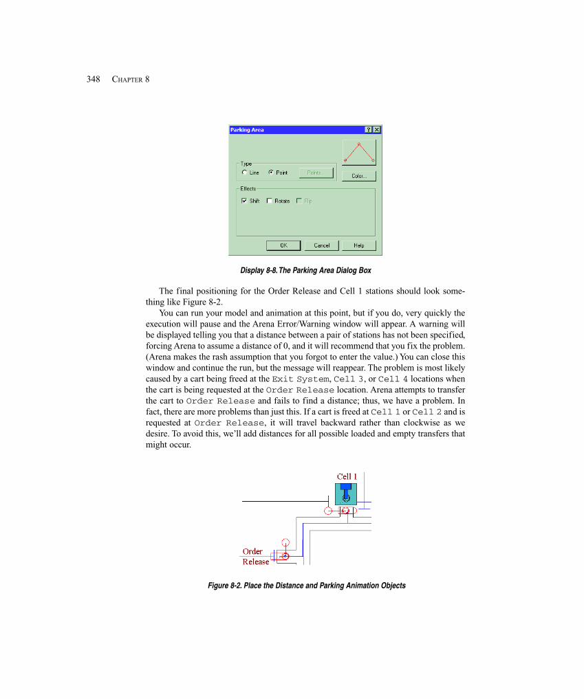
348 CHAPTER 8
Display 8-8. The Parking Area Dialog Box
The final positioning for the Order Release and Cell 1 stations should look some-thing like Figure 8-2.
You can run your model and animation at this point, but if you do, very quickly theexecution will pause and the Arena Error/Warning window will appear. A warning willbe displayed telling you that a distance between a pair of stations has not been specified,forcing Arena to assume a distance of 0, and it will recommend that you fix the problem.(Arena makes the rash assumption that you forgot to enter the value.) You can close thiswindow and continue the run, but the message will reappear. The problem is most likelycaused by a cart being freed at the Exit System, Cell 3, or Cell 4 locations whenthe cart is being requested at the Order Release location. Arena attempts to transferthe cart to Order Release and fails to find a distance; thus, we have a problem. Infact, there are more problems than just this. If a cart is freed at Cell 1 or Cell 2 and isrequested at Order Release, it will travel backward rather than clockwise as wedesire. To avoid this, we’ll add distances for all possible loaded and empty transfers thatmight occur.
Figure 8-2. Place the Distance and Parking Animation Objects
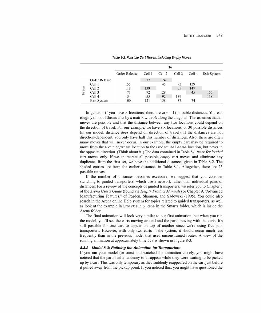
349ENTITY TRANSFER
Fro
m
Table 8-2. Possible Cart Moves, Including Empty Moves
To
Order Release Cell 1 Cell 2 Cell 3 Cell 4 Exit System
Order Release 37 74Cell 1 155 45 92 129Cell 2 118 139 55 147Cell 3 71 92 129 45 155Cell 4 34 55 92 139 118Exit System 100 121 158 37 74
In general, if you have n locations, there are n(n – 1) possible distances. You canroughly think of this as an n by n matrix with 0’s along the diagonal. This assumes that allmoves are possible and that the distance between any two locations could depend onthe direction of travel. For our example, we have six locations, or 30 possible distances(in our model, distance does depend on direction of travel). If the distances are notdirection-dependent, you only have half this number of distances. Also, there are oftenmany moves that will never occur. In our example, the empty cart may be required tomove from the Exit System location to the Order Release location, but never inthe opposite direction. (Think about it!) The data contained in Table 8-1 were for loadedcart moves only. If we enumerate all possible empty cart moves and eliminate anyduplicates from the first set, we have the additional distances given in Table 8-2. Theshaded entries are from the earlier distances in Table 8-1. Altogether, there are 25possible moves.
If the number of distances becomes excessive, we suggest that you considerswitching to guided transporters, which use a network rather than individual pairs ofdistances. For a review of the concepts of guided transporters, we refer you to Chapter 5of the Arena User’s Guide (found via Help > Product Manuals) or Chapter 9, “AdvancedManufacturing Features,” of Pegden, Shannon, and Sadowski (1995). You could alsosearch in the Arena online Help system for topics related to guided transporters, as wellas look at the example in Smarts195.doe in the Smarts folder, which is inside theArena folder.
The final animation will look very similar to our first animation, but when you runthe model, you’ll see the carts moving around and the parts moving with the carts. It’sstill possible for one cart to appear on top of another since we’re using free-pathtransporters. However, with only two carts in the system, it should occur much lessfrequently than in the previous model that used unconstrained routes. A view of therunning animation at approximately time 578 is shown in Figure 8-3.
8.3.2 Model 8-3: Refining the Animation for TransportersIf you ran your model (or ours) and watched the animation closely, you might havenoticed that the parts had a tendency to disappear while they were waiting to be pickedup by a cart. This was only temporary as they suddenly reappeared on the cart just beforeit pulled away from the pickup point. If you noticed this, you might have questioned the
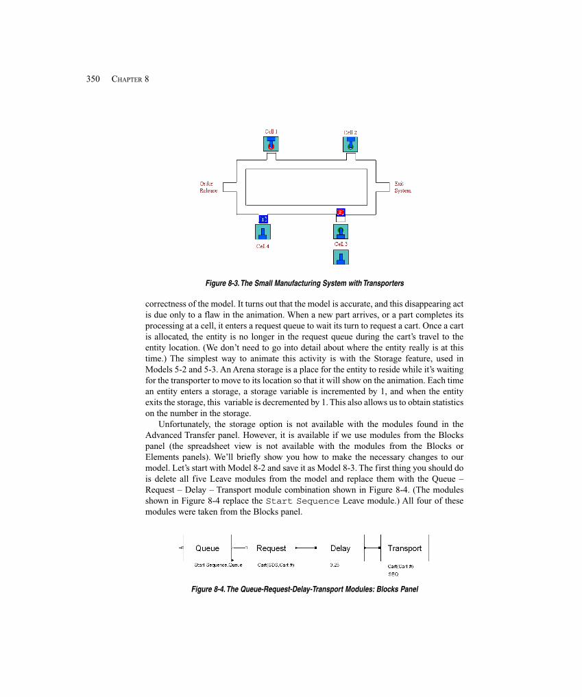
350 CHAPTER 8
Figure 8-3. The Small Manufacturing System with Transporters
correctness of the model. It turns out that the model is accurate, and this disappearing actis due only to a flaw in the animation. When a new part arrives, or a part completes itsprocessing at a cell, it enters a request queue to wait its turn to request a cart. Once a cartis allocated, the entity is no longer in the request queue during the cart’s travel to theentity location. (We don’t need to go into detail about where the entity really is at thistime.) The simplest way to animate this activity is with the Storage feature, used inModels 5-2 and 5-3. An Arena storage is a place for the entity to reside while it’s waitingfor the transporter to move to its location so that it will show on the animation. Each timean entity enters a storage, a storage variable is incremented by 1, and when the entityexits the storage, this variable is decremented by 1. This also allows us to obtain statisticson the number in the storage.
Unfortunately, the storage option is not available with the modules found in theAdvanced Transfer panel. However, it is available if we use modules from the Blockspanel (the spreadsheet view is not available with the modules from the Blocks orElements panels). We’ll briefly show you how to make the necessary changes to ourmodel. Let’s start with Model 8-2 and save it as Model 8-3. The first thing you should dois delete all five Leave modules from the model and replace them with the Queue –Request – Delay – Transport module combination shown in Figure 8-4. (The modulesshown in Figure 8-4 replace the Start Sequence Leave module.) All four of thesemodules were taken from the Blocks panel.
Figure 8-4. The Queue-Request-Delay-Transport Modules: Blocks Panel
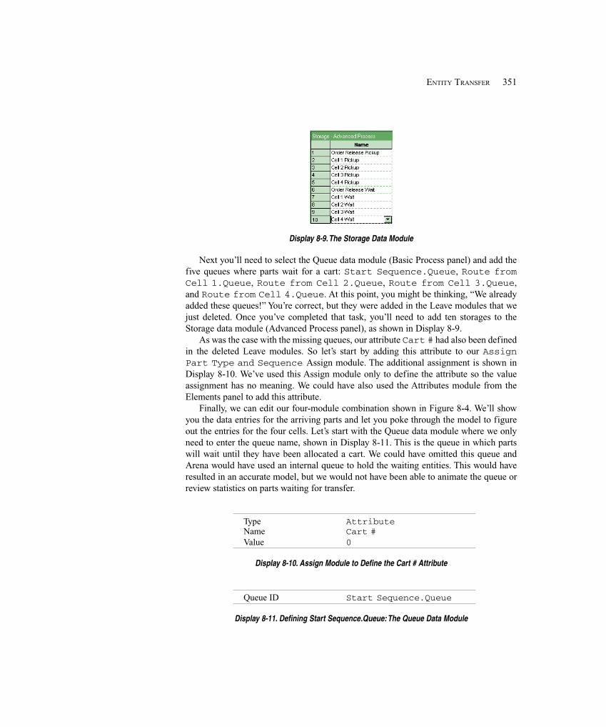
351ENTITY TRANSFER
Display 8-9. The Storage Data Module
Next you’ll need to select the Queue data module (Basic Process panel) and add thefive queues where parts wait for a cart: Start Sequence.Queue, Route fromCell 1.Queue, Route from Cell 2.Queue, Route from Cell 3.Queue,and Route from Cell 4.Queue. At this point, you might be thinking, “We alreadyadded these queues!” You’re correct, but they were added in the Leave modules that wejust deleted. Once you’ve completed that task, you’ll need to add ten storages to theStorage data module (Advanced Process panel), as shown in Display 8-9.
As was the case with the missing queues, our attribute Cart # had also been definedin the deleted Leave modules. So let’s start by adding this attribute to our AssignPart Type and Sequence Assign module. The additional assignment is shown inDisplay 8-10. We’ve used this Assign module only to define the attribute so the valueassignment has no meaning. We could have also used the Attributes module from theElements panel to add this attribute.
Finally, we can edit our four-module combination shown in Figure 8-4. We’ll showyou the data entries for the arriving parts and let you poke through the model to figureout the entries for the four cells. Let’s start with the Queue data module where we onlyneed to enter the queue name, shown in Display 8-11. This is the queue in which partswill wait until they have been allocated a cart. We could have omitted this queue andArena would have used an internal queue to hold the waiting entities. This would haveresulted in an accurate model, but we would not have been able to animate the queue orreview statistics on parts waiting for transfer.
Type AttributeName Cart #Value 0
Display 8-10. Assign Module to Define the Cart # Attribute
Queue ID Start Sequence.Queue
Display 8-11. Defining Start Sequence.Queue: The Queue Data Module
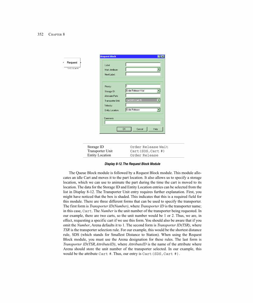
352 CHAPTER 8
Storage ID Order Release WaitTransporter Unit Cart(SDS,Cart #)Entity Location Order Release
Display 8-12. The Request Block Module
The Queue Block module is followed by a Request Block module. This module allo-cates an idle Cart and moves it to the part location. It also allows us to specify a storagelocation, which we can use to animate the part during the time the cart is moved to itslocation. The data for the Storage ID and Entity Location entries can be selected from thelist in Display 8-12. The Transporter Unit entry requires further explanation. First, youmight have noticed that the box is shaded. This indicates that this is a required field forthis module. There are three different forms that can be used to specify the transporter.The first form is Transporter ID(Number), where Transporter ID is the transporter name;in this case, Cart. The Number is the unit number of the transporter being requested. Inour example, there are two carts, so the unit number would be 1 or 2. Thus, we are, ineffect, requesting a specific cart if we use this form. You should also be aware that if youomit the Number, Arena defaults it to 1. The second form is Transporter ID(TSR), whereTSR is the transporter selection rule. For our example, this would be the shortest distancerule, SDS (which stands for Smallest Distance to Station). When using the RequestBlock module, you must use the Arena designation for these rules. The last form isTransporter ID(TSR,AttributeID), where AttributeID is the name of the attribute whereArena should store the unit number of the transporter selected. In our example, thiswould be the attribute Cart #. Thus, our entry is Cart(SDS,Cart #).
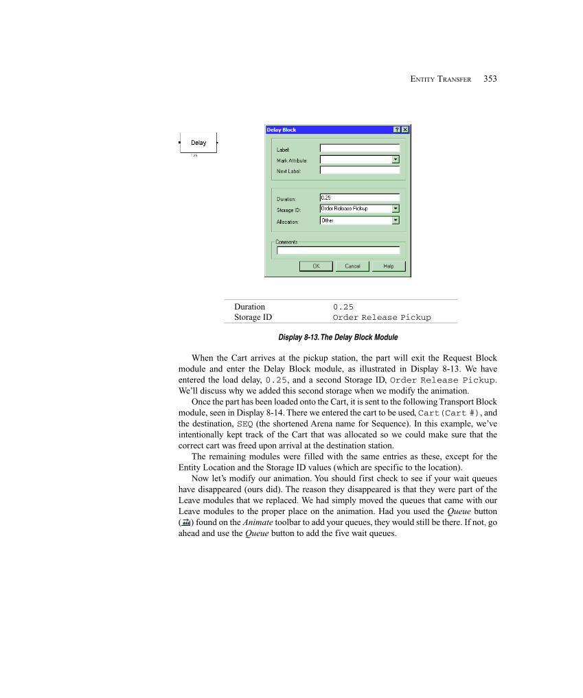
353ENTITY TRANSFER
Duration 0.25Storage ID Order Release Pickup
Display 8-13. The Delay Block Module
When the Cart arrives at the pickup station, the part will exit the Request Blockmodule and enter the Delay Block module, as illustrated in Display 8-13. We haveentered the load delay, 0.25, and a second Storage ID, Order Release Pickup.We’ll discuss why we added this second storage when we modify the animation.
Once the part has been loaded onto the Cart, it is sent to the following Transport Blockmodule, seen in Display 8-14. There we entered the cart to be used, Cart(Cart #), andthe destination, SEQ (the shortened Arena name for Sequence). In this example, we’veintentionally kept track of the Cart that was allocated so we could make sure that thecorrect cart was freed upon arrival at the destination station.
The remaining modules were filled with the same entries as these, except for theEntity Location and the Storage ID values (which are specific to the location).
Now let’s modify our animation. You should first check to see if your wait queueshave disappeared (ours did). The reason they disappeared is that they were part of theLeave modules that we replaced. We had simply moved the queues that came with ourLeave modules to the proper place on the animation. Had you used the Queue button( ) found on the Animate toolbar to add your queues, they would still be there. If not, goahead and use the Queue button to add the five wait queues.
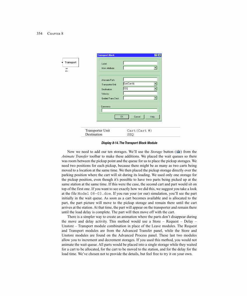
354 CHAPTER 8
Transporter Unit Cart(Cart #)Destination SEQ
Display 8-14. The Transport Block Module
Now we need to add our ten storages. We’ll use the Storage button ( ) from theAnimate Transfer toolbar to make these additions. We placed the wait queues so therewas room between the pickup point and the queue for us to place the pickup storages. Weneed two positions for each pickup, because there might be as many as two carts beingmoved to a location at the same time. We then placed the pickup storage directly over theparking position where the cart will sit during its loading. We used only one storage forthe pickup position, even though it’s possible to have two parts being picked up at thesame station at the same time. If this were the case, the second cart and part would sit ontop of the first one. If you want to see exactly how we did this, we suggest you take a lookat the file Model 08-03.doe. If you run your (or our) simulation, you’ll see the partinitially in the wait queue. As soon as a cart becomes available and is allocated to thepart, the part picture will move to the pickup storage and remain there until the cartarrives at the station. At that time, the part will appear on the transporter and remain thereuntil the load delay is complete. The part will then move off with the cart.
There is a simpler way to create an animation where the parts don’t disappear duringthe move and delay activity. This method would use a Store – Request – Delay –Unstore – Transport module combination in place of the Leave modules. The Requestand Transport modules are from the Advanced Transfer panel, while the Store andUnstore modules are found on the Advanced Process panel. These last two modulesallow you to increment and decrement storages. If you used this method, you would notanimate the wait queue. All parts would be placed into a single storage while they waitedfor a cart to be allocated, for the cart to be moved to the station, and for the delay for theload time. We’ve chosen not to provide the details, but feel free to try it on your own.
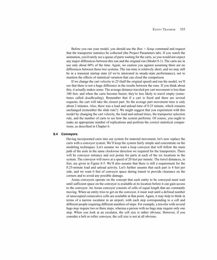
355ENTITY TRANSFER
Before you run your model, you should use the Run > Setup command and requestthat the transporter statistics be collected (the Project Parameters tab). If you watch theanimation, you’d rarely see a queue of parts waiting for the carts, so you would not expectany major differences between this run and the original run (Model 8-1). The carts are inuse only about 60% of the time. Again, we caution you against assuming there are nodifferences between these two systems. The run time is relatively short, and we may stillbe in a transient startup state (if we’re interested in steady-state performance), not tomention the effects of statistical variation that can cloud the comparison.
If we change the cart velocity to 25 (half the original speed) and run the model, we’llsee that there is not a huge difference in the results between the runs. If you think aboutthis, it actually makes sense. The average distance traveled per cart movement is less than100 feet, and when the carts become busier, they’re less likely to travel empty (some-times called deadheading). Remember that if a cart is freed and there are severalrequests, the cart will take the closest part. So the average part movement time is onlyabout 2 minutes. Also, there was a load and unload time of 0.25 minute, which remainsunchanged (remember the slide rule?). We might suggest that you experiment with thismodel by changing the cart velocity, the load and unload times, the transporter selectionrule, and the number of carts to see how the system performs. Of course, you ought tomake an appropriate number of replications and perform the correct statistical compar-isons, as described in Chapter 6.
8.4 Conveyors
Having incorporated carts into our system for material movement, let’s now replace thecarts with a conveyor system. We’ll keep the system fairly simple and concentrate on themodeling techniques. Let’s assume we want a loop conveyor that will follow the mainpath of the aisle in the same clockwise direction we required for the transporters. Therewill be conveyor entrance and exit points for parts at each of the six locations in thesystem. The conveyor will move at a speed of 20 feet per minute. The travel distances, infeet, are given in Figure 8-5. We’ll also assume that there is still a requirement for the0.25-minute load and unload activity. Let’s further assume that each part is 4 feet perside, and we want 6 feet of conveyor space during transit to provide clearance on thecorners and to avoid any possible damage.
Arena conveyors operate on the concept that each entity to be conveyed must waituntil sufficient space on the conveyor is available at its location before it can gain accessto the conveyor. An Arena conveyor consists of cells of equal length that are constantlymoving. When an entity tries to get on the conveyor, it must wait until a defined numberof unoccupied consecutive cells are available at that point. Again, it may help to think interms of a narrow escalator in an airport, with each step corresponding to a cell anddifferent people requiring different numbers of steps. For example, a traveler with severalbags may require two or three steps, whereas a person with no bags may require only onestep. When you look at an escalator, the cell size is rather obvious. However, if youconsider a belt or roller conveyor, the cell size is not at all obvious.
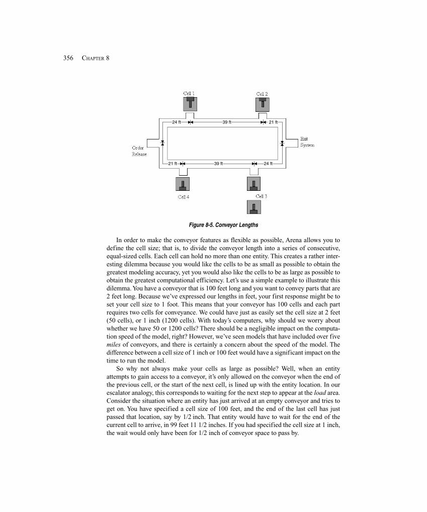
356 CHAPTER 8
21 ft39 ft24 ft
21 ft 39 ft 24 ft
Figure 8-5. Conveyor Lengths
In order to make the conveyor features as flexible as possible, Arena allows you todefine the cell size; that is, to divide the conveyor length into a series of consecutive,equal-sized cells. Each cell can hold no more than one entity. This creates a rather inter-esting dilemma because you would like the cells to be as small as possible to obtain thegreatest modeling accuracy, yet you would also like the cells to be as large as possible toobtain the greatest computational efficiency. Let’s use a simple example to illustrate thisdilemma. You have a conveyor that is 100 feet long and you want to convey parts that are2 feet long. Because we’ve expressed our lengths in feet, your first response might be toset your cell size to 1 foot. This means that your conveyor has 100 cells and each partrequires two cells for conveyance. We could have just as easily set the cell size at 2 feet(50 cells), or 1 inch (1200 cells). With today’s computers, why should we worry aboutwhether we have 50 or 1200 cells? There should be a negligible impact on the computa-tion speed of the model, right? However, we’ve seen models that have included over fivemiles of conveyors, and there is certainly a concern about the speed of the model. Thedifference between a cell size of 1 inch or 100 feet would have a significant impact on thetime to run the model.
So why not always make your cells as large as possible? Well, when an entityattempts to gain access to a conveyor, it’s only allowed on the conveyor when the end ofthe previous cell, or the start of the next cell, is lined up with the entity location. In ourescalator analogy, this corresponds to waiting for the next step to appear at the load area.Consider the situation where an entity has just arrived at an empty conveyor and tries toget on. You have specified a cell size of 100 feet, and the end of the last cell has justpassed that location, say by 1/2 inch. That entity would have to wait for the end of thecurrent cell to arrive, in 99 feet 11 1/2 inches. If you had specified the cell size at 1 inch,the wait would only have been for 1/2 inch of conveyor space to pass by.
357ENTITY TRANSFER
The basic message is that you need to consider the impact of cell size with respect tothe specific application you’re modeling. If the conveyor is not highly utilized, or thepotential slight delay in timing has no impact on the system’s performance, use a largecell size. If any of these are critical to the system performance, use a small cell size.There are two constraints to consider when making this decision. The entity size,expressed in number of cells, must be an integer so you cannot have an entity requiring1.5 cells; you would have to use one or two cells as the entity size. Also, the conveyorsegments (the length of a conveyor section from one location to another) must consist ofan integral number of cells. So, if your conveyor were 100 feet long, you could not use acell size of three.
Before we start adding conveyors to our model, let’s go over a few more concepts thatwe hope will be helpful when you try to build your own models with conveyors. As withResources and Transporters, Conveyors have several key words: Access, Convey, andExit. To transfer an entity with Arena conveyors, you must first Access space on theconveyor, then Convey the entity to its destination, and finally Exit the conveyor (to freeup the space). For representing the physical layout, an Arena conveyor consists of a seriesof segments that are linked together to form the entire conveyor. Each segment starts andends at an Arena station. You can only link these segments to form a line or loopconveyor. Thus, a single conveyor cannot have a diverge point that results in a conveyorsplitting into two or more downstream lines, or a converge point where two or moreupstream lines join. However, you can define multiple conveyors for these types ofsystems. For example, in a diverging system, you would convey the entity to the divergepoint, Access space on the appropriate next conveyor, Exit the current conveyor, andConvey the entity to its next destination. For our small manufacturing system, we’ll use asingle loop conveyor.
Arena has two types of conveyors: nonaccumulating and accumulating. Both types ofconveyors travel in only a single direction, and you can’t reverse them. These conveyorsfunction very much as their name would imply. Examples of a non-accumulatingconveyor would be a bucket or belt conveyor or our escalator. The spacing betweenentities traveling on these types of conveyors never changes, unless one entity exits andre-accesses space. Because of this constraint, nonaccumulating conveyors operate in aunique manner. When an entity accesses space on this type of conveyor, the entireconveyor actually stops moving or is disengaged. When the entity is conveyed, theconveyor is re-engaged while the entity travels to its destination. The conveyor is stoppedwhen the entity reaches its destination, the entity exits, and the conveyor is then restarted.If there is no elapsed time between the Access and Convey, or when the entity reaches itsdestination and then exits, then it’s as if the conveyor was never stopped. However, ifthere is a delay, such as for a load or unload activity of positive duration (which is the casein our system), you’ll see the conveyor temporarily stop while the load or unload occurs.
Accumulating conveyors differ in that they never stop moving. If an entity is stoppedon an accumulating conveyor, all other entities on that conveyor will continue on theirway. However, the stopped entity blocks any other entities from arriving at that locationso that the arriving entities accumulate behind the blocking entity. When the blocking
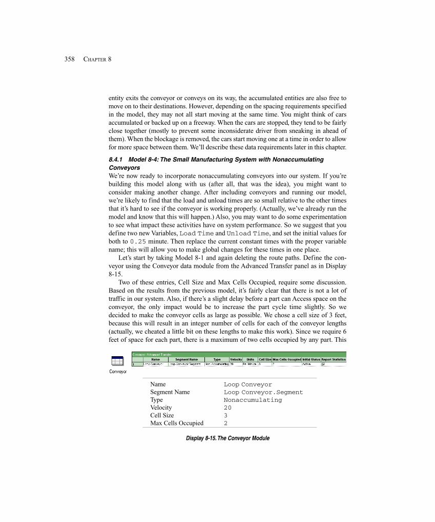
358 CHAPTER 8
entity exits the conveyor or conveys on its way, the accumulated entities are also free tomove on to their destinations. However, depending on the spacing requirements specifiedin the model, they may not all start moving at the same time. You might think of carsaccumulated or backed up on a freeway. When the cars are stopped, they tend to be fairlyclose together (mostly to prevent some inconsiderate driver from sneaking in ahead ofthem). When the blockage is removed, the cars start moving one at a time in order to allowfor more space between them. We’ll describe these data requirements later in this chapter.
8.4.1 Model 8-4: The Small Manufacturing System with NonaccumulatingConveyorsWe’re now ready to incorporate nonaccumulating conveyors into our system. If you’rebuilding this model along with us (after all, that was the idea), you might want toconsider making another change. After including conveyors and running our model,we’re likely to find that the load and unload times are so small relative to the other timesthat it’s hard to see if the conveyor is working properly. (Actually, we’ve already run themodel and know that this will happen.) Also, you may want to do some experimentationto see what impact these activities have on system performance. So we suggest that youdefine two new Variables, Load Time and Unload Time, and set the initial values forboth to 0.25 minute. Then replace the current constant times with the proper variablename; this will allow you to make global changes for these times in one place.
Let’s start by taking Model 8-1 and again deleting the route paths. Define the con-veyor using the Conveyor data module from the Advanced Transfer panel as in Display8-15.
Two of these entries, Cell Size and Max Cells Occupied, require some discussion.Based on the results from the previous model, it’s fairly clear that there is not a lot oftraffic in our system. Also, if there’s a slight delay before a part can Access space on theconveyor, the only impact would be to increase the part cycle time slightly. So wedecided to make the conveyor cells as large as possible. We chose a cell size of 3 feet,because this will result in an integer number of cells for each of the conveyor lengths(actually, we cheated a little bit on these lengths to make this work). Since we require 6feet of space for each part, there is a maximum of two cells occupied by any part. This
Name Loop ConveyorSegment Name Loop Conveyor.SegmentType NonaccumulatingVelocity 20Cell Size 3Max Cells Occupied 2
Display 8-15. The Conveyor Module
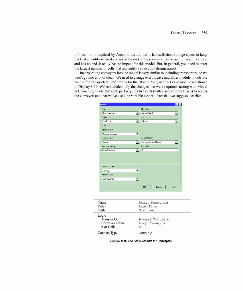
359ENTITY TRANSFER
information is required by Arena to assure that it has sufficient storage space to keeptrack of an entity when it arrives at the end of the conveyor. Since our conveyor is a loopand has no end, it really has no impact for this model. But, in general, you need to enterthe largest number of cells that any entity can occupy during transit.
Incorporating conveyors into the model is very similar to including transporters, so wewon’t go into a lot of detail. We need to change every Leave and Enter module, much likewe did for transporters. The entries for the Start Sequence Leave module are shownin Display 8-16. We’ve included only the changes that were required starting with Model8-1. You might note that each part requires two cells (with a size of 3 feet each) to accessthe conveyor, and that we’ve used the variable Load Time that we suggested earlier.
Name Start SequenceDelay Load TimeUnits Minutes
Logic Transfer Out Access Conveyor Conveyor Name Loop Conveyor # of Cells 2
Connect Type Convey
Display 8-16. The Leave Module for Conveyors
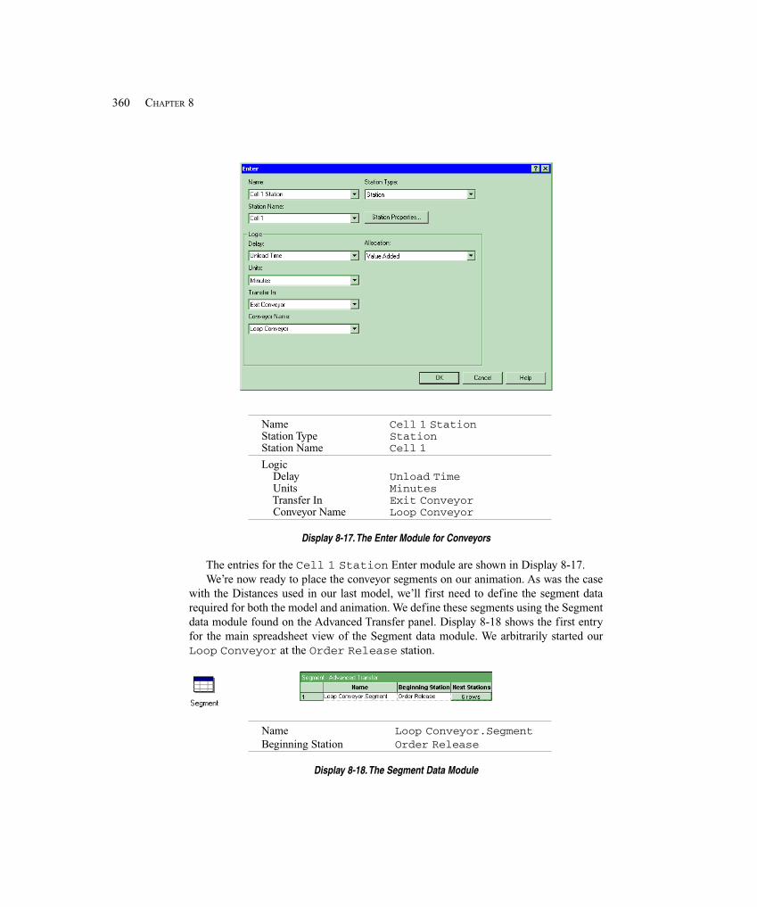
360 CHAPTER 8
Name Cell 1 StationStation Type StationStation Name Cell 1
Logic Delay Unload Time Units Minutes Transfer In Exit Conveyor Conveyor Name Loop Conveyor
Display 8-17. The Enter Module for Conveyors
The entries for the Cell 1 Station Enter module are shown in Display 8-17.We’re now ready to place the conveyor segments on our animation. As was the case
with the Distances used in our last model, we’ll first need to define the segment datarequired for both the model and animation. We define these segments using the Segmentdata module found on the Advanced Transfer panel. Display 8-18 shows the first entryfor the main spreadsheet view of the Segment data module. We arbitrarily started ourLoop Conveyor at the Order Release station.
Name Loop Conveyor.SegmentBeginning Station Order Release
Display 8-18. The Segment Data Module
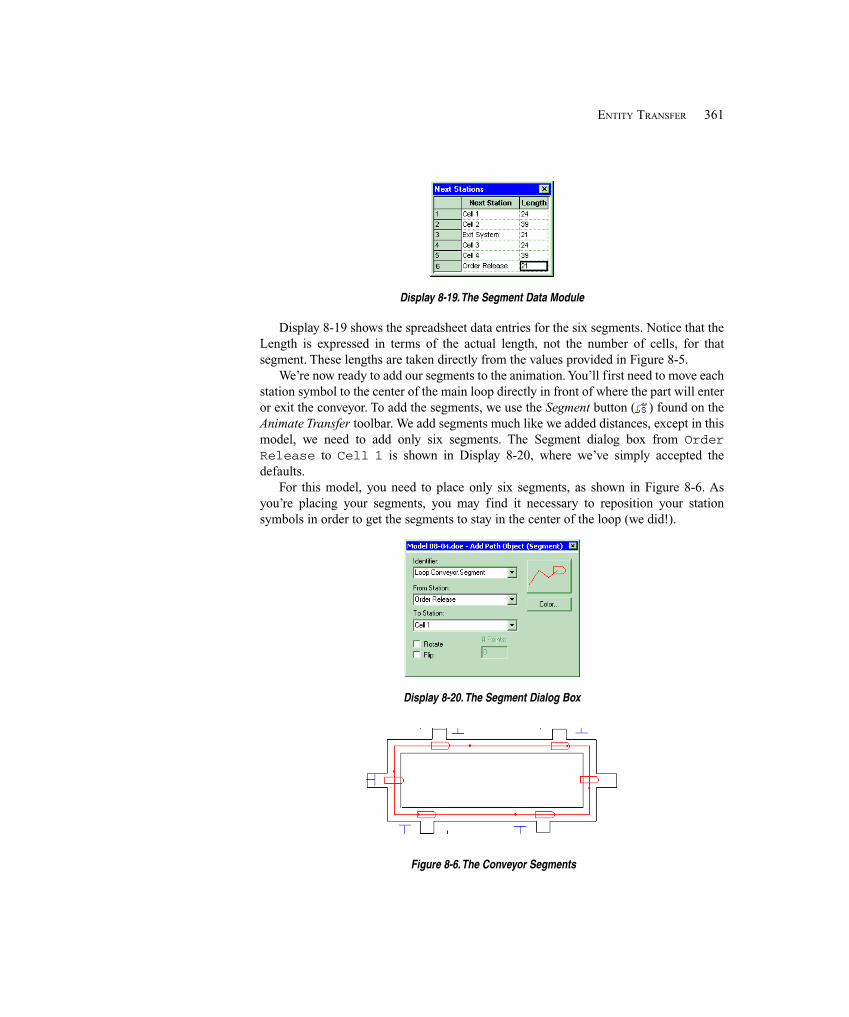
361ENTITY TRANSFER
Display 8-19. The Segment Data Module
Display 8-19 shows the spreadsheet data entries for the six segments. Notice that theLength is expressed in terms of the actual length, not the number of cells, for thatsegment. These lengths are taken directly from the values provided in Figure 8-5.
We’re now ready to add our segments to the animation. You’ll first need to move eachstation symbol to the center of the main loop directly in front of where the part will enteror exit the conveyor. To add the segments, we use the Segment button ( ) found on theAnimate Transfer toolbar. We add segments much like we added distances, except in thismodel, we need to add only six segments. The Segment dialog box from OrderRelease to Cell 1 is shown in Display 8-20, where we’ve simply accepted thedefaults.
For this model, you need to place only six segments, as shown in Figure 8-6. Asyou’re placing your segments, you may find it necessary to reposition your stationsymbols in order to get the segments to stay in the center of the loop (we did!).
Display 8-20. The Segment Dialog Box
Figure 8-6. The Conveyor Segments
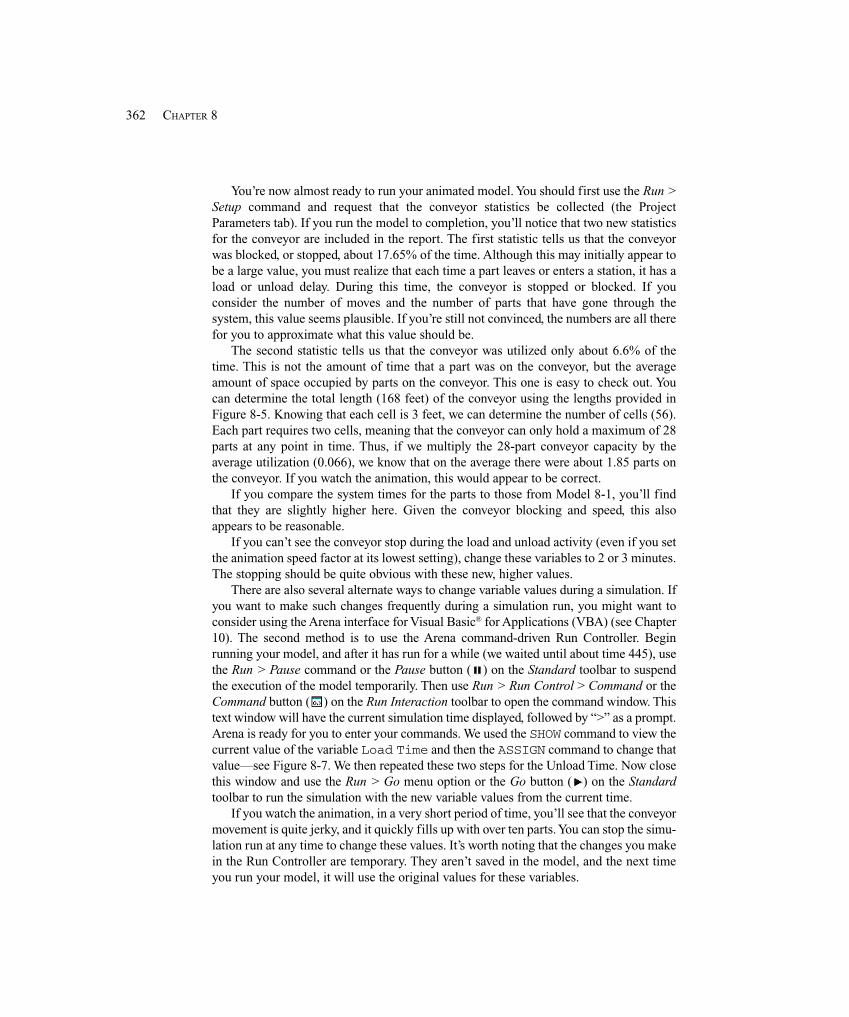
362 CHAPTER 8
You’re now almost ready to run your animated model. You should first use the Run >Setup command and request that the conveyor statistics be collected (the ProjectParameters tab). If you run the model to completion, you’ll notice that two new statisticsfor the conveyor are included in the report. The first statistic tells us that the conveyorwas blocked, or stopped, about 17.65% of the time. Although this may initially appear tobe a large value, you must realize that each time a part leaves or enters a station, it has aload or unload delay. During this time, the conveyor is stopped or blocked. If youconsider the number of moves and the number of parts that have gone through thesystem, this value seems plausible. If you’re still not convinced, the numbers are all therefor you to approximate what this value should be.
The second statistic tells us that the conveyor was utilized only about 6.6% of thetime. This is not the amount of time that a part was on the conveyor, but the averageamount of space occupied by parts on the conveyor. This one is easy to check out. Youcan determine the total length (168 feet) of the conveyor using the lengths provided inFigure 8-5. Knowing that each cell is 3 feet, we can determine the number of cells (56).Each part requires two cells, meaning that the conveyor can only hold a maximum of 28parts at any point in time. Thus, if we multiply the 28-part conveyor capacity by theaverage utilization (0.066), we know that on the average there were about 1.85 parts onthe conveyor. If you watch the animation, this would appear to be correct.
If you compare the system times for the parts to those from Model 8-1, you’ll findthat they are slightly higher here. Given the conveyor blocking and speed, this alsoappears to be reasonable.
If you can’t see the conveyor stop during the load and unload activity (even if you setthe animation speed factor at its lowest setting), change these variables to 2 or 3 minutes.The stopping should be quite obvious with these new, higher values.
There are also several alternate ways to change variable values during a simulation. Ifyou want to make such changes frequently during a simulation run, you might want toconsider using the Arena interface for Visual Basic® for Applications (VBA) (see Chapter10). The second method is to use the Arena command-driven Run Controller. Beginrunning your model, and after it has run for a while (we waited until about time 445), usethe Run > Pause command or the Pause button ( ) on the Standard toolbar to suspendthe execution of the model temporarily. Then use Run > Run Control > Command or theCommand button ( ) on the Run Interaction toolbar to open the command window. Thistext window will have the current simulation time displayed, followed by “>” as a prompt.Arena is ready for you to enter your commands. We used the SHOW command to view thecurrent value of the variable Load Time and then the ASSIGN command to change thatvalue—see Figure 8-7. We then repeated these two steps for the Unload Time. Now closethis window and use the Run > Go menu option or the Go button ( ) on the Standardtoolbar to run the simulation with the new variable values from the current time.
If you watch the animation, in a very short period of time, you’ll see that the conveyormovement is quite jerky, and it quickly fills up with over ten parts. You can stop the simu-lation run at any time to change these values. It’s worth noting that the changes you makein the Run Controller are temporary. They aren’t saved in the model, and the next timeyou run your model, it will use the original values for these variables.
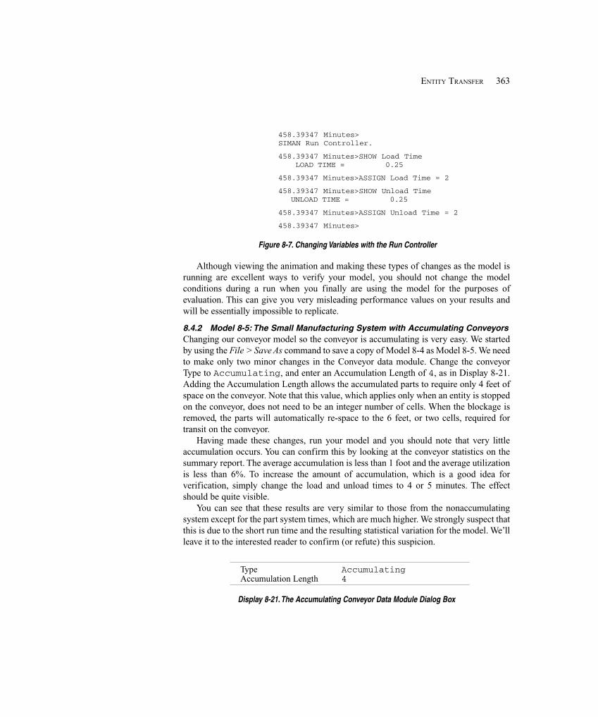
363ENTITY TRANSFER
458.39347 Minutes>SIMAN Run Controller.
458.39347 Minutes>SHOW Load Time LOAD TIME = 0.25
458.39347 Minutes>ASSIGN Load Time = 2
458.39347 Minutes>SHOW Unload TimeUNLOAD TIME = 0.25
458.39347 Minutes>ASSIGN Unload Time = 2
458.39347 Minutes>
Figure 8-7. Changing Variables with the Run Controller
Although viewing the animation and making these types of changes as the model isrunning are excellent ways to verify your model, you should not change the modelconditions during a run when you finally are using the model for the purposes ofevaluation. This can give you very misleading performance values on your results andwill be essentially impossible to replicate.
8.4.2 Model 8-5: The Small Manufacturing System with Accumulating ConveyorsChanging our conveyor model so the conveyor is accumulating is very easy. We startedby using the File > Save As command to save a copy of Model 8-4 as Model 8-5. We needto make only two minor changes in the Conveyor data module. Change the conveyorType to Accumulating, and enter an Accumulation Length of 4, as in Display 8-21.Adding the Accumulation Length allows the accumulated parts to require only 4 feet ofspace on the conveyor. Note that this value, which applies only when an entity is stoppedon the conveyor, does not need to be an integer number of cells. When the blockage isremoved, the parts will automatically re-space to the 6 feet, or two cells, required fortransit on the conveyor.
Having made these changes, run your model and you should note that very littleaccumulation occurs. You can confirm this by looking at the conveyor statistics on thesummary report. The average accumulation is less than 1 foot and the average utilizationis less than 6%. To increase the amount of accumulation, which is a good idea forverification, simply change the load and unload times to 4 or 5 minutes. The effectshould be quite visible.
You can see that these results are very similar to those from the nonaccumulatingsystem except for the part system times, which are much higher. We strongly suspect thatthis is due to the short run time and the resulting statistical variation for the model. We’llleave it to the interested reader to confirm (or refute) this suspicion.
Type AccumulatingAccumulation Length 4
Display 8-21. The Accumulating Conveyor Data Module Dialog Box
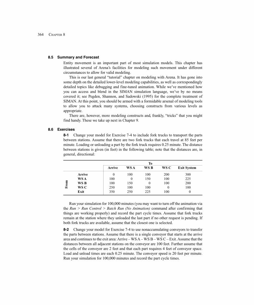
364 CHAPTER 8
8.5 Summary and Forecast
Entity movement is an important part of most simulation models. This chapter hasillustrated several of Arena’s facilities for modeling such movement under differentcircumstances to allow for valid modeling.
This is our last general “tutorial” chapter on modeling with Arena. It has gone intosome depth on the detailed lower-level modeling capabilities, as well as correspondinglydetailed topics like debugging and fine-tuned animation. While we’ve mentioned howyou can access and blend in the SIMAN simulation language, we’ve by no meanscovered it; see Pegden, Shannon, and Sadowski (1995) for the complete treatment ofSIMAN. At this point, you should be armed with a formidable arsenal of modeling toolsto allow you to attack many systems, choosing constructs from various levels asappropriate.
There are, however, more modeling constructs and, frankly, “tricks” that you mightfind handy. These we take up next in Chapter 9.
8.6 Exercises
8-1 Change your model for Exercise 7-4 to include fork trucks to transport the partsbetween stations. Assume that there are two fork trucks that each travel at 85 feet perminute. Loading or unloading a part by the fork truck requires 0.25 minute. The distancebetween stations is given (in feet) in the following table; note that the distances are, ingeneral, directional:
ToArrive WS A WS B WS C Exit System
Arrive 0 100 100 200 300WS A 100 0 150 100 225WS B 100 150 0 100 200WS C 250 100 100 0 100Exit 350 250 225 100 0
Run your simulation for 100,000 minutes (you may want to turn off the animation viathe Run > Run Control > Batch Run (No Animation) command after confirming thatthings are working properly) and record the part cycle times. Assume that fork trucksremain at the station where they unloaded the last part if no other request is pending. Ifboth fork trucks are available, assume that the closest one is selected.
8-2 Change your model for Exercise 7-4 to use nonaccumulating conveyors to transferthe parts between stations. Assume that there is a single conveyor that starts at the arrivearea and continues to the exit area: Arrive – WS A – WS B – WS C – Exit. Assume that thedistances between all adjacent stations on the conveyor are 100 feet. Further assume thatthe cells of the conveyor are 2 feet and that each part requires 4 feet of conveyor space.Load and unload times are each 0.25 minute. The conveyor speed is 20 feet per minute.Run your simulation for 100,000 minutes and record the part cycle times.
Fro
m
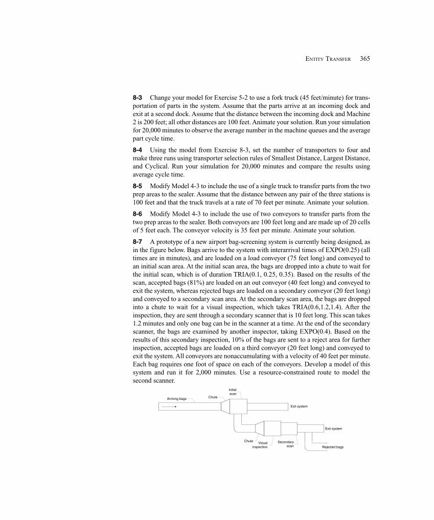
365ENTITY TRANSFER
8-3 Change your model for Exercise 5-2 to use a fork truck (45 feet/minute) for trans-portation of parts in the system. Assume that the parts arrive at an incoming dock andexit at a second dock. Assume that the distance between the incoming dock and Machine2 is 200 feet; all other distances are 100 feet. Animate your solution. Run your simulationfor 20,000 minutes to observe the average number in the machine queues and the averagepart cycle time.
8-4 Using the model from Exercise 8-3, set the number of transporters to four andmake three runs using transporter selection rules of Smallest Distance, Largest Distance,and Cyclical. Run your simulation for 20,000 minutes and compare the results usingaverage cycle time.
8-5 Modify Model 4-3 to include the use of a single truck to transfer parts from the twoprep areas to the sealer. Assume that the distance between any pair of the three stations is100 feet and that the truck travels at a rate of 70 feet per minute. Animate your solution.
8-6 Modify Model 4-3 to include the use of two conveyors to transfer parts from thetwo prep areas to the sealer. Both conveyors are 100 feet long and are made up of 20 cellsof 5 feet each. The conveyor velocity is 35 feet per minute. Animate your solution.
8-7 A prototype of a new airport bag-screening system is currently being designed, asin the figure below. Bags arrive to the system with interarrival times of EXPO(0.25) (alltimes are in minutes), and are loaded on a load conveyor (75 feet long) and conveyed toan initial scan area. At the initial scan area, the bags are dropped into a chute to wait forthe initial scan, which is of duration TRIA(0.1, 0.25, 0.35). Based on the results of thescan, accepted bags (81%) are loaded on an out conveyor (40 feet long) and conveyed toexit the system, whereas rejected bags are loaded on a secondary conveyor (20 feet long)and conveyed to a secondary scan area. At the secondary scan area, the bags are droppedinto a chute to wait for a visual inspection, which takes TRIA(0.6,1.2,1.4). After theinspection, they are sent through a secondary scanner that is 10 feet long. This scan takes1.2 minutes and only one bag can be in the scanner at a time. At the end of the secondaryscanner, the bags are examined by another inspector, taking EXPO(0.4). Based on theresults of this secondary inspection, 10% of the bags are sent to a reject area for furtherinspection, accepted bags are loaded on a third conveyor (20 feet long) and conveyed toexit the system. All conveyors are nonaccumulating with a velocity of 40 feet per minute.Each bag requires one foot of space on each of the conveyors. Develop a model of thissystem and run it for 2,000 minutes. Use a resource-constrained route to model thesecond scanner.
Visualinspection
Secondaryscan
Chute
Chute
Initialscan
Arriving bags
Exit system
Rejected bags
Exit system
366 CHAPTER 8
The current design calls for a chute capacity of 20 at the initial scan area and a totalcapacity of 25 at the secondary scan area, not including the bag undergoing the visualinspection. What percent of the time would you expect this capacity be exceeded? (Workthis exercise with infinite chute capacities, and just watch the percent of time the chutecapacities contemplated above would be exceeded if they were put into effect.) HINT:Add two time-persistent statistics to collect this information using logical expressionsthat evaluate to zero if the number of bags is less than the capacity, and to one if thecapacity is exceeded.
8-8 Develop a model of a cross-dock system that groups and transfers material forfurther shipment. This facility has five incoming docks and three outgoing docks. Trucksarrive at each of the incoming docks with loads of material on pallets. The interarrivaltime is UNIF(30, 60) between truck arrivals on each incoming dock (all times are inminutes). Each truck will have a number of pallets drawn from a UNIF(10, 22)distribution (round to the nearest integer) that need to be transferred to one of theoutgoing docks. Assume an equal probability of any incoming pallet going to any of thethree outgoing docks. When trucks arrive, an automatic unloading device unloads thepallets at the incoming dock. Assume that this requires no time, so the pallets areimmediately ready for transfer. The pallets are transferred by one of five fork trucks tothe outgoing docks, which are located on the other side of the building. The distancebetween any incoming dock and any outgoing dock is 80 feet, and the fork trucks travelat 75 feet per minute. The time for a fork truck to load a pallet is UNIF(0.3, 0.4) and tounload a pallet is UNIF(0.2, 0.4). The performance measure of interest is the averagetime a pallet spends in the system. (HINT: If you place all fork trucks at the outgoingdocks for their initial position, you don’t have to add distances between the incomingdocks.) Set the run length to be 720 minutes and regard this as a terminating simulation.Develop a model for each of the following two cases, and animate your models:
(a) Assume the priority is such that you want to transfer the pallets that have beenwaiting the longest. (HINT: Enter the name of the attribute with the arrival timein the priority box of the Transfer Out dialog box.)
(b) Because we want to be assured that an incoming truck can always unload,modify your model from part (a) above so that the pick-up priority is placed onthe incoming dock with the most pallets. (HINT: Develop an expression usingNQ for the priority field.)
Which of the above two options would appear to be “best”? Be sure to justify yourconclusions with a valid statistical analysis. Furthermore, for each option, study theeffect of having more fork trucks (up to seven); again, be aware of the gap in credibilitythat results from an inadequate statistical analysis.
8-9 A military ground force maintains a forward position and a rear depot 22 miles awayto supply it. There is a single commodity that is consumed at the forward position andresupplied to it from the rear supply depot; the commodity could be anything (ammuni-tion, fuel, food, etc.). Initially, there are 28 units of supply at the forward position (the
367ENTITY TRANSFER
commodity is in integer-valued units). Demands occur through time at the forward posi-tion, with inter-demand times being exponentially distributed with mean one hour; thefirst demand occurs not at time zero, but after one of these inter-demand times after timezero. When a demand occurs at the forward position it is for 1, 2, 3, ..., 10 units of thecommodity with respective probabilities 0.05, 0.07, 0.11, 0.04, 0.14, 0.13, 0.25, 0.03,0.13, and 0.05. After the demand occurs, if the forward supply is still more than s, noth-ing is done about replenishing; s is a fixed parameter of the model, and assume that it hasa value of 15. However, if the forward supply after the demand occurs is s or below, areorder message is sent to the rear supply depot immediately after the time of the demand.(By the way, the supply level at the forward position could become negative, representinga backorder that will be satisfied later by future resupply.) The amount ordered is
S — current forward supply
—
total amount of resupply on order from previous orders but not yet delivered to the forward position
where S is a fixed constant, equal to 45. The rear depot has a single clerk that processesorders in TRIA(30, 45, 90) minutes, and orders form a FIFO queue for this clerk. Next, atruck is requested to transport the order to the forward position; there are two trucks,each of which can carry only one order at a time regardless of the order’s size, and ordersform a FIFO queue for a truck. It takes between 10 and 20 minutes (uniformly distrib-uted) to load an order onto a truck. The trucks travel at 35 miles per hour in each direc-tion. When the truck arrives to the forward position, it takes between 5 and 10 minutes(uniformly distributed) to unload the truck, then the resupply occurs by incrementing theforward supply by the size of this order, and the amount on order is decremented by thesize of this order. The simulation is to run for 30 round-the-clock days. Make a plot ofthe forward supply as a function of time, similar to that of Model 5-4, with red versusblack curves; also animate truck movements, queues, and resources. Get the average ofthe forward-supply level. Also, collect the percent of time that there is nothing physicallyon hand at the forward supply; i.e., when the forward-supply level is zero or negative.Make 25 replications, and comment on the results. (HINTS: Depending on how you dothis, you made need a “fudge” factor consisting of a small delay to break a time tie prop-erly between two simultaneous events involved in placing an order. Also, you may wantto look at the Separate module in the Basic Process panel, which can “clone” an entity.)

368 CHAPTER 8
369A SAMPLER OF FURTHER MODELING ISSUES AND TECHNIQUES
CHAPTER 9
A Sampler of Further ModelingIssues and Techniques
In Chapters 4-8, we gave you a reasonably comprehensive tour of how to model differentkinds of systems by means of a sequence of progressively more complicated examples.We chose these examples with several goals in mind, including reality and importance(in our experience) of the application, illustration of various modeling issues, and indica-tion of how you can get Arena to represent things the way you want—in many cases,fairly easily and quickly. Armed with these skills, you’ll be able to build a rich variety ofvalid and effective simulation models.
But no reasonable set of digestible examples could possibly fathom all the nooks andcrannies of the kinds of modeling issues (and, yes, tricks) that people sometimes need toconsider, much less all of the features of Arena. And don’t worry, we’re not going toattempt that in this chapter either. But we would like to point out some of what weconsider to be the more important additional modeling issues and techniques (and tricks)and tell you how to get Arena to perform them for you.
We’ll do this by constructing more examples, but these will be more focused towardspecific modeling techniques and Arena features, so will be smaller in scope. In Section9.1, we’ll refine the conveyor models we developed in Chapter 8; in Section 9.2, we’lldiscuss a few more modeling refinements to the transporters from Chapter 8. In servicesystems, especially those involving humans standing around in line, there is oftenconsideration given to customer reneging (in other words, jumping out of line at somepoint); this is taken up in Section 9.3, along with the concept of balking. Section 9.4 goesinto methods (beyond the queues you’ve already seen) for holding entities at some point,as well as batching them together with the possibility of taking the batch apart later. InSection 9.5, we’ll discuss how to represent a tightly coupled system in which entitieshave to be allocated resources downstream from their present position before they canmove on; this is called overlapping resources from the entity viewpoint. Finally, Section9.6 briefly mentions a few other specific topics, including guided transporters, parallelqueues, and the possibility of complex decision logic and looping.
This chapter is structured differently from the earlier ones in that the sections are notnecessarily meant to be read through in sequence. Rather, it is intended to provide asampler of modeling techniques and Arena features that we’ve found useful in a varietyof applied projects.
9.1 Modeling Conveyors Using the Advanced Transfer PanelIn this section, we indicate some refinements to the basic conveyor models described inChapter 8.
370 CHAPTER 9
9.1.1 Model 9-1: Finite Buffers at StationsIn Chapter 8, we introduced you to Arena conveyors. In Section 8.4.1, we developed amodel, Model 8-4, for our small manufacturing system using nonaccumulating conveyorsas the method for transferring parts within our system. In developing that model, weassumed that there was an infinite buffer in front of each cell for the storage of partswaiting to be processed. This assumption allowed us to use the conveyor capabilitiesfound in the Enter and Leave modules. We did, however, need to add the Conveyor andSegment data modules from the Advanced Transfer panel to define our conveyor.
Now let’s modify that assumption and assume that there is limited space at Cells 1and 2 for the storage of unprocessed parts. In fact, let’s assume that there is only room forone unprocessed part at each cell. For this type of model, we need to define whathappens to a part that arrives at Cell 1 or 2 and finds that there is already a part occupyingthe limited buffer space. Assuming that we could determine a way to limit the bufferusing the Enter module (it can’t be done), it would be tempting simply to let the arrivingpart wait until the part already in the buffer is moved to the machine in that cell. Ofcourse, this could cause a significant logjam at these cells. Not only would parts not beable to enter the cell, but parts on their way to other cells would queue up behind themcreating yet another problem. It turns out that processed parts trying to leave the cellneed to access space on the conveyor before they can be conveyed to their nextdestination station. Yes, the space they’re trying to access is the same space occupied bythe part waiting to enter the cell. This would create what’s sometimes called a deadlockor gridlock.
So let’s use the following strategy for parts arriving at Cell 1 or 2. If there is not a partcurrently waiting in the buffer for the cell, the arriving part is allowed to enter the buffer.Otherwise, the arriving part is conveyed around the loop conveyor back to the same pointto try a second (or third, or fourth, etc.) time. To do this, we need to alter our model so wecan better control when the part exits the conveyor. The Advanced Transfer panelprovides five new modules for conveyors (Access, Convey, Exit, Start, and Stop) thatallow us to model conveyor activities at a more detailed level. The Exit module causes anentity to exit a conveyor, releasing the conveyor cell(s) it occupied. This is essentiallywhat happens when you select the Exit Conveyor option in the Transfer In dialog box ofthe Enter module. The Access module causes an entity to request or access space on aconveyor at a specific location, normally its current station location. The Convey moduleis used to convey the entity to its destination once it has successfully accessed therequired conveyor space. You are essentially requesting that Arena Access and Convey anentity when you select the Access Conveyor option in the Transfer Out dialog box of theLeave modules. The Start and Stop modules cause the conveyor to start and stop itsmovement, respectively. These two modules can be used to develop your own failurelogic or generally control when the conveyor is idle or running.
To develop our new model, we will start with Model 8-4 and replace the Enter andLeave modules for Cell 1 with our new modules, as shown in Figure 9-1.
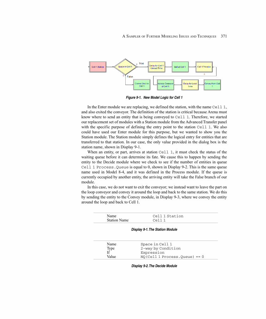
371A SAMPLER OF FURTHER MODELING ISSUES AND TECHNIQUES
Figure 9-1. New Model Logic for Cell 1
In the Enter module we are replacing, we defined the station, with the name Cell 1,and also exited the conveyor. The definition of the station is critical because Arena mustknow where to send an entity that is being conveyed to Cell 1. Therefore, we startedour replacement set of modules with a Station module from the Advanced Transfer panelwith the specific purpose of defining the entry point to the station Cell 1. We alsocould have used our Enter module for this purpose, but we wanted to show you theStation module. The Station module simply defines the logical entry for entities that aretransferred to that station. In our case, the only value provided in the dialog box is thestation name, shown in Display 9-1.
When an entity, or part, arrives at station Cell 1, it must check the status of thewaiting queue before it can determine its fate. We cause this to happen by sending theentity to the Decide module where we check to see if the number of entities in queueCell 1 Process.Queue is equal to 0, shown in Display 9-2. This is the same queuename used in Model 8-4, and it was defined in the Process module. If the queue iscurrently occupied by another entity, the arriving entity will take the False branch of ourmodule.
In this case, we do not want to exit the conveyor; we instead want to leave the part onthe loop conveyor and convey it around the loop and back to the same station. We do thisby sending the entity to the Convey module, in Display 9-3, where we convey the entityaround the loop and back to Cell 1.
Name Cell 1 StationStation Name Cell 1
Display 9-1. The Station Module
Name Space in Cell 1Type 2-way by ConditionIf ExpressionValue NQ(Cell 1 Process.Queue) == 0
Display 9-2. The Decide Module
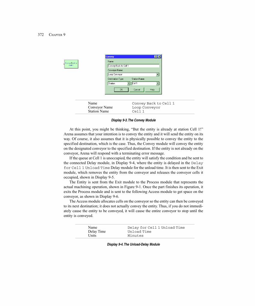
372 CHAPTER 9
Name Convey Back to Cell 1Conveyor Name Loop ConveyorStation Name Cell 1
Display 9-3. The Convey Module
At this point, you might be thinking, “But the entity is already at station Cell 1!”Arena assumes that your intention is to convey the entity and it will send the entity on itsway. Of course, it also assumes that it is physically possible to convey the entity to thespecified destination, which is the case. Thus, the Convey module will convey the entityon the designated conveyor to the specified destination. If the entity is not already on theconveyor, Arena will respond with a terminating error message.
If the queue at Cell 1 is unoccupied, the entity will satisfy the condition and be sent tothe connected Delay module, in Display 9-4, where the entity is delayed in the Delayfor Cell 1 Unload Time Delay module for the unload time. It is then sent to the Exitmodule, which removes the entity from the conveyor and releases the conveyor cells itoccupied, shown in Display 9-5.
The Entity is sent from the Exit module to the Process module that represents theactual machining operation, shown in Figure 9-1. Once the part finishes its operation, itexits the Process module and is sent to the following Access module to get space on theconveyor, as shown in Display 9-6.
The Access module allocates cells on the conveyor so the entity can then be conveyedto its next destination; it does not actually convey the entity. Thus, if you do not immedi-ately cause the entity to be conveyed, it will cause the entire conveyor to stop until theentity is conveyed.
Name Delay for Cell 1 Unload TimeDelay Time Unload TimeUnits Minutes
Display 9-4. The Unload-Delay Module
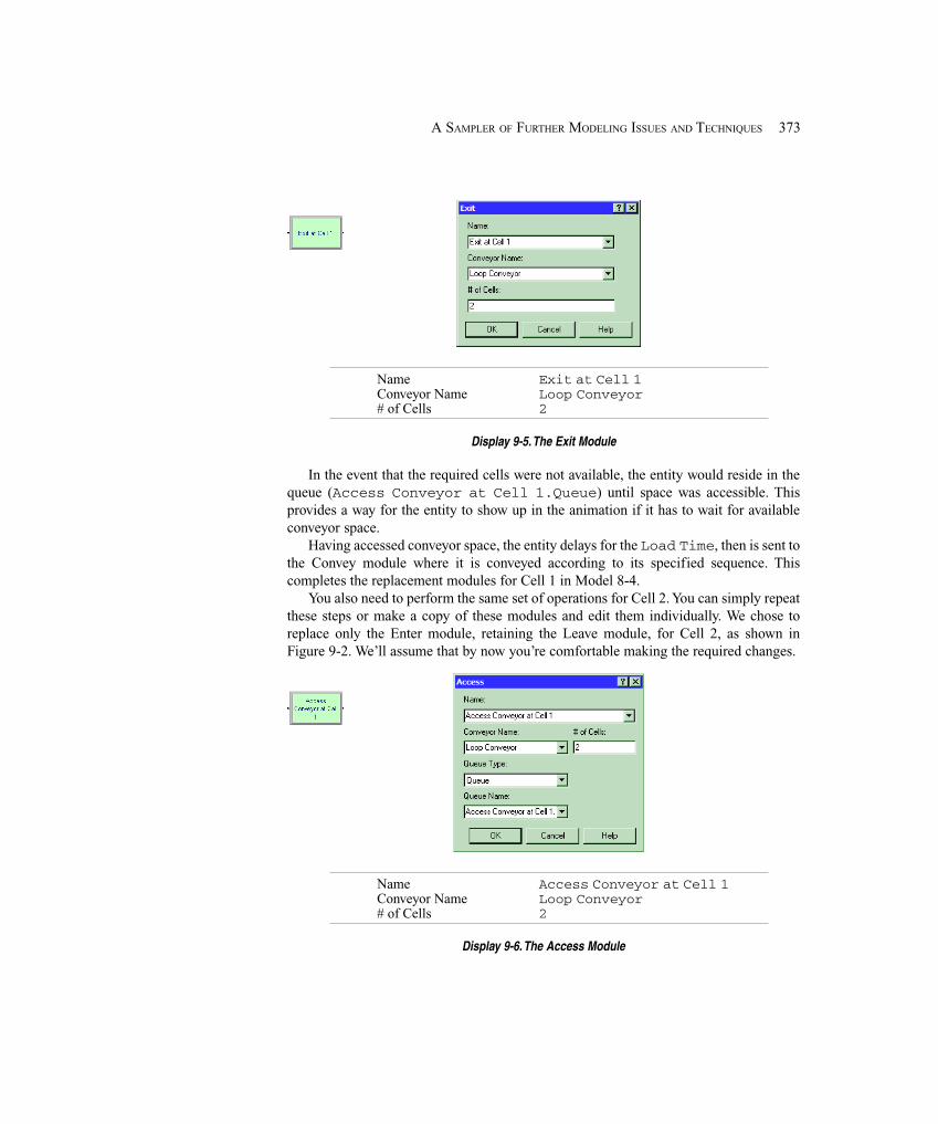
373A SAMPLER OF FURTHER MODELING ISSUES AND TECHNIQUES
Name Exit at Cell 1Conveyor Name Loop Conveyor# of Cells 2
Display 9-5. The Exit Module
In the event that the required cells were not available, the entity would reside in thequeue (Access Conveyor at Cell 1.Queue) until space was accessible. Thisprovides a way for the entity to show up in the animation if it has to wait for availableconveyor space.
Having accessed conveyor space, the entity delays for the Load Time, then is sent tothe Convey module where it is conveyed according to its specified sequence. Thiscompletes the replacement modules for Cell 1 in Model 8-4.
You also need to perform the same set of operations for Cell 2. You can simply repeatthese steps or make a copy of these modules and edit them individually. We chose toreplace only the Enter module, retaining the Leave module, for Cell 2, as shown inFigure 9-2. We’ll assume that by now you’re comfortable making the required changes.
Name Access Conveyor at Cell 1Conveyor Name Loop Conveyor# of Cells 2
Display 9-6. The Access Module
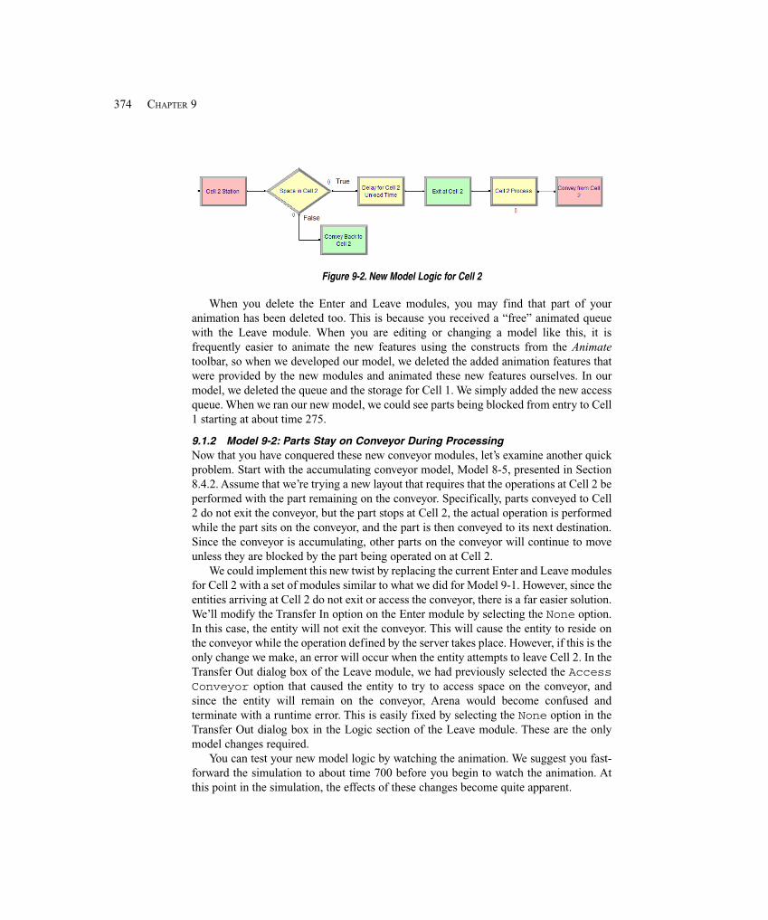
374 CHAPTER 9
Figure 9-2. New Model Logic for Cell 2
When you delete the Enter and Leave modules, you may find that part of youranimation has been deleted too. This is because you received a “free” animated queuewith the Leave module. When you are editing or changing a model like this, it isfrequently easier to animate the new features using the constructs from the Animatetoolbar, so when we developed our model, we deleted the added animation features thatwere provided by the new modules and animated these new features ourselves. In ourmodel, we deleted the queue and the storage for Cell 1. We simply added the new accessqueue. When we ran our new model, we could see parts being blocked from entry to Cell1 starting at about time 275.
9.1.2 Model 9-2: Parts Stay on Conveyor During ProcessingNow that you have conquered these new conveyor modules, let’s examine another quickproblem. Start with the accumulating conveyor model, Model 8-5, presented in Section8.4.2. Assume that we’re trying a new layout that requires that the operations at Cell 2 beperformed with the part remaining on the conveyor. Specifically, parts conveyed to Cell2 do not exit the conveyor, but the part stops at Cell 2, the actual operation is performedwhile the part sits on the conveyor, and the part is then conveyed to its next destination.Since the conveyor is accumulating, other parts on the conveyor will continue to moveunless they are blocked by the part being operated on at Cell 2.
We could implement this new twist by replacing the current Enter and Leave modulesfor Cell 2 with a set of modules similar to what we did for Model 9-1. However, since theentities arriving at Cell 2 do not exit or access the conveyor, there is a far easier solution.We’ll modify the Transfer In option on the Enter module by selecting the None option.In this case, the entity will not exit the conveyor. This will cause the entity to reside onthe conveyor while the operation defined by the server takes place. However, if this is theonly change we make, an error will occur when the entity attempts to leave Cell 2. In theTransfer Out dialog box of the Leave module, we had previously selected the AccessConveyor option that caused the entity to try to access space on the conveyor, andsince the entity will remain on the conveyor, Arena would become confused andterminate with a runtime error. This is easily fixed by selecting the None option in theTransfer Out dialog box in the Logic section of the Leave module. These are the onlymodel changes required.
You can test your new model logic by watching the animation. We suggest you fast-forward the simulation to about time 700 before you begin to watch the animation. Atthis point in the simulation, the effects of these changes become quite apparent.
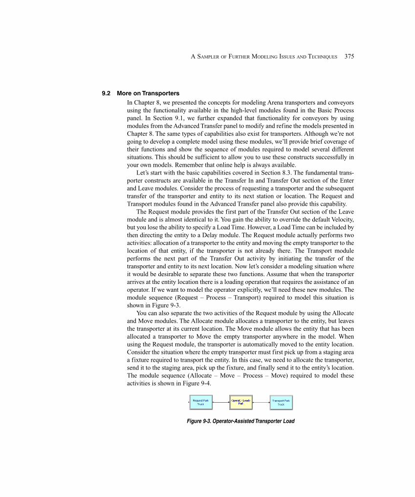
375A SAMPLER OF FURTHER MODELING ISSUES AND TECHNIQUES
9.2 More on Transporters
In Chapter 8, we presented the concepts for modeling Arena transporters and conveyorsusing the functionality available in the high-level modules found in the Basic Processpanel. In Section 9.1, we further expanded that functionality for conveyors by usingmodules from the Advanced Transfer panel to modify and refine the models presented inChapter 8. The same types of capabilities also exist for transporters. Although we’re notgoing to develop a complete model using these modules, we’ll provide brief coverage oftheir functions and show the sequence of modules required to model several differentsituations. This should be sufficient to allow you to use these constructs successfully inyour own models. Remember that online help is always available.
Let’s start with the basic capabilities covered in Section 8.3. The fundamental trans-porter constructs are available in the Transfer In and Transfer Out section of the Enterand Leave modules. Consider the process of requesting a transporter and the subsequenttransfer of the transporter and entity to its next station or location. The Request andTransport modules found in the Advanced Transfer panel also provide this capability.
The Request module provides the first part of the Transfer Out section of the Leavemodule and is almost identical to it. You gain the ability to override the default Velocity,but you lose the ability to specify a Load Time. However, a Load Time can be included bythen directing the entity to a Delay module. The Request module actually performs twoactivities: allocation of a transporter to the entity and moving the empty transporter to thelocation of that entity, if the transporter is not already there. The Transport moduleperforms the next part of the Transfer Out activity by initiating the transfer of thetransporter and entity to its next location. Now let’s consider a modeling situation whereit would be desirable to separate these two functions. Assume that when the transporterarrives at the entity location there is a loading operation that requires the assistance of anoperator. If we want to model the operator explicitly, we’ll need these new modules. Themodule sequence (Request – Process – Transport) required to model this situation isshown in Figure 9-3.
You can also separate the two activities of the Request module by using the Allocateand Move modules. The Allocate module allocates a transporter to the entity, but leavesthe transporter at its current location. The Move module allows the entity that has beenallocated a transporter to Move the empty transporter anywhere in the model. Whenusing the Request module, the transporter is automatically moved to the entity location.Consider the situation where the empty transporter must first pick up from a staging areaa fixture required to transport the entity. In this case, we need to allocate the transporter,send it to the staging area, pick up the fixture, and finally send it to the entity’s location.The module sequence (Allocate – Move – Process – Move) required to model theseactivities is shown in Figure 9-4.
Figure 9-3. Operator-Assisted Transporter Load
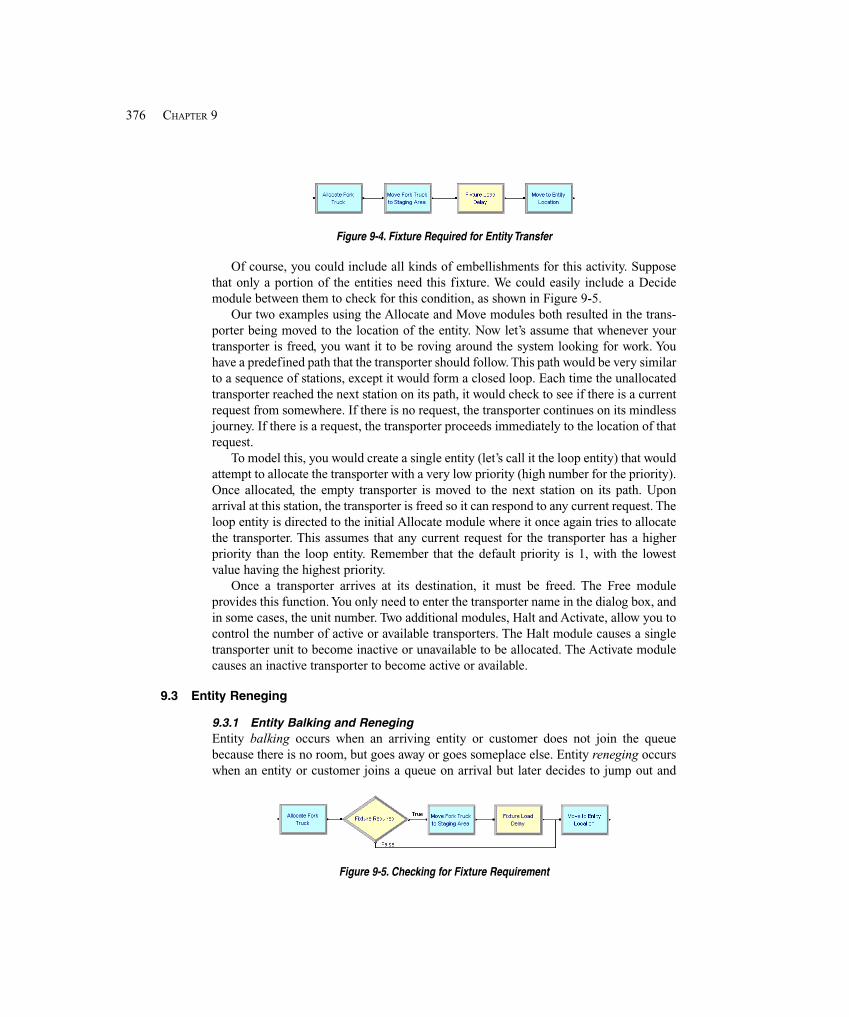
376 CHAPTER 9
Figure 9-4. Fixture Required for Entity Transfer
Of course, you could include all kinds of embellishments for this activity. Supposethat only a portion of the entities need this fixture. We could easily include a Decidemodule between them to check for this condition, as shown in Figure 9-5.
Our two examples using the Allocate and Move modules both resulted in the trans-porter being moved to the location of the entity. Now let’s assume that whenever yourtransporter is freed, you want it to be roving around the system looking for work. Youhave a predefined path that the transporter should follow. This path would be very similarto a sequence of stations, except it would form a closed loop. Each time the unallocatedtransporter reached the next station on its path, it would check to see if there is a currentrequest from somewhere. If there is no request, the transporter continues on its mindlessjourney. If there is a request, the transporter proceeds immediately to the location of thatrequest.
To model this, you would create a single entity (let’s call it the loop entity) that wouldattempt to allocate the transporter with a very low priority (high number for the priority).Once allocated, the empty transporter is moved to the next station on its path. Uponarrival at this station, the transporter is freed so it can respond to any current request. Theloop entity is directed to the initial Allocate module where it once again tries to allocatethe transporter. This assumes that any current request for the transporter has a higherpriority than the loop entity. Remember that the default priority is 1, with the lowestvalue having the highest priority.
Once a transporter arrives at its destination, it must be freed. The Free moduleprovides this function. You only need to enter the transporter name in the dialog box, andin some cases, the unit number. Two additional modules, Halt and Activate, allow you tocontrol the number of active or available transporters. The Halt module causes a singletransporter unit to become inactive or unavailable to be allocated. The Activate modulecauses an inactive transporter to become active or available.
9.3 Entity Reneging
9.3.1 Entity Balking and RenegingEntity balking occurs when an arriving entity or customer does not join the queuebecause there is no room, but goes away or goes someplace else. Entity reneging occurswhen an entity or customer joins a queue on arrival but later decides to jump out and
Figure 9-5. Checking for Fixture Requirement
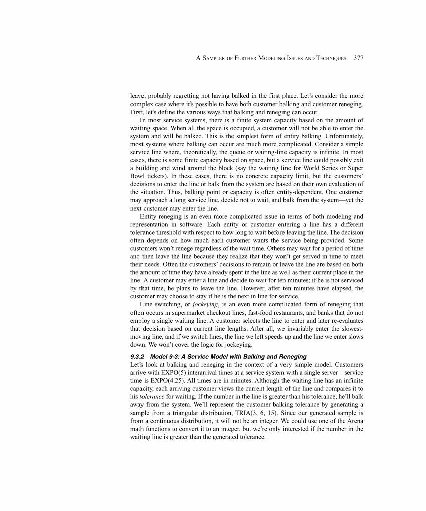
377A SAMPLER OF FURTHER MODELING ISSUES AND TECHNIQUES
leave, probably regretting not having balked in the first place. Let’s consider the morecomplex case where it’s possible to have both customer balking and customer reneging.First, let’s define the various ways that balking and reneging can occur.
In most service systems, there is a finite system capacity based on the amount ofwaiting space. When all the space is occupied, a customer will not be able to enter thesystem and will be balked. This is the simplest form of entity balking. Unfortunately,most systems where balking can occur are much more complicated. Consider a simpleservice line where, theoretically, the queue or waiting-line capacity is infinite. In mostcases, there is some finite capacity based on space, but a service line could possibly exita building and wind around the block (say the waiting line for World Series or SuperBowl tickets). In these cases, there is no concrete capacity limit, but the customers’decisions to enter the line or balk from the system are based on their own evaluation ofthe situation. Thus, balking point or capacity is often entity-dependent. One customermay approach a long service line, decide not to wait, and balk from the system—yet thenext customer may enter the line.
Entity reneging is an even more complicated issue in terms of both modeling andrepresentation in software. Each entity or customer entering a line has a differenttolerance threshold with respect to how long to wait before leaving the line. The decisionoften depends on how much each customer wants the service being provided. Somecustomers won’t renege regardless of the wait time. Others may wait for a period of timeand then leave the line because they realize that they won’t get served in time to meettheir needs. Often the customers’ decisions to remain or leave the line are based on boththe amount of time they have already spent in the line as well as their current place in theline. A customer may enter a line and decide to wait for ten minutes; if he is not servicedby that time, he plans to leave the line. However, after ten minutes have elapsed, thecustomer may choose to stay if he is the next in line for service.
Line switching, or jockeying, is an even more complicated form of reneging thatoften occurs in supermarket checkout lines, fast-food restaurants, and banks that do notemploy a single waiting line. A customer selects the line to enter and later re-evaluatesthat decision based on current line lengths. After all, we invariably enter the slowest-moving line, and if we switch lines, the line we left speeds up and the line we enter slowsdown. We won’t cover the logic for jockeying.
9.3.2 Model 9-3: A Service Model with Balking and RenegingLet’s look at balking and reneging in the context of a very simple model. Customersarrive with EXPO(5) interarrival times at a service system with a single server—servicetime is EXPO(4.25). All times are in minutes. Although the waiting line has an infinitecapacity, each arriving customer views the current length of the line and compares it tohis tolerance for waiting. If the number in the line is greater than his tolerance, he’ll balkaway from the system. We’ll represent the customer-balking tolerance by generating asample from a triangular distribution, TRIA(3, 6, 15). Since our generated sample isfrom a continuous distribution, it will not be an integer. We could use one of the Arenamath functions to convert it to an integer, but we’re only interested if the number in thewaiting line is greater than the generated tolerance.
378 CHAPTER 9
There are two ways to model the balking activity. Let’s assume that we create ourarrivals, generate our tolerance value from the triangular distribution, and assign thisvalue to an entity attribute. We could send our arrival to a Decide module and compareour sample value to the current number in the waiting line, using the Arena variable NQ.If the tolerance is less than or equal to the current number in queue, we balk the arrivalfrom the system. Otherwise, we enter the waiting line. An alternative method is to assignour tolerance to a variable and also use this same variable for the server queue capacity.We then send our arrival directly to the server. If the current number in the queue isgreater than or equal to the tolerance, which is equal to the queue capacity, the arrivalwill be balked automatically. Using the second method, it’s possible for the queuecapacity to be assigned a value less than the current number in queue. This method worksbecause Arena checks only the queue-capacity value when a new entity tries to enter thequeue. Thus, the current entities remain safely in the queue, regardless of the new queue-capacity value. We will use this second method when we develop our model.
To represent reneging, assume that arriving customers who decide not to balk arewilling to wait only a limited period of time before they renege from the queue. We willgenerate this renege tolerance time from an ERLA(15, 2) distribution (Erlang), whichhas a mean of 30, and assign it to an entity attribute in an Assign module. Modeling themechanics of the reneging activity can be a challenge. If we allow the arrival to enter thequeue and the renege time is reached, we need to be able to find the entity and remove itfrom the queue. At this point in our problem description, you might want to consideralternative methods to handle this. For example, we could define a variable that keepstrack of when the server will next be available. We generate the entity-processing timefirst and assign it to an attribute in an Assign module. We then send our entity to theDecide module where we check for balking. If the entity is not balked, we then check (inthe same Decide module) to see if the entity will begin service before its renege time. Ifnot, we renege the entity. Otherwise, we send the entity to an Assign module where weupdate our variable that tells us when the server will become available, then send theentity to the queue. This model logic may seem complicated, but can be summarized asfollows:
Define Available Time = Time in the future when server will be available
Create arrivalAssign Service TimeAssign the Time in the future the activity would renege, which is equal
to Tolerance Time + TNOWAssign Balk Limit
DecideIf Balk Limit > Number in queue
Balk entityIf Renege Time < Available Time
Renege entityElse
Assign Available Time = MX(Available Time , TNOW) + Service TimeSend entity to queue
Note the use of the “maximum” math function, MX.
379A SAMPLER OF FURTHER MODELING ISSUES AND TECHNIQUES
There is one problem with this logic that can be fixed easily—our number in queue isnot accurate because it won’t contain any entities that have not yet reneged. We can fixthis by sending our reneged entities to a Delay module where they are delayed by therenege time; we also specify a Storage (e.g., Renege_Customers). Now we change ourfirst Decide statement as follows:
If Balk Limit > Number in queue + NSTO(Renege_Customers)
We have to be careful about our statistics, but this approach will capture the renegingprocess accurately and avoid our having to alter the queue.
Let’s add one last caveat before we develop our model. Assume that the actualdecision of whether to renege is based not only on the renege time, but also on theposition of the customer in the queue. For example, customers may have reached theirrenege tolerance limit, but if they’re now at the front of the waiting line, they may justwait for service (i.e., renege on reneging). Let’s call this position in the queue where thecustomer will elect to stay, even if the customer renege time has elapsed, the customerstay zone. Thus, if the customer stay zone is 3 and the renege time for the customer hasexpired, the customer will stay in line anyway if they are one of the next three customersto be serviced.
We’ll generate this position number from a Poisson distribution, POIS(0.75). We’veused the Poisson distribution because it provides a reasonable approximation of thisprocess and also returns an integer value. For those of you with no access to Poissontables (you mean you actually sold your statistics book?), it is approximately equivalentto the following discrete empirical distribution: DISC(0.472, 0, 0.827, 1, 0.959, 2, 0.993,3, 0.999, 4, 1.0, 5). See Appendix C for more detail on this distribution.
This new decision process means that the above logic is no longer valid. We mustnow place the arriving customer in the waiting line and evaluate the reneging after therenege time has elapsed. However, if we actually go ahead and place the customer in thequeue, there’s no mechanism to detect that the renege time has elapsed. To overcome thisproblem, we’ll make a duplicate of each entity and delay it by the renege time. The origi-nal entity, which represents the actual customer, will be sent to the service queue. Afterthe renege-time delay, we’ll have the duplicate entity check the queue position of theoriginal entity. If the customer is no longer in the service queue (that is, the customer wasserved), we’ll just dispose of the duplicate entity. If the customer is still in the queue,we’ll check to see if that customer will renege. If the current queue position is within thecustomer stay zone, we’ll just dispose of the duplicate entity. Otherwise, we’ll have theduplicate entity remove the original entity from the service queue and dispose of bothitself and the original entity. This model logic is outlined as follows:
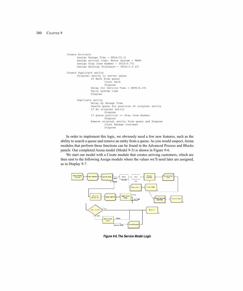
380 CHAPTER 9
Create ArrivalsAssign Renege Time = ERLA(15,2)Assign arrival time: Enter System = TNOWAssign Stay Zone Number = POIS(0.75)Assign Balking Tolerance = TRIA(3,6,15)
Create Duplicate entityOriginal entity to server queue
If Balk from queueCount balkDispose
Delay for Service Time = EXPO(4.25)Tally system timeDispose
Duplicate entityDelay by Renege TimeSearch queue for position of original entityIf No original entity
DisposeIf Queue position <= Stay Zone Number
DisposeRemove original entity from queue and Dispose
Count Renege customerDispose
In order to implement this logic, we obviously need a few new features, such as theability to search a queue and remove an entity from a queue. As you would suspect, Arenamodules that perform these functions can be found in the Advanced Process and Blockspanels. Our completed Arena model (Model 9-3) is shown in Figure 9-6.
We start our model with a Create module that creates arriving customers, which arethen sent to the following Assign module where the values we’ll need later are assigned,as in Display 9-7.
Figure 9-6. The Service Model Logic
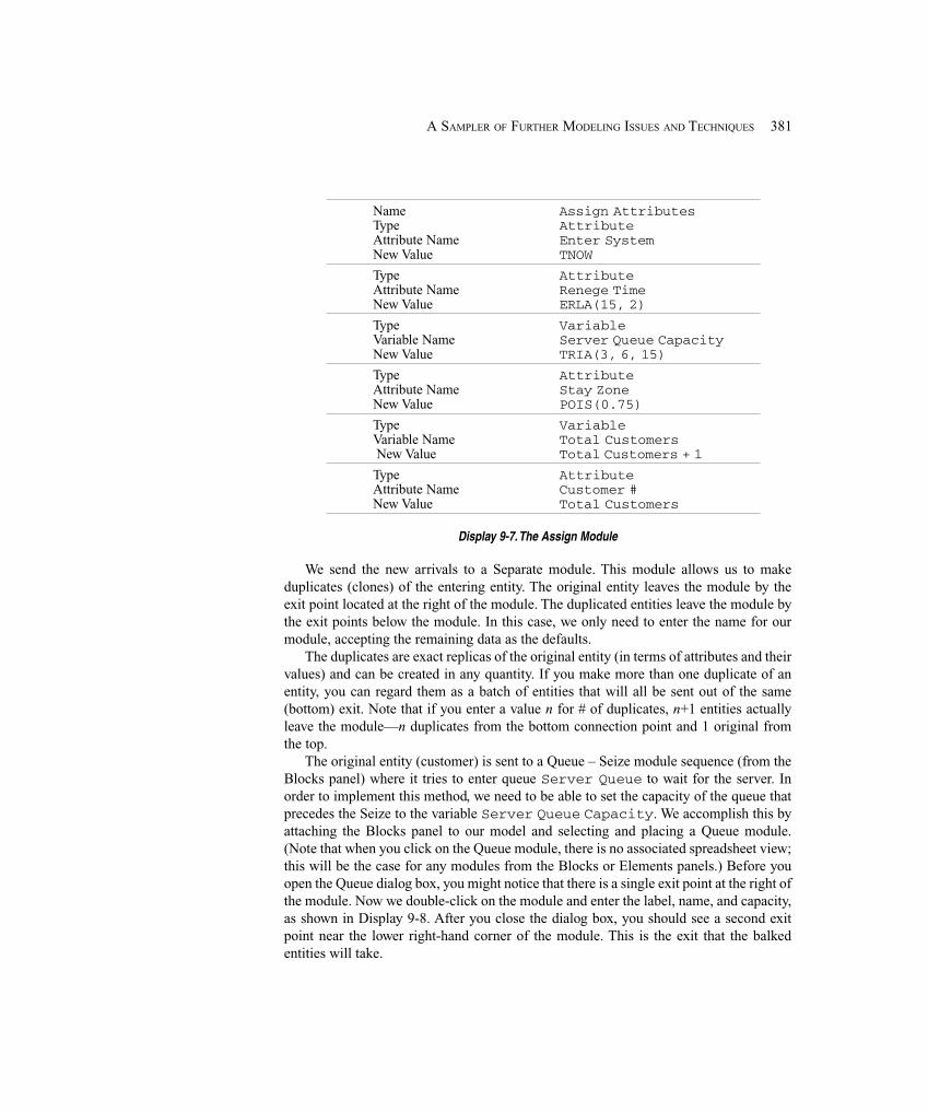
381A SAMPLER OF FURTHER MODELING ISSUES AND TECHNIQUES
Name Assign AttributesType AttributeAttribute Name Enter SystemNew Value TNOW
Type AttributeAttribute Name Renege TimeNew Value ERLA(15, 2)
Type VariableVariable Name Server Queue CapacityNew Value TRIA(3, 6, 15)
Type AttributeAttribute Name Stay ZoneNew Value POIS(0.75)
Type VariableVariable Name Total Customers New Value Total Customers + 1
Type AttributeAttribute Name Customer #New Value Total Customers
Display 9-7. The Assign Module
We send the new arrivals to a Separate module. This module allows us to makeduplicates (clones) of the entering entity. The original entity leaves the module by theexit point located at the right of the module. The duplicated entities leave the module bythe exit points below the module. In this case, we only need to enter the name for ourmodule, accepting the remaining data as the defaults.
The duplicates are exact replicas of the original entity (in terms of attributes and theirvalues) and can be created in any quantity. If you make more than one duplicate of anentity, you can regard them as a batch of entities that will all be sent out of the same(bottom) exit. Note that if you enter a value n for # of duplicates, n+1 entities actuallyleave the module—n duplicates from the bottom connection point and 1 original fromthe top.
The original entity (customer) is sent to a Queue – Seize module sequence (from theBlocks panel) where it tries to enter queue Server Queue to wait for the server. Inorder to implement this method, we need to be able to set the capacity of the queue thatprecedes the Seize to the variable Server Queue Capacity. We accomplish this byattaching the Blocks panel to our model and selecting and placing a Queue module.(Note that when you click on the Queue module, there is no associated spreadsheet view;this will be the case for any modules from the Blocks or Elements panels.) Before youopen the Queue dialog box, you might notice that there is a single exit point at the right ofthe module. Now we double-click on the module and enter the label, name, and capacity,as shown in Display 9-8. After you close the dialog box, you should see a second exitpoint near the lower right-hand corner of the module. This is the exit that the balkedentities will take.
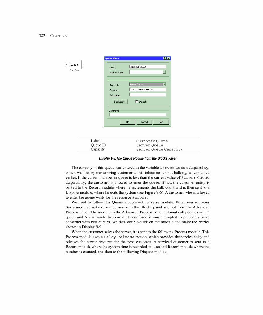
382 CHAPTER 9
Label Customer QueueQueue ID Server QueueCapacity Server Queue Capacity
Display 9-8. The Queue Module from the Blocks Panel
The capacity of this queue was entered as the variable Server Queue Capacity,which was set by our arriving customer as his tolerance for not balking, as explainedearlier. If the current number in queue is less than the current value of Server QueueCapacity, the customer is allowed to enter the queue. If not, the customer entity isbalked to the Record module where he increments the balk count and is then sent to aDispose module, where he exits the system (see Figure 9-6). A customer who is allowedto enter the queue waits for the resource Server.
We need to follow this Queue module with a Seize module. When you add yourSeize module, make sure it comes from the Blocks panel and not from the AdvancedProcess panel. The module in the Advanced Process panel automatically comes with aqueue and Arena would become quite confused if you attempted to precede a seizeconstruct with two queues. We then double-click on the module and make the entriesshown in Display 9-9.
When the customer seizes the server, it is sent to the following Process module. ThisProcess module uses a Delay Release Action, which provides the service delay andreleases the server resource for the next customer. A serviced customer is sent to aRecord module where the system time is recorded, to a second Record module where thenumber is counted, and then to the following Dispose module.
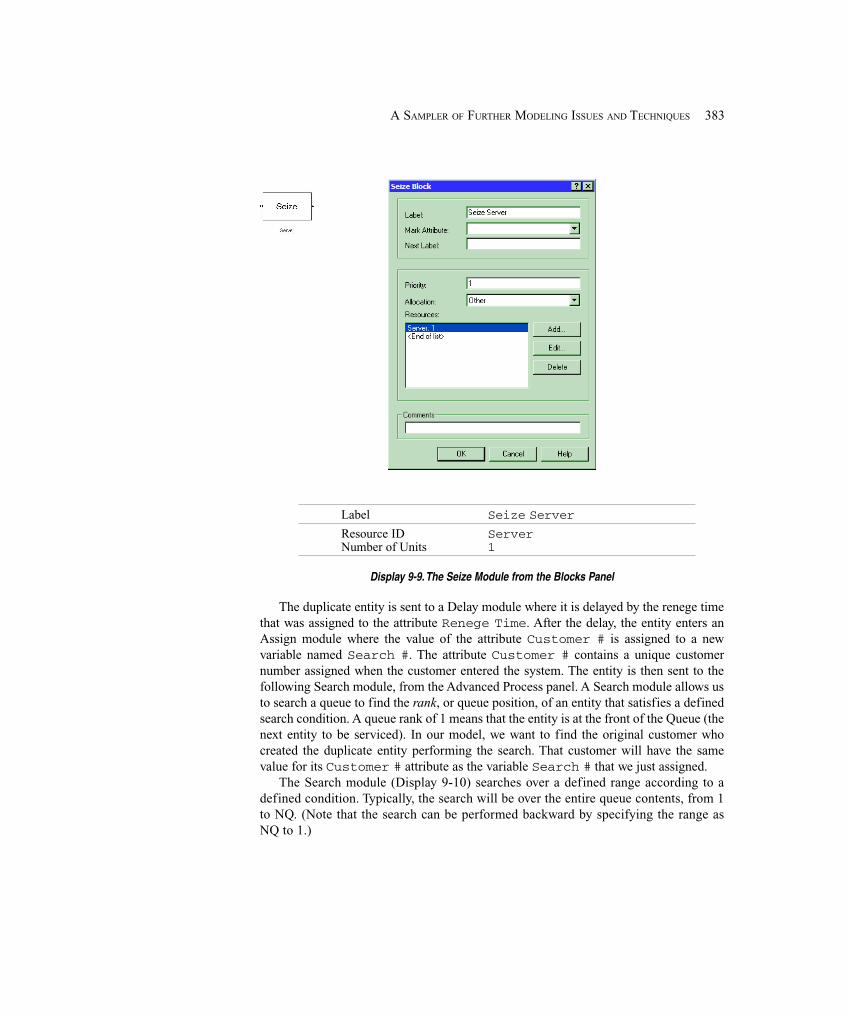
383A SAMPLER OF FURTHER MODELING ISSUES AND TECHNIQUES
Label Seize Server
Resource ID ServerNumber of Units 1
Display 9-9. The Seize Module from the Blocks Panel
The duplicate entity is sent to a Delay module where it is delayed by the renege timethat was assigned to the attribute Renege Time. After the delay, the entity enters anAssign module where the value of the attribute Customer # is assigned to a newvariable named Search #. The attribute Customer # contains a unique customernumber assigned when the customer entered the system. The entity is then sent to thefollowing Search module, from the Advanced Process panel. A Search module allows usto search a queue to find the rank, or queue position, of an entity that satisfies a definedsearch condition. A queue rank of 1 means that the entity is at the front of the Queue (thenext entity to be serviced). In our model, we want to find the original customer whocreated the duplicate entity performing the search. That customer will have the samevalue for its Customer # attribute as the variable Search # that we just assigned.
The Search module (Display 9-10) searches over a defined range according to adefined condition. Typically, the search will be over the entire queue contents, from 1to NQ. (Note that the search can be performed backward by specifying the range asNQ to 1.)
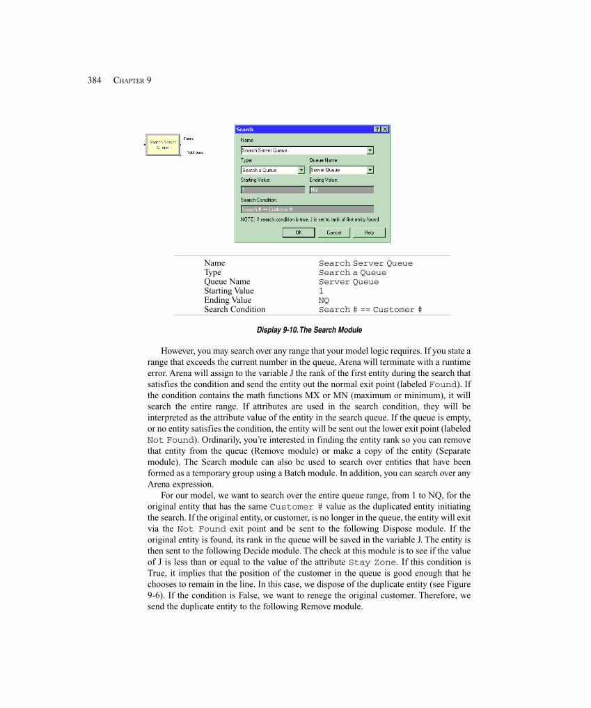
384 CHAPTER 9
Name Search Server QueueType Search a QueueQueue Name Server QueueStarting Value 1Ending Value NQSearch Condition Search # == Customer #
Display 9-10. The Search Module
However, you may search over any range that your model logic requires. If you state arange that exceeds the current number in the queue, Arena will terminate with a runtimeerror. Arena will assign to the variable J the rank of the first entity during the search thatsatisfies the condition and send the entity out the normal exit point (labeled Found). Ifthe condition contains the math functions MX or MN (maximum or minimum), it willsearch the entire range. If attributes are used in the search condition, they will beinterpreted as the attribute value of the entity in the search queue. If the queue is empty,or no entity satisfies the condition, the entity will be sent out the lower exit point (labeledNot Found). Ordinarily, you’re interested in finding the entity rank so you can removethat entity from the queue (Remove module) or make a copy of the entity (Separatemodule). The Search module can also be used to search over entities that have beenformed as a temporary group using a Batch module. In addition, you can search over anyArena expression.
For our model, we want to search over the entire queue range, from 1 to NQ, for theoriginal entity that has the same Customer # value as the duplicated entity initiatingthe search. If the original entity, or customer, is no longer in the queue, the entity will exitvia the Not Found exit point and be sent to the following Dispose module. If theoriginal entity is found, its rank in the queue will be saved in the variable J. The entity isthen sent to the following Decide module. The check at this module is to see if the valueof J is less than or equal to the value of the attribute Stay Zone. If this condition isTrue, it implies that the position of the customer in the queue is good enough that hechooses to remain in the line. In this case, we dispose of the duplicate entity (see Figure9-6). If the condition is False, we want to renege the original customer. Therefore, wesend the duplicate entity to the following Remove module.
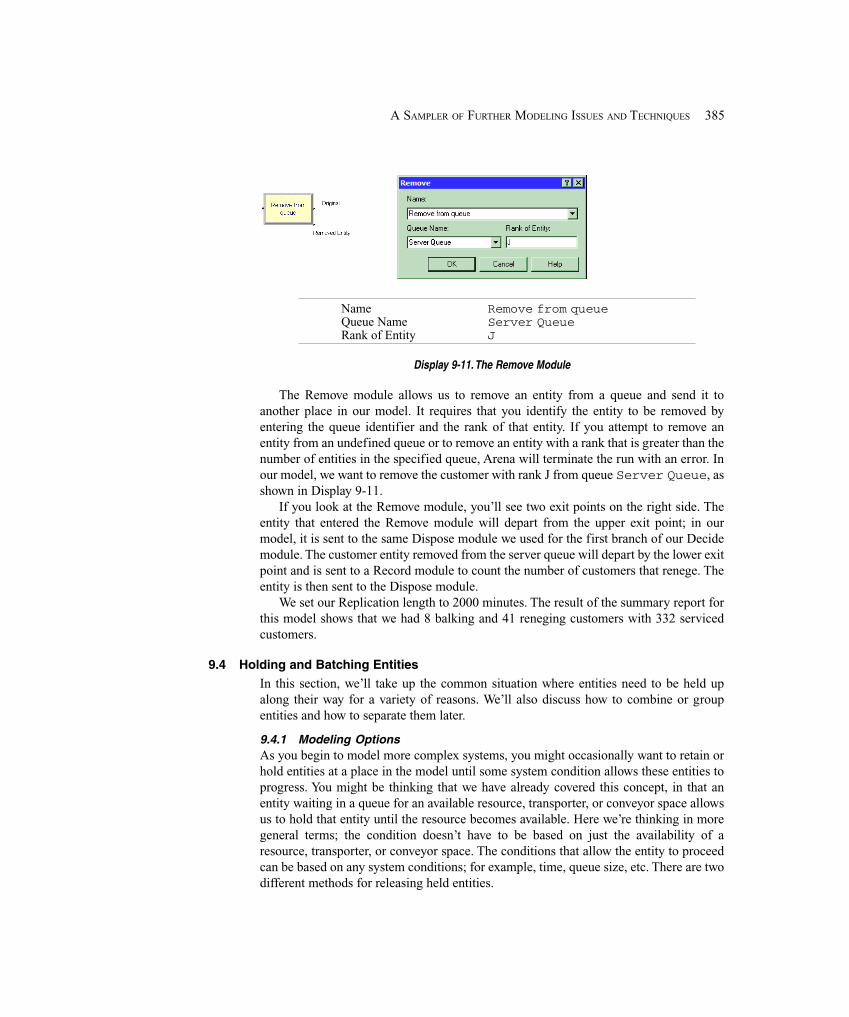
385A SAMPLER OF FURTHER MODELING ISSUES AND TECHNIQUES
Name Remove from queueQueue Name Server QueueRank of Entity J
Display 9-11. The Remove Module
The Remove module allows us to remove an entity from a queue and send it toanother place in our model. It requires that you identify the entity to be removed byentering the queue identifier and the rank of that entity. If you attempt to remove anentity from an undefined queue or to remove an entity with a rank that is greater than thenumber of entities in the specified queue, Arena will terminate the run with an error. Inour model, we want to remove the customer with rank J from queue Server Queue, asshown in Display 9-11.
If you look at the Remove module, you’ll see two exit points on the right side. Theentity that entered the Remove module will depart from the upper exit point; in ourmodel, it is sent to the same Dispose module we used for the first branch of our Decidemodule. The customer entity removed from the server queue will depart by the lower exitpoint and is sent to a Record module to count the number of customers that renege. Theentity is then sent to the Dispose module.
We set our Replication length to 2000 minutes. The result of the summary report forthis model shows that we had 8 balking and 41 reneging customers with 332 servicedcustomers.
9.4 Holding and Batching EntitiesIn this section, we’ll take up the common situation where entities need to be held upalong their way for a variety of reasons. We’ll also discuss how to combine or groupentities and how to separate them later.
9.4.1 Modeling OptionsAs you begin to model more complex systems, you might occasionally want to retain orhold entities at a place in the model until some system condition allows these entities toprogress. You might be thinking that we have already covered this concept, in that anentity waiting in a queue for an available resource, transporter, or conveyor space allowsus to hold that entity until the resource becomes available. Here we’re thinking in moregeneral terms; the condition doesn’t have to be based on just the availability of aresource, transporter, or conveyor space. The conditions that allow the entity to proceedcan be based on any system conditions; for example, time, queue size, etc. There are twodifferent methods for releasing held entities.
386 CHAPTER 9
The first method holds the entities in a queue until they receive permission or a signalto proceed from another entity in the system. For example, consider a busy intersectionwith a policeman directing traffic. Think of the cars arriving at the intersection as entitiesbeing held until they are allowed to proceed. Now think of the policeman as an entityeventually giving the waiting cars a signal to proceed. There may be ten cars waiting, butthe policeman may give only the first six permission to proceed.
The second method allows the held entities themselves to evaluate the systemconditions and determine when they should proceed. For example, think of a car wantingto turn across traffic into a driveway from a busy street with oncoming traffic;unfortunately, there’s neither a traffic light nor a policeman. If the car is the entity, itwaits until conditions are such that there is no oncoming traffic within a reasonabledistance and the driveway is clear for entry. In this case, the entity continuously evaluatesthe conditions until it is safe to make the turn. If there’s a second car that wants to makethe same turn directly behind the first, it waits until it is at the front of the line and thenperforms its own evaluation. We’ll illustrate both methods in Model 9-4 below.
There are also situations where you need to form batches of items or entities beforethey can proceed. Take the simplest case of forming batches of similar or identical items.For example, you’re modeling the packing operation at the end of a can line thatproduces beverages. You want to combine or group beverages into six-packs for thepacking operation. You might also have a secondary operation that combines 4 six-packsinto a case. In this illustration, the items or entities to be grouped are identical, and youwould most likely form a permanent group (that is, one that you’d never want to takeapart again later). Thus, six entities enter the grouping process and one entity, the six-pack, exits the process. However, if you’re modeling an operation that groups entitiesthat are later to be separated to continue individually on their way, you would want toform a temporary group. In the first case, you lose the unique attribute informationattached to each entity. In the second case, you want each entity departing the operationto retain the same attribute information it held when it joined the group. So when you’remodeling a grouping operation, you need to decide whether you want to form atemporary or permanent group. We’ll discuss both options in Model 9-4 below.
9.4.2 Model 9-4: A Batching Process ExampleRandomly arriving items are combined into batches before being processed. You mightthink of the process as an oven that cures the arriving items in batches. The maximumsize of the batch that can be sent to the process depends on the design capacity. Let’sassume that each item must be placed on a special fixture for the process, and these fix-tures are very expensive. The number of fixtures determines the process capacity. Let’sfurther assume that these fixtures are purchased in pairs. Thus, the process can have acapacity of 2, 4, 6, 8, etc. In addition, we’ll assume that the process requires a minimumbatch size of 2 before it can be started.
Arriving items are sent to a batching area where they wait for the process to becomeavailable. When the process becomes available, we must determine the batch size toprocess, or cause the process to wait for the arrival of enough additional items to make aviable batch. Here’s the decision logic required:
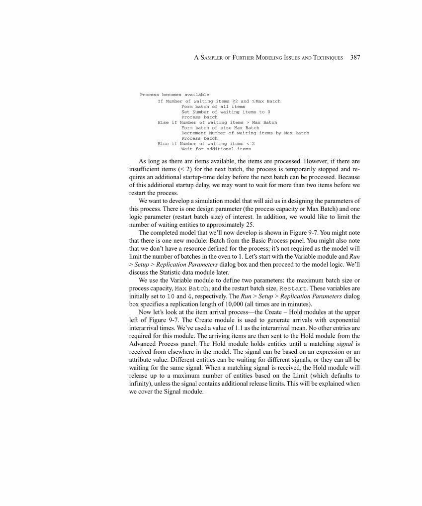
387A SAMPLER OF FURTHER MODELING ISSUES AND TECHNIQUES
Process becomes available
If Number of waiting items >_ 2 and <_ Max BatchForm batch of all itemsSet Number of waiting items to 0Process batch
Else if Number of waiting items > Max BatchForm batch of size Max BatchDecrement Number of waiting items by Max BatchProcess batch
Else if Number of waiting items < 2Wait for additional items
As long as there are items available, the items are processed. However, if there areinsufficient items (< 2) for the next batch, the process is temporarily stopped and re-quires an additional startup-time delay before the next batch can be processed. Becauseof this additional startup delay, we may want to wait for more than two items before werestart the process.
We want to develop a simulation model that will aid us in designing the parameters ofthis process. There is one design parameter (the process capacity or Max Batch) and onelogic parameter (restart batch size) of interest. In addition, we would like to limit thenumber of waiting entities to approximately 25.
The completed model that we’ll now develop is shown in Figure 9-7. You might notethat there is one new module: Batch from the Basic Process panel. You might also notethat we don’t have a resource defined for the process; it’s not required as the model willlimit the number of batches in the oven to 1. Let’s start with the Variable module and Run> Setup > Replication Parameters dialog box and then proceed to the model logic. We’lldiscuss the Statistic data module later.
We use the Variable module to define two parameters: the maximum batch size orprocess capacity, Max Batch; and the restart batch size, Restart. These variables areinitially set to 10 and 4, respectively. The Run > Setup > Replication Parameters dialogbox specifies a replication length of 10,000 (all times are in minutes).
Now let’s look at the item arrival process—the Create – Hold modules at the upperleft of Figure 9-7. The Create module is used to generate arrivals with exponentialinterarrival times. We’ve used a value of 1.1 as the interarrival mean. No other entries arerequired for this module. The arriving items are then sent to the Hold module from theAdvanced Process panel. The Hold module holds entities until a matching signal isreceived from elsewhere in the model. The signal can be based on an expression or anattribute value. Different entities can be waiting for different signals, or they can all bewaiting for the same signal. When a matching signal is received, the Hold module willrelease up to a maximum number of entities based on the Limit (which defaults toinfinity), unless the signal contains additional release limits. This will be explained whenwe cover the Signal module.
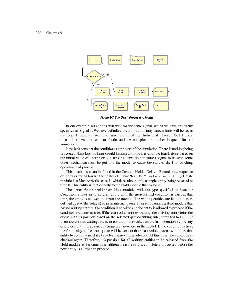
388 CHAPTER 9
Figure 9-7. The Batch Processing Model
In our example, all entities will wait for the same signal, which we have arbitrarilyspecified as Signal 1. We have defaulted the Limit to infinity since a limit will be set inthe Signal module. We have also requested an Individual Queue, Hold forSignal.Queue, so we can obtain statistics and plot the number in queue for ouranimation.
Now let’s consider the conditions at the start of the simulation. There is nothing beingprocessed; therefore, nothing should happen until the arrival of the fourth item, based onthe initial value of Restart. As arriving items do not cause a signal to be sent, someother mechanism must be put into the model to cause the start of the first batchingoperation and process.
This mechanism can be found in the Create – Hold – Delay – Record, etc., sequenceof modules found toward the center of Figure 9-7. The Create Scan Entity Createmodule has Max Arrivals set to 1, which results in only a single entity being released attime 0. This entity is sent directly to the Hold module that follows.
The Scan for Condition Hold module, with the type specified as Scan forCondition, allows us to hold an entity until the user-defined condition is true; at thattime, the entity is allowed to depart the module. The waiting entities are held in a user-defined queue (the default) or in an internal queue. If an entity enters a Hold module thathas no waiting entities, the condition is checked and the entity is allowed to proceed if thecondition evaluates to true. If there are other entities waiting, the arriving entity joins thequeue with its position based on the selected queue-ranking rule, defaulted to FIFO. Ifthere are entities waiting, the scan condition is checked as the last operation before anydiscrete-event time advance is triggered anywhere in the model. If the condition is true,the first entity in the scan queue will be sent to the next module. Arena will allow thatentity to continue until it’s time for the next time advance. At this time, the condition ischecked again. Therefore, it’s possible for all waiting entities to be released from theHold module at the same time, although each entity is completely processed before thenext entity is allowed to proceed.
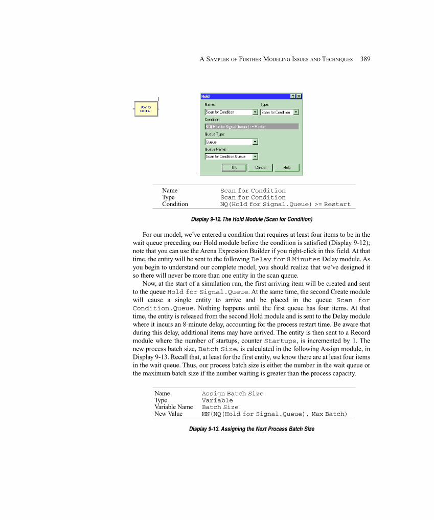
389A SAMPLER OF FURTHER MODELING ISSUES AND TECHNIQUES
Name Scan for ConditionType Scan for ConditionCondition NQ(Hold for Signal.Queue) >= Restart
Display 9-12. The Hold Module (Scan for Condition)
For our model, we’ve entered a condition that requires at least four items to be in thewait queue preceding our Hold module before the condition is satisfied (Display 9-12);note that you can use the Arena Expression Builder if you right-click in this field. At thattime, the entity will be sent to the following Delay for 8 Minutes Delay module. Asyou begin to understand our complete model, you should realize that we’ve designed itso there will never be more than one entity in the scan queue.
Now, at the start of a simulation run, the first arriving item will be created and sentto the queue Hold for Signal.Queue. At the same time, the second Create modulewill cause a single entity to arrive and be placed in the queue Scan forCondition.Queue. Nothing happens until the first queue has four items. At thattime, the entity is released from the second Hold module and is sent to the Delay modulewhere it incurs an 8-minute delay, accounting for the process restart time. Be aware thatduring this delay, additional items may have arrived. The entity is then sent to a Recordmodule where the number of startups, counter Startups, is incremented by 1. Thenew process batch size, Batch Size, is calculated in the following Assign module, inDisplay 9-13. Recall that, at least for the first entity, we know there are at least four itemsin the wait queue. Thus, our process batch size is either the number in the wait queue orthe maximum batch size if the number waiting is greater than the process capacity.
Name Assign Batch SizeType VariableVariable Name Batch SizeNew Value MN(NQ(Hold for Signal.Queue), Max Batch)
Display 9-13. Assigning the Next Process Batch Size
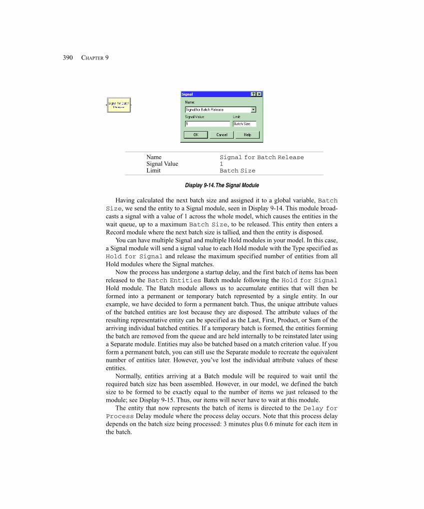
390 CHAPTER 9
Name Signal for Batch ReleaseSignal Value 1Limit Batch Size
Display 9-14. The Signal Module
Having calculated the next batch size and assigned it to a global variable, BatchSize, we send the entity to a Signal module, seen in Display 9-14. This module broad-casts a signal with a value of 1 across the whole model, which causes the entities in thewait queue, up to a maximum Batch Size, to be released. This entity then enters aRecord module where the next batch size is tallied, and then the entity is disposed.
You can have multiple Signal and multiple Hold modules in your model. In this case,a Signal module will send a signal value to each Hold module with the Type specified asHold for Signal and release the maximum specified number of entities from allHold modules where the Signal matches.
Now the process has undergone a startup delay, and the first batch of items has beenreleased to the Batch Entities Batch module following the Hold for SignalHold module. The Batch module allows us to accumulate entities that will then beformed into a permanent or temporary batch represented by a single entity. In ourexample, we have decided to form a permanent batch. Thus, the unique attribute valuesof the batched entities are lost because they are disposed. The attribute values of theresulting representative entity can be specified as the Last, First, Product, or Sum of thearriving individual batched entities. If a temporary batch is formed, the entities formingthe batch are removed from the queue and are held internally to be reinstated later usinga Separate module. Entities may also be batched based on a match criterion value. If youform a permanent batch, you can still use the Separate module to recreate the equivalentnumber of entities later. However, you’ve lost the individual attribute values of theseentities.
Normally, entities arriving at a Batch module will be required to wait until therequired batch size has been assembled. However, in our model, we defined the batchsize to be formed to be exactly equal to the number of items we just released to themodule; see Display 9-15. Thus, our items will never have to wait at this module.
The entity that now represents the batch of items is directed to the Delay forProcess Delay module where the process delay occurs. Note that this process delaydepends on the batch size being processed: 3 minutes plus 0.6 minute for each item inthe batch.
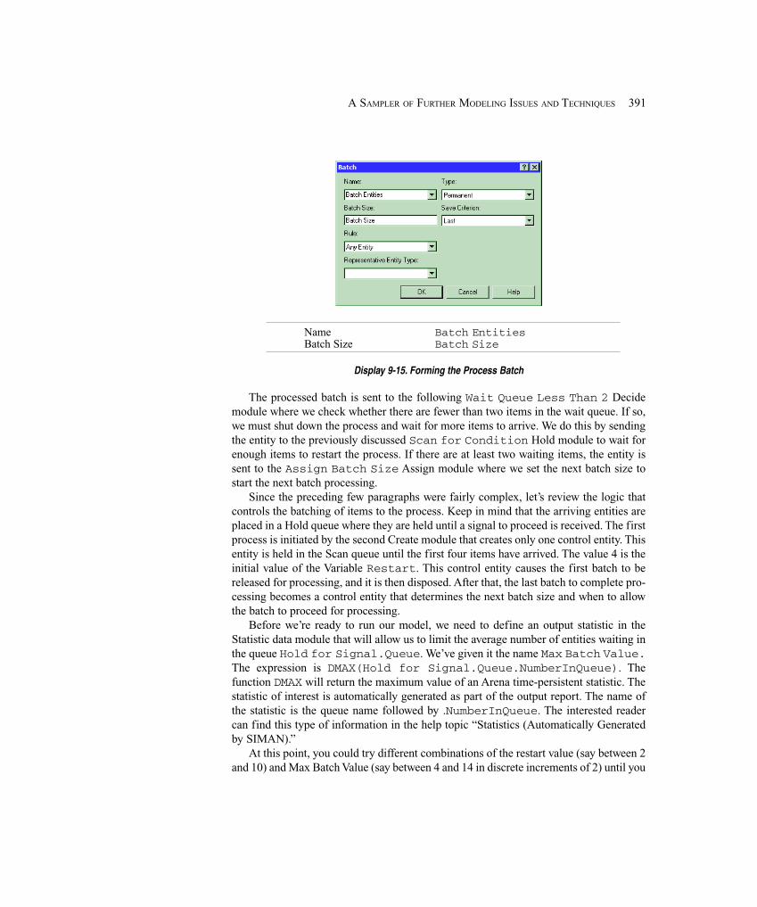
391A SAMPLER OF FURTHER MODELING ISSUES AND TECHNIQUES
Name Batch EntitiesBatch Size Batch Size
Display 9-15. Forming the Process Batch
The processed batch is sent to the following Wait Queue Less Than 2 Decidemodule where we check whether there are fewer than two items in the wait queue. If so,we must shut down the process and wait for more items to arrive. We do this by sendingthe entity to the previously discussed Scan for Condition Hold module to wait forenough items to restart the process. If there are at least two waiting items, the entity issent to the Assign Batch Size Assign module where we set the next batch size tostart the next batch processing.
Since the preceding few paragraphs were fairly complex, let’s review the logic thatcontrols the batching of items to the process. Keep in mind that the arriving entities areplaced in a Hold queue where they are held until a signal to proceed is received. The firstprocess is initiated by the second Create module that creates only one control entity. Thisentity is held in the Scan queue until the first four items have arrived. The value 4 is theinitial value of the Variable Restart. This control entity causes the first batch to bereleased for processing, and it is then disposed. After that, the last batch to complete pro-cessing becomes a control entity that determines the next batch size and when to allowthe batch to proceed for processing.
Before we’re ready to run our model, we need to define an output statistic in theStatistic data module that will allow us to limit the average number of entities waiting inthe queue Hold for Signal.Queue. We’ve given it the name Max Batch Value.The expression is DMAX(Hold for Signal.Queue.NumberInQueue). Thefunction DMAX will return the maximum value of an Arena time-persistent statistic. Thestatistic of interest is automatically generated as part of the output report. The name ofthe statistic is the queue name followed by .NumberInQueue. The interested readercan find this type of information in the help topic “Statistics (Automatically Generatedby SIMAN).”
At this point, you could try different combinations of the restart value (say between 2and 10) and Max Batch Value (say between 4 and 14 in discrete increments of 2) until you
392 CHAPTER 9
found the combination that provides the minimum number of startups. After all, there areonly 54 possible combinations. You could also create 54 different models and use PAN.We cheated and used OptQuest (see Section 6.6) to vary the variable Max Batch from 4to 14 in discrete increments of 2. The Restart variable was varied from 2 to 10 in dis-crete increments of 1. The objective was to minimize the number of startups with a con-straint that our Max Batch Value statistic not exceed 25. The best solution found was:
Max Batch = 10Restart = 8Max Batch Value = 24.9Startups = 30.6.
9.5 Overlapping Resources
In Chapters 4-8, we concentrated on building models using the modules available fromthe Basic Process, Advanced Process, and Advanced Transfer panels. Even though weused these modules in several different models, we still have not exhausted all thecapabilities.
As we developed models in the earlier chapters, we were not only interested inintroducing you to new Arena constructs, but we also tried to cover different modelingtechniques that might be useful. We have consistently presented new material in the formof examples that require the use of new modeling capabilities. Sometimes the fabricationof a good example to illustrate the need for new modeling capabilities is a daunting task.We have to admit that the example that we are about to introduce is a bit of a stretch, notonly in terms of the model description, but also the manner in which we develop themodel. However, if you bear with us through this model development, we think that youwill add several handy additions to your toolbox.
9.5.1 System DescriptionThe system we’ll be modeling is a tightly coupled, three-workstation production system.We have used the words “tightly coupled” because of the unique part-arrival process andbecause there is limited space for part buffering between the workstations.
We’ll assume an unlimited supply of raw materials that can be delivered to the systemon demand. When a part enters the first workstation, a request is automaticallyforwarded to an adjoining warehouse for the delivery of a replenishment part. Becausethe warehouse is performing other duties, the replenishment part is not always deliveredimmediately. Rather than model this activity in detail, we’ll assume an exponentialdelivery delay, with mean of 25 (all times are minutes), before the request is acted upon.At that point, we’ll assume the part is ready for delivery, with the delivery time followinga UNIF(10, 15) distribution. To start the simulation, we’ll assume that two parts areready for delivery to the first workstation.
Replenishment parts that arrive at the first workstation are held in a buffer until theworkstation becomes available. A part entering the first workstation immediatelyrequests a setup operator. The setup time is assumed to be EXPO(9). Upon completion ofthe setup, the part is processed by the workstation, lasting TRIA(10, 15, 20). Thecompleted part is then moved to the buffer between Workstations 1 and 2. This buffer

393A SAMPLER OF FURTHER MODELING ISSUES AND TECHNIQUES
space is limited to two parts; if the buffer is full, Workstation 1 is blocked until spacebecomes available. We’ll assume that all transfer times between workstations arenegligible, or occur in 0 time.
There are two almost-identical machines at Workstation 2. They differ only in thetime it takes to process a part: The processing times are TRIA(35, 40, 45) for Machine2A and TRIA(40, 45, 50) for Machine 2B. A waiting part will be processed by the firstavailable machine. If both machines are available, Machine 2A will be chosen. There isno setup required at this workstation. A completed part is then transferred to Workstation3. However, there is no buffer between Workstations 2 and 3. Thus, Workstation 3 mustbe available before the transfer can occur. (This really affects the system performance!)If Machines 2A and 2B both have completed parts (which are blocking these machines)waiting for Workstation 3, the part from Machine 2A is transferred first.
When a part enters Workstation 3, it requires the setup operator (the same operatorused for setup at Workstation 1). The setup time is assumed to be EXPO(9). The processtime at Workstation 3 is TRIA(9, 12, 16). The completed part exits the system at this point.
We also have failures at each workstation. Workstations 1 and 3 have a mean Up Timeof 600 minutes with a mean Down Time for repair of 45 minutes. Machines 2A and 2B,at Workstation 2, have mean Up Times of 500 minutes and mean Down Times of 25minutes. All failure and repair times follow an exponential distribution. One subtle butvery important point is that the Up Time is based only on the time that the machines areprocessing parts, not the elapsed time.
Now to complicate the issue even further, let’s assume that we’re interested in thepercent of time that the machines at each workstation are in different states. This shouldgive us a great amount of insight into how to improve the system. For example, if themachine at Workstation 1 is blocked a lot of the time, we might want to look at increasingthe capacity at Workstation 2.
The possible states for the different machines are as follows:
Workstation 1: Processing, Starved, Blocked, Failed, Waiting for setup,and Setup
Machines 2A and 2B: Processing, Starved, Blocked, and FailedWorkstation 3: Processing, Starved, Failed, Waiting for setup, and Setup.
We would also like to keep track of the percent of time the setup operator spends atWorkstations 1 and 3. These states would be: WS 1 Setup, WS 2 Setup, and Idle.
These are typical measures used to determine the effectiveness of tightly coupledsystems. They provide a great deal of information on what are the true system bottle-necks. Well, as long as we’ve gone this far, why not go all the way! Let’s also assume thatwe’d like to know the percent of time that the parts spend in all possible states. Arrangingfor this is a much more difficult problem. First, let’s define the system or cycle time for apart as starting when the delivery is initiated and ending when the part completes pro-cessing at Workstation 3. The possible part states are: Travel to WS 1, Wait for WS 1,Wait for setup at WS 1, Setup at WS 1, Process at WS 1, Blocked at WS 1, Wait for WS2, Process at WS 2, Blocked at WS 2, Wait for setup at WS 3, Setup at WS 3, and Processat WS 3. As we develop our model, we’ll take care to incorporate the resource states. But,
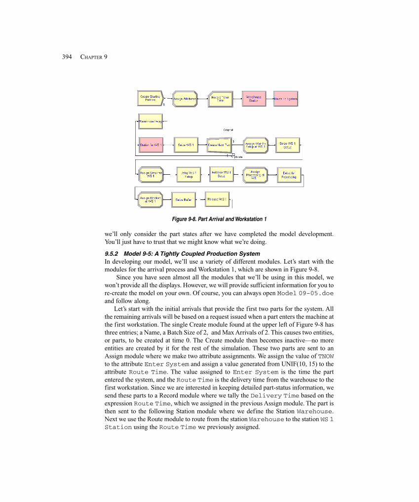
394 CHAPTER 9
Figure 9-8. Part Arrival and Workstation 1
we’ll only consider the part states after we have completed the model development.You’ll just have to trust that we might know what we’re doing.
9.5.2 Model 9-5: A Tightly Coupled Production SystemIn developing our model, we’ll use a variety of different modules. Let’s start with themodules for the arrival process and Workstation 1, which are shown in Figure 9-8.
Since you have seen almost all the modules that we’ll be using in this model, wewon’t provide all the displays. However, we will provide sufficient information for you tore-create the model on your own. Of course, you can always open Model 09-05.doeand follow along.
Let’s start with the initial arrivals that provide the first two parts for the system. Allthe remaining arrivals will be based on a request issued when a part enters the machine atthe first workstation. The single Create module found at the upper left of Figure 9-8 hasthree entries; a Name, a Batch Size of 2, and Max Arrivals of 2. This causes two entities,or parts, to be created at time 0. The Create module then becomes inactive—no moreentities are created by it for the rest of the simulation. These two parts are sent to anAssign module where we make two attribute assignments. We assign the value of TNOWto the attribute Enter System and assign a value generated from UNIF(10, 15) to theattribute Route Time. The value assigned to Enter System is the time the partentered the system, and the Route Time is the delivery time from the warehouse to thefirst workstation. Since we are interested in keeping detailed part-status information, wesend these parts to a Record module where we tally the Delivery Time based on theexpression Route Time, which we assigned in the previous Assign module. The part isthen sent to the following Station module where we define the Station Warehouse.Next we use the Route module to route from the station Warehouse to the station WS 1Station using the Route Time we previously assigned.
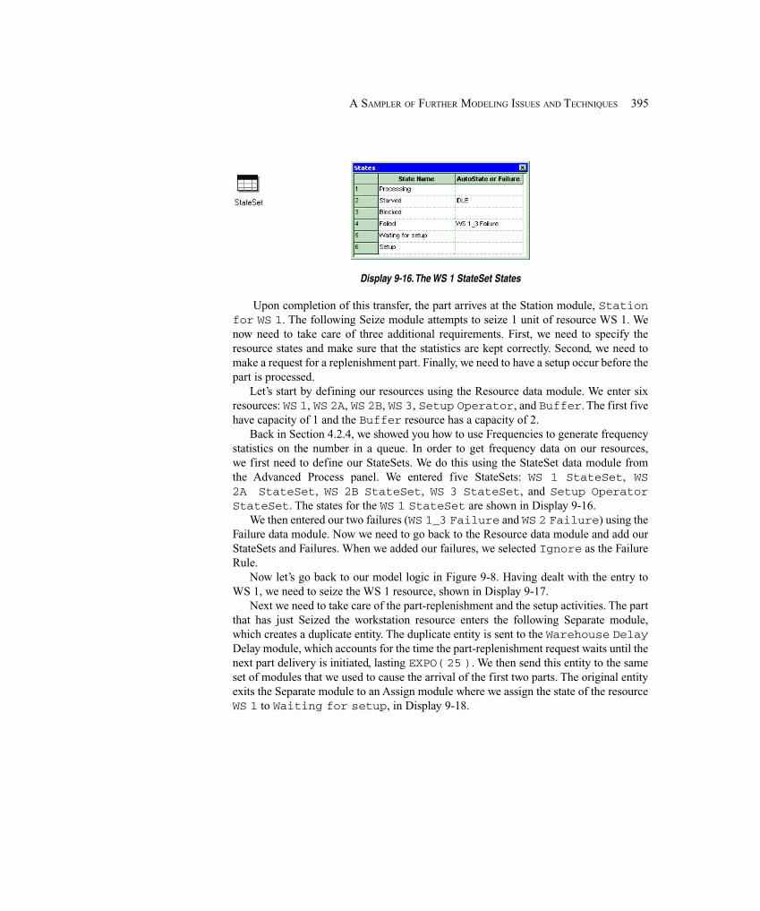
395A SAMPLER OF FURTHER MODELING ISSUES AND TECHNIQUES
Display 9-16. The WS 1 StateSet States
Upon completion of this transfer, the part arrives at the Station module, Stationfor WS 1. The following Seize module attempts to seize 1 unit of resource WS 1. Wenow need to take care of three additional requirements. First, we need to specify theresource states and make sure that the statistics are kept correctly. Second, we need tomake a request for a replenishment part. Finally, we need to have a setup occur before thepart is processed.
Let’s start by defining our resources using the Resource data module. We enter sixresources: WS 1, WS 2A, WS 2B, WS 3, Setup Operator, and Buffer. The first fivehave capacity of 1 and the Buffer resource has a capacity of 2.
Back in Section 4.2.4, we showed you how to use Frequencies to generate frequencystatistics on the number in a queue. In order to get frequency data on our resources,we first need to define our StateSets. We do this using the StateSet data module fromthe Advanced Process panel. We entered five StateSets: WS 1 StateSet, WS2A StateSet, WS 2B StateSet, WS 3 StateSet, and Setup OperatorStateSet. The states for the WS 1 StateSet are shown in Display 9-16.
We then entered our two failures (WS 1_3 Failure and WS 2 Failure) using theFailure data module. Now we need to go back to the Resource data module and add ourStateSets and Failures. When we added our failures, we selected Ignore as the FailureRule.
Now let’s go back to our model logic in Figure 9-8. Having dealt with the entry toWS 1, we need to seize the WS 1 resource, shown in Display 9-17.
Next we need to take care of the part-replenishment and the setup activities. The partthat has just Seized the workstation resource enters the following Separate module,which creates a duplicate entity. The duplicate entity is sent to the Warehouse DelayDelay module, which accounts for the time the part-replenishment request waits until thenext part delivery is initiated, lasting EXPO( 25 ). We then send this entity to the sameset of modules that we used to cause the arrival of the first two parts. The original entityexits the Separate module to an Assign module where we assign the state of the resourceWS 1 to Waiting for setup, in Display 9-18.
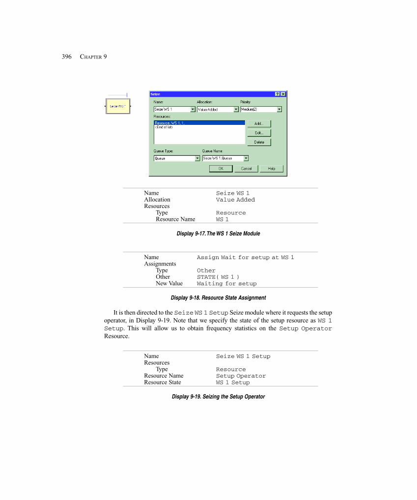
396 CHAPTER 9
Name Seize WS 1Allocation Value AddedResources
Type ResourceResource Name WS 1
Display 9-17. The WS 1 Seize Module
Name Assign Wait for setup at WS 1Assignments
Type OtherOther STATE( WS 1 )New Value Waiting for setup
Display 9-18. Resource State Assignment
It is then directed to the Seize WS 1 Setup Seize module where it requests the setupoperator, in Display 9-19. Note that we specify the state of the setup resource as WS 1Setup. This will allow us to obtain frequency statistics on the Setup OperatorResource.
Name Seize WS 1 SetupResources
Type ResourceResource Name Setup OperatorResource State WS 1 Setup
Display 9-19. Seizing the Setup Operator
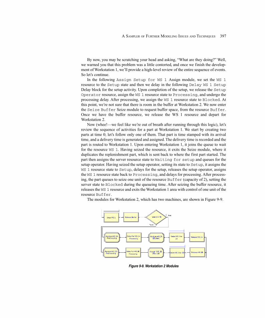
397A SAMPLER OF FURTHER MODELING ISSUES AND TECHNIQUES
By now, you may be scratching your head and asking, “What are they doing?” Well,we warned you that this problem was a little contorted, and once we finish the develop-ment of Workstation 1, we’ll provide a high-level review of the entire sequence of events.So let’s continue.
In the following Assign Setup for WS 1 Assign module, we set the WS 1resource to the Setup state and then we delay in the following Delay WS 1 SetupDelay block for the setup activity. Upon completion of the setup, we release the SetupOperator resource, assign the WS 1 resource state to Processing, and undergo theprocessing delay. After processing, we assign the WS 1 resource state to Blocked. Atthis point, we’re not sure that there is room in the buffer at Workstation 2. We now enterthe Seize Buffer Seize module to request buffer space, from the resource Buffer.Once we have the buffer resource, we release the WS 1 resource and depart forWorkstation 2.
Now (whee!—we feel like we’re out of breath after running through this logic), let’sreview the sequence of activities for a part at Workstation 1. We start by creating twoparts at time 0; let’s follow only one of them. That part is time stamped with its arrivaltime, and a delivery time is generated and assigned. The delivery time is recorded and thepart is routed to Workstation 1. Upon entering Workstation 1, it joins the queue to waitfor the resource WS 1. Having seized the resource, it exits the Seize module, where itduplicates the replenishment part, which is sent back to where the first part started. Thepart then assigns the server resource state to Waiting for setup and queues for thesetup operator. Having seized the setup operator, setting its state to Setup, it assigns theWS 1 resource state to Setup, delays for the setup, releases the setup operator, assignsthe WS 1 resource state back to Processing, and delays for processing. After process-ing, the part queues to seize one unit of the resource Buffer (capacity of 2), setting theserver state to Blocked during the queueing time. After seizing the buffer resource, itreleases the WS 1 resource and exits the Workstation 1 area with control of one unit of theresource Buffer.
The modules for Workstation 2, which has two machines, are shown in Figure 9-9.
Figure 9-9. Workstation 2 Modules
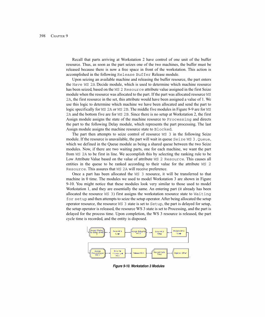
398 CHAPTER 9
Recall that parts arriving at Workstation 2 have control of one unit of the bufferresource. Thus, as soon as the part seizes one of the two machines, the buffer must bereleased because there is now a free space in front of the workstation. This action isaccomplished in the following Release Buffer Release module.
Upon seizing an available machine and releasing the buffer resource, the part entersthe Have WS 2A Decide module, which is used to determine which machine resourcehas been seized, based on the WS 2 Resource attribute value assigned in the first Seizemodule when the resource was allocated to the part. If the part was allocated resource WS2A, the first resource in the set, this attribute would have been assigned a value of 1. Weuse this logic to determine which machine we have been allocated and send the part tologic specifically for WS 2A or WS 2B. The middle five modules in Figure 9-9 are for WS2A and the bottom five are for WS 2B. Since there is no setup at Workstation 2, the firstAssign module assigns the state of the machine resource to Processing and directsthe part to the following Delay module, which represents the part processing. The lastAssign module assigns the machine resource state to Blocked.
The part then attempts to seize control of resource WS 3 in the following Seizemodule. If the resource is unavailable, the part will wait in queue Seize WS 3.Queue,which we defined in the Queue module as being a shared queue between the two Seizemodules. Now, if there are two waiting parts, one for each machine, we want the partfrom WS 2A to be first in line. We accomplish this by selecting the ranking rule to beLow Attribute Value based on the value of attribute WS 2 Resource. This causes allentities in the queue to be ranked according to their value for the attribute WS 2Resource. This assures that WS 2A will receive preference.
Once a part has been allocated the WS 3 resource, it will be transferred to thatmachine in 0 time. The modules we used to model Workstation 3 are shown in Figure9-10. You might notice that these modules look very similar to those used to modelWorkstation 1, and they are essentially the same. An entering part (it already has beenallocated the resource WS 3) first assigns the workstation resource state to Waitingfor setup and then attempts to seize the setup operator. After being allocated the setupoperator resource, the resource WS 3 state is set to Setup, the part is delayed for setup,the setup operator is released, the resource WS 3 state is set to Processing, and the part isdelayed for the process time. Upon completion, the WS 3 resource is released, the partcycle time is recorded, and the entity is disposed.
Figure 9-10. Workstation 3 Modules
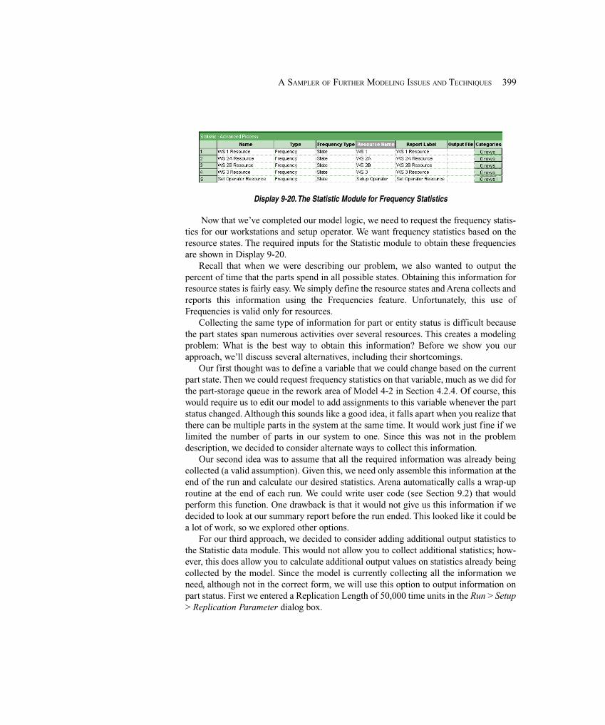
399A SAMPLER OF FURTHER MODELING ISSUES AND TECHNIQUES
Display 9-20. The Statistic Module for Frequency Statistics
Now that we’ve completed our model logic, we need to request the frequency statis-tics for our workstations and setup operator. We want frequency statistics based on theresource states. The required inputs for the Statistic module to obtain these frequenciesare shown in Display 9-20.
Recall that when we were describing our problem, we also wanted to output thepercent of time that the parts spend in all possible states. Obtaining this information forresource states is fairly easy. We simply define the resource states and Arena collects andreports this information using the Frequencies feature. Unfortunately, this use ofFrequencies is valid only for resources.
Collecting the same type of information for part or entity status is difficult becausethe part states span numerous activities over several resources. This creates a modelingproblem: What is the best way to obtain this information? Before we show you ourapproach, we’ll discuss several alternatives, including their shortcomings.
Our first thought was to define a variable that we could change based on the currentpart state. Then we could request frequency statistics on that variable, much as we did forthe part-storage queue in the rework area of Model 4-2 in Section 4.2.4. Of course, thiswould require us to edit our model to add assignments to this variable whenever the partstatus changed. Although this sounds like a good idea, it falls apart when you realize thatthere can be multiple parts in the system at the same time. It would work just fine if welimited the number of parts in our system to one. Since this was not in the problemdescription, we decided to consider alternate ways to collect this information.
Our second idea was to assume that all the required information was already beingcollected (a valid assumption). Given this, we need only assemble this information at theend of the run and calculate our desired statistics. Arena automatically calls a wrap-uproutine at the end of each run. We could write user code (see Section 9.2) that wouldperform this function. One drawback is that it would not give us this information if wedecided to look at our summary report before the run ended. This looked like it could bea lot of work, so we explored other options.
For our third approach, we decided to consider adding additional output statistics tothe Statistic data module. This would not allow you to collect additional statistics; how-ever, this does allow you to calculate additional output values on statistics already beingcollected by the model. Since the model is currently collecting all the information weneed, although not in the correct form, we will use this option to output information onpart status. First we entered a Replication Length of 50,000 time units in the Run > Setup> Replication Parameter dialog box.
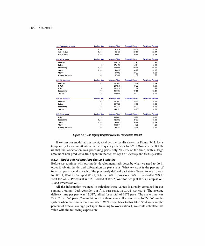
400 CHAPTER 9
Figure 9-11. The Tightly Coupled System Frequencies Report
If we ran our model at this point, we’d get the results shown in Figure 9-11. Let’stemporarily focus our attention on the frequency statistics for WS 1 Resource. It tellsus that the workstation was processing parts only 50.21% of the time, with a largeamount of non-productive time spent in the Waiting for setup and Setup states.
9.5.3 Model 9-6: Adding Part-Status StatisticsBefore we continue with our model development, let’s describe what we need to do inorder to obtain the desired information on part status. What we want is the percent oftime that parts spend in each of the previously defined part states: Travel to WS 1, Waitfor WS 1, Wait for Setup at WS 1, Setup at WS 1, Process at WS 1, Blocked at WS 1,Wait for WS 2, Process at WS 2, Blocked at WS 2, Wait for Setup at WS 3, Setup at WS3, and Process at WS 3.
All the information we need to calculate these values is already contained in oursummary output. Let’s consider our first part state, Travel to WS 1. The averagedelivery time per part was 12.517, tallied for a total of 1672 parts. The cycle time was225.07 for 1665 parts. You might note that there were still seven parts (1672-1665) in thesystem when the simulation terminated. We’ll come back to this later. So if we want thepercent of time an average part spent traveling to Workstation 1, we could calculate thatvalue with the following expression:

401A SAMPLER OF FURTHER MODELING ISSUES AND TECHNIQUES
((12.517 ∗ 1672) / (225.07 ∗ 1665)) ∗ 100.0
or 5.5848%. We can use this approach to calculate all of our values. Basically, wecompute the total amount of part time spent in each activity, divide it by the total amountof part time spent in all activities, and multiply by 100 to obtain the values in percentages.Since the last two steps of this calculation are always the same, we will first define anexpression, Tot, to represent this value (Expression data module). Note that by using anexpression, it will be computed only when required. That expression is as follows:
TAVG(Cycle Time) * TNUM(Cycle Time)/100
TAVG and TNUM are Arena variables that return the current average of a Tally andthe total number of Tally observations, respectively. The variable argument is the TallyID. In this case, we have elected to use the Tally name as defined in our Record module.In cases where Arena defines the Tally name (for example, for time-in-queue tallies), werecommend that you check a module’s drop-down list or Help for the exact name.
The information required to calculate three of our part states is contained in Tallies:Travel to WS 1, Wait for WS 1, and Wait for WS 2. The expressions required tocalculate these values are as follows:
TAVG(Delivery Time) * TNUM(Delivery Time)/TotTAVG(Seize WS 1.Queue.WaitingTime) *
TNUM(Seize WS 1.Queue.WaitingTime)/TotTAVG(Seize WS 2.Queue.WaitingTime) *
TNUM(Seize WS 2.Queue.WaitingTime)/Tot
The information for the remaining part states is contained in the frequency statistics.As you would expect, Arena also provides variables that will return information
about frequencies. The Arena variable FRQTIM returns the total amount of time that aspecified resource was in a specified category, or state. The complete expression for thisvariable is
FRQTIM(Frequency ID, Category)
The Frequency ID argument is the frequency name. The Category argument is thecategory name. Thus, our expression for Setup at WS 1 becomes
FRQTIM(WS 1 Resource, Setup)/Tot
where WS 1 Resource is the name of our previously defined frequency statistic(defined in the Statistic data module) and Setup is the category name for our setup statefor the WS 1 resource (defined in the StateSet data module).
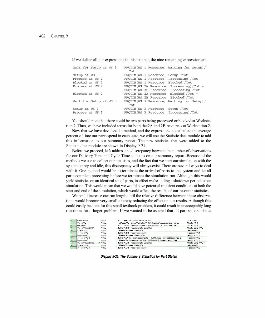
402 CHAPTER 9
If we define all our expressions in this manner, the nine remaining expression are:
Wait for Setup at WS 1 FRQTIM(WS 1 Resource, Waiting for Setup)/Tot
Setup at WS 1 FRQTIM(WS 1 Resource, Setup)/TotProcess at WS 1 FRQTIM(WS 1 Resource, Processing)/TotBlocked at WS 1 FRQTIM(WS 1 Resource, Blocked)/TotProcess at WS 2 FRQTIM(WS 2A Resource, Processing)/Tot +
FRQTIM(WS 2B Resource, Processing)/TotBlocked at WS 2 FRQTIM(WS 2A Resource, Blocked)/Tot +
FRQTIM(WS 2B Resource, Blocked)/TotWait for Setup at WS 3 FRQTIM(WS 3 Resource, Waiting for Setup)/
TotSetup at WS 3 FRQTIM(WS 3 Resource, Setup)/TotProcess at WS 3 FRQTIM(WS 3 Resource, Processing)/Tot
You should note that there could be two parts being processed or blocked at Worksta-tion 2. Thus, we have included terms for both the 2A and 2B resources at Workstation 2.
Now that we have developed a method, and the expressions, to calculate the averagepercent of time our parts spend in each state, we will use the Statistic data module to addthis information to our summary report. The new statistics that were added to theStatistic data module are shown in Display 9-21.
Before we proceed, let’s address the discrepancy between the number of observationsfor our Delivery Time and Cycle Time statistics on our summary report. Because of themethods we use to collect our statistics, and the fact that we start our simulation with thesystem empty and idle, this discrepancy will always exist. There are several ways to dealwith it. One method would be to terminate the arrival of parts to the system and let allparts complete processing before we terminate the simulation run. Although this wouldyield statistics on an identical set of parts, in effect we’re adding a shutdown period to oursimulation. This would mean that we would have potential transient conditions at both thestart and end of the simulation, which would affect the results of our resource statistics.
We could increase our run length until the relative difference between these observa-tions would become very small, thereby reducing the effect on our results. Although thiscould easily be done for this small textbook problem, it could result in unacceptably longrun times for a larger problem. If we wanted to be assured that all part-state statistics
Display 9-21. The Summary Statistics for Part States
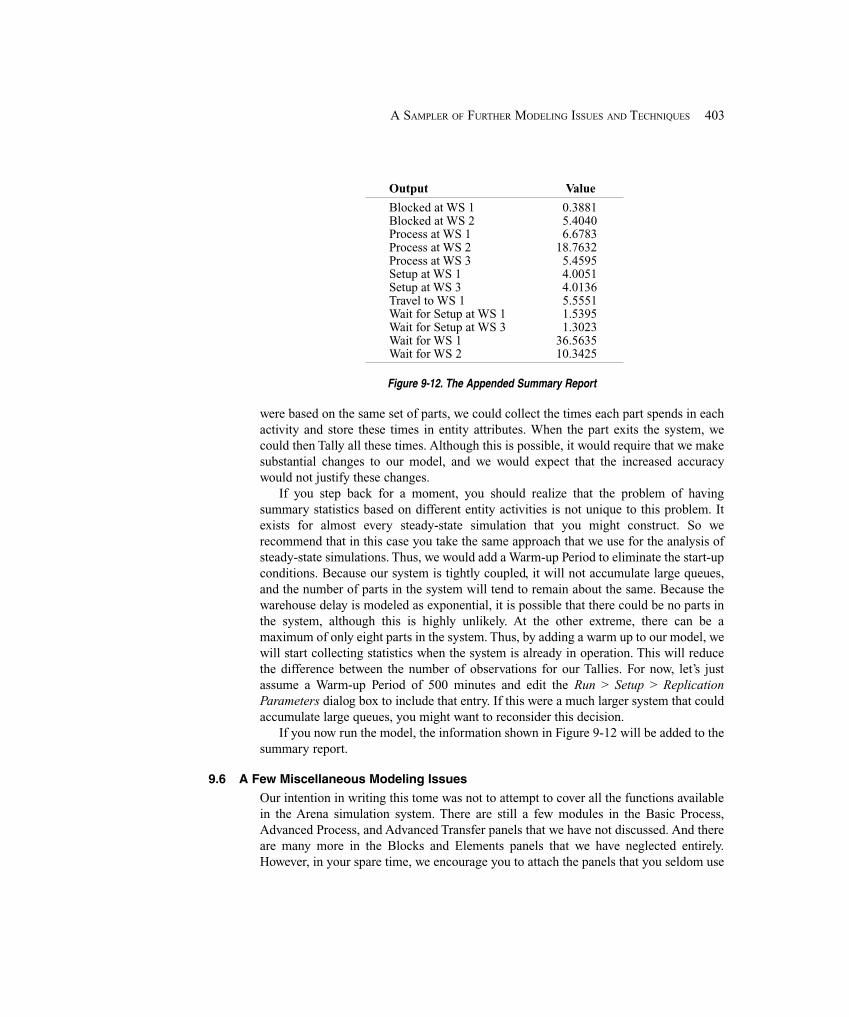
403A SAMPLER OF FURTHER MODELING ISSUES AND TECHNIQUES
Output Value
Blocked at WS 1 0.3881Blocked at WS 2 5.4040Process at WS 1 6.6783Process at WS 2 18.7632Process at WS 3 5.4595Setup at WS 1 4.0051Setup at WS 3 4.0136Travel to WS 1 5.5551Wait for Setup at WS 1 1.5395Wait for Setup at WS 3 1.3023Wait for WS 1 36.5635Wait for WS 2 10.3425
Figure 9-12. The Appended Summary Report
were based on the same set of parts, we could collect the times each part spends in eachactivity and store these times in entity attributes. When the part exits the system, wecould then Tally all these times. Although this is possible, it would require that we makesubstantial changes to our model, and we would expect that the increased accuracywould not justify these changes.
If you step back for a moment, you should realize that the problem of havingsummary statistics based on different entity activities is not unique to this problem. Itexists for almost every steady-state simulation that you might construct. So werecommend that in this case you take the same approach that we use for the analysis ofsteady-state simulations. Thus, we would add a Warm-up Period to eliminate the start-upconditions. Because our system is tightly coupled, it will not accumulate large queues,and the number of parts in the system will tend to remain about the same. Because thewarehouse delay is modeled as exponential, it is possible that there could be no parts inthe system, although this is highly unlikely. At the other extreme, there can be amaximum of only eight parts in the system. Thus, by adding a warm up to our model, wewill start collecting statistics when the system is already in operation. This will reducethe difference between the number of observations for our Tallies. For now, let’s justassume a Warm-up Period of 500 minutes and edit the Run > Setup > ReplicationParameters dialog box to include that entry. If this were a much larger system that couldaccumulate large queues, you might want to reconsider this decision.
If you now run the model, the information shown in Figure 9-12 will be added to thesummary report.
9.6 A Few Miscellaneous Modeling Issues
Our intention in writing this tome was not to attempt to cover all the functions availablein the Arena simulation system. There are still a few modules in the Basic Process,Advanced Process, and Advanced Transfer panels that we have not discussed. And thereare many more in the Blocks and Elements panels that we have neglected entirely.However, in your spare time, we encourage you to attach the panels that you seldom use

404 CHAPTER 9
and place some modules. Using the Help features will give you a good idea of what wehave omitted. In most cases, we suspect that you’ll never need these additional features.Before we close this chapter, we’d like to point out and briefly discuss a few features wehave not covered. We don’t feel that these topics require an in-depth understanding—only an awareness.
9.6.1 Guided TransportersThere is an entire set of features designed for use with guided transporters. Thesefeatures are useful not only for modeling automated guided vehicle (AGV) systems, butalso for warehousing systems and material-handling systems that use the concept of amoving cart, tote, jig, fixture, etc. Interestingly, they’re also great for representing manyamusement-park rides. Because this topic would easily fill an additional chapter or two,we’ve chosen not to present it in this book. However, you can find a complete discussionof these features in Chapter 9 of Pegden, Shannon, and Sadowski (1995).
9.6.2 Parallel QueuesThere are also two very specialized modules from the Blocks panel, QPick and PickQ,that are seldom used; but if you need them, they can make your modeling task mucheasier. The QPick module can be used to represent a process where you want to pick thenext entity for processing or movement from two or more different queues based onsome decision rule. Basically, the QPick module would sit between a set of detachedQueue modules and a module that allocates some type of scarce resource (for example,Allocate, Request, Access, or Seize modules). Let’s say that you have three differentstreams of entities converging at a point where they attempt to seize the same resource.Furthermore, assume that you want to keep the entities from each stream separate fromeach other. The modules required for this part of your model are shown in Figure 9-13.Each entity stream would end by sending the entity to its Detached queue (more on aDetached queue shortly). The link between the QPick and Queue modules is by moduleLabels. When the resource becomes available, it will basically ask the QPick module todetermine from which queue to select the next entity to be allocated the resource. Alsonote that you must use the Seize module from the Blocks panel for this to work, not theSeize module from the Advanced Process panel. When using modules from the Blockspanel, Arena does not automatically define queues, resources, etc. Thus, you may have toplace the corresponding modules from the Basic Process or Elements panels to definethese objects.
The PickQ module can be used to represent a process where you have a single arrivalstream, and you will use some decision rule to pick between two or more queues in whichto place the entity. Let’s assume that you have a stream of arriving entities that are to beloaded onto one of two available conveyors. The modules required for this part of yourmodel are shown in Figure 9-14 (the Access modules are from the Advanced Transferpanel). Note that you can’t specify internal queues for the Access modules, and thedecision as to which conveyor the entity is directed to is based on characteristics of thequeue, not the conveyors. The PickQ module can be used to direct entities to Access,Seize, Allocate, Request, or Queue modules, or any module that is preceded by a queue.
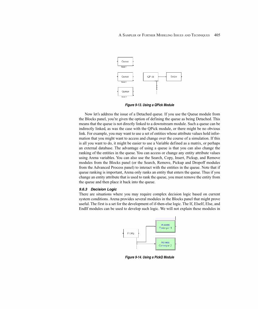
405A SAMPLER OF FURTHER MODELING ISSUES AND TECHNIQUES
Figure 9-13. Using a QPick Module
Now let’s address the issue of a Detached queue. If you use the Queue module fromthe Blocks panel, you’re given the option of defining the queue as being Detached. Thismeans that the queue is not directly linked to a downstream module. Such a queue can beindirectly linked, as was the case with the QPick module, or there might be no obviouslink. For example, you may want to use a set of entities whose attribute values hold infor-mation that you might want to access and change over the course of a simulation. If thisis all you want to do, it might be easier to use a Variable defined as a matrix, or perhapsan external database. The advantage of using a queue is that you can also change theranking of the entities in the queue. You can access or change any entity attribute valuesusing Arena variables. You can also use the Search, Copy, Insert, Pickup, and Removemodules from the Blocks panel (or the Search, Remove, Pickup and Dropoff modulesfrom the Advanced Process panel) to interact with the entities in the queue. Note that ifqueue ranking is important, Arena only ranks an entity that enters the queue. Thus if youchange an entity attribute that is used to rank the queue, you must remove the entity fromthe queue and then place it back into the queue.
9.6.3 Decision LogicThere are situations where you may require complex decision logic based on currentsystem conditions. Arena provides several modules in the Blocks panel that might proveuseful. The first is a set for the development of if-then-else logic. The If, ElseIf, Else, andEndIf modules can be used to develop such logic. We will not explain these modules in
Figure 9-14. Using a PickQ Module
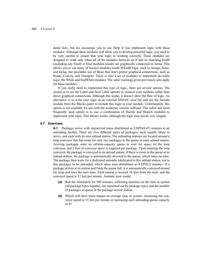
406 CHAPTER 9
detail here, but we encourage you to use Help if you implement logic with thesemodules. Although these modules will allow you to develop powerful logic, you need tobe very careful to ensure that your logic is working correctly. These modules aredesigned to work only when all of the modules between an If and its matching EndIf(including any ElseIf or Else modules inside) are graphically connected in Arena. Thisallows you to use many of Arena’s modules inside If/EndIf logic, such as Assign, Seize,and Delay, but precludes use of those that don’t permit graphical connections, such asRoute, Convey, and Transport. There is also a set of modules to implement do-whilelogic: the While and EndWhile modules. The same warnings given previously also applyfor these modules.
If you really need to implement this type of logic, there are several options. Theeasiest is to use the Label and Next Label options to connect your modules rather thandirect graphical connections. Although this works, it doesn’t show the flow of logic. Analternative is to write your logic as an external SIMAN .mod file and use the Includemodule from the Blocks panel to include this logic in your module. Unfortunately, thisoption is not available for use with the academic version software. The safest and mostfrequently used option is to use a combination of Decide and Branch modules toimplement your logic. This always works, although the logic may not be very elegant.
9.7 Exercises
9-1 Packages arrive with interarrival times distributed as EXPO(0.47) minutes to anunloading facility. There are five different types of packages, each equally likely toarrive, and each with its own unload station. The unloading stations are located around aloop conveyor that has room for only two packages in the queue at each unload station.Arriving packages enter an infinite-capacity queue to wait for space on the loopconveyor, and 2 feet of conveyor space is required per package. Upon entering the loopconveyor, the package is conveyed to its unload station. If there is room in the queue at itsunload station, the package is automatically diverted to the queue, which takes no time.The package then waits for a dedicated unloader (dedicated to this unload station, not tothis package) to be unloaded, which takes time distributed as EXPO(2) minutes. If apackage arrives at its station and finds the queue full, it is automatically conveyed aroundthe loop and tries the next time. Each station is located 10 feet from the next, and theconveyor speed is 12 feet per minute. Animate your model.
(a) Run the simulation for 500 minutes, collecting statistics on the time in system(all package types together, not separated out by package type), and the numberof packages in queue at the package-arrival station.
(b) Which will have more impact on average time in system: increasing the con-veyor speed to 15 feet per minute or increasing each unloading-queue capacityto 4?
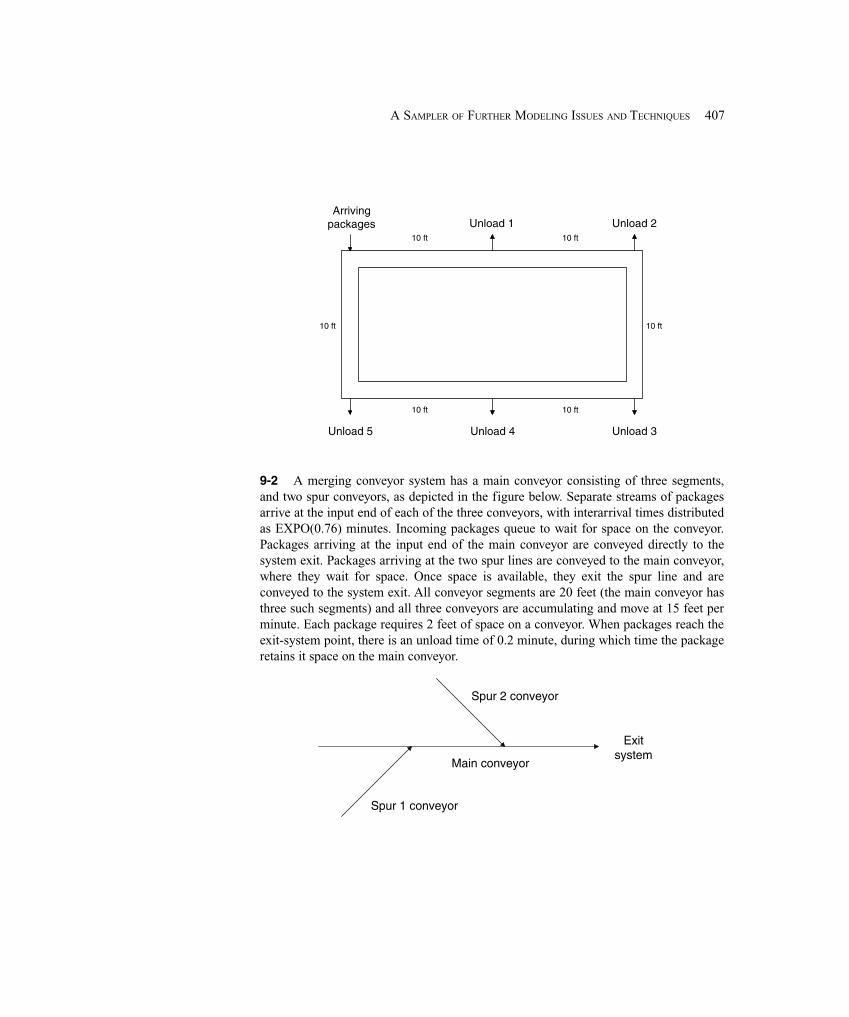
407A SAMPLER OF FURTHER MODELING ISSUES AND TECHNIQUES
Arrivingpackages Unload 1 Unload 2
Unload 3Unload 4Unload 5
10 ft 10 ft
10 ft10 ft
10 ft 10 ft
9-2 A merging conveyor system has a main conveyor consisting of three segments,and two spur conveyors, as depicted in the figure below. Separate streams of packagesarrive at the input end of each of the three conveyors, with interarrival times distributedas EXPO(0.76) minutes. Incoming packages queue to wait for space on the conveyor.Packages arriving at the input end of the main conveyor are conveyed directly to thesystem exit. Packages arriving at the two spur lines are conveyed to the main conveyor,where they wait for space. Once space is available, they exit the spur line and areconveyed to the system exit. All conveyor segments are 20 feet (the main conveyor hasthree such segments) and all three conveyors are accumulating and move at 15 feet perminute. Each package requires 2 feet of space on a conveyor. When packages reach theexit-system point, there is an unload time of 0.2 minute, during which time the packageretains it space on the main conveyor.
Spur 1 conveyor
Main conveyor
Spur 2 conveyor
Exitsystem
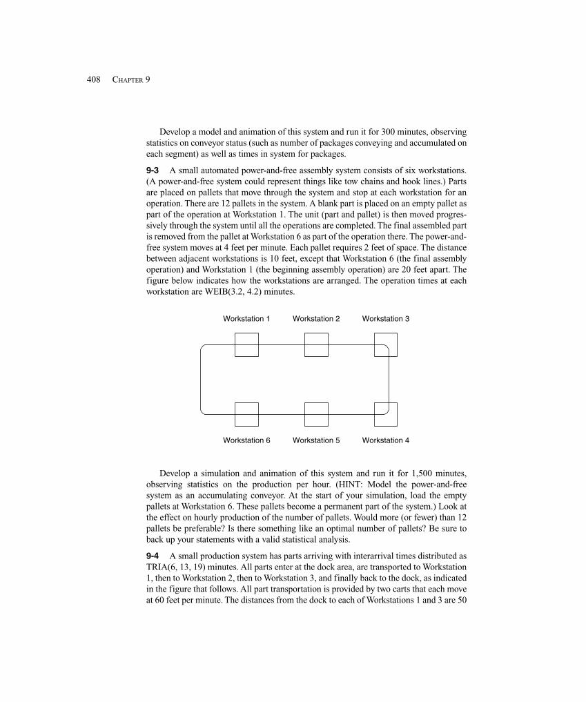
408 CHAPTER 9
Develop a model and animation of this system and run it for 300 minutes, observingstatistics on conveyor status (such as number of packages conveying and accumulated oneach segment) as well as times in system for packages.
9-3 A small automated power-and-free assembly system consists of six workstations.(A power-and-free system could represent things like tow chains and hook lines.) Partsare placed on pallets that move through the system and stop at each workstation for anoperation. There are 12 pallets in the system. A blank part is placed on an empty pallet aspart of the operation at Workstation 1. The unit (part and pallet) is then moved progres-sively through the system until all the operations are completed. The final assembled partis removed from the pallet at Workstation 6 as part of the operation there. The power-and-free system moves at 4 feet per minute. Each pallet requires 2 feet of space. The distancebetween adjacent workstations is 10 feet, except that Workstation 6 (the final assemblyoperation) and Workstation 1 (the beginning assembly operation) are 20 feet apart. Thefigure below indicates how the workstations are arranged. The operation times at eachworkstation are WEIB(3.2, 4.2) minutes.
Workstation 1 Workstation 2 Workstation 3
Workstation 4Workstation 5Workstation 6
Develop a simulation and animation of this system and run it for 1,500 minutes,observing statistics on the production per hour. (HINT: Model the power-and-freesystem as an accumulating conveyor. At the start of your simulation, load the emptypallets at Workstation 6. These pallets become a permanent part of the system.) Look atthe effect on hourly production of the number of pallets. Would more (or fewer) than 12pallets be preferable? Is there something like an optimal number of pallets? Be sure toback up your statements with a valid statistical analysis.
9-4 A small production system has parts arriving with interarrival times distributed asTRIA(6, 13, 19) minutes. All parts enter at the dock area, are transported to Workstation1, then to Workstation 2, then to Workstation 3, and finally back to the dock, as indicatedin the figure that follows. All part transportation is provided by two carts that each moveat 60 feet per minute. The distances from the dock to each of Workstations 1 and 3 are 50
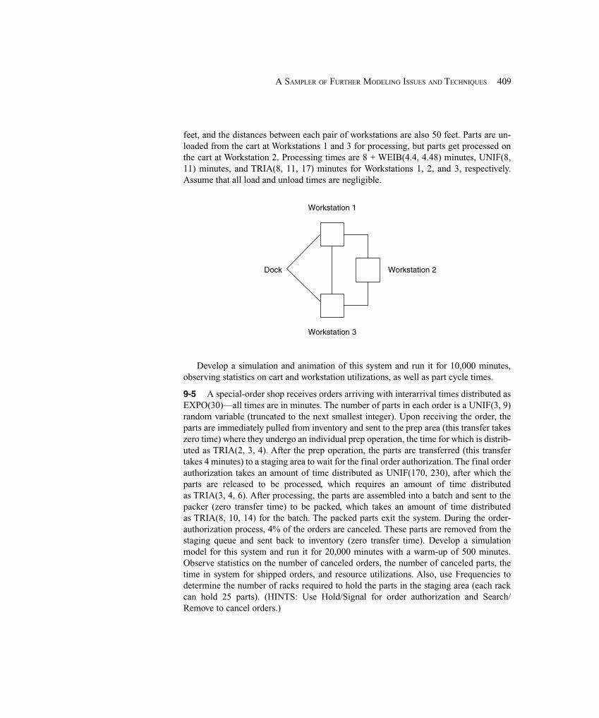
409A SAMPLER OF FURTHER MODELING ISSUES AND TECHNIQUES
feet, and the distances between each pair of workstations are also 50 feet. Parts are un-loaded from the cart at Workstations 1 and 3 for processing, but parts get processed onthe cart at Workstation 2. Processing times are 8 + WEIB(4.4, 4.48) minutes, UNIF(8,11) minutes, and TRIA(8, 11, 17) minutes for Workstations 1, 2, and 3, respectively.Assume that all load and unload times are negligible.
Workstation 1
Workstation 2
Workstation 3
Dock
Develop a simulation and animation of this system and run it for 10,000 minutes,observing statistics on cart and workstation utilizations, as well as part cycle times.
9-5 A special-order shop receives orders arriving with interarrival times distributed asEXPO(30)—all times are in minutes. The number of parts in each order is a UNIF(3, 9)random variable (truncated to the next smallest integer). Upon receiving the order, theparts are immediately pulled from inventory and sent to the prep area (this transfer takeszero time) where they undergo an individual prep operation, the time for which is distrib-uted as TRIA(2, 3, 4). After the prep operation, the parts are transferred (this transfertakes 4 minutes) to a staging area to wait for the final order authorization. The final orderauthorization takes an amount of time distributed as UNIF(170, 230), after which theparts are released to be processed, which requires an amount of time distributedas TRIA(3, 4, 6). After processing, the parts are assembled into a batch and sent to thepacker (zero transfer time) to be packed, which takes an amount of time distributedas TRIA(8, 10, 14) for the batch. The packed parts exit the system. During the order-authorization process, 4% of the orders are canceled. These parts are removed from thestaging queue and sent back to inventory (zero transfer time). Develop a simulationmodel for this system and run it for 20,000 minutes with a warm-up of 500 minutes.Observe statistics on the number of canceled orders, the number of canceled parts, thetime in system for shipped orders, and resource utilizations. Also, use Frequencies todetermine the number of racks required to hold the parts in the staging area (each rackcan hold 25 parts). (HINTS: Use Hold/Signal for order authorization and Search/Remove to cancel orders.)

410 CHAPTER 9
9-6 A food-processing system starts by processing a 25-pound batch of raw of product,which requires 1.05 + WEIB(0.982, 5.03) minutes. Assume an infinite supply of rawproduct. As soon as a batch has completed processing, it is removed from the processorand placed in a separator where it is divided into one-pound units. The separation processrequires 0.051 minute per pound. Note that this is not a “batch process,” but rather in each0.05 time unit a one-pound unit is completed. These one-pound units are sent to one ofthe three wrapping machines. Each wrapping machine has its own queue, with the unitbeing sent to the shortest queue. The wrappers are identical machines, except for theprocessing times. The wrapping times are constants of 0.20, 0.22, and 0.25 minute forwrappers 1, 2, and 3, respectively. The wrapped products are grouped, by wrapper, intobatches of six for final packaging. Once a group of six items is available, that group issent to a packer that packs the product, which takes 0.18 + WEIB(0.24, 4.79) minutes.These packages exit the system. Assume all transfer times are negligible.
(a) Develop a simulation and animation of this system and run it for 1,000 minutes,observing statistics on resource utilizations, queues, and the total number ofpackages shipped.
(b) Modify your model to include wrapper failures with the following characteris-tics for all wrappers: EXPO(20) for uptimes and EXPO(1) for repair times.
(c) Add a quality check to your model from part (b). Every half hour, a scan ismade, starting with the first wrapper queue, for products that are more than 4minutes old; that is, that exited the processor more than 4 minutes ago. Anysuch items are removed from the queue and disposed. It takes 3 seconds to findand remove each item. Keep track of the number of units removed.
9-7 A small automated system in a bakery produces loaves of bread. The dough-making machine ejects a portion of dough every UNIF(0.5, 1.0) minute. This portion ofdough enters a hopper to wait for space in the oven. The portions will be ejected from thehopper in groups of four and placed on the oven-load area to wait for space on the ovenconveyor. There is room for only one group of portions at the oven-load area. The ovenconveyor has 10 buckets, each 1 foot long, and moves at 0.34 feet per minute.
(a) Develop your model using the Hold (Scan for Condition), Signal, and Hold(Wait for Signal) modules for your logic to control the group of portions. Run itfor 3,000 minutes and observe statistics on the number of portions in thehopper, oven utilization, and the loaf output per hour.
(b) Modify your model from part (a) by replacing the Hold (Scan for Condition)module with logic developed based on the Decide module.
9-8 Customers arrive, with interarrival times distributed as EXPO(5)—all times are inminutes—at a small service center that has two servers, each with a separate queue. Theservice times are EXPO(9.8) and EXPO(9.4) for Servers 1 and 2, respectively. Arrivingcustomers join the shortest queue. Customer line switching occurs whenever the differ-ence between the queue lengths is 3 or more. At that time, the last customer in the longer
411A SAMPLER OF FURTHER MODELING ISSUES AND TECHNIQUES
queue moves to the end of the shorter queue. No additional movement, or line switching,in that direction occurs for at least the next 30 seconds. Develop a model and animationof this system and run it for 10,000 minutes. Observe statistics on the number of lineswitches, resource utilization, and queue lengths.
9-9 A small cross-docking system has three incoming docks and four outgoing docks.Trucks arrive at each of the three incoming docks with interarrival times distributed asUNIF(35, 55)—all times are in minutes. Each arriving truck contains UNIF(14, 30)pallets (truncated to the next smaller integer), which we can assume are unloaded in zerotime. Each pallet has an equal probability of going to any of the four outgoing docks.Transportation across the dock is provided by three fork trucks that each travel at 60 feetper minute. Assume that the distance between any incoming dock and any outgoing dockis 50 feet. Also assume that the distance between adjacent incoming docks (and adjacentoutgoing docks) is 15 feet.
(a) Develop a model in which the fork trucks remain where they drop off their lastload if there are no new requests pending.
(b) Modify your model so that free fork trucks are all sent to the middle (Dock 2)incoming dock to wait for their next load.
(c) Modify your model so that each fork truck is assigned a different home incom-ing dock and moves to that dock when there are no additional requests pending.
Compare the results of the above three systems, using the pallet system time as theprimary performance measure. Be sure to back up your comparison with a proper statis-tical analysis.
9-10 Develop a model and animation of a Ferris-wheel ride at a small, tacky county fair.Agitated customers (mostly small, over-sugared kids who don’t know any better) arriveat the ride with interarrival times distributed as EXPO(3) minutes and enter the mainqueue. When the previous ride has finished and the first customer is ready to get off, thenext five customers (or fewer if there are not five in the main queue) are let into the ridearea. As a customer gets off the Ferris wheel, the new customer gets on. Note that therecan be more current riders than new customers, or more new customers than currentriders. It requires UNIF(0.05, 0.15) minute to unload a current rider and UNIF(0.1, 0.2)to load a new rider. The Ferris wheel has only five single seats spaced about 10 feet apart.The wheel rotates at a velocity of 19 feet per minute. Each customer gets five revolutionson the wheel, and no new riders are allowed to board until the ride is complete. Riderswho get off the wheel run to the exit, which takes 2 minutes. We’re are not sure if theywant to get away or to be first in line at the next tacky ride. (HINTS: Use a conveyor torepresent the Ferris wheel itself. Use Wait/Signal to implement the loading andunloading rules.) By the way, the Ferris wheel was developed by the Pittsburgh bridgeengineer G. W. G. Ferris, who died in 1896 at the age of 37; its German name isRiesenrad, which translates roughly as “giant wheel.”

412 CHAPTER 9
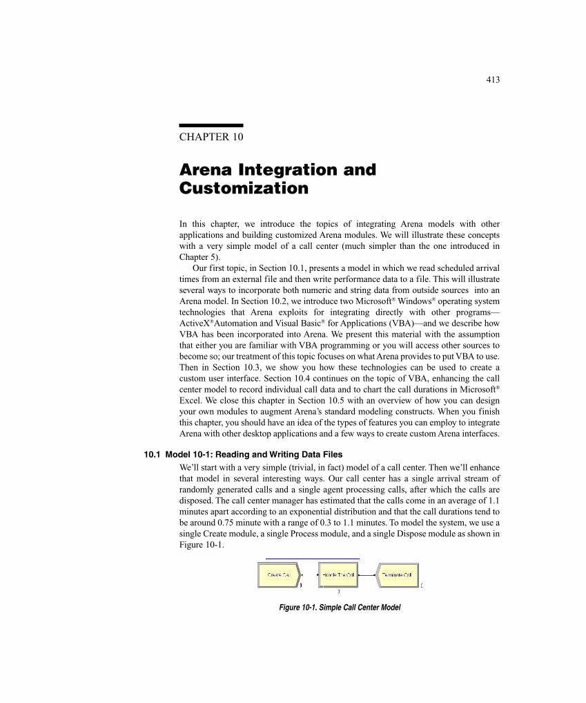
413ARENA INTEGRATION AND CUSTOMIZATION
CHAPTER 10
Arena Integration andCustomization
In this chapter, we introduce the topics of integrating Arena models with otherapplications and building customized Arena modules. We will illustrate these conceptswith a very simple model of a call center (much simpler than the one introduced inChapter 5).
Our first topic, in Section 10.1, presents a model in which we read scheduled arrivaltimes from an external file and then write performance data to a file. This will illustrateseveral ways to incorporate both numeric and string data from outside sources into anArena model. In Section 10.2, we introduce two Microsoft® Windows® operating systemtechnologies that Arena exploits for integrating directly with other programs—ActiveX®Automation and Visual Basic® for Applications (VBA)—and we describe howVBA has been incorporated into Arena. We present this material with the assumptionthat either you are familiar with VBA programming or you will access other sources tobecome so; our treatment of this topic focuses on what Arena provides to put VBA to use.Then in Section 10.3, we show you how these technologies can be used to create acustom user interface. Section 10.4 continues on the topic of VBA, enhancing the callcenter model to record individual call data and to chart the call durations in Microsoft®
Excel. We close this chapter in Section 10.5 with an overview of how you can designyour own modules to augment Arena’s standard modeling constructs. When you finishthis chapter, you should have an idea of the types of features you can employ to integrateArena with other desktop applications and a few ways to create custom Arena interfaces.
10.1 Model 10-1: Reading and Writing Data FilesWe’ll start with a very simple (trivial, in fact) model of a call center. Then we’ll enhancethat model in several interesting ways. Our call center has a single arrival stream ofrandomly generated calls and a single agent processing calls, after which the calls aredisposed. The call center manager has estimated that the calls come in an average of 1.1minutes apart according to an exponential distribution and that the call durations tend tobe around 0.75 minute with a range of 0.3 to 1.1 minutes. To model the system, we use asingle Create module, a single Process module, and a single Dispose module as shown inFigure 10-1.
Figure 10-1. Simple Call Center Model
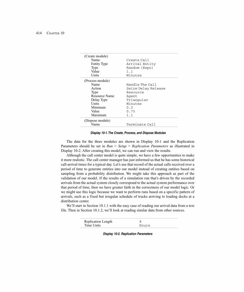
414 CHAPTER 10
(Create module)Name Create CallEntity Type Arrival EntityType Random (Expo)Value 1.1Units Minutes
(Process module)Name Handle The CallAction Seize Delay ReleaseType ResourceResource Name AgentDelay Type TriangularUnits MinutesMinimum 0.3Value 0.75Maximum 1.1
(Dispose module)Name Terminate Call
Display 10-1. The Create, Process, and Dispose Modules
The data for the three modules are shown in Display 10-1 and the ReplicationParameters should be set in Run > Setup > Replication Parameters as illustrated inDisplay 10-2. After creating this model, we can run and view the results.
Although the call center model is quite simple, we have a few opportunities to makeit more realistic. The call center manager has just informed us that he has some historicalcall-arrival times for a typical day. Let’s use that record of the actual calls received over aperiod of time to generate entities into our model instead of creating entities based onsampling from a probability distribution. We might take this approach as part of thevalidation of our model. If the results of a simulation run that’s driven by the recordedarrivals from the actual system closely correspond to the actual system performance overthat period of time, then we have greater faith in the correctness of our model logic. Orwe might use this logic because we want to perform runs based on a specific pattern ofarrivals, such as a fixed but irregular schedule of trucks arriving to loading docks at adistribution center.
We’ll start in Section 10.1.1 with the easy case of reading our arrival data from a textfile. Then in Section 10.1.2, we’ll look at reading similar data from other sources.
Replication Length 8Time Units Hours
Display 10-2. Replication Parameters
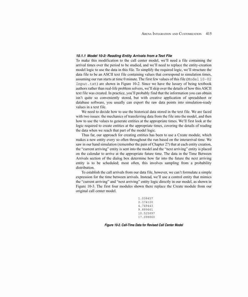
415ARENA INTEGRATION AND CUSTOMIZATION
10.1.1 Model 10-2: Reading Entity Arrivals from a Text FileTo make this modification to the call center model, we’ll need a file containing thearrival times over the period to be studied, and we’ll need to replace the entity-creationmodel logic to use the data in this file. To simplify the required logic, we’ll structure thedata file to be an ASCII text file containing values that correspond to simulation times,assuming our run starts at time 0 minute. The first few values of this file (Model 10-02Input.txt) are shown in Figure 10-2. Since we have the luxury of being textbookauthors rather than real-life problem solvers, we’ll skip over the details of how this ASCIItext file was created. In practice, you’ll probably find that the information you can obtainisn’t quite so conveniently stored, but with creative application of spreadsheet ordatabase software, you usually can export the raw data points into simulation-readyvalues in a text file.
We need to decide how to use the historical data stored in the text file. We are facedwith two issues: the mechanics of transferring data from the file into the model, and thenhow to use the values to generate entities at the appropriate times. We’ll first look at thelogic required to create entities at the appropriate times, covering the details of readingthe data when we reach that part of the model logic.
Thus far, our approach for creating entities has been to use a Create module, whichmakes a new entity every so often throughout the run based on the interarrival time. Wesaw in our hand simulation (remember the pain of Chapter 2?) that at each entity creation,the “current arriving” entity is sent into the model and the “next arriving” entity is placedon the calendar to arrive at the appropriate future time. The data in the Time BetweenArrivals section of the dialog box determine how far into the future the next arrivingentity is to be scheduled; most often, this involves sampling from a probabilitydistribution.
To establish the call arrivals from our data file, however, we can’t formulate a simpleexpression for the time between arrivals. Instead, we’ll use a control entity that mimicsthe “current arriving” and “next arriving” entity logic directly in our model, as shown inFigure 10-3. The first four modules shown there replace the Create module from ouroriginal call center model.
1.0384572.3741204.7494439.89966110.52589717.098860
Figure 10-2. Call-Time Data for Revised Call Center Model
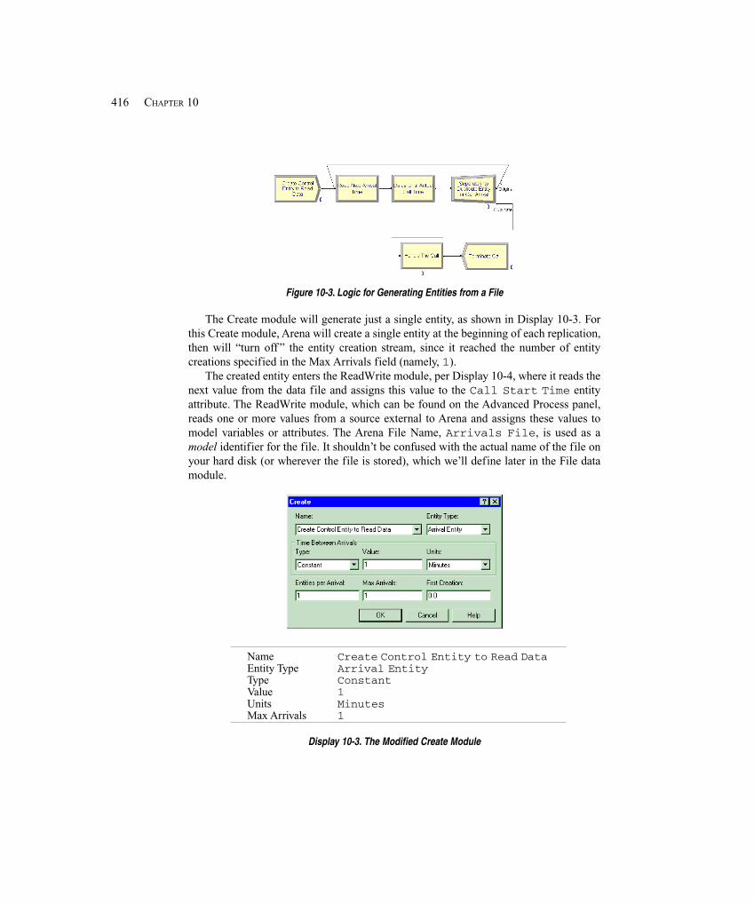
416 CHAPTER 10
Figure 10-3. Logic for Generating Entities from a File
The Create module will generate just a single entity, as shown in Display 10-3. Forthis Create module, Arena will create a single entity at the beginning of each replication,then will “turn off ” the entity creation stream, since it reached the number of entitycreations specified in the Max Arrivals field (namely, 1).
The created entity enters the ReadWrite module, per Display 10-4, where it reads thenext value from the data file and assigns this value to the Call Start Time entityattribute. The ReadWrite module, which can be found on the Advanced Process panel,reads one or more values from a source external to Arena and assigns these values tomodel variables or attributes. The Arena File Name, Arrivals File, is used as amodel identifier for the file. It shouldn’t be confused with the actual name of the file onyour hard disk (or wherever the file is stored), which we’ll define later in the File datamodule.
Name Create Control Entity to Read DataEntity Type Arrival EntityType ConstantValue 1Units MinutesMax Arrivals 1
Display 10-3. The Modified Create Module
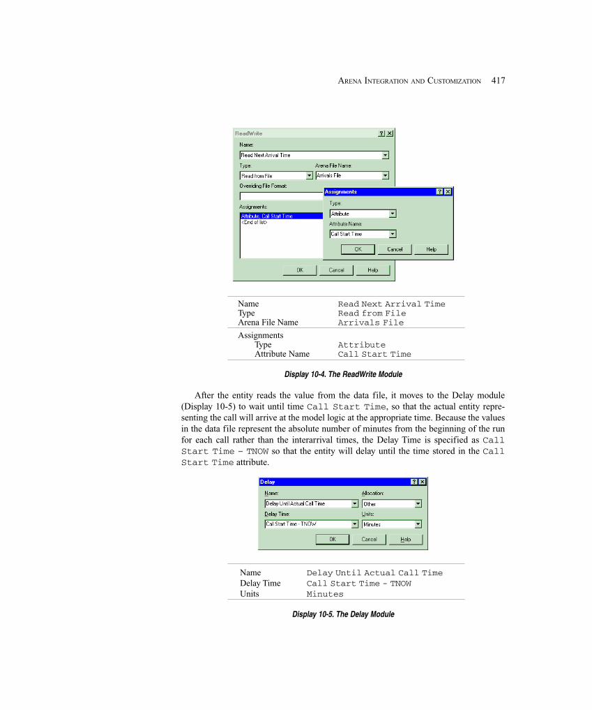
417ARENA INTEGRATION AND CUSTOMIZATION
Name Read Next Arrival TimeType Read from FileArena File Name Arrivals File
AssignmentsType AttributeAttribute Name Call Start Time
Display 10-4. The ReadWrite Module
After the entity reads the value from the data file, it moves to the Delay module(Display 10-5) to wait until time Call Start Time, so that the actual entity repre-senting the call will arrive at the model logic at the appropriate time. Because the valuesin the data file represent the absolute number of minutes from the beginning of the runfor each call rather than the interarrival times, the Delay Time is specified as CallStart Time – TNOW so that the entity will delay until the time stored in the CallStart Time attribute.
Name Delay Until Actual Call TimeDelay Time Call Start Time - TNOWUnits Minutes
Display 10-5. The Delay Module
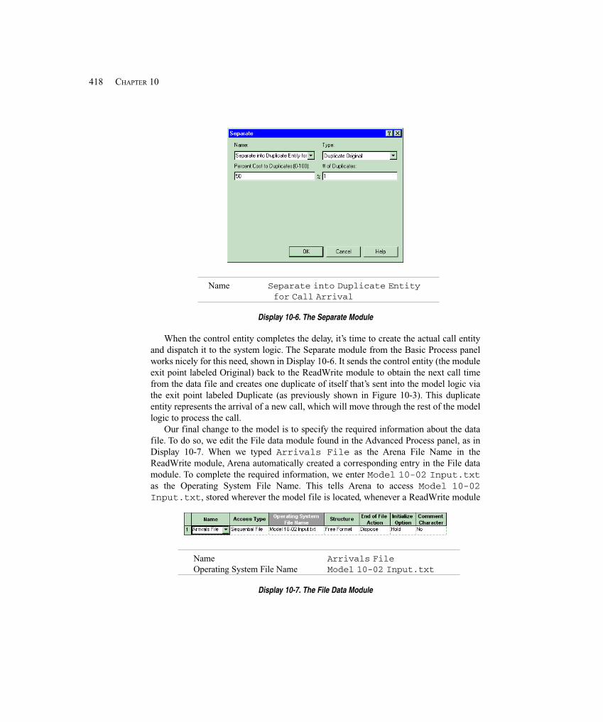
418 CHAPTER 10
Name Separate into Duplicate Entity for Call Arrival
Display 10-6. The Separate Module
When the control entity completes the delay, it’s time to create the actual call entityand dispatch it to the system logic. The Separate module from the Basic Process panelworks nicely for this need, shown in Display 10-6. It sends the control entity (the moduleexit point labeled Original) back to the ReadWrite module to obtain the next call timefrom the data file and creates one duplicate of itself that’s sent into the model logic viathe exit point labeled Duplicate (as previously shown in Figure 10-3). This duplicateentity represents the arrival of a new call, which will move through the rest of the modellogic to process the call.
Our final change to the model is to specify the required information about the datafile. To do so, we edit the File data module found in the Advanced Process panel, as inDisplay 10-7. When we typed Arrivals File as the Arena File Name in theReadWrite module, Arena automatically created a corresponding entry in the File datamodule. To complete the required information, we enter Model 10-02 Input.txtas the Operating System File Name. This tells Arena to access Model 10-02Input.txt, stored wherever the model file is located, whenever a ReadWrite module
Name Arrivals FileOperating System File Name Model 10-02 Input.txt
Display 10-7. The File Data Module

419ARENA INTEGRATION AND CUSTOMIZATION
references the Arena Arrivals File. (You could give a full path for the file, such asC:\My Documents\Cool Stuff\Model 10-02 Input.txt, but if you woulddecide to send the model and data file to someone else, they’d have to have the samefolder structure. Depending on your taste in folder names, this might or might not be agood idea.) We left the other options at their default values, including the file type asFree Format, which indicates that the Model 10-02 Input.txt file contains textvalues. We also retained the default end-of-file action as Dispose so that the controlentity will be disposed of after it reads the last value in the file, effectively terminatingthe arrival stream of entities to the model.
Using the data values in Figure 10-2 to step through the logic for the first two calls,our control entity will first read a value of 1.038 into its Call Start Time attributeafter it’s created at simulation time 0 (the start of the replication). It will delay for 1.038 –0 time units, leaving the Delay module at time 1.038. It creates a duplicate at that time,sending it to the Process module to begin the actual processing of a call. The control en-tity returns to the ReadWrite module, reading a value of 2.374 from the data file andoverwriting its Call Start Time attribute with this value. The control entity proceedsto the Delay module, where it delays for 2.374 – 1.038 = 1.336 time units, which causesArena to place the control entity on the event calendar with an event time that’s 1.336time units into the future (or an actual event time of 2.374). When it’s the control entity’sturn to be processed again, at simulation time 2.374, Arena will remove it from the eventcalendar and send it to the Separate module, where it will spawn a call entity with CallStart Time attribute value 2.374, representing the second call to enter the system.This will continue until all of the values in Model 10-02 Input.txt have been readby the control entity.
The simulation run will terminate under one of two conditions. If the run’s endingtime specified in the Run Setup dialog box occurs before all of the calls listed in the datafile have been created, Arena will end the run at that time; under no conditions can amodel run for longer than is defined. On the other hand, our model may terminate earlierthan the specified run length if all of the calls listed in the data file have been created andhave completed processing, leaving the event calendar empty. (Remember that thecontrol entity is disposed after it reads the last data value.) If Arena encounters acondition where there are no additional entities on the event calendar and no additionalother time-based controls to process, it will terminate the run after the last entity leavesthe model.
10.1.2 Model 10-3 and Model 10-4: Reading and Writing Access and Excel FilesWhat if instead of a text file the call-arrival data were in a Microsoft® Access database orMicrosoft® Excel spreadsheet file? We’ll explore how both of those can be handled easily.
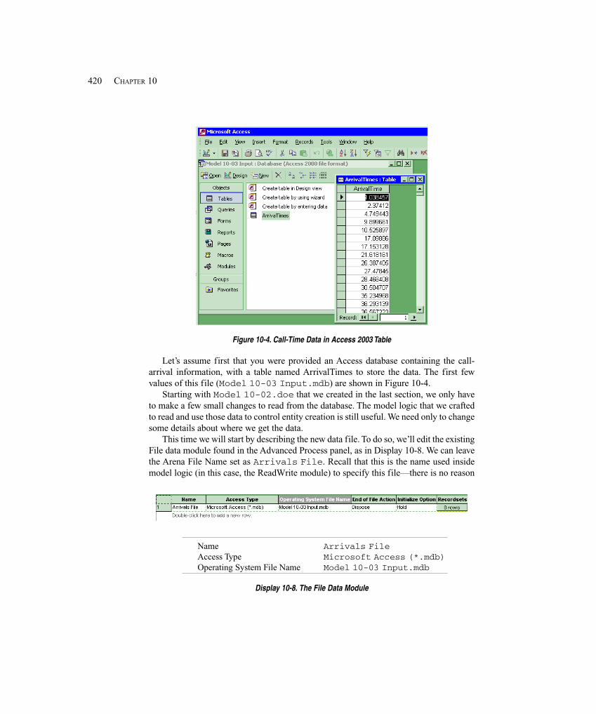
420 CHAPTER 10
Figure 10-4. Call-Time Data in Access 2003 Table
Let’s assume first that you were provided an Access database containing the call-arrival information, with a table named ArrivalTimes to store the data. The first fewvalues of this file (Model 10-03 Input.mdb) are shown in Figure 10-4.
Starting with Model 10-02.doe that we created in the last section, we only haveto make a few small changes to read from the database. The model logic that we craftedto read and use those data to control entity creation is still useful. We need only to changesome details about where we get the data.
This time we will start by describing the new data file. To do so, we’ll edit the existingFile data module found in the Advanced Process panel, as in Display 10-8. We can leavethe Arena File Name set as Arrivals File. Recall that this is the name used insidemodel logic (in this case, the ReadWrite module) to specify this file—there is no reason
Name Arrivals FileAccess Type Microsoft Access (*.mdb)Operating System File Name Model 10-03 Input.mdb
Display 10-8. The File Data Module
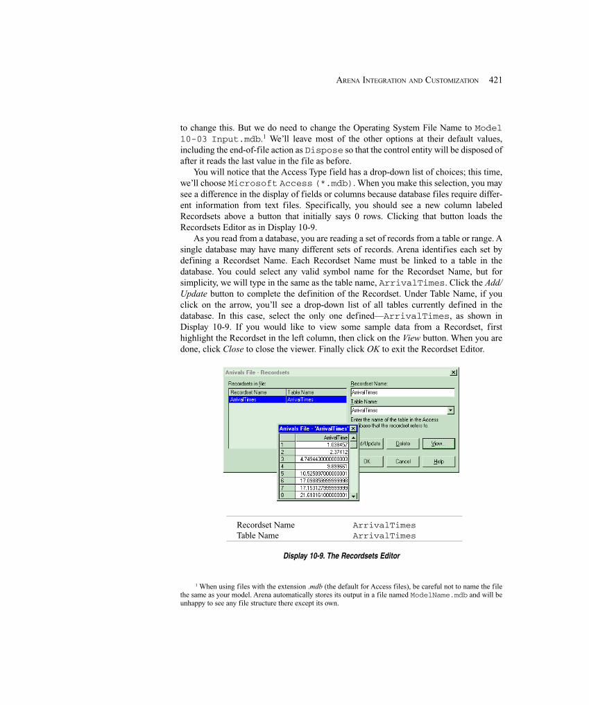
421ARENA INTEGRATION AND CUSTOMIZATION
to change this. But we do need to change the Operating System File Name to Model10-03 Input.mdb.1 We’ll leave most of the other options at their default values,including the end-of-file action as Dispose so that the control entity will be disposed ofafter it reads the last value in the file as before.
You will notice that the Access Type field has a drop-down list of choices; this time,we’ll choose Microsoft Access (*.mdb). When you make this selection, you maysee a difference in the display of fields or columns because database files require differ-ent information from text files. Specifically, you should see a new column labeledRecordsets above a button that initially says 0 rows. Clicking that button loads theRecordsets Editor as in Display 10-9.
As you read from a database, you are reading a set of records from a table or range. Asingle database may have many different sets of records. Arena identifies each set bydefining a Recordset Name. Each Recordset Name must be linked to a table in thedatabase. You could select any valid symbol name for the Recordset Name, but forsimplicity, we will type in the same as the table name, ArrivalTimes. Click the Add/Update button to complete the definition of the Recordset. Under Table Name, if youclick on the arrow, you’ll see a drop-down list of all tables currently defined in thedatabase. In this case, select the only one defined—ArrivalTimes, as shown inDisplay 10-9. If you would like to view some sample data from a Recordset, firsthighlight the Recordset in the left column, then click on the View button. When you aredone, click Close to close the viewer. Finally click OK to exit the Recordset Editor.
Recordset Name ArrivalTimesTable Name ArrivalTimes
Display 10-9. The Recordsets Editor
1 When using files with the extension .mdb (the default for Access files), be careful not to name the filethe same as your model. Arena automatically stores its output in a file named ModelName.mdb and will beunhappy to see any file structure there except its own.
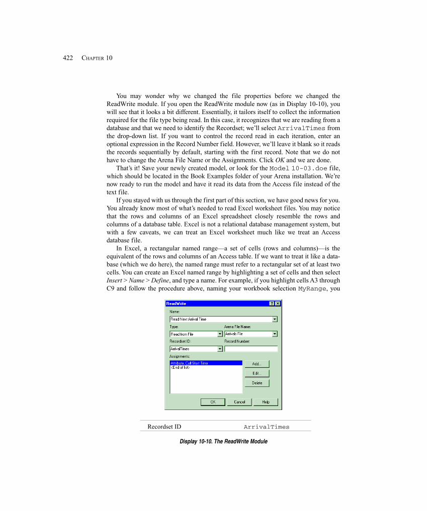
422 CHAPTER 10
You may wonder why we changed the file properties before we changed theReadWrite module. If you open the ReadWrite module now (as in Display 10-10), youwill see that it looks a bit different. Essentially, it tailors itself to collect the informationrequired for the file type being read. In this case, it recognizes that we are reading from adatabase and that we need to identify the Recordset; we’ll select ArrivalTimes fromthe drop-down list. If you want to control the record read in each iteration, enter anoptional expression in the Record Number field. However, we’ll leave it blank so it readsthe records sequentially by default, starting with the first record. Note that we do nothave to change the Arena File Name or the Assignments. Click OK and we are done.
That’s it! Save your newly created model, or look for the Model 10-03.doe file,which should be located in the Book Examples folder of your Arena installation. We’renow ready to run the model and have it read its data from the Access file instead of thetext file.
If you stayed with us through the first part of this section, we have good news for you.You already know most of what’s needed to read Excel worksheet files. You may noticethat the rows and columns of an Excel spreadsheet closely resemble the rows andcolumns of a database table. Excel is not a relational database management system, butwith a few caveats, we can treat an Excel worksheet much like we treat an Accessdatabase file.
In Excel, a rectangular named range—a set of cells (rows and columns)—is theequivalent of the rows and columns of an Access table. If we want to treat it like a data-base (which we do here), the named range must refer to a rectangular set of at least twocells. You can create an Excel named range by highlighting a set of cells and then selectInsert > Name > Define, and type a name. For example, if you highlight cells A3 throughC9 and follow the procedure above, naming your workbook selection MyRange, you
Recordset ID ArrivalTimes
Display 10-10. The ReadWrite Module
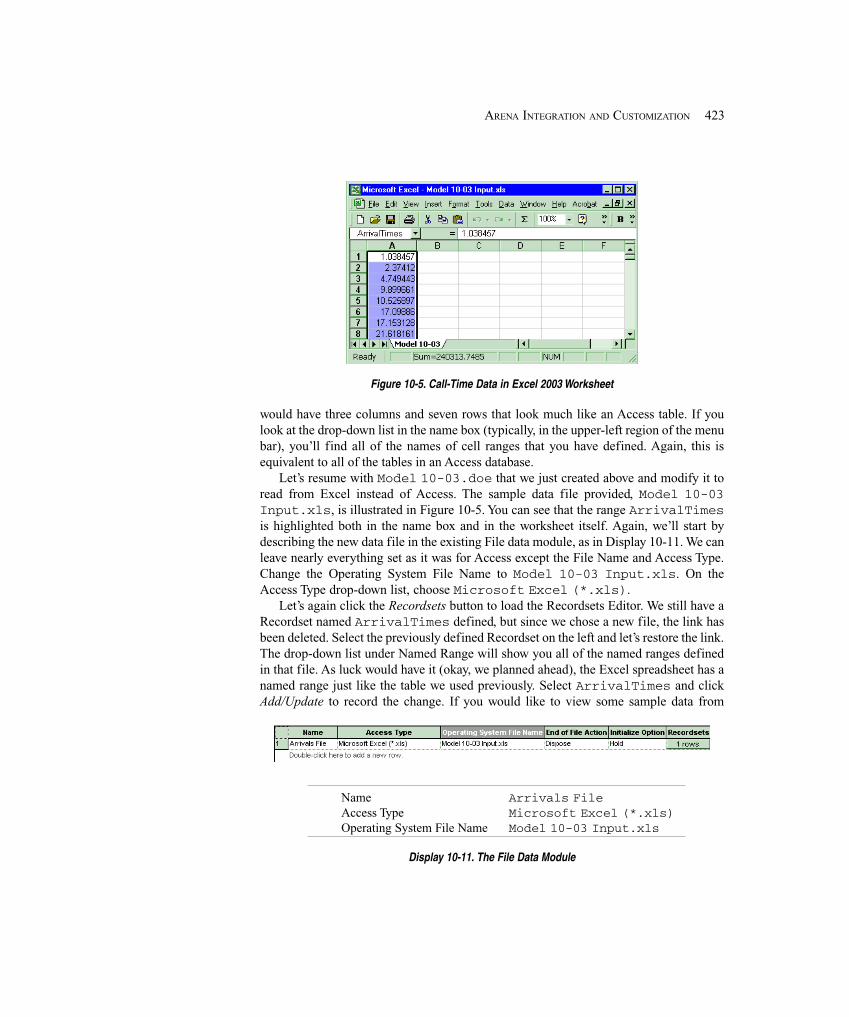
423ARENA INTEGRATION AND CUSTOMIZATION
Figure 10-5. Call-Time Data in Excel 2003 Worksheet
would have three columns and seven rows that look much like an Access table. If youlook at the drop-down list in the name box (typically, in the upper-left region of the menubar), you’ll find all of the names of cell ranges that you have defined. Again, this isequivalent to all of the tables in an Access database.
Let’s resume with Model 10-03.doe that we just created above and modify it toread from Excel instead of Access. The sample data file provided, Model 10-03Input.xls, is illustrated in Figure 10-5. You can see that the range ArrivalTimesis highlighted both in the name box and in the worksheet itself. Again, we’ll start bydescribing the new data file in the existing File data module, as in Display 10-11. We canleave nearly everything set as it was for Access except the File Name and Access Type.Change the Operating System File Name to Model 10-03 Input.xls. On theAccess Type drop-down list, choose Microsoft Excel (*.xls).
Let’s again click the Recordsets button to load the Recordsets Editor. We still have aRecordset named ArrivalTimes defined, but since we chose a new file, the link hasbeen deleted. Select the previously defined Recordset on the left and let’s restore the link.The drop-down list under Named Range will show you all of the named ranges definedin that file. As luck would have it (okay, we planned ahead), the Excel spreadsheet has anamed range just like the table we used previously. Select ArrivalTimes and clickAdd/Update to record the change. If you would like to view some sample data from
Name Arrivals FileAccess Type Microsoft Excel (*.xls)Operating System File Name Model 10-03 Input.xls
Display 10-11. The File Data Module
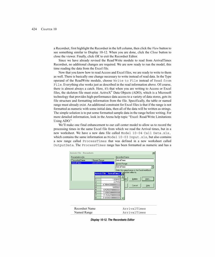
424 CHAPTER 10
a Recordset, first highlight the Recordset in the left column, then click the View button tosee something similar to Display 10-12. When you are done, click the Close button toclose the viewer. Finally, click OK to exit the Recordset Editor.
Since we have already revised the Read/Write module to read from ArrivalTimesRecordset, no additional changes are required. We are now ready to run the model, thistime reading the data from the Excel file.
Now that you know how to read Access and Excel files, we are ready to write to themas well. There is basically one change necessary to write instead of read data. In the Typeoperand of the ReadWrite module, choose Write to File instead of Read fromFile. Everything else works just as described in the read information above. Of course,there is almost always a catch. Here, it’s that when you are writing to Access or Excelfiles, the skeleton file must exist. ActiveX® Data Objects (ADO), which is a Microsofttechnology that provides high-performance data access to a variety of data stores, gets itsfile structure and formatting information from the file. Specifically, the table or namedrange must already exist. An additional constraint for Excel files is that if the range is notformatted as numeric with some initial data, then all of the data will be written as strings.The simple solution is to put some formatted sample data in the range before writing. Formore detailed information, look in the Arena help topic “Excel: Read/Write LimitationsUsing ADO.”
We’ll make one final enhancement to our call center model to allow us to record theprocessing times in the same Excel file from which we read the Arrival times, but in anew worksheet. We have a new data file called Model 10-04 Call Data.xls,which contains the same information as Model 10-03 Input.xls, but also containsa new range called ProcessTimes that was defined in a new worksheet calledOutputData. The ProcessTimes range has been formatted as numeric and has a
Recordset Name ArrivalTimesNamed Range ArrivalTimes
Display 10-12. The Recordsets Editor
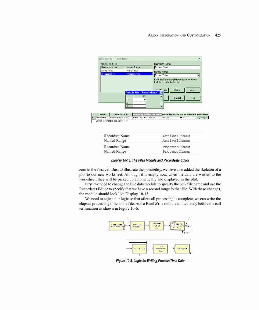
425ARENA INTEGRATION AND CUSTOMIZATION
Recordset Name ArrivalTimesNamed Range ArrivalTimes
Recordset Name ProcessTimesNamed Range ProcessTimes
Display 10-13. The Files Module and Recordsets Editor
zero in the first cell. Just to illustrate the possibility, we have also added the skeleton of aplot to our new worksheet. Although it is empty now, when the data are written to theworksheet, they will be picked up automatically and displayed in the plot.
First, we need to change the File data module to specify the new file name and use theRecordsets Editor to specify that we have a second range in that file. With these changes,the module should look like Display 10-13.
We need to adjust our logic so that after call processing is complete, we can write theelapsed processing time to the file. Add a ReadWrite module immediately before the calltermination as shown in Figure 10-6.
Figure 10-6. Logic for Writing Process Time Data
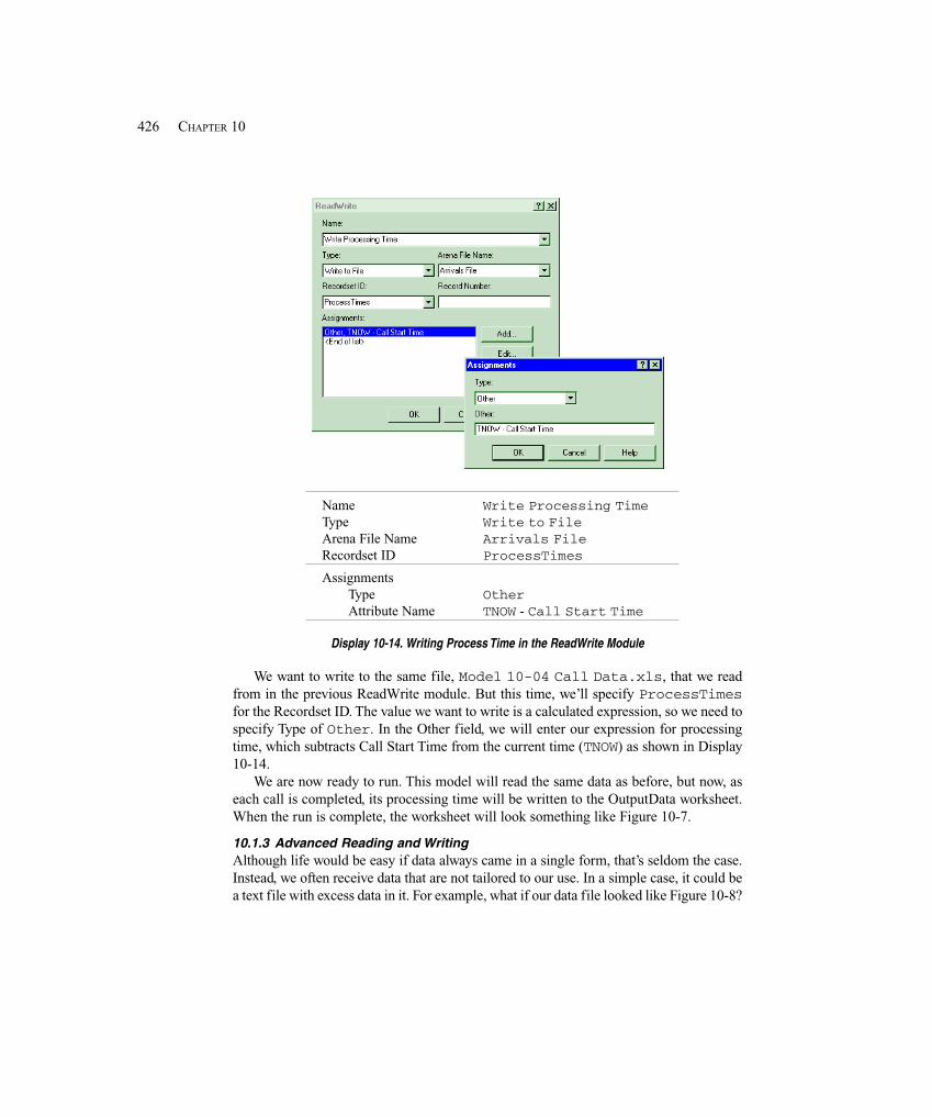
426 CHAPTER 10
Name Write Processing TimeType Write to FileArena File Name Arrivals FileRecordset ID ProcessTimes
AssignmentsType OtherAttribute Name TNOW - Call Start Time
Display 10-14. Writing Process Time in the ReadWrite Module
We want to write to the same file, Model 10-04 Call Data.xls, that we readfrom in the previous ReadWrite module. But this time, we’ll specify ProcessTimesfor the Recordset ID. The value we want to write is a calculated expression, so we need tospecify Type of Other. In the Other field, we will enter our expression for processingtime, which subtracts Call Start Time from the current time (TNOW) as shown in Display10-14.
We are now ready to run. This model will read the same data as before, but now, aseach call is completed, its processing time will be written to the OutputData worksheet.When the run is complete, the worksheet will look something like Figure 10-7.
10.1.3 Advanced Reading and WritingAlthough life would be easy if data always came in a single form, that’s seldom the case.Instead, we often receive data that are not tailored to our use. In a simple case, it could bea text file with excess data in it. For example, what if our data file looked like Figure 10-8?
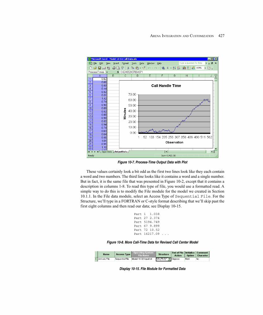
427ARENA INTEGRATION AND CUSTOMIZATION
Figure 10-7. Process-Time Output Data with Plot
These values certainly look a bit odd as the first two lines look like they each containa word and two numbers. The third line looks like it contains a word and a single number.But in fact, it is the same file that was presented in Figure 10-2, except that it contains adescription in columns 1-8. To read this type of file, you would use a formatted read. Asimple way to do this is to modify the File module for the model we created in Section10.1.1. In the File data module, select an Access Type of Sequential File. For theStructure, we’ll type in a FORTRAN or C-style format describing that we’ll skip past thefirst eight columns and then read our data; see Display 10-15.
Part 1 1.038Part 27 2.374Part 5194.749Part 67 9.899Part 72 10.52Part 16217.09 . . .
Figure 10-8. More Call-Time Data for Revised Call Center Model
Display 10-15. File Module for Formatted Data
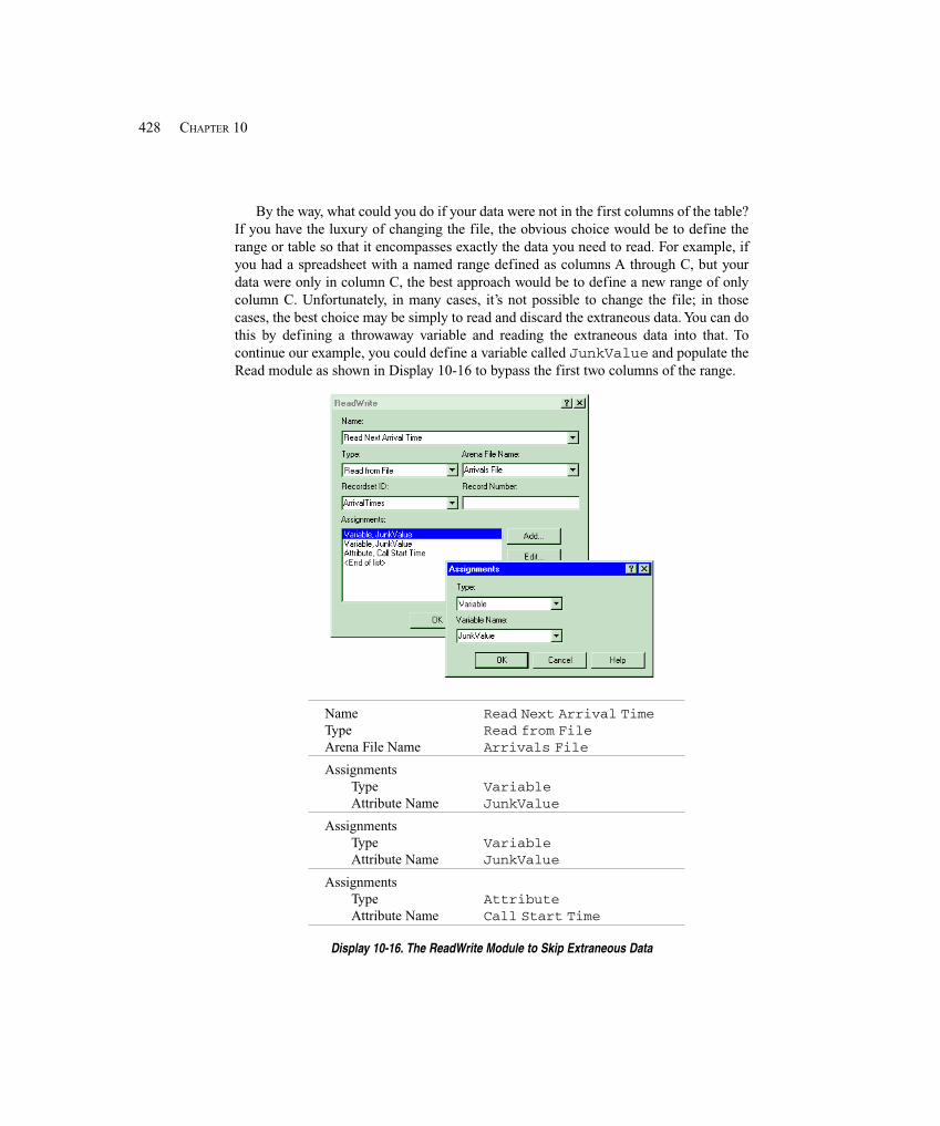
428 CHAPTER 10
By the way, what could you do if your data were not in the first columns of the table?If you have the luxury of changing the file, the obvious choice would be to define therange or table so that it encompasses exactly the data you need to read. For example, ifyou had a spreadsheet with a named range defined as columns A through C, but yourdata were only in column C, the best approach would be to define a new range of onlycolumn C. Unfortunately, in many cases, it’s not possible to change the file; in thosecases, the best choice may be simply to read and discard the extraneous data. You can dothis by defining a throwaway variable and reading the extraneous data into that. Tocontinue our example, you could define a variable called JunkValue and populate theRead module as shown in Display 10-16 to bypass the first two columns of the range.
Name Read Next Arrival TimeType Read from FileArena File Name Arrivals File
AssignmentsType VariableAttribute Name JunkValue
AssignmentsType VariableAttribute Name JunkValue
AssignmentsType AttributeAttribute Name Call Start Time
Display 10-16. The ReadWrite Module to Skip Extraneous Data
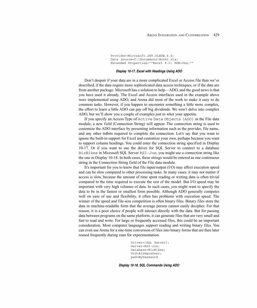
429ARENA INTEGRATION AND CUSTOMIZATION
Provider=Microsoft.JET.OLEDB.4.0;Data Source=C:\Documents\Book1.xls;Extended Properties=””Excel 8.0; HDR=Yes;””
Display 10-17. Excel with Headings Using ADO
Don’t despair if your data are in a more complicated Excel or Access file than we’vedescribed, if the data require more sophisticated data access techniques, or if the data arefrom another package. Microsoft has a solution to help—ADO, and the good news is thatyou have used it already. The Excel and Access interfaces used in the example abovewere implemented using ADO, and Arena did most of the work to make it easy to docommon tasks. However, if you happen to encounter something a little more complex,the effort to learn a little ADO can pay off big dividends. We won’t delve into complexADO, but we’ll show you a couple of examples just to whet your appetite.
If you specify an Access Type of Active Data Objects (ADO) in the File datamodule, a new field (Connection String) will appear. The connection string is used tocustomize the ADO interface by presenting information such as the provider, file name,and any other tidbits required to complete the connection. Let’s say that you want toignore the built-in support for Excel and customize your own, perhaps because you wantto support column headings. You could enter the connection string specified in Display10-17. Or if you want to use the driver for SQL Server to connect to a databaseBizBikes in Microsoft SQL Server RSI-Joe, you might use a connection string likethe one in Display 10-18. In both cases, these strings would be entered as one continuousstring in the Connection String field of the File data module.
It’s important for you to know that file input/output (I/O) may affect execution speedand can be slow compared to other processing tasks. In many cases, it may not matter ifaccess is slow, because the amount of time spent reading or writing data is often trivialcompared to the time required to execute the rest of the model. But I/O speed may beimportant with very high volumes of data. In such cases, you might want to specify thedata to be in the fastest or smallest form possible. Although ADO generally competeswell on ease of use and flexibility, it often has problems with execution speed. Thewinner of the speed and file-size competition is often binary files. Binary files store thedata in machine-readable form that the average person cannot easily decipher. For thatreason, it is a poor choice if people will interact directly with the data. But for passingdata between programs on the same platform, it can generate files that are very small andfast to read and write. For large or frequently accessed files, this could be an importantconsideration. Most computer languages support reading and writing binary files. Youcan even use Arena for a one-time conversion of files into binary forms that are then laterreused frequently during runs for experimentation.
Driver={SQL Server};Server=RSI-Joe;Database=BizBikes;Uid=BizWareUser;pwd=MyPassword
Display 10-18. SQL Commands Using ADO
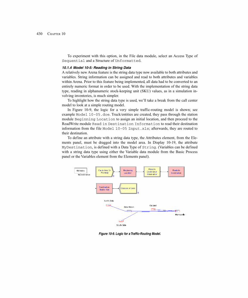
430 CHAPTER 10
To experiment with this option, in the File data module, select an Access Type ofSequential and a Structure of Unformatted.
10.1.4 Model 10-5: Reading in String DataA relatively new Arena feature is the string data type now available to both attributes andvariables. String information can be assigned and read to both attributes and variableswithin Arena. Prior to this feature being implemented, all data had to be converted to anentirely numeric format in order to be used. With the implementation of the string datatype, reading in alphanumeric stock-keeping unit (SKU) values, as in a simulation in-volving inventories, is much simpler.
To highlight how the string data type is used, we’ll take a break from the call centermodel to look at a simple routing model.
In Figure 10-9, the logic for a very simple traffic-routing model is shown; seeexample Model 10-05.doe. Truck/entities are created, they pass through the stationmodule Beginning Location to assign an initial location, and then proceed to theReadWrite module Read in Destination Information to read their destinationinformation from the file Model 10-05 Input.xls; afterwards, they are routed totheir destination.
To define an attribute with a string data type, the Attributes element, from the Ele-ments panel, must be dragged into the model area. In Display 10-19, the attributeMyDestination, is defined with a Data Type of String. (Variables can be definedwith a string data type using either the Variable data module from the Basic Processpanel or the Variables element from the Elements panel).
Figure 10-9. Logic for a Traffic-Routing Model.
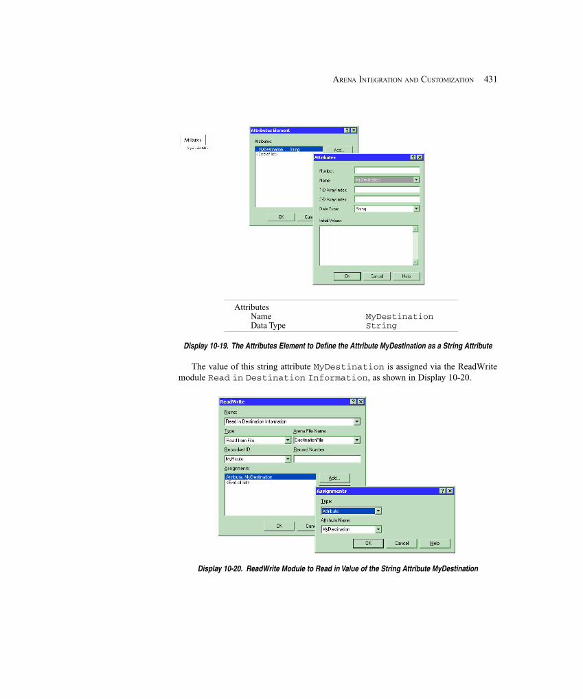
431ARENA INTEGRATION AND CUSTOMIZATION
AttributesName MyDestinationData Type String
Display 10-19. The Attributes Element to Define the Attribute MyDestination as a String Attribute
The value of this string attribute MyDestination is assigned via the ReadWritemodule Read in Destination Information, as shown in Display 10-20.
Display 10-20. ReadWrite Module to Read in Value of the String Attribute MyDestination
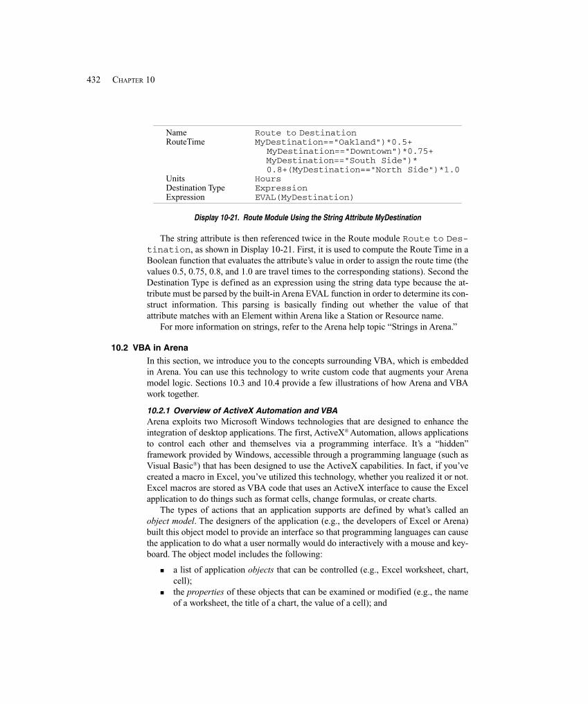
432 CHAPTER 10
Name Route to DestinationRouteTime MyDestination=="Oakland")*0.5+
MyDestination=="Downtown")*0.75+ MyDestination=="South Side")* 0.8+(MyDestination=="North Side")*1.0
Units HoursDestination Type ExpressionExpression EVAL(MyDestination)
Display 10-21. Route Module Using the String Attribute MyDestination
The string attribute is then referenced twice in the Route module Route to Des-tination, as shown in Display 10-21. First, it is used to compute the Route Time in aBoolean function that evaluates the attribute’s value in order to assign the route time (thevalues 0.5, 0.75, 0.8, and 1.0 are travel times to the corresponding stations). Second theDestination Type is defined as an expression using the string data type because the at-tribute must be parsed by the built-in Arena EVAL function in order to determine its con-struct information. This parsing is basically finding out whether the value of thatattribute matches with an Element within Arena like a Station or Resource name.
For more information on strings, refer to the Arena help topic “Strings in Arena.”
10.2 VBA in ArenaIn this section, we introduce you to the concepts surrounding VBA, which is embeddedin Arena. You can use this technology to write custom code that augments your Arenamodel logic. Sections 10.3 and 10.4 provide a few illustrations of how Arena and VBAwork together.
10.2.1 Overview of ActiveX Automation and VBAArena exploits two Microsoft Windows technologies that are designed to enhance theintegration of desktop applications. The first, ActiveX® Automation, allows applicationsto control each other and themselves via a programming interface. It’s a “hidden”framework provided by Windows, accessible through a programming language (such asVisual Basic®) that has been designed to use the ActiveX capabilities. In fact, if you’vecreated a macro in Excel, you’ve utilized this technology, whether you realized it or not.Excel macros are stored as VBA code that uses an ActiveX interface to cause the Excelapplication to do things such as format cells, change formulas, or create charts.
The types of actions that an application supports are defined by what’s called anobject model. The designers of the application (e.g., the developers of Excel or Arena)built this object model to provide an interface so that programming languages can causethe application to do what a user normally would do interactively with a mouse and key-board. The object model includes the following:
� a list of application objects that can be controlled (e.g., Excel worksheet, chart,cell);
� the properties of these objects that can be examined or modified (e.g., the nameof a worksheet, the title of a chart, the value of a cell); and

433ARENA INTEGRATION AND CUSTOMIZATION
� the methods (or actions) that can be performed on the objects or that they canperform (e.g., delete a worksheet, create a chart, merge cells).
When you install an application that contains an object model, its setup processregisters the object model with the Windows operating system (i.e., adds it to the list ofobject models that are available on your computer). Then, if you use a programminglanguage and want to utilize the application’s functionality, you can establish a referenceto its object model and program its objects directly. We’ll see how this works when wewrite VBA code in Arena to send data to Microsoft Excel. Many desktop applicationscan be automated (i.e., controlled by another application), including Microsoft Office,AutoCAD®, and Visio®. To create the program that controls the application, you can useprogramming languages like C++, Visual Basic, or Java.
The second technology exploited by Arena for application integration embeds a pro-gramming language (VBA) directly in Arena to allow you to write code that automatesother applications without having to purchase or install a separate programming lan-guage. VBA is the same language that works with Microsoft Office, AutoCAD, andArena. It’s also the same engine behind Visual Basic. When you install Arena, you alsoreceive this full Visual Basic programming environment, accessed via Tools > Macro >Show Visual Basic Editor.
These two technologies work together to allow Arena to integrate with other pro-grams that support ActiveX Automation. You can write Visual Basic code directly inArena (via the Visual Basic Editor) that automates other programs, such as Excel,AutoCAD, or Visio. In our enhancement to the call center model, we’ll create a newExcel worksheet, populate it with data during the simulation run, and automatically chartthe data, all without “touching” Excel directly. You also can write VBA code to automateArena, such as to add animation variables, get the values of simulation output statistics,or change the values of module operands.
When you write Visual Basic code using VBA in Arena, your code is stored with theArena model (.doe) file, just as VBA macros in Excel are stored in the spreadsheet (.xls)files. You have at your disposal the full arsenal of VBA features, including:
� Visual Basic programming constructs, such as Sub, Function, Class, If, Elseif,Endif, While, Wend, Do, On Error, and Select Case;
� UserForms (often referred to as dialog boxes) with an assortment of fancycontrols like toggle buttons, scroll bars, input boxes, command buttons, and theever-popular spin buttons;
� code-debugging tools like watches, breakpoints, and various step options; and� comprehensive help.
To open the Visual Basic Editor in Arena, select Tools > Macro > Show Visual BasicEditor, or click the corresponding button on the Integration toolbar ( ). This opens aseparate window that hosts all of the VBA code, forms, debugging interface, and accessto VBA help, as illustrated in Figure 10-10.
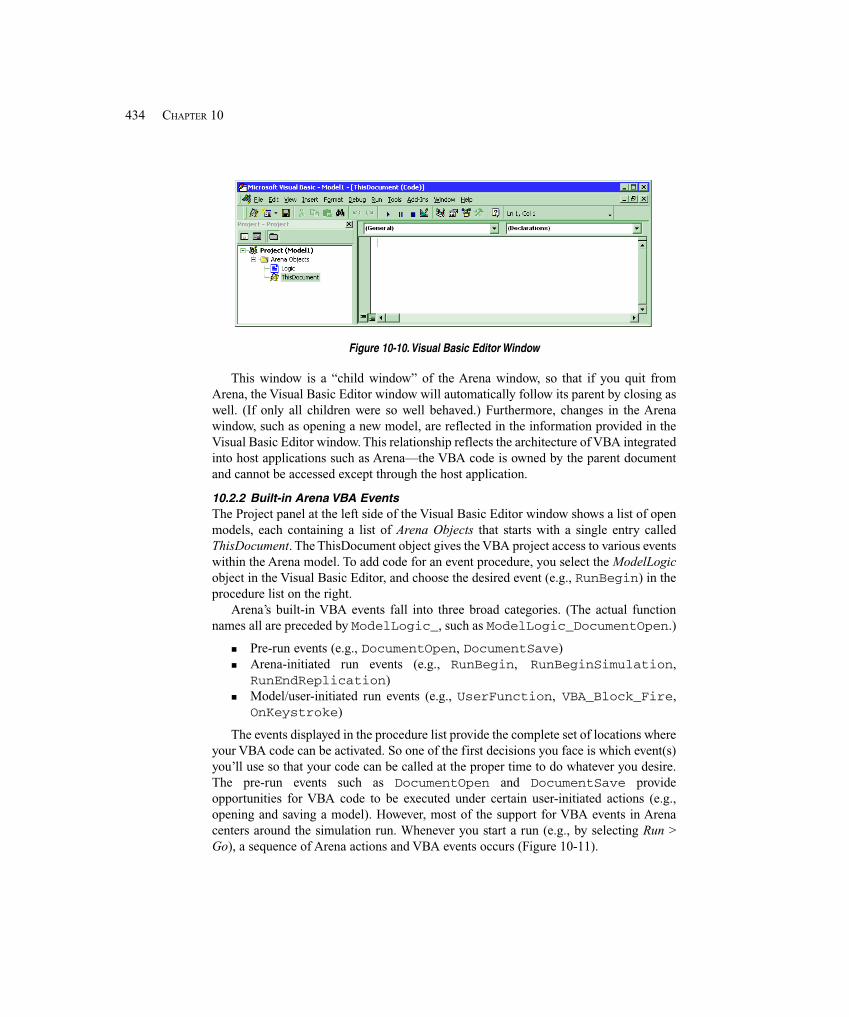
434 CHAPTER 10
Figure 10-10. Visual Basic Editor Window
This window is a “child window” of the Arena window, so that if you quit fromArena, the Visual Basic Editor window will automatically follow its parent by closing aswell. (If only all children were so well behaved.) Furthermore, changes in the Arenawindow, such as opening a new model, are reflected in the information provided in theVisual Basic Editor window. This relationship reflects the architecture of VBA integratedinto host applications such as Arena—the VBA code is owned by the parent documentand cannot be accessed except through the host application.
10.2.2 Built-in Arena VBA EventsThe Project panel at the left side of the Visual Basic Editor window shows a list of openmodels, each containing a list of Arena Objects that starts with a single entry calledThisDocument. The ThisDocument object gives the VBA project access to various eventswithin the Arena model. To add code for an event procedure, you select the ModelLogicobject in the Visual Basic Editor, and choose the desired event (e.g., RunBegin) in theprocedure list on the right.
Arena’s built-in VBA events fall into three broad categories. (The actual functionnames all are preceded by ModelLogic_, such as ModelLogic_DocumentOpen.)
� Pre-run events (e.g., DocumentOpen, DocumentSave)� Arena-initiated run events (e.g., RunBegin, RunBeginSimulation,
RunEndReplication)� Model/user-initiated run events (e.g., UserFunction, VBA_Block_Fire,
OnKeystroke)
The events displayed in the procedure list provide the complete set of locations whereyour VBA code can be activated. So one of the first decisions you face is which event(s)you’ll use so that your code can be called at the proper time to do whatever you desire.The pre-run events such as DocumentOpen and DocumentSave provideopportunities for VBA code to be executed under certain user-initiated actions (e.g.,opening and saving a model). However, most of the support for VBA events in Arenacenters around the simulation run. Whenever you start a run (e.g., by selecting Run >Go), a sequence of Arena actions and VBA events occurs (Figure 10-11).
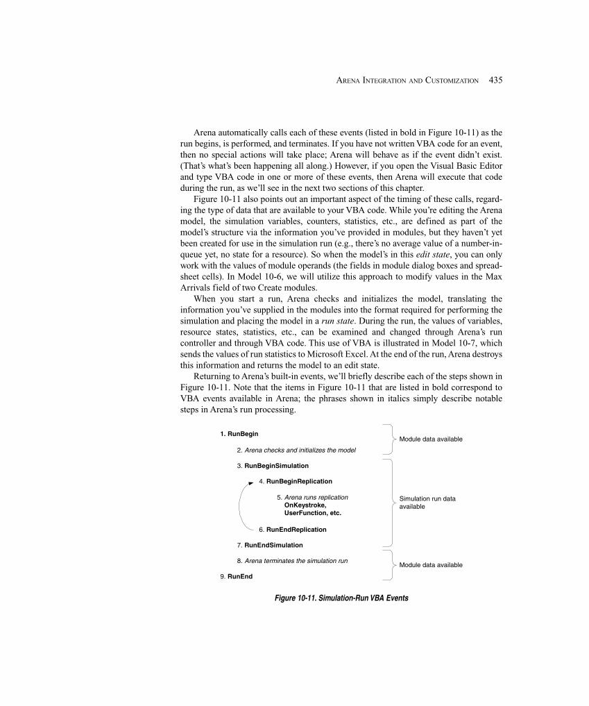
435ARENA INTEGRATION AND CUSTOMIZATION
Arena automatically calls each of these events (listed in bold in Figure 10-11) as therun begins, is performed, and terminates. If you have not written VBA code for an event,then no special actions will take place; Arena will behave as if the event didn’t exist.(That’s what’s been happening all along.) However, if you open the Visual Basic Editorand type VBA code in one or more of these events, then Arena will execute that codeduring the run, as we’ll see in the next two sections of this chapter.
Figure 10-11 also points out an important aspect of the timing of these calls, regard-ing the type of data that are available to your VBA code. While you’re editing the Arenamodel, the simulation variables, counters, statistics, etc., are defined as part of themodel’s structure via the information you’ve provided in modules, but they haven’t yetbeen created for use in the simulation run (e.g., there’s no average value of a number-in-queue yet, no state for a resource). So when the model’s in this edit state, you can onlywork with the values of module operands (the fields in module dialog boxes and spread-sheet cells). In Model 10-6, we will utilize this approach to modify values in the MaxArrivals field of two Create modules.
When you start a run, Arena checks and initializes the model, translating theinformation you’ve supplied in the modules into the format required for performing thesimulation and placing the model in a run state. During the run, the values of variables,resource states, statistics, etc., can be examined and changed through Arena’s runcontroller and through VBA code. This use of VBA is illustrated in Model 10-7, whichsends the values of run statistics to Microsoft Excel. At the end of the run, Arena destroysthis information and returns the model to an edit state.
Returning to Arena’s built-in events, we’ll briefly describe each of the steps shown inFigure 10-11. Note that the items in Figure 10-11 that are listed in bold correspond toVBA events available in Arena; the phrases shown in italics simply describe notablesteps in Arena’s run processing.
1. RunBegin
2. Arena checks and initializes the model
3. RunBeginSimulation
4. RunBeginReplication
Module data available
5. Arena runs replication OnKeystroke, UserFunction, etc.
6. RunEndReplication
7. RunEndSimulation
8. Arena terminates the simulation run
9. RunEnd
Simulation run dataavailable
Module data available
Figure 10-11. Simulation-Run VBA Events
436 CHAPTER 10
1. ModelLogic_RunBegin is called.At this point, VBA code can make changes to the structural data of the
model—that is, the values in module operands—and have the changes beincluded in the simulation run because the updated information will be part ofthe initialization and check of the model. You might use this event to query forinputs that will overwrite what’s stored in modules (e.g., a probability at aDecide module or update the capacity of a resource or perhaps even add logicbased on user input). This event’s use is illustrated later in Model 10-6.
2. Arena checks the model and initializes the simulation to a run state.This process takes place behind the scenes, with Arena verifying that your
model is ready to run and compiling the model, which may include the updatesmade during the RunBegin event. After the model is checked and initialized inthis step, Arena ignores what’s contained in the modules, working instead withthe simulation runtime data that change dynamically once the run has started. Atthis point, all variables have been assigned their initial values (e.g., the numbersyou typed in the Variable spreadsheet or updated during the RunBegin event),but no entities have yet entered the model.
3. ModelLogic_RunBeginSimulation is called.Here, Arena gives you the chance to insert VBA code that will be executed
only once at the beginning of the simulation run. (Of course, if Arena detectederrors in your model in Step 2, this event won’t be called; you first have to fixyour mistakes to allow proper initialization of the model.) When the VBA code inRunBeginSimulation is being executed, Arena holds off on starting thesimulation run. So at this point, you can safely load lots of data from outsidesources like Excel, Access, or Oracle®; display a UserForm to ask whoever’s run-ning your model for some sage advice, such as how many shifts they want to runin today’s simulation; or set up the headers in an Excel file that will be storingsome detailed simulation results (as we’ll see in Model 10-7). Often this code willend up assigning values to variables in the Arena model, though it also could cre-ate entities, alter resource capacities, or dozens of other things that you’ll findif you delve into the depths of the Arena object model. After yourRunBeginSimulation VBA code is finished doing its work, Arena moves tothe next step.
4. ModelLogic_RunBeginReplication is called.For each replication that you’ve defined for this run, Arena will call
RunBeginReplication at the beginning of the replication (i.e., before anyentities have entered the model). The types of things you might do here are simi-lar to those described for RunBeginSimulation—except that whatever youdefine in RunBeginReplication will be repeated at the beginning of eachreplication. We’ll see in Model 10-7 how these two events can be used together.
437ARENA INTEGRATION AND CUSTOMIZATION
5. Arena runs the simulation.Next, the model run is performed. In this step, entities are created and
disposed, resources are seized and released, etc.; basically all that stuff you’velearned in your suffering through the previous chapters of this book is put to work.During the run, Arena provides a number of opportunities for you to activate VBAcode, such as the following.
� ModelLogic_UserFunction—called whenever the UF variable isreferenced in Arena logic. This event might be used to perform complexcalculations for a process delay or decision criterion.
� ModelLogic_VBA_Block_Fire—called when an entity passesthrough a VBA module (from the Blocks panel) in model logic. This eventis used in Model 10-7 to write detailed information to Excel as each entitydeparts the model.
� ModelLogic_OnKeystroke—called whenever the user strikes a keyduring the simulation run. For example, your VBA code might display aUserForm with summary model status whenever the “1” key is pressed.
� ModelLogic_OnClearStatistics—called whenever statisticsare cleared, such as when simulation time reaches the value entered for thewarm-up period in the Run Setup dialog box. You might write VBA codehere to set certain model variables or to send an entity into the model toactivate specialized logic that augments the standard Arena statisticsinitialization.
6. ModelLogic_RunEndReplication is called if the simulation reaches theend of a replication.
This event typically stores VBA code that either writes some summary infor-mation to an external file, increments some global variables, or both. Note thatit’s only called when the run reaches the end of a replication; if the run is stoppedfor some other cause (such as the user clicking the End button on the Runtoolbar), then this event is not executed.
7. ModelLogic_RunEndSimulation is called.Regardless of how Arena ended the run, the VBA code in this event will be
executed. When RunEndSimulation is called, the runtime simulation dataare still available, so final statistics values, resource states, etc., can be accessedby the VBA code here. RunEndSimulation typically contains logic to writecustom statistics to files, spreadsheets, or databases, as well as “clean-up” code toclose files or display end-of-run messages.
8. Arena terminates the simulation run.This is the counterpart to Step 2. Arena clears all of the runtime simulation
data and returns the model to an edit state.
9. ModelLogic_RunEnd is called.Finally, the RunEnd VBA event is called, providing a balance to the
RunBegin event in Step 1. The VBA code in this event cannot access any
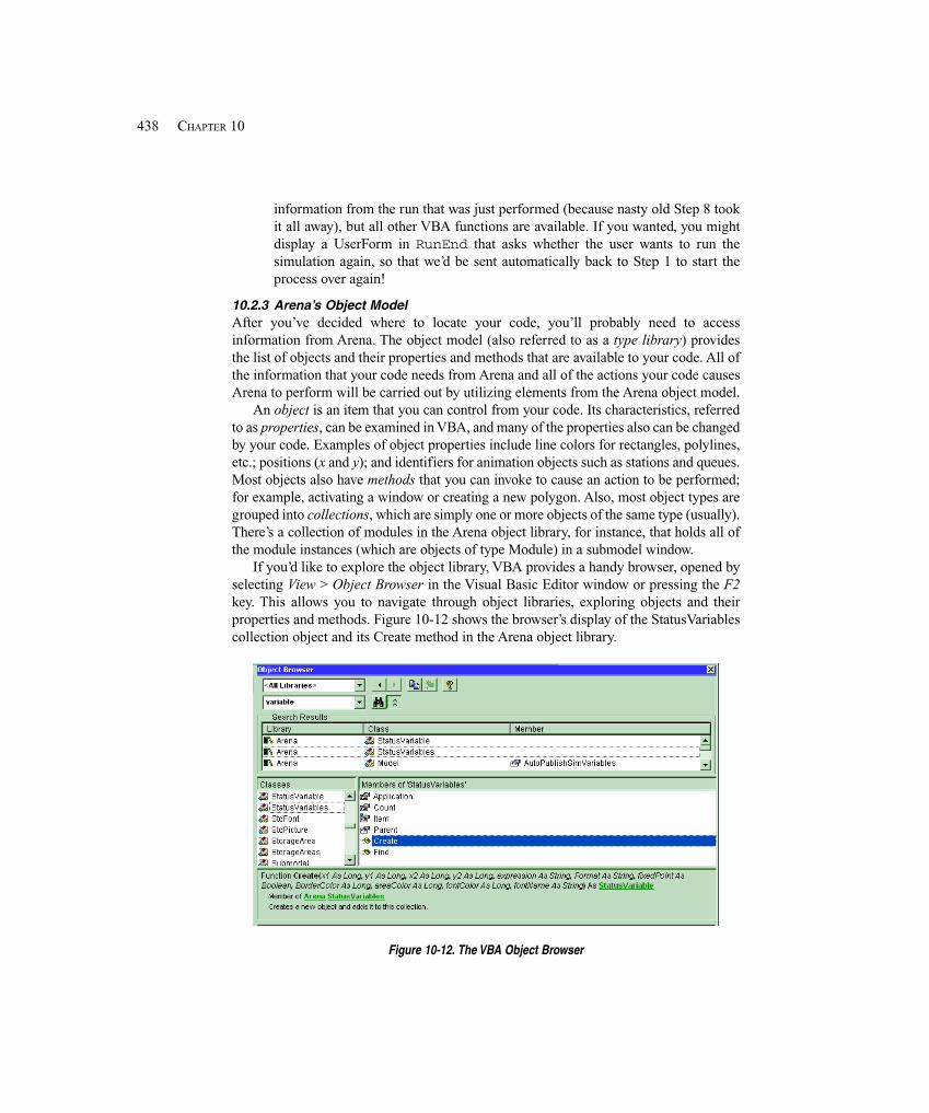
438 CHAPTER 10
information from the run that was just performed (because nasty old Step 8 tookit all away), but all other VBA functions are available. If you wanted, you mightdisplay a UserForm in RunEnd that asks whether the user wants to run thesimulation again, so that we’d be sent automatically back to Step 1 to start theprocess over again!
10.2.3 Arena’s Object ModelAfter you’ve decided where to locate your code, you’ll probably need to accessinformation from Arena. The object model (also referred to as a type library) providesthe list of objects and their properties and methods that are available to your code. All ofthe information that your code needs from Arena and all of the actions your code causesArena to perform will be carried out by utilizing elements from the Arena object model.
An object is an item that you can control from your code. Its characteristics, referredto as properties, can be examined in VBA, and many of the properties also can be changedby your code. Examples of object properties include line colors for rectangles, polylines,etc.; positions (x and y); and identifiers for animation objects such as stations and queues.Most objects also have methods that you can invoke to cause an action to be performed;for example, activating a window or creating a new polygon. Also, most object types aregrouped into collections, which are simply one or more objects of the same type (usually).There’s a collection of modules in the Arena object library, for instance, that holds all ofthe module instances (which are objects of type Module) in a submodel window.
If you’d like to explore the object library, VBA provides a handy browser, opened byselecting View > Object Browser in the Visual Basic Editor window or pressing the F2key. This allows you to navigate through object libraries, exploring objects and theirproperties and methods. Figure 10-12 shows the browser’s display of the StatusVariablescollection object and its Create method in the Arena object library.
Figure 10-12. The VBA Object Browser
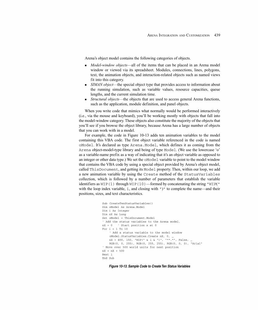
439ARENA INTEGRATION AND CUSTOMIZATION
Arena’s object model contains the following categories of objects.
� Model-window objects—all of the items that can be placed in an Arena modelwindow or viewed via its spreadsheet. Modules, connections, lines, polygons,text, the animation objects, and interaction-related objects such as named viewsfit into this category.
� SIMAN object—the special object type that provides access to information aboutthe running simulation, such as variable values, resource capacities, queuelengths, and the current simulation time.
� Structural objects—the objects that are used to access general Arena functions,such as the application, module definition, and panel objects.
When you write code that mimics what normally would be performed interactively(i.e., via the mouse and keyboard), you’ll be working mostly with objects that fall intothe model-window category. These objects also constitute the majority of the objects thatyou’ll see if you browse the object library, because Arena has a large number of objectsthat you can work with in a model.
For example, the code in Figure 10-13 adds ten animation variables to the modelcontaining this VBA code. The first object variable referenced in the code is namedoModel. It’s declared as type Arena.Model, which defines it as coming from theArena object-model-type library and being of type Model. (We use the lowercase ‘o’as a variable-name prefix as a way of indicating that it’s an object variable as opposed toan integer or other data type.) We set the oModel variable to point to the model windowthat contains the VBA code by using a special object provided by Arena’s object model,called ThisDocument, and getting its Model property. Then, within our loop, we adda new animation variable by using the Create method of the StatusVariablescollection, which is followed by a number of parameters that establish the variableidentifiers as WIP(1) through WIP(10)—formed by concatenating the string "WIP("with the loop index variable, i, and closing with ")" to complete the name—and theirpositions, sizes, and text characteristics.
Sub CreateTenStatusVariables()Dim oModel As Arena.ModelDim i As IntegerDim nX As LongSet oModel = ThisDocument.Model' Add the status variables to the Arena model.nX = 0 ' Start position x at 0For i = 1 To 10 ' Add a status variable to the model window oModel.StatusVariables.Create nX, 0, _ nX + 400, 150, "WIP(" & i & ")", "**.*", False, _ RGB(0, 0, 255), RGB(0, 255, 255), RGB(0, 0, 0), "Arial"' Move over 500 world units for next positionnX = nX + 500Next iEnd Sub
Figure 10-13. Sample Code to Create Ten Status Variables
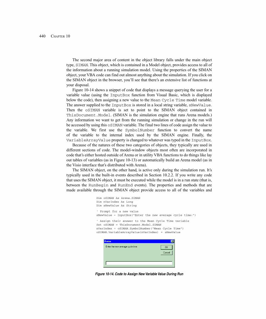
440 CHAPTER 10
The second major area of content in the object library falls under the main objecttype, SIMAN. This object, which is contained in a Model object, provides access to all ofthe information about a running simulation model. Using the properties of the SIMANobject, your VBA code can find out almost anything about the simulation. If you click onthe SIMAN object in the browser, you’ll see that there’s an extensive list of functions atyour disposal.
Figure 10-14 shows a snippet of code that displays a message querying the user for avariable value (using the InputBox function from Visual Basic, which is displayedbelow the code), then assigning a new value to the Mean Cycle Time model variable.The answer supplied to the InputBox is stored in a local string variable, sNewValue.Then the oSIMAN variable is set to point to the SIMAN object contained inThisDocument.Model. (SIMAN is the simulation engine that runs Arena models.)Any information we want to get from the running simulation or change in the run willbe accessed by using this oSIMAN variable. The final two lines of code assign the value tothe variable. We first use the SymbolNumber function to convert the nameof the variable to the internal index used by the SIMAN engine. Finally, theVariableArrayValue property is changed to whatever was typed in the InputBox.
Because of the natures of these two categories of objects, they typically are used indifferent sections of code. The model-window objects most often are incorporated incode that’s either hosted outside of Arena or in utility VBA functions to do things like layout tables of variables (as in Figure 10-13) or automatically build an Arena model (as inthe Visio interface that’s distributed with Arena).
The SIMAN object, on the other hand, is active only during the simulation run. It’stypically used in the built-in events described in Section 10.2.2. If you write any codethat uses the SIMAN object, it must be executed while the model is in a run state (that is,between the RunBegin and RunEnd events). The properties and methods that aremade available through the SIMAN object provide access to all of the variables and
Dim oSIMAN As Arena.SIMANDim nVarIndex As LongDim sNewValue As String
' Prompt for a new valuesNewValue = InputBox("Enter the new average cycle time:")
' Assign their answer to the Mean Cycle Time variableSet oSIMAN = ThisDocument.Model.SIMANnVarIndex = oSIMAN.SymbolNumber("Mean Cycle Time")oSIMAN.VariableArrayValue(nVarIndex) = sNewValue
Figure 10-14. Code to Assign New Variable Value During Run
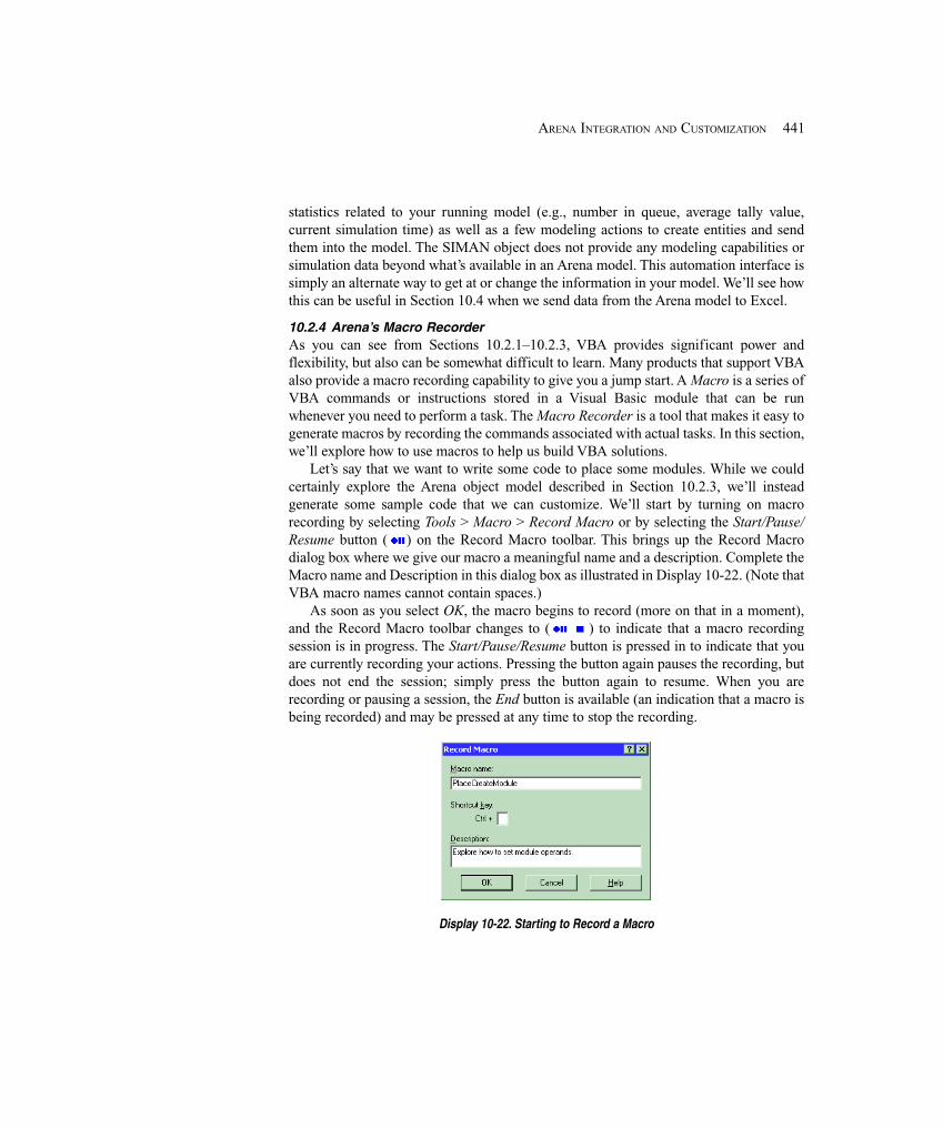
441ARENA INTEGRATION AND CUSTOMIZATION
statistics related to your running model (e.g., number in queue, average tally value,current simulation time) as well as a few modeling actions to create entities and sendthem into the model. The SIMAN object does not provide any modeling capabilities orsimulation data beyond what’s available in an Arena model. This automation interface issimply an alternate way to get at or change the information in your model. We’ll see howthis can be useful in Section 10.4 when we send data from the Arena model to Excel.
10.2.4 Arena’s Macro RecorderAs you can see from Sections 10.2.1–10.2.3, VBA provides significant power andflexibility, but also can be somewhat difficult to learn. Many products that support VBAalso provide a macro recording capability to give you a jump start. A Macro is a series ofVBA commands or instructions stored in a Visual Basic module that can be runwhenever you need to perform a task. The Macro Recorder is a tool that makes it easy togenerate macros by recording the commands associated with actual tasks. In this section,we’ll explore how to use macros to help us build VBA solutions.
Let’s say that we want to write some code to place some modules. While we couldcertainly explore the Arena object model described in Section 10.2.3, we’ll insteadgenerate some sample code that we can customize. We’ll start by turning on macrorecording by selecting Tools > Macro > Record Macro or by selecting the Start/Pause/Resume button ( ) on the Record Macro toolbar. This brings up the Record Macrodialog box where we give our macro a meaningful name and a description. Complete theMacro name and Description in this dialog box as illustrated in Display 10-22. (Note thatVBA macro names cannot contain spaces.)
As soon as you select OK, the macro begins to record (more on that in a moment),and the Record Macro toolbar changes to ( ) to indicate that a macro recordingsession is in progress. The Start/Pause/Resume button is pressed in to indicate that youare currently recording your actions. Pressing the button again pauses the recording, butdoes not end the session; simply press the button again to resume. When you arerecording or pausing a session, the End button is available (an indication that a macro isbeing recorded) and may be pressed at any time to stop the recording.
Display 10-22. Starting to Record a Macro
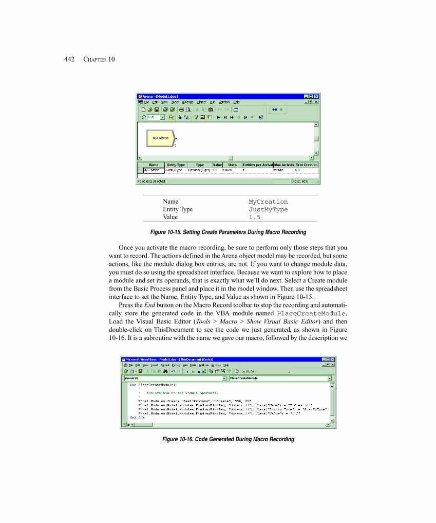
442 CHAPTER 10
Name MyCreationEntity Type JustMyTypeValue 1.5
Figure 10-15. Setting Create Parameters During Macro Recording
Once you activate the macro recording, be sure to perform only those steps that youwant to record. The actions defined in the Arena object model may be recorded, but someactions, like the module dialog box entries, are not. If you want to change module data,you must do so using the spreadsheet interface. Because we want to explore how to placea module and set its operands, that is exactly what we’ll do next. Select a Create modulefrom the Basic Process panel and place it in the model window. Then use the spreadsheetinterface to set the Name, Entity Type, and Value as shown in Figure 10-15.
Press the End button on the Macro Record toolbar to stop the recording and automati-cally store the generated code in the VBA module named PlaceCreateModule.Load the Visual Basic Editor (Tools > Macro > Show Visual Basic Editor) and thendouble-click on ThisDocument to see the code we just generated, as shown in Figure10-16. It is a subroutine with the name we gave our macro, followed by the description we
Figure 10-16. Code Generated During Macro Recording
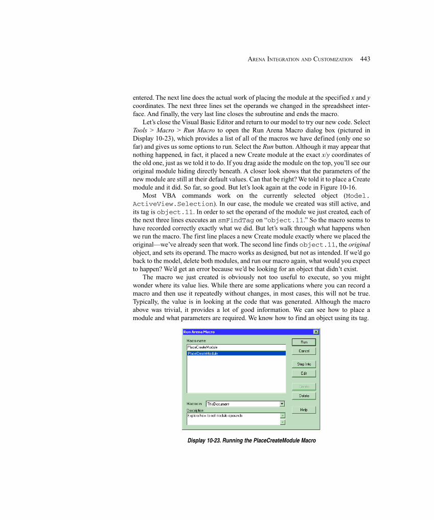
443ARENA INTEGRATION AND CUSTOMIZATION
entered. The next line does the actual work of placing the module at the specified x and ycoordinates. The next three lines set the operands we changed in the spreadsheet inter-face. And finally, the very last line closes the subroutine and ends the macro.
Let’s close the Visual Basic Editor and return to our model to try our new code. SelectTools > Macro > Run Macro to open the Run Arena Macro dialog box (pictured inDisplay 10-23), which provides a list of all of the macros we have defined (only one sofar) and gives us some options to run. Select the Run button. Although it may appear thatnothing happened, in fact, it placed a new Create module at the exact x/y coordinates ofthe old one, just as we told it to do. If you drag aside the module on the top, you’ll see ouroriginal module hiding directly beneath. A closer look shows that the parameters of thenew module are still at their default values. Can that be right? We told it to place a Createmodule and it did. So far, so good. But let’s look again at the code in Figure 10-16.
Most VBA commands work on the currently selected object (Model.ActiveView.Selection). In our case, the module we created was still active, andits tag is object.11. In order to set the operand of the module we just created, each ofthe next three lines executes an smFindTag on “object.11.” So the macro seems tohave recorded correctly exactly what we did. But let’s walk through what happens whenwe run the macro. The first line places a new Create module exactly where we placed theoriginal—we’ve already seen that work. The second line finds object.11, the originalobject, and sets its operand. The macro works as designed, but not as intended. If we’d goback to the model, delete both modules, and run our macro again, what would you expectto happen? We’d get an error because we’d be looking for an object that didn’t exist.
The macro we just created is obviously not too useful to execute, so you mightwonder where its value lies. While there are some applications where you can record amacro and then use it repeatedly without changes, in most cases, this will not be true.Typically, the value is in looking at the code that was generated. Although the macroabove was trivial, it provides a lot of good information. We can see how to place amodule and what parameters are required. We know how to find an object using its tag.
Display 10-23. Running the PlaceCreateModule Macro

444 CHAPTER 10
We know how to set the operands in a module, and we know the names of the threespecific operands we wanted to change. In short, that simple macro gave us a big jumpstart to writing some real code.
The primary value of the macro recorder is to make it easier to learn and prototypeVBA model extensions. Once you see how it’s done, you can use those same techniquesto solve other problems. There is no limit to the number of macros you can create, andyou can mix and match techniques from several different ones as needed. In short, themacro-recording capability, used in combination with the other techniques you learn inthis chapter, can be a powerful addition to your “bag of tricks.”
10.3 Model 10-6: Presenting Arrival Choices to the User
In Section 10.1, we exploited Arena features to integrate data into a model. Next, we’llturn our attention to how we can interact with someone who’s running an Arena model.
In Model 10-6, we’ll set up a mechanism for when the model runs that allows achoice to be made to use either call arrivals generated from a random process (as in theoriginal Model 10-1) or from a file (as in Model 10-2). At the beginning of a run, we’lldisplay a UserForm (VBA’s term for a dialog box) providing the options, as shown inFigure 10-17.
The user selects the desired option by clicking on the appropriate option button, thenclicks OK to allow the simulation run to commence. We’ll write VBA code to make therequired changes to the model so that only one of the call arrival types actually sendsentities into the model. And then at the end of this section, we have a surprise for you thatwill add a bit of pizzazz to the model with a quick bit of VBA code. Don’t peek ahead,though...you’ll have to make your way through the “fun with forms” material first!
10.3.1 Modifying the Creation LogicFirst, we need to set up the model so that it can generate entities from either the randomarrival process of Model 10-1 or the input file of Model 10-2. To do so, we’ll place bothsets of logic in the same model, connecting to the Process module that’s the beginning ofthe call logic, as in Figure 10-18.
Figure 10-17. Visual Basic UserForm
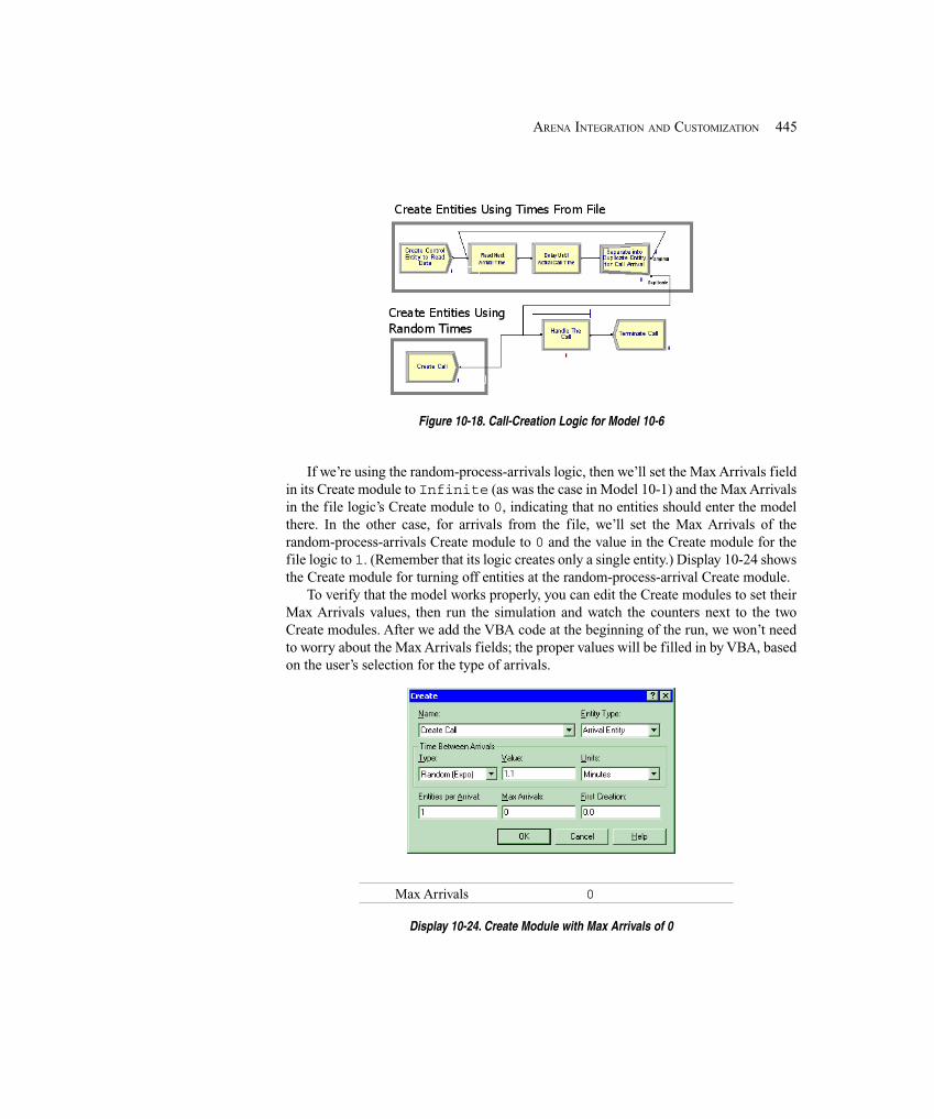
445ARENA INTEGRATION AND CUSTOMIZATION
Figure 10-18. Call-Creation Logic for Model 10-6
If we’re using the random-process-arrivals logic, then we’ll set the Max Arrivals fieldin its Create module to Infinite (as was the case in Model 10-1) and the Max Arrivalsin the file logic’s Create module to 0, indicating that no entities should enter the modelthere. In the other case, for arrivals from the file, we’ll set the Max Arrivals of therandom-process-arrivals Create module to 0 and the value in the Create module for thefile logic to 1. (Remember that its logic creates only a single entity.) Display 10-24 showsthe Create module for turning off entities at the random-process-arrival Create module.
To verify that the model works properly, you can edit the Create modules to set theirMax Arrivals values, then run the simulation and watch the counters next to the twoCreate modules. After we add the VBA code at the beginning of the run, we won’t needto worry about the Max Arrivals fields; the proper values will be filled in by VBA, basedon the user’s selection for the type of arrivals.
Max Arrivals 0
Display 10-24. Create Module with Max Arrivals of 0
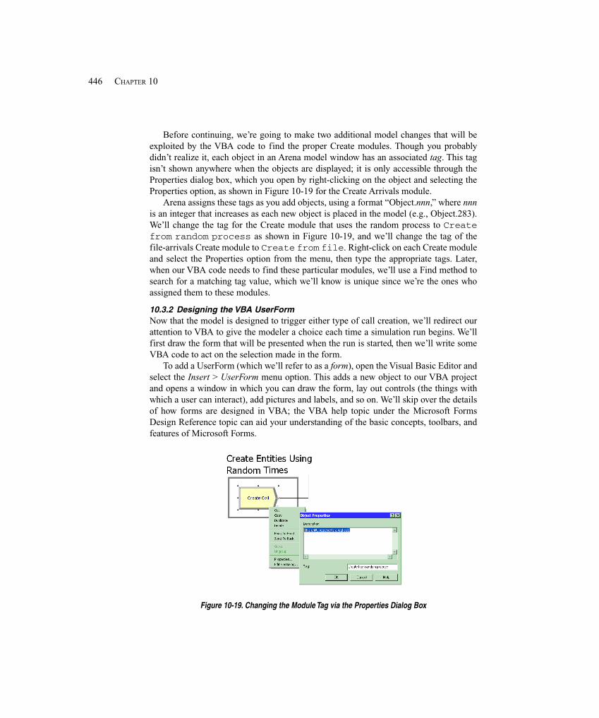
446 CHAPTER 10
Before continuing, we’re going to make two additional model changes that will beexploited by the VBA code to find the proper Create modules. Though you probablydidn’t realize it, each object in an Arena model window has an associated tag. This tagisn’t shown anywhere when the objects are displayed; it is only accessible through theProperties dialog box, which you open by right-clicking on the object and selecting theProperties option, as shown in Figure 10-19 for the Create Arrivals module.
Arena assigns these tags as you add objects, using a format “Object.nnn,” where nnnis an integer that increases as each new object is placed in the model (e.g., Object.283).We’ll change the tag for the Create module that uses the random process to Createfrom random process as shown in Figure 10-19, and we’ll change the tag of thefile-arrivals Create module to Create from file. Right-click on each Create moduleand select the Properties option from the menu, then type the appropriate tags. Later,when our VBA code needs to find these particular modules, we’ll use a Find method tosearch for a matching tag value, which we’ll know is unique since we’re the ones whoassigned them to these modules.
10.3.2 Designing the VBA UserFormNow that the model is designed to trigger either type of call creation, we’ll redirect ourattention to VBA to give the modeler a choice each time a simulation run begins. We’llfirst draw the form that will be presented when the run is started, then we’ll write someVBA code to act on the selection made in the form.
To add a UserForm (which we’ll refer to as a form), open the Visual Basic Editor andselect the Insert > UserForm menu option. This adds a new object to our VBA projectand opens a window in which you can draw the form, lay out controls (the things withwhich a user can interact), add pictures and labels, and so on. We’ll skip over the detailsof how forms are designed in VBA; the VBA help topic under the Microsoft FormsDesign Reference topic can aid your understanding of the basic concepts, toolbars, andfeatures of Microsoft Forms.
Figure 10-19. Changing the Module Tag via the Properties Dialog Box

447ARENA INTEGRATION AND CUSTOMIZATION
Figure 10-20. UserForm in VBA Project
For the VBA code to access the form, it needs to have a name. We’ll call itfrmArrivalTypeSelection by typing in the Name field of the Properties box, asin Figure 10-20.
To design the form’s contents, drag controls from the Control Toolbox onto the form.Drag a label onto the form and type its Caption field (in the Properties box) to match thedescriptive text in Figure 10-21 (Call entities can...). Next, drag an option buttononto the form below the label. Change its Name to optFromRandomProcess, itsCaption to Random interarrival-time process, and its Value to True so thatit is the default selection. Then add another option button named optFromFile, withArrival times from a file as its caption and a default value of False. The finalcontrol is the command button at the bottom of the form. Name it cmdOK with a captionof OK, and set its Default property to True so that the Enter key will act like thecommand button had been clicked.
This UserForm is now part of the Arena model; when you save the model file, theform will be saved with it. However, it’s not of much help to us until VBA knows what todo with the form. We’ll tackle that effort next.
Figure 10-21. UserForm Layout
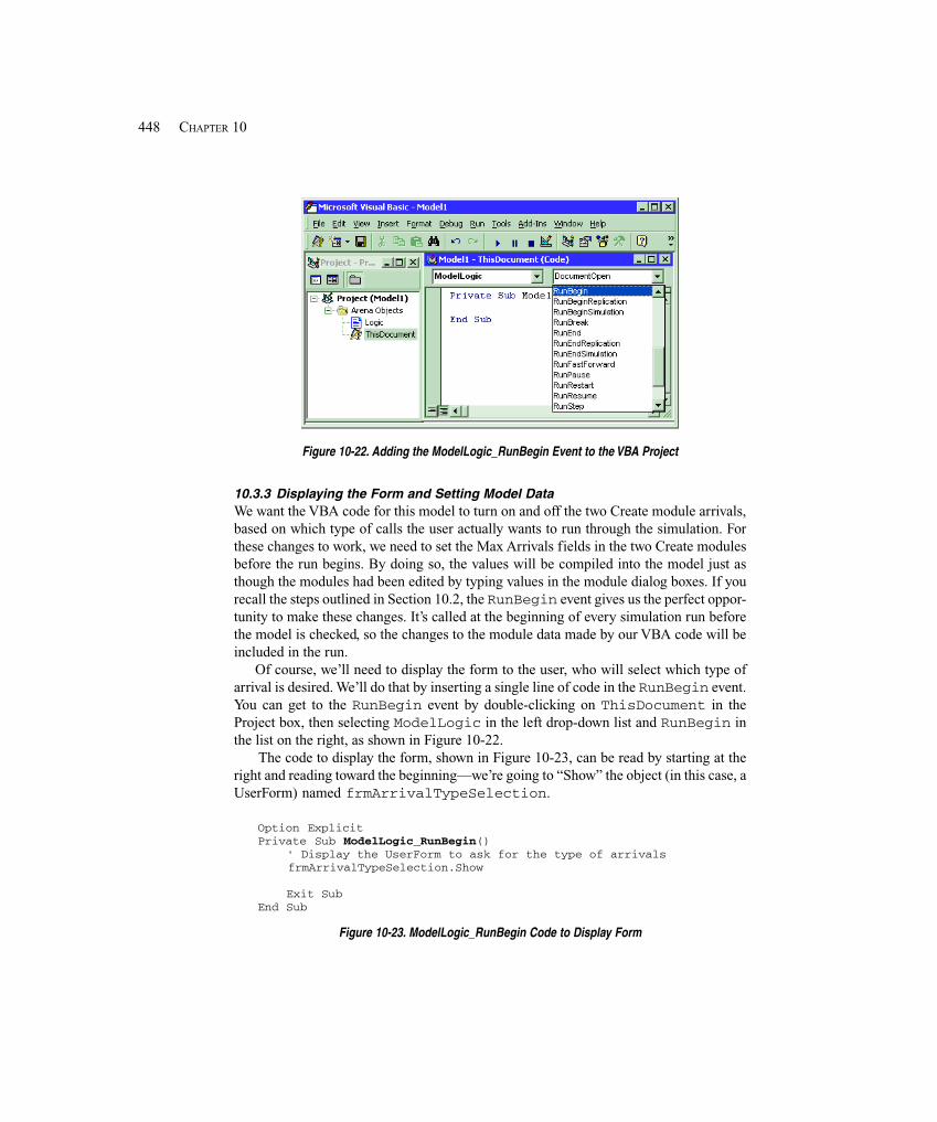
448 CHAPTER 10
Figure 10-22. Adding the ModelLogic_RunBegin Event to the VBA Project
10.3.3 Displaying the Form and Setting Model DataWe want the VBA code for this model to turn on and off the two Create module arrivals,based on which type of calls the user actually wants to run through the simulation. Forthese changes to work, we need to set the Max Arrivals fields in the two Create modulesbefore the run begins. By doing so, the values will be compiled into the model just asthough the modules had been edited by typing values in the module dialog boxes. If yourecall the steps outlined in Section 10.2, the RunBegin event gives us the perfect oppor-tunity to make these changes. It’s called at the beginning of every simulation run beforethe model is checked, so the changes to the module data made by our VBA code will beincluded in the run.
Of course, we’ll need to display the form to the user, who will select which type ofarrival is desired. We’ll do that by inserting a single line of code in the RunBegin event.You can get to the RunBegin event by double-clicking on ThisDocument in theProject box, then selecting ModelLogic in the left drop-down list and RunBegin inthe list on the right, as shown in Figure 10-22.
The code to display the form, shown in Figure 10-23, can be read by starting at theright and reading toward the beginning—we’re going to “Show” the object (in this case, aUserForm) named frmArrivalTypeSelection.
Option ExplicitPrivate Sub ModelLogic_RunBegin() ' Display the UserForm to ask for the type of arrivals frmArrivalTypeSelection.Show
Exit SubEnd Sub
Figure 10-23. ModelLogic_RunBegin Code to Display Form
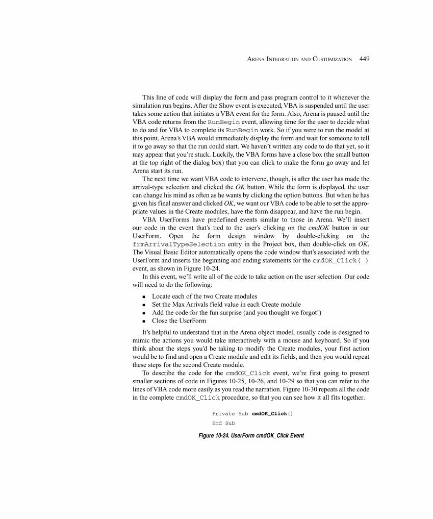
449ARENA INTEGRATION AND CUSTOMIZATION
This line of code will display the form and pass program control to it whenever thesimulation run begins. After the Show event is executed, VBA is suspended until the usertakes some action that initiates a VBA event for the form. Also, Arena is paused until theVBA code returns from the RunBegin event, allowing time for the user to decide whatto do and for VBA to complete its RunBegin work. So if you were to run the model atthis point, Arena’s VBA would immediately display the form and wait for someone to tellit to go away so that the run could start. We haven’t written any code to do that yet, so itmay appear that you’re stuck. Luckily, the VBA forms have a close box (the small buttonat the top right of the dialog box) that you can click to make the form go away and letArena start its run.
The next time we want VBA code to intervene, though, is after the user has made thearrival-type selection and clicked the OK button. While the form is displayed, the usercan change his mind as often as he wants by clicking the option buttons. But when he hasgiven his final answer and clicked OK, we want our VBA code to be able to set the appro-priate values in the Create modules, have the form disappear, and have the run begin.
VBA UserForms have predefined events similar to those in Arena. We’ll insertour code in the event that’s tied to the user’s clicking on the cmdOK button in ourUserForm. Open the form design window by double-clicking on thefrmArrivalTypeSelection entry in the Project box, then double-click on OK.The Visual Basic Editor automatically opens the code window that’s associated with theUserForm and inserts the beginning and ending statements for the cmdOK_Click( )event, as shown in Figure 10-24.
In this event, we’ll write all of the code to take action on the user selection. Our codewill need to do the following:
� Locate each of the two Create modules� Set the Max Arrivals field value in each Create module� Add the code for the fun surprise (and you thought we forgot!)� Close the UserForm
It’s helpful to understand that in the Arena object model, usually code is designed tomimic the actions you would take interactively with a mouse and keyboard. So if youthink about the steps you’d be taking to modify the Create modules, your first actionwould be to find and open a Create module and edit its fields, and then you would repeatthese steps for the second Create module.
To describe the code for the cmdOK_Click event, we’re first going to presentsmaller sections of code in Figures 10-25, 10-26, and 10-29 so that you can refer to thelines of VBA code more easily as you read the narration. Figure 10-30 repeats all the codein the complete cmdOK_Click procedure, so that you can see how it all fits together.
Private Sub cmdOK_Click()
End Sub
Figure 10-24. UserForm cmdOK_Click Event
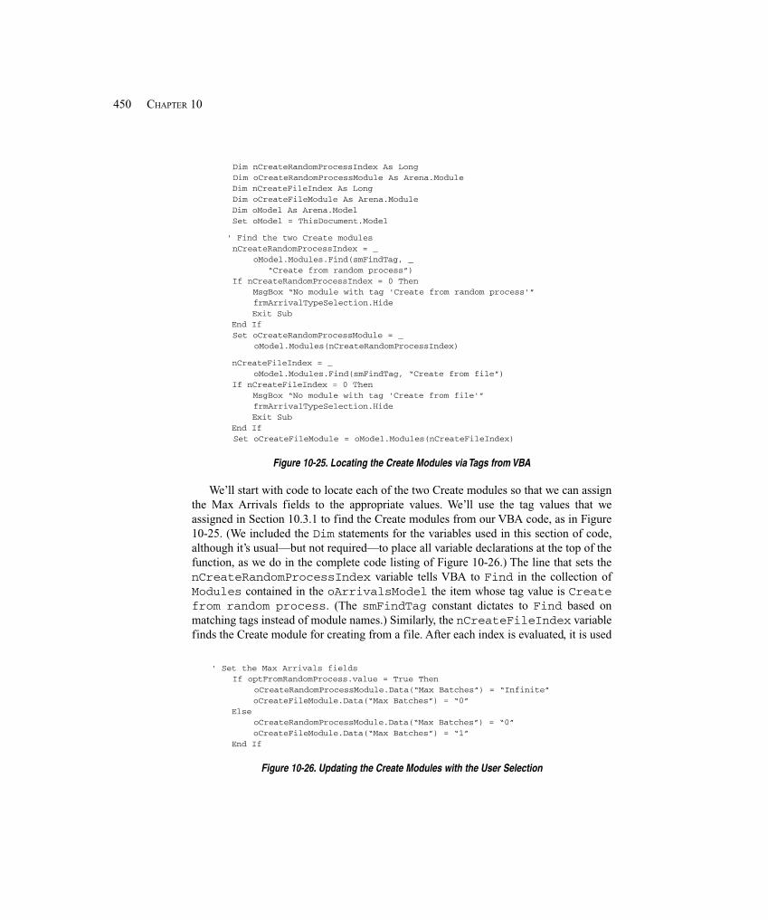
450 CHAPTER 10
Dim nCreateRandomProcessIndex As Long Dim oCreateRandomProcessModule As Arena.Module Dim nCreateFileIndex As Long Dim oCreateFileModule As Arena.Module Dim oModel As Arena.Model Set oModel = ThisDocument.Model
' Find the two Create modules nCreateRandomProcessIndex = _ oModel.Modules.Find(smFindTag, _ “Create from random process”) If nCreateRandomProcessIndex = 0 Then MsgBox “No module with tag 'Create from random process'” frmArrivalTypeSelection.Hide Exit Sub End If Set oCreateRandomProcessModule = _ oModel.Modules(nCreateRandomProcessIndex)
nCreateFileIndex = _ oModel.Modules.Find(smFindTag, “Create from file”) If nCreateFileIndex = 0 Then MsgBox “No module with tag 'Create from file'” frmArrivalTypeSelection.Hide Exit Sub End If Set oCreateFileModule = oModel.Modules(nCreateFileIndex)
Figure 10-25. Locating the Create Modules via Tags from VBA
We’ll start with code to locate each of the two Create modules so that we can assignthe Max Arrivals fields to the appropriate values. We’ll use the tag values that weassigned in Section 10.3.1 to find the Create modules from our VBA code, as in Figure10-25. (We included the Dim statements for the variables used in this section of code,although it’s usual—but not required—to place all variable declarations at the top of thefunction, as we do in the complete code listing of Figure 10-26.) The line that sets thenCreateRandomProcessIndex variable tells VBA to Find in the collection ofModules contained in the oArrivalsModel the item whose tag value is Createfrom random process. (The smFindTag constant dictates to Find based onmatching tags instead of module names.) Similarly, the nCreateFileIndex variablefinds the Create module for creating from a file. After each index is evaluated, it is used
' Set the Max Arrivals fields If optFromRandomProcess.value = True Then oCreateRandomProcessModule.Data(“Max Batches”) = “Infinite” oCreateFileModule.Data(“Max Batches”) = “0” Else oCreateRandomProcessModule.Data(“Max Batches”) = “0” oCreateFileModule.Data(“Max Batches”) = “1” End If
Figure 10-26. Updating the Create Modules with the User Selection
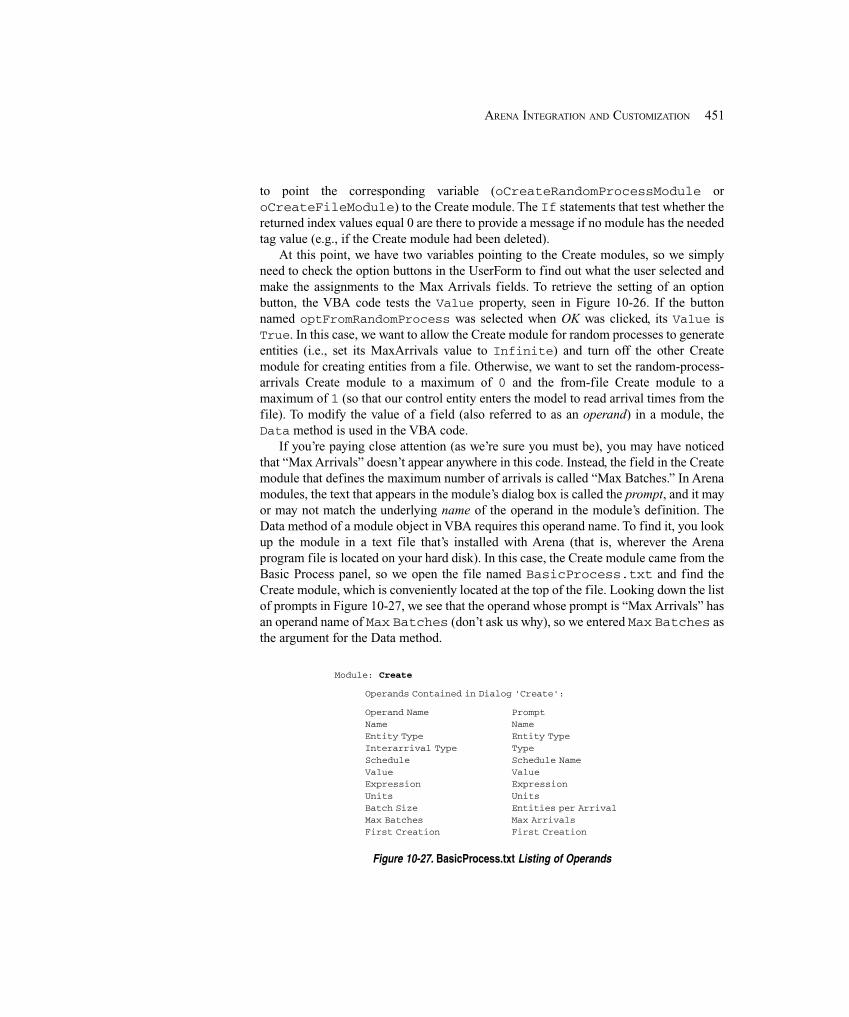
451ARENA INTEGRATION AND CUSTOMIZATION
to point the corresponding variable (oCreateRandomProcessModule oroCreateFileModule) to the Create module. The If statements that test whether thereturned index values equal 0 are there to provide a message if no module has the neededtag value (e.g., if the Create module had been deleted).
At this point, we have two variables pointing to the Create modules, so we simplyneed to check the option buttons in the UserForm to find out what the user selected andmake the assignments to the Max Arrivals fields. To retrieve the setting of an optionbutton, the VBA code tests the Value property, seen in Figure 10-26. If the buttonnamed optFromRandomProcess was selected when OK was clicked, its Value isTrue. In this case, we want to allow the Create module for random processes to generateentities (i.e., set its MaxArrivals value to Infinite) and turn off the other Createmodule for creating entities from a file. Otherwise, we want to set the random-process-arrivals Create module to a maximum of 0 and the from-file Create module to amaximum of 1 (so that our control entity enters the model to read arrival times from thefile). To modify the value of a field (also referred to as an operand) in a module, theData method is used in the VBA code.
If you’re paying close attention (as we’re sure you must be), you may have noticedthat “Max Arrivals” doesn’t appear anywhere in this code. Instead, the field in the Createmodule that defines the maximum number of arrivals is called “Max Batches.” In Arenamodules, the text that appears in the module’s dialog box is called the prompt, and it mayor may not match the underlying name of the operand in the module’s definition. TheData method of a module object in VBA requires this operand name. To find it, you lookup the module in a text file that’s installed with Arena (that is, wherever the Arenaprogram file is located on your hard disk). In this case, the Create module came from theBasic Process panel, so we open the file named BasicProcess.txt and find theCreate module, which is conveniently located at the top of the file. Looking down the listof prompts in Figure 10-27, we see that the operand whose prompt is “Max Arrivals” hasan operand name of Max Batches (don’t ask us why), so we entered Max Batches asthe argument for the Data method.
Module: Create
Operands Contained in Dialog 'Create':
○ ○ ○ ○ ○ ○ ○ ○ ○ ○ ○ ○ ○ ○ ○ ○ ○ ○ ○ ○ ○ ○ ○ ○ ○ ○ ○
Operand Name PromptName NameEntity Type Entity TypeInterarrival Type TypeSchedule Schedule NameValue ValueExpression ExpressionUnits UnitsBatch Size Entities per ArrivalMax Batches Max ArrivalsFirst Creation First Creation
Figure 10-27. BasicProcess.txt Listing of Operands
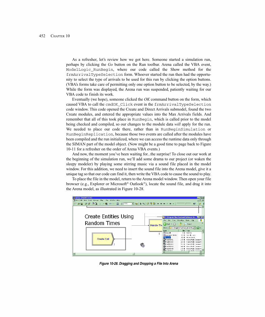
452 CHAPTER 10
As a refresher, let’s review how we got here. Someone started a simulation run,perhaps by clicking the Go button on the Run toolbar. Arena called the VBA event,ModelLogic_RunBegin, where our code called the Show method for thefrmArrivalTypeSelection form. Whoever started the run then had the opportu-nity to select the type of arrivals to be used for this run by clicking the option buttons.(VBA’s forms take care of permitting only one option button to be selected, by the way.)While the form was displayed, the Arena run was suspended, patiently waiting for ourVBA code to finish its work.
Eventually (we hope), someone clicked the OK command button on the form, whichcaused VBA to call the cmdOK_Click event in the frmArrivalTypeSelectioncode window. This code opened the Create and Direct Arrivals submodel, found the twoCreate modules, and entered the appropriate values into the Max Arrivals fields. Andremember that all of this took place in RunBegin, which is called prior to the modelbeing checked and compiled, so our changes to the module data will apply for the run.We needed to place our code there, rather than in RunBeginSimulation orRunBeginReplication, because those two events are called after the modules havebeen compiled and the run initialized, where we can access the runtime data only throughthe SIMAN part of the model object. (Now might be a good time to page back to Figure10-11 for a refresher on the order of Arena VBA events.)
And now, the moment you’ve been waiting for...the surprise! To close out our work atthe beginning of the simulation run, we’ll add some drama to our project (or waken thesleepy modeler) by playing some stirring music via a sound file placed in the modelwindow. For this addition, we need to insert the sound file into the Arena model, give it aunique tag so that our code can find it, then write the VBA code to cause the sound to play.
To place the file in the model, return to the Arena model window. Then open your filebrowser (e.g., Explorer or Microsoft® Outlook®), locate the sound file, and drag it intothe Arena model, as illustrated in Figure 10-28.
Figure 10-28. Dragging and Dropping a File Into Arena

453ARENA INTEGRATION AND CUSTOMIZATION
The sound object in the Arena model is an embedded file containing a copy of thefile we originally had on our disk. This file also could have been placed in the Arenamodel using the Windows clipboard or via the Edit > Insert New Object menu option inArena. The object itself is just like a sound file stored on your disk; double-click on it toplay its inspiring melody. To provide the sound object with a unique tag, right-click on itsicon in the Arena model window, select Properties from the menu, and enter MissionPossible for the Tag value.
Finally, return to the Visual Basic Editor window to insert the code that will activatethe sound file at the beginning of the run, shown in Figure 10-29. We once again use theFind method, this time from within the Embeddeds collection of the Model object, tosearch for the desired object. If we find the object with tag Mission Possible, thenwe activate it (in the case of a sound file, playing the sound) using the Do method of thecollection item at the appropriate index.
After you’ve run the simulation a few times, you may find that you have a compellingneed to disable the sound file. If so, feel free to turn off your computer speakers. Or youcan comment out the offensive lines of code by placing the statement, If 0, before thefirst line (where we retrieve the value of nSoundFileIndex) and the statement, EndIf, after the final line (the Do method). Later, if you want to restore the excitement toyour model, you can simply change the 0 to a 1 in the If statement, a handy trick forcode that you’re not sure you always want to utilize.
Now that we’ve completed all of our work, including the surprise, our last step is toclose the UserForm and exit the Click method of the OK button, so that Arena can beginthe simulation run. These lines of code are at the bottom of Figure 10-30, which lists thecomplete code for the cmdOK_Click event.
After the form is hidden and the cmdOK_Click procedure is exited, VBA codecontrol returns to the ModelLogic_RunBegin subroutine after the call to the Showevent for the form. Back in Figure 10-23, we saw that RunBegin simply exits thesubroutine. At this point, Arena checks the model, initializes the simulation run, andbegins the first replication, all while entertaining you with the inspiring music of ourembedded sound file.
Dim nSoundFileIndex As Long
' Play the sound file nSoundFileIndex = _ oModel.Embeddeds.Find(smFindTag, “Mission Possible”) If nSoundFileIndex > 0 Then _ oModel.Embeddeds.Item(nSoundFileIndex).Do
Figure 10-29. Code to Play Sound File

454 CHAPTER 10
Private Sub cmdOK_Click() ' Set the Max Arrivals field in each of the Create modules ' based on the selection in the UserForm Dim nCreateRandomProcessIndex As Long Dim oCreateRandomProcessModule As Arena.Module Dim nCreateFileIndex As Long Dim oCreateFileModule As Arena.Module Dim oModel As Arena.Model Dim nSoundFileIndex As Long Set oModel = ThisDocument.Model
' Find the two Create modules nCreateRandomProcessIndex = _ oModel.Modules.Find(smFindTag, _ “Create from random process”) If nCreateRandomProcessIndex = 0 Then MsgBox “No module with tag 'Create from random process'” frmArrivalTypeSelection.Hide Exit Sub End If Set oCreateRandomProcessModule = _ oModel.Modules(nCreateRandomProcessIndex)
nCreateFileIndex = _ oModel.Modules.Find(smFindTag, “Create from file”) If nCreateFileIndex = 0 Then MsgBox “No module with tag 'Create from file'” frmArrivalTypeSelection.Hide Exit Sub End If Set oCreateFileModule = oModel.Modules(nCreateFileIndex)
' Set the Max Arrivals fields If optFromRandomProcess.value = True Then oCreateRandomProcessModule.Data(“Max Batches”) = “Infinite” oCreateFileModule.Data(“Max Batches”) = “0” Else oCreateRandomProcessModule.Data(“Max Batches”) = “0” oCreateFileModule.Data(“Max Batches”) = “1” End If
' Play the sound file nSoundFileIndex = _ oModel.Embeddeds.Find(smFindTag, “Mission Possible”) If nSoundFileIndex > 0 Then _ oModel.Embeddeds.Item(nSoundFileIndex).Do
' Hide the UserForm to allow the run to begin frmArrivalTypeSelection.Hide Exit Sub
End Sub
Figure 10-30. Complete cmdOK_Click Event VBA Code
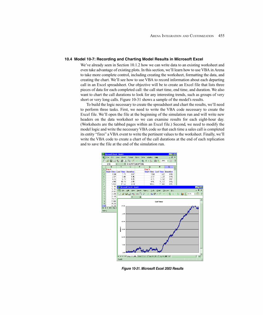
455ARENA INTEGRATION AND CUSTOMIZATION
10.4 Model 10-7: Recording and Charting Model Results in Microsoft Excel
We’ve already seen in Section 10.1.2 how we can write data to an existing worksheet andeven take advantage of existing plots. In this section, we’ll learn how to use VBA in Arenato take more complete control, including creating the worksheet, formatting the data, andcreating the chart. We’ll see how to use VBA to record information about each departingcall in an Excel spreadsheet. Our objective will be to create an Excel file that lists threepieces of data for each completed call: the call start time, end time, and duration. We alsowant to chart the call durations to look for any interesting trends, such as groups of veryshort or very long calls. Figure 10-31 shows a sample of the model’s results.
To build the logic necessary to create the spreadsheet and chart the results, we’ll needto perform three tasks. First, we need to write the VBA code necessary to create theExcel file. We’ll open the file at the beginning of the simulation run and will write newheaders on the data worksheet so we can examine results for each eight-hour day.(Worksheets are the tabbed pages within an Excel file.) Second, we need to modify themodel logic and write the necessary VBA code so that each time a sales call is completedits entity “fires” a VBA event to write the pertinent values to the worksheet. Finally, we’llwrite the VBA code to create a chart of the call durations at the end of each replicationand to save the file at the end of the simulation run.
Figure 10-31. Microsoft Excel 2003 Results
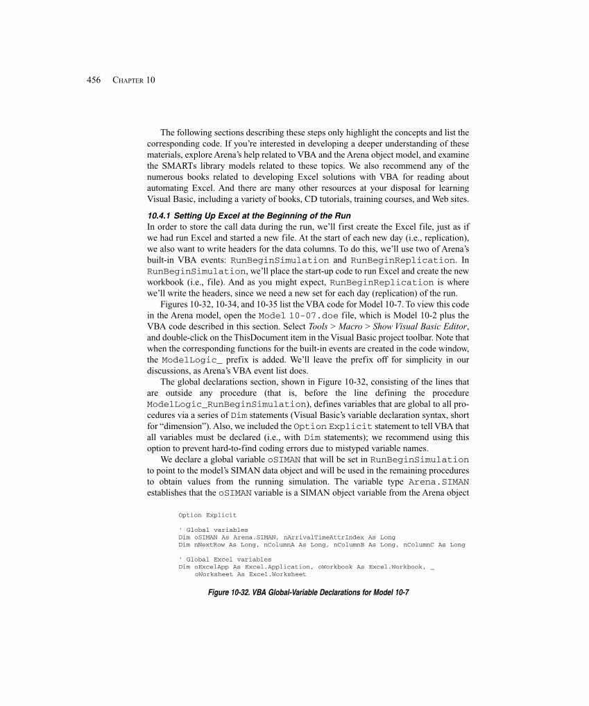
456 CHAPTER 10
The following sections describing these steps only highlight the concepts and list thecorresponding code. If you’re interested in developing a deeper understanding of thesematerials, explore Arena’s help related to VBA and the Arena object model, and examinethe SMARTs library models related to these topics. We also recommend any of thenumerous books related to developing Excel solutions with VBA for reading aboutautomating Excel. And there are many other resources at your disposal for learningVisual Basic, including a variety of books, CD tutorials, training courses, and Web sites.
10.4.1 Setting Up Excel at the Beginning of the RunIn order to store the call data during the run, we’ll first create the Excel file, just as ifwe had run Excel and started a new file. At the start of each new day (i.e., replication),we also want to write headers for the data columns. To do this, we’ll use two of Arena’sbuilt-in VBA events: RunBeginSimulation and RunBeginReplication. InRunBeginSimulation, we’ll place the start-up code to run Excel and create the newworkbook (i.e., file). And as you might expect, RunBeginReplication is wherewe’ll write the headers, since we need a new set for each day (replication) of the run.
Figures 10-32, 10-34, and 10-35 list the VBA code for Model 10-7. To view this codein the Arena model, open the Model 10-07.doe file, which is Model 10-2 plus theVBA code described in this section. Select Tools > Macro > Show Visual Basic Editor,and double-click on the ThisDocument item in the Visual Basic project toolbar. Note thatwhen the corresponding functions for the built-in events are created in the code window,the ModelLogic_ prefix is added. We’ll leave the prefix off for simplicity in ourdiscussions, as Arena’s VBA event list does.
The global declarations section, shown in Figure 10-32, consisting of the lines thatare outside any procedure (that is, before the line defining the procedureModelLogic_RunBeginSimulation), defines variables that are global to all pro-cedures via a series of Dim statements (Visual Basic’s variable declaration syntax, shortfor “dimension”). Also, we included the Option Explicit statement to tell VBA thatall variables must be declared (i.e., with Dim statements); we recommend using thisoption to prevent hard-to-find coding errors due to mistyped variable names.
We declare a global variable oSIMAN that will be set in RunBeginSimulationto point to the model’s SIMAN data object and will be used in the remaining proceduresto obtain values from the running simulation. The variable type Arena.SIMANestablishes that the oSIMAN variable is a SIMAN object variable from the Arena object
Option Explicit
' Global variablesDim oSIMAN As Arena.SIMAN, nArrivalTimeAttrIndex As LongDim nNextRow As Long, nColumnA As Long, nColumnB As Long, nColumnC As Long
' Global Excel variablesDim oExcelApp As Excel.Application, oWorkbook As Excel.Workbook, _ oWorksheet As Excel.Worksheet
Figure 10-32. VBA Global-Variable Declarations for Model 10-7
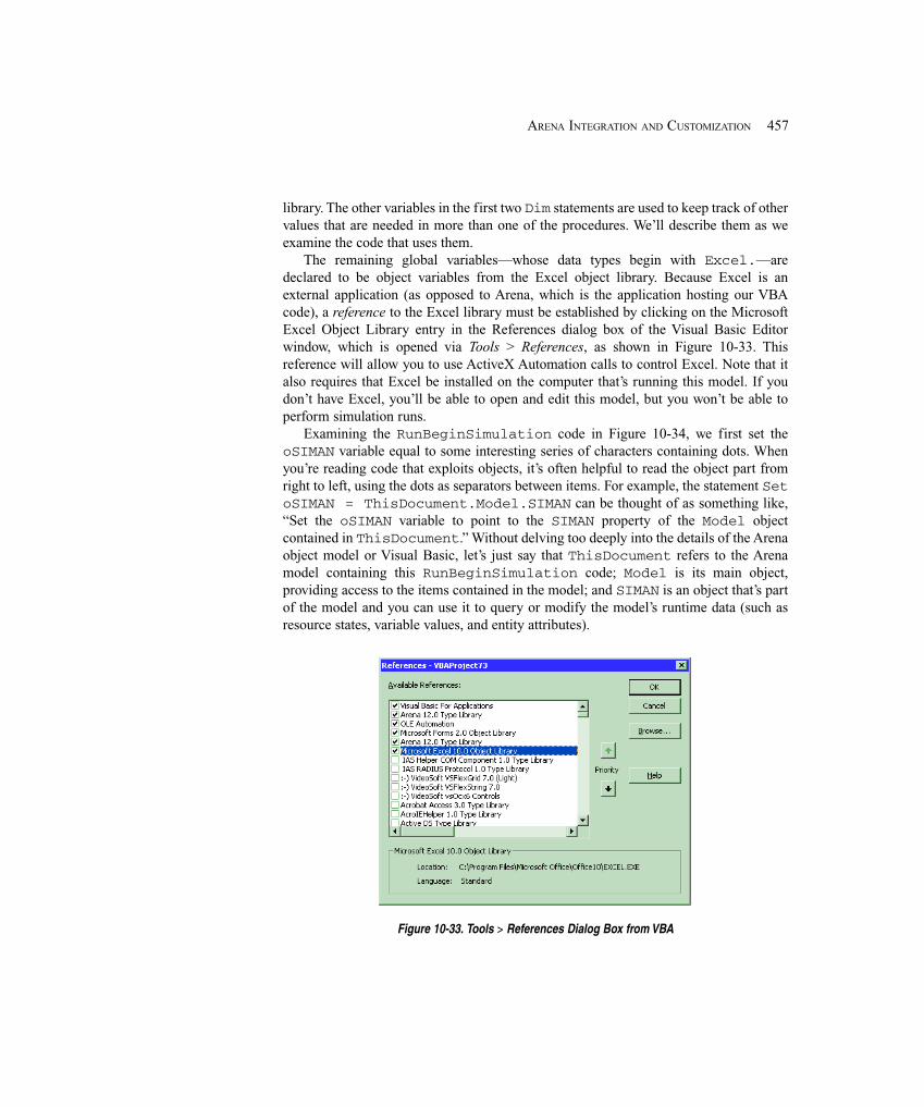
457ARENA INTEGRATION AND CUSTOMIZATION
library. The other variables in the first two Dim statements are used to keep track of othervalues that are needed in more than one of the procedures. We’ll describe them as weexamine the code that uses them.
The remaining global variables—whose data types begin with Excel.—aredeclared to be object variables from the Excel object library. Because Excel is anexternal application (as opposed to Arena, which is the application hosting our VBAcode), a reference to the Excel library must be established by clicking on the MicrosoftExcel Object Library entry in the References dialog box of the Visual Basic Editorwindow, which is opened via Tools > References, as shown in Figure 10-33. Thisreference will allow you to use ActiveX Automation calls to control Excel. Note that italso requires that Excel be installed on the computer that’s running this model. If youdon’t have Excel, you’ll be able to open and edit this model, but you won’t be able toperform simulation runs.
Examining the RunBeginSimulation code in Figure 10-34, we first set theoSIMAN variable equal to some interesting series of characters containing dots. Whenyou’re reading code that exploits objects, it’s often helpful to read the object part fromright to left, using the dots as separators between items. For example, the statement SetoSIMAN = ThisDocument.Model.SIMAN can be thought of as something like,“Set the oSIMAN variable to point to the SIMAN property of the Model objectcontained in ThisDocument.” Without delving too deeply into the details of the Arenaobject model or Visual Basic, let’s just say that ThisDocument refers to the Arenamodel containing this RunBeginSimulation code; Model is its main object,providing access to the items contained in the model; and SIMAN is an object that’s partof the model and you can use it to query or modify the model’s runtime data (such asresource states, variable values, and entity attributes).
Figure 10-33. Tools > References Dialog Box from VBA
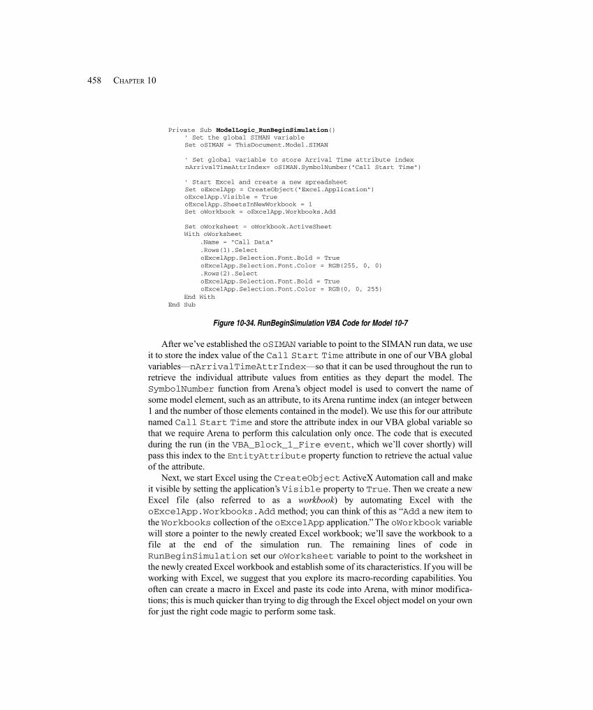
458 CHAPTER 10
Private Sub ModelLogic_RunBeginSimulation() ' Set the global SIMAN variable Set oSIMAN = ThisDocument.Model.SIMAN
' Set global variable to store Arrival Time attribute index nArrivalTimeAttrIndex= oSIMAN.SymbolNumber("Call Start Time")
' Start Excel and create a new spreadsheet Set oExcelApp = CreateObject("Excel.Application") oExcelApp.Visible = True oExcelApp.SheetsInNewWorkbook = 1 Set oWorkbook = oExcelApp.Workbooks.Add
Set oWorksheet = oWorkbook.ActiveSheet With oWorksheet .Name = "Call Data" .Rows(1).Select oExcelApp.Selection.Font.Bold = True oExcelApp.Selection.Font.Color = RGB(255, 0, 0) .Rows(2).Select oExcelApp.Selection.Font.Bold = True oExcelApp.Selection.Font.Color = RGB(0, 0, 255) End WithEnd Sub
Figure 10-34. RunBeginSimulation VBA Code for Model 10-7
After we’ve established the oSIMAN variable to point to the SIMAN run data, we useit to store the index value of the Call Start Time attribute in one of our VBA globalvariables—nArrivalTimeAttrIndex—so that it can be used throughout the run toretrieve the individual attribute values from entities as they depart the model. TheSymbolNumber function from Arena’s object model is used to convert the name ofsome model element, such as an attribute, to its Arena runtime index (an integer between1 and the number of those elements contained in the model). We use this for our attributenamed Call Start Time and store the attribute index in our VBA global variable sothat we require Arena to perform this calculation only once. The code that is executedduring the run (in the VBA_Block_1_Fire event, which we’ll cover shortly) willpass this index to the EntityAttribute property function to retrieve the actual valueof the attribute.
Next, we start Excel using the CreateObject ActiveX Automation call and makeit visible by setting the application’s Visible property to True. Then we create a newExcel file (also referred to as a workbook) by automating Excel with theoExcelApp.Workbooks.Add method; you can think of this as “Add a new item tothe Workbooks collection of the oExcelApp application.” The oWorkbook variablewill store a pointer to the newly created Excel workbook; we’ll save the workbook to afile at the end of the simulation run. The remaining lines of code inRunBeginSimulation set our oWorksheet variable to point to the worksheet inthe newly created Excel workbook and establish some of its characteristics. If you will beworking with Excel, we suggest that you explore its macro-recording capabilities. Youoften can create a macro in Excel and paste its code into Arena, with minor modifica-tions; this is much quicker than trying to dig through the Excel object model on your ownfor just the right code magic to perform some task.
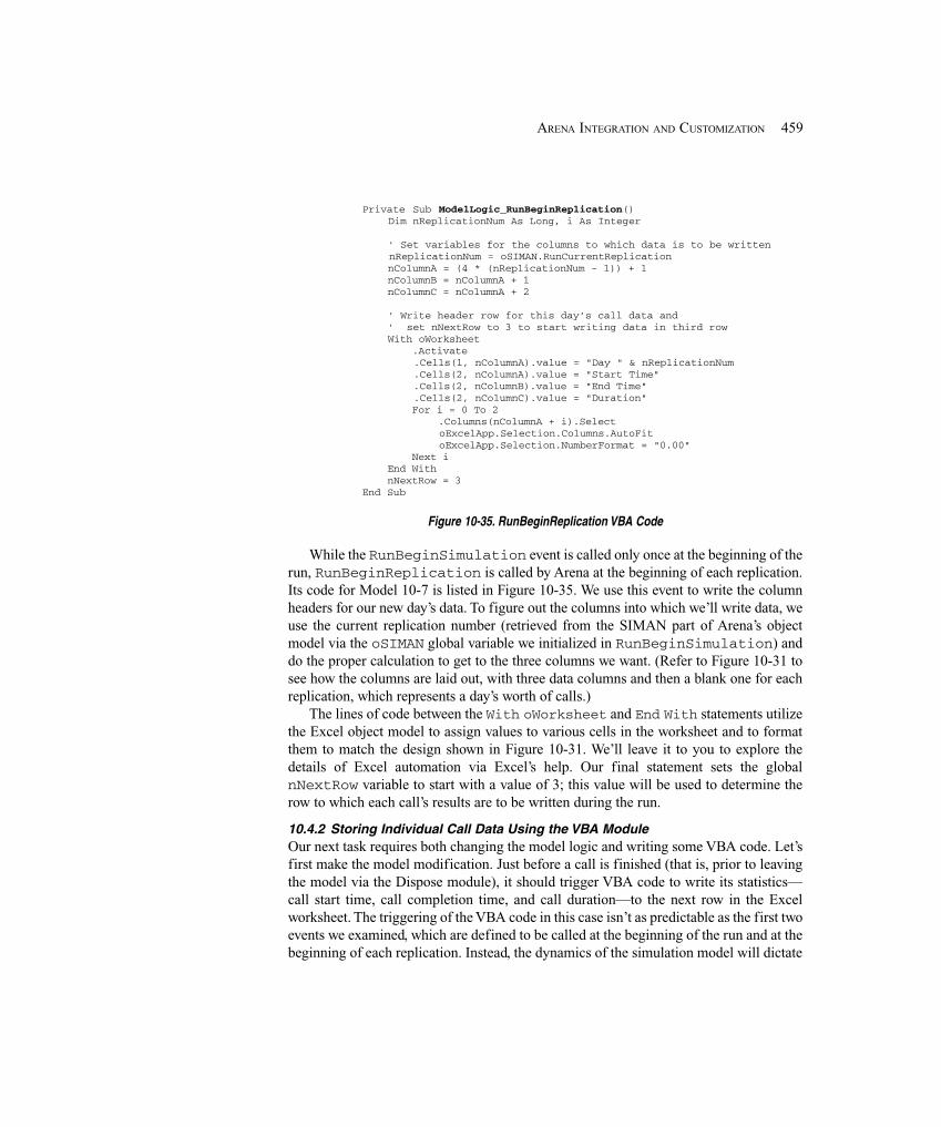
459ARENA INTEGRATION AND CUSTOMIZATION
Private Sub ModelLogic_RunBeginReplication() Dim nReplicationNum As Long, i As Integer
' Set variables for the columns to which data is to be written nReplicationNum = oSIMAN.RunCurrentReplication nColumnA = (4 * (nReplicationNum - 1)) + 1 nColumnB = nColumnA + 1 nColumnC = nColumnA + 2
' Write header row for this day’s call data and ' set nNextRow to 3 to start writing data in third row With oWorksheet .Activate .Cells(1, nColumnA).value = "Day " & nReplicationNum .Cells(2, nColumnA).value = "Start Time" .Cells(2, nColumnB).value = "End Time" .Cells(2, nColumnC).value = "Duration" For i = 0 To 2 .Columns(nColumnA + i).Select oExcelApp.Selection.Columns.AutoFit oExcelApp.Selection.NumberFormat = "0.00" Next i End With nNextRow = 3End Sub
Figure 10-35. RunBeginReplication VBA Code
While the RunBeginSimulation event is called only once at the beginning of therun, RunBeginReplication is called by Arena at the beginning of each replication.Its code for Model 10-7 is listed in Figure 10-35. We use this event to write the columnheaders for our new day’s data. To figure out the columns into which we’ll write data, weuse the current replication number (retrieved from the SIMAN part of Arena’s objectmodel via the oSIMAN global variable we initialized in RunBeginSimulation) anddo the proper calculation to get to the three columns we want. (Refer to Figure 10-31 tosee how the columns are laid out, with three data columns and then a blank one for eachreplication, which represents a day’s worth of calls.)
The lines of code between the With oWorksheet and End With statements utilizethe Excel object model to assign values to various cells in the worksheet and to formatthem to match the design shown in Figure 10-31. We’ll leave it to you to explore thedetails of Excel automation via Excel’s help. Our final statement sets the globalnNextRow variable to start with a value of 3; this value will be used to determine therow to which each call’s results are to be written during the run.
10.4.2 Storing Individual Call Data Using the VBA ModuleOur next task requires both changing the model logic and writing some VBA code. Let’sfirst make the model modification. Just before a call is finished (that is, prior to leavingthe model via the Dispose module), it should trigger VBA code to write its statistics—call start time, call completion time, and call duration—to the next row in the Excelworksheet. The triggering of the VBA code in this case isn’t as predictable as the first twoevents we examined, which are defined to be called at the beginning of the run and at thebeginning of each replication. Instead, the dynamics of the simulation model will dictate
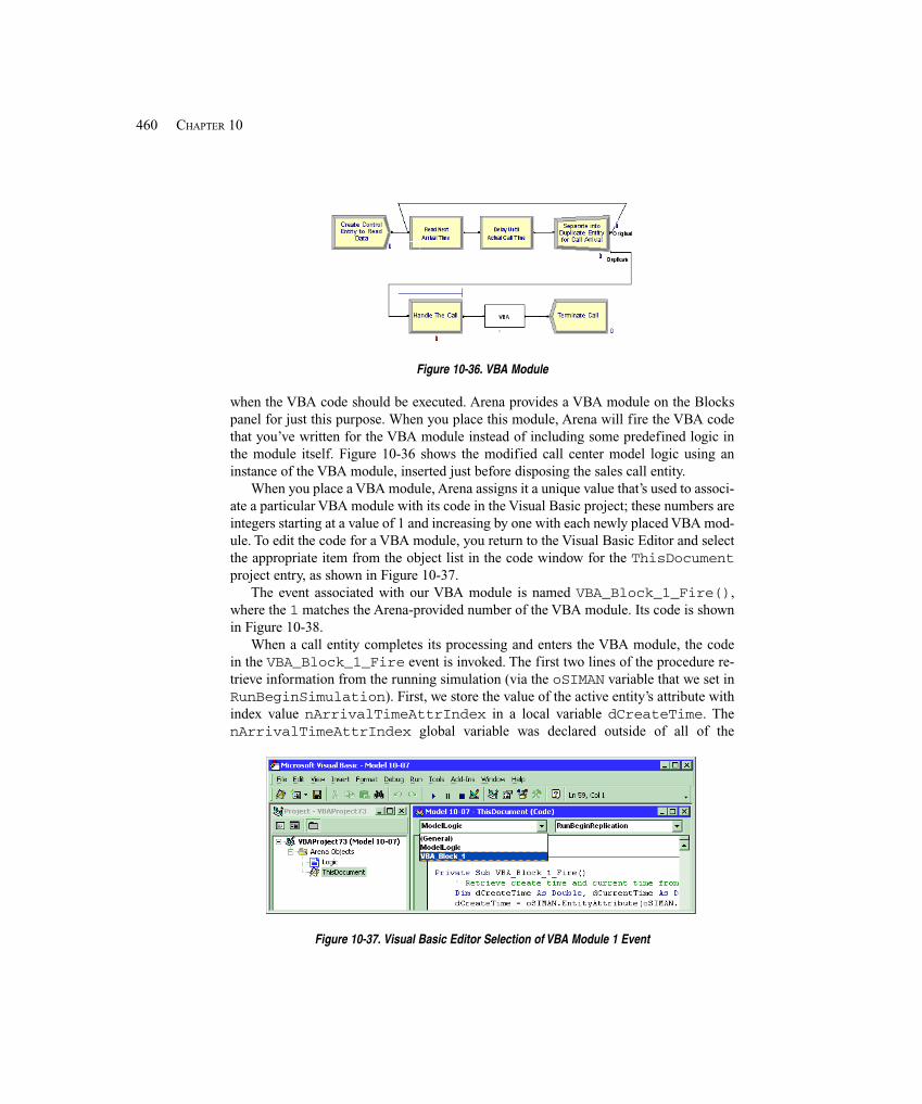
460 CHAPTER 10
Figure 10-36. VBA Module
when the VBA code should be executed. Arena provides a VBA module on the Blockspanel for just this purpose. When you place this module, Arena will fire the VBA codethat you’ve written for the VBA module instead of including some predefined logic inthe module itself. Figure 10-36 shows the modified call center model logic using aninstance of the VBA module, inserted just before disposing the sales call entity.
When you place a VBA module, Arena assigns it a unique value that’s used to associ-ate a particular VBA module with its code in the Visual Basic project; these numbers areintegers starting at a value of 1 and increasing by one with each newly placed VBA mod-ule. To edit the code for a VBA module, you return to the Visual Basic Editor and selectthe appropriate item from the object list in the code window for the ThisDocumentproject entry, as shown in Figure 10-37.
The event associated with our VBA module is named VBA_Block_1_Fire(),where the 1 matches the Arena-provided number of the VBA module. Its code is shownin Figure 10-38.
When a call entity completes its processing and enters the VBA module, the codein the VBA_Block_1_Fire event is invoked. The first two lines of the procedure re-trieve information from the running simulation (via the oSIMAN variable that we set inRunBeginSimulation). First, we store the value of the active entity’s attribute withindex value nArrivalTimeAttrIndex in a local variable dCreateTime. ThenArrivalTimeAttrIndex global variable was declared outside of all of the
Figure 10-37. Visual Basic Editor Selection of VBA Module 1 Event
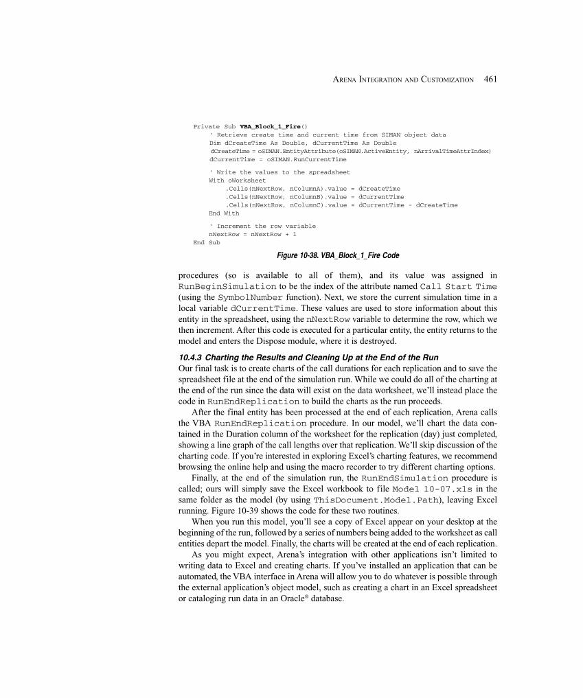
461ARENA INTEGRATION AND CUSTOMIZATION
Private Sub VBA_Block_1_Fire() ' Retrieve create time and current time from SIMAN object data Dim dCreateTime As Double, dCurrentTime As Double dCreateTime = oSIMAN.EntityAttribute(oSIMAN.ActiveEntity, nArrivalTimeAttrIndex) dCurrentTime = oSIMAN.RunCurrentTime
' Write the values to the spreadsheet With oWorksheet .Cells(nNextRow, nColumnA).value = dCreateTime .Cells(nNextRow, nColumnB).value = dCurrentTime .Cells(nNextRow, nColumnC).value = dCurrentTime - dCreateTime End With
' Increment the row variable nNextRow = nNextRow + 1End Sub
Figure 10-38. VBA_Block_1_Fire Code
procedures (so is available to all of them), and its value was assigned inRunBeginSimulation to be the index of the attribute named Call Start Time(using the SymbolNumber function). Next, we store the current simulation time in alocal variable dCurrentTime. These values are used to store information about thisentity in the spreadsheet, using the nNextRow variable to determine the row, which wethen increment. After this code is executed for a particular entity, the entity returns to themodel and enters the Dispose module, where it is destroyed.
10.4.3 Charting the Results and Cleaning Up at the End of the RunOur final task is to create charts of the call durations for each replication and to save thespreadsheet file at the end of the simulation run. While we could do all of the charting atthe end of the run since the data will exist on the data worksheet, we’ll instead place thecode in RunEndReplication to build the charts as the run proceeds.
After the final entity has been processed at the end of each replication, Arena callsthe VBA RunEndReplication procedure. In our model, we’ll chart the data con-tained in the Duration column of the worksheet for the replication (day) just completed,showing a line graph of the call lengths over that replication. We’ll skip discussion of thecharting code. If you’re interested in exploring Excel’s charting features, we recommendbrowsing the online help and using the macro recorder to try different charting options.
Finally, at the end of the simulation run, the RunEndSimulation procedure iscalled; ours will simply save the Excel workbook to file Model 10-07.xls in thesame folder as the model (by using ThisDocument.Model.Path), leaving Excelrunning. Figure 10-39 shows the code for these two routines.
When you run this model, you’ll see a copy of Excel appear on your desktop at thebeginning of the run, followed by a series of numbers being added to the worksheet as callentities depart the model. Finally, the charts will be created at the end of each replication.
As you might expect, Arena’s integration with other applications isn’t limited towriting data to Excel and creating charts. If you’ve installed an application that can beautomated, the VBA interface in Arena will allow you to do whatever is possible throughthe external application’s object model, such as creating a chart in an Excel spreadsheetor cataloging run data in an Oracle® database.
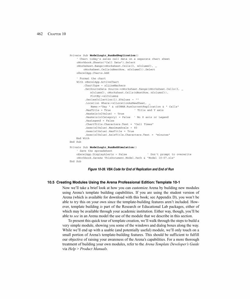
462 CHAPTER 10
Private Sub ModelLogic_RunEndReplication() ' Chart today’s sales call data on a separate chart sheet oWorkbook.Sheets("Call Data").Select oWorksheet.Range(oWorksheet.Cells(3, nColumnC), _ oWorksheet.Cells(nNextRow, nColumnC)).Select oExcelApp.Charts.Add
' Format the chart With oExcelApp.ActiveChart .ChartType = xlLineMarkers .SetSourceData Source:=oWorksheet.Range(oWorksheet.Cells(3, _ nColumnC), oWorksheet.Cells(nNextRow, nColumnC)),
PlotBy:=xlColumns.SeriesCollection(1).XValues = "".Location Where:=xlLocationAsNewSheet, _
Name:="Day " & oSIMAN.RunCurrentReplication & " Calls".HasTitle = True ' Title and Y axis.HasAxis(xlValue) = True.HasAxis(xlCategory) = False ' No X axis or Legend.HasLegend = False.ChartTitle.Characters.Text = "Call Times".Axes(xlValue).MaximumScale = 60.Axes(xlValue).HasTitle = True.Axes(xlValue).AxisTitle.Characters.Text = "minutes"
End WithEnd Sub
Private Sub ModelLogic_RunEndSimulation() ' Save the spreadsheet oExcelApp.DisplayAlerts = False ' Don’t prompt to overwrite oWorkbook.SaveAs ThisDocument.Model.Path & "Model 10-07.xls"End Sub
Figure 10-39. VBA Code for End of Replication and End of Run
10.5 Creating Modules Using the Arena Professional Edition: Template 10-1Now we’ll take a brief look at how you can customize Arena by building new modulesusing Arena’s template building capabilities. If you are using the student version ofArena (which is available for download with this book; see Appendix D), you won’t beable to try this on your own since the template-building features aren’t included. How-ever, template building is part of the Research or Educational Lab packages, either ofwhich may be available through your academic institution. Either way, though, you’ll beable to see in an Arena model the use of the module that we describe in this section.
To present this quick tour of template creation, we’ll walk through the steps to build avery simple module, showing you some of the windows and dialog boxes along the way.While we’ll end up with a usable (and potentially useful) module, we’ll only touch on asmall portion of Arena’s template-building features. This should be sufficient to fulfillour objective of raising your awareness of the Arena’s capabilities. For a more thoroughtreatment of building your own modules, refer to the Arena Template Developer’s Guidevia Help > Product Manuals.
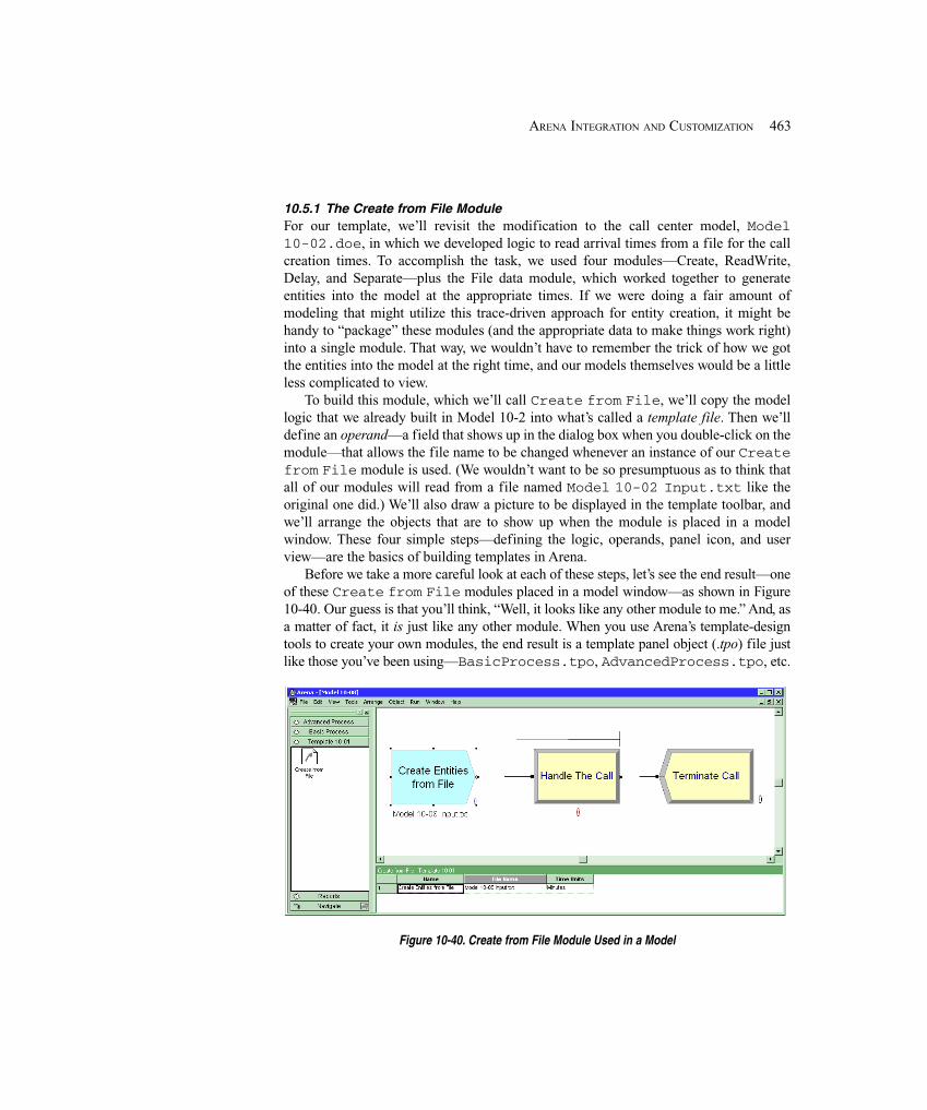
463ARENA INTEGRATION AND CUSTOMIZATION
10.5.1 The Create from File ModuleFor our template, we’ll revisit the modification to the call center model, Model10-02.doe, in which we developed logic to read arrival times from a file for the callcreation times. To accomplish the task, we used four modules—Create, ReadWrite,Delay, and Separate—plus the File data module, which worked together to generateentities into the model at the appropriate times. If we were doing a fair amount ofmodeling that might utilize this trace-driven approach for entity creation, it might behandy to “package” these modules (and the appropriate data to make things work right)into a single module. That way, we wouldn’t have to remember the trick of how we gotthe entities into the model at the right time, and our models themselves would be a littleless complicated to view.
To build this module, which we’ll call Create from File, we’ll copy the modellogic that we already built in Model 10-2 into what’s called a template file. Then we’lldefine an operand—a field that shows up in the dialog box when you double-click on themodule—that allows the file name to be changed whenever an instance of our Createfrom File module is used. (We wouldn’t want to be so presumptuous as to think thatall of our modules will read from a file named Model 10-02 Input.txt like theoriginal one did.) We’ll also draw a picture to be displayed in the template toolbar, andwe’ll arrange the objects that are to show up when the module is placed in a modelwindow. These four simple steps—defining the logic, operands, panel icon, and userview—are the basics of building templates in Arena.
Before we take a more careful look at each of these steps, let’s see the end result—oneof these Create from File modules placed in a model window—as shown in Figure10-40. Our guess is that you’ll think, “Well, it looks like any other module to me.” And, asa matter of fact, it is just like any other module. When you use Arena’s template-designtools to create your own modules, the end result is a template panel object (.tpo) file justlike those you’ve been using—BasicProcess.tpo, AdvancedProcess.tpo, etc.
Figure 10-40. Create from File Module Used in a Model
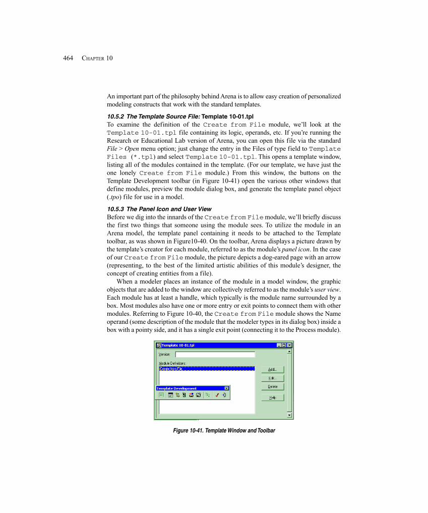
464 CHAPTER 10
An important part of the philosophy behind Arena is to allow easy creation of personalizedmodeling constructs that work with the standard templates.
10.5.2 The Template Source File: Template 10-01.tplTo examine the definition of the Create from File module, we’ll look at theTemplate 10-01.tpl file containing its logic, operands, etc. If you’re running theResearch or Educational Lab version of Arena, you can open this file via the standardFile > Open menu option; just change the entry in the Files of type field to TemplateFiles (*.tpl) and select Template 10-01.tpl. This opens a template window,listing all of the modules contained in the template. (For our template, we have just theone lonely Create from File module.) From this window, the buttons on theTemplate Development toolbar (in Figure 10-41) open the various other windows thatdefine modules, preview the module dialog box, and generate the template panel object(.tpo) file for use in a model.
10.5.3 The Panel Icon and User ViewBefore we dig into the innards of the Create from File module, we’ll briefly discussthe first two things that someone using the module sees. To utilize the module in anArena model, the template panel containing it needs to be attached to the Templatetoolbar, as was shown in Figure10-40. On the toolbar, Arena displays a picture drawn bythe template’s creator for each module, referred to as the module’s panel icon. In the caseof our Create from File module, the picture depicts a dog-eared page with an arrow(representing, to the best of the limited artistic abilities of this module’s designer, theconcept of creating entities from a file).
When a modeler places an instance of the module in a model window, the graphicobjects that are added to the window are collectively referred to as the module’s user view.Each module has at least a handle, which typically is the module name surrounded by abox. Most modules also have one or more entry or exit points to connect them with othermodules. Referring to Figure 10-40, the Create from File module shows the Nameoperand (some description of the module that the modeler types in its dialog box) inside abox with a pointy side, and it has a single exit point (connecting it to the Process module).
Figure 10-41. Template Window and Toolbar
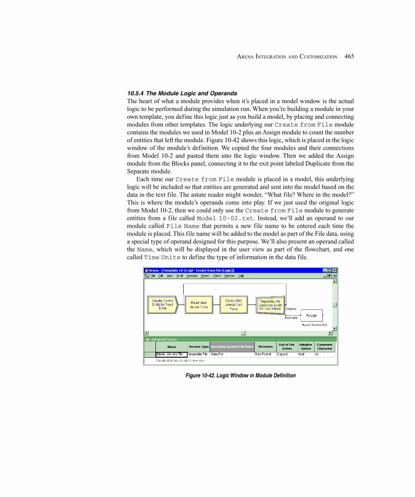
465ARENA INTEGRATION AND CUSTOMIZATION
10.5.4 The Module Logic and OperandsThe heart of what a module provides when it’s placed in a model window is the actuallogic to be performed during the simulation run. When you’re building a module in yourown template, you define this logic just as you build a model, by placing and connectingmodules from other templates. The logic underlying our Create from File modulecontains the modules we used in Model 10-2 plus an Assign module to count the numberof entities that left the module. Figure 10-42 shows this logic, which is placed in the logicwindow of the module’s definition. We copied the four modules and their connectionsfrom Model 10-2 and pasted them into the logic window. Then we added the Assignmodule from the Blocks panel, connecting it to the exit point labeled Duplicate from theSeparate module.
Each time our Create from File module is placed in a model, this underlyinglogic will be included so that entities are generated and sent into the model based on thedata in the text file. The astute reader might wonder, “What file? Where in the model?”This is where the module’s operands come into play. If we just used the original logicfrom Model 10-2, then we could only use the Create from File module to generateentities from a file called Model 10-02.txt. Instead, we’ll add an operand to ourmodule called File Name that permits a new file name to be entered each time themodule is placed. This file name will be added to the model as part of the File data, usinga special type of operand designed for this purpose. We’ll also present an operand calledthe Name, which will be displayed in the user view as part of the flowchart, and onecalled Time Units to define the type of information in the data file.
Figure 10-42. Logic Window in Module Definition
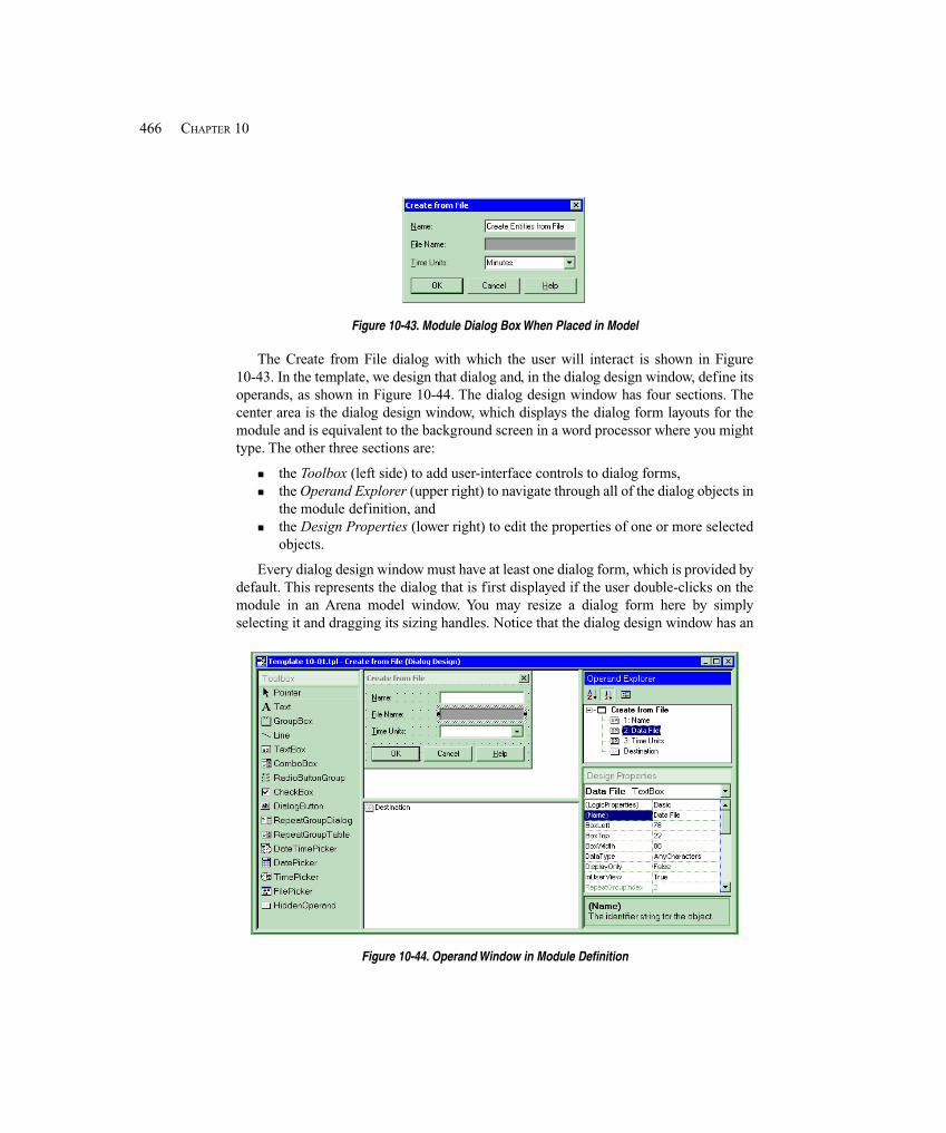
466 CHAPTER 10
Figure 10-43. Module Dialog Box When Placed in Model
The Create from File dialog with which the user will interact is shown in Figure10-43. In the template, we design that dialog and, in the dialog design window, define itsoperands, as shown in Figure 10-44. The dialog design window has four sections. Thecenter area is the dialog design window, which displays the dialog form layouts for themodule and is equivalent to the background screen in a word processor where you mighttype. The other three sections are:
� the Toolbox (left side) to add user-interface controls to dialog forms,� the Operand Explorer (upper right) to navigate through all of the dialog objects in
the module definition, and� the Design Properties (lower right) to edit the properties of one or more selected
objects.
Every dialog design window must have at least one dialog form, which is provided bydefault. This represents the dialog that is first displayed if the user double-clicks on themodule in an Arena model window. You may resize a dialog form here by simplyselecting it and dragging its sizing handles. Notice that the dialog design window has an
Figure 10-44. Operand Window in Module Definition
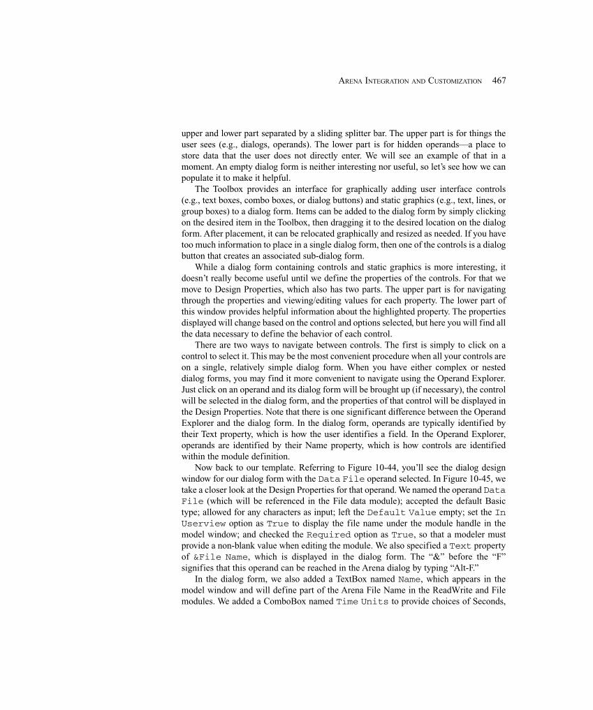
467ARENA INTEGRATION AND CUSTOMIZATION
upper and lower part separated by a sliding splitter bar. The upper part is for things theuser sees (e.g., dialogs, operands). The lower part is for hidden operands—a place tostore data that the user does not directly enter. We will see an example of that in amoment. An empty dialog form is neither interesting nor useful, so let’s see how we canpopulate it to make it helpful.
The Toolbox provides an interface for graphically adding user interface controls(e.g., text boxes, combo boxes, or dialog buttons) and static graphics (e.g., text, lines, orgroup boxes) to a dialog form. Items can be added to the dialog form by simply clickingon the desired item in the Toolbox, then dragging it to the desired location on the dialogform. After placement, it can be relocated graphically and resized as needed. If you havetoo much information to place in a single dialog form, then one of the controls is a dialogbutton that creates an associated sub-dialog form.
While a dialog form containing controls and static graphics is more interesting, itdoesn’t really become useful until we define the properties of the controls. For that wemove to Design Properties, which also has two parts. The upper part is for navigatingthrough the properties and viewing/editing values for each property. The lower part ofthis window provides helpful information about the highlighted property. The propertiesdisplayed will change based on the control and options selected, but here you will find allthe data necessary to define the behavior of each control.
There are two ways to navigate between controls. The first is simply to click on acontrol to select it. This may be the most convenient procedure when all your controls areon a single, relatively simple dialog form. When you have either complex or nesteddialog forms, you may find it more convenient to navigate using the Operand Explorer.Just click on an operand and its dialog form will be brought up (if necessary), the controlwill be selected in the dialog form, and the properties of that control will be displayed inthe Design Properties. Note that there is one significant difference between the OperandExplorer and the dialog form. In the dialog form, operands are typically identified bytheir Text property, which is how the user identifies a field. In the Operand Explorer,operands are identified by their Name property, which is how controls are identifiedwithin the module definition.
Now back to our template. Referring to Figure 10-44, you’ll see the dialog designwindow for our dialog form with the Data File operand selected. In Figure 10-45, wetake a closer look at the Design Properties for that operand. We named the operand DataFile (which will be referenced in the File data module); accepted the default Basictype; allowed for any characters as input; left the Default Value empty; set the InUserview option as True to display the file name under the module handle in themodel window; and checked the Required option as True, so that a modeler mustprovide a non-blank value when editing the module. We also specified a Text propertyof &File Name, which is displayed in the dialog form. The “&” before the “F”signifies that this operand can be reached in the Arena dialog by typing “Alt-F.”
In the dialog form, we also added a TextBox named Name, which appears in themodel window and will define part of the Arena File Name in the ReadWrite and Filemodules. We added a ComboBox named Time Units to provide choices of Seconds,
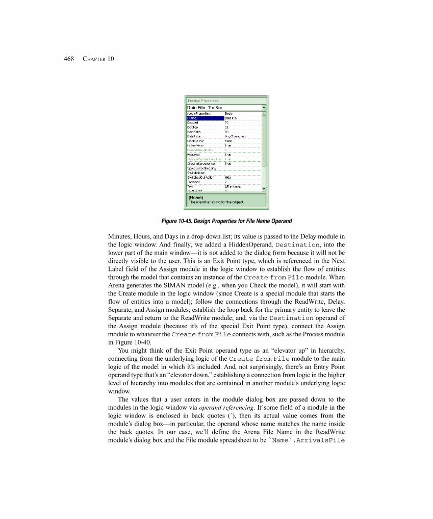
468 CHAPTER 10
Figure 10-45. Design Properties for File Name Operand
Minutes, Hours, and Days in a drop-down list; its value is passed to the Delay module inthe logic window. And finally, we added a HiddenOperand, Destination, into thelower part of the main window—it is not added to the dialog form because it will not bedirectly visible to the user. This is an Exit Point type, which is referenced in the NextLabel field of the Assign module in the logic window to establish the flow of entitiesthrough the model that contains an instance of the Create from File module. WhenArena generates the SIMAN model (e.g., when you Check the model), it will start withthe Create module in the logic window (since Create is a special module that starts theflow of entities into a model); follow the connections through the ReadWrite, Delay,Separate, and Assign modules; establish the loop back for the primary entity to leave theSeparate and return to the ReadWrite module; and, via the Destination operand ofthe Assign module (because it’s of the special Exit Point type), connect the Assignmodule to whatever the Create from File connects with, such as the Process modulein Figure 10-40.
You might think of the Exit Point operand type as an “elevator up” in hierarchy,connecting from the underlying logic of the Create from File module to the mainlogic of the model in which it’s included. And, not surprisingly, there’s an Entry Pointoperand type that’s an “elevator down,” establishing a connection from logic in the higherlevel of hierarchy into modules that are contained in another module’s underlying logicwindow.
The values that a user enters in the module dialog box are passed down to themodules in the logic window via operand referencing. If some field of a module in thelogic window is enclosed in back quotes (`), then its actual value comes from themodule’s dialog box—in particular, the operand whose name matches the name insidethe back quotes. In our case, we’ll define the Arena File Name in the ReadWritemodule’s dialog box and the File module spreadsheet to be `Name`.ArrivalsFile
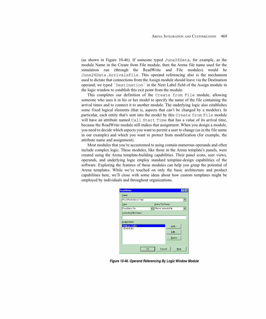
469ARENA INTEGRATION AND CUSTOMIZATION
(as shown in Figure 10-46). If someone typed June26Data, for example, as themodule Name in the Create from File module, then the Arena file name used for thesimulation run (through the ReadWrite and File modules) would beJune26Data.ArrivalsFile. This operand referencing also is the mechanismused to dictate that connections from the Assign module should leave via the Destinationoperand; we typed `Destination` in the Next Label field of the Assign module inthe logic window to establish this exit point from the module.
This completes our definition of the Create from File module, allowingsomeone who uses it in his or her model to specify the name of the file containing thearrival times and to connect it to another module. The underlying logic also establishessome fixed logical elements (that is, aspects that can’t be changed by a modeler). Inparticular, each entity that’s sent into the model by this Create from File modulewill have an attribute named Call Start Time that has a value of its arrival time,because the ReadWrite module still makes that assignment. When you design a module,you need to decide which aspects you want to permit a user to change (as in the file namein our example) and which you want to protect from modification (for example, theattribute name and assignment).
Most modules that you’re accustomed to using contain numerous operands and ofteninclude complex logic. These modules, like those in the Arena template’s panels, werecreated using the Arena template-building capabilities. Their panel icons, user views,operands, and underlying logic employ standard template-design capabilities of thesoftware. Exploring the features of these modules can help you grasp the potential ofArena templates. While we’ve touched on only the basic architecture and productcapabilities here, we’ll close with some ideas about how custom templates might beemployed by individuals and throughout organizations.
Figure 10-46. Operand Referencing By Logic Window Module
470 CHAPTER 10
10.5.5 Uses of TemplatesTemplates may be developed to address a wide range of needs. Some might be conceivedfor use by a large targeted market, such as the Arena Contact Center Template or theArena Packaging Template. Others might be more like a utility, such as the simpleexample presented in this chapter.
The most ambitious Arena templates are those that are developed for a commercialmarket, typically targeted at a particular industry, such as high-speed production orcustomer-relationship contact centers. There are two main advantages of industry-focused templates. First, the template can use terminology that is appropriate for theindustry, minimizing the abstraction needed for a modeler to translate a system into thesoftware. More importantly, through Arena’s hierarchy, a template can be built that isfully customized to represent accurately the elements of systems in the industry. Thedesigner of the template has the capabilities at hand to mimic exactly the behavior ofequipment, people, parts, components, etc., providing whatever spectrum of options isappropriate for the variations of these system elements. Furthermore, through theActiveX Automation technology supported by Arena, wizards and other utilities can becreated that work in cooperation with a particular template for generating specializedgraphs and reports, loading data directly from external databases, etc.
Many of the templates that are developed using Arena aid modelers in representing aparticular system, facility, or process. While they may not be “commercial-grade,” thesetemplates have many of the same goals as the industry templates and provide many of thesame benefits. Here, though, the focus might be narrower than a commercial template.For example, a template might be built for use in analyzing truck-loading schemes or forrepresenting dispatching rules of incoming calls to technicians. These application-focused templates benefit from Arena’s hierarchical structure in the same ways asindustry-focused templates: the interface presented to a modeler can be customized to bevery familiar (both in terms of graphical animation and the terminology presented to theuser); and the elements of the target application environment can be representedaccurately. In some cases, a modeler might build these templates just for his or her ownindividual use, if the same type of problem is likely to be modeled repeatedly. In othercases, templates might be created for use among modelers in a common group, andapplication templates can be shared among different modeling groups throughout anenterprise.
For an individual modeler, Arena templates afford the opportunity to reuse modelingtechniques that are learned in the process of building models. In the evolution ofprogramming tools, reusable code was captured in procedures/subroutines/functions;later, object-oriented tools allowed the full characteristics of “objects” represented in thesoftware to be defined for reuse. A module can be thought of as analogous to an object(in object-oriented software)—the module allows you to capture the completecharacteristics of a process that you want to model in a self-contained package that youmay reuse and that may be customized in each use. The Create from File modulesketched out in this section is an example of this type of template, where once amodeling technique was established and tested, its implementation details were “hidden”
471ARENA INTEGRATION AND CUSTOMIZATION
inside the definition of the module. Later uses of the same technique require littleknowledge of its approach or implementation details and have less risk of error since theembedded logic has already been tested.
10.6 Summary and Forecast
In this chapter, we have examined a number of topics that are part of a theme ofcustomizing different aspects of Arena modeling and integrating Arena with otherapplications. We took a whirlwind tour of VBA, saw how Arena and Microsoft Officecan work together to read in numeric or string data, and built a custom modelingconstruct of our own with Arena’s template-building tools. The material in this chapterrepresents the tip of the iceberg, with the intent of tickling your imagination for what’spossible and arming you with enough fundamental knowledge of the features to go offand explore on your own.
If you choose to continue, you’ll find that Chapter 11 takes on the topic of modelingcontinuous-change processes, such as the flow of liquid or bulk materials. Then we turnour attention to some important topics that underlie and support good simulation studiesin Chapters 12 and 13.
10.7 Exercises
10-1 Starting with Model 10-1, modify the logic to store the time between arrivals andthe processing time (excluding any waiting time) in attributes. Then use the ReadWritemodule from the Advanced Process panel to write this pair of attributes to an Excel orAccess file (or a text file if you don’t have either of these applications installed).
10-2 Start with Model 10-2 and use the data file you generated in Exercise 10-1 tospecify both call-arrival logic and call-handling time. Note that since the data are timebetween arrivals rather than absolute arrival time, slightly different logic will be re-quired. How do your results compare to those in Exercise 10-1?
10-3 Build a simple, single-server queueing model with entity interarrival times ofEXPO(0.25) minutes. Using the ReadWrite module, prompt and query at the beginningof the simulation run for the server’s process time mean (give a default value of 0.2minutes). Use this value to establish a uniform distribution on [a, b] where a is 10%below the entered mean and b is 10% above the entered mean. Run the simulation until300 entities have departed the model.
10-4 Create the model described in Exercise 10-3, replacing the ReadWrite moduleswith a VBA form that’s displayed at the beginning of the simulation run.
10-5 Using the single-server model from Exercise 10-4, add logic to play a sound ordisplay a message whenever the number of entities in the service queue exceeds somethreshold value. Allow the modeler to establish this threshold in the form that’s displayedat the beginning of the run.

472 CHAPTER 10
10-6 Present a VBA form at the end of the simulation run reporting the average andmaximum queue lengths for the product queues in Model 10-1. If you have a chartingprogram (e.g., Excel) installed on your computer, also draw a bar graph of the averagevalues.
10-7 Create a model that writes 1000 records to a file. Each record will include therecord number and ten random samples, each between 0 and 100,000. In Run > Setup >Reports, disable the normal model output by selecting SIMAN Summary Report asthe default output and select Disable generation of report database.Enable Run > Run Control > Batch Run (No Animation) so that we can execute as fast aspossible. Repeat this experiment using a text file, a binary file, an Excel file, an Accessfile, an XML file, and no file (just generate and discard the random samples). Comparethe execution time and the file sizes for each trial. If you have a fast machine, repeat with10,000 and 100,000 records.
473CONTINUOUS AND COMBINED DISCRETE/CONTINUOUS MODELS
CHAPTER 11
Continuous and CombinedDiscrete/Continuous Models
So far, whether you realized it or not, all of our modeling has been focused on discretesystems—that is, processes in which changes to the state of the system occur at isolatedpoints in time called events. In Arena, these event times are managed by the eventcalendar, with entities moving through the flowcharted process to define when changesin the system state will occur and what changes should take place (for example, aresource is released). In Chapter 2, our hand simulation accounted for all of thesetransitions, defining all of the events that could change the system and their exactoccurrence times. These discrete-event models can capture many types of systems, fromservice processes (such as the call center in Chapter 5) to manufacturing systems (suchas the small manufacturing system in Chapter 7).
In other cases, though, the state of the system might change continuously over time.Consider a brewery, where various ingredients (hops, barley, water) are mixed, heated,stored, and transferred in pipes among tanks. In this system, the process of emptying atank involves a flow of product. To model the volume of beer in the tank, you’d want tobe able to represent its rate of change over time and allow this rate to produce a smooth,continuous flow of lager into the target receptacle (preferably one that’s destined for yournext social gathering). The level of the tank at some future time can be calculated byapplying the rate of change to the starting level; simple arithmetic is all that’s needed,assuming that no intervening event occurs, such as a power outage, technicalmalfunction, or large sampling from a passing tour group. You may want to capture thesediscrete events that interact with this continuous process, such as closing a valve tointerrupt the emptying process and set the rate of change of the tank’s level to zero.
More complex processes may involve rates of change that depend on other continuousprocesses, in which case the future level value can’t be calculated so simply. In thesecases, integration algorithms are used to determine the levels based on the relationshipbetween the continuous processes. The temperature of water in an aquarium is an exampleof this type of system. It changes continuously over time, depending on factors such as theheat from sunlight, the change in temperature of the room in which it is displayed, and thecycling on and off of a heater. These elements—heat from the sun, room temperature, andwarmth generated by the heater—also change continuously. To capture these processesaccurately in a simulation model, specialized continuous-modeling approaches are usedthat allow these relationships to be defined as mathematical equations that areincorporated in the integration algorithm.
In this chapter, we’ll turn our attention to these processes in which the state of thesystem can change continuously over time. In Section 11.1, we discuss the nature ofcontinuous processes and introduce Arena’s terminology and constructs for modeling the
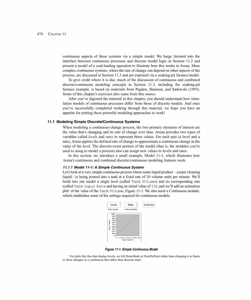
474 CHAPTER 11
continuous aspects of these systems via a simple model. We barge forward into theinterface between continuous processes and discrete model logic in Section 11.2 andpresent a model of a coal-loading operation to illustrate how this works in Arena. Morecomplex continuous systems, where the rate of change can depend on other aspects of theprocess, are discussed in Section 11.3 and are explored via a soaking-pit furnace model.
To give credit where it is due, much of the discussion of continuous and combineddiscrete/continuous modeling concepts in Section 11.3, including the soaking-pitfurnace example, is based on materials from Pegden, Shannon, and Sadowski (1995).Some of this chapter’s exercises also came from this source.
After you’ve digested the material in this chapter, you should understand how simu-lation models of continuous processes differ from those of discrete models. And onceyou’ve successfully completed working through this material, we hope you have anappetite for putting these powerful modeling approaches to work!
11.1 Modeling Simple Discrete/Continuous Systems
When modeling a continuous-change process, the two primary elements of interest arethe value that’s changing and its rate of change over time. Arena provides two types ofvariables called levels and rates to represent these values. For each pair (a level and arate), Arena applies the defined rate of change to approximate a continuous change in thevalue of the level. The discrete-event portion of the model (that is, the modules you’reused to using to model a process) also can assign new values to levels and rates.
In this section, we introduce a small example, Model 11-1, which illustrates howArena’s continuous and combined discrete/continuous modeling features work.
11.1.1 Model 11-1: A Simple Continuous SystemLet’s look at a very simple continuous process where some liquid product—carpet cleaningliquid—is being poured into a tank at a fixed rate of 10 volume units per minute. We’llbuild into our model a single level (called Tank Volume) and its corresponding rate(called Tank Input Rate and having an initial value of 10), and we’ll add an animationplot1 of the value of the Tank Volume, Figure 11-1. We also need a Continuous module,which establishes some of the settings required for continuous models.
Figure 11-1. Simple Continuous Model
1 For plots like this that display levels, we left DrawMode at PointToPoint rather than changing it to Stairsto show changes as a continuous line rather than discrete steps.
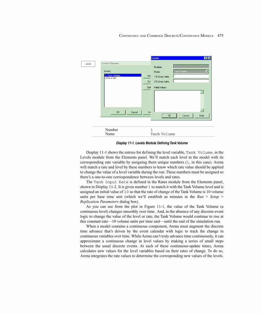
475CONTINUOUS AND COMBINED DISCRETE/CONTINUOUS MODELS
Number 1Name Tank Volume
Display 11-1. Levels Module Defining Tank Volume
Display 11-1 shows the entries for defining the level variable, Tank Volume, in theLevels module from the Elements panel. We’ll match each level in the model with itscorresponding rate variable by assigning them unique numbers (1, in this case). Arenawill match a rate and level by these numbers to know which rate value should be appliedto change the value of a level variable during the run. These numbers must be assigned sothere’s a one-to-one correspondence between levels and rates.
The Tank Input Rate is defined in the Rates module from the Elements panel,shown in Display 11-2. It is given number 1 to match it with the Tank Volume level and isassigned an initial value of 10 so that the rate of change of the Tank Volume is 10 volumeunits per base time unit (which we’ll establish as minutes in the Run > Setup >Replication Parameters dialog box).
As you can see from the plot in Figure 11-1, the value of the Tank Volume (acontinuous level) changes smoothly over time. And, in the absence of any discrete-eventlogic to change the value of the level or rate, the Tank Volume would continue to rise atthis constant rate—10 volume units per time unit—until the end of the simulation run.
When a model contains a continuous component, Arena must augment the discretetime advance that’s driven by the event calendar with logic to track the change incontinuous variables over time. While Arena can’t truly advance time continuously, it canapproximate a continuous change in level values by making a series of small stepsbetween the usual discrete events. At each of these continuous-update times, Arenacalculates new values for the level variables based on their rates of change. To do so,Arena integrates the rate values to determine the corresponding new values of the levels.
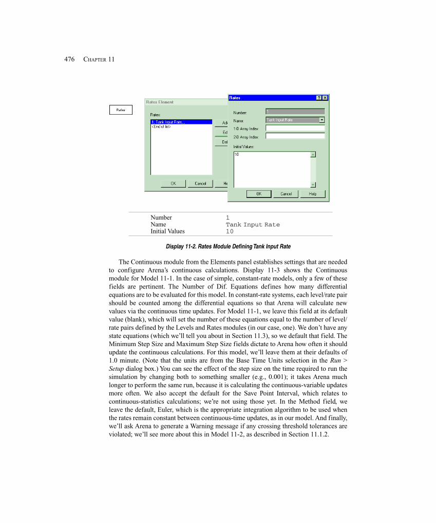
476 CHAPTER 11
Number 1Name Tank Input RateInitial Values 10
Display 11-2. Rates Module Defining Tank Input Rate
The Continuous module from the Elements panel establishes settings that are neededto configure Arena’s continuous calculations. Display 11-3 shows the Continuousmodule for Model 11-1. In the case of simple, constant-rate models, only a few of thesefields are pertinent. The Number of Dif. Equations defines how many differentialequations are to be evaluated for this model. In constant-rate systems, each level/rate pairshould be counted among the differential equations so that Arena will calculate newvalues via the continuous time updates. For Model 11-1, we leave this field at its defaultvalue (blank), which will set the number of these equations equal to the number of level/rate pairs defined by the Levels and Rates modules (in our case, one). We don’t have anystate equations (which we’ll tell you about in Section 11.3), so we default that field. TheMinimum Step Size and Maximum Step Size fields dictate to Arena how often it shouldupdate the continuous calculations. For this model, we’ll leave them at their defaults of1.0 minute. (Note that the units are from the Base Time Units selection in the Run >Setup dialog box.) You can see the effect of the step size on the time required to run thesimulation by changing both to something smaller (e.g., 0.001); it takes Arena muchlonger to perform the same run, because it is calculating the continuous-variable updatesmore often. We also accept the default for the Save Point Interval, which relates tocontinuous-statistics calculations; we’re not using those yet. In the Method field, weleave the default, Euler, which is the appropriate integration algorithm to be used whenthe rates remain constant between continuous-time updates, as in our model. And finally,we’ll ask Arena to generate a Warning message if any crossing threshold tolerances areviolated; we’ll see more about this in Model 11-2, as described in Section 11.1.2.
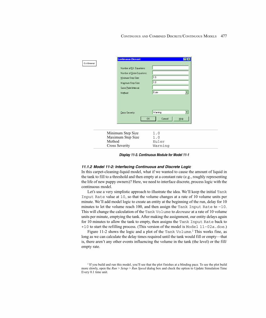
477CONTINUOUS AND COMBINED DISCRETE/CONTINUOUS MODELS
Minimum Step Size 1.0Maximum Step Size 1.0Method EulerCross Severity Warning
Display 11-3. Continuous Module for Model 11-1
11.1.2 Model 11-2: Interfacing Continuous and Discrete LogicIn this carpet-cleaning-liquid model, what if we wanted to cause the amount of liquid inthe tank to fill to a threshold and then empty at a constant rate (e.g., roughly representingthe life of new puppy owners)? Here, we need to interface discrete, process logic with thecontinuous model.
Let’s use a very simplistic approach to illustrate the idea. We’ll keep the initial TankInput Rate value at 10, so that the volume changes at a rate of 10 volume units perminute. We’ll add model logic to create an entity at the beginning of the run, delay for 10minutes to let the volume reach 100, and then assign the Tank Input Rate to –10.This will change the calculation of the Tank Volume to decrease at a rate of 10 volumeunits per minute, emptying the tank. After making the assignment, our entity delays againfor 10 minutes to allow the tank to empty, then assigns the Tank Input Rate back to+10 to start the refilling process. (This version of the model is Model 11-02a.doe.)
Figure 11-2 shows the logic and a plot of the Tank Volume.2 This works fine, aslong as we can calculate the delay times required until the tank would fill or empty—thatis, there aren’t any other events influencing the volume in the tank (the level) or the fill/empty rate.
2 If you build and run this model, you’ll see that the plot finishes at a blinding pace. To see the plot buildmore slowly, open the Run > Setup > Run Speed dialog box and check the option to Update Simulation TimeEvery 0.1 time unit.
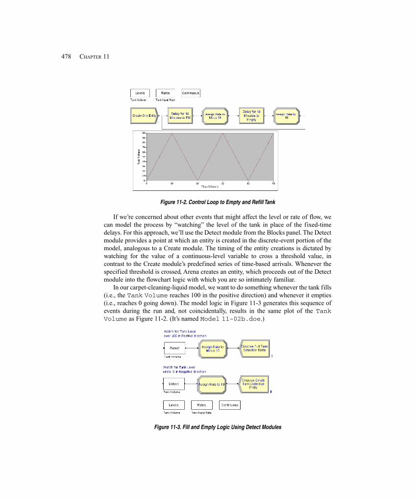
478 CHAPTER 11
Figure 11-2. Control Loop to Empty and Refill Tank
If we’re concerned about other events that might affect the level or rate of flow, wecan model the process by “watching” the level of the tank in place of the fixed-timedelays. For this approach, we’ll use the Detect module from the Blocks panel. The Detectmodule provides a point at which an entity is created in the discrete-event portion of themodel, analogous to a Create module. The timing of the entity creations is dictated bywatching for the value of a continuous-level variable to cross a threshold value, incontrast to the Create module’s predefined series of time-based arrivals. Whenever thespecified threshold is crossed, Arena creates an entity, which proceeds out of the Detectmodule into the flowchart logic with which you are so intimately familiar.
In our carpet-cleaning-liquid model, we want to do something whenever the tank fills(i.e., the Tank Volume reaches 100 in the positive direction) and whenever it empties(i.e., reaches 0 going down). The model logic in Figure 11-3 generates this sequence ofevents during the run and, not coincidentally, results in the same plot of the TankVolume as Figure 11-2. (It’s named Model 11-02b.doe.)
Figure 11-3. Fill and Empty Logic Using Detect Modules
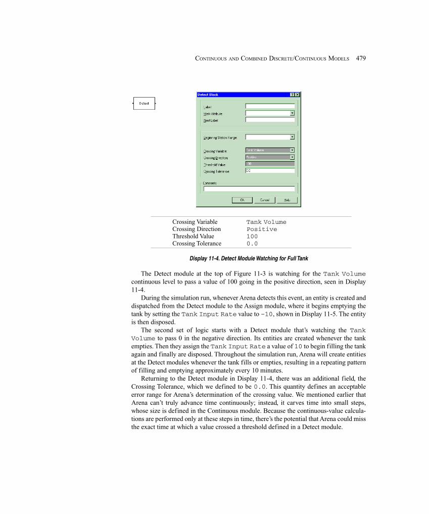
479CONTINUOUS AND COMBINED DISCRETE/CONTINUOUS MODELS
Crossing Variable Tank VolumeCrossing Direction PositiveThreshold Value 100Crossing Tolerance 0.0
Display 11-4. Detect Module Watching for Full Tank
The Detect module at the top of Figure 11-3 is watching for the Tank Volumecontinuous level to pass a value of 100 going in the positive direction, seen in Display11-4.
During the simulation run, whenever Arena detects this event, an entity is created anddispatched from the Detect module to the Assign module, where it begins emptying thetank by setting the Tank Input Rate value to –10, shown in Display 11-5. The entityis then disposed.
The second set of logic starts with a Detect module that’s watching the TankVolume to pass 0 in the negative direction. Its entities are created whenever the tankempties. Then they assign the Tank Input Rate a value of 10 to begin filling the tankagain and finally are disposed. Throughout the simulation run, Arena will create entitiesat the Detect modules whenever the tank fills or empties, resulting in a repeating patternof filling and emptying approximately every 10 minutes.
Returning to the Detect module in Display 11-4, there was an additional field, theCrossing Tolerance, which we defined to be 0.0. This quantity defines an acceptableerror range for Arena’s determination of the crossing value. We mentioned earlier thatArena can’t truly advance time continuously; instead, it carves time into small steps,whose size is defined in the Continuous module. Because the continuous-value calcula-tions are performed only at these steps in time, there’s the potential that Arena could missthe exact time at which a value crossed a threshold defined in a Detect module.
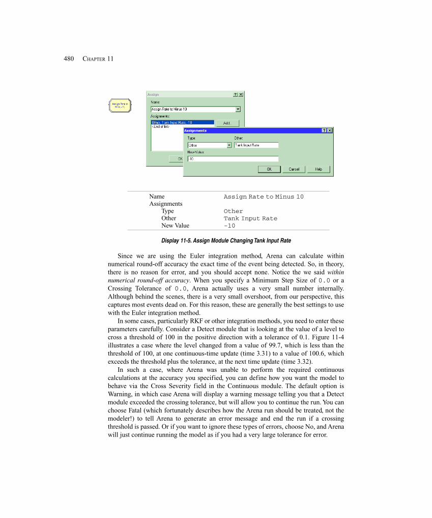
480 CHAPTER 11
Name Assign Rate to Minus 10Assignments
Type OtherOther Tank Input RateNew Value -10
Display 11-5. Assign Module Changing Tank Input Rate
Since we are using the Euler integration method, Arena can calculate withinnumerical round-off accuracy the exact time of the event being detected. So, in theory,there is no reason for error, and you should accept none. Notice the we said withinnumerical round-off accuracy. When you specify a Minimum Step Size of 0.0 or aCrossing Tolerance of 0.0, Arena actually uses a very small number internally.Although behind the scenes, there is a very small overshoot, from our perspective, thiscaptures most events dead on. For this reason, these are generally the best settings to usewith the Euler integration method.
In some cases, particularly RKF or other integration methods, you need to enter theseparameters carefully. Consider a Detect module that is looking at the value of a level tocross a threshold of 100 in the positive direction with a tolerance of 0.1. Figure 11-4illustrates a case where the level changed from a value of 99.7, which is less than thethreshold of 100, at one continuous-time update (time 3.31) to a value of 100.6, whichexceeds the threshold plus the tolerance, at the next time update (time 3.32).
In such a case, where Arena was unable to perform the required continuouscalculations at the accuracy you specified, you can define how you want the model tobehave via the Cross Severity field in the Continuous module. The default option isWarning, in which case Arena will display a warning message telling you that a Detectmodule exceeded the crossing tolerance, but will allow you to continue the run. You canchoose Fatal (which fortunately describes how the Arena run should be treated, not themodeler!) to tell Arena to generate an error message and end the run if a crossingthreshold is passed. Or if you want to ignore these types of errors, choose No, and Arenawill just continue running the model as if you had a very large tolerance for error.
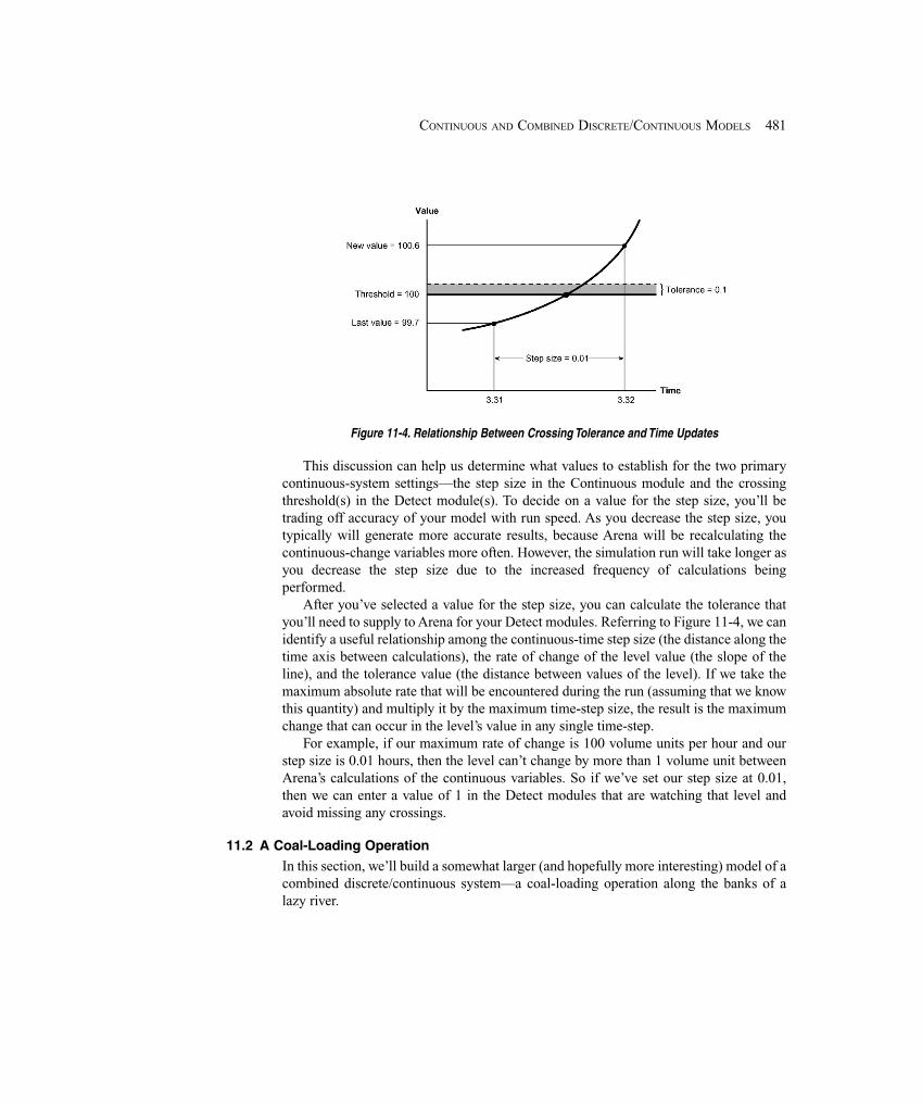
481CONTINUOUS AND COMBINED DISCRETE/CONTINUOUS MODELS
Figure 11-4. Relationship Between Crossing Tolerance and Time Updates
This discussion can help us determine what values to establish for the two primarycontinuous-system settings—the step size in the Continuous module and the crossingthreshold(s) in the Detect module(s). To decide on a value for the step size, you’ll betrading off accuracy of your model with run speed. As you decrease the step size, youtypically will generate more accurate results, because Arena will be recalculating thecontinuous-change variables more often. However, the simulation run will take longer asyou decrease the step size due to the increased frequency of calculations beingperformed.
After you’ve selected a value for the step size, you can calculate the tolerance thatyou’ll need to supply to Arena for your Detect modules. Referring to Figure 11-4, we canidentify a useful relationship among the continuous-time step size (the distance along thetime axis between calculations), the rate of change of the level value (the slope of theline), and the tolerance value (the distance between values of the level). If we take themaximum absolute rate that will be encountered during the run (assuming that we knowthis quantity) and multiply it by the maximum time-step size, the result is the maximumchange that can occur in the level’s value in any single time-step.
For example, if our maximum rate of change is 100 volume units per hour and ourstep size is 0.01 hours, then the level can’t change by more than 1 volume unit betweenArena’s calculations of the continuous variables. So if we’ve set our step size at 0.01,then we can enter a value of 1 in the Detect modules that are watching that level andavoid missing any crossings.
11.2 A Coal-Loading Operation
In this section, we’ll build a somewhat larger (and hopefully more interesting) model of acombined discrete/continuous system—a coal-loading operation along the banks of alazy river.
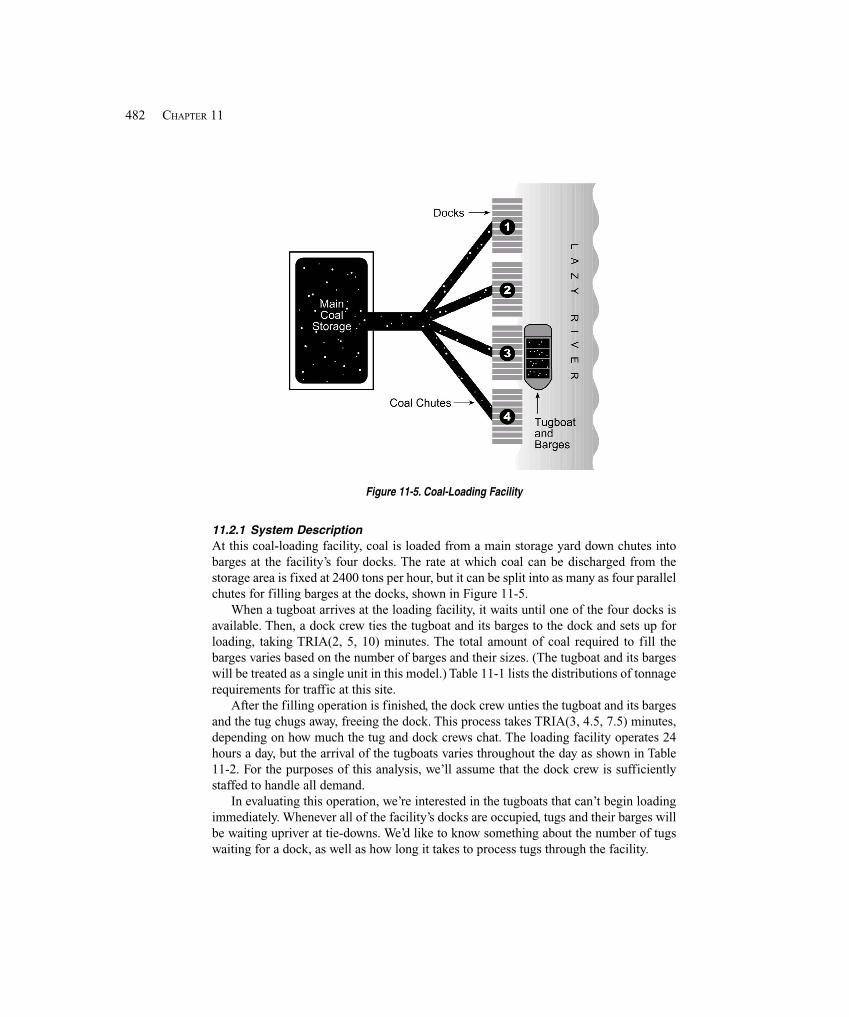
482 CHAPTER 11
Figure 11-5. Coal-Loading Facility
11.2.1 System DescriptionAt this coal-loading facility, coal is loaded from a main storage yard down chutes intobarges at the facility’s four docks. The rate at which coal can be discharged from thestorage area is fixed at 2400 tons per hour, but it can be split into as many as four parallelchutes for filling barges at the docks, shown in Figure 11-5.
When a tugboat arrives at the loading facility, it waits until one of the four docks isavailable. Then, a dock crew ties the tugboat and its barges to the dock and sets up forloading, taking TRIA(2, 5, 10) minutes. The total amount of coal required to fill thebarges varies based on the number of barges and their sizes. (The tugboat and its bargeswill be treated as a single unit in this model.) Table 11-1 lists the distributions of tonnagerequirements for traffic at this site.
After the filling operation is finished, the dock crew unties the tugboat and its bargesand the tug chugs away, freeing the dock. This process takes TRIA(3, 4.5, 7.5) minutes,depending on how much the tug and dock crews chat. The loading facility operates 24hours a day, but the arrival of the tugboats varies throughout the day as shown in Table11-2. For the purposes of this analysis, we’ll assume that the dock crew is sufficientlystaffed to handle all demand.
In evaluating this operation, we’re interested in the tugboats that can’t begin loadingimmediately. Whenever all of the facility’s docks are occupied, tugs and their barges willbe waiting upriver at tie-downs. We’d like to know something about the number of tugswaiting for a dock, as well as how long it takes to process tugs through the facility.
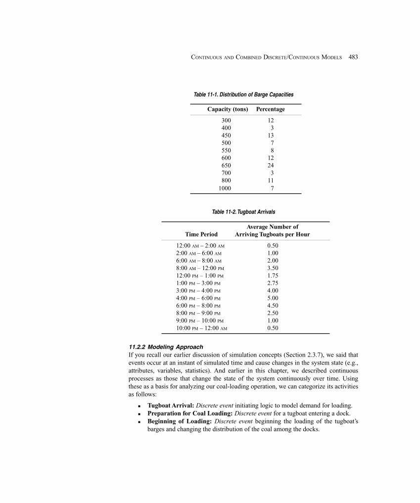
483CONTINUOUS AND COMBINED DISCRETE/CONTINUOUS MODELS
Table 11-1. Distribution of Barge Capacities
Capacity (tons) Percentage
300 12400 3450 13500 7550 8600 12650 24700 3800 11
1000 7
Table 11-2. Tugboat Arrivals
Average Number of Time Period Arriving Tugboats per Hour
12:00 AM – 2:00 AM 0.502:00 AM – 6:00 AM 1.006:00 AM – 8:00 AM 2.008:00 AM – 12:00 PM 3.5012:00 PM – 1:00 PM 1.751:00 PM – 3:00 PM 2.753:00 PM – 4:00 PM 4.004:00 PM – 6:00 PM 5.006:00 PM – 8:00 PM 4.508:00 PM – 9:00 PM 2.509:00 PM – 10:00 PM 1.0010:00 PM – 12:00 AM 0.50
11.2.2 Modeling ApproachIf you recall our earlier discussion of simulation concepts (Section 2.3.7), we said thatevents occur at an instant of simulated time and cause changes in the system state (e.g.,attributes, variables, statistics). And earlier in this chapter, we described continuousprocesses as those that change the state of the system continuously over time. Usingthese as a basis for analyzing our coal-loading operation, we can categorize its activitiesas follows:
� Tugboat Arrival: Discrete event initiating logic to model demand for loading.� Preparation for Coal Loading: Discrete event for a tugboat entering a dock.� Beginning of Loading: Discrete event beginning the loading of the tugboat’s
barges and changing the distribution of the coal among the docks.
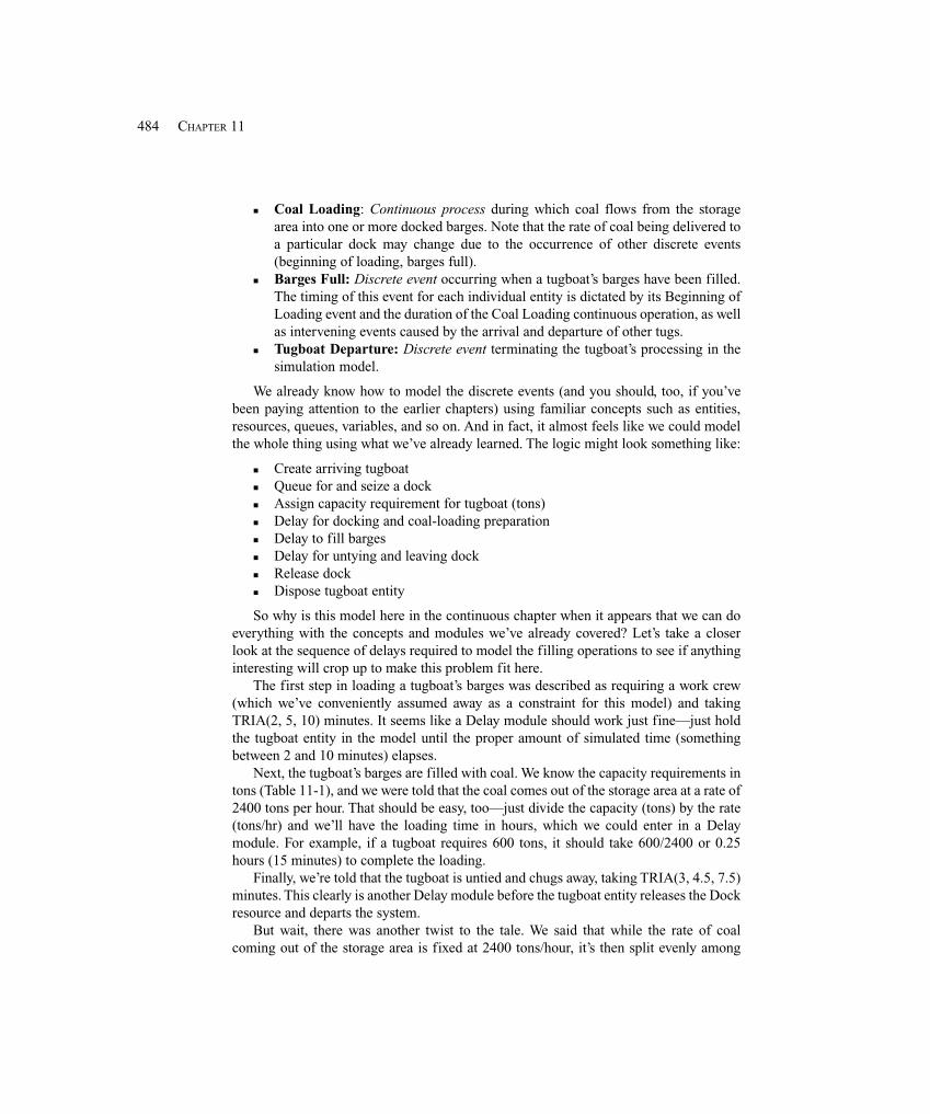
484 CHAPTER 11
� Coal Loading: Continuous process during which coal flows from the storagearea into one or more docked barges. Note that the rate of coal being delivered toa particular dock may change due to the occurrence of other discrete events(beginning of loading, barges full).
� Barges Full: Discrete event occurring when a tugboat’s barges have been filled.The timing of this event for each individual entity is dictated by its Beginning ofLoading event and the duration of the Coal Loading continuous operation, as wellas intervening events caused by the arrival and departure of other tugs.
� Tugboat Departure: Discrete event terminating the tugboat’s processing in thesimulation model.
We already know how to model the discrete events (and you should, too, if you’vebeen paying attention to the earlier chapters) using familiar concepts such as entities,resources, queues, variables, and so on. And in fact, it almost feels like we could modelthe whole thing using what we’ve already learned. The logic might look something like:
� Create arriving tugboat� Queue for and seize a dock� Assign capacity requirement for tugboat (tons)� Delay for docking and coal-loading preparation� Delay to fill barges� Delay for untying and leaving dock� Release dock� Dispose tugboat entity
So why is this model here in the continuous chapter when it appears that we can doeverything with the concepts and modules we’ve already covered? Let’s take a closerlook at the sequence of delays required to model the filling operations to see if anythinginteresting will crop up to make this problem fit here.
The first step in loading a tugboat’s barges was described as requiring a work crew(which we’ve conveniently assumed away as a constraint for this model) and takingTRIA(2, 5, 10) minutes. It seems like a Delay module should work just fine—just holdthe tugboat entity in the model until the proper amount of simulated time (somethingbetween 2 and 10 minutes) elapses.
Next, the tugboat’s barges are filled with coal. We know the capacity requirements intons (Table 11-1), and we were told that the coal comes out of the storage area at a rate of2400 tons per hour. That should be easy, too—just divide the capacity (tons) by the rate(tons/hr) and we’ll have the loading time in hours, which we could enter in a Delaymodule. For example, if a tugboat requires 600 tons, it should take 600/2400 or 0.25hours (15 minutes) to complete the loading.
Finally, we’re told that the tugboat is untied and chugs away, taking TRIA(3, 4.5, 7.5)minutes. This clearly is another Delay module before the tugboat entity releases the Dockresource and departs the system.
But wait, there was another twist to the tale. We said that while the rate of coalcoming out of the storage area is fixed at 2400 tons/hour, it’s then split evenly among
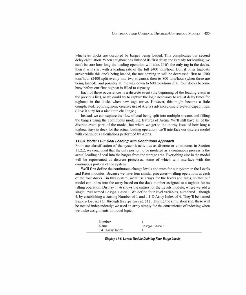
485CONTINUOUS AND COMBINED DISCRETE/CONTINUOUS MODELS
whichever docks are occupied by barges being loaded. This complicates our seconddelay calculation. When a tugboat has finished its first delay and is ready for loading, wecan’t be sure how long the loading operation will take. If it’s the only tug in the docks,then it will start with a loading rate of the full 2400 tons/hour. But, if other tugboatsarrive while this one’s being loaded, the rate coming in will be decreased: first to 1200tons/hour (2400 split evenly into two streams), then to 800 tons/hour (when three arebeing loaded), and possibly all the way down to 600 tons/hour if all four docks becomebusy before our first tugboat is filled to capacity.
Each of these occurrences is a discrete event (the beginning of the loading event inthe previous list), so we could try to capture the logic necessary to adjust delay times fortugboats in the docks when new tugs arrive. However, this might become a littlecomplicated, requiring some creative use of Arena’s advanced discrete-event capabilities.(Give it a try for a nice little challenge.)
Instead, we can capture the flow of coal being split into multiple streams and fillingthe barges using the continuous modeling features of Arena. We’ll still have all of thediscrete-event parts of the model, but where we get to the thorny issue of how long atugboat stays in dock for the actual loading operation, we’ll interface our discrete modelwith continuous calculations performed by Arena.
11.2.3 Model 11-3: Coal Loading with Continuous ApproachFrom our classification of the system’s activities as discrete or continuous in Section11.2.2, we concluded that the only portion to be modeled as a continuous process is theactual loading of coal into the barges from the storage area. Everything else in the modelwill be represented as discrete processes, some of which will interface with thecontinuous portion of the system.
We’ll first define the continuous-change levels and rates for our system in the Levelsand Rates modules. Because we have four similar processes—filling operations at eachof the four docks—in this system, we’ll use arrays for the levels and rates, so that ourmodel can index into the array based on the dock number assigned to a tugboat for itsfilling operation. Display 11-6 shows the entries for the Levels module, where we add asingle level named Barge Level. We define four level variables, numbered 1 though4, by establishing a starting Number of 1 and a 1-D Array Index of 4. They’ll be namedBarge Level(1) through Barge Level(4). During the simulation run, these willbe treated independently; we used an array simply for the convenience of indexing whenwe make assignments in model logic.
Number 1Name Barge Level1-D Array Index 4
Display 11-6. Levels Module Defining Four Barge Levels
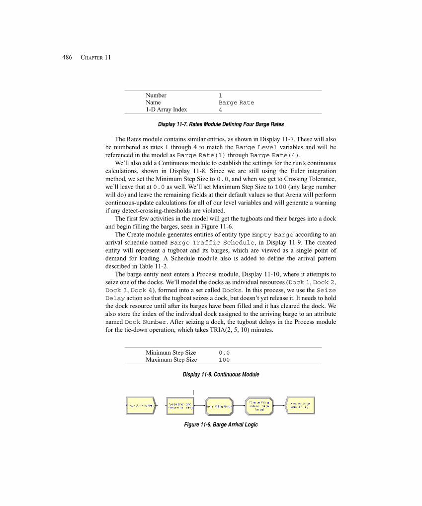
486 CHAPTER 11
Number 1Name Barge Rate1-D Array Index 4
Display 11-7. Rates Module Defining Four Barge Rates
The Rates module contains similar entries, as shown in Display 11-7. These will alsobe numbered as rates 1 through 4 to match the Barge Level variables and will bereferenced in the model as Barge Rate(1) through Barge Rate(4).
We’ll also add a Continuous module to establish the settings for the run’s continuouscalculations, shown in Display 11-8. Since we are still using the Euler integrationmethod, we set the Minimum Step Size to 0.0, and when we get to Crossing Tolerance,we’ll leave that at 0.0 as well. We’ll set Maximum Step Size to 100 (any large numberwill do) and leave the remaining fields at their default values so that Arena will performcontinuous-update calculations for all of our level variables and will generate a warningif any detect-crossing-thresholds are violated.
The first few activities in the model will get the tugboats and their barges into a dockand begin filling the barges, seen in Figure 11-6.
The Create module generates entities of entity type Empty Barge according to anarrival schedule named Barge Traffic Schedule, in Display 11-9. The createdentity will represent a tugboat and its barges, which are viewed as a single point ofdemand for loading. A Schedule module also is added to define the arrival patterndescribed in Table 11-2.
The barge entity next enters a Process module, Display 11-10, where it attempts toseize one of the docks. We’ll model the docks as individual resources (Dock 1, Dock 2,Dock 3, Dock 4), formed into a set called Docks. In this process, we use the SeizeDelay action so that the tugboat seizes a dock, but doesn’t yet release it. It needs to holdthe dock resource until after its barges have been filled and it has cleared the dock. Wealso store the index of the individual dock assigned to the arriving barge to an attributenamed Dock Number. After seizing a dock, the tugboat delays in the Process modulefor the tie-down operation, which takes TRIA(2, 5, 10) minutes.
Minimum Step Size 0.0Maximum Step Size 100
Display 11-8. Continuous Module
Figure 11-6. Barge Arrival Logic

487CONTINUOUS AND COMBINED DISCRETE/CONTINUOUS MODELS
Name Create Arriving BargeEntity Type Empty BargeTime Between Arrivals
Type ScheduleSchedule Name Barge Traffic Schedule
Display 11-9. Create Module for Arriving Empty Barges
Name Seize Dock and Prepare forFilling
Action Seize DelayResources
Type SetSet Name DocksSave Attribute Dock Number
Delay Type TriangularUnits MinutesMinimum 2Value (Most Likely) 5Maximum 10
Display 11-10. Process Module for Entering a Dock
After the tugboat entity has seized a dock and delayed for its tie-down time, it entersan Assign module to initiate the flow of coal into the barges. Remember that the actualrate of coal coming into a barge at a dock will depend on how many other docks arecurrently loading coal. Whenever the number of active docks (i.e., with barges beingloaded) changes, the 2400 tons/hour of coal leaving the storage area needs to be adjustedto maintain an even distribution among those docks. We’ll use a global variable,Filling Docks, to keep track of the number of docks that are loading. Then,whenever a new barge begins loading or reaches capacity, we’ll adjust the loading ratesin the active docks to be 2400/Filling Docks to keep our even distribution of coal.
In the Assign module, Display 11-11, the tugboat first increments the number ofdocks that are currently being filled (Filling Docks) by one. It then sets the rate offlow of coal flowing into its dock by assigning a new value to the rate variable at this dock,Barge Rate(Dock Number). And, so that we can later collect statistics on fillingtimes, we’ll assign the current simulation time to a global variable, Beginning FillTime(Dock Number). Later in the model, when a full barge departs, we’ll record thetime that the barge spent in dock. Finally, the tugboat determines its size by taking asample from a discrete probability distribution using the values provided in Table 11-1.This quantity is assigned to a variable, Barge Capacity(Dock Number), whichwe’ll use as the threshold value for a Detect module that’s watching for full tugboats ateach dock. We also opened the Variable module on the Basic Process panel and definedthe Beginning Fill Time and Barge Capacity variables, each with four rows.
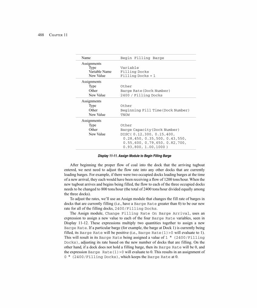
488 CHAPTER 11
Name Begin Filling Barge
AssignmentsType VariableVariable Name Filling DocksNew Value Filling Docks + 1
AssignmentsType OtherOther Barge Rate(Dock Number)New Value 2400 / Filling Docks
AssignmentsType OtherOther Beginning Fill Time(Dock Number)New Value TNOW
AssignmentsType OtherOther Barge Capacity(Dock Number)New Value DISC( 0.12,300, 0.15,400,
0.28,450, 0.35,500, 0.43,550, 0.55,600, 0.79,650, 0.82,700, 0.93,800, 1.00,1000 )
Display 11-11. Assign Module to Begin Filling Barge
After beginning the proper flow of coal into the dock that the arriving tugboatentered, we next need to adjust the flow rate into any other docks that are currentlyloading barges. For example, if there were two occupied docks loading barges at the timeof a new arrival, they each would have been receiving a flow of 1200 tons/hour. When thenew tugboat arrives and begins being filled, the flow to each of the three occupied docksneeds to be changed to 800 tons/hour (the total of 2400 tons/hour divided equally amongthe three docks).
To adjust the rates, we’ll use an Assign module that changes the fill rate of barges indocks that are currently filling (i.e., have a Barge Rate greater than 0) to be our newrate for all of the filling docks, 2400/Filling Docks.
The Assign module, Change Filling Rate On Barge Arrival, uses anexpression to assign a new value to each of the four Barge Rate variables, seen inDisplay 11-12. These expressions multiply two quantities together to assign a newBarge Rate. If a particular barge (for example, the barge at Dock 1) is currently beingfilled, its Barge Rate will be positive (i.e., Barge Rate(1)>0 will evaluate to 1).This will result in its Barge Rate being assigned a value of 1 * (2400/FillingDocks), adjusting its rate based on the new number of docks that are filling. On theother hand, if a dock does not hold a filling barge, then its Barge Rate will be 0, andthe expression Barge Rate(1)>0 will evaluate to 0. This results in an assignment of0 * (2400/Filling Docks), which keeps the Barge Rate at 0.
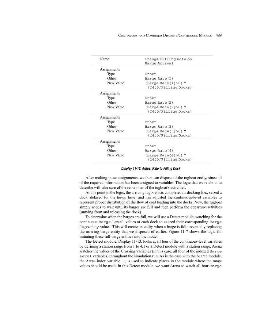
489CONTINUOUS AND COMBINED DISCRETE/CONTINUOUS MODELS
Name Change Filling Rate onBarge Arrival
AssignmentsType OtherOther Barge Rate(1)New Value (Barge Rate(1)>0) *
(2400/Filling Docks)
AssignmentsType OtherOther Barge Rate(2)New Value (Barge Rate(2)>0) *
(2400/Filling Docks)
AssignmentsType OtherOther Barge Rate(3)New Value (Barge Rate(3)>0) *
(2400/Filling Docks)
AssignmentsType OtherOther Barge Rate(4)New Value (Barge Rate(4)>0) *
(2400/Filling Docks)
Display 11-12. Adjust Rate to Filling Dock
After making these assignments, we then can dispose of the tugboat entity, since allof the required information has been assigned to variables. The logic that we’re about todescribe will take care of the remainder of the tugboat’s activities.
At this point in the logic, the arriving tugboat has completed its docking (i.e., seized adock, delayed for the tie-up time) and has adjusted the continuous-level variables torepresent proper distribution of the flow of coal loading into the docks. Now, the tugboatsimply needs to wait until its barges are full and then perform the departure activities(untying from and releasing the dock).
To determine when the barges are full, we will use a Detect module, watching for thecontinuous Barge Level values at each dock to exceed their corresponding BargeCapacity values. This will create an entity when a barge is full, essentially replacingthe arriving barge entity that we disposed of earlier. Figure 11-7 shows the logic forinitiating these full-barge entities into the model.
The Detect module, Display 11-13, looks at all four of the continuous-level variablesby defining a station range from 1 to 4. For a Detect module with a station range, Arenawatches the values of the Crossing Variables (in this case, all four of the indexed BargeLevel variables) throughout the simulation run. As is the case with the Search module,the Arena index variable, J, is used to indicate places in the module where the rangevalues should be used. In this Detect module, we want Arena to watch all four Barge
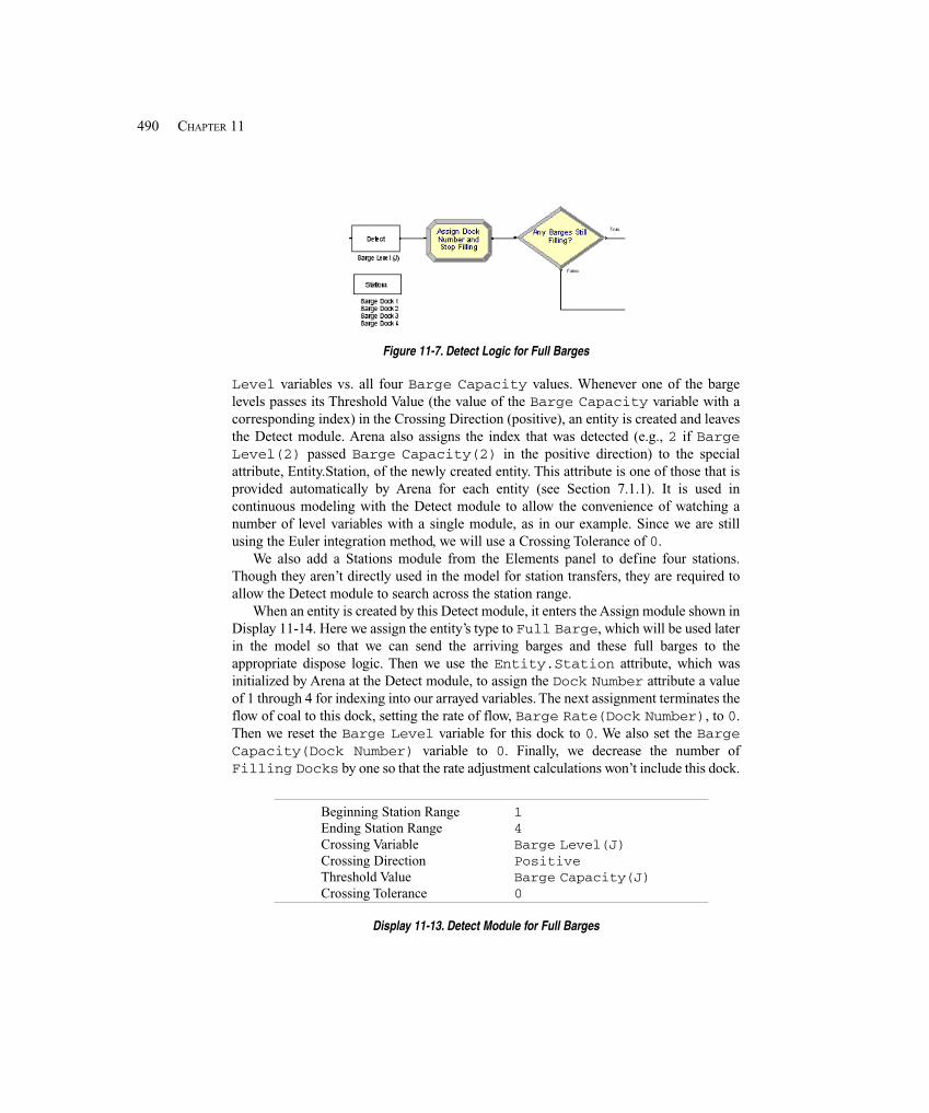
490 CHAPTER 11
Figure 11-7. Detect Logic for Full Barges
Level variables vs. all four Barge Capacity values. Whenever one of the bargelevels passes its Threshold Value (the value of the Barge Capacity variable with acorresponding index) in the Crossing Direction (positive), an entity is created and leavesthe Detect module. Arena also assigns the index that was detected (e.g., 2 if BargeLevel(2) passed Barge Capacity(2) in the positive direction) to the specialattribute, Entity.Station, of the newly created entity. This attribute is one of those that isprovided automatically by Arena for each entity (see Section 7.1.1). It is used incontinuous modeling with the Detect module to allow the convenience of watching anumber of level variables with a single module, as in our example. Since we are stillusing the Euler integration method, we will use a Crossing Tolerance of 0.
We also add a Stations module from the Elements panel to define four stations.Though they aren’t directly used in the model for station transfers, they are required toallow the Detect module to search across the station range.
When an entity is created by this Detect module, it enters the Assign module shown inDisplay 11-14. Here we assign the entity’s type to Full Barge, which will be used laterin the model so that we can send the arriving barges and these full barges to theappropriate dispose logic. Then we use the Entity.Station attribute, which wasinitialized by Arena at the Detect module, to assign the Dock Number attribute a valueof 1 through 4 for indexing into our arrayed variables. The next assignment terminates theflow of coal to this dock, setting the rate of flow, Barge Rate(Dock Number), to 0.Then we reset the Barge Level variable for this dock to 0. We also set the BargeCapacity(Dock Number) variable to 0. Finally, we decrease the number ofFilling Docks by one so that the rate adjustment calculations won’t include this dock.
Beginning Station Range 1Ending Station Range 4Crossing Variable Barge Level(J)Crossing Direction PositiveThreshold Value Barge Capacity(J)Crossing Tolerance 0
Display 11-13. Detect Module for Full Barges

491CONTINUOUS AND COMBINED DISCRETE/CONTINUOUS MODELS
Name Assign Dock Number and Stop Filling
AssignmentsType AttributeAttribute Name Entity.TypeNew Value Full Barge
AssignmentsType AttributeAttribute Name Dock NumberNew Value Entity.Station
AssignmentsType OtherOther Barge Rate(Dock Number)New Value 0
AssignmentsType OtherOther Barge Level(Dock Number)New Value 0
AssignmentsType OtherOther Barge Capacity(Dock Number)New Value 0
AssignmentsType VariableVariable Name Filling DocksNew Value Filling Docks - 1
Display 11-14. Assignments for Full Barge
At this point in the model, we have an entity that was created by the Detect modulebecause the filling operation finished at one of the docks. In the Assign module, westopped the flow of coal to that dock. Now, we need to adjust the flow to the other docks,if any are filling barges, to distribute the 2400 tons per hour evenly among them. First,we’ll use a Decide module, shown in Display 11-15, to check whether any docks arefilling barges.
Name Any Barges Still Filling?Type 2-way by ConditionIf VariableNamed Filling DocksIs >Value 0
Display 11-15. Decide Module Checking Whether Any Barges Are Filling
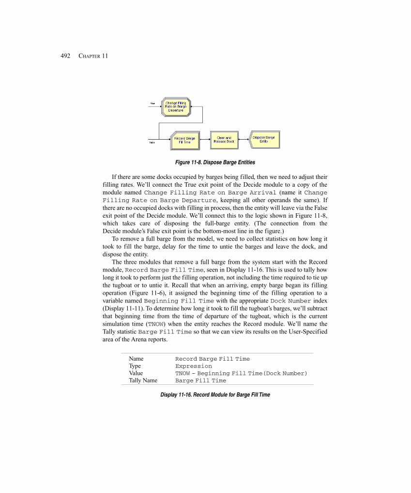
492 CHAPTER 11
Figure 11-8. Dispose Barge Entities
If there are some docks occupied by barges being filled, then we need to adjust theirfilling rates. We’ll connect the True exit point of the Decide module to a copy of themodule named Change Filling Rate on Barge Arrival (name it ChangeFilling Rate on Barge Departure, keeping all other operands the same). Ifthere are no occupied docks with filling in process, then the entity will leave via the Falseexit point of the Decide module. We’ll connect this to the logic shown in Figure 11-8,which takes care of disposing the full-barge entity. (The connection from theDecide module’s False exit point is the bottom-most line in the figure.)
To remove a full barge from the model, we need to collect statistics on how long ittook to fill the barge, delay for the time to untie the barges and leave the dock, anddispose the entity.
The three modules that remove a full barge from the system start with the Recordmodule, Record Barge Fill Time, seen in Display 11-16. This is used to tally howlong it took to perform just the filling operation, not including the time required to tie upthe tugboat or to untie it. Recall that when an arriving, empty barge began its fillingoperation (Figure 11-6), it assigned the beginning time of the filling operation to avariable named Beginning Fill Time with the appropriate Dock Number index(Display 11-11). To determine how long it took to fill the tugboat’s barges, we’ll subtractthat beginning time from the time of departure of the tugboat, which is the currentsimulation time (TNOW) when the entity reaches the Record module. We’ll name theTally statistic Barge Fill Time so that we can view its results on the User-Specifiedarea of the Arena reports.
Name Record Barge Fill TimeType ExpressionValue TNOW – Beginning Fill Time(Dock Number)Tally Name Barge Fill Time
Display 11-16. Record Module for Barge Fill Time
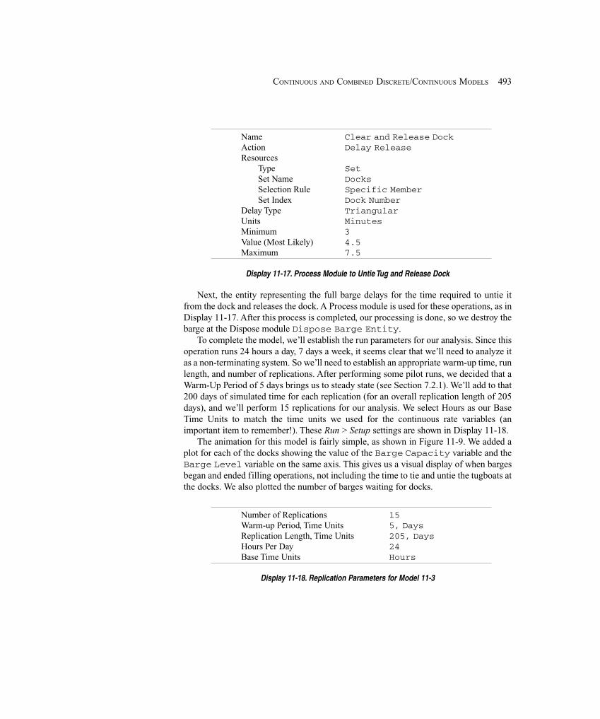
493CONTINUOUS AND COMBINED DISCRETE/CONTINUOUS MODELS
Name Clear and Release DockAction Delay ReleaseResources
Type SetSet Name DocksSelection Rule Specific MemberSet Index Dock Number
Delay Type TriangularUnits MinutesMinimum 3Value (Most Likely) 4.5Maximum 7.5
Display 11-17. Process Module to Untie Tug and Release Dock
Next, the entity representing the full barge delays for the time required to untie itfrom the dock and releases the dock. A Process module is used for these operations, as inDisplay 11-17. After this process is completed, our processing is done, so we destroy thebarge at the Dispose module Dispose Barge Entity.
To complete the model, we’ll establish the run parameters for our analysis. Since thisoperation runs 24 hours a day, 7 days a week, it seems clear that we’ll need to analyze itas a non-terminating system. So we’ll need to establish an appropriate warm-up time, runlength, and number of replications. After performing some pilot runs, we decided that aWarm-Up Period of 5 days brings us to steady state (see Section 7.2.1). We’ll add to that200 days of simulated time for each replication (for an overall replication length of 205days), and we’ll perform 15 replications for our analysis. We select Hours as our BaseTime Units to match the time units we used for the continuous rate variables (animportant item to remember!). These Run > Setup settings are shown in Display 11-18.
The animation for this model is fairly simple, as shown in Figure 11-9. We added aplot for each of the docks showing the value of the Barge Capacity variable and theBarge Level variable on the same axis. This gives us a visual display of when bargesbegan and ended filling operations, not including the time to tie and untie the tugboats atthe docks. We also plotted the number of barges waiting for docks.
Number of Replications 15Warm-up Period, Time Units 5, DaysReplication Length, Time Units 205, DaysHours Per Day 24Base Time Units Hours
Display 11-18. Replication Parameters for Model 11-3
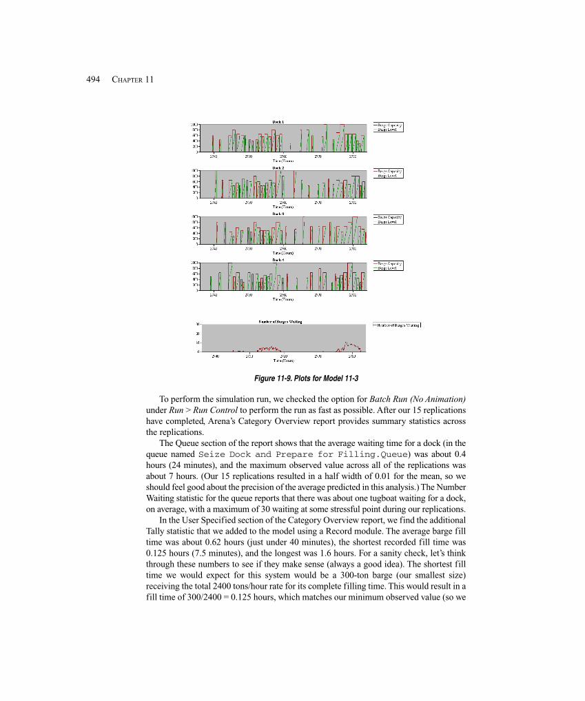
494 CHAPTER 11
Figure 11-9. Plots for Model 11-3
To perform the simulation run, we checked the option for Batch Run (No Animation)under Run > Run Control to perform the run as fast as possible. After our 15 replicationshave completed, Arena’s Category Overview report provides summary statistics acrossthe replications.
The Queue section of the report shows that the average waiting time for a dock (in thequeue named Seize Dock and Prepare for Filling.Queue) was about 0.4hours (24 minutes), and the maximum observed value across all of the replications wasabout 7 hours. (Our 15 replications resulted in a half width of 0.01 for the mean, so weshould feel good about the precision of the average predicted in this analysis.) The NumberWaiting statistic for the queue reports that there was about one tugboat waiting for a dock,on average, with a maximum of 30 waiting at some stressful point during our replications.
In the User Specified section of the Category Overview report, we find the additionalTally statistic that we added to the model using a Record module. The average barge filltime was about 0.62 hours (just under 40 minutes), the shortest recorded fill time was0.125 hours (7.5 minutes), and the longest was 1.6 hours. For a sanity check, let’s thinkthrough these numbers to see if they make sense (always a good idea). The shortest filltime we would expect for this system would be a 300-ton barge (our smallest size)receiving the total 2400 tons/hour rate for its complete filling time. This would result in afill time of 300/2400 = 0.125 hours, which matches our minimum observed value (so we
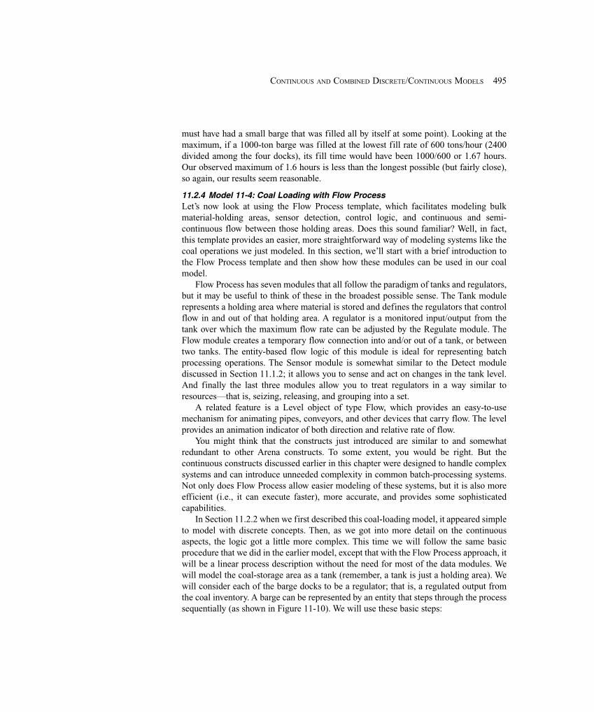
495CONTINUOUS AND COMBINED DISCRETE/CONTINUOUS MODELS
must have had a small barge that was filled all by itself at some point). Looking at themaximum, if a 1000-ton barge was filled at the lowest fill rate of 600 tons/hour (2400divided among the four docks), its fill time would have been 1000/600 or 1.67 hours.Our observed maximum of 1.6 hours is less than the longest possible (but fairly close),so again, our results seem reasonable.
11.2.4 Model 11-4: Coal Loading with Flow ProcessLet’s now look at using the Flow Process template, which facilitates modeling bulkmaterial-holding areas, sensor detection, control logic, and continuous and semi-continuous flow between those holding areas. Does this sound familiar? Well, in fact,this template provides an easier, more straightforward way of modeling systems like thecoal operations we just modeled. In this section, we’ll start with a brief introduction tothe Flow Process template and then show how these modules can be used in our coalmodel.
Flow Process has seven modules that all follow the paradigm of tanks and regulators,but it may be useful to think of these in the broadest possible sense. The Tank modulerepresents a holding area where material is stored and defines the regulators that controlflow in and out of that holding area. A regulator is a monitored input/output from thetank over which the maximum flow rate can be adjusted by the Regulate module. TheFlow module creates a temporary flow connection into and/or out of a tank, or betweentwo tanks. The entity-based flow logic of this module is ideal for representing batchprocessing operations. The Sensor module is somewhat similar to the Detect modulediscussed in Section 11.1.2; it allows you to sense and act on changes in the tank level.And finally the last three modules allow you to treat regulators in a way similar toresources—that is, seizing, releasing, and grouping into a set.
A related feature is a Level object of type Flow, which provides an easy-to-usemechanism for animating pipes, conveyors, and other devices that carry flow. The levelprovides an animation indicator of both direction and relative rate of flow.
You might think that the constructs just introduced are similar to and somewhatredundant to other Arena constructs. To some extent, you would be right. But thecontinuous constructs discussed earlier in this chapter were designed to handle complexsystems and can introduce unneeded complexity in common batch-processing systems.Not only does Flow Process allow easier modeling of these systems, but it is also moreefficient (i.e., it can execute faster), more accurate, and provides some sophisticatedcapabilities.
In Section 11.2.2 when we first described this coal-loading model, it appeared simpleto model with discrete concepts. Then, as we got into more detail on the continuousaspects, the logic got a little more complex. This time we will follow the same basicprocedure that we did in the earlier model, except that with the Flow Process approach, itwill be a linear process description without the need for most of the data modules. Wewill model the coal-storage area as a tank (remember, a tank is just a holding area). Wewill consider each of the barge docks to be a regulator; that is, a regulated output fromthe coal inventory. A barge can be represented by an entity that steps through the processsequentially (as shown in Figure 11-10). We will use these basic steps:
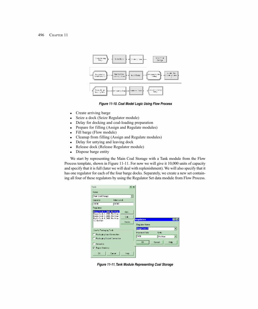
496 CHAPTER 11
Figure 11-10. Coal Model Logic Using Flow Process
� Create arriving barge� Seize a dock (Seize Regulator module)� Delay for docking and coal-loading preparation� Prepare for filling (Assign and Regulate modules)� Fill barge (Flow module)� Cleanup from filling (Assign and Regulate modules)� Delay for untying and leaving dock� Release dock (Release Regulator module)� Dispose barge entity
We start by representing the Main Coal Storage with a Tank module from the FlowProcess template, shown in Figure 11-11. For now we will give it 10,000 units of capacityand specify that it is full (later we will deal with replenishment). We will also specify that ithas one regulator for each of the four barge docks. Separately, we create a new set contain-ing all four of these regulators by using the Regulator Set data module from Flow Process.
Figure 11-11. Tank Module Representing Coal Storage
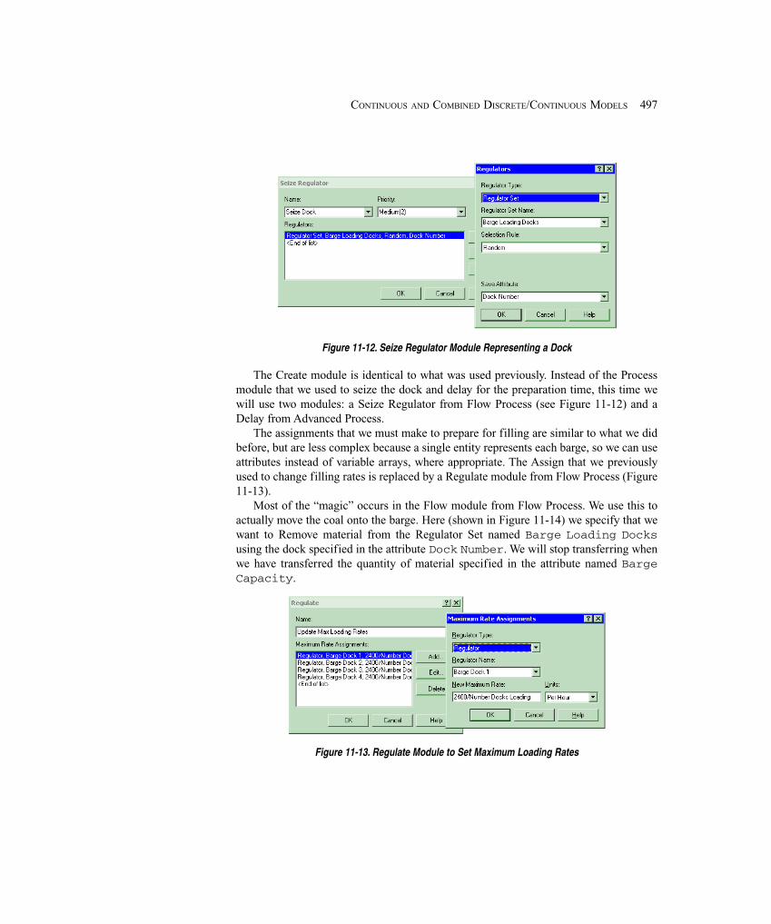
497CONTINUOUS AND COMBINED DISCRETE/CONTINUOUS MODELS
Figure 11-12. Seize Regulator Module Representing a Dock
The Create module is identical to what was used previously. Instead of the Processmodule that we used to seize the dock and delay for the preparation time, this time wewill use two modules: a Seize Regulator from Flow Process (see Figure 11-12) and aDelay from Advanced Process.
The assignments that we must make to prepare for filling are similar to what we didbefore, but are less complex because a single entity represents each barge, so we can useattributes instead of variable arrays, where appropriate. The Assign that we previouslyused to change filling rates is replaced by a Regulate module from Flow Process (Figure11-13).
Most of the “magic” occurs in the Flow module from Flow Process. We use this toactually move the coal onto the barge. Here (shown in Figure 11-14) we specify that wewant to Remove material from the Regulator Set named Barge Loading Docksusing the dock specified in the attribute Dock Number. We will stop transferring whenwe have transferred the quantity of material specified in the attribute named BargeCapacity.
Figure 11-13. Regulate Module to Set Maximum Loading Rates
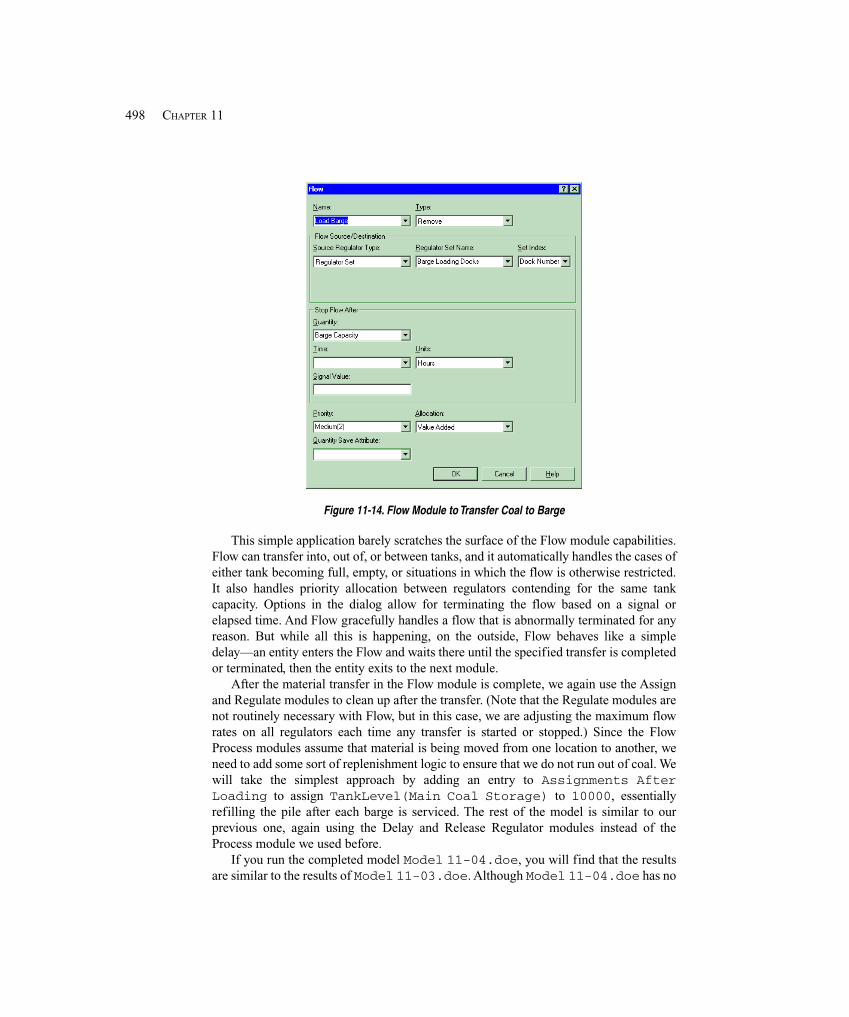
498 CHAPTER 11
Figure 11-14. Flow Module to Transfer Coal to Barge
This simple application barely scratches the surface of the Flow module capabilities.Flow can transfer into, out of, or between tanks, and it automatically handles the cases ofeither tank becoming full, empty, or situations in which the flow is otherwise restricted.It also handles priority allocation between regulators contending for the same tankcapacity. Options in the dialog allow for terminating the flow based on a signal orelapsed time. And Flow gracefully handles a flow that is abnormally terminated for anyreason. But while all this is happening, on the outside, Flow behaves like a simpledelay—an entity enters the Flow and waits there until the specified transfer is completedor terminated, then the entity exits to the next module.
After the material transfer in the Flow module is complete, we again use the Assignand Regulate modules to clean up after the transfer. (Note that the Regulate modules arenot routinely necessary with Flow, but in this case, we are adjusting the maximum flowrates on all regulators each time any transfer is started or stopped.) Since the FlowProcess modules assume that material is being moved from one location to another, weneed to add some sort of replenishment logic to ensure that we do not run out of coal. Wewill take the simplest approach by adding an entry to Assignments AfterLoading to assign TankLevel(Main Coal Storage) to 10000, essentiallyrefilling the pile after each barge is serviced. The rest of the model is similar to ourprevious one, again using the Delay and Release Regulator modules instead of theProcess module we used before.
If you run the completed model Model 11-04.doe, you will find that the resultsare similar to the results of Model 11-03.doe. Although Model 11-04.doe has no
499CONTINUOUS AND COMBINED DISCRETE/CONTINUOUS MODELS
animation, it has many good opportunities for animation. If you look in the Arena folderin the \Examples\FlowProcess subfolder, you will find a model named CoalLoading.doe. This is the same problem and approach discussed in Model11-04.doe, with some embellishments. The major change to the model (that willaffect the results) is that we no longer assume that the coal inventory is infinite. Instead,we have periodic deliveries by train to replenish the inventory. We also have a fixedmaximum inventory amount that can limit deliveries, and of course, if the pile everempties, it will limit shipments. Another change is that we model the barge movement inthe immediate vicinity. The rest of the changes are cosmetic, including animation of thetrains and barges, animation of coal transfers using flow levels, and some “fun”animation including passenger trains and an occasional water skier.
11.3 Continuous State-Change Systems
In Sections 11.1-11.3, we examined continuous processes in which the rate of change ofthe continuous variables (e.g., liquid in a tank, coal in a barge) was constant or changed atdiscrete points in time. Many physical systems fall into this category, particularly wheresome bulk or liquid product is being manufactured or transferred among containers.Arena is well equipped (and now, so are you) to analyze these processes accurately usingthe features we’ve presented thus far.
We’ll now turn our attention to slightly more complex continuous processes, wherethe rate values also change continuously over time. Many types of processes fall into thiscategory, particularly when physical activities involving temperature or chemicalreactions take place. Other cases, such as studies of large populations (e.g., for spread ofdisease), also call for the type of modeling approach we’ll discuss here.
To introduce you to the new concepts required to model these processes, we’ll use asimple example from the metals industry, where we need to model the temperature of afurnace and of the ingots being heated inside. We’ll examine the conceptual approachrequired to capture this process, and we’ll discuss the algorithms used by Arena tosimulate these types of systems. When you’ve mastered this material, you should bearmed with enough knowledge to identify the appropriate approach for simulatingcontinuous systems and to employ Arena to do the job successfully.
11.3.1 Model 11-5: A Soaking-Pit FurnaceThis system contains a soaking-pit furnace, where steel ingots are heated so they can berolled in the next stage of the process (Ashour and Bindingnavle, 1973). Ingots arrive tothis process approximately every 2.25 hours on average, following an exponentialdistribution for interarrival times. The furnace itself has space for at most nine ingots,which can be loaded and unloaded independently. If the furnace is full when a new ingotarrives, the ingot is held in a storage area until a space becomes available in the furnace.Each ingot is heated by the furnace to a temperature of 2200 degrees, then is removedand departs the system.
When an ingot is loaded into the furnace, its temperature is uniformly distributedbetween 300 and 500 degrees. Because it is cooler than the temperature of the furnace, itreduces the furnace temperature. For the purposes of our example, we’ll assume that this

500 CHAPTER 11
change takes place immediately and equals the difference between the furnacetemperature at the time the ingot is inserted and the ingot temperature, divided by thecurrent number of ingots in the furnace.
The heating process in the furnace causes the temperature to change by twice thedifference between 2600 and the current furnace temperature. The rate of change of aningot’s temperature while it’s in the furnace is 0.15 times the difference between thefurnace temperature and the ingot temperature.
For our study, we’d like to predict how many ingots are waiting to be loaded into thefurnace and the range of the furnace temperature as it varies with ingots being loaded andremoved.
11.3.2 Modeling Continuously Changing RatesTo model the furnace process, we’ll use many of the concepts and constructs that wereappropriate for capturing the coal-loading operation in Section 11.2. The elements thatchange continuously over time—the level variables for this model—are the furnacetemperature and the individual temperatures of the ingots in the furnace. We’ll defineone level for the overall furnace temperature and nine additional level variablesrepresenting the temperature of the ingots in the nine furnace positions (corresponding toits capacity of nine ingots). These levels are analogous to the level variables weestablished in the coal-loading operation to monitor the amount of coal loaded into atugboat’s barges.
Where things become interesting is when we look at the rates for this process—howthe temperature changes over time in the furnace and for heating the ingots. Previously,our rates held constant values over time, though we could introduce instantaneouschanges in the rates by assigning new values to them (for example, immediately dividingthe flow of coal differently among the four docks when a barge began or finished itsfilling operation). In the furnace system, though, the rate at which the furnace reheats toits target temperature of 2600 depends on its current temperature. Similarly, the rate atwhich an ingot is heated depends on both the temperature of the furnace and the ingottemperature. What complicates the determination of any of the rates or temperatures at apoint in time is that they’re all changing continuously over time.
Systems such as these are modeled using differential equations, which aremathematical equations that involve the derivative (rate of change) of one or morevariables. If we denote the value of some system variable (e.g., a temperature) as x, thenits derivative is denoted by dx/dt and defines its rate of change with respect to time.3 InArena, a level defines a system variable, x, and a rate defines its derivative, dx/dt. Whenwe can’t directly define a quantity’s value over time, we use this continuous-modelingapproach to calculate it indirectly via a differential equation.
The models that we’ve seen thus far in this chapter used simple differential equations,where the derivative (or rate) was a numerical value that changed only at discrete pointsin time (via model assignments). You might recall that when we added Continuous
3 Hopefully, this looks somewhat familiar from your extensive background in mathematics. If not, we’ll tryto keep things simple and will count on your initiative to find a good math text for a deeper explanation of howthis all works.
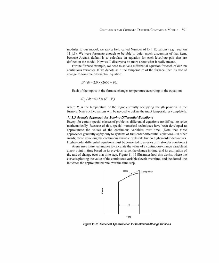
501CONTINUOUS AND COMBINED DISCRETE/CONTINUOUS MODELS
modules to our model, we saw a field called Number of Dif. Equations (e.g., Section11.1.1). We were fortunate enough to be able to defer much discussion of that item,because Arena’s default is to calculate an equation for each level/rate pair that aredefined in the model. Now we’ll discover a bit more about what it really means.
For the furnace example, we need to solve a differential equation for each of our tencontinuous variables. If we denote as F the temperature of the furnace, then its rate ofchange follows the differential equation:
dF / dt = 2.0 � (2600 � F).
Each of the ingots in the furnace changes temperature according to the equation:
dPj / dt = 0.15 � (F � P
j)
where Pj is the temperature of the ingot currently occupying the jth position in the
furnace. Nine such equations will be needed to define the ingot temperatures completely.
11.3.3 Arena’s Approach for Solving Differential EquationsExcept for certain special classes of problems, differential equations are difficult to solvemathematically. Because of this, special numerical techniques have been developed toapproximate the values of the continuous variables over time. (Note that theseapproaches generally apply only to systems of first-order differential equations—in otherwords, those involving the continuous variable or its rate but no higher-order derivatives.Higher-order differential equations must be converted to a series of first-order equations.)
Arena uses these techniques to calculate the value of a continuous-change variable ata new point in time based on its previous value, the change in time, and its estimation ofthe rate of change over that time step. Figure 11-15 illustrates how this works, where thecurve is plotting the value of the continuous variable (level) over time, and the dotted lineindicates the approximated rate over the time step.
Step error
Val
ue
Time
Rate }
t
Figure 11-15. Numerical Approximation for Continuous-Change Variables
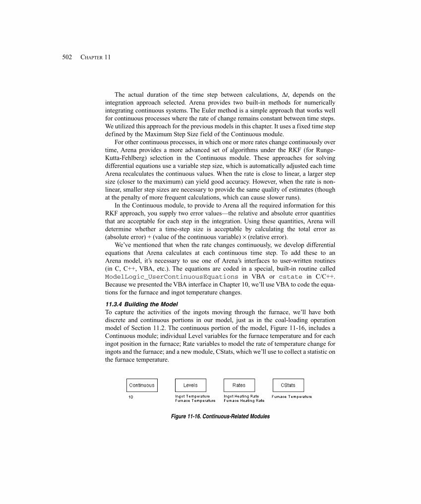
502 CHAPTER 11
The actual duration of the time step between calculations, Δt, depends on theintegration approach selected. Arena provides two built-in methods for numericallyintegrating continuous systems. The Euler method is a simple approach that works wellfor continuous processes where the rate of change remains constant between time steps.We utilized this approach for the previous models in this chapter. It uses a fixed time stepdefined by the Maximum Step Size field of the Continuous module.
For other continuous processes, in which one or more rates change continuously overtime, Arena provides a more advanced set of algorithms under the RKF (for Runge-Kutta-Fehlberg) selection in the Continuous module. These approaches for solvingdifferential equations use a variable step size, which is automatically adjusted each timeArena recalculates the continuous values. When the rate is close to linear, a larger stepsize (closer to the maximum) can yield good accuracy. However, when the rate is non-linear, smaller step sizes are necessary to provide the same quality of estimates (thoughat the penalty of more frequent calculations, which can cause slower runs).
In the Continuous module, to provide to Arena all the required information for thisRKF approach, you supply two error values—the relative and absolute error quantitiesthat are acceptable for each step in the integration. Using these quantities, Arena willdetermine whether a time-step size is acceptable by calculating the total error as(absolute error) + (value of the continuous variable) � (relative error).
We’ve mentioned that when the rate changes continuously, we develop differentialequations that Arena calculates at each continuous time step. To add these to anArena model, it’s necessary to use one of Arena’s interfaces to user-written routines(in C, C++, VBA, etc.). The equations are coded in a special, built-in routine calledModelLogic_UserContinuousEquations in VBA or cstate in C/C++.Because we presented the VBA interface in Chapter 10, we’ll use VBA to code the equa-tions for the furnace and ingot temperature changes.
11.3.4 Building the ModelTo capture the activities of the ingots moving through the furnace, we’ll have bothdiscrete and continuous portions in our model, just as in the coal-loading operationmodel of Section 11.2. The continuous portion of the model, Figure 11-16, includes aContinuous module; individual Level variables for the furnace temperature and for eachingot position in the furnace; Rate variables to model the rate of temperature change foringots and the furnace; and a new module, CStats, which we’ll use to collect a statistic onthe furnace temperature.
Figure 11-16. Continuous-Related Modules
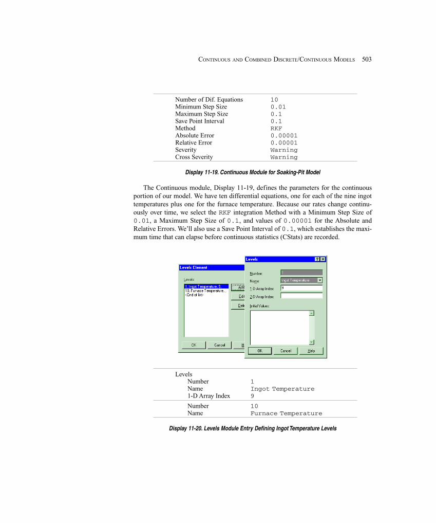
503CONTINUOUS AND COMBINED DISCRETE/CONTINUOUS MODELS
Number of Dif. Equations 10Minimum Step Size 0.01Maximum Step Size 0.1Save Point Interval 0.1Method RKFAbsolute Error 0.00001Relative Error 0.00001Severity WarningCross Severity Warning
Display 11-19. Continuous Module for Soaking-Pit Model
The Continuous module, Display 11-19, defines the parameters for the continuousportion of our model. We have ten differential equations, one for each of the nine ingottemperatures plus one for the furnace temperature. Because our rates change continu-ously over time, we select the RKF integration Method with a Minimum Step Size of0.01, a Maximum Step Size of 0.1, and values of 0.00001 for the Absolute andRelative Errors. We’ll also use a Save Point Interval of 0.1, which establishes the maxi-mum time that can elapse before continuous statistics (CStats) are recorded.
LevelsNumber 1Name Ingot Temperature1-D Array Index 9
Number 10Name Furnace Temperature
Display 11-20. Levels Module Entry Defining Ingot Temperature Levels
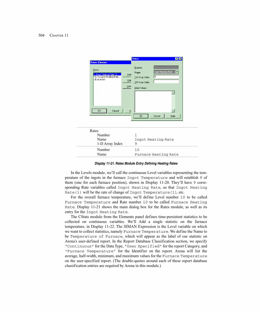
504 CHAPTER 11
RatesNumber 1Name Ingot Heating Rate1-D Array Index 9
Number 10Name Furnace Heating Rate
Display 11-21. Rates Module Entry Defining Heating Rates
In the Levels module, we’ll call the continuous Level variables representing the tem-perature of the ingots in the furnace Ingot Temperature and will establish 9 ofthem (one for each furnace position), shown in Display 11-20. They’ll have 9 corre-sponding Rate variables called Ingot Heating Rate, so that Ingot HeatingRate(1) will be the rate of change of Ingot Temperature(1), etc.
For the overall furnace temperature, we’ll define Level number 10 to be calledFurnace Temperature and Rate number 10 to be called Furnace HeatingRate. Display 11-21 shows the main dialog box for the Rates module, as well as itsentry for the Ingot Heating Rate.
The CStats module from the Elements panel defines time-persistent statistics to becollected on continuous variables. We’ll Add a single statistic on the furnacetemperature, in Display 11-22. The SIMAN Expression is the Level variable on whichwe want to collect statistics, namely Furnace Temperature. We define the Name tobe Temperature of Furnace, which will appear as the label of our statistic onArena’s user-defined report. In the Report Database Classification section, we specify“Continuous” for the Data Type, “User Specified” for the report Category, and“Furnace Temperature” for the Identifier on the report. Arena will list theaverage, half-width, minimum, and maximum values for the Furnace Temperatureon the user-specified report. (The double-quotes around each of these report databaseclassification entries are required by Arena in this module.)
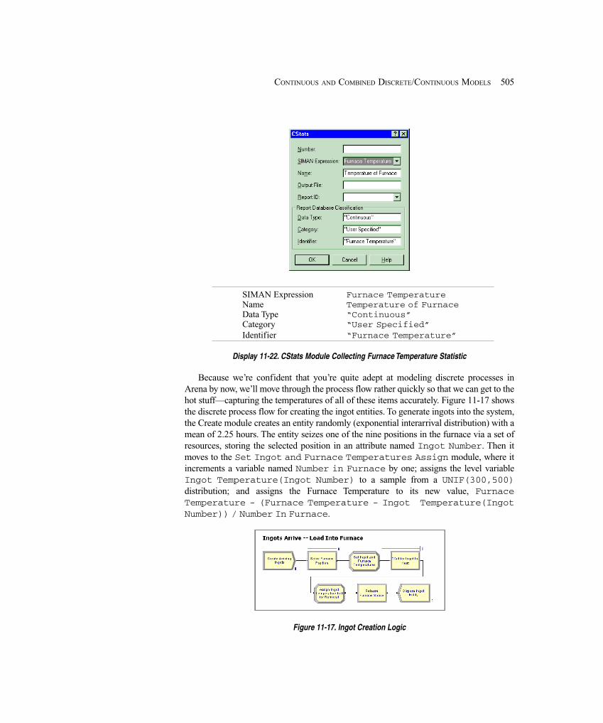
505CONTINUOUS AND COMBINED DISCRETE/CONTINUOUS MODELS
SIMAN Expression Furnace TemperatureName Temperature of FurnaceData Type “Continuous”Category “User Specified”Identifier “Furnace Temperature”
Display 11-22. CStats Module Collecting Furnace Temperature Statistic
Because we’re confident that you’re quite adept at modeling discrete processes inArena by now, we’ll move through the process flow rather quickly so that we can get to thehot stuff—capturing the temperatures of all of these items accurately. Figure 11-17 showsthe discrete process flow for creating the ingot entities. To generate ingots into the system,the Create module creates an entity randomly (exponential interarrival distribution) with amean of 2.25 hours. The entity seizes one of the nine positions in the furnace via a set ofresources, storing the selected position in an attribute named Ingot Number. Then itmoves to the Set Ingot and Furnace Temperatures Assign module, where itincrements a variable named Number in Furnace by one; assigns the level variableIngot Temperature(Ingot Number) to a sample from a UNIF(300,500)distribution; and assigns the Furnace Temperature to its new value, FurnaceTemperature - (Furnace Temperature - Ingot Temperature(IngotNumber)) / Number In Furnace.
Figure 11-17. Ingot Creation Logic
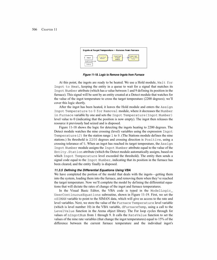
506 CHAPTER 11
Figure 11-18. Logic to Remove Ingots from Furnace
At this point, the ingots are ready to be heated. We use a Hold module, Wait forIngot to Heat, keeping the entity in a queue to wait for a signal that matches itsIngot Number attribute (which has a value between 1 and 9 defining its position in thefurnace). This signal will be sent by an entity created at a Detect module that watches forthe value of the ingot temperature to cross the target temperature (2200 degrees); we’llcover this logic shortly.
After the ingot has been heated, it leaves the Hold module and enters the AssignIngot Temperature to 0 for Removal module, where it decreases the Numberin Furnace variable by one and sets the Ingot Temperature(Ingot Number)level value to 0 (indicating that the position is now empty). The ingot then releases theresource it previously had seized and is disposed.
Figure 11-18 shows the logic for detecting the ingots heating to 2200 degrees. TheDetect module watches the nine crossing (level) variables using the expression IngotTemperature(J) for the station range 1 to 9. (The Stations module defines the ninestations.) Its threshold is 2200 degrees and crossing direction is Positive, using acrossing tolerance of 5. When an ingot has reached its target temperature, the AssignIngot Number module assigns the Ingot Number attribute equal to the value of theEntity.Station attribute (which the Detect module automatically assigns, based onwhich Ingot Temperature level exceeded the threshold). The entity then sends asignal code equal to the Ingot Number, indicating that its position in the furnace hasbeen cleared, and the entity finally is disposed.
11.3.5 Defining the Differential Equations Using VBAWe have completed the portion of the model that deals with the ingots—getting theminto the system, loading them into the furnace, and removing them when they’ve reachedthe target temperature. Now we’ll complete the model by defining the differential equa-tions that will dictate the rates of change of the ingot and furnace temperatures.
In the Visual Basic Editor, the VBA code is typed in the ModelLogic_UserContinuousEquations subroutine, shown in Figure 11-19. First, we set theoSIMAN variable to point to the SIMAN data, which will give us access to the rate andlevel variables. Next, we store the value of the Furnace Temperature level variable(which is level number 10) in the VBA variable, dFurnaceTemp, using a call to theLevelValue function in the Arena object library. The For loop cycles through forvalues of nIngotNum from 1 through 9. It calls the RateValue function to set thevalues of the nine rate variables (that change the ingot temperatures) equal to 15% of thedifference between the current furnace temperature and the individual ingot’s
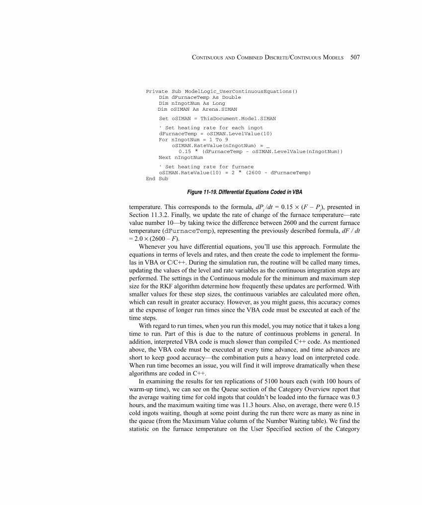
507CONTINUOUS AND COMBINED DISCRETE/CONTINUOUS MODELS
Private Sub ModelLogic_UserContinuousEquations() Dim dFurnaceTemp As Double Dim nIngotNum As Long
Dim oSIMAN As Arena.SIMAN
Set oSIMAN = ThisDocument.Model.SIMAN
' Set heating rate for each ingot dFurnaceTemp = oSIMAN.LevelValue(10) For nIngotNum = 1 To 9 oSIMAN.RateValue(nIngotNum) = _ 0.15 * (dFurnaceTemp - oSIMAN.LevelValue(nIngotNum)) Next nIngotNum
' Set heating rate for furnace oSIMAN.RateValue(10) = 2 * (2600 - dFurnaceTemp)End Sub
Figure 11-19. Differential Equations Coded in VBA
temperature. This corresponds to the formula, dPj /dt = 0.15 × (F – P
j), presented in
Section 11.3.2. Finally, we update the rate of change of the furnace temperature—ratevalue number 10—by taking twice the difference between 2600 and the current furnacetemperature (dFurnaceTemp), representing the previously described formula, dF / dt= 2.0 × (2600 – F).
Whenever you have differential equations, you’ll use this approach. Formulate theequations in terms of levels and rates, and then create the code to implement the formu-las in VBA or C/C++. During the simulation run, the routine will be called many times,updating the values of the level and rate variables as the continuous integration steps areperformed. The settings in the Continuous module for the minimum and maximum stepsize for the RKF algorithm determine how frequently these updates are performed. Withsmaller values for these step sizes, the continuous variables are calculated more often,which can result in greater accuracy. However, as you might guess, this accuracy comesat the expense of longer run times since the VBA code must be executed at each of thetime steps.
With regard to run times, when you run this model, you may notice that it takes a longtime to run. Part of this is due to the nature of continuous problems in general. Inaddition, interpreted VBA code is much slower than compiled C++ code. As mentionedabove, the VBA code must be executed at every time advance, and time advances areshort to keep good accuracy—the combination puts a heavy load on interpreted code.When run time becomes an issue, you will find it will improve dramatically when thesealgorithms are coded in C++.
In examining the results for ten replications of 5100 hours each (with 100 hours ofwarm-up time), we can see on the Queue section of the Category Overview report thatthe average waiting time for cold ingots that couldn’t be loaded into the furnace was 0.3hours, and the maximum waiting time was 11.3 hours. Also, on average, there were 0.15cold ingots waiting, though at some point during the run there were as many as nine inthe queue (from the Maximum Value column of the Number Waiting table). We find thestatistic on the furnace temperature on the User Specified section of the Category
508 CHAPTER 11
Overview report. There, the Continuous table lists our CStat information, which showsthat the average furnace temperature was 2514 degrees, the minimum was 301 degrees,and the maximum was 2600 degrees.
11.4 Summary and Forecast
Chapter 11 concludes the modeling topics of this book. In it, we examined Arena’sframework for modeling continuous-change systems. We also put together the discretemodeling concepts of our earlier chapters with continuous modeling, illustrating howthese concepts are applied together in two examples. Further, we built a model based onFlow Process constructs that blend these constructs.
When you are preparing to analyze a system in which fluids or other bulk materialsare being produced or handled, the continuous-modeling and Flow Process approachesshould be considered. Some systems may be modeled using both continuous and discreteconcepts, due to the nature of the material being modeled. Arena’s structure is designedto model any combination of discrete and continuous processes, using Flow Processmodules or the Detect module and assignments of continuous rate and level variablesillustrated in this chapter.
The remaining two chapters are not directly about modeling, but discuss importanttopics that are critical for performing good simulation studies. Chapter 12 rounds out ourtreatment of the probabilistic underpinnings and statistical issues in simulation, whichwe began in Section 2.6, Section 4.6, Chapter 6, and Section 7.2. Then in Chapter 13,we’ll provide you with some sage observations and advice about how to conduct simula-tion studies, including modeling, design, analysis, and (gasp!) dealing with people.
11.5 Exercises
11-1 Build a discrete-event model that changes the value of the volume in a tank asdescribed for Model 11-2b using a maximum step size of 0.01 minutes. Record time-persistent statistics on the volume in the tank, and compare the average reported volumefor an 800-hour run with the results from the continuous model (11-2b). Also comparethe computing time required to perform the simulation run for the discrete case vs. thecontinuous approach. (Note: For this comparison, clear the Update Simulation TimeEvery option in Run > Setup > Run Speed from Model 11-2b, and run both models inbatch mode. To show computing time, select SIMAN Summary Report under Run >Setup > Reports.)
11-2 The owner of a franchise of gas stations is interested in determining how large thestorage tank should be at a new station. Four gas pumps, all dispensing the same grade offuel, will be installed to service customers. Cars arrive according to an exponentialdistribution with a mean of 0.8 minute. (We’ll assume that this is uniform throughout thestation’s hours of operation.) Their time at the pump (from start to finish) follows atriangular distribution with parameters 2, 2.8, and 4 minutes. The cars require varyingamounts of fuel, distributed according to a triangular distribution with parameters 4, 7.5,and 15 gallons.
509CONTINUOUS AND COMBINED DISCRETE/CONTINUOUS MODELS
Refill trucks arrive according to a uniform distribution with a minimum interarrivaltime of 6.75 hours and a maximum of 8.25 hours. They carry enough fuel to refill thestorage tank and do so at a rate of 300 gallons per minute.
If the storage tank empties before a refill truck arrives, the pumps are closed until thestorage tank contains 100 gallons (from its next refill). For purposes of this analysis,assume that cars that are in-process when the tank empties can complete their service andthat waiting cars will stay at the station until the pumps reopen. However, any cars thatarrive while the pumps are closed will drive by to find another place to fill up.
Determine (to the nearest 100 gallons) the tank capacity that will result in fewer than0.1% of cars balking due to closed pumps.
11-3 An earnest analyst for Grace Enterprises, the owner of the coal-loading operationdescribed in Model 11-3, has become concerned that assuming that coal will always beavailable to load into the barges might not be realistic. She would like to refine theestimates of loading times and numbers of waiting barges by incorporating into hermodel the delivery of coal by train to the storage yard.
Trains are scheduled to arrive every eight hours throughout the day and night, andthey’re usually on time. Each train carries 12,000 tons of coal, which is unloaded into thestorage yard at a rate of 7,500 tons per hour. The storage yard can hold 17,000 tons ofcoal; for purposes of this analysis, cancel a train’s delivery if the yard is full at the train’sscheduled arrival time.
Modify Model 11-3 to incorporate the availability of coal in the storage yard so thatbarges will wait at the dock until coal is available for loading. Compare the average andmaximum number of barges waiting and the loading time of barges with the results fromModel 11-3.
11-4 O’Hare Candy Company, maker of tasty sweets, is preparing to install a newlicorice production facility and needs to determine the rates at which equipment shouldrun. In particular, they are interested in the cutting/wrapping machines, as they are proneto frequent breakdowns.
At this facility, there are three identical parallel lines fed by a single kitchenproducing continuous strands of licorice. Each line is fed licorice at a rate of 1374 kg/hour and has its own dedicated cut/wrap machine (modeled as a single process). Thewrappers cut the licorice into individual pieces and wrap them at a rate of 1500 kg/hour.These machines experience breakdowns of various forms. Analysis of breakdown datafrom similar equipment has concluded that the frequency is approximately onebreakdown per hour with a high degree of variability that can best be represented by anexponential distribution. The time to repair a breakdown varies quite a bit as well; it canbe modeled by a triangular distribution with parameters 3.75, 4.5, and 8.25 minutes.
It is very costly to shut down the kitchen, so surge tables will be located in front ofeach machine. The current design calls for a surge table capacity of 1000 kg. If theamount of product exceeds this capacity, then the rate at which the kitchen is feedingproduct to that machine is reduced to 900 kg/hour until less than 700 kg of licorice is onthe table.
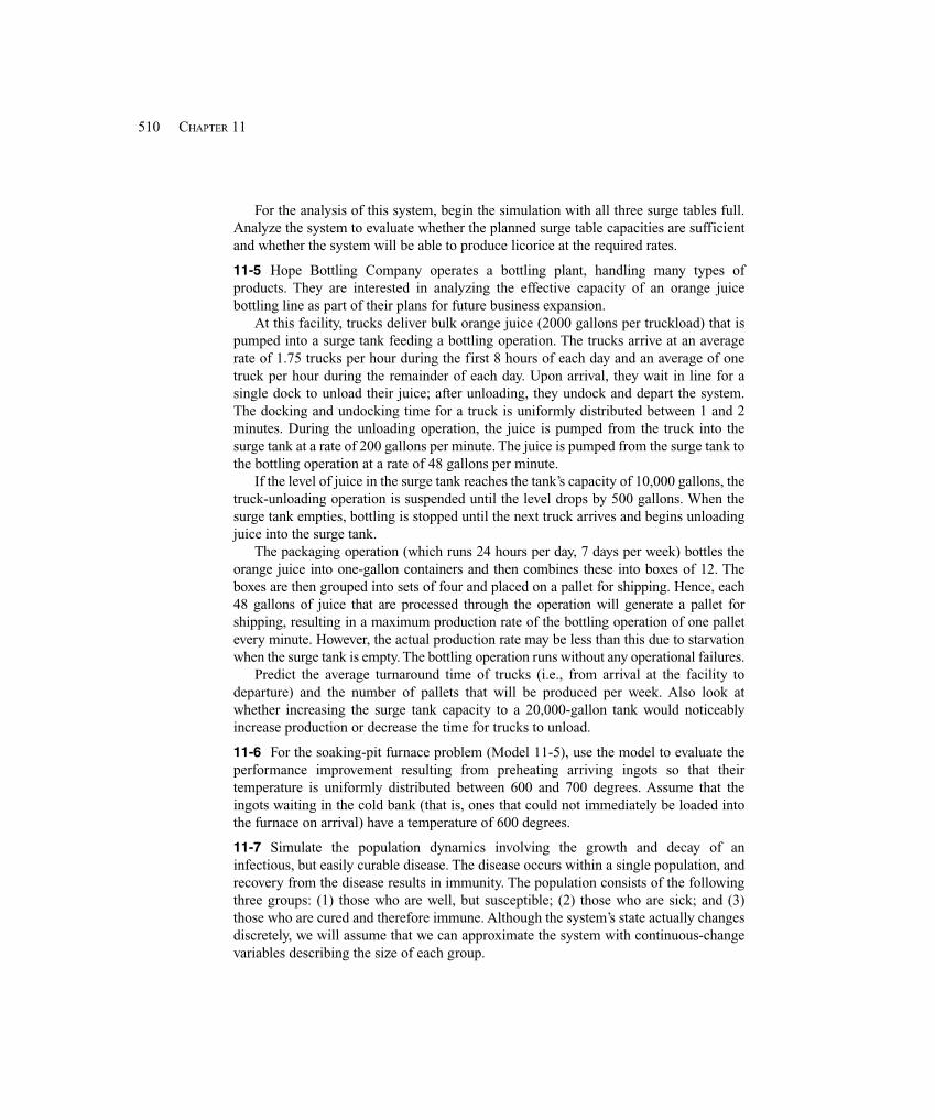
510 CHAPTER 11
For the analysis of this system, begin the simulation with all three surge tables full.Analyze the system to evaluate whether the planned surge table capacities are sufficientand whether the system will be able to produce licorice at the required rates.
11-5 Hope Bottling Company operates a bottling plant, handling many types ofproducts. They are interested in analyzing the effective capacity of an orange juicebottling line as part of their plans for future business expansion.
At this facility, trucks deliver bulk orange juice (2000 gallons per truckload) that ispumped into a surge tank feeding a bottling operation. The trucks arrive at an averagerate of 1.75 trucks per hour during the first 8 hours of each day and an average of onetruck per hour during the remainder of each day. Upon arrival, they wait in line for asingle dock to unload their juice; after unloading, they undock and depart the system.The docking and undocking time for a truck is uniformly distributed between 1 and 2minutes. During the unloading operation, the juice is pumped from the truck into thesurge tank at a rate of 200 gallons per minute. The juice is pumped from the surge tank tothe bottling operation at a rate of 48 gallons per minute.
If the level of juice in the surge tank reaches the tank’s capacity of 10,000 gallons, thetruck-unloading operation is suspended until the level drops by 500 gallons. When thesurge tank empties, bottling is stopped until the next truck arrives and begins unloadingjuice into the surge tank.
The packaging operation (which runs 24 hours per day, 7 days per week) bottles theorange juice into one-gallon containers and then combines these into boxes of 12. Theboxes are then grouped into sets of four and placed on a pallet for shipping. Hence, each48 gallons of juice that are processed through the operation will generate a pallet forshipping, resulting in a maximum production rate of the bottling operation of one palletevery minute. However, the actual production rate may be less than this due to starvationwhen the surge tank is empty. The bottling operation runs without any operational failures.
Predict the average turnaround time of trucks (i.e., from arrival at the facility todeparture) and the number of pallets that will be produced per week. Also look atwhether increasing the surge tank capacity to a 20,000-gallon tank would noticeablyincrease production or decrease the time for trucks to unload.
11-6 For the soaking-pit furnace problem (Model 11-5), use the model to evaluate theperformance improvement resulting from preheating arriving ingots so that theirtemperature is uniformly distributed between 600 and 700 degrees. Assume that theingots waiting in the cold bank (that is, ones that could not immediately be loaded intothe furnace on arrival) have a temperature of 600 degrees.
11-7 Simulate the population dynamics involving the growth and decay of aninfectious, but easily curable disease. The disease occurs within a single population, andrecovery from the disease results in immunity. The population consists of the followingthree groups: (1) those who are well, but susceptible; (2) those who are sick; and (3)those who are cured and therefore immune. Although the system’s state actually changesdiscretely, we will assume that we can approximate the system with continuous-changevariables describing the size of each group.
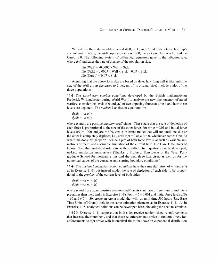
511CONTINUOUS AND COMBINED DISCRETE/CONTINUOUS MODELS
We will use the state variables named Well, Sick, and Cured to denote each group’scurrent size. Initially, the Well population size is 1000, the Sick population is 10, and theCured is 0. The following system of differential equations governs the infection rate,where d/dt indicates the rate of change of the population size.
d/dt (Well) = -0.0005 � Well � Sickd/dt (Sick) = 0.0005 � Well � Sick – 0.07 � Sickd/dt (Cured) = 0.07 � Sick
Assuming that the above formulas are based on days, how long will it take until thesize of the Well group decreases to 2 percent of its original size? Include a plot of thethree populations.
11-8 The Lanchester combat equations, developed by the British mathematicianFrederick W. Lanchester during World War I to analyze the new phenomenon of aerialwarfare, consider the levels x(t) and y(t) of two opposing forces at time t, and how theselevels are depleted. The modern Lanchester equations are
dx/dt = −a y(t)dy/dt = −b x(t)
where a and b are positive attrition coefficients. These state that the rate of depletion ofeach force is proportional to the size of the other force. For a = b = 0.01 and initial forcelevels x(0) = 1000 and y(0) = 500, create an Arena model that will run until one side orthe other is completely depleted, i.e., until x(t) = 0 or y(t) = 0, whichever comes first. Atwhat time does this happen? Include a plot of both force levels, as well as Variable ani-mations of them, and a Variable animation of the current time. Use Base Time Units ofHours. Note that analytical solutions to these differential equations can be developed,making simulation unnecessary. (Thanks to Professor Tom Lucas of the Naval Post-graduate School for motivating this and the next three Exercises, as well as for thenumerical values of the constants and starting boundary conditions.)
11-9 The ancient Lanchester combat equations have the same definition of x(t) and y(t)as in Exercise 11-8, but instead model the rate of depletion of each side to be propor-tional to the product of the current level of both sides:
dx/dt = −a x(t) y(t)dy/dt = −b x(t) y(t)
where a and b are again positive attrition coefficients (but have different units and inter-pretations than the a and b in Exercise 11-8). For a = b = 0.001 and initial force levels x(0)= 60 and y(0) = 30, create an Arena model that will run until time 500 hours (Use BaseTime Units of Hours.) Include the same animation elements as in Exercise 11-8. As inExercise 11-8, analytical solutions can be developed here, obviating the need to simulate.
11-10 In Exercise 11-8, suppose that both sides receive random-sized re-enforcementsthat increase their numbers, and that these re-enforcements arrive at random times. Re-enforcements to x(t) arrive with interarrival times that have an exponential distribution

512 CHAPTER 11
with mean 8 hours, and the first re-enforcement arrives not at time zero, but after one ofthese interarrival times. The size of the re-enforcement to x(t) has a Poisson distributionwith mean 20. Similarly, y(t) is re-enforced at interarrival times exponentially distributedwith mean 4 hours (the first re-enforcement arrives after one of these interarrival timespast time zero), and with re-enforcement sizes distributed as Poisson random with mean30. Run the model until one side or the other is completely depleted, with the same ani-mation elements as in Exercise 11-8. Do ten replications and make entries in the Statisticdata module that will produce an estimate of the probability that x wins (i.e., y(t) is de-pleted to zero first), the expected duration of the fight, and the expected final value ofx(t) − y(t), which could be positive or negative. Depending on the probability distribu-tions involved, this model does require simulation, since no analytical solution is avail-able, unlike in Exercise 11-8.
11-11Modify your ancient Lanchester model in Exercise 11-9 so that both sides receivere-enforcements as described in Exercise 11-10. The parameters of the re-enforcements,however, are different here: the mean times between x and y re-enforcements are respec-tively 5 and 4 hours, and the mean sizes of the re-enforcements to both sides is 5. As inExercise 11-10, do ten replications and make entries in the Statistic data module that willproduce an estimate of the probability that x wins (defined here as x(500) > y(500)) andthe expected final value of x(t) − y(t), which could be positive or negative. Depending onthe probability distributions involved, this model does require simulation, since no ana-lytical solution is available, unlike in Exercise 11-9.
513FURTHER STATISTICAL ISSUES
CHAPTER 12
Further Statistical Issues
One of the points we’ve tried to make consistently in this book is that a good simulationstudy involves more than building a good model (though good models are certainlyimportant too). In a simulation with stochastic (random) input, you’re going to getrandom output as well. Thus, it’s critical to understand how simulations generate thisrandomness in the input and what you can do about the resulting randomness in theoutput. We’ve already blended some of these statistical issues in with our tour throughmodel building and analysis, specifically in Section 2.6, Section 4.6, Chapter 6, andSection 7.2. Part of the point of those sections is that Arena can help you deal with theseissues, but you must be aware that they exist.
This chapter discusses additional statistical issues related to both the input and outputsides of a simulation. Random-number generators, the source of all randomness insimulations, are discussed in Section 12.1. Then in Section 12.2, we’ll talk about how togenerate observations on whatever input distributions you decided to use as part of yourmodeling. Section 12.3 discusses specifying and generating from a particular, yetimportant type of random input, a nonstationary Poisson process (which, by the way, wasintroduced in Model 5-2). Ways to reduce output variance (other than just simulatingsome more) are described in Section 12.4. The idea of sequential sampling—that is,deciding on the fly how much simulation-generated data you need—is the subject ofSection 12.5. The chapter concludes in Section 12.6 with brief mention of the possibilityof using experimental design in simulation. By the time you reach the end of this chapter,you should have a thorough understanding of statistical issues in simulation and knowhow Arena can help you deal with them.
Obviously, this chapter is a heavy user of foundational material in probability andstatistics. We’ve provided a refresher on these subjects in Appendix B of the book, whichyou might want to look at before going on. In addition, Appendix C contains a listing ofall the probability distributions supported by Arena.
12.1 Random-Number Generation
Hidden deep down in the engine room of any stochastic simulation is a random-numbergenerator (RNG) quietly churning away. The sole purpose of such a machine is toproduce a flow of numbers that are observations (also known as draws, samples, orrealizations) from a continuous uniform distribution between 0 and 1 (see Appendix C)and are independent of each other. In simulation, these are called random numbers. Thisis certainly not the only probability distribution from which you’ll want to drawobservations to drive your simulations (see Section 4.6), but as we’ll discuss in Sections12.2 and 12.3, generating observations from all other distributions and random processesstarts with random numbers.
514 CHAPTER 12
Any method for generating random numbers on a computer is just some kind ofrecursive algorithm that can repeat the same sequence of “random” numbers again andagain. For this reason, these are often called pseudorandom-number generators. Somepeople have worried philosophically that such methods are fundamentally flawed sincepart of what it means to be random is to be unpredictable. This might make for aninteresting after-dinner debate, but at a practical level, the issue is really not veryimportant. Modern and carefully constructed RNGs generally succeed at producing aflow of numbers that appear to be truly random, passing various statistical tests for bothuniformity and independence, as well as satisfying theoretically derived criteria for being“good.” Also, it’s quite helpful in simulation to be able to regenerate a specific sequenceof random numbers; this is an obvious aid in debugging (not to mention gradinghomework), but is also useful statistically, as we’ll describe in Section 12.4.
Unfortunately, there seems to be a common perception that any seeminglynonsensical method will, just because it looks weird, generate “random” numbers.Indeed, some extremely poor methods have been provided and used, possibly resulting ininvalid simulation results. Designing and implementing RNGs is actually quite subtle,and there has been a lot of research on these topics. In part because computers havebecome so fast, there continues to be work on developing new and better RNGs that cansatisfy the voracious appetite that modern simulations can have for random numbers.
So exactly how do RNGs work? Historically, the most common form (and the typestill built into a lot of simulation software, but not Arena . . . more on this issue below) iscalled a linear congruential generator (LCG). An LCG generates a sequence Z1, Z2, Z3,. . .of integers via the recursion
Zi = (aZ
i–1 + c) mod m
where m, a, and c are constants for the generator that must be chosen carefully, based onboth theoretical and empirical grounds, to produce a good flow of random numbers. The“mod m” operation means to divide by m and then return the remainder of this divisionto the left-hand-side as the next Z
i (for instance, 422 mod 63 is 44). As with any recur-
sion, an LCG must be initialized, so there is also a seed Z0 specified for the generator.This sequence of Z
i’s will be composed of integers, which is certainly not what we want
for a continuous distribution between 0 and 1. However, since the Zi’s are remainders of
division of other integers by m, they’ll all be between 0 and m – 1, so the final step is todefine U
i = Z
i/m, which will be between 0 and 1. The sequence U1, U2, U3,. . .are the
(pseudo-)random numbers returned for use in the simulation.As a tiny example (nobody should ever actually use this generator), take m = 63,
a = 22, c = 4, and Z0 = 19. The recursion generating the Z
i’s is thus Z
i = (22 Z
i–1 + 4) mod
63. Table 12-1 traces this generator through the first 70 generated random numbers, andyou can check some of the arithmetic. (We used a spreadsheet to generate this table.) Atfirst blush, scanning down through the U
i column gives the impression that these look
like pretty good random numbers—they’re certainly all between 0 and 1 (as they’reguaranteed to be by construction), they appear to be spread fairly uniformly over theinterval [0, 1], and they are evidently pretty well mixed up (independent). The sample
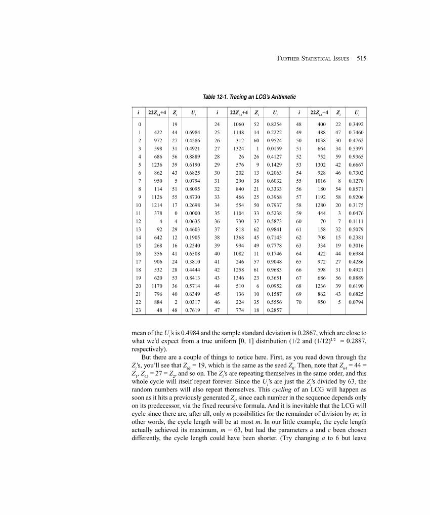
515FURTHER STATISTICAL ISSUES
Table 12-1. Tracing an LCG’s Arithmetic
i 22Zi-1
+4 Zi
Ui
i 22Zi-1
+4 Zi
Ui
i 22Zi-1
+4 Zi
Ui
0 19 24 1060 52 0.8254 48 400 22 0.3492
1 422 44 0.6984 25 1148 14 0.2222 49 488 47 0.7460
2 972 27 0.4286 26 312 60 0.9524 50 1038 30 0.4762
3 598 31 0.4921 27 1324 1 0.0159 51 664 34 0.5397
4 686 56 0.8889 28 26 26 0.4127 52 752 59 0.9365
5 1236 39 0.6190 29 576 9 0.1429 53 1302 42 0.6667
6 862 43 0.6825 30 202 13 0.2063 54 928 46 0.7302
7 950 5 0.0794 31 290 38 0.6032 55 1016 8 0.1270
8 114 51 0.8095 32 840 21 0.3333 56 180 54 0.8571
9 1126 55 0.8730 33 466 25 0.3968 57 1192 58 0.9206
10 1214 17 0.2698 34 554 50 0.7937 58 1280 20 0.3175
11 378 0 0.0000 35 1104 33 0.5238 59 444 3 0.0476
12 4 4 0.0635 36 730 37 0.5873 60 70 7 0.1111
13 92 29 0.4603 37 818 62 0.9841 61 158 32 0.5079
14 642 12 0.1905 38 1368 45 0.7143 62 708 15 0.2381
15 268 16 0.2540 39 994 49 0.7778 63 334 19 0.3016
16 356 41 0.6508 40 1082 11 0.1746 64 422 44 0.6984
17 906 24 0.3810 41 246 57 0.9048 65 972 27 0.4286
18 532 28 0.4444 42 1258 61 0.9683 66 598 31 0.4921
19 620 53 0.8413 43 1346 23 0.3651 67 686 56 0.8889
20 1170 36 0.5714 44 510 6 0.0952 68 1236 39 0.6190
21 796 40 0.6349 45 136 10 0.1587 69 862 43 0.6825
22 884 2 0.0317 46 224 35 0.5556 70 950 5 0.0794
23 48 48 0.7619 47 774 18 0.2857
mean of the Ui’s is 0.4984 and the sample standard deviation is 0.2867, which are close to
what we’d expect from a true uniform [0, 1] distribution (1/2 and (1/12)1/2 = 0.2887,respectively).
But there are a couple of things to notice here. First, as you read down through theZ
i’s, you’ll see that Z
63 = 19, which is the same as the seed Z
0. Then, note that Z
64 = 44 =
Z1, Z
65 = 27 = Z
2, and so on. The Z
i’s are repeating themselves in the same order, and this
whole cycle will itself repeat forever. Since the Ui’s are just the Z
i’s divided by 63, the
random numbers will also repeat themselves. This cycling of an LCG will happen assoon as it hits a previously generated Z
i, since each number in the sequence depends only
on its predecessor, via the fixed recursive formula. And it is inevitable that the LCG willcycle since there are, after all, only m possibilities for the remainder of division by m; inother words, the cycle length will be at most m. In our little example, the cycle lengthactually achieved its maximum, m = 63, but had the parameters a and c been chosendifferently, the cycle length could have been shorter. (Try changing a to 6 but leave
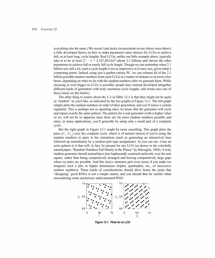
516 CHAPTER 12
everything else the same.) We weren’t just lucky (or persistent) in our choice since there’sa fully developed theory on how to make parameter-value choices for LCGs to achievefull, or at least long, cycle lengths. Real LCGs, unlike our little example above, typicallytake m to be at least 231 – 1 = 2,147,483,647 (about 2.1 billion) and choose the otherparameters to achieve full or nearly full cycle length. Though we can remember when 2.1billion was still a lot, such a cycle length is not as impressive as it once was, given today’scomputing power. Indeed, using just a garden-variety PC, we can exhaust all of the 2.1billion possible random numbers from such LCGs in a matter of minutes or at most a fewhours, depending on what we do with the random numbers after we generate them. Whilechoosing m even bigger in LCGs is possible, people have instead developed altogetherdifferent kinds of generators with truly enormous cycle lengths, and Arena uses one ofthese (more on this below).
The other thing to realize about the Ui’s in Table 12-1 is that they might not be quite
as “random” as you’d like, as indicated by the two graphs in Figure 12-1. The left graphsimply plots the random numbers in order of their generation, and you’ll notice a certainregularity. This is perhaps not so upsetting since we know that the generator will cycleand repeat exactly the same pattern. The pattern for a real generator (with a higher valueof m), will not be so apparent since there are far more random numbers possible andsince, in many applications, you’ll generally be using only a small part of a completecycle.
But the right graph in Figure 12-1 might be more unsettling. This graph plots thepairs (U
i , U
i+1) over the complete cycle, which is of natural interest if you’re using therandom numbers in pairs in the simulation (such as generating an interarrival timefollowed up immediately by a random part-type assignment). As you can see, it has aneerie pattern to it that will, in fact, be present for any LCG (as shown in the colorfullynamed paper, “Random Numbers Fall Mainly in the Planes” by Marsaglia, 1968). A trulyrandom generator should instead have dots haphazardly scattered uniformly over the unitsquare, rather than being compulsively arranged and leaving comparatively large gapswhere no pairs are possible. And this lattice structure gets even worse if you make (orimagine) such a plot in higher dimensions (triples, quadruples, etc., of successiverandom numbers). These kinds of considerations should drive home the point that“designing” good RNGs is not a simple matter, and you should thus be careful whenencountering some mysterious undocumented RNG.
Figure 12-1. Plots for an LCG
517FURTHER STATISTICAL ISSUES
The RNG originally in Arena, starting in the early 1980s with SIMAN, was an LCGwith m = 231 – 1, a = 75 = 16,807, and c = 0; the cycle length of it is m – 1 = 2.1 billion. Inits day, this generator was acceptable since it had been well tested and in fact delivered arespectable flow of random numbers. However, because computers have gotten muchfaster, it became apparent that this cycle length was no longer adequate and that this oldgenerator actually ran the risk of “lapping” itself around the entire cycle within a fewhours or maybe even minutes of simulating (which could obviously do serious damage tothe validity of your results).
So a new RNG has been installed in Arena (and is in the version of Arena that is usedwith this book), based on research by L’Ecuyer (1996, 1999) and L’Ecuyer, Simard,Chen, and Kelton (2002). While it uses some of the same ideas as LCGs (particularly themodulo-division operation), it differs in that (1) it involves two separate componentgenerators that are then combined, and (2) the recursion to get the next values looks backbeyond just the single preceding value. This kind of generator is called a combinedmultiple recursive generator (CMRG). First it starts up the two separate recursions,which you can think of as operating in parallel at the same time:
An = (1403580 A
n–2 – 810728 A
n–3) mod 4294967087
Bn = (527612 B
n–1 – 1370589 B
n–3) mod 4294944443
Then it combines these two values at the nth step as follows:
Zn = (A
n – B
n) mod 4294967087
Finally, this RNG delivers the nth random number Un as either
Zn / 4294967088, if Z
n > 0,
or4294967087 / 4294967088, if Z
n = 0.
To get the two recursions going, the generator must define a six-vector of seeds,composed of the first three A
n’s and the first three B
n’s.
The rather scary constants involved in this generator have been carefully chosen,based on the papers cited above, to ensure two very desirable properties. First, the statisti-cal properties of the random numbers produced are extremely strong; we get good distri-bution of the generated points, like the right-hand plot in Figure 12-1, but up through a45-dimensional cube rather than just the two dimensions of Figure 12-1. Second, whilethis generator will cycle (like LCGs), the length of this cycle is a stunning 3.1 × 1057,rather than the 2.1 × 10⁹ for the old generator. And the running speed on a per-random-number basis of the new generator is only slightly slower than the old one.
Let’s put into perspective the difference between the old and new cycle lengths. If theold generator can be exhausted in ten minutes (which it can on a 2 GHz PC if we just

518 CHAPTER 12
generate the random numbers and throw them away), the new generator would keep thismachine busy for about 2.78 × 1040 millennia. Now we know you’re thinking “sure, butin 1982 they thought 2.1 billion was a lot and it would last forever”—but even underMoore’s “law” (which observes that computers double in speed about every year and ahalf), it will be something like 216 years before a typical computer will be able toexhaust this new generator in a year of nonstop computing. So we’re good for a while,but we admit, not forever.
It turns out to be quite useful to be able to separate the cycle of a generator intoadjacent non-overlapping streams of random numbers, which we can effectively think ofas being separate “faucets” delivering different streams of random numbers. To define astream, we need to specify the seed vector (six numbers in the Arena generator) and takecare that successive streams’ seed vectors are “spaced apart” around the cycle so that thestreams are long. The Arena generator has facility for splitting the cycle of 3.1 × 1057
random numbers into 1.8 ×10¹⁹ separate streams, each of length 1.7 × 1038. Each streamis further subdivided into 2.3 × 10¹⁵ substreams of length 7.6 × 10²² apiece. Our weary2 GHz PC would take about 669 million years to exhaust one of the substreams; underMoore’s law, in 49 years, it will take a month to exhaust a substream—but 187 billionmillennia to exhaust a stream.
You can specify which stream is used whenever you ask for an observation from adistribution in Arena by appending the stream number to the distribution’s parameters;for instance, to generate an exponential observation with mean 6.7 from stream 4, useEXPO(6.7, 4). If you don’t specify a stream number, Arena defaults it to 10. (SinceArena does some of its own random-number generation, for instance in generatingnonstationary arrival patterns and in a “chance”-type Decide module, it uses stream 10for that, so you should avoid using stream 10 if you’re specifying your own streams.) Theidea of using separate streams of random numbers for individual purposes in asimulation (for instance, stream 1 for interarrival times between parts, stream 2 for parttypes, stream 3 for processing times, etc.) comes in quite handy for variance reduction,discussed in Section 12.4. Arena does not actually store all the seed vectors, but ratheruses a fast on-the-fly method to compute them when you reference the correspondingstream; for this reason, you should probably use the streams in order 1, 2, 3, etc., (butskip 10) so that Arena does not have to compute a bunch of seed vectors for interveningstreams that you’re not going to use.
Finally, if you’re making multiple replications of your model (see Chapter 6 andSection 7.2.2), Arena will automatically move to the beginning of the next substreamwithin all the streams you’re using (even if you’re just using the default stream 10) for thenext replication. As we’ll see in Section 12.4, this is important for synchronizingrandom-number use across variations of a model in order to improve the precision ofyour comparisons between alternatives.
While we feel that Arena’s current RNG is extremely good, you can choose to use theold one (though we don’t recommend it) if you really need to for some legacy reason. Todo so, you need only place a Seeds module from the Elements panel into your model;you will need to edit this module to avoid a run-time error, but it doesn’t matter what
519FURTHER STATISTICAL ISSUES
seed you specify for what stream (as long as you identify a stream you’re not using) sinceits mere presence tells Arena to use the old generator. Online help gives you furtherinformation about what this Seeds module does for the old generator. If you want to usethe new generator (which we strongly recommend), just make sure you don’t have aSeeds module present in your model.
12.2 Generating Random Variates
In Section 4.6, we discussed how you can select appropriate probability distributions torepresent random input for your model. Now that you know how to generate randomnumbers—that is, samples from a uniform distribution between 0 and 1—you need totransform them somehow into draws from the input probability distributions you wantfor your model. In simulation, people often refer to such draws as variates from thedistribution.
The precise method for generating variates from a distribution will, of course,depend on the form of the distribution and the numerical values you estimated orspecified its parameters to be, but there are some general ideas that apply across mostdistributions. Because implementation is a bit different for discrete and continuousrandom variables, we’ll consider them separately.
12.2.1 DiscreteLet’s start by considering discrete random variables (see Section B.2.2 in Appendix B).To take a simple concrete example, suppose you want to generate a discrete random vari-ate X having possible values –2, 0, and 3 with probability mass function (PMF) given by
0.1 for x = –2p(x) = P(X = x) = 0.5 for x = 0
0.4 for x = 3
Since the probabilities in a PMF have to add up to 1, we can divide the unit interval [0, 1]into subintervals with widths equal to the individual values given by the PMF, in this case,[0, 0.1), [0.1, 0.6), and [0.6, 1]. If we generate a random number U, it will be distributeduniformly over the whole interval [0, 1], so it will fall in the first subinterval withprobability 0.1 – 0 = 0.1, in the second with probability 0.6 – 0.1 = 0.5, and in the thirdsubinterval with probability 1 – 0.6 = 0.4. Thus, we would set X to its first value, –2, if Ufalls in the first subinterval, which will happen with probability 0.1 = p(–2), as desired.Similarly, we set X to 0 if U falls in the second subinterval (probability 0.5), and set X to 3if U falls in the third subinterval (probability 0.4). This process, which is pretty obviouslycorrect for generating X with the desired distribution, is depicted in Figure 12-2.
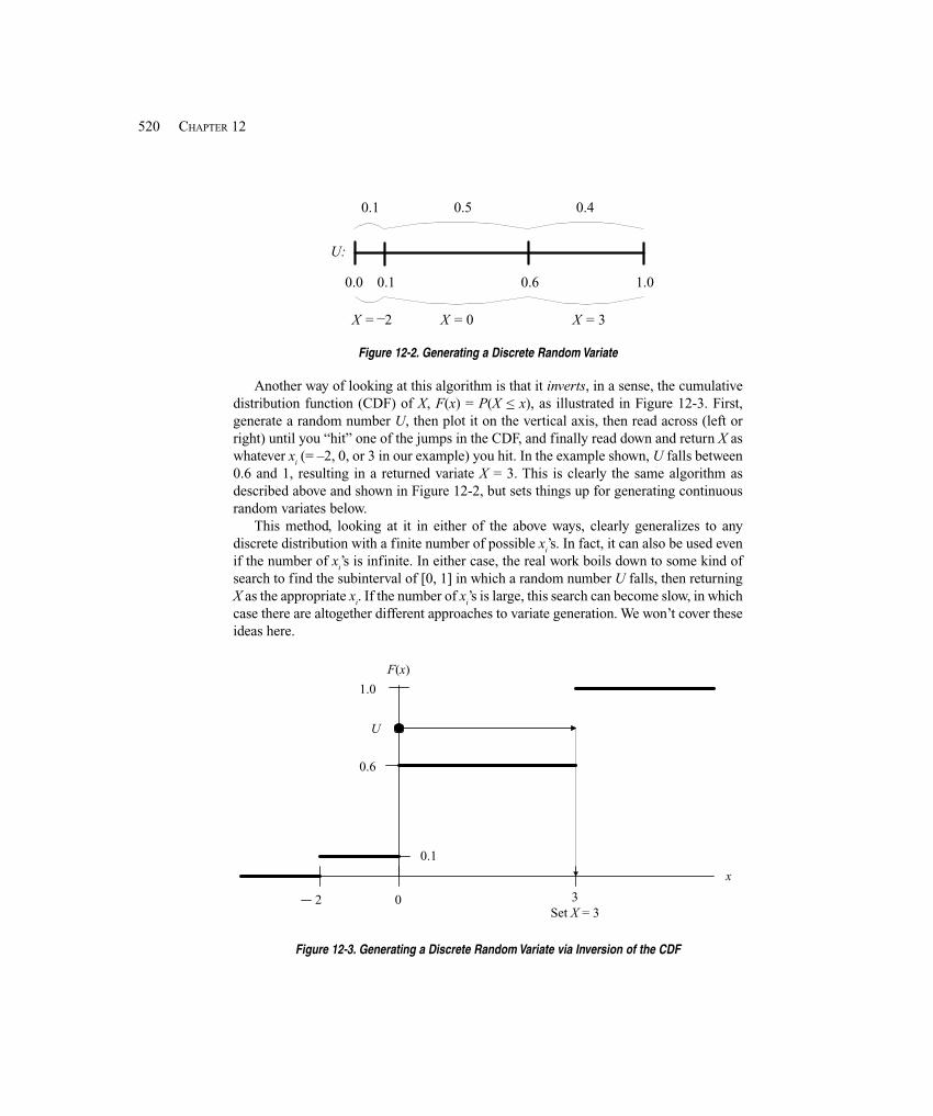
520 CHAPTER 12
0.0 0.6 1.00.1
0.1 0.5 0.4
X = 2 X = 0 X = 3
U:
Figure 12-2. Generating a Discrete Random Variate
Another way of looking at this algorithm is that it inverts, in a sense, the cumulativedistribution function (CDF) of X, F(x) = P(X < x), as illustrated in Figure 12-3. First,generate a random number U, then plot it on the vertical axis, then read across (left orright) until you “hit” one of the jumps in the CDF, and finally read down and return X aswhatever x
i (= –2, 0, or 3 in our example) you hit. In the example shown, U falls between
0.6 and 1, resulting in a returned variate X = 3. This is clearly the same algorithm asdescribed above and shown in Figure 12-2, but sets things up for generating continuousrandom variates below.
This method, looking at it in either of the above ways, clearly generalizes to anydiscrete distribution with a finite number of possible x
i’s. In fact, it can also be used even
if the number of xi’s is infinite. In either case, the real work boils down to some kind of
search to find the subinterval of [0, 1] in which a random number U falls, then returningX as the appropriate x
i. If the number of x
i’s is large, this search can become slow, in which
case there are altogether different approaches to variate generation. We won’t cover theseideas here.
2
1.0
3Set X = 3
x
0.6
0
F(x)
0.1
U
Figure 12-3. Generating a Discrete Random Variate via Inversion of the CDF
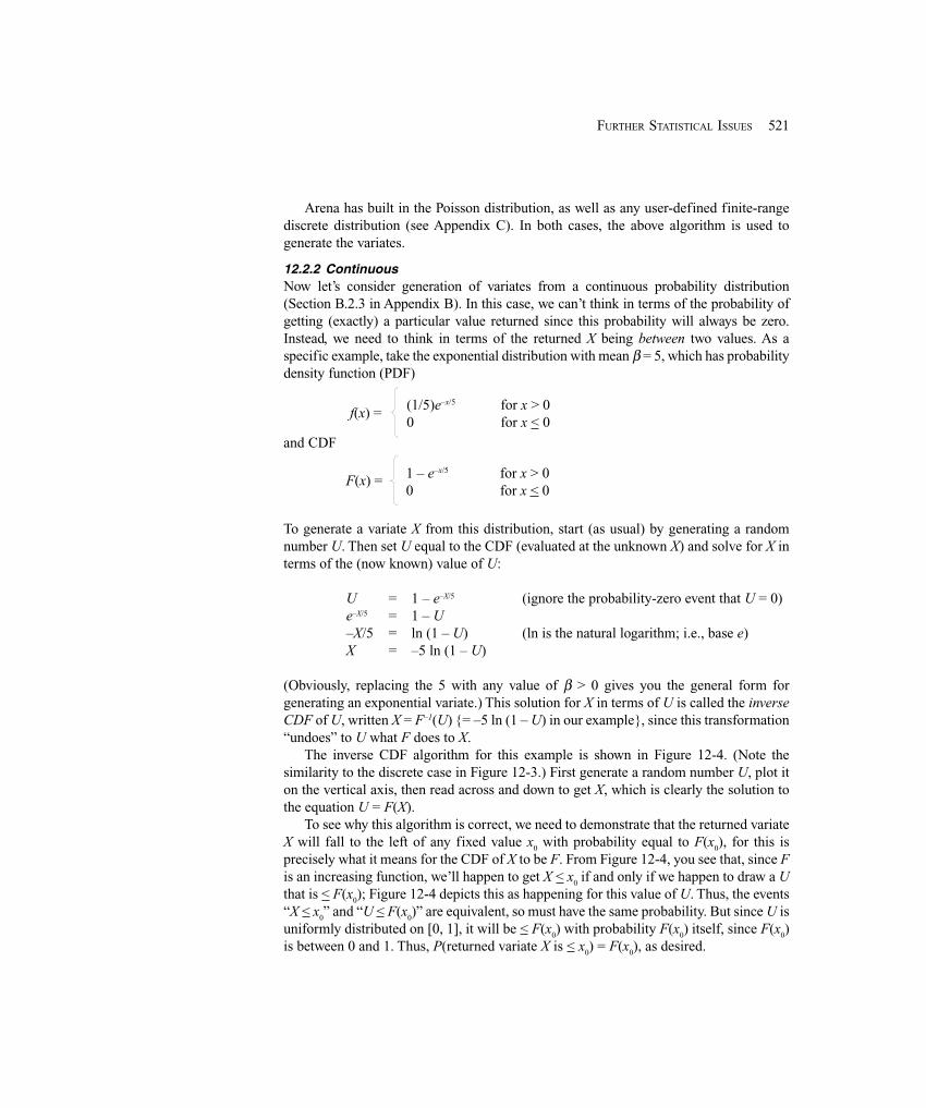
521FURTHER STATISTICAL ISSUES
Arena has built in the Poisson distribution, as well as any user-defined finite-rangediscrete distribution (see Appendix C). In both cases, the above algorithm is used togenerate the variates.
12.2.2 ContinuousNow let’s consider generation of variates from a continuous probability distribution(Section B.2.3 in Appendix B). In this case, we can’t think in terms of the probability ofgetting (exactly) a particular value returned since this probability will always be zero.Instead, we need to think in terms of the returned X being between two values. As aspecific example, take the exponential distribution with mean β = 5, which has probabilitydensity function (PDF)
and CDF
To generate a variate X from this distribution, start (as usual) by generating a randomnumber U. Then set U equal to the CDF (evaluated at the unknown X) and solve for X interms of the (now known) value of U:
U = 1 – e–X/5 (ignore the probability-zero event that U = 0)e–X/5 = 1 – U–X/5 = ln (1 – U) (ln is the natural logarithm; i.e., base e)X = –5 ln (1 – U)
(Obviously, replacing the 5 with any value of β > 0 gives you the general form forgenerating an exponential variate.) This solution for X in terms of U is called the inverseCDF of U, written X = F–1(U) {= –5 ln (1 – U) in our example}, since this transformation“undoes” to U what F does to X.
The inverse CDF algorithm for this example is shown in Figure 12-4. (Note thesimilarity to the discrete case in Figure 12-3.) First generate a random number U, plot iton the vertical axis, then read across and down to get X, which is clearly the solution tothe equation U = F(X).
To see why this algorithm is correct, we need to demonstrate that the returned variateX will fall to the left of any fixed value x0 with probability equal to F(x0), for this isprecisely what it means for the CDF of X to be F. From Figure 12-4, you see that, since Fis an increasing function, we’ll happen to get X < x0 if and only if we happen to draw a Uthat is < F(x0); Figure 12-4 depicts this as happening for this value of U. Thus, the events“X < x0” and “U < F(x0)” are equivalent, so must have the same probability. But since U isuniformly distributed on [0, 1], it will be < F(x0) with probability F(x0) itself, since F(x0)is between 0 and 1. Thus, P(returned variate X is < x0) = F(x0), as desired.
f(x) =(1/5)e–x/5 for x > 00 for x < 0
F(x) = 1 – e–x/5 for x > 00 for x < 0
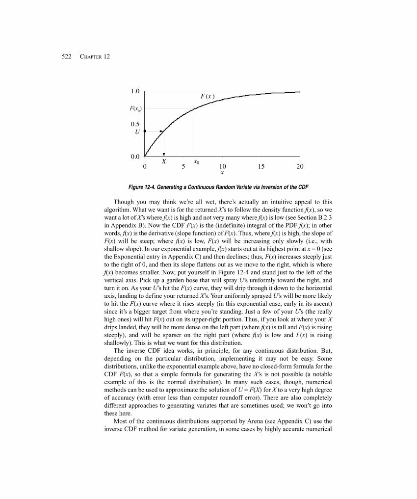
522 CHAPTER 12
0.0
0.5
1.0
0 5 10 15 20x
F (x )
U
X x0
Figure 12-4. Generating a Continuous Random Variate via Inversion of the CDF
Though you may think we’re all wet, there’s actually an intuitive appeal to thisalgorithm. What we want is for the returned X’s to follow the density function f(x), so wewant a lot of X’s where f(x) is high and not very many where f(x) is low (see Section B.2.3in Appendix B). Now the CDF F(x) is the (indefinite) integral of the PDF f(x); in otherwords, f(x) is the derivative (slope function) of F(x). Thus, where f(x) is high, the slope ofF(x) will be steep; where f(x) is low, F(x) will be increasing only slowly (i.e., withshallow slope). In our exponential example, f(x) starts out at its highest point at x = 0 (seethe Exponential entry in Appendix C) and then declines; thus, F(x) increases steeply justto the right of 0, and then its slope flattens out as we move to the right, which is wheref(x) becomes smaller. Now, put yourself in Figure 12-4 and stand just to the left of thevertical axis. Pick up a garden hose that will spray U’s uniformly toward the right, andturn it on. As your U’s hit the F(x) curve, they will drip through it down to the horizontalaxis, landing to define your returned X’s. Your uniformly sprayed U’s will be more likelyto hit the F(x) curve where it rises steeply (in this exponential case, early in its ascent)since it’s a bigger target from where you’re standing. Just a few of your U’s (the reallyhigh ones) will hit F(x) out on its upper-right portion. Thus, if you look at where your Xdrips landed, they will be more dense on the left part (where f(x) is tall and F(x) is risingsteeply), and will be sparser on the right part (where f(x) is low and F(x) is risingshallowly). This is what we want for this distribution.
The inverse CDF idea works, in principle, for any continuous distribution. But,depending on the particular distribution, implementing it may not be easy. Somedistributions, unlike the exponential example above, have no closed-form formula for theCDF F(x), so that a simple formula for generating the X’s is not possible (a notableexample of this is the normal distribution). In many such cases, though, numericalmethods can be used to approximate the solution of U = F(X) for X to a very high degreeof accuracy (with error less than computer roundoff error). There are also completelydifferent approaches to generating variates that are sometimes used; we won’t go intothese here.
Most of the continuous distributions supported by Arena (see Appendix C) use theinverse CDF method for variate generation, in some cases by highly accurate numerical
F(x0)
523FURTHER STATISTICAL ISSUES
approximation. A few of the distributions, though, use other methods if they areparticularly attractive in that case; refer to online help under the topic “Distributions” tosee exactly what Arena does to generate samples from each continuous distribution.
12.3 Nonstationary Poisson Processes
A lot of systems have some kind of externally originating events affecting them, likecustomers arriving, calls coming in, cars approaching an intersection, or accidentsoccurring in a plant. Often, it’s appropriate to model this kind of event process as beingrandom with some continuous probability distribution for inter-event times, implyingsome discrete distribution for the number of events occurring in a fixed interval of time.If the process governing the event occurrences is stationary over the time frame of thesimulation, you can just decide on the right inter-event-time distribution and generate theevents during the simulation as we’ve done in many models in the book (for example,with the Time Between Arrivals area in the Create module from the Basic Process panel).
However, many systems experience time-varying, or nonstationary patterns ofevents—the lunch stampede at a fast-food restaurant, morning and evening rush hours intraffic systems, mid-afternoon peaks of calls coming in to a call center, or a rash ofaccidents when the moon is full. While you might be tempted to ignore these patternsand make the events occur at some kind of “average” rate throughout your simulation,doing so could lead to seriously inaccurate results if there is much variation in the actualpattern. For instance, if we average the freeway load over 24 hours, there’s little doubtthat a small number of lanes would appear to be adequate in the model; in fact, though,rush hours would be impossible messes. So modeling nonstationary external events canbe a critical part of valid modeling in general.
Actually, we’ve already discussed a situation exactly like this, Model 5-2. Theexternal events are the incoming call arrivals, and we specified the observed rates (inarrivals per hour) for each 30-minute period in the Arrival Schedule line of theSchedule module.
The usual way to represent time-varying event patterns like this is by what’s called anonstationary Poisson process (NSPP). To use such a process, you need to specify a ratefunction, λ(t), that changes with time (t), having the rough interpretation that λ(t) is highfor times t when lots of events are happening, and low when things are quiet. Moreprecisely, the definition of an NSPP is that events occur one at a time, are independent ofeach other, and the number (count) of events occurring during and interval of time [t1, t2]is a Poisson random variable (see Appendix C) with expected value given by
∫=Λ 2
1
)(),( 21
t
tdtttt λ
which is large over time intervals where λ(t) is high and small when λ(t) is low.If you want to use an NSPP in a simulation, there are two issues: how to form an
estimate of λ(t), and then how to generate the arrivals in accordance with your estimatedrate function. The estimated rate function we used in Model 5-2 was piecewise constant,with (possible) changes of level occurring every 30 minutes. This approach is probably
524 CHAPTER 12
the most practical one since it’s quite general and easy to specify (though you must becareful about keeping the time units straight). There are, however, more sophisticatedways to estimate the rate function, including amplitudes and periodicities, with firmgrounding in statistical theory; see, for instance, Leemis (1991); Johnson, Lee, andWilson (1994); and Kuhl and Wilson (2000, 2001).
As long as you stick with a piecewise-constant estimated rate function, Arena has abuilt-in generation method, the use of which was illustrated in Model 5-2. The algorithmused is a speeded-up variation of a method attributed to Cinlar (1975, pp. 94–101). Ifyou’re interested in the details, see Arena’s Help topic “Non-Stationary ExponentialDistribution.”
12.4 Variance Reduction
As we’ve indicated in several places (including Sections 2.6, 4.6, 7.2, and Chapter 6),simulations using random variates from probability distributions as part of the input willin turn produce random output. In other words, there is some variance associated withthe output from a stochastic simulation. The more variance there is, the less precise areyour results; one manifestation of high variance is wide confidence intervals. So outputvariance is the enemy, and it would be nice to get rid of it, or at least reduce it. One (bad)way to eliminate variance in the output is to purge all the randomness from your inputs,perhaps by replacing the input random variables with their expected values. However, aswe demonstrated in Section 4.6.1, this might make your output nice and stable but it alsowill usually make it seriously wrong.
So, barring major violence to your model’s validity, the best you can really hope for isto reduce the variance in your output performance measures. One obvious way to do this isby just simulating more. For terminating models, this implies more replications (sinceextending the length of a replication would make the model invalid in the terminatingcase); in Section 6.3, we gave a couple of formulas from which you can approximate thenumber of replications you’ll need to bring a confidence-interval half width down to avalue small enough for you to live with. For steady-state models, you could also makemore replications if you’re taking the truncated-replications approach to analysis, asdiscussed in Section 7.2.2; or you could just make your (single) replication longer ifyou’re taking the batch-means approach (Section 7.2.3). In Section 12.5, we’ll discuss allof this in detail, including how you can get Arena to “decide” on the fly how muchsimulating to do.
But what we aspire to in this section is a free lunch. Getting more precise results bymore simulation work is not tricky, but there are some situations where you can achievethe same thing without doing any1 more work. What usually enables this is the fact that,unlike in most physical experiments, you’re in control of the randomness in a simulationexperiment since you can control the random-number generator, as discussed in Section12.1. This allows you to induce certain kinds of correlations that you can exploit to youradvantage to reduce the variance, and thus imprecision, of your output. These kinds ofschemes are called variance-reduction techniques (or sometimes variance-reduction
1 Well, hardly any.
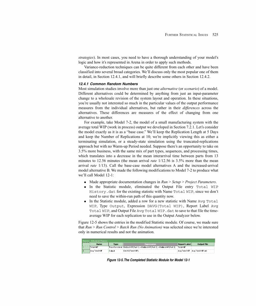
525FURTHER STATISTICAL ISSUES
strategies). In most cases, you need to have a thorough understanding of your model’slogic and how it’s represented in Arena in order to apply such methods.
Variance-reduction techniques can be quite different from each other and have beenclassified into several broad categories. We’ll discuss only the most popular one of themin detail, in Section 12.4.1, and will briefly describe some others in Section 12.4.2.
12.4.1 Common Random NumbersMost simulation studies involve more than just one alternative (or scenario) of a model.Different alternatives could be determined by anything from just an input-parameterchange to a wholesale revision of the system layout and operation. In these situations,you’re usually not interested so much in the particular values of the output performancemeasures from the individual alternatives, but rather in their differences across thealternatives. These differences are measures of the effect of changing from onealternative to another.
For example, take Model 7-2, the model of a small manufacturing system with theaverage total WIP (work in process) output we developed in Section 7.2.1. Let’s considerthe model exactly as it is as a “base case.” We’ll keep the Replication Length at 5 Daysand keep the Number of Replications at 10; we’re implicitly viewing this as either aterminating simulation, or a steady-state simulation using the truncated-replicationsapproach but with no Warm-up Period needed. Suppose there’s an opportunity to take on3.5% more business, with the same mix of part types, sequences, and processing times,which translates into a decrease in the mean interarrival time between parts from 13minutes to 12.56 minutes (the mean arrival rate 1/12.56 is 3.5% more than the meanarrival rate 1/13). Call the base-case model alternatives A and the increased-arrivalmodel alternative B. We made the following modifications to Model 7-2 to produce whatwe’ll call Model 12-1:
� Made appropriate documentation changes in Run > Setup > Project Parameters.� In the Statistic module, eliminated the Output File entry Total WIP
History.dat for the existing statistic with Name Total WIP, since we don’tneed to save the within-run path of this quantity now.
� In the Statistic module, added a row for a new statistic with Name Avg TotalWIP, Type Output, Expression DAVG(Total WIP), Report Label AvgTotal WIP, and Output File Avg Total WIP.dat to save to that file the time-average WIP for each replication to use in the Output Analyzer below.
Figure 12-5 shows the entries in the modified Statistic module. Of course, we made surethat Run > Run Control > Batch Run (No Animation) was selected since we’re interestedonly in numerical results and not the animation.
Figure 12-5. The Completed Statistic Module for Model 12-1
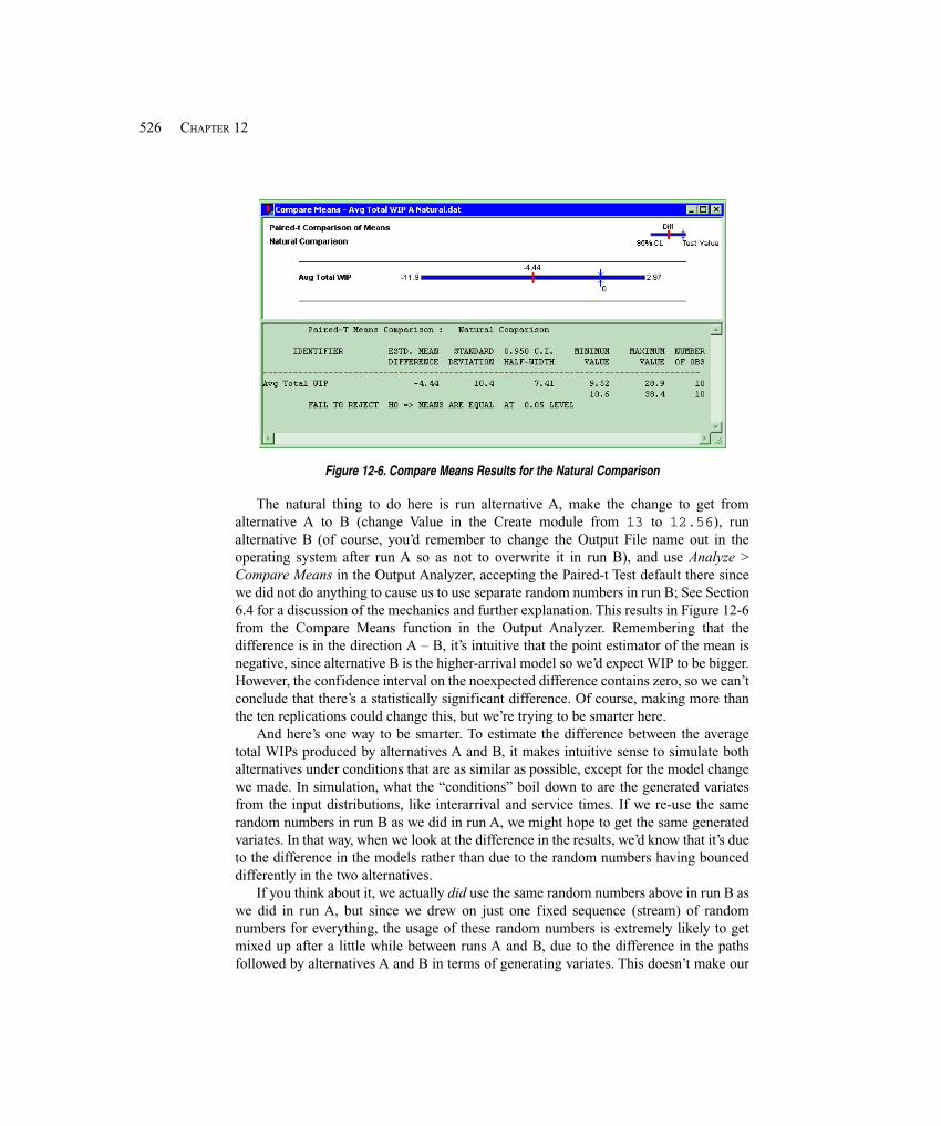
526 CHAPTER 12
Figure 12-6. Compare Means Results for the Natural Comparison
The natural thing to do here is run alternative A, make the change to get fromalternative A to B (change Value in the Create module from 13 to 12.56), runalternative B (of course, you’d remember to change the Output File name out in theoperating system after run A so as not to overwrite it in run B), and use Analyze >Compare Means in the Output Analyzer, accepting the Paired-t Test default there sincewe did not do anything to cause us to use separate random numbers in run B; See Section6.4 for a discussion of the mechanics and further explanation. This results in Figure 12-6from the Compare Means function in the Output Analyzer. Remembering that thedifference is in the direction A – B, it’s intuitive that the point estimator of the mean isnegative, since alternative B is the higher-arrival model so we’d expect WIP to be bigger.However, the confidence interval on the noexpected difference contains zero, so we can’tconclude that there’s a statistically significant difference. Of course, making more thanthe ten replications could change this, but we’re trying to be smarter here.
And here’s one way to be smarter. To estimate the difference between the averagetotal WIPs produced by alternatives A and B, it makes intuitive sense to simulate bothalternatives under conditions that are as similar as possible, except for the model changewe made. In simulation, what the “conditions” boil down to are the generated variatesfrom the input distributions, like interarrival and service times. If we re-use the samerandom numbers in run B as we did in run A, we might hope to get the same generatedvariates. In that way, when we look at the difference in the results, we’d know that it’s dueto the difference in the models rather than due to the random numbers having bounceddifferently in the two alternatives.
If you think about it, we actually did use the same random numbers above in run B aswe did in run A, but since we drew on just one fixed sequence (stream) of randomnumbers for everything, the usage of these random numbers is extremely likely to getmixed up after a little while between runs A and B, due to the difference in the pathsfollowed by alternatives A and B in terms of generating variates. This doesn’t make our
527FURTHER STATISTICAL ISSUES
statistical comparison in Figure 12-6 wrong (so long as we stick with the Paired-t Testrather than the Two-Sample-t Test), but it doesn’t accomplish the goal of generating thesame variates for the same purposes in runs A and B either. We need to be even smarter(as well as have a good random-number generator with lots of really long streams andsubstreams, which Arena has, as described in Section 12.1).
Here’s how to be even smarter. In this model, there are 14 sources of randomness—interarrival times, part indices, and 12 processing-time distributions as defined in Table7-1. For our comparison, we’d like to run both alternatives A and B with the “same”external loads. In this case, it means blank parts arriving at the same times, assigned thesame part indices, and experiencing the same processing times at each of the stops alongtheir ways. When we ran this comparison above, producing Figure 12-6, we didn’t doanything to try to get any of this to happen. True, the same random-number stream (thedefault, stream 10) was used for everything throughout both alternatives, and this streamstarted the first of the ten replications from the same seed for both alternatives. But dueto the change made in the model between the alternatives, this fixed sequence of randomnumbers will be used in a different order if, at any point during the runs, there is adifference in the order of execution in which the 14 places draw the variates they need.This causes the “external loads” to differ at this point, and likely from then on, which isnot the effect we want.
Instead, we need to synchronize the use of the random numbers across the modelalternatives, or at least do so as far as possible given the model logic and the changesbetween the alternatives. One approach (though not the only one) to this end is todedicate a stream of random numbers to each of the 14 places in the model where variatesare generated. This is like piping in separate “faucets” of random numbers to eachrandom-variate generator and other situations (like chance-type Decide modules andgeneration of nonstationary Poisson processes, neither of which occurs in this model)where a random number is needed. In this way, you can usually get reasonablesynchronization, though in complex models it might not ensure that everything ismatched up across the alternatives (which does not make your model in any wayincorrect or invalid, but it is not quite as close a match-up across the alternatives as youmight like in order to have the “same” external loads presented to both alternativemodels). However, there will still probably be at least some variance-reduction benefiteven though the matchups might not be quite perfect. This is the synchronizationapproach we’ll take in our example below.
A different way to attempt random-number synchronization, which might workbetter in some models, is to assign to each entity, immediately upon its arrival, attributevalues for all possible processing times, branching decisions, etc., that it might need onits entire path through the model. When the entity needs one of these values during itslife in the model, such as a processing time somewhere, you just read it out of theappropriate attribute of the entity rather than generate it on the spot. This might comecloser for some models to the ideal of having the “same” external conditions, but it canrequire a lot more computer memory if you need to hold lots of attributes for lots ofentities at the same time. If Arena has to use your disk drive to extend memory

528 CHAPTER 12
temporarily (called virtual memory), there can be a significant increase in execution timeas well since disk access is much slower than memory access. In this situation, you mightbe just as well off using this extra computer time doing more simulation (either morereplications or a longer single run). We won’t carry out this synchronization approach inour example below, but will leave it for you as Exercises 12-1 and 12-2.
Sometimes achieving full, complete, and certain synchronization in complex modelsis just impractical, in which case you might consider matching up what you can, andgenerating the rest independently. When you use the same random numbers acrosssimulated alternatives, synchronized in some way, you’re using a variance-reductiontechnique called common random numbers (CRN), also sometimes called matched pairsor correlated sampling.
To implement the first of the above two synchronization approaches to CRN (pipingin separate faucets of random numbers to the separate sources of randomness in a model)in Model 12-1, we modified it into what we’ll call Model 12-2. To each of the 14 variate-generation expressions, we added an extra parameter (see Section 12.1), assigning aunique stream number, as given in Table 12-2. We actually defined a Variable for eachstream number, initialized them all in the Variable module, and used the variable namesin the variate-generation expressions; this made it easier to carry out further experimentslater. We skipped over stream 10 since that’s Arena’s default stream and is used for thebuilt-in nonstationary-Poisson-process generator and any Chance-type Decide modules;fortunately, we have neither in our model so it’s easy to maintain proper synchronization.(See Exercise 12-7 for a way to trick chance-type Decide modules into using whateverrandom-number stream you want.) In this model, the processing times are assigned forCell 1 via an Expression, and for the other cells via assignments in the Sequences; Table12-2 also indicates where the required change was made.
Table 12-2. Stream Assignment and Usage for Model 12-2
Stream Location Number Usage Variable Name of Change
1 Interarrival Times S Interarrivals Create module2 Part Indices S Part Index Assign module3 Part Type 1 at Cell 1 S P1 C1 Expression module4 Part Type 1 at Cell 2 S P1 C2 Sequence module5 Part Type 1 at Cell 3 S P1 C3 Sequence module6 Part Type 1 at Cell 4 S P1 C4 Sequence module7 Part Type 2 at Cell 1 S P1 C1 Expression module8 Part Type 2 at Cell 2 (first visit) S P1 C2 Sequence module9 Part Type 2 at Cell 4 S P1 C4 Sequence module
11 Part Type 2 at Cell 2 (second visit) S P1 C2 Again Sequence module12 Part Type 2 at Cell 3 S P1 C3 Sequence module13 Part Type 3 at Cell 2 S P1 C2 Sequence module14 Part Type 3 at Cell 1 S P1 C1 Expression module15 Part Type 3 at Cell 3 S P1 C3 Sequence module
529FURTHER STATISTICAL ISSUES
These stream assignments dedicate a separate random-number stream to each sourceof randomness in the model, and they will be in effect for the running of both alternativesA and B. Recall that we’re doing ten replications of each alternative, and that the Arenarandom-number generator will automatically advance to the next substream within eachstream for each new replication. In this way, we’re assured that the matchup of randomnumbers across alternatives will stay synchronized beyond just the first replication, evenif the alternatives disagree about how many random numbers from a stream are used fora given replication. Since it will take at least 669 million years for a typical machine oftoday to exhaust a substream, we can be pretty sure that we won’t “lap” ourselves interms of substream usage from one replication to the next.
What we set up above is a fairly carefully synchronized random-number allocationfor CRN. What we did in Section 6.4 and to produce Figure 12-6 above, using the samestream (10) for everything might be described as using the same random numbers acrossthe alternatives, but in a disorganized, haphazard, and mostly unsynchronized way,diluting or even erasing the effect. It’s possible to simulate the alternatives usingcompletely different, and thus independent random numbers across the alternatives, butyou have to work to make this happen by bumping up the stream numbers in Table 12-2for, say, alternative B (but not A) so that streams 1–15 are not used. Thus, in a way, CRNis the “default” for the way most people would naturally run comparisons, but it’sextremely unlikely that proper synchronization of random-number usage will justhappen on its own unless your model is awfully simple.
Proceeding as in Section 6.4 and what we did to produce Figure 12-6 above, we madeten replications of alternatives A and B using Model 12-2 for both, with the streamassignments discussed above, resulting in synchronized CRN. We then invoked theAnalyze > Compare Means menu option in the Output Analyzer except calling forcomparisons of A against the CRN run of B, to get the results in Figure 12-7 for a 95%confidence interval on the difference between expected average total WIPs foralternative A minus alternative B (Figure 12-7 actually includes both this synchronized-CRN comparison as well as the unsynchronized “natural”). Looking back at Figure 12-6(repeated as the top comparison in Figure 12-7), the qualitative conclusion fromsynchronized CRN is the same as before—increasing the arrival rate increases averagetotal WIP, though the “natural” comparison could not conclude that with statisticalsignificance (at the 0.05 level) while the synchronized CRN comparison can. In terms ofthe precision of the estimate of the magnitude of this increase, though, the effect ofsynchronizing CRN is to reduce the confidence-interval half width fairly dramatically,from 7.41 to 0.711, without doing any more simulation work than before (ten replicationsof both alternative models). Thus, for this model with these comparisons, the benefitfrom properly synchronized CRN is quite apparent. The magnitude of the effect of CRNis highly model- and situation-dependent, and it is pretty potent in this example.Sometimes, however, it can be less dramatic, but the (small) effort to synchronize streamusage is still probably worthwhile in most cases.
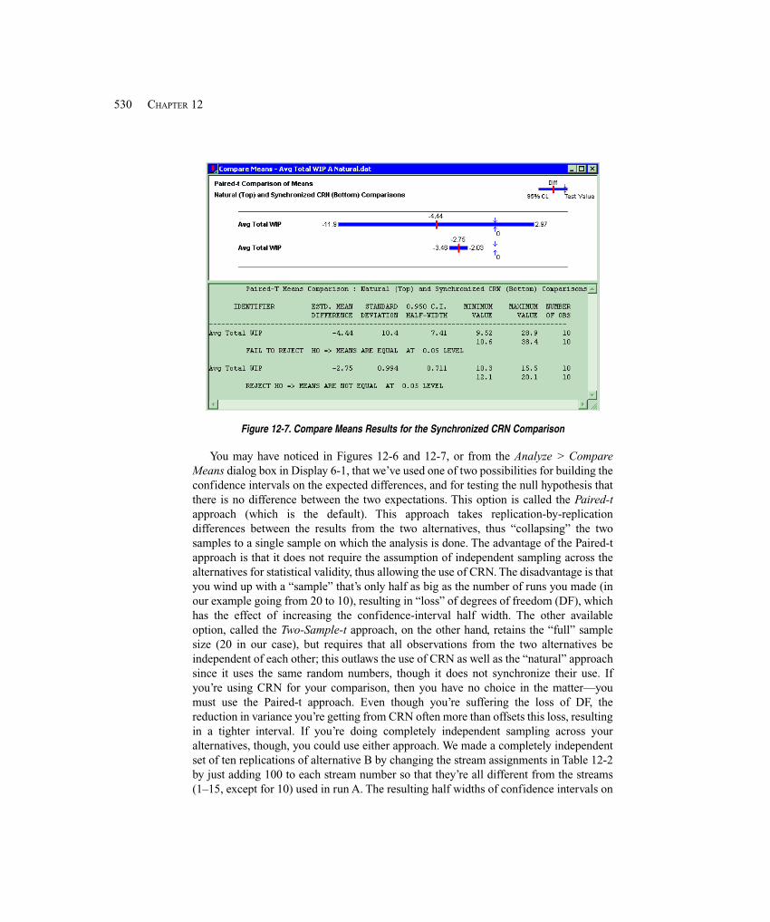
530 CHAPTER 12
Figure 12-7. Compare Means Results for the Synchronized CRN Comparison
You may have noticed in Figures 12-6 and 12-7, or from the Analyze > CompareMeans dialog box in Display 6-1, that we’ve used one of two possibilities for building theconfidence intervals on the expected differences, and for testing the null hypothesis thatthere is no difference between the two expectations. This option is called the Paired-tapproach (which is the default). This approach takes replication-by-replicationdifferences between the results from the two alternatives, thus “collapsing” the twosamples to a single sample on which the analysis is done. The advantage of the Paired-tapproach is that it does not require the assumption of independent sampling across thealternatives for statistical validity, thus allowing the use of CRN. The disadvantage is thatyou wind up with a “sample” that’s only half as big as the number of runs you made (inour example going from 20 to 10), resulting in “loss” of degrees of freedom (DF), whichhas the effect of increasing the confidence-interval half width. The other availableoption, called the Two-Sample-t approach, on the other hand, retains the “full” samplesize (20 in our case), but requires that all observations from the two alternatives beindependent of each other; this outlaws the use of CRN as well as the “natural” approachsince it uses the same random numbers, though it does not synchronize their use. Ifyou’re using CRN for your comparison, then you have no choice in the matter—youmust use the Paired-t approach. Even though you’re suffering the loss of DF, thereduction in variance you’re getting from CRN often more than offsets this loss, resultingin a tighter interval. If you’re doing completely independent sampling across youralternatives, though, you could use either approach. We made a completely independentset of ten replications of alternative B by changing the stream assignments in Table 12-2by just adding 100 to each stream number so that they’re all different from the streams(1–15, except for 10) used in run A. The resulting half widths of confidence intervals on
531FURTHER STATISTICAL ISSUES
the expected differences from Compare Means were 4.53 with the Paired-t approach and4.92 with the Two-Sample-t approach; both are valid, and there’s not much differencebetween them (they’re close to what we got from the “natural” comparison), but theyaren’t even close to being as precise as the 0.711 we got from synchronized CRN.
While the intuitive appeal of synchronized CRN, to “compare like with like,” is clear,there’s also a mathematical justification for the idea. Let X and Y denote the outputrandom variables for, respectively, alternatives A and B. In our example, X and Y wouldbe the averages over the ten replications of the average total WIP in each replication, inalternatives A and B. What we want to estimate is E(X) – E(Y) = E(X – Y), and our(unbiased) point estimator of it is just X – Y. If we make the runs independently, thevariance of our independent-samples estimator is
Var(X – Y) = Var(X) + Var(Y)
since, as random variables, X and Y are independent. If, however, we use synchronizedCRN, what we’re doing is inducing correlation, hopefully positive, between X and Y.Since correlation has the same sign as covariance (see Section B.2.4 in Appendix B), thevariance of our CRN estimator is
Var(X – Y) = Var(X) + Var(Y) – 2 Cov(X, Y),
which will be less than the variance of the independent-samples estimator since we’resubtracting a (hopefully) positive covariance. So, what’s needed to make CRN “work” isthat the outputs be positively correlated, and the stronger the better. While you can findexamples where the correlation is negative, causing CRN to “backfire,” such models aregenerally contrived pathologies just to make the point. In most cases, CRN will work,sometimes dramatically. It is true, though, that you can’t tell how well it will work untilyou actually do it. And, as you’ve seen above, CRN in its haphazard, unsynchronizedversion, is almost automatic—you have to work to avoid it. However, you probably won’tget much benefit unless you do something to synchronize the random-number usageacross the alternatives by assigning random-number streams carefully and with anunderstanding of how your model works.
12.4.2 Other MethodsIn addition to CRN, there are several other variance-reduction techniques, which we’lljust briefly mention here; see Chapter 3 of Bratley, Fox, and Schrage (1987) for moredetail on these and other methods. Unlike CRN, these techniques apply when you havejust a single model variant of interest.
The method of antithetic variates attempts to induce negative correlation betweenthe results of one replication and another, and uses this correlation to reduce variance. Ina terminating simulation, make the first replication “as usual,” but in the secondreplication, replace the random numbers U1, U2, . . . you used in the first replication by1 – U1, 1 – U2, etc. This still results in valid variate generation since, if U is distributeduniformly on [0, 1], then 1 – U is as well. The idea is that, since a “big” U results in a“small” 1 – U (and vice versa), the results from replications one and two will be
532 CHAPTER 12
negatively correlated. Your first observation for statistical analysis, then, is not the resultfrom the first replication, but rather the average of the results from the first tworeplications, which are treated as a pair. You could then go on and make replication threewith “fresh” (independent) U’s, then re-use these in replication four but in their antitheticform 1 – U; your second observation for statistical analysis is then the average of theresults from replications three and four. Within an antithetic pair, the (hopefully)negative correlation will cause the average of the two output statistics to snap in towardthe true expectation more closely than if they were independent. Like CRN, this methodrequires careful synchronization of random-number usage in your model, probablyinvolving streams and seeds. In Arena, you’d need to carry out some low-levelmanipulation to implement antithetic variates since there isn’t any direct support.
Control variates uses an ancillary “controlling” random variate to adjust your resultsup or down, as warranted by the control variate. For example, in Model 12-1, if we notedthat, in a particular replication, the average of the generated interarrival times of partshappened to be smaller than their expected value (which we’d know since we specifiedthe interarrival-time distribution as part of the model input), then it’s likely that we’reseeing higher-than-expected congestion measures and thus high average WIP in thisreplication. Thus, we’d adjust these output measures downward by some amount to“control” for the fact that we know that our parts were arriving faster than “usual.” Fromone replication to another, then, this adjustment will tend to dampen the variation of theresults around their (unknown) expectations, reducing variance. In a given model, thereare many potential control variates, and there are different ways to select from amongthem as well as to specify the direction and magnitude of the adjustment to thesimulation output. For further information on control variates, see, for example, Bauerand Wilson (1992) or Nelson (1990).
12.5 Sequential Sampling
When you do a simulation, you should always try to quantify the imprecision in yourresults. If this imprecision is not great enough to matter to you, you’re done. But if theimprecision is large enough to be upsetting, you need to do something to reduce it. InSection 12.4, we discussed variance-reduction techniques, which might help. And inSection 6.3, we gave a couple of formulas for approximating the number n of replicationsyou’d need (in a terminating model) to get a confidence-interval half width down to avalue small enough for you to live with.
But a rather obvious idea is just to keep simulating, one “step” at a time, until you’rehappy. In the case of terminating models, a “step” is the next replication; in the case ofsteady-state models, a “step” is either the next truncated replication (if you’re taking thatstrategy, as in Section 7.2.2); or if you’re doing batch means in a single replication (as inSection 7.2.3), extend by some amount the single replication you have going. Then, afterthis next “step,” check again to see, for instance, if the half width of the new confidenceinterval is small enough. If it is, you can stop; if not, keep going and make the next step.If you can afford to do so, such sequential sampling is usually fairly simple, and typicallywill get you the precision you need. What’s even better is that these ideas, while being

533FURTHER STATISTICAL ISSUES
entirely intuitive, are backed up by solid statistical theory; one consequence is that theactual coverage probability of your confidence interval will approach what it’s supposedto be as your smallness demands on the half width get tighter.
In this section, we’ll show you some examples of sequential sampling, indicatinghow you can set things up so that Arena will take care of the checking and stopping foryou. We’ll consider terminating simulations in Section 12.5.1 and the steady-state case inSection 12.5.2.
12.5.1 Terminating ModelsFirst let’s consider a terminating simulation. We’ll modify Model 12-2 (with the random-number streams set up) since you never know when you might want to do some variancereduction and synchronize the random numbers. We’ll view this as either a terminatingsimulation or as a steady-state simulation using the truncated-replications approach butwith no Warm-up Period needed. As the output performance measure of primary interest(the one whose confidence-interval half width we want to make sure is “small enough”),let’s take the average total WIP. We first made a fixed number of replications (25, ratherthan the original ten to give us a little better chance at getting a decent variance estimate),not really knowing how wide our confidence intervals would be; we got a 95%confidence interval of 13.03 ± 1.28. In Section 6.3, we also discussed two formulas forapproximating how many replications would be needed to reduce the half width of a 95%confidence interval to a fixed value; in this example, to reduce it from 1.28 to, say, 0.5,our formulas say to we’d need to make either about 124 or about 164 total replicationsinstead of 25, depending on which formula we used (and keep in mind that these areperhaps-crude approximations subject to uncertainty in the variance estimate from theseinitial 25 replications).
Let’s instead invoke the sequential-sampling idea to get this half width down to 0.5.We have to make a minor change to our model (into what we’ll call Model 12-3) to ask itto keep replicating until the across-replications 95% confidence-interval half width forthe average total WIP output performance measure falls below 0.5, then stop thereplications. Recall from Section 6.3 that if you call for multiple replications, Arena willautomatically compute 95% confidence intervals across the replications on quantitiesyou’ve specified for your reports; we’ll use internal Arena variables describing theseconfidence intervals to get sequential sampling going. The pertinent Arena variables are:
� ORUNHALF(Output ID), the half width of the automatic across-replicationsconfidence interval from however many replications have been completed, whereOutput ID is the identification of the output measure of interest (in our case, AvgTotal WIP);
� MREP, the total number of replications we’re asking for (initially the Number ofReplications field in Run > Setup > Replication Parameters);
� NREP, the replication number we’re on at the moment (= 1, 2, 3, . . .).
Here’s the general strategy. Initially, specify MREP to be some absurdly enormousvalue in the Number of Replications field in the Run > Setup > Replication Parametersdialog box; this gets the replications going and keeps them going until we cut them off
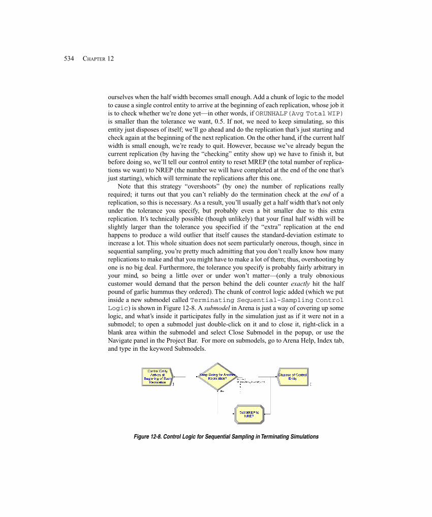
534 CHAPTER 12
ourselves when the half width becomes small enough. Add a chunk of logic to the modelto cause a single control entity to arrive at the beginning of each replication, whose job itis to check whether we’re done yet—in other words, if ORUNHALF(Avg Total WIP)is smaller than the tolerance we want, 0.5. If not, we need to keep simulating, so thisentity just disposes of itself; we’ll go ahead and do the replication that’s just starting andcheck again at the beginning of the next replication. On the other hand, if the current halfwidth is small enough, we’re ready to quit. However, because we’ve already begun thecurrent replication (by having the “checking” entity show up) we have to finish it, butbefore doing so, we’ll tell our control entity to reset MREP (the total number of replica-tions we want) to NREP (the number we will have completed at the end of the one that’sjust starting), which will terminate the replications after this one.
Note that this strategy “overshoots” (by one) the number of replications reallyrequired; it turns out that you can’t reliably do the termination check at the end of areplication, so this is necessary. As a result, you’ll usually get a half width that’s not onlyunder the tolerance you specify, but probably even a bit smaller due to this extrareplication. It’s technically possible (though unlikely) that your final half width will beslightly larger than the tolerance you specified if the “extra” replication at the endhappens to produce a wild outlier that itself causes the standard-deviation estimate toincrease a lot. This whole situation does not seem particularly onerous, though, since insequential sampling, you’re pretty much admitting that you don’t really know how manyreplications to make and that you might have to make a lot of them; thus, overshooting byone is no big deal. Furthermore, the tolerance you specify is probably fairly arbitrary inyour mind, so being a little over or under won’t matter—(only a truly obnoxiouscustomer would demand that the person behind the deli counter exactly hit the halfpound of garlic hummus they ordered). The chunk of control logic added (which we putinside a new submodel called Terminating Sequential-Sampling ControlLogic) is shown in Figure 12-8. A submodel in Arena is just a way of covering up somelogic, and what’s inside it participates fully in the simulation just as if it were not in asubmodel; to open a submodel just double-click on it and to close it, right-click in ablank area within the submodel and select Close Submodel in the popup, or use theNavigate panel in the Project Bar. For more on submodels, go to Arena Help, Index tab,and type in the keyword Submodels.
Figure 12-8. Control Logic for Sequential Sampling in Terminating Simulations
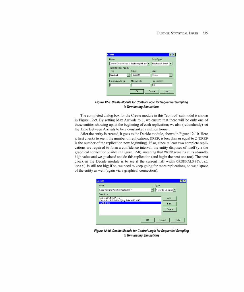
535FURTHER STATISTICAL ISSUES
Figure 12-9. Create Module for Control Logic for Sequential Samplingin Terminating Simulations
The completed dialog box for the Create module in this “control” submodel is shownin Figure 12-9. By setting Max Arrivals to 1, we ensure that there will be only one ofthese entities showing up, at the beginning of each replication; we also (redundantly) setthe Time Between Arrivals to be a constant at a million hours.
After the entity is created, it goes to the Decide module, shown in Figure 12-10. Hereit first checks to see if the number of replications, NREP, is less than or equal to 2 (NREPis the number of the replication now beginning). If so, since at least two complete repli-cations are required to form a confidence interval, the entity disposes of itself (via thegraphical connection visible in Figure 12-8), meaning that MREP remains at its absurdlyhigh value and we go ahead and do this replication (and begin the next one too). The nextcheck in the Decide module is to see if the current half width ORUNHALF(TotalCost) is still too big; if so, we need to keep going for more replications, so we disposeof the entity as well (again via a graphical connection).
Figure 12-10. Decide Module for Control Logic for Sequential Samplingin Terminating Simulations
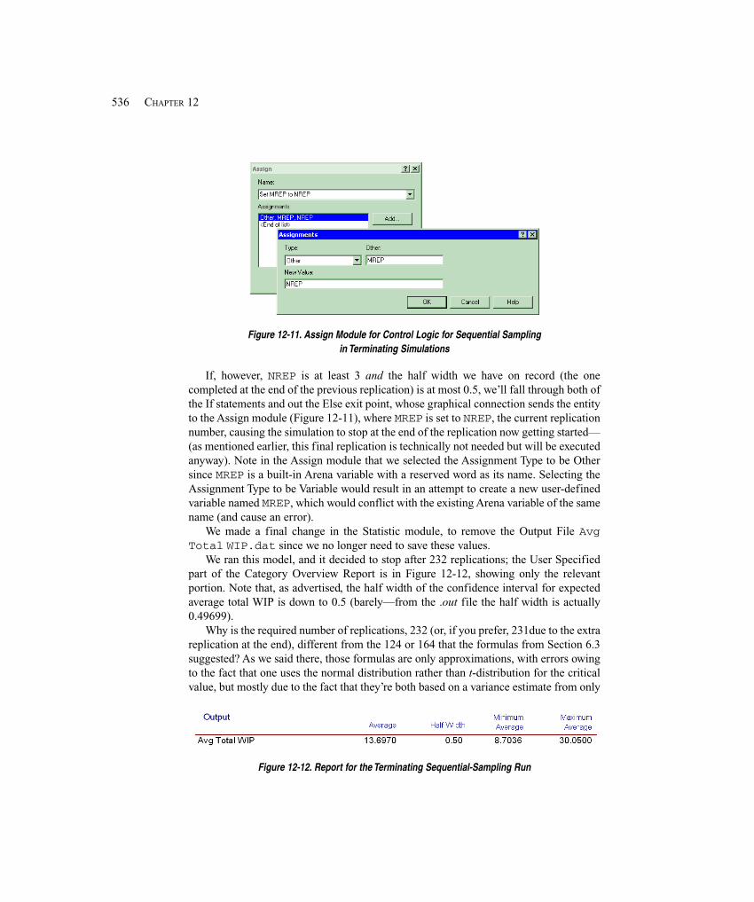
536 CHAPTER 12
Figure 12-11. Assign Module for Control Logic for Sequential Samplingin Terminating Simulations
If, however, NREP is at least 3 and the half width we have on record (the onecompleted at the end of the previous replication) is at most 0.5, we’ll fall through both ofthe If statements and out the Else exit point, whose graphical connection sends the entityto the Assign module (Figure 12-11), where MREP is set to NREP, the current replicationnumber, causing the simulation to stop at the end of the replication now getting started—(as mentioned earlier, this final replication is technically not needed but will be executedanyway). Note in the Assign module that we selected the Assignment Type to be Othersince MREP is a built-in Arena variable with a reserved word as its name. Selecting theAssignment Type to be Variable would result in an attempt to create a new user-definedvariable named MREP, which would conflict with the existing Arena variable of the samename (and cause an error).
We made a final change in the Statistic module, to remove the Output File AvgTotal WIP.dat since we no longer need to save these values.
We ran this model, and it decided to stop after 232 replications; the User Specifiedpart of the Category Overview Report is in Figure 12-12, showing only the relevantportion. Note that, as advertised, the half width of the confidence interval for expectedaverage total WIP is down to 0.5 (barely—from the .out file the half width is actually0.49699).
Why is the required number of replications, 232 (or, if you prefer, 231due to the extrareplication at the end), different from the 124 or 164 that the formulas from Section 6.3suggested? As we said there, those formulas are only approximations, with errors owingto the fact that one uses the normal distribution rather than t-distribution for the criticalvalue, but mostly due to the fact that they’re both based on a variance estimate from only
Figure 12-12. Report for the Terminating Sequential-Sampling Run
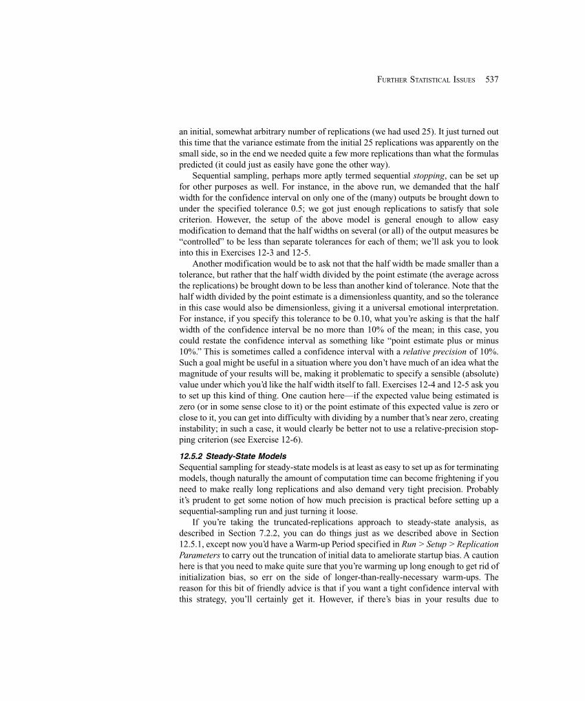
537FURTHER STATISTICAL ISSUES
an initial, somewhat arbitrary number of replications (we had used 25). It just turned outthis time that the variance estimate from the initial 25 replications was apparently on thesmall side, so in the end we needed quite a few more replications than what the formulaspredicted (it could just as easily have gone the other way).
Sequential sampling, perhaps more aptly termed sequential stopping, can be set upfor other purposes as well. For instance, in the above run, we demanded that the halfwidth for the confidence interval on only one of the (many) outputs be brought down tounder the specified tolerance 0.5; we got just enough replications to satisfy that solecriterion. However, the setup of the above model is general enough to allow easymodification to demand that the half widths on several (or all) of the output measures be“controlled” to be less than separate tolerances for each of them; we’ll ask you to lookinto this in Exercises 12-3 and 12-5.
Another modification would be to ask not that the half width be made smaller than atolerance, but rather that the half width divided by the point estimate (the average acrossthe replications) be brought down to be less than another kind of tolerance. Note that thehalf width divided by the point estimate is a dimensionless quantity, and so the tolerancein this case would also be dimensionless, giving it a universal emotional interpretation.For instance, if you specify this tolerance to be 0.10, what you’re asking is that the halfwidth of the confidence interval be no more than 10% of the mean; in this case, youcould restate the confidence interval as something like “point estimate plus or minus10%.” This is sometimes called a confidence interval with a relative precision of 10%.Such a goal might be useful in a situation where you don’t have much of an idea what themagnitude of your results will be, making it problematic to specify a sensible (absolute)value under which you’d like the half width itself to fall. Exercises 12-4 and 12-5 ask youto set up this kind of thing. One caution here—if the expected value being estimated iszero (or in some sense close to it) or the point estimate of this expected value is zero orclose to it, you can get into difficulty with dividing by a number that’s near zero, creatinginstability; in such a case, it would clearly be better not to use a relative-precision stop-ping criterion (see Exercise 12-6).
12.5.2 Steady-State ModelsSequential sampling for steady-state models is at least as easy to set up as for terminatingmodels, though naturally the amount of computation time can become frightening if youneed to make really long replications and also demand very tight precision. Probablyit’s prudent to get some notion of how much precision is practical before setting up asequential-sampling run and just turning it loose.
If you’re taking the truncated-replications approach to steady-state analysis, asdescribed in Section 7.2.2, you can do things just as we described above in Section12.5.1, except now you’d have a Warm-up Period specified in Run > Setup > ReplicationParameters to carry out the truncation of initial data to ameliorate startup bias. A cautionhere is that you need to make quite sure that you’re warming up long enough to get rid ofinitialization bias, so err on the side of longer-than-really-necessary warm-ups. Thereason for this bit of friendly advice is that if you want a tight confidence interval withthis strategy, you’ll certainly get it. However, if there’s bias in your results due to

538 CHAPTER 12
insufficient warm up, your sequentially-determined confidence intervals will betightening down around a biased point, meaning that the nice tight interval you get islikely to miss the mark in terms of covering the steady-state expected value. Anddepressingly, the tighter you make your interval, the worse this problem gets since thebias stays present but the interval gets smaller and thus more likely to miss the steady-state expectation of interest. Thus, the harder you work, the worse off you are in terms ofconfidence-interval coverage probability.
So, unless you’re quite confident that you’ve pretty much eliminated start-up bias, itmight be safer to set up a single long run that you then keep extending until the halfwidth of the resulting confidence interval satisfies your smallness criterion. In this case,the batch-means confidence intervals that Arena attempts to form from a single long run(Section 7.2.3) work quite nicely for this purpose. The key is the Run > Setup >Replication Parameters Terminating Condition field, where you specify the half-widthsmallness criterion (and remove all other replication-stopping devices from your model,such as the Replication Length field in Run > Setup > Replication Parameters). Thepertinent internal Arena variables for this are THALF(Tally ID), which returns thecurrent half width of the 95% confidence interval on a Tally statistic with Tally ID in itsargument, and DHALF(Dstat ID) for DSTAT (time-persistent) output statistics. Thebatching/rebatching scheme described in Section 7.2.3 takes over and your run will stopas soon as the Terminating Condition is satisfied. If a particular run length along the wayis not long enough to form a valid batch-means confidence interval, causing this schemeto conclude “(Insufficient)” or “(Correlated)” as described in Section 7.2.3, thenumerical value of the half-width variable is set by Arena to a huge number; this willcause your replication to be extended since the half width appears too large, which is thebehavior you want.
To illustrate this, let’s create Model 12-4 by modifying Model 7-4 from Section 7.2.3,which was originally set up for a single long run of 50 days of which the first two daysare discarded as a Warm-up Period. Our result from Section 7.2.3 was a 95% batch-means confidence interval of 13.6394 ± 1.38366 on steady-state expected average totalWIP. How about extending the run long enough for the half width to drop to 1, forexample? Making this change involves only a couple of modifications in Run > Setup >Replication Parameters, as shown in Figure 12-13. We’ve cleared the Replication Lengthfield (its default of “Infinite” appears after closing the dialog box) and filled in theTerminating Condition field with the stopping rule we want, DHALF(Total WIP) <1.0. We also removed the Output File Total WIP History One Long Run.datfrom the Statistic data module since we no longer need to save these values.
Part of the report is in Figure 12-14 and indicates that the desired precision for theTotal WIP output measure was indeed achieved, though again only barely, as we’dexpect from a sequential stopping rule. To achieve this, the model decided to extend itsrun length to almost 99 days (142148.4917 minutes, to be more precise), in comparisonwith the original 50-day run.
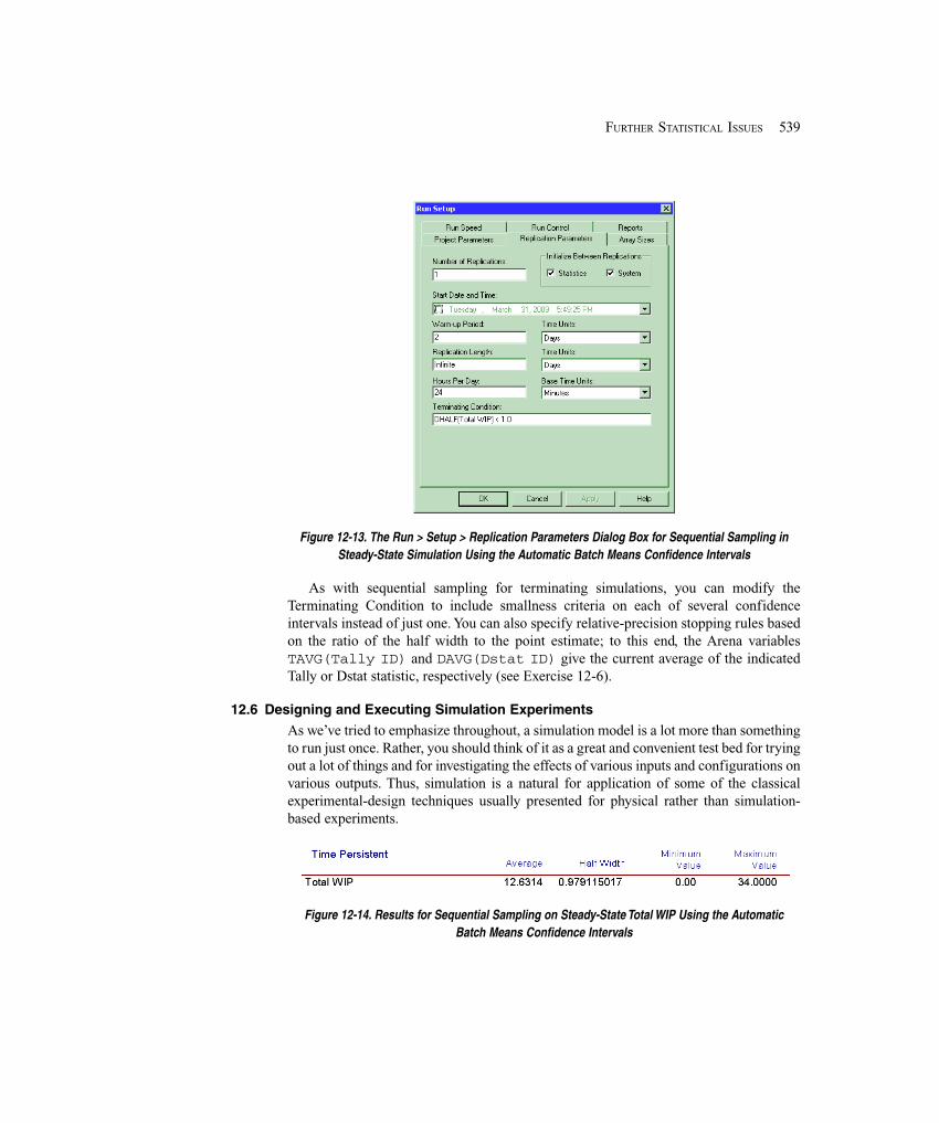
539FURTHER STATISTICAL ISSUES
Figure 12-13. The Run > Setup > Replication Parameters Dialog Box for Sequential Sampling inSteady-State Simulation Using the Automatic Batch Means Confidence Intervals
As with sequential sampling for terminating simulations, you can modify theTerminating Condition to include smallness criteria on each of several confidenceintervals instead of just one. You can also specify relative-precision stopping rules basedon the ratio of the half width to the point estimate; to this end, the Arena variablesTAVG(Tally ID) and DAVG(Dstat ID) give the current average of the indicatedTally or Dstat statistic, respectively (see Exercise 12-6).
12.6 Designing and Executing Simulation Experiments
As we’ve tried to emphasize throughout, a simulation model is a lot more than somethingto run just once. Rather, you should think of it as a great and convenient test bed for tryingout a lot of things and for investigating the effects of various inputs and configurations onvarious outputs. Thus, simulation is a natural for application of some of the classicalexperimental-design techniques usually presented for physical rather than simulation-based experiments.
Figure 12-14. Results for Sequential Sampling on Steady-State Total WIP Using the AutomaticBatch Means Confidence Intervals

540 CHAPTER 12
For instance, consider a model with five different input parameters or configurations.You’d like to know what the effect is on the results of changing a parameter or configura-tion from one level to another. Viewing the inputs and configurations as experimentalfactors, you could specify two possible levels for each and carry out a 25 factorial design,from which you could measure the main effects of and possible interactions between theinput factors on the outputs of interest, which are the responses for this simulation-basedexperiment. Unlike most physical experiments, you could then easily go on and replicatethe whole factorial experiment to place confidence intervals around the expected maineffects and interactions. Other possibilities include using common random numbersacross the design points (as a blocking variable in experimental-design terminology), theuse of screening designs to sort out which of many factors are really important, andsophisticated nonlinear and response-surface designs. For more on these and relatedissues, see Law and Kelton (2000).
12.7 Exercises
12-1 Modify Model 12-2 for a different way to allocate random numbers to supportsynchronization for CRN, as follows. When a new part arrives, (pre-)generate and storein attributes of this entity its processing-time requirements for all of the cells in itssequence. When a part entity gets to a cell, take its processing time from the appropriateattribute of the entity rather than generating it on the spot. Depending on how you set thisup, it might be useful to recall that the attribute Entity.JobStep of an entity is its stationnumber (1, 2, 3, ...) as it makes its way through the sequence. You might also find usefulthe Attributes element from the Elements panel to define a vector-valued attribute; toassign values to elements of this vector in an Assign module, you’ll need to choose theType to be Other. Use the same random-number-stream allocation as in Model 12-1.
12-2 In Exercise 12-1, is it necessary to have dedicated random-number streams inorder to achieve proper synchronization? Discuss this issue, experimenting with someexamples if appropriate.
12-3 Modify Model 12-3 from Section 12.5.1 to demand, in addition to the 95%confidence-interval half width on the expected average total WIP being no more than0.4, that the half width of the 95% confidence intervals on expected average total time insystem (for all part types combined) be no more than 3 minutes. One way to do this is tomodify the Decide module in Figure 12-10 by adding an additional Condition to keepreplicating (i.e., dispose of the checking entity) if any half width is still too big.
12-4 Modify Model 12-3 from Section 12.5.1 to demand instead that the ratio of the95% confidence-interval half width to the point estimate on the expected average totalWIP be less than 0.04, as described at the end of Section 12.5.1; i.e., form a 4% relative-precision confidence interval. The Arena variable ORUNAVG(Output ID) is the averageacross all completed replications of the output measure with this Output ID.
12-5 Combine Exercises 12-3 and 12-4, as follows. Set up a sequential-sampling run sothat you get 4% relative-precision confidence intervals on both the expected averagetotal WIP as well as on the expected total time in system.

541FURTHER STATISTICAL ISSUES
12-6 Modify Model 12-4 from Section 12.5.2 to terminate the replication when the ratioof the half width to the midpoint (point estimate) of the automatic batch-means run-timeconfidence interval on steady-state expected total WIP falls below 0.04; i.e., when therelative precision is 4%. The Arena variable DAVG(Dstat ID) returns the current averageof the indicated Dstat (i.e., time-persistent) statistic. Note that the condition you want tocheck is of the form H/A < 0.04, where H is the half width and A is the point estimate,which can be an uncomfortable calculation if A = 0 (which it will be at the start of yourrun). Instead, check the condition in its equivalent form, H < 0.04 A.
12-7 As noted in Section 12.4.1, Chance-type Decide modules use random-numberstream 10 for their hypercoin flips, and there’s no way to change that in the module.Describe (in words) how you could work around this to use whatever stream you want toaccomplish the same thing. Also, build a useless little Arena model (but one that runs)that does the same thing as a Decide module flipping a four-sided hypercoin withprobabilities 0.2, 0.5, 0.1, and 0.2 for outbound routes A, B, C, and D, respectively,except using random-number stream 77. Verify that your model produces decisions withprobabilities that are about right.

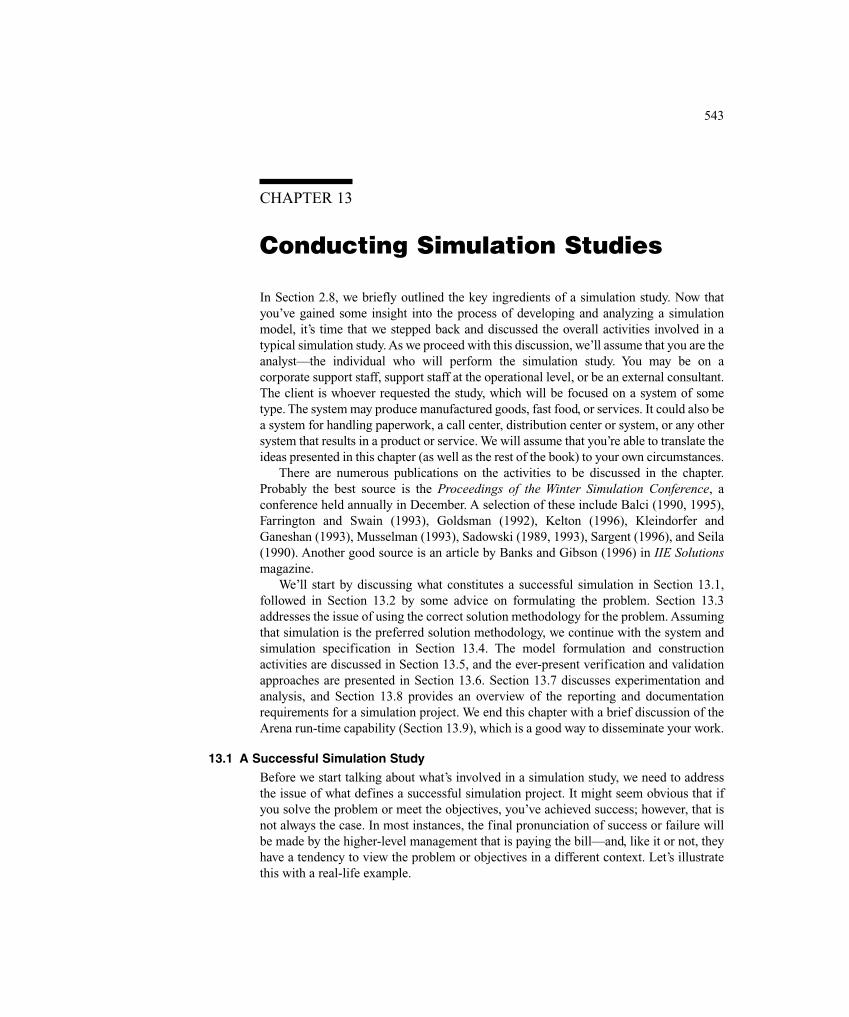
543CONDUCTING SIMULATION STUDIES
CHAPTER 13
Conducting Simulation Studies
In Section 2.8, we briefly outlined the key ingredients of a simulation study. Now thatyou’ve gained some insight into the process of developing and analyzing a simulationmodel, it’s time that we stepped back and discussed the overall activities involved in atypical simulation study. As we proceed with this discussion, we’ll assume that you are theanalyst—the individual who will perform the simulation study. You may be on acorporate support staff, support staff at the operational level, or be an external consultant.The client is whoever requested the study, which will be focused on a system of sometype. The system may produce manufactured goods, fast food, or services. It could also bea system for handling paperwork, a call center, distribution center or system, or any othersystem that results in a product or service. We will assume that you’re able to translate theideas presented in this chapter (as well as the rest of the book) to your own circumstances.
There are numerous publications on the activities to be discussed in the chapter.Probably the best source is the Proceedings of the Winter Simulation Conference, aconference held annually in December. A selection of these include Balci (1990, 1995),Farrington and Swain (1993), Goldsman (1992), Kelton (1996), Kleindorfer andGaneshan (1993), Musselman (1993), Sadowski (1989, 1993), Sargent (1996), and Seila(1990). Another good source is an article by Banks and Gibson (1996) in IIE Solutionsmagazine.
We’ll start by discussing what constitutes a successful simulation in Section 13.1,followed in Section 13.2 by some advice on formulating the problem. Section 13.3addresses the issue of using the correct solution methodology for the problem. Assumingthat simulation is the preferred solution methodology, we continue with the system andsimulation specification in Section 13.4. The model formulation and constructionactivities are discussed in Section 13.5, and the ever-present verification and validationapproaches are presented in Section 13.6. Section 13.7 discusses experimentation andanalysis, and Section 13.8 provides an overview of the reporting and documentationrequirements for a simulation project. We end this chapter with a brief discussion of theArena run-time capability (Section 13.9), which is a good way to disseminate your work.
13.1 A Successful Simulation Study
Before we start talking about what’s involved in a simulation study, we need to addressthe issue of what defines a successful simulation project. It might seem obvious that ifyou solve the problem or meet the objectives, you’ve achieved success; however, that isnot always the case. In most instances, the final pronunciation of success or failure willbe made by the higher-level management that is paying the bill—and, like it or not, theyhave a tendency to view the problem or objectives in a different context. Let’s illustratethis with a real-life example.
544 CHAPTER 13
An automotive supplier had developed a highly successful process for producing aspecialized set of parts for the automotive OEM (original equipment manufacturer) andafter market. The process was implemented using a high-volume, semi-automatedmanufacturing cell concept. Although the process produced a high-quality, low-cost part,the initial system was not achieving a high utilization for the key, and most expensive,piece of equipment in the process. Because of the variability in the types and quantitiesof parts being produced and the processing times of those parts, simulation was chosenas an analysis tool. The objective was to re-design the existing system or to design a newproduction system that would make better use of the key equipment—in other words, asystem that would achieve the same quality, but at a lower production cost per part. Asecondary objective was to devise a way to allow incremental increases in productionvolume by adding equipment to the system gradually, rather than just building a new cell.
The simulation study was undertaken, and after an extensive analysis of the existingsystem, it was determined that it was not possible to achieve the desired results with thecurrent cell concept. The simulation was then used to develop, design, and analyzeseveral new approaches. This resulted in a totally different production system design thatultimately was recommended to management as the production system of the future.This new system design met all the objectives, and the simulation study was pronounceda success by the project team. Management accepted the team’s recommendation andauthorized the construction of a system using the new design concept. The new systemwas built, but did not function as projected, causing management to pronounce thesimulation study a failure since the new system, which was built based on the results ofthe simulation, did not meet expectations. In fact, the resulting production output wasabout 30% lower than projected.
So what happened? Fortunately for the reputation of simulation, the simulation teamwas directed to conduct a post-analysis of the system. The simulation model of the newsystem was dusted off and compared to the actual system, which now existed. Thesimulation was modified to represent the system as it was actually constructed, and muchto the surprise of the simulation team, it predicted that the new system would produceexactly the volume that it was currently producing. So they looked at the modificationsthat were made to the simulation model and found that they could classify thesemodifications into two groups.
The first group of model modifications was composed of required data changes to themodel based on measurements of actual operation times occurring in the new system. Asis often the case, several new types of equipment were included in the new system design,and the vendors who provided this new equipment were rather optimistic in their estimatesof operation times. This accounted for about a third of the resulting production loss.
The second group of model modifications was composed of changes in the actualsystem design that was implemented. As it turns out, there were two critical errors madein the new system design. One was caused because the placement of the new system didnot allow for sufficient floor space as called for by the simulation design. Thus, thesystem design was modified to allow it to fit into the available space. The second errorwas due to changes requested by upper-level management in an attempt to decrease the
545CONDUCTING SIMULATION STUDIES
overall cost of the new system. These changes accounted for the remaining two thirds ofthe production loss.
So what are the lessons to be learned? First, the simulation team should haverecognized that the operation times for the new equipment were only estimates, and theyshould have conducted a sensitivity analysis of the model outputs to these input data. Thiswould have predicted a potential problem if the actual times were greater than the vendor-supplied estimates. If the times were critical, a penalty clause could have been included inthe contract for the new equipment stipulating that it perform as estimated. Second, thesimulation team should have tracked the implementation of the new system. This wouldhave allowed them to evaluate the proposed modifications before implementation. It mightnot have changed the results, but at least it would have predicted the outcome.
Let’s return to the initial issue of what defines a successful simulation project.Success seldom means that a good simulation model was developed. It more often meansthat the simulation study met the objectives set forth by the decision makers. This impliesthat it is very important to understand which metrics they will use.
If you’re asked to undertake a simulation study to redesign a current system, inquirefurther to gain a better understanding of what is expected. If that inquiry results in astatement that indicates that management is interested in finding out if it is possible tomake the system perform better, find out what “better” means. If better means that youare expected to reduce WIP (work in process) by 30%, reduce cycle times by 20%,increase resource utilizations by 15%, and meet all future customer due dates withoutany capital investment, you at least know that you’re facing an impossible mission. Werecommend that you elect not to accept the assignment. If, however, “better” means thatthe primary measures are WIP, cycle times, resource utilizations, and customer due datesbalanced against capital investment, you at least have a fighting chance of designing abetter system.
Unfortunately, you are seldom asked if you want to do the study; in most cases, youare just told to do the study. Even under these circumstances, you should identify thedecision maker and attempt to define the metrics by which the project will be measured.
If you’re about to undertake the first simulation study for a company or facility, it’scritical that it result in a success. If the first simulation study is labeled a failure, it isunlikely that a second study will ever be started. If you have a choice of simulation projects,select one that is simple and is almost guaranteed to result in a success. Once you haveachieved several successes, you might be able to afford a failure (but not a disaster).
There is also a peculiar dilemma frequently faced by the experienced simulationanalyst. If you use simulation as a standard tool through the design of a new system andthe new system works as advertised, what have you saved? If you had not usedsimulation, would the results have been any different? You really don’t know. So the toolworked, or at least you think it did, but you have no way of quantifying any savingsresulting from the application of the tool.
The one approach that is often suggested, but seldom used, is not to use simulationfor the design of the next new system. The assumption here is that the resulting systemwill not perform as advertised. After it’s clear that the system has problems, usesimulation to show how the system should have been designed. This would allow you to
546 CHAPTER 13
quantify the savings had you used simulation. This is clearly an extreme approach—andnot recommended by us—that’s based on numerous assumptions. Of course, there isalways the possibility that the system will perform just fine. (It can happen!) This wouldleave the value of simulation in even greater doubt in the eyes of management.
We close this section by again suggesting that you be aware that your definition ofsuccess may not be the same as that used by management. Although you may not be ableto control management’s evaluation, at least you should try to understand what measure-ments they will use in making their evaluation. Now let’s proceed with our discussion ofthe key activities of a good simulation study.
13.2 Problem Formulation
The first step in any problem-solving task is to define and formulate the problem. In thereal world, you are rarely handed some sheets of paper that completely define theproblem to be solved. Most often you (the analyst) will be approached by someone (theclient) who thinks that you might be able to help them. The initial problem is rarelydefined clearly. In fact, it may not even be obvious that simulation is the proper tool. Atthis point, you need to be able to open a dialog with the requester, or their designate, andbegin asking a series of questions that will ultimately allow you to define the problemcompletely. Often, the final problem you end up addressing is quite different from theone that was initially presented.
Many simulation studies deal with systems that are not meeting the client’sexpectations. The client wants to know: How do I fix it? Other simulation studies are notfocused on a known problem, but are trying to avoid a potential future problem. This ismost often the case when you’re using simulation to help design a new system. Yetanother class of simulation studies is composed of those focused on a system that hasbeen completely designed, but not yet constructed or implemented. In this case, you’rebeing asked if the system will perform as predicted.
So the problems are often put forth in the form of a series of questions: Can you fixit? Will it work? Can you help me make sure it will work? These are really the best kindsof problems because you have the potential to have an impact on the system (and yourcareer). The worst kind of problem is when you’re told that the company wants to startusing simulation, so they’ve requested that a simulation be developed for an arbitrarysystem.
Let’s assume that you have at least a vague notion of what the problem is, andhopefully, a better idea of what the system is. It might be a good idea to start with thesystem. Does the system currently exist, is it a new design, or has it not yet beendesigned? Knowing this, you can try to bound the system for the purpose of the study. Isthe system a single or a small number of operations, a large department, the entirefacility, or the entire company? Although it would be nice if you could draw walls aroundthe system so that there are no interactions with the other side of the wall (like the GreatWall of China), this is not likely to be the case. However, you might at least try to placeinitial bounds on the size of the system. Try not to cast these boundaries in stone, as youmay have to expand or contract them as you learn more about the problem and system.
547CONDUCTING SIMULATION STUDIES
Having established some initial boundaries, next try to define the performancemetrics. There are really two kinds of metrics with which you should be concerned. Thefirst, and most obvious, are the performance metrics that will be used to measure thequality of the system under study. The second, and maybe the most important, are theperformance metrics that will be used to measure the success of the study. Let’sconcentrate on the first kind of metrics. Although the client might imply that there is onlyone metric, there are almost always several that need to be considered. For example, theapplication may be a fast-food restaurant where the client is interested in being assuredthat any customer who enters the door receives his food within a given period of time.This is most likely not just a performance metric, but a performance objective. Othermetrics of interest could be the staffing required, the job assignments, the seatingcapacity, and the freshness of the food.
Having established how the performance of the system is to be measured, find out ifthere are current baseline values for these metrics. These values should be available if thesystem currently exists. If not, there may be similar existing systems that could be usedto provide estimates. In the worst case, at least design values should be available.Knowing what the current baseline metrics are (or at least using an estimate), what arethe expectations of the client? This type of information should provide some insight as tothe magnitude of the problem you have been handed.
By this time, you should have a fairly good understanding of the system (and its size),the performance metrics, and the expectations of the client. The next step is to select asolution methodology—don’t assume that you will always use simulation.
13.3 Solution Methodology
We’re not going to attempt to describe every problem-solution technique known tohumanity and recommend where they should be used. However, we do recommend thatyou at least consider alternative solution techniques. You should also give someconsideration to the cost of using a particular solution technique compared to thepotential benefits of the eventual solution. Unfortunately, identifying the best solutionmethodology is not always an easy task. If you determine that a specific methodologymight give you the best answer, but you have never used that technique, this might not bethe best time to experiment. Therefore, you might want to rephrase the question: Giventhe solution methodologies that you feel comfortable using, which will most likely givethe most cost-effective solution?
Sometimes the choice is obvious, at least to us. For example, if you’re being asked toperform a rough-capacity analysis of a proposed system, and you’re given only meanvalues for all the system parameters and you are only interested in average utilizations, itmight be faster (and just as accurate) to use a calculator to determine the answer. At theother extreme, you might be asked to find the set of optimal routes for a fleet of schoolbuses or garbage trucks. Although you could use simulation, there are other toolsspecifically designed to solve this problem. We would suggest you consider purchasing aproduct to implement such a tool.
You might first find out how much time you have to analyze the problem. If you needan answer immediately, then simulation is not normally an option. We hedged a little bit
548 CHAPTER 13
on this because there are rare circumstances where simulation can be used to analyzeproblems quickly. You might have a very simple problem, or a very small system, whichallows you to develop a simulation using the Arena high-level constructs in just a fewhours.
There are also instances where companies have devoted effort to develop genericsimulation models that can be altered quickly. These types of models are typically devel-oped when there are many similar systems within an organization. A generic simulationis then developed that can be used to model any of these systems by simply changing thedata. The task of changing the data can be made very easy if the values are contained inan external file or program. This external source might be a text file or a spreadsheet.Instances where this approach has been used include assembly lines, warehousing, fastfood, distribution centers, call centers, and manufacturing cells. An even more elegantapproach is based on the development of a company-specific template. This method wasbriefly discussed in Section 10.5.5.
Let’s assume that simulation is the correct technique for the problem. Now you needto define the system and the details of the resulting simulation.
13.4 System and Simulation Specification
So far we may have given the impression that a simulation study consists of a series ofwell-defined steps that need to be followed in a specific order, like a recipe from a cook-book. Although most experienced simulation analysts agree that there are usually somewell-defined activities or steps, they are often performed repeatedly in an interactivemanner. You may find that halfway through the development of a simulation, conditionssuddenly change, new information becomes available, or you gain early insight thatspawns new ideas. This might cause you to revisit the problem-formulation phase or toalter the design of your model drastically. This is not all that uncommon, so be preparedto back up and revisit the problem whenever conditions change.
The process of developing a specification can take many forms, depending on thesize of the study, the relationship between the analyst and client, and the ability of bothparties to agree on the details at this early stage. If one individual is playing both roles—client and analyst—this step might be combined with the model formulation andconstruction phases. Although it is still necessary to define and understand the systemcompletely, the development of a formal simulation specification is probably notrequired. However, if you find yourself at the other extreme, where the analyst is anexternal consultant, a formal specification can be very useful for both parties. For thepurpose of the following discussion, let’s assume we’re somewhere between the twoextremes. Let’s further assume that the client and analyst are not the same person and thata written document is to be developed.
Before we proceed, let’s summarize where we are in the process and where we wantto go. We’ve already formulated the problem and defined the objectives of the study.We’ve decided to use simulation as the means to solve our problem, and we’re now readyto define the details of the simulation study that will follow.
A good place to start is with the system itself. If the system exists, go visit the site andwalk through it. The best advice is to look, touch, and ask questions. You want to
549CONDUCTING SIMULATION STUDIES
understand what’s happening and why it’s happening, so don’t be afraid to ask questions,even ones that seem insignificant. Often you’ll find that activities are performed in aspecific way just because that’s the way they’ve always been done, while at other timesyou’ll find that there are very good reasons for a routine. As you learn more about thesystem, start thinking in terms of how you might model these activities. And even moreimportant, think about whether it’s necessary to include certain activities in thesimulation model. At this stage of the process, you’re a systems analyst, not a simulationmodeler. Thus, don’t be afraid to make recommendations that might improve the process.Providing early input that will result in only minor improvements can increase yourcredibility for the tasks to follow.
If the system is a new design, find out if there are similar existing systems that youmight tour. At the minimum, you’ll obtain a better understanding of the overall processthat you’re about to simulate. If the system exists only on paper, take a tour of the blue-prints. If there’s nothing on paper, develop a process flow diagram or a rough sketch ofthe potential system. You should do this with the client so that there is total agreement onthe specifics of the system.
With an understanding of the system to be modeled, it’s now time to gather allinterested parties in a conference room and develop your specification. There is no magicformula for such a specification, but generally it should contain the following elements:
� Simulation objectives� System description and modeling approach� Animation exactness� Model input and output� Project deliverables
The time required to obtain all the necessary information can vary from an hour to afew days. The discussions that yield the details of this specification should include all theinterested parties. In most cases, the discussions are focused on the system rather thanthe simulation because at this point, it is the one common ground. The types of questionsthat should be asked, and answered, are as follows:
� What is to be included in the simulation model?� At what level of detail should it be included?� What are the primary resources of the system?
What tasks or operations can they perform?� Are process plans or process flow diagrams available?
Are they up to date?Are they always followed?Under what conditions are they not followed?
� Are there physical, technological, or legal constraints on how the system operates?Can they be changed?
� Are there defined system procedures?Are they followed?Can new procedures be considered?
550 CHAPTER 13
� How are decisions made?Are there any exceptions?
� Are there data available?� Who will collect or assemble the data?
When will they be available?What form will they be in?How accurate are the data?Will they change, and if so, how will they change?
� Who will provide data estimates if data are not available?How accurate must they be?Will they require that a sensitivity analysis be conducted?
� What type of animation is required?Are there different animations required at different phases of the project?How will the animations be used?
� Who will verify and validate the model, and how will it be done?Are comparative data available?How accurate are the data?
� What kind of output is required?What are the primary performance measures?Can they be ranked or weighted?
� How general should the model be?Will it be revised for other decisions?
� Who will perform the analysis?What type of analysis is required?How confident do you have to be in your results?
� How many scenarios will be considered?What are they?
� What are the major milestones of the study?When do they need to be completed?
� What are the deliverables?
This is not intended to be a complete list, but it should give you a general idea of thedetail required.
Normally, these types of discussions are enlightening to both parties. In this type offorum, the analyst is asking questions and recording information. The assumption is thatthe client has all, or at least most, of the information required. Experience reveals asomewhat different situation. In most cases, the client is a team of three to six individualsrepresenting different levels of interest in the system. They generally have differentexpertise and knowledge of the system. It is not uncommon to find that these individualsdisagree strongly on some of the details of the system that may generally be confined toprocess descriptions and decision logic, but other areas are not excluded. This should notbe surprising, as you’re trying to get a complete understanding of the system, as well asconsensus on how the system works. If you’re faced with disagreement on certaindetails, we suggest that you stand back and let the client team arrive at a consensus.
551CONDUCTING SIMULATION STUDIES
If you’re developing a specification for the first time, don’t expect to get all youranswers during the initial meeting. You might want to consider the 70/20/10 rule.Through experience, we have found that about 70% of the time the client team will havethe complete answer or the information required. About 20% of the time the team willnot know the answer, but they know how to get it (e.g., they may have to ask Dennis, whoworks on the night shift). The remaining 10% of the time they have no idea what theanswer is or where they might find it (or there are several competing answers). Thismight surprise you, but this is a rather common phenomenon. Don’t let this bother you;just make it clear that you need the information and ask when it will be available.
During this meeting, you’ll also be exploring the availability, or lack thereof, of datato drive your simulation. Again, don’t expect to get all the data you need at this initialmeeting. However, it’s important to know what data ultimately will be available, andwhen. You should also make note of what data are from historical sources and what datawill be estimates. Finally, it might be advisable to identify the form in which the data willbe delivered, as well as who is responsible for collecting, assembling, or observing thedata. For a discussion of data issues, see Section 4.6.2.
Before you leave this meeting, you should identify one person from the client teamwho will serve as the primary contact for the study. When you return to your office,you’ll need to organize the information into a document that resembles a specification.We recommend that you do this as soon as possible, while the details are still fresh inyour mind. Even then you’ll undoubtedly find yourself scratching your head over at leastone item in your notes. Something that was very clear during the meeting may now lookmuddy. No problem! Get on the phone, fax, or e-mail and clarify it with your primarycontact.
Once you’ve developed this document, you should send it to the client for review. Itmay take several iterations before a final document emerges that’s agreed upon andacceptable to both parties. Upon completion, we recommend that both parties sign thisfinal document. If, during the simulation study, you find that conditions change, data arenot available, and so forth, you may find it necessary to revise this document.
We would love to be able to provide you with a detailed set of instructions on how toperform this entire task. Unfortunately, each simulation study is different, andcircumstances really dictate the amount of detail that’s required. We can, however, giveyou an idea of what a specification looks like. We were fortunate to receive permissionfrom The Washington Post to include a functional specification for a simulation study (seeAppendix A) that was developed as part of a consulting project conducted in the mid-1990s by the Systems Modeling consulting group. The original specification wasdeveloped by Scott Miller, a Systems Modeling consultant, for Gary Lucke and OlivierGirod of The Washington Post. Other than a few minor changes made for confidentialityand formatting reasons, it is the original document. We strongly suggest that you take timeto read it before you undertake your first specification. We do not suggest that you usethis form for all of your specifications, but it should provide an excellent starting point.
Throughout this discussion, we made the assumption that it’s possible to define thecomplete study before you start building the actual model. There are circumstanceswhere this is not possible. These types of projects are open ended in that the complete
552 CHAPTER 13
project is not yet defined or the direction of the project depends on the results obtained inthe early phases. Even though it may not be possible to specify the entire projectcompletely, the development of a specification still is often desirable. Of course, it meansthat you may have to amend or expand the specification frequently. As long as bothparties are agreeable, there’s no reason to avoid these types of projects. You just have tobe willing to accept the fact that direction of the project can change dramatically over itsduration. These are often called spiral projects in that they tend to spiral up into hugeprojects or spiral down into no project at all.
For now, let’s assume that you have specified the simulation, and it’s finally time tostart the model.
13.5 Model Formulation and Construction
The nice part of having a complete specification of the simulation model and study is thatit allows you to design the simulation model that can easily meet all of the objectives.Before you open a new model window and begin placing modules, we recommend thatyou spend some time formulating the model design. Some of the things that you want totake into consideration are the data structure or constraints, the type of analysis to beperformed, the type of animation required, and your current comprehension of Arena.The more complex the system, the more important the formulation.
For example, consider a simulation of a large warehouse with 500,000 SKUs. Youwill obviously need to develop a data structure that will contain the necessaryinformation on the changing state of the contents yet be easily accessed by the simulationmodel. If you’re interested only in the number of pickers and stockers required for agiven level of activity, it may not even be necessary to include information at the SKUlevel. You might create a model based on randomly created requests. If you can developaccurate expressions for the frequency and locations of these activities, this type ofmodel might answer your questions. However, if you’re interested in the details of thesystem, you would obviously need to create a much more elaborate model. You also needto understand the animation requirements. If no animation is required, you might modelthe picker movement and activities as a series of delays. If you need a detailed animation,you’ll have to structure your model, most likely using guided transporter constructs, toallow the actual movement and positioning of the pickers on the animation.
You should also consider the potential impact of different scenarios that must beevaluated. Should each scenario be created as a different model, or can a sufficientlygeneral model that requires only data changes be created? Consider our warehouse. Ifyou want to compare a manual picking operation to an automated picking operation, youmay require different models (although you may use the same data structure for bothmodels). However, if you simply want to compare different types of layouts, you mightdevelop a general model.
Once you’ve formulated a modeling approach, you need to consider what constructsyou’re going to use to build your model. So far we’ve advocated a top-down approach.This suggests that your first choice should be modules from the Basic Process panel,followed by modules from the Advanced Process and Advanced Transfer panels, andmodules from the Blocks and Elements panel only when required. This is a recommended
553CONDUCTING SIMULATION STUDIES
approach for the novice Arena user, but as you gain experience and confidence in yourmodeling skills, you’ll most likely take a different approach. Most experienced modelersprefer to start with the Advanced Process and Advanced Transfer panels and select fromthe other panels when required. This allows you to create exactly the type of modelrequired and gives you the maximum amount of flexibility.
Finally, you’re ready to open a new model window and begin the model construction,which is probably the most fun part of the entire study. Before you begin, we’d like tooffer one more piece of advice. As you become more experienced with the Arena system,you’ll start to develop habits—some good, some bad. You’ll tend to use those constructswith which you’re most familiar for every model you create. We recall a consultant whocreated a very detailed model of a complicated assembly system that used a series ofoverhead power-and-free conveyors to move the assembly through the system (this was anumber of years ago). About two days before the model was to be delivered to the client,it developed a bug. The consultant claimed it was caused by extraterrestrial beings, butwe suspect that it was a simple modeling error. Two long, sleepless nights later(accompanied by freely offered, unsolicited advice from the other consultants), the errorwas uncovered. A quick fix was added by using a series of Signal and Hold modules (seeSection 9.4) to synchronize the merging of subassembly conveyors, which solved theproblem. The model was delivered to the client and the study was ultimately a success.
What’s interesting about this extraterrestrial experience is that for the next severalyears, every model (and we mean every model) that the consultant created had at leastone pair of Signal and Hold modules. This habit did not result in inaccurate models, butthere were often simpler and more direct ways to model the system features. Theconsultant had stopped being creative in his model building and always used thoseconstructs that saved his career that fateful night. Essentially, he had developed a badhabit, which, by the way, was extremely hard to break.
Another example that comes to mind occurred around the time that the Arena systemwas first introduced. Prior to that time, the consultants at Systems Modeling developedall their simulation models using the SIMAN language. This required the creation of twoseparate files—the experiment and model files (see Section 7.1.6). Although there wereprograms available to aid in developing these files, almost all the consultants developedtheir models in a text editor. Once their models were running, they’d create the separateanimation of the model using the Cinema software. With the release of the Arena system,you could develop your entire model, including the animation, in one file using thepoint-and-click method with which you’re now familiar. The consultants felt verycomfortable with their text editors and were very reluctant to change their method ofmodeling. In fact, they went so far as to try to convince clients that the old way was thebest way.
Finally, something akin to an edict was passed down stating, “You will use the newArena system for all future models!” There was a lot of grumbling and complaining, butin a very short period of time, they were all working with the new software. In fact,before long you started to hear such comments as, “How did we ever do this beforeArena?” Of course, years later, one individual still claimed that it was easier to develop
554 CHAPTER 13
models in a text editor. We have omitted names to protect the innocent, or the not-so-innocent.
So we recommend that you be open-minded about the methods you use to buildmodels and the constructs that you choose to use. If there are other modelers in yourgroup, ask them how they would approach a new model. You might also considerattending conferences or user-group meetings to find out what your peers are doing.
With that last caution noted, you can start constructing your model. If the model issmall, you might place all the required modules, fill in the required data and hope that itworks right the first time. (It rarely does.) If the system to be modeled requires a large,complicated model, you might try to partition the model building into phases. Select aportion of the system and build a model of that portion, including at least a rough anima-tion. Once you are convinced it’s working correctly, add the next phase. Continue in thismanner until the entire model has been created. This approach makes model verification,which is our next topic, much easier.
13.6 Verification and Validation
Once you have a working model, and sometimes even while you are building it, it is timeto verify and then validate the model. Verification is the task of ensuring that the modelbehaves as you intended; more colloquially, it’s known as debugging the model.Validation is the task of ensuring that the model behaves the same as the real system. Webriefly introduced these topics in Sections 2.7 and 7.1.6. Let’s expand our discussion byfirst addressing the issue of verification.
You now have a completed simulation model, or at least a completed component, andyou’d like to be sure that the model is performing as designed. This may seem to be asimple task, but as your models and the systems they represent become more complicated,it can become very difficult. In larger models, you can have many different simultaneousactivities occurring that can cause interactions that were never intended. You’ll need todesign or develop tests that will allow you to ferret out the offending interactions or justthe plain and simple modeling mistakes. If you haven’t already developed an animation,we suggest that you complete that task before you start the verification phase. It does notneed to be the final animation, but it should have enough detail to allow you to view theactivities that are occurring within the system. You might start by checking the obvious.
Consider the system we modeled in Chapter 7, which produced three different parts.Alter your model so that it creates only a single instance of a Part Type 1, and watch thatsolitary part flow through the system. Repeat this for the other two part types. Change allyour model times to constant values, and release a limited number of parts into thesystem. The results should be predictable. Test the other extreme by decreasing the partinterarrival rate and observe what happens as the system becomes overloaded. Changethe part mix, processing times, failure rates, etc. What you’re trying to do is create a widevariety of different situations where your model logic might just fail. Of course, if youfind problems, correct them. You’ll have to decide if you need to repeat some of yourearlier tests.
555CONDUCTING SIMULATION STUDIES
Once you have completed the obvious tests, you should try to stand back andvisualize what types of scenarios you might consider in your analysis. Replicate theseprojected scenarios as best you can and see if your model still performs adequately. If youhave periods when you’re not using your computer, default the replication time and allowthe simulation to run for extended periods of time. This type of experiment might be bestperformed overnight. Carefully review the results from these runs, looking for hugequeues, resources not utilized, etc. Basically, you want to ask the following question: Dothese results make sense? If you have extended periods of time when you’re at your desk,but not using your computer, allow the model to run with the animation active. As timepermits, glance at the monitor and see if everything appears to be all right. If you areconfident that your model is working correctly, you’re ready for the acid test.
Reconvene the client group and show them your simulation. In most cases, thismeans the animation. If there are problems, this is probably where they will be detected.Once this group grants its blessing, you might try one more experiment before youpronounce your model verified. Ask the group if they’d like to change the model in anyway. Individuals who are familiar with the system, but not simulation, tend to thinkdifferently. They just might suggest modifications that you never considered.
Before you show your model to the client group, you should give some considerationto the level of detail required in the animation. In most cases, a rough animation showingthe basic activities is sufficient. You may have to describe what your animation isshowing, but once the individuals get beyond the pretty pictures, they are often able tovisualize their system. At the same time, be sensitive to the feedback provided by thegroup when they first view the animation. You might be surprised at the types ofreactions you’ll get. We have seen individuals unable to get beyond the fact that yourmachines are blue and their machines are green. If you detect these types of comments,take the time to make some changes. Ultimately, you want the client group to accept yourmodel as an accurate representation of their system. If you’re lucky, they’ll become yourstrongest supporters as you proceed with the project.
At this point, we should probably admit that it’s almost impossible to verify totally amodel for a complex system. We have seen verified models, which have already beenused for extensive analysis, suddenly produce flawed results. This is typically caused bya unique combination of circumstances that was never originally considered beingimposed on the model. Unfortunately, you need at least to consider that all of yourprevious analysis may be inaccurate. We should also point out that there’s no magic toverification, nor is there a single method accepted by all. The key is that you, and yourclient, become totally convinced that the model is working as intended. Having donethat, you are now ready to consider trying to validate the model. Although we are treatingverification and validation as two separate topics or tasks, the difference between the twois often blurred.
In order to validate a simulation model, you should compare the results from yourmodel to the results from the real system. If the system does not yet exist, you’re in troubleright from the start. Even if the system does exist, such a comparison may be a difficulttask. It’s not uncommon for organizations to keep extensive metrics on past systemperformance, but often they do not keep the information that tells you what the system
556 CHAPTER 13
was doing, making, or subject to during that time period. Even if the data exist, they maybe inaccurate or misleading.
Years ago, there was a large and complex simulation model developed for a facilitythat produced heavy-duty transmissions. The facility had approximately 1,400 machinesand resources grouped into about 30 departments. The model had been developed todetermine the sensitivity of product mix on the total throughput and the potential effectof introducing a new product line into the system. The primary performance measureswere all related to the system’s capacity. All of the process plans and process times weredownloaded from the facility’s databases. In addition, all the order releases wereavailable for the last year of production. It looked like it would be an easy task to validatethe model. Having already verified the model, the validation was undertaken.
The first set of runs produced results that totally mystified the clients. There werebottlenecks in the model that did not occur in the real system and bottlenecks in the realsystem that did not show up in the model results. In fact, a detailed comparison ofresource-utilization statistics from the model to the historical records showed that therewere major differences. This problem was resolved rather quickly when it became apparentthat the processing times maintained in the facility’s databases were based on standardtimes used for costing. They in no way represented the actual processing times observed onthe shop floor. Be aware that this is a fairly common problem. Data are often kept for theconvenience of the accountant, not the systems engineer. Luckily, someone had developeda set of conversion tables that converted the standard times to accurate processing times.These tables were included in the model and the validation process continued.
Everything looked good until a simulation run was made for the entire year, and theresults were compared to the historical records. Eleven of the 12 months producedalmost identical results. There was, however, one month near the middle of the simulatedyear where the records indicated that the output was approximately 40% larger than thatpredicted by the simulation model. A lot of time was spent trying to figure out what hadcaused this discrepancy. It was assumed that there was a problem with the simulationmodel—wrong! Finally, the analysis group started to suspect that maybe the historicaldata were flawed. By looking at the detailed statistics for the month in question, itbecame apparent that the resource statistics from the simulation closely matched therecorded statistics. In fact, it was quickly determined that the only difference was in thetotal number of transmissions produced. In addition, everyone was convinced that thesystem did not have the capacity to produce that many units. It took several weeks ofpart-time sleuthing before the answer emerged.
Someone finally realized that the month in question was the last month of thecompany’s fiscal year. As it turned out, there was a small amount of product that wasrejected for various reasons through the first 11 months of the year. These products weresimply set aside until the final month when they suddenly became acceptable and werereported as part of that month’s output. The reasoning was that it improved theperformance of the system for the year. Weeks later these products were formallyrejected, but the previous year’s records were never adjusted. Removing these rejecteditems from the monthly throughput finally allowed the model to be validated.
557CONDUCTING SIMULATION STUDIES
If accurate records on the actual system do not exist, then it may be impossible tovalidate the model. In that case, concentrate on the verification and use the bestjudgment of individuals who are the most familiar with the system’s capability.Sometimes individuals from the production floor have an uncanny ability to predict theperformance of a new system accurately. Remember, the key is for both the analyst andthe client to have confidence in the results from the model.
If you’ve gotten this far with your simulation project, you’ve cleared most of themajor hurdles. You’re now ready to use the model to answer some questions.
13.7 Experimentation and Analysis
We’ve already covered most, if not all, of the statistical issues associated with simulationanalysis, and we’ll not repeat that material here. However, there are several practicalimplications that we would like you to be aware of. Ideally, before you start any analysis,you would design a complete set of experiments that you intend to conduct. You would alsodecide on the types of analysis tools that you would be using. Although this may be ideal,it’s far from reality. In some cases, you just don’t have the luxury of sufficient time; in othercases, you don’t really know where you’re going with the analysis until you get there.
For example, if your objective is to improve the system throughput, you may notknow what changes are required to achieve that goal. Sometimes the best analysismethod is a group of knowledgeable individuals sitting around a computer suggestingand trying alternatives. This normally means that almost all the alternatives that areinvestigated will, at least, be feasible. One problem with this type of approach is that youmay be tempted to reduce run times drastically in order to reduce the time you have towait for the next set of results. Or worse yet, you may want to evaluate the system basedonly on a view of the animation. Don’t yield to this pressure as it can lead to a disaster(and disasters can alter the direction of your career).
You might also consider structuring your experimentation based on the type ofanalysis that needs to be performed. For the sake of this discussion, let’s identify threedifferent types of analysis: candidate, comparative, and predictive.
Candidate analysis is normally done during the early design phases of a system. Youare generally trying to identify the best candidate systems from a much larger group ofpotential designs that merit additional study. Models for these types of analysis arenormally lacking in detail. You might think of these as rough-cut capacity models. You’retrying to weed out the obvious losers and identify the potential winners. When you’reperforming this type of analysis, you can’t put much faith in the accuracy of the truesystem’s performance. You still need to make sure that you have a sufficient number ofreplications to provide good estimates of the system’s performance (or your run times areof sufficient length), but there is very little value in increasing the number of replications(or the run time) to obtain tighter confidence limits on your results.
Comparative analysis would normally be the next logical step in selecting the finalsystem design. You have a finite set of designs, and you want to compare them to identifythe best design. This type of analysis typically requires a more detailed model, but we’reonly concerned with comparing one system to another. For example, there may besystem activities that will affect the performance of the system, but the amount of the
558 CHAPTER 13
effect is common across all systems under consideration. For example, it may not benecessary to incorporate preventive maintenance or operator schedules into these typesof models. The activities that are common to all systems under consideration and havethe same effect do not have to be included in the models. For these types of systems,there may be value in increasing run times (or number of replications) to boost yourconfidence in selecting the best system.
Predictive analysis typically deals with only a few systems—often only one. By thistime, you’ve selected what appears to be the best system, and you’re now interested inestimating the actual performance of that system. This type of analysis requires that youinclude all activities that will affect the system’s ability to achieve the predictedperformance. At this point, you’ve selected the best system, and you’re going forth with arecommendation to build it, provided that it meets the required objectives. These types ofmodels need to be very detailed, and you also need to be confident in the data that arebeing used.
Regardless of the type of analysis you’re conducting, be careful not to make strongjudgments based on limited information. Be sure that your results are based on soundstatistical practice, and when you conclude that one system is better than another, be surethat there is a significant statistical difference between them. More details on these issuesare in Sections 6.4-6.6, 7.2, and 12.4-12.6.
Before proceeding, we find it necessary to point out again that the activities thatconstitute a simulation project appear to follow a logical time pattern. In reality, it’s notuncommon to jump back and forth between activities, often re-visiting activities that youthought were complete. In practice, you often find that a good project will force youthrough several iterations of these activities.
13.8 Presenting and Preserving the Results
When you get to this stage, you’ve completed at least the initial study, and you’re readyto go forth with your results. In many instances, only a written report is required orexpected. In other cases, you may have to go before a group of decision makers and givean informal or formal presentation of your results. This may actually be the mostimportant phase of the project because it may determine whether your results areaccepted. We’re not going to go into great detail about how to write or give a report. Ifyou feel that your skills are lacking, we suggest you find a book devoted to these subjectsor take a formal course to sharpen your skills. You’ll find that you’ll need these types ofskills in many other areas as well! However, there are a few obvious points to be made.
First, be sure you’re addressing the correct questions, and be sure to provide conciseanswers. Always include the equivalent of an executive summary that states yourrecommendations clearly—and the major reasons for them—in one page (or slide) orless. If possible, try to avoid presenting numbers in absolute terms; use ranges orconfidence intervals. Understand your audience before you proceed. If you havevolumes of material to support your recommendations, put them in an appendix or holdthem in reserve (to be used only if requested). Don’t be tempted to answer questionsabout features of the system that were not included in your model. Finally, be prepared toreceive instructions to go back and look at additional alternatives.
559CONDUCTING SIMULATION STUDIES
Preserving the results should be an ongoing task throughout the duration of theproject. Normally, we would call this the documentation process. It should include notonly the final recommendations, but also documentation of the model and the details ofthe analysis. It is true that most simulation projects are not revisited. But there areexceptions, and it is not uncommon to have to dust off an old model years later to performmore analysis. We’re aware of one simulation model developed in 1983, as a SIMANmodel, that’s still being used periodically, even though the model is basically the same.
Most practitioners agree that there’s a law of nature, or maybe even a theorem, aboutdocumentation. The more documentation that you have on a project, the lower theprobability of ever having to use the model again. It always seems to be those crashprojects that leave no time for documentation that you’re asked to resurrect years later.However, if you’ve followed our advice in this chapter, most of your documentation isalready available and in electronic form. If you store all of this information (simulationmodel, specification, report, and presentation) in the same folder, you’ve covered mostof the bases. An alternative is to use the methods described in Chapter 10 to embed theseitems directly into the simulation file.
You might also admit that in most cases the documentation will be used by someoneelse, if it’s used at all. Individuals are promoted, change positions or change organiza-tions, so your best approach to this task is to ask yourself what you’d want or need toknow if someone else had performed the original study. This may not help you, but thenext person will certainly be grateful.
13.9 Disseminating the Model
During the course of a simulation study, you will certainly share your simulation modeland animation with your client. If the clients have a copy of Arena, you only need to sendthem the latest model (.doe) file, and they can view and alter your model at any time. Ifthe clients (or anyone else, for that matter) do not have the software, this obviously won’twork.
Arena does have a run-time mode, which will allow the user to open, run, and viewthe animation and the results of any model. It allows the user to edit any existing data andre-save the model. However, it does not allow the user to add or alter any logic or datamodules. If the run-time version is required, you should contact Rockwell Automationfor more information.

561A FUNCTIONAL SPECIFICATION FOR THE WASHINGTON POST
APPENDIX A
A Functional Specification forThe Washington Post
A.1 Introduction
This appendix contains functional specification material provided to The WashingtonPost as part of a Systems Modeling simulation modeling consulting project (in the mid-1990s, which was prior to acquisition by Rockwell Automation). This project wasdelivered to Gary Lucke, manager of manufacturing systems engineering, and OlivierGirod, manager of industrial engineering, of The Washington Post. This file has beenmodified slightly to retain confidentiality of certain proprietary information. Some of thetechnology will appear dated, but we’ve left its original form from the time of thisproject because the process is unaffected by it.
A.1.1 Document OrganizationThis document is provided to describe the mailroom operations at The Washington Post’sSpringfield, Va., and proposed Maryland facilities. The description will include thedetail necessary to develop accurately an Arena simulation model of both operations.
This document is divided into six sections. The first section defines the objectives ofthe simulation project, the purpose of this document, the use of the Arena model, and thesoftware and hardware required to run the Arena model. The second section describes thephysical components of the mailroom operation, as well as the modeling approaches foreach component. The third section describes the animation of the simulation model. Thefourth section summarizes the user input requirements for the Arena model and thedesired output generated from the Arena model. The fifth section describes the projectdeliverables. Finally, the sixth section contains the agreement and acceptance signaturesrequired to proceed with the project.
A.1.2 Simulation ObjectivesThe objective of the simulation study is to provide The Washington Post with a decisionsupport tool that will assist in evaluating the truck-loading operation at the Springfieldplant as well as the proposed Maryland facility. The simulation will aid in assessing theimpact of press output, tray utilization, tray trip rate, and truck arrival patterns on theloading operations.
In order to obtain the simulation objectives, two simulation models will be developedunder this contract. These models will incorporate actual operational data andinformation collected from the Springfield and Maryland facilities. The simulation willutilize actual production sequences and decision logic required to represent facilityoperations accurately. In addition, the simulation will incorporate the information and
562 APPENDIX A
outputs generated by the AGV Roll Delivery simulation currently under development bySystems Modeling (SM), a material-handling vendor, and the newspaper.
The development of this model requires a number of tasks. Initially, a thoroughunderstanding of the newspaper’s Springfield and Maryland facilities is necessary toconceptualize and develop an accurate representation of this system. This process hasbeen, and will continue to be, a joint effort between The Washington Post and SystemsModeling. This procedure defines the user’s conceptualization of the system that SMwill use to develop the Arena simulation model. Included in this process is defining theinputs and outputs of the model, verifying that the Arena model has been implementedaccurately, and validating that the model accurately represents the facility.
Upon completion of the project, the newspaper will have a tool that will allow ananalyst to specify various operating scenarios for the mailroom facility, executesimulation experiments of the scenarios, and perform statistical analysis of the scenarios.
A.1.3 Purpose of the Functional SpecificationThis functional specification serves four purposes. First and foremost, this documentdescribes the mailroom operation at the newspaper’s Springfield and Maryland facilities,at the level of detail required for modeling purposes. This description includes processflow, equipment functionality, operating procedures and rules, system interactions, andlogistical issues. These systems must be thoroughly understood before they can berepresented in a computer simulation.
Second, the user input required to perform the simulation analysis is defined. Theinput required includes such things as the press behavior, dock allocations, truck loadtime, and other operational characteristics.
Third, the output generated by the computer simulation is defined. Output is gener-ally in the form of system performance measures from which the simulation analysis isperformed. These output statistics include such things as dock utilization, truck loadtimes, tray utilization, etc.
Finally, the project deliverables are described. The deliverables will be contained in athree-ring binder and will include computer diskettes containing the Arena model, inputdata files, hard copies of the data files, a user’s manual to describe how to use thesoftware, and the final report.
This document explicitly defines issues that are part of the quotation and otherunofficial documents exchanged by SM and The Washington Post. Therefore, for thoseissues that are discussed in other documents, this document supersedes allcorrespondence in defining the project.
A.1.4 Use of the ModelThe use of the simulation model will be detailed completely in the user’s manual providedat the completion of the project. Use of the model includes initializing the Arena modeland input files with the desired input parameters, running the model on the computer, andgenerating summary statistics and reports. The summary reports generated from variousruns can be compared to evaluate the impact of specific parameters on systemperformance.
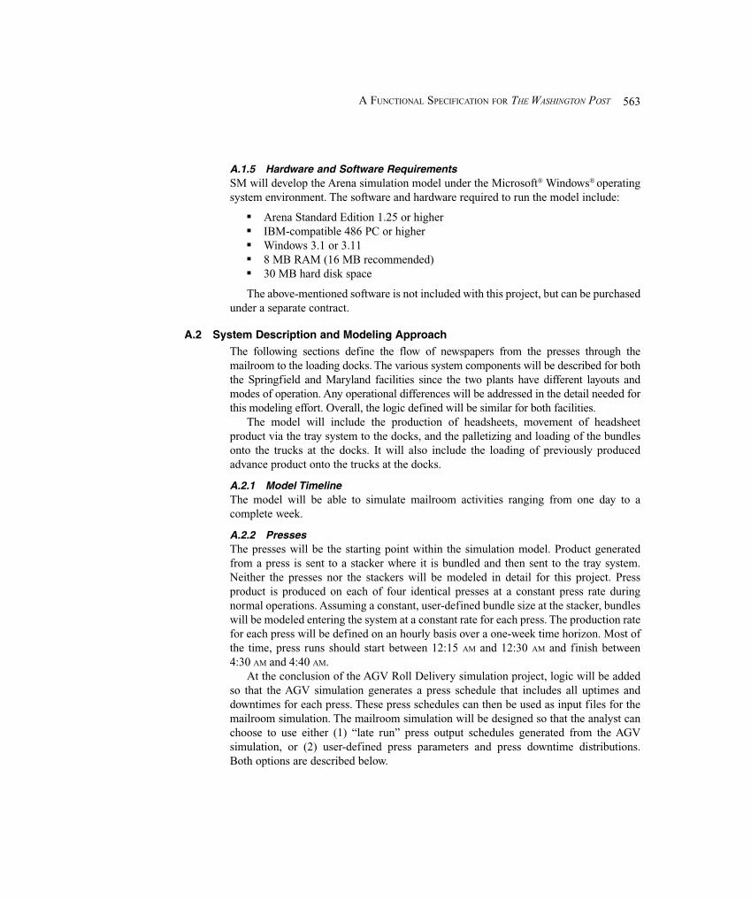
563A FUNCTIONAL SPECIFICATION FOR THE WASHINGTON POST
A.1.5 Hardware and Software RequirementsSM will develop the Arena simulation model under the Microsoft® Windows® operatingsystem environment. The software and hardware required to run the model include:
� Arena Standard Edition 1.25 or higher� IBM-compatible 486 PC or higher� Windows 3.1 or 3.11� 8 MB RAM (16 MB recommended)� 30 MB hard disk space
The above-mentioned software is not included with this project, but can be purchasedunder a separate contract.
A.2 System Description and Modeling Approach
The following sections define the flow of newspapers from the presses through themailroom to the loading docks. The various system components will be described for boththe Springfield and Maryland facilities since the two plants have different layouts andmodes of operation. Any operational differences will be addressed in the detail needed forthis modeling effort. Overall, the logic defined will be similar for both facilities.
The model will include the production of headsheets, movement of headsheetproduct via the tray system to the docks, and the palletizing and loading of the bundlesonto the trucks at the docks. It will also include the loading of previously producedadvance product onto the trucks at the docks.
A.2.1 Model TimelineThe model will be able to simulate mailroom activities ranging from one day to acomplete week.
A.2.2 PressesThe presses will be the starting point within the simulation model. Product generatedfrom a press is sent to a stacker where it is bundled and then sent to the tray system.Neither the presses nor the stackers will be modeled in detail for this project. Pressproduct is produced on each of four identical presses at a constant press rate duringnormal operations. Assuming a constant, user-defined bundle size at the stacker, bundleswill be modeled entering the system at a constant rate for each press. The production ratefor each press will be defined on an hourly basis over a one-week time horizon. Most ofthe time, press runs should start between 12:15 AM and 12:30 AM and finish between4:30 AM and 4:40 AM.
At the conclusion of the AGV Roll Delivery simulation project, logic will be addedso that the AGV simulation generates a press schedule that includes all uptimes anddowntimes for each press. These press schedules can then be used as input files for themailroom simulation. The mailroom simulation will be designed so that the analyst canchoose to use either (1) “late run” press output schedules generated from the AGVsimulation, or (2) user-defined press parameters and press downtime distributions.Both options are described below.
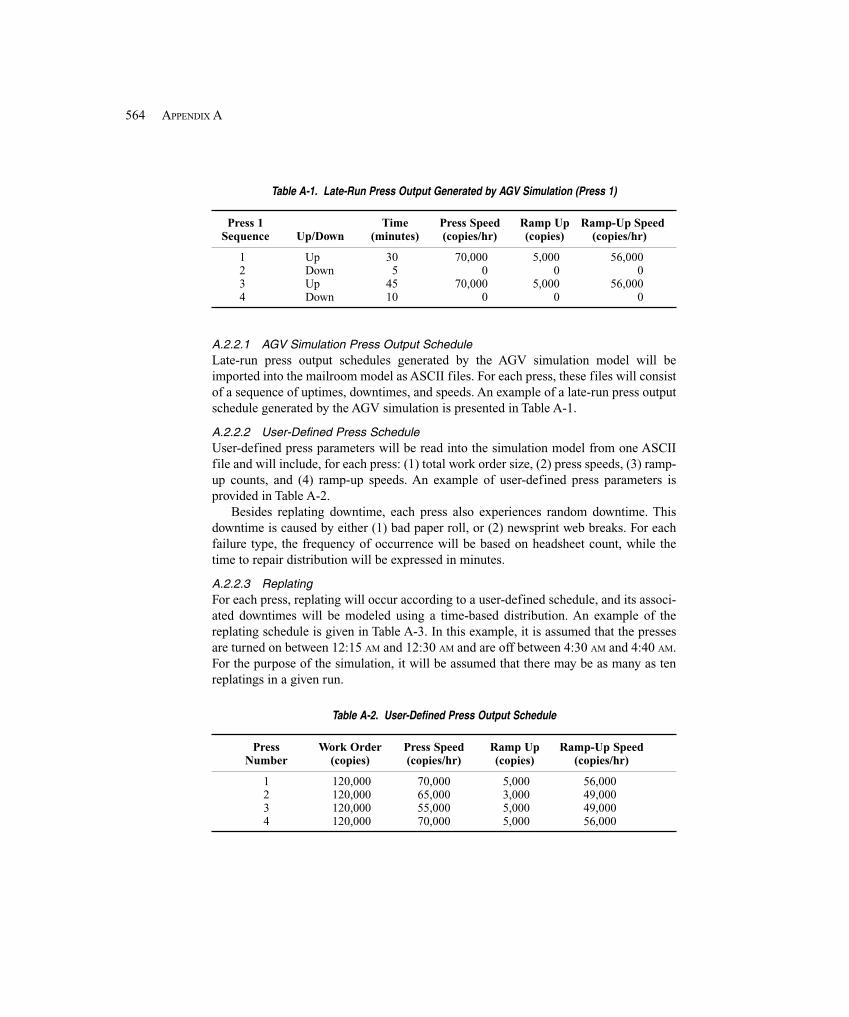
564 APPENDIX A
Table A-1. Late-Run Press Output Generated by AGV Simulation (Press 1)
Press 1 Time Press Speed Ramp Up Ramp-Up SpeedSequence Up/Down (minutes) (copies/hr) (copies) (copies/hr)
1 Up 30 70,000 5,000 56,0002 Down 5 0 0 03 Up 45 70,000 5,000 56,0004 Down 10 0 0 0
A.2.2.1 AGV Simulation Press Output ScheduleLate-run press output schedules generated by the AGV simulation model will beimported into the mailroom model as ASCII files. For each press, these files will consistof a sequence of uptimes, downtimes, and speeds. An example of a late-run press outputschedule generated by the AGV simulation is presented in Table A-1.
A.2.2.2 User-Defined Press ScheduleUser-defined press parameters will be read into the simulation model from one ASCIIfile and will include, for each press: (1) total work order size, (2) press speeds, (3) ramp-up counts, and (4) ramp-up speeds. An example of user-defined press parameters isprovided in Table A-2.
Besides replating downtime, each press also experiences random downtime. Thisdowntime is caused by either (1) bad paper roll, or (2) newsprint web breaks. For eachfailure type, the frequency of occurrence will be based on headsheet count, while thetime to repair distribution will be expressed in minutes.
A.2.2.3 ReplatingFor each press, replating will occur according to a user-defined schedule, and its associ-ated downtimes will be modeled using a time-based distribution. An example of thereplating schedule is given in Table A-3. In this example, it is assumed that the pressesare turned on between 12:15 AM and 12:30 AM and are off between 4:30 AM and 4:40 AM.For the purpose of the simulation, it will be assumed that there may be as many as tenreplatings in a given run.
Table A-2. User-Defined Press Output Schedule
Press Work Order Press Speed Ramp Up Ramp-Up SpeedNumber (copies) (copies/hr) (copies) (copies/hr)
1 120,000 70,000 5,000 56,0002 120,000 65,000 3,000 49,0003 120,000 55,000 5,000 49,0004 120,000 70,000 5,000 56,000
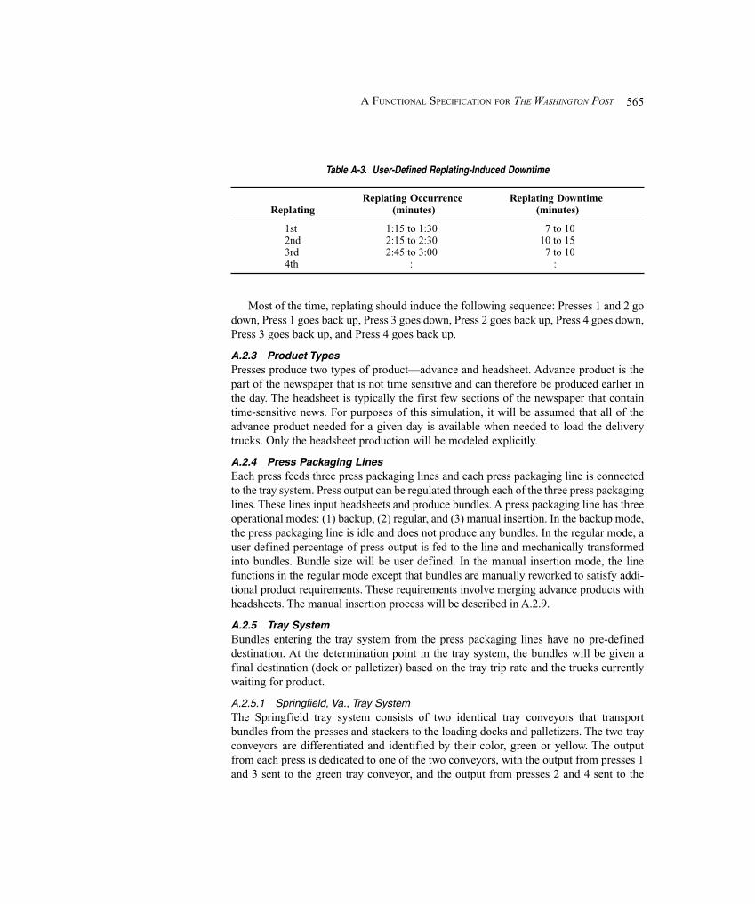
565A FUNCTIONAL SPECIFICATION FOR THE WASHINGTON POST
Table A-3. User-Defined Replating-Induced Downtime
Replating Occurrence Replating DowntimeReplating (minutes) (minutes)
1st 1:15 to 1:30 7 to 102nd 2:15 to 2:30 10 to 153rd 2:45 to 3:00 7 to 104th : :
Most of the time, replating should induce the following sequence: Presses 1 and 2 godown, Press 1 goes back up, Press 3 goes down, Press 2 goes back up, Press 4 goes down,Press 3 goes back up, and Press 4 goes back up.
A.2.3 Product TypesPresses produce two types of product—advance and headsheet. Advance product is thepart of the newspaper that is not time sensitive and can therefore be produced earlier inthe day. The headsheet is typically the first few sections of the newspaper that containtime-sensitive news. For purposes of this simulation, it will be assumed that all of theadvance product needed for a given day is available when needed to load the deliverytrucks. Only the headsheet production will be modeled explicitly.
A.2.4 Press Packaging LinesEach press feeds three press packaging lines and each press packaging line is connectedto the tray system. Press output can be regulated through each of the three press packaginglines. These lines input headsheets and produce bundles. A press packaging line has threeoperational modes: (1) backup, (2) regular, and (3) manual insertion. In the backup mode,the press packaging line is idle and does not produce any bundles. In the regular mode, auser-defined percentage of press output is fed to the line and mechanically transformedinto bundles. Bundle size will be user defined. In the manual insertion mode, the linefunctions in the regular mode except that bundles are manually reworked to satisfy addi-tional product requirements. These requirements involve merging advance products withheadsheets. The manual insertion process will be described in A.2.9.
A.2.5 Tray SystemBundles entering the tray system from the press packaging lines have no pre-defineddestination. At the determination point in the tray system, the bundles will be given afinal destination (dock or palletizer) based on the tray trip rate and the trucks currentlywaiting for product.
A.2.5.1 Springfield, Va., Tray SystemThe Springfield tray system consists of two identical tray conveyors that transportbundles from the presses and stackers to the loading docks and palletizers. The two trayconveyors are differentiated and identified by their color, green or yellow. The outputfrom each press is dedicated to one of the two conveyors, with the output from presses 1and 3 sent to the green tray conveyor, and the output from presses 2 and 4 sent to the
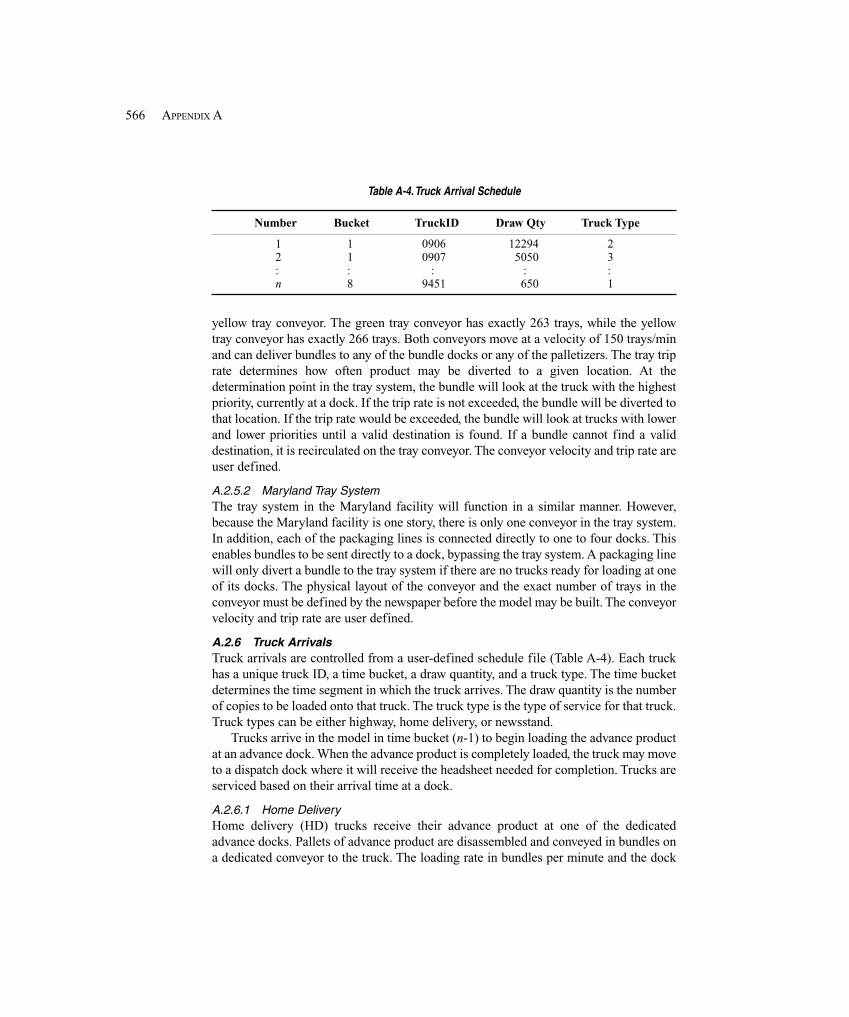
566 APPENDIX A
Table A-4. Truck Arrival Schedule
Number Bucket TruckID Draw Qty Truck Type
1 1 0906 12294 22 1 0907 5050 3: : : : :n 8 9451 650 1
yellow tray conveyor. The green tray conveyor has exactly 263 trays, while the yellowtray conveyor has exactly 266 trays. Both conveyors move at a velocity of 150 trays/minand can deliver bundles to any of the bundle docks or any of the palletizers. The tray triprate determines how often product may be diverted to a given location. At thedetermination point in the tray system, the bundle will look at the truck with the highestpriority, currently at a dock. If the trip rate is not exceeded, the bundle will be diverted tothat location. If the trip rate would be exceeded, the bundle will look at trucks with lowerand lower priorities until a valid destination is found. If a bundle cannot find a validdestination, it is recirculated on the tray conveyor. The conveyor velocity and trip rate areuser defined.
A.2.5.2 Maryland Tray SystemThe tray system in the Maryland facility will function in a similar manner. However,because the Maryland facility is one story, there is only one conveyor in the tray system.In addition, each of the packaging lines is connected directly to one to four docks. Thisenables bundles to be sent directly to a dock, bypassing the tray system. A packaging linewill only divert a bundle to the tray system if there are no trucks ready for loading at oneof its docks. The physical layout of the conveyor and the exact number of trays in theconveyor must be defined by the newspaper before the model may be built. The conveyorvelocity and trip rate are user defined.
A.2.6 Truck ArrivalsTruck arrivals are controlled from a user-defined schedule file (Table A-4). Each truckhas a unique truck ID, a time bucket, a draw quantity, and a truck type. The time bucketdetermines the time segment in which the truck arrives. The draw quantity is the numberof copies to be loaded onto that truck. The truck type is the type of service for that truck.Truck types can be either highway, home delivery, or newsstand.
Trucks arrive in the model in time bucket (n-1) to begin loading the advance productat an advance dock. When the advance product is completely loaded, the truck may moveto a dispatch dock where it will receive the headsheet needed for completion. Trucks areserviced based on their arrival time at a dock.
A.2.6.1 Home DeliveryHome delivery (HD) trucks receive their advance product at one of the dedicatedadvance docks. Pallets of advance product are disassembled and conveyed in bundles ona dedicated conveyor to the truck. The loading rate in bundles per minute and the dock

567A FUNCTIONAL SPECIFICATION FOR THE WASHINGTON POST
setup time in minutes are user defined. After receiving all of the advance product, the HDtruck can proceed to the regular dispatch docks where the same amount of headsheetproduct is loaded. Headsheet bundles arrive via the tray system. The loading rate inbundles per minute and the dock setup time in minutes are user defined. A user-definedpercentage of the HD trucks are deemed to be “slow” and as such have a longer load timeand setup time.
A.2.6.2 HighwayHighway (HWY) trucks are serviced at dedicated highway docks. Entire pallets ofadvance product are loaded by fork trucks onto the HWY trucks. The loading rate inpallets per minute and the wrap-up time (for last pallet) in minutes are user defined.Headsheet product destined for a HWY truck is sent to the palletizer dedicated to thatHWY truck. Pallets are formed and are then loaded onto the truck by fork trucks. Theloading rate and wrap-up time are the same as for the advance pallets. In addition, thereis a dock change time between trucks. A HWY truck remains at a dock until all of itsadvance and headsheet product have been loaded.
A.2.6.3 Newsstand/Street SalesNewsstand/street sales (NS/SS) trucks receive no advance product. Instead, upon arrivalat a dispatch dock, bundles are generated from the manual insertion process. Thesebundles travel via the tray system to the NS/SS truck. Load times and wrap-up times aresimilar to those for the HD trucks.
A.2.7 DocksIn the model, there are three types of docks: (1) pallet, (2) advance bundle, and (3)headsheet bundle. Pallet docks are designed for forktruck access and service HWYtrucks. Advance bundle docks are used to load the advance product onto the trucksduring time bucket (n-1). Headsheet bundle docks are used to load the headsheet productdelivered to the trucks via the tray system. A truck receives press product based on itsarrival time (FIFO) at a given dock area and not its dock location. For each dock type, thenumber of active docks will be user defined.
A.2.7.1 Springfield, Va., DocksThe Springfield facility has exactly 12 dedicated pallet docks, exactly 10 advance bundledocks, and exactly 14 dedicated headsheet bundle docks.
A.2.7.2 Maryland DocksThe proposed Maryland facility has exactly 10 combination pallet and advance bundledocks and 18 dedicated headsheet bundle docks.
A.2.8 PalletizersFor purposes of the simulation, all of the palletizers are assumed to be identical. Apalletizer is used to package headsheet bundles destined for a HWY truck at a palletdock. Each HWY truck at a dock has a dedicated palletizer. For purposes of the model, apalletizer acts as a possible destination for bundles on the tray system. The palletizing ofadvance product will not be modeled in this project. Palletizers operate at a constant rate
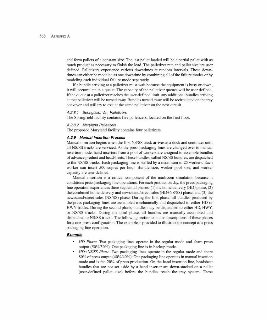
568 APPENDIX A
and form pallets of a constant size. The last pallet loaded will be a partial pallet with asmuch product as necessary to finish the load. The palletizer rate and pallet size are userdefined. Palletizers experience various downtimes at random intervals. These down-times can either be modeled as one downtime by combining all of the failure modes or bymodeling each individual failure mode separately.
If a bundle arriving at a palletizer must wait because the equipment is busy or down,it will accumulate in a queue. The capacity of the palletizer queues will be user defined.If the queue at a palletizer reaches the user-defined limit, any additional bundles arrivingat that palletizer will be turned away. Bundles turned away will be recirculated on the trayconveyor and will try to exit at the same palletizer on the next circuit.
A.2.8.1 Springfield, Va., PalletizersThe Springfield facility contains five palletizers, located on the first floor.
A.2.8.2 Maryland PalletizersThe proposed Maryland facility contains four palletizers.
A.2.9 Manual Insertion ProcessManual insertion begins when the first NS/SS truck arrives at a dock and continues untilall NS/SS trucks are serviced. As the press packaging lines are changed over to manualinsertion mode, hand inserters from a pool of workers are assigned to assemble bundlesof advance product and headsheets. These bundles, called NS/SS bundles, are dispatchedto the NS/SS trucks. Each packaging line is staffed by a maximum of 25 workers. Eachworker can insert 500 copies per hour. Bundle size, worker pool size, and workercapacity are user defined.
Manual insertion is a critical component of the mailroom simulation because itconditions press packaging line operations. For each production day, the press packagingline operation experiences three sequential phases: (1) the home delivery (HD) phase, (2)the combined home delivery and newsstand/street sales (HD+NS/SS) phase, and (3) thenewsstand/street sales (NS/SS) phase. During the first phase, all bundles produced bythe press packaging lines are assembled mechanically and dispatched to either HD orHWY trucks. During the second phase, bundles may be dispatched to either HD, HWY,or NS/SS trucks. During the third phase, all bundles are manually assembled anddispatched to NS/SS trucks. The following section contains descriptions of these phasesfor a one-press configuration. The example is provided to illustrate the concept of a presspackaging line operation.
Example
� HD Phase. Two packaging lines operate in the regular mode and share pressoutput (50%/50%). One packaging line is in backup mode.
� HD+NS/SS Phase. Two packaging lines operate in the regular mode and share80% of press output (40%/40%). One packaging line operates in manual insertionmode and is fed 20% of press production. On the hand insertion line, headsheetbundles that are not set aside by a hand inserter are down-stacked on a pallet(user-defined pallet size) before the bundles reach the tray system. These
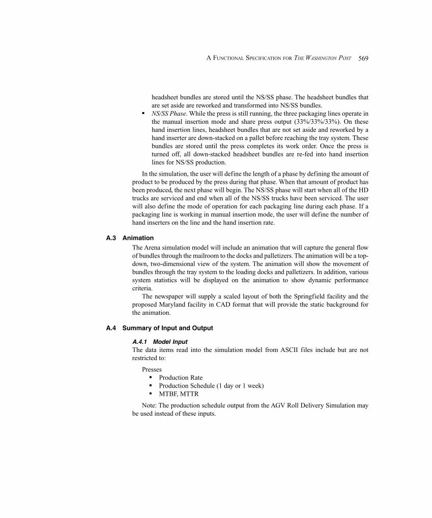
569A FUNCTIONAL SPECIFICATION FOR THE WASHINGTON POST
headsheet bundles are stored until the NS/SS phase. The headsheet bundles thatare set aside are reworked and transformed into NS/SS bundles.
� NS/SS Phase. While the press is still running, the three packaging lines operate inthe manual insertion mode and share press output (33%/33%/33%). On thesehand insertion lines, headsheet bundles that are not set aside and reworked by ahand inserter are down-stacked on a pallet before reaching the tray system. Thesebundles are stored until the press completes its work order. Once the press isturned off, all down-stacked headsheet bundles are re-fed into hand insertionlines for NS/SS production.
In the simulation, the user will define the length of a phase by defining the amount ofproduct to be produced by the press during that phase. When that amount of product hasbeen produced, the next phase will begin. The NS/SS phase will start when all of the HDtrucks are serviced and end when all of the NS/SS trucks have been serviced. The userwill also define the mode of operation for each packaging line during each phase. If apackaging line is working in manual insertion mode, the user will define the number ofhand inserters on the line and the hand insertion rate.
A.3 Animation
The Arena simulation model will include an animation that will capture the general flowof bundles through the mailroom to the docks and palletizers. The animation will be a top-down, two-dimensional view of the system. The animation will show the movement ofbundles through the tray system to the loading docks and palletizers. In addition, varioussystem statistics will be displayed on the animation to show dynamic performancecriteria.
The newspaper will supply a scaled layout of both the Springfield facility and theproposed Maryland facility in CAD format that will provide the static background forthe animation.
A.4 Summary of Input and Output
A.4.1 Model InputThe data items read into the simulation model from ASCII files include but are notrestricted to:
Presses� Production Rate� Production Schedule (1 day or 1 week)� MTBF, MTTR
Note: The production schedule output from the AGV Roll Delivery Simulation maybe used instead of these inputs.

570 APPENDIX A
Press Packaging Line� Line Activation Patterns (Modes, Phases)� Tray System� Velocity� Trip Rate (Docks)� Trip Rate (Palletizers)
Palletizers� Production Rate� Bundles per Pallet� MTBF, MTTR
Bundles� Copies per Bundle (Advance)� Copies per Bundle (Headsheet)� Copies per Bundle (Hand Insertion)
Process Time� Truck Load Rates
� HD-Headsheet (Reg)� HD-Headsheet (Slow)� HD-Advance� HWY (Last Pallet)� HWY (Other Pallets)
� Dock Change Times� HD-Headsheet (Reg)� HD-Headsheet (Slow)� HD-Advance� HWY
Truck Schedule (for Each Truck)� Bucket� Truck ID� Draw Qty� Truck Type
Hand Insertion� Hand Inserters per Line� Hand Inserter Service Rate
A.4.2 Model OutputThe following performance measures will be written to one or more ASCII data files atthe conclusion of the simulation run. These statistics will be collected and output on adaily and weekly basis.

571A FUNCTIONAL SPECIFICATION FOR THE WASHINGTON POST
Input Parameters� Process Times� Equipment and Resource Levels� Failure Rates
Press Activity (for Each Press)� Available Time (Up)� Total Production� Average Production Rate� Breakdown History
Hand Insert Activity (for Each Line)� Total Production� Average Production Rate� Down-Stacked Headsheet Bundles
Tray Activity� Utilization (Green & Yellow)
Bundles� Destination Statistics
Dispatch Statistics� Trucks Early� Trucks Late� Time to Complete Pct of Trucks
Bucket Loading (per Bucket)� Total Units Loaded (Actual)� Total Units Loaded (Scheduled)
Dock Statistics (per Dock)� Dock Utilization� Total Units Loaded� Utilization per Bucket
Truck Statistics (per Truck)� Dock Used� Advance Load Time� Wait Time� Idle Time� Load Time� Change Time� Summary for Each Truck Type
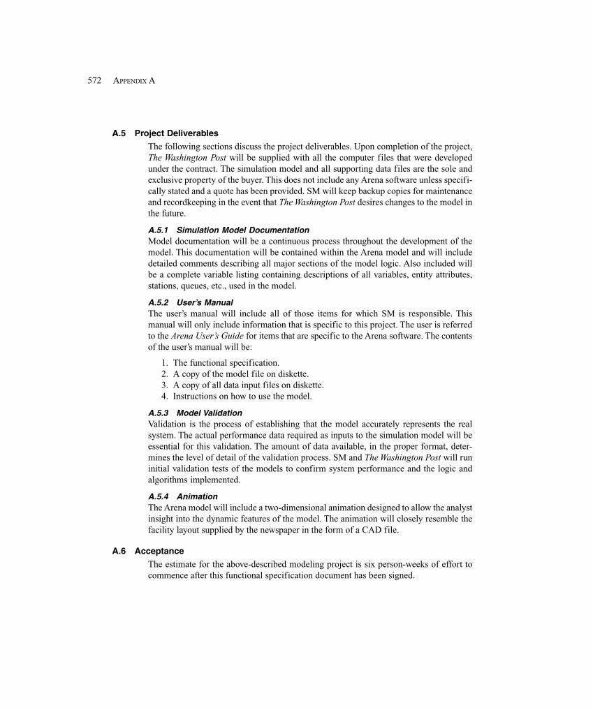
572 APPENDIX A
A.5 Project Deliverables
The following sections discuss the project deliverables. Upon completion of the project,The Washington Post will be supplied with all the computer files that were developedunder the contract. The simulation model and all supporting data files are the sole andexclusive property of the buyer. This does not include any Arena software unless specifi-cally stated and a quote has been provided. SM will keep backup copies for maintenanceand recordkeeping in the event that The Washington Post desires changes to the model inthe future.
A.5.1 Simulation Model DocumentationModel documentation will be a continuous process throughout the development of themodel. This documentation will be contained within the Arena model and will includedetailed comments describing all major sections of the model logic. Also included willbe a complete variable listing containing descriptions of all variables, entity attributes,stations, queues, etc., used in the model.
A.5.2 User’s ManualThe user’s manual will include all of those items for which SM is responsible. Thismanual will only include information that is specific to this project. The user is referredto the Arena User’s Guide for items that are specific to the Arena software. The contentsof the user’s manual will be:
1. The functional specification.2. A copy of the model file on diskette.3. A copy of all data input files on diskette.4. Instructions on how to use the model.
A.5.3 Model ValidationValidation is the process of establishing that the model accurately represents the realsystem. The actual performance data required as inputs to the simulation model will beessential for this validation. The amount of data available, in the proper format, deter-mines the level of detail of the validation process. SM and The Washington Post will runinitial validation tests of the models to confirm system performance and the logic andalgorithms implemented.
A.5.4 AnimationThe Arena model will include a two-dimensional animation designed to allow the analystinsight into the dynamic features of the model. The animation will closely resemble thefacility layout supplied by the newspaper in the form of a CAD file.
A.6 Acceptance
The estimate for the above-described modeling project is six person-weeks of effort tocommence after this functional specification document has been signed.
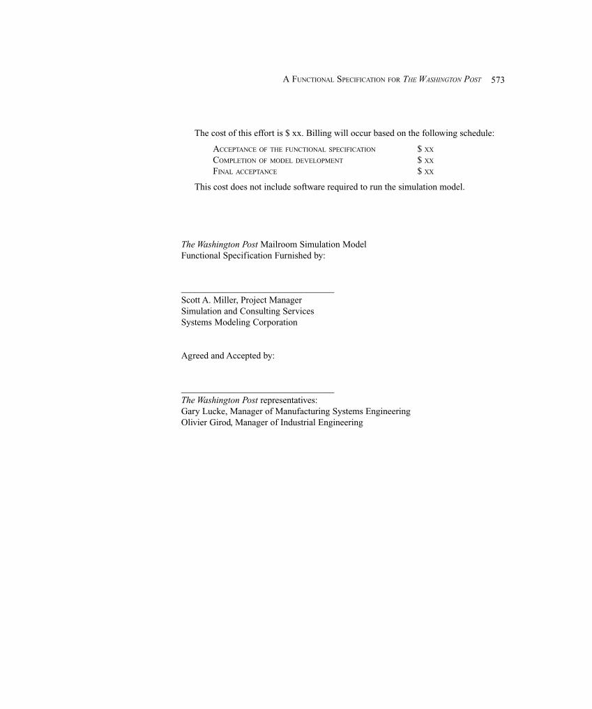
573A FUNCTIONAL SPECIFICATION FOR THE WASHINGTON POST
The cost of this effort is $ xx. Billing will occur based on the following schedule:
ACCEPTANCE OF THE FUNCTIONAL SPECIFICATION $ XX
COMPLETION OF MODEL DEVELOPMENT $ XX
FINAL ACCEPTANCE $ XX
This cost does not include software required to run the simulation model.
The Washington Post Mailroom Simulation ModelFunctional Specification Furnished by:
_________________________________Scott A. Miller, Project ManagerSimulation and Consulting ServicesSystems Modeling Corporation
Agreed and Accepted by:
_________________________________The Washington Post representatives:Gary Lucke, Manager of Manufacturing Systems EngineeringOlivier Girod, Manager of Industrial Engineering


575A REFRESHER ON PROBABILITY AND STATISTICS
APPENDIX B
A Refresher on Probability andStatistics
The purpose of this appendix is to provide a brief refresher on selected topics inprobability and statistics necessary to understand some of the probabilistic foundationsof simulation, as well as to design and analyze simulation experiments appropriately.While this material underlies many parts of the book (including every time we use aprobability distribution in a model to represent some random input quantity like a timeduration), it’s particularly relevant to Section 2.6, Section 4.6, Chapter 6, Section 7.2,and Chapter 12.
We intend this appendix to serve as a very brief tutorial, and not as anything like acomprehensive treatment of these topics. There are many excellent texts on probabilityand statistics in general, such as Anderson, Sweeney, and Williams (2006), Devore(2004), and Hogg and Craig (2005); for a free online “book” on the subject, which linksto additional online resources, see Lane (2009) at http://davidmlane.com/hyperstat/index.html.
Though we’ll start pretty much from scratch on probability and statistics, we doassume that you’re comfortable with algebraic manipulations, including summationnotation. For a complete understanding of continuous random variables (Section B.2.3),you’ll need to know some calculus, particularly integrals.
In Section B.1, we go over the basic ideas and terminology of probability. Section B.2contains a discussion about random variables in general, describing discrete andcontinuous random variables as well as joint distributions. The notion of sampling, andthe associated probabilistic structure, is discussed in Section B.3. Statistical inference,including point estimation, confidence intervals, and hypothesis testing, is covered inSections B.4–B.6. Throughout, we’ll make the discussion relevant to simulation by wayof examples.
B.1 Probability BasicsAn experiment is any activity you might undertake whose exact outcome is uncertain(until you do it and see what happens). While the term might conjure up images of highschool chemistry lab, its interpretation in probability is much broader. For instance:
� Flip a “fair” coin. Will it come up tails?� Throw a “fair” die (that’s singular for “dice”). Will it be 4? Will it be an odd
number? Will it be more than 2 but no more than 5?� Drive to work tomorrow. How long will it take? How long will you be delayed
because of construction? Will you be hit by an asteroid?
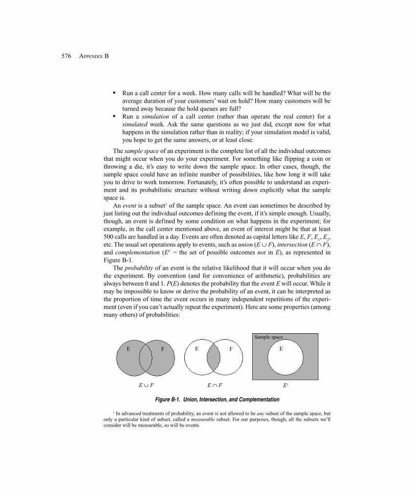
576 APPENDIX B
� Run a call center for a week. How many calls will be handled? What will be theaverage duration of your customers’ wait on hold? How many customers will beturned away because the hold queues are full?
� Run a simulation of a call center (rather than operate the real center) for asimulated week. Ask the same questions as we just did, except now for whathappens in the simulation rather than in reality; if your simulation model is valid,you hope to get the same answers, or at least close.
The sample space of an experiment is the complete list of all the individual outcomesthat might occur when you do your experiment. For something like flipping a coin orthrowing a die, it’s easy to write down the sample space. In other cases, though, thesample space could have an infinite number of possibilities, like how long it will takeyou to drive to work tomorrow. Fortunately, it’s often possible to understand an experi-ment and its probabilistic structure without writing down explicitly what the samplespace is.
An event is a subset1 of the sample space. An event can sometimes be described byjust listing out the individual outcomes defining the event, if it’s simple enough. Usually,though, an event is defined by some condition on what happens in the experiment; forexample, in the call center mentioned above, an event of interest might be that at least500 calls are handled in a day. Events are often denoted as capital letters like E, F, E
1, E
2,
etc. The usual set operations apply to events, such as union (E ∪ F), intersection (E ∩ F),and complementation (EC = the set of possible outcomes not in E), as represented inFigure B-1.
The probability of an event is the relative likelihood that it will occur when you dothe experiment. By convention (and for convenience of arithmetic), probabilities arealways between 0 and 1. P(E) denotes the probability that the event E will occur. While itmay be impossible to know or derive the probability of an event, it can be interpreted asthe proportion of time the event occurs in many independent repetitions of the experi-ment (even if you can’t actually repeat the experiment). Here are some properties (amongmany others) of probabilities:
Figure B-1. Union, Intersection, and Complementation
1 In advanced treatments of probability, an event is not allowed to be any subset of the sample space, butonly a particular kind of subset, called a measurable subset. For our purposes, though, all the subsets we’llconsider will be measurable, so will be events.
E F E F E
EcE ∪ F E ∩ F
Sample space
577A REFRESHER ON PROBABILITY AND STATISTICS
� If S is the entire sample space, then P(S) = 1.� If ∅ is the empty (null) event, then P(∅) = 0.� P(EC) = 1 – P(E).� P(E ∪ F) = P(E) + P(F) – P(E ∩ F).� If E and F are mutually exclusive (E ∩ F = ∅), then P(E ∪ F) = P(E) + P(F).� If E is a subset of F (i.e., the event E implies the event F), then P(E) < P(F).� If o
1, o
2, o
3, . . . are the individual outcomes in the sample space (finite or
infinite), then P oii
( )all ∑ = 1 .
Sometimes, the knowledge that one event occurred can alter the probability thatanother event also occurred. The conditional probability of E given F is defined as
P E F P E F P F( | ) ( ) / ( )= ∩
(assuming that P(F) > 0). The intuition for this is that knowing that F occurred reducesthe “world” from the whole sample space down to F, and so the only relevant part of E isthat part that intersects with F. This probability is then measured relative to the “size” ofthe reduced world, P(F).
Events E and F are called independent if P(E ∩ F) = P(E) P(F). If this is so, thenP(E|F) = P(E), and P(F|E) = P(F), by definition of conditional probability. In otherwords, knowing that one of two independent events has occurred tells you nothing aboutwhether the other one occurred.
There are a lot of different kinds of events and probabilities that come up in simula-tion. For example, you might want to ask about the probability that:
� a part passes inspection.� an arriving part is of priority 3.� a service time will be between 2 and 6.� no customers will arrive during a five-minute time interval.� the maximum queue length during a simulation will exceed 10.� the average time in system of parts is less than four hours.
B.2 Random Variables
Events can be defined in many different ways and can be very complex. One way ofquantifying and simplifying events is by defining random variables relating to them. Inthis section, we’ll discuss the basic ideas of random variables, their two basic forms(discrete and continuous), and then consider multiple random variables defined togetherand their possible relationships.
B.2.1 BasicsA random variable is a number whose value is determined by the outcome of anexperiment, so can be thought of as a quantification of an experiment. Technically, arandom variable is a function defined from the sample space to the real numbers. Assuch, it’s a rule or mapping that assigns a number to each possible outcome of theexperiment. While you can sometimes define a random variable in this way, by going
578 APPENDIX B
back to the sample space and assigning the mapping, you often just start by defining therandom variable without bothering with the sample space. A reasonable way to thinkabout a random variable is that it’s a number whose value you don’t know for sure beforedoing the experiment, but you will generally know something about it, like its range ofpossible values or its probability of being equal to something or falling in some range.Random variables are typically denoted by capital letters like X, Y, W
1, W
2, etc.
Random variables come in two basic “flavors”: discrete and continuous. A discreterandom variable can take on only certain separated values. For instance, the number ofdefective items in a shipment of 50 items would have to be an integer between 0 and 50.Another example of a discrete random variable is the number of times a part has toundergo inspection in order to pass; without further information, this random variablewould be a positive integer with no upper bound. Thus, a discrete random variable couldhave a finite or infinite range of possible values.
A continuous random variable, on the other hand, can take on any real value, possiblybounded on the left or the right. Continuous random variables typically representphysical measurements like time or distance. There are always infinitely many possiblevalues for a continuous random variable, even if there are limits on its value on bothends. For instance, if X is the time to process a part on a machine, the range would be[0, ∞) unless we assumed that no part was allowed to stay on the machine for longer thana certain time a, in which case the range would be [0, a].
In simulation, random variables are used for several different purposes. They oftenserve as “models” for input quantities like uncertain time durations (service orinterarrival times), the number of customers in an arriving group, or which of severaldifferent part types a given arriving part is. Random variables are also used to representoutput quantities like the average time in system, the number of customers served, or themaximum length of a buffer.
The probabilistic behavior of a random variable is described by its probabilitydistribution. Since the nature of this distribution is somewhat different for discrete andcontinuous random variables, we’ll consider them separately; we’ll also define somebasic properties of random variables, like expected value and variance.
B.2.2 DiscreteFor a discrete random variable X, there will be a list x
1, x
2, . . . (finite or infinite) of
possible values it can take on. Note that the xi’s are fixed, non-random values, but the
random variable X is, well, random. The probability mass function (PMF) is simply afunction that gives the probability that X will take on each of the possible values:
p(xi) = P(X = x
i)
for all i. Note that the statement “X = xi” is an event that may or may not happen, and the
PMF gives the probability that it does. The PMF may be expressed in a variety ofdifferent ways—a numerical list or table, a graph, or some kind of mathematical formula.Since the complete list of the x
i’s is supposed to represent all the different possible values
of X, . Usually, the PMF is estimated from data, or simply assumed.
∑ =i
ixp all
1)(
∑ =i
ixp all
1)(
579A REFRESHER ON PROBABILITY AND STATISTICS
The cumulative distribution function (CDF) of a discrete random variable X is afunction that gives the probability that X will be less than or equal to its argument:
.)()(such that all∑
≤
=xx
ii
i
xpxF
This summation is taken over all possible values xi that are < the argument x of F. Note
that 0 < F(x) < 1 for all x, that F(x) → 0 as x → – ∞, and that F(x) → 1 as x → + ∞. Thus,F(x) is a non-decreasing function going from 0 up to 1 as x goes from left to right. For adiscrete random variable, F(x) is a “step” function that’s flat between adjacent possiblevalues x
i, and takes a “jump” of height p(x
i) above x
i.
The probability of an event involving a discrete random variable X generally can befound by adding up the appropriate values of the PMF. For instance,
P a X b p xiia x bi
( ) ( )≤ < =
≤ <
∑all such that
.
This just says to add up the probabilities of those xi’s that are at least a but (strictly) less
than b. Note that with discrete random variables, you need to be careful about weak vs.strong inequalities.
Just as data sets have a “center” measured by the average of the data, randomvariables have a “center” in a certain sense. The expected value of the discrete randomvariable X is defined as
E X x p xi ii
( ) ( )= ∑all
(this is also called the mean or expectation of X and is often denoted by μ or, if there’sneed to identify the random variable, μ
X). This is a weighted average of the possible
values xi for X, with the weights’ being the respective probabilities of occurrence of each
xi. In this way, those x
i’s with high probability of occurrence are counted more heavily
than are those that are less likely to occur. If there are finitely many xi’s and each is
equally likely to occur, then E(X) is just the simple average of the xi’s since they all
“count” the same. Despite the name, it’s important to understand that E(X) is not to beinterpreted as the value of X you “expect” to get when you do the experiment defining X.Indeed, E(X) might not even be a possible value of a discrete random variable X (the x
i’s
might be integers but, depending on the situation, E(X) need not be an integer). Instead,interpret the expected value like this: do the experiment many times (technically,infinitely many times), observe a value of X each time, and compute the average of allthese values of X you observe—this average will be the expectation of X.
And just as data sets have a measure of variability, so too do random variables. Thevariance of the discrete random variable X is defined as
Var X x p xi ii
( ) ( ) ( )= −∑ μ 2
all
580 APPENDIX B
(often denoted σ 2 or σ X2 ), where μ is the expected value of X. This is a weighted average
of the squared deviation of the possible values xi around the expectation, with the
weights’ being the probability of occurrence of each xi. The variance is a measure of the
“spread” of the random variable about its mean. The units of the variance are the squaresof the units of X, so people often use the positive square root of the variance (denoted σor σ
X) as a measure of spread; this is called the standard deviation of X.
As mentioned earlier, there are different ways to define the PMF of a discreterandom variable. Arena supports several common discrete random variables for modelinginput quantities, and these are defined and described in Appendix C.
B.2.3 ContinuousA continuous random variable can take on any real value in some range. The range canbe limited or unlimited on either or both ends. No matter how narrow the range may be,a continuous random variable can always take on an infinite2 number of real values (i.e.,any value in a continuum). Thus, it doesn’t make sense to talk about the probability that acontinuous random variable equals (exactly) some fixed number x; technically, thisprobability will always be 0 even if x is within the range of X.
Instead, the probabilistic behavior of a continuous random variable is described interms of its falling between two fixed values, which can be far apart or close together.The probability density function (PDF) of a continuous random variable X is defined tobe a function f(x) with the following properties and interpretation:
� f(x) > 0 for all real values x.� The total area under f(x) is 1. In calculus terminology, the total integral of f(x) is 1:
∫∞+
∞−= 1)( dxxf .
� For any fixed real values a and b, with a < b, the probability that X will fallbetween a and b is the area under f(x) between a and b. In calculus terminology,
∫=≤≤b
adxxfbXaP .)()(
This last property says that if we slide a slim interval left and right along the x axis(keeping the width of the interval constant), we “pick up” more area (probability) inthose regions where the density is high, so we’re more likely to observe lots of values ofX where the density is high than where the density is low. If you think of repeating theexperiment many times and making a dot on the x axis where the value of the randomvariable X lands each time, your dots will be highly dense where the density function ishigh and of low density where the density function is low (get it?). Note that the height(value) of f(x) is itself not the probability of anything. Indeed, we don’t require that f(x)be < 1, and some PDFs can rise above 1 at some points; what’s required is that the total
2 More precisely, an uncountably infinite number of values, for those of you who are concerned with thedifferent sizes of infinity.
581A REFRESHER ON PROBABILITY AND STATISTICS
area under the PDF be equal to 1. For example, consider a uniform distribution between3.0 and 3.1. In order for the total area under the PDF to be equal to 1, the height f(x) forall possible values of x (between 3.0 and 3.1) needs to be equal to 10. Also, we couldspecify that f(x) = 0 for values of x in or outside of some range, which would mean thatthese ranges are impossible for the random variable X to fall in. Unlike discrete randomvariables, we can be sloppy with whether the endpoints of the ranges over which we wantprobabilities are defined by weak or strong inequalities (i.e., < is the same as < , and > isthe same as >).
The cumulative distribution function of a continuous random variable X has the samebasic definition and interpretation as for discrete random variables: F(x) = P(X < x) forall real values x. Thus, F(x) is the probability that X will land on or to the left of x. How-ever, computing it requires getting the area under the density function to the left of x:
∫ ∞−=
xdttfxF .)()(
Depending on the form of the PDF f(x), the CDF F(x) may or may not be expressible as aclosed-form formula involving x. For instance, the exponential and Weibull distributions(see Appendix C for definitions) do have simple formulas for the CDF, but the generalgamma and normal distributions do not. If the CDF is not expressible as a formula, itsevaluation must be left to some numerical method or a table (which is why every statis-tics book has a table of normal-distribution areas). As in the discrete case, the CDF F(x)for a continuous random variable rises from 0 at the extreme left to 1 at the extreme right,but in this case is a continuous function rather than a step function. Since f(x) is the slope(derivative) of F(x), those regions on the x axis where F(x) rises steeply are those regionswhere we’d get a lot of observations on X; conversely, where F(x) is relatively flat, wewon’t see many observations on X.
The expected value of a continuous random variable is, as in the discrete case, onemeasure of the “center” of the distribution and is the average of infinitely many observa-tions on X. It’s defined as
∫∞+
∞−= dxxxfXE )()(
and often denoted as μ or μX. Roughly, this is a weighted “average” of the x values, using
the density as the weighting function to count more heavily those values of x aroundwhich the density is high. The variance of X, measuring its “spread,” is
∫∞+
∞−−= dxxfxXVar )()()( 2μ
and often denoted σ 2 or σ X2 ; the positive square root of the variance (denoted σ or σ
X) is
the standard deviation.Arena supports several different continuous random variables for use in modeling
random input quantities; these are defined and discussed in Appendix C.
582 APPENDIX B
B.2.4 Joint Distributions, Covariance, Correlation, and IndependenceSo far we’ve considered random variables only one at a time. But sometimes theynaturally come in pairs or triples or even longer ordered sequences (having the wonderfulname tuples), which are called jointly distributed random variables or random vectors.For instance, in the input modeling for a job-shop simulation, an arriving order mighthave random variables representing the part type (dictating its route through the shop),priority, and processing times at the steps along its route. On the output side, thesimulation might generate a sequence W
1, W
2, W
3, . . . representing the times in system of
the finished parts in order of their exit. One issue that naturally arises, and which canaffect how we model and analyze such random vectors, is whether the random variablescomposing them are related to each other, and if so, how.
To address this, we’ll start with the complete probabilistic representation of randomvectors. In order to keep things at least partially digestible, we’ll consider just a pair(two-tuple) of random variables (X
1, X
2), but things extend in the obvious way to higher
dimensions. The joint CDF of (X1, X
2) is a function of two variables defined as
F x x P X x X x( , ) ( )1 2 1 1 2 2= ≤ ≤ and
for all pairs (x1, x
2) of real numbers. Often the word “and” is replaced by just a comma:
F x x P X x X x( , ) ( , )1 2 1 1 2 2= ≤ ≤ .
If the random variables are both discrete, the joint PMF is
p(x1, x
2) = P(X
1 = x
1, X
2 = x
2).
If the random variables are both continuous, the joint PDF is denoted f(x1, x
2), which you
can visualize as some kind of surface floating above the (x1, x
2) plane, and which has total
volume under it equal to one. The interpretation of the joint PDF in the continuous caseis this: the probability that X
1 will fall between a
1 and b
1, and, simultaneously, that X
2 will
fall between a2 and b
2, is the volume under the joint PDF above the rectangle [a
1, b
1] ×
[a2, b
2] in the (x
1, x
2) plane. In calculus notation, this interpretation is expressed as
The joint distribution (expressed as either the CDF, PMF, or PDF) contains a lot of infor-mation about the random vector. In practice, it’s usually not possible to know, or evenestimate, the complete joint distribution. Fortunately, we can usually address theissues we need to without having to know or estimate the full-blown joint distribution.
Given a joint distribution of two random variables, we can derive the individual, ormarginal,3 distributions of each of the random variables on their own. In the jointlydiscrete case, the marginal PMF of X
1 is, for all possible values x
1i of X
1,
3 The term “marginal” is not to suggest that these distributions are of questionable moral integrity. Rather,it simply refers to that fact that, in two dimensions for the jointly discrete case, if the joint probabilities arearranged in a table, then summing the rows and columns results in values on the margins of the table, whichwill be the individual “marginal” distributions.
∫ ∫=≤≤≤≤ 1
1
2
2
.),(),( 1221222111
b
a
b
adxdxxxfbXabXaP
583A REFRESHER ON PROBABILITY AND STATISTICS
p x P X x p x xX i i i jx j
1
2
1 1 1 1 2( ) ( ) ( , )= = = ∑all
and the marginal CDF of X1 is, for all real values of x,
F x p xX X iix xi
1 1
1
1( ) ( )=
≤
∑all such that
(symmetric definitions apply for X2). In the jointly continuous case, the marginal PDF of
X1 is
∫∞+
∞−= 2211 ),()(
1dxxxfxfx
and the marginal CDF of X1 is
dttfxFx
XX )()(1
11 1 ∫ ∞−=
(symmetrically for X2). Note that we can get the marginal distributions in this way from
the joint distribution, but knowledge of the marginal distributions is generally not suffi-cient to determine what the joint distribution is (unless X
1 and X
2 are independent random
variables, as discussed below).The covariance between the components X
1 and X
2 of a random vector is defined as
[ ]))(())((),( 221121 XEXXEXEXXCov −−= .
Note that the quantity inside the [ ] is a random variable with its own distribution, etc.,and the covariance is the expectation of this random variable. The covariance is a mea-sure of the (linear) relationship between X
1 and X
2, and can be positive, zero, or negative.
If the joint distribution is shaped so that, when X1 is above its mean, then X
2 tends to be
above its mean, then the covariance is positive; this implies that a small X1 tends to be
associated with a small X2 as well. On the other hand, if large X
1 is associated with small
X2 (and vice versa), then the covariance will be negative. If there is no tendency for X
1
and X2 to occur jointly in agreement or disagreement over being big or small, then the
covariance will be zero. Thus, the covariance tells us whether the two random variables inthe vector are (linearly) related or not, and if they are, whether the relationship is positiveor negative.
However, the covariance’s magnitude is difficult to interpret since it depends on theunits of measurement. To rectify this, the correlation between X
1 and X
2 is defined as
Cor X XCov X X
X X
( , )( , )
1 21 2
1 2
=σ σ
.
Clearly, the correlation has the same sign as the covariance (or is zero along with thecovariance), so the direction of any relationship is also indicated by the sign of thecorrelation. Also, the correlation is a dimensionless quantity (that is, it has no units of
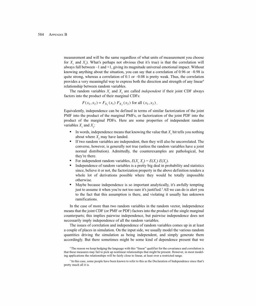
584 APPENDIX B
measurement and will be the same regardless of what units of measurement you choosefor X
1 and X
2). What’s perhaps not obvious (but it’s true) is that the correlation will
always fall between –1 and +1, giving its magnitude universal emotional impact. Withoutknowing anything about the situation, you can say that a correlation of 0.96 or –0.98 isquite strong, whereas a correlation of 0.1 or –0.08 is pretty weak. Thus, the correlationprovides a very meaningful way to express both the direction and strength of any linear4
relationship between random variables.The random variables X
1 and X
2 are called independent if their joint CDF always
factors into the product of their marginal CDFs:
F x x F x F x x xX X( , ) ( ) ( ) ( , )1 2 1 2 1 21 2= for all .
Equivalently, independence can be defined in terms of similar factorization of the jointPMF into the product of the marginal PMFs, or factorization of the joint PDF into theproduct of the marginal PDFs. Here are some properties of independent randomvariables X
1 and X
2:
� In words, independence means that knowing the value that X1 hit tells you nothing
about where X2 may have landed.
� If two random variables are independent, then they will also be uncorrelated. Theconverse, however, is generally not true (unless the random variables have a jointnormal distribution). Admittedly, the counterexamples are pathological, butthey’re there.
� For independent random variables, E(X1 X
2) = E(X
1) E(X
2).
� Independence of random variables is a pretty big deal in probability and statisticssince, believe it or not, the factorization property in the above definition renders awhole lot of derivations possible where they would be totally impossibleotherwise.
� Maybe because independence is so important analytically, it’s awfully temptingjust to assume it when you’re not too sure it’s justified.5 All we can do is alert youto the fact that this assumption is there, and violating it usually has unknownramifications.
In the case of more than two random variables in the random vector, independencemeans that the joint CDF (or PMF or PDF) factors into the product of the single marginalcounterparts; this implies pairwise independence, but pairwise independence does notnecessarily imply independence of all the random variables.
The issues of correlation and independence of random variables comes up in at leasta couple of places in simulation. On the input side, we usually model the various randomquantities driving the simulation as being independent, and simply generate themaccordingly. But there sometimes might be some kind of dependence present that we
5 In this case, some people have been known to refer to this as the Declaration of Independence since that’spretty much all it is.
4 The reason we keep hedging the language with this “linear” qualifier for the covariance and correlation isthat these measures may fail to pick up nonlinear relationships that might be present. However, in most model-ing applications the relationships will be fairly close to linear, at least over a restricted range.
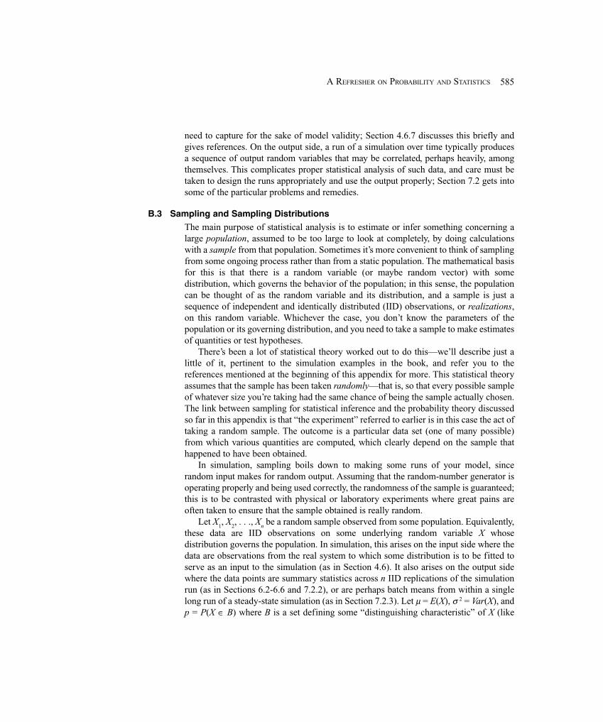
585A REFRESHER ON PROBABILITY AND STATISTICS
need to capture for the sake of model validity; Section 4.6.7 discusses this briefly andgives references. On the output side, a run of a simulation over time typically producesa sequence of output random variables that may be correlated, perhaps heavily, amongthemselves. This complicates proper statistical analysis of such data, and care must betaken to design the runs appropriately and use the output properly; Section 7.2 gets intosome of the particular problems and remedies.
B.3 Sampling and Sampling Distributions
The main purpose of statistical analysis is to estimate or infer something concerning alarge population, assumed to be too large to look at completely, by doing calculationswith a sample from that population. Sometimes it’s more convenient to think of samplingfrom some ongoing process rather than from a static population. The mathematical basisfor this is that there is a random variable (or maybe random vector) with somedistribution, which governs the behavior of the population; in this sense, the populationcan be thought of as the random variable and its distribution, and a sample is just asequence of independent and identically distributed (IID) observations, or realizations,on this random variable. Whichever the case, you don’t know the parameters of thepopulation or its governing distribution, and you need to take a sample to make estimatesof quantities or test hypotheses.
There’s been a lot of statistical theory worked out to do this—we’ll describe just alittle of it, pertinent to the simulation examples in the book, and refer you to thereferences mentioned at the beginning of this appendix for more. This statistical theoryassumes that the sample has been taken randomly—that is, so that every possible sampleof whatever size you’re taking had the same chance of being the sample actually chosen.The link between sampling for statistical inference and the probability theory discussedso far in this appendix is that “the experiment” referred to earlier is in this case the act oftaking a random sample. The outcome is a particular data set (one of many possible)from which various quantities are computed, which clearly depend on the sample thathappened to have been obtained.
In simulation, sampling boils down to making some runs of your model, sincerandom input makes for random output. Assuming that the random-number generator isoperating properly and being used correctly, the randomness of the sample is guaranteed;this is to be contrasted with physical or laboratory experiments where great pains areoften taken to ensure that the sample obtained is really random.
Let X1, X
2, . . ., X
n be a random sample observed from some population. Equivalently,
these data are IID observations on some underlying random variable X whosedistribution governs the population. In simulation, this arises on the input side where thedata are observations from the real system to which some distribution is to be fitted toserve as an input to the simulation (as in Section 4.6). It also arises on the output sidewhere the data points are summary statistics across n IID replications of the simulationrun (as in Sections 6.2-6.6 and 7.2.2), or are perhaps batch means from within a singlelong run of a steady-state simulation (as in Section 7.2.3). Let μ = E(X), σ 2 = Var(X), andp = P(X ∈ B) where B is a set defining some “distinguishing characteristic” of X (like
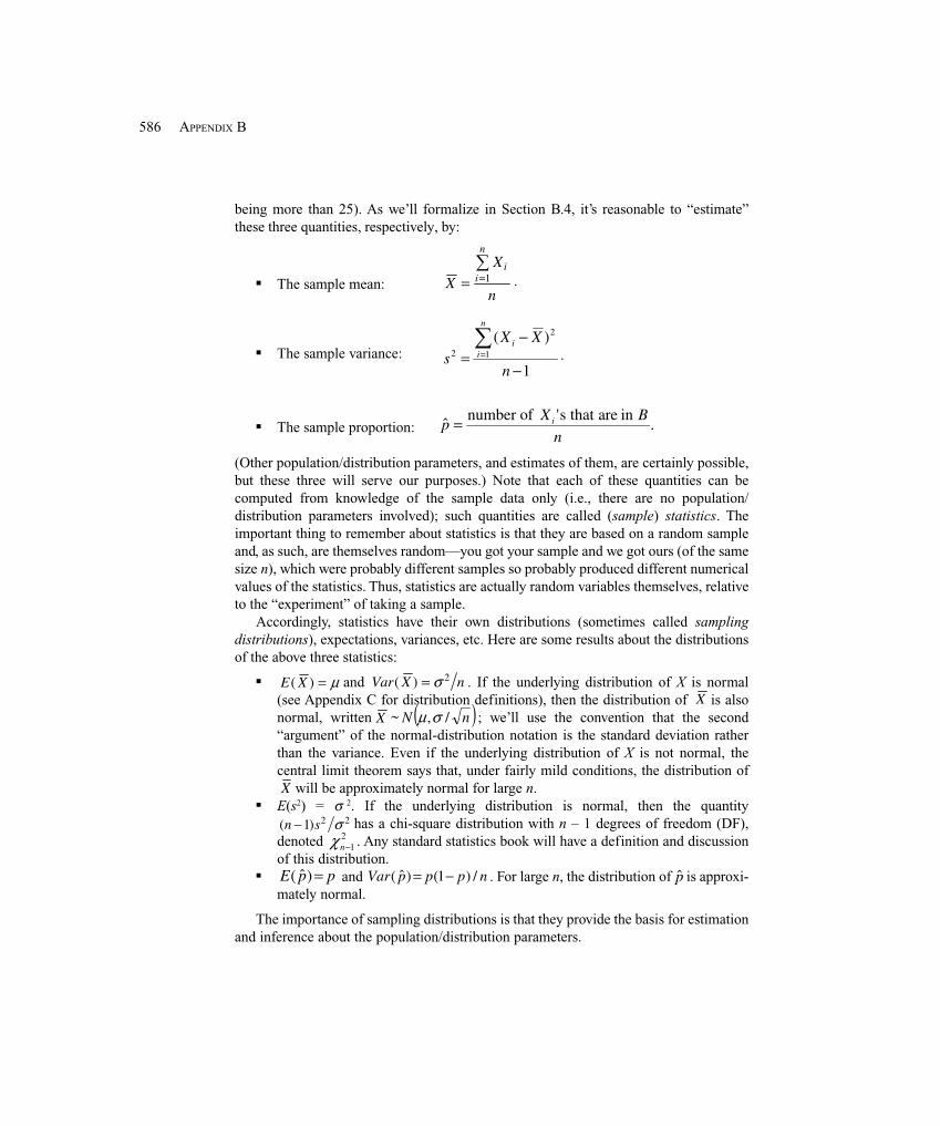
586 APPENDIX B
being more than 25). As we’ll formalize in Section B.4, it’s reasonable to “estimate”these three quantities, respectively, by:
� The sample mean: XX
n
ii
n
= =∑
1 .
� The sample variance: 1
)(1
2
2
−
−=∑
=
n
XXs
n
ii
.
� The sample proportion: .inarethats'ofnumber
ˆn
BXp i=
(Other population/distribution parameters, and estimates of them, are certainly possible,but these three will serve our purposes.) Note that each of these quantities can becomputed from knowledge of the sample data only (i.e., there are no population/distribution parameters involved); such quantities are called (sample) statistics. Theimportant thing to remember about statistics is that they are based on a random sampleand, as such, are themselves random—you got your sample and we got ours (of the samesize n), which were probably different samples so probably produced different numericalvalues of the statistics. Thus, statistics are actually random variables themselves, relativeto the “experiment” of taking a sample.
Accordingly, statistics have their own distributions (sometimes called samplingdistributions), expectations, variances, etc. Here are some results about the distributionsof the above three statistics:
� E X( ) = μ and Var X n( ) = σ 2 . If the underlying distribution of X is normal(see Appendix C for distribution definitions), then the distribution of X is alsonormal, written X ~ ( )nN /,σμ ; we’ll use the convention that the second“argument” of the normal-distribution notation is the standard deviation ratherthan the variance. Even if the underlying distribution of X is not normal, thecentral limit theorem says that, under fairly mild conditions, the distribution ofX will be approximately normal for large n.
� E(s2) = σ 2. If the underlying distribution is normal, then the quantity( )n s−1 2 2σ has a chi-square distribution with n – 1 degrees of freedom (DF),denoted 2
1−nχ . Any standard statistics book will have a definition and discussionof this distribution.
� ppE =)ˆ( and npppVar /)1()ˆ( −= . For large n, the distribution of p̂ is approxi-mately normal.
The importance of sampling distributions is that they provide the basis for estimationand inference about the population/distribution parameters.
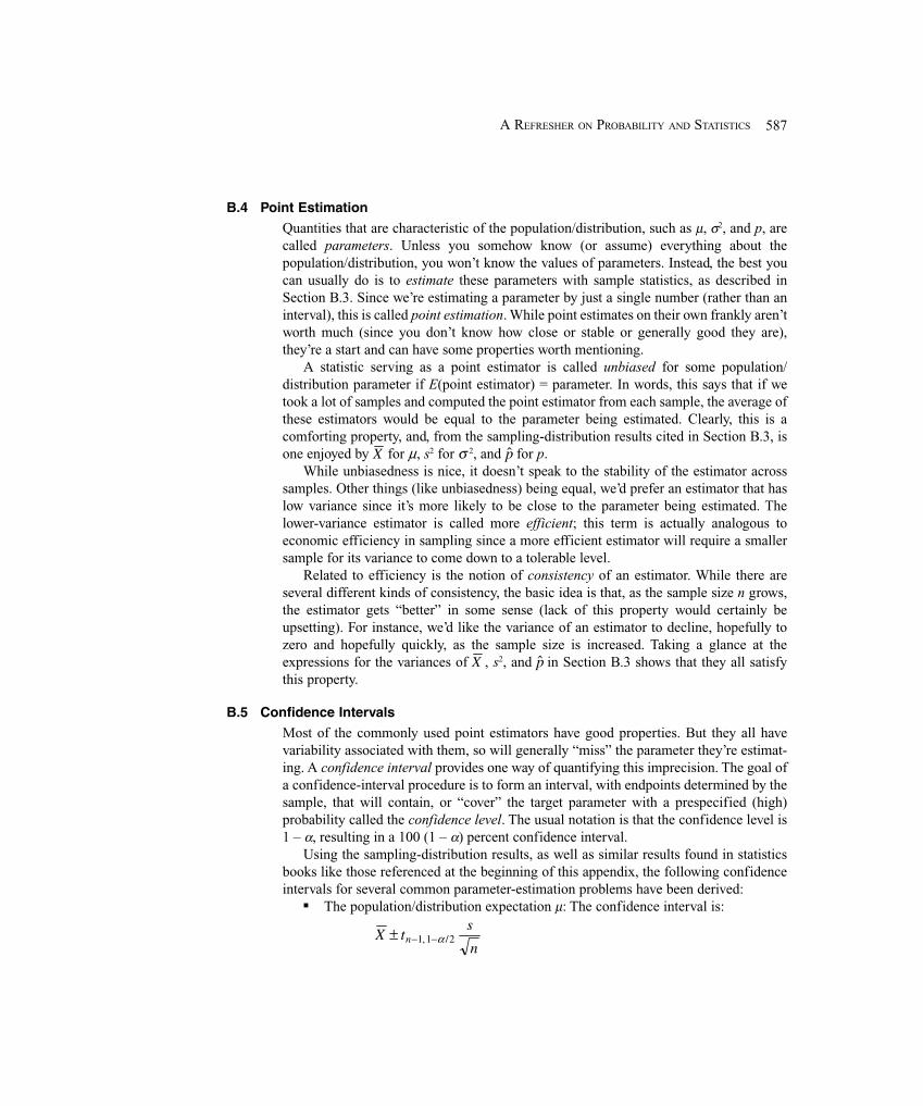
587A REFRESHER ON PROBABILITY AND STATISTICS
B.4 Point Estimation
Quantities that are characteristic of the population/distribution, such as μ, σ2, and p, arecalled parameters. Unless you somehow know (or assume) everything about thepopulation/distribution, you won’t know the values of parameters. Instead, the best youcan usually do is to estimate these parameters with sample statistics, as described inSection B.3. Since we’re estimating a parameter by just a single number (rather than aninterval), this is called point estimation. While point estimates on their own frankly aren’tworth much (since you don’t know how close or stable or generally good they are),they’re a start and can have some properties worth mentioning.
A statistic serving as a point estimator is called unbiased for some population/distribution parameter if E(point estimator) = parameter. In words, this says that if wetook a lot of samples and computed the point estimator from each sample, the average ofthese estimators would be equal to the parameter being estimated. Clearly, this is acomforting property, and, from the sampling-distribution results cited in Section B.3, isone enjoyed by X for �, s2 for σ 2, and p̂ for p.
While unbiasedness is nice, it doesn’t speak to the stability of the estimator acrosssamples. Other things (like unbiasedness) being equal, we’d prefer an estimator that haslow variance since it’s more likely to be close to the parameter being estimated. Thelower-variance estimator is called more efficient; this term is actually analogous toeconomic efficiency in sampling since a more efficient estimator will require a smallersample for its variance to come down to a tolerable level.
Related to efficiency is the notion of consistency of an estimator. While there areseveral different kinds of consistency, the basic idea is that, as the sample size n grows,the estimator gets “better” in some sense (lack of this property would certainly beupsetting). For instance, we’d like the variance of an estimator to decline, hopefully tozero and hopefully quickly, as the sample size is increased. Taking a glance at theexpressions for the variances of X , s2, and p̂ in Section B.3 shows that they all satisfythis property.
B.5 Confidence Intervals
Most of the commonly used point estimators have good properties. But they all havevariability associated with them, so will generally “miss” the parameter they’re estimat-ing. A confidence interval provides one way of quantifying this imprecision. The goal ofa confidence-interval procedure is to form an interval, with endpoints determined by thesample, that will contain, or “cover” the target parameter with a prespecified (high)probability called the confidence level. The usual notation is that the confidence level is1 – α, resulting in a 100 (1 – α) percent confidence interval.
Using the sampling-distribution results, as well as similar results found in statisticsbooks like those referenced at the beginning of this appendix, the following confidenceintervals for several common parameter-estimation problems have been derived:
� The population/distribution expectation μ: The confidence interval is:
X ts
nn± − −1 1 2, /α
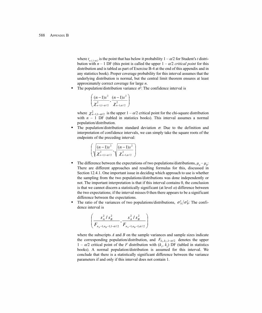
588 APPENDIX B
where tn-1,1-α/2
is the point that has below it probability 1 – α/2 for Student’s t distri-bution with n – 1 DF (this point is called the upper 1 – α/2 critical point for thisdistribution and is tabled as part of Exercise B-4 at the end of this appendix and inany statistics book). Proper coverage probability for this interval assumes that theunderlying distribution is normal, but the central limit theorem ensures at leastapproximately correct coverage for large n.
� The population/distribution variance σ2: The confidence interval is
⎟⎟
⎠
⎞
⎜⎜
⎝
⎛ −−
−−−2
2/,1
2
22/1,1
2 )1(,
)1(
αα χχ nn
snsn
where χ αn− −1 1 22
, / is the upper 1 – α/2 critical point for the chi-square distributionwith n – 1 DF (tabled in statistics books). This interval assumes a normalpopulation/distribution.
� The population/distribution standard deviation σ: Due to the definition andinterpretation of confidence intervals, we can simply take the square roots of theendpoints of the preceding interval:
⎟⎟
⎠
⎞
⎜⎜
⎝
⎛ −−
−−−2
2/,1
2
22/1,1
2 )1(,
)1(
αα χχ nn
snsn
� The difference between the expectations of two populations/distributions, μA – μ
B:
There are different approaches and resulting formulas for this, discussed inSection 12.4.1. One important issue in deciding which approach to use is whetherthe sampling from the two populations/distributions was done independently ornot. The important interpretation is that if this interval contains 0, the conclusionis that we cannot discern a statistically significant (at level α) difference betweenthe two expectations; if the interval misses 0 then there appears to be a significantdifference between the expectations.
� The ratio of the variances of two populations/distributions, σ σA B2 2 : The confi-
dence interval is
⎟⎟
⎠
⎞
⎜⎜
⎝
⎛
−−−−− 2/,1,1
22
2/1,1,1
22 /,
/
αα BABA nn
BA
nn
BA
F
ss
F
ss
where the subscripts A and B on the sample variances and sample sizes indicatethe corresponding population/distribution, and Fk k1 2 1 2, , /−α denotes the upper1 – α/2 critical point of the F distribution with (k
1, k
2) DF (tabled in statistics
books). A normal population/distribution is assumed for this interval. Weconclude that there is a statistically significant difference between the varianceparameters if and only if this interval does not contain 1.
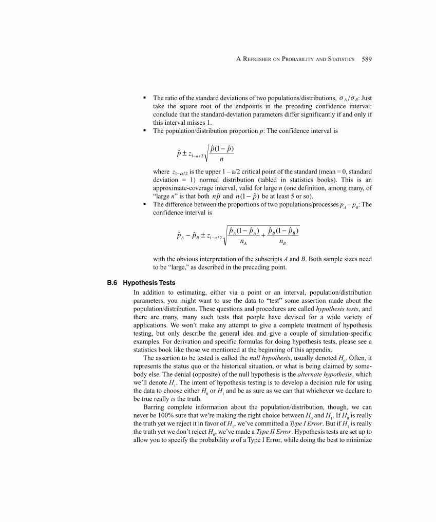
589A REFRESHER ON PROBABILITY AND STATISTICS
� The ratio of the standard deviations of two populations/distributions, σ σA B: Justtake the square root of the endpoints in the preceding confidence interval;conclude that the standard-deviation parameters differ significantly if and only ifthis interval misses 1.
� The population/distribution proportion p: The confidence interval is
n
ppzp a
)ˆ1(ˆˆ 2/1
−± −
where z1 2−α / is the upper 1 – a/2 critical point of the standard (mean = 0, standarddeviation = 1) normal distribution (tabled in statistics books). This is anapproximate-coverage interval, valid for large n (one definition, among many, of“large n” is that both pn ˆ and )ˆ1( pn − be at least 5 or so).
� The difference between the proportions of two populations/processes pA – p
B: The
confidence interval is
B
BB
A
AAaBA n
pp
n
ppzpp
)ˆ1(ˆ)ˆ1(ˆˆˆ 2/1
−+−±− −
with the obvious interpretation of the subscripts A and B. Both sample sizes needto be “large,” as described in the preceding point.
B.6 Hypothesis Tests
In addition to estimating, either via a point or an interval, population/distributionparameters, you might want to use the data to “test” some assertion made about thepopulation/distribution. These questions and procedures are called hypothesis tests, andthere are many, many such tests that people have devised for a wide variety ofapplications. We won’t make any attempt to give a complete treatment of hypothesistesting, but only describe the general idea and give a couple of simulation-specificexamples. For derivation and specific formulas for doing hypothesis tests, please see astatistics book like those we mentioned at the beginning of this appendix.
The assertion to be tested is called the null hypothesis, usually denoted H0. Often, it
represents the status quo or the historical situation, or what is being claimed by some-body else. The denial (opposite) of the null hypothesis is the alternate hypothesis, whichwe’ll denote H
1. The intent of hypothesis testing is to develop a decision rule for using
the data to choose either H0 or H
1 and be as sure as we can that whichever we declare to
be true really is the truth.Barring complete information about the population/distribution, though, we can
never be 100% sure that we’re making the right choice between H0 and H
1. If H
0 is really
the truth yet we reject it in favor of H1, we’ve committed a Type I Error. But if H
1 is really
the truth yet we don’t reject H0, we’ve made a Type II Error. Hypothesis tests are set up to
allow you to specify the probability α of a Type I Error, while doing the best to minimize
590 APPENDIX B
the probability β of a Type II Error. If you demand a really small α, you’ll get it but at thecost of a higher β (though the relationship between the two is not simple) unless you cango collect some more data. In hypothesis testing, H
0 and H
1 are not given equal
treatment—the benefit of the doubt is given to H0, so if we reject H
0, we’re making a
fairly strong and confident decision that H1 is true. But if we can’t mount enough
evidence against H0 to reject it, we haven’t necessarily “proved” that H
0 is the truth—
we’ve just failed to find evidence against it. The reason for failing to reject H0 could, of
course, be that it’s really true. But another reason for failing to reject H0 is that we just
don’t have enough data to “see” that H0 is false.
Another way to set up and carry out a test is not to make a firm yes/no decision, butrather quantify how “certain” you are about which hypothesis is correct. The p-value of adata set in a test is the probability of getting a data set, if H
0 is true, that’s more in favor of
H1 than the one you got. So if the p-value is tiny, you’re saying that it’s very hard to get
information more in favor of H1 than the information you already have in your data set,
so that the evidence for H1 is strong. If the p-value is large, say 0.3 or 0.6, then it’s entirely
possible that just by chance you’d get data more in favor of H1, so there’s no particular
reason to suspect H0. If the p-value is “on the edge,” say something like 0.1, you’re left
with an inconclusive result, which is sometimes all you can say with your data.One place in simulation that hypothesis tests come up is in fitting input probability
distributions to observed data on the input quantity being modeled (Section 4.6). Here,H
0 is the assertion that a particular candidate fitted distribution adequately explains the
data. If H0 is not rejected, then you have insufficient evidence that this distribution is
wrong, so you might go with it. The Arena Input Analyzer has two different tests for thisbuilt in, the chi-square test and the Kolmogorov-Smirnov test. These tests basically askhow close the fitted distribution is to the empirical distribution defined directly by thedata; for details on how these and other goodness-of-fit tests work, see any standardstatistics book.
Another place in simulation that a hypothesis test comes up is on the output side. Ifthere are several (more than two) models you’re comparing on the basis of some selectedoutput performance measure, a natural question is whether there’s any difference at allamong the means of this measure across the different models. A collection of specificproblems and techniques, called analysis of variance (ANOVA), is a standard part of anystatistics book, so we won’t go into its inner workings here. The null hypothesis is that allthe means across the different models are the same; if you do not reject this, you haveinsufficient evidence of any difference on this measure that the different models make.But if you reject H
0, you’re saying that there is some difference somewhere among the
means, though not that they’re all unique and different. A natural question in this case isthen precisely which means differ from which other ones, sometimes called multiplecomparisons in ANOVA. There have been several different methods developed forattacking this problem, three of which are due to Bonferroni, Scheffé, and Tukey. TheArena Output Analyzer (Section 6.4) has built-in facility for carrying out an ANOVAtest, including these multiple-comparisons methods.
591A REFRESHER ON PROBABILITY AND STATISTICS
Related to this goal, but more useful in simulation output analysis, is the question ofwhich among several variants (sometimes called scenarios) is best according to someoverall performance measure. The Arena Process Analyzer, or PAN (Section 6.5) has abuilt-in facility for identifying best scenarios and does so in a way related to hypothesistests.
B.7 Exercises
B-1 Suppose that X is a discrete random variable with probability mass function givenby p(1) = 0.1, p(2) = 0.3, p(3) = 0.3, p(4) = 0.2, and p(5) = 0.1.
(a) Plot p(x) for all x in the range.
(b) Compute numerically and plot the cumulative distribution function F(x).
(c) Compute P(1.4 ≤ X ≤ 4.2).
(d) Compute P(1.4 < X < 4.2).
(e) Compute the expected value E(X).
(f) Compute the variance Var(X).
(g) Compute the standard deviation of X.
B-2 Suppose that X has a (continuous) uniform distribution between 10 and 20 (seeAppendix C).
(a) Compute E(X).
(b) Compute Var(X).
(c) Compute P(X < 12).
(d) Compute P(X > 12).
(e) Compute P(X < 8 or X > 22).
B-3 Suppose that X is an exponential random variable with mean 5. (The cumulativedistribution function is F(x) = 1 – e–x/5 for x > 0, and F(x) = 0 for x < 0; see also AppendixC.)
(a) Compute P(X > 5).
(b) Compute P(1.4 ≤ X ≤ 4.2).
(c) Compute P(1.4 < X < 4.2).
B-4 Suppose that 7.3, 6.1, 3.8, 8.4, 6.9, 7.1, 5.3, 8.2, 4.9, and 5.8 are ten observationsfrom a normal distribution with unknown mean and unknown variance. Compute thesample mean, sample variance, and a 95 percent confidence interval for the populationmean. Here’s part of a t table that contains what you’ll need (and then some):
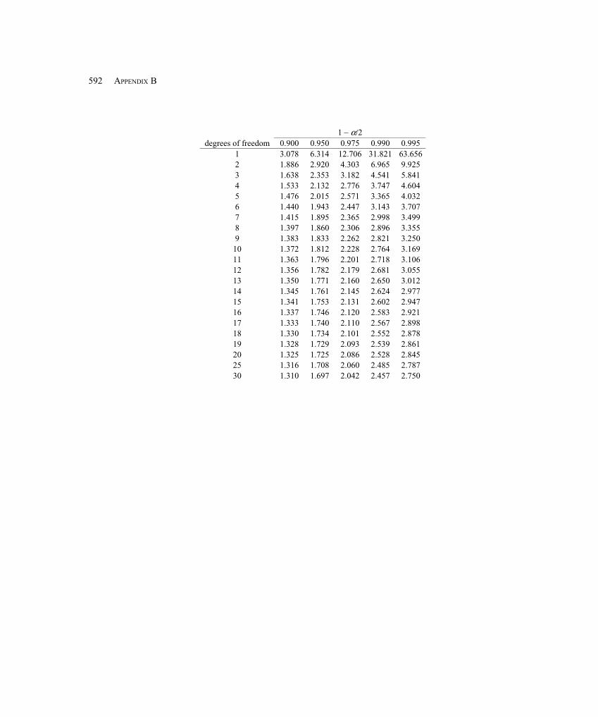
592 APPENDIX B
1 – α/2 degrees of freedom 0.900 0.950 0.975 0.990 0.995
1 3.078 6.314 12.706 31.821 63.656 2 1.886 2.920 4.303 6.965 9.925 3 1.638 2.353 3.182 4.541 5.841 4 1.533 2.132 2.776 3.747 4.604 5 1.476 2.015 2.571 3.365 4.032 6 1.440 1.943 2.447 3.143 3.707 7 1.415 1.895 2.365 2.998 3.499 8 1.397 1.860 2.306 2.896 3.355 9 1.383 1.833 2.262 2.821 3.250
10 1.372 1.812 2.228 2.764 3.169 11 1.363 1.796 2.201 2.718 3.106 12 1.356 1.782 2.179 2.681 3.055 13 1.350 1.771 2.160 2.650 3.012 14 1.345 1.761 2.145 2.624 2.977 15 1.341 1.753 2.131 2.602 2.947 16 1.337 1.746 2.120 2.583 2.921 17 1.333 1.740 2.110 2.567 2.898 18 1.330 1.734 2.101 2.552 2.878 19 1.328 1.729 2.093 2.539 2.861 20 1.325 1.725 2.086 2.528 2.845 25 1.316 1.708 2.060 2.485 2.787 30 1.310 1.697 2.042 2.457 2.750
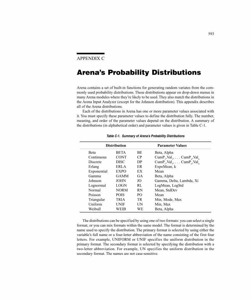
593ARENA’S PROBABILITY DISTRIBUTIONS
APPENDIX C
Arena’s Probability Distributions
Arena contains a set of built-in functions for generating random variates from the com-monly used probability distributions. These distributions appear on drop-down menus inmany Arena modules where they’re likely to be used. They also match the distributions inthe Arena Input Analyzer (except for the Johnson distribution). This appendix describesall of the Arena distributions.
Each of the distributions in Arena has one or more parameter values associated withit. You must specify these parameter values to define the distribution fully. The number,meaning, and order of the parameter values depend on the distribution. A summary ofthe distributions (in alphabetical order) and parameter values is given in Table C-1.
Table C-1. Summary of Arena’s Probability Distributions
Distribution Parameter Values
Beta BETA BE Beta, AlphaContinuous CONT CP CumP
1,Val
1, . . . CumP
n,Val
n
Discrete DISC DP CumP1,Val
1, . . . CumP
n,Val
n
Erlang ERLA ER ExpoMean, kExponential EXPO EX MeanGamma GAMM GA Beta, AlphaJohnson JOHN JO Gamma, Delta, Lambda, XiLognormal LOGN RL LogMean, LogStdNormal NORM RN Mean, StdDevPoisson POIS PO MeanTriangular TRIA TR Min, Mode, MaxUniform UNIF UN Min, MaxWeibull WEIB WE Beta, Alpha
The distributions can be specified by using one of two formats: you can select a singleformat, or you can mix formats within the same model. The format is determined by thename used to specify the distribution. The primary format is selected by using either thevariable’s full name or a four-letter abbreviation of the name consisting of the first fourletters. For example, UNIFORM or UNIF specifies the uniform distribution in theprimary format. The secondary format is selected by specifying the distribution with atwo-letter abbreviation. For example, UN specifies the uniform distribution in thesecondary format. The names are not case-sensitive.

594 APPENDIX C
In the primary format, you explicitly enter the parameters of the distribution asarguments of the distribution. For example, UNIFORM(10, 25) specifies a uniformdistribution with a minimum value of 10 and a maximum value of 25. In the alternativeformat, you indirectly define the parameters of the distribution by referencing a parameterset within the Parameters module from the Elements panel. For example,UN(DelayTime) specifies a uniform distribution with the minimum and maximumvalues defined in the parameter set named DelayTime. The main advantage of theindirect method of defining the parameters provided by the alternative format is that theparameters of the distribution can be modified from within the Parameters module.
The random-number stream, which is used by Arena in generating the sample, can alsobe specified in both formats. In the primary format, you enter the stream number as the lastargument following the parameter value list. For example, UNIFORM(10,25,2) specifiesa sample from a uniform distribution using random-number stream 2. In the secondaryformat, you enter the random-number stream as a second argument following the identifierfor the parameter set. For example, UN(DelayTime,PTimeStream) specifies a samplefrom a uniform distribution using random-number stream PTimeStream (which mustbe an expression defined to be the stream you want, and is not an entry in the Parametersmodule).
In the following pages, we provide a summary of each of the distributions supportedby Arena, listed in alphabetical order for easy reference. The summary includes theprimary and secondary formats for specifying the distribution and a brief description ofthe distribution. This description includes the density or mass function, parameters,range, mean, variance, and typical applications for the distribution. If you feel in need ofa brief refresher on probability and statistics, see Appendix B.
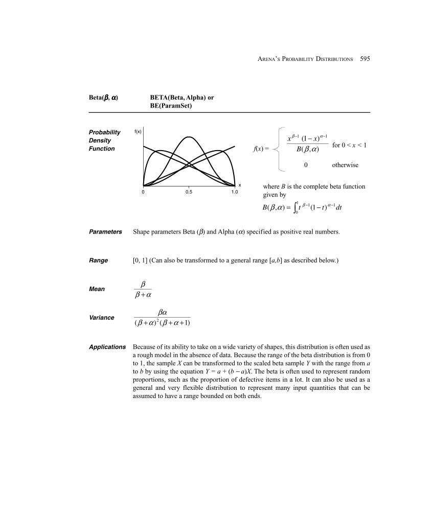
595ARENA’S PROBABILITY DISTRIBUTIONS
Because of its ability to take on a wide variety of shapes, this distribution is often used asa rough model in the absence of data. Because the range of the beta distribution is from 0to 1, the sample X can be transformed to the scaled beta sample Y with the range from ato b by using the equation Y = a + (b − a)X. The beta is often used to represent randomproportions, such as the proportion of defective items in a lot. It can also be used as ageneral and very flexible distribution to represent many input quantities that can beassumed to have a range bounded on both ends.
[0, 1] (Can also be transformed to a general range [a,b] as described below.)
ProbabilityDensityFunction
f(x)
0 0.5 1.0
x
Parameters
Range
Mean
Variance
Applications
where B is the complete beta functiongiven by
Beta(βββββ, ααααα) BETA(Beta, Alpha) orBE(ParamSet)
Shape parameters Beta (β) and Alpha (α) specified as positive real numbers.
for 0 < x < 1f(x) = ),(
)1( 11
αβ
αβ
B
xx −− −
0 otherwise
αββ+
)1()( 2 +++ αβαββα
∫−− −=
1
0
11 )1(),( dtttB αβαβ
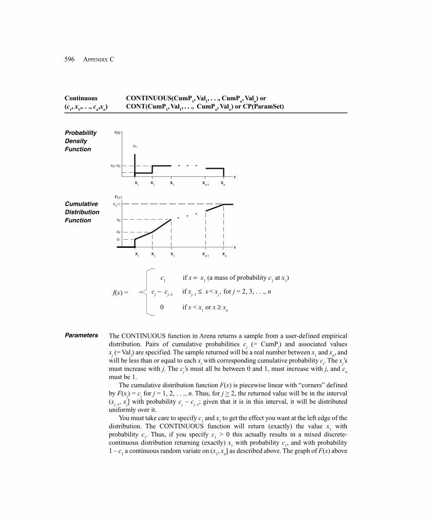
596 APPENDIX C
Parameters The CONTINUOUS function in Arena returns a sample from a user-defined empiricaldistribution. Pairs of cumulative probabilities c
j (= CumP
j) and associated values
xj (= Val
j) are specified. The sample returned will be a real number between x
1 and x
n, and
will be less than or equal to each xj with corresponding cumulative probability c
j. The x
j’s
must increase with j. The cj’s must all be between 0 and 1, must increase with j, and c
n
must be 1.The cumulative distribution function F(x) is piecewise linear with “corners” defined
by F(xj) = c
j for j = 1, 2, . . ., n. Thus, for j > 2, the returned value will be in the interval
(xj–1
, xj] with probability c
j – c
j–1; given that it is in this interval, it will be distributed
uniformly over it.You must take care to specify c
1 and x
1 to get the effect you want at the left edge of the
distribution. The CONTINUOUS function will return (exactly) the value x1 with
probability c1. Thus, if you specify c
1 > 0 this actually results in a mixed discrete-
continuous distribution returning (exactly) x1 with probability c
1, and with probability
1 – c1 a continuous random variate on (x
1, x
n] as described above. The graph of F(x) above
Continuous CONTINUOUS(CumP1, Val
1, . . ., CumP
n, Val
n) or
(c1, x
1,. . ., c
n,x
n) CONT(CumP
1, Val
1, . . ., CumP
n, Val
n) or CP(ParamSet)
ProbabilityDensityFunction
CumulativeDistributionFunction
f(x)
c3–c2
x1 x2 x3 xn-1 xn
x
f(x)
c2
c1
x1 x2 x3 xn-1 xn
x
c3
c1
cn=1
F(x)
c1
if x = x1 (a mass of probability c
1 at x
1)
f(x) =
0 if x < x1 or x ≥ x
n
cj − c
j−1if x
j−1 ≤ x < x
j, for j = 2, 3, . . ., n
x1
x2
x3
xn-1 xn
x1
x2
x3
xn-1 xn
597ARENA’S PROBABILITY DISTRIBUTIONS
Range
Applications
[x1, x
n]
The continuous empirical distribution is used to incorporate empirical data for continu-ous random variables directly into the model. This distribution can be used as an alterna-tive to a theoretical distribution that has been fitted to the data, such as in data that have amultimodal profile or where there are significant outliers.
depicts a situation where c1 > 0. On the other hand, if you specify c
1 = 0, you will get a
(truly) continuous distribution on [x1, x
n] as described above, with no “mass” of
probability at x1; in this case, the graph of F(x) would be continuous, with no jump at x
1.
As an example use of the CONTINUOUS function, suppose you have collected a setof data x
1, x
2, . . ., x
n (assumed to be sorted into increasing order) on service times, for
example. Rather than using a fitted theoretical distribution from the Input Analyzer(Section 4.5), you want to generate service times in the simulation “directly” from thedata, consistent with how they’re spread out and bunched up, and between the minimumx
1 and the maximum x
n you observed. Assuming that you don’t want a “mass” of
probability sitting directly on x1, you’d specify c
1 = 0 and then c
j = (j – 1)/(n – 1) for
j = 2, 3, . . ., n.
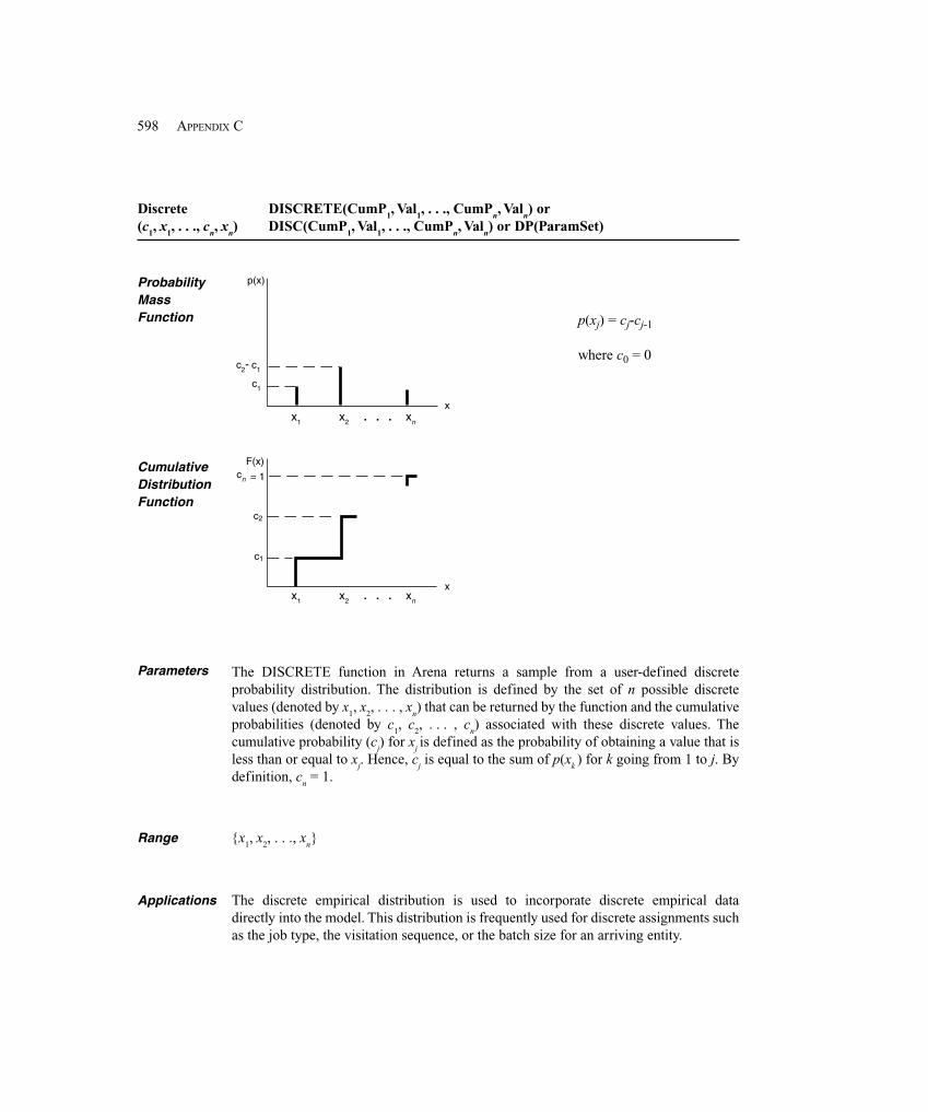
598 APPENDIX C
Parameters
ProbabilityMassFunction
CumulativeDistributionFunction
Range
Applications
Discrete DISCRETE(CumP1, Val
1, . . ., CumP
n, Val
n) or
(c1, x
1, . . ., c
n, x
n) DISC(CumP
1, Val
1, . . ., CumP
n, Val
n) or DP(ParamSet)
p(x)
c2–c1
x1 x2 xn
F(x)
c2
c1
c3 = 1
c1
x
x1 x2 xn
x
cn
p(xj) = cj-cj-1
where c0 = 0
The DISCRETE function in Arena returns a sample from a user-defined discreteprobability distribution. The distribution is defined by the set of n possible discretevalues (denoted by x
1, x
2, . . . , x
n) that can be returned by the function and the cumulative
probabilities (denoted by c1, c
2, . . . , c
n) associated with these discrete values. The
cumulative probability (cj) for x
j is defined as the probability of obtaining a value that is
less than or equal to xj. Hence, c
j is equal to the sum of p(x
k) for k going from 1 to j. By
definition, cn = 1.
{x1, x
2, . . ., x
n}
The discrete empirical distribution is used to incorporate discrete empirical datadirectly into the model. This distribution is frequently used for discrete assignments suchas the job type, the visitation sequence, or the batch size for an arriving entity.
x1 x2 xn. . .
x1 x2 xn. . .
c2- c1
c1
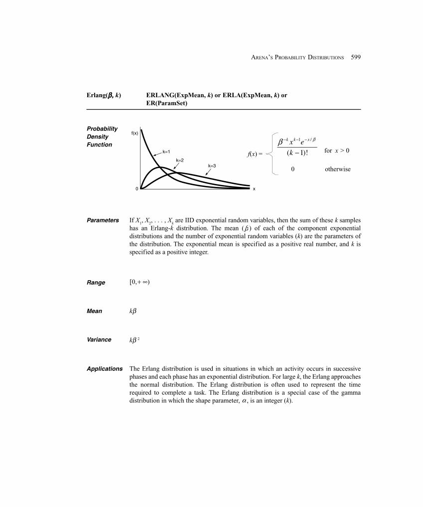
599ARENA’S PROBABILITY DISTRIBUTIONS
Erlang(β, β, β, β, β, k) ERLANG(ExpMean, k) or ERLA(ExpMean, k) orER(ParamSet)
Parameters
ProbabilityDensityFunction
Variance
Applications
Mean
Range
If X1, X
2, . . . , X
k are IID exponential random variables, then the sum of these k samples
has an Erlang-k distribution. The mean (β ) of each of the component exponentialdistributions and the number of exponential random variables (k) are the parameters ofthe distribution. The exponential mean is specified as a positive real number, and k isspecified as a positive integer.
kβ
[0,+ ∞)
kβ 2
The Erlang distribution is used in situations in which an activity occurs in successivephases and each phase has an exponential distribution. For large k, the Erlang approachesthe normal distribution. The Erlang distribution is often used to represent the timerequired to complete a task. The Erlang distribution is a special case of the gammadistribution in which the shape parameter, α , is an integer (k).
f(x)
0
k=1
k=2k=3
x
for x > 0f(x) =
0 otherwise
)!1(
/1
−
−−−
k
ex xkk ββ
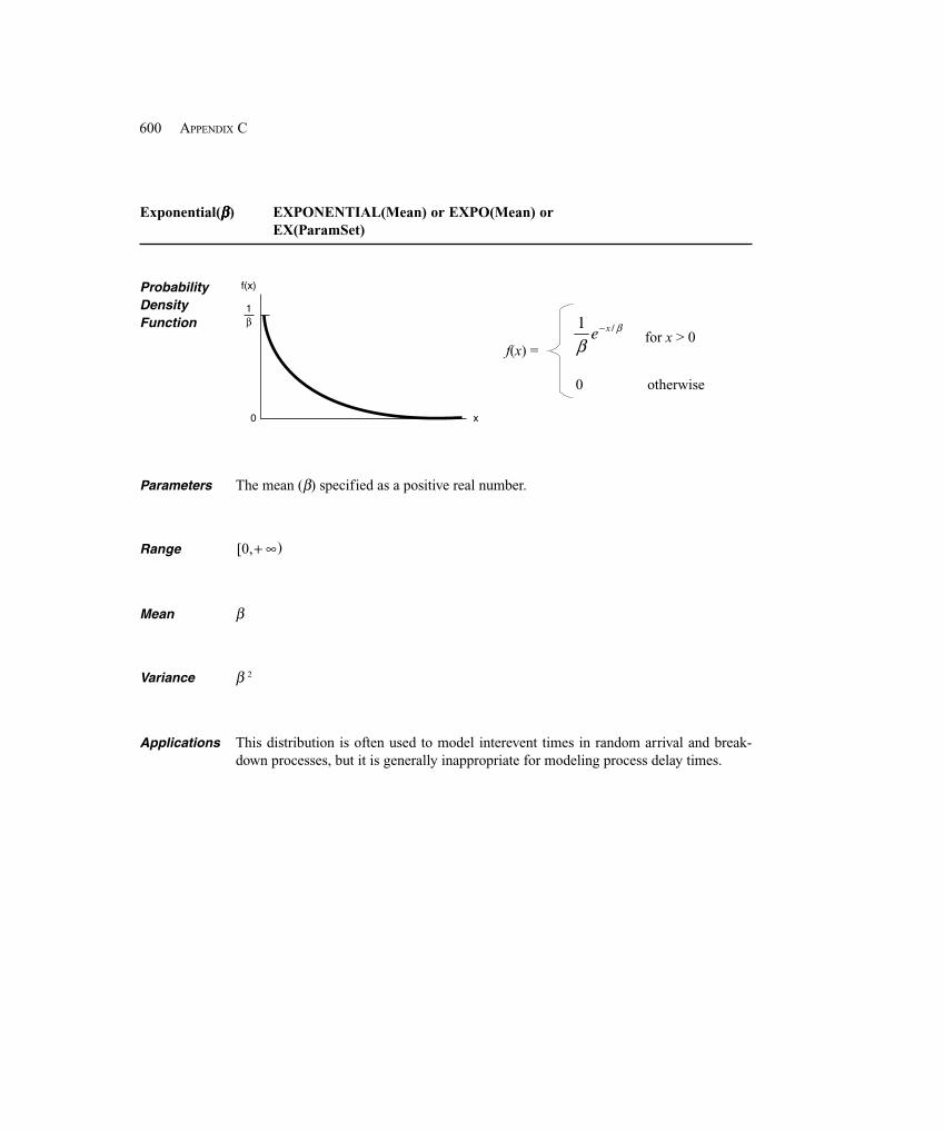
600 APPENDIX C
Exponential(βββββ) EXPONENTIAL(Mean) or EXPO(Mean) orEX(ParamSet)
Parameters
ProbabilityDensityFunction
Variance
Applications
Mean
Range
The mean (β) specified as a positive real number.
[0,+ ∞
β
β 2
This distribution is often used to model interevent times in random arrival and break-down processes, but it is generally inappropriate for modeling process delay times.
f(x)
0 x
1β
)
for x > 0f(x) =
0 otherwise
β
β/1 xe−
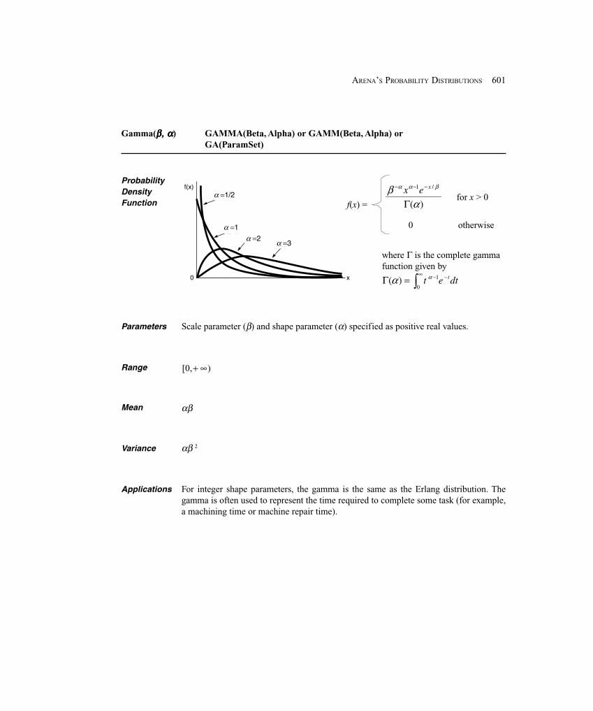
601ARENA’S PROBABILITY DISTRIBUTIONS
Gamma(β, αβ, αβ, αβ, αβ, α) GAMMA(Beta, Alpha) or GAMM(Beta, Alpha) orGA(ParamSet)
ProbabilityDensityFunction
Parameters
Range
Scale parameter (β) and shape parameter (α) specified as positive real values.
[0,+ ∞
Mean αβ
Variance αβ 2
Applications For integer shape parameters, the gamma is the same as the Erlang distribution. Thegamma is often used to represent the time required to complete some task (for example,a machining time or machine repair time).
for x > 0f(x) =
0 otherwise
)(
/1
αβ βαα
Γ
−−− xex
where Γ is the complete gammafunction given by
f(x)
0
k=1k=2
k=3
x
α=1/2
α =1
α =1/2
α =2 α =3
)
∫∞ −−=Γ
0
1)( dtet tαα
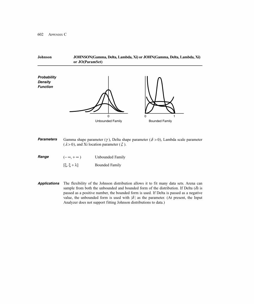
602 APPENDIX C
Johnson JOHNSON(Gamma, Delta, Lambda, Xi) or JOHN(Gamma, Delta, Lambda, Xi)or JO(ParamSet)
ProbabilityDensityFunction
0 0 1
Bounded FamilyUnbounded Family
Parameters Gamma shape parameter (γ ), Delta shape parameter (δ > 0), Lambda scale parameter(λ > 0), and Xi location parameter (ξ ).
(− ∞, + ∞ ) Unbounded FamilyRange
[ξ, ξ + λ] Bounded Family
Applications The flexibility of the Johnson distribution allows it to fit many data sets. Arena cansample from both the unbounded and bounded form of the distribution. If Delta (δ) ispassed as a positive number, the bounded form is used. If Delta is passed as a negativevalue, the unbounded form is used with |δ | as the parameter. (At present, the InputAnalyzer does not support fitting Johnson distributions to data.)
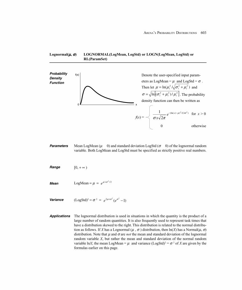
603ARENA’S PROBABILITY DISTRIBUTIONS
Lognormal(μμμμμ, σσσσσ) LOGNORMAL(LogMean, LogStd) or LOGN(LogMean, LogStd) orRL(ParamSet)
ProbabilityDensityFunction
Range
f(x)
0 x
Parameters Mean LogMean (μ 0) and standard deviation LogStd (σ 0) of the lognormal randomvariable. Both LogMean and LogStd must be specified as strictly positive real numbers.
Mean
Variance
Applications The lognormal distribution is used in situations in which the quantity is the product of alarge number of random quantities. It is also frequently used to represent task times thathave a distribution skewed to the right. This distribution is related to the normal distribu-tion as follows. If X has a Lognormal (μ , σ ) distribution, then ln(X) has a Normal(μ, σ)distribution. Note that μ and σ are not the mean and standard deviation of the lognormalrandom variable X, but rather the mean and standard deviation of the normal randomvariable lnX; the mean LogMean = μ and variance (LogStd)2 = σ 2 of X are given by theformulas earlier on this page.
[0, + ∞ )
)1(222 −+ σσμ ee
for x > 0f(x) =
0 otherwise
)2/())(ln( 22
2
1 σμ
πσ−− xe
x
2/2σμ +eLogMean = μ =
Denote the user-specified input param-
eters as LogMean = μ and LogStd = σ .
Then let )/ln( 222lll μσμμ += and
[ ]222 /)(ln lll μμσσ += . The probability
density function can then be written as
(LogStd)2 = σ 2 =
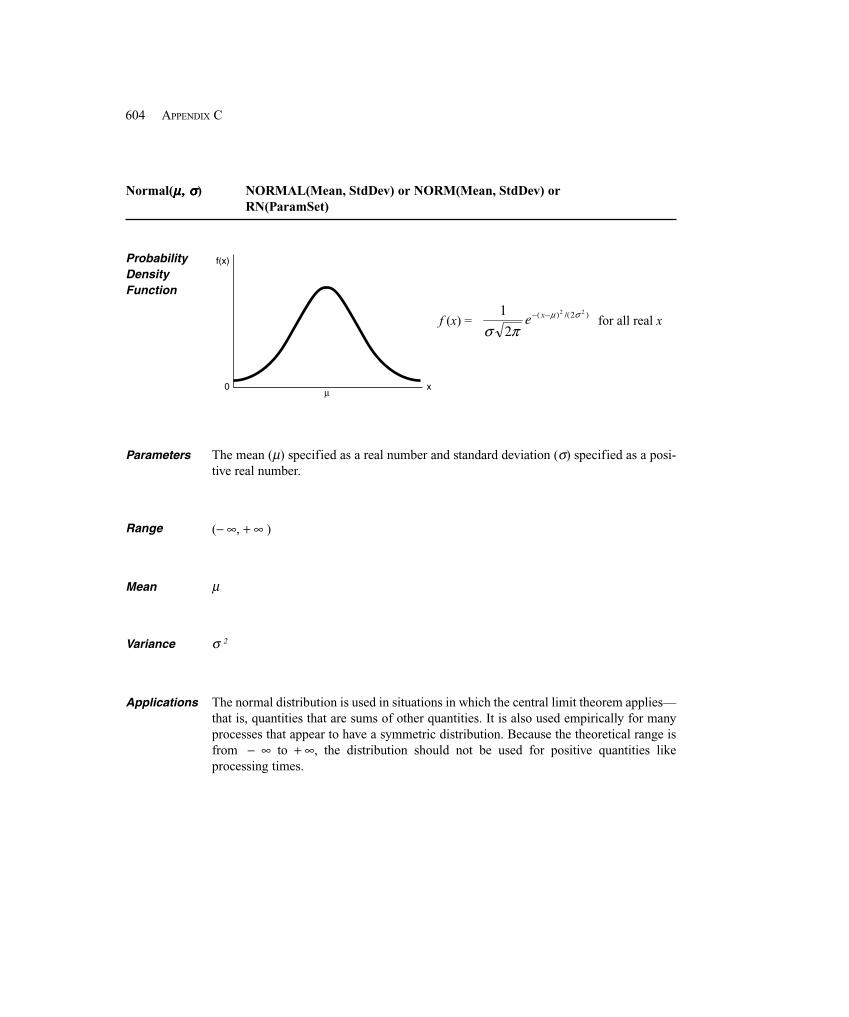
604 APPENDIX C
Normal(μ, σμ, σμ, σμ, σμ, σ) NORMAL(Mean, StdDev) or NORM(Mean, StdDev) orRN(ParamSet)
ProbabilityDensityFunction
(− ∞, + ∞ )Range
Parameters The mean (μ) specified as a real number and standard deviation (σ) specified as a posi-tive real number.
Mean
Variance
Applications The normal distribution is used in situations in which the central limit theorem applies—that is, quantities that are sums of other quantities. It is also used empirically for manyprocesses that appear to have a symmetric distribution. Because the theoretical range isfrom − ∞ to + ∞, the distribution should not be used for positive quantities likeprocessing times.
μ
σ 2
)2/()( 22
2
1 σμ
πσ−− xef (x) = for all real x
f(x)
0 xμ
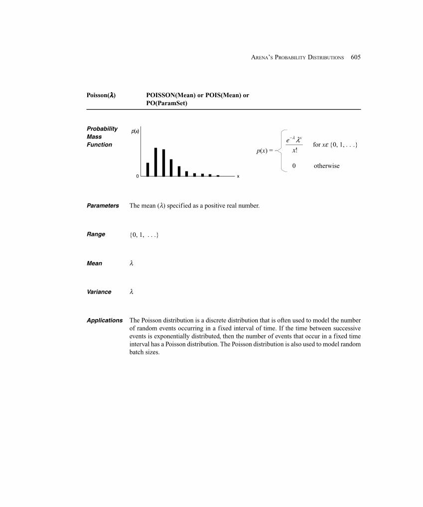
605ARENA’S PROBABILITY DISTRIBUTIONS
Poisson(λλλλλ) POISSON(Mean) or POIS(Mean) orPO(ParamSet)
ProbabilityMassFunction
The mean (λ) specified as a positive real number.Parameters
Range {0, 1, . . .}
Mean λ
λVariance
Applications The Poisson distribution is a discrete distribution that is often used to model the numberof random events occurring in a fixed interval of time. If the time between successiveevents is exponentially distributed, then the number of events that occur in a fixed timeinterval has a Poisson distribution. The Poisson distribution is also used to model randombatch sizes.
f(x)
0 x
p( )
for xε {0, 1, . . .}p(x) =
0 otherwise
!x
e xλλ−x
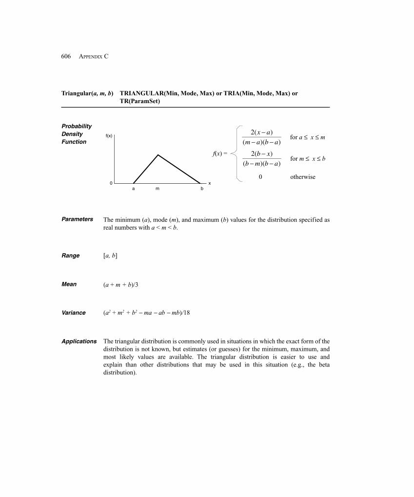
606 APPENDIX C
Triangular(a, m, b) TRIANGULAR(Min, Mode, Max) or TRIA(Min, Mode, Max) orTR(ParamSet)
ProbabilityDensityFunction
The minimum (a), mode (m), and maximum (b) values for the distribution specified asreal numbers with a < m < b.
Parameters
Range [a, b]
Mean
(a2 + m2 + b2 − ma − ab − mb)/18Variance
Applications
(a + m + b)/3
The triangular distribution is commonly used in situations in which the exact form of thedistribution is not known, but estimates (or guesses) for the minimum, maximum, andmost likely values are available. The triangular distribution is easier to use andexplain than other distributions that may be used in this situation (e.g., the betadistribution).
f(x)
0 xa m b
for a ≤ x ≤ m
f(x) =
0 otherwise
))((
)(2
abam
ax
−−−
))((
)(2
abmb
xb
−−−
for m ≤ x ≤ b
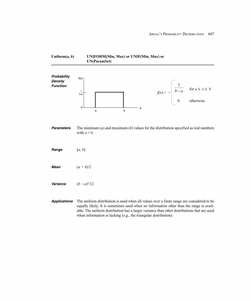
607ARENA’S PROBABILITY DISTRIBUTIONS
Uniform(a, b) UNIFORM(Min, Max) or UNIF(Min, Max) orUN(ParamSet)
ProbabilityDensityFunction
Parameters The minimum (a) and maximum (b) values for the distribution specified as real numberswith a < b.
Range [a, b]
Mean (a + b)/2
(b − a)2/12Variance
Applications The uniform distribution is used when all values over a finite range are considered to beequally likely. It is sometimes used when no information other than the range is avail-able. The uniform distribution has a larger variance than other distributions that are usedwhen information is lacking (e.g., the triangular distribution).
for a ≤ x ≤ bf(x) =
0 otherwise
ab −1
f(x)
0a
1
b
b–a1
b-a
x
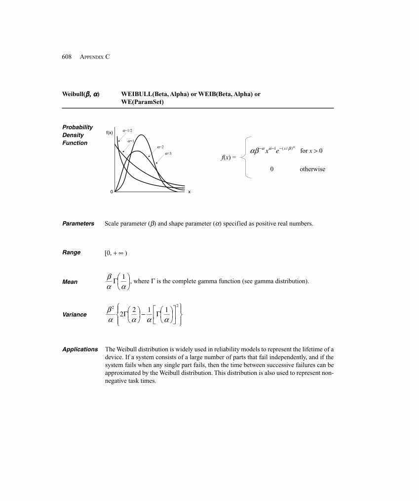
608 APPENDIX C
Weibull(β, αβ, αβ, αβ, αβ, α) WEIBULL(Beta, Alpha) or WEIB(Beta, Alpha) orWE(ParamSet)
ProbabilityDensityFunction
Parameters Scale parameter (β) and shape parameter (α) specified as positive real numbers.
Range
Mean
Variance
Applications
[0, + ∞ )
The Weibull distribution is widely used in reliability models to represent the lifetime of adevice. If a system consists of a large number of parts that fail independently, and if thesystem fails when any single part fails, then the time between successive failures can beapproximated by the Weibull distribution. This distribution is also used to represent non-negative task times.
f(x)
0 x
α=1/2
α=1
α=2
α=3
⎟⎠
⎞⎜⎝
⎛Γαα
β 1, where Γ is the complete gamma function (see gamma distribution).
⎪⎭
⎪⎬⎫
⎪⎩
⎪⎨⎧
⎥⎦
⎤⎢⎣
⎡⎟⎠
⎞⎜⎝
⎛Γ−⎟⎠
⎞⎜⎝
⎛Γ22 112
2αααα
β
for x > 0f(x) =
0 otherwise
αβαααβ )/(1 xex −−−
609ACADEMIC SOFTWARE INSTALLATION INSTRUCTIONS
APPENDIX D
Academic Software InstallationInstructions
Arena requires Microsoft® Windows® XP Professional (SP2 or later), Windows XP Home (SP2 or later),Windows 2000 Professional (SP4 or later), Windows 2000 Server (SP4 or later), Windows Server 2003(SP1 or later). Under Windows 2000 and Windows XP, you must have Administrator privileges to in-stall the software. 1 Arena 12.0 or later will install and run on Vista systems.
D.1 Authorization to Copy Software
This academic software can be installed on any university computer as well as onstudents’ computers. It is intended for use in conjunction with this book for the purposeof learning simulation and Arena. You have the right to use and make copies the softwarefor academic use for teaching and research purposes only. Commercial use of thesoftware is prohibited. Software support is supplied only to the registered instructor viathe instructions provided at the textbook Web site: http://www.mhhe.com/kelton.
This textbook describes the features and functionality of the latest version of Arenaavailable at the time of publication and uses it for compiling and running the examples,but it is expected that future versions of Arena can be used equally well with this book.Since new releases of Arena typically outpace updates to this textbook, academic institu-tions are encouraged to keep their lab and research software up to date and to make cop-ies of their latest install CDs available to students to replace what is available fordownload with this book. However, it is important that students use the same softwareversion as used in the labs because models are forward compatible, but not backwardcompatible (e.g., an Arena 10.0 model can be loaded into Arena 12.0, but an Arena 12.0model cannot be loaded into Arena 10.0).
D.2 Installing the Arena Software
Follow this sequence to install your Arena software. Please note that you cannot merelyaccept all the defaults; there are some specific steps you must follow during the installa-tion process:
1. Go to the following McGraw-Hill Web site and follow the instructions todownload and install the Arena software:
http://www.mhhe.com/kelton1 It is not necessary to have Administrator privileges to run Arena after installation. For more information
or help, please consult your Systems Administrator.
610 APPENDIX D
2. When installing the software, enter the word “STUDENT” when prompted for aserial number. This will activate a customized installation process and willprovide access to the examples referenced in the textbook.
3. The software will operate in student demonstration mode, however, those limitsare large enough to allow you to complete the assignments in this textbook.
License activation is not supplied with, or required for, the STUDENT version ofArena. If you see an option to install the activation for Arena, this option should becleared (unchecked). For more information on license activation or any other aspect ofinstallation, select Installation Notes from the Arena installation screen.
D.3 System Requirements
The minimum requirements/recommendations for running the Arena 12.0 software are:
� Microsoft® Windows® XP Professional (SP2 or later), Windows XP Home (SP2or later), Windows 2000 Professional (SP4 or later), Windows 2000 Server (SP4or later), Windows Server 2003 (SP1 or later). Arena 12.0 or later will install andrun on Vista systems.
� Microsoft Internet Explorer 6.0 (Service Pack 1) or later. (This does not need tobe your active browser, but some Internet Explorer components are necessaryfor Arena to work.)
� Adobe® Reader® 7.0 or later to view documentation� Hard drive with 75-250 MB free disk space (depending on options installed)� 256 RAM (or higher, depending on operating system)� Minimum Intel® Pentium® processor, 300Mhz or higher. The Arena software can
be run on single processor, dual processor, and dual-core processor computers;however, only one instance of Arena can be run at a time.
� The running and animation of simulation models can be calculation-intensive,so a faster processor with additional memory may result in significantlyimproved performance. In addition, a larger monitor and a screen resolution ofat least 1024 x 768 is recommended for improved animation viewing.
� Under Microsoft Windows 2000 and Windows XP, you must haveAdministrator privileges to install the software.
611REFERENCES
References
Anderson, D. R., D. J. Sweeney, and T. A. Williams, (2006), Essentials of Statistics forBusiness and Economics, 4th ed., Thomson South-Western, Cincinnati, OH.
Ashour, S. and S. G. Bindingnavle, (1973), “An Optimal Design of a Soaking Pit RollingMill System,” Simulation, vol. 20, pp. 207-14.
Balci, O., (1990), “Guidelines for Successful Simulation Studies,” Proceedings of the1990 Winter Simulation Conference, O. Balci et al. (eds.), pp. 25-32.
Balci, O., (1995), “Principles and Techniques of Simulation Validation, Verification, andTesting,” Proceedings of the 1995 Winter Simulation Conference, C. Alexopoulos etal. (eds.), pp. 147-154.
Banks, J. and R. R. Gibson, (1996), “Getting Started in Simulation Modeling,” IIESolutions, vol. 28, pp. 34-39.
Bauer, K. W. and J. R. Wilson, (1992), “Control-Variate Selection Criteria,” NavalResearch Logistics 39, pp. 307-321.
Bratley, P., B. L. Fox, and L. E. Schrage, (1987), A Guide to Simulation, 2d ed., Springer-Verlag, New York, NY.
Bretthauer, K. M., (2000), “Optimal Service and Arrival Rates in Jackson QueueingNetworks,” Naval Research Logistics 47, pp. 1-17.
Bretthauer, K. M. and M. J. Côté, (1998), “A Model for Planning ResourceRequirements in Health Care Organizations,” Decision Sciences 29, pp. 243-270.
Cinlar, E., (1975), Introduction to Stochastic Processes, Prentice-Hall, EnglewoodCliffs, NJ.
Devore, J. L., (2003), Probability and Statistics for Engineering and the Sciences, 6thed., Wadsworth Inc, Belmont, CA.
Devroye, L, (1986), Non-Uniform Random Variate Generation, Springer-Verlag, NewYork, NY.
Farrington, P. A. and J. J. Swain, (1993), “Design of Simulation Experiments withManufacturing Applications,” Proceedings of the 1993 Winter SimulationConference, G. W. Evans et al. (eds.), pp. 69-75.
Fishman, G. S. (1978), “Grouping Observations in Digital Simulation,” ManagementScience 24, pp. 510-521.
Forgionne, G. A., (1983) “Corporate Management Science Activities: An Update,”Interfaces, vol. 13, pp. 20-23.
Gass, Saul I. and Donald R. Gross, (2000), “In Memoriam: Carl M. Harris, 1940-2000,”INFORMS Journal on Computing 12, pp. 257-260.
Glover, F., J. Kelly, and M. Laguna, (1999), “New Advances for Wedding Optimizationand Simulation,” Proceedings of the 1999 Winter Simulation Conference, 255-260.
Goldsman, D., (1992), “Simulation Output Analysis,” Proceedings of the 1992 WinterSimulation Conference, J. J. Swain et al. (eds.), pp. 97-103.
Gross, D. and C.M. Harris, (1998), Fundamentals of Queueing Theory, 3d ed., Wiley,New York, NY.

612 REFERENCES
Harpell, J. L., M. S. Lane, and A. H. Mansour, (1989), “Operations Research in Practice:A Longitudinal Study,” Interfaces, vol. 19, pp. 65-74.
Harrison, J. M. and C. H. Loch, (1995), “Operations Management and Reengineering,”working paper, Graduate School of Business, Stanford University, Stanford, CA.
Hogg, R. V. and A. T. Craig, (2005), Introduction to Mathematical Statistics, 6th ed.,Macmillan, New York, NY.
Johnson, M. A., S. Lee, and J. R. Wilson, (1994), “Experimental Evaluation of aProcedure for Estimating Nonhomogeneous Poisson Processes Having CyclicBehavior,” ORSA Journal on Computing 6, pp. 356-368.
Kelton, W. D., (1996), “Statistical Issues in Simulation,” Proceedings of the 1996 WinterSimulation Conference, J. M. Charnes et al. (eds.), pp. 47-54.
Kleindorfer, G. B. and R. Ganeshan, (1993), “The Philosophy of Science and Validationin Simulation,” Proceedings of the 1993 Winter Simulation Conference, G. W. Evanset al. (eds.), pp. 50-57.
Kuhl, M. E. and J. R. Wilson (2000), “Least squares estimation of nonhomogeneousPoisson processes,” Journal of Statistical Computation and Simulation 67, pp. 75-108.
Kuhl, M. E. and J. R. Wilson (2001), “Modeling and simulating Poisson processeshaving trends on nontrigonometric cyclic effects,” European Journal of OperationalResearch 133, pp. 566-582.
Kulwiec, R. A., (1985), Materials Handling Handbook, 2d ed., John Wiley & Sons, Inc.,New York, NY.
L’Ecuyer, P., (1996), “Combined Multiple Recursive Generator,” Operations Research44, pp. 816–822.
L’Ecuyer, P., (1999), “Good Parameter Sets for Combined Multiple Recursive RandomNumber Generators,” Operations Research 47, pp. 159–164.
L’Ecuyer, P., R. Simard, E. J. Chen, and W. D. Kelton, (2002), “An Object-OrientedRandom-Number Package with Many Long Streams and Substreams,” OperationsResearch 50, pp. 1073-1075 (with accompanying Online Companion at http://or.pubs.informs.org/Media/L%27Ecuyer.pdf).
Lane, David M., (2009), HyperStat Online Textbook, http://davidmlane.com/hyperstat/index.html.
Lane, M. S., A. H. Mansour, and J. L. Harpell, (1993), “Operations Research Techniques:A Longitudinal Update 1973-1988,” Interfaces, vol. 23, pp. 63-68.
Law, A. M. and W. D. Kelton, (2000), Simulation Modeling and Analysis, 3d ed.,McGraw-Hill, New York, NY.
Leemis, L. M., (1991), “Nonparametric Estimation of the Intensity Function for aNonhomogeneous Poisson Process,” Management Science 37, pp. 886-900.
Lindley, D. V., (1952), “The Theory of Queues with a Single Server,” Proceedings of theCambridge Philosophical Society 48, pp. 277-289.
Marsaglia, G., (1968), “Random Numbers Fall Mainly in the Planes,” National Academyof Science Proceedings. vol. 61, pp. 25-28.

613REFERENCES
Morgan, B. J. T., (1984), Elements of Simulation, Chapman & Hall, London.Morgan, C. L., (1989), “A Survey of MS/OR Surveys,” Interfaces, vol. 19, pp. 95-103.Musselman, K. J., (1993), “Guidelines for Simulation Project Success,” Proceedings of
the 1993 Winter Simulation Conference, G. W. Evans et al. (eds.), pp. 58-64.Nance, R. E., (1996), A History of Discrete Event Simulation Programming Languages,
History of Programming Languages, T. J. Bergin and R. J. Gibson (eds.), ACM Pressand Addison-Wesley Publishing Company, pp. 369-427.
Nance, R. E. and R. G. Sargent, (2003), “Perspectives on the Evolution of Simulation,”Operations Research 50, pp. 161-172.
Nelson, B. L., (1990), “Control-Variate Remedies,” Operations Research 38, pp. 974-992.
Nelson, B. L., J. Swann, D. Goldsman, and W. Song, (2001), Simple Procedures forSelecting the Best Simulation System when the Number of Alternatives is Large,Operations Research 49, pp. 950-963.
Oracle Corporation, (2009), Crystal Ball, http://www.oracle.com/crystalball/index.html, Redwood Shores, CA.
Palisade Corporation, (2009), @RISK, http://www.palisade.com/, Ithaca, NY.Pegden, C. D., R. E. Shannon, and R. P. Sadowski, (1995), Introduction to Simulation
Using SIMAN, 2d ed., McGraw-Hill, New York, NY.Rasmussen, J. J. and T. George, (1978), “After 25 Years: A Survey of Operations
Research Alumni, Case Western Reserve University,” Interfaces, vol. 8, pp. 48-52.Sadowski, R. P., (1989), “The Simulation Process: Avoiding the Problems and Pitfalls,”
Proceedings of the 1989 Winter Simulation Conference, E. A. MacNair et al. (eds.),pp. 72-79.
Sadowski, R. P., (1993), “Selling Simulation and Simulation Results,” Proceedings ofthe 1993 Winter Simulation Conference, G. W. Evans et al. (eds.), pp. 65-68.
Sargent, R. G., (1996), “Verifying and Validating Simulation Models,” Proceedings ofthe 1996 Winter Simulation Conference, J. M. Charnes et al. (eds.), pp. 55-64.
Sargent, R. G., K. Kang, and D. Goldsman, (1992), “An Investigation of Finite-SampleBehavior of Confidence Interval Estimators,” Operations Research 40, pp. 898-913.
Schmeiser, B. W., (1982), “Batch Size Effects in the Analysis of Simulation Output,”Operations Research 30, pp. 556-568.
Schriber, T. J., (1969), Fundamentals of Flowcharting, John Wiley & Sons, Inc., NewYork, NY.
Seila, A. F., (1990), “Output Analysis for Simulation,” Proceedings of the 1990 WinterSimulation Conference, O. Balci et al. (eds.), pp. 49-54.
Shannon, R. E., S. S. Long, and B. P. Buckles, (1980), “Operations ResearchMethodologies in Industrial Engineering,” AIIE Trans., vol. 12, pp. 364-367.
Swart, W. and L. Donno, (1981), “Simulation Modeling Improves Operations, Planning,and Productivity for Fast Food Restaurants,” Interfaces, vol. 11, pp. 35-47.
Thomas, G. and J. DaCosta, (1979), “A Sample Survey of Corporate OperationsResearch,” Interfaces, vol. 9, pp. 102-111.


INDEX 615
Symbols
(s, S) inventory 251, 252.AND. 211.dat file 276, 282, 322.dgr file 282.doe file 55, 75, 285, 433.EQ. 211.exp file 110, 318.GE. 211.gif file 89.GT. 211.jpg file 89.LE. 211.LT. 211.mod file 110, 318, 406, 514.NE. 211.OR. 211.out file 78, 79.p file 285.pan file 285.plb file 67, 85, 99, 152.tpo file 80.tpo file extension 80.vsd file 98< 131, 211<< button 85<= 211<> 211== 211, 313> 131, 211>= 211? key 59, 89@RISK 472-way by Chance 124
A
Access module 357Accumulating conveyors 357, 408Accumulation Length 363Action 65, 83, 126Activate module 376Active Entity window 169ActiveX Automation 432ActiveX Data Objects 424ad hoc data 186Add button 83ADO 424
Advanced Process panel 11, 58, 67, 140,201, 207, 228, 249, 380
Advanced Set module 238Advanced Transfer panel 11, 58, 60, 160,
207Align 101, 105Allocate – Move 344Allocate module 375, 376Alt+ 54Alt+Prnt Scrn 57Alt+Tab 57Alternate hypothesis 589Alternatives 281Analysis of variance 590Analysis types 557
candidate 557comparative 557predictive 558
Analyst name 72, 89Anderson, D. 575, 611Animate At Desktop Color Depth 101Animate Connectors 69, 81, 101, 105Animate toolbar 84, 104
Plot 104Resource 104
Animate Transfer toolbar 105, 164Distance 105Intersection 105Network 105Parking 105Promote Path 105Route 105Segment 105Seize 105Station 105Storage 105Transporter 105
Animated routes 163Animated stations 163Animation 12, 67, 149
pulling it apart 150resource 67
Animation queue 149, 150Animation Speed Factor 131ANOVA 590Antithetic variates 9, 531Application solution templates 11
contact centers 11packaging lines 11
Arcs 104, 106

616 INDEX
Arena 10.doe files 55tour of 53window 55, 56
Arena folder 55, 80Arena help 102
index 102search 102table of contents 102
Arena hierarchy 206Arena icon 54Arena Input Analyzer 34Arena News Flash 100Arena Output Analyzer 34Arena Professional Edition 462Arena SMART files 102Arena Symbol Factory 100, 101Arena Template Developer’s Guide 462Arrange Icons 102Arrange menu 101
Align 101Bring to Front 101Change Object Snap Point 101Distribute 101Flip 101Flowchart Alignment 60, 101Group 101Send to Back 101Snap Object to Grid 101Ungroup 101
Arrange toolbar 71, 89, 105Align 105Bring to Front 105Flip 105Group 105Rotate 105Send to Back 105Space 105Ungroup 105
Arrival 25Arrival rate 43, 232ASCII text file 179Ashour, S. 499, 611Assign Block 259, 261, 262ASSIGN command 362Assign module
60, 119, 122, 351, 395, 496Attach template panel 80Attach Template Panel dialog 80Attractor points 106
Attribute 21, 26, 67, 119, 121Attributes Element 255, 351Auto-Connect 69, 81, 101, 119AutoCAD 98, 314, 433Autocorrelation 44, 46Automated guided vehicle (AGV) 341, 404Automated teller machines (ATMs) 2Average total time in system 32Average waiting time in queue 17, 32AVI Capture 101
B
Back quotes 468“Back-of-the-envelope” calculation 18Backfire 531Background 104backlogging 251Baking pan 113Balci, O. 543, 611Balking 204, 214, 376, 378Bambi 55Banks, J. 543, 611Base Time Units 16, 72, 75, 128, 307, 493Baseline values 547Basic Process panel 11, 57, 80, 119, 201,
207Basic Process panel modules
Assign 207Batch 207Create 207Decide 207Dispose 207Process 207Record 207Separate 207
Basic Process Variables 142BasicProcess.tpo 80Batch means 133, 326, 532, 538Batch module 60, 384, 387, 390Batch Run (No Animation) 110, 131, 144,
275, 322Batch sizes 328Batches 326, 386
permanent group 386temporary group 386
Batching 385, 386Bauer, K. 532, 611Bell curve 280Belt conveyor 357

INDEX 617
Beta distribution (BETA) (BE) 178, 593,595
Bézier Curve 104, 106Biased 321Bimodal 184, 185Bindingnavle, S. 499, 611Blocked 393Blocking 540Blocks 11, 58Blocks panel 11, 201, 207, 251, 350,
380, 403Blue ball 83“Blue” scenarios 288Bonferroni 590Book Examples folder 55Border 106Boundaries, system 546Box 89, 104, 106Box and Whisker 288Branch Block 259, 406Bratley, P. 531, 611Break 105“Break angel” 21Break on Module 105, 110, 170“Breakdown demon” 21Breakdowns 136Breakpoints 110Breakpoints window 169Bretthauer, K. M. 199, 611Bridge cranes 336Bring to Front 101, 105, 315Bucket 357Buckles, B. 6, 613Buffer space 392Buffers
finite 370infinite 370
Buffon, Comte de 8Buffon cross 9Buffon needle problem 9Build Expression 63, 142Busy 25, 136, 149Busy picture 85Buttons
Add 68, 83Box 89Bring to Front 315Check 130, 167Command 173, 362Connect 68
Distance 346Draw 89End 74Fast-Forward 131Fill Color 89Go 73, 130, 132, 362Grid 59Help 108Line Color 89Parking 347Pause 131, 362Plot 68, 85, 156Queue 353Resource 84, 314Route 164Segment 361Send to Back 89Show 59Snap 59Snap to Grid 59Station 163Step 131Storage 354Text 71, 89Text Color 71, 89Text String 89Transporter 342Zoom In 59Zoom Out 59
C
C 10, 11, 208C++ 11, 433CAD drawings 98, 301, 305, 314CAD packages 53Calendar Schedules 99Calendar window 169Call centers 203Candidate analysis 557Capacity 65, 66, 139Carts 341Cascade 56, 102Case sensitive 59, 89, 122Case Western Reserve University 5Categories 144Category 401Category by Replication report 74, 275, 326Category Overview report 74, 75, 132, 276

618 INDEX
CDF (cumulative distribution function) 520,579, 581
Cell size 356, 358Cells 355Central limit theorem 279, 586, 588Change Object Snap Point 101Chart Options 289Chart Type 288Check button 167Check Model 73, 105, 109, 130, 436Chen, E. 517, 612Chi-square distribution 183, 586, 588Chi-square test 590Cinema 318Cinlar, E. 524, 611Clicking 54
double 54right 54, 79
Client 543Clock 24CMRG 517Color palette 98Combat models 2, 366, 367, 511, 512Combined multiple recursive generator
(CMRG) 517ComboBox 467Command 105, 110, 173, 362Command buttons 82Common random numbers (CRN)
42, 525, 528Comparative analysis 557Compare like with like 531Compare Means 283, 529Comparing alternatives 36, 281Complement 576Computer simulation 5Conditional probability 577Confidence interval 36, 42, 79, 133, 276,
279, 284, 289, 324, 326, 529, 533,538, 587
for mean 587for standard deviation 588for variance 588meaning of 279on proportion 589on ratio of two standard deviations 589on ratio of two variances 588
Confidence level 279, 587Confidence-interval half width 133Connect 101, 103, 302, 335
Connect button 68Connect Type 338, 344Connecting modules 465Connections 68, 119, 335Connector Arrows 100Connectors, animation 69Consistency 587Constraints 250Contact centers 11, 58ContactCenter 101
Tools menu 100Context-sensitive Help 55, 103, 108Continuous 7Continuous CONT (CP) empirical distribution
593, 596Continuous Element 476, 500Continuous empirical distribution 179, 593,
596Continuous integration algorithm 476Continuous modeling with VBA 506Continuous random variable 521, 575, 578,
580Continuous step size 476, 481Continuous systems 208, 473, 481Continuous tolerance 481Continuous-time statistics 77Continuous/discrete models 477Control 54Control entity 415Control variates 532Controls 285Convey module 357Conveyor 355, 407Conveyor module 358Conveyor segments 360Conveyor statistics 362Conveyors 336, 355, 357, 370
accumulating 357, 408nonaccumulating 357, 358, 364, 370
Copy 54, 56, 99Copy Block 405Copy protection for Arena software 102Correlated 79, 133, 327, 531, 538Correlated sampling 528Correlation 582, 583Corresponding p-value 183, 590Cost measure 245Costing 64, 67, 237, 248Côté, M. J. 199, 611Count-based failure 140

INDEX 619
Counter 133Counter example 195Counter statistics 77Counters 73, 132County fair 411Covariance 531, 582, 583Craig, A. 575, 612Create Block 258Create from File 89Create module 54, 60, 62, 81, 119, 121,
209, 380, 387, 415, 445, 535CreateObject (VBA) 458Creating entities 415Critical point 588CRN 528, 529, 530Cross dock 366Crystal Ball 47Crystal Reports 77CStats Element 504Ctrl+ 54Ctrl+C 56Ctrl+Click 56Ctrl+D 80Ctrl+N 56Ctrl+O 56Ctrl+P 107Ctrl+Tab 56, 107Ctrl+V 56Cumulative distribution 39Cumulative distribution function (CDF)
520, 579, 581Cumulative probability 308Current Expression 87, 143Customer stay zone 379Cut 54, 56, 99, 103Cycle 518Cycle time 18, 393Cyclic 343Cyclical 312, 365Cycling 515
D
DaCosta, J. 6, 613Data collection 176, 177Data group 282Data modules 61
Advanced Set 238Conveyor 358
Distance 346, 347Entity 61, 63, 83, 128Expression 247, 306Failure 67, 140, 395File 418, 420, 423Queue 61, 67, 84, 142, 225, 351Resource 61, 65, 66, 84, 337, 339, 395Schedule 61, 138Segment 360Sequence 303, 306Set 61, 307StateSet 141, 395Statistic 142, 249, 276, 325, 387, 391Storage 351Transporter 342Variable 61, 205, 306, 387
Data tab 289Data Tip 61, 100
default descriptions 61user-defined descriptions 61
DAVG 257, 539, 541Deadheading 355Deadlock 370Debug Bar 100, 169
Active Entity window 169Breakpoints window 169Calendar window 169Watch windows 169
Debugging 109, 514Decide module 60, 111, 119, 124, 125,
214, 242, 376, 378, 406, 535Decision logic 405Decision variable 39Declaration of Independence 584Default description 61Degrees of freedom (DF) 36, 530, 586Delay 33, 65, 122Delay Block 261Delay module 242, 344, 417Delay Release 122Delay Type 65Delivery lag 252Departure 25Deselect All 99Destination Type 160, 309Detach 80, 98, 103Detaching a template panel 80Detect Block 478
relationship to step size 481Deterministic 7

620 INDEX
Devore, J. 575, 611Devroye, L. 190, 611DF (degrees of freedom) 530, 586DHALF 328Dialog boxes 54Dialog design window 466
Design Properties 466Operand Explorer 466Toolbox 466
Dialog form 467Differential equations 476, 500Differential-equation methods 5Direct connections 158, 161Discrete 7Discrete DISC (DP) empirical distribution
179, 379, 593, 598Discrete random variables 519, 578Discrete-event models 473Discrete-event simulations 33Discrete-parameter statistic 17Discrete-time statistics 17, 77Disks 54Display 82, 109, 119Display Composite View 103Dispose Block 259, 263Dispose module 60, 67, 85, 119, 126, 214Distance button 105, 346Distance module 346, 347Distance Set 342, 345Distances 347, 349, 360Distribute 101Distributions
beta 593, 595continuous empirical 593, 596discrete empirical 593Erlang 593exponential 19, 35, 62, 117, 120, 593gamma 593Johnson 593lognormal 593normal 65, 593Poisson 593sampling 585triangular 35, 65, 117, 593uniform 65, 593Weibull 117, 593
Do-while 406Documentation 48, 559Donno, L. 4, 613Double-clicking 54
Down Time 141, 393Down Time Units 141Draw toolbar 71, 88, 104, 106
Arcs 104, 106Background 104Bézier Curves 104, 106Box 104, 106Ellipse 104, 107Fill 104Fill Color 107Fill Pattern 104Line 104, 106Line Color 104, 107Line Style 107Line Width and Style 104Polygon 104, 106Polyline 104, 106Show Dimensions 104, 107Text 104, 107Text Color 107Window Background Color 107
Drop-down lists 122Dropoff Block 405Dstat ID 328DStats Element 256Duplicate 99Duplicate entities 418Duplicate Scenario 287Durations 138, 139, 237DXF format 98, 314Dynamic 7Dynamic objects 20Dynamic plots 85
E
Edit error 167Edit Exceptions 103Edit menu 99, 453
Calendar Schedules 99Copy 99Cut 99Deselect All 99Duplicate 99Entity Pictures 99Find 99Insert New Control 99Insert New Object 99Links 99

INDEX 621
Object 99OLE Link 99Paste 99Paste Link 99Properties 99Redo 99Select All 99Undo 99
Edit mode 74, 109Edit Time Patterns 103Edit via Dialog 138, 139Educational Lab package 462Effect 540Elements 11, 58, 254Elements panel 11, 208, 251, 254, 350,
351, 403, 518Ellipses 104, 107Else Block 405ElseIf Block 405Embeddeds collection (VBA) 453Empty and idle 16, 320Empty event 577End 109End button 74EndIf Block 405EndWhile Block 406Enter module 338, 344, 359, 360Entities 20
batching 385“fake” 21holding 385
Entities Element 255Entities per Arrival 63, 121Entity arrivals, reading from a text file 415Entity Location 352Entity module 61, 63, 83, 128Entity Picture Placement window 129,
152, 166Entity pictures 99, 129, 152, 166Entity reference point 152Entity statistics 67Entity Summary dialog 131Entity transfer 335Entity.JobStep (IS) attribute 303Entity.Sequence (NS) attribute 303, 308Entity.Station (M) attribute 303, 309, 490Entity.WaitTime 248Entry 81Entry point 68, 81ERLA (ER) 593, 599
Erlang distribution 178, 593, 599, 601Error Tolerance 288, 289, 290Errors/Warnings 167
window 109Esc key 109, 131Escalator 336, 357Estimate 587Estimated rate function 523Estimator efficiency 587Event 23, 25, 26, 576
calendar 23, 25, 26, 475future 23orientation 32record 23
Event process 523Excel 40
charting results (VBA) 455, 457macro 432
Exit 81, 98, 357Exit point 68, 81Expectation 579Expected value 579, 581Experiment 575Experiment file 318Experimental design 48, 539Exponential EXPO (EX) distribution 19, 35,
62, 117, 120, 178, 186, 593, 599, 600Export Model to Database 100, 101Export report 75Expression 139, 142, 247Expression Builder 63, 65, 71, 87, 88, 389Expression module 205, 247, 306Expression Type 142Expressions 205Expressions Element 255
F
F distribution 588F10 key 109F4 key 130F5 key 109, 130, 287Factorial design 540Factors 540Fail When 141Failed 136, 149Failed state 144Failure module 67, 140, 395Failure name 141

622 INDEX
Failure ruleIgnore 141Preempt 141Wait 141
Failures 135, 136, 140, 393, 395“Fake” entities 21Farrington, P. 543, 611Fast-Forward 109, 110, 131, 144Ferris, G. W. G. 411Ferris wheel 411FIFO (First in first out) 15, 337File data module 418, 420, 423File menu 98
DXF Import 98Exit 98Import Visio drawing 98Open color palette 98Print 98Print Preview 98Print Setup 98Save color palette 98Send 98Template panel attach/detach 98
Files 54Fill 104, 106Fill Color 107Fill Color button 89Fill Pattern 104Find 99, 130Find error 167Finite buffers 370First Creation 259First in first out (FIFO) 15, 67, 223, 337Fishman, G. 327, 611Fit All 181Fit All Summary 182Fit menu 181Fitting input distributions 178Flip 101, 105Flow module 495, 497Flow Process panel modules
Assign 496Flow 495Regulate 495Release Regulator 496Seize Regulator 496Sensor 495Tank 495
Flow Process template 495Flowchart 208
Flowchart Alignment 60, 101Flowchart modules 60
Activate 376Allocate 375, 376Assign 60, 119, 122, 351, 395Batch 60, 384, 387, 390Create 60, 62, 81, 119, 121, 209, 380,
387, 535Decide 60, 111, 119, 124, 125, 214,
242, 376, 378, 406, 535Delay 242, 344Dispose 60, 67, 85, 119, 126, 214Enter 338, 344, 359, 360Expression 205Free 376Halt 376Hold 387, 388, 389, 409, 410Leave 338, 343, 344, 351, 359Move 375, 376Process 60, 64, 83, 119, 124, 125, 344Record 60, 119, 126, 214, 382, 389Release 338Remove 384, 385, 409Request 344, 375Route 159, 160, 161, 309, 311, 338,
394Search 383, 384, 409Seize 337, 395, 396Separate 60, 381, 384, 390, 395Sequence 305Sets 234Signal 390, 409, 410Station 159, 160, 338, 394Statistic 250Transport 344, 375
Folders 54Forgionne, G. 6, 611Fork trucks 341, 364, 365FORTRAN 10, 12Fox, B. 531, 611Free 341, 345Free module 376Free Transporter 344Free-path transporters 341Freeway 358Frequencies 142, 395, 399Frequencies report 148, 400Frequencies statistic 135, 142Frequency 148Frequency ID 401

INDEX 623
Frequency Type 144FRQTIM 401Functional inverse 40Functional specification 561Future event 23
G
Gamma function 601Gamma GAMM (GA) distribution
178, 593, 599, 601Ganeshan, R. 543, 612Gantry cranes 336Garbage in, garbage out 177Garden hose 522Gass, S. 251Generalized parallel processing 90Generating random variates 34
continuous 521discrete 519
George, T. 5, 613Gibson, R. 543, 611Girod, O. 551, 561, 573Global variable 21, 205Glover, F. 295, 611Glue 81Glue to Guides 60, 99Go 73, 109, 130, 132, 287, 362Goldsman, D. 290, 329, 543, 611, 613Goodness-of-fit tests 590Gossett, W. 9GPSS 10Grading homework 514Graphical Schedule Editor 138, 139Graphics 106Graphics file 89Grid 59, 81, 105, 347Grid & Snap Settings 59Gridlock 370Gross, D. 251Group 101, 105Guessing 18Guided transporters 341, 404Guides 60, 81
H
H0 589H1 589
Half width 36, 79, 133, 276, 277, 326,327, 533, 536
Halt module 376Hand simulation 25, 53, 415Hand trucks 341Harpell, J. 6, 612Health-care models 2, 197, 198, 299Help 108Help button 108Help menu 102, 108
Arena Help 102Arena SMART Files 102Product Manuals 102Release Notes 102SMART files 108Support aned Training 102What’s This 102
Help topic 109HiddenOperand 468Hierarchical 11High Value 144High Value First 223Highlight Active Module 110, 169Histogram 180, 182Hogg, R. 575, 612Hold (Scan for Condition) 410Hold module 387, 388, 389, 409, 410Holding 385Holding cost 252Home 59Hook lines 408Hot key 59, 89Hours per day 72Hummus 534Hypothesis tests 284, 589
I
Identical 35Identifiers 150Identify Best Scenarios 288Idle 25, 136, 149Idle picture 85IF Block 405Ignore 136, 141, 237IID 274Implementation 545Import Model from Database 101

624 INDEX
ImportingCAD drawings 98graphics 106Visio drawing file 98
Inactive 136Independence 582Independent 35, 577, 584Independent and identically distributed (IID)
36, 274, 275, 585Independent random numbers 529Independent replications 274Independent sampling 530Index 102Industry-focused templates 470Infinite buffer 370Initial Picture 83, 128Initial Position 342Initialize Between Replications 274, 275Initialize model 436Initialize statistics 250Initialize system 250Input analysis 174Input Analyzer 34, 100, 175, 178, 179,
280, 590Input data 176Input probability distribution 34Ins key 80Insert Block 405Insert Chart 288Insert Control 286Insert New Control 99Insert New Object 89, 99Insert Response 286Installation of software 609Instantaneous Utilization 146, 195Insufficient 79, 133, 327, 538Integers 62Integrating desktop applications 413Integration 13Integration algorithm 476Integration toolbar 104
Module Data Transfer 104VBA Design Mode 104Visual Basic Editor 104
Interarrival time 16Intersection 105, 576Inventory 39, 366, 367Inventory model 251, 366, 367Inverse CDF 521, 522IS 303
J
J 384Java 433Jobstep attribute 303Jockeying 377Johnson JOHN (JO) distribution 593, 602Johnson, M. 524, 612Joint CDF (cumulative distribution function)
582Joint distributions 582Joint normal distribution 584Joint PDF (probability density function) 582Joint PMF (probability mass function) 582Jointly distributed random variables 582
K
Kang, K. 329, 613Kelly, J. 295, 611Kelton, W. D. 184, 190, 251, 297, 329,
517, 540, 543, 612Keyboard 54Kleindorfer, G. 543, 612Kolmogorov-Smirnov test 183, 590Kuhl, M. E. 524Kulwiec, R. 336, 612
L
Label 406Laguna, M. 295, 611Lanchester combat equations 511, 512Lanchester, F. 511Lane, D. 575Lane, M. 6, 612Languages
simulation 10Largest Distance 341, 343, 365Last in first out (LIFO) 223Lattice 516Law, A. 184, 189, 251, 297, 329, 540, 612Layers 100, 103, 130, 169LCG 514Lead time 252Leave module 338, 343, 344, 351, 359Leclerc, George Louis 8L’Ecuyer, P. 517, 612Lee, S. 524, 612

INDEX 625
Leemis, L. 524, 612Length of replication 72Level 474, 540Level animation 264Libraries 67License activation 610Likelihood 576Lindley’s formula 44Line Color 89, 104, 107Line Style 107Line Width and Style 104Linear congruential generator (LCG) 514Linear programming 5Lines 104, 106Links 99Load area 356Load time 358, 375Local variables 21Logarithms 317Logic area 64Logic modules
Create 415, 445Delay 417ReadWrite 416Separate 418
Logical model 4Logical structure 15Logistics models 2, 366, 367Lognormal LOGN (RL) distribution 178,
593, 603Long run 79, 133Long, S. 6, 613Look and feel 53Low Value First rule 223Lowest Attribute Value 67Lucas, T. 511Lucke, G. 551, 561, 573Lumped 284
M
M 279, 303M/M/1 19, 49M/U/1 queue 44Machines.plb 85Macro 101, 441Macro Recorder 441Mail 98Manage named views 105
Mansour, A. 6, 612Marbles 113Marginal CDF 583Marginal distribution 582Marginal PDF 583Markovian 19Marsaglia, G. 516, 612Matched pairs 528Material handling 336Math functions 377
maximum (MX) 384minimum (MN) 384
Mathematical model 4Mathematical programming 39Max Batch 387Max Cells Occupied 358Max Number of Branches 261Maximum math function (MX) 378, 384Maximum time waiting in queue 17Mean 579Measurable subset 576Mechanistic simulation 20Medical models 2, 197, 198, 299Members 238Menus 54, 98
Arrange 101Edit 99File 98Help 102Object 101Run 102Tools 100View 99Window 102
Metricsperformance 547
Metrics for success 545Microsoft Access 77Microsoft Office 433Microsoft Windows 53, 609Military models 2, 366, 367, 511, 512Miller, S. 551, 573Minimum math function (MN) 257, 384Minimum square error 182Minimum step size 476Mixed continuous-discrete 7MN 263, 384Model 3
debugging 109logical 4

626 INDEX
logical structure 15mathematical 4numerical structure 16tabletop 4
Model Documentation Report 61, 100, 101Model file 318, 433
new 54Model object (VBA) 439Model representation 47Model validation 414Model window 56
flowchart view 56, 57new 80spreadsheet view 56, 57
Modelingquantitative 175structural 175
Modeling approach 118Modeling flexibility 11ModelLogic_OnClearStatistics (VBA) 437ModelLogic_OnKeystroke (VBA) 437ModelLogic_RunBegin (VBA) 436, 448ModelLogic_RunBeginReplication (VBA)
436ModelLogic_RunBeginSimulation (VBA)
436, 456ModelLogic_RunEnd (VBA) 437ModelLogic_RunEndReplication (VBA)
437, 461ModelLogic_RunEndSimulation (VBA)
437, 461ModelLogic_UserFunction (VBA) 437ModelLogic_VBA_Block_Fire (VBA) 437Models
3-1: Browsing through an existing model62
3-2: Serial processing 903-3: Parallel processing 933-4 and 3-5: Effect of task-time variability
954-1: An electronic assembly and test system
1174-2: The enhanced electronic assembly and
test system 1344-3: Enhancing the animation 1494-4: The electronic assembly and test
system with part transfers 1584-5: Count negative Normal observations
1875-1: Simple call center system 202
5-2: Enhanced call center system 2315-3: Enhanced call center 2445-4: (s,S) inventory simulation 2519-1: Finite buffers at Stations 3709-2: Parts stay on conveyor during
processing 3749-3: Service model with balking and
reneging 3779-4: Batching process example 3869-5: Tightly coupled production system
3949-6: Adding part-status statistics 40010-1: Reading and writing data files 41310-2: Reading entity arrivals from a text
file 41510-3 and 10-4: Reading and writing Access
and Excel files 41910-5: Reading in String data 43010-6: Presenting arrival choices to the user
44410-7: Recording and charting model results
in Microsoft Excel 45511-1: A simple continuous system 47411-2: Interfacing continuous and discrete
logic 47711-3: Coal loading with continuous
approach 48511-4: Coal loading with Flow Process 49511-5: A soaking-pit furnace 499steady-state 524, 537terminating 524
Module Data Transfer 104Module drag and drop 81Module logic
defining 465Modules 57, 60
flowchart 60Moore’s “law” 518Morgan, B. 9, 612Morgan, C. 6, 613Morris, J. 116, 199Mouse 54Move module 375, 376Move Time 338, 344Moveable resources 336MR 173MREP 533, 535, 536Multiple comparisons 590Multivariate and correlated input data 189Musselman, K. 543, 613

INDEX 627
Mutually exclusive 577MX 256, 378, 384
N
N-way by Chance 214Name field 62Named Views 59, 89, 100, 108, 150Names 61Nance, R. 10, 12, 613Navigate 57Navigate panel
Thumbnail button 57NC 250Negative correlation 532Nelson, B. 290, 532, 613Network 105New Breakpoint button 169New model 103New model file 54News vendor problem 37Next Label 406No data 185Nonaccumulating conveyors 357, 358, 364,
370Nonstationary arrival process 188Nonstationary Poisson process (NSPP) 188,
234, 272, 523Normal density function 280Normal distribution
disadvantage of 187Normal NORM (RN) distribution 39, 65,
178, 187, 586, 593, 604NQ 87, 142, 156, 173, 378, 383NR 71, 88, 173NREP 533, 535, 536NS 303NSPP 523NSTO 379Null event 577Null hypothesis 589Num Reps 288Number busy 28Number of Replications 72, 133, 274Number waiting 28Numerical methods 522Numerical structure 16
O
Object 99Object menu
Animate At Desktop Color Depth 101Animate Connectors 101Auto-Connect 101Connect 101Smart Connection 101
Object model 432Object name 123Object properties 99Object Properties Description 61Objective
performance 547Objective function 39Objects (VBA) 432, 438
browsing 438collections 438methods 432properties 432, 438
OEM 544OLE link 99Open model 103Operand 463Operand name 451Operand referencing 468Optimization 39, 290Option buttons 54Option Explicit statement (VBA) 456Options 58, 101OptQuest for Arena 101, 273, 291, 295,
296OptTek Systems Inc. 291Oracle Corporation 47Order of operations 244Order-of-magnitude approximation 19Ordering cost 252Original equipment manufacturer 544ORUNAVG 540ORUNHALF 533, 535Other 307Outliers 184Output, random 6Output Analyzer 34, 100, 273, 276, 282,
284, 322, 328, 529, 590Output File 276, 282, 325Output ID 533Outputs Element 257

628 INDEX
Outputs statistics 133OVALUE 257Overall economic figure of merit 245Overlap 282Overlapping resources 369, 392Overview of a simulation study 47
P
p-values 183, 590Packaging 58Page Breaks 100Paired-t test 284, 530Palisade Corporation 47, 613PAN 285, 287, 288, 291, 296, 333PAN project 285Pan/zoom 59Panel icon 464Panels 57, 80
Advanced Process 11, 58, 67, 140, 201,207, 228, 249, 380
Advanced Transfer 11, 58, 60, 160, 207attach 98attach template 80Basic Process 11, 57, 80, 119, 201, 207Blocks 11, 58, 201, 207, 350, 380, 403detach 98Elements 11, 58, 208, 350, 351, 403,
518Navigate 57
Parallel queues 404Parameters 587Parameters Element 594Parking 105Parking Area 347Parking button 347Partial derivatives 5Paste 54, 56, 99, 103Paste Link 99Paths 54Pause 73, 109, 131, 362PDF (probability density function) 521, 580,
581Pegden, D. 58, 110, 184, 264, 319, 364,
404, 613Percent true 124Performance estimation 317Performance metrics 547Performance objective 547Permanent group 386
pi, estimation of 9PickQ Block 404Pickup Block 405Picture Editor 85, 152Picture library 85, 99, 152, 154Picture name 154Picture.Blue Ball 83Picture.Report 128Piecewise-constant rate function 188Pizzazz (with VBA) 444Plot 69, 104, 156, 263, 322Plot button 85PMF (probability mass function) 578Point estimation 587Point Type queue 151PointToPoint plot 70, 86Poisson POIS (PO) distribution 379, 593,
605Polygon 104, 106Polyline 104, 106Population 585Potted plants 156Power-and-free 408Precision 36, 278Prediction interval 279Predictive analysis 558Preempt 136, 137, 141Preferred Order rule 312, 343Presentation 558Preserving the results 559Print 75, 103Print Preview 103, 107Print Screen 57, 108Print Setup 107Printing 98, 107Priorities 65, 223, 338, 341Prnt Scrn 57, 108Probability 575, 576Probability board 113, 270Probability density function (PDF) 521, 580Probability distributions 34, 178, 575, 578,
593beta 178, 593, 595continuous 178, 593, 596discrete 178, 593, 598discrete empirical 379empirical 178Erlang 178, 593, 599exponential 178, 186, 593, 600gamma 178, 593, 601

INDEX 629
Johnson 593, 602lognormal 178, 593, 603normal 178, 187, 593, 604Poisson 379, 593, 605theoretical 178triangular 178, 186, 593, 606uniform 178, 186, 593, 607Weibull 178, 593, 608
Probability mass function (PMF) 519, 578Process Analyzer 75, 100, 273, 276, 285Process module 60, 64, 83, 119, 124,
125, 344Process orientation 33Process spreadsheet 66Processes 33Project bar 56, 57, 80Project Description 61, 72Project element 255Project parameters 72, 89, 127, 133Project title 72, 89Promote Path 105Properties dialog 446Pseudorandom-number generators 514
Q
QPick Block 404, 405Quantity 65Queue 22, 84Queue – Request – Delay – Transport 350Queue animation 67, 83, 124Queue Block 352Queue button 353Queue discipline 48Queue module 61, 67, 84, 142, 225, 351Queue Name 124, 142Queue position 383Queue ranking 405Queue Type 67Queue-ranking rule 388
First in first out (FIFO) 388Queueing theory 5, 19Queues 15, 22Quincunx 112
R
Radio buttons 54Random 6, 312, 343
Random (Expo) distribution 40, 62, 81, 307Random input 34, 175Random numbers 39, 513, 514Random Numbers Fall Mainly in the Planes
516Random output 34Random sample 585Random variables 175, 577Random variates 39, 519Random vector 582Random-number generator (RNG) 513, 529Random-number stream 146, 527, 529, 531,
533default stream 518
Random-number synchronization 527Randomness 34, 273Range 144Rank 383Rasmussen, J. 5, 613Rate function 523
estimated 523Rates 474Reading entity arrivals from a text file 415ReadWrite module 416Real numbers 62Realizations 20, 275, 513, 585Record Entity Statistics 127Record Macro toolbar 105Record module 60, 119, 126, 214, 382,
389Record of information 23“Red” scenarios 289Redo 99, 103Reduction in variance 530Regulate module 495, 497Relative precision 537, 539Release 22, 65Release module 338Release Notes 102Release Regulator module 496Release Resource 338Remainder 514Remove Block module 384, 385, 405, 409Reneging 376, 377, 379Replicate element 256Replication 35, 37, 79, 110, 324
independent 274length 128, 307, 538parameters 72, 89truncated 532

630 INDEX
Report 133, 558Report Database 100Report label 142Report statistics 64Reports 57, 74, 128, 145, 174
Category by Replication 74, 275Category Overview 74, 276Frequencies 400Resources 74SIMAN summary 78, 79
Reports panel 74Request 341, 345Request – Delay – Transport 344Request Block 344, 352, 375Requirement 250Research package 462Resource 65, 84, 104, 126, 314
unit 22Resource animation 67, 84Resource button 84Resource capacity 336Resource failures 135, 140Resource module 61, 65, 66, 84, 337,
339, 395Resource Name 65, 144, 238, 338Resource Picture 73Resource Picture Placement window 67, 84,
154Resource pictures 154Resource reference point 154Resource schedule 135, 136, 138Resource set 234Resource states 136, 393
Busy 136Failed 136Idle 136Inactive 136
Resource unit 22Resource-constrained entity transfer 336,
365Resources 22
overlapping 369Resources dialog 65Resources report 74Responses 285, 540Restricted percent 149Review Errors 110, 169Ride point 342Riesenrad 411Right-clicking 54, 79
RNG 513Rock music, annoying 203Rotate 105Roundoff error 16Route 105, 158, 164, 302, 335, 338Route dialog 164Route module 159, 160, 161, 309, 311,
338, 394Route path 159Route Time 160Routing 335Rulers 59, 81, 99, 105Run > Go 73Run > Setup 72, 89, 102, 127, 133Run Control 128Run Controller 173, 362Run controls 103Run Interaction toolbar 105, 109, 167, 173
Animate Connectors 105Break 105Break on Module 105Check Model 105Command 105Watch 105
Run length 24, 128, 133Run menu 102, 109
Batch Run (No Animation) 110Break on Module 110Breakpoints 110Check Model 102, 109Command 110End 102, 109Esc 109Fast-Forward 102, 109Go 102, 109Highlight Active Module 110Pause 102, 109Review Errors 102, 110Run Control 102Setup 102, 109Shift+F5 109SIMAN 102, 110Start Over 102, 109Step 102, 109Watch 110
Run mode 74, 109Run Speed 128Run termination 419Running models 109Runtime Elements Bar 100

INDEX 631
Runtime Elements window 171Active Areas 171Processes 171Queues 171Resources 171Statistics 171Variables 171
Runtime events (VBA) 434
S
Sadowski, R. 58, 110, 184, 264, 319, 364,404, 543, 613
Sample 585Sample mean 36, 277, 586Sample proportion 586Sample size 277Sample space 576Sample standard deviation 36Sample statistics 586Sample variance 586Sampling 585
sequential 9Sampling distributions 585, 586Sargent, R. 12, 329, 543, 613Save 83, 103Save Attribute 312Scale parameter 118Scan for Condition 388Scan queue 391Scatter search 291Scenario 285, 287Scenario properties 286Schedule 66, 136, 246Schedule module 61, 138Schedule name 136Schedule rule 136
Ignore 136Preempt 136, 137Wait 136, 137
Schedule type 237Scheduled Utilization 146, 148, 195Scheffé 590Schmeiser, B. 327, 613Schrage, L. 531, 611Schriber, T. 60, 613Science museums 113Search 102Search Block 383, 384, 405, 409
Seed 514Seeds Element 518Segment 105Segment button 361Segment dialog 361Segment module 360Seila, A. 543, 613Seize 22, 65, 105, 124Seize a Specific Member 312Seize area 85, 154Seize Delay 122Seize Delay Release 65, 122Seize module 337, 395, 396Seize priorities. See also Priority SeizesSeize Regulator module 496, 497Select All 99Selection rules 343
cyclical 312preferred order 312random 312
Send 98Send to Back 89, 101, 105Sensitivity analysis 175, 177, 545Sensor module 495Separate module 60, 381, 384, 390, 395,
418SEQ 353Sequence attribute 303Sequence module 303, 305, 306Sequences 159, 204, 301, 303, 308, 335,
338, 353Sequential option 309Sequential sampling 9, 532, 533Sequential stopping 537Service times 16Set 238Set index 234Set module 61, 238, 307Set name 234Sets, Seize a Specific Member 312Sets module 234Shannon, R. 6, 58, 110, 184, 264, 319,
364, 404, 613Shape parameter 118Shared queue 226, 337Shewhart, W. 9Shift key 54, 106Shift+F5 109Shortage cost 252Shortcut 54

632 INDEX
Shortest processing time rule 48Show button 59SHOW command 362Show Dimensions 104, 107Signal 386, 387Signal module 390, 409, 410SIMAN 10, 11, 12, 33, 58, 102, 110,
142, 201, 203, 207, 251, 318, 364,406
SIMAN object (VBA) 439SIMAN summary report 78, 79Simard, R. 517, 612SIMSCRIPT 10Simulating with spreadsheets 37Simulation 1
clock 22, 24computer 5continuous 7deterministic 7disadvantages of 6discrete 7discrete-event 33dynamic 7history of 12languages 10mixed continuous-discrete 7overview of a study 47specification 548static 7steady-state 206, 274, 301, 320, 328stochastic 7study 47terminating 206, 274, 533time frame 273
Simulation table 42Simulators 10Skewed 280SKU 304, 552SLAM 10Slide rule 317, 355Slow down 131Smallest Distance rule 341, 343, 365Smart Connect 81Smart Connection 69, 81, 101SMART files 108Snap 59, 81, 105, 151, 347Snap Object to Grid 59, 101Snap to Grid 81, 99Software installation 609Solution technique 547
Song, W. 290, 613Sorted 24Sound file (VBA) 452Space 105Specialized serial processing 90Speed up 131Spiral projects 552Split Screen 57, 100, 103Splitter bar 467Spreadsheet view 60, 63Spreadsheets 37, 53Stairs plot 70, 86Standard deviation 580, 581Standard percent 149Standard toolbar 103
Connect 103Context-sensitive Help 103Cut 103Detach 103Display Composite View 103Edit Exceptions 103Edit Time Patterns 103Layers 103New Model 103Open Model 103Paste 103Print 103Print Preview 103Redo 103Run Controls 103Save Model 103Split Screen 103Submodel 103Undo 103View a Region 103Zoom 103
Start button 54Start Date and Time 72Start Over 109Starting 24Starting conditions 24StateSet module 141, 395StateSets 395Static 7Static model 37Station 105, 163Station – Delay – Free 344Station attribute 303Station marker symbols 159Station module 159, 160, 310, 338, 394

INDEX 633
Station Name 160Station Object 159Station Transfers 158Station Type 160, 338Stationary Poisson process 234Stations 158Stations Element 490Statistic module 142, 249, 250, 256, 276,
325, 387, 391Statistical accumulators 23, 26Statistical analysis 48, 301Statistical analysis of output 146, 320Statistical method 281Statistical-accumulator variables 23Statistics 575, 586
continuous-time 76, 77counter 76, 77, 133discrete-time 76, 77dstat 327outputs 133tally 17, 76, 77, 133, 327time-persistent 17, 76, 77, 133, 327
Statistics collection 133Status bar 56, 58, 100, 131Stay on conveyor 374Steady state 79, 133, 274, 301, 320, 328,
524, 537Steady-state simulation 206, 274, 320Step 109, 131, 317Stochastic 6, 7Stock-keeping units (SKU) 304Stopping 24Stopping conditions 24, 127Storage 105Storage button 354Storage ID 352Storage module 351Store – Request – Delay – Unstore –
Transport 354Stream assignment 528, 529Streams of random numbers 518String data 430, 431Structural modeling 174“Student” 9Student’s t distribution 36, 588Sturrock, D. xviiiSubmodel 64, 103Subset 576Substreams 518Successful simulation 543
Support and Training 102Swain, J. 543, 611Swann, J. 290, 613Swart, W. 4, 613Sweeney, D. 575, 611SymbolNumber (VBA) 458Synchronization 527
random-number 527Synchronize 531, 533System 2, 543
examples of 2playing with 3
System boundaries 546System controls 288System requirements 610System time 393
T
t distribution 36, 588Tabletop model 4Tabu search 291Tag 446Tally 17, 77, 126, 133, 327, 401Tally name 126Tank module 495, 496TAVG 401, 539Template Attach 55Template building 462
Dialog design window 466Template Detach 55Template Development toolbar 464Template file 463Template folder 80Template toolbar 464Templates 11, 55
uses of 470Terminating 274, 524Terminating condition 538Terminating simulation 205, 274, 533Terminating systems 276Termination 73Text 104, 107, 158Text button 71, 88Text Color 71, 107Text Color button 89Text file 415Text String dialog 88TextBox 467

634 INDEX
THALF 328, 538The Washington Post 1, 551, 561Thermometer animations 264ThisDocument (VBA) 434Thomas, G. 6, 613Thumbnail button 57Tie-breaking 226Tightly coupled 369, 392, 394Tile 56, 102Time average 17Time Between Arrivals 62, 120Time frame of simulations 273Time persistent 133Time ties 244Time units 16, 72Time-average length of the queue 32Time-average number of parts waiting in the
queue 17Time-based failure 140Time-persistent curves 28Time-persistent statistics 17, 76, 77TNOW 24, 143, 169, 394TNUM 401Tolerance 534Toolbars 56, 100
Animate 104Animate Transfer 105, 164Arrange 71, 89, 105Draw 71, 88, 104, 106Integration 104Record Macro 105Run Interaction 105, 167, 173Standard 103View 104
Tools menu 100, 433Arena News Flash 100Arena Symbol Factory 100, 101AVI Capture 101ContactCenter 100, 101Export Model to Database 100, 101Import Model from Database 101Input Analyzer 100Macro 101Model Documentation Report 100, 101Options 101OptQuest for Arena 101Output Analyzer 100Process Analyzer 100Report Database 100
Tooltip 108, 286
Top-Level 57Total production 17Tour through Arena 53Tow chains 408Trace 26Transfer In 338, 375Transfer Out 338, 343, 366, 375Transfers 158Transport 341, 345Transport Block 344, 353, 375Transporter 105, 352Transporter button 342Transporter module 342Transporter Picture Placement window 342Transporter selection rules 341, 352
Cyclical 343, 365Largest Distance 341, 343, 365Preferred Order 343Random 343Smallest Distance 341, 343, 365Smallest Distance to Station (SDS) 352
Transporter Unit 352Transporters 336, 341, 342, 375
carts 341fork trucks 341, 364, 365free-path 341guided 341, 404hand trucks 341
Tree 75Triangular TRIA (TR) distribution 35, 65,
117, 178, 186, 593, 606Tricks 369Truncated replications 324, 532TSR rule 352Tukey 590Tuples 582Two-Sample-t test 284, 530Type 142, 238, 249Type I Error 589Type II Error 589Type III Error 5Type library (VBA) 438
U
Unbiased 587Uncorrelated 133Uncountably infinite 580Undo 71, 99, 103, 347

INDEX 635
Ungroup 101, 105Uniform UNIF (UN) distribution 65, 186,
593, 607Union 576Unit 22Unit Number 344Units field 62, 65Unload Time 358Up Time 141, 393Up Time Units 141Uptime in this State Only 141Use System Background Color 102Use These Responses 288User interface controls 467User specified 133User-defined description 61UserForm (VBA) 444Utilization 18, 32, 144, 146
Instantaneous 146Scheduled 146
V
Valid 7Validation 34, 47, 134, 316, 554, 555
of our model 414Validity 4, 5Value 144, 237Value, Duration combination 237Value field 62Variability 95Variable 21, 245
global 21statistical-accumulator 23
Variable animation 156Variable module 61, 205, 254, 306, 387Variables 26, 205
local 21Variables element 254Variance 524, 579, 581, 588Variance reduction 42, 524
strategies 524technique 9
Variates 519VBA Design Mode 104VBA module 460VBA runtime events 434VBA_Block (VBA) 437VBA_Block_Fire event 460
Velocity 344, 375Verification 47, 134, 316, 318, 554Verify 134Video player 73View All 105View menu 99
Connector Arrows 100Data Tips 100Debug Bar 100Glue to Guides 60, 99Grid 59, 100Grid & Snap Settings 59, 100Guides 60Layers 100Named Views 100Page Breaks 100Rulers 59, 99Runtime Elements Bar 100Snap 100Snap Object to Grid 59Snap to Grid 99Split Screen 100Status Bar 100Toolbars 100Zoom 100Zoom Factor 100
View Previous 105View Region 103View spreadsheet 60View toolbar 104
All 105Grid 105Named Views 105Previous 105Rulers 105Snap 105Zoom In 105Zoom Out 105
Views 58Named 59spreadsheet 63
Visio 314, 433Visio drawing file 98Visual Basic 10, 11, 104, 208, 433Visual Basic Editor 104, 433Visual Basic for Applications (VBA)
104, 362, 432continuous equations 506
Volatile 40

636 INDEX
W
Wait 136, 137, 141, 237Waiting lines 15Waiting time in queue 17Warm-up Period 72, 321, 323, 324, 326,
403, 537Watch 105, 110Watch windows 169WEIB (WE) 118, 593, 608Weibull distribution 117, 178, 593, 608What’s This 102While Block 406Williams, T. 575, 611Wilson, J. 524, 532, 611, 612Wind 113Window Background Color 107Window menu 102
Arrange Icons 102Cascade 102Tile 102Use System Background Color 102
Winter Simulation Conference 329WIP 111, 545Word processors 53Work in process (WIP) 111, 321, 545World space 58
Z
Zoom 100, 103, 105Zoom Factor 100Zoom In 59, 131Zoom Out 59, 131, 150


