Embed Size (px)
Citation preview

Research Archive
Citation for published version:C. Wang, S. Chang, and H. Wu, ‘Lagrangian Approach for Simulating Supercooled Large Droplets’ Impingement Effect’, Journal of Aircraft, Vol. 52 (2):524-537, March 2015.
DOI: https://doi.org/10.2514/1.C032765
Document Version:This is the Accepted Manuscript version. The version in the University of Hertfordshire Research Archive may differ from the final published version. Users should always cite the published version.
Copyright and Reuse: Copyright © 2014 by the American Institute of Aeronautics and Astronautics, Inc. All rights reserved.
This manuscript version is distributed in accordance with the Creative Commons Attribution Non Commercial (CC BY-NC 4.0) license, which permits others to distribute, remix, adapt, build upon this work non-commercially, and license their derivative works on different terms, provided the original work is properly cited and the use is non-commercial. See: http://creativecommons.org/licenses/by-nc/4.0/
EnquiriesIf you believe this document infringes copyright, please contact the Research & Scholarly Communications Team at [email protected]

A Lagrangian Approach for Simulating Supercooled
Large Droplets Impingement Effect
C. Wang1 and S. Chang2
Beijing University of Aeronautics and Astronautics, Beijing 100191, China
H. Wu3
School of Engineering, University of the West of Scotland, Paisley, PA1 2BE, United Kingdom
In this article, a droplet tracking method (DTM) and a splashing model have been developed
to calculate the droplet collection efficiency in super-cooled large droplets (SLD) regime using the
Lagrangian computational method. In DTM, the droplet deformation and the droplet-wall effects
(e.g. splashing, bouncing and re-impingement) which are the typical cases in SLD regime are
incorporated by introducing the mass residual ratio. The effects of the transition from the
conventional small droplets (CSD) impingement to SLD impingement as well as the splashed
secondary droplets on the droplet collection are considered in the current splashing model.
Performance and capacities of the DTM and the SLD splashing model are validated against the
alternative experimental reference data. The mass loss ratio and the mass back ratio are
introduced in order to explore the distribution and the quantity of the mass loss and mass back
caused by droplet splashing and re-impingement. The predicted results show that the quantity
and the distribution range of the mass back ratio on airfoil surfaces are relatively lower than that
of the mass loss ratio. A significant mass back is observed when the airfoil is contaminated with
ice. No mass loss or mass back is observed beyond the impinging region for the given conditions.
1 PhD Candidate, School of Aeronautic Science and Engineering.
2 Prof., School of Aeronautic Science and Engineering.
3 Lecturer, School of Engineering.

Nomenclature
Cd = drag coefficient
d = current droplet diameter [μm]
d0 = initial droplet diameter [μm]
dref = referred droplet diameter [μm]
ds = splashed (secondary) droplet diameter [μm]
din = incident droplet diameter [μm]
dsi = total separation between the trajectories at impact on the surface [m]
dyi = total separation between trajectories in the control volume in the free stream [m]
fH, f = splashing mass loss fraction
g = gravitational acceleration [m/s2]
H = modified Mundo parameter 2.0
1.25
d ,nOh Re
i = control volume number, droplet id number
Kf = momentum exchange coefficient
LWC = liquid water content [g/m3]
mf = droplet mass filmed on surface after splash [kg]
ms = droplet splashed mass on impact [kg]
md = initial incident droplet mass [kg]
mre = re-impingement droplet mass [kg]
Ms = total mass of droplet splashed out of the control volume [kg]
M0 = mass collection of the control volume in the case of excluding droplet splashing and
re-impinging effects [kg]
Mre = total mass re-impinges into the micro control volume [kg]
MVD = Median Volumetric Diameter [μm]
n = number of the collecting droplets of the control volume, impact frequency
ND = Best number 3 2
a d a 0 a4ρ ρ ρ gd 3μ
N = number of the splashed droplet
Oh = Ohnesorge number d 0 dμ d σρ
Re = relative Reynolds number a d a aρ u u d μ
Red = droplet Reynolds number 0 d d du dρ μ
Red,n = droplet Reynolds number characterized by droplet normal velocity d d ,n 0 dρ u d μ

S = airfoil curvilinear length [m]
t = time [s]
ud = droplet velocity [m/s]
ua = air velocity [m/s]
ut = terminal velocity [m/s]
us = splashed droplet velocity [m/s]
udx = droplet velocity in the x direction
udy = droplet velocity in the y direction
ud,n = normal component of droplet velocity
We = relative Weber number 2
a a dρ u u d σ
Wed = droplet Weber number 2
a d 0ρ u d σ
Wed,n = droplet Weber number characterized by droplet normal velocity 2
a d ,nρ u d σ
x, y, z = coordinators
△y = initial length between neighboring droplets in the free stream [m]
Greek Letters
α = angle of attack, AOA [deg]
βi = droplet collection efficiency
ζ = eccentricity parameter
6
1 1 0.007 We
η = residual ratio f dm m
θ0 = droplet incident angle [deg]
Λ = droplet frequency [1/s]
μa = droplet shear viscosity [Pa·s]
μd = air shear viscosity [Pa·s]
ρa = air density [kg/m3]
ρd = droplet density [kg/m3]
σ = surface tension coefficient [N/m]
ψls = mass loss ratio
ψbk = mass back ratio
Abbreviation
CFD = Computational Fluid Dynamics

CSD = Conventional Small Droplet
DPM = Discrete Particle Model
DTM = Droplet Tracking Method
SLD = Super-cooled Large Droplets
SIMPLE = Semi-Implicit Method for Pressure Linked Equations
TP = terminal point
UDF = User-Defined Function
WSU = Wichita State University
Subscripts
a = air
b = bouncing
cr = critical
d = droplet
i = id number, control volume number
n = the component in the normal direction
ns = no splashing
ns-re = re-impingement without splashing
re = re-impingement
ref = referred
s = splash term
s-re = re-impingement with splashing
t = the component in the tangential direction
0 = initial
Ⅰ. Introduction
IRCRAFT icing due to super-cooled large droplets (SLD), e.g. freezing drizzle and freezing rain,
with median volumetric diameter (MVD) larger than 50μm has taken on more serious potential hazards
in airplane flight than the conventional small droplet (CSD, MVD≤50μm) [1-3]. SLD tend to splash on
impact creating a large number of smaller droplets which are also referred to as the secondary droplets
A

increasing the potential for ice contamination on unprotected surfaces. Therefore, droplet splashing has
increased the randomness of the droplet impingement. Prediction of the droplet collection efficiency,
which is the essential part of ice accretion simulation, has thus become a challenging issue in SLD
regime.
To the best of authors’ knowledge, the earliest issues on the SLD dynamics e.g. droplet
deformation, breakup, splashing and bouncing are reported by Papadakis et al. [4-6]. Their
experimental results show that the significant discrepancies of the droplet impingement curves are
found between the numerical and the experimental data. And the reason for the higher numerical
predictions could be mainly attributed to less consideration of the SLD dynamics, especially the mass
loss due to droplet splashing. According to this, experiments on SLD dynamics have been expanded in
order to obtain a better understanding of the dynamics of large droplets collisions with aircraft [7-9].
On the numerical side, methods and models developed in Lagrangian [10] or Eulerian [11] frame of
reference are always applied to calculate the droplet collection efficiency in CSD regime. However, the
Lagrangian approach is more common in SLD regime, as droplet deformation, both the splashing and
bouncing effects are basically Lagrangian in nature. Although the mass deposition and loss due to
droplet splashing can be modeled in an Eulerian modelization through source or flux terms [12-14], the
droplet splashing and the re-impingement of the secondary droplets are rather difficult challenges to be
solved with a field approach. Recently, a significantly computational cost has been reported when
droplets re-impingement is considered in Eulerian framework [15]. This work describes the methods
and the models to perform the droplet collection efficiency calculations in SLD regime for the
Lagrangian approach.
In Lagrangian simulation of SLD impingement, the WSU (Wichita State University) splashing

model which is obtained by applying appropriate curve-fit equations to the predicted droplet
impingement efficiency [5, 16] is developed [17-18]. However, this model is not widely used since it
requires a high level of details of the key parameters in the model correlations. Afterwards, another
tentative model which is referred to as the LEWICE splashing/bouncing model is presented [19, 20].
This model is a modified version of Trujillo splashing model [21] and the significant characteristic of
the model is that if droplets impinge perpendicularly to the surface, no matter whether splashing occurs
or not, the predicted quantity of the mass loss is zero. Details of other splashing models as well as their
performance in SLD regime are summarized in [22]. Additionally, it is suggested that the droplet
splashing and the bouncing are the first-order effects on SLD impingement curve predictions while the
droplet deformation and the breakup are the second-order effects [19, 22].
Based on the above experimental and numerical investigations, it can be concluded that the
mechanism of SLD impingement is quite complicated and much efforts are still needed to model SLD
phenomenon and it is therefore imperative to develop more practical methods in SLD impingement
computation. In the current study, a new approach based on the Lagrangian method as well as a
splashing model is developed to calculate the droplet impingement in SLD regime. In the proposed
approach, the droplet deformation drag, the splashing/bouncing and the re-impingement effects will be
taken into account through semi-empirical correlations. The approach and the splashing model are
validated against a set of experimental data reported by Papadakis et al. [6, 23]. Finally, the mass loss
and the mass back (re-impingement) on airfoil surfaces will be addressed.
Ⅱ. Droplet Trajectory Equation
The following major assumptions are employed in the derivation of the governing equations:

(i) The mass transfer and the resulting momentum exchange between the air phase and the liquid
phase are assumed to be negligible;
(ii) No heat transfer or evaporation in the process of droplets movement and impingement. Thus,
the thermophysical properties of the droplets are assumed to be constant;
(iii) As the ratio between the air density and the droplet density is very small and droplets do not
rotate, the added mass force, the Basset history force, and the Magnus and Saffman forces are all
negligible in the present study;
(iv) No inter-droplet collision, coalescence or breakup before impacting on surface and the flow
field is unaffected by the presence of the droplet. Other simplifications are described in the due course
in the rest of the paper.
A. Droplet Motion Equation
When a droplet is subjected to flow with relative velocity, the forces induced by their motion
relative to the continuous phase are followed. The force balance equates the droplet inertia with the
forces acting on the particle, and can be written
d ad
f a d
d
ρ ρdK
dt ρ
uu u g (1)
where f a dK u u is the drag force per unit particle mass and
a d
f 2
d
18μ C ReK
24ρ d (2)
Here, du is the droplet velocity,
au is the air velocity, t is the time, g is the acceleration due to
gravity, aμ is the molecular viscosity of the air,
aρ is the density of the air, dρ and d refer to the
droplet density and diameter. dC is the drag coefficient defined in the drag model, see Section B. Re
is the relative Reynolds number defined as:
a a d
a
ρ u u dRe
μ
(3)
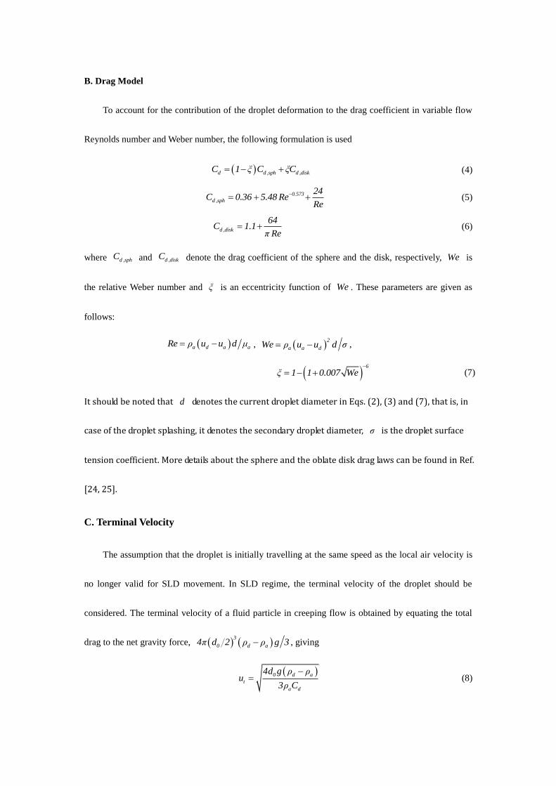
B. Drag Model
To account for the contribution of the droplet deformation to the drag coefficient in variable flow
Reynolds number and Weber number, the following formulation is used
d d ,sph d ,diskC 1 ξ C ξC (4)
0.573
d ,sph
24C 0.36 5.48 Re
Re
(5)
d ,disk
64C 1.1
π Re (6)
where d ,sphC and d ,diskC denote the drag coefficient of the sphere and the disk, respectively, We is
the relative Weber number and ξ is an eccentricity function of We . These parameters are given as
follows:
a d a aRe ρ u u d μ , 2
a a dWe ρ u u d σ ,
6
ξ 1 1 0.007 We
(7)
It should be noted that d denotes the current droplet diameter in Eqs. (2), (3) and (7), that is, in
case of the droplet splashing, it denotes the secondary droplet diameter, σ is the droplet surface
tension coefficient. More details about the sphere and the oblate disk drag laws can be found in Ref.
[24, 25].
C. Terminal Velocity
The assumption that the droplet is initially travelling at the same speed as the local air velocity is
no longer valid for SLD movement. In SLD regime, the terminal velocity of the droplet should be
considered. The terminal velocity of a fluid particle in creeping flow is obtained by equating the total
drag to the net gravity force, 3
0 d a4π d 2 ρ ρ g 3 , giving
0 d a
t
a d
4d g ρ ρu
3ρ C
(8)
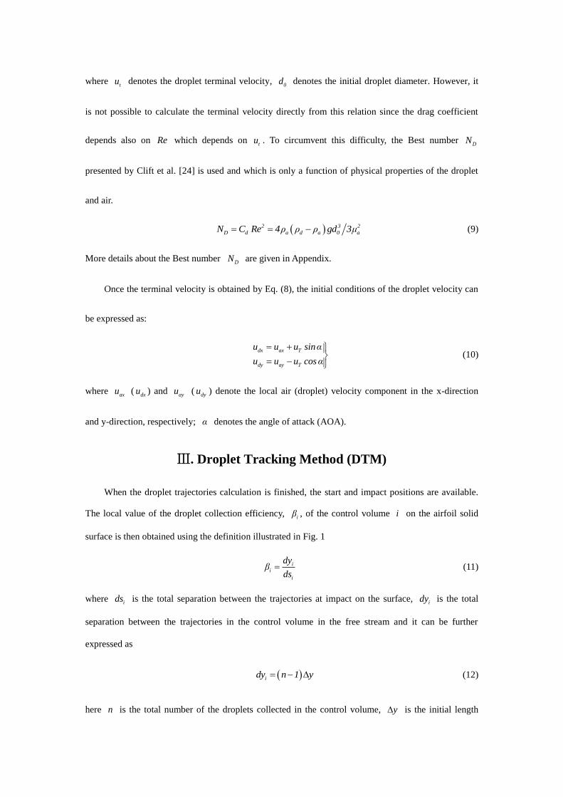
where tu denotes the droplet terminal velocity,
0d denotes the initial droplet diameter. However, it
is not possible to calculate the terminal velocity directly from this relation since the drag coefficient
depends also on Re which depends on tu . To circumvent this difficulty, the Best number
DN
presented by Clift et al. [24] is used and which is only a function of physical properties of the droplet
and air.
2 3 2
D d a d a 0 aN C Re 4ρ ρ ρ gd 3μ (9)
More details about the Best number DN are given in Appendix.
Once the terminal velocity is obtained by Eq. (8), the initial conditions of the droplet velocity can
be expressed as:
dx ax T
dy ay T
u u u sinα
u u u cosα
(10)
where axu (
dxu ) and ayu ( dyu ) denote the local air (droplet) velocity component in the x-direction
and y-direction, respectively; α denotes the angle of attack (AOA).
Ⅲ. Droplet Tracking Method (DTM)
When the droplet trajectories calculation is finished, the start and impact positions are available.
The local value of the droplet collection efficiency, iβ , of the control volume i on the airfoil solid
surface is then obtained using the definition illustrated in Fig. 1
i
i
i
dyβ
ds (11)
where ids
is the total separation between the trajectories at impact on the surface, idy is the total
separation between the trajectories in the control volume in the free stream and it can be further
expressed as
idy n 1 y (12)
here n is the total number of the droplets collected in the control volume, y is the initial length

between neighboring droplets in the free stream. In SLD impingement, droplet splashing and
re-impingement may occur at the same time and even at the same position. The total mass collected in
one control volume may be composed of the incoming mass from far field and the splashed secondary
droplets. At this point, the conventional method described above cannot be used directly to calculate
the droplet collection efficiency in SLD regime. For this reason, the residual ratio definition is
introduced to solve the problem.
dsi
dyiDroplet trajectories
Airfoil surface
Control Volume i
Fig. 1 Droplet trajectories and droplet collection of the control volume i
C. Residual Ratio
For a single droplet impact, the residual ratio η is defined as the ratio of the mass sticks on
surface, fm , to the initial mass of the incident droplet , dm , after impact.
f dη m m (13)
The residual ratio on surface can be divided into two categories according to whether
splashing/bouncing occurs or not.
(1) No Splashing
Two cases are considered in this impingement type, as shown in Fig. 2. In Fig. 2(a), for the initial
impingement, all the incident mass sticks on surface, then the residual ratio is
nsη 1 (14)

For the re-impingement case, as shown in Fig. 2(b), the residual ratio is given as
ns re re dη m m (15)
where rem denotes the secondary droplet mass.
md
mre
(a) Initial impingement (b) Re-impingement
Fig. 2 Droplet-wall interaction without droplet splashing
(2) Splashing
In the case of droplet splashing as shown in Fig. 3, part of the incident mass sticks on surface and
part is rejected on impact. Assume the rejected mass is sm , then the splashing mass loss fraction, f ,
is given as
s df m m (16)
For the initial splashing case as shown in Fig. 3 (a), the residual ratio is
sη 1 f (17)
The mass loss fraction, f , can be obtained from the splashing model described in Section D.
However, if the impact energy is high enough or the solid surface is in a special condition such as
covered with a thin film which is always the case for the icing surface, secondary splashing may also
occur, as shown in Fig. 3 (b). Then the residual ratio is
re
s re
d
mη f
m (18)
Droplet bouncing can be deemed as a special case of splashing, all the incident mass is rejected from

surface as shown in Fig. 3(c), thus the residual ratio at the impact point is given as
bη 0 (19)
ms
md
mrems
md md
(a) Initial impingement (b) Re-impingement (c) Bouncing
Fig. 3 Droplet-wall interaction with droplet splashing and bouncing
For the micro control volume i laying on the solid surface, it may contain all the impinging
types mentioned above. Therefore, the total residual ratio in the control volume i can be expressed as
i ns ns re s s re bη η η η η η (20)
where denotes the sum of the residual ratio for the same impinging type within the control
volume. Then the droplet collection efficiency of the micro control volume i , incorporated with the
effects of droplet splashing/bouncing and re-impingement, can be written as
i
i i
i
dyβ η
ds (21)
D. Splashing Model
Many splashing models exist in spray area (reciprocating engines, gas turbines, spray cooling
systems, ink-jet printing, etc) [21, 27-29], but if these models are applied to predict the mass loss
caused by SLD impingement directly, it will yield a very high mass loss and does not agree well with
the experimental results presented by Papadakis et al. [23]. The reports of [12, 17, 19] have shown that
the splashing mass loss fraction f must be a decreasing function of the incident angle and the normal
component of the incident droplet velocity, in order to be able to account for the experimental results
obtained by NASA [4, 23]. After several times of trying to fit the mass loss ratio with the experimental

database [4, 23, 29], a new splashing model which has been modified by Han et al. [29] as well as
Trujillo et al. [21] is proposed. In the current splashing model, both the droplets splashing ( 0 f 1 )
and the bouncing ( f 1 ) are coupled and the effects of the transition from the CSD impingement to
SLD impingement as well as secondary droplets on the droplet collection are considered. The
components of the modified version are described as follows.
(1) Splashing Threshold
2.0
1.25
d ,nH Oh Re 20 (22)
where H is a modified Mundo parameter [28, 29] represented as a function of the droplet Reynolds
number d ,nRe and Ohnesorge number Oh which are defined as d d ,n 0 dρ u d μ and d 0 dμ d σρ ,
respectively. Noting that the parameters of d ,nu and dρ in the droplet Reynolds number denote the
normal component of velocity and density of the incident droplet, respectively.
(2) Mass Loss Correlation
The mass loss prediction is modified by Han et al [29], their original correlation is presented in Eq.
(23) and the modified version is given as Eq. (24). The effects of the incident droplet diameter,
including the secondary droplet, and the velocity on the droplet collection efficiency have been
incorporated in the splashing model, see Eqs. (25)-(27).
1.57s
H cr
d
mf 0.75 1 exp 10 H H
m
(23)
where crH denotes the criteria of droplet splashing in Ref. [29]. The modified version of the
expression is given as:
s
1 0 ref 2 0 3 d ,n
d
mf 0.75φ d d φ sinθ φ We
m
0.4
0.125 0.22
01 exp cosθ H 20
0 f 1 (24)
where

4.0
1 0 ref 0 refφ d d 1 exp 0.80 d d
(25)
4.0
2 0 0φ sinθ 1 0.90 sinθ
(26)
6.0
3 d ,n d ,nφ We 1 0.07 We
(27)
where 0θ denotes the impact angle between the incident droplet velocity and the surface normal
vector (see Fig. 4). refd denotes the referred droplet diameter and 50 μm is selected as the size of the
referred diameter which is also the defined boundary between the CSD and SLD. is the droplet
incident frequency and d ,nWe is the droplet Weber number characterized by the normal component of
the droplet velocity, they are given as:
1 3
d1.5 ρ LWC
, 2
d ,n a d ,nWe ρ u d σ (28)
One significant characteristic of the splashing model is that for the CSD impingement the mass
loss fraction f is increasing with the increase of the incident droplet diameter, while for SLD
impingement the mass loss fraction performs a decreasing tendency with the increase of the incident
droplet diameter. This behavior is inspired by Honsek et al. [12], Wright [19] and Tan et al. [17]. In
Honsek’s work, an apparent deviation between the predicted droplet collection efficiency and the
experimental data is observed at larger MVDs, and DROP3D shows a lower-prediction on droplet
collection efficiency at the leading-edge area. In Tan’s reports, a decreasing tendency of the mass loss
fraction due to droplet splashing is found with the increase of droplet size in SLD regime. The
LEWICE splashing model presented by Wright reports zero mass loss if the droplet impact
perpendicularly in the leading-edge area, however, their numerical results [13] show that the LEWICE
model over-predicts the droplet collection efficiency in the stagnation point area especially for the
impact of the smaller size droplets. Therefore, by combination analysis of the SLD splashing models
above, the referred diameter 50 μm with the function 0 refd d is introduced into the current model

to modify the effect of the diameter on the droplet collection efficiency. It should be noted that, for the
CSD impingement, the predicted mass loss is of the order of 10-2, while for SLD impingement, it is of
the order of 10-1. This is reasonable because many experiments [4-6, 23] have served to demonstrate
that the mass loss from splashing is very low for the case of CSD impingement but it performs a
significant increasing tendency in the transition stage from the CSD impingement to SLD
impingement.
(3) Droplet Size and Velocity Profile
The size of the splashed secondary droplet sd is determined by Eq. (29). Finally, splashed
droplet number N may be determined from the total mass and diameters of the secondary droplets
combined with the principle of mass conservation, see Eq. (30).
s d
0.5 0.25
0 ad d
d ρ3
d ρWe Re (29)
3
s s dN 6m πd ρ (30)
where the droplet Weber number 2
d a d 0We ρ u d σ and the droplet Reynolds number
d d d 0 dRe ρ u d μ . However, due to the limitation of the capacity of the current computation and the
complexity in tracking large number of the splashed secondary droplets during splashing, the total
rejected mass from surface is assumed to be a mass package, as shown in Fig. 4. Therefore, the rejected
diameter and the momentum are finally expressed as 3s6m π and s sm u , respectively.
The velocity profile of the rejected droplet is described as [21]:
s ,t
0
d ,t
s ,n
0
d ,n
u0.85 0.0025θ
u
u0.12 0.0020θ
u
(31)
where the subscript t
and n stand for the components of the droplet velocity in the tangential and

normal directions; s and d denote the droplet splash and the original incident items.
mdudmsus
n
θ0
Fig. 4 Mass and momentum change due to droplet splashing.
E. Tracking the Residual Ratio on Solid Surface
In order to include both the effects of droplet splashing and re-impingement for calculating the
droplet collection efficiency, a droplet tracking method has been proposed. Three steps are mainly
contained in this method, (1) Classifying According to the Impact Frequency and the Location of the
Terminal Point. (2) Calculating the Residual Ratio at the Impact Point. (3) Sum All the Residual Ratio
in the Control Volume.
(1) Classifying According to the Impact Frequency and the Location of the Terminal Point
Droplets impinging on the solid surface can be simply subjected to splashing or not. For the case
without splashing, the residual ratio is 1, while if splashing occurs, the residual ratio is less than 1 and
the induced secondary droplets may partly or totally captured by the solid surface, or totally swept
away by the surrounding flow. Therefore, the residual ratio may be varying in different impinging cases.
Thus, to identify the impact types has become a necessary step before calculating the SLD collection
efficiency. Initially, every droplet is entitled with an id number at the released place and this id number
will remain unchanged even in the case of droplet splashing, the id number of the secondary droplet is
the same as the parent droplet. When the id number and the coordinates of the impact position (x, y, z)
are available, classifying the impact types becomes possible. The location of the terminal point of the

droplet trajectory provides a way to classify the impact types.
According to whether the terminal point (TP) of the single droplet trajectory is located on the solid
surface or not, the impact types can be classified into two categories. As shown in Fig. 5, the first is
that the TPs are located on the surface. In this case, the total incident droplet, whether droplet splashing
or not, is eventually caught by the surface. The solid surface appeared in Fig. 5 is an "iced" airfoil
provided by Papadakis et al. [6]. The initial incident droplet diameter is 236 μm and n denotes the
impact frequency. Since the rejected mass sm is varying on splash for different incidents, the splashed
diameter ( 3s sd 6m π ) exhibits different colour as shown in the figures. For the case of n 1 as
shown in Fig. 5(a), no splashing occurs and this impingement performs the same way with the CSD
impingement. For the cases of n 1 , as shown in Fig. 5 (b) and (c), re-impingement occurs.
(a) No splashing occurs, n=1
Iced airfoil surface
Droplet trajectory

(b) Splashing occurs, n=2 (c) Splashing occurs, n>2
Fig. 5 Droplet trajectory with the TP on the solid surface (MVD=236μm)
The second category is that after the splashing and re-impingement, part or all the incoming mass,
under the influence of the surrounding airflow, finally escapes the solid surface, as shown in Fig. 6. For
the first case as shown in Fig. 6 (a), splashing occurs and all the rejected mass flees the solid surface
without re-impingement. Droplet bouncing, in which the total incoming mass is rejected from surface,
can be classified into this category. For the second and the third cases, as shown in Fig. 6 (b) and (c),
droplet splashing and re-impingement occurs at the same time. Finally, part of the secondary incoming
mass flees away with the airflow. The quantity of the rejected mass shows a decreasing tendency with
the increase of the impact frequency. It should be noted that the impact frequency n is affected by
many factors such as velocity, turbulent flow and the bump solid surface. For each impingement, the
coordinators of the impact point, the diameters of the parent droplets (din) and the splashed secondary
droplets (ds) together with the id number [(x, y, z), id, din, ds] will be recorded for the following
calculation of the residual ratio.

(a) Splashing occurs, n=1
(b) splashing occurs, n=2 (c) splashing occurs, n>2
Fig. 6 Droplet trajectory with the TP out of the solid surface (MVD=236μm)
(2) Calculating the Residual Ratio at the Impact Point
Based on the classification and the recorded information [(x, y, z), id, din, ds] above, the residual
ratio at each impingement can be calculated and located. Fig. 7 shows an incident droplet titled with the
id number i impinging on the surface for about three times. At each impingement, it was ticked, e.g.
1, 2 and 3, respectively.
At point 1 the residual ratio is given as:
3
1 i ,s1 i ,0η 1 d d
(32)
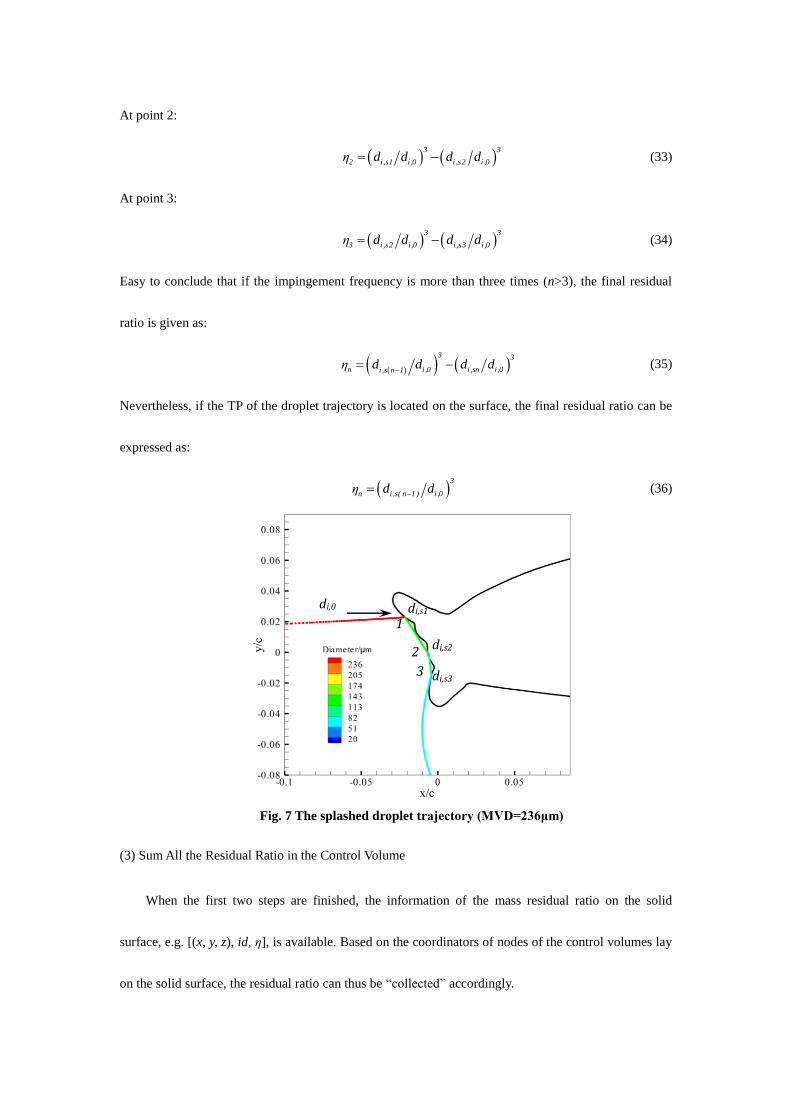
At point 2:
3 3
2 i ,s1 i ,0 i ,s2 i ,0η d d d d
(33)
At point 3:
3 3
3 i ,s2 i ,0 i ,s3 i ,0η d d d d
(34)
Easy to conclude that if the impingement frequency is more than three times (n>3), the final residual
ratio is given as:
3 3
n i ,0 i ,sn i ,0i ,s n 1η d d d d
(35)
Nevertheless, if the TP of the droplet trajectory is located on the surface, the final residual ratio can be
expressed as:
3
n i ,s( n 1 ) i ,0η d d (36)
Fig. 7 The splashed droplet trajectory (MVD=236μm)
(3) Sum All the Residual Ratio in the Control Volume
When the first two steps are finished, the information of the mass residual ratio on the solid
surface, e.g. [(x, y, z), id, η], is available. Based on the coordinators of nodes of the control volumes lay
on the solid surface, the residual ratio can thus be “collected” accordingly.
di,0 di,s1
di,s2
di,s3
1
2
3

In the current study, we introduce the mass loss ratio lsψ and the mass back ratio bkψ in order
to better illustrate the mass loss and gain due to the droplet splashing and re-impingement of the control
volume, respectively. Both of the two definitions are given as
s
ls
0 re
Mψ
M M
,
re
bk
0 re
Mψ
M M
(37)
where
sM denotes the total mass flows out the micro control volume, e.g. splashed mass;
reM denotes the total mass re-impinges into the micro control volume;
0M denotes the mass collection of the micro control volume in the case of excluding droplet splashing
and re-impinging effects. Thus, 0 reM M denotes the total droplet mass that flows into the micro
control volume.
F. Numerical Procedure
In the current study, the governing equations of the continuum described by Batchelor [31] are
solved with FLUENT (v6.3) general-purpose solver [32]. The analysis employed the SIMPLE
algorithm in the software together with the k-ε RNG turbulence model and near-wall functions. The
droplet motion equation described by Eq. (1) is solved with fourth-order Runge-Kutta scheme. The
deformation drag model together with the proposed splashing model are incorporated into the
governing equations with the help of user-defined function (UDF) and programmed in C code. The
macros used are mainly DEFINE_DPM_DRAG and DEFINE_DPM_BC. When the solutions of the
droplet trajectories and the droplet-wall interaction are finished, the data of the droplet coordinators, id
and diameters will become available. In the following step, all the parameters mentioned above will be
converted into a data format for application into a DTM code programmed in Visual Basic language.
Finally, the droplet collection efficiency is determined according to Eq. (21).

IV. Results and Discussion
In the following sections, the capabilities of the DTM and the splashing model are tested and
discussed. The physical models applied in this work are composed of a clean and 22.5-min “iced” Twin
Otter airfoils, clean and 22.5-min “iced” NACA23012 airfoils, which are all presented by Papadakis et
al. [6, 23]. The range of the droplet diameter varies from 11 μm to 236 μm, that is, the impingement of
both the CSD and the SLD impingements are included. Other details of the calculation conditions are
given in Table 1.
Table 1 Calculation Parameters
Twin Otter “iced” Twin Otter NACA23012 “iced”
NACA23012
Velocity/m·s-1 78.25 78.25 78.25 78.25
MVD (d0)/μm 11, 21, 79, 168 79, 168 111, 236 111, 236
LWC/g·m-3 0.05, 0.19,
0.496, 0.75 0.496, 0.75 0.73, 1.89 0.73, 1.89
AOA/deg 0 0 2.5 2.5
Chord/m 1.448 1.448 0.914 0.914
Pressure/kPa 99.974 99.974 99.974 99.974
Static Tem./K 280.37 280.37 280.37 280.37
References [17, 23] [17, 23] [6, 17] [6, 17]
G. Droplet Impingement Distribution on the Clean Airfoil Surface
The distribution of the droplet collection efficiency β on the airfoil is calculated using the DTM
including or excluding the effects of droplet splashing and re-impingement (namely “Incl. Spl. &
Re-imp.” and “Excl. Spl. & Re-imp.” for short). The computed results are validated against a set of
data originating from previous studies performed by Papadakis et al. [6, 23] at NASA Glenn’s Icing
Research Tunnel. Comparisons of the β plots are also performed with the numerical reference data of
LEWICE [6, 23]. The β curves are given as a function of the airfoil curvilinear length “ S ” starting

from the aerodynamic stagnation point of the airfoil ( S 0 ). The negative “ S ” denotes the lower
surface distance from the stagnation point of the airfoil, while the positive “ S ” denotes the upper
surface distance.
(1) Clean Twin Otter Airfoil
Fig. 8 reports the impingement distributions for the four MVDs on the clean Twin-Otter airfoil
surface. As the focus of the present paper is put on SLD impingement, therefore, only two size droplets,
MVD=11μm and MVD=21μm, are applied to test the capability and accuracy of the DTM method in
CSD impingement predictions. It can be seen from Fig. 8(a) and (b) that the β curves obtained with
DTM performed better agreement with the experimental data throughout the whole impingement
region than LEWICE’s results. Both the calculated results and the experimental data are performed a
higher collection efficiency at the stagnation point and a gradually decreasing tendency along the
chord-wise direction. The predicted maximum droplet collection efficiencies are given as 0.32
(MVD=11μm) and 0.52 (MVD=21μm), while the corresponding experimental results are 0.33
(MVD=11μm) and 0.52 (MVD=21μm). Since the mass loss due to the droplet splashing is very low as
previously mentioned in Section D(2), both the two β curves, “Incl. Spl. & Re-imp.” and “Excl. Spl.
& Re-imp.”, are almost totally coincided throughout the whole impinging region.
For SLD impingements as shown in Fig. 8(c) and (d), however, deviations between the β curves
obtained with and without Spl. & Re-imp. are observed. Both LEWICE and the curves excluding
splashing & re-impingement effects perform a significant higher prediction over the experimental
curves at the stagnation point and in the region where the impinging limits are approached. At MVD of
79 μm, see Fig. 8(c), the β curve obtained with splashing & re-impingement effects shows a perfect
agreement with the experimental results throughout the whole impinging region. The maximums of the

predicted and the experimental droplet collection efficiencies are given as 0.74 and 0.73, respectively.
At MVD of 168μm, see Fig. 8 (d), good agreement is also observed between the Spl. & Re-imp. curve
and the experimental curve except for a little deviation in a relatively small region ( S 0.08 and
S 0.2 ) on the upper surface. The maximums of the predicted and the experimental droplet collection
efficiencies are given as 0.85 and 0.82, respectively. One potential reason for the mismatch could be
due to the use of the droplet median volumetric diameter in the computation. Considering the
fluctuations in the experiments as reported in [6, 23], therefore, this deviation could not be only
attributable to the deficiency of the method or the splashing model.
(2) Clean NACA23012 Airfoil
Another test is performed on the clean NACA23012 airfoil, the numerical results and the
experimental reference data are plotted in Fig. 9. Perfect matches between the β curves obtained
including splashing & re-impingement effects and the experimental reference data as shown in Fig. 9(a)
and (b) have again demonstrated the significant contribution of the proposed splashing model to the
improvement of the droplet collection efficiency prediction. In splashing cases, the predicted maximum
droplet collection efficiencies are given as 0.87 (MVD=111 μm), 0.96 (MVD=236 μm), and the
corresponding experimental results are 0.85 (MVD=111 μm) and 0.95 (MVD=236 μm), respectively. It
should be noted that, at MVD=236 μm as shown in Fig. 9(b), the predicted droplet collection
efficiencies obtained by including and excluding splashing & re-impingement effects are almost
coincident in the vicinity area around the stagnation point, when comparing with the predicted β
curves, as shown in Fig. 8(c), (d) and Fig. 9(a). This is because the splashing model gives a lower
evaluation of the splashing mass loss with the increase of the droplet size, as previously illustrated in
Section D (2). It should be noted that the LEWICE’s results are obtained excluding the SLD dynamics

either [6, 23], that’s why good matches are also observed between the Excl. Spl. & Re-imp. curves and
LEWICE’s predictions, as shown in Fig. 8(c), (d), and Fig. 9(a), (b).
(a) MVD=11μm (b) MVD=21μm
(c) MVD=79μm (d) MVD=168μm
Fig. 8 Comparison of β distribution between computational and experimental results on the clean
Twin-Otter airfoil surface

(a) MVD=111μm (b) MVD=236μm
Fig. 9 Comparison of β distribution between the numerical and experimental results on the clean
NACA23012 airfoil surface
H. Droplet Impingement Distribution on the Iced Airfoil Surface
In this section, the capacities of the DTM together with the splashing model in predicting the
droplet collection efficiency of more complicated surface are examined. The rugged surfaces applied
are the Twin Otter airfoil and the NACA23012 airfoil, both with leading-edge double-horn glaze ice
contamination after 22.5 minutes [6, 23]. The rugged surface increases the complexity of splashing,
bouncing and re-impinging effects which is a more challenging test than the clean ones. The general
shapes of the iced airfoils are shown in Fig. 13. The droplet impinging area is divided into two regions,
region A and region B, by the ice horns, as shown in Fig. 10. It can be seen that the curves of the
droplet collection efficiency have changed greatly when comparing the “iced” β curves with the clean β
curves as shown in Fig. 8 and Fig. 9. As expected, both the Excl. Spl. & Re-imp. curves and LEWICE
curves give a higher prediction over the experimental reference data in the impinging region especially
in region A. However, when the droplet splashing and re-impingement effects are included, the
predicted β curves exhibit a significant improvement on the agreement with the experimental

reference data particularly in region A. Nevertheless, in the horn region (region B), a more challenging
match between the numerical and the experimental reference data is observed. Although the splashing
model is activated, the predicted droplet collection efficiency is still higher than the experimental data
for the case of MVD=79 μm impingement as shown in Fig. 10(a). At MVD=79 μm, the predicted
maximum droplet collection efficiency in splashing case is given as 0.73 and the experimental result is
0.62. The reason for this mismatch may be attributable to the simple assumption that the rejected
secondary mass from surface is taken as a mass parcel, as shown in Fig. 4. Other potential reasons
could be attributed to median volumetric diameter in the computation and the fluctuations in the
experiments. For the larger size droplet impingements involving 168 μm, 111 μm, 236 μm as shown in
Fig. 10(b), (c), and (d), it can be seen clearly that good agreement between the numerical and the
experimental reference data are observed when the droplet splashing and re-impingement effects are
included. In case of droplet splashing, the predicted maximum droplet collection efficiencies are 0.91
(MVD=168 μm), 0.78 (MVD=111 μm), 0.92 (MVD=236 μm), and the corresponding experimental
results are 0.95 (MVD=168 μm), 0.71 (MVD=111 μm), 0.88 (MVD=236 μm), respectively. Close
agreements between the numerical and the experimental reference data above allow to be concluded
that the DTM incorporated with the splashing model is able to predict the droplet collection more
accurately in SLD regime. Droplet splashing and re-impingement effects are relatively strong in the
horn regions. Calculation and analysis on the droplet splashing mass loss and the mass back (droplet
re-impingement) are expanded in the following sections.

(a) MVD=79μm (b) MVD=168μm
(c) MVD=111μm (d) MVD=236μm
Fig. 10 SLD impingement distributions on the iced airfoil surfaces of the
Twin Otter [(a) and (b)] and the NACA23012 [(c) and (d)]
I. Effects of Droplet Splashing and Re-impingement
In this section, the trajectories of the splashed secondary droplets are presented. The distributions
of the mass loss ratio and the mass back ratio on the clean and iced airfoil surfaces are calculated and
exhibited. The aim is to explore the characteristics of SLD impingement on the airfoil surfaces, which
is expected to provide a support for the experimental and numerical simulation of ice accretion in SLD
regime.
Region B
Region A
Region A

(1) Trajectory
The effects of surface characteristics on droplets splashing trajectories are presented in Fig. 11. It can
be seen that the droplet splashing is occurring almost in the whole impinging region. For the
impingement on the clean airfoil, as shown in Fig. 11(a), most of the ejected mass is escaping from the
surface when splashing occurs, no significant phenomenon of droplet re-impingement is observed in
the vicinity area of the leading edge. However, as shown in Fig. 11(b), for the impingement of droplet
on the more complex iced airfoil surface, the re-impingement of the ejected mass on the surface is
relatively more significant, especially in the area between the horns. Since the parameters of the
incident droplets, e.g. the incident angles, velocities and the existing surface curvature, are varying on
the solid surface, which make the secondary droplet diameters ejected from the surface is different
either, and the figures of droplet splashing are much like a kaleidoscope. It can be seen that the sizes of
the secondary droplets are gradually increasing along the chord-wise direction. As the shape of the
solid surface is changing with the increase of ice accretion, droplet splashing and re-impingement may
play an increasing important role in determining the droplet collection efficiency during the icing
process.
(a) Clean airfoil surface (b) Iced airfoil surface
Fig. 11 Droplet splashing and re-impingement on the clean (left) and iced (right) Twin Otter airfoil
surface at MVD=168μm
Clean airfoil surface Iced airfoil surface

(2) Mass Loss Ratio
The mass loss ratio lsψ denotes the ratio of the quantity of the splashed mass to the total liquid
mass collected by the control volume. Fig. 12 demonstrates the distributions of the mass loss ratio on
the clean airfoil surfaces. The impingement limits obtained in the condition of excluding droplet
splashing and the re-impinging effects are also presented on the airfoil surface. It can be seen clearly
that the droplet impinging range is enlarged with the increase of the incident droplet size. The mass loss
ratio is relatively lower at the leading edge of the airfoil and performs a general increasing tendency
when the impingement limits are approached. At the stagnation point, the mass loss ratio is 0.11
(MVD=79 μm), 0.08 (MVD=168 μm), 0.10 (MVD=111 μm), 0.05 (MVD=236 μm), respectively. A
gradually decreasing tendency is observed when the incident droplet diameter is increased for the given
conditions. However, the mass loss ratio performs a vibration distribution in the vicinity area near the
impingement limits, as shown in Fig. 12(a) and (b). It could be that the droplet splashing and
re-impingement occur at the same time in this area. For the impingements of 111 μm, 236 μm as shown
in Fig. 12(c) and (d), the mass loss ratio is sharply reduced to zero at the impingement limit points on
the upper and lower surfaces.
The distributions of the mass loss ratio on the iced airfoil surfaces are presented in Fig. 13. It can
be seen that the distribution of lsψ in the horn region (region B) is much irregular. It could be the
reason that the droplet incident angle has been changed greatly due to the accidented iced surface and
thus the mass loss caused by the droplet splashing is influenced accordingly. The level of lsψ
is in the
range of 0.05~0.22 in the horn region (region B). At the leeward side of the horns, as no droplet
impingement, the mass loss is zero. However, the mass loss ratio performs a similar distribution with
the clean surface in the region outside the horns (region A).

(a) MVD=79μm (b) MVD=168μm
(c) MVD=111μm (d) MVD=236μm
Fig. 12 Mass loss ratio distributions on the clean airfoil surfaces of the twin-otter [(a) and (b)] and the
NACA23012 [(c) and (d)]
(a) MVD=79μm (b) MVD=168μm
Region B
Region A
Impingement limits

(c) MVD=111μm (d) MVD=236μm
Fig. 13 Mass loss ratio distributions on the iced surfaces of the Twin-Otter [(a) and (b)] and the
NACA23012 [(c) and (d)] airfoils
(3) Mass Back Ratio
The mass back ratio bkψ denotes the ratio of the quantity of the re-impingement mass to the total
liquid mass collected by the control volume. The distributions of bkψ on the clean airfoil surface are
presented in Fig. 14. It shows that the range of the bkψ distribution on the clean surface is relatively
narrowed comparing with lsψ , particularly on the NACA23012 airfoil surface, as shown in Fig. 14(c)
and (d), no significant mass back is observed. In Fig. 14(a), for the impingement of MVD=79 μm, a
slight mass back on the upper surface is noticed, while for the impingement of MVD=168 μm in Fig.
14(b), the phenomenon of droplet re-impingement (mass back) is more significant. The results may
allow to be concluded that the droplets re-impingement is not only related to environmental conditions
but also the shape of the airfoil (length, depth, etc) is playing a key factor. However, when the airfoil is
covered with ice horns as shown in Fig. 15, the droplets re-impingement is observed in all the cases
and it mainly occurs in the horn region. The distribution level of the mass back ratio bkψ in the horn
region falls in the range of 0~0.22. In all cases, no mass back is observed out of the impinging region.
Through the analysis of the distributions of the mass loss ratio and the mass back ratio on the clean and

iced surfaces above, we can see that the effects of SLD dynamics, e.g. splashing and re-impingement,
on the droplet collection efficiency may be changed greatly due to ice accretion. At this point, it is
reasonable to conclude that the multi-step icing simulation is required especially in SLD icing
numerical simulation area in order to obtain accurate ice shapes.
(a) MVD=79μm (b) MVD=168μm
(c) MVD=111μm (d) MVD=236μm
Fig. 14 Mass back ratio distributions on the clean surfaces of the twin-otter [(a) and (b)] and the
NACA23012 [(c) and (d)] airfoils

(a) MVD=79μm (b) MVD=168μm
(c) MVD=111μm (d) MVD=236μm
Fig. 15 Mass back ratio distributions on the “iced” surfaces of the twin-otter [(a) and (b)] and the
NACA23012 [(c) and (d)] airfoils
V. Conclusions
This article presented an overview of the physical phenomena associated with ice accretion on
super-cooled large droplets (SLD), as well as developing a new Lagrangian droplet tracking method
(DTM) for the calculation of a two-dimensional droplet impingement, which is applicable in the CSD
and SLD regimes. The method has incorporated the effects of the droplet splashing/bouncing and
re-impingement by introducing the definition of the residual ratio. A SLD splashing model was

proposed to assess the mass loss during droplet-wall interactions. Capacities and performance of the
DTM and the splashing model were validated against a set of experimental reference data available for
different airfoils and SLD conditions. The results show that the DTM can predict droplet collection
efficiency accurately in SLD regime as well as the CSD impingement. The mass loss predicted by the
splashing model has contributed a great deal to the agreement between the numerical and the
experimental data. The slight deviations from experimental data observed in the simulation of the
validation test cases especially in the iced airfoil conditions maybe attributable either to the use of the
droplet median volumetric diameter in the computation or the simple assumption that the rejected
secondary mass from surface is taken as a mass parcel or to a deficiency in experimental measurement
methods.
The mass loss ratio and the mass back ratio caused by droplet splashing and re-impingement in
different SLD impinging conditions were addressed. The mass loss ratio generally performs an
increasing tendency from the stagnation point at the leading edge to the area where the impingement
limits are approached, but sharp to zero at the impinging limits on the clean airfoil surfaces. At the
stagnation point, a generally decreasing tendency of the mass loss ratio with the increase of droplet size
is observed at the given conditions. Distributions of the mass loss ratio on the iced airfoil surface are
more irregular and it could be attributable to the changes of the droplet incident angle caused by the
accidented iced surface and thus the quantity of the mass loss due to splashing is finally changed.
The range and level of the distributions of the mass back ratio on airfoil surfaces are relatively
narrowed and lower than that of mass loss ratio and no significant mass back is observed on the clean
NACA23012 airfoil at the given conditions. However, when the clean airfoil surfaces are contaminated
with horn ice shapes, a significant droplet re-impingement event is observed in the horn region. No
mass loss or mass back is observed beyond the impinging limits at the given conditions. Comparisons
of the droplet impingements, the mass loss ratio and the mass back ratio between the clean and iced
airfoils serve to conclude that SLD dynamics are affected greatly by surface shapes. Therefore,
multi-step icing simulation is thus becoming a strong requirement especially in SLD ice accretion
prediction.
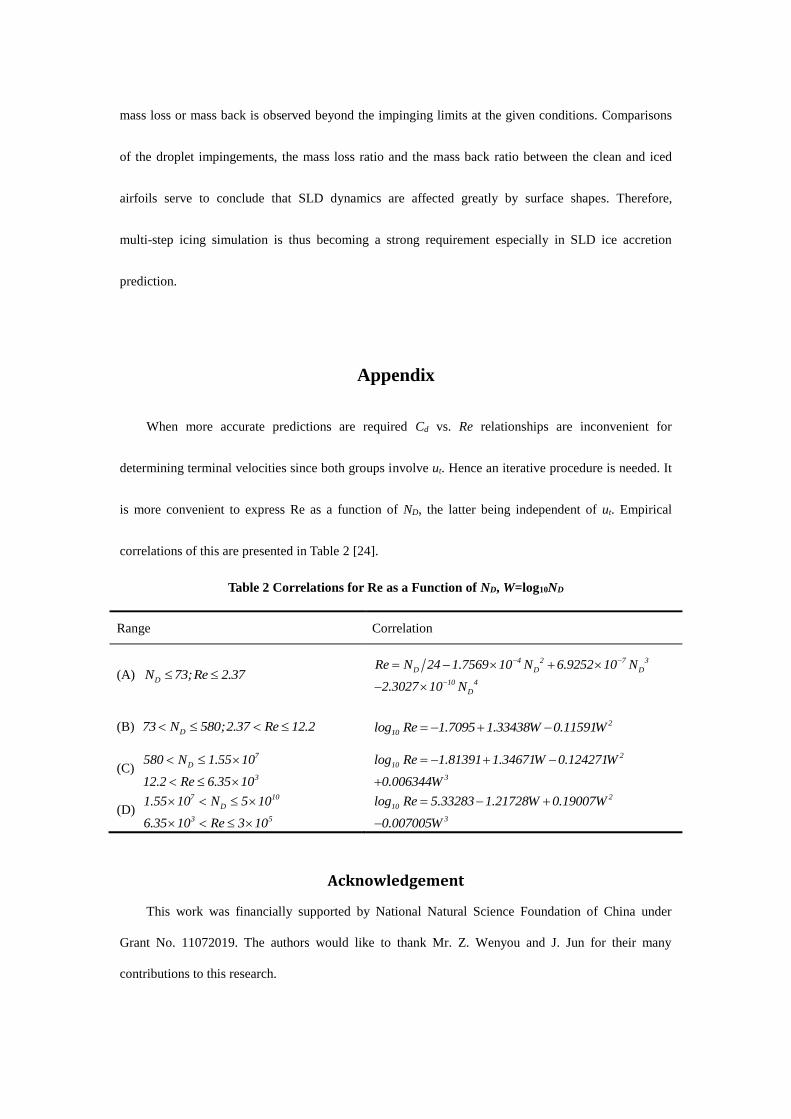
Appendix
When more accurate predictions are required Cd vs. Re relationships are inconvenient for
determining terminal velocities since both groups involve ut. Hence an iterative procedure is needed. It
is more convenient to express Re as a function of ND, the latter being independent of ut. Empirical
correlations of this are presented in Table 2 [24].
Table 2 Correlations for Re as a Function of ND, W=log10ND
Range Correlation
(A) DN 73;Re 2.37
4 2 7 3
D D D
10 4
D
Re N 24 1.7569 10 N 6.9252 10 N
2.3027 10 N
(B) D73 N 580;2.37 Re 12.2 2
10log Re 1.7095 1.33438W 0.11591W
(C) 7
D
3
580 N 1.55 10
12.2 Re 6.35 10
2
10
3
log Re 1.81391 1.34671W 0.124271W
0.006344W
(D) 7 10
D
3 5
1.55 10 N 5 10
6.35 10 Re 3 10
2
10
3
log Re 5.33283 1.21728W 0.19007W
0.007005W
Acknowledgement
This work was financially supported by National Natural Science Foundation of China under
Grant No. 11072019. The authors would like to thank Mr. Z. Wenyou and J. Jun for their many
contributions to this research.

Reference
[1] Hansman, R. J., “Droplet Size Distribution Effects on Aircraft Ice Accretion,” Journal of Aircraft 22, 1985.
doi: 10.2514/3.45156
[2] Russell Ashenden, William Lindberg, John D. Marwitz, and Benjamin Hoxie., "Airfoil performance
degradation by supercooled cloud, drizzle, and rain drop icing", Journal of Aircraft 33, 1996.
doi: 10.2514/3.47055
[3] Charles, M P., “Status of NTSB Aircraft Icing Certification-Related Safety Recommendations Issued As A
Result of the 1994 ATR-72 Accident at Roselawn,” IN. AIAA, Aerospace Sciences Meeting & Exhibit, 35th,
Reno, NV, Jan. 6-9, 1997.
[4] Papadakis, M, Hung, K. E., Yeong H. W., “Experimental Investigation of Water Impingement on Single and
Multi-Element Airfoils,” AIAA Paper 2000-0100, 2000.
[5] Papadakis, M., Hung, K. E., Vu, G. T., Yeong, H. W., Bidwell, C. S., Breer, M. D., and Bencic, T. J.,
“Experimental Investigation of Water Droplet Impingement on Airfoils, FiniteWings, and an S-Duct Engine
Inlet,” NASATM2002-211700, Oct. 2002.
[6] Papadakis, M., Rachman, A.,Wong, S. C., Yeong, H.W., Hung, K. E., and Bidwell, C. S., “Water
Impingement Experiments on a NACA23012 Airfoil with Simulated Glaze Ice Shapes,” AIAA Paper
2004-0565, 2004.
[7] Tan, S.C., Papadakis, M., Miller, D. Bencic, T., Tate, P., Laun, M.C., “Experimental Study of Large Droplet
Splashing and Breakup,” AIAA Paper AIAA- 2007-904, 2007.
[8] Vargas, M., Feo, A., “Deformation and Breakup of Water Droplets near an Airfoil Leading Edge,” Journal
of Aircraft 48, 2011.
doi: 10.2514/1.C031363
[9] Pierre Berthoumieu. “Experimental Study of Super-cooled Large Droplets Impact in an Icing Wind Tunnel,”
AIAA Paper, AIAA 2012-3130, 2012.
[10] Ruff, G. A., Berkowitz, B. M., “Prediction Code (LEWICE). Tech. Rep. CR-185129, NASA,” Users Manual
for the NASA Lewis Ice Accretion, 1990.
[11] Beaugendre, H., Morency, F., Habashi, W., “FENSAP-ICE's Three Dimensional In-Flight Ice Accretion
Module: ICE3D,” Journal of Aircraft 40, 2003.
doi: 10.2514/2.3113
[12] Honsek, R., and Habashi,W. G., “FENSAP-ICE: Eulerian Modeling of Droplet Impingement in the SLD
Regime of Aircraft Icing,” AIAA Paper 2006-465, 2006.
[13] Iuliano, E., Mingione, G., Petrosino, F., Hervy, F., “Eulerian Modeling of Large Droplet Physics Toward
Realistic Aircraft Icing Simulation,” Journal of Aircraft 48, 2011.
doi: 10.2514/1.C031326
[14] Fossati, M., Habashi, W. G., Baruzzi, G. S., “Simulation of Supercooled Large Droplet Impingement via
Reduced Order Technology,” Journal of Aircraft 49, 2012.
doi: 10.2514/1.C031326
[15] Bilodeau, D. R., Habashi, W. G., Fossati, M., Baruzzi, G. S., “An Eulerian Re-impingement Model of
Splashing and Bouncing Supercooled Large Droplets,” AIAA 2013-3058, 2013.
[16] Papadakis, M. , Rachman A. and Wong, S. C., Bidwell, C. and Bencic T., “An Experimental Investigation of
SLD Impingement on Airfoils and Simulated Ice Shapes”. AIAA 2003-01-2129, 2003.
[17] Tan, S.C., “A Tentative Mass Loss Model For Simulating Water Droplet,” AIAA Paper AIAA-2004-410,
2004.
[18] Tan, S. C., and Papadakis, M., “Droplet Breakup, Splashing and Re-Impingement on an Iced Airfoil,” AIAA
Paper 2005-5185, 2005.
[19] Wright, W. B. “Further Refinement of the LEWICE SLD Model,” AIAA Paper 2006-464, 2006.
[20] Wright, W. B., Potapczuk, M. G. Levinson, L.H. “Comparison of LEWICE and Glenn ICE in the SLD
Regime, ” AIAA Paper (2008) No. AIAA-2008-0439.
[21] Trujillo, M. F., Mathews, W. S., Lee, C. F., and Peters, J. E., “Modeling and Experiment of Impingement
and Atomization of a Liquid Spray on a Wall,” International Journal of Engine Research, Vol. 1, No. 1,
2000, pp. 87–105.
doi:10.1243/1468087001545281
[22] Wright, W. B., and Potapczuk, M. G., “Semi-Empirical Modeling of SLD Physics,” AIAA Paper 2004-0412,
2004; also NASA TM-2004-212916.
[23] Papadakis, M. ,Wong, S. C., Rachman, A., Hung, K. E., Vu, G. T., and Bidwell, C. S., “Large and Small
Droplet Impingement Data on Airfoils and Two Simulated Ice Shapes,” NASATM2007-213959, Oct. 2007.
[24] Clift, R., Grace, J. R., Weber, M. E., “Bubbles, Drops and Particles,” Academic Press, New York, 1978.
[25] Roland Schmehl, “Advanced Modeling of Droplet Deformation and Breakup For CFD Analysis of Mixture
Preparation,” 18th Annual Conference on Liquid Atomization and Spray Systems. ILASS-Europe 2002.
[26] Gent R. W., Dart N. P. and Cansdale J. T., “Aircraft Icing,” Phil. Trans. R. Soc. Lond. A 2000 358.
doi: 10.1098/rsta.2000.0689
[27] Bai, C., and Gosman, A. D., “Development of Methodology for Spray Impingement Simulation,” Society of
Automotive Engineers Paper 950283, 1995.
[28] Mundo, C., Tropea, C., and Sommerfeld, M., “Numerical and Experimental Investigation of Spray
Characteristics in the Vicinity of a Rigid Wall,” Experimental Thermal and Fluid Science, Vol. 15, No.
3,1997, pp. 228–237.
doi:10.1016/S0894-1777(97)00015-0
[29] Han, Z., Xu, Z., Trigui, N., “Spray/wall Interaction Models for Multidimensional Engine Simulation,”
International Journal of Engine Research 1, 2000, pp.127-146.
doi: 10.1243/1468087001545308
[30] Papadakis, M., Rachman, A.,Wong, S. C., Yeong, H.W., Hung, K. E.,Vu, G. T., and Bidwell, C. S., “Water
Droplet Impingement on Simulated Glaze, Mixed, and Rime Ice Accretions,” NASA TM2007-213961, Oct.
2007.
[31] Batchelor, G. K., “An Introduction to Fluid Dynamics,” Cambridge Univ. Press, Cambridge, England, 1967.
[32] FLUENT (6.3) User's Guide, Fluent Inc, September 2006.


