Residue and implicitization problem for rationalsurfaces

Mohamed Elkadi & Bernard MourrainGALAAD, INRIA & UMR CNRS 6621,UNSA

BP 93, 06902 Sophia-Antipolis, France{melkadi,mourrain}@sophia.inria.fr

March 3, 2003

AbstractThe implicitization problem of rational surfaces is a central chal-

lenge in computational aided geometric design. We propose a newalgorithm to solve it, based on the residue calculus in the general mul-tivariate setting. The proposed approach allows us to treat surfaceswith base points (without geometric hypothesis on the zero-locus ofbase points). The e�ciency of the method is illustrated by some ex-amples computed with maple software. We also give another appli-cation of the residue calculus to the computation of o�sets of rationalparametric surfaces.

Keywords Implicitization, Multivariable residue calculus, bezoutian matrix.

1 IntroductionA rational surface (S) in a 3D-space may be represented by a parametricrepresentation:

(S)

x =f (s, t)d1 (s, t)

y =g (s, t)d2 (s, t)

z =h (s, t)d3 (s, t)

where f, g, h, d1, d2, d3 are polynomials in two variables s and t with coe�-cients in a �eld K or by an implicit equation (i.e. an element F in K[x, y, z]of minimal degree satisfying F (a, b, c) = 0 for all (a, b, c) ∈ (S)

). These two

representations are important for di�erent reasons. For instance, the �rstone is useful for drawing (S) and the second one to intersect surfaces or todecide whether a point is in the given surface or not.

1

Here we will investigate the implicitization problem, that is the problemof converting a parametric representation of a rational surface into an implicitone.

These last decades have witnessed a renewal of the implicitization prob-lem of geometric objects motived by applications in computer aided geomet-ric design and geometric modeling ([20], [5], [15], [16], [9], [1], [11], [2], [18],[6], [12], [10]).

Classically the solution of this question is given by the elimination theorythrough essentially two classes of methods: Resultants and Gröbner bases.The techniques based on the resultants can produce extraneous terms alongwith the implicit equation. Moreover the expansion of this implicit equation(or a multiple of it) in the monomial basis is a time consuming task. Theresultants vanish identically in the presence of base points. In this case,adapted objects have been developed (residual resultants, see [?], [6], [8])but only under some restrictive geometric hypotheses on the zero-locus ofbase points which are di�cult to verify. The methods based on Gröbnerbases computations are fairly expensive in practice even if the dimension issmall.

Another class of methods based on moving surfaces exists (see [11], [21],[7]) but they su�er on the same kind of restrictions.

In [14] and [13] the theory of multivariate residues is used to implicitizesurfaces of a very special type. In this paper we propose to extend this ap-proach to solve the implicitization problem for general rational surfaces. Themethod is based on the bezoutian matrix computations which allow us toderive an algorithm for the computation of residues in the general multivari-ate setting (see propositions 2.10, 2.13). And the use of this algorithm givesthe implicit equation which are looking for. The philosophy of our methodis the following: The bezoutian gives a multiple of the desired equation andthe use of residue simpli�es the unwanted factor in it.

This approach works in the presence of base points and no geometrichypotheses on the zero-locus of base points are needed.

We note that our method for the implicitization of rational surface in the3D-space is valid for any hypersurface of the a�ne space Kn.

The paper is organized as follows: In section 2 we recall the constructionof bezoutian matrices and the residue associated to a polynomial map. Thenwe give an algorithm to compute algebraic relations between polynomialsbased on bezoutians. This algorithm is used for the computation of theresidue in the general multivariate case. Then we show that these matrixtechniques give a multiple of the implicit equation. In section 3 we describethe implicitization algorithm for rational surfaces and show that the use ofthe algorithm on residue calculus allows us to separate the extraneous factor(produced by bezoutian matrices) from the desired implicit equation andwe give some examples of computations in maple in order to illustrate ourapproach. In section 4 we give an application of the algorithm on residue

2

calculus to the computation of o�sets.Here are some notations that will be used hereafter. K denotes a �eld

of characteristic 0, K its algebraic closure, K[x] = K[x1, . . . , xn] the ringof polynomials in the variables x1, . . . , xn with coe�cients in K, K(x) itsfraction �eld. If α = (α1, . . . , αn) ∈ Nn, |α| = α1 + · · · + αn and xα =xα1

1 . . . xαnn . If n = 1 (resp. n = 2 or n = 3) we use the notation K[t] (resp.

K[s, t] or K[x, y, z]) instead of K[x1] (resp. K[x1, x2] or K[x1, x2, x3]).If L is an arbitrary �eld, we denote by L its algebraic closure.

2 Residue calculusLet us �rst de�ne the notion of bezoutian matrix that will be central in ourapproach for the implicitization problem.

De�nition 2.1 The bezoutian Θf0,...,fn of f0, . . . , fn ∈ K[x] is the polyno-mial in K[x, y] = K[x1, . . . , xn, y1, . . . , yn] de�ned by

Θf0,...,fn(x1, . . . , xn, y1, . . . , yn)=

∣∣∣∣∣∣∣

f0(x) θ1(f0)(x, y) · · · θn(f0)(x, y)... ... ... ...

fn(x) θ1(fn)(x, y) · · · θn(fn)(x, y)

∣∣∣∣∣∣∣

where θi(fj)(x, y) =

fj(y1, . . . , yi−1, xi, . . . , xn)− fj(y1, . . . , yi, xi+1, . . . , xn)xi − yi

∈ K[x, y].

If v = (vi), w = (wi) are two bases of K[x], and

Θf0,...,fn(x, y) =∑

i,j

µi,j vi ⊗ vj with µi,j ∈ K ,

the bezoutian matrix of f0, . . . , fn in the bases v and w is (µi,j)i,j . It willbe denoted by [Θf0,...,fn ]v,w.

The bezoutian matrix of f0, . . . , fn in the monomial bases is called thebezoutian matrix of f0, . . . , fn and denoted [Θf0,...,fn ].

When f0 is the constant 1 and f is the polynomial map (f1, . . . , fn), thebezoutian Θ1,f1,...,fn will be denoted by ∆f .

Let f1, . . . , fn be polynomials in K[x] = K[x1, . . . , xn], I be the ideal thatthey generate. We assume that A = K[x]/I is a �nite vector space over K(this means that the variety Z = Z(f1, . . . , fn) = {a ∈ Kn : f1(a) = · · · =fn(a) = 0} is �nite). We will recall the de�nition of the residue τf associatedto the map f = (f1, . . . , fn) and some of its important properties (for moredetails see [19], [17], [?], [3]).

3

Let us denote by K[x] the dual of K[x] (i.e. the set of K-linear maps fromK[x] to K). If ∆f =

∑α,β cα,β xαyβ with cα,β ∈ K, we de�ne the linear map

∆f. : K[x] → K[x]

λ 7→ ∆f.(λ) :=

∑α

(∑

β

cα,β λ(yβ))

xα.

De�nition 2.2 The residue τf of f = (f1, . . . , fn) is the linear form on K[x]such that

1. τf (h) = 0, ∀h ∈ I,

2. ∆f.(τf )− 1 ∈ I.

In the univariate case, if f = fd xd + · · ·+ f0 (with fd 6= 0), for h ∈ K[x]let r = rd−1x

d−1 + · · · + r0 be the remainder in the Euclidean division of hby f , then

τf (h) =rd−1

fd. (1)

In the multivariate case, if for each i = 1 . . . n, fi depends only on xi, thenτf (xα1

1 . . . xαnn ) = τf1(x

α11 ) . . . τfn(xαn

n ). (2)If the roots of f1 = · · · = fn = 0 are simple (i.e. the jacobian of f ,

Jac(f), does not vanish on Z = Z(f1, . . . , fn)), then for h ∈ K[x] we have

τf (h) =∑

ζ∈Zh(ζ)

Jac(f)(ζ).

But in the general multivariate setting the situation is more complicated.Our goal in this section is to show how to compute e�ectively τf (h) for anarbitrary map f = (f1, . . . , fn).

An important tool in the residue theory is the transformation law.Proposition 2.3 (Transformation law) Let g = (g1, . . . , gn) be another poly-nomial map such that the variety Z(g1, . . . , gn) is �nite and

∀ i = 1 . . . n , gi =n∑

j=1

ai,jfj with ai,j ∈ K[x].

Then for h ∈ K[x], τf (h) = τg

(hdet(ai,j)

).

Another important fact in this theory is the following:∀h ∈ K[x] , τf

(h Jac(f)

)= Tr(h) (3)

where Tr(h) denotes the trace of the endomorphism of multiplication by hin the vector space A = K[x]/I.

If ζ is in the �nite variety Z = Z(f1, . . . , fn), K[x]ζ denotes the local-ization of K[x] by the maximal ideal de�ned by ζ and Iζ the ideal of K[x]ζgenerated by f1, . . . , fn.

4

De�nition 2.4 Let ζ ∈ Z. The local residue of f at ζ is the linear formτf,ζ on K[x]ζ which vanishes on Iζ and which satis�es ∆f

.(τf,ζ)− 1 ∈ Iζ .If g is another polynomial map with a �nite variety Z(g). The residual

residue τf\g of f with respect to g is the total sum of local residues τf,ζ ,where ζ ranges over Z \ Z(g).

Remark 2.5 The total sum of local residues τf,ζ , where ζ ∈ Z, is the (global)residue τf de�ned in the de�nition 2.2.

We can now extend the action of τf to rational functions which are de�nedon Z: Let d ∈ K[x] such that d(ζ) 6= 0 for every ζ ∈ Z. Then there arepolynomials q1, . . . , qn, q which satisfy q1f1+· · ·+qnfn+qd = 1. For h ∈ K[x],we de�ne

τf

(h

d

)=

∑

ζ∈Zτf,ζ

(h

d

)=

∑

ζ∈Zτf,ζ(qh).

The multiplicity of a root ζ ∈ Z is µζ = τf,ζ

(Jac(f)

). As in the global

case (formula (3)), for h ∈ K[x], we have

τf,ζ(hJac(f))

= Tr(h) = µζh(ζ). (4)

2.1 Algebraic relationsThe e�ective construction of residue of a polynomial map is based on thecomputation of algebraic relations between this map and the coordinate func-tions. We give here a method using bezoutian matrices to get them.

Lemma 2.6 Assume that A = K[x]/I is a vector space of �nite dimensionD. Then there exists two bases v = (vi)i∈N and w = (wi)i∈N of K[x] suchthat (v1, . . . , vD) and (w1, . . . , wD) are bases of A, for i > D the elementsvi and wi belong to I = (f1, . . . , fn), and for any f0 in K[x] the matrix[Θf0,...,fn ]v,w is of the form

v1 . . . vD vD+1 . . .

Mf0 0

0 Lf0

w1...wD

wD+1...

(5)

where Mf0 is the matrix of multiplication by f0 in A in the basis (v1, . . . , vD).

Proof : For g ∈ K[x], we denote Θg,f1,...,fn by Θg. The vector space A isidenti�ed to {λ ∈ K[x] : λ(x) = 0 ∀x ∈ I}. Let us consider the subspacesE = Θ1

.(A) and F = Θ1/(A) of K[x]. Since f1, . . . , fn form a complete

5

intersection, Θ1. and Θ1

/ de�ne A-isomorphisms between A and A (see[17], [19], [3], [?]). We have K[x] = E ⊕ I = F ⊕ I, and Θ1 ∈ E ⊗F ⊕ I ⊗ I.

We deduce from Θf0(x, y)−f0(y)Θ1(x, y) ∈ (f1(y), . . . , fn(y)

)K[x, y] that

Θf0.(A) = (f0(y)Θ1).(A) ⊂ E, Θf0

/(A) ⊂ F , and that Θf0 ∈ E⊗F ⊕I⊗I.If v = (vi)i∈N and w = (wi)i∈N are two bases ofK[x] such that (v1, . . . , vD)

is a basis of E, (w1, . . . , wD) a basis of F , vi ∈ I and wi ∈ I for i > D,[Θf0 ]v,w has a block-diagonal form.

If Cf0 is the upper-left block in this decomposition and Mf0 is the matrixof multiplication by f0 in the basis (v1, . . . , vD) of A, we deduce from Θf0 =f0Θ1 in A⊗A that Cf0 = Mf0 C1.

Notice that C1 is the (invertible) matrix of Θ1. in the bases (v1, . . . , vD)

of A and its dual basis in A. By a change of bases we may assume that C1

is the identity matrix, and so [Θf0 ]v,w is the form (5). ¤Let f0, . . . , fn be n + 1 elements of K[x] such that the n polynomials

f1, . . . , fn are algebraically independent over K. For algebraic dimensionreasons there is a nonzero polynomial P such that P (f0, . . . , fn) = 0. Wewill show how to �nd such a P using elementary algebra.

Proposition 2.7 Let u = (u0, . . . , un) be new parameters and assume thatA = K[x]/(f1, . . . , fn) is a vector space of �nite dimension. Then everynonzero maximal minor P (u0, . . . , un) of the bezoutian matrix of the elementsf0 − u0, . . . , fn − un in K[u][x] satis�es the identity P (f0, . . . , fn) = 0.

Proof : For each i ∈ {1, . . . , n}, xi, f1, . . . , fn are algebraically dependentover K. Then if u = (u1, . . . , un) and f = (f1, . . . , fn), dimK(f)K(x) =dimK(u)K(u)[x]/(f − u) = d is �nite.

By lemma 2.6, there exists two bases v = (vi) and w = (wi) of K(u)[x]such that [Θg,f−u]v,w is of the form (5) for every g ∈ K[x]. By change ofbases there are invertible matrices R(u) and Q(u) with coe�cients in K(u)such that the bezoutian matrix

[Θf0−u0,f−u] = R(u)

(Mf0 − u0Id) 0

0 Lf0 − u0L1

Q(u)

Id is the identity matrix. Then a nonzero maximal minor P (u0, . . . , un) of[Θf0−u0,f−u] is a multiple of the characteristic polynomial of the multiplica-tion by f0 inK(u)[x]/(f−u). By Cayley-Hamilton's theorem P (f0, . . . , fn) =0. ¤

Remark 2.8 As in the proposition 2.7 if f0, d0, . . . , fn, dn are elements ofK[x], every nonzero maximal minor P (u0, . . . , un) of the bezoutian ma-

6

trix of the polynomials f0 − u0d0, . . . , fn − undn in K[u0, . . . , un][x] satis�esP

(f0

d0, . . . ,

fn

dn

)= 0.

In practice we use Gaussian elimination (Bareiss Method) in order to�nd a nonzero maximal minor of the bezoutian matrix.

In order to �nd an implicit equation of a rational surface (S) given bya rational parameterization x =

f(s, t)d1(s, t)

, y =g(s, t)d2(s, t)

, z =h(s, t)d3(s, t)

, wheref, g, h, d1, d2, d3 ∈ K[s, t], we compute a nonzero maximal minor of the be-zoutian matrix of xd1−f, yd2−g, zd3−h with respect to s, t. In general, thisyields a multiple of the implicit equation as shown by the following example.

Example 2.9 The surface (S) is parameterized by

x = s , y =t2s + 2t + s

t2, z =

t2 − 2st− 1t2

.

The bezoutian matrix of x − s, yt2 − t2s − 2t − s, zt2 − t2 + 2ts + 1 in(K[x, y, z])[s, t] is a 4× 4 matrix. Its determinant is

(z − 1)2(4x4 − 4x3y + x2z2 − 8x2z + 2xyz + 4x2 + y2 + 4z − 4).

The second factor in this expression is the expected implicit equation.The use of the bezoutian matrix produce an extraneous term along with

the implicit equation. We will see, in the next section, how to use the residuecalculus in order to remove the unwanted factor from this polynomial withoutfactorization. But �rst we will see how to compute e�ectively the residue τf

related to the map f = (f1, . . . , fn).

Proposition 2.10 For i ∈ {1, . . . , n}, letPi(u0, . . . , un) = ai,0(u1, . . . , un)umi

0 + · · ·+ ai,mi(u1, . . . , un)

be an algebraic relation between xi, f1, . . . , fn. If for each i = 1 . . . n, there iski ∈ {0, . . . , mi−1} such that ai,ki(0) 6= 0, then for h ∈ K[x] the computationof the multivariate residue τf (h) reduces to univariate residue calculus.

Proof : If ji = min{k : ai,k(0) 6= 0}, we have

gi(xi) = ai,ji(0)xmi−jii + · · ·+ ai,mi(0) =

n∑

j=1

Ai,jfj , Ai,j ∈ K[x].

We set g(x) =(g1(x1), . . . , gn(xn)

). By the transformation law and (2) there

are scalars cα, ci,α such that

τf (h) = τg

(hdet(Ai,j)

)=

∑α

cατg(xα) =∑

α=(α1,...,αn)

cα

n∏

i=1

τgi(xαii ).

¤

7

Remark 2.11 If w are formal parameters, similarly for every h ∈ K[x],τf−w(h) is a rational function in w whose denominator is the product ofpowers of a1,0(w), . . . , an,0(w). But it is not clear how to recover τf (h) fromthis function.

Proposition 2.10 yields a direct algorithm to compute the multivariableresidues for some maps by means of algebraic relations given by the be-zoutians. For an arbitrary map, the residue calculus can be done using thefollowing generalized transformation law due to C.A. Berenstein and A. Yger(see [4]).

2.2 Generalized transformation lawProposition 2.12 (Generalized transformation law [4]) Let (f0, . . . , fn) and(g0, . . . , gn) be two maps of K[t, x] = K[t, x1, . . . , xn] which de�ne �nite vari-eties. We assume that f0 = g0 and there are positive integers mi, i = 1 . . . n,and polynomials ai,j , i, j = 1 . . . n, such that

∀ i = 1 . . . n , fmi0 gi =

n∑

j=1

ai,jfj .

If h ∈ K[t, x], then τ(g0,...,gn)(h) = τ(f

m1+···+mn+10 ,f1...,fn)

(hdet(ai,j)

).

If f0 = x0 and m1 = · · · = mn = 0, the generalized transformation lawbecomes the (usual) transformation law (proposition 2.3).

For (α1, . . . , αn) ∈ Kn and a new variable t, we de�ne the integers mi andthe polynomials Ri, Si as follows: If Pi(u0, . . . , un) is an algebraic relationbetween xi, f1, . . . , fn, for example given by the proposition 2.7, then thereare Bi,j ∈ K[t, x1, . . . , xn] such that

Pi(xi, α1t, . . . , αnt) =∑n

j=1(fj − αjt)Bi,j = tmi(Ri(xi)− tSi(xi, t)

). (6)

From the transformation laws we deduce the following result:

Proposition 2.13 If for each i = 1 . . . n, the univariate polynomial Ri(xi)does not vanish identically, then for h ∈ K[x] we have

τf (h) =∑

k=(k1,...,kn)∈Nn:|k|≤|m|τ(t|m|+1−|k|,Rk1+1

1 ,...,Rkn+1n )

(Sk1

1 . . . Sknn hdet(Bi,j)

).

Proof : We deduce from (6) and proposition 2.12 that

τf (h) = τ(t,f1−α1t,...,fn−αnt)(h) = τ(t|m|+1,R1−tS1,...,Rn−tSn)

(hdet(Bi,j)

).

Using the identities

R|m|+1i − (tSi)|m|+1 = (Ri − tSi)

|m|∑

ki=0

R|m|−ki

i (tSi)ki , i = 1 . . . n ,

8

and the proposition 2.3 we have τ(t|m|+1,R1−tS1,...,Rn−tSn)

(hdet(Bi,j)

)=

∑

k∈Nn:|k|≤|m|τ(t|m|+1−|k|,Rk1+1

1 ,...,Rkn+1n )

(Sk1

1 . . . Sknn hdet(Bi,j)

).

¤Propositions 2.7 and 2.13 give an e�ective algorithm to compute the

residue of a polynomial map in the multivariable setting. They reduce themultivariate residue calculus to the univariate one.

3 Implicitization problemLet f, g, h, d1, d2, d3 be polynomials in K[s, t] and let

(S)

x =f(s, t)d1(s, t)

y =g(s, t)d2(s, t)

z =h(s, t)d3(s, t)

be the rational parameterization that they de�ne in K3. We are looking foran implicit equation of the image of (S). Let us consider the 3 polynomialsin (K[x, y, z])[s, t]

F (s, t) = x d1(s, t)− f(s, t)G(s, t) = y d2(s, t)− g(s, t)H(s, t) = z d3(s, t)− h(s, t).

We set Z0 = Z(G,H) = {(s, t) ∈ K(y, z)2

: G(s, t) = H(s, t) = 0} = Z1∪Z2,where Z1 = Z0∩Z(d1) = {(s, t) ∈ K(y, z)

2: G(s, t) = H(s, t) = d1(s, t) = 0}

and Z2 = Z0 \ Z1.If Z2 is �nite, let Q(x, y, z) be the following nonzero element

Q(x, y, z) =∏

(s,t)∈Z2

F (s, t) =( ∏

(s,t)∈Z2

d1(s, t))( ∏

(s,t)∈Z2

(x− f(s, t)

d1(s, t)))

=( ∏

(s,t)∈Z2

d1(s, t))(

xm + σ1(y, z)xm−1 + · · ·+ σm(y, z))

where m is the number of points (counting their multiplicities) in Z2 andσi(y, z) is the i-th elementary symmetric function of

{f(s, t)d1(s, t)

: (s, t) ∈ Z2

}.

Remark 3.1 If one denominator di in the parameterization of (S) is constant,in the de�nition of Q we replace F by the suitable polynomial.

9

Theorem 3.2 The implicit equation of the surface (S) is the squarefree partof the numerator of

E(x, y, z) = xm + σ1(y, z)xm−1 + · · ·+ σm(y, z).

Proof : Let us choose a point (y0, z0) in the open subset U of K2 suchthat the specialization Z2 of Z2 is �nite in K2 and the denominators ofσ1, . . . , σm do not vanish. Then we have Q(x0, y0, z0) = 0 if and only ifxm

0 +σ1(y0, z0)xm−10 +· · ·+σm(y0, z0) = 0, which is equivalent to the existence

of an element (s0, t0) ∈ Z2 (i.e. y0 =g(s0, t0)d1(s0, t0)

, z0 =h(s0, t0)d1(s0, t0)

) such that

x0 =f(s0, t0)d1(s0, t0)

. In other words on the open subset U , the numerator ofE(x, y, z) vanishes on a point (x0, y0, z0) i� this point is on the surface (S),which implies that the squarefree part of the numerator of E(x, y, z) is upto a scalar the implicit equations of (S). ¤

Remark 3.3 The squarefree part of a polynomial N(x, y, z) is obtained bycomputing N

gcd(N, ∂N∂x )

.

The implicit equation E(x, y, z) is a �residual resultant� as described in[?], so theorem 3.2 would be compare to [6] (we notice that in this last articlea geometric hypothesis on the zero-locus is needed).

The coe�cients σi(y, z) can be computed from the residual residue usingthe Newton identities: For i = 1 . . .m, we have

i σi(y, z) = −Si(y, z)− Si−1(y, z)σ1(y, z)− · · · − S1(y, z)σi−1(y, z) , (7)

where

Si(y, z) =∑

(s,t)∈Z2

(f(s, t)d1(s, t)

)i

= τ(G,H)\(d1)

(Jac(G,H)(s, t)

( f(s, t)d1(s, t)

)i)

are the Newton sums, Jac(G, H) is the Jacobian determinant of the map(G,H) and τ(G,H)\(d1) is the residual residue of (G,H) with respect to d1.Therefore, computing the implicit equation of (S) reduces to the computa-

tion of τ(G,H)\(d1) on Jac(G,H)(

f(s, t)d(s, t)

)i

and yields the following algorithm.

Algorithm 3.4 Input : Polynomials f, g, h, d1, d2, d3 in K[s, t].• Let G = y d2 − g and H = z d3 − h. Compute the degree m =

τ(G,H)\(d1)

(Jac(G,H)

)of the polynomial E in theorem 3.2.

• For i from 1 to m, compute

Si(y, z) = τ(G,H)\(d1)

(Jac(G,H)

( f(s, t)d1(s, t)

)i)

.

10

• Use Newton identities (7) to obtain the σi (y, z) from Si (y, z), i =1 . . . m.

Output : The squarefree part of the numerator of

E(x, y, z) = xm + σ1 (y, z) xm−1 + · · ·+ σm (y, z) .

3.1 Computing the residual residueAs mentioned above, the key ingredient for the implicitization in our ap-proach is the computation of the residual residue of (G,H) with respect to

d1 on Jac(G,H)(

f(s, t)d1(s, t)

)i

. We describe now two methods to obtain theseexpressions.

3.1.1 First methodWe have

Si(y, z) = τ(G,H)\(d1)

(Jac(G,H)

( f

d1

)i)

=∑

ζ∈Z2

τ(G,H),ζ

(Jac(G,H)

( f

d1

)i)

= limε→0

∑

ζ∈Z2

τ(G,H),ζ

(d1f

iJac(G,H)di+1

1 + ε

)= lim

ε→0τ(G,H)

(d1f

iJac(G,H)di+1

1 + ε

).

We deduce the following algorithm.

Algorithm 3.5 Input : Polynomials f, g, h, d1, d2, d3 in K[s, t].Compute an algebraic relation As(u0, u1, u2) between the polynomials

s, G = y d2 − g, H = z d3 − h in K[y, z][s, t] (proposition 2.7), and analgebraic relation At(u0, u1, u2) between the elements t, G, H.

• If the univariate polynomials Rs = As(s, 0, 0) and Rt = At(t, 0, 0) arenot vanishing identically (which is often the case), let M be the 2× 2

matrix such that M

(Rs

Rt

)=

(GH

).

� Compute the degree

m = τ(G,H)\(d1)

(Jac(G,H)

)= lim

ε→0τ(Rs,Rt)

(Jac(G, H) det(M)d1

d1 + ε

).

� For i from 1 to m, compute

Si(y, z) = τ(G,H)\(d1)

(Jac(G,H)

( f(s, t)d1(s, t)

)i)

= limε→0

τ(Rs,Rt)

(d1Jac(G,H) det(M)f i

di+11 + ε

).

11

• If RsRt ≡ 0, the Newton sums Si(y, z) = limε→0 τ(G,H)

(d1f

iJac(G,H)di+1

1 + ε

)

are computed using the algebraic relations As(u0, u1, u2), At(u0, u1, u2)and the formula in the proposition 2.13.

Output : The functions Si(y, z) = τ(G,H)\(d1)

(Jac(G,H)

( f(s, t)d1(s, t)

)i)

, i =

0 . . . m.

3.1.2 Second methodAn alternative method to compute the functions Si (y, z) consists in addinga new variable w to s and t.

We consider the following polynomials in (K(x, y, z)) [s, t, w]:

F (s, t, w) = F (s, t) = x d1(s, t)− f(s, t)G(s, t, w) = G(s, t) = y d2(s, t)− g(s, t)H(s, t, w) = H(s, t) = z d3(s, t)− h(s, t)W (s, t, w) = w d1(s, t)− 1.

We recall that Z0 = {(s, t) ∈ K(y, z)2

: G(s, t) = H(s, t) = 0} = Z1 ∪ Z2,with Z1 = Z (d1) ∩ Z0 and Z2 = Z0 \ Z1. We denote by

W ={

(s, t, w) ∈ K (y, z)3

: G (s, t, w) = H (s, t, w) = W (s, t, w) = 0}

and by Π the projection (s, t, w) ∈ K (y, z)3 7→ (s, t) ∈ K (y, z)

2.

Lemma 3.6 We have Π(W) = Z2.Proof : If (s, t, w) ∈ W, then G(s, t) = H(s, t) = 0 and d1 (s, t) 6= 0.Conversely if (s, t) ∈ Z2 then d1(s, t) 6= 0, and so

(s, t,

1d1(s, t)

) ∈ W. ¤The following lemma allows us to compute the Newton sums Si(y, z).

Lemma 3.7 For every i we have

Si(y, z) = τ(G,H)\(d1)

(Jac (G,H) (s, t)

(f (s, t)d1 (s, t)

)i)

= τ(G,H,W )

(Jac (G,H,W ) (s, t, w)

(wf(s, t)

)i).

Proof : By (4) and lemma 3.6,

Si(y, z) =∑

ζ∈Z2

(f(ζ)d1(ζ)

)i

=∑

ξ=(ζ,w)∈W

(wf(ζ)

)i

= τ(G,H,W )

(Jac (G,H, W )

(wf(s, t)

)i)

.

¤We have an algorithm similar to the algorithm 3.4.

12

Algorithm 3.8 Input : Polynomials f, g, h, d1, d2, d3 in K[s, t].Compute an algebraic relation As(u0, u1, u2, u3) between the polynomials

s, G = y d2 − g, H = z d3 − h,W = wd1 − 1 in K[y, z][s, t] (proposition 2.7),and an algebraic relation At(u0, u1, u2, u3) (resp. Aw(u0, u1, u2, u3)

)between

the elements t, G, H, W (resp. w,G, H,W ).• If the univariate polynomials Rs = As(s, 0, 0, 0), Rt = At(t, 0, 0, 0)

and Rw = Aw(w, 0, 0, 0) does not vanish identically (which is often the

case), let M be the 3× 3 matrix such that M

Rs

Rt

Rw

=

GHW

.

� Compute the degree

m = τ(G,H,W )

(Jac(G,H,W )

)= τ(Rs,Rt,Rw)

(Jac(G,H, W ) det(M)

).

� For i from 1 to m, compute

Si(y, z) = τ(G,H,W )

(Jac(G,H,W )(wf)i

)

= τ(Rs,Rt,Rw)

(Jac(G, H, W ) det(M)(wf)i

).

• If RsRtRw ≡ 0, Si(y, z) = τ(G,H,W )

(Jac(G,H, W )(wf)i

), for i =

0 . . . m, are computed using the algebraic relations As(u0, u1, u2, u3),At(u0, u1, u2, u3), Aw(u0, u1, u2, u3) and the formula in the proposition2.13.

Output : The functions Si(y, z) = τ(G,H,W )

(Jac(G,H, W )

(wf(s, t)

)i), i =

0 . . . m.

In the two proposed methods for computing the functions Si(y, z) weintroduce a new parameter. In the �rst one we introduce ε and in the secondone we add a variable w.

3.1.3 ExamplesWe give some simple examples to illustrate our approach for implicitizingrational surfaces. The computations are made in maple using the multires1library.Example (using algorithm 3.5) We turn back to the example 2.9. We have

f = s , g = t2s + 2t + s , h = t2 − 2ts− 1 ,

d1 = 1 , d2 = t2 , d3 = t2.

A nonzero maximal minor of the bezoutian matrix of xd1−f, yd2−g, zd3−his

B(x, y, z) = (z − 1)2(x2z2 − 8x2z + 2zxy + 4z − 4 + 4x4 + 4x2 − 4x3y + y2).1http://www-sop.inria.fr/galaad/logiciels/multires.html

13

The univariate polynomials Rs and Rt are equal to

Rs = −4 + 4z3 + 4s4 + 4s2 + 21s2z2 − 16s2z − 4s3y − 12z2 − 10z3s2 +z4s2 − 8zs4 + 4z2s4 + 2yz3s + 8ys3z − 4ys3z2 − 4z2ys + 2zsy +y2 − 2y2z + z2y2 + 12z

Rt = 4z − 4− 8t3y + 8t3yz + 16t2 − 20t2z + 4z2t2 + 4t4z2 − 8t4z + 4t4.

The computation of Newton sums gives

S0 = 4 , S1 = y , S2 = −12

z + 4z + y − 2 ,

S3 =14

y(−3z2 + 18z − 12 + 4y2)

S4 =18

z4 − 2z3 − z2y2 + 9z2 − 12z + 6y2z + y4 − 5y2 + 6.

And the equation implicit

E(x, y, z) = x4 + σ1x3 + σ2x

2 + σ3x + σ4

= x4 − x3y +14

x2z2 − 2x2z + x2 +12zxy + z +

14y2 − 1.

Example (using algorithm 3.8) Let

f = t− st , g = st , h = t2 + st ,

d1 = (1 + s + t)(s + t) , d2 = (1 + s + t)(t− s) , d3 = (1 + s + t)2.

A nonzero maximal minor of xd1 − f, yd2 − g, zd3 − h in K[x, y, z][s, t] is

z(x + 2yz − y)(x3z − 4x2y2 − zx2y + 8y3x2 − 2x2z + 4xy2 + xz + xyz −8y3x− z2x + xy2z + 2y3 + 7y2z − y2 + 2z2y − 9y3z − 2yz).

The polynomial Rs contains 53 monomials in s, y, z, its degree in s is 4, itsdegree in y, z is 7 and its degree in s, y, z is 10.

The polynomial Rt contains 21 monomials in t, y, z, its degree in t is 4,its degree in y, z is 5 and its degree in t, y, z is 8.

The polynomial Rw contains 83 monomials in w, y, z, its degree in w is3, its degree in y, z is 10 and its degree in w, y, z is 12.

The Newton sums are

S0 = 3

S1 =8y3 − 4y2 − yz − 2z

z

S2 =64y6 − 64y5 − 16y4z + 16y4 − 8y3z − y2z2 + 8y2z + 2z2y + 2z3 + 2z2

z2

S3 = −512y9 − 768y8 − 192y7z + 384y7 − 64y6 + 144y5z + 48y4z2 − 48y4z

z3

−y3z3 + 6y3z2 + 12z3y2 − 15y2z2 + 3yz4 − 9yz3 − 6z4 − 2z3

z3.

14

The implicit equation is the numerator of x3 + σ1x2 + σ2x + σ3, namely

x3z − 4x2y2 − zx2y + 8y3x2 − 2x2z + 4xy2 + xz + xyz − 8y3x− z2x +xy2z + 2y3 + 7y2z − y2 + 2z2y − 9y3z − 2yz.

Example (using algorithm 3.5) Let (S) be the bicubic given by the parame-terization

x = s(s2 − 5s)t3 − (s2 + 1)t2 + 4ts− s + ty = s(s + 1)2 + t3 + 3s2tz = t(t− 1)2 + s3t + 2s

The polynomial Rs (resp. Rt) contains 42 (resp. 50) monomials in s, y, z(resp. t, y, z) its degree in s, y, z (resp. t, y, z) is 12.

The degree m = S0(y, z) of the polynomial E(x, y, z) in x is 12, whereasthe degree of the implicit equation of the surface (S) in x, y, z is 18 andcontains 952 monomials.

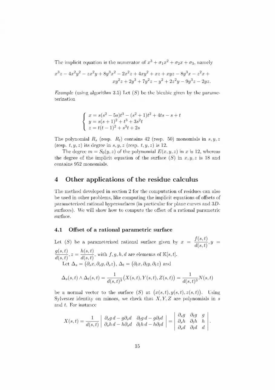
4 Other applications of the residue calculusThe method developed in section 2 for the computation of residues can alsobe used in other problems, like computing the implicit equations of o�sets ofparameterized rational hypersurfaces (in particular for plane curves and 3D-surfaces). We will show how to compute the o�set of a rational parametricsurface.

4.1 O�set of a rational parametric surface

Let (S) be a parameterized rational surface given by x =f(s, t)d(s, t)

, y =

g(s, t)d(s, t)

, z =h(s, t)d(s, t)

, with f, g, h, d are elements of K[s, t].

Let ∆s =(∂sx, ∂sy, ∂sz

), ∆t =

(∂tx, ∂ty, ∂tz

)and

∆s(s, t) ∧∆t(s, t) =1

d(s, t)3(X(s, t), Y (s, t), Z(s, t)

)=

1d(s, t)3

N(s, t)

be a normal vector to the surface (S) at(x(s, t), y(s, t), z(s, t)

). Using

Sylvester identity on minors, we check that X,Y, Z are polynomials in sand t. For instance

X(s, t) =1

d(s, t)

∣∣∣∣∂sg d− g∂sd ∂tg d− g∂td∂sh d− h∂sd ∂th d− h∂td

∣∣∣∣ =

∣∣∣∣∣∣

∂sg ∂tg g∂sh ∂th h∂sd ∂td d

∣∣∣∣∣∣.

15

We denote by ν(s, t) = X(s, t)2 + Y (s, t)2 + Z(s, t)2 the square of the normof N(s, t).

For any positive real number r, the r-o�set of (S) is the set of points atdistance r to (S). This set is parameterized by the two maps

(s, t) 7→ 1d(s, t)

f(s, t)g(s, t)h(s, t)

± r√

ν(s, t)N(s, t).

If the o�set is irreducible, then only one of these two maps is necessary.To compute the implicit equations of the union of the image of these

maps, using residues, we introduce the following equations

G(s, t, w, v) = y − g(s, t) w − r vY (s, t)H(s, t, w, v) = z − h(s, t) w − r vZ(s, t)W (s, t, w, v) = w d(s, t)− 1V (s, t, w, v) = v2 ν(s, t)− 1.

Let us denote by O the variety de�ned by G,H, W, V in K(y, z)4. Then

for any (s, t, w, v) ∈ O, we have y =g(s, t)d(s, t)

± rY (s, t)√ν(s, t)

and z =h(s, t)d(s, t)

±

rZ(s, t)√ν(s, t)

. By the same arguments as in the section 3, we obtain the fol-

lowing result:

Theorem 4.1 The squarefree part of the numerator of the polynomial∏

(s,t,w,v)∈O

(x− f(s, t)w − r v X(s, t)

)= xm + σ1(y, z) xm−1 + · · ·+ σm(y, z)

is the implicit equation of the r-o�set of (S).

The degree m of this polynomial is equal to τG,H,W,V

(Jac(G,H,W, V )

)and

the coe�cients σi(y, z) are deduced from the Newton sums

Si(y, z) = τG,H,W,V

((f(s, t) w+r v X(s, t)

)iJac(G,H, W, V ))

, i = 1 . . .m ,

using Newton identities (7).Other constructions used in CAGD can also be treated in this way.

5 ConclusionWe propose a new algorithm to solve the implicitization problem. This meth-ods seem to be a powerful tool to treat problems where base points occurred.This approach can be applied to other problems as the computation of the

16

equation of the o�set of a rational surface that is still consider a di�cultcomputational challenge.

The techniques based on bezoutians developed in this article seem tosu�er from the size of involved matrices. It would be interesting to useinterpolation techniques to evaluate them or to keep these matrices withoutdeveloping their determinants and to take the necessary monomials at theend of computations.

References[1] Alonso, C.; Gutierrez, J.; Recio, T. An implicitization algorithm with

fewer variables. Comput. Aided Geom. Des., 12(3):251�258, 1995.

[2] Aries, F.; Senoussi, R. An Implicitization Algorithm for Rational Sur-faces with no Base Points. J. Symb. Comput., 31:357�365, 2001.

[3] Becker, E.; Cardinal, J.P.; Roy, M.F.; Szafraniec, Z. Multivariate Be-zoutians, Kronecker symbol and Eisenbud-Levin formula. In Algorithmsin Algebraic Geometry and Applications, volume 143 of Prog. in Math.,pages 79�104. Birkhäuser, Basel, 1996.

[4] Berenstein, C.A.; Yger, A. Residue calculus and e�ective nullstellensatz.Amer. J. Math., 121:723�796, 1999.

[5] Buchberger, B. Applications of Groebner bases in nonlinear computa-tional geometry. In Trends in computer algebra, Lect. Notes Comput.Sci., volume 296, pages 52�80, 1988.

[6] Busé, L. Residual resultant over the projective plane and the implici-tization problem. Proceedings of the 2001 international symposium onsymbolic and algebraic computation, pages 48�55, 2001.

[7] Busé, L.; Cox, D.; D'Andrea, C. Implicitization of surfaces in P3 in thepresence of base points. preprint, 2002.

[8] Busé, L.; Jouanolou, J.P. On the closed image of a rational map andthe implicitization problem. preprint, 2002.

[9] Canny, J.F.; Manocha, D. Implicit representation of rational parametricsurfaces. J. Symb. Comput., 13(5):485�510, 1992.

[10] Corless, R.M.; Giesbrecht, M.; Kotsireas I.S.; Watt, S.M. NumericalImplicitization of Parametric Hypersurfaces with Linear Algebra. Art.Intel. Symb. Comp., pages 174�183, 2000.

[11] Cox, D.; Goldman, R.; Zhang, M. On the Validity of Implicitization byMoving Quadrics for Rational Surfaces with No Base Points. J. Symb.Comput., 29(3):419�440, 2000.

17

[12] Dokken, T. Approximate Implicitization. In Mathematical Methods inCAGD: 2000. Vanderbilt University Press, 2001.

[13] Gonzalez-Vega, L. Implicitization of parametric curves and surfacesby using multidimensional Newton formulae. J. Symb. Comput., 23(2-3):137�151, 1997.

[14] Gonzalez-Vega, L.; Trujillo, G. Implicitization of parametric curvesand surfaces by using symmetric functions. In Proceedings of the 1995international symposium on symbolic and algebraic computation, pages180�186. ACM Press, 1995.

[15] C.M. Ho�mann. Geometric and solid modeling: an introduction. Mor-gan Kaufmann Publishers Inc., 1989.

[16] Kalkbrener, M. Implicitization of rational parametric curves and sur-faces. In Applied algebra, algebraic algorithms and error-correcting codesProc. AAECC8, Lect. Notes Comput. Sci., volume 508, pages 249�259,1991.

[17] E. Kunz. Kähler di�erentials. Advanced lectures in Mathematics. Friedr.Vieweg and Sohn, 1986.

[18] Pérez-Díaz, S.; Schicho, J.; Sendra, J.R. Properness and Inversion ofRational Parametrizations of Surfaces. AAECC13, pages 29�51, 2002.

[19] U. Scheja, G.; Storch. Über Spurfunktionen bei vollständigen Durschnit-ten. J. Reine Angew Mathematik, 278:174�190, 1975.

[20] Sederberg, T.W.; Anderson, D.C.; Goldman, R.N. Implicit representa-tion of parametric curves and surfaces. Computer Vision, Graphics andImage Processing, 28:72�84, 1984.

[21] Sederberg, T.W.; Chen, F. Implicitzing using moving curves and sur-faces. In proceedings of SIGGRAPH, pages 301�308, 1995.

18