Embed Size (px)
Citation preview

BusinessInterdisciplinary Journal on Risk and Society
Review of
BusinessInterdisciplinary Journal on Risk and Society
Review of
Review
of Business | V
ol
um
e 41 ● N
um
be
r 2
BusinessInterdisciplinary Journal on Risk and Society
Review of
Volume 41, Number 2 | JuNe 2021
Non-Profit Org. U.S. Postage
PAIDSt. John’s University
New York
The Peter J. Tobin College of Business8000 Utopia Parkway
Queens, NY 11439stjohns.edu
Banking Deregulation and Investment-Cash Flow Sensitivity 1
Dawei Jin, Haizhi Wang, Tianyu Zhao, and Xinting Zhen
The Leader-Member Exchange (LMX) Influence at Organizations: The Moderating Role of Person-Organization (P-O) Fit 32
Omer Faruk Derindag, Ozgur Demirtas, and Ali Bayram
The Real Effect of Financial Reform: Evidence from Bond Market in China 49
Xian Gu, Lu Yun, and Shangwei Hao
Work Environment and Employee Performance: Evidence from Sell-Side Analysts 85
Shuya Liu and Kevin Sun

BusinessInterdisciplinary Journal on Risk and Society
Review of
Copyright © 2021, St. John’s University.
The views presented in the articles are those of the authors and do not represent an official statement of policy by St. John’s University.
EditorYun Zhu St. John’s University, United States
Advisory Board Iftekhar Hasan Fordham University, Bank of Finland, and University of Sydney, United States
Kose John New York University, United States
Steven Ongena University of Zurich, Swiss Finance Institute, KU Leuven, and Center for Economic and Policy Research (CEPR), Switzerland
Raghavendra Rau University of Cambridge, United Kingdom
David Reeb National University of Singapore, Singapore
Editorial BoardTuranay Caner North Carolina State University, United States
Santiago Carbó-Valverde CUNEF, Spain
Sandeep Dahiya Georgetown University, United States
Sudip Datta Wayne State University, United States
Co-Pierre Georg University of Cape Town, South Africa
Xian Gu Durham University, United Kingdom
Omrane Guedhami University of South Carolina, United States
Roman Horváth Charles University, Czech Republic
Patrick Flanagan St. John’s University, United States
Suk-Joong Kim University of New South Wales [UNSW] Sydney, Australia
Anzhela Knyazeva Security Exchange Commission, United States
Chih-Yung Lin National Chiao Tung University, Taiwan
Kristina Minnick Bentley University, United States
Jerry Parwada UNSW Sydney, Australia
Maurizio Pompella University of Siena, Italy
Steven W. Pottier University of Georgia, United States
Alon Raviv Bar Ilan, Israel
Victoria Shoaf St. John’s University, United States
Akhtar Siddique Office of the Comptroller of the Currency, United States
Benjamin Tabak FGV, Brazil
Tuomas Takalo Bank of Finland, Finland
Amine Tarazi University of Limoges, France
Krupa Viswanathan Temple University, United States
Wolf Wagner Rotterdam School of Management and CEPR, The Netherlands
Noriyoshi Yanase Keio University, Japan
Gaiyan Zhang University of Missouri–Columbia, United States
Hao Zhang Rochester Institute of Technology, United States
Review of Business is published twice a year.ISSN: 0034-6454
Review of Business is a peer-reviewed academic journal. The journal publishes original research articles in all academic fields of business, both theoretical and empirical, that will significantly contribute to the literature of business and allied disciplines. The journal advocates for research articles in imminent topics, such as sustainable development, technology- related business issues, and topics that enrich the interdisciplinary understanding of business.
The Peter J. Tobin College of BusinessSt. John’s UniversityNew York
www.stjohns.edu/ROB (for submissions, style guide, publishing agreement, and standards of integrity)
[email protected] (for inquiries and communications)

i
Fr o m t h e ed i t o r
We are delighted to share with you the June 2021 issue of Review of Business. This issue features four academic papers that span a diverse spectrum of empir-ical business studies and answer the surging call for research in financial regula-tion, business ethics, and sustainable development.
The lead article, “Banking Deregulation and Investment-Cash Flow Sen-sitivity” by Jin, Wang, Zhao, and Zhen, investigates the important role of the Riegle-Neal Interstate Banking and Branching Efficiency Act of 1994 (IBBEA) in explaining the documented declining trend of firms’ investment-cash flow sensi-tivity. The authors implement a difference-in-difference approach to investigate the effects of both the interstate and intrastate banking deregulation on sensitiv-ity of investment to internal cash flow at the firm-year level over the period 1970 to 2006. The paper shows that there exists a material drop in the firm’s sensi-tivity of investment to cash flow following the deregulation of restrictions on in-terstate and intrastate banking. Such effect is stronger among firms in industries that rely heavily on external finance, and among firms that are geographically lo-cated in the urban areas, suggesting that banking deregulation changes improve competition among banks and promote the use of bank loans as external financ-ing, and thus reduce sensitivity of investment to internally generated cash flows.
In the second article, “The Leader-Member Exchange (LMX) Influence at Organizations: The Moderating Role of Person-Organization (P-O) Fit,” Der-indag, Demirtas, and Bayram look into the concept of leader-member exchange (LMX) from the organizational prospect. The paper examines the influence of LMX on burnout, turnover intention, and organizational citizenship behaviors (OCB), and the moderating role of person-organization fit on these LMX influ-ences. Using a survey of 903 employees conducted in Kayseri—Turkey’s man-ufacturing region—the authors employ frequency analysis, reliability analysis, confirmatory factor analysis, and hierarchical regression analysis to show that leader-member interaction has a negative effect on burnout and intention to quit and has a positive effect on organizational citizenship behavior. In addition, person-organizational fit was found to have a moderating role in these relations.
The next article, “The Real Effect of Financial Reform: Evidence from Bond Market in China” by Gu, Yun and Hao, is motived by the lack of focus on the private bond market among the rich literature on the relationship between equi-ty market liberalization or overall financial development and economic growth. The study uses the policy shock of China’s bond issuance reform in 2015 to examine the effect on the cost of debt and debt choices. With a difference-in-dif-ference method and a bond-level dataset of 689 enterprise bonds and 1,295 cor-porate bonds, the authors find that at the bond level, the reform reduces the cost of bond financing in terms of bond yield spread by approximately 29.4 percent and enhances the bond issuance volume by approximately 1.7 percent. While, at the firm level, the reform reduces the cost of total debt by around 7.4 percent, enhances the public debt issuance instead of the private debt, and shortens the debt maturity. The evidence suggests that the private bond market liberalization reduces the cost of debt and alleviates financial constraints. The effect is also more significant for politically connected firms with more concentrated owner-

ii F R O M T H E E D I T O R
ship, indicating that they may use it as a way to insulate from bank monitoring. This paper, along with the lead article, provides insights into the outcome of financial deregulation.
Liu and Sun contribute their work “Work Environment and Employee Per-formance: Evidence from Sell-Side Analysts” as the last article of this issue. The paper uses Glassdoor ratings as a proxy for employee satisfaction of work en-vironment to examine how positive work environment affects employee perfor-mance. The authors find that in better-rated brokerage firms, analysts issue more frequent and more accurate earnings forecasts, and their stock recommendations produce a larger stock market reaction. In addition, the nonlinear relationship only exists after an analyst works for a brokerage firm for at least two years, and highly rated brokerages have better analyst retention and a lower percent-age of employee turnover. This article provides empirical evidence to the call for improving the working condition and pressure of gig workers and warehouse workers.
In short, we hope that that scholars and professionals will find this issue of RoB informative and enlightening. We will continue to publish high-quality, scholarly articles that answer the most imminent questions in the fast-changing world.
Yun Zhu, Editor

1
Dawei Jin, PhD, Zhongnan University of Economics and Law, [email protected]
Haizhi Wang, PhD, Illinois Institute of Technology, [email protected]
Tianyu Zhao, PhD, China Construction Bank, [email protected]
Xinting Zhen, PhD, Saint Michael’s College, [email protected]
Banking Deregulation and Investment-Cash Flow SensitivityDawei Jin
Haizhi Wang
Tianyu Zhao
Xinting Zhen
Abstract Motivation: Prior empirical studies show that there exists a declining pattern of investment-cash flow sensitivity during the banking deregulation period in the United States, but it is still unclear whether such deregulatory reforms that increase competition affect the sensitivity of investment to internally generated cash flows. This research provides empirical evidence to explain banking de-regulation as an important determinant of the documented declining trend of investment-cash flow sensitivity.
Premise: This study investigates the important role of the Riegle-Neal Interstate Banking and Branching Efficiency Act of 1994 (IBBEA) in explaining the doc-umented declining trend of firms’ investment-cash flow sensitivity. We predict that banking deregulation progress relaxes geographical restrictions on bank expansion and facilitates bank loan issuance as a main source of external financ-ing, and ultimately, reduces the sensitivity of investment to internally generated cash flows.
Approach: We implement a difference-in-difference approach to investigate the effects of both the interstate and intrastate banking deregulation on sensitivity of investment to internal cash flow at the firm-year level over the period 1970 to 2006. We also follow the conventional investment literature and apply the Erickson-Whited estimators to control for the measurement error of Tobin’s q.
Results: We document that there exists a material drop in the firm’s sensitivity of investment to cash flow following the deregulation of restrictions on interstate and intrastate banking. Particularly, such reduction effects are strong among firms in industries that rely heavily on external finance, and among firms that geographically located in the urban areas. Furthermore, we show that the reduc-
Rev
iew
of
Bus
ines
s 41
, no.
2, 1
–31.
Cop
yrig
ht ©
202
1 St
. Joh
n’s
Uni
vers
ity.
2 R E V I E W O F B U S I N E S S
tion effects of banking deregulation on investment-cash flow sensitivity is more pronounced for financially constrained firms with low hedging needs than for constrained firms with high hedging needs.
Conclusion: Banking deregulation changes improve competition among banks and promote the use of bank loans as external financing, and thus reduce sen-sitivity of investment to internally generated cash flows. Such reduction effects are mainly driven by financially constrained firms with low hedging needs and are more pronounced among urban firms than among small-city and rural-based firms.
Consistency: This research provides important implications on the role of fi-nancial market development for corporate investment. By making bank loans a more available external source of financing to firms after deregulation, com-petition-enhancing deregulatory changes reduce the sensitivity of investment to cash flows.
Keywords: banking deregulation, investment-cash flow sensitivity
JEL Classification Codes: G21, G28, G31, G32
INTRODUCTIONThe investigation of the investment-cash flow sensitivity continues to be one of the largest empirical literatures in corporate finance. A large body of research (Gilchrist and Himmelberg 1995; Kaplan and Zingales 1997; Cleary 1999; Gomes 2001; Alti 2003; Moyen 2004; Almeida and Campello 2007; Chow-dhury, Kumar, and Shome 2016), starting with Fazzari et al. (1988), have in-vestigated the investment decision of a firm in the capital markets. Specifically, in a perfect market, internal and external funds can be perfect substitutes, but the presence of information asymmetry due to market imperfections creates a wedge between internal and external funds and increases costs of external cap-ital. Therefore, firms are reluctant to invest more when their internal funds are low. Fazzari et al. (1988) imply that firms invest less and display a greater in-vestment-cash flow sensitivity when they are more likely to confront financial constraints.
Although there is debate on whether investment-cash flow sensitivities are good measures for detecting financing constraints (Kaplan and Zingales 1997, 2000; Fazzari, Hubbard, and Petersen 2000), researchers have widely applied the investment-cash flow regression as an important tool to explore the effects of mar-ket imperfections on firm investment and the impacts of managerial characteristics on corporate policies (Gilchrist and Himmelberg 1995; Hubbard 1998; Ascioglu, Hegde, and McDermott 2008; Attig et al. 2012; Moshirian et al. 2017; Agca and Mozumdar 2008; Derouiche, Hassan, and Amdouni 2018). More importantly, some existing empirical studies show consistent findings that there exists a declin-ing pattern of investment-cash flow sensitivity in the United States over the past several decades (Allayannis and Mozumdar 2004; Agca and Mozumdar 2008; Brown, Fazzari, and Petersen 2009; Chen and Chen 2012). The most possible and important reasons could be the changing composition of investment and the development of equity financial market as a source of funds, particularly for firms that report consistent negative cash flows (Brown and Petersen 2009).

B A N K I N G D E R E G U L A T I O N A N D I N V E S T M E N T - C A S H F L O W S E N S I T I V I T Y 3
Despite the prominence of the applications and declining trend of invest-ment-cash flow sensitivity in the current literature, what has received less atten-tion, is the relationship between deregulation changes that increase competition and the sensitivity of investment to internally generated cash flows. This is sur-prising. Banking deregulation reforms lower entry barriers to provide firms better access to external financing and improve competition for the banking industry (Koetter, Kolari, and Spierdijk 2012), and thus such deregulatory changes in the banking industry can affect the sensitivity of investment to internally generated cash flows. Therefore, from either the macro-economic or firm-investment per-spective, it is valuable to explore the impacts of banking deregulatory reforms that trigger greater competition among banks on firms’ investment-cash flow sensitivity.
This study aims to provide new insights into the current literature by explain-ing the declining trend of investment-cash flow sensitivity over the past several decades. We expand on this line of research by exploring banking deregulation as a possible determinant of the documented declining trend of investment-cash flow sensitivity during the period 1970 to 2006. Moreover, we notice that invest-ment-cash flow sensitivity shows a declining trend during the banking deregula-tion period in the United States, but we still know relatively little about whether such reduction is a coincidence, or if banking deregulation changes indeed explain the reduction of investment-cash flow sensitivity. This research intends to solve these unanswered questions by providing empirical evidence on the relationship between banking deregulatory reforms and investment-cash flow sensitivity.
As important sources of financing, banks take a vital role in providing external funds for corporations. One of the primary functions of banks is to gather information about borrowers in the process of lending and monitoring, and information asymmetries take an important role in affecting bank compe-tition (Marquez 2002). Banking deregulation facilitates geographical diversifi-cation and enhances direct access to borrowers (Hughes et al. 1996; Calomiris and Calomiris 2000; Petersen and Rajan 2002; Akhigbe and Whyte 2003), and consequently, reduces information asymmetry and enables better screening and monitoring (Degryse and Ongena 2005, 2008; Hauswald and Marquez 2006). Hauswald and Marquez (2003) provide theoretical models to show that faster dissemination of information could increase competition among lenders and benefit borrowers through lower interest rates. Empirical evidence presents con-sistent results that banking system became more efficient and competitive after the reform, so banking deregulation changes have accelerated economic growth (Black and Strahan 2002; Stiroh and Strahan 2003; Strahan 2003). Particularly, better growth performance is mainly due to better quality lending and lower loan prices after the reform (Jayaratne and Strahan 1996; Rice and Strahan 2010). If the cost for firms to access external funds is lower, then firms’ investments will be more independent with better internal cash flow because firms can raise external funds from banks with cost benefits. We therefore predict that banking deregulation progress relaxes geographical restrictions on bank expansion and facilitates bank loan issuance as a main source of external financing, ultimately reducing the sensitivity of investment to internally generated cash flows.
In this study, we focus on the Riegel-Neal Interstate Banking and Branch-ing Efficiency Act of 1994 (IBBEA) to investigate the impact of banking dereg-ulation on firms’ investment-cash flow sensitivity. The IBBEA lifted restrictions on commercial banks to allow free interstate branching and out-of-state acquisi-

4 R E V I E W O F B U S I N E S S
tion (Kroszner and Strahan 1999). We distinguish between interstate and intra-state deregulation (Koetter, Kolari, and Spierdijk 2012). Interstate deregulation (Inter) allowed out-of-state acquisition. Intrastate deregulation (Intra) relaxed restrictions on statewide branching by mergers and acquisitions of existing com-petitors and de novo branching within the state. In 1994 the IBBEA permitted free interstate branching and allowed out-of-state banks to integrate branching networks, which increased their market share after deregulation year.
Specifically in this study, we investigate the role of banking deregulation in investment-cash flow regressions by estimating dynamic investment models that include measures of external financing. We focus our data sample within the period from 1970 to 2006. The sampling period covers the years before and after the implementation of IBBEA and overlaps with the period of the declining trend of investment-cash flow sensitivity. By implementing a difference-in-dif-ference approach, we find that both interstate and intrastate banking deregu-lation significantly reduce sensitivity of investment to internal cash flow at the firm-year level, and such reduction effects are more pronounced among firms in industries that rely more heavily on external finance. We conduct several robust-ness checks and address endogeneity issues that confirm our conclusions. These findings are consistent with current literature that highlights a declining trend of investment-cash flow sensitivities in the United States during the past several de-cades (Agca and Mozumdar 2008; Chen and Chen 2012; Moshirian et al. 2017).
To control for the measurement error of Tobin’s q, we follow the conven-tional investment literature and apply the Erickson-Whited estimators (Brown and Petersen 2009; Erickson and Whited 2000, 2002, 2012). Our findings of estimated investment-cash flow effects are robust after the application of the Erickson-Whited estimators. Besides, we also propose additional tests to support the validity of our empirical identification strategy. We implement a dynamic difference-in-difference approach to verify that investment-cash flow sensitivity exhibits significant change around that implementation of IBBEA without pre-existing trends. In addition, we show that financially constrained firms, espe-cially constrained firms with low hedging needs, drive the negative relationship between banking deregulation and investment-cash flow sensitivity.
The rest of the paper is organized as follows. The next section provides institutional background information on the banking deregulation in the United States and reviews related literature. The section entitled Data, Sample, and Measures describes the data sampling process and explains variable construc-tion. The Results section shows empirical models and report results. The Con-clusion summarizes and concludes the paper.
LITERATURE REVIEW
Banking Deregulation in the United States
The banking industry in the United States has experienced a series of deregula-tion during the past four decades. Legislators have implemented deregulatory changes to gradually remove restrictions on banking geographic expansion since the 1970s. Such deregulation includes relaxing both interstate and intrastate bank-branching restrictions. Interstate and intrastate banking deregulation are different in their effects. Relaxing restrictions on interstate banking allows out-

B A N K I N G D E R E G U L A T I O N A N D I N V E S T M E N T - C A S H F L O W S E N S I T I V I T Y 5
of-state banks to acquire branches in other states, eliminating less efficient banks (Chava et al. 2013), increasing competition and improving openness of the take-over market in the banking industry (Black and Strahan 2002). Intrastate bank-ing deregulation allows bank holding companies to convert subsidiary banks into branches and permits banks to open new branches within state borders (Jayaratne and Strahan 1996).
In 1994, the U.S. Congress passed the Riegle-Neal Interstate Banking and Branching Efficiency Act (IBBEA) to permit both interstate banking and intra-state branching in almost all states. The unrestricted interstate banking took effect in 1995, and later in 1997, the IBEA legalized interstate branching across the United States to relax geographical restrictions on banking expansion. While IBBEA released the restrictions, it allowed states to follow a variety of means to implement out-of-state entry barriers from the time of enactment in 1994 until the branching trigger date of June 1, 1997.
A number of studies exploit the different patterns of changes in the de-regulation of banks across U.S. states to examine the impact of the exogenous shock in the banking industry on many aspects in economy and capital market (Jayaratne and Strahan 1996; Kroszner and Strahan 1999). Specifically, econ-omy growth and quality of bank lending increase with branching deregulation (Jayaratne and Strahan 1996). Banking deregulation fosters competition and banking consolidation helps entrepreneurship in the United States (Black and Strahan 2002; Strahan 2003). In addition, banking deregulation reforms bring exceptional growth in both entrepreneurship and business closures (Kerr and Nanda 2009), tighten income distribution by boosting incomes in the lower part of income distribution (Beck, Levine, and Levkov 2010), improve bank market power (Koetter, Kolari, and Spierdijk 2012), encourage small business lending (Rice and Strahan 2010), and foster innovation (Chava et al. 2013; Cornaggia et al. 2015). We anticipate that banking deregulation increases bank competition, provides firms easier access to raise funds, and therefore should be negatively associated with firms’ investment-cash flow sensitivity.
Banking Deregulation and Investment-Cash Flow Sensitivity
More recently, banks have become important sources of financing for corpora-tions in the United States. As financial intermediaries, banks have special screen-ing and monitoring abilities that capital market investors do not have (Diamond 1984, 1991; Boyd and Prescott 1986; Ramakrishnan and Thakor 1984). As main external funding providers, banks act as a natural hedge that reduces the cost of supplying liquidity when corporate sector’s liquidity demand rises (Kashyap, Rajan, and Stein 2002; Gatev and Strahan 2006). Therefore, banks can affect firms’ investment decisions in various ways (Zarutskie 2006; Amiti and Wein-stein 2018). By allowing banks to expand and enter different markets without restrictions, banking deregulation brings openness and increases competition to the entire banking industry in the United States (Black and Strahan 2002; Stiroh and Strahan 2003). Because interstate and intrastate banking deregulation have gradually removed barriers to competition among banks, banking deregulation may have improved efficiency for the whole banking industry and expanded the availability of financing. Consequently, the cost for firms to access external funds will be lower (Rice and Strahan 2010), and the firm investment should be

6 R E V I E W O F B U S I N E S S
more independent with internal cash flow (Lewellen and Lewellen 2016). There-fore, we predict that deregulatory reforms in the banking industry should reduce the sensitivity of investment to cash flow.
The relationship between investment and financing decisions, as a central issue in corporate finance, has been explored both theoretically and empirically in existing literatures. In the world of perfect and complete capital markets, a firm’s financial status is irrelevant for real investment decisions (Modigliani and Miller 1958). Nonetheless, research has shown that when firms operate in an imperfect or incomplete capital market where the cost of external financing exceeds internal financing, information asymmetry will exacerbate the cost of external financing, suggesting that internal funds and external funds are unlikely substitutes (Myers and Majluf 1984). This may increase firms’ reliance on inter-nal funding at the best level in investments, showing that financial structure is relevant to the investment decisions of companies (Fazzari et al. 1988).
Because of market imperfection and its associated impacts on firms’ invest-ment decisions, an important body of literature explores possible factors that af-fect firms’ investment-cash flow sensitivity in imperfect markets. These factors include dividend payout rates (Fazzari et al., 1988), bond rating (Gilchrist and Himmelberg 1995), institutional ownership and analyst coverage (Agca and Mo-zumdar 2008), probability of informed trading (Ascioglu, Hegde, and McDer-mott 2008), investor horizon (Attig et al. 2012), asset tangibility (Moshirian et al. 2017), and ownership structure (Derouiche, Hassan, and Amdouni 2018). Cleary, Povel, and Raith (2007) theoretically provide evidence to show that when firms are exposed to market imperfections, investment increases monotonically with in-ternal funds if they are large and decreases if they are low. Almeida and Campello (2007) identify the effects of financing frictions and find that investment-cash flow sensitivities are increasing in the degree of tangibility of constrained firms’ assets, but investment-cash flow sensitivities are unaffected by asset tangibility if firms are unconstrained. Chowdhury, Kumar, and Shome (2016) show that decreases in information asymmetry following the Sarbanes-Oxley Act are associated with reductions in investment-cash flow sensitivity. Main findings from these studies indicate that market imperfection creates information asymmetry, which decreases firm investment and increases the sensitivity of investment to fluctuations in in-ternally generated cash flows. Our research contributes to this line of research on determinants of firms’ investment-cash flow sensitivity.
Most empirical studies of the investment-cash flow sensitivity discuss the ex-istence of a downward trend in U.S. industry during the past several decades. For example, Fazzari et al. (1988) and Kaplan and Zingales (1997) report that invest-ment-cash flow sensitivity is within a range of 0.2 and 0.7. Cleary (1999) estimates a lower investment-cash flow sensitivity of 0.15 by using the data of 1,317 surviv-ing firms from 1988 to 1994. Rauh (2006) finds that firms that do not sponsor defined benefit pension plans undertake approximately 12 percent of the capital investment, and Rauh reports that investment-cash flow sensitivity equals 0.11 from 1990 to 1998. Brown, Fazzari, and Petersen (2009) report investment-cash flow sensitivities of 0.32 to 0.30 from 1970 to 1981, and a drop to 0.01 to 0.8 from 1994 to 2006. More recently, Chen and Chen (2012) provide evidence that investment-cash flow sensitivity has significantly declined since the mid-1970s and has completely disappeared in late 1990s. Lewellen and Lewellen (2016) show

B A N K I N G D E R E G U L A T I O N A N D I N V E S T M E N T - C A S H F L O W S E N S I T I V I T Y 7
that investment-cash flow sensitivity is still significant after late 1990s and report a continued decline of sensitivity from around 0.4 in 1970s to about 0.1 in late 1990s. Although investment-cash flow sensitivity shows a declining trend during the bank deregulation period, there is surprisingly little evidence to show whether such reduction is due to coincidence or is associated with deregulatory reforms from the banking industry. We therefore intend to contribute to the existing lit-erature by providing empirical evidence to reveal the connection between bank deregulatory reforms and the investment-cash flow sensitivity.
DATA, SAMPLE, AND MEASURES
Data and Sample
We use Compustat Industrial Annual Files as our primary data source of infor-mation to investigate the effects of banking deregulation on firm investment-cash flow sensitivity. To test the effects of bank branching deregulation on invest-ment-cash flow sensitivity, we choose 1970 to 2006 as our main sample period.
Following the conventional approach in investigations of corporate liquidity (Brown and Petersen, 2009), we include firms that are incorporated in the United States only, and we eliminate financial firms (Standard Industrial Classification [SIC] code 6000-6999) and utility firms (SIC code 4900-4999) because their op-erations are subject to particular regulations. To avoid potential business discon-tinuities caused by mergers and acquisitions, we exclude firm-year observations with asset or sales growth exceeding 100% (Almeida, Campello, and Weisbach 2004). To control Compustat’s backfilling bias, we follow Chen and Chen (2012) to exclude firms for which we cannot compute the lagged cash flow to capital ratio. To rule out the possibility that a substantial amount of cash following initial public offerings (IPO) affects investment-cash flow sensitivity, we exclude firms that have been public for fewer than four years in the Compustat database (Rajan and Zingales 1998). To mitigate outliers, we further conduct the following proce-dures: first, we eliminate firms that have negative assets or negative sales (Opler et al. 1999). We then exclude firm-year observations with market-to-book ratios that are negative or greater than 10 (Almeida and Campello 2007). Last, we exclude firms with capital, book assets, and sales less than $1 million in the previous year (Chen and Chen 2012). Moreover, we exclude firms with headquarters in Dela-ware and South Dakota because these two states have different banking structures due to government regulation (Black and Strahan 2002; Beck, Levine, and Levkov 2010). We winsorize all variables at the first and ninety-ninth percentiles of non-financial and nonutility firms in each year (Almeida, Campello, and Weisbach 2004, Almeida and Campello 2007). Our sampling procedure yields 79,357 firm-year observations, ranging from 1970 to 2006.
Main Explanatory Variables
As mentioned in the introduction, the Riegle-Neal Interstate Banking and Branch-ing Efficiency Act (IBBEA) was passed in 1994, allowing both unrestricted in-terstate banking and interstate branching. With the passage of IBBEA, unre-stricted interstate banking took effect in 1995, permitting commercial banks and bank holding companies to expand across different states in the United States.

8 R E V I E W O F B U S I N E S S
The interstate branching took effect in 1997, relaxing geographical restrictions on banking expansion. As described in Rice and Strahan (2010), the interstate branching was the watershed event of IBBEA. While IBBEA released restrictions and opened the door to nationwide branching, it allowed states to employ a variety of means to implement out-of-state entry barriers from the time of enact-ment in 1994 until the branching trigger date of June 1, 1997.
Existing research on banking deregulation distinguishes between interstate and intrastate deregulation (Kroszner and Strahan 1999; Koetter, Kolari, and Spi-erdijk 2012) from 1978 through 1995. States experienced a process of interstate bank deregulation by removing restrictions on interstate banking in a dynamic and state-specific approach. Therefore, states initiated interstate bank deregula-tion at different times and then followed different paths as they entered into agree-ments with other states. Intrastate deregulation relaxed prohibitions on statewide branching. Stiroh and Strahan (2003) further distinguish unrestricted intrastate branching. For consistency with most other banking investigations (Koetter, Ko-lari, and Spierdijk 2012), we focus on intrastate deregulation by means of permit-ting merger and acquisitions. Following previous literature (Kroszner and Strahan 1999; Koetter, Kolari, and Spierdijk 2012), we generate two dummy variables to represent banking deregulation events that occurred early in our sample period prior to 1997. We measure Inter as a dummy variable that equals 1 in the year and thereafter when the state adopts the interstate agreement permitting the bank expansion and equals 0 otherwise. Intra is a dummy variable that equals 1 in the year that intrastate banking was permitted by means of mergers and acquisitions and thereafter and equals 0 in all years until the deregulation.
Dependent Measure
Current literature of investment-cash flow sensitivity mainly focuses on physi-cal investment and finds that the investment-cash flow sensitivity for physical investment has fallen dramatically over time (Allayannis and Mozumdar 2004; Agca and Mozumdar 2008; Brown and Petersen 2009; Chowdhury, Kumar, and Shome 2016). Traditional (manufacturing) firms invest intensively if they oper-ate with a higher fraction of tangible capital. As part of the total productive cap-ital, tangible investment includes information about its marginal productivity. As the marginal productivity varies across different firms, the rate of investment also varies (Moshirian et al. 2017). We follow conventional studies (Kaplan and Zingales 1997; Almeida et al. 2004; Chen and Chen 2012) to use physical in-vestment as the dependent variable in our study, and measure Investment as the firm’s capital expenditures to the beginning-of-period stock of firm capital, which we defined as net property, plant, and equipment (PPE).1
Control Variables
In this analysis, we control for a vector of variables to capture firm characteris-tics. We measure Cash flow as operating cash flow divided by total assets (Faz-zari et al. 1988; Kaplan and Zingales 1997; Cleary 1999). We apply Tobin’s q in the previous year as a measurement of investment opportunities. We measure
1To check robustness, we also measure total investment (physical investment plus research and devel-opment [R&D]) scaled by total PPE and by total assets respectively. We find consistent results even if we apply the alternative measures.

B A N K I N G D E R E G U L A T I O N A N D I N V E S T M E N T - C A S H F L O W S E N S I T I V I T Y 9
Tobin’s q as the market value of assets minus the difference between the book value of assets and net PPE, scaled by net PPE (Kaplan and Zingales 1997; Chen and Chen 2012). We calculate the market value of assets as the market value of common stock plus total liability, plus preferred stock, and minus deferred taxes. We define Cash as the firm’s cash and short-term investments over the be-ginning period capital (Chen and Chen 2012). According to Brown and Petersen (2009), the failure to account for external finance can result in a downward omitted variable bias in the estimated cash flow coefficient. To control stock and debt effects, we measure Net new stock issuance as firm’s net new funds from stock issues to capital, and Net long-term debt issuance as net new long-term debt over beginning period capital. To avoid extreme values and possible outlier problem, we perform a 1 percent and 99 percent winsorization for all variables. We report the summary statistics of variables used in our analysis in Table 1.
TABLE 1. Summary Statistics
Variables N MeanStandard Deviation Minimum P25 P50 P75 Maximum
Investment 79,357 0.2417 0.2049 0 0.1097 0.1906 0.3069 1.4112
Cash flow 79,357 0.2232 0.7438 −9.6488 0.1191 0.2669 0.4667 3.0908
Inter 79,357 0.5936 0.4912 0 0 1 1 1
Intra 79,357 0.7019 0.4574 0 0 1 1 1
Firm size 79,357 4.8393 2.0216 −0.0284 3.3871 4.7198 6.1871 10.7866
Tobin’s q 79,357 1.3233 0.5654 0.0000 0.9498 1.1575 1.5223 4.4871
Cash 79,357 0.5532 2.2688 −0.0961 0.0563 0.1545 0.4302 216.6855
Net new stock issuance 79,357 0.0153 0.0494 0 0 0.0008 0.0065 0.6124
Net long-term debt issuance 79,357 0.0044 0.0829 −0.6138 −0.0193 0 0.0228 0.4336
Estimation Technique
Following previous literature (Stiroh and Strahan 2003; Koetter, Kolari, and Spi-erdijk 2012), we apply a difference-in-difference approach in this study to inves-tigate the effect of banking deregulation on investment-cash flow sensitivity and present our model in Equation (1). There is a concern that an unobservable vari-able, omitted from Equation (1), the general variation in a firm’s stance toward openness to bank deregulation might correlate with firms’ investments. The dif-ference-in-difference approach aims to address the omitted variable concern. Spe-cifically, following the standard investment-cash flow regression model (Fazzari et al. 1988; Brown and Petersen 2009), we create the basic regression model with an interaction term between cash flow and bank deregulation as follows:
Investmentijt 5 b0 1 b1 3 Cashflowijt 1 b2 3 Deregulationjt 1 b3 3 Cashflowijt 3
Deregulationjt 1 b4 3 Tobin’s qijt21 1 b5 3 Varijt 1 Firmt 1 ijt (1)
Where i indexes firms, j indexes states where the firms are headquar-tered, and t indexes year. Investmentijt is measured as capital expenditures over beginning-of-period capital, representing the physical investment for firm i that
10 R E V I E W O F B U S I N E S S
is headquartered in state j in year t. Cashflowijt is the internal cash flow ratio of firm i located in state j in year t. Tobin’s qijt21 is a proxy for investment opportu-nities. Deregulationjt captures either the interstate banking or intrastate branch-ing. It is the traditional dummy variable that equals 0 for state j in all years before state j eliminates interstate or intrastate banking restrictions, and equals 1 for state j that allow banks from at least one other state to establish subsidiaries within state j in and after year t. The coefficient b0 represents the intercept, and b1 measures investment-cash flow sensitivity. Cashflowijt 3 Deregulationjt is the interaction between corporate cash flow and banking deregulation. The coeffi-cient estimate b2 captures the effects of interstate and intrastate deregulation on investment-cash flow sensitivity, respectively. b3 represents the deregulation ef-fect on investment-cash flow sensitivity after relaxing restrictions on geographic expansion for banks, so our estimates of the banking deregulation effects on in-vestment-cash flow sensitivity are captured in b3.Varijt stands for a set of control variables to control for firm specifications. Particularly, we follow conventional studies (Bond and Meghir 1994; Brown, Fazzari, and Petersen 2009) to include firm’s cash, net stock and net debt issuances to control for possible omitted variable biases and to evaluate the changing role of external finance for invest-ment. We control for a year’s fixed effects, as indicated by Yeart . Firmi captures firm-specific effect that controls for all time-invariant determinants at the firm level. ijt is a random error term.
RESULTSThe analyses in this section focus on banking deregulation and investigate the effects of interstate and intrastate deregulation on firms’ investment-cash flow sensitivity. We test whether the sensitivity of investment to cash flow falls when states remove barriers of entry to banks from other states. The banking dereg-ulation provides us a natural laboratory to examine its effects and real conse-quences of regulatory changes, and existing research extensively uses the removal of regulatory restrictions to interstate banking as exogenous sources of variation in the competitiveness of banking markets (Jayaratne and Strahan 1996). Many states remove restrictions on interstate banking and intrastate branching at differ-ent times, and eventually all states remove restrictions on geographic expansion. We treat these over-time variations in regulatory status across different states as exogenous shocks, and use firms located in states not permitting the restrictions as the control group. Considering that a firm makes the majority of its financial decisions at the headquarters level, we focus on the state in which a firm’s head-quarters are located. We control for unobserved firm characteristics and aggregate shocks by including firm-fixed effects and year-fixed effects in our regressions.
Baseline Regression Testing the Effects of Bank Deregulation on Firm Investment-Cash Flow Sensitivity
First, we show our main results regarding the effects of various bank deregula-tion on investment-cash flow sensitivity. We report the results estimating Equa-tion (1) in Table 2 and show the results of the t-test between the treated group (when the deregulation dummy variables equal 1) and control group (when de-regulation dummy variables equal 0) in Appendix 3. In column 1 of Table 2, we

B A N K I N G D E R E G U L A T I O N A N D I N V E S T M E N T - C A S H F L O W S E N S I T I V I T Y 11
present our findings for investment-cash flow sensitivity by interstate banking. The coefficient estimate of the interaction term Cash flow × Inter is negative and significant at a 1 percent level (p < 0.01), suggesting that an increase in bank competition due to interstate deregulation reduces investment-cash flow sensi-tivity. To be more concrete, based on the coefficient estimate of the interaction term of Cash flow × Inter in column 1, firms that are headquartered in states with complete openness to interstate branching generate less investment-cash flow sensitivity after deregulation than firms that are headquartered in states with the most restrictions on interstate branching after deregulation. In the sense of economic significance, the results show that after the interstate banking de-regulation, firms’ investment-cash flow sensitivity decreases by 0.1075, repre-senting a 78 percent reduction (−0.1075/0.1381) of the investment-cash flow sensitivity before the interstate deregulation (which is 0.1381).
TABLE 2. Baseline Regression: The Effects of Bank Deregulation on Investment-Cash Flow Sensitivity
Independent Variables Dependent Variable: Investment
(1) (2)
Cash flow 0.1381*** 0.1255***
[0.0065] [0.0072]
Inter 0.0378***
[0.0053]
Cash flow × Inter −0.1075***
[0.0067]
Intra 0.0432***
[0.0043]
Cash flow × Intra −0.0896***
[0.0074]
Firm size 0.0192*** 0.0179***
[0.0021] [0.0021]
Tobin’s q 0.0232*** 0.0237***
[0.0006] [0.0006]
Cash 0.0450*** 0.0460***
[0.0024] [0.0024]
Net new stock issuance 0.3030*** 0.3066***
[0.0204] [0.0205]
Net long-term debt issuance 0.5700*** 0.5735***
[0.0134] [0.0133]
Constant −0.0679*** −0.0696***
[0.0151] [0.0149]
Firm fixed effects Yes Yes
Year fixed effects Yes Yes
Observations 79,357 79,357
Adjusted R-squared 0.4131 0.4091
Heteroscedasticity-consistent standard errors are clustered at the firm level. *, **, and *** represent statistical significance at the 10 percent, 5 percent, and 1 percent level, respectively.

12 R E V I E W O F B U S I N E S S
Similarly, we show the effect of intrastate banking on investment-cash flow sensitivity in column 2 and find that the coefficient of the interaction term Cash flow × Intra is negatively significant (p < 0.01). The coefficient of −0.0896 in-dicating that intrastate deregulation decreases investment-cash flow sensitivity by about 0.0896, showing a 71 percent drop (−0.0896/0.1255) of the invest-ment-cash flow sensitivity before intrastate deregulation (which is 0.1255). In addition, the coefficient is smaller in economic magnitude compared to its coun-terpart in column 1, revealing that interstate bank deregulation shows a larger effect in reducing investment-cash flow sensitivity. We include Tobin’s q as a control for investment demand. Consistent with Brown and Petersen (2009), we find a positive and significant coefficient of investment demand (p < 0.01) on investments. Moreover, we find that both net new stock issuance and net long-term debt issuance significantly increase investment-cash flow sensitivity (p < 0.01). This finding supports Brown and Petersen (2009) that public equity finance and debt finance became a much closer substitute for internal equity over the period we study.
Generalized Method of Moments (GMM) Regression: Correcting for Tobin’s q Measurement Error
To measure the unobservable investment opportunities of firms, Tobin’s q is the most common used factor in corporate finance. Poterba (1988) points out that measurement error in q may bias the empirical results of the investment-cash flow regressions, and similar concerns have been raised in subsequent studies as well (Brown and Petersen 2009; Erickson and Whited 2012). These studies indi-cate that Tobin’s q may not be a proper control for the investment opportunity set because there is a conceptual gap between true investment opportunities and observable measures (Erickson and Whited 2000, 2002, 2012).
Following Erickson and Whited (2012) (denoted as EW thereafter), we use the high-order moment estimators to control for the measurement error of Tobin’s q, and then to study whether the effects of bank deregulation on invest-ment-cash flow sensitivity are influenced by the measurement error of Tobin’s q. The EW estimators do not employ conventional instruments, but instead obtain identification from the third- and higher-order moments of the regression (Er-ickson and Whited 2012). We demean all variables at the firm level to control firm-fixed effects, and trim outliers in first differences at the 1 percent level. We include fixed firm and time effects in all GMM regressions and report the results of GMM regressions in Table 3. We use GEARY as the third-order moment esti-mator from Geary (1942). In addition, we apply generalized method of moments (GMM4) to indicate the EW estimator based on moments up to order four. Columns 1 and 2 report the results of GEARY, and columns 3 to 4 report the re-sults of GMM4. We find consistent results with our main ordinary least squares (OLS) results in Table 2 that both interstate and intrastate banking significantly reduce firms’ investment-cash flow sensitivity, showing that the main patterns in our baseline regression are unaffected when the regressions are estimated with GMM. Our results reveal that even after controlling the measurement error of Tobin’s q, banking deregulations still decrease investment-cash flow sensitivity significantly.

B A N K I N G D E R E G U L A T I O N A N D I N V E S T M E N T - C A S H F L O W S E N S I T I V I T Y 13
The Dynamic Effects of Bank Deregulation on Investment-Cash Flow Sensitivity
Although we provide evidence to demonstrate that the results hold when con-trolling for measurement error and including firm and year-fixed effects, con-cerns still remain that the state-level factors that manifest differently across U.S. states could have significant impacts on the firms’ investment decisions and on the timing of deregulation in different states (Kroszner and Strahan 1999). To alleviate the omitted variable concern, we examine the dynamics of invest-ment-cash flow sensitivity surrounding deregulation events. If the omitted vari-able concern indeed exists, we should observe changes in investment-cash flow sensitivity prior to the deregulation events.
Following Cornaggia et al. (2015), Bertrand and Mullainathan (2003) and Jiang et al. (2020), we construct a dynamic difference-in-difference approach to
TABLE 3. GMM Regressions: Correcting for Tobin’s q Measurement Error
Independent Variables Dependent Variable: Investment
GEARY GEARY GMM4 GMM4
(1) (2) (3) (4)
Cash flow 1.0283*** 0.8700*** 0.5645*** 0.4579***
(0.1845) (0.2841) (0.0329) (0.0395)
Inter 0.2690*** 0.1486***
(0.0490) (0.0107)
Cash flow × Inter −0.9740*** −0.5229***
(0.1794) (0.0322)
Intra 0.2720*** 0.1454***
(0.0874) (0.0131)
Cash flow × Intra −0.8178*** −0.4150***
(0.2777) (0.0387)
Firm size 0.0064* 0.0140*** 0.0152*** 0.0194***
(0.0037) (0.0038) (0.0010) (0.0008)
Tobin’s q 0.0316*** 0.0226*** 0.0252*** 0.0200***
(0.0042) (0.0033) (0.0025) (0.0023)
Cash 0.0292*** 0.0370*** 0.0370*** 0.0415***
(0.0043) (0.0042) (0.0024) (0.0023)
Net new stock issuance 0.2790*** 0.2442*** 0.2635*** 0.2478***
(0.0287) (0.0239) (0.0224) (0.0212)
Net long-term debt issuance 0.5329*** 0.5492*** 0.5483*** 0.5584***
(0.0180) (0.0163) (0.0139) (0.0132)
Firm fixed effects Yes Yes Yes Yes
Year fixed effects Yes Yes Yes Yes
Observations 79,357 79,357 79,357 79,357
Rho2 0.375 0.310 0.307 0.271
Heteroscedasticity-consistent standard errors are clustered at the firm level. *, **, and *** represent statistical significance at the 10 percent, 5 percent, and 1 percent level, respectively.

14 R E V I E W O F B U S I N E S S
include a set of dummy variables for the years surrounding the year that a state first relaxes its barriers to interstate banking and intrastate banking, respec-tively. We restrict our sample to a 10-year window surrounding state-deregu-lation years, with five years before and five years after, and thus this procedure leads to a sample size reduction. We generate six dummy variables around the deregulation time (Cornaggia et al. 2015), corresponding to six different peri-ods around each deregulation. We test the dynamic effects of the interstate and intrastate banking deregulation reforms separately. Specifically, Before21 and Before1 equal one for all years up to and including two years prior to the inter- and intra-deregulation, and one year prior to the deregulation reforms, respec-tively. By contrast, After1, After2, and After31 are dummy variables that equal one for one year post-deregulation, two years post-deregulation, and three years or more post-deregulation, respectively. We treat the deregulation year as the reference year in this setting. The coefficient estimates of Before21, and Before1 are important because their significance indicate whether there exists pre-period relationship between investment-cash flow sensitivity and deregulatory events. We estimate the following model:
Investmentijt 5 b1 3 Cashflowijt 1 b2 3 Before21 1 b3 3 Cashflowijt 3 Before21 1
b4 3 Before1 1 b5 3 Cashflowijt 3 Before1 1 b6 3 After1 1 b7 3 Cashflowijt 3
After1 1 b8 3 After2 1 b9 3 Cashflowijt 3 After2 1 b10 3 After31 1 b11 3
Cashflowijt 3 After31 1 b12 3 Qijt21 1 b13 3 Varijt 1 Firmi 1 Yeart 1 ijt (1)
We report the results of the dynamic effects of banking deregulation on in-vestment-cash flow sensitivity in Table 4. Columns 1 to 5 report the dynamic effects for interstate banking deregulation, whereas columns 6 to 10 focus on the intrastate deregulation. Columns 1 and 2 show that the coefficient estimates of pre-interstate deregulation dummies are all insignificant, indicating that there is no significant effect of banking deregulation on investment-cash flow sensitiv-ity in the pre-deregulation periods. Columns 3 to 5 report significant coefficient estimates of all post-deregulation dummies. These findings show that there is no pre-deregulation trend distorting our interpretation of the baseline regression re-sults. Moreover, we find consistent results for intrastate deregulation, indicating that the effect of intrastate deregulation on investment-cash flow sensitivity is per-sistent over time. Our results provide strong support for the notion that the effects of bank deregulatory on investment-cash flow sensitivity are non-transitory.
Subsample Analysis: External Financial Dependence
In this section, we examine whether regulatory-induced competition in the bank-ing industry has distinct effects on firms’ investment-cash flow sensitivity among firms in industries that show different levels of reliance on external financing. If regulatory reforms affect firms’ investment-cash flow sensitivity by changing the banking system, the effect of the banking deregulatory changes on firms’ in-vestment-cash flow sensitivity should be strong among firms that rely heavily on bank financing as the main external funding source. To estimate this prediction, we conduct subsample analysis for firms that belong to different industries of external financial dependence. We classify an industry based on its 3-digit SIC (Rajan and Zingales 1998; Cornaggia et al. 2015). We then follow Rajan and

B A N K I N G D E R E G U L A T I O N A N D I N V E S T M E N T - C A S H F L O W S E N S I T I V I T Y 15
TA
BL
E 4
. T
he E
ffec
ts o
f B
anki
ng D
ereg
ulat
ion
on I
nves
tmen
t-C
ash
Flow
Sen
siti
vity
: Dyn
amic
Eff
ects
Inde
pend
ent V
aria
bles
Dep
ende
nt V
aria
ble:
Inve
stm
ent
In
ters
tate
Der
egul
atio
nIn
tras
tate
Der
egul
atio
n
(1
)(2
)(3
)(4
)(5
)(6
)(7
)(8
)(9
)(1
0)
Cash
flow
0.08
09**
*0.
0806
***
0.08
44**
*0.
0852
***
0.09
49**
*0.
0814
***
0.08
18**
*0.
0825
***
0.10
11**
*0.
0980
***
[0.0
053]
[0.0
053]
[0.0
053]
[0.0
054]
[0.0
068]
[0.0
053]
[0.0
052]
[0.0
053]
[0.0
065]
[0.0
074]
Inte
r-Bef
ore
2−
0.00
67
[0.0
051]
Cash
flow
× In
ter-B
efor
e 2
0.01
85
[0.0
135]
Inte
r-Bef
ore
1−
0.00
18
[0.0
051]
Cash
flow
× In
ter-B
efor
e 1
0.01
86
[0.0
128]
Inte
r-Afte
r10.
0148
***
[0.0
053]
Cash
flow
× In
ter-A
fter1
−0.
0356
***
[0.0
130]
Inte
r-Afte
r20.
0053
[0.0
049]
Cash
flow
× In
ter-A
fter2
−0.
0324
***
[0.0
114]
Inte
r-Afte
r30.
0100
*
[0.0
060]
Cash
flow
× In
ter-A
fter3
−0.
0319
***
[0.0
083]
Intra
-Bef
ore
2−
0.00
94*
[0.0
055]
Cash
flow
× In
tra-B
efor
e 2
0.01
60
[0.0
144]
Intra
-Bef
ore
1−
0.00
03
[0.0
066]
Cash
flow
× In
tra-B
efor
e 1
0.00
46
[0.0
175]
(continued)

16 R E V I E W O F B U S I N E S S
Inde
pend
ent V
aria
bles
Dep
ende
nt V
aria
ble:
Inve
stm
ent
In
ters
tate
Der
egul
atio
nIn
tras
tate
Der
egul
atio
n
(1
)(2
)(3
)(4
)(5
)(6
)(7
)(8
)(9
)(1
0)
Intra
-Afte
r10.
0040
[0.0
058]
Cash
flow
× In
tra-A
fter1
−0.
0079
[0.0
146]
Intra
-Afte
r20.
0169
***
[0.0
043]
Cash
flow
× In
tra-A
fter2
−0.
0296
***
[0.0
075]
Intra
-Afte
r30.
0206
***
[0.0
052]
Cash
flow
× In
tra-A
fter3
−0.
0271
***
[0.0
090]
Firm
size
0.03
23**
*0.
0323
***
0.03
23**
*0.
0325
***
0.03
44**
*0.
0323
***
0.03
22**
*0.
0322
***
0.03
38**
*0.
0336
***
[0.0
041]
[0.0
041]
[0.0
041]
[0.0
041]
[0.0
042]
[0.0
041]
[0.0
041]
[0.0
041]
[0.0
030]
[0.0
041]
Tobi
n’s
q0.
0292
***
0.02
93**
*0.
0293
***
0.02
93**
*0.
0290
***
0.02
93**
*0.
0293
***
0.02
93**
*0.
0292
***
0.02
92**
*
[0.0
012]
[0.0
012]
[0.0
012]
[0.0
012]
[0.0
012]
[0.0
012]
[0.0
012]
[0.0
012]
[0.0
010]
[0.0
012]
Cash
0.06
54**
*0.
0655
***
0.06
54**
*0.
0655
***
0.06
52**
*0.
0656
***
0.06
55**
*0.
0655
***
0.06
55**
*0.
0655
***
[0.0
047]
[0.0
047]
[0.0
047]
[0.0
047]
[0.0
047]
[0.0
047]
[0.0
047]
[0.0
047]
[0.0
036]
[0.0
047]
Net
new
sto
ck is
suan
ce0.
3277
***
0.32
81**
*0.
3288
***
0.32
60**
*0.
3256
***
0.32
80**
*0.
3281
***
0.32
80**
*0.
3259
***
0.32
65**
*
[0.0
324]
[0.0
323]
[0.0
323]
[0.0
324]
[0.0
323]
[0.0
323]
[0.0
323]
[0.0
323]
[0.0
280]
[0.0
323]
Net
long
-term
deb
t iss
uanc
e0.
5589
***
0.55
88**
*0.
5597
***
0.55
91**
*0.
5565
***
0.55
91**
*0.
5592
***
0.55
92**
*0.
5579
***
0.55
80**
*
[0.0
208]
[0.0
208]
[0.0
207]
[0.0
208]
[0.0
208]
[0.0
208]
[0.0
208]
[0.0
208]
[0.0
176]
[0.0
208]
Cons
tant
−0.
1689
***
−0.
1682
***
−0.
1706
***
−0.
1727
***
−0.
1792
***
−0.
1690
***
−0.
1688
***
−0.
1691
***
−0.
1948
***
−0.
2033
***
[0.0
383]
[0.0
383]
[0.0
381]
[0.0
380]
[0.0
407]
[0.0
383]
[0.0
382]
[0.0
382]
[0.0
351]
[0.0
420]
Firm
fixe
d ef
fect
sYe
sYe
sYe
sYe
sYe
sYe
sYe
sYe
sYe
sYe
s
Year
fixe
d ef
fect
sYe
sYe
sYe
sYe
sYe
sYe
sYe
sYe
sYe
sYe
s
Obs
erva
tions
33,2
1633
,216
33,2
1633
,216
33,2
1633
,216
33,2
1633
,216
33,2
1633
,216
Adju
sted
R-s
quar
ed0.
4413
0.44
130.
4416
0.44
160.
4420
0.44
130.
4412
0.44
120.
4419
0.44
20
Hete
rosc
edas
ticity
-con
siste
nt s
tand
ard
erro
rs a
re c
lust
ered
at t
he fi
rm le
vel.
*, *
*, a
nd *
** re
pres
ent s
tatis
tical
sig
nific
ance
at t
he 1
0 pe
rcen
t, 5
perc
ent,
and
1 pe
rcen
t lev
el, r
espe
ctiv
ely.
TA
BL
E 4
. T
he E
ffec
ts o
f B
anki
ng D
ereg
ulat
ion
on I
nves
tmen
t-C
ash
Flow
Sen
siti
vity
: Dyn
amic
Eff
ects
(con
tinu
ed)

B A N K I N G D E R E G U L A T I O N A N D I N V E S T M E N T - C A S H F L O W S E N S I T I V I T Y 17
Zingales (1998) and Jiang et al. (2020) to define external financial dependence (EFD) as an industry-level indicator to measure the degree to which firms in that industry depend on external funds. An industry is classified as having high (low) EFD if the average EFD of all firms in that industry fall above (below) the sample median. We measure a firm’s EFD in its corresponding three-digit SIC industry in a year as capital expenditures minus cash flows from operations divided by capital expenditures. In Table 5, we report estimates for firms in industries that rely heavily on bank financing (high EFD), and firms in industries that show low dependence on bank financing (low EFD).
We show the results for firms in industries that rely heavily on external finance in columns 1 and 2 and show the results for firms that have low EFD in columns 3 and 4. First, consider the regression results on the subsample of firms with high EFD. We discover that the estimated coefficients of the interaction
TABLE 5. Subsample Analysis: External Financial Dependence
Independent Variables Dependent Variable: Investment
High EFD Low EFD
(1) (2) (3) (4)
Cash flow 0.1317*** 0.1224*** 0.0556 0.1198***
(0.0069) (0.0078) (0.0519) (0.0222)
Inter 0.0307*** 0.0251
(0.0059) (0.0184)
Cash flow × Inter −0.0923*** −0.0080
(0.0074) (0.0520)
Intra 0.0383*** 0.0273**
(0.0048) (0.0106)
Cash flow × Intra −0.0755*** −0.0733***
(0.0082) (0.0223)
Firm size 0.0239*** 0.0227*** 0.0157*** 0.0161***
(0.0026) (0.0026) (0.0033) (0.0033)
Tobin’s q 0.0281*** 0.0289*** 0.0148*** 0.0147***
(0.0009) (0.0009) (0.0009) (0.0009)
Cash 0.0560*** 0.0578*** 0.0249*** 0.0248***
(0.0033) (0.0034) (0.0033) (0.0033)
Net new stock issuance 0.2935*** 0.2963*** 0.0709** 0.0713**
(0.0257) (0.0258) (0.0286) (0.0287)
Net long-term debt issuance 0.6143*** 0.6175*** 0.1662*** 0.1665***
(0.0169) (0.0169) (0.0162) (0.0162)
Constant −0.0762*** −0.0811*** −0.0338 −0.0371
(0.0185) (0.0185) (0.0291) (0.0238)
Firm fixed effects Yes Yes Yes Yes
Year fixed effects Yes Yes Yes Yes
Observations 56,329 56,329 20,372 20,372
Adjusted R-squared 0.4258 0.4227 0.5487 0.5497
Heteroscedasticity-consistent standard errors are clustered at the firm level. *, **, and *** represent statistical significance at the 10 percent, 5 percent, and 1 percent level, respectively.

18 R E V I E W O F B U S I N E S S
terms Cash flow × Inter and Cash flow × Intra are both negatively significant (p < 0.01), suggesting economically large effects. As shown in column 1, the in-teraction term enters with a coefficient of −0.0923 indicating that firms’ invest-ment-cash flow sensitivity falls by about 0.0923 after the interstate deregulation. This is larger than the estimated coefficient on the interaction term Cash flow × Intra (−0.0755), showing that for firms with high EFD, interstate deregula-tion has a more pronounced effect than intrastate deregulation to reduce invest-ment-cash flow sensitivity.
Second, consider the results on the subsample of firms with low EFD. From column 3, we find that the coefficient of the interaction Cash flow × Inter (−0.0080) is neither statistically significant nor economically relevant. Further-more, the differences between the estimated coefficients on the interstate deregu-lation in the high EFD and low EFD subsamples are large. Specifically, comparing firms with high and low EFD, the estimate reveals that interstate deregulation leads to greater reduction in investment-cash flow sensitivity among firms that rely heavily on external bank financing. Therefore, we conclude that interstate deregulation has a much larger effect in reducing firms’ investment-cash flow sensitivity among firms that depend heavily on external finance. The interac-tion term Cash flow × Intra, in contrast, enters with a coefficient of −0.0733, showing that intrastate deregulation significantly reduces investment-cash flow sensitivity for the subsample of low EFD. However, the magnitude of the coeffi-cient estimate is apparently more pronounced for the high EFD subsample than for the low EFD subsample in absolute value terms. To summarize, our findings support the notion that interstate deregulation, compared with intrastate dereg-ulation, leads to a greater reduction effect on firms’ investment-cash flow sensi-tivity, on average, among firms that depend heavily on external finance.
Subsample Analysis: Does Firm Geographic Locations Matter?
Existing finance literature shows that despite sharp declines in transportation and communication costs with the development of technology, geographic location still plays a key role in local economies and takes an important role in affecting financial decisions (Lerner 1995; Coval and Moskowitz 1999; Huberman 2001; Loughran and Schultz 2005). It is expected that compared with firms based in rural locations, firms based in large metropolitan areas can more easily obtain information and participate in financial markets. We predict that firms with dif-ferent geographic locations should show distinct patterns of investment-cash flow sensitivity as the banking industry experiences deregulation reforms.
In this section, we explore whether and to what extent the deregulatory reforms in the banking industry affect firms’ investment-cash flow sensitivity among firms based on rural and urban geographic locations. Similar to Loughran and Schultz (2005), we define a firm as an urban firm if a company’s headquar-ters is 30 miles or less from the center of any of the largest metropolitan statisti-cal areas (MSAs)2 of the United States according to the 2000 census. We define a firm as a rural firm if its headquarters is 100 miles or more from the center of any of the 49 U.S. MSAs. Additionally, we define a company as a small-city company if the headquarters is more than 30 miles but less than 100 miles from the center of any of the 49 U.S. MSAs.
2The twelve largest MSAs include New York City, Los Angeles, Chicago, Washington-Baltimore, San Francisco, Philadelphia, Boston, Detroit, Dallas, Atlanta, Miami, and Houston.
B A N K I N G D E R E G U L A T I O N A N D I N V E S T M E N T - C A S H F L O W S E N S I T I V I T Y 19
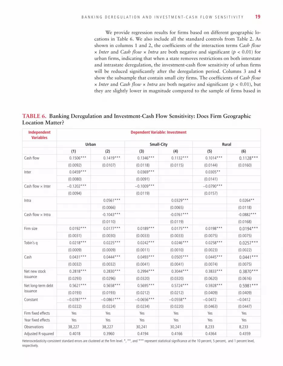
We provide regression results for firms based on different geographic lo-cations in Table 6. We also include all the standard controls from Table 2. As shown in columns 1 and 2, the coefficients of the interaction terms Cash flow × Inter and Cash flow × Intra are both negative and significant (p < 0.01) for urban firms, indicating that when a state removes restrictions on both interstate and intrastate deregulation, the investment-cash flow sensitivity of urban firms will be reduced significantly after the deregulation period. Columns 3 and 4 show the subsample that contain small city firms. The coefficients of Cash flow × Inter and Cash flow × Intra are both negative and significant (p < 0.01), but they are slightly lower in magnitude compared to the sample of firms based in
TABLE 6. Banking Deregulation and Investment-Cash Flow Sensitivity: Does Firm Geographic Location Matter?
Independent Variables
Dependent Variable: Investment
Urban Small-City Rural
(1) (2) (3) (4) (5) (6)
Cash flow 0.1506*** 0.1419*** 0.1346*** 0.1132*** 0.1014*** 0.1128***
(0.0092) (0.0107) (0.0118) (0.0115) (0.0144) (0.0160)
Inter 0.0459*** 0.0369*** 0.0305**
(0.0080) (0.0091) (0.0141)
Cash flow × Inter −0.1202*** −0.1009*** −0.0790***
(0.0094) (0.0119) (0.0157)
Intra 0.0561*** 0.0329*** 0.0264**
(0.0066) (0.0065) (0.0118)
Cash flow × Intra -0.1043*** -0.0761*** -0.0882***
(0.0110) (0.0119) (0.0168)
Firm size 0.0192*** 0.0177*** 0.0189*** 0.0175*** 0.0198*** 0.0194***
(0.0031) (0.0030) (0.0033) (0.0033) (0.0075) (0.0075)
Tobin’s q 0.0218*** 0.0225*** 0.0242*** 0.0246*** 0.0258*** 0.0257***
(0.0009) (0.0009) (0.0011) (0.0010) (0.0023) (0.0022)
Cash 0.0431*** 0.0444*** 0.0493*** 0.0505*** 0.0445*** 0.0441***
(0.0032) (0.0032) (0.0041) (0.0041) (0.0074) (0.0075)
Net new stock issuance
0.2818*** 0.2830*** 0.2994*** 0.3044*** 0.3833*** 0.3870***
(0.0293) (0.0296) (0.0320) (0.0320) (0.0620) (0.0616)
Net long-term debt issuance
0.5621*** 0.5658*** 0.5695*** 0.5724*** 0.5928*** 0.5981***
(0.0193) (0.0193) (0.0212) (0.0212) (0.0409) (0.0409)
Constant −0.0787*** −0.0861*** −0.0656*** −0.0558** −0.0472 −0.0412
(0.0222) (0.0224) (0.0234) (0.0220) (0.0463) (0.0447)
Firm fixed effects Yes Yes Yes Yes Yes Yes
Year fixed effects Yes Yes Yes Yes Yes Yes
Observations 38,227 38,227 30,241 30,241 8,233 8,233
Adjusted R-squared 0.4018 0.3960 0.4194 0.4166 0.4364 0.4359
Heteroscedasticity-consistent standard errors are clustered at the firm level. *, **, and *** represent statistical significance at the 10 percent, 5 percent, and 1 percent level, respectively.

20 R E V I E W O F B U S I N E S S
urban areas. Columns 5 and 6 report the results for the subsample of rural firms only, and we find a similar reduction pattern on investment-cash flow sensitivity after banking deregulation. However, the magnitudes of both interaction terms are much weaker for firms based in rural areas compared to firms based in small-city and urban areas. Our results reveal that banking deregulation presents more significant effects on urban-based firms than small-city- and rural-based firms. This provides consistent findings with existing literature that firms in ru-ral locations have more difficulty obtaining information from the capital market than firms based in large metropolitan areas; therefore, rural firms are likely to be less liquid than their urban counterparts (Loughran and Schultz 2005). As a result, when bank competition is intensified due to the removal of expansion barriers in the banking industry, firms based in urban areas with superior infor-mation can access the credit market easier than firms in rural areas, and conse-quently, those urban firms experience a larger decrease in investment-cash flow sensitivity than rural firms.
Financial Constraint and Hedging Needs
Acharya, Almeida, and Campello (2007) indicate that liquid assets are more valuable when firms face higher costs from external financing and higher uncer-tainty of financing profitable projects (hedging needs). Constrained firms with high hedging requirements normally place high marginal value on cash and rely heavily on liquid assets, and thereby have a strong tendency to save cash out of cash flow. Considering that financially constrained firms can behave quite dif-ferently given different hedging needs, we investigate how banking deregulation affects financially constrained firms’ investment-cash flow sensitivity when these firms face different hedging needs.
To proxy a firm’s financial constraint, we firstly measure KZ index (Kaplan and Zingales, 1997, Lamont et al., 2001)3. We categorize a firm as a constrained (unconstrained) firm if the firm is in the top (bottom) one-third of the index in a given year. We then partition our sample accordingly and keep constrained firms only for our empirical tests.
Following Acharya, Almeida, and Campello (2007), we construct two measures to gauge hedging needs. The first measure calculates the correlation between a firm’s cash flow from operations and its industry-level median R&D expenditures (classified by 3-digit SIC). This measure links R&D expenditures to growth opportunities. We calculate the correlation to assess whether a firm’s availability of internal funds is correlated with its investment demand. We define a firm with high hedging needs (r < −0.2) and low hedging needs (r > 0.2), then partition our data sample into two different subsamples that show different de-gree of hedging needs. We construct the second measure as follows: we compute the industry-median, three-years-ahead sales growth rate at the 3-digit SIC for each firm-year observation. Then we calculate the correlation between this mea-sure of industry-level demand and the firm’s cash flow. Using similar procedures,
3In an unreported table, we also follow Hadlock and Pierce (2010) to generate the second measure of financial constraint and denote it as SA index. We follow similar process to keep constrained firms only by categorizing a firm as a constrained (unconstrained) firm if the firm is in the top (bot-tom) one-third of the SA index in a given year, and then test for the financially constrained firms with different hedging needs. We find consistent results for both measures of financial constraints.

B A N K I N G D E R E G U L A T I O N A N D I N V E S T M E N T - C A S H F L O W S E N S I T I V I T Y 21
we partition our main data sample into subsamples with high hedging needs and low hedging needs, using the cutoffs of −0.2 and 0.2.4
We report our results for financially constrained firms with different hedg-ing needs in Table 7. We regress investment on interstate and intrastate deregu-lation, along with a set of control variables, while controlling for firm and year-fixed effects. We separate each constrained sample into firms with high hedging
TABLE 7. Banking Deregulation and Investment-Cash Flow Sensitivity: Hedging Needs for Financially Constrained Firms
Independent Variables Dependent Variable: Investment
High Hedging Needs: Sorted by Industry Sales Growth
Low Hedging Needs: Sorted by Industry Sales Growth
High Hedging Needs: Sorted by Industry R&D
Low Hedging Needs: Sorted by Industry R&D
(1) (2) (3) (4) (5) (6) (7) (8)
Cash flow 0.0602 0.0474 0.1455*** 0.1277*** 0.0914*** 0.0585* 0.1580*** 0.1497***
(0.0378) (0.0449) (0.0179) (0.0188) (0.0283) (0.0331) (0.0153) (0.0166)
Inter 0.0248 0.0236* 0.0236 0.0273***
(0.0227) (0.0127) (0.0262) (0.0096)
Cash flow × Inter
−0.0338 −0.1039*** −0.0676** −0.1129***
(0.0393) (0.0188) (0.0285) (0.0162)
Intra 0.0088 0.0267*** 0.0498*** 0.0327***
(0.0186) (0.0097) (0.0179) (0.0070)
Cash flow × Intra
−0.0186 −0.0818*** −0.0308 −0.0984***
(0.0457) (0.0196) (0.0335) (0.0175)
Firm size 0.0309*** 0.0309*** 0.0211*** 0.0206*** 0.0424*** 0.0419*** 0.0221*** 0.0214***
(0.0087) (0.0088) (0.0050) (0.0049) (0.0095) (0.0097) (0.0032) (0.0032)
Tobin’s q 0.0282*** 0.0283*** 0.0362*** 0.0368*** 0.0328*** 0.0335*** 0.0367*** 0.0371***
(0.0039) (0.0039) (0.0025) (0.0025) (0.0034) (0.0034) (0.0018) (0.0018)
Cash 0.0836*** 0.0841*** 0.0756*** 0.0800*** 0.0572*** 0.0602*** 0.1052*** 0.1086***
(0.0204) (0.0208) (0.0116) (0.0117) (0.0130) (0.0131) (0.0096) (0.0095)
Net new stock issuance
0.2560*** 0.2518*** 0.1814*** 0.1795*** 0.0260 0.0259 0.2865*** 0.2851***
(0.0769) (0.0770) (0.0571) (0.0568) (0.1047) (0.1047) (0.0426) (0.0426)
Net long- term debt issuance
0.4630*** 0.4636*** 0.5426*** 0.5461*** 0.4682*** 0.4676*** 0.5383*** 0.5427***
(0.0453) (0.0451) (0.0283) (0.0283) (0.0548) (0.0550) (0.0201) (0.0201)
Constant −0.0969 −0.0801 −0.0905*** −0.0947*** −0.1963*** −0.2262*** −0.0792*** −0.0836***
(0.0590) (0.0599) (0.0335) (0.0337) (0.0639) (0.0605) (0.0230) (0.0224)
Firm fixed effects
Yes Yes Yes Yes Yes Yes Yes Yes
Year fixed effects
Yes Yes Yes Yes Yes Yes Yes Yes
Observations 4,507 4,507 12,863 12,863 3,724 3,724 15,886 15,886
Adjusted R-squared
0.4617 0.4609 0.4694 0.4670 0.4000 0.3992 0.4852 0.4833
Heteroscedasticity-consistent standard errors are clustered at the firm level. *, **, and *** represent statistical significance at the 10 percent, 5 percent, and 1 percent level, respectively.
4We also apply various cut-off values to ensure that our findings are consistent.

22 R E V I E W O F B U S I N E S S
needs and low hedging needs, sorted by industry sales growth and industry R&D. Columns 1 to 4 report results for financially constrained firms with dif-ferent hedging needs sorted by industry sales growth, whereas columns 5 and 8 report results for constrained firms with hedging needs sorted by industry R&D.
We find that banking deregulation significantly reduces investment-cash flow sensitivity for financially constrained firms that have low hedging needs. The coefficient estimates of the interaction terms between banking deregulation and cash flow are insignificant for constrained firms with high hedging needs. Our findings indicate that financially constrained firms with low hedging needs are very sensitive to the external financial environment, and they benefit greatly from bank deregulation and enjoy favorable financing terms. These findings re-veal that the effects of banking deregulation on investment-cash flow sensitivity is more pronounced for constrained firms with low hedging needs than for con-strained firms with high hedging needs.
Robustness Checks: Subsample Analysis and Alternative Measures for Investment
Our first concern is about sampling issues. Most studies on investment-cash flow sensitivity mainly focus on manufacturing firms (Kaplan and Zingales 1997; Almeida et al. 2004; Chen and Chen 2012). In this section, following a typical sample used in the investment-cash flow literature (Brown and Petersen 2009), we examine publicly traded manufacturing firms based on two-digit SIC codes 20 to 39 with coverage in the Compustat database from 1970 to 2006 and test for the subsample of non-manufacturing firms simultaneously.
Another concern is about the alternative measurements of investment. According to Brown and Petersen (2009), firms can undertake different types of investments. In practice, firms allocate cash flow and external funds across multiple investments, which mainly refer to physical investment and R&D in-vestment. The U.S. economy has experienced a major transformation from tra-ditional manufacturing industries to high-tech and service-oriented industries, and such transformation is accompanied by a change from tangible to intangible capital; therefore the importance of R&D intensity has risen dramatically for U.S. firms (Brown and Petersen 2009; Brown et al. 2009). Consistent with most of the existing literature, we focus on physical investment in our previous tests. To test whether our baseline results still hold across different types of invest-ment, we use “broad” investment measures as alternative measurements of in-vestment in the regressions. Specifically, we follow Brown and Petersen (2009), Moshirian et al. (2017), and Jiang et al. (2020) to measure total investment as physical investment plus R&D scaled by PPE and total assets, respectively.
We evaluate the first concern and report our results for the subsample anal-ysis in Table 8. Columns 1 and 2 report the results for manufacturing firms only, whereas columns 3 and 4 report the results for non-manufacturing firms only. We find consistent results that bank branching deregulation and interstate de-regulation both significantly reduce physical investment-cash flow sensitivity for both subsampling firms.

B A N K I N G D E R E G U L A T I O N A N D I N V E S T M E N T - C A S H F L O W S E N S I T I V I T Y 23
TABLE 8. Robustness Check: Subsample Analysis
Independent Variables Dependent Variable: Investment
Manufacturing Firms Non-Manufacturing Firms
(1) (2) (3) (4)
Cash flow 0.1312*** 0.1121*** 0.1451*** 0.1394***
(0.0087) (0.0097) (0.0111) (0.0119)
Inter 0.0292*** 0.0459***
(0.0066) (0.0093)
Cash flow × Inter −0.0985*** −0.1171***
(0.0089) (0.0113)
Intra 0.0355*** 0.0491***
(0.0056) (0.0075)
Cash flow × Intra −0.0730*** −0.1079***
(0.0101) (0.0122)
Firm size 0.0167*** 0.0147*** 0.0243*** 0.0230***
(0.0029) (0.0030) (0.0033) (0.0033)
Tobin’s q 0.0222*** 0.0227*** 0.0254*** 0.0258***
(0.0008) (0.0008) (0.0010) (0.0011)
Cash 0.0436*** 0.0444*** 0.0476*** 0.0489***
(0.0030) (0.0031) (0.0040) (0.0040)
Net new stock issuance
0.2715*** 0.2776*** 0.3253*** 0.3256***
(0.0272) (0.0274) (0.0313) (0.0313)
Net long-term debt issuance
0.5232*** 0.5262*** 0.5945*** 0.5988***
(0.0187) (0.0187) (0.0195) (0.0195)
Constant −0.0658*** −0.0652*** −0.0869*** −0.0858***
(0.0202) (0.0200) (0.0248) (0.0245)
Firm fixed effects Yes Yes Yes Yes
Year fixed effects Yes Yes Yes Yes
Observations 39,014 39,014 40,343 40,343
Adjusted R-squared 0.4005 0.3954 0.4248 0.4222
Heteroscedasticity-consistent standard errors are clustered at the firm level. *, **, and *** represent statistical significance at the 10 percent, 5 percent, and 1 percent level, respectively.
We report our results for the alternative measures of investment in Table 9, columns 1 and 2 show the results when we replace dependent variable as total investment, scaled by PPE, whereas columns 3 and 4 report the results for total investment scaled by total assets. Our results indicate that the coefficients of the interaction terms Cash flow × Inter and Cash flow × Intra are both negative and significant at the 1 percent level during the main sample period if we apply total investment as the alternative measure of investment. By including R&D into our investment measure, our main results do not change in a material way compared to the results in Table 2.

24 R E V I E W O F B U S I N E S S
TABLE 9. Robustness Check: Alternative Measures of Investment
Independent Variables
Dependent Variable: Alternative Measures of Investment
Investment-R&D-Scaled by
PPE
Investment-R&D-Scaled by
PPE
Investment-R&D-Scaled by
Assets
Investment-R&D-Scaled by
Assets
(1) (2) (3) (4)
Cash flow 0.1455*** 0.1383*** 0.0006 0.0051***
(0.0091) (0.0101) (0.0017) (0.0018)
Inter 0.0445*** 0.0071***
(0.0068) (0.0018)
Cash flow × Inter −0.1240*** −0.0077***
(0.0106) (0.0018)
Intra 0.0430*** 0.0056***
(0.0056) (0.0015)
Cash flow × Intra −0.1104*** −0.0123***
(0.0111) (0.0019)
Firm size 0.0110*** 0.0093*** −0.0005 −0.0005
(0.0030) (0.0030) (0.0009) (0.0009)
Tobin’s q 0.0292*** 0.0298*** 0.0041*** 0.0041***
(0.0011) (0.0011) (0.0002) (0.0002)
Cash 0.0905*** 0.0918*** −0.0009 −0.0009
(0.0070) (0.0070) (0.0006) (0.0006)
Net new stock issuance
0.3515*** 0.3542*** 0.0573*** 0.0570***
(0.0302) (0.0303) (0.0077) (0.0077)
Net long-term debt issuance
0.6230*** 0.6255*** 0.1501*** 0.1502***
(0.0168) (0.0169) (0.0049) (0.0049)
Constant 0.0611*** 0.0680*** 0.0640*** 0.0655***
(0.0215) (0.0216) (0.0058) (0.0057)
Firm fixed effects Yes Yes Yes Yes
Year fixed effects Yes Yes Yes Yes
Observations 61,565 61,565 75,902 75,902
Adjusted R-squared 0.7045 0.7032 0.6214 0.6215
Heteroscedasticity-consistent standard errors are clustered at the firm level. *, **, and *** represent statistical significance at the 10 percent, 5 percent, and 1 percent level, respectively.
CONCLUSIONIn this study, we investigate the effects of bank deregulation reforms on invest-ment-cash flow sensitivity over the period 1970 to 2006 and provide empirical evidence to indicate that there exists a material drop in the firm’s sensitivity of investment to cash flow following the deregulation of restrictions on interstate and intrastate banking. Our findings are robust after testing different measures of key variables and using the GMM method to control measurement error in

B A N K I N G D E R E G U L A T I O N A N D I N V E S T M E N T - C A S H F L O W S E N S I T I V I T Y 25
Tobin’s q (Erickson and Whited 2012). We also test the dynamic effects of bank-ing deregulation on investment-cash flow sensitivity and find that the effects are significant only after bank deregulation years. In addition, we investigate how and to what extent banking deregulation affects investment-cash flow sensitivity among firms based in different geographic locations. We find that the effects are more pronounced among urban firms than among small-city and rural firms. Moreover, we show that the negative relation between banking deregulation and investment-cash flow sensitivity is driven by financially constrained firms, especially by constrained firms with low hedging needs. The findings are consis-tent with our prediction that banking deregulation changes improve competition among banks and promote the use of bank loans as external financing, and thus reduce sensitivity of investment to internally generated cash flows.
The above findings have important implications for the existing literature on the role of financial market development for corporate investment. By mak-ing bank loans a more available external source of financing to firms after de-regulation, competition-enhancing deregulatory changes reduce the sensitivity of investment to cash flows. Moreover, this paper attempts to fill an important gap in the existing literature by explaining banking deregulation as a possible deter-minant that explains the existence and downward trajectory of investment-cash flow sensitivity during the past several decades. The sharply declining invest-ment-cash flow sensitivity during the banking deregulation period is also consis-tent with the findings from Brown et al. (2009) that external financing becomes a better substitute for internal funds. Overall, our findings have obvious and important implications on the decisions of corporations and policy makers.
ReferencesAcharya, Viral V., Heitor Almeida, and Murillo Campello. 2007. “Is Cash Negative
Debt? A Hedging Perspective on Corporate Financial Policies.” Journal of Financial Intermediation 16, no. 4, 515–54.
Agca, Senay, and Abon Mozumdar. 2008. “The Impact of Capital Market Imperfections on Investment–Cash Flow Sensitivity.” Journal of Banking & Finance 32, no. 2, 207–16.
Akhigbe, Aigbe, and Ann Marie Whyte. 2003. “Changes in Market Assessments of Bank Risk Following the Riegle-Neal Act of 1994.” Journal of Banking & Finance 27, no. 1, 87–102.
Allayannis, George, and Abon Mozumdar. 2004. “The Impact of Negative Cash Flow and Influential Observations on Investment—Cash Flow Sensitivity Estimates.” Journal of Banking & Finance 28, no. 5, 901–30.
Almeida, Heitor, and Murillo Campello. 2007. “Financial Constraints, Asset Tangibility, and Corporate Investment.” The Review of Financial Studies 20, no. 5, 1429–60.
Almeida, Heitor, Murillo Campello, and Michael S. Weisbach. 2004. “The Cash Flow Sensitivity of Cash.” The Journal of Finance 59, no. 4, 1777–804.
Alti, Aydog–an. 2003. “How Sensitive Is Investment to Cash Flow When Financing Is Frictionless?” The Journal of Finance 58, no. 2, 707–22.
Amiti, Mary, and David E. Weinstein. 2018. “How Much Do Idiosyncratic Bank Shocks Affect Investment? Evidence from Matched Bank-Firm Loan Data.” Journal of Political Economy 126, no. 2, 525–87.
Ascioglu, Asli, Shantaram P. Hegde, and John B. McDermott. 2008. “Information Asym-metry and Investment–Cash Flow Sensitivity.” Journal of Banking & Finance 32, no. 6, 1036–48.

26 R E V I E W O F B U S I N E S S
Attig, Najah, Sean Cleary, Sadok El Ghoul, and Omrane Guedhami. 2012. “Institutional Investment Horizon and Investment–Cash Flow Sensitivity.” Journal of Banking & Finance 36, no. 4, 1164–80.
Beck, Thorsten, Ross Levine, and Alexey Levkov. 2010. “Big Bad Banks? The Winners and Losers from Bank Deregulation in the United States.” The Journal of Finance 65, no. 5, 1637–67.
Bertrand, Marianne, and Sendhil Mullainathan. 2003. “Enjoying the Quiet Life? Corpo-rate Governance and Managerial Preferences.” Journal of political Economy 111, no. 5, 1043–75.
Black, Sandra E., and Philip E. Strahan. 2002. “Entrepreneurship and Bank Credit Avail-ability.” The Journal of Finance 57, no. 6, 2807–33.
Bond, Stephen, and Costas Meghir. 1994. “Financial Constraints and Company Invest-ment.” Fiscal Studies 15, no. 2, 1–18.
Boyd, John H., and Edward C. Prescott. 1986. “Financial Intermediary-Coalitions.” Journal of Economic Theory 38, no. 2, 211–32.
Brown, James R., Steven M. Fazzari, and Bruce C. Petersen. 2009. “Financing Innova-tion and Growth: Cash Flow, External Equity, and the 1990s R&D Boom.” The Journal of Finance 64, no. 1, 151–85.
Brown, James R., and Bruce C. Petersen. 2009. “Why Has the Investment-Cash Flow Sensitivity Declined so Sharply? Rising R&D and Equity Market Developments.” Journal of Banking & Finance 33, no. 5, 971–84.
Calomiris, Charles W., and Charles W. Calomiris. 2000. U.S. Bank Deregulation in His-torical Perspective: Cambridge University Press.
Chava, Sudheer, Alexander Oettl, Ajay Subramanian, and Krishnamurthy V. Subramani-an. 2013. “Banking Deregulation and Innovation.” Journal of Financial Economics 109, no. 3, 759–74.
Chen, Huafeng Jason, and Shaojun Jenny Chen. 2012. “Investment-Cash Flow Sensitiv-ity Cannot Be a Good Measure of Financial Constraints: Evidence from the Time Series.” Journal of Financial Economics 103, no. 2, 393–410.
Chowdhury, Jaideep, Raman Kumar, and Dilip Shome. 2016. “Investment–Cash Flow Sensitivity Under Changing Information Asymmetry.” Journal of Banking & Fi-nance 62, 28–40.
Cleary, Sean. 1999. “The Relationship Between Firm Investment and Financial Status.” The Journal of Finance 54, no. 2, 673–92.
Cleary, Sean, Paul Povel, and Michael Raith. 2007. “The U-Shaped Investment Curve: Theory and Evidence.” Journal of Financial and Quantitative Analysis 42, no. 1, 1–39.
Cornaggia, Jess, Yifei Mao, Xuan Tian, and Brian Wolfe. 2015. “Does Banking Com-petition Affect Innovation?” Journal of Financial Economics 115, no. 1, 189–209.
Coval, Joshua D., and Tobias J. Moskowitz. 1999. “Home Bias at Home: Local Equity Preference in Domestic Portfolios.” The Journal of Finance 54, no. 6, 2045–73.
Degryse, Hans, and Steven Ongena. 2005. “Distance, Lending Relationships, and Com-petition.” The Journal of Finance 60, no. 1, 231–66.
Degryse, Hans, and Steven Ongena. 2008. “Competition and Regulation in the Bank-ing Sector: A Review of the Empirical Evidence on the Sources of Bank Rents.” In Handbook of Financial Intermediation and Banking, edited by Arnoud W. A. Boots, 483–554, Amsterdam: Elsevier.
Derouiche, Imen, Majdi Hassan, and Sarra Amdouni. 2018. “Ownership Structure and Investment-Cash Flow Sensitivity.” Journal of Management & Governance 22, no. 1, 31–54.
Diamond, Douglas W. 1984. “Financial Intermediation and Delegated Monitoring.” The Review of Economic Studies 51, no. 3, 393–414.
Diamond, Douglas W. 1991. “Monitoring and Reputation: The Choice Between Bank Loans and Directly Placed Debt.” Journal of Political Economy 99, no. 4, 689–721.
Erickson, Timothy, and Toni M. Whited. 2000. “Measurement Error and the Relation-ship Between Investment and q.” Journal of Political Economy 108, no. 5, 1027–57.

B A N K I N G D E R E G U L A T I O N A N D I N V E S T M E N T - C A S H F L O W S E N S I T I V I T Y 27
Erickson, Timothy, and Toni M. Whited. 2002. “Two-Step GMM Estimation of the Errors-in-Variables Model Using High-Order Moments.” Econometric Theory 18, no. 3, 776–99.
Erickson, Timothy, and Toni M. Whited. 2012. “Treating Measurement Error in Tobin’s q.” The Review of Financial Studies 25, no. 4, 1286–329.
Fazzari, Steven M., R. Glenn Hubbard, and Bruce C. Petersen. 2000. “Investment-Cash Flow Sensitivities Are Useful: A Comment on Kaplan and Zingales.” The Quarterly Journal of Economics 115, no. 2, 695–705.
Fazzari, Steven M., R. Glenn Hubbard, Bruce C. Petersen, Alan S. Blinder, and James M. Poterba. 1988. “Financing Constraints and Corporate Investment.” Brookings Papers on Economic Activity 1988, no. 1, 141–206.
Gatev, Evan, and Philip E. Strahan. 2006. “Banks’ Advantage in Hedging Liquidity Risk: Theory and Evidence from the Commercial Paper Market.” The Journal of Finance 61, no. 2, 867–92.
Geary, R. C. 1942. “The Estimation of Many Parameters.” Journal of the Royal Statisti-cal Society 105, no. 3, 213–7.
Gilchrist, Simon, and Charles P. Himmelberg. 1995. “Evidence on the Role of Cash Flow for Investment.” Journal of Monetary Economics 36, no. 3, 541–72.
Gomes, Joao F. 2001. “Financing Investment.” American Economic Review 91, no. 5, 1263–85.
Hadlock, Charles J., and Joshua R. Pierce. 2010. “New Evidence on Measuring Finan-cial Constraints: Moving Beyond the KZ Index.” The Review of Financial Studies 23, no. 5, 1909–40.
Hauswald, Robert, and Robert Marquez. 2003. “Information Technology and Financial Services Competition.” The Review of Financial Studies 16, no. 3, 921–48.
Hauswald, Robert, and Robert Marquez. 2006. “Competition and Strategic Informa-tion Acquisition in Credit Markets.” The Review of Financial Studies 19, no. 3, 967–1000.
Hubbard, R. Glenn. 1998. “Capital Market Imperfections and Investment.” Journal of Economic Literature 36, 193–225.
Huberman, Gur. 2001. “Familiarity Breeds Investment.” The Review of Financial Stud-ies 14, no. 3, 659–80.
Hughes, Joseph P., William Lang, Loretta J. Mester, and Choon-Geol Moon. 1996. “Ef-ficient Banking Under Interstate Branching.” Journal of Money, Credit, and Banking 28, no. 4, 1045–71.
Jayaratne, Jith, and Philip E. Strahan. 1996. “The Finance-Growth Nexus: Evidence from Bank Branch Deregulation.” The Quarterly Journal of Economics 111, no. 3, 639–70.
Jiang, Tianjiao, Ross Levine, Chen Lin, and Lai Wei. 2020. “Bank Deregulation and Corporate Risk.” Journal of Corporate Finance 60, article 101520.
Kaplan, Steven N., and Luigi Zingales. 1997. “Do Investment-Cash Flow Sensitivities Provide Useful Measures of Financing Constraints?” The Quarterly Journal of Eco-nomics 112, no. 1, 169–215.
Kaplan, Steven N., and Luigi Zingales. 2000. “Investment-Cash Flow Sensitivities Are Not Valid Measures of Financing Constraints.” The Quarterly Journal of Econom-ics 115, no. 2, 707–12.
Kashyap, Anil K., Raghuram Rajan, and Jeremy C. Stein. 2002. “Banks as Liquidity Providers: An Explanation for the Coexistence of Lending and Deposit-Taking.” The Journal of Finance 57, no. 1, 33–73.
Kerr, William R., and Ramana Nanda. 2009. “Democratizing Entry: Banking Deregula-tions, Financing Constraints, and Entrepreneurship.” Journal of Financial Econom-ics 94, no. 1, 124–49.
Koetter, Michael, James W. Kolari, and Laura Spierdijk. 2012. “Enjoying the Quiet Life Under Deregulation? Evidence from Adjusted Lerner Indices for U.S. Banks.” Re-view of Economics and Statistics 94, no. 2, 462–80.

28 R E V I E W O F B U S I N E S S
Kroszner, Randall S., and Phillip E. Strahan. 1999. “What Drives Deregulation? Eco-nomics and Politics of the Relaxation of Banking Branching Restrictions.” Quarter-ly Journal of Economics 104, 1437–67.
Lamont, Owen, Christopher Polk, and Jesús Saaá-Requejo. 2001. “Financial Constraints and Stock Returns.” The Review of Financial Studies 14, no. 2, 529–54.
Lerner, Josh. 1995. “Venture Capitalists and the Oversight of Private Firms.” The Jour-nal of Finance 50, no. 1, 301–18.
Lewellen, Jonathan, and Katharina Lewellen. 2016. “Investment and Cash Flow: New Evi-dence.” Journal of Financial and Quantitative Analysis 51, no. 4, 1135–64. doi: 10.1017/ S002210901600065X.
Loughran, Tim, and Paul Schultz. 2005. “Liquidity: Urban Versus Rural Firms.” Journal of Financial Economics 78, no. 2, 341–74.
Marquez, Robert. 2002. “Competition, Adverse Selection, and Information Dispersion in the Banking Industry.” The Review of Financial Studies 15, no. 3, 901–26.
Modigliani, Franco, and Merton H. Miller. 1958. “The Cost of Capital, Corporation Fi-nance, and the Theory of Investment.” American Economic Review 48, no. 3, 261–97.
Moshirian, Fariborz, Vikram Nanda, Alexander Vadilyev, and Bohui Zhang. 2017. “What Drives Investment–Cash Flow Sensitivity Around the World? An Asset Tan-gibility Perspective.” Journal of Banking & Finance 77, 1–17.
Moyen, Nathalie. 2004. “Investment–Cash Flow Sensitivities: Constrained versus Un-constrained Firms.” The Journal of Finance 59, no. 5, 2061–92.
Myers, Stewart C., and Nicholas S. Majluf. 1984. Corporate Financing and Investment Decisions When Firms Have Information That Investors Do Not Have. Working paper 1396. Cambridge, MA: National Bureau of Economic Research.
Opler, Tim, Lee Pinkowitz, René Stulz, and Rohan Williamson. 1999. “The Determi-nants and Implications of Corporate Cash Holdings.” Journal of Financial Econom-ics 52, no. 1, 3–46.
Petersen, Mitchell A., and Raghuram G. Rajan. 2002. “Does Distance Still Matter? The Information Revolution in Small Business Lending.” The Journal of Finance 57, no. 6, 2533–70.
Poterba, James M. 1988. “Comment on “Financing Constraints and Corporate Invest-ment.” Brookings Papers on Economic Activity 1, 200–6.
Rajan, Raghuram G., and Luigi Zingales. 1998. “Financial Dependence and Growth.” American Economic Review 88, no. 3, 559–86.
Ramakrishnan, Ram T. S., and Anjan V. Thakor. 1984. “Information Reliability and a The-ory of Financial Intermediation.” The Review of Economic Studies 51, no. 3, 415–32.
Rauh, Joshua D. 2006. “Investment and Financing Constraints: Evidence from the Fund-ing of Corporate Pension Plans.” The Journal of Finance 61, no. 1, 33–71.
Rice, Tara, and Philip E. Strahan. 2010. “Does Credit Competition Affect Small-Firm Finance?” The Journal of Finance 65, no. 3, 861–89.
Stiroh, Kevin J., and Philip E. Strahan. 2003. “Competitive Dynamics of Deregulation: Ev-idence from U.S. Banking.” Journal of Money, Credit, and Banking 35, no. 5, 801–28.
Strahan, Philip E. 2003. “The Real Effects of U.S. Banking Deregulation.” Review- Federal Reserve Bank of Saint Louis 85, no. 4, 111–28.
Zarutskie, Rebecca. 2006. “Evidence on the Effects of Bank Competition on Firm Bor-rowing and Investment.” Journal of Financial Economics 81, no. 3, 503–37.

B A N K I N G D E R E G U L A T I O N A N D I N V E S T M E N T - C A S H F L O W S E N S I T I V I T Y 29
APPENDIX 1: Variable Definition
Variable Description Source
Inter A dummy variable that equals 1 in the year and thereafter when the state adopts the interstate agreement permitting the bank expansion and equals 0 otherwise.
Intra A dummy variable that equals 1 in the year that intrastate banking was permitted by means of mergers and acquisitions and thereafter and equals 0 in all years until the deregulation.
Investment Firm’s capital expenditures to the beginning-of-period stock of firm capital, which is defined as net property, plant, and equipment (PPE).
Compustat
Investment-R&D-scaled by PPE Total investment as physical investment plus R&D, scaled by PPE. Compustat
Investment-R&D-scaled by assets Total investment as physical investment plus R&D, scaled by total assets. Compustat
Cash flow Operating cash flow scaled by total assets. Compustat
Firm size The natural logarithm of total assets. Compustat
Tobin’s q Market value of assets minus the difference between the book value of assets and net PPE, scaled by net PPE.
Compustat
Cash Firm’s cash and short-term investments over the beginning period capital. Compustat
Net new stock issuance Firm’s net new funds from stock issues over capital. Compustat
Net long term debt issuance Net new long-term debt over beginning period capital. Compustat
External financial dependence An industry-level indicator to measure the degree to which firms in that industry depend on external funds. External financial dependence at firm level is measured as capital expenditures minus cash flows from operations divided by capital expenditures.
Compustat
Firm geographic locations A firm is defined as an urban firm if a company’s headquarters is 30 miles or less from the center of any of the largest metropolitan statistical areas (MSAs) of the United States according to the 2000 census. A firm is defined as a rural firm if its headquarters is 100 miles or more from the center of any of the 49 U.S. MSAs. A firm is defined as a small-city company if the headquarters is more than 30 miles but less than 100 miles from the center of any of the 49 U.S. MSAs.
Compustat
Financial constraint Financial constraint measures, including the KZ index, which is calculated as 0.283 × capital − 1.002 × (cash flow/capital) + 3.319 × (debt/capital) − 39.368 × (annual dividends payments/capital) − 1.315 × (cash/capital).
Compustat
Hedging needs Measures to gauge firms’ hedging needs. The first measure is calculated as the correlation between a firm’s cash flow from operations and its industry-level median R&D expenditures; the second measure is calculated as the correlation between the industry-median, three-years-ahead sales growth rate and the firm’s cash flow. We define a firm with high hedging needs (r < −0.2) and low hedging needs (r > 0.2).
Compustat

30 R E V I E W O F B U S I N E S S
APPENDIX 2: Banking Deregulation Timing Across States in the United States
State Deregulation Timing
Interstate Intrastate
Montana 1993 1990
Nebraska 1990 1985
Nevada 1985 1960
New Hampshire 1987 1987
New Jersey 1986 1977
New Mexico 1989 1991
New York 1982 1976
North Carolina 1985 1960
North Dakota 1991 1987
Ohio 1985 1979
Oklahoma 1987 1988
Oregon 1986 1985
Pennsylvania 1986 1982
Rhode Island 1984 1960
South Carolina 1986 1960
South Dakota 1988 1960
Tennessee 1985 1985
Texas 1987 1988
Utah 1984 1981
Vermont 1988 1970
Virginia 1985 1978
Washington 1987 1985
West Virginia 1988 1987
Wisconsin 1987 1990
Wyoming 1987 1988
State Deregulation Timing
Interstate Intrastate
Alabama 1987 1981
Alaska 1982 1960
Arizona 1986 1960
Arkansas 1989 1994
California 1987 1960
Colorado 1988 1991
Connecticut 1983 1980
Delaware 1988 1960
Florida 1985 1988
Georgia 1985 1983
Hawaii 1997 1986
Idaho 1985 1960
Illinois 1986 1988
Indiana 1986 1989
Iowa 1991 1999
Kansas 1992 1987
Kentucky 1984 1990
Louisiana 1987 1988
Maine 1978 1975
Maryland 1985 1960
Massachusetts 1983 1984
Michigan 1986 1987
Minnesota 1986 1993
Mississippi 1988 1986
Missouri 1986 1990

B A N K I N G D E R E G U L A T I O N A N D I N V E S T M E N T - C A S H F L O W S E N S I T I V I T Y 31
APPENDIX 3: T-test Between the Treated Group (When the Deregulation Dummy Variables Equal to 1) and Control Group (When Deregulation Dummy Variables Equal 0)
Panel A: Inter-State Deregulation
Variables Mean Difference t-Statistics
Treated Group Control Group Treated-Control
Investment 0.2268 0.2635 0.0367*** 24.8573
Cash flow 0.1566 0.3205 0.1639*** 30.6754
Firm size 5.0602 4.5166 −0.5437*** −37.5367
Tobin’s q 2.7288 1.8383 −0.8905*** −58.2396
Cash 0.5968 0.3206 −0.2762*** −35.8077
Net new stock issuance 0.0054 0.0056 0.0003 0.7435
Net long-term debt issuance 0.0017 0.0083 0.0066*** 11.0068
Panel B: Intra-State Deregulation
Variables Mean Difference t-Statistics
Treated Group Control Group Treated-Control
Investment 0.2357 0.2559 0.0202*** 12.7378
Cash flow 0.1852 0.3127 0.1275*** 22.165
Firm size 4.9514 4.5756 −0.3758*** −24.0395
Tobin’s q 2.5983 1.8223 −0.7760*** −46.9254
Cash 0.5585 0.3104 −0.2482*** −29.8927
Net new stock issuance 0.0057 0.0049 −0.0008** −2.0439
Net long-term debt issuance 0.0028 0.0081 0.0053*** 8.2974
*, **, and *** represent statistical significance at the 10 percent, 5 percent, and 1 percent level, respectively.

32
Omer Faruk Derindag, PhD, Inonu University, [email protected]
Ozgur Demirtas, PhD, Kayseri University, [email protected]
Ali Bayram, PhD, Samsun University, [email protected]
The Leader-Member Exchange (LMX) Influence at Organizations: The Moderating Role of Person-Organization (P-O) FitOmer Faruk Derindag
Ozgur Demirtas
Ali Bayram
AbstractMotivation: In recent years, leader-member exchange (LMX) has become a widely utilized concept in business management and leadership literature. Ad-ditionally, business professionals and practitioners have been adopting this idea in their day-to-day management practices to ensure the effective performance of their teams.
Premise: This study investigates the influence of LMX on burnout, turnover in-tention, and organizational citizenship behaviors (OCB). In addition, we exam-ined the moderating role of person-organization fit on these LMX influences.
Approach: To address the moderating role of person-organization (P-O) fit on the relationships between the leader-member exchange (LMX) and burnout, LMX and turnover intention, and LMX and organizational citizenship behavior (OCB), a survey was conducted in Kayseri, Turkey’s manufacturing region. The sample consists of 903 employees who have direct relationships with their lead-ers. Frequency analysis, reliability analysis, confirmatory factor analysis, and hierarchical regression analysis were employed in the interpretation of the data obtained.
Results: The results of the study reveal that leader-member interaction has a negative effect on burnout and intention to quit and has a positive effect on organizational citizenship behavior. In addition, person-organizational fit was found to have a moderating role in these relations.
Rev
iew
of
Bus
ines
s 41
, no.
2, 3
2–48
. Cop
yrig
ht ©
202
1 St
. Joh
n’s
Uni
vers
ity.

T H E L E A D E R - M E M B E R E X C H A N G E ( L M X ) I N F L U E N C E A T O R G A N I Z A T I O N S 33
Conclusion: The studies on LMX theory revealed that leaders have the pro-pensity to trust their followers who displayed enthusiasm, and leaders pay less attention to other team members. The LMX theory kept evolving into a new structure concentrating more on the leader–team member relationship. There-fore, leader-member interaction influences burnout, turnover intention, empow-erment, employee performance, and organizational behavior.
Consistency: Regardless of the type of industry, the quality of the relationship and interaction between managers and employees is directly reflected in work out-comes. In this context, especially in risk management and in times of uncertainty, it is vital that the entire team can act in a coordinated and consistent manner. In professional life, stakeholders can adopt LMX as an effective tool for alleviating burnout and turnover intention and increasing OCB in their organizations.
Keywords: burnout, leader-member exchange, organizational citizenship behav-ior, person-organization fit, turnover intention
JEL Classification Codes: D23, L20, M12
INTRODUCTIONLeader-member exchange (LMX) was first introduced and studied as a vertical dyad linkage. The LMX concept was described as a dyadic, yet individual, con-nection between leaders and their followers (Dansereau, Graen, and Haga 1975, 49–50; Graen and Cashman 1975; Graen 1976, 1204–10). The LMX theory orig-inated in the 1970s by Dansereau and his colleagues. They designed the vertical dyad linkage theory (VDL) (Graen and Uhl-Bien 1995, 225–7; Day and Miscenko 2015, 11–2) that concentrates the actual relationships between the leaders and their subordinates. LMX has become a widely utilized concept in business man-agement and leadership literature, and business professionals and practitioners have adopted this idea in their day-to-day management practices to ensure teams perform effectively. The LMX theory approaches the leader and follower case putting the dyadic interaction into the center of the issue. The studies on LMX theory revealed that leaders have the propensity to trust their followers who dis-played enthusiasm, paying less attention to other team members. LMX theory has been under the spotlight of many researchers who study organizational behavior and leadership since LMX appeared in the 1970s. Also, the theory founders have developed new approaches over time. In the 1980s, the VDL phenomenon gained a new character and formation under dyadic, i.e., leader-member identification by leadership intervention as an alternative model to traditional, i.e., leader-group, LMX model (Scandura and Graen 1984, 429). In the 1990s, the LMX theory kept evolving into a new structure concentrating more on the leader–team member relationship. Therefore, leader-member interaction influences burnout, turnover intention, empowerment, employee performance, and organizational behavior (Northouse 2016, 145). In 1995, Graen and Uhl-Bien (1995, 226), addressed the development of LMX theory into four phases:
1. VDL
2. LMX

34 R E V I E W O F B U S I N E S S
3. Leadership making
4. Team making competence network
Within this theoretical paradigm, the leader-member exchange concept was nurtured in the academic environment. Graen and Uhl-Bien (1995, 231) distinguished the process of producing leaders into three steps: stranger, ac-quaintance, and mature partnership. Northouse (2016, 140) indicated that as the LMX approaches evolved, researchers focused on the way leaders can de-velop appropriate relationships to ensure high-level employee and group per-formance. Beyond the annotations above, in consequence of LMX phenom-enon, institutions may have their tailor-made relationship patterns based on the employees’ personality and their needs (Scandura and Lankau 1996, 257; Liden, Sparrowe, and Wayne 1997, 74).
In the context of LMX approach, followers move toward becoming team individuals depending on how well they interact with the leader and whether they extend their job duties. Followers who keep to only formal, title-based relationships with their leaders have difficulties becoming part of the group. Followers who are able to be in the informal group get additional attention, awareness, new possibilities, and incentives.
Numerous studies and meta-analyses have been conducted to understand the influences of LMX in business settings. Through their meta-analysis, Ger-stner and Day (1997, 835) indicated that there is a significant positive correla-tion between LMX and work performance, employee satisfaction and compe-tence, and engagement and turnover intention. Liden, Sparrowe, and Wayne (1997, 110–1), widely examined the LMX phenomenon and showed that var-ious business functions and processes are related to the LMX. They concluded that LMX theory should be studied under the effect of embedded relationships between the members and leaders, which can be investigated qualitatively. Ad-dressing almost all studies that analyze LMX theory with different measure-ment constructs, Schriesheim, Castro, and Cogliser (1999, 100–2) suggested more powerful validation tools to eliminate the complexity of the theoretical conceptualization of LMX dimensions. Another constructive suggestion made by Van Breukelen, Schyns, and Le Blanc (2006, 299) pointed out the clarifica-tion necessity in LMX definitions and measurements of the relationship quality. Rockstuhl et al. (2012, 1098) have approached the LMX concept in terms of cultural difference and indicated that, in both horizontal-individualistic and vertical-collectivistic cultures, leaders’ attitudes and behaviors toward members still play a critical role.
Generally, a good relationship between leaders and followers benefits from having a leader who can make great working connections. Whenever lead-ers and subordinates have superior interaction, they feel better, achieve more, and scale up the organization. With this in mind, we examine the influence of LMX on burnout, turnover intention, and organizational citizenship behaviors (OCB). In addition, we examine the moderating role of person-organization fit on these relationships (Figure 1). Our investigation of P-O fit’s moderating role distinguishes this study as the first to address P-O fit’s moderating role in the re-lationships between LMX-burnout, LMX-turnover intention, and LMX-OCB.
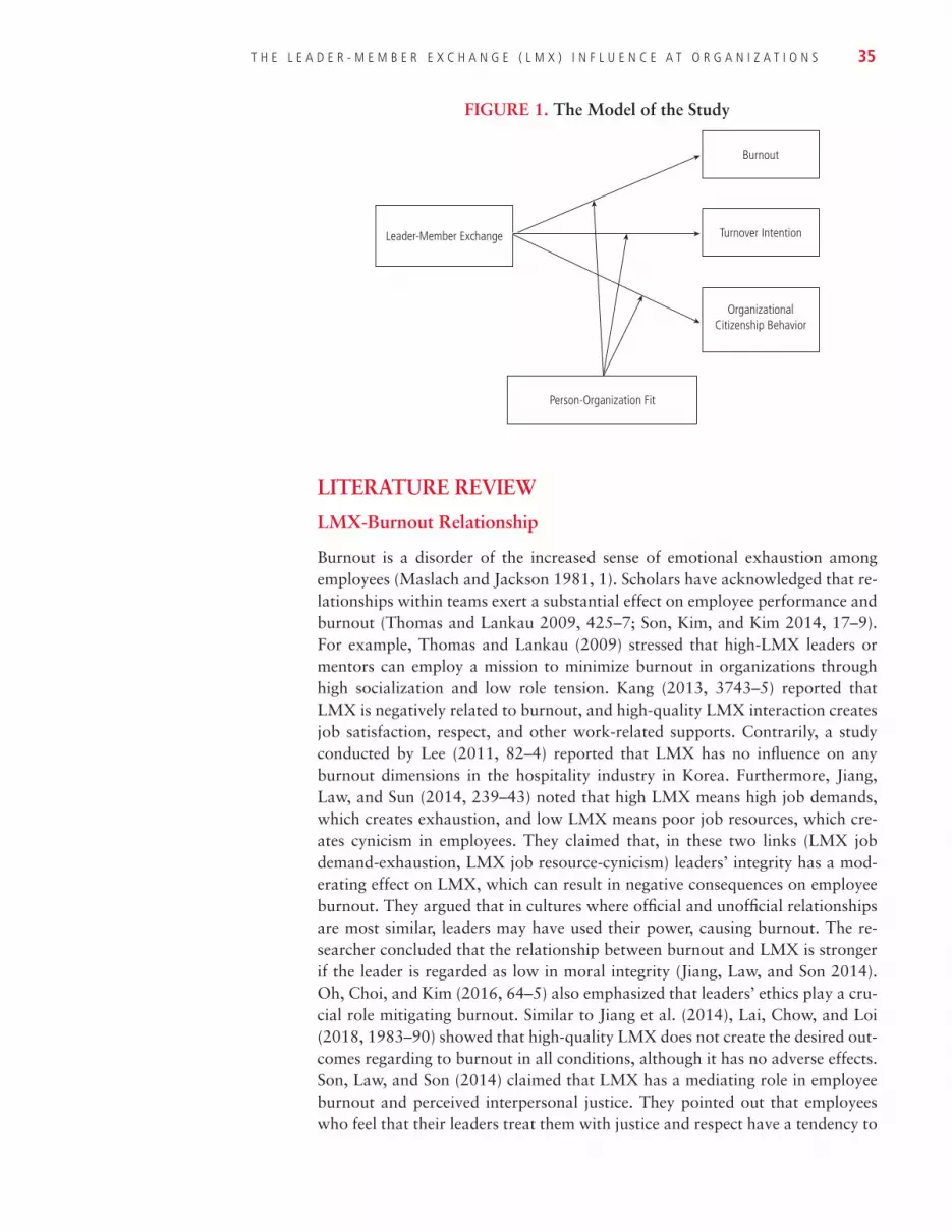
T H E L E A D E R - M E M B E R E X C H A N G E ( L M X ) I N F L U E N C E A T O R G A N I Z A T I O N S 35
LITERATURE REVIEW
LMX-Burnout Relationship
Burnout is a disorder of the increased sense of emotional exhaustion among employees (Maslach and Jackson 1981, 1). Scholars have acknowledged that re-lationships within teams exert a substantial effect on employee performance and burnout (Thomas and Lankau 2009, 425–7; Son, Kim, and Kim 2014, 17–9). For example, Thomas and Lankau (2009) stressed that high-LMX leaders or mentors can employ a mission to minimize burnout in organizations through high socialization and low role tension. Kang (2013, 3743–5) reported that LMX is negatively related to burnout, and high-quality LMX interaction creates job satisfaction, respect, and other work-related supports. Contrarily, a study conducted by Lee (2011, 82–4) reported that LMX has no influence on any burnout dimensions in the hospitality industry in Korea. Furthermore, Jiang, Law, and Sun (2014, 239–43) noted that high LMX means high job demands, which creates exhaustion, and low LMX means poor job resources, which cre-ates cynicism in employees. They claimed that, in these two links (LMX job demand-exhaustion, LMX job resource-cynicism) leaders’ integrity has a mod-erating effect on LMX, which can result in negative consequences on employee burnout. They argued that in cultures where official and unofficial relationships are most similar, leaders may have used their power, causing burnout. The re-searcher concluded that the relationship between burnout and LMX is stronger if the leader is regarded as low in moral integrity (Jiang, Law, and Son 2014). Oh, Choi, and Kim (2016, 64–5) also emphasized that leaders’ ethics play a cru-cial role mitigating burnout. Similar to Jiang et al. (2014), Lai, Chow, and Loi (2018, 1983–90) showed that high-quality LMX does not create the desired out-comes regarding to burnout in all conditions, although it has no adverse effects. Son, Law, and Son (2014) claimed that LMX has a mediating role in employee burnout and perceived interpersonal justice. They pointed out that employees who feel that their leaders treat them with justice and respect have a tendency to
FIGURE 1. The Model of the Study
Leader-Member Exchange
Burnout
Turnover Intention
OrganizationalCitizenship Behavior
Person-Organization Fit

36 R E V I E W O F B U S I N E S S
build self-worth and self-esteem, encouraging them to create good relationships with their leaders that in turn decrease burnout. In contrast to these studies, Huang and Simha (2018, 32–6) found that work-related factors are more in-fluential than organizational effects, including LMX. According to Huang and Simha (2018), employee cynicism cannot be addressed effectively with the help of LMX if job-related factors contribute to cynicism.
H1: LMX has a negative effect on burnout.
LMX-Turnover Intention
Burgess (1998, 55) defines turnover as “The movement of workers around the labor market, between firms, and among the states of employment, unemploy-ment, and inactivity.” In their meta-analytic review, Gerstner and Day (1997) indicated that there is a significant correlation between LMX and turnover in-tention. Bauer et al. (2006, 301–2) approached the turnover intention concept through personality qualities, and they found that LMX contributes to the per-formance and development of new introverted executives. When it comes to ex-troverted new executives, they cannot be considered as LMX-sensitive because their extroverted personality shows the same moderating effect as LMX (303). In their study, Harris, Wheeler, and Kacmar (2009, 381) appointed LMX as an independent variable and empowerment as a moderator, to show that LMX and empowerment were negatively and significantly related to turnover intentions, both independently and when they interact. Son, Kim, and Kim (2014) also demonstrated that relationships with leaders essentially influence turnover inten-tion. According to Kim, Lee, and Carlson (2010, 595), the U-shaped curvilinear LMX–turnover intention connection was demonstrated only among non-super-visory employees through a negative linear relationship observed between LMX and turnover intention only with supervisory workers.
Wang and Yi (2011, 429) have investigated the relationship between LMX and turnover intention through job satisfaction and job stress dimensions. The research results showed that even though job satisfaction and job stress mediate the LMX’s effectiveness on turnover intention, only job satisfaction plays a me-diating role. Job stress has no mediating character in the relationship between LMX and turnover as well as job satisfaction itself. However, job satisfaction entirely mediates the LMX and turnover intention relationship and LMX influ-ence turnover intention via its job satisfaction effect.
The connection between turnover intention and LMX has also been exam-ined in detail, and a number of researchers have agreed that LMX has a negative correlation on employees’ intention to leave (Griffeth, Hom, and Gaertner 2000, 483; Harris, Wheeler, and Kacmar 2009, 381; Kang 2013, 3743–5; Portoghese et al. 2014, 760–1; Kim and Barak 2015, 141; Yoo and Kim 2015, 91; Chan et al. 2017, 118). Portoghese et al. (2014, 760–1) defended that LMX has a positive impact in terms of employee performance and motivation as the leaders possess the power to design a favorable working climate. Kim and Barak (2015, 141) also confirmed and further claimed that LMX has a negative effect on turnover inten-tion in an educational environment). Regarding workplace loneliness, leaders and members’ loneliness congruence creates a high level of LMX, and this mediating effect of LMX affects turnover intention (Chen, Wen, and Liu 2016, 874–6).
H2: LMX has a negative effect on turnover intention.

T H E L E A D E R - M E M B E R E X C H A N G E ( L M X ) I N F L U E N C E A T O R G A N I Z A T I O N S 37
LMX–Organizational Citizenship Behavior (OCB)
OCB describes the situation when employees voluntarily help people on the job without any promised rewards (Organ 1988). One of the first attempts to under-stand the relationship between LMX and OCB in the context of social exchange was originated by Konovsky and Pugh (1994). They claimed that OCB occurs when the social exchange designs the quality of leader-member relationships (666–8).
A meta-analysis conducted by Ilies, Nahrgang, and Morgeson (2007, 272–4), based on 50 published and unpublished studies, revealed that LMX is positively and strongly related to OCB. The study also indicated that com-paring individual-targeted behaviors and organizational-targeted behaviors, the LMX has a stronger correlation in an individual setting. Another meta-analysis (Lapierre and Hackett 2007) is also consistent with the prior findings, and they further clarified the new use of OCB as it may boost LMX quality. Rockstuhl et al. (2012, 1098) tried to meta-analyze the role of national culture on the re-lationship of LMX and OCB with other dimensions, and the results show that national culture has no significant effect on OCB.
Concerning LMX’s effect on authoritative conduct, scientists have con-tended that this relationship is articulated in numerous settings (Wang, Chu, and Ni 2010, 162–6; Findikli 2015, 232–6; Matta et al. 2015, 1700–3; Van Knip-penberg, Van Prooijen, and Sleebos 2015, 156–7; Bowler, Paul, and Halbesleben 2017, 148–50). For instance, Bowler, Paul, and Halbesleben (2017) focused on how LMX could dually affect hierarchical citizenship conduct (OCB) as devotees can be seen as prudes, unfavorably influencing the workplace. In spite of the fact that Matta et al. (2015) concurred that a connection between OCB and LMX is clear, they required a more complete methodology. They focusing on OCB and the leader-employee dyad, finding that OCB was contrarily influenced if lead-ers and their subordinates held distinctive perspectives on the nature of LMX. Matta et al. (2015) accentuated that OCB could be high regardless of whether the partners considered LMX to be low, showing this setting is more appropriate than LMX quality. As indicated by Matta et al. (2015), researchers have focused on the viewpoint of leaders or behaviors of employees while the attention should be on both leaders and workers’ LMX. Van Knippenberg et al. (2015) included that the connection between LMX and OCB varies crosswise over societies, and collectivism assumes a moderating mechanism in the relationship between OCB and perceived organizational support. In their research, Asgari et al. (2008, 147) confirmed that the LMX is influenced by transformational and transactional leadership behaviors but LMX has no effect on OCB. Addressing the effect of LMX on OCB in the health field, Chen et al. (2008, 324–6) verified that OCB is indirectly affected by LMX through the established trust between nurses and head nurse and perceived leader support.
Kim, O’Neill, and Cho (2010, 534–6) analyzed the relationship between LMX and OCB in the context of employee envy, and results showed that low-quality LMX and high-quality LMX are determinative dimensions for envy. Low-quality LMX creates workplace envy. Therefore, the high level of envy serves low OCB. Under different LMX group structure with similar LMX pat-terns between coworkers, the relationship between high-quality LMX and OCB are infirm (Harris, Li, and Kirkman 2014, 326). Tang and Naumann (2015, 298–303) discovered that members who report that their leader shows benevolent or
38 R E V I E W O F B U S I N E S S
moral attitudes will have a positive view of their LMX with their manager and take part in OCB toward their colleagues. Leaders’ high-power distance weak-ens the positive connection between LMX and employees’ OCBs. Hence, this impact is more articulated in high job interdependence groups (Anand, Vidyar-thi, and Rolnicki 2018). Workers in high task interdependence groups driven by low power distance leaders take part in the most elevated scale of OCBs (Anand, Vidyarthi, and Rolnicki 2018, 489–95).
H3: LMX has a positive effect on organizational citizenship behavior.
Moderator: Person-Organization Fit (P-O Fit)
Person-environment fit theory was originated in the early twentieth century by Frank Parsons (1909, 3–5), who developed a career decision-making model. Parsons proposed another hypothetical structure concentrating on needs-sup-plies and demands-abilities fit. Over many decades, the theory has evolved through numerous contributions. P-O fit has a bilateral mechanism between the employee and organization in which individuals meet the requirements of the environment, and the organizations satisfy the preferences and desires of in-dividuals. In the 1930s, Murray (1938, 140) pointed out that institutions and needs are two entities that complete each other in terms of triggering members’ involvement.In the 1960s, specialists focused on job satisfaction as a significant part of P-O fit. Then in the 1990s, vocational choice, recruitment, and organi-zational culture became the focus concerning P-O fit. P-O fit can be defined as the compatibility between the workers and their working environment (Kristof 1996, 2–3). In this regard, it is crucial to understand the mutual fundamen-tal characteristics to conceptualize the P-O fit concept in a workplace (Kristof 1996). P-O fit includes the workplace, institutional variables, employees’ quali-ties, and objectives (Ployhart, Hale, and Campion 2014, 24–30).
P-O Fit’s Moderator Roles in the LMX-Burnout Relationship
The effect of P-O fit on employees has been contemplated for a considerable length of time. While moderator role of P-O fit in burnout or LMX has been studied individually (Erdogan, Kraimer, and Liden 2002, 1–6; Siegall and Mc-Donald 2004, 293–4), no study specifically investigated P-O fit’s moderator roles in the context of the LMX-burnout relationship.
P-O Fit’s Moderator Roles in the LMX–Turnover Intention Relationship
Scientists have concurred that the effect of P-O fit on turnover intention is more articulated than LMX’s impact (Hamid and Yahya 2016, 188–9; Rurkkhum 2018, 115–8). Therefore, similar to the research scarceness stated above, P-O fit’s moderator role in the context of the LMX–turnover intention relationship is not also addressed.
P-O Fit’s Moderator Roles in the LMX–Organizational Citizenship Behavior (OCB) Relationship
P-O fit’s moderator roles in the context of LMX–organizational citizenship be-havior (OCB) relationship has not been analyzed extensively. However, the im-pacts of P-O fit on OCB, as reinforcement, engagement, and culture have been

T H E L E A D E R - M E M B E R E X C H A N G E ( L M X ) I N F L U E N C E A T O R G A N I Z A T I O N S 39
observed to be key to employee performance (Farzaneh, Farashah, and Kazemi 2014, 674–8; Afsar and Badir 2016, 254–60). Ruiz-Palomino and Martínez-Cañas (2014, 96–8) concentrated on the ethical domain, stating that P-O fit is a mediator in the relationship between OCB and ethical culture.
The mentioned studies have revealed various aspects of the link between P-O fit and LMX, burnout, turnover intention, and OCB separately, but not di-rectly P-O fit’s roles on LMX-burnout, LMX–turnover intention, and the LMX-OCB relationship. These areas, the main focus of this study, still need to be explored, and additional research is needed to investigate the roles of the various LMX traits of relationships among the components under this construct. This paper’s main contribution is to establish a strong scientific ground for multidi-mensional LMX research.
H4a: Person-organization fit has a moderator role on the relationship be-tween LMX and burnout.
H4b: Person-organization fit has a moderator role on the relationship be-tween LMX and turnover intention.
H4c: Person-organization fit has a moderator role on the relationship be-tween LMX and organizational citizenship behavior.
METHODOLOGYIn this section, the research sample, the scales used, and the details about the reliability tests are discussed.
Sample
A survey was carried out with 1000 randomly selected full-time employees work-ing in organizations from manufacturing sectors operating in Kayseri, Turkey. After the missing and incorrect codes were distinguished, a total of 903 question-naires were evaluated. The return rate of the surveys was approximately 90%. When the participants were examined in terms of demographic characteristics:
• 25% were women and 75% were men
• The average age of the sample was 28.94
• 41.2% of the participants are married and 58.8% are single
• The educational status was 9.8% primary school, 16% secondary school, 45.2% high school, 13.1% associate degree, 14.2% undergraduate, and 1.7% graduate education
Measures
For this study, a questionnaire was used to collect data from the employees. In the first part, 37 expressions were prepared to determine the opinions of the participants regarding the research variables, and in the second part, a question-naire with four variables was prepared to determine the demographic distribu-tion of the participants. The statements in all scales were created to be answered in a seven-degree Likert format, and the instruction and printing of the scale were done accordingly. The ratings were “strongly disagree” (1), “disagree” (2), “partially disagree” (3), “undecided” (4), “partially agree” (5), “agree” (6), and “strongly agree” (7).

40 R E V I E W O F B U S I N E S S
Leader-Member Exchange Scale: The Leader-Member Exchange Scale de-veloped by Liden and Maslyn (1998) was used to measure the quality of the relations between employees and their superiors. Examples of items include:
• “My superior is pleased to work with me.”
• “Even if I do not know exactly about the subject, I will defend my superi-or’s decisions.”
• “When criticized by others, I defend my superior.”
• “The support and resources provided by my superior are more than they should be.”
The scale consists of 12 items, and the reliability of the scale (Cronbach’s alpha) is 0.911.
Person-Organization Fit Scale: The Person-Organization Fit Scale, which was suggested by Netemeyer et al., consisting of four expressions and one dimension, was used in this study. The sample items are:
• “There is a good harmony between my values and the business I work for.”
• “The business I work for has the same values as me about honesty.”
• “The business I work for has the same values as me for justice.”
• “This business has the same values as my colleagues.”
Cronbach’s Alpha value of the scale is 0.869.
Burnout Inventory: Seven items and a one-dimensional Burnout Inventory devel-oped by Kristensen et al. (2005, 199–201) were used to determine the burnout levels of the participants. Sample items include:
• “I feel exhausted by thinking about other workdays in the morning.”
• “In my spare time, I have enough energy for my family and friends.”
Cronbach’s Alpha value is 0.85 to 0.087.
Turnover Intention: The turnover intention scale, which includes three expres-sions and one dimension, suggested by Babin and Boles (1998, 89), was used. A sample scale item is “I think of quitting my job too often.” The reliability coefficient for the scale is 0.789.
Organizational Citizenship Behavior: A scale developed by Smith, Organ, and Near (1983, 656–7) was used to measure the level of organizational citizen-ship behavior of the participants. The scale consists of 16 expressions and two sub-dimensions. These dimensions are altruism and generalized harmony. Ex-ample items in the scale include: “I don’t waste time with empty conversations.” and “I help people who need it.” The reliability value of the scale is 0.854.
RESULTSConfirmatory factor analysis results applied to the scales are as seen in Table 1.

T H E L E A D E R - M E M B E R E X C H A N G E ( L M X ) I N F L U E N C E A T O R G A N I Z A T I O N S 41
The results of the confirmatory factor analysis regarding the variables in the study can be seen in Table 1. In light of the literature reviews (Bayram et al. 2019), it is possible to state that the confirmatory factor analysis results are within the acceptable limits of goodness of fit indices for all three variables. Thus, it is understood that the structures related to the variables are consistent and appropriate with the empirical data used in the analysis.
The mean and standard deviation values of the five variables considered in the study and the degree of relationship between these variables are shown in Table 2.
TABLE 2. Mean, Standard Deviation, and Correlations
Mean Standard Deviation
1 2 3 4 5
LMX 4.79 1.16 –
P-O Fit 4.92 1.19 0.507** –
Turnover Intention
3.19 1.38 −0.405** −0.451** –
Burnout 2.66 1.18 −0.434** −0.485** −0.443** –
OCB 4.61 1.24 0.529** 0.541** −0.381** −0.347** –
As seen in Table 2, the average values of the variables are between 2.66 and 4.92. Standard deviation values are very close to each other. Based on the above table, there are significant correlations between the study variables.
Hypotheses Testing
Before the research hypotheses were tested, centralization was performed in order to minimize the problem of multi-collinearity (Demirtas 2014, 144). Then, hier-archical regression analysis was used to test the established hypotheses (Table 3).
TABLE 1. CFI Analyses
Index Perfect Fit Acceptable Fit LMX P-O FitTurnover Intention
Burnout OCB
CFI 0.970 CFI 10.000 0.950 CFI 0.970 0.998 0.995 0.994 0.994 0.998
HOELTER 200 75 HOELTER 200 946 735 512 396 914
IFI 0.950 IFI 10.000 0.900 IFI 0.950 0.998 0.984 0.993 0.994 0.938
NFI 0.950 NFI 10.000 0.900 NFI 0.950 0.996 0.993 0.989 0.993 0.997
PCLOSE 00.05 0.601 0.355 0.397 0.082 0.746
RFI 0.900 < RFI 10.000 0.850 < RFI 0.900 0.988 0.978 0.943 0.948 0.990
RMSEA 0.000 RMSEA 0.05 0.050 RMSEA 0.080 0.041 0.054 0.028 0.070 0.036
TLI 0.95 TLI 1.000 0.900 TLI 0.950 0.993 0.984 0.954 0.955 0.995
χ2/df 0.000 χ2/df 2.000 2 χ2/df 3 2.478 2.664 2.364 2.806 2.178

42 R E V I E W O F B U S I N E S S
As can be seen from the values in Table 3, the LMX has negative effects on turnover intention (β = −0.405, p < 0.005), and burnout (β = −0.434, p < 0.005). LMX also has positive effect on organizational citizenship behavior (β = 0.529, p < 0.005). In addition, OCB has moderator roles on the relationships between LMX and turnover intention (β = −0.116, p < 0.005), LMX and burnout (β = −0.165, p < 0.005), LMX and organizational citizenship behaviors (β = 0.098, p < 0.005).
DISCUSSIONAs hypothesized, the result of this study revealed that leader-member exchange has a significant influence on turnover intention, burnout, and organizational citizenship behaviors. Additionally, it was found that person-organization fit has a moderator role in the relationship between LMX, turnover intention, burn-out, and OCB. The results of this study parallel the existing literature. Schol-ars have acknowledged that relationships within teams exert a substantial ef-fect on employee performance and burnout (Thomas and Lankau 2009; Kang 2013; Son, Kim, and Kim 2014). For example, Thomas and Lankau (2009) stressed that high-LMX leaders or mentors employ a mission to minimize burn-out in organizations through high socialization and low role tension. Gerstner and Day (1997) indicated that there is a significant correlation between LMX and turnover intention. Bauer et al. (2006) approached the turnover intention concept through personality qualities, and they found that LMX contributes to performance and development of new introverted executives. A meta-analysis conducted by Ilies, Nahrgang, and Morgeson (2007) based on 50 published and unpublished studies revealed that LMX is positively and strongly related to OCB. The effect of P-O fit on employees has been contemplated for a long time. While the moderator role of P-O fit in burnout, turnover intention, OCB, and LMX has been studied individually (Erdogan et al. 2002; Siegall and McDonald 2004; Farzaneh et al. 2014; Rurkkhum 2018), no study specifically investigates
TABLE 3. Hierarchical Regression Analysis Results
Turnover Intention Burnout OCB
(β) R2 R2 (β) R2 R2 (β) R2 R2
Step 1
LMX −0.405* 0.164 −0.434* 0.189 0.052 0.529* 0.153
F Value 176,205 208,968 108,823
Step 2
LMX −0.328* 0.246 0.082 −0.301* 0.282 0.093 0.589* 0.189 0.036
P-O Fit −0.458* −0.423* 0.276
F Value 145,945 177,355 64,353
Step 3
LMX −0.305* 0.323 0.077 −0.285* 0.334 0.052 0.575* 0.111 0.022
P-O Fit −0.427* −0.315* 0.213*
Interaction −0.116* −0.165* 0.098*
F Value 101,100 120,855 42,881
Interaction: LMX * P-O fit

T H E L E A D E R - M E M B E R E X C H A N G E ( L M X ) I N F L U E N C E A T O R G A N I Z A T I O N S 43
P-O fit’s moderator roles in the context of LMX–burnout turnover and OCB relationships.
The results may have important consequences for leadership roles, social justice, and social cohesion in organizations. Leaders are limited in their power and establish unequal LMXs with their subordinates (Dansereau Graen, and Haga 1975; Graen and Uhl-Bien 1995), which in turn affect influence social and personal expectations. Graen and Uhl-Bien (1995) described the LMX theory of leadership formation. They argued that supervisors should give an opportunity for all their subordinates to establish a high-quality relationship. The quality of work success of a leader depends on the overall performance of the organization. Developing more high-quality LMXs with subordinates will improve the overall job output efficiency of the superior (Graen and Uhl-Bien 1995). So, leaders need to give subordinates incentives to enhance the efficiency of LMXs. For instance, supervisors should build a welcoming and open environment, increase the number and variety of demanding assignments and tasks, set higher expec-tations, and provide constructive input to members of the out-group (Johnson and Hackman 2018).
As the standard of LMXs increases, organizational citizenship behaviors will become more optimistic, workgroup contact more cooperative, workgroup performance higher, and in contrast, burnout and turnover intention will be-come lower. Furthermore, since they have closed contact networks with their supervisors, workers in low-quality LMXs cannot be able to articulate their concerns or provide insight into resource allocation decision-making processes. Supervisors should proactively invite their subordinates (especially those in low-quality LMXs) to express and address concerns about distributive outcomes and procedural issues in line with the participatory decision-making process and organizational democracy.
As for how stakeholders in professional life can benefit from this work, it is the fact that the positive effects of LMX can be utilized as a catalyst through the OCB in the context of burnout, turnover intention, and organizational citi-zenship behaviors. In other words, OCB concept should be adapted to processes such as human resources development, performance appraisal, maximizing em-ployee satisfaction, increasing employee productivity, and increasing employee creativity.
This study also has some limitations. One drawback is the use of self-re-ports. In relation to cooperative communication, self-reports should vary across members of the same group. Moreover, the results are focused on assumptions and do not, thus, reflect real cooperative communication behaviors. Another possible disadvantage is the bias in the responses of study participants about social desirability. However, the differences in LMX quality responses, OCB, turnover, and burnout suggest that the bias to social desirability, if any, may have been minimal.
To sum up, this research empirically examined the hypothesized relation-ships between LMX, turnover intention, burnout, and OCB. Liden and his col-leagues (Dienesch and Liden 1986; Liden and Maslyn 1998) indicated that the standard of LMX could vary in multiple dimensions such as confidence, effect, loyalty, obligation, and respect. Future research should recognize individual as-pects of the LMX that affect the potential outcomes of employees. Other studies
44 R E V I E W O F B U S I N E S S
should also investigate particular convincing and insightful communication pat-terns and practices inside various LMXs that affect perceptions of social justice and/or related cooperative contact in wider contexts, such as communities and organizations.
ReferencesAfsar, B., and Y. F. Badir. 2016. “Person–Organization Fit, Perceived Organizational
Support, and Organizational Citizenship Behavior: The Role of Job Embedded-ness.” Journal of Human Resources in Hospitality and Tourism 15, no. 3, 252–78. DOI: 10.1080/15332845.2016.1147936.
Anand, S., P. Vidyarthi, and S. Rolnicki. 2018. “Leader-Member Exchange and Orga-nizational Citizenship Behaviors: Contextual Effects of Leader Power Distance and Group Task Interdependence.” The Leadership Quarterly 29, no. 4, 489–500. DOI: 10.1016/j.leaqua.2017.11.002.
Asgari, A., A. D. Silong, A. Ahmad, and B. Abu Sama. 2008. “The Relationship be-tween Transformational Leadership Behaviors, Leader-Member Exchange and Or-ganizational Citizenship Behaviors.” European Journal of Social Sciences 6, no. 4, 140–51. https://www.researchgate.net/publication/260294193_The_Relationship_ between_Transformational_Leadership_Behaviors_Leader-Member_Exchange_ and_Organizational_Citizenship_Behaviors
Babin, B. J., and J. S. Boles. 1998. “Employee Behavior in A Service Environment: A Model and Test of Potential Differences between Men and Women.” Journal of Marketing 62, no. 2, 77–91. DOI: 10.2307/1252162.
Bauer, T. N., B. Erdogan, R. C. Liden, and S. J. Wayne. 2006. “A Longitudinal Study of the Moderating Role of Extraversion: Leader-Member Exchange, Performance, and Turnover during New Executive Development.” Journal of Applied Psychology 91, no. 2, 298–310. DOI: 10.1037/0021-9010.91.2.298.
Bayram, A., M. Şeker, N. M. BüyüksivaslıoŞlu, M. Reyhancan, T. Vyacheslav, and B. Botakarayev. 2019. “The Mediating Role of Stress on the Relationship between Or-ganizational Culture and Dysfunctional Attitudes: A Field Study.” Elementary Edu-cation Online 19, no. 1, 147–56.
Bowler, W. M., J. B. Paul, and J. R. Halbesleben. 2017. “LMX and Attributions of Orga-nizational Citizenship Behavior Motives: When Is Citizenship Perceived as Brown-nosing?” Journal of Business and Psychology 34, no. 2, 139–52. DOI: 10.1007/s10869-017-9526–5.
Burgess, S. 1998. “Analyzing Firms, Jobs, and Turnover.” Monthly Labor Review 121, no. 7, 55–8. https://books.google.com.tr/books?id=mJrYJ-D5aVUC&printsec= frontcover&source=gbs_ge_summary_r&cad=0#v=onepage&q&f=false.
Chan, S. H., S. Y. Chok, S. Y. Lae, A. C. Lam, and C. Y. Lee. 2017. The Impact of Per-ceived Organizational Support, Job Satisfaction, Leader-Member Exchange (LMX) and Work-Life Balance on Employee’s Turnover Intention in Manufacturing In-dustry, Malaysia. Doctoral dissertation, UTAR. http://eprints.utar.edu.my/2646/1/ Final_Year_Project_(Group_9).pdf.
Chen, C. H. V., S. J. Wang, W. C. Chang, and C. S. Hu. 2008. “The Effect of Lead-er-Member Exchange, Trust, Supervisor Support on Organizational Citizenship Be-havior in Nurses.” Journal of Nursing Research 16, no. 4, 321–28. DOI: 10.1097/01.JNR.0000387319.28010.5e.
Chen, Y., Z. Wen, J. Peng, and X. Liu. 2016. “Leader-Follower Congruence in Loneli-ness, LMX and Turnover Intention.” Journal of Managerial Psychology 31 no. 4, 864–79. DOI: 10.1108/JMP-06–2015-0205.
Dansereau Jr, F., G. Graen, and W. J. Haga. 1975. “A Vertical Dyad Linkage Approach to Leadership within Formal Organizations: A Longitudinal Investigation of the Role Making Process.” Organizational Behavior and Human Performance 13, no. 1, 46–78. DOI:10.1016/0030–5073(75)90005-7.

T H E L E A D E R - M E M B E R E X C H A N G E ( L M X ) I N F L U E N C E A T O R G A N I Z A T I O N S 45
Day, D. V., and D. Miscenko. 2015. “Leader-Member Exchange (LMX): Construct Evo-lution, Contributions, and Future Prospects for Advancing Leadership Theory.” In The Oxford Handbook of Leader-Member Exchange, edited by T. N. Bauer and B. Erdogan, 9–28. New York, NY: Oxford University Press. DOI: 10.1093/oxfordhb/ 9780199326174.013.0008.
Demirtas, O. 2014. “Isyerlerinde Olumsuz Durumlari Ifsa Etmenin Etik Iklim Uze-rindeki Etkisi: Yildirma Algisinin Moderator Rolu/The Whistleblowing Impact on Ethical Climate: Moderator Role of Mobbing Perception.” Istanbul Üniversitesi Is-letme Fakültesi Dergisi 43, no. 1, 136–56. http://eds.a.ebscohost.com/eds/pdfviewer/ pdfviewer?vid=1&sid=0ee79c33-4df3-47bb-ad02–10945be5b421%40sessionmgr 4008.
Dienesch, R. M., and R. C. Liden. 1986. “Leader-Member Exchange Model of Leader-ship: A Critique and Further Development.” The Academy of Management Review 11, no. 3, 618. DOI: 10.2307/258314.
Erdogan, B., M. L. Kraimer, and R. C. Liden. 2002. “Person-Organization Fit and Work Attitudes: The Moderating Role of Leader-Member Exchange.” Academy of Man-agement Proceedings 2002, no. 1, F1–6.
Farzaneh, F., A. D. Farashah, and M. Kazemi. 2014. “The Impact of Person-Job Fit and Person-Organization Fit on OCB: The Mediating and Moderating Effects of Organi-zational Commitment and Psychological Empowerment.” Personnel Review 43, no. 5, 672–91. DOI: 10.1108/PR-07–2013-0118.
Findikli, M. M. A. 2015. Exploring the Consequences of Work Engagement: Relations Among OCB-I, LMX and Team Work Performance. Ege Academic Review 15, no. 2, 229–38. https://dergipark.org.tr/en/pub/eab/issue/39938/474503.
Gerstner, C. R., and D. V. Day. 1997. “Meta-Analytic Review of Leader–Member Ex-change Theory: Correlates and Construct Issues.” Journal of Applied Psychology 82, no. 6, 827–44. DOI:10.1037/0021-9010.82.6.827.
Graen, G. B., and M. Uhl-Bien. 1995. “Relationship-Based Approach to Leadership: Development of Leader-Member Exchange (LMX) Theory of Leadership over 25 Years: Applying a Multi-Level Multi-Domain Perspective.” The Leadership Quar-terly 6, 219–47. DOI: 10.1016/1048-9843(95)90036-5.
Graen, G. B. 1976. “Role-Making Process within Complex Organizations.” In Hand-book of Industrial and Organizational Psychology, edited by M. D. Dunnette, 1202–45. Chicago, IL: Rand McNally.
Graen, G. B., and J. F. Cashman. 1975. “A Role-Making Model of Leadership in Formal Organizations: A Developmental Approach.” Leadership Frontiers 143, 165.
Griffeth, R. W., P. W. Hom, S. Gaertner. 2000. “A Meta-Analysis of Antecedents and Correlates of Employee Turnover: Update, Moderator Tests, and Research Implica-tions for the Next Millennium.” Journal of Management 26, no. 3, 463–88. DOI: 10.1177/014920630002600305.
Hamid, S., and K. Yahya. 2016. “Mediating Role of Work Engagement on the Rela-tionship between Person-Job Fit and Employees’ Retention: Evidence from Semi-conductor Companies in Northern Region of Malaysia.” International Review of Management and Marketing 6, no. 7S, 187–94. https://econjournals.com/index.php/irmm/article/view/3251/pdf.
Harris, K. J., A. R. Wheeler, and K. M. Kacmar. 2009. “Leader–Member Exchange and Empowerment: Direct and Interactive Effects on Job Satisfaction, Turnover In-tentions, and Performance.” The Leadership Quarterly 20, no. 3, 371–82. DOI: 10.1016/j.leaqua.2009.03.006.
Harris, T. B., N. Li, and B. L. Kirkman. 2014. “Leader–Member Exchange (LMX) in Context: How LMX Differentiation and LMX Relational Separation Attenuate LMX’s Influence on OCB and Turnover Intention.” The Leadership Quarterly 25, no. 2, 314–28. DOI: 10.1016/j.leaqua.2013.09.001.
Huang, C.-S., and A. Simha. 2018. “The Mediating Role of Burnout in the Relationships between Perceived Fit, Leader–Member Exchange, Psychological Illness, and Job Performance.” International Journal of Stress Management 25, no. S1, 26–42. DOI: 10.1037/str0000077.

46 R E V I E W O F B U S I N E S S
Ilies, R., J. D. Nahrgang, and F. P. Morgeson. 2007. “Leader-Member Exchange and Citizenship Behaviors: A Meta-Analysis.” Journal of Applied Psychology 92, no. 1, 269–77. DOI: 10.1037/0021-9010.92.1.269.
Jiang, J. Y., K. S. Law, and J. J. Sun. 2014. “LMX and Burnout: The Moderating Role of Leader Integrity.” Management and Organization Review 10, 223–47. DOI: 10.1111/more.12022.
Johnson, C. E., and M. Z. Hackman. 2018. Leadership: A Communication Perspective. Long Grove, IL: Waveland Press.
Kang, J. 2013. “Relationship among Leader-Member Exchange (LMX), Burnout and Career Turnover Intention in Social Workers using SEM.” Journal of the Korea Academia-Industrial Cooperation Society 14, no. 8, 3739–47. DOI: 10.5762/KAIS.2013.14.8.3739.
Kim, A., and M. E. M. Barak. 2015. “The Mediating Roles of Leader–Member Exchange and Perceived Organizational Support in the Role Stress–Turnover Intention Rela-tionship among Child Welfare Workers: A Longitudinal Analysis.” Children and Youth Services Review 52, 135–43. DOI: 10.1016/j.childyouth.2014.11.009.
Kim, B. P., G. Lee, and K. D. Carlson, 2010. “An Examination of the Nature of the Relationship between Leader-Member-Exchange (LMX) and Turnover Intent at Dif-ferent Organizational Levels.” International Journal of Hospitality Management 29, no. 4, 591–7. DOI: 10.1016/j.ijhm.2009.10.025.
Kim, S., J. W. O’Neill, and H. M. Cho. 2010. “When Does an Employee Not Help Co-workers? The Effect of Leader–Member Exchange on Employee Envy and Organiza-tional Citizenship Behavior.” International Journal of Hospitality Management 29, no. 3, 530–7. DOI: 10.1016/j.ijhm.2009.08.003.
Konovsky, M. A., and S. D. Pugh. 1994. “Citizenship Behavior and Social Exchange.” Academy of Management Journal 37, no. 3, 656–69. DOI: 10.5465/256704.
Kristensen, T. S., M. Borritz, E. Villadsen, and K. B. Christensen. 2005. “The Copenha-gen Burnout Inventory: A New Tool for the Assessment of Burnout.” Work & Stress 19, no. 3, 192–207. DOI: 10.1080/02678370500297720.
Kristof, A. L. 1996. “PersonŞOrganization Fit: An Integrative Review of Its Conceptual-izations, Measurement, and Implications.” Personnel Psychology 49, no. 1, 1–49. DOI: 10.1111/j.1744-6570.1996.tb01790.x.
Lai, J. Y., C. W. Chow, and R. Loi. 2018. “The Interactive Effect of LMX and LMX Differentiation on Followers’ Job Burnout: Evidence from Tourism Industry in Hong Kong.” The International Journal of Human Resource Management 29, no. 12, 1972–98. DOI: 10.1080/09585192.2016.1216875.
Lapierre, L. M., and R. D. Hackett. 2007. “Trait Conscientiousness, LeaderŞMember Exchange, Job Satisfaction and Organizational Citizenship Behaviour: A Test of an Integrative Model.” Journal of Occupational and Organizational Psychology 80, no. 3, 539–54.
Lee, K. E. 2011. “Moderating Effects of Leader-Member Exchange (LMX) on Job Burn-out in Dietitians and Chefs of Institutional Foodservice.” Nutrition Research and Practice 5, no. 1, 80–7. DOI: 10.4162/nrp.2011.5.1.80
Liden R. C., R. T. Sparrowe, and S. J. Wayne. 1997. “Leader–Member Exchange Theory: The Past and Potential for Future.” In G. R. Ferris (Ed.), Research in Personnel and Human Resources Management (Vol. 15, 47–119). Greenwich, CT: Elsevier Science/JAI Press. https://www.researchgate.net/publication/232504779_Leader-member_exchange_theory_The_past_and_potential_for_the_future.
Liden, R. C., and J. M. Maslyn. 1998. “Multidimensionality of Leader-Member Ex-change: An Empirical Assessment through Scale Development.” Journal of Manage-ment 24, no. 1, 43–72. DOI: 10.1016/S0149–2063(99)80053–1.
Maslach, C., and S. E. Jackson. 1981. “The Measurement of Experienced Burnout.” Journal of Organizational Behavior 2, 99–113. DOI: 10.1002/job.4030020205.
Matta, F. K., B. A. Scott, J. Koopman, and D. E. Conlon. 2015. “Does Seeing ‘Eye to Eye’ Affect Work Engagement and Organizational Citizenship Behavior? A Role Theory Perspective on LMX Agreement.” Academy of Management Journal 58, no. 6, 1686–708. DOI: 10.5465/amj.2014.0106.

T H E L E A D E R - M E M B E R E X C H A N G E ( L M X ) I N F L U E N C E A T O R G A N I Z A T I O N S 47
Memon, M. A., R. Salleh, M. N. R. Baharom, H. Harun, and B. S. Iskandar. 2014. “Person-Organization Fit and Turnover Intention: The Mediating Role of Employ-ee Engagement.” Global Business and Management Research: An International Journal 6, no. 3, 205–209. https://www.researchgate.net/profile/Mumtaz_Memon/ publication/265856940_Person-Organization_Fit_and_Turnover_Intention_The_Mediating_Role_of_Employee_Engagement/links/541fdb350cf241a65a1acb05.pdf.
Murray, H. A. 1938. Explorations in Personality. New York, NY: Oxford University Press.
Netemeyer, R. G., J. S. Boles, D. O. McKee, and R. McMurrian. 1997. “An Investigation into the Antecedents of Organizational Citizenship Behaviors in a Personal Selling Context.” Journal of Marketing 61, no. 3, 85–98. DOI: 10.2307/1251791.
Northouse, P. G. 2016. Leadership: Theory and Practice, 7th ed. Thousand Oaks, CA: SAGE Publications.
Oh, Y. S., B. N. Choi, and A. S. Kim. 2016. “Effects of LMX and Perceived Ethics with Leader on Job Burnout.” Journal of Distribution Science 14, 59–66. DOI: 10.15722/jds.14.8.201608.59.
Organ, D. W. 1988. Issues in Organization and Management Series. Organizational Cit-izenship Behavior: The Good Soldier Syndrome. Lexington, MA: Lexington Books/D.C. Heath and Com.
Parsons, F. 1909. Choosing a Vocation. London: Gay & Hancock Ltd. https://archive.org/stream/choosingvocation00parsuoft?ref=ol#mode/2up.
Ployhart, R. E., D. Hale, and M. C. Campion. 2014. “Staffing within the Social Con-text.” In The Oxford Handbook of Organizational Climate and Culture, edited by B. Schneider and K. Barbera, 23–43. New York, NY: Oxford University Press. DOI: 10.1093/oxfordhb/9780199860715.013.0002.
Portoghese, I., M. Galletta, A. Battistelli, and M. P. Leiter. 2014. “A Multilevel Inves-tigation on Nursing Turnover Intention: The Cross-Level Role of Leader-Member Exchange.” Journal of Nursing Management 23, no. 6, 754–764. DOI: 10.1111/jonm.12205.
Rockstuhl, T., J. H. Dulebohn, S. Ang, and L. M. Shore. 2012. “Leader–Member Ex-change (LMX) and Culture: A Meta-Analysis of Correlates of LMX across 23 Countries.” Journal of Applied Psychology 97, no. 6, 1097–130. DOI: 10.1037/a00299781097.
Ruiz-Palomino, P., and R. Martínez-Cañas. 2014. “Ethical Culture, Ethical Intent, and Organizational Citizenship Behavior: The Moderating and Mediating Role of Person–Organization Fit.” Journal of Business Ethics 120, no. 1, 95–108. DOI: 10.1007/s10551-013–1650–1.
Rurkkhum, S. 2018. “The Impact of Person-Organization Fit and Leader-Member Ex-change on Withdrawal Behaviors in Thailand.” Asia-Pacific Journal of Business Ad-ministration 10, no. 2, 114–29. DOI: 10.1108/APJBA-07–2017-0071.
Scandura T. A., and M. J. Lankau. 1996. “Developing Diverse Leaders: A Leader Member Exchange Approach.” The Leadership Quarterly 7, no. 2, 243–63. DOI:10.1016/S1048-9843(96)90043-0.
Scandura, T. A., and G. B. Graen. 1984. “Moderating Effects of Initial Leader–Member Exchange Status on the Effects of a Leadership Intervention.” Journal of Applied Psychology 69, no. 3, 428–36. DOI: 10.1037/0021-9010.69.3.428.
Schriesheim, C. A., S. L. Castro, and C. C. Cogliser. 1999. “Leader-Member Exchange (LMX) Research: A Comprehensive Review of Theory, Measurement, and Da-ta-Analytic Practices.” The Leadership Quarterly 10, no. 1, 63–113. DOI: 10.1016/S1048-9843(99)80009–5.
Siegall, M., and T. McDonald. 2004. “Person-Organization Value Congruence, Burn-out and Diversion of Resources.” Personnel Review 33, no. 3, 291–301. DOI: 10.1108/00483480410528832.
Smith, C. A., D. W. Organ, and J. P. Near, 1983. “Organizational Citizenship Behavior: Its Nature and Antecedents.” Journal of Applied Psychology 68, no. 4, 653–63. DOI: 10.1037/0021-9010.68.4.653.

48 R E V I E W O F B U S I N E S S
Son, S., D. Y. Kim, and M. Kim. 2014. “How Perceived Interpersonal Justice Relates to Job Burnout and Intention to Leave: The Role of Leader-Member Exchange and Cognition-Based Trust in Leaders.” Asian Journal of Social Psychology 17, no. 1, 12–24. DOI: 10.1111/ajsp.12038.
Tang, C., and S. E. Naumann. 2015. “Paternalistic Leadership, Subordinate Perceived Leader–Member Exchange and Organizational Citizenship Behavior.” Journal of Management and Organization 21, no. 3, 291–306. DOI: 10.1017/jmo.2014.84.
Thomas, C. H., and M. J. Lankau. 2009. “Preventing Burnout: The Effects of LMX and Mentoring on Socialization, Role Stress, and Burnout.” Human Resource Manage-ment 48, no. 3, 417–32. DOI: 10.1002/hrm.20288.
Van Breukelen, W., B. Schyns, and P. Le Blanc. 2006. “Leader-Member Exchange The-ory and Research: Accomplishments and Future Challenges.” Leadership 2, no. 3, 295–316. DOI: 10.1177/1742715006066023.
Van Knippenberg, D., J. W. Van Prooijen, and E. Sleebos. 2015. “Beyond Social Ex-change: Collectivism’s Moderating Role in the Relationship between Perceived Organizational Support and Organizational Citizenship Behaviour.” Europe-an Journal of Work and Organizational Psychology 24, no. 1, 152–60. DOI: 10.1080/1359432X.2013.858699.
Wang, L., X. Chu, and J. Ni. 2010. “Leader-Member Exchange and Organizational Citizenship Behavior: A New Perspective from Perceived Insider Status and Chi-nese Traditionality.” Frontiers of Business Research in China 4 no. 1, 148–69. DOI: 10.1007/s11782-010-0007–1.
Wang, S., and X. Yi. 2011. “It’s Happiness That Counts: Full Mediating Effect of Job Sat-isfaction on the Linkage from LMX to Turnover Intention in Chinese Companies.” International Journal of Leadership Studies 6, no. 3, 337–56. https://www.regent.edu/acad/global/publications/ijls/new/vol6iss3/2_Wang_Happiness_pp337-356_ jmDF.pdf.
Yoo, E. H., and J. K. Kim. 2015. “Effects of HRM Practices and LMX on Turnover In-tention of SMEs Employees: Focusing on the Mediating Effects of Job Satisfaction.” Journal of the Korea Industrial Information Systems Research 20, no. 6, 91–106. DOI: 10.9723/jksiis.2015.20.6.091.
Zhang, M., F. Yan, W., Wang, and G. Li. 2017. “Is the Effect of Person-Organisation Fit on Turnover Intention Mediated by Job Satisfaction? A Survey of Communi-ty Health Workers in China.” BMJ Open 7, no. 2, e013872.
49
The Real Effect of Financial Reform: Evidence from Bond Market in China
Xian Gu
Lu Yun
Shangwei Hao
AbstractMotivation: There has been rich literature on the relationship between equity market liberalization or overall financial development and economic growth, however, very few studies focus on the private bond market. It is difficult to identify the causal effect of liberalization on the real economy because of the potential endogeneity problem. This paper provides new insights by explaining the real effect of financial reform on the private bond market, i.e., the corporate bond market, and tackling the endogeneity problems.
Premise: This study aims to examine the real effect of China’s bond issuance re-form in 2015 on the cost of debt and debt choices. We use this reform to address endogeneity concerns because this policy shock only targets on the corporate bond market, not on the enterprise bond market.
Approach: We employ a difference-in-difference method to investigate the ef-fects of liberalization of the private bond market on the cost of debt and debt structure from both the bond-level and listed-firm level. The bond-level dataset covers 689 enterprise bonds and 1,295 corporate bonds issued from 2007 to 2016. The listed firm–level dataset covers almost all the public firms on China A-share market from 2013 to 2016, including 2,500 firms across 17 industries.
Results: The bond-level results show that the reform reduces the cost of bond financing in terms of bond yield spread by approximately 29.4 percent and enhances the bond issuance volume by approximately 1.7 percent. At the list-ed-firm level, the reform reduces the cost of total debt by around 7.4 percent, enhances the public debt issuance instead of the private debt, and shortens the
Rev
iew
of
Bus
ines
s 41
, no.
3, 4
9–84
. Cop
yrig
ht ©
202
1 St
. Joh
n’s
Uni
vers
ity.
Xian Gu, PhD, Durham University, [email protected]
Lu Yun, Central University of Finance and Economics, [email protected]
Shangwei Hao, Central University of Finance and Economics, [email protected]
We benefited from the comments from Franklin Allen, Iftekhar Hasan, Haitian Lu, Ron Masulis, Xiaoran Ni (MFA discussant), Yongxian Tan (GCFC discussant), Seoyoung Kim (2016 FMA Asia Pacific discussant), Xiaowei Xu (2017 FMA discussant) and all the participants of the seminars and sessions at the Chinese Academy of Social Science IWEP, 2016 Midwest Finance Annual Meeting in Atlanta, 2016 Xiamen Greater China Finance Conference, 2016 FMA Asia Pacific Conference in Sydney and 2017 FMA Annual Meeting in Boston.

50 R E V I E W O F B U S I N E S S
debt maturity. Additional robustness tests show that the above results are more pronounced for state-owned companies.
Conclusion: The liberalization of the private bond market reduces the cost of debt and alleviates financial constraints. Furthermore, with less frictions in the public debt market, firms issue more public debt, i.e., bond, instead of private debt, i.e., bank loan. The effect is more significant for politically connected firms with more concentrated ownership, indicating that they may use it as a way to insulate from bank monitoring.
Consistency: This research provides important implications on the role of fi-nancial reform for the private bond market. Liberalization of the private bond market reduces the cost of debt and further raises the public debt over bank loans, which may help reduce the exposure to liquidity shock during economic downturns. The paper sheds light for policy makers who aim to alleviate finan-cial constraints and improve real growth through liberalizing capital markets.
Keywords: bond issuance reform, bond yield spreads, cost of debt, debt charac-teristics
JEL Classification Codes: G20, G31, G32
INTRODUCTIONThere has been an intense debate over the past few decades on the financial and economic impact of financial reform or liberalization in emerging and developing economies. Advocates show that financial liberalization helps to reduce frictions, and can thus reduce the cost of capital and boost economic growth (Tornell and Westermann 2005; Bekaert, Harvey, and Lundblad 2005). However, it has also been shown by Abiad and Mody (2005) that the policy changes in emerging eco-nomics tend to be episodic and the episodes themselves are embedded in a long-term process, leading to liberalization but sometimes reversals. Moreover, in the short run, liberalization may be followed by large booms and busts and trigger output collapse in economies with distorted capital markets in bank-based finan-cial systems (Kaminsky and Schmukler 2008; Levchenko et al. 2009).
Although there are merits to both sides of these arguments, in practice it is difficult to identify the causal effect of liberalization on the real economy be-cause of the potential endogeneity problem, indicating that the expected changes in firms’ cost of capital or investment decisions may cause its inclusion in the liberalization (Bekaert, Harvey, and Lundblad 2005; Vig 2013). Furthermore, there are huge differences in the structure of financial systems and also in the re-lated political and legal characteristics between countries, hence the cross-coun-try financial reform index may not be able to capture the heterogeneity on these factors. Another key issue is that there has been very little evidence on the lib-eralization of private bond markets, partly because private bond markets are relatively less important than equity markets in most countries, and also because bond data is difficult to obtain (Billett, King, and Mauer 2004).
This study aims to provide new insights by explaining the real effect of fi-nancial reform on the private bond market, i.e., the corporate bond market, and tackling the abovementioned endogeneity problems. We utilize a policy change in China, the bond issuance reform (the bond reform, or the reform, henceforth)

T H E R E A L E F F E C T O F F I N A N C I A L R E F O R M : E V I D E N C E F R O M B O N D M A R K E T I N C H I N A 51
that began in 2015. This reform provides a plausibly exogenous variation in cost of debt due to the market segmentation of China’s private bond markets.1
China provides a unique setting to study the effect of financial liberaliza-tion. China’s private bond markets have been segmented and regulated by dif-ferent authorities since they were established. The two separate bond markets, the enterprise bond market regulated by the National Development and Reform Commission (NDRC), and the corporate bond market regulated by the China Securities Regulatory Commission (CSRC) and stock exchanges, have been competitors for years. Besides having different regulators, another major differ-ence is market participants: the enterprise bond market is dedicated mostly to state-owned enterprise and non-listed firms in those industries supported by the government; the corporate bond market was only opened to the listed firms be-fore 2015 (not including the small- and medium-sized enterprise [SME] sector). Because of the intense competition and interest conflicts among different regu-lators, the corporate bond market regulated by the CSRC and stock exchanges has been growing slowly until the recent reform in January 2015. This reform essentially removed the sponsorship regime and scrutiny system for the issuance of corporate bonds, substantially altering the bond issuance regime from an ap-proval-based system to nearly a registering-based system. This measure has not only tremendously simplified the procedures and shortened the review period, but also allows all corporate firms, instead of only listed firms as in the previous years, to issue bonds in this market. On the other hand, the issuance process of enterprise bonds remains unchanged. Using this unique setting and employing a difference-in-difference (DID) method, we attempt to examine the causal effect of bond market liberalization on firms’ cost of debt and debt choice. We revisit the link between financial reform and corporate debt to determine whether and how much the change in the debt level and characteristics is caused by the re-lated regulatory policy. We use both a bond-level approach and a firm-level ap-proach to examine the causal link.2 In order to address the potential endogeneity problem, we employ the propensity score matching (PSM) algorithm to isolate the observable differences among the issuers in different bond markets and also use the difference-in-difference-in-difference (DIDID) method to further exam-ine whether there is heterogeneous treatment effect in DID.
One of the enduring puzzles surrounding China’s rapid economic growth in recent decades is how it was achieved despite an underdeveloped financial system. Since its entry to the World Trade Organization (WTO), China has ac-celerated financial reforms to liberalize its financial sector with an aim to further boost economic growth. Through an endeavor that has lasted for more than a decade, both the stock market and the private bond market have experienced continuous growth. On the other hand, recent years saw a slowdown of eco-
1China’s private bond markets include two sectors: the exchange-traded corporate bond market and the interbank enterprise bond market. The section entitled Institutional Background provides a detailed description of these two markets.
2Bessembinder et al. (2009) compare the bond-level approach with the firm-level approach for bond studies. It basically argues that the bond-level approach violates the assumption that the sample observations are independent with each other as some firms issued multiple bonds in the research time period, which further lowers the standard deviation of the sample. Therefore, they argue that it is better to use firm-level approach in this stance. However, our study employs both approaches as the bond-level approach will allow us to compare the bond yield both before and after the bond issuance reform by the same firm.

52 R E V I E W O F B U S I N E S S
nomic growth and an acceleration of accumulated financial risk. For instance, the debt level of non-financial firms has been rising rapidly since 2008’s global financial crisis, which has been regarded as one of the main threats to China’s financial stability in the medium or long run. According to Standard & Poor’s estimates, China’s corporate debt amounted to $16.1 trillion in 2014, equivalent to 160 percent of the gross domestic product (GDP) (Reuters 2015). China’s recent financial reforms provide an ideal laboratory to revisit the real effect of financial liberalization. Overall, this paper’s findings suggest that the bond issu-ance reform initiated at the beginning of 2015 significantly reduces the cost of bond by approximately 29.4 percent, while enhancing the bond issuance volume by approximately 1.7 percent. At the listed-firm level, the reform reduces the cost of total debt by 7.4 percent, while enhancing the public debt issuance over bank loans. The shift is more significant for the state-owned enterprises (SOEs), suggesting that the reform gives greater benefits to the more politically con-nected firms with more-concentrated ownership. This finding is also consistent with the literature on ownership structure and debt structure (Lin et al. 2011, 2013). However, the bond reform did not raise the corporate leverage signifi-cantly, suggesting that further reforms may not trigger higher debt problems in the corporate sector and pose additional risks to the financial stability.
The analyses presented in the paper contribute to several strands of litera-ture. On one hand, this paper provides new insights on the effect of bond market liberalization on the cost of debt and debt characteristics. Previously, the litera-ture has focused on equity market liberalization, overall financial development, and real growth, yet very few studies on the private bond market. This paper fills this gap and documents that better access to bond markets reduces the cost of debt and further affects the debt structure and maturity.
Our paper solves both the conceptual and econometric problems that exist in the recent financial liberalization studies using cross-country level data. First, as indicated by Levchenko, Ramciere, and Thoenig (2009), financial markets are not perfect within the country; thus, there is strong evidence showing that risk sharing between agents within a country is far from complete in both advanced and emerging economies. Therefore, using country-level data may lead us to generate estimates that are not informative about the welfare implications for the average individuals in the economy (Levchenko 2005; Broner and Ventura 2011).
Second, in general, there are enormous differences in the structure of finan-cial systems as well as in the related political and legal characteristics among countries. Using sector-level data may enable us to partly solve the previous problem, but it will still lead us to estimating the average effect of liberalization, while missing some of the most important effects of liberalization. Some Asian emerging economies, such as China, put forward financial liberalization very cautiously after the 1998 financial crises. This finding has also been highlighted by Abiad and Mody (2005), suggesting that reforms are not always pushed fur-ther during or after banking crises and that the reversal of liberalization occurs. After the 2008 financial crisis, most emerging market countries did not perform well in terms of real growth. Thus, it will be greatly revealing to examine the effects of liberalization using examples of Asia countries such as China.
Third, existing cross-country results are most likely to be subject to endog-eneity and omitted variable problems. In this paper, we use a difference-in-dif-

T H E R E A L E F F E C T O F F I N A N C I A L R E F O R M : E V I D E N C E F R O M B O N D M A R K E T I N C H I N A 53
ference strategy based on both a bond-level and a firm-level dataset to identify the causality effect of liberalization. Based on the institutional background of the bond issuance reform in China, the setting is less likely to suffer from the re-versed causality concern. Moreover, to remove the observable differences among the bond issuers in different markets, we employ the one-to-one propensity score matching (PSM) algorithm. For robustness, we also use the econometric strategy of DIDID to test whether there are heterogeneous treatment effects in the DID results (see also, e.g., Vig 2013).
The remainder of the paper is organized as follows:
• The next section provides the institutional background of the study and reviews the financial reforms related to debt-financing over the past decade in China.
• The section entitled Data, Variable, and Empirical Strategy describes the data and econometric methodologies employed.
• The Empirical Results section analyzes the baseline estimation results.
• Then the next section presents and discusses the effects of the financial reforms on debt characteristics.
• The Conclusion section summarizes and concludes the paper.
LITERATURE AND INSTITUTIONAL BACKGROUND
Related Literature
The existing financial liberalization literature mainly covers two aspects: growth gain and risk pain. From a theoretical perspective, traditional neoclassical models provide support for the benefits of financial liberalization. It has been demonstrated that liberalization should improve growth by reducing the cost of capital and fueling a significant boom in lending and stock market price. Other models have also been proposed to emphasize the risk side of financial liberal-ization. Both Allen and Gale (1999, 2000) and Schneider and Tornell (2004) show that banks will take more risks during financial liberalization. Tornell and Westermann (2005) argue that for some economies, due to credit restrictions and overall imperfections in financial markets, market failure, and distortions will pervade capital markets and then trigger lending boom-bust cycles in these countries. These viewpoints are also supported by evidence gathered during the Asian financial crisis in the 1990s. Many argue that the deregulation of the fi-nancial markets was the main trigger of the Asian crisis.
The frequent financial crises that occurred in emerging economies over the past two decades were followed by fast-growing empirical research on the effect of financial liberalization, yet the evidence overall is still quite inconclu-sive. Some studies support the link between financial liberalization and crises, whereas others back the opposite. For instance, Bekaert, Harvey, and Lundblad (2005) argue that in a general equity market, liberalization leads to an approx-imately 1 percent increase in annual real per capita GDP growth, after taking legal and institutional factors into account.

54 R E V I E W O F B U S I N E S S
The literature suggests that financial liberalization promotes growth. Rajan and Zingales (1998) use an industry-level panel of a large number of countries and find that financial development improves growth by cutting the cost of ex-ternal finance to firms. Studies with similar views include those of Bekaert and Harvey (2000), Henry (2000a, 2000b), Fisman and Love (2003) and Bekaert et al. (2007). They document that liberalization promotes economic growth by aligning growth opportunities and capital. Furthermore, Laeven (2003) uses a large sample of firms in 13 developing countries and finds that the effect of financial liberalization depends on the firm characteristics in the economy. Lib-eralization has an adverse effect on the financial constraints of large firms but a positive effect on SMEs because many large firms have better access to finance before liberalization. In this case, most SMEs should have benefited from liberal-ization. Gupta and Yuan (2009) find that the effect of liberalization also depends on whether financial reforms improve competition and lower entry barriers. The authors examine the growth effect of stock market liberalization in emerging economies and consistently find that industries that are more dependent on ex-ternal finance face better growth opportunities after liberalization; however, this higher growth is attributed mostly to an expansion in the size of existing firms.
Other empirical papers also focus on the risk impact of financial liberaliza-tion. Kaminsky and Schmukler (2008) construct a new comprehensive chronol-ogy of liberalization and show that the effects of liberalization vary with time. In the short run, liberalization is always followed by large booms and busts and triggers output collapses in economies with distortions in capital markets, and protected domestic financial institutions obtain access to new funds. In the long run, however, institutions improve, financial markets tend to stabilize, and liberalization eventually improves growth. Levchenko et al. (2009) examine the effects of liberalization at the industry level and find that financial liberalization has a positive effect on both growth and volatility of production across indus-tries, and the effects appear to be temporary rather than permanent.
Additionally, this paper relates to other studies on the financial develop-ment of China and other emerging economies. Some studies focus on the per-formance of informal finance relative to formal finance in China. For instance, Allen, Qian, and Qian (2005) argue that because fast-growing Chinese firms rely on alternative financing channels rather than on formal external finance, China may be an important counterexample to the legal and financial studies that focus on formal finance. However, Ayyagari, Demirguc-Kunt, and Maksimovic (2010) argue that bank financing has spurred firm growth in China. Using a dataset of 2400 Chinese firms, the authors examine whether informal finance serves as a substitute for the formal financial sector and show that firms with bank financ-ing grow faster than firms without bank financing. Based on these findings, they further question whether reputation and relationship-based financing are the main reasons for the rapid growth in developing countries. Certain studies also examine the impact of capital market development on firm growth in emerging economies. Didier and Schmukler (2013) use a dataset covering domestic and in-ternational capital-raising activity and performance by Chinese and Indian firms and find that the expansion of firms through issuing equity or bond has still been limited. However, firms that have access to market financing do grow faster during and after capital-raising activity. A number of other studies also find ev-
T H E R E A L E F F E C T O F F I N A N C I A L R E F O R M : E V I D E N C E F R O M B O N D M A R K E T I N C H I N A 55
idence of a positive relationship between financial development and economic growth in China, such as those by Guariglia and Poncent (2008), Yao and Yueh (2009), and Zhang, Wang, and Wang (2012). Over the last decade, the Chinese government has put forward a series of reform policies. As previously discussed, to some extent financial development is only the result of financial reform. Thus, the association between financial development and the real economy may not be a good measure for the effects of financial reforms. This has especially been the case in China over the past decade, as the government has controlled the pace of financial liberalization very cautiously. In this paper, we use the bond issuance reform’s shock to study the effects of the reform on the cost of debt and the debt characteristics of listed firms.
Institutional Background
China’s private bond market has been segmented and regulated under different authorities for years (He and Amstad 2019). The private bond market consists of two different markets: the interbank enterprise market and the exchange-traded corporate bond market, one regulated by the NDRC and the other regulated by the CSRC and stock exchanges, leading to the competition and interest conflicts between different regulators. The 2015’s bond reform in the corporate bond market was initiated by the CSRC, followed by vigorous growth in corporate bond issuance. According to the WIND database (Wind database n.d.), by the end of July 2016, China’s domestic bond market capitalization was 41.63 trillion RMB (6.28 trillion USD), very close to the domestic equity market’s 46.32 trillion RMB (6.99 trillion USD) capitalization. In this section, we will go through the institutional development of private bond market and the 2015’s bond issuance reform.
China’s Private Bond Market
An enterprise bond market was first introduced in China in 1996. This bond market is dedicated mostly to state-owned enterprises and non-listed firms in those industries supported by the government, and most of the money raised in this sector goes to government-supported projects, such as infrastructure. The is-suance of enterprise bonds must be approved by the NDRC individually, and all enterprise bonds are traded both in the interbank market and stock exchanges (see Appendix A1 on page 84).
However, before 2004, this market grew very slowly. Most Chinese firms relied mostly on bank loans for financing (Figure 1). In 2007, another private bond market, the corporate bond market for listed firms on the equity mar-ket was launched, supervised by the CSRC and two stock exchanges, and grew slowly from 2007 to 2011 (Figure 2). In 2012, the issuance of corporate bonds boomed, mostly because of the suspension of initial public offerings (IPOs) in the equity market from 2012 to 2013. Therefore, with the restart of IPOs at the end of 2013, corporate bond issuance shrank in the following year.
Since May 2012, the unlisted small- and medium-sized enterprises (SMEs) have also been allowed to issue bonds privately in the corporate bond market, and the issuance procedures are regulated by the Shanghai Stock Exchange or Shenzhen Stock Exchange. However, there is strict regulation in this sector on the requirements of medium-sized, small-sized, or micro-sized firms. For instance,

56 R E V I E W O F B U S I N E S S
financial firms and real estate firms are not allowed to issue bonds in this sector, and other SMEs in traditional industries, such as agriculture, may not be able to afford the relatively high at-issue bond yield in this sector. For the issuance pro-cedure, the corporate bond sector for listed firms is based on an approval system, whereas the SME corporate bond sector is based on a filing system. Therefore, it takes much less time to issue bonds in this small sector. All publicly issued corporate bonds for listed firms and the privately issued corporate bonds for unlisted SMEs are traded in the stock exchanges (see Appendix A1 on page 84).
FIGURE 1. Enterprise Bond Issuance (Supervised by the NDRC): 1998 to 2019
0%
1%
2%
3%
4%
5%
6%
7%
8%
9%
0
1,000
2,000
3,000
4,000
5,000
6,000
7,000
8,000
1998
1999
2000
2001
2002
2003
2004
2005
2006
2007
2008
2009
2010
2011
2012
2013
2014
2015
2016
2017
2018
2019
Issuance Amount (100 Million RMB, LHS)
Rate (%, RHS)
Source: WIND database, https://www.wind.com.cn/.
FIGURE 2. Corporate Bond Issuance (Supervised by the CSRC): 2007 to 2019
0%
1%
2%
3%
4%
5%
6%
7%
0
5,000
10,000
15,000
20,000
25,000
30,000
2007 2008 2009 2010 2011 2012 2013 2014 2015 2016 2017 2018 2019
SME Privately Issued Corporate Bond(100 Million RMB, LHS)
Publicly Issued Corporate Bond(100 Million RMB, LHS)
Interest Rate for Publicly Issued Corporate Bond (%, LHS)
Source: WIND database, https://www.wind.com.cn/.

T H E R E A L E F F E C T O F F I N A N C I A L R E F O R M : E V I D E N C E F R O M B O N D M A R K E T I N C H I N A 57
Other bond categories include treasury bonds, local government bonds, different types of financial bonds, and other short-term commercial papers (CPs), mid-term notes (MTNs), SME collective notes, and private placement notes (PPNs). A large portion of institutional investors in the bond market are commercial banks, which are severely risk averse, hence they prefer to invest in public bonds or private bonds by SOEs instead of private bonds by listed firms.3 Therefore, the trading of corporate bonds in the stock exchanges is far less active than that of bonds in the interbank market before 2015. The conflict of interest and intense competition among different authorities essentially drove the CSRC and stock exchanges to reform the corporate bond market.
The Bond Issuance Reform in 2015
On January 15, 2015, the CSRC announced a new reform policy on corporate bond issuance. In general, China’s corporate bond (as well as enterprise bond) issuance system has been an approval-based one, meaning that to issue bonds in this sector, firms must first look for sponsors who are responsible for due dili-gence. After preparing the filings, firms must wait for the reviews by the Issuance Scrutiny Committee in the CSRC (or the NDRC for enterprise bond issuance) and then finally obtain approval. The entire process is very similar to that of the IPO approval-based screening system. However, the bond issuance reform in January 2015 removed both the sponsorship regime and the issuance scrutiny regime, sug-gesting that firms can prepare all the filings and submit directly to the CSRC and then wait for a result. This measure has tremendously simplified the procedures and shortened the review period. The new system is regarded as one very close to a registering-based system. Moreover, the reform allows all corporate firms, instead of only listed firms as in the previous years, to issue bonds in this market (see Appendix A2 on page 84). A draft of the reform has been known to exist since December 2014, and the formal version was announced in January 2015.
After the new reform, the volume of corporate bond issuances grew dra-matically in 2015 (Figure 2). In 2015, there were 320 corporate bonds issued in this sector in total, valued at 52.51 billion RMB, compared with 76 corporate bonds valued at 7.59 billion RMB issued in 2014. In terms of market capitaliza-tion, the size of the public corporate bond market amounted to 183.55 billion RMB in December 2015, rising sharply from 99.53 billion RMB in December 2014, which may also be related to the severely devalued China A-Shares4 in the second half of 2015.
DATA, VARIABLE, AND EMPIRICAL STRATEGY
Bond-Level Dataset
We compile data at both the bond level and the listed-firm level. The bond-level dataset is constructed by merging together all the bonds traded in the enterprise bond market and the corporate bond market, covering 689 enterprise bonds and
3According to WIND, over 85 percent of bonds were traded by banks before the stock market crash in July 2016, whereas the ratio dropped slightly thereafter due to mutual funds, etc. increasing their positions in bonds.
4China A-shares are RMB-denominated equity shares of mainland China-based companies that trade on the two Chinese stock exchanges, the Shanghai Stock Exchange (SSE) and the Shenzhen Stock Exchange (SZSE).

58 R E V I E W O F B U S I N E S S
1,295 corporate bonds issued from 2007 to 2016.5 We exclude municipal in-vestment bonds (namely Chengtou bonds) because the issuance of these bonds is severely affected by the fiscal or infrastructure policies of the local governments. We then match the bond characteristics with the borrower (bond issuer) charac-teristics including firm size, firm age, leverage, tangibility, profitability, liquidity, etc. We winsorize all variables at the 1st and 99th percentile level. Both the bond characteristics and the borrower information are extracted from the WIND da-tabase, which is a leading Chinese financial terminal employed frequently by academic research.
Our main dependent variables at the bond-level check are At-issue bond yield, defined as the bond yield upon issuance, and Bond spread, defined as the differ-ence between At-issue bond yield and the 5-year treasury bond yield matched on the date of issuance. We also consider the key bond characteristics including Maturity, Issuance volume, and Bond rating score. Log(Issuance_volume) is the logarithm of the issuance volume. Bond rating score is the numeric score of the bond rating at issue, e.g., BBB+ for 1, A− for 2, etc.
In this dataset, we measure Post-reform as a dummy variable that equals 1 after 2015 and equals 0 otherwise.
We also control for the bond issuer (borrower) characteristics including SOE (state-owned enterprise) (Acharya, Qian, and Yang 2021), Firm age (Baker, Stein, and Wurgler 2003), Leverage, Tangibility, ROE (return on equity), and Liquidity (Berk, Green, and Naik 1999) for enterprise bonds and corporate bonds. SOE represents state-owned enterprise. Firm age is the bond issuance year minus the firm establishment year. Leverage is the total debt divided by total assets lagged one year. Tangibility is the fixed assets divided by total assets lagged one year. ROE is the net earnings after dividends to the average of equity at the close of the current year and the lagged one year. Liquidity is defined as the net cash flow divided by the total revenue lagged one year. All the variable definitions and data sources are given in Table 1.
Table 2 presents the summary statistics of bond and borrower characteristics for the bond sample. Panel A shows the summary statistics of bond character-istics. For the total private bonds by non-financial firms, At-issue bond yield ranges from 2.8 percent to 9.9 percent with a sample mean of 5.4 percent. Ma-turity (years) ranges from 1.5 years to 20 years, with a sample mean of 6.3 years. Bond rating score ranges from 4 to 9, with a sample mean of 7.3, and Issuance volume ranges from 50 million RMB from 20 billion RMB. Panel B shows the summary statistics of borrower characteristics. For total bond issuers, Total as-sets ranges from 1,166 million RMB to 271,694 million RMB, with a sample mean of 63,964 million RMB. Firm age ranges from 1 year to 31 years, with an average of 14 years. Bond ratio ranges from 0 to 17.8 percent with a sample mean of 3.7 percent. Leverage ranges from 16.4 percent to 81.9 percent, with an average of 59.7 percent. The average value of Coverage and Tangibility is 9.987
5The bond level data ranges from 2007 to 2016 because the corporate bond market was launched in 2007. Data after 2017 are not incorporated in the dataset because the strict regulation storm in financial institution in China started from the spring of 2017 makes the whole bond market vul-nerable and unpredictable. For the purpose of making a relatively balanced dataset, we use 2007 to 2014 as pre-reform period and 2015 to 2016 as post-reform period: 967 bonds were issued from 2007 to 2014 and 1017 bond were issued from 2015 to 2016. All the above information is illustrated in Figure 1 and Figure 2.

T H E R E A L E F F E C T O F F I N A N C I A L R E F O R M : E V I D E N C E F R O M B O N D M A R K E T I N C H I N A 59
and 22.6 percent, respectively. ROE ranges from 0.279 percent to 22.2 percent, with an average value of 9.501 percent. Liquidity ranges from −2.837 to 1.806, with a sample mean of 8.4 percent.
Listed Firm–Level Dataset
The listed firm–level dataset covers almost all the public firms on China A-Shares market from 2013 to 2016, including 2,500 firms across 17 industries (coded by the CSRC). Similar to Baker et al. (2003) and McLean, Zhang, and Zhao (2012), we exclude financial firms because they rely much more strongly on debt-financing than other non-financial firms. The listed firm information is from the WIND database. More specifically, our dataset contains information on the cost of debt, debt maturity, debt structure, and many other firm-level
TABLE 1. Variables and Definitions
Variables Definition SourceBond Level
Post-reform Equals 1 if period occurs after the bond reform; 0 otherwise WIND
Corporate bond Equals 1 if the bond was issued at the stock exchanges as a corporate bond; 0 otherwise WIND
At-issue bond yield Bond yield upon issuance WIND
Maturity (days) Bond maturity by day WIND
Maturity (years) Bond maturity by year WIND
Bond rating score Numeric score of bond rating, BB equals 1, BB+ equals 2, etc. (from BB to AAA+: 1 to 14) WIND
Issuance volume Bond total issuing volume in RMB value WIND
Bond spread Difference between at-issue bond yield and five-year treasury bond yield WIND
Firm Level
Cost of debt Financial costs-interest expense/average of total interest-bearing debt at the close of current year and lagged one year
WIND
Leverage Total debt/Total assets lagged one year WIND
Interest bearing debt/total assets Interest bearing debt/Total assets lagged one year WIND
Loans granted Value of financing though bank loans WIND
Bond value Bond book value WIND
Long-term debt/total liabilities Total long-term debt/total liabilities lagged one year WIND
Short-term debt/total liabilities Total short-term debt/total liabilities lagged one year WIND
Liquidity Net cash flow/total revenue lagged one year WIND
ROE Net earnings after dividends in year t/total equity lagged one year WIND
EBIT/assets Earnings before interest and tax (EBIT)/total assets lagged one year WIND
Tobin’s q adjusted Logarithm of (market value of equity + book value of assets − book value of equity)/book value of assets
WIND
Coverage Earnings before interest, tax depreciation, and amortization (EBITDA)/interest costs WIND, iFIND
Tangibility Fixed assets/total assets lagged one year WIND, iFIND
Firm size Logarithm of total assets WIND, iFIND
Firm age The bond issuing year minus the firm establishing year WIND, iFIND
SOE Equals 1 if the firm is state-owned enterprise (SOE); 0 otherwise WIND
Guarantee Equals 1 if the firm is guaranteed; 0 otherwise WIND
Unlisted Equals 1 if the firm is an unlisted firm; 0 otherwise WIND
Sources: iFIND database, https://www.51ifind.com/, WIND database, https://www.wind.com.cn/.

60 R E V I E W O F B U S I N E S S
TABLE 2. Summary Statistics
Panel A: Bond Characteristics
This table reports the descriptive statistics of the characteristics of both enterprise bonds and corporate bonds.
Enterprise Bonds
Observation Mean Standard Deviation Minimum Maximum
At-issue bond yield (%) 689 5.994 1.248 2.8 9
Maturity (days) 689 3,014.234 1,059.612 1,095 7,305
Maturity (years) 689 8.253 2.901 3 20
Bond rating score 689 7.525 1.345 5 9
Issuance volume (million RMB) 689 1,920.009 2,550.3 100 20,000
Bond spread (%) 689 2.673 1.181 0.332 5.819
Corporate Bond
Observation Mean Standard Deviation Minimum Maximum
At-issue bond yield (%) 1,295 5.159 1.404 2.83 9.9
Maturity (days) 1,295 1,946.5 639.091 546 5,479
Maturity (years) 1,295 5.329 1.750 1.5 15
Bond rating score 1,295 7.130 1.281 5 9
Issuance volume (million RMB) 1,295 1,500.438 1,587.47 50 16,000
Bond yield spread (%) 1,295 2.247 1.296 0.125 6.574
Total Private Bonds by Non-Financial Firms (Enterprise and Corporate Bond)
Observation Mean Standard Deviation Minimum Maximum
At-issue bond yield (%) 1,984 5.449 1.409 2.8 9.9
Maturity (days) 1,984 2317.3 956.360 546 7,305
Maturity (years) 1,984 6.345 2.618 1.5 20
Bond rating score 1,984 7.267 1.316 4 9
Issuance volume (million RMB) 1,984 1,646.146 19,85.183 50 20,000
Bond yield spread (%) 1,984 2.395 1.273 0.125 6.574
Panel B: Borrower Characteristics
This table reports the descriptive statistics of the borrower characteristics of both enterprise bonds and corporate bonds.
Enterprise Bond
Observation Mean Standard Deviation Minimum Maximum
Total assets (million RMB) 676 80,628.26 97,393.43 2,585.149 271,694.6
Firm age (years) 680 11.687 6.876 1 31
Bond ratio 676 0.036 0.043 0 0.178
Leverage 676 0.603 0.136 0.164 0.819
Coverage 412 9.761 23.766 1.019 300.826
Tangibility 676 0.263 0.187 0.000 0.573
ROE (%) 602 7.897 6.440 0.289 22.2
Liquidity 601 0.091 0.426 −2.837 1.806
(continued)

T H E R E A L E F F E C T O F F I N A N C I A L R E F O R M : E V I D E N C E F R O M B O N D M A R K E T I N C H I N A 61
Corporate Bond
Observation Mean Standard Deviation Minimum Maximum
Total assets (million RMB) 1,295 55,264.88 73,836.91 1,166.481 271,694.6
Firm age (years) 1,288 15.700 5.963 1 31
Bond ratio 1,295 0.038 0.047 0 0.178
Leverage 1,295 0.594 0.159 0.164 0.819
Coverage 800 10.103 23.970 0.883 300.826
Tangibility 1,291 0.206 0.184 0 0.573
ROE (%) 963 10.504 6.510 0.279 22.2
Liquidity 970 0.080 0.394 −2.837 1.806
Total Private Bonds by Non-Financial Firms (Enterprise and Corporate Bond)
Observation Mean Standard Deviation Minimum Maximum
Total assets (million RMB) 1,971 63,963.84 835,23.81 1,166.481 271,694.6
Firm age (years) 1,968 14.314 6.575 1 31
Bond ratio 1,971 0.037 0.045 0 0.178
Leverage 1,971 0.597 0.151 0.164 0.819
Coverage 1,212 9.987 23.891 0.883 300.826
Tangibility 1,967 0.226 0.187 0 0.573
ROE (%) 1,565 9.501 6.604 0.279 22.2
Liquidity 1,571 0.084 0.406 −2.837 1.806
Panel C: Differences in Key Bond and Borrower Characteristics
This table reports the differences between the bond characteristics of the corporate bonds and those of the enterprise bonds, and the differences between the borrower characteristics of the corporate bonds and those of the enterprise bonds as well. ***, **, and * imply the significance at 1 percent, 5 percent, and 10 percent level, respectively.
Bond Characteristics
Corporate Bond Enterprise Bond Difference
Mean Observation Mean Observation
At-issue bond yield (%) 5.159 1,295 5.994 689 −0.835***
(0.039) (0.048) (0.064)
Bond spread 2.247 1,295 2.673 689 −0.426***
(0.036) (0.045) (0.059)
Maturity (years) 5.329 1,295 8.253 689 −2.923***
(0.049) (0.111) (0.105)
Bond rating score 7.130 1,295 7.525 689 −0.396***
(0.036) (0.051) (0.061)
Issuance volume (million RMB) 1500.438 1,295 1920.009 689 −419.570***
(44.11) (97.159) (93.159)
TABLE 2. Summary Statistics (continued)
(continued)

62 R E V I E W O F B U S I N E S S
variables. We winsorize all variables excluding Cost of debt at the 1st and 99th percentile level. Because of large standard deviation of Cost of debt, we win-sorize it at 5th and 95th percentile level. Our sampling procedure yields 10,000 firm-year observations, ranging from 2013 to 2016.
In the listed-firm level check, we mainly use Cost of debt as the dependent variable. To measure Cost of debt, we use the ratio of financial costs/interest expense to total interest-bearing debts. Cost of debt includes the underwriting fee of bond issuing, interest payments related to debt-financing, and other inter-est-related fees, most of which have been included in financial costs according to the accounting rules in China.
We use two indicators to examine capital structure. Leverage equals total debt during a specific year t divided by total assets at the close of the same year t. Interest bearing debt to total assets equals the book value of interest-bearing debt in year t divided by total assets in the same year.
Bond value and Loans granted are used to indicate debt structure. Bond value equals the bond book value in a specific year t. Loans granted equals the value of financing through bank loans in year t scaled by total assets at the close of year t − 1.
Borrower Characteristics
Corporate Bond Enterprise Bond Difference
Mean Observation Mean Observation
Leverage 0.594 1,295 0.603 676 −0.008
(0.004) (0.005) (0.007)
ROE 10.504 963 7.897 602 2.607***
(0.210) (0.262) (0.337)
Liquidity 0.080 970 0.092 601 −0.012
(0.013) (0.017) (0.021)
Tangibility 0.206 1,291 0.263 676 −0.057***
(0.005) (0.007) (0.009)
Coverage 10.103 800 9.761 412 0.342
(0.847) (1.171) (1.449)
Bond ratio 0.038 1,295 0.036 676 0.001
(0.001) (0.002) (0.002)
Firm size 10.099 1,295 10.426 676 −0.327***
(0.037) (0.539) (0.065)
Firm age 15.700 1,295 11.687 680 4.014***
(0.166) (0.264) (0.298)
Guarantee 0.240 1,295 0.388 689 −0.147***
(0.012) (0.019) (0.021)
SOE 0.446 1,295 0.745 689 −0.299***
(0.014) (0.017) (0.022)
Unlisted
0.424 1,295 0.958 689 0.534***
(0.014) (0.008) (0.020)
TABLE 2. Summary Statistics (continued)

T H E R E A L E F F E C T O F F I N A N C I A L R E F O R M : E V I D E N C E F R O M B O N D M A R K E T I N C H I N A 63
In addition, we use two indicators to measure debt maturity. Short-term debt to total debt equals the book value of short-term loans and bonds in year t divided by total debt in the same year. Long-term debt to total debt equals the book value of total long-term loans and bonds in year t to total debt in the same year.
In this dataset, we measure Post-reform as a dummy variable that equals 1 in the years 2015 and 2016 and equals 0 in the years 2013 and 2014. The announcement of bond reform was made in January 2015. We define the years 2015 and 2016 as post-treatment period because it normally takes two to three months for the firms that hope to issue bonds in the corporate bond sector for preparation and application and the corresponding results can be reflected in financial statements in one to two years. For comparison purpose, we use data of previous two years as pre-treatment period.
For firm profitability, we employ two variables to measure it. ROE equals net earnings after dividends in year t divided by the average of equity at the close of year t − 1 and year t. To abstract from short-run fluctuations in interest and tax expenditures, we also examine EBIT to assets (Lin et al. 2013), which equals net earnings before interest and taxes during year t divided by total assets at the close of year t − 1. We use Liquidity, in terms of the net cash flow over revenue, defined as net earnings after dividends in year t divided by total revenue at the close of year t − 1, to measure firms’ liquidity condition. Moreover, we control for Tobin’s q adjusted (Vig 2013), which equals the natural logarithm of the sum of the market value of equity and the book value of assets minus the book value of equity, divided by total assets. Full definitions of the variables are provided in Table 1.
Empirical Strategy
Baseline Identification Strategy Using Bond-Level Approach
To evaluate the causal effects of the bond reform, we employ a difference-in-dif-ference strategy on a bond-level dataset covering both enterprise bonds and cor-porate bonds. This method compares the effect of an event (policy change in this setting) on groups affected by the event with that on groups that are unaffected. In both the treated group (the affected group) and the control group (the unaffected group), it is desirable to control for the common economic shocks that may affect the cost of debt or debt characteristics. Therefore, by comparing the difference between the treated group (the affected group) and the control group (unaffected group), the DID method will be able to eliminate the bias associated with the changes that could have affected the treated group other than the policy change.
This setting essentially provides a framework that solves the potential en-dogeneity problem from which studies on financial liberalization and the real economy may suffer. As explained in the previous section, the bond reform at the beginning of 2015 is largely driven by the intense competition in the segmented private bond market in China. In fact, most of the firms that have issued enter-prise bonds or corporate bonds are not financially constrained because of the strict entry barriers in the private bond market that require the firms to be either political connected or listed in the equity market. Therefore, to affect the cost of financing is not one of the most important incentives or expected results for liberalizing the corporate bond market.

64 R E V I E W O F B U S I N E S S
The baseline specification is as follows:
At issue bond yield or Bond spreadit 5 b1(Corporate bondi 3 Post-reformt) 1 b2 3 Xit 1 a1 1 dt 1 eit (1)
Where i indexes bonds, t indexes time. The main dependent variables are bond yield, which we use two variables, At-issue bond yield and Bond spread to measure. a1 is the industry fixed effects and dt is the year fixed effect. Corpo-rate bondi equals 1 if a bond is issued and traded in the corporate bond market (treated group) and equals zero otherwise (enterprise bonds, control group); and Post-reformt equals 1 if period t occurs after the reform and equals zero otherwise. For other variables, Xit represents a series of control variables, and eit is a clustered standard error term. The variable of interest is b1, which captures the DID effect. By incorporating the industry and year fixed effect into the model, we will be able to improve the precision of the estimate because we do not assume all the bonds in the treated or untreated group have the same average dependent variables and allow the intercepts to be different for each bond. Moreover, we do not assume that the common changes in the dependent variables around the reform is a simple change in level and allow those changes to vary over time. To estimate the impact of the bond reform on corporate bond issuance, we also employ Log(Issuance vol-ume) as the dependent variable. For robustness test, we also perform propensity score matching (PSM) algorithm without replacement based on bond rating score, leverage, ROE, liquidity, tangibility, bond ratio, firm size, and firm age.
Further Strategy Using Firm-Level Approach
However, as the bond-level approach treats each bond as a separate observation, this may present significant problems as some firms have issued multiple bonds in the dataset (Bessembinder et al. 2009). First, it violates the assumption that the sample observations are independent of each other, which leads to lowering the standard deviation of the sample and biasing the t-statistics upward. Second, it overweights the issuers with multiple bond observations in the sample, which are very likely to be larger firms with higher bond rating score. Hence, to over-come this potential issue, we then use the firm-level approach based on a listed firm dataset to further examine how the bond reform affects the cost of debt and debt characteristics for the listed firms. The reform should not affect all firms in the same manner. We expect the reform affects the bond issuance by SOEs more strongly than that by non-SOEs, for the following reasons. First, on the listed sector, the SOEs are more dependent on bond financing than non-SOEs.6 Sec-ond, the bond reform essentially speeds up the issuance process for listed firms while the issuance requirement (e.g., financial requirements, bond rating, etc.) is still strict compared to the privately issued bond market (SME bond sector).7 Hence, SOEs still have the advantage of stronger political connection to issue corporate bonds than non-SOEs. Chatterjee, Gu, and Hasan (2019) document
6According to WIND database, the average bond ratio in terms of total bond book value over total debt value for SOEs from 2014 to 2015 is around 14.1 percent, while that for non-SOEs is only around 7.8 percent.
7In order to issue corporate bonds, the listed firms have to get the bond rating higher than AA− from the leading rating agencies in China.

T H E R E A L E F F E C T O F F I N A N C I A L R E F O R M : E V I D E N C E F R O M B O N D M A R K E T I N C H I N A 65
that in China’s private bond market, state ownership brings strong preferential terms in bond issuance. Using the dummy for SOEs to classify firms into treated and control groups, we are able to classify our sample into two groups, SOEs as the treated group and non-SOEs as the control group. Then, through employing a similar DID strategy, we are able to identify the causal effect of the reform on the debt-related characteristics.
0%
2002
2003
2004
2005
2006
2007
2008
2009
2010
2011
2012
2013
2014
2015
2016
2017
2018
2019
1%
2%
3%
4%
5%
6%
7%
8%
Cost of Debt Non-SOE
Cost of Debt SOE
Benchmark Lending Interest Rate
SHIBOR Overnight Rate
FIGURE 3. Cost of Debt versus Benchmark Interest Rate: 2002 to 2019
Here, we plot the ratio of cost of debt for both the SOE group and non-SOE group and the benchmark interest rate from 2002 to 2019. Cost of debt is defined as the ratio of financial cost to total interest-bearing debt. The cost of debt of the SOE group and non-SOE group is trending closely in parallel between 2007 and 2014 (leading up to the bond reform), suggesting the parallel assumption of the DID is basically satisfied.
Source: WIND database, https://www.wind.com.cn/.
In Figure 3, we present the cost of debt of SOEs and non-SOEs as well as the benchmark-lending interest rate by financial institutions to individuals in the past decade which covers the reform period. The Shanghai Interbank Offered Rate (SHIBOR) overnight rate is also a type of benchmark lending rate in the interbank market; therefore, we plot it as well. Overall, the cost of debt of the listed firms shows a trend similar to that of the benchmark interest rate. The trend observed for the cost of debt by SOEs and non-SOEs closely parallels that observed between 2008 and 2014, leading up to the bond reform, demonstrat-ing that the parallel trends assumption of the DID approach is likely satisfied. However, the gap between the two lines of cost of debt of SOEs and non-SOEs widens after the bond reform because the cost of debt of SOEs has been more strongly reduced. The regression specification is as follows:
Cost of debtit or Debt characteristicsit 5 b1(di 3 pt) 1 b2 3 Xit 1 ai 1 dt 1 eit (2)
where i indexes firms; t indexes time; Cost of debt or debt characteristics (e.g., Leverage, Interest-bearing debt/total assets, Loans granted/total assets, Bond issuance/total assets, Bond value/total assets, Long-term bond issuance/to-

66 R E V I E W O F B U S I N E S S
tal assets, Short-term bond issuance/total assets, Long-term debt/total liabilities, and Short-term debt/total liabilities) is the dependent variable of interest; ai is the firm fixed effects and dt is the year fixed effects; pt equals 1 if a firm is in the treated group and equals zero otherwise; and di equals 1 if period t occurs after treatment and equals zero otherwise. Xit represents a series of control variables and eit is a clustered standard error term. b1 captures the DID effect.
EMPIRICAL RESULTSIn this section, we present the baseline results and robustness checks of how the bond reform affects the cost of debt at using both the bond-level approach and the firm-level approach. Using the strategy of DID, we find that both the cost of bond and that of total debt has been reduced significantly after the reform. Using the propensity score matching algorithm and the DIDID to address the potential endogeneity issue does not change the main results.
Effects of the Reform on Cost of Bond
Panel B of Table 3 presents the baseline results of the effect of the bond reform on the cost of bond financing in terms of the At-issue bond yield. We use both At-issue bond yield and Bond spread as the dependent variables. Post-reform isn’t included in the regression because we already control the year fixed effect. First, we include Corporate bond (group) dummy and other control variables as the independent variables in the regressions, as shown in columns 1 and 3. Corporate bond dummy enters negatively in the regressions, suggesting that the bond yield (spread) of the corporate bonds is essentially lower than that of the enterprise bonds. We then include the interaction term into the regressions in columns 2 and 4. The interaction term of Post-reform (treatment) dummy and Corporate bond (group) dummy enters with a statistically significantly negative sign at all specifications, indicating that the reform significantly reduces the bond yield of the corporate bonds. SOE enters negatively and significantly at roughly 1 percent level, meaning that state-owned companies tend to have lower cost of bond. Leverage enters positively and significantly at the 1 percent level, suggest-ing that for firms with higher leverage, the cost of bond financing is higher. ROE enter negatively and significantly, showing that for firms with a lower profitabil-ity, the cost of bond is higher. Firm age enters negatively and significantly as well, indicating that younger firms issue bonds at higher rates. In terms of economic magnitude, holding all the other factors at the mean level, the bond yield spread is 29.4 percent (0.661/2.247) lower for corporate bonds. In order to further re-move the observable differences between enterprise bond issuers and corporate bond issuers, we also employ the one-to-one propensity matching algorithm to select bond issuers based on bond issuers’ Firm size, Firm age, Tangibility, Lever-age, ROE, Liquidity, Bond ratio, and Bond rating score.8 In this way we are able to get a smaller and one-to-one matching bond sample (601 corporate bonds and 601 enterprise bonds). We report the results using the matched sample in columns 5 and 6. The results still remain unchanged and statistically significant.
8The covariate balance analysis of propensity score matching (PSM) is shown in Panel A of Table 3. The based model of PSM is presented in Panel B of Table 3, column 7.

T H E R E A L E F F E C T O F F I N A N C I A L R E F O R M : E V I D E N C E F R O M B O N D M A R K E T I N C H I N A 67
TABLE 3. The Effects of the Bond Reform on At-Issue Bond Yield (or Spread)
Panel A: Covariate Balance Analysis of Propensity Score Matching (PSM) Sample
This table reports the differences between the bond characteristics of the corporate bonds and those of the enterprise bonds in full sample and in propensity score matched sample.
Unmatched/Matched
Corporate Bond Enterprise Bond Difference
Mean Observation Mean Observation
Bond rating score U 7.130 1,295 7.525 689 −0.396***
(0.036) (0.051) (0.061)
M 7.208 601 7.341 601 −0.133*
(0.056) (0.537) (0.076)
Leverage U 0.594 1,295 0.603 676 −0.008
(0.004) (0.005) (0.007)
M 0.607 601 0.608 601 −0.001
(0.006) (0.005) (0.008)
ROE U 10.504 963 7.897 602 2.607***
(0.210) (0.262) (0.337)
M 8.618 601 7.908 601 0.710**
(0.235) (0.262) (0.35)
Liquidity U 0.080 970 0.092 601 −0.012
(0.013) (0.017) (0.021)
M 0.077 601 0.091 601 −0.015
(0.015) (0.017) (0.023)
Tangibility U 0.206 1,291 0.263 676 −0.057***
(0.005) (0.007) (0.009)
M 0.226 601 0.255 601 −0.030***
(0.008) (0.008) (0.011)
Bond ratio U 0.038 1,295 0.036 676 0.001
(0.001) (0.002) (0.002)
M 0.036 601 0.039 601 −0.003
(0.002) (0.002) (0.003)
Firm size U 10.099 1,295 10.426 676 −0.327***
(0.037) (0.539) (0.065)
M 10.320 601 10.437 601 −0.118
(0.052) (0.058) (0.078)
Firm age U 15.700 1,295 11.687 680 4.014***
(0.166) (0.264) (0.298)
M 13.747 601 12.183 601 1.564**
(0.206) (0.280) (0.348)
(continued)

68 R E V I E W O F B U S I N E S S
Panel B: The Effects of the Bond Reform on At-Issue Bond Yield (or Spread)
This table reports the results for the regression Bond Yield or Bond Yield Spreadi 5 b1(Corporate bondi 3 Post-reformt) 1 b2 3 Xi 1 al 1 dt 1 ei. Columns 1 to 4 are from full sample; Columns 5 and 6 are based on an one-to-one propensity score matching (PSM) sample. Column 7 is the based model of propensity score matching (PSM) sample. The matched sample comprises 601 corporate bonds and 601 enterprise bonds, whose issuers are selected based on firm size, firm age, tangibility, leverage, ROE, liquidity, coverage, and bond rating scores. The dependent variable is the At-issue bond yield or At-issue bond yield spread. Here, i indexes bond and t indexes time. al and dt are industry and time fixed effect respectively. Corporate bondi = 1 if the bond was issued at the stock exchanges as a corporate bond (treated) and equals zero otherwise (control); Post-reformt = 1 if period t occurs after the bond reform and equals zero otherwise. Xi represents a series of bond characteristics and borrower characteristics. ei is a clustered standard error term. In the sample of columns 1 to 4, corporate bonds form the treated group and enterprise bonds form the control group. The variable of interest is b1, which captures the DID effect. Robust standard errors are reported in parentheses. ***, **, and * imply the significance at 1 percent, 5 percent, and 10 percent level, respectively.
Dependent Variable At-Issue Bond Yield Bond Spread
Bond Spread (Propensity Score Matched Sample)
Corporate Bond (PSM First Stage)
(1) (2) (3) (4) (5) (6) (7)
Corporate bond −0.915*** −0.510*** −0.851*** −0.378*** −0.830*** −0.398***
(0.100) (0.154) (0.094) (0.138) (0.100) (0.148)
Post-reform × Corporate bond
−0.565*** −0.661*** −0.586***
(0.186) (0.170) (0.183)
Maturity (years) −0.003 −0.001 0.004 0.006 0.008 0.011
(0.010) (0.010) (0.010) (0.010) (0.010) (0.010)
SOE −0.876*** −0.887*** −0.901*** −0.914*** −0.879*** −0.890***
(0.058) (0.058) (0.056) (0.055) (0.065) (0.064)
Bond rating score −0.525*** −0.524*** −0.523*** −0.522*** −0.520*** −0.519*** −0.056
(0.022) (0.022) (0.021) (0.021) (0.025) (0.025) (0.062)
Leverage 1.066*** 1.122*** 1.107*** 1.173*** 1.166*** 1.232*** 0.102
(0.174) (0.173) (0.169) (0.168) (0.189) (0.187) (0.455)
ROE −0.021*** −0.021*** −0.023*** −0.022*** −0.024*** −0.023*** 0.065***
(0.004) (0.004) (0.004) (0.004) (0.004) (0.004) (0.009)
Liquidity −0.020 −0.016 −0.010 −0.004 −0.029 −0.024 0.258*
(0.057) (0.057) (0.055) (0.055) (0.059) (0.059) (0.151)
Tangibility −0.150 −0.162 −0.229 −0.244 −0.090 −0.099 −1.805***
(0.175) (0.176) (0.169) (0.170) (0.182) (0.182) (0.347)
Firm age −0.009*** −0.010*** −0.007** −0.008** −0.007 −0.007* 0.101***
(0.004) (0.004) (0.004) (0.003) (0.004) (0.004) (0.009)
Firm size −0.058
(0.069)
Bond ratio 5.078***
(1.422)
Constant Yes Yes Yes Yes Yes Yes Yes
Year fixed effect Yes Yes Yes Yes Yes Yes No
Industry fixed effect Yes Yes Yes Yes Yes Yes No
Adjusted R-square 0.664 0.666 0.596 0.599 0.624 0.627 0.128
Observation 1,564 1,564 1,564 1,564 1,202 1,202 1,564
TABLE 3. The Effects of the Bond Reform on At-Issue Bond Yield (or Spread) (continued)

T H E R E A L E F F E C T O F F I N A N C I A L R E F O R M : E V I D E N C E F R O M B O N D M A R K E T I N C H I N A 69
Table 4 presents the effects of the reform on bond issuance. In a similar manner, in column 1, we exclude the interaction term from the regressions, and in column 2, we incorporate the interaction term of the Post-reform (treatment) dummy and the Corporate bond (group) dummy into the regression. First, Cor-porate bond dummy enters insignificantly in regressions, meaning that there is no significant difference in bond issuance volume between corporate bond and enterprise bond. Second, the interaction term enters with a positive sign at all specifications, suggesting that the reform boosts the bond issuance in some way. In terms of economic magnitude, after the reform the issuance volume is on
TABLE 4. The Effects of the Bond Reform on Bond Issuance This table reports the results for the regression Log(Issuance volume)i 5 b1(Corporate bondi 3 Post-reformt) 1 b2 3 Xi 1 al 1 dt 1 ei. Columns 1 and 2 are from full sample; column 3 and 4 are based on an one-to-one propensity score matching (PSM) sample. The matched sample comprises 317 corporate bonds and 317 enterprise bonds, whose issuers are selected based on firm size, firm age, tangibility, leverage, ROE, liquidity, coverage and bond rating scores. The dependent variable is the logarithm of bond issuance volume. Here, i indexes bond and t indexes time. al and dt are industry and time fixed effect respectively. Corporate bondi = 1 if the bond was issued at the stock exchanges as a corporate bond (treated) and equals zero otherwise (control); Post-reformt = 1 if period t occurs after the bond reform and equals zero otherwise. Xi represents a series of bond characteristics and borrower characteristics. ei is a clustered standard error term. In the sample, corporate bonds form the treated group and enterprise bonds form the control group. The variable of interest is b1, which captures the DID effect. Robust standard errors are reported in parentheses. ***, **, and * imply the significance at 1 percent, 5 percent, and 10 percent level, respectively.
Dependent Variable Log(Issuance Volume) Log(Issuance Volume) (Propensity Score Matched Sample)
(1) (2) (3) (4)
Corporate bond 0.040 −0.146 0.070 −0.116
(0.063) (0.114) (0.066) (0.133)
Post-reform × Corporate bond 0.260** 0.252*
(0.129) (−0.148)
Maturity (years) 0.026*** 0.025*** 0.022** 0.021**
(0.009) (0.009) (0.009) (0.009)
Bond rating score 0.283*** 0.282*** 0.285*** 0.285***
(−0.018) (−0.017) (−0.02) (−0.02)
SOE 0.015 0.020 0.059 0.063
(0.042) (0.043) (0.048) (0.048)
Leverage 0.068 0.042 −0.096 −0.125
(0.129) (0.130) (0.148) (0.149)
ROE −0.000 −0.001 0.001 0.000
(0.003) (0.003) (0.003) (0.003)
Liquidity −0.011 −0.013 −0.051 −0.053
(0.043) (0.043) (0.050) (0.049)
Tangibility 0.560*** 0.566*** 0.587*** 0.591***
(0.138) (0.137) (0.147) (0.145)
Firm age 0.004 0.004 0.004 0.005
(0.003) (0.003) (0.003) (0.003)
Constant Yes Yes Yes Yes
Year fixed effect Yes Yes Yes Yes
Industry fixed effect Yes Yes Yes Yes
Adjusted R-square 0.381 0.382 0.412 0.413
Observation 1,564 1,564 1,202 1,202
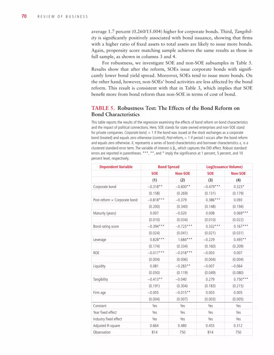
70 R E V I E W O F B U S I N E S S
average 1.7 percent (0.260/15.004) higher for corporate bonds. Third, Tangibil-ity is significantly positively associated with bond issuance, showing that firms with a higher ratio of fixed assets to total assets are likely to issue more bonds. Again, propensity score matching sample achieves the same results as those in full sample, as shown in columns 3 and 4.
For robustness, we investigate SOE and non-SOE subsamples in Table 5. Results show that after the reform, SOEs issue corporate bonds with signifi-cantly lower bond yield spread. Moreover, SOEs tend to issue more bonds. On the other hand, however, non-SOEs’ bond activities are less affected by the bond reform. This result is consistent with that in Table 3, which implies that SOE benefit more from bond reform than non-SOE in terms of cost of bond.
TABLE 5. Robustness Test: The Effects of the Bond Reform on Bond Characteristics This table reports the results of the regression examining the effects of bond reform on bond characteristics and the impact of political connections. Here, SOE stands for state owned enterprises and non-SOE stand for private companies. Corporate bondi = 1 if the bond was issued at the stock exchanges as a corporate bond (treated) and equals zero otherwise (control); Post-reformt = 1 if period t occurs after the bond reform and equals zero otherwise. Xi represents a series of bond characteristics and borrower characteristics. ei is a clustered standard error term. The variable of interest is b1, which captures the DID effect. Robust standard errors are reported in parentheses. ***, **, and * imply the significance at 1 percent, 5 percent, and 10 percent level, respectively.
Dependent Variable Bond Spread Log(Issuance Volume)
SOE Non-SOE SOE Non-SOE
(1) (2) (3) (4)
Corporate bond −0.318** −0.600** −0.479*** 0.323*
(0.158) (0.269) (0.131) (0.179)
Post-reform × Corporate bond −0.818*** −0.379 0.386*** 0.093
(0.200) (0.340) (0.148) (0.194)
Maturity (years) 0.007 −0.020 0.008 0.069***
(0.010) (0.034) (0.010) (0.022)
Bond rating score −0.394*** −0.723*** 0.332*** 0.167***
(0.024) (0.041) (0.021) (0.031)
Leverage 0.828*** 1.684*** −0.229 0.493**
(0.174) (0.334) (0.160) (0.209)
ROE −0.017*** −0.018*** −0.003 0.007
(0.004) (0.006) (0.004) (0.004)
Liquidity 0.081 −0.283** −0.007 −0.064
(0.050) (0.119) (0.049) (0.080)
Tangibility −0.413** −0.040 0.279 0.750***
(0.191) (0.304) (0.183) (0.215)
Firm age −0.005 −0.015** 0.003 0.005
(0.004) (0.007) (0.003) (0.005)
Constant Yes Yes Yes Yes
Year fixed effect Yes Yes Yes Yes
Industry fixed effect Yes Yes Yes Yes
Adjusted R-square 0.664 0.480 0.455 0.312
Observation 814 750 814 750

T H E R E A L E F F E C T O F F I N A N C I A L R E F O R M : E V I D E N C E F R O M B O N D M A R K E T I N C H I N A 71
Effects of the Reform on Cost of Debt
We use the listed firm–level dataset to further test how the bond reform affects firms’ cost of debt. The dataset covers 2,500 listed firms on China A-Shares market across 17 industries. Table 6 presents the list of industries and market capitalization. Table 7 reports the baseline results using the firm-level approach. We label the SOEs as the treated group and the non-SOEs as the control group. The After variable refers to the period after financial reforms (2015 and 2016), and Before refers to the period before financial reforms (2013 and 2014). We next collapse the data into single data points (based on average value) both before and after, which results in two data points per firm, one for the pre-re-form period and the other for the post-reform period. In Panel A, we report the before-after results for the variable Cost of debt. As shown, surrounding the re-form period, the average cost of debt for all the listed firms fell by approximately 0.26 percent, and the cost of the SOEs dropped more than that of the non-SOEs by approximately 0.4 percent.
TABLE 6. List of Industries and Market Capitalization
Industry Code
Industries Number of Listed Companies by 2016
Market Capitalization by 2016 (billion RMB)
1 Primary (agriculture) industry 39 1,653
2 Mining 69 62,110
3 Manufacturing 1,579 170,415
4 Electricity, gas, and water 93 29,833
5 Architecture 68 58,425
6 Wholesale and retail trade 140 20,822
7 Transport, storage, and post 79 23,609
8 Accommodations and restaurants 10 781
9 Information, transmission, computer science, and software
156 13,641
10 Real estate 123 57,268
11 Leasing and business service 33 5,392
12 Scientific research and technology service
17 599
13 Water, environment, and public service
27 2,874
14 Education 2 57
15 Health and social service 6 266
16 Culture, sports, and entertainment 35 2,616
17 Others 24 1,363
TOTAL 2,500 451,723
Source: WIND database, https://www.wind.com.cn/.
Next, we show that these patterns are statistically robust to the application of standard regression analysis. In addition, to control for firm-level heteroge-neity, we use firm fixed effect in all regressions and year fixed effect as well to control for aggregate external shocks, such as the economic downturn. In Table 8 on page 73, in columns 1 to 4, we investigate the effects of the bond reform

72 R E V I E W O F B U S I N E S S
TABLE 7. Empirical Strategy: DIDThis table introduces the basic empirical strategy. We divide firms (by industry) into two groups based on a measure of state ownership (SOE or non-SOE). The SOE group is the treated group whereas non-SOEs form the control group. After refers to the period after the bond reform in 2015. Before refers to the period before the reform. In this panel, we report the before-after results for cost of debt. Robust standard errors are reported in parentheses. ***, **, and * imply the significance at 1 percent, 5 percent, and 10 percent level, respectively.
Before After Difference Observation
Cost of Debt
Bond Issuance Reform (2013 to 2016)
SOE 0.0556 0.0516 −0.0051*** 3,606
(0.0006) (0.0006) (0.0009)
Non-SOE 0.0536 0.0526 −0.0010 6,093
(0.0006) (0.0005) (0.0008)
Difference −0.0040*** 10,000
(0.001)
on the Cost of debt using DID strategy. As reported in columns 1 and 2, the interaction term of Post-reform dummy and the group dummy enters negatively and statistically significantly, suggesting that the bond reform reduces the cost of debt during this period in the treatment group (SOE) relative to that in the control group (non-SOE). In terms of economic magnitude, the reform reduces the cost of debt significantly by approximately 7.4 percent (0.004/0.054).9 As also shown in Figure 3, the cost of debt was actually decreasing for both SOEs and non-SOEs during the period of economic growth and the loosened mone-tary policy. The benchmark lending interest rate went down from 6.00 percent to 4.75 percent and the SHIBOR overnight rate descended from 2.77 percent to 2.01 percent from 2014 to 2015. However, the cost of debt of the SOEs has been decreasing more significantly than that of the non-SOEs, suggesting that the bond reform causally reduced the cost of debt. Critically, to isolate the in-dependent relationship between the reform and the cost of debt, the analyses in Table 8 also control for more potential explanatory factors, as shown in column 2, and the results still hold.
Then in columns 3 and 4, we further control for the interaction of Liquid-ity or ROE and Post-reform dummy, and the results change little. However, the interactions all enter with statistically insignificant signs, suggesting that both before and after the reform, these firm factors do not have significant associa-tion with firms’ cost of debt. In addition, in Figure 4 on page 74, we plot the Epanechnikov kernel densities of cost of debt for both the treatment and con-trol groups before and after the bond issuance reform from 2013 to 2016. The figures show that there is a leftward shift for the kernel density for both groups after the reform. Furthermore, the shift in the density is more statistically signifi-cant for the control group because the Kolmogorov-Smirnov test for the equality of its distribution functions is rejected at the 1 percent level. These figures thus indicate that the bond reform causally reduce the cost of debt.
9In the listed firm–level dataset, the mean value of cost of debt in SOE group is 0.054.

T H E R E A L E F F E C T O F F I N A N C I A L R E F O R M : E V I D E N C E F R O M B O N D M A R K E T I N C H I N A 73
For robustness, we perform a DIDID check in columns 5 to 6 of Table 8. In the regressions, we still include firm and year fixed effects to control for het-erogeneity as well as other firm characteristics, such as firm size. In general, con-trolling for the triple interaction term among post-reform dummy, SOE group dummy, and firm characteristics changes the results very little, meaning that our baseline results still hold with the DIDID specification. First, the interaction term of Post-reform dummy and SOE dummy still enters negatively and statistically significantly, suggesting that the reform significantly reduced the cost of deb. Second, the triple interaction of Post-reform, the SOE dummy and Liquidity enters negatively but insignificantly, showing that SOEs with higher liquidity
TABLE 8. Effects of Financial Reforms on the Cost of DebtThis table reports results for the regression Cost of debtit 5 b1(di 3 pt) 1 b2 (di 3 pt 3 zi) 1 b3 3 Xit 1 al 1 dt 1 eit. The dependent variable is Cost of debt. Here, i indexes firm and t indexes time. al and dt are firm and time fixed effect respectively. di = 1 if unit is in treated group and equals zero otherwise; pt = 1 if period t occurs after treatment and equals zero otherwise. Xit represents a series of control variables, variables such as Net cash flow to revenue and ROE that can capture the cyclical factors. Zi represents a continuous variable that proxies for the characteristics of interest, such as profitability and liquidity reserves. ei is a clustered standard error term. We divide firms into two groups based on a measure of state ownership (SOE or non-SOE). The SOE group is the treated group whereas non-SOEs form the control group. b1 captures the DID effect and b2 captures the DIDID effect. Robust standard errors are reported in parentheses. ***, **, and * imply the significance at 1 percent, 5 percent, and 10 percent level, respectively.
Dependent Variable Cost of Debt
(1) (2) (3) (4) (5) (6)
Post-reform × SOE −0.004*** −0.004*** −0.004*** −0.003***
(0.001) (0.001) (0.001) (0.001)
Post-reform × Liquidity 0.003 0.003
(0.002) (0.003)
Post-reform × ROE 0.000 0.000
(0.000) (0.000)
Post-reform × SOE × Liquidity −0.001
(0.005)
Post-reform × SOE × ROE −0.000**
(0.000)
Liquidity 0.007*** 0.005** 0.005*
(0.002) (0.002) (0.003)
ROE −0.000** −0.000** −0.000**
(0.000) (0.000) (0.000)
SOE × Liquidity 0.000
(0.004)
SOE × ROE 0.000*
(0.000)
Other controls Yes Yes Yes Yes Yes Yes
Constant Yes Yes Yes Yes Yes Yes
Year fixed effect Yes Yes Yes Yes Yes Yes
Firm fixed effect Yes Yes Yes Yes Yes Yes
Adjusted R-square 0.028 0.032 0.029 0.026 0.032 0.029
Number of firms 2,441 2,441 2,441 2,441 2,441 2,441
Observation 9,699 9,696 9,696 9,696 9,696 9,699

74 R E V I E W O F B U S I N E S S
ratio do not show a significant advantage over SOEs with a lower liquidity ratio on the cost of financing. Third, the triple interaction of Post-reform, the SOE dummy and ROE enters negatively but statistically significantly, suggesting that after the reform, SOEs with higher profitability might have a lower cost of debt.
EFFECTS OF FINANCIAL REFORM ON DEBT CHARACTERISTICSOver the past decade, the leverage of listed SOEs has shown an upward trend and remained relatively high. It has been argued that Chinese SOEs currently have a high debt burden, which might pose a credit risk during a economic downturn in the near future. In this section, we further evaluate how more ac-cess to the bond market affects the debt characteristics of the listed sector in terms of leverage, debt structure, and maturity in the listed sector.
Financial Reforms and Leverage
Figure 5 shows the leverage of two firm groups, the listed SOEs and non-SOEs. It turns out that over the last decade, the leverage of all listed firms shows an up-ward trend from 2002 to 2010 and a downward trend since 2011. The leverage ratio decreased from approximately 65 percent in 2010 to 55 percent in recent years. Non-SOEs have lower leverage ratio than that of SOEs in the past years (Figure 5). This trend may be partly driven by the rapid development of the eq-
Before(2013–2014)
Before(2013–2014)
After(2015–2016)
25
20
15
Kern
el D
ensit
y
10
5
0
0 .05
Cost of Debt, SOE
.1 .15 0 .05
Cost of Debt, Non-SOE
SOE Group Non-SOE Group
.1 .15
25
20
15
Kern
el D
ensit
y
10
5
0
After(2015–2016)
FIGURE 4. Cost of Debt before and after the 2015 Bond Issuance Reform: 2013 to 2016
This figure depicts the Kernel density of the ratio of cost of debt for both the SOE (treatment) group and the non-SOE (control) group. Years spanned: 2013 to 2016.

T H E R E A L E F F E C T O F F I N A N C I A L R E F O R M : E V I D E N C E F R O M B O N D M A R K E T I N C H I N A 75
uity market. Apart from the policies in the banking sector and bond market, the government put forward a series of policies on the equity market to improve the market-financing mechanism. For instance, the equity market policies in recent years have included the establishment of the small- and medium-sized enter-prises (SME) sector in Shenzhen Stock Exchange (SZSE), the introduction of a sponsorship regime of IPOs instead of the quota regime, the non-tradable share issue reform, and the establishment of the growth enterprise market (GEM).
Table 9 presents the results for the effects of the reform on leverage, in terms of total debt divided by total assets and interest-bearing debt divided by total assets. In both regressions, we control for firm characteristics including Profit-ability and Tobin’s q adjusted, and year fixed effects as well. The interaction be-tween Post-reform dummy and group dummy poses significantly negative influ-ence on leverage and statistically insignificantly impact on interest bearing debt. It reveals that the reform has little significant effect on firms’ leverage in terms of debt level relative to total assets but no significant effect on interest bearing debt. This result might contradict the findings by Faulkender and Petersen (2006), which suggests that firms with access to bond markets have access to a greater supply of debt and thus are more highly leveraged. However, here we do not find significantly higher leverage after the bond reform which allows firms more access to the bond market.
Financial Reforms and Debt Structure
In Table 10 on page 77, we further examine how the reform affects the debt structure. We use bond book value divided by debt book value and bond book value divided by the total amount of bonds and loans as the dependent variable,
35%
40%
45%
50%
55%
60%
65%
70%
75%
SOE Mean
SOE Median
Non-SOE Mean
Non-SOE Median
2002
2003
2004
2005
2006
2007
2008
2009
2010
2011
2012
2013
2014
2015
2016
2017
2018
2019
FIGURE 5. Corporate Leverage for the Listed Sector: 2002 to 2019
Here, we plot the ratio of corporate leverage from 2002 to 2019. Corporate leverage is defined as the ratio of total liabilities to total assets. We also check with the ratio of total interest-bearing debts to total assets and it shows a similar trend with the ratio of total liabilities to total assets.
Source: WIND database, https://www.wind.com.cn/.

76 R E V I E W O F B U S I N E S S
respectively. The interaction all enters with significantly positive sign in the re-gression with bond issuance or bond value as the dependent variable, indicating that with the weakening of supply-side frictions of the corporate bond market, firms are showing a shift from bank loans to public debt. The results are robust no matter which measure we use for the bond value. This finding is also consis-tent with the literature on ownership structure and debt choice. Lin et al. (2013) argues that firms with a greater divergence between the control rights and cash-flow rights of the largest ultimate owner tend to rely more strongly on public debt financing than on bank loan debt as a way of avoiding scrutiny and insu-lating themselves from bank monitoring. Moreover notably, adjusted Tobin’s q also enters with a positive sign significantly at the 1 percent level, indicating that firms with higher equity market value relative to the replacement value may also choose to issue bonds instead of bank loans.
Financial Reforms and Debt Maturity
Next, we explore the effect of the bond reform on debt maturity. In Table 11 on page 78, columns 1 and 2 show the effect of the reforms on debt maturity in terms of long-term debt and short-term debt as a percentage of total liabilities. In a similar vein, we control for firm characteristics in the regressions. The results show that after the bond reform the SOEs issued more short-term debt than long-term debt. In terms of economic magnitude, the short-term debt ratio has
TABLE 9. Effects of the Financial Reforms on LeverageThis table reports results for the regression Leverageit 5 b1(di 3 pt) 1 b2 3 Xit 1 ai 1 dt 1 eit. The dependent variable is Leverage. Here, i indexes firm and t indexes time. ai and dt are firm and time fixed effect respectively. di = 1 if unit is in treated group and equals zero otherwise; pt = 1 if period t occurs after treatment and equals zero otherwise. Xit represents a series of control variables, variables such as EBIT to asset and Tobin’s q adjusted that can capture firm characteristics. eit is a clustered standard error term. We divide firms into two groups based on a measure of state ownership (SOE or non-SOE). The SOE group is the treated group whereas non-SOEs form the control group. The variable of interest is b1, which captures the DID effect. Robust standard errors are reported in parentheses. ***, **, and * imply the significance at 1 percent, 5 percent, and 10 percent level, respectively.
Dependent Variable Leverage (Total Debt/Total Assets)
Interest Bearing Debt/Total Assets
(1) (2)
Post-reform × SOE −0.017* −0.001
(0.009) (0.008)
EBIT/asset 1.390*** 0.816***
(0.108) (0.150)
Tobin’s q adjusted −27.420*** −5.442*
(3.347) (2.931)
Other controls Yes Yes
Constant Yes Yes
Year fixed effect Yes Yes
Firm fixed effect Yes Yes
Adjusted R-square 0.417 0.215
Number of firms 2,499 2,440
Observation 9,996 9,695

T H E R E A L E F F E C T O F F I N A N C I A L R E F O R M : E V I D E N C E F R O M B O N D M A R K E T I N C H I N A 77
been increased by approximately 7.4 percent, whereas the long-term debt ratio has been insignificantly increased by approximately 1.2 percent. The traditional theory on debt maturity (such as Barclay and Smith 1995) suggests that firms use the maturity of their debt to signal information to the market, that is, firms with more information asymmetries issue more short-term debt. It also consistent with the U.S. trend shown by Custodio, Ferreira, and Laureano (2013), which indicates that the public debt market supply side factor plays an important role in explaining why over the past three decades U.S. firms have been issuing more shorter-term debt than longer-term debt.
More Robustness Tests
To extend our firm-level research, we use bond issuer sample rather than listed firm sample to test the effect of bond reform on the cost of bond and the per-centage of bond issuance in total assets. This refined focus provides us 1562 bond issuers in our sample. Table 12 on page 79 presents the results of DIDID. In the regression, we include firm fixed effect to control for heterogeneity as well. Unlisted dummy equals 1 if the firm is unlisted and 0 otherwise. Small dummy equals 1 if firm’s logarithm of total assets is below the sample mean from 2014.
TABLE 10. Effects of the Financial Reforms on Debt Structure: Loans or Bond?This table reports results for the regression Debt Structureit 5 b1(di 3 pt) 1 b2 3 Xit 1 ai 1 dt 1 eit. The dependent variable is Loan granted to total assets or Bond issuance to total assets, or the Book value of bond to total debt. Here, i indexes firm and t indexes time. ai and dt are firm and time fixed effect respectively. di = 1 if unit is in treated group and equals zero otherwise; pt = 1 if period t occurs after treatment and equals zero otherwise. Xit represents a series of control variables, variables such as EBIT to asset and Tobin’s q adjusted that can capture firm characteristics. eit is a clustered standard error term. We divide firms into two groups based on a measure of state ownership (SOE or non-SOE). The SOE group is the treated group whereas non-SOEs form the control group. The variable of interest is b1, which captures the DID effect. Robust standard errors are reported in parentheses. ***, **, and * imply the significance at 1 percent, 5 percent, and 10 percent level, respectively.
Dependent Variable Bond Value/Total Debt Bond Value/(Bond Value + Loans Granted)
(1) (2)
Post reform × SOE 0.266*** 0.032***
(0.069) (0.011)
EBIT/asset 4.477*** −0.059
(1.160) (0.073)
Tobin’s q adjusted 171.600*** 7.302***
(46.080) (2.283)
Other controls Yes Yes
Constant Yes Yes
Year fixed effect Yes Yes
Firm fixed effect Yes Yes
Adjusted R-square 0.170 0.057
Number of firms 949 943
Observation 3,541 3,511

78 R E V I E W O F B U S I N E S S
We don’t control year fixed effect here because we put Post-reform in our re-gression and want to investigate the coefficient of this term. From columns 1 to 4, the interaction terms of the post-reform dummy and group dummies (namely Unlisted dummy, Small firm dummy, and SOE dummy) enter significantly neg-atively, suggesting that the bond reform decreases the cost of debt significantly for unlisted firms, small firms, and SOEs. Statistically significantly coefficients of the triple interactions of Post-reform, unlisted dummy, and the other two group dummies imply that unlisted small firms or unlisted SOEs are more sensitive to bond reform. One interpretation of this result is that unlisted firms were not allowed to issue bonds in the exchange market before the reform. Hence their cost of debt has been significantly decreased after the reform due to corporate bond issuance. On the other hand, although unlisted firms have been allowed to issue bonds publicly after the reform, the potential issuers still need to get ap-proved by the CSRC. The regulator prefers firm with good quality, which can be implied by firm size and state-ownership. Columns 6 to 10 show that firms issue more bonds after the reform and such effect is more significant for large firms, especially for large unlisted firms. A possible explanation is that the enterprise bond issuers, who are mostly large unlisted firms, have switched to the exchange market (corporate bond market) after the reform. However, the shortcoming of
TABLE 11. Effects of the Bond Issuance Reform on Debt MaturityThis table reports results for the regression Debt maturityit 5 b1(di 3 pt) 1 b2 3 Xit 1 ai 1 dt 1 eit. The dependent variable is bond maturity in terms of Long-term bond issuance to total assets or Short-term bond issuance to total assets, or debt maturity in terms of Long-term debt ratio or Short-term debt ratio. Here, i indexes firm and t indexes time. ai and dt are firm and time fixed effect respectively. di = 1 if unit is in treated group and equals zero otherwise; pt = 1 if period t occurs after treatment and equals zero otherwise. Xit represents a series of control variables, variables such as EBIT to asset, etc., that can capture firm characteristics. eit is a clustered standard error term. We divide firms into two groups based on a measure of state ownership (SOE or non-SOE). The SOE group is the treated group whereas non-SOEs form the control group. The variable of interest is b1, which captures the DID effect. Robust standard errors are reported in parentheses. ***, **, and * imply the significance at 1 percent, 5 percent, and 10 percent level, respectively.
Dependent Variable Short Term Debt/Total Liabilities Long Term Debt/Total Liabilities
(1) (2)
Post-reform × SOE 0.074*** 0.012
(0.022) (0.011)
EBIT/asset
2.758*** 0.562***
(0.240) (0.120)
Tobin’s q adjusted −10.310 10.890**
(7.922) (5.043)
Other controls Yes Yes
Constant Yes Yes
Year fixed effect Yes Yes
Firm fixed effect Yes Yes
Adjusted R-square 0.272 0.174
Number of firms 2,499 2,491
Observation 9,996 9,957

T H E R E A L E F F E C T O F F I N A N C I A L R E F O R M : E V I D E N C E F R O M B O N D M A R K E T I N C H I N A 79
using bond issuer data is that we can’t exclude the impact of the enterprise bond issuers.
To verify the above possible explanation and to solve the dataset drawbacks, we narrow the bond issuers’ full sample down to the switching sample, which contains companies that only issue enterprise bond before the bond reform and switch to issue both enterprise bond and corporate bond after the reform. The switching sample comprises 67 firms and they issued 328 bonds in total from 2007 to 2016. To be specific, they issued 187 enterprise bonds before the reform and 141 corporate bonds after the reform. In the switching sample, 95.08 per-cent of the firms are unlisted firms and 63.93 percent are SOEs. It is consistent with our inference that most switching firms are unlisted firms. In Panel B of Table 13, significantly negative sign of Post-reform represents that bond reform does economically reduce bond yield spread. SOE enters with a statistically sig-nificantly negative sign indicating that bond reform is more beneficial for SOEs.
TABLE 12. Effects of the Bond Reform on Bond Issuer CharacteristicsThis table reports results for the regression on the effects of the bond reform on bond issuers’ characteristics. Robust standard errors are reported in parentheses. ***, **, and * imply the significance at 1 percent, 5 percent, and 10 percent level, respectively.
Dependent Variable Cost of Debt (Bond Issuer) Bond Issuance/Total Assets (Bond Issuer)
(1) (2) (3) (4) (5) (6) (7) (8) (9) (10)
Post-reform 0.003 −0.001 0.001 −0.001 0.001 0.055*** 0.022*** 0.047*** 0.021*** 0.048***
(0.003) (0.001) (0.002) (0.001) (0.001) (0.013) (0.007) (0.010) (0.007) (0.010)
Post-reform × Unlisted
−0.006* −0.039***
(0.003) (0.013)
Post-reform × Small
−0.005** −0.033**
(0.002) (0.014)
Post-reform × SOE
−0.005*** −0.041***
(0.002) (0.010)
Post-reform × Unlisted × Small
−0.005** −0.035**
(0.002) (0.015)
Post-reform × Unlisted × SOE
−0.004*** −0.044***
(0.002) (0.010)
Log (Coverage)
−0.015*** −0.015*** −0.015*** −0.015*** −0.015*** −0.011* −0.014** −0.012* −0.014** −0.013**
(0.002) (0.002) (0.002) (0.002) (0.002) (0.007) (0.006) (0.006) (0.006) (0.006)
Log (Firm age)
−0.013 −0.013 −0.012 −0.012 −0.012 −0.004 0.001 0.011 0.005 0.018
(0.009) (0.008) (0.009) (0.008) (0.009) (0.065) (0.067) (0.065) (0.067) (0.065)
Constant Yes Yes Yes Yes Yes Yes Yes Yes Yes Yes
Year fixed effect
No No No No No No No No No No
Firm fixed effect
Yes Yes Yes Yes Yes Yes Yes Yes Yes Yes
Adjusted R-square
0.277 0.282 0.281 0.282 0.281 0.132 0.157 0.211 0.160 0.229
Observation 1,732 1,732 1,732 1,732 1,732 637 637 637 637 637

80 R E V I E W O F B U S I N E S S
TABLE 13. Robustness: Switching SamplePanel A: Summary Statistics of Bond CharacteristicsThe switching sample comprises 67 firms that issued 328 bonds in total from 2007 to 2016. Issuers in switching sample are selected based on this criteria: They only issued enterprise bond before bond reform and began to issue corporate bond after reform. In the switching sample, 95.08 percent of the firms are unlisted firms and 63.93 percent are SOEs.
BeforeObservation Mean Standard Deviation Minimum Maximum
Bond rating score 187 7.610 1.337 6 9Leverage 187 0.643 0.125 0.164 0.819Tangibility 187 0.311 0.217 0.002 0.573Liquidity 176 0.081 0.497 −2.837 1.806Firm age 187 11.604 6.357 1 28Firm size 187 10.970 1.304 8.140 12.512
AfterObservation Mean Standard Deviation Minimum Maximum
Bond rating score 141 7.745 1.284 6 9Leverage 141 0.653 0.118 0.188 0.819Tangibility 141 0.222 0.198 0.000 0.573Liquidity 141 0.087 0.454 −2.837 1.492Firm age 141 16.716 5.975 5 31Firm size 141 11.293 0.967 9.141 12.512
Panel B: Effects of the Bond Reform on Bond Yield Spread Using the Switching SampleThis table reports the results of switching sample for the regression Bond Yield Spreadi 5 b1(Post-reformt) 1 b2 3 Xi 1 a1 1 ei. The dependent variable is the at-issue bond yield spread. Here, i indexes bond and t indexes time. a1 is industry dummy. Post-reformt = 1 if period t occurs after the bond reform and equals zero otherwise. Xi represents a series of bond characteristics and borrower characteristics. ei is a clustered standard error term. The variable of interest is b1, which captures the time effect. Robust standard errors are reported in parentheses. ***, **, and * imply the significance at 1 percent, 5 percent, and 10 percent level, respectively.
Dependent Variable Bond Spread
(1) (2)Post-reform −0.985*** −1.015***
(0.101) (0.113)Bond rating score −0.588*** −0.549***
(0.047) (0.054)Log(Issuance volume) −0.039 −0.100
(0.070) (0.071)Maturity (years) 0.040*** 0.062***
(0.012) (0.012)SOE −0.507*** −0.604***
(0.119) (0.132)Leverage −0.039
(0.415)ROE −0.014
(0.009)Liquidity −0.133
(0.091)Tangibility −0.145
(0.364)Firm age 0.006
(0.008)Constant Yes YesYear fixed effect No NoIndustry fixed effect Yes YesAdjusted R-square 0.748 0.761Observation 328 317

T H E R E A L E F F E C T O F F I N A N C I A L R E F O R M : E V I D E N C E F R O M B O N D M A R K E T I N C H I N A 81
CONCLUSIONThe results reported in this paper provide new insights concerning the effects of financial reform on the cost of debt and firms’ debt structure using the evidence from the private bond market. In general, there has been rich literature on the relationship between equity market liberalization or overall financial develop-ment and economic growth, however, very few studies focus on the private bond market. This paper fills the gap on this.
Using the policy shock of China’s bond issuance reform, which basically changes the issuance procedure of corporate bond from an approval-based sys-tem to one very close to registering-based system, we find that the reform sig-nificantly reduces the cost of debt. The reform is essentially motivated by the competition and interest conflicts among different regulators, hence it provides a unique setting to study the real effect of bond market liberalization, which is less likely to suffer from the reverse causality issue. The bond-level results show that the reform reduces the cost of bond financing in terms of bond yield spread by approximately 29.4 percent and enhances the bond issuance volume by approximately 1.7 percent. Using propensity score matched sample in order to address the potential endogeneity problem makes the results stay constant. At the listed firm-level, the reform reduces the cost of total debt by around 7.4 per-cent, enhances the public debt issuance instead of the private debt, and shortens the debt maturity. Robustness checks such as DIDID and subsample tests do not change our main results.
The main implication of this paper is that the liberalization of the public debt market reduces the cost of debt and alleviates financial constraints. Further-more, with less friction in the public debt market, firms issue more public debt, i.e., bond, instead of private debt, i.e., bank loan, and more short-term debt. The effect is more significant for politically connected firms with more concentrated ownership, indicating that they may use it as a way to insulate from bank mon-itoring.
ReferencesAbiad A., and A. Mody. 2005. “Financial Reform: What Shakes It? What Shapes It?”
American Economic Review 95, no. 1, 66–88.Acharya, V. V., and S. Steffen. 2015. “The ‘Greatest’ Carry Trade Ever? Understanding
Eurozone Bank Risks.” Journal of Financial Economics 115, no. 2, 215–36.Acharya, V. V., J. Qian, and Z. Yang. 2021. In the Shadow of Banks: Wealth Manage-
ment Products and Bank Risk in China. NYU Stern School of Business working paper.
Allen, F., and D. Gale. 1999. “Bubbles, Crises and Policy.” Oxford Review of Economic Policy 15, no. 3, 9–18.
Allen, F., and D. Gale. 2000. “Bubbles and Crises.” The Economic Journal 110, no. 460, 236–55.
Allen, F., J. Qian, and X. Gu. 2015. “China’s Financial System: Growth and Risks.” Foundations and Trends in Finance 9, no. 3–4, 197–319.
Allen, F., J. Qian, and M. Qian. 2005. “Law, Finance and Economic Growth in China.” Journal of Financial Economics 77, no. 1, 57–116.
Allen, F., J. Qian, C. Zhang, and M. Zhao. 2010. China’s Financial System: Opportuni-ties and Challenges. National Bureau of Economic Research (NBER) working paper no. 17828.

82 R E V I E W O F B U S I N E S S
Ayyagari, M., A. Demirguc-Kunt, and V. Maksimovic. 2010. “Formal versus Informal Finance: Evidence from China.” Review of Financial Studies 23, no. 8, 3048–97.
Baker, M., J. Stein, and J. Wurgler. 2003. “When Does the Market Matter? Stock Prices and the Investment of Equity-Dependent Firms.” Quarterly Journal of Economics 118, no. 3, 969–1005.
Barclay, M. J., and C. W. Smith. 1995. “The Maturity Structure of Corporate Debt.” Journal of Finance 50, no. 2, 609–31.
Bekaert, G., and C. R. Harvey. 2000. “Foreign Speculators and Emerging Equity Mar-kets.” Journal of Finance 55, no. 2, 565–613.
Bekaert, G., C. R. Harvey, and C. Lundblad. 2005. “Does Financial Liberalization Spur Growth?” Journal of Financial Economics 77, no. 1, 3–56.
Bekaert, G., C. R. Harvey, C. Lundblad, and S. Siegel. 2007. “Growth Opportunities and Market Integration.” Journal of Finance 62, no. 3, 1081–137.
Berk, J., R. Green, and V. Naik. 1999. “Optimal Investment, Growth Options, and Secu-rity Returns.” Journal of Finance 54, no. 5, 1553–1607.
Bessembinder, H., K. M. Kahle, W. F. Maxwell, and D. Xu. 2009. “Measuring Abnormal Bond Performance.” Review of Financial Studies 22, no. 10, 4219–58.
Billett, M. T., T. D. King, and D. C. Mauer. 2004. “Bondholder Wealth Effects in Merg-ers and Acquisitions: New Evidence from the 1980s and 1990s.” Journal of Finance 59, no. 1, 107–35.
Broner, F., and J. Ventura. 2011. “Globalization and Risk Sharing.” Review of Economic Studies 78, no. 1, 49–82.
Chatterjee, S., X. Gu, and I. Hasan. 2019. Ownership Structure and the Cost of Debt: Evidence from Chinese Corporate Bond Market. Fordham University working paper.
Custodio, C., M. A. Ferreira, and L. Laureano. 2013. “Why Are U.S. Firms Using More Short-Term Debt?” Journal of Financial Economics 108, no. 1, 182–212.
Didier, T., and S. L. Schmukler. 2013. “The Financing and Growth of Firms in China and India: Evidence from Capital Markets.” Journal of International Money and Finance 39, no. C, 111–37.
Faulkender, M., and M. A. Petersen. 2006. “Does the Source of Capital Affect the Capi-tal Structure?” Review of Financial Studies 19, no. 1, 45–79.
Fisman, R., and I. Love. 2003. “Trade Credit, Financial Intermediary Development and Industry Growth.” Journal of Finance 58, no. 1, 353–74.
Guariglia, A., and S. Poncet. 2006. “Could Financial Distortions Be No Impediment to Economic Growth After All? Evidence from China.” Journal of Comparative Eco-nomics 36, no. 4, 633–57.
Gupta, N., and K. Yuan. 2009. “On the Growth Effect of Stock Market Liberalizations.” Review of Financial Studies 22, no. 11, 4715–52.
He, Z., and M. Amstad. 2019. Chinese Bond Market and Interbank Market. NBER working paper no. 25549.
Henry, P. B. 2000a. “Do Stock Market Liberalizations Cause Investment Booms.” Jour-nal of Financial Economics 58, no. 1–2, 301–34.
Henry, P. B. 2000b. “Stock Market Liberalization, Economic Reform, and Emerging Market Equity Prices.” Journal of Finance 55, no. 2, 529–63.
Kaminsky, G. L., and S. L. Schmukler. 2008. “Short-Run Pain, Long-Run Gain: Financial Liberalization and Stock Market Cycles.” Review of Finance 12, no. 2, 253–92.
Laeven, L. 2003. “Does Financial Liberalization Reduce Financing Constraints?” Finan-cial Management 32, no. 1.
Levchenko, A. A. 2005. “Financial Liberalization and Consumption Volatility in Devel-oping Countries.” IMF Staff Papers 52, no. 2, 237–59.
Levchenko, A. A., R. Ramciere, and M. Thoenig. 2009. “Growth and Risk at the In-dustry Level: The Real Effects of Financial Liberalization.” Journal of Development Economics 89, no. 2, 210–22.
Lin, C., Y. Ma, P. Malatesta, and Y. Xuan. 2011. “Ownership Structure and the Cost of Corporate Borrowing.” Journal of Financial Economics 100, no. 1, 1–23.

T H E R E A L E F F E C T O F F I N A N C I A L R E F O R M : E V I D E N C E F R O M B O N D M A R K E T I N C H I N A 83
Lin, C., Y. Ma, P. Malatesta, and Y. Xuan. 2013. “Corporate Ownership Structure and the Choice Between Bank Debt and Public Debt.” Journal of Financial Economics 109, no. 2, 517–34.
McLean, R. D., T. Zhang, and M. Zhao. 2012. “Why Does the Law Matter? Investor Protection and Its Effect on Investment, Finance, and Growth.” Journal of Finance 67, no. 1, 313–50.
Nabar, M., and K. Yan. 2013. Sector-Level Productivity, Structural Change, and Rebal-ancing in China. International Monetary Fund (IMF) working paper 13/240.
Qian, (QJ) J., P. E. Strahan, and Z. Yang. 2015. “The Impact of Incentives and Commu-nication Costs on Information Production: Evidence from Bank Lending.” Journal of Finance 70, no. 4, 1457–93.
Rajan, R. G., and L. Zingales. 1998. “Financial Dependence and Growth.” American Economic Review 88, no. 3, 559–86.
Reuters. 2015, July 15. “China defaults to rise as corporate debt burden climbs: S&P.” http://www.reuters.com/article/us-china-s-p-idUSKCN0PQ05K20150716.
Roberts, M. R., and A. Sufi. 2009. “Financial Contracting: A Survey of Empirical Re-search and Future Directions.” Annual Review of Financial Economics 1, no. 1, 207–26.
Scheneider, M., and A. Tornell. 2004. “Balance Sheet Effects, Bailout Guarantees, and Financial Crises.” Review of Economic Studies 71, no. 7, 883–913.
Song, Z., K. Storesletten, and F. Zilibotti. 2011. “Growing Like China.” American Eco-nomic Review 101, no. 1, 196–233.
Tornell, A., and F. Westermann. 2005. Boom-Bust Cycles and Financial Liberalization. Cambridge, MA: MIT Press.
Vig, V. 2013. “Access to Collateral and Corporate Debt Structure: Evidence from a Nat-ural Experiment.” Journal of Finance 68, no. 3, 881–928.
Wind database. n.d. Wind Information Technology Co., Ltd. https://www.wind.com.cn/.Yao, Y., and L. Yueh. 2009. “Law, Finance, and Economic Growth in China: an Intro-
duction.” World Development 37, no. 4, 753–62.Zhang, J., L. Wang, and S. Wang. 2012. “Financial Development and Economic Growth:
Recent Evidences from China.” Journal of Comparative Economics 40, no. 3, 393–
412.

84 R E V I E W O F B U S I N E S S
APPENDIX A1. All Types of Corporate Bond Sectors in ChinaThis table reports the regulator, regulatory system, the issuing entities, and offering methods in different sectors of corporate bond markets in China.
Sector Regulator Regulatory System Issuing Entity Offering Method
SME corporate bond
SSE; SZSE Filing system Medium-sized, small-sized, or micro-sized unlisted firms
Privately
Corporate bond CSRC Approval-based system Listed firms Publicly
Enterprise bond NDRC Approval-based system Unlisted firms, enterprises
Publicly
Commercial papers and mid-term notes
NAFMII* Registering system Non-financial firms Publicly
Private placement notes
NAFMII Registering system Non-financial firms Privately
*NAFMII is the National Association of Financial Market Institutional Investors.
APPENDIX A2. The Bond Issuance Reform in 2015This table compares the main changes in the issuance of corporate bonds between pre-reform period (before January 15, 2015) and post-reform period (after January 15, 2015).
Pre-Reform Post-Reform
An approval-based issuance system (similar with IPO system)
Still based on approval case by case
Sponsorship regime (investment banks responsible for the due diligence and filings)
Sponsorship regime removed
Reviews by the Issuance Scrutiny Committee in the CSRC
Issuance Scrutiny Committee regime removed
Only listed firms can issue bonds in the corporate bond sector (not including the SME sector)
All firms in the organization of companies can issue bonds in the corporate bond sector

85
Work Environment and Employee Performance: Evidence from Sell-Side Analysts
Shuya Liu
Kevin Sun
AbstractMotivation: While there is ample evidence that work environment quality is positively related to firm performance, there is limited evidence on whether the positive relation between work environment and firm performance is due to the claim that employees’ satisfaction with their work environment increases their job performance. We attempt to fill in this void by investigating how stock ana-lysts’ rating of work environment is related to their job performance.
Premise: We examine whether analysts in a better-rated work environment ex-pend more efforts, are more capable, and have high-quality stock recommenda-tions.
Approach: We use Glassdoor ratings as a proxy for employee satisfaction of work environment. Glassdoor.com is a website where current and past employ-ees can rate their overall work environment and provide feedback about their firms. We regress analysts forecast accuracy, forecast frequency, and stock mar-ket reaction to analysts’ buy/sell recommendation on Glassdoor ratings, and the squared term of Glassdoor ratings.
Results: We find that in better-rated brokerage firms, analysts issue more fre-quent and more accurate earnings forecasts, and their stock recommendations produce a larger stock market reaction. The coefficient on the squared term of Glassdoor rating is negative, indicating a concave relationship between work environment quality and job performance. We also find that this nonlinear rela-tionship only exists after an analyst works for a brokerage firm for at least two years. In addition, highly rated brokerages have better analyst retention and a lower percentage of employee turnover.
Conclusion: We find that out of five subcategories of work environment ratings, Career Opportunities and Culture & Values have consistently demonstrated their positive impact on analyst job performance. Our research demonstrates long-term benefits of investing in employees.
Rev
iew
of
Bus
ines
s 41
, no.
2, 8
5–11
7. C
opyr
ight
© 2
021
St. J
ohn’
s U
nive
rsit
y.
Shuya Liu, MS, St. John’s University, [email protected]
Kevin Sun, PhD, St. John’s University, [email protected]

86 R E V I E W O F B U S I N E S S
Consistency: Our research contributes to the literature on environment, sustain-ability, and governance (ESG) and labor economics. The findings indicate the need to spend on improving work environments that may improve employee performance.
Keywords: analysts forecast, analyst recommendation, forecast accuracy, fore-cast frequency, work environment
JEL Classification Codes: J24, G24
“Train people well enough so they can leave, treat them well enough so they don’t want to.”
—Sir richard BranSon
INTRODUCTIONIn recent management and labor economics literature, employees are increas-ingly viewed as firms’ intangible assets that can create new products, improve current products, and build strong customer relationships (Rajan and Zingales 1998; Zingales 2000; Carlin and Gervais 2009; Berk, Stanton, and Zechner 2010). Another stream of research shows that work environment can directly impact a firm’s profitability and competitive advantage, as well as firms’ stock market valuations (Edmans 2011; Green et al. 2019). While there is ample evi-dence that work environment quality is positively related to firm performance, there is limited evidence on whether the positive relation between work environ-ment and firm performance is due to the claim that employees’ satisfaction with their work environment increases their job performance.
We attempt to fill in this void by investigating how stock analysts’ rating of work environment is related to their job performance. Work environment is multi-dimensional. We define a satisfactory work environment as a workplace whose employees have many career upside opportunities, are well compensated with pay and benefits, are led by competent senior management, enjoy work/life balance, and can fit well with corporate culture and values. We examine each of these dimensions in this paper.
We use financial analysts in this study because the most important asset in this type of firm is human capital. Analyst reports and recommendations are highly skilled tasks created by each individual analyst; these reports and rec-ommendations can improve brokerage firms’ reputations and help to increase investment banking and trading revenues. Because these reports and their impact on the stock market are a publicly observable job output, our research presents a powerful setting to test the effect of work environment on job performance. Spe-cifically, we hypothesize that stock analysts in highly rated work environments expend more effort in their work; therefore, they are more capable of forecasting earnings and ultimately produce more impactful stock recommendations.
Prior studies argue that work environment affects job performance in three ways: recruiting, motivation, and retention. First, firms with a good reputation of treating employees well are likely to attract high-caliber job seekers (Belt and Paolillo 1982; Bretz and Judge 1994; Rau and Hyland 2002; Foster Thompson and Aspinwall 2009). Firms compete against each other not only in product and service markets, but also in the recruiting market for the best talent for bringing

W O R K E N V I R O N M E N T A N D E M P L O Y E E P E R F O R M A N C E : E V I D E N C E F R O M S E L L - S I D E A N A L Y S T S 87
success and profits to their firms. The information about a firm’s employee mo-rale and job satisfaction is widely spread by word of mouth, social media, and headhunters. Therefore, firms reputed to have pleasant work environments are more likely to receive a larger number of qualified applications than firms with worse reputations for the same job opening. In addition, potential recruits can get first-hand knowledge about a firm’s work environment during on-site inter-views. As a result, the recruiting process for firms that treat employees well and have a good work environment is likely to be more selective, which consequently may bring in more, better qualified employees.
Second, a firm’s work environment affects employees’ motivation and ef-fort. A pleasant work environment creates a positive effect on employees’ moods and reduces stress from demanding jobs. McGregor (1960) argues that in positive work environments, employees are more likely to align themselves with senior managers’ short-term goals and long-term strategies, thus inducing efforts to reach such goals (Akerlof 1982). Additionally, employees are afraid of losing satisfying jobs; they do not want to be fired by a firm with a good reputation (Shapiro and Stiglitz 1984). In this case, job security becomes an important factor in employee utility function, and thus, the increase in utility brought by job satis-faction and job security in a pleasant work environment motivates employees to work harder.
Third, a good work environment retains high-performing employees more effectively and thus keeps human capital and knowledge from leaving the com-pany to join competitors (Huselid 1995; Acharya and Subrahmanian 2013). In firms that increasingly rely on employees’ human capital, retaining key employ-ees is especially important in guaranteeing a firm’s strategic position and profit-ability relative to competitors. Essentially, a good work environment is less likely to lose the key employees that leads to a decline in firm performance.
However, the literature on work environment provides mixed evidence on the relation between employee job satisfaction and job performance, and we believe that it is an empirical question whether better work environment leads to better employee performance. High wages may increase employee job satisfaction, but prior literature has found that high wages do not automatically translate to bet-ter job performance. For example, Abowd (1989) shows that announcements of pay increases reduce market valuation.
Our study begins with analyst-level stock recommendations available on the Institutional Brokers Estimate System (I/B/E/S) database. The ratings of bro-kerage firms are collected from Glassdoor.com and data on stock returns are obtained from the Center for Research on Security Prices (CRSP). Empirical results are consistent with our hypothesis. We show that compared to analysts in less desirable work environments, analysts in better work environments issue a larger number of earnings forecasts, their earnings forecasts are more accurate, and their recommendation changes produce more significant stock price reac-tions. This positive relationship between work environment and productivity is, however, nonlinear: after satisfaction of work environment reaches a certain point, the relationship becomes negative.
We further examine how the relationship is established in the three chan-nels: recruiting, motivation, and retention. We find that our results are concen-trated in stock analysts with more than two years of experience at brokerage firms; we do not find such relationship from newly hired stock analysts. These

88 R E V I E W O F B U S I N E S S
results imply that a good work environment helps stock analysts improve their forecasting ability and market impact over time. Further, we find that there is a positive relationship between brokerage work environment and employee reten-tion, corroborating our main results on the relation between work environment and performance. In sum, among the three channels that we propose in explain-ing the relation between work environment and job performance, the motivation and retention channels play the most important roles.
As a contemporaneous study, Hope et al. (2020) also examine the ef-fect of work environment on financial analysts’ job performance. They find that work-life balance helps analysts do a better job, but this relationship becomes negative after a certain point, indicating a significant nonlinear relation between work-life balance satisfaction and analyst performance. Unlike Hope et al. (2020), who focus only on work-life balance, we consider various dimensions of employee rating of work environment and examine how each dimension affects stock analysts’ job performance. Overall employee rating of work environment should be determined by multiple factors. Because of the multi-dimensionality of work environment, Glassdoor.com endeavors to cover as many dimensions as possible by providing five subcategories of employee satisfaction rating: (1) Career Opportunities, (2) Compensations & Benefits, (3) Leadership Rating, (4) Work-Life Balance, and (5) Culture & Values. We agree with Hope et al. (2020) that work-life balance may play a significant role in affecting employee satisfac-tion, but it is also intriguing to compare work-life balance with other factors of employee satisfaction, such as monetary compensation and future career oppor-tunities. For example, according to our correlation results, work-life balance has little correlation with career opportunities and compensations and benefits; thus, we examine how various aspects of employee satisfaction affect stock analyst job performance differently. Specifically, we further examine which dimension of work environment is consistently the most important in impacting stock analyst job performance. Our results indicate that overall work environment helps im-prove analyst job performance. Out of the five subcategories, Career Opportu-nities and Culture & Values consistently demonstrate their usefulness in driving job performance.
Overall, our research contributes to the literature on environment, sustain-ability, and governance (ESG) and labor economics. Work environment is an im-portant component of ESG, but improving work environment is associated with costly expenditures such as better pay leaves. Therefore, it is important to ex-amine whether these costly expenditures for employees can be beneficial to em-ployers. There has been a stream of literature from labor economics on whether spending on work environment can maximize firm value. Edmans (2012) is the first paper that uses a large sample to show a positive relation between firms’ market values and work environment. However, Abowd (1989) shows that an-nouncements of pay increases reduce market valuation. Cronqvist et al. (2008) finds that higher pay leads to worse managerial entrenchment, which runs con-trary to Akerlof (1982) and Akerlof and Yellen (1986). Due to the lack of data on work environment ratings, researchers have not done any extensive exam-ination of the relation between work environment and job performance. With data on Glassdoor.com, we directly measure work environment and examine the relation on a large scale.

W O R K E N V I R O N M E N T A N D E M P L O Y E E P E R F O R M A N C E : E V I D E N C E F R O M S E L L - S I D E A N A L Y S T S 89
Stock analysts, as key employees of brokerage firms, constitute the most important intangible asset not shown on the balance sheet. Furthermore, using sell-side analysts for our research question has the benefit of having easily ob-servable job performance measures: Unlike firms that focus proxy for human capital by research and development (R&D) expenses, analyst reports are fre-quently issued, have immediate market impact, are quantifiable, and are publicly available. As a result, stock market impact of analyst recommendation reports is highly correlated to a broker’s reputation that may bring in potential trading revenue. Therefore, our research demonstrates long-term benefits of investing in employees for firms that highly depend on human capital. Our results also provide specific implications to brokerage houses in terms of improving stock analyst job performance. We consistently show that Career Opportunities and Culture & Values are the two most important determinants of stock analyst performance, emphasizing that brokerage houses need to pay more attention to these two components, among others, to improve employee success.
The remainder of the paper is structured as follows:
• Literature Review and Hypothesis Development reviews the relevant liter-ature and outlines our hypotheses.
• Sample Development and Research Design provides the research design and discusses the data and our sample.
• Empirical Results provides the data selection, descriptive statistics, and em-pirical results.
• Conclusion wraps up the paper and summarizes our findings.
LITERATURE REVIEW AND HYPOTHESIS DEVELOPMENTHuman resource strategy is used to improve an organization’s value from human capital management (e.g., Pfeffer 1994; Becker and Gerhart 1996). In modern firms that are becoming increasingly reliant on human capital, treating employ-ees well to maximize their potentials becomes an integral part of the firm value creation. There are many ways work environment affects human capital within a firm. First, a firm’s reputation and employee morale affect recruiting (Belt and Paolillo 1982; Bretz and Judge 1994; Rau and Hyland 2002; Dessler 2003; Fos-ter Thompson and Aspinwall 2009). Prior literature concludes that a company’s public image and reputation are directly related to its success in recruiting top talent. Examples of important public images and reputations are: environmental protection (Cober et al. 2004; Behrend, Baker, and Foster Thompson 2009), corporate social responsibility (Backhaus, Stone, and Heiner 2002), and pub-lished rankings of “Best Companies to Work For” by Fortune, Glassdoor, and LinkedIn.
Second, a firm’s work environment affects employees’ motivation and effort on the job. Sociology theories argue that work environment can induce efforts from employees (McGregor 1960). Similarly, Akerlof and Yellen (1986) argue that employees view good working environments as a “gift” from the company; therefore, they expend more effort on work as a response to the “gift.” From the view of reciprocity, Akerlof (1982) finds that managers who treat employees
90 R E V I E W O F B U S I N E S S
well can motivate employees for better job performance. Additionally, Wright and Kim (2004) find that working for a highly reputable firm can increase em-ployees’ self-esteem. A similar conclusion can be found in the social exchange model developed by Organ (1997). In addition, in a positive work environment, highly capable colleagues may create a positive peer pressure that motivates ev-eryone to perform.
Alternatively, a good work environment can put strong pressures on em-ployees who are afraid of being fired (Shapiro and Stiglitz 1984). In the tradi-tional version of agency theory by Jensen and Meckling (1976), employees and managers are shareholders’ agents with a utility function linked to compensa-tion. Workers generally want to avoid being fired from a job that they are satisfied with, and therefore, job security, in addition to monetary compensation, may be-come an important factor in their utility function. Assuming that their job secu-rity is positively related to their value creation for the firm, the utility function of workers in highly satisfying jobs will be aligned with creating shareholder wealth in order to secure their jobs. In sum, the fear of job loss can improve employee efforts and job performance.
Third, a pleasant work environment helps companies keep employee turn-over low, which prevents important employees from leaving the company to join competitors (Huselid 1995; Acharya and Subrahmanian 2013).
However, a pleasant work environment may entrench managers and em-ployees (Cronqvist et al. 2008). Hope et al. (2020) argue that one of the key employee benefits, work-life balance, may have a negative effect on job perfor-mance when employees take advantage of the relaxed environment and work less. In our study, we test whether stock analysts at brokerage firms with higher- rated work environments are more capable and work harder than those with lower-rated work environments, and whether such a relationship is nonlinear. Our first hypothesis stated in the alternative form is:
H1: Stock analysts in higher-rated work environments work harder and perform better, and the relation between work environment and per-formance is nonlinear.
Prior literature finds that analyst recommendation changes affect stock re-turns (Bjerring Lakonishok, and Vermaelen 1983; Womack 1996). However, not all recommendation changes are influential. Prior literature finds that factors such as certain skills, earnings forecasts accuracy, and analyst ability and effort spent on cash flow forecasts and long-term growth forecasts determine whether a recommendation is influential (DeFond and Mingyi 2003; Loh and Stulz 2011; Jung, Shane, and Yang 2012). If a brokerage firm’s work environment can re-cruit, motivate, and retain highly capable analysts, then analysts in these work environments should provide more influential stock recommendations to the stock market. This leads to our second hypothesis as follows:
H2: Stock analysts in a better work environment tend to provide more influential stock recommendations to stock investors, and this rela-tionship is nonlinear.
Lastly, we further examine how satisfaction with work environments af-fects job performance using the three channels we propose (i.e., recruiting, moti-vation, and retention). Specifically, we examine (1) whether the relation between

W O R K E N V I R O N M E N T A N D E M P L O Y E E P E R F O R M A N C E : E V I D E N C E F R O M S E L L - S I D E A N A L Y S T S 91
work environment and job performance is due to newly recruited analysts of brokerages with good work environment—recruiting channel; (2) whether the relation is more pronounced for analysts who work more than two years in brokerages with good work environment—motivation channel; and (3) whether the positive relation is due to highly rated brokerages having better employee retention—retention channel. This leads to our third hypothesis as follows:
H3A: There is a nonlinear relationship between brokerage work environ-ment and job performance of newly hired analysts.
H3B: There is a nonlinear relationship between brokerage work environ-ment and job performance of existing analysts.
H3C: There is a nonlinear relationship between brokerage work environ-ment and employee retention.
SAMPLE DEVELOPMENT AND RESEARCH DESIGNWe use Glassdoor ratings as a proxy for employee satisfaction with their work environment. Glassdoor.com is a website where current and past employees can rate their overall work environment and provide feedback about their firms. In addition to providing an overall rating of their employers, employees also have the option to rate their employers in five subcategories: (1) Career Op-portunities, (2) Compensation & Benefits, (3) Leadership Rating, (4) Work-Life Balance, and (5) Culture & Values. All the ratings on the website are based on a five-point scale. A high value indicates high employee satisfaction with the work environment.
Research Design for the Effect of Employee Satisfaction on Stock Analyst Effort
We examine whether stock analysts’ satisfaction with their work environment leads to more efforts and is positively associated with analysts’ performance. We use analysts’ frequency of earnings forecasts as a proxy for their efforts in understanding their covered firms’ financial status. To test the relation between work environment and earnings forecast frequency, we estimate the following model (1):
Forecast frequency = a0 + a1GRating + a2GRating2 + a3BSize + a4–8Firm_Characteristics + Industry fixed effects (1)
Where
Forecast Frequency = the number of earnings forecasts an analyst issues during the recommended firm’s current fiscal year
GRating = either Overall Rating or one of the following five subcategory rat-ings from Glassdoor:
1. Overall Rating = employee’s overall satisfaction with the work environ-ment of their company

92 R E V I E W O F B U S I N E S S
2. Career Opportunities = employee’s satisfaction with respect to their opportunities for advancement and career growth
3. Compensation & Benefits = employee’s satisfaction with respect to their compensation and benefits
4. Leadership = employee’s satisfaction with respect to the quality of se-nior management
5. Work-Life Balance = employee’s satisfaction with respect to their work-life balance
6. Culture and Values = employee’s satisfaction with respect to objectives and principles of the company
BSize = the number of analysts employed by each brokerage house per year
Firm_Characteristics = the following five firm characteristics, added to con-trol for the effects of firm characteristics on analysts’ earnings forecast frequency:
1. MB 5 market-to-book ratio at the day of recommendation revision, which is measured as stock price 3 the number of shares outstanding/shareholders’ common equity
2. Altman’s Z 5 Altman’s (1968) Z-score, computed as 1.2 3 working capital/total assets 1 1.4 3 retained earnings/total assets 1 3.3 3 pre-tax income/total assets 1 0.6 3 stock price 3 the number of common shares outstanding/total liabilities 1 1.0 3 net sales/total assets
3. LOSS 5 1 if a firm reports net loss before extraordinary items in year t and 0 otherwise
4. AGE 5 firm age, measured as the number of years a firm has been publicly traded on CRSP
5. LnMV 5 the natural logarithm of market value of equity at the end of fiscal year t for each firm
Research Design for the Effect of Employee Satisfaction on Stock Analysts’ Performance
We also examine stock analyst performance in two ways: (1) earnings forecast accuracy and (2) stock market reactions to stock recommendations. To test this, we alter model (1) by replacing Forecast Frequency with earnings forecast accu-racy (R_ACCURACY). To measure earnings forecast accuracy, we first compute the absolute difference between a firm’s actual earnings in a previous year and the most recent earnings forecast by an analyst following the firm. Then, follow-ing Clement (1999) and Jung, Shane, and Yang (2012), we scale the absolute value by using the following formula:
R_ACCURACY 5 (MAX(ACCURACY) 2 ACCURACY) / (MAX(ACCURACY) 2 MIN(ACCURACY))
Where

W O R K E N V I R O N M E N T A N D E M P L O Y E E P E R F O R M A N C E : E V I D E N C E F R O M S E L L - S I D E A N A L Y S T S 93
MAX and MIN indicate the highest and lowest value of ACCURACY among all stock analysts covering the same firm for the same period, respectively.
Thus, R_ACCURACY ranges from zero (i.e., the lowest earnings forecast accu-racy) to one (i.e., highest earnings forecast accuracy).
We also examine stock market reaction to stock recommendations as an-other measure of stock analyst job performance, following Jung, Shane, and Yang (2012). Specifically, we estimate the following model (2):
CAR 5 a0 1 a1Rec 1 a2GRating 3 Rec 1 a3GRating2 3 Rec 1 a4GRating 1 a5GRating2 1 a6BSize 3 Rec 1 a7–13(Analyst_Characteristics 3 Rec) 1 a14–18(Firm_Characteristics 3 Rec) 1 a19BSize 1 a20–26Analyst_Characteristics 1 a27–31Firm_Characteristics 1 Industry Fixed Effects (2)
Where
CAR = cumulative three-day stock returns after subtracting cumulative three-day CRSP value-weighted market return starting from the day of recom-mendation
Rec = the difference between an analyst’s prior recommendation and the most recent recommendation. Analyst stock recommendations are coded in five numerical values: “Strong Buy’’ (5 1), ‘‘Buy’’ (5 2), ‘‘Hold’’ (5 3), ‘‘Underperform’’ (5 4), and ‘‘Sell’’ (5 5). For example, Rec 5 3 (5 4 2 1) if a stock recommendation is upgraded from “Underperform” to “Strong Buy.” Thus, the range of recommendation change (i.e., Rec) is between 24 and 4.
Analyst_Characteristics = the following variables, added to control for the ef-fect of analyst characteristics on the stock market reaction to recommendation revisions.
1. LTGISS = 1 if an analyst issues a long-term earnings growth forecast for the recommended firm six months before the day of recommenda-tion revisions and 0 otherwise. LTGISS is added since Jung, Shane, and Yang (2012) document that analysts issuing long-term earnings growth forecasts tend to provide more influential stock recommendations due to their efforts to understand firms’ fundamentals. Consistent with Jung, Shane, and Yang (2012), we expect the coefficient on the interac-tion between LTGISS and REC to be positive.
2. CFISS = 1 if an analyst issues a cash flow forecast for the recommended firm six months before the day of recommendation revisions. Other-wise, CFISS = 0. Similar to long-term growth forecast LTGISS, CFISS controls for the possibility that cash flow forecasts reflect an analyst’s ability and effort to understand firms’ financial status. Additionally, firms with cash flow forecasts may have a more transparent informa-tion environment that allows analysts to make more accurate recom-

94 R E V I E W O F B U S I N E S S
mendations (DeFond and Mingyi 2003). We expect the coefficient on the interaction between CFISS and Rec to be positive.
3. FirmCov: The number of firms that each analyst follows per year.
4. IndCov: The number of Fama-French 48 industries that each analyst follows per year.
5. FirmExp: The number of years that each analyst issued one or more annual earnings forecasts for the recommended firm.
a. FirmCov, IndCov, and FirmExp are used as a proxy for the knowl-edge level that an analyst has about the recommended company and its industry. We expect the coefficients on the interaction between Rec and these variables to be positive.
6. R_ACCURACY is used to measure an analyst’s ability to issue more accurate earnings forecasts (Brown and Mohammad 2010).
7. Forecast frequency is used to measure the time and energy that an an-alyst expended in a recommended firm (Jacob, Lys, and Neale 1999; Clement and Tse 2003).
All other variables are defined in the previous section. Data related to analyst stock recommendation and analyst characteristics are from I/B/E/S. Firm-related variables are from Compustat. Stock price, stock returns, and the number of shares outstanding are from CRSP. If a stock recommendation is informative to stock investors, the coefficient on Rec will be significantly positive. More specifically, stock investors will react positively (negatively) to stock recommen-dation upgrades (downgrades). The variables of interest are a2 and a3. Our H2 predicts that the stock market reaction to stock recommendation change in-creases with Glassdoor ratings, but the increase attenuates with the increase in Glassdoor ratings. Therefore, we predict a positive a2 and a negative a3.
Research Design for the Effect of Work Environment on Turnover
To test H3, we examine whether a good work environment can help a company keep an analyst longer if the analyst is satisfied with their work. We use the per-centage of analyst departure as a measure of turnover rate and define it as fol-lows: Turnover = the number of analysts leaving from a brokerage house divided by the total number of analysts working for the brokerage house. The number of departures is the number of analysts who appear in the I/B/E/S database for the brokerage at the end of the previous year but disappear from the brokerage at the end of the current year. We then estimate model (3) to examine whether analysts from highly rated brokerage houses have a lower turnover rate.
Turnover 5 a0 1 a1GRating 1 a2GRating2 1 a3BSize 1 a4–10Analyst_Characteristics 1 a11–15Firm_Characteristics 1 Industry Fixed Effects (3)
Where all the variables are previously defined. We expect the coefficient on GRating to be negative if employee satisfaction discourages stock analysts from leaving from their brokerage house. We also expect that the coefficient on GRat-

W O R K E N V I R O N M E N T A N D E M P L O Y E E P E R F O R M A N C E : E V I D E N C E F R O M S E L L - S I D E A N A L Y S T S 95
ing2 is significantly positive if the negative relationship between employee satis-faction and turnover rate decreases with employee satisfaction.
EMPIRICAL RESULTS
Data Selection and Descriptive Statistics
Glassdoor.com started operations as an employer review site in 2008. The re-views are provided by past and current employees anonymously. To verify re-viewers’ identities, each reviewer is required to provide some forms of identi-fying information, including a valid email address, names of current or former employers, industry and job function, and salary information. Every review contains six ratings. The Overall Rating represents the rating from employees on their overall work environment. There are five subcategory ratings to the Overall Rating: Career Opportunities, Compensation & Benefits, Leadership Rating, Work-Life Balance, and Culture & Values. The data we collected from Glassdoor.com end in December 2017. Our testing period in this study is from 2008 to 2017.
We manually match Glassdoor brokerage name and I/B/E/S brokerage name based on Bloomberg and by going through analysts’ time spent at the brokerage from their LinkedIn profile. This process results in 41 brokerages that have both employee reviews on Glassdoor and data on earnings forecasts and stock recommendations on I/B/E/S (see Appendix).
Table 1 Panel A depicts the descriptive statistics of our data. All variables except Glassdoor ratings are winsorized at 1 percent and 99 percent. The first section of Table 1 Panel A contains the Glassdoor rating data. We include ratings from employees who have job titles or function as “analysts,” “equity research,” “equities,” “equity analyst,” or “investment analyst.” As a result, our sample contains 6,468 ratings of brokerages by analysts between 2008 and 2017. Based on Glassdoor’s description, each rating is based on a five-point scale: 0.00 to 1.50 (very dissatisfied), 1.51 to 2.50 (dissatisfied), 2.51 to 3.50 (it’s “OK”), 3.51 to 4.00 (satisfied), 4.01 to 5.00 (very satisfied). All ratings are calculated as a one-year rolling average for each brokerage. The table shows that the average of Overall Rating is approximately 3.57 with a median of 3.67, indicating that, on average, current and former analysts’ rating on their brokerages falls into the “satisfied” category. For each of the ratings, the distribution is evenly distrib-uted, with a lower end of Q1 to be 2.93 from Work-Life Balance, and a higher end of Q3 to be 3.87 from the Overall Rating. The low Work-Life Balance rat-ing is expected because the sell-side analyst job is demanding and requires a lot of overtime.
On average, the abnormal three-day return over the CRSP value-weighted index return (CAR) is −0.01, with Q1 at −0.03 and Q3 at 0.02. The mean rec-ommendation change (Rec) is −0.10 with a median of 0.00, a Q1 of −1.00, and a Q3 of 1.00, which demonstrates that there are an equal number of firms to be upgraded and downgraded by analysts. LTGISS is a dummy variable that indicates whether an analyst issues a long-term growth forecast for the firm. The mean LTGISS is 0.21 and median is 0.00, which is consistent with Jung, Shane, and Yang (2012) that issuing long-term forecasts reflects an analyst’s effort to analyze their covered firm’s long-term prospect and less than half of the analysts

96 R E V I E W O F B U S I N E S S
TABLE 1. Descriptive Statistics
Panel A: Variables Distribution
Variables N Mean SD Q3 Median Q1
Glassdoor Rating by Current and Former Employee
Overall Rating 35,724 3.57 0.61 3.87 3.67 3.15
Career Opps 35,560 3.45 0.63 3.78 3.49 3.04
Comp&Benfts 35,560 3.44 0.69 3.82 3.50 3.04
LeaderRating 35,526 3.36 0.77 3.85 3.35 3.00
Work Life Bal 35,560 3.30 0.76 3.67 3.33 2.93
Culture&Value 20,966 3.53 0.75 3.85 3.60 3.30
Recommendation Related Variables
CAR 35,724 −0.01 0.08 0.02 0.00 −0.03
∆Rec 35,724 −0.10 1.30 1.00 0.00 −1.00
LTGISS 35,724 0.21 0.41 0.00 0.00 0.00
CFISS 35,724 0.27 0.45 1.00 0.00 0.00
Analyst Characteristic
Forecast frequency 35,724 10.73 5.05 13.00 10.00 7.00
R_ACCURACY 35,724 0.75 0.29 0.96 0.86 0.63
FirmCov 35,724 12.08 6.99 16.00 11.00 7.00
IndCov 35,724 2.88 1.80 4.00 2.00 2.00
FirmExp 35,724 5.04 4.45 7.00 4.00 2.00
BSize 35,724 87.98 54.66 105.00 84.00 45.00
Firm Characteristic
MB 35,724 3.55 5.80 4.31 2.50 1.46
AltmanZ 35,724 4.28 4.88 5.16 3.11 1.64
Loss 35,724 0.21 0.40 0.00 0.00 0.00
Age 35,724 13.96 6.63 19.00 16.00 9.00
LnMV 35,724 22.03 1.57 23.12 21.98 20.96
Turnover 33,838 0.25 0.18 0.28 0.21 0.16
actually do that. Similarly, CFISS is a dummy variable that indicates whether an analyst issues a firm’s cash flow forecast. CFISS has a mean value of 0.27, which also implies that less than half of the analysts expend the effort to forecast a firm’s future cash flows.
The remainder of Table 1 Panel A depicts the descriptive statistics on an-alyst and firm characteristics. Forecast Frequency, the number of earnings fore-casts each analyst issues during the fiscal year, has an average of 10.73, indicat-ing that, on average, each analyst issues slightly fewer than 11 earnings forecasts in one year for each stock they cover. R_ACCURACY measures the absolute value of earnings forecast accuracy. It is scaled between 0 and 1: 1 being the most accurate and 0 being the least accurate among all analysts for the same firm. The mean is 0.75 and the median is 0.86, which suggests that most analysts are close to the more accurate side. FirmCov, the number of firms that an analyst covers, has an average of 12.08 and a median of 11.00. IndCov, the number of

W O R K E N V I R O N M E N T A N D E M P L O Y E E P E R F O R M A N C E : E V I D E N C E F R O M S E L L - S I D E A N A L Y S T S 97
Pane
l B: V
aria
bles
Cor
rela
tion
Pear
son
corre
latio
n co
effic
ient
s ar
e sh
own
belo
w th
e di
agon
al, w
hile
Spe
arm
an’s
rank
cor
rela
tion
coef
ficie
nts
are
show
n ab
ove
the
diag
onal
.
(1)
(2)
(3)
(4)
(5)
(6)
(7)
(8)
(9)
(10)
(11)
(12)
(13)
(14)
(15)
(16)
(17)
(18)
(19)
(20)
(21)
(22)
Ove
rall
Ratin
g (1
)1.
00
0.61
0.46
0.
80
0.34
0.
72
−0.
01
0.00
0.
02
0.07
0.
04
0.10
0.
03
−0.
03
0.01
0.
00
−0.
02
0.01
0.
01
0.06
0.
06
0.04
Care
er O
pps (
2)0.
72
1.00
0.
60
0.65
−
0.01
0.
46
0.08
0.
04
0.00
−
0.21
−
0.15
0.
11
0.04
0.
05
0.00
0.
02
−0.
01
0.02
0.
03
0.07
0.
01
−0.
06
Com
p&Be
nfts
(3)
0.62
0.
63
1.00
0.
65
−0.
07
0.34
0.
04
0.01
0.
02
−0.
06
−0.
06
0.13
0.
04
0.04
0.
00
0.01
−
0.03
−
0.01
0.
04
0.12
0.
03
−0.
09
Lead
erRa
ting
(4)
0.81
0.
73
0.56
1.
00
0.29
0.
71
0.06
0.
02
0.01
−
0.01
−
0.04
0.
06
0.03
0.
01
0.01
0.
02
0.00
0.
00
−0.
01
0.05
0.
04
−0.
04
Wor
k Lif
e Ba
l (5)
0.47
0.
19
0.10
0.
45
1.00
0.
32
−0.
08
−0.
03
−0.
01
0.16
0.
11
0.00
−
0.02
−
0.02
0.
00
0.00
0.
00
−0.
01
0.01
0.
01
−0.
07
0.10
Cultu
re&V
alue
(6)
0.79
0.
62
0.44
0.
72
0.47
1.
00
0.04
0.
02
0.02
−
0.07
−
0.04
0.
07
0.02
0.
01
0.01
0.
00
−0.
01
−0.
02
−0.
02
0.03
0.
06
−0.
08
Fore
cast
freq
uenc
y (7
)0.
00
0.06
0.
03
0.03
−
0.07
0.
04
1.00
0.
08
0.01
−
0.10
0.
07
0.05
−
0.05
0.
06
−0.
02
−0.
12
−0.
11
0.00
0.
05
0.11
0.
12
−0.
03
R_AC
CURA
CY (8
)0.
02
0.05
0.
02
0.03
−
0.03
0.
04
0.11
1.
00
0.00
−
0.05
−
0.04
−
0.01
−
0.01
0.
05
−0.
01
0.01
0.
04
0.03
0.
01
0.05
−
0.02
−
0.05
∆Rec
(9)
0.01
0.
00
0.01
0.
01
0.00
0.
00
0.01
0.
01
1.00
0.
00
0.02
0.
05
0.02
0.
00
0.47
0.
03
−0.
02
0.00
0.
02
0.06
0.
04
0.00
LTG
ISS
(10)
0.06
−
0.17
−
0.03
0.
00
0.17
−
0.02
−
0.09
−
0.04
0.
00
1.00
0.
38
0.02
0.
00
−0.
11
0.00
−
0.01
0.
01
−0.
07
−0.
01
0.07
0.
21
0.18
CFIS
S (1
1)0.
05
−0.
11
−0.
01
0.00
0.
12
0.04
0.
09
−0.
02
0.02
0.
38
1.00
0.
04
−0.
05
−0.
06
−0.
01
−0.
09
−0.
13
0.01
0.
01
0.05
0.
31
0.22
Firm
Cov
(12)
0.13
0.
11
0.16
0.
07
0.02
0.
07
0.06
−
0.01
0.
03
−0.
01
0.02
1.
00
0.40
−
0.03
0.
00
−0.
03
−0.
08
0.01
−
0.01
0.
05
0.20
0.
09
IndC
ov (1
3)0.
01
0.01
0.
01
0.00
0.
01
−0.
02
−0.
07
−0.
02
0.02
−
0.01
−
0.05
0.
45
1.00
0.
00
0.00
−
0.01
0.
01
−0.
12
0.05
0.
01
0.08
0.
05
Firm
Exp
(14)
0.00
0.
05
0.03
0.
01
−0.
03
0.02
0.
03
0.05
0.
01
−0.
08
−0.
03
−0.
02
−0.
03
1.00
0.
02
−0.
03
−0.
02
−0.
14
0.37
0.
17
−0.
05
−0.
11
CAR
(15)
0.00
0.
00
−0.
01
0.00
0.
01
0.01
0.
00
0.01
0.
35
0.00
0.
00
0.00
0.
01
0.03
1.
00
0.07
−
0.03
−
0.02
0.
04
0.05
0.
01
0.00
MB
(16)
0.00
0.
01
0.00
0.
01
0.00
0.
00
−0.
07
0.01
0.
01
−0.
02
−0.
05
−0.
01
−0.
02
−0.
04
0.05
1.
00
0.39
−
0.06
−
0.05
0.
19
−0.
02
−0.
02
Altm
anZ
(17)
−0.
03
−0.
01
−0.
03
0.00
0.
00
−0.
02
−0.
11
0.02
−
0.02
0.
00
−0.
10
−0.
04
−0.
03
−0.
09
−0.
08
0.21
1.
00
−0.
24
−0.
02
0.08
−
0.05
−
0.02
Loss
(18)
0.01
0.
02
−0.
01
0.01
−
0.01
−
0.01
0.
01
0.01
0.
00
−0.
07
0.01
0.
01
−0.
10
−0.
13
−0.
05
0.03
−
0.06
1.
00
−0.
22
−0.
34
−0.
08
0.01
Age
(19)
−0.
02
−0.
02
−0.
01
−0.
02
0.02
−
0.02
0.
06
0.04
0.
03
0.01
0.
02
−0.
01
0.04
0.
37
0.07
−
0.07
−
0.12
−
0.24
1.
00
0.31
0.
00
0.05
LnM
V (2
0)0.
10
0.09
0.
15
0.08
0.
02
0.07
0.
11
0.11
0.
05
0.08
0.
05
0.04
0.
00
0.17
0.
06
0.09
0.
03
−0.
35
0.31
1.
00
0.17
0.
02
BSize
(21)
0.07
−
0.01
0.
08
0.02
0.
00
0.05
0.
10
−0.
01
0.02
0.
31
0.41
0.
10
0.04
0.
01
0.01
−
0.01
−
0.03
−
0.06
0.
01
0.15
1.
00
0.14
Turn
over
(22)
−0.
02
−0.
29
−0.
21
−0.
06
0.30
−
0.09
−
0.11
−
0.09
0.
01
0.40
0.
32
0.06
0.
04
−0.
16
0.02
−
0.02
−
0.02
−
0.02
0.
05
0.03
0.
06
1.00

98 R E V I E W O F B U S I N E S S
Fama-French 48-industries that an analyst covers, has an average of 2.88 and a median of 2.00. FirmExp, an analyst’s years of covering a firm, shows a mean of 5.04 years and a median of 4.00 years. BSize represents the number of analysts a brokerage firm employs and has a mean of 87.98 and a median of 84.00. The bottom quartile of BSize is 45 and top quartile is 105. The mean value of Loss is 0.21, which indicates that, in our sample, about 21 percent of firms report losses. The descriptive statistics of other variables are unremarkable.
Table 1 Panel B shows correlation results among Glassdoor ratings and other variables. Pearson correlation coefficients are shown below the diagonal, while Spearman’s rank correlation coefficients are shown above the diagonal. Glassdoor ratings are highly correlated with each other. For example, Overall Rating (1) has a Pearson correlation coefficient of 0.81 with Leadership Rating (4). The correlation between Overall Rating (1) and Work-Life Balance (5) is the lowest among other determinants of overall satisfaction rating. For example, the Pearson (Spearman) correlation between Overall Rating and Work-Life Balance is about 0.47 (0.34). These correlations are much lower compared to correla-tions between Overall Rating and any other subcategory ratings. It is worth noting that the lowest correlation is between Compensation & Benefits (3) with Work-Life Balance (5) at 0.10, suggesting that high pay and good benefits comes with the sacrifice of work-life balance. The second lowest Pearson correlation is between Career Opportunities (2) and Work-Life Balance (5) at 0.19, suggesting that career advancement opportunities may sacrifice work-life balance. These high but not perfect correlations among employer ratings indicate that work environment is an integral system that encompasses many different perspectives, which balance and compensate for each other. More interestingly, based on Spearman’s rank correlation, Work-Life Balance is negatively correlated with Career Opportunities and Compensation & Benefits. Therefore, it is necessary to examine each component of employee satisfaction for our study. The low correlation between Work-Life Balance and other ratings may cause different empirical results from other subcategory ratings.
Employee Satisfaction and Employee Effort: Results Based on Earnings Forecast Frequency
Table 2 shows our results of estimating the model (1). In Panel A, our linear re-gression results for Overall Rating and its five subcategory Glassdoor ratings are presented in columns 1 through 6. We use industry fixed effects in our regression and report standard errors adjusted for clustering by analyst and year. In column 1, Overall Rating has a negative correlation with forecast frequency while in col-umns 2 through 6, none of the subcategories are significantly related to forecast frequency. In Table 2 Panel B, we show the nonlinear relationship between fore-cast frequency and work environment by including a second moment of Glass-door ratings in the regression. For columns 1 through 6, the Overall Rating and each of its five subcategories are positively related to forecast frequency, and the coefficients on their second moments are all significantly negative, supporting our hypothesis that employees in a better work environment work harder, but such relationship attenuates after a certain point. Overall, our results in Table 2 suggest that there is an inverse U-shaped relationship between forecast frequency and work environment rating.

W O R K E N V I R O N M E N T A N D E M P L O Y E E P E R F O R M A N C E : E V I D E N C E F R O M S E L L - S I D E A N A L Y S T S 99
TABLE 2. Analyst Work Environment and Earnings Forecast FrequencyThis table examines whether analyst work environment is associated with their effort, which is reflected in earnings forecast frequency. This table contains the result of estimating model (1). The dependent variable is Forecast Frequency. For conciseness, we do not show coefficients on industry dummy variables in the table. Standard errors adjusted for clustering are reported in parentheses.
Panel A: Linear Relation between Analyst Work Environment and Earnings Forecast Frequency
Variables (1) (2) (3) (4) (5) (6)
Overall Rating −0.246**
(0.124)
Career Opps 0.023
(0.171)
Comp&Benfts 0.061
(0.209)
LeaderRating 0.100
(0.119)
Work Life Bal −0.205
(0.248)
Culture&Value 0.070
(0.091)
BSize 0.007*** 0.007*** 0.007*** 0.007*** 0.007*** 0.008***
(0.002) (0.002) (0.002) (0.002) (0.002) (0.002)
MB −0.022** −0.023*** −0.023*** −0.023*** −0.023*** −0.014*
(0.009) (0.009) (0.009) (0.009) (0.009) (0.007)
AltmanZ −0.049*** −0.048*** −0.048*** −0.048*** −0.048*** −0.037***
(0.007) (0.007) (0.007) (0.007) (0.007) (0.007)
Loss 0.295** 0.278* 0.275* 0.274* 0.273* 0.152
(0.136) (0.143) (0.143) (0.142) (0.149) (0.128)
Age −0.010* −0.010* −0.010* −0.009* −0.010* −0.004
(0.006) (0.006) (0.006) (0.005) (0.005) (0.006)
InMV 0.395*** 0.388*** 0.384*** 0.386*** 0.388*** 0.382***
(0.037) (0.038) (0.037) (0.041) (0.041) (0.037)
Intercept 0.347 −0.441 −0.492 −0.674 0.303 −0.968
(1.109) (1.247) (1.204) (1.129) (1.198) (1.355)
Observations 27,238 27,098 27,098 27,067 27,098 16,529
Adjusted R2 0.215 0.212 0.213 0.212 0.213 0.235
Industry Fixed Effects Yes Yes Yes Yes Yes Yes
Cluster by Year Yes Yes Yes Yes Yes Yes
Cluster by Analyst Yes Yes Yes Yes Yes Yes
***, **, and * indicate significance at the 1 percent, 5 percent, and 10 percent level using the two-tailed tests, respectively.

100 R E V I E W O F B U S I N E S S
Employee Satisfaction and Employee Performance: Results Based on Earnings Forecast Accuracy
Based on our results of the nonlinear relationship between employees’ rating of work environment and employee effort, we examine how employee satisfaction affects employee performance, as measured by earnings forecast accuracy.
Table 3 Panel A shows the results of estimating the model (1) by using earn-ings forecast accuracy (R_ACCURACY) as the dependent variable. Columns 1 through 6 present our regression results for Overall Rating and its five subcat-egory Glassdoor ratings. We include industry fixed effects in the regression and report standard errors clustered by analyst and year in parentheses.
PANEL B: Nonlinear Relation between Analyst Work Environment and Earnings Forecast Frequency
Variables (1) (2) (3) (4) (5) (6)
Overall Rating 1.474**
(0.679)
Overall Rating2 −0.252***
(0.095)
Career Opps 3.130***
(0.942)
Career Opps2 −0.452***
(0.124)
Comp&Benfts 1.140**
(0.445)
Comp&Benfts2 −0.170**
(0.070)
LeaderRating 1.144***
(0.370)
LeaderRating2 −0.162***
(0.061)
Work Life Bal 2.234***
(0.598)
Work Life Bal2 −0.383***
(0.116)
Culture&Value 0.482*
(0.266)
Culture&Value2 −0.064*
(0.036)
Intercept and Control Variables
Yes Yes Yes Yes Yes Yes
Observations 27,238 27,098 27,098 27,067 27,098 16,529
Adjusted R2 0.216 0.216 0.213 0.213 0.218 0.236
Industry Fixed Effects Yes Yes Yes Yes Yes Yes
Cluster by Year Yes Yes Yes Yes Yes Yes
Cluster by Analyst Yes Yes Yes Yes Yes Yes
***, **, and * indicate significance at the 1 percent, 5 percent, and 10 percent level using the two-tailed tests, respectively.

W O R K E N V I R O N M E N T A N D E M P L O Y E E P E R F O R M A N C E : E V I D E N C E F R O M S E L L - S I D E A N A L Y S T S 101
Column 1 shows the regression result of the relationship between analyst fore-cast accuracy and their satisfaction of work environment proxied by Overall Rating. The coefficient on Overall Rating is not significant. The next five columns use five subcategory ratings. Except Culture & Values, the coefficients are not significant.
Table 3 Panel B shows the results of the nonlinear relationship between forecast accuracy and Glassdoor ratings by including the second moment of Glassdoor ratings to model (1). The results show that the coefficient on Overall
TABLE 3. Analyst Work Environment and Earnings Forecast AccuracyThis table examines whether analyst work environment is associated with their performance, which is reflected in earnings forecast accuracy. This table contains the result of estimating model (1). The dependent variable is R_ACCURACY. For conciseness, we do not show coefficients on industry dummy variables in the table. Standard errors adjusted for clustering are reported in parentheses.
Panel A: Linear Regression
Variables (1) (2) (3) (4) (5) (6)
Overall Rating 0.001
(0.005)
Career Opps 0.002
(0.005)
Comp&Benfts 0.003
(0.004)
LeaderRating 0.004
(0.004)
Work Life Bal −0.010
(0.007)
Culture&Value 0.013***
(0.004)
BSize −0.000*** −0.000*** −0.000*** −0.000*** −0.000*** −0.000***
(0.000) (0.000) (0.000) (0.000) (0.000) (0.000)
MB −0.000 −0.000 −0.000 −0.000 −0.000 −0.000
(0.000) (0.000) (0.000) (0.000) (0.000) (0.000)
AltmanZ 0.001 0.001 0.001 0.001 0.001 0.000
(0.000) (0.000) (0.000) (0.000) (0.000) (0.001)
Loss 0.038*** 0.037*** 0.037*** 0.037*** 0.037*** 0.036***
(0.006) (0.006) (0.006) (0.006) (0.006) (0.010)
Age 0.001** 0.001** 0.001** 0.001** 0.001** 0.000
(0.000) (0.000) (0.000) (0.000) (0.000) (0.000)
InMV 0.025*** 0.025*** 0.025*** 0.025*** 0.025*** 0.027***
(0.003) (0.003) (0.003) (0.002) (0.002) (0.003)
Intercept 0.144** 0.141** 0.142** 0.136** 0.180*** 0.095
(0.062) (0.064) (0.064) (0.061) (0.063) (0.091)
Observations 27,238 27,098 27,098 27,067 27,098 16,529
Adjusted R2 0.035 0.035 0.035 0.035 0.036 0.040
Industry Fixed Effects Yes Yes Yes Yes Yes Yes
Cluster by Year Yes Yes Yes Yes Yes Yes
Cluster by Analyst Yes Yes Yes Yes Yes Yes
***, **, and * indicate significance at the 1 percent, 5 percent, and 10 percent level using the two-tailed tests, respectively.

102 R E V I E W O F B U S I N E S S
Rating is significantly positive, while the coefficient on the second moment of Overall Rating is significantly negative, confirming that the relationship between forecast accuracy and the satisfaction of work environment is a concave func-tion. Columns 2 through 6 display the results of the five subcategory Glassdoor ratings. The nonlinear relationship holds only for ratings on Career Oppor-tunities, Compensation & Benefits, and Culture and Values. Other subcatego-ries such as the leadership rating and work-life balance do not demonstrate any significant relationship between the Glassdoor rating and earnings forecast ac-curacy. Overall, the results in Table 2 show that, in general, employee satisfac-tion improves employee performance, as reflected in earnings forecast accuracy. However, there is an inverse U-shaped relationship between analyst forecast ac-curacy and the rating of work environment.
Panel B: Second Moment Regression
Variables (1) (2) (3) (4) (5) (6)
Overall Rating 0.096***
(0.031)
Overall Rating2 −0.014***
(0.004)
Career Opps 0.084***
(0.030)
Career Opps2 −0.012***
(0.004)
Comp&Benfts 0.050***
(0.017)
Comp&Benfts2 −0.007**
(0.003)
LeaderRating 0.031
(0.025)
LeaderRating2 −0.004
(0.003)
Work Life Bal 0.025
(0.022)
Work Life Bal2 −0.005
(0.004)
Culture&Value 0.071***
(0.026)
Culture&Value2 −0.009***
(0.003)
Intercept and Control Variables Yes Yes Yes Yes Yes Yes
Observations 27,238 27,098 27,098 27,067 27,098 16,529
Adjusted R2 0.036 0.036 0.036 0.035 0.036 0.041
Industry Fixed Effects Yes Yes Yes Yes Yes Yes
Cluster by Year Yes Yes Yes Yes Yes Yes
Cluster by Analyst Yes Yes Yes Yes Yes Yes
***, **, and * indicate significance at the 1 percent, 5 percent, and 10 percent level using the two-tailed tests, respectively.

W O R K E N V I R O N M E N T A N D E M P L O Y E E P E R F O R M A N C E : E V I D E N C E F R O M S E L L - S I D E A N A L Y S T S 103
Employee Satisfaction and Employee Performance: Results Based on Stock Market Reaction to Recommendation Changes
In this section, we examine the relationship between employees’ rating of work environments and employee performance based on stock market reaction to stock recommendation changes, as stated in H2. To test this hypothesis, we first estimate the model (2) without the squared terms of employees’ rating of work environment. The results of estimating the model (2) are reported in Table 4 Panel A. We first find that the coefficients on recommendation changes are significantly positive, suggesting that stock investors generally positively (negatively) react to recommendation upgrades (downgrades). We also find that the coefficient on the interaction between recommendation changes and Overall Rating is insig-nificant, suggesting that there is no linear relationship between employee rating of work environment and the quality of stock recommendations. These results similarly apply to the five subcategories of employee satisfaction. Overall, we do not find a linear relationship between employee work environment and perfor-mance proxied by the stock market reaction to recommendations.
Then, we examine the nonlinear relationship and report the results in Table 4 Panel B. We find that the coefficient on Rec × Overall Rating is significantly positive while the coefficient on Rec × Overall Rating2 is significantly negative. The results indicate that stock investors’ reaction to recommendation changes by analysts with higher satisfaction of work environment is stronger, but the stock market reaction is weakened when employee satisfaction of work environ-ment increases, supporting our second hypothesis. We further examine the five subcategories of work environment rating, and find that the results with Career Opportunities, Leadership Rating, and Culture & Values are consistent with those based on Overall Rating. The results based on Compensations & Benefits and Work-Life Balance are generally insignificant.
The Effect of Analyst Experience on Our Results
We further examine how stock analyst experience at a specific firm affects our main results. Specifically, we split our sample into two subsamples: one sub-sample consists of newly hired analysts with less than two years of experience at a specific brokerage and the other subsample consists of stock analysts with two or more years of experience at a specific brokerage. We then perform our main regressions of equations (1) and (2) using either subsamples and report the results in Table 5. Panel A shows the results for newly hired analysts at a bro-kerage firm (i.e., analysts employed less than two years at a brokerage firm). The results show that Overall Rating, Career Opportunities, Compensation & Ben-efits, and Leadership Rating are not significantly related to forecast frequency for newly hired analysts. The only significant nonlinear relationship between work environment rating and forecast frequency is in the Work-Life Balance and Culture & Values subcategories.
Then, we run the same regression for analysts who have worked two or more years at a specific brokerage firm. The results (as shown in Table 5 Panel B) suggest an inverse U-shaped relationship between work environment rating and forecast frequency for Overall Rating, and for all subcategories except Culture & Values. Overall, the results in Table 5 support our first hypothesis, H1, that

104 R E V I E W O F B U S I N E S S
TABLE 4. Analyst Work Environment and Stock Market Reaction to Recommendation ChangesThis table examines whether analyst work environment is associated with their performance. This table contains the result of estimating model (2). The dependent variable is three-day cumulative abnormal return. For conciseness, we only include recommendation change and its interaction with other variables in the table. Standard errors adjusted for clustering are reported in parentheses.
Panel A: Linear Regression
Variables (1) (2) (3) (4) (5) (6)Rec 0.114*** 0.114*** 0.113*** 0.115*** 0.121*** 0.122***
(0.017) (0.016) (0.015) (0.016) (0.015) (0.013)
Rec*Overall Rating 0.001
(0.002)
Rec*Career Opps 0.001
(0.001)
Rec*Comp&Benfts 0.002
(0.002)
Rec*LeaderRating 0.000
(0.001)
Rec*Work Life Bal −0.001
(0.001)
Rec*Culture&Value 0.002
(0.001)
Rec*BSize 0.000*** 0.000*** 0.000*** 0.000*** 0.000*** 0.000
(0.000) (0.000) (0.000) (0.000) (0.000) (0.000)
Rec*LTGISS −0.004 −0.004 −0.005* −0.004 −0.004 −0.004
(0.003) (0.003) (0.003) (0.003) (0.003) (0.004)
Rec*CFISS −0.006** −0.006** −0.006** −0.006** −0.006** −0.004
(0.002) (0.002) (0.002) (0.002) (0.002) (0.003)
Rec*FirmCov −0.000 −0.000 −0.000 −0.000 −0.000 0.000
(0.000) (0.000) (0.000) (0.000) (0.000) (0.000)
Rec*IndCov −0.000 −0.000 −0.000 −0.000 −0.000 −0.000
(0.000) (0.000) (0.000) (0.000) (0.000) (0.000)
Rec*FirmExp 0.000 0.000 0.000 0.000 0.000 0.000
(0.000) (0.000) (0.000) (0.000) (0.000) (0.000)
Rec*Forecast Frequency 0.000 0.000 0.000 0.000 0.000 0.000
(0.000) (0.000) (0.000) (0.000) (0.000) (0.000)
Rec*R_ACCURACY −0.001 −0.001 −0.001 −0.001 −0.001 −0.004**
(0.002) (0.002) (0.001) (0.002) (0.002) (0.002)
Rec*MB −0.000*** −0.000*** −0.000*** −0.000*** −0.000*** −0.000***
(0.000) (0.000) (0.000) (0.000) (0.000) (0.000)
Rec*AltmanZ 0.001*** 0.001*** 0.001*** 0.001*** 0.001*** 0.001***
(0.000) (0.000) (0.000) (0.000) (0.000) (0.000)
Rec*Loss 0.013*** 0.013*** 0.013*** 0.013*** 0.013*** 0.015***
(0.002) (0.002) (0.002) (0.002) (0.002) (0.002)
Rec*Age −0.001*** −0.001*** −0.001*** −0.001*** −0.001*** −0.000***
(0.000) (0.000) (0.000) (0.000) (0.000) (0.000)
Rec*LnMV −0.004*** −0.004*** −0.004*** −0.004*** −0.004*** −0.005***
(0.001) (0.001) (0.000) (0.001) (0.001) (0.000)Intercept and Control Variables Yes Yes Yes Yes Yes Yes
Observations 35,724 35,560 35,560 35,526 35,560 20,966Adjusted R2 0.176 0.176 0.177 0.176 0.177 0.182Industry Fixed Effects Yes Yes Yes Yes Yes Yes
Cluster by Analyst Yes Yes Yes Yes Yes Yes
***, **, and * indicate significance at the 1 percent, 5 percent, and 10 percent level using the two-tailed tests, respectively.

W O R K E N V I R O N M E N T A N D E M P L O Y E E P E R F O R M A N C E : E V I D E N C E F R O M S E L L - S I D E A N A L Y S T S 105
Panel B: Second Moment Regression
Variables (1) (2) (3) (4) (5) (6)
Rec 0.094*** 0.078*** 0.109*** 0.107*** 0.114*** 0.116***
(0.018) (0.014) (0.015) (0.016) (0.015) (0.013)
Rec*Overall Rating 0.017**
(0.007)
Rec*Overall Rating2 −0.002**
(0.001)
Rec*Career Opps 0.027***
(0.007)
Rec*Career Opps2 −0.004***
(0.001)
Rec*Comp&Benfts 0.005
(0.005)
Rec*Comp&Benfts2 −0.001
(0.001)
Rec*LeaderRating 0.009*
(0.005)
Rec*LeaderRating2 −0.001*
(0.001)
Rec*Work Life Bal 0.004
(0.005)
Rec*Work Life Bal2 −0.001
(0.001)
Rec*Culture&Value 0.010**
(0.005)
Rec*Culture&Value2 −0.001*
(0.001)
Intercept and Control Variables Yes Yes Yes Yes Yes Yes
Observations 35,724 35,560 35,560 35,526 35,560 20,966
Adjusted R2 0.177 0.179 0.177 0.177 0.177 0.183
Industry Fixed Effects Yes Yes Yes Yes Yes Yes
Cluster by Analyst Yes Yes Yes Yes Yes Yes
***, **, and * indicate significance at the 1 percent, 5 percent, and 10 percent level using the two-tailed tests, respectively.

106 R E V I E W O F B U S I N E S S
TABLE 5. The Effect of Analyst Experience on the Relation between Analyst Work Environment and Earnings Forecast FrequencyThis table examines whether analyst work environment is associated with their efforts. This table contains the results of estimating model (1). The dependent variable is Forecast Frequency. For conciseness, we do not show coefficients on industry dummy variables on the table. Standard errors adjusted for clustering are reported in parentheses.
Panel A: First Two Years at a Brokerage
Variables (1) (2) (3) (4) (5) (6)
Overall Rating 1.176
(1.372)
Overall Rating2 −0.236
(0.220)
Career Opps 1.596
(1.539)
Career Opps2 −0.293
(0.219)
Comp&Benfts 1.066
(1.049)
Comp&Benfts2 −0.074
(0.149)
LeaderRating −0.557
(1.021)
LeaderRating2 0.067
(0.165)
Work Life Bal 3.515***
(1.176)
Work Life Bal2 −0.620**
(0.245)
Culture&Value 1.014**
(0.481)
Culture&Value2 −0.077
(0.070)
Intercept and Control Variables Yes Yes Yes Yes Yes Yes
Observations 4,063 4,055 4,055 4,046 4,055 2,040
Adjusted R2 0.215 0.213 0.216 0.209 0.229 0.299
Industry Fixed Effects Yes Yes Yes Yes Yes Yes
Cluster by Year Yes Yes Yes Yes Yes Yes
Cluster by Analyst Yes Yes Yes Yes Yes Yes
***, **, and * indicate significance at the 1 percent, 5 percent, and 10 percent level using the two-tailed tests, respectively.
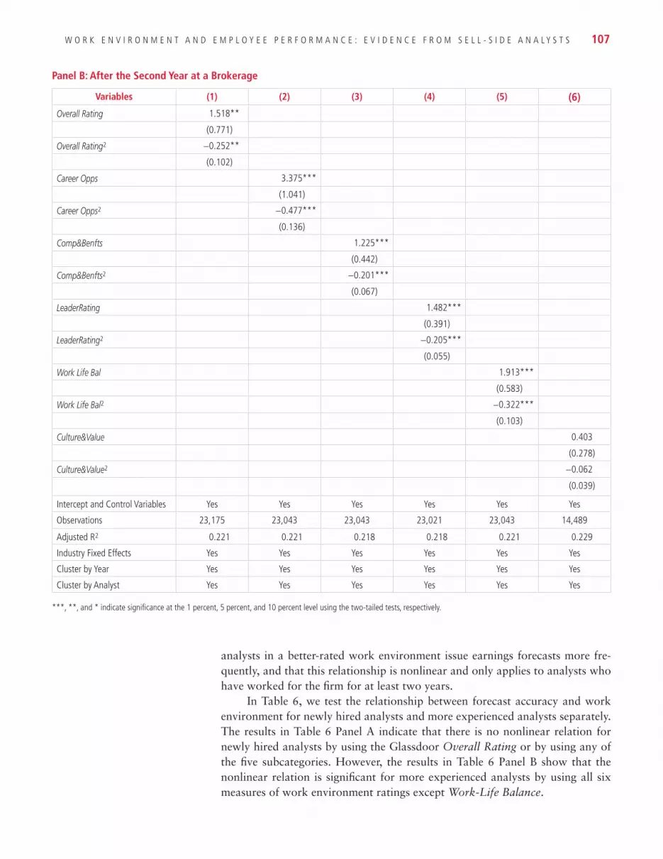
W O R K E N V I R O N M E N T A N D E M P L O Y E E P E R F O R M A N C E : E V I D E N C E F R O M S E L L - S I D E A N A L Y S T S 107
Panel B: After the Second Year at a Brokerage
Variables (1) (2) (3) (4) (5) (6)
Overall Rating 1.518**
(0.771)
Overall Rating2 −0.252**
(0.102)
Career Opps 3.375***
(1.041)
Career Opps2 −0.477***
(0.136)
Comp&Benfts 1.225***
(0.442)
Comp&Benfts2 −0.201***
(0.067)
LeaderRating 1.482***
(0.391)
LeaderRating2 −0.205***
(0.055)
Work Life Bal 1.913***
(0.583)
Work Life Bal2 −0.322***
(0.103)
Culture&Value 0.403
(0.278)
Culture&Value2 −0.062
(0.039)
Intercept and Control Variables Yes Yes Yes Yes Yes Yes
Observations 23,175 23,043 23,043 23,021 23,043 14,489
Adjusted R2 0.221 0.221 0.218 0.218 0.221 0.229
Industry Fixed Effects Yes Yes Yes Yes Yes Yes
Cluster by Year Yes Yes Yes Yes Yes Yes
Cluster by Analyst Yes Yes Yes Yes Yes Yes
***, **, and * indicate significance at the 1 percent, 5 percent, and 10 percent level using the two-tailed tests, respectively.
analysts in a better-rated work environment issue earnings forecasts more fre-quently, and that this relationship is nonlinear and only applies to analysts who have worked for the firm for at least two years.
In Table 6, we test the relationship between forecast accuracy and work environment for newly hired analysts and more experienced analysts separately. The results in Table 6 Panel A indicate that there is no nonlinear relation for newly hired analysts by using the Glassdoor Overall Rating or by using any of the five subcategories. However, the results in Table 6 Panel B show that the nonlinear relation is significant for more experienced analysts by using all six measures of work environment ratings except Work-Life Balance.

108 R E V I E W O F B U S I N E S S
TABLE 6. The Effect of Analyst Experience on the Relation between Analyst Work Environment and Earnings Forecast AccuracyThis table examines whether analyst work environment is associated with their performance, which is represented by earnings forecast accuracy. This table contains the result of estimating model (1). The dependent variable is R_ACCURACY. For conciseness, we do not show coefficients on industry dummy variables in the table. Standard errors adjusted for clustering are reported in parentheses.
Panel A: First Two Years at a Brokerage
Variables (1) (2) (3) (4) (5) (6)
Overall Rating 0.007
(0.053)
Overall Rating2 −0.004
(0.007)
Career Opps −0.015
(0.053)
Career Opps2 −0.001
(0.007)
Comp&Benfts −0.014
(0.037)
Comp&Benfts2 0.003
(0.005)
LeaderRating −0.029
(0.035)
LeaderRating2 0.003
(0.005)
Work Life Bal 0.030
(0.042)
Work Life Bal2 −0.009
(0.007)
Culture&Value −0.035
(0.047)
Culture&Value2 0.006
(0.006)
Intercept and Control Variables Yes Yes Yes Yes Yes Yes
Observations 4,063 4,055 4,055 4,046 4,055 2,040
Adjusted R2 0.032 0.030 0.029 0.030 0.036 0.041
Industry Fixed Effects Yes Yes Yes Yes Yes Yes
Cluster by Year Yes Yes Yes Yes Yes Yes
Cluster by Analyst Yes Yes Yes Yes Yes Yes
***, **, and * indicate significance at the 1 percent, 5 percent, and 10 percent level using the two-tailed tests, respectively.

W O R K E N V I R O N M E N T A N D E M P L O Y E E P E R F O R M A N C E : E V I D E N C E F R O M S E L L - S I D E A N A L Y S T S 109
In Table 7, we repeat the test by using model (2) to examine the effect of employee work environment rating on stock market reaction to recommenda-tions for newly hired analysts and more experienced analysts separately. Results in Table 7 Panel A show that for newly hired analysts, there is no relationship between the work environment and their recommendations’ market impact. In contrast, the results in Table 7 Panel B show that for analysts with at least two years of experience at a brokerage firm, there is a nonlinear relationship between the market impact of recommendation changes and several work environment ratings: Overall Rating, Career Opportunities, Leadership Rating, and Culture & Values.
Panel B: After the Second Year at a Brokerage
Variables (1) (2) (3) (4) (5) (6)
Overall Rating 0.111***
(0.032)
Overall Rating2 −0.015***
(0.004)
Career Opps 0.101***
(0.029)
Career Opps2 −0.014***
(0.004)
Comp&Benfts 0.062***
(0.020)
Comp&Benfts2 −0.010***
(0.003)
LeaderRating 0.045*
(0.025)
LeaderRating2 −0.006*
(0.004)
Work Life Bal 0.020
(0.021)
Work Life Bal2 −0.004
(0.003)
Culture&Value 0.086***
(0.024)
Culture&Value2 −0.011***
(0.003)
Intercept and Control Variables Yes Yes Yes Yes Yes Yes
Observations 23,175 23,043 23,043 23,021 23,043 14,489
Adjusted R2 0.038 0.038 0.038 0.037 0.037 0.042
Industry Fixed Effects Yes Yes Yes Yes Yes Yes
Cluster by Year Yes Yes Yes Yes Yes Yes
Cluster by Analyst Yes Yes Yes Yes Yes Yes
***, **, and * indicate significance at the 1 percent, 5 percent, and 10 percent level using the two-tailed tests, respectively.

110 R E V I E W O F B U S I N E S S
TABLE 7. The Effect of Analyst Experience on the Relation between Analyst Work Environment and Stock Market Reaction to Recommendation ChangesThis table examines whether analyst work environment is associated with their performance. This table contains the result of estimating model (2). The dependent variable is three-day cumulative abnormal return. For conciseness, we only include recommendation change and its interaction with work environment variables in the table. Standard errors adjusted for clustering are reported in parentheses.
Panel A: First Two Years at a Brokerage
(1) (2) (3) (4) (5) (6)
Rec 0.108*** 0.111*** 0.117*** 0.124*** 0.116*** 0.138***
(0.021) (0.023) (0.023) (0.021) (0.023) (0.026)
Rec*Overall Rating 0.013
(0.011)
Rec*Overall Rating2 −0.002
(0.002)
Rec*Career Opps 0.009
(0.011)
Rec*Career Opps2 −0.002
(0.002)
Rec*Comp&Benfts 0.003
(0.009)
Rec*Comp&Benfts2 −0.000
(0.002)
Rec*LeaderRating 0.000
(0.007)
Rec*LeaderRating2 −0.000
(0.001)
Rec*Work Life Bal 0.009
(0.008)
Rec*Work Life Bal2 −0.002
(0.001)
Rec*Culture&Value −0.002
(0.008)
Rec*Culture&Value2 0.001
(0.001)
Intercept and Control Variables Yes Yes Yes Yes Yes Yes
Observations 5,466 5,456 5,456 5,445 5,456 2,483
Adjusted R2 0.169 0.169 0.168 0.168 0.169 0.181
Industry Fixed Effects Yes Yes Yes Yes Yes Yes
Cluster by Analyst Yes Yes Yes Yes Yes Yes
***, **, and * indicate significance at the 1 percent, 5 percent, and 10 percent level using the two-tailed tests, respectively.
In summary, our results indicate that highly rated work environments mo-tivate analysts to work harder and consequently make their stock recommen-dations more impactful to stock investors. However, the results are driven by stock analysts who stay at their current job for at least two years. Interestingly, we find that work-life balance does not play an important role in affecting stock

W O R K E N V I R O N M E N T A N D E M P L O Y E E P E R F O R M A N C E : E V I D E N C E F R O M S E L L - S I D E A N A L Y S T S 111
analysts’ job performance. Rather, career opportunities and compensations and benefits play more important roles in improving earnings forecast accuracy and their recommendations’ market impact.
Work Environment and Turnover
Table 8 shows the results of testing H3 that good work environment helps retain analysts by using equation (3). Table 8 Panel A shows the results using a linear regression by only including the first moment of brokerage rating. The results indicate that Overall Rating, Leadership Rating, and Culture & Values help
Panel B: After the Second Year at a Brokerage
Variables (1) (2) (3) (4) (5) (6)
Rec 0.093*** 0.074*** 0.109*** 0.104*** 0.115*** 0.114***
(0.018) (0.014) (0.015) (0.016) (0.015) (0.012)
Rec*Overall Rating 0.016**
(0.007)
Rec*Overall Rating2 −0.002**
(0.001)
Rec*Career Opps 0.029***
(0.007)
Rec*Career Opps2 −0.004***
(0.001)
Rec*Comp&Benfts 0.005
(0.004)
Rec*Comp&Benfts2 −0.001
(0.001)
Rec*LeaderRating 0.010**
(0.005)
Rec*LeaderRating2 −0.002*
(0.001)
Rec*Work Life Bal 0.003
(0.006)
Rec*Work Life Bal2 −0.001
(0.001)
Rec*Culture&Value 0.011**
(0.005)
Rec*Culture&Value2 −0.002**
(0.001)
Intercept and Control Variables Yes Yes Yes Yes Yes Yes
Observations 30,258 30,104 30,104 30,081 30,104 18,483
Adjusted R2 0.179 0.182 0.180 0.179 0.179 0.183
Industry Fixed Effects Yes Yes Yes Yes Yes Yes
Cluster by Analyst Yes Yes Yes Yes Yes Yes
***, **, and * indicate significance at the 1 percent, 5 percent, and 10 percent level using the two-tailed tests, respectively.

112 R E V I E W O F B U S I N E S S
TABLE 8. Analyst Work Environment and Analyst TurnoverThis table examines whether analyst work environment is associated with their performance, reflected in earnings forecast accuracy. This table contains the result of estimating model (3). The dependent variable is Turnover. For conciseness, we do not show coefficients on industry dummy variables in the table. Standard errors adjusted for clustering are reported in parentheses.
Panel A: Linear Regression
Variables (1) (2) (3) (4) (5) (6)Overall Rating −0.034***
(0.011)
Career Opps −0.036
(0.023)
Comp&Benfts −0.019
(0.018)
LeaderRating −0.032***
(0.008)
Work Life Bal 0.020
(0.017)
Culture&Value −0.025***
(0.008)
BSize 0.000 0.000 0.000 0.000 0.000 −0.000*
(0.000) (0.000) (0.000) (0.000) (0.000) (0.000)
LTGISS 0.065 0.063* 0.063 0.067* 0.062* 0.101
(0.040) (0.038) (0.039) (0.040) (0.037) (0.070)
CFISS 0.037 0.034 0.034 0.035 0.033 0.090**
(0.037) (0.037) (0.036) (0.038) (0.037) (0.046)
FirmCov 0.000 0.000 −0.000 0.000 −0.000 0.001
(0.001) (0.001) (0.001) (0.001) (0.001) (0.002)
IndCov −0.002 −0.002 −0.002 −0.002 −0.002 0.003
(0.003) (0.003) (0.002) (0.003) (0.003) (0.003)
FirmExp −0.001 −0.001 −0.001 −0.001 −0.001 −0.005*
(0.002) (0.002) (0.002) (0.002) (0.002) (0.003)
Forecast Frequency −0.003 −0.003 −0.003 −0.003 −0.003 −0.003
(0.002) (0.002) (0.002) (0.002) (0.002) (0.003)
MB 0.000 0.000 0.000 0.000 0.000 −0.000
(0.000) (0.000) (0.000) (0.000) (0.000) (0.000)
AltmanZ 0.000 0.000 0.000 0.000 0.000 −0.000
(0.000) (0.000) (0.000) (0.000) (0.000) (0.000)
Loss 0.001 0.001 0.001 0.000 0.000 0.003
(0.006) (0.006) (0.006) (0.006) (0.006) (0.006)
Age 0.001 0.001 0.001 0.001 0.001 0.002***
(0.001) (0.001) (0.001) (0.001) (0.001) (0.001)
LnMV 0.004 0.004 0.004 0.003 0.003 0.002
(0.003) (0.003) (0.003) (0.003) (0.003) (0.003)
Intercept 0.283*** 0.278*** 0.214*** 0.277*** 0.109 0.327***
(0.045) (0.064) (0.059) (0.045) (0.087) (0.054)
Observations 25,725 25,585 25,585 25,554 25,585 15,016
Adjusted R2 0.076 0.079 0.067 0.083 0.069 0.148
Industry Fixed Effects Yes Yes Yes Yes Yes Yes
Cluster by Year Yes Yes Yes Yes Yes Yes
Cluster by Analyst Yes Yes Yes Yes Yes Yes
***, **, and * indicate significance at the 1 percent, 5 percent, and 10 percent level using the two-tailed tests, respectively.

W O R K E N V I R O N M E N T A N D E M P L O Y E E P E R F O R M A N C E : E V I D E N C E F R O M S E L L - S I D E A N A L Y S T S 113
Panel B: Second Moment Regression
Variables (1) (2) (3) (4) (5) (6)Overall Rating −0.234***
(0.073)Overall Rating2 0.030***
(0.010)Career Opps −0.229*
(0.118)Career Opps2 0.028*
(0.014)Comp&Benfts −0.096
(0.059)Comp&Benfts2 0.012
(0.009)LeaderRating −0.044
(0.047)LeaderRating2 0.002
(0.007)Work Life Bal 0.016
(0.072)Work Life Bal2 0.001
(0.013)Culture&Value −0.058
(0.063)Culture&Value2 0.005
(0.009)BSize 0.000 0.000 0.000 0.000 0.000 −0.000
(0.000) (0.000) (0.000) (0.000) (0.000) (0.000)LTGISS 0.063 0.063* 0.061 0.067 0.062* 0.101
(0.039) (0.038) (0.040) (0.041) (0.034) (0.070)CFISS 0.036 0.033 0.034 0.035 0.033 0.090**
(0.038) (0.036) (0.037) (0.038) (0.034) (0.046)FirmCov 0.000 0.000 0.000 0.000 −0.000 0.001
(0.001) (0.001) (0.001) (0.001) (0.001) (0.002)IndCov −0.002 −0.002 −0.002 −0.002 −0.002 0.003
(0.002) (0.002) (0.002) (0.003) (0.003) (0.002)FirmExp −0.001 −0.001 −0.001 −0.001 −0.001 −0.005*
(0.002) (0.002) (0.002) (0.002) (0.002) (0.003)Forecast Frequency −0.003 −0.002 −0.003 −0.003 −0.003 −0.003
(0.002) (0.002) (0.002) (0.002) (0.002) (0.003)MB 0.000 0.000 −0.000 0.000 0.000 −0.000
(0.000) (0.000) (0.000) (0.000) (0.000) (0.000)AltmanZ 0.000 0.000 0.000 0.000 0.000 −0.000
(0.000) (0.000) (0.000) (0.000) (0.000) (0.000)Loss 0.001 0.002 0.001 0.000 0.000 0.004
(0.006) (0.007) (0.006) (0.006) (0.006) (0.006)Age 0.000 0.000 0.000 0.000 0.001 0.002***
(0.001) (0.001) (0.001) (0.001) (0.001) (0.001)LnMV 0.005* 0.005 0.005 0.003 0.003 0.002
(0.003) (0.003) (0.003) (0.002) (0.003) (0.003)Intercept Yes Yes Yes Yes Yes Yes
Observations 25,725 25,585 25,585 25,554 25,585 15,016Adjusted R2 0.091 0.091 0.071 0.083 0.069 0.149Industry Fixed Effects Yes Yes Yes Yes Yes YesCluster by Year Yes Yes Yes Yes Yes YesCluster by Analyst Yes Yes Yes Yes Yes Yes
***, **, and * indicate significance at the 1 percent, 5 percent, and 10 percent level using the two-tailed tests, respectively.

114 R E V I E W O F B U S I N E S S
to reduce employee turnover. In Table 8 Panel B, we examine a nonlinear rela-tionship using model 3 and find that Overall Rating and Career Opportunities reduce employee turnover, but the marginal benefit attenuates with the increase in the rating. No other subcategories are significant. To summarize, Table 8 demonstrates a U-shaped relationship between the Overall Rating and employee turnover.
CONCLUSIONIn this paper, we examine how work environment affects employee job perfor-mance by using stock analysts and their brokerage houses. Prior studies have not provided conclusive evidence on whether better work environment leads to bet-ter job performance. By using the unique dataset supplied by Glassdoor.com, we attempt to find a relationship between analysts’ rating of work environment and their job performance proxied by observable efforts and performance measures such as earnings forecast frequency, forecast accuracy, and the market impact of their stock recommendations.
We find a concave relationship between analysts’ overall rating of work environment and their efforts and performance, suggesting that employee rating of work environment increases their performance up to some points, but the relation becomes weaker after the point, supporting our hypothesis that the re-lationship is nonlinear. Compared to Hope et al. (2020), who focus on work-life balance, we extensively examine all the components of work environment: (1) Career Opportunities, (2) Compensation & Benefits, (3) Leadership Rating, (4) Work-Life Balance, and (5) Culture & Values. We believe this is important since work-life balance is only one component of overall work environment. We find that out of five subcategories of work environment ratings, Career Opportuni-ties and Culture & Values have consistently demonstrated inverse U-shaped re-lationships with analyst job performance. Other subcategories, however, do not have consistently significant results. We find that work-life balance has the least influence on overall satisfaction rating among all the components. In addition, work-life balance is negatively correlated with other categories such as Career Opportunities and Compensation & Benefits, emphasizing the importance of examining all the components of overall satisfaction rating comprehensively.
ReferencesAbowd, J. 1989. “The Effect of Wage Bargains on the Stock Market Value of the Firm.”
American Economic Review 79, no. 4, 774–800.Acharya, V., R. Baghai, and K. Subrahmanian. 2013. “Labor Laws and Innovation.”
Journal of Law and Economics 56, no. 4, 997–1037.Akerlof, G. 1982. “Labor Contracts as Partial Gift Exchange.” Quarterly Journal of
Economics 97, no. 4, 543–69.Akerlof, G., and J. Yellen. 1986. Efficiency Wage Models of the Labor Market. Cam-
bridge: Cambridge University Press.Altman, E. I, 1968. “Financial Ratios, Discriminant Analysis, and the Prediction of Cor-
porate Bankruptcy.” Journal of Finance 23, no. 4, 589–609. Backhaus, K. B., B. A. Stone, and K. Heiner. 2002. “Exploring the Relationship Between
Corporate Social Performance and Employer Attractiveness.” Business & Society 41, no. 3, 292–318.

W O R K E N V I R O N M E N T A N D E M P L O Y E E P E R F O R M A N C E : E V I D E N C E F R O M S E L L - S I D E A N A L Y S T S 115
Bauer, R., K. Koedijk, and R. Otten. 2005. “International Evidence on Ethical Mutual Fund Performance and Investment Style.” Journal of Banking and Finance 29, no. 7, 1751–67.
Becker, B. E., and B. Gerhart, B. 1996. “The Impact of Human Resource Management on Organizational Performance: Progress and Prospects.” Academy of Management Journal 39, 779–801.
Behrend, T. S., B. A. Baker, and L. Foster Thompson. 2009. “Effects of Pro-Environ-mental Recruiting Messages: The Role of Organizational Reputation.” Journal of Business and Psychology 24, no. 3, 341–50.
Belt, J. A., and J. G. P. Paolillo. 1982. “The Influence of Corporate Image and Specificity of Candidate Qualifications on Response to Recruitment Advertising.” Journal of Management 8, no. 1, 105–12.
Berk, J., R. Stanton, and J. Zechner. 2010. “Human Capital, Bankruptcy, and Capital Structure.” Journal of Finance 65, no. 3, 891–926.
Bjerring, J., J. Lakonishok, and T. Vermaelen. 1983. “Stock Prices and Financial Ana-lysts’ Recommendations.” The Journal of Finance 38, no. 1, 187–204.
Boudreau, J., and S. Rynes. 1985. “Role of Recruitment in Staffing Utility Analysis.” Journal of Applied Psychology 70, no. 2, 354–66.
Bretz, R. D. Jr, and T. A. Judge. 1994. “The Role of Human Resource Systems in Job Applicant Decision Processes.” Journal of Management 20, no. 3, 531–51.
Brown, L. D., and E. Mohammad. 2010. “Is Analyst Earnings Forecast Ability Only Firm-Specific?” Contemporary Accounting Research 27, no. 3, 727–50.
Carlin, B., and S. Gervais. 2009. “Work Ethic, Employment Contracts, and Firm Value.” Journal of Finance 64, no. 2, 785–821.
Clement, M. 1999. “Analyst Forecast Accuracy: Do Ability, Resources, and Portfolio Complexity Matter?” Journal of Accounting and Economics 27, no. 3, 285–303.
Clement, M., and S. Tse. 2003. “Do Investors Respond to Analysts’ Forecast Revisions as if Forecast Accuracy Is All That Matters?” The Accounting Review 78, no. 1, 227–49.
Cober, R. T., D. J. Brown, L. M. Keeping, and P. E. Levy. 2004. “Recruitment on the Net: How Do Organizational Web Site Characteristics Influence Applicant Attraction?” Journal of Management 30, no. 5, 623–46.
Cronqvist, H., F. Heyman, M. Nilsson, H. Svaleryd, and J. Vlachos. 2008. “Do En-trenched Managers Pay Their Workers More?” Journal of Finance 64, no. 1, 309–39.
DeFond, M. L., and H. Mingyi. 2003. “An Empirical Analysis of Analysts’ Cash Flow Forecasts.” Journal of Accounting and Economics 35, no. 1, 73–100.
Dessler, G. 2003. Human Resource Management, 9th ed. Upper Saddle River, NJ: Pren-tice Hall.
Edmans, A. 2011. “Does the Stock Market Fully Value Intangibles? Employee Satisfac-tion and Equity Prices.” Journal of Financial Economics 101, no. 3, 621–40.
Edmans, A. 2012. “The Link Between Job Satisfaction and Firm Value, With Implica-tions for Corporate Social Responsibility.” Academy of Management Perspectives 26, no. 4, 1–19.
Edmans, A. 2014. “Blockholders and Corporate Governance.” Annual Review of Finan-cial Economics, Annual Reviews 6, no. 1, 23–50.
Edmans, A., L. Li, and C. Zhang. 2014. “Employee Satisfaction, Labor Market Flexibil-ity, and Stock Returns Around the World NBER.” Working paper no. 20300.
Foster Thompson, L., and K. R. Aspinwall. 2009. “The Recruitment Value of Work/Life Benefits.” Personnel Review 38, no. 2, 195–210.
Gorton, G., and F. Schmid. 2004. “Capital, Labor, and the Firm: A Study of German Co-determination.” Journal of the European Economic Association 2, no. 5, 863–905.
Green, T. C., R. Huang, Q. Wen, and D. Zhou. 2019. “Crowdsourced Employer Reviews and Stock Returns.” Journal of Financial Economics 134, no. 1, 236–51.
Hope, O., C. Li, A. Lin, and M. Rabier. 2020. Happy Analysts. Accounting, Organiza-tions, and Society. Forthcoming.

116 R E V I E W O F B U S I N E S S
Huselid, M. 1995. “The Impact of Human Resource Management Practices on Turnover, Productivity, and Corporate Financial Performance.” The Academy of Management Journal 38, no. 3, 635–72.
Jacob, J., T. Lys, and M. Neale. 1999. “Expertise in Forecasting Performance of Security Analysts.” Journal of Accounting and Economics 28, no. 1, 51–82.
Jensen, M., and W. Meckling. 1976. “Theory of the Firm: Managerial Behavior, Agency Costs, and Capital Structure.” Journal of Financial Economics 3, no. 4, 305–60.
Jung, B., P. Shane, and Y. Yang. 2012. “Do Financial Analysts’ Long-Term Growth Fore-casts Matter? Evidence from Stock Recommendations and Career Outcomes.” Jour-nal of Accounting and Economics 53, nos. 1–2, 55–76.
Loh, R., and R. Stulz. 2011. “When Are Analyst Recommendation Changes Influential?” The Review of Financial Studies 24, no. 2, 593–627.
McGregor, D. 1960. The Human Side of Enterprise. New York, NY: McGraw-Hill. Organ, D. W. 1997. “Organizational Citizenship Behavior: It’s Construct Clean-Up
Time.” Human Performance 10, no. 2, 85–97.Pfeffer, J. 1994. Competitive Advantage through People. Boston, MA: Harvard Business
School Press.Rajan, R., and L. Zingales. 1998. “Power in a Theory of the Firm.” Quarterly Journal of
Economics 113, no. 2, 387–432.Rau, B. L., and M. M. Hyland. 2002. “Role Conflict and Flexible Work Arrangements:
The Effects on Applicant Attraction.” Personnel Psychology 55, no. 1, 111–36.Shapiro, C., and J. Stiglitz. 1984. “Equilibrium Unemployment as a Worker Discipline
Device.” American Economic Review 74, no. 3, 433–44.Womack, K. 1996. “Do Brokerage Analysts’ Recommendations Have Investment Val-
ue?” The Journal of Finance 51, no. 1, 137–67.Wright, B. E., and S. Kim. 2004. Participation’s Influence on Job Satisfaction: The Impor-
tance of Job Satisfaction: The Importance of Job Characteristics.” Review of Public Personnel Administration 24, no 1, 18–40.
Zingales, L. 2000. “In Search of New Foundations.” Journal of Finance 55, no. 4, 1623–53.

W O R K E N V I R O N M E N T A N D E M P L O Y E E P E R F O R M A N C E : E V I D E N C E F R O M S E L L - S I D E A N A L Y S T S 117
APPENDIX: List of Brokerage House Names
Aegis CapitalAvondale PartnersRobert W. Baird & Co.The Blackstone GroupBear StearnsWilliam BlairBrown Brothers HarrimanBMO Capital MarketsCanaccord Genuity GroupCantor FitzgeraldEdward JonesEvercore PartnersGoldman SachsGuggenheim Securities LLCHSBC North America Holdings Inc. or HSBC Overseas Holdings (UK) Ltd.JefferiesJP MorganLazardLehman BrothersMacquarie GroupMerrill Lynch or Bank of America Merrill LynchMesirow FinancialMizuho Securities or Mizuho Financial GroupMorgan StanleyMorningstarNeedham & Co.Nomura SecuritiesOppenheimer HoldingsPerella Weinberg PartnersPiper JaffrayPNC Financial Services GroupRaymond James Financial or Morgan Keegan Inc.RBC Dominion SecuritiesSunTrust Robinson HumphreyBB&T Capital MarketsSidoti & Company, LLCCitiStifel FinancialUBS Investment BankWachovia Securities Inc.Banc of America Securities LLC

BusinessInterdisciplinary Journal on Risk and Society
Review of
Copyright © 2021, St. John’s University.
The views presented in the articles are those of the authors and do not represent an official statement of policy by St. John’s University.
EditorYun Zhu St. John’s University, United States
Advisory Board Iftekhar Hasan Fordham University, Bank of Finland, and University of Sydney, United States
Kose John New York University, United States
Steven Ongena University of Zurich, Swiss Finance Institute, KU Leuven, and Center for Economic and Policy Research (CEPR), Switzerland
Raghavendra Rau University of Cambridge, United Kingdom
David Reeb National University of Singapore, Singapore
Editorial BoardTuranay Caner North Carolina State University, United States
Santiago Carbó-Valverde CUNEF, Spain
Sandeep Dahiya Georgetown University, United States
Sudip Datta Wayne State University, United States
Co-Pierre Georg University of Cape Town, South Africa
Xian Gu Durham University, United Kingdom
Omrane Guedhami University of South Carolina, United States
Roman Horváth Charles University, Czech Republic
Patrick Flanagan St. John’s University, United States
Suk-Joong Kim University of New South Wales [UNSW] Sydney, Australia
Anzhela Knyazeva Security Exchange Commission, United States
Chih-Yung Lin National Chiao Tung University, Taiwan
Kristina Minnick Bentley University, United States
Jerry Parwada UNSW Sydney, Australia
Maurizio Pompella University of Siena, Italy
Steven W. Pottier University of Georgia, United States
Alon Raviv Bar Ilan, Israel
Victoria Shoaf St. John’s University, United States
Akhtar Siddique Office of the Comptroller of the Currency, United States
Benjamin Tabak FGV, Brazil
Tuomas Takalo Bank of Finland, Finland
Amine Tarazi University of Limoges, France
Krupa Viswanathan Temple University, United States
Wolf Wagner Rotterdam School of Management and CEPR, The Netherlands
Noriyoshi Yanase Keio University, Japan
Gaiyan Zhang University of Missouri–Columbia, United States
Hao Zhang Rochester Institute of Technology, United States
Review of Business is published twice a year.ISSN: 0034-6454
Review of Business is a peer-reviewed academic journal. The journal publishes original research articles in all academic fields of business, both theoretical and empirical, that will significantly contribute to the literature of business and allied disciplines. The journal advocates for research articles in imminent topics, such as sustainable development, technology- related business issues, and topics that enrich the interdisciplinary understanding of business.
The Peter J. Tobin College of BusinessSt. John’s UniversityNew York
www.stjohns.edu/ROB (for submissions, style guide, publishing agreement, and standards of integrity)
[email protected] (for inquiries and communications)

BusinessInterdisciplinary Journal on Risk and Society
Review of
BusinessInterdisciplinary Journal on Risk and Society
Review of
Review
of Business | V
ol
um
e 41 ● N
um
be
r 2
BusinessInterdisciplinary Journal on Risk and Society
Review of
Volume 41, Number 2 | JuNe 2021
Non-Profit Org. U.S. Postage
PAIDSt. John’s University
New York
The Peter J. Tobin College of Business8000 Utopia Parkway
Queens, NY 11439stjohns.edu
Banking Deregulation and Investment-Cash Flow Sensitivity 1
Dawei Jin, Haizhi Wang, Tianyu Zhao, and Xinting Zhen
The Leader-Member Exchange (LMX) Influence at Organizations: The Moderating Role of Person-Organization (P-O) Fit 32
Omer Faruk Derindag, Ozgur Demirtas, and Ali Bayram
The Real Effect of Financial Reform: Evidence from Bond Market in China 49
Xian Gu, Lu Yun, and Shangwei Hao
Work Environment and Employee Performance: Evidence from Sell-Side Analysts 85
Shuya Liu and Kevin Sun


![41 \]'[;plouytdsaz 5 - NJ.gov](https://img.pdfslide.net/doc/110x75/631bc6d87051d371800f2c5b/41-plouytdsaz-5-njgov.jpg)

