Embed Size (px)
Citation preview

An Apriori-based Approach for First-Order Temporal Pattern Mining
Sandra de Amo1∗ Daniel A. Furtado1† Arnaud Giacometti2 Dominique Laurent3
1Universidade Federal de UberlandiaComputer Science Department
Uberlandia, Brazil
2Universite de ToursLI / UFR de Sciences / Blois-France
3Universite de Cergy-Pontoise / Departement des Sciences InformatiquesCergy-Pontoise-France
[email protected], [email protected], [email protected]
AbstractPrevious studies on mining sequential patterns have focused on temporal patterns specified by some form of
propositional temporal logic. However, there are some interesting sequential patterns whose specification needs a
more expressive formalism, the first-order temporal logic. In this paper, we focus on the problem of mining multi-
sequential patterns which are first-order temporal patterns (not expressible in propositional temporal logic). We
propose two Apriori-based algorithms to perform this mining task. The first one, the PM (Projection Miner) Algo-
rithm adapts the key idea of the classical GSP algorithm for propositional sequential pattern mining by projecting
the first-order pattern in two propositional components during the candidate generation and pruning phases. The
second algorithm, the SM (Simultaneous Miner) Algorithm, executes the candidate generation and pruning phases
without decomposing the pattern, that is, the mining process, in some extent, does not reduce itself to its proposi-
tional counterpart. Our extensive experiments shows that SM scales up far better than PM.
Key Words : Temporal Data Mining, Sequence Mining, Sequential Patterns, Temporal Data Mining, Frequent
Patterns, Knowledge Discovery.
1. Introduction
The problem of discovering sequential patterns in temporal data have been extensively studied inseveral recent papers [2, 3, 8, 7, 9] and its importance is fully justified by the great number of potentialapplication domains where mining sequential patterns appear as a crucial issue, such as financial market(evolution of stock market shares quotations), retailing (evolution of clients purchases), medicine (evo-lution of patients symptoms), local weather forecast, telecommunication (sequences of alarms output bynetwork switches), etc. Different kinds of sequential patterns have been proposed as well as general for-malisms and algorithms for expressing and mining them [16, 14, 15]. Most of these patterns are specifiedby formalisms which are, in some extent, reducible to Propositional Temporal Logic. For instance, let usconsider the (propositional) sequential patterns of form< i1, i2, . . . , in > (whereij are set of items) thathave been extensively studied in the literature in the past years ([2, 3, 8, 7]). This pattern is considered
∗This author was supported in part by CNPq/Brazil and by the cooperation program Capes-Cofecub 301/00-2,
between Brazil and France.†This author was supported by CNPq/Brazil.
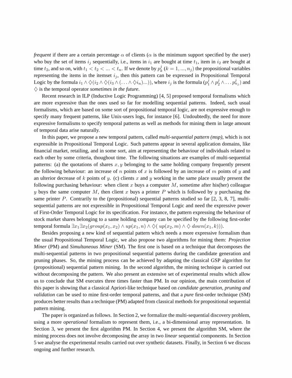
frequentif there are a certain percentageα of clients (α is the minimum support specified by the user)who buy the set of itemsij sequentially, i.e., items ini1 are bought at timet1, item in i2 are bought attime t2, and so on, witht1 < t2 < ... < tn. If we denote bypj
k (k = 1, ..., nj) the propositional variablesrepresenting the items in the itemsetij , then this pattern can be expressed in Propositional TemporalLogic by the formulai1 ∧♦(i2 ∧♦(i3 ∧ (. . .∧♦in)...)), whereij is the formula (pj
1 ∧ pj2 ∧ . . . pj
nj ) and♦ is the temporal operatorsometimes in the future.
Recent research in ILP (Inductive Logic Programming) [4, 5] proposed temporal formalisms whichare more expressive than the ones used so far for modelling sequential patterns. Indeed, such usualformalisms, which are based on some sort of propositional temporal logic, are not expressive enough tospecify many frequent patterns, like Unix-users logs, for instance [6]. Undoubtedly, the need for moreexpressive formalisms to specify temporal patterns as well as methods for mining them in large amountof temporal data arise naturally.
In this paper, we propose a new temporal pattern, calledmulti-sequential pattern (msp), which is notexpressible in Propositional Temporal Logic. Such patterns appear in several application domains, likefinancial market, retailing, and in some sort, aim at representing the behaviour of individuals related toeach other by some criteria, thoughout time. The following situations are examples of multi-sequentialpatterns: (a) the quotations of sharesx, y belonging to the same holding company frequently presentthe following behaviour: an increase ofn points ofx is followed by an increase ofm points ofy andan ulterior decrease ofk points ofy. (c) clientsx andy working in the same place usually present thefollowing purchasing behaviour: when clientx buys a computerM , sometime after his(her) colleaguey buys the same computerM , then clientx buys a printerP which is followed byy purchasing thesame printerP . Contrarily to the (propositional) sequential patterns studied so far [2, 3, 8, 7], multi-sequential patterns are not expressible in Propositional Temporal Logic and need the expressive powerof First-Order Temporal Logic for its specification. For instance, the pattern expressing the behaviour ofstock market shares belonging to a same holding company can be specified by the following first-ordertemporal formula∃x1∃x2(group(x1, x2) ∧ up(x1, n) ∧ ♦( up(x2,m) ∧ ♦ down(x1, k))).
Besides proposing a new kind of sequential pattern which needs a more expressive formalism thanthe usual Propositional Temporal Logic, we also propose two algorithms for mining them:ProjectionMiner (PM) andSimultaneous Miner(SM). The first one is based on a technique that decomposes themulti-sequential patterns in two propositional sequential patterns during the candidate generation andpruning phases. So, the mining process can be achieved by adapting the classical GSP algorithm for(propositional) sequential pattern mining. In the second algorithm, the mining technique is carried outwithout decomposing the pattern. We also present an extensive set of experimental results which allowus to conclude that SM executes three times faster than PM. In our opinion, the main contribution ofthis paper is showing that a classical Apriori-like technique based oncandidate generation, pruning andvalidationcan be used to mine first-order temporal patterns, and that apurefirst-order technique (SM)produces better results than a technique (PM) adapted from classical methods for propositional sequentialpattern mining.
The paper is organized as follows. In Section 2, we formalize the multi-sequential discovery problem,using a moreoperationalformalism to represent them, i.e., a bi-dimensional array representation. InSection 3, we present the first algorithm PM. In Section 4, we present the algorithm SM, where themining process does not involve decomposing the array in twolinear sequential components. In Section5 we analyse the experimental results carried out over synthetic datasets. Finally, in Section 6 we discussongoing and further research.

2. Problem Formalization
In this section, we will formalize the problem of discovering multi-sequential patterns. We supposethe existence of a finite setI of itemsand a finite setC of object identifiers. From now on, we will callthe elements ofC clients1. Items are denoted bya, b, c, ... and client ids byc1, c2, c3, .... We suppose anordering overC such thatc1 < c2 < c3 < .... For the sake of simplifying the presentation, we will onlyconsider sequence patterns whose elements areitemsinstead ofitemsets.
Let us consider a database schemaD = {Tr(T, IdCl, Item, IdG)}. A datasetD is an instanceoverD. Here,T is the time attribute whose domain (denoted dom(T )) isN. AttributesIdCl, Item andIdG stand for client identifiers, items and group identifiers respectively. Their domain areC, I andNrespectively. The table illustrated in Figure 1(a) is a dataset.
T IdCl Item IdG T IdCl Item IdG
1 c1 a 1 1 c7 a 33 c1 b 1 3 c7 c 35 c1 a 1 4 c7 b 32 c2 b 1 2 c8 b 33 c2 c 1 5 c8 a 34 c3 a 1 2 c9 b 43 c4 a 2 4 c9 a 45 c5 a 2 1 c10 a 44 c6 b 2 3 c10 b 4
5 c11 d 4
IdG MSeq
1 {< a,⊥, b,⊥, a >,
<⊥, b, c,⊥,⊥>,
<⊥,⊥,⊥, a,⊥>}2 {<⊥,⊥, a,⊥,⊥>,
<⊥,⊥,⊥,⊥, a >,
<⊥,⊥,⊥, b,⊥>}3 {< a,⊥, c, b,⊥>,
<⊥, b,⊥,⊥, a >}4 {<⊥, b,⊥, a,⊥>,
< a,⊥, b,⊥,⊥>,
<⊥,⊥,⊥,⊥, d >}(a) (b)
Figure 1: Dataset
A sequenceis a lists =< i1, . . . , im >, where each elementij ∈ I ∪ {⊥}. The symbol⊥ standsfor “don’t care” (m is called thelength of s and is denoted| s |). A multi-sequenceis a finite setσ = {s1, . . . , sn}, where eachsi is a sequence and for eachi, j ∈ {1, . . . , n} we have| si | = | sj | = k
(k is called thelengthof σ and is denotedl(σ)). Thej-th component of sequencesi is denotedsij .
A dataset can be easily transformed into a table of multi-sequences. Figure 1 (b) illustrates thistransformation for datasetD of Figure 1(a). The values of attributeIdG are calledgroups. If (g, m) isin the transformed dataset then we denotem by S(g).
A multi-sequential pattern(or mspfor short) is a multi-sequence satisfying the following conditions:(1) for eachj ∈ {1, . . . , k} there existsi ∈ {1, . . . , n} such thatsi
j ∈ I and for alll 6= i we haveslj
= ⊥, (2) for eachi ∈ {1, . . . , n} there existsj ∈ {1, . . . , k} such thatsij 6= ⊥. The cardinality ofσ is
called therank of σ and is denoted byr(σ). Multi-sequences can be represented by a bi-dimensionalarray where rows are related to clients and columns (bottom-up ordered) are related to time. Formsps,the conditions (1) and (2) above are interpreted in the array representation as follows: (1) enforces thatfor each row, there exists a unique position containing an item and all the other positions contain theelement⊥. Intuitively, this condition means that at each time we focus only on one client purchases. (2)means that for each column there exists at least one position containing an item. The following exampleillustrates this definition.
1Depending on the application,itemscan be interpreted as articles in a supermarket, stock marketup(n) and
down(p), etc, andclientscan be interpreted as clients, stock market shares, etc.
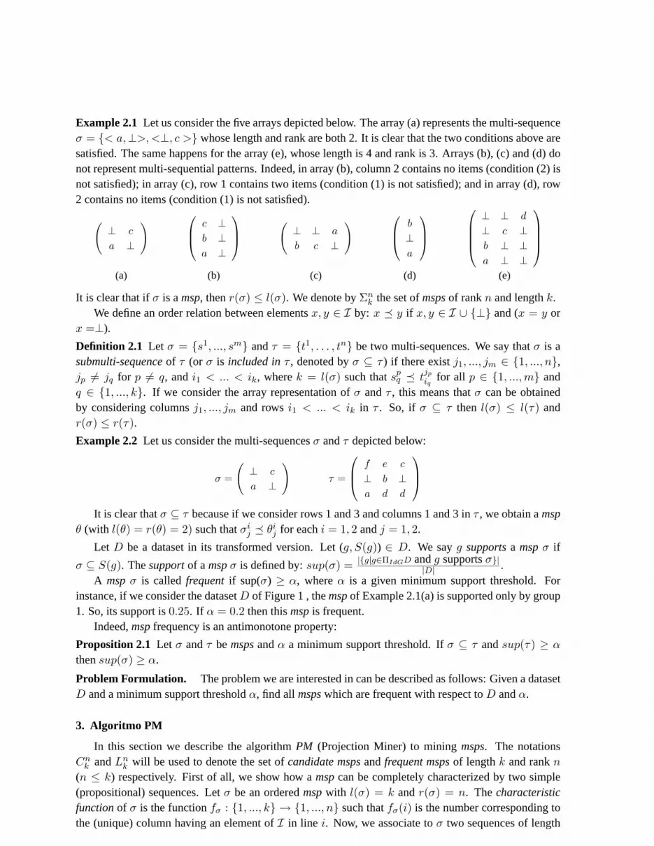
Example 2.1 Let us consider the five arrays depicted below. The array (a) represents the multi-sequenceσ = {< a,⊥>,<⊥, c >} whose length and rank are both 2. It is clear that the two conditions above aresatisfied. The same happens for the array (e), whose length is 4 and rank is 3. Arrays (b), (c) and (d) donot represent multi-sequential patterns. Indeed, in array (b), column 2 contains no items (condition (2) isnot satisfied); in array (c), row 1 contains two items (condition (1) is not satisfied); and in array (d), row2 contains no items (condition (1) is not satisfied).
(⊥ c
a ⊥
)
c ⊥b ⊥a ⊥
(⊥ ⊥ a
b c ⊥
)
b
⊥a
⊥ ⊥ d
⊥ c ⊥b ⊥ ⊥a ⊥ ⊥
(a) (b) (c) (d) (e)
It is clear that ifσ is amsp, thenr(σ) ≤ l(σ). We denote byΣnk the set ofmspsof rankn and lengthk.
We define an order relation between elementsx, y ∈ I by: x ¹ y if x, y ∈ I ∪ {⊥} and (x = y orx =⊥).
Definition 2.1 Let σ = {s1, ..., sm} andτ = {t1, . . . , tn} be two multi-sequences. We say thatσ is asubmulti-sequenceof τ (or σ is included inτ , denoted byσ ⊆ τ ) if there existj1, ..., jm ∈ {1, ..., n},jp 6= jq for p 6= q, andi1 < ... < ik, wherek = l(σ) such thatsp
q ¹ tjp
iqfor all p ∈ {1, ..., m} and
q ∈ {1, ..., k}. If we consider the array representation ofσ andτ , this means thatσ can be obtainedby considering columnsj1, ..., jm and rowsi1 < ... < ik in τ . So, if σ ⊆ τ then l(σ) ≤ l(τ) andr(σ) ≤ r(τ).
Example 2.2 Let us consider the multi-sequencesσ andτ depicted below:
σ =
(⊥ c
a ⊥
)τ =
f e c
⊥ b ⊥a d d
It is clear thatσ ⊆ τ because if we consider rows 1 and 3 and columns 1 and 3 inτ , we obtain amspθ (with l(θ) = r(θ) = 2) such thatσi
j ¹ θij for eachi = 1, 2 andj = 1, 2.
Let D be a dataset in its transformed version. Let (g, S(g)) ∈ D. We sayg supportsa mspσ if
σ ⊆ S(g). Thesupportof amspσ is defined by:sup(σ) = |{g|g∈ΠIdGD andg supportsσ}||D| .
A mspσ is called frequentif sup(σ) ≥ α, whereα is a given minimum support threshold. Forinstance, if we consider the datasetD of Figure 1 , themspof Example 2.1(a) is supported only by group1. So, its support is0.25. If α = 0.2 then thismspis frequent.
Indeed,mspfrequency is an antimonotone property:
Proposition 2.1 Let σ andτ bemspsandα a minimum support threshold. Ifσ ⊆ τ andsup(τ) ≥ α
thensup(σ) ≥ α.
Problem Formulation. The problem we are interested in can be described as follows: Given a datasetD and a minimum support thresholdα, find all mspswhich are frequent with respect toD andα.
3. Algoritmo PM
In this section we describe the algorithmPM (Projection Miner) to miningmsps. The notationsCn
k andLnk will be used to denote the set ofcandidate mspsandfrequent mspsof lengthk and rankn
(n ≤ k) respectively. First of all, we show how amspcan be completely characterized by two simple(propositional) sequences. Letσ be an orderedmspwith l(σ) = k andr(σ) = n. Thecharacteristicfunctionof σ is the functionfσ : {1, ..., k} → {1, ..., n} such thatfσ(i) is the number corresponding tothe (unique) column having an element ofI in line i. Now, we associate toσ two sequences of length

k, denoted byΠt(σ) (the item-sequenceof σ) andΠs(σ) (the shape-sequence), as follows: Πt(σ) isthe projection ofσ over the time axis andΠs(σ) = < fσ(1), ..., fσ(k) >. For instance, ifσ is themspillustrated in Example 2.1 (e), thenΠt(σ) =< a, b, c, d > andΠs(σ) =< 1, 1, 2, 3 >. It is easy to verifythat amspis completely characterized by its shape-sequence and item-sequence. The numbersk andn
are called thelengthandrank of the shape-sequenceΠs(σ) respectively. We denote byproj (σ) the pair(Πt(σ),Πs(σ)). The inverse function is denote by£, that isΠt(σ) £ Πs(σ) = σ.
In algorithm PM, the setLnk+1 is obtained fromLn
k andLn−1k . In order to do so, themspsin Ln
k
are projected in two sequence components: ashape-sequenceand anitem-sequence. At (sub)-iterationk + 1 of the iterationn, the set of candidate shape-sequences and item-sequences of rankn and lengthk + 1 (denotedCIn
k+1 andCSnk+1 respectively) are generated respectively from the sets of frequent
shape-sequencesLSnk , LSn−1
k and frequent item-sequencesLInk , LIn−1
k , obtained in previous iterations.Figure 2 illustrates how the setLn
k+1 is obtained fromLnk andLn−1
k .
Lnk
LInk
LSnk
Join
Join
LIn-1k
LSn-1k
(pre)CInk+1
(pre)CSnk+1
Prunning
Prunning
LIn-1k
LSn-1k
CInk+1
CSnk+1
LI + nk
LS +nk
Cnk+1 Ln
k+1Validation
i
s
proj
Candidate Generation
Figure 2:Lnk+1 is obtained fromLn
k andLn−1k
The algorithm PM is given in Figure 3. At the steps3.5 and3.9.6we used the operator£ to jointhe item-sequences and shape-sequences. In this process, each shape-sequence inCSn
k is joined with allitem-sequences ofCIn
k . The resulting set ofmspsis Cnk (also denoted byCIn
k £ CSnk ). TheJoinI op-
eration joins the item-sequences inLInk ∪LIn−1
k and returns the setCInk+1 of candidate item-sequences.
Analogously, theJoinS operation yields the set of shape-candidatesCSnk+1 by joining shape-sequences
in LSnk ∪ LSn−1
k . The details of these join operations are given in section 3.1 below. The functionprojcomputes the projectionsΠi andΠs for all mspsin Ln
k and returns the setsLInk andLSn
k .
3.1. Candidate Generation
TheJoinI operation between candidate item-sequences (CInk ) is computed as in [3]. Concerning
the generation of the candidate shape-sequences, there are three possibilities for computing the result oftheJoinS operation. Figure 4 illustrates each of these cases. We explain below the three cases.
Let σ = < σ1, σ2, ..., σk > andτ = < τ1, τ2, ..., τk > be two shape-sequences of ranknσ andnτ
respectively. Let denote byσfirst and τ last the sequences obtained by eliminating the first elementof σ and the last element ofτ respectively. Ifσfirst = τ last thenσ andτ are joinable. In this case(Case 1), the resulting sequence is< σ1, σ2, ..., σk, τk >. Otherwise, we test ifτ last
i + 1 = σlasti for
all i = 1, ..., k. If this is verified (Case 2a) thenσ andτ are joinable and one resulting sequence is< σ1, . . . , σk, τk + 1 >. We next test (Case 2b) if Inc(τ )last
i = σlasti for all i = 1, ..., k, where Inc(τ )i
= τi + 1 if τi + 1 < max(nσ, nτ ) and Inc(τ )i = 1 otherwise. If this is verified then a second resultingsequence is also obtained, defined as< σ1, . . . , σk, Inc(τ)k >.
The following example illustrates the process of the candidate generation in PM.
Example 3.1 Let us suppose thatL23 andL1
3 contain themspsσ andτ given below:

(α: minimum support,N : number of data multi-sequences,D: dataset)
1. k = 0; n = 1;2. Repeat
2.1k = k + 1;
2.2L1k = frequent sequences of rank 1 and lengthk (uses GSP);
2.3 if L1k 6= ∅ then { LI1
k = L1k; LS1
k = {< 1, 1, . . . , 1 >} };Until L1
k = ∅;3. Repeat
3.1n = n + 1; k = n;
3.2CInn = JoinI(LIn−1
n−1 , LIn−1n−1 ); (Candidate item-sequences generated fromLIn−1
n−1 )
3.3CSnn = {< 1, 2, ..., n >}
3.4 deleteall candidatesσ ∈ CInn such that∃τ ⊆ σ, l(τ) = n− 1 andτ /∈ LIn−1
n−1 (pruning);
3.5Cnn = CIn
n £ CSnn (build the candidatesmsps)
3.6 Foreachgroupg in D doIncrement the count of all candidatemspsin Cn
n that are contained inS(g);3.7Ln
n = candidates inCnn with count≥ αN ;
3.8(LInn , LSn
n) = proj (Lnn); (projects item-sequences and shape-sequences ofLn
n into LInn andLSn
n );
3.9 Repeat3.9.1k = k + 1;
3.9.2CInk = JoinI(LIn−1
k−1 ∪ LInk−1, LIn−1
k−1 ∪ LInk−1);
(Candidate item-sequences generated fromLIn−1k−1 andLIn
k−1)
3.9.3 deleteall candidatesσ ∈ CInk such that∃τ ⊆ σ, l(τ) = k − 1 andτ /∈ LIn−1
k−1 ∪ LInk−1;
(pruning item-sequences)
3.9.4CSnk = JoinS(LSn−1
k−1 ∪ LSnk−1, LSn−1
k−1 ∪ LSnk−1);
(Candidate shape-sequences generated fromLSn−1k−1∪LSn
k−1)
3.9.5 deleteall candidatesσ ∈ CSnk such that∃τ ⊆ σ andτ /∈ LSn−1
k−1 ∪ LSnk−1;
(pruning shape-sequences)
3.9.6Cnk = CIn
k £ CSnk
3.9.7 Foreachgroupg in D doIncrement the count of all candidatemspsin Cn
k that are contained inS(g);3.9.8Ln
k = candidates inCnk with count≥ αN ;
3.9.9(LInk , LSn
k ) =proj (Lnk ); (projects item-sequences and shape-sequences ofLn
k )
Until Lnk = ∅;
Until Lnn = ∅;
Figure 3: Algorithm PM
1 1 2 2 3
1 2 2 3 21 1 2 2 3 2
Case 1
1 2 2 2 3
1 1 1 2 3
1 2 2 2 3 42 2 2 3 4
+1
Case 2a
1 2 2 2 3
1 1 1 2 3
1 2 2 2 3 12 2 2 3 1
incr()
Case 2b
Figure 4: Joiningshape-sequences
σ =
⊥ c
⊥ b
a ⊥
andτ =
d
c
b
γ =
⊥ d
⊥ c
⊥ b
a ⊥

We join σ andτ in order to obtain the candidatemspγ of rank 2 and length 4. We haveΠi(σ) =< a, b, c > ∈ LI2
3 , Πs(σ) =< 1, 2, 2 > ∈ LS23 , Πi(τ) =< b, c, d > ∈ LI1
3 andΠs(τ) =< 1, 1, 1 >
∈ LS13 . By joining the item-sequences< a, b, c > and< b, c, d > we obtain the item-sequence<
a, b, c, d > ∈ LI24 . By joining the shape-sequences< 1, 2, 2 > and< 1, 1, 1 > (Case 2a), we obtain
the shape-sequence< 1, 2, 2, 2 > ∈ LS24 . We notice that Case 2b does not apply here. The sequences
< a, b, c, d > and< 1, 2, 2, 2 > uniquely characterize themspγ ∈ C24 .
Theorem 3.1 For alln, k, 1 ≤ n ≤ k, we haveLnk ⊆ Cn
k .
Support Counting. The technique used in the Validation Phase is the same used in Algorithm SM andis outlined at the end of the next section.
4. Algorithm SM
In this section we present the algorithmSM (Simultaneous Miner) for miningmsps. We remind thatCn
k andLnk denotes respectively the set ofcandidate mspsand frequent mspsof lengthk and rankn,
wheren ≤ k.
The general structure of the algorithm is that it generates first the frequentmspsof rank 1 (L11, L
12, L
13,
. . .) using for this task an algorithm for mining (simple) sequential patterns (for instance, the algorithmGSP [3]). After that, for eachn > 1 (a given rank) it generates iteratively the setsCn
k of candidatemspsof lengthk ≥ n. For the initial casek = n, Cn
n is generated fromLn−1n−1, which has been already
generated in the previous step corresponding to rankn − 1. For the casek > n, the setCnk (containing
the potentially frequentmspsof lengthk and rankn) is generated fromLn−1k−1 andLn
k−1 which have beenalready generated in previous steps. It finds the support for these candidatemspsduring the pass over thedataset. At the end of the pass, it generates the setLn
k , the candidatemspswhich are actually frequent.Thesemspsbecome the seed for the next passk + 1. In Figure 5(a), we illustrate how the setLn
k isobtained from previous steps and in Figure 5(b), we illustrate the whole mining process.
rank
length
k=1
k=2
k=3
k=4
n=1 n=2 n=3 n=4
L11
L12
L13
L14
L22
L23
L24
L33
L34 L4
4
(a)
Lnk-1
Generation
Ln-1k-1
(pre)Cnk Prunning
Ln-1k-1
Cnk
L + nk-1
Lnk
Validation
(b)
Figure 5:Lnk is obtained fromLn−1
k−1 andLnk−1
The algorithm SM is given in Figure 4. At the pass where frequentmspsof lengthk and rankn aregenerated, the algorithm first generates the setCn
k , the candidatemsps(steps3.2and3.6.2). After that, itprunes fromCn
k themspswhich containmspsnot belonging toLn−1k−1 andLn
k−1: according to proposition2.1, these prunedmspshave no chance to be frequent (steps3.3, 3.6.3and3.6.4). After the pruningphase, the support of the candidates is measured by making a pass over the dataset (steps3.4and3.6.5).In paragraph 4.1, we show in detail how candidatemspsin Cn
k are built from the setsLn−1k−1 andLn
k−1
which have already been calculated in previous steps.

(α: minimum support,N : number of data multi-sequences,D: dataset)
1. n = 1; k = 0;2. Repeat
2.1k = k + 1;
2.2L1k = frequent sequences of rank 1 and lengthk (uses GSP)
Until L1k = ∅;
3. Repeat3.1n = n + 1; k = n;
3.2Cnn = Ln−1
n−1 1 Ln−1n−1 (New candidate msps of rankn and lengthn are generated fromLn−1
n−1)
(For details on the operator1, see Section 4.1);
3.3 deleteall candidatesσ ∈ Cnn such that∃τ ⊆ σ, τ ∈ Σn−1
n−1 andτ /∈ Ln−1n−1 (pruning);
3.4 Foreachgroupg in D doIncrement the count of all candidatemspsin Cn
n that are contained inS(g);3.5Ln
n = candidates inCnn with count≥ αN ;
3.6 Repeat3.6.1k = k + 1;
3.6.2Cnk = (Ln−1
k−1 1 Ln−1k−1) ∪ (Ln
k−1 1 Lnk−1) ∪ (Ln−1
k−1 1 Lnk−1) ∪ (Ln
k−1 1 Ln−1k−1)
(New candidate msps of rankn and lengthk are generated
fromLn−1k−1 andLn
k−1 See Section 4.1 for details);
3.6.3 deleteall candidatesσ ∈ Cnk such that∃τ ⊆ σ, τ ∈ Σn−1
k−1 andτ /∈ Ln−1k−1 ; (pruning 1)
3.6.4 deleteall candidatesσ ∈ Cnk such that∃τ ⊆ σ, τ ∈ Σn
k−1 andτ /∈ Lnk−1; (pruning 2)
3.6.5 Foreachgroupg in D doIncrement the count of all candidatemspsin Cn
k that are contained inS(g);3.6.6Ln
k = candidates inCnk with count≥ αN ;
Until Lnk = ∅;
Until Lnn = ∅
Figure 6: Algorithm SM
4.1. Candidate Generation
Now, we show how to generate potentially frequentmspsin Σnk (recall thatΣn
k denotes the set ofmspsof rankn and lengthk). In this construction, we will suppose that the columns of eachmspσ ∈ Σn
k
are ordered by an ordering which is naturally induced by the time level ordering. For instance, in Figure7 (e) we have a not orderedmsp(left) and the samemspwhere columns have been ordered (right).
We will use the following notation in the sequel: ifσ ∈ Σnk thenσ andσ denotes the multi-sequences
(not necessarilymsps) obtained by deleting, respectively, rown and row 1 fromσ.As we can see in line3.6.2of SM description, there are four possibilities to obtain a candidate in
Cnk : (1) by joining twomspsof Ln−1
k−1 , (2) by joining twomspsof Lnk−1, (3) by joining amspsof Ln−1
k−1
with a mspof Lnk−1 and (4) by joining amspsof Ln
k−1 with a mspof Ln−1k−1 . Figure 7(a) to (e) gives the
conditions for twomspsbeing joinable (below each figure) as well as the result of the join operation, inthe four cases.
The following theorem guarantees that : (1) all frequentmspsof Σnk are included inCn
k and (2)Cnk
is minimal, in the sense that it contains only the potentially frequentmspsof Σnk :
Theorem 4.1 For all n, k, 1 ≤ n ≤ k, we have: (1)Lnk ⊆ Cn
k . (2) If σ ∈ Σnk and there existsτ ⊆ σ,
τ 6= σ, such thatτ is not frequent, thenσ 6∈ Cnk .
For lake of space, the proof of this theorem is given in the Appendix.

a
b
c
de
f
g
b
cd
ef
a
bc
d
ef
gLn-1k-1
Ln-1k-1 L
nk
Case 1: if we eliminate the first column ofσ and last column ofτ then the resultingmspsare identical.
a
bc
d
ef
g
bcd
ef
a
bcd
ef
gLnk-1
Lnk-1 L
nk
Case 2a:σ andτ are identical.
a
bc
d
ef
g
bc
d
ef
a
bc
d
ef
gLnk-1
Lnk-1 L
nk
Case 2b:σ andτ are identical after shifting the colomns ofτone place to the right.
a
bc
de
g
b
c
def
a
bc
def
g
f
Ln-1k-1
Lnk-1 L
nk
Case 3:σ andτ are identical and the last column ofτ oonlycontain the symbol⊥.
a
b
c
de
f
g
b
cd
ef
a
b
c
d
ef
gLnk-1
Ln-1k-1 L
nk
Case 4: The first column ofσ only contains the symbol⊥ andσis identical toτ after shiftingσ one place to the left.
d ⊥ ⊥⊥ c ⊥⊥ ⊥ b
⊥ ⊥ a
→
⊥ ⊥ d
⊥ c ⊥b ⊥ ⊥a ⊥ ⊥
(e) A mspand its ordered version
Figure 7: Joiningmsps
4.2. Support Counting
In order to reduce I/O operations over the dataset and compute the support of eachmspin Cnk by
executing only one pass over the dataset, we will find all candidatesσ which are included inS(g), foreach data multi-sequenceS(g). In order to reduce the number of candidates which have to be tested forinclusion for each data multi-sequenceS(g), we will use a technique similar to the one described in [2]for counting the support of sequences, by storing the set of candidatesmspsCn
k in a setof hash-trees.For lack of space, we omit these technical details here.
5. Experimental Results
To evaluate the performance of the algorithms SM e PM, we ran several experiments using syntheticdatasets. Our experiments have been executed on a Pentium 4 of 2.4 GHz with 1GB of main memoryand running Windows XP Professional.
5.1. Synthetic Data
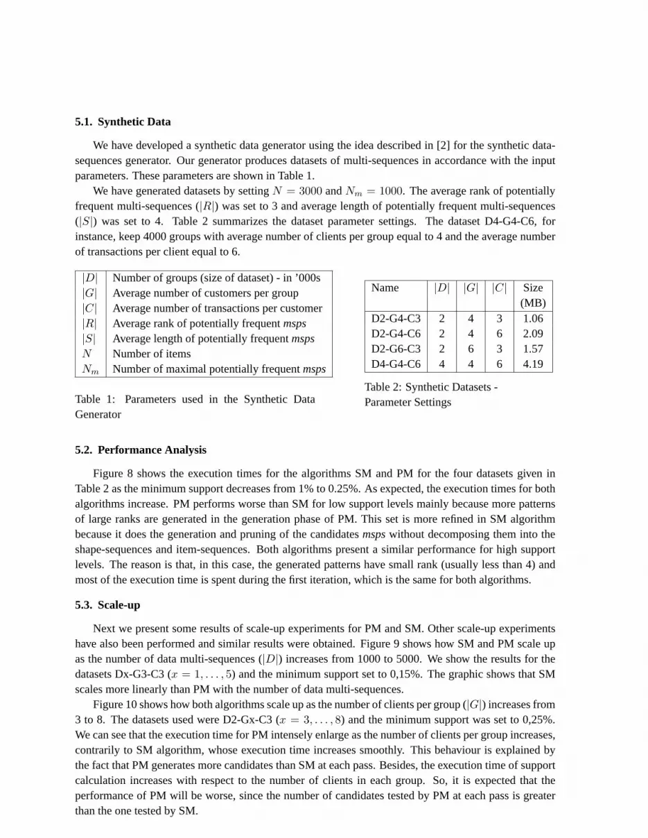
We have developed a synthetic data generator using the idea described in [2] for the synthetic data-sequences generator. Our generator produces datasets of multi-sequences in accordance with the inputparameters. These parameters are shown in Table 1.
We have generated datasets by settingN = 3000 andNm = 1000. The average rank of potentiallyfrequent multi-sequences (|R|) was set to 3 and average length of potentially frequent multi-sequences(|S|) was set to 4. Table 2 summarizes the dataset parameter settings. The dataset D4-G4-C6, forinstance, keep 4000 groups with average number of clients per group equal to 4 and the average numberof transactions per client equal to 6.
|D| Number of groups (size of dataset) - in ’000s|G| Average number of customers per group|C| Average number of transactions per customer|R| Average rank of potentially frequentmsps|S| Average length of potentially frequentmspsN Number of itemsNm Number of maximal potentially frequentmsps
Table 1: Parameters used in the Synthetic DataGenerator
Name |D| |G| |C| Size(MB)
D2-G4-C3 2 4 3 1.06D2-G4-C6 2 4 6 2.09D2-G6-C3 2 6 3 1.57D4-G4-C6 4 4 6 4.19
Table 2: Synthetic Datasets -Parameter Settings
5.2. Performance Analysis
Figure 8 shows the execution times for the algorithms SM and PM for the four datasets given inTable 2 as the minimum support decreases from 1% to 0.25%. As expected, the execution times for bothalgorithms increase. PM performs worse than SM for low support levels mainly because more patternsof large ranks are generated in the generation phase of PM. This set is more refined in SM algorithmbecause it does the generation and pruning of the candidatesmspswithout decomposing them into theshape-sequences and item-sequences. Both algorithms present a similar performance for high supportlevels. The reason is that, in this case, the generated patterns have small rank (usually less than 4) andmost of the execution time is spent during the first iteration, which is the same for both algorithms.
5.3. Scale-up
Next we present some results of scale-up experiments for PM and SM. Other scale-up experimentshave also been performed and similar results were obtained. Figure 9 shows how SM and PM scale upas the number of data multi-sequences (|D|) increases from 1000 to 5000. We show the results for thedatasets Dx-G3-C3 (x = 1, . . . , 5) and the minimum support set to 0,15%. The graphic shows that SMscales more linearly than PM with the number of data multi-sequences.
Figure 10 shows how both algorithms scale up as the number of clients per group (|G|) increases from3 to 8. The datasets used were D2-Gx-C3 (x = 3, . . . , 8) and the minimum support was set to 0,25%.We can see that the execution time for PM intensely enlarge as the number of clients per group increases,contrarily to SM algorithm, whose execution time increases smoothly. This behaviour is explained bythe fact that PM generates more candidates than SM at each pass. Besides, the execution time of supportcalculation increases with respect to the number of clients in each group. So, it is expected that theperformance of PM will be worse, since the number of candidates tested by PM at each pass is greaterthan the one tested by SM.

Figure 8: Execution times: Synthetic Data
Figure 9: Scale-up w.r.t to data multi-sequences Figure 10: Scale-up w.r.t. clients per group
6. Ongoing and Further Research
At the present time, we are investigating constraint-based methods for restricting the candidate searchspace. Often, users require richer mechanisms for specifying patterns of interest, rather than the simplemechanism provided by minimum support. Concerning the classical problem of mining sequential pat-terns [2], one of the most flexible tools enabling user-controlled focus to be incorporated into the patternmining process has been proposed in [17]: besides the dataset, the user proposes a regular expression asinput, which aims at capturing the shape of patterns he/she is interested in discovering. The automatonassociated to this regular expression is incorporated into the mining process which outputs the sequen-

tial patterns exceeding a minimum support threshold and which are accepted by the automaton. We areinvestigating the introduction of regular expression restrictions overmspsand the development of algo-rithms to minemspssatisfying such restrictions. Another line of future research concerns performancecomparison between our Apriori-based method SM and methods for first-order sequential pattern miningbased on Inductive Logic Programming.
References
[1] R. Agrawal, H. Mannila, R. Srikant, H. Toivonen, and A. I. Verkamo.Fast Discovery of AssociationRules.In Fayyad, U.M., Piatetsky-Shapiro, G., Smyth, P; and Uthurusamy, R., eds. Advances in Knowl-edge Discovery and Data Mining, AAAI Press, 1995.
[2] R. Agrawal, R. Srikant.Mining Sequential Patterns.Proc. of the Int. Conference on Data Engineering(ICDE), Taipei, Taiwan, March 1995.
[3] R. Agrawal, R. Srikant.Mining Sequential Patterns: Generalizations and Performance Improvements.Proc. of the Fifth Int. Conference on Extending Database Technology (EDBT), Avignon, France, March1996.
[4] C. Masson, F. Jacquenet.Mining Frequent Logical Sequences with Spirit-Log.In ILP 2003, LNAI 2583,pp. 166-182, 2003, Springer-Verlag 2003.
[5] Sau Dan Lee, Luc De Raedt:Constraint Based Mining of First Order Sequences in SeqLog.In Proc. ofthe Workshop on Multi-Relational Data Mining, ACM SIGKDD 2002, Edmonton, Alberta, Canada, July2002.
[6] N. Jacobs, H. Blockeel.From shell logs to shell scripts.In Rouveiros, c. ed.: Proc. 11th InternationalConference, ILP 2001, LNCS 2157, pp. 80-90.
[7] J. Han, J. Pei, B. Mortazavi-Asl, Q. Chen, U. Dayal, and M. Hsu.Free-Span: Frequent Pattern-ProjectedSequential Pattern Mining.KDD 2000, 355-359
[8] Mohammed J. ZakiSPADE: An Efficient Algorithm for Mining Frequent Sequences.Machine Learning,0, 1-31, 2000.
[9] H. Pinto, J. Han, J. Pei, K. Wang, Q. Chen, U. Dayal.Multi-dimensional Sequential Pattern Mining.CIKM 2001, pp. 81-88.
[10] H. Mannila, H. Toivonen, A.I. VerkamoDiscovery of frequent episodes in event sequences.Data Miningand Knowledge Discovery 1(3): 259 - 289, November 1997.
[11] C. Bettini, X.S. Wang, S. Jajodia.Testing Complex Temporal Relationships Involving Multiple Granu-larities and Its Application to Data Mining.Proc. of ACM PODS, pp. 68-78, Montreal, 1996.
[12] G. Das,K-I. Lin, H. Mannila, G. Renganathan, P. Smyth.Rule discovery from time series.Proc. of the4th International Conference of Knowledge Discovery and Data Mining. pp 16-22, AAAI Press.
[13] H. Lu, L. Feng, J. Han.Beyond Intra-Transaction Association Analysis: Mining Multi-DimensionalInter-Transaction Association Rules.ACM Transactions on Information Systems, 18(4): 423-454, 2000.
[14] B. Padmanabhan, A. Tuzhilin.Pattern Discovery in Temporal Databases: A Temporal Logic Approach.KDD 1996, pp. 351-355.
[15] G. Berger, A. Tuzhilin.Discovering Unexpected Patterns in Temporal Data Using Temporal Logic.Tem-poral Databases, Dagstuhl 1997, 281-309.
[16] M. V. Joshi, G. Karypis, V. Kumar.A Universal Formulation of Sequential Patterns.Technical Report,Department of Computer Science, University of Minnesota, 1999.
[17] M.N. Garofalakis, R. Rastogi, K. Shim.SPIRIT: Sequential Pattern Mining with Regular ExpressionConstraints.In Proc. of the 25th VLDB Conference, Edinburgh, Scotland, 1999.

APPENDIX
Proof of Theorem 4.1(1) Let σ ∈ Ln
k . We suppose the columns ofσ are ordered according to the procedureColumnOrdgiven in the beginning of this section. Forn = 1, the result is verified, because the candidate generationprocedure used in algorithm Apriori-All is correct, i.e., the set of candidates always contain all frequentsequences. Forn = k = 2, the result is also verified: indeed, asσ ∈ L2
2, the msps{< σ11 >} and
{< σ22 >} are inL1
1. So, by construction ofC22 , it is clear thatL2
2 ⊆ C22 . Let n, k, 2 ≤ n ≤ k, k ≥ 3.
We have the following cases to consider:• the (unique) item of line2 is placed in column 1 and (a) there exists an item in columnn placed in aline i, with i < k: in this case,σ ∈ Ln
k 1nk Ln
k , (b) columnn contain only one item, which is placed inline k: in this case,σ ∈ Ln−1
k−1 1nk Ln
k .• the (unique) item of line2 is placed in column 2 and (a) there exists an item in columnn placed in aline i, with i < k: in this case,σ ∈ Ln
k 1nk Ln−1
k−1 , (b) columnn contain only one item, which is placedin line k: in this case,σ ∈ Ln−1
k−1 1nk Ln−1
k−1 .
(2) Sinceτ ⊆ σ andτ 6= σ, thenτ ∈ Σmp with m < n or p < k, then:
• Let m < n andm ≤ p ≤ k. In this case,τ is obtained by deleting at least one column ofσ andone of the lines corresponding to the items in this column. Sop < k. We can suppose, without loss ofgenerality, that only one column has been deleted, i.e.m = n− 1. We can affirm thatτ is contained in amspτ ′ ∈ Σn−1
k−1 , such thatτ ′ ⊆ σ. Sinceτ is not frequent, thenτ ′ is not frequent as well, i.e.,τ ′ 6∈ Ln−1k−1 .
Then, by construction of themspsin Cnk , σ 6∈ Cn
k .• Let m = n andn ≤ p < k. In this case,τ is obtained by deleting at least one line ofσ. We cansuppose, without loss of generality, that only one line has been deleted. Thus,τ ∈ Σn
k−1. Sinceτ is notfrequent, i.e.τ 6∈ Ln
k−1 then, by construction of themspsin Cnk , σ 6∈ Cn
k . 2
Proof of Theorem 3.1. This proof follows from the previous proof of Theorem 4.1: In fact, theJoinS
operation between shape-sequences is defined in such a way thatΠs((Ln−1k−1 1 Ln−1
k−1)∪(Ln−1k−1 1 Ln
k−1)∪(Ln
k−1 1 Lnk−1)∪ (Ln
k−1 1 Lnk−1)) = JoinS(Πs(Ln−1
k−1), Πs(Ln−1k−1)) ∪ JoinS(Πs(Ln−1
k−1),Πs(Lnk−1)) ∪
JoinS(Πs(Lnk−1), Πs(Ln−1
k−1)) ∪ JoinS(Πs(Lnk−1), Πs(Ln
k−1)).


