Riparian zone evapotranspiration estimation from diurnal groundwater level fluctuations

This article was published in an Elsevier journal. The attached copyis furnished to the author for non-commercial research and

education use, including for instruction at the author’s institution,sharing with colleagues and providing to institution administration.

Other uses, including reproduction and distribution, or selling orlicensing copies, or posting to personal, institutional or third party

websites are prohibited.

In most cases authors are permitted to post their version of thearticle (e.g. in Word or Tex form) to their personal website orinstitutional repository. Authors requiring further information

regarding Elsevier’s archiving and manuscript policies areencouraged to visit:

http://www.elsevier.com/copyright

http://www.elsevier.com/copyright

Author's personal copy

Riparian zone evapotranspiration estimation fromdiurnal groundwater level fluctuations

Zoltan Gribovszki a,b,*, Peter Kalicz a, Jozsef Szilagyi b,c, Mihaly Kucsara a

a Institute of Geomatics and Civil Engineering, University of West Hungary, Sopron H-9400, Hungaryb Department of Hydraulic and Water Resources Engineering, Budapest University of Technology and Economics,Budapest H-1111, Hungaryc School of Natural Resources, University of Nebraska – Lincoln, Lincoln, NE 68583, USA

Received 19 January 2007; received in revised form 19 October 2007; accepted 25 October 2007

KEYWORDSEvapotranspiration;Riparian zone;Diurnal groundwaterlevel fluctuations

Summary Riparian vegetation typically has a great influence on groundwater level andgroundwater-sustained stream baseflow. By modifying the well-known method by White[White, W.N., 1932. Method of estimating groundwater supplies based on discharge byplants and evaporation from soil – results of investigation in Escalante Valley, Utah – USGeological Survey. Water Supply Paper 659-A, 1–105] an empirical and hydraulic versionof a new technique were developed to calculate evapotranspiration (ET) from groundwaterlevel readings in the riparian zone. The method was tested with hydrometeorological datafrom the Hidegvız Valley experimental catchment, located in the Sopron Hills region at thewestern border of Hungary. ET rates of the proposed method lag behind those of the Pen-man–Monteith method but otherwise the two estimates compare favorably for the day. Atnights, the new technique yields more realistic values than the Penman–Monteith equa-tion. On a daily basis the newly-derived ET rates are typically 50% higher than the onesobtainable with the original White method. Sensitivity analysis showed that the more reli-able hydraulic version of our ET estimation technique is most sensitive (i.e., linearly) to thelaboratory- and/or slug-test derived values of the saturated hydraulic conductivity andspecific yield taken from the riparian zone.ª 2007 Elsevier B.V. All rights reserved.

Introduction

The diurnal cycle of the climate forcing, such as tempera-ture, solar radiation, and humidity often induces a similardaily fluctuation in the groundwater level of the riparianzone and, especially during drought periods, in the flow rateof the adjacent low-order stream through the mediation of

0022-1694/$ - see front matter ª 2007 Elsevier B.V. All rights reserved.doi:10.1016/j.jhydrol.2007.10.049

* Corresponding author. Address: Institute of Geomatics and CivilEngineering, University of West Hungary, Sopron H-9400, Hungary.Tel.: +36 99 518 314; fax: +36 99 518 123.

E-mail addresses: [email protected] (Z. Gribovszki), [email protected] (P. Kalicz), [email protected] (J. Szilagyi).

Journal of Hydrology (2008) 349, 6–17

ava i lab le at www.sc iencedi rec t . com

journal homepage: www.elsevier .com/ locate / jhydro l


the riparian vegetation. This vegetation effect on thegroundwater levels and baseflow rates occurs as a resultof a daily rhythm in the metabolism of the vegetation mod-ulated by phenological changes through the seasons. Meta-bolic changes in the vegetation are accompanied bysimilar changes in transpiration rates. In riparian forests ofdense cover, soil evaporation during drought periods is of-ten negligible in comparison with the transpiration ratesof vegetation. Several authors have investigated the linkagebetween riparian transpiration and streamflow rates (Trox-ell, 1936; Croft, 1948; Tschinkel, 1963; Reigner, 1966;Portge, 1996; Lundquist and Cayan, 2002; Loheide et al.,2005; Butler et al., 2007; Boronina et al., 2005) but only afew attempted to estimate the evapotranspiration (ET) rate

of the riparian zone (White, 1932; Bond et al., 2002; Baueret al., 2004; Nachabe et al., 2005) by using of the observedstreamflow, groundwater or soil moisture fluctuations or toprovide an analytical description of these signals (Czikow-sky, 2003; Czikowsky and Fitzjarrald, 2004).

A typically observable diurnal pattern in groundwater le-vel and streamflow rate is displayed in Fig. 1 for a forestedriparian zone in western Hungary. The maxima occur in themorning hours, between 6 and 8 a.m., and the minima in theafternoon, between 4 and 5 p.m. (Gribovszki et al., 2006).Both signals are characterized by sharp lower extrema,but the peak regions of the streamflow signal are morerounded. Notably the two extrema do not overlap perfectlyin time, the groundwater extrema lag behind those of thestreamflow rate by about 1–1.5 h. To our best knowledgeno such lag has ever been reported in the literature before.In an accompanying paper by Szilagyi et al. (2007) to thispresent work the problem is further investigated.

The transpiration demand of the vegetation is generallymet by the soil moisture of the riparian zone and/or directlyby the groundwater. In drought periods the groundwater ofthe riparian zone used by evapotranspiration is typicallyreplenished via groundwater flow from areas farther awayfrom the stream (Fig. 2) or by so-called induced recharge,when, due to a reversed hydraulic gradient, the groundwa-ter flow is directed from the channel toward the riparianzone. Around the timing of the groundwater level extrema,supply, Qnet [LT

�1], and demand, ET [LT�1], are in an equi-librium in Eq. (1)

dS

dt¼ Q net � ET ð1Þ

Gro

undw

ater

leve

l [m

]

371.

5537

1.60

371.

65

05 Sep 06 Sep 07 Sep

0.6

0.8

1.0

1.2

Bas

eflo

w [l

/s]

Groundwater levelBaseflow

Figure 1 Observed diurnal fluctuations in riparian groundwa-ter level and baseflow values.

Figure 2 Schematic model of the riparian zone.

Riparian zone evapotranspiration estimation from diurnal groundwater level fluctuations 7


where S [L] is the stored water volume per unit area. Aroundthe extrema dS/dt = 0, dS/dt > 0 and Qnet > ET on the risinglimb and dS/dt < 0 and Qnet < ET on the falling limb of thegroundwater hydrograph. The ET rate is largest during theday when the groundwater level curve is about the steepeston the descending limb, which is typically close to the radi-ation maxima. The smallest ET rate however does not nec-essarily take place when the ascending limb of thegroundwater level signal is the steepest, rather, just priorto dawn when vapor pressure deficit is at its diurnal mini-mum. The minima in the riparian zone groundwater levelis accompanied by the steepest hydraulic gradients, so whenET starts to decrease, the steep hydraulic gradient can de-liver water to the riparian zone very efficiently, replenishingit fastest right after the occurrence of the groundwater le-vel minimum, thus somewhat (but not entirely) independentof the actual ET rate, at least for a while (for more detail,see the accompanying paper by Szilagyi et al., 2007). Thismechanism is especially true in valley settings (Fig. 2),where farther away from the stream the groundwater levelis deeper below the surface, thus, being less affected by thediurnal fluctuations in the transpiration rate of vegetation.

White (1932) published a method of estimating riparianET rates on a daily time step based on fluctuations in thegroundwater level. He assumed that during the predawn/dawn hours when ET is negligible, the rate of the observedgroundwater level increase is directly proportional to therate groundwater is supplied to the riparian zone from theneighboring areas. The slope, r [LT�1], of the tangential linedrawn to the groundwater level curve in these sections(Fig. 3), multiplied by specific yield value, Sy [–], of theriparian zone, therefore, represents the rate of water sup-ply to a unit area. By extending the tangential line over a24-h period and taking the difference in groundwater levels,one would obtain an estimate of the total water supply tothe unit area over a day. The so-obtained daily rate of watersupply must typically be modified by s [L], the difference inthe observed groundwater level over the 24-h period, sinceit rarely happens that the groundwater level returns to thesame elevation a day before. The daily ET rate this way isobtained as

ET ¼ Syð24r � sÞ ð2Þ

where r is the mean hourly rate of groundwater level in-crease from midnight to 4 a.m.

Meyboom (1964) suggested a 50% reduction (which hecalled the readily available specific yield) of the labora-tory-derived specific yield value in Eq. (2). A reduction iscertainly justified since it takes some time for the drainageto adjust to any new conditions introduced depending onsuch variables as soil-aquifer type, the thickness of the va-dose zone, as well as aquifer and stream geometry (e.g.,Szilagyi, 2004).

Based on the study of Nachabe (2002), Loheide et al.(2005) suggested certain guidelines and an equation to ob-tain Sy as a function of sediment texture, depth to thegroundwater table and elapsed time (t) of the drainage.The relationship is based on the Brooks and Corey (1964)model that gives the volumetric water content (h) as

hðWÞ ¼ hR þ ðhS � hRÞha

W

� �k

ð3Þ

where ha [L] is the air entry pressure, W [L] is the pressure/suction head, k [–] is the pore-size index, hS [–] is the totalporosity, and hR [–] is the residual water content. With thehelp of Eq. (3) Sy becomes

SyðtÞ ¼Kt

DhhB � hR

hS � hR

� �2þ3kk hSurface � hR

hS � hR

� �2þ3kk

" #

þ ðhS � hRÞ 1� hB � hR

hS � hR

� �ð4Þ

where K [LT�1] is the saturated hydraulic conductivity ofthe soil, Dh is the change in the groundwater surfaceposition over time t, and hSurface is the actual water contentat the surface, which will depend on the actual depth to thegroundwater table. hB [–] is an additional parameter of thewater content profile defined as

hBðtÞ ¼ hR þ ðhS � hRÞDhðhS � hRÞ

2þ3kk K

! 12þ3k

k�1

t1

1�2þ3kk ð5Þ

Here K is calculated with the help of the Kozeny–Carmanrelationship as KS ¼ Bhn

e, where he is the effective porosity(i.e., total porosity minus the water content at a pressurehead of �33 kPa) and B [LT�1] and n [–] are empiricalparameters. When K is in cm h�1 then n and B obtain valuesof 4 and 1058, respectively.

Loheide et al. (2005) demonstrated via numerical model-ing experiments that the ET rate given by the White methodis not influenced perceptably by the geometry of the vadosezone. Although the White method yields reasonable esti-mates of daily ET, provided an appropriate Sy value is em-ployed Loheide et al. (2005), it has a weak point. Namely,it assumes that water supply to the riparian zone would hap-pen at a constant rate, observable when ET is negligible(Fig. 3), over the day. As mentioned earlier, this is hardlythe case since the hydraulic gradient changes over thecourse of the day as the riparian zone groundwater levelfluctuates. This fluctuation causes a time-varying water sup-ply to the area, since, especially in a valley setting with pre-dominantly horizontal groundwater flow, groundwaterlevels farther away from the stream (i.e., beyond the ripar-ian zone where depth to the groundwater is larger) typicallyexpress much diminished diurnal fluctuations (Fig. 2), thus

Time [hours of day]

Gro

undw

ater

leve

l [m

]

371.

6037

1.65

371.

7037

1.75

12:00 00:00 12:00 00:00 12:00

24r

s

Figure 3 The basic principle of the original White method.

8 Z. Gribovszki et al.


causing diurnally varying hydraulic gradients between thevalley-side and the riparian zone. The same head fluctua-tions may be true for a deep aquifer case with mainly verti-cal flow in the riparian zone.

While the White method (and its modification presentedbelow) aims to describe storage changes within the satu-rated zone only, implicitly it accounts (at least partially)for moisture withdrawal (depending on the depth of thewater table) from the vadose zone as well. Vadose zoneET does not come solely from the vadose zone soil moisturebecause this soil moisture always has a close hydraulic con-nection with the groundwater table through the capillaryfringe, therefore it is indirectly included in the water bal-ance of the groundwater system. Loheide et al. (2005) dem-onstrated via numerical experiments that water extractedfrom a 1-m-thick vadose zone shows up in the ET estimatesof the White method so that it accounts for 19–23–28%(i.e., for silt, loam, and medium sand, respectively) of thetotal vadose zone water extraction. This however shouldnot be surprising since moisture extraction from the vadosezone can depress the groundwater table due to a reversedhydraulic gradient.

Shah et al. (2007) performed numerical simulations topartition total ET into vadose zone and groundwater ET.They found that for a water table within half meter of theland surface, nearly all ET came from the groundwaterdue to the close hydraulic connection between the unsatu-rated and saturated zones. Depending on the soil type, theyalso reported a decoupling of the groundwater and unsatu-rated zone moisture dynamics starting at water table depthsbetween 0.3 and 1.0 m for deep-rooted vegetation.

Hydraulic theory-based modification of theWhite method for riparian zone ET estimation

Since drought period water supply to the riparian zone istypically regulated by the hydraulic gradients between thebackground (i.e., away from the stream and the riparianzone) and the area in question, as well as between the samearea and the stream, it must be included in the ET estima-tion method. The lumped version of the mass-conservationequation Eq. (1), can also be written as

dS

dt¼ Sy

dh

dt¼ Q net � ET ð6Þ

where h [L] is the groundwater elevation within the control(unit) area. The net water supply, Qnet, is defined as the dif-ference between in- (Qin) and outflows (Qout) to it. The lat-ter flow rates (assuming mainly horizontal flow) areformulated by Darcy’s equation using the Dupuit approxima-tion (Harr, 1962; Kovacs, 1972)

Q net ¼ Q in � Q out ¼kðH2 � h2Þ2d1ðL� lÞ �

k h2 � h20

� �2d1l

ð7aÞ

Here H [L] is the groundwater elevation in the background(where diurnal fluctuations are not apparent) at a distanceL [L] from the stream, l [L] is the distance from the controlarea to the stream, h0 [L] is the water level in the stream(Fig. 2), k [LT�1] is the (preferably slug-test derived) satu-rated hydraulic conductivity of the soil-aquifer system,and d1 [L] is the unit distance along the stream. H, h and

h0 are taken relative to an assumed horizontal imperviouslayer (Fig. 2) not necessarily at the streambed elevation.Note that the above formulation of Eq. (7a) assumes succes-sive steady-state conditions at each time step of the Qnet

calculations, which is not strictly true.When the flow is mainly vertical in the riparian zone

(i.e., deep aquifer case) Eq. (7a) can be substituted byDarcy’s equation

Q net ¼ kvH � h

l0ð7bÞ

where H now is the total (‘background’) head at a depth of l 0

below the reference level, and kv is the saturated hydraulicconductivity value for vertical flow.

Before the application of the hydraulic theory, one has todecide about the location at which the groundwater levelsmust be observed and its temporal derivatives be com-puted. As Bauer et al. (2004) and Loheide et al. (2005) dem-onstrated, the middle part of the riparian zone expressesthe least spatial variations and represents average condi-tions as long as the riparian zone vegetation is fairly homo-geneous. They also note that boundary-condition effects(such as a heavily damped signal of diurnal groundwater le-vel fluctuations near the channel) typically die out within afew meters from the stream.

This way the steps of the suggested new ET estimationapproach are the following. First the groundwater level re-cord is differenced in time (half-hourly or hourly time stepsare convenient) to obtain dh/dt. This new time-series(Fig. 4) can be assumed to be directly proportional to thedifference between water supply (Qnet) and demand (ET)over the riparian zone. Qnet is derived next in two differentways: as an empirical, and as a hydraulic approach.

In the empirical approach the maximum of Qnet for eachday was calculated by selecting the largest positive time-rate of change value in the groundwater level readings such

0.6

0.8

1.0

1.2

1.4

Gro

undw

ater

leve

l [m

]

Groundwater level in the riparian zoneGroundwater level in the background

[m/3

0−m

in.]

−0.0

10.

000.

01

29 Aug 30 Aug 31 Aug 01 Sep 02 Sep 03 Sep

Timerate of change in riparian groundwater levelNet inflow (empirical)Net inflow (hydraulic)

12

Figure 4 Measured groundwater levels within the riparianzone, calculated time-rate of change in the measured ground-water level values, and the Qnet water supply estimates, dividedby Sy for better comparison.



as Qnet � Sy dh/dt, while the minimum was obtained by cal-culating the mean of the smallest time-rate of change in htaken in the predawn/dawn hours. The averaging is neces-sary in order to minimize the relatively large role of mea-surement error when the changes are small. The resultingvalues of the Qnet extrema in Fig. 4 then were assigned tothose temporal locations where the groundwater level ex-trema took place. It was followed by a spline interpolationof the Qnet values to derive intermediate values betweenthe specified extrema. Most probably the resulting empiricalmaxima are somewhat smaller than the corresponding ac-tual maximum supply rates by virtue of the ET term beingunaccounted for in Eq. (6) in this empirical method. Atthe same time, the estimated minima are somewhat largerthan the actual minimum supply rates, due to the necessaryaveraging and due to observational evidence that groundwa-ter levels reach their maxima somewhat later, i.e., between6 and 8 a.m. in the summer. However, the dh/dt values ofthis period (i.e., between 6 and 8 a.m.) should not be usedbecause by that time ET may have already become signifi-cant, thus leading to increased dh/dt rates, groundwater le-vel values not affected by ET were chosen from thepredawn/dawn hours for analysis.

The hydraulic approach estimates Qnet from Eqs. (6) and(7a) or (7b). In case of a predominantly horizontal flow thek, h, and l values are typically known from measurements,but the values of H and L need to be determined. The latterdistance is largely determined by the width of the riparianzone. In case of a predominantly vertical flow situation(i.e., deep aquifer case) the kv and h values are known typ-ically from measurements, but the values of H and l 0 may be

estimated again. In lieu of measurements, l 0 can be takenequal to the thickness of the aquifer below the stream.

The corresponding H values can then be obtained fromEq. (6) in combination of Eq. (7a) or (7b), realizing that inthe predawn/dawn hours ET is close to zero in Eq. (6), as

H ¼

ffiffiffiffiffiffiffiffiffiffiffiffiffiffiffiffiffiffiffiffiffiffiffiffiffiffiffiffiffiffiffiffiffiffiffiffiffiffiffiffiffiffiffiffiffiffiffiffiffiffiffiffiffiffiffiffiffiffiffiffiffiffiffiffiffiffiffiffiffiffiffi2ðL� lÞ Syd1

k

dh

dtþ h2 � h2

0

2l

!þ h2

vuut ð8aÞ

H ¼ Sykv

dh

dtl0 þ h ð8bÞ

which, thus, yields an estimate for the ‘background’groundwater elevation/head each day. Note that during adrought period even this background groundwater elevationchanges from day-to-day along a typically slow recessioncurve (Fig. 4) for the horizontal flow scenario. Similar slowchanges can be expected for H in the deep aquifer case aswell. To obtain intermediate H values, again a spline inter-polation was employed in Fig. 4. The subsequent Qnet valuesover the day are then obtained from Eq. (7a) or (7b) by mak-ing use of the interpolated H values. In the present study itwas possible to check the accuracy of the H estimates bycomparing them to well readings along the valley slope(Fig. 5), and a good agreement was found with Eq. (8a).

If one has information of the groundwater flow directionwithin the riparian zone, which often times deviates signif-icantly from a direction perpendicular to the stream, thenthe l and L distances must be taken along that directionof the groundwater flow. This situation is investigated inmore detail later during the sensitivity test of the method.

Figure 5 The experimental catchment and the location of the groundwater wells as well as the micrometeorological stationemployed in the study.



Finally, the ET rates, characteristic of the riparian zone,can be obtained by rearranging Eq. (6) as

ET ¼ Q net � Sydh

dtð9Þ

For the present ET estimation method the importance of acontinuous record of high accuracy groundwater level mea-surements at a high temporal resolution cannot be stressedenough because differentiation of the groundwater level re-cord may invoke large errors in the resulting ET estimationwhenever the original groundwater level measurementsare inaccurate. In order to reduce this uncertainty, theapplication of a low-pass numerical filter (smoother) is rec-ommended. Care must however be taken not to oversmooththe data because it can lead to loosing important detailsabout the nature of the diurnal fluctuations. A recom-mended approach is to collect measurements at the largestpossible frequency and apply a filter accordingly. For exam-ple, if one would like to use 30-min data for analysis thenthe sampling interval should be at least 10 min.

Application of the ET estimation method to asmall experimental catchment in Hungary

Both the empirical and hydraulic versions of the proposedET estimation method were tested at a small (drainage areais 6 km2) experimental watershed (Fig. 5) in the Sopron Hillsof western Hungary.

The geology of the catchment is made up of stronglyunclassified crystalline bedrock deposited in the tertiary(Miocene) period, along with fluvial sediments depositedin five distinct layers. On the surface only the two upperlayers of the latter appear. Over the slopes and hilltopsthe so-called Fels}otodl Gravel Formation is found in a10–50 m-thick layer. This layer contains coarse gravel andfine loam as well, so it is strongly unclassified. In the valleybottoms, a finer-grained layer, the Magasberc Sand Forma-tion appears, which is a good aquifer, giving rise to peren-nial streams (Kishazi and Ivancsics, 1985).

The riparian zone vegetation in the valleys is a typicalphreatophyte intrazonal ecosystem dominated by alder (Al-nus glutinosa (L.) Gaertn.). The mean height of the young-to middle-aged riparian forest stand is about 15 m with amean trunk diameter (at a height of 1.3 m) of 13 cm. Leafarea index (LAI) of this forest stand was 7.4.

The area enjoys a sub-alpine climate, with daily meantemperatures of 17 �C in the summer, and 0 �C in the win-ter, and with an annual precipitation of 750 mm, late springand early summer being the wettest and fall the driest sea-sons (Danszky, 1963; Marosi and Somogyi, 1990).

The depth to the groundwater in the riparian zone variesbetween 60 to 90 cm during typical drought periods. Conse-quently, the root system of the trees is in direct contactwith the saturated zone, or at least the capillary fringethroughout the year. Following Shah et al. (2007), thedecoupling of the groundwater dynamics from the vadosezone in the soil of our experimental site was found to startat a depth of 0.8–0.9 m, therefore almost all year long thetotal ET is very close to groundwater ET.

The groundwater measurements for the study took placeat the north-eastern corner of the catchment in a well de-noted by 2+ in Fig. 5, situated in the middle of an approxi-mately 20-m wide riparian zone of the west bank of thestream. Groundwater levels (h) in that well were recordedby a pressure transducer at a 10-min sampling interval andwith an accuracy of 1 mm. The well was dug with an 80-mm drill. The PVC well casing has a diameter of 63 mm,screened at the bottom 1 m, starting 25 cm below the sur-face. The space between the casing and the wall of theborehole is filled with coarse sand.

The parameter values derived for the study are listed inTable 1. The values of H were calculated by Eq. (8a) as afunction of the measured h values in the well. For eachday, the Sy values were estimated by Eqs. (3)–(5) basedon the groundwater extrema values and the elapsed timebetween them. The required Brooks and Corey modelparameter values in Table 1 were obtained by the help oflaboratory-derived water-retention curves using samples ta-ken from the location of the well. The parameter values ofEq. (3) were then adjusted by trial-and-error until a favor-able match was obtained with the sample retention curves.In the calculation of the Sy value no hysteresis effect couldbe taken into consideration because we had only the dryingcurve of the soil water characteristics. The effective poros-ity value (he) required by the Kozeny–Carman equation wasalso derived from the laboratory samples. As a result, Sychanged between 0.039 and 0.103, with a median value of0.071, in the study period. Note that the Kozeny–Carmanequation, when employing laboratory samples, yielded asaturated hydraulic conductivity value (K = 2 Æ 10�7 m s�1)which is a magnitude smaller than the slug-test derived val-ues in Table 2. This is not surprising considering the increas-ing importance of preferential flow with growing scale (e.g.,Brutsaert and Nieber, 1977; Szilagyi et al., 1998).

Representative drought periods for the analysis werechosen from 2005. The ET estimates produced by the cur-rent method were compared with those of the Penman–Monteith method (Allen et al., 1998) at a 30-min resolution,and of the original White method, Eq. (2), on a daily basis.Although the present method calculates mainly

Table 1 Study site parameters for the ET calculations

ka (m/s) l (m) L (m) h0 (m) k (–) hS (–) hR (–) he (–) Bb nb (–)

Employed (median) value 1.8 Æ 10�5 9.4 40 0.23 0.32 0.379 0.035 0.091 2.94 Æ 10�3 4Observed range 1.1 Æ 10�6 � 2.9 Æ 10�4 – – – – – – – – –a Determined from 16 slug-tests (Schwartz and Zhang (2003)) and validated by inverse modeling (Kovacs and Szanyi (2005)) against

groundwater level readings of the surrounding piezometer nest.b From Maidment (1993) (m/s).



groundwater ET, the estimated ET values are very close tototal ET rates obtained by the Penman–Monteith equation.

Hughes et al. (2001) found the Penman–Monteithmethod to be one of the most reliable in estimating evapo-transpiration from densely vegetated surfaces. ThePenman–Monteith method derives ET as

ET ¼ DðR0 � SÞ þ qcpVPDr�1a

Lv½Dþ cð1þ rcr�1a Þ�ð10Þ

where the Penman–Monteith ET is in mm day�1, Lv, is thelatent heat of vaporization (MJ kg�1), D is the slope of thesaturation vapour pressure curve (kPa �C�1), c is the psy-chrometric constant (kPa �C�1), R0 is the net radiation(MJ m�2 day�1), VPD is the vapour pressure deficit (kPa), Sis the soil heat flux and temporary storage of energy intothe tree itself (MJ m�2 day�1), q is the air density (kg m�3),cp is the specific heat of moist air (kJ kg�1 �C�1), ra is theaerodynamic resistance (s m�1), and rc is the bulk canopyresistance (s m�1).

Data required by the Penman–Monteith method were ob-tained from a micrometeorological station which, however,is not situated in the valley but rather on a hillslope, 1.9 kmto the south from the riparian zone studied (Fig. 5). Becausethe tree canopy is 10–15 m above the ground in the studycatchment, soil heat flux contributions to the available en-ergy for the canopy were considered negligible. The tempo-rary storage of energy into the tree trunks and limbs wasestimated at 5% of the solar radiation (Goodrich et al.,2000). Goodrich et al. (2000) also recommend to employ ahigh rc value (i.e., 5000 s m�1) for the nighttime period soas to extinguish ET at night. But this probably is not realisticbecause nocturnal sap flow measurements indicate thatnighttime ET could be as high as 10–25% of the daily totals(Gazal et al., 2006). As a consequence, positive ET values

during the night, as our estimates suggest (Figs. 6 and 7),can be quite realistic. Seasonal changes in the rc value werecalculated based on LAI measurements (rc = 200/ LAI [Allenet al., 1998]) over the growing season, and here it was alsoassumed Goodrich et al. (2000) that before foliation andafter defoliation rc = 1000 s m�1.

Note that the Penman–Monteith ET values maybe signif-icantly different from the riparian ET estimates for objec-tive reasons and not only for possible deficiencies in theproposed method because the meteorological tower is at aconsiderable distance from the riparian zone and has a sig-nificantly more exposed location on a hillslope. The PMmethod estimates total ET (i.e., groundwater plus vadosezone ET) and not only the portion of ET that derives fromthe groundwater. Furthermore, groundwater and soil mois-ture conditions maybe quite different on a hillslope wherethe tower is located from the ones characteristic of theriparian zone within a valley setting. All said, the Pen-man–Monteith estimates still represent ‘‘real-world’’ ETvalues for a well-watered vegetation that can be used as abench-mark to compare the estimates of the proposedmethod with.

In the 2005 growing season (May–October) there werealtogether 100 days (Fig. 6) that could be included in theanalysis. Days with less than 2–3 mm of precipitation didnot present any problem for the ET estimation becausethese light rain events cannot produce any measurablegroundwater recharge due to the high interception lossescharacteristic of these forests. In a prolonged (i.e., longerthan 5 days) drought period even a 5 mm rain (e.g., May30, July 25, and September 26 in Fig. 6) will not disturbthe present ET estimation method, however, a mere 3 mmof rain can affect it if it takes place not long after a previouslarger precipitation event. Large rain events can affect the

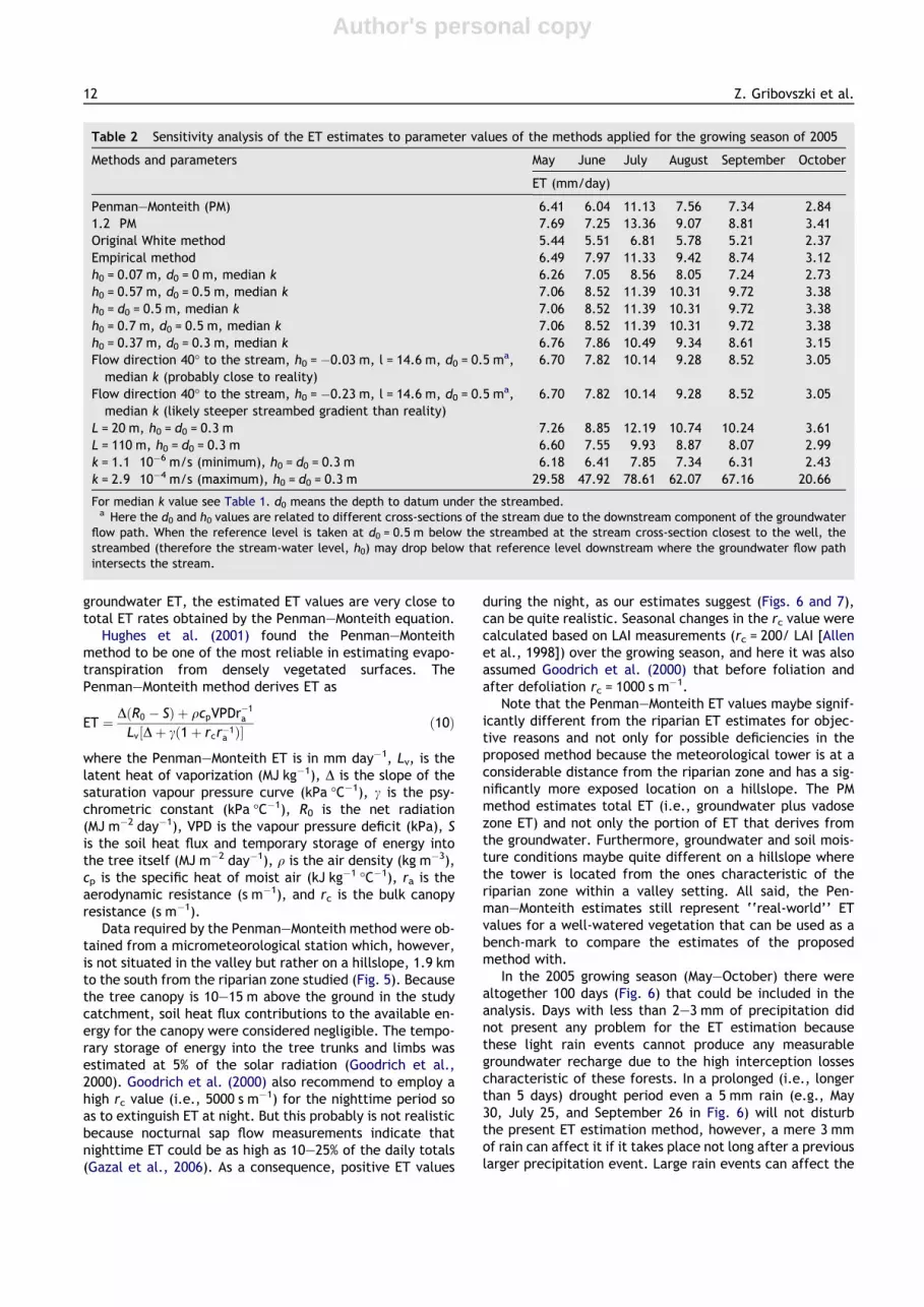
Table 2 Sensitivity analysis of the ET estimates to parameter values of the methods applied for the growing season of 2005

Methods and parameters May June July August September October

ET (mm/day)

Penman–Monteith (PM) 6.41 6.04 11.13 7.56 7.34 2.841.2 Æ PM 7.69 7.25 13.36 9.07 8.81 3.41Original White method 5.44 5.51 6.81 5.78 5.21 2.37Empirical method 6.49 7.97 11.33 9.42 8.74 3.12h0 = 0.07 m, d0 = 0 m, median k 6.26 7.05 8.56 8.05 7.24 2.73h0 = 0.57 m, d0 = 0.5 m, median k 7.06 8.52 11.39 10.31 9.72 3.38h0 = d0 = 0.5 m, median k 7.06 8.52 11.39 10.31 9.72 3.38h0 = 0.7 m, d0 = 0.5 m, median k 7.06 8.52 11.39 10.31 9.72 3.38h0 = 0.37 m, d0 = 0.3 m, median k 6.76 7.86 10.49 9.34 8.61 3.15Flow direction 40� to the stream, h0 = �0.03 m, l = 14.6 m, d0 = 0.5 ma,median k (probably close to reality)

6.70 7.82 10.14 9.28 8.52 3.05

Flow direction 40� to the stream, h0 = �0.23 m, l = 14.6 m, d0 = 0.5 ma,median k (likely steeper streambed gradient than reality)

6.70 7.82 10.14 9.28 8.52 3.05

L = 20 m, h0 = d0 = 0.3 m 7.26 8.85 12.19 10.74 10.24 3.61L = 110 m, h0 = d0 = 0.3 m 6.60 7.55 9.93 8.87 8.07 2.99k = 1.1 Æ 10�6 m/s (minimum), h0 = d0 = 0.3 m 6.18 6.41 7.85 7.34 6.31 2.43k = 2.9 Æ 10�4 m/s (maximum), h0 = d0 = 0.3 m 29.58 47.92 78.61 62.07 67.16 20.66

For median k value see Table 1. d0 means the depth to datum under the streambed.a Here the d0 and h0 values are related to different cross-sections of the stream due to the downstream component of the groundwater

flow path. When the reference level is taken at d0 = 0.5 m below the streambed at the stream cross-section closest to the well, thestreambed (therefore the stream-water level, h0) may drop below that reference level downstream where the groundwater flow pathintersects the stream.



present ET estimation method for up to 2 days, so thoseperiods were excluded from the analysis. It was observedthat the empirical version of the present method is moresensitive to the disturbing effects of precipitation thanthe hydraulic one, as well as to periods with little diurnalchange in the groundwater levels. While the hydraulic ver-sion functioned well even in these periods, for the sake ofcomparison between the two versions, such days were ex-cluded from the subsequent analysis. In addition, a two-week period at the end of June was also excluded fromthe analysis due to instrumentation problems.

Results and discussion

Thirty-minutes ET estimates by the present method arecompared with the Penman–Monteith estimates in Fig. 7.The former yields higher ET rates during the nights, as ex-plained above, so for comparison, only the daily valuesshould be considered.

Cross-correlation analysis of the 30-min ET values be-tween the Penman–Monteith and the present method showa peak (r = 0.85–0.93) generally at a separation distance of60–90 min (larger lag time typical at the start and even atthe end of the vegetation period) with the new method’svalues lagging behind those of the Penman–Monteith ap-proach. Extra long (180 min) lags can be detected in thebeginning of May, in the middle and end of October.60–90 min lags can also be found between the groundwaterlevel and discharge response to increased or decreasedET demand, therefore a difference between the local andoverall hydraulic gradients can cause the lag, as it isexplained in the accompanying paper by Szilagyi et al.(2007). On the other hand, the lag can be the consequenceof the delayed water transport mechanism in the trees be-cause the trunk of the trees can store a relatively high

amount of water, and this storage capacity allows some dif-ference between the time of the transpiration and absorp-tion of water from the soil. In consequence, the smallerthe water transport (i.e., ET) compared to the storedamount of water in the trees and/or the harder it is to ab-sorb moisture from a drying soil, the larger the lag.

The hydraulic version of the new method occasionallyyields zero or negative ET values in the evening hours (7–9 p.m.) in summer period when the groundwater levelbounces back fast after intensive mid-day ET rates. This oc-curs because the groundwater flow is described by threecontrol points, out of which only one is located strictly with-in the riparian zone (the other one is at the bank of thestream, while the third one [the background value] is out-side the domain ET exerts its diurnal influence upon). Duringfast groundwater recovery, following intensive ET rates inthe riparian zone the dS/dt term in Eq. (6) is positive but oc-curs with a negative sign when obtaining the ET value, thusif the groundwater supply rate to the area is underestimatedas a result of the too few control points then the resultingET rate will become negative. This kind of error typicallyhappens at the end of extended drought periods of thesummer.

Fig. 8 displays the estimated ET rates on a daily basis, ob-tained by summing the 30-min values over the days. Bothversions of the proposed method yield significantly largerdaily rates than the original White approach. These differ-ences (as percentage of the White method’s monthly value)from May to October, are 24, 43, 54, 62, 65, 33 for thehydraulic and 19, 45, 66, 63, 68, 32 for the empirical ver-sions, respectively. The explanation lies in the differentassumptions the two methods employ. The original Whiteapproach assumes a constant rate of groundwater supplyto the riparian zone throughout the day estimated whenET is close to zero in the predawn/dawn hours, when thesupply rate is diminished due to a deflated hydraulic gradi-

0

10

20

30

40

Rai

n [m

m/d

ay]

0.4

0.6

0.8

1.0

1.2

Gro

undw

ater

leve

l [m

]E

T[m

m/3

0min

.]

0.0

0.5

1.0

ET(empirical) ET (hydraulic)

May Jun Jul Aug Sep Oct

Figure 6 Precipitation, groundwater level measurements and calculated ET rates for the 2005 growing season.



ent. In contrast, the proposed method accounts for (even ifsometime incorrectly) this diurnal change in the hydraulicgradient which has a maximum when ET is most intensive(in fact, a bit later due to the earlier mentioned delay inthe groundwater response to changes in ET rates) and min-imum in the morning hours.

Loheide et al. (2005) concluded in their numerical studythat the White method gave reliable riparian zone ET esti-mates. However, the ET rates they applied in their modelwere rather small (1 mm d�1), in fact, almost a magnitudesmaller than what was observed in our experimental catch-ment in Hungary, therefore leading to relatively small diur-nal groundwater level fluctuations (<1.5 cm), which thuswould not cause a significant change in the overall hydraulicgradients throughout the day. Indeed, with such low ETrates there is hardly any difference in the estimatesbetween the original White approach and our proposedmethod. However, when the daily ET rate (estimated by

0.0

0.4

0.8

ET

val

ues

(mm

/30−

min

)

23 May 24 May 25 May 26 May 27 May 28 May 29 May0.

00.

40.

8

ET

val

ues

(mm

/30−

min

)

18 Jul 19 Jul 20 Jul 21 Jul 22 Jul 23 Jul 24 Jul

0.0

0.4

0.8

ET

val

ues

(mm

/30−

min

)

29 Aug 30 Aug 31 Aug 01 Sep 02 Sep 03 Sep 04 Sep

0.0

0.4

0.8

ET

val

ues

(mm

/30−

min

)

08 Oct 09 Oct 10 Oct 11 Oct 12 Oct 13 Oct 14 Oct

ET (Penman−Monteith)ET (empirical)ET (hydraulic)

Figure 7 Comparison of the 30-min ET estimates with those of the Penman–Monteith method for some selected growing seasonperiods.

05

1015

ET

val

ues

(mm

/day

)


ET (White)ET (PM)ET (empirical)ET (hydraulic)

Figure 8 Daily ET rates by the original White approach andPenman–Monteith (PM) method, as well as by the empirical andhydraulic versions of the present ET calculation method for the2005 growing season.



the Penman–Monteith method) is about 10 mm a day, as inour experimental watershed, the difference between thetwo methods is significant.

Finally, Fig. 9 displays the estimated daily mean ET ratesby month. Note that these values account predominantly fordry days only. The largest difference between the methodsis found in July when ET rates and, thus, groundwaterdynamics are most intensive. And conversely, the differentmethods give the most uniform ET estimates in May andOctober when the amplitude of the diurnal ET fluctuationis typically small, thus leading to limited diurnal changesin the overall hydraulic gradients within the riparian zone.

Among the two versions of the present ET method, thehydraulic approach yields higher ET estimates in thedamped diurnal ET amplitude months (May and October),while in the intervening period the empirical approachproduces the larger ET estimates. The reason lies in theabove-mentioned property of the hydraulic version ofunderestimating high groundwater supply rates to the ripar-ian zone. Even with this known error in the hydraulicversion, it probably produces more reliable ET estimateswithin the day than the empirical one, because (a) theshape of its ET-curve is closer to the shape of the Pen-man–Monteith derived diurnal ET signal, and; (b) its netinflow values in Fig. 4 reproduce better the time-rate ofchange in groundwater levels through time, and so are prob-ably closer to reality, than those of the empirical one, whichcome from a curve fitting of a spline interpolation method,thus are somewhat detached from physical reality betweenthe measurements. The empirical method on the otherhand, is more suitable for defining a lower limit (>0) forthe ET rate (see its description above), thus it can help incalibrating the hydraulic version.

In comparison of the present ET estimates (3.2–10.5 mm d�1) with other study results, it can be stated thatthese values typically represent the high-end values of thoseestimates. For example, Toth (2007), based on groundwaterlevel readings of piezometer nests, found summer riparianET rates of 2–12 mm d�1 for the same experimental catch-ment in a very shallow groundwater environment (ground-water depths were between 0.2 and 1.3 m from thesurface, therefore the calculated ground water ET fraction

is very close to the total ET rate). Around the world, apply-ing different measurement and estimation techniques,Bauer et al. (2004) obtained riparian ET rates of 0.06–4.3 mm d�1 for mixed (trees, shrub, and grasses) vegetationof variable density in Botswana, where continuous ground-water level readings of piezometers were used for the esti-mates (groundwater depths varied between 2 and 3 m fromthe surface, therefore the calculated groundwater ET frac-tion may be comparable to vadose zone ET). Butler et al.(2007) obtained ET rates of 2.9–9.3 mm d�1 also for mixedvegetation type based on continuous groundwater levelreadings (groundwater depths were between 0.3 and 3.4 mfrom the surface, therefore calculated groundwater ETrates were close to total ET when groundwater levels wereclose to the surface and were smaller than total ET whengroundwater levels were deeper). Nachabe et al. (2005) cal-culated monthly average total ET rates of 1.5–3.5 mm d�1

for a pasture and 1.5–6.3 mm d�1 for a low-lying forest withthe help of continuous soil moisture profile measurementsin Florida. Gazal et al. (2006) found 2–7 mm d�1 for a semi-arid cottonwood forest; Goodrich et al. (2000) obtained 4–8 mm d�1 also for mixed vegetation, while Hughes et al.(2001) found 2–6 mm d�1 for a temperate salt marsh in Aus-tralia. For the last three experiments sap flow measure-ments and micrometeorological methods were used forcalculating total ET. Unfortunately, important vegetationcharacteristics (such as LAI) cannot always be deduced fromthese studies. Notwithstanding, the present riparian ET esti-mation method seems to yield realistic values, especially,when one considers the ready access of vegetation to thegroundwater, the abundance of available energy in thegrowing season considered, as well as a large value of LAI,all combined with a favorable match with the Penman–Mon-teith ET values as control.

Sensitivity analysis of the hydraulic method can be sum-marized (Table 2) as follows. (a) The method is least sensi-tive to the value of h0, i.e., the water-level in the stream.Between the two extremes of h0 = 0 m and h0 = 0.2 m (floodlevel), assuming the reference level is at the channel-bedelevation of the stream, the resulting daily ET values dif-fered only in the third decimals. Thus any effect of diurnalfluctuation in the stream level (which was less than 1 cm inthis catchment) to the ET estimate is negligible. (b) Themethod is only slightly sensitive to the choice of the Lparameter. Even an about 5-fold change in its value af-fected the daily ET estimates by a mere 20%. (c) The meth-od is moderately sensitive to the elevation of the datum.With every 0.1 m lowering of the datum (within the 0–0.5 m interval, which seems realistic in our case), the dailyET estimates increased by only 3–5%. (d) The method is sim-ilarly sensitive to the angle formed by the main groundwaterflow direction and the stream. Based on simultaneous read-ings of well-water levels, this angle in the study catchmentis about 40� downstream. Accounting for this, mainly by theenlarged value of l, lead to a 5–14% decrease in the daily ETvalues. (e) Finally, the ET estimates depend most strongly,i.e., linearly (see Eqs. (7a), (7b) and (9) on the values of thespecific yield, Sy, and the saturated hydraulic conductivity,k. Thus, the key of reliable ET-rate estimates with the pres-ent method lies in the accuracy of the estimated field-scalevalues of the hydraulic parameters, k and Sy. The observedchanges in the ET estimates during the sensitivity analysis,

02

46

810

12

ET

val

ues

(mm

/day

)


ET (White)ET (empirical)ET (hydraulic)ET (PM)

Figure 9 Daily mean ET rates by month of the original Whiteapproach and Penman–Monteith (PM) method, as well as of theempirical and hydraulic versions of the present ET estimationmethod for the 2005 growing season.



reported in Table 2, occurred more markedly during theperiod of intensive ET and groundwater dynamics (July–September), and less so in May and October.

In summary the following can be stated. The current ETestimation method is a modified version of the originalWhite method (1932). It considers the growing season diur-nal fluctuations of the riparian zone groundwater levels andcan fairly well estimate the daily ET rates from high fre-quency samples (10-min or finer) of the groundwater levelin a single well. Interestingly, the sub-daily ET-rate esti-mates are typically delayed by a few hours in comparisonwith Penman–Monteith derived ET values. The new methodhas two versions (i.e., empirical and hydraulic). Thehydraulic version requires field-scale values of the saturatedhydraulic conductivity (k) of the riparian zone as well astime-varying estimates of the specific yield (Sy) beside thehigh frequency groundwater level readings and the distance(l) of the groundwater well to the stream along the direc-tion of the main riparian groundwater flowpath. The accu-racy of the ET estimates is most sensitive (i.e., linearly)to the effective field-scale value of k and Sy. In the absenceof the reliable field-scale value of k and/or when l is un-known, the empirical version of the proposed ET estimationmethod is recommended to be applied which yields ET esti-mates comparable to those by the hydraulic version.

Acknowledgement

This research was partly funded by grants from the Forest-and Wood Utilization Regional University Knowledge Centre(ERFARET) and from the Hungarian Scientific Research Fund(OTKA, # F-046720).

The authors are grateful to Peter Vig for supplying 30-min meteorological data applied in the analysis, and tothe three anonymous reviewers whose comments and sug-gestions greatly improved this study.

References

Allen, R.G., Pereira, L.S., Raes, D., Smith, M., 1998. Cropevapotranspiration – Guidelines for computing crop waterrequirements. Vol. 56 of FAO Irrigation and Drainage. FAO,Rome, URL http://www.fao.org/docrep/X0490E/x0490e06.htm.

Bauer, P., Thabeng, G., Stauffer, F., Kinzelbach, W., 2004.Estimation of the evapotranspiration rate from diurnal ground-water level fluctuations in the Okavango Delta, Botswana. J.Hydrol. 288 (3–4), 344–355.

Bond, B.J., Jones, J.A., Moore, G., Phillips, N., Post, D., McDonnell,J.J., 2002. The zone of vegetation influence on baseflowrevealed by diel patterns of streamflow and vegetation wateruse in a headwater basin. Hydrol. Process. 16 (8), 1671–1677.

Boronina, A., Golubev, S., Balderer, W., 2005. Estimation of actualevapotranspiration from an alluvial aquifer of the Kouris catch-ment (Cyprus) using continuous streamflow records. Hydrol.Process. 19, 4055–4068.

Brooks, R.H., Corey, A.T., 1964. Hydraulic properties of porousmedia. Hydrol. Paper 3, Colorado State University, Fort Collins.

Brutsaert, W., Nieber, J.L., 1977. Regionalized drought flowhydrographs from a mature glaciated plateau. Water Resour.Res. 13 (3), 637–643.

Butler, J.J., Kluitenberg, G.J., Whittemore, D.O., Loheide II, S.P.,Jin, W., Billinger, M.A., Zhan, X., 2007. A field investigation of

phreatophyte-induced fluctuations in the water table. WaterResour. Res. 43, W02404. doi:10.1029/2005WR004627.

Croft, A.R., 1948. Water loss by stream surface evaporation andtranspiration by riparian vegetation. Trans. Am. Geophys. Union29 (2), 235–239.

Czikowsky, J., 2003. Seasonal and Successional Effects on Evapo-transpiration and Streamflow. M.S. Thesis, Department of Earthand Atmospheric Sciences, The University at Albany, StateUniversity of New York, pp. 105.

Czikowsky, J.M., Fitzjarrald, D.R., 2004. Evidence of seasonalchanges in evapotranspiration in eastern US hydrologicalrecords. J. Hydromet. 5, 974–988.

Danszky, I. (Ed.), 1963. Magyarorszag Erd}ogazdasagi TajainakErd}ofelujıtasi, Erd}otelepıtesi Iranyelvei es Eljarasai, I.Nyugat-Dunantul Erd}ogazdasagi Tajcsoport [Regenerationand Afforestration Guidelines of Hungarian ForestRegions, I. Western-Transdanubian Forest Region]. OrszagosErdeszeti F}oigazgatosag, Budapest pp. 557 (inHungarian).

Gazal, R.M., Scott, R.L., Goodrich, D.C., Williams, D.G.,2006. Controls on transpiration in a semiarid ripariancottonwood forest. Agric. Forest Meteorol. 137 (1–2),56–67.

Goodrich, D.C., Scott, R., Qi, J., Goff, B., Unkrich, C.L., Moran,M.S., Williams, D., Schaeffer, S., Snyder, K., MacNish, R.,Maddockb, T., Poole, D., Chehbounif, A., Cooperg, D.I.,Eichingerh, W.E., Shuttleworthb, W.J., Kerri, Y., Marsetta, R.,Ni, W., 2000. Seasonal estimates of riparian evapotranspirationusing remote and in situ measurements. Agric. Forest Meteorol.105 (1–3), 281–309.

Gribovszki, Z., Kalicz, P., Kucsara, M., 2006. Streamflow charac-teristics of two forested catchments in Sopron Hills. ActaSilvatica et Lignaria Hungarica 2, 81–92. http://aslh.nyme.hu/.

Harr, M.E., 1962. Groundwater and Seepage. McGraw-Hill, NewYork, pp. 315.

Hughes, C.E., Kalma, J.D., Binning, P., Willgoose, G.R., Vertzonis,M., 2001. Estimating evapotranspiration for a temperate saltmarsh, Newcastle, Australia. Hydrol. Process. 15, 957–975.doi:10.1002/hyp.189.

Kishazi, P., Ivancsics, J., 1985. Sopron kornyeki uledekek osszefog-lalo foldtani ertekelese [Geological assessment of sediments inthe neighbourhood of Sopron]. Manuscript pp. 48 (in Hungarian).

Kovacs, G., 1972. A szivargas hidraulikaja [Seepage Hydraulics].Akademiai Kiado, Budapest. pp. 536 (in Hungarian).

Kovacs, B., Szanyi, J., 2005. Hidrodinamikai es transz-portmodellezes II. [Hydrodinamic and Transport Modeling].Gama Geo, Budapest. pp. 213 (in Hungarian).

Loheide II, S.P., Butler, J.J., Gorelick, S.M., 2005. Use of diurnalwater table fluctuations to estimate groundwater consumptionby phreatophytes: A saturated–unsaturated flow assessment.Water Resour. Res. 41, W07030. doi:10.1029/2005WR003942.

Lundquist, J.D., Cayan, D.R., 2002. Seasonal and spatial patterns indiurnal cycles in streamflow in the western United States. J.Hydromet. 3, 591–603.

Maidment, D.R. (Ed.), 1993. Handbook of Hydrology. McGraw-Hill,New York.

Marosi, S., Somogyi, S. (Eds.), 1990. Magyarorszag KistajainakKatasztere I. [Cadastre of Small Regions in Hungary I.]. MTAFoldrajztudomanyi Kutato Intezet, Budapest. pp. 479 (inHungarian).

Meyboom, P., 1964. Three observations on streamflow depletion byphreatophytes. J. Hydrol. 2, 248–261.

Nachabe, M.H., 2002. Analytical expressions for transient specificyield and shallow water table drainage. Water Resour. Res. 38(10), 1193. doi:10.1029/2001WR00107.

Nachabe, M., Shah, N., Ross, M., Vomacka, J., 2005. Evapotrans-piration of two vegetation covers in a shallow water tableenvironment. Soil Sci. Soc. Am. J. 69, 492–499.



Portge, K.H., 1996. Tagesperiodische Schwankungen des Abflussesin kleinen Einzugsgebieten als Ausdruck komplexer Wasser- undStoffflusse [Daily Fluctuations in Water and Mass Transport of aSmall Catchment]. Erich Goltze, Gottingen. pp. 104 (inGerman).

Reigner, I.C., 1966. A method for estimating streamflow loss byevapotranspiration from the riparian zone. Forest Sci. 12, 130–139.

Schwartz, W.F., Zhang, H., 2003. Fundamentals of Groundwater.Wiley, New York, pp. 592.

Shah, N., Nachabe, M., Ross, M., 2007. Extinction depth andevapotranspiration from ground water under selected landcovers. Ground Water 45 (3), 329–338. doi:10.1111/j.1745-6584.2007.00302.x.

Szilagyi, J., 2004. Vadose zone influences on aquifer parameterestimates of saturated-zone hydraulic theory. J. Hydrol. 286,78–86.

Szilagyi, J., Parlange, M.B., Albertson, J.D., 1998. Recession flowanalysis for aquifer parameter determination. Water Resour.Res. 34 (7), 1851–1857.

Szilagyi, J., Gribovszki, Z., Kalicz, P., Kucsara, M., 2007. On diurnalriparian zone groundwater-level and streamflow fluctuatuons. J.Hydrol. 349, 1–5.

Toth, A., 2007. Vızkedvel}o erd }Ollomanyok es a talajvız kapcso-latanak elemzese a Sopron melletti Hidegvız-volgyben [Analysisof the relationship between phreatophyte vegetation and thegroundwater in the forested Hidegvız Valley experimentalcatchment near Sopron. Master’s Thesis, Institute of Geomaticsand Civil Engineering, University of West-Hungary, Sopron. pp.60 (in Hungarian).

Troxell, H.C., 1936. The diurnal fluctuation in the groundwater andflow of the Santa Ana River and its meaning. Trans. Am.Geophys. Union 17, 496–504.

Tschinkel, H.M., 1963. Short-term fluctuation in streamflow asrelated to evaporation and transpiration. J. Geophys. Res. 68(24), 6459–6469.

White, W.N., 1932. Method of estimating groundwater suppliesbased on discharge by plants and evaporation from soil – resultsof investigation in Escalante Valley, Utah – US GeologicalSurvey. Water Supply Paper 659-A, 1–105.


Documents

Riparian zone evapotranspiration estimation from diurnal groundwater level fluctuations