Risk Aversion and Expected-Utility Theory:Coherence for Small- and Large-Stakes Gambles

James C. CoxUniversity of Arizonajcox@bpa.arizona.edu

Vjollca SadirajUniversity of Amsterdam

vjollca@fee.uva.nl

January 2001; revised July 2001

1

Risk Aversion and Expected-Utility Theory:Coherence for Small- and Large-Stakes Gambles

By James C. Cox and Vjollca Sadiraj1

1. Introduction

A central objective in developing an empirical science is coherence in the application of theory to

data from different sources. Thus, Rabin (2000) raises an important question concerning

coherence of the application of concave expected-utility theory to explain risk-averse behavior for

both small-stakes gambles used in laboratory experiments and large-stakes gambles observed in

everyday life. Rabin’s discussion of the implications of his calibration theorem, and his

discussion of loss aversion, raise some issues for which there is an absence of clarity in the

literature on decision theory. In order to help clarify the differences between decision theories,

we draw attention to the distinction between expected-utility theory and expected-utility models.

We address the coherence question for both of the commonly-used expected-utility models, the

expected-utility of terminal wealth (EUTW) model and the expected-utility of income (EUI)

model, and for a more general model, the expected-utility of income and initial wealth (EUI&IW)

model. We explain that Rabin’s calibration theorem has no implication for the EUI model

because of its fixed reference point of zero income. The EUI&IW model includes initial wealth as

a reference point but the calibration theorem has no implication for this model because initial

wealth is not additive to income in the utility function for this model. In contrast, if there is

empirical support for the hypothesized type of small-stakes risk aversion, then the calibration

theorem and corollary have implications for applicability of the EUTW model.

Clarification of the distinction between expected-utility theory and specific expected-

utility models also helps to clarify the implications of loss aversion for decision theory. We

explain that loss aversion is consistent with some expected-utility models, hence it is consistent

with expected-utility theory. Thus, if a researcher observes loss-averse behavior, he should not,

2

ipso facto, be motivated to reject expected-utility theory in favor of some alternative such as

prospect theory, although he should be motivated to reject one specific expected-utility model.

We review a small part of the literature that reports data showing risk-averse behavior in

laboratory experiments. The common features of the these experiments are: (1) consistent one-

sided deviations of subjects’ choices from the predictions of risk neutrality, in the direction

consistent with risk aversion; (2) no relevance of loss aversion; and (3) researchers’ use of

expected-utility models for which the calibration theorem has no implication. Clarification of the

implications of the calibration theorem is important to proper analysis of data from experiments

and to proper review for journals of papers reporting experiments.2

2. Expected-Utility Theory vs. Expected-Utility Models

We define “expected-utility theory” as the theory of decision-making under risk based on a set of

axioms for a preference ordering that includes the independence axiom or an alternative that

implies that the (expected) utility function that represents the ordering is linear in probabilities.

Linearity in probabilities implies that indifference curves in the Machina (1982) triangle diagram

and the probability simplex are parallel straight lines. Thus, we include within expected-utility

theory any model of decision-making under risk that has parallel straight-line indifference curves

in the Machina triangle.

Expected-utility theory and alternative decision theories are concerned with the properties

of preference orderings of probability distributions of “prizes.” The identity of the prizes depends

on the decision context that is modeled and on assumptions made by the theorist. We shall

confine our discussion to decision contexts in which the prizes are amounts of money. Within this

context, we identify two expected-utility models that are commonly used, the expected-utility of

terminal wealth model and the expected-utility of income model. We also discuss a third model,

the expected-utility of income and initial wealth model. The distinctions among the models are in

3

the assumed identity of the prizes. All of the models have parallel straight-line indifference

curves in the Machina triangle, hence are included within expected-utility theory.

2.1 The EUTW Model

The expected-utility of terminal wealth (EUTW) model is based on the assumption that the prizes

are amounts of terminal wealth. This model was used in the seminal work of Arrow (1971) and

Pratt (1964) in which they analyzed possible wealth effects on willingness to bear risks. This

model is commonly used in theoretical papers on various topics.

It will help explain some essential distinctions between models to briefly review the

familiar triangle-diagram representation of indifference curves for simple gambles (Machina,

1987). Consider three amounts of monetary gains (or amounts of income), iy , i = 1,2,3 such that

321 yyy << . Assume that the iy occur with probabilities, ip , i = 1,2,3 such that

1321 =++ ppp . If w is the decision-maker’s initial wealth, then the expected-utility function

for the EUTW model is written as

(1) �=

+=3

1)(

iiiW ywupU .

Since 312 1 ppp −−= , indifference curves for expected-utility function (1) can be represented

in the triangle diagram in Figure 1. Indifference curves are parallel straight lines because

expected-utility function (1) is linear in probabilities. Higher (respectively lower) Arrow-Pratt

absolute risk aversion implies steeper (respectively flatter) slope of the indifference curves. Thus

if expected-utility function (1) exhibits non-constant absolute risk aversion then the slopes of the

indifference curves in Figure 1 depend on the amount of initial wealth, w . In the special cases in

which expected-utility function (1) exhibits constant absolute risk aversion or the agent is risk

neutral, the slope of the indifference curves in Figure 1 is invariant to changes in w .

4

2.2 The EUI Model

The expected-utility of income (EUI) model is based on the assumption that the prizes are

amounts of income (or, equivalently, changes in wealth or gains and loses). The EUI model is

commonly used in theoretical modeling, most notably in the theory of auctions. Thus, most

bidding models are based on the expected-utility axioms, the assumption that the prizes are

amounts of income, and the assumption of Bayesian-Nash equilibrium.3

Considering the same three-outcome lottery as above, the expected-utility function for the

EUI model is written as

(2) �=

=3

1)(

iiiI yvpU .

Obviously, indifference curves for this model are parallel straight lines whose slope is

independent of initial wealth.

2.3 The EUI&IW Model

We here discuss a more general expected-utility model. Assume that the prizes are ordered pairs

of amounts of initial wealth and income, ),( iyw , i = 1,2,3. Then the expected-utility function

can be written as

(3) �=

=3

1),(

iiiIW ywpU υ .

Indifference curves for this model are parallel straight lines. The Arrow-Pratt measure of absolute

risk aversion for this model is

(4) ),(),(

2

22

ywywRA υ

υ−= .

The absolute risk aversion measure can be assumed to be increasing, constant, or decreasing in

income and/or initial wealth. But imposition of some reasonable regularity properties on the

utility function makes it possible to relate the slope of the indifference curves to AR . For

5

example, assume that the marginal utility of income decreases as initial wealth increases and that

AR is decreasing in income. In that case, if AR is decreasing in initial wealth then the slope of

the indifference curves is also decreasing in initial wealth.

3. Coherence for Small- and Large-Stakes Gambles

Rabin argues that concave expected-utility theory does not provide a coherent theory of both

small-stakes and large-stakes risk aversion. The argument is presented in the form of calibrations

based on the theorem and corollary that are reported in his Table I and Table II. Part of our

argument will be presented in the form of alternative calibrations. We first discuss coherence for

the EUI model that is widely applied in bidding theory. Subsequently, we discuss the EUI&IW

model and the EUTW model.

3.1 Coherence with the EUI Model

The use of income as the argument of the expected-utility function implies a fixed reference point

of zero income, which makes it impossible to construct Rabin’s calibration theorem. Rather than

reviewing the construction of the theorem, we will provide an example which demonstrates that

expected-utility theory can provide a coherent explanation of both small-stakes and large-stakes

risk aversion. Our example constitutes a counterexample to the belief that Rabin’s conclusions

about incoherence of small-stakes and large-stakes risk aversion hold for the EUI model.

Consider the example used by Rabin in which it is assumed that a decision-maker would

reject a gamble that yields a gain of $110 and a loss of $100 with equal probability. We will

compare implied levels of risk aversion for the EUI model with the levels given in Rabin’s Tables

I and II for the EUTW model. The second and third columns of our Table I reproduce some

results reported in Rabin’s Table I and Table II. The “Table I Rejections” we reproduce are

implied by the corollary to the calibration theorem if the agent is assumed to reject the 50-50, lose

6

$100/ gain $110 gamble for all initial wealth levels. Such an agent would also reject a gamble in

which he would, with equal probability, lose $1000 or gain any arbitrarily large amount. The

“Table II Rejections” we reproduce are derived from the assumption that the agent will reject the

50-50, lose $100/ gain $110 gamble for all initial wealth levels no greater than $300,000. In that

case, the agent would also reject a gamble in which he would, with equal probability, lose

$20,000 or gain $160,000,000,000 when his initial wealth is $290,000.

Now consider risk aversion with the EUI model. Assume the von Neumann-Morgenstern

utility function that “values” amounts of income, y according to:

(5) u(y) = 200520

200 −++ y, if 100−<y ,

= 200200 −+ y , if 100100 ≤≤− y ,

= 2002300

3002200 −++ y

, if 100>y .

This function is globally weakly concave, as assumed for the utility of terminal wealth functions

in Rabin’s theorem and corollary. Using (5), one finds that an expected-utility maximizer would

reject the 50-50, lose $100/ gain $110 gamble. But the agent would also accept the gambles in

the “Equation (5) Acceptance” column of Table I. Thus, risk aversion over small-stakes gambles

does not imply ridiculous levels of risk aversion over large-stakes gambles with the EUI model.

Another example is provided by the function,

(6) u(y) = day −+ 9.0)( , if 10−<≤− ya ,

= 2020 −+ y , if 1010 ≤≤− y ,

= ,)( 9.0 cby −+ if 10>y ,

where: a = 35,704,682.29; d = 6,272,672.839; b = 8,676,235,339; c = 880,031,446.3. This

function is strictly concave on the domain that is bounded from below by a− . Using (6), one

7

finds that an expected-utility maximizer would reject the 50-50, lose $100/ gain $110 gamble.

But the agent would also accept the gambles in the “Equation (6) Acceptance” column of Table I.

Thus, once again we observe that risk aversion over small-stakes gambles is consistent with

sensible levels of risk aversion over large-stakes gambles with the EUI model.

3.2 Coherence with the EUI&IW Model

The EUI&IW model contains the EUI model as a special case. Thus the preceding discussion

should make it obvious that the EUI&IW model can provide a coherent explanation of both

small- and large-stakes risk aversion.

3.3 Incoherence with the EUTW Model

Rabin’s theorem is based on the assumption that the “prizes” that are ordered by the preference

ordering defined by the expected-utility axioms are amounts of terminal wealth. The theorem and

corollary imply logical propositions of the form: If an agent would reject a specified small-stakes

gamble for all of the assumed values of initial wealth then the agent would also reject the

following large-stakes gambles. Obviously, the consequent, then statement does not follow unless

the antecedent, if statement is assumed.

Use of the calibration theorem and corollary to criticize application of models to analysis

of experimental data transforms the antecedent in a purely logical proposition into an empirical

hypothesis requiring support. Reflection on the small-stakes risk aversion hypothesized in the

corollary suggests the type of data that are needed to support a conclusion of incoherence.

Obviously, it would be impossible to conduct money payoff experiments with subjects whose

actual personal wealth varied over the whole real line. Therefore, it is impossible that empirical

support for the assumptions in Rabin’s Table I calibration could ever be provided. Furthermore,

it would be virtually impossible to conduct experiments with individual subjects whose actual

personal wealth took on all values up to $300,000. In contrast, one could recruit subjects from a

8

subject pool consisting of distinct individuals with wealth levels varying over a range large

enough to make use of the logic of the calibration theorem. In that case, the data would confound

heterogeneity in subjects’ risk attitudes with variability in their individual wealth levels. But such

an across-subjects experimental design would be a reasonable approach to providing empirical

support for the type of small-stakes risk aversion assumed in Rabin’s Table II calibration.

Furthermore, it is a reasonable conjecture that the (typically-unobserved) variability in wealth

across subjects in earlier experiments on risk attitudes has sufficient variability for this purpose.

Therefore, Rabin’s calibration theorem does make questionable the coherence of applications of

the EUTW model to small-stakes and large-stakes gambles.

4. Loss Aversion and Expected-Utility Theory

We have explained that observations of risk-averse behavior in laboratory experiments can be

rationalized by some concave expected-utility models without producing incoherence with

applications of those models to larger-stakes gambles. But this explanation should not be

misinterpreted as a denial of other possible causes of risk-avoiding behavior. Loss aversion is a

possible explanation of such behavior in some circumstances. But the relation between loss

aversion and expected-utility theory requires some careful re-examination within the context of

the issues raised in Rabin’s paper.

Observing that expected-utility theory contains more than the EUTW model helps one to

understand the essential differences between that theory and its alternatives. Some researchers

believe that loss aversion distinguishes expected-utility theory from alternatives such as prospect

theory (Kahneman and Tversky, 1979; Rabin, 2000; Rabin and Thaler, 2001). But loss aversion,

as illustrated in Figure 2, is consistent with the EUI and EUI&IW models, hence it is consistent

with expected-utility theory. Empirical tests that can discriminate on a fundamental level between

expected-utility theory and its alternatives must be based on differences between the implications

of alternative sets of axioms, not different subsidiary assumptions about what the prizes are to

9

which the axioms are applied. Thus, observations of Allais paradox behavior are empirical

inconsistencies with expected-utility theory because they are inconsistent with the Machina-

triangle indifference curves being parallel straight lines (Machina, 1982, 1987). In contrast,

observations of loss-averse behavior are consistent with the indifference curves being parallel

straight lines, hence they are consistent with expected-utility theory.

5. Lottery Payoffs in Experiments

In concluding his argument, Rabin (2000, pp. 1286-7) criticizes the use of lottery payoffs in

experiments: “The problem with this lottery procedure is that it is known to be sufficient only

when we maintain the expected-utility hypothesis. But then it is not necessary — since expected-

utility theory tells us that people will be virtually risk neutral in decisions on the scale of

laboratory stakes. … the lottery procedure, which is motivated solely by expected utility theory’s

assumption that preferences are linear in probabilities and that risk attitudes come only from the

curvature of the utility-of-wealth function, has little presumptive value in ‘neutralizing’ risk

aversion.”

Lottery payoffs were introduced into decision theory by Smith (1961). They were used

in experiments first by Roth and Malouf (1979) and, subsequently, by Roth and Murnigham

(1982), Roth and Schoumaker (1983), and many others. Neither Smith’s theoretical argument nor

most applications in experiments requires use of the EUTW model rather than the EUI model.

Therefore, Rabin’s calibration theorem has no general implication for applicability of lottery

payoffs in experiments.

The problem with lottery payoffs does not derive from the calibration theorem but rather

from experimental studies that conclude that they do not successfully induce risk attitudes on

subjects. Thus, Walker, Smith, and Cox (1990) and Cox and Oaxaca (1995) report that lottery

payoffs do not successfully control subjects’ risk attitudes in bidding (market) experiments.

Selten, Sadrieh, and Abbink (1999) report that lottery payoffs fail to induce risk neutral behavior

10

in non-market experiments. It is clear that the empirical failure of lottery payoffs is a failure of

expected utility theory. But alternative decision theories have not been subjected to similar tests

with lottery payoffs that are appropriate in the absence of linearity in probabilities, hence it is

unknown whether any of them would fare any better.

6. Exogenous Risky Income

Subjects in experiments may have risky incomes that are exogenous to experimental treatments.

Any such risky income would not ordinarily be observed by experimenters. The existence of

exogenous risky income raises some questions about rational behavior, and the modeling of

rational behavior, that are well beyond a critical discussion of the calibration theorem. These

questions revolve around the implications of integration, or non-integration, of risky incomes

from different decision contexts. But it is germane to discussion of the calibration theorem to

ask whether integration of exogenous large-stakes risks with endogenous small-stakes risks has

implications for applicability of concave expected-utility theory.

Consider the following example. Assume that an experimental subject rejects the 50-50,

lose $100, gain $110 gamble. Also assume that this subject has exogenous risky income with a

mean value of $10,000. If the subject does not integrate the endogenous and exogenous risks

then the argument in subsection 3.1 tells us that there is no implication of ridiculous large-stakes

risk aversion. Thus we will here focus on the case where the subject is assumed to integrate the

endogenous and exogenous risky incomes. If the risky incomes are integrated by addition, does

concavity necessarily have an untenable implication? In other words, does small-stakes risk

aversion that is endogenous to an experiment, together with exogenous large-stakes risky income,

have calibration-theorem-like implications for large-stakes risk aversion?

Let the random variables, X and Y denote the exogenous and endogenous risky incomes.

The risky income that is assumed to be endogenous to an experiment is the 50-50, lose $100, gain

$110 gamble. The exogenous income is assumed to have a log-normal distribution with mean of

11

$10,000 and variance of $90,000. Assume the von Neumann-Morgenstern utility function that

“values” sums of amounts of income, yx + according to:

(7) 200520

800,9)( −+++−=+ yxyxu , if 900,9<+ yx

= 200800,9 −++− yx , if 100,10900,9 ≤+≤ yx

= 2002300

3002800,9 −+++− yx

, if 100,10>+ yx .

It is straightforward to show that equation (7) and the assumed log-normal distribution of X imply

that the agent will reject the 50-50, lose $100, gain $110 gamble. Does the agent have reasonable

large-stakes risk aversion? Yes, the minimum gain that would be required to get a decision-

maker with expected utility function including (7) and the assumed log-concave distribution of

exogenous income to accept a gamble with 0.5 probability of losing $20,000, and 0.5 probability

of receiving the gain, is a gain of $44,000.

7. Data Supporting Risk Aversion Over Small Stakes

Central elements in the discussion are whether there are data that support decision-makers’ risk

aversion over small-stakes gambles and whether, as maintained by Rabin, this risk-avoiding

behavior can be explained by loss aversion. There is a large literature of experimental economics

papers that report behavior which is consistent with concave expected-utility models but

inconsistent with their risk-neutral special cases. The risk aversion interpretation of much of this

data requires maintained hypotheses about Nash equilibrium, rational expectations, etc. Thus,

recent experiments by Holt and Laury (2000) are very informative because they do not require

complicated maintained hypotheses to interpret the data.

12

7.1 Risk Aversion in Choices Between Binary Lotteries

In one of their several treatments, Holt and Laury asked subjects to choose one lottery from each

of the 10 pairs of binary lotteries in Table 2. First, note that none of the lotteries involves losses,

hence loss aversion is irrelevant to interpreting the data. Secondly, note that a risk-neutral

expected-utility maximizer will choose option A in the first four rows of Table 2 and choose

option B in rows five through ten. A risk-preferring expected-utility maximizer will “cross over”

from choosing option A to choosing option B at some row weakly between row one and row five.

And a risk-averse expected-utility maximizer will cross over from choosing option A to choosing

option B at some row weakly between row five and row ten. Choice of option A in row five and

below is consistent only with risk aversion. Results from this experimental treatment involving

175 subjects are reported in Figure 3. Note that 81% of the subjects are still choosing option A in

row 5; that is, 81% of the subjects are risk averse. Thus the data clearly provide strong support for

risk aversion for small-stakes payoffs.4

There is a large literature of experimental economics papers that report risk-averse

behavior in contexts that are more complicated than choice between binary lotteries. Because

more complicated hypotheses are required to interpret the data in these alternative environments,

the conclusion that decision-makers’ risk aversion explains one-sided deviations from the

predictions of risk-neutral models has been more controversial than for choice over binary

lotteries. Private value auctions are one context in which there is a large amount of data that are

inconsistent with risk neutrality.

7.2 Risk Aversion in Private Value Auctions

Vickrey (1961) developed a theory of bidding in first-price sealed-bid auctions based on the

expected-utility axioms, the income assumption about the identity of the prizes, and the

assumption of Bayesian-Nash equilibrium. For the case in which private values for the auctioned

13

item are drawn independently from the uniform distribution on [0, vh], the risk-neutral

equilibrium bid function for single-unit auctions with n bidders is

(8) ii vn

nb 1−= .

As explained by Vickrey, risk-averse bidders will bid higher amounts than those given by

equation (8).

There is a large literature on experiments with first-price private-value auctions that

reports data that are inconsistent with bid function (8) because virtually all of the bids are higher

than (n-1)vi/n. Bidding more than (n-1)vi/n cannot be a way to avoid losses; hence such

apparently risk-averse bidding behavior cannot be explained by loss aversion. Tests of bidding

theory have used both market prices and individual-subject data. For example, Cox, Smith, and

Walker (1988) and Cox and Oaxaca (1996a) report tests based on auction market prices,

individual bids and values, and decision-makers’ expected money payoffs from bidding.

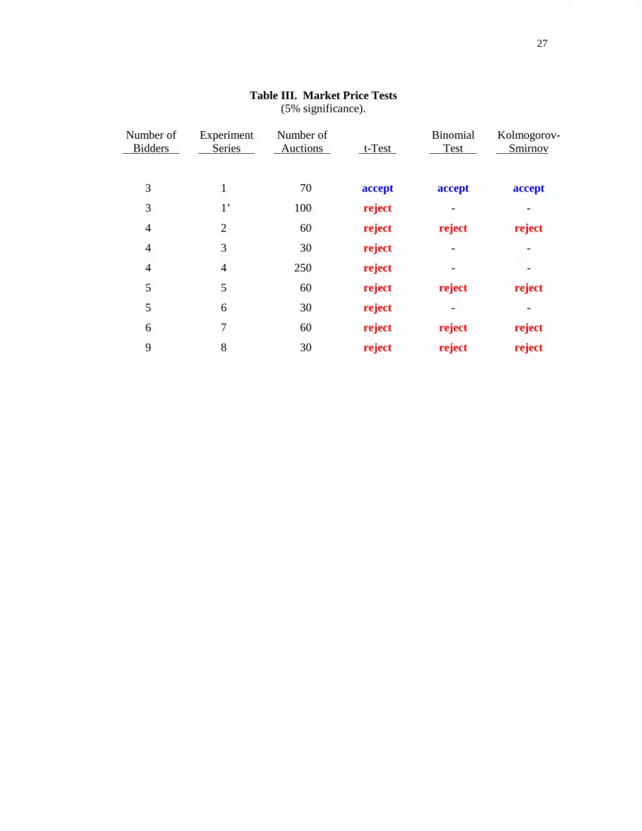
Table 3 reports one-tailed tests based on market prices from Cox, Smith, and Walker

(1988). For all data except for one series of three-bidder auctions, the hypothesis that market

prices reflect risk-neutral bidding is rejected in favor of the alternative that prices are consistent

with risk-averse bidding. The one series of three-bidder auctions was unusual in that there was a

large discrete unit of account because of the pairing with Dutch auctions (Cox, Roberson, and

Smith, 1982).

Figure 4 reports tests from Cox and Oaxaca (1996a). All bars except the left-most report

tests of the risk-neutral model. The right-most bar in Figure 4 reports results from a test with

expected foregone earnings from higher-than-risk-neutral bidding that applies the metric in

Friedman (1992). The hypothesis of zero foregone expected earnings is rejected in favor of

positive foregone expected earnings for 90% of the subjects. Thus 90% of the subjects are

foregoing significant amounts of expected earnings in order to decrease the risk of losing the

auction below that implied by the risk-neutral bid function. All of the other bars in Figure 4

14

report tests based on bids and values. The second-from-right bar reports that the risk-neutral bid

function (8) is rejected in favor of a naïve linear bid function, that can lie above (8), for 90% of

the subjects. The middle bar reports that the risk-neutral bid function is rejected in favor of the

constant relative risk-averse model (CRRAM) for 90% of the subjects.5 This alternative model,

CRRAM, is based on a family of power functions in which the bidder-specific risk attitude

parameters do not all have to equal 1, as in the risk-neutral model (Cox, Roberson, and Smith,

1982; Cox, Smith, and Walker, 1982). The second-from-left bar reports that the risk-neutral bid

function (8) is rejected in favor of a naïve two-part bid function, that can lie above (8), for 100%

of the subjects.

Overwhelming rejection of the risk-neutral bidding model brings up the question of

whether more general models, not based on the risk neutrality assumption, are consistent with

bidding behavior. The left-most bar in Figure 4 reports a test of CRRAM against the naïve two-

part bid function; note that CRRAM is rejected for 52.5% of the subjects, whereas the risk-neutral

model is rejected for 100% of the subjects by this test. Thus, replacing the risk-neutral model with

a parametric model in which individual agents can be heterogeneously risk averse produces

consistency with data for almost one-half of the subjects.

Figure 5 reports tests of a non-parametric model in which individual risk attitudes are

only restricted by the requirement that the utility function be log-concave, meaning that it is

nowhere more convex than the exponential function (Cox, Smith, and Walker, 1988; Cox and

Oaxaca, 1996a). This log-concave model (LCM) implies that the bid function is monotonically

increasing, with a slope everywhere less than 1. Figure 5 shows results from tests of LCM

reported by Cox and Oaxaca (1996a). The solid bars show results from tests that use the research

hypothesis as the null hypothesis while the cross-hatched bars are for tests where the research

hypothesis is the alternative hypothesis. The left-most pair of bars show the results from rank

correlation tests of the positive monotonicity property of the LCM. Positive rank correlation of

bids and values is not rejected for any of the subjects whereas negative rank correlation is rejected

15

for 100% of the subjects. The middle pair of bars shows results from parametric monotonicity

tests. Positive monotonicity of the estimated bid function slopes can be rejected for only 0.1% of

the subjects. Non-positive monotonicity of bid function slopes can be rejected for 95.7% of the

subjects. The right-most bars in Figure 5 show results from tests of the unitary slope property of

LCM. Note that the restriction that the bid function slope is everywhere less than 1 can be

rejected for only 2.6% of the subjects. The hypothesis that the bid function slope is everywhere

greater than 1 can be rejected for 64.9% of the subjects.

Of course, it is impossible to “prove” that bids are higher than risk-neutral bids because

of decision-makers’ risk aversion. But the alternative explanations that have been embodied in

models, such as utility from the event of winning, have been tested and rejected in favor of risk-

averse bidding theory (Cox, Smith, and Walker, 1988). And data from psychological surveys and

blood tests provide some additional support for the risk aversion explanation (Harlow and Brown,

1990). But there are some seemingly anomalous data from third-price auctions (Kagel and

Levine, 1993).6

It may also turn out that the empirical regularities in auction-experiment data can be

rationalized by models that do not have linear indifference curves in the Machina triangle. One

example that illustrates this point is the following. Yaari’s (1989) dual theory is characterized by

a “utility function” that is linear in payoffs and convex in cumulative probabilities for risk averse

agents.7 The assumption of convex power function transformations of winning-bid probabilities

leads to the same form of equilibrium bid function as in CRRAM, which is based on expected

utility theory.8

7.3 Risk Aversion in Search Experiments

Sequential job search experiments provide another context in which there are data supporting

risk-averse behavior over small stakes. The theory is based on the expected-utility axioms,

amounts of income as the prizes, and solution of the dynamic search problem by backwards

16

recursion. Subjects cannot lose money in most of these search experiments, hence loss aversion

cannot explain the observed behavior.

In search from known distributions without recall opportunities, 77% of 600 search

terminations were consistent with the varying predictions of the risk-neutral model over several

treatments, whereas 94% were consistent with the weakly risk-averse version of the theory (Cox

and Oaxaca, 1989). In search from known distributions with perfect or stochastic recall of past

offers, 61% of search terminations were consistent with the risk-neutral model whereas 96% were

consistent with the weakly risk-averse model (Cox and Oaxaca, 1996b). In tests with reservation

wage data for search from known distributions, the risk-neutral reservation wage path was

rejected with data from all of the experimental treatments whereas the weakly risk-averse

reservation wage path was not rejected with data for any of the three treatments (Cox and Oaxaca,

1992a, 1992b). In search from unknown distributions, 70% of search terminations were

consistent with risk-neutral predictions whereas 88% were consistent with the weakly risk-averse

model (Cox and Oaxaca, 2000).

Of course, it is impossible to “prove” that many decision-makers stop searching earlier

than predicted by risk-neutral search theory, or that their reservation wages are higher than risk-

neutral reservation wages, because of risk aversion. But alternative explanations embodied in

models have not been developed and tested. There are some anomalous data (Sonnemans, 1998,

2000).

8. Concluding Remarks

A central issue in developing an empirical science is coherence in the application of theory to

data from different sources. While such coherence is not always possible, it remains a central

objective. The principal of parallelism, that the same laws apply inside and outside the laboratory,

is a hallmark of an experimental science whether it be natural science (Shapley, 1964) or

economics (Smith, 1982). Thus, Rabin (2000) raises an important question concerning coherence

17

of the application of concave expected-utility theory to explain risk-averse behavior for both

small-stakes gambles used in laboratory experiments and large-stakes gambles observed in

everyday life.

We have addressed the coherence question for both of the commonly-used expected-

utility models, the expected-utility of terminal wealth (EUTW) model and the expected-utility of

income (EUI) model, and for a more general model, the expected-utility of income and initial

wealth (EUI&IW) model. We have explained that the calibration theorem and corollary have no

implication for the EUI model because of its fixed reference point of zero income. The EUI&IW

model includes initial wealth as a reference point but the calibration theorem has no implication

for this model because initial wealth is not additive to income in the utility function. In contrast,

with empirical support for the hypothesized type of small-stakes risk aversion, the theorem and

corollary do have implications for applicability of the EUTW model.

Let us suppose that the across-subjects comparisons that can be made with existing data

provide empirical support for results similar to Rabin’s Table II calibrations. What experimental

studies are then called into question? We have already explained that typical experimental papers

on auctions and search are immune to criticisms based on the calibration theorem because they

test hypotheses derived with the EUI model. But what about other experiments involving

decisions in risky environments? If the authors used the EUTW model and strict concavity to

derive the tested hypotheses then their papers are subject to the criticisms stated in Rabin’s paper.

This brings up the question of whether similar hypotheses could be derived from an alternative

model, such as EUI or EUI&IW, and tested with the same data.

The calibration theorem does not provide a general critique of lottery payoffs designed to

control subjects’ risk attitudes. The reason is that the theoretical basis for lottery payoffs is

linearity in probabilities; it does not require terminal wealth to be the assumed argument of an

expected-utility function. The main critique of lottery payoffs is provided by experimental data

18

that support conclusions that they do not succeed in inducing predicted behavior. These data are,

of course, inconsistent with expected utility theory.

Rabin attributes risk-avoiding behavior in experiments to loss aversion. While loss

aversion may be empirically significant in some contexts, it cannot explain choices between

binary lotteries when the possible payoffs for the lotteries exclude losses. Experiments with such

lotteries provide unambiguous support for risk aversion. Bids in first-price private-value auctions

that exceed risk-neutral theoretical bids cannot be explained by loss aversion because such bids

do not avoid or minimize any possible losses. Search terminations earlier than predicted by risk-

neutral search theory and reservation wages that exceed risk-neutral reservation wages cannot be

explained by loss aversion because no losses are possible in most of the sequential search

experiments.

Both loss aversion and risk aversion are consistent with expected-utility theory. Loss

aversion is inconsistent with the EUTW model but it is consistent with the EUI and EUI&IW

models. Assuming that loss aversion is inconsistent with expected-utility theory confuses an

inconsistency with a secondary assumption about the identity of “prizes” with an inconsistency

with a set of axioms. The Allais paradox is inconsistent with the axioms, loss aversion is not.

Observations of risk-averse behavior in laboratory experiments can be rationalized by

concave expected-utility theory without producing incoherence with applications of that theory to

large-stakes gambles. Thus, expected-utility theory can provide a coherent explanation of risk

aversion in both laboratory and field environments. Then the decision about whether to apply

expected-utility theory in both environments or neither can be based upon whether or not known

inconsistencies with the axioms, such as the Allais paradox, are judged to be of sufficient

importance to justify sacrificing the simplicity of the theory. There is a substantial literature that

reports data from experiments that are inconsistent with parallel straight-line indifference curves

in the Machina triangle. But that, in itself, does not imply that expected-utility theory should be

rejected. The relevant question is whether there is an alternative theory that performs so much

19

better in predicting data that it justifies paying the cost of abandoning the parsimony of expected-

utility theory. Papers reporting direct tests of the implications of expected-utility theory’s linear

indifference curves, and the implications of the alternative indifference maps provided by other

theories, typically conclude that the data are significantly inconsistent with all of the decision

theories (see, for example, Harless and Camerer, 1994; Hey and Orme, 1994).

20

Endnotes

1. We are grateful for research support from the Decision Risk and Management Science

Program of the National Science Foundation (grant number SES9818561). Helpful

comments and suggestions were provided by Matthew Rabin and Peter P. Wakker. Some of

the arguments in this paper were presented in the first author’s Keynote Lecture at the

October 2000 European meeting of the Economic Science Association.

2. In just one three-week period the following was observed. A colleague of one of the authors

received a referee report stating that the concave expected-utility model he was using to

explain systematic one-sided deviations from the predictions of expected value maximization

could not be correct, “… as shown by Rabin (2000).” Friends of the authors had a paper

reporting experiments with matching pennies games involving more and less risky

alternatives rejected because the referees claimed that Rabin (2000) had shown that risk

aversion could not explain the one-sided deviations from risk neutral predictions. The

authors received in the mail a working paper reporting experiments with private value

auctions in which is was stated that the higher-than-risk-neutral bids that were observed could

not be explained by subjects’ risk aversion because “…if we take the implied estimates of

risk aversion seriously, they imply pathologically risk-averse behavior over larger sums of

money (Rabin, 2000).” Friends of the authors had a paper reporting auction experiments

rejected by a journal in large part because a referee stated that their use of risk aversion had

been shown to be incorrect by Rabin (2000).

3. See, for examples, Vickrey (1961), Riley and Samuelson (1981), Milgrom and Weber (1982),

and McAfee and McMillan (1987).

4. Holt and Laury (2000) also report results from several other treatments, including ones

involving lower and higher money payoffs and others involving small and large hypothetical

payoffs.

21

5. The name “constant-relative risk-averse” model was used because of the identification of this

risk attitude with power function utility despite the fact that the Arrow-Pratt analysis does not

apply to the EUI model.

6. We use the phrase “seemingly anomalous” because relating data from third price auctions to

data from first price auctions raises some issues that have not been examined. The existing

interpretation of data from third price auctions is based on the assumption of global strict

concavity. But part of the domain of the equilibrium bid function for the third price auction

is in the loss domain. If the subjects exhibit loss aversion then the inconsistency with global

concavity could come entirely from the loss domain, which is irrelevant for making

comparisons with the first price auction.

7. Yaari’s (1989) development of his theory uses a functional representation that is concave in

decumulative probabilities.

8. The derivation is contained in unpublished notes of the authors.

22

References

Arrow, Kenneth (1971): Essays in the Theory of Risk-Bearing. Chicago: Markham Publishing Co.

Cox, James C. and Ronald L. Oaxaca (1989): “Laboratory Experiments with a Finite Horizon JobSearch Model,” Journal of Risk and Uncertainty, 2, 301-29.

Cox, James C. and Ronald L. Oaxaca (1992a): “Tests for a Reservation Wage Effect,” in J.Geweke, (ed.), Decision-Making Under Risk and Uncertainty: New Models and EmpiricalFindings. Dordrecht: Kluwer Academic Publishers.

Cox, James C. and Ronald L. Oaxaca (1992b): “Direct tests of the Reservation Wage Property,”Economic Journal, 102, 1423-32.

Cox, James C. and Ronald L. Oaxaca (1995): “Inducing Risk-Neutral Preferences: FurtherAnalysis of the Data,” Journal of Risk and Uncertainty, 11, 65-79.

Cox, James C. and Ronald L. Oaxaca (1996a): “Is Bidding Behavior Consistent with BiddingTheory for Private Value Auctions?”, in R. Mark Isaac (ed.), Research in ExperimentalEconomics, vol.6. Greenwich: JAI Press.

Cox, James C. and Ronald L. Oaxaca (1996b): “Testing Job Search Models: The LaboratoryApproach,” in S. Polachek (ed.), Research in Labor Economics, vol. 15. Greenwich: JAI Press.

Cox, James C. and Ronald L. Oaxaca (2000): “Good News and Bad News: Search fromUnknown Wage Offer Distributions,” Experimental Economics, 2, 197-225.

Cox, James C., Bruce Roberson, and Vernon L. Smith (1982): “Theory and Behavior of SingleObject Auctions,” in Vernon L. Smith (ed.), Research in Experimental Economics, vol. 2.Greenwich: JAI Press.

Cox, James C., Vernon L. Smith, and James M. Walker (1982): “Auction Market Theory ofHeterogeneous Bidders” Economics Letters, 9, 319-25.

Cox, James C., Vernon L. Smith, and James M. Walker (1988): “Theory and Individual Behaviorof First-Price Auctions,” Journal of Risk and Uncertainty, 1, 61-99.

Friedman, Daniel (1992): “Theory and Misbehavior of First-Price Auctions: Comment,”American Economic Review, 82, 1374-8.

Harless, David W. and Colin F. Camerer (1994): “The Predictive Utility of Generalized ExpectedUtility Theories, Econometrica, 62, 1251-89.

Harlow, Van and Keith Brown (1990): “Understanding and Assessing Financial Risk Tolerance:A Biological Perspective,” Financial Analysts Journal, 80, 50-62.

Hey, John D. and Chris Orme (1994): “Investigating Generalizations of Expected Utility TheoryUsing Experimental Data,” Econometrica, 62, 1291-326.

23

Holt, Charles A. and Susan K. Laury (2000): “Risk Aversion and Incentive Effects,” DiscussionPaper, Georgia State University.

Kahneman, Daniel, Jack L. Knetsch, and Richard H. Thaler (1991): “Anomalies: The EndowmentEffect, Loss Aversion, and Status Quo Bias,” Journal of Economic Perspectives, 5, 193-206.

Kahneman, Daniel and Amos Tversky (1979): “Prospect Theory: An Analysis of Decision UnderRisk,” Econometrica, 47, 263-91.

Kagel, John H. and Dan Levin (1993): “Independent Private Value Auctions: Bidder Behavior inFirst, Second and Third Price Auctions with Varying Numbers of Bidders,” Economic Journal,103, 868-79.

Machina, Mark J. (1982), “‘Expected Utility’ Analysis Without the Independence Axiom,”Econometrica, 50, 121-54.

Machina, Mark J. (1987): “Choice under Uncertainty: Problems Solved and Unsolved,” Journalof Economic Perspectives, 1, 121-54.

McAfee, R. Preston and John McMillan (1987): “Auctions and Bidding,” Journal of EconomicLiterature, 25, 699-738.

Milgrom, Paul R. and Robert J. Weber (1982): “A Theory of Auctions and Competitive Bidding,”Econometrica, 50, 1089-122.

Pratt, John W. (1964): “Risk Aversion in the Small and in the Large,” Econometrica, 32, 123-36.

Rabin, Matthew (2000): “Risk Aversion and Expected Utility Theory: A Calibration Theorem,”Econometrica, 68, 1281-92.

Rabin, Matthew and Richard Thaler (2001): “Anomalies: Risk Aversion,” Journal of EconomicPerspectives, 15, 219-32.

Riley, John G. and William F. Samuelson (1981): “Optimal Auctions,” American EconomicReview, 71, 381-92.

Roth, Alvin E. and Michael W. K.Malouf (1979): “The Role of Information in Bargaining,”Psychological Review, 86, 574-94.

Roth, Alvin E. and J. Keith Murnigham (1982): “The Role of Information in Bargaining: AnExperimental Study,” Econometrica, 50, 1123-42.

Roth, Alvin E.Roth and Schoumaker (1983): “Expectations and Reputations in Bargaining: AnExperimental Study, American Economic Review, 73, 362-72.

Selten, Reinhard, Abdolkarim Sadrieh, and Klaus Abbink (1999): “Money Does not Induce RiskNeutral Behavior, but Binary Lotteries Do Even Worse,” Theory and Decision, 46, 231-52.

Shapley, Harlow (1964): Of Stars and Men. Boston.

24

Smith, Cedric A. B. (1961): “Consistency in Statistical Inference and Decisions,” Journal of theRoyal Statistical Society, Ser. B, 23, 1-25.

Smith, Vernon L. (1982): “Microeconomic Systems as an Experimental Science,” AmericanEconomic Review, 72, 923-55.

Sonnemans, Joep (1998): “Strategies of Search,” Journal of Economic Behavior andOrganization, 35, 309-32.

Sonnemans, Joep (2000): “Decisions and Strategies in a Sequential Search Environment,”Journal of Economic Psychology, 21, 91-102.

Walker, James M., Vernon L. Smith, and James C. Cox (1990): “Inducing Risk-NeutralPreferences: An Examination in a Controlled Market Environment,” Journal of Risk andUncertainty, 3, 5-24.

Yaari, Menahem E. (1987): “The Dual Theory of Choice under Risk,” Econometrica, 55, 95-115.

Vickrey, William (1961): “Counterspeculation, Auctions, and Competitive Sealed Tenders,”Journal of Finance, 16, 8-37.

25

Table I. If Averse to 50-50 Lose $100 / Gain $110,Will Reject or Accept 50-50 $Lose /$Gain Bets

$ Lose $ GainTable I

RejectionsTable II

RejectionsEq. (5)

AcceptancesEq. (6)

Acceptances400 550 550 655 690600 990 990 1,000 1,040800 2,090 2,090 1,350 1,385

1,000 ∞ 718,190 1,695 1,7302,000 ∞ 12,210,880 3,425 3,4604,000 ∞ 60,528,930 6,890 6,9256,000 ∞ 180,000,000 10,355 10,3908,000 ∞ 510,000,000 13,820 13,85510,00 ∞ 1,300,000,000 17,285 17,320

20,000 ∞ 160,000,000,000 34,605 34,640

26

Table II. Ten Paired Lottery-Choice Decisions

Option A Option B Expected PayoffDifference

1/10 of $40.00, 9/10 of $32.002/10 of $40.00, 8/10 of $32.003/10 of $40.00, 7/10 of $32.004/10 of $40.00, 6/10 of $32.005/10 of $40.00, 5/10 of $32.006/10 of $40.00, 4/10 of $32.007/10 of $40.00, 3/10 of $32.008/10 of $40.00, 2/10 of $32.009/10 of $40.00, 1/10 of $32.0010/10 of $40.00, 0/10 of $32.00

1/10 of $77.00, 9/10 of $2.002/10 of $77.00, 8/10 of $2.003/10 of $77.00, 7/10 of $2.004/10 of $77.00, 6/10 of $2.005/10 of $77.00, 5/10 of $2.006/10 of $77.00, 4/10 of $2.007/10 of $77.00, 3/10 of $2.008/10 of $77.00, 2/10 of $2.009/10 of $77.00, 1/10 of $2.0010/10 of $77.00, 0/10 of $2.00

$23.30$16.60$9.90$3.20-$3.50-$10.20-$16.90-$23.60-$30.30-$37.00

27

Table III. Market Price Tests(5% significance).

Number of Experiment Number of Binomial Kolmogorov- Bidders Series Auctions t-Test Test Smirnov

3 1 70 accept accept accept

3 1’ 100 reject - -

4 2 60 reject reject reject

4 3 30 reject - -

4 4 250 reject - -

5 5 60 reject reject reject

5 6 30 reject - -

6 7 60 reject reject reject

9 8 30 reject reject reject

28

Figure 1. Expected Utility Indifference Curves in the Triangle Diagram

increasing preference

1

10)( 11 xprobP =

)( 33 xprobP =

29

Figure 2. Loss Aversion

30

Figure 3. Risk-Averse Choices from Pairs of Binary Lotteries

0

0,2

0,4

0,6

0,8

1

1,2

1 2 3 4 5 6 7 8 9 10

Row

Prop

ortio

n of

Opt

ion

A C

hoic

es

31

Figure 4. Risk-Averse Bidding Behavior

0

10

20

30

40

50

60

70

80

90

100

1 2 3 4 5

Perc

enta

ge o

f Sub

ject

s fo

r W

hom

the

Mod

el is

Rej

ecte

d

R N Mzero v s.Positiv efo re gonee arn ings

R N M v s.N a ï v e lin ear

R N M v s.CR R AM

R N M v s.N a ï v e 2

part

CR R AMv s. N a ï v e

2 part

32

0

10

20

30

40

50

60

70

80

90

100

Bid/valuerank

correlationtest

Parametricmonotonicity

test

Parametricunitary slope

test

Perc

enta

ge o

f Sub

ject

s fo

r Who

mth

e H

ypot

hesi

s is

Rej

ecte

d

Research hypothesisis the null hypothesis

Research hypothesisis the alternative hypothesis

Figure 5. Equilibrium-Consistent Bidding Behavior