618 IEEE JOURNAL OF SELECTED TOPICS IN SIGNAL PROCESSING, VOL. 1, NO. 4, DECEMBER 2007

Robust Predictive Quantization: Analysis andDesign Via Convex Optimization

Alyson K. Fletcher, Member, IEEE, Sundeep Rangan, Vivek K Goyal, Senior Member, IEEE, andKannan Ramchandran, Fellow, IEEE

Abstract—Predictive quantization is a simple and effectivemethod for encoding slowly-varying signals that is widely usedin speech and audio coding. It has been known qualitatively thatleaving correlation in the encoded samples can lead to improvedestimation at the decoder when encoded samples are subjectto erasure. However, performance estimation in this case hasrequired Monte Carlo simulation. Provided here is a novel methodfor efficiently computing the mean-squared error performanceof a predictive quantization system with erasures via a convexoptimization with linear matrix inequality constraints. Themethod is based on jump linear system modeling and applies toany autoregressive moving average (ARMA) signal source andany erasure channel described by an aperiodic and irreducibleMarkov chain. In addition to this quantification for a given en-coder filter, a method is presented to design the encoder filter tominimize the reconstruction error. Optimization of the encoderfilter is a nonconvex problem, but we are able to parameterizewith a single scalar a set of encoder filters that yield low MSE. Thedesign method reduces the prediction gain in the filter, leaving theredundancy in the signal for robustness. This illuminates the basictradeoff between compression and robustness.

Index Terms—Differential pulse code modulation, erasure chan-nels, joint source-channel coding, linear matrix inequalities.

I. INTRODUCTION

PREDICTIVE quantization is one of the most widely-usedmethods for encoding time-varying signals. It essentially

quantizes changes in the signal from one sample to the next,rather than quantizing the samples themselves. If the signal isslowly varying relative to the sample rate, predictive quantiza-tion can result in a significant reduction in distortion for a fixednumber of bits per sample—a large coding gain [1]. Due to itseffectiveness and simplicity, predictive quantization is the basisof most speech encoders [2]. It is also used in some audio coders[3] and, in a sense, in motion-compensated video coding [4].

Manuscript received February 1, 2007; revised September 1, 2007. This workwas supported in part by a University of California President’s Postdoctoral Fel-lowship and the Texas Instruments Leadership University Program. This workwas presented in part at the IEEE International Symposium on InformationTheory, Chicago, IL, June/July 2004 and the IEEE International Conference onImage Processing, Singapore, October 2004. The associate editor coordinatingthe review of this manuscript and approving it for publication was Dr. Zhi-Quan(Tom) Luo.

A. K. Fletcher and K. Ramchandran are with the University of California,Berkeley, CA 94720 USA (e-mail: alyson@eecs.berkeley.edu; kannanr@eecs.berkeley.edu).

S. Rangan is with Qualcomm Flarion Technologies, Bedminster, NJ 07921USA (e-mail: s.rangan@qualcomm.com).

V. K. Goyal is with the Massachusetts Institute of Technology, Cambridge,MA 02139 USA (e-mail: vgoyal@mit.edu).

Digital Object Identifier 10.1109/JSTSP.2007.910622

A prohibitive weakness of predictive quantization is itsrelative lack of robustness to losses (or erasures) of quantizedsamples. Since predictive quantization essentially encodes onlychanges in the signal, a loss of any one quantized sample resultsin errors that propagate into future samples.

For an ergodic channel with known expected probability oferasure, an information-theoretically optimal approach is to usea block erasure-correcting code to mitigate the losses [5]. Ifthe probability of erasure is unknown or the erasures are adver-sarial, a rateless code could be effective for such an application[6]. However, both of these approaches induce added end-to-enddelay because coding is done over blocks. Predictive quantiza-tion is attractive because it adds no delay.

The purpose of this paper is to consider predictive quantiza-tion with losses, where the quantized samples must be trans-mitted without channel coding and the decoder must recon-struct the signal without additional delay. We develop a novelapproach to quantifying the performance of these systems thatuses jump linear state space systems and convex optimizationwith linear matrix inequalities. We also present a new designmethod that optimizes the encoder to minimize the distortiongiven the loss statistics. Such performance computation and en-coder optimization previously required system simulation.

A. Jump Linear Systems

Jump linear systems are linear state-space systems with time-varying dynamics governed by a finite-state Markov chain. Suchsystems have been studied as early as the 1960s, but gained sig-nificant interest in the 1990s, when it was shown in [7] that theycan be analyzed via a convex optimization approach known aslinear matrix inequalities (LMIs). LMI-constrained optimiza-tions and their application to jump linear systems are summa-rized in several books such as [8] and [9].

To describe the lossy predictive quantization problem witha jump linear system, this paper models the source signal tobe quantized and the encoder prediction filter with linear state-space systems. The quantization noise is approximated as addi-tive white and Gaussian. The channel between the encoder anddecoder is then modeled as a random erasure channel wherethe losses of the quantized samples are described by a finite-state Markov chain. The resulting system—signal generation,encoding, and channel—can be represented with a single jumplinear state-space model.

B. Preview of Main Results

Using jump linear estimation results in [10]–[12], we showthat the minimum average reconstruction error achievable at the

1932-4553/$25.00 © 2007 IEEE

FLETCHER et al.: ROBUST PREDICTIVE QUANTIZATION 619

decoder can be computed with a simple LMI-constrained opti-mization. A jump linear reconstruction filter at the decoder thatachieves the minimal reconstruction error is also presented.

The proposed LMI method is quite general in that it appliesto autoregressive moving average (ARMA) signal models ofany order, encoder filters of any order, and any Markov erasurechannel. The Markov modeling is particularly important: Withchannel coding and sufficient interleaving, the overall systemperformance is governed only by the average loss rate. How-ever, with uncoded transmission, it is necessary to model theexact channel dynamics and time correlations between losses,and Markov models can capture such dynamics easily.

Using the LMI method to evaluate the effect of losses, wepropose a method for optimizing the encoder filter to minimizethe distortion given the loss statistics. The method essentially at-tempts to reduce the prediction gain in the filter, thereby leavingredundancy in the quantized samples that can be exploited at thedecoder to overcome the effect of losses.

The approach illuminates a general tradeoff between com-pression and robustness. Compression inherently removes re-dundancy, reducing the required data rate, but also making thesignal more vulnerable to losses. The results in this paper canbe seen as a method for optimizing this tradeoff for linear pre-dictive quantization by controlling the prediction gain in the en-coder.

A final, and more minor, contribution of the paper is thata number of standard results for lossless predictive quantizerdesign are rederived in state-space form; these state-space for-mulas seem to not be widely known. The state-space method canincorporate the effect of closed-loop quantization noise moreeasily than frequency-domain methods such as [13] and [14].Also, the state-space results show an interesting connection tolossy estimation with no quantization as studied in [15].

C. Previous Work

In making predictive quantization robust to losses of trans-mitted data, the prevailing methods are focused entirely on thedecoder. When the source is a stationary Gaussian process, theoptimal estimator is clearly a Kalman filter. Authors such asChen and Chen [16] and Gündüzhan and Momtahan [17] haveextended this to speech coding and have obtained significant im-provements over simpler interpolation techniques. While mo-tion compensation in video coding is more complicated thanlinear prediction, the extensive literature on error concealmentin video coding is also related. See [18], [19] for surveys and[20] for recent techniques employing Kalman filtering. Anotherline of related research uses residual source redundancy to aidin channel decoding [21]–[25]. These works are all focusedon discrete-valued sources sent over discrete memoryless chan-nels, and most of them assume retransmission of incorrectly de-coded blocks. Here we consider the end-to-end communicationproblem, with a continuous-valued source and potentially com-plicated source and channel dynamics.

D. Comments on the Scope of the Results

The results presented here allow an ARMA signal model andMarkov erasure channel, each of arbitrary order. Our convexoptimization framework can be applied with greater generality.

In particular, the source signal can have any finite number ofmodes, each described by an ARMA model, as long as themodes form a Markov chain and the transitions in this Markovchain are provided as side information. Also, the channel canbe generalized to have any linear, additive white noise descrip-tion in each Markov chain state. We have omitted these moregeneral formulations for clarity. Amongst the more generalformulations in [11] is an optimization of filters for multipledescription coding of speech as proposed in [26].

The main limitation of this work is the need for some sim-plifying assumptions regarding the distribution of quantizationnoise (see Section III-B). These are merely approximations tothe true characteristics of quantization noise that simplify ourdevelopments. We believe that finer characterization of quanti-zation noise would have significant effect only if the estimatorswere allowed to be nonlinear. To justify the model more rigor-ously, we could employ vector quantizers and results from [27].This would unnecessarily complicate our development.

E. Organization of the Paper

Section II defines jump linear systems and presents the keytheoretical result that relates minimum estimation error in ajump linear system to an LMI-constrained convex optimization.Section III then explains how predictive quantization can bemodeled in state space. As shown in Section IV, transmissionof quantized prediction errors over a Markov erasure channelturns the overall system into a jump linear system for which theresult of Section II applies to determine the encoding perfor-mance. The effect of optimizing the encoding is shown throughnumerical examples in Section V.

II. LMI SOLUTIONS TO OPTIMAL JUMP LINEAR ESTIMATION

A jump linear system is a linear state-space system with timevariations driven by a Markov chain. A complete discussionof such systems can be found in [9], [11]. Here, we presentan LMI-constrained optimization solution to the specific jumplinear estimation problem arising in predictive quantizer design.Our result is closely related to the dual control problem pre-sented in [10]. A complete discussion and proofs of the broaderestimation result this is based on can be found in [11].

A discrete-time jump linear system is a state-space system ofthe form

(1)

where is unit-variance, zero-mean white noise, isan internal state, is an output signal to be estimated,and is an observed signal. The parameter is a dis-crete-time Markov chain with a finite number of possiblestates: . Thus, a jump linear systemis a standard linear state-space system, where each systemmatrix can, at any time, take on one of possible values. Theterm “jump” indicates that changes in the Markov stateresult in discrete changes, or jumps, in the system dynamics.We will denote the Markov chain transition probabilities by

and assume that the Markov

620 IEEE JOURNAL OF SELECTED TOPICS IN SIGNAL PROCESSING, VOL. 1, NO. 4, DECEMBER 2007

chain is aperiodic and irreducible. Thus, there is a unique sta-tionary distribution satisfying the equations

for .We consider the estimation of the unknown signal from

the observed signal . We assume that the estimator knowsthe Markov state ; the estimation problem for the casewhen is unknown is a more difficult, nonlinear estimationproblem considered, e.g., in [28]–[30].

Under the assumption that is known, the estimator es-sentially sees a linear system with known time variations. Con-sequently, the optimal estimate for can be computed witha standard Kalman filter [31]. (To establish notation, standardKalman filtering is reviewed in Appendix A.) However, withoutactual simulation of the filter, there is no simple method to com-pute the average performance of the estimator as a functionof the Markov statistics. Also, the estimator requires a Riccatiequation update with each time sample that may be computa-tionally difficult.

We thus consider a suboptimal jump-linear estimator of theform: when

(2)

The estimator (2) is itself a jump linear system whose input is theobserved signal and output is the estimate . The systemis defined by the two sets of matrices:and . The estimator is similar in formto the causal Kalman estimator [Appendix A, (39)], except thatthe gain matrices are time varying via the Markov state .

Given an estimator of the form (2) for the system (1), we candefine the error variance

where the dependence on and is through the estimatein (2). The goal is to find gain matrices and to minimize

(3)

The following result from [11], [12] shows that the optimizationcan be solved with an LMI-constrained optimization. The paper[12] also precisely defines MS stabilizing, a condition on thegain matrices and to guarantee that the state estimatesare bounded.

Theorem 1: Consider the jump linear estimation problemabove.

a) Suppose that is onto for all , and suppose thatthere exist matrices and , parti-tioned as

(4)

satisfying

(5)

where is defined by

(6)

(7)

Then, for all . Also, if we define

(8)

the set of matrices is MS stabilizing and themean-squared error is bounded by

(9)

where and .b) Conversely, for any set of MS stabilizing gain matrices

, there must exist matrices and satisfying(5) and

(10)

Combining parts (a) and (b) of Theorem 1, we see that theminimum estimation error is given by

(11)

where the first minimization is over MS stabilizing gain matrices, and the second minimization is over matrices and

satisfying (4) and (5). For a fixed set of transition probabili-ties, , the objective function (11) and constraint (5) are linearin the variables and . Consequently, the optimization canbe solved with LMI constraints, thus providing a simple way tooptimize the jump linear estimator.

III. STATE-SPACE MODELING OF PREDICTIVE QUANTIZATION

A. System Model

Since predictive quantization is traditionally analyzed in thefrequency domain, we will need to first rederive some standardresults in state space. For simplicity, this section considers onlypredictive quantization without losses. The lossy case, which isour main interest, will be considered in Section IV.

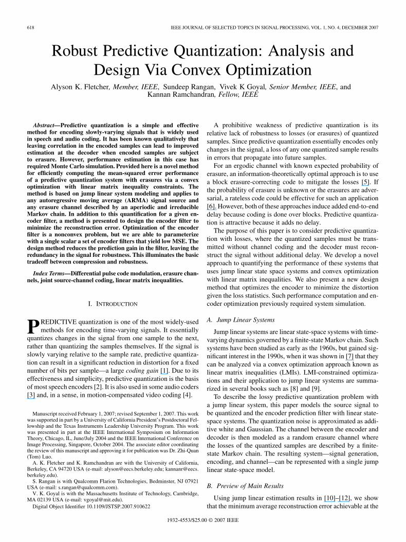
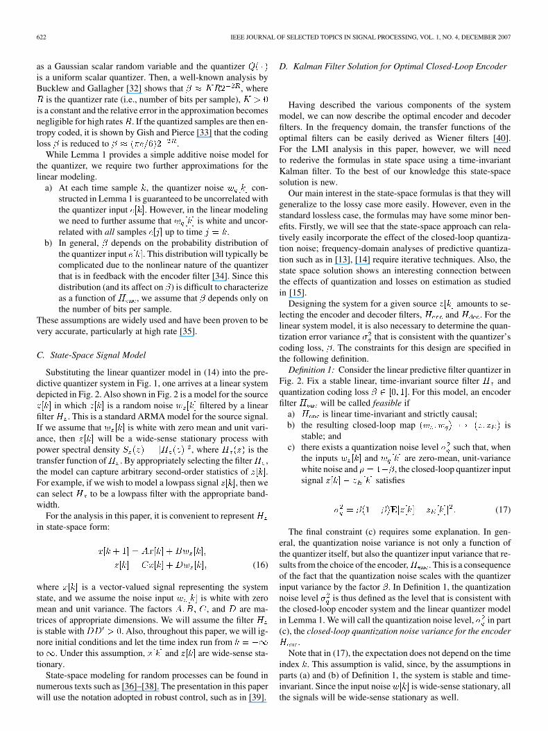
Fig. 1 shows the model we will use for the predictive quan-tizer encoder and decoder. The signal to be quantized is calledthe “source” and denoted by . The predictive quantizer en-coder consists of a linear filter , in feedback with a scalarquantizer . The filter will be called the encoder filter

FLETCHER et al.: ROBUST PREDICTIVE QUANTIZATION 621

Fig. 1. Predictive quantizer encoder and decoder with a general higher-order filter.

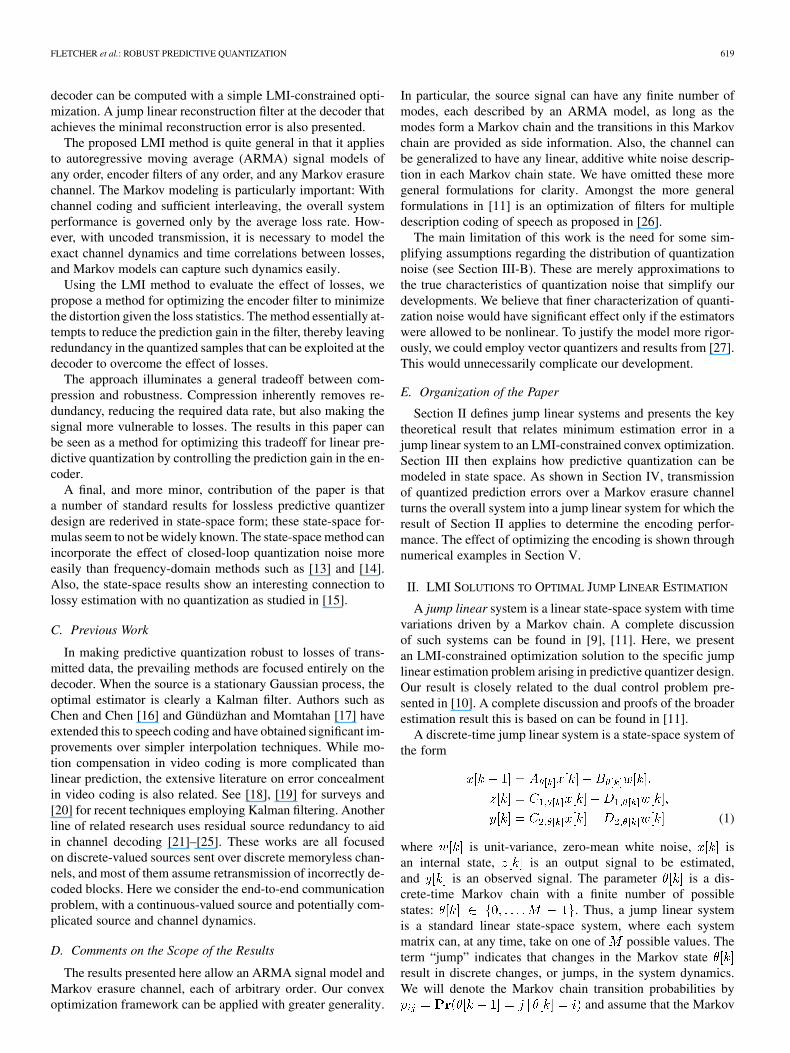
Fig. 2. Linear model for the predictive quantizer system. The quantizer is replaced by a linear gain and additive noise, and the source signal, z[k], is described asfiltered white noise.

and its output is denoted . The quantizer output sample se-quence is denoted . The decoder is represented by the linearfilter , which operates on the quantizer samples to pro-duce the final decoder output is denoted . The decoderoutput is the final estimate of the original signal , soideally is close to .

B. Linear Quantizer Model

Due to the nonlinear nature of the scalar quantizer, an exactanalysis of the predictive quantizer system is difficult. The clas-sical approach to deal with the nonlinearity is to approximatethe quantizer as a linear gain with additive white noise (AWN).One such model is provided by the following lemma.

Lemma 1: Consider the predictive quantizer system in Fig. 1.Suppose that the closed-loop system is well-posed and stableand all the resulting signals are wide-sense stationary randomprocesses with zero mean. In addition, suppose that the scalarquantizer function is designed such that

(12)

Also, let

(13)

It follows that the quantizer output can then be written (as shownin Fig. 2)

(14)

where is a zero-mean, unit-variance signal, uncorrelatedwith , and

(15)

Proof: See Appendix C-1.The lemma shows that the quantizer can be described as a

linear gain , along with additive noise uncorrelated withthe quantizer input . Observe that since is normalizedto have unit variance, the variance of the additive noise is .

The assumption (12) is that, for each partition region, thefunction will output the conditional mean. This condition issatisfied by optimal quantizers, or more generally, whenever thequantization decoder mapping is optimal, regardless of whetherthe encoder mapping is optimal [1]. Moreover, the conditionwill hold approximately for uniform quantizers at high rates.

The factor in (13) is a proportionality constant between thequantizer input variance and quantizer error variance. The pa-rameter can thus be seen as a measure of the quantizer’s relativeaccuracy. In [1], the factor is called the coding gain of thequantizer. Following this terminology, we will call either theinverse coding gain or coding loss.

In general, will depend on the quantizer input distribution,specific scalar quantizer design and number of bits per sample.In particular, it is independent of the encoder and decoder fil-ters, and can therefore be treated as a design constant. For ex-ample, suppose the input to the quantizer is well-approximated

622 IEEE JOURNAL OF SELECTED TOPICS IN SIGNAL PROCESSING, VOL. 1, NO. 4, DECEMBER 2007

as a Gaussian scalar random variable and the quantizeris a uniform scalar quantizer. Then, a well-known analysis byBucklew and Gallagher [32] shows that , where

is the quantizer rate (i.e., number of bits per sample),is a constant and the relative error in the approximation becomesnegligible for high rates . If the quantized samples are then en-tropy coded, it is shown by Gish and Pierce [33] that the codingloss is reduced to .

While Lemma 1 provides a simple additive noise model forthe quantizer, we require two further approximations for thelinear modeling.

a) At each time sample , the quantizer noise con-structed in Lemma 1 is guaranteed to be uncorrelated withthe quantizer input . However, in the linear modelingwe need to further assume that is white and uncor-related with all samples up to time .

b) In general, depends on the probability distribution ofthe quantizer input . This distribution will typically becomplicated due to the nonlinear nature of the quantizerthat is in feedback with the encoder filter [34]. Since thisdistribution (and its affect on ) is difficult to characterizeas a function of , we assume that depends only onthe number of bits per sample.

These assumptions are widely used and have been proven to bevery accurate, particularly at high rate [35].

C. State-Space Signal Model

Substituting the linear quantizer model in (14) into the pre-dictive quantizer system in Fig. 1, one arrives at a linear systemdepicted in Fig. 2. Also shown in Fig. 2 is a model for the source

in which is a random noise filtered by a linearfilter . This is a standard ARMA model for the source signal.If we assume that is white with zero mean and unit vari-ance, then will be a wide-sense stationary process withpower spectral density , where is thetransfer function of . By appropriately selecting the filter ,the model can capture arbitrary second-order statistics of .For example, if we wish to model a lowpass signal , then wecan select to be a lowpass filter with the appropriate band-width.

For the analysis in this paper, it is convenient to representin state-space form:

(16)

where is a vector-valued signal representing the systemstate, and we assume the noise input is white with zeromean and unit variance. The factors , and are ma-trices of appropriate dimensions. We will assume the filteris stable with . Also, throughout this paper, we will ig-nore initial conditions and let the time index run fromto . Under this assumption, and are wide-sense sta-tionary.

State-space modeling for random processes can be found innumerous texts such as [36]–[38]. The presentation in this paperwill use the notation adopted in robust control, such as in [39].

D. Kalman Filter Solution for Optimal Closed-Loop Encoder

Having described the various components of the systemmodel, we can now describe the optimal encoder and decoderfilters. In the frequency domain, the transfer functions of theoptimal filters can be easily derived as Wiener filters [40].For the LMI analysis in this paper, however, we will needto rederive the formulas in state space using a time-invariantKalman filter. To the best of our knowledge this state-spacesolution is new.

Our main interest in the state-space formulas is that they willgeneralize to the lossy case more easily. However, even in thestandard lossless case, the formulas may have some minor ben-efits. Firstly, we will see that the state-space approach can rela-tively easily incorporate the effect of the closed-loop quantiza-tion noise; frequency-domain analyses of predictive quantiza-tion such as in [13], [14] require iterative techniques. Also, thestate space solution shows an interesting connection betweenthe effects of quantization and losses on estimation as studiedin [15].

Designing the system for a given source amounts to se-lecting the encoder and decoder filters, and . For thelinear system model, it is also necessary to determine the quan-tization error variance that is consistent with the quantizer’scoding loss, . The constraints for this design are specified inthe following definition.

Definition 1: Consider the linear predictive filter quantizer inFig. 2. Fix a stable linear, time-invariant source filter andquantization coding loss . For this model, an encoderfilter will be called feasible if

a) is linear time-invariant and strictly causal;b) the resulting closed-loop map is

stable; andc) there exists a quantization noise level such that, when

the inputs and are zero-mean, unit-variancewhite noise and , the closed-loop quantizer inputsignal satisfies

(17)

The final constraint (c) requires some explanation. In gen-eral, the quantization noise variance is not only a function ofthe quantizer itself, but also the quantizer input variance that re-sults from the choice of the encoder, . This is a consequenceof the fact that the quantization noise scales with the quantizerinput variance by the factor . In Definition 1, the quantizationnoise level is thus defined as the level that is consistent withthe closed-loop encoder system and the linear quantizer modelin Lemma 1. We will call the quantization noise level, in part(c), the closed-loop quantization noise variance for the encoder

.Note that in (17), the expectation does not depend on the time

index . This assumption is valid, since, by the assumptions inparts (a) and (b) of Definition 1, the system is stable and time-invariant. Since the input noise is wide-sense stationary, allthe signals will be wide-sense stationary as well.

FLETCHER et al.: ROBUST PREDICTIVE QUANTIZATION 623

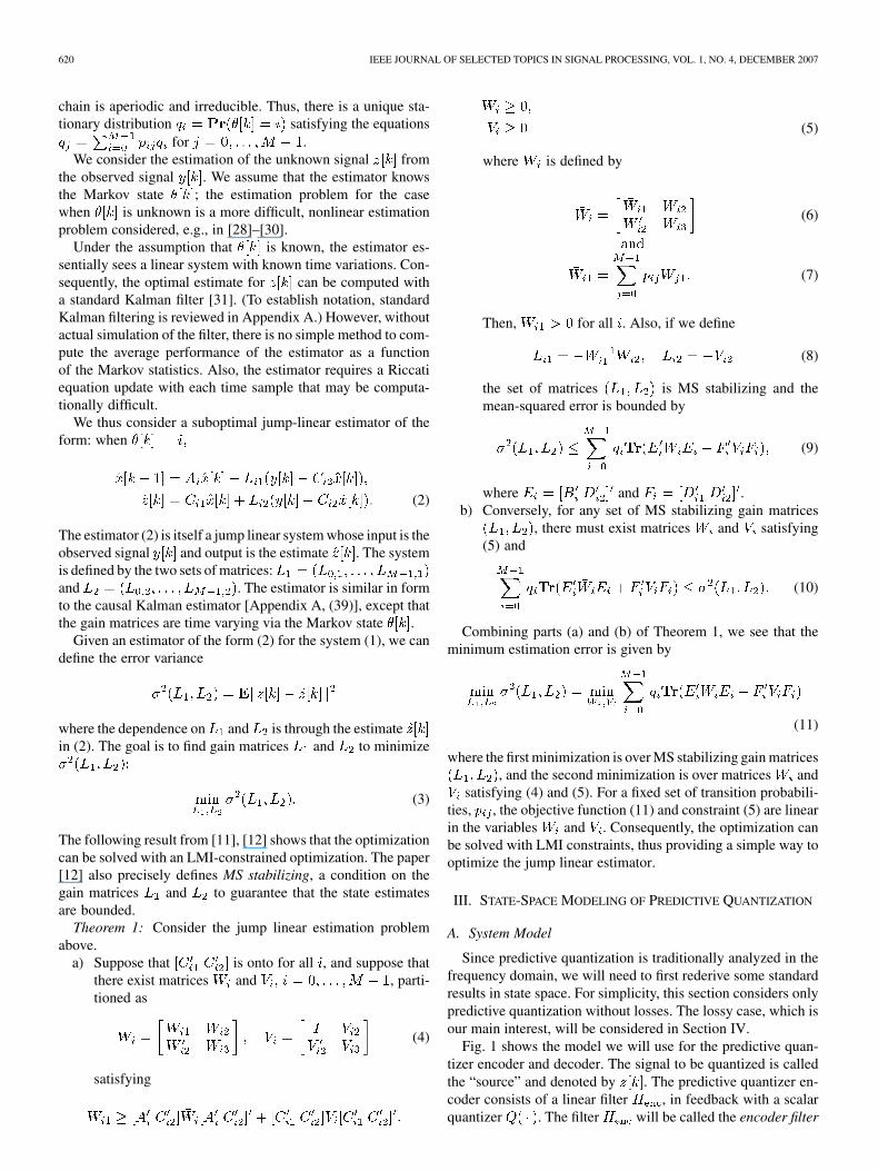
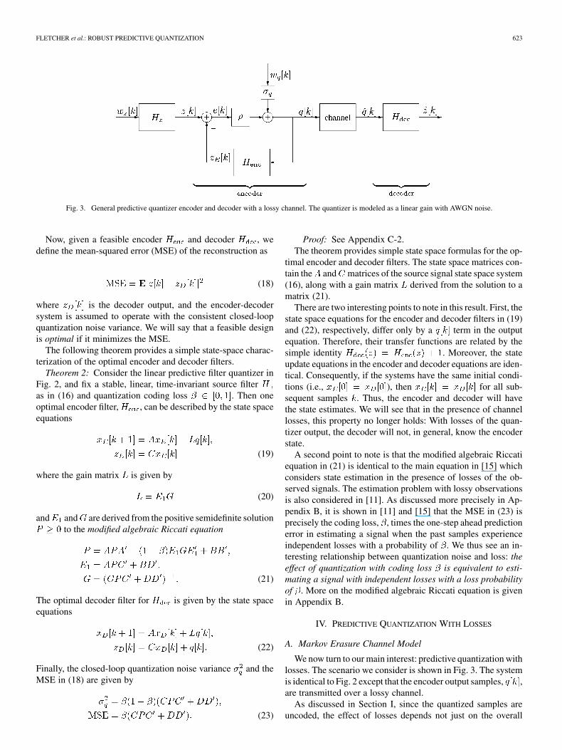
Fig. 3. General predictive quantizer encoder and decoder with a lossy channel. The quantizer is modeled as a linear gain with AWGN noise.

Now, given a feasible encoder and decoder , wedefine the mean-squared error (MSE) of the reconstruction as

(18)

where is the decoder output, and the encoder-decodersystem is assumed to operate with the consistent closed-loopquantization noise variance. We will say that a feasible designis optimal if it minimizes the MSE.

The following theorem provides a simple state-space charac-terization of the optimal encoder and decoder filters.

Theorem 2: Consider the linear predictive filter quantizer inFig. 2, and fix a stable, linear, time-invariant source filteras in (16) and quantization coding loss . Then oneoptimal encoder filter, , can be described by the state spaceequations

(19)

where the gain matrix is given by

(20)

and and are derived from the positive semidefinite solutionto the modified algebraic Riccati equation

(21)

The optimal decoder filter for is given by the state spaceequations

(22)

Finally, the closed-loop quantization noise variance and theMSE in (18) are given by

(23)

Proof: See Appendix C-2.The theorem provides simple state space formulas for the op-

timal encoder and decoder filters. The state space matrices con-tain the and matrices of the source signal state space system(16), along with a gain matrix derived from the solution to amatrix (21).

There are two interesting points to note in this result. First, thestate space equations for the encoder and decoder filters in (19)and (22), respectively, differ only by a term in the outputequation. Therefore, their transfer functions are related by thesimple identity . Moreover, the stateupdate equations in the encoder and decoder equations are iden-tical. Consequently, if the systems have the same initial condi-tions (i.e., ), then for all sub-sequent samples . Thus, the encoder and decoder will havethe state estimates. We will see that in the presence of channellosses, this property no longer holds: With losses of the quan-tizer output, the decoder will not, in general, know the encoderstate.

A second point to note is that the modified algebraic Riccatiequation in (21) is identical to the main equation in [15] whichconsiders state estimation in the presence of losses of the ob-served signals. The estimation problem with lossy observationsis also considered in [11]. As discussed more precisely in Ap-pendix B, it is shown in [11] and [15] that the MSE in (23) isprecisely the coding loss, , times the one-step ahead predictionerror in estimating a signal when the past samples experienceindependent losses with a probability of . We thus see an in-teresting relationship between quantization noise and loss: theeffect of quantization with coding loss is equivalent to esti-mating a signal with independent losses with a loss probabilityof . More on the modified algebraic Riccati equation is givenin Appendix B.

IV. PREDICTIVE QUANTIZATION WITH LOSSES

A. Markov Erasure Channel Model

We now turn to our main interest: predictive quantization withlosses. The scenario we consider is shown in Fig. 3. The systemis identical to Fig. 2 except that the encoder output samples, ,are transmitted over a lossy channel.

As discussed in Section I, since the quantized samples areuncoded, the effect of losses depends not just on the overall

624 IEEE JOURNAL OF SELECTED TOPICS IN SIGNAL PROCESSING, VOL. 1, NO. 4, DECEMBER 2007

erasure probability, but the exact dynamics of the loss process.We will assume that there is an underlying Markov chain

, and the erasures occur when the Markov chainenters a subset of states, . We define

and as in Section II and again assume the Markov chainis aperiodic and irreducible. We will denote the channel outputby and take the output to be zero when the sample is lost.Thus,

(24)

The Markov model is extremely general and captures a largerange of erasure processes including independent erasures,Gilbert–Elliot erasures and fixed-length burst erasures.

B. Encoder Design

The goal of robust predictive quantization is: given a signalmodel (16) and statistics on the Markov erasure channel state ,to design the encoder and decoder to minimize theaverage reconstruction error. We first consider the design of theencoder filter .

Following the structure of the optimal encoder (19) for thelossless case, we will assume that the encoder filter for the lossychannel takes the same form:

(25)

This encoder filter (25) is identical to optimal filter (19) for thelossless system, except that we can use any gain matrix . Inthis way, we treat as a design parameter that can be optimizeddepending on the loss and source statistics.

It should be stated that, in fixing the encoder to be of the form(25), we have eliminated certain degrees of freedom in the en-coder design. The LMI framework would allow the matricesand in (25) to differ from the corresponding quantities in (16).But, as we will see, the optimization philosophy in Section IV-Ewill lead us to (25). We therefore impose this form at the onsetto simplify the following discussion.

Our first result for the lossy case characterizes the set of fea-sible encoder gain matrices.

Theorem 3: Consider the predictive quantizer encoder in Fig.3 where is described by (16) and the encoder filter isdescribed by (25) for some encoder gain matrix . Assume that

is stable and suppose there exists a satisfying theLyapunov equation

(26)

with

(27)

Then the encoder (25) is feasible in the sense of Definition 1,and the corresponding closed-loop quantization noise level isgiven by

(28)

Proof: See Appendix C-3.Theorem 3 provides a simple way of testing the feasibility of

a candidate gain matrix and determining the correspondingquantization noise level. Specifically, the gain matrix is fea-sible if the solution to the Lyapunov equation (26) satisfies

and the condition in (27). If the gain matrix is fea-sible, the closed-loop quantization noise level is given by (28).

It can be shown that the optimal encoder gain for the loss-less system (from Theorem 2) is precisely the gain matrix thatminimizes the resulting quantization noise variance . How-ever, in the presence of losses, we will see that the optimal gaindoes not necessarily minimize the quantization noise: The quan-tizer input variance can be seen as a measure of how much en-ergy the prediction filter subtracts out from the previous quan-tizer output samples. With losses, the optimal filter may not sub-tract out all the energy, thereby leaving some redundancy in thequantizer output samples and thus improving the robustness tolosses.

C. Jump Linear Decoder

Having characterized the set of feasible encoders, we can nowconsider the decoder. Given an encoder, the decoder must essen-tially estimate the source signal from the quantizer outputsamples that are not lost. We can set this estimation problemup as a jump linear filtering problem and then apply the resultsin Section II.

To employ the jump linear framework, we need to construct asingle jump linear state-space system that describes the signals

and . To this end, we combine the encoder , thesource generating filter , and the linear quantizer. The com-bined system has two states: in the source signal modeland in the prediction filter, and we can define the jointstate vector . We also let denote thejoint noise vector , which contains boththe source signal input and quantization noise. We can now viewthe signals and as outputs of a single system whoseinput is and state is .

There are two cases for the state and output equations for thesystem: when the sample is received by the decoder, andwhen the sample is lost. We will first consider the case whenthe sample is not lost. In this case, . Using thisfact along with (16), (25) and (14), we obtain the larger statespace system

(29)

where

, and . The system (29)expresses the source signal and the channel output as

FLETCHER et al.: ROBUST PREDICTIVE QUANTIZATION 625

outputs of a single larger state space system. The system hastwo inputs: the noise vector and the signal . When thesample is not lost over the channel, the input is knownto the decoder. Hence we have added the subscript NL on thematrices, and to indicate the “no loss” matrices.

When the sample is lost:

(30)

where and .Thus, from the perspective of the decoder, the combined

signal-encoder system alternates between two possible models:(29) when the sample is not lost in the channel, and (30)when the sample is lost. Now, in the model we have assumed inSection IV-A, the loss event occurs when the Markov stateenters a subset of the discrete states denoted . We can thuswrite the signal-encoder system as a jump linear system drivenby the channel Markov state : When

(31)

where the system matrices are given by

and is the known input

The matrices and do not vary with .Following Section II, we can consider a jump linear estimator

of the following form: When

(32)

where and are gain matrices that are to be determinedby the optimization.

Before considering the optimization, it is useful to comparethe jump linear estimator (32) with the decoder for the losslesscase in (22). The most significant difference is that the decoderin (32) must estimate the states, , for the source signalsystem, as well as the encoder states, . In the losslesscase, the decoder receives all the quantized samples . Con-sequently, by running the encoder filter (19), it can reconstructthe encoder state . Therefore, the decoder need only esti-mate the signal state . However, with losses, the encoderstate is unknown to the decoder and the decoder must estimateboth and . In particular, if in the lossless problemone must estimate a state of dimension , the lossy estimatormust estimate a state of dimension .

A second difference is the gain matrices and . In thedecoder (22) for the lossless channel, the gain matrices are con-

stant. Moreover, where is the optimal encoder gainmatrix, and . In the jump linear decoder (32), the gainmatrices and vary with the Markov state and do notnecessarily have any simple relation with the encoder matrix.

D. LMI Analysis

Having modeled the system and decoder as jump linear sys-tems, we can now find the optimal decoder gain matricesand in (32) using the LMI analysis in Section II. Specifically,Theorem 1 provides an LMI-constrained optimization for com-puting the gain matrices and that minimize the MSE,

(33)

where the expectation is over the random signal , the quan-tization noise and Markov state sequence . For the de-coder problem, the MSE in (33) is precisely the mean-squaredreconstruction error between the original signal and the de-coder output . Again, recall that since we have assumed thesystem is stable and all signals are wide-sense stationary, theMSE in (33) does not depend on the time .

The LMI method thus provides a simple way of computingthe minimum reconstruction error for a given source signalmodel, predictive encoder and channel loss statistics. Byvarying the channel loss model parameters, one can thus quan-tify the effect of channel losses on a predictive quantizationsystem with a given encoder.

The overall analysis algorithm can be described as follows:Algorithm 1 (LMI Analysis): Consider the predictive quan-

tizer system in Fig. 3. Suppose the source signal is gen-erated by a stable LTI system of the form (16), the predictionfilter can be described by (25) for a given gain matrix , and thequantizer can be described by (14). Let be the quanti-zation coding loss, so that . Suppose the channel era-sures can be described by an aperiodic and irreducible -stateMarkov chain . Then, the optimal decoder of the form (32)can be computed as follows.

1) Use Theorem 3 to determine if the encoder gain matrixis feasible. Specifically, verify that there is a solution

to the Lyapunov equation (26), and confirm that thesolution satisfies (27). If is not feasible, stop since theMSE is infinite.

2) Compute the closed-loop quantization noise, in (28).3) Compute the jump linear system matrices

and as in Section IV-C.4) Use Theorem 1 to compute the optimal gain matrices

and for the decoder (32) and the corresponding recon-struction MSE: .

E. Encoder Gain Optimization

Algorithm 1 in the previous section describes how to com-pute the minimum MSE achievable at the decoder for a givenpredictive encoder. However, to maximize the robustness of theoverall quantizer system, one would like to select the predictiveencoder that minimizes this MSE.

To be more specific, let be the minimum achievableMSE for a given encoder gain matrix . This minimum error,

, can be computed from Algorithm 1 given a modelfor the signal and a Markov loss model for the channel. Ideally,

626 IEEE JOURNAL OF SELECTED TOPICS IN SIGNAL PROCESSING, VOL. 1, NO. 4, DECEMBER 2007

one would like to search over all gain matrices to minimize. That is, we wish to compute the optimal encoder gain

matrix:

(34)

Unfortunately, this minimization is difficult. The functionis, in general, a complex nonlinear function of the

coefficients of . The global minimum cannot be found withoutan exhaustive search. If the filter (16) for the signal hasorder , then will have coefficients to optimize over. There-fore, even at small filter orders, a direct search over possiblegain matrices will be prohibitively difficult.

To overcome this difficulty, we propose the following simple,but suboptimal, search. For each , we compute a can-didate gain matrix given by

(35)

where and are derived from the solutions to themodified algebraic Riccati equations,

(36)

We can then minimize the MSE, searching over the single pa-rameter :

(37)

Similarly to (34), the minimization in (37) is not necessarilyconvex, and an exact solution would require an exhaustivesearch. However, since is a scalar parameter and dependenceon is continuous, a good approximate solution to (37) can befound by testing a small number of values of .

This suboptimal search over the candidate gain matricescan be motivated as follows: From Theorem 2, we see that when

is precisely the optimal encoder gain matrix for thelossless system. For other values of is the optimal gainmatrix for a lossless channel, but with a higher effective codingloss given by . As decreases from 1 to0, this effective coding loss, , increases from to 1. The in-crease in the coding loss represents an increase in the effec-tive quantization noise. The logic in the suboptimal search (37)is that the modifications for the encoder for higher quantizationnoise should be qualitatively similar to the modifications nec-essary for channel losses. As the quantization noise increases,the prediction filter is less able to rely on past quantized sam-ples and will naturally decrease the weighting of those samplesin the prediction output. This removal of past samples from theprediction output will leave redundancy in the quantized sam-ples and should improve the robustness to channel losses.

V. NUMERICAL EXAMPLES

To illustrate the robust predictive quantization design method,we consider the quantization of the output of a second-orderChebyshev lowpass filter with cutoff frequency drivenby a zero-mean white Gaussian input. For the quantizer ,

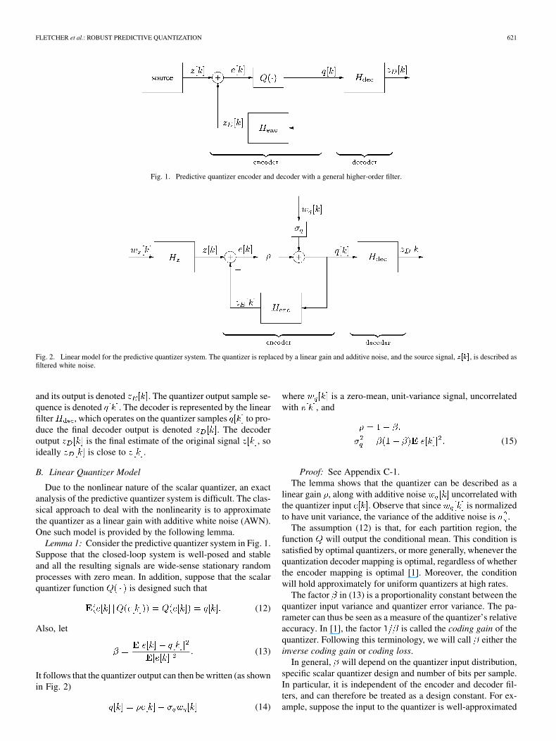
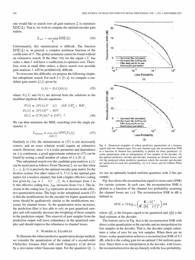
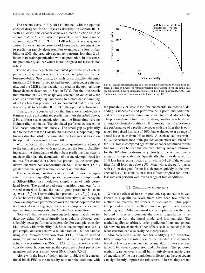
Fig. 4. Numerical examples of robust predictive quantization of a lowpasssignal with two channel types. For each channel type, the reconstruction SNRas a function of channel loss probability is plotted for three quantizers: (i)scalar quantization with no interpolation of lost samples at the decoder; (ii)the optimal predictive encoder and decoder assuming no channel losses; and(iii) the proposed robust predictive quantizer where the encoder and decoderare optimized for each loss probability. (a) i.i.d. losses and (b) Gilbert–Elliotchannel.

we use an optimally-loaded uniform quantizer with 2 bits persample.

Fig. 4(a) shows the reconstruction signal-to-noise ratio (SNR)for various systems. In each case, the reconstruction SNR isplotted as a function of the channel loss probability assumingthe channel losses are i.i.d. The reconstruction SNR in dB isdefined as

where is the lowpass signal to be quantized and is thefinal estimate at the decoder.

The bottom curve in Fig. 4(a) is the reconstruction SNR withdirect scalar quantization at the encoder and no interpolation forlost samples at the decoder. That is, the decoder simply substi-tutes a value of zero for any lost samples. When there are nolosses, scalar quantization achieves a reconstruction SNR of 9.3dB, which is the coding gain for an optimal 2-bit uniform quan-tizer. Since there is no interpolation at the decoder, with losses,the reconstruction error decays linearly with the loss probability.

FLETCHER et al.: ROBUST PREDICTIVE QUANTIZATION 627

The second curve in Fig. 4(a) is obtained with the optimalencoder designed for no losses as described in Section III-D.With no losses, this encoder achieves a reconstruction SNR ofapproximately 21.7 dB which represents a prediction gain ofapproximately dB relative to scalar quanti-zation. However, in the presence of losses the improvement dueto prediction rapidly decreases. For example, at a loss proba-bility of 20%, the predictive quantizer performs less than 2 dBbetter than scalar quantization with no prediction. In this sense,the predictive quantizer which is not designed for losses is notrobust.

The bold curve depicts the computed performance of robustpredictive quantization when the encoder is optimized for theloss probability. Specifically, for each loss probability, the min-imization (37) is performed to find the optimal encoder gain ma-trix, and the MSE at the decoder is based on the optimal jumplinear decoder described in Section IV-C. For the line-searchminimization in (37), we adaptively selected 20 values of foreach loss probability. By comparing to a more dense samplingof for a few loss probabilities, we concluded that this methodwas adequate to get within 0.05 dB of the optimal performance.

Finally, the ’s connected by a thin line show simulated per-formance using the optimized prediction filters described above,2-bit uniform scalar quantization, and the linear time-varyingKalman filter estimator. The simulated performance tracks theLMI-based computations closely. The small gap is primarilydue to the fact that the LMI bound assumes a suboptimal jumplinear estimator, while the simulated performance is based onthe optimal time-varying Kalman filter.

With no losses, the robust predictive quantizer is identicalto the optimal encoder with no losses. As the loss probabilityincreases, the degradation of the robust predictive quantizer ismuch smaller than the degradation of the encoder optimized forno loss. For example, at a 20% loss probability, the robust pre-dictive quantizer has a reconstruction SNR more than 4.5 dBgreater than the system without encoder optimization.

The same design method can be used for more compli-cated channels. Fig. 4(b) repeats the previous example witha Gilbert–Elliot loss model—a simple channel with corre-lated losses. The good-to-bad state transition parameter isvaried from 0 to 1, and the bad-to-good parameter is set to

. The resulting loss probability is .As can be seen in Fig. 4(b), the robust predictive quantizer againshows an improved performance over the encoder optimized forno losses. As with Fig. 4(a), the results computed via convexoptimizations are supported by Monte Carlo simulation.

Note well that we are comparing techniques that do not in-duce any delay. When arbitrarily large delay is allowed, con-siderably better performance is possible. For example, consideri.i.d. losses with probability 0.5. Since the example uses 2 bitsper sample, one can achieve a reliable rate of 1 bit per sampleusing ideal forward error correction (FEC). It can be verifiedusing the methods in Section III-D that such a system wouldachieve a reconstruction SNR of 12.4 dB for the source underconsideration. In comparison, the optimized robust predictivequantizer achieves a much lower SNR of only 7.0 dB.

Along with the issue of delay, another problem with conven-tional block FEC is the necessity to match the code rate with

Fig. 5. Quantizer performance as a function the loss probability with three dif-ferent prediction filters: (a) robust prediction filter designed for the actual lossprobability; (b) filter optimized for no loss; and (c) filter optimized for 10% loss.Simulation conditions are identical to those in Fig. 4(b).

the probability of loss: if too few codewords are received, de-coding is impossible and performance is poor; and additionalcodewords beyond the minimum needed to decode do not help.The proposed predictive quantizer design method is robust overa range of channel conditions. To illustrate this, Fig. 5 showsthe performance of a predictive coder with the filter that is opti-mized for a fixed loss rate of 10%, but evaluated over a range ofactual losses rates from 0% to 100%. At each actual loss proba-bility, the performance of the predictive quantizer optimized forthe 10% loss is compared against the encoder optimized for thetrue loss. It can be seen that the predictive quantizer optimizedfor the 10% loss performs very closely to the optimal over arange of loss probabilities. Specifically, the filter designed for10% loss has a reconstruction error within 0.4 dB of the optimalfilter for all loss rates above 5%. Meanwhile, the performancewith a filter designed for no loss degrades quickly in the pres-ence of loss. The conclusion is that a filter designed for a smallloss rate can perform well over a range of loss conditions.

VI. CONCLUDING COMMENTS

While the effect of losses in predictive quantization is wellknown at a qualitative level, there have been few practicalmethods to quantify the effects of such losses. This paperhas presented a novel method based on jump linear systemmodeling and LMI-constrained convex optimization that canbe used to precisely compute the overall degradation in re-construction from the signal model and loss statistics. Themethod applies to arbitrary-order prediction filters and generalMarkov erasure channels. Other effects such as the delay in thereconstruction can also easily be incorporated.

Also presented is a method for modifying the predictionfilter to improve the robustness of the encoder. The approach,based on leaving redundancy in the signal, illustrates a generaltradeoff between compression and robustness. The proposedmethod searches over a small but intuitively-reasonable classof encoders. While our simulations indicate that these encoderscan significantly improve the robustness to losses, they are not

628 IEEE JOURNAL OF SELECTED TOPICS IN SIGNAL PROCESSING, VOL. 1, NO. 4, DECEMBER 2007

necessarily optimal. We also have not explored varying thesampling rate, e.g., to provide opportunity for channel coding.

APPENDIX ASTEADY-STATE KALMAN FILTER EQUATIONS

The Kalman filter is widely used in linear estimation prob-lems and covered in several standard texts such as [31] and [38].However, the analysis in this paper requires a slightly non-stan-dard form, used in modern robust control texts such as [39]. Itis useful to briefly review the equations that will be used.

To describe the Kalman filter, consider a linear state spacesystem of the form

(38)

We assume the input is a white Gaussian process with zeromean and unit variance. The Kalman filtering problem is to es-timate the first output signal and state from the secondoutput . The signal represents an unknown signal thatwe wish to estimate, and is the observed signal.

Define the state and output estimates:

Thus, is the MMSE estimate of the state given theobserved output up to sample . While the Kalman filter canbe used to compute the estimates for any and , we will beinterested here in three specific estimates:

• : The causal estimate of given the observationsof up to time .

• : The strictly causal estimate of given theobservations of up to time .

• : The strictly causal estimate of the state .To avoid the effect of initial conditions, we will assume all

signals are wide-sense stationary. Under the additional technicalassumptions that is detectable and , it can beshown that the optimal estimate for the above three quantities isgiven by recursive Kalman filter equations:

(39)

where and are known as the Kalman gain matrices andwill be described momentarily. We see that the Kalman filter isitself a linear time-invariant state-space filter whose input isand outputs are the estimates of and .

The filter (39) are sometimes called the time-invariant orsteady-state equations, since the gain matrices and donot vary with time. In general, to account for either initialconditions or time-varying systems, the gain matrices and

would need to be time-varying. However, since we will only

be interested in time-invariant systems and asymptotic perfor-mance, the time-invariant form considered here is sufficient.

The gain matrices and in (39) can be determined fromthe solution to the well-known algebraic Riccati equation givenby

(40)

where and .Under the assumption that is detectable and ,it can be shown that (40) has a unique positive semi-definitesolution . The gain matrices are then given by

(41)

where

(42)

The algebraic Riccati equation solution has the interpreta-tion of the state-estimation error variance:

Also, the mean-squared output errors are given by

(43)

(44)

where .

APPENDIX BMODIFIED ALGEBRAIC RICCATI EQUATION

The analysis in Section III-D results in a modified form of thestandard algebraic Riccati equation,

(45)

for a loss parameter . When , the equationreduces to the standard algebraic Riccati equation (40); when

, it reduces to the discrete Lyapunov equation.

A similar equation arises in [15] and [11], which considerstate estimation of a system (38) with i.i.d. erasures of the ob-servation signal . A result in [11] specifically shows the fol-lowing: Suppose that is the output of a linear state-spacesystem

(46)

where is unit-variance white noise. Let representthe one-step ahead prediction of from past samples

, where

FLETCHER et al.: ROBUST PREDICTIVE QUANTIZATION 629

That is, is the estimate of from past samples,where the samples are lost with probability . If the losses arei.i.d. and is the optimal jump linear estimator (dis-cussed in Section II), it is shown in [11] that the resulting re-construction error is given by

where is the solution to the modified algebraic Riccati equa-tion (45). Comparing this result with Theorem 2, we see thatthere is one-to-one correspondence between the effects of i.i.d.losses and quantization.

As discussed in [11], the modified algebraic Riccati equationcan be solved via an LMI-constrained optimization. However, inthe special case of a scalar output, the following simple iterativeprocedure is also possible.

Suppose has a scalar output, i.e., is a row vector. For, define the matrix function . Then, it is

easy to verify that is a solution to (45) if and only if thereexists a satisfying the following coupled equations:

(47)

(48)

(49)

For a fixed , (47)–(48) is a standard algebraic Riccati equationand can be easily solved for . Also, it can be verified that thesolution monotonically increases with . This leads to thefollowing iterative bisection search procedure.

• Step 1: Find minimum and maximum values, and, for the possible solution .

• Step 2: Set to the midpoint of the interval,.

• Step 3: Solve the algebraic Riccati equation (47)–(48) forusing the midpoint value of .

• Step 4: If then setand return to Step 2; otherwise, set

and return to Step 2.This iterative procedure will converge exponentially to apair satisfying the coupled (47)–(49).

APPENDIX CPROOFS

1) Proof of Lemma 1

To simplify the notation in this proof, we will omit the timeindex on all signals. From (12), , so

(50)

Combining (50) and (13), we obtain

Therefore,

(51)

Now, let , so that . Sinceand are zero mean, so is . Also, using (50) and (51),

, soand are uncorrelated. Finally,

Therefore, if we define and as in (15) and let ,we have that is a zero-mean process, uncorrelated with ,with unit variance and satisfying .

2) Proof of Theorem 2

We know from [1] that the optimal encoder and decoder filtersmust be the MMSE estimators,

That is, must be the MMSE estimate of given thequantized samples up to time . The optimal de-coder output is the MMSE estimate using the samples up to time

. Since the system is linear and time-invariant, both esti-mators are given by standard time-invariant Kalman filters.

The Kalman filter equations are summarized in Appendix A.To employ the equations, we need to first combine the quantizerand signal model into a single state-space system. To this end,we combine (16) with (14) to obtain

(52)

where . If we define the vector noiseand let

, and , then (52) can be rewritten as

(53)

We have now described the observed output and signal to beestimated as outputs of a single linear state-space system.We can then apply standard Kalman filter equations from Ap-pendix A to obtain the estimator

630 IEEE JOURNAL OF SELECTED TOPICS IN SIGNAL PROCESSING, VOL. 1, NO. 4, DECEMBER 2007

where is the Kalman gain matrix. Note that we have used thefact that is a known input, since it can be computed from

. If we define the state ,and use the fact that , the encoder equationscan be rewritten as

(54)Now, since

(55)Using this identity along with the fact that in (54), weobtain the encoder equations in (19).

Next, we derive the expression for the Kalman gain matrix. To this end, first observe that, using (44), the quantizer input

variance is given by

where is the error variance matrix. Using (17), the quantizererror variance is given by

Now using the fact that and , the matrixin (40) is given by

(56)Thus,

where and . Thisproves (21). Substituting (56) into the expression for in (41):

which proves (20).Now, substituting the expressions for and into

the expression for in (42), we obtain

(57)

Substituting (55), (56) and (57) in (39),

As discussed above, the optimal decoder output is given by. Therefore, if we define the decoder state as

, we obtain the decoder equations

(58)Finally, substituting (56) and (57) into the expression for the

MSE in (43),

3) Proof of Theorem 3

We need to show that, if satisfies the conditions in Theorem3, the resulting encoder in (25) satisfies the three conditions inDefinition 1. For any gain matrix , the encoder (25) is linear,time invariant and strictly causal, and therefore satisfies condi-tion (a) of Definition 1.

To prove condition (b), define the error signals,and . Combining (16), (25)

and (14), we obtain

(59)The system (59) is a standard LTI system. If we define theclosed-loop matrices and

and let , then is unit-variance whitenoise, and (59) can be rewritten as

(60)Now, suppose there exists a satisfying (26). The condi-tion is equivalent to

(61)

Now, since is stable, is stable. Also, since ,for any matrix and is detectable. By a standardresult for Lyapunov equations (see, for example, [37]), the exis-tence of a matrix satisfying (61) implies that is stableand

(62)This in turn implies that, for any , the mapping

is stable. Also, since is stable, the map is stable.Therefore, since , the mappingis well-posed and stable and the gain matrix satisfies condition(b).

FLETCHER et al.: ROBUST PREDICTIVE QUANTIZATION 631

For condition (c), we must show that if is defined as in (28),the resulting closed-loop system satisfies ,where . Combining (62)and (28),

Hence, and, thus, is the quantization noiselevel for .

REFERENCES

[1] A. Gersho and R. M. Gray, Vector Quantization and Signal Compres-sion. Boston, MA: Kluwer, 1992.

[2] R. V. Cox, “Speech coding,” in The Digital Signal Processing Hand-book. Boca Raton, FL: CRC and IEEE Press, 1998, ch. 45, pp.45.1–45.19.

[3] A. Gersho, “Advances in speech and audio compression,” Proc. IEEE,vol. 82, no. 6, pp. 900–918, Jun. 1994.

[4] D. LeGall, “MPEG: A video compression standard for multimedia ap-plications,” Commun. ACM, vol. 34, no. 4, pp. 46–58, Apr. 1991.

[5] T. M. Cover and J. A. Thomas, Elements of Information Theory. NewYork: Wiley, 1991.

[6] M. Luby, “LT codes,” in Proc. IEEE Symp. Found. Comp. Sci., Van-couver, BC, Canada, Nov. 2002, pp. 271–280.

[7] M. Ait Rami and L. El Ghaoui, “LMI optimization for nonstandardRiccati equations arising in stochastic control,” IEEE Trans. Automat.Control, vol. 41, no. 11, pp. 1666–1671, Nov. 1996.

[8] S. P. Boyd, L. El Ghaoui, E. Feron, and V. Balakrishnan, Linear MatrixInequalities in System and Control Theory. Philadelphia, PA: SIAM,1994.

[9] O. L. V. Costa, M. D. Fragoso, and R. P. Marques, Discrete-TimeMarkov Jump Linear Systems, ser. Probability and Its Applications.London, U.K.: Springer, 2005.

[10] O. L. V. Costa, J. B. R. do Val, and J. C. Geromel, “A convex program-ming approach to H -control of discrete-time Markovian jump linearsystems,” Int. J. Control, vol. 66, no. 4, pp. 557–559, Apr. 1997.

[11] A. K. Fletcher, “A jump linear framework for estimation and robustcommunication with Markovian source and channel dynamics,” Ph.D.dissertation, Univ. California, Berkeley, 2005.

[12] A. K. Fletcher, S. Rangan, V. K. Goyal, and K. Ramchandran, “Causaland strictly causal estimation for jump linear systems: An LMI anal-ysis,” in Proc. Conf. Inform. Sci. & Sys., Princeton, NJ, Mar. 2006.

[13] E. G. Kimme and F. F. Kuo, “Synthesis of optimal filters for a feedbackquantization scheme,” IEEE Trans. Circuits Syst., vol. 10, no. 3, pp.405–413, Sep. 1963.

[14] O. G. Guleryuz and M. T. Orchard, “On the DPCM compression ofGaussian autoregressive sequences,” IEEE Trans. Inform. Theory, vol.47, no. 3, pp. 945–956, Mar. 2001.

[15] B. Sinopoli, L. Schenato, M. Franceschetti, K. Poolla, M. I. Jordan, andS. S. Sastry, “Kalman filtering with intermittent observations,” IEEETrans. Automat. Control, vol. 49, no. 9, pp. 1453–1464, Sept. 2004.

[16] Y.-L. Chen and B.-S. Chen, “Model-based multirate representationof speech signals and its applications to recover of missing speechpackets,” IEEE Trans. Speech Audio Process., vol. 5, no. 3, pp.220–231, May 1997.

[17] E. Gündüzhan and K. Momtahan, “A linear prediction based packetloss concealment algorithm for PCM coded speech,” IEEE Trans.Speech Audio Process., vol. 9, no. 8, pp. 778–785, Nov. 2001.

[18] Y. Wang and Q.-F. Zhu, “Error control and concealment for video com-munication: A review,” Proc. IEEE, vol. 86, no. 5, pp. 974–997, May1998.

[19] Y. Wang, S. Wenger, J. Wen, and A. K. Katsaggelos, “Error resilientvideo coding techniques,” IEEE Signal Process. Mag., vol. 17, no. 3,pp. 61–82, July 2000.

[20] W.-N. Lie and Z.-W. Gao, “Video error concealment by integratinggreedy suboptimization and Kalman filtering techniques,” IEEE Trans.Circuits Syst. Video Technol., vol. 16, no. 8, pp. 982–992, Aug. 2006.

[21] R. Anand, K. Ramchandran, and I. V. Kozintsev, “Continuous errordetection (CED) for reliable communication,” IEEE Trans. Commun.,vol. 49, no. 9, pp. 1540–1549, Sept. 2001.

[22] G. Buch, F. Burkert, J. Hagenauer, and B. Kukla, “To compress or notto compress?,” in IEEE Globecom, London, Nov. 1996, pp. 196–203.

[23] J. Chou and K. Ramchandran, “Arithmetic coding-based continuouserror detection for efficient ARQ-based image transmission,” IEEE J.Sel. Areas Commun., vol. 18, no. 6, pp. 861–867, June 2000.

[24] J. Hagenauer, “Source-controlled channel decoding,” IEEE Trans.Commun., vol. 43, no. 9, pp. 2449–2457, Sept. 1995.

[25] K. Sayood and J. C. Borkenhagen, “Use of residual redundancy in thedesign of joint source/channel coders,” IEEE Trans. Comm., vol. 39,no. 6, pp. 838–846, Jun. 1991.

[26] A. Ingle and V. A. Vaishampayan, “DPCM system design for diversitysystems with applications to packetized speech,” IEEE Trans. SpeechAudio Process., vol. 3, no. 1, pp. 48–57, Jan. 1995.

[27] D. L. Neuhoff, “On the asymptotic distribution of errors in vector quan-tization,” IEEE Trans. Inform. Theory, vol. 42, no. 2, pp. 461–468, Mar.1996.

[28] H. A. P. Blom and Y. Bar-Shalom, “The interacting multiple modelalgorithm for systems with Markovian switching coefficients,” IEEETrans. Automat. Control, vol. 33, no. 8, pp. 780–783, Aug. 1988.

[29] O. L. V. Costa, “Linear minimum mean square error estimation fordiscrete-time Markovian jump linear systems,” IEEE Trans. Automat.Control, vol. 39, no. 8, pp. 1685–1689, Aug. 1994.

[30] A. Doucet, A. Logothetis, and V. Krishnamurthy, “Stochastic samplingalgorithms for state estimation of jump Markov linear systems,” IEEETrans. Automat. Control, vol. 45, no. 1, pp. 188–202, Jan. 2000.

[31] A. V. Balakrishnan, Kalman Filtering Theory. New York: Springer,Feb. 1984.

[32] J. A. Bucklew and N. C. Gallagher, Jr, “Some properties of uniformstep size quantizers,” IEEE Trans. Inform. Theory, vol. IT-26, no. 5,pp. 610–613, Sept. 1980.

[33] H. Gish and J. P. Pierce, “Asymptotically efficient quantizing,” IEEETrans. Inform. Theory, vol. IT-14, no. 5, pp. 676–683, Sept. 1968.

[34] R. M. Gray, “Quantization noise spectra,” IEEE Trans. Inform. Theory,vol. 36, no. 6, pp. 1220–1244, Nov. 1990.

[35] H. Viswanathan and R. Zamir, “On the whiteness of high-resolutionquantization errors,” IEEE Trans. Inform. Theory, vol. 47, no. 5, pp.2029–2038, July 2001.

[36] P. E. Caines, Linear Stochastic Systems. New York: Wiley, 1988.[37] F. M. Callier and C. A. Desoer, Linear Systems Theory. New York:

Springer, 1994.[38] P. R. Kumar and P. Varaiya, Stochastic Systems: Estimation, Identifi-

cation, and Adaptive Control. Englewood Cliffs, NJ: Prentice-Hall,1986.

[39] K. Zhou, J. C. Doyle, and K. Glover, Robust and Optimal Control.Upper Saddle River, NJ: Prentice-Hall, 1995.

[40] P. M. Clarkson, Optimal and Adaptive Signal Processing. BocaRaton, FL: CRC, 1993.

Alyson K. Fletcher (M’07) received the B.S. degreein mathematics from the University of Iowa, IowaCity, and the M.S. degree in electrical engineering in2002 and the M.A. degree in mathematics and Ph.D.degree in electrical engineering, both in 2006, fromthe University of California, Berkeley.

She is currently a President’s PostdoctoralFellow at the University of California, Berkeley.Her research interests include estimation, imageprocessing, statistical signal processing, sparseapproximation, wavelets, and control theory.

Dr. Fletcher is a member of SWE, SIAM, and Sigma Xi. In 2005, she re-ceived the University of California Eugene L. Lawler Award, the Henry LuceFoundation’s Clare Boothe Luce Fellowship, and the Soroptimist DissertationFellowship.

632 IEEE JOURNAL OF SELECTED TOPICS IN SIGNAL PROCESSING, VOL. 1, NO. 4, DECEMBER 2007

Sundeep Rangan received the B.A.Sc. degree inelectrical engineering from the University of Wa-terloo, Waterloo, ON, Canada, in 1992, and the M.S.and Ph.D. degrees in electrical engineering from theUniversity of California, Berkeley in 1995 and 1997,respectively.

He was then a Postdoctoral Research Fellow at theUniversity of Michigan, Ann Arbor. He joined theWireless Research Center at Bell Laboratories, Lu-cent Technologies, in 1998. In 2000, he co-founded,with four others, Flarion Technologies which devel-

oped and commercialized an early OFDM cellular wireless data system. Flarionwas acquired by Qualcomm in 2006. He is currently a Director of Engineeringat Qualcomm Technologies, where he is involved in the development of nextgeneration cellular wireless systems. His research interests include communi-cations, wireless systems, information theory, estimation, and control theory.

Vivek K Goyal (S’92–M’98–SM’03) received theB.S. degree in mathematics and the B.S.E. degree inelectrical engineering (both with highest distinction)from the University of Iowa, Iowa City, in 1993. Hereceived the M.S. and Ph.D. degrees in electricalengineering from the University of California,Berkeley, in 1995 and 1998, respectively.

He was a Member of Technical Staff in the Math-ematics of Communications Research Department ofBell Laboratories, Lucent Technologies, 1998–2001;and a Senior Research Engineer for Digital Fountain,

Inc., 2001–2003. He is currently Esther and Harold E. Edgerton Assistant Pro-fessor of electrical engineering at the Massachusetts Institute of Technology,Cambridge. His research interests include source coding theory, sampling, quan-tization, and information gathering and dispersal in networks.

Dr. Goyal is a member of Phi Beta Kappa, Tau Beta Pi, Sigma Xi, Eta KappaNu and SIAM. In 1998, he received the Eliahu Jury Award of the Universityof California, Berkeley, awarded to a graduate student or recent alumnus foroutstanding achievement in systems, communications, control, or signal pro-cessing. He was also awarded the 2002 IEEE Signal Processing Society Mag-azine Award and an NSF CAREER Award. He serves on the IEEE Signal Pro-cessing Society’s Image and Multiple Dimensional Signal Processing TechnicalCommittee and as a permanent Conference Co-chair of the SPIE Wavelets con-ference series.

Kannan Ramchandran (S’92–M’93–SM’98–F’05)received the Ph.D. degree in electrical engineeringfrom Columbia University, New York, in 1993.

He has been a Professor in the EECS at theUniversity of California at Berkeley since 1999.From 1993 to 1999, he was on the faculty of theECE Department at the University of Illinois atUrbana-Champaign. Prior to that, he was a Memberof the Technical Staff at AT&T Bell Laboratories,Whippany, NJ, from 1984 to 1990. His currentresearch interests include distributed signal pro-

cessing architectures and decentralized coding algorithms for sensor and adhoc wireless networks, multi-user information theory, content delivery forpeer-to-peer and wireless networks, media security and information-hiding,and multiresolution statistical image processing and modeling.

Dr. Ramchandran received the Eliahu I. Jury Award in 1993 at Columbia Uni-versity for the best doctoral thesis in the area of systems, signal processing, andcommunications, an NSF CAREER award in 1997, the ONR and ARO YoungInvestigator Awards in 1996 and 1997 respectively, the Henry Magnuski Out-standing Young Scholar Award from the ECE Department at UIUC in 1998,and the Okawa Foundation Prize from the EECS Department at UC Berkeley in2001. He is the co-recipient of two Best Paper Awards from the IEEE Signal Pro-cessing Society (1993, 1997), and of several best paper awards at conferencesand workshops in his field. He serves on numerous technical program commit-tees for premier conferences in information theory, communications, and signaland image processing. He was co-chair of the Third IEEE/ACM Symposium onInformation Processing for Sensor Networks (IPSN) at Berkeley in 2004. Hehas been a member of the IEEE Image and Multidimensional Signal ProcessingTechnical Committee and the IEEE Multimedia Signal Processing TechnicalCommittee, and has served as an Associate Editor for the IEEE TRANSACTIONS

ON IMAGE PROCESSING.