Embed Size (px)
Citation preview
50, F.D.
EC
UL Roosevelt A
ww
Robustn
ViUniv
MaECARES, Uni
DUniv
CARES wo
ECARES LB - CP 114/Ave., B-1050ww.ecares.o
ness for D
ncenzo Veraversity of Na
arjorie Gassnversité Libre
Darwin Ugartversity of Na
rking pap
/04 0 Brussels Borg
Dummies
ardi amur
ner e de Bruxelle
te amur
er 2012‐0
BELGIUM
s
s
015
Robustness for dummies
Vincenzo Verardi�, Marjorie Gassnerz and Darwin Ugartex.
May 3, 2012
AbstractIn the robust statistics literature, a wide variety of models have been devel-
oped to cope with outliers in a rather large number of scenarios. Nevertheless,a recurrent problem for the empirical implementation of these estimators isthat optimization algorithms generally do not perform well when dummy vari-ables are present. What we propose in this paper is a simple solution tothis involving the replacement of the sub-sampling step of the maximizationprocedures by a projection-based method. This allows us to propose robustestimators involving categorical variables, be they explanatory or dependent.Some Monte Carlo simulations are presented to illustrate the good behaviorof the method.
Highlights:
� We propose a solution to the problem of dummy variables in robust regressionoptimisation algorithms
� We propose a method to deal with outliers in a wide variety of qualitativedependent variable regression models
Keywords: S-estimators, Robust Regression, Dummy Variables, Outliers
�CORRESPONDING AUTHOR. University of Namur (CRED) Rempart de la Vierge, 8. B-5000Namur, Belgium. E-mail: [email protected]. tel +32-2-650 44 98, fax +32-2-650 44 95 andUniversité libre de Bruxelles (ECARES and CKE). Vincenzo Verardi is Associated Researcher ofthe FNRS and gratefully acknowledges their �nancial support.
zUniversité libre de Bruxelles (ECARES, SBS-EM and CKE), CP 139, Av. F.D. Roosevelt, 50,B-1050 Brussels, Belgium. E-mail: [email protected].
xUniversity of Namur (CRED) Rempart de la Vierge, 8. B-5000 Namur, Belgium. E-mail:[email protected].
1

1 Introduction
The goal of regression analysis is to �nd out how a dependent variable is related to
a set of explanatory ones. Technically speaking, it consists in estimating the (p� 1)
column vector � of unknown parameters in
y = X� + " (1)
where y is the (n � 1) dependent variable vector and X is the (n � p) matrix of
regressors. Matrix X is composed of two blocks X1 (associated with the (p1 � 1)
coe¢ cient-vector �1), which is a (n� p1) matrix of (p1 � 1) dummy variables and a
column of ones (for the constant) and X2 (associated with the (p2 � 1) coe¢ cient-
vector �2), which is a (n� p2) matrix of continuous variables and � = (�01; �02)0.
In this approach, one variable, y, is considered to be dependent on p others, the
Xs (with p = p1 + p2), known as independent or explanatory. Parameter vector � is
generally estimated by reducing an aggregate prediction error.
In linear models in which y is continuous, the most common estimation method
is Least Squares (LS) which minimizes the sum of the squared residuals, equivalent
to minimizing the variance of the residuals. One of the problems associated with
LS is the possible distortion of the estimations induced by the existence of outliers
(i.e. data lying far away from the majority of the observations). In the literature,
three ways of dealing with outliers have been proposed. The �rst one is to modify
the aggregate prediction error in such a way that atypical individuals are awarded
limited importance. A second is to �robustify� the �rst order condition associated
with the optimization problem and replace classical estimators with some robust
counterpart (e.g. replacing means with medians or covariance matrices with robust
scatter matrices etc.). The third possibility, very closely linked to the second, is
2
to use an outlier identi�cation tool to detect the outliers and call on a one-step
reweighted classical estimator to re-�t the model, thereby reducing the in�uence of
the outliers. The �rst solution is theoretically the most appealing but its practical
implementation is quite cumbersome since, to the best of our knowledge, existing
codes to �t highly robust estimations have di¢ culties in dealing with explanatory
dummy variables and a really convincing solution does not exist. What we propose
in this paper is to follow the logic of the third method to provide a good starting
point for an iteratively reweighted least-squares estimator that will make the �rst
solution implementable in practice even when dummy variables are present.
As far as qualitative and limited dependent variable (QDV) models are concerned,
some robust (implementable) estimators that minimize an aggregate prediction error
are available for binary dependent variable logit models (see Croux and Haesbroeck,
2003 and Bianco and Yohai, 1996) but, as far as we know, there are no well accepted
robust-to-outliers alternatives to Probit, or multinomial, or ordered logit/probit mod-
els. We therefore follow the third path here and propose an outlier identi�cation tool
that can be used to �ag all types of atypical individuals in a wide variety of qualita-
tive and limited dependent variable models to subsequently �t one-step reweighted
models leading to a simple robusti�cation of the most commonly used regression
models. While this is probably less appealing from a theoretical viewpoint than
what we propose for linear regression models, we believe it is a substantial contri-
bution to the applied researcher toolbox, as a wide variety of robust models can be
consistently estimated following a similar reasoning.
The structure of the paper is the following: after this short introduction, in
section 2 we present a brief overview of the typology of outliers that may exist in
linear regression models as well as robust regression estimators designed to cope with
them. In section 3 we present an outlier identi�cation tool for regression analysis that
3
handles dummies and in section 4 we present how this can be used in the context of
qualitative dependent variables models. Some simulations are presented in section 5
to illustrate the behavior of the proposed methodology. Finally, section 6 concludes.
2 Outliers and robust linear regression estimators
Before introducing robust regression estimators, it is important to brie�y recall the
types of outliers that may exist in regression analysis. To start with, leverage points
are observations outlying in the space of the explanatory variables (the x-dimension).
They are de�ned as �good�if they are located in a narrow interval around the re-
gression hyperplane and �bad� if they are outside of it. The term vertical outlier
characterizes points that are not outlying in the x-dimension, but are so in the
vertical dimension. Since good leverage points do not a¤ect the estimation of the
coe¢ cients, they are generally not treated di¤erently from the bulk of the data.
However, as pointed out by Dehon et al. (2009) among others, such points must
nonetheless be analyzed separately from the others since they are not generated by
the model underlying the vast majority of the observations. Moreover, they distort
the inference.
When estimating parameter vector � in equation (1) using ordinary least squares
(LS), the aggregate prediction error to be minimized is the sum of the squared
residuals, i.e.
�LS = argmin�
nXi=1
r2i (�) (2)
with ri(�) = yi �Xi� for 1 � i � n: By squaring the residuals, LS awards excessive
importance to observations with very large residuals and, consequently, the estimated
4
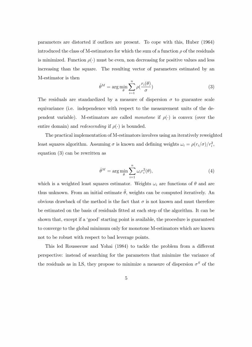
parameters are distorted if outliers are present. To cope with this, Huber (1964)
introduced the class of M-estimators for which the sum of a function � of the residuals
is minimized. Function �(�) must be even, non decreasing for positive values and less
increasing than the square. The resulting vector of parameters estimated by an
M-estimator is then
�M = argmin�
nXi=1
�(ri(�)
�) (3)
The residuals are standardized by a measure of dispersion � to guarantee scale
equivariance (i.e. independence with respect to the measurement units of the de-
pendent variable). M-estimators are called monotone if �(�) is convex (over the
entire domain) and redescending if �(�) is bounded.
The practical implementation of M-estimators involves using an iteratively reweighted
least squares algorithm. Assuming � is known and de�ning weights !i = �(ri=�)=r2i ,
equation (3) can be rewritten as
�M = argmin�
nXi=1
!ir2i (�); (4)
which is a weighted least squares estimator. Weights !i are functions of � and are
thus unknown. From an initial estimate ~�, weights can be computed iteratively. An
obvious drawback of the method is the fact that � is not known and must therefore
be estimated on the basis of residuals �tted at each step of the algorithm. It can be
shown that, except if a �good�starting point is available, the procedure is guaranteed
to converge to the global minimum only for monotone M-estimators which are known
not to be robust with respect to bad leverage points.
This led Rousseeuw and Yohai (1984) to tackle the problem from a di¤erent
perspective: instead of searching for the parameters that minimize the variance of
the residuals as in LS, they propose to minimize a measure of dispersion �S of the
5
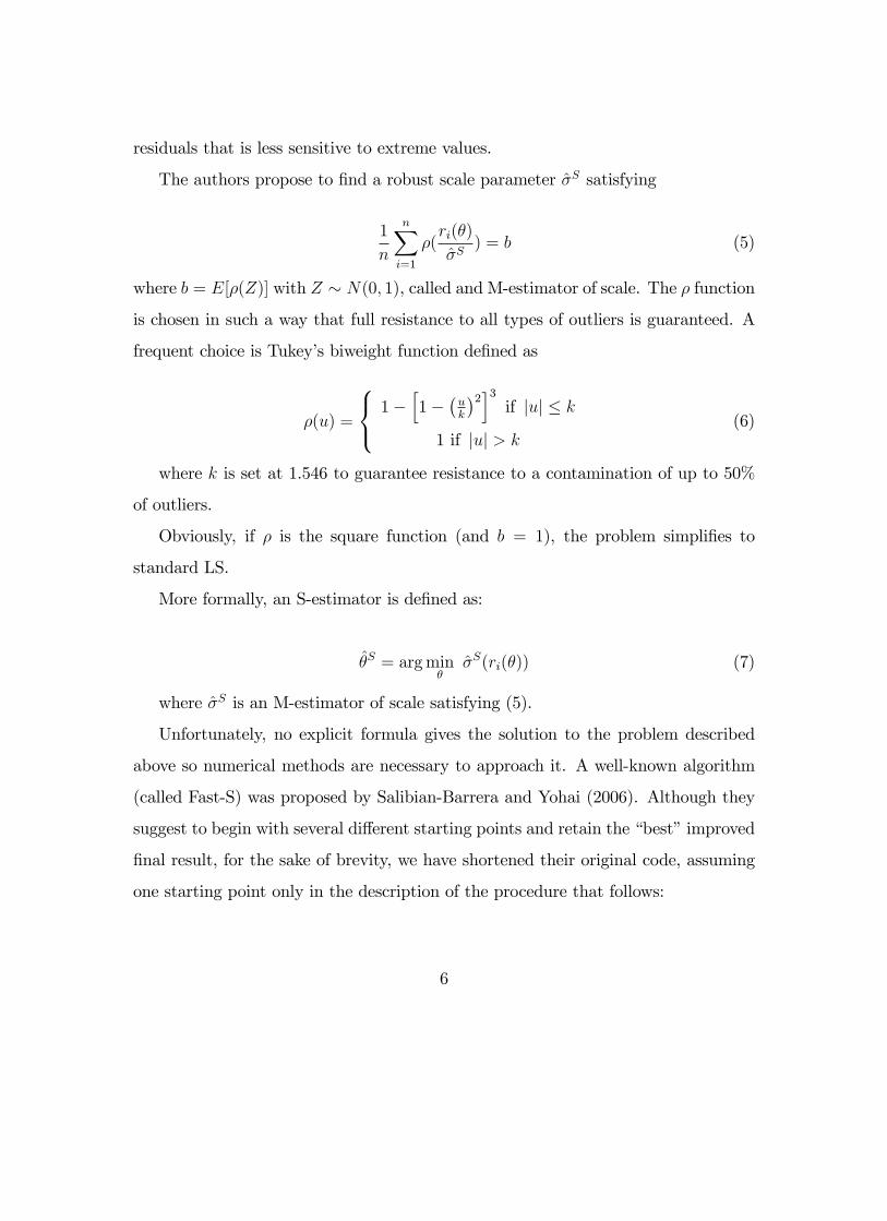
residuals that is less sensitive to extreme values.
The authors propose to �nd a robust scale parameter �S satisfying
1
n
nXi=1
�(ri(�)
�S) = b (5)
where b = E[�(Z)] with Z � N(0; 1), called and M-estimator of scale. The � function
is chosen in such a way that full resistance to all types of outliers is guaranteed. A
frequent choice is Tukey�s biweight function de�ned as
�(u) =
8<: 1�h1�
�uk
�2i3if juj � k
1 if juj > k(6)
where k is set at 1.546 to guarantee resistance to a contamination of up to 50%
of outliers.
Obviously, if � is the square function (and b = 1), the problem simpli�es to
standard LS.
More formally, an S-estimator is de�ned as:
�S = argmin��S(ri(�)) (7)
where �S is an M-estimator of scale satisfying (5).
Unfortunately, no explicit formula gives the solution to the problem described
above so numerical methods are necessary to approach it. A well-known algorithm
(called Fast-S) was proposed by Salibian-Barrera and Yohai (2006). Although they
suggest to begin with several di¤erent starting points and retain the �best�improved
�nal result, for the sake of brevity, we have shortened their original code, assuming
one starting point only in the description of the procedure that follows:
6
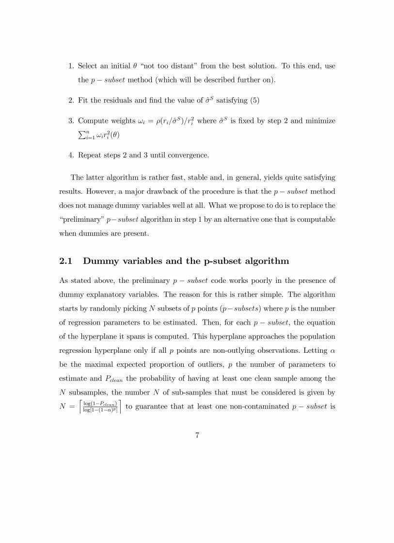
1. Select an initial � �not too distant� from the best solution. To this end, use
the p� subset method (which will be described further on).
2. Fit the residuals and �nd the value of �S satisfying (5)
3. Compute weights !i = �(ri=�S)=r2i where �S is �xed by step 2 and minimizePn
i=1 !ir2i (�)
4. Repeat steps 2 and 3 until convergence.
The latter algorithm is rather fast, stable and, in general, yields quite satisfying
results. However, a major drawback of the procedure is that the p� subset method
does not manage dummy variables well at all. What we propose to do is to replace the
�preliminary�p�subset algorithm in step 1 by an alternative one that is computable
when dummies are present.
2.1 Dummy variables and the p-subset algorithm
As stated above, the preliminary p � subset code works poorly in the presence of
dummy explanatory variables. The reason for this is rather simple. The algorithm
starts by randomly picking N subsets of p points (p�subsets) where p is the number
of regression parameters to be estimated. Then, for each p � subset, the equation
of the hyperplane it spans is computed. This hyperplane approaches the population
regression hyperplane only if all p points are non-outlying observations. Letting �
be the maximal expected proportion of outliers, p the number of parameters to
estimate and Pclean the probability of having at least one clean sample among the
N subsamples, the number N of sub-samples that must be considered is given by
N =llog(1�Pclean)log[1�(1��)p]
mto guarantee that at least one non-contaminated p � subset is
7
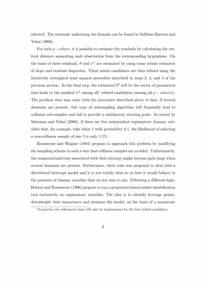
selected. The rationale underlying the formula can be found in Salibian-Barrera and
Yohai (2006).
For each p�subset, it is possible to estimate the residuals by calculating the ver-
tical distance separating each observation from the corresponding hyperplane. On
the basis of these residuals, � and �S are estimated by using some robust estimator
of slope and residual dispersion. These initial candidates are then re�ned using the
iteratively reweighted least squares procedure described in steps 2, 3, and 4 of the
previous section. As the �nal step, the estimated �S will be the vector of parameters
that leads to the smallest �S among all� re�ned candidates (among all p� subsets).
The problem that may arise with the procedure described above is that, if several
dummies are present, this type of subsampling algorithm will frequently lead to
collinear sub-samples and fail to provide a satisfactory starting point. As stated by
Maronna and Yohai (2000), if there are �ve independent explanatory dummy vari-
ables that, for example, take value 1 with probability 0.1, the likelihood of selecting
a non-collinear sample of size 5 is only 1.1%.
Rousseeuw and Wagner (1994) propose to approach this problem by modifying
the sampling scheme in such a way that collinear samples are avoided. Unfortunately,
the computational time associated with their strategy might become quite large when
several dummies are present. Furthermore, their code was proposed to deal with a
distributed intercept model and it is not totally clear to us how it would behave in
the presence of dummy variables that do not sum to one. Following a di¤erent logic,
Hubert and Rousseeuw (1996) propose to run a projection-based outlier identi�cation
tool exclusively on explanatory variables. The idea is to identify leverage points,
downweight their importance and estimate the model, on the basis of a monotonic
�In practice the re�nement steps will only be implemented for the best initial candidates.
8
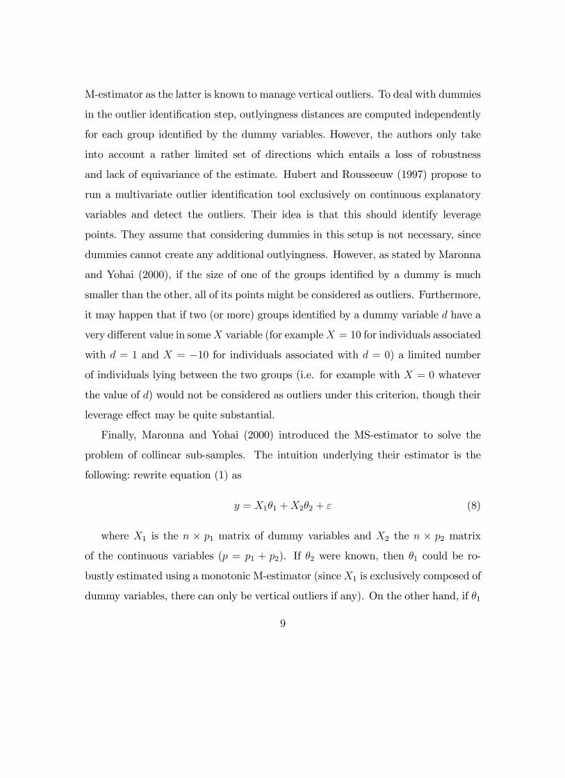
M-estimator as the latter is known to manage vertical outliers. To deal with dummies
in the outlier identi�cation step, outlyingness distances are computed independently
for each group identi�ed by the dummy variables. However, the authors only take
into account a rather limited set of directions which entails a loss of robustness
and lack of equivariance of the estimate. Hubert and Rousseeuw (1997) propose to
run a multivariate outlier identi�cation tool exclusively on continuous explanatory
variables and detect the outliers. Their idea is that this should identify leverage
points. They assume that considering dummies in this setup is not necessary, since
dummies cannot create any additional outlyingness. However, as stated by Maronna
and Yohai (2000), if the size of one of the groups identi�ed by a dummy is much
smaller than the other, all of its points might be considered as outliers. Furthermore,
it may happen that if two (or more) groups identi�ed by a dummy variable d have a
very di¤erent value in someX variable (for exampleX = 10 for individuals associated
with d = 1 and X = �10 for individuals associated with d = 0) a limited number
of individuals lying between the two groups (i.e. for example with X = 0 whatever
the value of d) would not be considered as outliers under this criterion, though their
leverage e¤ect may be quite substantial.
Finally, Maronna and Yohai (2000) introduced the MS-estimator to solve the
problem of collinear sub-samples. The intuition underlying their estimator is the
following: rewrite equation (1) as
y = X1�1 +X2�2 + " (8)
where X1 is the n � p1 matrix of dummy variables and X2 the n � p2 matrix
of the continuous variables (p = p1 + p2). If �2 were known, then �1 could be ro-
bustly estimated using a monotonic M-estimator (sinceX1 is exclusively composed of
dummy variables, there can only be vertical outliers if any). On the other hand, if �1
9
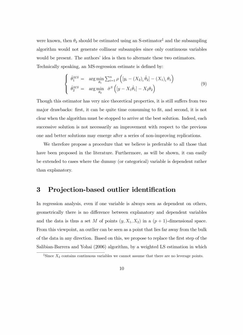
were known, then �2 should be estimated using an S-estimatorz and the subsampling
algorithm would not generate collinear subsamples since only continuous variables
would be present. The authors�idea is then to alternate these two estimators.
Technically speaking, an MS-regression estimate is de�ned by:8><>:�MS1 = argmin
�1
Pni=1 �
�[yi � (X2)i �2]� (X1)i �1
��MS2 = argmin
�2�S�[y �X1�1]�X2�2
� (9)
Though this estimator has very nice theoretical properties, it is still su¤ers from two
major drawbacks: �rst, it can be quite time consuming to �t, and second, it is not
clear when the algorithm must be stopped to arrive at the best solution. Indeed, each
successive solution is not necessarily an improvement with respect to the previous
one and better solutions may emerge after a series of non-improving replications.
We therefore propose a procedure that we believe is preferable to all those that
have been proposed in the literature. Furthermore, as will be shown, it can easily
be extended to cases where the dummy (or categorical) variable is dependent rather
than explanatory.
3 Projection-based outlier identi�cation
In regression analysis, even if one variable is always seen as dependent on others,
geometrically there is no di¤erence between explanatory and dependent variables
and the data is thus a set M of points (y;X1; X2) in a (p + 1)-dimensional space.
From this viewpoint, an outlier can be seen as a point that lies far away from the bulk
of the data in any direction. Based on this, we propose to replace the �rst step of the
Salibian-Barrera and Yohai (2006) algorithm, by a weighted LS estimation in which
zSince X2 contains continuous variables we cannot assume that there are no leverage points.
10
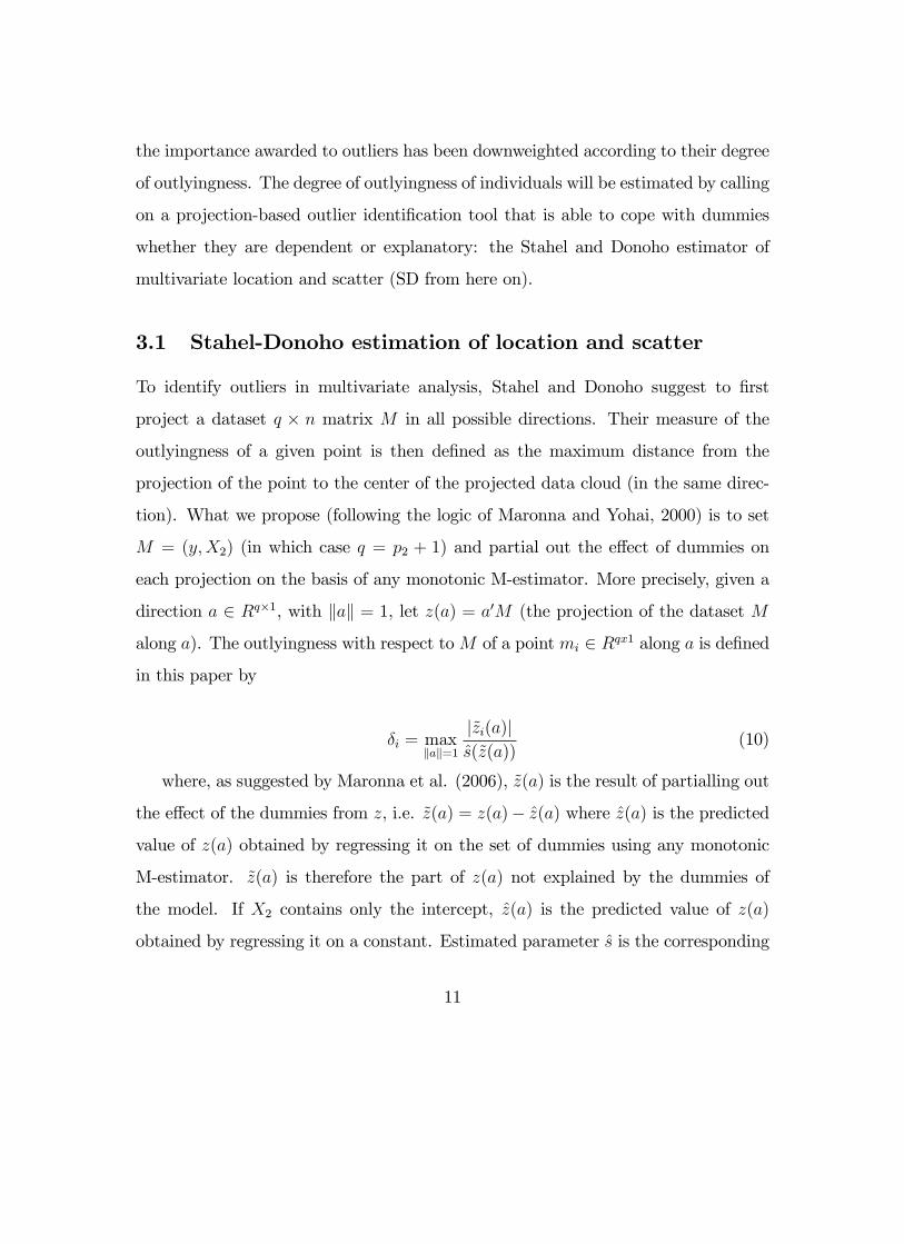
the importance awarded to outliers has been downweighted according to their degree
of outlyingness. The degree of outlyingness of individuals will be estimated by calling
on a projection-based outlier identi�cation tool that is able to cope with dummies
whether they are dependent or explanatory: the Stahel and Donoho estimator of
multivariate location and scatter (SD from here on).
3.1 Stahel-Donoho estimation of location and scatter
To identify outliers in multivariate analysis, Stahel and Donoho suggest to �rst
project a dataset q � n matrix M in all possible directions. Their measure of the
outlyingness of a given point is then de�ned as the maximum distance from the
projection of the point to the center of the projected data cloud (in the same direc-
tion). What we propose (following the logic of Maronna and Yohai, 2000) is to set
M = (y;X2) (in which case q = p2 + 1) and partial out the e¤ect of dummies on
each projection on the basis of any monotonic M-estimator. More precisely, given a
direction a 2 Rq�1, with kak = 1, let z(a) = a0M (the projection of the dataset M
along a). The outlyingness with respect toM of a point mi 2 Rqx1 along a is de�ned
in this paper by
�i = maxkak=1
j~zi(a)js(~z(a))
(10)
where, as suggested by Maronna et al. (2006), ~z(a) is the result of partialling out
the e¤ect of the dummies from z, i.e. ~z(a) = z(a)� z(a) where z(a) is the predicted
value of z(a) obtained by regressing it on the set of dummies using any monotonic
M-estimator. ~z(a) is therefore the part of z(a) not explained by the dummies of
the model. If X2 contains only the intercept, z(a) is the predicted value of z(a)
obtained by regressing it on a constant. Estimated parameter s is the corresponding
11
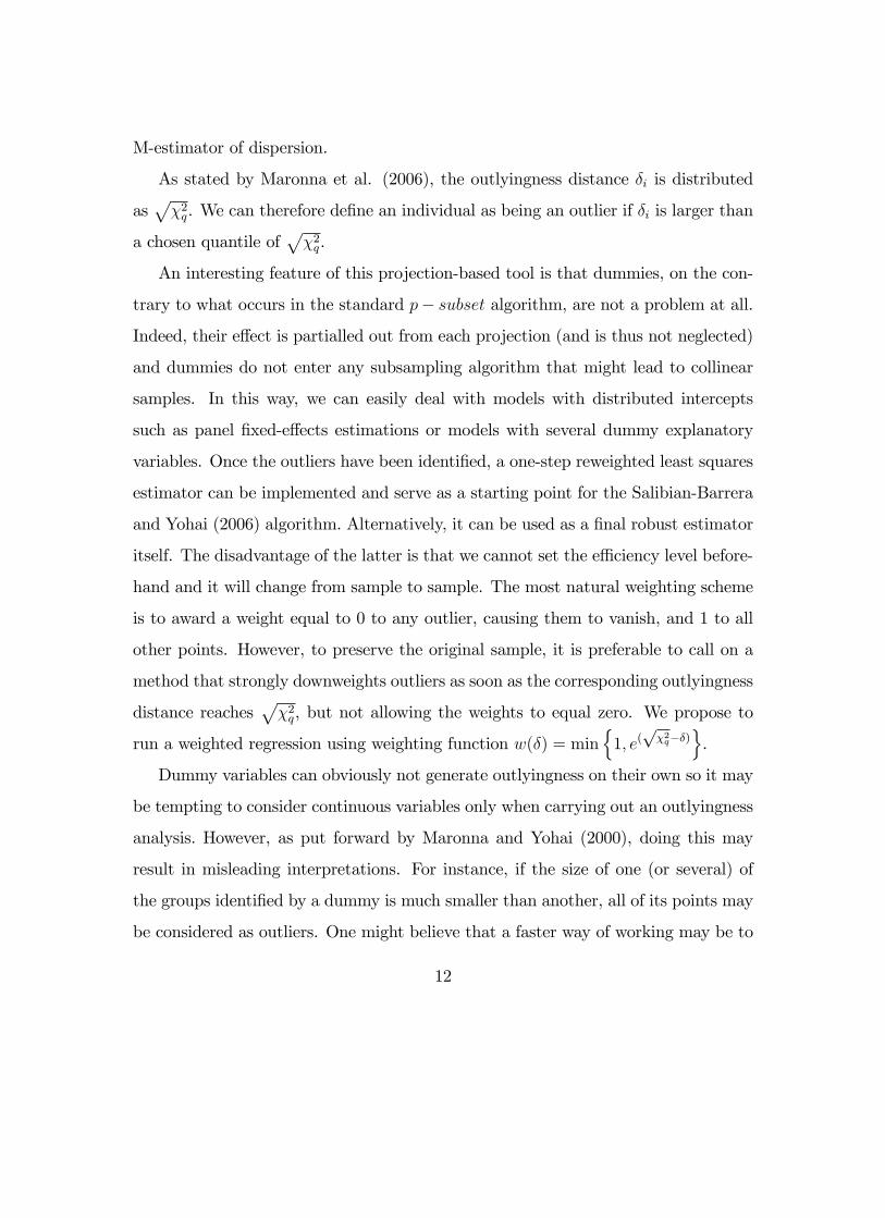
M-estimator of dispersion.
As stated by Maronna et al. (2006), the outlyingness distance �i is distributed
asp�2q. We can therefore de�ne an individual as being an outlier if �i is larger than
a chosen quantile ofp�2q.
An interesting feature of this projection-based tool is that dummies, on the con-
trary to what occurs in the standard p� subset algorithm, are not a problem at all.
Indeed, their e¤ect is partialled out from each projection (and is thus not neglected)
and dummies do not enter any subsampling algorithm that might lead to collinear
samples. In this way, we can easily deal with models with distributed intercepts
such as panel �xed-e¤ects estimations or models with several dummy explanatory
variables. Once the outliers have been identi�ed, a one-step reweighted least squares
estimator can be implemented and serve as a starting point for the Salibian-Barrera
and Yohai (2006) algorithm. Alternatively, it can be used as a �nal robust estimator
itself. The disadvantage of the latter is that we cannot set the e¢ ciency level before-
hand and it will change from sample to sample. The most natural weighting scheme
is to award a weight equal to 0 to any outlier, causing them to vanish, and 1 to all
other points. However, to preserve the original sample, it is preferable to call on a
method that strongly downweights outliers as soon as the corresponding outlyingness
distance reachesp�2q, but not allowing the weights to equal zero. We propose to
run a weighted regression using weighting function w(�) = minn1; e(
p�2q��)
o.
Dummy variables can obviously not generate outlyingness on their own so it may
be tempting to consider continuous variables only when carrying out an outlyingness
analysis. However, as put forward by Maronna and Yohai (2000), doing this may
result in misleading interpretations. For instance, if the size of one (or several) of
the groups identi�ed by a dummy is much smaller than another, all of its points may
be considered as outliers. One might believe that a faster way of working may be to
12
partial out the e¤ect of the dummies from each continuous variable in turn using M-
estimators of regression and implementing SD on the �tted residuals. Unfortunately
this would lead to a non-a¢ ne equivariant estimate.
4 Outliers in qualitative and limited dependent
variable models
By projecting the dataset in all directions we do not treat the dependent variable
di¤erently from the explanatory ones. The outlier identi�cation tool we propose can
therefore be directly extended to robustify a wide variety of qualitative dependent
variable models. For example, to estimate a robust Logit or Probit model, we could
simply identify outliers in the set M=(y;X1; X2) where y is a dummy variable, and
run a reweighted estimator. In the case of a categorical dependent variable model,
whether the categories are ordered or not, a matrix of dummies D can be created
to identify each category, then SD can be run on the extended set of variables
M = (D;X1; X2). Having identi�ed the outliers, a reweighted estimator can easily
be implemented. This principle can be applied to robustly estimate ordered and
multinomial Logits/Probits, etc. In two-stage models such as instrumental variables
or control function approaches (such as treatment regression), letting the matrix of
excluded instruments be denoted by Z, SD can be applied to M = (y;X1; X2; Z)
and outliers can be identi�ed using the procedure we propose. We can then proceed
as suggested previously to obtain a robust two-stage estimator. Following the same
logic, this can be extended to a huge set of alternative regression models.
13
5 Simulations
To illustrate the good behavior of the outlier identi�cation tool and of the subse-
quent implemented procedure to �t (i) an S-estimator for linear models with dummy
variables based on IRLS or (ii) a one-step reweighted QDV estimator and (iii) a
treatment regression, we ran some Monte Carlo simulations.
We computed a very large number of simulations based on many di¤erent se-
tups. In the end, because the results were very similar, we decided to retain some
representative scenarios to illustrate our point.
5.1 Linear regression models
The aim of this set of simulations is to check if our modi�ed algorithm estimates the
coe¢ cients associated with the continuous variables appropriately in the presence of
explanatory dummy variables. We will thus focus on the continuous variables only.
The e¤ect on dummy variables will be discussed in the two-stage estimation methods
simulation section.
We simulate 1000 samples of 1000 observations each. The Data Generating
Process (DGP) considered for the Monte Carlo simulations is described below. In
DGP 1.1, no dummy explanatory variable is present; in DGP 1.2 and DGP 1.3, 25
dummies are present. The di¤erence between the latter two lies in the fact that, in
DGP 1.2, the sum of the values of the dummies must be at most 1, which is not
necessarily the case in DGP 1.3. DGP 1.2 is set up following the logic of models
with distributed intercepts such as, for example, panel data �xed-e¤ect models.
DGP 1.1 y =3Pi=1
xi + e ; for i = 1; 2; 3
where e � N(0; 1) and xiiid� N(0; 1)
14
DGP 1.2 y =3Pi=1
xi + d+ e ; for i = 1; 2; 3
where e � N(0; 1), xiiid� N(0; 1) and d � round(U [0; 1] � 25)
DGP 1.3 y =3Pi=1
xi +25Pj=1
dj + e ; for i = 1; 2; 3 and j = 1; :; 25
where e � N(0; 1), xiiid� N(0; 1) and dj
iid� round(U [0; 1])
Without loss of generality, we chose to set all regression parameters to 1 and the
constant to 0. In all simulations, we decided to focus on the coe¢ cient associated
with x1. If there is no contamination, this is of no importance whatsoever since
all coe¢ cients associated with the x variables should behave in a similar way. If
y is contaminated (e.g. the value of the y variable of a given percentage of the
observations is larger by a �xed number of units than what the DGP associated with
the vast majority of the observations would suggest), the e¤ect on the coe¢ cients
associated with all x variables should be the same. Finally if only variable x is
contaminated this e¤ect will only be observed on the estimated coe¢ cient associated
with this speci�c variable and does not spread over to the other coe¢ cients given
the i:i:d: nature of the data.
To grasp the in�uence of the outliers, we will consider �ve contamination scenar-
ios: the �rst one, which we call clean, involves no contamination. Then, two setups
are considered in which the y-value of 5% of the observations is respectively set at
5 and 10 units larger than what the DGP would suggest. They are called Vertical
5 and Vertical 10 setups. We do not expect the in�uence of these outliers to be
strong on the coe¢ cient associated with x1 since it is well known that vertical out-
liers a¤ect the level of the regression line (hyperplane) rather than its slope. To force
a strong e¤ect on the slope we should consider a much higher contamination. The
e¤ect of the latter contamination on the constant (and as a consequence on dummy
15
explanatory variables) should be much higher but we do not focus on this here. We
will come back to this in section 5.3. Finally, two setups are considered in which
the x1-value of 5% of the observations is awarded a value respectively set at 5 and
10 units larger than what the DGP would suggest. They are called Bad Leverage 5
and Bad Leverage 10 setups. We expect these outliers to severely bias the classical
estimations.
In each case, we compare the behavior of the classical estimator to that of the
S-estimator computed using our the modi�ed version of the Fast-S algorithm.
5.2 Qualitative dependent variable models
The aim of this set of simulations is to check how the outlier identi�cation tool we
propose and the subsequent reweighted estimator behaves with QDV models. We
concentrate here on single dummy dependent variable models, but we also run several
simulations on ordered and unordered categorical dependent variable models. Simu-
lations lead to similar results. This was to be expected since the problem is virtually
the same. Indeed, to detect the outliers in categorical dependent variable models,
the �rst thing to do is to convert all categorical variables into a series of dummies
identifying each category. Since the projection tool does not make any di¤erence
between right-hand-side and left-hand-side variables, there is no di¤erence whatso-
ever between a simple binary dependent variable model with dummy explanatory
variables and a categorical dependent variable model for outlier identi�cation. We
simulate 1000 samples of 1000 observations each. The DGP we consider here is
DGP 2.1 y = I(pPi=1
xi + e > 0) with p = 2; 5; 10,
where I is the indicator function, xi � N(0; 1) and e � Logistic (Logit model).
16
We consider three contamination setups inspired by Croux and Haesbroeck (2003).
A �rst one, called clean with no contamination, a second one called mild in which
5% of all of the xs are awarded a value 1:5pp larger than what the DGP would
suggest and the corresponding y variable is set to zero and a setup called severe in
which 5% of all of the xs are awarded a value 5pp units larger than the DGP would
suggest and the corresponding y variable is set to zero.
We compare the behavior of the classical Logit with (i) the robust Logit pro-
posed by Croux and Haesbroeck (2003), (ii) a reweighted estimator called W1Logit
using weights wi = I��i <
p�2p�and (iii) a reweighted estimator called W2Logit
using weights wi = minf1; ep�2p��ig where � is the outlyingness distance obtained by
running SD on the dataset as explained above.
5.3 Two-stage models
The aim of this set of simulations is to check how the outlier identi�cation tool we
propose and the subsequent reweighted estimator behave in the frame of limited de-
pendent variable models. We consider here a treatment regression model as described
by Maddala (1983) (i.e. a model where a dummy explanatory variable is endogenous
and must therefore be instrumented). Note that we estimated the model by stan-
dard IV and the generality of the results remains the same. We do not present the
results here to keep the number of tables as limited as possible. We simulated 1000
samples of 1000 observations each. The process (DGP) considered for the Monte
Carlo simulations is
DGP 3.1
8>>><>>>:y1 =
3Pi=1
xi +3Pj=1
I(xj > 0) + y2 + e1
y2 = I
2Pj=1
zj + e2 > 0
!
17
where ei � N(0; 1); xi � N(0; 1), xj � N(0; 1); zj � N(0; 1) with corr(e1; e2) = 0:75
This procedure is basically a two-step one. A �rst step in which a dummy variable
y2 is generated, and a second one in which a continuous y1 variable is generated. To
grasp the in�uence of outliers, we consider six contamination scenarios: the �rst one
involves no contamination: we call it clean. Then we consider two contamination
setups in the �rst stage similarly to what we did in DGP 2.1. We call it �rst-stage
mild when 5% of the zs are awarded a value 1:5p2 larger than what the DGP would
suggest and the corresponding y2 variable is set to zero, and a setup called �rst-stage
severe when 5% of the zs are awarded a value 5p2 units larger than what the DGP
would suggest and the corresponding y variable is set to zero. Then, two setups
are considered in which the x1 variable of 5% of the observations is awarded a value
respectively 5 and 10 units larger than what the DGP would suggest. They are called
second-stage bad leverage 5 and second-stage bad leverage 10 setups. Finally, the y
variable of 5% of the observations is awarded a value 10 units above what the DGP
would suggest. This setup is called second-stage vertical 10.
Since this simulation setup is very general and covers the scenarios considered
above, we present the Bias and MSE associated with all coe¢ cients.
6 Results
The results of the simulations are presented in Tables 1 to 5. Each time the Bias is
larger that 10%, the Bias and MSE are given in bold.
18
6.1 Linear regression model
Table 1 shows that the modi�cation of the Fast-S algorithm we propose performs
well, with or without explanatory dummy variables. As expected, the bias of the
classical estimator with mild vertical contamination is limited. Nevertheless, the
MSE suggests that the robust counterpart should be preferred. The Bias and MSE
of the S-estimator are very small and similar for dummy explanatory variables and
distributed intercept. This means that a robust panel Fixed-e¤ect estimator could
be �tted by simply adding individual constants to a cross-sectional regression, and
the model could be estimated using an S-estimator that is well known to have nice
equivariance properties.
[INSERT TABLE 1 HERE]
6.2 Qualitative dependent variable models
Table 2 shows that the reweighted estimators we propose resist to the presence of
outliers and lead to estimations that are much less biased than with the classical
Logit estimator. With mild contamination they also turn out to be preferable to the
Robust Logit estimator. There is no evidence in favor of one or the other of the two
weighting schemes.
[INSERT TABLE 2 HERE]
6.3 Limited dependent variable models
Tables 3 to 5 show that, the reweighted estimators we propose resist to the presence
of outliers and lead to estimations that are much less biased than with the classical
19
Logit estimator in all scenarios. Again, there is no evidence in favor of one or the
other of the two weighting schemes.
[INSERT TABLES 3 TO 5 HERE]
7 Conclusion
The literature on robust regression models has grown substantially during the last
decade. As a consequence, a wide variety of models have been developed to cope
with outliers in a rather large number of scenarios. Nevertheless, a recurrent problem
for the empirical implementation of these estimators is that optimization algorithms
generally do not perform well when dummy variables are present. What we propose
in this paper is a simple solution to this involving the replacement of the sub-sampling
step of the maximization procedures by a projection-based method. The underly-
ing idea is to project the �regression�data cloud (considering both dependent and
explanatory variables) in all possible directions, partialling out dummies from each
projection. In this way, outliers are identi�ed and a reweighted estimator is �tted
awarding a lower weight to atypical individuals. The latter estimator can then either
be used as such, or as the starting point of an iteratively reweighted algorithm such
as Fast-S proposed by Salibian-Barrera and Yohai (2006) to compute S-estimators.
We run some simple Monte Carlo simulations and show that the method we propose
behaves quite well in a large number of situations. We therefore believe that this
paper is a step forward for the practical implementation of robust estimators and,
consequently, allows them to enter mainstream applied econometrics and statistics.
20
References
[1] Bianco, A.M.and Yohai, V.J., 1996. Robust estimation in the logistic regression
model. In: Robust Statistics, Data Analysis, and Computer Intensive Methods.
Lecture Notes in Statistics, 109. Edited by H. Rieder Springer Verlag, New York,
17-34.
[2] Croux, C. and Haesbroeck, G., 2003. Implementing the Bianco and Yohai esti-
mator for Logistic Regression, Computational Statistics and Data Analysis, 44,
273-295.
[3] Dehon, C., Gassner, M. and Verardi, V., 2009. Beware of Good Outliers and
Overoptimistic Conclusions, Oxford Bulletin of Economics and Statistics, 71,
437-452.
[4] Donoho., D.L., 1982. Breakdown properties of multivariate location estimators.
Qualifying paper, Harvard University, Boston.
[5] Huber, P., 1964. Robust estimation of a location parameter. Annals of Mathe-
matical Statistics, 35, 73-101.
[6] Hubert, M. and Rousseeuw, P. J.,1996. Robust regression with both continuous
and binary regressors. Journal of Statistical Planning and Inference. 57, 153-163.
[7] Hubert, M., and Rousseeuw, P.J., 1997. A regression analysis with categorical
covariables, two-way heteroscedasticity, and hidden outliers. In The Practice
of Data Analysis: Essays in Honor of J.W. Tukey. Edited by D.R. Brillinger,
L.T. Fernholz and S. Morgenthaler, Princeton, New Jersey, Princeton University
Press, 193-202.
21
[8] Maddala, G. S. 1983. Limited-Dependent and Qualitative Variables in Econo-
metrics. Cambridge: Cambridge University Press
[9] Maronna, R. A. and Yohai, V. J., 2000. Robust regression with both continuous
and categorical predictors. Journal of Statistical Planning and Inference. 89,
197-214.
[10] Maronna, R., Martin, D. and Yohai, V., 2006. Robust Statistics, Wiley, New
York, NY.
[11] Rousseeuw, P. J. and Yohai, V., 1984. Robust regression by means of S-
estimators. In Robust and Nonlinear Time Series Analysis, Lecture Notes in
Statistics No. 26, Edited by Franke, J., Härdle, W. and Martin, D., Springer
Verlag, Berlin, 256-272.
[12] Rousseeuw P.J., Wagner J., 1994. Robust regression with a distributed intercept
using least median of squares. Computational Statistics and Data Analysis, 17,
65-76.
[13] Salibian-Barrera, M. and Yohai, V.J., 2006. A fast algorithm for S-regression
estimates. Journal of Computational and Graphical Statistics 15, 414-427.
[14] Stahel, W. A., 1981. Robuste Schätzungen: In�nitesimale Optimalität und
Schätzungen von Kovarianzmatrizen. Ph.D. thesis, ETH Zürich.
22
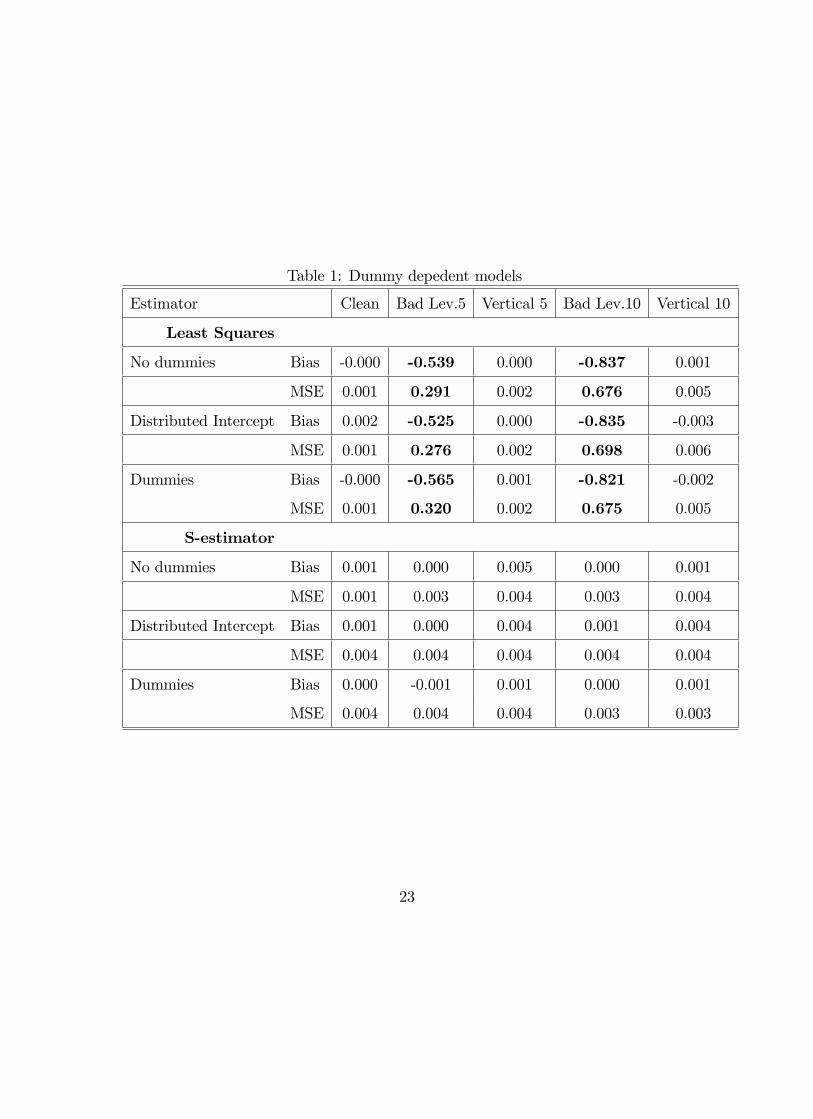
Table 1: Dummy depedent models
Estimator Clean Bad Lev.5 Vertical 5 Bad Lev.10 Vertical 10
Least Squares
No dummies Bias -0.000 -0.539 0.000 -0.837 0.001
MSE 0.001 0.291 0.002 0.676 0.005
Distributed Intercept Bias 0.002 -0.525 0.000 -0.835 -0.003
MSE 0.001 0.276 0.002 0.698 0.006
Dummies Bias -0.000 -0.565 0.001 -0.821 -0.002
MSE 0.001 0.320 0.002 0.675 0.005
S-estimator
No dummies Bias 0.001 0.000 0.005 0.000 0.001
MSE 0.001 0.003 0.004 0.003 0.004
Distributed Intercept Bias 0.001 0.000 0.004 0.001 0.004
MSE 0.004 0.004 0.004 0.004 0.004
Dummies Bias 0.000 -0.001 0.001 0.000 0.001
MSE 0.004 0.004 0.004 0.003 0.003
23
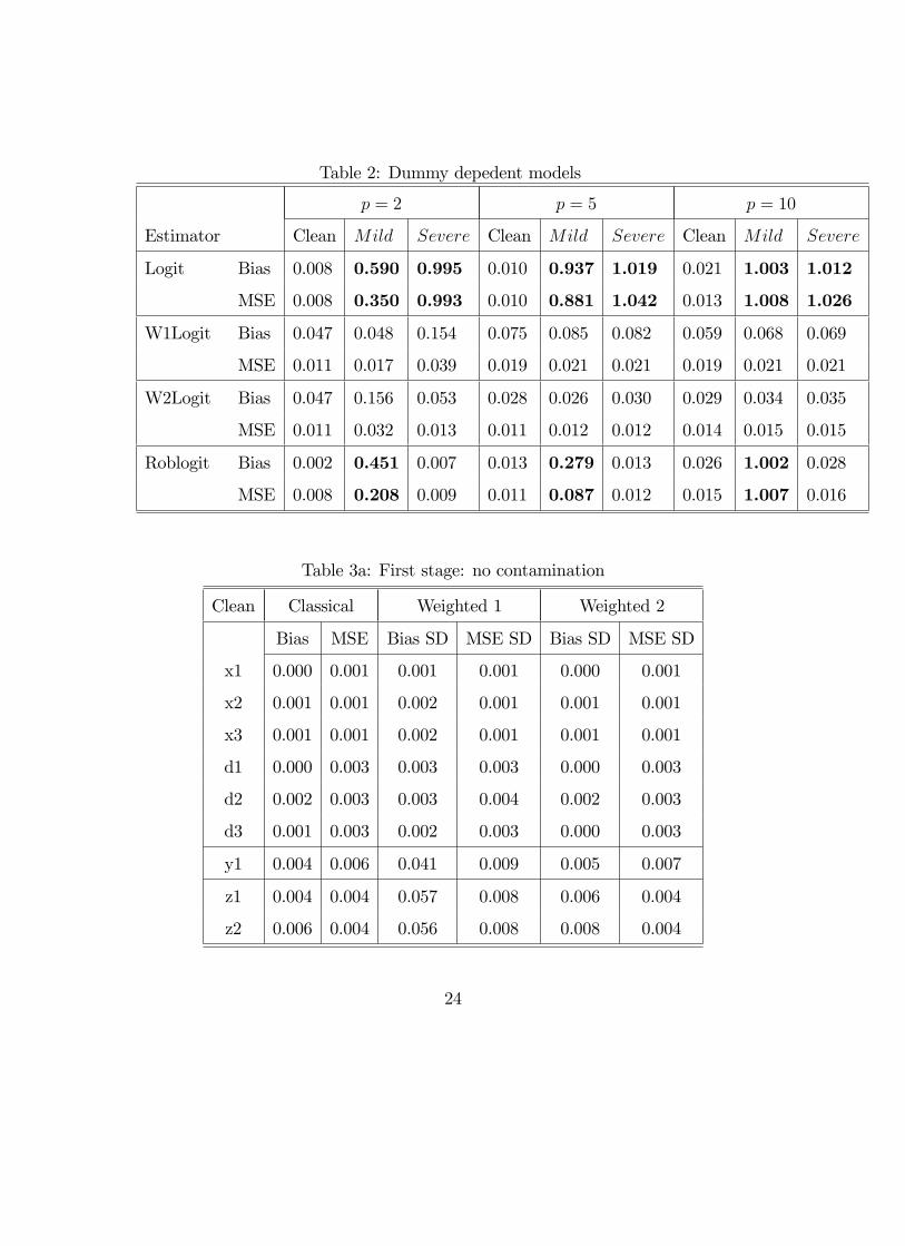
Table 2: Dummy depedent models
p = 2 p = 5 p = 10
Estimator Clean Mild Severe Clean Mild Severe Clean Mild Severe
Logit Bias 0.008 0.590 0.995 0.010 0.937 1.019 0.021 1.003 1.012
MSE 0.008 0.350 0.993 0.010 0.881 1.042 0.013 1.008 1.026
W1Logit Bias 0.047 0.048 0.154 0.075 0.085 0.082 0.059 0.068 0.069
MSE 0.011 0.017 0.039 0.019 0.021 0.021 0.019 0.021 0.021
W2Logit Bias 0.047 0.156 0.053 0.028 0.026 0.030 0.029 0.034 0.035
MSE 0.011 0.032 0.013 0.011 0.012 0.012 0.014 0.015 0.015
Roblogit Bias 0.002 0.451 0.007 0.013 0.279 0.013 0.026 1.002 0.028
MSE 0.008 0.208 0.009 0.011 0.087 0.012 0.015 1.007 0.016
Table 3a: First stage: no contamination
Clean Classical Weighted 1 Weighted 2
Bias MSE Bias SD MSE SD Bias SD MSE SD
x1 0.000 0.001 0.001 0.001 0.000 0.001
x2 0.001 0.001 0.002 0.001 0.001 0.001
x3 0.001 0.001 0.002 0.001 0.001 0.001
d1 0.000 0.003 0.003 0.003 0.000 0.003
d2 0.002 0.003 0.003 0.004 0.002 0.003
d3 0.001 0.003 0.002 0.003 0.000 0.003
y1 0.004 0.006 0.041 0.009 0.005 0.007
z1 0.004 0.004 0.057 0.008 0.006 0.004
z2 0.006 0.004 0.056 0.008 0.008 0.004
24
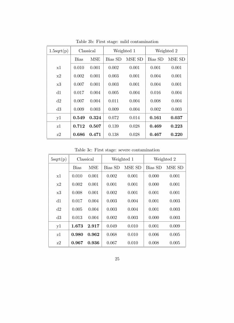
Table 3b: First stage: mild contamination
1.5sqrt(p) Classical Weighted 1 Weighted 2
Bias MSE Bias SD MSE SD Bias SD MSE SD
x1 0.010 0.001 0.002 0.001 0.001 0.001
x2 0.002 0.001 0.003 0.001 0.004 0.001
x3 0.007 0.001 0.003 0.001 0.004 0.001
d1 0.017 0.004 0.005 0.004 0.016 0.004
d2 0.007 0.004 0.011 0.004 0.008 0.004
d3 0.009 0.003 0.009 0.004 0.002 0.003
y1 0.549 0.324 0.072 0.014 0.161 0.037
z1 0.712 0.507 0.139 0.028 0.469 0.223
z2 0.686 0.471 0.138 0.028 0.467 0.220
Table 3c: First stage: severe contamination
5sqrt(p) Classical Weighted 1 Weighted 2
Bias MSE Bias SD MSE SD Bias SD MSE SD
x1 0.010 0.001 0.002 0.001 0.000 0.001
x2 0.002 0.001 0.001 0.001 0.000 0.001
x3 0.008 0.001 0.002 0.001 0.001 0.001
d1 0.017 0.004 0.003 0.004 0.001 0.003
d2 0.005 0.004 0.003 0.004 0.001 0.003
d3 0.013 0.004 0.002 0.003 0.000 0.003
y1 1.673 2.917 0.049 0.010 0.001 0.009
z1 0.980 0.962 0.068 0.010 0.006 0.005
z2 0.967 0.936 0.067 0.010 0.008 0.005
25
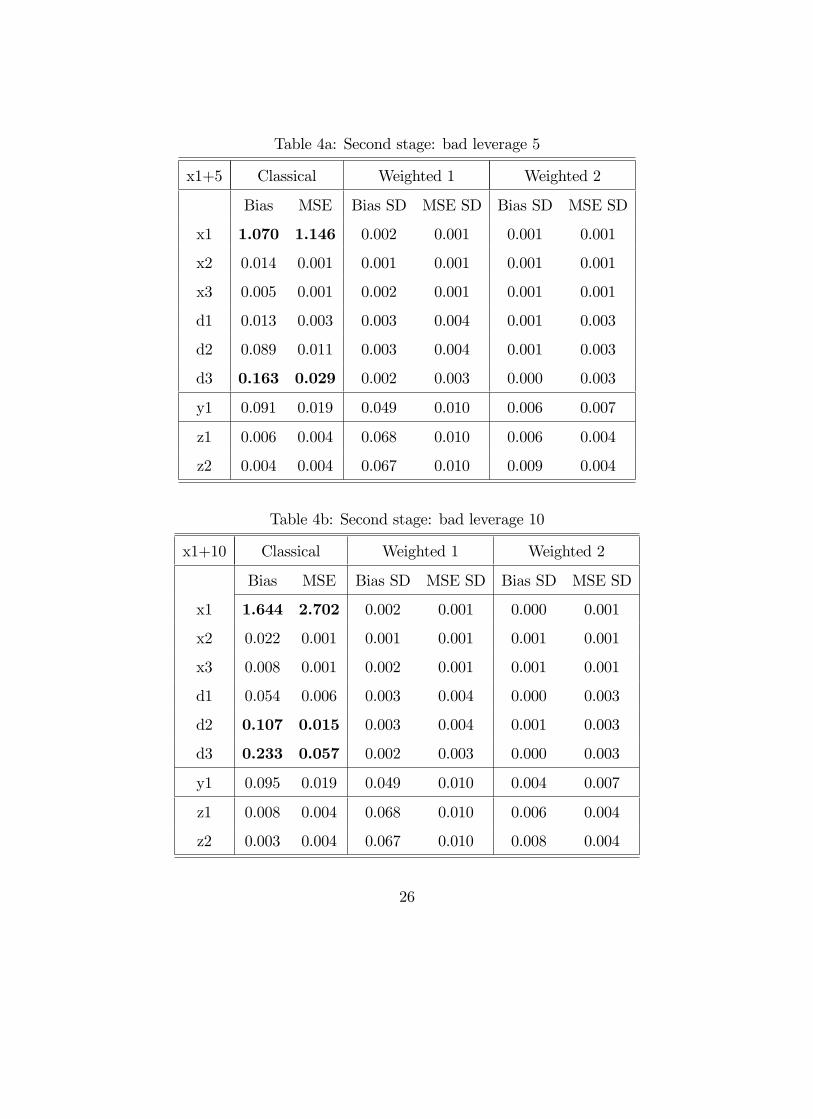
Table 4a: Second stage: bad leverage 5
x1+5 Classical Weighted 1 Weighted 2
Bias MSE Bias SD MSE SD Bias SD MSE SD
x1 1.070 1.146 0.002 0.001 0.001 0.001
x2 0.014 0.001 0.001 0.001 0.001 0.001
x3 0.005 0.001 0.002 0.001 0.001 0.001
d1 0.013 0.003 0.003 0.004 0.001 0.003
d2 0.089 0.011 0.003 0.004 0.001 0.003
d3 0.163 0.029 0.002 0.003 0.000 0.003
y1 0.091 0.019 0.049 0.010 0.006 0.007
z1 0.006 0.004 0.068 0.010 0.006 0.004
z2 0.004 0.004 0.067 0.010 0.009 0.004
Table 4b: Second stage: bad leverage 10
x1+10 Classical Weighted 1 Weighted 2
Bias MSE Bias SD MSE SD Bias SD MSE SD
x1 1.644 2.702 0.002 0.001 0.000 0.001
x2 0.022 0.001 0.001 0.001 0.001 0.001
x3 0.008 0.001 0.002 0.001 0.001 0.001
d1 0.054 0.006 0.003 0.004 0.000 0.003
d2 0.107 0.015 0.003 0.004 0.001 0.003
d3 0.233 0.057 0.002 0.003 0.000 0.003
y1 0.095 0.019 0.049 0.010 0.004 0.007
z1 0.008 0.004 0.068 0.010 0.006 0.004
z2 0.003 0.004 0.067 0.010 0.008 0.004
26
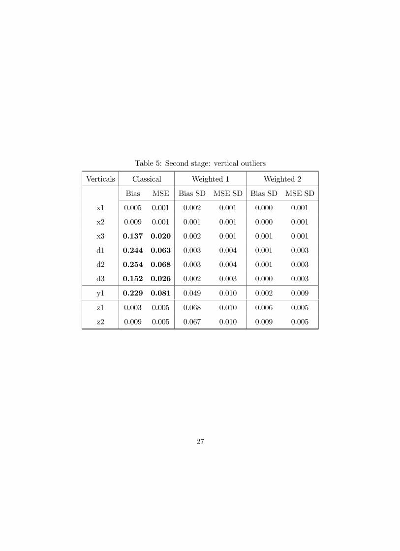
Table 5: Second stage: vertical outliers
Verticals Classical Weighted 1 Weighted 2
Bias MSE Bias SD MSE SD Bias SD MSE SD
x1 0.005 0.001 0.002 0.001 0.000 0.001
x2 0.009 0.001 0.001 0.001 0.000 0.001
x3 0.137 0.020 0.002 0.001 0.001 0.001
d1 0.244 0.063 0.003 0.004 0.001 0.003
d2 0.254 0.068 0.003 0.004 0.001 0.003
d3 0.152 0.026 0.002 0.003 0.000 0.003
y1 0.229 0.081 0.049 0.010 0.002 0.009
z1 0.003 0.005 0.068 0.010 0.006 0.005
z2 0.009 0.005 0.067 0.010 0.009 0.005
27


