Rotary-Linear Axes for High Speed Machining

by

Michael Kevin Liebman

A.B., Physics (1996)Princeton University

S. M., Mechanical Engineering (1998)Massachusetts Institute of Technology

Submitted to the Department of Mechanical Engineeringin partial fulfillment of the requirements for the degree of

Doctor of Philosophy in Mechanical Engineering

at the

MASSACHUSETTS INSTITUTE OF TECHNOLOGY

September 2001

@ Massachusetts Institute of Technology 2001. All rights reserved.

A uthor ...................Department of Mechanical Engineering

July 10, 2001

C ertified by ........................... ....... ........................David L. Trumper

Asssociate Professor of Mechanical EngineeringThesis SuDervisor

Accepted by ......................Ain A. Sonin

MASSACHUSETS INSTITUTF hairman, Departmental Committee on Graduate StudentsOF TECHNOLOGY -himn

DEC 1 0 2001BARKE

LIBRARIES

'-N

Rotary-Linear Axes for High Speed Machining

by

Michael Kevin Liebman

Submitted to the Department of Mechanical Engineeringon July 10, 2001, in partial fulfillment of the

requirements for the degree ofDoctor of Philosophy in Mechanical Engineering

Abstract

This thesis presents the design, analysis, fabrication, and control of a rotary-linearaxis; this axis is a key subsystem for high speed, 5-axis machine tools intended forfabricating centimeter-scale parts. The rotary-linear axis is a cylinder driven inde-pendently in rotation and translation. This hybridization minimizes machine inertiasand thereby maximizes accelerations allowing for the production of parts with com-plex surfaces rapidly and accurately. Such parts might include dental restorations,molds, dies, and turbine blades.

The hybrid rotary and linear motion provides special challenges for precision actu-ation and sensing. Our prototype rotary-linear axis consists of a central shaft, 3/4 inch(1.91 cm) in diameter and 15 inches (38.10 cm) long, supported by two cylindrical airbearings. The axis has one inch (2.54 cm) of linear travel and unlimited rotary travel.Two frameless permanent magnet motors respectively provide up to 41 N continuousforce and 0.45 N-m continuous torque. The rotary motor is composed of commerciallyavailable parts; the tubular linear motor is completely custom-built. The prototypeaxis achieves a linear acceleration of 3 g's and a rotary acceleration of 1,300 rad/s2 .With higher power current amplifiers and reduced sensor inertia, we predict the axiscould attain peak accelerations of 12 g's and 17,500 rad/s 2 at low duty cycles.

This thesis also examines several concepts for developing a precision rotary-linearsensor that can tolerate axial translation. Our prototype rotary sensor uses two laserinterferometers to measure the orientation of a slightly tilted mirror attached to theshaft. A third interferometer measures shaft translation. The rotary axis has a controlbandwidth of 40 Hz; the linear axis has a bandwidth of 70 Hz. The rotary-linear axishas 2.5 nm rms linear positioning noise and 3.1 prad rms rotary positioning noise.

This thesis presents one novel 5-axis machine topology which uses two rotary-linear axes. The first axis rotates and translates the part. The second axis carriesthe cutting tool and provides high speed spindle rotation as well as infeed along theaxis of rotation. For use as a spindle, precision rotary sensing is not required, and asensorless control scheme based on motor currents and voltages can be used.

Thesis Supervisor: David L. TrumperTitle: Asssociate Professor of Mechanical Engineering

Acknowledgments

I am extremely fortunate to have been able to work with so many fantastic people

during the course of this research. I am most grateful to Professor David Trumper,

my advisor for the past 5 years, for teaching me most of what I know about electro-

magnetics, controls, and design. He has been a constant source of inspiration and a

great role model. He is also one of the most brilliant people I have ever met. I am

particularly honored to be the first Doctoral student to graduate from his lab since

he received tenure.

I thank my thesis committee for their help throughout this research and for teach-

ing some of the best classes I have taken. Professor Sanjay Sarma was especially

helpful in teaching me about toolpaths and machine topologies. His math class on

random, cool topics introduced me to many interesting phenomena. Professor Jeffrey

Lang helped me with several motor design issues and with implementing sensorless

control. I thoroughly enjoyed his electromagnetics class with extremely clear lectures

illustrated with colored chalk and containing a series of excellent demos. Professor

Alex Slocum is a great resource who always has new ideas. His precision machine

course and book have helped me in numerous ways over the last five years.

I am glad I had a chance to work with Marsette Vona, a Master's student, over

the past year and a half. Marsette did a fantastic job designing and fabricating the

sensor and making it work. He also built a custom link between the laser axis cards

and the dSPACE board. Moreover, he was a sounding board for all aspects of the

project and provided numerous valuable suggestions. I thank him for all his hard

work on the project and will miss working with him.

Several people suggested and helped us develop various optical sensors. I thank

Dr. Carl Zanoni, Vice President of R & D at Zygo Corporation, for suggesting the

helicoid sensor concept to us. I also thank Dr. William Plummer, Director of Optical

Engineering at Polaroid, and Donald Combs, Douglas Goodman, and Jeffrey Roblee,

all of Polaroid, for meeting with us several times to discuss the possibility of fabri-

cating the helicoid mirror. I thank Professor George Barbastathis in the Mechanical

Engineering Dept. at MIT for his help with various optical sensor concepts. Also, I

thank Professor John Ziegert in the Mechanical Engineering Dept. at the University

of Florida for suggesting the half-wave plate sensor concept to us.

During my five years in the Precision Motion Control Lab, I have had the pleasure

of working with a fantastic group of graduate students. I have learned a tremendous

amount from them and they have each helped me in some aspect of this work. In

the early days, Won-jong Kim taught me about motor design and analysis. Pradeep

Subrahmanyan and I discussed all sorts of things, and he taught me a great deal

about controls. Paul Konkola was always ready to kick around new ideas as well.

Steve Ludwick, David Ma, David Chargin, and Joe Calzaretta were always eager to

show me the latest fast tool servo work and were valuable resources. I thank Katie

Lilienkamp for her dynamic signal analyzer software which is incredibly useful. Ming-

chih Weng was always ready to talk about electromagnetics. When he left, I turned

to Xiaodong Lu, who also taught me about flexible modes. When I needed some

practical advice on how to build something, I turned to Marten Byl. Rick Montesanti

was another mechanical whiz who gave me many ideas. I have also enjoyed working

along side Robin Ritter, Claudio Salvatore, Amar Kendale, and Andrew Stein.

I thank David Rodriguera and Maureen Lynch for their help ordering equipment

and avoiding the MIT bureaucracy. I thank Gerry Wentworth, Mark Belanger, and

Bob Kane for their assistance in the machine shop.

I thank my parents and sister for all their encouragement, love, and support.

Finally, I thank Coach Kandiah, my boxing coach, for training me for five years.

Boxing helped me survive this long journey. I also thank all the MIT Boxing Club

members whom I've had the pleasure of training with over the years.

This research was funded by NSF grant award number DMI-0084981, "Rotary-

Linear Hybrid Axes for Meso-scale Machining," and the Charles E. Reed Faculty

Initiatives Fund.

For Mom, Dad, and Judith

Contents

1 Introduction1.1 Background . . . . . . . . . . . . . . . . . . . . . . . . . . .1.2 Thesis Overview. . . . . . . . . . . . . . . . . . . . . . . . .

1.2.1 z-0 Horizontal Trunnion Machine Tool . . . . . . . .1.2.2 Prototype z-0 Axis . . . . . . . . . . . . . . . . . . .1.2.3 z-0 M otor . . . . . . . . . . . . . . . . . . . . . . . .1.2.4 z-6 Sensor . . . . . . . . . . . . . . . . . . . . . . . .1.2.5 Prototype Axis Specifications . . . . . . . . . . . . .1.2.6 z-0 Axis Ultimate Performance Specifications . . . .

1.3 Thesis Contributions . . . . . . . . . . . . . . . . . . . . . .1.4 Thesis Organization . . . . . . . . . . . . . . . . . . . . . . .

2 Five-Axis Machine Tools2.1 Introduction . . . . . . . . . . . . . . . . . . . . . . . . . . .2.2 Applications . . . . . . . . . . . . . . . . . . . . . . . . . . .

2.2.1 Fabricating Customized Dental Restorations . . . . .2.2.2 Fabricating Other Small, Complex Parts . . . . . . .

2.3 Classification of Existing Topologies . . . . . . . . . . . . . .2.3.1 Rotating, Swivel Spindle Machines . . . . . . . . . .2.3.2 Swivel, Tilt Spindle Machines . . . . . . . . . . . . .2.3.3 Swivel Spindle, Rotating Part Machines . . . . . . .2.3.4 Horizontal Machines with Rotary Tables on Trunnions2.3.5 Vertical Machines with Rotary Tables c

2.4 Toolpath Generation . . . . . . . . . . . . . .2.5 Acceleration Scaling Laws . . . . . . . . . . .

2.5.1 Linear Accelerations . . . . . . . . . .2.5.2 Rotary Accelerations . . . . . . . . . .

2.6 New Topology Concepts with Integrated Axes2.7 z-0 Horizontal Trunnion Topology . . . . . . .2.8 Sum m ary . . . . . . . . . . . . . . . . . . . .

3 Rotary-Linear Motion3.1 Review of Existing z-0 Stage Designs . . . . .

3.1.1 Teletype Positioning Mechanism . . . .3.1.2 Philips Electromagnetic Actuator . . .

U1 Trunnions . . . . . . 56. . . . . . . . . . . . . 57. . . . . . . . . . . . . 58. . . . . . . . . . . . . 58. . . . . . . . . . . . . 60. . . . . . . . . . . . . 62. . . . . . . . . . . . . 64. . . . . . . . . . . . . 68

71717173

9

27. . . . . 27. . . . . 29. . . . . 29. . . . . 31. . . . . 33. . . . . 34. . . . . 36. . . . . 36. . . . . 39. . . . . 40

43. . . . . 43. . . . . 45. . . . . 45. . . . . 47. . . . . 47. . . . . 49. . . . . 51. . . . . 52

. . . . 54

3.1.3 z-# Induction Actuator . . . . . . . . . . . . . . . . . .3.1.4 Electro-Scientific Industries Drilling Spindle . . . . . .3.1.5 Anorad Rotary-Linear Actuator . . . . . . . . . . . . .

3.2 Rotary-Linear Motor Concepts . . . . . . . . . . . . . . . . . .3.2.1 Permanent Magnet Motor vs. Induction Motor . . . .3.2.2 Stacked vs. Separated Motor Configurations . . . . . .

3.3 Rotary-Linear Bearing Concepts . . . . . . . . . . . . . . . . .3.3.1 Hydrostatic Bearings . . . . . . . . . . . . . . . . . . .3.3.2 Orifice Air Bearings . . . . . . . . . . . . . . . . . . . .3.3.3 Porous Graphite Air Bearings . . . . . . . . . . . . . .

3.4 Rotary-Linear Sensor Concepts . . . . . . . . . . . . . . . . .3.4.1 Sensor Specifications . . . . . . . . . . . . . . . . . . .3.4.2 Introduction to Rotary-Linear Interferometric Sensors .3.4.3 Prism-Mirror Sensor . . . . . . . . . . . . . . . . . . .3.4.4 Tilted-Mirror Sensor . . . . . . . . . . . . . . . . . . .3.4.5 Helicoid Mirror Sensor . . . . . . . . . . . . . . . . . .3.4.6 Rotating Half-Wave Plate Sensor . . . . . . . . . . . .3.4.7 Rotating Polarizer Sensor . . . . . . . . . . . . . . . .3.4.8 2-D Encoder . . . . . . . . . . . . . . . . . . . . . . . .

3.5 Sum m ary . . . . . . . . . . . . . . . . . . . . . . . . . . . . .

4 Rotary-Linear Motor Design & Analysis4.1 Motor Scaling Laws for High Accelerations4.2 Linear Motor Electromechanical Analysis . . .

4.2.1 Analytical Framework . . . . . . . . .4.2.2 Force . . . . . . . . . . . . . . . . . . .4.2.3 Power . . . . . . . . . . . . . . . . . .

4.3 Linear Motor Design for High Accelerations4.3.1 Motor Sizing . . . . . . . . . . . . . .4.3.2 Magnetic Pitch Length Selection . . .4.3.3 Coil Thickness . . . . . . . . . . . . . .4.3.4 Air Gap . . . . . . . . . . . . . . . . .4.3.5 Magnet Thickness . . . . . . . . . . . .4.3.6 Magnet Array . . . . . . . . . . . . . .

4.4 Linear Motor Force Constant Calculation . . .4.5 Linear Motor Force Constant Measurement . .4.6 Rotary Motor Selection for High Accelerations4.7 Rotary Motor Torque Constant Measurement4.8 Sum m ary . . . . . . . . . . . . . . . . . . . .

5 Tilted-Mirror Sensor Design & Analysis5.1 Tilted-Mirror Sensor Basic Analysis . . . . . .

5.1.1 Determining Rotation Angle . . . . . .5.1.2 Sensor Resolution . . . . . . . . . . . .5.1.3 Sensor Maximum Angular Velocity . .

111. . . . . . . 112. . . . . . . 114. . . . . . . 114. . . . . . . 118. . . . . . . 119. . . . . . . 120. . . . . . . 121. . . . . . . 123. . . . . . . 125. . . . . . . 127. . . . . . . 128. . . . . . . 133. . . . . . . 135. . . . . . . 139. . . . . . . 140. . . . . . . 142. . . . . . . 144

147148149150153

10

7780838687929394949596979899

101102105108108108

5.2 Tilted-Mirror Sensor Full Analysis . . . . . . . . . . . . . . . . . . . . 1535.2.1 Path Length Equations . . . . . . . . . . . . . . . . . . . . . . 1545.2.2 Calibration Constants . . . . . . . . . . . . . . . . . . . . . . 1545.2.3 Compensation for Non-Ideal Measurement Beam Locations . . 155

5.3 Automatic Calibration Routine . . . . . . . . . . . . . . . . . . . . . 1565.4 Singularities without Direct z Measurement . . . . . . . . . . . . . . 1575.5 Interferometer Angular Tolerance . . . . . . . . . . . . . . . . . . . . 1585.6 Experimental Measurement of Sensor Noise . . . . . . . . . . . . . . . 1615.7 Summary . . . . . . . . . . . . . . . . . . . . . . . . . . . . . . . . . 161

6 Prototype z-0 Axis 1636.1 Air Bearing . . . . . . . . . . . . . . . . . . . . . . . . . . . . . . . . 1646.2 Base . . . . . . . . . . . . . . . . . . . . . . . . . . . . . . . . . . . . 1676.3 Shaft . . . . . . . . . . . . . . . . . . . . . . . . . . . . . . . . . . . . 168

6.3.1 Material & Form . . . . . . . . . . . . . . . . . . . . . . . . . 1686.3.2 Geometry . . . . . . . . . . . . . . . . . . . . . . . . . . . . . 169

6.4 Sensor . . . . . . . . . . . . . . . . . . . . . . . . . . . . . . . . . . . 1716.4.1 Tilted-Mirror Sensor . . . . . . . . . . . . . . . . . . . . . . . 1726.4.2 Small Z-Mirror Sensor . . . . . . . . . . . . . . . . . . . . . . 1746.4.3 Interferometer Mounts . . . . . . . . . . . . . . . . . . . . . . 175

6.5 Linear Motor Permanent Magnet Rotor . . . . . . . . . . . . . . . . . 1776.5.1 Magnets . . . . . . . . . . . . . . . . . . . . . . . . . . . . . . 1786.5.2 Back Iron Octagon . . . . . . . . . . . . . . . . . . . . . . . . 1806.5.3 Octagonal Ring Assembly . . . . . . . . . . . . . . . . . . . . 1816.5.4 Assembly of Rings onto Shaft . . . . . . . . . . . . . . . . . . 183

6.6 Linear Motor Stator . . . . . . . . . . . . . . . . . . . . . . . . . . . 1846.6.1 Coils . . . . . . . . . . . . . . . . . . . . . . . . . . . . . . . . 1856.6.2 Cooling . . . . . . . . . . . . . . . . . . . . . . . . . . . . . . 1866.6.3 Stator Back Iron . . . . . . . . . . . . . . . . . . . . . . . . . 1886.6.4 Stator Endcap . . . . . . . . . . . . . . . . . . . . . . . . . . . 1906.6.5 Coil Spacers . . . . . . . . . . . . . . . . . . . . . . . . . . . . 1916.6.6 Stator Assembly . . . . . . . . . . . . . . . . . . . . . . . . . 1916.6.7 Assembly of Stator around Rotor . . . . . . . . . . . . . . . . 194

6.7 Rotary Motor . . . . . . . . . . . . . . . . . . . . . . . . . . . . . . . 1956.8 Summary . . . . . . . . . . . . . . . . . . . . . . . . . . . . . . . . . 196

7 Field Orientation Principle 1997.1 DC Motor Modeling . . . . . . . . . . . . . . . . . . . . . . . . . . . 200

7.1.1 Terminal Voltages . . . . . . . . . . . . . . . . . . . . . . . . . 2037.1.2 Torque . . . . . . . . . . . . . . . . . . . . . . . . . . . . . . . 2047.1.3 Power . . . . . . . . . . . . . . . . . . . . . . . . . . . . . . . 205

7.2 DC Motor Control . . . . . . . . . . . . . . . . . . . . . . . . . . . . 2057.2.1 Armature Control . . . . . . . . . . . . . . . . . . . . . . . . . 2067.2.2 Field Weakening Control . . . . . . . . . . . . . . . . . . . . . 2067.2.3 Combined Control . . . . . . . . . . . . . . . . . . . . . . . . 207

11

7.3 Permanent Magnet Synchronous Motor Modeling in ab7.3.1 Stator-to-Rotor Flux Linkages . . . . . .7.3.2 Stator Inductances . . . . . . . . . . . .7.3.3 Stator Terminal Voltages . . . . . . . . .7.3.4 Torque . . . . . . . . . . . . . . . . . . .

7.4 dq Transformations . . . . . . . . . . . . . . . .7.4.1 Complex Current Vector . . . . . . . . .7.4.2 abc a c Transformation . . . . . . . .7.4.3 a3 dq Transformation . . . . . . . . .7.4.4 dq Transformation Matrix T . . . . . . .

7.5 Permanent Magnet Synchronous Motor Modelin7.5.1 Stator Flux Linkages . . . . . . . . . . .7.5.2 Stator Terminal Voltages . . . . . . . . .7.5.3 Power . . . . . . . . . . . . . . . . . . .7.5.4 Torque . . . . . . . . . . . . . . . . . . .

7.6 Permanent Magnet Synchronous Motor Control7.6.1 Homing the Motor . . . . . . . . . . . .

7.7 Sum m ary . . . . . . . . . . . . . . . . . . . . .

8 Control System8.1 Power Amplifier . . . . . . . . . . . . . . . . . .

8.1.1 Coil M odel . . . . . . . . . . . . . . . .8.1.2 PI Controller Design . . . . . . . . . . .8.1.3 Controller Performance . . . . . . . . . .8.1.4 Reduced Gain Configuration . . . . . . .

8.2 Linear axis compensator design . . . . . . . . .8.2.1 M odeling . . . . . . . . . . . . . . . . .8.2.2 Control Design . . . . . . . . . . . . . .8.2.3 Performance . . . . . . . . . . . . . . . .

8.3 Rotary Axis Compensator Design . . . . . . . .8.3.1 M odeling . . . . . . . . . . . . . . . . .8.3.2 Control Design . . . . . . . . . . . . . .8.3.3 Performance . . . . . . . . . . . . . . . .

8.4 Dynamic Stiffness . . . . . . . . . . . . . . . . .8.4.1 Dynamic Stiffness Required for Grinding8.4.2 System Dynamic Stiffness Model . . . .

8.5 Sensorless Operation for z-0 Spindle . . . . . . .8.5.1 Sensorless Control Schemes . . . . . . .8.5.2 Observer Model . . . . . . . . . . . . . .8.5.3 Model Parameters . . . . . . . . . . . .8.5.4 Experimental Results . . . . . . . . . . .

8.6 Sum m ary . . . . . . . . . . . . . . . . . . . . .

g in dq

in dq

c Variables . . 208. . . . . . . . . 211. . . . . . . . . 212. . . . . . . . . 213. . . . . . . . . 214. . . . . . . . . 216. . . . . . . . . 218. . . . . . . . . 220. . . . . . . . . 221. . . . . . . . . 222Variables . . . 224

. . . . . . . . . 224

. . . . . . . . . 226

. . . . . . . . . 227

. . . . . . . . . 228/ariables . . . . 230

. . . . . . . . . . . . 231

. . . . . . . . . . . . 232

235. . . . . . . . . . . . 236. . . . . . . . . . . . 237. . . . . . . . . . . . 238. . . . . . . . . . . . 240. . . . . . . . . . . . 243. . . . . . . . . . . . 244. . . . . . . . . . . . 246. . . . . . . . . . . . 255. . . . . . . . . . . . 258. . . . . . . . . . . . 260. . . . . . . . . . . . 261. . . . . . . . . . . . 264. . . . . . . . . . . . 267. . . . . . . . . . . . 269. . . . . . . . . . . . 269. . . . . . . . . . . . 270. . . . . . . . . . . . 273. . . . . . . . . . . . 273. . . . . . . . . . . . 274. . . . . . . . . . . . 276. . . . . . . . . . . . 278. . . . . . . . . . . . 280

12

9 Control Implementation 2839.1 O verview . . . . . . . . . . . . . . . . . . . . . . . . . . . . . . . . . . 2849.2 Development Stages . . . . . . . . . . . . . . . . . . . . . . . . . . . . 287

9.2.1 Homing Motor . . . . . . . . . . . . . . . . . . . . . . . . . . 2879.2.2 Commutating Motor . . . . . . . . . . . . . . . . . . . . . . . 2879.2.3 Sensor . . . . . . . . . . . . . . . . . . . . . . . . . . . . . . . 2889.2.4 Closed-Loop Control . . . . . . . . . . . . . . . . . . . . . . . 2889.2.5 Stateflow Controller . . . . . . . . . . . . . . . . . . . . . . . 288

9.3 Stateflow Controller . . . . . . . . . . . . . . . . . . . . . . . . . . . . 2899.4 Motor Control . . . . . . . . . . . . . . . . . . . . . . . . . . . . . . . 2899.5 Sensor Processing . . . . . . . . . . . . . . . . . . . . . . . . . . . . . 2949.6 Automatic Calibration Routine . . . . . . . . . . . . . . . . . . . . . 2969.7 Sensorless Processing . . . . . . . . . . . . . . . . . . . . . . . . . . . 2969.8 Sum m ary . . . . . . . . . . . . . . . . . . . . . . . . . . . . . . . . . 298

10 Conclusions & Suggestions for Future Work 29910.1 Summary . . . . . . . . . . . . . . . . . . . . . . . . . . . . . . . . . 29910.2 Conclusions . . . . . . . . . . . . . . . . . . . . . . . . . . . . . . . . 30110.3 Suggestions for Future Work . . . . . . . . . . . . . . . . . . . . . . . 304

10.3.1 2-D Encoder Sensor . . . . . . . . . . . . . . . . . . . . . . . . 30510.3.2 Cradle on z-0 Axis . . . . . . . . . . . . . . . . . . . . . . . . 30610.3.3 Index Table with Reach-In Actuator . . . . . . . . . . . . . . 30710.3.4 z-0 Spindle Prototype . . . . . . . . . . . . . . . . . . . . . . 30710.3.5 z-0 Horizontal Trunnion 5-Axis Grinding Machine . . . . . . . 307

A Continuum Electromechanical Analysis of Permanent Magnet Syn-chronous Linear Motor with Iron Backing 309A.1 Magnetoquasistatics and Fourier Series Notation . . . . . . . . . . . . 311A.2 Transfer Relations and Boundary Conditions . . . . . . . . . . . . . . 312A.3 Field Solutions for Magnets . . . . . . . . . . . . . . . . . . . . . . . 313

A.3.1 Transfer Relations . . . . . . . . . . . . . . . . . . . . . . . . 314A.3.2 Continuity of Magnetic Vector Potential . . . . . . . . . . . . 315A.3.3 Jump Conditions . . . . . . . . . . . . . . . . . . . . . . . . . 315A .3.4 Solutions . . . . . . . . . . . . . . . . . . . . . . . . . . . . . . 315

A.4 Field Solutions for Coils . . . . . . . . . . . . . . . . . . . . . . . . . 316A.4.1 Transfer Relations . . . . . . . . . . . . . . . . . . . . . . . . 317A.4.2 Continuity of Magnetic Vector Potential . . . . . . . . . . . . 317A.4.3 Jump Conditions . . . . . . . . . . . . . . . . . . . . . . . . . 318A .4.4 Solutions . . . . . . . . . . . . . . . . . . . . . . . . . . . . . . 318

A .5 Total Fields . . . . . . . . . . . . . . . . . . . . . . . . . . . . . . . . 319A.6 Motor Force via Maxwell Stress Tensor . . . . . . . . . . . . . . . . . 320A.7 Power Optimal Coil Thickness . . . . . . . . . . . . . . . . . . . . . . 324

A.7.1 Analytical Results . . . . . . . . . . . . . . . . . . . . . . . . 324A.7.2 Coil Thickness Selection . . . . . . . . . . . . . . . . . . . . . 325

13

B Induction Motor OptimizationB.1 Induction Motor Model ...........B.2 Power Optimal Slip Speed .........B.3 Power Optimal Rotor Thickness .......

C Magnetic Circuit Analysis ApproximationC. 1 Assumptions .................C.2 Magnetic Circuit Analysis .........

of Magnetic Fields

D Mechanical DrawingsD .1 Shaft . . . . . . . . . . . . . . .D.2 Machine Base ..........D.3 Linear Motor Coil .........D.4 Linear Motor Magnet ArrayD.5 Linear Motor Stator BackironD.6 Helicoid Mirror . . . . . . . . .

E Electrical SchematicsE.1 Motor Phases, Power Amplifiers, and dSPACEE.2 dSPACE DAC Connector Pinouts . . . . . . .E.3 dSPACE ADC Connector Pinouts . . . . . . .E.4 RS-422 Data Link: 4284 DSP to dSPACE . .

Signal Connections

F Vendors

14

327. 327. 329. 329

331. 332. 332

335335337338339340341

343343345346347

349

. . . . . . . . . . . . .

. . . . . . . . . . . . .

. . . . . . . . . . . . .

List of Figures

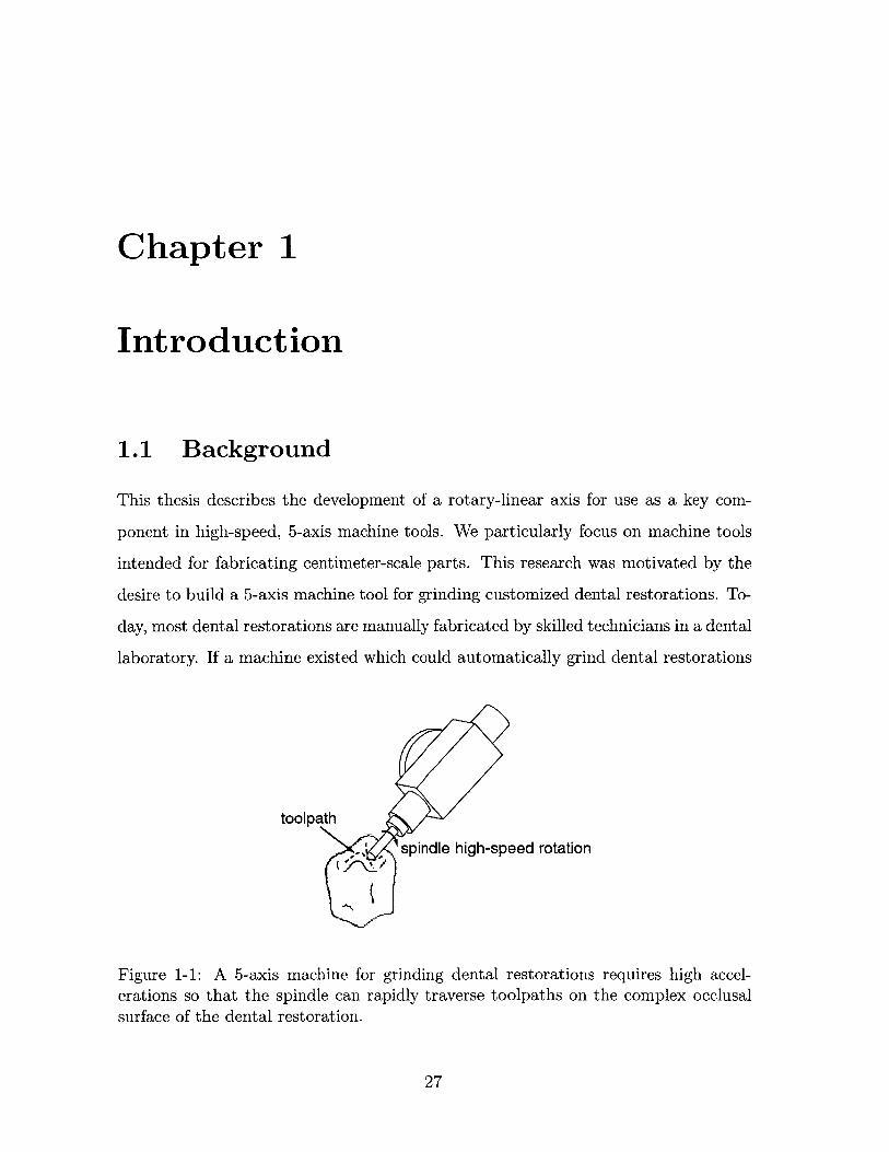
1-1 A 5-axis machine for grinding dental restorations requires high acceler-ations so that the spindle can rapidly traverse toolpaths on the complexocclusal surface of the dental restoration. . . . . . . . . . . . . . . . 27

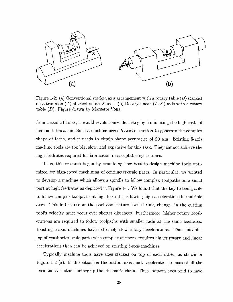
1-2 (a) Conventional stacked axis arrangement with a rotary table (B)stacked on a trunnion (A) stacked on an X-axis. (b) Rotary-linear(A-X) axis with a rotary table (B). Figure drawn by Marsette Vona. 28

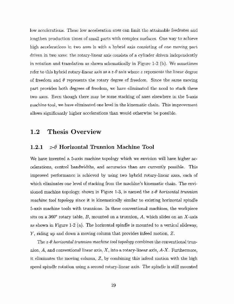
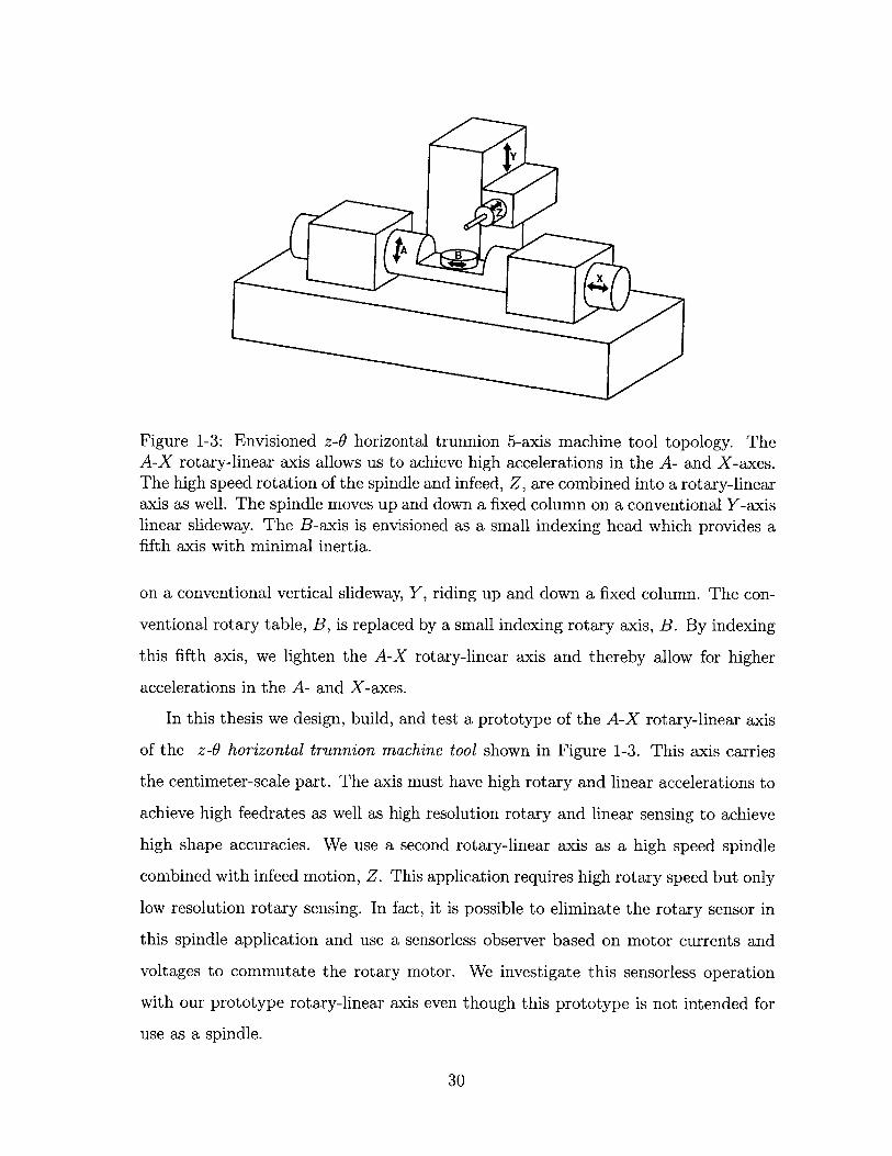
1-3 Envisioned z-0 horizontal trunnion 5-axis machine tool topology. TheA-X rotary-linear axis allows us to achieve high accelerations in the A-and X-axes. The high speed rotation of the spindle and infeed, Z, arecombined into a rotary-linear axis as well. The spindle moves up anddown a fixed column on a conventional Y-axis linear slideway. TheB-axis is envisioned as a small indexing head which provides a fifthaxis with minimal inertia. . . . . . . . . . . . . . . . . . . . . . . . . 30

1-4 The prototype z-0 axis consists of a central shaft riding in two cylin-drical air bearings. The frameless rotary motor on the left made fromcommercially available parts generates torque; the custom-built tubu-lar linear motor on the right generates force. On the far left is a 1 inch(2.54 cm) diameter mirror for z measurement, and on the far right isa 3 inch (7.62 cm) diameter, slightly tilted mirror for 0 measurement. 31

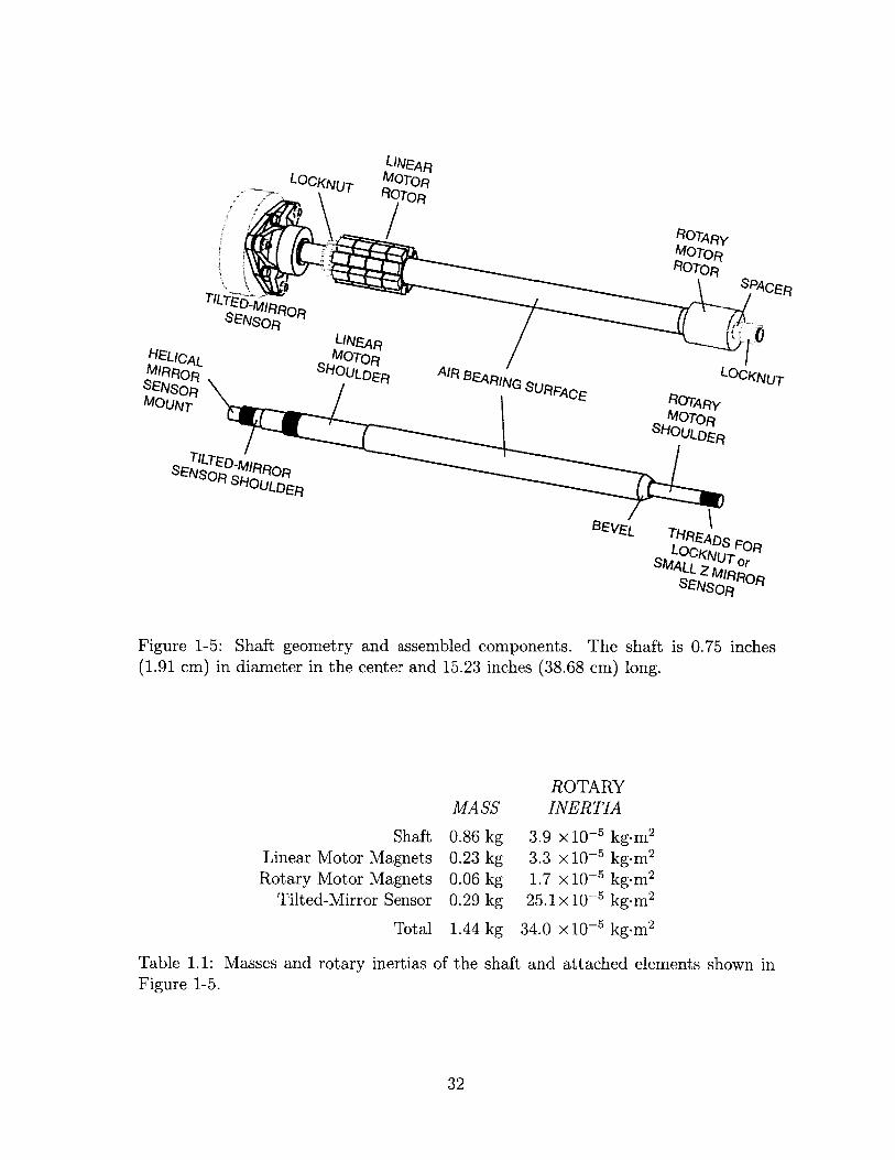
1-5 Shaft geometry and assembled components. The shaft is 0.75 inches(1.91 cm) in diameter in the center and 15.23 inches (38.68 cm) long. 32

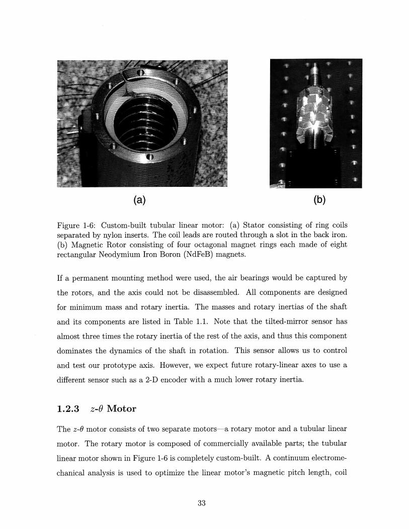
1-6 Custom-built tubular linear motor: (a) Stator consisting of ring coilsseparated by nylon inserts. The coil leads are routed through a slot inthe back iron. (b) Magnetic Rotor consisting of four octagonal magnetrings each made of eight rectangular Neodymium Iron Boron (NdFeB)m agnets. . . . . . . . . . . . . . . . . . . . . . . . . . . . . . . . . . . 33

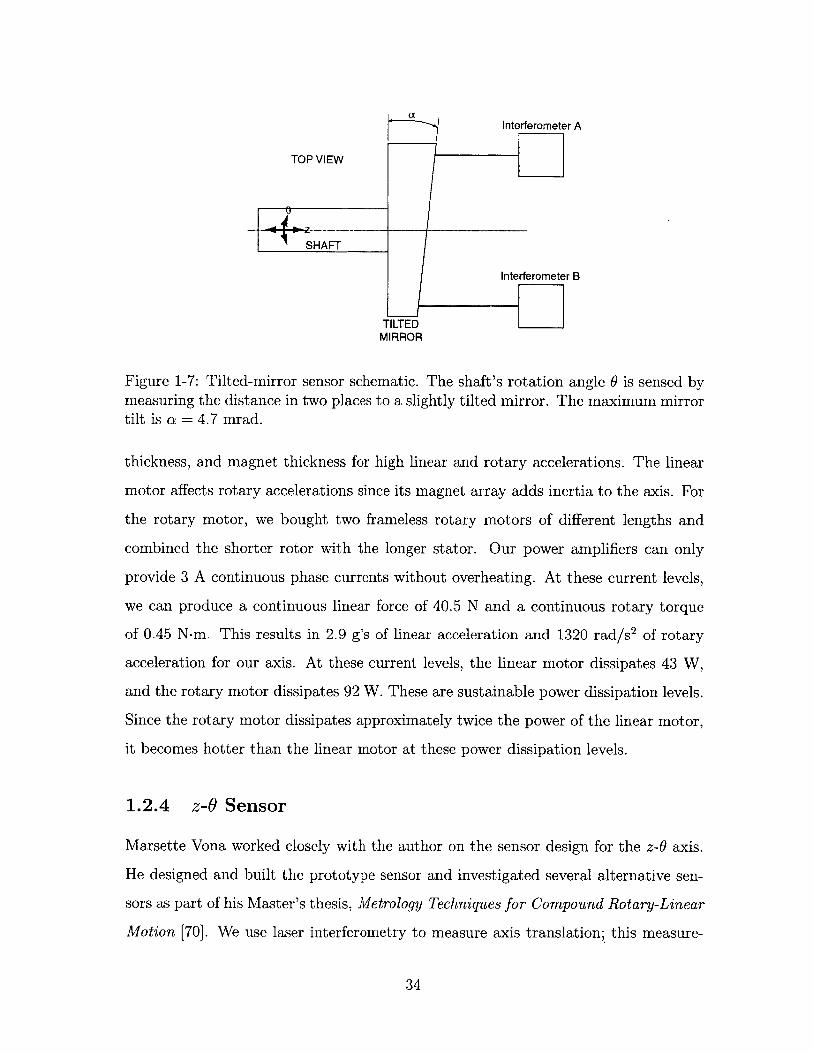
1-7 Tilted-mirror sensor schematic. The shaft's rotation angle 0 is sensedby measuring the distance in two places to a slightly tilted mirror. Themaximum mirror tilt is a = 4.7 mrad. . . . . . . . . . . . . . . . . . . 34

1-8 Prototype tilted-mirror sensor mounted on the z-0 axis. The sensor ismounted to a wobble plate so we can experiment with changing them irror tilt angle. . . . . . . . . . . . . . . . . . . . . . . . . . . . . . 35

2-1 Two examples of milling machines: (a) vertical 3-axis machine (b)vertical 5-axis machine with swiveling spindle (A) and rotating part (C). 44

15

2-2 A 5-axis grinding machine must be designed so that the spindle canrapidly traverse optimal toolpaths on the complex occlusal surface ofa dental restoration. . . . . . . . . . . . . . . . . . . . . . . . . . . . 46

2-3 Rotating (C), swivel (A/B) spindle. . . . . . . . . . . . . . . . . . . . 502-4 Swivel (A), tilt (B) spindle. . . . . . . . . . . . . . . . . . . . . . . . 512-5 Two examples of swivel (B) spindle, rotating (C/A) part topologies. . 532-6 Rotary table (B), mounted on a trunnion (A) in a horizontal machine

tool. Figure drawn by Marsette Vona . . . . . . . . . . . . . . . . . . 542-7 Rotary table (C), mounted on a trunnion (A) in a vertical machine

tool. Figure drawn by Marsette Vona . . . . . . . . . . . . . . . . . . 562-8 First Fourier component of a toolpath on the surface of a part with

characteristic dimension 1 and amplitude A. Infeed motion is along thez-axis and crossfeed motion is along the x-axis. . . . . . . . . . . . . 59

2-9 Spindles cutting the crests of sinusoidal surfaces and maintaining theirangular positions normal to the part surfaces. For the same crossfeedvelocity, the spindle in (b) must have higher angular accelerations thanspindle in (a). . . . . . . . . . . . . . . . . . . . . . . . . . . . . . . . 60

2-10 Possible 5-axis machine topology using a rotary-linear axis. . . . . . . 622-11 Crossed rotary-linear axes 5-axis machine topology. . . . . . . . . . . 642-12 A common stacked-axis arrangement used in horizontal multi-axis ma-

chine tools is compared to our proposed rotary-linear axis. (a) Rotaryindex table (B) is mounted on a trunnion (A) which is moved by alinear axis (X). (b) Our rotary-linear (A-X) axis eliminates the con-ventional stacking of axes. Figure drawn by Marsette Vona. . . . . . 65

2-13 Envisioned z-0 horizontal trunnion 5-axis machine tool topology. TheA-X rotary-linear axis allows us to achieve high accelerations in the A-and X-axes. The high speed rotation of the spindle and infeed, Z, arecombined into a rotary-linear axis as well. The spindle moves up anddown a fixed column on a conventional Y-axis linear slideway. TheB-axis is envisioned as a small indexing head which provides the fifthaxis with minimal inertia. . . . . . . . . . . . . . . . . . . . . . . . . 66

3-1 Rotary & linear magnetomotive positioning mechanism for printerspatented by Teletype Corporation in 1973. Figure from U. S. Patent3,745,433 [31]. . . . . . . . . . . . . . . . . . . . . . . . . . . . . . . . 72

3-2 Electromagnetic actuator with a cylindrical translation coil and a toroidalrotation coil patented by Philips Corporation in 1997. Figure from U.S. Patent 5,600,189 [68]. . . . . . . . . . . . . . . . . . . . . . . . . . 73

3-3 A 2-D optical encoder for rotary <W and linear z sensing. Two maskswith slits are used for each degree of freedom. The slits in the twomasks are displaced by one-quarter pitch of the encoder grid to providequadrature signals. Figure from U. S. Patent 5,600,189 [68]. . . . . . 77

3-4 z-0 induction actuator. Figure from [12]. . . . . . . . . . . . . . . . . 783-5 Cross-section of z-0 induction actuator. Figure from [12]. . . . . . . . 793-6 Optical rotation sensor based on crossed polarizers. Figure from [12]. 80

16

3-7 High speed drilling spindle with reciprocating ceramic shaft patentedby Electro-Scientific Industries in 1999. Figure from U. S. Patent5,997,223 [36]. . . . . . . . . . . . . . . . . . . . . . . . . . . . . . . . 81

3-8 Rotary-linear actuator patented by Anorad Corporation in 1999. Theview on the right is a cross-section through the motor. Figures fromU. S. Patent 5,982,053 [8]. . . . . . . . . . . . . . . . . . . . . . . . . 83

3-9 Two possible realizations of a checkboard magnet array are shown.Anorad's Rotary-Linear Actuator uses this type of magnet array. Fig-ures from U. S. Patent 5,982,053 [8]. . . . . . . . . . . . . . . . . . . 85

3-10 2-D optical encoder for use as a rotary and linear sensor. Figure fromU. S. Patent 5,982,053 [8]. . . . . . . . . . . . . . . . . . . . . . . . . 86

3-11 Schematic showing layers in a permanent magnet motor and an induc-tion motor. The permanent magnet motor has a surface-wound stator,and the induction motor has a slotted stator . . . . . . . . . . . . . . 88

3-12 Power vs. force for comparable permanent magnet and induction mo-tors. Both motors have a spatial wavelength of 1 = 6 cm, and a workingarea of 36 cm2 . . . . . . . . . . . . . . . . . . . . . . . . . . . . . . . 91

3-13 Power vs. force for comparable permanent magnet and induction mo-tors. This figure zooms in on the force range of 0-100 N in Figure 3-12. 91

3-14 (a) Stacked motor and (b) separated motor configurations. The checker-board magnet array used in the stacked motor can have only a 50%packing density. . . . . . . . . . . . . . . . . . . . . . . . . . . . . . . 92

3-15 Schematic showing general difficulties with designing an interferometricrotary-linear sensor: (a) A laser beam is directed normally at a tiltedmirror so that it returns to the detector. (b) As the shaft and mirrorrotate, the beam traces out an ellipse in the measurement plane and somisses the detector. (c) As the shaft and mirror translate, the majorand minor diameters of the ellipse change. . . . . . . . . . . . . . . . 98

3-16 Prism-mirror sensor. A prism with apex angle / deviates a laser beamto reflect normally from a mirror tilted at an angle of a. Unfortunately,the optical path distance does not change with x so the sensor cannotmeasure x motion. . . . . . . . . . . . . . . . . . . . . . . . . . . . . 100

3-17 Tilted-mirror sensor. Two interferometers measure distance to a slightlytilted mirror. The mirror tilt, a, is 4.7 milliradians. . . . . . . . . . . 102

3-18 Helicoid Miror Sensor. The laser interferometer measurement beamis directed normal to a radial wedge, or helicoid, mirror so that shaftrotation is measured. Another beam measures translation by reflectingoff the flat mirror in the center. A detailed mechanical drawing of thehelicoid mirror is shown in Figure D-6. Figure drawn by Marsette Vona. 103

3-19 Helicoid sensor periscope concept. A small periscope is attached to therotary-linear axis, and the massive helicoid mirror is held stationary.The periscope optics scan the surface of the helicoid. Figure drawn byM arsette Vona [70]. . . . . . . . . . . . . . . . . . . . . . . . . . . . . 104

17

3-20 Rotating half-wave plate sensor. The optical path length of the mea-surement beams changes as the half-wave plate rotates. Two beamspolarized in different ways are needed for quadrature sensing. . . . . . 105

4-1 Layers of electromagnetic material in a surface wound permanent mag-net motor. . . . . .. ... ..... . . .... . . . . . . . . . . .. . ... . 115

4-2 Here are the five layers used for the continuum electromechanical anal-ysis of the linear motor. The Fourier expansions for the magnetizationand current density are given. The layer thicknesses are F, xO, and A.The unprimed coordinate frame is fixed to the stator, and the primedcoordinate frame moves with the magnetic rotor. . . . . . . . . . . . 116

4-3 Power dissipation as a function of coil thickness. . . . . . . . . . . . . 1264-4 Motor force at constant power, total mass, and linear acceleration as

functions of linear motor magnet thickness. . . . . . . . . . . . . . . . 1304-5 Linear motor power for a given linear acceleration vs. magnet thickness. 1314-6 Rotary motor torque, total inertia, and rotary acceleration as functions

of linear motor magnet thickness. . . . . . . . . . . . . . . . . . . . . 1324-7 Rotary motor power for a given rotary acceleration vs. linear motor

m agnet thickness . . . . . . . . . . . . . . . . . . . . . . . . . . . . . 1334-8 Finite-element plots of magnetic flux lines for three different magnet

arrays: (a) Ideal infinitely repeating magnet array. (b) N-S-N singlepitch magnet array. (c) N-S single pitch magnet array. Magnet array(b) approximates the ideal array (a) better than magnet array (c).Grey areas are permeable back iron. The dotted lines in (a) representboundaries of perfect symmetry. . . . . . . . . . . . . . . . . . . . . . 134

4-9 The first harmonic component of current density is shown in red su-perposed over the actual rectangular distribution of current density inthe stator shown in blue. Current density is plotted as a function ofaxial distance, z. . . . . . . . . . . . . . . . . . . . . . . . . . . . . . 137

4-10 Measuring linear force with a piezoelectric load cell. . . . . . . . . . . 1404-11 Linear motor force vs. current. . . . . . . . . . . . . . . . . . . . . . 1414-12 Measured rotary motor back EMF waveforms. The 8-pole motor is

spinning at 20 rev/s. . . . . . . . . . . . . . . . . . . . . . . . . . . . 144

5-1 Schematic of the tilted-mirror sensor. The shaft's translation z androtation 0 are sensed by measuring the distance to a slightly tiltedmirror in two places. . . . . . . . . . . . . . . . . . . . . . . . . . . . 149

5-2 Determination of tilted-mirror sensor resolution. The rotation angle,0, is calculated by 6 = arctan(di - z)/(d2 - z). Both di - z and d2 - zchange in increments of 0.625 nm. The maximum change in 0 occurswhen d2 - z is equal to its maximum value, 135 pm, and d, - z changesfrom 0 to 0.625 nm. The resolution is AO = 4.6 pirad. . . . . . . . . . 151

18

5-3 In general, the observed resolution due to an incremental change ind, - z or d2 - z is a function of angle 0. For 0 = 36.9', an incrementalchange in d, - z results in an angle change of AO = 3.7 prad. Thisis the resolution observed experimentally at one angle and shown inF igure 5-7. . . . . . . . . . . . . . . . . . . . . . . . . . . . . . . . . 151

5-4 It is possible to measure rotation angle and translation of the rotary-linear axis without using a third beam to directly measure translation.However, at the angle depicted in the figure, a small clockwise rotationof the mirror increases the distance measured by the A and B intefer-ometers by the same amount; thus, it cannot be distinguished from atranslation of the axis away from the interferometers. This singularityoccurs when the line connecting the two interferometer beams is par-allel to the line connecting the mirror's high and low points. Anothersingularity occurs when the shaft is rotated 1800 from the orientationshow n. . . . . . . . . . . . . . . . . . . . . . . . . . . . . . . . . . . . 158

5-5 Measurement and reference beam paths in a 2-pass laser interferometerwhen the target mirror is (a) perfectly normal to the measurementbeam and (b) tilted by a small angle, a. In case (b) the measurementbeam is displaced from the reference beam by an amount proportionalto mirror tilt, a, and distance between the interferometer and the targetmirror, d. Figure drawn by Marsette Vona. . . . . . . . . . . . . . . . 159

5-6 Linear axis interferometer sensor noise. The controller and air bearingsare turned off. The rms noise level is 0.35 nm. . . . . . . . . . . . . . 160

5-7 Rotary axis tilted-mirror sensor noise. The controller and air bearingsare turned off. The rms noise level is 2.6 prad. . . . . . . . . . . . . . 160

6-1 The prototype z-0 axis consists of a central shaft riding in two cylindri-cal air bearings. A frameless rotary motor on the left generates torque,and the custom-built tubular linear motor on the right generates force.On the far left is a 1 inch (2.54 cm) diameter mirror for z measure-ment, and on the far right is a 3 inch (7.62 cm) diameter, slightly tiltedmirror for 0 measurement. . . . . . . . . . . . . . . . . . . . . . . . . 163

6-2 Load vs. air gap in 3/4 inch New Way air bushing. Figure from NewWay Bearings (see Appendix F) . . . . . . . . . . . . . . . . . . . . . 165

6-3 New Way Bearings (Appendix F) 3/4 inch porous graphite air bushing(left) and pillow block (right). . . . . . . . . . . . . . . . . . . . . . . 166

6-4 The precision ground stainless steel shaft rides in two air bushings.Shoulders and threads are machined into the shaft for attaching themagnetic rotors and sensor mirror mounts. . . . . . . . . . . . . . . . 167

6-5 Shaft geometry and assembled components. The shaft is 0.75 inchin diameter in the center and 15.23 inches long. Figure D-1 shows adetailed mechanical drawing of the shaft. . . . . . . . . . . . . . . . . 170

6-6 Tilted-mirror mount. Figure drawn by Marsette Vona [70]. . . . . . . 1726-7 Tilted-mirror mount assembled on the z-0 axis. . . . . . . . . . . . . 1736-8 Small z mirror mount. Figure drawn by Marsette Vona [70]. . . . . . 174

19

6-9 Small z mirror mount assembled on the z-0 axis. . . . . . . . . . . . . 1756-10 The tilted-mirror sensor and small z-mirror sensor are located on op-

posite ends of the shaft. The three Plane Mirror Interferometers (PMI)are shown along with their receivers. Figure drawn by Marsette Vona[70]. . . . . . . . . . . . . . . . . . . . . . . . . . . . . . . . . . . . . 176

6-11 Compact mount for the tilted-mirror sensor's interferometer optics andreceivers. . . . . . . . . . . . . . . . . . . . . . . . . . . . . . . . . . . 176

6-12 Approximate laser beam paths for the three, two-pass plane mirrorinterferom eters. . . . . . . . . . . . . . . . . . . . . . . . . . . . . . . 177

6-13 An ideal configuration of radially magnetized ring magnets for a tubu-lar linear m otor.. .. . .... .. .. .. .. . . . . . . . . . .. .. . . 178

6-14 On the left is an exterior octagonal ring magnet for a tubular linear mo-tor. On the right is the fixture used to assemble the magnets. Picturestaken by Michael Berhan [5]. . . . . . . . . . . . . . . . . . . . . . . . 179

6-15 The back iron for the linear motor magnets. Eight NdFeB magnets areglued to the flats, and the center portion fits onto a shoulder of theshaft, which is made of a magnetic stainless steel. . . . . . . . . . . . 180

6-16 Drawing of the octagonal back iron with eight NdFeB magnets glued toit. A detailed mechanical drawing is shown in Figure D-4 of Appendix D. 180

6-17 Assembly of the magnet array with the first fixture. . . . . . . . . . . 1826-18 Assembly of the magnet array with the second fixture. The steel optical

table partially shorts out the magnets already assembled and attractsthe incoming magnet so that the force required to position it is reduced. 183

6-19 Radially magnetized linear motor magnet ring. . . . . . . . . . . . . . 1846-20 The first magnet ring has been slid onto the shaft's shoulder. The

aluminum endcap centers the ring on the ferromagnetic shaft duringassem bly. . . . . . . . . . . . . . . . . . . . . . . . . . . . . . . . . . 184

6-21 Linear motor permanent magnet rotor. The four magnet rings areaxially clamped by the locknut. . . . . . . . . . . . . . . . . . . . . . 185

6-22 Linear motor coil. It was wound by Wirewinders (see Appendix F). . 1866-23 The linear motor magnet ring is shown inside the linear motor coil.

This picture is similar to a cross-section of the assembled motor. . . . 1876-24 A separated end-turn coil allows each layer of the coil to be directly

cooled [41]. This technique could be used in future generations ofmotors for the z-6 axis. . . . . . . . . . . . . . . . . . . . . . . . . . . 188

6-25 Linear motor stator back iron. . . . . . . . . . . . . . . . . . . . . . . 1896-26 Linear motor stator endcap. . . . . . . . . . . . . . . . . . . . . . . . 1906-27 Nylon coil spacer. . . . . . . . . . . . . . . . . . . . . . . . . . . . . . 1916-28 Linear motor stator assembly. Nylon spacers separate the coils. Coil

leads are routed through a slit in the back iron. The stack of coils andspacers is axially clamped by endcaps (not shown). . . . . . . . . . . 192

6-29 Linear motor stator. . . . . . . . . . . . . . . . . . . . . . . . . . . . 1936-30 Jacking mechanism for assembling the stator around the rotor. . . . . 1946-31 Aerotech rotary motor permanent magnet rotor mounted on shaft. . . 196

20

7-1 Schematic cross-section of a DC motor. The field windings and theirmagnetic fields are shown in red; the armature windings and theirmagnetic fields are shown in blue. . . . . . . . . . . . . . . . . . . . . 201

7-2 Circuit model for field windings and armature windings in a DC motor. 2037-3 Control block diagram showing a DC motor driving an inertial load. . 2067-4 Control ranges for a DC Motor in steady state. Figure adapted from

Leonhard [40]. . . . . . . . . . . . . . . . . . . . . . . . . . . . . . . . 2077-5 Symmetrical three-phase permanent magnet synchronous motor. The

permanent magnet is modeled by a field winding on the rotor. Thestator windings are typically connected in a wye configuration as shownon the right. . . . . . . . . . . . . . . . . . . . . . . . . . . . . . . . . 209

7-6 The magnetic flux lines produced by coil aa' in the stator of a cylin-drical rotary motor are shown. The a-axis points in the direction ofthe magnetic flux produced. Actual field lines are perpendicular to thestator and rotor back irons. ... .... .. ... . . . . .. . . ... . 210

7-7 The abc axes form a three-phase AC system fixed in the stator frame.The o43 axes represent an equivalent two-phase AC system fixed inthe stator frame. The dq axes represent an equivalent two-phase DCsystem that rotates with the rotor flux. . . . . . . . . . . . . . . . . . 217

7-8 Block diagram of 3-phase permanent magnet synchronous motor con-trol in dq variables. The transformations inside the motor block arepart of the motor model. . . . . . . . . . . . . . . . . . . . . . . . . . 230

7-9 Controller design in dq variables is analogous to DC motor controllerdesign . . . . . . . . . . . . . . . . . . . . . . . . . . . . . . . . . . . . 231

8-1 Current control circuit for each motor phase. . . . . . . . . . . . . . . 2368-2 Spectrum analyzer configuration for measuring the transfer function

V/V4 ......................................... 2378-3 Measured bode plot for the transfer function V 5/V 4 from Figure 8-2,

for one of the linear motor phases. . . . . . . . . . . . . . . . . . . . . 2388-4 Block diagram of PI current controller. . . . . . . . . . . . . . . . . . 2398-5 Linear motor current amplifier closed-loop Bode plot. . . . . . . . . . 2418-6 Rotary motor current amplifier closed-loop Bode plot. . . . . . . . . . 2418-7 Linear motor current amplifier step response . . . . . . . . . . . . . . 2428-8 Rotary motor current amplifier step response. . . . . . . . . . . . . . 2428-9 Block diagram of PA12A power amplifier loop. RG reduces the band-

width of the feedback loop around the op amp without affecting thegain from V3 to V4 . . . . . . . . . . . . . . . . . . . . . . . . . . . . . 243

8-10 Linear axis control block diagram. . . . . . . . . . . . . . . . . . . . . 2458-11 Measured linear axis open-loop Bode plot (from control effort, u, to

position, z). The initial model shown for comparison consists of asingle mass, the D/A gain, the power amplifier gain, and the motorforce constant. The z sensor is an interferometer measuring distancefrom the tilted mirror. . . . . . . . . . . . . . . . . . . . . . . . . . . 248

21

8-12 Canonical two-mass system. Measurement x1 is collocated with theactuator; measurement x2 is non-collocated with the actuator. .... .249

8-13 Measured linear axis open-loop Bode plots (from control effort, u, toposition, z). We compare the Bode plot of the z-axis using the tiltedmirror interferometer, a non-collocated sensor, with the Bode plot ofthe z-axis using the small z mirror interferometer on the other end ofthe shaft, a collocated sensor. . . . . . . . . . . . . . . . . . . . . . . 250

8-14 Linear axis open-loop Bode plots of collocated and non-collocated mod-els of the z-axis. . . . . . . . . . . . . . . . . . . . . . . . . . . . . . . 253

8-15 Tilted-mirror mount. Figure drawn by Marsette Vona [70]. . . . . . . 2548-16 Measured linear axis open-loop Bode plots (from control effort, u, to

position, z). Increasing the pre-load on the the tilted-mirror mount(shown in Figure 8-15 increases the resonant frequency. . . . . . . . . 255

8-17 Linear axis open-loop Bode plot (from control effort, u, to position, z).The experimental measurement is shown with red x's, and the finalmodel is shown in blue. The final model is based on an initial modelwith a collocated resonance shown in cyan. When the power amplifierdynamics are added, the model appears as shown in green. When atime delay due to the digital control is added, the final model in blueis obtained. . . . . . . . . . . . . . . . . . . . . . . . . . . . . . . . . 256

8-18 Linear axis negative loop transmission Bode plot. Red x's indicatemeasured data. Blue line is modeled response. . . . . . . . . . . . . . 257

8-19 Linear axis closed-loop Bode plot. . . . . . . . . . . . . . . . . . . . . 2588-20 Linear axis step response. . . . . . . . . . . . . . . . . . . . . . . . . 2598-21 Linear axis closed-loop positioning noise of 2.5 nm rms. . . . . . . . . 2598-22 Rotary axis control block diagram. . . . . . . . . . . . . . . . . . . . 2608-23 Measured rotary axis open-loop Bode plot (from control effort, u, to

angle, 6) . . . . . . . . . . . . . . . . . . . . . . . . . . . . . . . . . . 2618-24 Cantilever beam with distributed mass, m, stiffness, k, length, 1, and

lumped m ass, M . . . . . . . . . . . . . . . . . . . . . . . . . . . . . . 2638-25 Measured rotary axis negative loop transmission Bode plots. The res-

onance at 1000 rad/s is non-collocated when measured at small anglesaround a shaft angle at 0 = 0 rad but is collocated when measuredaround 6 = -57r/4. . . . . . . . . . . . . . . . . . . . . . . . . . . . . 265

8-26 Measured rotary axis negative loop transmission Bode plot. . . . . . . 2668-27 Measured rotary axis closed-loop Bode plot. ...... ........ 2678-28 Measured rotary axis step response. Placing the lead compensation in

the feedback path reduces the overshoot. . . . . . . . . . . . . . . . . 2688-29 Rotary axis closed-loop positioning noise of 3.1 p-rad rms. . . . . . . . 2688-30 Model of linear axis dynamic stiffness for our prototype axis at different

closed-loop control bandwidths. The controller we implemented has aclosed-loop bandwidth of 600 rad/s. . . . . . . . . . . . . . . . . . . . 270

8-31 Model of rotary axis dynamic stiffness at a 1 cm radius for our proto-type axis at different closed-loop control bandwidths. The controllerwe implemented has a closed-loop bandwidth of 250 rad/s. . . . . . . 271

22

8-32 Spin-down test. . . . . . . . . . . . . . . . . . . . . . . . . . . . . . . 2778-33 Sensorless speed control step response. Estimated speed, CD, and es-

timated quadrature current, iq, for a step change in reference speedfrom 28.27 rad/s (4.5 rev/s) to 40.84 rad/s (6.5 rev/s). The system isrunning under closed-loop speed control with estimated speed, Co usedas a measured signal, and estimated angle, 0, used to commutate therotary m otor. . . . . . . . . . . . . . . . . . . . . . . . . . . . . . . . 279

9-1 M ain control panel. . . . . . . . . . . . . . . . . . . . . . . . . . . . . 2849-2 Control panel which allows control of sinusoidal motion in both z and 0.2859-3 Top level of the combined Simulink & Stateflow program which controls

the prototype z-0 axis. . . . . . . . . . . . . . . . . . . . . . . . . . . 2869-4 Stateflow Power On state. . . . . . . . . . . . . . . . . . . . . . . . . 2909-5 Stateflow Power Off state. . . . . . . . . . . . . . . . . . . . . . . . . 2919-6 Main Program subsystem. This subsystem contains the control algo-

rithms for the linear and rotary axes. . . . . . . . . . . . . . . . . . . 2929-7 The rotary axis compensator is shown here. This compensator is con-

tained in the "leadlag controller 1" block in Figure 9-6. . . . . . . . . 2939-8 Smallest Angle subsystem. This subsystem brings the angular error

between the reference and sensed angles back into the range -7r to 7r. 2939-9 Motor Commutation subsystem. The dq transformations for motor

commutation are contained in this subsystem labeled "DQ - > ABCRO T _LIN ." . . . . . . . . . . . . . . . . . . . . . . . . . . . . . . . . 293

9-10 Sensor Processing subsystem. . . . . . . . . . . . . . . . . . . . . . . 2959-11 Sensorless observer subsystem. . . . . . . . . . . . . . . . . . . . . . . 297

10-1 Two types of rotary-linear sensors: (a) surface area and (b) end-on.Figure drawn by Marsette Vona . . . . . . . . . . . . . . . . . . . . . 302

10-2 A cradle mounted on the rotary-linear axis holds a small index tableand the workpiece. . . . . . . . . . . . . . . . . . . . . . . . . . . . . 305

10-3 z-0 horizontal trunnion 5-axis grinding machine. . . . . . . . . . . . . 306

A-i The analysis of this appendix is developed for the motor on the leftwith magnet and coil back iron. Due to the symmetry between thismotor and the U-shaped motor geometry on the right, the analysisapplies to U-shaped motors as well. . . . . . . . . . . . . . . . . . . . 310

A-2 Here are the five layers used in the continuum electromechanical anal-ysis of our linear motor. The Fourier expansions for the magnetizationand current density are given. Also note the two coordinate systemsand the layer thicknesses, IF, xo, and A. The primed frame moves withthe m agnet array. . . . . . . . . . . . . . . . . . . . . . . . . . . . . . 312

23

A-3 We calculate the forces on this imaginary box. From our analysis weknow the fields for the side of the box in the air gap. The oppositeside is at inifinity where the fields are zero. The remaining two edgesof the box enclose an integral number of magnet periods so that bysymmetry the stresses along these sides cancel. . . . . . . . . . . . . . 321

B-1 Schematic showing induction motor model. The stator's windings aremodeled by a thin current sheet, and the rotor is also modeled as athin current sheet. . . . . . . . . . . . . . . . . . . . . . . . . . . . . 327

B-2 Induction motor power dissipation per force, P/F, as a function ofRotor Thickness, A,. The power optimal slip, S+ (Ar, A, kd), is cal-culated for each rotor thickness. . . . . . . . . . . . . . . . . . . . . . 330

C-1 Magnetic circuit with permanent magnet . . . . . . . . . . . . . . . . 331

D-1 Shaft mechanical drawing . . . . . . . . . . . . . . . . . . . . . . . . 336D-2 Machine base mechanical drawing . . . . . . . . . . . . . . . . . . . . 337D-3 Linear motor coil mechanical drawing . . . . . . . . . . . . . . . . . . 338D-4 Linear motor magnet array mechanical drawing . . . . . . . . . . . . 339D-5 Linear motor stator back iron mechanical drawing . . . . . . . . . . . 340D-6 Helicoid mirror mechanical drawing. Figure drawn by Marsette Vona. 341

E-1 Rotary motor terminal block connections. . . . . . . . . . . . . . . . 344

24

List of Tables

1.1 Masses and rotary inertias of the shaft and attached elements shownin Figure 1-5. . . . . . . . . . . . . . . . . . . . . . . . . . . . . . . . 32

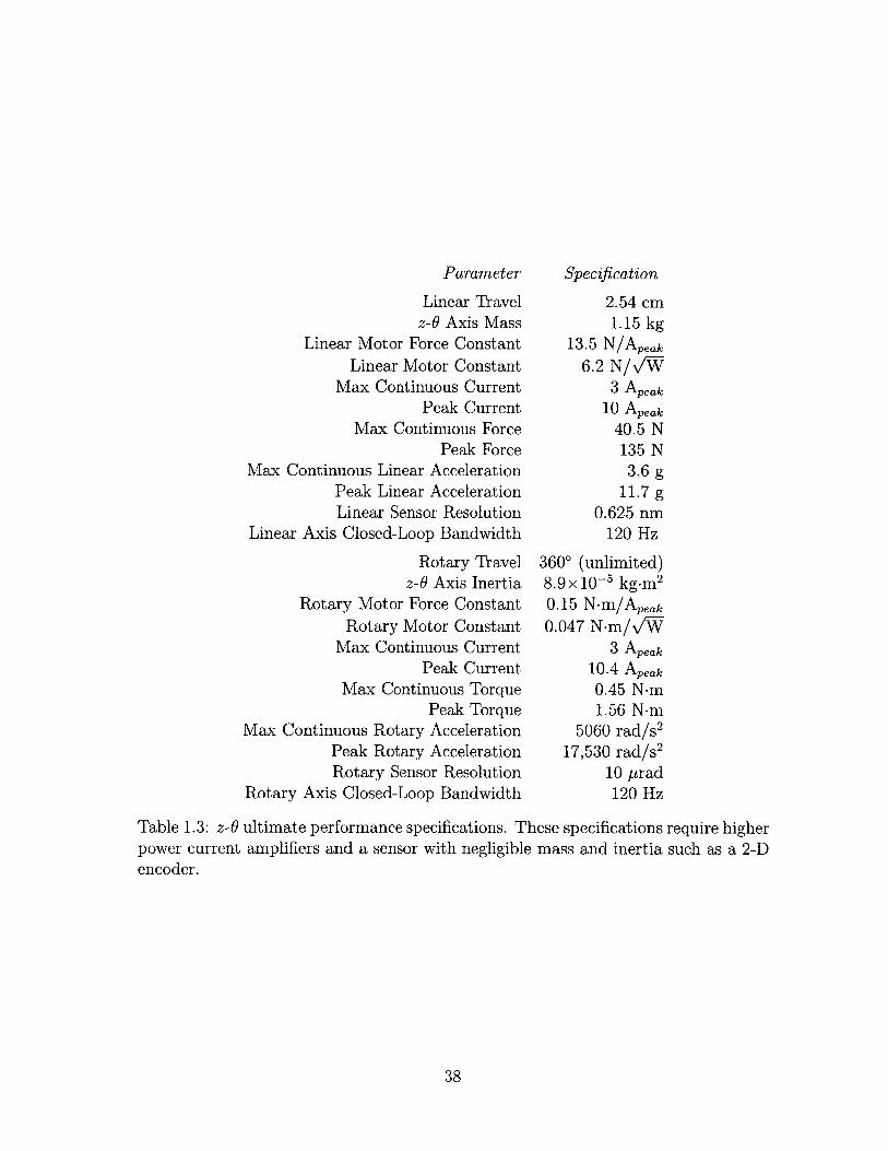
1.2 z-0 prototype specifications. . . . . . . . . . . . . . . . . . . . . . . . 361.3 z-0 ultimate performance specifications. These specifications require

higher power current amplifiers and a sensor with negligible mass andinertia such as a 2-D encoder. . . . . . . . . . . . . . . . . . . . . . . 38

3.1 z-0 induction actuator specifications [12]. . . . . . . . . . . . . . . . . 783.2 Anorad Cyclone S50 preliminary specifications. . . . . . . . . . . . . 843.3 Permanent magnet motor parameters . . . . . . . . . . . . . . . . . . 883.4 Induction motor parameters. . . . . . . . . . . . . . . . . . . . . . . . 883.5 Desired z-6 sensor specifications . . . . . . . . . . . . . . . . . . . . . 973.6 Slow and fast refractive indices, n, and nr, of some birefringent crys-

tals. Data from [24]. . . . . . . . . . . . . . . . . . . . . . . . . . . . 105

4.1 Electromechanical model variables . . . . . . . . . . . . . . . . . . . . 1184.2 Motor force and power dissipation at different air gaps. The calcula-

tions assume a motor magnetic pitch length of 1 = 5.283 cm. . . . . . 1274.3 Parameters used in the linear motor magnet thickness optimization.

Note that these are approximations of parameters used during the de-sign process and not the final parameter values. . . . . . . . . . . . . 129

4.4 Linear motor parameters . . . . . . . . . . . . . . . . . . . . . . . . . 1364.5 Calculation of achievable angular accelerations with different Aerotech

frameless rotary motors. Total Inertia includes the shaft and linearmotor inertias of 7.5 x 10- kg-m2. . . . . . . . . . . . . . . . . . . . 142

5.1 Tilted-mirror sensor specifications. . . . . . . . . . . . . . . . . . . . 1485.2 Tilted-mirror sensor calibration constants. The constants listed apply

to the two interferometer measurement beams. . . . . . . . . . . . . . 155

8.1 Resistances, inductances, and time constants of motor phases. . . . . 2398.2 Values of resistances and capacitances for the current amplifier circuit

shown in Figure 8-1 for the two motors . . . . . . . . . . . . . . . . . 2408.3 Model parameters for sensorless observer. . . . . . . . . . . . . . . . . 276

E. 1 Motor phases, power amplifiers, and dSPACE signal connections. . . 343E.2 dSPACE DAC connector pinouts. . . . . . . . . . . . . . . . . . . . . 345

25

E.3 dSPACE ADC connector pinouts. Note that channels 1, 5, 9, and 13are measured simultaneously, and then channels 2, 6, 10, and 14 areread next. . . . . . . . . . . . . . .. . . ... . . . . . . . . . . . . . . 346

E.4 RS-422 data link between 4284 DSP board and dSPACE. See [70] form ore details. . . . . . . . . . . . . . . . . . . . . . . . . . . . . . . . . 347

26

Chapter 1

Introduction

1.1 Background

This thesis describes the development of a rotary-linear axis for use as a key com-

ponent in high-speed, 5-axis machine tools. We particularly focus on machine tools

intended for fabricating centimeter-scale parts. This research was motivated by the

desire to build a 5-axis machine tool for grinding customized dental restorations. To-

day, most dental restorations are manually fabricated by skilled technicians in a dental

laboratory. If a machine existed which could automatically grind dental restorations

toolpath

spindle high-speed rotation

Figure 1-1: A 5-axis machine for grinding dental restorations requires high accel-erations so that the spindle can rapidly traverse toolpaths on the complex occlusalsurface of the dental restoration.

27

A

X

(a) (b)

Figure 1-2: (a) Conventional stacked axis arrangement with a rotary table (B) stackedon a trunnion (A) stacked on an X-axis. (b) Rotary-linear (A-X) axis with a rotarytable (B). Figure drawn by Marsette Vona.

from ceramic blanks, it would revolutionize dentistry by eliminating the high costs of

manual fabrication. Such a machine needs 5 axes of motion to generate the complex

shape of teeth, and it needs to obtain shape accuracies of 20 Am. Existing 5-axis

machine tools are too big, slow, and expensive for this task. They cannot achieve the

high feedrates required for fabrication in acceptable cycle times.

Thus, this research began by examining how best to design machine tools opti-

mized for high-speed machining of centimeter-scale parts. In particular, we wanted

to develop a machine which allows a spindle to follow complex toolpaths on a small

part at high feedrates as depicted in Figure 1-1. We found that the key to being able

to follow complex toolpaths at high feedrates is having high accelerations in multiple

axes. This is because as the part and feature sizes shrink, changes in the cutting

tool's velocity must occur over shorter distances. Furthermore, higher rotary accel-

erations are required to follow toolpaths with smaller radii at the same feedrates.

Existing 5-axis machines have extremely slow rotary accelerations. Thus, machin-

ing of centimeter-scale parts with complex surfaces, requires higher rotary and linear

accelerations than can be achieved on existing 5-axis machines.

Typically machine tools have axes stacked on top of each other, as shown in

Figure 1-2 (a). In this situation the bottom axis must accelerate the mass of all the

axes and actuators further up the kinematic chain. Thus, bottom axes tend to have

28

low accelerations. These low acceleration axes can limit the attainable feedrates and

lengthen production times of small parts with complex surfaces. One way to achieve

high accelerations in two axes is with a hybrid axis consisting of one moving part

driven in two axes: the rotary-linear axis consists of a cylinder driven independently

in rotation and translation as shown schematically in Figure 1-2 (b). We sometimes

refer to this hybrid rotary-linear axis as a z-6 axis where z represents the linear degree

of freedom and 6 represents the rotary degree of freedom. Since the same moving

part provides both degrees of freedom, we have eliminated the need to stack these

two axes. Even though there may be some stacking of axes elsewhere in the 5-axis

machine tool, we have eliminated one level in the kinematic chain. This improvement

allows significantly higher accelerations than would otherwise be possible.

1.2 Thesis Overview

1.2.1 z-0 Horizontal Trunnion Machine Tool

We have invented a 5-axis machine topology which we envision will have higher ac-

celerations, control bandwidths, and accuracies than are currently possible. This

improved performance is achieved by using two hybrid rotary-linear axes, each of

which eliminates one level of stacking from the machine's kinematic chain. The envi-

sioned machine topology, shown in Figure 1-3, is named the z-6 horizontal trunnion

machine tool topology since it is kinematically similar to existing horizontal spindle

5-axis machine tools with trunnions. In these conventional machines, the workpiece

sits on a 360' rotary table, B, mounted on a trunnion, A, which slides on an X-axis

as shown in Figure 1-2 (a). The horizontal spindle is mounted to a vertical slideway,

Y, riding up and down a moving column that provides infeed motion, Z.

The z-0 horizontal trunnion machine tool topology combines the conventional trun-

nion, A, and conventional linear axis, X, into a rotary-linear axis, A-X. Furthermore,

it eliminates the moving column, Z, by combining this infeed motion with the high

speed spindle rotation using a second rotary-linear axis. The spindle is still mounted

29

Y

JA B

Figure 1-3: Envisioned z-0 horizontal trunnion 5-axis machine tool topology. TheA-X rotary-linear axis allows us to achieve high accelerations in the A- and X-axes.The high speed rotation of the spindle and infeed, Z, are combined into a rotary-linearaxis as well. The spindle moves up and down a fixed column on a conventional Y-axislinear slideway. The B-axis is envisioned as a small indexing head which provides afifth axis with minimal inertia.

on a conventional vertical slideway, Y, riding up and down a fixed column. The con-

ventional rotary table, B, is replaced by a small indexing rotary axis, B. By indexing

this fifth axis, we lighten the A-X rotary-linear axis and thereby allow for higher

accelerations in the A- and X-axes.

In this thesis we design, build, and test a prototype of the A-X rotary-linear axis

of the z-0 horizontal trunnion machine tool shown in Figure 1-3. This axis carries

the centimeter-scale part. The axis must have high rotary and linear accelerations to

achieve high feedrates as well as high resolution rotary and linear sensing to achieve

high shape accuracies. We use a second rotary-linear axis as a high speed spindle

combined with infeed motion, Z. This application requires high rotary speed but only

low resolution rotary sensing. In fact, it is possible to eliminate the rotary sensor in

this spindle application and use a sensorless observer based on motor currents and

voltages to commutate the rotary motor. We investigate this sensorless operation

with our prototype rotary-linear axis even though this prototype is not intended for

use as a spindle.

30

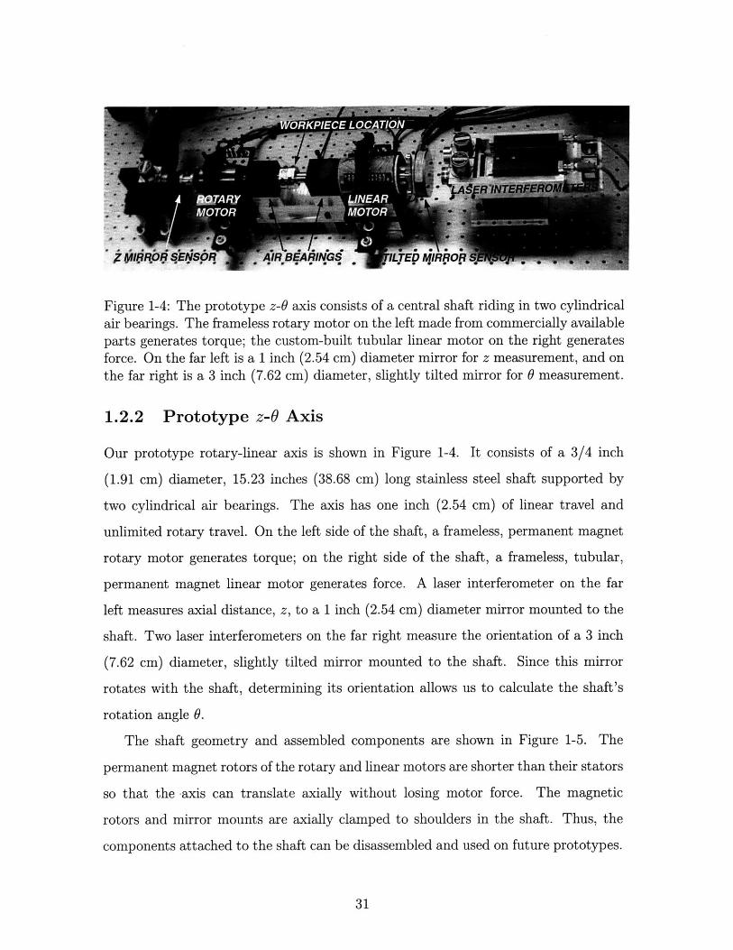
Figure 1-4: The prototype z-6 axis consists of a central shaft riding in two cylindricalair bearings. The frameless rotary motor on the left made from commercially availableparts generates torque; the custom-built tubular linear motor on the right generatesforce. On the far left is a 1 inch (2.54 cm) diameter mirror for z measurement, and onthe far right is a 3 inch (7.62 cm) diameter, slightly tilted mirror for 0 measurement.

1.2.2 Prototype z-0 Axis

Our prototype rotary-linear axis is shown in Figure 1-4. It consists of a 3/4 inch

(1.91 cm) diameter, 15.23 inches (38.68 cm) long stainless steel shaft supported by

two cylindrical air bearings. The axis has one inch (2.54 cm) of linear travel and

unlimited rotary travel. On the left side of the shaft, a frameless, permanent magnet

rotary motor generates torque; on the right side of the shaft, a frameless, tubular,

permanent magnet linear motor generates force. A laser interferometer on the far

left measures axial distance, z, to a 1 inch (2.54 cm) diameter mirror mounted to the

shaft. Two laser interferometers on the far right measure the orientation of a 3 inch

(7.62 cm) diameter, slightly tilted mirror mounted to the shaft. Since this mirror

rotates with the shaft, determining its orientation allows us to calculate the shaft's

rotation angle 9.

The shaft geometry and assembled components are shown in Figure 1-5. The

permanent magnet rotors of the rotary and linear motors are shorter than their stators

so that the -axis can translate axially without losing motor force. The magnetic

rotors and mirror mounts are axially clamped to shoulders in the shaft. Thus, the

components attached to the shaft can be disassembled and used on future prototypes.

31

HELICALAMir,-

rfORSENSORMOUNT

TILSENS

Figure 1-5:(1.91 cm) in

LINEARLOCKNUT MLTSR

TILTED..MIRRSENSORO~

RO.~4 ~O~or AR -

rf mNING SUppACE F0APVROTARyMOTOR

SHOULDER

TED.MI OROR' SHOU5Re

BeVEL THREADSLOCKNUTOr

SMA L , N RI OR

Shaft geometry and assembled components. The shaft is 0.75 inchesdiameter in the center and 15.23 inches (38.68 cm) long.

MASSROTARYINERTIA

Shaft 0.86 kg 3.9 x10- 5 kg.m 2

-. ,'JI fltpj Vil p

Linear Motor MagnetsRotary Motor Magnets

Tilted-Mirror Sensor

0.23 kg0.06 kg0.29 kg

3.3 x10- 5 kg.m 2

1.7 x10- 5 kg.m 2

25.1x 10-5 kg-m 2

Total 1.44 kg 34.0 x 10- 5 kg.m 2

Table 1.1: Masses and rotary inertias of the shaft and attached elements shown inFigure 1-5.

32

Luoe UT

(a) (b)

Figure 1-6: Custom-built tubular linear motor: (a) Stator consisting of ring coilsseparated by nylon inserts. The coil leads are routed through a slot in the back iron.(b) Magnetic Rotor consisting of four octagonal magnet rings each made of eightrectangular Neodymium Iron Boron (NdFeB) magnets.

If a permanent mounting method were used, the air bearings would be captured by

the rotors, and the axis could not be disassembled. All components are designed

for minimum mass and rotary inertia. The masses and rotary inertias of the shaft

and its components are listed in Table 1.1. Note that the tilted-mirror sensor has

almost three times the rotary inertia of the rest of the axis, and thus this component

dominates the dynamics of the shaft in rotation. This sensor allows us to control

and test our prototype axis. However, we expect future rotary-linear axes to use a

different sensor such as a 2-D encoder with a much lower rotary inertia.

1.2.3 z-0 Motor

The z-0 motor consists of two separate motors-a rotary motor and a tubular linear

motor. The rotary motor is composed of commercially available parts; the tubular

linear motor shown in Figure 1-6 is completely custom-built. A continuum electrome-

chanical analysis is used to optimize the linear motor's magnetic pitch length, coil

33

Interferometer A

TOP VIEW

SHAFT

Interferometer B

TILTEDMIRROR

Figure 1-7: Tilted-mirror sensor schematic. The shaft's rotation angle 0 is sensed bymeasuring the distance in two places to a slightly tilted mirror. The maximum mirrortilt is a = 4.7 mrad.

thickness, and magnet thickness for high linear and rotary accelerations. The linear

motor affects rotary accelerations since its magnet array adds inertia to the axis. For

the rotary motor, we bought two frameless rotary motors of different lengths and

combined the shorter rotor with the longer stator. Our power amplifiers can only

provide 3 A continuous phase currents without overheating. At these current levels,

we can produce a continuous linear force of 40.5 N and a continuous rotary torque

of 0.45 N.m. This results in 2.9 g's of linear acceleration and 1320 rad/s 2 of rotary

acceleration for our axis. At these current levels, the linear motor dissipates 43 W,

and the rotary motor dissipates 92 W. These are sustainable power dissipation levels.

Since the rotary motor dissipates approximately twice the power of the linear motor,

it becomes hotter than the linear motor at these power dissipation levels.

1.2.4 z-0 Sensor

Marsette Vona worked closely with the author on the sensor design for the z-0 axis.

He designed and built the prototype sensor and investigated several alternative sen-

sors as part of his Master's thesis, Metrology Techniques for Compound Rotary-Linear

Motion [70]. We use laser interferometry to measure axis translation; this measure-

34

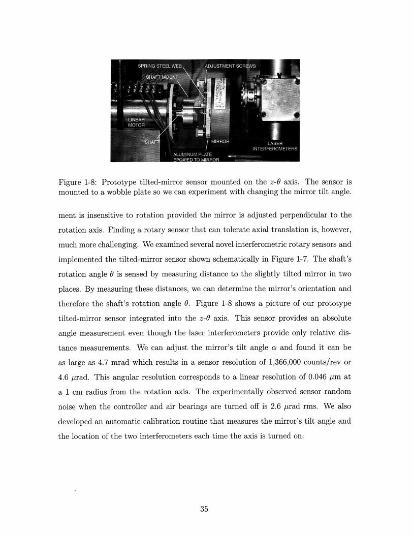
Figure 1-8: Prototype tilted-mirror sensor mounted on the z-0 axis. The sensor ismounted to a wobble plate so we can experiment with changing the mirror tilt angle.

ment is insensitive to rotation provided the mirror is adjusted perpendicular to the

rotation axis. Finding a rotary sensor that can tolerate axial translation is, however,

much more challenging. We examined several novel interferometric rotary sensors and

implemented the tilted-mirror sensor shown schematically in Figure 1-7. The shaft's

rotation angle 0 is sensed by measuring distance to the slightly tilted mirror in two

places. By measuring these distances, we can determine the mirror's orientation and

therefore the shaft's rotation angle 9. Figure 1-8 shows a picture of our prototype

tilted-mirror sensor integrated into the z-0 axis. This sensor provides an absolute

angle measurement even though the laser interferometers provide only relative dis-

tance measurements. We can adjust the mirror's tilt angle a and found it can be

as large as 4.7 mrad which results in a sensor resolution of 1,366,000 counts/rev or

4.6 prad. This angular resolution corresponds to a linear resolution of 0.046 pm at

a 1 cm radius from the rotation axis. The experimentally observed sensor random

noise when the controller and air bearings are turned off is 2.6 Prad rms. We also

developed an automatic calibration routine that measures the mirror's tilt angle and

the location of the two interferometers each time the axis is turned on.

35

5 M

1.2.5 Prototype Axis Specifications

The prototype z-6 axis specifications are summarized in Table 1.2. The axis has

2.54 cm of linear travel and unlimited rotary travel. Its mass is 1.44 kg, and its

rotary inertia is 34.0 x 10-5 kg.m 2 . The linear axis has a control bandwidth of 70 Hz

and has 2.5 nm rms linear positioning noise; the rotary axis has a control bandwidth

of 40 Hz and has 3.1 prad rms rotary positioning noise.

Parameter

Linear Travelz-0 Axis Mass

Linear Motor Force ConstantLinear Motor Constant

Max Continuous CurrentMax Continuous Force

Max Linear AccelerationLinear Sensor Resolution

Linear Axis Closed-Loop BandwidthLinear Positioning Noise

Rotary Travelz-0 Axis Inertia

Rotary Motor Force ConstantRotary Motor Constant

Max Continuous CurrentMax Continuous Torque

Max Rotary AccelerationRotary Sensor Resolution

Rotary Axis Closed-Loop BandwidthRotary Positioning Noise

Specification

2.54 cm1.44 kg

13.5 N/Apeak6.2 N/v'W

3 Apeak40.5 N

2.9 g0.625 nm

70 Hz2.5 nm rms

3600 (unlimited)34.0 x 10- kg.m 2

0.15 N-m/Apeak

0.047 N.m/v/W3 Apeak

0.45 N-m1320 rad/s 2

4.6 prad (1,366,000 counts/rev)40 Hz

3.1 prad rms

Table 1.2: z-6 prototype specifications.

1.2.6 z-0 Axis Ultimate Performance Specifications

With two changes to our prototype axis-higher power current amplifiers and a dif-

ferent rotary sensor-we could achieve much higher accelerations:

* Our current amplifiers are thermally limited to about 3 A continuous current.

36

For safety, we do not allow higher currents, even for short time periods. The

rotary motor is rated for up to 10.4 A of peak current; the linear motor can

withstand similar peak currents. Thus, upgrading to higher power amplifiers

would increase our peak force, torque, and acceleration levels by a factor of

about 3. These extremely high peak accelerations can only be used at low

duty cycles or the motors will overheat. Even at low duty cycles, high peak

accelerations can improve machine tool performance significantly. They allow

target feedrates to be reached in much shorter distances. They also enable the

tool to follow toolpaths with smaller radii at higher feedrates.

e The tilted-mirror sensor works well and allows us to control the prototype axis.

However, since its rotary inertia dominates that of the rest of the axis, we expect

to use a different sensor in the future. A likely candidate is a 2-D encoder sensor

which uses a 2-D encoder grid of negligible mass and rotary inertia. Replacing

the tilted-mirror sensor with one of negligible mass and inertia eliminates 20%

of the axis mass and 74% of the axis inertia.

After making these changes, the z-0 axis could achieve peak linear accelerations

of 11.7 g and peak rotary accelerations of 17,530 rad/s 2 for short time periods. The

improved performance specifications are summarized in Table 1.3.

37

Parameter

Linear Travelz-6 Axis Mass

Linear Motor Force ConstantLinear Motor Constant

Max Continuous CurrentPeak Current

Max Continuous ForcePeak Force

Max Continuous Linear AccelerationPeak Linear AccelerationLinear Sensor Resolution

Linear Axis Closed-Loop Bandwidth

Rotary Travelz-0 Axis Inertia

Rotary Motor Force ConstantRotary Motor Constant

Max Continuous CurrentPeak Current

Max Continuous TorquePeak Torque

Max Continuous Rotary AccelerationPeak Rotary AccelerationRotary Sensor Resolution

Rotary Axis Closed-Loop Bandwidth

Specification

2.54 cm1.15 kg

13.5 N/Apeak6.2 N/VW

3 Apeak10 Apeak

40.5 N135 N3.6 g

11.7 g0.625 nm

120 Hz

3600 (unlimited)8.9x10-5 kg.m 2

0.15 N-m/Apeak0.047 N.m/v'W

3 Apeak10.4 Apeak

0.45 N-m1.56 N-m

5060 rad/s 2

17,530 rad/s 2

10 prad120 Hz

Table 1.3: z-0 ultimate performance specifications. These specifications require higherpower current amplifiers and a sensor with negligible mass and inertia such as a 2-Dencoder.

38

1.3 Thesis Contributions

The main contribution of this thesis is the development of a rotary-linear axis for

use as a key component in high-speed, 5-axis machine tools intended for fabricating

centimeter-scale parts. We present design, analysis, fabrication, and control tech-

niques for this axis. We envision that this axis can be used in novel 5-axis grinding

machines to fabricate dental restorations and other such parts. This could change

fabrication of dental restorations from a manual skilled art to a precise, fast, com-

puter numerically controlled (CNC) process. Specific thesis contributions are listed

below:

" Developed the rotary-linear axis as a key machine tool component especially

suited for high-speed, multi-axis machine tools for fabricating centimeter-scale

parts. (Chapter 2)

" Designed, analyzed (Chapters 4 & 5) and fabricated (Chapter 6) the prototype

rotary-linear axis.

" Designed, fabricated, and tested a rotary-linear motor which includes a custom-

built tubular-linear motor. (Chapters 4 & 6)

" Developed a continuum electromechanical analysis for permanent magnet syn-

chronous motors with iron backing. (Appendix A)

" Developed a permanent magnet motor design procedure based on this motor

analysis. This procedure explains how to optimize motor pitch length, coil

thickness, magnet thickness, and air gap for maximum rotary and linear accel-

erations. (Chapter 4)

" Developed an analysis to compare permanent magnet and induction motors to

allow selection for our application. (Section 3.2.1; Appendix B)

" Invented a 5-axis machine tool topology optimized for centimeter-scale parts

that allows for accurate, high-speed machining. (Chapter 2)

39

" Investigated interferometric and other rotary sensor designs that can tolerate

axial translation. (Chapter 5; section 3.4)

* Invented and tested a tilted-mirror interferometric rotary sensor that tolerates

axial translation and integrated it into the prototype axis. (Chapters 5 & 9;

section 6.4)

" Developed a controller for the rotary-linear axis. (Chapters 8 & 9)

" Developed a classification of 5-axis machine tool topologies based on their ro-

tating axes. (Section 2.3)

" Wrote a comprehensive tutorial on field-oriented control of permanent magnet

motors. (Chapter 7)

" Integrated across the mechanical, electrical, and control engineering disciplines

to combine the z-0 motor and z-0 sensor into a clean, well-modeled structure

that allows for accurate control. (Chapters 6 & 8)

1.4 Thesis Organization

Chapter 2, Five-Axis Machine Tools, explains why 5-axis machines are needed and

reviews existing designs. We classify existing 5-axis machine tools into five categories

based on their rotary axes: There are two classes of rotating spindle machines, two

classes of rotating part machines, and one class in which both spindle and part rotate.

We then look at some new 5-axis machine concepts that incorporate rotary-linear axes.

The rest of the thesis focuses on the rotary-linear axis itself.

Chapter 3, Rotary-Linear Motion, begins by reviewing existing z-6 stage designs.

We critique the actuators, sensors, and overall integration of these varied designs,

and point out the many challenges inherent in building rotary-linear stages. Next we

consider possible motor, bearing, and sensor concepts for our stage. We present an

analysis showing that in our force range permanent magnet motors are more power

40

efficient than induction motors. We also present several concepts for rotary sensors

that allow axial movement.

Chapter 4, Rotary-Linear Motor Design & Analysis, starts off by developing simple

motor scaling laws for achieving high accelerations. We then summarize the results

of the continuum electromechanical analysis of permanent magnet motors provided

in Appendix A. Using the results of this analysis, we show how to optimize motor

parameters such as pitch length, coil thickness, air gap, and magnet thickness for

achieving high rotary and linear accelerations. We measure the linear motor force

constant with a load cell and measure the rotary motor force constant via its back

electromotive force (EMF).

Chapter 5, Tilted-Mirror Sensor Design, explains how the tilted-mirror sensor

works. We first provide a simple analysis of an ideal sensor and then provide a

complete analysis to handle the complications of the practical implementation.

Chapter 6, Prototype z-0 Axis, describes the fabrication of the prototype axis.

We look at the shaft design and how the motors and sensors attach to it. We also

look at the construction of the sensor mirror mounts. The second half of this chapter

describes the complete fabrication of the custom-built tubular linear motor. We show

how high-strength magnets are assembled to form the magnetic rotor and how the

stator is designed and built.

Chapter 7, Field Orientation Principle, is a tutorial on the dq transformations

used to simplify AC motor control. It starts off by reviewing DC motor modeling

and control. The remainder of the chapter focuses on the 3-phase permanent magnet

motor. We show how to model this motor in the 3-phase abc frame and how to

transform the model to a frame moving with the rotor, the dq frame. We show that

in the dq frame, motor torque is proportional to q-axis current so that the 3-phase

motor is as easy to control as a DC motor.

Chapter 8, Control System, describes the modeling and compensation of the rotary

and linear axes and shows closed-loop step responses and Bode plots of the final

controller designs. This chapter also describes the design of analog power amplifier

circuits used to provide motor phase currents and the implementation of a sensorless

41

observer for the rotary axis.

Chapter 9, Control Implementation, describes how the control system is imple-

mented on the digital signal processor (DSP). We explain how we built up the control

code from initial motor testing through the final control scheme. We describe the

top-level finite state controller used to sequence events and respond to events. We

also look at motor control, sensor processing, an automatic sensor calibration routine,

and sensorless processing.

Chapter 10, Conclusions & Suggestions for Future Work, describes several paths

for continuing the research on the rotary-linear axis and its integration into a small

5-axis machine tool.

Appendix A, Continuum Electromechanical Analysis of Permanent Magnet Syn-

chronous Linear Motor with Iron Backing, presents this detailed analysis. The results

of this analysis are used in Chapter 4 to optimize the linear motor design.

Appendix B, Induction Motor Optimization, shows how to select the power opti-

mal rotor slip speed and rotor thickness for an induction motor. This analysis is used

to compare permanent magnet motors and induction motors in Chapter 3.

Appendix C, Magnetic Circuit Analysis Approximation of Magnetic Fields, derives

a convenient approximation for magnetic fields due to permanent magnets. It can be

used to estimate magnetic fields in iron-backed motors.

Appendix D, Mechanical Drawings, contains detailed mechanical drawings of the

shaft, machine base, and linear motor parts.

Appendix E, Electrical Schematics, lists electrical connections between the motors,

the power amplifiers, and the DSP board.

Appendix F, Vendors, lists key vendors who provided parts for the prototype axis.

42

Chapter 2

Five-Axis Machine Tools

Our research began with the desire to design a five-axis machine tool optimized for

centimeter-scale parts. This chapter starts off by describing why five-axis machine

tools are needed and by giving some example applications. Next, we survey and

classify existing five-axis machine tool topologies. We will see that existing machine

topologies do not readily scale down for the production of centimeter-scale parts. We

also look at toolpath generation and see how the need for high accelerations drives the

design of a machine topology optimized for small parts. In particular, we develop the

idea of a hybrid axis to minimize machine inertias and maximize accelerations. We

show several new machine topologies incorporating such a hybrid axis. The chapter

ends with a discussion of the machine topology we think is the best candidate, which

incorporates two hybrid rotary-linear axes-one to provide rotary and linear motion

of the part, the other to provide high speed rotation of the spindle and infeed.

2.1 Introduction

An ordinary vertical milling machine is a three-axis machine tool. The table holding

the workpiece can be moved in three linear axes, X, Y, and Z, relative to the milling

spindle as shown in Figure 2-1 (a). By convention the z-axis is aligned with the

spindle's rotation axis, which is the vertical axis in this instance. The spindle's high-

speed rotation is not counted as one of the machine tool's axes.

43

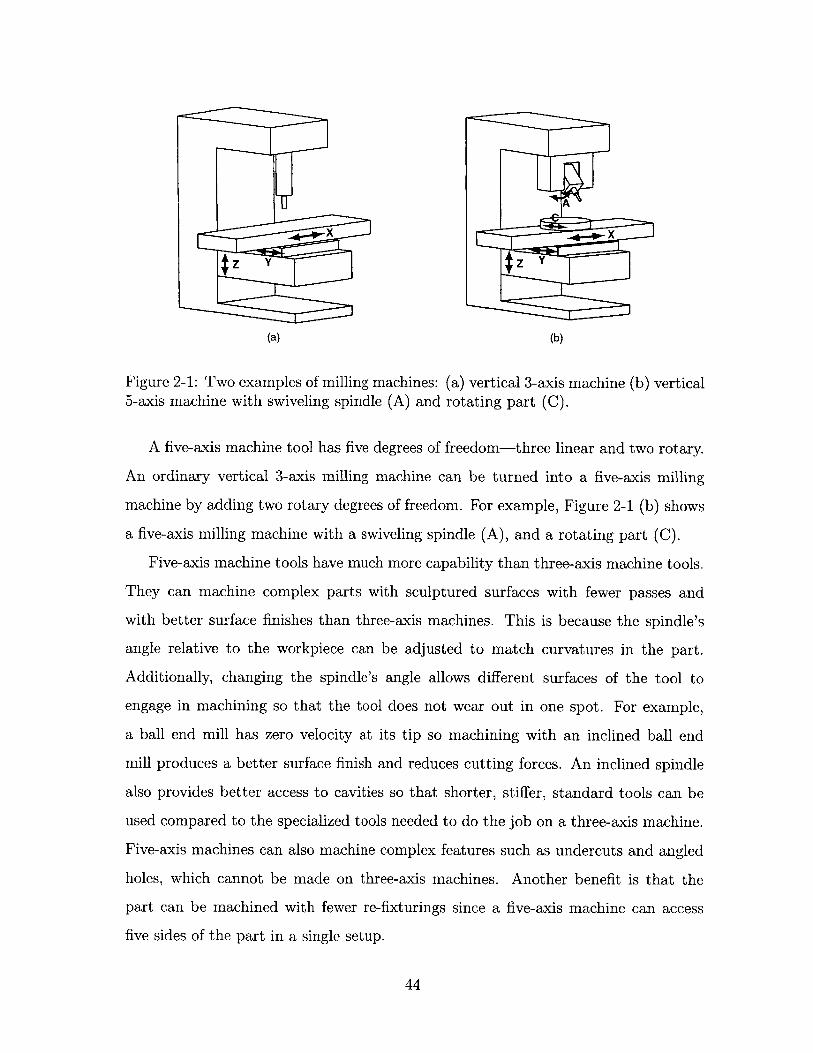
A

X xY z Y

(a) (b)

Figure 2-1: Two examples of milling machines: (a) vertical 3-axis machine (b) vertical5-axis machine with swiveling spindle (A) and rotating part (C).

A five-axis machine tool has five degrees of freedom-three linear and two rotary.

An ordinary vertical 3-axis milling machine can be turned into a five-axis milling

machine by adding two rotary degrees of freedom. For example, Figure 2-1 (b) shows

a five-axis milling machine with a swiveling spindle (A), and a rotating part (C).

Five-axis machine tools have much more capability than three-axis machine tools.

They can machine complex parts with sculptured surfaces with fewer passes and

with better surface finishes than three-axis machines. This is because the spindle's

angle relative to the workpiece can be adjusted to match curvatures in the part.

Additionally, changing the spindle's angle allows different surfaces of the tool to

engage in machining so that the tool does not wear out in one spot. For example,

a ball end mill has zero velocity at its tip so machining with an inclined ball end

mill produces a better surface finish and reduces cutting forces. An inclined spindle

also provides better access to cavities so that shorter, stiffer, standard tools can be

used compared to the specialized tools needed to do the job on a three-axis machine.

Five-axis machines can also machine complex features such as undercuts and angled

holes, which cannot be made on three-axis machines. Another benefit is that the

part can be machined with fewer re-fixturings since a five-axis machine can access

five sides of the part in a single setup.

44

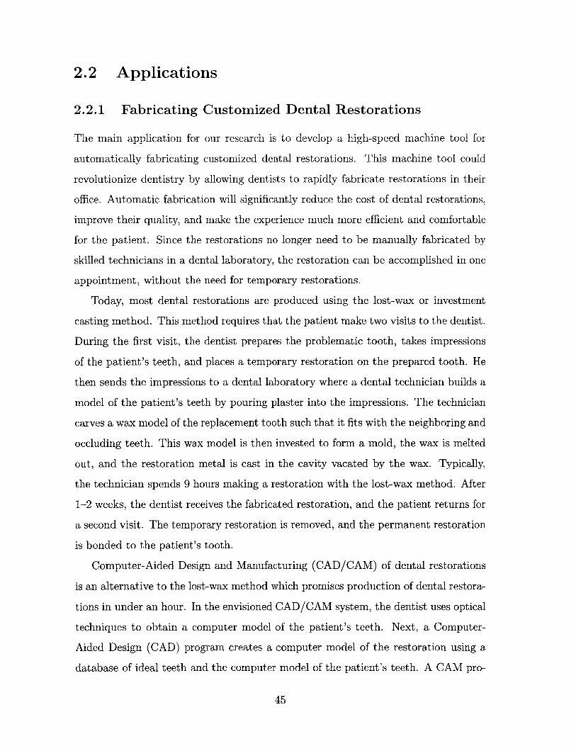
2.2 Applications

2.2.1 Fabricating Customized Dental Restorations

The main application for our research is to develop a high-speed machine tool for

automatically fabricating customized dental restorations. This machine tool could

revolutionize dentistry by allowing dentists to rapidly fabricate restorations in their

office. Automatic fabrication will significantly reduce the cost of dental restorations,

improve their quality, and make the experience much more efficient and comfortable

for the patient. Since the restorations no longer need to be manually fabricated by

skilled technicians in a dental laboratory, the restoration can be accomplished in one

appointment, without the need for temporary restorations.

Today, most dental restorations are produced using the lost-wax or investment

casting method. This method requires that the patient make two visits to the dentist.

During the first visit, the dentist prepares the problematic tooth, takes impressions

of the patient's teeth, and places a temporary restoration on the prepared tooth. He

then sends the impressions to a dental laboratory where a dental technician builds a

model of the patient's teeth by pouring plaster into the impressions. The technician

carves a wax model of the replacement tooth such that it fits with the neighboring and

occluding teeth. This wax model is then invested to form a mold, the wax is melted

out, and the restoration metal is cast in the cavity vacated by the wax. Typically,

the technician spends 9 hours making a restoration with the lost-wax method. After

1-2 weeks, the dentist receives the fabricated restoration, and the patient returns for

a second visit. The temporary restoration is removed, and the permanent restoration

is bonded to the patient's tooth.

Computer-Aided Design and Manufacturing (CAD/CAM) of dental restorations

is an alternative to the lost-wax method which promises production of dental restora-

tions in under an hour. In the envisioned CAD/CAM system, the dentist uses optical

techniques to obtain a computer model of the patient's teeth. Next, a Computer-

Aided Design (CAD) program creates a computer model of the restoration using a

database of ideal teeth and the computer model of the patient's teeth. A CAM pro-

45

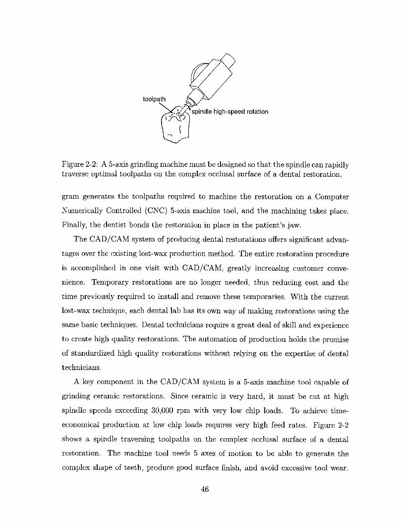
toolpath

spindle high-speed rotation

Figure 2-2: A 5-axis grinding machine must be designed so that the spindle can rapidlytraverse optimal toolpaths on the complex occlusal surface of a dental restoration.

gram generates the toolpaths required to machine the restoration on a Computer

Numerically Controlled (CNC) 5-axis machine tool, and the machining takes place.

Finally, the dentist bonds the restoration in place in the patient's jaw.

The CAD/CAM system of producing dental restorations offers significant advan-

tages over the existing lost-wax production method. The entire restoration procedure

is accomplished in one visit with CAD/CAM, greatly increasing customer conve-

nience. Temporary restorations are no longer needed, thus reducing cost and the

time previously required to install and remove these temporaries. With the current

lost-wax technique, each dental lab has its own way of making restorations using the

same basic techniques. Dental technicians require a great deal of skill and experience

to create high quality restorations. The automation of production holds the promise

of standardized high quality restorations without relying on the expertise of dental

technicians.

A key component in the CAD/CAM system is a 5-axis machine tool capable of

grinding ceramic restorations. Since ceramic is very hard, it must be cut at high

spindle speeds exceeding 30,000 rpm with very low chip loads. To achieve time-

economical production at low chip loads requires very high feed rates. Figure 2-2

shows a spindle traversing toolpaths on the complex occlusal surface of a dental

restoration. The machine tool needs 5 axes of motion to be able to generate the

complex shape of teeth, produce good surface finish, and avoid excessive tool wear.

46

The shape accuracy desired is on the order of 20 gm. The machine should also be

small enough to fit easily into a dentist's office. These requirements rule out the use

of any existing small machine tools. Large machine tools, besides requiring a large

amount of space, cannot possibly achieve the high feedrates required due to their

large inertias. Designers of existing machine tools think big, and their designs do not

readily scale down to the centimeter-scale range required for restorations.

2.2.2 Fabricating Other Small, Complex Parts

The manufacturing, medical, automotive, aerospace, and electronics industries require

many small parts with delicate features and demanding tolerances. Often each part

required has a unique geometry. This makes it inefficient to produce parts such as

molds, dies, and dental restorations with electrical-discharge machining or investment

casting techniques as is the current practice. A direct 5-axis CNC machining operation

will be a superior way of producing these parts. It will allow for faster and easier

fabrication, lower costs, more accurate parts, and more flexibility. Unfortunately

no small, accurate 5-axis machine tools exist today which can produce these parts

efficiently.

In addition to dental restorations, examples of small, complex parts that require

5-axis machining are aerospace components, heart valves, EDM electrodes, gear set

pinions and wheels, indexing cams, jewelry, optical lenses, musical instrument com-

ponents, compressor screw pairs, turbines, mold cavities, impellers, and prosthetics.

2.3 Classification of Existing Topologies

Before embarking on the design of a new five-axis machine tool, in this section we

survey and classify existing five-axis machine tool topologies. The American Society

of Mechanical Engineers's (ASME) Methods for Performance Evaluation of Com-

puter Numerically Controlled Machining Centers [3] provides a nice classification of

three-axis machine tools. Three-axis machine tools, like the vertical three-axis mill of

Figure 2-1 (a), generally provide three linear degrees of freedom between the spindle

47

and the workpiece. The ASME standard first differentiates between horizontal spin-

dle and vertical spindle machines. Horizontal spindle machines are further classified

based on the column's motion. There are horizontal machines with a fixed column,

a traveling column, and a traveling column with a fixed table. Vertical machines are

classified based on column or gantry motion. There are vertical machines with a fixed

column, a traveling column, and a movable column with a fixed table. The vertical

gantry machines are split into fixed bridge machines and traveling gantry machines.

A five-axis machine provides five degrees of freedom-three linear and two rotary-

between the tool and the part. Figure 2-1 (b) shows a five-axis milling machine with

a swiveling spindle and a rotating part. The ASME standard provides only two rep-

resentative examples of five-axis machines and does not attempt a full classification

of five-axis machines. This may be because there are so many permutations of axes

possible in a five-axis machine tool that we cannot hope to distinctly classify every

possible configuration. For example, there are 720 ways of placing the X, Y,Z, A,

and B axes on either the spindle or the workpiece when different stacking orders of

the axes are distinct:

5P5 - 1 +5 P4 -1P1 +5P3 -2P2 +5 P2 -3P3 +5 P1 -4P4 + 1 .P 5 = 720

Here ,Pk is the number of permutations of n objects taken k at a time,

n Pk = n!(n - k)!

We propose a classification of existing serial five-axis machines based mainly on

their rotary axes. It is the rotary axes, after all, that distinguish five-axis machines

from their more ordinary cousins, the three-axis machines. The classification of ex-

isting five-axis machines is further simplified by the fact that rotary axes are usually

stacked on top of linear axes and not vice versa. For example, it is common to stack a

rotary axis on top of an X-Y table, but rarely, if ever, would the X-Y table be stacked

on top of a rotary axis. Since our classification is based on the two rotary axes, each

of our five-axis machine categories includes a large number of permutations based on

48

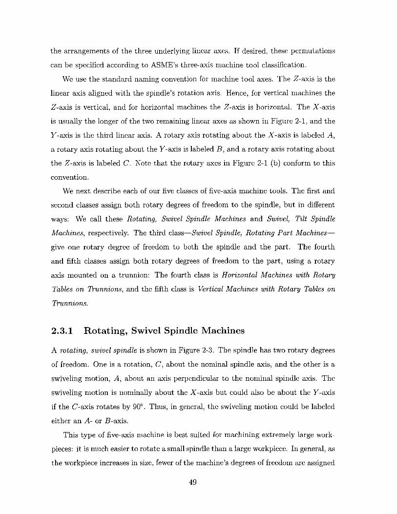
the arrangements of the three underlying linear axes. If desired, these permutations

can be specified according to ASME's three-axis machine tool classification.

We use the standard naming convention for machine tool axes. The Z-axis is the

linear axis aligned with the spindle's rotation axis. Hence, for vertical machines the

Z-axis is vertical, and for horizontal machines the Z-axis is horizontal. The X-axis

is usually the longer of the two remaining linear axes as shown in Figure 2-1, and the

Y-axis is the third linear axis. A rotary axis rotating about the X-axis is labeled A,

a rotary axis rotating about the Y-axis is labeled B, and a rotary axis rotating about

the Z-axis is labeled C. Note that the rotary axes in Figure 2-1 (b) conform to this

convention.

We next describe each of our five classes of five-axis machine tools. The first and

second classes assign both rotary degrees of freedom to the spindle, but in different

ways: We call these Rotating, Swivel Spindle Machines and Swivel, Tilt Spindle

Machines, respectively. The third class-Swivel Spindle, Rotating Part Machines-

give one rotary degree of freedom to both the spindle and the part. The fourth

and fifth classes assign both rotary degrees of freedom to the part, using a rotary

axis mounted on a trunnion: The fourth class is Horizontal Machines with Rotary

Tables on Trunnions, and the fifth class is Vertical Machines with Rotary Tables on

Trunnions.

2.3.1 Rotating, Swivel Spindle Machines

A rotating, swivel spindle is shown in Figure 2-3. The spindle has two rotary degrees

of freedom. One is a rotation, C, about the nominal spindle axis, and the other is a

swiveling motion, A, about an axis perpendicular to the nominal spindle axis. The

swiveling motion is nominally about the X-axis but could also be about the Y-axis

if the C-axis rotates by 900. Thus, in general, the swiveling motion could be labeled

either an A- or B-axis.

This type of five-axis machine is best suited for machining extremely large work-

pieces: it is much easier to rotate a small spindle than a large workpiece. In general, as

the workpiece increases in size, fewer of the machine's degrees of freedom are assigned

49

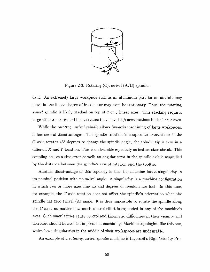
A

Figure 2-3: Rotating (C), swivel (A/B) spindle.

to it. An extremely large workpiece such as an aluminum part for an aircraft may

move in one linear degree of freedom or may even be stationary. Thus, the rotating,

swivel spindle is likely stacked on top of 2 or 3 linear axes. This stacking requires

large stiff structures and big actuators to achieve high accelerations in the linear axes.

While the rotating, swivel spindle allows five-axis machining of large workpieces,

it has several disadvantages. The spindle rotation is coupled to translation: if the

C axis rotates 450 degrees to change the spindle angle, the spindle tip is now in a

different X and Y location. This is undesirable especially as feature sizes shrink. This

coupling causes a sine error as well: an angular error in the spindle axis is magnified

by the distance between the spindle's axis of rotation and the tooltip.

Another disadvantage of this topology is that the machine has a singularity in

its nominal position with no swivel angle. A singularity is a machine configuration

in which two or more axes line up and degrees of freedom are lost. In this case,

for example, the C-axis rotation does not affect the spindle's orientation when the

spindle has zero swivel (A) angle. It is thus impossible to rotate the spindle along

the C-axis, no matter how much control effort is expended in any of the machine's

axes. Such singularities cause control and kinematic difficulties in their vicinity and

therefore should be avoided in precision machining. Machine topologies, like this one,

which have singularities in the middle of their workspaces are undesirable.

An example of a rotating, swivel spindle machine is Ingersoll's High Velocity Pro-

50

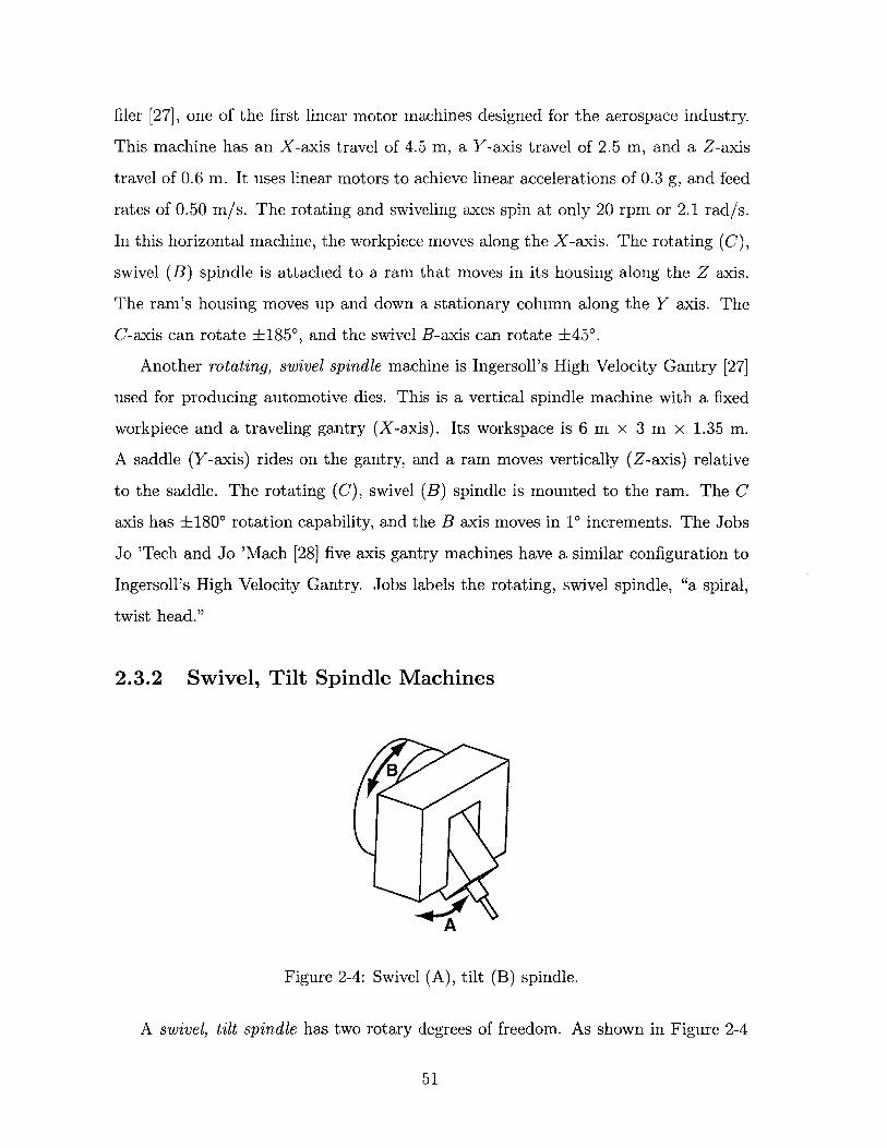
filer [27], one of the first linear motor machines designed for the aerospace industry.

This machine has an X-axis travel of 4.5 m, a Y-axis travel of 2.5 m, and a Z-axis

travel of 0.6 m. It uses linear motors to achieve linear accelerations of 0.3 g, and feed

rates of 0.50 m/s. The rotating and swiveling axes spin at only 20 rpm or 2.1 rad/s.

In this horizontal machine, the workpiece moves along the X-axis. The rotating (C),swivel (B) spindle is attached to a ram that moves in its housing along the Z axis.

The ram's housing moves up and down a stationary column along the Y axis. The

C-axis can rotate ±1850, and the swivel B-axis can rotate ±450.

Another rotating, swivel spindle machine is Ingersoll's High Velocity Gantry [27]

used for producing automotive dies. This is a vertical spindle machine with a fixed

workpiece and a traveling gantry (X-axis). Its workspace is 6 m x 3 m x 1.35 m.

A saddle (Y-axis) rides on the gantry, and a ram moves vertically (Z-axis) relative

to the saddle. The rotating (C), swivel (B) spindle is mounted to the ram. The C

axis has ±180' rotation capability, and the B axis moves in 10 increments. The Jobs

Jo 'Tech and Jo 'Mach [28] five axis gantry machines have a similar configuration to

Ingersoll's High Velocity Gantry. Jobs labels the rotating, swivel spindle, "a spiral,

twist head."

2.3.2 Swivel, Tilt Spindle Machines

B

A

Figure 2-4: Swivel (A), tilt (B) spindle.

A swivel, tilt spindle has two rotary degrees of freedom. As shown in Figure 2-4

51

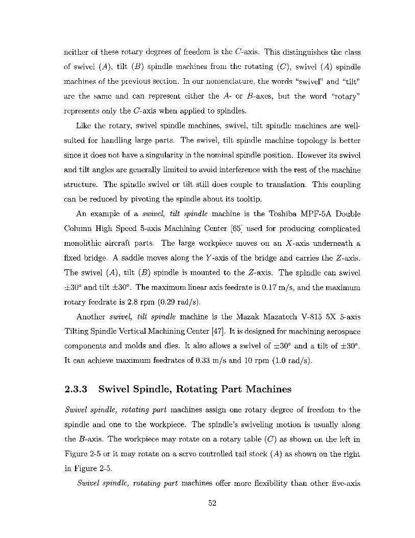
neither of these rotary degrees of freedom is the C-axis. This distinguishes the class

of swivel (A), tilt (B) spindle machines from the rotating (C), swivel (A) spindle

machines of the previous section. In our nomenclature, the words "swivel" and "tilt"

are the same and can represent either the A- or B-axes, but the word "rotary"

represents only the C-axis when applied to spindles.

Like the rotary, swivel spindle machines, swivel, tilt spindle machines are well-

suited for handling large parts. The swivel, tilt spindle machine topology is better

since it does not have a singularity in the nominal spindle position. However its swivel

and tilt angles are generally limited to avoid interference with the rest of the machine

structure. The spindle swivel or tilt still does couple to translation. This coupling

can be reduced by pivoting the spindle about its tooltip.

An example of a swivel, tilt spindle machine is the Toshiba MPF-5A Double

Column High Speed 5-axis Machining Center [65] used for producing complicated

monolithic aircraft parts. The large workpiece moves on an X-axis underneath a

fixed bridge. A saddle moves along the Y-axis of the bridge and carries the Z-axis.

The swivel (A), tilt (B) spindle is mounted to the Z-axis. The spindle can swivel

±300 and tilt ±30'. The maximum linear axis feedrate is 0.17 m/s, and the maximum

rotary feedrate is 2.8 rpm (0.29 rad/s).

Another swivel, tilt spindle machine is the Mazak Mazatech V-815 5X 5-axis

Tilting Spindle Vertical Machining Center [47]. It is designed for machining aerospace

components and molds and dies. It also allows a swivel of +30' and a tilt of ±30'.

It can achieve maximum feedrates of 0.33 m/s and 10 rpm (1.0 rad/s).

2.3.3 Swivel Spindle, Rotating Part Machines

Swivel spindle, rotating part machines assign one rotary degree of freedom to the

spindle and one to the workpiece. The spindle's swiveling motion is usually along

the B-axis. The workpiece may rotate on a rotary table (C) as shown on the left in

Figure 2-5 or it may rotate on a servo controlled tail stock (A) as shown on the right

in Figure 2-5.

Swivel spindle, rotating part machines offer more flexibility than other five-axis

52

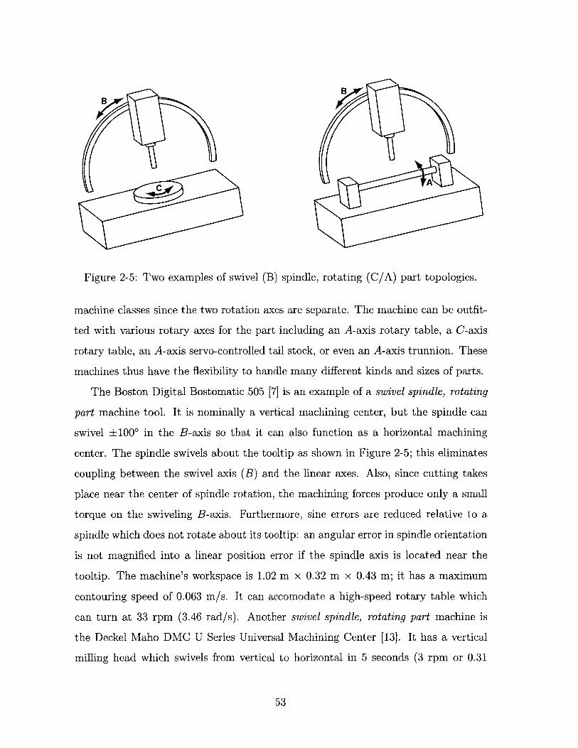
Figure 2-5: Two examples of swivel (B) spindle, rotating (C/A) part topologies.

machine classes since the two rotation axes are separate. The machine can be outfit-

ted with various rotary axes for the part including an A-axis rotary table, a C-axis

rotary table, an A-axis servo-controlled tail stock, or even an A-axis trunnion. These

machines thus have the flexibility to handle many different kinds and sizes of parts.

The Boston Digital Bostomatic 505 [7] is an example of a swivel spindle, rotating

part machine tool. It is nominally a vertical machining center, but the spindle can

swivel ±1000 in the B-axis so that it can also function as a horizontal machining

center. The spindle swivels about the tooltip as shown in Figure 2-5; this eliminates

coupling between the swivel axis (B) and the linear axes. Also, since cutting takes

place near the center of spindle rotation, the machining forces produce only a small

torque on the swiveling B-axis. Furthermore, sine errors are reduced relative to a

spindle which does not rotate about its tooltip: an angular error in spindle orientation

is not magnified into a linear position error if the spindle axis is located near the

tooltip. The machine's workspace is 1.02 m x 0.32 m x 0.43 m; it has a maximum

contouring speed of 0.063 m/s. It can accomodate a high-speed rotary table which

can turn at 33 rpm (3.46 rad/s). Another swivel spindle, rotating part machine is

the Deckel Maho DMC U Series Universal Machining Center [13]. It has a vertical

milling head which swivels from vertical to horizontal in 5 seconds (3 rpm or 0.31

53

AqC

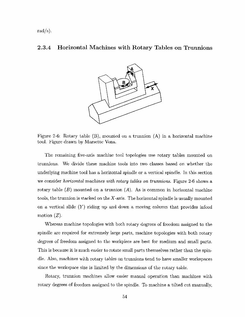
rad/s).

2.3.4 Horizontal Machines with Rotary Tables on Trunnions

BX

Figure 2-6: Rotary table (B), mounted on a trunnion (A) in a horizontal machinetool. Figure drawn by Marsette Vona.

The remaining five-axis machine tool topologies use rotary tables mounted on

trunnions. We divide these machine tools into two classes based on whether the

underlying machine tool has a horizontal spindle or a vertical spindle. In this section

we consider horizontal machines with rotary tables on trunnions. Figure 2-6 shows a

rotary table (B) mounted on a trunnion (A). As is common in horizontal machine

tools, the trunnion is stacked on the X-axis. The horizontal spindle is usually mounted

on a vertical slide (Y) riding up and down a moving column that provides infeed

motion (Z).

Whereas machine topologies with both rotary degrees of freedom assigned to the

spindle are required for extremely large parts, machine topologies with both rotary

degrees of freedom assigned to the workpiece are best for medium and small parts.

This is because it is much easier to rotate small parts themselves rather than the spin-

dle. Also, machines with rotary tables on trunnions tend to have smaller workspaces

since the workspace size is limited by the dimensions of the rotary table.

Rotary, trunnion machines allow easier manual operation than machines with

rotary degrees of freedom assigned to the spindle. To machine a tilted cut manually,

54

the workpiece is tilted and rotated to the appropriate plane, and the operator can

proceed as if he were using a 3-axis machine. In a rotating, swivel spindle machine,

however, the spindle is at an angle, so it is not easy to make a tilted cut manually.

Horizontal rotary trunnion machines do not have a singularity in the nominal posi-

tion of the rotary axes. Vertical rotary trunnion machines do have a singularity since

the spindle axis is aligned with the rotary table's axis (C for vertical machines). Also,

chips fall off of horizontal spindle machines better than vertical spindle machines.

Makino's MC-5XA series of 5-axis machining centers [45] are examples of horizon-

tal machines with rotary tables on trunnions. They have the standard configuration

of axes mentioned for this machine tool topology: the trunnion is on an X-axis slide,

and the spindle is on a vertical slide (Y) on a moving column (Z). The smallest

machine in the series, the MC56-5XA has a maximum workpiece diameter of 0.6 m.

The trunnion (A) has a 1200 travel (+20' to -1000), and the rotary table (B) can

rotate 3600. The maximum feedrates for the linear axes are 0.2 m/s; for the trunnion

axis the maximum feedrate is 2.8 rpm (0.3 rad/s), and for the rotary table it is 4.7

rpm (0.5 rad/s).

Many other machine tools have a similar topology:

* Toshiba's BMC 1000 (5), Horizontal Machining Center (5-Axis Control) [65]

" Mazak's Mazatech H-630 5X, 5-Axis Simultaneously Controlled Horizontal Ma-

chining Center [47]

* Yasda's YBM700/900-NTT, 5-Axis Precision Center [78]

* Deckel Maho's DMU-P Series with NC swivel rotary table [13]

Most horizontal machines have a rotary axis (B) mounted on a trunnion (A).

However, Makino's MC-5XB [45] has a trunnion-like axis (A) mounted on a rotary

axis (B). This machine topology reverses the order of the two rotary axes, so we

classify it as a sub-class within horizontal machines with rotary tables on trunnions.

It allows for larger workpieces, up to 2.2 m in diameter, than Makino's MC-5XA line

of regular rotary on trunnion machines. However, the feedrates, are much slower since

55

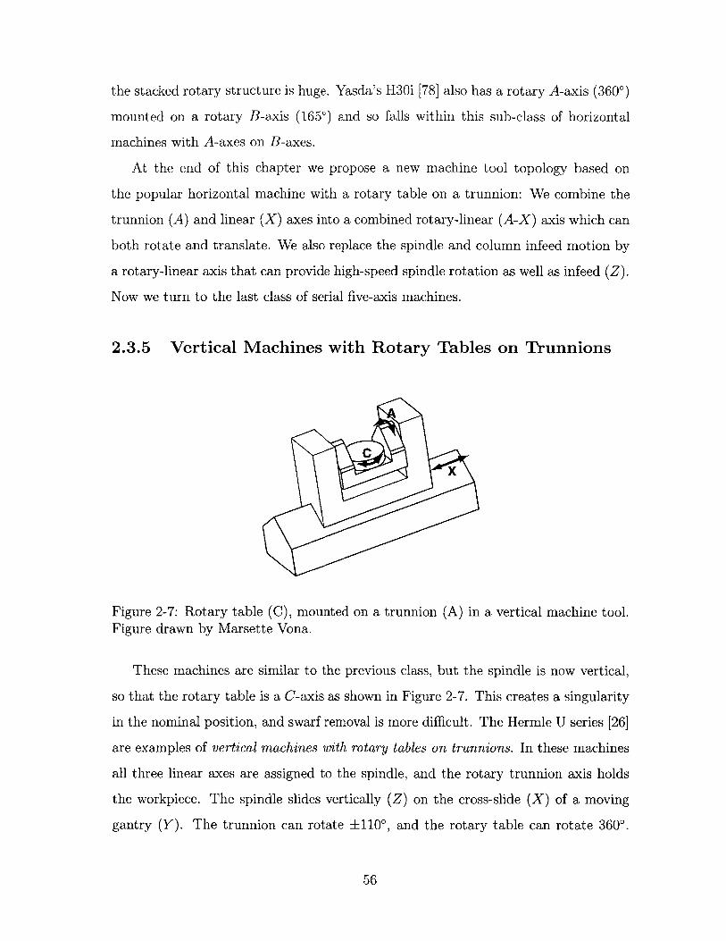
the stacked rotary structure is huge. Yasda's H30i [78] also has a rotary A-axis (3600)

mounted on a rotary B-axis (1650) and so falls within this sub-class of horizontal

machines with A-axes on B-axes.

At the end of this chapter we propose a new machine tool topology based on

the popular horizontal machine with a rotary table on a trunnion: We combine the

trunnion (A) and linear (X) axes into a combined rotary-linear (A-X) axis which can

both rotate and translate. We also replace the spindle and column infeed motion by

a rotary-linear axis that can provide high-speed spindle rotation as well as infeed (Z).

Now we turn to the last class of serial five-axis machines.

2.3.5 Vertical Machines with Rotary Tables on Trunnions

CX

Figure 2-7: Rotary table (C), mounted on a trunnion (A) in a vertical machine tool.Figure drawn by Marsette Vona.

These machines are similar to the previous class, but the spindle is now vertical,

so that the rotary table is a C-axis as shown in Figure 2-7. This creates a singularity

in the nominal position, and swarf removal is more difficult. The Hermle U series [26]

are examples of vertical machines with rotary tables on trunnions. In these machines

all three linear axes are assigned to the spindle, and the rotary trunnion axis holds

the workpiece. The spindle slides vertically (Z) on the cross-slide (X) of a moving

gantry (Y). The trunnion can rotate +1100, and the rotary table can rotate 360'.

56

Other vertical rotary, trunnion machines include Mikron's UCP710 [49] and Makino's

V55-5XA [45].

The Mori Seiki M-400C1 [50] and Deckel Maho DMU50 [13] machines have slightly

different topologies. In both these machines the trunnion is arranged sideways so

that the trunnion axis is a B-axis rather than an A-axis. These two machines form a

subclass of sideways trunnion vertical machines.

2.4 Toolpath Generation

Usually a machine is designed without regard for toolpaths, and then the Computer-

Aided Manufacturing (CAM) program must make do with the machine's limited

feedrates and accelerations. In machining complex centimeter-scale parts, the accel-

erations are so high that the machine must be specifically designed with the toolpaths

in mind in order to achieve good performance. High rotary accelerations are espe-

cially crucial as the part size decreases, and most existing machine tools have very

low rotary accelerations. Our rotary-linear axis can achieve high rotary and linear

accelerations since it reduces the coupling and stacking of axes and keeps inertias low.

Thus, it is a natural choice for use in machining small, complex parts.

Many researchers have investigated aspects of toolpath generation. In practice,

most toolpaths are currently generated by using isocurves of the parametric sur-

face representation or by intersecting the desired surface with equally-spaced planes

resulting in a contour plot suitable for 3-axis milling. Two main goals of toolpath gen-

eration are to achieve the minimum toolpath length and the minimum cusp height.

These are competing goals since cusp height can be reduced by moving toolpaths

closer together, but this increases the toolpath length. Elber and Cohen [17] present

an algorithm to adaptively develop isocurves for 5-axis milling. Choi [9] addresses

the issue of generating the cutter location data, the tool's orientation at each point

along the toolpath, in 5-axis machining given a specified toolpath. The goal is to

minimize cusp height. Morishige [51] presents a collision avoidance algorithm for use

in generating cutter location data.

57

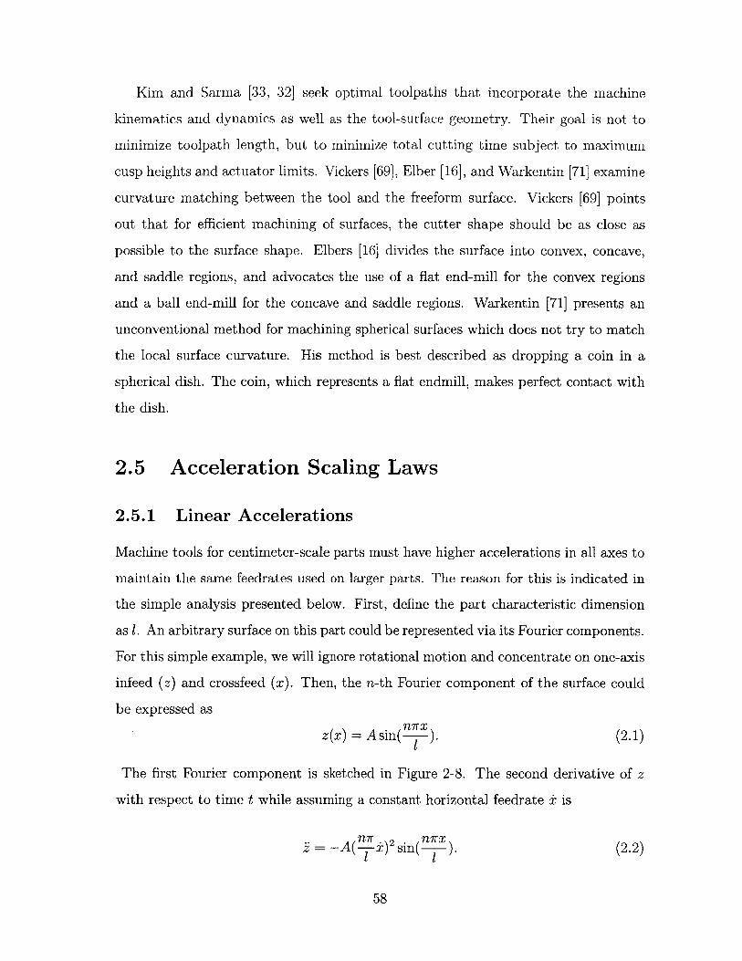
Kim and Sarma [33, 32] seek optimal toolpaths that incorporate the machine

kinematics and dynamics as well as the tool-surface geometry. Their goal is not to

minimize toolpath length, but to minimize total cutting time subject to maximum

cusp heights and actuator limits. Vickers [69], Elber [16], and Warkentin [71] examine

curvature matching between the tool and the freeform surface. Vickers [69] points

out that for efficient machining of surfaces, the cutter shape should be as close as

possible to the surface shape. Elbers [16] divides the surface into convex, concave,

and saddle regions, and advocates the use of a flat end-mill for the convex regions

and a ball end-mill for the concave and saddle regions. Warkentin [71] presents an

unconventional method for machining spherical surfaces which does not try to match

the local surface curvature. His method is best described as dropping a coin in a

spherical dish. The coin, which represents a flat endmill, makes perfect contact with

the dish.

2.5 Acceleration Scaling Laws

2.5.1 Linear Accelerations

Machine tools for centimeter-scale parts must have higher accelerations in all axes to

maintain the same feedrates used on larger parts. The reason for this is indicated in

the simple analysis presented below. First, define the part characteristic dimension

as 1. An arbitrary surface on this part could be represented via its Fourier components.

For this simple example, we will ignore rotational motion and concentrate on one-axis

infeed (z) and crossfeed (x). Then, the n-th Fourier component of the surface could

be expressed asnrr

z(x) = A sin( ). (2.1)1

The first Fourier component is sketched in Figure 2-8. The second derivative of z

with respect to time t while assuming a constant horizontal feedrate ± is

= -A( .±)2 sin( "). (2.2)

58

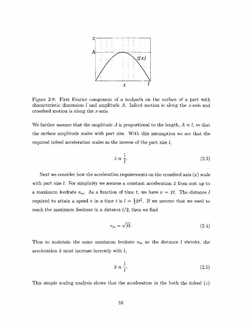
z

Zx)

Figure 2-8: First Fourier component of a toolpath on the surface of a part withcharacteristic dimension 1 and amplitude A. Infeed motion is along the z-axis andcrossfeed motion is along the x-axis.

We further assume that the amplitude A is proportional to the length, A oc 1, so that

the surface amplitude scales with part size. With this assumption we see that the

required infeed acceleration scales as the inverse of the part size 1,

1 C (2.3)1

Next we consider how the acceleration requirements on the crossfeed axis (x) scale

with part size 1. For simplicity we assume a constant acceleration z from rest up to

a maximum feedrate vm. As a function of time t, we have v = ,t. The distance 1

required to attain a speed v in a time t is 1 = pt2. If we assume that we need to

reach the maximum feedrate in a distance 1/2, then we find

Vm = V T. (2.4)

Thus to maintain the same maximum feedrate Vm as the distance 1 shrinks, the

acceleration z must increase inversely with 1,

1 C (2.5)1

This simple scaling analysis shows that the acceleration in the both the infeed (z)

59

/

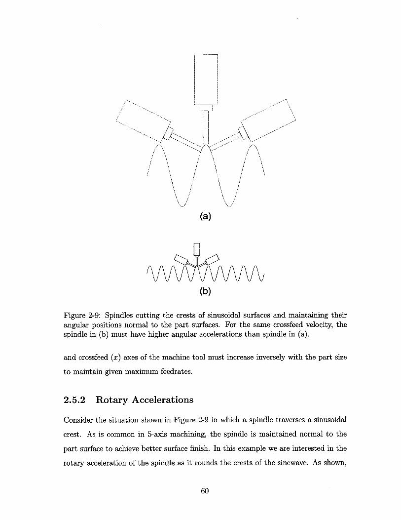
(a)

(b)

Figure 2-9: Spindles cutting the crests of sinusoidal surfaces and maintaining theirangular positions normal to the part surfaces. For the same crossfeed velocity, thespindle in (b) must have higher angular accelerations than spindle in (a).

and crossfeed (x) axes of the machine tool must increase inversely with the part size

to maintain given maximum feedrates.

2.5.2 Rotary Accelerations

Consider the situation shown in Figure 2-9 in which a spindle traverses a sinusoidal

crest. As is common in 5-axis machining, the spindle is maintained normal to the

part surface to achieve better surface finish. In this example we are interested in the

rotary acceleration of the spindle as it rounds the crests of the sinewave. As shown,

60

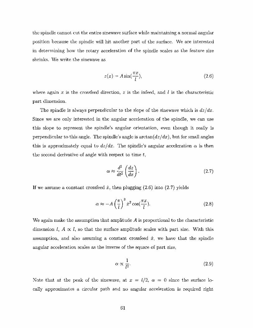
the spindle cannot cut the entire sinewave surface while maintaining a normal angular

position because the spindle will hit another part of the surface. We are interested

in determining how the rotary acceleration of the spindle scales as the feature size

shrinks. We write the sinewave as

z(x) = A sin( ), (2.6)

where again x is the crossfeed direction, z is the infeed, and 1 is the characteristic

part dimension.

The spindle is always perpendicular to the slope of the sinewave which is dz/dx.

Since we are only interested in the angular acceleration of the spindle, we can use

this slope to represent the spindle's angular orientation, even though it really is

perpendicular to this angle. The spindle's angle is arctan(dz/dx), but for small angles

this is approximately equal to dz/dx. The spindle's angular acceleration a is then

the second derivative of angle with respect to time t,

a~ d2 dz'. (2.7)TOj '\dx,)

If we assume a constant crossfeed ±, then plugging (2.6) into (2.7) yields

7,T 3 rX7

a ~ -A (--) 2 cos(T). (2.8)

We again make the assumption that amplitude A is proportional to the characteristic

dimension 1, A oc 1, so that the surface amplitude scales with part size. With this

assumption, and also assuming a constant crossfeed i-, we have that the spindle

angular acceleration scales as the inverse of the square of part size,

a oc (2.9)

Note that at the peak of the sinewave, at x = 1/2, a = 0 since the surface lo-

cally approximates a circular path and no angular acceleration is required right

61

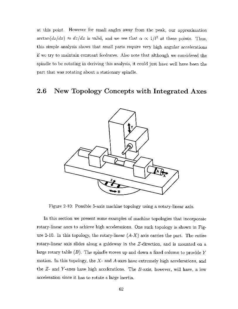
at this point. However for small angles away from the peak, our approximation

arctan(dz/dx) _ dz/dx is valid, and we see that a oc 1/12 at these points. Thus,

this simple analysis shows that small parts require very high angular accelerations

if we try to maintain constant feedrates. Also note that although we considered the

spindle to be rotating in deriving this analysis, it could just have well have been the

part that was rotating about a stationary spindle.

2.6 New Topology Concepts with Integrated Axes

A

z

VB

Figure 2-10: Possible 5-axis machine topology using a rotary-linear axis.

In this section we present some examples of machine topologies that incorporate

rotary-linear axes to achieve high accelerations. One such topology is shown in Fig-

ure 2-10. In this topology, the rotary-linear (A-X) axis carries the part. The entire

rotary-linear axis slides along a guideway in the Z-direction, and is mounted on a

large rotary table (B). The spindle moves up and down a fixed column to provide Y

motion. In this topology, the X- and A-axes have extremely high accelerations, and

the Z- and Y-axes have high accelerations. The B-axis, however, will have, a low

acceleration since it has to rotate a large inertia.

62

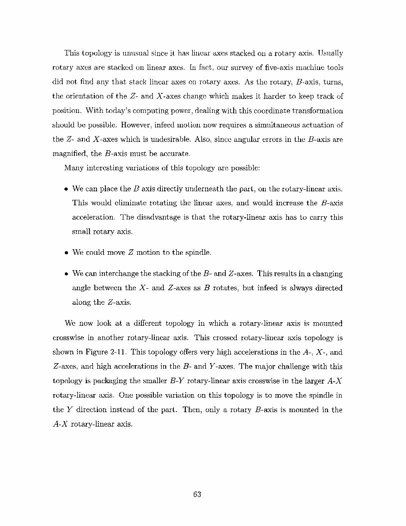
This topology is unusual since it has linear axes stacked on a rotary axis. Usually

rotary axes are stacked on linear axes. In fact, our survey of five-axis machine tools

did not find any that stack linear axes on rotary axes. As the rotary, B-axis, turns,

the orientation of the Z- and X-axes change which makes it harder to keep track of

position. With today's computing power, dealing with this coordinate transformation

should be possible. However, infeed motion now requires a simultaneous actuation of

the Z- and X-axes which is undesirable. Also, since angular errors in the B-axis are

magnified, the B-axis must be accurate.

Many interesting variations of this topology are possible:

" We can place the B axis directly underneath the part, on the rotary-linear axis.

This would eliminate rotating the linear axes, and would increase the B-axis

acceleration. The disadvantage is that the rotary-linear axis has to carry this

small rotary axis.

" We could move Z motion to the spindle.

* We can interchange the stacking of the B- and Z-axes. This results in a changing

angle between the X- and Z-axes as B rotates, but infeed is always directed

along the Z-axis.

We now look at a different topology in which a rotary-linear axis is mounted

crosswise in another rotary-linear axis. This crossed rotary-linear axis topology is

shown in Figure 2-11. This topology offers very high accelerations in the A-, X-, and

Z-axes, and high accelerations in the B- and Y-axes. The major challenge with this

topology is packaging the smaller B-Y rotary-linear axis crosswise in the larger A-X

rotary-linear axis. One possible variation on this topology is to move the spindle in

the Y direction instead of the part. Then, only a rotary B-axis is mounted in the

A-X rotary-linear axis.

63

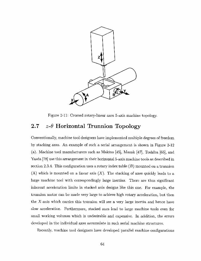
Z

YA B

X

Figure 2-11: Crossed rotary-linear axes 5-axis machine topology.

2.7 z-0 Horizontal Trunnion Topology

Conventionally, machine tool designers have implemented multiple degrees of freedom

by stacking axes. An example of such a serial arrangement is shown in Figure 2-12

(a). Machine tool manufacturers such as Makino [45], Mazak [47], Toshiba [65], and

Yasda [78] use this arrangement in their horizontal 5-axis machine tools as described in

section 2.3.4. This configuration uses a rotary index table (B) mounted on a trunnion

(A) which is mounted on a linear axis (X). The stacking of axes quickly leads to a

large machine tool with correspondingly large inertias. There are thus significant

inherent acceleration limits in stacked axis designs like this one. For example, the

trunnion motor can be made very large to achieve high rotary acceleration, but then

the X-axis which carries this trunnion will see a very large inertia and hence have

slow acceleration. Furthermore, stacked axes lead to large machine tools even for

small working volumes which is undesirable and expensive. In addition, the errors

developed in the individual axes accumulate in such serial machine structures.

Recently, machine tool designers have developed parallel machine configurations

64

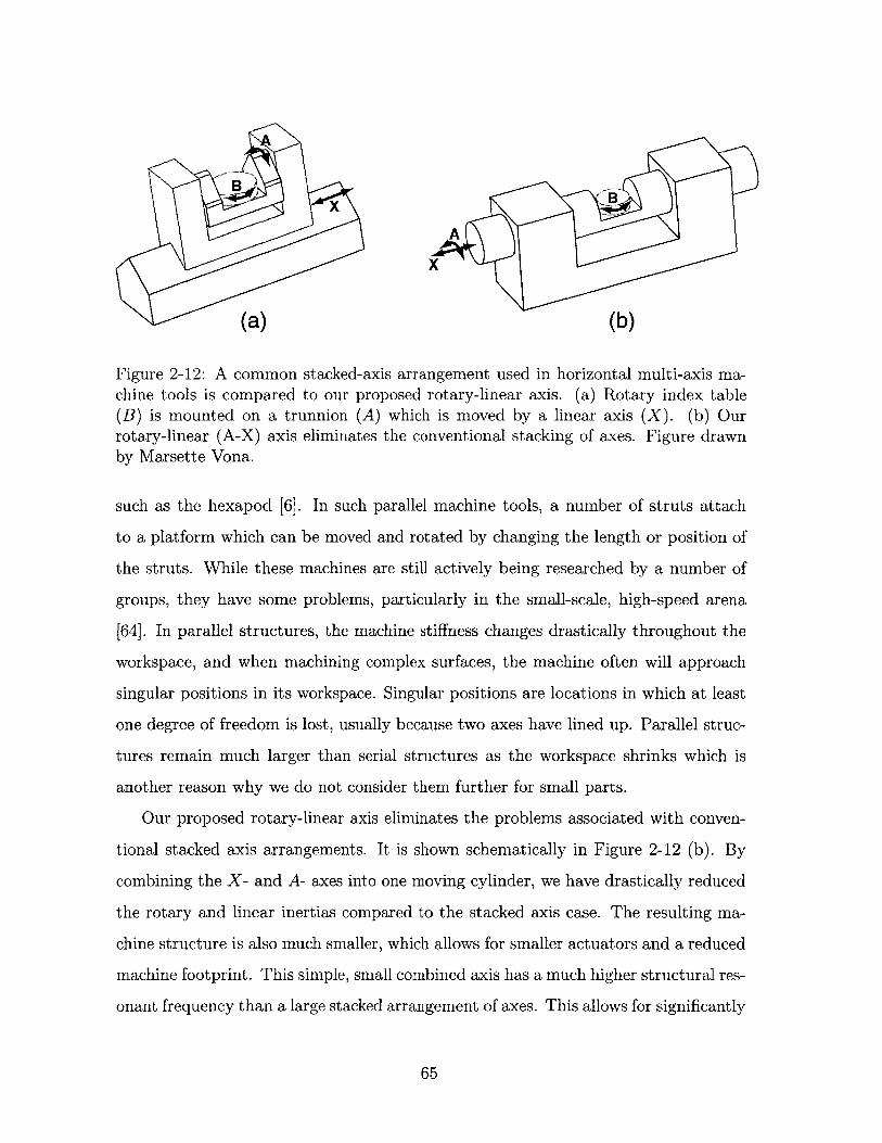
A

X

(a) (b)

Figure 2-12: A common stacked-axis arrangement used in horizontal multi-axis ma-

chine tools is compared to our proposed rotary-linear axis. (a) Rotary index table

(B) is mounted on a trunnion (A) which is moved by a linear axis (X). (b) Ourrotary-linear (A-X) axis eliminates the conventional stacking of axes. Figure drawn

by Marsette Vona.

such as the hexapod [6]. In such parallel machine tools, a number of struts attach

to a platform which can be moved and rotated by changing the length or position of

the struts. While these machines are still actively being researched by a number of

groups, they have some problems, particularly in the small-scale, high-speed arena

[64]. In parallel structures, the machine stiffness changes drastically throughout the

workspace, and when machining complex surfaces, the machine often will approach

singular positions in its workspace. Singular positions are locations in which at least

one degree of freedom is lost, usually because two axes have lined up. Parallel struc-

tures remain much larger than serial structures as the workspace shrinks which is

another reason why we do not consider them further for small parts.

Our proposed rotary-linear axis eliminates the problems associated with conven-

tional stacked axis arrangements. It is shown schematically in Figure 2-12 (b). By

combining the X- and A- axes into one moving cylinder, we have drastically reduced

the rotary and linear inertias compared to the stacked axis case. The resulting ma-

chine structure is also much smaller, which allows for smaller actuators and a reduced

machine footprint. This simple, small combined axis has a much higher structural res-

onant frequency than a large stacked arrangement of axes. This allows for significantly

65

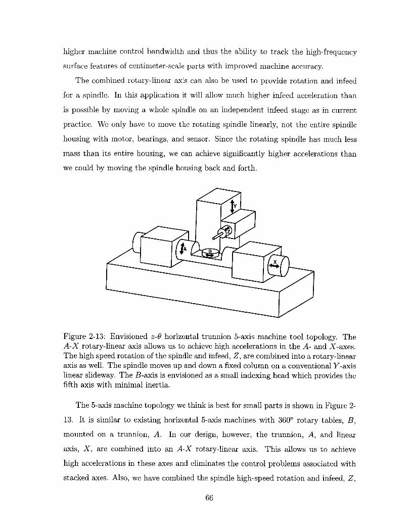
higher machine control bandwidth and thus the ability to track the high-frequency

surface features of centimeter-scale parts with improved machine accuracy.

The combined rotary-linear axis can also be used to provide rotation and infeed

for a spindle. In this application it will allow much higher infeed acceleration than

is possible by moving a whole spindle on an independent infeed stage as in current

practice. We only have to move the rotating spindle linearly, not the entire spindle

housing with motor, bearings, and sensor. Since the rotating spindle has much less

mass than its entire housing, we can achieve significantly higher accelerations than

we could by moving the spindle housing back and forth.

Y

JA B

Figure 2-13: Envisioned z-0 horizontal trunnion 5-axis machine tool topology. TheA-X rotary-linear axis allows us to achieve high accelerations in the A- and X-axes.The high speed rotation of the spindle and infeed, Z, are combined into a rotary-linearaxis as well. The spindle moves up and down a fixed column on a conventional Y-axislinear slideway. The B-axis is envisioned as a small indexing head which provides thefifth axis with minimal inertia.

The 5-axis machine topology we think is best for small parts is shown in Figure 2-

13. It is similar to existing horizontal 5-axis machines with 3600 rotary tables, B,

mounted on a trunnion, A. In our design, however, the trunnion, A, and linear

axis, X, are combined into an A-X rotary-linear axis. This allows us to achieve

high accelerations in these axes and eliminates the control problems associated with

stacked axes. Also, we have combined the spindle high-speed rotation and infeed, Z,

66

into a rotary-linear axis as well. For this spindle application, the rotary-linear axis

does not require precision rotary sensing, only precision linear sensing.

The inclusion of a continuous B-axis may add considerable inertia to the rotary-

linear axis. Thus, we have chosen to use an indexed B-axis instead of a continuous

axis. This indexed axis allows for five-sided machining and allows the rotary-linear

axis to achieve higher accelerations. The only functionality lost by indexing this axis

is the ability to drill arbitrarily angled holes which is not often required. It is still

possible to machine freeform surfaces with three or four continuous axes when the

other axes are indexed. Suh and Lee [62] present a method for machining freeform

surfaces with one or two indexed axes that minimizes the number of times the index

table needs to be indexed. Our design further reduces the added inertia of this index

table by offloading its actuator. Thus, in order to index the table, the rotary-linear

axis would return to a home position, and a mechanical reach-in actuator would

engage the index table.

Our design assigns both rotary degrees of freedom to the centimeter-scale part

since it has a much smaller rotary inertia than the spindle. This is because the part

is roughly a centimeter cube, whereas the spindle is larger and has significant length.

The rotary inertia of a long cylinder with mass m and length 1 about one end is

m12 /3. Thus, since the spindle has more mass than the part and has a length longer

than a centimeter it will have a much higher rotary inertia than the part does.

The combined rotary-linear axis with index table that carries the workpiece pro-

vides three degrees of freedom for nearly the mass and inertia of one conventional

rotary degree of freedom. The spindle combined with infeed motion allows us to just

move the rotating spindle, not the whole spindle housing. In effect, we get the spindle

infeed motion for free, whereas in a conventional horizontal spindle machine, spindle

infeed requires moving a massive column.

67

2.8 Summary

In this chapter we presented a classification of existing 5-axis machine tools based

mainly on their rotary axes. These machines all have many levels of stacked axes

in their kinematic chains which results in limited linear accelerations and low rotary

accelerations. For machining complex centimeter-scale parts, we require high rotary

and linear accelerations to be able to follow toolpaths at high feedrates. We derived

some simple scaling laws that show that infeed and crossfeed accelerations are in-

versely proportional to the part size, 1. Also, we derived that rotary accelerations

are inversely proportional to the square of the part size, 2, if we want to maintain

constant feedrates as the part size and features shrink.

Thus, it is key to have high accelerations for machining centimeter-scale parts. In

particular since the rotary accelerations are inversely proportional to the square of

the part size, we need higher rotary accelerations more than higher linear accelera-

tions. This intuitively makes sense since if you want to write with a pen on a small

centimeter-scale object you are holding in the palm of your hand, you know you will

have to rotate either the pen or the object a lot. A bigger object, however, is easier

to write on.

The rotary-linear axis is a key component that allows for higher accelerations in

two axes since it eliminates one level in the machine's kinematic chain. This axis can

be incorporated into many novel machine tool topologies. The z-0 horizontal trunnion

topology is one topology that seems promising. It uses one rotary-linear axis to carry

the part. This rotary-linear axis gives us the very high angular acceleration that we

need for small parts. Without using a rotary-linear axis, the only way to achieve high

rotary acceleration is to use a large rotary motor. The linear axis carrying the rotary

motor then has to move the entire large rotary motor, and the linear axis will have

reduced acceleration. Our machine topology also uses the rotary-linear axis as a high

speed spindle combined with infeed motion. In this application, we get the linear

degree of freedom almost for free compared to a conventional solution which requires

moving the entire spindle housing for infeed.

68

In the remainder of this thesis we focus on the rotary-linear axis itself. Our

prototype axis is mainly intended as the precision axis for carrying the workpiece.

However, we also use this testbed to examine some aspects of using a rotary-linear

axis in a spindle application. In the next chapter we review existing rotary-linear

stage designs and examine concepts for rotary-linear motors, bearings, and sensors.

69

70

Chapter 3

Rotary-Linear Motion

3.1 Review of Existing z-O Stage Designs

3.1.1 Teletype Positioning Mechanism

In 1973, Teletype Corporation patented a rotary and linear magnetomotive position-

ing mechanism for telegraph receivers and printers [31]. As shown in Figure 3-1 this

device positions a cylinder carrying an array of alphanumeric character dies. The

desired character die is rotationally and axially aligned with a hammer. The ham-

mer prints the character by pressing a piece of paper and an inking ribbon into the

die. This patent attempts to increase printing speed and accuracy by replacing the

complex mechanical means for rotary and linear positioning used previously.

The rotary and linear motion is created by two one-phase, Lorentz force motors

located on either end of the type carrier cylinder. These motors are both of the moving

coil type. Two fixed C-shaped magnets produce radial magnetic fields at both ends

of the cylinder. The coils are attached to the cylinder and produce a Lorentz force

density, J x B, where J is current density in the coils and B is the radial magnetic

field produced by the magnets. The linear motor coil 23 generates a linear force, but

the portion of the coil in the open section of the C-shaped magnet does not generate

any force since there is no magnetic field there. This open section is required so that

the printhead can access the paper. The rotary motor is simple but quite inefficient.

71

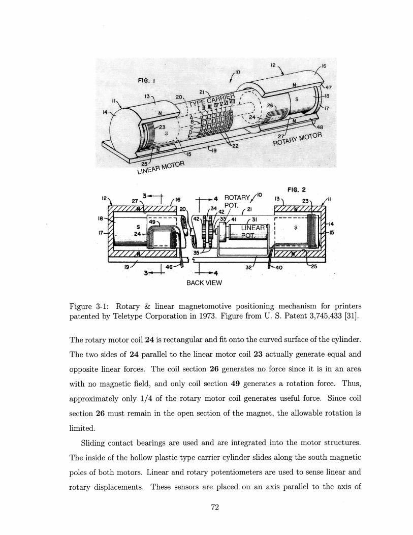
12

FIG. 212 2 6 4 ROTARY/ 1 I2

18 -1 42 41 31

1932 40-25

BACK VIEW

Figure 3-1: Rotary & linear magnetomotive positioning mechanism for printerspatented by Teletype Corporation in 1973. Figure from U. S. Patent 3,745,433 [31].

The rotary motor coil 24 is rectangular and fit onto the curved surface of the cylinder.

The two sides of 24 parallel to the linear motor coil 23 actually generate equal and

opposite linear forces. The coil section 26 generates no force since it is in an area

with no magnetic field, and only coil section 49 generates a rotation force. Thus,

approximately only 1/4 of the rotary motor coil generates useful force. Since coil

section 26 must remain in the open section of the magnet, the allowable rotation is

limited.

Sliding contact bearings are used and are integrated into the motor structures.

The inside of the hollow plastic type carrier cylinder slides along the south magnetic

poles of both motors. Linear and rotary potentiometers are used to sense linear and

rotary displacements. These sensors are placed on an axis parallel to the axis of

72

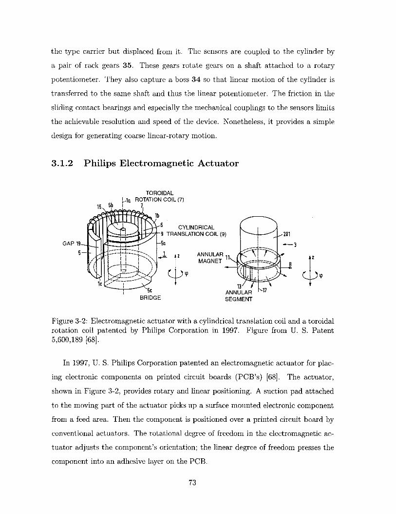
the type carrier but displaced from it. The sensors are coupled to the cylinder by

a pair of rack gears 35. These gears rotate gears on a shaft attached to a rotary

potentiometer. They also capture a boss 34 so that linear motion of the cylinder is

transferred to the same shaft and thus the linear potentiometer. The friction in the

sliding contact bearings and especially the mechanical couplings to the sensors limits

the achievable resolution and speed of the device. Nonetheless, it provides a simple

design for generating coarse linear-rotary motion.

3.1.2 Philips Electromagnetic Actuator

TOROIDALla ROTATION COIL (7)

19 5b7

1b

6 CYLINDRICAL9 TRANSLATION COIL (9) : -201

GAP 19 -5a---3

S- - :2 1 2 ANNULAR ~

13AUANNULAR 1

BRIDGE SEGMENT

z

Figure 3-2: Electromagnetic actuator with a cylindrical translation coil and a toroidalrotation coil patented by Philips Corporation in 1997. Figure from U. S. Patent5,600,189 [68].

In 1997, U. S. Philips Corporation patented an electromagnetic actuator for plac-

ing electronic components on printed circuit boards (PCB's) [68]. The actuator,

shown in Figure 3-2, provides rotary and linear positioning. A suction pad attached

to the moving part of the actuator picks up a surface mounted electronic component

from a feed area. Then the component is positioned over a printed circuit board by

conventional actuators. The rotational degree of freedom in the electromagnetic ac-

tuator adjusts the component's orientation; the linear degree of freedom presses the

component into an adhesive layer on the PCB.

73

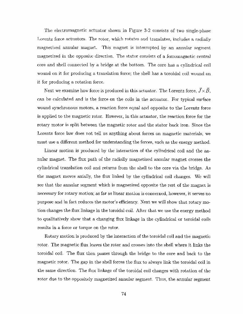
The electromagnetic actuator shown in Figure 3-2 consists of two single-phase

Lorentz force actuators. The rotor, which rotates and translates, includes a radially

magnetized annular magnet. This magnet is interrupted by an annular segment

magnetized in the opposite direction. The stator consists of a ferromagnetic central

core and shell connected by a bridge at the bottom. The core has a cylindrical coil

wound on it for producing a translation force; the shell has a toroidal coil wound on

it for producing a rotation force.

Next we examine how force is produced in this actuator. The Lorentz force, Jx B,

can be calculated and is the force on the coils in the actuator. For typical surface

wound synchronous motors, a reaction force equal and opposite to the Lorentz force

is applied to the magnetic rotor. However, in this actuator, the reaction force for the

rotary motor is split between the magnetic rotor and the stator back iron. Since the

Lorentz force law does not tell us anything about forces on magnetic materials, we

must use a different method for understanding the forces, such as the energy method.

Linear motion is produced by the interaction of the cylindrical coil and the an-

nular magnet. The flux path of the radially magnetized annular magnet crosses the

cylindrical translation coil and returns from the shell to the core via the bridge. As

the magnet moves axially, the flux linked by the cylindrical coil changes. We will

see that the annular segment which is magnetized opposite the rest of the magnet is

necessary for rotary motion; as far as linear motion is concerned, however, it serves no

purpose and in fact reduces the motor's efficiency. Next we will show that rotary mo-

tion changes the flux linkage in the toroidal coil. After that we use the energy method

to qualitatively show that a changing flux linkage in the cylindrical or toroidal coils

results in a force or torque on the rotor.

Rotary motion is produced by the interaction of the toroidal coil and the magnetic

rotor. The magnetic flux leaves the rotor and crosses into the shell where it links the

toroidal coil. The flux then passes through the bridge to the core and back to the

magnetic rotor. The gap in the shell forces the flux to always link the toroidal coil in

the same direction. The flux linkage of the toroidal coil changes with rotation of the

rotor due to the oppositely magnetized annular segment. Thus, the annular segment

74

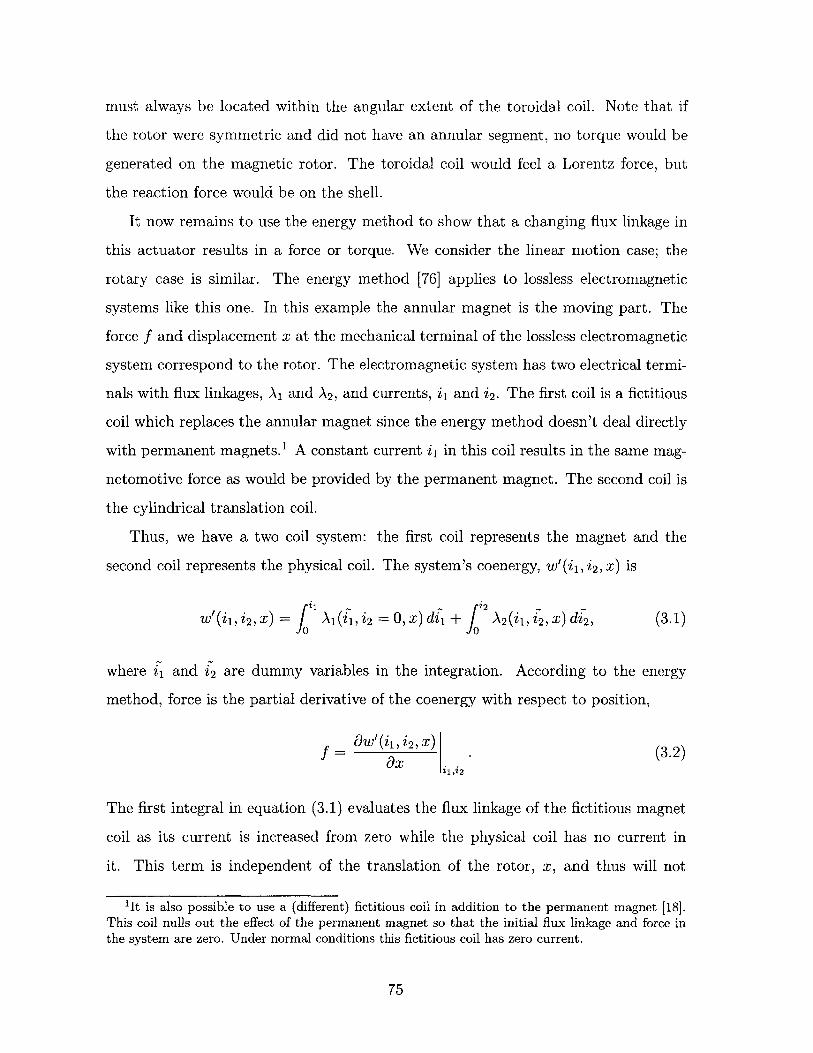
must always be located within the angular extent of the toroidal coil. Note that if

the rotor were symmetric and did not have an annular segment, no torque would be

generated on the magnetic rotor. The toroidal coil would feel a Lorentz force, but

the reaction force would be on the shell.

It now remains to use the energy method to show that a changing flux linkage in

this actuator results in a force or torque. We consider the linear motion case; the

rotary case is similar. The energy method [76] applies to lossless electromagnetic

systems like this one. In this example the annular magnet is the moving part. The

force f and displacement x at the mechanical terminal of the lossless electromagnetic

system correspond to the rotor. The electromagnetic system has two electrical termi-

nals with flux linkages, A1 and A2, and currents, il and i2 . The first coil is a fictitious

coil which replaces the annular magnet since the energy method doesn't deal directly

with permanent magnets.1 A constant current il in this coil results in the same mag-

netomotive force as would be provided by the permanent magnet. The second coil is

the cylindrical translation coil.

Thus, we have a two coil system: the first coil represents the magnet and the

second coil represents the physical coil. The system's coenergy, w'(ii, i2 , X) is

w'(ii, i2 , x) = A1(ii, i2 = 0, x) di1 + j A2 (ii, i 2 , x) di2 , (3.1)

where i 1 and i2 are dummy variables in the integration. According to the energy

method, force is the partial derivative of the coenergy with respect to position,

Ow'(ii, i 2 , X)f = .9 0 (3.2)

ii,i2

The first integral in equation (3.1) evaluates the flux linkage of the fictitious magnet

coil as its current is increased from zero while the physical coil has no current in

it. This term is independent of the translation of the rotor, x, and thus will not

'It is also possible to use a (different) fictitious coil in addition to the permanent magnet [18].This coil nulls out the effect of the permanent magnet so that the initial flux linkage and force inthe system are zero. Under normal conditions this fictitious coil has zero current.

75

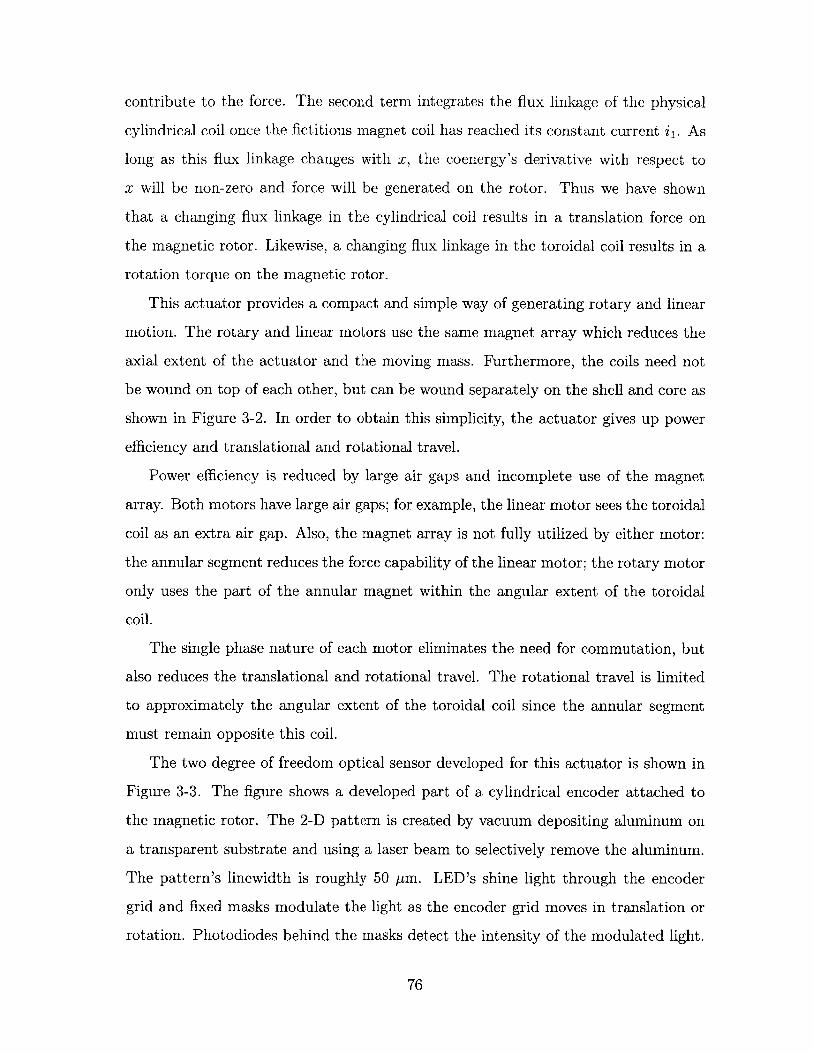
contribute to the force. The second term integrates the flux linkage of the physical

cylindrical coil once the fictitious magnet coil has reached its constant current ii. As

long as this flux linkage changes with x, the coenergy's derivative with respect to

x will be non-zero and force will be generated on the rotor. Thus we have shown

that a changing flux linkage in the cylindrical coil results in a translation force on

the magnetic rotor. Likewise, a changing flux linkage in the toroidal coil results in a

rotation torque on the magnetic rotor.

This actuator provides a compact and simple way of generating rotary and linear

motion. The rotary and linear motors use the same magnet array which reduces the

axial extent of the actuator and the moving mass. Furthermore, the coils need not

be wound on top of each other, but can be wound separately on the shell and core as

shown in Figure 3-2. In order to obtain this simplicity, the actuator gives up power

efficiency and translational and rotational travel.

Power efficiency is reduced by large air gaps and incomplete use of the magnet

array. Both motors have large air gaps; for example, the linear motor sees the toroidal

coil as an extra air gap. Also, the magnet array is not fully utilized by either motor:

the annular segment reduces the force capability of the linear motor; the rotary motor

only uses the part of the annular magnet within the angular extent of the toroidal

coil.

The single phase nature of each motor eliminates the need for commutation, but

also reduces the translational and rotational travel. The rotational travel is limited

to approximately the angular extent of the toroidal coil since the annular segment

must remain opposite this coil.

The two degree of freedom optical sensor developed for this actuator is shown in

Figure 3-3. The figure shows a developed part of a cylindrical encoder attached to

the magnetic rotor. The 2-D pattern is created by vacuum depositing aluminum on

a transparent substrate and using a laser beam to selectively remove the aluminum.

The pattern's linewidth is roughly 50 pm. LED's shine light through the encoder

grid and fixed masks modulate the light as the encoder grid moves in translation or

rotation. Photodiodes behind the masks detect the intensity of the modulated light.

76

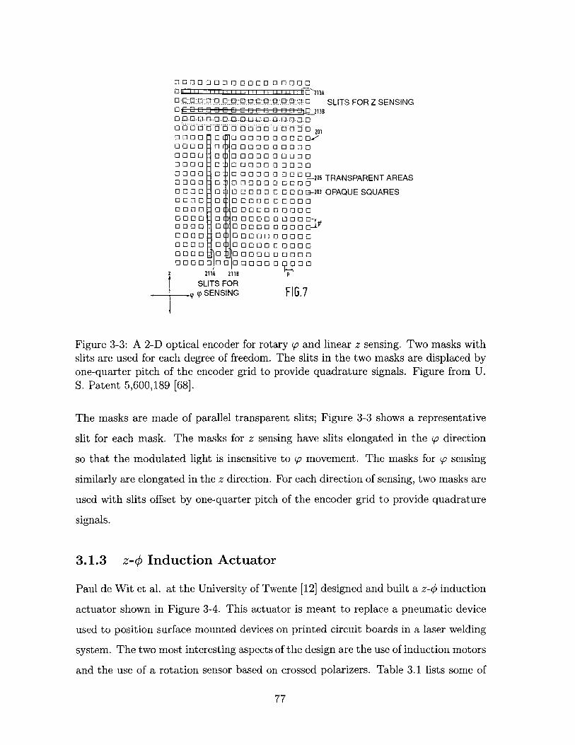
000000000000000000o 1 J 1 1 12 1 1 1 11 11 1 213A0.00. flij.0 0'0- 0000

0,E B EjB E B E9B BB tt[0213B0000 n.00 3J 0.0000 0000 00 0 00 00 0 0 00 0 20100001 0 0 0 I 100000030D 0--0000- 0(100000 000000000- 0(300000 000000000 0I 0 0000 000000000 01300000 000002050 00 0 0 00000 000000000 01000000D0 00 -2030000- 01300000 000000000- 01300000 000000000 03 00000 00 00 0-]0000 01100000 0000 j.

000*0 011010000[100000000 01100000 000000000 E 0 J0 00 00 00 00 0000300001000000 YY00

z 211A 2118

SLITS FORp SENSING

SLITS FOR Z SENSING

TRANSPARENT AREAS

OPAQUE SQUARES

P

FIG.7

Figure 3-3: A 2-D optical encoder for rotary o and linear z sensing. Two masks withslits are used for each degree of freedom. The slits in the two masks are displaced byone-quarter pitch of the encoder grid to provide quadrature signals. Figure from U.S. Patent 5,600,189 [68].

The masks are made of parallel transparent slits; Figure 3-3 shows a representative

slit for each mask. The masks for z sensing have slits elongated in the 0 direction

so that the modulated light is insensitive to 'p movement. The masks for p sensing

similarly are elongated in the z direction. For each direction of sensing, two masks are

used with slits offset by one-quarter pitch of the encoder grid to provide quadrature

signals.

3.1.3 z-<0 Induction Actuator

Paul de Wit et al. at the University of Twente [12] designed and built a z-<0 induction

actuator shown in Figure 3-4. This actuator is meant to replace a pneumatic device

used to position surface mounted devices on printed circuit boards in a laser welding

system. The two most interesting aspects of the design are the use of induction motors

and the use of a rotation sensor based on crossed polarizers. Table 3.1 lists some of

77

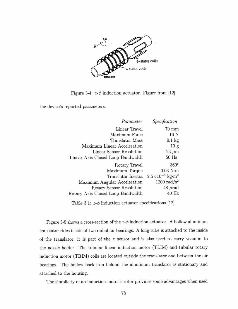
-stator coils

z-stator coilsz-rtatr coil

Figure 3-4: z-0 induction actuator. Figure from [12].

the device's reported parameters.

Parameter Specification

Linear Travel 70 mmMaximum Force 16 NTranslator Mass 0.1 kg

Maximum Linear Acceleration 10 gLinear Sensor Resolution 23 pm

Linear Axis Closed Loop Bandwidth 50 Hz

Rotary Travel 3600Maximum Torque 0.03 N-mTranslator Inertia 2.5x 10' kg.m 2

Maximum Angular Acceleration 1200 rad/s 2

Rotary Sensor Resolution 48 ptradRotary Axis Closed Loop Bandwidth 40 Hz

Table 3.1: z-# induction actuator specifications [12].

Figure 3-5 shows a cross-section of the z-# induction actuator. A hollow aluminum

translator rides inside of two radial air bearings. A long tube is attached to the inside

of the translator; it is part of the z sensor and is also used to carry vacuum to

the nozzle holder. The tubular linear induction motor (TLIM) and tubular rotary

induction motor (TRIM) coils are located outside the translator and between the air

bearings. The hollow back iron behind the aluminum translator is stationary and

attached to the housing.

The simplicity of an induction motor's rotor provides some advantages when used

78

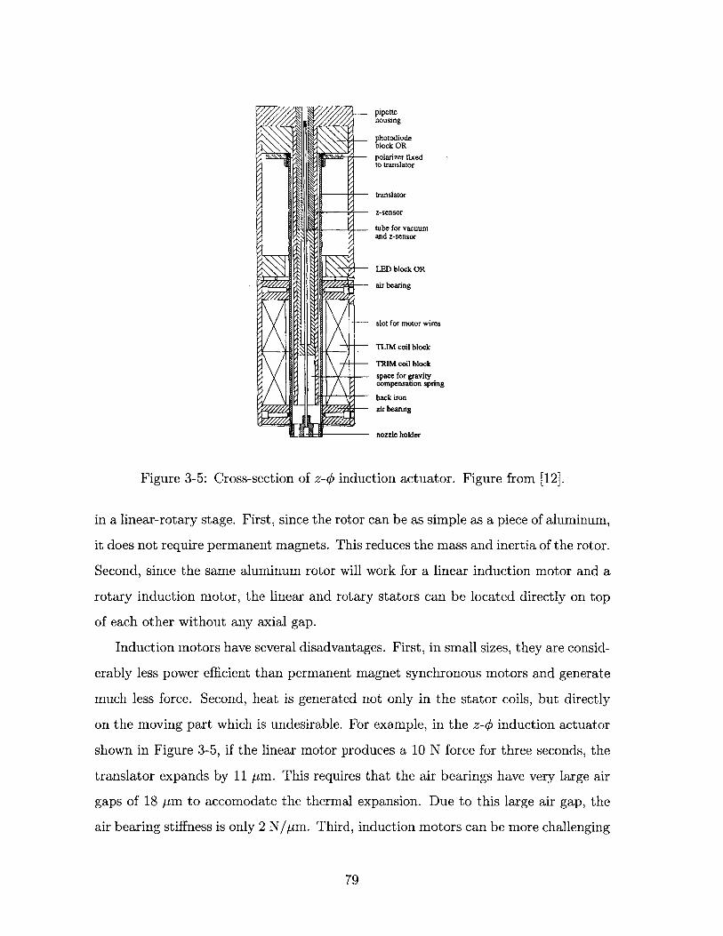
- pipettehousing

photodiodeblock ORpolarizer fixedto translator

translator

z-sensor

tube for vacuumand z-sensor

LED block OR

air bearing

slot for motor wires

TLIM coil block

TRIM coil blockspace for gravitycompensation spring

back ironair bearing

nozzle holder

Figure 3-5: Cross-section of z-# induction actuator. Figure from [12].

in a linear-rotary stage. First, since the rotor can be as simple as a piece of aluminum,

it does not require permanent magnets. This reduces the mass and inertia of the rotor.

Second, since the same aluminum rotor will work for a linear induction motor and a

rotary induction motor, the linear and rotary stators can be located directly on top

of each other without any axial gap.

Induction motors have several disadvantages. First, in small sizes, they are consid-

erably less power efficient than permanent magnet synchronous motors and generate

much less force. Second, heat is generated not only in the stator coils, but directly

on the moving part which is undesirable. For example, in the z-0 induction actuator

shown in Figure 3-5, if the linear motor produces a 10 N force for three seconds, the

translator expands by 11 pm. This requires that the air bearings have very large air

gaps of 18 pm to accomodate the thermal expansion. Due to this large air gap, the

air bearing stiffness is only 2 N/pm. Third, induction motors can be more challenging

79

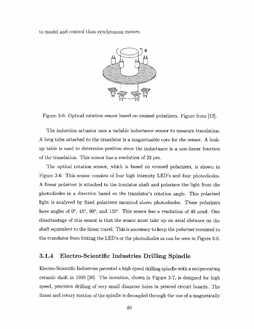
to model and control than synchronous motors.

Figure 3-6: Optical rotation sensor based on crossed polarizers. Figure from [12].

The induction actuator uses a variable inductance sensor to measure translation.

A long tube attached to the translator is a magnetizable core for the sensor. A look-

up table is used to determine position since the inductance is a non-linear function

of the translation. This sensor has a resolution of 23 pm.

The optical rotation sensor, which is based on crossed polarizers, is shown in

Figure 3-6. This sensor consists of four high intensity LED's and four photodiodes.

A linear polarizer is attached to the tranlator shaft and polarizes the light from the

photodiodes in a direction based on the translator's rotation angle. This polarized

light is analyzed by fixed polarizers mounted above photodiodes. These polarizers

have angles of 00, 450, 900, and 1350. This sensor has a resolution of 48 Prad. One

disadvantage of this sensor is that the sensor must take up an axial distance on the

shaft equivalent to the linear travel. This is necessary to keep the polarizer mounted to

the translator from hitting the LED's or the photodiodes as can be seen in Figure 3-6.

3.1.4 Electro- Scientific Industries Drilling Spindle

Electro-Scientific Industries patented a high speed drilling spindle with a reciprocating

ceramic shaft in 1999 [36]. The invention, shown in Figure 3-7, is designed for high

speed, precision drilling of very small diameter holes in printed circuit boards. The

linear and rotary motion of the spindle is decoupled through the use of a magnetically

80

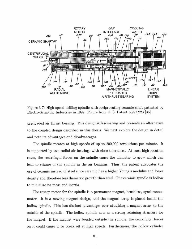
CERAMIC SHA

CENTRIFUGAL

/A8

;3

ROTARMOTO

I48

FT62

Y GAPR INTERFACE

94 14 /08 /,v

7/

881i

COOLINGWATER

/28 /2W4/ac//4

70 SZ 82 72 7&1 89 /0Z' /1 1/A MAGNETICALLY

AIR BEARING PRELOADEDAIR THRUST BEARING

Ii"!46NS

I

I/O 'lbS

LINEARDRIVE

SYSTEM

Figure 3-7: High speed drilling spindle with reciprocating ceramic shaft patented byElectro-Scientific Industries in 1999. Figure from U. S. Patent 5,997,223 [36].

pre-loaded air thrust bearing. This design is fascinating and presents an alternative

to the coupled design described in this thesis. We next explore the design in detail

and note its advantages and disadvantages.

The spindle rotates at high speeds of up to 200,000 revolutions per minute. It

is supported by two radial air bearings with close tolerances. At such high rotation

rates, the centrifugal forces on the spindle cause the diameter to grow which can

lead to seizure of the spindle in the air bearings. Thus, the patent advocates the

use of ceramic instead of steel since ceramic has a higher Young's modulus and lower

density and therefore less diametric growth than steel. The ceramic spindle is hollow

to minimize its mass and inertia.

The rotary motor for the spindle is a permanent magnet, brushless, synchronous

motor. It is a moving magnet design, and the magnet array is placed inside the

hollow spindle. This has distinct advantages over attaching a magnet array to the

outside of the spindle. The hollow spindle acts as a strong retaining structure for

the magnet. If the magnet were bonded outside the spindle, the centrifugal forces

on it could cause it to break off at high speeds. Furthermore, the hollow cylinder

81

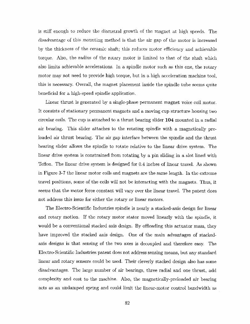
is stiff enough to reduce the diametral growth of the magnet at high speeds. The

disadvantage of this mounting method is that the air gap of the motor is increased

by the thickness of the ceramic shaft; this reduces motor efficiency and achievable

torque. Also, the radius of the rotary motor is limited to that of the shaft which

also limits achievable accelerations. In a spindle motor such as this one, the rotary

motor may not need to provide high torque, but in a high acceleration machine tool,

this is necessary. Overall, the magnet placement inside the spindle tube seems quite

beneficial for a high-speed spindle application.

Linear thrust is generated by a single-phase permanent magnet voice coil motor.

It consists of stationary permanent magnets and a moving cup structure housing two

circular coils. The cup is attached to a thrust bearing slider 104 mounted in a radial

air bearing. This slider attaches to the rotating spindle with a magnetically pre-

loaded air thrust bearing. The air gap interface between the spindle and the thrust

bearing slider allows the spindle to rotate relative to the linear drive system. The

linear drive system is constrained from rotating by a pin sliding in a slot lined with

Teflon. The linear drive system is designed for 0.4 inches of linear travel. As shown

in Figure 3-7 the linear motor coils and magnets are the same length. In the extreme

travel positions, some of the coils will not be interacting with the magnets. Thus, it

seems that the motor force constant will vary over the linear travel. The patent does

not address this issue for either the rotary or linear motors.

The Electro-Scientific Industries spindle is nearly a stacked-axis design for linear

and rotary motion. If the rotary motor stator moved linearly with the spindle, it

would be a conventional stacked axis design. By offloading this actuator mass, they

have improved the stacked axis design. One of the main advantages of stacked-

axis designs is that sensing of the two axes is decoupled and therefore easy. The

Electro-Scientific Industries patent does not address sensing means, but any standard

linear and rotary sensors could be used. Their cleverly stacked design also has some

disadvantages. The large number of air bearings, three radial and one thrust, add

complexity and cost to the machine. Also, the magnetically-preloaded air bearing

acts as an undamped spring and could limit the linear-motor control bandwidth as

82

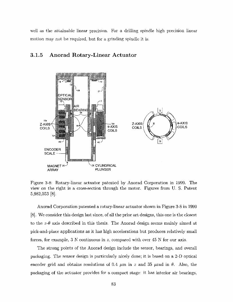
well as the attainable linear precision. For a drilling spindle high precision linear

motion may not be required, but for a grinding spindle it is.

3.1.5 Anorad Rotary-Linear Actuator

15a

Z-AXIS 1COILS

45

ENCODERSCALE -- _-

MAGNET 25

ARRAY

Z-AXIS 0-AXISCOILS COILS

--- 15b

O-AXISCOILS

46OF1

26 CYLINDRICALPLUNGER

Figure 3-8: Rotary-linear actuator patented by Anorad Corporation in 1999. Theview on the right is a cross-section through the motor. Figures from U. S. Patent5,982,053 [8].

Anorad Corporation patented a rotary-linear actuator shown in Figure 3-8 in 1999

[8]. We consider this design last since, of all the prior art designs, this one is the closest

to the z-0 axis described in this thesis. The Anorad design seems mainly aimed at

pick-and-place applications as it has high accelerations but produces relatively small

forces, for example, 3 N continuous in z, compared with over 45 N for our axis.

The strong points of the Anorad design include the sensor, bearings, and overall

packaging. The sensor design is particularly nicely done; it is based on a 2-D optical

encoder grid and obtains resolutions of 0.4 pm in z and 35 prad in 0. Also, the

packaging of the actuator provides for a compact stage: it has interior air bearings,

83

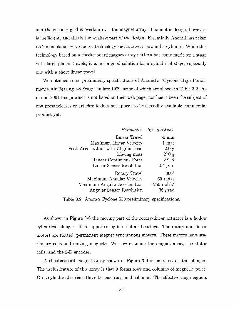
and the encoder grid is overlaid over the magnet array. The motor design, however,

is inefficient, and this is the weakest part of the design. Essentially Anorad has taken

its 2-axis planar servo motor technology and rotated it around a cylinder. While this

technology based on a checkerboard magnet array pattern has some merit for a stage

with large planar travels, it is not a good solution for a cylindrical stage, especially

one with a short linear travel.

We obtained some preliminary specifications of Anorad's "Cyclone High Perfor-

mance Air Bearing z-0 Stage" in late 1999, some of which are shown in Table 3.2. As

of mid-2001 this product is not listed on their web page, nor has it been the subject of

any press releases or articles; it does not appear to be a readily available commercial

product yet.

Parameter Specification

Linear Travel 50 mmMaximum Linear Velocity 1 m/s

Peak Acceleration with 70 gram load 2.0 gMoving mass 270 g

Linear Continuous Force 2.9 NLinear Sensor Resolution 0.4 pm

Rotary Travel 3600Maximum Angular Velocity 60 rad/s

Maximum Angular Acceleration 1250 rad/s 2

Angular Sensor Resolution 35 prad

Table 3.2: Anorad Cyclone S50 preliminary specifications.

As shown in Figure 3-8 the moving part of the rotary-linear actuator is a hollow

cylindrical plunger. It is supported by internal air bearings. The rotary and linear

motors are slotted, permanent magnet synchronous motors. These motors have sta-

tionary coils and moving magnets. We now examine the magnet array, the stator

coils, and the 2-D encoder.

A checkerboard magnet array shown in Figure 3-9 is mounted on the plunger.

The useful feature of this array is that it forms rows and columns of magnetic poles.

On a cylindrical surface these become rings and columns. The effective ring magnets

84

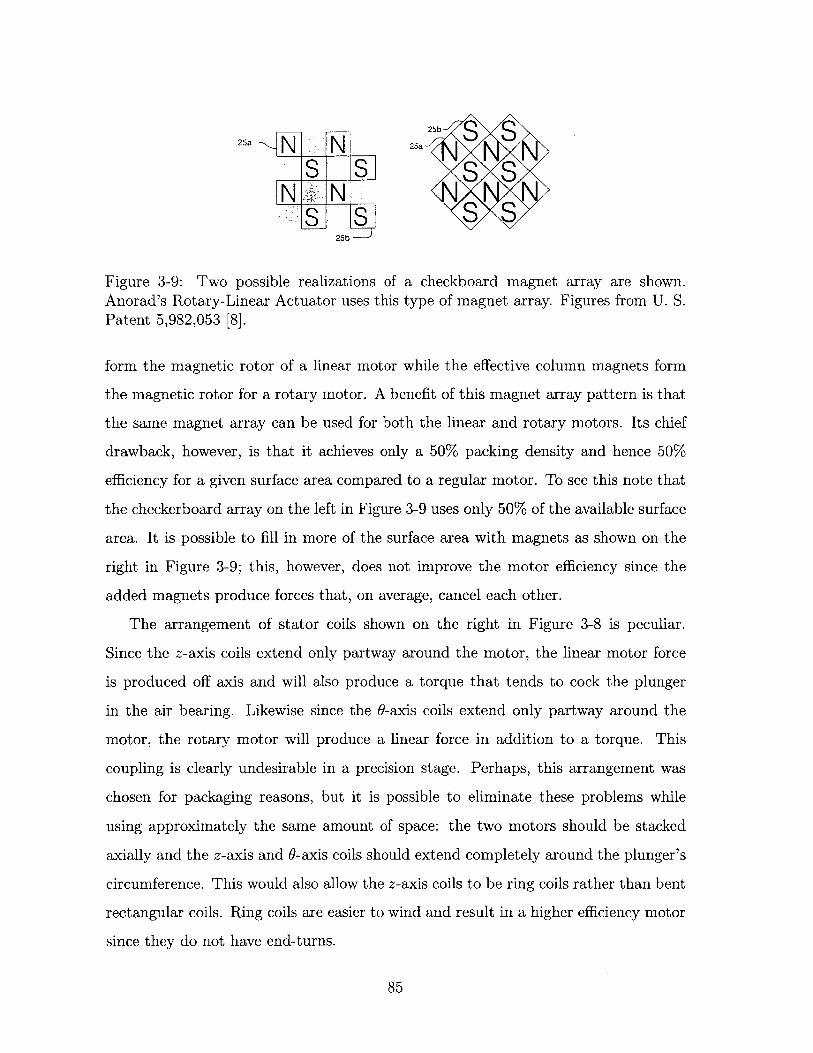
25b S25a N 25a 2 S s

S S S SN: N

S S S S25b

Figure 3-9: Two possible realizations of a checkboard magnet array are shown.Anorad's Rotary-Linear Actuator uses this type of magnet array. Figures from U. S.Patent 5,982,053 [8].

form the magnetic rotor of a linear motor while the effective column magnets form

the magnetic rotor for a rotary motor. A benefit of this magnet array pattern is that

the same magnet array can be used for both the linear and rotary motors. Its chief

drawback, however, is that it achieves only a 50% packing density and hence 50%

efficiency for a given surface area compared to a regular motor. To see this note that

the checkerboard array on the left in Figure 3-9 uses only 50% of the available surface

area. It is possible to fill in more of the surface area with magnets as shown on the

right in Figure 3-9; this, however, does not improve the motor efficiency since the

added magnets produce forces that, on average, cancel each other.

The arrangement of stator coils shown on the right in Figure 3-8 is peculiar.

Since the z-axis coils extend only partway around the motor, the linear motor force

is produced off axis and will also produce a torque that tends to cock the plunger

in the air bearing. Likewise since the 0-axis coils extend only partway around the

motor, the rotary motor will produce a linear force in addition to a torque. This

coupling is clearly undesirable in a precision stage. Perhaps, this arrangement was

chosen for packaging reasons, but it is possible to eliminate these problems while

using approximately the same amount of space: the two motors should be stacked

axially and the z-axis and 0-axis coils should extend completely around the plunger's

circumference. This would also allow the z-axis coils to be ring coils rather than bent

rectangular coils. Ring coils are easier to wind and result in a higher efficiency motor

since they do not have end-turns.

85

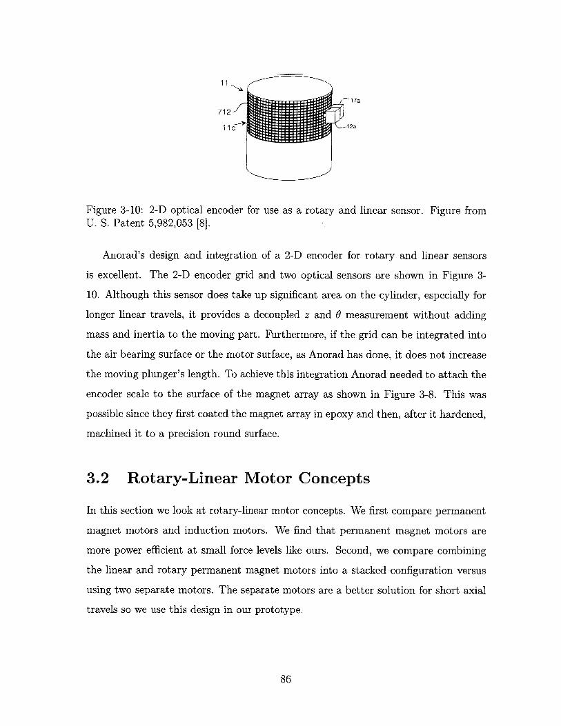
11

17a

712

11 c 12a

Figure 3-10: 2-D optical encoder for use as a rotary and linear sensor. Figure fromU. S. Patent 5,982,053 [8].

Anorad's design and integration of a 2-D encoder for rotary and linear sensors

is excellent. The 2-D encoder grid and two optical sensors are shown in Figure 3-

10. Although this sensor does take up significant area on the cylinder, especially for

longer linear travels, it provides a decoupled z and 0 measurement without adding

mass and inertia to the moving part. Furthermore, if the grid can be integrated into

the air bearing surface or the motor surface, as Anorad has done, it does not increase

the moving plunger's length. To achieve this integration Anorad needed to attach the

encoder scale to the surface of the magnet array as shown in Figure 3-8. This was

possible since they first coated the magnet array in epoxy and then, after it hardened,

machined it to a precision round surface.

3.2 Rotary-Linear Motor Concepts

In this section we look at rotary-linear motor concepts. We first compare permanent

magnet motors and induction motors. We find that permanent magnet motors are

more power efficient at small force levels like ours. Second, we compare combining

the linear and rotary permanent magnet motors into a stacked configuration versus

using two separate motors. The separate motors are a better solution for short axial

travels so we use this design in our prototype.

86

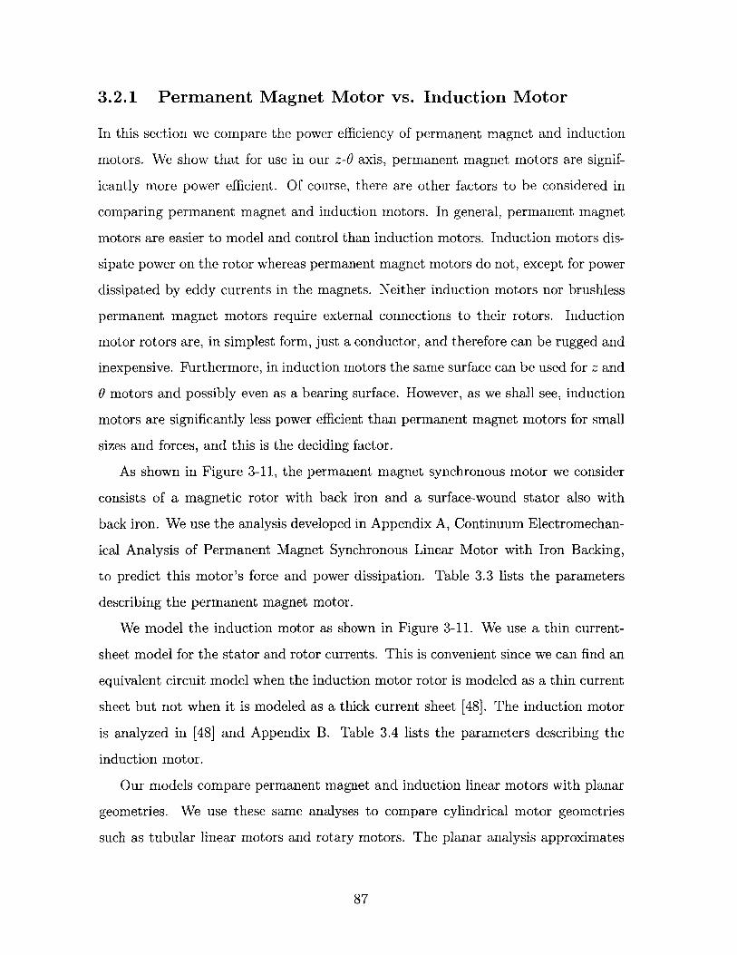
3.2.1 Permanent Magnet Motor vs. Induction Motor

In this section we compare the power efficiency of permanent magnet and induction

motors. We show that for use in our z-0 axis, permanent magnet motors are signif-

icantly more power efficient. Of course, there are other factors to be considered in

comparing permanent magnet and induction motors. In general, permanent magnet

motors are easier to model and control than induction motors. Induction motors dis-

sipate power on the rotor whereas permanent magnet motors do not, except for power

dissipated by eddy currents in the magnets. Neither induction motors nor brushless

permanent magnet motors require external connections to their rotors. Induction

motor rotors are, in simplest form, just a conductor, and therefore can be rugged and

inexpensive. Furthermore, in induction motors the same surface can be used for z and

6 motors and possibly even as a bearing surface. However, as we shall see, induction

motors are significantly less power efficient than permanent magnet motors for small

sizes and forces, and this is the deciding factor.

As shown in Figure 3-11, the permanent magnet synchronous motor we consider

consists of a magnetic rotor with back iron and a surface-wound stator also with

back iron. We use the analysis developed in Appendix A, Continuum Electromechan-

ical Analysis of Permanent Magnet Synchronous Linear Motor with Iron Backing,

to predict this motor's force and power dissipation. Table 3.3 lists the parameters

describing the permanent magnet motor.

We model the induction motor as shown in Figure 3-11. We use a thin current-

sheet model for the stator and rotor currents. This is convenient since we can find an

equivalent circuit model when the induction motor rotor is modeled as a thin current

sheet but not when it is modeled as a thick current sheet [48]. The induction motor

is analyzed in [48] and Appendix B. Table 3.4 lists the parameters describing the

induction motor.

Our models compare permanent magnet and induction linear motors with planar

geometries. We use these same analyses to compare cylindrical motor geometries

such as tubular linear motors and rotary motors. The planar analysis approximates

87

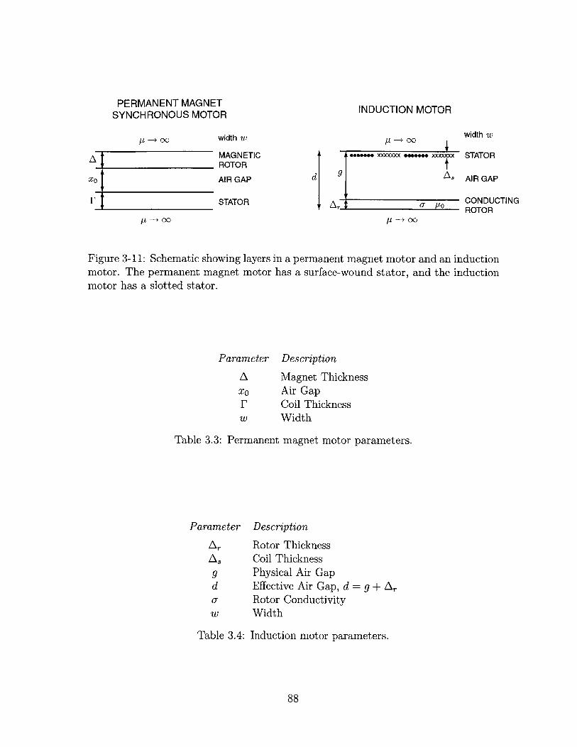
PERMANENT MAGNETSYNCHRONOUS MOTOR

width w

MAGNETICROTOR

AIR GAP

STATOR

dj

INDUCTION MOTOR

/I -- * 0A06.66.. xxxxxxx *ego** xxxxxxx

p ---+ 00

width w

STATOR

AIR GAP

CONDUCTINGROTOR

Figure 3-11: Schematic showing layers in a permanent magnet motor and an inductionmotor. The permanent magnet motor has a surface-wound stator, and the inductionmotor has a slotted stator.

Parameter

AxoI'w

Description

Magnet ThicknessAir GapCoil ThicknessWidth

Table 3.3: Permanent magnet motor parameters.

Parameter

ArAsgd-

w

Description

Rotor ThicknessCoil ThicknessPhysical Air GapEffective Air Gap, d = g + A,Rotor ConductivityWidth

Table 3.4: Induction motor parameters.

88

A

X0

pA

a cylindrical analysis but avoids the complexities of using Bessel functions.

Force and Power Scaling Laws

In a permanent magnet synchronous motor, force is produced by stator currents

interacting with the magnetic field created by the magnets. Thus, the permanent

magnet motor force, Fpm, is proportional to stator current, I,

Fpm c I. (3.3)

Power dissipation in the permanent magnet motor, Pm, is due to Joule heating in

the stator and so is proportional to current squared,

Ppm 0c12. (3.4)

In an induction motor, force is produced by the interaction between stator and rotor

currents. Since rotor currents are induced by stator currents, induction motor force,

Find, is proportional to stator current squared,

Find 0c I2 . (3.5)

Power dissipation in the stator and rotor is also proportional to current squared, so

total induction motor power dissipation is

Pind OC I2. (3.6)

Thus, for an induction motor, power is proportional to force,

Pind X Fnd,

but for a permanent magnet motor, power is proportional to force squared,

Pm oc F.

89

(3.7)

(3.8)

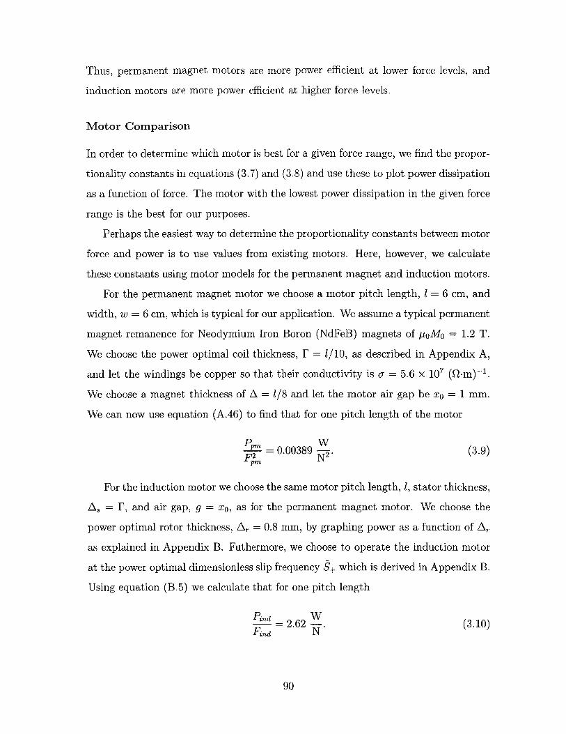
Thus, permanent magnet motors are more power efficient at lower force levels, and

induction motors are more power efficient at higher force levels.

Motor Comparison

In order to determine which motor is best for a given force range, we find the propor-

tionality constants in equations (3.7) and (3.8) and use these to plot power dissipation

as a function of force. The motor with the lowest power dissipation in the given force

range is the best for our purposes.

Perhaps the easiest way to determine the proportionality constants between motor

force and power is to use values from existing motors. Here, however, we calculate

these constants using motor models for the permanent magnet and induction motors.

For the permanent magnet motor we choose a motor pitch length, l = 6 cm, and

width, w = 6 cm, which is typical for our application. We assume a typical permanent

magnet remanence for Neodymium Iron Boron (NdFeB) magnets of poMo = 1.2 T.

We choose the power optimal coil thickness, F = 1/10, as described in Appendix A,

and let the windings be copper so that their conductivity is o = 5.6 x 107 (Q-m)-1 .

We choose a magnet thickness of A = l/8 and let the motor air gap be xO = 1 mm.

We can now use equation (A.46) to find that for one pitch length of the motor

P WF2 = 0.00389 . (3.9)

For the induction motor we choose the same motor pitch length, 1, stator thickness,

AS = F, and air gap, g = xO, as for the permanent magnet motor. We choose the

power optimal rotor thickness, A, = 0.8 mm, by graphing power as a function of A,

as explained in Appendix B. Futhermore, we choose to operate the induction motor

at the power optimal dimensionless slip frequency S+ which is derived in Appendix B.

Using equation (B.5) we calculate that for one pitch length

P.nd = 2.62 - (3.10)Find N

90

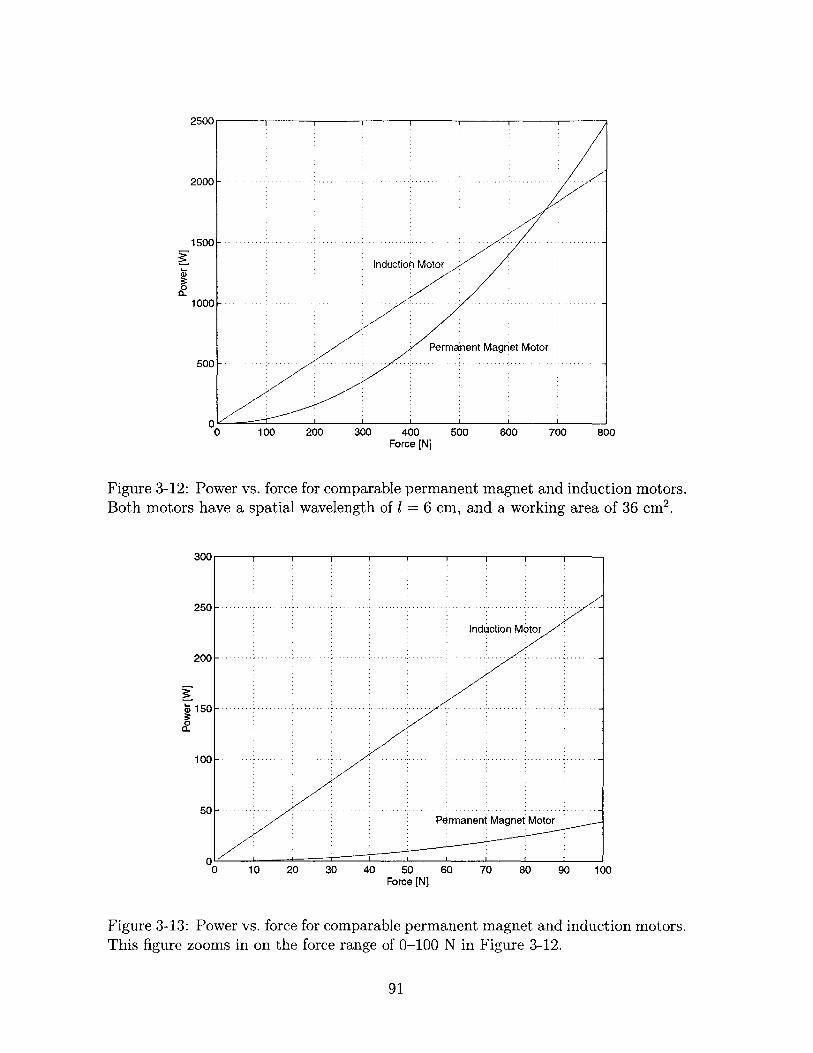
2500

20001

1500

0

1000

500

0 100 200 300 400 500 600 700 800Force [N]

Figure 3-12: Power vs. force for comparable permanent magnet and induction motors.Both motors have a spatial wavelength of 1 = 6 cm, and a working area of 36 cm 2.

300

250-

200

0a.

50

001

A

0 10 20 30 40 50 60 70 80 90 100Force [N]

Figure 3-13: Power vs. force for comparable permanent magnet and induction motors.This figure zooms in on the force range of 0-100 N in Figure 3-12.

91

Induction Motor

Permanent Magnet Motor

-

Induction Motor

Permanent Magnet Motor50F

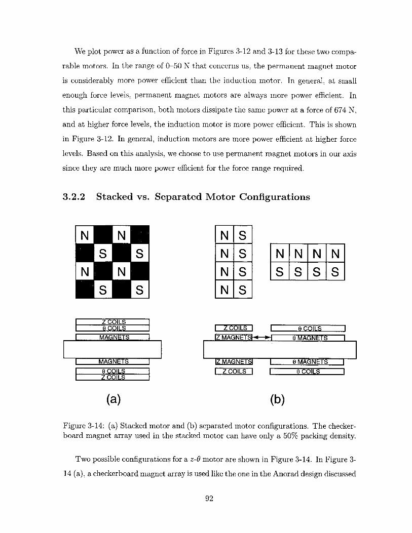
We plot power as a function of force in Figures 3-12 and 3-13 for these two compa-

rable motors. In the range of 0-50 N that concerns us, the permanent magnet motor

is considerably more power efficient than the induction motor. In general, at small

enough force levels, permanent magnet motors are always more power efficient. In

this particular comparison, both motors dissipate the same power at a force of 674 N,

and at higher force levels, the induction motor is more power efficient. This is shown

in Figure 3-12. In general, induction motors are more power efficient at higher force

levels. Based on this analysis, we choose to use permanent magnet motors in our axis

since they are much more power efficient for the force range required.

3.2.2 Stacked vs. Separated Motor Configurations

N

N

N

N

S

S_

S_

S

N N N N

S S S S_

Z COILS IZ MAGNET'S1

Z COILS

MAGNETS

MAGNETS IZ MAGNETSIZ COILS0 COILS

Z COILS

(a)

0 COILS0 MAGNETS |

| 0 MAGNETS |

0 COILS

(b)

Figure 3-14: (a) Stacked motor and (b) separated motor configurations. The checker-board magnet array used in the stacked motor can have only a 50% packing density.

Two possible configurations for a z-0 motor are shown in Figure 3-14. In Figure 3-

14 (a), a checkerboard magnet array is used like the one in the Anorad design discussed

92

0 MAGNETS

in section 3.1.5. This same magnet array can interact with either z or 9 coils to

produce force since it has both rows and columns of magnetic poles. If we filled in

the magnet array this would no longer be the case, so this magnet array can have

only a 50% packing density.2 An alternative, more conventional, design is to use

two separate magnet arrays as shown in Figure 3-14 (b). In this case 100% magnet

packing density is achieved, but two different magnet arrays are required.

Although the stacked motor with a checkerboard magnet array appears more

axially compact at first, it is less power efficient than two separate motors for short

axial travels. First, note that since the checkerboard magnet array has a 50% packing

density, it needs twice the area to have the same number of magnets as the separated

motors. Second, since the z coils see the 9 coils as an additional air gap, and vice

versa, the combined motor is less power efficient than the separated motors. The one

disadvantage of the separated motors is the wasted axial travel between them. In

fact, however, it is allowable for the z magnets to go under the 0 coils, or vice versa,

since no net force will be produced.

Since our axis has a short axial travel, we choose to use two separate motors.

We design the motors so that the magnetic rotors are axially shorter than their

corresponding stators by at least our one inch of axial travel. Thus, the rotors always

produce full force inside their stators even as they translate axially with the z-0

shaft. We look at the detailed motor design and optimization in the next chapter,

Rotary-Linear Motor Design & Analysis.

3.3 Rotary-Linear Bearing Concepts

Air bearings and hydrostatic bearings are natural choices for providing smooth trans-

lation and rotation. Rolling element bearings and sliding contact bearings have exces-

sive friction for high-speed precision motion control. This friction reduces positioning

accuracy, limits achievable accelerations, and generates unwanted heat. Magnetic

2A checkerboard array of north and south poles without gaps does not have rows and columnsof north and south poles and produces no force when interacting with z or 0 coils.

93

bearings would work, but they are too costly and are not required. Thus, we focus

on air and hydrostatic bearings.

3.3.1 Hydrostatic Bearings

Hydrostatic bearings offer significantly more damping than air bearings. This is desir-

able in axes of grinding machines to eliminate chatter and high frequency excitation.

However, at high speeds, hydrostatic bearings dissipate a lot of power as heat. Thus,

high speed spindles are made with air bearings, not hydrostatic bearings. The other

downside of hydrostatic bearings is that they require an oil pump and recirculation

system. Since we could implement air bearings without this added overhead, this was

the deciding factor in choosing air bearings for our prototype axis.

Kotilainen and Slocum [38, 37] recently investigated modular self-compensating

hydrostatic bearings. These cast bearings have self-compensating grooves located on

the internal bearing surface which makes them simple to use and inexpensive. They

would be a good choice for bearings in future rotary-linear axes. This type of self-

compensated bearing was developed by Wasson [72]. He located the self-compensating

geometry on the outer surface of the shaft rather than the inner surface of the bearing.

It is desirable to have the geometry on the inner surface of the bearing when the shaft

travels axially as it does in a rotary-linear axis.

3.3.2 Orifice Air Bearings

The two major air bearing technologies are orifice and porous graphite air bearings.

We examine both these technologies and choose porous graphite air bearings since

they are cheaper, less sensitive to debris, and easier to integrate into our prototype.

Professional Instruments (see Appendix F) makes cylindrical orifice air bearings. Al-

though many orifice air bearings use the orifice to restrict air flow, Professional Instru-

ments' air bearings are elementally compensated with a proprietary groove technology

in the bearing surface. Orifice and groove compensated air bearings are sensitive to

debris which can block the orifices or grooves and crash the bearing. This is especially

94

a concern for us since the translation of the shaft can bring debris into the bearing.

Professional Instruments suggests using a custom bearing with a special low-pressure

region in front of the actual bearing. The clearance in this region would be small, but

larger than that of the actual air bearing. The length of this region would be half the

travel of the axis, about 1 centimeter, so that the shaft would never bring debris into

the air bearing region as it translated axially. The Professional Instruments cylindri-

cal air bearings each consist of two discrete bearing regions so that the bearing can

exert a moment on the shaft. Since we want to use two air bearings in our design, the

system would be over-constrained. The design could still work if a flexure, such as a

circular diaphragm, is used to position one bearing and eliminate the over-constraint.

The cost of the orifice bearing is higher than the porous graphite bearing; the need

for a special clearance region and mounting method would make this a much more

expensive and complex option.

3.3.3 Porous Graphite Air Bearings

An alternative air bearing technology commercialized by New Way Bearings (see

Appendix F) uses porous graphite. The air pressure is uniformly distributed at the

bearing surface, and the porous graphite restricts and dampens the air flow [14]. For

small air gaps below 4 pm the air film in porous graphite bearings can provide squeeze

film damping, while orifice air bearings do not have much damping. Also, if debris do

get into the bearing, the soft graphite will scratch locally, but the rest of the bearing

can carry the load and the bearing will not crash. Furthermore, if there is a loss of

air, the porous graphite bearing can tolerate some sliding contact since the graphite

is soft compared to a steel shaft. In an orifice bearing, the bearing is typically hard

coated aluminum or stainless steel which can mar and scratch a steel shaft. Another

advantage of the porous graphite air bearings is that they are packaged with O-rings

that are compliant enough to allow the bearings to self-align. This eliminates the

overconstraint problem faced with Professional Instruments' bearings. In addition

to their crash resistance, added damping, and self-alignment properties, the New

Way bearings are also cheaper and more readily available, so we choose them for our

95

prototype.

3.4 Rotary-Linear Sensor Concepts

We need to measure rotation and translation of the z-0 axis so that we can control

the axis position. Although many types of rotary sensors and linear sensors exist, few

of them allow the moving part to both rotate and translate. Among common linear

sensors, laser interferometers and linear variable differential transformers (LVDT's)

allow rotation movement as well as translation. However, common rotary sensors do

not allow translation. For example, a standard optical encoder does not allow the

encoder disk to translate axially in its housing.

In this section we investigate various rotary-linear sensor concepts. Since linear

sensors that can tolerate rotation exist, we particularly focus on developing a rotary

sensor that can tolerate translation. In section 3.1, Review of Existing z-6 Stages,

we already saw a number of rotary-linear sensor concepts such as a rotating polarizer

and a 2-D optical encoder. We briefly review these and present additional concepts

in this section.

For our initial prototype, we choose to implement the tilted-mirror sensor. The

design and analysis of this sensor is described in detail in chapter 5, Tilted-Mirror

Sensor Design, and its fabrication is described in section 6.4 of Chapter 6, Prototype

z-6 Axis. This sensor works very well for our initial prototype but is not intended

to be the final sensor solution due to its large mass and inertia. The tilted-mirror's

inertia is 2.8 times greater than the inertia of the entire rest of the axis, and its

mass causes a cantilever resonance that limits the bandwidth of the rotary controller.

Originally, we planned to replace this sensor with the helicoid mirror sensor. That did

not happen, however, since the the helicoid mirror proved too expensive to fabricate.

Also, implementing the tilted-mirror sensor proved more challenging than we initially

thought. The next generation rotary-linear axis prototype will likely use a 2-D encoder

as a sensor.

96

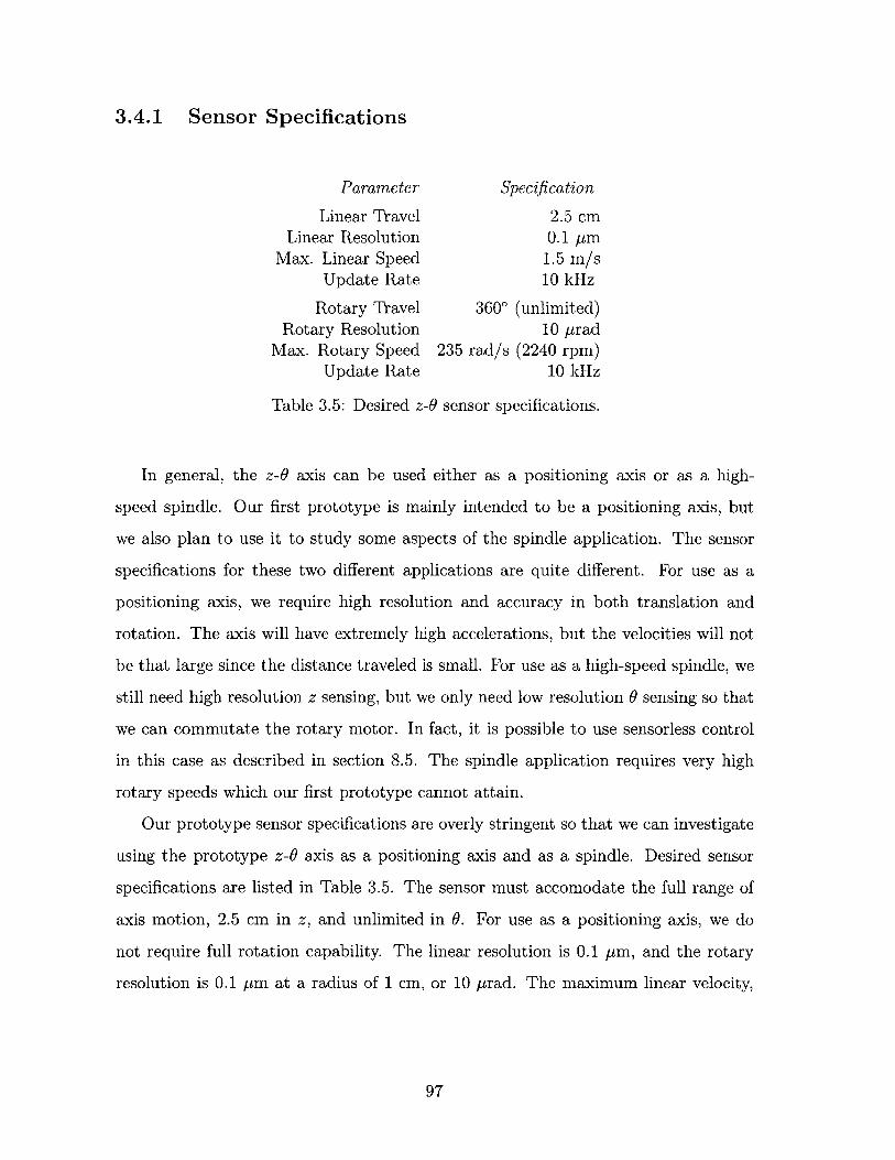
3.4.1 Sensor Specifications

Parameter Specification

Linear Travel 2.5 cmLinear Resolution 0.1 Am

Max. Linear Speed 1.5 m/sUpdate Rate 10 kHz

Rotary Travel 3600 (unlimited)Rotary Resolution 10 prad

Max. Rotary Speed 235 rad/s (2240 rpm)Update Rate 10 kHz

Table 3.5: Desired z-0 sensor specifications.

In general, the z-6 axis can be used either as a positioning axis or as a high-

speed spindle. Our first prototype is mainly intended to be a positioning axis, but

we also plan to use it to study some aspects of the spindle application. The sensor

specifications for these two different applications are quite different. For use as a

positioning axis, we require high resolution and accuracy in both translation and

rotation. The axis will have extremely high accelerations, but the velocities will not

be that large since the distance traveled is small. For use as a high-speed spindle, we

still need high resolution z sensing, but we only need low resolution 0 sensing so that

we can commutate the rotary motor. In fact, it is possible to use sensorless control

in this case as described in section 8.5. The spindle application requires very high

rotary speeds which our first prototype cannot attain.

Our prototype sensor specifications are overly stringent so that we can investigate

using the prototype z-0 axis as a positioning axis and as a spindle. Desired sensor

specifications are listed in Table 3.5. The sensor must accomodate the full range of

axis motion, 2.5 cm in z, and unlimited in 6. For use as a positioning axis, we do

not require full rotation capability. The linear resolution is 0.1 pm, and the rotary

resolution is 0.1 pm at a radius of 1 cm, or 10 prad. The maximum linear velocity,

97

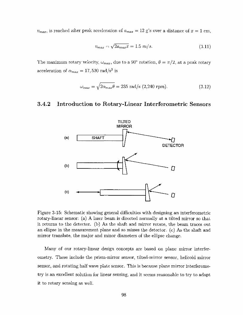
Vmax, is reached after peak acceleration of amax = 12 g's over a distance of x = 1 cm,

Vmax = V 2amaxx = 1.5 m/s. (3.11)

The maximum rotary velocity, Wmax, due to a 900 rotation, 0 = 7r/2, at a peak rotary

acceleration of amax = 17, 530 rad/s 2 is

Wmax = 2amax6 = 235 rad/s (2,240 rpm). (3.12)

3.4.2 Introduction to Rotary-Linear Interferometric Sensors

TILTEDMIRROR

(a)

(b)

SHAFT

(C)

DETECTOR

LI

Figure 3-15: Schematic showing general difficulties with designing an interferometricrotary-linear sensor: (a) A laser beam is directed normally at a tilted mirror so thatit returns to the detector. (b) As the shaft and mirror rotate, the beam traces outan ellipse in the measurement plane and so misses the detector. (c) As the shaft andmirror translate, the major and minor diameters of the ellipse change.

Many of our rotary-linear design concepts are based on plane mirror interfer-

ometry. These include the prism-mirror sensor, tilted-mirror sensor, helicoid mirror

sensor, and rotating half wave plate sensor. This is because plane mirror interferome-

try is an excellent solution for linear sensing, and it seems reasonable to try to adapt

it to rotary sensing as well.

98

One of the main difficulties in designing a rotary interferometric sensor that can

tolerate rotary and linear movement is getting the laser beam to hit the detector. For

example, consider the situation shown in Figure 3-15 (a): We measure distance to a

tilted mirror attached to a rotating shaft. As the shaft rotates, the path length of

the laser beam changes. In order to achieve high resolution we would like to tilt the

mirror by several degrees. We send the beam in at a slight tilt as shown in Figure 3-

15 (a) so that it reflects normally off the mirror and hits a detector. However, as

shown in Figure 3-15 (b), when the mirror has rotated, the beam no longer returns

to the sensor. Furthermore, as shown in Figure 3-15 (c), when the shaft translates

axially, the beam walks along the mirror since the beam is tilted.

Each of our sensor concepts deals with this issue. The prism-mirror sensor sends

the laser beam in parallel to the rotation axis so that the beam does not walk. It

uses a prism to refract the beam so that the beam always reflects normally off the

tilted mirror. Unfortunately, as is shown in section 3.4.3, the optical path length

is constant as the shaft rotates, so that the sensor will, in fact, not sense rotation.

The tilted-mirror sensor avoids the problems shown in Figure 3-15 by limiting the

mirror tilt to very small angles of milliradians. This is the sensor we implement on

our prototype axis. It is described in detail in Chapter 5.

The helicoid mirror sensor provides a radial ramp surface to the beam so that the

beam sees a constant mirror tilt as the shaft rotates. Thus it is possible to reflect

the beam normally off the helicoid, although the angle is still limited by beam walk.

The rotating half-wave plate sensor uses a beam parallel to the axis of rotation which

reflects normally off a mirror so that the problems of Figure 3-15 are avoided. We

now look at these concepts in greater detail.

3.4.3 Prism-Mirror Sensor

One of our first ideas for a rotary-linear sensor is shown in cross-section in Figure 3-

16. Initially, we were excited by this idea since it avoids the problems shown in

Figure 3-15:

99

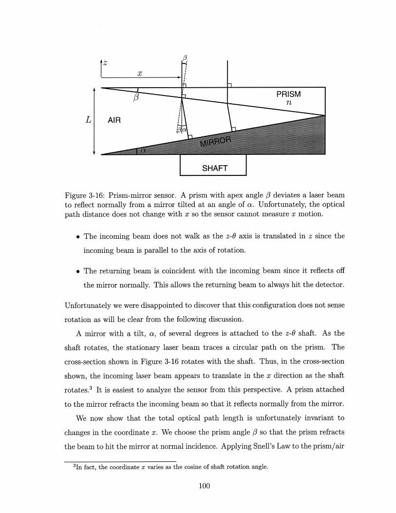
13 PRISM

LAIR

SHAFT

Figure 3-16: Prism-mirror sensor. A prism with apex angle 3 deviates a laser beamto reflect normally from a mirror tilted at an angle of a. Unfortunately, the opticalpath distance does not change with x so the sensor cannot measure x motion.

" The incoming beam does not walk as the z-0 axis is translated in z since the

incoming beam is parallel to the axis of rotation.

" The returning beam is coincident with the incoming beam since it reflects off

the mirror normally. This allows the returning beam to always hit the detector.

Unfortunately we were disappointed to discover that this configuration does not sense

rotation as will be clear from the following discussion.

A mirror with a tilt, a, of several degrees is attached to the z-0 shaft. As the

shaft rotates, the stationary laser beam traces a circular path on the prism. The

cross-section shown in Figure 3-16 rotates with the shaft. Thus, in the cross-section

shown, the incoming laser beam appears to translate in the x direction as the shaft

rotates. 3 It is easiest to analyze the sensor from this perspective. A prism attached

to the mirror refracts the incoming beam so that it reflects normally from the mirror.

We now show that the total optical path length is unfortunately invariant to

changes in the coordinate x. We choose the prism angle 3 so that the prism refracts

the beam to hit the mirror at normal incidence. Applying Snell's Law to the prism/air

3In fact, the coordinate x varies as the cosine of shaft rotation angle.

100

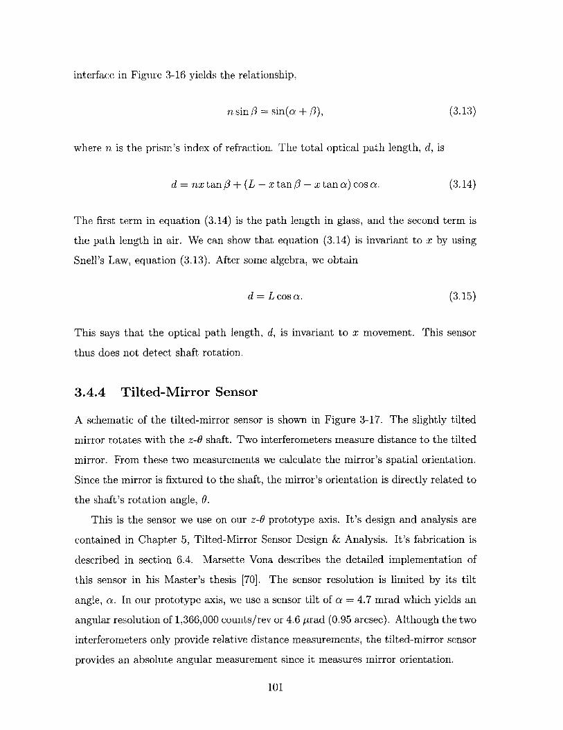
interface in Figure 3-16 yields the relationship,

n sin 3 = sin(a + 3), (3.13)

where n is the prism's index of refraction. The total optical path length, d, is

d = nxtan/3 + (L - x tan/3 - xtan a) cos a. (3.14)

The first term in equation (3.14) is the path length in glass, and the second term is

the path length in air. We can show that equation (3.14) is invariant to x by using

Snell's Law, equation (3.13). After some algebra, we obtain

d = L cos a. (3.15)

This says that the optical path length, d, is invariant to x movement. This sensor

thus does not detect shaft rotation.

3.4.4 Tilted-Mirror Sensor

A schematic of the tilted-mirror sensor is shown in Figure 3-17. The slightly tilted

mirror rotates with the z-0 shaft. Two interferometers measure distance to the tilted

mirror. From these two measurements we calculate the mirror's spatial orientation.

Since the mirror is fixtured to the shaft, the mirror's orientation is directly related to

the shaft's rotation angle, 0.

This is the sensor we use on our z-6 prototype axis. It's design and analysis are

contained in Chapter 5, Tilted-Mirror Sensor Design & Analysis. It's fabrication is

described in section 6.4. Marsette Vona describes the detailed implementation of

this sensor in his Master's thesis [70]. The sensor resolution is limited by its tilt

angle, a. In our prototype axis, we use a sensor tilt of a = 4.7 mrad which yields an

angular resolution of 1,366,000 counts/rev or 4.6 prad (0.95 arcsec). Although the two

interferometers only provide relative distance measurements, the tilted-mirror sensor

provides an absolute angular measurement since it measures mirror orientation.

101

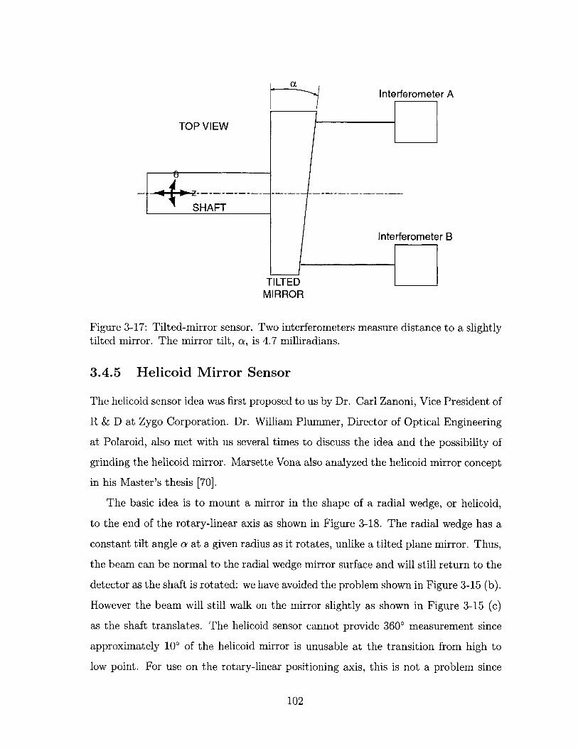
Interferometer A

TOP VIEW

SHAFT

Interferometer B

TILTEDMIRROR

Figure 3-17: Tilted-mirror sensor. Two interferometers measure distance to a slightlytilted mirror. The mirror tilt, a, is 4.7 milliradians.

3.4.5 Helicoid Mirror Sensor

The helicoid sensor idea was first proposed to us by Dr. Carl Zanoni, Vice President of

R & D at Zygo Corporation. Dr. William Plummer, Director of Optical Engineering

at Polaroid, also met with us several times to discuss the idea and the possibility of

grinding the helicoid mirror. Marsette Vona also analyzed the helicoid mirror concept

in his Master's thesis [70].

The basic idea is to mount a mirror in the shape of a radial wedge, or helicoid,

to the end of the rotary-linear axis as shown in Figure 3-18. The radial wedge has a

constant tilt angle a at a given radius as it rotates, unlike a tilted plane mirror. Thus,

the beam can be normal to the radial wedge mirror surface and will still return to the

detector as the shaft is rotated: we have avoided the problem shown in Figure 3-15 (b).

However the beam will still walk on the mirror slightly as shown in Figure 3-15 (c)

as the shaft translates. The helicoid sensor cannot provide 3600 measurement since

approximately 100 of the helicoid mirror is unusable at the transition from high to

low point. For use on the rotary-linear positioning axis, this is not a problem since

102

Figure 3-18: Helicoid Miror Sensor. The laser interferometer measurement beamis directed normal to a radial wedge, or helicoid, mirror so that shaft rotation ismeasured. Another beam measures translation by reflecting off the flat mirror in thecenter. A detailed mechanical drawing of the helicoid mirror is shown in Figure D-6.Figure drawn by Marsette Vona.

we do not need to spin the part all the way around.

We designed on paper a helicoid sensor with a 1 mm pitch and a 1.5 inch radius.

This results in a tilt angle of a = 4.2 mrad. One of the main benefits of the helicoid

sensor is that it can have a macroscopic tilt angle, whereas the tilted-mirror sensor

must have a small tilt angle so that the beam returns to the detector. In fact, however,

the tilt angle for the helicoid mirror is roughly the same as that of the tilted-mirror

sensor. Thus, the helicoid mirror sensor offers roughly the same resolution as the

tilted-mirror sensor. Before testing the tilted-mirror sensor we did not know we would

be able to achieve such a large tilt, and so the helicoid sensor seemed to promise much

higher resolution at that time.

Another complication with the helicoid mirror sensor is that the helicoid surface

has small principal curvatures, whereas the tilted-mirror is globally flat. We esti-

mate that for our proposed helicoid mirror the principal curvatures are 0.110 m-1

103

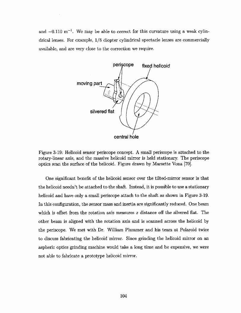
and -0.110 m 1 . We may be able to correct for this curvature using a weak cylin-

drical lenses. For example, 1/8 diopter cylindrical spectacle lenses are commercially

available, and are very close to the correction we require.

pen cope fixe helicoid

moving part

silvered flat

central hole

Figure 3-19: Helicoid sensor periscope concept. A small periscope is attached to therotary-linear axis, and the massive helicoid mirror is held stationary. The periscopeoptics scan the surface of the helicoid. Figure drawn by Marsette Vona [70].

One significant benefit of the helicoid sensor over the tilted-mirror sensor is that

the helicoid needn't be attached to the shaft. Instead, it is possible to use a stationary

helicoid and have only a small periscope attach to the shaft as shown in Figure 3-19.

In this configuration, the sensor mass and inertia are significantly reduced. One beam

which is offset from the rotation axis measures z distance off the silvered flat. The

other beam is aligned with the rotation axis and is scanned across the helicoid by

the periscope. We met with Dr. William Plummer and his team at Polaroid twice

to discuss fabricating the helicoid mirror. Since grinding the helicoid mirror on an

aspheric optics grinding machine would take a long time and be expensive, we were

not able to fabricate a prototype helicoid mirror.

104

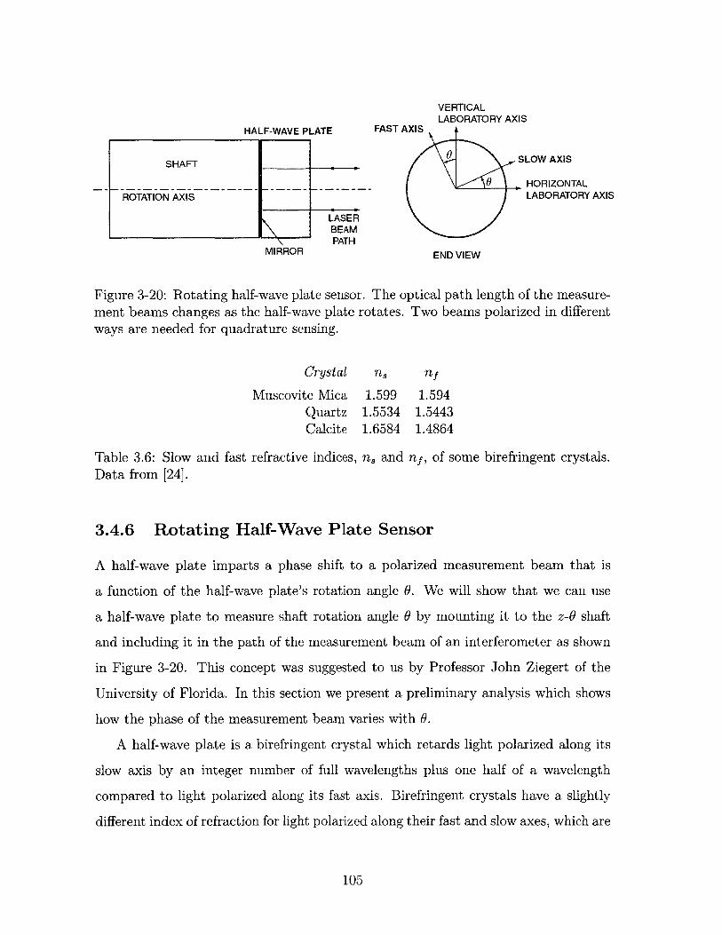
HALF-WAVE PL

SHAFT

ROTATION AXIS

VERTICALLABORATORY AXIS

ATE FAST AXIS

SLOW AXIS

0 ,HORIZONTALLABORATORY AXIS

LASEABEAMP-ATi

MIRROR END VIEW

Figure 3-20: Rotating half-wave plate sensor. The optical path length of the measure-ment beams changes as the half-wave plate rotates. Two beams polarized in differentways are needed for quadrature sensing.

Crystal n. nf

Muscovite Mica 1.599 1.594Quartz 1.5534 1.5443Calcite 1.6584 1.4864

Table 3.6: Slow and fast refractive indices, n. and nf, of some birefringent crystals.Data from [24].

3.4.6 Rotating Half-Wave Plate Sensor

A half-wave plate imparts a phase shift to a polarized measurement beam that is

a function of the half-wave plate's rotation angle 6. We will show that we can use

a half-wave plate to measure shaft rotation angle 0 by mounting it to the z-0 shaft

and including it in the path of the measurement beam of an interferometer as shown

in Figure 3-20. This concept was suggested to us by Professor John Ziegert of the

University of Florida. In this section we present a preliminary analysis which shows

how the phase of the measurement beam varies with 0.

A half-wave plate is a birefringent crystal which retards light polarized along its

slow axis by an integer number of full wavelengths plus one half of a wavelength

compared to light polarized along its fast axis. Birefringent crystals have a slightly

different index of refraction for light polarized along their fast and slow axes, which are

105

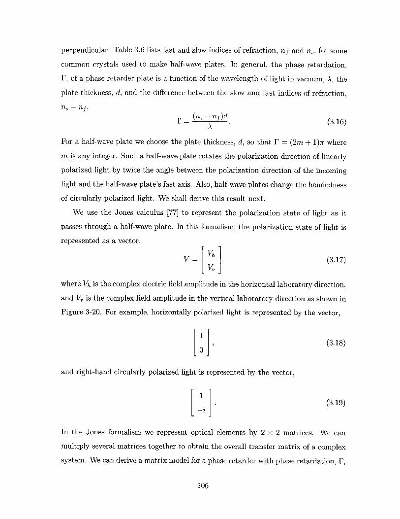
perpendicular. Table 3.6 lists fast and slow indices of refraction, nf and n, for some

common crystals used to make half-wave plates. In general, the phase retardation,

F, of a phase retarder plate is a function of the wavelength of light in vacuum, A, the

plate thickness, d, and the difference between the slow and fast indices of refraction,

ns - nf,

F = (n. - Tf)d (3.16)

For a half-wave plate we choose the plate thickness, d, so that F = (2m + 1)7r where

m is any integer. Such a half-wave plate rotates the polarization direction of linearly

polarized light by twice the angle between the polarization direction of the incoming

light and the half-wave plate's fast axis. Also, half-wave plates change the handedness

of circularly polarized light. We shall derive this result next.

We use the Jones calculus [77] to represent the polarization state of light as it

passes through a half-wave plate. In this formalism, the polarization state of light is

represented as a vector,

V= Vh3.17)V

where Vh is the complex electric field amplitude in the horizontal laboratory direction,

and V, is the complex field amplitude in the vertical laboratory direction as shown in

Figure 3-20. For example, horizontally polarized light is represented by the vector,

1(3.18)

0

and right-hand circularly polarized light is represented by the vector,

1(3.19)

In the Jones formalism we represent optical elements by 2 x 2 matrices. We can

multiply several matrices together to obtain the overall transfer matrix of a complex

system. We can derive a matrix model for a phase retarder with phase retardation, F,

106

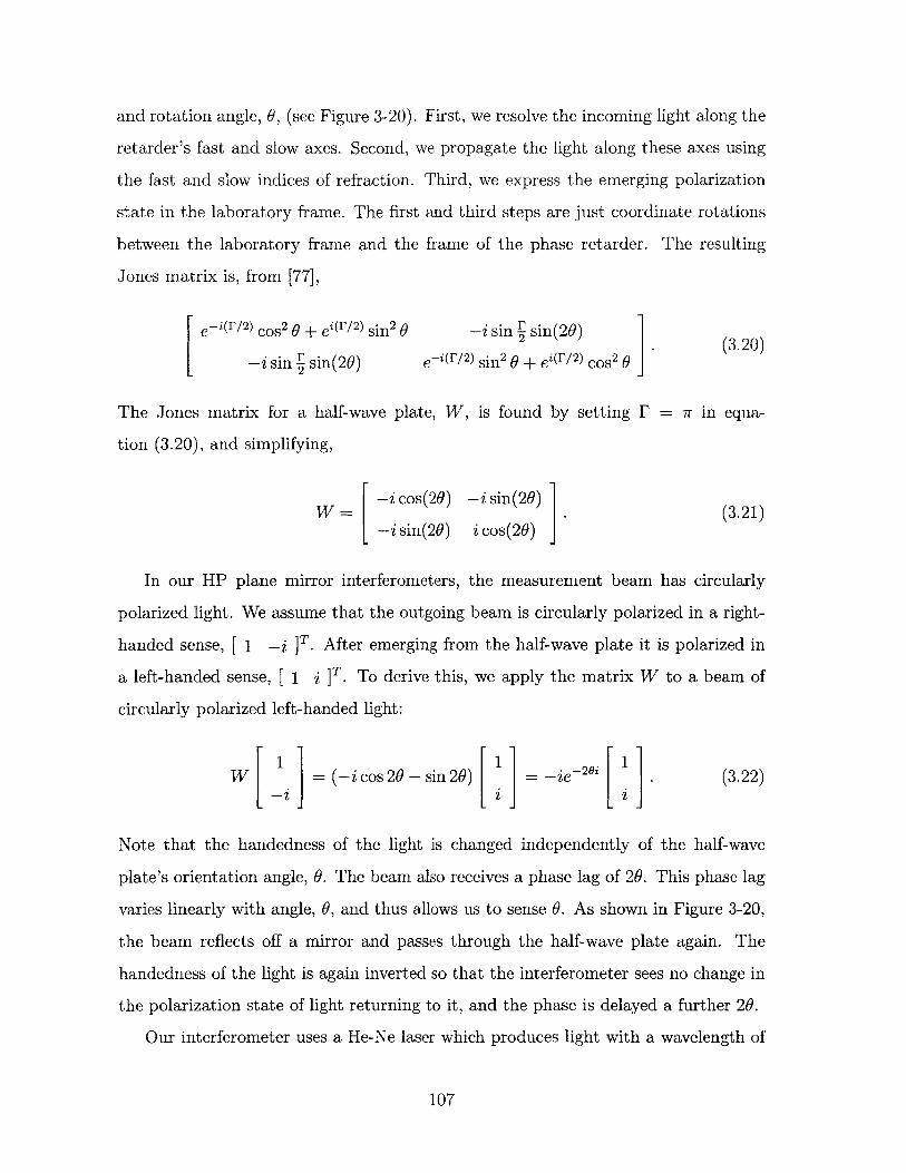
and rotation angle, 6, (see Figure 3-20). First, we resolve the incoming light along the

retarder's fast and slow axes. Second, we propagate the light along these axes using

the fast and slow indices of refraction. Third, we express the emerging polarization

state in the laboratory frame. The first and third steps are just coordinate rotations

between the laboratory frame and the frame of the phase retarder. The resulting

Jones matrix is, from [77],

e-i(r/2) cos 2 0 + ei(F/2) sin2 0 -i sin 1 sin(20).(3.20)

-i sin § sin(29) e-i(r/2) sin 2 6 + ei(r/ 2) cos 2 0 J

The Jones matrix for a half-wave plate, W, is found by setting F = r in equa-

tion (3.20), and simplifying,

[ -i cos(20) -i sin(26) (3.21)-i sin(20) i cos(20)

In our HP plane mirror interferometers, the measurement beam has circularly

polarized light. We assume that the outgoing beam is circularly polarized in a right-

handed sense, [ 1 -i JT. After emerging from the half-wave plate it is polarized in

a left-handed sense, [ 1 I ]T. To derive this, we apply the matrix W to a beam of

circularly polarized left-handed light:

W = (-i cos 26 - sin 26) = -ie- 2 0 [ . (3.22)-i i Li

Note that the handedness of the light is changed independently of the half-wave

plate's orientation angle, 6. The beam also receives a phase lag of 29. This phase lag

varies linearly with angle, 0, and thus allows us to sense 6. As shown in Figure 3-20,

the beam reflects off a mirror and passes through the half-wave plate again. The

handedness of the light is again inverted so that the interferometer sees no change in

the polarization state of light returning to it, and the phase is delayed a further 26.

Our interferometer uses a He-Ne laser which produces light with a wavelength of

107

A = 632.8 nm. A rotation of 0 = r/2 delays the measurement beam by A. Since the

interferometers have a resolution of 0.625 nm, this sensor achieves a rotary resolution

of632.8 un 2ir

x = 4050 counts/rev. (3.23)0.625 nm 7r/2

This resolution is too low for our application. However, it may be possible to increase

the resolution by using a half-wave plate that delays the phase by F = (2m + 1)7r,

where the integer m is made as large as possible. For this purpose it is desirable to use

a material that has a large difference between its fast and slow indices of refraction

so that the thickness required is not too great.

3.4.7 Rotating Polarizer Sensor

An optical sensor based on crossed polarizers is shown in Figure 3-6 and discussed

on page 80 of section 3.1.3, "z-# Induction Actuator." This sensor has a reported

resolution of 48 prad.

3.4.8 2-D Encoder

A 2-D transmissive optical encoder is shown in Figure 3-3 and discussed on page 76 of

section 3.1.2, "Philips Electromagnetic Actuator." This 2-D encoder transmits light

through a grid of transmissive and opaque sections and uses masks with elongated

slits to modulate the light.

A 2-D reflective optical encoder is shown in Figure 3-10 and discussed on page 86

of section 3.1.5, "Anorad Rotary-Linear Actuator." This sensor provides a resolution

of 0.4 pm in translation and 35 prad in rotation.

3.5 Summary

In this chapter we first reviewed existing rotary-linear stage designs. Two of the

more interesting designs were the Electro-Scientific Industries spindle and the Anorad

actuator. The Electro-Scientific Industries spindle has permanent magnets for the

108

rotary motor inside of a hollow ceramic shaft so that they would not fly off of the

shaft at high rotary speeds. This spindle also uses a magnetically preloaded air thrust

bearing to couple the linear drive system to the rotating spindle. The Anorad design

implements a 2-D encoder and integrates it into the motor surface.

We then developed rotary-linear motor concepts. We showed that permanent mag-

net motors are much more power efficient than induction motors for our application.

We also showed that for short axial travels, separate permanent magnet motors are

more power efficient than a motor with a combined magnet array. We then examined

several rotary interferometric sensors that can tolerate axial translation. We showed

that the prism-mirror sensor unfortunately does not sense rotation. The tilted-mirror

sensor is incorporated into our prototype axis but has significant rotary inertia. The

helicoid mirror sensor is not readily manufacturable. The rotating half-wave plate

sensor concept is promising and should be investigated further.

A 2-D encoder may be the simplest and most cost-effective solution for use on

future rotary-linear axes. Initially, we gravitated towards an end-on interferometric-

based sensor since we wanted to save the added shaft length required for a sensor with

a 2-D grid. In implementing the tilted-mirror sensor, however, we ended up adding at

least as much shaft length and significant mass and inertia. The added inertia reduces

the axis's angular acceleration; the added mass creates a cantilever resonance which

limits the achievable rotary axis bandwidth. Although a 2-D encoder requires some

area on the surface of the shaft, the 2-D grid adds an insignificant mass and inertia

to the shaft. Furthermore, it is possible to create the 2-D grid on the same surface

used for a magnetic rotor [8] or air bearing. This reduces the shaft length further. In

the next chapter we look at the design and analysis of the rotary and linear motors.

109

110

Chapter 4

Rotary-Linear Motor Design &

Analysis

This chapter discusses the design and analysis of the rotary and linear motors which

rotate and translate the z-0 axis. Although both motors are permanent magnet

synchronous motors, there are many differences between them. We designed and

fabricated the linear motor and therefore had a great deal of freedom in optimizing

this motor for the z-0 axis. Most of this chapter is therefore concerned with the design

and analysis of the linear motor. We purchased the rotary motor which limited our

available options. We explain how we selected this motor to achieve maximum axis

accelerations.

Our main goal in designing the motors is to maximize achievable linear and rotary

accelerations. These high accelerations are required for high-speed machining of small,

complex parts. We use frameless motors with the rotors mounted on the moving axis

and stators fixed to the machine base. It is the mass and inertia of the rotors that

mainly concern us since these add to the mass and inertia of the moving part. Within

reason, the sizes of the stators do not matter since they are mounted to the machine

base.

In this chapter, we first present some simple scaling laws for achieving high rotary

and linear accelerations. Next, we summarize the continuum electromechanical anal-

ysis for permanent magnet motors which is presented in detail in Appendix A. We

111

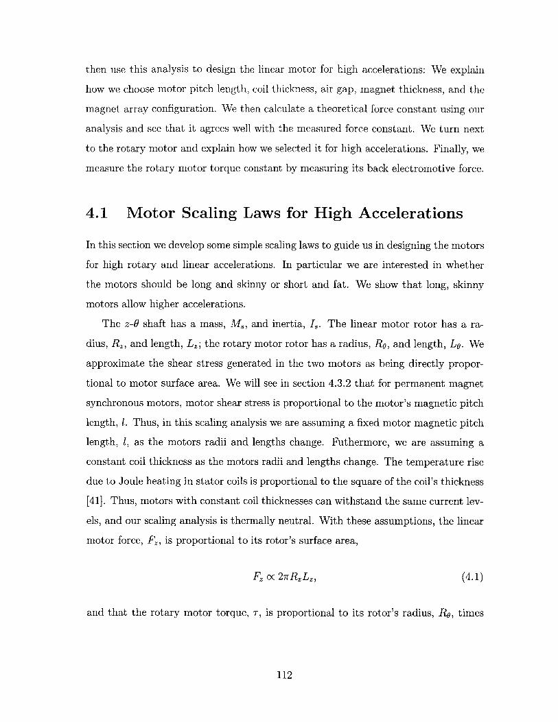
then use this analysis to design the linear motor for high accelerations: We explain

how we choose motor pitch length, coil thickness, air gap, magnet thickness, and the

magnet array configuration. We then calculate a theoretical force constant using our

analysis and see that it agrees well with the measured force constant. We turn next

to the rotary motor and explain how we selected it for high accelerations. Finally, we

measure the rotary motor torque constant by measuring its back electromotive force.

4.1 Motor Scaling Laws for High Accelerations

In this section we develop some simple scaling laws to guide us in designing the motors

for high rotary and linear accelerations. In particular we are interested in whether

the motors should be long and skinny or short and fat. We show that long, skinny

motors allow higher accelerations.

The z-0 shaft has a mass, M, and inertia, I,. The linear motor rotor has a ra-

dius, RZ, and length, Lz; the rotary motor rotor has a radius, RO, and length, LO. We

approximate the shear stress generated in the two motors as being directly propor-

tional to motor surface area. We will see in section 4.3.2 that for permanent magnet

synchronous motors, motor shear stress is proportional to the motor's magnetic pitch

length, 1. Thus, in this scaling analysis we are assuming a fixed motor magnetic pitch

length, 1, as the motors radii and lengths change. Futhermore, we are assuming a

constant coil thickness as the motors radii and lengths change. The temperature rise

due to Joule heating in stator coils is proportional to the square of the coil's thickness

[41]. Thus, motors with constant coil thicknesses can withstand the same current lev-

els, and our scaling analysis is thermally neutral. With these assumptions, the linear

motor force, Fz, is proportional to its rotor's surface area,

F oc 27rRLz, (4.1)

and that the rotary motor torque, -T, is proportional to its rotor's radius, RO, times

112

its rotor's surface area,

T oc 2rR2 Lo. (4.2)

The total system mass, M, is

M = -rp(R2L, + R2Lo) + M, (4.3)

where p is the density of the rotor. The total system inertia, I, is

1I = -1rp(.R L + R 4Lo) + Is. (4.4)

2

Thus, the linear acceleration, a, is related to the rotors' geometries by

a oc (4.5)7rp(R2 L + R2Lo) + Mj'

and the rotary acceleration, a, is related to the rotors' geometries by

2wrR2Loa oc 104(4.6)

a 7rp(R4Lz + R Lo) + Is(

We would like to choose the radii and lengths of the two rotors, RZ, LZ, R0 , and Lo,

such that the linear and rotary accelerations, a and a, are both large. The design will

need to be balanced so that both a and a are large. For example, a design with a big

linear motor and small rotary motor will have a high linear acceleration but low rotary

acceleration. If either motor is too small, it will not contribute to the system mass

and inertia much, and we can increase the corresponding acceleration by making this

motor larger. Once the motor's mass and inertia are no longer insignificant compared

to that of the rest of the system, we want to know if it is better to increase the motor's

length or radius.

First, consider the choice of the linear motor's radius, R2, and length, L2. One

way to think about this optimization is to maximize linear force, F, oc R2Lz, without

letting the total system mass and inertia get too large. The linear motor contributes

a mass proportional to R2 Lz to the system mass, and an inertia proportional to R'Lz

113

to the system inertia. Thus, we are much better off choosing a larger value of L, and

a smaller value of R, which corresponds to a long, skinny motor.

Second, consider the choice of the rotary motor's radius, RO, and length, LO. We

want to maximize rotary motor torque, R2LO, without letting the total system mass

and inertia get too large. The rotary motor contributes a mass proportional to R2LO

to the system mass, and an inertia proportional to R'LO to the system inertia. The

inertia term again leads us favor increases in LO over RO resulting in a long, skinny

motor. In this chapter, we use a similar scaling analysis to optimize the magnet

thickness of the linear motor for high accelerations, and to select a rotary motor for

high accelerations.

4.2 Linear Motor Electromechanical Analysis

In this section we present the results of an electromechanical analysis of an iron-backed

permanent magnet synchronous motor. We use the analytical framework of Melcher

[48] in which layers of electromagnetic material-such as magnets, air gap, coils, and

iron-are described by transfer relations. Prior analyses by Trumper [66, 67] and

Kim [34] have investigated ironless motors with a variety of magnet arrays. This type

of analysis provides a wealth of information for optimization and design of motors.

The author's Master's thesis, Thermally Efficient Linear Motor Analysis & Design

[41] extends the analysis presented by Trumper, Kim, and Williams [66] to include an

iron backing behind both the magnet array and the coils. In this section we present

the framework for this analysis and its key results. We use the key results-analytical

expressions for motor force and power consumption-to design the z-axis motor of

the z-0 axis. The details of the continuum electromechanical analysis are presented

in Appendix A.

4.2.1 Analytical Framework

Figure 4-1 shows a schematic of the layers of electromagnetic material in an iron-

backed, surface-wound, permanent magnet motor. An air gap separates the stator

114

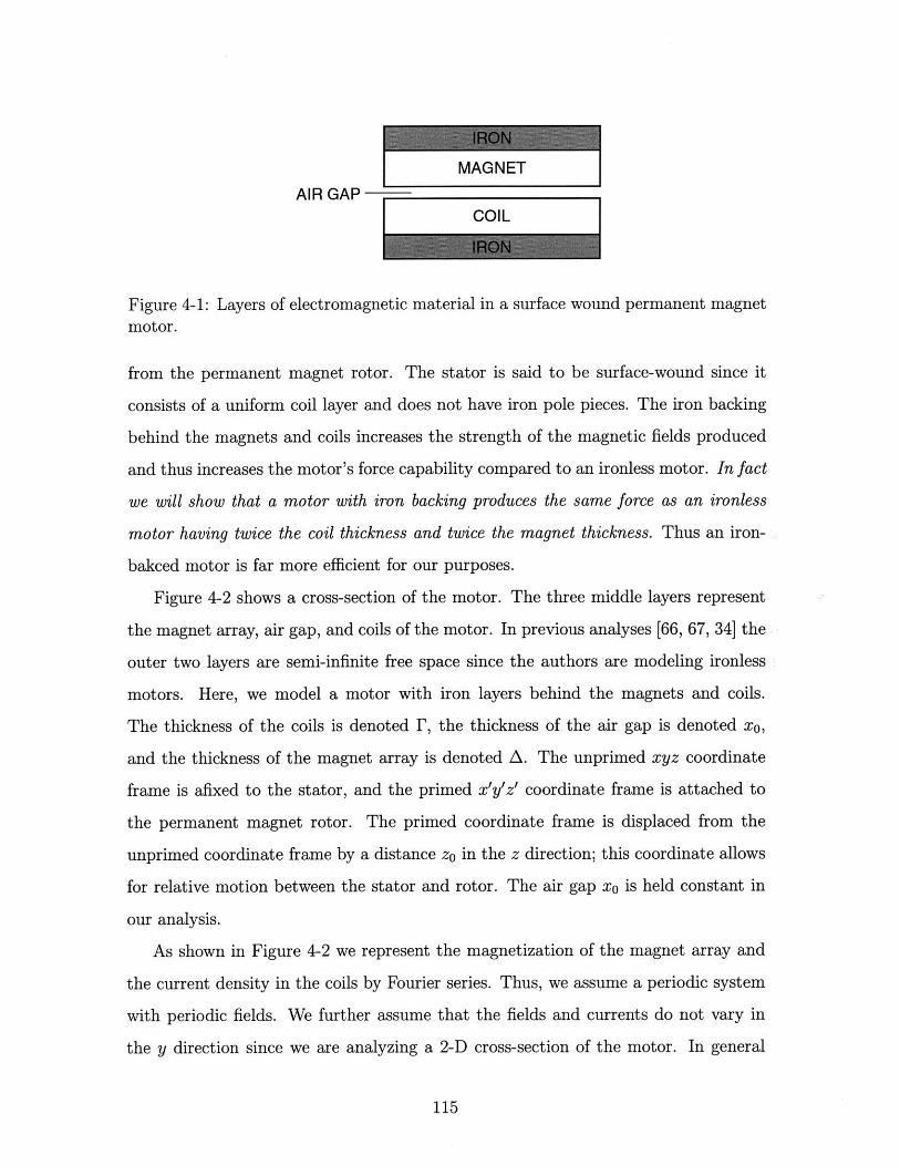
MAGNET

AIR GAP-COIL ;

Figure 4-1: Layers of electromagnetic material in a surface wound permanent magnetmotor.

from the permanent magnet rotor. The stator is said to be surface-wound since it

consists of a uniform coil layer and does not have iron pole pieces. The iron backing

behind the magnets and coils increases the strength of the magnetic fields produced

and thus increases the motor's force capability compared to an ironless motor. In fact

we will show that a motor with iron backing produces the same force as an ironless

motor having twice the coil thickness and twice the magnet thickness. Thus an iron-

bakced motor is far more efficient for our purposes.

Figure 4-2 shows a cross-section of the motor. The three middle layers represent

the magnet array, air gap, and coils of the motor. In previous analyses [66, 67, 34] the

outer two layers are semi-infinite free space since the authors are modeling ironless

motors. Here, we model a motor with iron layers behind the magnets and coils.

The thickness of the coils is denoted F, the thickness of the air gap is denoted xo,

and the thickness of the magnet array is denoted A. The unprimed xyz coordinate

frame is afixed to the stator, and the primed x'y'z' coordinate frame is attached to

the permanent magnet rotor. The primed coordinate frame is displaced from the

unprimed coordinate frame by a distance zo in the z direction; this coordinate allows

for relative motion between the stator and rotor. The air gap x0 is held constant in

our analysis.

As shown in Figure 4-2 we represent the magnetization of the magnet array and

the current density in the coils by Fourier series. Thus, we assume a periodic system

with periodic fields. We further assume that the fields and currents do not vary in

the y direction since we are analyzing a 2-D cross-section of the motor. In general

115

- Msfflwwe -

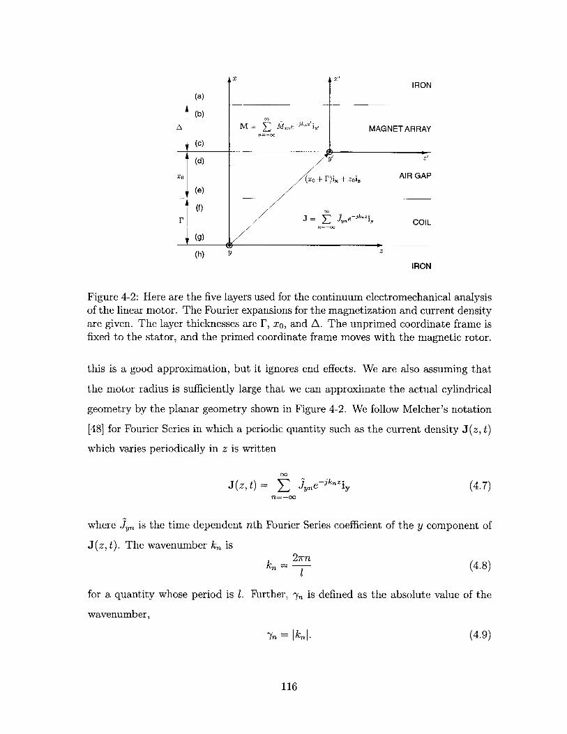
X

M = I.nek-j z'ix

L X/

IRON

MAGNET ARRAY

(c)

(d) y Z'

XO (Xo + r)i. + zoi AIR GAP

(e)

(f) 00

J = E J,,e-jkzi Y COIL

(g)

(h) Y Z

IRON

Figure 4-2: Here are the five layers used for the continuum electromechanical analysisof the linear motor. The Fourier expansions for the magnetization and current densityare given. The layer thicknesses are F, x0 , and A. The unprimed coordinate frame isfixed to the stator, and the primed coordinate frame moves with the magnetic rotor.

this is a good approximation, but it ignores end effects. We are also assuming that

the motor radius is sufficiently large that we can approximate the actual cylindrical

geometry by the planar geometry shown in Figure 4-2. We follow Melcher's notation

[48] for Fourier Series in which a periodic quantity such as the current density J(z, t)

which varies periodically in z is written

00

J(z, t) = 1 jyne-jk-iyn=-o

(4.7)

where jyn is the time dependent nth Fourier Series coefficient of the y component of

J(z, t). The wavenumber kn is27rn

kn = 1(4.8)

for a quantity whose period is 1. Further, 'y, is defined as the absolute value of the

wavenumber,

y = Ik.n.

116

(4.9)

(a)

(b)

A

The upper and lower sides of the boundaries in Figure 4-2 are labeled with the

letters (a) through (h). We are interested in finding the vector potential A. and the

magnetic field intensity H, at the top and bottom of each surface. Melcher's transfer

relations describe the fields within the layers. They relate the H 's and Ay's for the

two edges of a layer via two coupled equations. We also use jump conditions for AY

and H, across the four layer boundaries. Our goal is to find Hzf and H on the (d)surface so that we can evaluate the Maxwell stress tensor along this plane to find an

expression for the force produced on the rotor of the motor. In order to simplify the

analysis, we solve the layer problem first for the fields due to the magnets and then

for the fields due to the coils. These two solutions can then be superposed because

the problem is linear. Appendix A, "Continuum Electromechanical Analysis of a

Permanent Magnet Synchronous Linear Motor with Iron Backing," carries out this

analysis in detail.

Although we represent the magnetization M and the current density J by Fourier

series with infinite harmonics, in order to obtain simple analytic results we consider

only the fundamental harmonics of these periodic distributions. Even with this as-

sumption considerable algebra is necessary and we use Maple [73, 25], a symbolic

math software package, to do the algebra.

For a magnet array of alternating N-S poles, the fundamental Fourier coefficients

for the square wave representing the magnetization are

- 2MX(1) = -Moj

7r- 2- = 2-Moj, (4.10)

ir

where ttoMo is the remanence of the permanent magnets. We write the fundamental

Fourier coefficients of the current density as

Jy(i) = Ja+jJ

JY(-1) = Ja - b (4.11)

117

poMo Magnetic Remanence1 Magnetic Pitch (distance between North poles in N-S-N-S magnet array)y Wavenumber of fundamental harmonic (= 71 = 27r/l)F Coil ThicknessA Magnet ThicknessxO Air Gap Thicknessw Motor WidthzO Translation of Rotor Relative to Stator

2Ja Peak Current Density of Phase a2J Peak Current Density of Phase b

Table 4.1: Electromechanical model variables

where 2Ja and 2J are peak current densities of two sinusoidally distributed phases.

4.2.2 Force

In Appendix A, we derive that the force per spatial wavelength, 1, produced by a

motor of width, w, with iron behind the magnets and coils, and with sinusoidally

distributed two-phase stator windings is

F =1o2o [2 e2Y(A+r+xo) _1 (Ja cos yzo + JA sin yzo). (4.12)

This result is an extension of the results in [66, 67] which accounts for the back iron.

Table 4.1 lists the variables used in this equation.

It is illuminating to examine the limit of the force produced by an iron-backed

motor, equation (4.12), when

e27(A+ +xo) >> 1, (4.13)

or, for instance,

e2-(A+r+xo) > 10, (4.14)

which can be re-written as

A + F + x0 > (0.18)1. (4.15)

Since the sum of the magnet thickness, A, coil thickness, F, and air gap, xo, in a

118

motor is usually greater than 0.18 times the motor's magnetic pitch, 1, this condition

is usually satisfied. Under this approximation, equation (4.12) simplifies to

Fz = PMOW1 [(1 - e-27r)(I _ e-2,)e-^O] (Ja cos yzo + Jbsin yzo). (4.16)

For comparison, we repeat-in suggestive form-the solution for the ironless case

with a Halbach magnet array which has appeared in several papers, [66, 67]:

F2 = pMo V2 [(1 - e--)(1 - e--z)e-xO (J cos-yzo + Jbsin yzo). (4.17)72

The V in equation (4.17) is there since this equation applies to a motor using a

Halbach magnet array. For ironless motors, the Halbach magnet array produces a

field that is v2 times stronger than a conventional N-S magnet array.

Equations (4.16) for the iron-backed motor and (4.17) for the ironless motor are

quite similar. Apart from the N2, which was discussed previously, they can be made

identical by the following equalities:

Fironless = 2 Firon (4.18)

Aironless = 2 Airon (4.19)

The advantages of an iron-backed motor are clear: We can achieve the same force

in an iron-backed motor with half the magnet thickness and half the coil thickness

of an ironless motor. This result is reasonable since an iron layer behind a magnet

produces the image of that magnet, thus effectively doubling its size. The same is

true for the coil. This result is only strictly true when the limit of equation (4.13)

holds, as will be the case in most motors.

4.2.3 Power

In this section, we derive an expression for the power dissipation in the motor as a

function of the various motor parameters. We can invert equation (4.12) to yield the

119

commutation law for our motor. We then can calculate the power dissipation using

an average value of J 2 /U [67]. We introduce the variables N, for the number of spatial

periods 1 of the coils and Nm for the number of spatial periods 1 of the magnets which

interact with the coils. The power dissipation Pt for the motor with iron is thereby

found to be

(3)2Ns7r4F e2y(A+r+xo) - 1 2

Ngo-(poMo) 2 l 3 e'Yxo(e 2YA - 1)(e 2Yr - 1) 1 * (4.20)

For comparison, we repeat the result from [67] for the ironless motor as well:

(3)N,7 4F e 2xoN2o-(poMo) 2wl 3 [(1 e-Yr)2(l - e-YA) 2 I F (4.21)

The factor of three in equations (4.20) and (4.21) is added in the original analysis

by Trumper, Williams, and Nguyen [67] to account for non-idealities in the packing

factor of the windings, winding length in the end-turns, and fringing fields. Applying

the approximation of equation (4.13) to the power dissipation expression for the motor

with iron backing, equation (4.20), yields

(3)2N, 7r4r e 2-xo 2- Ngo-(poMo) 2wl 3 (1 e-2y)2( e-2yA)2 (4.22)

We use this result in the next section to design our motor for minimum power dissi-

pation.

4.3 Linear Motor Design for High Accelerations

The first step of our linear motor design procedure is to estimate the approximate

motor area needed to produce the required 40 N of force. We then select the motor

magnetic pitch length, 1 ~ 5.0 cm, which is a key motor design parameter. Next, we

use the motor model of the previous section to find the power optimal coil thickness,

F. To find the power optimal magnet thickness, A, we use an analysis similar to the

scaling analysis of section 4.1. However, we incorporate the motor model to predict

120

force produced as a function of A instead of assuming force produced is proportional

to motor area as is done in equation (4.1).

Once we have determined the motor's ideal parameters, it remains to set the mo-

tor's actual parameters as close to these as possible subject to availability of materials

and other system design constraints. In section 4.4 we calculate the linear motor force

constant using the motor's actual parameters and the motor model of section 4.2. In

section 4.5, we experimentally measure the linear motor force constant and verify our

theoretical calculation.

4.3.1 Motor Sizing

We size our motor using an estimated shear force density of 1 N/cm 2 (1.4 psi). To

arrive at this value, we use the Lorentz force density,

F =J x B, (4.23)

where F is the volume force density, f is current density in the armature windings,

and B is air gap magnetic flux. Based on our prior experience with motors, we

estimate that we can achieve a thermally limited current density of

J = 5 x 106 A/m 2 (4.24)

in the motor coils. To estimate the magnetic field, B, we use the simple magnetic

circuit analysis of Appendix C which says that B is a fraction of the magnet's rema-

nent magnetic field, B,. The fraction is the ratio of the magnet thickness, A, to the

total effective air gap, A + r + xo, comprised of the magnet thickness, A, actual air

gap, xo, and coil thickness, F:

B = Br (Ar (4.25)

121

For NdFeB rare-earth permanent magnets, B, ~ 1.2 T, so that after allowing for

some leakage we assume we can achieve an average magnetic field of

B = 0.4 T (4.26)

over the coil region. Inserting these values of J and B into the Lorentz force density,

equation (4.23), we calculate an average volume force density of

F = 2 N/cm 3. (4.27)

in the coil volume. To turn this volume force density into a shear force density we

multiply by an estimated coil thickness of

F = 0.5 cm. (4.28)

The estimated shear force density is

f = 1 N/cm2 (1.4 psi). (4.29)

This is the shear force density for small, surface-wound permanent magnet motors

like the one we design in this thesis. For larger motors, force densities can be as high

as 10 N/cm2 . This is because the coil thickness will be much larger than F = 0.5 cm.

Also, motors with slotted stators have higher magnetic fields, B, since the coil thick-

ness does not contribute to the effective air gap seen by the magnets in equation (4.25).

Thus slotted motors can achieve magnetic fields closer to the remanent magnetic field

strength.

We use the shear force density to determine how large a tubular area the motor

requires to achieve its target of 40 N force. We choose a rotor outside diameter of

approximately d = 3 cm, so that the rotor circumference is wrd = 9.4 cm. Thus, to

122

achieve a 40 N force, the motor length should be approximately

40 N _40 N-- -0 4.2 cm. (4.30)f'7rd (1 N/cm 2)(9.4 cm)

This motor size is quite reasonable for our z-0 axis.

4.3.2 Magnetic Pitch Length Selection

The magnetic pitch length, i, is the periodicity length of the magnet array; it is the

distance between two north poles in the alternating north-south permanent magnet

array of the rotor. The whole motor can be scaled with this parameter. For example,

we can imagine a family of motor designs in which the coil thickness, F, magnet

thickness, A, and air gap, xO, all scale with magnetic pitch, i. This scaling makes

sense since it is inherent in the force equation (4.16) and power equation (4.22) of our

motor model: The motor force and power depend only on the ratios r/l, A/1, and

xo/l, and not directly on F, A, or xo. Recall that y = 27r/i, so that the factors, y1,

yA, and 7xo, are all ratios with respect to i.

The motor force and power do, of course, depend on i itself in addition to the

ratios F/i, A/i, and xo/l. It is this dependence that can guide our selection of l and

thus the motor's overall scale. We are also interested in how the force and power

depend on the motor's width, w. First, we look at the motor force for a family of

motors in which we maintain constant ratios F/i, A/i, and xo/l as l varies. We also

assume the current densities in the two-phase windings, Ja and Jb, are constant as 1

varies. For this family of motors, the force per unit area of motor, f', is proportional

to 1,

f= OC1. (4.31)iw

This may at first seem surprising since it says that motor force per area increases as the

pitch length inreases. It can be understood as follows: As the pitch length increases,

the magnet thickness increases proportionally to maintain the same magnetic field in

the air gap. The force increases proportionally to I since the coil carries the same

123

current density in the same magnetic field but is now proportionally thicker. This

explains why the shear force density for our motor is 1 N/cm 2 but can increase up to

10 N/cm2 for larger motors. The shear force density should be roughly proportional

to 1.

We now look at how power dissipation varies for this family of motors. Setting

the ratios F/I, A/i, and xo/l constant in equation (4.22), the power, Pt, per force

level squared, F2, isPtN 8Nt .s (4.32)

Here, N, is the number of spatial periods 1 of coils, and Nm is the number of spatial

periods 1 of magnets which interact with the coils. First, let's consider how to design

for minimum power dissipation if we had no other design constraints. According to

equation (4.32), we want to decrease N, and increase Nm. However, the number of

magnet periods interacting with coils must be less than or equal to the number of coil

periods, Nm < N,. The best we can do is to set Nm = N,. The power scaling law,

equation (4.32), also tells us that power dissipation is inversely proportional to motor

width w and the square of the magnetic pitch length, 1. With no other constraints

we choose the largest motor possible to minimize power dissipation.

Of course, however, motor size is limited so we should really re-phrase the opti-

mization problem as follows: Given a fixed motor length, L, how should we choose 1 to

improve power efficiency? Do we want only one magnetic wavelength, Nm = 1, with

1 = L, or is it better to have k wavelengths, Nm = k, each of length, 1 = L/k? We

add the fixed motor length constraint by setting the number of magnetic wavelengths,

Nm, times the length of each wavelength, 1, to be constant. The same condition holds

for the stator wavelengths Ns. Our fixed motor length constraint is

N,1 = Nml = const. (4.33)

We also fix the motor width,

w = const. (4.34)

124

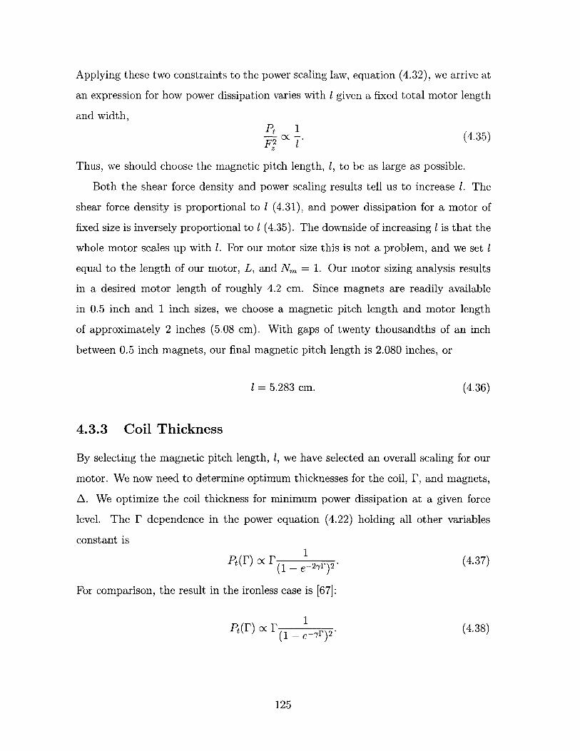
Applying these two constraints to the power scaling law, equation (4.32), we arrive at

an expression for how power dissipation varies with 1 given a fixed total motor length

and width,

zPF 1

Thus, we should choose the magnetic pitch length, 1, to be as large as possible.

Both the shear force density and power scaling results tell us to increase 1. The

shear force density is proportional to 1 (4.31), and power dissipation for a motor of

fixed size is inversely proportional to 1 (4.35). The downside of increasing I is that the

whole motor scales up with 1. For our motor size this is not a problem, and we set 1

equal to the length of our motor, L, and Nm = 1. Our motor sizing analysis results

in a desired motor length of roughly 4.2 cm. Since magnets are readily available

in 0.5 inch and 1 inch sizes, we choose a magnetic pitch length and motor length

of approximately 2 inches (5.08 cm). With gaps of twenty thousandths of an inch

between 0.5 inch magnets, our final magnetic pitch length is 2.080 inches, or

1 = 5.283 cm. (4.36)

4.3.3 Coil Thickness

By selecting the magnetic pitch length, 1, we have selected an overall scaling for our

motor. We now need to determine optimum thicknesses for the coil, F, and magnets,

A. We optimize the coil thickness for minimum power dissipation at a given force

level. The F dependence in the power equation (4.22) holding all other variables

constant is

Pt(F) cF 1 (4.37)(1 - e 2 y) 2

For comparison, the result in the ironless case is [67]:

Pt(F) oc F 1 (4.38)(1 - --

4)2

125

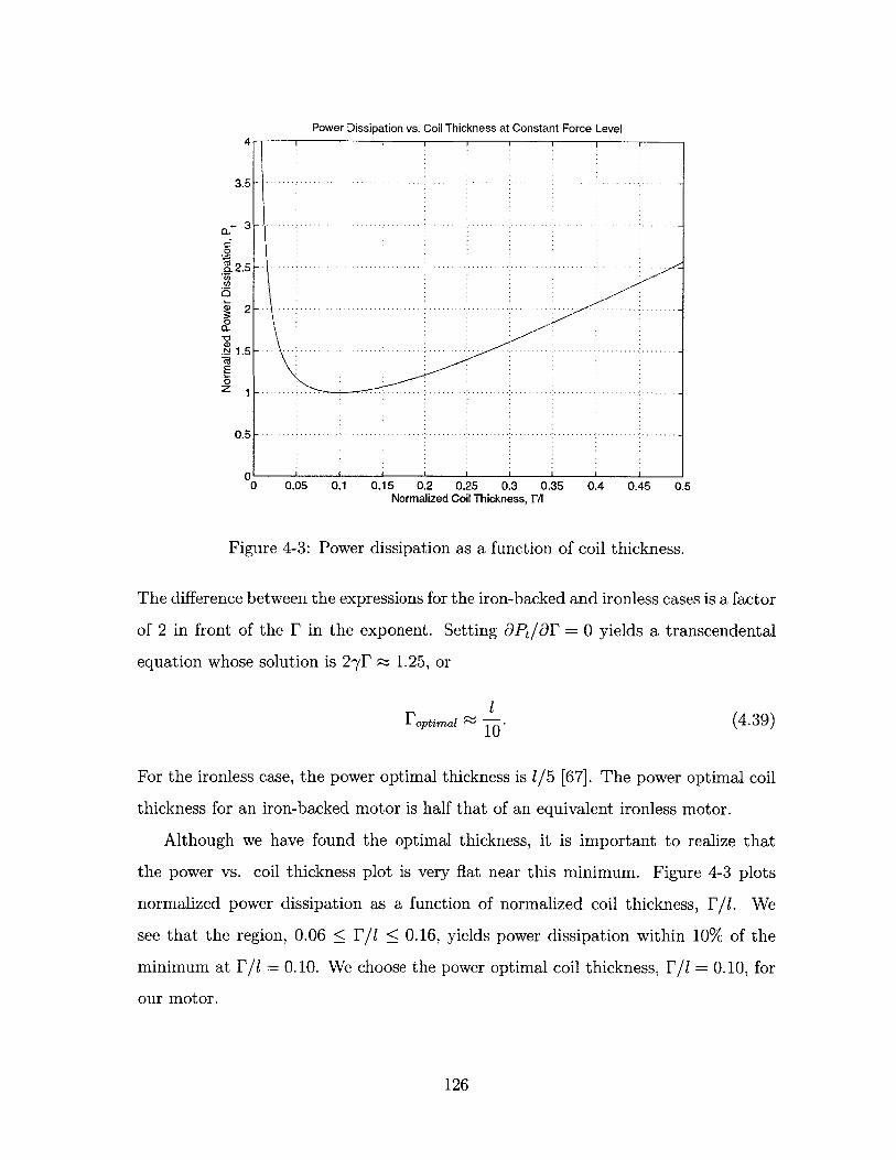
Power Dissipation vs. Coil Thickness at Constant Force LevelA.

3.5

-30

6c2.5

20

N 1.5

E0Z i

0.51

UI0 0.05 0.1 0.15 0.2 0.25 0.3 0.35 0.4 0.45 0.5

Normalized Coil Thickness, r/

Figure 4-3: Power dissipation as a function of coil thickness.

The difference between the expressions for the iron-backed and ironless cases is a factor

of 2 in front of the F in the exponent. Setting OPt/OF = 0 yields a transcendental

equation whose solution is 2-yF 0 1.25, or

1 optimai ~ . (4.39)

For the ironless case, the power optimal thickness is 1/5 [67]. The power optimal coil

thickness for an iron-backed motor is half that of an equivalent ironless motor.

Although we have found the optimal thickness, it is important to realize that

the power vs. coil thickness plot is very flat near this minimum. Figure 4-3 plots

normalized power dissipation as a function of normalized coil thickness, F/1. We

see that the region, 0.06 < F/i < 0.16, yields power dissipation within 10% of the

minimum at F/1 = 0.10. We choose the power optimal coil thickness, F/i = 0.10, for

our motor.

126

- - - - -. ....................

........................ .......................-

..........-. ...--. ..-. ....-. ....-. ...-. ...- -. .. -.

...... -.. .. - -.. ........ ..... .

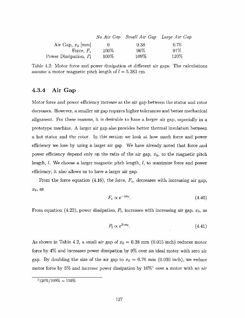
No Air Gap Small Air Gap Large Air Gap

Air Gap, xO [mm] 0 0.38 0.76Force, F2 100% 96% 91%

Power Dissipation, Pt 100% 109% 120%

Table 4.2: Motor force and power dissipation at different air gaps. The calculationsassume a motor magnetic pitch length of 1 = 5.283 cm.

4.3.4 Air Gap

Motor force and power efficiency increase as the air gap between the stator and rotor

decreases. However, a smaller air gap requires higher tolerances and better mechanical

alignment. For these reasons, it is desirable to have a larger air gap, especially in a

prototype machine. A larger air gap also provides better thermal insulation between

a hot stator and the rotor. In this section we look at how much force and power

efficiency we lose by using a larger air gap. We have already noted that force and

power efficiency depend only on the ratio of the air gap, xo, to the magnetic pitch

length, 1. We choose a larger magnetic pitch length, 1, to maximize force and power

efficiency; it also allows us to have a larger air gap.

From the force equation (4.16), the force, F, decreases with increasing air gap,

xo, as

Foc e -xO. (4.40)

From equation (4.22), power dissipation, Pt, increases with increasing air gap, xo, as

Pt oc e2) . (4.41)

As shown in Table 4.2, a small air gap of xo = 0.38 mm (0.015 inch) reduces motor

force by 4% and increases power dissipation by 9% over an ideal motor with zero air

gap. By doubling the size of the air gap to xo = 0.76 mm (0.030 inch), we reduce

motor force by 5% and increase power dissipation by 10%1 over a motor with an air

1120%/109% = 110%

127

gap of xO = 0.38 mm. Since for mechanical reasons it is desirable to have a larger air

gap in a prototype motor, and the decrease in motor performance is not great, we

choose a larger air gap of

XO = 0.84 mm. (4.42)

4.3.5 Magnet Thickness

Thicker magnets increase the motor's force and decrease its power dissipation. From

equation (4.16), with all other variables constant, the force approaches a maximum

value exponentially as magnet thickness, A, increases,

F, oc (I - e-2YA) . (4.43)

This proportionality assumes constant currents and hence constant power dissipa-

tion. From equation (4.22), with all other variables constant, the power dissipation

approaches a minimum value exponentially as magnet thickness increases,

1Pt 0c 2- (4-44)

(1 - e-2YA)2

(

This proportionality assumes constant motor force. Thus, in general, one should

choose magnets as thick as possible subject to motor size and magnet cost constraints.

Since the additional force and power efficiency gained with increasing magnet thick-

ness fall off exponentially, there will be an optimum magnet thickness; for any further

increase in magnet thickness, the increased motor size and magnet cost outweight the

improvement in motor force and power efficiency.

In the design of the z-6 axis, however, we must also take into account that added

magnet thickness increases the mass and inertia of the moving shaft. In particular, we

are not so much interested in minimizing power dissipation for a given force level, but

rather we are interested in minimizing power dissipation for a given acceleration level.

Thus, instead of using power dissipation per force squared, P/Fz, as an optimization

metric, we use linear motor power dissipation per linear acceleration, Pt/a 2, and

128

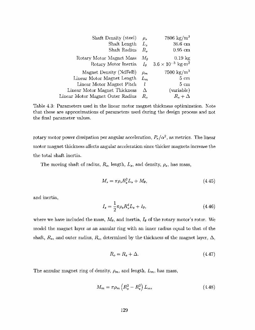
Shaft Density (steel)Shaft LengthShaft Radius

Rotary Motor Magnet MassRotary Motor Inertia

Magnet Density (NdFeB)Linear Motor Magnet Length

Linear Motor Magnet PitchLinear Motor Magnet Thickness

Linear Motor Magnet Outer Radius

PsLsRS

7806 kg/m 3

36.6 cm0.95 cm

0.19 kg1o 3.6 x 10- 5 kg-m 2

PmLm

1A

7500 kg/m 3

5 cm5 cm

(variable)R, + A

Table 4.3: Parameters used in the linear motor magnet thickness optimization. Notethat these are approximations of parameters used during the design process and notthe final parameter values.

rotary motor power dissipation per angular acceleration, P/a 2 , as metrics. The linear

motor magnet thickness affects angular acceleration since thicker magnets increase the

the total shaft inertia.

The moving shaft of radius, R,, length, L,, and density, ps, has mass,

M = .rp8R2 L + Mo, (4.45)

and inertia,1

Is = - rpR4L, + I0,2(4.46)

where we have included the mass, Mo, and inertia, Io of the rotary motor's rotor. We

model the magnet layer as an annular ring with an inner radius equal to that of the

shaft, R., and outer radius, R,, determined by the thickness of the magnet layer, A,

Ro = Rs + A. (4.47)

The annular magnet ring of density, pm, and length, Lm, has mass,

Mm = 7rPm (RO - RS) Lm, (4.48)

129

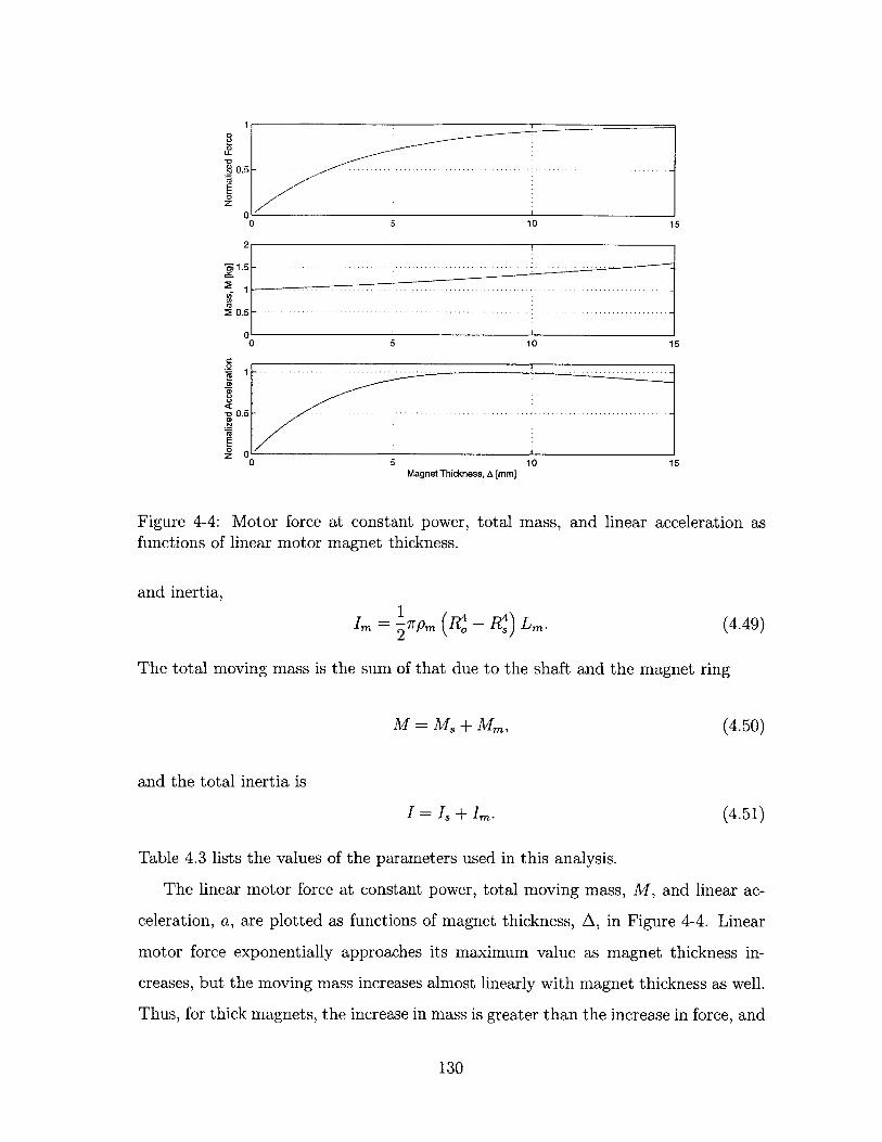
0

-

E0z

0.5

-1.5

20.5

a0

a)

1 0.

0.5

0zo0Magnet Thickness, A [mm]

10 15

Figure 4-4: Motor force at constant power, total mass, and linear acceleration asfunctions of linear motor magnet thickness.

and inertia,

Im = 1 pm( R4 - R 4 Lm. (4.49)

The total moving mass is the sum of that due to the shaft and the magnet ring

MMs Mm, (4.50)

I = Is + Im. (4.51)

Table 4.3 lists the values of the parameters used in this analysis.

The linear motor force at constant power, total moving mass, M, and linear ac-

celeration, a, are plotted as functions of magnet thickness, A, in Figure 4-4. Linear

motor force exponentially approaches its maximum value as magnet thickness in-

creases, but the moving mass increases almost linearly with magnet thickness as well.

Thus, for thick magnets, the increase in mass is greater than the increase in force, and

130

0 5 10 15

- 10 .5

-. ........-. .-.- .-. -. -. . -. -. -.-.-.-. .-.- .-. ..-

and the total inertia is

- - - - - - -- - - -- - - - -.......- ........ ....... ........ .......-

1

0 10 15

- .............-. ..-

- -- -.-.-. .-.-.-.-.- .

-

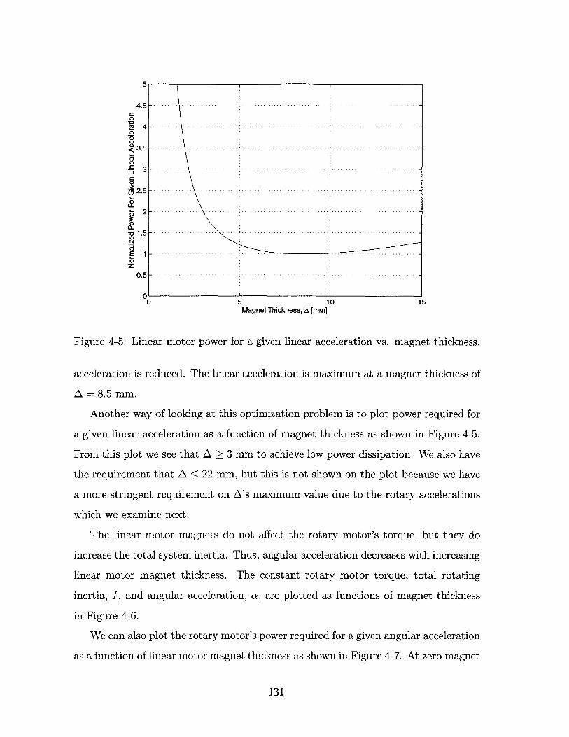
5

4 .5 - - - -.-.- .- . -

0

4 - -. -... ... .. .... ........

aD

2.5 - -. -. - -........... -. -.. -.

0

0

<3.5 ---- -

005 10 15

Magnet Thickness, A [mm]

Figure 4-5: Linear motor power for a given linear acceleration vs. magnet thickness.

acceleration is reduced. The linear acceleration is maximum at a magnet thickness of

A = 8.5 mm.

Another way of looking at this optimization problem is to plot power required for

a given linear acceleration as a function of magnet thickness as shown in Figure 4-5.

From this plot we see that A > 3 mm to achieve low power dissipation. We also have

the requirement that A < 22 mm, but this is not shown on the plot because we have

a more stringent requirement on A's maximum value due to the rotary accelerations

which we examine next.

The linear motor magnets do not affect the rotary motor's torque, but they do

increase the total system inertia. Thus, angular acceleration decreases with increasing

linear motor magnet thickness. The constant rotary motor torque, total rotating

inertia, I, and angular acceleration, oz, are plotted as functions of magnet thickness

in Figure 4-6.

We can also plot the rotary motor's power required for a given angular acceleration

as a function of linear motor magnet thickness as shown in Figure 4-7. At zero magnet

131

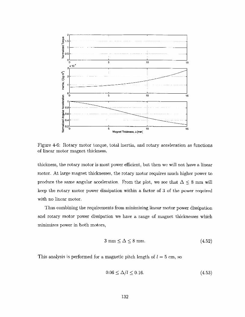
0

0

0

.5

*1

00 5 10 1x 10

0)

0

0.8

-0.6

- 0.4

E 0.20

z Magnet Thickness, A [mm]

5

15

10 15

Figure 4-6: Rotary motor torque, total inertia, and rotary acceleration as functionsof linear motor magnet thickness.

thickness, the rotary motor is most power efficient, but then we will not have a linear

motor. At large magnet thicknesses, the rotary motor requires much higher power to

produce the same angular acceleration. From the plot, we see that A < 8 mm will

keep the rotary motor power dissipation within a factor of 3 of the power required

with no linear motor.

Thus combining the requirements from minimizing linear motor power dissipation

and rotary motor power dissipation we have a range of magnet thicknesses which

minimizes power in both motors,

3 mm < A < 8 mm. (4.52)

This analysis is performed for a magnetic pitch length of I = 5 cm, so

0.06 < A/1 < 0.16. (4.53)

132

10

-. -.. ....-. .

....... ...............

-

- ............. .-. ...............-. ...-. .-.-. .-.-.-. .-. -

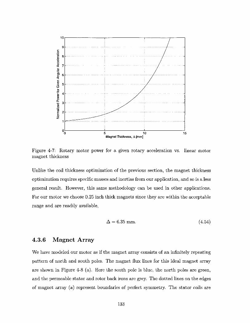
10

0

a)

0

0

E 2 - - -. . -.. .... -. -. - -. .. ............. .. ... . ....0

00 5 10 15

Magnet Thickness, A [mm]

Figure 4-7: Rotary motor power for a given rotary acceleration vs. linear motormagnet thickness

Unlike the coil thickness optimization of the previous section, the magnet thickness

optimization requires specific masses and inertias from our application, and so is a less

general result. However, this same methodology can be used in other applications.

For our motor we choose 0.25 inch thick magnets since they are within the acceptable

range and are readily available,

A = 6.35 mm. (4.54)

4.3.6 Magnet Array

We have modeled our motor as if the magnet array consists of an infinitely repeating

pattern of north and south poles. The magnet flux lines for this ideal magnet array

are shown in Figure 4-8 (a). Here the south pole is blue, the north poles are green,

and the permeable stator and rotor back irons are grey. The dotted lines on the edges

of magnet array (a) represent boundaries of perfect symmetry. The stator coils are

133

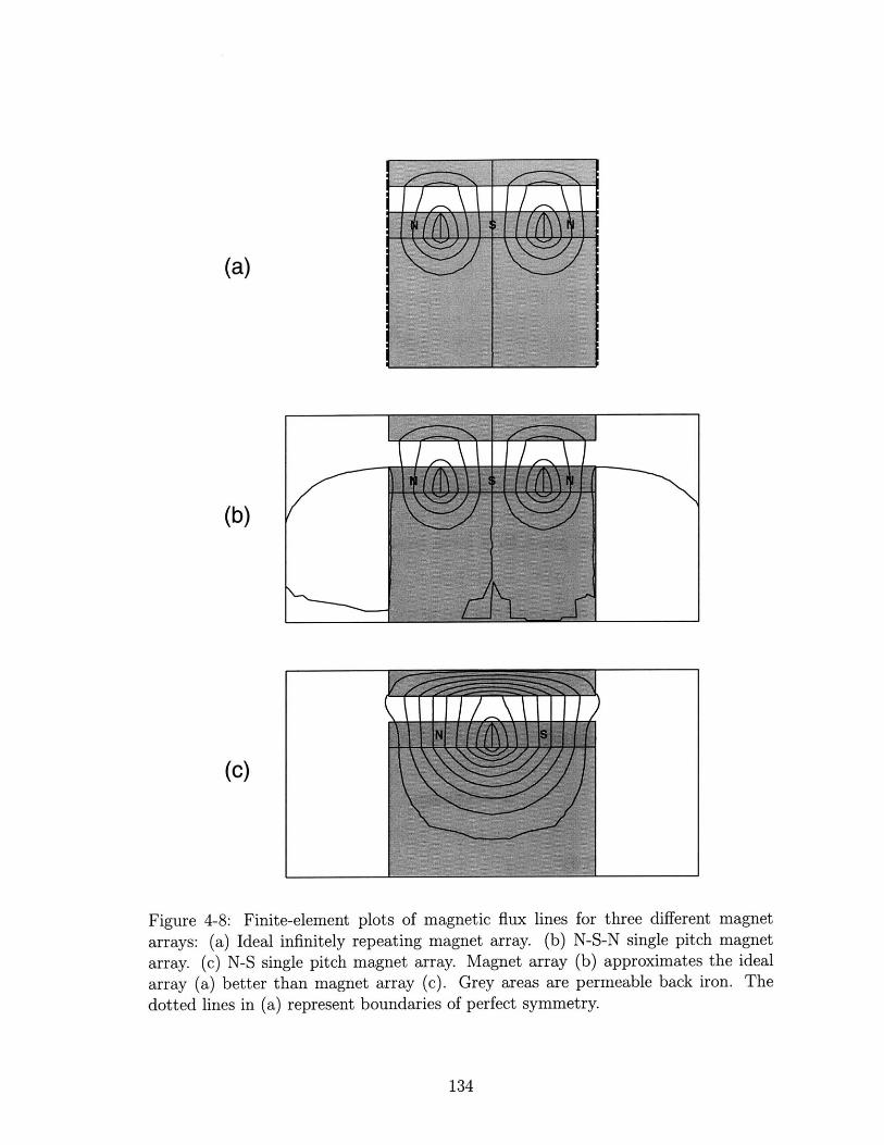
I I / - \ II/ \ \I

(a)

(b)

(c)

Figure 4-8: Finite-element plots of magnetic flux lines for three different magnet

arrays: (a) Ideal infinitely repeating magnet array. (b) N-S-N single pitch magnetarray. (c) N-S single pitch magnet array. Magnet array (b) approximates the ideal

array (a) better than magnet array (c). Grey areas are permeable back iron. The

dotted lines in (a) represent boundaries of perfect symmetry.

134

U 111 / \AIII )

not shown but would be in the air gap which the magnet flux crosses.

In section 4.3.2, we choose to use only one magnetic pitch length in our motor so

the rotor will have only one north and one south pole-not an infinite array. Two

possible ways of arranging the magnets in one pitch length are shown in Figure 4-8 (b)

and (c). In array (b) the north magnet is divided into two halves placed symmetrically

on either side of the south pole, but in array (c) the north and south poles are placed

side-by-side. Magnet array (b) approximates the ideal array better than magnet array

(c) due to its symmetry. Both arrays (b) and (c) suffer from end-effects. However,

the stator and rotor back irons in array (c) carry much more magnetic flux than

in the ideal array. We implement magnet array (b) in our linear motor since it

better approximates the ideal array. In addition to reducing the thickness of back

iron required, array (b) has shorter magnetic flux paths than array (c). Since back

iron has some finite permeability, the shorter flux paths in array (b) result in higher

magnetic fields in the air gap.

The north and south poles in the arrays in Figure 4-8 are adjacent to each other.

The magnetic material near the boundaries between magnets of opposite magneti-

zation is wasted since it produces little flux that crosses the air gap. In effect, the

adjacent edges of magnets of opposite magnetization short each other out and pro-

vide little useful magnetic flux. Thus, in retrospect, it would have been desirable to

have small gaps between the magnets. This would eliminate magnet mass without

affecting force much, thus boosting overall system acceleration. The range of obtain-

able magnet sizes is limited: this change could be made most easily by increasing the

magnetic pitch length and introducing space between the north and south magnets.

4.4 Linear Motor Force Constant Calculation

This section calculates the linear motor force constant using the force equation (4.16),

= p~MoiW1 [(1 - e-2,r)(i _ e2y-)e-o] (J cos yzo + Jb sin yzo). (4.55)

135

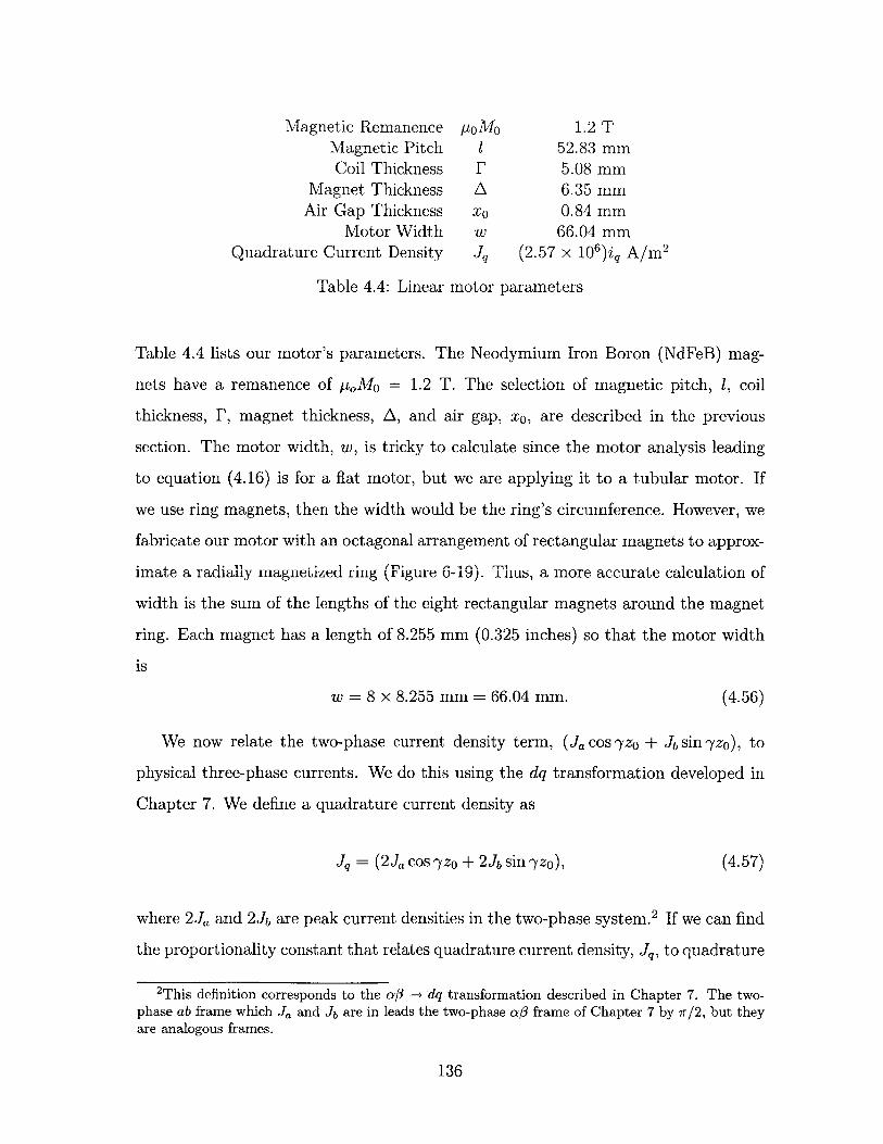
Magnetic Remanence poMo 1.2 TMagnetic Pitch 1 52.83 mmCoil Thickness F 5.08 mm

Magnet Thickness A 6.35 mmAir Gap Thickness xO 0.84 mm

Motor Width w 66.04 mmQuadrature Current Density Jq (2.57 x 106)iq A/M 2

Table 4.4: Linear motor parameters

Table 4.4 lists our motor's parameters. The Neodymium Iron Boron (NdFeB) mag-

nets have a remanence of puMo = 1.2 T. The selection of magnetic pitch, 1, coil

thickness, F, magnet thickness, A, and air gap, xo, are described in the previous

section. The motor width, w, is tricky to calculate since the motor analysis leading

to equation (4.16) is for a flat motor, but we are applying it to a tubular motor. If

we use ring magnets, then the width would be the ring's circumference. However, we

fabricate our motor with an octagonal arrangement of rectangular magnets to approx-

imate a radially magnetized ring (Figure 6-19). Thus, a more accurate calculation of

width is the sum of the lengths of the eight rectangular magnets around the magnet

ring. Each magnet has a length of 8.255 mm (0.325 inches) so that the motor width

is

w = 8 x 8.255 mm = 66.04 mm. (4.56)

We now relate the two-phase current density term, (J cos yzo + J sin -yzo), to

physical three-phase currents. We do this using the dq transformation developed in

Chapter 7. We define a quadrature current density as

Jq = (2Ja cos yzo + 2Jsin yzo), (4.57)

where 2Ja and 2J are peak current densities in the two-phase system. 2 If we can find

the proportionality constant that relates quadrature current density, Jq, to quadrature

2This definition corresponds to the a3 -+ dq transformation described in Chapter 7. The two-phase ab frame which Ja and Jb are in leads the two-phase ao frame of Chapter 7 by wr/2, but theyare analogous frames.

136

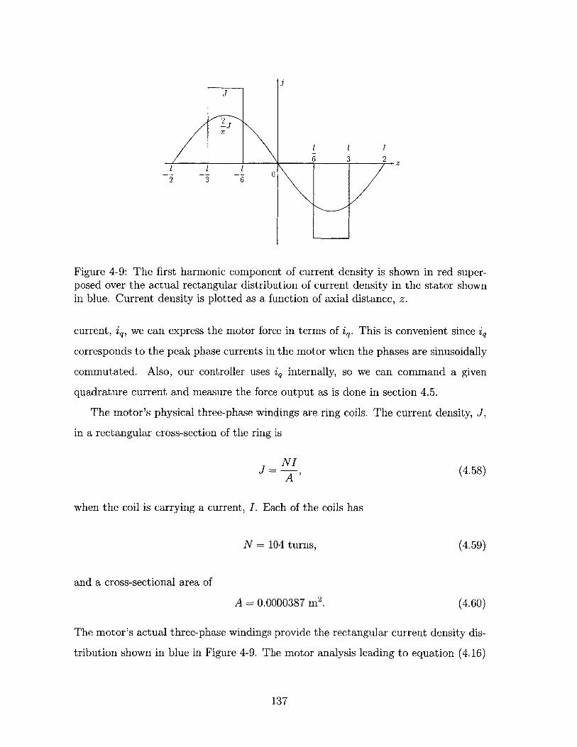
2

6 3 2 z

03 6

Figure 4-9: The first harmonic component of current density is shown in red super-posed over the actual rectangular distribution of current density in the stator shownin blue. Current density is plotted as a function of axial distance, z.

current, iq, we can express the motor force in terms of iq. This is convenient since iq

corresponds to the peak phase currents in the motor when the phases are sinusoidally

commutated. Also, our controller uses iq internally, so we can command a given

quadrature current and measure the force output as is done in section 4.5.

The motor's physical three-phase windings are ring coils. The current density, J,

in a rectangular cross-section of the ring is

S= NI (4.58)A

when the coil is carrying a current, I. Each of the coils has

N = 104 turns, (4.59)

and a cross-sectional area of

A = 0.0000387 m2 . (4.60)

The motor's actual three-phase windings provide the rectangular current density dis-

tribution shown in blue in Figure 4-9. The motor analysis leading to equation (4.16)

137

assumes that the stator windings produce sinusoidal current density distributions.

Thus, we use the first harmonic component of the actual rectangular current density

distribution. The first harmonic component3 is shown in blue in Figure 4-9. It has a

peak amplitude 2/7 times that of the actual current density in the coils, J.

We can now express quadrature current density, Jq, in terms of quadrature current,

zq,

Jq = (q (4.61)7r 2 A

= (2.57 x 106 )iq. (4.62)

The factor of 2/7r accounts for taking the first harmonic of the rectangular current

density distribution. The factor of 3/2 accounts for the greater number of turns in

the two-phase frame than the three-phase frame as explained in section 7.4.2.

Evaluating the force equation (4.16), with the motor parameters in Table 4.4 we

obtain a predicted force constant of

Kt = 14.23 N/Apeak, (4.63)

where the force constant Kt is defined by

Fz = Ktiq. (4.64)

It is interesting to also calculate the force constant using the more accurate force

equation (4.12) which does not make the approximation, e2 y(A+r+xo) > 1. In this

case we find Kt = 15.02 N/Apeak which is within 6% of the approximate value given

by equation (4.16).

3The easiest way to calculate the Fourier coefficients of a rectangular function is to find theFourier coefficients of its derivative and relate these to the coefficients of the original signal. It iseasy to find the Fourier coefficients of the derivative since this sequence consists of impulses. Fordetails, see, for example, Oppenheim & Willsky [56]

138

4.5 Linear Motor Force Constant Measurement

The motor force constant, Kt, for a three-phase motor is the force produced when the

motor phases are supplied with sinusoidally commutated currents. The force constant

can be expressed in terms of the peak or root mean square (rms) amplitudes of these

currents. In general motor force constants can be measured in two ways:

" The force can be directly measured as a function of phase current amplitude.

" The back-EMF voltage at a constant velocity can be measured and related to

the motor force constant.

Since our linear motor has only a limited travel, we cannot maintain a constant

velocity over several pitch lengths of the motor. Therefore, we measure the motor's

force directly as a function of phase current amplitude. In the rotary motor case, it

is harder to measure torque or force at a radius without a special setup, but it is easy

to spin the rotary motor at constant velocity and measure the back EMF voltage.

Thus, we use the back-EMF method to determine the rotary motor force constant in

section 4.7.

We measure linear motor force as a function of quadrature current, iq. A constant

quadrature current corresponds to three-phase sinusoidal commutation with peak

phase current amplitudes of iq. The quadrature current and its relation to phase

currents is discussed in Chapter 7. The axis's linear position, z, is measured and used

to commutate the linear motor.

We measure linear motor force with a Kistler model 9212 load cell. This piezo-

electric device produces 53.45 pC/lbf and has a load capacity of 5000 lbf. A Kistler

Dual Mode Amplifier with a long time constant is used to measure the charge pro-

duced by the load cell. The load cell is mounted to an aluminum plate on an L-block

which is bolted to the optical table. The load cell is fixtured to the aluminum plate

with a double-ended screw. The z-6 axis pushes against the other end as shown in

Figure 4-10. The small z-mirror is removed from the end of the axis for this test so

z is measured from the tilted-mirror and used to commutate the motor.

139

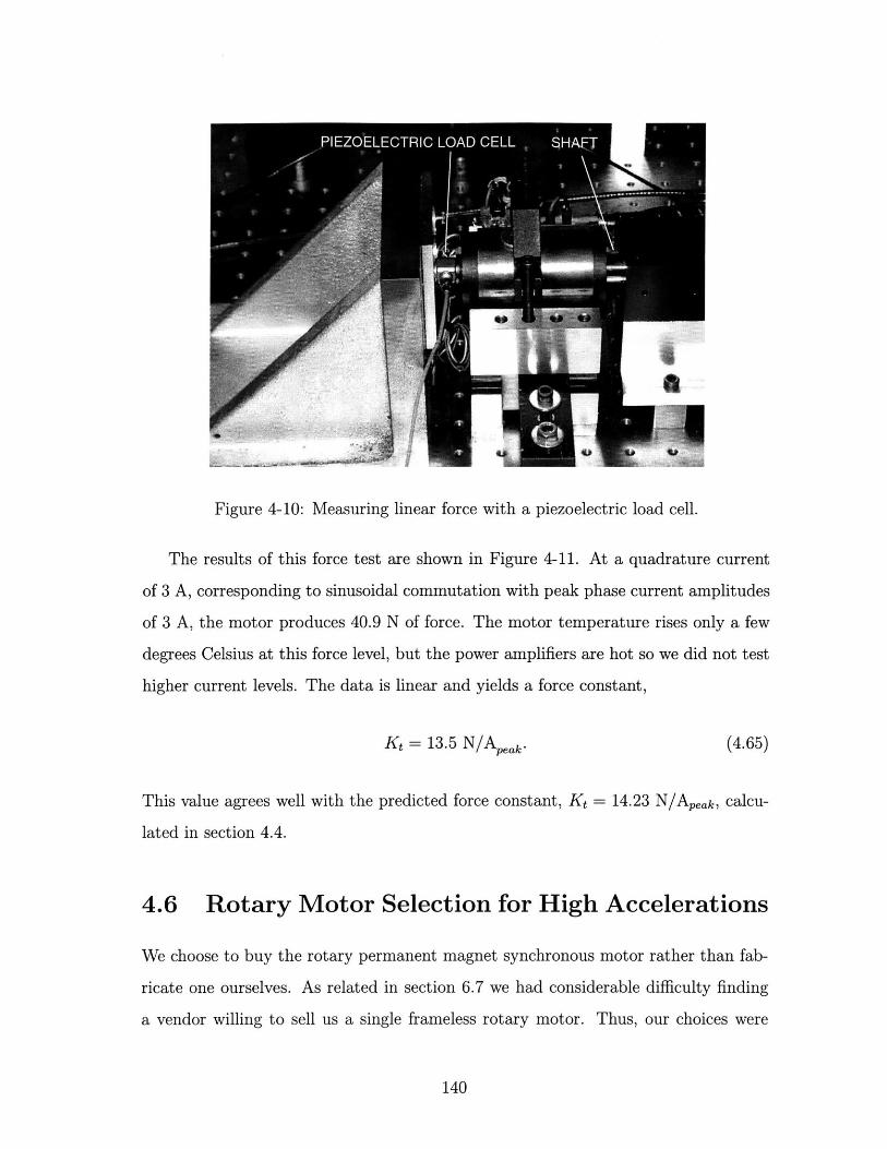
Figure 4-10: Measuring linear force with a piezoelectric load cell.

The results of this force test are shown in Figure 4-11. At a quadrature current

of 3 A, corresponding to sinusoidal commutation with peak phase current amplitudes

of 3 A, the motor produces 40.9 N of force. The motor temperature rises only a few

degrees Celsius at this force level, but the power amplifiers are hot so we did not test

higher current levels. The data is linear and yields a force constant,

Kt = 13.5 N/Apeak. (4.65)

This value agrees well with the predicted force constant, Kt = 14.23 N/Aeak, calcu-

lated in section 4.4.

4.6 Rotary Motor Selection for High Accelerations

We choose to buy the rotary permanent magnet synchronous motor rather than fab-

ricate one ourselves. As related in section 6.7 we had considerable difficulty finding

a vendor willing to sell us a single frameless rotary motor. Thus, our choices were

140

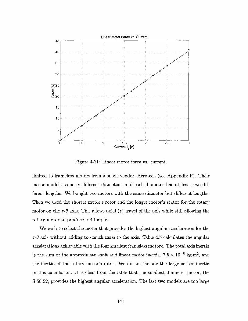
45

40

35

30

E-25

0

LL 20

15

10

0

Linear Motor Force vs. Current

-. . ... ........ ..... .....

-................ -.. ........... ......... .....

0.5 1 1.5Current I [Al

2 2.5 3

Figure 4-11: Linear motor force vs. current.

limited to frameless motors from a single vendor, Aerotech (see Appendix F). Their

motor models come in different diameters, and each diameter has at least two dif-

ferent lengths. We bought two motors with the same diameter but different lengths.

Then we used the shorter motor's rotor and the longer motor's stator for the rotary

motor on the z-6 axis. This allows axial (z) travel of the axis while still allowing the

rotary motor to produce full torque.

We wish to select the motor that provides the highest angular acceleration for the

z-0 axis without adding too much mass to the axis. Table 4.5 calculates the angular

accelerations achievable with the four smallest frameless motors. The total axis inertia

is the sum of the approximate shaft and linear motor inertia, 7.5 x 10-5 kg-m 2 , and

the inertia of the rotary motor's rotor. We do not include the large sensor inertia

in this calculation. It is clear from the table that the smallest diameter motor, the

S-50-52, provides the highest angular acceleration. The last two models are too large

141

5

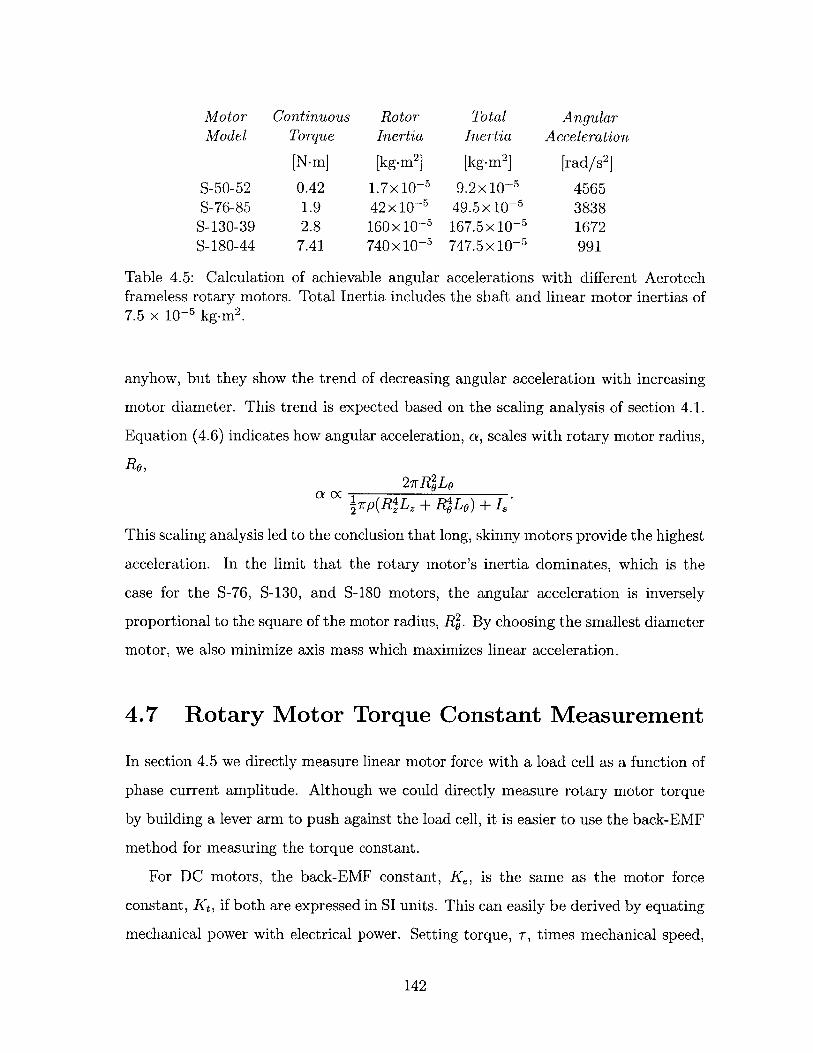
Motor Continuous Rotor Total AngularModel Torque Inertia Inertia Acceleration

[N-m] [kg.m 2 ] [kg.m 2] [rad/s 2]

S-50-52 0.42 1.7x10- 5 9.2x10 5 4565S-76-85 1.9 42 x10- 5 49.5 x 10- 5 3838

S-130-39 2.8 160 x 10- 5 167.5 x 10- 5 1672S-180-44 7.41 740 x 10- 5 747.5 x 10- 5 991

Table 4.5: Calculation of achievable angular accelerations with different Aerotechframeless rotary motors. Total Inertia includes the shaft and linear motor inertias of

7.5 x 10-5 kg.m 2.

anyhow, but they show the trend of decreasing angular acceleration with increasing

motor diameter. This trend is expected based on the scaling analysis of section 4.1.

Equation (4.6) indicates how angular acceleration, a, scales with rotary motor radius,

Ro,27rR 2 Loa (X 1 4w~L

7rp(R4L, + R LO)+ Is

This scaling analysis led to the conclusion that long, skinny motors provide the highest

acceleration. In the limit that the rotary motor's inertia dominates, which is the

case for the S-76, S-130, and S-180 motors, the angular acceleration is inversely

proportional to the square of the motor radius, R2. By choosing the smallest diameter

motor, we also minimize axis mass which maximizes linear acceleration.

4.7 Rotary Motor Torque Constant Measurement

In section 4.5 we directly measure linear motor force with a load cell as a function of

phase current amplitude. Although we could directly measure rotary motor torque

by building a lever arm to push against the load cell, it is easier to use the back-EMF

method for measuring the torque constant.

For DC motors, the back-EMF constant, Ke, is the same as the motor force

constant, Kt, if both are expressed in SI units. This can easily be derived by equating

mechanical power with electrical power. Setting torque, r, times mechanical speed,

142

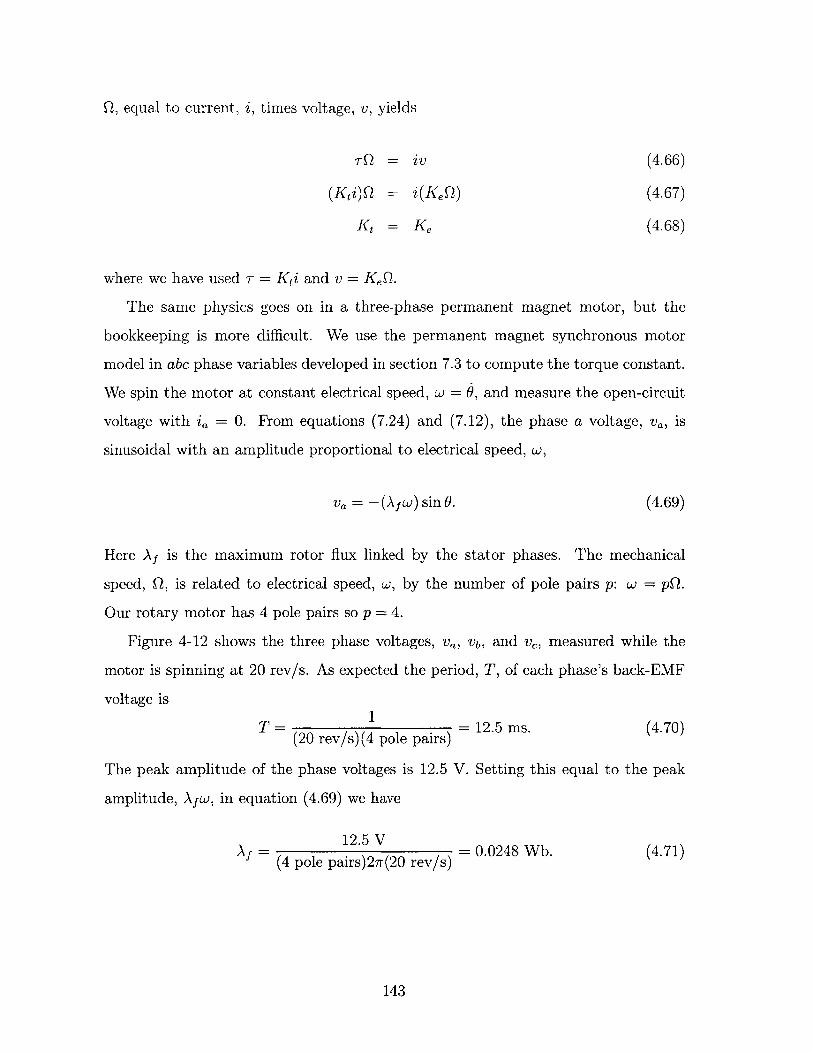
Q, equal to current, i, times voltage, v, yields

TQ = tv (4.66)

(Kti)Q = i(KeQ) (4.67)

Kt = Ke (4.68)

where we have used T = Kti and v = KeQ.

The same physics goes on in a three-phase permanent magnet motor, but the

bookkeeping is more difficult. We use the permanent magnet synchronous motor

model in abc phase variables developed in section 7.3 to compute the torque constant.

We spin the motor at constant electrical speed, w = 6, and measure the open-circuit

voltage with ia = 0. From equations (7.24) and (7.12), the phase a voltage, va, is

sinusoidal with an amplitude proportional to electrical speed, w,

Va = - (Afw) sin 6. (4.69)

Here Af is the maximum rotor flux linked by the stator phases. The mechanical

speed, Q, is related to electrical speed, w, by the number of pole pairs p: W = pQ.

Our rotary motor has 4 pole pairs so p = 4.

Figure 4-12 shows the three phase voltages, Va, Vb, and ve, measured while the

motor is spinning at 20 rev/s. As expected the period, T, of each phase's back-EMF

voltage is1

T 12.5 ms. (4.70)(20 rev/s)(4 pole pairs)

The peak amplitude of the phase voltages is 12.5 V. Setting this equal to the peak

amplitude, Afw, in equation (4.69) we have

12.5 VAf = 0.0248 Wb. (4.71)

(4 pole pairs)27r(20 rev/s)

143

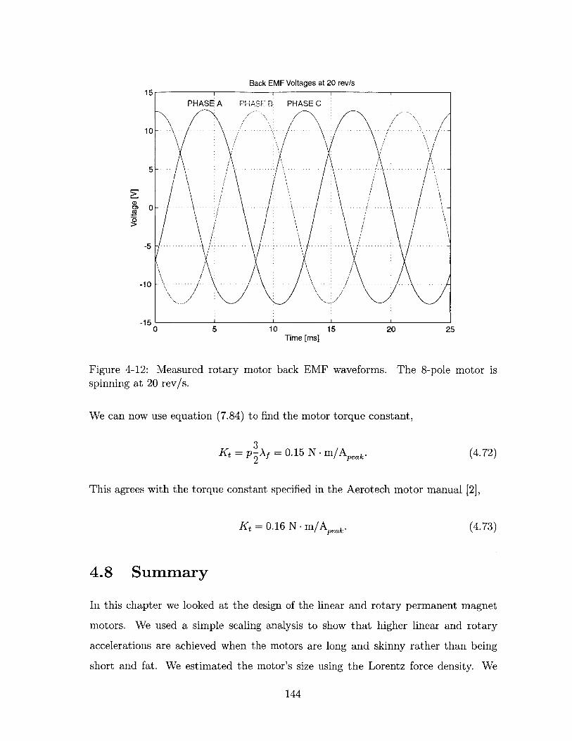
Back EMF Voltages at 20 rev/s

10Time [ms]

15

Figure 4-12: Measured rotary motor back EMF waveforms. Thespinning at 20 rev/s.

We can now use equation (7.84) to find the motor torque constant,

8-pole motor is

3Kt = p3Af = 0.15 N - m/Apeak.2

(4.72)

This agrees with the torque constant specified in the Aerotech motor manual [2],

Kt = 0.16 N -m/Apeak. (4.73)

4.8 Summary

In this chapter we looked at the design of the linear and rotary permanent magnet

motors. We used a simple scaling analysis to show that higher linear and rotary

accelerations are achieved when the motors are long and skinny rather than being

short and fat. We estimated the motor's size using the Lorentz force density. We

144

15

10

5

0)

0)0

PHASE A PHASE B PHASE C

. -. -.

- ..

- . .-. - - \ -

.- - . -. -

......... ................. ........... .. .......

-5

-10

-150 5 20 25

then proceeded to design the permanent magnet synchronous linear motor using the

results of a continuum electromechanical analysis contained in Appendix A.

We chose the motor magnetic pitch length 1 to be as large as possible, the full

length of the motor. This is because the motor's shear stress is proportional to

1, and it's power dissipation is inversely proportional to 1 for a fixed total motor

length and width. In general, one wants to choose as large a motor pitch length

as possible. However, as 1 increases, the coil thickness and magnet thickness must

increase proportionally. Therefore, for large motors it makes sense to limit the size

of 1 and have a motor with many pitch lengths rather than just one. We used the

analytical expression for power dissipation to find the power optimal coil thickness

range which is 0.06 < F/i < 0.16 where F is the coil thickness. We selected the

motor's magnet thickness by optimizing power dissipation for given linear and rotary

acceleration levels. For our application the optimal linear motor magnet thickness

range happens to be the same as the coil thickness range, 0.06 < A/i < 0.16, where

A is the magnet thickness. The coil thickness optimization is a general result, but the

magnet thickness optimization uses specific masses and inertias for our rotary axis.

We showed two ways of measuring motor force constants. We measured the linear

motor force constant directly with a piezoelectric load cell. We found that the mea-

sured force constant of 13.5 N/Apeak agreed well with the predicted force constant of

14.23 N/Apeak. We measured the rotay motor force constant by looking at its back

EMF while the motor was spinning at 20 rev/s. This measurement corresponded to

a motor force constant of 0.15 N-m/Aeak which agrees with the value specified by

the vendor, 0.16 N-m/Aeak.

One change we would make to the linear motor is to leave gaps between the north

and south magnets since these adjacent portions of the magnets short each other out

and produce no useful magnetic field. This change would reduce the magnet weight

with negligible effects on the motor operation or power efficiency.

In the next chapter we look at how we can precisely measure the translation and

rotation of our axis. These measurements are necessary not only to position the

workpiece on a precision rotary-linear axis, but also to commutate the rotary and

145

linear motors.

146

Chapter 5

Tilted-Mirror Sensor Design &

Analysis

This chapter presents, the design, analysis, and implementation of a tilted-mirror

sensor to measure shaft rotation, 0, and translation, z. Precision rotary measurement

is necessary for our prototype axis since it is intended for positioning the workpiece.

Rotary-linear axes intended for use as spindles do not require precision rotary mea-

surement; instead, a sensorless control scheme can be used as described in section 8.5.

The tilted-mirror sensor consists of a 3 inch (7.62 cm) diameter mirror mounted

on the end of the rotary-linear shaft. It has a slight tilt of 4.7 mrad (16 arcmin)

with respect to a plane normal to the shaft's axis of rotation. Two plane-mirror

interferometers measure distance to the tilted-mirror, and from these measurements

we can calculate shaft rotation, 0, and translation, z. In order to avoid singularities in

this sensor implementation, we also directly measure translation, z, with a third laser

interferometer; this interferometer measures distance to a small, non-tilted mirror on

the opposite end of the shaft. Table 5.1 summarizes the performance of the tilted-

mirror sensor.

In section 3.4 we examined several possible sensor concepts for measuring rotary-

linear motion. These included the prism-mirror sensor, the tilted-mirror sensor, the

helicoid mirror sensor, the rotating half-wave plate sensor, the rotating polarizer

sensor, and the 2-D encoder. In this chapter we focus on the design and analysis

147

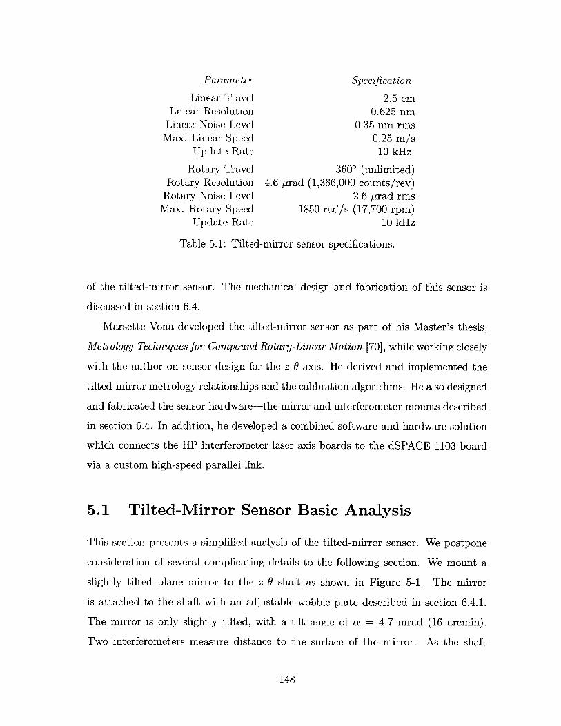
Parameter Specification

Linear Travel 2.5 cmLinear Resolution 0.625 nm

Linear Noise Level 0.35 nm rmsMax. Linear Speed 0.25 m/s

Update Rate 10 kHz

Rotary Travel 3600 (unlimited)Rotary Resolution 4.6 prad (1,366,000 counts/rev)

Rotary Noise Level 2.6 prad rmsMax. Rotary Speed 1850 rad/s (17,700 rpm)

Update Rate 10 kHz

Table 5.1: Tilted-mirror sensor specifications.

of the tilted-mirror sensor. The mechanical design and fabrication of this sensor is

discussed in section 6.4.

Marsette Vona developed the tilted-mirror sensor as part of his Master's thesis,

Metrology Techniques for Compound Rotary-Linear Motion [70], while working closely

with the author on sensor design for the z-0 axis. He derived and implemented the

tilted-mirror metrology relationships and the calibration algorithms. He also designed

and fabricated the sensor hardware-the mirror and interferometer mounts described

in section 6.4. In addition, he developed a combined software and hardware solution

which connects the HP interferometer laser axis boards to the dSPACE 1103 board

via a custom high-speed parallel link.

5.1 Tilted-Mirror Sensor Basic Analysis

This section presents a simplified analysis of the tilted-mirror sensor. We postpone

consideration of several complicating details to the following section. We mount a

slightly tilted plane mirror to the z-6 shaft as shown in Figure 5-1. The mirror

is attached to the shaft with an adjustable wobble plate described in section 6.4.1.

The mirror is only slightly tilted, with a tilt angle of a = 4.7 mrad (16 arcmin).

Two interferometers measure distance to the surface of the mirror. As the shaft

148

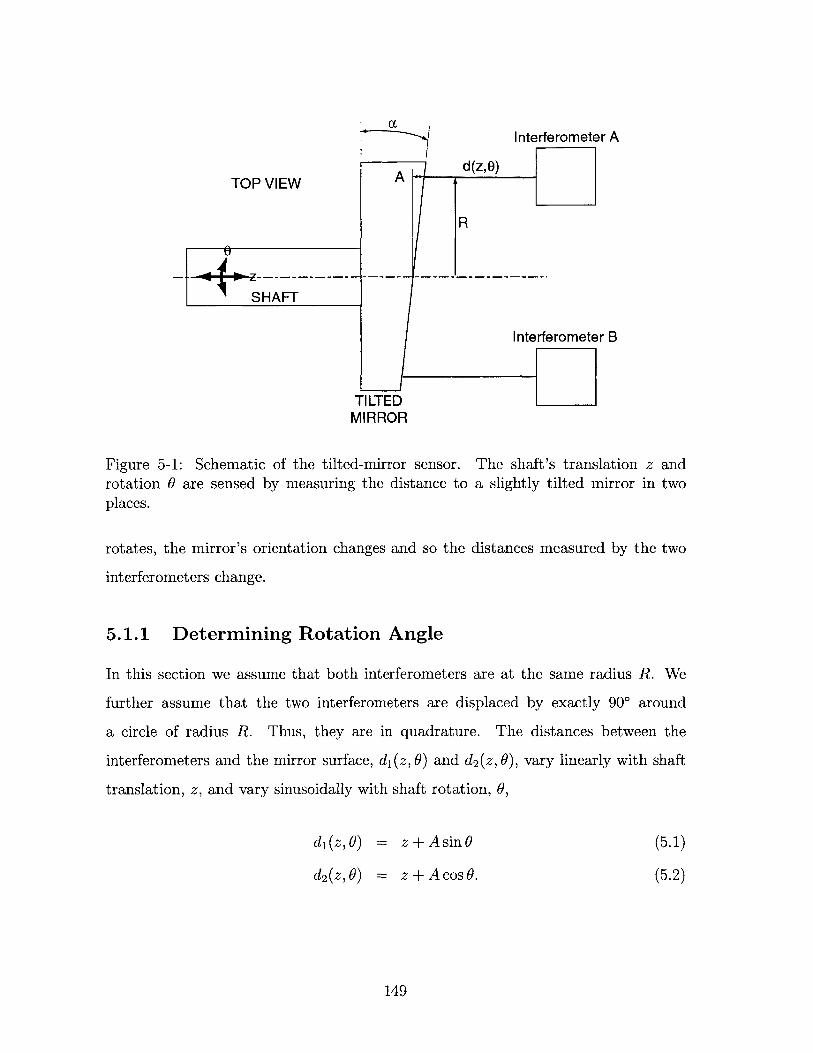
cL

ATOP VIEW

Ld=L7 1SHAFT

Interferometer A

d(z,9)

R

Interferometer B

TILTEDMIRROR

Figure 5-1: Schematic of the tilted-mirror sensor. The shaft's translation z androtation 6 are sensed by measuring the distance to a slightly tilted mirror in twoplaces.

rotates, the mirror's orientation changes and so the distances measured by the two

interferometers change.

5.1.1 Determining Rotation Angle

In this section we assume that both interferometers are at the same radius R. We

further assume that the two interferometers are displaced by exactly 900 around

a circle of radius R. Thus, they are in quadrature. The distances between the

interferometers and the mirror surface, d, (z, 6) and d2 (z, 0), vary linearly with shaft

translation, z, and vary sinusoidally with shaft rotation, 0,

di(z, 6) =

d2(z,0) =

z + A sin 6

z + A cos 0.

149

(5.1)

(5.2)

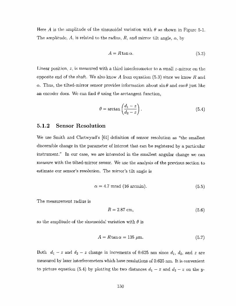
Here A is the amplitude of the sinsusoidal variation with 6 as shown in Figure 5-1.

The amplitude, A, is related to the radius, R, and mirror tilt angle, a, by

A = Rtana. (5.3)

Linear position, z, is measured with a third interferometer to a small z-mirror on the

opposite end of the shaft. We also know A from equation (5.3) since we know R and

oz. Thus, the tilted-mirror sensor provides information about sin 6 and cos 0 just like

an encoder does. We can find 6 using the arctangent function,

0 = arctan ( z (5.4)d2 - z

5.1.2 Sensor Resolution

We use Smith and Chetwynd's [61] definition of sensor resolution as "the smallest

discernible change in the parameter of interest that can be registered by a particular

instrument." In our case, we are interested in the smallest angular change we can

measure with the tilted-mirror sensor. We use the analysis of the previous section to

estimate our sensor's resolution. The mirror's tilt angle is

a = 4.7 mrad (16 arcmin). (5.5)

The measurement radius is

R = 2.87 cm, (5.6)

so the amplitude of the sinsusoidal variation with 6 is

A = Rtana = 135 Mm. (5.7)

Both d, - z and d 2 - z change in increments of 0.625 nm since dl, d2, and z are

measured by laser interferometers which have resolutions of 0.625 nm. It is convenient

to picture equation (5.4) by plotting the two distances di - z and d2 - z on the y-

150

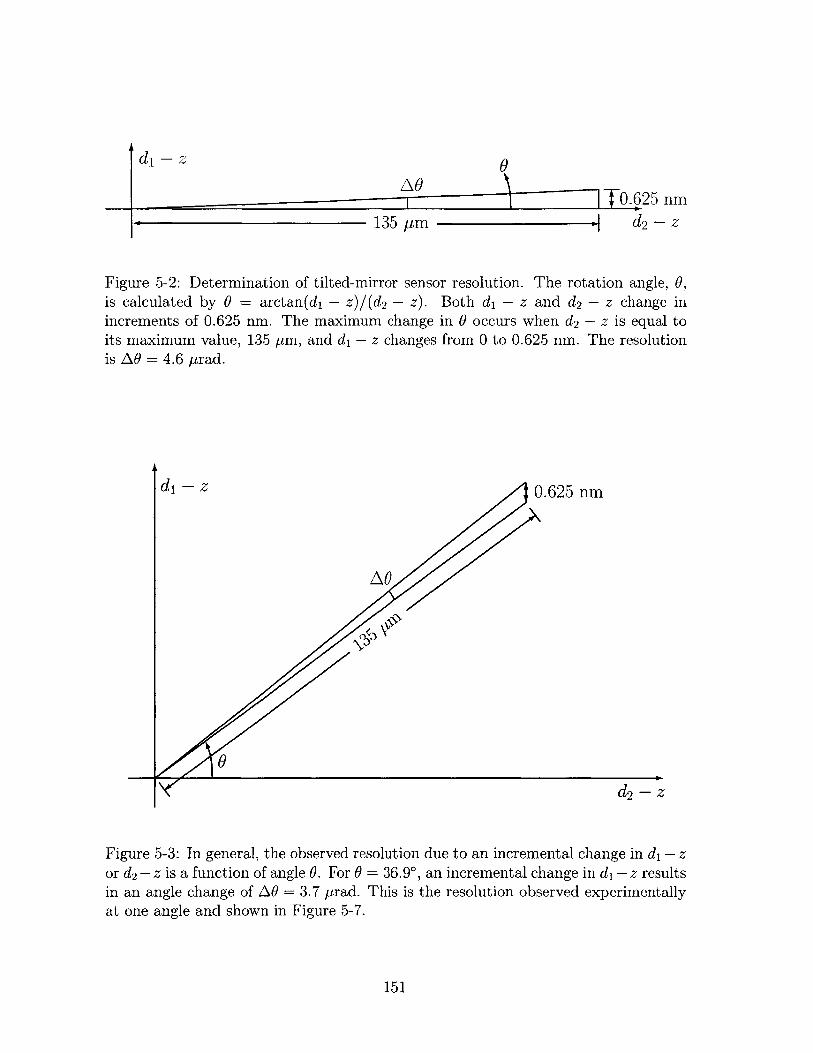
d- z

-A 1T0.625 nm

135 pm d2 - Z

Figure 5-2: Determination of tilted-mirror sensor resolution. The rotation angle, 0,is calculated by 0 = arctan(di - z)/(d2 - z). Both d, - z and d 2 - z change inincrements of 0.625 nm. The maximum change in 0 occurs when d2 - z is equal toits maximum value, 135 pm, and d, - z changes from 0 to 0.625 nm. The resolutionis AO = 4.6 prad.

di - z 0.625 nm

AO

d2 - z

Figure 5-3: In general, the observed resolution due to an incremental change in d, - zor d2- z is a function of angle 0. For 0 = 36.90, an incremental change in d, - z resultsin an angle change of AO = 3.7 prad. This is the resolution observed experimentally

at one angle and shown in Figure 5-7.

151

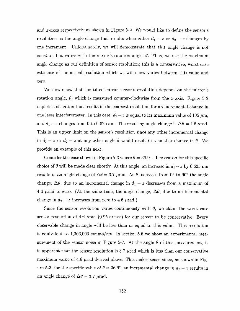
and x-axes respectively as shown in Figure 5-2. We would like to define the sensor's

resolution as the angle change that results when either d, - z or d2 - z changes by

one increment. Unfortunately, we will demonstrate that this angle change is not

constant but varies with the mirror's rotation angle, 0. Thus, we use the maximum

angle change as our definition of sensor resolution; this is a conservative, worst-case

estimate of the actual resolution which we will show varies between this value and

zero.

We now show that the tilted-mirror sensor's resolution depends on the mirror's

rotation angle, 9, which is measured counter-clockwise from the x-axis. Figure 5-2

depicts a situation that results in the coarsest resolution for an incremental change in

one laser interferometer. In this case, d2 - z is equal to its maximum value of 135 pm,

and d, - z changes from 0 to 0.625 nm. The resulting angle change is AO = 4.6 Prad.

This is an upper limit on the sensor's resolution since any other incremental change

in d, - z or d2 - z at any other angle 0 would result in a smaller change in 6. We

provide an example of this next.

Consider the case shown in Figure 5-3 where 6 = 36.90. The reason for this specific

choice of 0 will be made clear shortly. At this angle, an increase in d, - z by 0.625 nm

results in an angle change of AO = 3.7 prad. As 9 increases from 0' to 900 the angle

change, AO, due to an incremental change in d, - z decreases from a maximum of

4.6 prad to zero. (At the same time, the angle change, AO, due to an incremental

change in d2 - z increases from zero to 4.6 prad.)

Since the sensor resolution varies continuously with 9, we claim the worst case

sensor resolution of 4.6 prad (0.95 arcsec) for our sensor to be conservative. Every

observable change in angle will be less than or equal to this value. This resolution

is equivalent to 1,366,000 counts/rev. In section 5.6 we show an experimental mea-

surement of the sensor noise in Figure 5-7. At the angle 9 of this measurement, it

is apparent that the sensor resolution is 3.7 prad which is less than our conservative

maximum value of 4.6 prad derived above. This makes sense since, as shown in Fig-

ure 5-3, for the specific value of 9 = 36.9', an incremental change in d, - z results in

an angle change of AO = 3.7 prad.

152

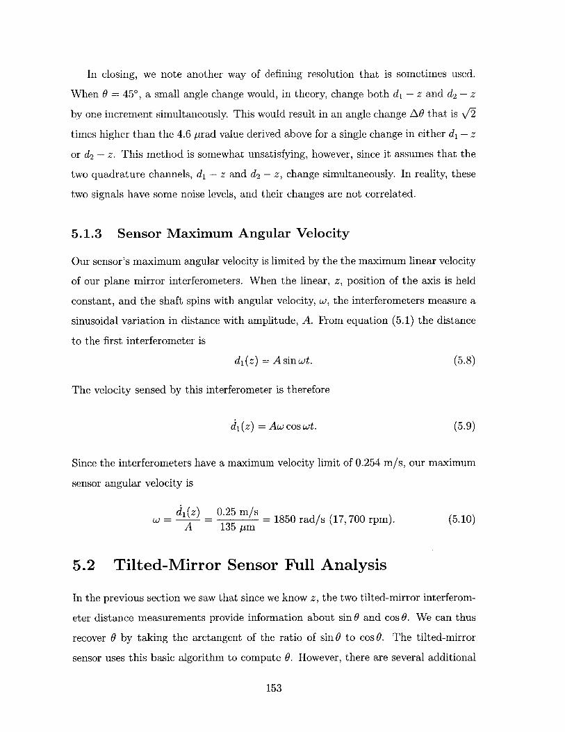
In closing, we note another way of defining resolution that is sometimes used.

When 0 = 450, a small angle change would, in theory, change both d, - z and d2 - z

by one increment simultaneously. This would result in an angle change AO that is V2

times higher than the 4.6 prad value derived above for a single change in either d, - z

or d2- z. This method is somewhat unsatisfying, however, since it assumes that the

two quadrature channels, d, - z and d 2 - z, change simultaneously. In reality, these

two signals have some noise levels, and their changes are not correlated.

5.1.3 Sensor Maximum Angular Velocity

Our sensor's maximum angular velocity is limited by the the maximum linear velocity

of our plane mirror interferometers. When the linear, z, position of the axis is held

constant, and the shaft spins with angular velocity, w, the interferometers measure a

sinusoidal variation in distance with amplitude, A. From equation (5.1) the distance

to the first interferometer is

di(z) = A sin wt. (5.8)

The velocity sensed by this interferometer is therefore

di(z) = Aw cos wt. (5.9)

Since the interferometers have a maximum velocity limit of 0.254 m/s, our maximum

sensor angular velocity is

d,(z) - 0.25 in/s = 1850 rad/s (17, 700 rpm). (5.10)A 135 pm

5.2 Tilted-Mirror Sensor Full Analysis

In the previous section we saw that since we know z, the two tilted-mirror interferom-

eter distance measurements provide information about sin 0 and cos 0. We can thus

recover 0 by taking the arctangent of the ratio of sin0 to cos0. The tilted-mirror

sensor uses this basic algorithm to compute 0. However, there are several additional

153

details that we consider in this section. In particular, we allow the two beams to

have different radii and also allow them to be close to, but not exactly, in quadra-

ture. Also, the laser interferometers only provide a relative distance measurement.

Thus, it is important for us to know what orientation the mirror is in when the two

interferometer beams read zero.

5.2.1 Path Length Equations

We let each interferometer beam' have a different radius, R1 and R 2, and phase offset

with respect to a horizontal plane, #1 and #2. We can now re-write the path length

equations (5.1) and (5.2) as

di(z, 6) = z + A, sin(O - #1) + C1 (5.11)

d2 (z, 0) = z+A 2 sin(9- 02 ) + C2. (5.12)

Here C1 and C2 are constants that depend on when the laser interface electronics are

zeroed. The two amplitudes, A1 and A2, are related to mirror tilt, a, and beam radii,

R1 and R 2, by

A1 = R1 tan a (5.13)

A2 = R2 tan a. (5.14)

5.2.2 Calibration Constants

There are six constants in the path length equations (5.11) and (5.12) which we need

to know in order to calculate 0. They are the amplitudes, A1 and A2 , the phases, #1and 02, and the zero offsets, C1 and C2. These parameters are listed in Table 5.2. In

section 5.3 we describe an automatic calibration procedure we use to determine these

six constants. For now, we assume they are known.

'In fact, we are using two-pass plane mirror interferometers so that each beam that we talk aboutreally consists of two beams. By considering their average radius and phase offset, we can treat eachinterferometer as if it had only one beam halfway between the two actual beams.

154

Parameter Description

A1, A2 Amplitude of Sinusoidal Variation in Distance with Mirror Rotation0 1, 0 2 Phase Offset of Measurement Beam from Horizontal PlaneC1, C2 Zero Offset of Measurement Beam

Table 5.2: Tilted-mirror sensor calibration constants. The constants listed apply tothe two interferometer measurement beams.

5.2.3 Compensation for Non-Ideal Measurement Beam Lo-

cations

In the simplified analysis of section 5.1 we assume that the two beams have the

same radii and are perfectly in quadrature. In reality, the beams have different radii,

and their phase difference is not exactly 900. These non-idealities are included in

equations (5.11) and (5.12). We solve equations (5.11) and (5.12) for the two signals,

sin(O - #1) and sin(6 -02),

sin(6 - #1) = dj(z,)-z-C, (5.15)A1

sin(9 - #2 ) = d2 (Z,0) - Z 02 (5.16)A 2

By dividing by the amplitudes, A1 and A2, which are proportional to beam radii, R1

and R2 , we compensate for the different beam radii.

We now show how to find 0 using sin(0- 01) and sin(6-0 2 ) given that we know #1and 02. It is convenient to solve the problem in a frame rotated by 01. We introduce

the angle, 9', which is 0 when 0 = #1,

6' = 0 - 01. (5.17)

We also introduce the phase difference between the two measurement beams,

#d = #1 - 02, (5.18)

155

which is close to 900. Using these transformations, equations (5.15) and (5.16) become

sin 0 = dl(zO) (5.19)A1

, d2(z,O) - z -02sin(9' - #d) = . (5.20)

A2

Equation (5.19) provides sin 9'. We can find cos 6' by expanding sin(O' - #d) in equa-

tion (5.20) using the trigonometric identity for the sine of the difference of two angles

and solving for cos 6',

Cos' sin(9' - #bd)- sin O'cosOd (5.21)Sin Od

We can now use the arctangent function to find 9' and add #1 to transform back to

9,

( = arctan 9' + , (5.22)(cos 6'

where sin 9' and cos 6' are given by equations (5.19) and (5.21).

5.3 Automatic Calibration Routine

We develop an automatic calibration routine to measure the calibration constants

listed in Table 5.2. These constants are the amplitudes of sinusoidal variations in dis-

tance with mirror rotation, A1 and A2, the phase offsets of the measurement beams

from the horizontal plane, #1 and #2, and the zero offsets of the measurement beams,

C1 and C2. The amplitudes, A1 and A2, are related to the radii of the measurement

beams and mirror tilt angle by equations (5.13) and (5.14). We perform this cali-

bration routine each time the rotary-linear axis is turned on. Once these constants

have been determined, we can use equations (5.18)-(5.22) to calculate shaft rotation

angle, 6.

The automatic calibration routine first homes both motors by energizing one phase

in each motor and waiting for the resulting rotary and linear stage oscillations to die

down. Then the laser interferometers are zeroed in the software. At this time, the

156

z-axis controller is turned on, and holds the z-axis at a constant position. The 0-axis

controller is also turned on and spins the axis under closed-loop control at 2.5 rev/s.

Since the calibration constants have not yet been determined, the sensor processing

software uses an inital guess for the set of calibration constants listed in Table 5.2.

As the rotor spins, the software records the distances measured by the two tilted-

mirror interferometers, d, and d2, for 5 seconds at a 5 kHz rate. This data is fit to

the model described by equations (5.11) and (5.12). We assume that the rotor spins

at a constant rate of w = 15.708 rad/s (2.5 rev/s). This assumption allows us fit

the data to the model using a linear least-squares algorithm described in Marsette

Vona's thesis [70]. From the least-squares fit, we determine A 1, A 2, q1, 0 2, C1, and

C2 . We then compare the model using these parameters to the data and determine

the maximum error.

Typically, after one fit, the maximum error is higher than our threshold value of

150 nm. This is because the axis is not spinning at exactly w = 15.708 rad/s since

the metrology equations are using initial guess calibration parameters. To improve

the fit, we take another data set, but this time we use the calibration parameters we

just determined from the least-squares fit. We continue this bootstrapping process

until the maximum error is under 150 nm. This usually requires 4-8 iterations.

Periodically we update the initial guess parameters with a set of final fit parameters,

and this usually decreases the number of iterations required till the error is below the

threshold.

5.4 Singularities without Direct z Measurement

In our prototype axis, we measure z with a third interferometer. It is also possible to

determine z using just the two tilted-mirror beams, but this results in a singularity at

two angular positions [70]. One of these singular positions is shown in Figure 5-4, and

the other occurs when the shaft is rotated 180' from this angle. The singularity occurs

when the line connecting the two interferometers is parallel to the line connecting

the mirror's high and low points. At this angle a small clockwise rotation of the

157

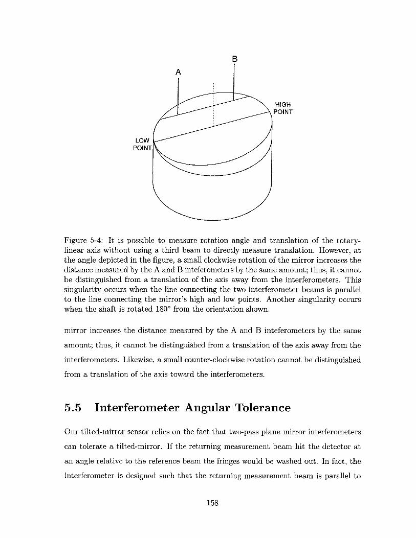
B

HIGHPOINT

LOWPOINT

Figure 5-4: It is possible to measure rotation angle and translation of the rotary-linear axis without using a third beam to directly measure translation. However, atthe angle depicted in the figure, a small clockwise rotation of the mirror increases thedistance measured by the A and B inteferometers by the same amount; thus, it cannotbe distinguished from a translation of the axis away from the interferometers. Thissingularity occurs when the line connecting the two interferometer beams is parallelto the line connecting the mirror's high and low points. Another singularity occurswhen the shaft is rotated 1800 from the orientation shown.

mirror increases the distance measured by the A and B inteferometers by the same

amount; thus, it cannot be distinguished from a translation of the axis away from the

interferometers. Likewise, a small counter-clockwise rotation cannot be distinguished

from a translation of the axis toward the interferometers.

5.5 Interferometer Angular Tolerance

Our tilted-mirror sensor relies on the fact that two-pass plane mirror interferometers

can tolerate a tilted-mirror. If the returning measurement beam hit the detector at

an angle relative to the reference beam the fringes would be washed out. In fact, the

interferometer is designed such that the returning measurement beam is parallel to

158

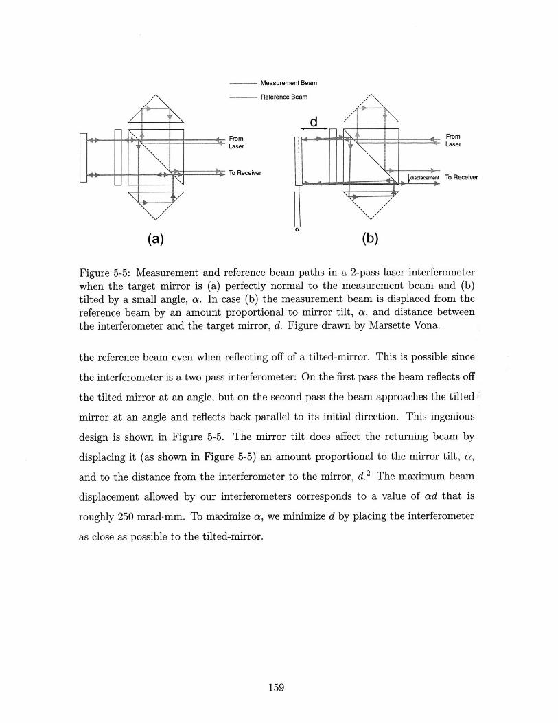
Measureme

Reference

- e

romLaser

To Receiver

(a)

nt Beam

Beam

displacement

a

FromLaser

To Receiver

Figure 5-5: Measurement and reference beam paths in a 2-pass laser interferometerwhen the target mirror is (a) perfectly normal to the measurement beam and (b)tilted by a small angle, a. In case (b) the measurement beam is displaced from thereference beam by an amount proportional to mirror tilt, a, and distance betweenthe interferometer and the target mirror, d. Figure drawn by Marsette Vona.

the reference beam even when reflecting off of a tilted-mirror. This is possible since

the interferometer is a two-pass interferometer: On the first pass the beam reflects off

the tilted mirror at an angle, but on the second pass the beam approaches the tilted

mirror at an angle and reflects back parallel to its initial direction. This ingenious

design is shown in Figure 5-5. The mirror tilt does affect the returning beam by

displacing it (as shown in Figure 5-5) an amount proportional to the mirror tilt, a,

and to the distance from the interferometer to the mirror, d.2 The maximum beam

displacement allowed by our interferometers corresponds to a value of ad that is

roughly 250 mrad-mm. To maximize a, we minimize d by placing the interferometer

as close as possible to the tilted-mirror.

159

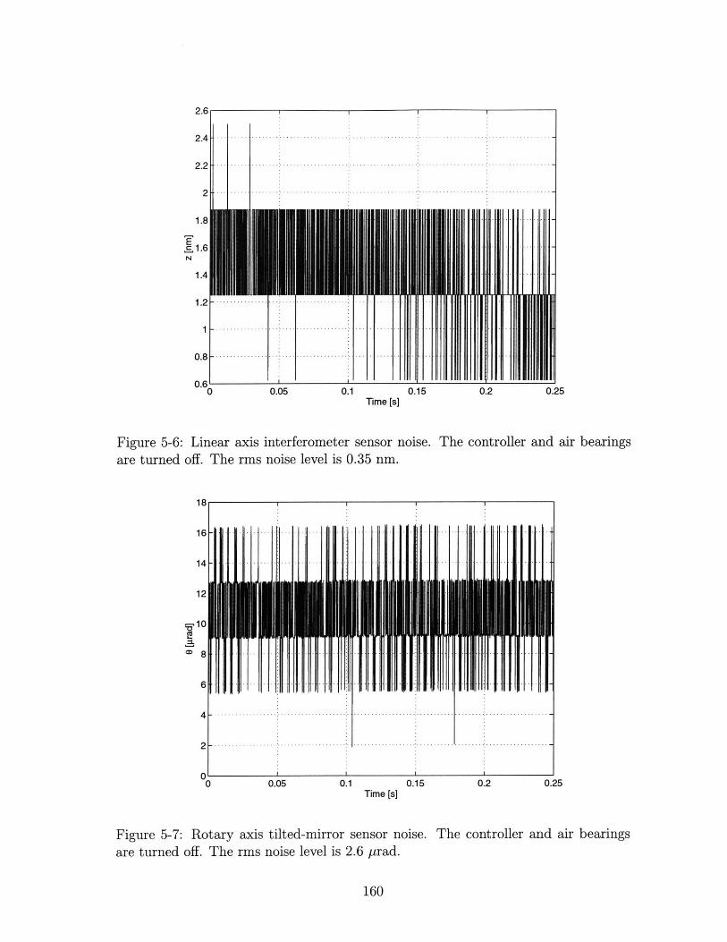
2.6-

2.4-

2.2-

2

1.8

1.6

1.4

1.2

0.8-

0.6>0

Figure 5-6:are turned

Linear axis interferometer sensor noise.off. The rms noise level is 0.35 nm.

The controller and air bearings

-- ----ui-F

II- -.- -I- .- .

0.05 0.1

DII -I .HI .101..I.-. . -. .-. . --. .-

Time [s]0.15 0.2

Figure 5-7: Rotary axis tilted-mirror sensor noise. The controller and air bearingsare turned off. The rms noise level is 2.6 rad.

160

E

0.05 0.1 0.15Time [s]

0.2 0.25

18

16

14

12

-10

6

4

2

0 0.25

-. ......... -. ...- ...- .... -. ..

-. -. . -. . ----.. ........ -.. ...............

-- -. . -.. .. . ..-.. . . .. .-.. . .. .- --.. . .. .. . .. . .

--.. ....... -. .

-.. ..-.. . ---.. .

- ... --. .. --. .. -

11 1 .11 11 -

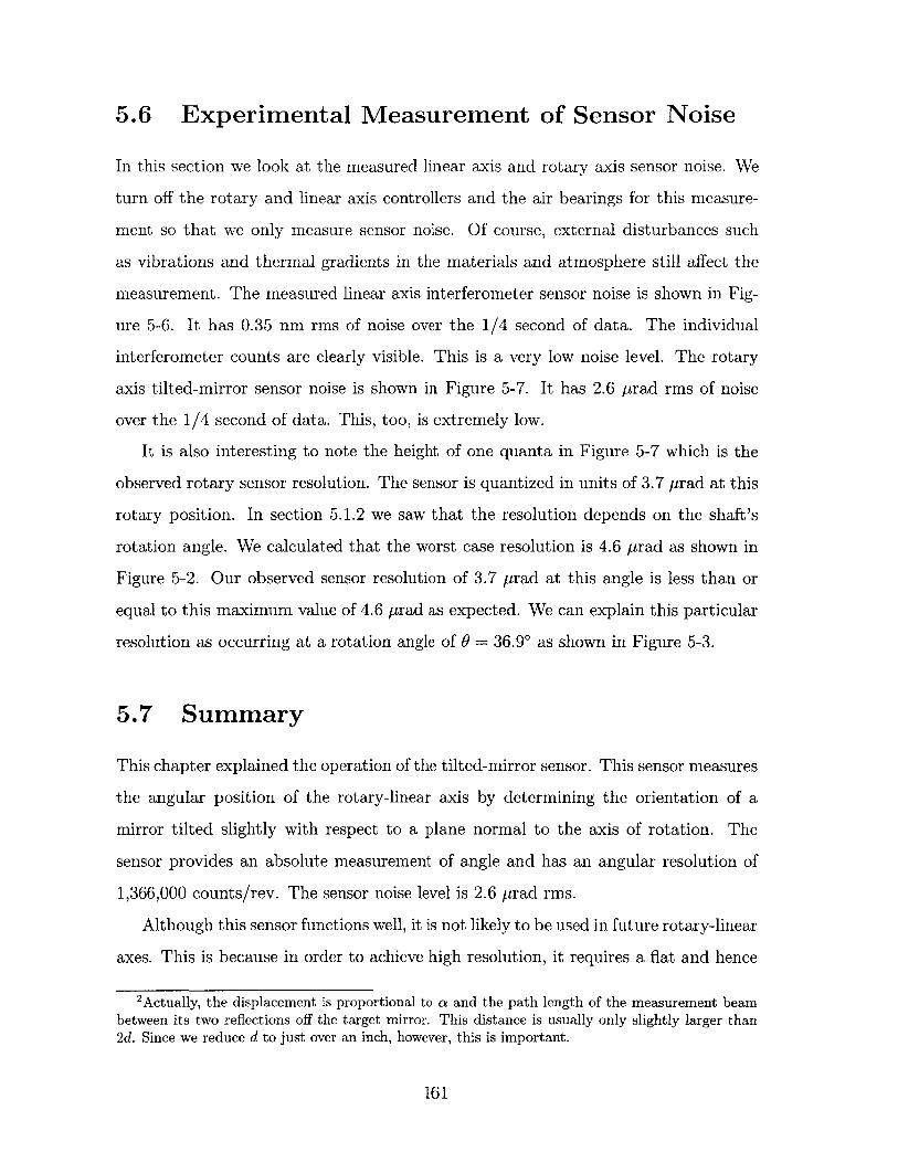
5.6 Experimental Measurement of Sensor Noise

In this section we look at the measured linear axis and rotary axis sensor noise. We

turn off the rotary and linear axis controllers and the air bearings for this measure-

ment so that we only measure sensor noise. Of course, external disturbances such

as vibrations and thermal gradients in the materials and atmosphere still affect the

measurement. The measured linear axis interferometer sensor noise is shown in Fig-

ure 5-6. It has 0.35 nm rms of noise over the 1/4 second of data. The individual

interferometer counts are clearly visible. This is a very low noise level. The rotary

axis tilted-mirror sensor noise is shown in Figure 5-7. It has 2.6 Arad rms of noise

over the 1/4 second of data. This, too, is extremely low.

It is also interesting to note the height of one quanta in Figure 5-7 which is the

observed rotary sensor resolution. The sensor is quantized in units of 3.7 Arad at this

rotary position. In section 5.1.2 we saw that the resolution depends on the shaft's

rotation angle. We calculated that the worst case resolution is 4.6 Arad as shown in

Figure 5-2. Our observed sensor resolution of 3.7 Arad at this angle is less than or

equal to this maximum value of 4.6 Arad as expected. We can explain this particular

resolution as occurring at a rotation angle of 0 = 36.90 as shown in Figure 5-3.

5.7 Summary

This chapter explained the operation of the tilted-mirror sensor. This sensor measures

the angular position of the rotary-linear axis by determining the orientation of a

mirror tilted slightly with respect to a plane normal to the axis of rotation. The

sensor provides an absolute measurement of angle and has an angular resolution of

1,366,000 counts/rev. The sensor noise level is 2.6 Arad rms.

Although this sensor functions well, it is not likely to be used in future rotary-linear

axes. This is because in order to achieve high resolution, it requires a flat and hence

2 Actually, the displacement is proportional to a and the path length of the measurement beambetween its two reflections off the target mirror. This distance is usually only slightly larger than2d. Since we reduce d to just over an inch, however, this is important.

161

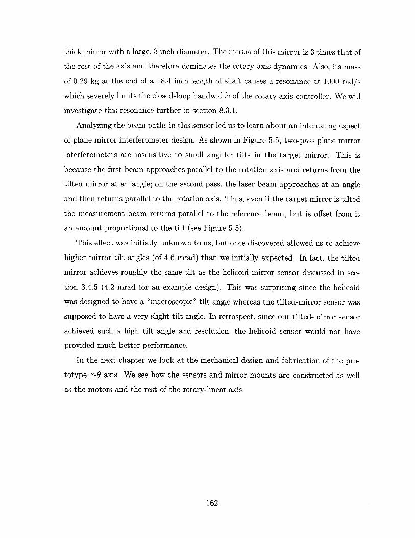
thick mirror with a large, 3 inch diameter. The inertia of this mirror is 3 times that of

the rest of the axis and therefore dominates the rotary axis dynamics. Also, its mass

of 0.29 kg at the end of an 8.4 inch length of shaft causes a resonance at 1000 rad/s

which severely limits the closed-loop bandwidth of the rotary axis controller. We will

investigate this resonance further in section 8.3.1.

Analyzing the beam paths in this sensor led us to learn about an interesting aspect

of plane mirror interferometer design. As shown in Figure 5-5, two-pass plane mirror

interferometers are insensitive to small angular tilts in the target mirror. This is

because the first beam approaches parallel to the rotation axis and returns from the

tilted mirror at an angle; on the second pass, the laser beam approaches at an angle

and then returns parallel to the rotation axis. Thus, even if the target mirror is tilted

the measurement beam returns parallel to the reference beam, but is offset from it

an amount proportional to the tilt (see Figure 5-5).

This effect was initially unknown to us, but once discovered allowed us to achieve

higher mirror tilt angles (of 4.6 mrad) than we initially expected. In fact, the tilted

mirror achieves roughly the same tilt as the helicoid mirror sensor discussed in sec-

tion 3.4.5 (4.2 mrad for an example design). This was surprising since the helicoid

was designed to have a "macroscopic" tilt angle whereas the tilted-mirror sensor was

supposed to have a very slight tilt angle. In retrospect, since our tilted-mirror sensor

achieved such a high tilt angle and resolution, the helicoid sensor would not have

provided much better performance.

In the next chapter we look at the mechanical design and fabrication of the pro-

totype z-6 axis. We see how the sensors and mirror mounts are constructed as well

as the motors and the rest of the rotary-linear axis.

162

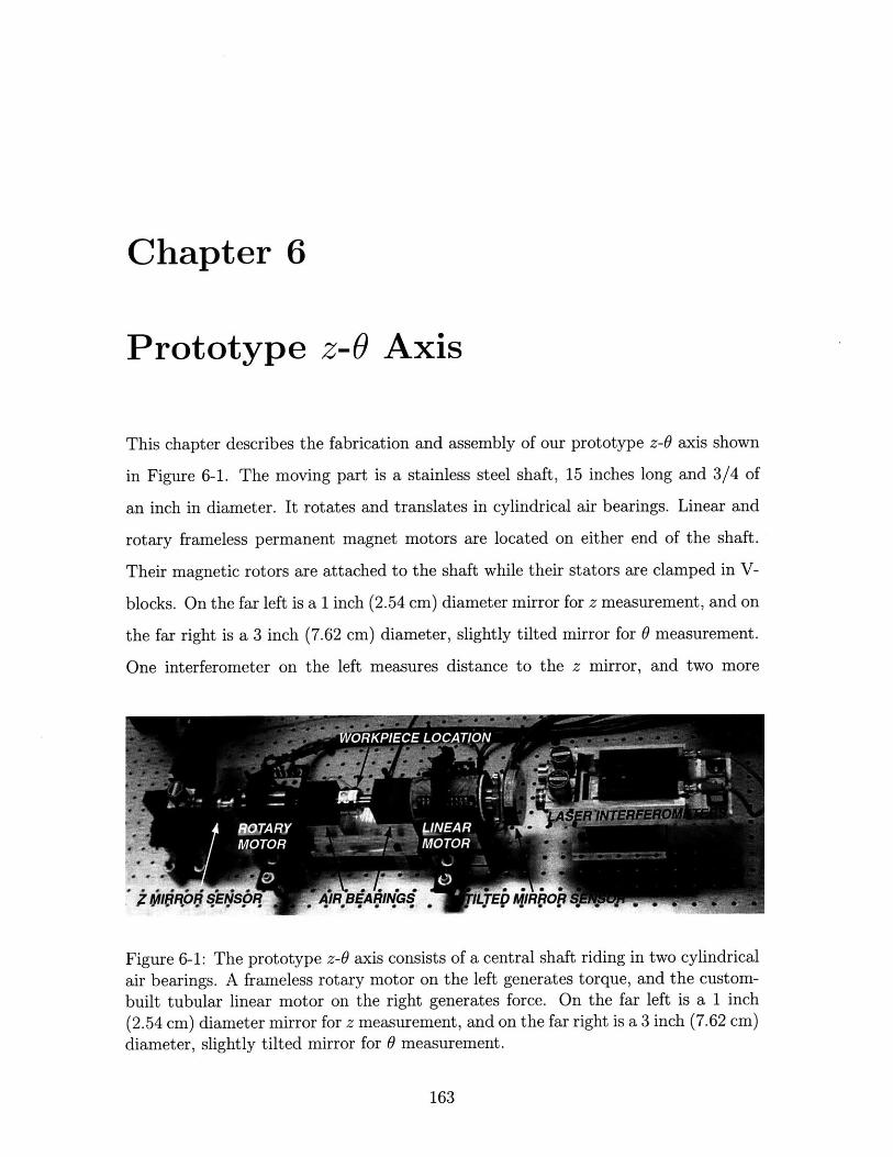
Chapter 6

Prototype z-O Axis

This chapter describes the fabrication and assembly of our prototype z-0 axis shown

in Figure 6-1. The moving part is a stainless steel shaft, 15 inches long and 3/4 of

an inch in diameter. It rotates and translates in cylindrical air bearings. Linear and

rotary frameless permanent magnet motors are located on either end of the shaft.

Their magnetic rotors are attached to the shaft while their stators are clamped in V-

blocks. On the far left is a 1 inch (2.54 cm) diameter mirror for z measurement, and on

the far right is a 3 inch (7.62 cm) diameter, slightly tilted mirror for 0 measurement.

One interferometer on the left measures distance to the z mirror, and two more

AIAR BfQ IN EAR IRJO,Z#ff?.O OR WT. ..

Figure 6-1: The prototype z-0 axis consists of a central shaft riding in two cylindrical

air bearings. A frameless rotary motor on the left generates torque, and the custom-

built tubular linear motor on the right generates force. On the far left is a 1 inch

(2.54 cm) diameter mirror for z measurement, and on the far right is a 3 inch (7.62 cm)

diameter, slightly tilted mirror for 0 measurement.

163

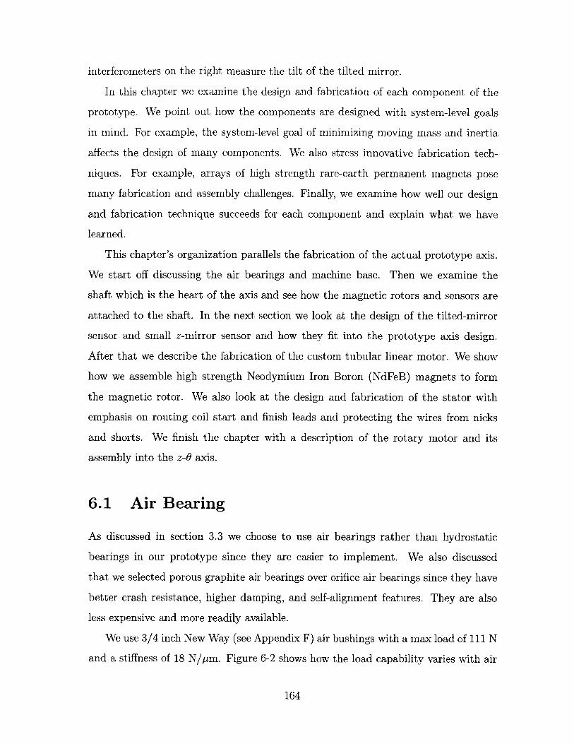
interferometers on the right measure the tilt of the tilted mirror.

In this chapter we examine the design and fabrication of each component of the

prototype. We point out how the components are designed with system-level goals

in mind. For example, the system-level goal of minimizing moving mass and inertia

affects the design of many components. We also stress innovative fabrication tech-

niques. For example, arrays of high strength rare-earth permanent magnets pose

many fabrication and assembly challenges. Finally, we examine how well our design

and fabrication technique succeeds for each component and explain what we have

learned.

This chapter's organization parallels the fabrication of the actual prototype axis.

We start off discussing the air bearings and machine base. Then we examine the

shaft which is the heart of the axis and see how the magnetic rotors and sensors are

attached to the shaft. In the next section we look at the design of the tilted-mirror

sensor and small z-mirror sensor and how they fit into the prototype axis design.

After that we describe the fabrication of the custom tubular linear motor. We show

how we assemble high strength Neodymium Iron Boron (NdFeB) magnets to form

the magnetic rotor. We also look at the design and fabrication of the stator with

emphasis on routing coil start and finish leads and protecting the wires from nicks

and shorts. We finish the chapter with a description of the rotary motor and its

assembly into the z-0 axis.

6.1 Air Bearing

As discussed in section 3.3 we choose to use air bearings rather than hydrostatic

bearings in our prototype since they are easier to implement. We also discussed

that we selected porous graphite air bearings over orifice air bearings since they have

better crash resistance, higher damping, and self-alignment features. They are also

less expensive and more readily available.

We use 3/4 inch New Way (see Appendix F) air bushings with a max load of 111 N

and a stiffness of 18 N/pm. Figure 6-2 shows how the load capability varies with air

164

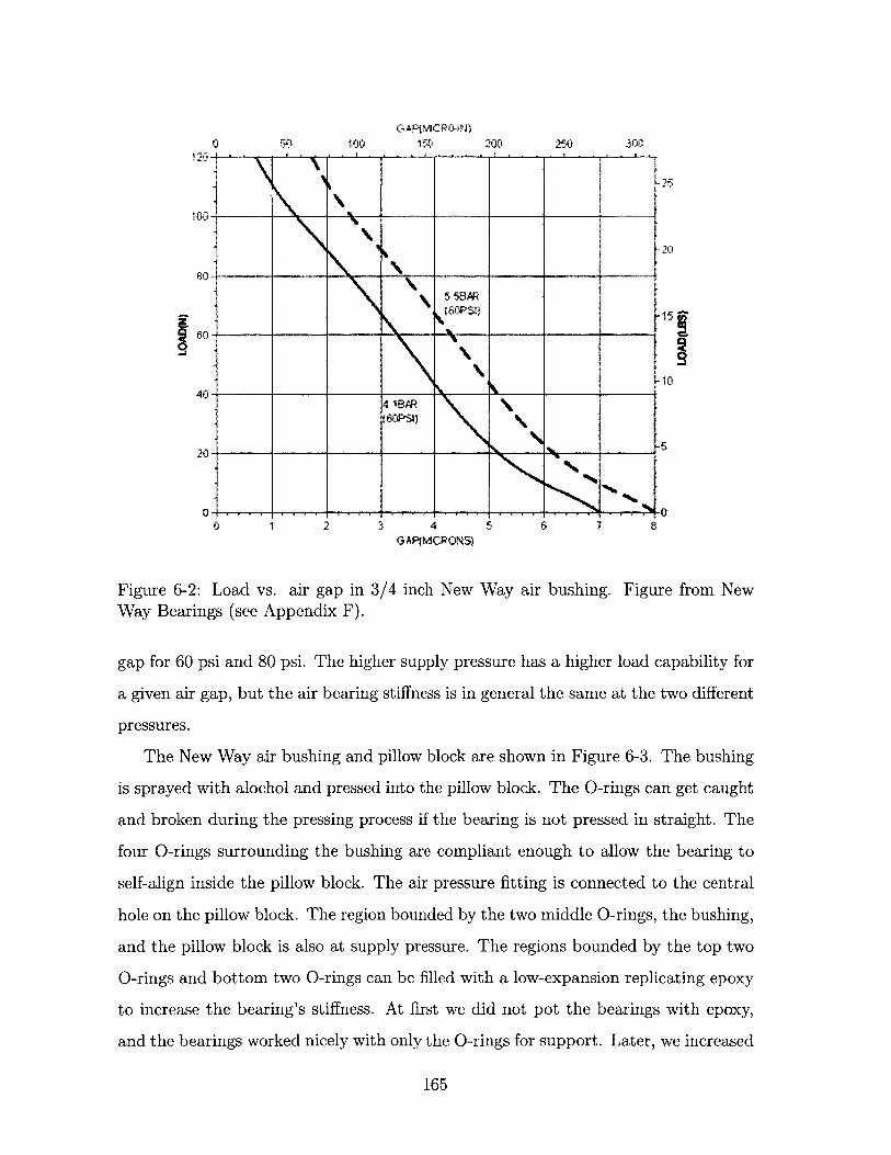
~APjMICR ~100 iCO

4GAP(MICR ON$)

Figure 6-2: Load vs. air gap inWay Bearings (see Appendix F).

3/4 inch New Way air bushing. Figure from New

gap for 60 psi and 80 psi. The higher supply pressure has a higher load capability for

a given air gap, but the air bearing stiffness is in general the same at the two different

pressures.

The New Way air bushing and pillow block are shown in Figure 6-3. The bushing

is sprayed with alochol and pressed into the pillow block. The O-rings can get caught

and broken during the pressing process if the bearing is not pressed in straight. The

four O-rings surrounding the bushing are compliant enough to allow the bearing to

self-align inside the pillow block. The air pressure fitting is connected to the central

hole on the pillow block. The region bounded by the two middle O-rings, the bushing,

and the pillow block is also at supply pressure. The regions bounded by the top two

O-rings and bottom two 0-rings can be filled with a low-expansion replicating epoxy

to increase the bearing's stiffness. At first we did not pot the bearings with epoxy,

and the bearings worked nicely with only the O-rings for support. Later, we increased

165

0

I

Nt2

0

0 I 5 & 7

40 1SA

15

4

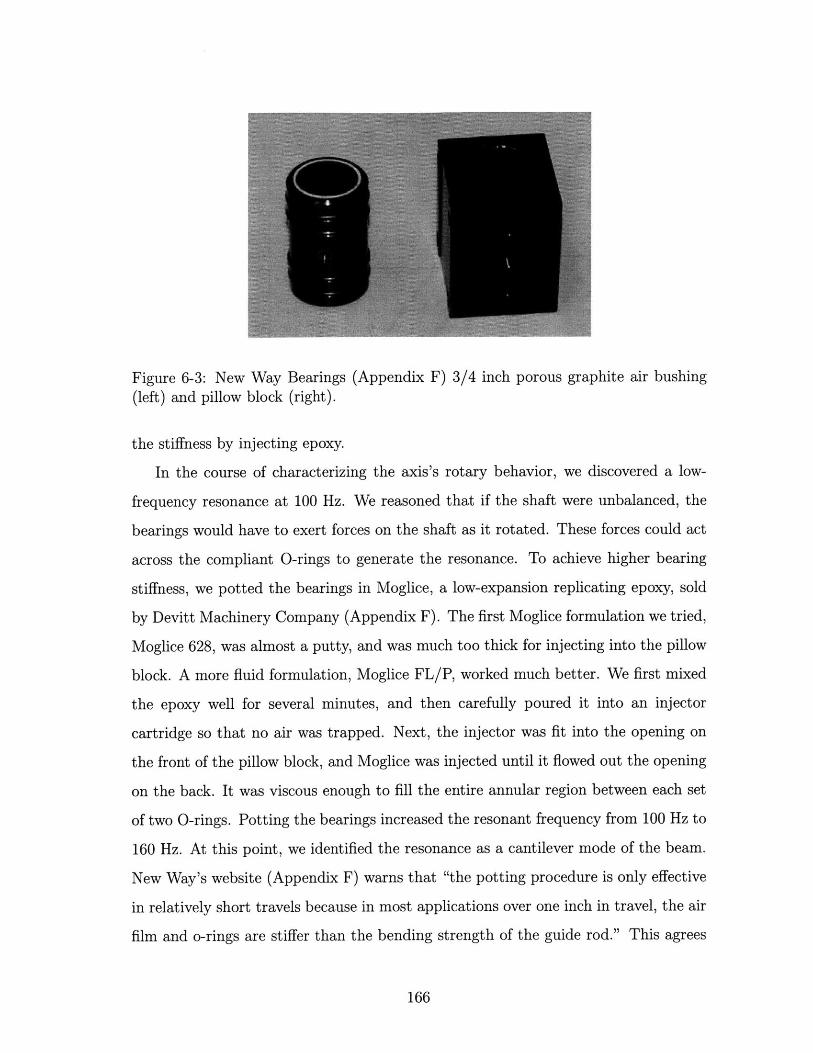
Figure 6-3: New Way Bearings (Appendix F) 3/4 inch porous graphite air bushing(left) and pillow block (right).

the stiffness by injecting epoxy.

In the course of characterizing the axis's rotary behavior, we discovered a low-

frequency resonance at 100 Hz. We reasoned that if the shaft were unbalanced, the

bearings would have to exert forces on the shaft as it rotated. These forces could act

across the compliant O-rings to generate the resonance. To achieve higher bearing

stiffness, we potted the bearings in Moglice, a low-expansion replicating epoxy, sold

by Devitt Machinery Company (Appendix F). The first Moglice formulation we tried,

Moglice 628, was almost a putty, and was much too thick for injecting into the pillow

block. A more fluid formulation, Moglice FL/P, worked much better. We first mixed

the epoxy well for several minutes, and then carefully poured it into an injector

cartridge so that no air was trapped. Next, the injector was fit into the opening on

the front of the pillow block, and Moglice was injected until it flowed out the opening

on the back. It was viscous enough to fill the entire annular region between each set

of two 0-rings. Potting the bearings increased the resonant frequency from 100 Hz to

160 Hz. At this point, we identified the resonance as a cantilever mode of the beam.

New Way's website (Appendix F) warns that "the potting procedure is only effective

in relatively short travels because in most applications over one inch in travel, the air

film and o-rings are stiffer than the bending strength of the guide rod." This agrees

166

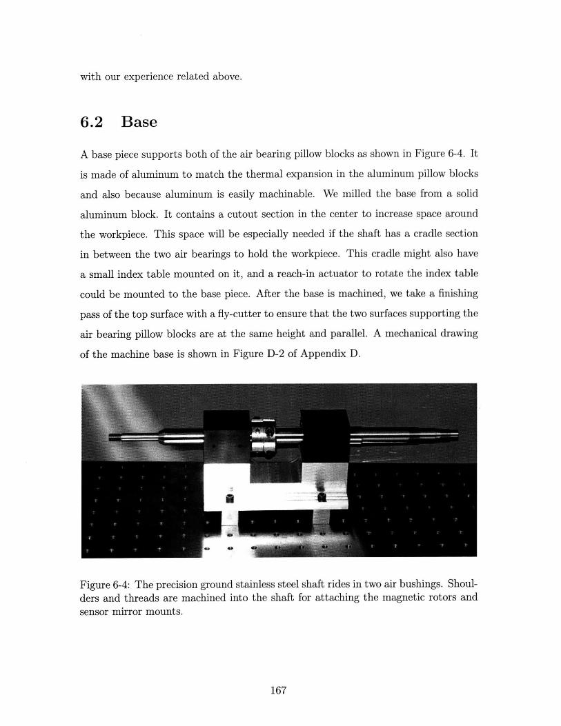
with our experience related above.

6.2 Base

A base piece supports both of the air bearing pillow blocks as shown in Figure 6-4. It

is made of aluminum to match the thermal expansion in the aluminum pillow blocks

and also because aluminum is easily machinable. We milled the base from a solid

aluminum block. It contains a cutout section in the center to increase space around

the workpiece. This space will be especially needed if the shaft has a cradle section

in between the two air bearings to hold the workpiece. This cradle might also have

a small index table mounted on it, and a reach-in actuator to rotate the index table

could be mounted to the base piece. After the base is machined, we take a finishing

pass of the top surface with a fly-cutter to ensure that the two surfaces supporting the

air bearing pillow blocks are at the same height and parallel. A mechanical drawing

of the machine base is shown in Figure D-2 of Appendix D.

Figure 6-4: The precision ground stainless steel shaft rides in two air bushings. Shoul-ders and threads are machined into the shaft for attaching the magnetic rotors andsensor mirror mounts.

167

6.3 Shaft

The shaft, shown in Figure 6-4, is the heart of the axis. It holds the workpiece and

accelerates it in translation and rotation. The magnetic rotors of the two frameless

motors are both attached to the shaft to provide force and torque. A two degree of

freedom position sensor is also mounted to the shaft.

Our primary concern in designing the shaft is minimizing its mass and rotary

inertia to maximize achievable accelerations. We must also ensure that the resulting

shaft is stiff enough to handle the accelerating forces and machining forces without

deflecting. A stiffer structure with a lower mass and inertia also has a higher natural

frequency which allows for higher control bandwidth. Finally, the shaft must be

designed so that it can be fabricated economically and quickly.

6.3.1 Material & Form

The shaft is made from solid precision ground stainless steel. We were fortunate to find

a vendor, Thomson Industries (Appendix F), which would sell us a custom machined

shaft at a reasonable cost with a very fast turnaround time. Most other vendors

were not interested in our order, asked for exorbitant prices for the special machining

required, and gave delivery dates of many months. This practical restriction forced

us to compromise on the shaft's material and form.

Initially it seemed the stiffness of a 3/4 inch solid stainless steel shaft was signif-

icantly higher than required. Thus we considered aluminum solid shafts and hollow

stainless steel shafts since they would have reduced mass and inertia and yet they

have sufficient stiffness. As it turned out, even with the solid stainless steel shaft,

stiffness has become an issue since the rotary sensor is much heavier than initially

envisioned. In order to work in air bearings, an aluminum shaft would need a hard

coat of roughly one-half thousandth of an inch. The shaft would need to be custom

precision ground and machined for us and then hard coated. No vendor we contacted

was willing to do this quickly and inexpensively.

Next we considered using tubular shafting instead of solid shafting to attempt

168

to reduce mass and inertia without affecting stiffness significantly. Unfortunately,

Thomson's tubular steel shafting, unlike its solid shafting, is not available in the

ultraprecision N Class which has a tolerance of two ten thousandths of an inch. This

tolerance is required for the shaft to work with the New Way air bushings. Thomson

could precision grind a tubular shaft for us to this tolerance level, but the costs were

very high since they would have to grind an entire twelve foot length of shafting. In

addition, a tubular shaft cannot have deep shoulders machined into it; our final design

does have deep shoulders to accommodate the magnet array of the rotary motor.

The shaft's magnetic properties also affect the machine design. We use a 440EH

stainless steel, which is ferromagnetic. This enables us to use the shaft indirectly as

back iron for the linear motor magnet array. The linear motor magnets are mounted

on thin octagonal pieces of steel with circular cutouts so that they can be mounted

on the shaft (see Figure 6-15). The octagonal back iron would surely saturate if not

for the presence of the magnetic shaft inside it. If the shaft is made of a non-magnetic

material, the octagonal pieces would have to be significantly thicker adding mass and

inertia to the axis.

6.3.2 Geometry

As explained in the previous section, we first selected the shaft's material and form-

a stainless steel, solid shaft. In this section, we explain the design of the shaft's

geometry-its precision machined shoulders and threads. These features must provide

some means for attaching the two magnetic rotors and the sensor mirror mounts.

Furthermore, we must carefully examine the allowed axial travel of the shaft and

make sure that a rotor will not crash into an air bearing, or a sensor mirror into a

stator as the shaft translates. Thus, designing the shaft's geometry required us to

envision the entire machine and design many other key parts concurrently. It also

required careful attention to details.

We attached the magnetic rotors to the shaft by axially clamping them against

shoulders machined into the shaft. The shoulders' diameters are a few ten-thousandths

of an inch smaller than the rotors' inner diameters so that the rotors slide on with

169

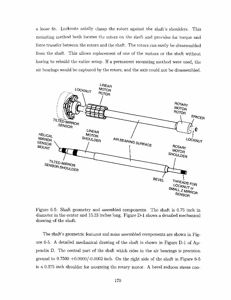
a loose fit. Locknuts axially clamp the rotors against the shaft's shoulders. This

mounting method both locates the rotors on the shaft and provides for torque and

force transfer between the rotors and the shaft. The rotors can easily be disassembled

from the shaft. This allows replacement of one of the motors or the shaft without

having to rebuild the entire setup. If a permanent mounting method were used, the

air bearings would be captured by the rotors, and the axis could not be disassembled.

HELICALMIRRORSENSORMOUNT

SEN,<

L/NeApLOCKNUT M07TOR

ROTOR

T A RSPACE

SHOUL KR

XTED..MIRRR~ORSHOUfSMLUL

BEVEL TOCA E O

SNS OR

Figure 6-5: Shaft geometry and assembled components. The shaft is 0.75 inch indiameter in the center and 15.23 inches long. Figure D-1 shows a detailed mechanicaldrawing of the shaft.

The shaft's geometric features and some assembled components are shown in Fig-

ure 6-5. A detailed mechanical drawing of the shaft is shown in Figure D-1 of Ap-

pendix D. The central part of the shaft which rides in the air bearings is precision

ground to 0.7500 +0.0000/-0.0002 inch. On the right side of the shaft in Figure 6-5

is a 0.375 inch shoulder for mounting the rotary motor. A bevel reduces stress con-

170

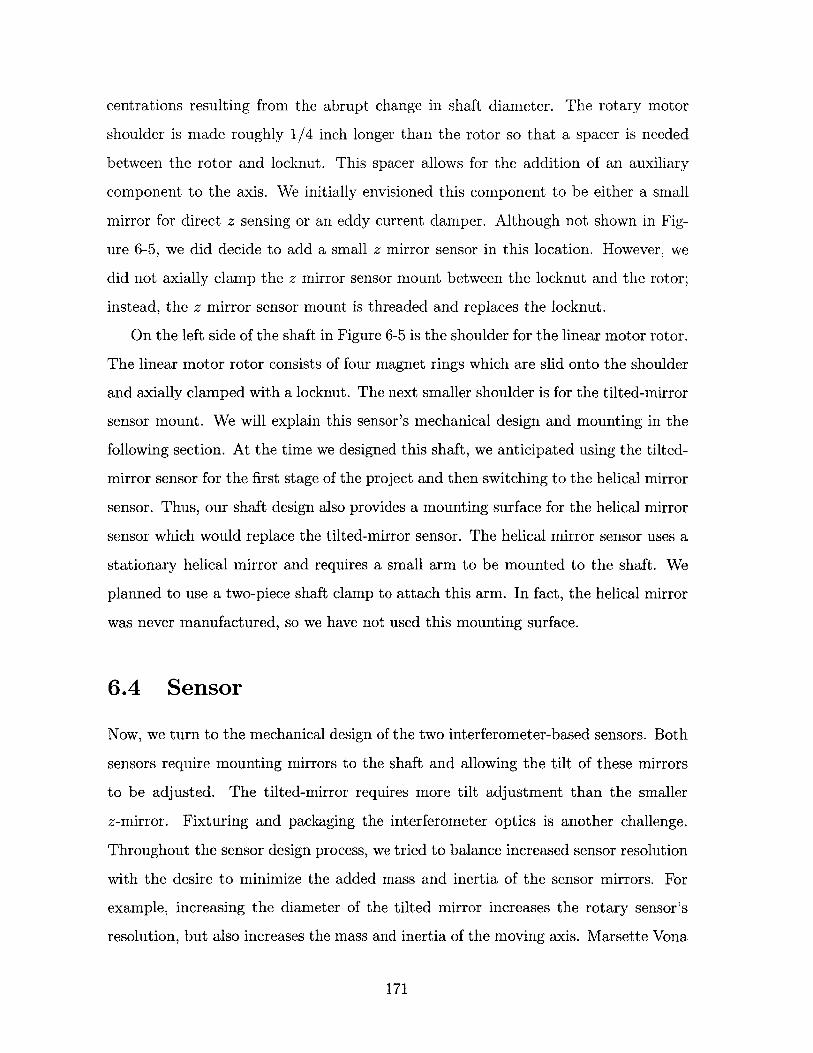
centrations resulting from the abrupt change in shaft diameter. The rotary motor

shoulder is made roughly 1/4 inch longer than the rotor so that a spacer is needed

between the rotor and locknut. This spacer allows for the addition of an auxiliary

component to the axis. We initially envisioned this component to be either a small

mirror for direct z sensing or an eddy current damper. Although not shown in Fig-

ure 6-5, we did decide to add a small z mirror sensor in this location. However, we

did not axially clamp the z mirror sensor mount between the locknut and the rotor;

instead, the z mirror sensor mount is threaded and replaces the locknut.

On the left side of the shaft in Figure 6-5 is the shoulder for the linear motor rotor.

The linear motor rotor consists of four magnet rings which are slid onto the shoulder

and axially clamped with a locknut. The next smaller shoulder is for the tilted-mirror

sensor mount. We will explain this sensor's mechanical design and mounting in the

following section. At the time we designed this shaft, we anticipated using the tilted-

mirror sensor for the first stage of the project and then switching to the helical mirror

sensor. Thus, our shaft design also provides a mounting surface for the helical mirror

sensor which would replace the tilted-mirror sensor. The helical mirror sensor uses a

stationary helical mirror and requires a small arm to be mounted to the shaft. We

planned to use a two-piece shaft clamp to attach this arm. In fact, the helical mirror

was never manufactured, so we have not used this mounting surface.

6.4 Sensor

Now, we turn to the mechanical design of the two interferometer-based sensors. Both

sensors require mounting mirrors to the shaft and allowing the tilt of these mirrors

to be adjusted. The tilted-mirror requires more tilt adjustment than the smaller

z-mirror. Fixturing and packaging the interferometer optics is another challenge.

Throughout the sensor design process, we tried to balance increased sensor resolution

with the desire to minimize the added mass and inertia of the sensor mirrors. For

example, increasing the diameter of the tilted mirror increases the rotary sensor's

resolution, but also increases the mass and inertia of the moving axis. Marsette Vona

171

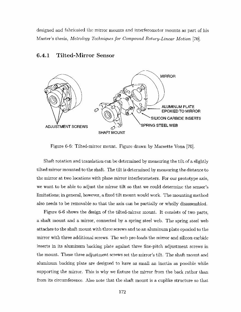
designed and fabricated the mirror mounts and interferometer mounts as part of his

Master's thesis, Metrology Techniques for Compound Rotary-Linear Motion [70].

6.4.1 Tilted-Mirror Sensor

ADJUSTMENT SCREWS

MIRROR

ALUMINUM PLATEEPOXIED TO MIRROR

SILICON CARBIDE INSERTS

SPRING STEEL WEB

SHAFT MOUNT

Figure 6-6: Tilted-mirror mount. Figure drawn by Marsette Vona [70].

Shaft rotation and translation can be determined by measuring the tilt of a slightly

tilted mirror mounted to the shaft. The tilt is determined by measuring the distance to

the mirror at two locations with plane mirror interferometers. For our prototype axis,

we want to be able to adjust the mirror tilt so that we could determine the sensor's

limitations; in general, however, a fixed tilt mount would work. The mounting method

also needs to be removable so that the axis can be partially or wholly disassembled.

Figure 6-6 shows the design of the tilted-mirror mount. It consists of two parts,

a shaft mount and a mirror, connected by a spring steel web. The spring steel web

attaches to the shaft mount with three screws and to an aluminum plate epoxied to the

mirror with three additional screws. The web pre-loads the mirror and silicon carbide

inserts in its aluminum backing plate against three fine-pitch adjustment screws in

the mount. These three adjustment screws set the mirror's tilt. The shaft mount and

aluminum backing plate are designed to have as small an inertia as possible while

supporting the mirror. This is why we fixture the mirror from the back rather than

from its circumference. Also note that the shaft mount is a cuplike structure so that

172

the smaller diameter portion of the mount can fit inside the linear motor stator if the

axis is translated. This reduces the shaft's length.

SPIG TE WESDUTETSRW

Figure 6-7: Tilted-mirror mount assembled on the z-0 axis.

This modular mount can be assembled and disassembled from the shaft. First, the

shaft mount is placed onto a shoulder of the shaft labeled the "tilted-mirror sensor

shoulder" in Figure 6-5. Then, a locknut is tightened against the mount using a

custom-machined spanner wrench which is required due to the limited space around

the locknut. Next, the spring steel web is attached to the shaft mount and then the

mirror's aluminum backing plate. The mirror extends just beyond the end of the

shaft. The adjustment screws can now be turned to achieve the desired mirror tilt.

Figure 6-7 shows the tilted-mirror mount assembled on the shaft.

This tilted-mirror mount is successful at mounting the mirror and allowing the

tilt to be adjusted. The mass and inertia of the sensor are also significantly reduced

over other possible designs. Nonetheless, the sensor adds considerable inertia to the

axis: The sensor's inertia is 25.1 x 1i-5 kg.m2 compared to 8.9 x 1i-5 kg.m 2 for the

shaft and two rotors. The sensor inertia reduces the angular acceleration of the axis

by almost a factor of four compared to a sensor with negligible inertia. The sensor's

mass, 0.29 kg, does not significantly reduce the axis's linear acceleration since the

173

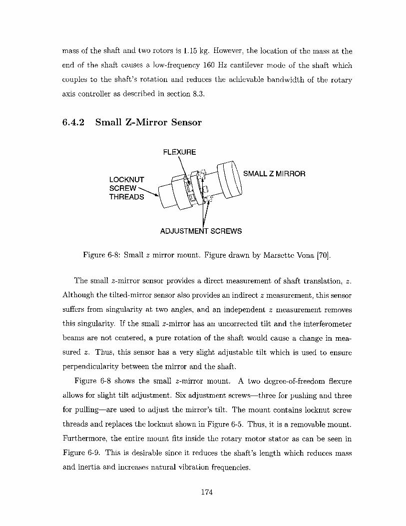
mass of the shaft and two rotors is 1.15 kg. However, the location of the mass at the

end of the shaft causes a low-frequency 160 Hz cantilever mode of the shaft which

couples to the shaft's rotation and reduces the achievable bandwidth of the rotary

axis controller as described in section 8.3.

6.4.2 Small Z-Mirror Sensor

FLEXURE

SMALL Z MIRRORLOCKNUTSCREWTHREADS

ADJUSTME T SCREWS

Figure 6-8: Small z mirror mount. Figure drawn by Marsette Vona [70].

The small z-mirror sensor provides a direct measurement of shaft translation, z.

Although the tilted-mirror sensor also provides an indirect z measurement, this sensor

suffers from singularity at two angles, and an independent z measurement removes

this singularity. If the small z-mirror has an uncorrected tilt and the interferometer

beams are not centered, a pure rotation of the shaft would cause a change in mea-

sured z. Thus, this sensor has a very slight adjustable tilt which is used to ensure

perpendicularity between the mirror and the shaft.

Figure 6-8 shows the small z-mirror mount. A two degree-of-freedom flexure

allows for slight tilt adjustment. Six adjustment screws-three for pushing and three

for pulling-are used to adjust the mirror's tilt. The mount contains locknut screw

threads and replaces the locknut shown in Figure 6-5. Thus, it is a removable mount.

Furthermore, the entire mount fits inside the rotary motor stator as can be seen in

Figure 6-9. This is desirable since it reduces the shaft's length which reduces mass

and inertia and increases natural vibration frequencies.

174

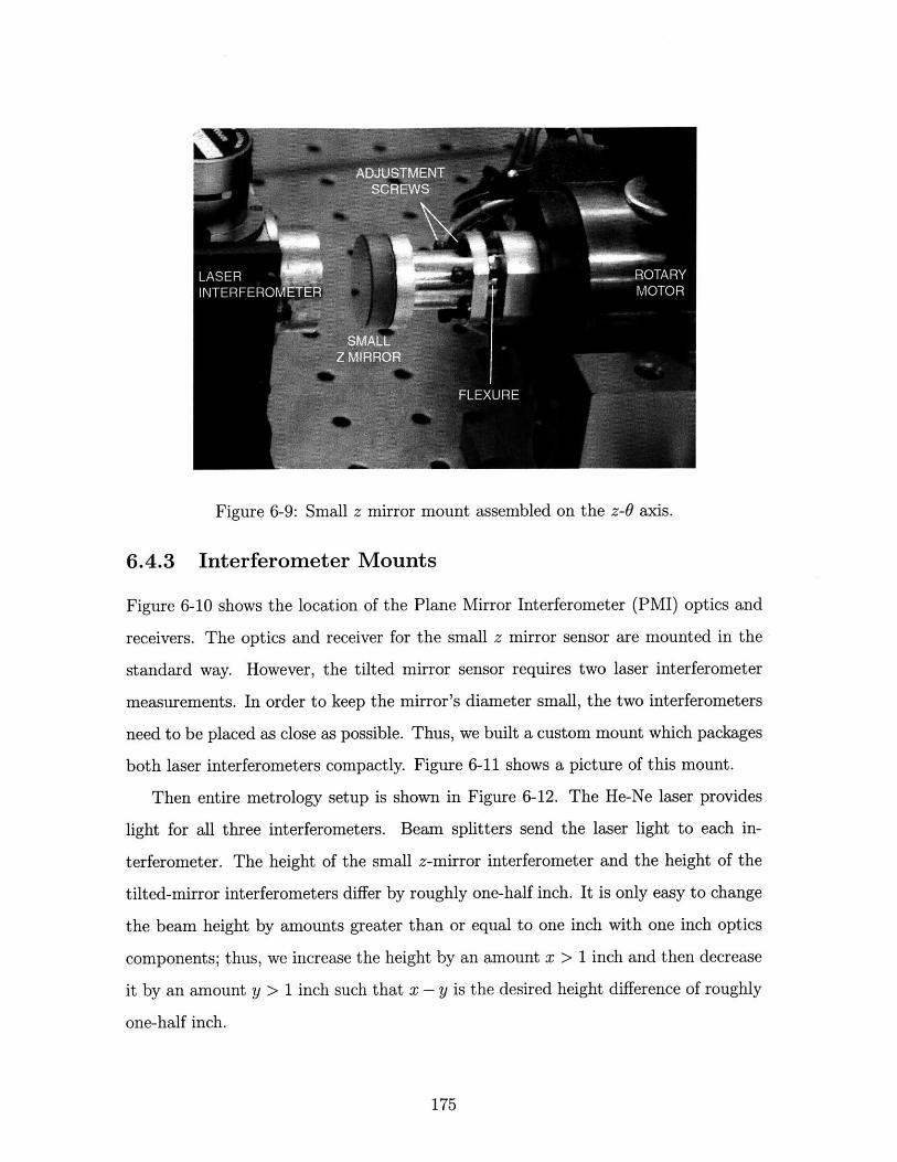
Figure 6-9: Small z mirror mount assembled on the z-0 axis.

6.4.3 Interferometer Mounts

Figure 6-10 shows the location of the Plane Mirror Interferometer (PMI) optics and

receivers. The optics and receiver for the small z mirror sensor are mounted in the

standard way. However, the tilted mirror sensor requires two laser interferometer

measurements. In order to keep the mirror's diameter small, the two interferometers

need to be placed as close as possible. Thus, we built a custom mount which packages

both laser interferometers compactly. Figure 6-11 shows a picture of this mount.

Then entire metrology setup is shown in Figure 6-12. The He-Ne laser provides

light for all three interferometers. Beam splitters send the laser light to each in-

terferometer. The height of the small z-mirror interferometer and the height of the

tilted-mirror interferometers differ by roughly one-half inch. It is only easy to change

the beam height by amounts greater than or equal to one inch with one inch optics

components; thus, we increase the height by an amount x > 1 inch and then decrease

it by an amount y > 1 inch such that x - y is the desired height difference of roughly

one-half inch.

175

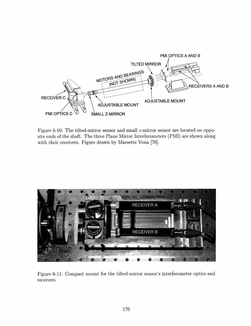
PMI OPTICS A AND B

TILTED MIRROR

RECEIVERS A AND B

RECEIVERC -ADJUSTABLE MOUNT

ADJUSTABLE MOUNT

PMI OPTICS C SMALL Z-MIRROR

Figure 6-10: The tilted-mirror sensor and small z-mirror sensor are located on oppo-site ends of the shaft. The three Plane Mirror Interferometers (PMI) are shown alongwith their receivers. Figure drawn by Marsette Vona [70].

Figure 6-11: Compact mount for the tilted-mirror sensor's interferometer optics andreceivers.

176

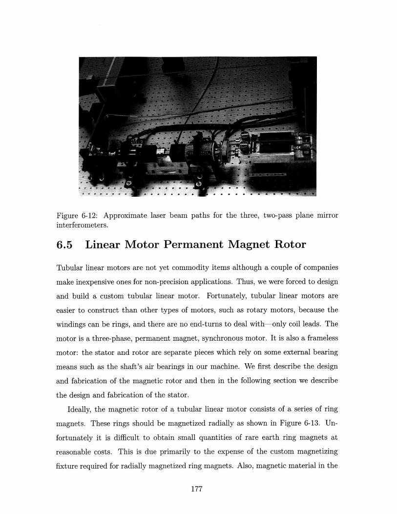
Figure 6-12: Approximate laser beam paths for the three, two-pass plane mirrorinterferometers.

6.5 Linear Motor Permanent Magnet Rotor

Tubular linear motors are not yet commodity items although a couple of companies

make inexpensive ones for non-precision applications. Thus, we were forced to design

and build a custom tubular linear motor. Fortunately, tubular linear motors are

easier to construct than other types of motors, such as rotary motors, because the

windings can be rings, and there are no end-turns to deal with-only coil leads. The

motor is a three-phase, permanent magnet, synchronous motor. It is also a frameless

motor: the stator and rotor are separate pieces which rely on some external bearing

means such as the shaft's air bearings in our machine. We first describe the design

and fabrication of the magnetic rotor and then in the following section we describe

the design and fabrication of the stator.

Ideally, the magnetic rotor of a tubular linear motor consists of a series of ring

magnets. These rings should be magnetized radially as shown in Figure 6-13. Un-

fortunately it is difficult to obtain small quantities of rare earth ring magnets at

reasonable costs. This is due primarily to the expense of the custom magnetizing

fixture required for radially magnetized ring magnets. Also, magnetic material in the

177

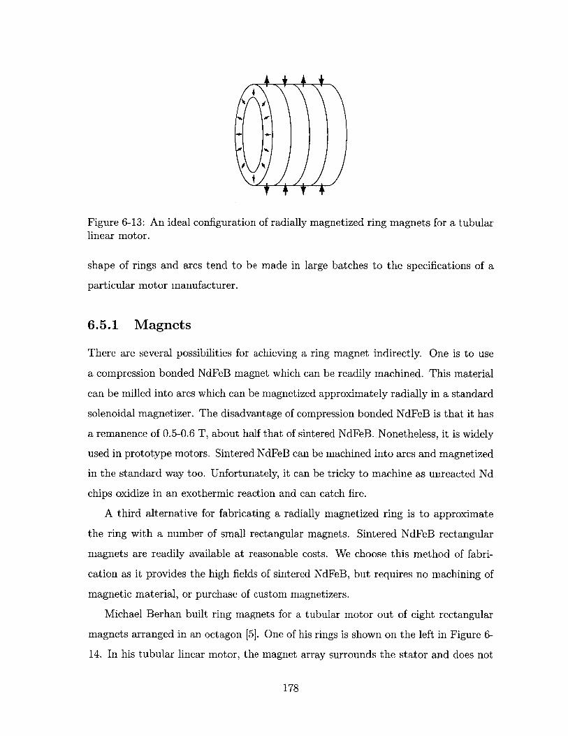
Figure 6-13: An ideal configuration of radially magnetized ring magnets for a tubularlinear motor.

shape of rings and arcs tend to be made in large batches to the specifications of a

particular motor manufacturer.

6.5.1 Magnets

There are several possibilities for achieving a ring magnet indirectly. One is to use

a compression bonded NdFeB magnet which can be readily machined. This material

can be milled into arcs which can be magnetized approximately radially in a standard

solenoidal magnetizer. The disadvantage of compression bonded NdFeB is that it has

a remanence of 0.5-0.6 T, about half that of sintered NdFeB. Nonetheless, it is widely

used in prototype motors. Sintered NdFeB can be machined into arcs and magnetized

in the standard way too. Unfortunately, it can be tricky to machine as unreacted Nd

chips oxidize in an exothermic reaction and can catch fire.

A third alternative for fabricating a radially magnetized ring is to approximate

the ring with a number of small rectangular magnets. Sintered NdFeB rectangular

magnets are readily available at reasonable costs. We choose this method of fabri-

cation as it provides the high fields of sintered NdFeB, but requires no machining of

magnetic material, or purchase of custom magnetizers.

Michael Berhan built ring magnets for a tubular motor out of eight rectangular

magnets arranged in an octagon [5]. One of his rings is shown on the left in Figure 6-

14. In his tubular linear motor, the magnet array surrounds the stator and does not

178

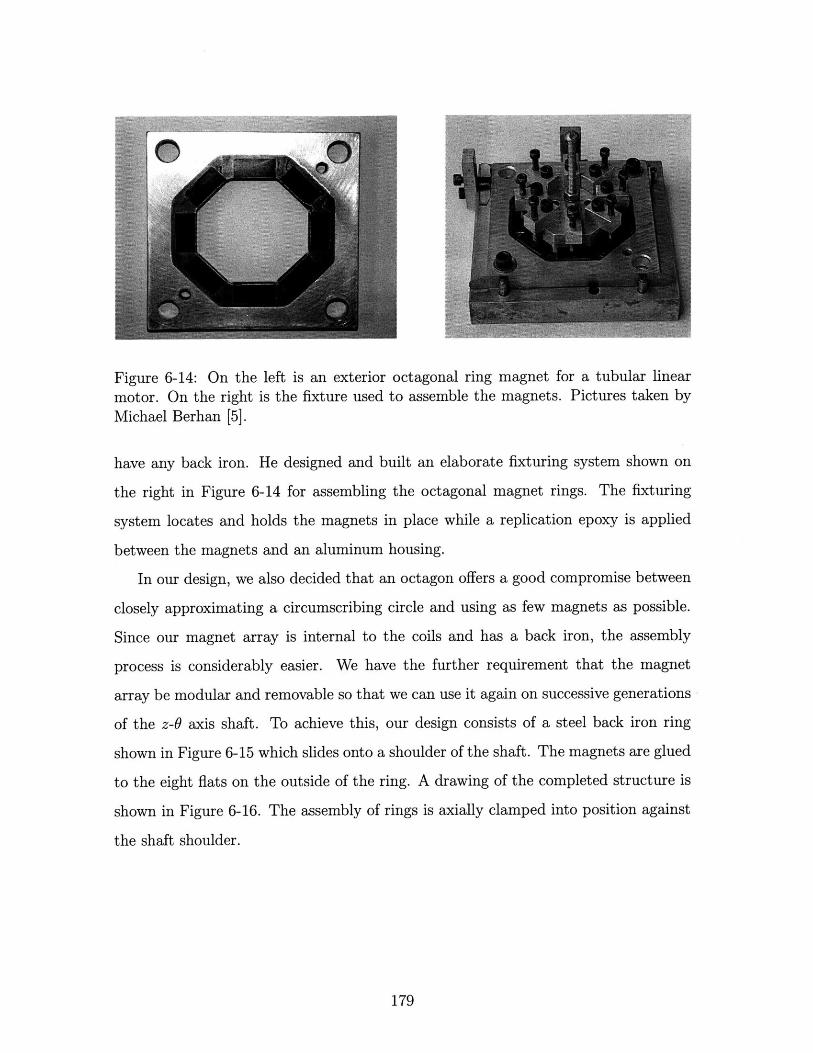
Figure 6-14: On the left is an exterior octagonal ring magnet for a tubular linearmotor. On the right is the fixture used to assemble the magnets. Pictures taken byMichael Berhan [5].

have any back iron. He designed and built an elaborate fixturing system shown on

the right in Figure 6-14 for assembling the octagonal magnet rings. The fixturing

system locates and holds the magnets in place while a replication epoxy is applied

between the magnets and an aluminum housing.

In our design, we also decided that an octagon offers a good compromise between

closely approximating a circumscribing circle and using as few magnets as possible.

Since our magnet array is internal to the coils and has a back iron, the assembly

process is considerably easier. We have the further requirement that the magnet

array be modular and removable so that we can use it again on successive generations

of the z-0 axis shaft. To achieve this, our design consists of a steel back iron ring

shown in Figure 6-15 which slides onto a shoulder of the shaft. The magnets are glued

to the eight flats on the outside of the ring. A drawing of the completed structure is

shown in Figure 6-16. The assembly of rings is axially clamped into position against

the shaft shoulder.

179

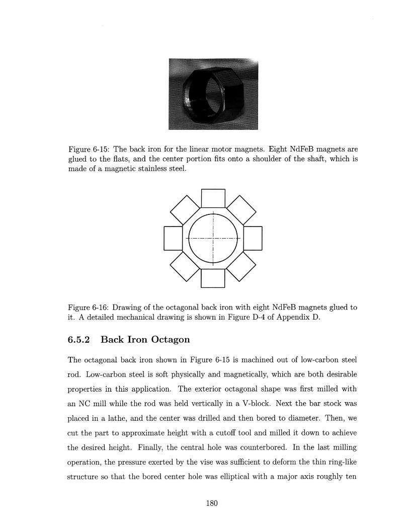
Figure 6-15: The back iron for the linear motor magnets. Eight NdFeB magnets areglued to the flats, and the center portion fits onto a shoulder of the shaft, which ismade of a magnetic stainless steel.

Figure 6-16: Drawing of the octagonal back iron with eight NdFeB magnets glued toit. A detailed mechanical drawing is shown in Figure D-4 of Appendix D.

6.5.2 Back Iron Octagon

The octagonal back iron shown in Figure 6-15 is machined out of low-carbon steel

rod. Low-carbon steel is soft physically and magnetically, which are both desirable

properties in this application. The exterior octagonal shape was first milled with

an NC mill while the rod was held vertically in a V-block. Next the bar stock was

placed in a lathe, and the center was drilled and then bored to diameter. Then, we

cut the part to approximate height with a cutoff tool and milled it down to achieve

the desired height. Finally, the central hole was counterbored. In the last milling

operation, the pressure exerted by the vise was sufficient to deform the thin ring-like

structure so that the bored center hole was elliptical with a major axis roughly ten

180

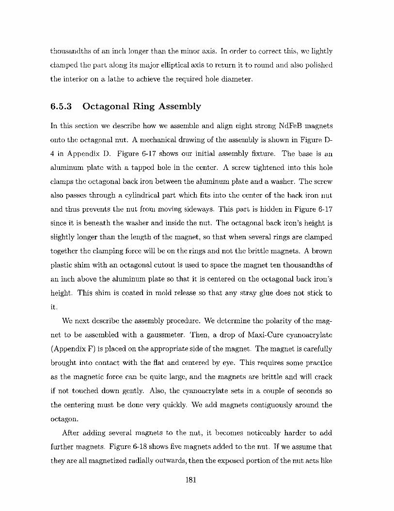
thousandths of an inch longer than the minor axis. In order to correct this, we lightly

clamped the part along its major elliptical axis to return it to round and also polished

the interior on a lathe to achieve the required hole diameter.

6.5.3 Octagonal Ring Assembly

In this section we describe how we assemble and align eight strong NdFeB magnets

onto the octagonal nut. A mechanical drawing of the assembly is shown in Figure D-

4 in Appendix D. Figure 6-17 shows our initial assembly fixture. The base is an

aluminum plate with a tapped hole in the center. A screw tightened into this hole

clamps the octagonal back iron between the aluminum plate and a washer. The screw

also passes through a cylindrical part which fits into the center of the back iron nut

and thus prevents the nut from moving sideways. This part is hidden in Figure 6-17

since it is beneath the washer and inside the nut. The octagonal back iron's height is

slightly longer than the length of the magnet, so that when several rings are clamped

together the clamping force will be on the rings and not the brittle magnets. A brown

plastic shim with an octagonal cutout is used to space the magnet ten thousandths of

an inch above the aluminum plate so that it is centered on the octagonal back iron's

height. This shim is coated in mold release so that any stray glue does not stick to

it.

We next describe the assembly procedure. We determine the polarity of the mag-

net to be assembled with a gaussmeter. Then, a drop of Maxi-Cure cyanoacrylate

(Appendix F) is placed on the appropriate side of the magnet. The magnet is carefully

brought into contact with the flat and centered by eye. This requires some practice

as the magnetic force can be quite large, and the magnets are brittle and will crack

if not touched down gently. Also, the cyanoacrylate sets in a couple of seconds so

the centering must be done very quickly. We add magnets contiguously around the

octagon.

After adding several magnets to the nut, it becomes noticeably harder to add

further magnets. Figure 6-18 shows five magnets added to the nut. If we assume that

they are all magnetized radially outwards, then the exposed portion of the nut acts like

181

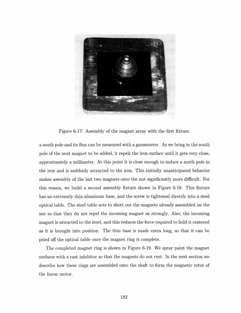
Figure 6-17: Assembly of the magnet array with the first fixture.

a south pole and its flux can be measured with a gaussmeter. As we bring in the south

pole of the next magnet to be added, it repels the iron surface until it gets very close,

approximately a millimeter. At this point it is close enough to induce a north pole in

the iron and is suddenly attracted to the iron. This initially unanticipated behavior

makes assembly of the last two magnets onto the nut significantly more difficult. For

this reason, we build a second assembly fixture shown in Figure 6-18. This fixture

has an extremely thin aluminum base, and the screw is tightened directly into a steel

optical table. The steel table acts to short out the magnets already assembled on the

nut so that they do not repel the incoming magnet as strongly. Also, the incoming

magnet is attracted to the steel, and this reduces the force required to hold it centered

as it is brought into position. The thin base is made extra long, so that it can be

pried off the optical table once the magnet ring is complete.

The completed magnet ring is shown in Figure 6-19. We spray paint the magnet

surfaces with a rust inhibitor so that the magnets do not rust. In the next section we

describe how these rings are assembled onto the shaft to form the magnetic rotor of

the linear motor.

182

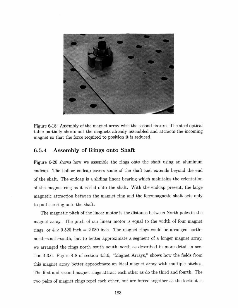
Figure 6-18: Assembly of the magnet array with the second fixture. The steel opticaltable partially shorts out the magnets already assembled and attracts the incomingmagnet so that the force required to position it is reduced.

6.5.4 Assembly of Rings onto Shaft

Figure 6-20 shows how we assemble the rings onto the shaft using an aluminum

endcap. The hollow endcap covers some of the shaft and extends beyond the end

of the shaft. The endcap is a sliding linear bearing which maintains the orientation

of the magnet ring as it is slid onto the shaft. With the endcap present, the large

magnetic attraction between the magnet ring and the ferromagnetic shaft acts only

to pull the ring onto the shaft.

The magnetic pitch of the linear motor is the distance between North poles in the

magnet array. The pitch of our linear motor is equal to the width of four magnet

rings, or 4 x 0.520 inch = 2.080 inch. The magnet rings could be arranged north-

north-south-south, but to better approximate a segment of a longer magnet array,

we arranged the rings north-south-south-north as described in more detail in sec-

tion 4.3.6. Figure 4-8 of section 4.3.6, "Magnet Arrays," shows how the fields from

this magnet array better approximate an ideal magnet array with multiple pitches.

The first and second magnet rings attract each other as do the third and fourth. The

two pairs of magnet rings repel each other, but are forced together as the locknut is

183

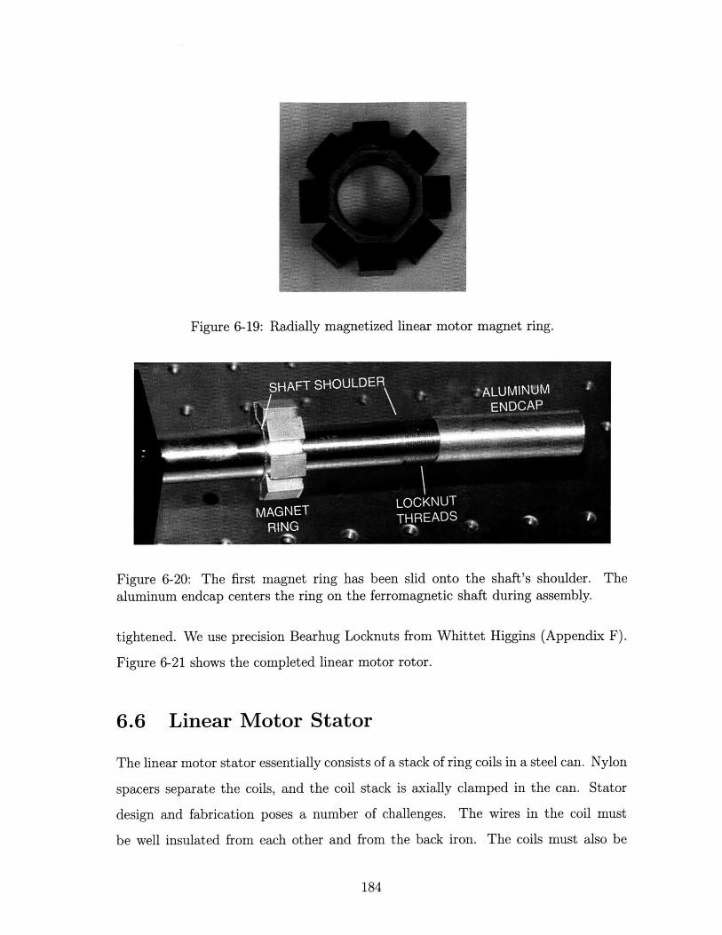
Figure 6-19: Radially magnetized linear motor magnet ring.

Figure 6-20: The first magnet ring has been slid onto the shaft's shoulder. Thealuminum endcap centers the ring on the ferromagnetic shaft during assembly.

tightened. We use precision Bearhug Locknuts from Whittet Higgins (Appendix F).

Figure 6-21 shows the completed linear motor rotor.

6.6 Linear Motor Stator

The linear motor stator essentially consists of a stack of ring coils in a steel can. Nylon

spacers separate the coils, and the coil stack is axially clamped in the can. Stator

design and fabrication poses a number of challenges. The wires in the coil must

be well insulated from each other and from the back iron. The coils must also be

184

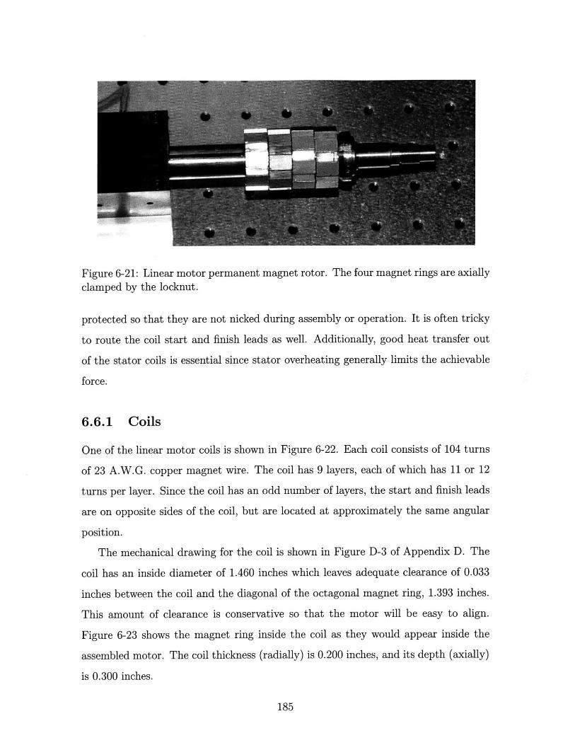
11I1,,I Mi I ~ -

Figure 6-21: Linear motor permanent magnet rotor. The four magnet rings are axiallyclamped by the locknut.

protected so that they are not nicked during assembly or operation. It is often tricky

to route the coil start and finish leads as well. Additionally, good heat transfer out

of the stator coils is essential since stator overheating generally limits the achievable

force.

6.6.1 Coils

One of the linear motor coils is shown in Figure 6-22. Each coil consists of 104 turns

of 23 A.W.G. copper magnet wire. The coil has 9 layers, each of which has 11 or 12

turns per layer. Since the coil has an odd number of layers, the start and finish leads

are on opposite sides of the coil, but are located at approximately the same angular

position.

The mechanical drawing for the coil is shown in Figure D-3 of Appendix D. The

coil has an inside diameter of 1.460 inches which leaves adequate clearance of 0.033

inches between the coil and the diagonal of the octagonal magnet ring, 1.393 inches.

This amount of clearance is conservative so that the motor will be easy to align.

Figure 6-23 shows the magnet ring inside the coil as they would appear inside the

assembled motor. The coil thickness (radially) is 0.200 inches, and its depth (axially)

is 0.300 inches.

185

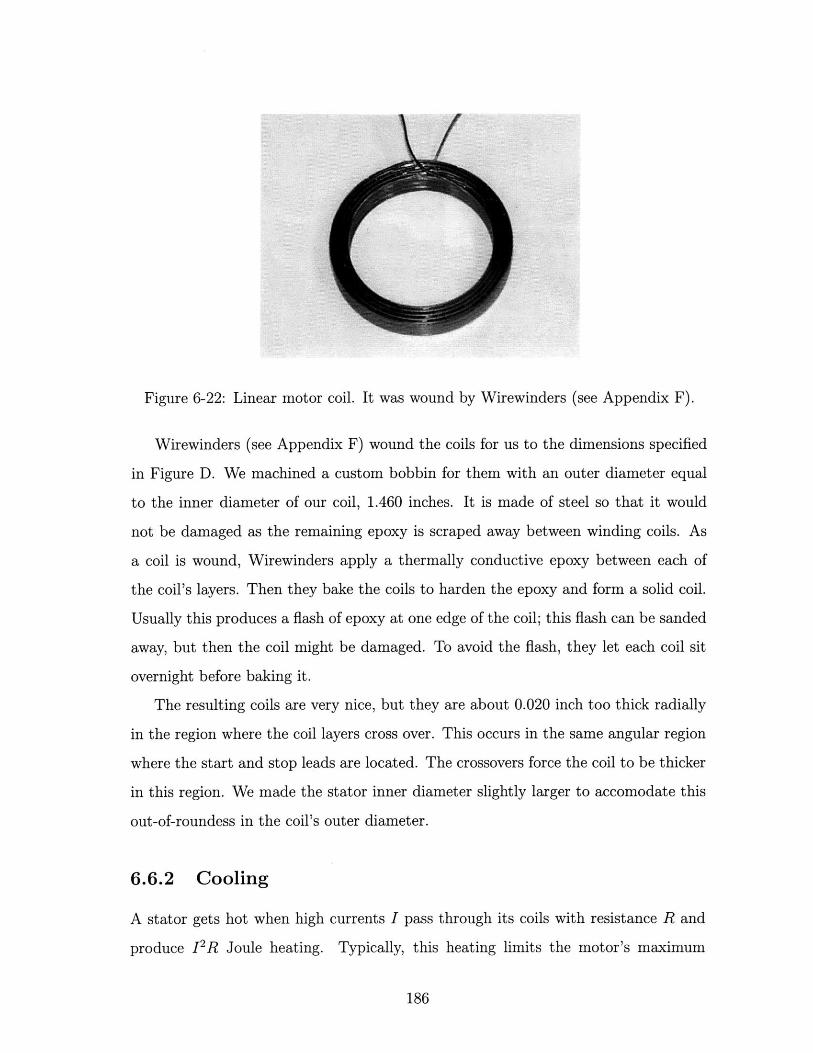
Figure 6-22: Linear motor coil. It was wound by Wirewinders (see Appendix F).

Wirewinders (see Appendix F) wound the coils for us to the dimensions specified

in Figure D. We machined a custom bobbin for them with an outer diameter equal

to the inner diameter of our coil, 1.460 inches. It is made of steel so that it would

not be damaged as the remaining epoxy is scraped away between winding coils. As

a coil is wound, Wirewinders apply a thermally conductive epoxy between each of

the coil's layers. Then they bake the coils to harden the epoxy and form a solid coil.

Usually this produces a flash of epoxy at one edge of the coil; this flash can be sanded

away, but then the coil might be damaged. To avoid the flash, they let each coil sit

overnight before baking it.

The resulting coils are very nice, but they are about 0.020 inch too thick radially

in the region where the coil layers cross over. This occurs in the same angular region

where the start and stop leads are located. The crossovers force the coil to be thicker

in this region. We made the stator inner diameter slightly larger to accomodate this

out-of-roundess in the coil's outer diameter.

6.6.2 Cooling

A stator gets hot when high currents I pass through its coils with resistance R and

produce PR Joule heating. Typically, this heating limits the motor's maximum

186

RRMMNM - I - Em - -

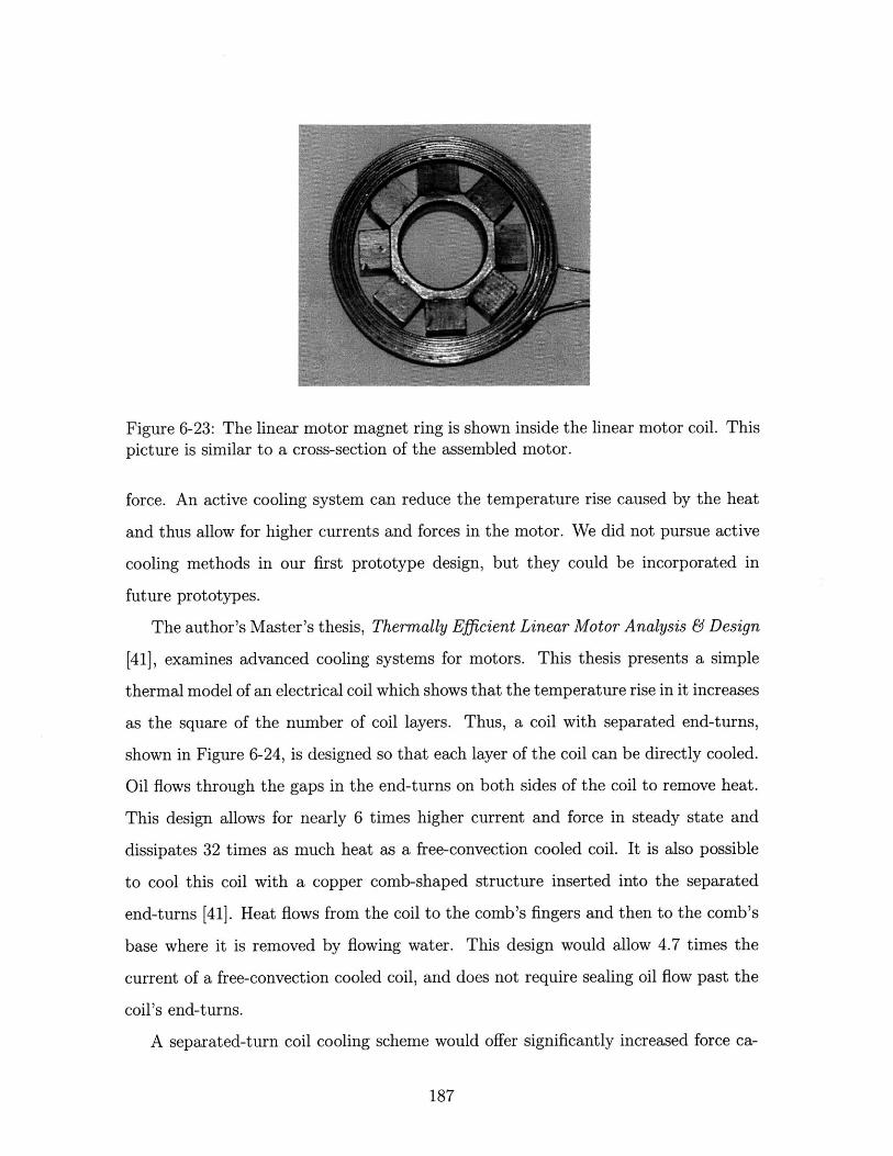
Figure 6-23: The linear motor magnet ring is shown inside the linear motor coil. Thispicture is similar to a cross-section of the assembled motor.

force. An active cooling system can reduce the temperature rise caused by the heat

and thus allow for higher currents and forces in the motor. We did not pursue active

cooling methods in our first prototype design, but they could be incorporated in

future prototypes.

The author's Master's thesis, Thermally Efficient Linear Motor Analysis & Design

[41], examines advanced cooling systems for motors. This thesis presents a simple

thermal model of an electrical coil which shows that the temperature rise in it increases

as the square of the number of coil layers. Thus, a coil with separated end-turns,

shown in Figure 6-24, is designed so that each layer of the coil can be directly cooled.

Oil flows through the gaps in the end-turns on both sides of the coil to remove heat.

This design allows for nearly 6 times higher current and force in steady state and

dissipates 32 times as much heat as a free-convection cooled coil. It is also possible

to cool this coil with a copper comb-shaped structure inserted into the separated

end-turns [41]. Heat flows from the coil to the comb's fingers and then to the comb's

base where it is removed by flowing water. This design would allow 4.7 times the

current of a free-convection cooled coil, and does not require sealing oil flow past the

coil's end-turns.

A separated-turn coil cooling scheme would offer significantly increased force ca-

187

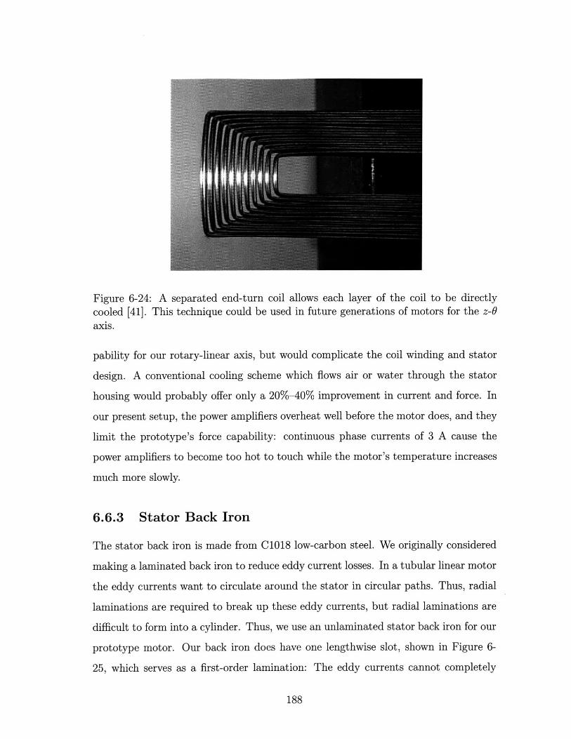
Figure 6-24: A separated end-turn coil allows each layer of the coil to be directlycooled [41]. This technique could be used in future generations of motors for the z-6axis.

pability for our rotary-linear axis, but would complicate the coil winding and stator

design. A conventional cooling scheme which flows air or water through the stator

housing would probably offer only a 20%-40% improvement in current and force. In

our present setup, the power amplifiers overheat well before the motor does, and they

limit the prototype's force capability: continuous phase currents of 3 A cause the

power amplifiers to become too hot to touch while the motor's temperature increases

much more slowly.

6.6.3 Stator Back Iron

The stator back iron is made from C1018 low-carbon steel. We originally considered

making a laminated back iron to reduce eddy current losses. In a tubular linear motor

the eddy currents want to circulate around the stator in circular paths. Thus, radial

laminations are required to break up these eddy currents, but radial laminations are

difficult to form into a cylinder. Thus, we use an unlaminated stator back iron for our

prototype motor. Our back iron does have one lengthwise slot, shown in Figure 6-

25, which serves as a first-order lamination: The eddy currents cannot completely

188

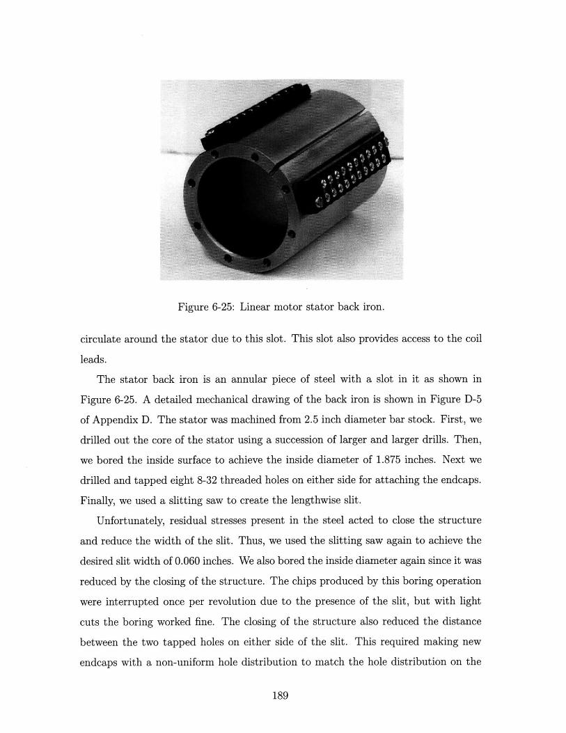
Figure 6-25: Linear motor stator back iron.

circulate around the stator due to this slot. This slot also provides access to the coil

leads.

The stator back iron is an annular piece of steel with a slot in it as shown in

Figure 6-25. A detailed mechanical drawing of the back iron is shown in Figure D-5

of Appendix D. The stator was machined from 2.5 inch diameter bar stock. First, we

drilled out the core of the stator using a succession of larger and larger drills. Then,

we bored the inside surface to achieve the inside diameter of 1.875 inches. Next we

drilled and tapped eight 8-32 threaded holes on either side for attaching the endcaps.

Finally, we used a slitting saw to create the lengthwise slit.

Unfortunately, residual stresses present in the steel acted to close the structure

and reduce the width of the slit. Thus, we used the slitting saw again to achieve the

desired slit width of 0.060 inches. We also bored the inside diameter again since it was

reduced by the closing of the structure. The chips produced by this boring operation

were interrupted once per revolution due to the presence of the slit, but with light

cuts the boring worked fine. The closing of the structure also reduced the distance

between the two tapped holes on either side of the slit. This required making new

endcaps with a non-uniform hole distribution to match the hole distribution on the

189

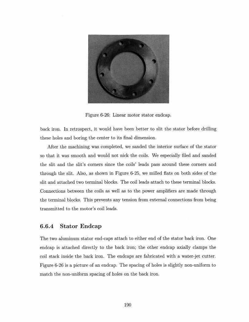
Figure 6-26: Linear motor stator endcap.

back iron. In retrospect, it would have been better to slit the stator before drilling

these holes and boring the center to its final dimension.

After the machining was completed, we sanded the interior surface of the stator

so that it was smooth and would not nick the coils. We especially filed and sanded

the slit and the slit's corners since the coils' leads pass around these corners and

through the slit. Also, as shown in Figure 6-25, we milled flats on both sides of the

slit and attached two terminal blocks. The coil leads attach to these terminal blocks.

Connections between the coils as well as to the power amplifiers are made through

the terminal blocks. This prevents any tension from external connections from being

transmitted to the motor's coil leads.

6.6.4 Stator Endcap

The two aluminum stator end-caps attach to either end of the stator back iron. One

endcap is attached directly to the back iron; the other endcap axially clamps the

coil stack inside the back iron. The endcaps are fabricated with a water-jet cutter.

Figure 6-26 is a picture of an endcap. The spacing of holes is slightly non-uniform to

match the non-uniform spacing of holes on the back iron.

190

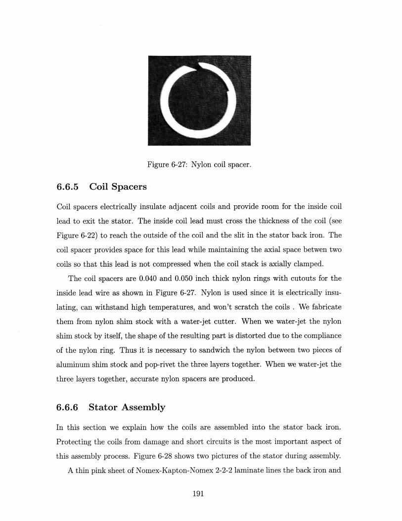
Figure 6-27: Nylon coil spacer.

6.6.5 Coil Spacers

Coil spacers electrically insulate adjacent coils and provide room for the inside coil

lead to exit the stator. The inside coil lead must cross the thickness of the coil (see

Figure 6-22) to reach the outside of the coil and the slit in the stator back iron. The

coil spacer provides space for this lead while maintaining the axial space betwen two

coils so that this lead is not compressed when the coil stack is axially clamped.

The coil spacers are 0.040 and 0.050 inch thick nylon rings with cutouts for the

inside lead wire as shown in Figure 6-27. Nylon is used since it is electrically insu-

lating, can withstand high temperatures, and won't scratch the coils . We fabricate

them from nylon shim stock with a water-jet cutter. When we water-jet the nylon

shim stock by itself, the shape of the resulting part is distorted due to the compliance

of the nylon ring. Thus it is necessary to sandwich the nylon between two pieces of

aluminum shim stock and pop-rivet the three layers together. When we water-jet the

three layers together, accurate nylon spacers are produced.

6.6.6 Stator Assembly

In this section we explain how the coils are assembled into the stator back iron.

Protecting the coils from damage and short circuits is the most important aspect of

this assembly process. Figure 6-28 shows two pictures of the stator during assembly.

A thin pink sheet of Nomex-Kapton-Nomex 2-2-2 laminate lines the back iron and

191

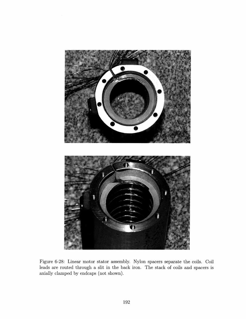
Figure 6-28: Linear motor stator assembly. Nylon spacers separate the coils. Coilleads are routed through a slit in the back iron. The stack of coils and spacers isaxially clamped by endcaps (not shown).

192

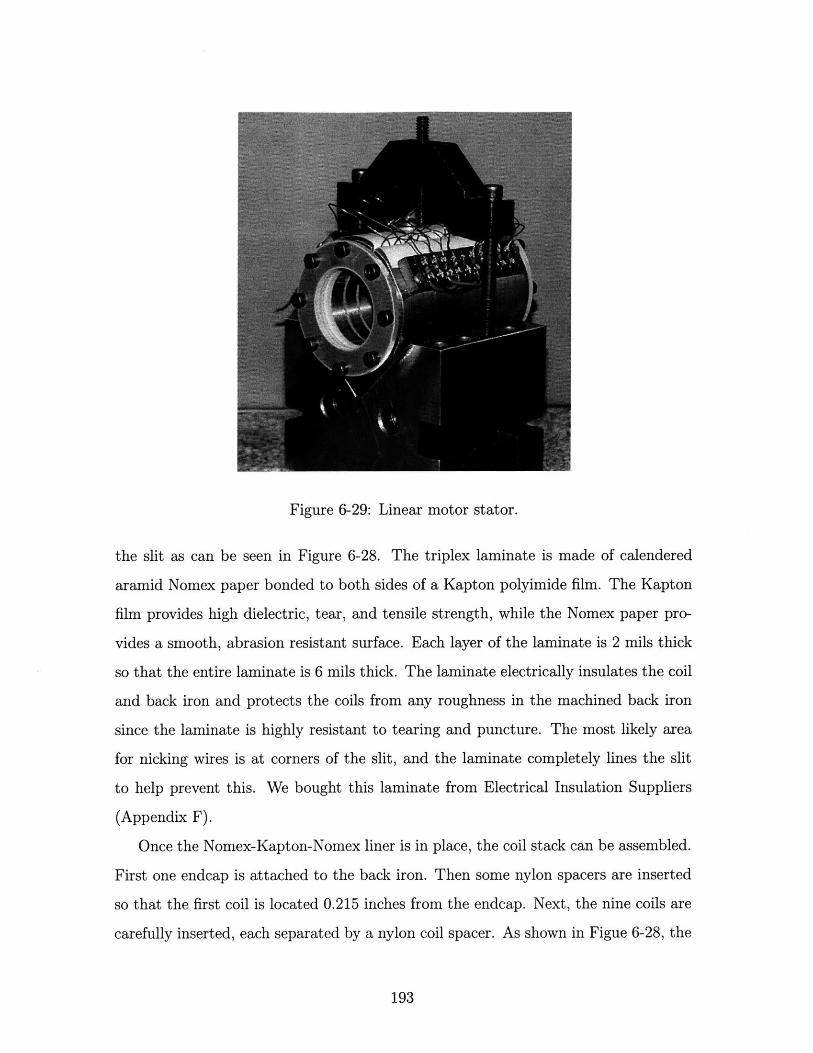
Figure 6-29: Linear motor stator.

the slit as can be seen in Figure 6-28. The triplex laminate is made of calendered

aramid Nomex paper bonded to both sides of a Kapton polyimide film. The Kapton

film provides high dielectric, tear, and tensile strength, while the Nomex paper pro-

vides a smooth, abrasion resistant surface. Each layer of the laminate is 2 mils thick

so that the entire laminate is 6 mils thick. The laminate electrically insulates the coil

and back iron and protects the coils from any roughness in the machined back iron

since the laminate is highly resistant to tearing and puncture. The most likely area

for nicking wires is at corners of the slit, and the laminate completely lines the slit

to help prevent this. We bought this laminate from Electrical Insulation Suppliers

(Appendix F).

Once the Nomex-Kapton-Nomex liner is in place, the coil stack can be assembled.

First one endcap is attached to the back iron. Then some nylon spacers are inserted

so that the first coil is located 0.215 inches from the endcap. Next, the nine coils are

carefully inserted, each separated by a nylon coil spacer. As shown in Figue 6-28, the

193

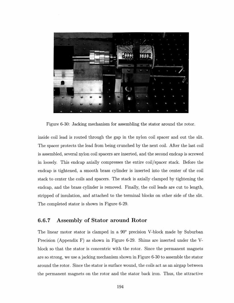
Figure 6-30: Jacking mechanism for assembling the stator around the rotor.

inside coil lead is routed through the gap in the nylon coil spacer and out the slit.

The spacer protects the lead from being crunched by the next coil. After the last coil

is assembled, several nylon coil spacers are inserted, and the second endcap is screwed

in loosely. This endcap axially compresses the entire coil/spacer stack. Before the

endcap is tightened, a smooth brass cylinder is inserted into the center of the coil

stack to center the coils and spacers. The stack is axially clamped by tightening the

endcap, and the brass cylinder is removed. Finally, the coil leads are cut to length,

stripped of insulation, and attached to the terminal blocks on other side of the slit.

The completed stator is shown in Figure 6-29.

6.6.7 Assembly of Stator around Rotor

The linear motor stator is clamped in a 900 precision V-block made by Suburban

Precision (Appendix F) as shown in Figure 6-29. Shims are inserted under the V-

block so that the stator is concentric with the rotor. Since the permanent magnets

are so strong, we use a jacking mechanism shown in Figure 6-30 to assemble the stator

around the rotor. Since the stator is surface wound, the coils act as an airgap between

the permanent magnets on the rotor and the stator back iron. Thus, the attractive

194

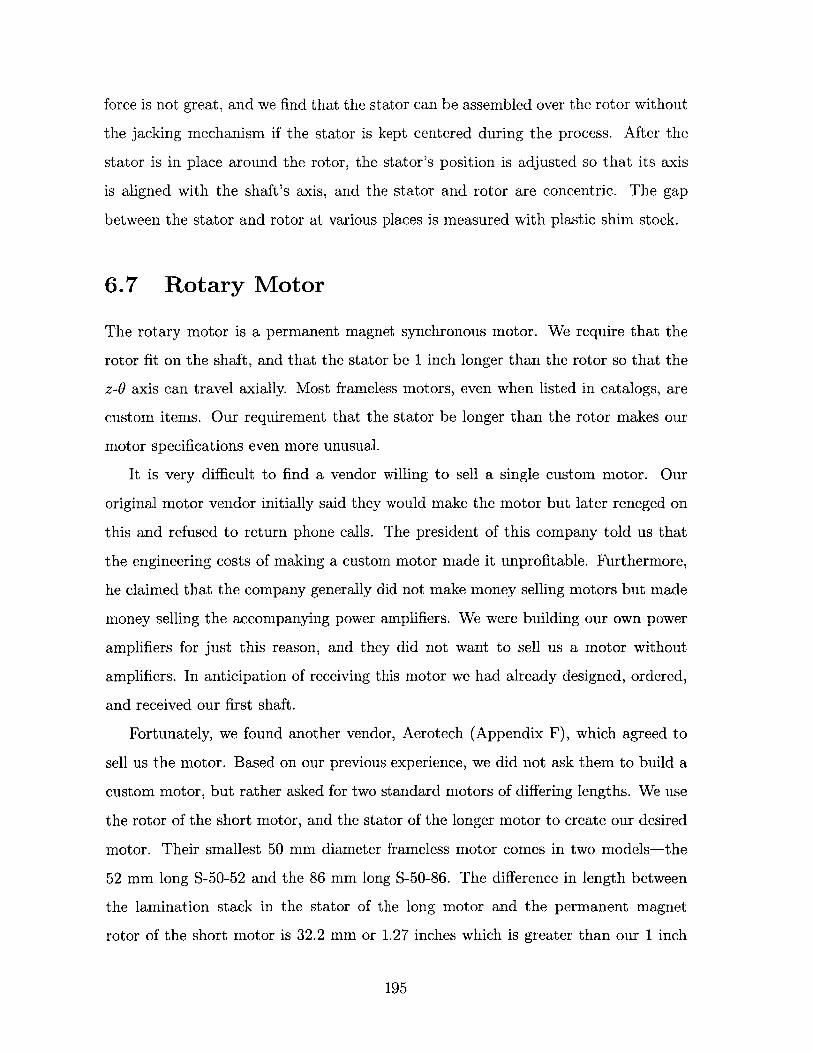
force is not great, and we find that the stator can be assembled over the rotor without

the jacking mechanism if the stator is kept centered during the process. After the

stator is in place around the rotor, the stator's position is adjusted so that its axis

is aligned with the shaft's axis, and the stator and rotor are concentric. The gap

between the stator and rotor at various places is measured with plastic shim stock.

6.7 Rotary Motor

The rotary motor is a permanent magnet synchronous motor. We require that the

rotor fit on the shaft, and that the stator be 1 inch longer than the rotor so that the

z-0 axis can travel axially. Most frameless motors, even when listed in catalogs, are

custom items. Our requirement that the stator be longer than the rotor makes our

motor specifications even more unusual.

It is very difficult to find a vendor willing to sell a single custom motor. Our

original motor vendor initially said they would make the motor but later reneged on

this and refused to return phone calls. The president of this company told us that

the engineering costs of making a custom motor made it unprofitable. Furthermore,

he claimed that the company generally did not make money selling motors but made

money selling the accompanying power amplifiers. We were building our own power

amplifiers for just this reason, and they did not want to sell us a motor without

amplifiers. In anticipation of receiving this motor we had already designed, ordered,

and received our first shaft.

Fortunately, we found another vendor, Aerotech (Appendix F), which agreed to

sell us the motor. Based on our previous experience, we did not ask them to build a

custom motor, but rather asked for two standard motors of differing lengths. We use

the rotor of the short motor, and the stator of the longer motor to create our desired

motor. Their smallest 50 mm diameter frameless motor comes in two models-the

52 mm long S-50-52 and the 86 mm long S-50-86. The difference in length between

the lamination stack in the stator of the long motor and the permanent magnet

rotor of the short motor is 32.2 mm or 1.27 inches which is greater than our 1 inch

195

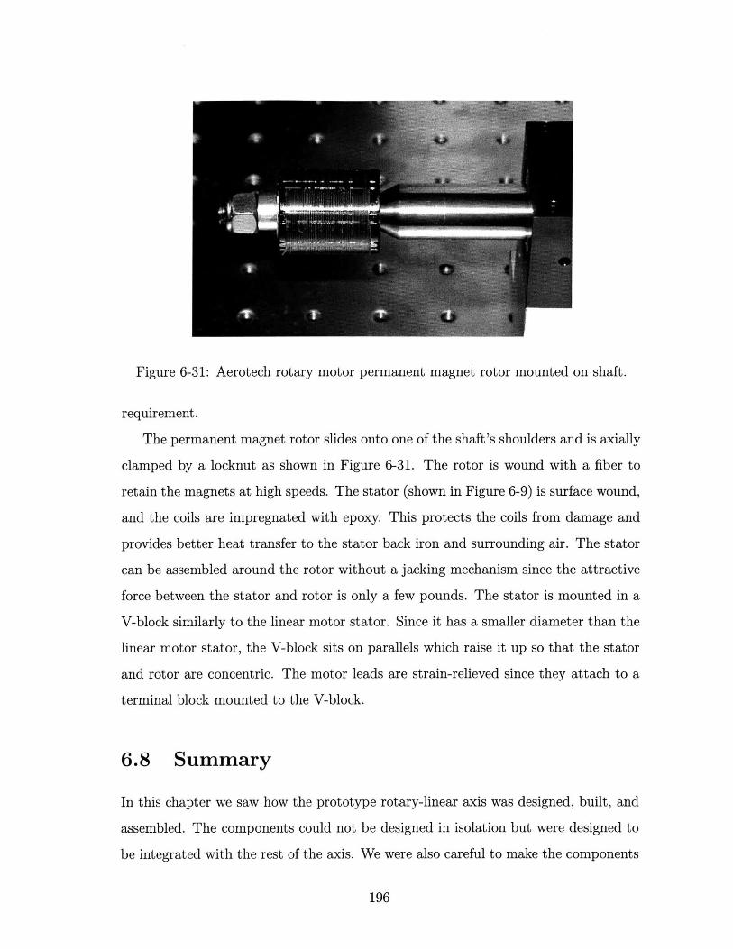
Figure 6-31: Aerotech rotary motor permanent magnet rotor mounted on shaft.

requirement.

The permanent magnet rotor slides onto one of the shaft's shoulders and is axially

clamped by a locknut as shown in Figure 6-31. The rotor is wound with a fiber to

retain the magnets at high speeds. The stator (shown in Figure 6-9) is surface wound,

and the coils are impregnated with epoxy. This protects the coils from damage and

provides better heat transfer to the stator back iron and surrounding air. The stator

can be assembled around the rotor without a jacking mechanism since the attractive

force between the stator and rotor is only a few pounds. The stator is mounted in a

V-block similarly to the linear motor stator. Since it has a smaller diameter than the

linear motor stator, the V-block sits on parallels which raise it up so that the stator

and rotor are concentric. The motor leads are strain-relieved since they attach to a

terminal block mounted to the V-block.

6.8 Summary

In this chapter we saw how the prototype rotary-linear axis was designed, built, and

assembled. The components could not be designed in isolation but were designed to

be integrated with the rest of the axis. We were also careful to make the components

196

modular so that they could be re-used on future rotary-linear axis prototypes. For

example, to build the next prototype axis, the designer might want to re-use the

tubular linear motor and rotary motor but incorporate a different rotary sensor. In

this case the designer could specify a shaft with the same shoulder diameters as ours,

though its length and other features might be different; the frameless rotary and

linear motors could be disassembled and reassembled on the new shaft.

We were suprised to find that we could position the linear and rotary motor

stators over the permanent magnet rotors by hand. Initially, we planned various

jacking mechanisms and built one (shown in Figure 6-30) to allow us to position the

stators around the permanent magnet rotors. We feared that the magnetic attraction

would be extremely large and could damage the axis or motor if not constrained by a

jacking mechanism. The surface wound nature of both motors in which the coil acts

as a large air gap reduces the attraction force significantly. There is a large attraction

force, but the assembly can be accomplished without a jacking mechanism if the rotor

is kept centered.

We mounted the two motor stators in V-blocks so that they would be solidly

supported and would not vibrate due to reaction forces. However, the stands for

the interferometer mounts are made of two thin parallel plates as can be seen in

Figure 6-10. We found that if the interferometer mount holding the tilted-mirror

sensor was tapped while the rotary axis controller was holding an angular position,

the shaft would rotate suddenly a small amount. The vibration in the interferometer

mount fooled the system into thinking the axis had rotated away from its nominal

position, and the controller commanded a restoring torque from the rotary motor.

Interferometers should be mounted on a solid support so that they don't vibrate

relative to the optical table.

The next chapter is a tutorial on field orientated control. It shows how to model

and control three phase motors using a convenient set of transformations. The fol-

lowing chapter explains the control of the prototype rotary-linear axis we constructed

in this chapter.

197

198

Chapter 7

Field Orientation Principle

This chapter is a tutorial on the field orientation principle, especially as it applies to

permanent magnet synchronous motors. This tutorial is included in this thesis for

two main reasons. First, it provides the equations necessary to commutate the linear

and rotary permanent magnet synchronous motors we use in our rotary-linear axis.

In fact, only sections 7.4.2 and 7.4.3 of this chapter are needed to do this. Second,

we provide a model of the permanent magnet motor in dq coordinates in section 7.6

which is needed for sensorless control. We implement a sensorless control scheme for

the rotary motor in section 8.5 of the next chapter. The material in this chapter also

is used to simplify the calculation of the linear and rotary motor force constants in

sections 4.5 and 4.7 respectively.

This review of field orientated control synthesizes material from a number of ex-

cellent sources. These include Leonhard's text, Control of Electrical Drives [40], and

Fitzgerald, Kingsley, and Umans's text, Electric Machinery [18]. We also draw upon

lecture notes written by MIT Professor James Kirtley [35] and notes written by MIT

Professors Jeffrey Lang, George Verghese, and Marija Ilic [39]. In this tutorial chapter,

we combine these different perspectives into a coherent and continuous introduction

to field orientated control.

The field orientation principle allows us to control AC motors as if they were

DC brushed motors. AC motors, such as synchronous and induction motors, have

multiple phases and complex transient behavior, which make them difficult to control.

199

Under common simplifying assumptions, brushed DC motors are simple to control:

the armature current is directly proportional to the rotor torque. Application of the

field orientation principle allows us to transform stator currents for an AC motor

into direct and quadrature currents, which are analogous to the field and armature

currents in a brushed DC motor. Using these field orientation transformations yields

commutation laws by which AC motors can be readily controlled.

In this chapter we first review DC motor modeling. The mechanical commuta-

tion in a DC motor makes controlling it easy: torque is proportional to armature

current. We also show how field weakening control can be used to enable high-speed

operation. In the remainder of the chapter we focus on a specific AC motor, the

3-phase permanent magnet synchronous motor. We first model this motor in 3-phase

variables abc; the resulting torque expression shows that the motor ideally requires

sinusoidal commutation to produce constant torque output. Next, we derive the field

orientation or dq transformations, which transform variables from the abc frame to a

two-phase frame rotating with the rotor called the dq frame. We apply these trans-

formations to our three-phase motor model in the abc frame and derive an equivalent

motor model in the dq frame. This dq motor model is analogous to the DC motor

model since torque is directly proportional to q axis current. Using these results, in

the last section we show how a 3-phase permanent magnet synchronous motor can be

controlled in the same manner as a DC motor using the dq transformations.

7.1 DC Motor Modeling

Direct current (DC) motors are commonly used in variable speed drives. They are

flexible in allowing for operation at a wide range of speeds and torques. They can

be modeled simply and therefore controlled with minimal complexity. Their main

disadvantage is the need for mechanical commutation which requires periodic main-

tenance of brushes, limits speed and power, and causes friction. We review DC motor

modeling and control in this section. In the next section we show how the field ori-

entation transformations allow AC motors to be controlled with the same conceptual

200

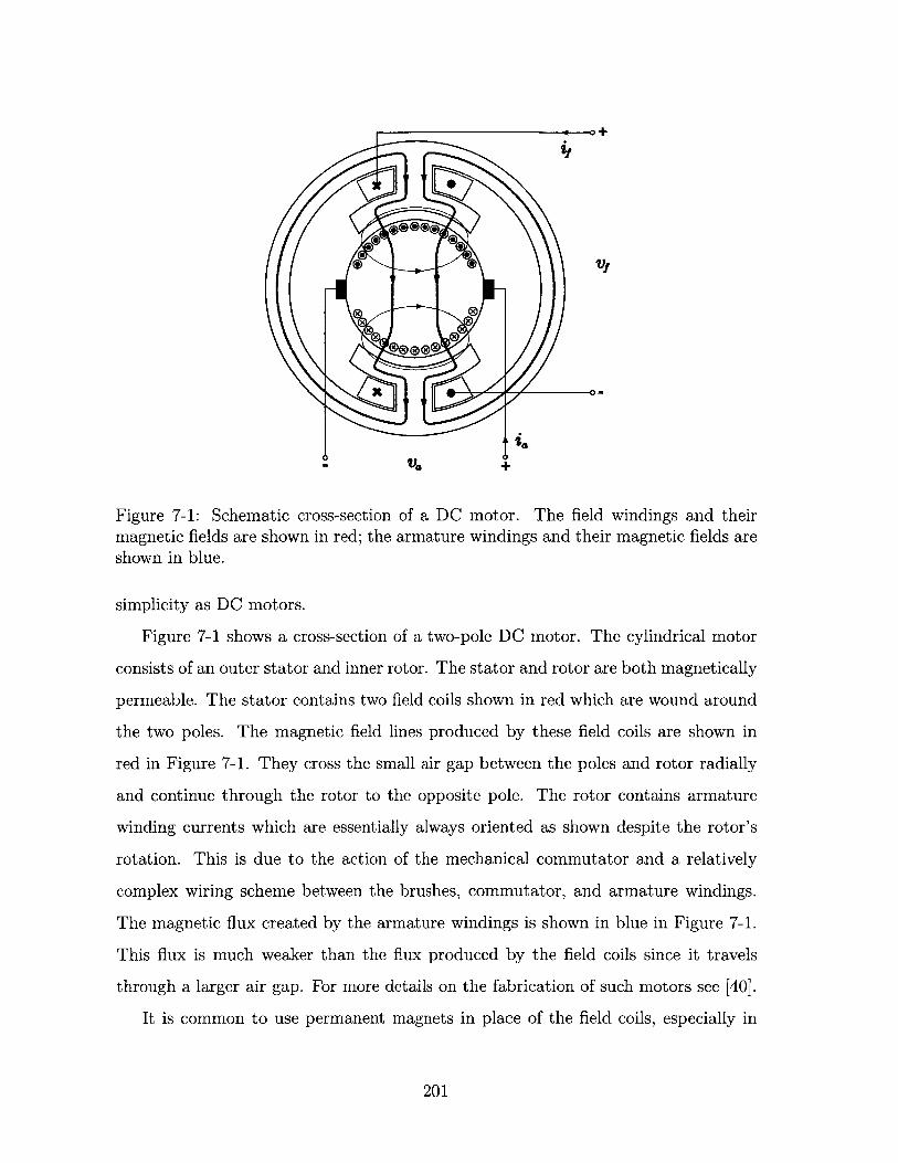
VIX @,. X

X 0-

Figure 7-1: Schematic cross-section of a DC motor. The field windings and theirmagnetic fields are shown in red; the armature windings and their magnetic fields areshown in blue.

simplicity as DC motors.

Figure 7-1 shows a cross-section of a two-pole DC motor. The cylindrical motor

consists of an outer stator and inner rotor. The stator and rotor are both magnetically

permeable. The stator contains two field coils shown in red which are wound around

the two poles. The magnetic field lines produced by these field coils are shown in

red in Figure 7-1. They cross the small air gap between the poles and rotor radially

and continue through the rotor to the opposite pole. The rotor contains armature

winding currents which are essentially always oriented as shown despite the rotor's

rotation. This is due to the action of the mechanical commutator and a relatively

complex wiring scheme between the brushes, commutator, and armature windings.

The magnetic flux created by the armature windings is shown in blue in Figure 7-1.

This flux is much weaker than the flux produced by the field coils since it travels

through a larger air gap. For more details on the fabrication of such motors see [40].

It is common to use permanent magnets in place of the field coils, especially in

201

smaller servomotors. Permanent magnets eliminate the field coils and their power

supplies and are more compact than field coils in smaller motors. However, since

the flux supplied by the permanent magnets cannot be varied in operation, some

flexibility is lost in motor control. We will consider the more general case of a motor

with field windings; a motor with permanent magnets will have the same behavior as

a motor with constant current in the field windings.

Although controlling a DC motor is easy, DC motor design and analysis can

be quite complicated. For example, the mechanical commutator uses brushes and

a complex armature winding pattern to maintain a spatially fixed distribution of

currents in the rotating rotor. In practice, the design of such DC motor armature

windings is something of a black art. A second complication is that the magnetic field

produced by the armature tends to distort the main air gap flux produced by the field

coils. Fortunately this field is much weaker than the main flux since it has a larger

effective airgap as described above. In large machines, this effect is sometimes further

reduced by using compensating windings in the stator poles. These compensating

windings are connected in series to the armature windings but have current flowing

in the opposite direction. Thus, these windings can cancel the flux produced by the

armature windings. There are other subtleties to DC motor design as described in

[40, 18], but fortunately a simple analysis is all that is required for most control

applications.

The ease with which DC motors can be controlled is due to the fixed spatial ar-

rangement of the main flux and armature flux. In Figure 7-1 the main flux (in red)

is directed downward. We shall call this the direct-axis flux. The armature flux (in

blue) is oriented 90 electrical degrees from the main flux and is also therefore called

the quadrature-axis flux. The fixed 900 angle between the direct-axis flux and the

quadrature-axis flux produces maximum torque. In DC motors the mechanical com-

mutator maintains these two axes essentially perpendicular to each other as the rotor

rotates. As a result, DC motors are relatively easy to control. In AC motors, we must

perform the commutation electrically, without the aid of a mechanical commutator.

If we can achieve the same effect in an AC motor, with the direct and quadrature

202

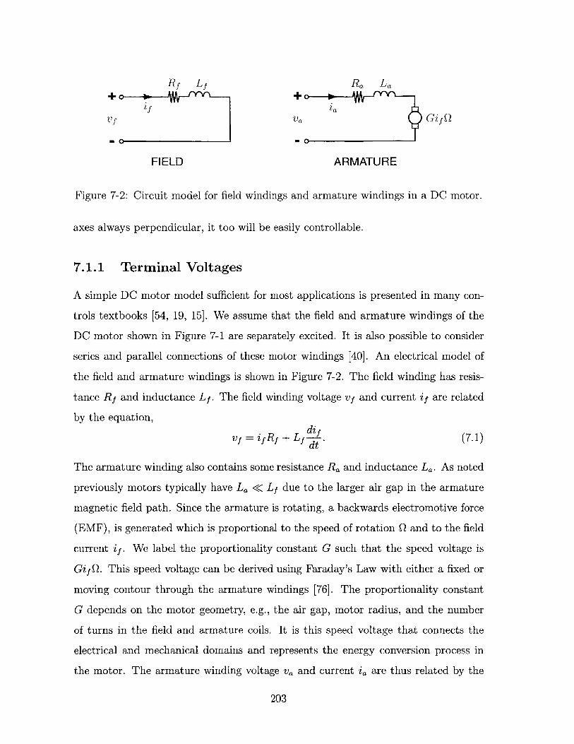
J?f Lf Ra La

If iaV a GifQ

FIELD ARMATURE

Figure 7-2: Circuit model for field windings and armature windings in a DC motor.

axes always perpendicular, it too will be easily controllable.

7.1.1 Terminal Voltages

A simple DC motor model sufficient for most applications is presented in many con-

trols textbooks [54, 19, 15]. We assume that the field and armature windings of the

DC motor shown in Figure 7-1 are separately excited. It is also possible to consider

series and parallel connections of these motor windings [40]. An electrical model of

the field and armature windings is shown in Figure 7-2. The field winding has resis-

tance Rf and inductance Lf. The field winding voltage vf and current if are related

by the equation,dif

Vf = if R1 + L1 di (7.1)

The armature winding also contains some resistance Ra and inductance La. As noted

previously motors typically have La < Lf due to the larger air gap in the armature

magnetic field path. Since the armature is rotating, a backwards electromotive force

(EMF), is generated which is proportional to the speed of rotation Q and to the field

current if. We label the proportionality constant G such that the speed voltage is

Gi1 Q. This speed voltage can be derived using Faraday's Law with either a fixed or

moving contour through the armature windings [76]. The proportionality constant

G depends on the motor geometry, e.g., the air gap, motor radius, and the number

of turns in the field and armature coils. It is this speed voltage that connects the

electrical and mechanical domains and represents the energy conversion process in

the motor. The armature winding voltage va and current ia are thus related by the

203

equation,

Va = iaRa + L, +GiGQ. (7.2)

7.1.2 Torque

The radial magnetic flux produced by the field winding interacts with the current

in the armature windings to produce a force at the radius of the rotor. The force

produced is calculated using the Lorentz force density,

F = JxB, (7.3)

where F is the volume force density, J is current density in the armature windings, and

B is air gap magnetic flux. The resulting torque T contains the same proportionality

constant G introduced to calculate the backwards electromotive force:

T = Gifia. (7.4)

Assuming nonlinearities such as magnetic saturation in the stator are not present, the

torque is directly proportional to both the field and armature windings. For smaller

motors with permanent magnet excitation, the field current is essentially constant

and it is common to define a motor torque constant,

Kt = Gif, (7.5)

such that torque is directly proportional to armature current,

T = Ktia. (7.6)

The above Lorentz force calculation yields the correct force and torque for the

motor, but there is a subtlety regarding its use [76]. Typically the armature windings

are placed in teeth on the rotor surface to reduce the effective size of the motor's

air gap. In fact, most of the magnetic flux crossing the air gap goes through these

204

permeable teeth and not through the coils. Hence, force is mainly produced in the

magnetically permeable teeth of the rotor and not in the coils. Nevertheless, the

true force can still be calculated exactly, by naively assuming all the magnetic flux

goes through the coils. This surprising result can be explained best in terms of the

Maxwell stress tensor [76]. The force on an object can be calculated by integrating the

Maxwell stess tensor over the surface of the object. Since only the surface magnetic

fields enter into this calculation, the details of how the magnetic fields act inside the

volume do not change the net force.

7.1.3 Power

The motor directly converts electrical power absorbed by the speed voltage into me-

chanical power. The electrical power pe is equal to the armature current ia multiplied

by the speed voltage, GifQ,

Pe = GifiaQ. (7.7)

The mechanical power generated pm is equal to the torque, r = Gifia, multiplied by

the angular speed Q,

Pm = GifiaQ. (7.8)

Earlier, we assumed that the proportionality constant G in the torque expression was

identical to the proportionality constant G in the back EMF expression. The basis

for this assumption was that a lumped electromechanical analysis of the motor would

yield identical expressions for G in both cases. Another common way to show this

equivalence is by assuming that the electrical power Pe and mechanical power pm

expressions above are equal. From this it also follows that the torque and back EMF

constants are the same.

7.2 DC Motor Control

In this section, we show that a DC motor can be easily controlled using the model we

have just developed. We consider the problem of controlling the angular position of

205

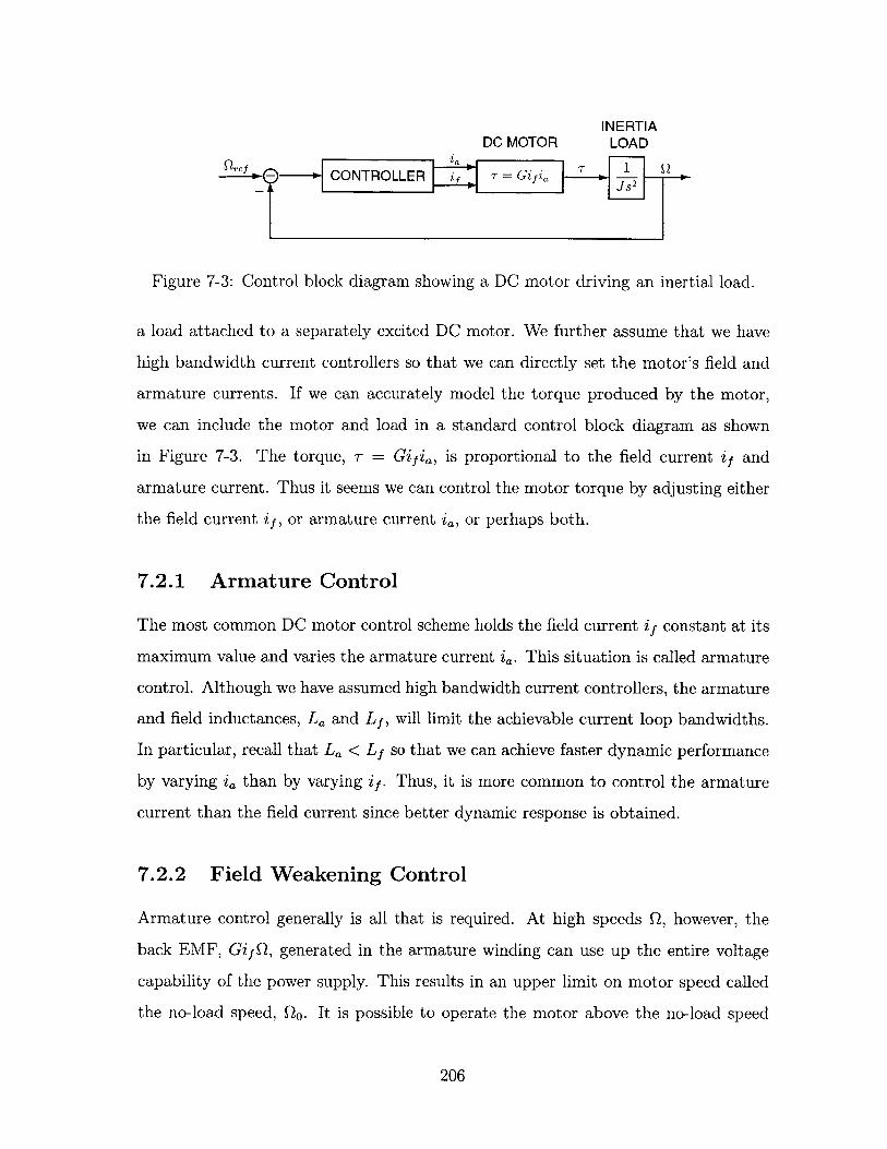
INERTIADC MOTOR LOAD

Pref ±- iL T 1 QRe 9 -+CONTROLLE = Gifi 82+ER~ J j 1 J 8 2

Figure 7-3: Control block diagram showing a DC motor driving an inertial load.

a load attached to a separately excited DC motor. We further assume that we have

high bandwidth current controllers so that we can directly set the motor's field and

armature currents. If we can accurately model the torque produced by the motor,

we can include the motor and load in a standard control block diagram as shown

in Figure 7-3. The torque, T = Gifia, is proportional to the field current if and

armature current. Thus it seems we can control the motor torque by adjusting either

the field current if, or armature current i, or perhaps both.

7.2.1 Armature Control

The most common DC motor control scheme holds the field current if constant at its

maximum value and varies the armature current i,. This situation is called armature

control. Although we have assumed high bandwidth current controllers, the armature

and field inductances, L, and L, will limit the achievable current loop bandwidths.

In particular, recall that La < Lf so that we can achieve faster dynamic performance

by varying i, than by varying if. Thus, it is more common to control the armature

current than the field current since better dynamic response is obtained.

7.2.2 Field Weakening Control

Armature control generally is all that is required. At high speeds Q, however, the

back EMF, GifQ, generated in the armature winding can use up the entire voltage

capability of the power supply. This results in an upper limit on motor speed called

the no-load speed, Qo. It is possible to operate the motor above the no-load speed

206

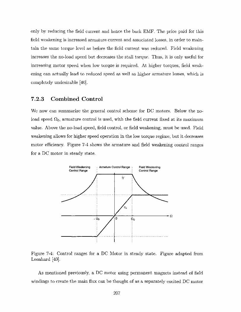
only by reducing the field current and hence the back EMF. The price paid for this

field weakening is increased armature current and associated losses, in order to main-

tain the same torque level as before the field current was reduced. Field weakening

increases the no-load speed but decreases the stall torque. Thus, it is only useful for

increasing motor speed when low torque is required. At higher torques, field weak-

ening can actually lead to reduced speed as well as higher armature losses, which is

completely undesirable [40].

7.2.3 Combined Control

We now can summarize the general control scheme for DC motors. Below the no-

load speed Q0, armature control is used, with the field current fixed at its maximum

value. Above the no-load speed, field control, or field weakening, must be used. Field

weakening allows for higher speed operation in the low torque regime, but it decreases

motor efficiency. Figure 7-4 shows the armature and field weakening control ranges

for a DC motor in steady state.

Field Weakening Armature Control Range Field WeakeningControl Range Control Range

Figure 7-4: Control ranges for a DC Motor in steady state. Figure adapted fromLeonhard [40].

As mentioned previously, a DC motor using permanent magnets instead of field

windings to create the main flux can be thought of as a separately excited DC motor

207

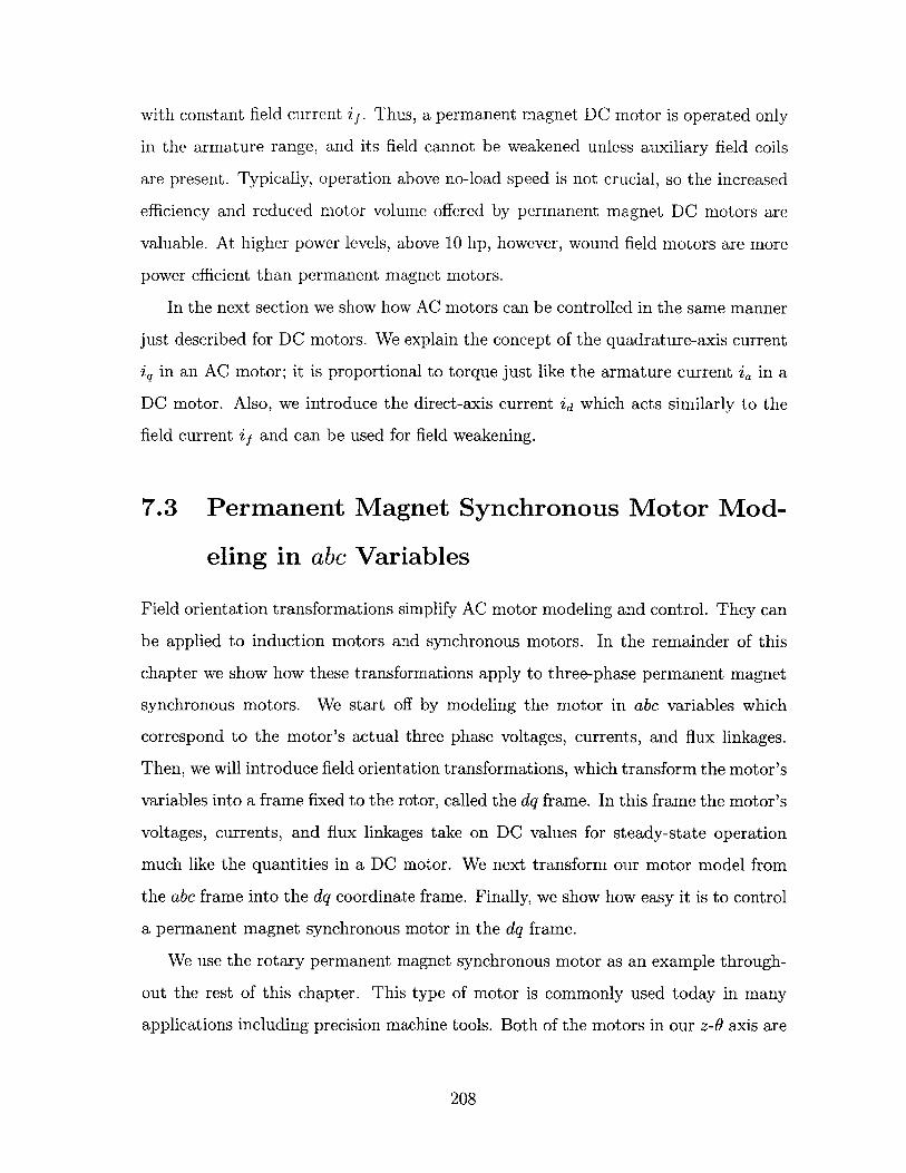
with constant field current if. Thus, a permanent magnet DC motor is operated only

in the armature range, and its field cannot be weakened unless auxiliary field coils

are present. Typically, operation above no-load speed is not crucial, so the increased

efficiency and reduced motor volume offered by permanent magnet DC motors are

valuable. At higher power levels, above 10 hp, however, wound field motors are more

power efficient than permanent magnet motors.

In the next section we show how AC motors can be controlled in the same manner

just described for DC motors. We explain the concept of the quadrature-axis current

iq in an AC motor; it is proportional to torque just like the armature current ia in a

DC motor. Also, we introduce the direct-axis current id which acts similarly to the

field current if and can be used for field weakening.

7.3 Permanent Magnet Synchronous Motor Mod-

eling in abc Variables

Field orientation transformations simplify AC motor modeling and control. They can

be applied to induction motors and synchronous motors. In the remainder of this

chapter we show how these transformations apply to three-phase permanent magnet

synchronous motors. We start off by modeling the motor in abc variables which

correspond to the motor's actual three phase voltages, currents, and flux linkages.

Then, we will introduce field orientation transformations, which transform the motor's

variables into a frame fixed to the rotor, called the dq frame. In this frame the motor's

voltages, currents, and flux linkages take on DC values for steady-state operation

much like the quantities in a DC motor. We next transform our motor model from

the abc frame into the dq coordinate frame. Finally, we show how easy it is to control

a permanent magnet synchronous motor in the dq frame.

We use the rotary permanent magnet synchronous motor as an example through-

out the rest of this chapter. This type of motor is commonly used today in many

applications including precision machine tools. Both of the motors in our z-0 axis are

208

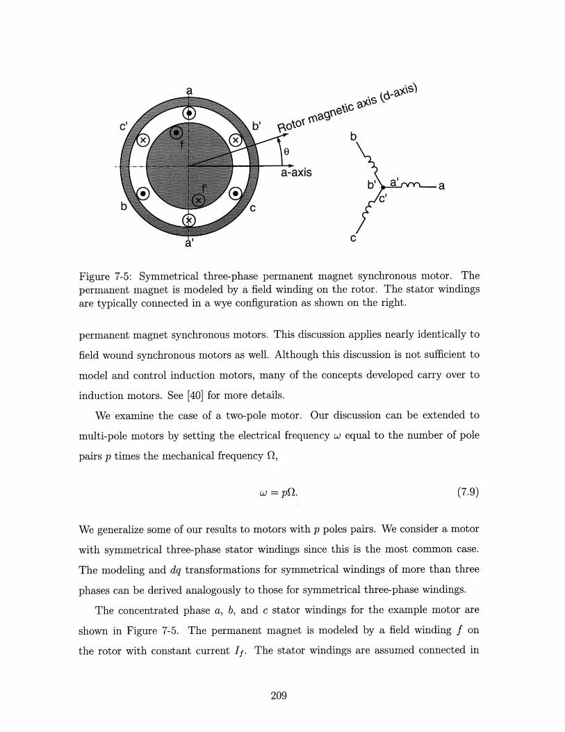
x xb

a-axisb, aab' a' a

CI

C

Figure 7-5: Symmetrical three-phase permanent magnet synchronous motor. Thepermanent magnet is modeled by a field winding on the rotor. The stator windingsare typically connected in a wye configuration as shown on the right.

permanent magnet synchronous motors. This discussion applies nearly identically to

field wound synchronous motors as well. Although this discussion is not sufficient to

model and control induction motors, many of the concepts developed carry over to

induction motors. See [40] for more details.

We examine the case of a two-pole motor. Our discussion can be extended to

multi-pole motors by setting the electrical frequency w equal to the number of pole

pairs p times the mechanical frequency Q,

(7.9)

We generalize some of our results to motors with p poles pairs. We consider a motor

with symmetrical three-phase stator windings since this is the most common case.

The modeling and dq transformations for symmetrical windings of more than three

phases can be derived analogously to those for symmetrical three-phase windings.

The concentrated phase a, b, and c stator windings for the example motor are

shown in Figure 7-5. The permanent magnet is modeled by a field winding f on

the rotor with constant current If. The stator windings are assumed connected in

209

W = pQ.

a

Figure 7-6: The magnetic flux lines produced by coil aa' in the stator of a cylindricalrotary motor are shown. The a-axis points in the direction of the magnetic fluxproduced. Actual field lines are perpendicular to the stator and rotor back irons.

the wye configuration shown in Figure 7-5. The three stator currents, ia, ib, 'c, are

functions of time t and may vary in any way provided that they are balanced,

,(7.10)

due to the summation of the currents at the isolated neutral point of the wye con-

nection. Thus, only two of the three currents can be set independently. We avoid

writing time dependence explicitly as ia(t) to simplify the notation. All currents,

voltages and flux-linkages with lower-case letters denote time-varying quantities. It

is also possible to drive the three phases independently as long as they are driven so

that they are balanced.

Each concentrated coil in Figure 7-5 represents a distributed coil which produces

a sinusoidal magnetic flux and magnetomotive force in the air gap. The direction

of the magnetic flux defines the coil's magnetic axis. Figure 7-6 shows the a-axis

corresponding to coil aa'. In Figure 7-5, the magnetic axis of rotor coil ff' is rotated

by an angle t from the magnetic axis of stator coil aa'. The magnetic axis of the rotor

coil ff' rotates with the rotor. Later, we will see that this magnetic axis aligned with

the rotor's flux is the d-axis of the dq coordinate frame.

We now model the flux linkages of the three stator coils, Aa, Ab, and Ac, as functions

of the three stator currents, i2a ib, , and the three flux linkages between the stator

210

coils and the rotor, Aaf, Abf, and Acf:

Aa Laa Lab Lac ia Aaf

Ab 2 ba Lbb Lbc ib + Abf (7.11)

Ac Lca cb Lcc ic A c

The script L represents an inductance which in general could be a function of rotor

angle 0. Here, Laa denotes the self-inductance of phase a, and Lab denotes the mutual

inductance between phases a and b. This notation is the same as that used in Electric

Machinery [18]. We could have extended the inductance matrix to be 4 x 4 by

including the rotor coil and the stator-to-rotor mutual inductances and rotor self-

inductance. For a permanent magnet rotor, this coil is imaginary so we are not

interested in its internal details. Thus it is more convenient to include these terms

via the stator-to-rotor flux linkages A14, Abf, and Af. This notation reduces the

model order from four to three and more closely describes the quantities of interest in

a permanent magnet motor. Next, we briefly examine the stator-to-rotor flux linkages

and the stator inductances in our model.

7.3.1 Stator-to-Rotor Flux Linkages

We assume the permanent magnet rotor produces only fundamental space harmonic

magnetic flux so that the flux linked by the stator phases varies as the cosine of angle

from each phase's magnetic axis. In a real machine there are higher-order spatial

harmonics, but the fundamental harmonic provides the main torque generating terms.

Later, we will see that the dq transformations assume this same simple fundamental

space harmonic distribution of magnetic flux. The flux linkages between the rotor

and the three phase windings are thus modeled as

Aaf = Af cos 0 (7.12)

27rAbf =Af cos (0- - (7.13)

4g(Acf = Af cos (0- --3 (7.14)

211

where Af is the maximum flux produced by the magnets which links each coil.1

7.3.2 Stator Inductances

Our motor has a cylindrical rotor, so each stator phase has a self-inductance L which

in the simplest model is independent of 0,

Laa = Lbb = Ccc = L. (7.15)

The stator self-inductance L includes both self-inductance due to the space-fundamental

component of flux Lo as well as self-inductance due to the armature leakage flux L1,

L = Lo + L1 . (7.16)

See Electric Machinery [18] for a model explicitly containing the leakage inductance

terms. The stator mutual inductances M are also independent of 0,

Lab = Lac = Lba = Lbc = Lca = Lcb = -M, (7.17)

where M > 0. The stator mutual inductances are negative since a positive current

in coil aa' creates flux that links coil bb' negatively as can be seen in Figure 7-5.

The mutual inductance M is the negative of one-half the space-fundamental self-

inductance, Lo. This is due to the fact that the armature phases are displaced by 27

The fraction of flux produced by coil aa' and linked by coil bb' in Figure 7-5 is

- r cosOdO (

f= .r2 (7.18)f"/2cos d0 2

Here the integral from -7r/2 to 7r/2 is the total flux produced by coil aa' and the

integral from -7r/6 to 7r/6 is the flux produced by coil aa' and linked by coil bb'.

'In the case of a wound-field synchronous motor, the maximum flux linked by the stator coilsfrom the rotor, Af, is equal to the maximum mutual inductance between the stator coils and rotorcoil, Laf, and the current in the rotor coil if, Af = Lafif.

212

The flux linkage by phase a is the sum of flux linkages due to its self-inductance,

mutual inductance with coils b and c, and flux linkage with the rotor,

Aa = Lia - Mib - Mic + Aaf. (7.19)

Under balanced three-phase conditions in the stator,

Za = - ic, (7.20)

so that we can rewrite Aa in terms of only the phase a current,

a = (L + M)ia + a~f. (7.21)

This is a useful simplification since we can now define a synchronous inductance,

Ls = L + M, (7.22)

which is the apparent phase a self-inductance looking at phase a's terminals. In reality

the synchronous inductance Ls is produced by phase a's true self-inductance L and

its mutual inductance M with phases b and c along with their associated currents.

However, the balanced three-phase conditions allow us to express the sum of the

currents ib and ic in terms of ia so that we can combine the effects of the self- and

mutual-inductances. The flux linkages in phases b and c simplify in the same manner.

7.3.3 Stator Terminal Voltages

The terminal voltage Va of phase a is the sum of its resistive drop iaR and the time

rate of change of its flux linkage, dAa/dt,

Va = i dR + A, (7.23)Va~aR+dt

213

where R is the resistance in each armature phase. Using (7.21) and (7.22), we can

write the terminal relations for the three phases as

Va = iaR+ Ls d" + dAaf (7.24)dt dt

Vb = ibR+Ls +dAbf (7.25)dt dtdie d Acf

VC = icR + Ls + .f (7.26)dt dt

Thus, we see that the phase a voltage, Va, is the sum of a resistive drop, iaR, a voltage

due to the synchronous inductance, Ls(dia/dt), and a voltage due to the changing

flux linkage with the rotor, dAaf/dt. This last term, dAaf/dt, is a speed voltage which,

in light of (7.12), is proportional to dO/dt.2

7.3.4 Torque

We will calculate the torque produced by our motor using the energy method [76].

The coenergy of our electro-mechanical system is

W'(ia, ib, ici6) =

-Ls(Z2 + i2 + il)

Af cos(9)ia + Af COS (0- ib + Af COS ( - ic. (7.27)

The first term includes the self- and mutual-inductances of the armature phases and

the next three terms are the torque-producing terms representing the rotor flux linked

by the armature phases. Torque T is the partial derivative of coenergy w' (ia, ib , ic, 6)

with respect to 0,

aW'(ia7bi, ic, 0)T=

Za,lb,'Ic

21n the case of a wound-field synchronous motor, Aaf = Lafif cos 0 and the term, dAaf /dt, containsa transformer voltage proportional to dif/dt and a speed voltage proportional to dO/dt. Since for apermanent magnet rotor the field current is constant, if = If, the transformer voltage disappears,and we have only a speed voltage.

214

2 -x 47r-Af [i sin(O) + ib sin ( - - ) + i, sin ( - - . (7.28)

(7.28) is a general expression for the torque T produced in our motor as a function

of the three phase currents, ia, ib, and i. Notice that this expression is complicated

and that it is not immediately obvious how we should control the three currents ia,

ib, and ic in order to produce a given amount of torque T. The standard solution is

to drive the three phases with currents that are sinusoidal functions of rotor angle 0,

Ia = -Is sin(6)27r

ib= -Is sin (----3

47ic= -Is sin (0- -, (7.29)

where Is is the peak amplitude of the stator phase currents. Substituting the currents

in equations (7.29) into the torque expression, (7.28), and simplifying yields

3T = -IsAf. (7.30)

2

Under this commutation law, torque is independent of rotation, and proportional to

the strength of the permanent magnets Af and to the peak amplitude of the armature

currents Is in equations (7.29). By commanding the peak current amplitude Is as

a function of time, we can control the motor's torque as a function of time. The

particular choice of phase currents which are sinusoidal functions of rotor angle 6

given by equations (7.29) is called sinusoidal commutation. It is often used in motor

drives because it simplifies the general complicated torque expression, (7.28), to a

simple expression, (7.31), which can be used in motor control systems. This can also

be shown to be the power optimal commutation pattern.

The torque expression in (7.31) for the permanent magnet synchronous motor

with sinusoidal commutation is similar to the torque expression for the DC motor,

(7.6), which we repeat here,

7 = Ktia.

215

If we define the torque constant Kt of the permanent magnet synchronous motor to

be equal to (3/2)Af, its torque is

T= KtIs. (7.31)

Thus, just as DC motor torque is directly proportional to armature current ia, torque

produced by a synchronous motor with sinusoidal commutation is proportional to the

peak current amplitude Is.

Sinusoidal commutation is the key to transforming the complicated torque ex-

pression, (7.28), into the simple torque expression, (7.31). In the next section, we

introduce the dq transformation. After that we apply it to the synchronous motor

and see that it provides the same simplification in the torque equation as sinusoidal

commutation does. It also gives us a better understanding of our motor. In effect,

sinusoidal commutation transforms the phase currents to a frame rotating with the

rotor angle 0. This is the same thing that the dq transformations do: sinusoidal

commutation follows naturally from the dq transformations. We will see that the

peak current amplitude Is of sinusoidal commutation is equal to the quadrature-axis

current iq in the dq frame.

7.4 dq Transformations

In this section we derive the field orientated or dq transformations which simplify AC

motor modeling and control. We continue to use the example of a two-pole, three-

phase permanent magnet synchronous motor. First, we develop the abc <--+ ao trans-

formation which transforms between a three-phase AC system, abc, and a two-phase

AC system, a. Second, we develop the a# <-+ dq transformation which transforms

between a two-phase AC system, a3, and a two-phase DC system, dq, which rotates

with the rotor. We derive these transfomations by equating the magnetomotive forces

in the air gap of the motor in the three different frames. Third, we introduce a trans-

formation matrix T which transforms currents, voltages, and flux linkages directly

216

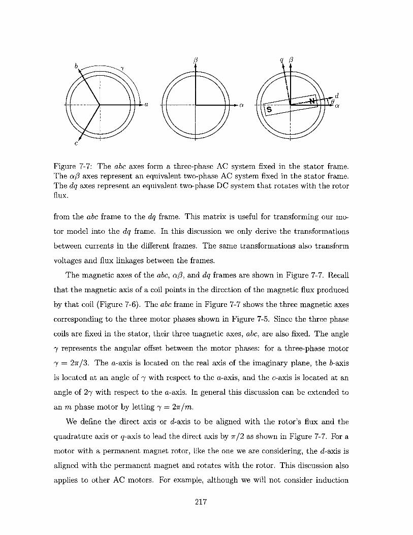
b

d

C

Figure 7-7: The abc axes form a three-phase AC system fixed in the stator frame.

The o3 axes represent an equivalent two-phase AC system fixed in the stator frame.The dq axes represent an equivalent two-phase DC system that rotates with the rotor

flux.

from the abc frame to the dq frame. This matrix is useful for transforming our mo-

tor model into the dq frame. In this discussion we only derive the transformations

between currents in the different frames. The same transformations also transform

voltages and flux linkages between the frames.

The magnetic axes of the abc, a, and dq frames are shown in Figure 7-7. Recall

that the magnetic axis of a coil points in the direction of the magnetic flux produced

by that coil (Figure 7-6). The abc frame in Figure 7-7 shows the three magnetic axes

corresponding to the three motor phases shown in Figure 7-5. Since the three phase

coils are fixed in the stator, their three magnetic axes, abc, are also fixed. The angle

y represents the angular offset between the motor phases: for a three-phase motor

y = 27r/3. The a-axis is located on the real axis of the imaginary plane, the b-axis

is located at an angle of -y with respect to the a-axis, and the c-axis is located at an

angle of 27 with respect to the a-axis. In general this discussion can be extended to

an m phase motor by letting -y = 2wr/m.

We define the direct axis or d-axis to be aligned with the rotor's flux and the

quadrature axis or q-axis to lead the direct axis by 7r/2 as shown in Figure 7-7. For a

motor with a permanent magnet rotor, like the one we are considering, the d-axis is

aligned with the permanent magnet and rotates with the rotor. This discussion also

applies to other AC motors. For example, although we will not consider induction

217

motors further here, the d-axis of induction motors is aligned with the direction of

rotor flux and slips relative to the rotor position to induce rotor currents. In deriving

the transformation from the abc frame to the dq frame, we will find it convenient to

introduce an intermediate frame, the a3 frame. The a3 frame has two magnetic axes

as shown in Figure 7-7. The a-axis is aligned with the a-axis, and the -axis leads

the a-axis by 7r/2. These axes are fixed in space.

7.4.1 Complex Current Vector

We derive the abc <-+ a,3 and a3 <- dq transformations for currents, i. The transfor-

mations are derived by equating the air gap magnetomotive force in the three different

frames. These same transformations also apply to voltages, v, and flux linkages, A.

First, let's develop an expression for the air gap magnetomotive force in the abc

frame. Let F(a, t) be the number of ampere-turns enclosed by a closed loop magnetic

flux path (such as the ones shown in Figure 7-6) which crosses the air gap radially at

an angle a at time t. For the idealized motor shown in Figure 7-5 the coils of each

phase are infinitely thin and the ampere-turns wave, which is equal to the air gap

magnetomotive force, would be a square wave. In reality, the coils have some finite

width, and motors are often designed such that the spatial ampere-turns distribution

is sinusoidal. We will model the spatial ampere-turns distribution of each phase as

sinusoidal and centered on the phase's magnetic axis. The dq transformations assume

only pure sinusoidal magnetomotive force waves exist in the motor. Thus the ampere-

turns of a closed loop flux path crossing the air gap at an angle a is

F(a, t) = Nabc [ia cos a + ib cos(a - -) + ic cos(a - 2-y)], (7.32)

where Nabc is the number of turns in each coil. We can simplify the math by using

complex numbers, for example, by substituting

1.cos a= (e3c + e-3 ), (7.33)

2

218

and by introducing a time-dependent complex current vector,

Zts = Za + ibe' + ice 2 - isej, (7.34)

where is and ( are the time-dependent magnitude and phase of the complex current

vector iS. Using (7.32), (7.33) and (7.34) we can write the ampere-turns wave F(a, t)

as

F(at) = Nabc + = Nabcis cos( - a). (7.35)2S

(7.32) expresses the ampere-turns wave as a superposition of sinusoidal waves centered

on the three magnetic axes with magnitudes determined by the three phase currents,

ia, iib, and ic. (7.35) says that the same ampere-turns wave can also be thought of as a

single sinusoidal wave with instantaneous magnitude is whose peak is instantaneously

located at an angle ( from the a-axis.

At this point it should be stressed that the phase currents, ia, ib, and ic, can vary

as functions of time in any arbitrary manner provided they are balanced. Although we

are using a complex vector is, we have not specialized to steady state operation, and

our complex quantities should not be mistaken for complex phasors used to describe

steady state oscillation.

As an example of the formalism we have developed, let's consider the special case

of steady-state rotation of the stator magnetomotive force at speed W. If we feed the

stator with balanced, three phase currents with peak amplitude IM,

ia = IM COS(wt), (7.36)

ib = IM COS(wt - 'y), (7.37)

ic = IM cos(wt - 27), (7.38)

(7.34) tells us that is = 3IM and ((t) = wt. Thus the magnetomotive force wave

F(a, t) has a fixed magnitude of !NabcIM, and rotates at constant angular velocity

W.

219

7.4.2 abc *-4 0 Transformation

The first transformation of interest converts between a three-phase AC system with

fixed axes abc and a two-phase AC system with fixed axes a3. The abc +-+ a3 trans-

formation can be derived by equating the magnetomotive forces in the two frames,

Nabc (ia + ibe 3 + iced) = NQ(ia + jio). (7.39)

Here NcO is the number of turns in the ao frame, and i0 and io are equivalent currents

in the two-phase ao frame. We may choose the ratio Na,/Nabc arbitrarily, as it just

changes the the current transformation by a constant factor. We adopt the most

commonly used ratio of

Nabc (7.40)Nabc 2

This ratio is often used since it preserves the magnitude of currents between the two

frames. This is especially useful in motor control when the magnitudes of currents

are of interest. This normalization is used by Fitzgerald, Kingsley, and Umans [18],

Kirtley [35], Analog Devices [4, 52], and Texas Instruments [63]. An alternative choice

is_ = 3

(7.41)Nabe 2

which is often used in more theoretical treatments because it makes the transforma-

tions unitary and power invariant. This normalization is used by Lang, Verghese, and

Ilic [39] and Jones [30, 29]. Finally, Leonhard [40] uses the ratio

N = 1, (7.42)

Nabc

possibly because the number of coil turns is constant under this transformation.

(7.39) with the normalization condition, (7.40), and the condition for balanced

currents, equation (7.10), yields the a -+ abc transformation,

'ta =

220

c= - )iQ -4 i1 . (7.43)

The inverse abc - a,3 transformation is

za = ia

i,3= ()ib-- i. (7.44)73= vf3-

7.4.3 13 <-+ dq Transformation

The second transformation converts between a two-phase AC system with fixed axes

a#3 and a two-phase DC system with rotating axes dq. The dq system corresponds

to a DC motor, and in steady state the direct and quadrature currents, voltages, are

flux linkages are constant. We define 0 as the angle of rotation of the dq frame from

the a4 frame as shown in Figure 7-7. The a# <-+ dq transformation can be derived

by equating the magnetomotive force in the fixed a,3 frame and in the rotating dq

frame,

Nao (i + jib) = Ndq ((id + .iiq) ejo) . (7.45)

Setting the number of turns in the ao frame, N,, equal to the number of turns in

the dq frame, Ndq,Ndq 1 (7.46)Nafi'

preserves current magnitudes, power, and the number of turns between these two

frames. From (7.45) we can solve for the dq -- a/ transformation, which is just a

2-D rotation from the dq frame to the a# frame,

ia = id cos - iq sin0 (7.47)

i = isin 0 + iq cos 6. (7.48)

221

The inverse a/3 -+ dq transformation is

id = icos0+ipsin0 (7.49)

iq = -i, sin 0 + i cos 0. (7.50)

7.4.4 dq Transformation Matrix T

We can write the abc <-+ a3 and a3 <-+ dq transformations as matrices and multiply

them to obtain a single matrix transformation T which transforms quantities from

the abc frame directly to the dq frame. This transformation matrix is mainly useful in

converting motor models from the abc frame to the dq frame for theoretical reasons.

For example, implementing a sensorless control scheme in the dq frame requires us

to convert motor variables between the abc and dq frames. Currents, voltages, and

flux linkages are all transformed by the same matrix T. Also, in order to obtain a

square, and hence invertible matrix, we need to include a zero-sequence component

denoted by subscript 0 into the dq frame.3 Under balanced three-phase conditions the

zero-sequence components are zero and are therefore usually ignored [18]. Combining

the two transformations into one matrix T is useful for theoretical reasons but is not

preferred for real-time computations because it is less computationally efficient.

We define a vector Uabc of parameters in the abc frame, where u can represent

currents i, voltages v, or flux linkages A,

Ua

Uabc= Ub . (7.51)

Uc

We also define the vector Udq of corresponding parameters in the dq frame, where

3This frame is sometimes called the dqO frame for this reason.

222

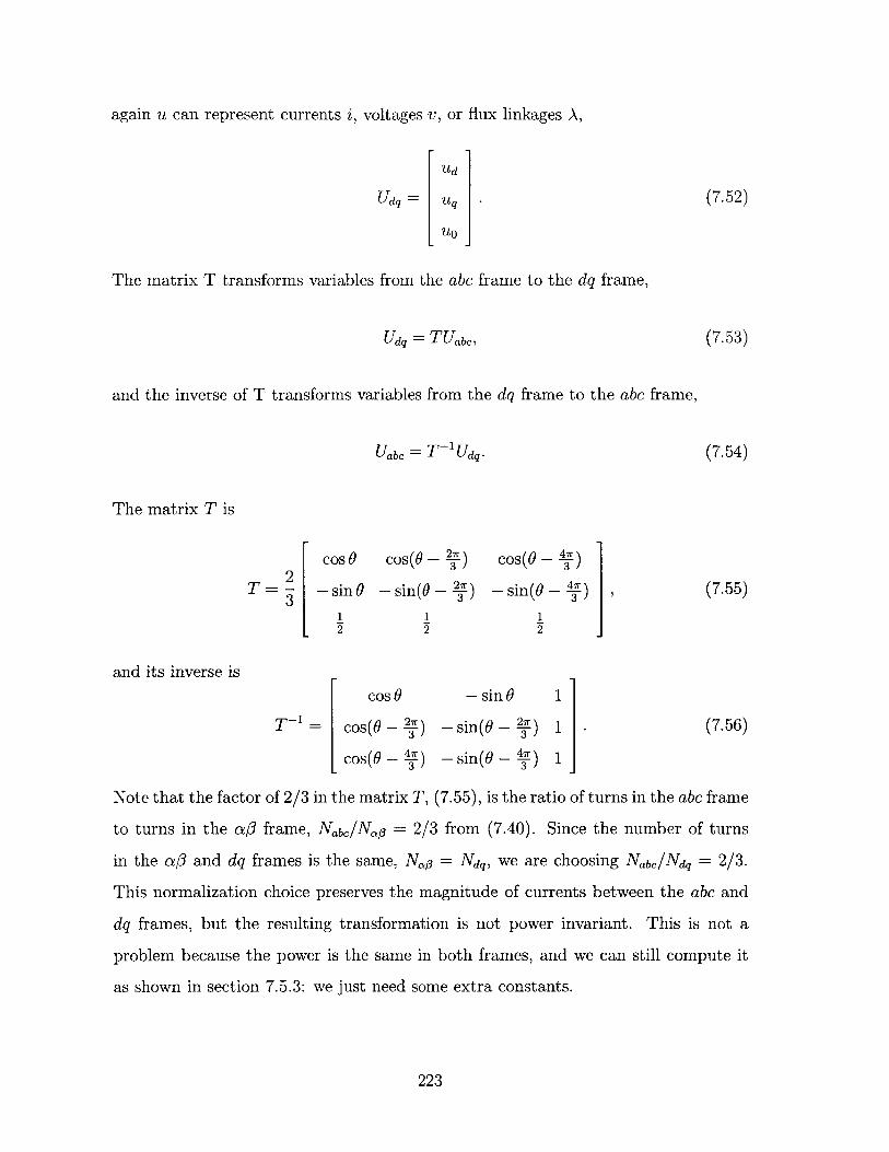
again u can represent currents i, voltages v, or flux linkages A,

Ud

Udq= Uq (7.52)

U0

The matrix T transforms variables from the abc frame to the dq frame,

Udq = TUabc, (7.53)

and the inverse of T transforms variables from the dq frame to the abc frame,

Uabc = T-1 Uq. (7.54)

The matrix T is

Cos9 cos( - ) cos( - )

T= - sin0 -sin(6 -2) -sin(6- ) , (7.55)

11 1

and its inverse iscos 9 -sin0 1

T-1 cos(6 - 2) -sin(6 - ) 1 . (7.56)

cos(6 - ) -sin( - ) 1

Note that the factor of 2/3 in the matrix T, (7.55), is the ratio of turns in the abc frame

to turns in the a3 frame, Nabc/Naf = 2/3 from (7.40). Since the number of turns

in the a,3 and dq frames is the same, Nfl = Ndq, we are choosing Nabc/Ndq = 2/3.

This normalization choice preserves the magnitude of currents between the abc and

dq frames, but the resulting transformation is not power invariant. This is not a

problem because the power is the same in both frames, and we can still compute it

as shown in section 7.5.3: we just need some extra constants.

223

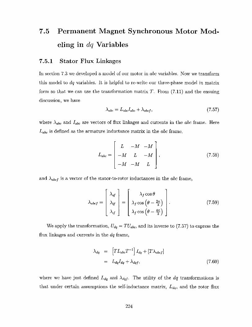
7.5 Permanent Magnet Synchronous Motor Mod-

eling in dq Variables

7.5.1 Stator Flux Linkages

In section 7.3 we developed a model of our motor in abc variables. Now we transform

this model to dq variables. It is helpful to re-write our three-phase model in matrix

form so that we can use the transformation matrix T. From (7.11) and the ensuing

discussion, we have

Aabc = Labclabc + Aabcf, (7-57)

where Aabc and Iabc are vectors of flux linkages and currents in the abc frame. Here

Labc is defined as the armature inductance matrix in the abc frame,

L -M -M

Labc = -M L -M , (7.58)

-M -M L

and Aabcf is a vector of the stator-to-rotor inductances in the abc frame,

Aaf Af cos 1Aabcf = A bf Af cos 0 - - (7.59)

A . Af cos ( - 47)

We apply the transformation, Udq = TUabc, and its inverse to (7.57) to express the

flux linkages and currents in the dq frame,

Adq = [TLabCT1I Idq + [TAabcf

= Ldqldq + Adqf, (7.60)

where we have just defined Ldq and Adqf. The utility of the dq transformations is

that under certain assumptions the self-inductance matrix, Ldq, and the rotor flux

224

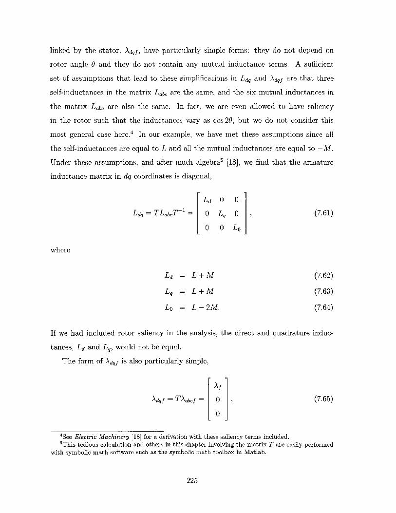
linked by the stator, Adqf, have particularly simple forms: they do not depend on

rotor angle 0 and they do not contain any mutual inductance terms. A sufficient

set of assumptions that lead to these simplifications in Ldq and Adqf are that three

self-inductances in the matrix Labc are the same, and the six mutual inductances in

the matrix Labc are also the same. In fact, we are even allowed to have saliency

in the rotor such that the inductances vary as cos 20, but we do not consider this

most general case here.4 In our example, we have met these assumptions since all

the self-inductances are equal to L and all the mutual inductances are equal to -M.

Under these assumptions, and after much algebra' [18], we find that the armature

inductance matrix in dq coordinates is diagonal,

Ld 0 0

Ldq = TLabcT-1 = 0 Lq 0 , (7.61)

0 0 Lo

where

Ld = L+M (7.62)

Lq = L+M (7.63)

Lo = L - 2M. (7.64)

If we had included rotor saliency in the analysis, the direct and quadrature induc-

tances, Ld and Lq, would not be equal.

The form of Adqf is also particularly simple,

Af

Adqf = TAabcf = 0 , (7.65)

0

4See Electric Machinery [18] for a derivation with these saliency terms included.5This tedious calculation and others in this chapter involving the matrix T are easily performed

with symbolic math software such as the symbolic math toolbox in Matlab.

225

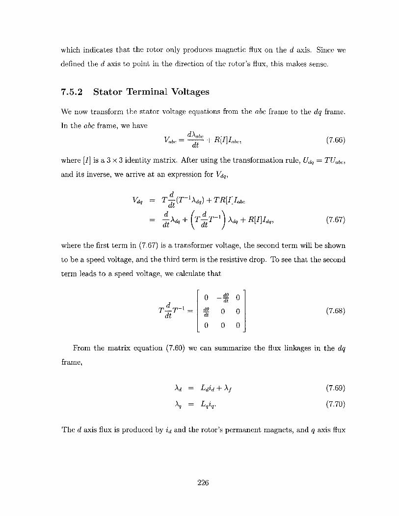
which indicates that the rotor only produces magnetic flux on the d axis. Since we

defined the d axis to point in the direction of the rotor's flux, this makes sense.

7.5.2 Stator Terminal Voltages

We now transform the stator voltage equations from the abc frame to the dq frame.

In the abc frame, we have

Varc = dAabc + R[I]Iabc,dt(7.66)

where [I] is a 3 x 3 identity matrix. After using the transformation rule, Udq = TUbc,

and its inverse, we arrive at an expression for Vq,

Vdq = T (T-Adq)+ TR[I]Iabc

=Adq+( T dT- ) Adq+ R[I]Iq,(7.67)

where the first term in (7.67) is a transformer voltage, the second term will be shown

to be a speed voltage, and the third term is the resistive drop. To see that the second

term leads to a speed voltage, we calculate that

dt

0dO

0

-d 0dt

0 0

0 0

(7.68)

From the matrix equation (7.60) we can summarize the flux linkages in the dq

frame,

Ad = Ldid+ Af

Aq = Lqiq.

(7.69)

(7.70)

The d axis flux is produced by id and the rotor's permanent magnets, and q axis flux

226

is produced by iq. From equations (7.67) and (7.68), the voltages in the dq frame are

dd= d t qa-- (7.71)

Vq=i d gwh,(7.72)

where w = dO/dt is the rotor's speed. The first terms in equations (7.71) and (7.72)

are the resistive drop, the second terms are transformer voltages, and the third terms

are speed voltages.

7.5.3 Power

It is often easier to find motor power in the dq frame than in the abc frame. This

is because the dq currents and voltages are constant in steady-state operation, while

the abc currents and voltages are sinusoids. In the abc frame power p is

P = Vaia + Vbib + Vcic = Vabclabc. (7.73)

Transforming to the dq frame, we have

pJ = VcT ('T T(TTIabc

= Vdq [(T TY T-1I dq

3. 3.= Vdid + Vqiq + 3voio, (7.74)

since0 0

(T T-1= 0 g 0 . (7.75)

0 0 3

As mentioned in section 7.4.4, our transformation matrix T is not power invariant.

We can see this because the coefficients in (7.74) are 3/2, 3/2, and 3; a power invariant

transformation would have all unity coefficients. We see from this derivation that a

unitary transformation matrix would lead to a power invariant transformation since

227

(7.75) would then be an identity matrix.

7.5.4 Torque

We can find the torque in two different ways, either by using energy arguments or

transforming the torque expression in the abc frame. First, we find the torque using

energy arguments. If we use equations (7.71) and (7.72) to substitute for vd and

Vq in the power equation, (7.74), we will find terms due to resistive loss, changes

in stored energy, and electro-mechanical power conversion. The electro-mechanical

power conversion or back EMF terms can be divided by mechanical speed to yield

the motor torque,

T = p 3(Adiq - Aqid), (7.76)

where we have generalized to a motor with p pole pairs. We generalize to p pole pairs

because our rotary motor has p = 4 pole pairs and we would like to develop a model

for it in the dq frame. We can write this torque in terms of the motor's inductances

using equations (7.69) and (7.70),

3T = p(Af + (Ld - Lq)Id)Iq. (7.77)

2

Our example permanent magnet motor has a smooth rotor so Ld = Lq, and its torque

is thus3

T = P3iqAf. (7.78)

The permanent magnets provide the d axis flux of Af, and we can control the motor

torque by adjusting the quadrature current iq which is proportional to motor torque.

We now re-derive this torque expression in a different way by using the transfor-

mation matrix T. We can write our expression for torque in the abc frame, (7.28), in

matrix form as

T = d (AjcTf) 'abc- (7-79)

228

We transform Aabcf and abc to the dq frame using the transformation matrix T,

T = ( fTT)'TT)1) T 1 (T abc )

+O (Aqf(T-1) T-Idq

T T f [d ((TT)1) Tj Iq, (7.80)

where we have used d(A3qf)/dO = 0 in going from the second to the third line. The

matrix expression in square brackets simplifies to

0 0

(TT)-1) T-- -3 0 0 . (7.81)

0 0 0

Our torque expression in the dq frame is now quite simple since Adqf = [Af, 0, O]T:

3T = p-iqAf. (7.82)

This is the same torque expression we arrived at via the energy method, (7.78). We

have again generalized to a motor with p pole pairs in (7.82).

We can rewrite (7.82) as

T = Ktiq (7.83)

where Kt is the motor torque constant,

3Kt =p 3Af. (7.84)

The quadrature current, iq, transforms to 3-phase currents with peak amplitudes equal

to iq since our transformation preserves current magnitudes. Thus, Kt is the mo-

tor force constant expressed in units of Newton-meters per peak amps, [N-m/Aeak].

Since root mean square currents, irms, are related to peak currents, ipeak, by irms =

(1/v2)ipeak, the motor force constant is v1Kt in units of Newton-meters per rms

229

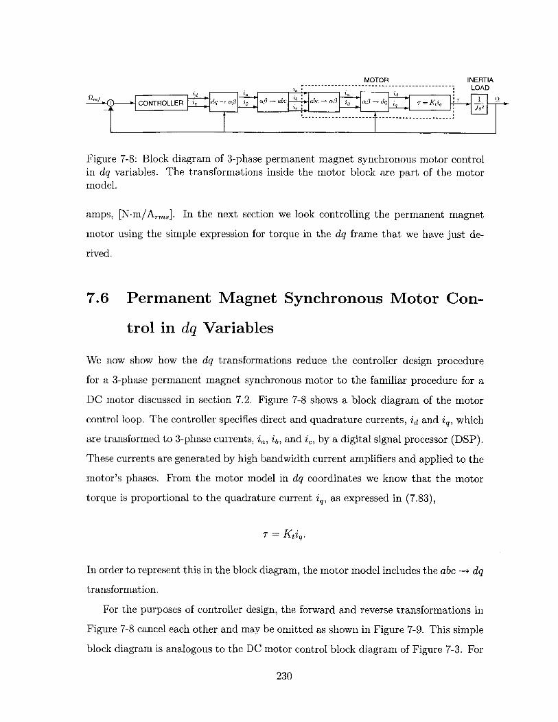
MOTOR INERTIA~ ~~- ---- - LOAD

1e :ET C/ bCONTROLLER iq dq-+Q3 a -c/-abc Lb abc-+o a3 dq I T=Ktiq

Figure 7-8: Block diagram of 3-phase permanent magnet synchronous motor controlin dq variables. The transformations inside the motor block are part of the motormodel.

amps, [N-m/Arms]. In the next section we look controlling the permanent magnet

motor using the simple expression for torque in the dq frame that we have just de-

rived.

7.6 Permanent Magnet Synchronous Motor Con-

trol in dq Variables

We now show how the dq transformations reduce the controller design procedure

for a 3-phase permanent magnet synchronous motor to the familiar procedure for a

DC motor discussed in section 7.2. Figure 7-8 shows a block diagram of the motor

control loop. The controller specifies direct and quadrature currents, id and iq, which

are transformed to 3-phase currents, ia, ib, and ic, by a digital signal processor (DSP).

These currents are generated by high bandwidth current amplifiers and applied to the

motor's phases. From the motor model in dq coordinates we know that the motor

torque is proportional to the quadrature current iq, as expressed in (7.83),

T = Ktiq.

In order to represent this in the block diagram, the motor model includes the abc -+ dq

transformation.

For the purposes of controller design, the forward and reverse transformations in

Figure 7-8 cancel each other and may be omitted as shown in Figure 7-9. This simple

block diagram is analogous to the DC motor control block diagram of Figure 7-3. For

230

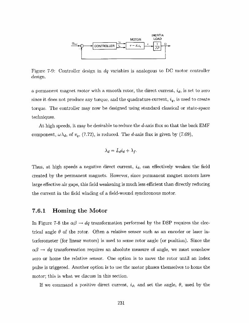
INERTIAMOTOR LOAD

-[CONTROLLER . = K.i. .

Figure 7-9: Controller design in dq variables is analogous to DC motor controllerdesign.

a permanent magnet motor with a smooth rotor, the direct current, id, is set to zero

since it does not produce any torque, and the quadrature current, j , is used to create

torque. The controller may now be designed using standard classical or state-space

techniques.

At high speeds, it may be desirable to reduce the d-axis flux so that the back EMF

component, wAd, of Vq, (7.72), is reduced. The d-axis flux is given by (7.69),

Ad = Ldid + Af.

Thus, at high speeds a negative direct current, id, can effectively weaken the field

created by the permanent magnets. However, since permanent magnet motors have

large effective air gaps, this field weakening is much less efficient than directly reducing

the current in the field winding of a field-wound synchronous motor.

7.6.1 Homing the Motor

In Figure 7-8 the a3 -- dq transformation performed by the DSP requires the elec-

trical angle 0 of the rotor. Often a relative sensor such as an encoder or laser in-

terferometer (for linear motors) is used to sense rotor angle (or position). Since the

ao -+ dq transformation requires an absolute measure of angle, we must somehow

zero or home the relative sensor. One option is to move the rotor until an index

pulse is triggered. Another option is to use the motor phases themselves to home the

motor; this is what we discuss in this section.

If we command a positive direct current, id, and set the angle, 6, used by the

231

ao --> dq transformation, we create flux along the d-axis which is at an angle 0 from

the a-axis (see Figure 7-7). The rotor of the motor will line up with this flux produced

by stator currents. After waiting for the resulting oscillatory motion of the rotor to

die down, we know that the rotor is pointing at an angle 0 from the a-axis. For

example, to align the rotor with the a-axis, we would set 0 = 0, and to align the rotor

with the b-axis, we would set 0 = 27r/3.

7.7 Summary

This tutorial chapter introduces the field orientation transformations for three phase

permanent magnet synchronous motors. We reviewed the standard modeling and

control of brushed DC motors first since these are well understood. Later in the

chapter we showed that three phase permanent magnet motors can be controlled in

a similar manner using the field orientation transformations. We also developed a

model for a 3-phase permanent magnet motor in abc coordinates and transformed it

into dq coordinates.

Three phase permanent magnet motors can be controlled without the field ori-

entation transformations presented in this chapter. However, the field orientation

transformations simplify our understanding of these motors and make it easier for us

to commutate them and measure their parameters. For example, what does it mean

to speak of a three phase motor's force constant in Newtons per amp if there are

three phases? What current are we talking about? As we saw in this chapter, the

current level is really the amplitude of the three sinusoidal phase currents. It's much

easier to think of the motor force constant as Newtons per amp of quadrature current,

sq. The quadrature current directly produces motor torque, and the field orientation

transformations convert the actual phase currents into the quadrature current, or vice

versa.

In addition to being used for motor commutation, the field orientation transfor-

mations provide us with a simple model of the motor in the dq frame. At the end of

the next chapter, we will use this model to create a sensorless observer for the rotary

232

motor. First, though, the next chapter looks at the motor power amplifier circuits

and the linear and rotary axis control design.

233

234

Chapter 8

Control System

In this chapter we look at the control system which runs the two axes of our prototype

rotary-linear axis. In the first section, we look at the design of the analog power

amplifier current control loop. This high bandwidth controller provides currents to

each phase of the rotary and linear 3-phase motors. In the following two sections

we look at the design of the linear and then rotary axis controllers. We control the

linear and rotary axes separately since their dynamics are largely uncoupled. For

each axis, we show measured Bode plots of the open-loop plant. We then explain

the causes of initially unmodeled resonances and develop appropriate models and

possible mechanisms for these modes. Using the open-loop Bode plot, we explain

how we design an appropriate controller for each axis and show the resulting loop

transmission Bode plot. For each axis, we then show the performance achieved via

closed-loop Bode plots, step responses, and positioning noise. The linear axis has

a 70 Hz closed-loop bandwidth and 2.5 nm rms positioning noise. The rotary axis

has a 40 Hz closed-loop bandwidth and 3.1 prad rms positioning noise. In the final

section of the chapter we present a sensorless control scheme for spinning the rotary

motor using only measurements of the motor's phase currents and voltages. Such an

approach would be helpful for controlling a rotary-linear high speed spindle. In this

application, precise angular positioning is not required; we only need to implement

speed control and require angle only for motor commutation. We have successfully

implemented sensorless control at a rotation speed of 390 rpm (40.84 rad/s) on our

235

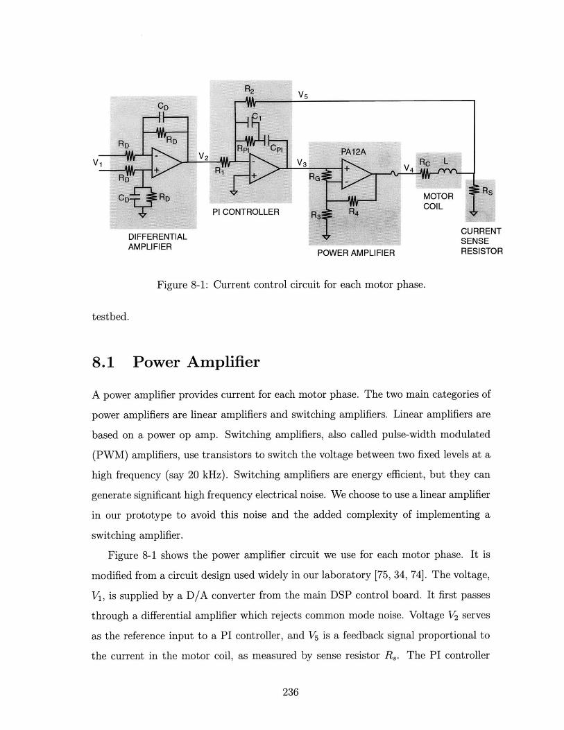
V5

V1 -V2 -V3 +Rc L+ R1 V410

RD + RG RCD RD MOTOR

PI CONTROLLER R13 R4 COI

DIFFERENTIAL CURRENT

AMPLIFIERSEEPOWER AMPLIFIER RESISTOR

Figure 8-1: Current control circuit for each motor phase.

testbed.

8.1 Power Amplifier

A power amplifier provides current for each motor phase. The two main categories of

power amplifiers are linear amplifiers and switching amplifiers. Linear amplifiers are

based on a power op amp. Switching amplifiers, also called pulse-width modulated

(PWM) amplifiers, use transistors to switch the voltage between two fixed levels at a

high frequency (say 20 kHz). Switching amplifiers are energy efficient, but they can

generate significant high frequency electrical noise. We choose to use a linear amplifier

in our prototype to avoid this noise and the added complexity of implementing a

switching amplifier.

Figure 8-1 shows the power amplifier circuit we use for each motor phase. It is

modified from a circuit design used widely in our laboratory [75, 34, 74]. The voltage,

V1, is supplied by a D/A converter from the main DSP control board. It first passes

through a differential amplifier which rejects common mode noise. Voltage V2 serves

as the reference input to a PI controller, and V5 is a feedback signal proportional to

the current in the motor coil, as measured by sense resistor R,. The PI controller

236

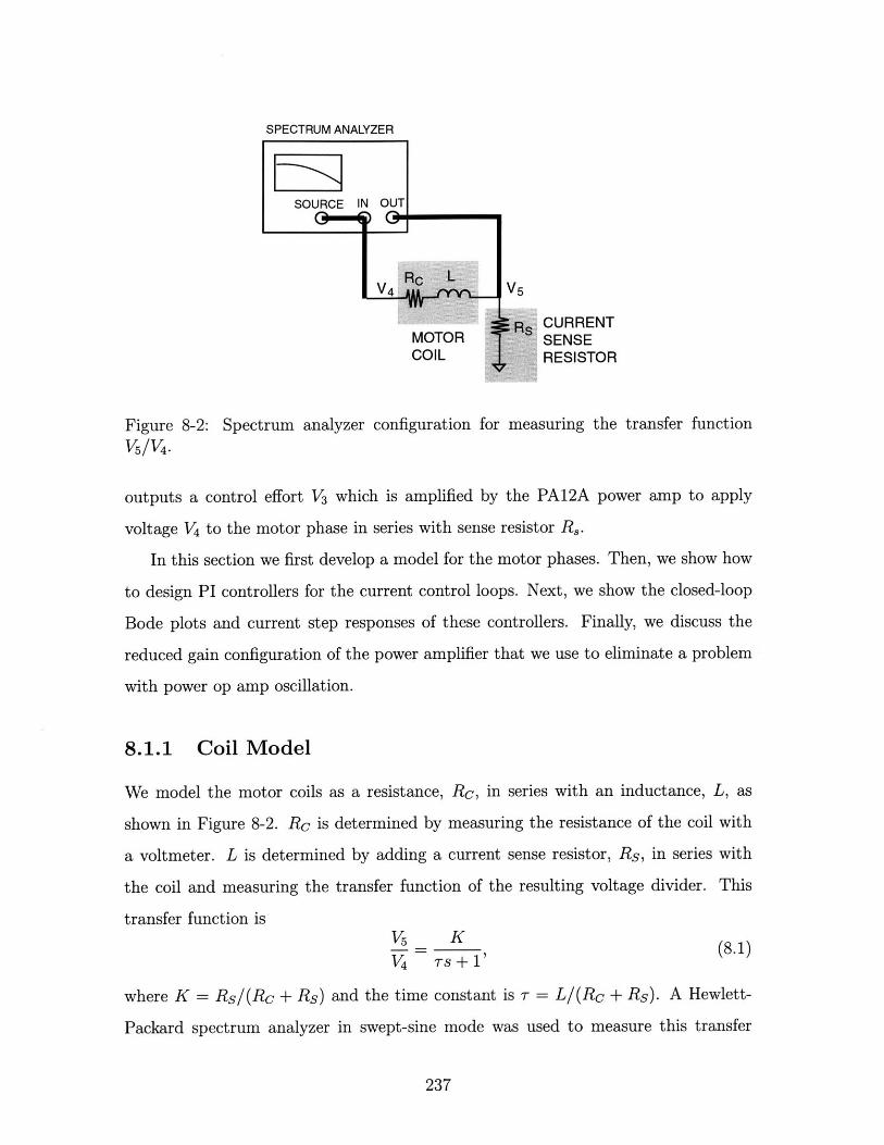
SPECTRUM ANALYZER

SOURCE IN OUT

V4 RC L V

RS CURRENTMOTOR SENSECOIL RESISTOR

Figure 8-2: Spectrum analyzer configuration for measuring the transfer function

V5/V 4.

outputs a control effort V3 which is amplified by the PA12A power amp to apply

voltage V4 to the motor phase in series with sense resistor Rs.

In this section we first develop a model for the motor phases. Then, we show how

to design PI controllers for the current control loops. Next, we show the closed-loop

Bode plots and current step responses of these controllers. Finally, we discuss the

reduced gain configuration of the power amplifier that we use to eliminate a problem

with power op amp oscillation.

8.1.1 Coil Model

We model the motor coils as a resistance, RC, in series with an inductance, L, as

shown in Figure 8-2. Rc is determined by measuring the resistance of the coil with

a voltmeter. L is determined by adding a current sense resistor, Rs, in series with

the coil and measuring the transfer function of the resulting voltage divider. This

transfer function isV5 (8.1)V4 TS + '

where K = Rs/(Rc + Rs) and the time constant is T = L/(Rc + Rs). A Hewlett-

Packard spectrum analyzer in swept-sine mode was used to measure this transfer

237

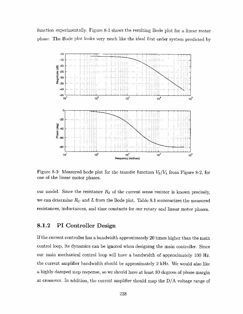
function experimentally. Figure 8-3 shows the resulting Bode plot for a linear motor

phase. The Bode plot looks very much like the ideal first order system predicted by

-10

-15

-20

-25

E -30

2 -35

-40

-451

0

-20

:S -40

(L -60

-80

1

0 102 103

10 1

102 10 3Frequency (rad/sec)

Figure 8-3: Measured bode plot for the transfer function V5 /V 4 from Figure 8-2, forone of the linear motor phases.

our model. Since the resistance Rs of the current sense resistor is known precisely,

we can determine RC and L from the Bode plot. Table 8.1 summarizes the measured

resistances, inductances, and time constants for our rotary and linear motor phases.

8.1.2 PI Controller Design

If the current controller has a bandwidth approximately 20 times higher than the main

control loop, its dynamics can be ignored when designing the main controller. Since

our main mechanical control loop will have a bandwidth of approximately 100 Hz,

the current amplifier bandwidth should be approximately 2 kHz. We would also like

a highly damped step response, so we should have at least 80 degrees of phase margin

at crossover. In addition, the current amplifier should map the D/A voltage range of

238

- - - -- -.... -

- - - - -.....- . .

- - -- - - - ...-

- - - -...-

10 4 10 5

I

0

- - -... -. .... ...

-........ - - - - -.- .

- -.-.-.-.-.-

- -- - - - -.. --. - - - - . -

I

00

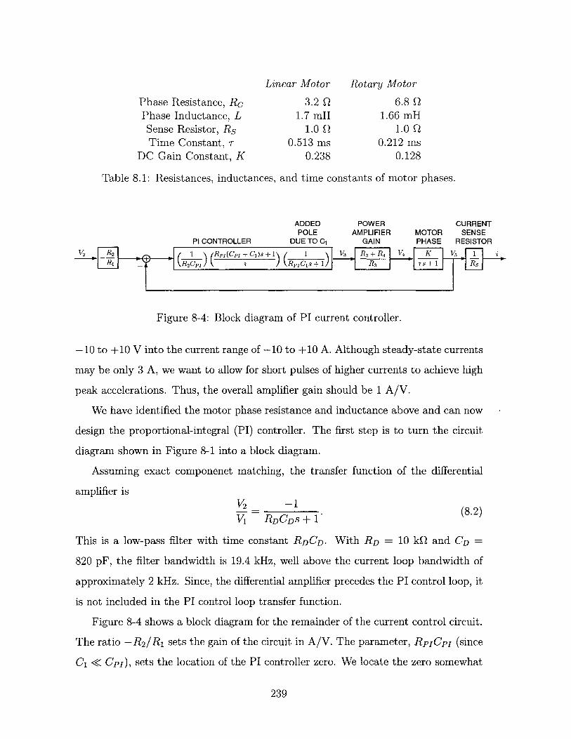
Linear Motor Rotary Motor

Phase Resistance, RC 3.2 Q 6.8 QPhase Inductance, L 1.7 mH 1.66 mHSense Resistor, Rs 1.0 Q 1.0 QTime Constant, T 0.513 ms 0.212 ms

DC Gain Constant, K 0.238 0.128

Table 8.1: Resistances, inductances, and time constants of motor phases.

ADDED POWER CURRENTPOLE AMPLIFIER MOTOR SENSE

PI CONTROLLER DUE TO C1 GAIN PHASE RESISTOR

V2 IM (1P (Rpi (cPl +CI)s + 1) (1 V3 R±R V4 K V5 1W R2 CP1 C s Re 1Cis+1 R3 Ts+I

Figure 8-4: Block diagram of PI current controller.

-10 to +10 V into the current range of -10 to +10 A. Although steady-state currents

may be only 3 A, we want to allow for short pulses of higher currents to achieve high

peak accelerations. Thus, the overall amplifier gain should be 1 A/V.

We have identified the motor phase resistance and inductance above and can now

design the proportional-integral (PI) controller. The first step is to turn the circuit

diagram shown in Figure 8-1 into a block diagram.

Assuming exact componenet matching, the transfer function of the differential

amplifier isV2 -1(2)V1 RDCDS + I

This is a low-pass filter with time constant RDCD. With RD = 10 kQ and CD =

820 pF, the filter bandwidth is 19.4 kHz, well above the current loop bandwidth of

approximately 2 kHz. Since, the differential amplifier precedes the PI control loop, it

is not included in the PI control loop transfer function.

Figure 8-4 shows a block diagram for the remainder of the current control circuit.

The ratio -R 2/R 1 sets the gain of the circuit in A/V. The parameter, RpCpi (since

C1 < Cj), sets the location of the PI controller zero. We locate the zero somewhat

239

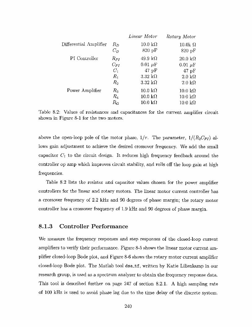
Linear Motor Rotary Motor

Differential Amplifier RD 10.0 kQ 10.0k QCD 820 pF 820 pF

PI Controller Rp1 49.9 kQ 20.0 kQCPI 0.01 [iF 0.01 [tFC1 47pF 47pFR1 3.32 kQ 2.0 kQR2 3.32 kQ 2.0 kQ

Power Amplifier R3 10.0 kQ 10.0 kQR4 10.0 kQ 10.0 kQRG 10.0 kQ 10.0 kQ

Table 8.2: Values of resistances and capacitances for the current amplifier circuitshown in Figure 8-1 for the two motors.

above the open-loop pole of the motor phase, 1/r. The parameter, 1/(R 2 CPI) al-

lows gain adjustment to achieve the desired crossover frequency. We add the small

capacitor C1 to the circuit design. It reduces high frequency feedback around the

controller op amp which improves circuit stability, and rolls off the loop gain at high

frequencies.

Table 8.2 lists the resistor and capacitor values chosen for the power amplifier

controllers for the linear and rotary motors. The linear motor current controller has

a crossover frequency of 2.2 kHz and 90 degrees of phase margin; the rotary motor

controller has a crossover frequency of 1.9 kHz and 90 degrees of phase margin.

8.1.3 Controller Performance

We measure the frequency responses and step responses of the closed-loop current

amplifiers to verify their performance. Figure 8-5 shows the linear motor current am-

plifier closed-loop Bode plot, and Figure 8-6 shows the rotary motor current amplifier

closed-loop Bode plot. The Matlab tool dsa-tf, written by Katie Lilienkamp in our

research group, is used as a spectrum analyzer to obtain the frequency response data.

This tool is described further on page 247 of section 8.2.1. A high sampling rate

of 100 kHz is used to avoid phase lag due to the time delay of the discrete system.

240

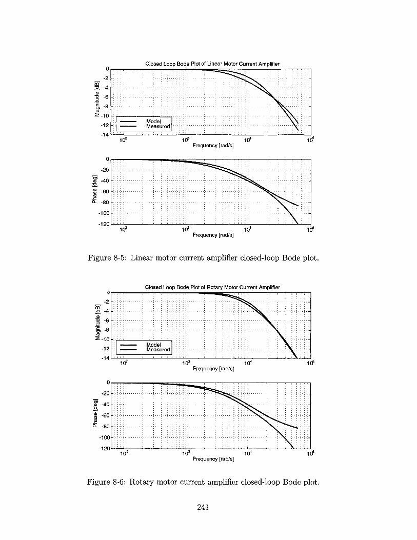
0

-2CO

-4

-6

S-8ca

2-10

-12

-14

i &Frequency [rad/s]

i04 1id

Figure 8-5: Linear motor current amplifier closed-loop Bode plot.

Closed Loop Bode Plot of Rotary Motor Current Amplifier0.-

103

103

Frequency [rad/s]

Frequency [rad/s]

104 1d5

10 10

Figure 8-6: Rotary motor current amplifier closed-loop Bode plot.

241

Closed Loop Bode Plot of Linear Motor Current Amplifier

ModelMeasured - -

102 104 10Frequency [rad/s]

...-....-.-

- ...................-. ...-. ..- ...-

- ..... -... -...- .

-.. ....................................-. . -. . -.-

,a

(D~(n

0

-20

-40

-60

-80

-100

-1201o2d

-2-4

-6

2-10

-12

-14

Model- - Measured

U)V

U)Ct)CU-ca-

0

-20 -......

-40 ..

-60 - - - -.-.-. -. -

-80 . - -

-100 - - -

-190102

0

-. .......

--. .....

....... ... ... ..- -

-.. .. .. -- - - -. - - -.. ..

. . ... .... ..-

-.... -.-..... .......... ......... ...-

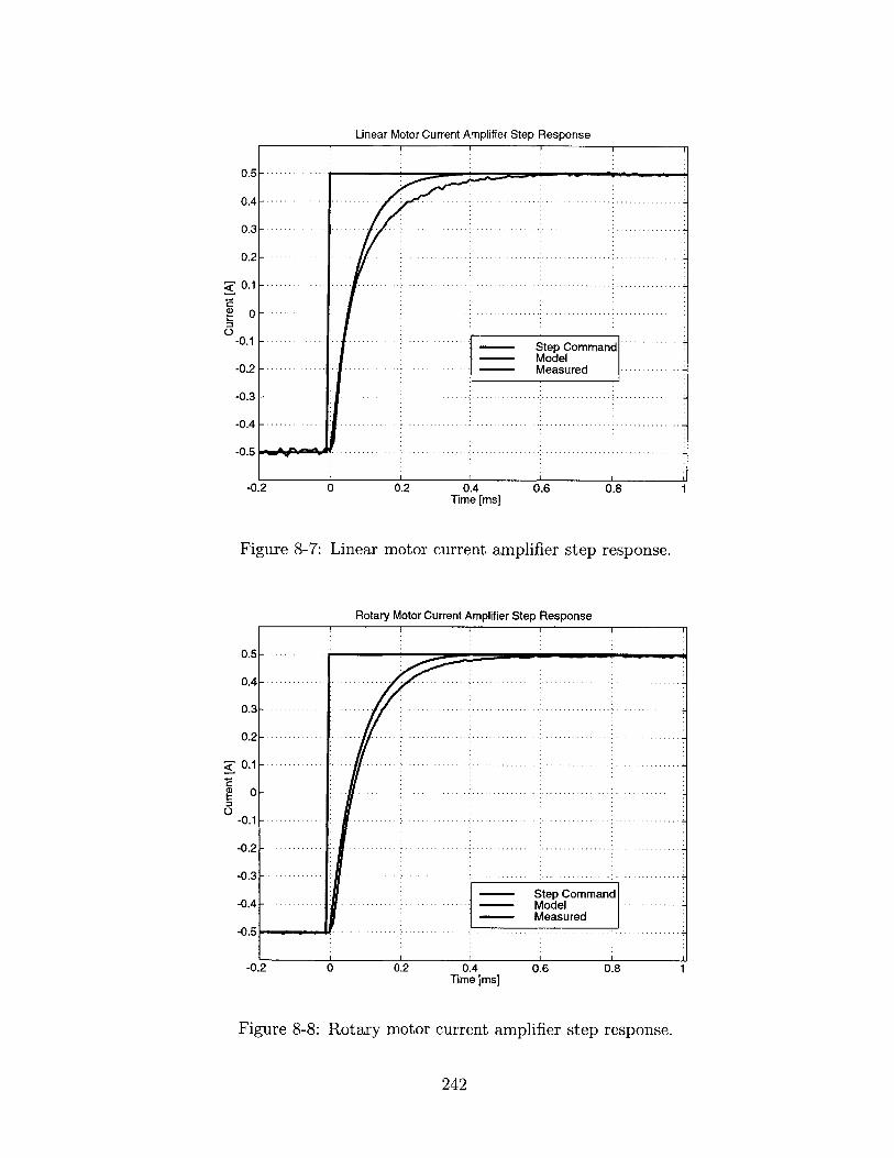
0.6 0.8 1

Figure 8-8: Rotary motor current amplifier step response.

242

Linear Motor Current Amplifier Step Response

2

0.5

0.4

0.3

0.2

0.1

0

-0.1

-0.2

-0.3

-0.4

-0.5

-0.

...............

.................... . ....... .......

............. . ... ..... . .................... ...... ...............

. .............. . ... .. ...... ........... .............. ............ .

. .............. . .... .......................... ............. .. ............... ............

. .............. . ... ............. ............... ............. ................ ............

. ... . . ... .. .... ........Step CommandModel

.......... . ... .. ....... ... ........ M e a s u re d ........

. .............. .. .. ............ ...... ..... ....... .... .....* .................

. .............. ... .......... ... .......... .. ........ ....... ............

w e . .. ............... ............... .................. ...............

0 0.2 0.4Time [ms]

0.6 0.8 1

Figure 8-7: Linear motor current amplifier step response.

Rotary Motor Current Amplifier Step Response

2

0.5

0.4

0.3

0.2

0.1

0

-0.1

-0.2

-0.3

-0.4

-0.5

-0.

...............

................... .. . ...... ....... ..... .. ....... ............

. .............. . ... ... ... .............. ................. .......* ....... ............

. .............. . ... ...... .......... ... ............. ................ ....... .... ...7

. .............. . ... . ................. .............I ......... ... ............... ......... ......

. ............. .. .. .. ....... ... ................ ... ............... ... ... ......

. .............. . .. ... ......................... ...... .. ................ ... ..........

. .............. .. . .. ...... ....... .. ............ ........

. ................. ................ ............... .............. ... ............... .......... .....

Step Comman.............. . ................ .............. M o d e l .........

Measured.............. ................................ ................

Q

0 0.2 0.4Time [ms]

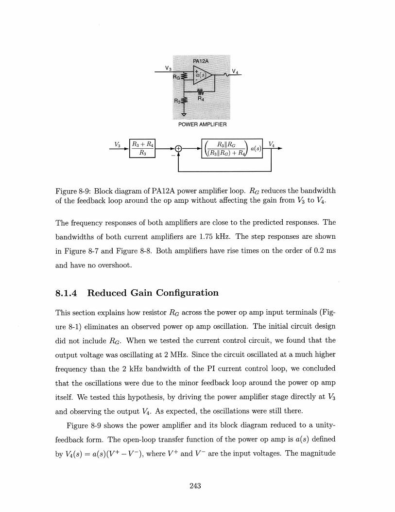
V3 V4

POWER AMPLIFIER

-R3 R4 R3||RG T)as4

Ra _ R3||RG) +

Figure 8-9: Block diagram of PA12A power amplifier loop. RG reduces the bandwidthof the feedback loop around the op amp without affecting the gain from V3 to V4 .

The frequency responses of both amplifiers are close to the predicted responses. The

bandwidths of both current amplifiers are 1.75 kHz. The step responses are shown

in Figure 8-7 and Figure 8-8. Both amplifiers have rise times on the order of 0.2 ms

and have no overshoot.

8.1.4 Reduced Gain Configuration

This section explains how resistor RG across the power op amp input terminals (Fig-

ure 8-1) eliminates an observed power op amp oscillation. The initial circuit design

did not include RG. When we tested the current control circuit, we found that the

output voltage was oscillating at 2 MHz. Since the circuit oscillated at a much higher

frequency than the 2 kHz bandwidth of the PI current control loop, we concluded

that the oscillations were due to the minor feedback loop around the power op amp

itself. We tested this hypothesis, by driving the power amplifier stage directly at V3

and observing the output V4. As expected, the oscillations were still there.

Figure 8-9 shows the power amplifier and its block diagram reduced to a unity-

feedback form. The open-loop transfer function of the power op amp is a(s) defined

by V4(s) = a(s)(V+ - V-), where V+ and V- are the input voltages. The magnitude

243

of the loop transmission is

( R + a(s). (8.3)( R3|G) +(R4

One may improve the stability of this minor feedback loop by increasing the ideal low

frequency gain, (R 3 + R 4)/R 3 , which reduces the magnitude of the loop tranmission.

The ideal low frequency gain should roughly map the range of V3 , typically +15 V,

into the range of V4 which is determined by the power supply used with the power

op amp. Thus, for a given application the ideal low frequency gain may not be able

to be increased. The inclusion of RG in the circuit provides an additional degree of

freedom such that the ideal gain, (R3 + R4 )/R 3 , and the loop transmission can be

adjusted independently [57]. Note that for any value of RG, including inifinity (no

RG), the ideal low-frequency gain of this amplifier is

V4 R 3 + R 4 (8.4)V3 R3

This is the gain shown in the Power Amplifier Gain block in Figure 8-4. The magni-

tude of the minor loop transmission given in equation (8.3) decreases as RG increases.

Thus, adding the resistor RG into the circuit reduces the bandwidth and increases the

stability of the minor feedback loop around the power op amp, but has no significant

effect on the major PI feedback loop (Figure 8-4).

8.2 Linear axis compensator design

One of the main benefits of our rotary-linear axis is that the mechanical system is

simple and therefore easy to model and control. The air bearings provide essentially

frictionless guidance, and the forces and torques produced by the motors can be cal-

culated accurately. As a first approximation, we can model the linear axis mechanical

system as a mass and the rotary axis mechanical system as an inertia. Of course,

there are additional resonances and other dynamics, especially at higher frequencies.

In subsequent sections we examine these higher order effects in detail and see how

244

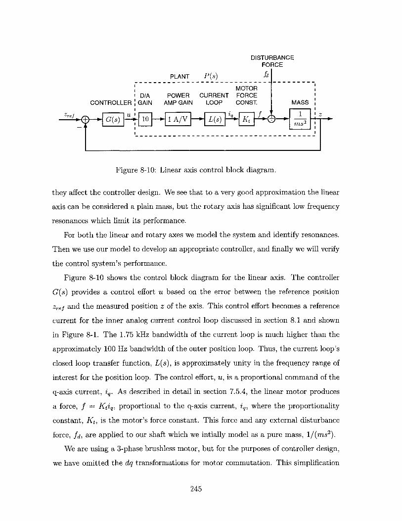
DISTURBANCEFORCE

PLANT P(s) fd

MOTORD/A POWER CURRENT FORCE

CONTROLLER: GAIN AMP GAIN LOOP CONST. MASS

Zref~~ ___ ,Zref (+-+ G(s) ~~ 1- A/ -+ L(s) K;1] Z

Figure 8-10: Linear axis control block diagram.

they affect the controller design. We see that to a very good approximation the linear

axis can be considered a plain mass, but the rotary axis has significant low frequency

resonances which limit its performance.

For both the linear and rotary axes we model the system and identify resonances.

Then we use our model to develop an appropriate controller, and finally we will verify

the control system's performance.

Figure 8-10 shows the control block diagram for the linear axis. The controller

G(s) provides a control effort u based on the error between the reference position

zef and the measured position z of the axis. This control effort becomes a reference

current for the inner analog current control loop discussed in section 8.1 and shown

in Figure 8-1. The 1.75 kHz bandwidth of the current loop is much higher than the

approximately 100 Hz bandwidth of the outer position loop. Thus, the current loop's

closed loop transfer function, L(s), is approximately unity in the frequency range of

interest for the position loop. The control effort, u, is a proportional command of the

q-axis current, iq. As described in detail in section 7.5.4, the linear motor produces

a force, f = Ktiq, proportional to the q-axis current, iq, where the proportionality

constant, Kt, is the motor's force constant. This force and any external disturbance

force, fd, are applied to our shaft which we intially model as a pure mass, 1/(ms 2 ).

We are using a 3-phase brushless motor, but for the purposes of controller design,

we have omitted the dq transformations for motor commutation. This simplification

245

is possible since the motor inherently performs the reverse dq transformations as is

shown in Figure 7-8 and discussed in section 7.4. Thus, even though we are using a

3-phase brushless motor, we can design the control system as if we are using a brushed

DC motor with armature current, iq, motor constant, Kt, and force, f = Ktiq. Said

another way, the commutation laws are suppressed in Figure 8-10, and we treat the

motor as a brushed DC motor with a single coil current iq.

The sensor dynamics do not appear in the control block diagram. The laser

interferometer has a much higher bandwidth than our position loop, and we have

provided gains in our DSP so that the interferometer's counts are converted to meters.

Now that we have an initial model of the linear axis control loop, we need to

verify it experimentally and see what other effects may be present in our system. In

particular, we suspect that the moving mechanics will have some higher frequency

resonances which we have not yet modeled. We also expect additional phase loss

due to time delays associated with the zero-order hold in the D/A converter and the

digitial implementation of the controller.

8.2.1 Modeling

An initial model of the linear-axis plant is shown in Figure 8-10. It consists of the

D/A gain, the power amplifier gain, the analog closed-loop current control, the motor

constant, and the shaft's mass. We have already measured many of these components

separately. For example, the power amplifier gain and closed-loop current control

transfer function are measured in section 8.1.3, and the motor constant is measured in

section 4.2. The only component we have not already measured is the shaft mechanical

dynamics model which initially consists of a pure mass.

In order to measure P(s) we want to measure the transfer function from u to z.

We can do this by applying a sine wave at different frequencies at u and measuring

the amplitude and phase of z at each frequency. Since there is no mechanical spring

in the system, if we attempt to measure this transfer function open-loop, the shaft

will tend to wander from its intial position after executing many open-loop sinusoidal

cycles. This is not usually a problem in a rotary system, but for a linear system with

246

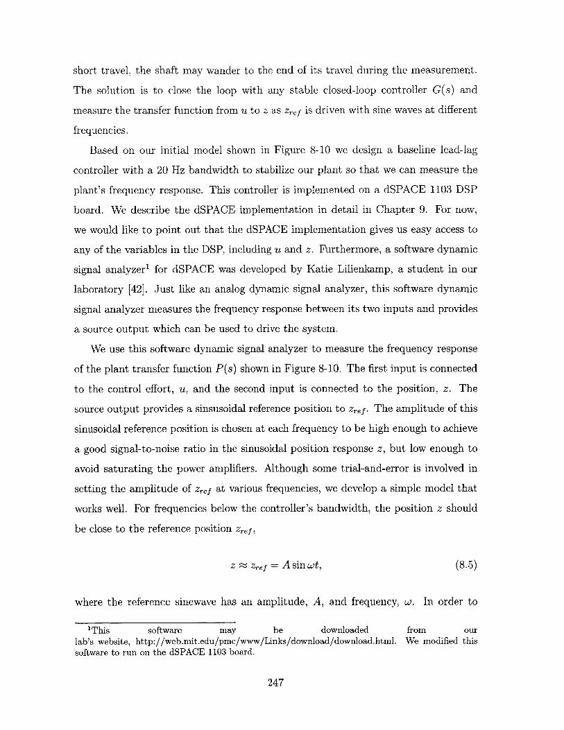
short travel, the shaft may wander to the end of its travel during the measurement.

The solution is to close the loop with any stable closed-loop controller G(s) and

measure the transfer function from u to z as zref is driven with sine waves at different

frequencies.

Based on our initial model shown in Figure 8-10 we design a baseline lead-lag

controller with a 20 Hz bandwidth to stabilize our plant so that we can measure the

plant's frequency response. This controller is implemented on a dSPACE 1103 DSP

board. We describe the dSPACE implementation in detail in Chapter 9. For now,

we would like to point out that the dSPACE implementation gives us easy access to

any of the variables in the DSP, including u and z. Furthermore, a software dynamic

signal analyzer1 for dSPACE was developed by Katie Lilienkamp, a student in our

laboratory [42]. Just like an analog dynamic signal analyzer, this software dynamic

signal analyzer measures the frequency response between its two inputs and provides

a source output which can be used to drive the system.

We use this software dynamic signal analyzer to measure the frequency response

of the plant transfer function P(s) shown in Figure 8-10. The first input is connected

to the control effort, u, and the second input is connected to the position, z. The

source output provides a sinsusoidal reference position to zef. The amplitude of this

sinusoidal reference position is chosen at each frequency to be high enough to achieve

a good signal-to-noise ratio in the sinusoidal position response z, but low enough to

avoid saturating the power amplifiers. Although some trial-and-error is involved in

setting the amplitude of Zef at various frequencies, we develop a simple model that

works well. For frequencies below the controller's bandwidth, the position z should

be close to the reference position zef,

z ~ zef = A sin wt, (8.5)

where the reference sinewave has an amplitude, A, and frequency, w. In order to

'This software may be downloaded from ourlab's website, http://web.mit.edu/pmc/www/Links/download/download.html. We modified thissoftware to run on the dSPACE 1103 board.

247

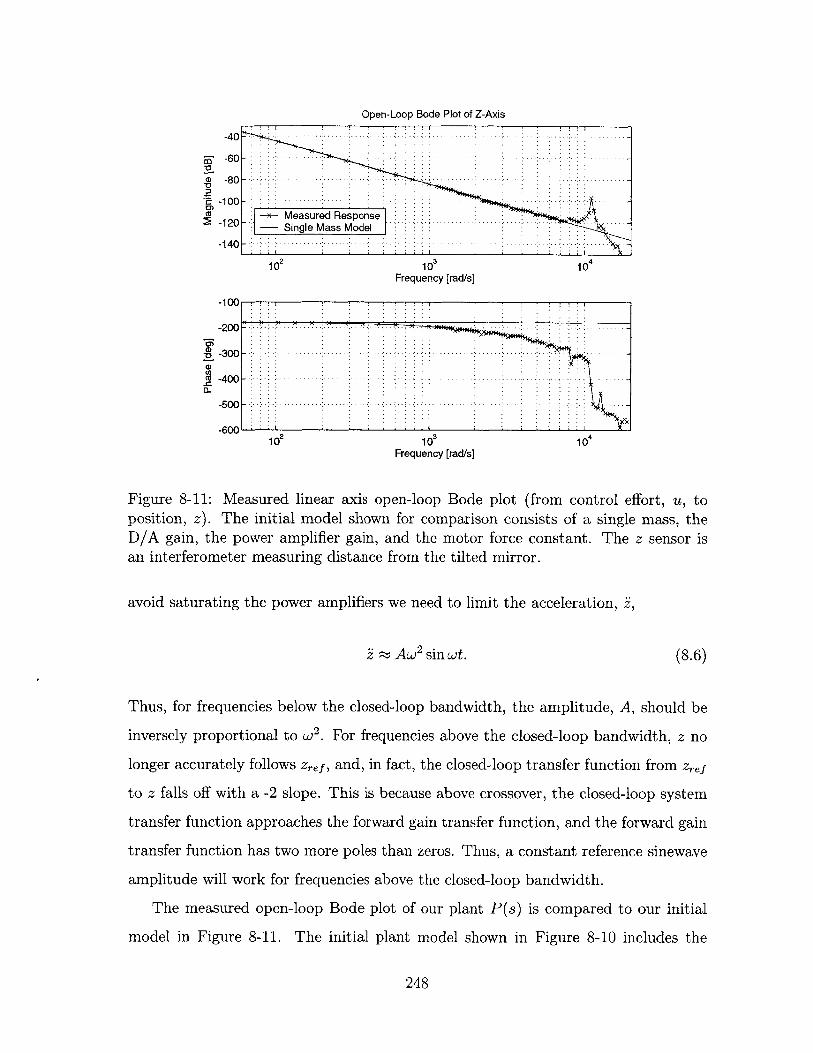
Open-Loop Bode Plot of Z-Axis

-60 -

-8 0 - -... . -. .... ...

-100-,

-120 - Measured ResponseSingle Mass Model

-140 -- ?

102 10 3 10 4

Frequency [rad/s]

-100

-200 - -.-

. ~ -300 - . . . . . . .. . . .... . . .. . . . . . .

-400

-500 - -... ---..

-600102 10 104

Frequency [rad/s]

Figure 8-11: Measured linear axis open-loop Bode plot (from control effort, u, toposition, z). The initial model shown for comparison consists of a single mass, theD/A gain, the power amplifier gain, and the motor force constant. The z sensor isan interferometer measuring distance from the tilted mirror.

avoid saturating the power amplifiers we need to limit the acceleration, i,

~ Aw2 sin wt. (8.6)

Thus, for frequencies below the closed-loop bandwidth, the amplitude, A, should be

inversely proportional to w2 . For frequencies above the closed-loop bandwidth, z no

longer accurately follows zref, and, in fact, the closed-loop transfer function from zref

to z falls off with a -2 slope. This is because above crossover, the closed-loop system

transfer function approaches the forward gain transfer function, and the forward gain

transfer function has two more poles than zeros. Thus, a constant reference sinewave

amplitude will work for frequencies above the closed-loop bandwidth.

The measured open-loop Bode plot of our plant P(s) is compared to our initial

model in Figure 8-11. The initial plant model shown in Figure 8-10 includes the

248

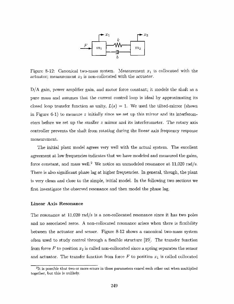
[*X k

F1 2

b

Figure 8-12: Canonical two-mass system. Measurement x1 is collocated with theactuator; measurement X2 is non-collocated with the actuator.

D/A gain, power amplifier gain, and motor force constant; it models the shaft as a

pure mass and assumes that the current control loop is ideal by approximating its

closed loop transfer function as unity, L(s) = 1. We used the tilted-mirror (shown

in Figure 6-1) to measure z initially since we set up this mirror and its interferom-

eters before we set up the smaller z mirror and its interferometer. The rotary axis

controller prevents the shaft from rotating during the linear axis frequency response

measurement.

The initial plant model agrees very well with the actual system. The excellent

agreement at low frequencies indicates that we have modeled and measured the gains,

force constant, and mass well.2 We notice an unmodeled resonance at 11,020 rad/s.

There is also significant phase lag at higher frequencies. In general, though, the plant

is very clean and close to the simple, initial model. In the following two sections we

first investigate the observed resonance and then model the phase lag.

Linear Axis Resonance

The resonance at 11,020 rad/s is a non-collocated resonance since it has two poles

and no associated zeros. A non-collocated resonance arises when there is flexibility

between the actuator and sensor. Figure 8-12 shows a canonical two-mass system

often used to study control through a flexible structure [19]. The transfer function

from force F to position x2 is called non-collocated since a spring separates the sensor

and actuator. The transfer function from force F to position x1 is called collocated

2It is possible that two or more errors in these parameters cancel each other out when multipliedtogether, but this is unlikely.

249

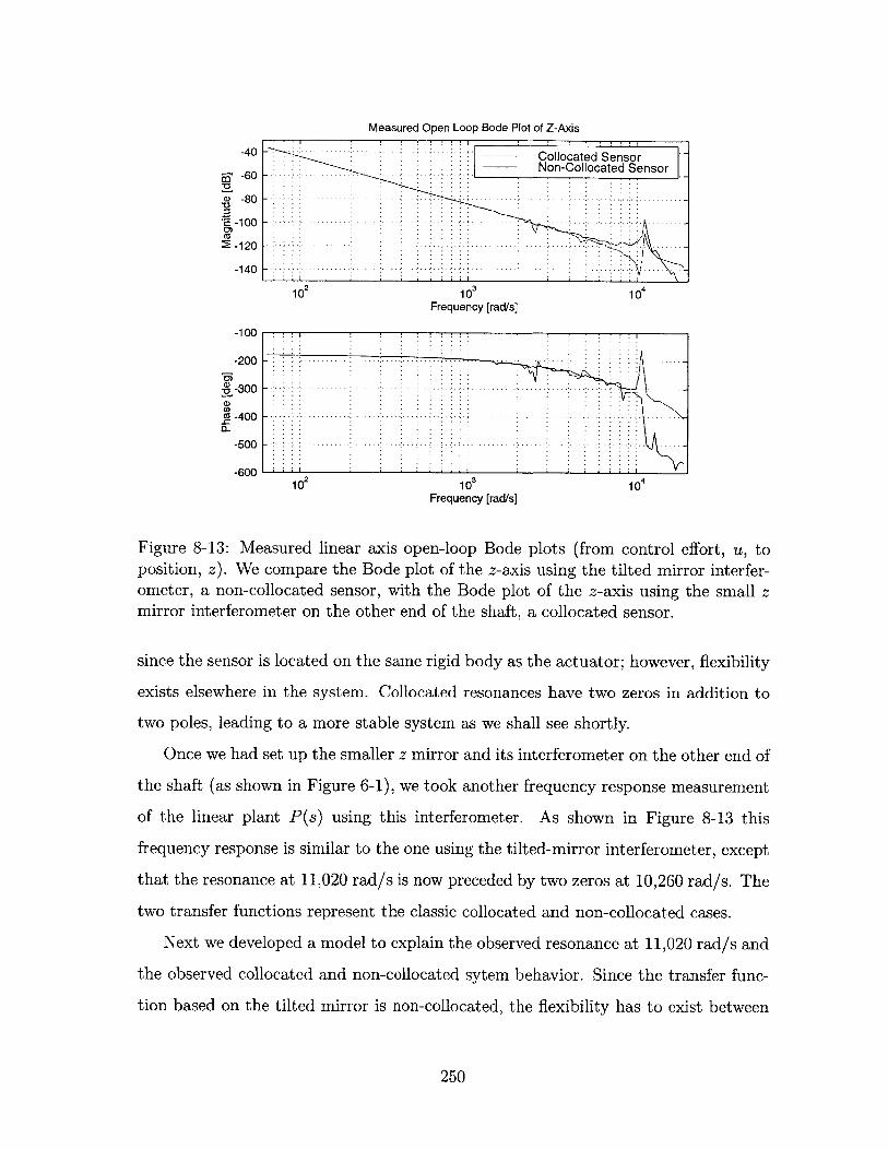
Measured Open Loop Bode Plot of Z-Axis

-40 -Collocated Sensor60 --Non-Collocated Sensor

a - 0 -6--.-- -

-80

-100

102 10 10 4

Frequency [rad/s]

-100

-200

-300 -..-..-

0 -400 -. .. .- -.... .

-500

-00102 10 10 4

Frequency [rad/s]

Figure 8-13: Measured linear axis open-loop Bode plots (from control effort, u, toposition, z). We compare the Bode plot of the z-axis using the tilted mirror interfer-ometer, a non-collocated sensor, with the Bode plot of the z-axis using the small zmirror interferometer on the other end of the shaft, a collocated sensor.

since the sensor is located on the same rigid body as the actuator; however, flexibility

exists elsewhere in the system. Collocated resonances have two zeros in addition to

two poles, leading to a more stable system as we shall see shortly.

Once we had set up the smaller z mirror and its interferometer on the other end of

the shaft (as shown in Figure 6-1), we took another frequency response measurement

of the linear plant P(s) using this interferometer. As shown in Figure 8-13 this

frequency response is similar to the one using the tilted-mirror interferometer, except

that the resonance at 11,020 rad/s is now preceded by two zeros at 10,260 rad/s. The

two transfer functions represent the classic collocated and non-collocated cases.

Next we developed a model to explain the observed resonance at 11,020 rad/s and

the observed collocated and non-collocated sytem behavior. Since the transfer func-

tion based on the tilted mirror is non-collocated, the flexibility has to exist between

250

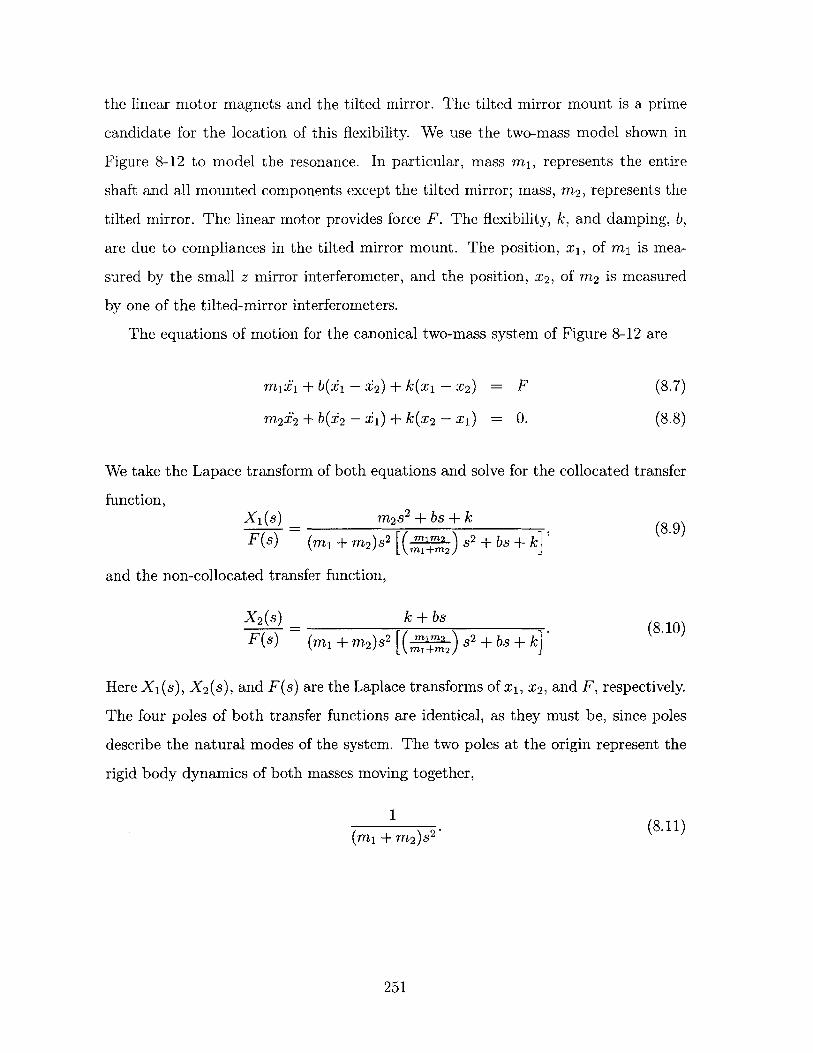
the linear motor magnets and the tilted mirror. The tilted mirror mount is a prime

candidate for the location of this flexibility. We use the two-mass model shown in

Figure 8-12 to model the resonance. In particular, mass m1 , represents the entire

shaft and all mounted components except the tilted mirror; mass, M 2 , represents the

tilted mirror. The linear motor provides force F. The flexibility, k, and damping, b,

are due to compliances in the tilted mirror mount. The position, x1 , of mi is mea-

sured by the small z mirror interferometer, and the position, x2 , of M 2 is measured

by one of the tilted-mirror interferometers.

The equations of motion for the canonical two-mass system of Figure 8-12 are

mizi + b(Y 1 - Y 2 ) + k(xi - x 2 ) = F (8.7)

M2E2+ b(2 - Y1)+ k(x2 - X1) = 0. (8.8)

We take the Lapace transform of both equations and solve for the collocated transfer

function,X1 (s) m 2

2 + bs + k (89)F(s) (min+ m 2 )s 2

[( M2 + bs + k'

and the non-collocated transfer function,

X 2(s) k + bs

F(s) (mi + m 2)s2[ (i)S2 + bs + k]

Here X,(s), X 2 (s), and F(s) are the Laplace transforms of x 1 , x 2 , and F, respectively.

The four poles of both transfer functions are identical, as they must be, since poles

describe the natural modes of the system. The two poles at the origin represent the

rigid body dynamics of both masses moving together,

1 2(8.11)

(Mi + m 2)s2

251

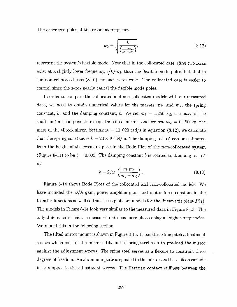
The other two poles at the resonant frequency,

WO k (8.12)( ml-+m2 /

represent the system's flexible mode. Note that in the collocated case, (8.9) two zeros

exist at a slightly lower frequency, k/rm2 , than the flexible mode poles, but that in

the non-collocated case (8.10), no such zeros exist. The collocated case is easier to

control since the zeros nearly cancel the flexible mode poles.

In order to compare the collocated and non-collocated models with our measured

data, we need to obtain numerical values for the masses, m, and m 2 , the spring

constant, k, and the damping constant, b. We set min = 1.256 kg, the mass of the

shaft and all components except the tilted mirror, and we set m 2 = 0.190 kg, the

mass of the tilted-mirror. Setting wo = 11, 020 rad/s in equation (8.12), we calculate

that the spring constant is k = 20 x 106 N/m. The damping ratio ( can be estimated

from the height of the resonant peak in the Bode Plot of the non-collocated system

(Figure 8-11) to be ( = 0.005. The damping constant b is related to damping ratio (

by,

b = 2(wo (n 2 . (8.13)\mil + M2/

Figure 8-14 shows Bode Plots of the collocated and non-collocated models. We

have included the D/A gain, power amplifier gain, and motor force constant in the

transfer functions as well so that these plots are models for the linear-axis plant P(s).

The models in Figure 8-14 look very similar to the measured data in Figure 8-13. The

only difference is that the measured data has more phase delay at higher frequencies.

We model this in the following section.

The tilted mirror mount is shown in Figure 8-15. It has three fine pitch adjustment

screws which control the mirror's tilt and a spring steel web to pre-load the mirror

against the adjustment screws. The sping steel serves as a flexure to constrain three

degrees of freedom. An aluminum plate is epoxied to the mirror and has silicon carbide

inserts opposite the adjustment screws. The Hertzian contact stiffness between the

252

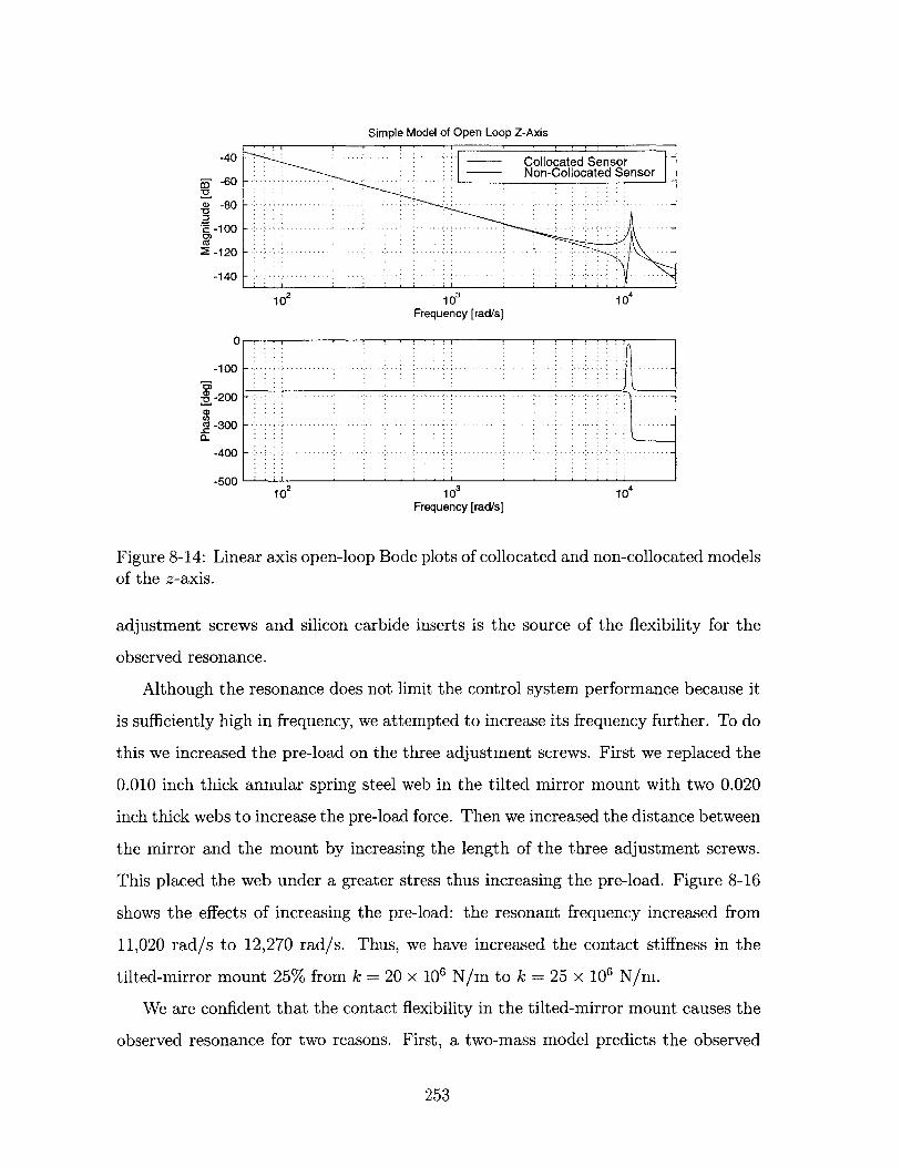
Simple Model of Open Loop Z-Axis

-4 !.!.!.!..!.!...

on-Collocated Sensor-......- Non-Collocated Sensor

F* -60. ....I. ..

-80 - -.-.-.-

- -100 - -- --

2 -120 -. .. . -.. .... .. .

-14 0 -. ....-. .... ...

102 10 10

Frequency [rad/s]

-100 ----

00. . . . . .. .. .. . .. .. . . . . . . ...

S -200 - . -... .. ...

-c-400 ...

-500110 2 10 3104

Frequency [rad/s]

Figure 8-14: Linear axis open-loop Bode plots of collocated and non-collocated modelsof the z-axis.

adjustment screws and silicon carbide inserts is the source of the flexibility for the

observed resonance.

Although the resonance does not limit the control system performance because it

is sufficiently high in frequency, we attempted to increase its frequency further. To do

this we increased the pre-load on the three adjustment screws. First we replaced the

0.010 inch thick annular spring steel web in the tilted mirror mount with two 0.020

inch thick webs to increase the pre-load force. Then we increased the distance between

the mirror and the mount by increasing the length of the three adjustment screws.

This placed the web under a greater stress thus increasing the pre-load. Figure 8-16

shows the effects of increasing the pre-load: the resonant frequency increased from

11,020 rad/s to 12,270 rad/s. Thus, we have increased the contact stiffness in the

tilted-mirror mount 25% from k = 20 x 106 N/m to k = 25 x 106 N/m.

We are confident that the contact flexibility in the tilted-mirror mount causes the

observed resonance for two reasons. First, a two-mass model predicts the observed

253

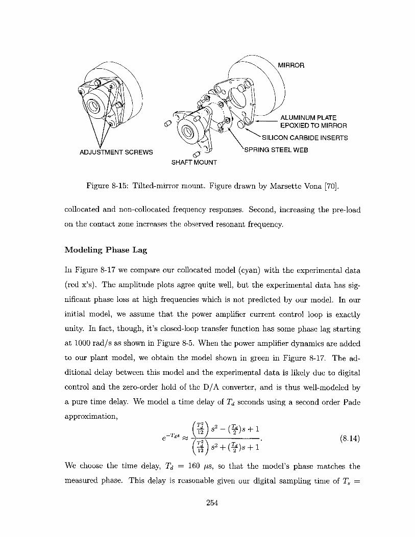
ADJUSTMENT SCREWS

MIRROR

ALUMINUM PLATEEPOXIED TO MIRROR

SILICON CARBIDE INSERTS

SPRING STEEL WEB

SHAFT MOUNT

Figure 8-15: Tilted-mirror mount. Figure drawn by Marsette Vona [70].

collocated and non-collocated frequency responses. Second, increasing the pre-load

on the contact zone increases the observed resonant frequency.

Modeling Phase Lag

In Figure 8-17 we compare our collocated model (cyan) with the experimental data

(red x's). The amplitude plots agree quite well, but the experimental data has sig-

nificant phase loss at high frequencies which is not predicted by our model. In our

initial model, we assume that the power amplifier current control loop is exactly

unity. In fact, though, it's closed-loop transfer function has some phase lag starting

at 1000 rad/s as shown in Figure 8-5. When the power amplifier dynamics are added

to our plant model, we obtain the model shown in green in Figure 8-17. The ad-

ditional delay between this model and the experimental data is likely due to digital

control and the zero-order hold of the D/A converter, and is thus well-modeled by

a pure time delay. We model a time delay of Td seconds using a second order Pade

approximation,

. )S2 - (__)s + 1

sd 2 + (-)s+(8.14)

We choose the time delay, Td = 160 ps, so that the model's phase matches the

measured phase. This delay is reasonable given our digital sampling time of T, =

254

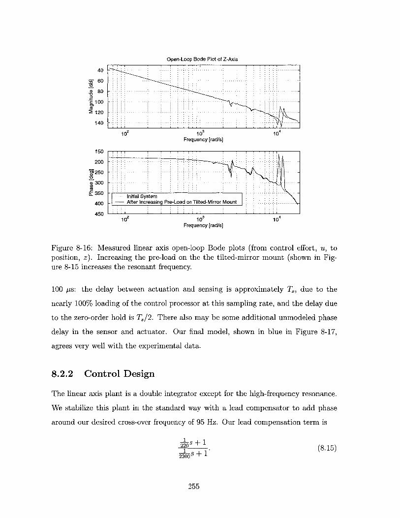
Open-Loop Bode Plot of Z-Axis

40 -

60 -

8 0 -. ...-. ....-. . - -.. ...

' 1 0 0 - -.-.-

CU1 2 0 .........-. ...-.-.-.-

140 -.-.-

102 10 104

Frequency [rad/s]

150

200 - -.-.-.-

- 2 5 0 - ......... ...... .. ... .--

3 0 0 - ....... ... .. - -.. .... ..... .... ... . ... .....50

Cd

- 3Initial System400 - After Increasing Pre-Load on Tilted-Mirror Mount

450102 10 3 10

Frequency [rad/s]

Figure 8-16: Measured linear axis open-loop Bode plots (from control effort, u, toposition, z). Increasing the pre-load on the the tilted-mirror mount (shown in Fig-ure 8-15 increases the resonant frequency.

100 ps: the delay between actuation and sensing is approximately Ts, due to the

nearly 100% loading of the control processor at this sampling rate, and the delay due

to the zero-order hold is T,/2. There also may be some additional unmodeled phase

delay in the sensor and actuator. Our final model, shown in blue in Figure 8-17,

agrees very well with the experimental data.

8.2.2 Control Design

The linear axis plant is a double integrator except for the high-frequency resonance.

We stabilize this plant in the standard way with a lead compensator to add phase

around our desired cross-over frequency of 95 Hz. Our lead compensation term is

- s+120 . (8.15)

2200s + 1

255

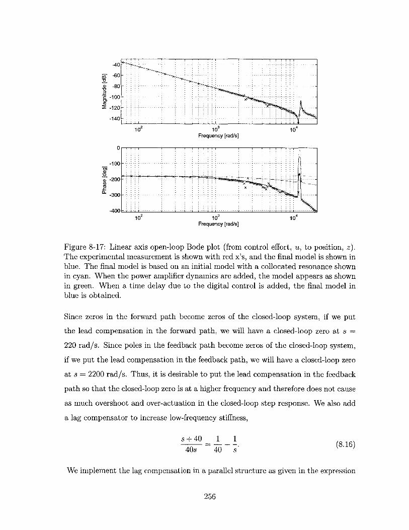
-40

-8 0 - .. .. . ......-. ...

-100 - - - --

-12 0 -

102 10 104

Frequency [rad/s]

CO

-100 - --..-.-

-4 0 0 - .... -. -.. . .j

10 2 10 3 10 4

Frequency [rad/s}

Figure 8-17: Linear axis open-loop Bode plot (from control effort, u, to position, z).The experimental measurement is shown with red x's, and the final model is shown inblue. The final model is based on an initial model with a collocated resonance shownin cyan. When the power amplifier dynamics are added, the model appears as shownin green. When a time delay due to the digital control is added, the final model inblue is obtained.

Since zeros in the forward path become zeros of the closed-loop system, if we put

the lead compensation in the forward path, we will have a closed-loop zero at s =

220 rad/s. Since poles in the feedback path become zeros of the closed-loop system,

if we put the lead compensation in the feedback path, we will have a closed-loop zero

at s = 2200 rad/s. Thus, it is desirable to put the lead compensation in the feedback

path so that the closed-loop zero is at a higher frequency and therefore does not cause

as much overshoot and over-actuation in the closed-loop step response. We also add

a lag compensator to increase low-frequency stiffness,

s+40 1 1 (816)40s 40 s

We implement the lag compensation in a parallel structure as given in the expression

256

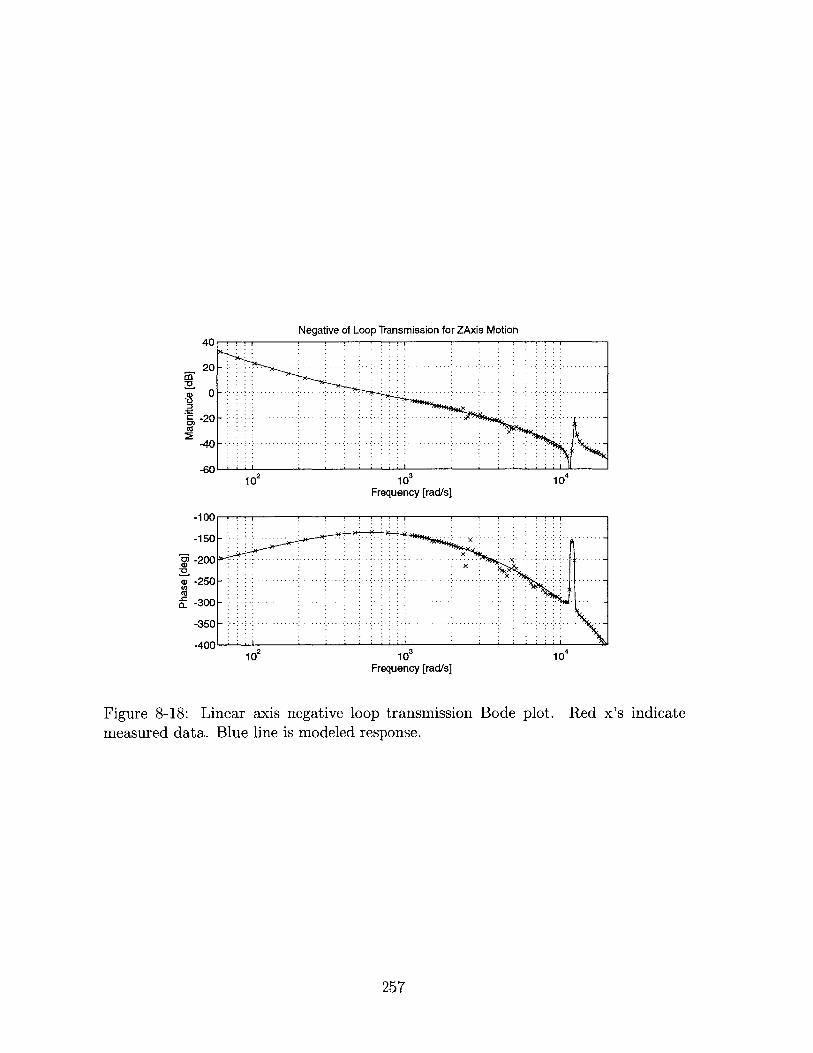
Negative of Loop Transrmission for ZA xis Motion

........-. .. -. . ........ ....

-. .....-. ..-. .-

- ....... -. .....-. .- ..-. .-

- ......... -.. . .... ........

10FFrequency [rad/s]

10FFrequency [rad/s]

Figure 8-18: Linear axis negative loop transmission Bode plot.measured data. Blue line is modeled response.

Red x's indicate

257

20

> 0

-20

-40

- I

-150

-6-200

cD -250Cd

-300

-350

-400

104

104102

- - x - ......... -

. . . .-. . -.. ...... .......... ...

.. . . . . . . . . . . .. . ... .. . ... .. ... .. . .. .. ..

- ........-. ... -.-.-. -.

- . - - . .

10 2

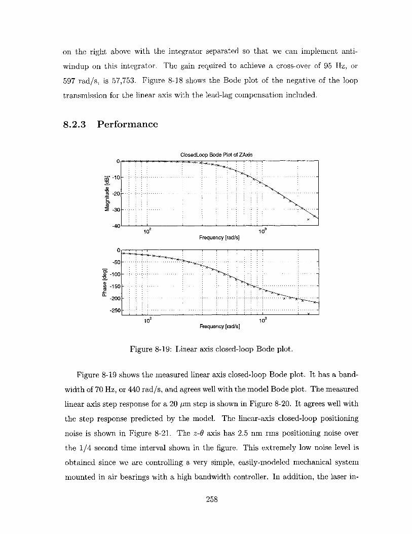
on the right above with the integrator separated so that we can implement anti-

windup on this integrator. The gain required to achieve a cross-over of 95 Hz, or

597 rad/s, is 57,753. Figure 8-18 shows the Bode plot of the negative of the loop

transmission for the linear axis with the lead-lag compensation included.

8.2.3 Performance

ClosedLoop Bode Plot of ZAxis

a* -10

-20C

2 -30

102

-50

-100

-150Cd

-200

-250

Frequency [rad/s]

Frequency [rad/s]

10

103

Figure 8-19: Linear axis closed-loop Bode plot.

Figure 8-19 shows the measured linear axis closed-loop Bode plot. It has a band-

width of 70 Hz, or 440 rad/s, and agrees well with the model Bode plot. The measured

linear axis step response for a 20 pm step is shown in Figure 8-20. It agrees well with

the step response predicted by the model. The linear-axis closed-loop positioning

noise is shown in Figure 8-21. The z-0 axis has 2.5 nm rms positioning noise over

the 1/4 second time interval shown in the figure. This extremely low noise level is

obtained since we are controlling a very simple, easily-modeled mechanical system

mounted in air bearings with a high bandwidth controller. In addition, the laser in-

258

n

n

-. .... -. ...... . -.- .-.- .

........ . .... . . ... . .. . .. .. .. .. .. .. .. .. ..x .

. .... .. ...... .. .. - .. .. .. ..

...........................

.............

- - - -- -

- - - - -..... ....

-. ..-. .. -.-. ...- .x.-.-.

- .............-. .-. ....- - -

102

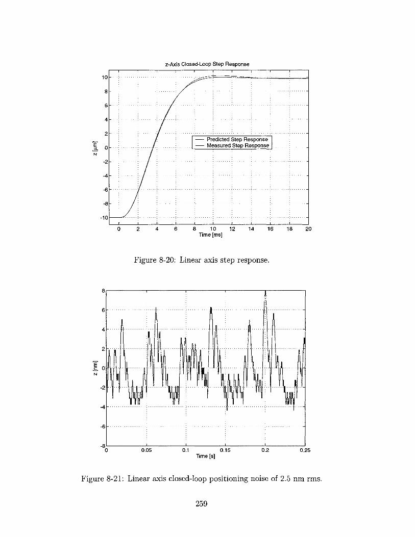
0 2 4 6 8 10 12 14 16 18 20Time [ms]

Figure 8-20: Linear axis step response.

z-Axis Closed-Loop Step Response

........... ... ........ ......

.....................................

........... .................. ........: ........... ........... ................... ..

..... ........... ... .........

q ..............................Pedicted Step Response

....... ......... Measured Step Response ........ ........

..................

........................

............. ....... ......... ...... .... ................ .................

.................. ..................q .......... ..............

... .................. .. ........... ....... ...............

10

8

6

4

2

0

-2

-4

-6

-8

-10

. ... ........ .......... .. ................. ........ . .......................... .................

.......... ................................... .................................. ................. ........................... ............................. ...... ............................................................................................................ .. . . . . . . . . .. .. . . . . . .. . . . . . . . . ... ... .. .. .. .. .. . . . . . . . . . . . . . . . . .. .. .. .. . . . . . .

. . . .. .. . . . ... . . . . . . . . . .. . . . . . . . . . . . . . . . . . . . . . . . . . . .. . . . . . .

-ts0 0.05 0.1 0.15 0.2 0.25

Time [s]

Figure 8-21: Linear axis closed-loop positioning noise of 2.5 nrn rms.

259

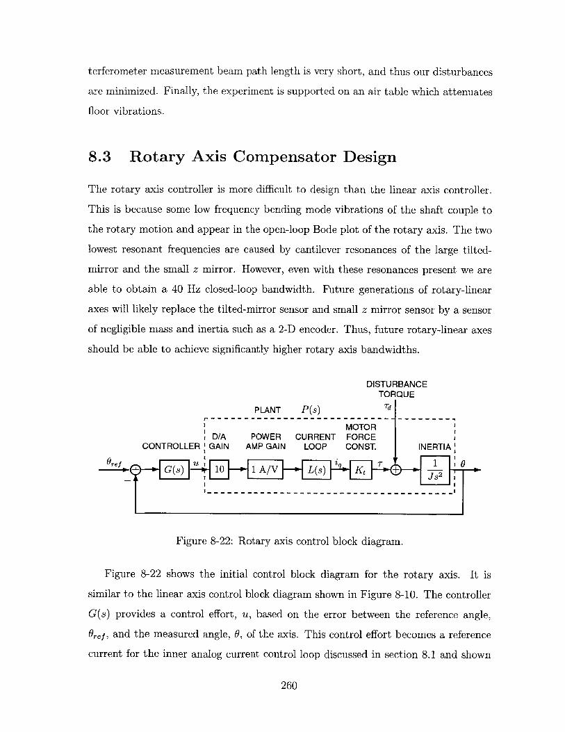
terferometer measurement beam path length is very short, and thus our disturbances

are minimized. Finally, the experiment is supported on an air table which attenuates

floor vibrations.

8.3 Rotary Axis Compensator Design

The rotary axis controller is more difficult to design than the linear axis controller.

This is because some low frequency bending mode vibrations of the shaft couple to

the rotary motion and appear in the open-loop Bode plot of the rotary axis. The two

lowest resonant frequencies are caused by cantilever resonances of the large tilted-

mirror and the small z mirror. However, even with these resonances present we are

able to obtain a 40 Hz closed-loop bandwidth. Future generations of rotary-linear

axes will likely replace the tilted-mirror sensor and small z mirror sensor by a sensor

of negligible mass and inertia such as a 2-D encoder. Thus, future rotary-linear axes

should be able to achieve significantly higher rotary axis bandwidths.

DISTURBANCETORQUE

PLANT P(s) Td

MOTORD/A POWER CURRENT FORCE

CONTROLLER GAIN AMP GAIN LOOP CONST. INERTIA'

G(s) i L(s) -+

Figure 8-22: Rotary axis control block diagram.

Figure 8-22 shows the initial control block diagram for the rotary axis. It is

similar to the linear axis control block diagram shown in Figure 8-10. The controller

G(s) provides a control effort, u, based on the error between the reference angle,

Oref, and the measured angle, 6, of the axis. This control effort becomes a reference

current for the inner analog current control loop discussed in section 8.1 and shown

260

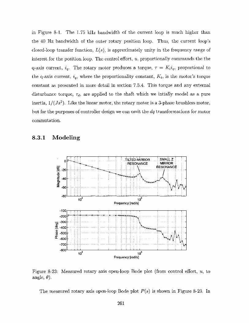
in Figure 8-1. The 1.75 kHz bandwidth of the current loop is much higher than

the 40 Hz bandwidth of the outer rotary position loop. Thus, the current loop's

closed-loop transfer function, L(s), is approximately unity in the frequency range of

interest for the position loop. The control effort, u, proportionally commands the the

q-axis current, iq. The rotary motor produces a torque, T = Ktiq, proportional to

the q-axis current, iq, where the proportionality constant, Kt, is the motor's torque

constant as presented in more detail in section 7.5.4. This torque and any external

disturbance torque, Td, are applied to the shaft which we intially model as a pure

inertia, 1/(Js2 ). Like the linear motor, the rotary motor is a 3-phase brushless motor,

but for the purposes of controller design we can omit the dq transformations for motor

commutation.

8.3.1 Modeling

0 TILTED-MIRROR SMALL ZRESONANCE MIRROR

RESONANCE2.-20 - - . -.-.-. \ -.

-40 -

-80102 10

Frequency [rad/si

-100

-200-

-300 - - -

CD)M -400 - -... -.. -...

-500 -

-600 - -

-700--

-800102 10

Frequency [rad/s]

Figure 8-23: Measured rotary axis open-loop Bode plot (from control effort, u, toangle, 0).

The measured rotary axis open-loop Bode plot P(s) is shown in Figure 8-23. In

261

the figure we identify the two lowest rotary axis resonances as cantilever vibrations

of the large tilted-mirror and small z mirror on the shaft. In this section, we look at

the tests and calculations that let us identify the causes of these observed resonances.

In the following section we show how we compensate this system to achieve as high a

closed-loop bandwidth as possible, and in the final section we look at the closed-loop

performance.

Perhaps the most reliable way to identify a mechanical resonance is to drive the

system at that frequency and use some sort of probe to determine the shape of the

associated modes. In the simplest case, a handheld stylus or even a screwdriver

allows one to directly feel the amplitude of motion. At the resonant frequency, the

vibration has a relatively large amplitude and so is easy to observe. The use of a

probe enhances one's sense of touch, and enables detection of even small vibrations.

We used this method to help identify our resonances. When the system is driven

in rotation with a 1000 rad/s sinusoid, the tilted-mirror sensor mount vibrates with

the greatest amplitude. When the system is driven in rotation with a 2,513 rad/s

sinusoid, the small z mirror sensor mount vibrates with the greatest amplitude.

We also find that the amplitude of vibration of the small z mirror sensor resonance

changes as the shaft is translated. This lends credence to the claim that this is

a cantilever resonance since we expect the cantilever resonant frequency to depend

critically on the shaft length. It is harder to observe a change in vibration amplitude

of the tilted-mirror resonance as the shaft translates because the 1 inch shaft travel

does not change the length of the reduced diameter shaft that mostly causes the

vibration. As shown in Figure 6-5, the rotary motor shoulder has half the diameter

of the main part of the shaft. Thus, most of the bending flexibility occurs in this

section of the shaft so that changing the length of the thicker part of the shaft does

not affect the resonant frequency much.

Initially, the low-frequency resonance attributed to the tilted-mirror occurred at

a frequency of 628 rad/s. At this time, the air bearings sat in O-rings in their

pillowblocks as described in section 6.1. In an attempt to increase the frequency of

this resonance, we potted the air bearings in a low-expansion replicating epoxy. This

262

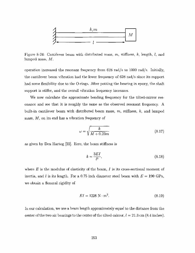
k~mM

Figure 8-24: Cantilever beam with distributed mass, m, stiffness, k, length, 1, andlumped mass, M.

operation increased the resonant frequency from 628 rad/s to 1000 rad/s. Initially,

the cantilever beam vibration had the lower frequency of 628 rad/s since its support

had some flexibility due to the O-rings. After potting the bearing in epoxy, the shaft

support is stiffer, and the overall vibration frequency increases.

We now calculate the approximate bending frequency for the tilted-mirror res-

onance and see that it is roughly the same as the observed resonant frequency. A

built-in cantilever beam with distributed beam mass, m, stiffness, k, and lumped

mass, M, on its end has a vibration frequency of

kW = V' :(8.17)

M+ 0.23m

as given by Den Hartog [22]. Here, the beam stiffness is

3EIk = , , (8.18)

where E is the modulus of elasticity of the beam, I is its cross-sectional moment of

inertia, and 1 is its length. For a 0.75 inch diameter steel beam with E = 190 GPa,

we obtain a flexural rigidity of

EI = 1228 N - m2 . (8.19)

In our calculation, we use a beam length approximately equal to the distance from the

center of the two air bearings to the center of the tilted-mirror, 1 = 21.3 cm (8.4 inches).

263

This length of shaft has a bending stiffness of

k = 0.38 N/pm. (8.20)

We let the distributed shaft mass, m, be the sum of the shaft mass plus the mass

of the linear motor magnets, m = 0.71 kg, and the lumped mass to be the mass

of the tilted-mirror and mount, M = 0.23 kg. Using equation (8.17) we obtain an

approximate bending mode frequency of

W = 980 rad/s. (8.21)

This result agrees well with our observed resonance at 1,000 rad/s. Given the uncer-

tainty in choosing the appropriate shaft length, 1, for this calculation, this agreement

is better than can be expected. This calculation mainly serves to confirm that such

a cantilever resonance would have a frequency in the same range as the observed

frequency.

8.3.2 Control Design

In this section we describe the design of the rotary axis compensation. Our ultimate

design achieves a 30 Hz cross-over frequency and a 40 Hz bandwidth. The resonance

at 1000 rad/s limits our achievable bandwidth. We use a lead-lag controller just as

in the compensation of the linear axis. However, we also add another pole to reduce

the magnitude of high frequency resonances and to add negative phase for phase

stabilization [211 of the 1000 rad/s resonance.

At one point during the design of the rotary axis, we achieved a high 70 Hz

closed-loop bandwidth controller by phase stabilizing the first resonant frequency at

1000 rad/s. Unfortunately, we discovered that the axis was unstable in some angle

ranges of the rotary-linear axis although it was stable for most angles. We discovered

that the resonance changes from a non-collocated resonance to a collocated resonance

at different angles. Figure 8-25 shows this difference in Bode plots of the negative

264

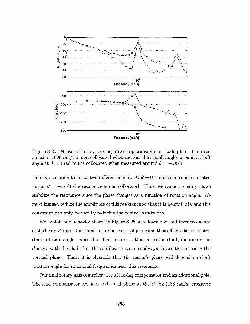
-10-

-1 -2-0-

-2 5 -- -. . . -.. ....-. -.. -.. ..

-3010

Frequency [rad/s]

-2 0 0 -.. -. . - -.. .. -. -.. ... -.. .. . . -. . - -... .... ...- ....- ....- -

-5001103

Frequency [rad/s]

Figure 8-25: Measured rotary axis negative loop transmission Bode plots. The reso-nance at 1000 rad/s is non-collocated when measured at small angles around a shaftangle at 9 = 0 rad but is collocated when measured around 9 = -57r/4.

loop transmission taken at two different angles. At 9 = 0 the resonance is collocated

but at 9 = -57r/4 the resonance is non-collocated. Thus, we cannot reliably phase

stabilize the resonance since the phase changes as a function of rotation angle. We

must instead reduce the amplitude of this resonance so that it is below 0 dB, and this

constraint can only be met by reducing the control bandwidth.

We explain the behavior shown in Figure 8-25 as follows: the cantilever resonance

of the beam vibrates the tilted-mirror in a vertical plane and thus affects the calculated

shaft rotation angle. Since the tilted-mirror is attached to the shaft, its orientation

changes with the shaft, but the cantilever resonance always shakes the mirror in the

vertical plane. Thus, it is plausible that the sensor's phase will depend on shaft

rotation angle for rotational frequencies near this resonance.

Our final rotary axis controller uses a lead-lag compensator and an additional pole.

The lead compensator provides additional phase at the 30 Hz (188 rad/s) crossover

265

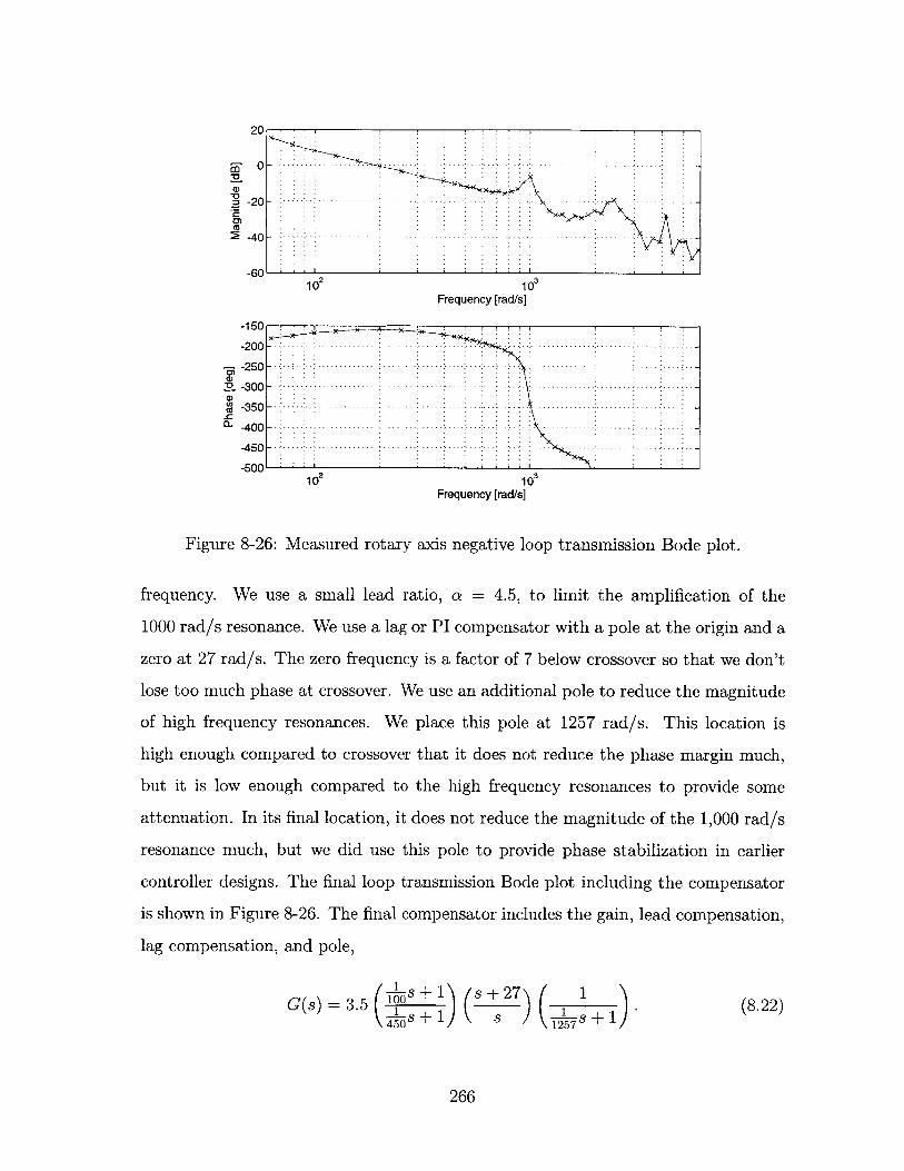
U 0 -.. ....

-20 - -.-.-

S-40-

-60102 10 3

Frequency [rad/s]

-150-200 - - -

~-250---25 .......................... .......... .... . . .. . . . . .. . .

-300 :- - - -

-35 ..... .. ........ ..............................~-350----400 - ..............

-450 - . - -.-.-50. .. . . . . . . . . . ....... .. ...... ...............

-500102 103

Frequency [rad/s]

Figure 8-26: Measured rotary axis negative loop transmission Bode plot.

frequency. We use a small lead ratio, a = 4.5, to limit the amplification of the

1000 rad/s resonance. We use a lag or PI compensator with a pole at the origin and a

zero at 27 rad/s. The zero frequency is a factor of 7 below crossover so that we don't

lose too much phase at crossover. We use an additional pole to reduce the magnitude

of high frequency resonances. We place this pole at 1257 rad/s. This location is

high enough compared to crossover that it does not reduce the phase margin much,

but it is low enough compared to the high frequency resonances to provide some

attenuation. In its final location, it does not reduce the magnitude of the 1,000 rad/s

resonance much, but we did use this pole to provide phase stabilization in earlier

controller designs. The final loop transmission Bode plot including the compensator

is shown in Figure 8-26. The final compensator includes the gain, lead compensation,

lag compensation, and pole,

-- 3-s +1 s +27 ) 1G(s) = 0 8.1 S0 1 .+ (8.22)-. s + 1-5 s (1s51

266

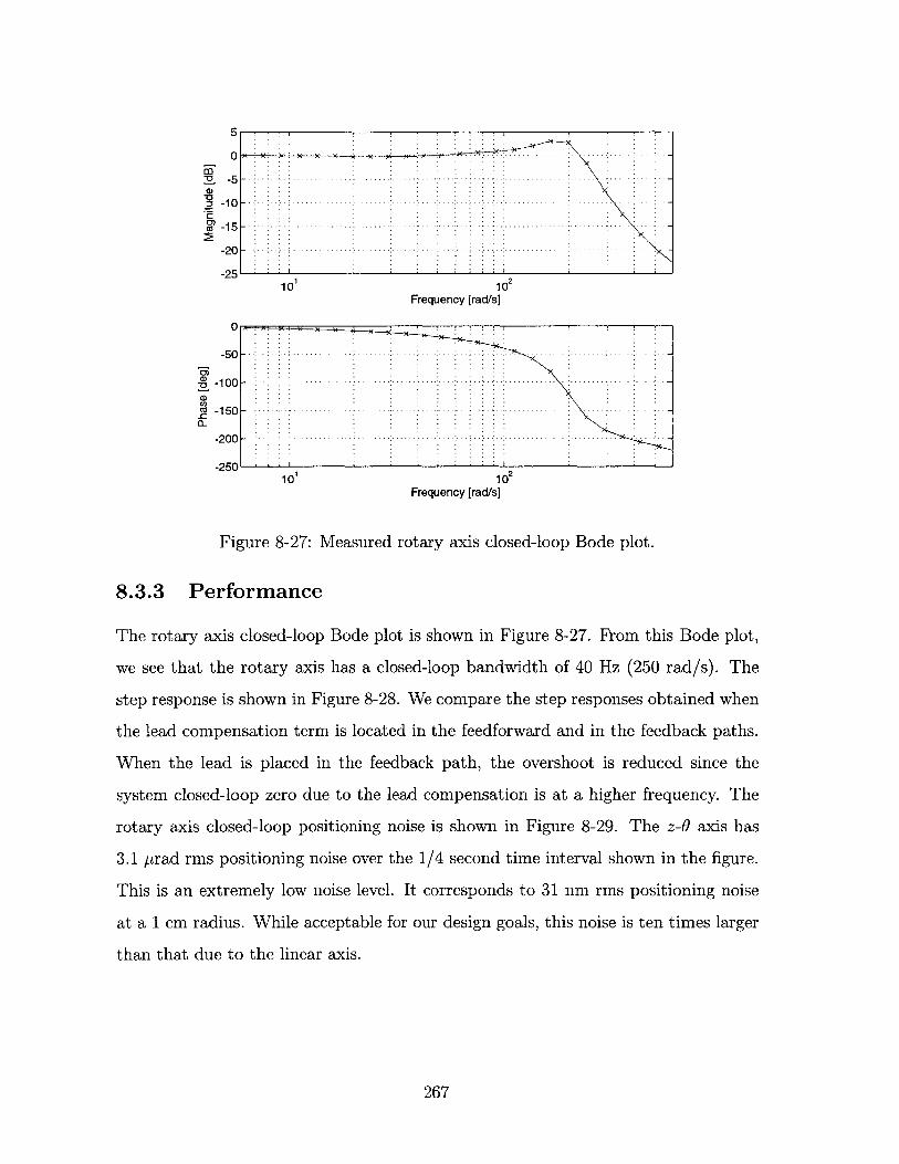
0 -

~-10 ----

-20

-25 210 102

Frequency [rad/s]

-50 --- --

- -100 - - -.-.-.

cu-150 - -a_

-200 - -- - -- - - -.-.-. -

-250210 102

Frequency [rad/s]

Figure 8-27: Measured rotary axis closed-loop Bode plot.

8.3.3 Performance

The rotary axis closed-loop Bode plot is shown in Figure 8-27. From this Bode plot,

we see that the rotary axis has a closed-loop bandwidth of 40 Hz (250 rad/s). The

step response is shown in Figure 8-28. We compare the step responses obtained when

the lead compensation term is located in the feedforward and in the feedback paths.

When the lead is placed in the feedback path, the overshoot is reduced since the

system closed-loop zero due to the lead compensation is at a higher frequency. The

rotary axis closed-loop positioning noise is shown in Figure 8-29. The z-0 axis has

3.1 prad rms positioning noise over the 1/4 second time interval shown in the figure.

This is an extremely low noise level. It corresponds to 31 nm rms positioning noise

at a 1 cm radius. While acceptable for our design goals, this noise is ten times larger

than that due to the linear axis.

267

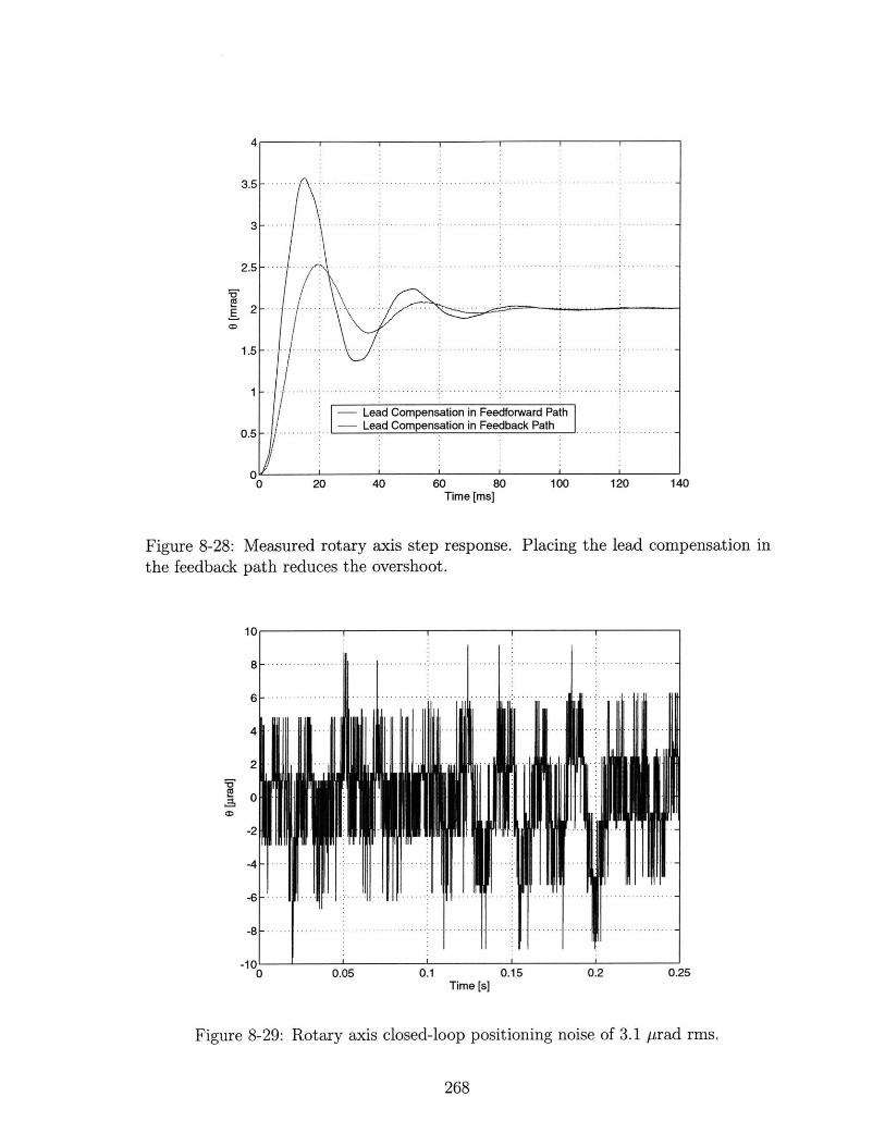
Figurethe fee

0 20 40 60 80 100 120 140Time [ms]

8-28: Measured rotary axis step response. Placing the lead compensation indback path reduces the overshoot.

10 T

4

2 - - -. -.-.-.

-2

-4 - - - - - - - -

-6 .. .. ..

-10L .......0 0.05 0.1 0.15 0.2 0.25

Time [s]

Figure 8-29: Rotary axis closed-loop positioning noise of 3.1 prad rms.

268

3.5

3

2.5

E2

1.5

1

0.5

-- -Compensation in Feedforward -P-a

- Lead Compensation in Feedforward Path- Lead Compensation in Feedback Path

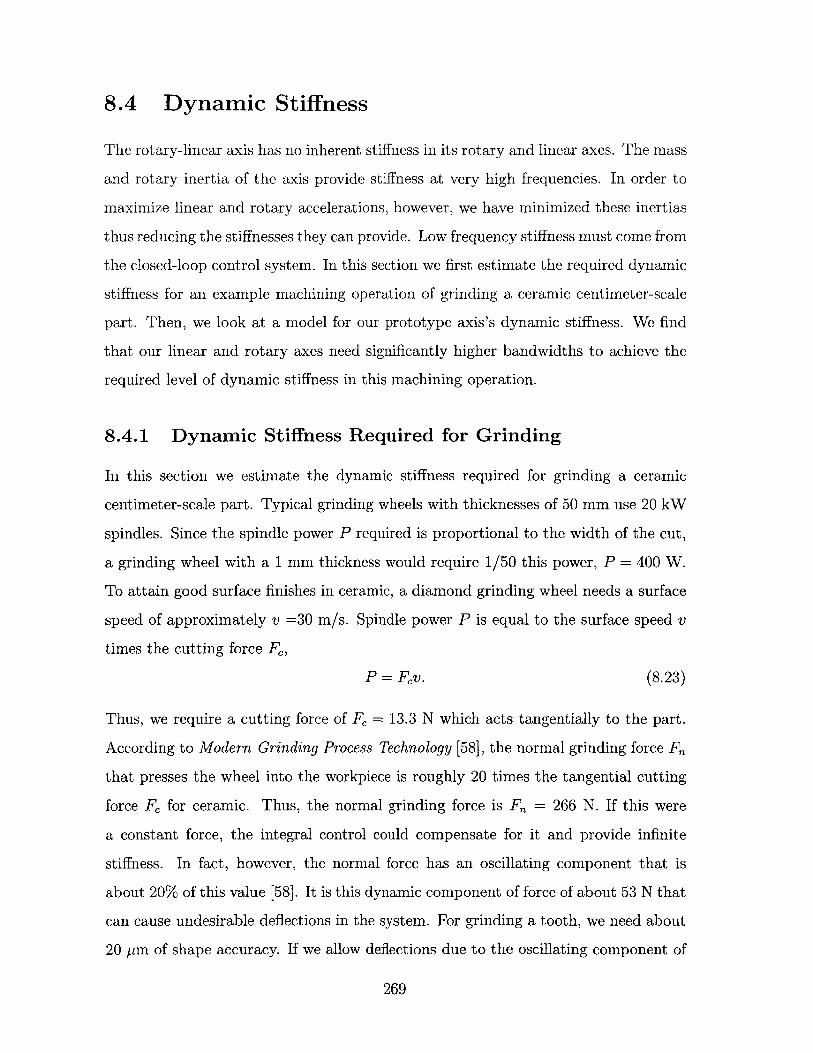
8.4 Dynamic Stiffness

The rotary-linear axis has no inherent stiffness in its rotary and linear axes. The mass

and rotary inertia of the axis provide stiffness at very high frequencies. In order to

maximize linear and rotary accelerations, however, we have minimized these inertias

thus reducing the stiffnesses they can provide. Low frequency stiffness must come from

the closed-loop control system. In this section we first estimate the required dynamic

stiffness for an example machining operation of grinding a ceramic centimeter-scale

part. Then, we look at a model for our prototype axis's dynamic stiffness. We find

that our linear and rotary axes need significantly higher bandwidths to achieve the

required level of dynamic stiffness in this machining operation.

8.4.1 Dynamic Stiffness Required for Grinding

In this section we estimate the dynamic stiffness required for grinding a ceramic

centimeter-scale part. Typical grinding wheels with thicknesses of 50 mm use 20 kW

spindles. Since the spindle power P required is proportional to the width of the cut,

a grinding wheel with a 1 mm thickness would require 1/50 this power, P = 400 W.

To attain good surface finishes in ceramic, a diamond grinding wheel needs a surface

speed of approximately v =30 m/s. Spindle power P is equal to the surface speed v

times the cutting force F.,

P = Fv. (8.23)

Thus, we require a cutting force of F, = 13.3 N which acts tangentially to the part.

According to Modern Grinding Process Technology [58], the normal grinding force Fn

that presses the wheel into the workpiece is roughly 20 times the tangential cutting

force Fc for ceramic. Thus, the normal grinding force is Fn = 266 N. If this were

a constant force, the integral control could compensate for it and provide infinite

stiffness. In fact, however, the normal force has an oscillating component that is

about 20% of this value [58]. It is this dynamic component of force of about 53 N that

can cause undesirable deflections in the system. For grinding a tooth, we need about

20 pm of shape accuracy. If we allow deflections due to the oscillating component of

269

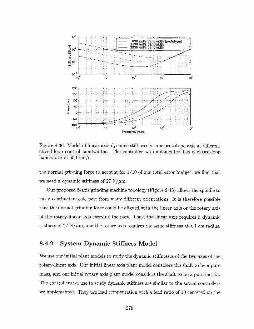
E 2 3000 rad/s bandwidth=10

10

1-2

100 10' 102 103 10 4

200

150 -

100 .. ..- .- .-.-

-0 50 -

-105 0 . . 2.. .. . 10. 10 . . . . . . .. . .. . . .. .

10 10 10 10 10Frequency [rad/s]

Figure 8-30: Model of linear axis dynamic stiffness for our prototype axis at differentclosed-loop control bandwidths. The controller we implemented has a closed-loopbandwidth of 600 rad/s.

the normal grinding force to account for 1/10 of our total error budget, we find that

we need a dynamic stiffness of 27 N/pm.

Our proposed 5-axis grinding machine topology (Figure 2-13) allows the spindle to

cut a centimeter-scale part from many different orientations. It is therefore possible

that the normal grinding force could be aligned with the linear axis or the rotary axis

of the rotary-linear axis carrying the part. Thus, the linear axis requires a dynamic

stiffness of 27 N/pm, and the rotary axis requires the same stiffness at a 1 cm radius.

8.4.2 System Dynamic Stiffness Model

We use our initial plant models to study the dynamic stiffnesses of the two axes of the

rotary-linear axis. Our initial linear axis plant model considers the shaft to be a pure

mass, and our initial rotary axis plant model considers the shaft to be a pure inertia.

The controllers we use to study dynamic stiffness are similar to the actual controllers

we implemented. They use lead compensation with a lead ratio of 10 centered on the

270

600 rad/s bandwidth (prototype)140IA rndis hndA/idth

104

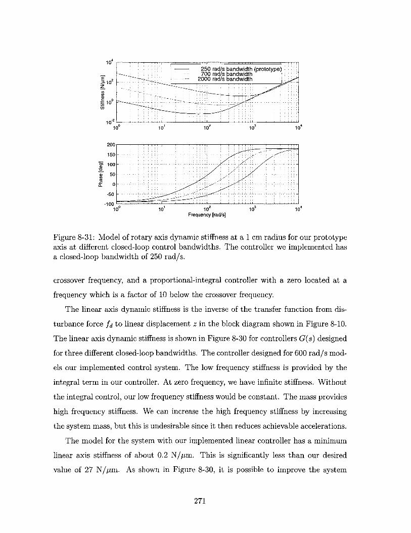
104250 rad/s bandwidth (prototype700 rad/s bandwidth

2000 rad/s bandwidth

10-

10

-2

100 101 102 10 10 4

200

150

100 -......

CD)

-50 -

-100 010 10 102 10 10

Frequency [rad/s]

Figure 8-31: Model of rotary axis dynamic stiffness at a 1 cm radius for our prototypeaxis at different closed-loop control bandwidths. The controller we implemented hasa closed-loop bandwidth of 250 rad/s.

crossover frequency, and a proportional-integral controller with a zero located at a

frequency which is a factor of 10 below the crossover frequency.

The linear axis dynamic stiffness is the inverse of the transfer function from dis-

turbance force fd to linear displacement z in the block diagram shown in Figure 8-10.

The linear axis dynamic stiffness is shown in Figure 8-30 for controllers G(s) designed

for three different closed-loop bandwidths. The controller designed for 600 rad/s mod-

els our implemented control system. The low frequency stiffness is provided by the

integral term in our controller. At zero frequency, we have infinite stiffness. Without

the integral control, our low frequency stiffness would be constant. The mass provides

high frequency stiffness. We can increase the high frequency stiffness by increasing

the system mass, but this is undesirable since it then reduces achievable accelerations.

The model for the system with our implemented linear controller has a minimum

linear axis stiffness of about 0.2 N/pm. This is significantly less than our desired

value of 27 N/pm. As shown in Figure 8-30, it is possible to improve the system

271

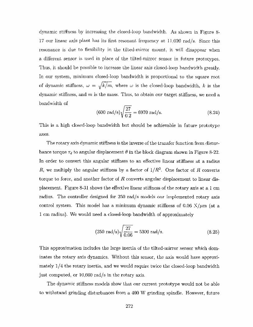
dynamic stiffness by increasing the closed-loop bandwidth. As shown in Figure 8-

17 our linear axis plant has its first resonant frequency at 11,020 rad/s. Since this

resonance is due to flexibility in the tilted-mirror mount, it will disappear when

a different sensor is used in place of the tilted-mirror sensor in future prototypes.

Thus, it should be possible to increase the linear axis closed-loop bandwidth greatly.

In our system, minimum closed-loop bandwidth is proportional to the square root

of dynamic stiffness, w = k/rm, where w is the closed-loop bandwidth, k is the

dynamic stiffness, and m is the mass. Thus, to obtain our target stiffness, we need a

bandwidth of

(600 rad/s) 5_- = 6970 rad/s. (8.24)

This is a high closed-loop bandwidth but should be achievable in future prototype

axes.

The rotary axis dynamic stiffness is the inverse of the transfer function from distur-

bance torque Td to angular displacement 6 in the block diagram shown in Figure 8-22.

In order to convert this angular stiffness to an effective linear stiffness at a radius

R, we multiply the angular stiffness by a factor of 1/R 2 . One factor of R converts

torque to force, and another factor of R converts angular displacement to linear dis-

placement. Figure 8-31 shows the effective linear stiffness of the rotary axis at a 1 cm

radius. The controller designed for 250 rad/s models our implemented rotary axis

control system. This model has a minimum dynamic stiffness of 0.06 N/Pm (at a

1 cm radius). We would need a closed-loop bandwidth of approximately

27(250 rad/s) = 5300 rad/s. (8.25)

0.06

This approximation includes the large inertia of the tilted-mirror sensor which dom-

inates the rotary axis dynamics. Without this sensor, the axis would have approxi-

mately 1/4 the rotary inertia, and we would require twice the closed-loop bandwidth

just computed, or 10,600 rad/s in the rotary axis.

The dynamic stiffness models show that our current prototype would not be able

to withstand grinding disturbances from a 400 W grinding spindle. However, future

272

prototypes without the resonances caused by the tilted-mirror sensor could achieve

much higher closed-loop bandwidths and therefore dynamic stiffnesses. It is also

possible that the grinding forces are not as great as we have estimated. If the machine

uses high speed grinding, the surface speeds are greater, and the cutting and normal

forces are smaller.

8.5 Sensorless Operation for z-O Spindle

Our prototype z-6 axis is primarily intended for positioning the workpiece in a small

multi-axis machine tool. For this application, precision rotary and linear sensing are

required. Another application for the z-0 axis is as a spindle carrying the cutting

tool. In this application, the rotary axis provides spindle high speed rotation, and

the linear axis provides infeed. For use as a spindle, precision rotary sensing is no

longer required. However, we do need coarse rotary sensing to be able to commutate

the rotary motor and deliver power to the cutting tool. It is desirable to eliminate the

mass, inertia, cost, and complexity of the rotary sensor. In this section we implement

a sensorless control scheme on our prototype axis to see if it is feasible for use with

a z-0 spindle. The sensorless control scheme uses measurements of the motor phase

currents and voltages to estimate rotation angle. In this section we first review various

sensorless control schemes and then implement one, a nonlinear observer developed

by Jones and Lang [29, 30], on our prototype axis. We are successfully able to run

our rotary axis under closed-loop sensorless control with their observer.

8.5.1 Sensorless Control Schemes

Numerous sensorless control schemes have been developed for permanent magnet

motors. Many of these schemes only work for specific types of permanent magnet

motors with specific current drives. The most popular class of sensorless control

schemes uses the motor's back electromotive force (EMF) to detect motor speed. If

there is no current in a motor phase, the back EMF directly provides speed voltage

and hence speed information. If a phase current exists, then the back EMF can

273

be found using the stator phase's voltage equation and a measurement of the phase

voltage. This, however, requires differentiation of the current which introduces noise

into the estimate. Back EMF schemes do not work at low speeds or standstill when

the speed voltage is too small and at too low a frequency.

A second technique that does work at low speeds is based on variable inductance.

If the rotor has saliency, as is sometimes the case with buried magnet motors, this

saliency can be detected as a function of rotation angle [10]. A third technique is

to use an observer to estimate the motor's parameters. The observer also provides

an estimate of some measurable quantity, and the error between this estimate and

an experimentally measured value provides corrective feedback. References to papers

using variations of these three sensorless control schemes are provided in articles by

French and Acarnley [20] and Lorenz [44].

Sensorless drives for spindles are already being sold commercially. MTS Systems

Corp. [53 sells a line of modular sensorless drives for induction motors and brush-

less DC motors. These drives provide velocity control up to 32,000 rpm for various

machine tool applications [1].

We choose to implement a nonlinear sensorless observer for permanent magnet

synchronous motors developed by Jones and Lang [29, 30]. This observer operates

in the dq frame and estimates direct and quadrature currents, rotor speed, and rotor

angle. The estimated rotor angle is used to transform measured phase currents and

voltages into the dq frame. This makes the observer nonlinear. This paper develops

the observer and performs simulations but does not use the observer to control a

motor. Sepe and Lang [60, 59] extends this work to control a motor based on the

sensorless observer. In addition this work adaptively estimates mechanical parameters

and load torque.

8.5.2 Observer Model

In this section we develop a state-space observer for our rotary permanent magnet

synchronous motor. The observer works in the dq frame and estimates motor direct

current, id, quadrature current, iq, rotor velocity, w, and rotor position, 6. We denote

274

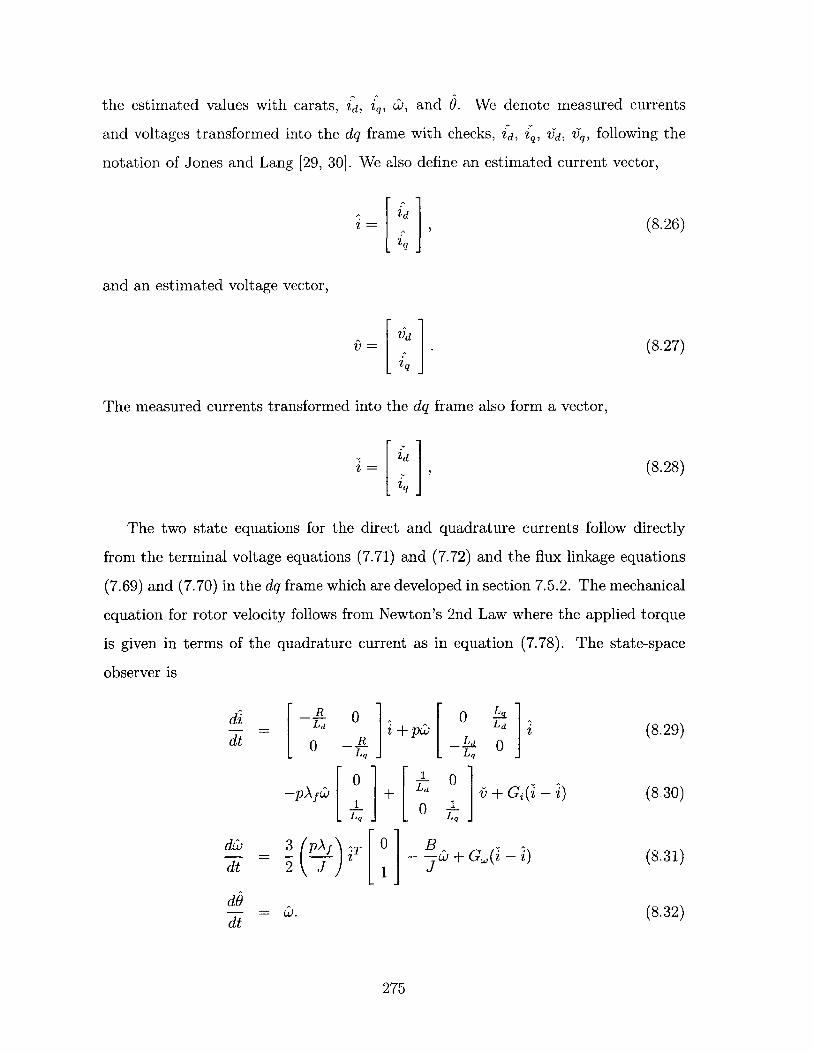
the estimated values with carats, W, q, L, and 0. We denote measured currents

and voltages transformed into the dq frame with checks, j, , Vd, 'q, following the

notation of Jones and Lang [29, 30]. We also define an estimated current vector,

F id1

:1 = (8.26)[ q j

and an estimated voltage vector,

1I . (8.27)[ q j

The measured currents transformed into the dq frame also form a vector,

i = ] (8.28)L~ 'q j

The two state equations for the direct and quadrature currents follow directly

from the terminal voltage equations (7.71) and (7.72) and the flux linkage equations

(7.69) and (7.70) in the dq frame which are developed in section 7.5.2. The mechanical

equation for rotor velocity follows from Newton's 2nd Law where the applied torque

is given in terms of the quadrature current as in equation (7.78). The state-space

observer is

di R 00 L__ i+ PJ J (8.29)

dt 0 PR _LdL q j Lq

0 0-pAf c + Ld v + Gi(z - i) (8.30)

1 0 -

d ) 3 (Phf'5 0 B- =- -- iT + Gw(i - i) (8.31)dt 2 J 1

d -= .(8.32)dO 8.2

275

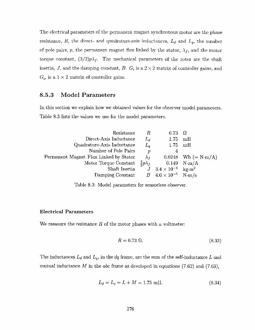
The electrical parameters of the permanent magnet synchronous motor are the phase

resistance, R, the direct- and quadrature-axis inductances, Ld and Lq, the number

of pole pairs, p, the permanent magnet flux linked by the stator, Af, and the motor

torque constant, (3/2)pAf. The mechanical parameters of the rotor are the shaft

inertia, J, and the damping constant, B. Gi is a 2 x 2 matrix of controller gains, and

G, is a 1 x 2 matrix of controller gains.

8.5.3 Model Parameters

In this section we explain how we obtained values for the observer model parameters.

Table 8.3 lists the values we use for the model parameters.

ResistanceDirect-Axis Inductance

Quadrature-Axis InductanceNumber of Pole Pairs

Permanent Magnet Flux Linked by StatorMotor Torque Constant

Shaft InertiaDamping Constant

Table 8.3: Model parameters

RfLd

Lqp

Af

2pAfJB

6.731.751.75

40.0248

0.1493.4 x 10-4

4.0 x 10-5

QmHmH

Wb (= N.m/A)N-m/Akg.m 2

N-m/s

for sensorless observer.

Electrical Parameters

We measure the resistance R of the motor phases with a voltmeter:

R = 6.73 Q. (8.33)

The inductances Ld and Lq, in the dq frame, are the sum of the self-inductance L and

mutual inductance M in the abc frame as developed in equations (7.62) and (7.63),

Ld = Lq = L + M = 1.75 mH. (8.34)

276

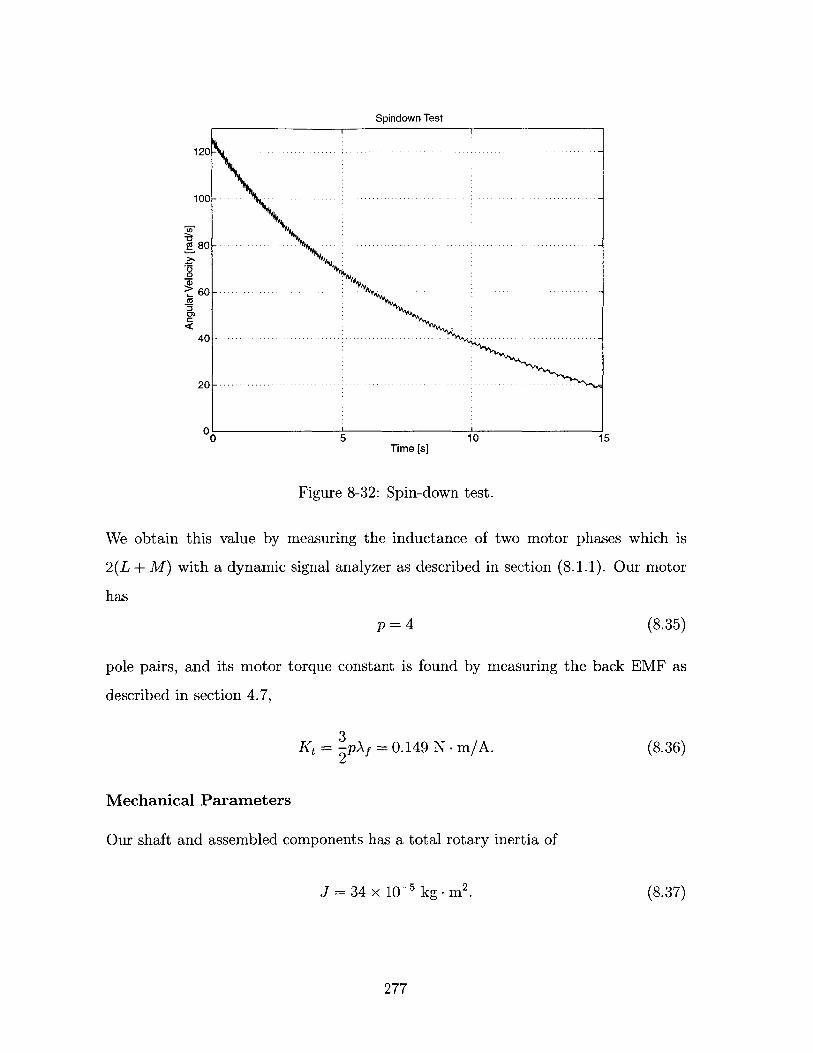
Spindown Test

120-- -

100 - - - -.-.-.-

0 --

20 -- ----

0

01540 5 10 1sTime [s]

Figure 8-32: Spin-down test.

We obtain this value by measuring the inductance of two motor phases which is

2(L + M) with a dynamic signal analyzer as described in section (8.1.1). Our motor

has

p = 4 (8.35)

pole pairs, and its motor torque constant is found by measuring the back EMF as

described in section 4.7,

Kt = pAf = 0.149 N -m/A. (8.36)2

Mechanical Parameters

Our shaft and assembled components has a total rotary inertia of

J = 34 x 10-5 kg - M2 . (8.37)

277

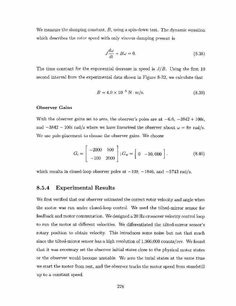
We measure the damping constant, B, using a spin-down test. The dynamic equation

which describes the rotor speed with only viscous damping present is

dwJ + Bw = 0. (8.38)dt

The time constant for the exponential decrease in speed is J/B. Using the first 10

second interval from the experimental data shown in Figure 8-32, we calculate that

B = 4.0 x 10-5 N -m/s. (8.39)

Observer Gains

With the observer gains set to zero, the observer's poles are at -6.6, -3842 + 100i,

and -3842 - 100i rad/s where we have linearized the observer about w = 87r rad/s.

We use pole-placement to choose the observer gains. We choose

-2000 100Gi = [ 20001G = [0 -10,0001. (8.40)

which results in closed-loop observer poles at -100, -1846, and -5743 rad/s.

8.5.4 Experimental Results

We first verified that our observer estimated the correct rotor velocity and angle when

the motor was run under closed-loop control. We used the tilted-mirror sensor for

feedback and motor commutation. We designed a 20 Hz crossover velocity control loop

to run the motor at different velocities. We differentiated the tilted-mirror sensor's

rotary position to obtain velocity. This introduces some noise but not that much

since the tilted-mirror sensor has a high resolution of 1,366,000 counts/rev. We found

that it was necessary set the observer initial states close to the physical motor states

or the observer would become unstable. We zero the intial states at the same time

we start the motor from rest, and the observer tracks the motor speed from standstill

up to a constant speed.

278

40

Eo5.. . . . . . ..). .. . .. . . . .

wD

250 -0 -10 -0 -5 0 50 10 10 20 2

Time [ms]

-200 -150 -100 -50 0 50 100 150 200 250Time [ms]

Figure 8-33: Sensorless speed control step response. Estimated speed, CD, andestimated quadrature current, iq, for a step change in reference speed from28.27 rad/s (4.5 rev/s) to 40.84 rad/s (6.5 rev/s). The system is running underclosed-loop speed control with estimated speed, Ca used as a measured signal, andestimated angle, 9, used to commutate the rotary motor.

After the observer was working, we used the estimated rotor position 9 and esti-

mated rotor velocity Co to implement closed-loop sensorless control. Instead of using

the tilted-mirror sensor for motor commutation and velocity feedback, we use 9 and

cD respectively. Figure 8-33 shows a step response in rotor velocity to a change in ref-

erence speed from 28.27 rad/s (4.5 rev/s) to 40.84 rad/s (6.5 rev/s). The estimated

quadrature current Z:q is also shown. The ripple in the CD and iq is proportional to

rotor speed.

These experimental results demonstrate that it is feasible to use a sensorless con-

trol scheme on a rotary-linear axis used as a spindle. Thus, we can eliminate the need

to design and incorporate a rotary sensor in spindle applications. Since designing and

integrating the rotary sensor is one of the main challenges in building rotary-linear

axes, this is an extremely useful result.

279

0

0

-25

- - -.. . . . . . . .

- -.

5

0

8.6 Summary

The first topic of this chapter was the design of an analog power op amp current

amplifier for providing current to the motor phases. We learned that we could stabilize

the power op amp and eliminate its oscillation by adding a resistor R0 across the two

op amp inputs. This resistor reduces the bandwidth of the minor loop feedback

around the power op amp but does not affect the ideal gain of the power op amp,

(R 3 + R4 )/R 3. Hence it improves power op amp stability but does not affect the

major current amplifier PI feedback loop.

Next we modeled and controlled the linear axis. We found an initially unmodeled

resonance at 11,020 rad/s and identified it as flexibility in the contact stiffness of

the tilted-mirror mount. We were able to model this resonance very closely using a

classic two-mass system where one mass was the tilted-mirror and the other was the

rest of the axis. The linear axis closed-loop bandwidth could be made higher than

our final controller design of 70 Hz since the linera axis plant is so ideal and has no

low frequency resonances.

The rotary axis plant has significant low frequency resonances which limit the

closed-loop bandwidth which can be obtained on our prototype axis to 40 Hz. The

two main resonances are due to cantilever modes of the tilted mirror and small z

mirror, respectively, on the shaft. From this we learn that we should pay particular

attention to putting any significant mass at the ends of the shaft in future designs.

We may also want to reduce the shaft length in future designs since these bending

modes are the lowest in frequency and caused us the most trouble.

We then estimated the dynamic stiffness required in a grinding operation to be

27 N/ptm. Our prototype axis has a linear axis dynamic stiffness of 0.2 N/pum and a

rotary axis dynamic stiffness of 0.06 N/pm at a 1 cm radius. Thus, the current system

does not have enough dynamic stiffness to withstand a grinding operation. Signifi-

cant increases in closed-loop bandwidth are required to achieve the target stiffness.

These may be possible with an improved shaft structure which does not have the low

frequency cantilever resonances. It is also possible that the stiffness required for high

280

speed grinding is significantly less than the stiffness we have estimated. Nonetheless,

we learned that dynamic stiffness is an important issue that needs to be addressed in

future rotary-linear axes.

Finally, we showed the viability of a sensorless control scheme for spindle ap-

plications. We found that the sensorless control scheme worked well but was very

sensitive to some of the model parameters. For example, a 10% change in the model

rotary motor force constant would drive the estimator unstable. The main conclusion

from this investigation, though, is that we can avoid using a rotary sensor in spindle

applications.

In the next chapter we show how the control algorithms we developed in this

chapter are implemented on a DSP to control our prototype rotary-linear axis.

281

282

Chapter 9

Control Implementation

This chapter describes the software that runs our prototype z-0 axis. Our software

runs on a dSPACE 1103 DSP board (see Appendix F) that uses a 400 MHz PowerPC

processor. We program this board via Matlab's Simulink and Stateflow packages.

Mastering Simulink 2 [11] is a good Simulink reference and tutorial, and the Stateflow

User's Guide [46] is a comprehensive Stateflow reference which is available on-line at

the Mathwork's website. Simulink is good for programming algebraic computations

and compensation transfer functions. Stateflow provides supervisory control via finite

state control; it allows the definition of system states, events, and transitions between

states. Matlab's Real-Time Workshop compiles our combined graphical Simulink and

Stateflow program and dSPACE supplied software takes care of hardware interfacing

with the DSP. We also use dSPACE's ControlDesk software to create interactive

control panels for running our prototype rotary-linear axis.

In this chapter we first present an overview of the control implementation. Next

we describe the order in which we put the various pieces of the control code together.

The development stages we go through are applicable to a wide range of machines

with actuators and sensors, even if their controllers are implemented on a completely

different system. We then describe some of the software in more detail. We look at the

Stateflow controller, the closed-loop compensators, motor control, sensor processing,

the automatic calibration routine, and sensorless processing.

283

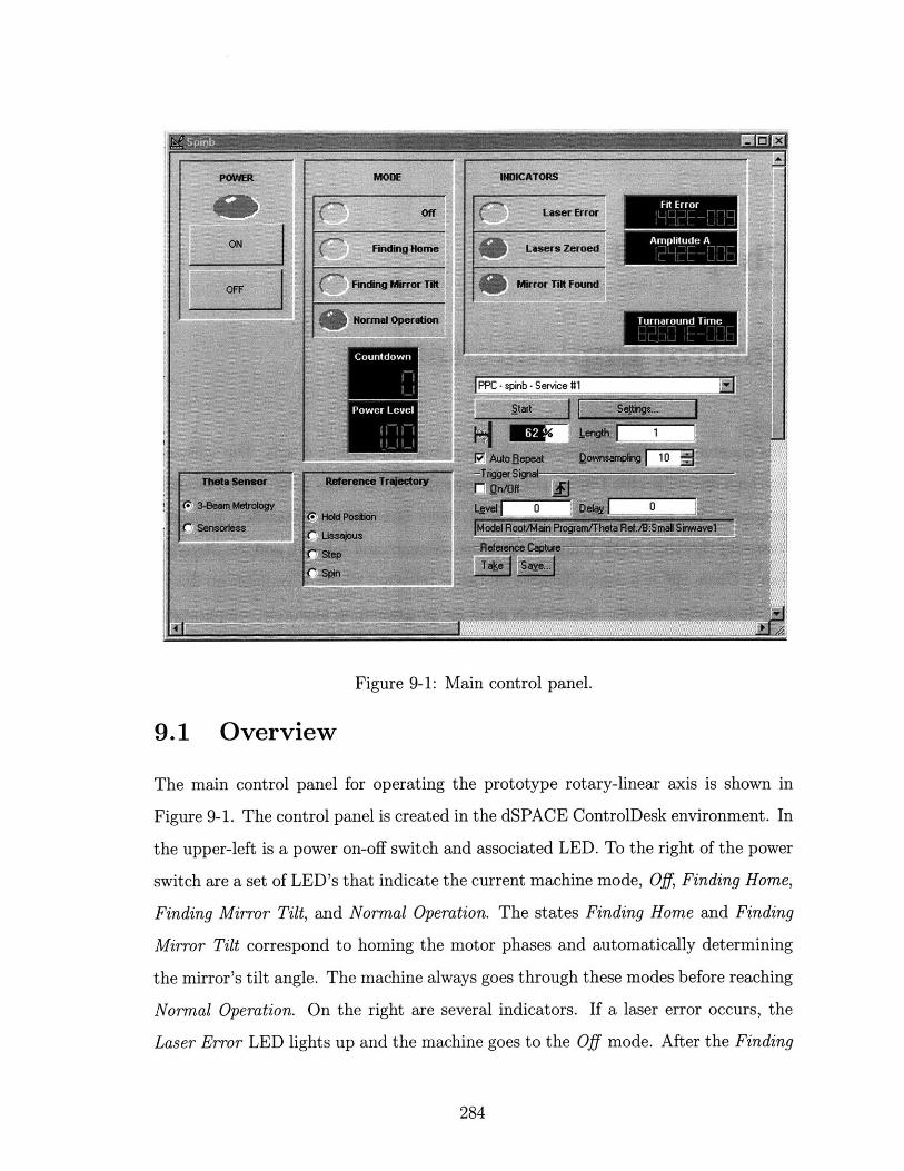
Figure 9-1: Main control panel.

9.1 Overview

The main control panel for operating the prototype rotary-linear axis is shown in

Figure 9-1. The control panel is created in the dSPACE ControlDesk environment. In

the upper-left is a power on-off switch and associated LED. To the right of the power

switch are a set of LED's that indicate the current machine mode, Off, Finding Home,

Finding Mirror Tilt, and Normal Operation. The states Finding Home and Finding

Mirror Tilt correspond to homing the motor phases and automatically determining

the mirror's tilt angle. The machine always goes through these modes before reaching

Normal Operation. On the right are several indicators. If a laser error occurs, the

Laser Error LED lights up and the machine goes to the Off mode. After the Finding

284

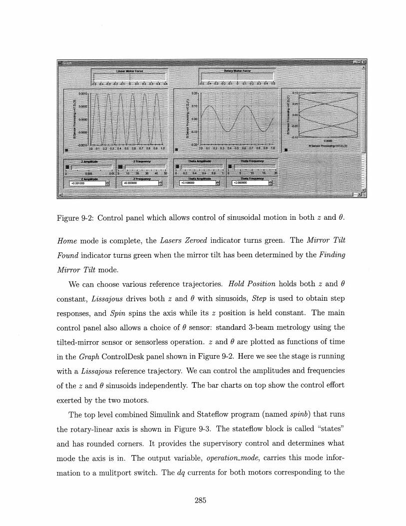
Figure 9-2: Control panel which allows control of sinusoidal motion in both z and 9.

Home mode is complete, the Lasers Zeroed indicator turns green. The Mirror Tilt

Found indicator turns green when the mirror tilt has been determined by the Finding

Mirror Tilt mode.

We can choose various reference trajectories. Hold Position holds both z and 9

constant, Lissajous drives both z and 9 with sinusoids, Step is used to obtain step

responses, and Spin spins the axis while its z position is held constant. The main

control panel also allows a choice of 9 sensor: standard 3-beam metrology using the

tilted-mirror sensor or sensorless operation. z and 9 are plotted as functions of time

in the Graph ControlDesk panel shown in Figure 9-2. Here we see the stage is running

with a Lissajous reference trajectory. We can control the amplitudes and frequencies

of the z and 9 sinusoids independently. The bar charts on top show the control effort

exerted by the two motors.

The top level combined Simulink and Stateflow program (named spinb) that runs

the rotary-linear axis is shown in Figure 9-3. The stateflow block is called "states"

and has rounded corners. It provides the supervisory control and determines what

mode the axis is in. The output variable, operation-mode, carries this mode infor-

mation to a mulitport switch. The dq currents for both motors corresponding to the

285

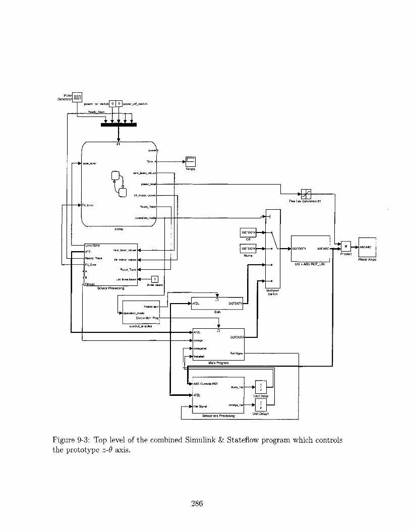
Generator

power_on switch pawer_oft_switch

Readv Trace 1

itpower

laser error Time.A

Scopezero laser values

power ee

tilt mirror values P -

Pow LFit Error ResetTrace

operation_ -m -, -

states

Off

Laser Error

ATZL zero laservalues D

ReadyTrace tilt mirror-values -- -- m

FitError

A Reset Trace --

B use three beam

Omega three beam

Sensor Processing MultiportSwitch

Enable spin TL:O:]dJ

Soperation-mode Spin

Enable Main PrF

control-enables

ATZLDOTDQT

Nomega

omegahatRef Signal

thetahat

Main Program

ABC Currents ROT 7 ;]threta hat -

z

ATZL Unit Delay

Ret Signal omega-hat

Sensorless Processing Unit Delayl

ev Saturation 01

DOTl ABCABC X ABCABC

Product

Power Amps

Figure 9-3: Top level of the combined Simulink & Stateflow program which controlsthe prototype z-0 axis.

286

current operation mode are passed through this multiport switch. They are then con-

verted to abc phase currents and sent to the power amplifiers. The Sensor Processing

subsystem's main function is to output a vector labeled ATZL which has the current

shaft angle (A), the rotary motor electrical angle (T), the linear position (Z), and

the linear motor electrical angle (L). This position information is fed to the Main

Program subsystem which has the rotary and linear compensators in it. The Sensor-

less Processing subsystem provides estimates of rotary electrical angle, theta-hat, and

shaft speed, omega-hat, which can be used to control the motor in the Main Program

subsystem. Next we look at how this complex system can be developed one piece at

a time.

9.2 Development Stages

Developing a complex controller like the one shown in Figure 9-3 may seem to be a

daunting task, but it can readily be built up in simple stages. This section describes

just one possible ordering that makes sense; there are certainly alternative develop-

ment strategies. Often, for example, it makes sense to start controlling whatever

hardware one receives first.

9.2.1 Homing Motor

As a first step, we connect the D/A channels on the dSPACE 1103 board to our power

amplifiers. We command a constant current in one of the three phases in each motor

and check that the motors respond by oscillating about fixed home positions.

9.2.2 Commutating Motor

The next step is to implement the dq transformations, or motor commutation laws,

described in sections 7.4.2 and 7.4.3. These transformations require a measurement of

motor electrical angle so any sensor processing needs to be done as well. It is possible

to intially commutate the motor "open-loop" by specifying the electrical angle if the

287

sensor is not yet available.

With sensing of electrical angle, a constant quadrature current should provide a

constant force or torque in one direction. If the force or torque is not constant the

signs of the motor phases should be checked, and also the calculation of electrical

angle might be wrong. It is essential to solve all these problems here so that smooth

force and torque are obtained before closing the loop around the motors.

9.2.3 Sensor

The sensor software can be developed simultaneously with the initial motor software.

The amount of software required will depend greatly on the sensor type and the DSP

system. For example an encoder requires very little user processing if the DSP has

encoder interface electronics built-in. Our custom tilted-mirror sensor requires a great

deal of software to process the laser interferometer measurements. Later we added

even more software to automatically measure the mirror tilt.

9.2.4 Closed-Loop Control

Once the motor and sensor are both working well, we can design a controller and

close the loop. The frequency response of the plant should be measured from actuator

command to sensor response. Based on this Bode plot, a controller can be designed.

This data should also be compared to a plant model, and unexpected behavior should

be investigated. This process is described for our linear axis in section 8.2 and for

our rotary axis in section 8.3. The closed-loop controller can then be implemented.

It is always a good idea to measure the Bode plot of the negative of the loop transfer

function to ensure that the desired crossover and phase margin have been achieved.

9.2.5 Stateflow Controller

If desired, a supervisory control routine can be added at any stage of development.

In fact, for some applications, this might be done as one of the first steps. We use

the Stateflow controller to switch between different operation modes, detect laser

288

errors, and sequence the automatic calibration routine for our sensor. We look at this

controller in more detail next.

9.3 Stateflow Controller

Our Stateflow controller is shown in Figures 9-4 and 9-5. It consists of two main

states, the Power-On state of Figure 9-4 and the PowerOff state of Figure 9-5.

As shown in Figure 9-5 there are several transitions between these two states. For

example, if the Off button in ControlDesk is hit, the system goes into the Power-Off

state. Likewise, if the On button in ControlDesk is hit, the system goes into the

Power-On state after checking that there are no laser errors. If a laser error occurs

while the system is in the PowerOn state, the top transition sends the controller

to the Power-Off state and sets flags indicating that the initial calibration routines

need to be re-run.

The Power-On state consists of two sub-states that run at the same time, Timer

and Series. The Timer state acts as a countdown timer. The Series state has a series

of states relating to machine start-up and calibration. For example, the Initialization

state, sets operationmode to 2 and starts the timer. As shown in the top level model

in Figure 9-3, operation-mode equal to 2 selects the dq currents for homing the motor

to pass through the multiport switch.

9.4 Motor Control

The "Main Program" subsystem in the top level control program (Figure 9-3) is

shown in Figure 9-6. It contains the rotary and linear axis compensation as well as

the generation of reference trajectories. A speed control loop for spinning the motor is

also included on the bottom and can be used instead of the angular position loop. The

compensation for the rotary axis is contained in the block labeled "leadlag controller

1.," It is shown in Figure 9-7.

Note that the rotary axis error passes through a block labeled "Smallest Angle

289

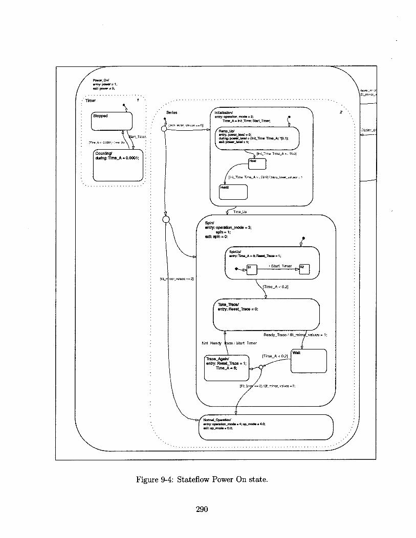
PbwerLOn/entry: power - 1;edit: power - 0;

Timer

Stopped

topped

tartTie-

Counting/cdkjring: TimeA = 0.0001;

1 -

Series

[zez _aser cafues=

ut v rtryalues 2]

NorMLOperafto/entry- operationmode = 4; opmJode 4.0;exit: op_Mode = 0.0;

Figure 9-4: Stateflow Power On state.

290

I:2lnitialization/

entry: operation-mode = 2;Time_A = InitL.Tme; Startimer;

RampUp/enty- power-level = 0during: powerlavel = (InitjTime Time.A) *(0.1);exit: power.jevel = 1;

nflm_Tire Te >= 10]

T eJd

tlniLTinte lTmeA ,=29.0)? zero Waeyla

e- jaertdal e

[laser a01

Spin/entry: operationmode = 3;

spin = 1;exit: spin = 0;

spinUp/entry:TtmeA = ; RmTrace = 1;

,Time A < 6,2]

TakeTrace/entry: ResetTrace =0;

ReadyTrace /tilt mir values = 1;

Not-Ready_ ace / Start Timer

(WaitTrace_Again/ [TimeA < 0,2]entry: ResetL_Trace = 1;

Time_A = 6;

[Fit Er. == O]iifilt mirror_ vatues = 2;K,

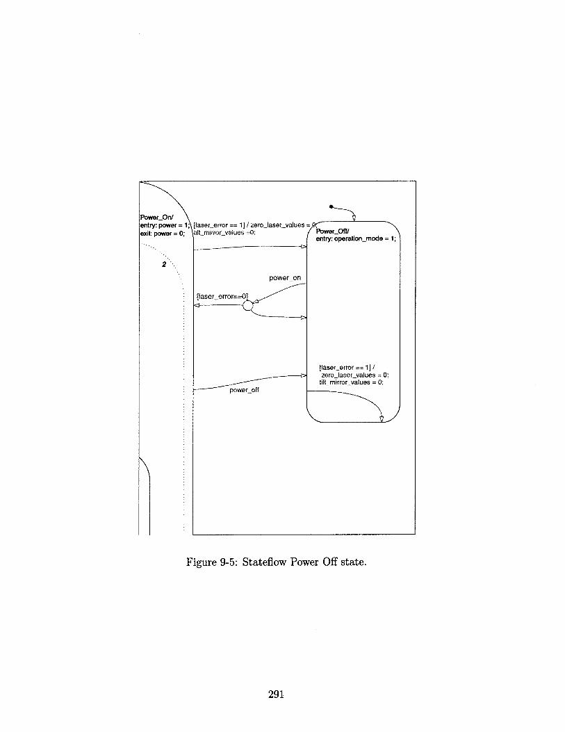
[laser error == 1 /zero-laservaluestilt mirror-values =0; P rOff/

entry: operationmode = 1;

power-on

laser-error==0]

power-off

Figure 9-5: Stateflow Power Off state.

291

PowerOn/entry: power = 1;exit: power = 0;

2

[laser-error == 1] /ze -ro aservalues = 0;tilt-mirror values = 0:

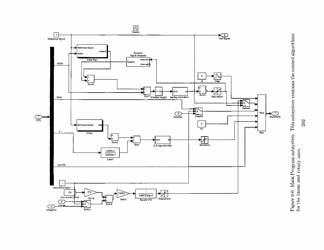
Enable

Reference Signal

sensorless?0yes

25 2*pi 0.0251 1

spin sped(r + 1/(90*2*pi)s+p V/s) Gain3 Gain2 Transfer Fcn Saturation2

ome. a Sum8

omegahat Switch

of Signal

-11 Reference Signal

- lh thetaref DynamicSr SmaleSignal Analyzer

Theta Ref. channeltSneOut

-4 s, channe12

Sum5

Sum7 Smallest Angle1 leadlag controllerl

thetahat SNitch3

idlF

pl:I JSaturation

Mux

Mux

R

I

alpha

theta

ATZL

zrne ga z

Z Ref.

Sum2 error aSum su~m K & Lag controller

1/220s+1

1/2200s+1

Lead1

lambda

P_

bfl

04-D

C-)

4-)

DQTDQTr

bCd

Ctl

)

id Fast

Su4 Saturation1l

Switch2

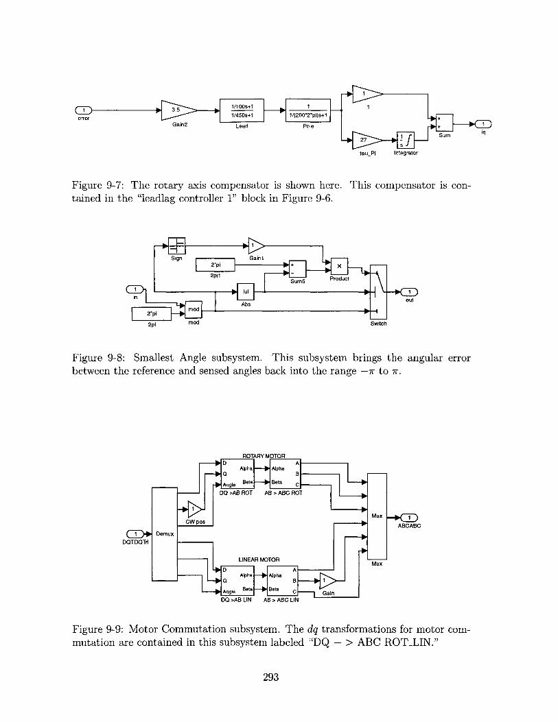
Ci> - .5 145s1 1/(200*2*pi)s+1

Gain2 Lead Pole+

271Sumq

tauPI Integrator

Figure 9-7: The rotary axis compensator is shown here. This compensator is con-tained in the "leadlag controller 1" block in Figure 9-6.

Sign Gainl2*pi +x- -

2pil Sum5 Prdc

2*piAb

2pi mod Switch

Figure 9-8: Smallest Angle subsystem. This subsystem brings the angular errorbetween the reference and sensed angles back into the range -7r to 7r.

ROTARY MOTOR

Apha - Alpha

S Angle Beta - Beta C

DQ >AB ROT AB > ABC ROT

MuxCW pos ACB

DemuxDQTDQTrI

LINEAR MOTOR u

A lpha -yAlpha

Angle Beta - Bea C -- | G iDQ >AB LIN AB > ABC LIN

Figure 9-9: Motor Commutation subsystem. The dq transformations for motor com-mutation are contained in this subsystem labeled "DQ - > ABC ROT-LIN."

293

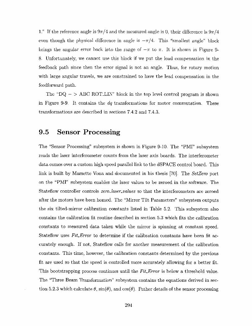
1." If the reference angle is 97r/4 and the measured angle is 0, their difference is 9-N/4

even though the physical difference in angle is -7r/4. This "smallest angle" block

brings the angular error back into the range of -7r to r. It is shown in Figure 9-

8. Unfortunately, we cannot use this block if we put the lead compensation in the

feedback path since then the error signal is not an angle. Thus, for rotary motion

with large angular travels, we are constrained to have the lead compensation in the

feedforward path.

The "DQ - > ABC ROTLIN" block in the top level control program is shown

in Figure 9-9. It contains the dq transformations for motor commutation. These

transformations are described in sections 7.4.2 and 7.4.3.

9.5 Sensor Processing

The "Sensor Processing" subsystem is shown in Figure 9-10. The "PMI" subsystem

reads the laser interferometer counts from the laser axis boards. The interferometer

data comes over a custom high speed parallel link to the dSPACE control board. This

link is built by Marsette Vona and documented in his thesis [70]. The SetZero port

on the "PMI" subsystem enables the laser values to be zeroed in the software. The

Stateflow controller controls zero-laser-values so that the interferometers are zeroed

after the motors have been homed. The "Mirror Tilt Parameters" subsystem outputs

the six tilted-mirror calibration constants listed in Table 5.2. This subsystem also

contains the calibration fit routine described in section 5.3 which fits the calibration

constants to measured data taken while the mirror is spinning at constant speed.

Stateflow uses FitError to determine if the calibration constants have been fit ac-

curately enough. If not, Stateflow calls for another measurement of the calibration

constants. This time, however, the calibration constants determined by the previous

fit are used so that the speed is controlled more accurately allowing for a better fit.

This bootstrapping process continues until the FitError is below a threshold value.

The "Three Beam Transformation" subsystem contains the equations derived in sec-

tion 5.2.3 which calculate 0, sin(O), and cos(6). Futher details of the sensor processing

294

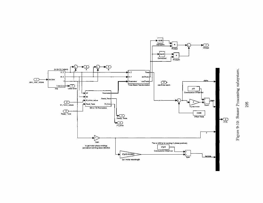
(output in meters)

A Z

B Z

Set Zerozero-laser-values Z

Laser Error L

PMJ Laser Error

tillmirrorvalues

ResetTrace

5 + 6A B

JA5 Z Theta

B Z sin(Theta)

- ------ Parameters cos(Theta)--

AZ PrameersThree Beam Transformation

-- 0 BZReadyTrace

tift-mirror_values

Reset_Trace FitError -

Mirror Tilt Parameters

ReadyTrace

Fit_Error

Gain

to get motor phase windingsand sensor pointing same direction

2*pV(0.052832)

2pi / motor wavelengtl

du/dt

Derivative X 7

Product Omega

du/dtx

DerivativelProduct

CK> alphause three beam

pi/2

Commutation Offset iot

Sum lambd

8 pole motor

0.836Offset Theta

Sz

This is (4/3)*pi for exciting C phase positively

I4*pi/3] "

Commutation Offset Lin +a bd

sum lmd

Cn

-4

tC

UI)

ATZL 6

;-

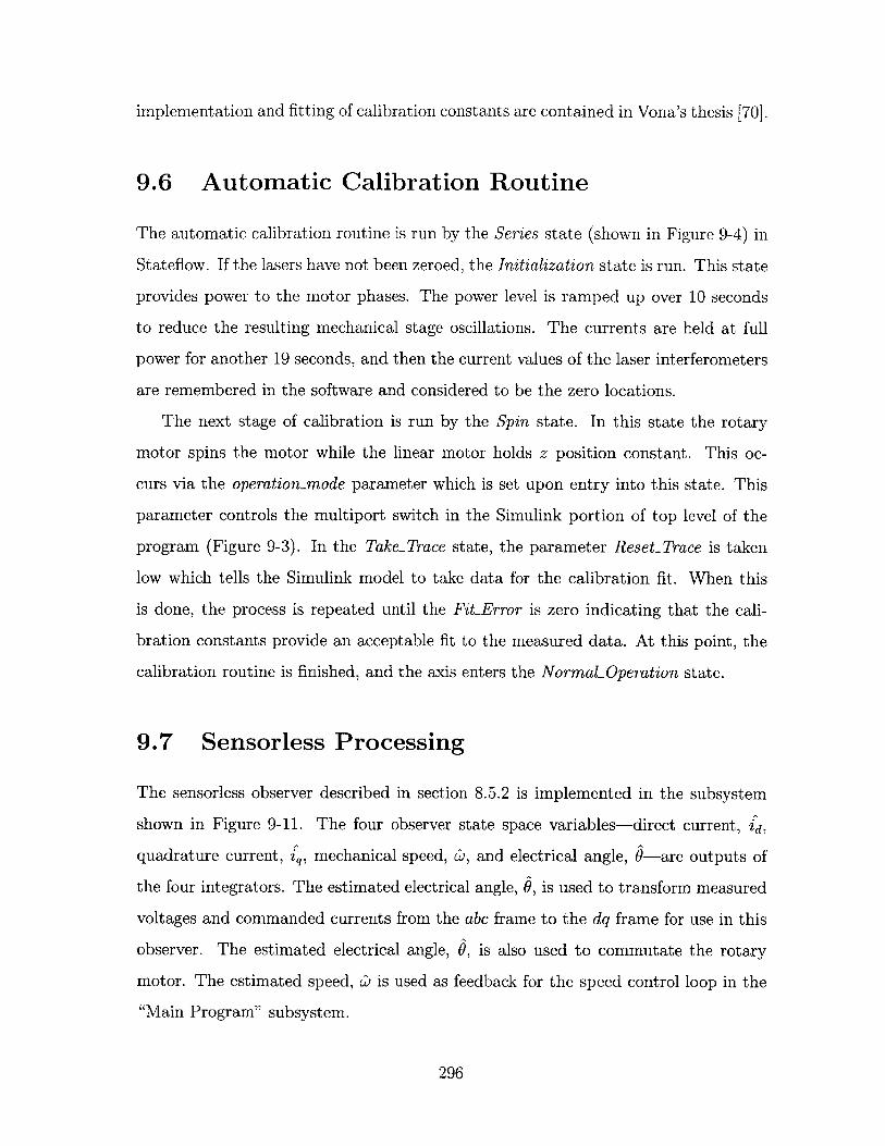
implementation and fitting of calibration constants are contained in Vona's thesis [70].

9.6 Automatic Calibration Routine

The automatic calibration routine is run by the Series state (shown in Figure 9-4) in

Stateflow. If the lasers have not been zeroed, the Initialization state is run. This state

provides power to the motor phases. The power level is ramped up over 10 seconds

to reduce the resulting mechanical stage oscillations. The currents are held at full

power for another 19 seconds, and then the current values of the laser interferometers

are remembered in the software and considered to be the zero locations.

The next stage of calibration is run by the Spin state. In this state the rotary

motor spins the motor while the linear motor holds z position constant. This oc-

curs via the operation-mode parameter which is set upon entry into this state. This

parameter controls the multiport switch in the Simulink portion of top level of the

program (Figure 9-3). In the Take-Trace state, the parameter Reset-Trace is taken

low which tells the Simulink model to take data for the calibration fit. When this

is done, the process is repeated until the FitError is zero indicating that the cali-

bration constants provide an acceptable fit to the measured data. At this point, the

calibration routine is finished, and the axis enters the NormaLOperation state.

9.7 Sensorless Processing

The sensorless observer described in section 8.5.2 is implemented in the subsystem

shown in Figure 9-11. The four observer state space variables-direct current, Zd,

quadrature current, i^,, mechanical speed, LZ, and electrical angle, 0-are outputs of

the four integrators. The estimated electrical angle, 9, is used to transform measured

voltages and commanded currents from the abc frame to the dq frame for use in this

observer. The estimated electrical angle, 9, is also used to commutate the rotary

motor. The estimated speed, cD is used as feedback for the speed control loop in the

"Main Program" subsystem.

296

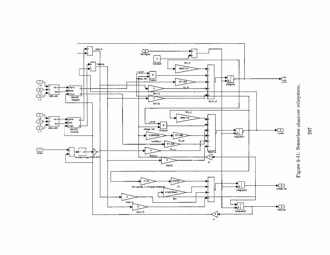
v a AA Alpha Alpha

2 B Betvb v Bela Betav_b C Bj t Angle

3 c ABC>AB ABVDsVCVoltages

4a A Alpha Alpha D5 B

L-b C Bets Bea

6 ABC>ABic Currents

7+Angle in out

Smallest Angle An

+ de

)Ie Erro

ta iq

7

8 a

Ret Signal

Constant R/L-dE 3845.714

~t r t

1/L d

Gi(1,1)

Gi(1,2)

3845.714

Ld hatx

omega-hat Producti

Lambda-f 1/L-ql571.428

0 r/Lq

Gi(2.11

I i I -I-

SumLd

Sum Lq

,1 ,

Gi(2,2)

3/2 Lambdaef = Kt (peak Amper e /

4.OeSt(34e5)

B/JGw(l,1

0

Gw(1 2)

Integrator

lntegratorl

Ld h,

i-q hat

omega hat

e hIntegrtor3t4

D

-D

af)

Q)

cIn

-4

-44

- i

Integrator2

+ delta id

i q

9.8 Summary

There is no question that the dSPACE system greatly simplified our control imple-

mentation. For example, it took us just minutes to change control transfer functions.

Overall, it definitely saved us months of work over implementing the controller di-

rectly in C or assembly language.

In some respects, however, the dSPACE system is non-ideal. The graphical pro-

gramming language of Simulink and Stateflow is good for algorithmic calculations,

but implementing conditional branching and control structures is cumbersome. Al-

though Stateflow helps significantly in this regard, it can be extremely difficult to

program. This is because it is easy to design an infinite loop into the Stateflow dia-

gram without realizing it. The cause of the infinite loop is often subtle and requires

consideration of the order in which Stateflow evaluates entries and exits of states

during each execution cycle. We found that the Stateflow debugger helped us greatly

to identify these loops. Unfortunately the debugger does not work when the code

is run in real-time, so the model must be debugged in simulation. Once we got the

Stateflow component working, it did a very nice job of controlling the machine states,

sequencing events, and shutting down the machine in case of laser errors.

Another major difficulty with the dSPACE controller is that the programmer

loses control over the order in which code runs during the sample time. For simple

programs, this is not generally a problem. As the complexity of the program increases

and the full sample time is used, however, the programmer generally would like to

have more control over the order and timing of code execution. We found that in our

final controller implementations our code execution time was bumping up against the

100 ps sample time. Thus, we would sometimes get task overruns, and it was not

clear how we could best avoid this and why it only occurred during certain tasks such

as at the end of the initial calibration routine.

In the final chapter of this thesis we look at what we have learned and future

research directions for continuing work on rotary-linear axes.

298

Chapter 10

Conclusions & Suggestions for

Future Work

10.1 Summary

The precision positioning and high acceleration capabilities of rotary-linear axes make

them an enabling technology for rapidly producing complex parts to micron-level

accuracies. In this thesis, we introduced rotary-linear axes as key components for use

in novel multi-axis machine tools. We reviewed and classified existing 5-axis machine

tool topologies and realized that topologies that stack machine tool axes can achieve

only limited accelerations. By combining the rotational and translational degrees of

freedom into one moving part, the rotary-linear axis offers higher accelerations and

higher control bandwidths than are currently achievable.

We presented a general investigation into rotary-linear motion. Precision actu-

ation and sensing of rotary-linear motion is especially challenging. We reviewed

existing rotary-linear stage designs and found many interesting designs for achiev-

ing rotary-linear actuation and sensing. However, these designs do not have the

force, precision sensing, and precision positioning capabilities required for use in high-

performance machine tools. Thus, in this thesis we developed a rotary-linear axis as

a key subsystem for precision, multi-axis machine tools. We fabricated a prototype

axis and controlled both axes to test the feasibility of our rotary-linear axis design.

299

Overall, this thesis shows that rotary-linear axes are a viable component for use in

precision, multi-axis machine tools. Our prototype rotary-linear axis achieves a linear

acceleration of 3 g's and a rotary acceleration of 1,300 rad/s 2. These acceleration

levels are far higher than today's most capable multi-axis machine tools can achieve.

Furthermore, with higher power current amplifiers and reduced sensor inertia, we

predict the axis could attain peak accelerations of 12 g's and 17,500 rad/s 2 at low

duty cycles.

Our prototype axis uses a plane mirror interferometer with a resolution of 0.625 nm

to measure linear motion. The axis uses a novel tilted-mirror sensor with a resolution

of 4.6 prad (1,336,000 counts/rev). This sensor uses two laser interferometers to

measure the orientation of a tilted mirror attached to the rotary-linear shaft. The

axis's simple mechanical system allows for high bandwidth controllers, 40 Hz for the

rotary axis and 70 Hz for the linear axis. Under closed-loop control, the axis achieves

2.5 nm of linear positioning noise and 3.1 prad of rotary positioning noise.

We have developed a framework for designing rotary-linear motors. We showed

that for small force levels, permanent magnet synchronous motors are more power

efficient than induction motors. Also, for short axial travels like ours, separate ro-

tary and linear permanent magnet motors are more power efficient than a combined

permanent magnet motor. We developeded a scaling analysis that shows that long,

skinny motors are preferred for achieving high linear and rotary accelerations. We

used this analysis to select commercially available rotary motor parts that maximized

the axis's accelerations. We derived a continuum electromechanical analysis for a per-

manent magnet linear motor with iron backing. The results of this analysis allowed

us to optimize the linear motor for high accelerations.

Our prototype rotary and linear motors perform exceptionally well. The rotary

motor is composed of commercially available parts; the tubular linear motor is com-

pletely custom-built. Both motors have a solid construction and have not had any

electrical shorts. The short rotor, long stator concept used to allow axial travel in

both motors does not have any undesirable side effects. It is important to make sure

that at the extremes of the axial travel, the permanent magnet rotor is still within the

300

stator, as in our prototype; otherwise the magnetic attraction between the permanent

magnet rotor and the stator back iron can overwhelm the linear motor.

We investigated many rotary sensor concepts that can tolerate axial travel. Most

of our ideas are based on plane-mirror interferometry. The prism-mirror sensor uses

a prism to refract the laser beam so that it always reflects normally off a tilted

mirror attached to the shaft. Unfortunately, the optical path length does not depend

on rotation angle so this sensor will not sense shaft rotation. The helicoid mirror

sensor seems promising, but the fabrication of the helicoid mirror would be difficult

and expensive. The resolution offered by this sensor is not much greater than our

prototype tilted-mirror sensor.

Our prototype tilted-mirror sensor achieves high resolution and allows us to control

and test our prototype rotary-linear axis. However, it is not likely to be a final

solution. It's inertia accounts for 74% of the prototype axis's total inertia. It's

mass accounts for only 20% of the axis's total mass, but its location at the end of

the axis causes a low frequency, 1000 rad/s, cantilever resonance. This resonance

shows up in the rotary-axis plant and limits the rotary axis closed-loop bandwidth

to 40 Hz. Thus, a next generation rotary-linear prototype axis would likely use a

different rotary sensor. We have also shown the viability of rotary sensorless control

for use with rotary-linear axes designed for a spindle applications.

We have developed many concepts and analyses related to rotary-linear actuation

and sensing. Furthermore, we have successfully integrated these analyses and de-

signs into a prototype axis which demonstrates the high accelerations and precision

positioning performance rotary-linear axes can achieve.

10.2 Conclusions

We learned a great deal about rotary-linear motion that will affect the design of

future rotary-linear axes. One of the most important lessons we learned was that

interferometric sensors using large mirrors are not the ultimate solution for rotary

sensing on these axes. Our tilted-mirror sensor is successful in measuring rotation

301

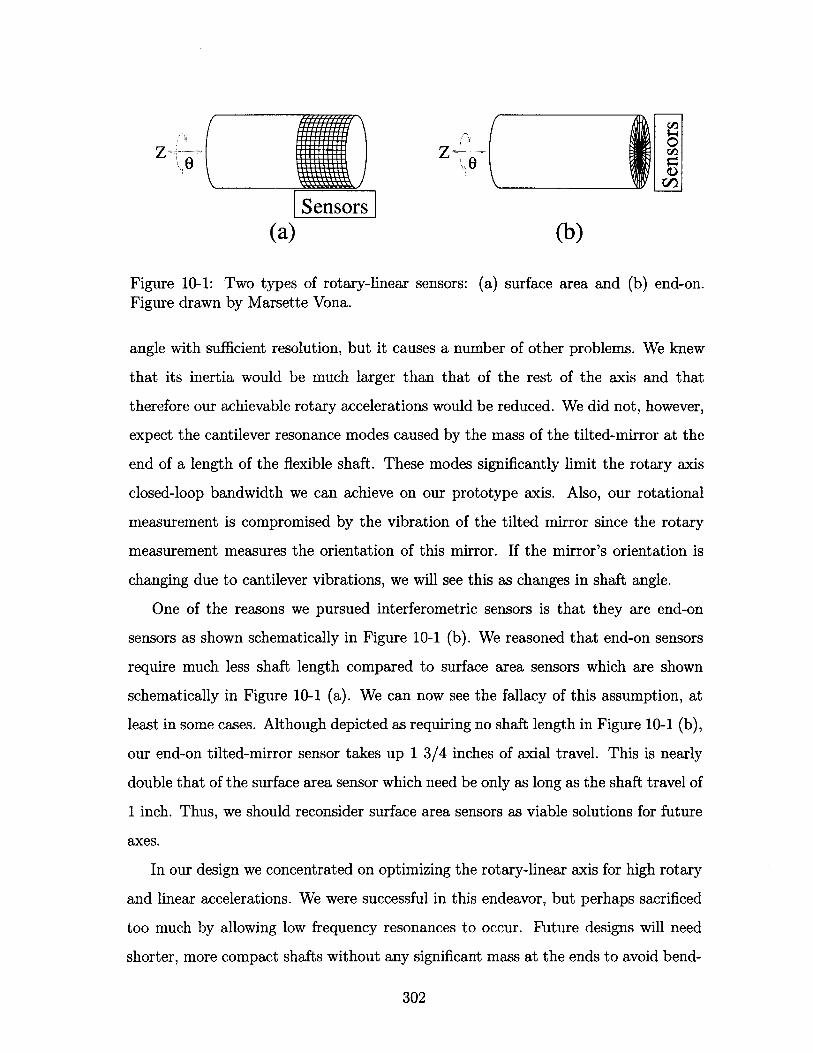
Sensors

(a) (b)

Figure 10-1: Two types of rotary-linear sensors: (a) surface area and (b) end-on.Figure drawn by Marsette Vona.

angle with sufficient resolution, but it causes a number of other problems. We knew

that its inertia would be much larger than that of the rest of the axis and that

therefore our achievable rotary accelerations would be reduced. We did not, however,

expect the cantilever resonance modes caused by the mass of the tilted-mirror at the

end of a length of the flexible shaft. These modes significantly limit the rotary axis

closed-loop bandwidth we can achieve on our prototype axis. Also, our rotational

measurement is compromised by the vibration of the tilted mirror since the rotary

measurement measures the orientation of this mirror. If the mirror's orientation is

changing due to cantilever vibrations, we will see this as changes in shaft angle.

One of the reasons we pursued interferometric sensors is that they are end-on

sensors as shown schematically in Figure 10-1 (b). We reasoned that end-on sensors

require much less shaft length compared to surface area sensors which are shown

schematically in Figure 10-1 (a). We can now see the fallacy of this assumption, at

least in some cases. Although depicted as requiring no shaft length in Figure 10-1 (b),

our end-on tilted-mirror sensor takes up 1 3/4 inches of axial travel. This is nearly

double that of the surface area sensor which need be only as long as the shaft travel of

1 inch. Thus, we should reconsider surface area sensors as viable solutions for future

axes.

In our design we concentrated on optimizing the rotary-linear axis for high rotary

and linear accelerations. We were successful in this endeavor, but perhaps sacrificed

too much by allowing low frequency resonances to occur. Future designs will need

shorter, more compact shafts without any significant mass at the ends to avoid bend-

302

ing resonances. Futhermore, although increasing the shaft diameter reduces rotary

and linear accelerations, it may be necessary to do this to achieve higher bending stiff-

nesses. We will need to increase the frequency of these bending resonances to achieve

higher closed-loop bandwidths. These higher bandwidths are required for achieving

sufficient dynamic stiffness to tolerate the oscillating component of grinding forces.

We learned some valuable techniques for fabricating permanent magnet motors.

We found that using an iron backing plate to short out some of flux from the perma-

nent magnets made it easier to attach the last few magnets in a ring configuration

for the rotor. We also found that cyanoacrylate works well for attaching the magnets

to the backiron. None of the magnets has fallen off our rotor since fabrication. Of

course, we are not spinning the motor at high speeds, but the system has survived

impulses of force. These occur when a laser is blocked while the axis is running, and

it hits a stop at one end of travel after the controller shuts off the power.

We found that our method for insulating the stator coils and routing the motor's

lead wires worked well also. The slot in the stator for the entry and exit of coil leads

did not cause any noticeable motor cogging. This is because the motor is surface

wound and there is therefore a large effective air gap between permanent magnet rotor

and the stator. The Nomex-Kapton-Nomex protective film and nylon coil separators

insulated and protected the motor coils from damage, nicks, and shorts.

We developed a general design procedure for permanent magnet synchronous mo-

tors. In particular, we learned that permanent magnet synchronous motor shear stress

increases proportionally to the motor pitch length, 1, if we consider motors whose di-

mensions scale with 1. Thus one generally wants to choose the largest pitch length

possible. Of course, since the motor's layer thicknesses scale with 1, this imposes a

limit on how large 1 can be made. We learned that the power optimal coil thickness

is 1/10 for permanent magnet synchronous motors with iron backing. Others have

shown that the power optimal coil thickness for permanent magnet synchronous mo-

tors with not iron backing is 1/5. In keeping with this comparison, our analysis shows

that we can achieve the same force in an iron-backed motor with half the magnet

thickness and half the coil thickness of an ironless motor. This result is reasonable

303

since the iron backing layer produces the image of the coil or magnet, thus effectively

doubling its size.

The tilted-mirror sensor achieved much higher resolution than we initially thought.

This was due primarily to the large tilt angle of 4.6 mrad we were able to achieve.

We discovered that our two-pass plane mirror interferometers are designed to accept

some tilt in the target mirror. Tilt in the target mirror offsets the measurement beam

from its nominal position but surprisingly does not change the returning measurement

beam direction. In the end we found that the tilt angle of our tilted-mirror sensor

was nearly the same as for the proposed helicoid sensor. This was surprising since

the helicoid mirror sensor was supposed to have a large tilt angle whereas we had

thought of the tilted-mirror sensor as having only a very slight tilt angle. Thus, the

helicoid sensor would not offer much more resolution. Initially, we had planned that

the tilted-mirror sensor would only be an interim sensor until the helicoid mirror

sensor could be fabricated.

10.3 Suggestions for Future Work

Future research and development of rotary-linear axes can proceed in many direc-

tions. In this section we present several of these research directions. The ultimate

goal of future research and development will be to achieve a modular rotary-linear

axis machine tool subsystem that can be incorporated into precision multi-axis ma-

chine tools for fabricating centimeter-scale parts. We hope such machines will prove

valuable in a wide variety of applications. In particular, we hope that the fabrication

of dental restorations may be automated by such a machine.

One of the most exciting aspects of this research is that it cuts across many disci-

plines including dynamics, controls, electromechanics, optics, and precision machine

design. Therefore, it offers numerous challenges and opportunities for researchers

who are interested in these disciplines and enjoy combining them to achieve balanced

designs. Depending on the interests of future researchers, research on rotary-linear

axes can proceed along several directions. In the following sections we describe each

304

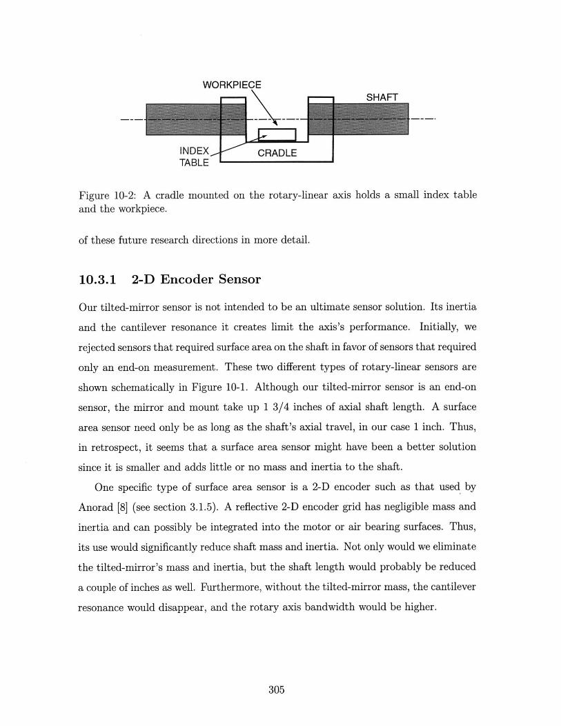
WORKPIECESHAFT

INDEX CRADLETABLE

Figure 10-2: A cradle mounted on the rotary-linear axis holds a small index tableand the workpiece.

of these future research directions in more detail.

10.3.1 2-D Encoder Sensor

Our tilted-mirror sensor is not intended to be an ultimate sensor solution. Its inertia

and the cantilever resonance it creates limit the axis's performance. Initially, we

rejected sensors that required surface area on the shaft in favor of sensors that required

only an end-on measurement. These two different types of rotary-linear sensors are

shown schematically in Figure 10-1. Although our tilted-mirror sensor is an end-on

sensor, the mirror and mount take up 1 3/4 inches of axial shaft length. A surface

area sensor need only be as long as the shaft's axial travel, in our case 1 inch. Thus,

in retrospect, it seems that a surface area sensor might have been a better solution

since it is smaller and adds little or no mass and inertia to the shaft.

One specific type of surface area sensor is a 2-D encoder such as that used by

Anorad [8] (see section 3.1.5). A reflective 2-D encoder grid has negligible mass and

inertia and can possibly be integrated into the motor or air bearing surfaces. Thus,

its use would significantly reduce shaft mass and inertia. Not only would we eliminate

the tilted-mirror's mass and inertia, but the shaft length would probably be reduced

a couple of inches as well. Furthermore, without the tilted-mirror mass, the cantilever

resonance would disappear, and the rotary axis bandwidth would be higher.

305

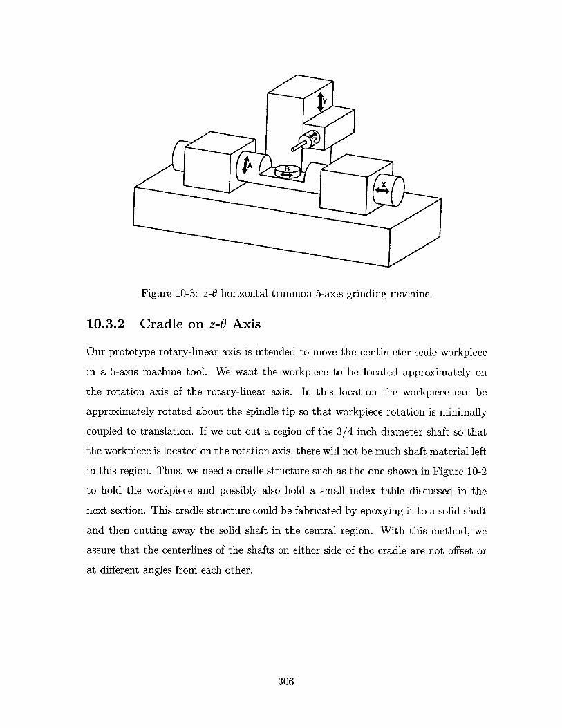
Y

JA B

Figure 10-3: z-0 horizontal trunnion 5-axis grinding machine.

10.3.2 Cradle on z-0 Axis

Our prototype rotary-linear axis is intended to move the centimeter-scale workpiece

in a 5-axis machine tool. We want the workpiece to be located approximately on

the rotation axis of the rotary-linear axis. In this location the workpiece can be

approximately rotated about the spindle tip so that workpiece rotation is minimally

coupled to translation. If we cut out a region of the 3/4 inch diameter shaft so that

the workpiece is located on the rotation axis, there will not be much shaft material left

in this region. Thus, we need a cradle structure such as the one shown in Figure 10-2

to hold the workpiece and possibly also hold a small index table discussed in the

next section. This cradle structure could be fabricated by epoxying it to a solid shaft

and then cutting away the solid shaft in the central region. With this method, we

assure that the centerlines of the shafts on either side of the cradle are not offset or

at different angles from each other.

306

10.3.3 Index Table with Reach-In Actuator

Our envisioned 5-axis machine topology is shown in Figure 10-3. As discussed in

section 2.7, the B-axis can be an index table to allow for five-sided machining. We

can reduce the added inertia of this index table by offloading its actuator. In order

to index the table, the rotary-linear axis would return to a home position, and the

reach-in actuator would engage the index table. The design of this index table and

associated reach-in actuator form another research project related to rotary-linear

axes. Existing index tables do not come in sizes smaller than 2 1/2 inches in diameter.

10.3.4 z-O Spindle Prototype

Another avenue of research is to design a prototype rotary-linear axis specialized for

use as a high-speed spindle combined with infeed. Our prototype axis is primarily

intended to be used for positioning the workpiece. For use as a spindle, the rotary-

linear axis might have both motors next to each other and bearings on either end.

Precision rotary sensing is no longer required, and the sensorless control scheme de-

veloped by Jones & Lang [29] and implemented in this thesis can be used. The z-0

spindle should be mainly optimized for high linear accelerations since rotation will

generally be maintained at a constant speed.

10.3.5 z-0 Horizontal Trunnion 5-Axis Grinding Machine

It would be very exciting to integrate the rotary-linear positioning axis into a 5-axis

machine tool such as the one shown in Figure 10-3. This machine ideally also has

a z-6 spindle and a cradle with a small index table as have already been discussed.

However, an initial prototype machine might use conventional axes instead.

To machine parts with complex surfaces, we will need to have efficient geomet-

ric algorithms to generate toolpaths which incorporate the specific kinematic and

dynamic properties of the machine tool. The rotary-linear axis provides extremely

high accelerations in two axes, and the toolpath generation algorithm should take

advantage of this capability.

307

Controlling the machine tool to follow complex surfaces at very high speeds also

requires significant research in control theory. We will need to develop algorithms

for following high-acceleration, high-frequency trajectories with small errors. Fur-

thermore, we will need to avoid resonances induced by the grinding process. Some

form of adaptive feedforward control may well allow this. The machine's simplicity

allows it to be modeled accurately which makes it easier to develop advanced control

schemes.

In designing this machine we should work with researchers and manufacturers

in the machine tool and dental fields in order to see our concepts used in practical

devices and have a significant impact on these industries.

308

Appendix A

Continuum Electromechanical

Analysis of Permanent Magnet

Synchronous Linear Motor with

Iron Backing

This Appendix presents the continuum electromechanical analysis of a permanent

magnet synchronous linear motor with iron backing. The analytical expressions for

motor force and power derived in this Appendix are used in Chapter 4 to design and

optimize the linear motor of the z-6 axis. We use the analytical framework of Melcher

[48] in which layers of electromagnetic material such as magnets, air gap, and coils

are described by transfer relations. This analysis extends prior anaylses [66, 67, 34]

of ironless linear motors by including iron backing behind the magnet and coil arrays.

The analysis in this Appendix first appeared in Chapter 2 of the author's Master's

thesis, Thermally Efficient Linear Motor Analysis & Design [41].

One of the main results of prior analyses [66, 67, 34] motors is that the power

optimal coil thickness for an ironless stator in a single-sided motor is approximately

1/5 where l is the magnet pitch. There is some confusion in the industry about the

definition of magnet pitch. For example, for a N-S magnet array, some vendors define

309

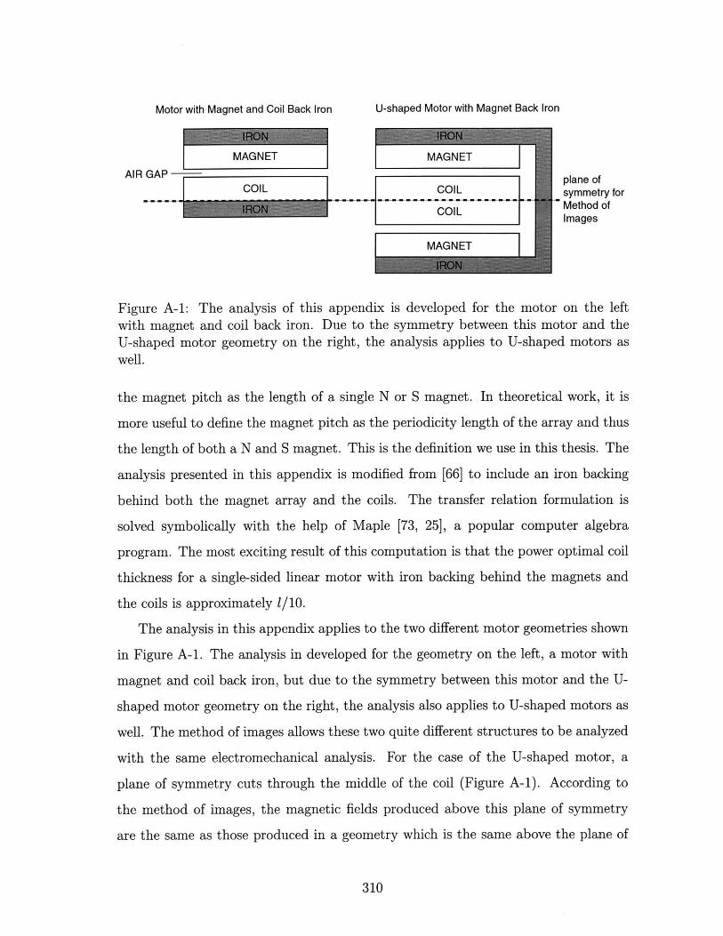
Motor with Magnet and Coil Back Iron

MAGNET

U-shaped Motor with Magnet Back Iron

MAGNETAIR GAP plane of

COIL COIL symmetry forMethod ofImages

MAGNET

Figure A-1: The analysis of this appendix is developed for the motor on the leftwith magnet and coil back iron. Due to the symmetry between this motor and theU-shaped motor geometry on the right, the analysis applies to U-shaped motors aswell.

the magnet pitch as the length of a single N or S magnet. In theoretical work, it is

more useful to define the magnet pitch as the periodicity length of the array and thus

the length of both a N and S magnet. This is the definition we use in this thesis. The

analysis presented in this appendix is modified from [66] to include an iron backing

behind both the magnet array and the coils. The transfer relation formulation is

solved symbolically with the help of Maple [73, 25], a popular computer algebra

program. The most exciting result of this computation is that the power optimal coil

thickness for a single-sided linear motor with iron backing behind the magnets and

the coils is approximately 1/10.

The analysis in this appendix applies to the two different motor geometries shown

in Figure A-1. The analysis in developed for the geometry on the left, a motor with

magnet and coil back iron, but due to the symmetry between this motor and the U-

shaped motor geometry on the right, the analysis also applies to U-shaped motors as

well. The method of images allows these two quite different structures to be analyzed

with the same electromechanical analysis. For the case of the U-shaped motor, a

plane of symmetry cuts through the middle of the coil (Figure A-1). According to

the method of images, the magnetic fields produced above this plane of symmetry

are the same as those produced in a geometry which is the same above the plane of

310

symmetry but has iron below. Thus the power optimal coil thickness for the U-shaped

motor is twice that of the single-sided motor, or 1/5. In the next section we present

the details of the motor continuum electromechanics.

A.1 Magnetoquasistatics and Fourier Series Nota-

tion

A permanent magnet motor is a magnetoquasistatic (MQS) system [23]. Under this

approximation Maxwell's Equations for the magnetic field intensity H, magnetic flux

density B, electric displacement D, and electric field E are:

VxH = Jf (A.1)

V-B = 0 (A.2)

Vx E = 01 (A.3)

where Jf is the free current density and M is the magnetization. We also have

continuity of free charge,

V.Jf =0, (A.4)

and a constitutive law relating magnetization, M, field intensity, H, and flux density,

B,

B = po(H + M). (A.5)

We assume that the system is periodic and represent the periodic fields in our

problem with Fourier series. We follow Melcher's notation [48] for a field quantity 4:

4J(z, t) = $ ~,(t)e-ikz (A.6)n=-oc

where27rn

kn = 1(A.7)

311

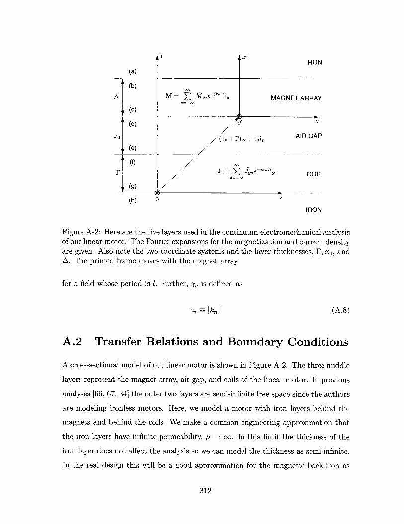
x x'IRON

(a)

(b)M = 1Z fe-ik"'ix, MAGNET ARRAY

(C)

(d) y' Z'

(X0 + F)i. + zoi, AIR GAP

(e)

J= Z .e-k~ziy COILn=-oo

(g)

(h) Z

IRON

Figure A-2: Here are the five layers used in the continuum electromechanical analysisof our linear motor. The Fourier expansions for the magnetization and current densityare given. Also note the two coordinate systems and the layer thicknesses, F, x0 , andA. The primed frame moves with the magnet array.

for a field whose period is 1. Further, 'ya is defined as

a = Ikn I. (A.8)

A.2 Transfer Relations and Boundary Conditions

A cross-sectional model of our linear motor is shown in Figure A-2. The three middle

layers represent the magnet array, air gap, and coils of the linear motor. In previous

analyses [66, 67, 34] the outer two layers are semi-infinite free space since the authors

are modeling ironless motors. Here, we model a motor with iron layers behind the

magnets and behind the coils. We make a common engineering approximation that

the iron layers have infinite permeability, p -+ oo. In this limit the thickness of the

iron layer does not affect the analysis so we can model the thickness as semi-infinite.

In the real design this will be a good approximation for the magnetic back iron as

312

long as we make the iron layer thick enough to avoid saturation. It is interesting to

note that for the coil back iron which models the symmetry of the U-shaped motor

(Figure A-1), the condition p -+ oo is not an approximation but is in fact exact. This

is because physically there is no coil back iron in the U-shaped motor; we include this

layer so that we need only analyze half of a symmetric structure. We saw that this

conclusion followed from the Method of Images (Figure A-1).

The upper and lower sides of the boundaries are labeled with the letters (a)

through (h). The first step of our analysis involves finding the vector potential Ay

and the magnetic field intensity H, at the top and bottom of each surface. From

these surface variables we will see that we can find the field distributions everywhere.

Thus we have sixteen unknowns and will need sixteen simultaneous linear equations

to solve the problem. Melcher's transfer relations describe the fields within the layers.

They relate the H2's and Ay's for the two edges of a layer via two coupled equations.

The semi-infinite layers provide only one equation each. This gives us eight equations.

Four more equations come from jump conditions for AY across the four boundaries

(separating the five layers). An additional four equations come from jump conditions

on H, across the four boundaries.

Our ultimate goal is to find Hzfn and Hn so that we can evaluate the stress tensor

along this plane to find an expression for the force produced on the magnets by the

motor. In order to simplify the analysis, we solve the layer problem first for the

fields due to the magnet and then for the fields due to the coils. These two solutions

can then be superposed because the problem is linear. The primed coordinate frame

shown in Figure A-2 contains the magnet array and moves relative to the coils thus

allowing motion between the two parts of the motor.

A.3 Field Solutions for Magnets

We follow previous convention and use a superscript S to denote the field due to the

coils only (which are part of the stator in the original analyses). Likewise a superscript

of M will denote a field due only to the magnets. In this section we solve for the

313

fields due to the magnets alone. These fields are denoted by a left superscript M, e.g.

Mgz-

A.3.1 Transfer Relations

Due to the semi-infinite plane of material at boundary (a) with t - oc we have

Mfzn =0. (A.9)

As given in [34, 66], transfer relations for the magnet region are

cosh(knA)-1sinh(knA)

cosh(k A)-1sinh(knA) IJ-OMxn. (A.10)

The air gap transfer relations are

[M dyn

M Aeyn

yn

yn

I (A.11)

The transfer relations for the current carrying layer assuming zero current density are

1* (A.12)

We have left out the source term for the current here since this part of the analysis

is only concerned with the fields caused by the magnet. The relation for the bottom

M -+ oo material is

(A. 13)

.[M ftb

zn

MHHz~n

k0 IPto[I - coth(kA)

1sinh(kA)

1isinh(kA)

coth(kA) L

MAbyn

M c jyn J

+

zn

L zn I kn

Pto [- coth(kZo)

1sinh(kx)

11sinh(kxo)

coth(kxo)

LMf 1zn

MZn

kn

[to

-coth(kF)

1L sinh(kF)

11sinh(kr)

coth(kF)

Mfzhn = 0.

314

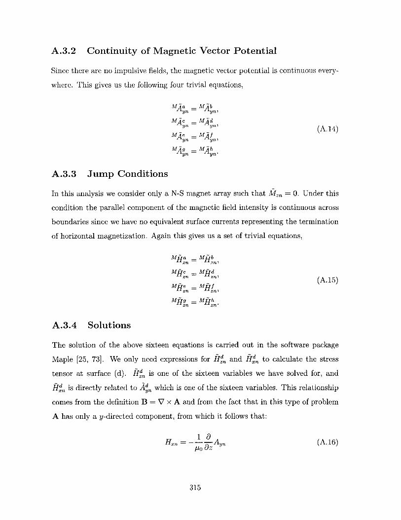
A.3.2 Continuity of Magnetic Vector Potential

Since there are no impulsive fields, the magnetic vector potential is continuous every-

where. This gives us the following four trivial equations,

MAa _MAbyn yn,

MAC _ MAdyn "n' (A.14)

MAe - MAfyn yn,

M g _ MAhyn yn-

A.3.3 Jump Conditions

In this analysis we consider only a N-S magnet array such that lz = 0. Under this

condition the parallel component of the magnetic field intensity is continuous across

boundaries since we have no equivalent surface currents representing the termination

of horizontal magnetization. Again this gives us a set of trivial equations,

Mfa - MftbHzn zfl

Mfc MftdH zcn -Lzn)(A .15)

Mge _ M f

MAYg - Mfth

A.3.4 Solutions

The solution of the above sixteen equations is carried out in the software package

Maple [25, 73]. We only need expressions for Hzn and Hn to calculate the stress

tensor at surface (d). Hz' is one of the sixteen variables we have solved for, and

fjd is directly related to A which is one of the sixteen variables. This relationship

comes from the definition B = V x A and from the fact that in this type of problem

A has only a y-directed component, from which it follows that:

108Hxn = -1aAyn (A.16)

Ao Oz

315

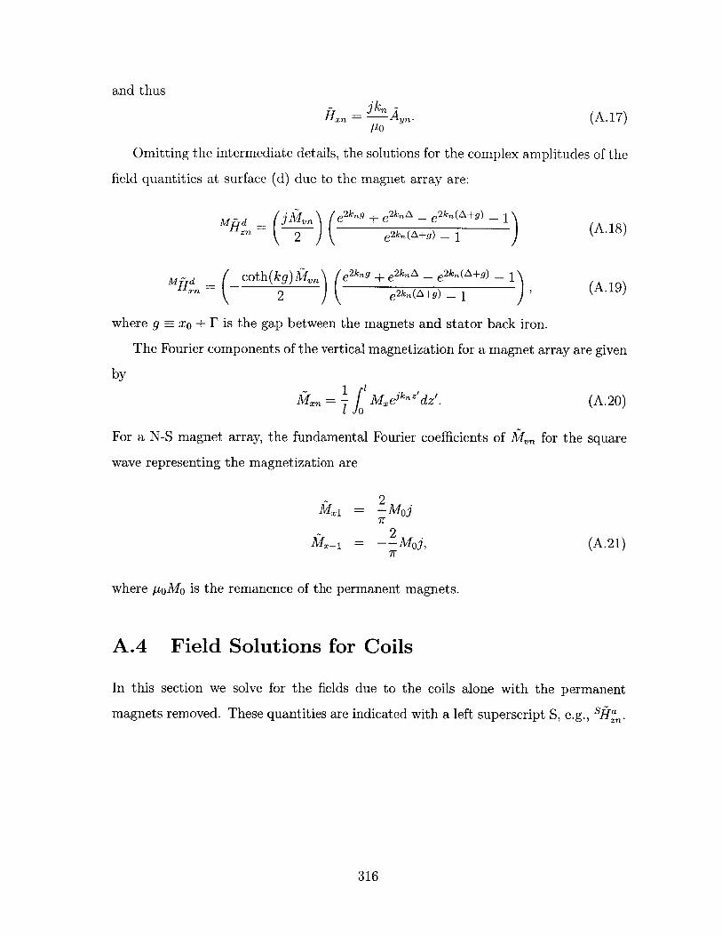
and thus

fix = jkn Ayn. (A. 17)Po

Omitting the intermediate details, the solutions for the complex amplitudes of the

field quantities at surface (d) due to the magnet array are:

Mfd =(jKvn' (e2kng + e2knA _ e 2 kn(A+g) _ izn = 2 e 2kn(A+g) - 1 (A.18)

Md ctkg) Men )e2k" + e2knA _ e 2kn (A +9) _Mfd 2 ) + 2 () - ) - 1), (A.19)

where g = xo + F is the gap between the magnets and stator back iron.

The Fourier components of the vertical magnetization for a magnet array are given

by

] r = Mxejk"z'dz'. (A.20)

For a N-S magnet array, the fundamental Fourier coefficients of Mn for the square

wave representing the magnetization are

~ 2Mk1 = -Moj

7

211_1 = -_Moj, (A.21)

7r~

where poMo is the remanence of the permanent magnets.

A.4 Field Solutions for Coils

In this section we solve for the fields due to the coils alone with the permanent

magnets removed. These quantities are indicated with a left superscript S, e.g., Sftza

316

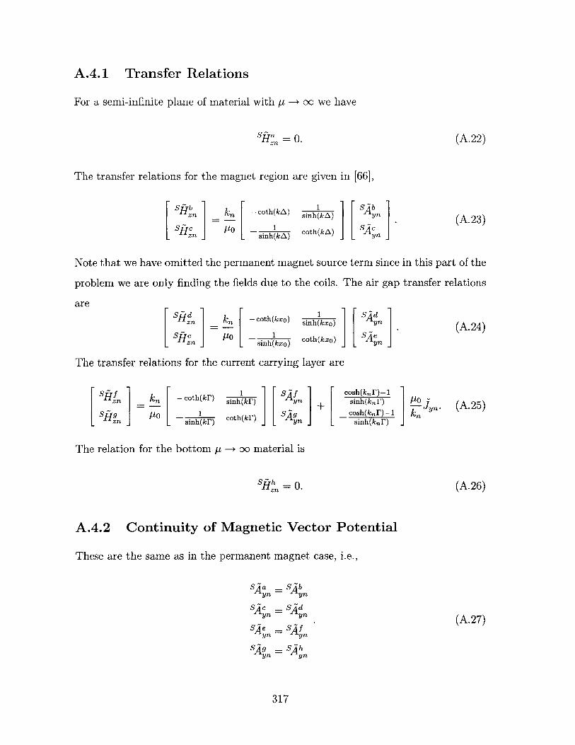
A.4.1 Transfer Relations

For a semi-infinite plane of material with p -+ oc we have

Sfta = 0.T Zn

The transfer relations for the magnet region are given in [661,

[ -coth(kA)

1sinh(kEA)

1isinh(kA)

coth(kA)

SAbyn

SAcyn

(A.22)

(A.23)INote that we have omitted the permanent magnet source term since in this part of the

problem we are only finding the fields due to the coils. The air gap transfer relations

are

[ k[_PO

-coth(kxo)

1sinh(kxO)

iisinh(kxo)

coth(kxo)

The transfer relations for the current carrying layer are

[SAdyn

ynJ

(A.24)

1 1thk [S f 1- coth(P) sinh(kr) yn1 coth(k I) SI

sinh(kF) JtL) yn J+

cosh(knF)-1 1sinh(kn]r)cosh(k F) -1

sinh(knr) J

The relation for the bottom p -+ oc material is

SHzn = 0.

A.4.2 Continuity of Magnetic Vector Potential

These are the same as in the permanent magnet case, i.e.,

SAa = SAbyn yn

SAC = SAdyn yn

SAe _SA fyn yn

S = SA hyn yn

317

[Sft f1zn

Sp Izn j

(A.25)

(A.26)

(A.27)

Hzn _j

Sfjdzn

S zn

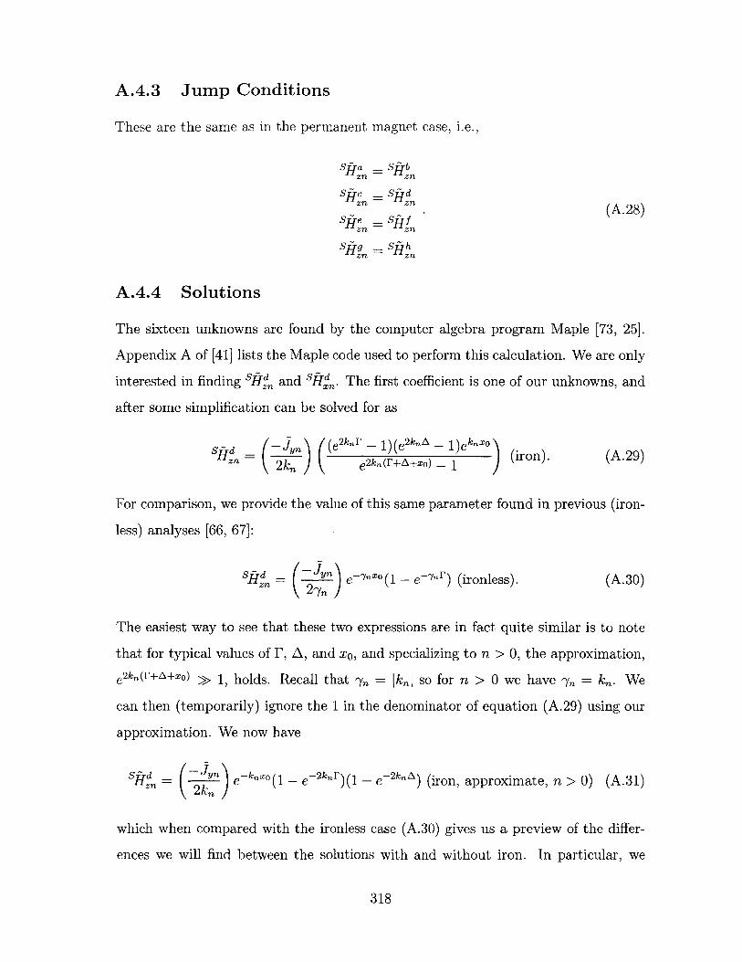
A.4.3 Jump Conditions

These are the same as in the permanent magnet case, i.e.,

S - - SftbHZn 21Zn

Sf c - S/pHzn 2fl (A.28)Sf~ - S/fzn zn

Hzn -Lzn

A.4.4 Solutions

The sixteen unknowns are found by the computer algebra program Maple [73, 25].

Appendix A of [41] lists the Maple code used to perform this calculation. We are only

interested in finding SfIn and Sid . The first coefficient is one of our unknowns, and

after some simplification can be solved for as

Sftd (=~ ( (e2 knP - 1) (e2kA - 1)eknXO.s 2kJ e2kn(r+A+xo) - 1 ) (iron). (A.29)

For comparison, we provide the value of this same parameter found in previous (iron-

less) analyses [66, 67]:

sfJ - ( n) e-YnXo (1 - e -^n) (ironless). (A.30)

The easiest way to see that these two expressions are in fact quite similar is to note

that for typical values of IF, A, and xo, and specializing to n > 0, the approximation,

e 2kn(F+A+xo) > 1, holds. Recall that -yn = IknI so for n > 0 we have 'y1 = kn. We

can then (temporarily) ignore the 1 in the denominator of equation (A.29) using our

approximation. We now have

sd ( - ) eknxo _ 2 knP(1 - e 2 knA) (iron, approximate, n > 0) (A.31)

which when compared with the ironless case (A.30) gives us a preview of the differ-

ences we will find between the solutions with and without iron. In particular, we

318

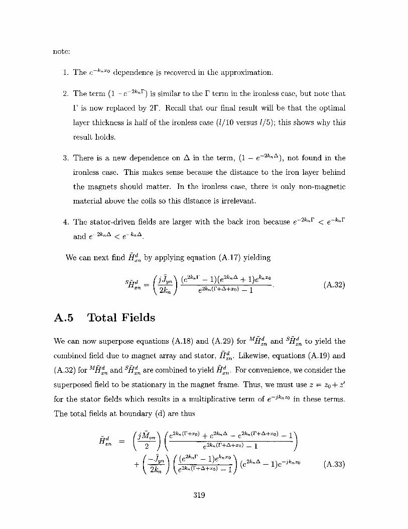
note:

1. The e-kxo dependence is recovered in the approximation.

2. The term (1 - e- 2kF) is similar to the F term in the ironless case, but note that

F is now replaced by 2F. Recall that our final result will be that the optimal

layer thickness is half of the ironless case (1/10 versus 1/5); this shows why this

result holds.

3. There is a new dependence on A in the term, (1 - e- 2knA), not found in the

ironless case. This makes sense because the distance to the iron layer behind

the magnets should matter. In the ironless case, there is only non-magnetic

material above the coils so this distance is irrelevant.

4. The stator-driven fields are larger with the back iron because e- 2kF < e-kar

and e-- 2knA <e-knA

We can next find H, by applying equation (A.17) yielding

S _ d jyn i (e 2 kn,' - 1)(e 2 knA + 1)eknxo

= x 2kJ e2kn(r+A+xo) - 1(A32)

A.5 Total Fields

We can now superpose equations (A.18) and (A.29) for Mfjd and SHd to yield the

combined field due to magnet array and stator, Hn. Likewise, equations (A.19) and

(A.32) for Mffd and skId are combined to yield Hxn. For convenience, we consider the

superposed field to be stationary in the magnet frame. Thus, we must use z = zo + z'

for the stator fields which results in a multiplicative term of e-knzo in these terms.

The total fields at boundary (d) are thus

H - _d lkn e 2kn (1'+xo) + e2knA _ ± 2kn(r+A+xo)_

zn - 2 )(e e2 kn ( -+A+xo) _ -

(-jyn) ((e 2 knr - 1)eknxo

2kJ e2kn(r+A+xo) - 1 )e- (A.33)

319

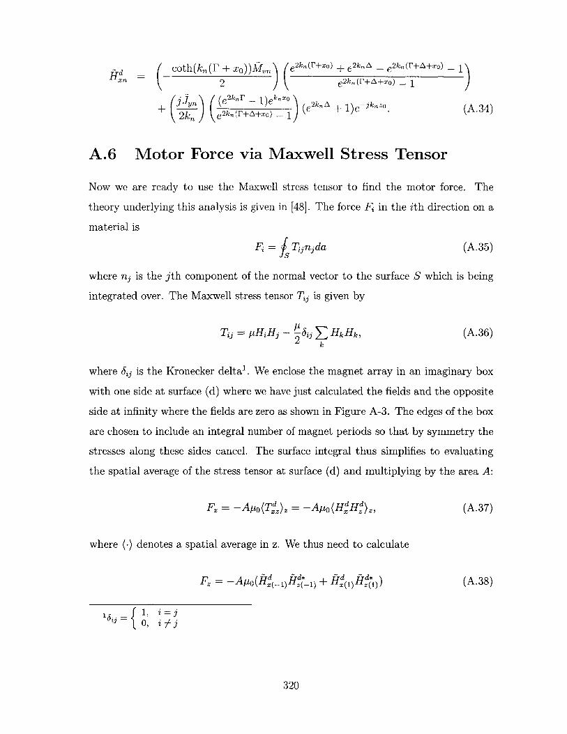
ft = coth(kn(IF + Xo))fkvn) e2k((r+xo) _ e 2 knA - e2k,(r+A+xo) _Hn 2 e2k,,(r+A+xo)-

+ jy (e 2knr _ k.xo 2n kZ(+ k) (e 2kri1kxo) (e2knA _ -)e nzo. (A.34)

A.6 Motor Force via Maxwell Stress Tensor

Now we are ready to use the Maxwell stress tensor to find the motor force. The

theory underlying this analysis is given in [48]. The force F in the ith direction on a

material is

Fi= Tin da (A.35)

where n is the jth component of the normal vector to the surface S which is being

integrated over. The Maxwell stress tensor Tij is given by

Tj = ZHH - Aij 7 HH, (A.36)

where 6ij is the Kronecker delta1 . We enclose the magnet array in an imaginary box

with one side at surface (d) where we have just calculated the fields and the opposite

side at infinity where the fields are zero as shown in Figure A-3. The edges of the box

are chosen to include an integral number of magnet periods so that by symmetry the

stresses along these sides cancel. The surface integral thus simplifies to evaluating

the spatial average of the stress tensor at surface (d) and multiplying by the area A:

Fz = -Apo(Tiz)z = -Apo(HxHz)z, (A.37)

where (-) denotes a spatial average in z. We thus need to calculate

Fz = -Apo(H(- 1) H*-1) Hz+ (1)H()) (A.38)

16i{ 11 i =0, i 7 j

320

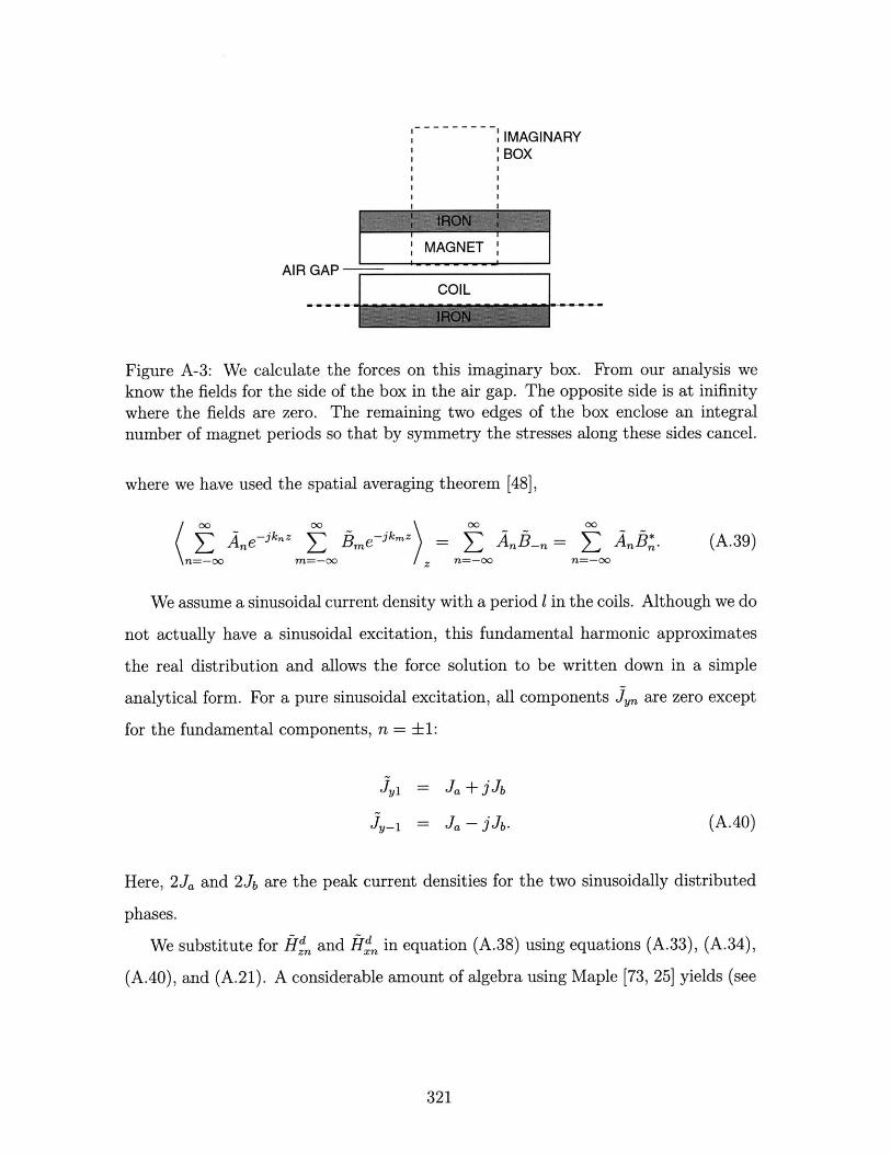
IMAGINARYBOX

MAGNETAIR GAP

COIL

Figure A-3: We calculate the forces on this imaginary box. From our analysis weknow the fields for the side of the box in the air gap. The opposite side is at inifinitywhere the fields are zero. The remaining two edges of the box enclose an integral

number of magnet periods so that by symmetry the stresses along these sides cancel.

where we have used the spatial averaging theorem [48],

(Eg0 Aneiknz E~o knmekz = =: A~3, E A. * (A.39)

We assume a sinusoidal current density with a period 1 in the coils. Although we do

not actually have a sinusoidal excitation, this fundamental harmonic approximates

the real distribution and allows the force solution to be written down in a simple

analytical form. For a pure sinusoidal excitation, all components Jyn are zero except

for the fundamental components, n = +1:

J1y = Ja + J

Jy_1 = Ja - jJ. (A.40)

Here, 2Ja and 2J are the peak current densities for the two sinusoidally distributed

phases.

We substitute for Hz" and H/d in equation (A.38) using equations (A.33), (A.34),

(A.40), and (A.21). A considerable amount of algebra using Maple [73, 25] yields (see

321

Appendix A of [41])

W2M 2 -eYXO(e2 YA - 1)(e 2Yr - 1)-F = poMo -2 e7a~~o (J. COS _YZ + A Sin ZO). (A.41)

This equation is the key result of this analysis. It predicts the force per spatial

wavelength produced by a motor with iron behind the magnets and coils, and with

a sinusoidally distributed stator winding. This result is an extension of the results

in [66, 67] which accounts for the back iron. Our analysis was for a N-S magnet

array, but a simple adjustment of equation (A.21) will allow for other arrays such

as the Halbach configuration. For comparison, we repeat-in a suggestive form-the

solution for the ironless case with a Halbach magnet array which has appeared in

several papers [66, 67]:

F2= 1PMo /2 [(I - eyr)(I - e-^YA)e-Yxo (J cOS Yzo + JA sin yzo). (A.42)72

Some comments are in order:

* The V2 in equation (A.42) is there since this equation applies to a motor using a

Halbach magnet array. For ironless motors, the Halbach magnet array produces

a field that is v times stronger than a conventional N-S magnet array. Had

a normal N-S array been used in that computation, the v'2 would not appear.

A comparison of four magnet arrays-regular N-S, four block Halbach, ideal

Halbach, and vertical sinusoidal-is done in a paper by Trumper et. al. [67].

Note well, however, that in the case of a motor with iron (A.41) the substitution

of a Halbach array for a N-S array will not improve the force by a factor of V2_.

The improvement will be much less. An intuitive explanation for this is that the

magnetic back iron is placed on the low-field side of the Halbach array and thus

affects the field less than for a N-S array. John Ofori offers another intuitive

explanation for the effects of back iron on magnet arrays using the Method of

Images [55].

This leads to the following pedantic point. The proper way to compare equa-

322

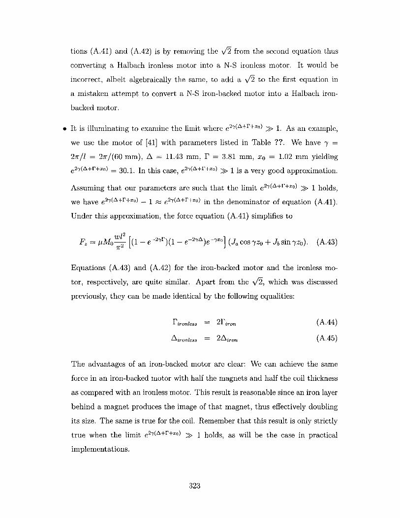
tions (A.41) and (A.42) is by removing the V12 from the second equation thus

converting a Halbach ironless motor into a N-S ironless motor. It would be

incorrect, albeit algebraically the same, to add a x/'2 to the first equation in

a mistaken attempt to convert a N-S iron-backed motor into a Halbach iron-

backed motor.

e It is illuminating to examine the limit where e2y(A+r+xo) > 1. As an example,

we use the motor of [41] with parameters listed in Table ??. We have -y =

27r/l = 27r/(60 mm), A = 11.43 mm, F = 3.81 mm, xo = 1.02 mm yielding

e 2(A+r+xo) = 30.1. In this case, e2 y(A+r+xo) > 1 is a very good approximation.

Assuming that our parameters are such that the limit e27(A+r+xo) > 1 holds,

we have e2-(A+r+xo) _ I . e2-y(A+r+xo) in the denominator of equation (A.41).

Under this approximation, the force equation (A.41) simplifies to

F= uMo- [(1 - e-2r)( _-2, )--,e' (Ja cosyzo + Jbsin yzo). (A.43)

Equations (A.43) and (A.42) for the iron-backed motor and the ironless mo-

tor, respectively, are quite similar. Apart from the V2, which was discussed

previously, they can be made identical by the following equalities:

Fironless = 2firom (A.44)

Aironiess = 2Airon (A.45)

The advantages of an iron-backed motor are clear: We can achieve the same

force in an iron-backed motor with half the magnets and half the coil thickness

as compared with an ironless motor. This result is reasonable since an iron layer

behind a magnet produces the image of that magnet, thus effectively doubling

its size. The same is true for the coil. Remember that this result is only strictly

true when the limit e2-(A++xo) > 1 holds, as will be the case in practical

implementations.

323

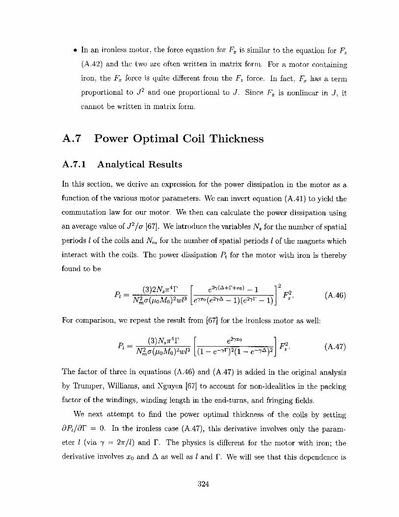
* In an ironless motor, the force equation for F, is similar to the equation for F

(A.42) and the two are often written in matrix form. For a motor containing

iron, the F, force is quite different from the F, force. In fact, F, has a term

proportional to J 2 and one proportional to J. Since F. is nonlinear in J, it

cannot be written in matrix form.

A.7 Power Optimal Coil Thickness

A.7.1 Analytical Results

In this section, we derive an expression for the power dissipation in the motor as a

function of the various motor parameters. We can invert equation (A.41) to yield the

commutation law for our motor. We then can calculate the power dissipation using

an average value of J 2 /a [67]. We introduce the variables N for the number of spatial

periods 1 of the coils and Nm for the number of spatial periods 1 of the magnets which

interact with the coils. The power dissipation Pt for the motor with iron is thereby

found to be

(3)2N, 7F L e 2 y(A+r+xo) _ 1 ] 2N2 - (2oMo)2w 3 [e-o(e2yA _ 1)(e2 r - 1) F (A.46)

For comparison, we repeat the result from [67] for the ironless motor as well:

(3)N,7r4r e 2-yo2N,27(poMo)2wl 3 (I _ e-yr)2(7 - e-YA)2] F (A.47)

The factor of three in equations (A.46) and (A.47) is added in the original analysis

by Trumper, Williams, and Nguyen [67] to account for non-idealities in the packing

factor of the windings, winding length in the end-turns, and fringing fields.

We next attempt to find the power optimal thickness of the coils by setting

OPt/t9F = 0. In the ironless case (A.47), this derivative involves only the param-

eter 1 (via y = 27r/i) and F. The physics is different for the motor with iron; the

derivative involves xo and A as well as 1 and F. We will see that this dependence is

324

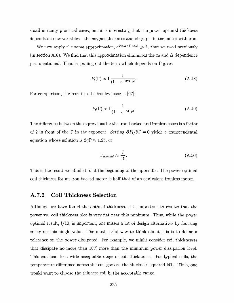
small in many practical cases, but it is interesting that the power optimal thickness

depends on new variables-the magnet thickness and air gap-in the motor with iron.

We now apply the same approximation, e 2^(+r+xo) >> 1, that we used previously

(in section A.6). We find that this approximation eliminates the xo and A dependence

just mentioned. That is, pulling out the term which depends on F gives

Pt(F) oc F - (A.48)(1 - e(A.)

For comparison, the result in the ironless case is [67]:

Pt (r) oc r . (A.49)(1 - e--Y)2

The difference between the expressions for the iron-backed and ironless cases is a factor

of 2 in front of the F in the exponent. Setting DPt/F = 0 yields a transcendental

equation whose solution is 2yF = 1.25, or

Foptima e -. (A.50)roptmal 10'

This is the result we alluded to at the beginning of the appendix. The power optimal

coil thickness for an iron-backed motor is half that of an equivalent ironless motor.

A.7.2 Coil Thickness Selection

Although we have found the optimal thickness, it is important to realize that the

power vs. coil thickness plot is very flat near this minimum. Thus, while the power

optimal result, 1/10, is important, one misses a lot of design alternatives by focusing

solely on this single value. The most useful way to think about this is to define a

tolerance on the power dissipated. For example, we might consider coil thicknesses

that dissipate no more than 10% more than the minimum power dissipation level.

This can lead to a wide acceptable range of coil thicknesses. For typical coils, the

temperature difference across the coil goes as the thickness squared [41]. Thus, one

would want to choose the thinnest coil in the acceptable range.

325

However, if a cooling system such as the separated end-turn cooling scheme shown

in Figure 6-24 and documented in [41] is used, the coil temperature rise does not

depend on coil thickness. In this case, we want to choose the thickest coil in our

acceptable range defined by power dissipation. We do this because each coil thickness

in the acceptable range dissipates roughly the same power and produces exactly the

same force. If we are producing the same force with a thicker coil, the current density

must be smaller than it would be for a thin coil. If the coil is thicker by a factor of

k, it will produce k times more force if the magnetic field and current density are the

same. The magnetic field will be reduced since there is now a larger effective air gap.

However, the magnetic field falls off slower than 1/k, and so the current density in

the coil must also be smaller. Hence, we can probably increase the current density in

the thicker coil until we again reach the limit of our cooling system.

326

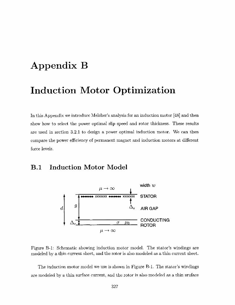
Appendix B

Induction Motor Optimization

In this Appendix we introduce Melcher's analysis for an induction motor [48] and then

show how to select the power optimal slip speed and rotor thickness. These results

are used in section 3.2.1 to design a power optimal induction motor. We can then

compare the power efficiency of permanent magnet and induction motors at different

force levels.

B.1 Induction Motor Model

I -+ 00 'I....... xxxxxxx ..... XXXXx

9 AS

Tr~~l a p-o

width w

STATOR

AIR GAP

CONDUCTINGROTOR

L -+ 00

Figure B-1: Schematic showing induction motor model. The stator's windings aremodeled by a thin current sheet, and the rotor is also modeled as a thin current sheet.

The induction motor model we use is shown in Figure B-1. The stator's windings

are modeled by a thin surface current, and the rotor is also modeled as a thin sruface

327

d

current. The actual stator windings have a thickness, A,,, and the actual rotor has a

thickness, Ar. The motor's actual air gap is g, but since our motor analysis assumes

an infinitely thin rotor, we account for the rotor's actual thickness, Ar, by using an

effective air gap,

d = g + A,. (B.1)

We do not include the stator thickness, since we assume that the stator windings

are wound in slots. The motor has a width, w. The rotor has conductivity, a,

and permeability, Mo. For simplicity we assume the stator windings have the same

conductivity, a, as the rotor. The stator and rotor are backed by infinitely permeable

backiron.

The wavelength of the stator coils is 1, and it is convenient to define the wavenum-

ber k = 27r/l. The stator is excited with balanced sinusoidal two phase currents with

frequency w such that the resulting current density wave is a pure traveling wave.

Phase a has Na peak turns per unit length and current amplitude I. The rotor

moves with linear speed U relative to the stator. We define a dimensionless num-

ber, S+, following [48] which is proportional to the slip speed, w/k - U. This slip

occurs between the speed of the traveling wave of stator currents, w/k, and the rotor

mechanical speed, U. The dimensionless slip speed is

S+ = k (w - kU). (B.2)

As derived by Melcher [48], the induction motor produces a force,

1W/ pO S+NZ I2F= .wa (B.3)

2 sinh2 (kd) \\1 + S2 coth2(kd)) (

By integrating the Joule heating in the two current sheets we obtain an expression

for the total power, P, dissipated in the induction motor,

2w N 2 1 S2P = wI Na( + + (B.4)

2 (AsOl Au sinh2(kd) (1 + S+ coth 2 (kd))

328

Here the first term is due to power dissipated on the stator, and the second term is due

to power dissipated on the rotor. Solving equation (B.3) for N2I- and substituting

into equation (B.4) yields power for a given force,

p sinh2(kd) (1 + Si coth 2 (kd)) S++ .(B.5)

F AsoIpoS+ ArUJo

We use this expression to find the power optimal slip speed, S+, and rotor thickness,

B.2 Power Optimal Slip Speed

We find the power optimal slip speed, S+, by finding the slip speed which minimizes

power dissipation, equation (B.5),

a - = 0. (B.6)aS+ (F)

After some algebra, we find that the power optimal slip speed, S+, is a function of

rotor thickness, Ar, stator thickness, A., and kd,

Ar sinh 2(kd) 2

S+(Ar, AS, kd) = 2 . (B.7)(A'r cosh2(kd) + As)

B.3 Power Optimal Rotor Thickness

We try to find the power optimal rotor thickness, a,, in the same way by solving,

( - = 0. (B.8)

However, this results in an algebraic equation which is fourth order in Ar. Since it is

difficult to solve this equation analytically, we solve it numerically by plotting P/F

as a function of Ar as shown in Figure B-2. Since power optimal slip frequency, S+,

is a function of rotor thickness, Ar, we calculate S+(Ar, As, kd) for each value of Ar.

329

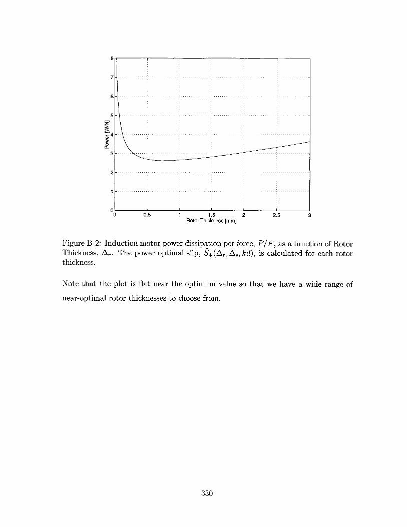
6- -

a.

0'0 0.5 1 1.5 2 2.5 3

Rotor Thickness [mm]

Figure B-2: Induction motor power dissipation per force, P/F, as a function of RotorThickness, A,. The power optimal slip, S+(Ar, As, kd), is calculated for each rotorthickness.

Note that the plot is flat near the optimum value so that we have a wide range of

near-optimal rotor thicknesses to choose from.

330

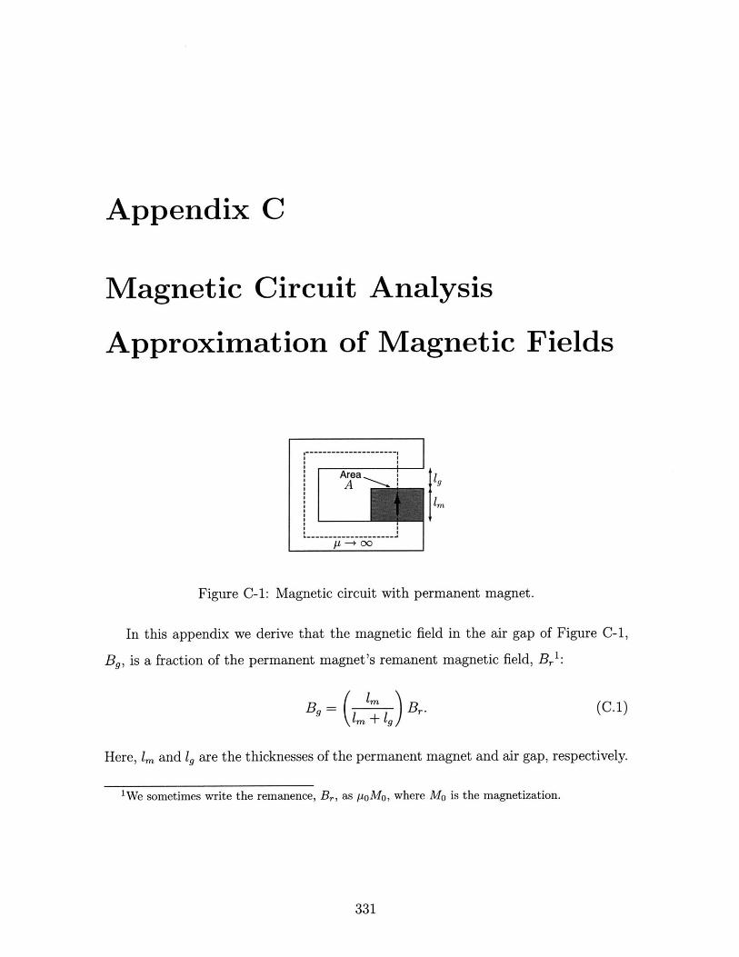
Appendix C

Magnetic Circuit Analysis

Approximation of Magnetic Fields

Area

im

Figure C-1: Magnetic circuit with permanent magnet.

In this appendix we derive that the magnetic field in the air gap of Figure C-1,

B9 , is a fraction of the permanent magnet's remanent magnetic field, B,1:

B= ( i) Br. (C.1)(1m + 19)

Here, 1m and 19 are the thicknesses of the permanent magnet and air gap, respectively.

1We sometimes write the remanence, Br, as poMo, where MO is the magnetization.

331

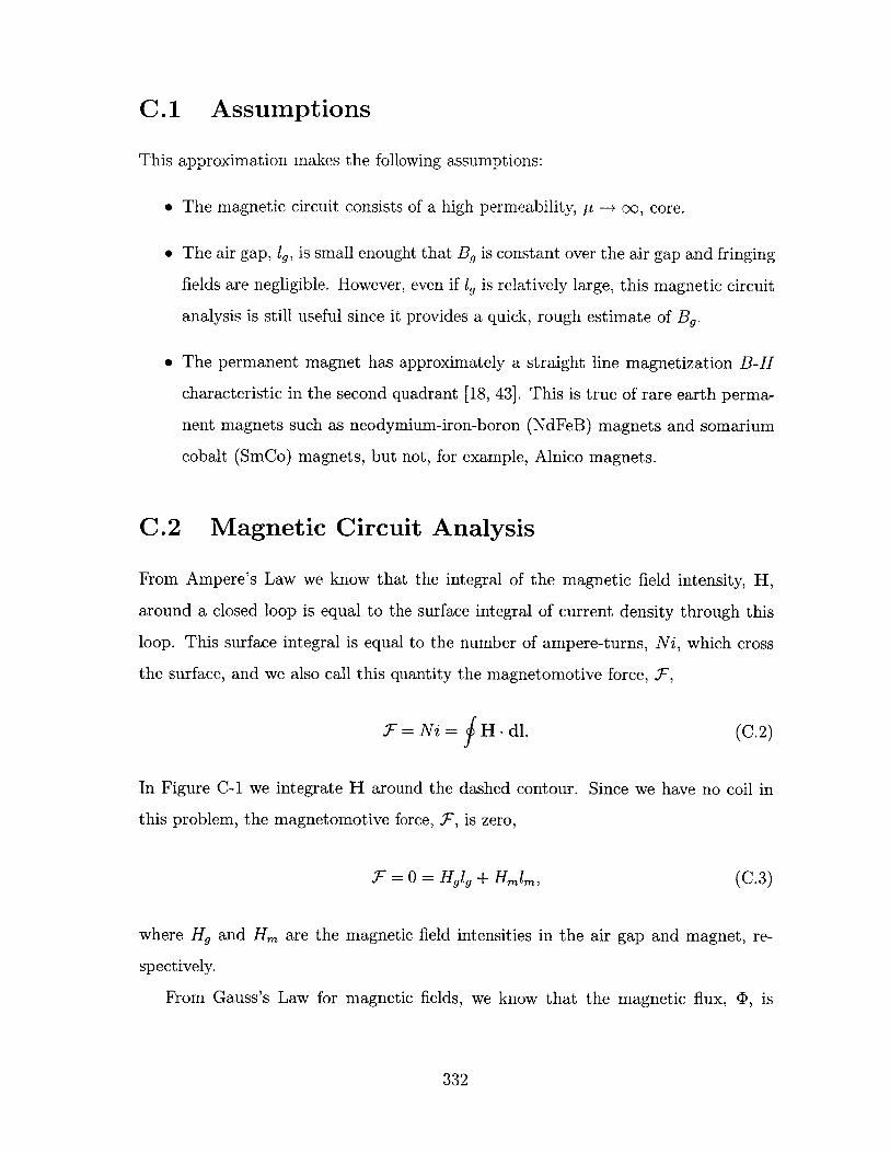
C. 1 Assumptions

This approximation makes the following assumptions:

" The magnetic circuit consists of a high permeability, p --+ o, core.

" The air gap, 1g, is small enought that B. is constant over the air gap and fringing

fields are negligible. However, even if 1g is relatively large, this magnetic circuit

analysis is still useful since it provides a quick, rough estimate of B..

" The permanent magnet has approximately a straight line magnetization B-H

characteristic in the second quadrant [18, 43]. This is true of rare earth perma-

nent magnets such as neodymium-iron-boron (NdFeB) magnets and somarium

cobalt (SmCo) magnets, but not, for example, Alnico magnets.

C.2 Magnetic Circuit Analysis

From Ampere's Law we know that the integral of the magnetic field intensity, H,

around a closed loop is equal to the surface integral of current density through this

loop. This surface integral is equal to the number of ampere-turns, Ni, which cross

the surface, and we also call this quantity the magnetomotive force, F,

F = Ni = H - dl. (C.2)

In Figure C-1 we integrate H around the dashed contour. Since we have no coil in

this problem, the magnetomotive force, F, is zero,

m =0 = H91g+ Hm, (C.3)

where H. and Hm are the magnetic field intensities in the air gap and magnet, re-

spectively.

From Gauss's Law for magnetic fields, we know that the magnetic flux, <D, is

332

continuous, so

BgA = BA, (C.4)

or

B, = Bm (C.5)

since the areas are equal in this example.

The only other relationships we need to solve the problem are the constitutive laws

for the air gap and permanent magnet which relate magnetic field, B, to magnetic

field intensity, H. For the air gap, we assume a pemeability of Mo,

B9 = poHg. (C.6)

For the permanent magnet, we assume a straight line B-H characterisitc in the second

quadrant,

Bm = Br + pOHm. (C.7)

Combining equations (C.3), (C.5), (C.6), and (C.7) and solving for B. yields the

result, equation (C.1),

Bg= "i Br.IM + 19

333

334

Appendix D

Mechanical Drawings

D.1 Shaft

335

SEE DETAIL LEFT SIDE SEE DETAIL R IGHT SIDE

CLASS N 60 Case Shafting

-. 7500+000

SCALE 0.500

-- 4.267 REF- c 8.833 REF ca 2. 130 REt-

-=315. 230 RE F EBB-

- -m .210 -e

E- .375 REF - -

EAN. THREADMPIN. THREA) LENGTHLENGTH

.446 .716 - : .480: |[ 2.040

0.560 67 0.0000-. 7 -0.0005

-0.500 + * 0000DETA IL LEFT S IDE.37 o+--.0005 SCALE 2.000-0.0005

0H-0I (N-0) LOCKNUT THREADS H-03 (N-03) LOCKNUT THREADS32 PER INCH32PRIC

ALL UNMARKED RADII AT STEPS IN SHAFT0.015 RAD

MIN. THREADLENGTH

.25 1.580- .550-

DETAIL RIGHT SIDE.125 SCAL E 2. 000 381 HED

Figure D-1: Shaft mechanical drawing

336

--

----------- -

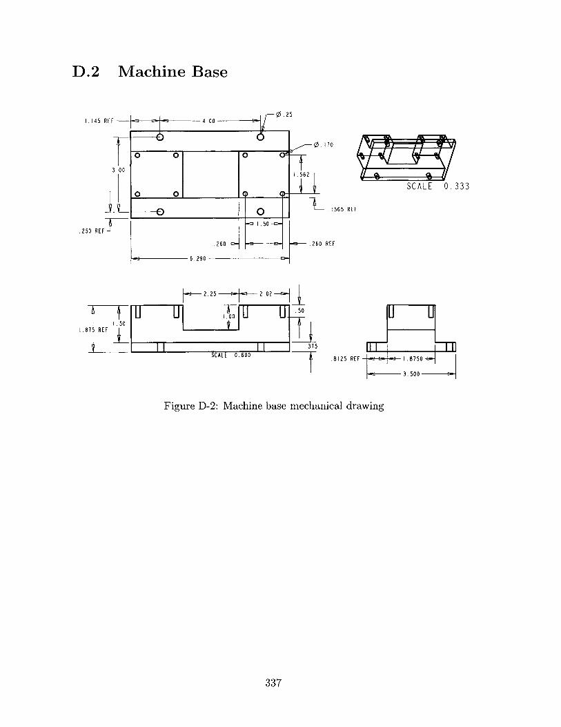
D.2 Machine Base

3.00

I- .' -

o o 0

o 0 0 __

0 01 0

.250 RET

.260 1

6.290

0 . 170

1562

.1565 REF

.260 REF

2.25 2.02

50

1.875 REF I.0

375

SCALE 0.600.8125 REF 1.875

3.500

Figure D-2: Machine base mechanical drawing

337

1.145 ~-t--- r-K

SCALE 0.333

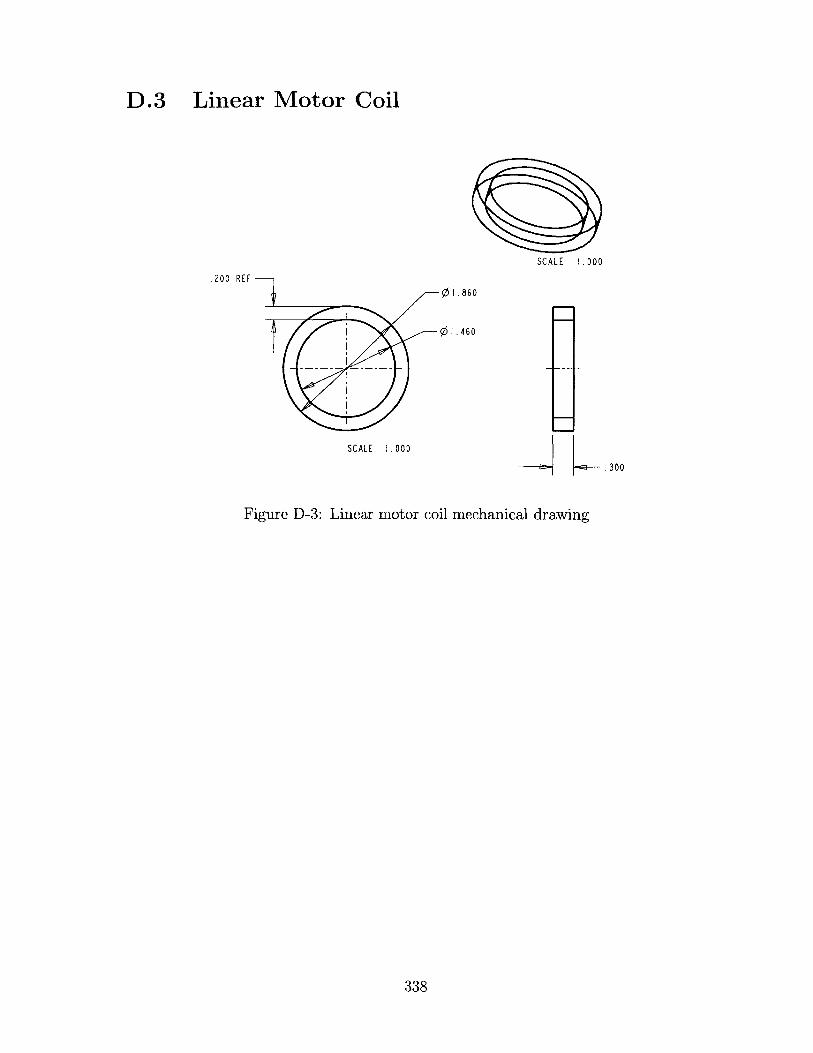
D.3 Linear Motor Coil

0SCALE 1.000

.200 REF

01.860

01.460

SCALE 1.000

F300

Figure D-3: Linear motor coil mechanical drawing

338

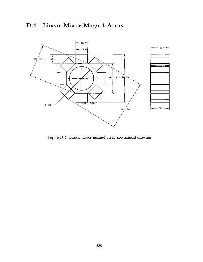
D.4 Linear Motor Magnet Array

-- .350m

7-325

.915 REF .255

845 REF 1.355

0.671

1.393 REF

Figure D-4: Linear motor magnet array mechanical drawing

339

.50

.520

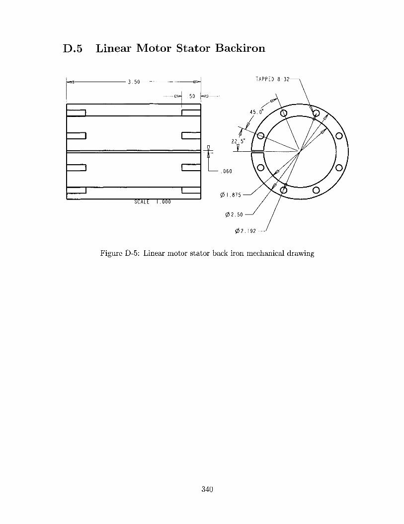
D.5 Linear Motor Stator Backiron

3. 50

.50

TAPPED 8-32

4 5. 0

060 0

01.875U

O2.50

02 .192

Figure D-5: Linear motor stator back iron mechanical drawing

340

SCALE 1.000

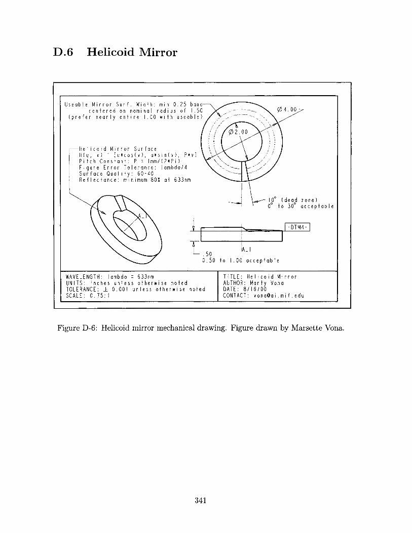
D.6 Helicoid Mirror

Useable Mirror Surf. Width: min 0.25 bandcentered on nominal radius of 1.50 0 4.00

(prefer nearly entire l.00 with useable)

02.00

Helicoid Mirror SurfaceH (u, V) : [U*C05(V), U*5in(V), P*V]Pitch Constant: P Imm/(2*Pi)Figure Error Tolerance: lambda/4Surface Quality: 60-40Reflectance: minimum 80% at 633nm

100 (de ad z00 t o 3 00 a cpaIe

I- --DTM4-

A- I

to 1.00 acceptable0.50

WAVELENGTH: lambda : 633nm TITLE: He licoid MirrorUNITS: inches unless otherwise noted AUTHOR: Mar ty VonaTOLERANCE: ± 0.001 unless otherwise n otfed DATE: 8/16/00SCALE: 0.75:1 CONTACT: vona@ai.mit.edu

Figure D-6: Helicoid mirror mechanical drawing. Figure drawn by Marsette Vona.

341

cceptable

342

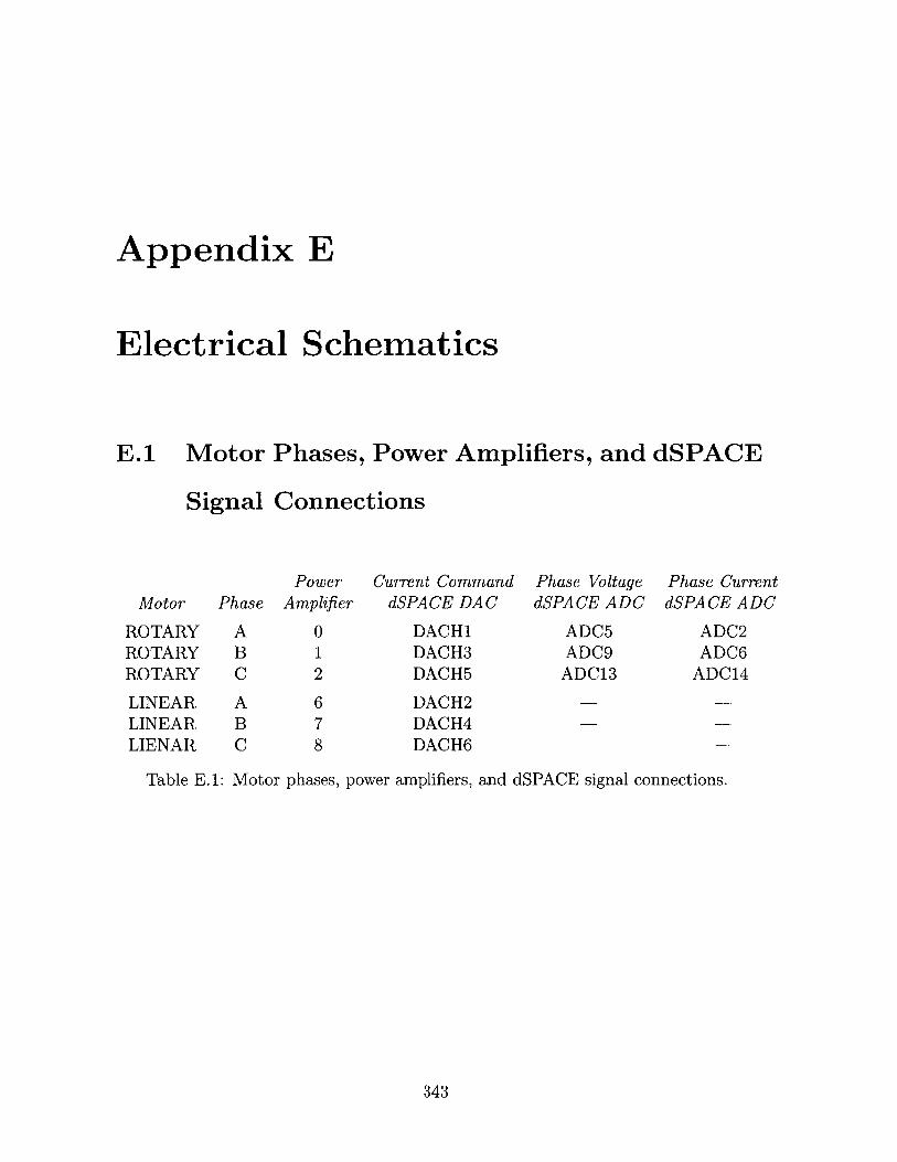
Appendix E

Electrical Schematics

E.1 Motor Phases, Power Amplifiers, and dSPACE

Signal Connections

PowerMotor Phase Amplifier

ROTARYROTARYROTARY

LINEARLINEARLIENAR

ABC

ABC

012

678

Current CommanddSPACE DAC

DACHIDACH3DACH5

Phase VoltagedSPACE ADC

ADC5ADC9

ADC13

Phase CurrentdSPACE ADC

ADC2ADC6

ADC14

DACH2DACH4DACH6

Table E.1: Motor phases, power amplifiers, and dSPACE signal connections.

343

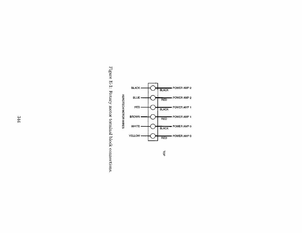
BLACK -

BLUE -

RED -

BROWN -

WHITE -

YELLOW -

- POWER AMP 2BLCK

- POWER AMP 2

- POWER AMP 1BLACK

- POWER AMP 1RED

- POWER AMP 0

POWER AMP 0

O'-

0

C+

9)00

0

0 -I0-u

m

0-I

mC*)

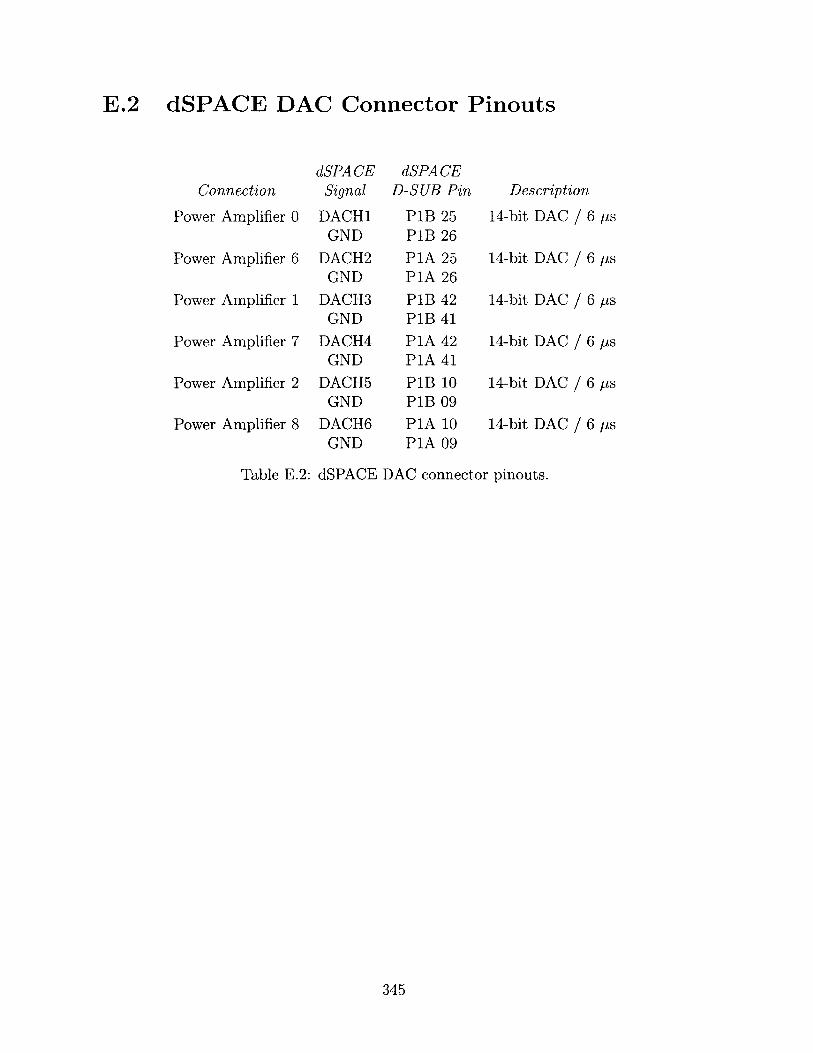
E.2 dSPACE DAC Connector Pinouts

Connection

Power Amplifier 0

Power Amplifier 6

Power Amplifier 1

Power Amplifier 7

Power Amplifier 2

Power Amplifier 8

dSPA CESignal

DACHIGND

DACH2GND

DACH3GND

dSPA CED-SUB Pin

PiB 25PiB 26PIA 25PIA 26PiB 42PiB 41

DACH4 P1A 42GND P1A 41

DACH5GND

DACH6GND

PiB 10PiB 09PIA 10PIA 09

Description

14-bit DAC / 6 ps

14-bit DAC / 6 ps

14-bit DAC / 6 ps

14-bit DAC / 6 ps

14-bit DAC / 6 ps

14-bit DAC / 6 ps

Table E.2: dSPACE DAC connector pinouts.

345

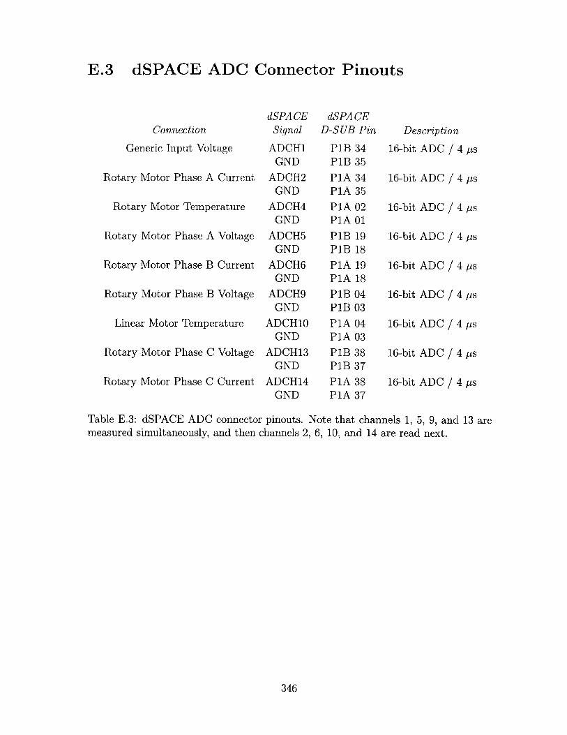
E.3 dSPACE ADC Connector Pinouts

Connection

Generic Input Voltage

Rotary Motor Phase A Current

Rotary Motor Temperature

Rotary Motor Phase A Voltage

Rotary Motor Phase B Current

Rotary Motor Phase B Voltage

Linear Motor Temperature

Rotary Motor Phase C Voltage

Rotary Motor Phase C Current

dSPA CESignal

ADCH1GND

ADCH2GND

ADCH4GND

ADCH5GND

ADCH6GND

ADCH9GND

ADCH1OGND

ADCH13GND

ADCH14GND

dSPA CED-SUB Pin

P1BP1B

PlAPlA

PIAPlA

PIBP1B

PlAPIA

P1BPIB

PlAPIA

PIBP1B

PIAPIA

3435

34350201191819180403040338373837

Description

16-bit ADC / 4 ps

16-bit ADC / 4 ps

16-bit ADC / 4 ps

16-bit ADC / 4 ps

16-bit ADC / 4 ps

16-bit ADC / 4 ps

16-bit ADC / 4 ps

16-bit ADC / 4 ps

16-bit ADC / 4 ps

Table E.3: dSPACE ADC connector pinouts. Note that channels 1, 5, 9, and 13 aremeasured simultaneously, and then channels 2, 6, 10, and 14 are read next.

346

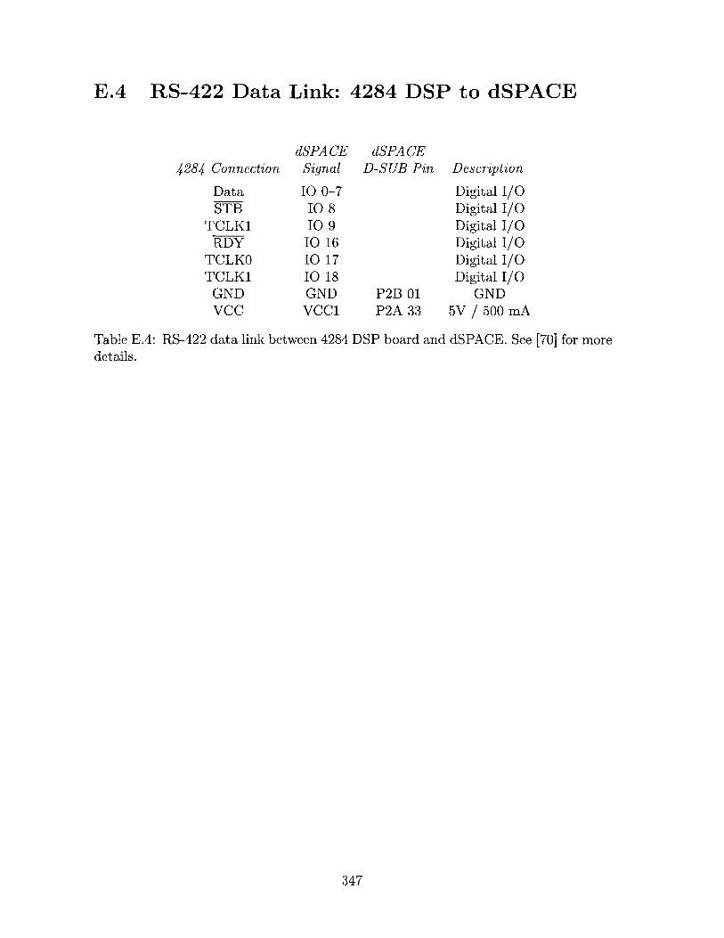
E.4 RS-422 Data Link: 4284 DSP to dSPACE

4284 Connection

DataSTB

TCLK1RDY

TCLKOTCLK1

GNDvcC

dSPA CESignal

10 0-7108109

10 16IO 17IO 18GNDvCci

dSPA CED-SUB Pin

P2B 01P2A 33

Description

Digital I/ODigital I/ODigital I/ODigital I/ODigital I/ODigital I/O

GND5V / 500 mA

Table E.4: RS-422 data link between 4284details.

DSP board and dSPACE. See [70] for more

347

348

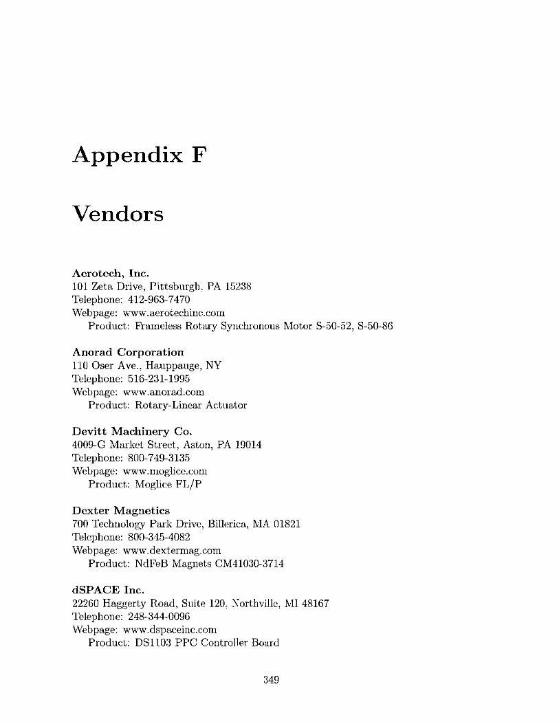
Appendix F

Vendors

Aerotech, Inc.101 Zeta Drive, Pittsburgh, PA 15238Telephone: 412-963-7470Webpage: www.aerotechinc.com

Product: Frameless Rotary Synchronous Motor S-50-52, S-50-86

Anorad Corporation110 Oser Ave., Hauppauge, NYTelephone: 516-231-1995Webpage: www.anorad.com

Product: Rotary-Linear Actuator

Devitt Machinery Co.4009-G Market Street, Aston, PA 19014Telephone: 800-749-3135Webpage: www.moglice.com

Product: Moglice FL/P

Dexter Magnetics700 Technology Park Drive, Billerica, MA 01821Telephone: 800-345-4082Webpage: www.dextermag.com

Product: NdFeB Magnets CM41030-3714

dSPACE Inc.22260 Haggerty Road, Suite 120, Northville, MI 48167Telephone: 248-344-0096Webpage: www.dspaceinc.com

Product: DS1103 PPC Controller Board

349

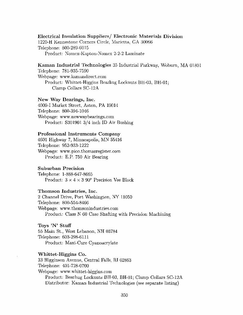
Electrical Insulation Suppliers/ Electronic Materials Division1220-H Kennestone Corners Circle, Marietta, GA 30066Telephone: 800-289-6015

Product: Nomex-Kapton-Nomex 2-2-2 Laminate

Kaman Industrial Technologies 35 Industrial Parkway, Woburn, MA 01801Telephone: 781-935-7590Webpage: www.kamandirect.com

Product: Whittet-Higgins Bearhug Locknuts BH-03, BH-01;Clamp Collars SC-12A

New Way Bearings, Inc.4009-I Market Street, Aston, PA 19014Telephone: 800-394-1046Webpage: www.newwaybearings.com

Product: S301901 3/4 inch ID Air Bushing

Professional Instruments Company4601 Highway 7, Minneapolis, MN 55416Telephone: 952-933-1222Webpage: www.pico.thomasregister.com

Product: E.P. 750 Air Bearing

Suburban PrecisionTelephone: 1-888-647-8665

Product: 3 x 4 x 3 900 Precision Vee Block

Thomson Industries, Inc.2 Channel Drive, Port Washington, NY 11050Telephone: 800-554-8466Webpage: www.thomsonindustries.com

Product: Class N 60 Case Shafting with Precision Machining

Toys 'N' Stuff55 Main St., West Lebanon, NH 03784Telephone: 603-298-6111

Product: Maxi-Cure Cyanoacrylate

Whittet-Higgins Co.33 Higginson Avenue, Central Falls, RI 02863Telephone: 401-728-0700Webpage: www.whittet-higgins.com

Product: Bearhug Locknuts BH-03, BH-01; Clamp Collars SC-12ADistributor: Kaman Industrial Technologies (see separate listing)

350

Wirewinders151 Mont Vernon Rd., Milford, NH 03055Telephone: 603-673-1763

Product: Linear Motor Coils

351

352

Bibliography

[1] Sensorless drives improve spindles. American Machinist, page 15, April 2001.

[2] Aerotech, Inc., 101 Zeta Drive, Pittsburgh, PA, 15238. S-Series Frameless MotorUser's Manual, August 2000.

[3] American Society of Mechanical Engineers, New York. Methods for PerformanceEvaluation of Computer Numerically Controlled Machining Centers, March 1993.ASME B5.54-1992.

[4] Analog Devices. Reference Frame Conversions with the ADMC401, June 1999.Application Note: AN401-11.

[5] Michael Tekletsion Berhan. Implementation of a halbach array in a tubular linearmotor. Master's thesis, Mechanical Engineering Dept., Massachusetts Instituteof Technology, June 1996.

[6] C. R. Boer, L. Molinari-Tosatti, and K. S. Smith, editors. Parallel KinematicMachines. Springer-Verlag, New York, 1999.

[7] Boston Digital Corporation, Granite Park, Milford, MA 01757. BostoMatic 505.

[8] Anwar Chitayat. Rotary-linear actuator. U. S. Pat. No. 5,982,053, AnoradCorporation, 1999.

[9] B. K. Choi, J. W. Park, and C. S. Jun. Cutter-location data optimization in5-axis machining. Computer-Aided Design, 25(6):377-386, June 1993.

[10] M. J. Corley and R. D. Lorenz. Rotor position and velocity estimation for apermanent magnet synchronous machine at standstill and high speeds. IEEETransactions on Industry Applications, 34(4):784-789, July 1998.

[11] Jame B. Dabney and Thomas L. Harman. Mastering Simulink 2. Prentice Hall,Upper Saddle River, NJ, 1998.

[12] Paul de Wit, Johannes van Dijk, Tim Blomer, and Peter Rutgers. Mechatronicdesign of a z-<0 induction actuator. In 1997 Eighth International Conference onElectrical Machines and Drives, pages 279-283, Stevenage, England, 1997.

[13] Deckel Maho Gildemeister America Inc., 13509 South Point Blvd., Charlotte,NC 28273. DMC U Series, DMU-P Series.

353

[14] Drew Devitt. History of air bearings. PT Design Motion Systems, April 1999.

[15] Richard C. Dorf. Modern Control Systems. Addison-Wesley Publishing Com-pany, New York, 1995.

[16] Gershon Elber. Freeform surface region optimization for 3-axis and 5-axis milling.Computer-Aided Design, 27(6):465-470, June 1995.

[17] Gershon Elber and Elaine Cohen. Toolpath generation for freeform surface mod-els. Computer-Aided Design, 26(6):490-496, June 1994.

[18] A. E. Fitzgerald, Jr. Charles Kingsley, and Stephen D. Umans. Electric Machin-ery. McGraw-Hill, Inc., New York, 1990.

[19] Gene F. Franklin, J. David Powell, and Michael Workman. Digital Control ofDynamic Systems. Addison-Wesley, Reading, Massachusetts, 1998.

[20] Chris French and Paul Acarnley. Control of permanent magnet motor drivesusing a new position estimation technique. IEEE Transactions on Industry Ap-plications, 32(5):1089-1097, September 1996.

[21] L. A. Gould, W. R. Markey, J. K. Roberge, and D. L. Trumper. Control systemstheory. Technical report, Massachusetts Institute of Technology, 1997.

[22] J. P. Den Hartog. Mechanical Vibrations. Dover Publications, Inc., New York,1985.

[23] Hermann A. Haus and James R. Melcher. Electromagnetic Fields and Energy.Prentice-Hall, Englewood Cliffs, New Jersey, 1989.

[24] Eugene Hecht. Optics. Addison Wesley Longman, Inc., New York, 1998.

[25] Andr6 Heck. Introduction to Maple. Springer, New York, 1996.

[26] Hermle Machine Co., 9600 S. Franklin Drive, Franklin, WI 53132. C600U,C800U, C1200U.

[27] Ingersoll Milling Machine Company, 707 Fulton Ave., Rockford, IL 61103. HighVelocity Profiler, High Velocity Gantry.

[28] JOBS, Inc., 1397 Piedmont Suite 100, Troy, MI 48083. Jo 'Tech, Jo 'Mach.

[29] Lawrence A. Jones and Jeffrey H. Lang. A state observer for the permanent-magnet synchronous motor. IEEE Transactions on Industrial Electronics,36(3):374-382, August 1989.

[30] Lawrence Anthony Jones. A state observer for the permanent magnet mo-tor. Master's thesis, Electrical Engineering and Computer Science Dept., Mas-sachusetts Institute of Technology, May 1988.

354

[31] Edward Kelby, Jr. and Alan G. Wallskog. Rotary & linear magnetomotive posi-tioning mechanism. U. S. Pat. No. 3,745,433, Teletype Corporation, 1971.

[32] Taejung Kim. Time-Optimal CNC Tool Paths: A Mathematical Model of Ma-chining. PhD thesis, Mechanical Engineering Dept., Massachusetts Institute ofTechnology, February 2001.

[33] Taejung Kim and Sanjay E. Sarma. Toolpath generation along directions ofmaximum kinematic performance; a first cut at machine-optimal paths. Acceptedby Computer Aided Design, 2001.

[34] Won-jong Kim. High-Precision Planar Magnetic Levitation. PhD thesis, Electri-cal Engineering and Computer Science Dept., Massachusetts Institute of Tech-nology, June 1997.

[35] James L. Kirtley Jr. 6.685 Electric Machinery Lecture Notes. Technical report,Massachusetts Institute of Technology, 2000.

[36] Wojciech B. Kosmowski. High speed drilling spindle with reciprocating ceramicshaft and double-gripping centrifugal chuck. U. S. Pat. No. 5,997,223, Electro-Scientific Industries, 1999.

[37] Markku S. Kotilainen. Design and Manufacturing of Modular Self-CompensatingHydrostatic Journal Bearings. PhD thesis, Mechanical Engineering Dept., Mas-sachusetts Institute of Technology, May 2000.

[38] Markku S. Kotilainen and Alexander H. Slocum. Manufacturing of cast mono-lithic hydrostatic journal bearings. Precision Engineering, 25(3):235-244, July2001.

[39] Jeffrey H. Lang, George C. Verghese, and Marija D. Ilic. Electrical MachineSystems: Dynamics, Estimation, and Control. Technical report, MassachusettsInstitute of Technology, 2000.

[40] Werner Leonhard. Control of Electrical Drives. Springer, New York, 1997.

[41] Michael Kevin Liebman. Thermally efficient linear motor analysis & design.Master's thesis, Mechanical Engineering Dept., Massachusetts Institute of Tech-nology, February 1998.

[42] Katie A. Lilienkamp and David L. Trumper. Dynamic signal analyzer for dspace.In Proceedings of the dSPACE User's Conference, May 2000.

[43] James D. Livingston. Driving Force: The Natural Magic of Magnets. HarvardUniversity Press, Cambridge, MA, 1996.

[44] Robert D. Lorenz. Advances in electric drive control. In Electric Machines andDrives, pages 9-16, 1999.

355

[45] Makino Inc., 7680 Innovation Way, Mason, OH 45040. V55-5XA, MC-5XA,MC-5XB.

[46] The Mathworks Inc. Stateflow User's Guide, September 2000.http://www.mathworks.com.

[47] Mazak Corporation, 8025 Production Drive, Florence, KY 41042. Mazatech H-630 5X, Mazatech V-815 5X.

[48] James R. Melcher. Continuum Electromechanics. The MIT Press, Cambridge,Massachusetts, 1981.

[49] Mikron Corp., 600 Pepper Street USA-Monroe, CT 06468. UCP710.

[50] Mori Seiki U.S.A., Inc., 9145 Currency Street, Irving, Texas 75063. M-400C1.

[51] K. Morishige, Y. Takeuchi, and K. Kase. Tool path generation using c-space for5-axis control machining. Journal of Manufacturing Science and Engineering,121:144-149, February 1999.

[52] J. F. Moynihan, P. Kettle, and A. Murray. High performance control of acservomotors using an integrated dsp. Intelligent Motion, pages 213-222, May1998.

[53] MTS Systems Corp., Automation Division, Eden Prairie, MN. SpindleBlok,DriveBlok, IndexBlock.

[54] Norman S. Nise. Control Systems Engineering. Addison-Wesley Publishing Com-pany, New York, 1995.

[55] John Ofori-Tenkorang. Permanent-Magnet Synchronous Motors and AssociatedPower Electronics for Direct-Drive Vehicle Propulsion. PhD thesis, ElectricalEngineering and Computer Science Dept., Massachusetts Institute of Technology,September 1996.

[56] Alan V. Oppenheim and Alan S. Willsky. Signals & Systems. Prentice Hall,Upper Saddle River, NJ, 1997.

[57] James K. Roberge. Operational Amplifiers, Theory and Practice. John Wiley &Sons, Inc., New York, 1975.

[58] Stuart C. Salmon. Modern Grinding Process Technology. McGraw-Hill, Inc.,New York, 1992.

[59] Raymond B. Sepe. Adaptive Control of the Permanent-Magnet SynchronousMotor. PhD thesis, Electrical Engineering and Computer Science Dept., Mas-sachusetts Institute of Technology, September 1990.

356

[60] Raymond B. Sepe and Jeffrey H. Lang. Real-time observer-based (adaptive)control of a permanent-magnet synchronous motor without mechanical sensors.IEEE Transactions on Industry Applications, 28(6):1345-1352, November 1992.

[61] S. T. Smith and D. G. Chetwynd. Foundations of Ultraprecision MechanismDesign. Gordon and Breach Science Publishers, Canda, 1997.

[62] Suk-Hwan Suh and Jung-Jae Lee. Five-axis part machining with three-axis cncmachine and indexing table. Transactions of the ASME, Journal of Manufac-turing Science and Engineering, 120(22):120-128, February 1988.

[63] Texas Instruments Europe. Field Orientated Control of 3-Phase AC-Motors,February 1998. Literature Number: BPRA073.

[64] Jiri Tlusty, John Ziegert, and Shannon Ridgeway. Fundamental comparison ofthe use of serial and parallel kinematics for machine tools. Annals of CIRP,48(1):351-356, 1999.

[65] Toshiba Machine Co., America, 755 Greenleaf Ave., Elk Grove Village, IL 60007.BMC 1000 (5), MPF-5A.

[66] David L. Trumper, Won-jong Kim, and Mark E. Williams. Design and anal-ysis framework for linear permanent-magnet machines. IEEE Transactions onIndustry Applications, 32(2):371-379, March/April 1996.

[67] David L. Trumper, Mark E. Williams, and Tiep H. Nguyen. Magnet arrays forsynchronous machines. In Proceedings of the IEEE IAS 28th Annual Meeting,pages 216-223, Toronto, Canada, October 1993.

[68] Johannes M. A. M. Van Geel, Johan C. Compter, and Volker Kessler. Electro-magnetic actuator having a cylindrical translation coil and a toroidal rotationcoil, actuator unit comprising the actuator and a measurement system, and ma-chine comprising the actuator or the actuator unit. U. S. Pat. No. 5,600,189, U.S. Philips Corporation, 1997.

[69] G. W. Vickers and K. W. Quan. Ball-mills versus end-mills for curved sur-face machining. Transactions of ASME, Journal of Engineering for Industry,111(22):22-26, February 1989.

[70] Marsette Arthur Vona. Metrology techniques for compound rotary-linear mo-tion. Master's thesis, Electrical Engineering and Computer Science Dept., Mas-sachusetts Institute of Technology, June 2001.

[71] A. Warkentin, S. Bedi, and F. Ismail. Five-axis milling of spherical surfaces.International Journal of Machine Tools Manufacture, 36(2):229-243, 1996.

[72] Kevin L. Wasson. Hydrostatic Machine Tool Spindles. PhD thesis, MechanicalEngineering Dept., Massachusetts Institute of Technology, May 1996.

357

[73] Waterloo Maple Inc. Maple V Release 4, 1996.

[74] Ming-chih Weng. Magnetic Suspension and Vibration Control of Flexible Struc-tures for Non-contact Processing. PhD thesis, Mechanical Engineering Dept.,Massachusetts Institute of Technology, February 2000.

[75] Mark E. Williams. Precision Six Degree of Freedom Magnetically-Levitated Pho-tolithography Stage. PhD thesis, Mechanical Engineering Dept., MassachusettsInstitute of Technology, October 1997.

[76] Herbert Woodson and James Melcher. Electromechanical Dynamics. KriegerPublishing Company, Malabar, Florida, 1990.

[77] Amnon Yariv. Optical Electronics. Saunders College Publishing, A Division ofHolt, Rinehart and Winston, Inc., Chicago, 1991.

[78] Yasda Precision America Corp., 751 Landmeier Road, Elk Grove Village, IL60007. YBM-700NTT, YBM-900NTT, H30i.

358