Round Robin characterization - SIO Grafen

Round Robin characterization

Marie Ernstsson, Ann-Sofi Kindstedt Danielsson and Karin Persson, RISE

Melina da Silva and Ola Lyckfeldt, RISE IVF

Szymon Sollami Delekta, Viktoriia Mishukova, Kristinn Gylfason, Frank

Niklaus, antong Li, KTH Royal Inst . of Technology

Johan Ek Weis, Chalmers Industriteknik

2019-03-06

SIO Grafen Round Robin

SIO Grafen | [email protected] | siografen.se

Introduction ................................................................................................................................ 3

Investigated material and characterisation techniques ............................................................... 3

Thermal Gravimetric Analysis, TGA ..................................................................................... 5

BET method ......................................................................................................................... 6

X-ray Photoelectron Spectroscopy, XPS ................................................................................ 9

Scanning electron microscopy, SEM .................................................................................... 11

Comparison of BET, SEM and XPS .................................................................................... 13

Outlook ..................................................................................................................................... 15

Summary and conclusion ......................................................................................................... 16

Bibliography ............................................................................................................................. 18

Appendix XPS procedure ......................................................................................................... 19

Appendix Flake size by SEM ................................................................................................... 20



Introduction

There are many different kinds of graphene materials available on the market. However, the

suppliers do not specify the material in an equivalent way. It can therefore be difficult to find

graphene with desired and well-defined properties. In order to ensure the availability of

quality-assured graphene, SIO Grafen have initiated characterization cheques where Swedish

companies can get funding to characterise and quality-proof graphene materials. Data from

these characterisations are used to build up an open database of quality assured graphene

materials.

In order to accelerate the work of building the open database, this complementary Round

Robin project was started. The purpose of the project was also to increase the knowledge

within the Swedish network of how to characterise graphene.

Four measurement techniques X-ray Photoelectron Spectroscopy (XPS), Scanning Electron

Microscopy (SEM), Thermal Gravimetric Analysis (TGA) and the Brunauer Emmett Teller

(BET) method were used by three analysis providers to characterise six different graphene

materials. Two of the techniques were used by two of the companies in parallel such that the

results can be compared. The aim was to have all analysers use all the measurement

techniques. However, we were not able to engage organisations offering all techniques.

Investigated material and characterisation techniques

A combination of different techniques was chosen in this project:

Thermal Gravimetric Analysis (TGA) is a technique where the mass of a material is

measured as a function of temperature. It can therefore give information of for

example thermal decomposition.

BET is a method for measuring the surface area. This is a relatively straightforward

technique, with limited sample preparation needed. As the surface area of a monolayer

is known (2 630 m2/g), an approximate number of layers can be estimated by dividing

this number by the measured surface area of the sample.

X-ray Photoelectron Spectroscopy (XPS) was chosen as it is an excellent technique for

chemical characterization of surfaces, and it is straightforward to quantify data into the



surface chemical composition expressed in atomic%, with very limited need for

sample preparation.

Scanning Electron Microscopy (SEM) is a common technique for imaging small

objects. SEM images can provide a lot of information and the lateral size can be

analysed. The drawback for SEM analysis of graphene, is that the sample preparation

is important for the result and can be challenging.

Analysis providers within Sweden could apply to participate in the project through an open

call. The participants and their characterisation techniques are listed in Table 1.

Table 1 Analysis providers and the characterisation techniques they used. Analysis provider Characterisation techniques

KTH Royal Institute of Technology

SEM

RISE Research Institutes of Sweden

BET and XPS (additionally TGA)

RISE IVF (previously SWEREA IVF)

BET and SEM (additionally helium pycnometry)

In order to ensure that graphene material relevant for the Swedish industry would be

characterised, project managers of previous projects within SIO Grafen were invited to

suggest materials to be analysed. The three suppliers with the highest number of votes were

selected, and two different types of graphene material were purchased from each supplier.

There was a larger interest in GNP materials (four products) compared to GO and rGO (one

product each), as listed in Table 2. The program office of SIO Grafen redistributed the

graphene samples in anonymous containers in order to eliminate any kind of unintentional

bias by the analysis providers.

The analysis providers were informed of the type of graphene (GNP, rGO or GO) and any

recommendations regarding solubility in any solvents as provided by the material suppliers.

The term GNP is here used to describe any material with a lower oxygen content than rGO

and GO, and not with the purpose of distinguishing between thinner and thicker material. This

was needed in order to facilitate the handling of the material and for the sample preparation.



Table 2 Characterised graphene products, as selected by project managers of previous projects within SIO Grafen.

Supplier Product Type of graphene

2D Fab Standard GNP

2D Fab Extra exfoliated

GNP

Abalonyx 1.8 GO

Abalonyx 2.1 rGO

XG Science XGNP M25 GNP

XG Science XGNP C750H GNP

The good practice guide on characterisation of the structure of graphene1 developed by the

National Physical Laboratory (NPL) was used as a reference and starting point for the sample

preparation and characterisation, especially for the SEM studies.

Thermal Gravimetric Analysis, TGA

TGA was not included as one of the initially intended measurement techniques. It was added

as the information from a TGA analysis could provide important information for the sample

preparation for the BET and XPS measurements. The TGA measurements were performed

using a Mettler Toledo TGA 2 system under a nitrogen flow of 50 ml/min. The ash content

was analysed after 10 min at 800 under an oxygen flow of 50 ml/min.

The TGA measurements showed good reproducibility between runs. The moisture content

(weight loss under 100 was significantly higher for GO than the other samples, as

expected. The GO additionally had a very sharp weight loss at approximately 210 . These

weight losses are assumed to correspond to the removal of oxygen containing groups on the

surface of the flakes.

The rGO is manufactured by reduction of GO. This process removes the more volatile oxygen

groups and leaves more stable oxygen groups on the edges of the flakes. The TGA analysis of

rGO therefore shows a significantly larger relative weight loss at higher temperatures than the

GO. The proportion of this weight loss is similar for rGO and GO if the signals are

normalized after the most volatile components of GO have been removed. That is, the amount



of more stable oxygen groups in rGO and GO are similar. This is not unexpected as the GO

and rGO are from the same producer, but significantly different result could be observed

when comparing rGO and GO from different producers.

Both GNP samples from 2D Fab had a very small weight loss (0.5 wt%) all the way up to 800

The GNP samples from XG Science behaved similarly to each other with 2-3 wt% loss up

to -9 wt% in the high temperature range, see Table 3. Only a very limited

amount of ash content was detected in the investigated samples.

Table 3 Weight loss in different temperature ranges as measured by TGA. Sample Weight loss

25-100 (wt%)

Weight loss 100-250 (wt%)

Weight loss 250-800 (wt%)

Ash (wt%)

XGNP M25 1.8 0.8 8.1 0.4

Abalonyx 2.1 3.4 0.8 23.4 1.3

XGNP C750H 3.1 1.0 8.9 -0.3

2D Fab extra 0.0 0.4 0.2 0.9

Abalonyx 1.8 11.9 78.9 3.7 0.2

2D Fab standard

0.1 0.1 0.2 0.3

BET method

The density of the samples was initially measured by helium pycnometry. This was done due

to that some BET-software requires information of the density, in order to calibrate the results

with a known sample. Some suppliers specify the density, but this is not standard. The

measurements resulted in similar results for the different samples, see Table 4.

The only sample preparation for the BET measurements was degassing. The GNP samples

were degassed for 2 h at 100 C. No significant difference was found between vacuum (13.33

Pa, used by RISE) and nitrogen (used by RISE IVF) atmospheres. The GO and rGO samples

were also degassed at 40 C for 12 h, which resulted in better curve fits in the BET procedure.



There is a standard for BET analysis of carbon-based powders (ASTM D6556-10), which

recommends degassing at 300 C for 3 h. The degassing temperature used here was kept

lower as the TGA measurements had shown significant weight loss for especially the GO at

lower temperatures. Which also could explain why the degassing at lower temperatures gave

better curve fits in the BET procedure for the GO and rGO samples.

The BET measurements were made with a Gemini VII 2390, Micromeritics system at RISE

IVF and a Micromeritics 3Flex system at RISE.

BET measurements were conducted at 11 partial pressures in the range of 0.05-0.30 P/P0 and

suitable pressures were chosen for best linear fit in the BET transform plot, see Figure 1.

Figure 1 BET transform plot of XGnP C750 and linear fitting, yielding a surface area of 738 m2/g, which can be compared with 750 m2/g as stated by the supplier. The slope is related to the surface area and the intercept to the C value.

The measurements performed at the two different locations resulted in very similar results,

see Table 4.

The C value in the BET fitting procedure should be in the range 50-300. However, both test

sites found negative values of the C value for sample XGNP M25. This is due to low affinity



to the nitrogen gas, and therefore the BET theory is not valid for this measurement. This could

explain the different value given by the supplier (120-150 m2/g) compared to the measured

values here (60.6 and 60.2 m2/g).

The other main difference can be seen in the GO sample Abalonyx 1.8. The C parameter for

this GO sample measured at RISE was higher than 300, which indicates a strong affinity to

nitrogen. The C parameter measured at RISE IVF was 166, which could explain the

difference in results.

One sample measured here (XGnP C750) was also measured in a study by Kovtun et al.2,

who used higher degassing temperatures (300 C). The reported surface area for this sample

was similar as measured by Kovtun et al.2 (745 50 m2/g), the supplier (750 m2/g) and here

(738 m2/g and 702 m2/g). However, exfoliation of graphene has been reported at 195 C and

high vacuum (<1Pa)3. The limiting vacuum for this is not known.

Table 4 Comparison of the surface area of the samples as measured by RISE, RISE IVF and as stated by the supplier. Not all suppliers specify the surface area. Sample Density

[g/cm3]

Surface area according to supplier

[m2/g]

Surface area measured by RISE IVF

[m2/g]

Surface area measured by RISE

[m2/g]

XGNP M25 1.89 120 -150 60.6 60.2

Abalonyx 2.1

2.40 - 417.4 428.8

XGNP C750H

2.03 750 702.3 738

2D Fab extra

2.11 - 26.8 26.9

Abalonyx 1.8

1.88 - 3.00 12.5

2D Fab standard

2.21 - 23.5 23.8



X-ray Photoelectron Spectroscopy, XPS

XPS spectra were recorded using a Kratos AXIS UltraDLD x-ray photoelectron spectrometer

(Kratos Analytical, Manchester, UK). The samples were analysed using a monochromatic Al

x-ray source, and the ultra-high vacuum during XPS analysis was about 2 x 10-8 torr.

The graphene powders were analysed as received, with each powder poured directly into a

circular cavity (with a diameter of about 5 mm), on a sample holder made of copper. The

analysis area was below 1 mm2, with most of the signal from an area of about 700 x 300 m2.

The obtained XPS data were consequently average values collected from many particles.

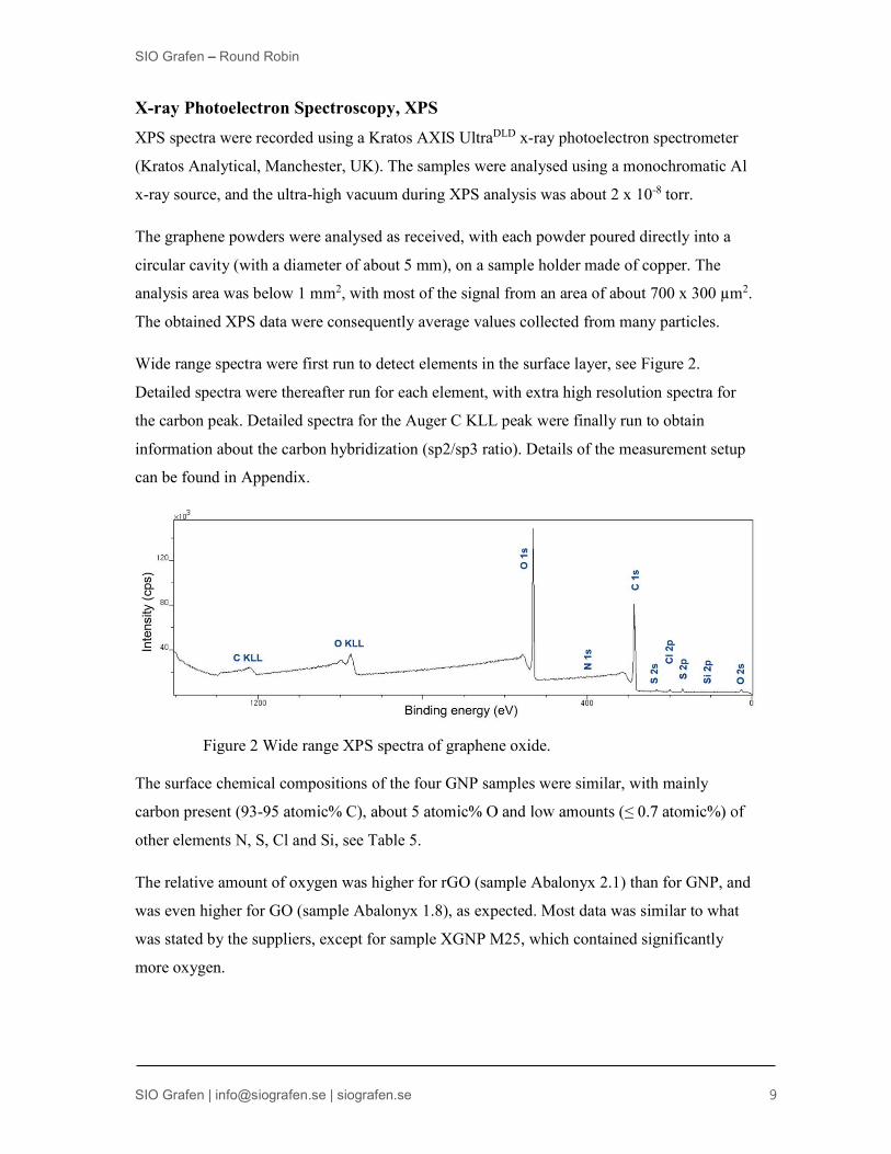
Wide range spectra were first run to detect elements in the surface layer, see Figure 2.

Detailed spectra were thereafter run for each element, with extra high resolution spectra for

the carbon peak. Detailed spectra for the Auger C KLL peak were finally run to obtain

information about the carbon hybridization (sp2/sp3 ratio). Details of the measurement setup

can be found in Appendix.

Figure 2 Wide range XPS spectra of graphene oxide.

The surface chemical compositions of the four GNP samples were similar, with mainly

carbon present (93-

other elements N, S, Cl and Si, see Table 5.

The relative amount of oxygen was higher for rGO (sample Abalonyx 2.1) than for GNP, and

was even higher for GO (sample Abalonyx 1.8), as expected. Most data was similar to what

was stated by the suppliers, except for sample XGNP M25, which contained significantly

more oxygen.



Table 5 Relative surface composition in atomic % as measured by XPS. - = signal in detailed spectra at noise level (below about 0.05-0.1 atomic %) ( ) = weak peak, signal close to noise level in detailed spectra

Sample Data According to supplier

Atomic% Atomic Ratio

Sample C O N Si Cl S O/C

XGNP M25

C > 99,5%

O < 1%

92.9 5.8 0.7 - - 0.5 0.06

Abalonyx 2.1

C ~85% 85.8 13.8 - - 0.2 0.3 0.16

XGNP C750H

N ~1%

O ~8%

95.1 4.7 (0.1) (<0.05) - - 0.05

2D Fab extra

94.6 5.1 - (<0.05) (<0.1) 0.2 0.05

Abalonyx 1.8

C/O ratio 2,5-2,6

65.9 32.4 0.2 0.4 0.3 0.7 0.49

2D Fab standard

94.9 4.9 - - (<0.1) (<0.1) 0.05

All samples except XGNP C750H contained a low amount of sulphur . A

peak at about 169 eV was obtained for all of these samples, which corresponds to the oxidized

form of sulphur (sulphate/sulphonate functional groups). The spectrum from the XGNP M25

sample additionally had a peak at 164 eV, which indicates the presence of unoxidized sulphur

(e.g. thiol or disulphide groups).

One main peak was observed in the carbon 1s spectra (at 284.5-284.7 eV) of the GNP

samples. The main peak has a very long slope on the high-binding energy side, corresponding

to the energy loss structure of the C 1s peak (noted for carbon compounds with some

conductivity, e.g. graphene and graphite). The slope contains both chemically shifted low

intensity peaks, and true loss structures such as aromatic ring shake-up peaks, but the shape of

the slope is complex rendering specific assignments difficult. This shape of the C 1s peak is

typical for graphite and graphene samples.

Additional chemically shifted peaks corresponding to different C-O functional groups were

detected in the slope on the high-binding energy side (overlapping with the energy loss



structure) in the spectra of the rGO and GO samples. These peaks correspond to different

functional groups. However, it is not straightforward to curve-fit and quantify these shifted

peaks, due to overlap with the energy loss structure.

A curve-fit could in principle be done by adjusting the baseline in order to exclude the energy

loss structure. However, this is difficult to do with high certainty. An easy test to check the

validity of any fitting procedure is to compare the oxygen to carbon atomic ratio calculated

from the functional groups from the fitting of the carbon 1s peak, with the ratio calculated

from the total amount of oxygen and carbon (in atomic%).

Information about the carbon hybridization (sp2/sp3) can be obtained from the differentiated

x-ray induced Auger spectra (XAES) of the C KLL signal. The line widths of the Auger peak

C KLL can be associated to the D-parameter, the distance between the maximum and

minimum in the derivate of C KLL spectra. A value of 22-23 was found for the GNP and rGO

samples, mainly corresponding to sp2 carbon. Two values of the D-parameter were obtained

for the GO sample, 22 (sp2 carbon) and 17 (ca 40% sp2 and 60% sp3 carbon). This is

expected for graphene oxide, where both sp2 and sp3 type of carbons are present.

Scanning electron microscopy, SEM 1 was used as a starting point for sample preparation. The samples

for SEM were prepared by similar, but slightly different, methods by KTH and RISE IVF. In

brief, the graphene was dispersed in water at a concentration of approximately 0.1 mg/ml. If

this did not result in a stable dispersion, isopropanol (IPA) was used as solvent instead. The

dispersion was thereafter sonicated for 10 min.

KTH centrifuged the dispersion (500 rpm for 3 min) and drop-casted the supernatant on a 300

nm SiO2 /Si wafer. The sample was then left to dry in a fumehood for two days. RISE IVF left

the dispersion to stand, instead of the centrifugation step.

Acceleration voltages of 3-5 kV and working distances of 3-4 mm were used in the SEM.

Representative regions with many non-overlapping flakes were imaged. Two different

methods were used to analyse the flake size distribution by the two organisations. KTH used

an image processing software to quickly get a statistical distribution of all particles in the

image. The 25th and 75th percentiles can be found using the software, which gives a

significantly more reliable picture of the sample than a mean or median value. RISE IVF, on



the other hand, manually measured individual flakes, resulting in an upper and lower

estimate of the flake size, see Table 6.

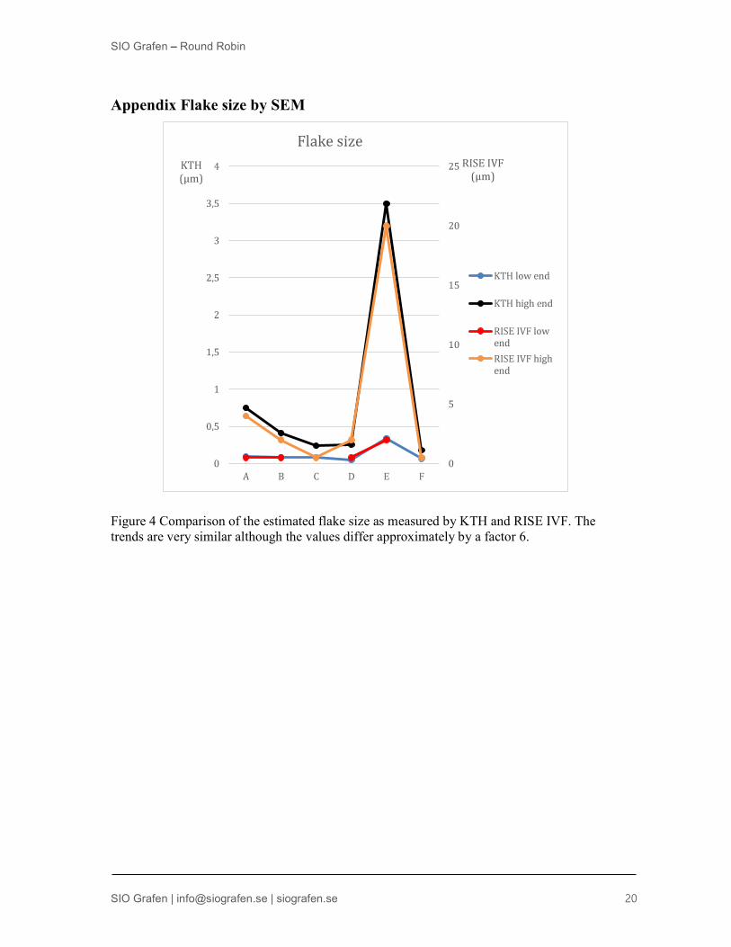
The procedure using the software analysis and centrifugation during the sample preparation

consistently gives lower values of the flake size than the procedure using the manual analysis

and natural sedimentation during the sample preparation. This difference is approximately a

factor 6 over all the investigated samples, see Figure 4 in appendix. One part of the

explanation to this could be that whereas the manual analysis specifically investigates single

flakes, the automatic software analysis includes everything contained in the sample. The great

number of small particles (< 100 nm) therefore reduces the size estimates when using the

software as compared to the manual analysis. Another reason could be that the centrifugation

step is significantly more efficient at separating different sizes, and thereby leaving smaller

particles in the deposited supernatant.

Table 6 Data from the SEM characterisation where the image processing was done manually and using an image processing software compared with data from the suppliers. Sample Solvent for

sample preparation

According to supplier

[ ]

Software analysis Manual analysis

25th percentile

[ ]

75th percentile

[ ]

Lower estimate

[ ]

Upper estimate

[ ]

XGNP M25

DI water 25 0.094 0.75 0.5 4

Abalonyx 2.1

IPA - 0.087 0.41 0.5 2

XGNP C750H

DI water < 2 0.089 0.24 0.5

2D Fab extra

IPA - 0.051 0.26 0.5 2

Abalonyx 1.8

DI water - 0.34 3.5 2 20

2D Fab standard

IPA - 0.069 0.18 0.5

Only one of the suppliers (XG Science) specified the flake size. The sizes measured here are

significantly smaller than stated by the supplier. This could partly be due to different

measurement methods. Both this measured difference and the fact that most producers did not



specify the size/size distribution, highlights the importance of characterization and validation

of purchased materials.

The sample preparation was more challenging than expected. It is imperative for the analysis

to prepare samples with a high density of flakes on the surface, but these flakes should not be

overlapping. This is complicated as it is not straightforward to prepare a proper suspension of

graphene.

One advantage of SEM compared to other techniques is that it gives information about the

shape of the particles. Although the technique was used to quantify the lateral dimensions

here, SEM can also give an impression of whether the flakes are thin or thick and the general

shape, such as if they for example are large and flat, or more equiaxed spheres.

One drawback of the SEM procedure is that there is a risk that the graphene flakes

agglomerate during the sample preparation. In some images it is possible to see smaller flakes

laying on top of larger particles, see for example Figure 3.

Figure 3 Smaller and thinner flakes can be found on top of larger particles.

Comparison of BET, SEM and XPS

It is interesting to compare the results from the different characterization methods. The

sample which contained the largest and thinnest flakes among these in the SEM study was the



GO product 1.8 from Abalonyx. This is in contrast to the low surface area according to the

BET characterisation, where no dispersion had been used. This supports that the dispersion

method (or lack of it) strongly influences the SEM and BET results. The good results after

dispersion in water or IPA using SEM, may also be due to that GO is easier to disperse, than

GNP and rGO.

Only limited sample preparation is required for the BET, TGA and XPS analysis. The

corresponding surface area (BET) and chemical composition data (XPS) measured here was

also in general in agreement with the data provided by the suppliers. The surface area

measured at the two different locations in this study were also in agreement.

On one hand, the limited sample preparation is a huge advantage for these techniques as the

sample is largely unaffected by the characterisation procedure. On the other hand, the most

interesting surface area is not that of the pristine powder, but rather how the material performs

in combination with other materials, for example in a formulated product or in a composite.

The extent to which graphene materials deagglomerate or exfoliate during processing varies

significantly between different materials, and the dispersion techniques used. The final

surface area between the graphene and a potential matrix will therefore be different from the

surface area of the untreated powder as measured here by BET. That is, a graphene sample

with lower surface area as measured by BET, could potentially still have a higher effective

surface area exposed to the matrix. It could, in the future, be interesting to compare how well

different graphene materials can be dispersed in standard solvents, as is being done with

carbon black in application labs today.

SEM characterisation requires more sample preparation. The lateral sizes measured by

similar, but different, methods at the two locations in this study differed approximately by a

factor 6 for all samples. The values provided by the suppliers were significantly larger than

any measured here. This could both be due to the sample preparation and unintentional bias

when selecting the investigated areas. Nevertheless, SEM is a powerful technique for

characterising the morphology and size.

The lateral size, thickness and chemical composition are some of the most important

provide this data, potentially as

there are no standards for this yet. This again highlights the importance of standardisation and

validation.



Outlook

Characterisation and standardisation of graphene are seen as some of the main challenges for

the continued development of graphene technology. There is several ongoing activities done

in this area. The International Electrotechnical Commission (IEC) TC 113 currently has

approximately 30 projects/documents related to development of standardisation of graphene.

The British Standards Institution published a Publicly Available Specification (PAS)

regarding properties of graphene flakes4 during this project. The scope of this PAS was to

guide graphene suppliers and manufacturers on what properties to specify. The particle

thickness, lateral size, specific surface area, moisture content, bulk density and a chemical

analysis are deemed as the most important properties that should be supplied. The PAS does

not discuss how these properties should be measured, but the methods chosen here (BET,

SEM and XPS) analyse these recommended properties.

Some notable recent academic publications include the work by Kauling et al.5 where they

have looked at the worldwide graphene flake production and found that a vast majority of the

commercial products are dominated by thicker graphite microplatelets rather than graphene

flakes. The study investigated material from 60 producers, but did unfortunately not reveal

them 6 However, the study once again

highlights the need for standardisation and characterization.

Kovtun et al. investigated 12 different commercial graphene materials using light scattering,

BET and XPS.7 They discuss that although the light scattering technique is developed for

spherical particles, it is a complete, fast and reliable method to describe the size distribution.

In one of the few characterisation cheques which have been utilised within SIO Grafen, SEM

was used to estimate the particle size distribution. This estimated the particle size as

approximately 20 times smaller than the laser diffraction method used by the supplier.

The National Physical Laboratory (NPL) are involved and leading many of the projects on

graphene standardisation in Europe. NPL also published the Good practice guide on

characterisation of the structure of graphene.1 They have recently been investigating

Differential centrifugal sedimentation (DCS) as a good method for characterising the size

distribution quickly. This method can then be used together with more advanced techniques

for calibration.



An advantage of light scattering techniques and DCS

preparation that for example electron microscopy does where particles for example might

agglomerate. The whole sample is also measured, which eliminates any risk of unintentional

bias, when choosing representative regions as in the SEM study.

On the other hand, images from SEM give more information about the shape that can be

difficult to quantify, whereas light scattering

Summary and conclusion

Six graphene materials were characterised using four techniques (BET, SEM, TGA and XPS)

by three different analysis providers. The procedure was set up as a blind test where the

analysis providers were unaware of exactly what materials were investigated.

The BET and XPS analysis in general resulted in similar data as provided by the suppliers.

There was a larger difference between the lateral size measured by SEM here and that

provided by the suppliers. There was also a difference between the values found at the two

locations in this study, which could be due to the difference in sample preparation

(centrifugation vs natural sedimentation) and data analysis (manual of individual flakes vs

image processing software). Only a limited amount of data was provided by the suppliers,

which highlights the importance of standardised characterization.

The analysis also shows that there is a broad range of flake and particle sizes in the samples.

Consequently, there is a need to specify not only the flake size of the largest flakes, but also

the distribution of flake sizes and distribution of graphene vs other forms of carbon particles.

It is therefore also imperative that the sample preparation results in a representative picture of

the whole sample, which can be challenging. A combination of manual and software analysis

is recommended in order to ensure that a statistically relevant number of representative flakes

is investigated.

The data found here has been added to the open database.

The knowledge of how to characterise graphene was increased in the participating teams and

this document can be used to facilitate future measurements.

Graphene can be characterised using many different techniques. Many of these which are

used today are advanced and expensive techniques, which require expert operators often



situated at research institutes or universities. There is therefore a need to also establish easier

and faster techniques which can be used as routine measurements in-house at companies.

This study consolidates the need to improve best practises of sample preparation, for training

on 2D material analysis even for skilled characterising operators, as well as a need for

graphene providers to specify the content of their product.



Bibliography

1 Pollard, A. J., Paton, K. R., Clifford, C. A. & Legge, E. Good Practice Guide No. 145 - Characterization of the Structure of Graphene. (2017).

2. Kovtun, A. et al. Benchmarking of graphene-based materials: real commercial products versus ideal graphene - Supporting info. 2D Mater. 6, 025006 (2019).

3. Lv, W. et al. Low-Temperature Exfoliated Graphenes: Vacuum-Promoted Exfoliation and Electrochemical Energy Storage. ACS Nano 3, 3730 3736 (2009).

4. Properties of graphene flakes Guide. (2018).

5. Kauling, A. P. et al. The Worldwide Graphene Flake Production. Adv. Mater. 1803784 (2018). doi:10.1002/adma.201803784

6. Nature 562, 502 503 (2018).

7. Kovtun, A. et al. Benchmarking of graphene-based materials: real commercial products versus ideal graphene. 2D Mater. 6, 025006 (2019).



Appendix XPS procedure

The different XPS spectra were run in the following order:

1.Wide (survey) spectra were run to detect elements present in the surface layer.

Wide spectra: pass energy 160, step size 1 eV

2.High-resolution carbon spectra were thereafter run, to see if any chemical shifts due to

different functional groups could be observed.

High-resolved carbon spectra: pass energy 20, step size 0.1 eV

3.Detail spectra were then run for each element, and the relative surface compositions

expressed in atomic % were quantified from the detail spectra.

Detail spectra: pass energy 80, step size 0.1 eV

4.Auger C KLL spectra were finally run, to see if any information could be obtained about

the carbon hybridization (sp2/sp3 ratio) from the D-parameter.

Auger C KLL spectra: pass energy 40, step size 0.1 eV



Appendix Flake size by SEM

Figure 4 Comparison of the estimated flake size as measured by KTH and RISE IVF. The trends are very similar although the values differ approximately by a factor 6.

Documents

Round Robin characterization - SIO Grafen