Embed Size (px)
Citation preview
THÈSE
Pour obtenir le grade de
DOCTEUR DE L’UNIVERSITÉ DE GRENOBLESpécialité : Informatique
Arrêté ministérial : 7 août 2006
Présentée par
Michał KRÓL
Thèse dirigée par Andrzej Duda, Franck Rousseau
préparée au sein de UMR 5217 - LIG - Laboratoire d’Informatique
de Grenoble
et de École Doctorale Mathématiques, Sciences et Technologies
de l’Information, Informatique (EDMSTII)
Routing in Wireless Sensor Net-works
Thèse soutenue publiquement le 15 Mars 2016,
devant le jury composé de :
Mr Serge Fdida
Professeur, UPMC, Rapporteur
Mr Olivier Festor
Professeur, Université de Lorraine, Telecom Nancy, Rapporteur
Mr Eric Fleury
Professeur, ENS Lyon, Examinateur
Mr Franck Rousseau
Maitre de Conférences, Grenoble INP – Ensimag, Directeur de thèse
Mr Andrzej Duda
Professeur, Grenoble INP – Ensimag, Directeur de thèse

iii
Acknowledgments
I would like to thank most especially my supervisor and mentor Prof. Andrzej
Duda. You taught me a great deal about how to do research. Thank you for your
trust and freedom in exploring different research directions. I would like to express
my gratitude for your contributions to this work including sleepless nights before
deadlines and your invaluable support in my future projects.
I am also very grateful to Dr. Franck Rousseau for your guidance, patience, and
encouragement at the early stage of my research. Thanks for all that I have learnt
from you.
I am also thankful to my friends and colleagues from the Drakkar team, espe-
cially to Maciej, Nazim, Iza, Ana, Tristan, Pierre, Gabriele and many others.
I would like to thank my great flatmates Claire, Melissa, Coline, Coralie and
Marlene, my ”Grenuls” friends Camille, Julie, Martin, Champion, Marion, mem-
bers of the polish family Gosia, Julian, Justyna, Nico, Asia, Rafa�l, Audrey, Artur,
Tomek, Liv, Radek, Sophie and others Arnaud, Julien. Thank you for sharing good
and slightly worse moments, for being there when I needed it and making my stay
in Grenoble a wonderful experience.
Finally, my deepest gratitude goes to my parents, sister, aunt and grandpar-
ents for your unconditional love, endless support throughout my entire life, and
understanding of my decisions.

v
Abstract
The Internet of Things (IoT) paradigm envisions expanding the current Internet
with a huge number of intelligent communicating devices. Wireless Sensor Networks
(WSN) deploy the devices running on limited energy supplies and measuring en-
vironmental phenomena (like temperature, radioactivity, or CO2). Popular WSN
applications include monitoring, telemetry, and natural disaster prevention. Major
WSN challenges are energy efficiency, overcoming impairments of wireless medium,
and self-organisation. WSN integrating IoT will rely on a set of open standards
striving to offer scalability and reliability in a variety of operating scenarios and
conditions. Nevertheless, the current state of the standards present interoperability
issues and can benefit from further improvements. The contributions of the thesis
are the following:
We perform an extensive study of Bloom Filters and their use in encoding node
characteristics in a compact form in IP addresses. Different techniques of
compression and variants of filters allowed us to develop an efficient system
closing the gap between feature-routing and classic approaches compatible
with IPv6 networks.
We propose Featurecast, a routing protocol/naming service for WSN. It allows to
query sensor networks using a set of characteristics while fitting in an IPv6
packet header. We integrate our protocol with RPL and introduce a new
metric that increases routing efficiency. We validate its performance in both
extensive simulations and experimentations on real sensors on a large-scale
Senslab testbed [1]. Large-scale simulations demonstrate the advantages of
our protocol in terms of memory usage, control overhead, packet delivery
rate, and energy consumption.
We introduce WEAVE, a routing protocol for networks with geolocation. Our
solution does not use any control messages and learns its paths only by ob-
serving incoming traffic. Several mechanisms are introduced to keep a fixed-
size header, bypass both small as well as large obstacles, and support efficient
communication between nodes. We performed simulations on a large scale in-
volving more than 19 000 nodes and real-sensor experimentations on the FIT
IoT-lab testbed. Our results show that we achieve much better performance
than other protocols, especially in large and dynamic networks, without in-
troducing any control overhead.
Key words: Wireless Sensor Networks, 6LoWPAN, RPL, self-organization,
routing, data-centric, georouting, experimental study.
vi
Resume
Le paradigme d’Internet des objets (IoT) envisage d’etendre l’Internet actuel
avec un grand nombre de dispositifs intelligents. Les reseaux de capteurs sans fil
(WSN) sont deployes sous forme d’equipements autonomes en energie dissemines
dans l’environnement pour y collecter des mesures de phenomenes physiques, comme
la temperature, la radioactivite, ou le taux de CO2. Des applications typiques des
WSN sont la surveillance, la telemetrie, la prevention des catastrophes naturelles.
Les defis majeurs des WSN sont l’efficacite energetique, la robustesse aux faib-
lesses des communications sans fil, et le fonctionnement de maniere auto-organisee.
L’integration des WSN dans l’IoT reposera sur des standards ouverts s’efforcant
d’offrir evolutivite et fiabilite dans une variete de scenarios et de conditions de fonc-
tionnement. Neanmoins, en l’etat actuel, les standards presentes des problemes
d’interoperabilite et peuvent beneficier d’ameliorations certaines. Les contributions
de la these sont les suivantes :
Nous avons effectue une etude approfondie des filtres de Bloom et de leur utilisation
pour le codage des caracteristiques des nœud dans l’adresse IP. Differentes
techniques de compression et variantes de filtres nous ont permis de developper
un systeme efficace qui comble l’ecart entre le routage par caracteristiques et
l’approche classique compatible avec les reseaux IPv6.
Nous proposons Featurecast, un protocole de routage / service de nommage pour
WSN. Il permet d’interroger les reseaux de capteurs en utilisant un ensemble
de caracteristiques, tout en restant compatible l’entete de paquet IPv6. Nous
integrons notre protocole dans RPL et introduisons une nouvelle metrique,
ce qui augmente l’efficacite du routage. Nous verifions ses performances par
des simulations approfondies et des experimentations sur des capteurs reels
sur la plate-forme d’experimentation a grande echelle Senslab [1]. Les simu-
lations demontrent les avantages de notre protocole en termes d’utilisation de
la memoire, de surcharge de controle, de taux de livraison de paquets et de
consommation d’energie.
Nous introduisons WEAVE, un protocole de routage pour les reseaux avec geolo-
calisation. Notre solution n’utilise pas de messages de controle et apprend
ses chemins seulement en observant le trafic en transit. Plusieurs mecanismes
sont introduits pour garder une en-tete de taille fixe, contourner a la fois
les petits et les grands obstacles, et fournir une communication efficace entre
les nœuds. Nous avons effectue des simulations a grande echelle impliquant
plus de 19 000 noeuds et des experiences avec des capteurs reels sur la plate-
vii
forme d’experimentation FIT IoT-lab [2]. Nos resultats montrent que nous
atteignons de bien meilleures performances que les autres protocoles, en par-
ticulier dans les grands reseaux dynamiques, cela sans introduire de surcharge
de controle.
Mots cles: reseaux de capteurs sans fil, 6LoWPAN, RPL, auto-organisation,
routage, approche orientee donnees, routage geographique, etude experimentale.

Contents
I Introduction . . . . . . . . . . . . . . . . . . . . . . . . . . . . . . . . . 7
1 Organization of the Thesis . . . . . . . . . . . . . . . . . . . . . . . . . . . 9
1.1 Wireless Sensor Networks . . . . . . . . . . . . . . . . . . . . . . . . 9
1.2 Internet of Things . . . . . . . . . . . . . . . . . . . . . . . . . . . . 11
1.3 Overview of the thesis . . . . . . . . . . . . . . . . . . . . . . . . . 12
II State of the Art . . . . . . . . . . . . . . . . . . . . . . . . . . . . . . 15
2 WSN Characteristics . . . . . . . . . . . . . . . . . . . . . . . . . . . . . . 17
3 Routing Issues in Wireless Sensor Networks . . . . . . . . . . . . . . . . . 23
3.1 Classification of Routing Protocols . . . . . . . . . . . . . . . . . . 24
4 Network Layer Routing Protocols . . . . . . . . . . . . . . . . . . . . . . . 27
4.1 RPL Routing Protocol . . . . . . . . . . . . . . . . . . . . . . . . . 27
4.1.1 Upward Routing Topological Structure . . . . . . . . . . . . 28
4.1.2 DODAG Rank . . . . . . . . . . . . . . . . . . . . . . . . . . 28
4.1.3 DODAG Rank Types . . . . . . . . . . . . . . . . . . . . . . 29
4.1.4 DODAG Construction Process . . . . . . . . . . . . . . . . . 29
4.1.5 DODAG Maintenance . . . . . . . . . . . . . . . . . . . . . . 30
4.1.6 Downward Paths . . . . . . . . . . . . . . . . . . . . . . . . 30
4.2 RRPL . . . . . . . . . . . . . . . . . . . . . . . . . . . . . . . . . . 31
4.3 Trickle: a Network-Wide Broadcast Protocol . . . . . . . . . . . . . 32
4.4 Summary . . . . . . . . . . . . . . . . . . . . . . . . . . . . . . . . . 33
5 Geographic Routing . . . . . . . . . . . . . . . . . . . . . . . . . . . . . . 35
5.1 Greedy and Face Routing . . . . . . . . . . . . . . . . . . . . . . . . 35
5.2 S4: a Small State and Small Stretch Routing Protocol . . . . . . . 36
5.3 GDSTR and GDSTR-3D . . . . . . . . . . . . . . . . . . . . . . . . 37
5.4 Binary Waypoint Routing . . . . . . . . . . . . . . . . . . . . . . . 39
5.5 Multi-hop Delaunay Triangulation . . . . . . . . . . . . . . . . . . . 40
5.6 Summary . . . . . . . . . . . . . . . . . . . . . . . . . . . . . . . . . 42
6 Application Layer Protocols in Wireless Sensor Networks . . . . . . . . . 45
6.1 CoAP . . . . . . . . . . . . . . . . . . . . . . . . . . . . . . . . . . . 45
6.1.1 RESTful Interface . . . . . . . . . . . . . . . . . . . . . . . . 47
6.1.2 Resource Directory . . . . . . . . . . . . . . . . . . . . . . . 47
6.2 Directed Diffusion . . . . . . . . . . . . . . . . . . . . . . . . . . . . 48
6.3 Logical Neighborhoods . . . . . . . . . . . . . . . . . . . . . . . . . 50
6.4 CCN – Content-Centric Networking . . . . . . . . . . . . . . . . . . 52
6.5 Summary . . . . . . . . . . . . . . . . . . . . . . . . . . . . . . . . . 54
x Contents
III Featurecast: a Group Communication Service for WSN . . . . 57
7 Rationale . . . . . . . . . . . . . . . . . . . . . . . . . . . . . . . . . . . . 59
8 Principles of Featurecast . . . . . . . . . . . . . . . . . . . . . . . . . . . . 63
8.1 Featurecast Addresses . . . . . . . . . . . . . . . . . . . . . . . . . . 63
8.2 Constructing Routing Tables . . . . . . . . . . . . . . . . . . . . . . 65
8.2.1 Creating a routing structure. . . . . . . . . . . . . . . . . . . 65
8.2.2 Advertising Features . . . . . . . . . . . . . . . . . . . . . . 67
8.3 Forwarding . . . . . . . . . . . . . . . . . . . . . . . . . . . . . . . . 67
8.4 Topology Maintenance . . . . . . . . . . . . . . . . . . . . . . . . . 68
9 Compact Representation of Features . . . . . . . . . . . . . . . . . . . . . 69
9.1 Bloom Filters . . . . . . . . . . . . . . . . . . . . . . . . . . . . . . 69
9.2 Solution1: Straight Bloom Filters . . . . . . . . . . . . . . . . . . . 70
9.3 Solution 2: Fixed Size Filter with Compression . . . . . . . . . . . 70
9.4 Solution 3: Position List in the Address, Filter in the Routing Tables 73
9.5 Solution 4: Bloom Filter in Addresses and a Bit Position List in the
Routing Table . . . . . . . . . . . . . . . . . . . . . . . . . . . . . . 73
9.6 Comparison of Solutions . . . . . . . . . . . . . . . . . . . . . . . . 74
9.7 Computational Overhead. . . . . . . . . . . . . . . . . . . . . . . . 74
9.8 Routing Entry Aggregation. . . . . . . . . . . . . . . . . . . . . . . 75
10 Implementation and Evaluation . . . . . . . . . . . . . . . . . . . . . . . . 77
10.1 Evaluation Setup . . . . . . . . . . . . . . . . . . . . . . . . . . . . 77
10.2 Scenarios . . . . . . . . . . . . . . . . . . . . . . . . . . . . . . . . . 77
10.2.1 Building Control . . . . . . . . . . . . . . . . . . . . . . . . . 78
10.2.2 Random Topology . . . . . . . . . . . . . . . . . . . . . . . . 78
10.3 Results: Memory Footprint in the Building Control Scenario . . . . 78
10.4 Results: Message Overhead in the Building Control Scenario . . . . 79
10.5 Results: Random Topology Scenario . . . . . . . . . . . . . . . . . 83
10.6 Discussion of Packet Drops Due to Inexistent Addresses . . . . . . . 86
11 Conclusion . . . . . . . . . . . . . . . . . . . . . . . . . . . . . . . . . . . 87
IV WEAVE: Efficient Geographical Routing in Large-Scale Net-
works . . . . . . . . . . . . . . . . . . . . . . . . . . . . . . . . . . . . . . . 89
12 Rationale . . . . . . . . . . . . . . . . . . . . . . . . . . . . . . . . . . . . 91
13 Principles of the WEAVE Protocol . . . . . . . . . . . . . . . . . . . . . . 95
13.1 Protocol Overview . . . . . . . . . . . . . . . . . . . . . . . . . . . . 95
13.2 Packet Structure . . . . . . . . . . . . . . . . . . . . . . . . . . . . . 97
13.3 Principles of Packet Forwarding . . . . . . . . . . . . . . . . . . . . 98
13.4 Learning Partial Routes . . . . . . . . . . . . . . . . . . . . . . . . 99
13.5 Address Space Partitioning . . . . . . . . . . . . . . . . . . . . . . . 100
Contents xi
13.6 Constructing Routing Tables . . . . . . . . . . . . . . . . . . . . . . 102
13.7 Details of Packet Forwarding . . . . . . . . . . . . . . . . . . . . . . 102
13.8 Checkpoint Creation . . . . . . . . . . . . . . . . . . . . . . . . . . 104
13.9 Path Exploration and Backtracking . . . . . . . . . . . . . . . . . . 108
13.10 Refreshing Routing Information . . . . . . . . . . . . . . . . . . . . 108
13.11 A note on the backtracking mechanism . . . . . . . . . . . . . . . . 109
13.12 Loop-freeness . . . . . . . . . . . . . . . . . . . . . . . . . . . . . . 110
14 Evaluation . . . . . . . . . . . . . . . . . . . . . . . . . . . . . . . . . . . . 113
14.1 Experiments on a Testbed . . . . . . . . . . . . . . . . . . . . . . . 113
14.2 Simulations . . . . . . . . . . . . . . . . . . . . . . . . . . . . . . . 115
14.3 Initial Simulation Comparisons . . . . . . . . . . . . . . . . . . . . 115
14.4 Learning Phase . . . . . . . . . . . . . . . . . . . . . . . . . . . . . 119
14.5 Dynamic networks . . . . . . . . . . . . . . . . . . . . . . . . . . . . 120
14.6 Concave Obstacles . . . . . . . . . . . . . . . . . . . . . . . . . . . . 123
14.7 Realistic Geographic Topology . . . . . . . . . . . . . . . . . . . . . 124
14.8 Comparison with Standard Routing . . . . . . . . . . . . . . . . . . 125
15 Conclusion . . . . . . . . . . . . . . . . . . . . . . . . . . . . . . . . . . . 127
V Conclusion and Future Work . . . . . . . . . . . . . . . . . . . . . . 129
16 Overall Conclusions and Future Work . . . . . . . . . . . . . . . . . . . . 131
16.1 Summary of the Results and Final Conclusions . . . . . . . . . . . 131
16.2 Future Work . . . . . . . . . . . . . . . . . . . . . . . . . . . . . . . 132
17 Publications . . . . . . . . . . . . . . . . . . . . . . . . . . . . . . . . . . . 135
Bibliography . . . . . . . . . . . . . . . . . . . . . . . . . . . . . . . . . . . . 137

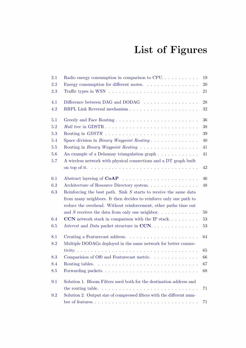
List of Figures
2.1 Radio energy consumption in comparison to CPU. . . . . . . . . . . 19
2.2 Energy consumption for different motes. . . . . . . . . . . . . . . . 20
2.3 Traffic types in WSN . . . . . . . . . . . . . . . . . . . . . . . . . . 21
4.1 Difference between DAG and DODAG . . . . . . . . . . . . . . . . 28
4.2 RRPL Link Reversal mechanism . . . . . . . . . . . . . . . . . . . . 32
5.1 Greedy and Face Routing . . . . . . . . . . . . . . . . . . . . . . . . 36
5.2 Hull tree in GDSTR . . . . . . . . . . . . . . . . . . . . . . . . . . . 38
5.3 Routing in GDSTR . . . . . . . . . . . . . . . . . . . . . . . . . . . 39
5.4 Space division in Binary Waypoint Routing . . . . . . . . . . . . . . 40
5.5 Routing in Binary Waypoint Routing . . . . . . . . . . . . . . . . . 41
5.6 An example of a Delaunay triangulation graph . . . . . . . . . . . . 41
5.7 A wireless network with physical connections and a DT graph built
on top of it. . . . . . . . . . . . . . . . . . . . . . . . . . . . . . . . 42
6.1 Abstract layering of CoAP . . . . . . . . . . . . . . . . . . . . . . 46
6.2 Architecture of Resource Directory system. . . . . . . . . . . . . . . 48
6.3 Reinforcing the best path. Sink S starts to receive the same data
from many neighbors. It then decides to reinforce only one path to
reduce the overhead. Without reinforcement, other paths time out
and S receives the data from only one neighbor. . . . . . . . . . . . 50
6.4 CCN network stack in comparison with the IP stack. . . . . . . . . 53
6.5 Interest and Data packet structure in CCN. . . . . . . . . . . . . . 53
8.1 Creating a Featurecast address. . . . . . . . . . . . . . . . . . . . . 64
8.2 Multiple DODAGs deployed in the same network for better connec-
tivity. . . . . . . . . . . . . . . . . . . . . . . . . . . . . . . . . . . . 65
8.3 Comparision of Of0 and Featurecast metric. . . . . . . . . . . . . . 66
8.4 Routing tables. . . . . . . . . . . . . . . . . . . . . . . . . . . . . . 67
8.5 Forwarding packets. . . . . . . . . . . . . . . . . . . . . . . . . . . . 68
9.1 Solution 1. Bloom Filters used both for the destination address and
the routing table. . . . . . . . . . . . . . . . . . . . . . . . . . . . . 71
9.2 Solution 2. Output size of compressed filters with the different num-
ber of features. . . . . . . . . . . . . . . . . . . . . . . . . . . . . . . 71
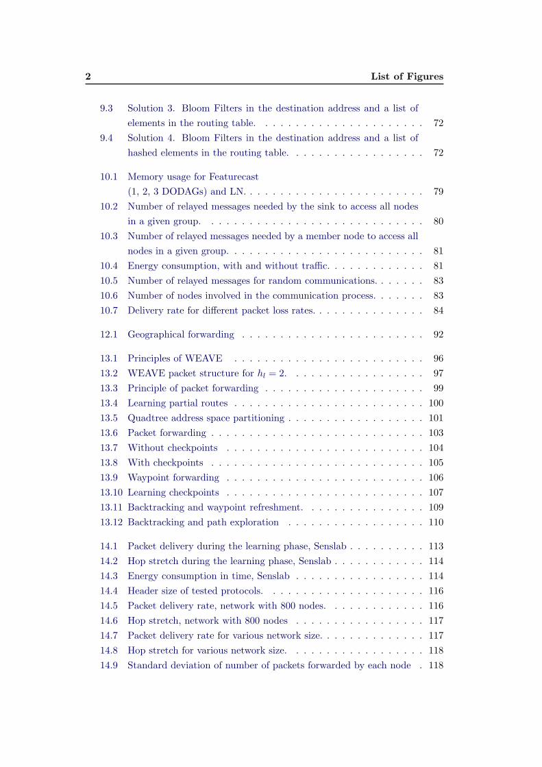
2 List of Figures
9.3 Solution 3. Bloom Filters in the destination address and a list of
elements in the routing table. . . . . . . . . . . . . . . . . . . . . . 72
9.4 Solution 4. Bloom Filters in the destination address and a list of
hashed elements in the routing table. . . . . . . . . . . . . . . . . . 72
10.1 Memory usage for Featurecast
(1, 2, 3 DODAGs) and LN. . . . . . . . . . . . . . . . . . . . . . . . 79
10.2 Number of relayed messages needed by the sink to access all nodes
in a given group. . . . . . . . . . . . . . . . . . . . . . . . . . . . . 80
10.3 Number of relayed messages needed by a member node to access all
nodes in a given group. . . . . . . . . . . . . . . . . . . . . . . . . . 81
10.4 Energy consumption, with and without traffic. . . . . . . . . . . . . 81
10.5 Number of relayed messages for random communications. . . . . . . 83
10.6 Number of nodes involved in the communication process. . . . . . . 83
10.7 Delivery rate for different packet loss rates. . . . . . . . . . . . . . . 84
12.1 Geographical forwarding . . . . . . . . . . . . . . . . . . . . . . . . 92
13.1 Principles of WEAVE . . . . . . . . . . . . . . . . . . . . . . . . . 96
13.2 WEAVE packet structure for hl = 2. . . . . . . . . . . . . . . . . . 97
13.3 Principle of packet forwarding . . . . . . . . . . . . . . . . . . . . . 99
13.4 Learning partial routes . . . . . . . . . . . . . . . . . . . . . . . . . 100
13.5 Quadtree address space partitioning . . . . . . . . . . . . . . . . . . 101
13.6 Packet forwarding . . . . . . . . . . . . . . . . . . . . . . . . . . . . 103
13.7 Without checkpoints . . . . . . . . . . . . . . . . . . . . . . . . . . 104
13.8 With checkpoints . . . . . . . . . . . . . . . . . . . . . . . . . . . . 105
13.9 Waypoint forwarding . . . . . . . . . . . . . . . . . . . . . . . . . . 106
13.10 Learning checkpoints . . . . . . . . . . . . . . . . . . . . . . . . . . 107
13.11 Backtracking and waypoint refreshment. . . . . . . . . . . . . . . . 109
13.12 Backtracking and path exploration . . . . . . . . . . . . . . . . . . 110
14.1 Packet delivery during the learning phase, Senslab . . . . . . . . . . 113
14.2 Hop stretch during the learning phase, Senslab . . . . . . . . . . . . 114
14.3 Energy consumption in time, Senslab . . . . . . . . . . . . . . . . . 114
14.4 Header size of tested protocols. . . . . . . . . . . . . . . . . . . . . 116
14.5 Packet delivery rate, network with 800 nodes. . . . . . . . . . . . . 116
14.6 Hop stretch, network with 800 nodes . . . . . . . . . . . . . . . . . 117
14.7 Packet delivery rate for various network size. . . . . . . . . . . . . . 117
14.8 Hop stretch for various network size. . . . . . . . . . . . . . . . . . 118
14.9 Standard deviation of number of packets forwarded by each node . 118
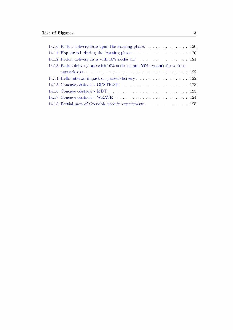
List of Figures 3
14.10 Packet delivery rate upon the learning phase. . . . . . . . . . . . . 120
14.11 Hop stretch during the learning phase. . . . . . . . . . . . . . . . . 120
14.12 Packet delivery rate with 10% nodes off. . . . . . . . . . . . . . . . 121
14.13 Packet delivery rate with 10% nodes off and 50% dynamic for various
network size. . . . . . . . . . . . . . . . . . . . . . . . . . . . . . . . 122
14.14 Hello interval impact on packet delivery . . . . . . . . . . . . . . . . 122
14.15 Concave obstacle - GDSTR-3D . . . . . . . . . . . . . . . . . . . . 123
14.16 Concave obstacle - MDT . . . . . . . . . . . . . . . . . . . . . . . . 123
14.17 Concave obstacle - WEAVE . . . . . . . . . . . . . . . . . . . . . . 124
14.18 Partial map of Grenoble used in experiments. . . . . . . . . . . . . 125

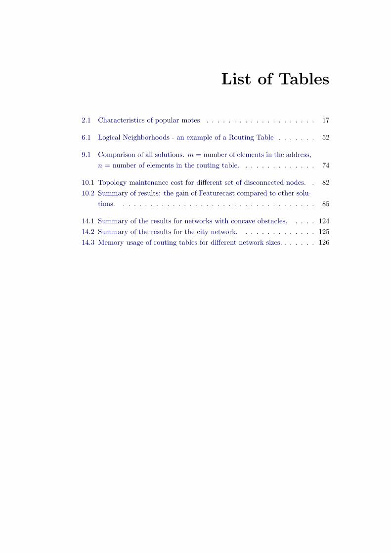
List of Tables
2.1 Characteristics of popular motes . . . . . . . . . . . . . . . . . . . . 17
6.1 Logical Neighborhoods - an example of a Routing Table . . . . . . . 52
9.1 Comparison of all solutions. m = number of elements in the address,
n = number of elements in the routing table. . . . . . . . . . . . . . 74
10.1 Topology maintenance cost for different set of disconnected nodes. . 82
10.2 Summary of results: the gain of Featurecast compared to other solu-
tions. . . . . . . . . . . . . . . . . . . . . . . . . . . . . . . . . . . . 85
14.1 Summary of the results for networks with concave obstacles. . . . . 124
14.2 Summary of the results for the city network. . . . . . . . . . . . . . 125
14.3 Memory usage of routing tables for different network sizes. . . . . . . 126


Part I
Introduction

Chapter 1
Organization of the Thesis
Contents
1.1 Wireless Sensor Networks . . . . . . . . . . . . . . . . . . . . . . . . 9
1.2 Internet of Things . . . . . . . . . . . . . . . . . . . . . . . . . . . . 11
1.3 Overview of the thesis . . . . . . . . . . . . . . . . . . . . . . . . . . 12
1.1 Wireless Sensor Networks
Wireless Sensor Networks have recently become one of the research domains that
develop the most. A lot of interest from the scientific community as well as from
the industry result in a rapid development of new types of devices, technologies,
and protocols. Indeed, the ease of deployment and the large amount of possible
uses justify such a great interest.
Wireless Sensor Networks consist of many small nodes communicating through
a wireless channel. They can provide some valuable data sensing the environment
as well as interact with their surrounding through actuators. The small size and
low cost allow sensors to be easily integrated in the environment, providing a non-
intrusive way to make our lives easier and improve industrial processes. Intended
large scale deployments (we can even read about hundred thousands or millions of
devices) will be made possible by a low price of WSN devices[3] [4]. WSN nodes
(also called motes) are embedded systems with limited resources: low-power, low-
range, low-bandwidth communications, small memory, and finally, a small battery
or an energy harvesting device. Moreover, the characteristics of WSN radio chips
such as 802.15.4 or Bluetooth Low Energy (BLE) are far inferior compared to the
popular 802.11 WiFi technology, especially when it comes to the emitted power and
coverage. The original idea for deploying nodes over a large area combined with a
small radio range leads to the multihop operation of WSN.
WSN motes may have various characteristics. Within the same base platform,
they can integrate many types of sensors (temperature, light, humidity, cameras, ac-
celerometers, etc.) or actuators (air conditioning, door control, alarms, etc.). WSN
10 Chapter 1. Organization of the Thesis
can thus be used in many different scenarios. Environment surveillance can track
animals, helping to understand their migrations. A WSN can easily detect a fire
and alert a fire brigade. The concept of intelligent buildings becomes more and
more popular. Temperature/humidity sensors can cooperate with the air condition
systems to maintain optimal conditions and save energy. Movement detection sen-
sors connecting to a identification system can turn on/off the light when needed
and prevent unauthorized access to restricted areas.
Many cities adopt WSN to improve the quality of life of their citizens. Barcelona
creates BCN Smart City [5] providing smart parking spots, a service for elderly
people needing help, a network of smart buses and many more.
We can distinguish between several ways of interacting with sensor networks.
The first one is a ”pull mode”, where to get data we need to query our network.
In the second one, a sensor node automatically reports data to the sink. The
communication can be triggered by a timer (time driven) or an observed phenomena
(event-driven). All those modes can be useful in different scenarios and require a
suitable way of communication.
The great interest in WSN led to the development of many different operating
systems for motes. The most popular TinyOS [6] and Contiki [7] as well as RIOT
[8], MANTIS [9] or Nano-RK [10] provide different programming models, scheduling
systems, memory management and communication protocol stacks. With such a
variety of systems, developers can easily construct applications.
As WSN contain a large number of nodes, routing becomes an important chal-
lenge. Classical IP networks have a static structure, which allows to introduce some
kind of hierarchy and benefit from address aggregation. In WSN, the topology may
change rapidly because of link/nodes failures and a possibility of nodes to be mobile,
so such approach is not suitable. A WSN is thus usually a flat multihop network
difficult to organise, especially with a limited amount of resources. A routing algo-
rithm needs to be developed carefully to introduce a minimal overhead and ensure
equal and minimal energy consumption.
Sensors are often deployed in places difficult to reach or where human inter-
vention can be challenging. Therefore, we want to apply a ”deploy and forget”
approach, where sensors are placed and then they remain autonomous. A network
needs to discover all its parts, organize the communication and efficiently deliver
data. The tasks can be extremely difficult to accomplish with a high probability
of node failures, frequent topology changes and the influence of the environment
difficult to predict. A WSN needs to perform efficient self-organize and self-healing
processes.
At the same time, wireless networks can exhibit some unexpected and varying
1.2. Internet of Things 11
behaviour. The impact of obstacles such as buildings, furniture, trees, is difficult to
predict during a simulation process and results in asymmetric links, important fad-
ing, or unstable communication, which routing protocols need to take into account.
Nowadays, sensor nodes can be powered in different ways. A battery is still
the most popular way, but main powered motes can also be a possibility. ”Green
sensors” gain more and more interest allowing to recharge the battery using har-
vesting technologies such as solar panels. However, in all those cases, the energy
consumption remains the critrical concern for WSN developers influencing directly
the network lifetime.
All those constraints make the WSN a challenging technology that requires a
careful and complex design, and makes the development process difficult.
1.2 Internet of Things
With the rapid development of embedded systems and WSN, we witness the
emergence of the Internet of Things (IoT). Under this term, all ”things” such as
sensors, electronic devices, computers, despite different technologies, are connected
to a single, global network, where every device can reach every other device. IPv6
provides enough addressing space to uniquely identify all such devices, which is
necessary for the Internet of Things to work. The Internet of Things allows to access
many different devices using the same protocol with the well-known communication
interface. It enables new attractive applications, simplifies the development process,
reduces costs, and makes the physical environment accessible for almost everyone.
Application examples are numerous. Health surveillance systems will be able to
check the status of our body, compare it with our records in databases and notify a
doctor if necessary. An intelligent fridge will be able to automatically order food for
the whole family. The Internet of Things can also become a core part of intelligent
vehicle systems able to easily exchange information to get us safe to our destination.
The research on WSN contribute to the development of the Internet of Things and
enables large deployments of sensor nodes in various domains (smart homes, smart
cities, smart grids, environmental sensing, critical infrastructure surveillance, etc.).
However, this concept also raises many new problems and challenges. Unlike in
classic IPv4 networks, a large number of nodes in the Internet of Things can be
mobile or connected only from time to time. So, it may be impossible to maintain
a fixed structure that allows to aggregate addresses and simplify routing. We also
have to deal with a much larger number of nodes that require much resources. It
is a problem especially for embedded devices, whose resources are very limited. As
routing protocols exchange more information, they need more and more bandwidth
12 Chapter 1. Organization of the Thesis
and control traffic may even exceed data traffic. It can be a serious issue, especially
in wireless scenarios, where the available bandwidth is also limited.
1.3 Overview of the thesis
This thesis considers routing and naming schemes in WSN and provides two
major contributions. First, we propose Featurecast, a new protocol allowing to
efficiently query a sensor network. Featurecast is easy for users to use, outperforms
already existing solutions, and remains compatible with classical IPv6 networks.
Our second contribution targets networks with nodes knowing their positions.
For such networks, we propose WEAVE, a new protocol for geographic routing.
We have validated the feasibility and performance of all proposed schemes through
detailed simulations and evaluation on experimental testbeds.
The thesis is organized as follows.
The second part presents the state of the art including all relevant related work
according to the studied communication layers. We present an overview of routing
protocols in WSNs, focusing notably on distance-vector (gradient) and geographic
routing. We conclude this part by a detailed discussion on the utility of the cross-
layer and data-centric approaches, and their application to address challenges of
the IoT paradigm.
The third part presents the concept of Featurecast with addressing and routing
based on node features defined as predicates. For instance, we can send a packet
to the address composed of features temperature and Room D to reach all nodes
with a temperature sensor located in Room D. Each node constructs its address
from the set of its features and disseminates it in the network so that intermediate
nodes can build routing tables. In this way, a node can send a packet to a set of
nodes matching given features. We also present a routing system based on RPL
[11], which allows to forward packets in Featurecast network in an efficient way. Our
experiments and evaluation of this scheme show very good performance compared
to Logical Neighborhoods (LN) [12] and IP multicast with respect to the memory
footprint and message overhead.
The fourth part presents WEAVE, a geographic routing protocol. With the
development of geolocation as well as virtual coordinate systems, a large part of
nodes in a network is able to determine their positions. WEAVE uses a quad-tree
algorithm to divide the network space and select a set of waypoints that can be used
to route packets. WEAVE does not use any control messages nor central nodes
forwarding more traffic than the others and introduces only a minimal overhead
adding a small header to the forwarded packets. With a fixed-size header, the

1.3. Overview of the thesis 13
protocol can be easily integrated into already existing geographical routing protocols
to improve their performance. WEAVE proves to be as efficient as traditional
routing protocols, while using a much lower amount of memory and limiting the
bandwidth usage.
The fifth part terminates this thesis by summarizing the main contributions.
The final remarks provides motivation for further possible research directions that
could stem out from our work.


Part II
State of the Art

Chapter 2
WSN Characteristics
The goal of this part is to give a general overview of the tremendous research
efforts in WSN that led to the standardization of protocols that are becoming the
building stone of the Internet of Things (IoT). In particular, we will focus our
attention on routing protocols and naming services for WSN, the domains closely
related to the subject of our research. We first present classical routing approaches
in Low power and Lossy Networks (LLN) based on 6LoWPAN [13]—an adaptation
layer for IPv6. Then, we describe different techniques based on geographic routing,
content-centric forwarding, and different types of flooding.
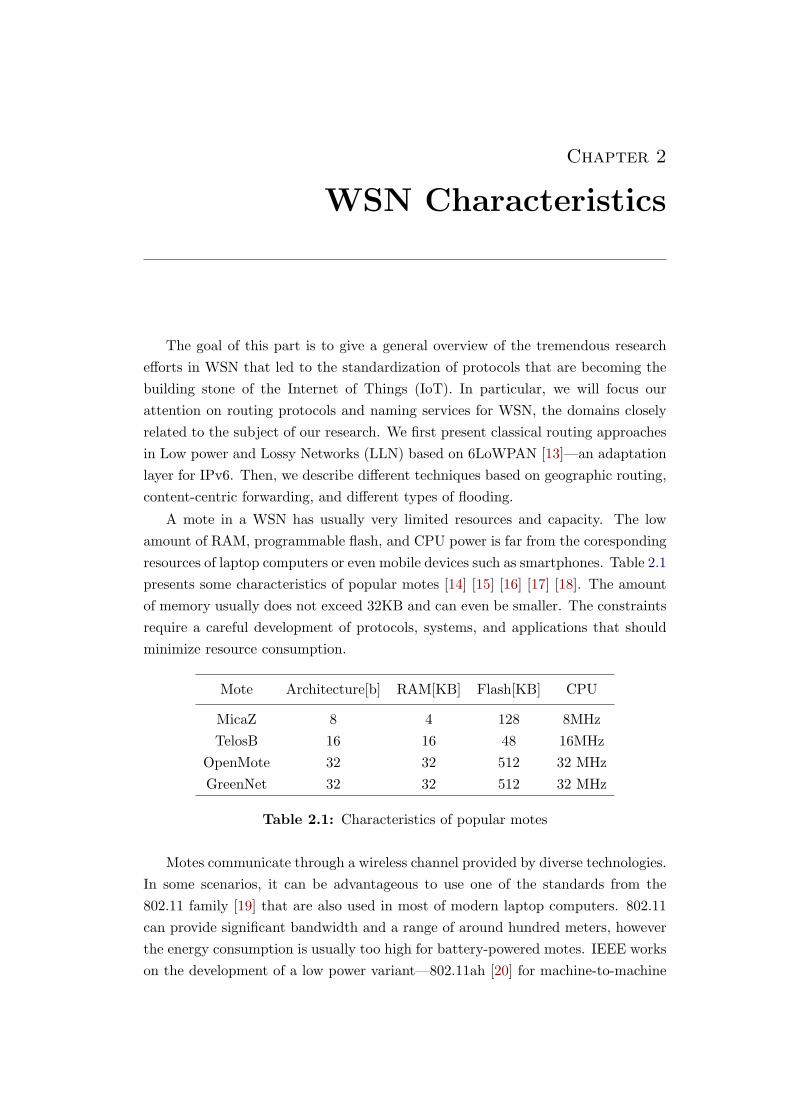
A mote in a WSN has usually very limited resources and capacity. The low
amount of RAM, programmable flash, and CPU power is far from the coresponding
resources of laptop computers or even mobile devices such as smartphones. Table 2.1
presents some characteristics of popular motes [14] [15] [16] [17] [18]. The amount
of memory usually does not exceed 32KB and can even be smaller. The constraints
require a careful development of protocols, systems, and applications that should
minimize resource consumption.
Mote Architecture[b] RAM[KB] Flash[KB] CPU
MicaZ 8 4 128 8MHz
TelosB 16 16 48 16MHz
OpenMote 32 32 512 32 MHz
GreenNet 32 32 512 32 MHz
Table 2.1: Characteristics of popular motes
Motes communicate through a wireless channel provided by diverse technologies.
In some scenarios, it can be advantageous to use one of the standards from the
802.11 family [19] that are also used in most of modern laptop computers. 802.11
can provide significant bandwidth and a range of around hundred meters, however
the energy consumption is usually too high for battery-powered motes. IEEE works
on the development of a low power variant—802.11ah [20] for machine-to-machine
18 Chapter 2. WSN Characteristics
communications that aims at extending the range to cover larger distances while
consuming litlle energy.
Some motes use the Bluetooth technology [21]. It provides similar characteristics
to the 802.11 standards, but with a lower range, while being oriented more towards
directly connecting two peers (master/slave mode). It limits its use in scenarios
in which we need to broadcast data. Nevertheless, the recent BLE technology
(Bluetooth Low Energy) is appearing as an interesing variant for low power motes.
IEEE developed a specific standard for Low Power and Lossy Networks: 802.15.4
[22] that provided the PHY and MAC layers to the ZigBee protocol stack [23].
802.15.4 offers a medium range (around 50m), low data rates (up to 250kb/s),
achieves low energy consumption, and benefits from low manufacture costs. All
these characteristics make 802.15.4 particularly suitable for WSN. It is currently
the most popular standard solution supported by modern motes. Because of a
small communication range in 802.15.4 networks, nodes cannot directly access all
peers in a given topology. In such multi-hop networks, packets need to be forwarded
several times before reaching their destination. This way of operation requires the
use of routing protocols for establishing end-to-end connectivity.
Recently, several initiatives have considered bringing long-range communica-
tions to energy constrained IoT motes. Good examples are LoRa (Long Range
Low Rate) [24] [25] and SIGFOX [26]. LoRa targets machine-to-machine commu-
nications within a 10km range with a support for up to millions of nodes with a low
energy consumption. SIGFOX offers very small rates between 100 b/s and 1000
b/s with an announced rqnge of 40km in open space. SIGFOX devices can only
transmit a limited number of small messages per day. In spite of the interest spawn
by the technologies, their deployment is still at its beginning and they are far away
from being available on existing motes.
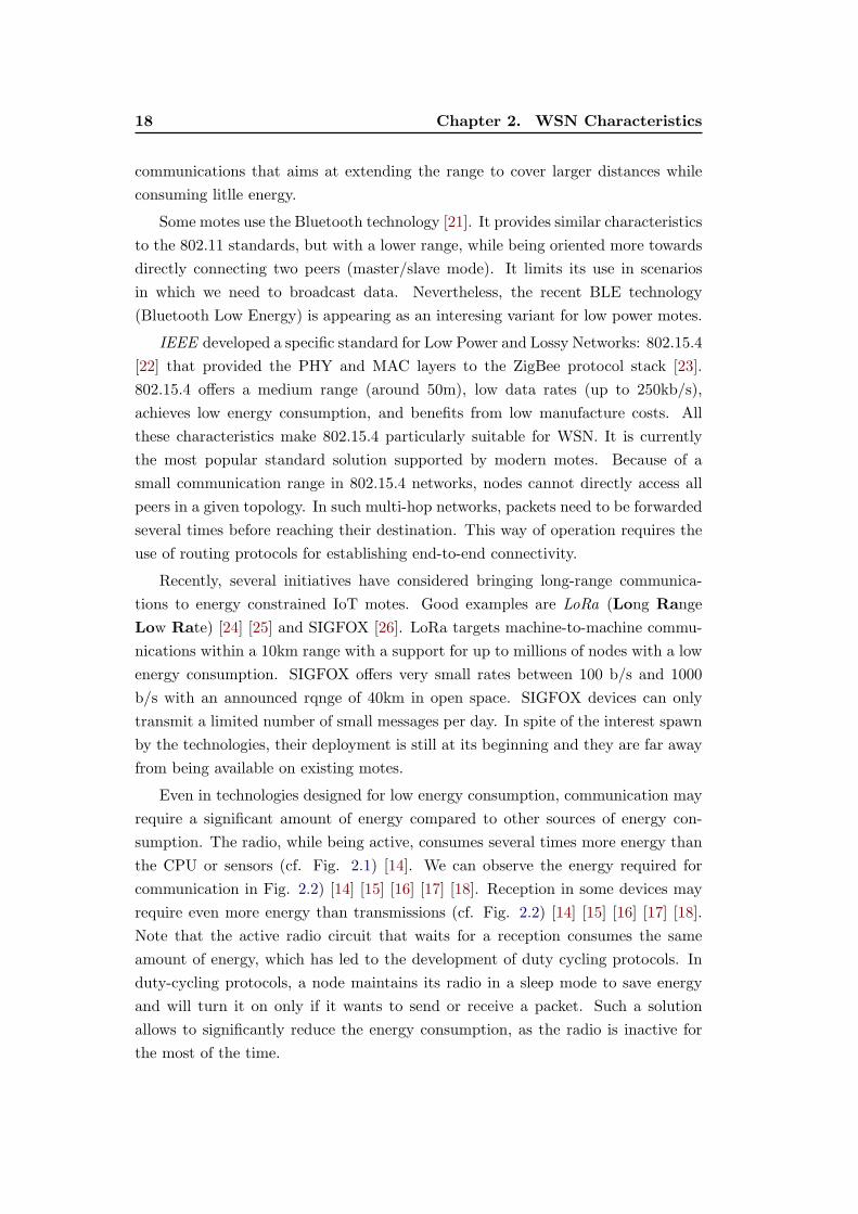
Even in technologies designed for low energy consumption, communication may
require a significant amount of energy compared to other sources of energy con-
sumption. The radio, while being active, consumes several times more energy than
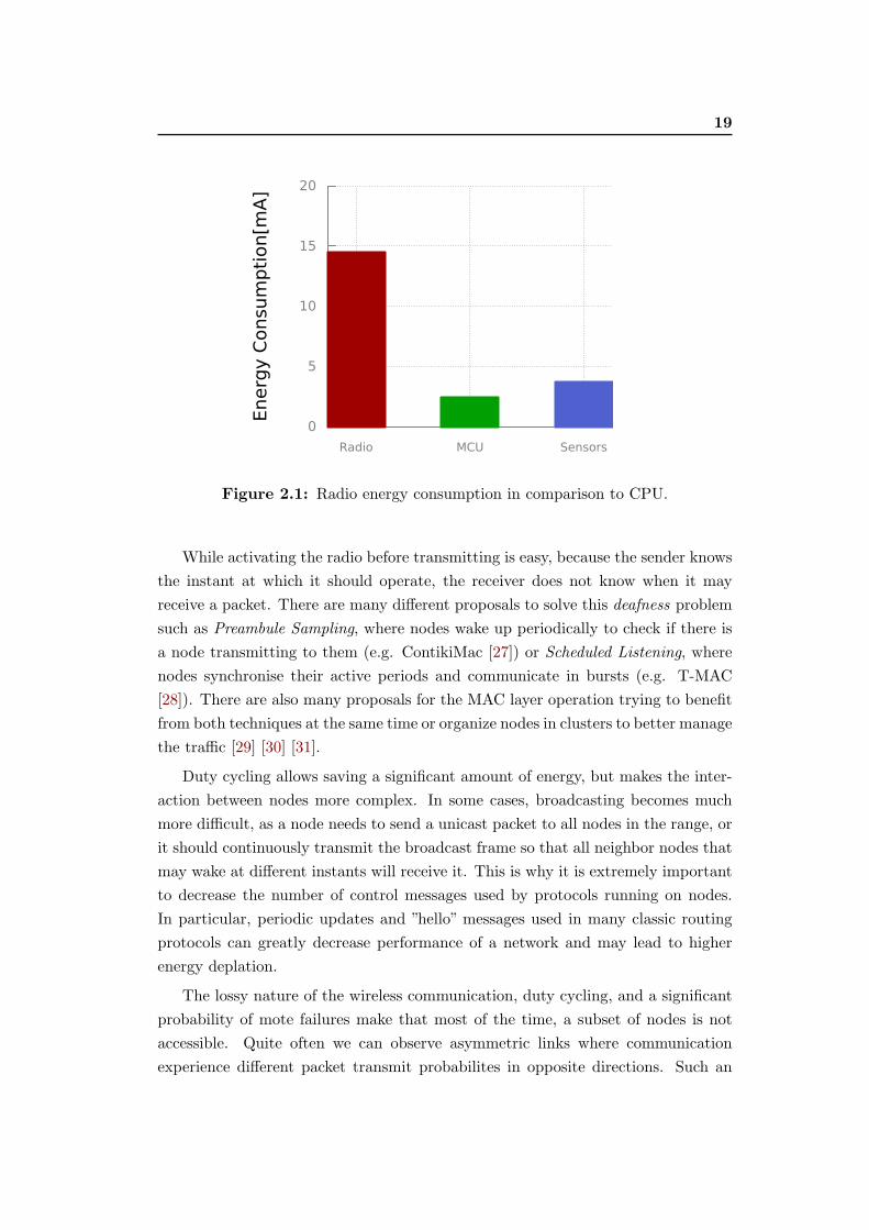
the CPU or sensors (cf. Fig. 2.1) [14]. We can observe the energy required for
communication in Fig. 2.2) [14] [15] [16] [17] [18]. Reception in some devices may
require even more energy than transmissions (cf. Fig. 2.2) [14] [15] [16] [17] [18].
Note that the active radio circuit that waits for a reception consumes the same
amount of energy, which has led to the development of duty cycling protocols. In
duty-cycling protocols, a node maintains its radio in a sleep mode to save energy
and will turn it on only if it wants to send or receive a packet. Such a solution
allows to significantly reduce the energy consumption, as the radio is inactive for
the most of the time.
19
0
5
10
15
20
Radio MCU Sensors
Energ
y C
onsum
pti
on[m
A]
Figure 2.1: Radio energy consumption in comparison to CPU.
While activating the radio before transmitting is easy, because the sender knows
the instant at which it should operate, the receiver does not know when it may
receive a packet. There are many different proposals to solve this deafness problem
such as Preambule Sampling, where nodes wake up periodically to check if there is
a node transmitting to them (e.g. ContikiMac [27]) or Scheduled Listening, where
nodes synchronise their active periods and communicate in bursts (e.g. T-MAC
[28]). There are also many proposals for the MAC layer operation trying to benefit
from both techniques at the same time or organize nodes in clusters to better manage
the traffic [29] [30] [31].
Duty cycling allows saving a significant amount of energy, but makes the inter-
action between nodes more complex. In some cases, broadcasting becomes much
more difficult, as a node needs to send a unicast packet to all nodes in the range, or
it should continuously transmit the broadcast frame so that all neighbor nodes that
may wake at different instants will receive it. This is why it is extremely important
to decrease the number of control messages used by protocols running on nodes.
In particular, periodic updates and ”hello” messages used in many classic routing
protocols can greatly decrease performance of a network and may lead to higher
energy deplation.
The lossy nature of the wireless communication, duty cycling, and a significant
probability of mote failures make that most of the time, a subset of nodes is not
accessible. Quite often we can observe asymmetric links where communication
experience different packet transmit probabilites in opposite directions. Such an
20 Chapter 2. WSN Characteristics
0
5
10
15
20
25
MIC
Az
Telo
sB
OpenM
ote
Gre
enN
et
Sm
art
MeshIP
Energ
y c
onsum
pti
on [
mA
]
TxRx
CPU
Figure 2.2: Energy consumption for different motes.
environment may experience imortant network dynamics and unstable topology.
This is also the reason for which routing protocols designed for classic IP networks
may perform in an insufficient way in WSN.
Because of the broadcast nature of the wireless medium, motes cannot structure
the network with subnetwork prefixes and use address aggregation to reduce the
size of routing tables, which results in the need of using host routes. Nevertheless,
it is possible to create some clusters with coordination nodes, but such solutions
increase the control message overhead and cause unequal energy consumption, thus
decreasing the network lifetime.
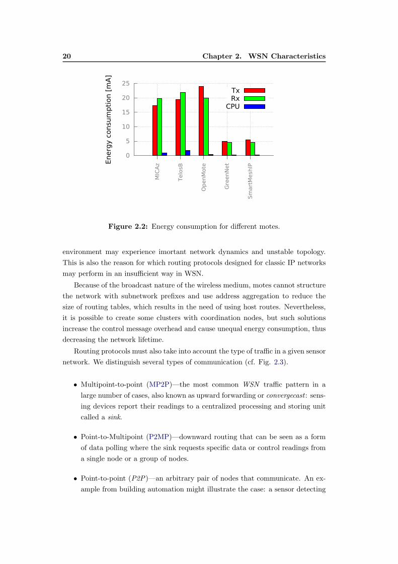
Routing protocols must also take into account the type of traffic in a given sensor
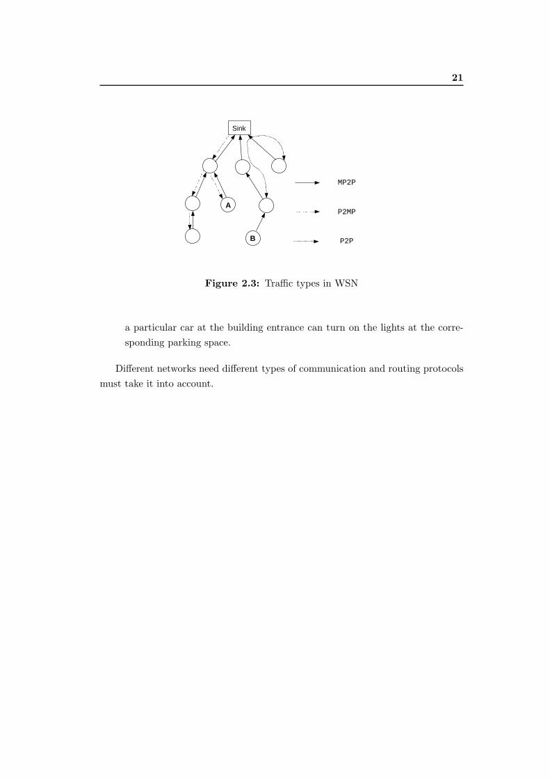
network. We distinguish several types of communication (cf. Fig. 2.3).
• Multipoint-to-point (MP2P)—the most common WSN traffic pattern in a
large number of cases, also known as upward forwarding or convergecast : sens-
ing devices report their readings to a centralized processing and storing unit
called a sink.
• Point-to-Multipoint (P2MP)—downward routing that can be seen as a form
of data polling where the sink requests specific data or control readings from
a single node or a group of nodes.
• Point-to-point (P2P)—an arbitrary pair of nodes that communicate. An ex-
ample from building automation might illustrate the case: a sensor detecting
21
MP2P
P2MP
P2P
Sink
A
B
Figure 2.3: Traffic types in WSN
a particular car at the building entrance can turn on the lights at the corre-
sponding parking space.
Different networks need different types of communication and routing protocols
must take it into account.

Chapter 3
Routing Issues in Wireless
Sensor Networks
Contents
3.1 Classification of Routing Protocols . . . . . . . . . . . . . . . . . . . 24
Routing is the key element of all networks. The process of forwarding packets
from a source to a destination allows nodes to exchange data. The topic was well
investigated during many years of research resulting in many efficient and robust
protocols for classical IP networks ([32], [33], [34]). However, a rapid development
of wireless technologies, mobile devices and rapid growth of the number of users
changed many features of modern networks. With new characteristics, we need new
routing protocols able to deal with emerging challenges [35] [36]. This is especially
true in Wireless Sensor Networks, which in many ways are different from classic
networks. A good routing protocol must achieve:
• Low control traffic overhead: the amount of control messages shall be
limited to reduce the energy consumption.
• High packet delivery rate: retransmitting lost packets consumes significant
amount of energy, reducing network lifetime.
• Optimal routing: routing protocols shall create the shortest path to the
destination, the shortest in the sense of some metric.
• Low memory consumption and processing cost: a routing protocol is
only a part of the whole system installed on motes, so it cannot consume too
many resources.
• Ability to deal with network dynamics: routing protocols must be able
to update outdated paths and create new ones.
24 Chapter 3. Routing Issues in Wireless Sensor Networks
3.1 Classification of Routing Protocols
Classification of routing protocols is a difficult task, because of a large number
of proposed solutions. They can be divided using different criteria:
• with/without paths – protocols with paths construct routes along which
packets will be forwarded. Usually, they require more resources/control mes-
sages to maintain paths than protocols without them, but then, routing is
more efficient. Protocols without paths do not use routes. Nodes forward
packets based on the characteristics of their neighbors and/or the information
contained in packets.
• proactive/reactive – proactive protocols establish and maintain routes to
every destination in the network from the beginning. Reactive ones establish
paths ”on demand”, only when a node wants to reach a given destination.
• end-point/data-centric – end-point protocols focus on reaching target nodes
identified by a unique identifier or address. The data-centric approach focuses
on data rather than on identifier/addresses.
• single/multipath – multipath protocols establish multiple paths to destina-
tions. They can be used to increase protocol robustness, load-balancing, or
performance.
• flat/hierarchical – hierarchical protocol are often based on clustering. By
choosing cluster heads and establishing inter-cluster communication only be-
tween them, we can significantly reduce memory usage and simplify routing
process. However, managing a cluster requires much more energy consump-
tion on cluster heads, which can shorten the network lifetime.
• single/cross layer – usually, routing only resides in the 3rd layer of the
OSI/ISO model. However, close cooperation with other layers (especially the
MAC layer), can bring significant benefits to the routing efficiency and is used
by many protocols for WSN. The wrawback is that each such dependency
limits the flexibility of the protocol and its ability to coexist with different
technologies.
• traffic mode – protocols can be classified based on the type of supported
communication, such as: unicast, multicast, many-to-one, etc.
Different surveys on routing protocols used different classification methods de-
pending upon chosen protocols. However, more and more protocols combine dif-
ferent techniques and cannot be easily classified. Having this in mind, in the rest
3.1. Classification of Routing Protocols 25
of this part, we divide the protocols into three categories: pure structure building
WSN routing protocols (focusing only on establishing paths between destinations),
geographic routing protocols, and application layer protocols including naming sys-
tems/grammars helping to exchange data.

Chapter 4
Network Layer Routing
Protocols
Contents
4.1 RPL Routing Protocol . . . . . . . . . . . . . . . . . . . . . . . . . 27
4.1.1 Upward Routing Topological Structure . . . . . . . . . . . . . 28
4.1.2 DODAG Rank . . . . . . . . . . . . . . . . . . . . . . . . . . 28
4.1.3 DODAG Rank Types . . . . . . . . . . . . . . . . . . . . . . . 29
4.1.4 DODAG Construction Process . . . . . . . . . . . . . . . . . 29
4.1.5 DODAG Maintenance . . . . . . . . . . . . . . . . . . . . . . 30
4.1.6 Downward Paths . . . . . . . . . . . . . . . . . . . . . . . . . 30
4.2 RRPL . . . . . . . . . . . . . . . . . . . . . . . . . . . . . . . . . . . 31
4.3 Trickle: a Network-Wide Broadcast Protocol . . . . . . . . . . . . . 32
4.4 Summary . . . . . . . . . . . . . . . . . . . . . . . . . . . . . . . . . 33
We start with the description of the routing protocols that reside only in 3rd
OSI/ISO layer. Such protocols usually construct a routing structure and follow
classical approaches (distance vector or link state). We present RPL, a distance
vector protocol for WSN and its enhancements.
4.1 RPL Routing Protocol
Routing Protocol for Low-Power and Lossy Networks (RPL) is a distance-vector
routing protocol to support a variety of network traffic patterns already mentioned
in the previous sections (cf. Fig. 2.3). Before the standardisation of RPL, a special
working group called ROLL strived to cover a comprehensive number of various use
cases: Home Automation [37], Commercial Building Automation [38], Industrial
Automation [39], Urban Environments [40]. Anticipating the IoT, ROLL requires
the interoperability with IPv6 and 6LoWPAN as well the compliance with a vari-
ety of link layers, supporting both wireless and PLC (Power Line Communication).
28 Chapter 4. Network Layer Routing Protocols
DAG DODAG
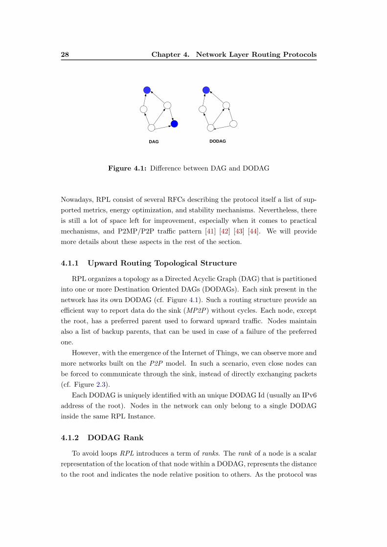
Figure 4.1: Difference between DAG and DODAG
Nowadays, RPL consist of several RFCs describing the protocol itself a list of sup-
ported metrics, energy optimization, and stability mechanisms. Nevertheless, there
is still a lot of space left for improvement, especially when it comes to practical
mechanisms, and P2MP/P2P traffic pattern [41] [42] [43] [44]. We will provide
more details about these aspects in the rest of the section.
4.1.1 Upward Routing Topological Structure
RPL organizes a topology as a Directed Acyclic Graph (DAG) that is partitioned
into one or more Destination Oriented DAGs (DODAGs). Each sink present in the
network has its own DODAG (cf. Figure 4.1). Such a routing structure provide an
efficient way to report data do the sink (MP2P) without cycles. Each node, except
the root, has a preferred parent used to forward upward traffic. Nodes maintain
also a list of backup parents, that can be used in case of a failure of the preferred
one.
However, with the emergence of the Internet of Things, we can observe more and
more networks built on the P2P model. In such a scenario, even close nodes can
be forced to communicate through the sink, instead of directly exchanging packets
(cf. Figure 2.3).
Each DODAG is uniquely identified with an unique DODAG Id (usually an IPv6
address of the root). Nodes in the network can only belong to a single DODAG
inside the same RPL Instance.
4.1.2 DODAG Rank
To avoid loops RPL introduces a term of ranks. The rank of a node is a scalar
representation of the location of that node within a DODAG, represents the distance
to the root and indicates the node relative position to others. As the protocol was
4.1. RPL Routing Protocol 29
designed to be generic, the exact calculation of the rank is left to custom Objective
Functions (OF ). However, it must always monotonically decrease as gradients flow
towards the DODAG destination.
4.1.3 DODAG Rank Types
The node rank can serve as a routing constraint (a way of pruning potential
forwarders not satisfying specific properties, e.g. use only paths traversing main
powered nodes). It can also serve as an additive metric (a way of estimating the
route cost, e.g. use the path that minimizes the energy consumption). OF ranks
can be divided into two mains classes:
• Node type – takes into account node properties to calculate a rank value.
A rank can map node state (ability to aggregate the data, high workload);
node enegy (type of power source, remaining energy); or a simple hop count
indicating the distance to the DODAG root.
• Link type – takes into account the properties of a linke between a node and
its neighbor. Nodes can advertise recently estimated throughput (or range
of supported values), observed latency, link reliability (using either the Link
Quality Level [LQL] or the Expected Transmission Count [ETX] metric), or
link color (a set of custom flags allowing the use of user defined rules).
The network sink (DODAG root) can construct multiple DODAGs, using dif-
ferent OF s in order to optimize paths for various use cases. Once a component
of the metric changes, the rank needs be recalculated. However, due to unstable
links, it is recommended to use a threshold while advertising those changes in the
network. Too frequent notifications can increase energy consumption and impact
the stability of the network.
4.1.4 DODAG Construction Process
In order to construct a new DODAG a root start sending DIO (Destination
Information Object) packets to link-local multicast. The DIO packet contains in-
formation allowing to identify the DODAG (RPLInstanceId, DODAGId), a type of
rank used by the OF, version number and additional control information. Upon
receiving a DIO packet each node will add its sender to the candidate neighbor set.
A restricted subset of the candidate neighbor set, containing nodes with lower rank
forms a parent set. Finally, the node chooses a preferred parent optimizing the OF
goal. The node can then start sending its own DIO messages adding its own metric
to the one, advertised by the parent. Recent studies show that the convergence
30 Chapter 4. Network Layer Routing Protocols
time does not depend on the number of nodes present in the network, but rather
on the number of hops between the root and the furthest nodes [45].
4.1.5 DODAG Maintenance
RPL requires an external mechanism to monitor the connectivity between neigh-
bors. Typical choices or that task are Neighbor Unreachability Detection (NUD) or
Bidirectional Forwarding Detection (BFD). Some recent studies show, that level 2
mechanism can perform significantly better in many cases[46]. If the preferred par-
ent gets disconnected, it must be replace by another one from the list. However, if
the parent set is empty the disconnected node poisons its subtree with infinite rank.
To restore the connectivity we can use global or local repair mechanisms. Global
repair mechanism is initiated by the DODAG root. It increments the DODAG ver-
sion and floods the network with new DIO messages. Global repair is the most sure
technique, but introduces significant message overhead, requires a lot of time and is
inefficient with frequent topology changes. Local repair mechanisms rebuild only a
small part of the DODAG using much less resources, but can construct suboptimal
paths [47].
As each node belonging to a DODAG periodically sends DIO packets to an-
nounce its rank, RPL sends DIO packets using the Trickle timer [48]. The Trickle
timer is explained in more details further in this section.
4.1.6 Downward Paths
RPL uses Destination Advertisement Object (DAO) messages to establish Down-
ward routes.and support P2MP and P2P traffic. Each node can send a DAO in order
advertise its address. The packet is sent to the parents and forward to the sink,
filling up the routing tables. While sending DIO messages is based on well-defined
Trickle timer, there are no specification for sending DAO packets. The most natural
way would be to resend them just after they expire. However, it was proven that
in networks experiencing packet looses it can be more beneficial to send multiple
messages in a short period of time in order to increase the probability of establishing
a path [41].
RPL supports two modes of downward routing:
• Storing – all nodes maintain downward routing tables for their sub-DODAG
• Non-storing- all packets between nodes are forwarded to the root, which
stores complete routing tables and uses source forwarding to deliver the pack-
ets.
4.2. RRPL 31
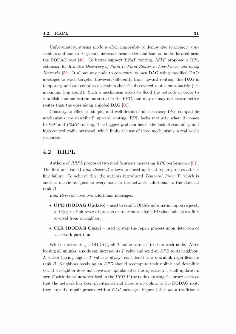
Unfortunately, storing mode is often impossible to deploy due to memory con-
straints and non-storing mode increases header size and load on nodes located near
the DODAG root [49]. To better support P2MP routing, IETF proposed a RPL
extension for Reactive Discovery of Point-to-Point Routes in Low-Power and Lossy
Networks [50]. It allows any node to construct its own DAG using modified DAO
messages to reach targets. However, differently from upward routing, this DAG is
temporary and can contain constraints that the discovered routes must satisfy (i.e.
maximum hop count). Such a mechanism needs to flood the network in order to
establish communication, as stated in the RFC, and may or may not create better
routes than the ones along a global DAG [50].
Contrary to efficient, simple, and well detailed (all necessary IPv6 compatible
mechanisms are described) upward routing, RPL lacks maturity when it comes
to P2P and P2MP routing. The biggest problem lies in the lack of scalability and
high control traffic overhead, which limits the use of those mechanisms in real world
scenarios.
4.2 RRPL
Authors of RRPL proposed two modifications increasing RPL performance [51].
The first one, called Link Reversal, allows to speed up local repair process after a
link failure. To achieve this, the authors introduced Temporal Order T , which is
another metric assigned to every node in the network, additional to the classical
rank R.
Link Reversal uses two additional messages:
• UPD (DODAG Update) – used to send DODAG information upon request,
to trigger a link reversal process or to acknowledge UPD that indicates a link
reversal from a neighbor.
• CLR (DODAG Clear) – used to stop the repair process upon detection of
a network partition.
While constructing a DODAG, all T values are set to 0 on each node. After
loosing all uplinks, a node can increase its T value and send an UPD to its neighbor.
A sensor having higher T value is always considered as a downlink regardless its
rank R. Neighbors receiving an UPD should recompute their uplink and downlink
set. If a neighbor does not have any uplinks after this operation it shall update its
own T with the value advertised in the UPD. If the nodes starting the process detect
that the network has been partitioned and there is no uplink to the DODAG root,
they stop the repair process with a CLR message. Figure 4.2 shows a traditional
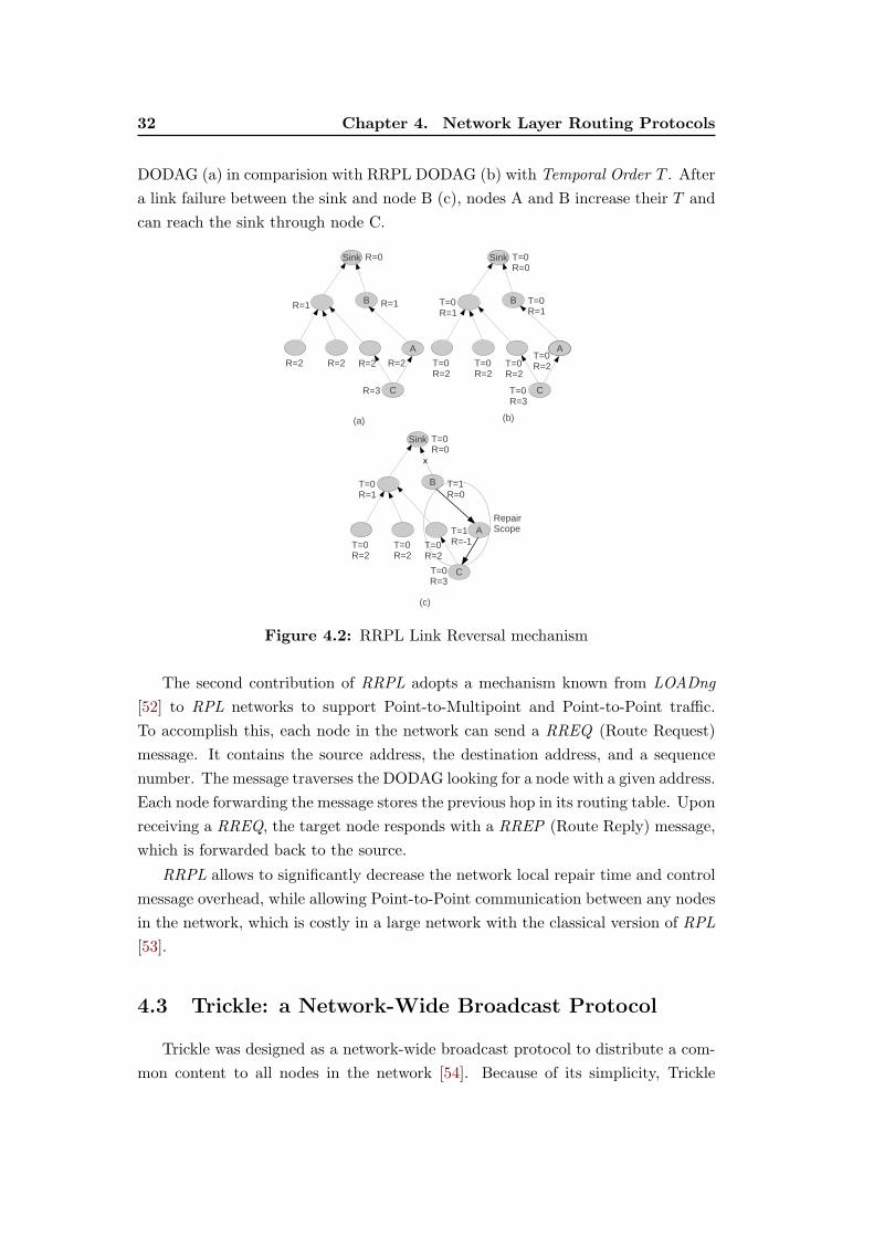
32 Chapter 4. Network Layer Routing Protocols
DODAG (a) in comparision with RRPL DODAG (b) with Temporal Order T . After
a link failure between the sink and node B (c), nodes A and B increase their T and
can reach the sink through node C.
Figure 4.2: RRPL Link Reversal mechanism
The second contribution of RRPL adopts a mechanism known from LOADng
[52] to RPL networks to support Point-to-Multipoint and Point-to-Point traffic.
To accomplish this, each node in the network can send a RREQ (Route Request)
message. It contains the source address, the destination address, and a sequence
number. The message traverses the DODAG looking for a node with a given address.
Each node forwarding the message stores the previous hop in its routing table. Upon
receiving a RREQ, the target node responds with a RREP (Route Reply) message,
which is forwarded back to the source.
RRPL allows to significantly decrease the network local repair time and control
message overhead, while allowing Point-to-Point communication between any nodes
in the network, which is costly in a large network with the classical version of RPL
[53].
4.3 Trickle: a Network-Wide Broadcast Protocol
Trickle was designed as a network-wide broadcast protocol to distribute a com-
mon content to all nodes in the network [54]. Because of its simplicity, Trickle
4.4. Summary 33
achieves really good performance and quite commonly becomes a comparison point
to many unicast protocols [55]. However, it is sometimes less costly to broadcast
data to all nodes than maintaining a routing topology using more sophisticated
routing protocols. Trickle is now the IETF standard [48] and is a part of the RPL
protocol.
Trickle uses a ”polite gossip” protocol. It assumes that data exchanged in the
network has its own global version/sequence number, so that the protocol is able
to determine which one is newer. Each node keeps a sequence number of the last
packet it has received and the content of several last packets themselves. Nodes
divide time into small intervals. During each interval, nodes broadcast a metadata
packet with the last sequence number received. However, nodes are ”polite” and do
not send the metadata packet if they overhear at least k other nodes advertising the
same sequence number. If a node overhears another node that advertises a smaller
sequence number, it rebroadcasts its last packets to put it up to date. In the
same way, a node overhearing a larger sequence number, rebroadcasts its metadata,
to invoke packet retransmission. Eventually, all nodes in the network receive the
propagated content with a minimal overhead.
4.4 Summary
So far, we have introduced some background information on routing protocols
for Wireless Sensor Networks. The described protocols belong to Layer 3, they only
focus on packet forwarding, and require additional mechanisms for naming/address
resolution. Classical solutions such as RPL usually work well in many-to-one com-
munication scenarios, but scale badly because all nodes need to exchange control
messages. It becomes a major problem while experiencing network dynamics. The
routing structure needs to be constantly updated with every single change in the
topology. Also, one-to-many and many-to-many communication is somewhat lack-
ing and difficult to introduce with a limited amount of resources. Trickle, being the
only presented protocol without routing structure, does not generate any control
messages, but requires flooding the whole network, which limits its use in unicast
communication. In the next chapter, we introduce geographic layer protocols ben-
efiting from node locations.

Chapter 5
Geographic Routing
Contents
5.1 Greedy and Face Routing . . . . . . . . . . . . . . . . . . . . . . . . 35
5.2 S4: a Small State and Small Stretch Routing Protocol . . . . . . . . 36
5.3 GDSTR and GDSTR-3D . . . . . . . . . . . . . . . . . . . . . . . . 37
5.4 Binary Waypoint Routing . . . . . . . . . . . . . . . . . . . . . . . . 39
5.5 Multi-hop Delaunay Triangulation . . . . . . . . . . . . . . . . . . . 40
5.6 Summary . . . . . . . . . . . . . . . . . . . . . . . . . . . . . . . . . 42
Because of possible node failures and the lack of the backbone infrastructure,
Wireless Sensor Networks cannot benefit from address aggregation. Protocols based
on clustering and a hierarchy usually introduce a lot of control traffic and can
cause unequal energy consumption. The development of cheaper and less complex
localisation systems as well as new protocols calculating virtual coordinates allow to
use node positions in the routing system. Geographic routing usually requires less
memory usage, control traffic, and presents an interesting alternative to classical
routing protocols. In this section, we briefly present the most popular geographic
routing protocols being used in 2D and 3D environments.
5.1 Greedy and Face Routing
The basic scheme of geographic routing is Greedy Routing. Each node in the
network maintains a list of its neighbors. To forward a packet to destination d,
a node looks into its neighbor table and chooses a node whose distance to d is
the smallest. Greedy Routing, besides neighbor discovery, does not require any
control messages nor routing tables. It requires almost no modification to work in
3D environments. However, its efficiency is quite limited—Greedy Routing cannot
deal with local minima (the nodes that do not have any neighbor with the smaller
distance to the destination) and will drop packets without trying to bypass obstacles
[56] [57]. Many protocols presented later in this section use use greedy forwarding
until a packet is stuck in a concave node and then try to go around a void or an

36 Chapter 5. Geographic Routing
obstacle. This approach may result in not optimal routes, because forwarding may
start in a wrong direction and then is forced to make a detour.
The first solution to guarantee stateless packet deliv- ery in two dimensions
(2D) under some assumptions was face routing: GFG (Greedy-Face-Greedy) [9]
and GPSR [10]. Nodes do not maintain any non local infor- mation to successfully
forward packets from sources to destinations.
Face Routing is a solution initially proposed in GFG [58] and GPSR [59]. With
the same assumptions as in Greedy Routing, it guarantees packet delivery, but re-
quires the planar graph of wireless connectivity. When encountering an obstacle,
Face Routing tries to bypass it clockwise or counter-clockwise.
SS DD
Greedy Routing
Optimal Path
SS DD
Face Routing
Optimal Path
Figure 5.1: Greedy and Face Routing
Face routing requires the construction of a planar graph (a graph with no cross-
ing edges), which is difficult in real wireless environments and may result in sub-
optimal routes [60]. Stateless face routing protocols operate under heavy unrealistic
assumptions, hence they do not work in real networks and a graph planarization
process, like installing some state information in Cross Links Detection Protocol
(CLDP) [61], is required.
5.2 S4: a Small State and Small Stretch Routing Pro-
tocol
S4 is a geographical routing protocol based on compact routing schemes [62].
At the beginning, a random set of√N nodes is chosen as beacons. Then, each
node establishes its local cluster Ck(s). Such a cluster of node s contains all nodes
that are closer to s than the closest beacon L(s) and is local for every node in the
network. Nodes knows the shortest path to each node in their local clusters and
to every beacon in the network. When trying to send a packet to destination d, a
node checks if it belongs to its local cluster. If not, the packet is sent to the closest
beacon to d. To use such routing scheme, nodes in S4 need to maintain:
• a local cluster table,
5.3. GDSTR and GDSTR-3D 37
• shortest paths to every beacon in the network.
To accomplish the first task, nodes use Scoped Distance Vector (SDV). Each
node s keeps a tuple for every destination in its local cluster containing:
• d - destination id,
• n - id of the next hop toward the destination,
• m(s, d) - distance to d,
• seqno - sequence number,
• scope(d) - the distance between d and its closest beacon.
Each node propagates the information stored in its routing table. However, an
update about destination d will be retransmitted only by neighbors who are closer
to d than its closest beacon. Sequence numbers allow to suppress retransmission
of entries that were not modified. Both mechanisms allow to significantly decrease
the amount of updates in the network.
To maintain connectivity between clusters, each beacon creates a spanning tree
to every node in the network done by simple flooding. To enhance broadcast re-
liability, S4 applies a simple system where packets are retransmitted until a node
overhears its retransmission by a certain number of neighbors.
The last component of S4 deals with node and link failures. If node s does not
receive an acknowledgement within a given number of retransmissions, it broadcasts
failure recovery request. Each neighbor receiving such a request calculates its
priority p based on its position and distance from the destination. A node with the
highest priority is chosen as a next hop, replacing the failed node.
As the name indicates, S4 offers low hop stretch and low memory usage. How-
ever, it requires a significant amount of control traffic. With a large number of
beacons, there is a lot of broadcast transmissions in the network, which can cause
high energy consumption especially in duty cycled networks.
5.3 GDSTR and GDSTR-3D
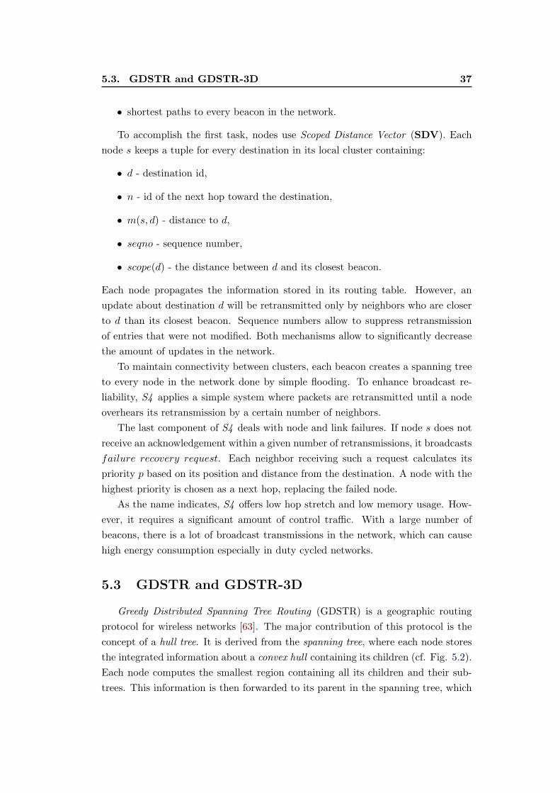
Greedy Distributed Spanning Tree Routing (GDSTR) is a geographic routing
protocol for wireless networks [63]. The major contribution of this protocol is the
concept of a hull tree. It is derived from the spanning tree, where each node stores
the integrated information about a convex hull containing its children (cf. Fig. 5.2).
Each node computes the smallest region containing all its children and their sub-
trees. This information is then forwarded to its parent in the spanning tree, which
38 Chapter 5. Geographic Routing
aggregates the information and continues the process. Each region is represented as
a 5-point convex hull. With such a representation, GDSTR requires a small amount
Figure 5.2: Hull tree in GDSTR
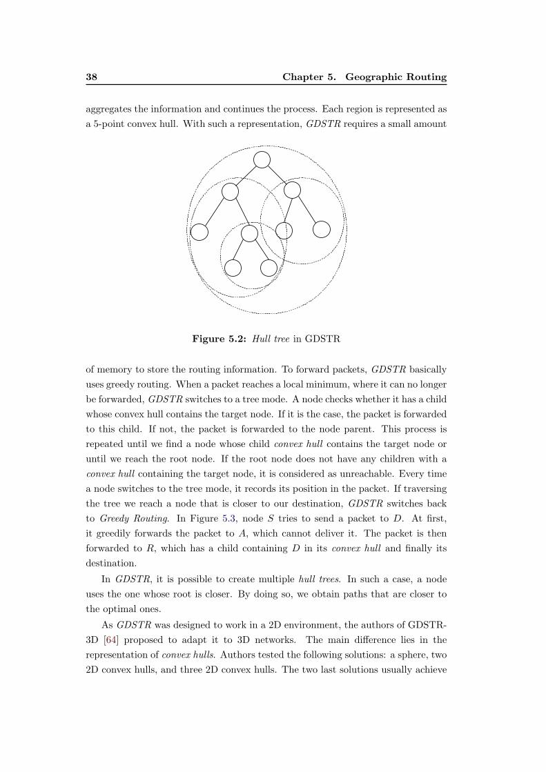
of memory to store the routing information. To forward packets, GDSTR basically
uses greedy routing. When a packet reaches a local minimum, where it can no longer
be forwarded, GDSTR switches to a tree mode. A node checks whether it has a child
whose convex hull contains the target node. If it is the case, the packet is forwarded
to this child. If not, the packet is forwarded to the node parent. This process is
repeated until we find a node whose child convex hull contains the target node or
until we reach the root node. If the root node does not have any children with a
convex hull containing the target node, it is considered as unreachable. Every time
a node switches to the tree mode, it records its position in the packet. If traversing
the tree we reach a node that is closer to our destination, GDSTR switches back
to Greedy Routing. In Figure 5.3, node S tries to send a packet to D. At first,
it greedily forwards the packet to A, which cannot deliver it. The packet is then
forwarded to R, which has a child containing D in its convex hull and finally its
destination.
In GDSTR, it is possible to create multiple hull trees. In such a case, a node
uses the one whose root is closer. By doing so, we obtain paths that are closer to
the optimal ones.
As GDSTR was designed to work in a 2D environment, the authors of GDSTR-
3D [64] proposed to adapt it to 3D networks. The main difference lies in the
representation of convex hulls. Authors tested the following solutions: a sphere, two
2D convex hulls, and three 2D convex hulls. The two last solutions usually achieve
5.4. Binary Waypoint Routing 39
R
D
S
A
Figure 5.3: Routing in GDSTR
much better results than a sphere. GDSTR-3D uses a 2-hop Greedy Routing as
its routing base, where nodes store the information about their 2-hop neighbors to
determine the best hop. This solution significantly increases the delivery rate, but
also increases memory usage.
Both solutions present an interesting approach characterised by small memory
usage and low hop stretch. However, as both solutions use a spanning tree, they
are not resistant to network dynamics and can generate large amounts of control
traffic during node failures, especially for nodes located near the tree root.
5.4 Binary Waypoint Routing
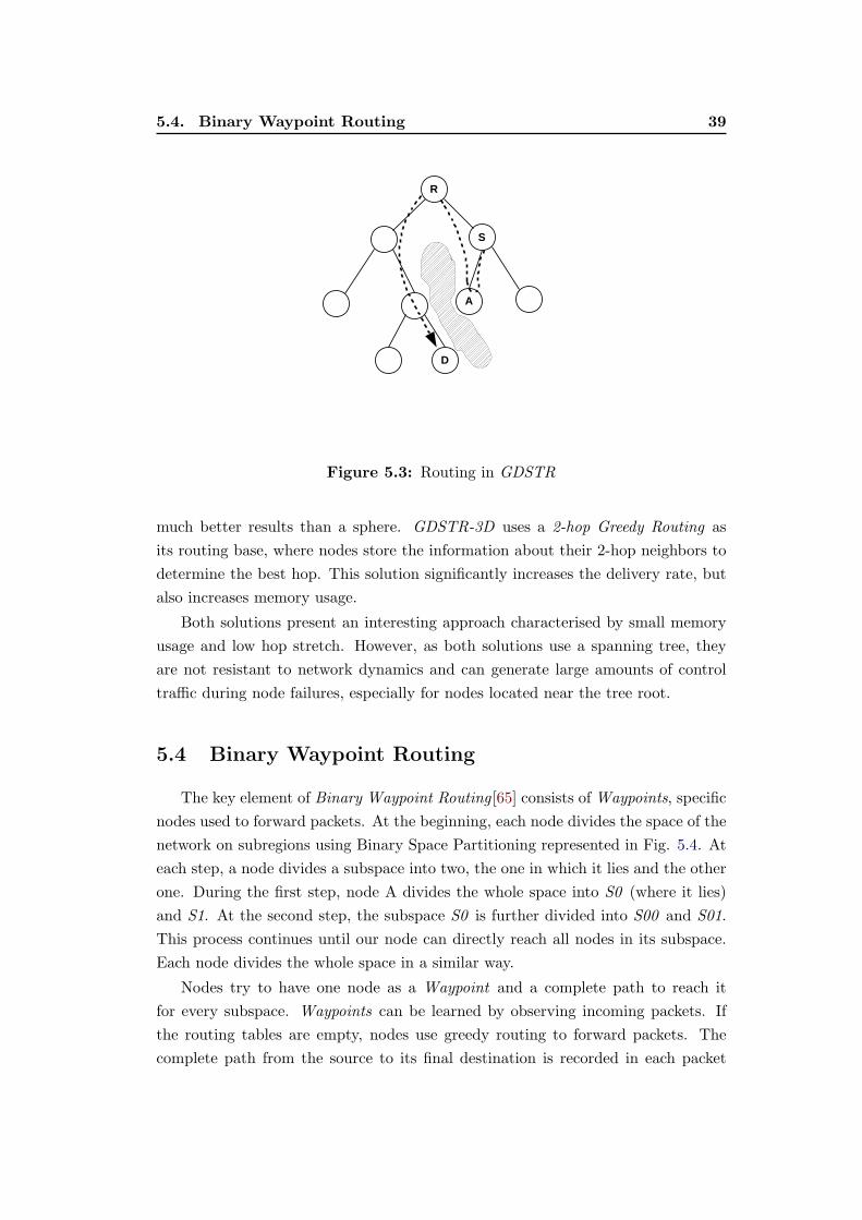
The key element of Binary Waypoint Routing [65] consists of Waypoints, specific
nodes used to forward packets. At the beginning, each node divides the space of the
network on subregions using Binary Space Partitioning represented in Fig. 5.4. At
each step, a node divides a subspace into two, the one in which it lies and the other
one. During the first step, node A divides the whole space into S0 (where it lies)
and S1. At the second step, the subspace S0 is further divided into S00 and S01.
This process continues until our node can directly reach all nodes in its subspace.
Each node divides the whole space in a similar way.
Nodes try to have one node as a Waypoint and a complete path to reach it
for every subspace. Waypoints can be learned by observing incoming packets. If
the routing tables are empty, nodes use greedy routing to forward packets. The
complete path from the source to its final destination is recorded in each packet
40 Chapter 5. Geographic Routing
A
S1
S01
S001
S0001
Figure 5.4: Space division in Binary Waypoint Routing
header. A node forwarding a packet checks its source. If it lies in a subspace for
which it still does not have any Waypoint, it stores the complete path in its routing
table.
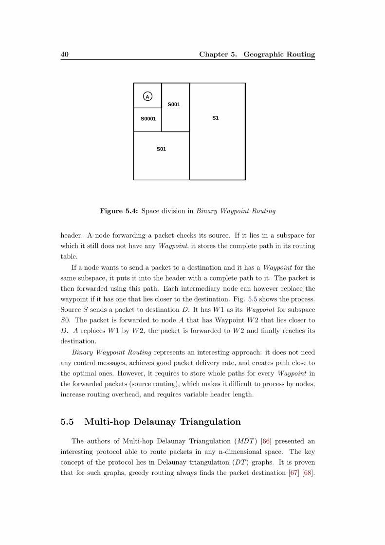
If a node wants to send a packet to a destination and it has a Waypoint for the
same subspace, it puts it into the header with a complete path to it. The packet is
then forwarded using this path. Each intermediary node can however replace the
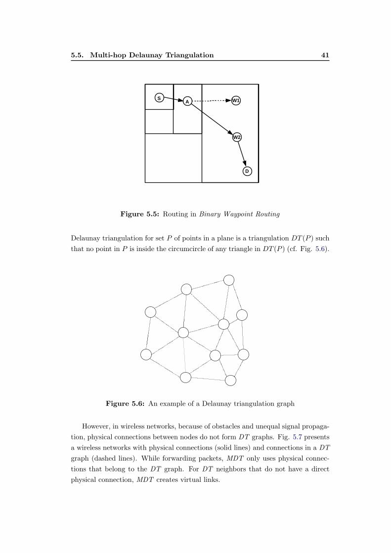
waypoint if it has one that lies closer to the destination. Fig. 5.5 shows the process.
Source S sends a packet to destination D. It has W1 as its Waypoint for subspace
S0. The packet is forwarded to node A that has Waypoint W2 that lies closer to
D. A replaces W1 by W2, the packet is forwarded to W2 and finally reaches its
destination.
Binary Waypoint Routing represents an interesting approach: it does not need
any control messages, achieves good packet delivery rate, and creates path close to
the optimal ones. However, it requires to store whole paths for every Waypoint in
the forwarded packets (source routing), which makes it difficult to process by nodes,
increase routing overhead, and requires variable header length.
5.5 Multi-hop Delaunay Triangulation
The authors of Multi-hop Delaunay Triangulation (MDT ) [66] presented an
interesting protocol able to route packets in any n-dimensional space. The key
concept of the protocol lies in Delaunay triangulation (DT ) graphs. It is proven
that for such graphs, greedy routing always finds the packet destination [67] [68].
5.5. Multi-hop Delaunay Triangulation 41
S
D
A W1
W2
Figure 5.5: Routing in Binary Waypoint Routing
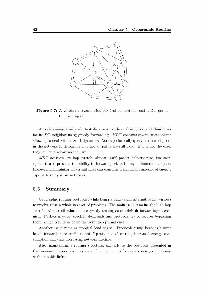
Delaunay triangulation for set P of points in a plane is a triangulation DT (P ) such
that no point in P is inside the circumcircle of any triangle in DT (P ) (cf. Fig. 5.6).
Figure 5.6: An example of a Delaunay triangulation graph
However, in wireless networks, because of obstacles and unequal signal propaga-
tion, physical connections between nodes do not form DT graphs. Fig. 5.7 presents
a wireless networks with physical connections (solid lines) and connections in a DT
graph (dashed lines). While forwarding packets, MDT only uses physical connec-
tions that belong to the DT graph. For DT neighbors that do not have a direct
physical connection, MDT creates virtual links.
42 Chapter 5. Geographic Routing
Figure 5.7: A wireless network with physical connections and a DT graph
built on top of it.
A node joining a network, first discovers its physical neighbor and than looks
for its DT neighbor using greedy forwarding. MDT contains several mechanisms
allowing to deal with network dynamics. Nodes periodically query a subset of peers
in the network to determine whether all paths are still valid. If it is not the case,
they launch a repair mechanism.
MDT achieves low hop stretch, almost 100% packet delivery rate, low stor-
age cost, and presents the ability to forward packets in any n-dimensional space.
However, maintaining all virtual links can consume a significant amount of energy,
especially in dynamic networks.
5.6 Summary
Geographic routing protocols, while being a lightweight alternative for wireless
networks, raise a whole new set of problems. The main issue remains the high hop
stretch. Almost all solutions use greedy routing as the default forwarding mecha-
nism. Packets may get stuck in dead-ends and protocols try to recover bypassing
them, which results in paths far from the optimal ones.
Another issue remains unequal load share. Protocols using beacons/cluster
heads forward more traffic to this ”special nodes” causing increased energy con-
sumption and thus decreasing network lifetime.
Also, maintaining a routing structure, similarly to the protocols presented in
the previous chapter, requires a significant amount of control messages increasing
with unstable links.

5.6. Summary 43
Some protocols require strong assumptions on the underlying network graph
such as the unit disk or a planar graph, which limits their use.
In the next chapter, we introduce application layer protocols, providing naming
schemes for nodes, usually in addition to a routing protocol.

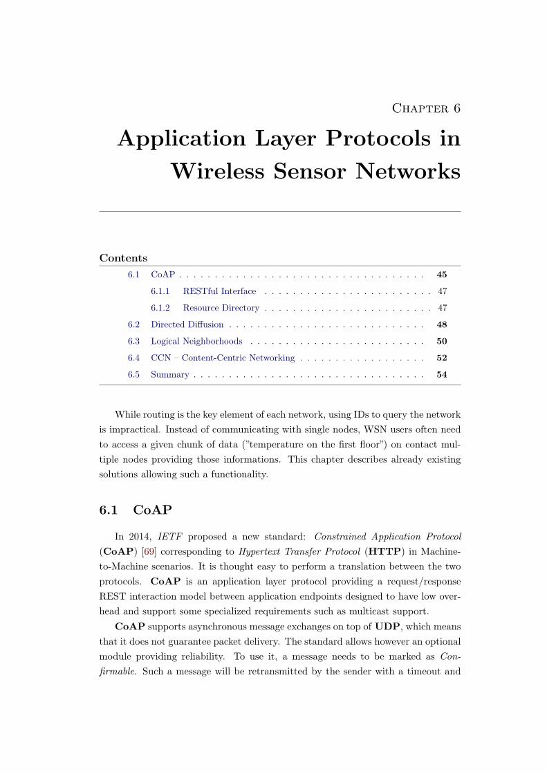
Chapter 6
Application Layer Protocols in
Wireless Sensor Networks
Contents
6.1 CoAP . . . . . . . . . . . . . . . . . . . . . . . . . . . . . . . . . . . 45
6.1.1 RESTful Interface . . . . . . . . . . . . . . . . . . . . . . . . 47
6.1.2 Resource Directory . . . . . . . . . . . . . . . . . . . . . . . . 47
6.2 Directed Diffusion . . . . . . . . . . . . . . . . . . . . . . . . . . . . 48
6.3 Logical Neighborhoods . . . . . . . . . . . . . . . . . . . . . . . . . 50
6.4 CCN – Content-Centric Networking . . . . . . . . . . . . . . . . . . 52
6.5 Summary . . . . . . . . . . . . . . . . . . . . . . . . . . . . . . . . . 54
While routing is the key element of each network, using IDs to query the network
is impractical. Instead of communicating with single nodes, WSN users often need
to access a given chunk of data (”temperature on the first floor”) on contact mul-
tiple nodes providing those informations. This chapter describes already existing
solutions allowing such a functionality.
6.1 CoAP
In 2014, IETF proposed a new standard: Constrained Application Protocol
(CoAP) [69] corresponding to Hypertext Transfer Protocol (HTTP) in Machine-
to-Machine scenarios. It is thought easy to perform a translation between the two
protocols. CoAP is an application layer protocol providing a request/response
REST interaction model between application endpoints designed to have low over-
head and support some specialized requirements such as multicast support.
CoAP supports asynchronous message exchanges on top of UDP, which means
that it does not guarantee packet delivery. The standard allows however an optional
module providing reliability. To use it, a message needs to be marked as Con-
firmable. Such a message will be retransmitted by the sender with a timeout and
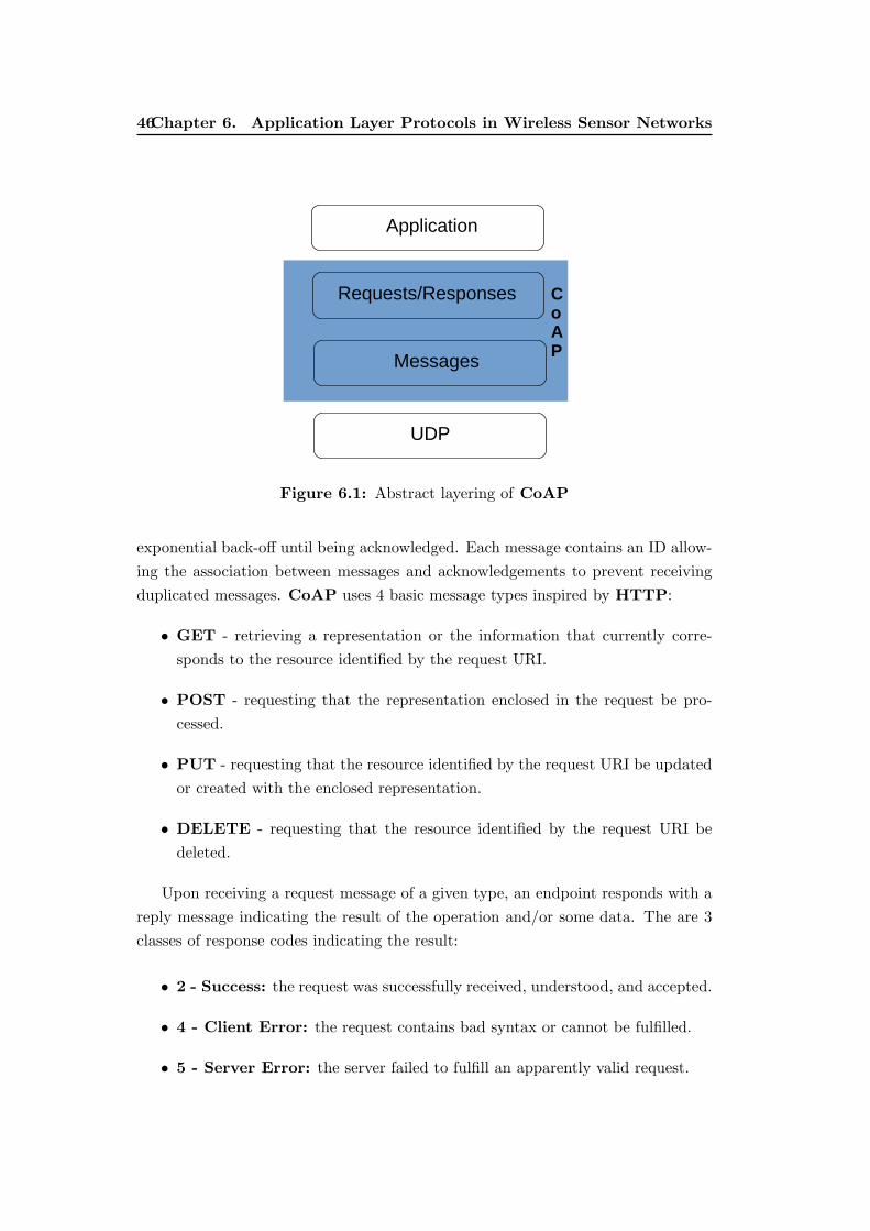
46Chapter 6. Application Layer Protocols in Wireless Sensor Networks
Application
Requests/Responses
Messages
UDP
C
o
A
P
Figure 6.1: Abstract layering of CoAP
exponential back-off until being acknowledged. Each message contains an ID allow-
ing the association between messages and acknowledgements to prevent receiving
duplicated messages. CoAP uses 4 basic message types inspired by HTTP:
• GET - retrieving a representation or the information that currently corre-
sponds to the resource identified by the request URI.
• POST - requesting that the representation enclosed in the request be pro-
cessed.
• PUT - requesting that the resource identified by the request URI be updated
or created with the enclosed representation.
• DELETE - requesting that the resource identified by the request URI be
deleted.
Upon receiving a request message of a given type, an endpoint responds with a
reply message indicating the result of the operation and/or some data. The are 3
classes of response codes indicating the result:
• 2 - Success: the request was successfully received, understood, and accepted.
• 4 - Client Error: the request contains bad syntax or cannot be fulfilled.
• 5 - Server Error: the server failed to fulfill an apparently valid request.
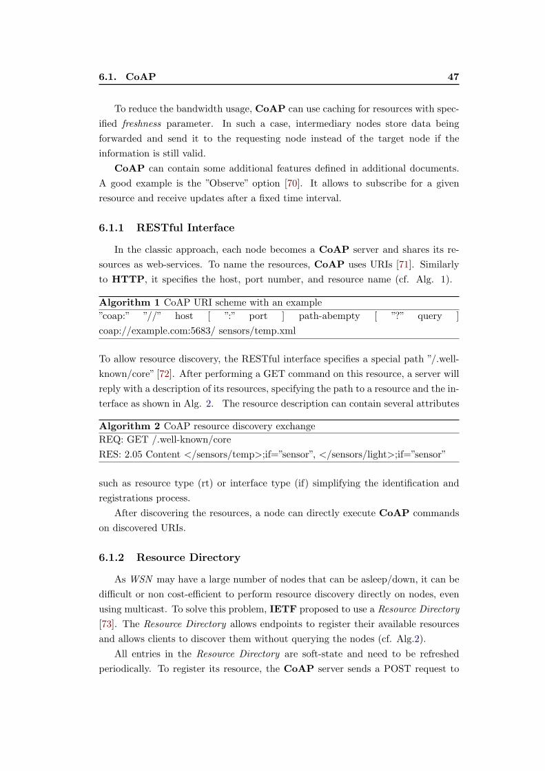
6.1. CoAP 47
To reduce the bandwidth usage, CoAP can use caching for resources with spec-
ified freshness parameter. In such a case, intermediary nodes store data being
forwarded and send it to the requesting node instead of the target node if the
information is still valid.
CoAP can contain some additional features defined in additional documents.
A good example is the ”Observe” option [70]. It allows to subscribe for a given
resource and receive updates after a fixed time interval.
6.1.1 RESTful Interface
In the classic approach, each node becomes a CoAP server and shares its re-
sources as web-services. To name the resources, CoAP uses URIs [71]. Similarly
to HTTP, it specifies the host, port number, and resource name (cf. Alg. 1).
Algorithm 1 CoAP URI scheme with an example
”coap:” ”//” host [ ”:” port ] path-abempty [ ”?” query ]
coap://example.com:5683/ sensors/temp.xml
To allow resource discovery, the RESTful interface specifies a special path ”/.well-
known/core” [72]. After performing a GET command on this resource, a server will
reply with a description of its resources, specifying the path to a resource and the in-
terface as shown in Alg. 2. The resource description can contain several attributes
Algorithm 2 CoAP resource discovery exchange
REQ: GET /.well-known/core
RES: 2.05 Content </sensors/temp>;if=”sensor”, </sensors/light>;if=”sensor”
such as resource type (rt) or interface type (if) simplifying the identification and
registrations process.
After discovering the resources, a node can directly execute CoAP commands
on discovered URIs.
6.1.2 Resource Directory
As WSN may have a large number of nodes that can be asleep/down, it can be
difficult or non cost-efficient to perform resource discovery directly on nodes, even
using multicast. To solve this problem, IETF proposed to use a Resource Directory
[73]. The Resource Directory allows endpoints to register their available resources
and allows clients to discover them without querying the nodes (cf. Alg.2).
All entries in the Resource Directory are soft-state and need to be refreshed
periodically. To register its resource, the CoAP server sends a POST request to
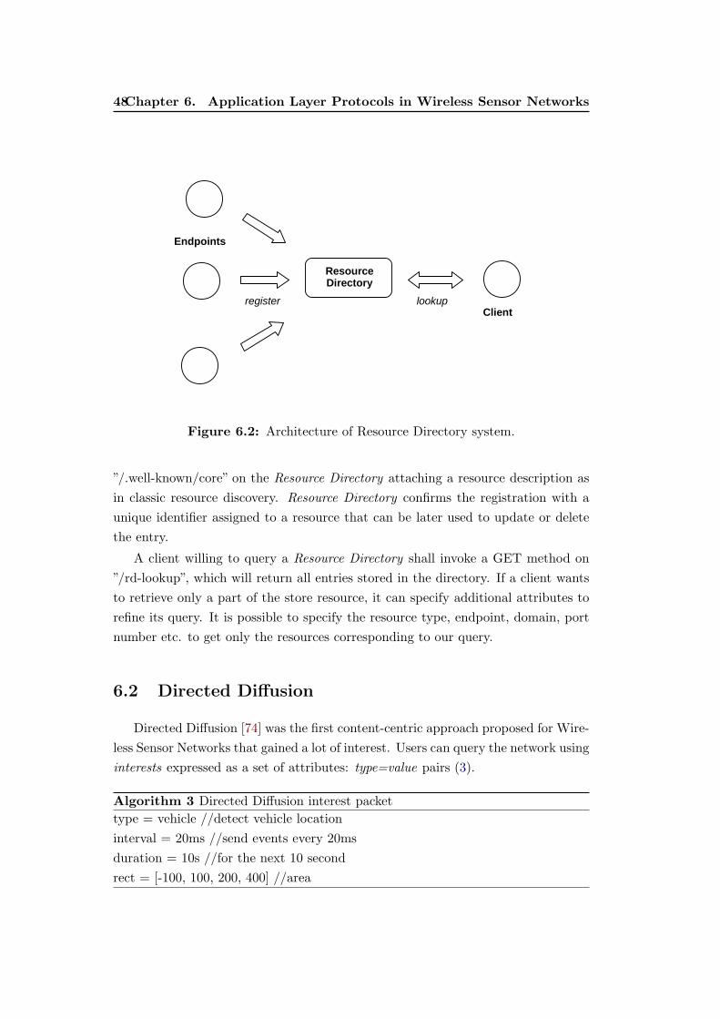
48Chapter 6. Application Layer Protocols in Wireless Sensor Networks
Resource Directory
register lookup
Endpoints
Client
Figure 6.2: Architecture of Resource Directory system.
”/.well-known/core” on the Resource Directory attaching a resource description as
in classic resource discovery. Resource Directory confirms the registration with a
unique identifier assigned to a resource that can be later used to update or delete
the entry.
A client willing to query a Resource Directory shall invoke a GET method on
”/rd-lookup”, which will return all entries stored in the directory. If a client wants
to retrieve only a part of the store resource, it can specify additional attributes to
refine its query. It is possible to specify the resource type, endpoint, domain, port
number etc. to get only the resources corresponding to our query.
6.2 Directed Diffusion
Directed Diffusion [74] was the first content-centric approach proposed for Wire-
less Sensor Networks that gained a lot of interest. Users can query the network using
interests expressed as a set of attributes: type=value pairs (3).
Algorithm 3 Directed Diffusion interest packet
type = vehicle //detect vehicle location
interval = 20ms //send events every 20ms
duration = 10s //for the next 10 second
rect = [-100, 100, 200, 400] //area
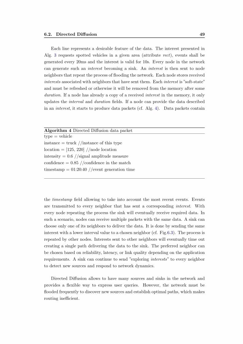
6.2. Directed Diffusion 49
Each line represents a desirable feature of the data. The interest presented in
Alg. 3 requests spotted vehicles in a given area (attribute rect), events shall be
generated every 20ms and the interest is valid for 10s. Every node in the network
can generate such an interest becoming a sink. An interest is then sent to node
neighbors that repeat the process of flooding the network. Each node stores received
interests associated with neighbors that have sent them. Each interest is ”soft-state”
and must be refreshed or otherwise it will be removed from the memory after some
duration. If a node has already a copy of a received interest in the memory, it only
updates the interval and duration fields. If a node can provide the data described
in an interest, it starts to produce data packets (cf. Alg. 4). Data packets contain
Algorithm 4 Directed Diffusion data packet
type = vehicle
instance = truck //instance of this type
location = [125, 220] //node location
intensity = 0.6 //signal amplitude measure
confidence = 0.85 //confidence in the match
timestamp = 01:20:40 //event generation time
the timestamp field allowing to take into account the most recent events. Events
are transmitted to every neighbor that has sent a corresponding interest. With
every node repeating the process the sink will eventually receive required data. In
such a scenario, nodes can receive multiple packets with the same data. A sink can
choose only one of its neighbors to deliver the data. It is done by sending the same
interest with a lower interval value to a chosen neighbor (cf. Fig.6.3). The process is
repeated by other nodes. Interests sent to other neighbors will eventually time out
creating a single path delivering the data to the sink. The preferred neighbor can
be chosen based on reliability, latency, or link quality depending on the application
requirements. A sink can continue to send ”exploring interests” to every neighbor
to detect new sources and respond to network dynamics.
Directed Diffusion allows to have many sources and sinks in the network and
provides a flexible way to express user queries. However, the network must be
flooded frequently to discover new sources and establish optimal paths, which makes
routing inefficient.
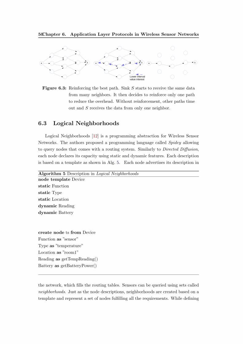
50Chapter 6. Application Layer Protocols in Wireless Sensor Networks
AS
AS
Lower interval
value interest
AS
Figure 6.3: Reinforcing the best path. Sink S starts to receive the same data
from many neighbors. It then decides to reinforce only one path
to reduce the overhead. Without reinforcement, other paths time
out and S receives the data from only one neighbor.
6.3 Logical Neighborhoods
Logical Neighborhoods [12] is a programming abstraction for Wireless Sensor
Networks. The authors proposed a programming language called Spidey allowing
to query nodes that comes with a routing system. Similarly to Directed Diffusion,
each node declares its capacity using static and dynamic features. Each description
is based on a template as shown in Alg. 5. Each node advertises its description in
Algorithm 5 Description in Logical Neighborhoods
node template Device
static Function
static Type
static Location
dynamic Reading
dynamic Battery
create node ts from Device
Function as ”sensor”
Type as ”temperature”
Location as ”room1”
Reading as getTempReading()
Battery as getBatteryPower()
the network, which fills the routing tables. Sensors can be queried using sets called
neighborhoods. Just as the node descriptions, neighborhoods are created based on a
template and represent a set of nodes fulfilling all the requirements. While defining

6.3. Logical Neighborhoods 51
a neighborhood, we can use features defined by nodes brought together by logical
operators such as AND, OR, and NOT (cf. Alg. 6).
Algorithm 6 A sample LN query
neighborhood template HighTempSens (threshold)
with Function = ”sensor” and
Type = ”temperature” and
Reading > threshold
create neighborhood hts100
from HighTempSens(threshold : 100)
max hops 2
credits 30
Logical Neighborhoods propose a special routing system allowing Spidey to work
efficiently. As mentioned before, each node advertises its capabilities in special Pro-
fileAdv messages that contain a node description. Nodes receiving such a message
check whether they already have information about the advertised features. If not
or if the advertised cost is lower that the one present in the memory, the routing
tables are updated and the message is rebroadcasted. Fig. 6.1 presents a sample
routing table. Each entry contains:
• Id - identifying the entry
• Attribute,Value - an attribute and its value
• Cost - cost of reaching the closest node with an attribute
• Links - indicating with which other entries the given entry is connected. Such
a representation allows to reduce the memory usage. Instead of storing every
combination of attributes, we only store single features and connect them
using the Links field.
• DecPath - decreasing path. A neighbor advertising the smallest cost to reach
a given attribute.
• IncPaths - increasing paths. Neighbors advertising a higher cost to reach a
given attribute.
• Source - a node whose information has been inserted in the ProfileAdv mes-
sage.
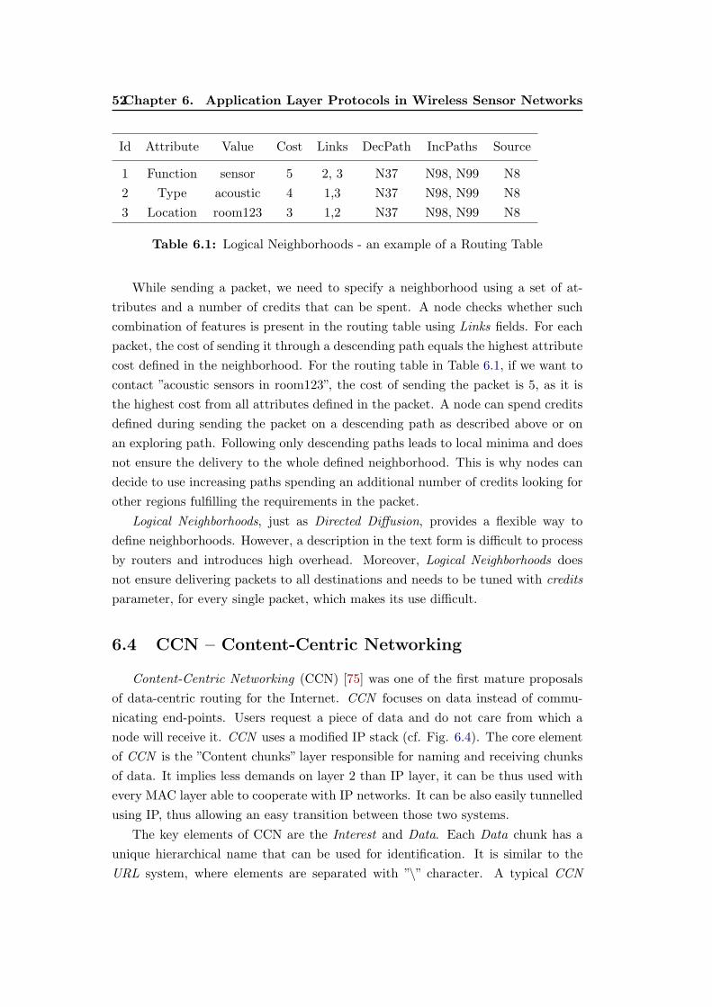
52Chapter 6. Application Layer Protocols in Wireless Sensor Networks
Id Attribute Value Cost Links DecPath IncPaths Source
1 Function sensor 5 2, 3 N37 N98, N99 N8
2 Type acoustic 4 1,3 N37 N98, N99 N8
3 Location room123 3 1,2 N37 N98, N99 N8
Table 6.1: Logical Neighborhoods - an example of a Routing Table
While sending a packet, we need to specify a neighborhood using a set of at-
tributes and a number of credits that can be spent. A node checks whether such
combination of features is present in the routing table using Links fields. For each
packet, the cost of sending it through a descending path equals the highest attribute
cost defined in the neighborhood. For the routing table in Table 6.1, if we want to
contact ”acoustic sensors in room123”, the cost of sending the packet is 5, as it is
the highest cost from all attributes defined in the packet. A node can spend credits
defined during sending the packet on a descending path as described above or on
an exploring path. Following only descending paths leads to local minima and does
not ensure the delivery to the whole defined neighborhood. This is why nodes can
decide to use increasing paths spending an additional number of credits looking for
other regions fulfilling the requirements in the packet.
Logical Neighborhoods, just as Directed Diffusion, provides a flexible way to
define neighborhoods. However, a description in the text form is difficult to process
by routers and introduces high overhead. Moreover, Logical Neighborhoods does
not ensure delivering packets to all destinations and needs to be tuned with credits
parameter, for every single packet, which makes its use difficult.
6.4 CCN – Content-Centric Networking
Content-Centric Networking (CCN) [75] was one of the first mature proposals
of data-centric routing for the Internet. CCN focuses on data instead of commu-
nicating end-points. Users request a piece of data and do not care from which a
node will receive it. CCN uses a modified IP stack (cf. Fig. 6.4). The core element
of CCN is the ”Content chunks” layer responsible for naming and receiving chunks
of data. It implies less demands on layer 2 than IP layer, it can be thus used with
every MAC layer able to cooperate with IP networks. It can be also easily tunnelled
using IP, thus allowing an easy transition between those two systems.
The key elements of CCN are the Interest and Data. Each Data chunk has a
unique hierarchical name that can be used for identification. It is similar to the
URL system, where elements are separated with ”\” character. A typical CCN
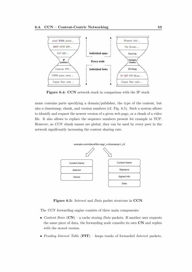
6.4. CCN – Content-Centric Networking 53
Figure 6.4: CCN network stack in comparison with the IP stack.
name contains parts specifying a domain/publisher, the type of the content, but
also a timestamp, chunk, and version numbers (cf. Fig. 6.5). Such a system allows
to identify and request the newest version of a given web page, or a chunk of a video
file. It also allows to replace the sequence numbers present for example in TCP.
However, as CCN chunk names are global, they can be used by every peer in the
network significantly increasing the content sharing rate.
Content Name
Selector
Nonce
Content Name
Signature
Signed Info
Data
example.com/videos/film.mpg/_v<timestamp>/_s3
Figure 6.5: Interest and Data packet structure in CCN.
The CCN forwarding engine consists of three main components:
• Content Store (CN) – a cache storing Data packets. If another user requests
the same piece of data, the forwarding node consults its own CN and replies
with the stored version.
• Pending Interest Table (PIT) – keeps tracks of forwarded Interest packets.
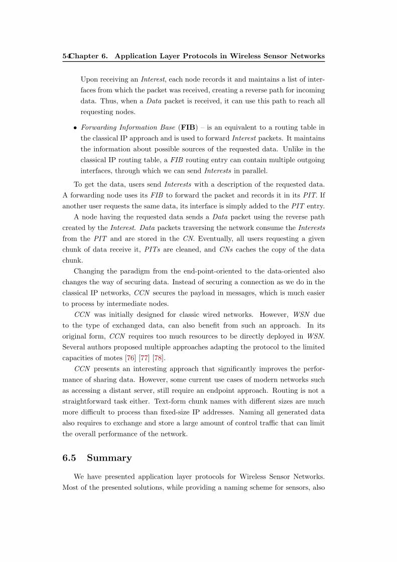
54Chapter 6. Application Layer Protocols in Wireless Sensor Networks
Upon receiving an Interest, each node records it and maintains a list of inter-
faces from which the packet was received, creating a reverse path for incoming
data. Thus, when a Data packet is received, it can use this path to reach all
requesting nodes.
• Forwarding Information Base (FIB) – is an equivalent to a routing table in
the classical IP approach and is used to forward Interest packets. It maintains
the information about possible sources of the requested data. Unlike in the
classical IP routing table, a FIB routing entry can contain multiple outgoing
interfaces, through which we can send Interests in parallel.
To get the data, users send Interests with a description of the requested data.
A forwarding node uses its FIB to forward the packet and records it in its PIT. If
another user requests the same data, its interface is simply added to the PIT entry.
A node having the requested data sends a Data packet using the reverse path
created by the Interest. Data packets traversing the network consume the Interests
from the PIT and are stored in the CN. Eventually, all users requesting a given
chunk of data receive it, PITs are cleaned, and CNs caches the copy of the data
chunk.
Changing the paradigm from the end-point-oriented to the data-oriented also
changes the way of securing data. Instead of securing a connection as we do in the
classical IP networks, CCN secures the payload in messages, which is much easier
to process by intermediate nodes.
CCN was initially designed for classic wired networks. However, WSN due
to the type of exchanged data, can also benefit from such an approach. In its
original form, CCN requires too much resources to be directly deployed in WSN.
Several authors proposed multiple approaches adapting the protocol to the limited
capacities of motes [76] [77] [78].
CCN presents an interesting approach that significantly improves the perfor-
mance of sharing data. However, some current use cases of modern networks such
as accessing a distant server, still require an endpoint approach. Routing is not a
straightforward task either. Text-form chunk names with different sizes are much
more difficult to process than fixed-size IP addresses. Naming all generated data
also requires to exchange and store a large amount of control traffic that can limit
the overall performance of the network.
6.5 Summary
We have presented application layer protocols for Wireless Sensor Networks.
Most of the presented solutions, while providing a naming scheme for sensors, also
6.5. Summary 55
include a layer 3 routing protocol allowing to exchange packets. However, closely
coupled OSI/ISO layers limit the use of the proposed protocols in various scenarios.
CoAP, the de facto standard application layer protocol for WSN, introduces a very
inefficient approach with a central server storing all the information about motes in
the network.
Pure content-centric approach presented by CCN can be efficient while delivering
data to many recipients. However, it limits its use in many scenarios including using
actuators. Also, limited amount of mote resources and big volumes of generated
information, makes naming and caching data difficult.
Both Logical Neighborhoods and Directed Diffusion suffer from routing sys-
tems introducing a significant amount of unnecessary traffic. What is more, both
solutions are difficult to integrate into existing networks because of custom gram-
mars/naming schemes.
In the next part, we introduce an IPv6 compliant routing protocol allowing
for content-centric names without using any translation or naming service. The
further part proposes a geographic routing protocol with equal load share, no control
message overhead, and paths close to optimal ones.


Part III
Featurecast: a Group
Communication Service for
WSN

Chapter 7
Rationale
Wireless sensor networks need to support specific traffic patterns related to
sensor applications. One of their most important goals is to forward collected data
to one or several sinks. They also have to support downward traffic from a sink to
all or some sensor nodes. This traffic pattern results from the need for configuring
nodes, querying sensors, or transmitting commands to actuators. Sensor nodes
may require communication with other nodes, for instance for aggregating data or
collaborating on a common reaction to local events.
In addition to the standard unicast communication, many sensor network ap-
plications may benefit from multicasting to forward packets to a group of nodes or
report data to multiple sinks [79, 80, 81]. Multicasting results in a reduced number
of packets forwarded in the network, which in turn limits energy consumption—
compared to unicast, nodes transmit less packets when using multicast, because
packets are only replicated when needed.
Unicast and multicast are address-centric communication modes in which source
and destination addresses identify endpoint nodes. Such modes are suitable for
structured addresses that result in small routing tables. Data or content-centric
routing focuses on the packet content instead of communication endpoints. In the
context of sensor networks, Directed Diffusion was one of the first proposals for
sensor data dissemination based on this approach [74, 82]: sensor nodes attach at-
tributes (name-value pairs) to generated data, consumers specify interests for sensor
data in terms of attributes, and sensors send unicast data packets to consumers.
The data-centric paradigm is appealing for sensor networks, because it fits very
well their data-oriented nature, however the approach incurs significant overhead
by attaching attributes to data, which is prohibitive in energy constrained networks.
Directed Diffusion uses flooding to disseminate interests for sensor data, which is
inefficient in wireless networks. Moreover, it does not scale well in networks with
many sinks that transmit many different queries [83].
Logical Neighborhoods (LN) proposed a similar abstraction, but at the appli-
cation layer: a node declaratively specifies the characteristics of its neighbors in
terms of attributes and the cost of reaching them [12]. A template specifies the
attributes of a node. Nodes broadcast their attributes to neighbors that store the
60 Chapter 7. Rationale
information in a table and re-broadcast them if there is a change in the existing
state created by the advertisement. The propagation of advertisements creates a
state distributed over the nodes that contains the cost of reaching the closest node
with a given attribute. To find a node with an attribute, a node broadcasts an
application message containing the neighborhood template. The approach suffers
from significant overhead of transmitting attributes and templates. The overhead
in terms of the number of transmitted messages is also important compared to the
ideal multicast routing based on the minimum spanning tree rooted at the sender.
Finally, all solutions based on data-centric approach require a specific grammar
that may be difficult to process by sensors and significantly slows down the routing
process.
In this paper, we propose Featurecast, a network layer communication mode
well suited for sensor networks. One of our main design goals was to create a
system able to cooperate with already existing IPv6 networks. Unlike Directed
Diffusion, Featurecast is address-centric, but it uses a data-centric approach to
create addresses and operate routing: addresses correspond to a set of features
characterizing sensor nodes. Features are predicates, not attributes, which allows
us to represent them in a compact way in address fields of packets and in routing
tables.
Nodes disseminate Featurecast addresses in the network following a structure
usually constructed for routing standard unicast packets such as a Collection Tree
(CT) [84] or a DODAG (Destination Oriented Directed Acyclic Graph) [11]. Inter-
mediate nodes merge the features of nodes reachable on a given link and construct
a compact routing table for further packet forwarding. Based on the routing tables,
a packet can reach all nodes characterized by a given set of features. Our proposal
does not define any specific grammar for features, which makes it extremely flexible
and easy to use. We propose a specific compact encoding allowing for fitting a Fea-
turecast address into the standard multicast IPv6 address field. To the best of our
knowledge, Featurecast is the only protocol able to take advantage of a data-centric
approach in traditional IPv6 networks.
We have implemented Featurecast and the proposed scheme for routing in Con-
tiki OS [85] and integrated them within its uIPv6 (micro Internet Protocol) stack.
The implementation provides Featurecast at the network layer unlike other propos-
als that use application layer overlays. To evaluate Featurecast, we have simulated
in Cooja an application scenario developed for CoAP group communications [86]
with several sensors placed across buildings, wings, and rooms. We have compared
Featurecast with Logical Neighborhoods (LN) [12] and IP multicast with respect to
the memory footprint and message overhead. Featurecast results in a significantly
61
smaller memory footprint and a lower average number of messages for updating
routing tables compared to other schemes.

Chapter 8
Principles of Featurecast
We want to provide a new communication mode for wireless sensor networks to
designate relevant sensor nodes or data destinations by means of their characteristics
and not with some low level identifiers or node addresses. For instance, we may
want to get the“average temperature on the 1st floor”or“turn off all the lights in the
building”. Such reasoning is close to applications that take advantage of sensors and
actuators. Obviously, we could support such messages by associating a multicast
group with each query, however, the number of such groups may quickly become
too large, because of all possible combinations of characteristics.
We introduce below the notion of Featurecast addresses, present the construction
of routing tables, and the forwarding process.
8.1 Featurecast Addresses
We assume that each sensor defines a set of its features, for instance its capabil-
ity of sensing the environment (temperature, humidity), location (sector 5, 1st
floor), state (low-energy), or some other custom features (my favorite nodes).
Features are predicates, i.e., statements that may be true or false (in the previous
examples, we explicitly state features that are true). Predicates are commonly used
to represent the properties of objects and we use them here to represent the proper-
ties of sensors: if f is a predicate on sensor X, we say that f is a property of sensor
X. Note that features are not attributes (i.e., name:value pairs), which allows us
to represent them in a much more compact way without loosing any flexibility (cf.
8.1). We assume that there is no coordination in defining features, but all features
are known and each node can define its features at will.
A sensor node derives its Featurecast address from its features—more formally,
a node address is the set:
A = {f1, f2, ..., fn}, fi ∈ F , (8.1)
where fi is a feature predicate and F is the set of all possible features with car-
dinality of N . Features in the network may evolve in time and nodes may change
their features, for instance the location of a node may change when it moves or a
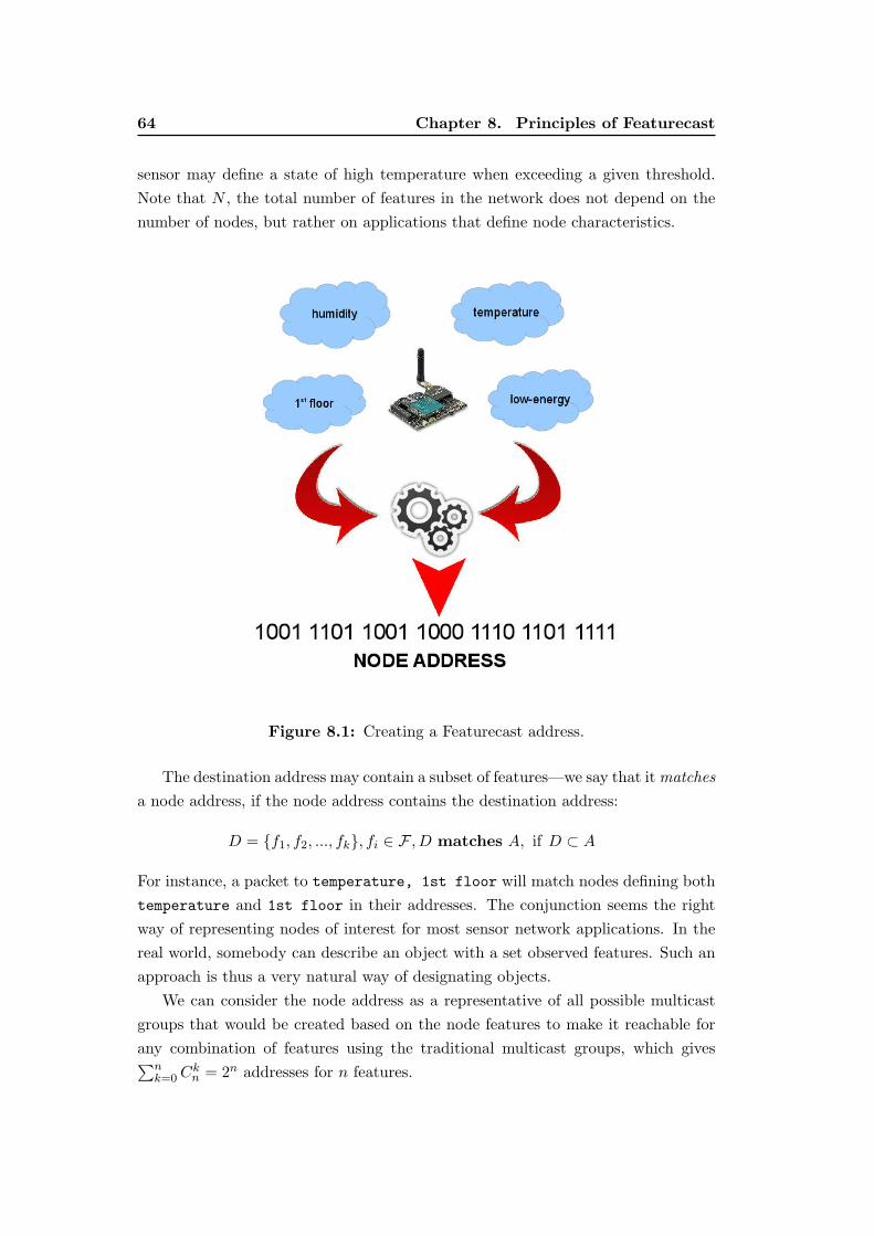
64 Chapter 8. Principles of Featurecast
sensor may define a state of high temperature when exceeding a given threshold.
Note that N , the total number of features in the network does not depend on the
number of nodes, but rather on applications that define node characteristics.
Figure 8.1: Creating a Featurecast address.
The destination address may contain a subset of features—we say that itmatches
a node address, if the node address contains the destination address:
D = {f1, f2, ..., fk}, fi ∈ F , D matches A, if D ⊂ A
For instance, a packet to temperature, 1st floor will match nodes defining both
temperature and 1st floor in their addresses. The conjunction seems the right
way of representing nodes of interest for most sensor network applications. In the
real world, somebody can describe an object with a set observed features. Such an
approach is thus a very natural way of designating objects.
We can consider the node address as a representative of all possible multicast
groups that would be created based on the node features to make it reachable for
any combination of features using the traditional multicast groups, which gives�n
k=0Ckn = 2n addresses for n features.
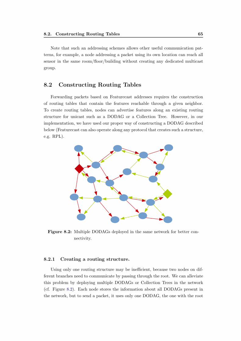
8.2. Constructing Routing Tables 65
Note that such an addressing schemes allows other useful communication pat-
terns, for example, a node addressing a packet using its own location can reach all
sensor in the same room/floor/building without creating any dedicated multicast
group.
8.2 Constructing Routing Tables
Forwarding packets based on Featurecast addresses requires the construction
of routing tables that contain the features reachable through a given neighbor.
To create routing tables, nodes can advertise features along an existing routing
structure for unicast such as a DODAG or a Collection Tree. However, in our
implementation, we have used our proper way of constructing a DODAG described
below (Featurecast can also operate along any protocol that creates such a structure,
e.g. RPL).
Figure 8.2: Multiple DODAGs deployed in the same network for better con-
nectivity.
8.2.1 Creating a routing structure.
Using only one routing structure may be inefficient, because two nodes on dif-
ferent branches need to communicate by passing through the root. We can alleviate
this problem by deploying multiple DODAGs or Collection Trees in the network
(cf. Figure 8.2). Each node stores the information about all DODAGs present in
the network, but to send a packet, it uses only one DODAG, the one with the root
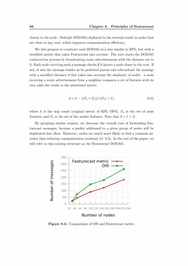
66 Chapter 8. Principles of Featurecast
closest to the node. Multiple DODAGs deployed in the network result in nodes that
are close to any root, which improves communication efficiency.
We also propose to construct each DODAG in a way similar to RPL, but with a
modified metric that takes Featurecast into account. The root starts the DODAG
construction process by broadcasting route advertisements with the distance set to
0. Each node receiving such a message checks if it knows a node closer to the root. If
not, it sets the message sender as its preferred parent and rebroadcast the message
with a modified distance d that takes into account the similarity of nodes—a node
receiving a route advertisement from a neighbor compares a set of features with its
own adds the result to the advertised metric:
d = h− (|Fn ∩ Fs|)/(|Fn|+ 1), (8.2)
where h is the hop count (original metric of RPL OF0), Fn is the set of node
features, and Fs is the set of the sender features. Note that h+ 1 > d.
By grouping similar sensors, we decrease the overall cost of forwarding Fea-
turecast messages, because a packet addressed to a given group of nodes will be
duplicated less often. Moreover, nodes are much more likely to find a common an-
cestor thus reducing communication overhead (cf. 8.3). In the rest of the paper, we
will refer to this routing structure as the Featurecast DODAG.
0
50
100
150
200
250
300
350
20 40 60 80 100 120 140 160 180 200 220 240
Num
ber
of
messages
Number of nodes
Featurecast metricOf0
Figure 8.3: Comparision of Of0 and Featurecast metric.
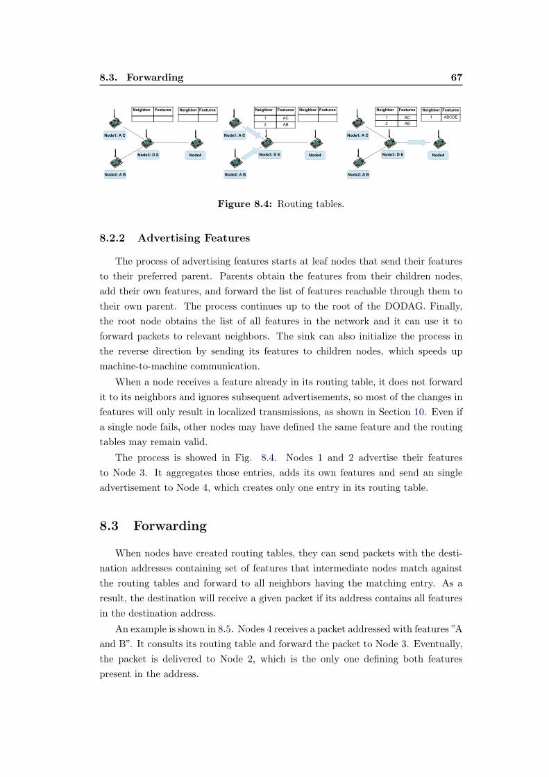
8.3. Forwarding 67
Node2: A B
Node1: A C
Node3: D E
Neighbor Features Neighbor Features
Node4
Node2: A B
Node1: A C
Node3: D E
Neighbor Features
1 AC
2 AB
Neighbor Features
Node4
Node2: A B
Node1: A C
Node3: D E
Neighbor Features
1 AC
2 AB
Neighbor Features
1 ABCDE
Node4
Figure 8.4: Routing tables.
8.2.2 Advertising Features
The process of advertising features starts at leaf nodes that send their features
to their preferred parent. Parents obtain the features from their children nodes,
add their own features, and forward the list of features reachable through them to
their own parent. The process continues up to the root of the DODAG. Finally,
the root node obtains the list of all features in the network and it can use it to
forward packets to relevant neighbors. The sink can also initialize the process in
the reverse direction by sending its features to children nodes, which speeds up
machine-to-machine communication.
When a node receives a feature already in its routing table, it does not forward
it to its neighbors and ignores subsequent advertisements, so most of the changes in
features will only result in localized transmissions, as shown in Section 10. Even if
a single node fails, other nodes may have defined the same feature and the routing
tables may remain valid.
The process is showed in Fig. 8.4. Nodes 1 and 2 advertise their features
to Node 3. It aggregates those entries, adds its own features and send an single
advertisement to Node 4, which creates only one entry in its routing table.
8.3 Forwarding
When nodes have created routing tables, they can send packets with the desti-
nation addresses containing set of features that intermediate nodes match against
the routing tables and forward to all neighbors having the matching entry. As a
result, the destination will receive a given packet if its address contains all features
in the destination address.
An example is shown in 8.5. Nodes 4 receives a packet addressed with features ”A
and B”. It consults its routing table and forward the packet to Node 3. Eventually,
the packet is delivered to Node 2, which is the only one defining both features
present in the address.
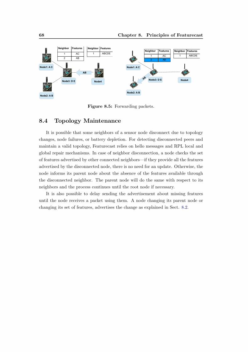
68 Chapter 8. Principles of Featurecast
Node2: A B
Node1: A C
Node3: D E
Neighbor Features
1 AC
2 AB
Neighbor Features
1 ABCDE
Node4
AB
Node2: A B
Node1: A C
Node3: D E
Neighbor Features
1 AC
2 AB
Neighbor Features
1 ABCDE
Node4
Figure 8.5: Forwarding packets.
8.4 Topology Maintenance
It is possible that some neighbors of a sensor node disconnect due to topology
changes, node failures, or battery depletion. For detecting disconnected peers and
maintain a valid topology, Featurecast relies on hello messages and RPL local and
global repair mechanisms. In case of neighbor disconnection, a node checks the set
of features advertised by other connected neighbors—if they provide all the features
advertised by the disconnected node, there is no need for an update. Otherwise, the
node informs its parent node about the absence of the features available through
the disconnected neighbor. The parent node will do the same with respect to its
neighbors and the process continues until the root node if necessary.
It is also possible to delay sending the advertisement about missing features
until the node receives a packet using them. A node changing its parent node or
changing its set of features, advertises the change as explained in Sect. 8.2.
Chapter 9
Compact Representation of
Features
We have followed several design guidelines for the compact representation. First,
we want an open network able to accept any feature defined on nodes. Second,
the addressing scheme should not depend on the number of features defined in
the network—we do not want to force the user to define a hierarchy of features.
Most of data-centric approaches use a grammar exchanged in a text form. Such an
approach is often a problem while integrating such solutions into real life scenarios.
We want our solution to still use user-friendly addresses, while being easily stored
and processed by nodes. We then need fixed-size addresses for efficient forwarding
and possibility to integrate Featurecast within the standard IPv6 addressing scheme
with 112 bits in the multicast IPv6 address. Such integration will show that a data-
centric approach may have the same overhead as address-centric solutions and lead
to easy integration with existing networks. A part of such an IPv6 address can
be used for a global prefix and routed in the Internet. Finally, we want to take
into account resource constraints (memory size) of sensor nodes for storing routing
tables.
We also want to avoid global synchronization mechanisms disseminating a map-
ping between features and their binary representation. Such a solution would result
in a significantly higher volume of communications and could delay packet forward-
ing during the feature update. For these reasons, we have decided to use hash
functions and a structure allowing to efficiently store many hashes—a Bloom filter.
9.1 Bloom Filters
A Bloom filter is a probabilistic structure allowing for efficient storage of a set
of elements. A typical filter contains an array of m bits. At the beginning all bits
are set to 0. There are k hash functions that map an element to a bit position in
the array. When inserting an element into a filter, we compute k hash functions on
the element and set all the resulting bits to 1. If a bit was already set to 1, we do
not change it. To check whether an element belongs to a set, we compute the same

70 Chapter 9. Compact Representation of Features
hash functions on the element and check if all corresponding bit positions are set
to 1. If not, we are sure that the element does not belong to the set.
False positives may occur in Bloom filters: it is possible that all bits correspond-
ing to the hash functions on a tested element are set to 1 by other stored elements,
even if the element does not belong to the set. The probability of false positives
depends on the number of stored elements n and the size of the filter (m and k):
p ≈ (1− e−km/n)k. (9.1)
To maintain the same false positive rate with a growing number of elements, we
need to increase the number of bits and hash functions, which results in larger
memory consumption and increased computational overhead.
9.2 Solution1: Straight Bloom Filters
The first possible solution is to use Bloom filters of the same size to represent
a set of features in the destination address and in the routing table entry for each
neighbor (cf. Fig. 9.1). To decide where to forward the packet, we only have to
verify if all bits set in the address are also set in the routing entry for a given
neighbor.
However, such a solution limits the number of possible features to store in the
routing tables.
If n is the number of elements in the filter (features in our case) and p is the
required probability of false positives, the minimum number of bits m for the filter
is m ≥ n log2(e) × log2(1/p). To achieve the probability of 2%, we need 5 bits
per feature. To fit 112 bits available in IPv6 address, we would be able to store
only 22 features with 2% of false positives, the value we consider as sufficient for
the packet destination address (as we store features for only one sensor or a group
of sensor), but insufficient for routing tables in which we would need to store all
features defined in the network in the worst case. Enhanced versions of the Bloom
filter such as Compressed Bloom Filters can only slightly reduce the size of the filter
while introducing some computational overhead [87].
9.3 Solution 2: Fixed Size Filter with Compression
We need a much bigger Bloom filter in the routing tables to be able to store
many features. A 1024 bit filter can store 128 elements with the probability of
false positives p128 ≈ 3%. However, we do not have 1024 bits available in the IPv6
address field. One way to use such big filters is to compress them. The filters in
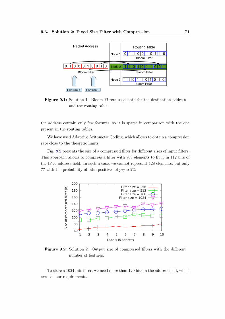
9.3. Solution 2: Fixed Size Filter with Compression 71
00 01010001 01 10110101
Feature 2Feature 1
1 010100110
01 01101101
Routing Table
Node 1
Node 2
Node 3
Packet Address
Bloom Filter
Bloom Filter
Bloom Filter
Bloom Filter
Figure 9.1: Solution 1. Bloom Filters used both for the destination address
and the routing table.
the address contain only few features, so it is sparse in comparison with the one
present in the routing tables.
We have used Adaptive Arithmetic Coding, which allows to obtain a compression
rate close to the theoretic limits.
Fig. 9.2 presents the size of a compressed filter for different sizes of input filters.
This approach allows to compress a filter with 768 elements to fit it in 112 bits of
the IPv6 address field. In such a case, we cannot represent 128 elements, but only
77 with the probability of false positives of p77 ≈ 2%
60
80
100
120
140
160
180
200
1 2 3 4 5 6 7 8 9 10
Siz
e o
f com
pre
ssed fi
lter
[b]
Labels in address
Filter size = 256Filter size = 512Filter size = 768
Filter size = 1024
Figure 9.2: Solution 2. Output size of compressed filters with the different
number of features.
To store a 1024 bits filter, we need more than 120 bits in the address field, which
exceeds our requirements.
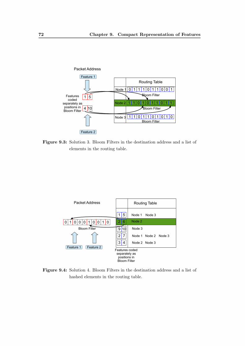
72 Chapter 9. Compact Representation of Features
1
104
5
00 10110111
Feature 2
Feature 1
0 111101011
01 01101101
Routing Table
Node 1
Node 2
Node 3
Packet Address
Bloom Filter
Bloom Filter
Bloom Filter
Features coded
separately as positions in Bloom Filter
Figure 9.3: Solution 3. Bloom Filters in the destination address and a list of
elements in the routing table.
Routing Table
2 600 01010001
Feature 2Feature 1
Packet Address
Bloom Filter 9 10
1 5
2 7
3 4
Node 1 Node 3
Node 2
Node 3
Node 1
Node 2
Node 2 Node 3
Node 3
Features coded separately as positions in Bloom Filter
Figure 9.4: Solution 4. Bloom Filters in the destination address and a list of
hashed elements in the routing table.

9.4. Solution 3: Position List in the Address, Filter in the RoutingTables 73
9.4 Solution 3: Position List in the Address, Filter in
the Routing Tables
To support a larger amount of elements in the routing tables, we propose to use
a Bloom Filter of the size allowing to store all elements with a low false positives
rate. As such a filter has a large size, we cannot store it in the address field in the
same way. An element put in the filter sets k bits to 1, where k is the number of
hash functions.
We can thus represent the position of each bit in the address field instead of
using a Bloom Filter (cf. Figure 9.3). Knowing the position of bits set to 1, we can
compare it with the corresponding bits in the Bloom Filter present in the routing
table. The size of each represented element depends on the size of the Bloom Filter
and the number of hash functions s = k log2(m). For a Bloom Filter with 1024 bits
et 2 hash functions, s = 20, so we can represent up to 5 features in 112 bits of the
header.
9.5 Solution 4: Bloom Filter in Addresses and a Bit
Position List in the Routing Table
We describe here the proposed compact representation of features that satis-
fies our requirements: being able to represent around 10 features in a destination
address limited to 112 bits with a small false positive probability and potentially
representing all features in the network in the routing tables with a small memory
footprint.
The proposed solution consists of using a different feature representation in the
routing tables: nodes represent a single feature in the routing table as the positions
of bits set in the Bloom filter. For example, we represent a feature that sets bits on
positions 5 and 76 in the Bloom Filter with the two numbers in the routing table
(cf. Figure 9.4). Nodes use a Bloom filter in the address field as described above.
The probability of two different features having the same representation in the
routing table is: pN = N/mk, where N is the number of features in the network
and m is the size of the Bloom filter in bits. The size of each represented feature
in an address depends on the Bloom filter size and the number of hash functions:
s = k log2(m).
Taking into account Eq. 9.1, this solution allows supporting 200 different fea-
tures in the routing table with the probability of false positives less than 2%, which
satisfies our requirements. As we want to use a 112 bit long Bloom filter and 2 hash
functions, we only need 2 bytes to store a feature in the routing table, which results
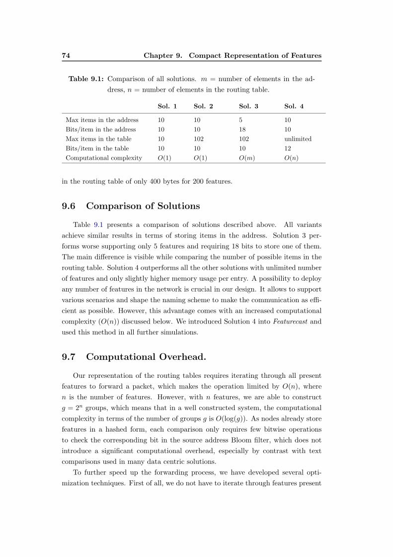
74 Chapter 9. Compact Representation of Features
Table 9.1: Comparison of all solutions. m = number of elements in the ad-
dress, n = number of elements in the routing table.
Sol. 1 Sol. 2 Sol. 3 Sol. 4
Max items in the address 10 10 5 10
Bits/item in the address 10 10 18 10
Max items in the table 10 102 102 unlimited
Bits/item in the table 10 10 10 12
Computational complexity O(1) O(1) O(m) O(n)
in the routing table of only 400 bytes for 200 features.
9.6 Comparison of Solutions
Table 9.1 presents a comparison of solutions described above. All variants
achieve similar results in terms of storing items in the address. Solution 3 per-
forms worse supporting only 5 features and requiring 18 bits to store one of them.
The main difference is visible while comparing the number of possible items in the
routing table. Solution 4 outperforms all the other solutions with unlimited number
of features and only slightly higher memory usage per entry. A possibility to deploy
any number of features in the network is crucial in our design. It allows to support
various scenarios and shape the naming scheme to make the communication as effi-
cient as possible. However, this advantage comes with an increased computational
complexity (O(n)) discussed below. We introduced Solution 4 into Featurecast and
used this method in all further simulations.
9.7 Computational Overhead.
Our representation of the routing tables requires iterating through all present
features to forward a packet, which makes the operation limited by O(n), where
n is the number of features. However, with n features, we are able to construct
g = 2n groups, which means that in a well constructed system, the computational
complexity in terms of the number of groups g is O(log(g)). As nodes already store
features in a hashed form, each comparison only requires few bitwise operations
to check the corresponding bit in the source address Bloom filter, which does not
introduce a significant computational overhead, especially by contrast with text
comparisons used in many data centric solutions.
To further speed up the forwarding process, we have developed several opti-
mization techniques. First of all, we do not have to iterate through features present
9.8. Routing Entry Aggregation. 75
at every neighbor. This modification significantly reduces the overhead especially
at nodes close to the root, which have many such features. Second, we start the
forwarding process from features being present at only one neighbor. If any of them
is present in the source address, we just need to check if this neighbor defines all
required features without iterating through the whole table.
9.8 Routing Entry Aggregation.
As Featurecast may operate over multiple DODAGs, we aggregate the same
routing entries from multiple DODAGs: for features defined on the same set of
neighbors in different DODAGs, we only keep a single entry, which results in a
reduced amount of memory without introducing any computational overhead during
forwarding.

Chapter 10
Implementation and Evaluation
We have implemented Featurecast in Contiki OS (ver. 2.6) [85]. For performance
evaluation, we have run simulations in Cooja, a simulator that emulates both the
software and hardware of sensor nodes. As an execution platform, we have used
Sky Motes with CC2420 2.4 GHz radio and ContikiMAC at Layer 2.
Contiki supports the RPL routing protocol to build a DODAG that takes into
account the distance to the sink in terms of the number of hops, the metric defined
by Objective Function Zero (OF0). We have modified the metric for constructing
the Featurecast DODAG to reflect similarity of stored features (cf. Sect. 8.2).
10.1 Evaluation Setup
We have compared Featurecast with Logical Neighborhoods (LN) [12], which
proposes a similar abstraction, but at the application layer, and the traditional IP
Multicast as it is the recommended solution for group communications in WSN
[86]. We have set the parameters of LN (exploration parameter E and the number
of credits) to the values used in the LN evaluation [12]. Note that LN does not
guarantee packet delivery for a small amount of credits, so we have used the LN
recommended values [12].
As there is no implementation of any multicast routing protocol in Contiki (ver.
2.6), we have implemented a simple routing protocol in which nodes willing to join
a multicast group just send a message towards their parents in the RPL DODAG
using UDP. Each sensor, after receiving the message, waits for an advertisement
from its children, adds its own advertisement, and sends it up through the DODAG.
We use the number of control messages exchanged for maintaining Featurecast or
multicast routing as the main comparison index. They directly influence the energy
consumption of nodes and the network lifetime.
10.2 Scenarios
We consider two scenarios: i) the building control application developed for
CoAP group communication [86] and ii) a random topology of nodes with random
features.

78 Chapter 10. Implementation and Evaluation
10.2.1 Building Control
The building control scenario uses a deployment scheme in which sensor nodes
are placed in several buildings across multiple floors, wings, and rooms. The scenario
considers sensor nodes of multiple types (e.g. measuring temperature, humidity,
luminosity, etc.). CoAP clients communicate with sensor nodes by means of URLs
with a hierarchical structure that encodes the node location and its capabilities using
the following format: node_type.room.wing.floor.building. If qi is a number of
elements on each level, then to be able to access any set of nodes, we need to define
a label for each feature at each level (u being the number of levels in the URL):�u
i=1 qi.
We need the same amount of features for LN expressed in the form of attributes.
If we use IP multicast in the same scenario, we have to define a multicast group
for each combination, which results in�u
i=1 qi. If we want to use the URLs that do
not contain all the defined levels (e.g. bldg1.all_nodes), the number of multicast
groups is even higher:�u
i=1(qi + 1).
10.2.2 Random Topology
In the second scenario, we evaluate communication performance in a random
topology. Each node chooses its address as a set of 10 random features. After
establishing the routing infrastructure, we choose a random node to send a packet
to a randomly chosen group. We vary the network size from 50 to 500 nodes and
average the results from 100 different runs. A UDP packet with 100B payload is
generated every 30s.
10.3 Results: Memory Footprint in the Building Con-
trol Scenario
First, we perform our evaluation in the building control scenario with 128 sensor
nodes across 2 buildings (Building 1 and 2), 2 floors in each building (Floor 1 and
2), 2 wings (East, West), 4 rooms in each wing (Room 1 to 4), and 2 sensor types
(light, temperature). We place 2 temperature and 2 light sensors in each room.
We place nodes at regular intervals on a 16x8 matrix and assign the right features
simulating the given scenario. Featurecast and LN require 12 features or attributes
to in this scenario, while with IP multicast, we need 405 groups. We place the sink
in the center of the network. We also evaluate Featurecast with 2 and 3 DODAGs
(Featurecast2 and Featurecast3 respectively).
We can note that in this scenario, Featurecast is extremely scalable. If we want
to connect another building with a similar infrastructure, we need to add only one
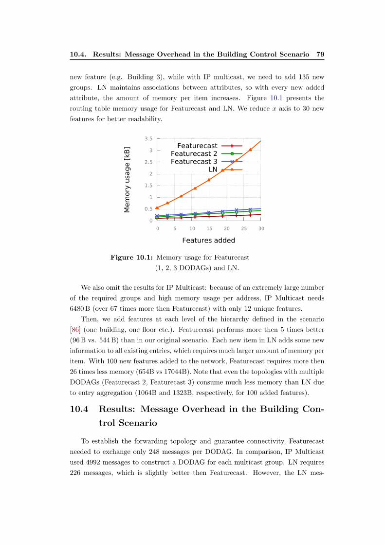
10.4. Results: Message Overhead in the Building Control Scenario 79
new feature (e.g. Building 3), while with IP multicast, we need to add 135 new
groups. LN maintains associations between attributes, so with every new added
attribute, the amount of memory per item increases. Figure 10.1 presents the
routing table memory usage for Featurecast and LN. We reduce x axis to 30 new
features for better readability.
0
0.5
1
1.5
2
2.5
3
3.5
0 5 10 15 20 25 30
Mem
ory
usage [
kB
]
Features added
FeaturecastFeaturecast 2Featurecast 3
LN
Figure 10.1: Memory usage for Featurecast
(1, 2, 3 DODAGs) and LN.
We also omit the results for IP Multicast: because of an extremely large number
of the required groups and high memory usage per address, IP Multicast needs
6480B (over 67 times more then Featurecast) with only 12 unique features.
Then, we add features at each level of the hierarchy defined in the scenario
[86] (one building, one floor etc.). Featurecast performs more then 5 times better
(96B vs. 544B) than in our original scenario. Each new item in LN adds some new
information to all existing entries, which requires much larger amount of memory per
item. With 100 new features added to the network, Featurecast requires more then
26 times less memory (654B vs 17044B). Note that even the topologies with multiple
DODAGs (Featurecast 2, Featurecast 3) consume much less memory than LN due
to entry aggregation (1064B and 1323B, respectively, for 100 added features).
10.4 Results: Message Overhead in the Building Con-
trol Scenario
To establish the forwarding topology and guarantee connectivity, Featurecast
needed to exchange only 248 messages per DODAG. In comparison, IP Multicast
used 4992 messages to construct a DODAG for each multicast group. LN requires
226 messages, which is slightly better then Featurecast. However, the LN mes-
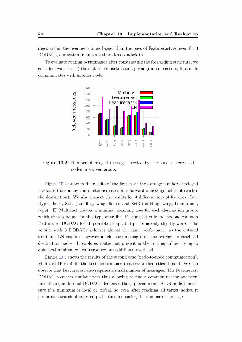
80 Chapter 10. Implementation and Evaluation
sages are on the average 5 times bigger than the ones of Featurecast, so even for 3
DODAGs, our system requires 2 times less bandwidth.
To evaluate routing performance after constructing the forwarding structure, we
consider two cases: i) the sink sends packets to a given group of sensors, ii) a node
communicates with another node.
0
20
40
60
80
100
120
140
160
type
room
floor
win
g
bld
g
set_
1
set_
2
set_
3
Rela
yed m
essages Multicast
FeaturecastFeaturecast3
LN
Figure 10.2: Number of relayed messages needed by the sink to access all
nodes in a given group.
Figure 10.2 presents the results of the first case: the average number of relayed
messages (how many times intermediate nodes forward a message before it reaches
the destination). We also present the results for 3 different sets of features: Set1
(type, floor), Set2 (building, wing, floor), and Set3 (building, wing, floor, room,
type). IP Multicast creates a minimal spanning tree for each destination group,
which gives a bound for this type of traffic. Featurecast only creates one common
Featurecast DODAG for all possible groups, but performs only slightly worse. The
version with 3 DODAGs achieves almost the same performance as the optimal
solution. LN requires however much more messages on the average to reach all
destination nodes. It explores routes not present in the routing tables trying to
quit local minima, which introduces an additional overhead.
Figure 10.3 shows the results of the second case (node-to-node communication).
Multicast IP exhibits the best performance that sets a theoretical bound. We can
observe that Featurecast also requires a small number of messages. The Featurecast
DODAG connects similar nodes thus allowing to find a common nearby ancestor.
Introducing additional DODAGs decreases the gap even more. A LN node is never
sure if a minimum is local or global, so even after reaching all target nodes, it
performs a search of external paths thus increasing the number of messages.
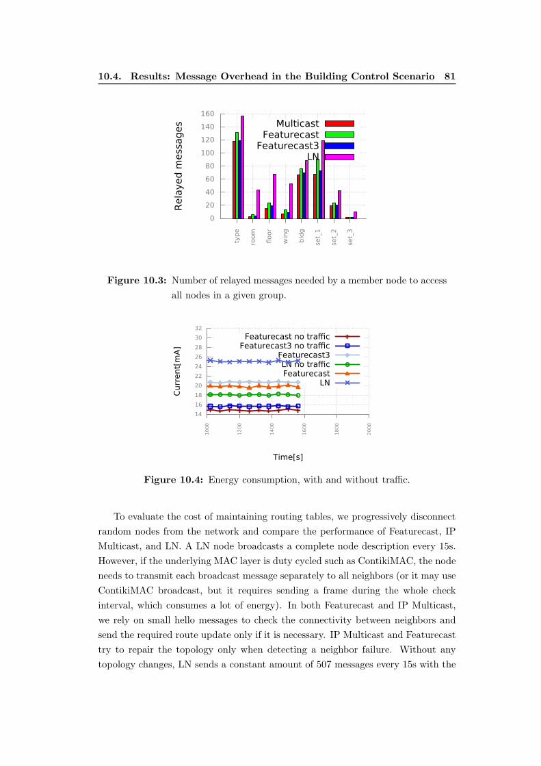
10.4. Results: Message Overhead in the Building Control Scenario 81
0
20
40
60
80
100
120
140
160
type
room
floor
win
g
bld
g
set_
1
set_
2
set_
3
Rela
yed m
essages Multicast
FeaturecastFeaturecast3
LN
Figure 10.3: Number of relayed messages needed by a member node to access
all nodes in a given group.
14
16
18
20
22
24
26
28
30
32
10
00
12
00
14
00
16
00
18
00
20
00
Curr
ent[
mA
]
Time[s]
Featurecast no trafficFeaturecast3 no traffic
Featurecast3LN no trafficFeaturecast
LN
Figure 10.4: Energy consumption, with and without traffic.
To evaluate the cost of maintaining routing tables, we progressively disconnect
random nodes from the network and compare the performance of Featurecast, IP
Multicast, and LN. A LN node broadcasts a complete node description every 15s.
However, if the underlying MAC layer is duty cycled such as ContikiMAC, the node
needs to transmit each broadcast message separately to all neighbors (or it may use
ContikiMAC broadcast, but it requires sending a frame during the whole check
interval, which consumes a lot of energy). In both Featurecast and IP Multicast,
we rely on small hello messages to check the connectivity between neighbors and
send the required route update only if it is necessary. IP Multicast and Featurecast
try to repair the topology only when detecting a neighbor failure. Without any
topology changes, LN sends a constant amount of 507 messages every 15s with the
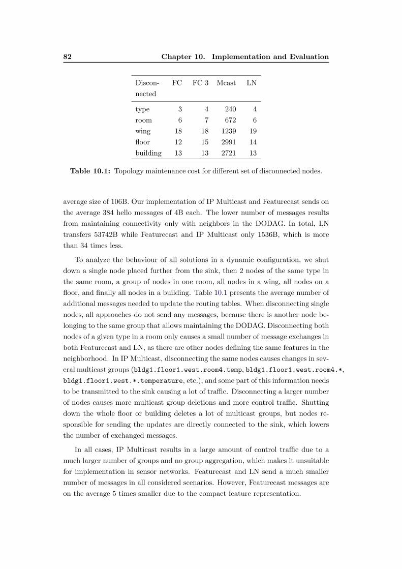
82 Chapter 10. Implementation and Evaluation
Discon- FC FC 3 Mcast LN
nected
type 3 4 240 4
room 6 7 672 6
wing 18 18 1239 19
floor 12 15 2991 14
building 13 13 2721 13
Table 10.1: Topology maintenance cost for different set of disconnected nodes.
average size of 106B. Our implementation of IP Multicast and Featurecast sends on
the average 384 hello messages of 4B each. The lower number of messages results
from maintaining connectivity only with neighbors in the DODAG. In total, LN
transfers 53742B while Featurecast and IP Multicast only 1536B, which is more
than 34 times less.
To analyze the behaviour of all solutions in a dynamic configuration, we shut
down a single node placed further from the sink, then 2 nodes of the same type in
the same room, a group of nodes in one room, all nodes in a wing, all nodes on a
floor, and finally all nodes in a building. Table 10.1 presents the average number of
additional messages needed to update the routing tables. When disconnecting single
nodes, all approaches do not send any messages, because there is another node be-
longing to the same group that allows maintaining the DODAG. Disconnecting both
nodes of a given type in a room only causes a small number of message exchanges in
both Featurecast and LN, as there are other nodes defining the same features in the
neighborhood. In IP Multicast, disconnecting the same nodes causes changes in sev-
eral multicast groups (bldg1.floor1.west.room4.temp, bldg1.floor1.west.room4.*,
bldg1.floor1.west.*.temperature, etc.), and some part of this information needs
to be transmitted to the sink causing a lot of traffic. Disconnecting a larger number
of nodes causes more multicast group deletions and more control traffic. Shutting
down the whole floor or building deletes a lot of multicast groups, but nodes re-
sponsible for sending the updates are directly connected to the sink, which lowers
the number of exchanged messages.
In all cases, IP Multicast results in a large amount of control traffic due to a
much larger number of groups and no group aggregation, which makes it unsuitable
for implementation in sensor networks. Featurecast and LN send a much smaller
number of messages in all considered scenarios. However, Featurecast messages are
on the average 5 times smaller due to the compact feature representation.
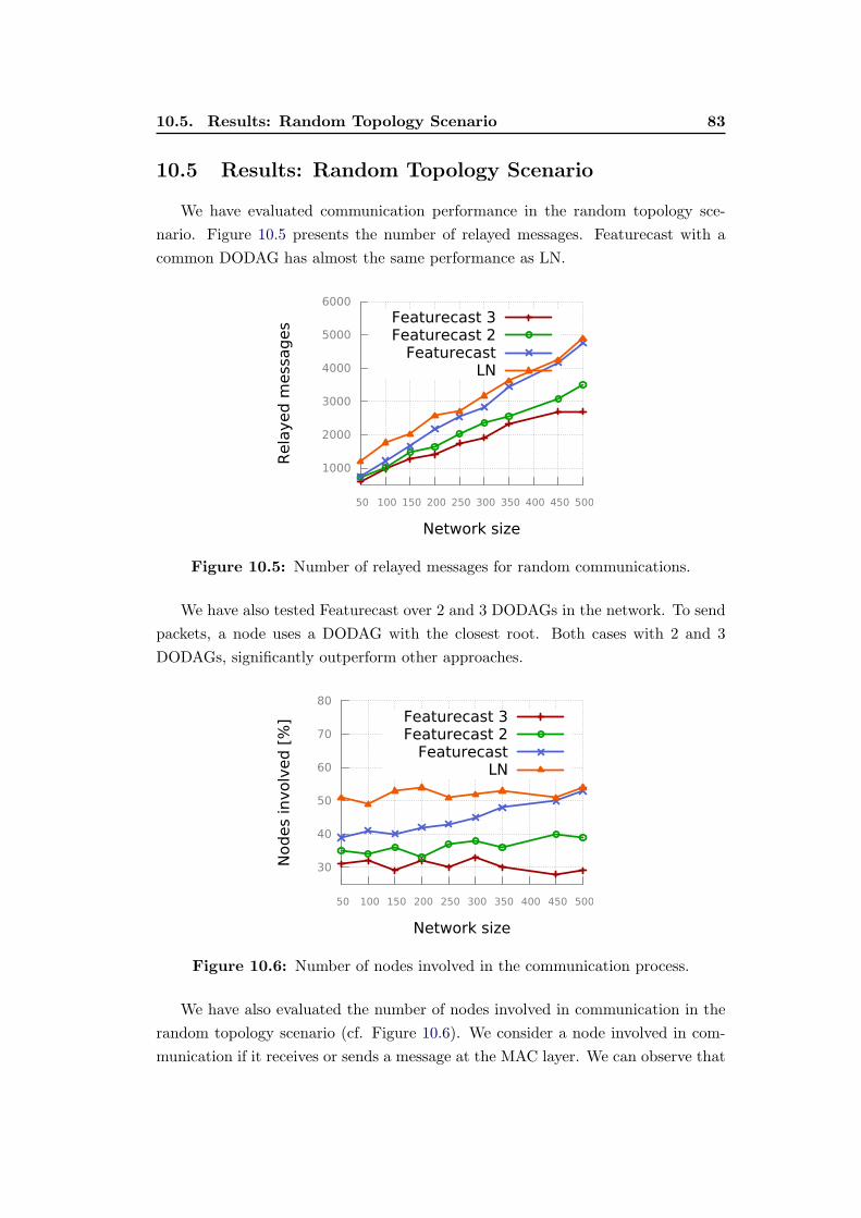
10.5. Results: Random Topology Scenario 83
10.5 Results: Random Topology Scenario
We have evaluated communication performance in the random topology sce-
nario. Figure 10.5 presents the number of relayed messages. Featurecast with a
common DODAG has almost the same performance as LN.
1000
2000
3000
4000
5000
6000
50 100 150 200 250 300 350 400 450 500
Rela
yed m
essages
Network size
Featurecast 3Featurecast 2
FeaturecastLN
Figure 10.5: Number of relayed messages for random communications.
We have also tested Featurecast over 2 and 3 DODAGs in the network. To send
packets, a node uses a DODAG with the closest root. Both cases with 2 and 3
DODAGs, significantly outperform other approaches.
30
40
50
60
70
80
50 100 150 200 250 300 350 400 450 500
Nodes involv
ed [
%]
Network size
Featurecast 3Featurecast 2
FeaturecastLN
Figure 10.6: Number of nodes involved in the communication process.
We have also evaluated the number of nodes involved in communication in the
random topology scenario (cf. Figure 10.6). We consider a node involved in com-
munication if it receives or sends a message at the MAC layer. We can observe that
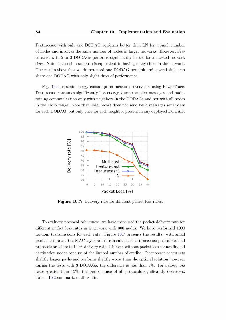
84 Chapter 10. Implementation and Evaluation
Featurecast with only one DODAG performs better than LN for a small number
of nodes and involves the same number of nodes in larger networks. However, Fea-
turecast with 2 or 3 DODAGs performs significantly better for all tested network
sizes. Note that such a scenario is equivalent to having many sinks in the network.
The results show that we do not need one DODAG per sink and several sinks can
share one DODAG with only slight drop of performance.
Fig. 10.4 presents energy consumption measured every 60s using PowerTrace.
Featurecast consumes significantly less energy, due to smaller messages and main-
taining communication only with neighbors in the DODAGs and not with all nodes
in the radio range. Note that Featurecast does not send hello messages separately
for each DODAG, but only once for each neighbor present in any deployed DODAG.
50
55
60
65
70
75
80
85
90
95
100
0 5 10 15 20 25 30 35 40
Delivery
rate
[%
]
Packet Loss [%]
MulticastFeaturecast
Featurecast3LN
Figure 10.7: Delivery rate for different packet loss rates.
To evaluate protocol robustness, we have measured the packet delivery rate for
different packet loss rates in a network with 300 nodes. We have performed 1000
random transmissions for each rate. Figure 10.7 presents the results: with small
packet loss rates, the MAC layer can retransmit packets if necessary, so almost all
protocols are close to 100% delivery rate. LN even without packet loss cannot find all
destination nodes because of the limited number of credits. Featurecast constructs
slightly longer paths and performs slightly worse than the optimal solution, however
during the tests with 3 DODAGs, the difference is less than 1%. For packet loss
rates greater than 15%, the performance of all protocols significantly decreases.
Table. 10.2 summarizes all results.
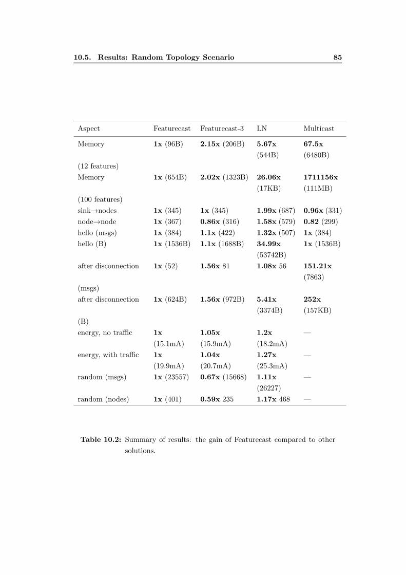
10.5. Results: Random Topology Scenario 85
Aspect Featurecast Featurecast-3 LN Multicast
Memory 1x (96B) 2.15x (206B) 5.67x
(544B)
67.5x
(6480B)
(12 features)
Memory 1x (654B) 2.02x (1323B) 26.06x
(17KB)
1711156x
(111MB)
(100 features)
sink→nodes 1x (345) 1x (345) 1.99x (687) 0.96x (331)
node→node 1x (367) 0.86x (316) 1.58x (579) 0.82 (299)
hello (msgs) 1x (384) 1.1x (422) 1.32x (507) 1x (384)
hello (B) 1x (1536B) 1.1x (1688B) 34.99x
(53742B)
1x (1536B)
after disconnection 1x (52) 1.56x 81 1.08x 56 151.21x
(7863)
(msgs)
after disconnection 1x (624B) 1.56x (972B) 5.41x
(3374B)
252x
(157KB)
(B)
energy, no traffic 1x
(15.1mA)
1.05x
(15.9mA)
1.2x
(18.2mA)
—
energy, with traffic 1x
(19.9mA)
1.04x
(20.7mA)
1.27x
(25.3mA)
—
random (msgs) 1x (23557) 0.67x (15668) 1.11x
(26227)
—
random (nodes) 1x (401) 0.59x 235 1.17x 468 —
Table 10.2: Summary of results: the gain of Featurecast compared to other
solutions.
86 Chapter 10. Implementation and Evaluation
10.6 Discussion of Packet Drops Due to Inexistent Ad-
dresses
Finally, we have investigated packet drops due to non-existent conjunction of
features. The drops result from the aggregation of features in routing tables and
not keeping more information about their compositions. If Sa is a set of features in
an address, Sit a set of features in the routing table for neighbor i, and Sn a set of
features defined by a node, the packet drop occurs when:Sa ⊂ Sit ∧ �Sn, Sa ⊂ Sn.
In our scenario, the packet drop may occur if an address contains a combination
of features that are not defined by any node, for example Building 1 and Build-
ing 2. In this case, the packet can be routed through nodes that may have both
features available through the same neighbor. Eventually, it will be dropped by a
sensor node that routes packets to this group through different nodes. Creating an
invalid address with the location feature usually will not cause a lot of unnecessary
traffic, however putting for instance only temperature and light into an address
will cause global network flooding even if there is no node defining both features.
To alleviate this problem, a packet drop may be signaled by an ICMP packet,
so that the user can avoid sending packets with the address in the future. An-
other problem arises if there are nodes defining for instance both temperature and
light, but the rest of nodes defines only one of them. In such a case, a new fea-
ture temperature_light shall be defined allowing to efficiently query both types
of nodes. However, the problem heavily depends on applications and will not occur
in a well configured network (as indicated above).
Chapter 11
Conclusion
We presented Featurecast, a group communication protocol for Wireless Sensor
Networks. Unlike CCN [75], Featurecast is end-point centric, but creates addresses
using a content-centric approach. Nodes are named using a set of their features,
which can describe node location (”room1”), capacity (”temperature sensor”), state
(”low energy”) or any other characteristic. Name translation is based on hashing.
Such an approach eliminates the need for a translation service and allows to easily
add/delete features, both being costly in networks using CoAP.
While providing a group communication scheme, Featurecast remains fully com-
pliant with classic IPv6 networks, making it easy to deploy. It only requires a
designated range of addresses indicated by a 16-bit prefix. This feature makes
our approach different from multiple group communication protocols [74] [12] un-
able to fit into an existing infrastructure or requiring costly tunnelling. Bringing
human-friendly names into IPv6 networks was possible thanks to an innovative use
of modified Bloom Filters, which, to the best of our knowledge, was never used like
this before.
Featurecast creates a routing structure based on RPL DODAG. Protocols using
a some kind of distribution trees usually suffer from costly communication in M2M
communication scenarios. In our solution, we keep the node description in its
address. It allows us to use new metrics connecting similar nodes in the network
and thus making direct node communication more efficient.
Routing tables only store the sets of available features without their combina-
tions. Such an approach reduces memory usage and control message overhead. Our
simulations show that our protocol outperforms similar approaches, such as Logical
Neighborhoods, in terms of almost all tested metrics.

Part IV
WEAVE: Efficient Geographical
Routing in Large-Scale
Networks

Chapter 12
Rationale
We consider routing in large-scale networks that forward traffic in a multi-hop
way and exhibit dynamic behavior—links may go up and down, nodes may join and
leave the network. Good examples are wireless ad hoc, mesh, and sensor networks.
The last type of wireless networks is becoming increasingly important for cyber
physical systems and the future Internet of Things. Such networks significantly dif-
fer from the multi-hierarchical organization of the current Internet: their structure
is flat, they may include a large number of nodes having constrained processing
power and connectivity, and links between them may have similar characteristics.
In many cases, the knowledge of their location is important and nodes may be
placed in a 3D space of the real world.
Traditional MANET routing protocols that rely on topology or route discovery
such as OLSR, AODV, DSDV, DSR [88, 89, 90, 91], be they reactive or proactive, do
not properly work in this context; due to the lack of hierarchy, the routing protocols
need to disseminate a lot of topology information or route discovery requests and
host routes managed by the protocols resulting in large routing tables.
In such large-scale dynamic networks, geographical routing appears as an in-
teresting alternative approach. Instead of disseminating topology information and
computing state information stored in nodes to support routing, nodes are addressed
using their geographic coordinates. This approach becomes particularly attractive
for devices that come with GPS. In the absence of GPS, the location information
can be obtained from relative or virtual positioning based on estimation of the sig-
nal strength. When nodes know their geographic locations, it is straightforward to
route packets using greedy forwarding simply by locally computing distances: a node
forwards an incoming packet to the neighbor closest to the final destination [92, 93].
Greedy forwarding is simple, it does not require any topology information nor
routing tables, but it only works in networks with sufficient density without cover-
age defects such as voids or obstacles. Otherwise, a concave node that has no further
neighbors closer to the destination has to drop packets [56, 57]. To improve packet
delivery ratio, most geographical forwarding protocols proceed in two phases: they
use greedy forwarding until a packet is stuck in a concave node and then try to
go around a void or an obstacle. This approach may result in not optimal routes,
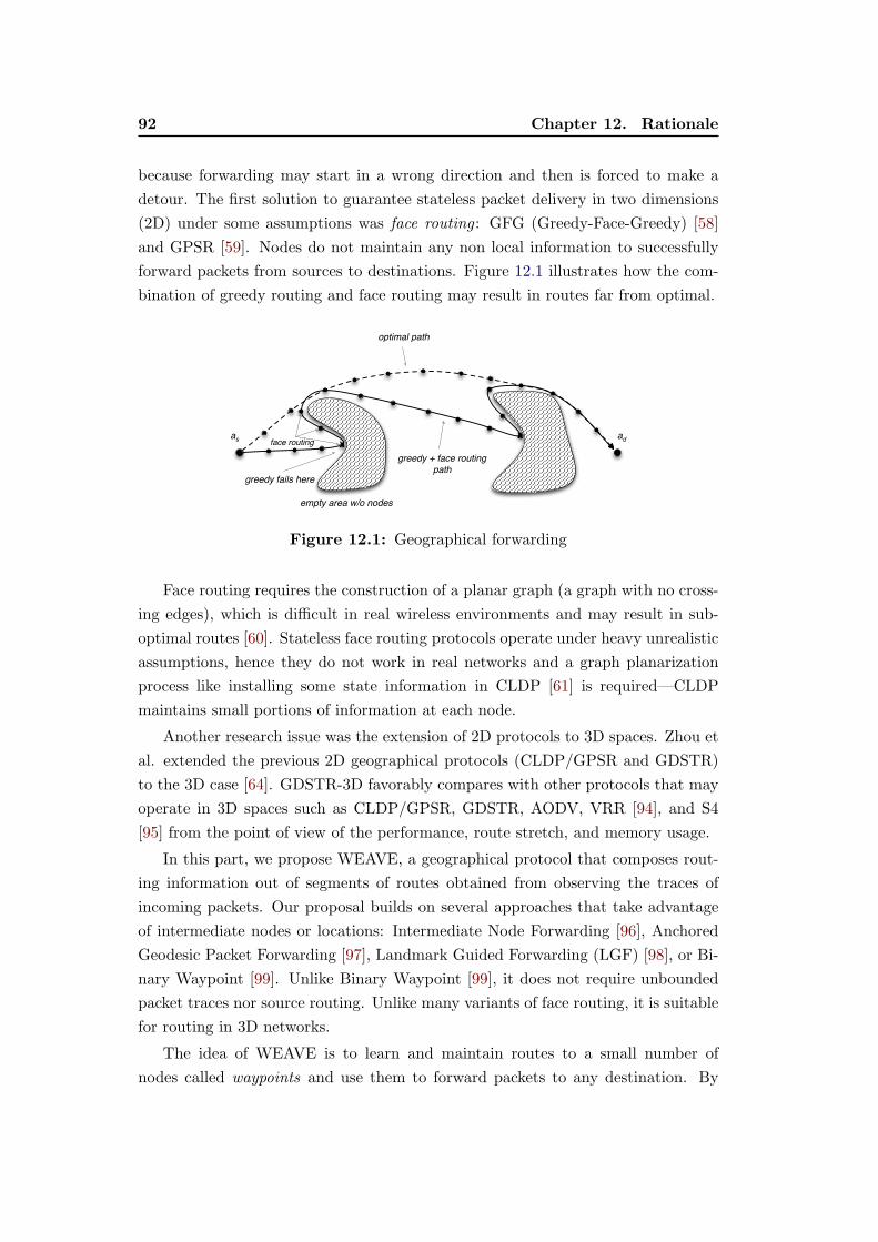
92 Chapter 12. Rationale
because forwarding may start in a wrong direction and then is forced to make a
detour. The first solution to guarantee stateless packet delivery in two dimensions
(2D) under some assumptions was face routing : GFG (Greedy-Face-Greedy) [58]
and GPSR [59]. Nodes do not maintain any non local information to successfully
forward packets from sources to destinations. Figure 12.1 illustrates how the com-
bination of greedy routing and face routing may result in routes far from optimal.
�
�
�����������������
������������
���������������������
����
��������������������
������������
�� ��
Figure 12.1: Geographical forwarding
Face routing requires the construction of a planar graph (a graph with no cross-
ing edges), which is difficult in real wireless environments and may result in sub-
optimal routes [60]. Stateless face routing protocols operate under heavy unrealistic
assumptions, hence they do not work in real networks and a graph planarization
process like installing some state information in CLDP [61] is required—CLDP
maintains small portions of information at each node.
Another research issue was the extension of 2D protocols to 3D spaces. Zhou et
al. extended the previous 2D geographical protocols (CLDP/GPSR and GDSTR)
to the 3D case [64]. GDSTR-3D favorably compares with other protocols that may
operate in 3D spaces such as CLDP/GPSR, GDSTR, AODV, VRR [94], and S4
[95] from the point of view of the performance, route stretch, and memory usage.
In this part, we propose WEAVE, a geographical protocol that composes rout-
ing information out of segments of routes obtained from observing the traces of
incoming packets. Our proposal builds on several approaches that take advantage
of intermediate nodes or locations: Intermediate Node Forwarding [96], Anchored
Geodesic Packet Forwarding [97], Landmark Guided Forwarding (LGF) [98], or Bi-
nary Waypoint [99]. Unlike Binary Waypoint [99], it does not require unbounded
packet traces nor source routing. Unlike many variants of face routing, it is suitable
for routing in 3D networks.
The idea of WEAVE is to learn and maintain routes to a small number of
nodes called waypoints and use them to forward packets to any destination. By
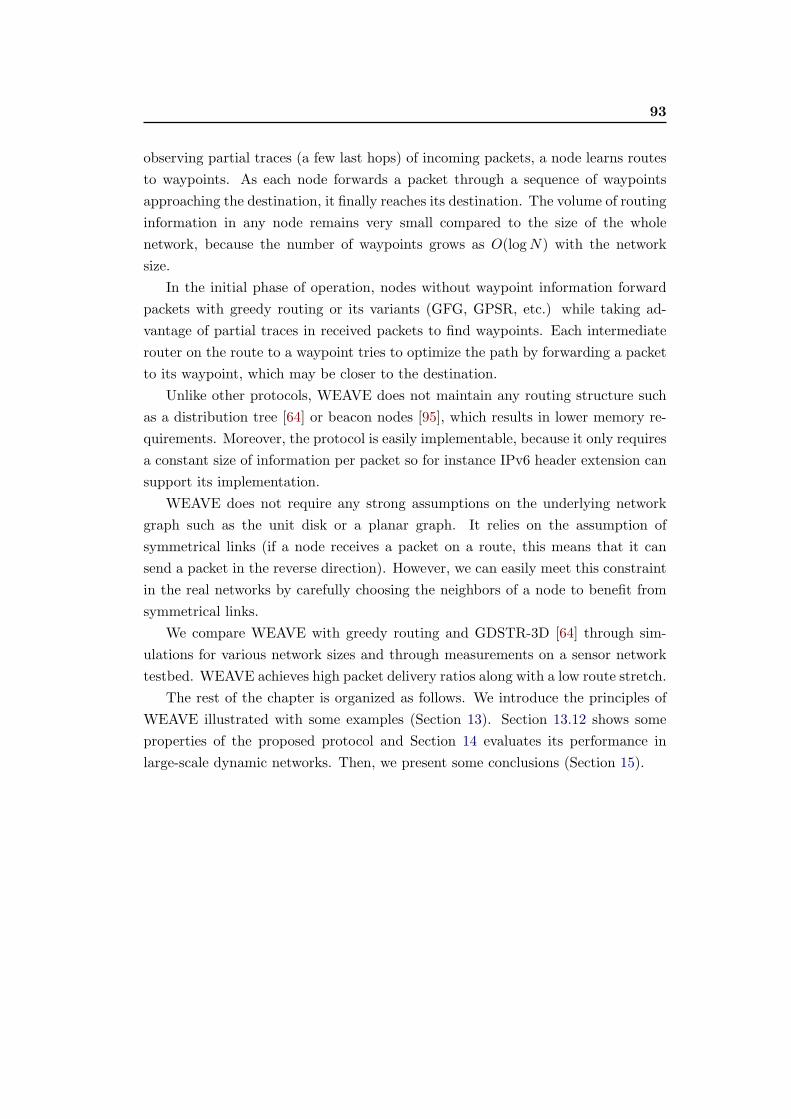
93
observing partial traces (a few last hops) of incoming packets, a node learns routes
to waypoints. As each node forwards a packet through a sequence of waypoints
approaching the destination, it finally reaches its destination. The volume of routing
information in any node remains very small compared to the size of the whole
network, because the number of waypoints grows as O(logN) with the network
size.
In the initial phase of operation, nodes without waypoint information forward
packets with greedy routing or its variants (GFG, GPSR, etc.) while taking ad-
vantage of partial traces in received packets to find waypoints. Each intermediate
router on the route to a waypoint tries to optimize the path by forwarding a packet
to its waypoint, which may be closer to the destination.
Unlike other protocols, WEAVE does not maintain any routing structure such
as a distribution tree [64] or beacon nodes [95], which results in lower memory re-
quirements. Moreover, the protocol is easily implementable, because it only requires
a constant size of information per packet so for instance IPv6 header extension can
support its implementation.
WEAVE does not require any strong assumptions on the underlying network
graph such as the unit disk or a planar graph. It relies on the assumption of
symmetrical links (if a node receives a packet on a route, this means that it can
send a packet in the reverse direction). However, we can easily meet this constraint
in the real networks by carefully choosing the neighbors of a node to benefit from
symmetrical links.
We compare WEAVE with greedy routing and GDSTR-3D [64] through sim-
ulations for various network sizes and through measurements on a sensor network
testbed. WEAVE achieves high packet delivery ratios along with a low route stretch.
The rest of the chapter is organized as follows. We introduce the principles of
WEAVE illustrated with some examples (Section 13). Section 13.12 shows some
properties of the proposed protocol and Section 14 evaluates its performance in
large-scale dynamic networks. Then, we present some conclusions (Section 15).

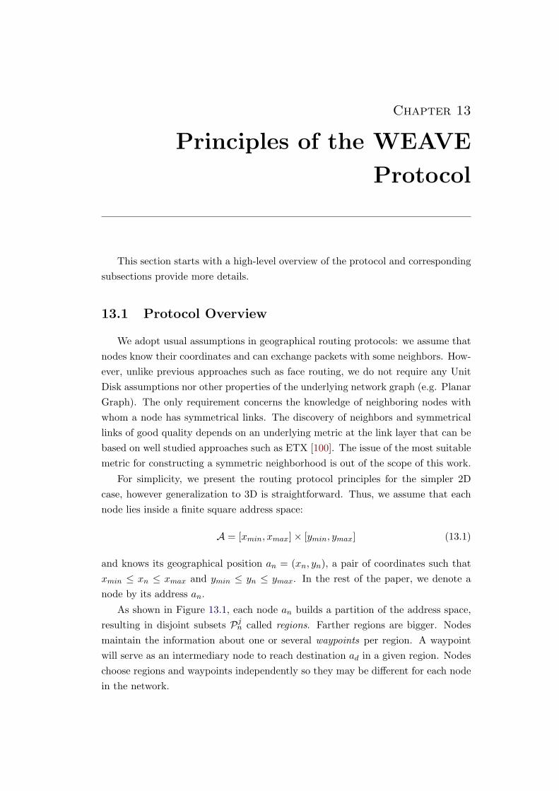
Chapter 13
Principles of the WEAVE
Protocol
This section starts with a high-level overview of the protocol and corresponding
subsections provide more details.
13.1 Protocol Overview
We adopt usual assumptions in geographical routing protocols: we assume that
nodes know their coordinates and can exchange packets with some neighbors. How-
ever, unlike previous approaches such as face routing, we do not require any Unit
Disk assumptions nor other properties of the underlying network graph (e.g. Planar
Graph). The only requirement concerns the knowledge of neighboring nodes with
whom a node has symmetrical links. The discovery of neighbors and symmetrical
links of good quality depends on an underlying metric at the link layer that can be
based on well studied approaches such as ETX [100]. The issue of the most suitable
metric for constructing a symmetric neighborhood is out of the scope of this work.
For simplicity, we present the routing protocol principles for the simpler 2D
case, however generalization to 3D is straightforward. Thus, we assume that each
node lies inside a finite square address space:
A = [xmin, xmax]× [ymin, ymax] (13.1)
and knows its geographical position an = (xn, yn), a pair of coordinates such that
xmin ≤ xn ≤ xmax and ymin ≤ yn ≤ ymax. In the rest of the paper, we denote a
node by its address an.
As shown in Figure 13.1, each node an builds a partition of the address space,
resulting in disjoint subsets Pjn called regions. Farther regions are bigger. Nodes
maintain the information about one or several waypoints per region. A waypoint
will serve as an intermediary node to reach destination ad in a given region. Nodes
choose regions and waypoints independently so they may be different for each node
in the network.
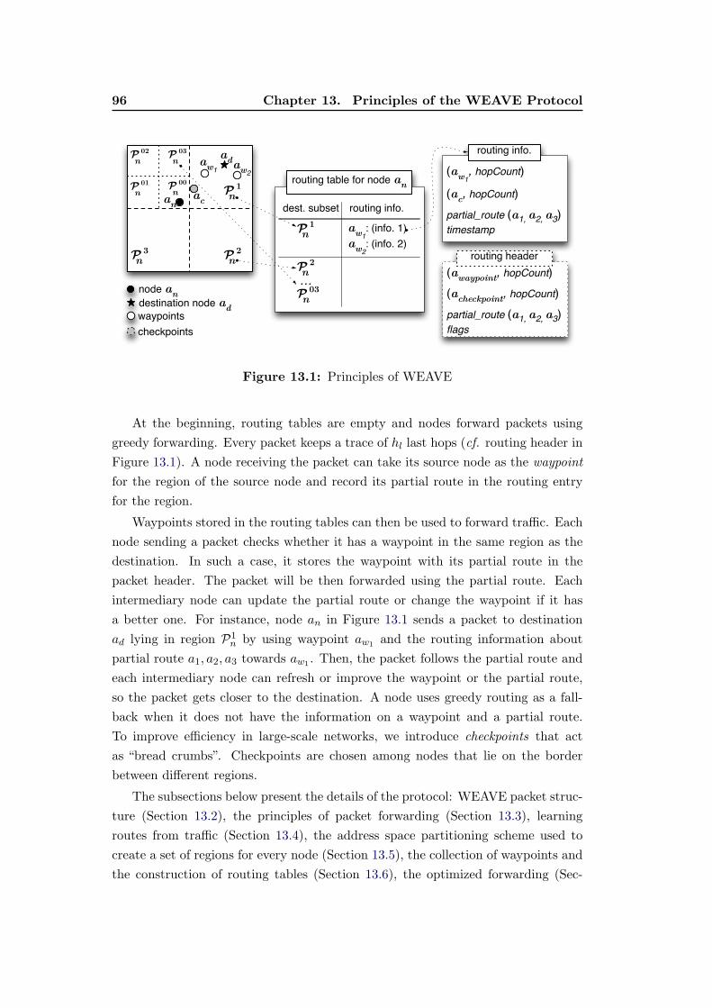
96 Chapter 13. Principles of the WEAVE Protocol
�aw������������
�ac�����������
���������������a���a���a�����������
������������ �������������
�
aw������������
aw������������
�����an
��������������������������a
d
�����������
�������������
�����������������������an
�awaypoint
������������a
checkpoint�����������
���������������a���a���a������
��������������
� 00
n � 1n
� 1n
� 2n � 2
n
� 3n
� 01
n
� 02
n� 03
n
an
ada
w� aw�
� 03n
ac
Figure 13.1: Principles of WEAVE
At the beginning, routing tables are empty and nodes forward packets using
greedy forwarding. Every packet keeps a trace of hl last hops (cf. routing header in
Figure 13.1). A node receiving the packet can take its source node as the waypoint
for the region of the source node and record its partial route in the routing entry
for the region.
Waypoints stored in the routing tables can then be used to forward traffic. Each
node sending a packet checks whether it has a waypoint in the same region as the
destination. In such a case, it stores the waypoint with its partial route in the
packet header. The packet will be then forwarded using the partial route. Each
intermediary node can update the partial route or change the waypoint if it has
a better one. For instance, node an in Figure 13.1 sends a packet to destination
ad lying in region P1n by using waypoint aw1
and the routing information about
partial route a1, a2, a3 towards aw1. Then, the packet follows the partial route and
each intermediary node can refresh or improve the waypoint or the partial route,
so the packet gets closer to the destination. A node uses greedy routing as a fall-
back when it does not have the information on a waypoint and a partial route.
To improve efficiency in large-scale networks, we introduce checkpoints that act
as “bread crumbs”. Checkpoints are chosen among nodes that lie on the border
between different regions.
The subsections below present the details of the protocol: WEAVE packet struc-
ture (Section 13.2), the principles of packet forwarding (Section 13.3), learning
routes from traffic (Section 13.4), the address space partitioning scheme used to
create a set of regions for every node (Section 13.5), the collection of waypoints and
the construction of routing tables (Section 13.6), the optimized forwarding (Sec-
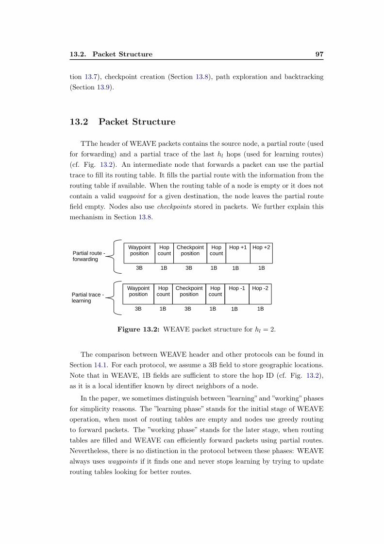
13.2. Packet Structure 97
tion 13.7), checkpoint creation (Section 13.8), path exploration and backtracking
(Section 13.9).
13.2 Packet Structure
TThe header of WEAVE packets contains the source node, a partial route (used
for forwarding) and a partial trace of the last hl hops (used for learning routes)
(cf. Fig. 13.2). An intermediate node that forwards a packet can use the partial
trace to fill its routing table. It fills the partial route with the information from the
routing table if available. When the routing table of a node is empty or it does not
contain a valid waypoint for a given destination, the node leaves the partial route
field empty. Nodes also use checkpoints stored in packets. We further explain this
mechanism in Section 13.8.
Waypoint position
Hop count
Checkpoint position
Hop count
Hop +1 Hop +2
3B 1B 1B
Partial route - forwarding
Partial trace - learning
1B3B 1B
Waypoint position
Hop count
Checkpoint position
Hop count
Hop -1 Hop -2
3B 1B 1B1B3B 1B
Figure 13.2: WEAVE packet structure for hl = 2.
The comparison between WEAVE header and other protocols can be found in
Section 14.1. For each protocol, we assume a 3B field to store geographic locations.
Note that in WEAVE, 1B fields are sufficient to store the hop ID (cf. Fig. 13.2),
as it is a local identifier known by direct neighbors of a node.
In the paper, we sometimes distinguish between ”learning”and ”working”phases
for simplicity reasons. The ”learning phase” stands for the initial stage of WEAVE
operation, when most of routing tables are empty and nodes use greedy routing
to forward packets. The ”working phase” stands for the later stage, when routing
tables are filled and WEAVE can efficiently forward packets using partial routes.
Nevertheless, there is no distinction in the protocol between these phases: WEAVE
always uses waypoints if it finds one and never stops learning by trying to update
routing tables looking for better routes.
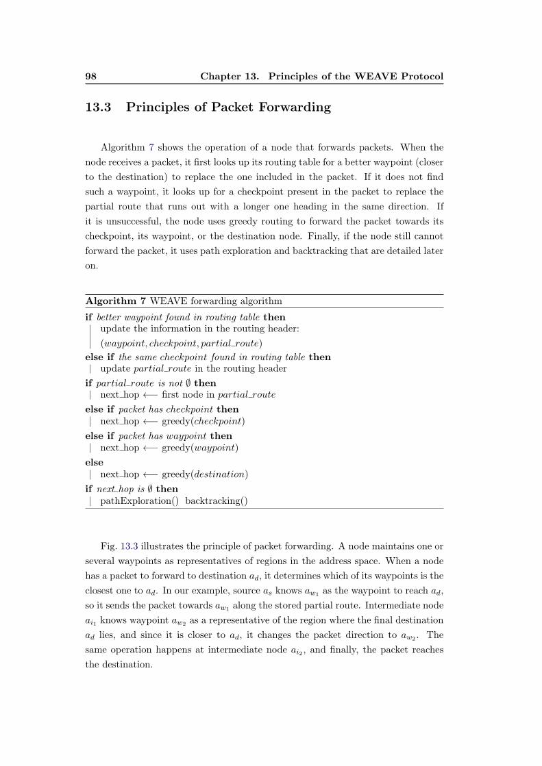
98 Chapter 13. Principles of the WEAVE Protocol
13.3 Principles of Packet Forwarding
Algorithm 7 shows the operation of a node that forwards packets. When the
node receives a packet, it first looks up its routing table for a better waypoint (closer
to the destination) to replace the one included in the packet. If it does not find
such a waypoint, it looks up for a checkpoint present in the packet to replace the
partial route that runs out with a longer one heading in the same direction. If
it is unsuccessful, the node uses greedy routing to forward the packet towards its
checkpoint, its waypoint, or the destination node. Finally, if the node still cannot
forward the packet, it uses path exploration and backtracking that are detailed later
on.
Algorithm 7 WEAVE forwarding algorithm
if better waypoint found in routing table thenupdate the information in the routing header:
(waypoint, checkpoint, partial route)
else if the same checkpoint found in routing table thenupdate partial route in the routing header
if partial route is not ∅ thennext hop ←− first node in partial route
else if packet has checkpoint thennext hop ←− greedy(checkpoint)
else if packet has waypoint thennext hop ←− greedy(waypoint)
elsenext hop ←− greedy(destination)
if next hop is ∅ thenpathExploration() backtracking()
Fig. 13.3 illustrates the principle of packet forwarding. A node maintains one or
several waypoints as representatives of regions in the address space. When a node
has a packet to forward to destination ad, it determines which of its waypoints is the
closest one to ad. In our example, source as knows aw1as the waypoint to reach ad,
so it sends the packet towards aw1along the stored partial route. Intermediate node
ai1 knows waypoint aw2as a representative of the region where the final destination
ad lies, and since it is closer to ad, it changes the packet direction to aw2. The
same operation happens at intermediate node ai2 , and finally, the packet reaches
the destination.
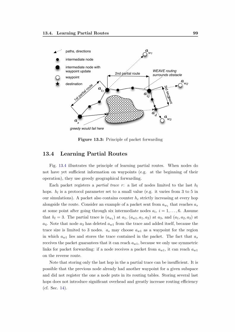
13.4. Learning Partial Routes 99
�����������������
�����������������
�������������������������������������
�
����������������������
�������������������������������
as
ad
��������
aw�
aw�
aw�
ai�
ai�
�����������������
����������������������������
�����������
Figure 13.3: Principle of packet forwarding
13.4 Learning Partial Routes
Fig. 13.4 illustrates the principle of learning partial routes. When nodes do
not have yet sufficient information on waypoints (e.g. at the beginning of their
operation), they use greedy geographical forwarding.
Each packet registers a partial trace r: a list of nodes limited to the last hl
hops. hl is a protocol parameter set to a small value (e.g. it varies from 3 to 5 in
our simulations). A packet also contains counter hc strictly increasing at every hop
alongside the route. Consider an example of a packet sent from aw1that reaches as
at some point after going through six intermediate nodes ai, i = 1, . . . , 6. Assume
that hl = 3. The partial trace is (aw1) at a1, (aw1, a1, a2) at a3, and (a1, a2, a3) at
a4. Note that node a3 has deleted aw1 from the trace and added itself, because the
trace size is limited to 3 nodes. as may choose aw1 as a waypoint for the region
in which aw1 lies and stores the trace contained in the packet. The fact that as
receives the packet guarantees that it can reach aw1, because we only use symmetric
links for packet forwarding: if a node receives a packet from aw1, it can reach aw1
on the reverse route.
Note that storing only the last hop in the a partial trace can be insufficient. It is
possible that the previous node already had another waypoint for a given subspace
and did not register the one a node puts in its routing tables. Storing several last
hops does not introduce significant overhead and greatly increase routing efficiency
(cf. Sec. 14).
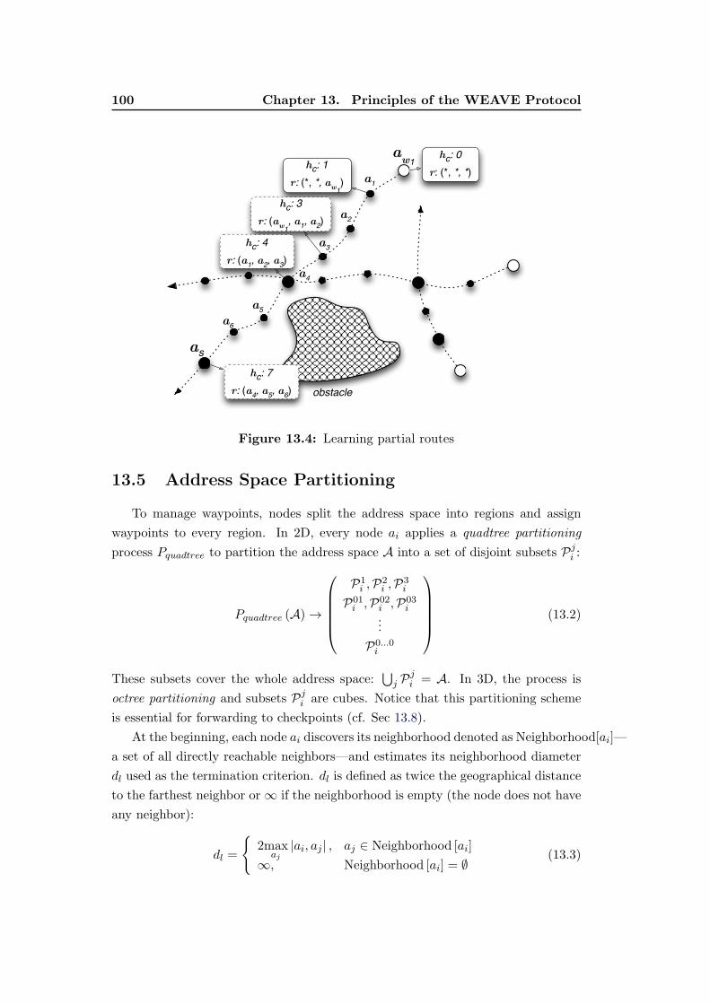
100 Chapter 13. Principles of the WEAVE Protocol
h����r���������a
w��
h����r������������
��������
aw�
a�
a�
a�
a�
a�
a�a�
h����r���a
w���a���a��
h����r���a���a���a��
h����r���a���a���a��
Figure 13.4: Learning partial routes
13.5 Address Space Partitioning
To manage waypoints, nodes split the address space into regions and assign
waypoints to every region. In 2D, every node ai applies a quadtree partitioning
process Pquadtree to partition the address space A into a set of disjoint subsets Pji :
Pquadtree (A) →
P1i ,P
2i ,P
3i
P01i ,P02
i ,P03i
...
P0...0i
(13.2)
These subsets cover the whole address space:�
j Pji = A. In 3D, the process is
octree partitioning and subsets Pji are cubes. Notice that this partitioning scheme
is essential for forwarding to checkpoints (cf. Sec 13.8).
At the beginning, each node ai discovers its neighborhood denoted as Neighborhood[ai]—
a set of all directly reachable neighbors—and estimates its neighborhood diameter
dl used as the termination criterion. dl is defined as twice the geographical distance
to the farthest neighbor or ∞ if the neighborhood is empty (the node does not have
any neighbor):
dl =
�
2maxaj
|ai, aj | , aj ∈ Neighborhood [ai]
∞, Neighborhood [ai] = ∅(13.3)
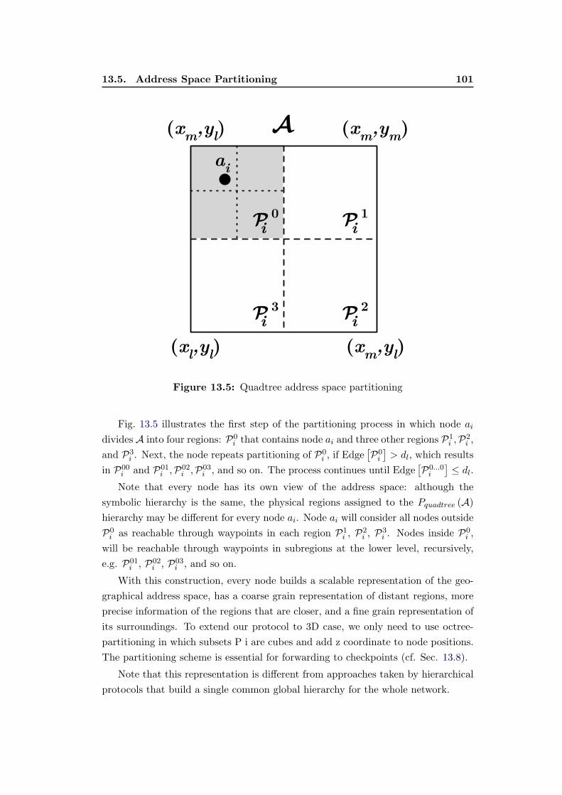
13.5. Address Space Partitioning 101
� 3
� 1
� 2
� 0
ai
�
(xl,y
l) (x
m,y
l)
(xm
,yl) (x
m,y
m)
i i
ii
Figure 13.5: Quadtree address space partitioning
Fig. 13.5 illustrates the first step of the partitioning process in which node ai
divides A into four regions: P0i that contains node ai and three other regions P1
i ,P2i ,
and P3i . Next, the node repeats partitioning of P0
i , if Edge�
P0i
�
> dl, which results
in P00i and P01
i ,P02i ,P03
i , and so on. The process continues until Edge�
P0...0i
�
≤ dl.
Note that every node has its own view of the address space: although the
symbolic hierarchy is the same, the physical regions assigned to the Pquadtree (A)
hierarchy may be different for every node ai. Node ai will consider all nodes outside
P0i as reachable through waypoints in each region P1
i , P2i , P
3i . Nodes inside P0
i ,
will be reachable through waypoints in subregions at the lower level, recursively,
e.g. P01i , P02
i , P03i , and so on.
With this construction, every node builds a scalable representation of the geo-
graphical address space, has a coarse grain representation of distant regions, more
precise information of the regions that are closer, and a fine grain representation of
its surroundings. To extend our protocol to 3D case, we only need to use octree-
partitioning in which subsets P i are cubes and add z coordinate to node positions.
The partitioning scheme is essential for forwarding to checkpoints (cf. Sec. 13.8).
Note that this representation is different from approaches taken by hierarchical
protocols that build a single common global hierarchy for the whole network.
102 Chapter 13. Principles of the WEAVE Protocol
13.6 Constructing Routing Tables
To forward packets, each node maintains a routing table containing up to L
waypoint routing entries per region—node ai has to know the waypoint to use for
destination address ad that lies in a given region P�
i . When node ai receives a
packet from source as ∈ P�
i with partial trace r, checkpoint ac, and hop counter
hc, it creates a waypoint routing entry w = (aw, Hw, hc, rw, ac) containing five
fields: waypoint address aw = as, waypoint metric Hw = |ai, aw| /hc, partial route
rw = r−1, and checkpoint ac described later on.
MetricHw reflects the“quality”of a waypoint: we want to keep a set of waypoint
entries with the largest Hw, because in this case, packets cross long distances per
hop count. Note that the shortest path between as and ad computed by OSPF
would have the maximal value of Hw for this pair of nodes. The metric allows to
memorize and route along OSPF-like paths, which is good, because it improves the
routing performance, i.e. route stretch is small. We have tested other waypoint
metrics such as: min |ai, aw|, max |ai, aw|, no metric (we just store last L entries).
In all cases, we have obtained a lower reachability ratio and longer routes than for
Hw.
Note also that maximizing Hw does not mean that nodes will suffer from poor
performance due to long wireless links of low quality [101]: in our case, metric Hw
is only applied to routes and not to links—nodes discover their neighbors using a
link layer metric and choose only good quality symmetrical links.
A node may store several waypoint entries WP�
i= {w1, . . . , wk}, k ≤ L for each
region P�
i and we have ∀wj ∈ WP�
i: awj
∈ P�
i . The number of waypoint entries to
store for each region is a protocol parameter L. Each node may store up to L best
waypoints with maximal Hw values and it discards other potential waypoint entries.
Only one entry per aw may exist in the node routing table. A packet forwarded
more than once by a node can only generate a single entry at this node the first
time it crosses the node, when its hc value is small and thus Hw is large.
13.7 Details of Packet Forwarding
To forward a packet, a node inserts the address of the best waypoint routing
entry into the packet header—a single fixed size field is sufficient—and sends it to
the next hop defined in the partial route rw. If there is no waypoint for a destination,
the node uses greedy routing.
Fig. 13.6 presents the following example. Assume that node ai receives a packet
whose waypoint field is empty and final destination is ad. Waypoint entry wk is
selected from WP�
i= {w1, . . . , wn} found in the routing table, such that ad ∈ P�
i ,
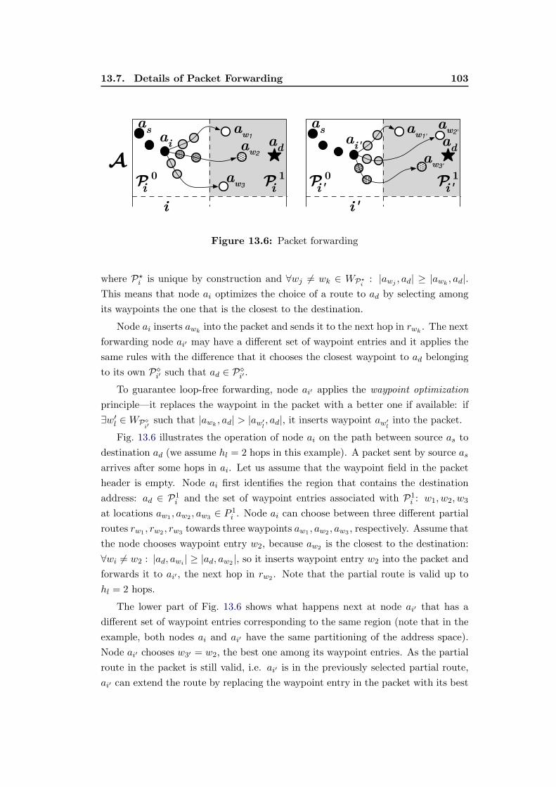
13.7. Details of Packet Forwarding 103
ai
� 1i
� 0i
as a
w�a
daw�
aw�
�a
i'
� 1i'
� 0i'
as a
w��a
d
aw��
aw��
i i'
Figure 13.6: Packet forwarding
where P�
i is unique by construction and ∀wj �= wk ∈ WP�
i: |awj
, ad| ≥ |awk, ad|.
This means that node ai optimizes the choice of a route to ad by selecting among
its waypoints the one that is the closest to the destination.
Node ai inserts awkinto the packet and sends it to the next hop in rwk
. The next
forwarding node ai� may have a different set of waypoint entries and it applies the
same rules with the difference that it chooses the closest waypoint to ad belonging
to its own P�
i� such that ad ∈ P�
i� .
To guarantee loop-free forwarding, node ai� applies the waypoint optimization
principle—it replaces the waypoint in the packet with a better one if available: if
∃w�
l ∈ WP�
i�such that |awk
, ad| > |aw�
l, ad|, it inserts waypoint aw�
linto the packet.
Fig. 13.6 illustrates the operation of node ai on the path between source as to
destination ad (we assume hl = 2 hops in this example). A packet sent by source as
arrives after some hops in ai. Let us assume that the waypoint field in the packet
header is empty. Node ai first identifies the region that contains the destination
address: ad ∈ P1i and the set of waypoint entries associated with P1
i : w1, w2, w3
at locations aw1, aw2
, aw3∈ P 1
i . Node ai can choose between three different partial
routes rw1, rw2
, rw3towards three waypoints aw1
, aw2, aw3
, respectively. Assume that
the node chooses waypoint entry w2, because aw2is the closest to the destination:
∀wi �= w2 : |ad, awi| ≥ |ad, aw2
|, so it inserts waypoint entry w2 into the packet and
forwards it to ai� , the next hop in rw2. Note that the partial route is valid up to
hl = 2 hops.
The lower part of Fig. 13.6 shows what happens next at node ai� that has a
different set of waypoint entries corresponding to the same region (note that in the
example, both nodes ai and ai� have the same partitioning of the address space).
Node ai� chooses w3� = w2, the best one among its waypoint entries. As the partial
route in the packet is still valid, i.e. ai� is in the previously selected partial route,
ai� can extend the route by replacing the waypoint entry in the packet with its best
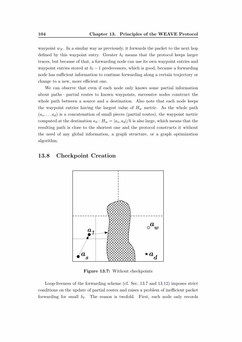
104 Chapter 13. Principles of the WEAVE Protocol
waypoint w3� . In a similar way as previously, it forwards the packet to the next hop
defined by this waypoint entry. Greater hl means that the protocol keeps larger
traces, but because of that, a forwarding node can use its own waypoint entries and
waypoint entries stored at hl − 1 predecessors, which is good, because a forwarding
node has sufficient information to continue forwarding along a certain trajectory or
change to a new, more efficient one.
We can observe that even if each node only knows some partial information
about paths—partial routes to known waypoints, successive nodes construct the
whole path between a source and a destination. Also note that each node keeps
the waypoint entries having the largest value of Hw metric. As the whole path
(as, . . . ad) is a concatenation of small pieces (partial routes), the waypoint metric
computed at the destination ad : Hw = |as, ad|/h is also large, which means that the
resulting path is close to the shortest one and the protocol constructs it without
the need of any global information, a graph structure, or a graph optimization
algorithm.
13.8 Checkpoint Creation
aw
as
ad
a�
Figure 13.7: Without checkpoints
Loop-freeness of the forwarding scheme (cf. Sec. 13.7 and 13.12) imposes strict
conditions on the update of partial routes and raises a problem of inefficient packet
forwarding for small hl. The reason is twofold. First, each node only records
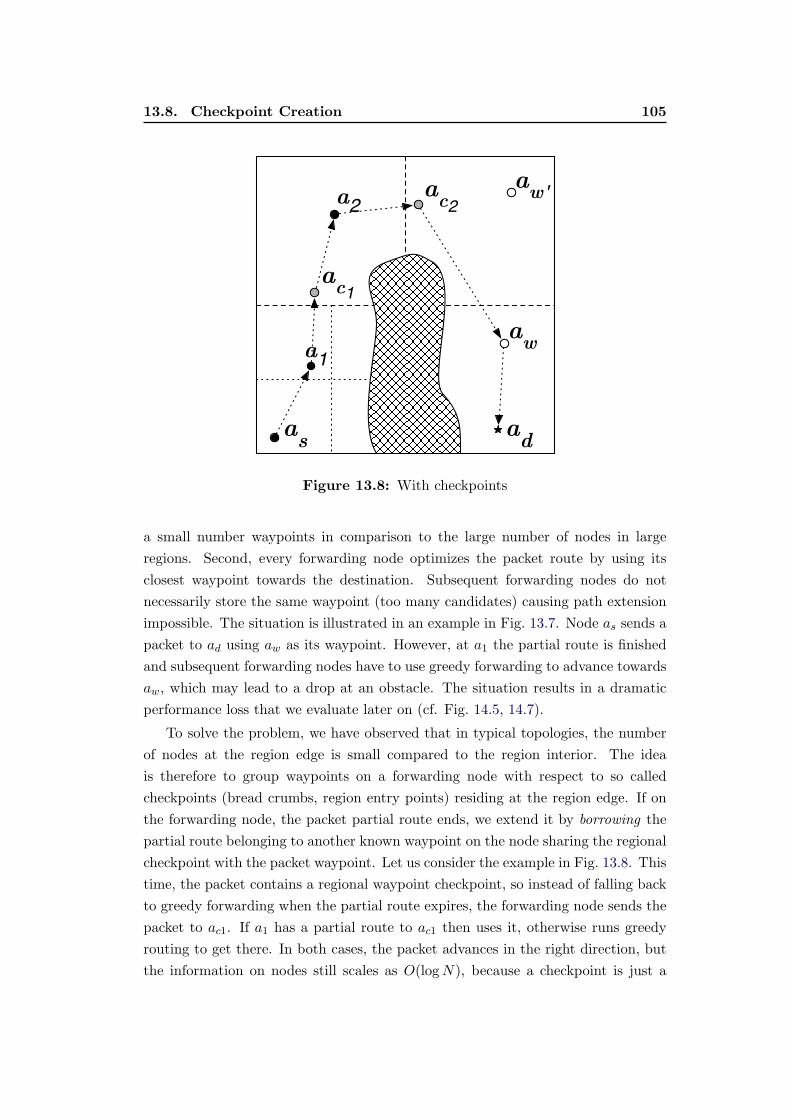
13.8. Checkpoint Creation 105
ac�
aw'a
c�
aw
as
ad
a�
a�
Figure 13.8: With checkpoints
a small number waypoints in comparison to the large number of nodes in large
regions. Second, every forwarding node optimizes the packet route by using its
closest waypoint towards the destination. Subsequent forwarding nodes do not
necessarily store the same waypoint (too many candidates) causing path extension
impossible. The situation is illustrated in an example in Fig. 13.7. Node as sends a
packet to ad using aw as its waypoint. However, at a1 the partial route is finished
and subsequent forwarding nodes have to use greedy forwarding to advance towards
aw, which may lead to a drop at an obstacle. The situation results in a dramatic
performance loss that we evaluate later on (cf. Fig. 14.5, 14.7).
To solve the problem, we have observed that in typical topologies, the number
of nodes at the region edge is small compared to the region interior. The idea
is therefore to group waypoints on a forwarding node with respect to so called
checkpoints (bread crumbs, region entry points) residing at the region edge. If on
the forwarding node, the packet partial route ends, we extend it by borrowing the
partial route belonging to another known waypoint on the node sharing the regional
checkpoint with the packet waypoint. Let us consider the example in Fig. 13.8. This
time, the packet contains a regional waypoint checkpoint, so instead of falling back
to greedy forwarding when the partial route expires, the forwarding node sends the
packet to ac1. If a1 has a partial route to ac1 then uses it, otherwise runs greedy
routing to get there. In both cases, the packet advances in the right direction, but
the information on nodes still scales as O(logN), because a checkpoint is just a
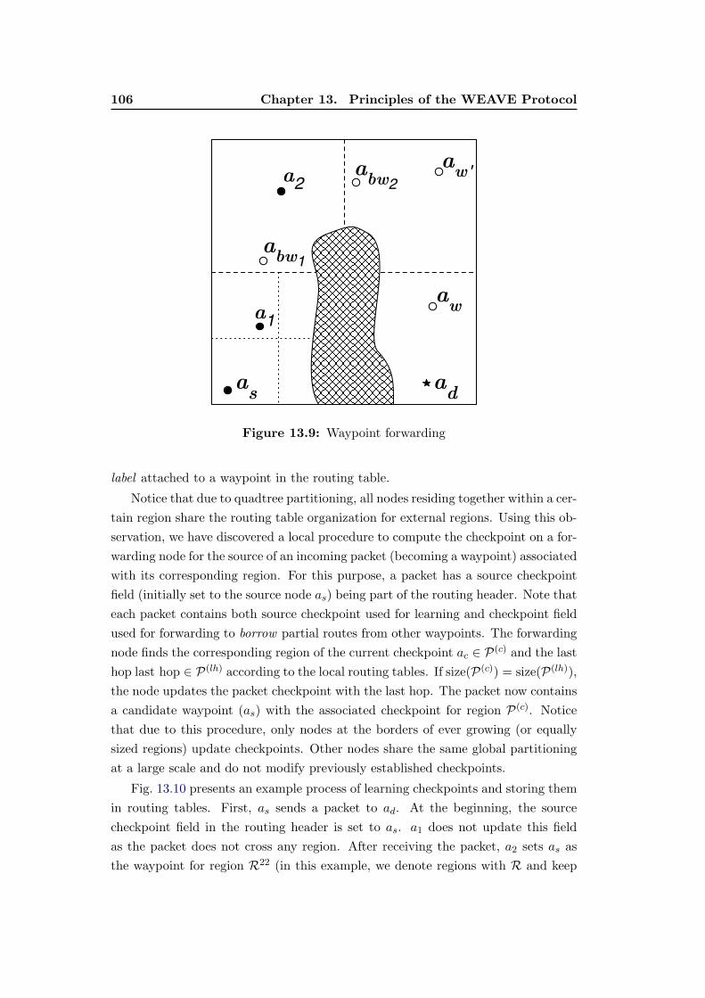
106 Chapter 13. Principles of the WEAVE Protocol
abw�
aw'a
bw�
aw
as
ad
a�
a�
Figure 13.9: Waypoint forwarding
label attached to a waypoint in the routing table.
Notice that due to quadtree partitioning, all nodes residing together within a cer-
tain region share the routing table organization for external regions. Using this ob-
servation, we have discovered a local procedure to compute the checkpoint on a for-
warding node for the source of an incoming packet (becoming a waypoint) associated
with its corresponding region. For this purpose, a packet has a source checkpoint
field (initially set to the source node as) being part of the routing header. Note that
each packet contains both source checkpoint used for learning and checkpoint field
used for forwarding to borrow partial routes from other waypoints. The forwarding
node finds the corresponding region of the current checkpoint ac ∈ P(c) and the last
hop last hop ∈ P(lh) according to the local routing tables. If size(P(c)) = size(P(lh)),
the node updates the packet checkpoint with the last hop. The packet now contains
a candidate waypoint (as) with the associated checkpoint for region P(c). Notice
that due to this procedure, only nodes at the borders of ever growing (or equally
sized regions) update checkpoints. Other nodes share the same global partitioning
at a large scale and do not modify previously established checkpoints.
Fig. 13.10 presents an example process of learning checkpoints and storing them
in routing tables. First, as sends a packet to ad. At the beginning, the source
checkpoint field in the routing header is set to as. a1 does not update this field
as the packet does not cross any region. After receiving the packet, a2 sets as as
the waypoint for region R22 (in this example, we denote regions with R and keep
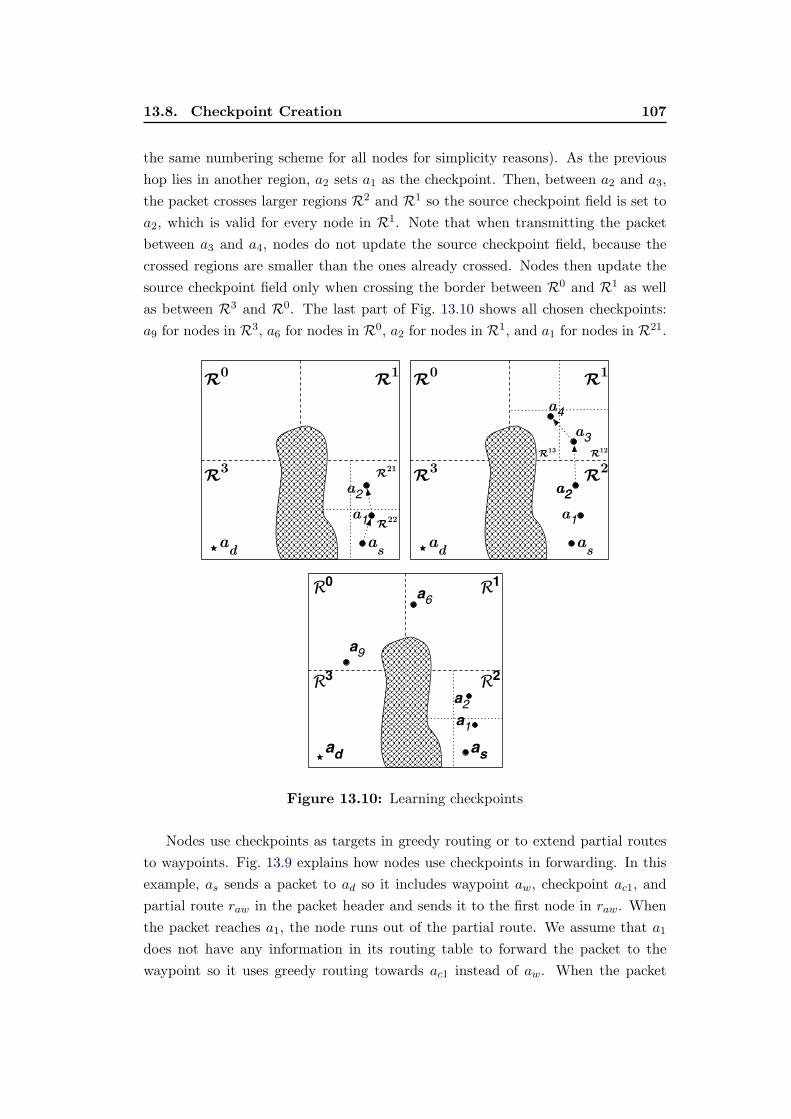
13.8. Checkpoint Creation 107
the same numbering scheme for all nodes for simplicity reasons). As the previous
hop lies in another region, a2 sets a1 as the checkpoint. Then, between a2 and a3,
the packet crosses larger regions R2 and R1 so the source checkpoint field is set to
a2, which is valid for every node in R1. Note that when transmitting the packet
between a3 and a4, nodes do not update the source checkpoint field, because the
crossed regions are smaller than the ones already crossed. Nodes then update the
source checkpoint field only when crossing the border between R0 and R1 as well
as between R3 and R0. The last part of Fig. 13.10 shows all chosen checkpoints:
a9 for nodes in R3, a6 for nodes in R0, a2 for nodes in R1, and a1 for nodes in R21.
ad
as
�0 �1
�21�3
�22
a�a�
�12
�2�13
ad
as
�0 �1
�3
a�a�a�
a�
a�
��
��
��
��
��
��
��
��
��
��
Figure 13.10: Learning checkpoints
Nodes use checkpoints as targets in greedy routing or to extend partial routes
to waypoints. Fig. 13.9 explains how nodes use checkpoints in forwarding. In this
example, as sends a packet to ad so it includes waypoint aw, checkpoint ac1, and
partial route raw in the packet header and sends it to the first node in raw. When
the packet reaches a1, the node runs out of the partial route. We assume that a1
does not have any information in its routing table to forward the packet to the
waypoint so it uses greedy routing towards ac1 instead of aw. When the packet
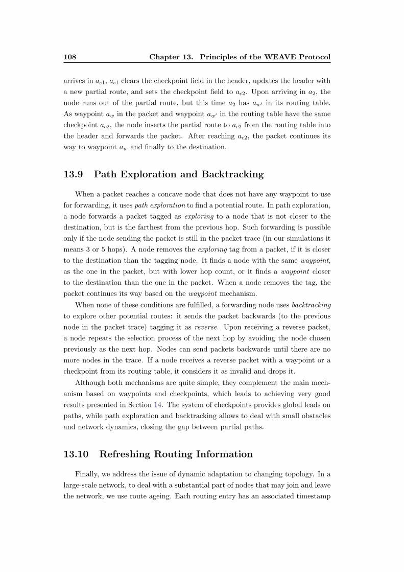
108 Chapter 13. Principles of the WEAVE Protocol
arrives in ac1, ac1 clears the checkpoint field in the header, updates the header with
a new partial route, and sets the checkpoint field to ac2. Upon arriving in a2, the
node runs out of the partial route, but this time a2 has aw� in its routing table.
As waypoint aw in the packet and waypoint aw� in the routing table have the same
checkpoint ac2, the node inserts the partial route to ac2 from the routing table into
the header and forwards the packet. After reaching ac2, the packet continues its
way to waypoint aw and finally to the destination.
13.9 Path Exploration and Backtracking
When a packet reaches a concave node that does not have any waypoint to use
for forwarding, it uses path exploration to find a potential route. In path exploration,
a node forwards a packet tagged as exploring to a node that is not closer to the
destination, but is the farthest from the previous hop. Such forwarding is possible
only if the node sending the packet is still in the packet trace (in our simulations it
means 3 or 5 hops). A node removes the exploring tag from a packet, if it is closer
to the destination than the tagging node. It finds a node with the same waypoint,
as the one in the packet, but with lower hop count, or it finds a waypoint closer
to the destination than the one in the packet. When a node removes the tag, the
packet continues its way based on the waypoint mechanism.
When none of these conditions are fulfilled, a forwarding node uses backtracking
to explore other potential routes: it sends the packet backwards (to the previous
node in the packet trace) tagging it as reverse. Upon receiving a reverse packet,
a node repeats the selection process of the next hop by avoiding the node chosen
previously as the next hop. Nodes can send packets backwards until there are no
more nodes in the trace. If a node receives a reverse packet with a waypoint or a
checkpoint from its routing table, it considers it as invalid and drops it.
Although both mechanisms are quite simple, they complement the main mech-
anism based on waypoints and checkpoints, which leads to achieving very good
results presented in Section 14. The system of checkpoints provides global leads on
paths, while path exploration and backtracking allows to deal with small obstacles
and network dynamics, closing the gap between partial paths.
13.10 Refreshing Routing Information
Finally, we address the issue of dynamic adaptation to changing topology. In a
large-scale network, to deal with a substantial part of nodes that may join and leave
the network, we use route ageing. Each routing entry has an associated timestamp
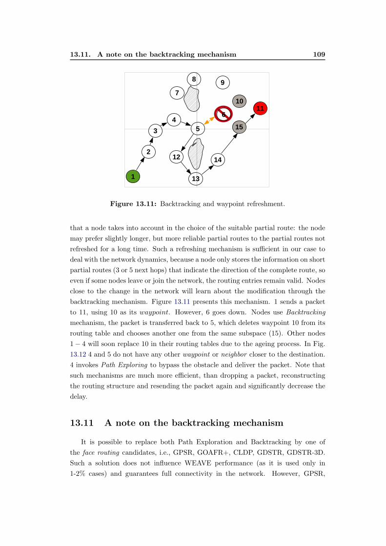
13.11. A note on the backtracking mechanism 109
1
2
3
4
5
6
7
89
11
10
12
13
14
15
Figure 13.11: Backtracking and waypoint refreshment.
that a node takes into account in the choice of the suitable partial route: the node
may prefer slightly longer, but more reliable partial routes to the partial routes not
refreshed for a long time. Such a refreshing mechanism is sufficient in our case to
deal with the network dynamics, because a node only stores the information on short
partial routes (3 or 5 next hops) that indicate the direction of the complete route, so
even if some nodes leave or join the network, the routing entries remain valid. Nodes
close to the change in the network will learn about the modification through the
backtracking mechanism. Figure 13.11 presents this mechanism. 1 sends a packet
to 11, using 10 as its waypoint. However, 6 goes down. Nodes use Backtracking
mechanism, the packet is transferred back to 5, which deletes waypoint 10 from its
routing table and chooses another one from the same subspace (15). Other nodes
1− 4 will soon replace 10 in their routing tables due to the ageing process. In Fig.
13.12 4 and 5 do not have any other waypoint or neighbor closer to the destination.
4 invokes Path Exploring to bypass the obstacle and deliver the packet. Note that
such mechanisms are much more efficient, than dropping a packet, reconstructing
the routing structure and resending the packet again and significantly decrease the
delay.
13.11 A note on the backtracking mechanism
It is possible to replace both Path Exploration and Backtracking by one of
the face routing candidates, i.e., GPSR, GOAFR+, CLDP, GDSTR, GDSTR-3D.
Such a solution does not influence WEAVE performance (as it is used only in
1-2% cases) and guarantees full connectivity in the network. However, GPSR,
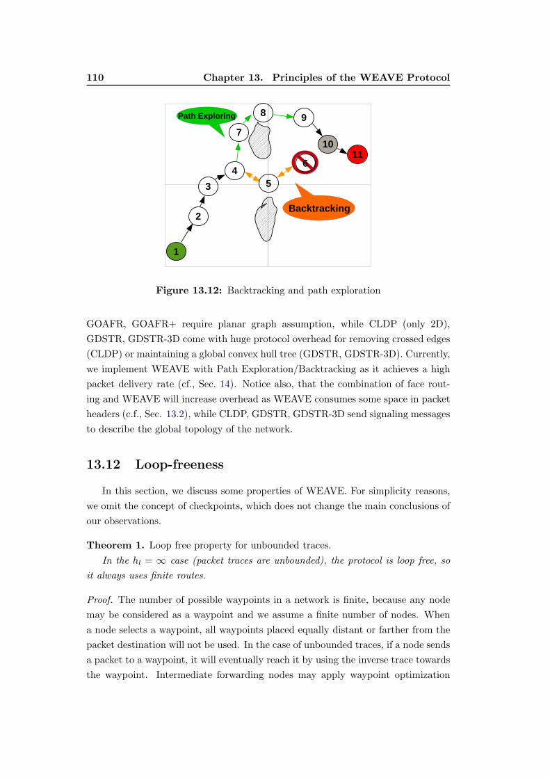
110 Chapter 13. Principles of the WEAVE Protocol
1
Path Exploring
Backtracking2
3
4
5
6
7
89
1110
Figure 13.12: Backtracking and path exploration
GOAFR, GOAFR+ require planar graph assumption, while CLDP (only 2D),
GDSTR, GDSTR-3D come with huge protocol overhead for removing crossed edges
(CLDP) or maintaining a global convex hull tree (GDSTR, GDSTR-3D). Currently,
we implement WEAVE with Path Exploration/Backtracking as it achieves a high
packet delivery rate (cf., Sec. 14). Notice also, that the combination of face rout-
ing and WEAVE will increase overhead as WEAVE consumes some space in packet
headers (c.f., Sec. 13.2), while CLDP, GDSTR, GDSTR-3D send signaling messages
to describe the global topology of the network.
13.12 Loop-freeness
In this section, we discuss some properties of WEAVE. For simplicity reasons,
we omit the concept of checkpoints, which does not change the main conclusions of
our observations.
Theorem 1. Loop free property for unbounded traces.
In the hl = ∞ case (packet traces are unbounded), the protocol is loop free, so
it always uses finite routes.
Proof. The number of possible waypoints in a network is finite, because any node
may be considered as a waypoint and we assume a finite number of nodes. When
a node selects a waypoint, all waypoints placed equally distant or farther from the
packet destination will not be used. In the case of unbounded traces, if a node sends
a packet to a waypoint, it will eventually reach it by using the inverse trace towards
the waypoint. Intermediate forwarding nodes may apply waypoint optimization
13.12. Loop-freeness 111
and each replacement of a waypoint by a better one reduces the number of still
valid waypoints by at least 1. The number of possible waypoint replacements is
also finite. This contradicts the condition for obtaining loops and infinite routes:
an infinite number of waypoint replacements is necessary to create an infinite route
from partial routes of finite length.
Theorem 2. In the hl < ∞ case, the protocol is also loop free and it provides finite
routes.
Proof. Let us assume that there is a loop, so there are three possibilities. First, the
waypoint is regularly replaced with a better one closer to the destination, but then
the same argument as above applies: in this case, the number of legitimate way-
points is decreasing, which is in contradiction with the presence of a loop. Second,
the path to the current waypoint is extended on the way by a forwarding node. Due
to the fact that forwarding node can only extend the route if and only if the current
hc to the waypoint is lower than the waypoint hc in the packet, the path cannot
be extended indefinitely. Third, if the path extension to the current waypoint does
not exist nor a closer waypoint was found, the procedure switches back to greedy
forwarding, which does not result in loops.

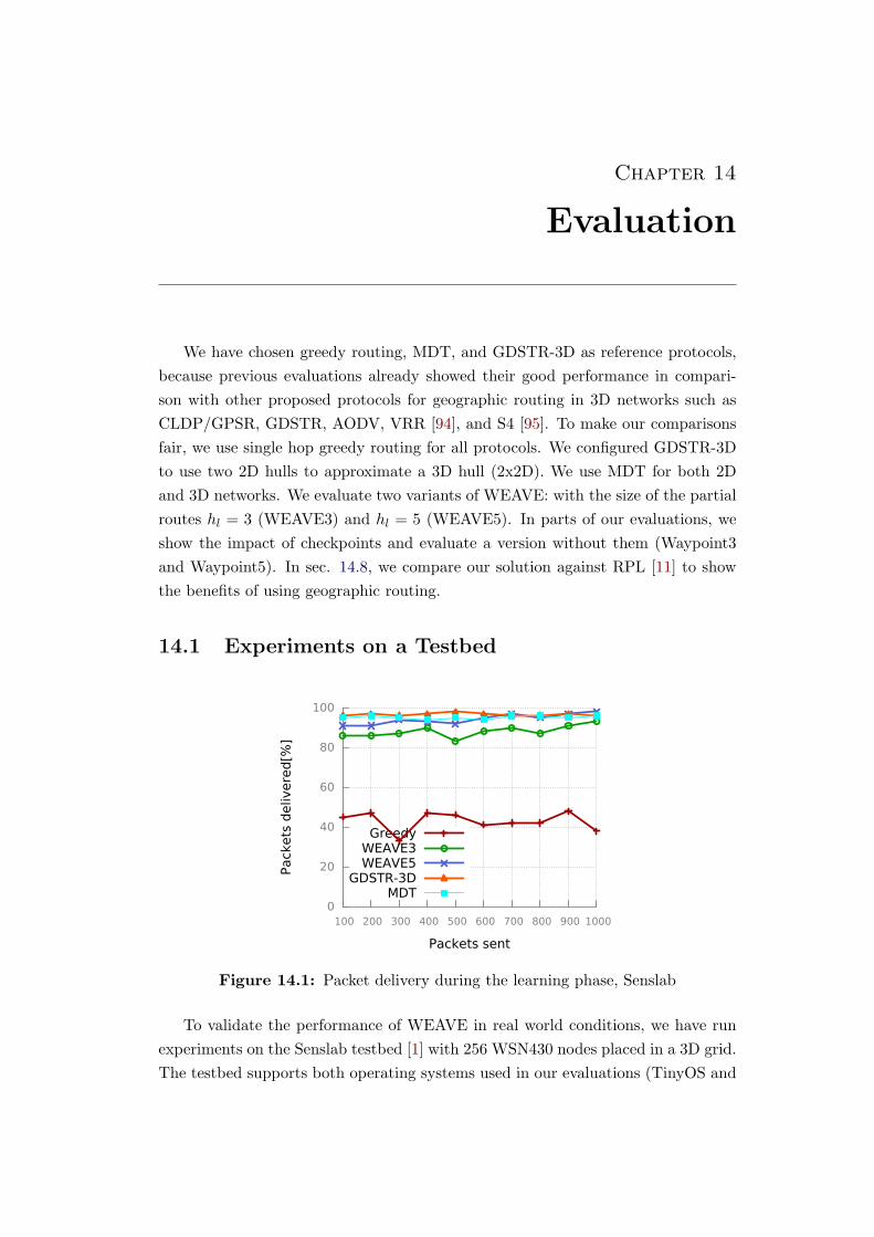
Chapter 14
Evaluation
We have chosen greedy routing, MDT, and GDSTR-3D as reference protocols,
because previous evaluations already showed their good performance in compari-
son with other proposed protocols for geographic routing in 3D networks such as
CLDP/GPSR, GDSTR, AODV, VRR [94], and S4 [95]. To make our comparisons
fair, we use single hop greedy routing for all protocols. We configured GDSTR-3D
to use two 2D hulls to approximate a 3D hull (2x2D). We use MDT for both 2D
and 3D networks. We evaluate two variants of WEAVE: with the size of the partial
routes hl = 3 (WEAVE3) and hl = 5 (WEAVE5). In parts of our evaluations, we
show the impact of checkpoints and evaluate a version without them (Waypoint3
and Waypoint5). In sec. 14.8, we compare our solution against RPL [11] to show
the benefits of using geographic routing.
14.1 Experiments on a Testbed
0
20
40
60
80
100
100 200 300 400 500 600 700 800 900 1000
Packets
delivere
d[%
]
Packets sent
GreedyWEAVE3WEAVE5
GDSTR-3DMDT
Figure 14.1: Packet delivery during the learning phase, Senslab
To validate the performance of WEAVE in real world conditions, we have run
experiments on the Senslab testbed [1] with 256 WSN430 nodes placed in a 3D grid.
The testbed supports both operating systems used in our evaluations (TinyOS and
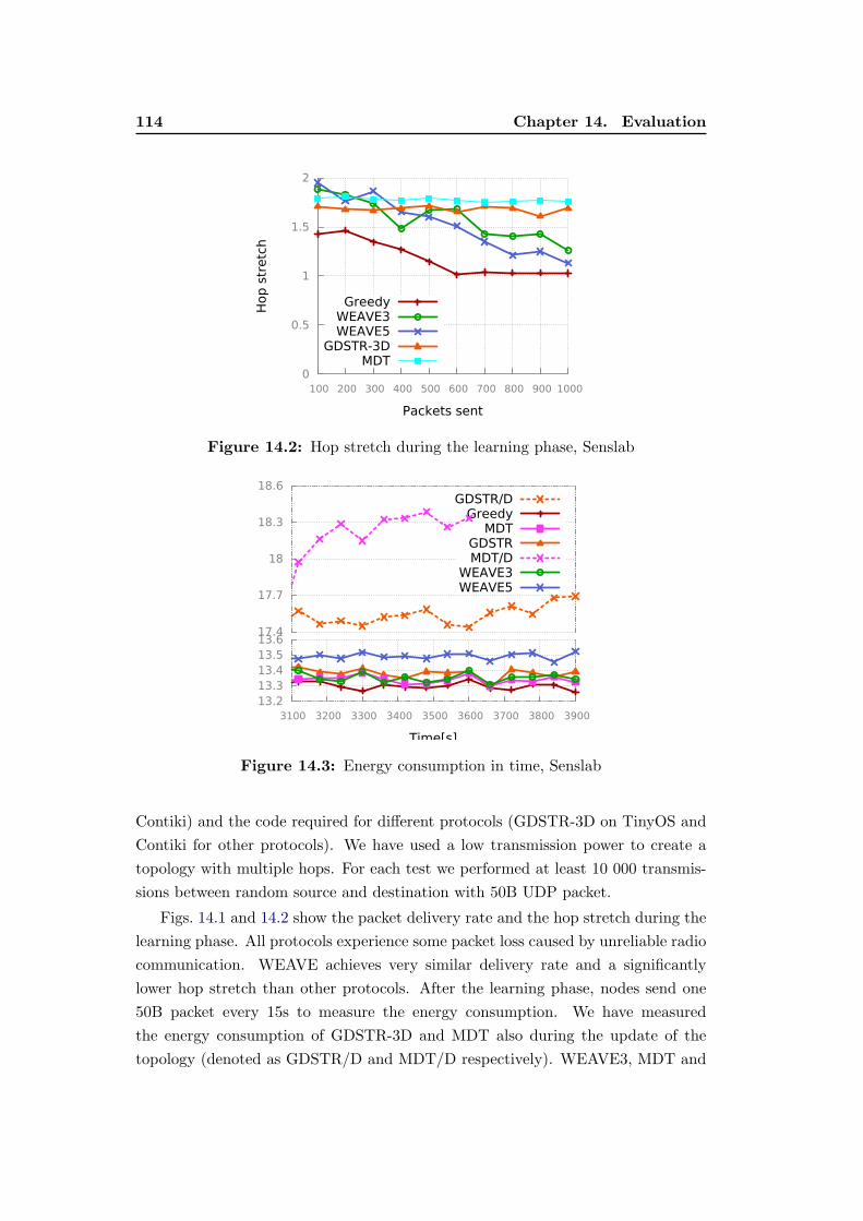
114 Chapter 14. Evaluation
0
0.5
1
1.5
2
100 200 300 400 500 600 700 800 900 1000
Hop s
tretc
h
Packets sent
GreedyWEAVE3WEAVE5
GDSTR-3DMDT
Figure 14.2: Hop stretch during the learning phase, Senslab
13.2
13.3
13.4
13.5
13.6
3100 3200 3300 3400 3500 3600 3700 3800 3900
Time[s]
17.4
17.7
18
18.3
18.6GDSTR/D
GreedyMDT
GDSTRMDT/D
WEAVE3WEAVE5
Figure 14.3: Energy consumption in time, Senslab
Contiki) and the code required for different protocols (GDSTR-3D on TinyOS and
Contiki for other protocols). We have used a low transmission power to create a
topology with multiple hops. For each test we performed at least 10 000 transmis-
sions between random source and destination with 50B UDP packet.
Figs. 14.1 and 14.2 show the packet delivery rate and the hop stretch during the
learning phase. All protocols experience some packet loss caused by unreliable radio
communication. WEAVE achieves very similar delivery rate and a significantly
lower hop stretch than other protocols. After the learning phase, nodes send one
50B packet every 15s to measure the energy consumption. We have measured
the energy consumption of GDSTR-3D and MDT also during the update of the
topology (denoted as GDSTR/D and MDT/D respectively). WEAVE3, MDT and
14.2. Simulations 115
GDSTR-3D have similar header sizes (8B/4B difference), so energy consumption
for transmissions is almost the same. Increasing the trace size to 5 in the WEAVE5
variant, increases the header size and thus energy consumption, but less than 1%.
During topology modifications, GDSTR-3D consumes 30% more energy to send
updates to every neighbor in the spanning tree. MDT requires even more control
traffic to discover all DT neighbors.
14.2 Simulations
To evaluate WEAVE for a larger parameter space, we have run simulations using
the following tools:
ns-3: greedy routing, GDSTR-3D, MDT and WEAVE for large-scale networks
(> 1000 nodes).
Cooja(v.2.6): greedy routing, MDT and WEAVE for small networks (≤ 1000
nodes). We have used Sky Motes as the execution platform with CC2420 2.4 GHz
radio and ContikiMAC at Layer 2.
TOSSIM(v.2.1): GDSTR-3D for small networks (≤ 1000 nodes), Micaz Motes
with an ideal radio channel as the execution platform. The source code from the
authors [64].
There are multiple reasons for using three different simulators. First, ns-3 uses a
simplified representation of lower layers, so we can test the behavior of the protocols
in large-scale networks. Second, through Cooja and TOSSIM, we study a real
protocol stack implementation executed in a controlled simulated environment, but
the number of simulated nodes is highly limited. As GDSTR-3D is implemented on
TinyOS, TOSSIM is required to run the code. Other protocols were implemented
in Cooja under Contiki. We argue, however, that the performance of a routing
protocol is only marginally affected by the type of the operating system and lower
layer protocols.
Unless stated differently in all our simulations we used the same packet loss rate,
as experienced during test on Senslab Testbed (1%). For each set of parameters we
randomly generated at least 20 topologies, performed at least 10 000 transmission
between random pairs of nodes for each of them and took the average result. Hop
stretch is calculated only for packets reaching the destination.
14.3 Initial Simulation Comparisons
Figure 14.4 presents a comparison between data packet header sizes of tested
protocols. We assume 3B coordinates (x, y, z) for packet source and destination.
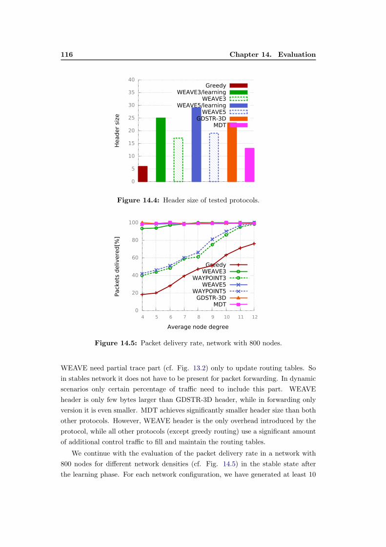
116 Chapter 14. Evaluation
0
5
10
15
20
25
30
35
40
Header
siz
e
GreedyWEAVE3/learning
WEAVE3WEAVE5/learning
WEAVE5GDSTR-3D
MDT
Figure 14.4: Header size of tested protocols.
0
20
40
60
80
100
4 5 6 7 8 9 10 11 12
Packets
delivere
d[%
]
Average node degree
GreedyWEAVE3
WAYPOINT3WEAVE5
WAYPOINT5GDSTR-3D
MDT
Figure 14.5: Packet delivery rate, network with 800 nodes.
WEAVE need partial trace part (cf. Fig. 13.2) only to update routing tables. So
in stables network it does not have to be present for packet forwarding. In dynamic
scenarios only certain percentage of traffic need to include this part. WEAVE
header is only few bytes larger than GDSTR-3D header, while in forwarding only
version it is even smaller. MDT achieves significantly smaller header size than both
other protocols. However, WEAVE header is the only overhead introduced by the
protocol, while all other protocols (except greedy routing) use a significant amount
of additional control traffic to fill and maintain the routing tables.
We continue with the evaluation of the packet delivery rate in a network with
800 nodes for different network densities (cf. Fig. 14.5) in the stable state after
the learning phase. For each network configuration, we have generated at least 10
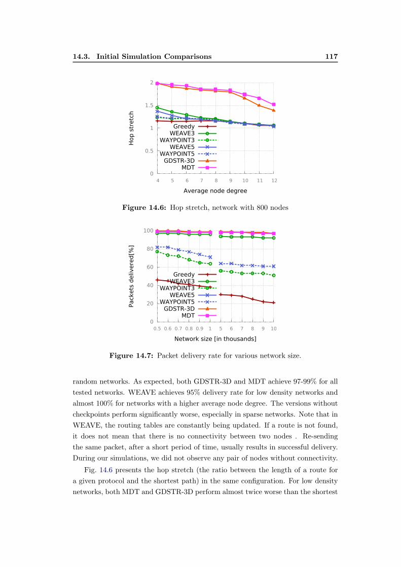
14.3. Initial Simulation Comparisons 117
0
0.5
1
1.5
2
4 5 6 7 8 9 10 11 12
Hop s
tretc
h
Average node degree
GreedyWEAVE3
WAYPOINT3WEAVE5
WAYPOINT5GDSTR-3D
MDT
Figure 14.6: Hop stretch, network with 800 nodes
0
20
40
60
80
100
0.5 0.6 0.7 0.8 0.9 1 5 6 7 8 9 10
Packets
delivere
d[%
]
Network size [in thousands]
GreedyWEAVE3
WAYPOINT3WEAVE5
WAYPOINT5GDSTR-3D
MDT
Figure 14.7: Packet delivery rate for various network size.
random networks. As expected, both GDSTR-3D and MDT achieve 97-99% for all
tested networks. WEAVE achieves 95% delivery rate for low density networks and
almost 100% for networks with a higher average node degree. The versions without
checkpoints perform significantly worse, especially in sparse networks. Note that in
WEAVE, the routing tables are constantly being updated. If a route is not found,
it does not mean that there is no connectivity between two nodes . Re-sending
the same packet, after a short period of time, usually results in successful delivery.
During our simulations, we did not observe any pair of nodes without connectivity.
Fig. 14.6 presents the hop stretch (the ratio between the length of a route for
a given protocol and the shortest path) in the same configuration. For low density
networks, both MDT and GDSTR-3D perform almost twice worse than the shortest
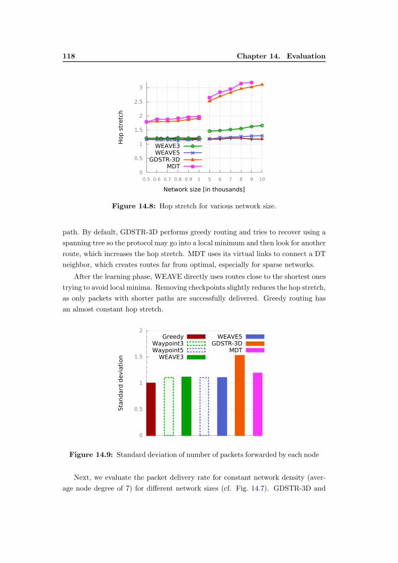
118 Chapter 14. Evaluation
0
0.5
1
1.5
2
2.5
3
0.5 0.6 0.7 0.8 0.9 1 5 6 7 8 9 10
Hop s
tretc
h
Network size [in thousands]
GreedyWEAVE3WEAVE5
GDSTR-3DMDT
Figure 14.8: Hop stretch for various network size.
path. By default, GDSTR-3D performs greedy routing and tries to recover using a
spanning tree so the protocol may go into a local minimum and then look for another
route, which increases the hop stretch. MDT uses its virtual links to connect a DT
neighbor, which creates routes far from optimal, especially for sparse networks.
After the learning phase, WEAVE directly uses routes close to the shortest ones
trying to avoid local minima. Removing checkpoints slightly reduces the hop stretch,
as only packets with shorter paths are successfully delivered. Greedy routing has
an almost constant hop stretch.
0
0.5
1
1.5
2
Sta
ndard
devia
tion
GreedyWaypoint3Waypoint5
WEAVE3
WEAVE5GDSTR-3D
MDT
Figure 14.9: Standard deviation of number of packets forwarded by each node
Next, we evaluate the packet delivery rate for constant network density (aver-
age node degree of 7) for different network sizes (cf. Fig. 14.7). GDSTR-3D and
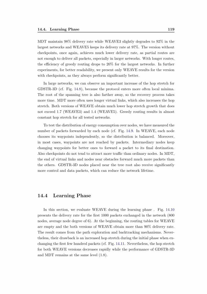
14.4. Learning Phase 119
MDT maintain 98% delivery rate while WEAVE3 slightly degrades to 92% in the
largest networks and WEAVE5 keeps its delivery rate at 97%. The version without
checkpoints, once again, achieves much lower delivery rate, as partial routes are
not enough to deliver all packets, especially in larger networks. With longer routes,
the efficiency of greedy routing drops to 20% for the largest networks. In further
experiments, for better readability, we present only WEAVE results for the version
with checkpoints, as they always perform significantly better.
In large networks, we can observe an important increase of the hop stretch for
GDSTR-3D (cf. Fig. 14.8), because the protocol enters more often local minima.
The root of the spanning tree is also farther away, so the recovery process takes
more time. MDT more often uses longer virtual links, which also increases the hop
stretch. Both versions of WEAVE obtain much lower hop stretch growth that does
not exceed 1.7 (WEAVE3) and 1.4 (WEAVE5). Greedy routing results in almost
constant hop stretch for all tested networks.
To test the distribution of energy consumption over nodes, we have measured the
number of packets forwarded by each node (cf. Fig. 14.9. In WEAVE, each node
chooses its waypoints independently, so the distribution is balanced. Moreover,
in most cases, waypoints are not reached by packets. Intermediary nodes keep
changing waypoints for better ones to forward a packet to its final destination.
Also checkpoints do not tend to attract more traffic than ordinary nodes. In MDT,
the end of virtual links and nodes near obstacles forward much more packets than
the others. GDSTR-3D nodes placed near the tree root also receive significantly
more control and data packets, which can reduce the network lifetime.
14.4 Learning Phase
In this section, we evaluate WEAVE during the learning phase . Fig. 14.10
presents the delivery rate for the first 1000 packets exchanged in the network (800
nodes, average node degree of 6). At the beginning, the routing tables for WEAVE
are empty and the both versions of WEAVE obtain more than 90% delivery rate.
The result comes from the path exploration and backtracking mechanisms. Never-
theless, their drawback is an increased hop stretch during the initial phase when ex-
changing the first few hundred packets (cf. Fig. 14.11. Nevertheless, the hop stretch
for both WEAVE versions decreases rapidly while the performance of GDSTR-3D
and MDT remains at the same level (1.8).
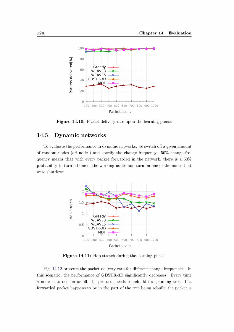
120 Chapter 14. Evaluation
0
20
40
60
80
100
100 200 300 400 500 600 700 800 900 1000
Packets
delivere
d[%
]
Packets sent
GreedyWEAVE3WEAVE5
GDSTR-3DMDT
Figure 14.10: Packet delivery rate upon the learning phase.
14.5 Dynamic networks
To evaluate the performance in dynamic networks, we switch off a given amount
of random nodes (off nodes) and specify the change frequency—50% change fre-
quency means that with every packet forwarded in the network, there is a 50%
probability to turn off one of the working nodes and turn on one of the nodes that
were shutdown.
0
0.5
1
1.5
2
100 200 300 400 500 600 700 800 900 1000
Hop s
tretc
h
Packets sent
GreedyWEAVE3WEAVE5
GDSTR-3DMDT
Figure 14.11: Hop stretch during the learning phase.
Fig. 14.12 presents the packet delivery rate for different change frequencies. In
this scenario, the performance of GDSTR-3D significantly decreases. Every time
a node is turned on or off, the protocol needs to rebuild its spanning tree. If a
forwarded packet happens to be in the part of the tree being rebuilt, the packet is
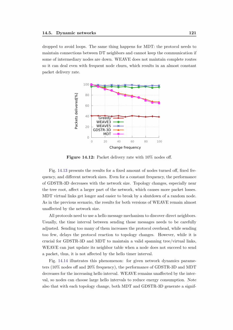
14.5. Dynamic networks 121
dropped to avoid loops. The same thing happens for MDT: the protocol needs to
maintain connections between DT neighbors and cannot keep the communication if
some of intermediary nodes are down. WEAVE does not maintain complete routes
so it can deal even with frequent node churn, which results in an almost constant
packet delivery rate.
0
20
40
60
80
100
0 20 40 60 80 100
Packets
delivere
d[%
]
Change frequency
GreedyWEAVE3WEAVE5
GDSTR-3DMDT
Figure 14.12: Packet delivery rate with 10% nodes off.
Fig. 14.13 presents the results for a fixed amount of nodes turned off, fixed fre-
quency, and different network sizes. Even for a constant frequency, the performance
of GDSTR-3D decreases with the network size. Topology changes, especially near
the tree root, affect a larger part of the network, which causes more packet losses.
MDT virtual links get longer and easier to break by a shutdown of a random node.
As in the previous scenario, the results for both versions of WEAVE remain almost
unaffected by the network size.
All protocols need to use a hello message mechanism to discover direct neighbors.
Usually, the time interval between sending those messages needs to be carefully
adjusted. Sending too many of them increases the protocol overhead, while sending
too few, delays the protocol reaction to topology changes. However, while it is
crucial for GDSTR-3D and MDT to maintain a valid spanning tree/virtual links,
WEAVE can just update its neighbor table when a node does not succeed to send
a packet, thus, it is not affected by the hello timer interval.
Fig. 14.14 illustrates this phenomenon: for given network dynamics parame-
ters (10% nodes off and 20% frequency), the performance of GDSTR-3D and MDT
decreases for the increasing hello interval. WEAVE remains unaffected by the inter-
val, so nodes can choose large hello intervals to reduce energy consumption. Note
also that with each topology change, both MDT and GDSTR-3D generate a signif-
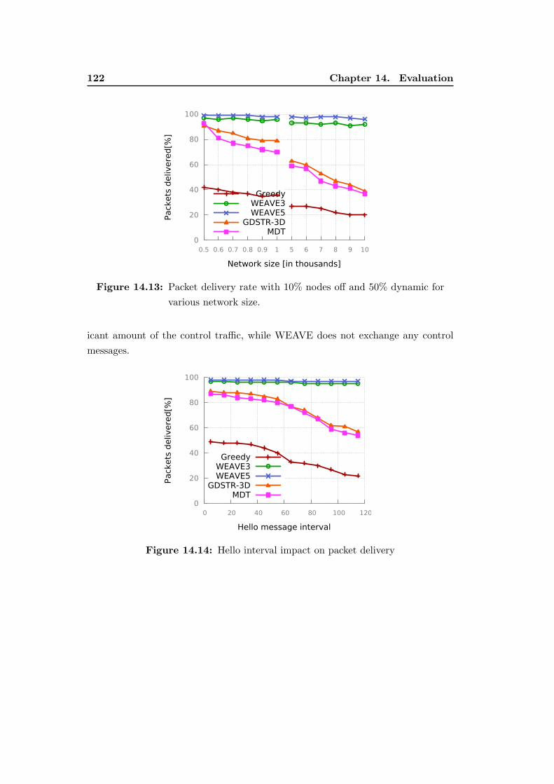
122 Chapter 14. Evaluation
0
20
40
60
80
100
0.5 0.6 0.7 0.8 0.9 1 5 6 7 8 9 10
Packets
delivere
d[%
]
Network size [in thousands]
GreedyWEAVE3WEAVE5
GDSTR-3DMDT
Figure 14.13: Packet delivery rate with 10% nodes off and 50% dynamic for
various network size.
icant amount of the control traffic, while WEAVE does not exchange any control
messages.
0
20
40
60
80
100
0 20 40 60 80 100 120
Packets
delivere
d[%
]
Hello message interval
GreedyWEAVE3WEAVE5
GDSTR-3DMDT
Figure 14.14: Hello interval impact on packet delivery
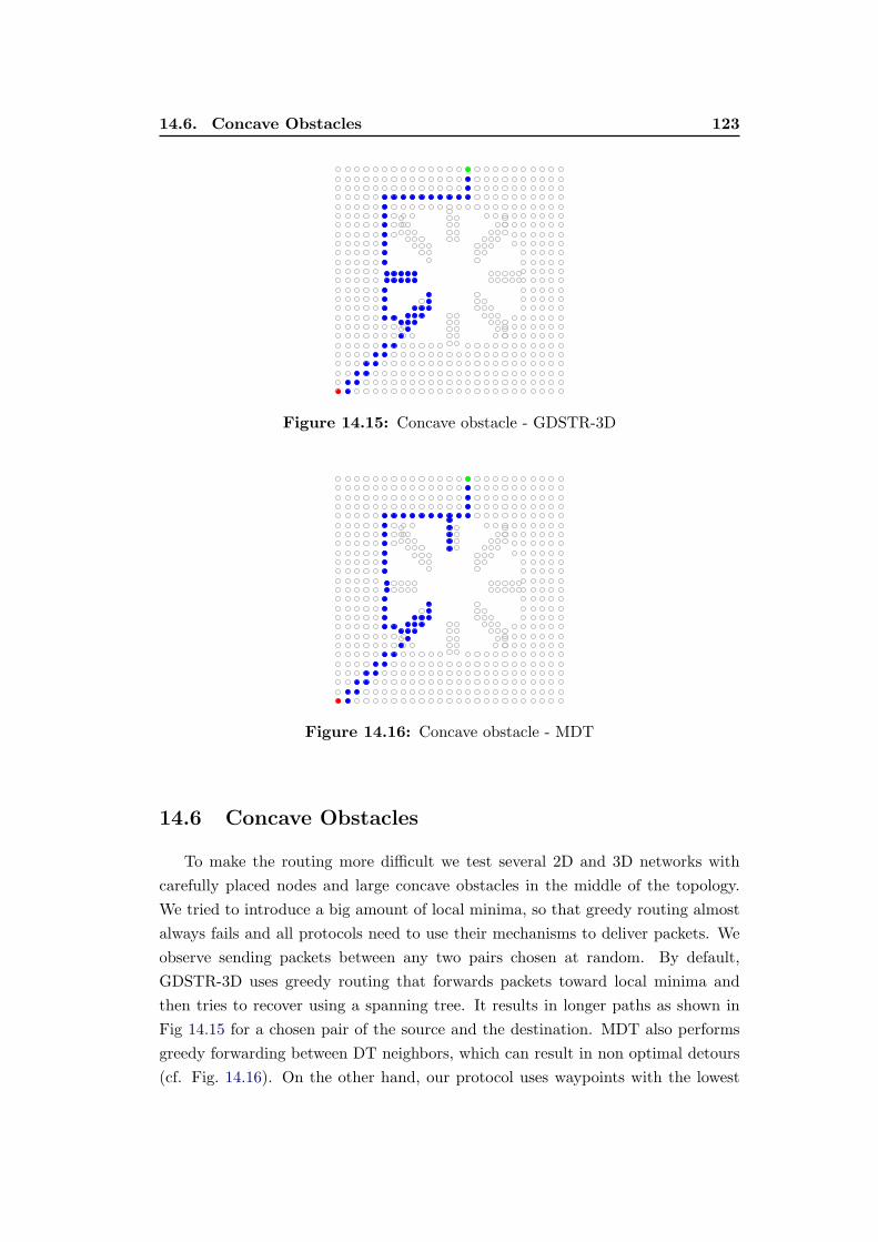
14.6. Concave Obstacles 123
Figure 14.15: Concave obstacle - GDSTR-3D
Figure 14.16: Concave obstacle - MDT
14.6 Concave Obstacles
To make the routing more difficult we test several 2D and 3D networks with
carefully placed nodes and large concave obstacles in the middle of the topology.
We tried to introduce a big amount of local minima, so that greedy routing almost
always fails and all protocols need to use their mechanisms to deliver packets. We
observe sending packets between any two pairs chosen at random. By default,
GDSTR-3D uses greedy routing that forwards packets toward local minima and
then tries to recover using a spanning tree. It results in longer paths as shown in
Fig 14.15 for a chosen pair of the source and the destination. MDT also performs
greedy forwarding between DT neighbors, which can result in non optimal detours
(cf. Fig. 14.16). On the other hand, our protocol uses waypoints with the lowest
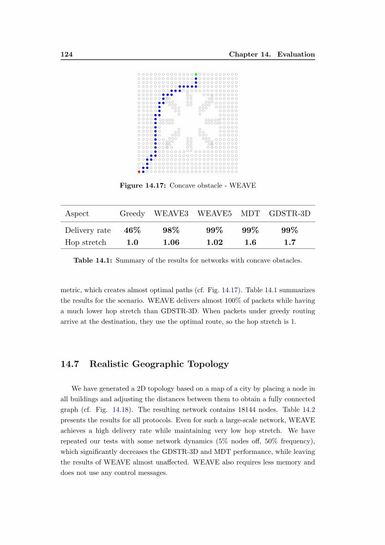
124 Chapter 14. Evaluation
Figure 14.17: Concave obstacle - WEAVE
Aspect Greedy WEAVE3 WEAVE5 MDT GDSTR-3D
Delivery rate 46% 98% 99% 99% 99%
Hop stretch 1.0 1.06 1.02 1.6 1.7
Table 14.1: Summary of the results for networks with concave obstacles.
metric, which creates almost optimal paths (cf. Fig. 14.17). Table 14.1 summarizes
the results for the scenario. WEAVE delivers almost 100% of packets while having
a much lower hop stretch than GDSTR-3D. When packets under greedy routing
arrive at the destination, they use the optimal route, so the hop stretch is 1.
14.7 Realistic Geographic Topology
We have generated a 2D topology based on a map of a city by placing a node in
all buildings and adjusting the distances between them to obtain a fully connected
graph (cf. Fig. 14.18). The resulting network contains 18144 nodes. Table 14.2
presents the results for all protocols. Even for such a large-scale network, WEAVE
achieves a high delivery rate while maintaining very low hop stretch. We have
repeated our tests with some network dynamics (5% nodes off, 50% frequency),
which significantly decreases the GDSTR-3D and MDT performance, while leaving
the results of WEAVE almost unaffected. WEAVE also requires less memory and
does not use any control messages.
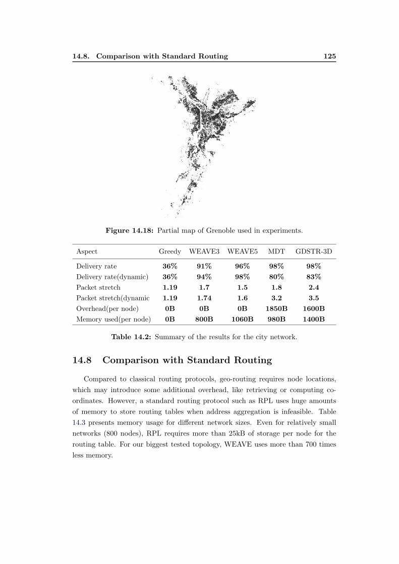
14.8. Comparison with Standard Routing 125
Figure 14.18: Partial map of Grenoble used in experiments.
Aspect Greedy WEAVE3 WEAVE5 MDT GDSTR-3D
Delivery rate 36% 91% 96% 98% 98%
Delivery rate(dynamic) 36% 94% 98% 80% 83%
Packet stretch 1.19 1.7 1.5 1.8 2.4
Packet stretch(dynamic 1.19 1.74 1.6 3.2 3.5
Overhead(per node) 0B 0B 0B 1850B 1600B
Memory used(per node) 0B 800B 1060B 980B 1400B
Table 14.2: Summary of the results for the city network.
14.8 Comparison with Standard Routing
Compared to classical routing protocols, geo-routing requires node locations,
which may introduce some additional overhead, like retrieving or computing co-
ordinates. However, a standard routing protocol such as RPL uses huge amounts
of memory to store routing tables when address aggregation is infeasible. Table
14.3 presents memory usage for different network sizes. Even for relatively small
networks (800 nodes), RPL requires more than 25kB of storage per node for the
routing table. For our biggest tested topology, WEAVE uses more than 700 times
less memory.
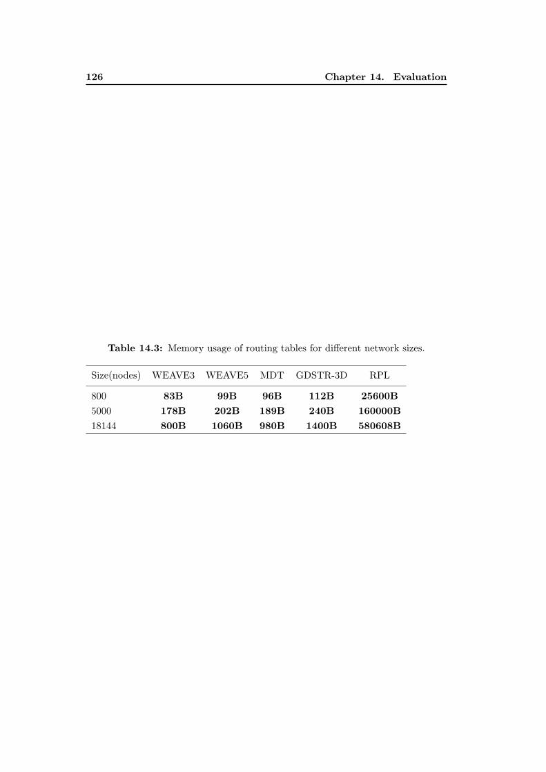
126 Chapter 14. Evaluation
Table 14.3: Memory usage of routing tables for different network sizes.
Size(nodes) WEAVE3 WEAVE5 MDT GDSTR-3D RPL
800 83B 99B 96B 112B 25600B
5000 178B 202B 189B 240B 160000B
18144 800B 1060B 980B 1400B 580608B
Chapter 15
Conclusion
In this part, we have presented WEAVE, a geographical routing protocol for
large-scale dynamic multi-hop wireless networks. The solution focuses on forwarding
packets between nodes and does not provide any naming scheme nor position/id
translation system. Our protocol does not use whole paths to destinations or use
any control messages. It fills up routing tables with hints only by observing incoming
traffic. Such a property makes it very different from a whole bunch of protocols
[88, 89, 64] that introduce a significant control overhead and need to maintain
a routing structure. It becomes important especially while experiencing network
dynamics, so common in lossy wireless networks. WEAVE does not require to
update its routing tables with every topology change.
Instead of maintaining the information on whole routes, WEAVE constructs
them out of partial routes to waypoints. The key element of WEAVE is a system
of checkpoints used as “bread crumbs”. Partial paths are enough to maintain low
hop stretch in contrast to solutions based on face routing [58] [59].
Waypoints and checkpoints are selected randomly by every node, which leads
to equal traffic load and eliminates issues with ”special nodes” that forward more
packets than others, a common problem of protocols introducing some kind of a
hierarchy [95].
Such a design makes WEAVE highly resistant to network dynamics and allows
achieving very good performance results with small overhead. The volume of the
routing information at any node remains very small compared to the size of the
whole network, because the number of waypoints grows logarithmically with the
network size. In this way, the protocol achieves good scalability.
We have compared WEAVE against greedy routing, MDT [66], and GDSTR-3D
[64] through measurements on a sensor network testbed and simulations for various
network sizes. Our results show that WEAVE achieves a high packet delivery rate,
low stretch, and balanced energy consumption.


Part V
Conclusion and Future Work

Chapter 16
Overall Conclusions and Future
Work
The problem of routing has received a lot of attention from the research com-
munity and could be considered a kind of a ”solved problem”. However, emerging
wireless technologies, miniaturization and new communication models have intro-
duced many new requirements for routing protocols especially in the domain of IoT.
The aim of this dissertation is to enrich the state of the art in routing protocols for
WSN/IoT. We have elaborated our contributions as addressing real world problems
expressed both by industry as well as academia. This chapter concludes the the-
sis by summarizing the main contributions, the results, and hinting some research
perspectives.
16.1 Summary of the Results and Final Conclusions
Our first contribution consists of Featurecast – a routing/naming system for
WSN. We have developed an extremely simple, flexible and yet powerful grammar
based on sensor characteristics, which allows us to specify destinations and query
groups of sensors. To the best of our knowledge, Featurecast is the first system
allowing to use characteristic-based routing in IPv6/6LoWPAN networks.
We have integrated our system with RPL to make it more interoperable and
easy to use. The integration was preceded by an extensive study and comparisons
of Bloom Filters and different techniques allowing to squeeze many features into
routing tables without limiting their capacity. Thanks to node features inside the
address, we were able to use a new metric that compares sensor characteristics and
groups the similar ones. This solution allowed to increase the routing efficiency and
eliminate some of the well-known problems with distribution trees. The complete
system was tested against both classic and recently proposed solutions in many
simulation scenarios as well as on a real sensor tested. Memory usage is significantly
lower than for any other compared solution, while achieving high packet delivery
and lower control message overhead.
132 Chapter 16. Overall Conclusions and Future Work
The second contribution isWEAVE, a geographic routing protocol for WSN/IoT.
We have based our solution on Binary Waypoint Routing and adapted it to fit the
required information into a fixed size header. We have developed the concept of
”Checkpoints” that reflect a path taken by packets during the learning phase. ”Path
Exploration”and ”Reverse Packet” increase the protocol robustness and allow to by-
pass local obstacles. The protocol also consists of several mechanisms preventing
routing loops. WEAVE does not involve any control message overhead. It learns
only from looking at the forwarded packet and learns new path to reach destina-
tions. WEAVE achieves very good packet delivery rate. Its advantage is even more
visible in scenarios with large or dynamic networks. As WEAVE does not create
complete paths to destinations, but maintains only approximate and partial route
information, which makes it much more resistant to node failures and topology
changes.
16.2 Future Work
Featurecast proves itself useful in querying local networks. However, global com-
munication using such a system still needs to be investigated. We can consider
both cooperation with traditional multicast protocols that can interconnect
different domains as well as developing an autonomous system providing both
global and local communications.
We have developed a simple metric connecting nodes with similar sets of features.
However, our solution is simple and treats all features in the same way. We
can go much further and test node similarity with more sophisticated met-
rics (features based on node location can be considered as more important).
A deeper insight on impact of such metrics can be beneficial also for net-
works that does not use Featurecast, but can still benefit from having more
information about nodes in addresses.
To evaluate Featurecast, we have used scenarios proposed by IETF [86]. However,
it would be interesting to evaluate the protocol in already deployed, intelli-
gent building environments and to compare the results with previously used
industrial solutions.
Featurecast performance heavily depends on proposed the feature scheme. Using a
flat structure without any hierarchy can significantly increase memory usage,
while well balanced structure can push the benefits to the maximum. We
can consider evaluating the protocol in the worst and best case scenarios to
prepare a list of hints for users creating a Featurecast routing structure.
16.2. Future Work 133
Featurecast achieves good routing performance compared to other existing solu-
tions. However, it is still based on a distribution tree, which can become an
issue in some scenarios. Developing a better system that does not introduce
a fixed routing structure can be an interesting idea. New possibilities open
when we could combine feature-based networks with georouting. Mapping fea-
tures on given regions, while maintaining connectivity using a protocol such
as WEAVE, can provide some new interesting results.
WEAVE provides an efficient geographic routing system. However, it cannot guar-
antee a 100% packet delivery, which may be crucial in some scenarios. A solu-
tion to this issue can be merging WEAVE and some other routing techniques
such as Face Routing. Our protocol already achieves high packet delivery rate
(close to 100%), so the addition would only be used in few cases without a
significant impact on path stretch or message overhead.
WEAVE was evaluated using a point-to-point communication pattern. However,
with small modification, it can provide an efficient way in one-to-many and
many-to-many scenarios. Using already established waypoints and check-
points can bring some interesting results.
WEAVE is able to deliver packets even if the position of the destination node is
not accurate. Some protocols are also able to do it [66], while others cannot
[64]. It could be interesting to compare WEAVE with other protocols in such
scenarios and evaluate the influence of the localization accuracy on routing
performance.

Chapter 17
Publications
• Micha�l Krol, Franck Rousseaux, Andrzej Duda, “Weave: Efficient Geograph-
ical Routing in Large-Scale Networks”, pages 1-13, EWSN’16 (the scope of
the EWSN Conference was broaden to International Conference on Embed-
ded Wireless Systems and Networks organized in cooperation with ACM
SIGBED), 2016 - accepted for publication (acceptance ratio of full papers:
30.4%).
• Henry-Joseph Audeoud, Micha�l Krol, Martin Heusse, and Andrzej Duda,“Low
Overhead Loop-Free Routing in Wireless Sensor Networks”, pages 1-8, IEEE
WiMob’15, Abu Dhabi, UAE.
• Micha�l Krol, Franck Rousseaux, Andrzej Duda, “Featurecast - group commu-
nication service for WSN”, pages 1-11, IETF Internet-Draft.
• Micha�l Krol, Franck Rousseaux, Andrzej Duda, “Featurecast: Lightweight
Data-Centric Communications for Wireless Sensor Networks”, pages 1-16,
EWSN’15 (European Conference on Wireless Sensor Networks), 2015 (accep-
tance ratio of full papers: 21.5%).
• Micha�l Krol, Franck Rousseaux, Andrzej Duda, “Compact address represen-
tation for feature routing” (”Representation compacte des adresses pour le
routage par caracteristiques”), pages 1-4, ALGOTEL’14.

Bibliography
[1] Cement Burin des Rosiers et al. SensLAB: Very Large Scale Open Wireless
Sensor Network Testbed. In Proc. 7th TridentCOM Conference, Shanghai,
Chine, April 2011. v, vi, 113
[2] Olivier Fambon, E Fleury, Gaetan Harter, Roger Pissard-Gibollet, and
Frederic Saint-Marcel. Fit iot-lab tutorial: hands-on practice with a very
large scale testbed tool for the internet of things. 10emes journees franco-
phones Mobilite et Ubiquite, UbiMob2014, 2014. vii
[3] Wint Yi Poe and Jens B Schmitt. Node deployment in large wireless sensor
networks: coverage, energy consumption, and worst-case delay. In Asian
Internet Engineering Conference, pages 77–84. ACM, 2009. 9
[4] Stavros Toumpis and Leandros Tassiulas. Optimal deployment of large wire-
less sensor networks. Information Theory, IEEE Transactions on, 52(7):2935–
2953, 2006. 9
[5] Tuba Bakıcı, Esteve Almirall, and JonathanWareham. A smart city initiative:
the case of barcelona. Journal of the Knowledge Economy, 4(2):135–148, 2013.
10
[6] Philip Levis, Sam Madden, Joseph Polastre, Robert Szewczyk, Kamin White-
house, Alec Woo, David Gay, Jason Hill, Matt Welsh, Eric Brewer, et al.
Tinyos: An operating system for sensor networks. In Ambient intelligence,
pages 115–148. Springer, 2005. 10
[7] Adam Dunkels, Bjorn Gronvall, and Thiemo Voigt. Contiki-a lightweight
and flexible operating system for tiny networked sensors. In Local Computer
Networks, 2004. 29th Annual IEEE International Conference on, pages 455–
462. IEEE, 2004. 10
[8] Emmanuel Baccelli, Oliver Hahm, Mesut Gunes, Matthias Wahlisch, and
Thomas C Schmidt. Riot os: Towards an os for the internet of things. In
Computer Communications Workshops (INFOCOM WKSHPS), 2013 IEEE
Conference on, pages 79–80. IEEE, 2013. 10
[9] Shah Bhatti, James Carlson, Hui Dai, Jing Deng, Jeff Rose, Anmol Sheth,
Brian Shucker, Charles Gruenwald, Adam Torgerson, and Richard Han. Man-
tis os: An embedded multithreaded operating system for wireless micro sensor
platforms. Mobile Networks and Applications, 10(4):563–579, 2005. 10
138 Bibliography
[10] Anand Eswaran, Anthony Rowe, and Raj Rajkumar. Nano-rk: an energy-
aware resource-centric rtos for sensor networks. In Real-Time Systems Sym-
posium, 2005. RTSS 2005. 26th IEEE International, pages 10–pp. IEEE, 2005.
10
[11] T. Winter and P. Thubert. Rpl: Ipv6 routing protocol for low power and lossy
networks. Technical Report version 4, IETF draft, October 2009. 12, 60, 113
[12] L. Mottola and G. Picco. Logical Neighborhoods: A Programming Abstrac-
tion for Wireless Sensor Networks. In Proc. IEEE DCOSS, 2006. 12, 50, 59,
60, 77, 87
[13] G. Montenegro, N. Kushalnagar, J. Hui, and D. Culler. Transmission of
IPv6 Packets over IEEE 802.15.4 Networks. RFC 4944 (Proposed Standard),
September 2007. Updated by RFCs 6282, 6775. 17
[14] MicaZ Datasheet. 17, 18
[15] TelosB Datasheet. 17, 18
[16] OpenMote Datasheet. 17, 18
[17] GreenNet Datasheet. 17, 18
[18] SmartMeshIP Datasheet. 17, 18
[19] IEEE 802.15.11a/b/n/g standard http://standards.ieee.org/about/get/
802/802.11.html. 17
[20] TONI Adame, Albert Bel, Boris Bellalta, JAUME Barcelo, and Miquel Oliver.
Ieee 802.11 ah: the wifi approach for m2m communications. Wireless Com-
munications, IEEE, 21(6):144–152, 2014. 17
[21] IEEE 802.15.1 -2002 standard http://standards.ieee.org/findstds/
standard/802.15.1-2002.html. 18
[22] IEEE 802.15.4. WPAN task group 4. http://www.ieee802.org/15/pub/
TG4.html, 2006. 18
[23] ZigBee Alliance. Zigbee specification, 2006. 18
[24] LoRa Alliance Website. Accessed on 2015-10-16. 18
[25] Semtech. SX1272 LoRa Datasheet. Accessed on 2015-10-16. 18
[26] SigFox Website. Accessed on 2015-10-16. 18
Bibliography 139
[27] Adam Dunkels. The contikimac radio duty cycling protocol. 2011. 19
[28] Tijs Van Dam and Koen Langendoen. An adaptive energy-efficient mac pro-
tocol for wireless sensor networks. In Proceedings of the 1st international con-
ference on Embedded networked sensor systems, pages 171–180. ACM, 2003.
19
[29] Michael I Brownfield, Kaveh Mehrjoo, Almohonad S Fayez, and Nathaniel
J Davis Iv. Wireless sensor network energy-adaptive mac protocol. 2006. 19
[30] Cristina Cano, Boris Bellalta, Anna Sfairopoulou, and Jaume Barcelo. A
low power listening mac with scheduled wake up after transmissions for wsns.
Communications Letters, IEEE, 13(4):221–223, 2009. 19
[31] Pei Huang, Li Xiao, Soroor Soltani, Matt W Mutka, and Ning Xi. The evolu-
tion of mac protocols in wireless sensor networks: A survey. Communications
Surveys & Tutorials, IEEE, 15(1):101–120, 2013. 19
[32] K. Lougheed and Y. Rekhter. Border Gateway Protocol (BGP). RFC 1105
(Experimental), June 1989. Obsoleted by RFC 1163. 23
[33] J. Moy. OSPF Version 2. RFC 2328 (INTERNET STANDARD), April 1998.
Updated by RFCs 5709, 6549, 6845, 6860. 23
[34] D. Oran. OSI IS-IS Intra-domain Routing Protocol. RFC 1142 (Historic),
February 1990. Obsoleted by RFC 7142. 23
[35] John A Stankovic. Research challenges for wireless sensor networks. ACM
SIGBED Review, 1(2):9–12, 2004. 23
[36] Jamal N Al-Karaki and Ahmed E Kamal. Routing techniques in wireless
sensor networks: a survey. Wireless communications, IEEE, 11(6):6–28, 2004.
23
[37] A. Brandt, J. Buron, and G. Porcu. Home Automation Routing Requirements
in Low-Power and Lossy Networks. RFC 5826 (Informational), April 2010.
27
[38] J. Martocci, P. De Mil, N. Riou, and W. Vermeylen. Building Automation
Routing Requirements in Low-Power and Lossy Networks. RFC 5867 (Infor-
mational), June 2010. 27
[39] K. Pister, P. Thubert, S. Dwars, and T. Phinney. Industrial Routing Re-
quirements in Low-Power and Lossy Networks. RFC 5673 (Informational),
October 2009. 27
140 Bibliography
[40] M. Dohler, T. Watteyne, T. Winter, and D. Barthel. Routing Requirements
for Urban Low-Power and Lossy Networks. RFC 5548 (Informational), May
2009. 27
[41] Thomas Clausen and Ulrich Herberg. Some Considerations on Routing in Par-
ticular and Lossy Environments. IETF Workshop on Interconnecting Smart
Objects with the Internet, 2011. 28, 30
[42] Thomas Clausen, Ulrich Herberg, and Matthias Philipp. A critical evalua-
tion of the ipv6 routing protocol for low power and lossy networks (rpl). In
Wireless and Mobile Computing, Networking and Communications (WiMob),
2011 IEEE 7th International Conference on, pages 365–372. IEEE, 2011. 28
[43] JeongGil Ko, Stephen Dawson-Haggerty, Omprakash Gnawali, David Culler,
and Andreas Terzis. Evaluating the performance of rpl and 6lowpan in tinyos.
In Workshop on Extending the Internet to Low Power and Lossy Networks
(IP+ SN). Citeseer, 2011. 28
[44] N Accettura, LA Grieco, G Boggia, and P Camarda. Performance analysis
of the rpl routing protocol. In Mechatronics (ICM), 2011 IEEE International
Conference on, pages 767–772. IEEE, 2011. 28
[45] Olfa Gaddour, Anis Koubaa, Shafique Chaudhry, Miled Tezeghdanti, and
Mohamed Abid. Simulation and Performance Evaluation of DAG Construc-
tion with RPL. In Third International Conference on Commmunications and
Networking (COMNET’2012), Hammamet, Tunisia, 29 Mars, 1 April, April
2012. 30
[46] H.R. Kermajani and C. Gomez. Route change latency in low-power and lossy
wireless networks using rpl and 6lowpan neighbor discovery. In Computers
and Communications (ISCC), 2011 IEEE Symposium on, pages 937 –942, 28
2011-july 1 2011. 30
[47] J. P. Vasseur J. Tripathi, J. C. de Oliveira. A performance evaluation study
of rpl: Routing protocol for low power and lossy networks. Conference on
Information Sciences and Systems (CISS), 2010. 30
[48] P. Levis, T. Clausen, J. Hui, O. Gnawali, and J. Ko. The Trickle Algorithm.
RFC 6206 (Proposed Standard), March 2011. 30, 33
[49] W. Xie, M. Goyal, H. Hosseini, J. Martocci, Y. Bashir, E. Baccelli, and
A. Durresi. A performance analysis of point-to-point routing along a directed
acyclic graph in low power and lossy networks. In Proceedings of the 2010
Bibliography 141
13th International Conference on Network-Based Information Systems, NBIS
’10, pages 111–116, Washington, DC, USA, 2010. IEEE Computer Society. 31
[50] M. Goyal, E. Baccelli, M. Philipp, A. Brandt, and J. Martocci. Reactive
Discovery of Point-to-Point Routes in Low-Power and Lossy Networks. RFC
6997 (Experimental), August 2013. 31
[51] Chi-Anh La, Martin Heusse, and Andrzej Duda Grenoble. Link reversal and
reactive routing in low power and lossy networks. In Personal Indoor and Mo-
bile Radio Communications (PIMRC), 2013 IEEE 24th International Sympo-
sium on, pages 3386–3390. IEEE, 2013. 31
[52] G. Montenegro S. Yoo K. Kim, S. D. Park and N. Kushalnagar. Internet
Draft, work in progress - 6LoW- PAN Ad Hoc On-Demand Distance Vector
Routing (LOAD), 2007. 32
[53] Adnan Aijaz, Hongjia Su, and A Hamid Aghvami. Enhancing rpl for cognitive
radio enabled machine-to-machine networks. In Wireless Communications
and Networking Conference (WCNC), 2014 IEEE, pages 2090–2095. IEEE,
2014. 32
[54] P. Levis, N. Patel, D. Culler, and S. Shenker. Trickle: A self-regulating
algorithm for code propagation and maintenance in wireless sensor networks.
In Proceedings of the USENIX Symposium on Networked Systems Design &
Implementation (NSDI), March 2004. 32
[55] M Milosh Stolikj, TMM Meyfroyt, PJL Cuijpers, and JJ Lukkien. Improving
the performance of trickle-based data dissemination in low-power networks.
2014. 33
[56] I. Stojmenovic. Position-Based Routing in Ad Hoc Networks. IEEE Commu-
nications Magazine, 40(7):128–134, Jul 2002. 35, 91
[57] N. Arad and Y. Shavitt. Minimizing Recovery State in Geographic Ad Hoc
Routing. IEEE Transactions on Mobile Computing, 8(2):203–217, Feb 2009.
35, 91
[58] P. Bose, P. Morin, I. Stojmenovic, and J. Urrutia. Routing with Guaranteed
Delivery in Ad Hoc Wireless Networks. In DIAL’M, pages 48–55, Seattle,
USA, 1999. 36, 92, 127
[59] Brad Karp and H. T. Kung. Greedy Perimeter Stateless Routing for Wireless
Networks. In Proc. of MOBICOM, Boston, USA, August 2000. 36, 92, 127
142 Bibliography
[60] Young-Jin Kim, Ramesh Govindan, Brad Karp, and Scott Shenker. Lazy
Cross-Link Removal for Geographic Routing. In Proc. of SENSYS, pages
112–124, 2006. 36, 92
[61] Y.J. Kim, R. Govindan, B. Karp, and S. Shenker. Geographic Routing Made
Practical. In Proc. NSDI, pages 112–124, 2005. 36, 92
[62] Mikkel Thorup and Uri Zwick. Compact routing schemes. In Proceedings of
the thirteenth annual ACM symposium on Parallel algorithms and architec-
tures, pages 1–10. ACM, 2001. 36
[63] Ben Leong, Barbara Liskov, and Robert Morris. Geographic routing without
planarization. In Proceedings of the 3rd Conference on Networked Systems
Design & Implementation - Volume 3, NSDI’06, pages 25–25, Berkeley, CA,
USA, 2006. USENIX Association. 37
[64] Leong B. Zhou J., Chen Y. Practical 3D Geographic Routing for Wireless
Sensor Networks. In Proc. SenSys, pages 337–350, New York, NY, USA, 2010.
38, 92, 93, 115, 127, 133
[65] Eryk Schiller, Paul Starzetz, Franck Rousseau, and Andrzej Duda. Binary
waypoint geographical routing in wireless mesh networks. In Proceedings of
the 11th International Symposium on Modeling, Analysis and Simulation of
Wireless and Mobile Systems, MSWiM ’08, pages 252–259, New York, NY,
USA, 2008. ACM. 39
[66] Simon S Lam and Chen Qian. Geographic routing in d-dimensional spaces
with guaranteed delivery and low stretch. In Proceedings of the ACM SIG-
METRICS joint international conference on Measurement and modeling of
computer systems, pages 257–268. ACM, 2011. 40, 127, 133
[67] Prosenjit Bose and Pat Morin. Online routing in triangulations. In Algorithms
and Computation, pages 113–122. Springer, 1999. 40
[68] D-Y Lee and Simon S Lam. Protocol design for dynamic delaunay triangula-
tion. In Distributed Computing Systems, 2007. ICDCS’07. 27th International
Conference on, pages 26–26. IEEE, 2007. 40
[69] Z. Shelby, K. Hartke, and C. Bormann. The Constrained Application Protocol
(CoAP). RFC 7252 (Proposed Standard), June 2014. 45
[70] K. Hartke. Observing Resources in CoAP. Internet Draft, December 2014.
47
Bibliography 143
[71] Z. Shelby. Constrained RESTful Environments (CoRE) Link Format. RFC
6690 (Proposed Standard), August 2012. 47
[72] M. Nottingham and E. Hammer-Lahav. Defining Well-Known Uniform Re-
source Identifiers (URIs). RFC 5785 (Proposed Standard), April 2010. 47
[73] C. Bormann Z. Shelby. CoRE Resource Directory. Internet Draft, November
2014. 47
[74] C. Intanagonwiwat, R. Govindan, and D. Estrin. Directed Diffusion: a Scal-
able and Robust Communication Paradigm for Sensor Networks. In Proc. of
MOBICOM, pages 56–67, 2000. 48, 59, 87
[75] Van Jacobson, Diana K. Smetters, James D. Thornton, Michael F. Plass,
Nicholas H. Briggs, and Rebecca L. Braynard. Networking named content.
In Proceedings of the 5th International Conference on Emerging Networking
Experiments and Technologies, CoNEXT ’09, pages 1–12, New York, NY,
USA, 2009. ACM. 52, 87
[76] Younes Abidy, Bilel Saadallahy, Abdelkader Lahmadi, and Olivier Festor.
Named data aggregation in wireless sensor networks. In Network Operations
and Management Symposium (NOMS), 2014 IEEE, pages 1–8. IEEE, 2014.
54
[77] Zhong Ren, Mohamed Ahmed Hail, and Horst Hellbruck. Ccn-wsn-a
lightweight, flexible content-centric networking protocol for wireless sensor
networks. In Intelligent Sensors, Sensor Networks and Information Process-
ing, 2013 IEEE Eighth International Conference on, pages 123–128. IEEE,
2013. 54
[78] Jan Pieter Meijers, Marica Amadeo, Claudia Campolo, Antonella Molinaro,
Stefano Yuri Paratore, Giuseppe Ruggeri, and Marthinus J Booysen. A two-
tier content-centric architecture for wireless sensor networks. In Network Pro-
tocols (ICNP), 2013 21st IEEE International Conference on, pages 1–2. IEEE,
2013. 54
[79] Qingfeng Huang, Chenyang Lu, and Gruia-Catalin Roman. Spatiotemporal
Multicast in Sensor Networks. In Proc. ACM SenSys, pages 205–217, New
York, NY, USA, 2003. ACM. 59
[80] Roland Flury and Roger Wattenhofer. Routing, Anycast, and Multicast for
Mesh and Sensor Networks. In IEEE INFOCOM, May 2007. 59
144 Bibliography
[81] Lu Su, Bolin Ding, Yong Yang, Tarek F. Abdelzaher, Guohong Cao, and
Jennifer C. Hou. oCast: Optimal Multicast Routing Protocol for Wireless
Sensor Networks. In Proc. of ICNP, pages 151–160, 2009. 59
[82] C. Intanagonwiwat, R. Govindan, D. Estrin, J. Heidemann, and F. Silva.
Directed Diffusion for Wireless Sensor Networking. IEEE/ACM Trans. Netw.,
11(1):2–16, 2003. 59
[83] Peter Hebden and Adrian Pearce. Data-Centric Routing Using Bloom Filters
in Wireless Sensor Networks. In Proc. of ICISIP-06, pages 72–78, 2006. 59
[84] O. Gnawali, R. Fonseca, K. Jamieson, D. Moss, and P. Levis. Collection tree
protocol. In Proc. ACM SenSys, Berkeley, CA, USA, 2009. 60
[85] A. Dunkels, B. Gronvall, and T. Voigt. Contiki—a Lightweight and Flexible
Operating System for Tiny Networked Sensors. In IEEE EMNETS, Tampa,
Florida, USA, November 2004. 60, 77
[86] A. Rahman and E.O. Dijk. Group Communication for CoAP. IETF draft-
ietf-core-groupcomm-07, May 2013. 60, 77, 79, 132
[87] Michael Mitzenmacher. Compressed Bloom Filters . In Proceedings of PODC
’01, volume 1, pages 144–150. ACM, 2001. 70
[88] Thomas Clausen and Philippe Jacquet. Optimized Link State Routing Pro-
tocol (OLSR). RFC 3626, IETF, October 2003. 91, 127
[89] Charles E. Perkins, Elisabeth M. Belding Royer, and Samir R. Das. Ad hoc
on-demand distance vector (AODV) routing. RFC 3561, IETF, July 2003.
91, 127
[90] J. Li, J. Jannotti, D. S. J. De Couto, D. R. Karger, and R. Morris. A Scalable
Location Service for Geographic Ad Hoc Routing. In Proc. MOBICOM, pages
120–130, Boston, Massachusetts, August 2000. 91
[91] R. Jain, A. Puri, and R. Sengupta. Geographical Routing Using Partial In-
formation for Wireless Ad Hoc Networks. IEEE Personal Comm., February
2001. 91
[92] H. Takagi and L. Kleinrock. Optimal Transmission Ranges for Randomly
Distributed Packet Radio Terminals. IEEE Transactions on Communications,
32(3):246–257, Mar 1984. 91
Bibliography 145
[93] G. G. Finn. Routing and Addressing Problems in Large Metropolitan-Scale
Internetworks. Technical Report ISI/RR-87-180, Information Sciences Insti-
tute, Mars 1987. 91
[94] Matthew Caesar, Miguel Castro, and Edmund B. Nightingale. Virtual Ring
Routing: Network Routing Inspired by DHTs. In In Proc. of ACM SIG-
COMM, pages 351–362, 2006. 92, 113
[95] Yun Mao, Feng Wang, Lili Qiu, Simon S. Lam, and Jonathan M. Smith. S4:
Small State and Small Stretch Routing Protocol for Large Wireless Sensor
Networks. In Proc. of the Usenix NSDI Conference, 2007. 92, 93, 113, 127
[96] D. S. J. De Couto and R. Morris. Location Proxies and Intermediate Node
Forwarding for Practical Geographic Forwarding. Technical Report MIT-
LCS-TR-824, MIT Laboratory for Computer Science, June 2001. 92
[97] L. Blazevic, J.-Y. Le Boudec, and S. Giordano. A Location-Based Routing
Method for Mobile Ad Hoc Networks. IEEE Transactions on Mobile Com-
puting, 4(2):97–110, 2005. 92
[98] M. Lim, A. Chesterfield, J. Crowcroft, and J. Chesterfield. Landmark Guided
Forwarding. In ICNP, pages 169–178, 2005. 92
[99] E. Schiller, P. Starzetz, F. Rousseau, and A. Duda. Binary Waypoint Geo-
graphical Routing in Wireless Mesh Networks. In Proc. ACM MSWiM, 2008.
92
[100] Douglas S. J. De Couto, Daniel Aguayo, John Bicket, and Robert Morris.
A High-Throughput Path Metric for Multi-Hop Wireless Routing. In Proc.
MOBICOM, pages 134–146, New York, NY, USA, 2003. 95
[101] K. Seada, M. Zuniga, A. Helmy, and B. Krishnamachari. Energy-Efficient
Forwarding Strategies for Geographic Routing in Lossy Wireless Sensor Net-
works. In Proc. SenSys, pages 108–121, 2004. 102

146 Bibliography