S -wave velocity structure, mantle xenoliths and the upper mantle beneath the Kaapvaal craton

Geophys. J. Int. (2006) 167, 171–186 doi: 10.1111/j.1365-246X.2006.03005.x

GJI

Sei

smol

ogy

S-wave velocity structure, mantle xenoliths and the upper mantlebeneath the Kaapvaal craton

Angela Marie Larson,1,∗ J. Arthur Snoke2 and David E. James3

1Department of Geosciences, Virginia Tech, 4044 Derring (0420), Blacksburg, VA 24061, USA2Department of Geosciences, Virginia Tech, 4044 Derring (0420), Blacksburg, VA 24061, USA. E-mail: [email protected] of Terrestrial Magnetism, Carnegie Institution of Washington, 5241 Broad Branch Rd. NW, Washington, DC 20015, USA

Accepted 2006 March 14. Received 2006 March 13; in original form 2004 November 10

S U M M A R YInversion of two-station Rayleigh-wave fundamental-mode phase velocities across the undis-turbed region of the southern Kaapvaal craton south of the Bushveld Province producesvelocity-depth models quantitatively similar to those estimated from low-T mantle xenolithsbrought to the surface in Cretaceous-age kimberlite pipes that erupted in the same region.The cratonic xenolith suite was previously analysed thermobarometrically and chemically toobtain the equilibrium P-T conditions from which the seismic velocities and density of thecratonic mantle to about 180 km depth were calculated. As the xenoliths represent a snapshotof the mantle at the time of their eruption, comparison with recently recorded seismic dataprovides an opportunity to compare and contrast the independently gained results. We form acomposite reference velocity model using xenolith values for the depth range 50–180 km withan interpolated join to PREM for the depth range 220–500 km, and a regionally determinedcrustal model for the upper 35 km. This composite served as the starting model for a linearizedleast-squares inversion (LLSI) using fundamental-mode Rayleigh-wave phase velocities in theperiod range 18–171 s measured for five events along 16 two-station paths within the southernKaapvaal craton. Based on xenolith data, we constrain the vP/vS ratio in the inversion to varyfrom about 1.72 in the uppermost mantle to 1.78 at 180 km depth. The velocity structuresdetermined by surface-wave inversion are consistent with those derived from the xenolith data,suggesting that the velocity structure (i.e. thermal structure) of the mantle to a depth of 180 kmbeneath the Kaapvaal craton today is similar to that at ∼70–90 Ma, the time of kimberlite erup-tion. Results from both surface-wave inversion and xenolith calculations indicate that S-wavevelocities decrease slightly with depth beneath the craton, from a value around 4.7 km s−1 inthe uppermost mantle to about 4.60–4.65 km s−1 at a depth of 180–200 km. We performedtests based on a wide range of starting models, and found no models with a minimum vS

in the mantle less than about 4.55 km s−1 down to a depth of 250 km within the resolutionpossible from an inversion based on fundamental-mode Rayleigh waves. Additional analysisof synthetic models, using a combination of LLSI and the neighbourhood algorithm, showsthat if there was a low-velocity zone such as that reported by Priestley in 1999, our analysisprocedure would have found it.

Key words: Archaean, continental evolution, inverse theory, Rayleigh waves, seismic array,upper mantle.

1 I N T RO D U C T I O N

Southern Africa is an amalgamation of Archean cratons and mobile

belts of Proterozoic and younger ages (Fig. 1). The region of study

centres on the 2.7–3.6 Ga Kaapvaal craton. The craton is bounded

∗Now at: Department of Geosciences, Pennsylvania State University,

University Park, PA 16802, USA.

on three sides by Proterozoic mobile belts. The northern sector of

the craton was intruded ∼2.0 Ga by the Bushveld Complex, the

world’s largest known layered mafic intrusion. Numerous kimber-

lite eruptions occurred throughout southern Africa ca. 90 Ma, trans-

porting large quantities of mantle xenoliths, some diamond bearing,

from depths as great as 200+ km. Despite the continental collisions,

marginal subduction zones, and mafic intrusions, the deep mantle

root of the Kaapvaal craton has survived since its formation in the

Archean.

C© 2006 The Authors 171Journal compilation C© 2006 RAS

172 A. M. Larson, J. A. Snoke and D. E. James

20˚E 22˚E 24˚E 26˚E 28˚E 30˚E 32˚E 34˚E32˚S

30˚S

28˚S

26˚S

24˚S

22˚SL I M P O P O B E L T

K A A P V A A L

C R A T O N

K H E I S S

B E L T

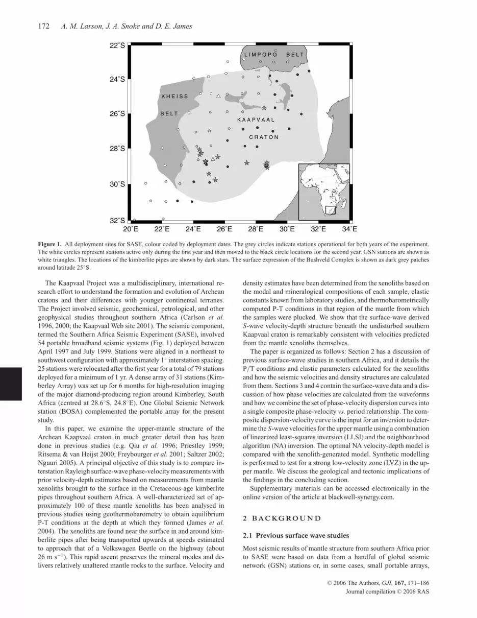
Figure 1. All deployment sites for SASE, colour coded by deployment dates. The grey circles indicate stations operational for both years of the experiment.

The white circles represent stations active only during the first year and then moved to the black circle locations for the second year. GSN stations are shown as

white triangles. The locations of the kimberlite pipes are shown by dark stars. The surface expression of the Bushveld Complex is shown as dark grey patches

around latitude 25◦S.

The Kaapvaal Project was a multidisciplinary, international re-

search effort to understand the formation and evolution of Archean

cratons and their differences with younger continental terranes.

The Project involved seismic, geochemical, petrological, and other

geophysical studies throughout southern Africa (Carlson et al.1996, 2000; the Kaapvaal Web site 2001). The seismic component,

termed the Southern Africa Seismic Experiment (SASE), involved

54 portable broadband seismic systems (Fig. 1) deployed between

April 1997 and July 1999. Stations were aligned in a northeast to

southwest configuration with approximately 1◦ interstation spacing.

25 stations were relocated after the first year for a total of 79 stations

deployed for a minimum of 1 yr. A dense array of 31 stations (Kim-

berley Array) was set up for 6 months for high-resolution imaging

of the major diamond-producing region around Kimberley, South

Africa (centred at 28.6◦S, 24.8◦E). One Global Seismic Network

station (BOSA) complemented the portable array for the present

study.

In this paper, we examine the upper-mantle structure of the

Archean Kaapvaal craton in much greater detail than has been

done in previous studies (e.g. Qiu et al. 1996; Priestley 1999;

Ritsema & van Heijst 2000; Freybourger et al. 2001; Saltzer 2002;

Nguuri 2005). A principal objective of this study is to compare in-

terstation Rayleigh surface-wave phase-velocity measurements with

prior velocity-depth estimates based on measurements from mantle

xenoliths brought to the surface in the Cretaceous-age kimberlite

pipes throughout southern Africa. A well-characterized set of ap-

proximately 100 of these mantle xenoliths has been analysed in

previous studies using geothermobarometry to obtain equilibrium

P-T conditions at the depth at which they formed (James et al.2004). The xenoliths are found near the surface in and around kim-

berlite pipes after being transported upwards at speeds estimated

to approach that of a Volkswagen Beetle on the highway (about

26 m s−1). This rapid ascent preserves the mineral modes and de-

livers relatively unaltered mantle rocks to the surface. Velocity and

density estimates have been determined from the xenoliths based on

the modal and mineralogical compositions of each sample, elastic

constants known from laboratory studies, and thermobarometrically

computed P-T conditions in that region of the mantle from which

the samples were plucked. We show that the surface-wave derived

S-wave velocity-depth structure beneath the undisturbed southern

Kaapvaal craton is remarkably consistent with velocities predicted

from the mantle xenoliths themselves.

The paper is organized as follows: Section 2 has a discussion of

previous surface-wave studies in southern Africa, and it details the

P/T conditions and elastic parameters calculated for the xenoliths

and how the seismic velocities and density structures are calculated

from them. Sections 3 and 4 contain the surface-wave data and a dis-

cussion of how phase velocities are calculated from the waveforms

and how we combine the set of phase-velocity dispersion curves into

a single composite phase-velocity vs. period relationship. The com-

posite dispersion-velocity curve is the input for an inversion to deter-

mine the S-wave velocities for the upper mantle using a combination

of linearized least-squares inversion (LLSI) and the neighbourhood

algorithm (NA) inversion. The optimal NA velocity-depth model is

compared with the xenolith-generated model. Synthetic modelling

is performed to test for a strong low-velocity zone (LVZ) in the up-

per mantle. We discuss the geological and tectonic implications of

the findings in the concluding section.

Supplementary materials can be accessed electronically in the

online version of the article at blackwell-synergy.com.

2 B A C KG RO U N D

2.1 Previous surface wave studies

Most seismic results of mantle structure from southern Africa prior

to SASE were based on data from a handful of global seismic

network (GSN) stations or, in some cases, small portable arrays,

C© 2006 The Authors, GJI, 167, 171–186

Journal compilation C© 2006 RAS

S-wave velocity structure beneath the Kaapvaal craton 173

so that structural models tended to be averaged over several distinct

geological provinces (e.g. Chichowicz & Green 1992; Zhao et al.1999; Qiu et al. 1996; Priestley 1999; Ritsema & van Heijst 2000).

The first surface-wave studies based on SASE data were phase-delay

analyses by Freybourger et al. (2001) and Saltzer (2002) using joint

Rayleigh- and Love-wave inversion. Both studies worked with aver-

ages over the entire SASE deployment zone, smoothing differences

between geologically distinct Archean, Proterozoic and Phanerozoic

provinces. In addition to these published studies, doctoral disserta-

tions by Nguuri (2005) and Gore (2005) contain preliminary anal-

yses of interstation surface-wave dispersion based on SASE data

to constrain the S-wave velocity in the crust and upper mantle of

southern Africa. Both used two-station group- and phase-velocity

inversions following the procedures used by Snoke & James (1997),

but only Nguuri’s study region included the Kaapvaal craton. That

work, however, included events only from the first year of observa-

tion, and some paths crossed the Bushveld Complex (see Fig. 1).

For this study, we confine our observations to the undisturbed south-

ern part of the Kaapvaal craton, a constraint that eliminates 11 of

Nguuri’s 16 Rayleigh-wave paths.

Several studies of crustal and Moho structure beneath southern

Africa have been published previously (e.g. Nguuri et al. 2001;

Niu & James 2002; James et al. 2003). The most relevant of those

studies for our purposes is that of Niu & James (2002) who use

data from the dense Kimberley Array to examine the crust and

Moho in detail. Using teleseismic receiver functions and traveltimes

from local events, they find that the crust is about 35 km thick in

the immediate vicinity of the Kimberley Array. They also conclude

that the Moho is flat and very sharply defined, with a crust–mantle

transition of less than 0.5 km beneath the Kimberley Array. The Niu

& James crustal model is incorporated as part of the starting model

for our surface-wave inversion.

2.2 Xenoliths

A large number of well-characterized mantle samples were analysed

as part of a larger on/off-craton xenolith comparison study to esti-

mate seismic velocities and density of the mantle from which the

samples were derived (James et al. 2004). The samples used came

primarily from the Kaapvaal collection of F. R. Boyd, and their

kimberlite pipe locations are shown in Fig. 1. The xenoliths were

erupted ca 90 Ma and consist dominantly of olivine and orthopy-

roxene, with or without lesser amounts of garnet, clinopyroxene and

spinel. Samples were analysed both for their mineral modes and for

the composition of the individual minerals. Elastic constants appro-

priate for the equilibrium P-T of the individual samples are then

used to calculate average seismic velocities and densities for each

sample.

The equilibrium temperature and pressure of the garnet lherzo-

lites and harzburgites can be determined from two metamorphic

reactions using the amounts of mineral modes within a sample.

James et al. (2004) used the O’Neill & Wood (1979) thermometer

coupled with the MacGregor (1974) barometer. This geothermo-

barometry applied to the low-T cratonic xenoliths produced aver-

age temperature-depth curves consistent with published geotherms

from heat flow (Jones 1988) and placed the samples in the correct

part of the diamond-graphite stability field. Equilibrium P-T cannot

be calculated reliably for the spinel lherzolites/harzburgites, both

because they are derived from shallow depths and exhibit clear ev-

idence of mineral disequilibrium (Boyd et al. 1999) and because

there are large uncertainties in the available geobarometers. James

et al. (2004) assumed uppermost mantle temperatures of 450◦C at

50 km depth to calculate seismic velocities and density for these

samples. The elastic parameters (adiabatic bulk moduli, shear mod-

uli, densities and their P-T derivatives) were compiled from prior

laboratory studies (Agee 1998; Anderson & Isaak 1995; Bass 1995;

Duffy & Anderson 1989; Liebermann 2000; Murakami & Yoshioka

2001). Elastic parameters for each mineral phase in each xenolith

sample were computed based on calculated equilibrium pressure and

temperature. Seismic velocities and density were then calculated for

each sample. For this study, the most essential seismic parameter is

S-wave velocity, shown vs. depth in Fig. 2.

We note that velocities calculated from high-frequency labora-

tory measurements may be slightly higher than those observed at

surface-wave frequencies (see also, Jackson et al. 2005). This fre-

quency effect, which becomes significant at temperatures above

about 1000◦C, has not been measured for the coarse composites

of the Earth’s upper mantle, although it is predicted to be ‘much

milder than in the fine-grained materials tested in the laboratory. . . ’

(Jackson et al. 2005). Frequency dependency remains a general con-

cern when applying experimental data to seismological results, but

it is not one that can be quantified with present information (see also

Watt et al. 1976).

As seen in Fig. 2, S-wave velocity decreases slightly with depth

along a trend that is reasonably well fit by a straight line (coefficient

of determination of 0.45). The Poisson’s ratio, P-wave velocity and

density vs. depth (not shown) have positive slopes. We use linear

best fits based on the xenolith data between 50 and 180 km depths

for the modelling that is described in the following sections.

3 P RO C E S S I N G T H E

S U R FA C E - WAV E DATA

3.1 Methodology

We calculate interstation fundamental-mode Rayleigh-wave phase

velocities from observed waveforms using the two-station great-

circle-path method and utilize those data as input for an inversion

to obtain the S-wave velocity structure. To select events for this

study, we sorted the composite list of SASE events by body-wave

magnitude (m) and surface wave magnitude (M). We considered

only events with m and M greater than 5.0 and 6.0, respectively.

Interstation paths were strictly confined to regions of undisturbed

craton south of the Bushveld Complex.

Of the 32 events we originally selected, only five events (Table 1

and Fig. 3) produced well-recorded surface-wave arrivals at station

pairs meeting the maximum acceptable difference in backazimuth

(3◦) as well as the minimum allowed interstation distance (200 km).

3.2 Pre-processing

Several pre-processing steps were taken to ascertain the quality of

the signals as well as the viability of the station pairs. Since this

study uses Rayleigh waves, only the vertical-component records

were analysed. The vertical-component records were resampled

(decimated from the original sample rate of 20 sps to 1 sps) and in-

strument corrected to obtain a displacement record. There were two

types of instrumentation in the portable array in addition to the GSN

station BOSA. The latter consists of a Geotech KS-5400 borehole

sensor with a GS21 datalogger. The portable-array seismographs

used had Streckeisen STS-2 with either 16- or 24-bit digitizers. All

records were instrument correct using an appropriate pole-zero file.

C© 2006 The Authors, GJI, 167, 171–186



Figure 2. Calculated S-wave velocities for the Kaapvaal craton xenoliths. Spinel lherzolite/harzburgite velocities are based on an assumed depth of 50 km and

an equilibrium temperature of 450◦C, averaged over all samples. The estimated errors in depth and velocities for the other data points are within the size of the

symbols. The equation for the best-fit line is V S = 4.710–3.9 × 10−4 z, where z = depth in km. The coefficient of determination is 0.45. (Adapted from James

et al. 2004).

Table 1. Earthquake event data for five events used.

Year DoY Hr Min Sec. Lat. Long. Depth Mb MS Dist. Baz.

1997 130 07 57 29.7 33.825 59.809 10.0 6.4 7.3 68.904 30.6

1997 187 09 54 0.7 −30.058 −71.872 19.0 5.8 6.5 82.408 240.3

1997 288 01 03 33.4 −30.933 −71.220 58.0 6.8 6.8 81.516 239.7

1998 012 10 14 7.6 −30.985 −71.410 35.0 5.8 6.2 81.638 239.6

1998 246 17 37 58.2 −29.450 −71.715 27.0 6.2 6.6 82.557 240.9

The first five columns have the date and time of the earthquake (DoY stands for Day of Year). The next three columns are the location (latitude, longitude and

depth) of the event. Columns nine and ten refer to the calculated body- and surface-wave magnitudes, and the last two columns (distance [Dist.] and

backazimuth [Baz.]) are relative to station sa31, at the approximate centre of the array.

When instrument correcting, a zero-phase high-pass filter (with a

standard corner frequency of 0.005 Hz) was applied to deal with the

decreased signal-to-noise ratio at long periods.

The 16-bit dataloggers recorded signals on separate high- and

low-gain channels. Signal saturation on high-gain channels was a

recurring problem for the large amplitude events used for this study.

In cases of saturation, the high- and low-gain signals were integrated

after correcting for the relative offset and magnification based on the

common non-clipped parts of the record. Failure to note saturation

before the instrument correction is applied can result in distorted

waveforms that are no longer visibly apparent after instrument cor-

rection. (See Larson (2004, Figs 13 and 14) for examples showing

saturated and corrected waveforms.)

After records were decimated and instrument corrected, a repre-

sentative sampling of one or two stations was made and a frequency-

time analysis (FTAN) was performed to identify a range of

appropriate periods/frequencies and velocities for that event. Our

FTAN analysis follows the methodology introduced by Dziewonski

et al. (1969), enhanced by using instantaneous frequency to allow

for amplitude variations with frequency (Levshin et al. 1989) and

the display-enhancing filter introduced by Nyman & Landisman

(1977)—whereby the Gaussian filter width is proportional to the

square root of the period. All of the selected decimated and

instrument-corrected vertical-displacement time series were pre-

pared for further analysis by filtering in both the time and frequency

domains. In the time domain, a 15 per cent cosine taper was applied

starting at the maximum and minimum group velocities of interest,

and in the frequency domain a 15 per cent cosine taper was applied

starting at 0.005 Hz on the low side and 0.06 Hz on the high side.

This step aided in the identification of usable stations for the event,

since poorly recorded waveforms could be identified easily after

filtering.

Sixteen acceptable paths traversing the southern Kaapvaal craton

from the five events make up the final data set (Fig. 4). Some in-

terstation paths for the same event are collinear and some paths use

the same two-station pair as other events.

3.3 Calculating phase velocities

Phase velocities were calculated from surface-wave waveforms.

Rather than calculating phase velocities at selected frequencies as

is done in many studies (Freybourger et al. 2001; Saltzer 2002), this

study computed the interstation Green’s function in the frequency

C© 2006 The Authors, GJI, 167, 171–186



60°W 30°W 0° 30°E 60°E

30°S

0°

30°N

Figure 3. The epicentres for the five selected events, indicated by stars. Four events are in western South America and one is in Iran. The great-circle paths are

drawn from the epicentres to station sa31 (the approximate centre of the array) and they all cross first-order tectonic boundaries at near-normal incidence. In

southern Africa, station deployments are marked by dots, and the Kaapvaal craton is shaded in grey.

22˚E 24˚E 26˚E 28˚E

30˚S

28˚S

26˚S

1213

14 15

16 17

18

1920

22 23 24 25

26

27 28

2930 31

32 3334

37 38 39 40

bosa

Figure 4. Map showing the 16 paths from the five events. Interstation great-circle paths are shown although they may differ slightly from actual great-circle

paths from epicentre to station, as the great-circle path may not pass exactly through the near-station. Stations are denoted by numbers (e.g. 16 is for station

sa16) or letters (bosa). Kimberlite pipes are shown as stars.

domain to calculate the full phase-velocity spectrum in a single set

of computations. An important feature of this technique is that it

gives estimates of standard deviations for the phase velocities at

each frequency. It does this by time shifting the near-station wave-

form to the far-station time using the calculated phase velocities, and

then the coherency of the two waveforms is calculated as a function

of frequency. An example of the output is shown in Fig. 5. A full

set of output plots is included in Larson (2004) and in the online

supplementary appendix.

For inversion, we include phase velocities in the period range 18

to 171 s. At periods shorter than about 18 s, energy in the teleseismic

arrivals drops off and the arrivals tend to be scattered by small-scale

heterogeneities. At periods longer than about 171 s, the data are

poorly constrained (loss of signal to noise) and the frequency–time-

analysis plots lose coherence.

After computing the Rayleigh-wave phase-velocity dispersion

curves for the five events along 16 paths, we combined the curves

into a single composite curve. Individual phase-velocity values were

C© 2006 The Authors, GJI, 167, 171–186



Figure 5. Left: Small circles are phase velocities calculated from the observed waveforms for the interstation path between stations sa17 and sa33 for event

98246. The (vertical) error bar for each phase velocity is based on the coherence of the two waveforms after the near-station waveform has been time shifted

to the far-station epicentral distance using the calculated phase velocities. The solid line is the phase-velocity dispersion curve generated from the velocity

model XNLTH. DIST and BAZ are the epicentral distance and backazimuth, respectively, at sa33. Right: DDIST and DBAZ indicate the interstation distance

(δ distance) and the absolute value of the difference between the backazimuths of the far station with respect to the epicentre and the near station. The dotted

lines in the subplots are for spectral amplitudes (top) and the time-shifted time-series (bottom) from sa17 (near station). The solid lines are for the (unaltered)

sa33 waveform.

weighted by the inverse of their estimated error to allow well-

constrained data to be better represented in the final values. The

unrealistic oscillation in the observed phase velocities in the 30–

50 s range in Fig. 5 are an indication of waveform complexity that

may be associated with a non-planar wave front at those periods.

Such oscillations are seen in other paths (see the online supple-

mentary appendix) but not at the same periods. Preliminary tests of

wave front modelling, following a procedure similar to that used by

Forsyth and co-workers (Forsyth & Li 2005; Li et al. 2003; Weer-

aratne et al. 2003) find no evidence of systematic bias in the average

phase velocities, and that such oscillations simply raise the variance.

We conclude that our use of a single composite curve from 16 paths

for the phase velocities is representative of that region of the Kaap-

vaal craton.

4 S U R FA C E - WAV E I N V E R S I O N

Our surface-wave inversion procedure is as follows:

(1) Construct or choose a starting velocity-structure model (vP,

vS , density, and Q) from the surface to 500 km depth.

(2) Calculate dispersion velocities for the starting model and

compare them with the observed dispersion velocities. The com-

parison is done by calculating a misfit φ defined as

φ =

√√√√√√∑N

j=1

[o j −c j

σ j

]2

∑Nj=1 .

[1

σ 2j

] , (1)

where N is the number of dispersion velocities (14 in these runs), oj

and cj are the observed and calculated values, respectively, for the jthdispersion velocity, and σ j is the estimated standard deviation for oj.

Note that if the mean of the observed–calculated phase velocities

were zero, the definition of misfit would reduce to the standard

deviation.

(3) Perform the inversion. Objectives are (1) to find the velocity

structure that is the best fit to the observed dispersion velocities, and

(2) calculate statistics on the ensemble of models that are acceptable

fits to the observed dispersion. These statistics allow us to address

such questions as consistency between the velocity model calcu-

lated from the xenolith analysis and those that fit the surface-wave

dispersion, and if the surface-wave data is or is not consistent with

a significant LVZ in the upper mantle.

In the remainder of this section, we discuss the creation of the start-

ing model based on the xenolith analyses, the inversion process, and

tests to find the dependence of our results on the starting model.

The models found from the inversion do not have a strong LVZ, yet

at least one published model (Priestley 1999) has an upper-mantle

LVZ. Accordingly, we perform tests with a synthetic data set to as-

certain the confidence level that such an LVZ is inconsistent with

our dispersion data.

4.1 The xenolith-based starting model

A major objective of this study is to compare the xenolith-inferred

velocity structure with that inferred from the pure-path surface

C© 2006 The Authors, GJI, 167, 171–186



waves calculated using the composite phase velocities as discussed

above. The xenolith analyses (James et al. 2004) produce a velocity

structure from sub-Moho depths to about 180 km. The surface-wave

analysis produces estimates of the interstation fundamental-mode

Rayleigh phase velocities over the undisturbed region of the Kaap-

vaal craton containing the kimberlite pipes (Fig. 1).

To construct a starting model for the inversion, one needs ve-

locities and densities for both the crust and for depths greater than

180 km.

The period range (in seconds) covered by the phase velocities

corresponds roughly to the depths (in km) sampled by the surface

waves. The shorter periods (<30 s) sample an average crust, and

even the shortest periods included in our analysis (16 s) are not very

sensitive to the detailed crustal structure. Consequently, the crustal

model is taken from Niu & James (2002) and James et al. (2003),

and the inversion treats the full crust as a single model parameter,

so only the average crustal velocity can be changed in the inversion.

The model XNLTH incorporates the Niu & James (2002) crust and

a xenolith-derived upper mantle to 180 km. The velocities are then

smoothly extrapolated between the 180 km xenolith velocity and

the 220+ km velocities for PREM (Dziewonski & Anderson 1981).

PREM was chosen because it is a commonly used reference model

and it is consistent with an extension of the xenolith upper-mantle

values such that the two models can be seamlessly merged without

major distortions in the velocity-depth model. The PREM model

is then continued to 500 km depth. This is the starting model used

for the inversion. The fully tabulated XNLTH model is given in the

supplementary materials (in the online version of the article).

A comment about the maximum depth: The maximum period

for which we have dispersion data is 170 s. It has been asserted

in some studies that fundamental-mode Rayleigh waves at such a

period have little resolution below 220 km (e.g. Saltzer 2002). We

agree, but as Ritsema & van Heijst (2000) have noted, velocities

at depths greater than that can affect the dispersion velocities sig-

nificantly at periods as short as 150 s. Larson (2004) and Snoke

et al. (2004) find results consistent with the conclusions reached

by Ritsema & van Heijst, and accordingly, our velocity models are

prescribed to a depth of 500 km. Perturbations of the velocity struc-

ture in the neighbourhood algorithm inversion are zero for depths

greater than 400 km.

4.2 The inversion process

Our inversion process is done in two stages:

(1) The first stage is to do a LLSI, using a program written by

Herrmann (1987), to find the model that provides a best least-squares

fit to the dispersion data.

Figure 6. Interpolation model parameters used in the NA analysis. The perturbations in the NA run range from ±0.6 km s−1 in the crust (parameter 1) to

±1.75 km s−1 for parameter 8.

(2) That best-fit least-squares model is then used as the base

model for a NA inversion. NA refines the LLSI best-fit model and

extracts information about the ensemble of models that provide

an acceptable fit the dispersion data. The NA was introduced by

Sambridge (1999a, 1999b) and applied to a surface-wave data set

similar to this but for a different study region (the Parana Basin,

Brazil) by Snoke & Sambridge (2002).

Velocity models in Herrmann’s LLSI program are defined by

constant-velocity layers, and the S-wave velocities in each layer are

the model parameters for the inversion. The XNLTH model con-

sists of 48 layers, which means there are 48 model parameters for

the LLSI. We use the ‘damped differential smoothing’ option in the

LLSI, which minimizes sharp changes between neighbouring model

parameters. LLSI requires a ‘starting model’ that must be close to the

final model for the assumptions of linearization to be valid. The NA

uses subprograms from the LLSI program for its forward modelling

and hence works with models for the velocity structure parametrized

the same way as in the LLSI model. In the present study, the

Poisson’s ratio, density, and anelasticity are prescribed for each layer

and fixed throughout the inversion. Fixing both the Poisson’s ratio

and the density for each layer is a modification from our previous

work, in which the density was derived from the P-wave velocity

(e.g. Birch 1961). Because there is no simple relationship between

P-wave velocity and density covering both crust and mantle, we

fix the density to cratonic values as measured for the xenoliths.

(The surface-wave inversion has little sensitivity to density and P-

wave velocity, so these factors produce only second-order effects.)

The anelasticity is also fixed to cratonic values, and causal Q mod-

elling is used in the forward modelling.

As the present study includes no development of the NA, the

reader is referred to the above papers for background. A brief

overview of the NA is given in the supplementary materials (in

the online version of the article). We give here the specifics of the

procedure for the NA inversion used in the present study.

NA inversions typically have fewer model parameters than LLSI.

As the NA process involves searches throughout the model space,

having a large number of model parameters becomes computation-

ally prohibitive. The NA model parameters used in this study are

eight overlapping, weighted averages over the velocity-depth model

(Fig. 6). These model parameters are introduced as perturbations of

the base model. Since the dispersion values do not extend to suf-

ficiently short periods to resolve details in the crust, the crust is

represented by a single ‘box car’—uniform weighting. The depth

range for parameters increases with increasing depth, reflecting

the fact that the resolving kernels are broader at greater depths

(e.g. Figure 9 in Weeraratne et al. 2003). The perturbations go

to zero at 400 km, and the PREM standard Earth model is used

C© 2006 The Authors, GJI, 167, 171–186



Figure 7. Left: symbols are the composite data set, and the solid line is the fit to that data for model XNLTH (no inversion). Right: the S-wave velocity profile

vs. depth. The solid line is the XNLTH model for S-wave velocity that is used as the starting model for inversions.

at depths greater than 400 km. For this model parametrization,

only the average velocities are constrained below depths of about

300 km.

The parametrization we use for NA assumes a smooth veloc-

ity structure within the mantle, so if one had a priori knowledge

of a mantle discontinuity, the model parametrization should be

changed accordingly. Also, with so few model parameters, NA will

not find velocity models with shapes significantly different from

the base model. These are the reasons we do not use the starting

model as a base model, but rather use LLSI to prepare the NA base

model.

In NA one searches the entire model-parameter space, so models

with low misfits that are clearly unphysical can be formed. One class

of such models is models in which adjacent parameters oscillate

in sign leading to an ‘S’-shaped velocity structure. (Such models

will also occur in LLSI when the damping becomes very small and

the inversion matrix is ill conditioned.) To eliminate inclusion of

extreme examples of such models in the ensemble of acceptable

models, we modify eq. 1 for the misfit in an NA inversion by adding

‘penalty terms’ P1 and P2:

φ ⇒ φ + P1 + P2, (2)

where P1 is zero unless the absolute value of the difference between

successive parameters in the range 2–8 for that model realization

is ≥0.12. In that case, P1 = 5 km s−1. If the absolute differences

between successive parameters are not at or above the threshold, but

the absolute difference between alternate parameters (e.g. parame-

ters 2 and 4) is ≥0.12, then P1 = 2 km s−1. Because we require that

perturbations go to zero for depths greater than 400 km, we con-

sider it an unphysical artefact of the inversion if the last parameter

(parameter 8 in this case) is large in magnitude so that there is a

sharp gradient between 350 km and 400 km depth. Accordingly, we

set P2 = 2 km s−1 if the absolute value of parameter 7 is greater

than 0.18, or P2 = 5 km s−1 if parameter 8 has an absolute value

greater than 0.12. (Parameter 8 is examined first.)

The threshold values for P1 and P2 were set by trial and error

and were the minimum values in our tests that precluded only truly

unrealistic situations. The same thresholds were used for all NA

inversions in this paper. In Section A2 of the appendix, we show

results from NA inversions with and without P2 in the misfit.

The initial stage in the NA application used here produces

500 models. We carry out 95 iterations, each of which generates

100 new models, for a grand total of 10 000 models. All models with

misfit ≤0.015 km s−1 are included, a value that includes all mod-

els that fit within the error estimates for the dispersion velocities.

4.3 Inversion results using the XNLTH starting model

The symbols in the left-hand side panel of Fig. 7 are the composite-

set dispersion values, and the solid line defines the calculated values

for velocity model XNLTH shown in the right-hand side panel.

For this data set, the XNLTH model is already such a good fit

to the data that results are effectively the same if we skip the LLSI

stage. However, because other cases we consider do not have such

a good fit for the starting model, we do not to omit the LLSI stage

in results we present here.

We start the LLSI with heavy damping: typically 80 per cent of

the maximum eigenvalue of the ‘A’ matrix (Herrmann 1987: the

manual for program SURF in Volume IV). For this case, the misfit

dropped by a factor of two in the first LLSI run with that damping,

but it did not drop significantly in subsequent iterations as damping

was decreased. Accordingly, the velocity structure used as a base

model for the NA inversion is the output of LLSI after one iteration

at 80 per cent damping.

In the early stages of model evaluations, the NA works in an ‘ex-

ploratory’ mode, searching widely over the full parameter space.

Later runs concentrate on regions with smaller misfit, and at some

stage the process become ‘exploitative’—producing low-misfit

models that differ little from one another. If one continues the run

well into the exploitative stage, the average model will not change,

but the estimated standard deviations will decrease. The estimated

standard deviation is most representative of the possible models at

the point when the process changes from exploration to exploitation

modes.

From the tabulated values (Table 2), one sees that exploration

is still the dominant mode through 6000 evaluations. Even for

C© 2006 The Authors, GJI, 167, 171–186



Table 2. Statistical data from NA inversions.

Total Acceptable Misfit V S(120) SD(120)

10 000 1916 0.0061 4.6681 0.029

9000 1084 0.0062 4.6750 0.032

8000 404 0.0065 4.6858 0.038

7000 60 0.0067 4.6901 0.042

6000 4 0.0075 4.6527 0.053

The number of acceptable models at different stages of the NA inversion

for which model XNLTH is the starting model for the LLSI/NA inversion.

V S and SD are the computed average velocity and standard deviation in

km s−1 for the layer starting at 265 km depth.

the run stopping at 7000 model evaluations, the calculated disper-

sions visually fill the range spanned by the error estimates at the

longest periods. Because of the decrease in misfit between 7000

and 8000 model evaluations, the average model after 8000 model

Figure 8. Top: Predicted Rayleigh wave phase velocities and velocity-depth profiles for the ensemble of the 404 models with misfits ≤0.015 km s−1 from the

first 8000 model evaluations in the NA run. Symbols (not visible) with error bars in the left-hand side panel are from the composite data set. Lines are dispersions

calculated from the velocity models shown to the right. Bottom: Left-hand side panel shows the seismic dispersion data (symbols and error bars) with the solid

line for the dispersion values calculated from the model shown on the right. The average model (DATA-X) from the ensemble of the 404 acceptable models

generated by the NA procedure is shown as the solid line in the right-hand side panel, along with calculated standard deviations in velocity at selected depths.

Also shown for reference is XNLTH (dashed line), the xenolith-derived velocity model that is the starting model for the LLSI/NA inversion.

evaluations is chosen as the NA ‘average fit’ model that is carried

forward.

The top panel in Fig. 8 displays both the dispersion values and

models for all models with misfits ≤0.015 km s−1 for the first 8000

models in the NA run; the bottom panel of Fig. 8 shows the calculated

dispersion for the ‘average’ model (DATA-X) of that ensemble of

models. Also included are standard deviations at selected depths of

the S-wave velocity calculated from the ensemble of models.

Fig. 8 shows that although the misfit has improved from

0.0154 km s−1 for model XNLTH to 0.0065 km s−1 for model

DATA-X, the differences in the two models are not significant (based

on the standard deviations for model DATA-X). This shows, there-

fore, that the velocities inferred from the xenolith analyses (James

et al. 2004) are consistent with those found from inversion of the

surface-wave dispersion.

Convention in naming velocity models: Model DATA-X (Fig. 8)

is named to indicate that the target dispersion velocities are the

C© 2006 The Authors, GJI, 167, 171–186



composite set dispersion velocities ‘data,’ and the ‘X’ signifies that

the starting model is model XNLTH. In the following sections, dif-

ferent starting models or target dispersion velocities will be anno-

tated using the same convention.

4.4 Sensitivity to the starting model

Construction of the XNLTH model is based on three assumptions:

a Kaapvaal crustal structure (with a Moho depth of 35 km), an

uppermost-mantle structure to 180 km depth based on the analy-

ses of xenoliths, and the PREM model for the upper mantle from

220 depth to 500 km depth. For the NA inversion, we require that

the velocity perturbations go to zero for depths greater than 400 km,

so the calculated models are essentially constrained to PREM for

depths greater than about 350 km. As shown above, the XNLTH

model is a remarkably good fit to the surface-wave dispersion data.

We accordingly did LLSI/NA inversions with several different start-

ing models for the mantle from the Moho to 500 km depth to test

the robustness of our results. We report here on results for which the

starting model is the commonly used global model IASP91 (Kennett

& Engdahl 1991). We incorporated the Kaapvaal crustal struc-

ture (leading to model IASP91K), but left the Q model as before.

Because model IASP91 has a first-order discontinuity at 410 km

depth, inversion results for this case were constrained to match the

starting model at depths greater than 410 km.

The final value for the damping in LLSI was 0.1 per cent the max-

imum eigenvalue, and the ensemble of acceptable solutions (misfit

≤0.015) totalled 512 models after 8000 model evaluations in NA.

The final model, DATA-I, is shown in Fig. 9. The velocities do

not differ significantly from those in DATA-X for depths greater

than about 50 km—which includes the depth range covered by the

xenolith analyses. Figures and discussion about the inversion using

starting model IASP91K are given in the supplementary materials

(in the online version of the article).

Hence, we conclude that, to first order, models obtained by our

LLSI/NA inversion are insensitive to the starting model for the upper

mantle.

4.5 Synthetics tests for the existence of a low-velocity zone

In oceans and in many tectonic regions, the asthenosphere is char-

acterized seismically by a major LVZ, where the S-wave velocity

is at least 5 per cent lower than non-asthenospheric values at that

depth. In regions for which the top of the LVZ is at a depth of around

60 km, that depth can be determined if well-constrained dispersion

data are obtained for periods up to ∼80 s (e.g. Woods & Okal 1996;

Priestley & Tilmann 1999).

In continental shield regions, such LVZs are rarely observed even

with a data set that includes well-constrained phase velocities to

periods as large as 150 s (e.g. Snoke & James 1997; Ritsema & van

Heijst 2000; Snoke & Sambridge 2002).

One published study using surface-wave inversion reports a LVZ

within an African craton: in the Tanzanian craton, Weeraratne et al.(2003) find shear velocities of 4.20 ± 0.05 km s−1 at depths of

200–250 km. The authors conjecture that these anomalously low

velocities may be caused by the spreading of a mantle plume head

beneath the craton. The Tanzanian craton case is also complicated

by the fact that it is bounded both east and west by the East African

Rift with very low upper mantle velocities.

Most studies of the southern African cratons (e.g. Ritsema & van

Heijst 2000; Freybourger et al. 2001; James et al. 2001; Saltzer

2002; Gore 2005; Nguuri 2005) find no evidence for a strong LVZ.

Figure 9. Output models for LLSI/NA inversions. Models P99K-X and

DATA-X have model XNLTH as the starting model, while model DATA-I

has IASP91K as the starting model. Models DATA-X and DATA-I have as a

target a best fit to the composite set of observed interstation phase velocities

(symbols with their estimated errors in the left-hand side panel in Fig. 7),

and model P99K-X has P99K as its target model.

An exception is a model for southern Africa which has a strong LVZ

reported by Qiu et al. (1996), later revised by Priestley (1999)—

a co-author on the earlier study. The Priestley model (henceforth

called P99) is for a broad region of southern Africa that includes the

Kaapvaal craton (in addition to a number of Proterozoic mobile

belts), so the LVZ in that model may not reflect the structure in

the southern Kaapvaal craton. In the appendix, we use the analysis

procedures discussed above to see (1) how compatible our disper-

sion data are with P99 and (2) if our inversion procedure would be

able to reproduce such a model from a synthetic dispersion data set

calculated from P99.

As seen by the results presented in Section A1 of the appendix,

the P99 model is a very poor fit to our data (Fig. A1). Further, if there

were a LVZ such as in model P99K (model P99 with the Kaapvaal

crust), our analysis procedure for a dispersion set at these periods

with these estimated errors would have found it (model P99K-X in

Fig. 9).

5 D I S C U S S I O N

In all cases considered in this study, the ensemble-average models

produced by NA do not differ significantly from the LLSI output

model. In fact, as shown in Section A2 of the appendix, doing an

NA inversion without LLSI preparing the base model may have a

C© 2006 The Authors, GJI, 167, 171–186



model space that does not include the ‘best’ models because our NA

formulation has so few model parameters. What NA brings to the

table is information about the ensemble of models that provide an

acceptable fit to the data—in the two cases discussed here, fitting

either the observed or the synthetic Rayleigh-wave fundamental-

mode phase velocities within their estimated errors. Based on an

analysis of the statistics of the ensemble of acceptable models, we

conclude (1) the ensemble-average velocity structure is consistent

with the velocity structure derived from xenolith analyses and (2)

that the NA ensemble-average model derived from dispersion for

a model with a LVZ such as that in Priestley’s (1999) model dif-

fers significantly from the ensemble average for models that fit the

observed dispersion.

Note that inversions from long-period fundamental-mode

Rayleigh waves lack the resolution to find regions of high (or low) ve-

locities over depth ranges of less than about 50 km at depths greater

than ∼150 km. This can be seen from the right-hand side panel in

Fig. A3: LLSI, using 10 km thick velocity layers, spread the discon-

tinuity at 160 km depth over about 50 km.

When discussing the velocity structure in cratons, it is important

to recognize the distinction between a LVZ (such as in the Priestley

1999, model) and the gradual decrease in vS with depth. As shown

by James et al. (2004), the pressure and temperature derivatives of

the major mantle minerals are such that even under conditions of

a cratonic geotherm, the negative thermal gradient slightly exceeds

the positive pressure gradient, meaning that S-wave velocities will

decrease slightly with depth for the same composition rock. Thus,

in both this study and our Brazilian studies (Snoke & James 1997;

Snoke & Sambridge 2002), we find a slight decrease in vS with depth

in the upper mantle, but the velocities are not less than 4.6 km s−1.

The velocities we find in our shield models at 250 km depth are

about the same as in IASP91; the difference is that our velocities

in the uppermost mantle are significantly higher—4.7 km s−1 for

model DATA-X and 4.5 km s−1 for IASP91 at 50 km depth.

Bell et al. (2003) suggested that southern Africa is a thermally

evolving system, with the time scale of thermal diffusion lasting

hundreds of Ma for major mantle heating events. The current study

seems to indicate that for depths less than 180 km there is no signifi-

cant difference between the seismic structure of ∼70–90 Ma (when

most of the kimberlite pipes erupted) and today, suggesting that the

geotherm in the upper 200 km or so of the mantle beneath the craton

is largely unchanged. We would note in this regard, however, that

the seismic velocities calculated for many of the high-T xenoliths

(not shown in Fig. 2), all of which are derived from depths greater

than 180 km, are substantially lower than the velocities implied

by the surface-wave inversions. While James et al. (2004) concluded

that the high-T xenoliths from beneath the Kaapvaal craton had been

thermally perturbed locally immediately prior to eruption, there is

no firm evidence that those same thermal perturbations did not affect

the entire base of the cratonic lithosphere. If the thermal perturba-

tion were regional rather than local, then the results of this study

would suggest that the deep mantle beneath the craton has returned

to a lower equilibrium geotherm since the Cretaceous.

S-wave anisotropy has been measured for the southern

Kaapvaal craton both in the laboratory on mantle xenoliths

(Ben-Ismail et al. 2001) and via SKS splitting measurements (Silver

et al. 2001). In both instances, the results suggest a relatively weak

level of anisotropy in the region of study. On the other hand, previ-

ous surface wave results involving both Rayleigh and Love waves

(Saltzer 2002; Freybourger et al. 2001) indicate that there may be

a significant component of radial anisotropy in regions beneath

southern Africa. Both of those studies postulated that anisotropy

accounted for at least some of the anomalous LVZ results of Qiu

et al. (1996) and Priestley (1999). We have not dealt with the is-

sue of anisotropy in the present paper. The results presented in this

study show close agreement between S-wave velocity structure from

Rayleigh inversion and measurements on mantle xenoliths. One im-

plication of this close agreement is that radial anisotropy may not

be a major factor in the upper mantle structure beneath the southern

Kaapvaal.

A C K N O W L E D G M E N T S

The Kaapvaal Project involved the efforts of more than 100 people

affiliated with about 30 institutions. Details of participants and a

project summary can be found on the Kaapvaal Web site (2001).

We owe a special debt of appreciation to Dr Rod Green of Green’s

Geophysics who sited and constructed almost all of the stations oc-

cupied by the experiment in southern Africa and helped maintain

them during the course of the experiment. Others who made ma-

jor contributions to the field operations include Sue Webb, Dr Jock

Robey, Josh Harvey, Lindsey Kennedy, Dr Frieder Reichhardt and

Magi Reichhardt, Jane Gore, Dr Teddy Zengeni, Tarzan Kwadiba,

Peter Burkholder and Mpho Nkwaane. Finally special thanks to

Carl Ebeling and the rest of the crew at the PASSCAL instrument

centre for a job well done. The Kaapvaal Project was funded by

the National Science Foundation Continental Dynamics Program

(EAR–9526840) and by several public and private sources in south-

ern Africa. AML thanks the Carnegie Institution for summer support

and to Jane Gore and Teresia Nguuri for sharing their dissertations

prior to formal publication. Map figures were produced with GMT

(Wessel & Smith 1991), and other graphics plus some of the event

processing was produced using SAC (Goldstein et al. 2003). Finally,

we thank an anonymous reviewer for comments and suggestions that

improved the paper.

R E F E R E N C E S

Agee, C.B., 1998. Phase transformations and seismic structure in the upper

mantle and transition zone, in Ultrahigh-Pressure Mineralogy: Physicsand Chemistry of the Earth’s Deep Interior, pp. 165–203, ed. Hemley,

R.J., Mineral. Soc. of Am., Washington, DC.

Anderson, O.L. & Isaak, D.G., 1995. Elasticity of minerals, glasses, and

melts, in Mineral Physics and Crystallography: A Handbook of PhysicalConstants, AGU Reference Shelf, Vol. 2, pp. 64–97, ed. Ahrens, T.J., AGU,

Washington, DC.

Bass, D.R., 1995. Elastic constants of mantle minerals at high temperature,

in Mineral Physics and Crystallography: A Handbook of Physical Con-stants, AGU Reference Shelf, Vol. 2, pp. 46–63, ed. Ahrens, T.J., AGU,

Washington, DC.

Bell, D.R., Schmitz, M.D. & Janney, P.E., 2003. Mesozoic thermal evolution

of the southern African mantle lithosphere, Lithos, 71, 273–287.

Ben-Ismail, W., Barruol, G. & Mainprice, D., 2001. The Kaapvaal craton

seismic anisotropy: a petrophysical analysis of upper mantle kimberlite

nodules, Geophys. Res. Lett., 28(13), 2497–2500.

Birch, F., 1961. The velocity of compressional waves in rocks to 10 kilobars,

Part 2, J. geophys. Res., 66, 2199–2224.

Boyd, F.R., Pearson, D.G. & Mertzman, S.A., 1999. Spinel-facies peridotites

from the Kaapvaal Root from The J.B. Dawson Volume: Proceedings of7th International Kimberlite Conference, ed. Gurney, J.J., Gurney, J.L.,

Pascoe, M.D. & Richardson, S.H., Red Roof Design, Cape Town, South

Africa.

Carlson, R.W., Grove, T.L., de Wit, M.J. & Gurney, J.J., 1996. Program to

study the crust and mantle of the Archean craton in southern Africa, EOS,Trans. Am. geophys. Un., 77, 273–277.

C© 2006 The Authors, GJI, 167, 171–186



Carlson, R.W. et al., 2000. Continental growth, preservation and modification

in southern Africa, GSA Today, 10, 1–7.

Chichowicz, A. & Green, R.W.E., 1992. Tomographic study of upper mantle

structure of the South African continent, using waveform inversion, Phys.Earth plant. Inter., 72, 276–285.

Duffy, T.S. & Anderson, D.L., 1989. Seismic velocities in mantle minerals

and the mineralogy of the upper mantle, J. geophys. Res., 94, 1895–1912.

Durrheim, R.J. & Green, R.W.E., 1992. A seismic refraction investigation of

the Archaean Kaapvaal Craton, South Africa, using mine tremors as the

energy source, Geophys. J. Int., 108, 812–832.

Dziewonski, A., Block, S. & Landisman, M., 1969. A technique for the

analysis of transient seismic signals, Bull. seism. Soc. Am., 59, 427–444.

Dziewonski, A.M. & Anderson, D.L., 1981. Preliminary reference Earth

model, Phys. Earth planet. Inter., 25, 297–356.

Forsyth, D.W. & Li, A., 2005. Array-analysis of two-dimensional variations

in surface wave velocity and azimuthal anisotropy in the presence of mul-

tipathing interference, in Seismic Data Analysis and Imaging with Globaland Local Arrays, eds Levander, A. & Nolet, G., Geophys. Monogr.,

Series, Vol. 157, pp. 81–98, AGU, Washington, D.C. in press.

Freybourger, M., Gaherty, J.B., Jordan, T.H. & the Kaapvaal Seismic Group,

2001. Structure of the Kaapvaal craton from surface waves, Geophys. Res.Lett., 28(13), 2489–2492.

Friederich, W., 1998. Wave-theoretical inversion of teleseismic surface

waves in a regional network: phase velocity maps and a three-dimensional

upper-mantle shear-wave velocity model for southern Germany, Geophys.J. Int., 132, 203–225.

Goldstein, P., Dodge, D., Firpo, M. & Minner, L., 2003. SAC2000: Sig-

nal processing and analysis tools for seismologists and engineers, Inter-national Handbook of Earthquake and Engineering Seismology, Part B,

pp. 1613– 1614 and accompanying CD, eds Lee, W.H.K., Kanamori, H.,

Jennings, P.C. & Kisslinger, C., Academic Press, San Diego.

Gore, J., 2005. Structure of the crust and uppermost mantle of the southern

part of the Zimbabwe craton and the Limpopo Belt from receiver function

and surface wave analyses, PhD dissertation (Univ. of Zimbabwe, Harare),

Zimbabwe.

Herrmann, R.B., 1987. Computer programs in seismology, St. Louis Uni-

versity, St. Louis, Missouri.

Jackson, I., Webb, S., Weston, I. & Boness, D., 2005. Frequency depen-

dence of elastic wave speeds at high temperature: a direct experimental

demonstration, Phys Earth planet. Inter., 148, 85–96.

James, D.E., Fouch, M.J., VanDecar, J.C., van der Lee, S. & Kaapvaal Seismic

Group, 2001. Tectospheric structure beneath southern Africa, Geophys.Res. Lett., 28(13), 2485–2488.

James, D.E., Niu, F. & Rokosky, J., 2003. Crustal structure of the Kaapvaal

craton and its significance for early crustal evolution, Lithos, 71, 412–429.

James, D.E., Boyd, F.R., Schutt, D., Bell, D.R. & Carlson, R.W., 2004. Xeno-

lith constraints on seismic velocities in the upper mantle beneath southern

Africa, G3, 5(1), doi:10.1029/2003GC000551 (Q01002), 1–32.

Jones, M.Q.W., 1988. Heat flow in the Witwatersrand Basin and environs

and its significance for the South African shield geotherm and lithosphere

thickness, J. geophys. Res., 93, 3243–3260.

Kaapvaal Web site, 2001.<http://www.ciw.edu/mantle/kaapvaal/>.

Kennett, B.L.N. & Engdahl, E.R., 1991. Traveltimes for global earthquake

location and phase identification, Geophys. J. Int., 105, 429–465.

Larson, A.M., 2004. S-wave velocity structure beneath the Kaapvaal

Craton from surface-wave inversions compared with estimates from

mantle xenoliths, M.S. thesis, p. 75, Virginia Tech, Blacksburg,

VA. The URL for the thesis (PDF file, 5.22 Mb) is <http://scholar.

lib.vt.edu/theses/available/etd-07272004-145628/>.

Levshin, A.L., Yanovskaia, T.B., Lander, A.V., Bukchin, B.G., Barmin, M.P.,

Ramikova, L.I. & Its, E.N., 1989. Surface waves in vertically inhomoge-

neous media, in Surface Waves in a Laterally Inhomogeneous Earth, pp.

131–182, ed. Keilis-Borok, V.I., Kluwer, Dordrecht.

Li, A., Forsyth, D.W. & Fischer, K.M., 2003. Shear velocity structure and

azimuthal anisotropy beneath eastern North America from Rayleigh wave

inversion, J. geophys. Res., 108(8), doi:10.1029/2002JB002259.

Liebermann, R.C., 2000. Elasticity of mantle minerals (experimental stud-

ies), in Earth’s Deep Interior: Mineral Physics and Tomography from the

Atomic to the Global Scale, Geophys. Monogr. Ser., Vol. 117, pp. 181–199,

eds Karato, S. et al., AGU. Washington, DC.

MacGregor, I.D., 1974. The system MgO − Al2O3 − SiO2: solubility of

Al2O3 in enstatite for spinel and garnet peridotite compositions, Am.Mineral., 59, 110–119.

Murakami, T. & Yoshioka, S., 2001. The relationship between the physical

properties of the assumed pyrolite composition and depth distributions

of seismic velocities in the upper mantle, Phys. Earth planet. Inter., 125,1–17.

Nguuri, T., 2005. Crustal structure of the Kaapvaal craton and surrounding

mobile belts: analysis of teleseismic P waveforms and surface wave inver-

sions, PhD dissertation,(Bernard Price Institute of Geophysical Research,

School of Earth Sciences, University of the Witwatersrand, South Africa).

Nguuri, T., Gore, J., James, D.E., Webb, S.J., Wright, C., Zengeni, T.G.,

Gwavava, O., Snoke, J.A. and Kaapvaal Seismic Group, 2001. Crustal

structure beneath southern Africa and its implications for the formation

and evolution of the Kaapvaal and Zimbabwe cratons, Geophys. Res. Lett.,28(13), 2501–2504.

Niu, F. & James, D.E., 2002. Fine structure of the lowermost crust beneath the

Kaapvaal craton and its implications for crustal formation and evolution,

Earth planet. Sci. Lett., 200, 121–130.

Nyman, D.C. & Landisman, M., 1977. The display-equalized filter for

frequency-time analysis, Bull. seism. Soc. Am., 67, 393–404.

O’Neill, H.S.C. & Wood, B.J., 1979. An experimental study of Fe-Mg parti-

tioning between garnet and olivine and its calibration as a geothermometer,

Contrib. Mineral. Petrol., 70, 59–70.

Priestley, K., 1999. Velocity structure of the continental upper mantle: evi-

dence from southern Africa, Lithos, 48, 45–56.

Priestley, K. & Tilmann, F., 1999. Shear-wave structure of the lithosphere

above the Hawaiian hot spot from two-station Rayleigh wave phase ve-

locity measurements, Geophys. Res. Lett., 26(10), 1493–1496.

Qiu, X., Priestley, K. & McKenzie, D., 1996. Average lithosphere structure

of southern Africa, Geophys. J. Int., 127, 563–587.

Ritsema, J. & van Heijst, H., 2000. New seismic model of the upper mantle

beneath Africa, Geology, 28, 63–66.

Saltzer, R.L., 2002. Upper mantle structure of the Kaapvaal craton from

surface wave analysis—a second look, Geophys. Res. Lett., 29(6),

10.1029/2001GL013702 (4 pp.).

Sambridge, M., 1999a. Geophysical inversion with a neighbourhood al-

gorithm I: searching a parameter space, Geophys. J. Int., 138, 479–

494.

Sambridge, M., 1999b. Geophysical Inversion with a Neighbourhood Algo-

rithm II: appraising the ensemble, Geophys. J. Int. 138, 727–746.

Silver, P.G., Gao, S.S., Liu, K.H. & the Kaapvaal Seismic Group, 2001.

Mantle deformation beneath southern Africa, Geophys. Res. Lett., 28(13),

2493–2396.

Snoke, J.A. & James, D.E., 1997. Lithospheric structure of the Chaco and

Parana Basins of South America from surface-wave inversion, J. geophys.Res., 102, 2939–2951.

Snoke, J.A. & Sambridge, M., 2002. Constraints on the S-wave velocity

structure in a continental shield from surface-wave data: comparing lin-

earized least-squares inversion and the direct-search neighbourhood al-

gorithm, J. geophys. Res., 107, doi:10.1029/2001JB000498 (8 pp.).

Snoke, J.A., James, D.E. & Larson, A.M., 2004. Resolution and Sensitivity

Considerations Relating Velocity Models and Surface-Wave Dispersion,

Eastern Section Seismological Society Annual Meeting (Blacksburg, VA,

October): Seism. Res. Lett., 76, 120.

Watt, J.P., Davies, G.F. & O’Connell, R.J., 1976. The elastic properties

of composite minerals, REv. Geophys. and Space Physics, 14, 541–

563.

Weeraratne, D.S., Forsyth, D.W. & Fischer, K.M., 2003. Evidence for an

upper mantle plume beneath the Tanzanian craton from Rayleigh wave

tomography, J. geophys. Res., 108(9), doi:10.1029/2002JB002273.

Wessel, P. & Smith, W.H.F., 1991. Free software helps map and display data,

EOS, Trans. Am. geophys. Un., 72, 441.

Woods, M.T. & Okal, E.A., 1996. Rayleigh-wave dispersion along the Hawai-

ian Swell: a test of lithospheric thinning by thermal rejuvenation at a

hotspot, Geophys. J. Int., 125, 325–339.

C© 2006 The Authors, GJI, 167, 171–186



Zhao, M., Langston, C.A., Nyblade, A.A. & Owens, T.J., 1999. Upper mantle

velocity structure beneath southern Africa from modeling regional seismic

data, J. geophys. Res., 104(B3), 4783–4794.

A P P E N D I X

A1: Tests for a Low-Velocity Zone in the Kaapvaal Craton

The original Qiu et al. (1996) model has a significant LVZ with

decreasing velocity beginning at 120 km depth and reaching a min-

imum velocity of 4.32 km s−1 at 250 km. In a subsequent study,

Priestley (1999) included additional data and refined the analysis.

His model (P99) is shown in the top half of Fig. A1 along with

calculated dispersions compared with our observed values. Model

P99 still includes a LVZ, but it is not as extreme as that proposed in

Qiu et al. (Priestley’s model is not tabulated, so we used Qiu et al.’smodel which is tabulated in their Table 5 and modified those S-wave

velocities based on Priestley’s Fig. 5. We did not modify the P-wave

velocity or density, as those had been determined separately—and

the inversion is not very sensitive to them, in any event.) Because

model P99 averaged over a broad region of southern Africa, we

chose to replace its crust with the Kaapvaal crust (model P99K).

The improvement in misfit—0.111 km s−1 to 0.039 km s−1—shows

that the P99 model is not optimized for the Kaapvaal craton. (In

model P99K we also use the PREM for depths greater than 400 km,

but that constraint had a negligible effect on the misfit for our data

set.) As with all surface-wave studies for southern Africa prior to

2001, P99 was based on very few widely spaced stations within

southern Africa, and the paths analysed include regions that vary

from cratons to extensive mobile belts. We conjecture that the P99

model is heavily influenced by tectonic terranes other than the cra-

ton that were traversed by the surface waves. P99, therefore, does

Figure A1. Plots as in Fig. 7 but for Priesley’s (1999) model P99. Panel on the left-hand side shows the dispersion (solid line) calculated from he P99 model

along with symbols for the observed dispersion. The panel on the right shows models P99 and XNLTH. When we modify model P99 by putting in the Kaapvaal

crust and fixed velocities at depths greater than 400 km to the PREM values, the misfit improves from 0.106 to 0.037 km s−1. The revised model, P99K, is the

one we used as a Target model for our inversions.

not even approximately represent ‘cratonic’ areas—a fact acknowl-

edged by Priestley (1999, p. 54).

To test whether our modelling procedure could detect a LVZ such

as that shown in P99K, we follow the procedure developed by Snoke

& Sambridge (2002) for a study of the mantle beneath the Brazilian

Parana basin; We apply the inversion process described above to a

synthetic phase velocity vs. period data set that is an exact fit for the

P99K model.

The data for our synthetic tests are a data set of phase veloc-

ity vs. period that covers the same period range as the composite

surface-wave data set (Fig. 7) and has the same estimated errors,

but the average values are an exact fit for model P99K. The P99K

and XNLTH models are shown in the top right-hand side panel of

Fig. A2, and the phase velocities produced by P99K are shown in

the top left panel. The misfit is 0.027 km s−1. (Visually the fit looks

poorer, but the fit is less good for phase velocities with relatively

large estimated errors.)

In this inversion, vP is constrained to be unchanged because vP

does not have a strong LVZ in the Qiu et al. model. (However, the

differences between vP-constrained inversions and those in which

Poisson’s ratio is held constant are not significant.)

As with our data inversion, the starting model is model XNLTH.

Because the data set provided a perfect fit to the model, damping

down to 0.001 per cent produced stable models. For the LLSI for

model IASP91K, the minimum damping for which the results are

stable is limited to 0.1 per cent, so we stopped the inversion at that

step. Because model XNLTH is a smooth model within the mantle,

and because we use the differential damping in our implementation

of LLSI, the inversion cannot introduce a LVZ in the mantle.

Fig. A3 shows the results from the NA run using the LLSI output

model as the base model. Keeping only the first 8000 model evalu-

ations resulted in 512 acceptable models and still covered the range

of acceptable dispersions (upper left-hand side plot in Fig. A3).

C© 2006 The Authors, GJI, 167, 171–186



Figure A2. As in Fig. A1, except here the dispersion ‘data’ are exact fits of the phase velocities for model P99K and the solid line is the calculated dispersions

for model XNLTH. For this inversion, model XNLTH is the starting model and model P99K is the target model.

Figure A3. The solid line in the left-hand side panel is for model P99K-X, which is the output from the inversion for which model XNLTH is the starting

model. That model is shown in the right-hand side panel along with the target model P99K.

A2: Fine tuning the NA Inversion

In the NA inversions presented in this paper, the base model was

prepared by first doing a LLSI. The LLSI stage is not necessary

for the composite data set and the XNLTH model as a base model

because that model is very close to the final model (e.g. Fig. 8). We

tried NA inversions for other starting models without using LLSI to

prepare the base model, but the results were not satisfactory. Because

the use of NA in surface-wave inversions is fairly new, we feel it

instructive to show the results from one of these runs. Further, it

was while doing the inversion shown here that we realized the need

for including the penalty function P2 in the misfit function. We,

therefore, show results from NA inversions with no LLSI preparation

for the base model first with P2 and then with no P2.

C© 2006 The Authors, GJI, 167, 171–186



Figure A4. An NA inversion as in Fig. A3 except that model XNLTH is the base model. Shown are the dispersion and velocity model (P99K-NAr) for the

ensemble average of the 376 models with misfits ≤0.015 km s−1 from the first 9000 model evaluations in the NA run. Also shown is the target model P99K

(dashed line).

Figure A5. An NA inversion as in Fig. A4 except that there is no P2 in the misfit.d Shown are the dispersion and velocity model (P99K-NA) for the ensemble

average of the 433 models with misfits ≤0.015 km s−1 from the first 8000 model evaluations in the NA run. Also shown is the target model P99K (dashed line).

The target model for the inversions discussed in this section is

model P99K, with dispersions shown as symbols in Figs. A2 and

A3. In this case, we do not use LLSI, so model XNLTH is the

NA base model. Shown in Fig. A4 is the ensemble-average model

(P99K-NAr) for this NA inversion with misfit as defined above in

eq. 2: including both penalty terms. Model P99-NAr has a shape

similar to that of the target model P99K, but it is not a very good

fit at long periods and has a poor misfit: 0.01 km s−1 compared to

0.00003 km s−1 for the NA inversion with the same target model but

using the LLSI-derived model P99K-LS as the base model. These

results support the statements made in the first paragraph of the

DISCUSSION section: for these inversions, there are so few model

C© 2006 The Authors, GJI, 167, 171–186



parameters in the NA inversion that its model space will not always

include the ‘best’ models.

Fig. A5 shows the ensemble-average model (P99K-NA) for the

same NA inversion except that we did not include P2 in the misfit.

Recall that for our NA runs, the model perturbations are zero for

all depths greater than 400 km. Without P2, the magnitude of the

highest parameters can be very large resulting in (to us) a physically

unreasonable velocity gradient between 300 and 400 km depths.

Note that although the misfit is significantly less than that for model

P99K-NA, it is still significantly larger than the misfit for model

P99K-LS.

Note that the misfit for model P99-NA is more than 100 times

larger than that for model P99K-LI (Fig. A3). This demonstrates

that NA, having only eight model parameters in our implementa-

tion, will not find the truly ‘best’ models unless the base model has

a shape that does not differ significantly that model. This is why

we now always use LLSI to prepare the base model. This again

demonstrates the limited model space sampled by our parametriza-

tion for NA and reinforces our policy of always preceding NA with

a LLSI.

S U P P L E M E N TA RY M AT E R I A L

The following supplementary material is available for this article

online:

Appendix S1. Includes sections on (i) dispersion data and veloc-

ity & dispersion tables, (ii) the neighbourhood algorithm, and (iii)

sensitivity to the starting model.

This material is available as part of the online from

http://www.blackwell-synergy.com/doi/abs/10.1111/j.1365-246x.

2006.03005.x

Please note: Blackwell Publishing are not responsible for the content

or functionality of any supplementary materials supplied by the au-

thors. Any queries (other than missing material) should be directed

to the corresponding author for the article.

C© 2006 The Authors, GJI, 167, 171–186


Documents

S -wave velocity structure, mantle xenoliths and the upper mantle beneath the Kaapvaal craton