arX

iv:a

stro

-ph/

0410

195v

1 7

Oct

200

4Astron. Nachr./AN325(2004) 6/7, xxx–xxx

SDSS Data Management and Photometric Quality Assessment

Z IVEZIC1,2, R.H. LUPTON1 , D. SCHLEGEL1 , B. BOROSKI3 , J. ADELMAN -MCCARTHY3 ,B. YANNY 3 , S. KENT3 , C. STOUGHTON3 , D. FINKBEINER1 , N. PADMANABHAN 4 ,C.M. ROCKOSI5 , J.E. GUNN1 , G.R. KNAPP1 , M.A. STRAUSS1 , G.T. RICHARDS1 , D.EISENSTEIN6 , T. NICINSKI7 , S.J. KLEINMAN 8 , J. KRZESINSKI8 , P.R. NEWMAN8 , S.SNEDDEN8 , A.R. THAKAR 9 , A. SZALAY 9 , J.A. MUNN10, J.A. SMITH 11 , D. TUCKER3 ,and B.C. LEE12

1 Princeton University Observatory, Princeton, NJ 085442 H.N. Russell Fellow, on leave from the University of Washington (e-mail: ivezic@astro.princeton.edu)3 Fermi National Accelerator Laboratory, P.O. Box 500, Batavia, IL 605104 Princeton University, Dept. of Physics, Princeton, NJ 085445 University of Washington, Dept. of Astronomy, Box 351580, Seattle, WA 981956 Steward Observatory, 933 N. Cherry Ave., Tucson, AZ 857217 CMC Electronics Aurora, 43W752 Route 30, Sugar Grove, IL 605548 Apache Point Observatory, 2001 Apache Point Road, P.O. Box 59, Sunspot, NM 88349-00599 Department of Physics and Astronomy, The John Hopkins University, 3701 San Martin Drive, Baltimore, MD 21218

10 U.S. Naval Observatory, Flagstaff Station, P.O. Box 1149, Flagstaff, AZ 8600211 Space Instr. & Systems Engineering, ISR-4, MS D448, Los Alamos National Laboratory Los Alamos, NM 8754512 Lawrence Berkeley National Laboratory, One Cyclotron Road, MS 50R5032, Berkeley, CA, 94720

Received; accepted; published online

Abstract. We summarize the Sloan Digital Sky Survey data acquisition and processing steps, and describerunQA, a pipelinedesigned for automated data quality assessment. In particular, we show how the position of the stellar locus in color-colordiagrams can be used to estimate the accuracy of photometriczeropoint calibration to better than 0.01 mag in 0.03 deg2

patches. Using this method, we estimate that typical photometric zeropoint calibration errors for SDSS imaging data are notlarger than∼ 0.01 mag in theg, r, andi bands, 0.02 mag in thez band, and 0.03 mag in theu band (root-mean-scatter forzeropoint offsets).

Key words: Surveys – Techniques: photometric – Methods: data analysis– Stars: fundamental parameters – Stars: statistics

c©0000 WILEY-VCH Verlag GmbH & Co. KGaA, Weinheim

1. Introduction

Modern large-scale digital sky surveys, such as SDSS,2MASS, and FIRST, are opening new frontiers in astronomy.Due to large data rates, they require sophisticated data ac-quisition, processing and distribution systems. The quality ofdata is of paramount importance for their scientific impact,but its quantitative assessment is a difficult problem – mainlybecause it is not known very precisely what measurement val-ues to expect. In the majority of large surveys to date, dataquality assessment has not been fully automated and has re-quired substantial human intervention – a significant short-

coming and resource sink when the data rate and volume arelarge.

The SDSS (Sloan Digital Sky Survey, York et al. 2000,Abazajian et al. 2003) is an optical imaging and spectroscopicsurvey, which aims to cover one quarter of the sky, and obtainhigh-quality spectra for 100,000 quasars, a similar numberofstars, and a million galaxies. The SDSS observing, data pro-cessing, and data dissemination are highly automated opera-tions – occasionally, SDSS is referred to as ascience factory(to date, over a thousand journal papers are based on, or referto, SDSS). We provide a brief summary of these operationsin Section 2.

3 PHOTOMETRIC QUALITY ASSURANCE 2.3 Data processing factory

As has been the case for other surveys with large datarates, the data quality assessment and assurance has been ahard problem for SDSS. Recently, we have developed a set oftools, organized in therunQA pipeline, that are used to auto-matically assess the quality of SDSS imaging data products,and report all instances where it is substandard. The mainideas and results are described in Section 3, and further dis-cussed in Section 4.

2. SDSS data flow and processing

2.1. Overview of SDSS imaging data

SDSS is providing homogeneous and deep (r < 22.5) pho-tometry in five pass-bands (u, g, r, i, and z, Fukugita etal. 1996; Gunn et al. 1998; Smith et al. 2002; Hogg et al.2002) accurate to 0.02 mag (rms, for sources not limited byphoton statistics, Ivezic et al. 2003). The survey sky cover-age of 10,000 deg2 in the Northern Galactic Cap, and∼ 200

deg2 in the Southern Galactic Hemisphere, will result in pho-tometric measurements for over 100 million stars and a simi-lar number of galaxies. Astrometric positions are accuratetobetter than 0.1 arcsec per coordinate (rms) for sources withr < 20.5m (Pier et al. 2003), and the morphological informa-tion from the images allows reliable star-galaxy separation tor ∼ 21.5m (Lupton et al. 2002).

2.2. Data acquisition

The data acquisition system (Petravick et al. 1994) recordsinformation from the imaging camera, spectrographs, andphotometric telescope (used to obtain photometric calibrationdata). The imaging camera produces the highest data rate (∼20 GB/hour). Each system uses report files to track the obser-vations.

Data from the imaging camera (thirty photometric, twelveastrometric, and two focus CCDs, Gunn et al. 1998) are col-lected in the drift scan mode. The images that correspond tothe same sky location in each of the five photometric filters(these five images are collected over∼5 minutes, with 54 secper individual exposure) are grouped together for processingas a field. Frames from the astrometric and focus CCDs arenot saved, but rather, stars from them are detected and mea-sured in real time to provide feedback on telescope trackingand focus. This same analysis is done for the photometricCCDs, and we save these results along with the actual frames.

Data from the spectrographs are read from the four CCDs(one red channel and one blue channel in each of the twospectrographs) after each exposure. A complete set of ex-posures includes bias, flat, arc, and science exposures takenthrough the fibers, as well as a uniformly illuminated flat totake out pixel-to-pixel variations.

Data from the photometric telescope (PT) include biasframes, dome and twilight flats for each filter, measurementsof primary standards in each filter, and measurements of sec-ondary calibration patches (calibrated using primary stan-dards, and sufficiently faint to be unsaturated in the main sur-vey data) in each filter.

All of these systems are supported by a common set ofobservers’ programs, with observer interfaces customizedforeach system to optimize the observing efficiency.

2.3. Data processing factory

Data from Apache Point Observatory (APO) are transferredto Fermilab for processing and calibration via magnetictape (using a commercial carrier), with critical, low-volumesamples sent over the Internet. Imaging data are processedwith the imaging pipelines: the astrometric pipeline (astrom)performs the astrometric calibration (Pier et al. 2003); thepostage-stamp pipeline (psp) characterizes the behavior ofthe point-spread function (PSF) as a function of time and lo-cation in the focal plane; the frames pipeline (frames) finds,deblends, and measures the properties of objects; and the finalcalibration pipeline (nfcalib) applies the photometric calibra-tion to the objects. This calibration uses the results of thePTdata processed with the monitor telescope pipeline (mtpipe).The combination of the psp and frames pipelines is some-times referred to asphoto (Lupton et al. 2002).

Individual imaging runs that interleave are prepared forspectroscopy with the following steps:resolve selects a pri-mary detection for objects that fall in an overlap area; thetarget selection pipeline (target) selects objects for spectro-scopic observation (for galaxies see Strauss et al. 2002, forquasars Richards et al. 2002, and for luminous red galaxiesEisenstein et al. 2002); and the plate pipeline (plate) spec-ifies the locations of the plates on the sky and the locationof holes to be drilled in each plate (Blanton et al. 2003).Spectroscopic data are first extracted and calibrated with thetwo-dimensional pipeline (spectro2d) and then classified andmeasured with the one-dimensional pipeline (spectro1d).

A compendium of technical details about individualpipelines and data processing can be found in Stoughton etal. (2002), Abazajian et al. (2003, 2004), and on the SDSSweb site (www.sdss.org).

2.4. Data dissemination

There are three database servers that can be used to accessthe public imaging and spectroscopic SDSS data. The search-able Catalog Archive Server and Skyserver contain the mea-sured and calibrated parameters from all objects in the imag-ing survey and the spectroscopic survey. The Data ArchiveServer contains the rest of the data products, such as the cor-rected imaging frames and the calibrated spectra. More de-tails about user interfaces can be found on the SDSS web site(www.sdss.org).

3. Photometric quality assurance

SDSS imaging data are photometrically calibrated using anetwork of calibration stars obtained in∼2 degree largepatches by the Photometric Telescope (Smith et al. 2002).The quality of SDSS photometry stands out among availablelarge-area optical sky surveys (Ivezic et al. 2003, Sesar et

3.2 Photometric zeropoint calibration 3 PHOTOMETRIC QUALITY ASSURANCE

al. 2004). Nevertheless, the achieved accuracy is occasion-ally worse than the nominal 0.02 mag (root-mean-square forsources not limited by photon statistics). Typical causes ofsubstandard photometry include an incorrectly modeled PSF(usually due to fast changing atmospheric seeing, or lackof a sufficient number of the isolated bright stars neededfor modeling), unrecognized changes in atmospheric trans-parency, errors in photometric zeropoint calibration, effectsof crowded fields at low Galactic latitudes, undersampledPSF in excellent seeing conditions (<∼ 0.8 arcsec; the pixelsize is 0.4 arcsec), incorrect flatfield, or bias vectors, scatteredlight etc. Such effects can conspire to increase the photomet-ric errors to levels as high as 0.05 mag.

It is desirable to recognize and record all instances of sub-standard photometry, as well as to routinely track the overalldata integrity. Due to the high data volume, such proceduresneed to be fully automated. In this Section we describe suchprocedures, implemented in therunQA pipeline, for trackingthe accuracy of PSF photometry and photometric zeropointcalibration.

3.1. Point spread function photometry

The PSF flux is computed using the PSF as a weighting func-tion. While this flux is optimal for faint point sources (in par-ticular, it is vastly superior to aperture photometry at thefaintend), it is also sensitive to inaccurate PSF modeling, whichattempts to capture the complex PSF behavior. Even in theabsence of atmospheric inhomogeneities, the SDSS telescopedelivers images whose FWHMs vary by up to 15% from oneside of a CCD to the other; the worst effects are seen in thechips farthest from the optical axis. Moreover, since the atmo-spheric seeing varies with time, the delivered image qualityis a complex two-dimensional function even on the scale of asingle frame. Without an accurate model, the PSF photome-try would have errors up to 0.10-0.15 mag. The description ofthe point-spread function is also critical for star-galaxysepa-ration and for unbiased measures of the shapes of nonstellarobjects.

The SDSS imaging PSF is modeled heuristically in eachband using a Karhunen-Loeve (K-L) transform (Lupton et al.2002). Using stars brighter than roughly 20th magnitude, thePSF from a series of five frames is expanded into eigenimagesand the first three terms are retained. The variation of thesecoefficients is then fit up to a second order polynomial in eachchip coordinate.

The success of this K-L expansion (a part of thepsppipeline) is gauged by comparing PSF photometry based onthe modeled K-L PSFs with large-aperture photometry for thesame (bright) stars. In addition to initial comparison imple-mented inpsp, the quality assurance pipelinerunQA performsthe same analysis using outputs from theframes pipeline,which have more accurately measured object parameters andmore robust star/galaxy separation.

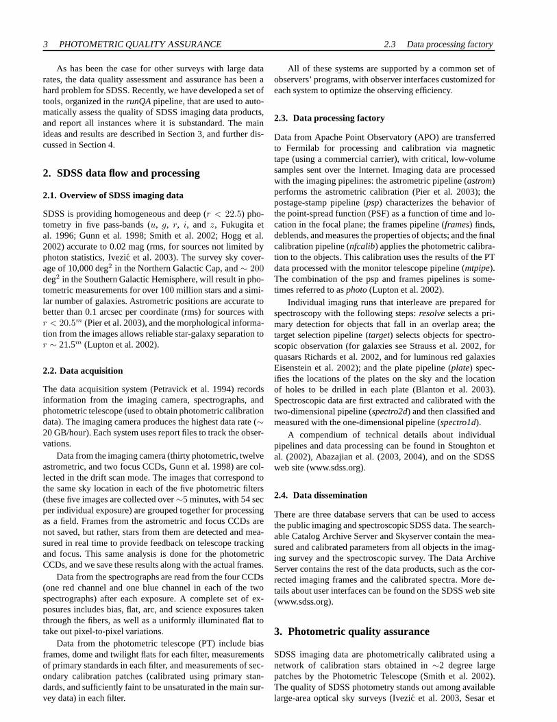
Typical behavior of the difference between aperture andPSF magnitudes as a function of time is shown in Fig. 1. Thelow-order statistics of medians, evaluated for each field andband, are used to recognize and flag all fields with substan-dard PSF photometry. Such “bad” fields usually also have

substandard star-galaxy separation and other measurementsthat critically depend on the accurate PSF model.

Fig. 1.An example of output from the SDSS photometric as-surance pipelinerunQA. The top five panels show the differ-ence between aperture and PSF magnitudes of stars brighterthanm ∼19, as a function of time (1 field = 36 sec), for fiveSDSS bands. The statistics for medians, evaluated for eachfield, are shown next to each panel (maxoff is the maximumdeviation from zero,sigma is the rms scatter). The verticallines in each panel mark bad fields. The bottom two panelsshow the image quality in ther band (FWHM and its timederivative) as a function of time.

3.2. Photometric zeropoint calibration

Data from each camera column, and for a given run, are inde-pendently calibrated. The calibration pipelinenfcalib reportsthe rms (dis)agreement, which is typically∼0.02 mag (thecore width, but the distribution is not necessarily Gaussian).There are usually several calibration patches for a given run,which are separated by of order an hour of scanning time.Thus, any changes in atmospheric transparency, or other con-ditions affecting the photometric sensitivity, may not be rec-ognized on shorter timescales. In addition, the stability ofphotometric calibration across the sky is sensitive to system-atic errors in the calibration star network. Hence, it is desir-able to have an independent estimate of the stability of pho-

3 PHOTOMETRIC QUALITY ASSURANCE 3.2 Photometric zeropointcalibration

tometric calibration across the sky, as well as of its behavioron short time scales (say, a few minutes).

A dense network of calibration stars (>∼100 stars perdeg2) across the sky, accurate to∼0.01 mag, in five SDSSbands, which could be used for an independent verificationof SDSS photometric calibration, does not yet exist. Fortu-nately, the distribution of stars in SDSS color-color diagramsseems fairly stable across the sky (<0.01 mag), and offers anindirect but powerful test of photometric zeropoint calibra-tion.

3.2.1. Definition of the stellar locus in the SDSSphotometric system

The majority of stars detected by SDSS are on the main se-quence (>98%, Finlator et al. 2001, Helmi et al. 2002). Theyform a well defined sequence, usually referred to as a “stellarlocus”, in color-color diagrams (Lenz et al, 1998, Fan 1999,Smolcic et al. 2004). The particular morphology displayed bythe stellar locus can be used to measure whether it is “in thesame place” for independently calibrated data.

The methodology used to derive the principal colorswhich track the position of the stellar locus is described inHelmi et al. (2002). Briefly, two principal axes,P1 andP2,are defined along the locus and perpendicular to the locus, forthe appropriately chosen parts of the locus, and in three color-color planes spanned by SDSS photometric system. The colorperpendicular to the locus,P2, is adjusted for a small depen-dence on apparent magnitude (<0.01 mag/mag), to obtainP ′

2,

which is then used for high-precision tracking of the locusposition.

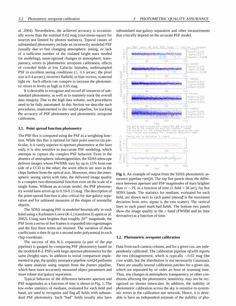
There are four principal colors used byrunQA: s (the bluepart of the locus in theg-r vs.u-g plane),w (blue part inr-ivs. g-r), x (red part inr-i vs.g-r), andy (red part ini-z vs.r-i). As an example, the definition and properties of thew

color are shown in Fig. 2. The principal colors are defined bythe following linear combinations of magnitudes in the fiveSDSS bands:

P ′2

= Au + B g + C r + D i + E z + F, (1)

and

P1 = A′ u + B′ g + C′ r + D′ i + E′ z + F ′, (2)

whereP ′2 = s, w, x, y are the principal colors perpendicu-

lar to the locus in a particular color-color diagram, andP1

(for eachP ′2) are the corresponding principal axes along the

locus. All the measurements are corrected for interstellarex-tinction using the Schlegel, Finkbeiner & Davis (1998) map(SFD). The adopted coefficientsA−F andA′−F ′ are listedin Tables 1 and 2. Stars used for estimating the position ofthe stellar locus must not have processing flags BRIGHT,SATUR, and BLENDED set (see Stoughton et al. 2002 formore details aboutphoto processing flags), and must also sat-isfy r < rmax andPmin

1< P1 < Pmax

1, with rmax, Pmin

1

andPmax

1 for each principal color listed in Table 3. The typ-ical width of the stellar locus (the rms distribution width foreach principal color) is listed in the last column in Table 3.

Even at high galactic latitudes (|b| > 30), the surface den-sity of stars satisfying these criteria is sufficient for evaluating

P2

P1

0 1 2-0.5

0

0.5

1

1.5

2

0 1 2-0.5

0

0.5

1

1.5

2

-0.4 -0.2 0 0.2 0.422

20

18

16

14

-0.4 -0.2 0 0.2 0.422

20

18

16

14

-0.2 0 0.222

20

18

16

14

-0.2 0 0.2

22

20

18

16

14

-0.1 0 0.10

5

10

15

20

-0.1 0 0.10

5

10

15

20

Fig. 2.An example of the definition of principal color axes incolor-color diagrams. The top left panel shows ther − i vs.g − r color-color diagram, with theP1 axis along the bluepart of the locus, andP2 perpendicular to the locus. The topright panel shows theP2 color as a function ofr magnitude.The w principal color, shown as a function ofr magnitudein the bottom left panel, is obtained by correctingP2 for itssmall dependence onr, and renormalizing it such thatw er-ror (random, not systematic) is comparable to the mean errorin the g, r, andi bands. The solid histogram in the bottomright panel shows the distribution ofw color for stars withr < 20. The dashed histogram shows the distribution ofw

color constructed with the mean of five measurements (i.e.five passes over a given region of sky). The distribution rmswidth decreases from 0.025 mag to 0.022 mag, which impliesthat single measurement error for thew color is∼0.01 mag,and that the intrinsic locus width in thew direction is∼0.02mag.

the mean of the principal colors with an error of∼ 0.01 magper SDSS field (area of 0.032 deg2). The mean error valuesper SDSS field for each principal color are listed in Table 3(σ). The principal colors are evaluated byrunQA in four fieldwide bins, yielding errors twice as small as those listed inTable 3.

The achievable accuracy in the determination of the po-sition of the stellar locus depends on the number of stars inthe sample and the intrinsic locus width. While the measuredlocus width is broadened by photometric errors, its value is,nevertheless, dominated by the intrinsic distribution of stellarproperties such as metallicity and surface gravity. This con-clusion is based on a comparison of the locus width for a setof single measurements, and using the mean values for fivemeasurements of the same stars (see the bottom right panelin Fig. 2). Although the latter data have much smaller mea-surement errors, the width of the distribution is not signifi-cantly decreased, showing that most of the observed width isintrinsic.

3.2 Photometric zeropoint calibration 3 PHOTOMETRIC QUALITY ASSURANCE

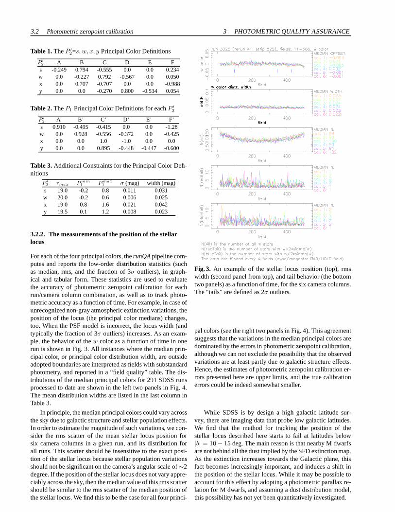
Table 1.TheP ′2=s, w, x, y Principal Color Definitions

P ′

2 A B C D E Fs -0.249 0.794 -0.555 0.0 0.0 0.234w 0.0 -0.227 0.792 -0.567 0.0 0.050x 0.0 0.707 -0.707 0.0 0.0 -0.988y 0.0 0.0 -0.270 0.800 -0.534 0.054

Table 2.TheP1 Principal Color Definitions for eachP ′2

P ′

2 A’ B’ C’ D’ E’ F’s 0.910 -0.495 -0.415 0.0 0.0 -1.28w 0.0 0.928 -0.556 -0.372 0.0 -0.425x 0.0 0.0 1.0 -1.0 0.0 0.0y 0.0 0.0 0.895 -0.448 -0.447 -0.600

Table 3.Additional Constraints for the Principal Color Defi-nitions

P ′

2 rmax P min

1 P max

1 σ (mag) width (mag)s 19.0 -0.2 0.8 0.011 0.031w 20.0 -0.2 0.6 0.006 0.025x 19.0 0.8 1.6 0.021 0.042y 19.5 0.1 1.2 0.008 0.023

3.2.2. The measurements of the position of the stellarlocus

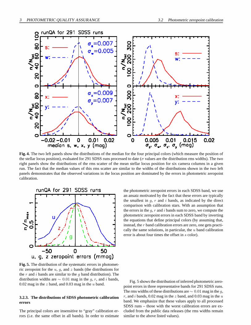
For each of the four principal colors, therunQA pipeline com-putes and reports the low-order distribution statistics (suchas median, rms, and the fraction of 3σ outliers), in graph-ical and tabular form. These statistics are used to evaluatethe accuracy of photometric zeropoint calibration for eachrun/camera column combination, as well as to track photo-metric accuracy as a function of time. For example, in case ofunrecognized non-gray atmospheric extinction variations, theposition of the locus (the principal color medians) changes,too. When the PSF model is incorrect, the locus width (andtypically the fraction of 3σ outliers) increases. As an exam-ple, the behavior of thew color as a function of time in onerun is shown in Fig. 3. All instances where the median prin-cipal color, or principal color distribution width, are outsideadopted boundaries are interpreted as fields with substandardphotometry, and reported in a “field quality” table. The dis-tributions of the median principal colors for 291 SDSS runsprocessed to date are shown in the left two panels in Fig. 4.The mean distribution widths are listed in the last column inTable 3.

In principle, the median principal colors could vary acrossthe sky due to galactic structure and stellar population effects.In order to estimate the magnitude of such variations, we con-sider the rms scatter of the mean stellar locus position forsix camera columns in a given run, and its distribution forall runs. This scatter should be insensitive to the exact posi-tion of the stellar locus because stellar population variationsshould not be significant on the camera’s angular scale of∼2degree. If the position of the stellar locus does not vary appre-ciably across the sky, then the median value of this rms scattershould be similar to the rms scatter of the median position ofthe stellar locus. We find this to be the case for all four princi-

Fig. 3. An example of the stellar locus position (top), rmswidth (second panel from top), and tail behavior (the bottomtwo panels) as a function of time, for the six camera columns.The “tails” are defined as 2σ outliers.

pal colors (see the right two panels in Fig. 4). This agreementsuggests that the variations in the median principal colorsaredominated by the errors in photometric zeropoint calibration,although we can not exclude the possibility that the observedvariations are at least partly due to galactic structure effects.Hence, the estimates of photometric zeropoint calibrationer-rors presented here are upper limits, and the true calibrationerrors could be indeed somewhat smaller.

While SDSS is by design a high galactic latitude sur-vey, there are imaging data that probe low galactic latitudes.We find that the method for tracking the position of thestellar locus described here starts to fail at latitudes below|b| = 10 − 15 deg. The main reason is that nearby M dwarfsare not behind all the dust implied by the SFD extinction map.As the extinction increases towards the Galactic plane, thisfact becomes increasingly important, and induces a shift inthe position of the stellar locus. While it may be possible toaccount for this effect by adopting a photometric parallax re-lation for M dwarfs, and assuming a dust distribution model,this possibility has not yet been quantitatively investigated.

3 PHOTOMETRIC QUALITY ASSURANCE 3.2 Photometric zeropointcalibration

Fig. 4. The two left panels show the distributions of the median for the four principal colors (which measure the position ofthe stellar locus position), evaluated for 291 SDSS runs processed to date (σ values are the distribution rms widths). The tworight panels show the distributions of the rms scatter of themean stellar locus position for six camera columns in a givenrun. The fact that the median values of this rms scatter are similar to the widths of the distributions shown in the two leftpanels demonstrates that the observed variations in the locus position are dominated by the errors in photometric zeropointcalibration.

Fig. 5. The distribution of the systematic errors in photomet-ric zeropoint for theu, g, andz bands (the distributions forther andi bands are similar to theg band distribution). Thedistribution widths are∼ 0.01 mag in theg, r, andi bands,0.02 mag in thez band, and 0.03 mag in theu band.

3.2.3. The distributions of SDSS photometric calibrationerrors

The principal colors are insensitive to “gray” calibrationer-rors (i.e. the same offset in all bands). In order to estimate

the photometric zeropoint errors in each SDSS band, we usean ansatz motivated by the fact that these errors are typicallythe smallest ing, r and i bands, as indicated by the directcomparison with calibration stars. With an assumption thatthe errors in theg, r andi bands sum to zero, we compute thephotometric zeropoint errors in each SDSS band by invertingthe equations that define principal colors (by assuming that,instead, ther band calibration errors are zero, one gets practi-cally the same solutions, in particular, theu band calibrationerror is about four times the offset ins color).

Fig. 5 shows the distribution of inferred photometric zero-point errors in three representative bands for 291 SDSS runs.The rms widths of these distributions are∼ 0.01 mag in theg,r, andi bands, 0.02 mag in thez band, and 0.03 mag in theuband. We emphasize that these values apply to all processedSDSS runs – those with the worst calibration errors are ex-cluded from the public data releases (the rms widths remainsimilar to the above listed values).

References References

4. Astrometric calibration, star/galaxyclassification, flatfield vectors, etc.

Additional tasks performed by therunQA pipeline include ananalysis of the accuracy of relative astrometric calibration1

(transformations between positions measurements in the fiveSDSS bands), and analysis of median principal colors as afunction of chip position to track the flatfield vector accu-racy. For example, the latter was used to discover that (and toderive appropriate corrections for) the shapes of the flatfieldvectors vary with time (on a scale of several dark runs), up to20% in someu band chips.

A similar pipeline,matchQA, compares two observationsof the same area on the sky. It quantifies the repeatability ofSDSS measurements, and provides a handle on the sensitiv-ity of measured parameters to varying observing conditions(such as seeing and sky brightness). For example, its outputsdemonstrate that the star/galaxy classification is typically re-peatable at the> 99% level at the bright end (r < 20), and atthe > 95% level for sources as faint asr = 21.5. Further-more, a direct comparison of photometry for multiply ob-served sources demonstrates that not only are the (random)photometric errors small (∼0.02 mag), but they themselvesare accurately determined by the photometric pipeline (seeFig. 2 in Ivezic et al. 2003). Furthermore, the tails of the pho-tometric error distribution are well controlled and practicallyGaussian (see Fig. 3 in Ivezic et al. 2003).

5. Discussion

SDSS is an excellent example of a modern astronomical sur-vey – it produces unprecedentedly accurate data (∼10 timesmore accurate than previous large-scale optical sky surveys,such as POSS, see Sesar et al. 2004), with a large peak datarate (20 GB/hr), and is built upon sophisticated data acqui-sition, processing and distribution systems (∼million lines ofcode), that were developed by a large number of collaborators(∼50). The success of SDSS provides encouragement thateven more ambitious surveys, such as LSST (Tyson 2002),which is expected to produce and immediately process 20 TBof data per observing night, may also be successful endeav-ors.

SDSS also demonstrated, as described in this contribu-tion, that a quantitative and efficient data quality assessmentcan be designed and implemented even when the “true an-swers” are not known for individual measurements. However,the method described here is not universal – it applies only tothe wavelength range accessed by SDSS (0.3–1µm), and toGalactic latitudes more than∼15 degree from the galacticplane. Despite these shortcomings, it is a robust automatedmethod that tracks the accuracy of SDSS photometric zero-point calibration to better than 0.01 mag. We estimated, usingthis method, that typical photometric zeropoint calibration er-rors for SDSS imaging data are not larger than∼ 0.01 mag

1 The accuracy of absolute and relative astrometric calibration isdiscussed in detail by Pier et al. (2003).

in theg, r, andi bands, 0.02 mag in thez band, and 0.03 magin theu band.

Acknowledgements. Funding for the creation and distribution of theSDSS Archive has been provided by the Alfred P. Sloan Foundation,the Participating Institutions, the National Aeronauticsand SpaceAdministration, the National Science Foundation, the U.S.Depart-ment of Energy, the Japanese Monbukagakusho, and the Max PlanckSociety. The SDSS Web site is http://www.sdss.org/.

The SDSS is managed by the Astrophysical Research Consor-tium (ARC) for the Participating Institutions. The Participating In-stitutions are The University of Chicago, Fermilab, the Institute forAdvanced Study, the Japan Participation Group, The Johns Hop-kins University, Los Alamos National Laboratory, the Max-Planck-Institute for Astronomy (MPIA), the Max-Planck-Institutefor As-trophysics (MPA), New Mexico State University, Universityof Pitts-burgh, Princeton University, the United States Naval Observatory,and the University of Washington.

ZI thanks Princeton University for generous financial support.

References

Abazajian, K., Adelman, J.K., Agueros, M., et al. 2003, AJ, 126,2081

Abazajian, K., Adelman, J.K., Agueros, M., et al. 2004, AJ, 128,502

Blanton, M.R., Lupton, R.H., Maley, F.M., et al. 2003, AJ, 125, 2276Eisenstein, D.J., Annis, J., Gunn, J.E., et al. 2001, AJ, 122, 2267Fan, X. 1999, AJ , 117, 2528Finlator, K., Ivezic,Z., Fan, X., et al. 2000, AJ, 120, 2615 (F00)Fukugita, M., Ichikawa, T., Gunn, J.E., Doi, M., Shimasaku,K., &

Schneider, D.P. 1996, AJ, 111, 1748Gunn, J.E., Carr, M., Rockosi, C., et al. 1998, AJ, 116, 3040Helmi, A. 2002, Ap&SS, 281, 351Hogg, D.W., Finkbeiner, D.P., Schlegel, D.J. & Gunn, J.E. 2002, AJ,

122, 2129Ivezic, Z., Lupton, R.H., Anderson, S., et al. 2003a, Proceedings of

the WorkshopVariability with Wide Field Imagers, Mem. Soc.Ast. It., 74, 978 (also astro-ph/0301400)

Lenz, D.D., Newberg, J., Rosner, R., Richards, G.T., Stoughton, C.1998, ApJS, 119, 121

Lupton, R.H., Ivezic,Z., Gunn, J.E., Knapp, G.R., Strauss, M.A. &Yasuda, N. 2002, in “Survey and Other Telescope Technologiesand Discoveries”, Tyson, J.A. & Wolff, S., eds. Proceedingsofthe SPIE, 4836, 350

Petravick, D., Berman, E., MacKinnon, B., et al. 1994, Proc.SPIE,2198, 935

Pier, J.R., Munn, J.A., Hindsley, R.B., Hennesy, G.S., Kent, S.M.,Lupton, R.H. & Ivezic,Z. 2003, AJ, 125, 1559

Richards, G.T., Fan, X., Newberg, H.J., et al. 2002, AJ, 123,2945Schlegel, D., Finkbeiner,D.P. & Davis, M. 1998, ApJ 500, 525Sesar, B., Svilkovic, D., Ivezic,Z., et al. 2004, submitted to AJ, also

astro-ph/0403319Smolcic, V., Ivezic,Z., Knapp, G.R., et al. 2004, submitted to ApJ,

also astro-ph/0403218Smith, J.A., Tucker, D.L., Kent, S.M., et al. 2002, AJ, 123, 2121Stoughton, C., Lupton, R.H., Bernardi, M., et al. 2002, AJ, 123, 485Strauss, M.A., Weinberg. D.H., Lupton, R.H., et al. 2002, AJ, 124,

1810Tyson, J.A. 2002, in “Survey and Other Telescope Technologies and

Discoveries”, Tyson, J.A. & Wolff, S., eds. Proceedings of theSPIE, 4836, 10

York, D.G., Adelman, J., Anderson, S., et al. 2000, AJ, 120, 1579