Seasonal variability of the Canary Current: A numerical study

Evan Mason,1,2 Francois Colas,3 Jeroen Molemaker,3 Alexander F. Shchepetkin,3

Charles Troupin,4 James C. McWilliams,3 and Pablo Sangrà2

Received 17 September 2010; revised 1 March 2011; accepted 14 March 2011; published 1 June 2011.

[1] A high‐resolution numerical model study of the Canary Basin in the northeastsubtropical Atlantic Ocean is presented. A long‐term climatological solution from theRegional Oceanic Modeling System (ROMS) reveals mesoscale variability associated withthe Azores and Canary Current systems, the northwest African coastal upwelling, and theCanary Island archipelago. The primary result concerns the Canary Current (CanC)which, in the solution, transports ∼3 Sv southward in line with observations. The simulatedCanC has a well‐defined path with pronounced seasonal variability. This variability isshown to be mediated by the westward passage of two large annually excited counterrotatinganomalous structures that originate at the African coast. The anomalies have a sea surfaceexpression, permitting their validation using altimetry and travel at the phase speedof baroclinic planetary (Rossby) waves. The role of nearshore wind stress curl variabilityas a generating mechanism for the anomalies is confirmed through a sensitivity experimentforced by low‐resolution winds. The resulting circulation is weak in comparison to thebase run, but the propagating anomalies are still discernible, so we cannot discount afurther role in their generation being played by annual reversals of the large‐scaleboundary flow that are known to occur along the African margin. An additional sensitivityexperiment, where the Azores Current is removed by closing the Strait of Gibraltarpresents the same anomalies and CanC behavior as the base run, suggesting that the CanCis rather insensitive to upstream variability from the Azores Current.

Citation: Mason, E., F. Colas, J. Molemaker, A. F. Shchepetkin, C. Troupin, J. C. McWilliams, and P. Sangrà (2011), Seasonalvariability of the Canary Current: A numerical study, J. Geophys. Res., 116, C06001, doi:10.1029/2010JC006665.

1. Introduction

[2] Motivated by interest in the seasonal variability of thedynamics and processes in the eastern boundary of theNorth Atlantic Subtropical Gyre (NASG), a climatology‐forced quasi‐equilibrium numerical model configurationhas been developed using the Regional Oceanic ModelingSystem (ROMS) [Shchepetkin and McWilliams, 2005,2009]. The model is configured with a domain (outlined inred in Figure 1) spanning the Canary Basin at a mesoscaleresolution of 7.5 km, and is integrated for 50 years. The longsolution permits a robust evaluation to be made of the sea-sonal cycle and variability in this region. Our focus in thispaper is on the seasonality of the Canary Current (CanC)north of the Canary Island archipelago. The CanC has beenfrequently observed but has not yet been the subject of ahigh‐resolution climatological numerical study. An impor-

tant open question concerns the path of the CanC. While abroad seasonal cycle has been identified, questions remainabout variability in the path of the current, and its interactionwith the coastal upwelling region. We comment also on theimportance of the Azores Current (AzC) as a source for theCanC in the light of results from an additional simulationwhere the AzC is removed by closing the Strait of Gibraltar.[3] The paper is organized as follows. Sections 2 and 3

briefly reviews our current knowledge of the physical ocean-ography of the study region. In section 4 we describe theROMSmodel configuration and the methodologies developedin realizing the present solution. Section 5 presents a validationof the model solution through comparison with observa-tions. This solution is presently in use as a parent solution toforce the boundaries of several higher‐resolution nestedregional configurations within the Canary Basin; the vali-dation serves to underpin these future studies as well asthe results presented in this paper. Section 6 addresses thecentral question concerning the CanC analysis identifiedabove. Results from two sensitivity experiments are pre-sented in section 7. Finally, we make some brief conclusionsin section 8.

2. The Canary Current System

[4] The Canary Current System (CCS) lies within theCanary Basin, whose limits are loosely defined between 10°

1Departament d’Oceanografía Física, Institut de Ciències del Mar,CMIMA‐CSIC, Barcelona, Spain.

2Departamento de Física, Universidad de Las Palmas de Gran Canaria,Las Palmas de Gran Canaria, Spain.

3Institute of Geophysics and Planetary Physics, University ofCalifornia, Los Angeles, California, USA.

4GeoHydrodynamics and Environment Research, Universitè de Liège,Liège, Belgium.

Copyright 2011 by the American Geophysical Union.0148‐0227/11/2010JC006665

JOURNAL OF GEOPHYSICAL RESEARCH, VOL. 116, C06001, doi:10.1029/2010JC006665, 2011

C06001 1 of 20

Figure 1. Topology and schematic surface circulation of the Canary Basin in the subtropical northeastAtlantic. The boundary of the L0 model domain is outlined in red. Red circles show the positions ofmoorings used in the text (see section 5.1 and Table 1). AzC, Azores Current; CanC, Canary Current;CanUC, Canary Upwelling Current; EBC, Eastern Boundary Current (see section 3); MC, MauritaniaCurrent; NEC, North Equatorial Current; NECC, North Equatorial Countercurrent; PC, Portugal Current;MAR, Mid‐Atlantic Ridge; LP, Lanzarote Passage. Dark blue dashed line marks the position of the CapeVerde Frontal Zone. Contours in black mark isobaths at 200, 1000, 3000, 4000, and 5000 m.

MASON ET AL.: CANARY CURRENT SEASONAL VARIABILITY C06001C06001

2 of 20

and 40°N in the northeast Atlantic Ocean [Spall, 1990;Arhan et al., 1994; Arístegui et al., 2006]. Figure 1 presentsa schematic diagram of the large‐scale current structure, anda key to the main geographic and bathymetric features. Atthe Gulf of Cadiz in the north, the Strait of Gibraltar facil-itates exchange between the North Atlantic and the Medi-terranean Sea. Several island groupings populate the region,including the Canary Island archipelago near to Cape Juby(∼28.5°N), and Madeira which lies in deep waters ∼800 kmoffshore of Cape Sim (∼31.4°N).[5] The CCS, composed of the Canary Current and the

Canary Upwelling Current (CanUC), is one of the four mainupwelling regions of the world ocean and therefore supportsan important fishery [Arístegui et al., 2009]. The northeast-erly alongshore Trade wind regime drives a near‐permanentupwelling of relatively cool North Atlantic Central Water(NACW) into the euphotic zone [Lathuiliére et al., 2008].The winds, which reach their peak in summer, are modu-lated by the seasonal migration of the Azores high‐pressurecell [Wooster et al., 1976; Mittelstaedt, 1991]. Connectivityin the CCS between the open ocean and the coastalupwelling is uniquely enhanced by the Canary Islands,whose presence just off the northwest African coast perturbsboth the atmospheric and oceanic flow [Arístegui et al.,1994; Barton et al., 1998; Brochier et al., 2011].[6] The CanC constitutes the eastern boundary current of

the NASG and, as such, has generally been viewed as abroad weak flow spanning the transition zone between theopen ocean and the coastal region. The current transports∼3 Sv southwestward, parallel to the African coast, andoccupies much of the central water layer (∼0–700 m)[Stramma, 1984; Stramma and Siedler, 1988;Navarro‐Pérezand Barton, 2001; Fraile‐Nuez and Hernández‐Guerra,2006; Machín et al., 2006]. Originating in the regionbetween Madeira and the African coast, the CanC is seen asa natural extension of the zonal AzC as it approaches theeastern boundary [Stramma, 1984]. Stramma and Siedler[1988] showed that the current demonstrates seasonaldependence, it tends to be found far offshore near toMadeira in winter while in summer it strengthens and occu-pies a more central position between Madeira and theAfrican coast. After passing the Canary Islands, the CanCfeeds into the North Equatorial Current (NEC) north ofthe Cape Verde Frontal Zone (CVFZ) [Barton, 1987; Zenket al., 1991; Hernández‐Guerra et al., 2005].[7] Recent studies suggest that the CanC north of the

Canary Islands has a better defined pathway than has pre-viously been recognized [Zhou et al., 2000; Pelegrí et al.,2005a; Machín et al., 2006]. In a series of seasonal merid-ional geostrophic velocity sections at 32°N in 1997 and1998, Machín et al. [2006] observed the CanC to be a rel-atively strong (>0.08 m s−1) ∼800 m deep current closelycentered around 14°W in summer. Pelegrí et al. [2005a]stress close interconnectivity between the open oceanCanC and the coastal upwelling region: The CanUC, thenearshore equatorward surface jet associated with theupwelling [Pelegrí et al., 2006], is present for most ofthe year over the northwest African shelf. In late autumn,the portion of the CanUC near to the Canary archipelagoreverses and, in the vicinity of Cape Ghir, detaches from thecoast and moves offshore. Pelegrí et al. [2005a] speculatethat this leads to the formation of a large wintertime cyclonic

circulation cell that extends around the archipelago.Cyclonic flow around the Canary Islands would imply alarge‐scale poleward flow at the eastern boundary (i.e.,within the ∼1300 m deep Lanzarote Passage (LP) thatseparates the easternmost of the Canary Islands from theAfrican continent; Figure 1), yet the mean flow here isequatorward. However, there is observational evidence forperiodic (typically autumn) poleward flows in the upperlevels of the LP [Hernández‐Guerra et al., 2002; Knollet al., 2002; Machín and Pelegrí, 2009; Fraile‐Nuez et al.,2010; Machín et al., 2010] (lending support to Pelegríet al.’s [2005a] suggestion of a cyclonic loop). As weshall show in sections 6 and 7 these reversals at the easternboundary may play an important role in the variability of theCanC, and so a brief description of this boundary flow iswarranted.

3. Variability in the Lanzarote Passage

[8] The flow through the LP is generally considered to bea part of the CanC. However, owing to its location betweenthe Canary Islands and the African boundary, its dynamicsmay be expected to differ from the open ocean CanC. It isalso important to note that, given its dimensions, it can beconsidered a large‐scale flow, and should not be confusedwith the CanUC that is found along the African slope andshelf. The flow spans over half the breadth of the LP(∼90 km), and contains three water masses: a central waterlayer composed of NACW (∼0–600 m), and an intermediatelayer with both Antarctic Intermediate Water (AAIW;∼600–1100 m) and Mediterranean Water (MW; ∼900 m tothe bottom). The LP is a conduit for the northward pene-tration of AAIW along the African boundary, which hasbeen observed beyond the passage to as far north as 33°N inautumn [Machín and Pelegrí, 2009].[9] Some authors [e.g., Fraile‐Nuez et al., 2010] have

referred to the LP flow as the Eastern Boundary Current(EBC; use of capitals distinguishes it from the generic easternboundary current) and we herein adopt this term to differ-entiate it from the CanC and the CanUC. In addition, whereappropriate we use the notation EBCNACW and EBCAAIW torefer to the passage flow within the respective water layers.[10] The mean EBCNACW and EBCAAIW flows are equa-

torward and poleward, respectively. This is confirmed by a9 year time series of current meter data from a mooringwithin the LP that shows a close inverse relationshipbetween the transports in the two layers, suggesting thatthey may be strongly coupled [Fraile‐Nuez et al., 2010].The current meters also clearly show brief reversals in themean flow in both layers that take place around November.Machín and Pelegrí [2009] and Machín et al. [2010] focuson the AAIW layer and propose that remote forcing relatedto potential vorticity conservation in the eastern tropicalAtlantic drives the EBCAAIW reversals. The poleward extentof the EBCNACW reversal is not reported, but Machín et al.[2006] observed a 0.5 Sv poleward flow over the NACWlayer near the coast at 32°N in January 1997, indicating thatit may round Cape Ghir.[11] The CCS is therefore a complex region, composed of

a number of distinct currents and countercurrents, that aredriven by both local and remote forcing. Yet despite theefforts outlined above, uncertainty remains about the posi-

MASON ET AL.: CANARY CURRENT SEASONAL VARIABILITY C06001C06001

3 of 20

tion of the CanC and its seasonal dependence, and themechanism(s) which govern its variability.

4. The ROMS Model

[12] Following the examples of the ROMS U.S. WestCoast and Peru upwelling quasi‐equilibrium model simula-tions of Marchesiello et al. [2003] and Penven et al. [2005],respectively, we base our model on a monthly climatologicalforcing cycle. This approach, where synoptic and interan-nual forcing is excluded, reveals the intrinsic variability thatoccurs at smaller scales within a regional system, whilecapturing basin‐scale structures that are determined by low‐frequency atmospheric forcing at the surface and alsotransmitted through the open model boundaries.[13] ROMS is a free surface primitive equation curvilinear

coordinate ocean model, where the barotropic and baroclinicmomentum equations are resolved separately. ROMS uses aterrain‐following (or sigma) vertical coordinate system. Weuse the UCLA version of the ROMS code which features amodification to the commonly used Flather‐type [Flather,1976] barotropic open boundary condition that improvesthe solution behavior near the open boundaries (for themodifications see Mason et al. [2010]), and a new sigmacoordinate transformation that helps mitigate pressure gra-dient errors [Shchepetkin and McWilliams, 2009]. Subgrid‐scale vertical mixing processes are parameterized using thenonlocal K profile planetary (KPP) boundary layer formu-lation of Large et al. [1994]. ROMS features weakly dif-fusive advection schemes making it a preferred choice forhigh‐resolution simulations where small‐scale processesbecome important.

4.1. Model Domain and Configuration

[14] The ocean model experiments were conducted usinga 442 × 646 × 32 grid covering the northeast Atlantic (∼1°–45°W, ∼6°–51°N; 3300 × 4830 km2). All four modelboundaries are open. Increased near‐surface resolution isachieved using a surface stretching factor �s = 6, while at

the bottom �b = 0. The sigma coordinate system is a newformulation that ensures good resolution of the thermo-cline independently of the total depth, h [Shchepetkin andMcWilliams, 2009].[15] A prime requirement for a valid solution are correct

levels of mesoscale variability for the AzC [Smith et al.,2000]. We therefore (1) leave the Strait of Gibraltar openand parameterize the flux of MW into the domain as detailedin section 4.3 (see also section 7.1) and (2) use a smallsponge nmax = 25 m2 s−1 along the open boundaries in ordernot to suppress variability generated at the open westernboundary where the AzC enters the domain. (Early experi-ments with a 15 km grid using sponge values of�25 m2 s−1

were unsatisfactory because the high sea surface heightvariance west of the Mid‐Atlantic Ridge seen in Figure 6c,which is associated with the North Atlantic Current, waslargely absent.)[16] Raw bathymetry data are taken from the ETOPO2

2′ topography of Smith and Sandwell [1997] and coarsened(by weighted averaging with a cosine‐shaped windowfunction) to prevent aliasing errors before interpolation tothe model grid. To facilitate exchange at the open Strait ofGibraltar boundary the topography there is manually mod-ified to ensure a minimum sill depth of 300 m. Finallyseveral passes of a smoothing filter reduce the r factor tobelow 0.2 (r = Dh/2h) [Haidvogel and Beckmann, 1999].Points where the model grid depth is shallower than 15 mare reset to 15 m.[17] In the interior of the computational domain we use no

explicit horizontal “eddy” viscosity or tracer diffusivity, themodel instead relies solely on numerical dissipation fromthe third‐order upstream‐biased advection schemes. Weapply a linear (quadratic) bottom drag with coefficient rD =3.0 × 10 m s−4.

4.2. Forcing and Initial File Preparation

[18] Monthly climatological surface forcing files arecreated using the tools described by Penven et al. [2008],

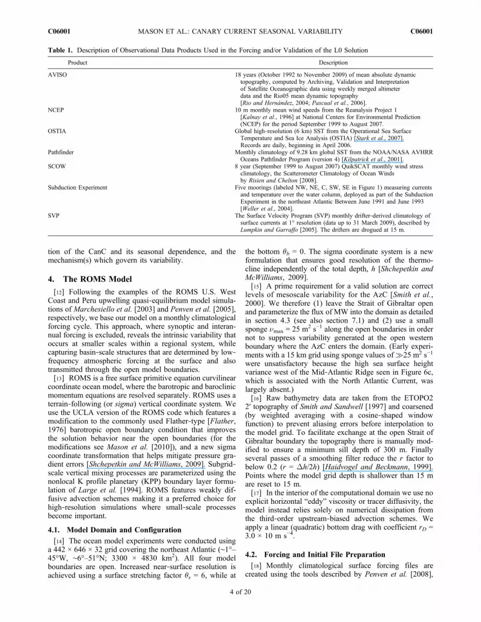
Table 1. Description of Observational Data Products Used in the Forcing and/or Validation of the L0 Solution

Product Description

AVISO 18 years (October 1992 to November 2009) of mean absolute dynamictopography, computed by Archiving, Validation and Interpretationof Satellite Oceanographic data using weekly merged altimeterdata and the Rio05 mean dynamic topography[Rio and Hernández, 2004; Pascual et al., 2006].

NCEP 10 m monthly mean wind speeds from the Reanalysis Project 1[Kalnay et al., 1996] at National Centers for Environmental Prediction(NCEP) for the period September 1999 to August 2007.

OSTIA Global high‐resolution (6 km) SST from the Operational Sea SurfaceTemperature and Sea Ice Analysis (OSTIA) [Stark et al., 2007].Records are daily, beginning in April 2006.

Pathfinder Monthly climatology of 9.28 km global SST from the NOAA/NASA AVHRROceans Pathfinder Program (version 4) [Kilpatrick et al., 2001].

SCOW 8 year (September 1999 to August 2007) QuikSCAT monthly wind stressclimatology, the Scatterometer Climatology of Ocean Windsby Risien and Chelton [2008].

Subduction Experiment Five moorings (labeled NW, NE, C, SW, SE in Figure 1) measuring currentsand temperature over the water column, deployed as part of the SubductionExperiment in the northeast Atlantic Between June 1991 and June 1993[Weller et al., 2004].

SVP The Surface Velocity Program (SVP) monthly drifter‐derived climatology ofsurface currents at 1° resolution (data up to 31 March 2009), described byLumpkin and Garraffo [2005]. The drifters are drogued at 15 m.

MASON ET AL.: CANARY CURRENT SEASONAL VARIABILITY C06001C06001

4 of 20

which include heat and freshwater (E‐P) fluxes providedby the 1° Comprehensive Ocean‐Atmosphere Data Set(COADS) climatology [Worley et al., 2005]. We use a 0.25°surface wind stress product, the 8 year Scatterometer Cli-matology of Ocean Winds (SCOW, based on QuikSCAT)climatology by Risien and Chelton [2008] (see Table 1).[19] Figure 2 shows fields of the mean SCOW winter and

summer wind stress curl along the northwest African coast.There is a general dominance of strong nearshore cycloniccurl, and weak anticyclonic curl offshore [Bakun andNelson, 1991; Mittelstaedt, 1991]. The alongshore cyclo-nic curl has been discussed by Milliff et al. [1996], and is aneffect of the land–sea temperature contrast: warmer tem-peratures over northwest Africa set up a persistent conti-nental low‐pressure region, which diverts the localanticyclonic atmospheric winds and sets up strong quasi‐permanent wind stress curl patterns off the African coast.Intense cyclonic curl in summer off Capes Ghir and Simmay also be related to the influence of the Atlas mountainchain (Figure 2) on the summer Trade winds [Hagen et al.,1996]. Nearshore wind drop off close to the coastalboundary may also be a source of cyclonic curl, but this ismost likely absent from the fields in Figure 2 as it is notadequately resolved by the QuikSCAT scatterometer [Capetet al., 2004]. Figures 2a and 2b illustrate the large differ-ences in wind stress curl that occur along the coast over theseasonal cycle.[20] Thermal forcing at the sea surface is linearized around

climatological sea surface temperature (SST; 9.28 kmPathfinder, Table 1) [Barnier et al., 1998]. There is a mildrestoration (90 days) of the sea surface salinity (SSS) toclimatological values [Barnier et al., 1995]. As northwest

Africa riverine discharges are small [Warrick and Fong,2004] rivers are not included in the configuration.[21] Lateral boundary forcing and initialization files

are prepared using temperature and salinity data fromthe monthly northeast Atlantic climatology (hereinafterNEAClim) of Troupin et al. [2010]. This climatology has agrid resolution of 0.1° and is based on a data set compiledfrom multiple sources, from which duplicates and outliersare removed. The interpolation technique consists of solvinga variational principle that takes into account the misfitbetween the data and the reconstructed field, and the regu-larity (or smoothness) of the field. The interpolation isperformed using a finite element method which allows for abetter resolution of the coastal area. Hence, use of NEAClim(as opposed to lower‐resolution climatologies) may beadvantageous in nearshore regions, and also to better resolvedynamically important features such as the frontal systemassociated with the AzC at the western model boundary.[22] Geostrophic baroclinic velocity components (u) are

calculated through the thermal wind relation, where thehorizontal velocity at the sea surface (uz) is the referencevelocity. uz is obtained through the geostrophic relation,where z is first interpolated to the model grid from amonthly sea surface height (SSH) climatology compiledfrom 15 years of Archiving, Validation, and Interpretationof Satellite Oceanographic data (AVISO) absolute sea leveldata (see Table 1). An Ekman velocity correction is thenapplied to u over a variable depth Ekman layer [Mason,2009]. Barotropic velocities (u) are calculated by integrat-ing over h. Finally, a barotropic flux correction is calculatedand applied to the velocities in order to enforce volumeconservation [Penven et al., 2006; Mason et al., 2010]. The

Figure 2. Normalized wind stress curl from the QuikSCAT‐derived SCOW wind stress climatology ofRisien and Chelton [2008] over the northeast Atlantic in (a) winter and (b) summer. Vectors show thewind speed and direction. The zero wind stress curl is contoured in black. Contours over land (1000 and2000 m) show the Atlas Mountains.

MASON ET AL.: CANARY CURRENT SEASONAL VARIABILITY C06001C06001

5 of 20

eastern boundary (Strait of Gibraltar) is treated differentlyas detailed in section 4.3. All of the variables located atthe boundaries are saved to a monthly (2‐D) boundaryforcing file.[23] The model is initialized using January values from

NEAClim and AVISO, processed similarly to the boundaryforcing file so that geostrophic velocities are available aswell as tracers.

4.3. Parameterization at the Strait of Gibraltar

[24] The 2 grid cell open boundary at the 300 m deepStrait of Gibraltar is a critical location that controls theexchange between surface outflow of NACW from theAtlantic and, at depth, the Atlantic inflow of dense MW. Aparameterization of the prognostic variables in the lateralboundary forcing file enforces the required fluxes which are,approximately, 0.7 Sv (MW, 150–300 m) and 0.8 Sv(NACW, 0–150 m) [Tsimplis and Bryden, 2000; Bascheket al., 2001; Harzallah, 2009]. Following the methodologylaid out by Peliz et al. [2007] we use monthly Strait ofGibraltar salinity and temperature profiles from NEAClimfor the top layer while, for the bottom layer, temperature andsalinity for all months are set as follows: 150+ m (14.23°C,38.35); 170+ m (13.0°C, 38.5); 200+ m (12.8°C, 38.51);250+ m (12.6°C, 38.65). A simple algebraic curve gives a uvelocity profile appropriate to the required Strait of Gibraltarvolume transport. We do not introduce seasonality into thetransport. (During development of the configuration wewere not aware of any studies of transport variability in theStrait of Gibraltar, however information provided by Soto‐Navarro et al. [2010] may be useful in future configura-tions.) The cross‐strait velocity, n, is set to 0 m s−1.

5. Model Validation

[25] In this section a validation of the model solution(hereinafter L0) is performed by comparing instantaneous,mean and eddy variables with observations. This is a com-mon approach to the evaluation of model skill in long‐termclimatological solutions [Marchesiello et al., 2003; Penvenet al., 2005; Shchepetkin and McWilliams, 2009]. The50 year L0 solution reaches equilibrium after ∼4 years[Mason, 2009]. Averages from the solution are saved every3 days. Annual and seasonal means are computed using thelast 40 years (i.e., years 11–50). The seasons are defined assuccessive 3 month periods starting from winter defined asmonths 1–3. The observational data sources and productsused throughout the text are summarized in Table 1.

5.1. SST, Surface Velocity, and Thermocline Evolution

[26] The region of the Canary Current System experiencesan important seasonal cycle in SST [Barton et al., 1998;Pelegrí et al., 2005a]. Figure 3 compares summer fields ofL0 and OSTIA SST (Table 1) in 2 successive years. Alsoplotted are geostrophic velocity vectors computed fromROMS SSH (h) and merged satellite altimeter data fromAVISO (Table 1). Figures 3a–3d are presented primarily todemonstrate the realistic and intrinsic variability achievedwithin the L0 solution despite our choice of a climatologicalforcing regime [Marchesiello et al., 2003]. The generaldistribution of SST in the model agrees rather well with theOSTIA SST. Elevated SST is seen in the Gulf of Cadiz,

along the axis of the AzC at ∼34°N, and in the lee of theCanary Islands. Cooler SSTs correspond to upwelling cen-ters along the coasts; the model SST shows a cold biaswhich is possibly a consequence of uncertainty in thenearshore model wind structure [Capet et al., 2004; Penvenet al., 2005]. Upwelling‐related filament activity is evidentat the major capes, particularly at Cape Ghir [Pelegrí et al.,2005b]. The velocity vectors reveal an abundance of meso-scale meanders and eddies, many of which are clearlyassociated with the AzC to the north, and with the CanaryIslands to the south. Yet these features are ubiquitous out-side of these dynamical centers as well. In the region of theCanC a number of coherent structures and recirculations ofboth signs are visible in the model and observations thatchannel and modify the mean equatorward flow. The spatialscales of the modeled and observed structures are quitesimilar.[27] Long‐term means of SST can be a valid diagnostic of

model skill. However, because observed SST is used as acorrection for the ROMS surface heat fluxes [Penven et al.,2005], such a comparison (i.e., long‐term model SST withobserved SST) may be misleading. Instead, in Figure 4 wecompare monthly means of thermocline temperature fromthe five Subduction Experiment moorings (SubExp; seeTable 1 and labels NW, NE, C, SW, SE on Figure 1) withcolocated L0 temperature profiles. The temperature recordsshow a seasonal evolution that penetrates down to about∼100 m in both the moorings and L0. A shallow seasonalthermocline grows in spring and summer, followed by itserosion in autumn and winter. A time delay between thewarming of the upper thermocline, which continues to warmafter SST has begun to cool, and the surface layers is evidentat the central and northern locations. Mixed layer depths(MLD) are also plotted in Figure 4, estimated following thecriterion of de Boyer Montégut et al. [2004]. MLD spikes inSubExp at NW and NE in April are likely to be caused bythe passing of eddies; eddy variability was dominant in themoored velocity records at NE. Weller et al. [2004] notedthat, contrary to expectation, winter MLD does not shoalsignificantly to the south in the SubExp records; thisbehavior is seen also in L0. Deepening of the mixed layer atC and NW is a result of trade‐wind‐driven Ekman pumping.At SE, the winter MLD is associated with upwelling andshoaling toward the African continent. Mixed layer tem-perature, however, shows a clearer spatial trend, with thetemperature at NW and NE the coldest in winter, and that atSW the warmest for much of the year. Figure 4 demon-strates that the model has a good response to local forcing atthe surface, and that spatial and temporal variability of themixed layer depth is well simulated.

5.2. Mediterranean Water Spreading

[28] A major feature of the thermohaline field of the NorthAtlantic is the Mediterranean salt tongue [Richardson et al.,1989, 2000]. Figure 5a shows the model annual meansalinity at 1000 m. For comparison, the observed annualmean field from NEAClim is presented in Figure 5b. TheNEAClim data show the salty MW signal extending west-ward away from the Iberian Peninsula, with the largestvalues for both salinity (and temperature [see Mason, 2009])found just offshore of Cape Roca at 38.8°N (Figure 1). Themodel salinity anomaly is similar in its zonal distribution at

MASON ET AL.: CANARY CURRENT SEASONAL VARIABILITY C06001C06001

6 of 20

this latitude, although its latitudinal range is rather smallerthan the observed anomaly, particularly to the north.

5.3. Zonal Surface Currents

[29] The mean annual distributions of zonal surface cur-rents from L0 (Figure 6a) and from the SVP (Figure 6b)drifter climatology (Table 1) are shown in Figure 6. TheSVP velocity field has a generally broad pattern which maybe attributed to sampling bias and to the coarse 1° resolutionof the data. The zonal components of the NASG stand out.The AzC is visible at ∼34°N extending eastward toward theGulf of Cadiz, its intensity varies but generally decreasesalong its length. In the southern half of the domain thewestward flowing NEC is dominant. The ROMS velocitydistribution shows a good qualitative correspondence withthe SVP velocities. The large‐scale NASG features, i.e.,AzC and NEC are evident, though have finer structure thanthe SVP patterns. The model AzC is strongest between ∼19°

and 40°W, similarly to the SVP. Along ∼32.5°N there is azonal counterflow in the model data which is not seen in thedrifter data; the Azores CountercCurrent (AzCC) is gener-ally described as being to the north of the AzC [Alves andColin de Verdière, 1999] but there are also reports of itspresence to the south [Pingree, 1997]. The model NEC doesnot reproduce the ∼0.2 m s−1 velocities seen in the SVP data.This may in part be a result of blocking at the model outflowboundary in the southwest of the domain, which Masonet al. [2010] have shown can have an impact on the interiorsolution.[30] Strong eastward flows in the northwest of the domain

and in the south are associated with the NAC [Rossby, 1996]and the NECC [Lumpkin and Garraffo, 2005], respectively.

5.4. Sea Surface Height Variance

[31] SSH variance is calculated from the model h fields andcompared with SSH observations from AVISO (Table 1).

Figure 3. Comparison of SST from L0 (a, c) ROMS and (b, d) OSTIA in two consecutive summers. TheL0 (OSTIA) data are 3 day (daily) averages. Vector arrows show nearest contemporaneous surface geo-strophic velocities from L0 and from AVISO (AVISO are weekly averages). L0 dates correspond to day/month/year of the solution.

MASON ET AL.: CANARY CURRENT SEASONAL VARIABILITY C06001C06001

7 of 20

Figure 6 shows fields of the annual mean L0 (Figure 6c) andAVISO (Figure 6d) SSH variance. The large‐scale distri-bution of variability is similar in both model and altimetry.High SSH variability is associated with the AzC and theNAC, where baroclinic and barotropic instability is respon-sible for intense eddy generation [Le Traon and De Mey,1994; Rossby, 1996]. The AzC appears as a broader fea-ture than on the zonal velocity plots (Figures 6a and 6b) as aresult of meanders and eddy activity along its length. Theturbulent NAC occupies much of the northwestern quarterof the domain [Colin de Verdière et al., 1989; Müller andSiedler, 1992]; its eastern extent is constrained by theMAR [Bower et al., 2002]. Increased variability is also seenin the lee of the Canary Islands where topography‐currentinteraction produces an energetic eddy field [Arístegui et al.,1994; Sangrà et al., 2009]. Both the CanC and the NEChave relatively weak variability, in agreement with otherstudies [Smith et al., 2000; Zhou et al., 2000].

[32] In general, the variability of the major currents andstructures in the model is lower than the observations, par-ticularly for the AzC. Also, in the region off Cape Ghir it issurprising that the model variability is marginally lower thanthat of the observations, as it has been shown that the modelupwelling here is too strong (section 5.1); this would beexpected to lead to greater baroclinic instability at theupwelling front. We suggest that these differences may be aconsequence of the use of a temporally smooth monthlyclimatological wind stress to force the model.

6. Model Canary Current

[33] In section 5.4 the model solution has been shown togive a good representation of the mean and eddy circulationof the eastern subtropical gyre, of which the CanC is anintegral part. We now examine the seasonal variability of themodeled CanC.

Figure 4. Comparison of monthly mean temperature within the top 200 m from (b, d, f, h, j) the five Sub-duction Experiment moorings (refer to Figure 1 for the mooring locations) and (a, c, e, g, i) L0. The mixedlayer depth is plotted in black. Periods/depths with missing Subduction Experiment data are masked.

MASON ET AL.: CANARY CURRENT SEASONAL VARIABILITY C06001C06001

8 of 20

6.1. Seasonal Mean Circulation

[34] Seasonal mean fields of the L0 depth‐integrated (0–600 m) stream function are shown in Figure 7. The streamfunction (Y) is computed following the procedure outlinedby Penven et al. [2005] where Y is derived from the Laplaceequation

r2Y ¼ r ^~u; ð1Þ

with r ^ ~u the vertical relative vorticity. Solving thisequation leads to a representation of the nondivergent part ofthe horizontal mean currents, i.e., the geostrophic component.[35] We focus on the region of the CanC in Figure 7

between Madeira, the Canary archipelago, and the Africancoast and see that, while a net equatorward flux that corre-sponds to the CanC is evident, the long‐term mean circu-lation displays significant loops and meanders. In winter(Figure 7a) closed streamlines about a local Y maximum at∼32°N, 12°W suggest a large coherent anticyclonic flowstructure, which we mark A1. In the subsequent seasons(Figures 7b–7d) the position of A1 is seen to track westwardacross the domain (monthly maps, not shown, confirm thispicture). A1 makes small changes in meridional position(∼1° southward in autumn) which may be associated withtopographic steering near Madeira. A1 appears to originatenear to Cape Sim in autumn (marked A1 with a star inFigure 7d) and, after a yearlong passage exits the domain tothe west in winter (A1 with a triangle in Figure 7a). Themeridional transports associated with A1 along ∼32°N arerelatively high; if we accept that the southward compo-nent of A1 (i.e., the flow at its eastern flank) correspondsto the CanC, then we can conclude that the zonal positionof the modeled CanC is mediated by the westward passageof A1.

[36] A1 has a corresponding cyclonic structure at the localY minimum, marked C1, to the south. The two structures areout of phase, with C1 leading A1 by a season. C1 originatessouth of Cape Ghir in spring (marked C1 with a star inFigure 7b), and leaves the domain over a year later insummer (C1 with a triangle in Figure 7b). C1 has greatermeridional variability (between ∼29.5° and 30.5°N) thanA1, being at its maximum (minimum) in winter (spring/summer). Interaction between C1 and A1 is evident in eachseason, but is strongest in autumn when it results in intensenorthwestward flow offshore of Cape Ghir (Figure 7d).[37] Figures 7a and 7d partially validate the hypothesis of

Pelegrí et al. [2005a] (see section 2) for an offshoreexcursion of the nearshore equatorward flow at Cape Ghirand the development of a cyclonic loop around the CanaryIslands in winter. The required autumn reversal in the direc-tion of flow along the eastern boundary (i.e., EBCNACW;section 3) is present in the model (maximum in November),in good agreement with observations. (We note that whileL0 successfully captures the central water reversal, a fullexamination of the intermediate level behavior is pending[Mason, 2009].) However, in the model the loop is closed tothe north of the archipelago, rather than the south as pro-posed by Pelegrí et al. [2005a].

6.2. Seasonal Variability at 32°N

[38] Figure 8 shows L0 seasonal sections (0–700 m) ofmean meridional velocity across the CanC at 32°N, betweenthe African coast and Madeira. In winter (Figure 8a), abarotropic core of equatorward flow is found at ∼11°W(∼150 km off the coast). Further to the west at ∼13°W thereis a strong poleward flow, also barotropic. These flows canbe related to A1 in Figure 7a, such that the equatorwardcomponent is the wintertime CanC. This pattern can beobserved over the subsequent seasons in Figures 8b–8d. In

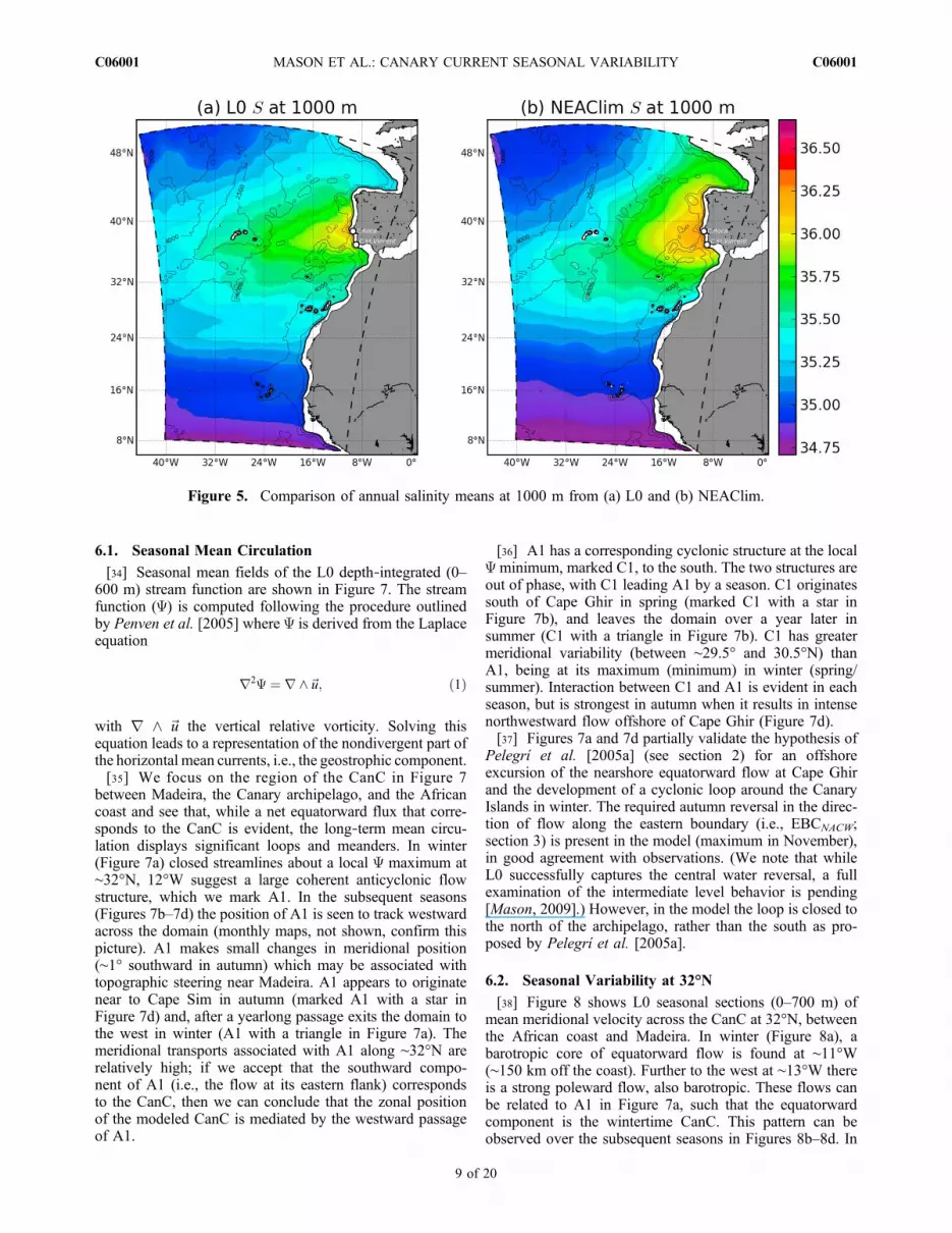
Figure 5. Comparison of annual salinity means at 1000 m from (a) L0 and (b) NEAClim.

MASON ET AL.: CANARY CURRENT SEASONAL VARIABILITY C06001C06001

9 of 20

spring (Figure 8b), strong equatorward flow close to thecoast corresponds to the CanUC as the Trade winds begintheir seasonal intensification [Wooster et al., 1976; Pelegríet al., 2006]. By the summertime (Figure 8c), a compar-atively broad surface‐intensified CanC is centered about14°W. At the coast, the CanUC is well developed and has anassociated poleward undercurrent at depth. The undercurrentis the only poleward flux in the summer section, aside froma shallow surface Ekman layer. Strong equatorward flow at∼16.5°W (weak but present in spring also) is likely relatedto localized recirculation around Madeira, which forms abarrier to the AzC [Zhou et al., 2000]. Lastly, in autumn(Figure 8d) the CanC is identified at ∼16°W. At the coast,the CanUC is replaced by a strong poleward flow centered ataround 300 m. Further offshore at ∼11.5°W there is a second,weaker, barotropic poleward flow. Figures 8a–8d underlinethe conclusion for westward migration of the CanC at 32°Nin association with the propagation of A1, and demonstratethe vertical extent of the anomaly throughout the centralwater layer.[39] Figure 9 compares model seasonal means of accu-

mulated (east to west) barotropic transport at 32°N with the

transport derived through the Sverdrup relation [Sverdrup,1942]

v ¼ r ^~�

h��0; ð2Þ

where r ^ ~� is the curl of the seasonal mean SCOW windstress (Table 1), b is the meridional gradient of the Coriolisparameter (∼2.2 × 10−11 m−1 s−1) and r0 is the model meanseawater density (1027.4 kg m−3). Both the model andSverdrup transports are meridionally averaged over the lat-itude range 30.5°–33.5°N. The L0 transports presented aredenoted as L05–15, meaning averages computed from L0years 5–15. Use of L05–15 facilitates comparison with twoshorter sensitivity runs (L0NCEP and L0NOMW, also shown inFigure 9) which are discussed below in section 7.[40] For each season the L05–15 transports in Figure 9

converge toward the Sverdrup relation values at ∼18°–19°W indicating that the CanC is largely wind driven overthe study region. However there are significant localdepartures along each transect that suggest that the modelcirculation experiences additional forcings to the local wind

Figure 6. (a, b) Comparison of annual mean zonal velocities from L0 (depth averaged 10–20 m) andfrom the SVP drifter climatology. The 300 and 3000 m isobaths are plotted in black. SVP regions withless than 100 drifter days per square degree are masked. (c, d) Comparison of annual mean fields of seasurface height variance from L0 and from AVISO. The 300 and 3000 m isobaths are plotted in white.

MASON ET AL.: CANARY CURRENT SEASONAL VARIABILITY C06001C06001

10 of 20

forcing. Offshore (west of ∼10°W) the positions of thesedepartures are clearly linked to the seasonal propagation ofthe A1 anomaly. In autumn the effect is amplified by thelarge‐scale poleward flow reversal in the near‐shelf region(∼10°–12°W) evidenced in Figures 7 and 8.

6.3. Observational Evidence for Modeled SeasonalVariability

[41] It is useful to compare the above model results withavailable observational evidence. The suggested positions ofthe CanC as interpreted by Machín et al. [2006] from a boxmodel study using in situ data collected at ∼32°N duringfour individual cruises in 1997 and 1998 were shown by reddashed vertical lines in Figure 8. (See Figures 19 and 20 ofthe observational study by Machín et al. [2006]. Figure 19shows seasonal vertical sections of absolute geostrophicvelocity. Figure 20 shows schematic diagrams for eachseason that give the core position and breadth of the CanC.)The primary important point is that Machín et al. [2006]observed a clear westward progression in the position of theobserved CanC from spring through autumn (Figures 8b–8d),in accord with our conclusions from the model in sections 6.1

and 6.2. In summer the modeled and observed core positionsare identical. In winter, however, Machín et al. [2006] placethe core in a central position at ∼14°W, which is ∼250 kmfurther offshore than the winter L0 CanC. They describethe CanC as broad (∼280 km) and generally weak. However,an examination of Machín et al.’s [2006] vertical section ofwinter geostrophic velocity (their Figure 19c) reveals apattern between 100 and 400 km from the coast that is infact quite similar to the L0 velocity structure shown inFigure 8a. Most importantly, their Figure 19 shows a core ofstrong southward flow at ∼180 km offshore, which coin-cides rather well with the L0 CanC position identified inFigure 8a at ∼11°W.[42] Table 2 presents mean annual and seasonal equator-

ward transports of the CanC calculated between 10.5° and17°W at 32°N. Means from L0 and from the observedtransports of Machín et al. [2006] are shown. Included alsoare the 11 year means L05–15, L0NCEP and L0NOMW whichare discussed below in section 7. The annual transports aresimilar for both model and observations. Seasonally,important discrepancies appear to occur in summer andautumn. The model transports are higher in summer, while

Figure 7. Seasonal mean L0 depth‐integrated (0–600 m) stream function (Y). Contour intervals areequivalent to 0.5 Sv. Blue (red) shading represents positive (negative) Y; flow along positive closed Yisolines is clockwise and vice versa. Local maxima (minima) near 32°N (30°N) labeled A1 (C1) markthe passage of an anomalous anticyclonic (cyclonic) mesoscale structure. A1 (C1) with a star indicatesthe assumed location and season of birth of A1 (C1). A1 (C1) with a triangle shows the position ofA1 (C1) from the previous cycle.

MASON ET AL.: CANARY CURRENT SEASONAL VARIABILITY C06001C06001

11 of 20

those of Machín et al. [2006] are higher in autumn. Wesuggest a credible explanation for the apparent discrepancyis that the autumn cruise data used by Machín et al. [2006]were collected in September (1997), a summer month in ourseasonal means (the L0 mean for September is 5.4 Sv).Considering this fact we conclude that the summer andautumn model transports do correspond well with those ofMachín et al. [2006].[43] In Figure 10 we compare mean seasonal sea level

anomalies (SLA) from L0 (Figures 10a–10d) and AVISOaltimetry (Figures 10e–10h). For the altimetry we use theperiod 1999–2007, which is the same period as the SCOWwind stress. The modeled and observed SLAs show goodagreement in their large‐scale magnitudes and distributions,with evidence of a seasonal cycle, upwelling and equator-ward flow in summer, and a flow reversal along the coast inautumn. The seasonal cycle can be generalized as a mini-mum in SSH along the coast during peak upwelling insummer; over the subsequent seasons this minimum pro-pagates offshore. These patterns of seasonal offshore prop-agation of SSH anomalies have been observed in both

models and altimetry at the California and Peru upwellingsand have been linked to wind‐generated westward propa-gating baroclinic planetary waves [Marchesiello et al., 2003;Penven et al., 2005].[44] The positions of structures A1 and C1 (previously

identified in Figure 7) are seen to coincide closely with fea-tures (highs and lows) in the model SLAs (Figures 10a–10d).Analogous structures in the altimeter SLA are speculativelylabeled A1obs and C1obs in Figures 10e–10h. The corre-spondence between the modeled and observed SLAanomalies is reasonably good, especially for A1. The closestmatches occur in summer and autumn, although in autumnA1 is notably more pronounced than A1obs. Between sum-mer and autumn C1obs accelerates away from the coast morerapidly than C1; thereafter the two have similar propagationrates although C1obs leads C1 by ∼2°.

6.4. Planetary Waves as a Mechanism for SeasonalVariability

[45] Many reports suggest the presence of westwardpropagating baroclinic planetary (Rossby) waves within the

Figure 8. L0 seasonal mean zonal sections of meridional velocity at 32°N. The CanC is visible, partic-ularly in summer where it is centered at ∼14°W and reaches 0.05 m s−1. Velocity contours are plottedevery 0.01 m s−1, solid (dashed) contours show northward positive (southward negative) velocity. Thethick (thin) red dashed lines show the core (outer limits of the) seasonal positions of the CanC as observedby Machín et al. [2006].

MASON ET AL.: CANARY CURRENT SEASONAL VARIABILITY C06001C06001

12 of 20

Canary Basin [Lippert and Käse, 1985; Barnier, 1988;Siedler and Finke, 1993; Polito and Cornillon, 1997;Hagen, 2001, 2005; Osychny and Cornillon, 2004; Hirschiet al., 2007; Lecointre et al., 2008]. (It is argued that thebulk of westward energy propagation at midlatitudes is morerepresentative of nonlinear vertically coherent eddies than oflinear Rossby waves [Chelton et al., 2007]; we thereforefollow Lecointre et al. [2008] in using the term “planetarywave” as a generic descriptor of westward propagatingsignals.) Siedler and Finke [1993] analysed data from azonal array of five moorings just west of the Canary Islands.They observed annual and semiannual planetary waves withzonal wavelengths of 100–200 and 300 km, respectively.Hagen [2005], working with hydrographic data from theopen ocean in the Canary Basin, described waves at 32°Nwith wavelengths of 428 km and periods of 289 days. Heshowed that waves observed in satellite SLA north of 22°Nappear to be seasonally excited. The possibility that west-ward propagating seasonally forced planetary waves maydisturb time mean meridional currents (such as the CanC) israised by Hagen [2001].[46] Potential instigators of planetary waves exist at the

eastern boundary of the Canary Basin, notably temporalvariation of the wind stress curl and change of currentdirection. Sturges and Hong [1995] showed a link betweenwind stress and anomalies in the thermocline depth along32°N; they showed the spectrum of the (COADS) wind

stress curl to have a peak at 12 months, the intensity gen-erally decreasing from west to east. Polito and Cornillon[1997] attributed the generation of midlatitude planetarywaves observed through altimetry in the North Atlantic tofluctuations in the wind stress curl at the eastern boundary.Krauss and Wuebber [1982] highlighted the dominance ofline sources of wind stress along eastern boundaries asplanetary wave forcing mechanisms, as opposed to directwind stress generation. In section 4.2 we noted the signifi-cant small‐scale variability in the SCOW wind stress curl

Figure 9. Comparison of seasonal mean accumulated (starting from the eastern boundary) meridionalbarotropic transports from the model (L05–15, L0NOMW, and L0NCEP), with the Sverdrup transport derivedfrom the curl of the SCOW wind stress. Grey shading highlights difference between L05–15 andSverdrupSCOW. The transports are meridionally averaged over the latitudes 30.5°–33.5°N.

Table 2. Mean Annual and Seasonal Equatorward Transports (Sv)in the CanC in the Layer 0–700 m, at 32°N Between 10.5° and17°Wa

Solution Annual Winter Spring Summer Autumn

L0 3.1 1.5 2.8 5.7 2.5L05–15 3.0 1.3 3.0 5.3 2.6L0NCEP 1.2 0.1 1.3 2.5 0.9L0NOMW 3.3 1.7 3.4 5.9 2.3Machín et al.

[2006]b3.0 ± 1.2 1.7 ± 1.0 2.8 ± 1.2 2.9 ± 1.1 4.5 ± 1.2

aValues are shown for the model solutions L0, L05–15, L0NCEP, andL0NOMW and from the observational study of Machín et al. [2006]. TheL0NCEP and L0NOMW solutions are discussed in section 7.

bThe annual observed values are computed from the four seasonal cruisesat 32°N that took place in 1997 and 1998.

MASON ET AL.: CANARY CURRENT SEASONAL VARIABILITY C06001C06001

13 of 20

encountered along the coast near to Capes Ghir and Simover the seasonal cycle.[47] Concerning coastal current reversals, Mysak [1983]

demonstrated that a fluctuating eastern boundary currentcan be an efficient generator of annual period baroclinicplanetary waves off Vancouver Island in the North Pacific.In section 3 we outlined the annual reversals in the EBCflow that take place along the eastern boundary, and whichare captured by the model (Figures 7 and 10). Siedler andFinke [1993] observed strong changes in the current nearthe western Canary Islands, and concluded that, along withwind stress, these were potential candidates for the forcingof the planetary waves they observed at 28°N.[48] Planetary waves forced at the eastern boundary by

combinations of alongshore wind stress fluctuations andequatorially forced Kelvin waves propagating along thecoast have been observed in the tropical Atlantic between 4°and 24°N [Chu et al., 2007]. In the present case the influ-ence of Kelvin waves is unlikely as their northwardprogress is impeded by the frontal regions associated with thenorthwest African upwelling [Lazar et al., 2006; Polo et al.,2007].[49] Longitude/time plots (Hovmöler) of monthly mean

SSH anomalies and wind stress curl at 32°N (further filteredby meridional averaging between 31.5° and 32.5°N) arepresented in Figure 11. Figures 11a and 11b show SSH datafromAVISO altimetry and L0, respectively, while Figure 11dshows the SCOW wind stress curl. (Figures 11c and 11e arediscussed in section 7.) Three annual cycles are repeated tobetter illustrate periodicity in the signals. To filter the SSHseasonal cycle we take the difference between each timeband and its mean, and then bin the output according to itsmonth, prior to averaging. The largest west–east amplitudedifference occurs in summer for both SSH data sets, withthe difference being largest in the model; reasons for thedivergence in amplitude may include uncertainty in thenearshore structure of the model wind forcing [Capet et al.,

2004], interannual variability in the altimeter data, and con-tamination of the altimeter data close to land [Ducet et al.,2000].[50] Periodicity at annual time scales is evident in both the

observed and modeled SSH anomalies of Figure 11. Thecycle for the nearshore wind stress curl is more complex;between early winter and late summer there is generallystrong positive curl within 200 km of the shore, with twopeaks occurring in late winter and summer. The SSH timeseries show clear westward propagation of growing positiveanomalies, originating in autumn near to the coast andarriving at the western boundary the following summer.This equates to a propagation rate across the domain of∼0.03m s−1, in good agreement with observations (0.032m s−1)and theoretical estimates (0.021 m s−1) for the phase speedsof longer‐period planetary waves in this region [Osychnyand Cornillon, 2004; Hagen, 2005]. The anomalies corre-spond to anticyclonic structure A1 shown in Figures 7 and10. The propagating structure is less well defined in theAVISO data than in L0. Following its autumn generation theAVISO signal is unclear until early winter at ∼11–12°W.This behavior can also be observed in Figure 10 above. Theautumn generation of the A1 anomaly coincides with a brieftransition in the nearshore wind stress curl, which reversessign for ∼3 months in early autumn.

7. Sensitivity Experiments

[51] Two experiments were performed in order to examinethe sensitivity of the CanC to upstream variability, and tovariability in the large nearshore positive wind stress curl.Annual mean depth‐integrated (surface to 7°C isotherm)stream functions calculated from these solutions are shownin Figure 12.[52] For comparison, Figure 12a shows the stream func-

tion from L05–15. The AzC at 34°N is the striking feature inthe L05–15 circulation, transporting over 9 Sv at ∼21°W. In

Figure 10. Seasonal mean sea level anomalies. (a–d) The SLAs from L0 and (e–h) the AVISO SLAs(for the same time period as the SCOW wind stress, i.e., 1999–2007) are shown. Contours are plottedin white every 0.5 cm.

MASON ET AL.: CANARY CURRENT SEASONAL VARIABILITY C06001C06001

14 of 20

the Gulf of Cadiz and west of southern Iberia, a large zonalcyclonic recirculation cell loops around Cape St. Vincentbefore detaching and extending offshore. This cell is relatedto the topographic b plume of Kida et al. [2008], which is aconsequence of the geometry of the gulf and entrainment ofsurface waters into the outflowing MW plume [Peliz et al.,2007]. The cyclonic cell, which may be seen as the AzC(and counterflowing AzCC), has been modeled by Peliz et al.[2007] and observations have been reported by Lamas et al.[2010]. The AzC in Figure 12a has three southward turn-ing branches at ∼27°, ∼20° and ∼16°W near Madeira, con-sistent with observations [Stramma and Siedler, 1988;Juliano and Alves, 2007]. The Madeira branch transports∼3 Sv as it transitions to the CanC. Off the African coastnorth and south of Cape Ghir are two large lobes of cyclonic

circulation. The southern lobe is associated with C1, and theregion between it and the northern lobe is the location of A1.

7.1. Sensitivity to Azores Current Variability

[53] Given the idea that the AzC feeds the CanC, thequestion arises as to how sensitive the CanC might be toupstream variability, i.e., changes in the strength of the AzC.It is well established that the AzC in a numerical model canbe removed by closing the Strait of Gibraltar [Jia, 2000;Kida et al., 2008; Volkov and Fu, 2010]. We therefore ranan additional sensitivity experiment (hereinafter L0NOMW)using the standard L0 SCOW wind and a closed strait.L0NOMW was run for 15 years, and annual and seasonalmeans of the prognostic variables were computed usingyears 5–15.

Figure 11. Longitude/time plots showing three repeated yearly cycles of monthly mean SSH and windstress curl at 32°N (meridionally averaged between 31.5° and 32.5°N). SSH is taken from (a) AVISOaltimetry, (b) L0, and (c) L0NCEP. Contours are shown in black at −0.055, −0.005, and 0.045 m. Years6–18 (1995–2007) are used from L0/L0NCEP (AVISO). Wind stress curl is taken from (d) SCOW and(e) NCEP. Contours are shown in black every 0.2 N m−3 × 1e6. Intense negative curl in SCOW at thewestern boundary is associated with Madeira. The seasons are labeled W, S, S, and A for winter, spring,summer, and autumn, respectively.

MASON ET AL.: CANARY CURRENT SEASONAL VARIABILITY C06001C06001

15 of 20

[54] The effect of the closure of the Strait of Gibraltarupon the AzC can be seen in Figure 12b. The L0NOMW AzCis visible but weak, transporting ∼2 Sv at ∼21°W, less than aquarter of the L05–15 value. This remnant AzC signal islikely related to the wind [Townsend et al., 2000; Özgökmenet al., 2001]. However, the most interesting aspect of thecomparison between the L05–15 and L0NOMW solutions is thesouthward circulation of the CanC below about 32°N.

Despite the marked differences in the AzC to the north, thetwin lobes in L0NOMW between Cape Ghir, Madeira and theCanary Islands are remarkably similar to those in L05–15 inFigure 12a. Table 2 presents L0NOMW annual and seasonaltransports across 32°N, these are consistent with but slightlyhigher than the L05–15 and L0 transports. There is also closeagreement between the seasonal accumulated transportsfrom L0NOMW and L05–15 at 32°N in Figure 9. In addition, aplot of the seasonal stream function for L0NOMW (not shown)similar to Figure 7 shows there to be no difference in thepositions of anomalies A1 and C1; the anomalies werehowever slightly more intense, which is in agreement withhigher L0NOMW transports across 32°N (Table 2). Theresults from the L0NOMW experiment suggest that the CanaryCurrent is relatively insensitive to variability in the AzCtransport.

7.2. Sensitivity to Wind Stress Curl Variability

[55] To directly examine sensitivity to the wind stress curlwe ran an additional numerical experiment forced bymonthly mean climatological wind stress derived from 10 mwind speed data at 2.5° resolution from the NCEP Reanal-ysis Project 1 (see Table 1). The climatological periodchosen was 1999–2007 in order to correspond with theSCOW wind stress used for L0. Wind stresses were derivedfrom wind speeds following Yelland et al. [1998]. Theevolution of the NCEP wind stress curl along 32°N is shownin the longitude/time plot of Figure 11e, where it can becompared with SCOW in the adjacent panel. The NCEPmonthly means are markedly smoother than SCOW,although the large‐scale structure and seasonal cycle arenominally resolved; a wide band (>1°) of relatively weakcyclonic curl is seen along the coast, and anticyclonic curlover the open ocean. However the (cyclonic) small‐scalestructure seen in the alongshore SCOW curl is entirelyabsent. The NCEP‐forced simulation, hereinafter L0NCEP,was run for 18 years. Annual and seasonal means of theprognostic variables were computed using years 5–15.[56] Figure 12c shows the L0NCEP annual mean stream

function. The circulation is weaker than L05–15. The AzCtransports ∼6 Sv at ∼21°W, and the Madeira branch to thesouth is absent. The southern lobe of cyclonic flow ismissing, while the northern lobe is present but weak. Fieldsof the L0NCEP seasonal stream function (not shown) havesimilar large‐scale patterns as presented for L0 in Figure 7,but the transports are reduced and there are only hints of theA1 and C1 anomalies.[57] Figure 11c shows the L0NCEP monthly mean SSH

anomaly at 32°N. Small zonal gradients relative to AVISOand L0 (Figures 11a and 11b) confirm an overall weakercirculation. Nevertheless, a weak seasonal cycle persists thatis qualitatively comparable to AVISO and L0, and sugges-tive of a traveling A1 anomaly. Table 2 shows that theL0NCEP seasonal transports are between 53 and 93% smallerthan those of L0. Lastly, with reference to the seasonalSverdrup transport comparisons of Figure 9, the L0NCEPaccumulated transports at 32°N are weak and diverge sig-nificantly from the Sverdrup and L05–15 transports; this is tobe expected given the gross difference in resolution betweenthe SCOW and NCEP wind data. However, the L0NCEPtransports do display the local structure identified in Figure 9

Figure 12. Comparison of the depth‐integrated (surface to7°C isotherm) annual mean stream function (Y) for (a)L05–15, (b) L0NCEP, and (c) L0NOMW. Contour intervals areequivalent to 1 Sv. Blue (red) shading represents positive(negative) Y; flow along positive closed Y isolines is clock-wise and vice versa.

MASON ET AL.: CANARY CURRENT SEASONAL VARIABILITY C06001C06001

16 of 20

for L05–15, and this may be related to the weak travelinganomalies seen in Figure 11c.[58] Figure 12c indicates that the annual mean circulation

(and by extension the seasonal circulation) in the studyregion is significantly changed with the use of the low‐resolution NCEP wind speed product. The largest differ-ences in the structure of the curl between the SCOW andNCEP wind stresses are along the coast. We thereforeconclude that small‐scale variability in the cyclonic windstress curl in the vicinity of Cape Ghir (evidenced inFigure 11d) is likely to play an important role in the gen-eration of the A1 and C1 anomalies. However, given thepersistence of weak traveling anomalies in L0NCEP seen inFigure 11c, we suggest that a second potential contributor tothe formation of the anomalies is the autumn flow reversalof the EBC along the eastern boundary. This phenomenon isless easy to test in a sensitivity experiment using the L0configuration, as it is more difficult to exclude.

8. Summary and Conclusions

[59] Results are presented from a high‐resolution clima-tological ocean model simulation for the Canary Basin,using the ROMS ocean model. The focus is on the sea-sonality of the Canary Current between the latitudes ofMadeira and the Canary Island archipelago. The modelsolution reaches equilibrium after a few years, and thereafterpresents no significant drift over its 50 year timespan. Avalidation exercise, comparing model (instantaneous, sea-sonal mean and eddy mean) quantities with appropriateobservations (from databases, climatologies, and the pub-lished literature), shows the model to attain a credible rep-resentation of the dynamics of the Canary region: mesoscalevariability, mean circulation and the seasonal cycle.[60] The major currents of the eastern subtropical gyre are

well reproduced. The Azores Current is at its correct loca-tion, and has levels of mesoscale variability that are com-parable with altimeter estimates. The open boundary at theStrait of Gibraltar permits the entrance of dense Mediterra-nean Water into the model domain; the resulting traceranomaly spreads at depth into the Atlantic in a realisticmanner. Along the eastern boundary the seasonal CanaryUpwelling Current jet develops in response to increasedupwelling‐favorable alongshore wind forcing in spring andsummer. The well documented reversal of the large‐scaleboundary flow (central water levels) takes place in autumn.[61] From an analysis of the simulated Canary Current

circulation we present a novel finding. The seasonal cycle ofthe CanC in the study region is mediated by the passage oftwo large‐scale coherent anomalous structures that propa-gate westward following their respective origins near theAfrican coast. Seasonal means of the depth‐integratedstream function show an anticyclonic anomaly (A1) thatappears north of Cape Ghir in autumn. In spring a cycloniccounterpart (C1) begins to develop south of Cape Ghir. Weargue that the core position of the CanC is associated withthe equatorward components of these swirling anomalies asthey progress westward away from the African coast.[62] The above result is supported by observational data.

The anomalies have a surface expression and are thereforevisible to satellite‐borne altimeters. Sea level anomaly fields

from the model and from altimetry are comparable, thecyclonic and anticyclonic structures show up as respectivenegative and positive anomalies. The pair are phase lockedto the annual cycle and are seen to travel westward at theapproximate phase speed of first‐mode baroclinic planetary(Rossby) waves at Canary Basin latitudes (∼3 cm s−1 or2.6 km d−1).[63] Seasonal meridional transports calculated at the lati-

tude of the anticyclone (32°N) are in close agreement withsimilarly located transports from published in situ observa-tions; the observations include the full extent of the NACWlayer and indicate a general westward seasonal progressionof the core of the CanC. Plots of seasonal accumulatedtransport at 32°N computed through the Sverdrup relationconfirm that the CanC is largely wind driven. Total modelaccumulated transports are in agreement with the Sverdrupvalues. However the model transports show local departuresfrom the Sverdrup transports, and the zonal locations ofthese departures correspond to that of A1. This reinforcesthe argument for coastal generation and offshore propaga-tion of A1.[64] Sensitivity experiments have led to the isolation of

two potential candidates for the forcing of the anomalies,namely: (1) small‐scale variability in the local wind stresscurl at the eastern boundary and (2) major periodic reversalsin the flow along the eastern boundary.[65] In a first experiment to evaluate the role of upstream

influence on the CanC by the AzC, we ran a 15 year sim-ulation where the AzC was largely removed (transportreduced by ∼85%) by closing the model boundary at theStrait of Gibraltar. We observed minimal impact on theCanC in terms of both its mean position and transport. Thisresult suggests that the CanC is insensitive to variability inthe strength of the AzC.[66] In a second experiment a low‐resolution wind stress

product was used to force the model. The change from high‐resolution wind forcing results in a globally weak circula-tion; transport by the CanC is reduced by ∼60% and thecurrent’s mean path, shown by isolines of the stream func-tion, is significantly altered. Nevertheless there is still weakwestward propagation of sea level anomalies. We thereforefind that nearshore variability in the wind stress curl isimportant for the dynamics of planetary‐wave‐like anoma-lies that significantly influence the path of the CanCbetween Madeira and the Canary Islands. However, wecannot discount a dynamical contribution from the annualreversal of the large‐scale flow along the eastern boundary.

[67] Acknowledgments. Evan Mason is supported by the Spanishgovernment through projects MOC2 (CTM2008‐06438‐C02‐01) andRODA (CTM2004‐06842‐CO3‐03). Pablo Sangrà was a visiting scholarat the Institute of Geophysics and Planetary Physics at UCLA, supportedby a Spanish government scholarship (Salvador de Madariaga, PR2010‐0517). ROMS development at UCLA is supported by the Office of NavalResearch (currently grant N00014‐08‐1‐0597). This work was partiallysupported by the National Center for Supercomputing Applications undergrant number OCE030007 and utilized the abe system. The altimeter pro-ducts were produced by SSALTO/DUACS and distributed by AVISO, withsupport from CNES. NCEP Reanalysis data provided by the NOAA/OAR/ESRL PSD, Boulder, Colorado, USA, from their website at http://www.esrl.noaa.gov/psd/. We are grateful to Jose Luis Pelegrí for his helpful com-ments on various aspects of the CCS circulation. Lastly, we thank the editorand two anonymous reviewers whose input has substantially improved thispaper.

MASON ET AL.: CANARY CURRENT SEASONAL VARIABILITY C06001C06001

17 of 20

ReferencesAlves, M. L. G. R., and A. Colin de Verdière (1999), Instability dynamicsof a subtropical jet and applications to the Azores Front Current System:Eddy‐driven mean flow, J. Phys. Oceanogr., 29(5), 837–864,doi:10.1175/1520-0485(1999)029<0837:IDOASJ>2.0.CO;2.

Arhan, M., A. Colin de Verdiére, and L. Mémery (1994), The easternboundary of the subtropical North Atlantic, J. Phys. Oceanogr., 24(6),1295–1316, doi:10.1175/1520-0485(1994)024<1295:TEBOTS>2.0.CO;2.

Arístegui, J., P. Sangrà, S. Hernández‐León, M. Cantón, A. Hernández‐Guerra, and J. L. Kerling (1994), Island‐induced eddies in the CanaryIslands, Deep Sea Res., 49(10), 1087–1101, doi:10.1016/0967-0637(94)90058-2.

Arístegui, J., X. A. Álvarez‐Salgado, E. D. Barton, F. G. Figueiras,S. Hernández‐León, C. Roy, and A. M. P. Santos (2006), Oceanographyand fisheries of the Canary Current/Iberian region of the eastern NorthAtlantic, in The Sea: Ideas and Observations on Progress in the Studyof the Seas, vol. 14, pp. 878–931, chap. 23, edited by A. R. Robinsonand K. H. Brink, Harvard Univ. Press, Cambridge, Mass.

Arístegui, J., E. D. Barton, X. A. Álvarez‐Salgado, A. M. P. Santos, F. G.Figueiras, S. Kifani, S. Hernández‐León, E. Mason, and E. Machú(2009), Sub‐regional ecosystem variability in the Canary Current upwell-ing, Prog. Oceanogr., 83(1–4), 33–48, doi:10.1016/j.pocean.2009.07.031.

Bakun, A., and C. S. Nelson (1991), The seasonal cycle of wind‐stress curlin subtropical eastern boundary current regions, J. Phys. Oceanogr.,21(12), 1815–1834, doi:10.1175/1520-0485(1991)021<1815:TSCOWS>2.0.CO;2.

Barnier, B. (1988), A numerical study on the influence of the mid‐AtlanticRidge on nonlinear first‐mode baroclinic Rossby waves generated byseasonal winds, J. Phys. Oceanogr., 18(3), 417–433.

Barnier, B., L. Siefridt, and P. Marchesiello (1995), Thermal forcing for aglobal ocean circulation model using a three‐year climatology ofECMWF analyses, J. Mar. Syst., 6(4), 363–380, doi:10.1016/0924-7963(94)00034-9.

Barnier, B., P. Marchesiello, A. P. de Miranda, J.‐M. Molines, andM. Coulibaly (1998), A sigma‐coordinate primitive equation model forstudying the circulation in the South Atlantic. Part I: Model configurationwith error estimates, Deep Sea Res., 45(4–5), 543–572, doi:10.1016/S0967-0637(97)00086-1.

Barton, E. D. (1987), Meanders, eddies and intrusions in the thermohalinefront off northwest Africa, Oceanol. Acta, 10(3), 267–283.

Barton, E. D., et al. (1998), The transition zone of the Canary Currentupwelling region, Prog. Oceanogr., 41(4), 455–504, doi:10.1016/S0079-6611(98)00023-8.

Baschek, B., U. Send, J. G. Lafuente, and J. Candela (2001), Transportestimates in the Strait of Gibraltar with a tidal inverse model, J. Geophys.Res., 106(C12), 31,033–31,044, doi:10.1029/2000JC000458.

Bower, A. S., B. Le Cann, T. Rossby, W. Zenk, J. Gould, K. Speer, P. L.Richardson, M. D. Prater, and H. M. Zhang (2002), Directly measuredmid‐depth circulation in the northeastern North Atlantic Ocean, Nature,419, 603–607, doi:10.1038/nature01078.

Brochier, T., E. Mason, M. Moyano, A. Berraho, F. Colas, P. Sangrà,S. Hernández‐León, O. Ettahiri, and C. Lett (2011), Ichthyoplanktontransport from the African coast to the Canary Islands, J. Mar. Syst.,doi:10.1016/j.jmarsys.2011.02.025, in press.

Capet, X. J., P. Marchesiello, and J. C. McWilliams (2004), Upwellingresponse to coastal wind profiles, Geophys. Res. Lett., 31, L13311,doi:10.1029/2004GL020123.

Chelton, D. B., M. G. Schlax, R. M. Samelson, and R. A. de Szoeke(2007), Global observations of large oceanic eddies, Geophys. Res. Lett.,34, L15606, doi:10.1029/2007GL030812.

Chu, P. C., L. M. Ivanov, O. M. Melnichenko, and N. C. Wells (2007), Onlong baroclinic Rossby waves in the tropical North Atlantic observedfrom profiling floats, J. Geophys. Res., 112, C05032, doi:10.1029/2006JC003698.

Colin de Verdière, A., H. Merchier, and M. Arhan (1989), MesoscaleVariability transition from the western to the eastern Atlantic along48°N, J. Phys. Oceanogr., 19(8), 1149–1170, doi:10.1175/1520-0485(1989)019<1149:MVTFTW>2.0.CO;2.

de Boyer Montégut, C., G. Madec, A. S. Fischer, A. Lazar, and D. Iudicone(2004), Mixed layer depth over the global ocean: An examination of pro-file data and a profile‐based climatology, J. Geophys. Res., 109, C12003,doi:10.1029/2004JC002378.

Ducet, N., P.‐Y. Le Traon, and G. Reverdin (2000), Global high‐resolutionmapping of ocean circulation from TOPEX/Poseidon and ERS‐1 and ‐2,J. Geophys. Res., 105(C8), 19,477–19,498.

Flather, R. A. (1976), A tidal model of the north–west European continentalshelf, Mem. Soc. R. Sci. Liège, 6(10), 141–164.

Fraile‐Nuez, E., and A. Hernández‐Guerra (2006), Wind‐driven circulationfor the eastern North Atlantic Subtropical Gyre from Argo data, Geophys.Res. Lett., 33, L03601, doi:10.1029/2005GL025122.

Fraile‐Nuez, E., F. Machín, P. Vélez‐Belchí, F. Lóez‐Laatzen, R. Borges,V. Benítez‐Barrios, and A. Hernández‐Guerra (2010), Nine years ofmass transport data in the eastern boundary of the North Atlantic Subtrop-ical Gyre, J. Geophys. Res., 115, C09009, doi:10.1029/2010JC006161.

Hagen, E. (2001), Northwest Africa upwelling scenario, Oceanol. Acta, 24,suppl. 1, 113–128, doi:10.1016/S0399-1784(00)01110-5.

Hagen, E. (2005), Zonal wavelengths of planetary Rossby waves derivedfrom hydrographic transects in the northeast Atlantic Ocean, J. Ocea-nogr., 61, 1039–1046, doi:10.1007/s10872-006-0020-3.

Hagen, E., C. Zuelicke, and R. Feistel (1996), Near‐surface structures in theCape Ghir filament off Morocco, Oceanol. Acta, 19(6), 577–598.

Haidvogel, D. B., and A. Beckmann (1999), Numerical Ocean CirculationModeling, Imperial Coll. Press, London.

Harzallah, A. (2009), Flow variability in the Strait of Gibraltar: TheMediterranean adjustment to tidal forcing, Deep Sea Res., 56(4), 459–470, doi:10.1016/j.dsr.2008.12.001.

Hernández‐Guerra, A., et al. (2002), Temporal variability of mass transportin the Canary Current, Deep Sea Res., 49(17), 3415–3426, doi:10.1016/S0967-0645(02)00092-9.

Hernández‐Guerra, A., E. Fraile‐Nuez, F. López‐Laatzen, A. Martínez,G. Parrilla, and P. Vélez‐Belchí (2005), Canary Current and North Equa-torial Current from an inverse box model, J. Geophys. Res., 110, C12019,doi:10.1029/2005JC003032.

Hirschi, J. M., P. D. Killworth, and J. R. Blundell (2007), Subannual, sea-sonal, and interannual variability of the North Atlantic Meridional Over-turning Circulation, J. Phys. Oceanogr., 37(5), 1246–1265, doi:10.1175/JPO3049.1.

Jia, Y. (2000), Formation of an Azores Current due to Mediterranean over-flow in a modeling study of the North Atlantic, J. Phys. Oceanogr., 30(9),2342–2358, doi:10.1175/1520-0485(2000)030<2342:FOAACD>2.0.CO;2.

Juliano, M. F., and M. L. G. Alves (2007), The Atlantic subtropical front/current systems of Azores and St. Helena, J. Phys. Oceanogr., 37(11),2573–2598, doi:10.1175/2007JPO3150.1.

Kalnay, E., et al. (1996), The NCEP/NCAR 40‐year reanalysis project,Bull. Am. Meteorol. Soc., 77, 437–471, doi:10.1175/1520-0477(1996)077<0437:TNYRP>2.0.CO;2.

Kida, S., J. F. Price, and J. Yang (2008), The upper oceanic response tooverflows: A mechanism for the Azores Current, J. Phys. Oceanogr.,38(4), 880–895, doi:10.1175/2007JPO3750.1.

Kilpatrick, K., G. P. Podesta, and R. Evans (2001), Overview of theNOAA/NASA Advanced Very High Resolution Radiometer Pathfinderalgorithm for sea surface temperature and associated matchup database,J. Geophys. Res., 106(C5), 9179–9197.

Knoll, M., A. Hernández‐Guerra, B. Lenz, F. López‐Laatzen, F. Machín,T. J. Müller, and G. Siedler (2002), The eastern boundary current systembetween the Canary Islands and the African Coast, Deep Sea Res., 49(17),3427–3440, doi:10.1016/S0967-0645(02)00105-4.

Krauss, W., and C. Wuebber (1982), Response of the North Atlantic toannual wind variations along the eastern coast, Deep Sea Res., 29(7),851–868, doi:10.1016/0198-0149(82)90050-4.

Lamas, L., Á. Peliz, I. Ambar, A. B. Aguiar, N. Maximenko, and A. Teles‐Machado (2010), Evidence of time‐mean cyclonic cell southwest ofthe Iberian Peninsula: The Mediterranean outflow‐driven b‐plume?,Geophys. Res. Lett., 37, L12606, doi:10.1029/2010GL043339.

Large, W. G., J. C. McWilliams, and S. C. Doney (1994), Oceanic verticalmixing: A review and a model with a vertical K‐profile boundary layerparameterization, Rev. Geophys., 32(4), 363–403.

Lathuiliére, C., V. Echevin, and M. Lévy (2008), Seasonal and intraseaso-nal surface chlorophyll‐a variability along the northwest African coast,J. Geophys. Res., 113, C05007, doi:10.1029/2007JC004433.

Lazar, A., I. Polo, S. Arnault, and G. Mainsant (2006), Kelvin wave activityin the eastern tropical Atlantic, paper presented at 15 Years of Progress inRadar Altimetry Symposium, Eur. Space Agency, Venice, Italy.

Lecointre, A., T. Penduff, P. Cipollini, R. Tailleux, and B. Barnier (2008),Depth dependence of westward‐propagating North Atlantic featuresdiagnosed from altimetry and a numerical 1/6° model, Ocean Sci., 4,99–113.

Le Traon, P.‐Y., and P. De Mey (1994), The eddy field associated with theAzores Front east of the Mid‐Atlantic Ridge as observed by the Geosataltimeter, J. Geophys. Res., 99(C5), 9907–9924, doi:10.1029/93JC03513.

Lippert, A., and R. H. Käse (1985), Stochastic wind forcing of baroclinicRossby waves in the presence of a meridional boundary, J. Phys. Ocea-nogr., 15(2), 184–194, doi:10.1175/1520-0485(1985)015<0184:SWFOBR>2.0.CO;2.

MASON ET AL.: CANARY CURRENT SEASONAL VARIABILITY C06001C06001

18 of 20

Lumpkin, R., and Z. Garraffo (2005), Evaluating the decomposition oftropical Atlantic drifter observations, J. Atmos. Oceanic Technol., 22(9),1403–1415, doi:10.1175/JTECH1793.1.

Machín, F., and J. L. Pelegrí (2009), Northward penetration of AntarcticIntermediate Water off northwest Africa, J. Phys. Oceanogr., 39(3),512–535, doi:10.1175/2008JPO3825.1.

Machín, F., A. Hernández‐Guerra, and J. L. Pelegrí (2006), Mass fluxes inthe Canary Basin, Prog. Oceanogr., 70(2–4), 416–447.

Machín, F., J. L. Pelegrí, E. Fraile‐Nuez, P. Vélez‐Belchí, F. Lóez‐Laatzen,and A. Hernández‐Guerra (2010), Seasonal flow reversals of intermediatewaters in the Canary Current System east of the Canary Islands, J. Phys.Oceanogr., 40(8), 1902–1909, doi:10.1175/2010JPO4320.1.

Marchesiello, P., J. C. McWilliams, and A. F. Shchepetkin (2003), Equilib-rium structure and dynamics of the California Current System, J. Phys.Oceanogr., 33(4), 753–783, doi:10.1175/1520-0485(2003)33<753:ESADOT>2.0.CO;2.

Mason, E. (2009), High‐resolution modelling of the Canary Basin oceaniccirculation, Ph.D. thesis, 235 pp., Univ. de Las Palmas de Gran Canaria,Las Palmas de Gran Canaria, Spain.

Mason, E., J. Molemaker, F. Colas, A. F. Shchepetkin, J. C. McWilliams,and P. Sangrà (2010), Procedures for offline grid nesting in regionalocean models, Ocean Modell., 35(1–2), 1–15, doi:10.1016/j.ocemod.2010.05.007.

Milliff, R. D., W. G. Large, W. R. Holland, and J. C. McWilliams (1996),The General circulation responses of high‐resolution North AtlanticOcean models to synthetic scatterometer winds, J. Phys. Oceanogr.,26(9), 1747–1768.

Mittelstaedt, E. (1991), The ocean boundary along the northwest Africancoast: Circulation and oceanographic properties at the sea surface, Prog.Oceanogr., 26(4), 307–355, doi:10.1016/0079-6611(91)90011-A.

Müller, T. J., and G. Siedler (1992), Multi‐year current time series in theeastern North Atlantic Ocean, J. Mar. Res., 50, 63–98.

Mysak, L. A. (1983), Generation of annual Rossby waves in the NorthPacific, J. Phys. Oceanogr., 13(10), 1908–1923.

Navarro‐Pérez, E., and E. D. Barton (2001), Seasonal and interannualvariability of the Canary Current, Sci. Mar., 65, suppl. 1, 205–213.

Osychny, V., and P. Cornillon (2004), Properties of Rossby waves in theNorth Atlantic estimated from satellite data, J. Phys. Oceanogr., 34(1),61–76, doi:10.1175/1520-0485(2004)034<0061:PORWIT>2.0.CO;2.

Özgökmen, T. M., E. P. Chassignet, and C. G. H. Rooth (2001), On theConnection between the Mediterranean outflow and the Azores Current,J. Phys. Oceanogr., 31(2), 461–480, doi:10.1175/1520-0485(2001)031<0461:OTCBTM>2.0.CO;2.

Pascual, A., Y. Faugère, G. Larnicol, and P.‐Y. Le Traon (2006), Improveddescription of the ocean mesoscale variability by combining four satellitea l t imeters , Geophys . Res . Le t t . , 33 , L02611, doi :10.1029/2005GL024633.

Pelegrí, J. L., et al. (2005a), Coupling between the open ocean and thecoastal upwelling region off northwest Africa: Water recirculation andoffshore pumping of organic matter, J. Mar. Syst., 54(1–4), 3–37,doi:10.1016/j.jmarsys.2004.07.003.

Pelegrí, J. L., et al. (2005b), Hydrographic cruises off northwest Africa:The Canary Current and the Cape Ghir region, J. Mar. Syst., 54(1–4),39–63, doi:10.1016/j.jmarsys.2004.07.001.

Pelegrí, J. L., A. Marrero‐Díaz, and A. W. Ratsimandresy (2006), Nutrientirrigation of the North Atlantic, Prog. Oceanogr., 70(2–4), 366–406,doi:10.1016/j.pocean.2006.03.018.

Peliz, Á. J., J. Dubert, P. Marchesiello, and A. Teles‐Machado (2007),Circulation in the Gulf of Cadiz: Model and mean flow structure, J. Geo-phys. Res., 112, C11015, doi:10.1029/2007JC004159.

Penven, P., V. Echevin, J. Pasapera, F. Colas, and J. Tam (2005), Averagecirculation, seasonal cycle, and mesoscale dynamics of the Peru CurrentSystem: A modeling approach, J. Geophys. Res., 110, C10021,doi:10.1029/2005JC002945.

Penven, P., L. Debreu, P. Marchesiello, and J. C. McWilliams (2006), Eval-uation and application of the ROMS 1‐way embedding procedure to thecentral California upwelling system, Ocean Modell., 12(1–2), 157–187,doi:10.1016/j.ocemod.2005.05.002.

Penven, P., P. Marchesiello, L. Debreu, and J. Lefevre (2008), Softwaretools for pre‐ and post‐processing of oceanic regional simulations,Environ. Model. Software, 23(5), 660–662, doi:10.1016/j.envsoft.2007.07.004.

Pingree, R. D. (1997), The Eastern Subtropical Gyre (North Atlantic): Flowrings recirculations structure and subduction, J. Mar. Biol. Assoc. U. K.,77(3), 573–624, doi:10.1017/S0025315400036109.

Polito, P. S., and P. Cornillon (1997), Long baroclinic Rossby wavesdetected by TOPEX/POSEIDON, J. Geophys. Res., 102(C2), 3215–3235, doi:10.1029/96JC03349.

Polo, I., A. Lazar, B. Rodriguez‐Fonseca, and S. Arnault (2007), OceanicKelvin waves and tropical Atlantic intraseasonal variability: 1. Kelvinwave characterization, J. Geophys. Res., 113, C07009, doi:10.1029/2007JC004495.

Richardson, P. L., J. F. Price, D. Walsh, L. Armi, and M. Schröder (1989),Tracking three meddies with SOFAR floats, J. Phys. Oceanogr., 19(3),371–383, doi:10.1175/1520-0485(1989)019<0371:TTMWSF>2.0.CO;2.

Richardson, P. L., A. S. Bower, and W. Zenk (2000), A census of Meddiestracked by floats, Prog. Oceanogr., 45(2), 209–250, doi:10.1016/S0079-6611(99)00053-1.

Rio, M.‐H., and F. Hernández (2004), A mean dynamic topography com-puted over the world ocean from altimetry, in situ measurements and ageoid model, J. Geophys. Res., 109, C12032, doi:10.1029/2003JC002226.

Risien, C. M., and D. B. Chelton (2008), A global climatology of surfacewind and wind stress fields from eight years of QuikSCAT scatterometerdata , J . Phys. Oceanogr. , 38 (11) , 2379–2413, doi :10.1175/2008JPO3881.1.

Rossby, T. (1996), The North Atlantic Current and surrounding waters: Atthe crossroads, Rev. Geophys., 34(4), 463–481.

Sangrà, P., et al. (2009), The Canary Eddy Corridor: A major pathway forlong‐lived eddies in the subtropical North Atlantic, Deep Sea Res., 56,2100–2114, doi:10.1016/j.dsr.2009.08.008.

Shchepetkin, A. F., and J. C. McWilliams (2005), The Regional OceanicModeling System (ROMS): A split‐explicit, free‐surface, topography‐following‐coordinate oceanic model, Ocean Modell., 9(4), 347–404,doi:10.1016/j.ocemod.2004.08.002.

Shchepetkin, A. F., and J. C. McWilliams (2009), Correction and commen-tary for “Ocean forecasting in terrain‐following coordinates: Formula-tion and skill assessment of the Regional Ocean Modeling System” byHaidvogel et al., J. Comp. Phys. 227, pp. 3595–3624, J. Comput. Phys.,228(24), 8985–9000, doi:10.1016/j.jcp.2009.09.002.

Siedler, G., and M. Finke (1993), Long‐period transport changes in theeastern North Atlantic and their simulation by propagating waves,J. Geophys. Res., 98(C2), 2393–2406, doi:10.1029/92JC02122.

Smith, R. D., M. E. Maltrud, F. O. Bryan, and M. W. Hecht (2000), Numer-ical simulation of the North Atlantic Ocean at 1/10°, J. Phys. Oceanogr.,30(7), 1532–1561, doi:10.1175/1520-0485(2000)030<1532:NSOTNA>2.0.CO;2.

Smith, W. H. F., and D. T. Sandwell (1997), Global sea floor topographyfrom satellite altimetry and ship depth soundings, Science, 277(5334),1956–1962, doi:10.1126/science.277.5334.1956.

Soto‐Navarro, J., F. Criado‐Aldeanueva, J. García‐Lafuente, andA. Sánchez‐Román (2010), Estimation of the Atlantic inflow through the Strait ofGibraltar from climatological and in situ data, J. Geophys. Res., 115,C10023, doi:10.1029/2010JC006302.

Spall, M. A. (1990), Circulation in the Canary Basin: A model/data analy-sis, J. Geophys. Res., 95(C6), 9611–9628.

Stark, J. D., C. J. Donlon, M. J. Martin, and M. E. McCulloch (2007),OSTIA: An operational, high resolution, real time, global sea surfacetemperature analysis system, in OCEANS 2007—Europe, pp. 1–4,doi:10.1109/OCEANSE.2007.4302251, Inst. of Electr. and Electr.Eng., Piscataway, N. J.

Stramma, L. (1984), Geostrophic transport in the warm water sphere of theeastern subtropical North Atlantic, J. Mar. Res., 42, 537–558.

Stramma, L., and G. Siedler (1988), Seasonal changes in the North AtlanticSubtropical Gyre, J. Geophys. Res., 93(C7), 8111–8118.

Sturges, W., and B. G. Hong (1995), Wind forcing of the Atlantic thermo-cline along 32°N at low frequencies, J. Phys. Oceanogr., 25(7), 1706–1715, doi:10.1175/1520-0485(1995)025<1706:WFOTAT>2.0.CO;2.

Sverdrup, H. U. (1942), Wind‐driven currents in a baroclinic ocean; withapplication to the equatorial currents of the eastern Pacific, Proc. Natl.Acad. Sci. U. S. A., 33, 318–326.

Townsend, T. L., H. E. Hurlburt, and P. J. Hogan (2000), Modeled Sverdrupflow in the North Atlantic from 11 different wind stress climatologies,Dyn. Atmos. Oceans, 32(3–4), 373–417, doi:10.1016/S0377-0265(00)00052-X.

Troupin, C., F. Machín, M. Ouberdous, D. Sirjacobs, A. Barth, and J.‐M.Beckers (2010), High‐resolution climatology of the northeast Atlanticusing Data‐Interpolating Variational Analysis (DIVA), J. Geophys. Res.,115, C08005, doi:10.1029/2009JC005512.

Tsimplis, M. N., and H. L. Bryden (2000), Estimation of the transportsthrough the Strait of Gibraltar, Deep Sea Res., 47(12), 2219–2242,doi:10.1016/S0967-0637(00)00024-8.

Volkov, D. L., and L.‐L. Fu (2010), On the reasons for the formation andvariability of the Azores Current, J. Phys. Oceanogr., 40(10), 2197–2220, doi:10.1175/2010JPO4326.1.

Warrick, J. A., and D. A. Fong (2004), Dispersal scaling from the world’srivers, Geophys. Res. Lett., 31, L04301, doi:10.1029/2003GL019114.

MASON ET AL.: CANARY CURRENT SEASONAL VARIABILITY C06001C06001

19 of 20

Weller, R. A., M. A. Furey, P. W. Spall, and R. E. Davis (2004), The large‐scale context for oceanic subduction in the Northeast Atlantic, Deep SeaRes., 51(5), 665–699, doi:10.1016/j.dsr.2004.01.003.

Wooster, W. S., A. Bakun, and D. R. McLain (1976), The seasonal upwell-ing cycle along the eastern boundary of the North Atlantic, J. Mar. Res.,34, 131–140.

Worley, S. J., S. D. Woodruff, R. W. Reynolds, S. J. Lubker, and N. Lott(2005), ICOADS release 2.1 data and products, Int. J. Climatol., 25(7),823–842, doi:10.1002/joc.1166.

Yelland, M. J., B. I. Moat, P. K. Taylor, R. W. Pascal, J. Hutchings, andV. C. Cornell (1998), Wind stress measurements from the open oceancorrected for airflow distortion by the ship, J. Phys. Oceanogr., 28(7),1511–1526, doi:10.1175/1520-0485(1998)028<1511:WSMFTO>2.0.CO;2.

Zenk, W., B. Klein, and M. Schröder (1991), Cape Verde frontal zone,Deep Sea Res., 38(S1), 505–530.

Zhou, M., J. D. Paduan, and P. P. Niiler (2000), Surface currents in theCanary Basin from drifter observations, J. Geophys. Res., 105(C9),21,893–21,911.

F. Colas, J. C. McWilliams, J. Molemaker, and A. F. Shchepetkin,Institute of Geophysics and Planetary Physics, University of California,3637 Geology Bldg., 405 Hilgard Ave., Los Angeles, CA 90095‐1567,USA.E. Mason, Departament d’Oceanografía Física, Institut de Ciències del

Mar, CMIMA‐CSIC, Passeig Marítim de la Barceloneta 37‐49, E‐08003Barcelona, Spain. (emason@icm.csic.es)P. Sangrà, Departamento de Física, Universidad de Las Palmas de Gran

Canaria, Campus de Tafira, E‐35017 Las Palmas de Gran Canaria, Spain.C. Troupin, GeoHydrodynamics and Environment Research, Universitè

de Liège, Allée du 6 Août 17, Sart Tilman B5a, B‐4000 Liège 1, Belgium.

MASON ET AL.: CANARY CURRENT SEASONAL VARIABILITY C06001C06001

20 of 20