Embed Size (px)
Citation preview
Evaluating Spatial and Seasonal Variability of Wetlands in Eastern Ontario
using Remote Sensing and GIS
By
Laura Dingle Robertson, B.A. (Hons.), M.Sc.
A thesis submitted to
the Faculty of Graduate and Postdoctoral Affairs
in partial fulfillment of the requirements of the degree of
Doctor of Philosophy
Department of Geography and Environmental Studies
Carleton University
Ottawa, Ontario
May, 2014
© Laura Dingle Robertson, 2014
ii
ABSTRACT
Wetlands provide many ecological services, but are under threat from climate change
and land modification amongst other stressors. The Ontario Ministry of Natural Resources
(OMNR) currently uses the field-based Ontario Wetland Evaluation System (OWES) to
assign scores to wetlands for planning and conservation purposes. These evaluations have
been primarily from the field observer’s viewpoint, but were often augmented using analog
air photo and/or digital ortho-photo interpretation. With such an approach overall spatial and
temporal wetland dynamics were often overlooked or under represented. This research
evaluated attributes in four wetland complexes through three seasons using remote sensing
data. Landsat 5 Thematic Mapper (TM, 30m) Radarsat-2 (8m), and WorldView-2 (0.5-2m)
imagery were acquired, and several types of image metrics (e.g. vegetation indices, texture,
and object metrics) were evaluated in mapping 14 OWES attributes. Differences were found
in overall and specific class related accuracies for all 14 attributes of interest depending upon
time of year, location, and/or data used. Eight attributes were successfully assessed using
existing data or data developed using the methods of this research. Scores derived for four
of those attributes were equivalent to the OWES field-measured scores. Some general
technical conclusions from the research were that high resolution optical imagery provided
higher overall accuracies for most attributes of interest. Coarse resolution optical imagery
had higher overall accuracy for the attribute Open Water Type. Radar-based variables did
not improve overall accuracies, but the addition of these variables to the optical imagery
object-based image analysis (OBIA) improved some individual class accuracies. With
respect to season of image acquisition, spring or summer imagery produced the highest
accuracies. These results support an overview perspective with a top-down investigative

iii
approach for wetlands analysis in that they expose the inconsistencies and some
consistencies in results between sites, between imagery types and/or at different times of
year.
iv
ACKNOWLEDGEMENTS
This research was funded by the Ontario Ministry of Natural Resources (C. Davies)
and by an NSERC Discovery Grant to D. King. Radarsat-2 imagery and additional student
funding were provided by the Landscape Science and Technology Division of Environment
Canada.
My many thanks are given to Dr. Douglas J. King for his advice and guidance. Thanks
for sticking with me and letting me ‘enjoy’ the process, because I’ve always said it’s about
the journey; I’m happy to finally have arrived! Further thanks are given to my committee,
Dr. Chris Davies, Dr. Murray Richardson, Dr. Scott Mitchell, and Dr. Sean Carey for their
insight and dedication to this work.
Fieldwork would not have been possible without the assistance of Blair Kennedy,
Valerie Torontow, Chris Czerwinski, Victoria Putinski and Brook Beauliua. Thank you for
the support and camaraderie, especially in some really uncomfortable places.
To my friends and family thank you for your ongoing support and encouragement.
Thank you to Alistair Robertson for your continued belief in me and for all those nights up
with the boys. You’ve once again shown that you are my greatest friend and biggest
supporter.
“It’s been a hard day’s night, and I’ve been working like a dog...”
Lennon/McCartney

v
TABLE OF CONTENTS
ABSTRACT ...................................................................................................................... ii
ACKNOWLEDGEMENTS ............................................................................................. iv
TABLE OF CONTENTS .................................................................................................. v
LIST OF TABLES ........................................................................................................... ix
LIST OF FIGURES ........................................................................................................ xiv
LIST OF APPENDICES ............................................................................................... xxii
LIST OF ACRONYMS ................................................................................................ xxiii
1.0 Introduction ............................................................................................................ 1
1.1 Research goal ............................................................................................................................... 3 1.2 Research objectives ...................................................................................................................... 4 1.3 Research contributions ................................................................................................................. 4 1.4 Thesis structure ............................................................................................................................ 5
2.0 Background ............................................................................................................ 8
2.1 Functional description of wetlands .............................................................................................. 8 2.2 Wetlands of Ontario ................................................................................................................... 11
2.2.1 History of wetlands in Ontario .............................................................................................. 11 2.2.2 OMNR role in wetland management ..................................................................................... 12
2.3 Methods to evaluate wetlands .................................................................................................... 13 2.3.1 Ontario wetland inventory schemes ....................................................................................... 13 2.3.2 Ontario wetland evaluations .................................................................................................. 15
2.4 Wetland attributes typically measured in the field that have shown potential for estimation using remote sensing .................................................................................................................. 18
2.5 Scale ........................................................................................................................................... 22 2.5.1 The pattern-attribute-process relationship: influences of scale.............................................. 24
2.6 Remote sensing of wetlands ....................................................................................................... 24 2.6.1 Previous reviews of wetland remote sensing ......................................................................... 24 2.6.2 GIS analyses of wetlands ....................................................................................................... 42 2.6.3 Sensors used for wetland attribute analysis pertinent to this research ................................... 44
2.7 Remote sensing of hydrology and forestry as it relates to wetland research .............................. 49 2.7.1 Hydrology .............................................................................................................................. 49 2.7.2 Forestry .................................................................................................................................. 50
2.8 Remote sensing methods for the mapping the 14 selected OWES attributes ............................. 51 2.8.1 Object-based image analysis ................................................................................................. 52 2.8.2 Linear Spectral Unmixing (LSU) .......................................................................................... 57 2.8.3 Classification of remote sensing imagery .............................................................................. 60 2.8.4 Radar imagery analyses ......................................................................................................... 64
2.9 Selection of OWES attributes for image modelling and classification ...................................... 73 2.9.1 Wetland Type (Biological and Special Feature components) ................................................ 81
vi
2.9.2 Vegetation Community Forms (VCFs, Biological component) ............................................ 83 2.9.3 Open Water Type (Biological component) ............................................................................ 85 2.9.4 Inundation Extent (Hydrologic component) .......................................................................... 85 2.9.5 Number of Wetland Types (Biological component) .............................................................. 89 2.9.6 Diversity of Surrounding Habitat (Biological component) ................................................... 90 2.9.7 Proximity to Other Wetlands (Biological component) .......................................................... 90 2.9.8 Wetland Size (Biological component) ................................................................................... 91 2.9.9 Hunting (Social component) .................................................................................................. 92 2.9.10 Ownership Patterns (Social component) ........................................................................... 93 2.9.11 Wetland Basin Size (Hydrologic component) ................................................................... 93 2.9.12 Rarity of Wetland in the Landscape (Special Features component) .................................. 94 2.9.13 Anthropogenic Disturbance (Social component) .............................................................. 96
3.0 Study areas and remotely sensed imagery............................................................ 98
3.1 Study region and study areas ..................................................................................................... 98 3.1.1 Selection of wetland complexes .......................................................................................... 100
3.2 Remotely sensed imagery ........................................................................................................ 112 3.2.1 WorldView-2 ....................................................................................................................... 113 3.2.2 Landsat TM 5 ...................................................................................................................... 114 3.2.3 Radarsat-2 ............................................................................................................................ 115
4.0 Methods .............................................................................................................. 117
4.1 Methods to segment, classify, and map Wetland Type using optical and radar imagery ......... 117 4.1.1 Field analysis for Wetland Type .......................................................................................... 119 4.1.2 OBIA using spring 2010 WorldView-2 imagery ................................................................. 120 4.1.3 OBIA using 2010 spring Landsat 5 TM imagery ................................................................ 127 4.1.4 Radarsat-2 image processing, classification and analyses for Wetland Type ...................... 130 4.1.5 Wetland Type classification accuracy assessment ............................................................... 133
4.2 Methods to segment, classify, and map VCFs using optical and radar imagery ...................... 135 4.2.1 Segmentation methods using spring 2010 WorldView-2 imagery ...................................... 135 4.2.2 Classification methods using spring 2010 WorldView-2 imagery ...................................... 136 4.2.3 Segmentation and classification methods using spring 2010 Landsat 5 TM imagery ......... 137 4.2.4 Radarsat-2 image processing and analysis for VCFs .......................................................... 137
4.3 Methods to segment, classify, and map Open Water Types using optical imagery ................. 137 4.4 Methods to segment, classify, and map Inundation Extent using optical imagery .................. 138
4.4.1 Field analysis ...................................................................................................................... 139 4.4.2 Semi-variogram analysis of VWC ....................................................................................... 139 4.4.3 Pixel-based image processing .............................................................................................. 141
4.5 GIS analysis of derived imagery and existing LIO layers........................................................ 143 4.5.1 Number of Wetland Types for the Biological component ................................................... 143 4.5.2 Diversity of Surrounding Habitat for the Biological component ......................................... 143 4.5.3 Proximity to Other Wetlands for the Biological component ............................................... 144 4.5.4 Wetland Size for the Biological component ........................................................................ 144 4.5.5 Hunting Pattern mapping for the Social component ........................................................... 144 4.5.6 Ownership Patterns for the Social component .................................................................... 144 4.5.7 Wetland Basin Size for the Hydrologic component ............................................................ 145 4.5.8 Rarity of Wetlands and Rarity in Landscape for the Special Feature component ............... 145
4.6 Compare the scores derived from the geo-spatial analysis to the OWES field-based scores ... 145
vii
4.7 Review of temporal remote sensing data in classification of wetland attributes and analysis of attribute changes over the long term ......................................................................................... 146
4.7.1 Wetland Type, VCFs, and Open Water Types .................................................................... 146 4.7.2 Inundation Extent ................................................................................................................ 147 4.7.3 Anthropogenic Disturbance ................................................................................................. 147
5.0 Results ................................................................................................................ 149
5.1 Wetland Types ......................................................................................................................... 152 5.1.1 Segmentation and classification of Wetland Type using optical and radar imagery ........... 152 5.1.2 Results from OBIA using spring 2010 Landsat 5 TM imagery for Wetland Type .............. 169 5.1.3 Radarsat-2 image processing, classification and analyses for Wetland Type ...................... 176 5.1.4 Summary of main findings for Wetland Type ..................................................................... 198
5.2 VCFs ........................................................................................................................................ 200 5.2.1 VCF classification using OBIA and 2010 spring WorldView-2 imagery ........................... 201 5.2.2 VCF classification using OBIA and 2010 spring Landsat 5 TM imagery ........................... 205 5.2.3 VCF classification using Radarsat-2 data ............................................................................ 207 5.2.4 Summary of main findings for VCF classification .............................................................. 211
5.3 Open Water Type ..................................................................................................................... 212 5.3.1 Open Water Type classification using OBIA and 2010 spring WorldView-2 imagery ....... 212 5.3.2 Open Water Type OBIA classification using 2010 spring Landsat 5 TM imagery ............. 216 5.3.3 Summary of main findings for Open Water Type ............................................................... 218
5.4 Inundation Extent ..................................................................................................................... 219 5.4.1 Pixel-based analysis of spring 2010 WorldView-2 imagery vegetation index relationships
with VWC thresholds as an indicator of Inundation Extent ................................................ 219 5.4.2 Summary of main findings for Inundation Extent ............................................................... 226
5.5 GIS analysis of derived imagery and existing LIO layers for selected OWES attributes ........ 226 5.5.1 Number of Wetland Types .................................................................................................. 226 5.5.2 Diversity of Surrounding Habitat ........................................................................................ 228 5.5.3 Proximity to Other Wetlands ............................................................................................... 230 5.5.4 Hunting Pattern mapping ..................................................................................................... 232 5.5.5 Ownership Patterns for the Social category ......................................................................... 234 5.5.6 Wetland area and basin area measurements for Wetland Attenuation Factor...................... 234 5.5.7 Rarity of Wetlands and Rarity in Landscape for the Special Feature category ................... 235 5.5.8 Summary of main findings of the GIS analysis of maps created in this research and existing
LIO layers for OWES attributes .......................................................................................... 236 5.6 Comparative analyses of wetland attribute scores derived from geo-spatial data, and OWES
scores ....................................................................................................................................... 236 5.6.1 Wetland Type ...................................................................................................................... 237 5.6.2 VCFs and Number of VCF .................................................................................................. 238 5.6.3 Open Water Type ................................................................................................................ 239 5.6.4 Number of Wetland Types .................................................................................................. 239 5.6.5 Diversity of Surrounding Habitat ........................................................................................ 240 5.6.6 Proximity to Other Wetlands ............................................................................................... 240 5.6.7 Wetland Size for the Biological component ........................................................................ 241 5.6.8 Hunting Pattern method and Ownership Patterns for the Social component and Wetland
Attenuation Factor for the Hydrologic component .............................................................. 243 5.6.9 Rarity of Wetland Type and Rarity in Landscape for the Special Feature category ............ 243
viii
5.6.10 Summary of main findings for the comparison of attribute scores derived from geo-spatial data to OWES scores ......................................................................................................... 245
5.7 Assessing seasonal and inter-annual differences in the OWES attributes................................ 245 5.7.1 Temporal analysis for Wetland Type .................................................................................. 246 5.7.2 Temporal analyses for VCFs ............................................................................................... 253 5.7.3 Temporal analyses for Open Water Type ............................................................................ 259 5.7.4 Temporal analyses for Inundation Extent ............................................................................ 263
5.8 Two-date temporal comparison of fraction maps as an indicator of Anthropogenic Influence. .... ................................................................................................................................................. 267
5.8.1 Summary of the main findings for the two-date temporal comparison of fraction maps ... 271
6.0 Discussion and conclusions ................................................................................ 273
6.1 Findings and contributions of this research ............................................................................. 273 6.1.1 Contributions of the research to wetland and remote sensing science ................................. 273 6.1.2 Technical successes and contributions ................................................................................ 279 6.1.3 OBIA segmentation for object creation ............................................................................... 284 6.1.4 Radar analysis ...................................................................................................................... 288 6.1.5 Vegetation index thresholding for wet extent mapping ....................................................... 294 6.1.6 GIS thematic map analyses and scoring .............................................................................. 294 6.1.7 Temporal analyses ............................................................................................................... 297
6.2 Recommendations .................................................................................................................... 300 6.3 Overall limitations of this research .......................................................................................... 304 6.4 Further research directions ....................................................................................................... 307
6.4.1 Technical research directions .............................................................................................. 308 6.5 Conclusions .............................................................................................................................. 309
7.0 References .......................................................................................................... 311
8.0 Appendices …………………………………………………………………….338
ix
LIST OF TABLES
Table 2.1. Wetland Type classifications highlighting the hydrologic, biological and physical/geochemical influences (OWES, 2002). ..................................................... 17
Table 2.2. A synopsis of the types of remote sensing and GIS analyses methods for wetlands in general. .................................................................................................................. 37
Table 2.3. Sensors used for remote sensing of wetlands in this research. MS is multi-spectral, PAN is panchromatic, and TIR is thermal infrared. .................................................. 45
Table 2.4. OWES components and wetland attributes selected for this research. .............. 74
Table 2.5. A synopsis of the 14 selected OWES attributes, their synonyms in geomatics literature and corresponding remote sensing and GIS methods applied in previous studies. ....................................................................................................................... 76
Table 2.6. OWES scoring system for VCFs by Number of Forms (OWES Southern Manual, 2002). ......................................................................................................................... 84
Table 2.7. Eight OWES Open Water Types and their associated scores (OWES Southern Manual, 2002)............................................................................................................ 86
Table 2.8. Connections and scores for measuring the Proximity to Other Wetlands. ........ 91
Table 2.9. Table for size score (Biological Component) (after Table 5 in OWES Southern Manual, 2013)............................................................................................................ 92
Table 2.10. Scores given for wetland presence within the landscape and by Wetland Type in the three site districts representing the area of interest (after Table 4, OWES Southern Manual, 2002). ........................................................................................... 94
Table 3.1 Field investigation dates and time spent in the field for the OWES field-based evaluations. .............................................................................................................. 102
Table 3.2. Summary of the four wetlands selected for this research. ............................... 102
Table 3.3. Detailed list of the imagery used in this research including season, date acquired and details related to the type of imagery. ............................................................... 112
Table 4.1. Summary of the field sites presented in detail in Appendix B and presented on the Figure 4.3. .......................................................................................................... 120
Table 4.2. Experimental design matrix showing shape/colour and compactness/ smoothness tests implemented after Tian and Chen (2007). ....................................................... 121
x
Table 4.3. The average and minimum Bhattacharyya Distance separabilities for the class training data. ............................................................................................................ 124
Table 5.1. Summary of the key findings of the results in structural order of this chapter.149
Table 5.2A. Error matrix for the spring 2010 Loch GarryWorldView-2 and DEM object-based MLC (7-classes). ........................................................................................... 159
Table 5.2B. Accuracy statistics (%) for the spring 2010 Loch GarryWorldView-2 and DEM OBIA MLC (7-classes)............................................................................................ 159
Table 5.3A. Error matrix for the spring 2010 Loch Garry WorldView-2 and DEM object-based MLC (5-classes). ........................................................................................... 160
Table 5.3B. Accuracy statistics (%) for the spring 2010 Loch Garry WorldView-2 and DEM object-based MLC (5-classes). ................................................................................ 161
Table 5.4. Accuracy statistics for 5-class CTA (GINI algorithm) of segmented spring 2010 WorldView-2 imagery and DEM at all study sites. ................................................ 165
Table 5.5A. Error matrix for the spring 2010 Loch Garry WorldView-2 and DEM object-based GINI CTA (5-classes). .................................................................................. 168
Table 5.5B. Accuracy statistics (%) for the spring 2010 Loch Garry WorldView-2 and DEM object-based GINI CTA (5-classes). ....................................................................... 168
Table 5.6. Wetland Type accuracies (%) per combination of data type and segmentation (yes/no) for spring Landsat TM imagery. The highest accuracy per site is highlighted in yellow. ................................................................................................................. 171
Table 5.7. Accuracy statistics (%)for Wetland Type CTA classifications using the spring 2010 Landsat TM data and the DEM, original and unmixed, segmented and not segmented, at Marlborough Forest. Highest accuracy was achieved for test 5 (orange highlight). Other highlights of the best and worst results for some classes are described in the text. ................................................................................................................ 174
Table 5.8. Error matrix for the spring 2010 Marlborough Forest Landsat 5 TM GINI CTA of the 5 EM derived fraction maps, no segmentation, no DEM. ............................. 175
Table 5.9. Marlborough Forest CTA accuracies (%) utilizing the segmented WorldView-2 imagery (four spectral bands), the DEM, HH and HV images, and Landsat 5 TM unsegmented 5 EM fraction images. Orange highlights the class (Swamp) that improved with the addition of the HH, HV images................................................. 182
Table 5.10. Minimum, maximum and average co- and cross-pol pedestal heights from training areas from the steep incidence angle spring/fall and summer imagery. .... 192
xi
Table 5.11. Minimum, maximum and average summed co- and cross-pol pedestal heights for samples extracted from the steep incidence angle summer imagery. ................ 194
Table 5.12. Accuracies (%) for Loch Garry utilizing the WorldView-2 imagery (four spectral bands), the DEM, summer CP variables images for a Wishart unsupervised, MLC, and CTA classifiers. Orange highlight shows that the Fen improved with the addition of the CP variables. ................................................................................... 199
Table 5.13. CTA accuracies (%) for Number of VCFs for the four sites. Input data were: segmented spring WorldView-2 imagery (four spectral bands) and the DEM. Classes A, B and C represent 1 to 3, 4 to 5, and 6 or more forms, respectively. ................. 203
Table 5.14. CTA accuracy statistics for the VCFs including accuracies (%) for the four sites. Input data were the segmented spring WorldView-2 imagery (four spectral bands) and the DEM (see Section 2.9.2 for descriptions of each class). ................................... 206
Table 5.15. Summary of the Landsat CTA accuracy statistics for the 3 form (A, B, C) and VCFs providing accuracies (%) for the four sites. Loch Garry, Mer Bleue Bog and Marlborough Forest were processed using an April 2010 image and Westport Bog was processed using a March 2010 image. Yellow shading highlights the highest accuracy per site. .................................................................................................................... 207
Table 5.16. OBIA CTA results for Open Water Type providing accuracies (%) for the four sites. Input imagery included the segmented spring 2010 WorldView-2 imagery (four spectral bands) and a DEM...................................................................................... 215
Table 5.17. OBIA CTA results for Open Water Type providing accuracies (%) per site for the four sites. Input data included 5 fraction maps not segmented and the original segmented data both including the DEM. Yellow highlights the best results per class. ................................................................................................................................. 216
Table 5.18. Number and type of wetlands from OWES evaluations and from the image classification of this research. .................................................................................. 227
Table 5.19. Land cover types within 1.5km of the wetland complex boundaries: OWES field evaluation and those derived from the land cover maps created or obtained for this research. ................................................................................................................... 229
Table 5.20. Hydrological Proximity to Other Wetlands as measured during the OWES evaluation and derived from geospatial data. .......................................................... 231
Table 5.21. OWES Wetland Type field observed fractional areas and scores (columns 2, 3); Wetland Type mapping fractional areas and scores (columns 4, 5). ....................... 237
Table 5.22. Scores derived for Open Water Types were based upon the image-derived thematic map and compared to those listed in the OWES field evaluations. See Section 2.9.3 for type descriptions. ...................................................................................... 239
xii
Table 5.23. OWES and thematic map scores derived for the Number of Wetland Types. ................................................................................................................................. 240
Table 5.24. Scores for the hydrological Proximity to Other Wetlands as measured in the field and derived from geospatial data. ............................................................................ 241
Table 5.25a. Scores for the Wetland Size attribute evaluated in the OWES. ................... 242
Table 5.25b. Scores for the Wetland Size attribute derived from geospatial data. ........... 243
Table 5.26. Rarity of Wetland Type and Rarity of Wetlands in the Landscape observed from OWES and geospatial data. ..................................................................................... 244
Table 5.27. OBIA CTA accuracy statistics for the Wetland Type class accuracies (%) for the four sites using the various combinations of seasonal data. .............................. 249
Table 5.28. Landsat TM 5 CTA accuracies (%) A) best spring result; B) summer results using same configuration of data; and C) best summer results. .............................. 251
Table 5.29. CTA accuracy statistics (%) for the Number of VCFs for the combinations of seasonal imagery for Mer Bleue Bog. Class A, B, and C represent 1 to 3, 4 to 5 forms, and 6 or more forms, respectively (Section 2.9.2). ................................................. 255
Table 5.30. CTA error matrices for the Number of VCFs for A) spring; B) summer; C) fall; D) spring/fall; E) summer/fall for Mer Bleue Bog. Class A, B, C representing 1 to 3, 4 to 5, and 6 or more forms, respectively (Section 2.9.2). ...................................... 256
Table 5.31. CTA accuracy statistics (%) for the VCFs for the combinations of seasonal WorldView-2 imagery for Mer Bleue Bog. ............................................................ 258
Table 5.32. CTA accuracy statistics (%) for the Open Water Types for Mer Bleue Bog for the combinations of seasonal WorldView-2 imagery. ............................................ 259
Table 5.33. CTA accuracy statistics for the Open Water Types providing accuracies (%) for seasonal Landsat TM 5 imagery for Loch Garry. .................................................... 260
Table 6.1. List of the highest accuracies obtained for Wetland Type (Bog, Fen, Marsh, Swamp); VCFs (overall accuracy only); # of VCFs (A = 3 or less forms, B = 4 -5 forms, C = 6 or more); and Open Water Types (refer to Table 2.7 for Type definitions). OA (%) is Overall Accuracy and, under each individual class, PA (%) / UA(%) are presented. Definitions of codes of data types and seasons are: WV (WorldView-2); L(Landsat TM-5); R2 (Radarsat-2); DEM (DEM); 5EM (5 Automatically selected EM); 3EM (3 manually selected EM); HH & HV (HH and HV backscatter) CP (Cloude-Pottier components); SU (Summer); SP(Spring); F(Fall); and where seasons were combined, ‘/’ means both/all were used. All of the best accuracies were obtained using some form of OBIA and CTA, or pixel-based CTA alone (for EM classifications). ........................................................................................................ 282

xiii
Table 6.2. Recommendations for selection of data based upon the majority results presented in this research. ........................................................................................................ 283
Table 6.3. Recommendations for OMNR to utilize results from this research. ................ 301
xiv
LIST OF FIGURES
Figure 1.0. Conceptual flow chart of the overall thesis. ....................................................... 7
Figure 2.1. Components of wetlands and how the components interact. Solid lines are a direct influence while dotted/dashed lines represent feedback mechanisms (after Mitsch and Gosselink, 2007). The wetness and overall flow paths (hydrology) affect the physiochemical environment (e.g. causing anaerobic conditions and changing water levels), which then influences the vegetation as specific species will be present or absent depending on these factors. ........................................................................ 10
Figure 2.2. Simplified object-based hierarchy with the lowest level representing pixels and the top level representing the whole scene. Mid-levels represent segmented object levels. Examples of classes at mid-levels are for illustrative purposes only. ............ 55
Figure 2.3. A simple classification tree. Red and NIR represent spectral bands. ............... 61
Figure 2.4. A conceptual representation of different scattering mechanisms in a wetland complex for C-band data (after Bourgeau-Chavez et al., 2010; Fernandez-Ordonez et al., 2010; OWES, 2002). A = Volume scattering; B = Surface scattering; C = Double bounce........................................................................................................................ 65
Figure 2.5. Typical polarimetric signatures for (A) Sphere, flat plane or trihedral corner reflector (often representing surface scattering)); (B) Bragg model; (C) Dihedral corner reflector (double-bounce scattering); (D) Multiple, dissimilar scatterers. After Figures 5.1 – 5.4, (NRCAN.gc.ca/earth-sciences/node/2163, 2008). ....................... 70
Figure 2.6. Scattering regions of the α-H plane. Physical characteristics of each zone are described in Cloude and Pottier, 1997. ...................................................................... 71
Figure 2.7. Wetland vegetation VCFs and symbols (after Figure 11, OWES Southern Manual, 2013)............................................................................................................ 84
Figure 2.8. Open Water Type drawings (after Figure 17, OWES Southern Manual, 2013). ................................................................................................................................... 86
Figure 2.9. Eastern Ontario Subsection of Site Regions and Site Districts in Southern Ontario (after Figure 16, OWES Southern Manual, 2002). .................................................... 95
Figure 3.1. Eastern Ontario and the position of the four wetland complex study areas in Kemptville area. Study areas are red squares. ........................................................... 99
Figure 3.2. Loch Garry Wetland Complex: CIR (colour infrared) WorldView-2 composite (Summer 2010) with OMNR wetland layer (2013) overlaid. Black outline highlights the focussed area of interest where field work was performed. Light blue colour is CIR representation of some of the water in this image; an indication the image is potentially substandard. ............................................................................................................. 103
xv
Figure 3.3. Marlborough Forest Wetland Complex: CIR WorldView-2 composite (Spring 2010) with OMNR wetland layer (2013) overlaid. Black outline highlights the focussed area of interest where field work was performed. Red circle highlights Bog on OMNR wetland layer. Light blue in this image is the CIR representation of bare fields. ....................................................................................................................... 107
Figure 3.4. Mer Bleue Conservation Area: CIR WorldView-2 composite (Spring 2010) with OMNR wetland layer (2013) overlaid. Black outline highlights the area of focus where field work was performed. ....................................................................................... 108
Figure 3.5. Photographs near the public boardwalk at Mer Bleue Bog. Yellow circles highlight the presence of tamarack (sparse, and denser) that in the 2013 OWES would indicate this area is fen or swamp............................................................................ 109
Figure 3.6. Westport-Nelson Wetland Complex: CIR WorldView-2 composite (Spring 2010) with OMNR wetland layer (2013) overlaid. Black outline highlights the area of interest where field work was performed. ............................................................... 111
Figure 3.7. True colour composite of WorldView-2 imagery at Westport Bog. .............. 115
Figure 4.1. Detailed workflow of the entire methods structure (Provided digitally with thesis).
Figure 4.2. A workflow of the methods used to segment, classify and map Wetland Type using optical and radar imagery. ............................................................................. 118
Figure 4.3. Location of field sites at each wetland site. .................................................... 125
Figure 4.4. A simple classification tree. Red and NIR represent spectral bands. ............. 127
Figure 4.5. Example of the training site monitoring graph for the GINI splitting tree on the Loch Garry spring training sites for the Landsat TM imagery (X-axis represents classes: Class 1-Water; Class 2-Upland; Class 3-Fen; Class 4-Swamp; Class 5-Marsh). ................................................................................................................................. 129
Figure 4.6. Theoretical display of created objects. Once rasterized, (e.g. pixel values B) all pixels within an object maintain the original object value. The blue square in pixel values B is an example of the location of a validation sample. The red square outlines the complete MMU of the validation site (e.g. 90 x 90 m). .................................... 134
Figure 4.7. A workflow of the methods used to segment, classify, and map VCFs using optical and radar imagery. ....................................................................................... 136
Figure 4.8. A workflow of the methods used to segment, classify and map Open Water Type using optical and radar imagery. ............................................................................. 138
xvi
Figure 4.9. A workflow of the methods used to segment, classify and map Inundation Extent using optical and radar imagery. ............................................................................. 140
Figure 4.10. A workflow of the methods used to segment, classify and map Anthropogenic Disturbance using optical imagery. ......................................................................... 148
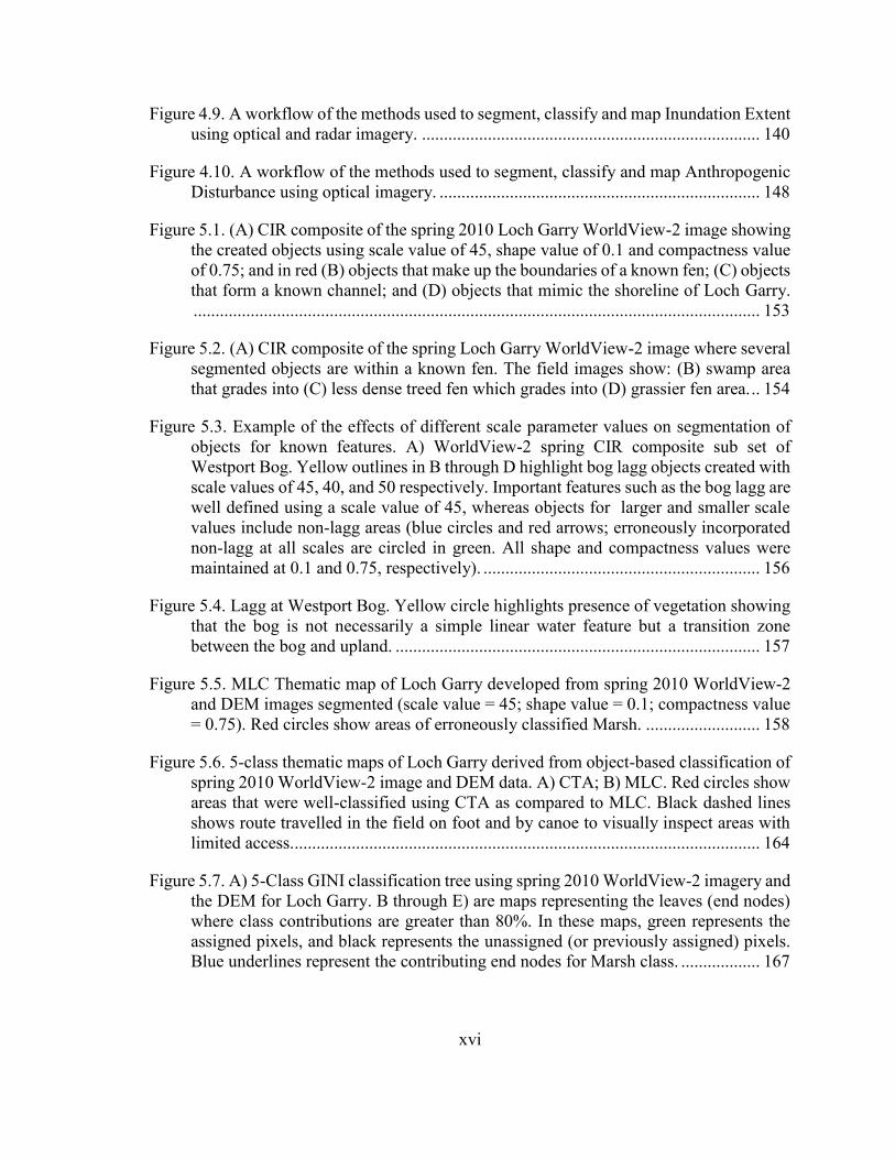
Figure 5.1. (A) CIR composite of the spring 2010 Loch Garry WorldView-2 image showing the created objects using scale value of 45, shape value of 0.1 and compactness value of 0.75; and in red (B) objects that make up the boundaries of a known fen; (C) objects that form a known channel; and (D) objects that mimic the shoreline of Loch Garry. ................................................................................................................................. 153
Figure 5.2. (A) CIR composite of the spring Loch Garry WorldView-2 image where several segmented objects are within a known fen. The field images show: (B) swamp area that grades into (C) less dense treed fen which grades into (D) grassier fen area. .. 154
Figure 5.3. Example of the effects of different scale parameter values on segmentation of objects for known features. A) WorldView-2 spring CIR composite sub set of Westport Bog. Yellow outlines in B through D highlight bog lagg objects created with scale values of 45, 40, and 50 respectively. Important features such as the bog lagg are well defined using a scale value of 45, whereas objects for larger and smaller scale values include non-lagg areas (blue circles and red arrows; erroneously incorporated non-lagg at all scales are circled in green. All shape and compactness values were maintained at 0.1 and 0.75, respectively). ............................................................... 156
Figure 5.4. Lagg at Westport Bog. Yellow circle highlights presence of vegetation showing that the bog is not necessarily a simple linear water feature but a transition zone between the bog and upland. ................................................................................... 157
Figure 5.5. MLC Thematic map of Loch Garry developed from spring 2010 WorldView-2 and DEM images segmented (scale value = 45; shape value = 0.1; compactness value = 0.75). Red circles show areas of erroneously classified Marsh. .......................... 158
Figure 5.6. 5-class thematic maps of Loch Garry derived from object-based classification of spring 2010 WorldView-2 image and DEM data. A) CTA; B) MLC. Red circles show areas that were well-classified using CTA as compared to MLC. Black dashed lines shows route travelled in the field on foot and by canoe to visually inspect areas with limited access........................................................................................................... 164
Figure 5.7. A) 5-Class GINI classification tree using spring 2010 WorldView-2 imagery and the DEM for Loch Garry. B through E) are maps representing the leaves (end nodes) where class contributions are greater than 80%. In these maps, green represents the assigned pixels, and black represents the unassigned (or previously assigned) pixels. Blue underlines represent the contributing end nodes for Marsh class. .................. 167
xvii
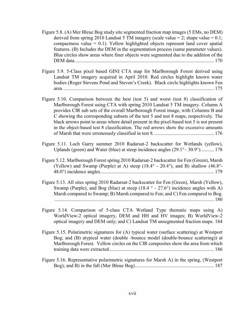
Figure 5.8. (A) Mer Bleue Bog study site segmented fraction map images (5 EMs, no DEM) derived from spring 2010 Landsat 5 TM imagery (scale value = 2; shape value = 0.1; compactness value = 0.1). Yellow highlighted objects represent land cover spatial features. (B) Includes the DEM in the segmentation process (same parameter values). Blue circles show areas where finer objects were segmented due to the addition of the DEM data................................................................................................................. 170
Figure 5.9. 5-Class pixel based GINI CTA map for Marlborough Forest derived using Landsat TM imagery acquired in April 2010. Red circles highlight known water bodies (Roger Stevens Pond and Steven’s Creek). Black circle highlights known Fen area. ......................................................................................................................... 175
Figure 5.10. Comparison between the best (test 5) and worst (test 8) classification of Marlborough Forest using CTA with spring 2010 Landsat 5 TM imagery. Column A provides CIR sub sets of the overall Marlborough Forest image, with Columns B and C showing the corresponding subsets of the test 5 and test 8 maps, respectively. The black arrows point to areas where detail present in the pixel-based test 5 is not present in the object-based test 8 classification. The red arrows show the excessive amounts of Marsh that were erroneously classified in test 8. ................................................ 176
Figure 5.11. Loch Garry summer 2010 Radarsat-2 backscatter for Wetlands (yellow), Uplands (green) and Water (blue) at steep incidence angles (29.1°– 30.9°). .......... 178
Figure 5.12. Marlborough Forest spring 2010 Radarsat-2 backscatter for Fen (Green), Marsh (Yellow) and Swamp (Purple) at A) steep (18.4° - 20.4°), and B) shallow (46.8°- 48.0°) incidence angles. ........................................................................................... 179
Figure 5.13. All sites spring 2010 Radarsat-2 backscatter for Fen (Green), Marsh (Yellow), Swamp (Purple), and Bog (blue) at steep (18.4 ° - 27.6°) incidence angles with A) Marsh compared to Swamp; B) Marsh compared to Fen; and C) Fen compared to Bog. ................................................................................................................................. 180
Figure 5.14. Comparison of 5-class CTA Wetland Type thematic maps using A) WorldView-2 optical imagery, DEM and HH and HV images; B) WorldView-2 optical imagery and DEM only; and C) Landsat TM unsegmented fraction maps. 184
Figure 5.15. Polarimetric signatures for (A) typical water (surface scattering) at Westport Bog; and (B) atypical water (double -bounce model (double-bounce scattering)) at Marlborough Forest. Yellow circles on the CIR composites show the area from which training data were extracted. .................................................................................... 186
Figure 5.16. Representative polarimetric signatures for Marsh A) in the spring, (Westport Bog); and B) in the fall (Mer Bleue Bog)................................................................ 187
xviii
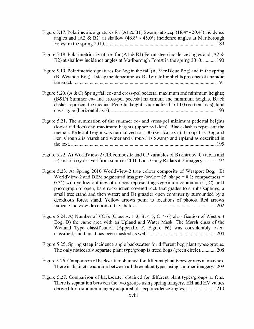
Figure 5.17. Polarimetric signatures for (A1 & B1) Swamp at steep (18.4° - 20.4°) incidence angles and (A2 & B2) at shallow (46.8° - 48.0°) incidence angles at Marlborough Forest in the spring 2010. ........................................................................................ 189
Figure 5.18. Polarimetric signatures for (A1 & B1) Fen at steep incidence angles and (A2 & B2) at shallow incidence angles at Marlborough Forest in the spring 2010. .......... 190
Figure 5.19. Polarimetric signatures for Bog in the fall (A, Mer Bleue Bog) and in the spring (B, Westport Bog) at steep incidence angles. Red circle highlights presence of sporadic tamarack. ................................................................................................................. 191
Figure 5.20. (A & C) Spring/fall co- and cross-pol pedestal maximum and minimum heights; (B&D) Summer co- and cross-pol pedestal maximum and minimum heights. Black dashes represent the median. Pedestal height is normalized to 1.00 (vertical axis); land cover type (horizontal axis). .................................................................................... 193
Figure 5.21. The summation of the summer co- and cross-pol minimum pedestal heights (lower red dots) and maximum heights (upper red dots). Black dashes represent the median. Pedestal height was normalized to 1.00 (vertical axis). Group 1 is Bog and Fen, Group 2 is Marsh and Water and Group 3 is Swamp and Upland as described in the text. .................................................................................................................... 195
Figure 5.22. A) WorldView-2 CIR composite and CP variables of B) entropy, C) alpha and D) anisotropy derived from summer 2010 Loch Garry Radarsat-2 imagery. ......... 197
Figure 5.23. A) Spring 2010 WorldView-2 true colour composite of Westport Bog; B) WorldView-2 and DEM segmented imagery (scale = 25, shape = 0.1; compactness = 0.75) with yellow outlines of objects representing vegetation communities; C) field photograph of open, bare rock/lichen covered rock that grades to shrubs/saplings, a small tree stand and then water; and D) grassier open community surrounded by a deciduous forest stand. Yellow arrows point to locations of photos. Red arrows indicate the view direction of the photos. ................................................................ 202
Figure 5.24. A) Number of VCFs (Class A: 1-3; B: 4-5; C: > 6) classification of Westport Bog; B) the same area with an Upland and Water Mask. The Marsh class of the Wetland Type classification (Appendix F, Figure F6) was considerably over-classified, and thus it has been masked as well. ...................................................... 204
Figure 5.25. Spring steep incidence angle backscatter for different bog plant types/groups. The only noticeably separate plant type/group is treed bogs (green circle). ........... 208
Figure 5.26. Comparison of backscatter obtained for different plant types/groups at marshes. There is distinct separation between all three plant types using summer imagery. 209
Figure 5.27. Comparison of backscatter obtained for different plant types/groups at fens. There is separation between the two groups using spring imagery. HH and HV values derived from summer imagery acquired at steep incidence angles. ........................ 210
xix
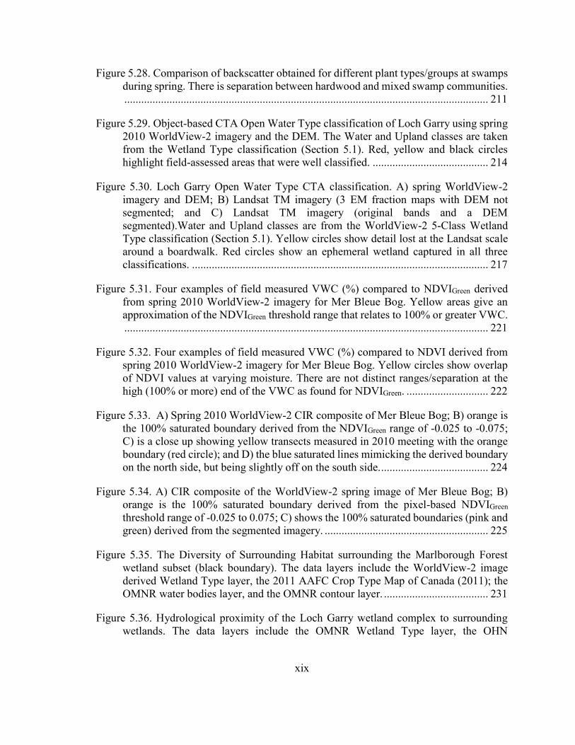
Figure 5.28. Comparison of backscatter obtained for different plant types/groups at swamps during spring. There is separation between hardwood and mixed swamp communities. ................................................................................................................................. 211
Figure 5.29. Object-based CTA Open Water Type classification of Loch Garry using spring 2010 WorldView-2 imagery and the DEM. The Water and Upland classes are taken from the Wetland Type classification (Section 5.1). Red, yellow and black circles highlight field-assessed areas that were well classified. ......................................... 214
Figure 5.30. Loch Garry Open Water Type CTA classification. A) spring WorldView-2 imagery and DEM; B) Landsat TM imagery (3 EM fraction maps with DEM not segmented; and C) Landsat TM imagery (original bands and a DEM segmented).Water and Upland classes are from the WorldView-2 5-Class Wetland Type classification (Section 5.1). Yellow circles show detail lost at the Landsat scale around a boardwalk. Red circles show an ephemeral wetland captured in all three classifications. ......................................................................................................... 217
Figure 5.31. Four examples of field measured VWC (%) compared to NDVIGreen derived from spring 2010 WorldView-2 imagery for Mer Bleue Bog. Yellow areas give an approximation of the NDVIGreen threshold range that relates to 100% or greater VWC. ................................................................................................................................. 221
Figure 5.32. Four examples of field measured VWC (%) compared to NDVI derived from spring 2010 WorldView-2 imagery for Mer Bleue Bog. Yellow circles show overlap of NDVI values at varying moisture. There are not distinct ranges/separation at the high (100% or more) end of the VWC as found for NDVIGreen. ............................. 222
Figure 5.33. A) Spring 2010 WorldView-2 CIR composite of Mer Bleue Bog; B) orange is the 100% saturated boundary derived from the NDVIGreen range of -0.025 to -0.075; C) is a close up showing yellow transects measured in 2010 meeting with the orange boundary (red circle); and D) the blue saturated lines mimicking the derived boundary on the north side, but being slightly off on the south side. ...................................... 224
Figure 5.34. A) CIR composite of the WorldView-2 spring image of Mer Bleue Bog; B) orange is the 100% saturated boundary derived from the pixel-based NDVIGreen threshold range of -0.025 to 0.075; C) shows the 100% saturated boundaries (pink and green) derived from the segmented imagery. .......................................................... 225
Figure 5.35. The Diversity of Surrounding Habitat surrounding the Marlborough Forest wetland subset (black boundary). The data layers include the WorldView-2 image derived Wetland Type layer, the 2011 AAFC Crop Type Map of Canada (2011); the OMNR water bodies layer, and the OMNR contour layer. ..................................... 231
Figure 5.36. Hydrological proximity of the Loch Garry wetland complex to surrounding wetlands. The data layers include the OMNR Wetland Type layer, the OHN
xx
watercourses layer; the OMNR water bodies layer, and original Loch Garry boundary layer. ........................................................................................................................ 232
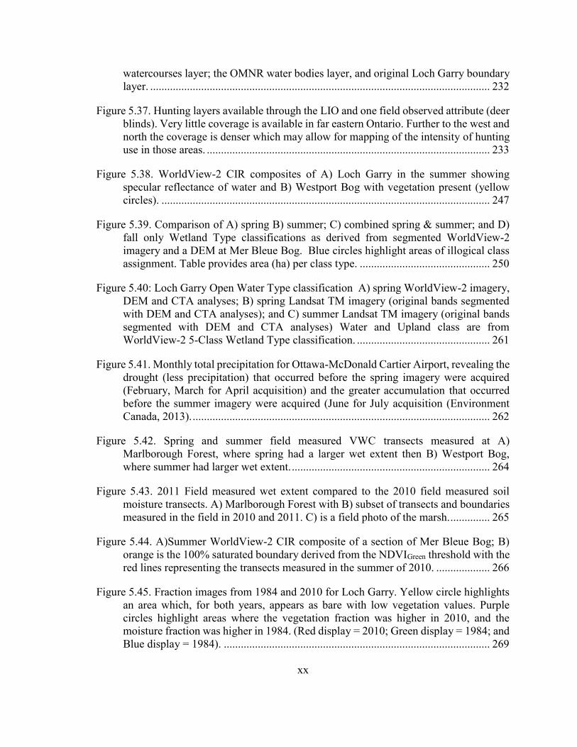
Figure 5.37. Hunting layers available through the LIO and one field observed attribute (deer blinds). Very little coverage is available in far eastern Ontario. Further to the west and north the coverage is denser which may allow for mapping of the intensity of hunting use in those areas. .................................................................................................... 233
Figure 5.38. WorldView-2 CIR composites of A) Loch Garry in the summer showing specular reflectance of water and B) Westport Bog with vegetation present (yellow circles). .................................................................................................................... 247
Figure 5.39. Comparison of A) spring B) summer; C) combined spring & summer; and D) fall only Wetland Type classifications as derived from segmented WorldView-2 imagery and a DEM at Mer Bleue Bog. Blue circles highlight areas of illogical class assignment. Table provides area (ha) per class type. .............................................. 250
Figure 5.40: Loch Garry Open Water Type classification A) spring WorldView-2 imagery, DEM and CTA analyses; B) spring Landsat TM imagery (original bands segmented with DEM and CTA analyses); and C) summer Landsat TM imagery (original bands segmented with DEM and CTA analyses) Water and Upland class are from WorldView-2 5-Class Wetland Type classification. ............................................... 261
Figure 5.41. Monthly total precipitation for Ottawa-McDonald Cartier Airport, revealing the drought (less precipitation) that occurred before the spring imagery were acquired (February, March for April acquisition) and the greater accumulation that occurred before the summer imagery were acquired (June for July acquisition (Environment Canada, 2013). ......................................................................................................... 262
Figure 5.42. Spring and summer field measured VWC transects measured at A) Marlborough Forest, where spring had a larger wet extent then B) Westport Bog, where summer had larger wet extent. ...................................................................... 264
Figure 5.43. 2011 Field measured wet extent compared to the 2010 field measured soil moisture transects. A) Marlborough Forest with B) subset of transects and boundaries measured in the field in 2010 and 2011. C) is a field photo of the marsh. .............. 265
Figure 5.44. A)Summer WorldView-2 CIR composite of a section of Mer Bleue Bog; B) orange is the 100% saturated boundary derived from the NDVIGreen threshold with the red lines representing the transects measured in the summer of 2010. ................... 266
Figure 5.45. Fraction images from 1984 and 2010 for Loch Garry. Yellow circle highlights an area which, for both years, appears as bare with low vegetation values. Purple circles highlight areas where the vegetation fraction was higher in 2010, and the moisture fraction was higher in 1984. (Red display = 2010; Green display = 1984; and Blue display = 1984). .............................................................................................. 269

xxi
Figure 5.46. A) 1984 CIR composite of Landsat TM image; B) 2010 CIR composite of Landsat TM image; and C) temporal composite (Red display = 2010; Green display = 1984; and Blue display = 1984) of vegetation fractions derived from the previous two images. The yellow circle highlights the change from water body to vegetation; and the yellow arrow points to a flooded area. .............................................................. 271
Figure 6.1. Workflow for six OWES attributes that can be implemented immediately or with some investigation (Wet Extent with existing QuickBird data). ............................. 303
xxii
LIST OF APPENDICES
APPENDIX A. Wetland Attenuation Factor scoring method…………………………….338
APPENDIX B. Field data including sites and photographs………………………………339
APPENDIX C. Training separabilities for Loch Garry spring, summer and combined imagery and segmentation scale parameter values of 25, 45 and 75…………………….365
APPENDIX D. Results from Wetland Type segmentations for Marlborough Forest, Mer Bleue Bog and Westport Bog…………………………………………………………….368
APPENDIX E. Results from CTA testing of GINI, Gain Ratio and Entropy algorithms…370
APPENDIX F. Results from Wetland Type classifications for Marlborough Forest, Mer Bleue Bog and Westport Bog…………………………………………………………….371
APPENDIX G. LSU details for all four sites………………………………………….….380
APPENDIX H. Sites and polarimetric signatures for Bog, Fen, Marsh, Swamp, Water and Upland………...………………………………………………………………………….396
APPENDIX I. Pedestal height analysis for spring and summer radar imagery…………...407
APPENDIX J. Field-measured VWC% for all four sites and two seasons……………..…411
APPENDIX K. GIS analysis for Diversity of the Surrounding Habitat and the Proximity of Other Wetlands attributes for Loch Garry, Mer Bleue Bog and Westport Bog…….......…412
APPENDIX L. Multi-season WorldView-2 CTA results for Number of VCFs, VCFs and Open Water Types for Loch Garry, Marlborough Forest and Westport Bog……………..418
APPENDIX M. Relative calibration data for temporal analysis of Landsat 5 TM vegetation fraction images …………………………………………………..………………………421
xxiii
LIST OF ACRONYMS
AIRSAR Airborne Synthetic Aperture Radar
ALOS Advanced Land Observing Satellite
ANN Artificial Neural Network
ASTER Advanced Spaceborne Thermal Emission and Reflection Radiometer
AVHRR Advanced Very High Resolution Radiometer
BRDF Bidirectional Reflectance Distribution Function
CA Conservation Authority
CAA Conservation Authorities Act
CART Classification and Regression Tree
CIR Colour-infrared
COA Canada-Ontario Agreement Respecting the Great Lakes Basin Ecosystem
Co-Pol Co-polarisation
CP Cloude-Pottier
Cross-Pol Cross-polarisation
CTA Classification Tree Analysis
CWI Canadian Wetland Inventory
DEM Digital Elevation Model
DRAPE Digital Raster Acquisition Project for the East
DTW Depth to Water
EM Endmembers
ERS-1 European Remote Sensing Satellite

xxiv
ET Evapotranspiration
ETM+ Enhanced Thematic Mapper +
ESP Estimation of Scale Parameter
FNEA Fractal Net Evolution Approach
GIS Geographic Information Systems
GLWCAP Great Lakes Wetland Conservation Action Plan
GPS Global Positioning System
GLCM Grey level co-occurrence matrix
HEP Habitat Evaluation Procedure
HGM Hydrogeomorphic Classification for Wetlands
HH, HV, VH, VV Various forms of co- and cross-polarisation (H=Horizontal, V=Vertical)
IEA Iterative Error Analysis
IRS Indian Remote Sensing
ISODATA Iterative Self-Organizing Data Analysis Technique
JERS-1 Japanese Earth Resources Satellite
LiDAR Light detection and ranging
LIO Land Information Ontario
LSU Linear Spectral Unmixing
LULC Land use land cover
MCARI Modified Chlorophyll Absorption Ratio Index
MEIS-II Multispectral Electro optical Imaging Scanner
MERIS MEdium Resolution Imaging Spectrometer
MIR Mid-infrared
MLC Maximum Likelihood Classification
xxv
MMU Minimum Mapping Unit
MODIS Moderate Resolution Imaging Spectroradiometer
MSS Multi-spectral scanner
NAPP Net Aerial Primary Production
NASA National Aeronautics and Space Administration
NDVI Normalized Difference Vegetation Index
NDWI Normalized Difference Water Index
NHIC Natural Heritage Information Centre
NIR Near-infrared
NRVIS Natural Resources Values and Information System
OBIA Object-based Image Analysis
OBM Ontario Base Maps
OMNR Ontario Ministry of Nature Resources
OWES Ontario Wetland Evaluation System
PA Producer’s Accuracy
PAD Peace-Athabasca River Delta
PALSAR Phased Array L-band Synthetic Aperture Radar
PAN Panchromatic
PCC Pixels Correctly Classified
PIF Pseudo-invariant Features
RF Random Forest
RMSE Root Mean Square Error
SAR Synthetic Aperture Radar
SIR Shuttle Imaging Radar
xxvi
SOLRIS Southern Ontario Land Resources Information Systems
SOWCA Southern Ontario Wetland Conversion Analysis
SPOT Système Pour l'Observation de la Terre
SRTM Shuttle Radar Topography Mission
SVM Support Vector Machine
SWI Soil Water Index
SWIR Short-Wavelength Infrared
TM Thematic Mapper
TP Total Power
TPH Total Petroleum Hydrocarbons
TSI Topographic Soils Index
UA User’s Accuracy
UTM Universal Transverse Mercator
VCF Vegetation Community Forms
VIS Visible portion of the electromagnetic spectrum
VWC Volumetric soil water content
VWI Vegetation-water index
WGS World Geodetic System
1
1.0 Introduction
Wetlands are dynamic ecosystems with climatic, geomorphologic, biological and
hydrologic influences (National Wetlands Working Group, 1997). Through these natural and
anthropogenic forces wetlands are constantly changing (Foley et al., 2005; Mitsch and
Gosselink, 2007). Wetlands provide benefits including functions that are described as “the
things that wetlands do” (Bartoldus, 1999) such as: flood water control, ground water
recharge and discharge, nutrient, sediment, and contaminant retention, food web support,
shoreline stabilization, erosion control, storm protection, stabilization of local climatic
conditions, water transport, wildlife habitat, etc. (Lodge et al., 1995; Hruby et al., 1998;
Thiesing, 2001; OWES, 2002; Carletti et al., 2004; Papas and Holmes, 2007). Wetlands also
provide values such as products or services which include recreational, cultural, heritage,
educational, and aboriginal use, fisheries, water supply, wildlife, forage, agricultural, and
forest resources, etc. (Roth et al., 1996; Bartoldus, 1999; OWES, 2002; Carletti et al., 2004;
Papas and Holmes, 2007). These many functions and values and the dynamic nature of
wetlands highlight the need to monitor and manage wetlands at the local, national, and global
levels. Evaluating wetlands hierarchically top-down from the general to the more specific,
from ecological processes to wetland attributes to spatial patterns is one approach. This is in
contrast to bottom-up from the specific to the general, linking spatial pattern to wetland
attributes to ecological processes.
Ecological processes in wetlands operate over multiple spatial, temporal, and
organizational scales and include such things as nutrient cycling, succession, hydrologic

2
functioning (Smith et al., 2008; Castaneda and Herrero, 2008; Lang and Kasischke, 2008;
Pavelsky and Smith, 2008; Dewan and Yamaguchi, 2009). Attributes such as flood
attenuation, wetland diversity, etc. are used as indicators of these processes. Attributes can
also be indicators of site characteristics. High biomass such as peat can indicate a mature
ecosystem (Mitsch and Gosselink, 2007). Pattern can be used to assess these attributes. For
example, attributes of wetlands, vegetation composition and structure, etc. are used as
indicators of wetland diversity. Therefore through mapping of the attributes, knowledge
about the processes that are occurring within wetland complexes can be obtained. Wetland
complexes can be described as dense and/or proximal groupings of wetland types (e.g. bog,
fen, swamp, marsh) with functional relationships where each wetland unit contributes to the
whole complex, thus making it important to consider all units together (OWES, 2002). A
key assumption is that wetland processes can be used as indicators of wetland health and
functioning and therefore, in wetland evaluation systems, the presence or degree of presence
of these processes can be used in land management.
The Ontario Wetland Evaluation System (OWES) is used by the Ontario Ministry of
Natural Resources (OMNR) for the evaluation and scoring of wetlands in Ontario. The
method assesses functions of wetlands in ecological processes, and the social and economic
values wetlands provide to humans in four major components: Biological, Hydrologic,
Social and Special Features. Components are comprised of sub-components and ‘attributes’
and in the OWES some attributes describe ecological processes directly, while others
describe wetland characteristics from which a process or an evaluation of the state of a
3
process can be inferred. The current system is costly, and evaluations quickly become
obsolete. Remote sensing is one way that wetland attributes can be monitored across
wetlands and has many advantages over traditional field based methods (Lee and Lunetta,
1995; Ramsey, 1998; Ozesmi and Bauer, 2002; Mitsch and Gosselink, 2007). This research,
in collaboration with the OMNR, was designed to develop and review remote sensing and
geographic information systems (GIS) methods for wetland attribute classification. The
attributes considered in this research and selected from the OWES included: Wetland Type,
Vegetation Community Forms (VCFs), Open Water Type, Inundation Extent, Number of
Wetland Types, Diversity of Surrounding Habitat, Proximity to Other Wetlands, Wetland
Size, Hunting, Ownership Patterns, Wetland Basin Size, Rarity of the Wetland in the
Landscape, Rarity of Wetland, and Anthropogenic Disturbance. The selection of these 14
attributes was made based upon their potential to be assessed using remote sensing and GIS
and their overall contribution to the OWES score for a given wetland.
1.1 Research goal
The overall goal of this research was to determine the potential to map OWES
attributes in wetland complexes using spatial patterns extracted from remote sensing and
other geospatial data using two imagery types, optical and radar, at multiple spatial, spectral
and temporal resolutions and extents. From this, knowledge gained on how the mapping of
the attributes differ with changing spatial, spectral and temporal resolution can be applied to
wetland status evaluation and land management planning.

4
1.2 Research objectives
Objective 1 of this research was to map selected OWES attributes that have known
wetland pattern-attribute associations. The spatial and spectral resolutions and extents for
which the results were most accurate were then determined.
Objective 2 was to compare and relate the scores determined for each of these
attributes to field-evaluated OWES scores to determine if these methods can be related to,
and/or integrated into the existing evaluation system.
Objective 3 was to assess temporal remote sensing data in classification of the
wetland attributes and analyze attribute changes over two decades.
1.3 Research contributions
The overall scope of this research is large and unique as it includes multiple attributes
across varying natural and human-constructed components of wetlands incorporating
analyses of imagery type, resolution and spatial extent; seasonality and temporal change;
remote sensing and GIS methods; and applying this information to an existing wetland
management system for a spatially diverse region. This research contributes to the general
body of knowledge of wetland science and in particular, the use of remote sensing and GIS
to map wetlands attributes. This research also provided direction and contributions to the
existing wetland status evaluation methodology currently in use in Ontario, Canada.
5
1.4 Thesis structure
This thesis follows a traditional structure beginning with this introductory chapter.
Chapter 2 contains the background information on wetlands in general, including an
understanding of wetlands worldwide, in Canada and in particular the history and
management of wetlands in Ontario. The chapter next provides an overview of the existing
field-based methods to classify wetlands. Chapter 2 continues with an overview on remote
sensing of wetlands, GIS analysis of wetlands, and remote sensing of hydrology and forestry
as it relates to this research. Next, more specific background is given for general remote
sensing and GIS methods and data types used for this wetland analyses. Finally, the remote
sensing methods used to assess the 14 attributes are described, the general background on
the methods chosen for this research is provided, and a description of the OWES attributes
scoring methods for analysis is given. Chapter 3 provides the details on the study sites, and
the remote sensing and GIS data used for this research.
For clarity and consistency all further chapters are organized in modular format by
objective as listed above. For any repetitive information (e.g. method used), the reader will
be instructed to review the pertinent area of the previous section that contained the same
information. Chapter 4 provides the methods that were carried out for each objective.
Chapter 5 presents the results of the attribute mapping, the findings in relation to the
application of these methods in the OWES evaluation system and the temporal analysis. The
discussion of these findings is found in Chapter 6, with a complete appraisal of the benefits

6
and limitations of this research and recommendations for implementation of the findings.
Chapter 6 then summarizes the thesis and provides the conclusions and future directions.
Figure 1.1 provides a conceptual flow chart of the research and thesis structure.
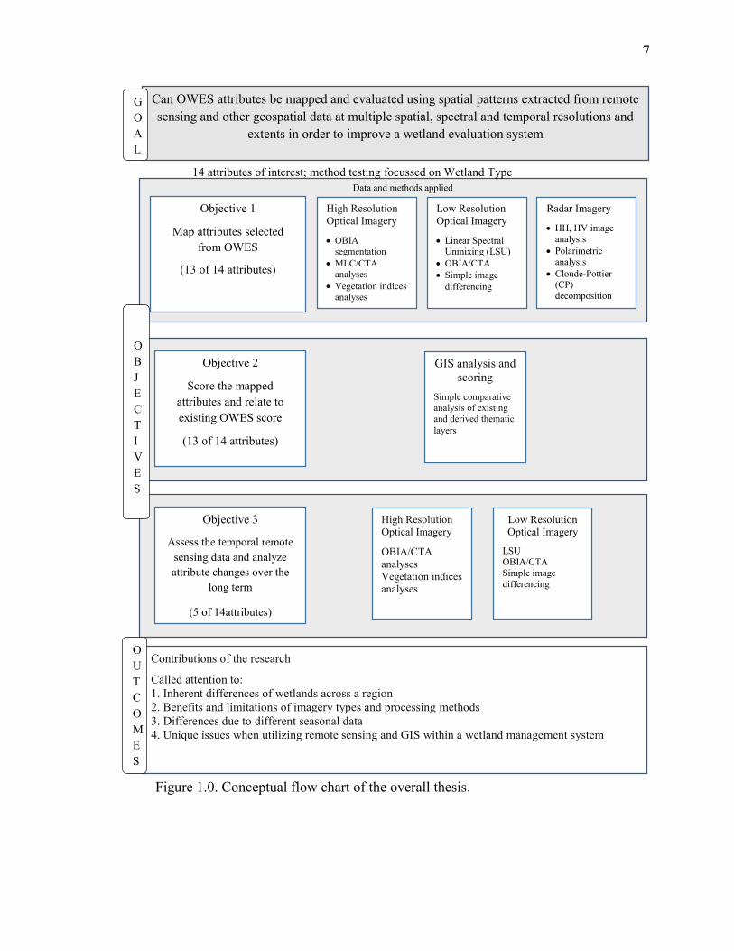
7
Can OWES attributes be mapped and evaluated using spatial patterns extracted from remote sensing and other geospatial data at multiple spatial, spectral and temporal resolutions and
extents in order to improve a wetland evaluation system
Contributions of the research
Called attention to: 1. Inherent differences of wetlands across a region 2. Benefits and limitations of imagery types and processing methods 3. Differences due to different seasonal data 4. Unique issues when utilizing remote sensing and GIS within a wetland management system
Objective 2
Score the mapped attributes and relate to existing OWES score
(13 of 14 attributes)
GIS analysis and scoring
Simple comparative analysis of existing and derived thematic layers
High Resolution Optical Imagery
OBIA segmentation
MLC/CTA analyses
Vegetation indices analyses
Low Resolution Optical Imagery
Linear Spectral Unmixing (LSU)
OBIA/CTA Simple image
differencing
Radar Imagery
HH, HV image analysis
Polarimetric analysis
Cloude-Pottier (CP) decomposition
Objective 3
Assess the temporal remote sensing data and analyze attribute changes over the
long term
(5 of 14attributes)
High Resolution Optical Imagery
OBIA/CTA analyses Vegetation indices analyses
Low Resolution Optical Imagery
LSU OBIA/CTA Simple image differencing
OBJECTIVES
GOAL
14 attributes of interest; method testing focussed on Wetland Type
Objective 1
Map attributes selected from OWES
(13 of 14 attributes)
OUTCOMES
Figure 1.0. Conceptual flow chart of the overall thesis.
Data and methods applied
8
2.0 Background
This chapter gives the definitions of wetlands and common wetland types, and it
describes the overall function of wetlands in the context of the OWES. Scale is defined as it
relates to this research, and describes the pattern-attribute-process relationship. The chapter
then reviews the literature on sensor and imagery types as well as the image analyses and
GIS methods that have been used in past efforts to map the 14 wetland attributes of this
research, with emphasis on those sensors and methods that were employed in this research.
2.1 Functional description of wetlands
The Convention on Wetlands is an intergovernmental treaty that was developed at
Ramsar, Iran in 1971. It provides a framework for the conservation of wetlands globally
(Ramsar Convention Secretariat, 2006). The Ramsar Convention Manual (2006) gives a
definition of wetlands as “Areas where water is the primary factor controlling the
environment and the associated plant and animal life. They occur where the water table is at
or near the surface of the land, or where the land is covered by shallow water.” Wetland
types are specifically defined as “Areas of marsh, fen, peatland or water, whether natural or
artificial, permanent or temporary, with water that is static or flowing, fresh, brackish or salt,
including areas of marine water, the depth of which at low tide does not exceed six metres”
(Ramsar Convention Secretariat, 2006).
Canada has had a national interest in wetlands since the 1960s and is a contracting
party of the Ramsar Convention (Ramsar Convention Secretariat, 2006). As a contracting
9
party, Canada has agreed to work towards the “wise use” of all wetlands through
management, policy and legislation; to designate suitable wetlands for the Ramsar List; and
to cooperate internationally on shared wetlands and wetland policy (Ramsar Convention
Secretariat, 2006). In total, Canada has an estimated 24% of the world’s wetlands
representing approximately 150 million hectares (National Wetlands Working Group, 1997).
Losses to Canadian wetlands are dependent upon their location. Those wetlands located in
less populated areas are less impacted than those located in more populated regions. Overall,
losses range across Canada from an estimated 65 to 85% of pre-settlement area (National
Wetlands Working Group, 1988).
In Canada, wetland management falls under the jurisdiction of the provinces while
the territories share their responsibility with the federal government, and aboriginal agencies
(Lynch-Stewart, 1994). The federal government of Canada has had a wetlands policy since
March 1992. This policy aims to ensure the conservation of wetlands to sustain both
ecological and socio-economic functions (Government of Canada, 1991). The Canadian
government defines a wetland as “land that is saturated with water long enough to promote
wetland or aquatic processes as indicated by poorly drained soils, hydrophytic vegetation
and various kinds of biological activity which are adapted to a wet environment. Wetlands
in Canada include bogs, fens, marshes, swamps and shallow waters (usually 2 m deep or
less)” (National Wetlands Working Group, 1997). This definition has been adopted by the
OWES (excluding shallow waters, OWES, 2002).
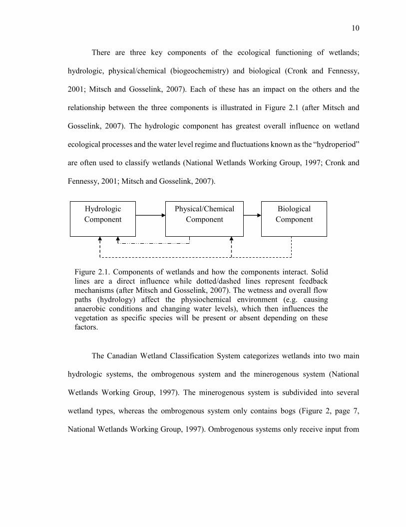
10
There are three key components of the ecological functioning of wetlands;
hydrologic, physical/chemical (biogeochemistry) and biological (Cronk and Fennessy,
2001; Mitsch and Gosselink, 2007). Each of these has an impact on the others and the
relationship between the three components is illustrated in Figure 2.1 (after Mitsch and
Gosselink, 2007). The hydrologic component has greatest overall influence on wetland
ecological processes and the water level regime and fluctuations known as the “hydroperiod”
are often used to classify wetlands (National Wetlands Working Group, 1997; Cronk and
Fennessy, 2001; Mitsch and Gosselink, 2007).
The Canadian Wetland Classification System categorizes wetlands into two main
hydrologic systems, the ombrogenous system and the minerogenous system (National
Wetlands Working Group, 1997). The minerogenous system is subdivided into several
wetland types, whereas the ombrogenous system only contains bogs (Figure 2, page 7,
National Wetlands Working Group, 1997). Ombrogenous systems only receive input from
Figure 2.1. Components of wetlands and how the components interact. Solid lines are a direct influence while dotted/dashed lines represent feedback mechanisms (after Mitsch and Gosselink, 2007). The wetness and overall flow paths (hydrology) affect the physiochemical environment (e.g. causing anaerobic conditions and changing water levels), which then influences the vegetation as specific species will be present or absent depending on these factors.
Hydrologic Component
Physical/Chemical Component
Biological Component

11
precipitation and are hydrologically isolated (National Wetlands Working Group, 1997). The
minerogenous wetland types are categorized by influences of the biological component (e.g.
vegetation present) which is affected by the physical/chemical component.
The physical/chemical component (biogeochemical cycling) of wetlands is
concerned with chemical conversions and chemical movement. These can include
movement within the soil profile, or through conversions to gases (e.g. denitrification) and
release into the atmosphere. Many of these movements, cycles and transformations are
caused by the lack of soil oxygen (i.e. anaerobic conditions) because of the overwhelming
presence of water (Smith et al., 2003). The changes and cycles then effect the vegetation
present in the system.
The biological component includes both plants and animals; however for
classification of wetlands, the focus is on the vegetative elements. For multi-cellular
vegetation, the main distinction between wetlands and other areas is the adaptation of
wetland plants (e.g. hydrophytes) to saturated conditions (Cronk and Fennessy, 2001). The
types of adapted vegetation are often used in the classification of wetlands.
2.2 Wetlands of Ontario
2.2.1 History of wetlands in Ontario
Approximately 29.2 million hectares of wetlands, approximately 20% of Canadian
and approximately 5% of the world’s wetlands are located in Ontario, the majority of which
are located in the north (National Wetlands Working Group, 1988). The losses in Ontario
12
include destruction along the Great Lakes Water Basin of approximately 72% of pre-
settlement area (National Wetlands Working Group, 1988; GLWCAP, 2012). Around major
cities in Ontario wetland losses range from approximately 37% around Kitchener up to 97%
around the city of Windsor (National Wetlands Working Group, 1988). The largest losses
were found in southwestern Ontario and some parts of eastern Ontario. Historically,
wetlands were believed to be unsuitable for use and were converted to agricultural lands,
hydro right-of ways, edge of transportation corridors and forest clearings (GLWCAP, 2012).
Several methods have been used to assess these land conversions, and the spatial trends of
wetlands in Ontario from pre-settlement to more recent times. The Snell Report
(Environment Canada, 1987) assessed these types of conversions from approximately 1800
to 1982. The Southern Ontario Wetland Conversion Analysis (SOWCA) converted the Snell
methodology to GIS-based analysis and further assessed the spatial trends in wetlands from
pre-settlement to 2002 (SOWCA, 2010). From that analysis it was found that there continues
to be losses of wetland area in Ontario of up to 0.12% per year (SOWCA, 2010).
2.2.2 OMNR role in wetland management
OMNR’s role in wetland management is a partnership between the OMNR and
wetland conservation associates such as Ducks Unlimited Canada, Nature Conservancy,
Ontario Nature, etc. Wetland protection and conservation in Ontario falls under the
Provincial Policy Statement, the Ontario government’s statement on land use planning, and
the Conservation Authorities Act (CAA). The CAA is administered by 36 Conservation
Authorities (CAs) that regulate development and activities adjacent to, and within wetlands
13
(Conservation Ontario, 2009). The OMNR wetland conservation staff is responsible for
providing policy advice and support, assisting in the development of several conservation
plans, including the Great Lakes Wetland Conservation Action Plan (GLWCAP), the North
American Waterfowl Management Plan and the Canada-Ontario Agreement Respecting the
Great Lakes Basin Ecosystem (COA), as well as in maintaining and providing training on
the existing OWES (OMNR, 2013).
2.3 Methods to evaluate wetlands
There are many different methods that are used to identify (e.g. Hydrogeomorphic
(HGM) Classification for Wetlands (Brinson, 1993)); inventory (e.g. Canadian Wetland
Inventory (CWI, Milton and Hélie, 2003)); and evaluate wetlands (e.g. Habitat Evaluation
Procedure (HEP, US Fish and Wildlife Service, 1980), among others). See Dingle
Robertson and King, 2008 for a complete review of these and other methods to that time
(available digitally with this thesis)). These methods provide information about wetland
functions and values for land management purposes (Thiesing, 2001). For the purposes of
this research, the focus is on methods used in Ontario.
2.3.1 Ontario wetland inventory schemes
The main objective of wetland inventory is to provide a visual representation, count
or catalogue of the extent and/or type of wetlands (such as bog, fen, marsh, swamp) that are
present in a landscape (Thiesing, 2001; Dahl and Watmough, 2007).
14
The Natural Resources Values and Information System (NRVIS) layers provide
coverage of the province of Ontario (NRVIS, 2002). This information was published as
OMNR Ontario Base Maps (OBM) at 1:10,000 (southern Ontario) and 1:20,000 scales
(northern Ontario) and included manually interpreted wetlands assessed from aerial
photography obtained in the spring. Newer layers include OWES evaluated wetlands that
were taken from the OMNR’s evaluated wetland files (OWES, 2002, e.g., NRVIS Wetland
Unit).
The Southern Ontario Land Resource Information System (SOLRIS, 2003) land
use/land cover classification follows the ecological land classification system for southern
Ontario (Lee et al., 1998; SOLRIS, 2008). Ecological land classifications include all
components of earth systems (e.g. air, water, land, biota, etc.) and are based upon the
hierarchical structure of ecosystems that are nested within other ecosystems (Environment
Canada, 2005). This inventory used remote sensing and spatial modelling techniques to
identify and classify wetland features at the community series level to delineate wetlands
not previously inventoried by NRVIS (“Unevaluated Wetlands”) and to identify ephemeral
wetlands. Data used included Landsat, Radarsat, and Indian Remote Sensing (IRS) imagery
(23 m, multispectral), OMNR Forest Resources Inventory photos, CIR (colour-infrared)
aerial photos, high and medium precision DEMs (Digital Elevation Models), a topographic
soils index (TSI) derived from OBM contours and a quaternary geology layer, and the
NRVIS layers for Wetlands, Open Water and Wooded Area, (SOLRIS, 2003). This adaptive
method was applied to a reference site to compare with wetland evaluations obtained through
15
fieldwork, OWES derived maps, and the NRVIS Wetland layer. The overall accuracy
between the two classes of Wetland and Upland was approximately 90% utilizing one
reference site near Bolton, Ontario (906 ha). Using only the high precision DEM method,
overall accuracy was for the two classes were 82%. The research presented in this thesis was
designed to classify individual Wetland Types such as Bog, Fen, Marsh and Swamp through
the use of higher resolution imagery.
SOLRIS layers are currently used in the Canadian Wetland Inventory
(http://maps.ducks.ca/cwi/). The OMNR has merged all existing wetland layers for Ontario
(specifically NRVIS and SOLRIS) to create one layer representing the most up-to-date,
accurate wetland information.
2.3.2 Ontario wetland evaluations
Functional wetland evaluations investigate the functions that wetlands provide. They
are often model-based and allow for a high degree of reproducibility and predictable
outcomes (Thiesing, 2001). The methods and models applied can be based on current/recent
field data, existing archived data or a combination of both. Other components that are not
considered to be wetland functions can be included, but the majority of elements assessed
are functional. The general expertise needed to perform these evaluations ranges from
trained lay persons to specialists in geology, hydrology and/or ecology (wetland scientists)
(Smith et al., 1995; Bartoldus, 1999). These methods can assess individual wetlands to
wetland-complexes across regions.
16
To respond to the illustrated conversion of wetland land cover, and wetland losses
modeled in the Snell Report (Environment Canada, 1987), the OMNR developed the OWES.
This functional method assessed ecological processes, with the addition of several social and
economic values, evaluated in four categories: Biological, Hydrologic, Social and Special
Features. Each category’s particular functions and/or values were selected based upon
consultation with experts and are typically characteristic of Ontario wetland ecosystems
(OWES, 2002). Scores are derived for each function/value and are subsequently summed
for each category and then for the entire wetland. Provincial ‘significance’ is given based
upon the total score for all four categories (or if the total value of the "Special Features"
category is higher than 250). The significance designation allows for the protection of the
wetland and for special consideration to be given during development. The OWES adopted
generalized categories of four Wetland Types outlined in Table 2.1.
The Biological component of the OWES consists of three sub-components:
productivity, biodiversity and size. The Social component evaluates the values that wetlands
provide to humans including economically valuable products, recreational activities,
landscape aesthetics, education and public awareness, proximity to areas of human
settlement, ownership, aboriginal values and cultural heritage. The Hydrologic component
has categories of flood attenuation, water quality improvement, carbon sink, shoreline
erosion control, groundwater recharge. The Special Features component contains classes of
rarity, significant features and habitat, ecosystem age, and Great Lakes coastal wetlands.
Under each of these subcategories there are attributes that are assessed in the field or through
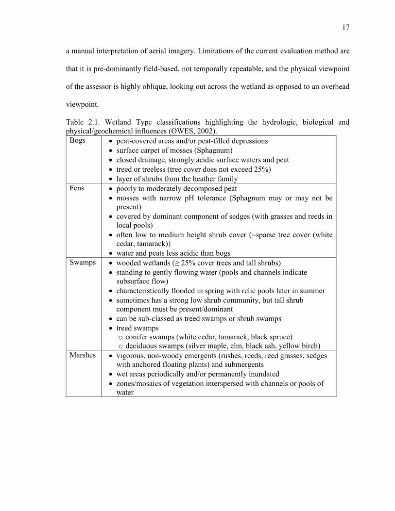
17
a manual interpretation of aerial imagery. Limitations of the current evaluation method are
that it is pre-dominantly field-based, not temporally repeatable, and the physical viewpoint
of the assessor is highly oblique, looking out across the wetland as opposed to an overhead
viewpoint.
Table 2.1. Wetland Type classifications highlighting the hydrologic, biological and physical/geochemical influences (OWES, 2002). Bogs peat-covered areas and/or peat-filled depressions
surface carpet of mosses (Sphagnum) closed drainage, strongly acidic surface waters and peat treed or treeless (tree cover does not exceed 25%) layer of shrubs from the heather family
Fens poorly to moderately decomposed peat mosses with narrow pH tolerance (Sphagnum may or may not be
present) covered by dominant component of sedges (with grasses and reeds in
local pools) often low to medium height shrub cover (~sparse tree cover (white
cedar, tamarack)) water and peats less acidic than bogs
Swamps wooded wetlands (≥ 25% cover trees and tall shrubs) standing to gently flowing water (pools and channels indicate
subsurface flow) characteristically flooded in spring with relic pools later in summer sometimes has a strong low shrub community, but tall shrub
component must be present/dominant can be sub-classed as treed swamps or shrub swamps treed swamps o conifer swamps (white cedar, tamarack, black spruce) o deciduous swamps (silver maple, elm, black ash, yellow birch)
Marshes vigorous, non-woody emergents (rushes, reeds, reed grasses, sedges with anchored floating plants) and submergents
wet areas periodically and/or permanently inundated zones/mosaics of vegetation interspersed with channels or pools of
water
18
Some of the categories and scoring methods are qualitative and subjective, and some
of the attributes that have been historically scored in the OWES cannot be detected directly
or indirectly using remotely sensed imagery. Additionally, OWES evaluations are limited to
a single measurement and observational scale, and depending upon the location in Ontario
and the availability of funds, there has been little temporal repetition of these evaluations
over the last 20-30 years.
2.4 Wetland attributes typically measured in the field that have shown potential for estimation using remote sensing
There are many methods used in the field to measure different wetland attributes.
Bio-assessments are based on the premise that the biotic community found in a wetland
reflects its overall health or condition (Papas and Holmes, 2007). As wetlands are altered,
the diversity of the biotic component typically declines and the species composition changes.
Often, terms such as “biotic integrity”, “ecological integrity”, “biological condition”
(Adamus, 1995) are associated with bio-assessments. These types of methods are most
commonly based on metrics that characterize the abundance, diversity and distribution of
plants and animals. Although habitat maps derived from remote sensing and GIS are used in
conjunction with field-based data, generally it is not possible to assess other information
about animals with geo-spatial data. One of the most straightforward and common attributes
that can be detected and analysed using remotely sensed images are the biomass, abundance,
diversity and distribution of vegetation.
19
For example, Hardisky et al. (1984) used a hand-held spectroradiometer to mimic
three of the Landsat TM (Thematic Mapper) 4 bands (red, NIR (near-infrared), MIR (mid-
infrared)) and regressed spectral indices such as NDVI (Normalized Difference Vegetation
Index), and an infrared index where MIR was substituted for RED in the traditional NDVI
equation, against biomass found in salt-marshes. They then used the models to predict
above-ground biomass derived from clipped samples of live and dead vegetation, and net
aerial primary production (NAPP). The MIR-based index provided a better biomass model
for sampling done from May through July while NDVI was better for biomass sampled
between August to October, however both indices underestimated NAPP.
Li et al. (2007) had found in the literature that there were strong positive and linear
correlations between biomass and backscatter of SAR (synthetic aperture radar). They
compared Radarsat-1 backscatter and Landsat TM NDVI in regression modelling of
mangrove biomass in the Pearl River Delta region of China. Overall, Radarsat-1 provided a
more accurate model and increasing backscatter was well correlated with increasing
biomass.
Dillabaugh and King (2008) used IKONOS imagery to model field sampled biomass
in three riparian marshes, in eastern Ontario. They extracted GLCM (Grey level co-
occurrence matrix) image textures such as Homogeneity, Contrast, Dissimilarity, etc. using
two window sizes (3 x 3 and 5 x 5) and several vegetation indices from the imagery. Using
stepwise regression they obtained a highly significant model that was subsequently used to
map continuous biomass distribution in the three wetlands. However, due to an RMSE (root
20
mean square error) of about 40% (relative to the mean field measured biomass), they
aggregated the data into three classes of biomass (high, medium, low) to produce a map that
corresponded well to the known spatial distribution of biomass in the wetlands. Biomass
mapping was not undertaken in this research
There have been many studies that have attempted to map Wetland Types and
vegetation abundance, diversity, structure and distribution to varying degrees of success
using methods such as pattern prediction of plant species, habitat quality assessment and
diversity, interpolation of soil pH distribution in combination with thematic maps to assess
species distribution of mangroves, mapping wetland area using a Bayesian probability model
as a post-classifier to improve the quality of a thematic map, and using DEMs derived from
high resolution LiDAR data to improve classification of Wetland Type mapping (Pope et
al., 1997; Baghdadi et al., 2001; Harvey and Hill, 2003; O’Hara et al., 2003; Berberoglu et
al., 2004; Rogers and Kearney, 2004; Racine et al., 2005; Schmid et al.., 2005; Belluco et
al., 2006; Chiu and Couloigner, 2006; Filippi and Jensen, 2006; Durieux et al., 2007; Grenier
et al., 2007; Ghioca-Robrecht et al., 2008; Laba et al., 2008; Bourgeau-Chavez et al., 2010;
Melendez-Pastor et al., 2010; Dribault et al., 2012; Bourgeau-Chavez et al., 2013; Evans
and Costa, 2013). Accuracies for these studies range from 70% to 100% depending on the
image type, method used and number of class types. Further description of some of these
studies are found in Tables 2.2 and 2.3.
For wetland hydrologic function, attributes that are commonly assessed in the field
such as soil moisture and wet extent have also been successfully mapped using remote
21
sensing. For example, Quinton et al. (2003) determined the relationships between fen and
bog cover types and runoff discharged from the Liard river drainage basin in the Northwest
Territories, Canada. Land cover was classified using IKONOS and Landsat images.
Additional data layers included topographic data to compute drainage area, density and
average slope. Stream discharge was monitored at gauging stations. Using both land cover
classifications, the overall area covered by fens and bogs was estimated, as well as the
connectivity of wetland pixels in the drainage basin system. These measures were
subsequently correlated to the amount of annual runoff and a small degree of correlation was
found between annual runoff and percent cover (fens and bogs). Individually these relations
were correlated in opposite directions due to the unique hydrologic functioning of each
wetland type.
Harris et al. (2005) related changes in surface and near-surface soil moisture to
spectral characteristics of Sphagnum moss in a Welsh bog, (Cors Fochno, Britain). The
samples were saturated and kept in environmental cabinets and were allowed to dry over 15
days. They were gradually re-hydrated using rainfall simulators for 6 days until reaching full
saturation. A handheld spectroradiometer was used with wavebands between 0.35 to
2.50μm. They found that decreasing soil moisture increased VIS (visible), NIR and MIR
reflectance and there were strong correlations between soil moisture and water and
vegetation indices. Water indices (WBI, bands in the NIR), and Moisture Stress Index
(MSI)) were sensitive to reductions in soil moisture but not as sensitive to re-wetting for one
of the species. MSI gave a good indication of soil moisture conditions although that was
22
dependent on the target species. Both vegetation indices showed some indication of plant-
water stress associated with drying.
Pavelsky and Smith (2008) assessed the relationship between floodplain inundation
and river level fluctuations using MODIS (Moderate Resolution Imaging
Spectroradiometer) time series data in the Peace-Athabasca River Delta (PAD), a Ramsar
Convention wetland. Water surface elevation at four locations in the PAD was highly
correlated with MODIS inundated area generated from the NIR band for 2007 when water
levels, inundation and connectivity were high, as compared to 2006 when water levels were
lower.
2.5 Scale
Scale is central to understanding the complexity of the world’s ecosystems and
ecosystem processes (Marceau and Hay, 1999). Scale can be defined as the spatial or
temporal elements of an attribute that display discernible levels of organization (Turner et
al., 2001). It is linked to the attribute of interest and is often described as the “window” of
perception (Marceau, 1999; Marceau and Hay, 1999; Hay et al., 2003). In ecology, scale is
often characterized by the ‘grain’ which refers to the smallest spatial resolution in observed
data and the ‘extent’, which is the size of an area of interest such as the study area “window”
(Turner et al., 2001). In digital remote sensing, the nominal ground pixel size, often referred
to as the spatial resolution, is essentially interchangeable with grain (Lillesand et al., 2008).
Wu and Loucks (1995) state that the scale of observation of an attribute can act as a “blinder,
23
magnifier or filter”. The challenge is to determine the most appropriate window size or
spatial extent in which an observed attribute is most indicative of a physical ecosystem, or
of wetland attributes and processes. This research is concerned with the concepts of
measurement (resolution) scale and observational (extent) scale (Quattrochi and Goodchild,
1997). Wu and Li (2009) use a similar definition, but consider observation scale to be
resolution and geographic scale as extent. To avoid confusion, this research utilized the
definition from Quattrochi and Goodchild (1997), but in either case it is concerned with
changing resolution and extent. For example, if an attribute such as wetland type or wetland
edge/boundary is mapped from remotely sensed imagery, how does that change if the
measurement (resolution) and observational (extent) scales change? Another form of scale
that is used in geomatics is geographic scale which is the relationship between a distance or
point on a map to that on the earth’s surface. Wu and Li (2009) refer to this as the
cartographic scale. This research did not address geographical scale in a theoretical manner,
however it was considered when changing the measurement and observational scales.
Historically, scale issues were not addressed in investigations of ecological attributes
and processes (Marceau and Hay, 1999), however more recently there has been increasing
interest in scale and scale issues (e.g. Nagabhatia, et al., 2010; Di Sabatino et al., 2013;
Muster et al., 2013, among others). There are two main components of the scale issue
(Marceau, 1999; Marceau and Hay, 1999; Wilbanks 2006). First, an appropriate
measurement and observational scale (resolution and/or extent) must be selected when trying
to map a particular geographical or ecological attribute or process and second, an
24
understanding of the relationships between scales and the rules that govern them (e.g. cross-
scale interactions) is also necessary (Marceau and Hay, 1999; Wilbanks, 2006; Schooley and
Branch, 2007).
2.5.1 The pattern-attribute-process relationship: influences of scale
Ecological processes operate over multiple spatial and temporal scales. Nutrient
cycling, succession, flood attenuation can be described as ecological processes (Castaneda
and Herrero, 2008; Lang and Kasischke, 2008; Dewan and Yamaguchi, 2009). Wetland
attributes are often used as indicators of these processes. Patterns in geospatial and/or
temporal data can be used to estimate or indicate these attributes, which, in turn, can
contribute to assessment of a given ecological process. For example, mapping of the attribute
‘wet extent’ may be accomplished through detection of edge patterns derived from
classifications of water or vegetation, or from edges derived from model-based prediction of
soil moisture and the saturation extent. Such mapping of wet extent then contributes to
improving the understanding of the overall ability of a wetland to attenuate floods (Odum
and Barrett, 2005).
2.6 Remote sensing of wetlands
2.6.1 Previous reviews of wetland remote sensing
As stated above, remote sensing can provide spatial and temporal data at different
scales that are used to extract patterns indicative of wetland attributes. Many remote sensing
studies have linked observed pattern to processes that occur in wetlands, although in general
25
the assessed attributes related to only one of the wetland components such as the Biological,
Hydrologic, Social and Special Features etc. and, in many cases, such studies have only been
concerned with one measurement and observational scale. Through a review of the literature,
this section outlines and synthesizes results obtained in previous studies that were used to
inform the selection of the remotely sensed imagery and methods of this research. Results
are included where they are included in the reviews.
Rundquist et al. (2001) reviewed the current state of remote sensing of wetlands to
that date by listing the imagery types and methods used in previous studies, including air
photos to delineate wetlands, or the use of temporal photo sequences to assess vegetation
growth over time. They discussed airborne multispectral imaging and the use of such
imagery to derive wetland type thematic maps, map wetland conditions, relate wetland
vegetation to water temperature using a thermal band, and estimate vegetation structure.
Satellite multispectral imaging at multiple spatial and spectral resolutions had been used
successfully to delineate wetlands, estimate open water using spectral unmixing, and thermal
imagery had been used to discern floating vegetation. Finally, they discussed radar imaging
and found that L-band data best discriminated the land-water interface, combinations of
Landsat and radar imagery were best for wetland mapping and radar imagery better detected
stands of emergent, floating and submerged macrophytes. Shorter radar wavelengths were
best for detection of open surface water and to estimate soil-moisture levels.
Following their review of image types, Rundquist et al. (2001) reviewed typical
wetland applications using remotely-sensed data in a similar manner as those listed in Table
26
2.2. First, they listed different inventory and mapping applications including the two national
surveys made by the U.S. Fish and Wildlife Service to map four broad wetland types: inland-
fresh, inland-saline, coastal freshwater and coastal-saline. With the addition of further data,
they categorized wetlands into a hierarchical system similar to the Canadian Wetland
Classification system. For measuring vegetative biomass, they reviewed several studies that
correlated biomass with radiance in specific spectral bands and with indices derived from
combinations of spectral bands. The third category they assessed was detection of change
and that included studies that used image algebra to delineate and quantify seasonal change
in particular vegetation. At that time it was suggested that further investigation into all of
these types of research was warranted. Rundquist et al. (2001) concluded that the majority
of the research in the literature had been on identifying and classifying wetlands, and
measuring biomass. The authors suggested that research on spectral reflectance
characteristics of wetland species was limited, therefore the research presented in this thesis
aimed to look at the spectral reflectance characteristics of wetland vegetation with a variety
of sensors such as WorldView-2, Landsat TM and Radarsat-2. Rundquist et al. (2001) also
stated that information on environmental factors such as wet soils and standing water were
limited. This research consequently investigated relationships of soil moisture to different
spectral variables such as vegetation indices or radar backscatter. Finally, the authors
suggested that basic research into controlled, experimental settings was warranted. This was
out of the scope of this research as it did not fit the mandate from the OMNR and the OWES.
27
Ozesmi and Bauer (2002) reviewed the current state of satellite remote sensing of
wetlands to that date. In contrast to Rundquist et al. (2001), they first described the types of
wetlands that had been studied using satellite remote sensing and concluded that the simplest
types to assess were permanently flooded or open water, and then marshes, swamps,
(deciduous then coniferous), and shrub-scrub wetlands. All of these types of wetlands have
been well studied worldwide. Ozesmi and Bauer (2002) next reviewed the types of imagery
that were most useful and, similarly to Rundquist et al. (2001), found that satellite
multispectral imagery such as Landsat MSS (Multi-Spectral Scanner)/TM, SPOT (Système
Pour l'Observation de la Terre), IRS, AVHRR (Advanced Very High Resolution
Radiometer) were useful to identify wetland types while radar, including Radarsat-1 and
ERS-1 (European Remote Sensing Satellite) C-band data were found to be useful to detect
the difference between flooded and non-flooded areas. Ozesmi and Bauer (2002) also listed
the types of techniques used for wetlands identification, which included: visual
interpretation, unsupervised classification such as ISODATA (Iterative Self-Organizing
Data Analysis Technique), principal component analysis, supervised classification such as
maximum likelihood classification (MLC), hybrid classification through combinations of
supervised and unsupervised classification, vegetation indices such as NDVI, spectral
mixture analysis along with sub-pixel classification, and rule-based classifiers. Ozesmi and
Bauer (2002) concluded that the techniques that improved classification of wetlands were
those that used multi-temporal data and ancillary data. The research presented in this thesis
utilized multi-temporal data obtained for different seasons, and through years to ensure that
28
classifications of wetlands would be optimized. Additionally, the research presented here
added ancillary data such as DEM and other geospatial data from the LIO (Land Information
Ontario) to improve upon classification accuracies. Ozesmi and Bauer (2002) suggested that
layer or rule-based method had better results over typical statistical classification methods.
The research presented in this thesis selected the newer rule-based method of CTA
(Classification Tree Analysis) to compare to a typical statistical classifier such as MLC to
see if these trends continued. The authors suggested that combination of radar and optical
research had not been fully explored. This research aimed to add to the literature by
exploring the combinations of radar variables with optical imagery to determine if it would
improve classification results.
Davidson and Finlayson (2007) reviewed remote sensing for wetland inventory and
assessment, which determines the status of a wetland, and wetland monitoring to implement
management techniques. Landsat and ASTER (Advanced Spaceborne Thermal Emission
and Reflection Radiometer) data were cited as being particularly useful due to their low/free
cost, long time series, and global coverage. They identified that few studies to that time had
undertaken to identify wetlands across large extents, such as continent-scale or globally.
Davidson and Finlayson (2007) acknowledged that with the increasing availability of new
satellites and sensors, there was an increased ability to investigate time-series aspects of
wetland extent and individual wetland features. The research presented in this thesis aimed
to take advantage of these data, such as the long-term Landsat datasets and to investigate
vegetation trends in wetlands. Davidson and Finlayson (2007) also suggested that the Earth
29
Observation techniques may improve the understanding of the biogeochemical cycles,
however this was out of the scope of this research, and the researcher’s expertise.
More specifically, Silva et al. (2008) reviewed remote sensing for the mapping of
aquatic vegetation. They reviewed optical remote sensing methods to distinguish between
submerged, floating, and emergent plants. The green region of the spectrum was considered
to be the most useful followed by the red and red-edge regions. The main challenge of the
work was to reduce the influence from the water component, the presence of material such
as plankton, sediment or organic material, and organisms that cover plant surfaces. They
indicated that the optical spectral reflectance in blue, green, red and NIR, of emergent species
would typically be higher than the submerged species. Sensors that could be used to detect
these species included air photography, digital camera and videographic sensors, airborne or
satellite hyperspectral systems, general satellite sensors such as Landsat, SPOT and
IKONOS, and SAR sensors such as JERS-1 (Japanese Earth Resources Satellite), Radarsat-
1, ERS-1/2. Methods to assess vegetation biomass included principal component analysis,
percent cover, leaf area index and model-predicted physiological characteristics such as
chlorophyll concentration, etc. Results included R2 values from 0.79 to 0.85. For radar
mapping of macrophytes, accuracies were indicated to be between 65 to 97% and some
specific species could be determined. Silva et al. (2008) concluded that hyperspectral data
appeared to be very promising for wetland vegetation analysis, however the cost and extent
of that type of imagery meant that it was not conducive for a regional program such as the
OWES and therefore was not used in this research. Silva et al. (2008) also suggested that
30
combining Radarsat-2 imagery and optical imagery could provide a good data set for
investigating emergent wetland vegetation. The research presented in this thesis aimed to
combine optical imagery (WorldView-2 and Landsat TM) with derived Radarsat-2 variables
to see if that would improve classification of wetland vegetation.
More recently, Adams et al. (2010) reviewed multispectral and hyperspectral remote
sensing for wetland vegetation mapping. A wide variety studies used multi-spectral data
such as SPOT, Landsat and IKONOS data to map vegetation types in wetlands. Techniques
included supervised and unsupervised classification, vegetation index clustering and change
detection. Levels of accuracy ranged to a maximum of 80% with IKONOS data and it was
found that Landsat and SPOT data were insufficient for mapping vegetation species in great
detail. To improve upon these accuracies, further techniques had been developed including
knowledge-based classifications and combining GIS with remotely sensed data. Accuracies
ranged from 81% with digital aerial imagery to 53% with Landsat imagery. Other methods
that improved overall classification accuracies included the use of non-parametric artificial
neural networks, fuzzy, and decision tree classifiers. Adams et al. (2010) concluded that
mapping with higher resolution imagery would improve upon classification accuracies. The
research presented here aimed to determine if this held true by using higher resolution
imagery from a newer optical sensor, WorldView-2. Adams et al. (2010) also found that
using knowledge-based classification methods and combining these with ancillary data
improved upon classification accuracies. This research attempted to explore these findings
by combining optical imagery, radar imagery, DEMs and other ancillary geospatial data to
31
improve upon wetland mapping. Although Adams et al. (2010) found that in the literature
there were relationships between remotely sensed variables and leaf-area index and other
biophysical variables, these were deemed out of scope for this research due to the intensive
nature of field assessment for reference data for these types of variables such as clipping and
processing biomass in the field. They also suggested that more classification techniques
needed to be adopted to improve spatial accuracies. This research aimed to investigate this
by combining OBIA with CTA which, at that time, was limited in the literature, and
comparing that to traditional knowledge-based methods like MLC.
Radar has been the subject of several reviews of its utility in mapping wetlands.
Kasischke et al. (1997) reviewed the use of radar for ecological applications. Most studies
to evaluated single or multiple polarizations in single or multiple wavelengths. Long wave
bands, such as L and P were generally found to interact with large branches or trunks while
shorter wavelengths such as C or X, interact with small branches, leaves or needles. The
presence of water such as in wetlands often produced double-bounce scattering from the
water surface and vegetation edge, producing a stronger ground-vegetation response. The
polarization state of the backscatter is measurable and dependent upon the orientation of the
scattering elements present in the vegetation. Kasischke et al. (1997) next discussed methods
used with SAR data to map land cover types. Classifications included manual image
interpretation, and unsupervised and supervised classification. Classification accuracies with
MLC were greater than 90%. Using multi-temporal SAR data or multi-frequency SAR data
was one manner to identify vegetation types. Surface characteristics that could be detected
32
with SAR included inundation, and differences between marshes and flooded forests.
Particularly for wetland inundation and vegetation, SAR data backscatter increases had been
shown in flooded forest, but this was typically only detected with L- or P-band data. Where
there was no woody vegetation, such as in marshes, specular (forward) scattering resulted in
a decrease in backscatter. Kasischke et al. (1997) concluded to that time that the utility of
polarimetric data as compared to multispectral data still required investigation for land cover
classification. They particularly indicated that like-band HH and VV imagery radars could
detect flooding under vegetation and for that, L- and P- band were most optimal. They
indicated that C-band data worked best for wetlands dominated with herbaceous vegetation.
For this research, C-band Radarsat-2 data was obtained for free and additionally several of
the wetland complexes in the study area included herbaceous vegetation wetlands. Therefore
it was decided to investigate the utility of the C-band Radarsat-2 imagery. The fully
polarimetric nature of the Radarsat-2 imagery also allowed for further investigation into the
co-polarisation (co-pol) and cross-polarisation (cross-pol) variables. Kasischke et al. (1997)
finally concluded that the temporal ability of radar imagery would be useful for variations
in soil moisture and variations in flooding in non-wooded wetlands. It was decided to
investigate this type of temporal analysis by utilizing multi-season Radarsat-2 imagery.
More recently, Henderson and Lewis (2008) reviewed the overall state of wetland
detection using radar imagery. They reviewed the five previous major reviews, including
Kasischke et al. (1997) and then subsequently reviewed the remaining 60 plus studies that
had been published between 1998 and their publication date. Studies during that time period
33
included research using sensors such as Radarsat-1, JERS-1, SIR-C (shuttle imaging radar),
AIRSAR (National Aeronautics and Space Administration’s Airborne Synthetic Aperture
Radar P-, L- and C-band) and ERS data. Classes of Wetland Types and vegetation that had
been classified in these studies included: mangrove forest, various tidal subclasses of
mangrove, flooded forests, outer and inner salt marsh as well as other coastal marsh types,
swamps, various coastal and interior fen types, including treed fen and shrub fen, and bog,
with many other variations listed. Methods included: conventional manual interpretation
through tone and texture, classification of wetland classes using radar backscatter and
various classifiers, statistically modelling vegetation parameters such as tree height,
diameter, density, and basal area against backscatter (best correlation to biomass (0.94)); and
combining radar with optical imagery in classification (class accuracies ranged from 71 –
92%). As a conclusion, Henderson and Lewis (2008) indicated that as more studies are
published there is less consistency between results indicating that many methods and
combinations of image types and locations have been used, but results and recommendations
vary for all. Henderson and Lewis (2008) also concluded that C-band data would be useful
for herbaceous wetland discrimination, but both L- and C- band were needed for separating
forest from herbaceous. This research, as noted, freely obtained Radarsat-2 data and it was
decided to investigate the utility of the Radarsat-2 imagery alone, and combined with the
optical imagery. Henderson and Lewis (2008) suggested that multi-polarization data were
good as, or better than multi-temporal imagery. One benefit of this research was the
acquisition of both multi-polarized, and temporal data and the ability to assess both of these.
34
The authors also suggested that while steep incident angle imagery was preferable, more
information would be provided with multiple incident angles. It was attempted in this
research to obtain multiple incident angle imagery, although the main request was for steep
incident angle imagery which had been shown to be preferred for wetland discrimination.
Finally, for analysis techniques Henderson and Lewis (2008) indicated that the success of
the technique was highly dependent upon the site location, sensor specifications and
environmental characteristics, making it difficult to narrow down the preferred
methodology. However, what they did find is that radar and optical combinations always
produced better results, however without a consistent set of combination(s). This research
attempted to confirm and add to the literature by combining optical and radar variables with
CTA and OBIA, newer analysis methods that had not yet been fully explored in the literature.
A final article that warrants review in the context of this thesis is Touzi et al. (2007),
which gives an indication of wetland classification potential utilizing newer polarimetric
capabilities, specifically of Radarsat-2 imagery. For a specific wetland, Mer Bleue Bog,
which is also one of the study sites of this research, they showed that there was limited
capability of single-polarization C-band data and discussed the use of the Cloude-Pottier
(1997) and Touzi (2007) decompositions for mapping Wetland Types of marsh, treed bog,
shrub bog, and fen as well as upland classes of deciduous forest and agricultural fields. They
found that the Touzi decomposition parameters distinguished these classes well, improving
slightly on the Cloude-Pottier decomposition parameters, although accuracy statistics for the
thematic map produced were not provided. The paper suggests that the Cloude-Pottier alpha
35
and entropy combined alone does not allow for discrimination of wetland vegetation species
(Touzi et al., 2007) and that Touzi decomposition would be preferable.
This section now focusses on the literature on remote sensing methods that are
directly pertinent to this research. There are many methods that can be used to map wetland
attributes that have been described above and a further brief synopsis is provided in Table
2.2 following the structure of Rundquist et al. (2002). This synopsis overlaps with
Henderson and Lewis (2008) and Adams et al. (2010) as it was completed at the beginning
of this research to inform the overall directions taken and selection of appropriate methods.
General analyses performed with remotely sensed imagery can be broken down into
three broad categories including: attribute mapping, biophysical modeling and temporal
analysis. Table 2.2 summarizes these including the scale of the study, the method used, and
the potential applications. There is some overlap between categories as certain types of
classifiers or analysis techniques can be applied in more than one category (1st column of
Table 2.2). The accuracies of the varying classifications listed in the table range from about
30% to 100%. Typically classifications with 4 or more class types had lower accuracies (30
to 75%), whereas classifications with 1 to 3 classes had higher accuracies (85 to 100%). For
statistical relations between geospatial and biophysical variables, R2 values were typically
moderate (0.5-0.7) to high (near 0.9), depending on the sensor, resolution, attribute
precision, environmental conditions, etc. Biophysical variables typically had lower R2 values
ranging 0.5-0.6 whereas some hydrological variables such as flooded extent had higher R2
values such as 0.9 or higher. Specific accuracies related to the 14 Wetland Type attributes

36
found in the literature are discussed in Table 2.5. This research was designed to improve on
or meet these general accuracies using a different, newer high resolution imagery type
(WorldView-2) and by combining existing variables from moderate resolution image types
such as Radarsat-2 polarimetric data with Landsat TM-5 derived variables.
There are both benefits and limitations to employing remote sensing analyses for
wetland mapping. The key benefits include that remote sensing provides spatially extensive
coverage including adjacent upland areas. This means all points within an area have
associated data compared to field sampling techniques where only a sub-portion of an area
can be sampled. With remote sensing repeatable data acquisition at varying temporal scales
is achievable and the digital nature of satellite remote sensing products allowing for complex
analyses (Ozesmi and Bauer, 2002).
Limitations of remote sensing for wetland assessment include wetland temporal
dynamics (both seasonally and annually), which make it difficult to represent all possible
wetland characteristics with only one date of imagery or with individual dates of imagery
over several years as phenology and hydrology vary from year to year due to environmental
conditions. Therefore, even images obtained on anniversary dates are affected by differences
in snowpack and weather occurring before they were acquired. Remote sensing analysis is
based on image representation of surface reflectance, which is an indirect indicator of many
surface attributes.
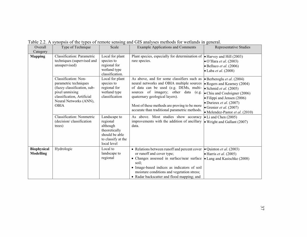
37
Table 2.2. A synopsis of the types of remote sensing and GIS analyses methods for wetlands in general. Overall
Category Type of Technique Scale Example Applications and Comments Representative Studies
Mapping Classification: Parametric techniques (supervised and unsupervised)
Local for plant species to regional for wetland type classification.
Plant species, especially for determination of rare species.
Harvey and Hill (2003) O’Hara et al. (2003) Belluco et al. (2006) Laba et al. (2008)
Classification: Non-parametric techniques (fuzzy classification, sub-pixel unmixing classification, Artificial Neural Networks (ANN), OBIA
Local for plant species to regional for wetland type classification
As above, and for some classifiers such as neural networks and OBIA multiple sources of data can be used (e.g. DEMs, multi-sources of imagery; other data (e.g. quaternary geological layers). Most of these methods are proving to be more accurate than traditional parametric methods.
Berberoglu et al. (2004) Rogers and Kearney (2004) Schmid et al. (2005) Chiu and Couloigner (2006) Filippi and Jensen (2006) Durieux et al. (2007) Grenier et al. (2007) Melendez-Pastor et al. (2010)
Classification: Nonmetric (decision/ classification trees)
Landscape to regional although theoretically should be able to classify at the local level
As above. Most studies show accuracy improvements with the addition of ancillary data.
Li and Chen (2005) Wright and Gallant (2007)
Biophysical Modelling
Hydrologic Local to landscape to regional
Relations between runoff and percent cover or runoff and cover type;
Changes assessed in surface/near surface soil;
Image-based indices as indicators of soil moisture conditions and vegetation stress;
Radar backscatter and flood mapping; and
Quinton et al. (2003) Harris et al. (2005) Lang and Kasischke (2008)
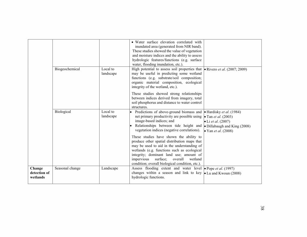
38
Water surface elevation correlated with inundated area (generated from NIR band).
These studies showed the value of vegetation and moisture indices and the ability to assess hydrologic features/functions (e.g. surface water, flooding inundation, etc.).
Biogeochemical Local to landscape
High potential to assess soil properties that may be useful in predicting some wetland functions (e.g. substrate/soil composition; organic material composition, ecological integrity of the wetland, etc.).
These studies showed strong relationships between indices derived from imagery, total soil phosphorus and distance to water control structures.
Rivero et al. (2007; 2009)
Biological Local to landscape
Predictions of above-ground biomass and net primary productivity are possible using image-based indices; and
Relationships between tide height and vegetation indices (negative correlations).
These studies have shown the ability to produce other spatial distribution maps that may be used to aid in the understanding of wetlands (e.g. functions such as ecological integrity; dominant land use; amount of impervious surface; overall wetland condition; overall biological condition, etc.).
Hardisky et al. (1984) Tan et al. (2003) Li et al. (2007) Dillabaugh and King (2008) Yan et al. (2008)
Change detection of wetlands
Seasonal change Landscape Assess flooding extent and water level changes within a season and link to key hydrologic functions.
Pope et al. (1997) Lu and Kwoun (2008)
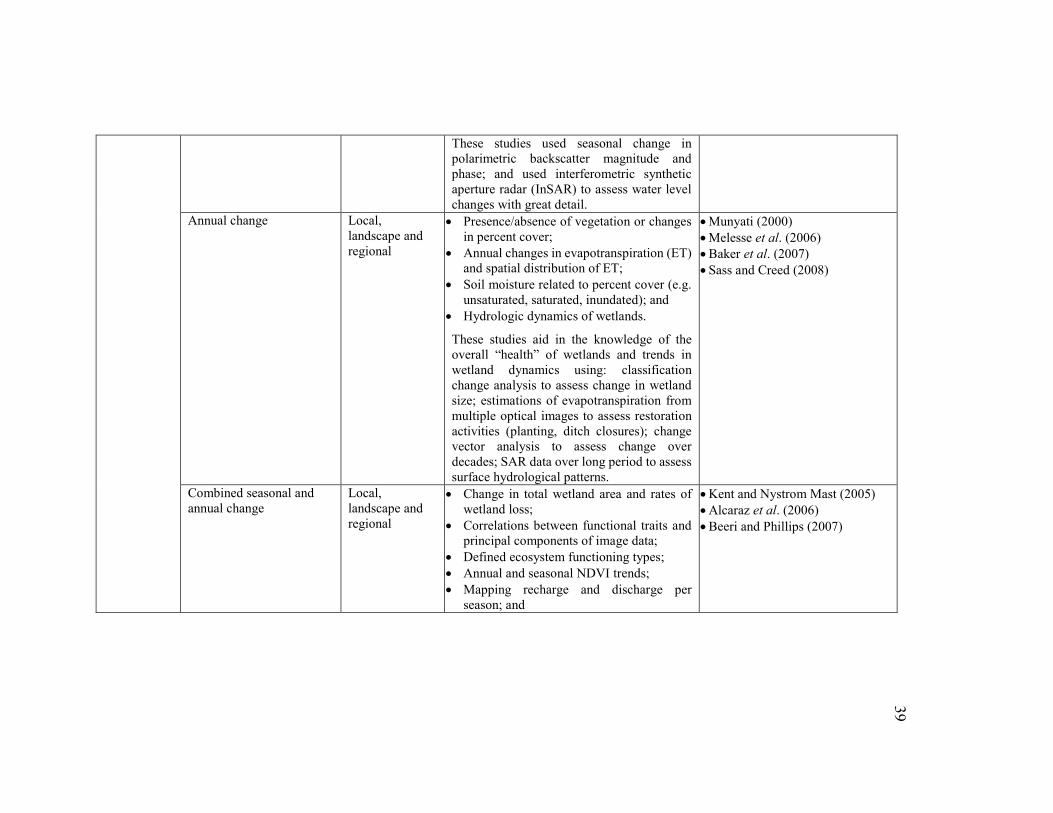
39
These studies used seasonal change in polarimetric backscatter magnitude and phase; and used interferometric synthetic aperture radar (InSAR) to assess water level changes with great detail.
Annual change Local, landscape and regional
Presence/absence of vegetation or changes in percent cover;
Annual changes in evapotranspiration (ET) and spatial distribution of ET;
Soil moisture related to percent cover (e.g. unsaturated, saturated, inundated); and
Hydrologic dynamics of wetlands.
These studies aid in the knowledge of the overall “health” of wetlands and trends in wetland dynamics using: classification change analysis to assess change in wetland size; estimations of evapotranspiration from multiple optical images to assess restoration activities (planting, ditch closures); change vector analysis to assess change over decades; SAR data over long period to assess surface hydrological patterns.
Munyati (2000) Melesse et al. (2006) Baker et al. (2007) Sass and Creed (2008)
Combined seasonal and annual change
Local, landscape and regional
Change in total wetland area and rates of wetland loss;
Correlations between functional traits and principal components of image data;
Defined ecosystem functioning types; Annual and seasonal NDVI trends; Mapping recharge and discharge per
season; and
Kent and Nystrom Mast (2005) Alcaraz et al. (2006) Beeri and Phillips (2007)
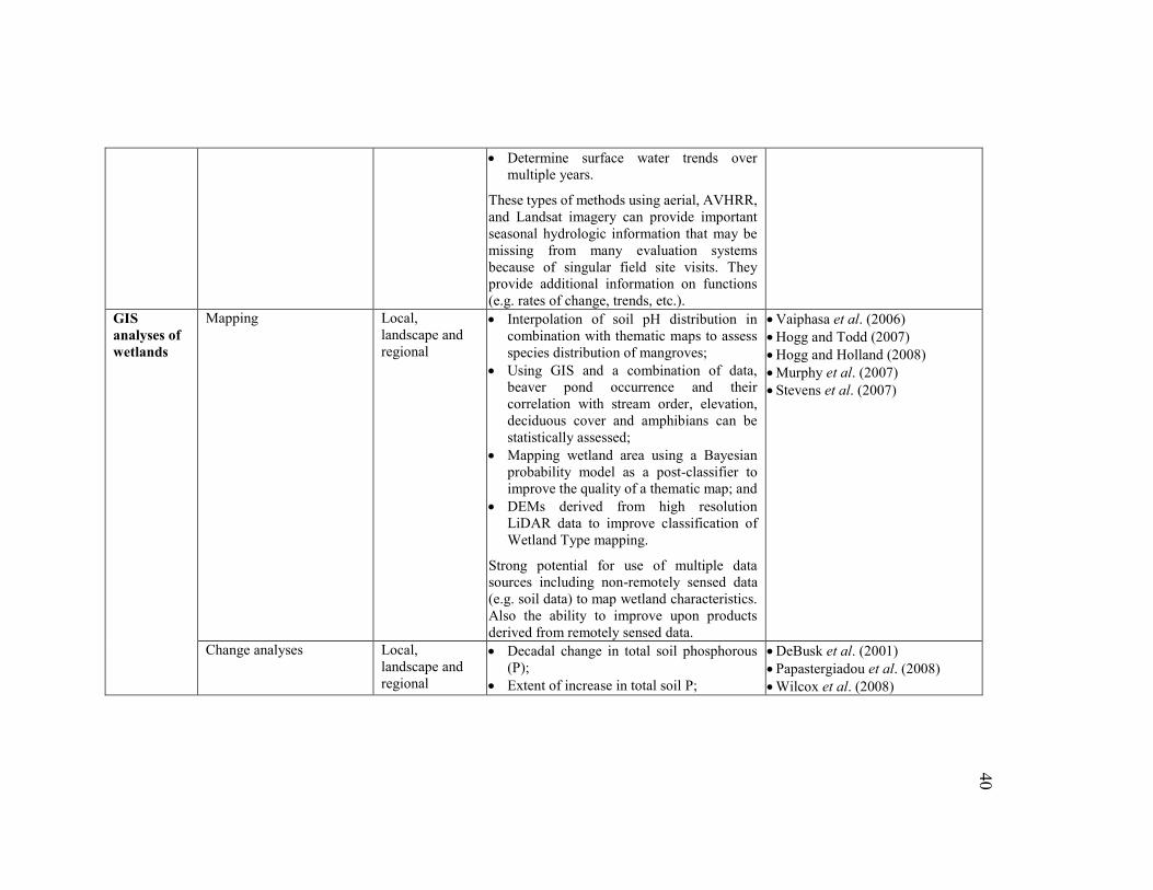
40
Determine surface water trends over multiple years.
These types of methods using aerial, AVHRR, and Landsat imagery can provide important seasonal hydrologic information that may be missing from many evaluation systems because of singular field site visits. They provide additional information on functions (e.g. rates of change, trends, etc.).
GIS analyses of wetlands
Mapping Local, landscape and regional
Interpolation of soil pH distribution in combination with thematic maps to assess species distribution of mangroves;
Using GIS and a combination of data, beaver pond occurrence and their correlation with stream order, elevation, deciduous cover and amphibians can be statistically assessed;
Mapping wetland area using a Bayesian probability model as a post-classifier to improve the quality of a thematic map; and
DEMs derived from high resolution LiDAR data to improve classification of Wetland Type mapping.
Strong potential for use of multiple data sources including non-remotely sensed data (e.g. soil data) to map wetland characteristics. Also the ability to improve upon products derived from remotely sensed data.
Vaiphasa et al. (2006) Hogg and Todd (2007) Hogg and Holland (2008) Murphy et al. (2007) Stevens et al. (2007)
Change analyses Local, landscape and regional
Decadal change in total soil phosphorous (P);
Extent of increase in total soil P;
DeBusk et al. (2001) Papastergiadou et al. (2008) Wilcox et al. (2008)

41
Change in land cover types in wetlands; Changes in wetland plant communities;
and Changes in water levels. These studies have shown that hydrologic dynamics of wetlands and soil properties can be monitored effectively using GIS.
Biophysical modeling Local, landscape and regional
Predicting patterns of plant species; Assessing habitat quality and diversity; and Impacts of human activity by
characterization of activities and water chemistry.
These studies have accurately assessed biophysical properties of wetlands.
van Horssen et al. (1999) Berberoglu et al. (2004) Morrice et al. (2008)
Population analyses and habitat conservation
Local, and landscape
Calculation of population and habitat requirement statistics;
Habitat suitability assessment; Connectivity of core areas assessment; and Assessment of breeding bird wetland
habitat. These studies were able to assess fauna population statistics and information when remote sensing is not readily available or applicable.
Beazley et al. (2005) Connor and Gabor (2006)
42
As it can be seen from the review above it is well accepted that the advantages of
using remote sensing for wetland analysis outweigh the limitations (Lee and Lunetta, 1995;
Ozesmi and Bauer, 2002; Davidson and Finlayson, 2007; Moffett and Gorelick, 2013). In
this research to address these limitations, especially temporal issues, analyses were
conducted on image date selection and long term differences in image variables.
2.6.2 GIS analyses of wetlands
As a broader framework and set of tools to represent, process and analyze geo-spatial
and temporal data, GIS is useful because of its capability to integrate a number of data types,
including remotely sensed data (e.g. thematic maps, change statistics, biophysically
modelled variables, etc.) and other geo-spatial data types such as soils data, topographic, and
census data, etc. Rather than derive metrics directly from imagery (e.g. using band
brightness/reflectance or radar backscatter), information is derived from products previously
created such as thematic maps, DEMs, etc., many which may have been derived from
remotely sensed imagery. To maintain consistency with the presentation of the remote
sensing methods in this chapter, focus is placed on GIS methods utilized in this research.
More generalized methods are outlined in Table 2.2.
Many of the attributes of interest for this research require boundaries be identified.
There have been many GIS-based studies that have used both remotely sensed data and other
geo-spatial data to map wetlands and wetland boundaries. Topography is a key component
for mapping and evaluating wetlands. It acts as a major control on wetland distribution
(Murphy et al., 2007) and influences many of the processes that occur within wetlands,
specifically the hydrologic functioning, distribution of soil carbon stocks, decomposition,
net primary production, among others (Ferone and Devito, 2004; Ju and Chen, 2005; Murphy
43
et al., 2007; Murphy et al., 2009). DEMs, as representations of topography, are often used
to derive wetland variables. Topographic indices, such as the soil wetness index (SWI) and
depth-to-water (DTW) index (Murphy et al., 2009) are often derived from DEMs that are,
in turn, generally created with remotely sensed imagery (e.g. LiDAR, optical imagery,
interferometric radar, etc.).
Hogg and Todd (2007) compared three methods to delineate the boundaries of
wetlands in Ontario. They used a DEM to derive wetland terrain variables (topographic
index, contributing area and slope, standard deviation of slope, planform curvature, profile
curvature, amongst others). Logistic regression was used to determine which variables
should be retained for subsequent mapping. The first model was the visual derivative
threshold method (where topographic index and positive mass balance hydraulic slope (two
uncorrelated variables) were used in a density slicing approach; the second model was a
logistic regression model of the variables; and the third model used a classification and
regression tree (CART) statistical analysis. Using the visual derivative threshold method,
the overall accuracy was 99% however 37% of upland was also mapped as wetland. With
reduction of the threshold values, the wetland mapping accuracy decreased significantly. For
the CART method, the overall validation accuracy was 84%.
Hogg and Holland (2008) compared the use of a high resolution DEM that was
derived from LiDAR data to a coarser DEM (20m resolution) to classify wetland types using
the CART methodology described above (Hogg and Todd, 2007). They found that the
addition of the high resolution DEM improved the overall mapping of Wetland Types.
Many layers containing information on hunting, recreation and land ownership are
available from the OMNR. These types of layers can be used as predictor variables in

44
analyses of current and potential wetland land-use change in a GIS. For example, Allen et
al. (2002) attempted to determine suitable predictors of potential land use change around the
South Carolina coastal area. Using spatial logistic regression analysis, they found that land
ownership variables and primary roads were strong predictors of commercial development,
while beachfront, open view, private ownership data were indicators of residential
development. Prediction success for the model was 90% for residential, and 92% for non-
residential parcel use. For the social features and features relating to human constructs such
as ownership there is fewer studies that relate to this work. Available such studies are listed
in Table 2.5.
2.6.3 Sensors used for wetland attribute analysis pertinent to this research
The sensors used for wetland mapping can be categorized by the measurement and
observational scale at which imagery is obtained. For this research, wetland analyses were
conducted using two measurement and observational scales of optical imagery and one of
radar imagery (Table 2.3). The following section outlines the capabilities of the sensors to
record particular listed aspects of wetland vegetation structure and form, wetland hydrology
and general land use land cover configuration as well as previous studies that have used such
imagery for wetland analyses. For specific methods selected for this research more detail is
provided in sections 2.8.1 to 2.8.4.
Optical imagery may include the spectral bands in the ultraviolet, visible, and
infrared portions of the electromagnetic spectrum. The spectral bands and spectral resolution
(the bandwidth of each spectral band) impact the type and precision/accuracy of information
derived for wetlands. Healthy vegetation reflects strongly in the NIR (approximately 0.7 to
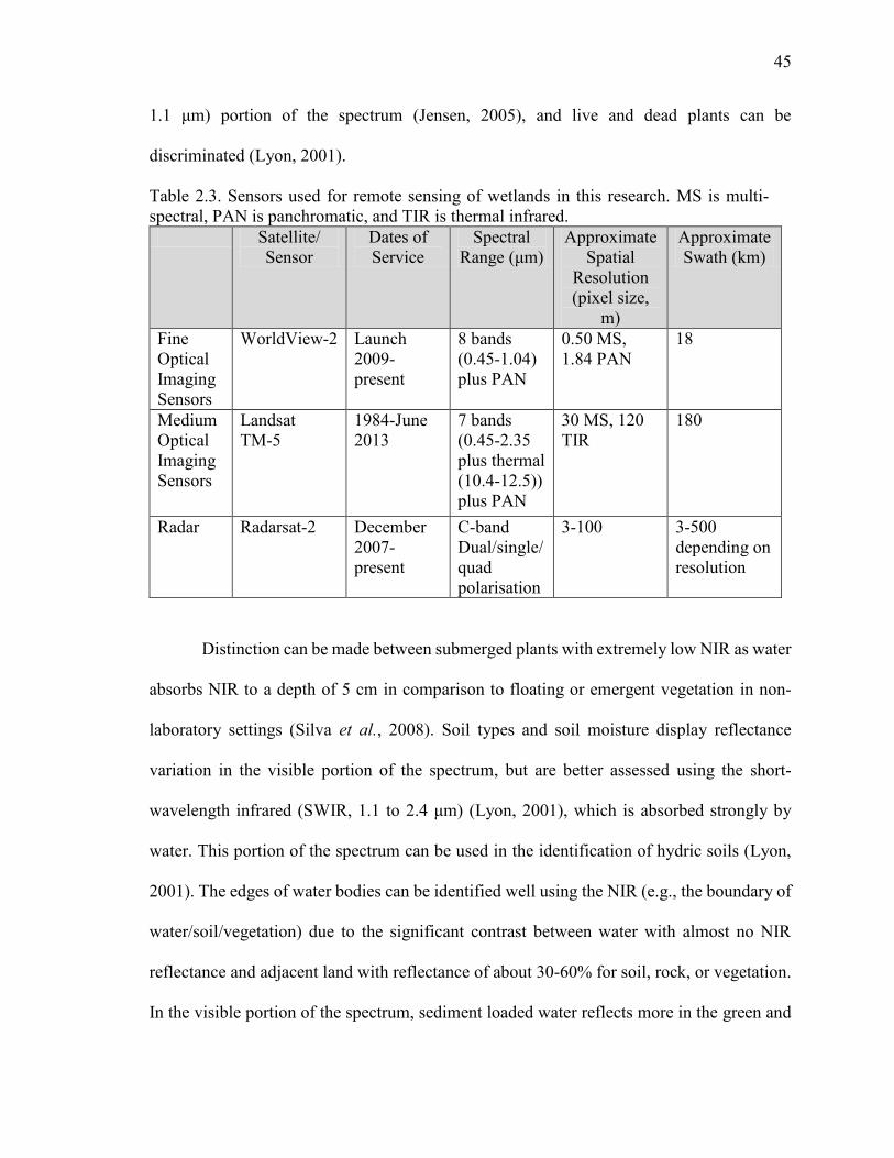
45
1.1 μm) portion of the spectrum (Jensen, 2005), and live and dead plants can be
discriminated (Lyon, 2001).
Table 2.3. Sensors used for remote sensing of wetlands in this research. MS is multi-spectral, PAN is panchromatic, and TIR is thermal infrared.
Satellite/ Sensor
Dates of Service
Spectral Range (μm)
Approximate Spatial
Resolution (pixel size,
m)
Approximate Swath (km)
Fine Optical Imaging Sensors
WorldView-2 Launch 2009- present
8 bands (0.45-1.04) plus PAN
0.50 MS, 1.84 PAN
18
Medium Optical Imaging Sensors
Landsat TM-5
1984-June 2013
7 bands (0.45-2.35 plus thermal (10.4-12.5)) plus PAN
30 MS, 120 TIR
180
Radar Radarsat-2 December 2007- present
C-band Dual/single/ quad polarisation
3-100
3-500 depending on resolution
Distinction can be made between submerged plants with extremely low NIR as water
absorbs NIR to a depth of 5 cm in comparison to floating or emergent vegetation in non-
laboratory settings (Silva et al., 2008). Soil types and soil moisture display reflectance
variation in the visible portion of the spectrum, but are better assessed using the short-
wavelength infrared (SWIR, 1.1 to 2.4 μm) (Lyon, 2001), which is absorbed strongly by
water. This portion of the spectrum can be used in the identification of hydric soils (Lyon,
2001). The edges of water bodies can be identified well using the NIR (e.g., the boundary of
water/soil/vegetation) due to the significant contrast between water with almost no NIR
reflectance and adjacent land with reflectance of about 30-60% for soil, rock, or vegetation.
In the visible portion of the spectrum, sediment loaded water reflects more in the green and
46
red than clear water. Shallow water may also reflect more in the visible than deep water if
radiation can penetrate to the bottom of the water body and reflect back to the sensor.
Vegetation and water indices (some calculation/combination of several spectral bands) can
often improve discrimination of water, soil and vegetation and model their condition (Rivero
et al., 2009; Satyanarayana et al., 2011; Kim et al., 2012).
Although there are no strict definitions, high resolution optical imagery typically has
minimum pixel sizes in the range of a few centimetres to approximately 5 m with swaths
covering up to 20 km. Such images can cover individual wetlands (e.g. a marsh within a
wetland complex) or small wetland complexes, and can provide information about spatial
characteristics within wetlands (e.g., classify specific salt-marsh vegetation (Belluco et al.,
2006); relate remotely sensed derived metrics to biomass (Dillabaugh and King, 2008);
examine the distribution of beaver dams (Stevens et al., 2007); identify dredged soil disposal
sites, and sites colonized by the common reed (Hudon et al., 2005)). High resolution optical
imagery has been used to map Wetland Types on an island in Yueqing Bay China (Zhang et
al., 2011) and to estimate biomass in densely vegetated wetlands in South Africa (Mutanga
et al., 2012). In the latter, normalized difference indices using the same formulation NDVI
were calculated from all possible two-band combinations of the eight bands for WorldView-
2 imagery. These indices were the same form as the common NDVI derived as:
𝑁𝐷𝑉𝐼𝑖 = (𝑁𝐼𝑅−𝑅)
(𝑁𝐼𝑅+𝑅) Eq.2.1
where NIR is the near-infrared spectral band of a sensor; and
R represents the red spectral band of same sensor.
A model was constructed relating these values to field sampled biomass using
random forest (RF) regression (an ensemble learning method, also known as bagging or
47
bootstrap aggregation). They were able to identify the smallest number of index images that
provided the best biomass prediction model (R2 0.76; RMSE = 12.9% of mean biomass).
The indices included red-edge and NIR1 bands, red-edge and NIR2 bands and the green and
NIR2 bands).
For optical imagery with moderate resolutions, minimum pixel sizes are typically in
the tens of metres and swaths of up to 200 km. Such images encompass whole wetland
complexes (landscape level) and cover regional areas (e.g. eastern or southern Ontario).
Minimum wetland sizes for mapping are greater than 1 ha at these scales (Jensen, 2005) and
applications include landscape level analysis such as mapping of the Prairie Potholes
Regions (Mita et al., 2007); estimation of carbon emissions from peat along the coastal plain
in North Carolina, USA (Poulter et al., 2007); and delineation of plant functional types at
Poyang Lake, China (Dronova et al., 2012).
The potential for mapping wetlands at landscape to regional scales has been shown
with radar imagery for very broad land cover classes (e.g. wetland and non-wetland), and
broad wetland vegetation classes (e.g. shrub, forested, etc.) (Hess et al., 2003; Racine et al.,
2005; Durieux et al., 2007; Grenier et al., 2007; Touzi et al., 2007; Henderson and Lewis,
2008; Marechal et al., 2012). It works well in detecting seasonal changes, including flooding
(Pope et al., 1997; Lu and Kwoun, 2008). SAR sensors emit microwave pulses in
wavelengths that are generally unaffected by atmospheric moisture, dust or clouds. They are
also not limited by time of day sun-angle acquisition issues that impact optical imagery
(Fernandez-Ordonez et al., 2010). Wavelengths are also longer than traditional optical
analysis allowing for different information to be derived from the landscape. Strong positive
and linear correlations have been found between radar backscatter and wetland vegetation
48
biomass (Li et al., 2007). Radar imagery has proven useful for mapping Wetland Type
classes and specific wetland vegetation, including invasive species (Li and Chen, 2005;
Racine et al., 2005; Grenier et al., 2007). Radarsat-2 has been used to identify and delineate
seasonal flooded extent in a time series for a wetland in Brittany, France (Marechal et al.,
2012).
Wavelengths that work well for the detection of wetlands include C-band
(approximately 5.6 cm wavelength) and L-band (approximately 20 cm wavelength) at
landscape to regional scales. Longer wavelengths penetrate deeper into vegetation canopies
than shorter wavelengths and are better suited to modelling and mapping of forested
wetlands and swamps with standing dead trees. C-band has been shown to detect herbaceous
wetlands (Henderson and Lewis, 2008) and to detect open smooth water due to specular
reflectance of the pulse away from the sensor, which creates a black object in the imagery.
Depending on the spatial resolution, incidence angle and canopy openness, radar signals may
‘double bounce’ or corner reflect off trunks, such as standing snags in open swamps or
emergent vegetation (e.g. reeds) (Karszenbaum et al., 2000; Kandus et al., 2001) producing
bright point signals. Radar can also be polarized in both the emitted and received signals. In
general in the literature, HH polarisation was generally used more than VV, but cross-pol
(HV or VH) was also useful (Li and Chen, 2005; Henderson and Lewis, 2008; Lu and
Kwoun, 2008). HH polarisation was better correlated with soil moisture and inundation than
VV polarisation (Dobson and Ulaby, 1988; Lang and Kasischke, 2008), however, at
shallower incidence angle, soil moisture was less influential on all polarisations (HH, HV,
VH, VV) (McNairn et al., 2002). Many Wetland Types (bog, fen, saline and freshwater
marsh) have been better discriminated with HH polarisation than with VV (Li and Chen,
49
2005; Henderson and Lewis, 2008; Lu and Kwoun, 2008), however VV has been shown to
be useful for cattail and low density marshes (Henderson and Lewis, 2008). The swath of
satellite-based radar images can range from 20 km to 500 km and can cover similar areas as
high to moderate resolution optical imagery. Polarimetric decompositions, either coherent
or incoherent, express the scattering matrix as some combination or summation of the
scattering responses from the surface (Touzi, 2007). These variables have been used to
categorize Wetland Types (bog, treed bog, fen, marsh) (Touzi et al., 2007).
2.7 Remote sensing of hydrology and forestry as it relates to wetland research
Hydrology has a significant role in wetlands, and forest structure has sometimes been
found to be similar to the structure of swamp vegetation, therefore it is important to consider
some of the literature as it relates to the wetland analysis in this research.
2.7.1 Hydrology
Pietroniro and Leconte (2005) reviewed the research in remote sensing for
hydrological applications in Canada. The particular sensors found to be most useful included
Radarsat-1, AQUA and ENVISAT for soil moisture, Landsat for vegetation and SPOT,
ERS-1/2, Radarsat-1 and Landsat for surface water. In one study, near surface soil moisture
could be extracted from SAR data using linear regression between backscatter and measured
soil moisture, however, they noted that these models could not be transferred between sites
of interest. In another study, using polarimetric data from the Canadian Convair-580 C-band
SAR system, it was not possible to develop a conclusive relationship between soil moisture
and backscatter response. For surface water, Pietroniro and Leconte (2005) discussed the
use of the near and mid-infrared portion of the spectrum as important to contrast between
50
water and vegetation. Additionally, SAR systems showed utility in differentiating between
open water and vegetation, however these results are complicated by the Bragg effect, which
produces backscattering from surface waves.
More recently, Klemas (2011) reviewed remote sensing in hydrology and showed
the utility of using LiDAR for discrimination of flooded marsh types and separation between
plant species as well as multi- and hyper-spectral imagery for discrimination of Wetland
Types and bio-chemical and bio-physical properties of wetland vegetation. Methods used
included common pixel-based classification such as MLC, but it was also shown that OBIA
was frequently being used as a means to capture spatial pattern of spectrally mixed land
covers, like submerged vegetation.
2.7.2 Forestry
Govender et al. (2009) reviewed the use of remote sensing data and the development
of spectral reflectance indices to detect plant water stress. The spectral bands that proved
useful to detect plant stress included those in the visible, near- and short-wave infrared
portions of the spectrum. Particularly, they found research that related changes in the green
band due to chloroplast deterioration. They also reviewed studies that showed green and NIR
ratios to be highly correlated with chlorophyll concentration. In addition, they summarized
research that used Landsat bands 5 and 7, representing the short-wave infrared portion of the
spectrum, to model and map soil and vegetation water content.
Roberts et al. (2007) reviewed the current literature to that time to assess the state of
the remote sensing of forest structure. Categories of detectable variables were given for
different satellite resolutions. Contextual forest attributes such as leaf area index, timber
volume, above-ground biomass and basal area could be well estimated with Landsat TM and
51
ETM+ sensors utilizing regression or classification methods. Accuracies were given as
mostly R2 values ranging from 0.67 to 0.83. For variables such as forest age class, individual
tree detection and crown detection, and mangrove species mapping, high resolution
multispectral or hyperspectral sensors were required (e.g. satellite sensors such as IKONOS;
airborne hyperspectral sensors such as the CASI). With such high resolution imagery, image
spatial information such as image texture, and object-based classification were found to
improve biophysical estimates with R2 values of 0.76 to 0.82, and species classifications
with overall accuracies ranging from 67% to 89%.
2.8 Remote sensing methods for the mapping the 14 selected OWES attributes
The remote sensing image analyses methods applied to map the 14 attributes in this
research used the spectral bands of the imagery, mathematical combinations and
decompositions of that spectral information, additional geo-spatial data including DEMs,
and social spatial information. The overall methods that were used to derive data are
described in this section as background information. Equations numbers are only given for
those equations used in this research; other equations given in the text are for definition
purposes only. Metrics that have potential to be evaluated through remote sensing and other
geospatial data are of interest for this research and include: object and sub-pixel spatial
configuration; vegetation indices thresholds, classification methods, and radar-based
variables (Ju and Chen, 2005; Artigas and Yang, 2006; Frieswyk and Zedler, 2007; Rivero
et al., 2007). Some of these particular methods were repeatedly used for mapping several of
the attributes and are noted as such in each particular attribute section following the methods
descriptions and backgrounds in sections 2.8.1 to 2.8.2.
52
2.8.1 Object-based image analysis
The main intent of OBIA is to segment imagery into objects representing relative
spatial homogeneity in reflectance and then classify the segmented objects as land cover
classes (e.g. bogs, upland forest, streams) of interest.
The technical objective in segmentation is to define objects that have minimized
within-object variability, and maximized between-object variability. The creation of objects
from individual pixels is based upon the spectral and spatial properties of neighbouring
pixels and subsequently created objects (Burnett and Blaschke, 2003). Segmentation
algorithms are categorized as edge-based and area-based (Jensen, 2005). Edges occur where
there are sharp changes in brightness values. In edge-based segmentation the growth of
objects is based upon the edges and linked edges that may signify borders. Problems can
occur if edges are not present where a real border exists, or if edges are present where no
real border exists. Area-based (also known as region-based or region growing) segmentation
compares pixels or groups of pixels (the ‘seed’) and merges comparable areas as long as
they are homogenous within a defined tolerance. Large heterogeneous areas can also be split
into smaller homogenous units. Some segmentation algorithms use a combination of
splitting and merging.
The following discussion focuses on the aspects of eCognition Developer 64 (8.64)
which is a widely available object-based software suite that was used in this research. It
includes the most common algorithm for object segmentation, the area-based algorithm
known as multi-resolution segmentation. Marpu et al. (2010) showed that this algorithm was
one of the two best from a comparison of 12 segmentation algorithms in terms of positional
accuracy of segmentation of land cover objects using IKONOS imagery in an urban setting
53
and vegetative area. The evaluation of the 12 algorithms was completed by comparing
created objects with reference segments for 10 reference areas. The algorithms were assessed
based upon lost pixels and extra pixels in relation to the reference data. The other algorithm
that performed well was SEGEN (Gofman, 2006). eCognition was chosen for this research
because it performed as well as the SEGEN algorithm in this study, it performed well in
other studies of land cover classification (Benz et al., 2004; Yu et al., 2006; Dingle
Robertson and King, 2011; Barker and King, 2012), and it was available for this research.
The key parameter in multi-resolution segmentation is a unitless variable of scale
that is correlated to the image’s pixel size and is related to the parameters of colour (spectral
(or other pixel value (e.g. DEM)) information) and shape (the physical characteristics of the
image features (Laliberte et al., 2004) further defined by smoothness and compactness).
Most researchers follow a “trial and error” process in order to determine the best scale, shape
and compactness values (Ouyang et al., 2011; Duro et al., 2012; Aguilar et al., 2013).
Traditionally, this has been through comparison of how well the segmented object
boundaries align with visually interpreted objects. Tian and Chen (2007) utilized a matrix
format and visual interpretation to test scale parameter selection. Dronova et al. (2012) used
nine scale parameters (2 to 10) to create wetland objects varying of sizes based upon field
observations, and assessed the scale parameter accuracy based upon the accuracy obtained
in classification. More recently, the estimation of scale parameter (ESP) tool developed by
Dragut et al. (2010) was proposed as a means to automatically and quantitatively optimize
scale parameter value selection. This tool creates objects at a variety of scale parameter
values and calculates the local variance of the object heterogeneity. Subsequently, the local
variance is plotted against the change in scale parameter value and the rate of change is
54
calculated. They found that the tool enabled an accurate selection of a scale parameter value
for a variety of image types. As this tool by Dragut et al., (2010) was developed during this
research, and subsequently published after OBIA had been completed for this research it was
not employed. Instead, this research followed the `trial and error` matrix method proposed
by Tian and Chen (2007) and qualitatively assessed the accuracy of the scale parameter value
based upon assessed overall classification accuracy.
Once the scale parameter has been selected, objects are segmented based upon
similarity of pixels, contrast of an object with neighbouring objects and object shape
characteristics. In general, the larger the value of the scale parameter the larger the resulting
image objects (Benz et al., 2004). Objects are grown evenly and simultaneously across the
entire scene. Colour and shape (smoothness and compactness) can be weighted by the user
(Laliberte et al., 2004). As objects are created they are merged together following the scale,
shape, colour, smoothness and compactness parameter values. The process ends once the
growth of the objects satisfy the values of scale, colour and compactness defined (Laliberte
et al., 2004). This creates one object level in a hierarchy (Figure 2.2). The multi-resolution
segmentation process can be applied again with a different scale parameter value to the first
object level to obtain a second level of objects at a higher or lower level in the hierarchy.
Once segmented, objects can be classified at any level within the developed hierarchy.
In previous research it has been found that OBIA produces more useful thematic
maps showing land cover entities as humans perceive them as compared to pixel-based
thematic maps (Dingle Robertson and King, 2011; Brenner et al., 2012; Dronova et al.,
2012; Duro et al., 2012; Meneguzzo et al., 2013).
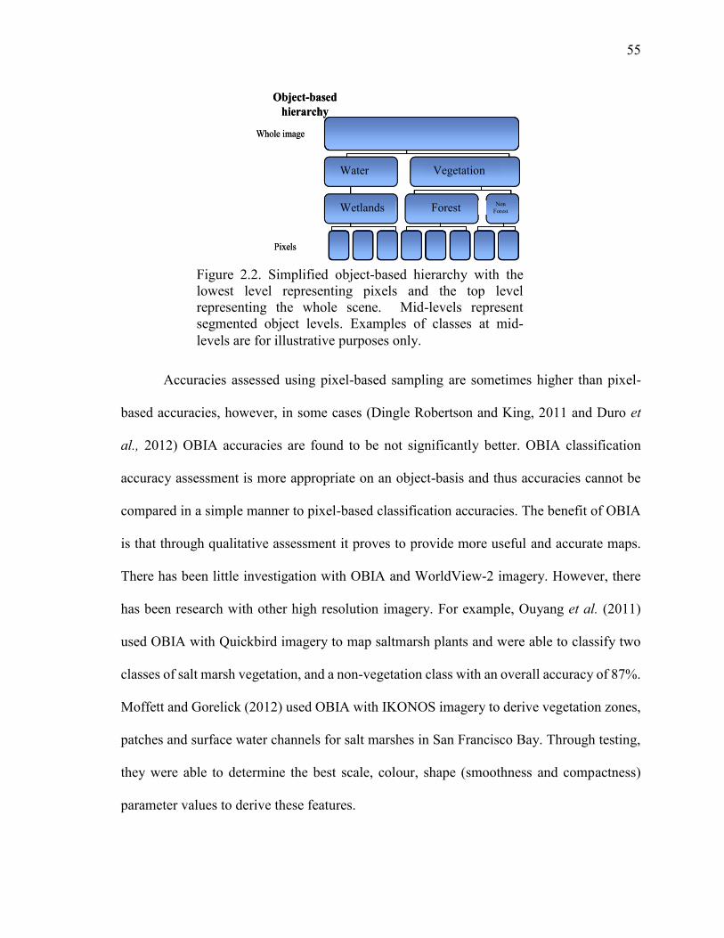
55
Accuracies assessed using pixel-based sampling are sometimes higher than pixel-
based accuracies, however, in some cases (Dingle Robertson and King, 2011 and Duro et
al., 2012) OBIA accuracies are found to be not significantly better. OBIA classification
accuracy assessment is more appropriate on an object-basis and thus accuracies cannot be
compared in a simple manner to pixel-based classification accuracies. The benefit of OBIA
is that through qualitative assessment it proves to provide more useful and accurate maps.
There has been little investigation with OBIA and WorldView-2 imagery. However, there
has been research with other high resolution imagery. For example, Ouyang et al. (2011)
used OBIA with Quickbird imagery to map saltmarsh plants and were able to classify two
classes of salt marsh vegetation, and a non-vegetation class with an overall accuracy of 87%.
Moffett and Gorelick (2012) used OBIA with IKONOS imagery to derive vegetation zones,
patches and surface water channels for salt marshes in San Francisco Bay. Through testing,
they were able to determine the best scale, colour, shape (smoothness and compactness)
parameter values to derive these features.
Object-based hierarchy
Whole image
Pixels
hierarchyhierarchyObject-based
hierarchy
Whole image
Pixels
Figure 2.2. Simplified object-based hierarchy with the lowest level representing pixels and the top level representing the whole scene. Mid-levels represent segmented object levels. Examples of classes at mid-levels are for illustrative purposes only.
Water Vegetation
Wetlands Forest Non Forest
56
For combining optical and radar imagery with OBIA, Grenier et al. (2007) used
Landsat ETM+ and Radarsat-1 imagery to map wetlands in two sites for the Canadian
Wildlife Service Canadian Wetland Inventory (CWI) with the five classes of Bog, Fen,
Marsh, Swamp and Shallow Water. Objects were found at each of three segmentation levels
and were subsequently merged back into the five classes of interest. Accuracy was assessed
both thematically and spatially based on interpretation of Landsat colour composites and use
of photos taken from a helicopter. For thematic accuracy, all wetlands were combined into
one wetlands class versus ‘other’ (open water was not validated as confusion was thought to
be very low), resulting in 82% and 90% accuracy for the two study sites. In addition,
accuracy was assessed between the five wetland classes, resulting in 76% and 68%,
respectively
Durieux et al. (2007) used 300 m pixel MEdium Resolution Imaging Spectrometer
Instrument (MERIS) data, 100 m pixel JERS-1 radar data, and SRTM (Shuttle Radar
Topography Mission) to classify wetland complexes (seven classes: river, riparian
vegetation, lichen and mosses, lakes, dark taiga, broadleaf forest, bogs and anthropic
area/bare soil) in western Siberia. A Landsat TM derived pixel-based thematic map with an
accuracy of 89% was used for validation. The object-based technique used was the fractal
net evolution approach (FNEA) which segments images simultaneously at two levels and
then subsequently builds semantics between the levels and the corresponding level units
(patches). The first object level was created using multi-resolution segmentation solely based
upon the radar backscatter coefficient and the second object level was created using the
spectral difference algorithm for three MERIS bands (555-565 nm, green; 677.5-685 nm,
red; and 855-875 nm, NIR). A classification rule set was defined using the three levels of
57
segmentation (e.g. objects that overlapped SRTM water bodies and areas with low
backscatter on the radar image were considered lakes). The overall accuracy for this
classification was 72.5%.
Based upon the literature, it was expected that OBIA applied to WorldView-2
imagery and combinations of other data types (including radar) would improve upon
accuracies in the literature which, for example, ranged from 68% to 76% when more than
two Wetland Types were classified using lower spatial resolution imagery. Similarly, it was
expected that these data and methods would improve upon accuracies reported in the
literature for VCFs, which ranged from 76-91%. It was hoped that OBIA would prove to be
useful with higher resolution imagery alone and combined with radar imagery, which has
not been shown in the literature for Open Water Type.
2.8.2 Linear Spectral Unmixing (LSU)
Individual pixels are often comprised of more than one land cover class (e.g., 25%
water, 30% soil, 45% vegetation). While fuzzy classification and resulting membership
scores may indicate the degree of similarity of pixel values to individual class training data,
and the scores may be related to proportion of each land cover type in a pixel, LSU or spectral
mixture analysis is a technique directly linked to reflectance theory of linear mixing of
radiance from land cover types within a pixel area (Jensen, 2005).
Endmembers (EMs) represent the major radiometric land covers such as water,
asphalt, concrete, healthy vegetation canopy, etc. present in an image (Neville et al., 1998).
These can be manually selected using known training areas of pure pixels, however a
limitation is that there are often few known sites where an area would be completely pure.
Other more automated methods of choosing EMs have been developed; one of the most
58
common that was used in this research is the iterative error analysis (IEA) algorithm. An
initial vector (the mean spectrum of the data) is chosen to start the process. A constrained
unmixing (where each fraction must fall between 0 and 1 (Neville et al., 1998)) is then
performed and an error image is developed. The process chooses the EM as that which
minimizes the remaining error in the unmixed image, therefore the average of the vectors
with the largest error (distance from the initial vector) is assumed to be the first EM. Another
constrained unmixing occurs and the error image is found again. The average of the vectors
with the largest distance from the first EM is considered the second EM. This process
continues until all EMs are found or a specified number is reached.
From the location of EMs within an n-dimensional space, a linear mixing model
(Rogers and Kearney, 2004) is used to determine the proportion of each EM in each pixel.
The most commonly used model (and associated with most remote sensing software) is the
Least-Squares Mixing Model (Shimabukuro and Smith, 1991), which defines the spectral
signature of a pixel per spectral band as the sum of the reflectance of each land cover type
within that pixel and the associated error:
𝜌𝑖,𝑗,𝑘 = ∑ 𝐹𝑖,𝑗,𝑚𝑚=1,𝑝 ∗ 𝜌𝑚,𝑘 ∗ 𝑒𝑖,𝑗 Eq. 2.2
where ρi,j,k is the total reflectance of a pixel for row i, column j;
band k; Fi,j,m is the proportion of each pure component m of a pixel for row i, column j;
ρm,k is the reflectance for that pure component m in band k; and
e is the error associated with the estimation of each of the components for each pixel
ei,j.
The constraint of this model ensures that pure EM proportions range between 0 and
1. This means that the proportions of the components are normalized to a common range of
59
potential values. The assumption of this model is that the sum of the fractions with a pixel
is equal to the total pixel surface; i.e., that there is no other radiance that is unaccounted for
(Shimabukuro and Smith, 1991). There have been only two or three studies found on
research conducted utilizing LSU for wetlands and only one study found that used fraction
maps as input to OBIA for any type of land cover mapping.
Schmid et al. (2005) used spectral unmixing of hyperspectral aerial imagery, Landsat
and ASTER imagery to detect changes in wetlands in La Mancha Alta, Spain. Five EMs
were derived from the higher resolution hyperspectral imagery including: hydrophytic
vegetation, wetland soils A (dried, exposed soil surface with seasonal flooding) and B
(cultivation practices bare soil: fallow or sowed with crops), wet salt crust and upland soil.
The EMs were transferred to the coarser multispectral satellite data (Landsat and ASTER)
showing that their spectral characteristics remained relatively stable in this process. This
subsequently allowed for the temporal comparison and determination of change using the
multi-date medium resolution multispectral imagery.
Melendez–Pastor et al. (2010) used land cover components (vegetation, soil, water)
from LSU of Landsat 5 imagery to compare temporal changes at El Hondo Natural Park
wetland, Spain. Their results showed a significant increase (+123.8%) in the soil fraction
between a non-drought year (2001) and a drought year (2004/05).
The ability of the land cover fractions to indicate change based upon climatic
differences (Schmid et al., 2005; Melendez-Pastor et al., 2010) or human-based changes in
other ecosystems such as slash and burn in the Amazon (Adams et al., 1995) or tundra land
cover change (Olthof and Fraser, 2007) led to the selection of this attribute to classify
imagery and assess change through time based upon these fractions. Additionally, the lack
60
of previous studies on LSU applied in OBIA suggested this could be a significant
contribution to the literature. It is also hoped that this type of analysis will improve upon the
existing assessment of anthropogenic disturbance in the literature with accuracies that
ranged from 85 to 89%. Finally, LSU was also selected for the potential of the sub-pixel
information, while maintaining the coverage and cost of a product like Landsat which would
be practical and cost-effective for a regionally diverse monitoring system like OWES.
2.8.3 Classification of remote sensing imagery
A traditional parametric method, supervised MLC is often used as a base comparison
for other classification methods (Flanders et al., 2003) and was selected for the same purpose
in this thesis. For selected classes such as Bog, Fen, Marsh, etc., training pixels are selected
from the image that are representative of the spectral and/or spatial characteristics of a class
of interest. MLC is generally an optimal classifier if pixels forming a training class are
normally distributed and there is some previous knowledge regarding the landscape (Jensen,
2005). Given this condition, the statistical probability (the Bayesian likelihood) can be
calculated that an unknown pixel (or object) belongs to a particular land cover category. The
separability of the training data can be analyzed using multivariate inverse variance-
covariance weighted measures of distance between class means, such as the Bhattacharyya
Distance (Haralick and Fu, 1983). In this research, the algorithm scaled the resultant
distance into a range between 0 and 2, where 0 indicates complete overlap of two classes
and 2 indicates a complete separation between the two classes. As Bhattacharrya Distance
is non-linear, values of 1.9 and greater are often used to indicate good separabililty and
values of 1.7-1.9 may indicate potential for accurate classification. Following the training
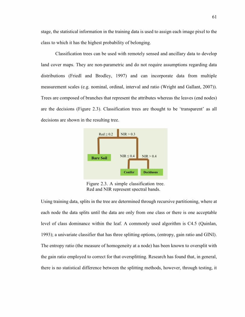
61
stage, the statistical information in the training data is used to assign each image pixel to the
class to which it has the highest probability of belonging.
Classification trees can be used with remotely sensed and ancillary data to develop
land cover maps. They are non-parametric and do not require assumptions regarding data
distributions (Friedl and Brodley, 1997) and can incorporate data from multiple
measurement scales (e.g. nominal, ordinal, interval and ratio (Wright and Gallant, 2007)).
Trees are composed of branches that represent the attributes whereas the leaves (end nodes)
are the decisions (Figure 2.3). Classification trees are thought to be ‘transparent’ as all
decisions are shown in the resulting tree.
Using training data, splits in the tree are determined through recursive partitioning, where at
each node the data splits until the data are only from one class or there is one acceptable
level of class dominance within the leaf. A commonly used algorithm is C4.5 (Quinlan,
1993); a univariate classifier that has three splitting options, (entropy, gain ratio and GINI).
The entropy ratio (the measure of homogeneity at a node) has been known to oversplit with
the gain ratio employed to correct for that oversplitting. Research has found that, in general,
there is no statistical difference between the splitting methods, however, through testing, it
Red ≥ 0.2
NIR > 0.4 NIR ≤ 0.4
NIR > 0.3
Coniferous
Deciduous
Bare Soil
Figure 2.3. A simple classification tree. Red and NIR represent spectral bands.
62
is recommended to use GINI over the other two options (Zambon et al., 2006; Duro, pers.
comm. 2012). The GINI algorithm was selected for this research.
GINI measures the impurity at a given node that is at a maximum when all the pixels
are equally distributed among all classes. The main splitting criterion is the reduction of that
impurity. GINI starts by finding the largest homogenous class within a dataset and isolates
it, and repeats until all data are parsed (Zambon et al., 2006).
𝐺𝐼𝑁𝐼 (𝑡) = ∑ 𝑝𝑖(1 − 𝑝𝑖)𝑖 Eq. 2.3
where pi is the relative frequency at node t, (determined by dividing the total number
of observations of the classi by the total number of observations); and
t represents any node (parent or child) at which a given split of the data is performed
(Apte and Weiss, 1997).
Subsequent nodes are then segregated in the same manner until further divisions are not
possible. Auto-pruning, which removes any leaves with pixel counts less than or equal to a
defined within-class proportion, can be implemented.
Overfitting occurs when a classification tree model follows the structure of the
training data too closely (Khoshgoftaar and Allen, 2001). The model appears to be accurate
in classifying the training data, but is much less accurate when it comes to non-training pixels
or objects. Boosting and bagging are methods of training sample manipulation (Du et al.,
2010). Boosting applies the classification tree model with each subsequent classification
dependent upon the previous. Classes that are incorrectly predicted in the previous
classification can be weighted more heavily in the training data. Boosting sometimes results
in overfitting of the training data. Bagging (bootstrap aggregation), trains the classification
tree by selecting random subsets of the training data and repeating the classification (Du et
63
al., 2010). An example of bagging is the RF classification algorithm (Breiman, 2001;
Mutanga et al., 2012).
Wright and Gallant (2007) assessed palustrine wetlands in Yellowstone National
Park using Landsat 5 TM for various data from 1988 to 2002. The classes of interest included
two levels, one level for palustrine wetlands and non-wetlands (uplands) and one level for
the five classes within the wetlands. Canonical discriminant analysis was used with multiple
spectral, and spatial data inputs. Error was assessed using 100,000 pixels sampled from
locations not used for training or decision tree pruning. Overall, they found the addition of
the non-spectral data (GIS, terrain, and image texture) halved the overall error rate in
detection of palustrine wetlands for the coarser wetlands/no wetlands model. Additionally,
the classification tree technique improved the discrimination between emergent wetlands
and other classes. Wright and Gallant (2007) listed kappa coefficients for each model to
detect palustrine wetlands that ranged from 0.41 to 0.68.
Davranche et al., (2010) used a binary classification tree algorithm from R software,
(RPart) using multi-spectral indices as data input derived from SPOT-5 data to classify reeds
and submerged macrophytes. Their overall accuracies ranged 85% to 98%.
In other land cover studies, Jiao et al. (2011) used a C4.5-based classification tree to
improve MODIS land cover classification by combining spectral data and reflectance
anisotropy (BRDF, Bidirectional Reflectance Distribution Function) over the Canadian
Boreal Forest resulting in an increase in overall accuracy by 2.92% with UA (User’s
Accuracy) and PA (Producer’s Accuracy) improving by 8.64% and 7.81%, respectively.
64
Zhao et al. (2012) tested four classification tree algorithms (Model-10, Model-09,
CTm-1, CTm-2) with Landsat ETM+ imagery to classify aquatic vegetation of emergent,
floating-leaf, submerged vegetation and open water testing a variety of spectral indices such
as NDVI, NDWI, etc. as input. The best classification tree was Model-10 and had class
accuracies ranging from 88 to 98%.
2.8.4 Radar imagery analyses
Radar image analysis was not a central focus of this research; methods were selected
that were straightforward to implement and combine with optical imagery, in order to
determine the potential for integration into an operational wetland evaluation system such
as OWES. Radarsat-2 data were selected because they were provided at no cost, thus other
data types, including those at different wavelengths were not considered. Radar imagery has
proven useful for assessing wetland classes and vegetation (Li and Chen, 2005; Racine et
al., 2005; Grenier et al., 2007; Marechal et al., 2012). Scattering mechanisms of the ground
cover are an important component of radar analysis and include surface scattering, volume
scattering, and double-bounce/multiple scattering which are represented conceptually for C-
band data in Figure 2.4 (after Bourgeau-Chavez et al., 2010; Fernandez-Ordonez et al.,
2010) for wetlands.
Particularly well understood is the relationship between radar backscatter and a
variety of land covers and/or other ground-based measures. The radar backscatter coefficient
is an indication of the average backscattered power in relation to the incident power and is
represented as σº (Ulaby et al., 1988), measured in decibels (dB).
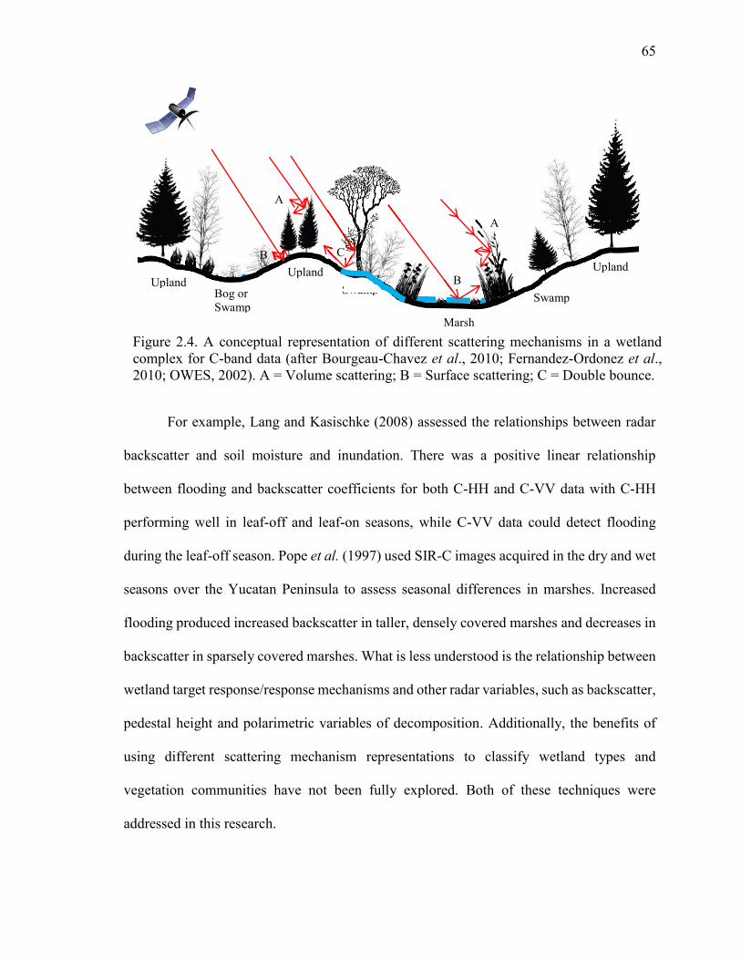
65
For example, Lang and Kasischke (2008) assessed the relationships between radar
backscatter and soil moisture and inundation. There was a positive linear relationship
between flooding and backscatter coefficients for both C-HH and C-VV data with C-HH
performing well in leaf-off and leaf-on seasons, while C-VV data could detect flooding
during the leaf-off season. Pope et al. (1997) used SIR-C images acquired in the dry and wet
seasons over the Yucatan Peninsula to assess seasonal differences in marshes. Increased
flooding produced increased backscatter in taller, densely covered marshes and decreases in
backscatter in sparsely covered marshes. What is less understood is the relationship between
wetland target response/response mechanisms and other radar variables, such as backscatter,
pedestal height and polarimetric variables of decomposition. Additionally, the benefits of
using different scattering mechanism representations to classify wetland types and
vegetation communities have not been fully explored. Both of these techniques were
addressed in this research.
Bog or Swamp
Upland Upland
Swamp
Marsh
Swamp
Upland Swamp
Figure 2.4. A conceptual representation of different scattering mechanisms in a wetland complex for C-band data (after Bourgeau-Chavez et al., 2010; Fernandez-Ordonez et al., 2010; OWES, 2002). A = Volume scattering; B = Surface scattering; C = Double bounce.
A
B
A
C B
66
A full review of the HH, VV and HV abilities are listed under the discussion of Radar
imagery in general. In particular, Banks et al. (2011) were able to discriminate between some
classes of arctic shoreline land cover by comparing the HH and HV on a scatterplot
particularly from imagery with shallow incidence angles. Baghdadi et al. (2001) assessed
Radarsat-1 backscatter coefficients of six land covers in Mer Bleue Bog by plotting the HH,
VV, and HV response for various incidence angles over three months in 1995. The cross-
pol response provided the best discrimination between the six classes. Several wetland
studies have utilized this graphical relationship of polarisation response at various incidence
angles to discriminate classes (Baghdadi et al., 2001; Horitt et al., 2003; Marti-Cardona et
al., 2010).
Bartsch et al. (2007) assessed the suitability of using satellite radar imagery for
monitoring wetlands in the boreal and sub-arctic in Russia. They used ENVISAT SAR to
relate backscatter to scatterometer data from SeaWinds/QuikScat by comparing the diurnal
effects within the backscatter data to map soil moisture and freeze/thaw boundaries. They
determined the permanent detectable thaw lake size to be 2 ha. They also presented
representative monthly backscatter values for wetlands.
Polarimetric radar measures the polarisation properties of a surface. Surfaces respond
to incident polarized radiation by reflecting partially polarized and depolarized radiation
(van Zyl et al., 1987). The response gives an indication of the properties of the surface and
allows for types of scattering to be distinguished. Fully polarimetric radar systems measure
the characteristics of the surface for all configurations (e.g. HH, VV, HV, VH) as well as
providing phase information. They improve upon data acquired in single polarisations, for
which it is difficult to distinguish between different types of scatterers. Stokes parameters
67
describe the polarisation state and phase. Coherency matrices are the second order statistical
representation of the variations and correlations of that polarisation state and phase (van Zyl
et al., 1987).
The polarimetric information of the wave is measured (or referenced) in relation to
a global 3-dimensional Cartesian coordinate system with the origin situated within the
scatterer (van Zyl et al., 1987; Banks et al., 2011). Information measured includes: power
(backscatter), ellipticity (χ), and orientation angle (ψ). As a backscattered wave travels, at
each point in space, the electric vector of the wave rotates in a plane perpendicular to the
direction of the wave (creating a shape). If the wave appears to be rotating clockwise it is
denoted as right-handed; left-handed waves rotate counter clockwise (van Zyl et al., 1987).
This “handedness” provides the sign (+ or -) of the ellipticity, while the angular values of
ellipticity are an indication of the wave rotation shape (circular (45º), linear (0º), or
elliptical). The orientation angle is the angle between the backscattered wave and either the
horizontal (0 or 180º) or vertical plane (90º). Polarimetric signatures are the graphical
representation of surface response and can aid in understanding of the scattering mechanisms
at those targets. Pedestal height is a way to measure randomness in the scattering process
(Lee and Pottier, 2009). Measuring pedestal height is the same as the ratio of the minimum
eigenvalue to the maximum eigenvalue, which is also a ratio of the unpolarized component
in the average return (Lee and Pottier, 2009). As pedestal height increases, diffuse scattering
increases and depolarization increases (Evans et al., 1988; Boerner et al., 1998; McNairn et
al, 2002; Touzi et al., 2004).
There are four types of models expected for polarimetric signatures: (A) sphere, flat
plane or trihedral corner reflector (often representing surface scattering)); (B) Bragg Model
68
(defines ocean wavelengths as a function of radar wavelength and incident angle; pedestal
height is close to zero); (C) dihedral corner reflector (double-bounce scattering); (D)
multiple, dissimilar scatterers, which look typically like the shapes found in the graphs in
Figure 2.5.
Evans et al. (1988) related differences in polarimetric signatures for five varied
samples of landcover including ocean, park and three urban sites. The ocean with waves
followed the Bragg Model and had low pedestal height (more polarized return), while the
park, with a variety of vegetation including grassy, shrubby and forest areas, had the highest
pedestal height, indicating multiple scatterers and a depolarized return signal. Boerner et al.
(1998) described the pedestal heights for a variety of crop areas from bare soil, with the
lowest pedestal height, potato with an intermediate pedestal height to corn with the highest
pedestal height. The signature plot for bare soil was smooth and flat (representing surface
scattering), that for potato more peaked but still relatively smooth, representing surface
scattering, while the corn plot showed multiple scattering due to its lower spatial uniformity
and the variation in the corn leaves and between corn rows (Boerner et al., 1998).
Several techniques extract different representations of scattering mechanisms of the
coherency matrix (Liao and Wang 2009). These variables can then be compared in a plane
to determine classes of interest, or utilized with classifications to determine the land cover
classes on the ground. One common technique is the Cloude-Pottier (CP) method (Cloude
and Pottier, 1996, 1997; Touzi et al., 2007; Liao and Wang, 2010; Sartori et al., 2011;
Schmitt and Brisco, 2013). Targets contain not only radar response but speckle (noise) and
random scattering (from surface and volume components), therefore the analysis to
determine the underlying (or true) scattering of the target requires multivariate statistical
69
description through matrix mathematics (Cloude and Pottier, 1996). The CP decomposition
theorem starts with a 3x3 (square) matrix which contains the eigenvalues from which
entropy and anisotropy are derived, and the 3x3 unitary (orthogonal) matrix, from which the
alpha angle is derived. These three components relate to the physical scattering mechanisms
(surface, volume and double bounce/multiple scattering) of the target.
Entropy (H, between 0 and 1) represents the degree of randomness:
𝐻 = ∑ 𝑝𝑖3𝑖=1 log3(𝑝𝑖) Eq. 2.4
where pi is the probability of the eigenvalue λi.
𝑝𝑖 = 𝜆𝑖
∑ 𝜆𝑘3𝑘=1
Eq. 2.5
When H = 0 there it implies a non-depolarizing scattering process and generally relates to
one dominant scattering mechanism and H=1 relates to depolarizing surfaces (Liao and
Wang, 2009; Cloude and Pottier, 1996, 1997).
Anisotropy (A, between 0 and 1) represents defines the relation between the second
and third eigenvalues and is a measure of the difference between the secondary scattering
mechanisms.
𝐴 = 𝜆2− 𝜆3
𝜆2+ 𝜆3 Eq. 2.6
where A=0 the two mechanism are mixed in equal proportions and the associated
eigenvalues are equal. When A is close to 1, the second eigenvalue is much larger than the
third eigenvalue and the second mechanism is dominant over the third. This provides
information complementary to the entropy and allows for interpretation of the surface
scatterers.
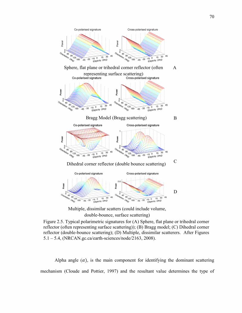
70
Alpha angle (𝛼), is the main component for identifying the dominant scattering
mechanism (Cloude and Pottier, 1997) and the resultant value determines the type of
Sphere, flat plane or trihedral corner reflector (often representing surface scattering)
Bragg Model (Bragg scattering)
Dihedral corner reflector (double bounce scattering)
Figure 2.5. Typical polarimetric signatures for (A) Sphere, flat plane or trihedral corner reflector (often representing surface scattering)); (B) Bragg model; (C) Dihedral corner reflector (double-bounce scattering); (D) Multiple, dissimilar scatterers. After Figures 5.1 – 5.4, (NRCAN.gc.ca/earth-sciences/node/2163, 2008).
A
B
C
Multiple, dissimilar scatters (could include volume, double-bounce, surface scattering)
D
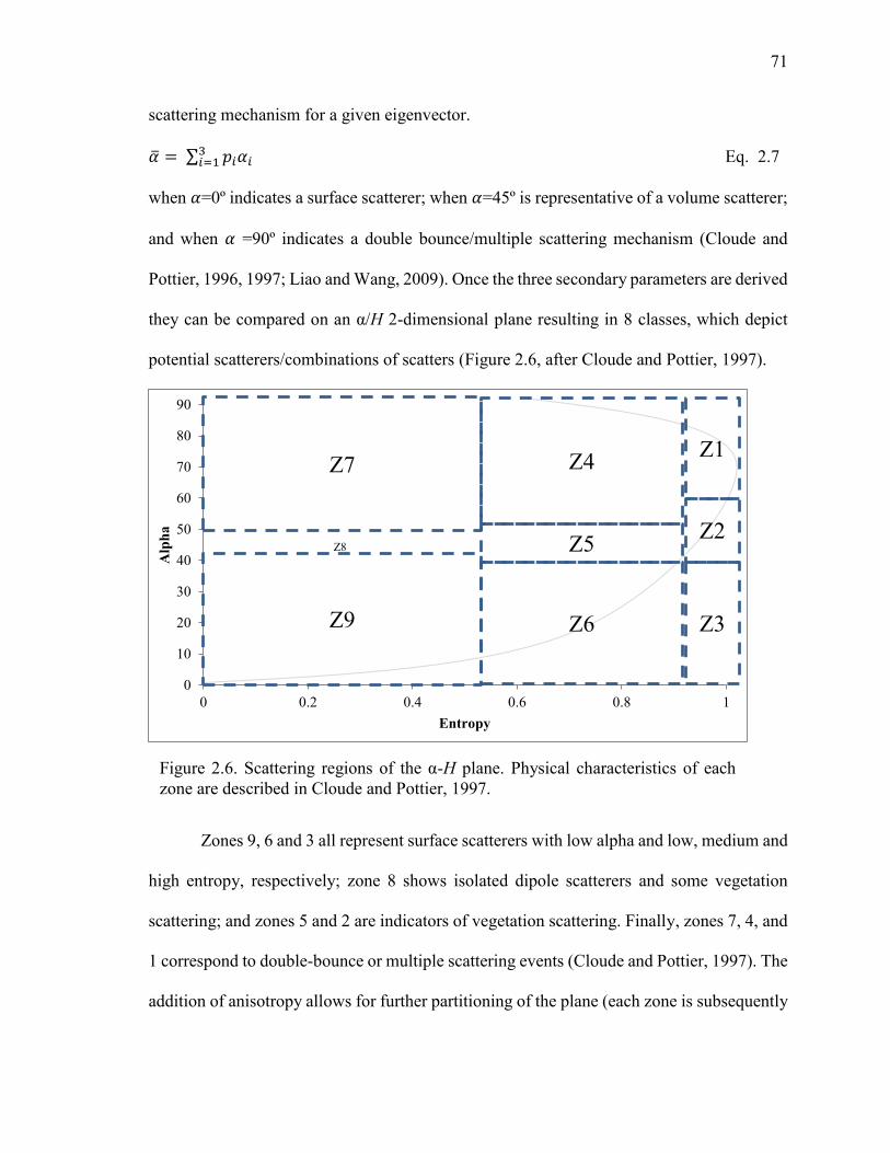
71
scattering mechanism for a given eigenvector.
�̅� = ∑ 𝑝𝑖𝛼𝑖3𝑖=1 Eq. 2.7
when 𝛼=0º indicates a surface scatterer; when 𝛼=45º is representative of a volume scatterer;
and when 𝛼 =90º indicates a double bounce/multiple scattering mechanism (Cloude and
Pottier, 1996, 1997; Liao and Wang, 2009). Once the three secondary parameters are derived
they can be compared on an α/H 2-dimensional plane resulting in 8 classes, which depict
potential scatterers/combinations of scatters (Figure 2.6, after Cloude and Pottier, 1997).
Zones 9, 6 and 3 all represent surface scatterers with low alpha and low, medium and
high entropy, respectively; zone 8 shows isolated dipole scatterers and some vegetation
scattering; and zones 5 and 2 are indicators of vegetation scattering. Finally, zones 7, 4, and
1 correspond to double-bounce or multiple scattering events (Cloude and Pottier, 1997). The
addition of anisotropy allows for further partitioning of the plane (each zone is subsequently
0
10
20
30
40
50
60
70
80
90
0 0.2 0.4 0.6 0.8 1
Alp
ha
Entropy
Z7
Z8
Z9
Z4
Z5
Z6
Z1
Z2
Z3
Figure 2.6. Scattering regions of the α-H plane. Physical characteristics of each zone are described in Cloude and Pottier, 1997.
72
split into two ((resulting in 16 potential zones of scattering) Cloude and Pottier, 1997). The
Wishart unsupervised classification utilizes these zones (either 8 or 16) as training areas.
Wishart unsupervised classifier assigns pixels to classes similarly in a process to a k-means
algorithm (Anfinsen et al., 2007), but rather than using the sample-cluster mean vector
distance to cluster the data, Wishart uses a matrix derived distance (Anfinsen et al., 2007).
Sartori et al. (2011), using ALOS (Advanced Land Observing Satellite) PALSAR
(Phased Array L-band Synthetic Aperture Radar) data, compared a rule-based classification
to the CP decomposition variables, the H/α plane + Wishart classifications, and other
polarimetric variables to map macrophyte species in the Amazon floodplain wetlands in
Brazil. They found that the CP decomposition variables (the H/α plane) were able to separate
the floodplain from the upland, macrophytes from floodable (affected by the annual flood
pulse) areas of trees and shrubs, but they could not distinguish between the macrophyte
species. The Wishart H/α classifier was not able to separate the floodplain from the upland,
but was able to separate floodable trees and shrubs from macrophyte species.
Touzi et al. (2007) compared the Touzi decomposition (Touzi, 2007) to the CP
decomposition and found that the Touzi variables were better in discrimination of wetland
vegetation. This study was conducted at Mer Bleue Bog, one of the sites for this research.
As others have found that CP components can distinguish between classes such as upland,
wetland, forest and shrub (Sartori et al., 2011) or that higher alpha values indicated flooded
vegetation (Schmitt and Brisco, 2013), and instead of repeating the methods in Touzi et al.
(2007), it was decided to evaluate the potential of addition of the CP components to other
imagery types or variables in improving wetland classifications.
73
Based upon the literature review in the previous sections it was expected that
utilizing radar and optical variables together in classification with OBIA and CTA would
improve upon overall accuracies presented as 86 – 89% for Wetland Type classification, and
greater than 76% for VCFs. For Open Water Type, using with OBIA optical imagery with
radar and DEM information using a non-parametric classifier was expected to improve upon
results from other studies that have used one data type, and/or pixel-based classification,
and/or parametric classifiers.
2.9 Selection of OWES attributes for image modelling and classification
Chisholm et al. (1997) developed predictive linear regression models to identify
whether different combinations OWES attributes contributed more to the overall wetland
score. Eight variables were identified that contributed most to the overall score and included
wetland size (log), wetland type rarity, recreational activities, flood attenuation, open water
types, proximity to human settlement, proximity to other wetlands, and education and public
awareness. In conjunction with this, and after review of the OWES with OMNR experts and
users, a subset of the OWES attributes were selected based on their potential for detection,
estimation or classification in remotely sensed imagery and/or their potential to be derived
from existing GIS data. These were selected prior to in-depth review of the remote sensing
literature. The second criterion was that selected attributes had to contribute most to an
overall OWES wetland score (Chisholm et al., 1997). Table 2.4 lists, from the 2002 Southern
Ontario Evaluation manual (2002), each of the OWES components, the sub-component and
the selected attribute to be mapped in this research. In some cases, attributes were duplicated
under different OWES components. The methods used for each attribute are listed in the
rightmost column and described in Chapter 4. The description of each attribute and its
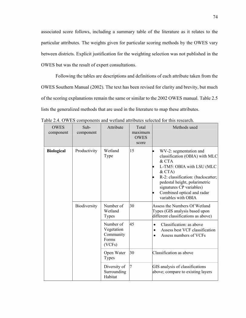
74
associated score follows, including a summary table of the literature as it relates to the
particular attributes. The weights given for particular scoring methods by the OWES vary
between districts. Explicit justification for the weighting selection was not published in the
OWES but was the result of expert consultations.
Following the tables are descriptions and definitions of each attribute taken from the
OWES Southern Manual (2002). The text has been revised for clarity and brevity, but much
of the scoring explanations remain the same or similar to the 2002 OWES manual. Table 2.5
lists the generalized methods that are used in the literature to map these attributes.
Table 2.4. OWES components and wetland attributes selected for this research. OWES
component Sub-
component Attribute Total
maximum OWES score
Methods used
Biological Productivity Wetland Type
15 WV-2: segmentation and classification (OBIA) with MLC & CTA
L-TM5: OBIA with LSU (MLC & CTA)
R-2: classification: (backscatter; pedestal height, polarimetric signatures CP variables)
Combined optical and radar variables with OBIA
Biodiversity
Number of Wetland Types
30 Assess the Numbers Of Wetland Types (GIS analysis based upon different classifications as above)
Number of Vegetation Community Forms (VCFs)
45 Classification: as above Assess best VCF classification Assess numbers of VCFs
Open Water Types
30 Classification as above
Diversity of Surrounding Habitat
7 GIS analysis of classifications above; compare to existing layers
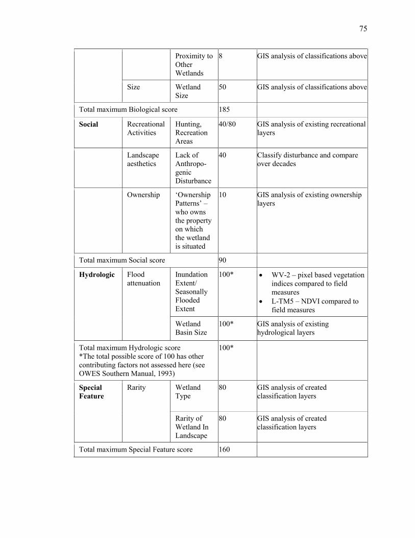
75
Proximity to Other Wetlands
8 GIS analysis of classifications above
Size Wetland Size
50 GIS analysis of classifications above
Total maximum Biological score 185
Social Recreational Activities
Hunting, Recreation Areas
40/80 GIS analysis of existing recreational layers
Landscape aesthetics
Lack of Anthropo-genic Disturbance
40 Classify disturbance and compare over decades
Ownership ‘Ownership Patterns’ – who owns the property on which the wetland is situated
10 GIS analysis of existing ownership layers
Total maximum Social score 90
Hydrologic Flood attenuation
Inundation Extent/ Seasonally Flooded Extent
100* WV-2 – pixel based vegetation indices compared to field measures
L-TM5 – NDVI compared to field measures
Wetland Basin Size
100* GIS analysis of existing hydrological layers
Total maximum Hydrologic score *The total possible score of 100 has other contributing factors not assessed here (see OWES Southern Manual, 1993)
100*
Special Feature
Rarity Wetland Type
80 GIS analysis of created classification layers
Rarity of Wetland In Landscape
80 GIS analysis of created classification layers
Total maximum Special Feature score 160
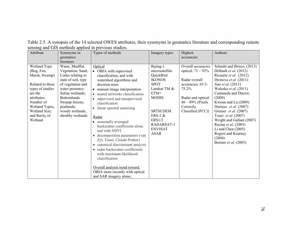
76
Table 2.5. A synopsis of the 14 selected OWES attributes, their synonyms in geomatics literature and corresponding remote sensing and GIS methods applied in previous studies.
Attribute Synonyms in geomatics literature
Types of methods Imagery types Highest accuracies
Authors
Wetland Type (Bog, Fen, Marsh, Swamp) Related to these types of studies are the attributes: Number of Wetland Types, Wetland Size; and Rarity of Wetland
Water, Mudflat, Vegetation, Sand; Codes relating to state of soil, type of vegetation and water presence; Saline wetlands; Bottomlands Swamp forests; peatlands; woody wetlands, shrubby wetlands
Optical OBIA with supervised
classification, and with watershed algorithms and decision trees
manual image interpretation neural networks classification supervised and unsupervised
classification linear spectral unmixing Radar seasonally averaged
backscatter coefficients alone and with NDVI
decomposition parameters (van Zyl, Touzi, Cloude-Pottier)
canonical discriminant analysis radar backscatter coefficients
with maximum likelihood classification
Overall analysis trend toward: OBIA more recently with optical and SAR imagery alone;
Bejing-1 microsatellite QuickBird IKONOS SPOT Landsat TM & ETM+ MODIS SRTM DEM ERS-2 & ERS1/2 RADARSAT-1 ENVISAT ASAR
Overall accuracies optical: 71 – 92% Radar overall accuracies: 65.5-75.2% Radar and optical: 86 – 89% (Pixels Correctly Classified (PCC))
Schmitt and Brisco, (2013) Dribault et al. (2012) Ricaurte et al. (2012) Dronova et al. (2011) Jiao et al. (2011) Waleska et al. (2011) Castaneda and Ducrot, (2009) Kwoun and Lu (2009) Durieux et al. (2007) Grenier et al. (2007) Touzi et al. (2007) Wright and Gallant (2007) Racine et al. (2005) Li and Chen (2005) Rogers and Kearney (2004) Bernier et al. (2003)
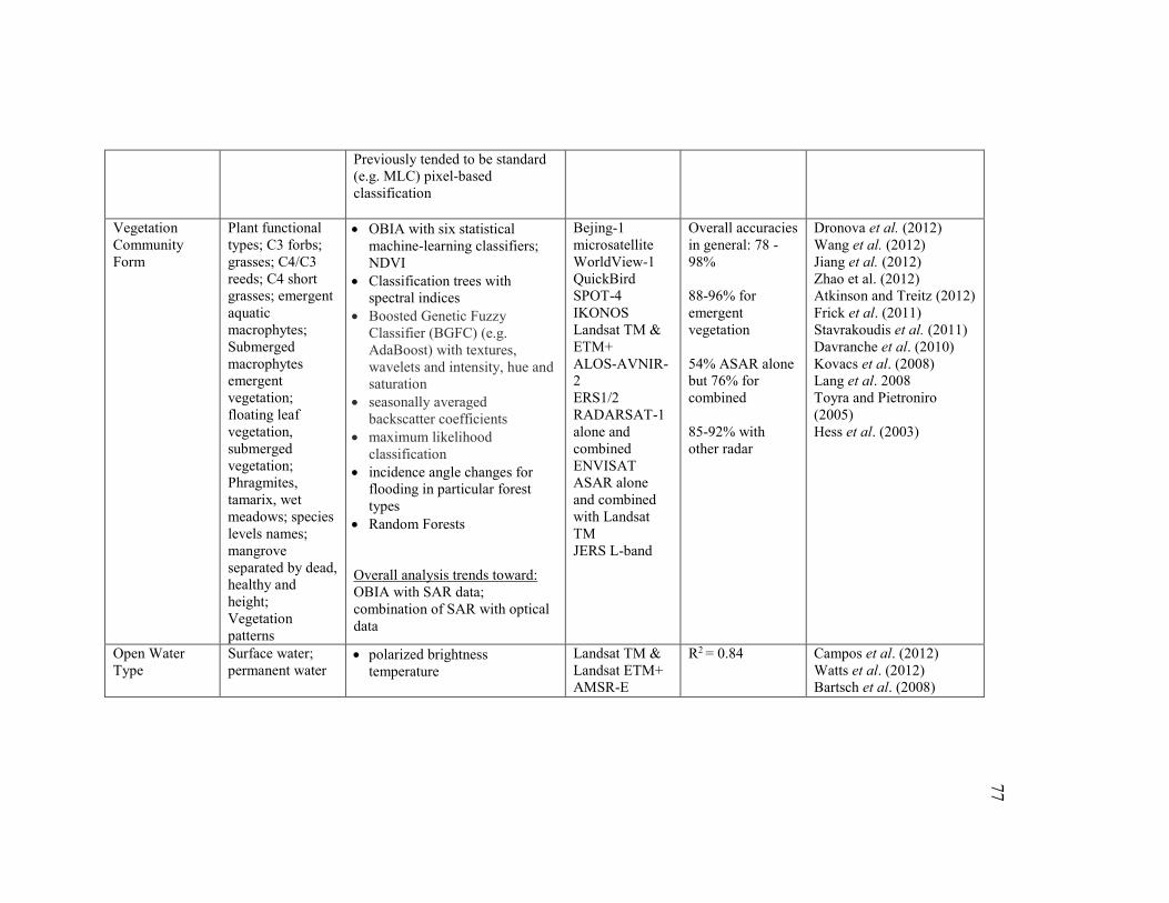
77
Previously tended to be standard (e.g. MLC) pixel-based classification
Vegetation Community Form
Plant functional types; C3 forbs; grasses; C4/C3 reeds; C4 short grasses; emergent aquatic macrophytes; Submerged macrophytes emergent vegetation; floating leaf vegetation, submerged vegetation; Phragmites, tamarix, wet meadows; species levels names; mangrove separated by dead, healthy and height; Vegetation patterns
OBIA with six statistical machine-learning classifiers; NDVI
Classification trees with spectral indices
Boosted Genetic Fuzzy Classifier (BGFC) (e.g. AdaBoost) with textures, wavelets and intensity, hue and saturation
seasonally averaged backscatter coefficients
maximum likelihood classification
incidence angle changes for flooding in particular forest types
Random Forests Overall analysis trends toward: OBIA with SAR data; combination of SAR with optical data
Bejing-1 microsatellite WorldView-1 QuickBird SPOT-4 IKONOS Landsat TM & ETM+ ALOS-AVNIR-2 ERS1/2 RADARSAT-1 alone and combined ENVISAT ASAR alone and combined with Landsat TM JERS L-band
Overall accuracies in general: 78 -98% 88-96% for emergent vegetation 54% ASAR alone but 76% for combined 85-92% with other radar
Dronova et al. (2012) Wang et al. (2012) Jiang et al. (2012) Zhao et al. (2012) Atkinson and Treitz (2012) Frick et al. (2011) Stavrakoudis et al. (2011) Davranche et al. (2010) Kovacs et al. (2008) Lang et al. 2008 Toyra and Pietroniro (2005) Hess et al. (2003)
Open Water Type
Surface water; permanent water
polarized brightness temperature
Landsat TM & Landsat ETM+ AMSR-E
R2 = 0.84 Campos et al. (2012)
Watts et al. (2012) Bartsch et al. (2008)
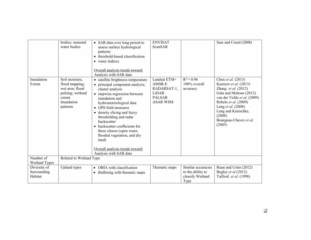
78
bodies; seasonal water bodies
SAR data over long period to assess surface hydrological patterns
threshold-based classification water indices Overall analysis trends toward: Analysis with SAR data
ENVISAT ScanSAR
Sass and Creed (2008)
Inundation Extent
Soil moisture, flood mapping; wet area; flood pulsing; wetland extent Inundation patterns
satellite brightness temperature principal component analysis;
cluster analysis stepwise regression between
inundation and hydrometerological data
GPS field measures density slicing and fuzzy
thresholding and radar backscatter
backscatter coefficients for three classes (open water, flooded vegetation, and dry land)
Overall analysis trends toward: Analysis with SAR data
Landsat ETM+ AMSR-E RADARSAT-1, LiDAR PALSAR ASAR WSM
R2 = 0.96
100% overall accuracy
Chen et al. (2013) Kuenzer et al. (2013) Zhang et al. (2012) Gala and Melesse (2012) van der Velde et al. (2009) Rebelo et al. (2009) Lang et al. (2008) Lang and Kasischke, (2008) Bourgeau-Chavez et al. (2005)
Number of Wetland Types
Related to Wetland Type
Diversity of Surrounding Habitat
Upland types OBIA with classification Buffering with thematic maps
Thematic maps Similar accuracies to the ability to classify Wetland Type
Ruan and Ustin (2012) Begley et al (2012) Tufford et al. (1998)
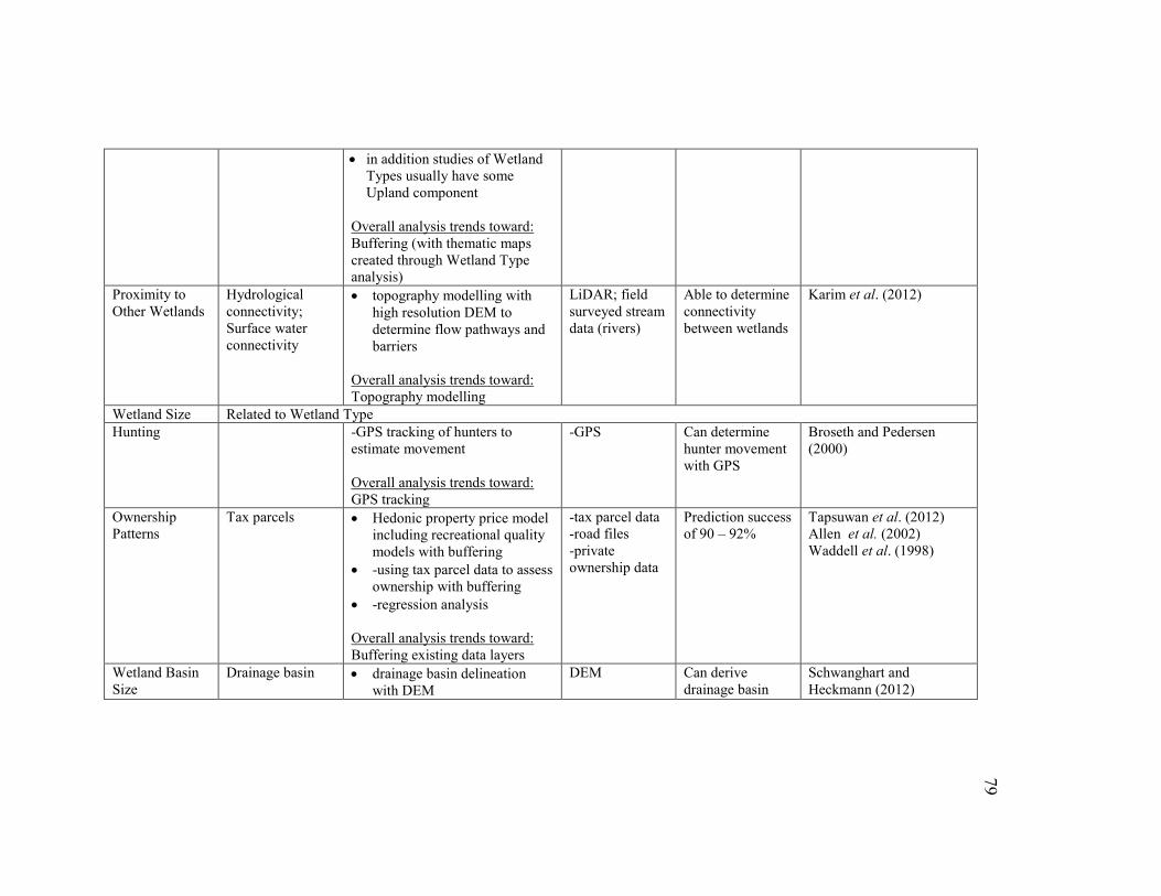
79
in addition studies of Wetland Types usually have some Upland component
Overall analysis trends toward: Buffering (with thematic maps created through Wetland Type analysis)
Proximity to Other Wetlands
Hydrological connectivity; Surface water connectivity
topography modelling with high resolution DEM to determine flow pathways and barriers
Overall analysis trends toward: Topography modelling
LiDAR; field surveyed stream data (rivers)
Able to determine connectivity between wetlands
Karim et al. (2012)
Wetland Size Related to Wetland Type Hunting -GPS tracking of hunters to
estimate movement Overall analysis trends toward: GPS tracking
-GPS Can determine hunter movement with GPS
Broseth and Pedersen (2000)
Ownership Patterns
Tax parcels Hedonic property price model including recreational quality models with buffering
-using tax parcel data to assess ownership with buffering
-regression analysis Overall analysis trends toward: Buffering existing data layers
-tax parcel data -road files -private ownership data
Prediction success of 90 – 92%
Tapsuwan et al. (2012) Allen et al. (2002) Waddell et al. (1998)
Wetland Basin Size
Drainage basin drainage basin delineation with DEM
DEM Can derive drainage basin
Schwanghart and Heckmann (2012)
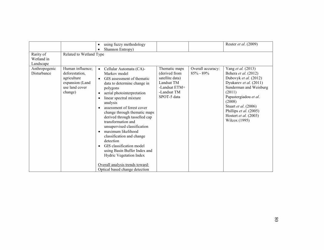
80
using fuzzy methodology Shannon Entropy)
Reuter et al. (2009)
Rarity of Wetland in Landscape
Related to Wetland Type
Anthropogenic Disturbance
Human influence; deforestation, agriculture expansion (Land use land cover change)
Cellular Automata (CA)-Markov model
GIS assessment of thematic data to determine change in polygons
aerial photointerpretation linear spectral mixture
analysis assessment of forest cover
change through thematic maps derived through tasselled cap transformation and unsupervised classification
maximum likelihood classification and change detection
GIS classification model using Basin Buffer Index and Hydric Vegetation Index
Overall analysis trends toward: Optical based change detection
Thematic maps (derived from satellite data) Landsat TM -Landsat ETM+ -Landsat TM SPOT-5 data
Overall accuracy: 85% - 89%
Yang et al. (2013) Behera et al. (2012) Dubovyk et al. (2012) Dyukarev et al. (2011) Sunderman and Weisburg (2011) Papastergiadou et al. (2008) Stuart et al. (2006) Phillips et al. (2005) Hostert et al. (2003) Wilcox (1995)
81
81
2.9.1 Wetland Type (Biological and Special Feature components)
Wetland Types in the literature may be any relevant class name such as water,
mudflat, vegetation, sand, saline wetlands, swamp forests, bottomlands, wood wetlands,
shrubby wetlands, etc. In this research, Wetland Type refers the National Wetland
Classification System classes of Bog, Fen, Marsh and Swamp (National Wetlands Working
Group, 1988), as used by the OWES. Overall classification accuracy for these types of
classes have ranged from 66% to 92%, depending on the number of classes and their
specificity, the data, and the methods used (Bernier et al., 2003; Rogers and Kearney, 2004;
Li and Chen, 2005; Racine et al., 2005; Wright and Gallant, 2007; Touzi et al., 2007;
Grenier et al., 2007; Durieux et al., 2007; Castaneda and Ducrot, 2009; Kwoun and Lu,
2009; Jiao et al., 2011; Dronova et al., 2011; Ricaurte et al., 2012). The overall trend in the
research is toward utilizing OBIA combined with variations of optical and radar images, as
well as derived image variables. This research was designed to contribute to this growing
body of work.
The methods selected to map Wetland Types and reasons for selecting them are
outlined in section 2.8.1 through 2.8.4 because those methods are used repeatedly for 5 of
the 14 attributes. In relation to SOLRIS (2003), which is the current method used to
inventory wetlands in Southern Ontario, these methods were employed to minimize the data
used, use newer higher resolution optical imagery and newer fully polarimetric radar
variables, and determine if the overall accuracies (82% to 95%) could be maintained or
improved for more than one reference site.
82
82
Based upon the overall literature analysis of this chapter, it was expected that using
OBIA with WorldView-2 imagery and combinations of other imagery types such as
Radarsat-2 polarimetric variables, Landsat 5 data and CTA, would improve upon the
accuracies listed in the literature which range in overall accuracy from 71 – 92%.
Additionally, the potential for application of LSU fractions with OBIA and/or CTA and
moderate resolution data such as Landsat to derive subpixel land cover and land cover
change information was deemed to be high. The minimal literature on this topic suggested
that this approach may contribute significantly to advancement of wetland mapping and
monitoring.
For scoring Wetland Type for the OWES, the proportion of each Wetland Type to
the whole wetland complex, known as Fractional Area (FA = area Wetland Type/total
wetland area), is calculated and then multiplied by a weight for the given wetland type as
follows:
Bog = FA x 3
Fen = FA x 6
Swamp = FA x 8
Marsh = FA x 15
The complete score for Wetland Type (category) is determined by summing the individual
scores per individual type of wetland.
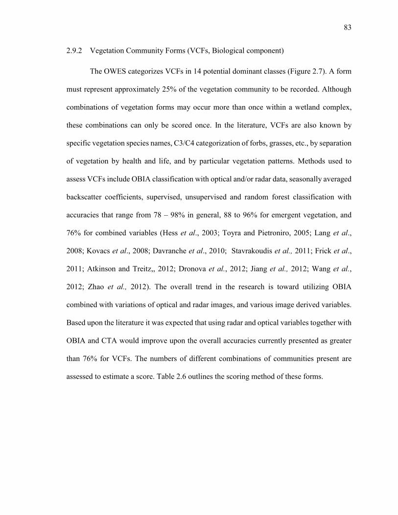
83
83
2.9.2 Vegetation Community Forms (VCFs, Biological component)
The OWES categorizes VCFs in 14 potential dominant classes (Figure 2.7). A form
must represent approximately 25% of the vegetation community to be recorded. Although
combinations of vegetation forms may occur more than once within a wetland complex,
these combinations can only be scored once. In the literature, VCFs are also known by
specific vegetation species names, C3/C4 categorization of forbs, grasses, etc., by separation
of vegetation by health and life, and by particular vegetation patterns. Methods used to
assess VCFs include OBIA classification with optical and/or radar data, seasonally averaged
backscatter coefficients, supervised, unsupervised and random forest classification with
accuracies that range from 78 – 98% in general, 88 to 96% for emergent vegetation, and
76% for combined variables (Hess et al., 2003; Toyra and Pietroniro, 2005; Lang et al.,
2008; Kovacs et al., 2008; Davranche et al., 2010; Stavrakoudis et al., 2011; Frick et al.,
2011; Atkinson and Treitz,, 2012; Dronova et al., 2012; Jiang et al., 2012; Wang et al.,
2012; Zhao et al., 2012). The overall trend in the research is toward utilizing OBIA
combined with variations of optical and radar images, and various image derived variables.
Based upon the literature it was expected that using radar and optical variables together with
OBIA and CTA would improve upon the overall accuracies currently presented as greater
than 76% for VCFs. The numbers of different combinations of communities present are
assessed to estimate a score. Table 2.6 outlines the scoring method of these forms.
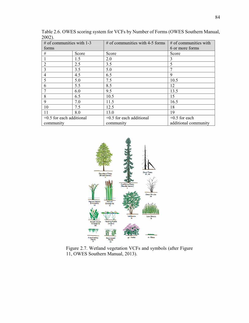
84
84
Table 2.6. OWES scoring system for VCFs by Number of Forms (OWES Southern Manual, 2002).
# of communities with 1-3 forms
# of communities with 4-5 forms # of communities with 6 or more forms
# Score Score Score 1 1.5 2.0 3 2 2.5 3.5 5 3 3.5 5.0 7 4 4.5 6.5 9 5 5.0 7.5 10.5 6 5.5 8.5 12 7 6.0 9.5 13.5 8 6.5 10.5 15 9 7.0 11.5 16.5 10 7.5 12.5 18 11 8.0 13.0 19 +0.5 for each additional community
+0.5 for each additional community
+0.5 for each additional community
Figure 2.7. Wetland vegetation VCFs and symbols (after Figure 11, OWES Southern Manual, 2013).
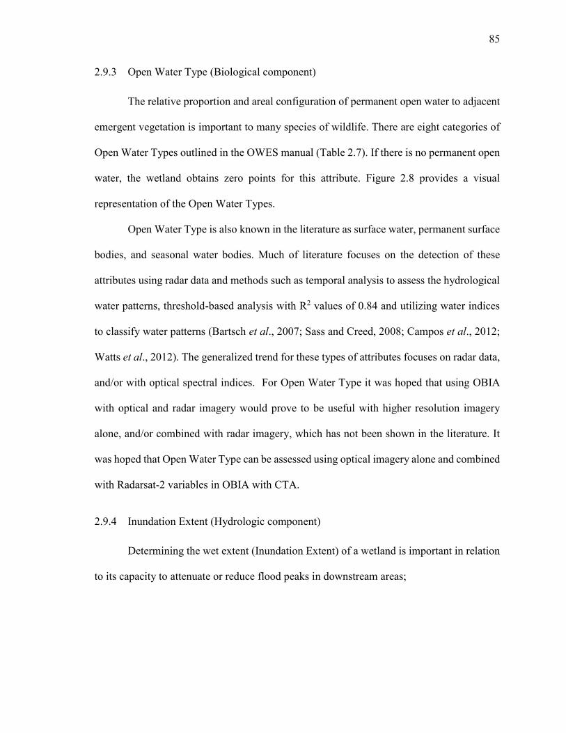
85
85
2.9.3 Open Water Type (Biological component)
The relative proportion and areal configuration of permanent open water to adjacent
emergent vegetation is important to many species of wildlife. There are eight categories of
Open Water Types outlined in the OWES manual (Table 2.7). If there is no permanent open
water, the wetland obtains zero points for this attribute. Figure 2.8 provides a visual
representation of the Open Water Types.
Open Water Type is also known in the literature as surface water, permanent surface
bodies, and seasonal water bodies. Much of literature focuses on the detection of these
attributes using radar data and methods such as temporal analysis to assess the hydrological
water patterns, threshold-based analysis with R2 values of 0.84 and utilizing water indices
to classify water patterns (Bartsch et al., 2007; Sass and Creed, 2008; Campos et al., 2012;
Watts et al., 2012). The generalized trend for these types of attributes focuses on radar data,
and/or with optical spectral indices. For Open Water Type it was hoped that using OBIA
with optical and radar imagery would prove to be useful with higher resolution imagery
alone, and/or combined with radar imagery, which has not been shown in the literature. It
was hoped that Open Water Type can be assessed using optical imagery alone and combined
with Radarsat-2 variables in OBIA with CTA.
2.9.4 Inundation Extent (Hydrologic component)
Determining the wet extent (Inundation Extent) of a wetland is important in relation
to its capacity to attenuate or reduce flood peaks in downstream areas;
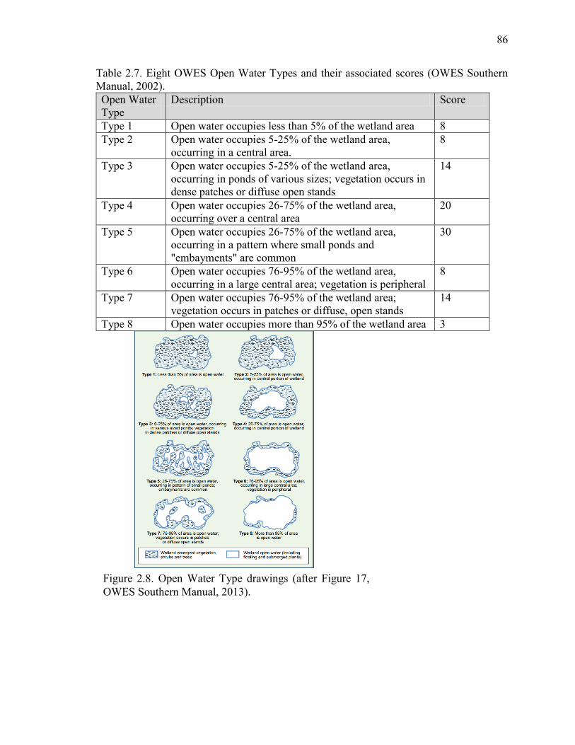
86
86
Table 2.7. Eight OWES Open Water Types and their associated scores (OWES Southern Manual, 2002). Open Water Type
Description Score
Type 1 Open water occupies less than 5% of the wetland area 8 Type 2 Open water occupies 5-25% of the wetland area,
occurring in a central area. 8
Type 3 Open water occupies 5-25% of the wetland area, occurring in ponds of various sizes; vegetation occurs in dense patches or diffuse open stands
14
Type 4 Open water occupies 26-75% of the wetland area, occurring over a central area
20
Type 5 Open water occupies 26-75% of the wetland area, occurring in a pattern where small ponds and "embayments" are common
30
Type 6 Open water occupies 76-95% of the wetland area, occurring in a large central area; vegetation is peripheral
8
Type 7 Open water occupies 76-95% of the wetland area; vegetation occurs in patches or diffuse, open stands
14
Type 8 Open water occupies more than 95% of the wetland area 3
Figure 2.8. Open Water Type drawings (after Figure 17, OWES Southern Manual, 2013).
87
87
this is an important ecological function, as well as providing obvious human value function
(OWES, 2002). Inundation extent could be considered the maximum size of a wetland when
considering its hydrological function to attenuate flood peaks.
The specific use of vegetation indices selected for this research is presented here as
it only relates to this one attribute. There are approximately 150 different types of vegetation
indices (Asner, 1998) proposed in a wide variety of studies that support the use of the
different indices to establish different patterns in wetlands. Mathematical combinations of
two or more spectral bands have been shown to be reliable indicators of vegetation
health/primary productivity such as NDVI (Eq. 2.1); moisture content in the canopy (NDWI,
Normalized Difference Water Index)(Gao, 1996)); or through inference, of soil composition
(MCARI, Modified Chlorophyll Absorption Ratio Index best estimated soil Total Petroleum
Hydrocarbons (TPH) (Zhu et al., 2013).
As a variant of NDVI, NDVIgreen is derived as:
𝑁𝐷𝑉𝐼𝑔𝑟𝑒𝑒𝑛 = (𝑁𝐼𝑅−𝐺)
(𝐺+𝑁𝐼𝑅) Eq. 2.8
where NIR is the near-infrared spectral band of a sensor; and
G represents the green spectral band of same sensor.
NDVIGreen has not been shown to determine wet extents of wetlands, habitat, or wetland
type in the literature. NDVIGreen was developed as a way to estimate plant chlorophyll
(Gitelson and Merzlyak, 1997), which changes throughout a plant’s lifespan and as it reacts
to stressors (such as soil moisture levels). Similar indices have been used to map habitat,
wetland type and plant functional types in the literature. Delgado and Marin (2013) utilized
88
88
Landsat-derived NDVI values to map swan habitat in a southern Chilean wetland. They
found they were able to estimate habitat area, but not determine individual vegetation
species.
Wang et al. (2012) classified plant functional types at Poyang Lake, China
(freshwater lake-wetland) using time series of NDVI and another of the vegetation-water
index (VWI = time series NDVI/Submersion Time Index) derived from Beijing-1
microsatellite (32m pixels with 3 spectral bands, green (0.52-0.62 μm; red (0.63-0.69 μm)
and NIR (0.76-0.09 μm)). They obtained an overall accuracy of 81.3% for 3 plant functional
types (and 3 general classes, water, mudflat and sand).
Campos et al. (2012) detected seasonal and permanent surface water utilizing
NDWIGreen/MIR (Gao, 1996) and NDWINIR/MIR (Xu, 2006) derived from multi-temporal
series of Landsat 5 TM and 7 ETM+ (Enhanced Thematic Mapper Plus) imagery over
Mauritania.
Lang et al. (2008) used multi-date C-band data from ERS-2 and ENVISAT to
compare with field observation of inundation and soil moisture, deriving principal
components from both leaf-off and leaf-on data sets. The comparative analysis resulted in
R2 for soil moisture from 0.55 to 0.90 and for inundated area R2 values from 0.06 to 0.81.
van der Velde et al. (2009) assessed the backscatter signatures derived from single
polarized (HH, VV) ASAR WSM imagery of grassland and a wetland to conduct multi-
variate analysis of soil moisture, soil temperature and vegetation biomass against SPOT
89
89
NDVI. The correlation calculated between backscatter and wetland soil moisture were 0.62;
with wetland NDVI was 0.56 and with soil temperatures was 0.64.
This research builds on the literature by: 1) evaluating various vegetation indices
derived from more recent imagery such as WorldView-2 as well as Landsat TM imagery to
determine an optimal index for mapping the wet extent boundary, and 2) to correlate radar
parameters against transect measured soil moisture and to use that relationship to estimate
the location of wet extent. (Lang et al., 2008; van der Velde et al., 2009).
The scoring of flood attenuation is complex and requires knowledge of the wetland
of interest and the surrounding wetlands within the same basin. The complete outline of this
scoring method is given in Appendix A.
2.9.5 Number of Wetland Types (Biological component)
For this and the following attributes up to Anthropogenic Disturbance, the main
requirement of the collaboration with the OMNR was to assess the LIO data and use it in
simple GIS applications as described in section 2.6.2 to determine if these data and methods
were sufficient to map these attributes. There are methods in the remote sensing and GIS
literature that are used to derive new thematic data to map these variables and these are listed
in Table 2.5, however, they were out of the scope of this research.
The OWES assumes that for every additional Wetland Type present in a wetland or
wetland complex, species presence should increase by 50%, therefore the score increases
incrementally by a factor of ~1.5 with each additional Wetland Type, resulting in scores as
90
90
follows (maximum of 30 points): One Wetland Type = 9 points, Two Wetland Types = 13
points, Three Wetland Types = 20 points, Four Wetland Types = 30 points.
2.9.6 Diversity of Surrounding Habitat (Biological component)
Surrounding habitat can act as both a buffer to wetlands (e.g. providing access to the
wetlands) or as a deterrent to use (e.g. intense human activity). Surrounding habitats were
assessed as those that were within 1.5 km straight line distance to the edge of the wetland
and that had a MMU of 0.5 ha or greater (following the criteria as the OWES, 2002). The
OWES scoring of these habitats gives one point to each of the following (maximum of 7
points): row crop, pasture, abandoned agricultural land, deciduous forest, coniferous forest,
mixed forest, abandoned pits and quarries, open lake or deep river, fence rows with deep
cover, or shelterbelts, terrain appreciably undulating, hilly or with ravines, creek flood plain.
2.9.7 Proximity to Other Wetlands (Biological component)
When wetlands are located close to one another wildlife can move between them
allowing for extended use of habitat, breeding areas, food sources among others, and
therefore the associated value of the wetland is increased (OWES, 2002). The most valuable
wetlands are those that are connected hydrologically via surface water, even if that surface
water is seasonal. The scoring of proximity is made from the boundary of the entire wetland
complex, and not for wetlands within the complex, which are assumed to have proximity of
0 km. The scores for this category are assessed for the highest valued category (maximum
of 8 points) and are outlined in Table 2.8.
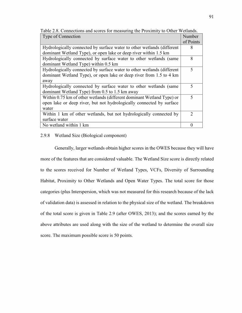
91
91
Table 2.8. Connections and scores for measuring the Proximity to Other Wetlands. Type of Connection Number
of Points Hydrologically connected by surface water to other wetlands (different dominant Wetland Type), or open lake or deep river within 1.5 km
8
Hydrologically connected by surface water to other wetlands (same dominant Wetland Type) within 0.5 km
8
Hydrologically connected by surface water to other wetlands (different dominant Wetland Type), or open lake or deep river from 1.5 to 4 km away
5
Hydrologically connected by surface water to other wetlands (same dominant Wetland Type) from 0.5 to 1.5 km away
5
Within 0.75 km of other wetlands (different dominant Wetland Type) or open lake or deep river, but not hydrologically connected by surface water
5
Within 1 km of other wetlands, but not hydrologically connected by surface water
2
No wetland within 1 km 0
2.9.8 Wetland Size (Biological component)
Generally, larger wetlands obtain higher scores in the OWES because they will have
more of the features that are considered valuable. The Wetland Size score is directly related
to the scores received for Number of Wetland Types, VCFs, Diversity of Surrounding
Habitat, Proximity to Other Wetlands and Open Water Types. The total score for those
categories (plus Interspersion, which was not measured for this research because of the lack
of validation data) is assessed in relation to the physical size of the wetland. The breakdown
of the total score is given in Table 2.9 (after OWES, 2013); and the scores earned by the
above attributes are used along with the size of the wetland to determine the overall size
score. The maximum possible score is 50 points.
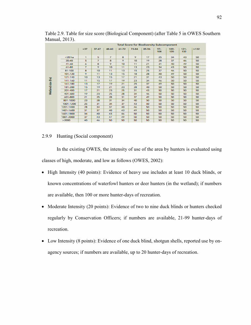
92
92
2.9.9 Hunting (Social component)
In the existing OWES, the intensity of use of the area by hunters is evaluated using
classes of high, moderate, and low as follows (OWES, 2002):
High Intensity (40 points): Evidence of heavy use includes at least 10 duck blinds, or
known concentrations of waterfowl hunters or deer hunters (in the wetland); if numbers
are available, then 100 or more hunter-days of recreation.
Moderate Intensity (20 points): Evidence of two to nine duck blinds or hunters checked
regularly by Conservation Officers; if numbers are available, 21-99 hunter-days of
recreation.
Low Intensity (8 points): Evidence of one duck blind, shotgun shells, reported use by on-
agency sources; if numbers are available, up to 20 hunter-days of recreation.
Table 2.9. Table for size score (Biological Component) (after Table 5 in OWES Southern Manual, 2013).
93
93
2.9.10 Ownership Patterns (Social component)
Ownership of a wetland is an indicator of the value of a wetland to humans. Privately
held lands have less value than publicly owned wetlands (OWES, 2002) due to lack of
accessibility and inability to direct conservation. The scoring of this attribute is made by
estimating the percentage (fractional area, FA) of ownership of a wetland and multiplying it
by a factor depending upon the ownership pattern, to a maximum of 10 points.
Private or Crown lands, held under contract or in trust for wetland protection FA x 10
Public land FA x 8
Private land FA x 4
2.9.11 Wetland Basin Size (Hydrologic component)
Upstream detention attributes are often used to determine the net benefit of the
wetland in relation to the all the other possible detention areas upstream of the wetland.
Theoretically, if there are detention areas (other wetlands, especially riverine wetlands,
rivers and lakes, etc.) upstream of the evaluated wetland, the overall hydrological detention
value of the downstream wetland is reduced. However, with the removal of the upstream
areas (anthropogenic disturbance/development) the value of the downstream area will
obviously increase. As well, if a wetland represents 50% of total storage or more in its basin
(based on area), it will provide maximum detention benefits regardless of its position
(Adamus and Stockwell, 1983). Three factors need to be determined to assess the overall
effectiveness for flood attenuation of a wetland complex: wetland basin size, size of the
wetland, and size of other detention areas in the basin.
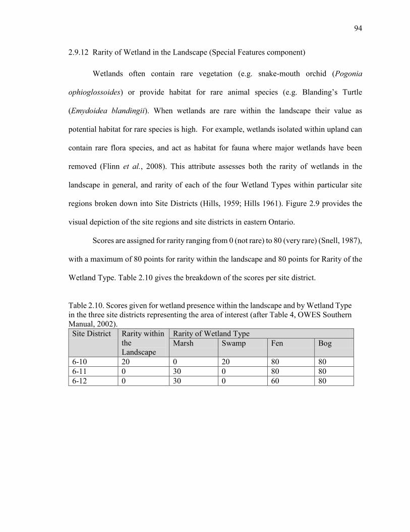
94
94
2.9.12 Rarity of Wetland in the Landscape (Special Features component)
Wetlands often contain rare vegetation (e.g. snake-mouth orchid (Pogonia
ophioglossoides) or provide habitat for rare animal species (e.g. Blanding’s Turtle
(Emydoidea blandingii). When wetlands are rare within the landscape their value as
potential habitat for rare species is high. For example, wetlands isolated within upland can
contain rare flora species, and act as habitat for fauna where major wetlands have been
removed (Flinn et al., 2008). This attribute assesses both the rarity of wetlands in the
landscape in general, and rarity of each of the four Wetland Types within particular site
regions broken down into Site Districts (Hills, 1959; Hills 1961). Figure 2.9 provides the
visual depiction of the site regions and site districts in eastern Ontario.
Scores are assigned for rarity ranging from 0 (not rare) to 80 (very rare) (Snell, 1987),
with a maximum of 80 points for rarity within the landscape and 80 points for Rarity of the
Wetland Type. Table 2.10 gives the breakdown of the scores per site district.
Table 2.10. Scores given for wetland presence within the landscape and by Wetland Type in the three site districts representing the area of interest (after Table 4, OWES Southern Manual, 2002). Site District Rarity within
the Landscape
Rarity of Wetland Type Marsh Swamp Fen Bog
6-10 20 0 20 80 80 6-11 0 30 0 80 80 6-12 0 30 0 60 80
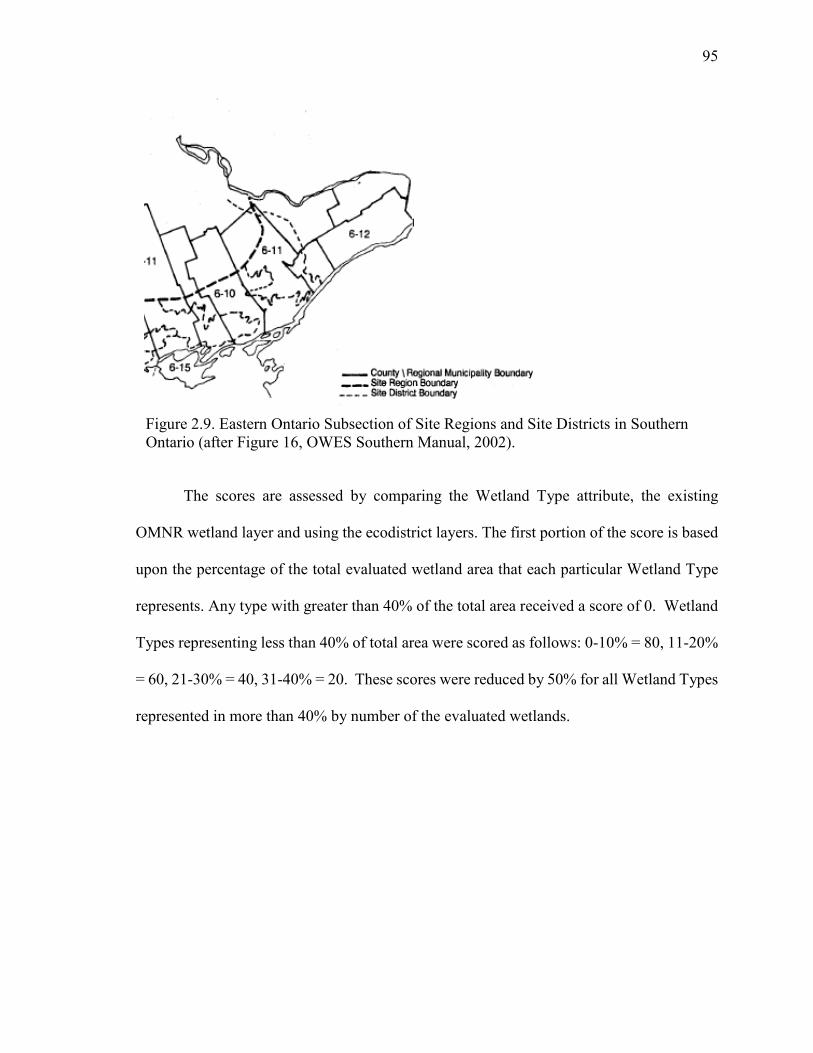
95
95
The scores are assessed by comparing the Wetland Type attribute, the existing
OMNR wetland layer and using the ecodistrict layers. The first portion of the score is based
upon the percentage of the total evaluated wetland area that each particular Wetland Type
represents. Any type with greater than 40% of the total area received a score of 0. Wetland
Types representing less than 40% of total area were scored as follows: 0-10% = 80, 11-20%
= 60, 21-30% = 40, 31-40% = 20. These scores were reduced by 50% for all Wetland Types
represented in more than 40% by number of the evaluated wetlands.
Figure 2.9. Eastern Ontario Subsection of Site Regions and Site Districts in Southern Ontario (after Figure 16, OWES Southern Manual, 2002).
96
96
2.9.13 Anthropogenic Disturbance (Social component)
This attribute indicates human impacts on the aesthetics of a wetland (OWES, 2002).
Impacts include: roads, utility corridors, buildings, dumps, fill, channelization, dredging,
drainage ditches, control dams and other human uses.
In the literature, Anthropogenic Disturbance is also known as human influence,
deforestation, agriculture expansion, and land use land cover (LULC) change. Methods used
to assess these changes include GIS assessment of thematic data to determine change in
polygons, aerial photointerpretation, LSU, assessment of forest cover change through
thematic maps derived through tasselled cap transformation, unsupervised classification,
MLC and change detection, and GIS classification models using Basin Buffer Index and
Hydric Vegetation Index, and Cellular Automata-Markov Chain modelling. Data types used
with these methods have included Landsat TM and ETM+, and SPOT-5 data. Overall
accuracies range from 85% to 89% (Wilcox, 1995; Phillips et al., 2005; Stuart et al., 2006;
Papastergiadou et al., 2008; Dyukarev et al., 2011; Behera et al., 2012; Yang et al., 2013).
Previous studies using unmixed image fractions in land cover change analysis based
upon climatic differences (Schmid et al., 2005; Melendez-Pastor et al., 2010) or human-
based changes in other ecosystems such as slash and burn in the Amazon (Adams et al.,
1995) or tundra land cover change (Olthof and Fraser, 2007) led to the selection in the
research of LSU to assess anthropogenic change through time. There is little literature on
the use of such fractions with OBIA and none that was found for wetland applications,
suggesting that, if successful, this could be a novel contribution. It was also hoped that this

97
97
type of analysis would improve upon the existing assessment of anthropogenic disturbance
in the literature with accuracies ranging from 85 to 89%.
For OWES scoring, the areal extent of disturbances is estimated as localized
situations are separated from more widespread disturbances. The amount of water pollution
is also assessed in this category.
This attribute is scored as follows (maximum of 7 points):
Human disturbances absent or nearly so = 7
One or several localized disturbances = 4
Moderate disturbance; localized water pollution = 2
Wetland intact but impairment of ecosystem quality intense in some areas = 1
Extreme ecological degradation, or water pollution severe and widespread = 0
98
98
3.0 Study areas and remotely sensed imagery
This chapter provides a description of the study areas and then discusses the optical
and radar satellite imagery used for this research.
3.1 Study region and study areas
This research was carried out in eastern Ontario, Canada (Figure 3.1), a region of
approximately 15,500 km2 which is a mix of agricultural, forest, and urban lands including
the city of Ottawa on the northern edge. Wetlands are distributed throughout the region and
are predominantly swamps and marshes with fewer bogs and fens (National Wetlands
Working Group, 1997). Agriculture is dominant near the St. Lawrence and Ottawa Rivers,
and in the flat landscapes from Ottawa east towards the Québec border. In the northwest of
the area, and along the Frontenac Axis (a strip of the Canadian shield linking to the
Adirondacks in the south), there are generally thin soils over igneous and metamorphic
bedrock with limited agriculture potential (Baldwin et al., 2000).
There are many lakes on the shield portion of study region, allowing for wetland
formation in bays, and along shores. Around Westport Bog the area of lakes is
approximately 11,686 hectares (116 km2). Some lakes along the axis are marl-based
resulting kettle hole-type formations (Keddy, 1995). Forest covers about 38% of the eastern
Ontario region, and varies from about 60% on the shield in the northwest, to less than 30%
in the east.
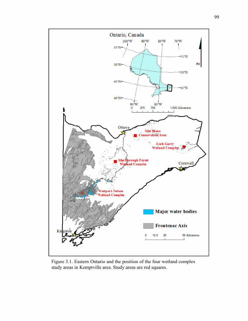
99
99
Figure 3.1. Eastern Ontario and the position of the four wetland complex study areas in Kemptville area. Study areas are red squares.
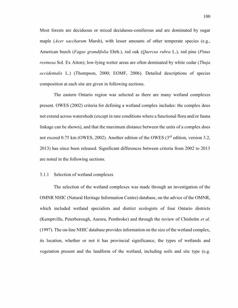
100
100
Most forests are deciduous or mixed deciduous-coniferous and are dominated by sugar
maple (Acer saccharum Marsh), with lesser amounts of other temperate species (e.g.,
American beech (Fagus grandifolia Ehrh.), red oak (Quercus rubra L.), red pine (Pinus
resinosa Sol. Ex Aiton); low-lying wetter areas are often dominated by white cedar (Thuja
occidentalis L.) (Thompson, 2000; EOMF, 2006). Detailed descriptions of species
composition at each site are given in following sections.
The eastern Ontario region was selected as there are many wetland complexes
present. OWES (2002) criteria for defining a wetland complex includes: the complex does
not extend across watersheds (except in rare conditions where a functional flora and/or fauna
linkage can be shown), and that the maximum distance between the units of a complex does
not exceed 0.75 km (OWES, 2002). Another edition of the OWES (3rd edition, version 3.2,
2013) has since been released. Significant differences between criteria from 2002 to 2013
are noted in the following sections.
3.1.1 Selection of wetland complexes
The selection of the wetland complexes was made through an investigation of the
OMNR NHIC (Natural Heritage Information Centre) database, on the advice of the OMNR,
which included wetland specialists and district ecologists of four Ontario districts
(Kemptville, Peterborough, Aurora, Pembroke) and through the review of Chisholm et al.
(1997). The on-line NHIC database provides information on the size of the wetland complex,
its location, whether or not it has provincial significance, the types of wetlands and
vegetation present and the landform of the wetland, including soils and site type (e.g.
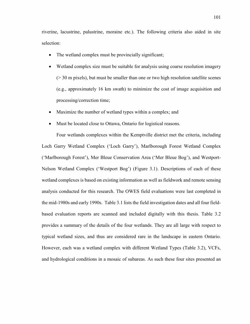
101
101
riverine, lacustrine, palustrine, moraine etc.). The following criteria also aided in site
selection:
The wetland complex must be provincially significant;
Wetland complex size must be suitable for analysis using coarse resolution imagery
(> 30 m pixels), but must be smaller than one or two high resolution satellite scenes
(e.g., approximately 16 km swath) to minimize the cost of image acquisition and
processing/correction time;
Maximize the number of wetland types within a complex; and
Must be located close to Ottawa, Ontario for logistical reasons.
Four wetlands complexes within the Kemptville district met the criteria, including
Loch Garry Wetland Complex (‘Loch Garry’), Marlborough Forest Wetland Complex
(‘Marlborough Forest’), Mer Bleue Conservation Area (‘Mer Bleue Bog’), and Westport-
Nelson Wetland Complex (‘Westport Bog’) (Figure 3.1). Descriptions of each of these
wetland complexes is based on existing information as well as fieldwork and remote sensing
analysis conducted for this research. The OWES field evaluations were last completed in
the mid-1980s and early 1990s. Table 3.1 lists the field investigation dates and all four field-
based evaluation reports are scanned and included digitally with this thesis. Table 3.2
provides a summary of the details of the four wetlands. They are all large with respect to
typical wetland sizes, and thus are considered rare in the landscape in eastern Ontario.
However, each was a wetland complex with different Wetland Types (Table 3.2), VCFs,
and hydrological conditions in a mosaic of subareas. As such these four sites presented an
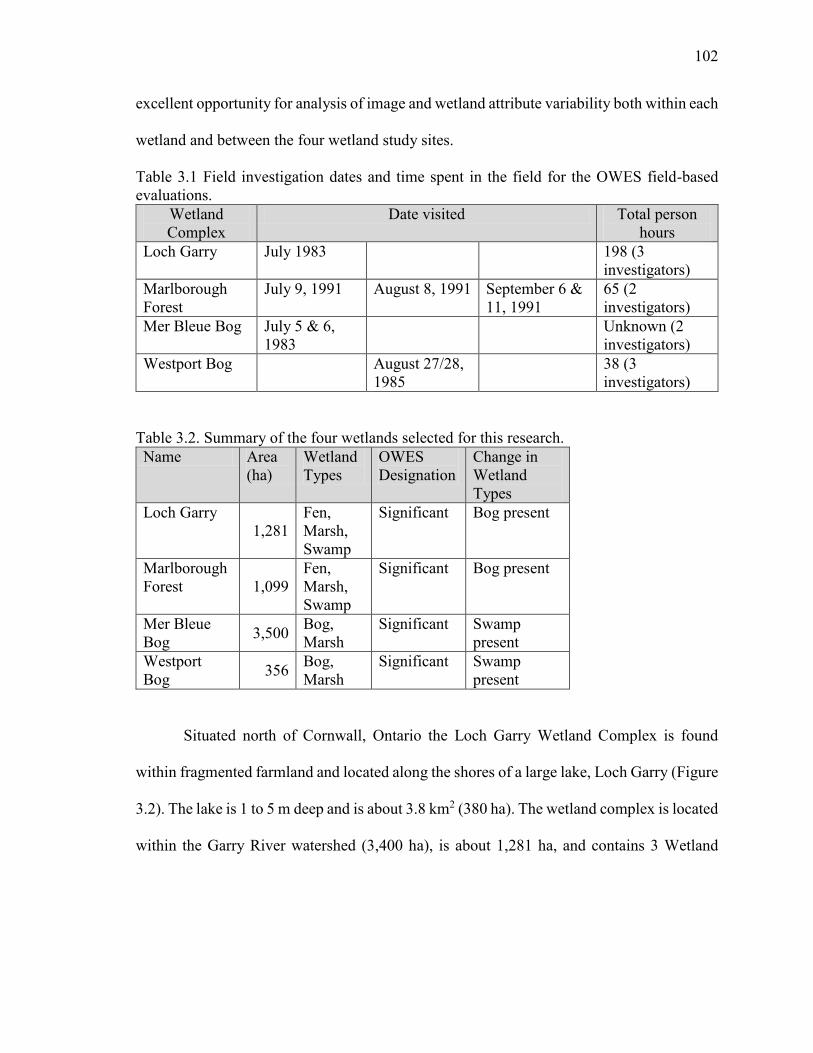
102
102
excellent opportunity for analysis of image and wetland attribute variability both within each
wetland and between the four wetland study sites.
Table 3.1 Field investigation dates and time spent in the field for the OWES field-based evaluations.
Wetland Complex
Date visited Total person hours
Loch Garry July 1983 198 (3 investigators)
Marlborough Forest
July 9, 1991 August 8, 1991 September 6 & 11, 1991
65 (2 investigators)
Mer Bleue Bog July 5 & 6, 1983
Unknown (2 investigators)
Westport Bog August 27/28, 1985
38 (3 investigators)
Table 3.2. Summary of the four wetlands selected for this research. Name Area
(ha) Wetland Types
OWES Designation
Change in Wetland Types
Loch Garry 1,281
Fen, Marsh, Swamp
Significant Bog present
Marlborough Forest 1,099
Fen, Marsh, Swamp
Significant Bog present
Mer Bleue Bog 3,500 Bog,
Marsh Significant Swamp
present Westport Bog 356 Bog,
Marsh Significant Swamp
present
Situated north of Cornwall, Ontario the Loch Garry Wetland Complex is found
within fragmented farmland and located along the shores of a large lake, Loch Garry (Figure
3.2). The lake is 1 to 5 m deep and is about 3.8 km2 (380 ha). The wetland complex is located
within the Garry River watershed (3,400 ha), is about 1,281 ha, and contains 3 Wetland
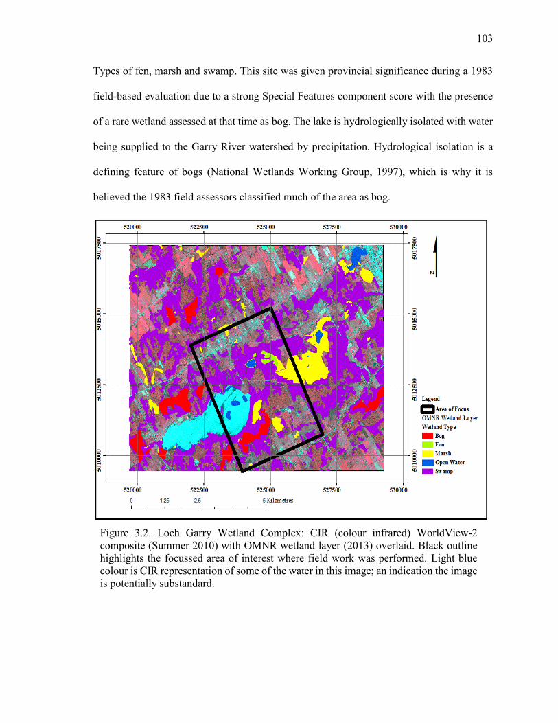
103
103
Types of fen, marsh and swamp. This site was given provincial significance during a 1983
field-based evaluation due to a strong Special Features component score with the presence
of a rare wetland assessed at that time as bog. The lake is hydrologically isolated with water
being supplied to the Garry River watershed by precipitation. Hydrological isolation is a
defining feature of bogs (National Wetlands Working Group, 1997), which is why it is
believed the 1983 field assessors classified much of the area as bog.
Figure 3.2. Loch Garry Wetland Complex: CIR (colour infrared) WorldView-2 composite (Summer 2010) with OMNR wetland layer (2013) overlaid. Black outline highlights the focussed area of interest where field work was performed. Light blue colour is CIR representation of some of the water in this image; an indication the image is potentially substandard. .
104
104
Based upon this research (e.g. field observed vegetation, and spectral response in
imagery), the Wetland Type originally identified as bog (bright red in Figure 3.2) is thought
to be Fen. Fen vegetation identified in the field included: stunted tamarack (Larix laricina
(Du Roi) K.Koch), low shrubs such as sweet gale (Myrica gale L.), dwarf birch (Betula
pumila L.), bog willow (fen indicator species, Salix pedicellaris Pursh); herbs including
pitcher plant (Sarracenia purpurea L.), buckbean (fen indicator species, Menyanthes
trifoliate L.), ferns (Dryopteris spp.) and numerous narrow leaved emergents (including
sedges (Carex spp.) and rushes (Juncus spp.)). Also present as a minor component were
cattails (Typha latifolia L.). Sphagnum moss (Sphagnum spp.) and brown mosses
(Campylium stellatum Hedw., Drepanocladus revolvens (Sm.) Warnst, Tomenthypnum
nitens Hedw., Scorpidium scorpioides, Hedw.) were abundantly present. An expert field
ecologist at OMNR agreed this area most resembles Fen, but the SOLRIS classification
shows it as mostly Bog.
Marsh-dominant vegetation identified in the field consisted mainly of robust
emergents (cattails, common reeds (Phragmites australis (Cav.) Trin. Ex Steud, subspecies
australis, Phragmites australis (Cav.) Trin. Ex Steud subspecies americanus,), bulrushes
(Scirpus spp.) etc.), components of free-floating plants (duckweed (Lemna spp.)), rooted
floating plants (yellow pond lily (Nuphar variegatum Engelm. Ex Durand), fragrant white
water lily (Nymphaea ordorata Aiton) and watershield (Brasenia schreberi J.F. Gmel)). In
ecotonal areas such as marsh and swamp, and/or marsh and fen, swamp and fen vegetation
were present (to a minor degree) and included: tall shrubs of red-osier dogwood (Cornus
105
105
stolonifera L.), speckled alder (Alnus incana (L.) Moench), willow (Salix spp.); herbs such
as ferns, spotted joe-pye weed (Eupatorium maculatum (L.) E.E. Lamont), purple loosestrife
(Lythrum salicaria L.); narrow leaved emergents such as sedges and Canada bluejoint
(Calamagrostis Canadensis (Michx.) P. Beauv.); and broad-leaved emergents such as wild
calla (Calla palustris L.).
Swamp vegetation included large components of dead coniferous (particularly dead
eastern white cedar) along with live cedar, tamarack, white pine (Pinus strobus L.), black
spruce (Picea mariana (Mill.) Britton, Stems & Poggenburg), hemlock (Tsuga Canadensis
(L.) Carrière), and balsam fir (Abies balsamea (L.) Mill). In areas of mixed-forest swamp,
hardwood vegetation included black ash and maple. White spruce (Picea glauca (Moench)
Voss) was present along with aspen (Populous spp.), jack pine (Pinus banksiana Lamb.)
and red and white pine in drier sites; wetter sites had black spruce with eastern white cedar
and black ash.
The Marlborough Forest Wetland Complex (Figure 3.3) of approximately 1,099 ha
is located south-west of Ottawa, within less fragmented farmland but near industrial land
uses (e.g. quarrying). With extensive hunting, ATV and snowmobile use, this complex is
recreationally active. For the purposes of this research some components of the Richmond
Wetland and Steven Creek Wetland Complex were also included. The complex was OWES
assessed in 1991 and was given provincial significance due to the presence of rare Wetland
Types (Fen and Bog) and rare vegetation species (e.g. orchids). During field work for this
research, an attempt was made to locate the assessed bog (0.03% of the area, OMNR wetland
106
106
layer; see red circle Figure 3.3), but there was not a wetland of any type visible in that area
in either spring or summer.
The fen vegetation included extensive sedge in wide open meadows with pitcher
plants, some orchid species (unidentified) and, along the ecotone zone with swamps, low
shrubs of creeping snowberry (Gaultheria hispidula (L.) Muhl. Ex Bigelow), leatherleaf
(Chamaedaphne calyculata (L.) Moench), and willow species.
Marsh vegetation was largely sedges and cattails with some floating and free-
floating plants such as yellow pond lily, duckweed and watershield. Coniferous swamps
were dominant in this region, primarily cedar with minor tamarack, fern and grass
components. In areas of standing water there was dead cedar as well as floating species such
as duckweed, water shield and pondweed (Potamogeton spp.). In dryer areas, or later in the
season, the understorey often consisted of grasses such as marsh timothy (Muhlenbergia
glomerata (Willd.) Trin.), reeds and canary grasses (Phalaris arundinacea L.) and herbs
such as ferns and poison ivy (Rhus radicans (L.) Kuntze). In mixed or predominantly
hardwood swamps the tree species included black ash and maple with similar understoreys.
In some minor cases there was the presence of cattails, especially in marsh/swamp ecotonal
areas.
The Mer Bleue Conservation Area (‘Mer Bleue Bog’, Figure 3.3) is found within the
city limits of Ottawa, with extensive suburban development to the north, and surrounded by
farmland to the south and east. This well-studied area of approximately 3,500 ha is a wetland
of international importance (Ramsar-designated, Ramsar, 2006) and is also provincially
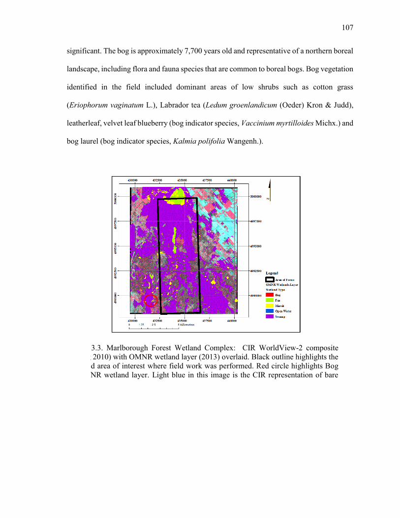
107
107
significant. The bog is approximately 7,700 years old and representative of a northern boreal
landscape, including flora and fauna species that are common to boreal bogs. Bog vegetation
identified in the field included dominant areas of low shrubs such as cotton grass
(Eriophorum vaginatum L.), Labrador tea (Ledum groenlandicum (Oeder) Kron & Judd),
leatherleaf, velvet leaf blueberry (bog indicator species, Vaccinium myrtilloides Michx.) and
bog laurel (bog indicator species, Kalmia polifolia Wangenh.).
Figure 3.3. Marlborough Forest Wetland Complex: CIR WorldView-2 composite (Spring 2010) with OMNR wetland layer (2013) overlaid. Black outline highlights the focussed area of interest where field work was performed. Red circle highlights Bog on OMNR wetland layer. Light blue in this image is the CIR representation of bare fields.
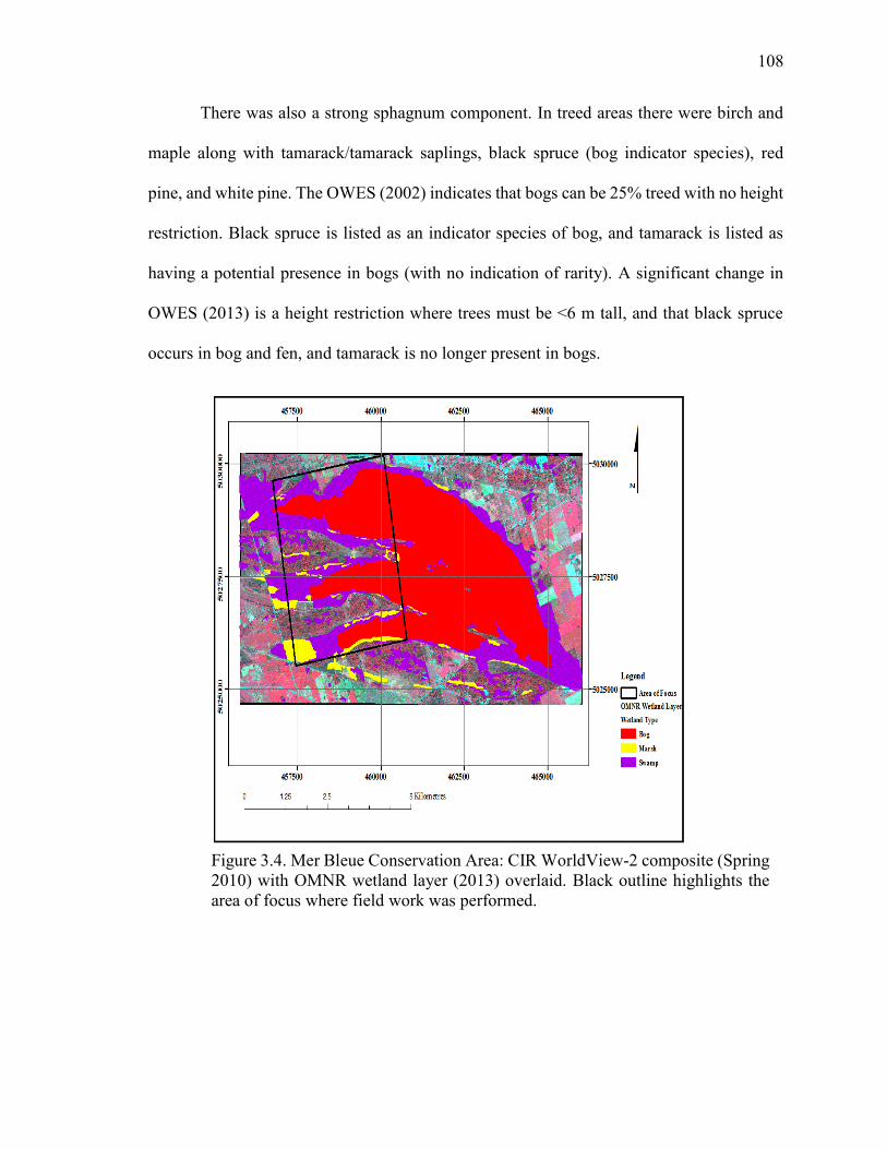
108
108
There was also a strong sphagnum component. In treed areas there were birch and
maple along with tamarack/tamarack saplings, black spruce (bog indicator species), red
pine, and white pine. The OWES (2002) indicates that bogs can be 25% treed with no height
restriction. Black spruce is listed as an indicator species of bog, and tamarack is listed as
having a potential presence in bogs (with no indication of rarity). A significant change in
OWES (2013) is a height restriction where trees must be <6 m tall, and that black spruce
occurs in bog and fen, and tamarack is no longer present in bogs.
Figure 3.4. Mer Bleue Conservation Area: CIR WorldView-2 composite (Spring 2010) with OMNR wetland layer (2013) overlaid. Black outline highlights the area of focus where field work was performed.
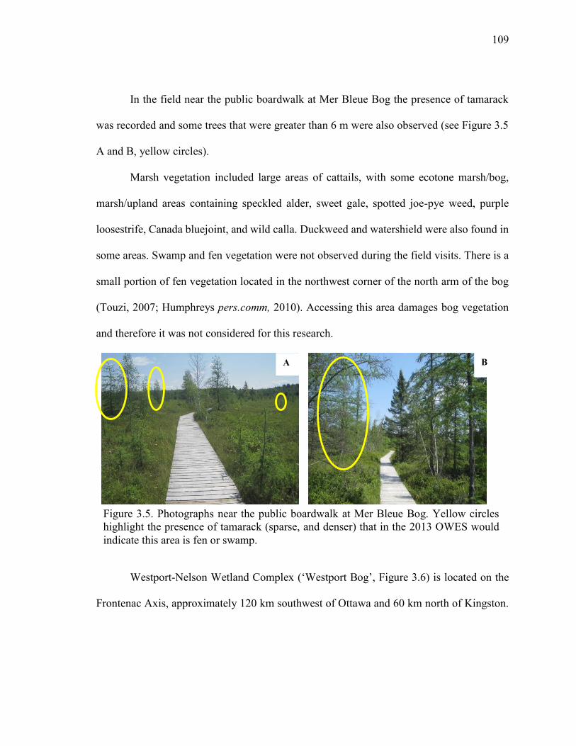
109
109
In the field near the public boardwalk at Mer Bleue Bog the presence of tamarack
was recorded and some trees that were greater than 6 m were also observed (see Figure 3.5
A and B, yellow circles).
Marsh vegetation included large areas of cattails, with some ecotone marsh/bog,
marsh/upland areas containing speckled alder, sweet gale, spotted joe-pye weed, purple
loosestrife, Canada bluejoint, and wild calla. Duckweed and watershield were also found in
some areas. Swamp and fen vegetation were not observed during the field visits. There is a
small portion of fen vegetation located in the northwest corner of the north arm of the bog
(Touzi, 2007; Humphreys pers.comm, 2010). Accessing this area damages bog vegetation
and therefore it was not considered for this research.
Westport-Nelson Wetland Complex (‘Westport Bog’, Figure 3.6) is located on the
Frontenac Axis, approximately 120 km southwest of Ottawa and 60 km north of Kingston.
Figure 3.5. Photographs near the public boardwalk at Mer Bleue Bog. Yellow circles highlight the presence of tamarack (sparse, and denser) that in the 2013 OWES would indicate this area is fen or swamp.
A B
110
110
The axis divides the St. Lawrence lowlands and the Great Lakes lowlands. Bedrock is often
found to be exposed at the surface, or covered with thin soils (Keddy, 1995). The area was
forested in the past, but logging has depleted most areas of old-growth (Keddy, 1995).
Current forest vegetation generally contains northern hardwoods (maple, beech, birch)
mixed with spruce, pine and fir (Keddy, 1995). Irregular topography and marl-based ponds
and lakes restrict the hydrology of the area (Keddy, 1995). Wetlands present include bog,
marsh and swamp with some poor fen (not observed, and very rare (Keddy, 1995)). Bogs
listed and confirmed in the field included open and treed bogs (<25%) (very minor
component overall)) with treed areas containing some minor deciduous saplings such as
birch, and minor tamarack along with some dead coniferous.
In open bog areas the vegetation included willow, black chokeberry (Aronia
melanocarpa (Michx) Elliott), cotton grass, sweet gale, rushes, tall and short grasses. The
bog area of observation was surrounded by a well-defined lagg. A lagg is a transition zone
where runoff collects from both the bog and the surrounding upland area (Howie and Tromp-
van Meervald, 2011), and is a strong indicator of a raised bog. The vegetation observed in
the lagg was fen- or marsh-like in nature and included cattails, wild calla and rooted-floating
and free-floating plants such as duckweed and watershield. Vegetation present in a lagg
often has fen characteristics and “raised bogs that are physically constrained by basins often
develop a “moat-like” lagg” (Howie and Tromp-van Meervald, 2011).
Marsh vegetation included homogenous areas of rushes, cattails, and some sedge
species along with duckweed, watershield, yellow pond lily and wild calla. There was a
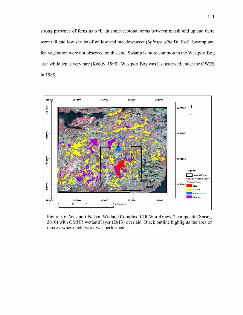
111
111
strong presence of ferns as well. In some ecotonal areas between marsh and upland there
were tall and low shrubs of willow and meadowsweet (Spiraea alba Du Roi). Swamp and
fen vegetation were not observed on this site. Swamp is more common in the Westport Bog
area while fen is very rare (Keddy, 1995). Westport Bog was last assessed under the OWES
in 1985.
Figure 3.6. Westport-Nelson Wetland Complex: CIR WorldView-2 composite (Spring 2010) with OMNR wetland layer (2013) overlaid. Black outline highlights the area of interest where field work was performed.
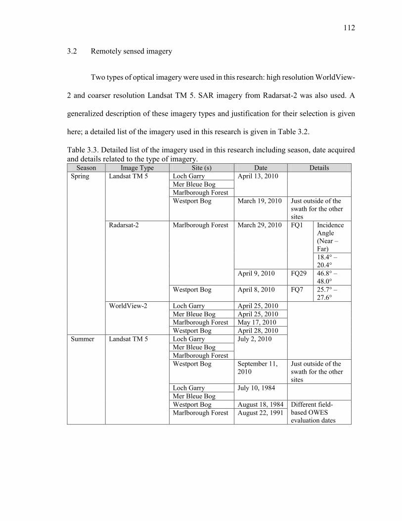
112
112
3.2 Remotely sensed imagery
Two types of optical imagery were used in this research: high resolution WorldView-
2 and coarser resolution Landsat TM 5. SAR imagery from Radarsat-2 was also used. A
generalized description of these imagery types and justification for their selection is given
here; a detailed list of the imagery used in this research is given in Table 3.2.
Table 3.3. Detailed list of the imagery used in this research including season, date acquired and details related to the type of imagery.
Season Image Type Site (s) Date Details Spring Landsat TM 5 Loch Garry April 13, 2010
Mer Bleue Bog Marlborough Forest Westport Bog March 19, 2010 Just outside of the
swath for the other sites
Radarsat-2 Marlborough Forest March 29, 2010 FQ1 Incidence Angle (Near – Far) 18.4° – 20.4°
April 9, 2010 FQ29 46.8° – 48.0°
Westport Bog April 8, 2010 FQ7 25.7° – 27.6°
WorldView-2 Loch Garry April 25, 2010 Mer Bleue Bog April 25, 2010 Marlborough Forest May 17, 2010 Westport Bog April 28, 2010
Summer Landsat TM 5 Loch Garry July 2, 2010 Mer Bleue Bog Marlborough Forest Westport Bog September 11,
2010 Just outside of the swath for the other sites
Loch Garry July 10, 1984 Mer Bleue Bog Westport Bog August 18, 1984 Different field-
based OWES evaluation dates
Marlborough Forest August 22, 1991
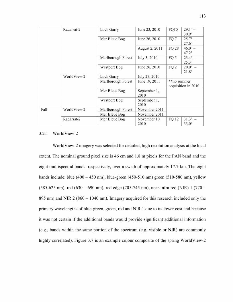
113
113
Radarsat-2 Loch Garry June 23, 2010 FQ10 29.1° – 30.9°
Mer Bleue Bog June 26, 2010 FQ 7 25.7° – 27.6°
August 2, 2011 FQ 28 46.0° – 47.2°
Marlborough Forest July 3, 2010 FQ 5 23.4° – 25.3°
Westport Bog June 26, 2010 FQ 2 20.0° –21.8°
WorldView-2 Loch Garry July 27, 2010 Marlborough Forest June 19, 2011 **no summer
acquisition in 2010 Mer Bleue Bog September 1,
2010
Westport Bog September 1, 2010
Fall WorldView-2 Marlborough Forest November 2011 Mer Bleue Bog November 2011
Radarsat-2 Mer Bleue Bog November 10 2010
FQ 12 31.3° – 33.0°
3.2.1 WorldView-2
WorldView-2 imagery was selected for detailed, high resolution analysis at the local
extent. The nominal ground pixel size is 46 cm and 1.8 m pixels for the PAN band and the
eight multispectral bands, respectively, over a swath of approximately 17.7 km. The eight
bands include: blue (400 – 450 nm), blue-green (450-510 nm) green (510-580 nm), yellow
(585-625 nm), red (630 – 690 nm), red edge (705-745 nm), near-infra red (NIR) 1 (770 –
895 nm) and NIR 2 (860 – 1040 nm). Imagery acquired for this research included only the
primary wavelengths of blue-green, green, red and NIR 1 due to its lower cost and because
it was not certain if the additional bands would provide significant additional information
(e.g., bands within the same portion of the spectrum (e.g. visible or NIR) are commonly
highly correlated). Figure 3.7 is an example colour composite of the spring WorldView-2
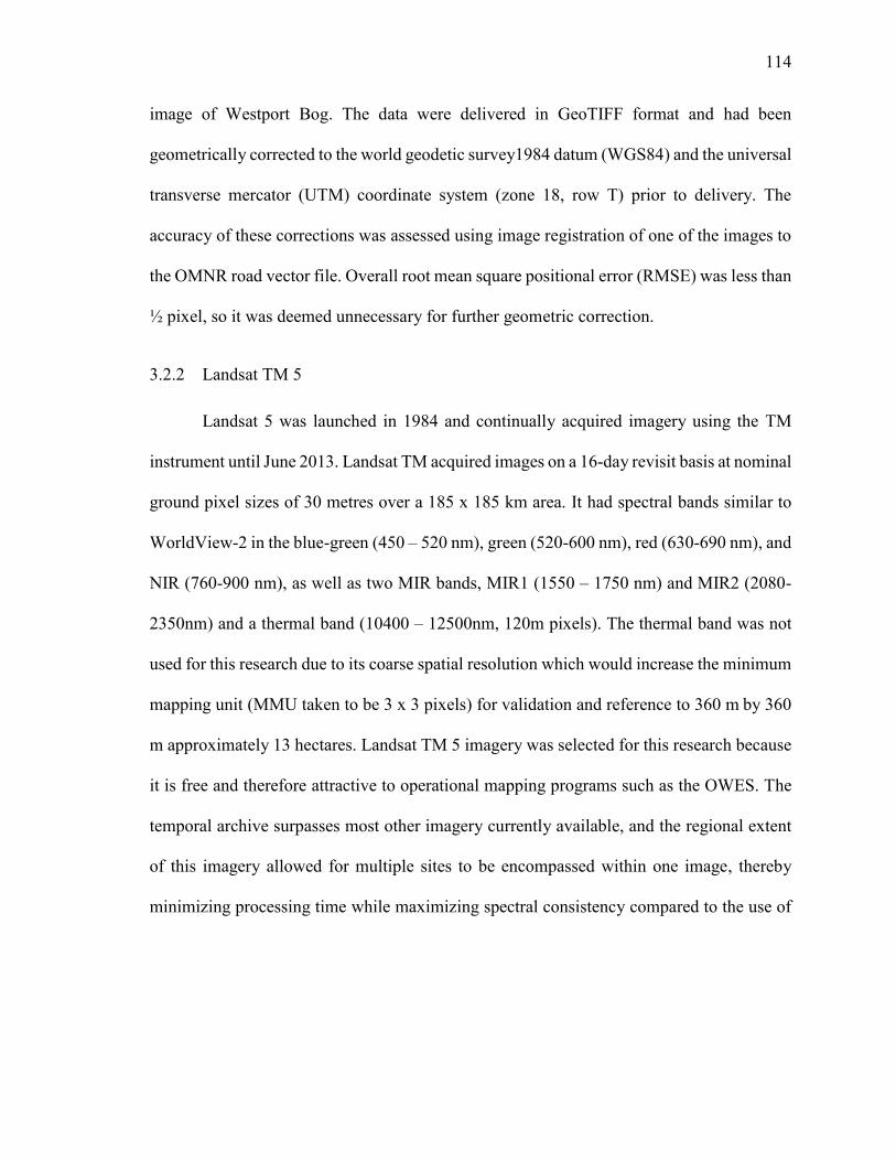
114
114
image of Westport Bog. The data were delivered in GeoTIFF format and had been
geometrically corrected to the world geodetic survey1984 datum (WGS84) and the universal
transverse mercator (UTM) coordinate system (zone 18, row T) prior to delivery. The
accuracy of these corrections was assessed using image registration of one of the images to
the OMNR road vector file. Overall root mean square positional error (RMSE) was less than
½ pixel, so it was deemed unnecessary for further geometric correction.
3.2.2 Landsat TM 5
Landsat 5 was launched in 1984 and continually acquired imagery using the TM
instrument until June 2013. Landsat TM acquired images on a 16-day revisit basis at nominal
ground pixel sizes of 30 metres over a 185 x 185 km area. It had spectral bands similar to
WorldView-2 in the blue-green (450 – 520 nm), green (520-600 nm), red (630-690 nm), and
NIR (760-900 nm), as well as two MIR bands, MIR1 (1550 – 1750 nm) and MIR2 (2080-
2350nm) and a thermal band (10400 – 12500nm, 120m pixels). The thermal band was not
used for this research due to its coarse spatial resolution which would increase the minimum
mapping unit (MMU taken to be 3 x 3 pixels) for validation and reference to 360 m by 360
m approximately 13 hectares. Landsat TM 5 imagery was selected for this research because
it is free and therefore attractive to operational mapping programs such as the OWES. The
temporal archive surpasses most other imagery currently available, and the regional extent
of this imagery allowed for multiple sites to be encompassed within one image, thereby
minimizing processing time while maximizing spectral consistency compared to the use of
115
115
multiple images, which has been shown to degrade classification accuracy (Pax-Lenney et
al., 2001; Dingle Robertson and King, 2011).
Although Landsat 7 ETM+ data were available, in 2003 the satellite’s scan line
corrector failed, resulting in reduced quality of data.
3.2.3 Radarsat-2
Radarsat-2 is a C-band sensor with advanced polarimetric capabilities and multiple
possible resolutions and image swaths that have proven advantageous in wetland mapping.
Figure 3.7. True colour composite of WorldView-2 imagery at Westport Bog.
116
116
Radarsat-2 imagery used in this research was acquired in descending mode in fine quad-
polarisation (Henderson and Lewis, 2008). The nominal ground pixel size is theoretically 8
m at the steepest incidence angle and as most of the imagery was acquired with steep
incidence angles (low FQs (fine quad) beams) the general nominal ground pixel size of the
raw radar imagery is about 9.5 m. This resolution is hereafter called ‘medium’ resolution
(between WorldView-2 and Landsat TM 5) with a local spatial extent of approximately 25
x 25 km2. Due to the noisy nature of raw radar imagery and the general requirement to filter
it prior to processing, the nominal ground pixel size of the filtered imagery is degraded and
can be considered ‘coarse’ resolution, in the same class as Landsat imagery.
Radarsat-2 imagery was selected for this research because the imagery swath
covered each wetland complex, it has been shown to work well in detecting open water and
herbaceous wetlands, and it has been previously used to detect wetland types at Mer Bleue
Bog (Touzi et al., 2007). It is also relatively simple for Canadian government organizations
to acquire. The imagery of this research was acquired through the assistance of Environment
Canada, and the potential for inter-governmental collaboration with the Ontario government
made the use of this imagery appealing. Additionally, the different spectral nature and
information content of radar imagery compared to optical imagery made these data a
compelling addition to this research. All other data including a 10 m digital elevation model
(DEM, Version 2.0.0, horizontal accuracy +/- 10m; vertical accuracy +/- 5 m, (LIO, OMNR,
2006) were obtained from the LIO.
117
117
4.0 Methods
This chapter is structured to follow the three main objectives of this research: map
the selected OWES attributes for one season which was selected as spring; score the mapped
attributes and then compare those scores to OWES scores; and assess the temporal remote
sensing data in classification of wetland attributes, and analyze attribute changes over the
long term. Under each objective, the methods are described by attribute, including the field
work completed to obtain reference data. Where the methods are repeated, the reader is
directed to the section in Chapter 4 where that information is located. Figure 4.1 (provided
digitally with this thesis) provides a detailed workflow of the entire methods structure.
Portions of Figure 4.1 accompany each attribute section as workflow diagrams.
Objective 1 Methods: Map the selected OWES attributes for one season
4.1 Methods to segment, classify, and map Wetland Type using optical and radar imagery
Figure 4.2 provides the workflow for the methods used to segment, classify and map
Wetland Type. Potential for mapping Wetland Type was assessed as it is important in both
the Biological and Special Features components. OWES Wetland Types were defined in
Table 2.1 and included Marsh, Fen, Bog and Swamp. In addition, a survey was made of the
surrounding landforms and areas that were transition zones (ecotones) between Wetland
Types, or between Wetland Type and Upland. Upland types included: Coniferous Forest,
Hardwood Forest, Mixed Forest, Open Grassy Field, Agriculture, Shrub Area, Impervious
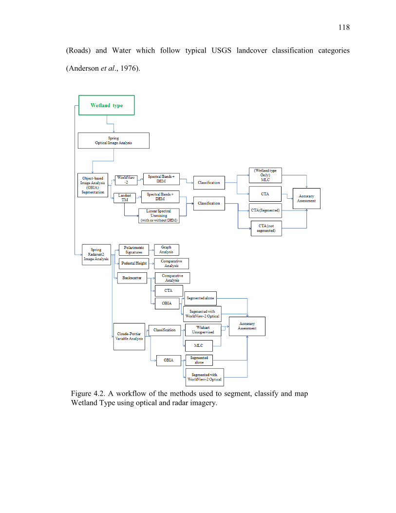
118
118
(Roads) and Water which follow typical USGS landcover classification categories
(Anderson et al., 1976).
Figure 4.2. A workflow of the methods used to segment, classify and map Wetland Type using optical and radar imagery.
119
119
4.1.1 Field analysis for Wetland Type
Defining characteristics of the attribute ‘Wetland Type’ were based upon vegetation
present, hydrologic conditions, and their spatial arrangement, both which have the potential
to be assessed using remote sensing. In the spring and summer of 2010 and 2011, in the four
study areas, validation sites of a MMU of 90 x 90 m (3 x 3 Landsat pixels) were established
using a tape measure or visually using a laser range finder (e.g. at the edge of marsh, deep
swamp, unstable bog/fen, protected bog, etc.). A survey was made of the land cover types
present, and a GPS (Global Positioning System) waypoint was taken at the edge of the site
using a Trimble Juno SB (expected real time accuracy of approximately 2-5 m
(www.trimble.com, 2013)). Where there was confusion between Wetland Types (e.g. Fen
and Bog), the vegetation present was assessed to determine if there were indicator species
present (as outlined in the OWES Southern Manual, 2002). Effort was made to accumulate
multiple samples for each land cover type (e.g., 15 to 50 (Jensen, 2000; Foody, 2002;
Lillesand et al., 2008), but for rare wetlands of fen and bog it was often impossible to find
more than one or two examples within a particular wetland complex. In addition, all four
Wetland Types were not observed in each wetland. The size of the MMU also limited the
number of samples of Wetland Type(s) that could be recorded; smaller areas were observed
but could not be used in calibration and training. In addition to these field data, calibration
and validation training areas for the Water class were supplemented by visual interpretation
of high resolution DRAPE (Digital Raster Acquisition Project for the East, Ontario
Geospatial Data Exchange (OGDE, ©2008 Queen’s Printer)) imagery. This aerial CIR
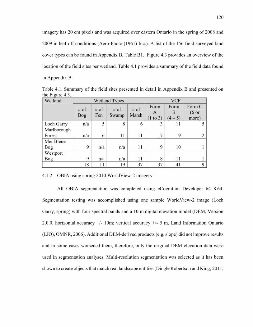
120
120
imagery has 20 cm pixels and was acquired over eastern Ontario in the spring of 2008 and
2009 in leaf-off conditions (Aero-Photo (1961) Inc.). A list of the 156 field surveyed land
cover types can be found in Appendix B, Table B1. Figure 4.3 provides an overview of the
location of the field sites per wetland. Table 4.1 provides a summary of the field data found
in Appendix B.
Table 4.1. Summary of the field sites presented in detail in Appendix B and presented on the Figure 4.3. Wetland Wetland Types VCF
# of Bog
# of Fen
# of Swamp
# of Marsh
Form A
(1 to 3)
Form B
(4 – 5)
Form C (6 or more)
Loch Garry n/a 5 8 6 3 11 5 Marlborough Forest n/a 6 11 11 17 9 2 Mer Bleue Bog 9 n/a n/a 11 9 10 1 Westport Bog 9 n/a n/a 11 8 11 1 18 11 19 37 37 41 9
4.1.2 OBIA using spring 2010 WorldView-2 imagery
All OBIA segmentation was completed using eCognition Developer 64 8.64.
Segmentation testing was accomplished using one sample WorldView-2 image (Loch
Garry, spring) with four spectral bands and a 10 m digital elevation model (DEM, Version
2.0.0, horizontal accuracy +/- 10m; vertical accuracy +/- 5 m, Land Information Ontario
(LIO), OMNR, 2006). Additional DEM-derived products (e.g. slope) did not improve results
and in some cases worsened them, therefore, only the original DEM elevation data were
used in segmentation analyses. Multi-resolution segmentation was selected as it has been
shown to create objects that match real landscape entities (Dingle Robertson and King, 2011;
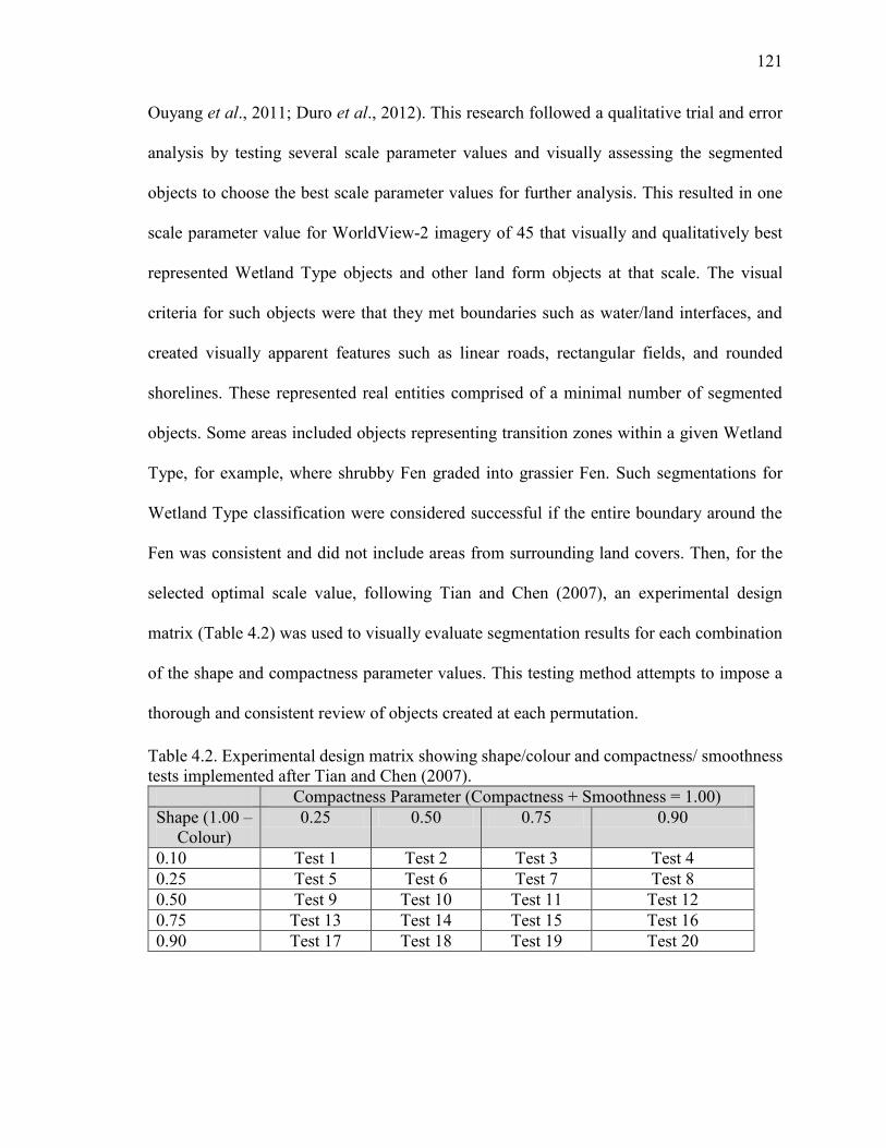
121
121
Ouyang et al., 2011; Duro et al., 2012). This research followed a qualitative trial and error
analysis by testing several scale parameter values and visually assessing the segmented
objects to choose the best scale parameter values for further analysis. This resulted in one
scale parameter value for WorldView-2 imagery of 45 that visually and qualitatively best
represented Wetland Type objects and other land form objects at that scale. The visual
criteria for such objects were that they met boundaries such as water/land interfaces, and
created visually apparent features such as linear roads, rectangular fields, and rounded
shorelines. These represented real entities comprised of a minimal number of segmented
objects. Some areas included objects representing transition zones within a given Wetland
Type, for example, where shrubby Fen graded into grassier Fen. Such segmentations for
Wetland Type classification were considered successful if the entire boundary around the
Fen was consistent and did not include areas from surrounding land covers. Then, for the
selected optimal scale value, following Tian and Chen (2007), an experimental design
matrix (Table 4.2) was used to visually evaluate segmentation results for each combination
of the shape and compactness parameter values. This testing method attempts to impose a
thorough and consistent review of objects created at each permutation.
Table 4.2. Experimental design matrix showing shape/colour and compactness/ smoothness tests implemented after Tian and Chen (2007).
Compactness Parameter (Compactness + Smoothness = 1.00) Shape (1.00 –
Colour) 0.25 0.50 0.75 0.90
0.10 Test 1 Test 2 Test 3 Test 4 0.25 Test 5 Test 6 Test 7 Test 8 0.50 Test 9 Test 10 Test 11 Test 12 0.75 Test 13 Test 14 Test 15 Test 16 0.90 Test 17 Test 18 Test 19 Test 20
122
122
OBIA classification of Wetland Type classes was completed using PCI Geomatica
(MLC) and IDRISI Taiga (CTA, (C4.5, Quinlan, 1993)). Training areas were derived from
the field data and in some cases, such as for Water, were supplemented from the DRAPE
imagery. Training data were generated for classes of Water, Upland, and the Wetland Types
that were present. Individual examples (Appendix B, Tables B2 to B5) are given for each of
the four study areas, however for comprehensive training, several samples from across each
wetland complex were selected to represent the variety in each class. In some cases, the class
of Uplands was separated into more specific classes containing forests, agricultural fields,
urban land covers, etc. due to spectral reflectance differences. The band data were visually
assessed as normal to very slightly positively skewed (see also Table 4.3) using the
mean:median ratio. Values close to 1.0 indicate a normal distribution, which is an important
assumption of parametric classifiers such as the MLC.
The mean:median ratio was checked for all training samples in each band for each
Wetland Type. Values differing from 1.0 by a large amount such as 0.1-0.2 or more (Jensen,
2005) indicate non-normal data. The range for training samples data at Loch Garry was
normally distributed. The other three sites were expected to also have normally distributed
training data for the Worldview-2 imagery.
The spectral reflectance curves of each training sample group followed general
curves of Wetland Types and underlying vegetation found in the literature (Mertes et al.,
1993, Anderson and Perry, 1996; Silva et al., 2008; Govender et al., 2009). Differences in
123
123
the visible reflection are found with higher green band reflection which relates the changes
in the chlorophyll concentration, and lower values in blue and red due to pigment absorption.
(Anderson and Perry, 1996; Govender et al., 2009). Highest values in NIR were related to
the cell structure (Mertes et al., 1993; Anderson and Perry, 1996). Additionally the presence
of water resulted in higher, but still significantly low values in the blue band, and the addition
of sediments, or flora in the water resulted in increasing values of the red or red-edge (Mertes
et al., 1993; Silva et al., 2008).
Separability of training data for the Wetland Types of interest in the WorldView-2
spring Loch Garry segmented image with a scale parameter of 45 were next tested for the
spring data, the summer data and the spring and summer data combined. The common
separability metric Bhattacharyya Distance (Haralick and Fu, 1983) was selected. It is non-
linear: values of 1.9 and greater are often used to indicate good separability and values of
1.7-1.9 may indicate potential for accurate classification. The Loch Garry image was
selected for testing as there were three Wetland Types in Loch Garry representing the
greatest variety of the four study sites, as well as for logistical reasons as it was the first
image to be delivered. Holding the shape and compactness parameter values constant at 0.1
and 0.75, respectively, the first test evaluated class separability for a scale parameter value
of 45 for the spring imagery. This was repeated using the summer imagery, and the spring
and summer imagery combined. The average and minimum separabilities for each test are
given in Table 4.3. These values show that separability of the training data for all class pairs
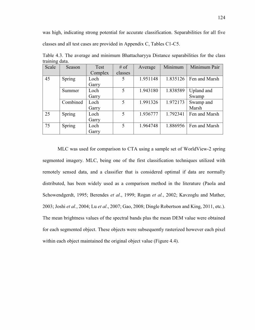
124
124
was high, indicating strong potential for accurate classification. Separabilities for all five
classes and all test cases are provided in Appendix C, Tables C1-C5.
Table 4.3. The average and minimum Bhattacharyya Distance separabilities for the class training data. Scale Season Test
Complex # of
classes Average Minimum Minimum Pair
45 Spring Loch Garry
5 1.951148 1.835126 Fen and Marsh
Summer Loch Garry
5 1.943180 1.838589 Upland and Swamp
Combined Loch Garry
5 1.991326 1.972173 Swamp and Marsh
25 Spring Loch Garry
5 1.936777 1.792341 Fen and Marsh
75 Spring Loch Garry
5 1.964748 1.886956 Fen and Marsh
MLC was used for comparison to CTA using a sample set of WorldView-2 spring
segmented imagery. MLC, being one of the first classification techniques utilized with
remotely sensed data, and a classifier that is considered optimal if data are normally
distributed, has been widely used as a comparison method in the literature (Paola and
Schowendgerdt, 1995; Berendes et al., 1999; Rogan et al., 2002; Kavzoglu and Mather,
2003; Joshi et al., 2004; Lu et al., 2007; Gao, 2008; Dingle Robertson and King, 2011, etc.).
The mean brightness values of the spectral bands plus the mean DEM value were obtained
for each segmented object. These objects were subsequently rasterized however each pixel
within each object maintained the original object value (Figure 4.4).
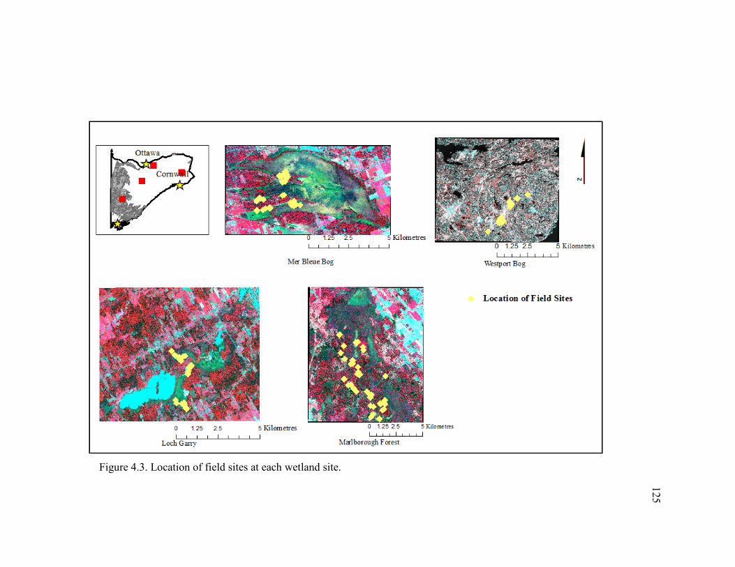
125
Figure 4.3. Location of field sites at each wetland site.
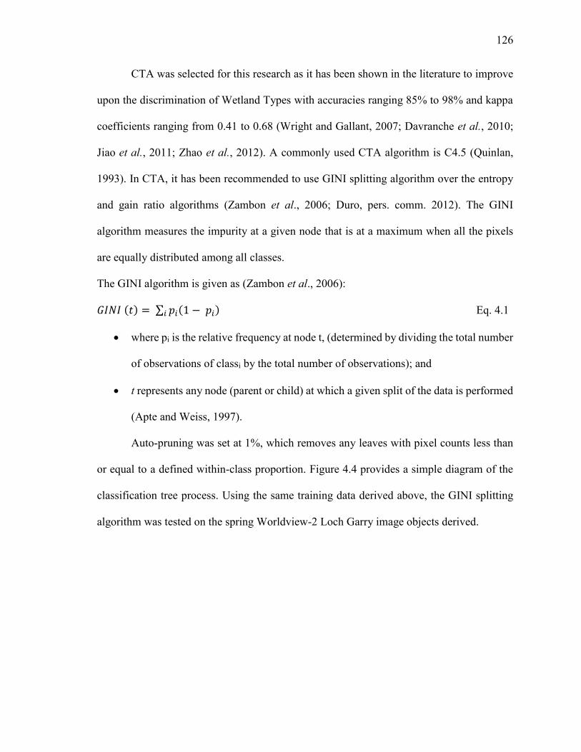
126
CTA was selected for this research as it has been shown in the literature to improve
upon the discrimination of Wetland Types with accuracies ranging 85% to 98% and kappa
coefficients ranging from 0.41 to 0.68 (Wright and Gallant, 2007; Davranche et al., 2010;
Jiao et al., 2011; Zhao et al., 2012). A commonly used CTA algorithm is C4.5 (Quinlan,
1993). In CTA, it has been recommended to use GINI splitting algorithm over the entropy
and gain ratio algorithms (Zambon et al., 2006; Duro, pers. comm. 2012). The GINI
algorithm measures the impurity at a given node that is at a maximum when all the pixels
are equally distributed among all classes.
The GINI algorithm is given as (Zambon et al., 2006):
𝐺𝐼𝑁𝐼 (𝑡) = ∑ 𝑝𝑖(1 − 𝑝𝑖)𝑖 Eq. 4.1
where pi is the relative frequency at node t, (determined by dividing the total number
of observations of classi by the total number of observations); and
t represents any node (parent or child) at which a given split of the data is performed
(Apte and Weiss, 1997).
Auto-pruning was set at 1%, which removes any leaves with pixel counts less than
or equal to a defined within-class proportion. Figure 4.4 provides a simple diagram of the
classification tree process. Using the same training data derived above, the GINI splitting
algorithm was tested on the spring Worldview-2 Loch Garry image objects derived.
127
During classification, the accuracy of the training data was assessed by observing a
monitoring graph that shows the proportion of misclassified or re-assigned training pixels
in a given iteration. The final graph that is produced indicates the stability of the training
data: positive values indicate a class has obtained training pixels from another class and
negative values indicate training pixels have been lost to another class. In the case of Loch
Garry spring training sites, there was minimal (+/- 1%) deviation from 0 indicating that the
training classes were well trained and classified. There is no quantitative measure of how
many training pixels have been lost or gained during the process.
4.1.3 OBIA using 2010 spring Landsat 5 TM imagery
Segmentation testing was completed as outlined in section 4.1.2. The Landsat image
was clipped to match the WorldView-2 images for each focus area at each wetland complex.
This minimized the unknown variability found in those areas outside the study complexes.
Previous testing (Dingle Robertson and King, 2011) with the eCognition multi-resolution
segmentation algorithm has shown that a scale parameter value of 10 (shape parameter value
of 0.1 and compactness parameter value of 0.5) works well for Landsat 5 TM imagery in
eastern Ontario landscapes so it was used for this research as well. The spring 2010 image
with six spectral bands and the DEM were used as inputs.
Red ≥ 0.2
NIR > 0.4 NIR ≤ 0.4
NIR > 0.3
Coniferous
Deciduous
Bare Soil
Figure 4.4. A simple classification tree. Red and NIR represent spectral bands.
128
Segmentation was also completed using LSU fraction maps. LSU was selected for
this portion of the research as land cover fractions have been shown to be able to provide
subpixel information in moderate and coarse resolution imagery to be useful in identification
of land cover change over time (Adams et al., 1995; Schmid et al., 2005; Olthof and Fraser,
2007; Melandez-Pastor et al., 2010). To derive the LSU fraction maps, three manually-
selected EMs were trained. DRAPE imagery was used with the field survey data to select
the pure sites of bare ground, water and vegetation. The Least-Squares Mixing Model
(Shimabukuro and Smith, 1991) defines the spectral reflectance in a pixel of a given spectral
band as the sum of the reflectance of each land cover type within that pixel and the associated
error.
The Least Squares Mixing Model (Shimabukuro and Smith, 1991) is given as:
𝜌𝑖,𝑗,𝑘 = ∑ 𝐹𝑖,𝑗,𝑚𝑚=1,𝑝 ∗ 𝜌𝑚,𝑘 ∗ 𝑒𝑖,𝑗 Eq. 4.2
where ρi,j,k is the total reflectance of a pixel for row i, column j, band k;
Fi,j,m is the proportion of each pure component (end member) m of a pixel for row i,
column j;
ρm,k is the reflectance for that pure component m in band k; and
e is the error associated with the estimation of each of the components for each pixel
ei,j.
The above process was repeated using five EMs automatically selected using the IEA
algorithm, which iteratively finds the average of the vectors with the largest errors for a
specified number of EMs. Each fraction and the sum of the fractions are constrained to a
values between 0 and 1 (Neville et al., 1998).
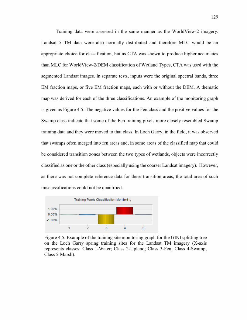
129
Training data were assessed in the same manner as the WorldView-2 imagery.
Landsat 5 TM data were also normally distributed and therefore MLC would be an
appropriate choice for classification, but as CTA was shown to produce higher accuracies
than MLC for WorldView-2/DEM classification of Wetland Types, CTA was used with the
segmented Landsat images. In separate tests, inputs were the original spectral bands, three
EM fraction maps, or five EM fraction maps, each with or without the DEM. A thematic
map was derived for each of the three classifications. An example of the monitoring graph
is given as Figure 4.5. The negative values for the Fen class and the positive values for the
Swamp class indicate that some of the Fen training pixels more closely resembled Swamp
training data and they were moved to that class. In Loch Garry, in the field, it was observed
that swamps often merged into fen areas and, in some areas of the classified map that could
be considered transition zones between the two types of wetlands, objects were incorrectly
classified as one or the other class (especially using the coarser Landsat imagery). However,
as there was not complete reference data for these transition areas, the total area of such
misclassifications could not be quantified.
Figure 4.5. Example of the training site monitoring graph for the GINI splitting tree on the Loch Garry spring training sites for the Landsat TM imagery (X-axis represents classes: Class 1-Water; Class 2-Upland; Class 3-Fen; Class 4-Swamp; Class 5-Marsh).
130
4.1.4 Radarsat-2 image processing, classification and analyses for Wetland Type
Radar imagery analyses were not a central focus of the thesis; as such methods were
selected that were straightforward to implement and combine with optical imagery, in order
to evaluate the potential for integration into an operational wetland evaluation system such
as OWES. Radarsat-2 processing was completed using PolSarPro_v4.2.0, NEST4C-1.1, and
Polarimetric Workstation Software (PWSv5r5.3, Touzi et al., 2010). Raw radar imagery was
processed to sigma nought values and extracted to full resolution. Using these data, the
polarimetric signatures were first generated from training polygons at the same field sites
used for the optical imagery. The polarimetric graphs for Wetland Type were subsequently
analyzed in terms of their shape, position of peaks and troughs, and pedestal height. Based
on the literature, polarimetric plots were analyzed for the dominant type(s) of scattering
mechanism such as surface, Bragg, double bounce, and volume, as depicted in Figure 2.5.
Pedestal height gave an indication of the degree of depolarization in the target response,
with a low value representing polarized response and increasing values representing
increased depolarization (Evans et al., 1988; Boerner et al., 1998; McNairn et al, 2002;
Touzi et al., 2004; Touzi et al., 2010).
The radar data, including the HH, HV, VH, VV images and CP decomposition
variables were geocorrected using NEST4C-1.1 allowing for comparison to the validation
data, and to use in segmentation and classifications with the geocorrected optical imagery.
The four corners (longitude and latitude) were obtained, and the scene boundaries were set.
Next the range and azimuth were determined and, target image pass times were calculated.
Tie points (geolocation points) were developed from the latitude/longitude and slant range
time derived from the geolocation grid from the original product. The correction occurred
131
individually at each cell where latitude and longitude for corrected cell is related to the
corresponding position of the cell in the original image and four pixels immediately adjacent
to it.
Slant range (R) was calculated for the cell using the slant range time and bi-quadratic
interpolation; zero Doppler Time (T) was computed and then bias-corrected zero Doppler
time (Tc=T+R*2/C) where C is the speed of light; finally the azimuth index (Ia) was
computed using zero Doppler time and the range image index (Ir) was computed using slant
range (R). The corrected cell value was computed with Ia and Ir using bilinear interpolation,
and corrected to a WGS84 UTM (zone 18 row T) ellipsoid. The corrected images were
assessed through a comparison to the OMNR road vector file. These corrections showed
minimal positional error (approximately less than 1 pixel) and therefore, these final images
were deemed suitable for addition to, and use with the optical imagery (segmentation) and
for accuracy assessment of products derived directly from the radar imagery. The normality
of the radar data was not assessed, as based on results from the Worldview tests of
classification, CTA was selected over MLC, and CTA does not require normal distributions.
A 7 x 7 enhanced Lee adaptive filter was then applied to the raw radar data to reduce
speckle while maintaining edges or sharp features in the image. This filter and window size
was selected following De Leeuw (2009) who found that they outperformed about 20 other
speckle filters/window size combinations and had speckle reduction rates up to 70%. Once
the radar data, were filtered they were used for a variety of analyses as follows.
HV and HH images were derived and samples were taken at field validation locations
for all land cover types (up to 5 depending upon the study area), at all study areas (4), for all
seasons of data (3), and for all incidence angles (ranging from steep (18.4º) to shallow
(48.0º)). The literature has shown that HH has proven useful for distinguishing Bog, Fen,
132
freshwater versus saline marsh, and forested areas with water, and that, in general, HH is
preferable over VV data (Li and Chen, 2005; Henderson and Lewis, 2008; Lang et al., 2008;
Lang and Kasischke, 2008; Lu and Kwoun, 2008). HV has also been shown to produce high
accuracies for certain wetland classifications (Baghdadi et al., 2001; Henderson and Lewis,
2008). These data were plotted on scatter graphs to determine if Wetland Type could be
distinguished based upon backscatter for this polarisation combination. HV and HH images
were then used to classify the Wetland Types using CTA. Finally, the HV and HH images
were added to the OBIA segmentation/CTA classification along with the WorldView-2
spring imagery and the DEM to determine if they improved the Wetland Type classification
accuracy. OBIA parameter values were the same as for the WorldView-2 data (scale value
= 45; shape value = 0.1; compactness value = 0.75).
Decomposition of polarimetric radar data was selected for this research because
previous studies had found that decomposition components provided significant
discrimination between Wetland Types (Touzi, 2007;Touzi et al, 2007; Sartori et al., 2011;
Bourgeau-Chavez et al., 2013; Schmitt and Brisco, 2013). Of the various decomposition
techniques that have been proposed, CP components have been shown to distinguish
between Wetland Type classes such as Upland, Wetland, Forest and Shrub (Sartori et al.,
2011), and that higher alpha values distinguished greater flooding in vegetated areas
compared to areas with less flooding and lower alpha values (Schmitt and Brisco, 2013).
Other studies have found other decomposition techniques to perform well in wetland
mapping for various purposes and in some cases comparisons were made between
techniques. For example, Touzi (2007) and Touzi et al. (2007), working in a single wetland,
Mer Bleue Bog, which was also a site of this research, found that the Touzi decomposition
components provided better discrimination of the Wetland Types than CP components.
133
However, based on the availability and ease of implementation of the CP decomposition
technique, it was selected to determine if the addition of the CP components to other imagery
types or variables could improve the overall classification.
The CP decomposition process starts with a 3x3 (square) matrix that contains the
eigenvalues from which entropy and anisotropy are derived, and the 3x3 unitary
(orthogonal) matrix, from which the alpha angle is derived. These three components relate
to the physical scattering mechanisms (surface, volume and double bounce/multiple
scattering) of the target. The components are given as: entropy (H, between 0 and 1)
representing the degree of randomness; anisotropy (A, between 0 and 1) represents the
relation between the second and third eigenvalues and is a measure of the difference between
the secondary scattering mechanisms; and alpha which identifies the dominant scattering
mechanism (Cloude and Pottier, 1997).
The components entropy, anisotropy and alpha were derived from the Loch Garry
summer image and used as inputs to a Wishart unsupervised eight-class classification, and
to a MLC using the same training sites as for the WorldView-2 and Landsat TM
classifications. The CP components were also assessed in classification using the CTA
method (pixel-based), and using OBIA segmentation/CTA classification, combined with the
WorldView-2 imagery and the DEM.
4.1.5 Wetland Type classification accuracy assessment
Thematic map accuracies were assessed using standard error matrices and accuracy
statistics, which are well known and used in remote sensing. An error matrix compares
validation (reference) data with the classification data (Congalton and Green, 1993; Foody,
2002) and provides information regarding the errors of omission (exclusion of pixels from
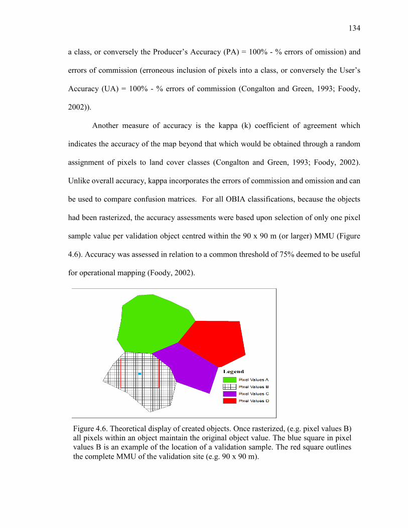
134
a class, or conversely the Producer’s Accuracy (PA) = 100% - % errors of omission) and
errors of commission (erroneous inclusion of pixels into a class, or conversely the User’s
Accuracy (UA) = 100% - % errors of commission (Congalton and Green, 1993; Foody,
2002)).
Another measure of accuracy is the kappa (k) coefficient of agreement which
indicates the accuracy of the map beyond that which would be obtained through a random
assignment of pixels to land cover classes (Congalton and Green, 1993; Foody, 2002).
Unlike overall accuracy, kappa incorporates the errors of commission and omission and can
be used to compare confusion matrices. For all OBIA classifications, because the objects
had been rasterized, the accuracy assessments were based upon selection of only one pixel
sample value per validation object centred within the 90 x 90 m (or larger) MMU (Figure
4.6). Accuracy was assessed in relation to a common threshold of 75% deemed to be useful
for operational mapping (Foody, 2002).
Figure 4.6. Theoretical display of created objects. Once rasterized, (e.g. pixel values B) all pixels within an object maintain the original object value. The blue square in pixel values B is an example of the location of a validation sample. The red square outlines the complete MMU of the validation site (e.g. 90 x 90 m).
135
Separate groups of field and image-based reference data were used for both training
and validation, generally in a ratio of 30:70%, respectively, between training and validation
samples (Foody, 2002; McCoy, 2005). The field-based reference data sets were particularly
small; by splitting them 30:70% this ensured a large enough representative training set,
while maintaining a large representative portion to generate accuracy statistics. However,
due to the aforementioned issue of small reference sample sizes, in some cases, these splits
were not possible for Open Water Types, which was a relatively rare class in the landscape.
4.2 Methods to segment, classify, and map VCFs using optical and radar imagery
Part of the challenge of this research was minimizing the number of methods while
maximizing the outcomes and accuracies of the attributes mapped. After determining that
the method that obtained the best results for Wetland Type mapping was OBIA segmentation
followed by CTA classification this method was applied for the VCFs. Figure 4.7 provides
the workflow for the methods used to segment, classify and map VCFs.
4.2.1 Segmentation methods using spring 2010 WorldView-2 imagery
WorldView-2 imagery were segmented using the four spectral bands and the DEM
with the multi-resolution segmentation algorithm and a scale parameter value of 25, shape
parameter value of 0.1 and compactness parameter value of 0.75 which, visually represented
these types of classes best.
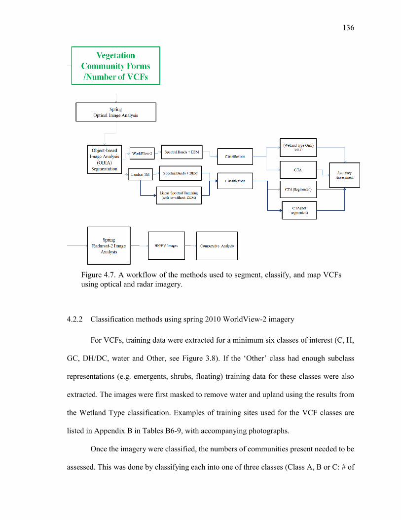
136
4.2.2 Classification methods using spring 2010 WorldView-2 imagery
For VCFs, training data were extracted for a minimum six classes of interest (C, H,
GC, DH/DC, water and Other, see Figure 3.8). If the ‘Other’ class had enough subclass
representations (e.g. emergents, shrubs, floating) training data for these classes were also
extracted. The images were first masked to remove water and upland using the results from
the Wetland Type classification. Examples of training sites used for the VCF classes are
listed in Appendix B in Tables B6-9, with accompanying photographs.
Once the imagery were classified, the numbers of communities present needed to be
assessed. This was done by classifying each into one of three classes (Class A, B or C: # of
Figure 4.7. A workflow of the methods used to segment, classify, and map VCFs using optical and radar imagery.
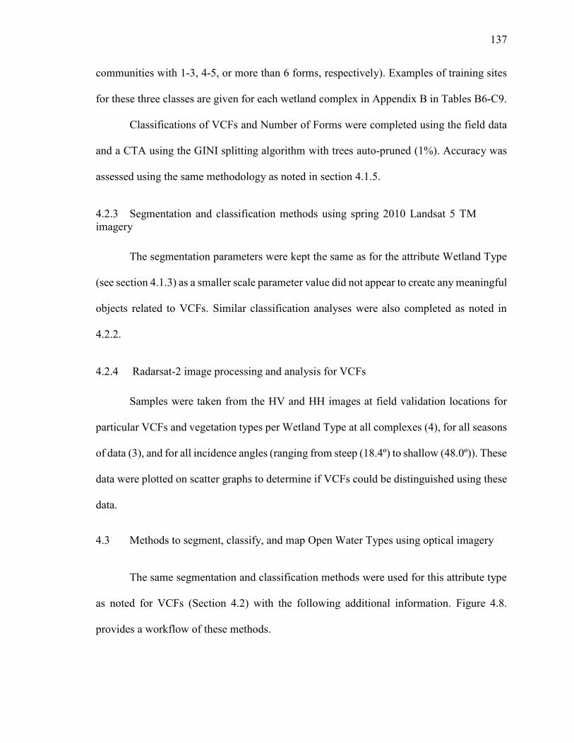
137
communities with 1-3, 4-5, or more than 6 forms, respectively). Examples of training sites
for these three classes are given for each wetland complex in Appendix B in Tables B6-C9.
Classifications of VCFs and Number of Forms were completed using the field data
and a CTA using the GINI splitting algorithm with trees auto-pruned (1%). Accuracy was
assessed using the same methodology as noted in section 4.1.5.
4.2.3 Segmentation and classification methods using spring 2010 Landsat 5 TM imagery
The segmentation parameters were kept the same as for the attribute Wetland Type
(see section 4.1.3) as a smaller scale parameter value did not appear to create any meaningful
objects related to VCFs. Similar classification analyses were also completed as noted in
4.2.2.
4.2.4 Radarsat-2 image processing and analysis for VCFs
Samples were taken from the HV and HH images at field validation locations for
particular VCFs and vegetation types per Wetland Type at all complexes (4), for all seasons
of data (3), and for all incidence angles (ranging from steep (18.4º) to shallow (48.0º)). These
data were plotted on scatter graphs to determine if VCFs could be distinguished using these
data.
4.3 Methods to segment, classify, and map Open Water Types using optical imagery
The same segmentation and classification methods were used for this attribute type
as noted for VCFs (Section 4.2) with the following additional information. Figure 4.8.
provides a workflow of these methods.
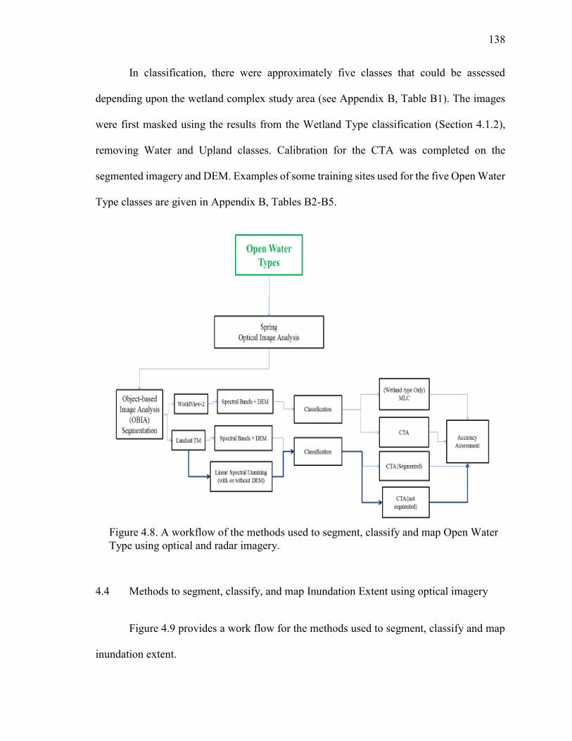
138
In classification, there were approximately five classes that could be assessed
depending upon the wetland complex study area (see Appendix B, Table B1). The images
were first masked using the results from the Wetland Type classification (Section 4.1.2),
removing Water and Upland classes. Calibration for the CTA was completed on the
segmented imagery and DEM. Examples of some training sites used for the five Open Water
Type classes are given in Appendix B, Tables B2-B5.
4.4 Methods to segment, classify, and map Inundation Extent using optical imagery
Figure 4.9 provides a work flow for the methods used to segment, classify and map
inundation extent.
Figure 4.8. A workflow of the methods used to segment, classify and map Open Water Type using optical and radar imagery.
139
4.4.1 Field analysis
In spring and summer 2010 transects of 50 m or greater (relating to the resolution of
the Landsat TM imagery) were assessed from uplands to the visual marker of wetness (e.g.
presence of water) in a direction approximately perpendicular to the wetland edge.
Volumetric soil water content (VWC %), the ratio of water volume to total volume,
was measured using a HydroSense Soil Water Measurement System (Campbell Scientific
Inc., Canada) at 1 m increments along the transects. The Inundation Extent (wet extent) was
assessed as the first occurrence of 100% VWC. 100% VWC would be expected once the
probes were inserted into standing water. This was repeated for 48 VWC transects in the
spring of 2010 (30 into marshes, 11 into swamps, 3 into fens (the rarest Wetland Type) and
6 into bogs. In the spring of 2011, 117 boundaries were mapped (tracking along the wet
boundary at the four sites) and crossing the 48 VWC transects from the previous year. The
edge was followed until it could no longer be visually assessed, it became physically
impenetrable, or it was at the intersection with a manmade structure (e.g. a road or path).
Field data for VWC% is found in Appendix J.
4.4.2 Semi-variogram analysis of VWC
Semi-variogram analysis was conducted to determine the range of spatial
dependence of these field data along a given transect and to use that information in selection
of data for statistical analysis against the remote sensing data. VWC showed spatial
dependence along some transects, but not for others (land cover dependent).
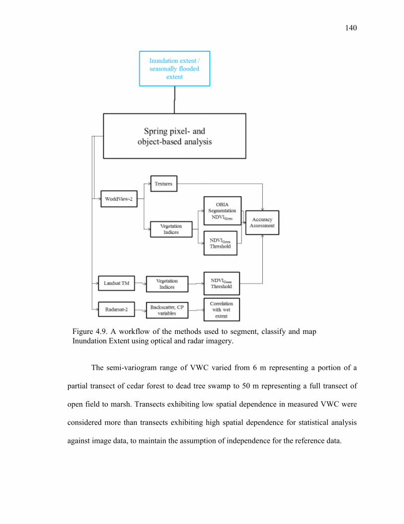
140
The semi-variogram range of VWC varied from 6 m representing a portion of a
partial transect of cedar forest to dead tree swamp to 50 m representing a full transect of
open field to marsh. Transects exhibiting low spatial dependence in measured VWC were
considered more than transects exhibiting high spatial dependence for statistical analysis
against image data, to maintain the assumption of independence for the reference data.
Figure 4.9. A workflow of the methods used to segment, classify and map Inundation Extent using optical and radar imagery.
141
4.4.3 Pixel-based image processing
The approach taken for image detection of inundation extent was to extract high
resolution image parameters deemed to have potential for detection of the water-vegetation
edge, including vegetation indices and texture metrics. A WorldView-2 pan-sharpened
image (spatial resolution of approximately 0.46 m) was initially developed by merging the
high resolution PAN image with the low resolution multi-spectral images (approximately
1.8 m), after which a subset of the study area was used for the following processes. Vrabel
(2000) showed that sharpened images have increased utility of vegetation indices over those
derived from the original low resolution imagery. In this research principal components
analysis of the spectral bands was conducted and the PAN band was substituted for PC1,
which generally represents overall image brightness similar to the PAN band (Welch and
Ehlers, 1987).
GLCM texture metrics (after Haralick, and Fu, 1983) were extracted including:
Contrast, Correlation, Entropy and Homogeneity (Baraldi and Parmiggiani, 1995). They
were selected as each measures different aspects of the imagery (e.g. Homogeneity measures
the image uniformity; Contrast measures the opposite of Homogeneity (or the heterogeneity)
and detects edges well; Entropy measures the randomness within the image; Correlation
measures the linear dependency of neighbouring pixels (Baraldi and Parmiggiani, 1995)).
However, scatterplots of field measured % VWC compared with texture values showed no
discernible relationships, and image texture was not explored further for detecting
inundation extent.
It has been shown in the literature that vegetation structure and composition can be
related to the wetness, or wetness gradient of the underlying soil (Gitelson and Merzlyak,
142
1997; Campos et al., 2012; Wang et al., 2012; Zhou Demin et al., 2012; Delgado and Marin,
2013). Vegetation indices derived from multi-spectral band ratios are important and
commonly used tools for measuring vegetation health and structure. Fourteen vegetation
indices were calculated using the pan-sharpened WorldView-2 imagery, including NDVI,
NDVIBlue, NDVIGreen, WDVI, TVI, TTVI, RVI, PVI, PVI1, PVI2, PVI3, NRVI, EVI, EVI2.
They were selected because they have been shown to be sensitive to soil moisture gradients
and/or vegetation gradients (Li and Liu, 2004; Mutanga and Skidmore, 2004; Wu et al.,
2007; Wang et al., 2008). In plotting each against field-measured VWC, it was revealed that
NDVIgreen had the best relationship. The plots were used to determine a threshold value of
NDVIgreen values that corresponded to 100% VWC. NDVIGreen has not previously been used
in detection of the wet extent of wetlands, habitat, or wetland type. It was developed as a
way to estimate plant chlorophyll (Gitelson and Merzlyak, 1997), which changes throughout
a plants lifespan and as it reacts to stressors (such as soil moisture levels). However, as
shown later in Section 5.4, its response to wet extent in the study wetland of this research
was very distinct.
The range of NDVIgreen values was subsequently used to derive a boundary that
represented the wet extent (100% VWC) for each image for each wetland complex. An
attempt was also made to see if the same NDVIGreen/VWC relationship could be found using
objects that were segmented from the WorldView-2 NDVIGreen derived. In addition, the
same object- and pixel-based analyses were conducted using the Landsat data with inputs
including NDVIGreen and the unmixed fraction maps. Radarsat-2 backscatter was also
compared to field-measured VWC to see if there was a relationship between these variables.
In the literature, HH polarisation has generally been found to be better correlated with soil
moisture than VV polarisation (Dobson and Ulaby, 1988; Lang and Kasischke, 2008),
143
however, at shallower incidence angle, soil moisture was found to be less influential on all
polarisations (HH, HV, VH, VV) (McNairn et al., 2002).
4.5 GIS analysis of derived imagery and existing LIO layers
All processing of GIS variables was completed using thematic maps created in this
research, existing data layers found in the OMNR’s LIO and using ArcMAP 10.0 software
(ESRI). One of the main requirements of the collaboration with the OMNR was to determine
if the data existing in the LIO were sufficient to map these attributes.
The following attributes required some degree of GIS analyses including Number of
Wetland Types, Diversity of Surrounding Habitat, Proximity to Other Wetlands, Wetland
Size, Hunting/Recreation Areas, Proximity to Human Areas, Ownership Patterns, Wetland
Basin Size, and Rarity of Wetland and Rarity of Wetland in Landscape. Analyses included
combining thematic layers, making measurements, buffering, counting, and measuring
hydrologic surface connections and distance of connections. The methods implemented
were relatively simple and straightforward for each attribute type and therefore a workflow
figure is not provided. The following paragraphs list the layers that were used per attribute.
4.5.1 Number of Wetland Types for the Biological component
The thematic maps developed in the above-noted analysis were used as input to
determine the Number of Wetland Types present in each wetland complex.
4.5.2 Diversity of Surrounding Habitat for the Biological component
The layers of Wetland Type derived from this research were combined with existing
layers from the LIO that included: contours, water bodies, and a 2011 AAFC Crop Type
144
Map of Canada from Agriculture Canada. The presence of the surrounding habitat was
assessed by taking a 1.5 km straight line distance (buffer) surrounding each wetland
boundary within the wetland complex and around the boundary of each wetland complex.
4.5.3 Proximity to Other Wetlands for the Biological component
These hydrological surface connections were assessed by measuring these above-
ground surface water paths up to 4 km from the boundaries of the study-site wetland
complexes to other wetlands/wetland complexes using the Wetland Type thematic map
derived from this research, the OMNR water bodies layer that provides large lakes and ponds
information, the rivers layer, and the OMNR wetland layer.
4.5.4 Wetland Size for the Biological component
The Wetland Size was determined by using the 2013 OMNR wetland layer as the
Wetland Type layer derived in this research was a subset of the entire complex.
4.5.5 Hunting Pattern mapping for the Social component
In the field in 2010, GPS waypoints were taken when hunting blinds were located
by chance. These data, along with existing LIO layers of trap lines, trapper cabins, recreation
access points, traditional land use areas and trails present were used to assess intensity of
hunting usage at each wetland complex.
4.5.6 Ownership Patterns for the Social component
Data from the LIO of Land Ownership, Crown Land – MNR Non-Freehold
Disposition Public, Crown Land – MNR Unpatented Public, Crown Land Use Policy Atlas,
145
Crown Leased Land, and Traditional Land Use Area were combined to determine a
percentage of ownership for the wetland areas in each wetland complex study site.
4.5.7 Wetland Basin Size for the Hydrologic component
The attribute Inundation Extent (see Sections 2.9.4; 4.4) was the best indicator of the
‘true’ size of the wetland in terms of its ability to attenuate floods. The size of the catchment
basin and catchment basin upstream of the wetland area were derived from the LIO
watershed layer. The size of the other detention areas within the basins were derived from
the existing LIO wetland layer and from water bodies and rivers layers.
4.5.8 Rarity of Wetlands and Rarity in Landscape for the Special Feature component
These attributes were assessed by comparing the derived Wetland Type attribute layer, the existing OMNR wetland layer and using the site district and site region layers. Objective 2 Methods: Compare and relate the scores determined for each of these attributes to the field-evaluated OWES scores
4.6 Compare the scores derived from the geo-spatial analysis to the OWES field-based
scores
The second objective of this research was to compare the geo-spatial derived
attributes’ scores to the field-based OWES database of wetland “scores” (from field
evaluations) to determine if these geo-spatial methods can be related to, and/or integrated
with the existing system. Using the results derived from methods presented above, a score
was determined using the scoring methods provided in section 2.9.1 to 2.9.13 for each
attribute and compared to the OWES score for the same attribute.
146
Objective 3 Methods: Review of temporal remote sensing data in classification of wetland attributes and analysis of attribute changes over the long term.
4.7 Review of temporal remote sensing data in classification of wetland attributes and
analysis of attribute changes over the long term
Wetlands are dynamic and assessing them during one season only or at one time
within one season only may limit or skew results. This section outlines methods that were
used to map the temporal change of attributes between seasons and inter-annually to
determine how the accuracy values or scoring results changed between seasons. This was
completed for Wetland Type, VCFs, Open Water Types and Inundation Extent. The methods
that were used to: 1) collect validation data and 2) process and analyze imagery are already
listed in the corresponding sections above (section 4.1 to 4.4).
The second portion of the temporal analysis evaluated how change can occur over
longer terms (decadal) by analysing the Landsat 5 TM imagery (i.e., the only imagery
available at this temporal scale). This was specifically done for Anthropogenic Disturbance,
which can be assessed through land use change analysis.
4.7.1 Wetland Type, VCFs, and Open Water Types
Classifications using OBIA and CTA with spring, summer, fall and combined
WorldView-2 imagery were completed for these attributes as described in sections 4.1 – 4.3
and following Figures 4.2, 4.6 and 4.7. Accuracy was assessed and the best season for
imagery acquisition was determined. Statistical comparison of the accuracies was conducted
using McNemar’s test (McNemar 1947), which is non-parametric and based on the
classifiers’ error matrices, determining if column and row frequencies are equal (null
147
hypothesis) (de Leeuw et al. 2006; Gao et al. 2006). This test has been previously used to
compare accuracies of two or more classifications (Dingle Robertson and King, 2011; Duro
et al., 2012).
4.7.2 Inundation Extent
The spring and summer 2010 and 2011 field data were plotted on line graphs to
determine if there was a spatial difference in VWC measured in the field between seasons,
and the seasonal difference in wetland wet extents where VWC = 100%. Next, thresholds
for the summer WorldView-2 imagery were developed in the same manner as the spring
imagery as outlined in section 4.4. Finally, a comparison was made to determine if the
distance between the wet extents (Inundation Extent) matched the distance between the
threshold-derived extents in the imagery.
4.7.3 Anthropogenic Disturbance
A change in biomass can be an indicator of anthropogenic disturbance, and this can
be assessed using remotely sensed imagery. Figure 4.10 provides the workflow for this
attribute. Landsat 5 TM images from 2010 and from the year in which the original field-
based OWES evaluations (Table 3.1) were completed (or the closest-date, best quality, non-
cloudy imagery were compared. Land cover fraction analyses have been shown to indicate
change based upon climatic or human influences (Adams et al., 1995; Schmid et al., 2005;
Olthof and Fraser, 2007; Melendez-Pastor et al., 2010) and were therefore selected to assess
change through time in the wetlands of this research.
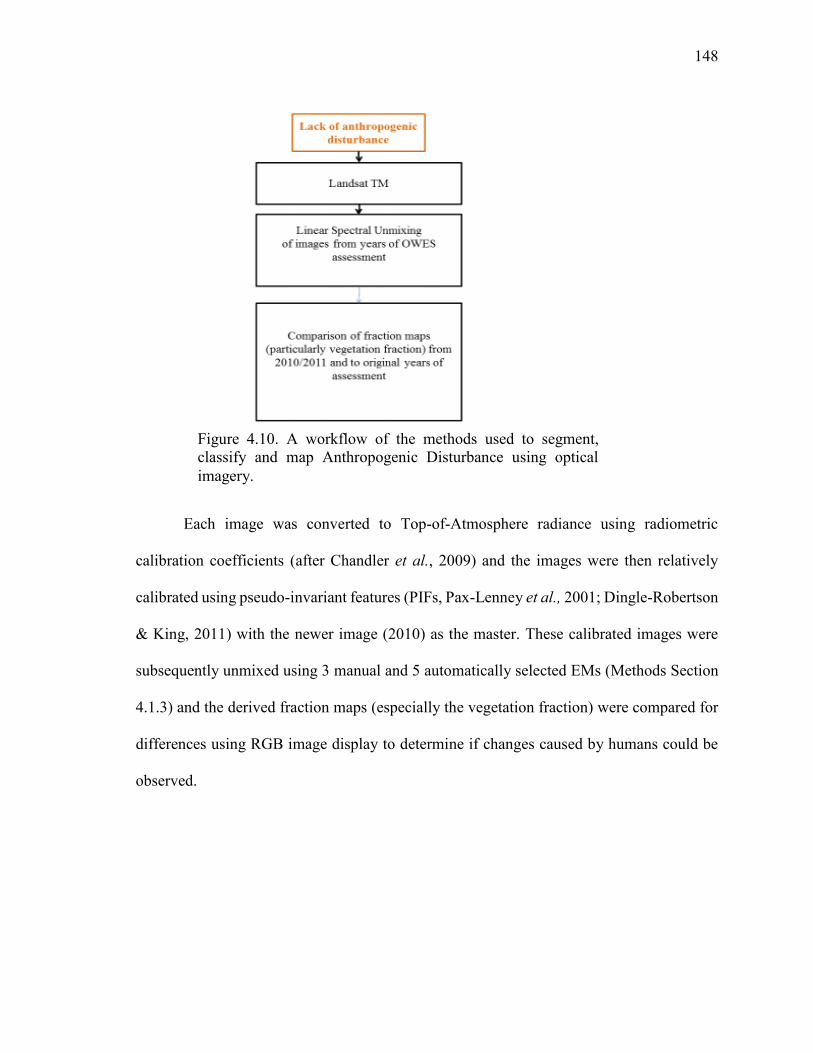
148
Each image was converted to Top-of-Atmosphere radiance using radiometric
calibration coefficients (after Chandler et al., 2009) and the images were then relatively
calibrated using pseudo-invariant features (PIFs, Pax-Lenney et al., 2001; Dingle-Robertson
& King, 2011) with the newer image (2010) as the master. These calibrated images were
subsequently unmixed using 3 manual and 5 automatically selected EMs (Methods Section
4.1.3) and the derived fraction maps (especially the vegetation fraction) were compared for
differences using RGB image display to determine if changes caused by humans could be
observed.
Figure 4.10. A workflow of the methods used to segment, classify and map Anthropogenic Disturbance using optical imagery.
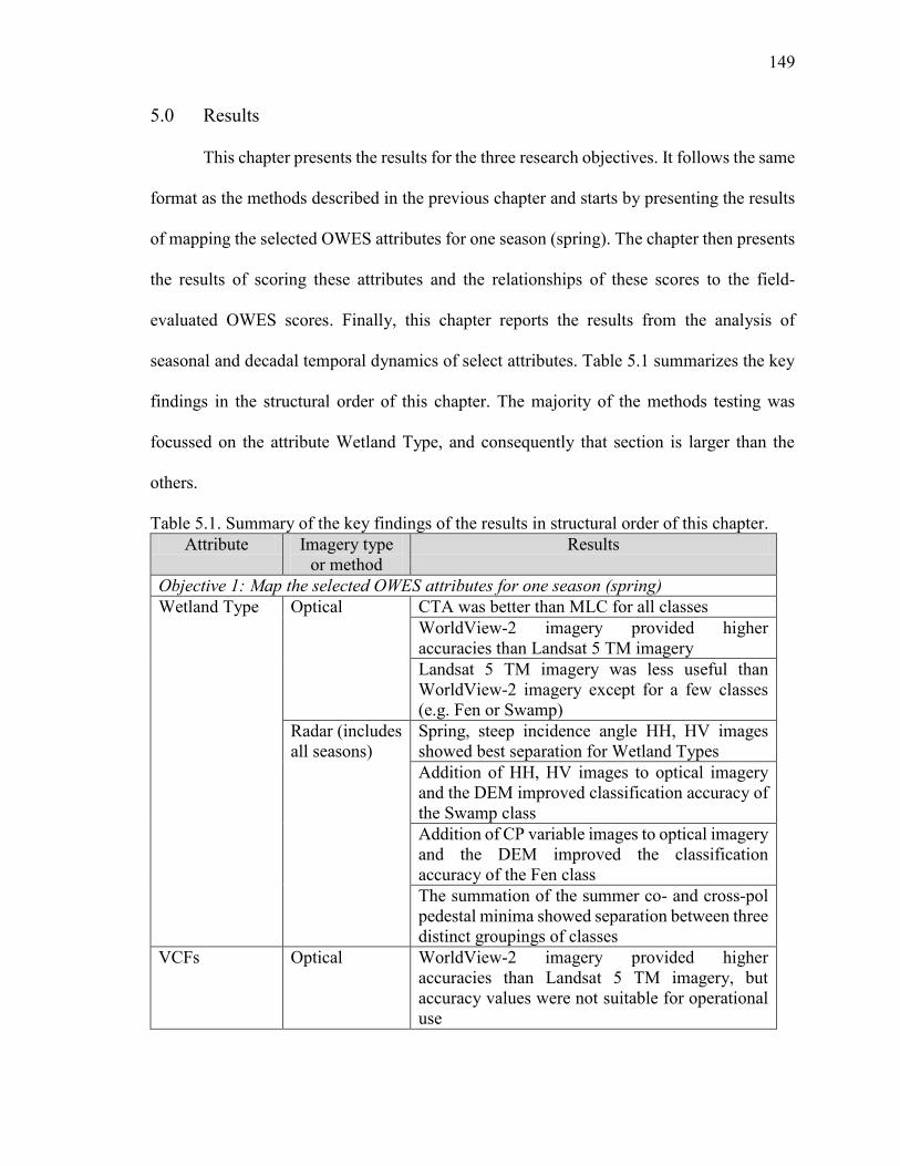
149
5.0 Results
This chapter presents the results for the three research objectives. It follows the same
format as the methods described in the previous chapter and starts by presenting the results
of mapping the selected OWES attributes for one season (spring). The chapter then presents
the results of scoring these attributes and the relationships of these scores to the field-
evaluated OWES scores. Finally, this chapter reports the results from the analysis of
seasonal and decadal temporal dynamics of select attributes. Table 5.1 summarizes the key
findings in the structural order of this chapter. The majority of the methods testing was
focussed on the attribute Wetland Type, and consequently that section is larger than the
others.
Table 5.1. Summary of the key findings of the results in structural order of this chapter. Attribute Imagery type
or method Results
Objective 1: Map the selected OWES attributes for one season (spring) Wetland Type Optical CTA was better than MLC for all classes
WorldView-2 imagery provided higher accuracies than Landsat 5 TM imagery Landsat 5 TM imagery was less useful than WorldView-2 imagery except for a few classes (e.g. Fen or Swamp)
Radar (includes all seasons)
Spring, steep incidence angle HH, HV images showed best separation for Wetland Types Addition of HH, HV images to optical imagery and the DEM improved classification accuracy of the Swamp class Addition of CP variable images to optical imagery and the DEM improved the classification accuracy of the Fen class The summation of the summer co- and cross-pol pedestal minima showed separation between three distinct groupings of classes
VCFs Optical WorldView-2 imagery provided higher accuracies than Landsat 5 TM imagery, but accuracy values were not suitable for operational use
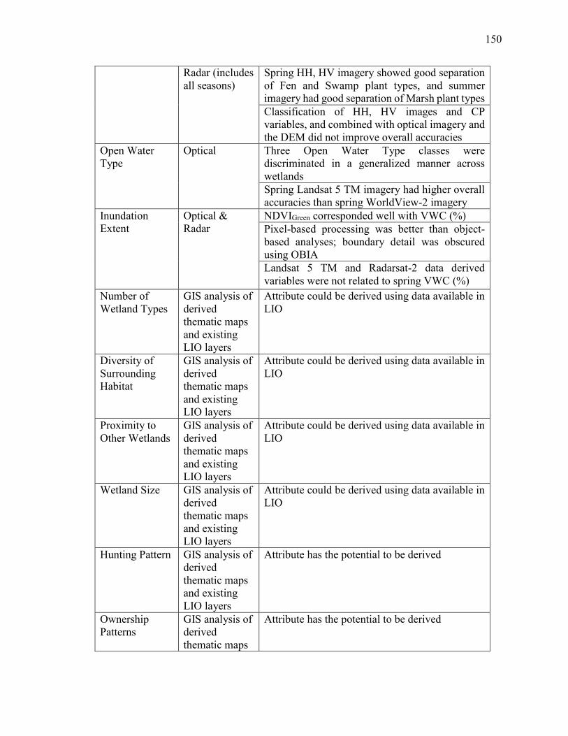
150
Radar (includes all seasons)
Spring HH, HV imagery showed good separation of Fen and Swamp plant types, and summer imagery had good separation of Marsh plant types Classification of HH, HV images and CP variables, and combined with optical imagery and the DEM did not improve overall accuracies
Open Water Type
Optical Three Open Water Type classes were discriminated in a generalized manner across wetlands Spring Landsat 5 TM imagery had higher overall accuracies than spring WorldView-2 imagery
Inundation Extent
Optical & Radar
NDVIGreen corresponded well with VWC (%) Pixel-based processing was better than object-based analyses; boundary detail was obscured using OBIA Landsat 5 TM and Radarsat-2 data derived variables were not related to spring VWC (%)
Number of Wetland Types
GIS analysis of derived thematic maps and existing LIO layers
Attribute could be derived using data available in LIO
Diversity of Surrounding Habitat
GIS analysis of derived thematic maps and existing LIO layers
Attribute could be derived using data available in LIO
Proximity to Other Wetlands
GIS analysis of derived thematic maps and existing LIO layers
Attribute could be derived using data available in LIO
Wetland Size GIS analysis of derived thematic maps and existing LIO layers
Attribute could be derived using data available in LIO
Hunting Pattern GIS analysis of derived thematic maps and existing LIO layers
Attribute has the potential to be derived
Ownership Patterns
GIS analysis of derived thematic maps
Attribute has the potential to be derived
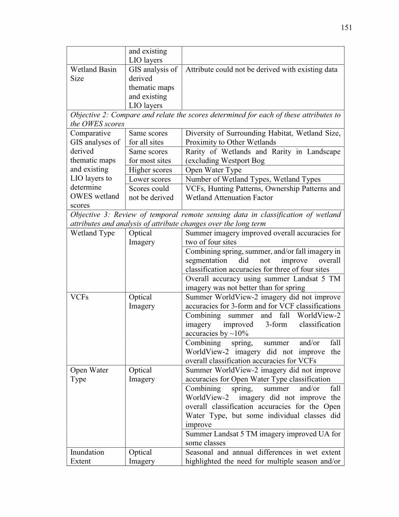
151
and existing LIO layers
Wetland Basin Size
GIS analysis of derived thematic maps and existing LIO layers
Attribute could not be derived with existing data
Objective 2: Compare and relate the scores determined for each of these attributes to the OWES scores Comparative GIS analyses of derived thematic maps and existing LIO layers to determine OWES wetland scores
Same scores for all sites
Diversity of Surrounding Habitat, Wetland Size, Proximity to Other Wetlands
Same scores for most sites
Rarity of Wetlands and Rarity in Landscape (excluding Westport Bog
Higher scores Open Water Type Lower scores Number of Wetland Types, Wetland Types Scores could not be derived
VCFs, Hunting Patterns, Ownership Patterns and Wetland Attenuation Factor
Objective 3: Review of temporal remote sensing data in classification of wetland attributes and analysis of attribute changes over the long term Wetland Type Optical
Imagery Summer imagery improved overall accuracies for two of four sites Combining spring, summer, and/or fall imagery in segmentation did not improve overall classification accuracies for three of four sites Overall accuracy using summer Landsat 5 TM imagery was not better than for spring
VCFs Optical Imagery
Summer WorldView-2 imagery did not improve accuracies for 3-form and for VCF classifications Combining summer and fall WorldView-2 imagery improved 3-form classification accuracies by ~10% Combining spring, summer and/or fall WorldView-2 imagery did not improve the overall classification accuracies for VCFs
Open Water Type
Optical Imagery
Summer WorldView-2 imagery did not improve accuracies for Open Water Type classification Combining spring, summer and/or fall WorldView-2 imagery did not improve the overall classification accuracies for the Open Water Type, but some individual classes did improve Summer Landsat 5 TM imagery improved UA for some classes
Inundation Extent
Optical Imagery
Seasonal and annual differences in wet extent highlighted the need for multiple season and/or
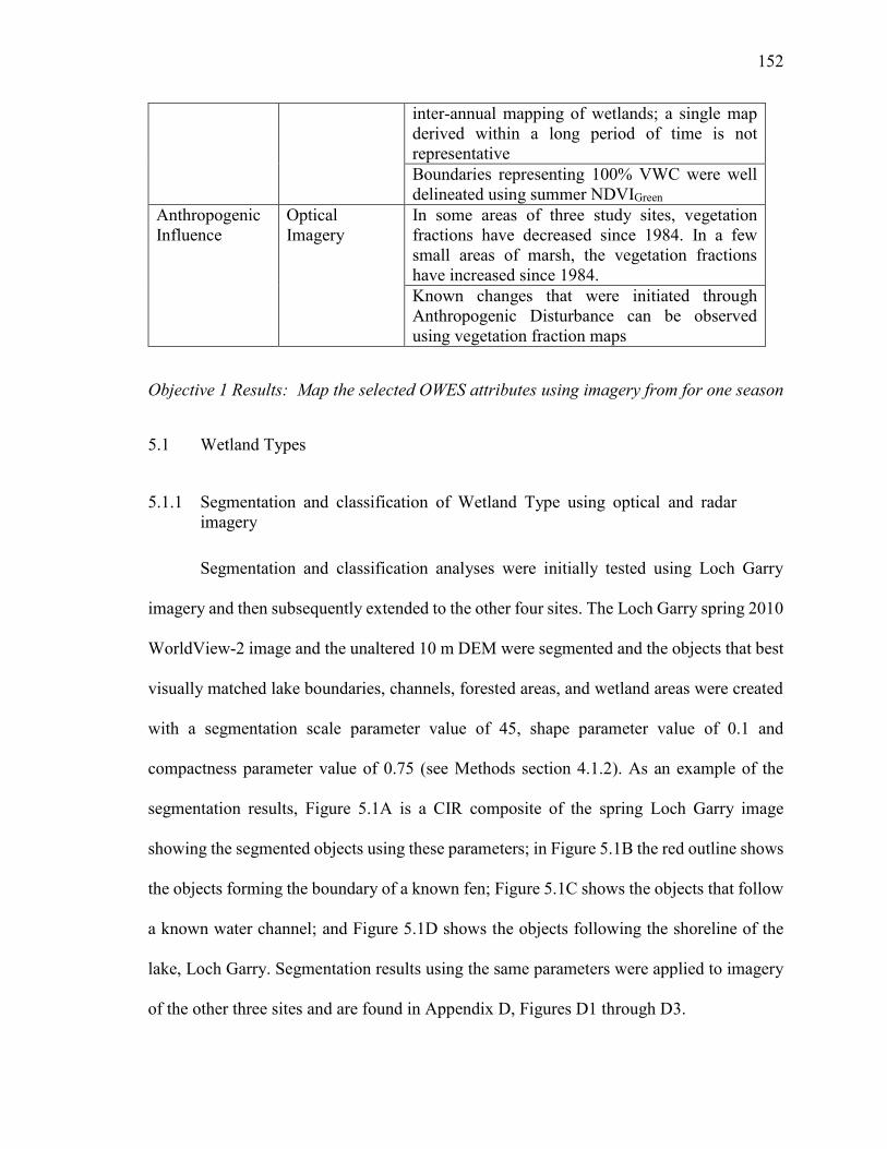
152
inter-annual mapping of wetlands; a single map derived within a long period of time is not representative Boundaries representing 100% VWC were well delineated using summer NDVIGreen
Anthropogenic Influence
Optical Imagery
In some areas of three study sites, vegetation fractions have decreased since 1984. In a few small areas of marsh, the vegetation fractions have increased since 1984. Known changes that were initiated through Anthropogenic Disturbance can be observed using vegetation fraction maps
Objective 1 Results: Map the selected OWES attributes using imagery from for one season
5.1 Wetland Types
5.1.1 Segmentation and classification of Wetland Type using optical and radar imagery
Segmentation and classification analyses were initially tested using Loch Garry
imagery and then subsequently extended to the other four sites. The Loch Garry spring 2010
WorldView-2 image and the unaltered 10 m DEM were segmented and the objects that best
visually matched lake boundaries, channels, forested areas, and wetland areas were created
with a segmentation scale parameter value of 45, shape parameter value of 0.1 and
compactness parameter value of 0.75 (see Methods section 4.1.2). As an example of the
segmentation results, Figure 5.1A is a CIR composite of the spring Loch Garry image
showing the segmented objects using these parameters; in Figure 5.1B the red outline shows
the objects forming the boundary of a known fen; Figure 5.1C shows the objects that follow
a known water channel; and Figure 5.1D shows the objects following the shoreline of the
lake, Loch Garry. Segmentation results using the same parameters were applied to imagery
of the other three sites and are found in Appendix D, Figures D1 through D3.
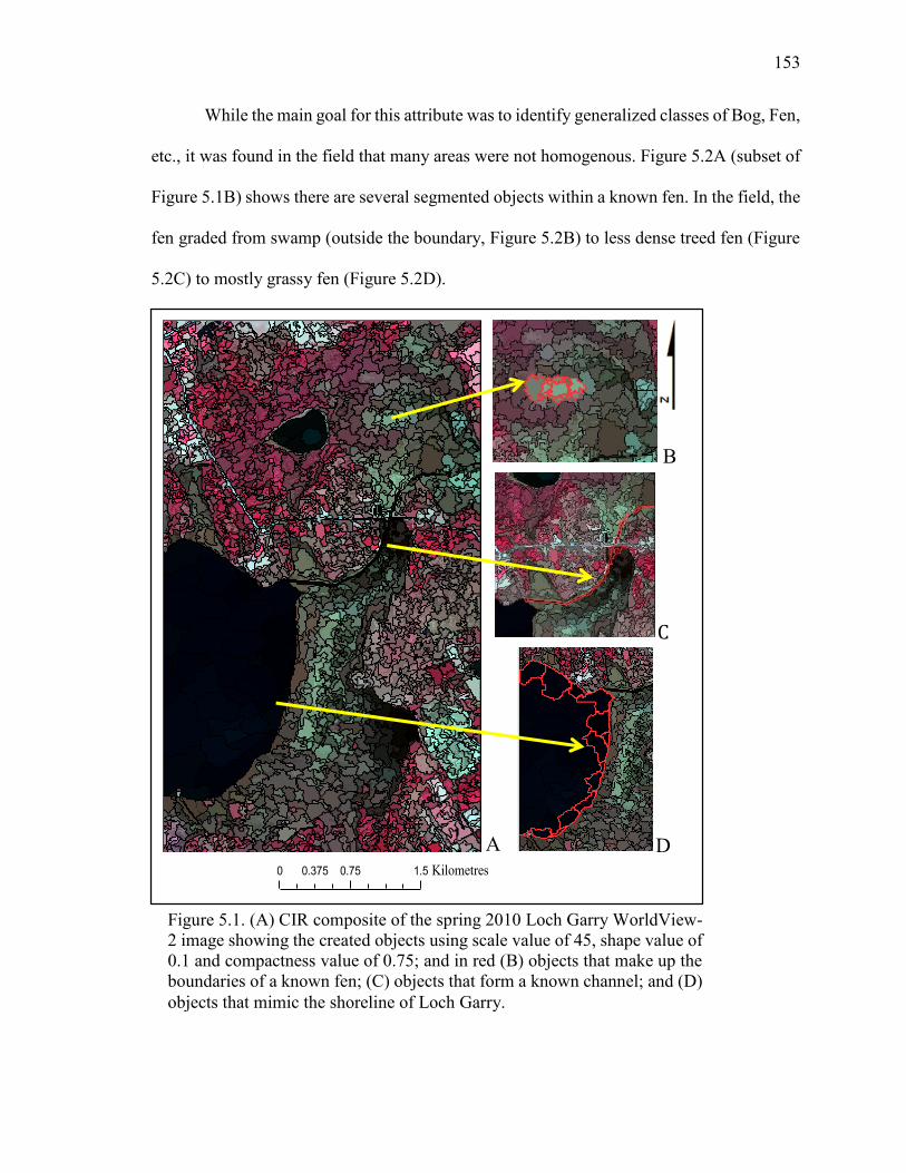
153
While the main goal for this attribute was to identify generalized classes of Bog, Fen,
etc., it was found in the field that many areas were not homogenous. Figure 5.2A (subset of
Figure 5.1B) shows there are several segmented objects within a known fen. In the field, the
fen graded from swamp (outside the boundary, Figure 5.2B) to less dense treed fen (Figure
5.2C) to mostly grassy fen (Figure 5.2D).
0 0.75 1.50.375 Kilometres
A
B
C
D
Figure 5.1. (A) CIR composite of the spring 2010 Loch Garry WorldView-2 image showing the created objects using scale value of 45, shape value of 0.1 and compactness value of 0.75; and in red (B) objects that make up the boundaries of a known fen; (C) objects that form a known channel; and (D) objects that mimic the shoreline of Loch Garry.
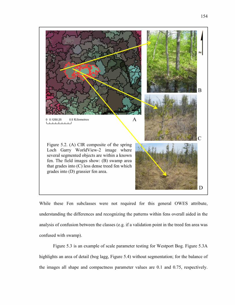
154
While these Fen subclasses were not required for this general OWES attribute,
understanding the differences and recognizing the patterns within fens overall aided in the
analysis of confusion between the classes (e.g. if a validation point in the treed fen area was
confused with swamp).
Figure 5.3 is an example of scale parameter testing for Westport Bog. Figure 5.3A
highlights an area of detail (bog lagg, Figure 5.4) without segmentation; for the balance of
the images all shape and compactness parameter values are 0.1 and 0.75, respectively.
0 0.25 0.50.125 Kilometres A
B
C
D
Figure 5.2. (A) CIR composite of the spring Loch Garry WorldView-2 image where several segmented objects are within a known fen. The field images show: (B) swamp area that grades into (C) less dense treed fen which grades into (D) grassier fen area.
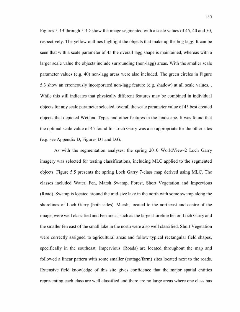
155
Figures 5.3B through 5.3D show the image segmented with a scale values of 45, 40 and 50,
respectively. The yellow outlines highlight the objects that make up the bog lagg. It can be
seen that with a scale parameter of 45 the overall lagg shape is maintained, whereas with a
larger scale value the objects include surrounding (non-lagg) areas. With the smaller scale
parameter values (e.g. 40) non-lagg areas were also included. The green circles in Figure
5.3 show an erroneously incorporated non-lagg feature (e.g. shadow) at all scale values. .
While this still indicates that physically different features may be combined in individual
objects for any scale parameter selected, overall the scale parameter value of 45 best created
objects that depicted Wetland Types and other features in the landscape. It was found that
the optimal scale value of 45 found for Loch Garry was also appropriate for the other sites
(e.g. see Appendix D, Figures D1 and D3).
As with the segmentation analyses, the spring 2010 WorldView-2 Loch Garry
imagery was selected for testing classifications, including MLC applied to the segmented
objects. Figure 5.5 presents the spring Loch Garry 7-class map derived using MLC. The
classes included Water, Fen, Marsh Swamp, Forest, Short Vegetation and Impervious
(Road). Swamp is located around the mid-size lake in the north with some swamp along the
shorelines of Loch Garry (both sides). Marsh, located to the northeast and centre of the
image, were well classified and Fen areas, such as the large shoreline fen on Loch Garry and
the smaller fen east of the small lake in the north were also well classified. Short Vegetation
were correctly assigned to agricultural areas and follow typical rectangular field shapes,
specifically in the southeast. Impervious (Roads) are located throughout the map and
followed a linear pattern with some smaller (cottage/farm) sites located next to the roads.
Extensive field knowledge of this site gives confidence that the major spatial entities
representing each class are well classified and there are no large areas where one class has
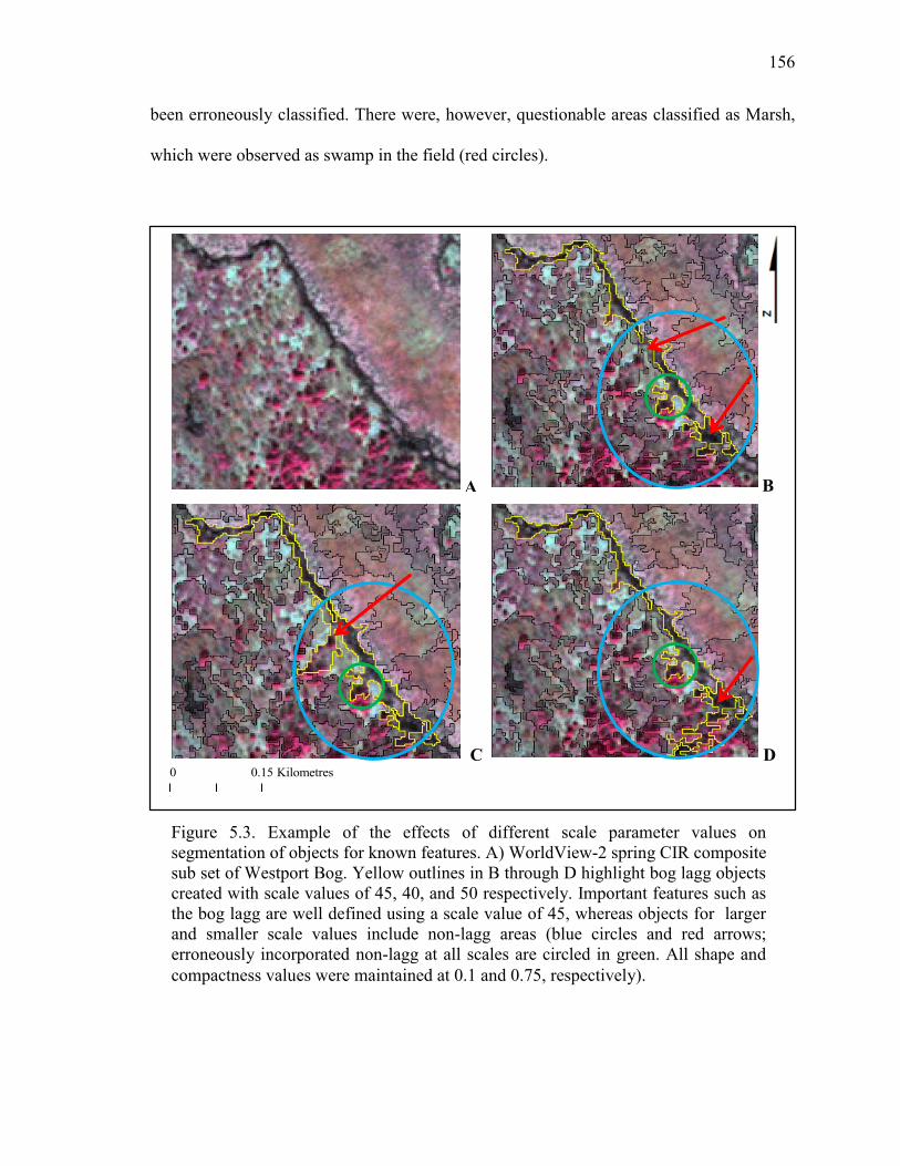
156
been erroneously classified. There were, however, questionable areas classified as Marsh,
which were observed as swamp in the field (red circles).
0 0.15 Kilometres
B
C D
Figure 5.3. Example of the effects of different scale parameter values on segmentation of objects for known features. A) WorldView-2 spring CIR composite sub set of Westport Bog. Yellow outlines in B through D highlight bog lagg objects created with scale values of 45, 40, and 50 respectively. Important features such as the bog lagg are well defined using a scale value of 45, whereas objects for larger and smaller scale values include non-lagg areas (blue circles and red arrows; erroneously incorporated non-lagg at all scales are circled in green. All shape and compactness values were maintained at 0.1 and 0.75, respectively).
A
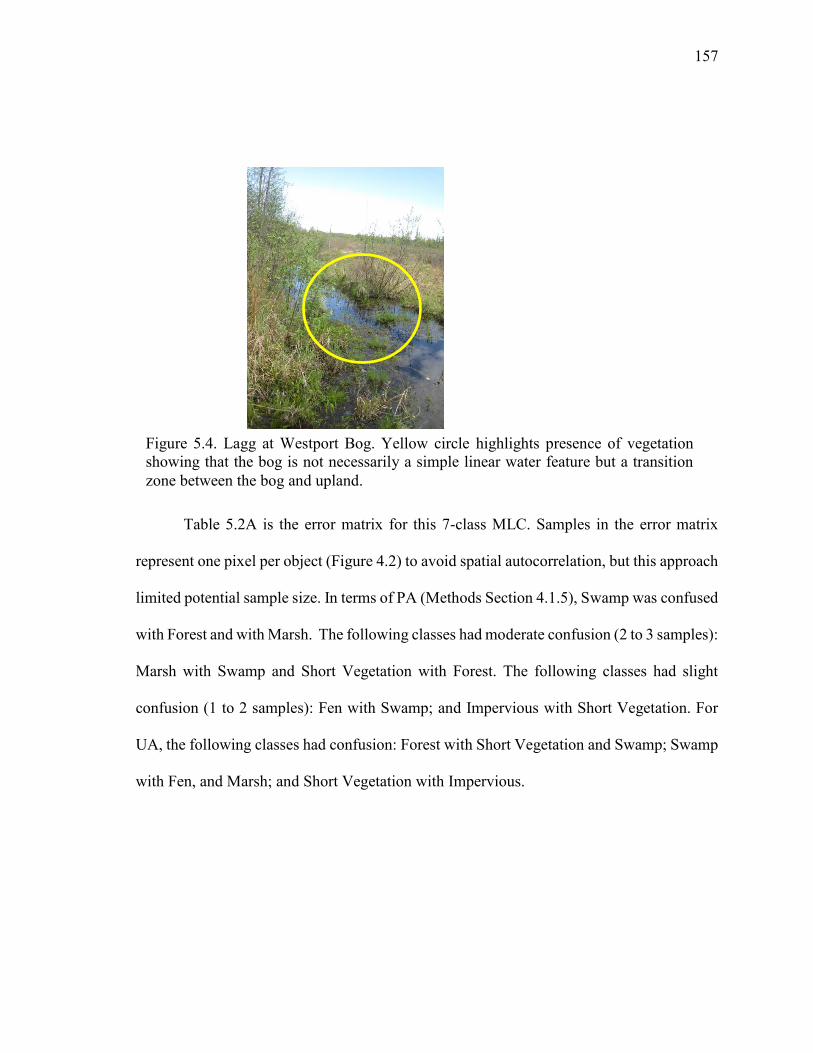
157
Table 5.2A is the error matrix for this 7-class MLC. Samples in the error matrix
represent one pixel per object (Figure 4.2) to avoid spatial autocorrelation, but this approach
limited potential sample size. In terms of PA (Methods Section 4.1.5), Swamp was confused
with Forest and with Marsh. The following classes had moderate confusion (2 to 3 samples):
Marsh with Swamp and Short Vegetation with Forest. The following classes had slight
confusion (1 to 2 samples): Fen with Swamp; and Impervious with Short Vegetation. For
UA, the following classes had confusion: Forest with Short Vegetation and Swamp; Swamp
with Fen, and Marsh; and Short Vegetation with Impervious.
Figure 5.4. Lagg at Westport Bog. Yellow circle highlights presence of vegetation showing that the bog is not necessarily a simple linear water feature but a transition zone between the bog and upland.
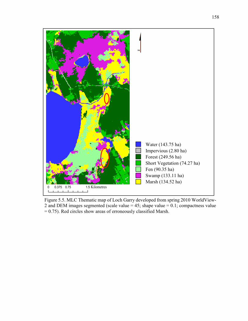
158
0 0.75 1.50.375 Kilometres
Figure 5.5. MLC Thematic map of Loch Garry developed from spring 2010 WorldView-2 and DEM images segmented (scale value = 45; shape value = 0.1; compactness value = 0.75). Red circles show areas of erroneously classified Marsh.
Water (143.75 ha) Impervious (2.80 ha) Forest (249.56 ha) Short Vegetation (74.27 ha) Fen (90.35 ha) Swamp (133.11 ha) Marsh (134.52 ha)
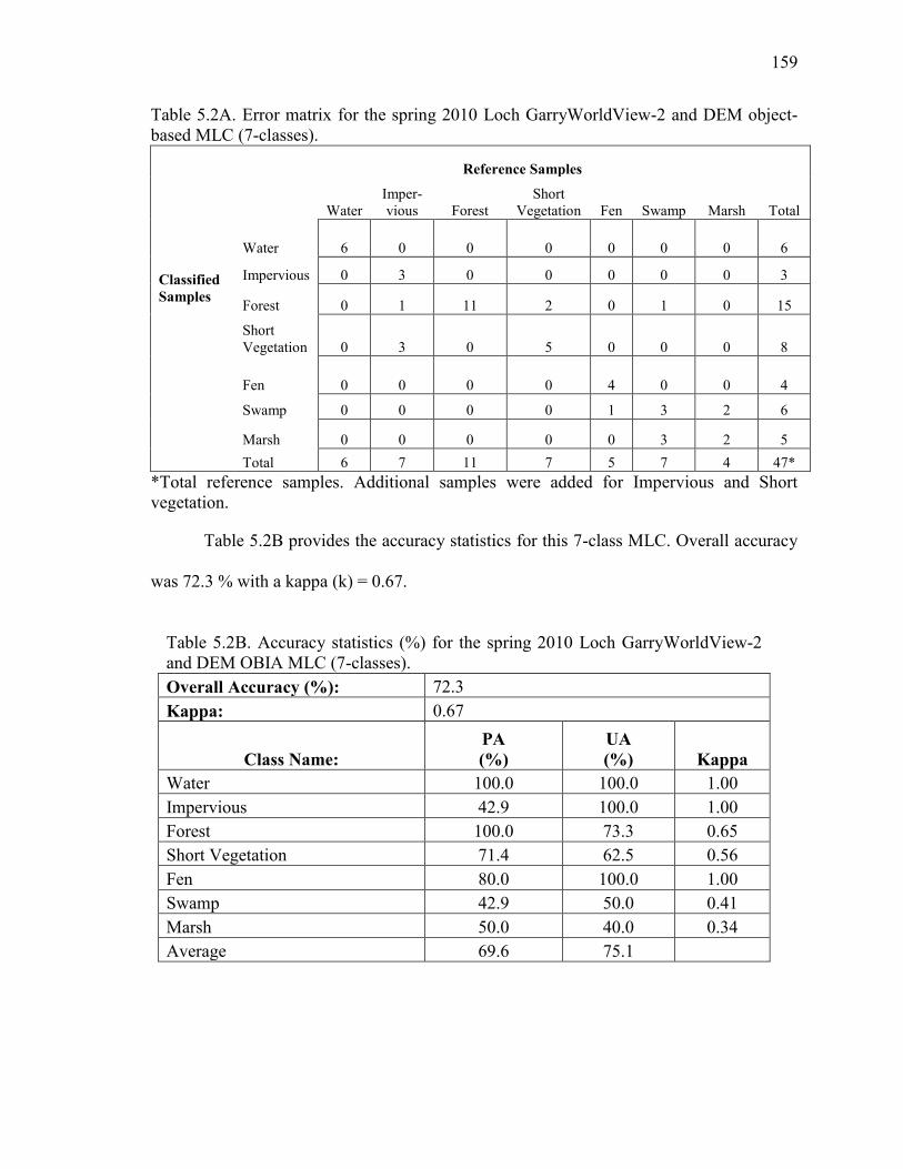
159
Table 5.2A. Error matrix for the spring 2010 Loch GarryWorldView-2 and DEM object-based MLC (7-classes).
Reference Samples
Water Imper-vious Forest
Short Vegetation Fen
Swamp
Marsh
Total
Classified Samples
Water 6 0 0 0 0 0 0 6
Impervious 0 3 0 0 0 0 0 3
Forest 0 1 11 2 0 1 0 15
Short Vegetation 0 3 0 5 0 0 0 8
Fen 0 0 0 0 4 0 0 4
Swamp 0 0 0 0 1 3 2 6
Marsh 0 0 0 0 0 3 2 5 Total 6 7 11 7 5 7 4 47*
*Total reference samples. Additional samples were added for Impervious and Short vegetation.
Table 5.2B provides the accuracy statistics for this 7-class MLC. Overall accuracy
was 72.3 % with a kappa (k) = 0.67.
Table 5.2B. Accuracy statistics (%) for the spring 2010 Loch GarryWorldView-2 and DEM OBIA MLC (7-classes). Overall Accuracy (%): 72.3
Kappa: 0.67
Class Name: PA (%)
UA (%) Kappa
Water 100.0 100.0 1.00 Impervious 42.9 100.0 1.00 Forest 100.0 73.3 0.65 Short Vegetation 71.4 62.5 0.56 Fen 80.0 100.0 1.00 Swamp 42.9 50.0 0.41 Marsh 50.0 40.0 0.34 Average 69.6 75.1
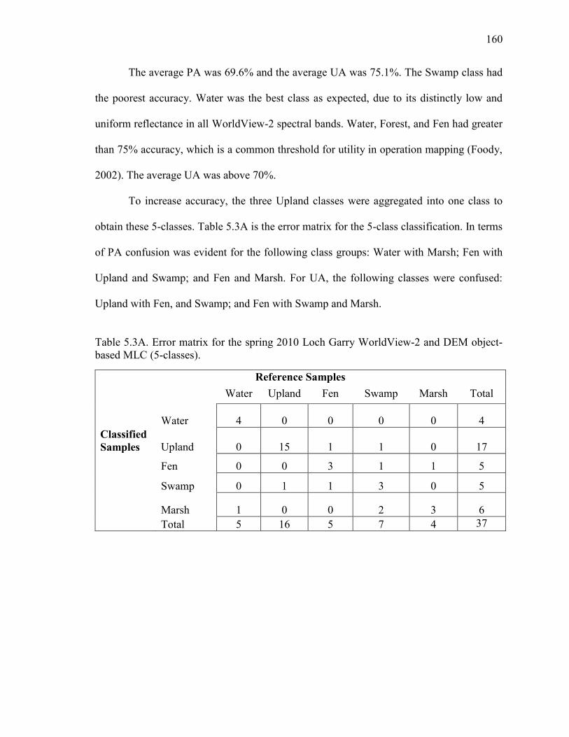
160
The average PA was 69.6% and the average UA was 75.1%. The Swamp class had
the poorest accuracy. Water was the best class as expected, due to its distinctly low and
uniform reflectance in all WorldView-2 spectral bands. Water, Forest, and Fen had greater
than 75% accuracy, which is a common threshold for utility in operation mapping (Foody,
2002). The average UA was above 70%.
To increase accuracy, the three Upland classes were aggregated into one class to
obtain these 5-classes. Table 5.3A is the error matrix for the 5-class classification. In terms
of PA confusion was evident for the following class groups: Water with Marsh; Fen with
Upland and Swamp; and Fen and Marsh. For UA, the following classes were confused:
Upland with Fen, and Swamp; and Fen with Swamp and Marsh.
Table 5.3A. Error matrix for the spring 2010 Loch Garry WorldView-2 and DEM object-based MLC (5-classes).
Reference Samples Water Upland Fen Swamp Marsh Total
Water 4 0 0 0 0 4 Classified Samples Upland 0 15 1 1 0 17 Fen 0 0 3 1 1 5 Swamp 0 1 1 3 0 5
Marsh 1 0 0 2 3 6 Total 5 16 5 7 4 37
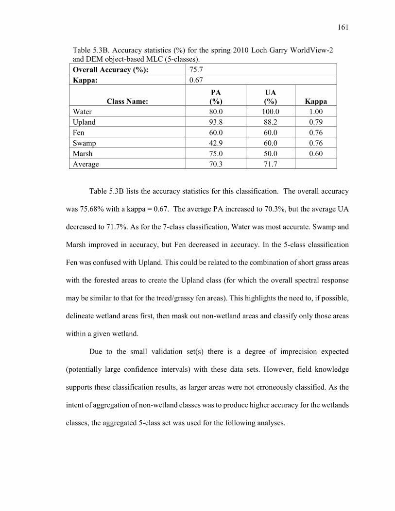
161
Table 5.3B. Accuracy statistics (%) for the spring 2010 Loch Garry WorldView-2 and DEM object-based MLC (5-classes). Overall Accuracy (%): 75.7
Kappa: 0.67
Class Name: PA (%)
UA (%) Kappa
Water 80.0 100.0 1.00 Upland 93.8 88.2 0.79 Fen 60.0 60.0 0.76 Swamp 42.9 60.0 0.76 Marsh 75.0 50.0 0.60 Average 70.3 71.7
Table 5.3B lists the accuracy statistics for this classification. The overall accuracy
was 75.68% with a kappa = 0.67. The average PA increased to 70.3%, but the average UA
decreased to 71.7%. As for the 7-class classification, Water was most accurate. Swamp and
Marsh improved in accuracy, but Fen decreased in accuracy. In the 5-class classification
Fen was confused with Upland. This could be related to the combination of short grass areas
with the forested areas to create the Upland class (for which the overall spectral response
may be similar to that for the treed/grassy fen areas). This highlights the need to, if possible,
delineate wetland areas first, then mask out non-wetland areas and classify only those areas
within a given wetland.
Due to the small validation set(s) there is a degree of imprecision expected
(potentially large confidence intervals) with these data sets. However, field knowledge
supports these classification results, as larger areas were not erroneously classified. As the
intent of aggregation of non-wetland classes was to produce higher accuracy for the wetlands
classes, the aggregated 5-class set was used for the following analyses.
162
Table 5.4 provides the CTA classification accuracies for the spring 2010
WorldView-2 imagery plus DEM using the GINI algorithm. The site with the highest
accuracy was Loch Garry (86.5%), which was markedly higher than the MLC overall
accuracy for the same wetland. Figure 5.6A presents the Loch Garry 5-class CTA
classification next to the 5-class MLC map (Figure 5.6B). The site with the lowest overall
accuracy was Marlborough Forest (70.0%). For wetland types, Fen had the highest average
PA and UA (PA = 90.0%; UA = 75.0%) while Bog had the lowest average PA (65.93%)
and UA (50.3%). Results for other CTA tests using the entropy and gain ratio tree-creation
algorithms were poorer and can be found in Appendix E, Figure E1. In relation to the overall
literature for Wetland Type classification, these results were comparable, as they fell with
the typical overall accuracies of 71% to 92%.
For both techniques, areas that were well classified included the water channel in the
centre, the small lake to the northwest, and the shoreline of Loch Garry, etc. CTA appears
to have performed better for the swamp areas around the lake in the north of the map and
particularly the areas at the edge of the upland in the southeast (red circles) which were
observed in the field. Similarly, the representation of Fen along the small lake shoreline in
the CTA map is believed to be more accurate than the Upland and Marsh classes in the MLC
map. Access to those areas was limited, however the vegetation was similar to what was
observed beside a man-made boardwalk, and observed while canoeing (black dashed lines).
In terms of total area per Wetland Type, the CTA map had more classified Swamp and Fen
and less Marsh and Upland. In relation to the percent cover that was measured during the
field-based OWES evaluation, the CTA method came closer to approximating the values of
the subset area on the whole, with Fen cover representing 12% (CTA), 10% (MLC), and
14% (field), respectively. Swamp cover was 32% (CTA), 17% (MLC) and 40% (field),
163
respectively. Marsh was under estimated by both methods, being 8% (CTA), 11% (MLC),
and 46% (field), respectively.
Figure 5.7A is the classification tree created using the 5-class training sites and the
GINI algorithm. The first major split (Band 4 (NIR) < 8 DN) accounted for 97.18% of Class
1 (Water) and is represented in Figure 5.8B. The next branch is a decision where DEM >
71.5 m ASL and accounts for 93.25% of the Upland class (Figure 5.7E). Both of these are
logical and expected as water has very low NIR reflectance compared to other land cover
types and upland is usually at higher elevation than wetland. Literature using these
techniques for wetlands is lacking, thus these results are relatively new and direct
comparisons to previous studies not possible. As an example of a broader land cover
classification, Baker et al. (2006) showed similar initial splits with elevation and NIR in
classifying Agriculture, Wetland, Riparian, Forest and Rangeland using Landsat ETM+
imagery, however, the first major split was not NIR as found in this research, but elevation
due to the wider elevation range of that study. Also included in their CTA were the Tasselled
Cap variables of Brightness, Wetness, Greenness and % hydric soils, so a direct comparison
with this research is difficult. Also not given was the amount of pixels contributing to the
class. Much of the other literature using CTA for broader land cover classification does not
provide the actual decision trees for analysis or comparison.
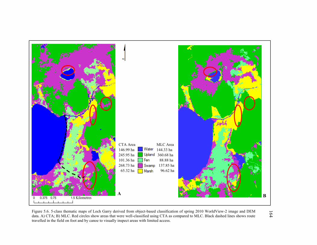
164
CTA Area MLC Area 146.99 ha 144.33 ha 245.95 ha 360.68 ha 101.36 ha 88.88 ha 268.73 ha 137.85 ha 65.32 ha 96.62 ha
Figure 5.6. 5-class thematic maps of Loch Garry derived from object-based classification of spring 2010 WorldView-2 image and DEM data. A) CTA; B) MLC. Red circles show areas that were well-classified using CTA as compared to MLC. Black dashed lines shows route travelled in the field on foot and by canoe to visually inspect areas with limited access.
B 0 0.75 1.50.375 KilometresA
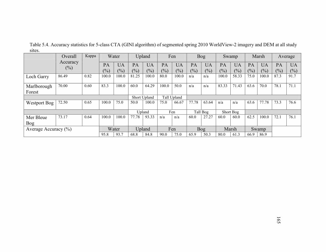
165
Table 5.4. Accuracy statistics for 5-class CTA (GINI algorithm) of segmented spring 2010 WorldView-2 imagery and DEM at all study sites.
Overall Accuracy
(%)
Kappa Water Upland Fen Bog Swamp Marsh Average
PA (%)
UA (%)
PA (%)
UA (%)
PA (%)
UA (%)
PA (%)
UA (%)
PA (%)
UA (%)
PA (%)
UA (%)
PA (%)
UA (%)
Loch Garry 86.49 0.82 100.0 100.0 81.25 100.0 80.0 100.0 n/a n/a 100.0 58.33 75.0
100.0 87.3 91.7
Marlborough Forest
70.00 0.60 83.3 100.0 60.0 64.29 100.0 50.0 n/a n/a 83.33 71.43 63.6 70.0 78.1 71.1
Short Upland Tall Upland Westport Bog 72.50 0.65 100.0 75.0 50.0 100.0 75.0 66.67 77.78 63.64 n/a n/a 63.6
77.78 73.3 76.6
Upland Fen Tall Bog Short Bog Mer Bleue Bog
73.17 0.64 100.0 100.0 77.78 93.33 n/a n/a 60.0 27.27 60.0 60.0 62.5 100.0 72.1 76.1
Average Accuracy (%) Water Upland Fen Bog Marsh Swamp 95.8 93.7 68.8 84.8 90.0 75.0 65.9 50.3 80.0 61.3 66.9 86.9
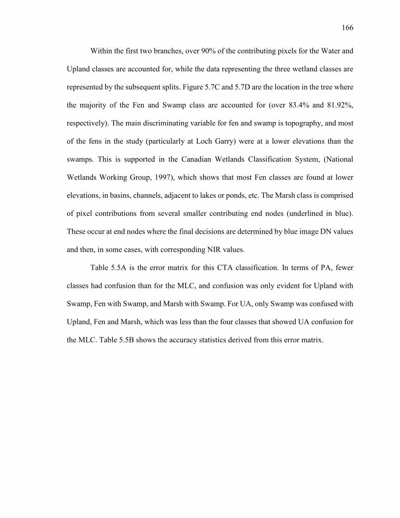
166
Within the first two branches, over 90% of the contributing pixels for the Water and
Upland classes are accounted for, while the data representing the three wetland classes are
represented by the subsequent splits. Figure 5.7C and 5.7D are the location in the tree where
the majority of the Fen and Swamp class are accounted for (over 83.4% and 81.92%,
respectively). The main discriminating variable for fen and swamp is topography, and most
of the fens in the study (particularly at Loch Garry) were at a lower elevations than the
swamps. This is supported in the Canadian Wetlands Classification System, (National
Wetlands Working Group, 1997), which shows that most Fen classes are found at lower
elevations, in basins, channels, adjacent to lakes or ponds, etc. The Marsh class is comprised
of pixel contributions from several smaller contributing end nodes (underlined in blue).
These occur at end nodes where the final decisions are determined by blue image DN values
and then, in some cases, with corresponding NIR values.
Table 5.5A is the error matrix for this CTA classification. In terms of PA, fewer
classes had confusion than for the MLC, and confusion was only evident for Upland with
Swamp, Fen with Swamp, and Marsh with Swamp. For UA, only Swamp was confused with
Upland, Fen and Marsh, which was less than the four classes that showed UA confusion for
the MLC. Table 5.5B shows the accuracy statistics derived from this error matrix.
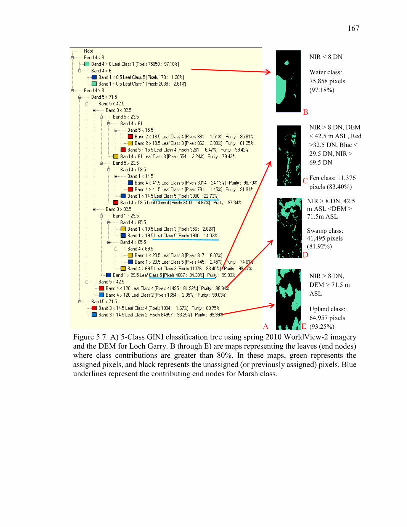
167
B
NIR < 8 DN
Water class: 75,858 pixels (97.18%)
NIR > 8 DN, 42.5 m ASL <DEM > 71.5m ASL
Swamp class: 41,495 pixels (81.92%)
NIR > 8 DN, DEM > 71.5 m ASL
Upland class: 64,957 pixels (93.25%)
NIR > 8 DN, DEM < 42.5 m ASL, Red >32.5 DN, Blue < 29.5 DN, NIR > 69.5 DN
Fen class: 11,376 pixels (83.40%)
C
D
E A Figure 5.7. A) 5-Class GINI classification tree using spring 2010 WorldView-2 imagery and the DEM for Loch Garry. B through E) are maps representing the leaves (end nodes) where class contributions are greater than 80%. In these maps, green represents the assigned pixels, and black represents the unassigned (or previously assigned) pixels. Blue underlines represent the contributing end nodes for Marsh class.
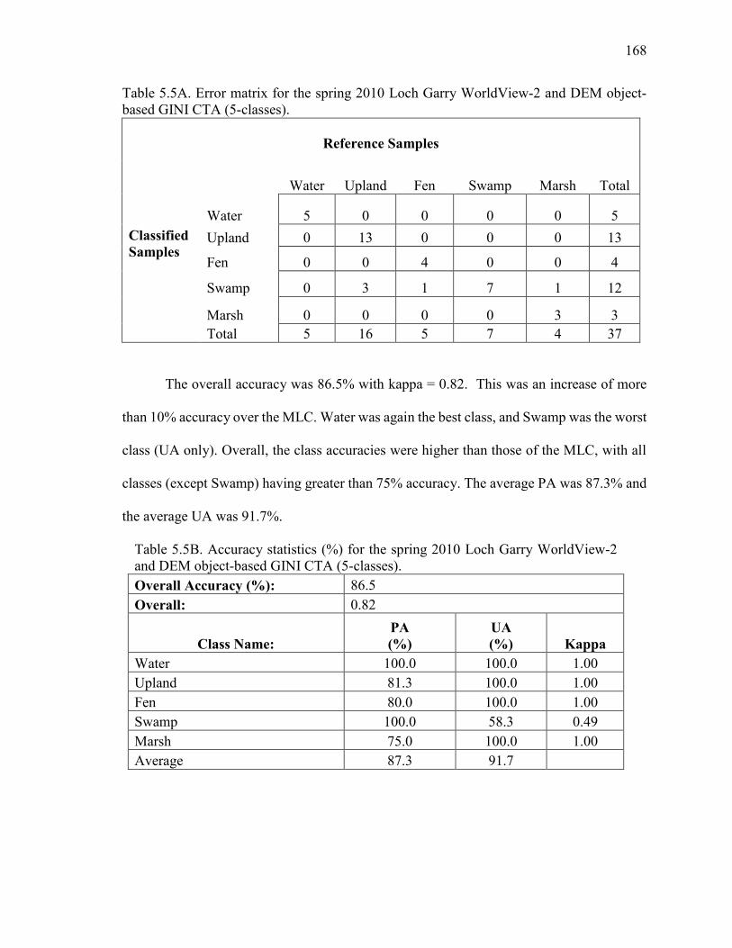
168
Table 5.5A. Error matrix for the spring 2010 Loch Garry WorldView-2 and DEM object-based GINI CTA (5-classes).
Reference Samples
Classified Samples
Water Upland Fen Swamp Marsh
Total
Water 5 0 0 0 0 5 Upland 0 13 0 0 0 13
Fen 0 0 4 0 0 4
Swamp 0 3 1 7 1 12
Marsh 0 0 0 0 3 3 Total 5 16 5 7 4 37
The overall accuracy was 86.5% with kappa = 0.82. This was an increase of more
than 10% accuracy over the MLC. Water was again the best class, and Swamp was the worst
class (UA only). Overall, the class accuracies were higher than those of the MLC, with all
classes (except Swamp) having greater than 75% accuracy. The average PA was 87.3% and
the average UA was 91.7%.
Table 5.5B. Accuracy statistics (%) for the spring 2010 Loch Garry WorldView-2 and DEM object-based GINI CTA (5-classes). Overall Accuracy (%): 86.5
Overall: 0.82
Class Name: PA (%)
UA (%) Kappa
Water 100.0 100.0 1.00 Upland 81.3 100.0 1.00 Fen 80.0 100.0 1.00 Swamp 100.0 58.3 0.49 Marsh 75.0 100.0 1.00 Average 87.3 91.7
169
Similar results for the CTA GINI classification of the other three study sites can be
found in Appendix F, Figures F1 to F6 and Tables F1A & B to F3A & B.
5.1.2 Results from OBIA using spring 2010 Landsat 5 TM imagery for Wetland Type
Segmentation was evaluated for the Loch Garry site using the Landsat TM imagery
and the DEM with a scale value of 10, a shape value of 0.1 and compactness value of 0.5.
As expected, segmented objects aligned with the shoreline of Loch Garry, and the outlines
of farms fields, and some wetland areas. Objects were not created for the water channel, but
that channel was incorporated into objects of the surrounding land cover. Such detail was
lost due to the coarser nature of the original imagery. See Appendix G, Figures G1A - D for
examples of this segmentation.
All details regarding LSU and the development of the fraction maps are found in
Appendix G. Two sets of fraction maps were created: 1) 3 manually selected EMs
(vegetation, moisture, bare); and 2) 5 automatically generated EMs (three bare, vegetation
and moisture). Analyses of the residual maps showed that values were closer to zero for the
five EM fraction maps, indicating higher unmixing precision. Therefore, they were
subsequently used in segmentation and classification.
Segmented objects created using a scale value of 10, shape value of 0.1 and
compactness value of 0.5 were mostly meaningless as many crossed Wetland Type
boundaries or were not representative of known shapes (e.g. farm fields, see Appendix D
for examples). Consequently, smaller scale and compactness values were tested. Figure 5.8A
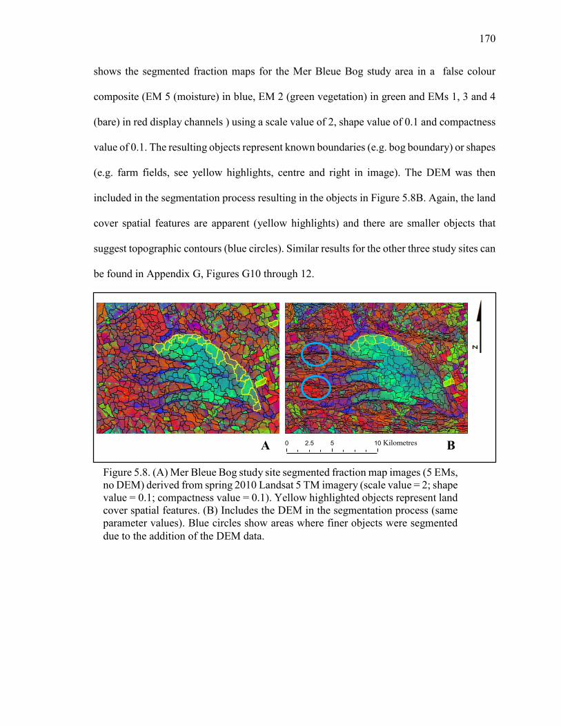
170
shows the segmented fraction maps for the Mer Bleue Bog study area in a false colour
composite (EM 5 (moisture) in blue, EM 2 (green vegetation) in green and EMs 1, 3 and 4
(bare) in red display channels ) using a scale value of 2, shape value of 0.1 and compactness
value of 0.1. The resulting objects represent known boundaries (e.g. bog boundary) or shapes
(e.g. farm fields, see yellow highlights, centre and right in image). The DEM was then
included in the segmentation process resulting in the objects in Figure 5.8B. Again, the land
cover spatial features are apparent (yellow highlights) and there are smaller objects that
suggest topographic contours (blue circles). Similar results for the other three study sites can
be found in Appendix G, Figures G10 through 12.
A B
Figure 5.8. (A) Mer Bleue Bog study site segmented fraction map images (5 EMs, no DEM) derived from spring 2010 Landsat 5 TM imagery (scale value = 2; shape value = 0.1; compactness value = 0.1). Yellow highlighted objects represent land cover spatial features. (B) Includes the DEM in the segmentation process (same parameter values). Blue circles show areas where finer objects were segmented due to the addition of the DEM data.
0 5 102.5 Kilometres
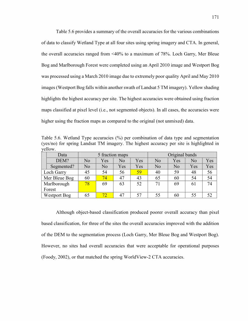
171
Table 5.6 provides a summary of the overall accuracies for the various combinations
of data to classify Wetland Type at all four sites using spring imagery and CTA. In general,
the overall accuracies ranged from <40% to a maximum of 78%. Loch Garry, Mer Bleue
Bog and Marlborough Forest were completed using an April 2010 image and Westport Bog
was processed using a March 2010 image due to extremely poor quality April and May 2010
images (Westport Bog falls within another swath of Landsat 5 TM imagery). Yellow shading
highlights the highest accuracy per site. The highest accuracies were obtained using fraction
maps classified at pixel level (i.e., not segmented objects). In all cases, the accuracies were
higher using the fraction maps as compared to the original (not unmixed) data.
Table 5.6. Wetland Type accuracies (%) per combination of data type and segmentation (yes/no) for spring Landsat TM imagery. The highest accuracy per site is highlighted in yellow. Data 5 fraction maps Original bands
DEM? No Yes No Yes No Yes No Yes Segmented? No No Yes Yes No No Yes Yes
Loch Garry 45 54 56 59 40 59 48 56 Mer Bleue Bog 60 74 47 43 65 60 54 54 Marlborough Forest
78 69 63 52 71 69 61 74
Westport Bog 65 72 47 57 55 60 55 52
Although object-based classification produced poorer overall accuracy than pixel
based classification, for three of the sites the overall accuracies improved with the addition
of the DEM to the segmentation process (Loch Garry, Mer Bleue Bog and Westport Bog).
However, no sites had overall accuracies that were acceptable for operational purposes
(Foody, 2002), or that matched the spring WorldView-2 CTA accuracies.
172
Table 5.7 is an example of detailed class-level accuracies for the eight tests of data
type at Marlborough Forest. They can be compared to the results for the original Landsat
TM data. Overall, the highest accuracies were obtained using 5 EMs without segmentation
and without the DEM (overall accuracy = 78.3%; kappa = 0.72). The addition of the DEM
did not improve overall accuracy except for the segmented original band data. Segmenting
the fraction map images and subsequently classifying them with the GINI CTA (with or
without the DEM) did not improve the overall classification accuracy results, and produced
poor results across all classes. Thus, pixel-based classification of unmixed fraction maps for
Wetland Type was found to be the best approach for spring Landsat TM imagery.
Marsh had the lowest accuracy across all data types (average PA = 37.5%; average
UA= 28.1%). It was the only class that benefitted from segmentation of the fraction maps
(Table 5.7, test 5 where Marsh values are highlighted in teal) and segmentation of the
original band data (Table 5.7, test 4 highlighted in green). The poor overall results are related
to the small spatial extent of marsh occurrences in relation to the pixel size of the Landsat
imagery. Additionally, this imagery was acquired in April when marsh vegetation (reeds,
grasses, etc.) is mostly senescent and yellow and water is dominant. The error matrices show
that Marsh was sometimes confused (1 to 3 samples) with Water and confused with the other
classes in the other tests (1 to 2 samples) (see Appendix G, Tables G5 to G12 for error
matrices).
Fen was well classified using all data configurations, as were Water and Upland.
However, test 4 also shows that Fen UA was improved for Fen class using the segmented
173
data (highlighted in teal). Swamp was generally most accurate with pixel-based
classification and without the DEM (highlighted in pink). However, in two cases, the Swamp
class improved with the addition of the DEM to the original band data (tests 2 and 4
highlighted in yellow).
Figure 5.9 shows the Marlborough Forest 5-class GINI CTA map derived using the
test 5 configuration. It can be seen that the known water areas are well defined, particularly
Roger Steven’s pond and the channel (Steven`s Creek) to the east of it (red circles). Fen
areas correspond to the known fen at the centre of the image (black circle). Swamp areas are
seen throughout the image with Marsh classified areas corresponding to smaller marsh
patches located to the southeast, through the centre of the image and surrounding the water
bodies. Table 5.8 is the error matrix for this classification.
For PA confusion was evident for: Upland with Marsh and Fen; and Swamp with
Marsh and with Fen. For UA, Water was confused with Marsh; Upland with Fen and Marsh;
and Swamp with Marsh and Fen. Similar classifications’ thematic maps for the other three
sites can be found in Appendix G (Figure G11 to G13).
Figure 5.10 provides a comparison between the best and the worst overall
classifications (tests 5 and 8, respectively) with the original spring 2010 Landsat 5 TM CIR
image given for reference. It can be seen that the test 8 map does not have the detail found
in the test 5 map (black arrows). In the field, this area was not a homogenous area of Upland,
but Upland interspersed with wet patches.
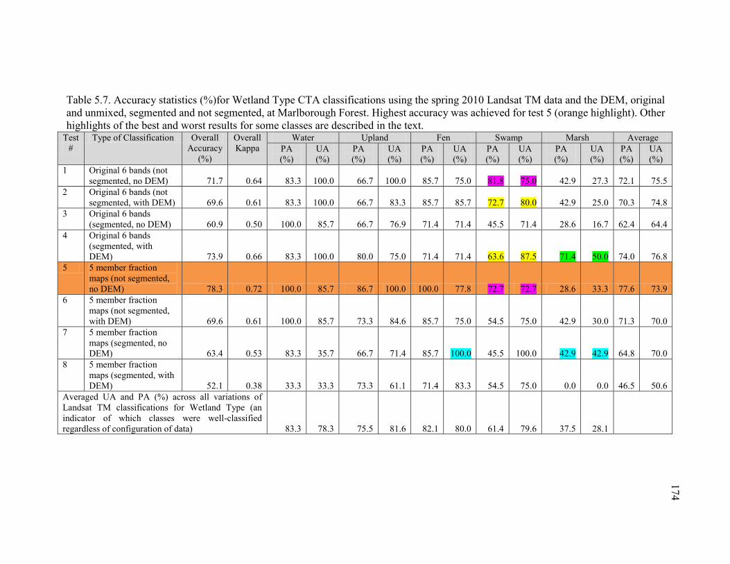
174
Table 5.7. Accuracy statistics (%)for Wetland Type CTA classifications using the spring 2010 Landsat TM data and the DEM, original and unmixed, segmented and not segmented, at Marlborough Forest. Highest accuracy was achieved for test 5 (orange highlight). Other highlights of the best and worst results for some classes are described in the text.
Test #
Type of Classification Overall Accuracy
(%)
Overall Kappa
Water Upland Fen Swamp Marsh Average PA (%)
UA (%)
PA (%)
UA (%)
PA (%)
UA (%)
PA (%)
UA (%)
PA (%)
UA (%)
PA (%)
UA (%)
1 Original 6 bands (not segmented, no DEM) 71.7 0.64 83.3 100.0 66.7 100.0 85.7 75.0 81.8 75.0 42.9 27.3 72.1 75.5
2 Original 6 bands (not segmented, with DEM) 69.6 0.61 83.3 100.0 66.7 83.3 85.7 85.7 72.7 80.0 42.9 25.0 70.3 74.8
3 Original 6 bands (segmented, no DEM) 60.9 0.50 100.0 85.7 66.7 76.9 71.4 71.4 45.5 71.4 28.6 16.7 62.4 64.4
4 Original 6 bands (segmented, with DEM) 73.9 0.66 83.3 100.0 80.0 75.0 71.4 71.4 63.6 87.5 71.4 50.0 74.0 76.8
5 5 member fraction maps (not segmented, no DEM) 78.3 0.72 100.0 85.7 86.7 100.0 100.0 77.8 72.7 72.7 28.6 33.3 77.6 73.9
6 5 member fraction maps (not segmented, with DEM) 69.6 0.61 100.0 85.7 73.3 84.6 85.7 75.0 54.5 75.0 42.9 30.0 71.3 70.0
7 5 member fraction maps (segmented, no DEM) 63.4 0.53 83.3 35.7 66.7 71.4 85.7 100.0 45.5 100.0 42.9 42.9 64.8 70.0
8 5 member fraction maps (segmented, with DEM) 52.1 0.38 33.3 33.3 73.3 61.1 71.4 83.3 54.5 75.0 0.0 0.0 46.5 50.6
Averaged UA and PA (%) across all variations of Landsat TM classifications for Wetland Type (an indicator of which classes were well-classified regardless of configuration of data) 83.3 78.3 75.5 81.6 82.1 80.0 61.4 79.6 37.5 28.1
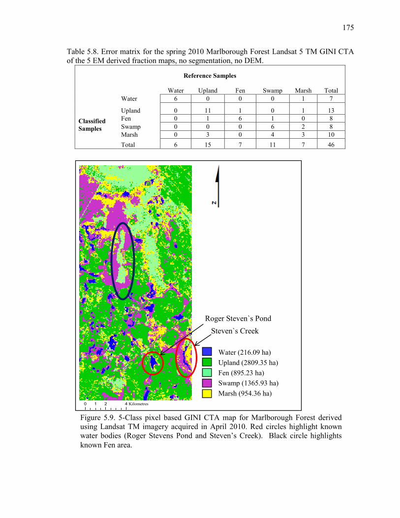
175
Table 5.8. Error matrix for the spring 2010 Marlborough Forest Landsat 5 TM GINI CTA of the 5 EM derived fraction maps, no segmentation, no DEM.
Reference Samples
Water Upland Fen Swamp Marsh
Total Classified Samples
Water 6 0 0 0 1 7
Upland 0 11 1 0 1 13 Fen 0 1 6 1 0 8 Swamp 0 0 0 6 2 8 Marsh 0 3 0 4 3 10 Total 6 15 7 11 7 46
Figure 5.9. 5-Class pixel based GINI CTA map for Marlborough Forest derived using Landsat TM imagery acquired in April 2010. Red circles highlight known water bodies (Roger Stevens Pond and Steven’s Creek). Black circle highlights known Fen area.
Water (216.09 ha) Upland (2809.35 ha) Fen (895.23 ha) Swamp (1365.93 ha) Marsh (954.36 ha)
0 2 41 Kilometres
Steven`s Creek Roger Steven`s Pond
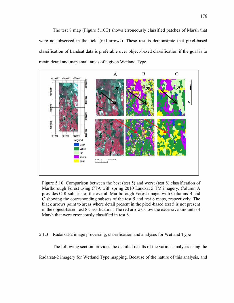
176
The test 8 map (Figure 5.10C) shows erroneously classified patches of Marsh that
were not observed in the field (red arrows). These results demonstrate that pixel-based
classification of Landsat data is preferable over object-based classification if the goal is to
retain detail and map small areas of a given Wetland Type.
5.1.3 Radarsat-2 image processing, classification and analyses for Wetland Type
The following section provides the detailed results of the various analyses using the
Radarsat-2 imagery for Wetland Type mapping. Because of the nature of this analysis, and
Figure 5.10. Comparison between the best (test 5) and worst (test 8) classification of Marlborough Forest using CTA with spring 2010 Landsat 5 TM imagery. Column A provides CIR sub sets of the overall Marlborough Forest image, with Columns B and C showing the corresponding subsets of the test 5 and test 8 maps, respectively. The black arrows point to areas where detail present in the pixel-based test 5 is not present in the object-based test 8 classification. The red arrows show the excessive amounts of Marsh that were erroneously classified in test 8.
A B C
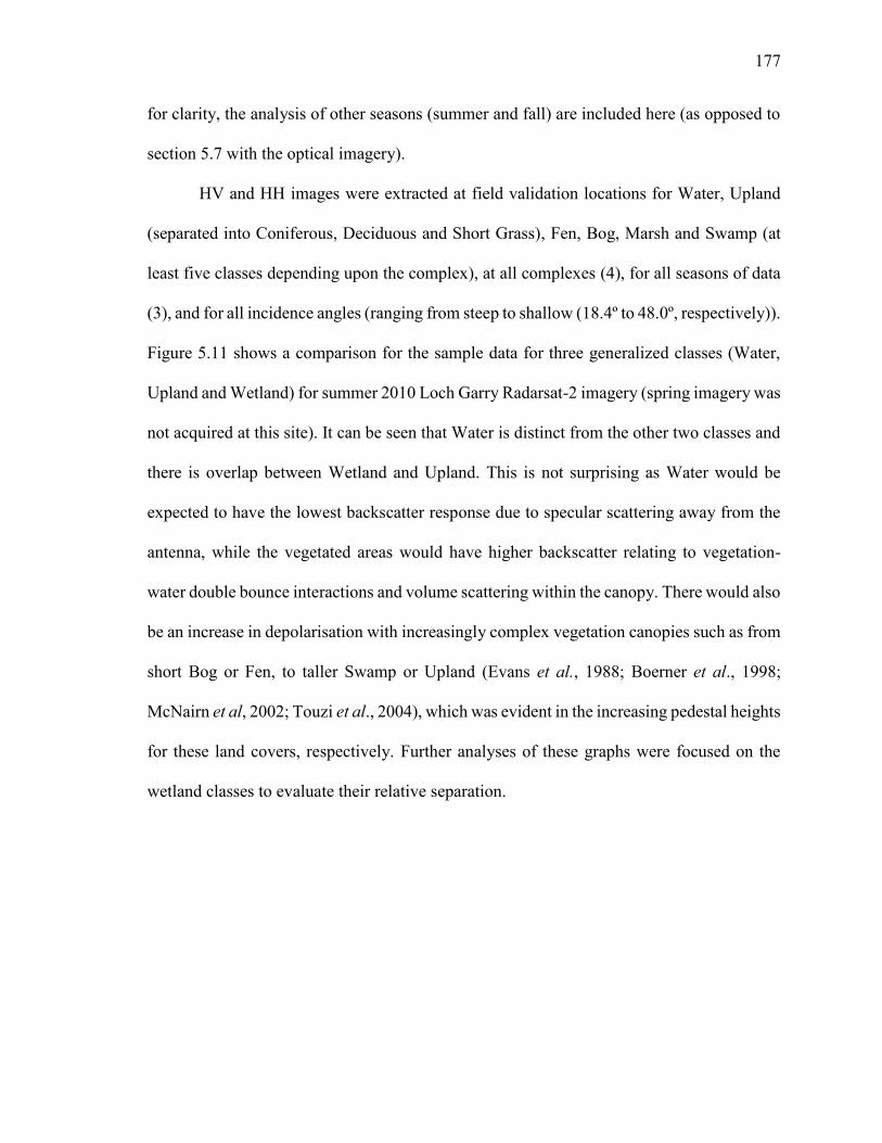
177
for clarity, the analysis of other seasons (summer and fall) are included here (as opposed to
section 5.7 with the optical imagery).
HV and HH images were extracted at field validation locations for Water, Upland
(separated into Coniferous, Deciduous and Short Grass), Fen, Bog, Marsh and Swamp (at
least five classes depending upon the complex), at all complexes (4), for all seasons of data
(3), and for all incidence angles (ranging from steep to shallow (18.4º to 48.0º, respectively)).
Figure 5.11 shows a comparison for the sample data for three generalized classes (Water,
Upland and Wetland) for summer 2010 Loch Garry Radarsat-2 imagery (spring imagery was
not acquired at this site). It can be seen that Water is distinct from the other two classes and
there is overlap between Wetland and Upland. This is not surprising as Water would be
expected to have the lowest backscatter response due to specular scattering away from the
antenna, while the vegetated areas would have higher backscatter relating to vegetation-
water double bounce interactions and volume scattering within the canopy. There would also
be an increase in depolarisation with increasingly complex vegetation canopies such as from
short Bog or Fen, to taller Swamp or Upland (Evans et al., 1988; Boerner et al., 1998;
McNairn et al, 2002; Touzi et al., 2004), which was evident in the increasing pedestal heights
for these land covers, respectively. Further analyses of these graphs were focused on the
wetland classes to evaluate their relative separation.
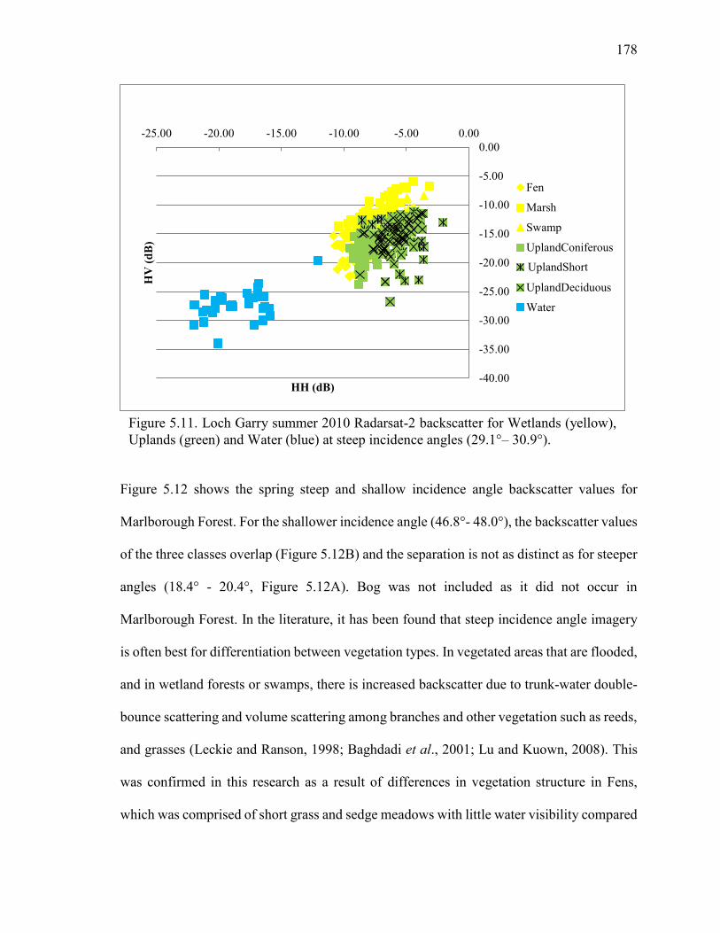
178
Figure 5.12 shows the spring steep and shallow incidence angle backscatter values for
Marlborough Forest. For the shallower incidence angle (46.8°- 48.0°), the backscatter values
of the three classes overlap (Figure 5.12B) and the separation is not as distinct as for steeper
angles (18.4° - 20.4°, Figure 5.12A). Bog was not included as it did not occur in
Marlborough Forest. In the literature, it has been found that steep incidence angle imagery
is often best for differentiation between vegetation types. In vegetated areas that are flooded,
and in wetland forests or swamps, there is increased backscatter due to trunk-water double-
bounce scattering and volume scattering among branches and other vegetation such as reeds,
and grasses (Leckie and Ranson, 1998; Baghdadi et al., 2001; Lu and Kuown, 2008). This
was confirmed in this research as a result of differences in vegetation structure in Fens,
which was comprised of short grass and sedge meadows with little water visibility compared
-40.00
-35.00
-30.00
-25.00
-20.00
-15.00
-10.00
-5.00
0.00-25.00 -20.00 -15.00 -10.00 -5.00 0.00
HV
(dB
)
HH (dB)
Fen
Marsh
Swamp
UplandConiferous
UplandFarm
UplandDeciduous
Water
Figure 5.11. Loch Garry summer 2010 Radarsat-2 backscatter for Wetlands (yellow), Uplands (green) and Water (blue) at steep incidence angles (29.1°– 30.9°).
UplandShort Grass
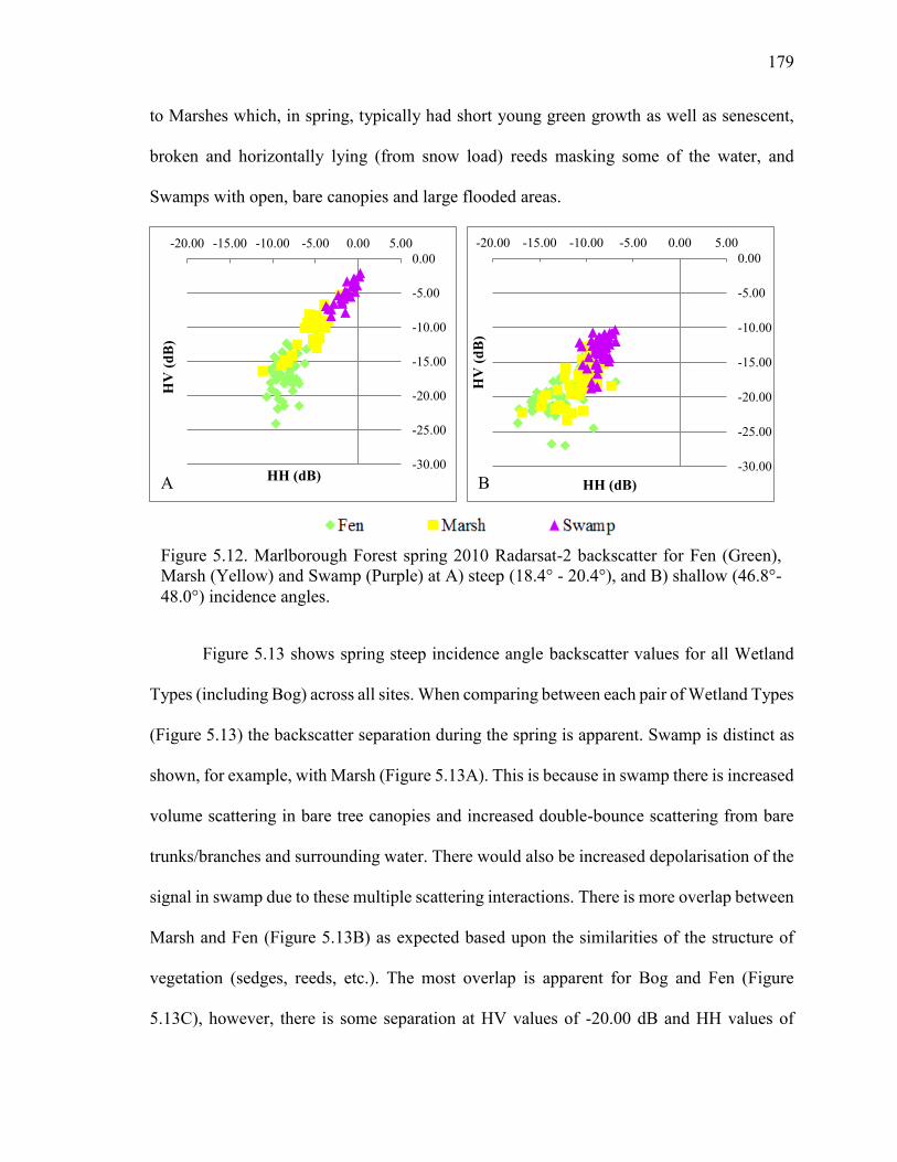
179
to Marshes which, in spring, typically had short young green growth as well as senescent,
broken and horizontally lying (from snow load) reeds masking some of the water, and
Swamps with open, bare canopies and large flooded areas.
Figure 5.13 shows spring steep incidence angle backscatter values for all Wetland
Types (including Bog) across all sites. When comparing between each pair of Wetland Types
(Figure 5.13) the backscatter separation during the spring is apparent. Swamp is distinct as
shown, for example, with Marsh (Figure 5.13A). This is because in swamp there is increased
volume scattering in bare tree canopies and increased double-bounce scattering from bare
trunks/branches and surrounding water. There would also be increased depolarisation of the
signal in swamp due to these multiple scattering interactions. There is more overlap between
Marsh and Fen (Figure 5.13B) as expected based upon the similarities of the structure of
vegetation (sedges, reeds, etc.). The most overlap is apparent for Bog and Fen (Figure
5.13C), however, there is some separation at HV values of -20.00 dB and HH values of
-30.00
-25.00
-20.00
-15.00
-10.00
-5.00
0.00-20.00 -15.00 -10.00 -5.00 0.00 5.00
HV
(dB
)
HH (dB)
Figure 5.12. Marlborough Forest spring 2010 Radarsat-2 backscatter for Fen (Green), Marsh (Yellow) and Swamp (Purple) at A) steep (18.4° - 20.4°), and B) shallow (46.8°- 48.0°) incidence angles.
-30.00
-25.00
-20.00
-15.00
-10.00
-5.00
0.00-20.00 -15.00 -10.00 -5.00 0.00 5.00
HV
(dB
)HH (dB)A B
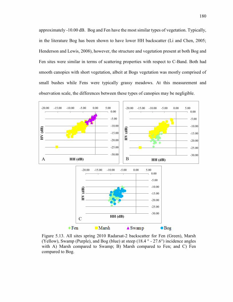
180
approximately -10.00 dB. Bog and Fen have the most similar types of vegetation. Typically,
in the literature Bog has been shown to have lower HH backscatter (Li and Chen, 2005;
Henderson and Lewis, 2008), however, the structure and vegetation present at both Bog and
Fen sites were similar in terms of scattering properties with respect to C-Band. Both had
smooth canopies with short vegetation, albeit at Bogs vegetation was mostly comprised of
small bushes while Fens were typically grassy meadows. At this measurement and
observation scale, the differences between these types of canopies may be negligible.
-30.00
-25.00
-20.00
-15.00
-10.00
-5.00
0.00-20.00 -15.00 -10.00 -5.00 0.00 5.00
HV
(dB
)
HH (dB)-30.00
-25.00
-20.00
-15.00
-10.00
-5.00
0.00-20.00 -15.00 -10.00 -5.00 0.00 5.00
HV
(dB
)
HH (dB)
-30.00
-25.00
-20.00
-15.00
-10.00
-5.00
0.00-20.00 -15.00 -10.00 -5.00 0.00 5.00
HV
(dB
)
HH (dB)
Figure 5.13. All sites spring 2010 Radarsat-2 backscatter for Fen (Green), Marsh (Yellow), Swamp (Purple), and Bog (blue) at steep (18.4 ° - 27.6°) incidence angles with A) Marsh compared to Swamp; B) Marsh compared to Fen; and C) Fen compared to Bog.
A B
C
181
Overall, from the above analyses, the best separation between Wetland Type classes
based upon backscatter was found using spring steep angle imagery. These results were
expected to lead to good overall classification of Wetland Type. Classifying backscatter
images for Wetland Type using CTA (segmented or not segmented), or pixel-based MLC
did not produce higher accuracies than those achieved for the optical plus DEM data. The
addition of HH and HV images to the optical imagery analysis did not improve the overall
results and caused large areas to be erroneously classified. For example, in Mer Bleue Bog,
large areas of the bog were erroneously classified as Marsh; in Marlborough Forest, large
areas (various land cover types) were erroneously classified as Fen. Table 5.9 illustrates this
for Marlborough Forest classified using CTA and the following input data: 1) object-based
classification of WorldView-2, DEM and HH, HV images; 2) object-based classification of
WorldView-2 and DEM; and 3) pixel-based Landsat TM 5 EM fraction maps (no DEM).
The only class improvement evident using HH, HV data was for Swamp.
Figure 5.14 provides a visual comparison of these classifications. In the north part of
the map, detail is lacking in an over-classified Fen area (black circle). The WorldView-
2/DEM derived map also over-estimated the amount of fen present there. In Figure 5.14A
there is an erroneous indication of Marsh (red circle) that is not present in Figure 5.14B.
There is more linear detail between farm fields in the northeast corner on Figure 5.14A than
there is in Figure 5.14B, however both do not capture Steven’s Creek (blue circle) as Figure
5.14C does. The pixel-based classification of fraction images derived from the coarser
resolution Landsat TM spring imagery (Figure 5.14C) had the most detail of the three maps.
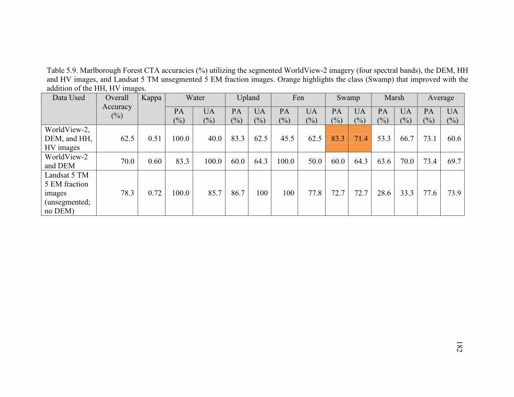
182
Table 5.9. Marlborough Forest CTA accuracies (%) utilizing the segmented WorldView-2 imagery (four spectral bands), the DEM, HH and HV images, and Landsat 5 TM unsegmented 5 EM fraction images. Orange highlights the class (Swamp) that improved with the addition of the HH, HV images.
Data Used Overall Accuracy
(%)
Kappa Water Upland Fen Swamp Marsh Average
PA (%)
UA (%)
PA (%)
UA (%)
PA (%)
UA (%)
PA (%)
UA (%)
PA (%)
UA (%)
PA (%)
UA (%)
WorldView-2, DEM, and HH, HV images
62.5 0.51 100.0 40.0 83.3 62.5 45.5 62.5 83.3 71.4 53.3 66.7 73.1 60.6
WorldView-2 and DEM 70.0 0.60 83.3 100.0 60.0 64.3 100.0 50.0 60.0 64.3 63.6 70.0 73.4 69.7
Landsat 5 TM 5 EM fraction images (unsegmented; no DEM)
78.3 0.72 100.0 85.7 86.7 100 100 77.8 72.7 72.7 28.6 33.3 77.6 73.9
183
In terms of area of each Wetland Type, there was more Fen classified in the combined
optical/radar imagery and the radar images alone (Figures 5.14A and B, respectively), as
compared to the optical imagery alone which had greater area of Swamp and Marsh
classified.
Polarimetric signatures were generated from training data for Water, Upland, Fen,
Bog, Swamp and Marsh across all four sites, at two incidence angles (steep and shallow)
and for three seasons. Polarimetric signature outputs included polarimetric signature graphs,
and the minimum and maximum co- and cross-pol orientation and ellipticity angle statistics.
Table I1 in Appendix H provides the signature location references and location details of the
training sites for all of the sample signatures along with the accompanying polarimetric
signature graphs. Typically there are four types of models expected for polarimetric
signatures (Figure 2.5). Polarimetric signatures, elliptical and orientation angles are statistics
rather than images.
The following provides examples of typical and atypical response curves for Water,
Fen, Bog, Swamp and Marsh using spring data. In addition, one fall signature is shown to
illustrate whether fall data could be used given spring data were not available. The majority
of the accompanying photographs were taken in spring (April 2010) with some from the
summer (July/August 2010). A comparison of the maximum co- and cross-pol orientation
(ψ) and ellipticity angles (χ) for spring steep incidence angle data follows these graphical
analyses.
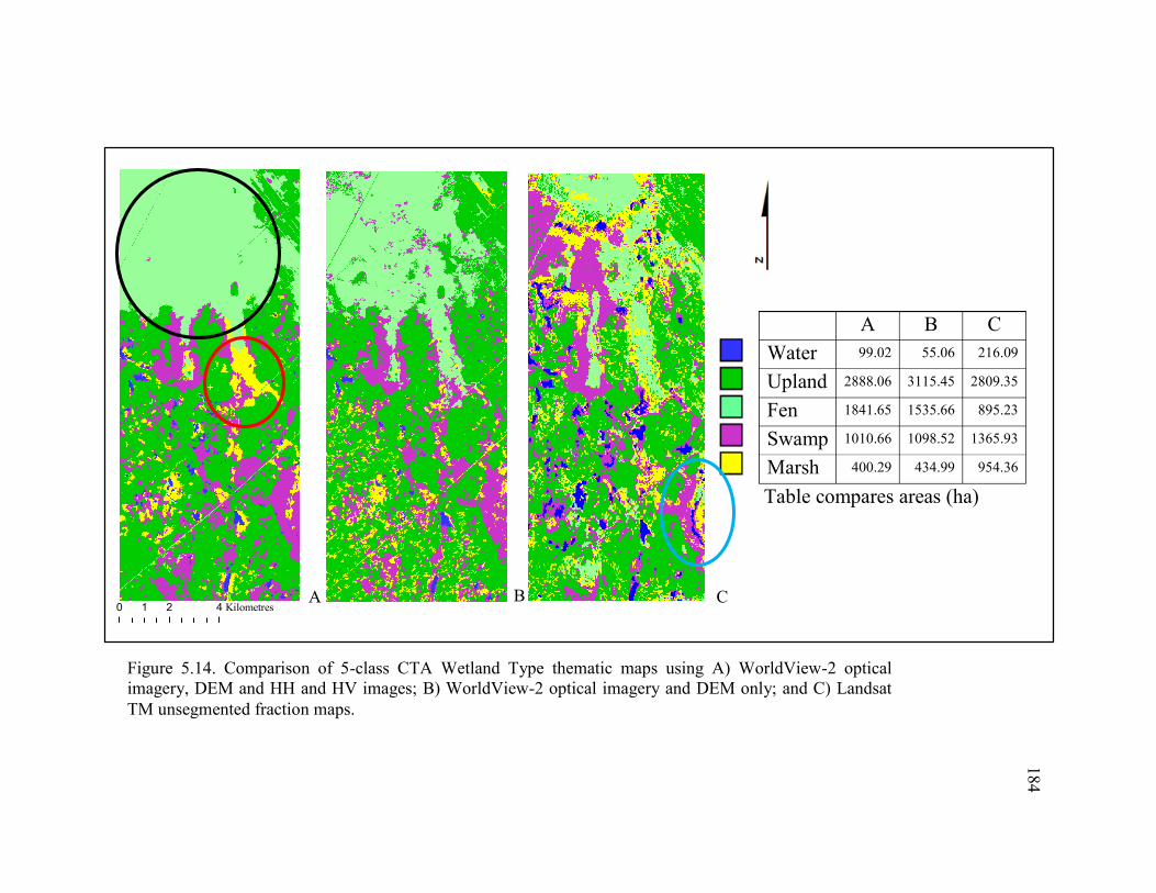
184
A B
Figure 5.14. Comparison of 5-class CTA Wetland Type thematic maps using A) WorldView-2 optical imagery, DEM and HH and HV images; B) WorldView-2 optical imagery and DEM only; and C) Landsat TM unsegmented fraction maps.
C
A B C Water 99.02 55.06 216.09
Upland 2888.06 3115.45 2809.35
Fen 1841.65 1535.66 895.23
Swamp 1010.66 1098.52 1365.93
Marsh 400.29 434.99 954.36
Table compares areas (ha)
0 2 41 Kilometres
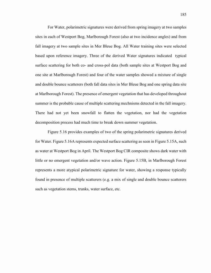
185
For Water, polarimetric signatures were derived from spring imagery at two samples
sites in each of Westport Bog, Marlborough Forest (also at two incidence angles) and from
fall imagery at two sample sites in Mer Bleue Bog. All Water training sites were selected
based upon reference imagery. Three of the derived Water signatures indicated typical
surface scattering for both co- and cross-pol data (both sample sites at Westport Bog and
one site at Marlborough Forest) and four of the water samples showed a mixture of single
and double bounce scatterers (both fall data sites in Mer Bleue Bog and one spring data site
at Marlborough Forest). The presence of emergent vegetation that has developed throughout
summer is the probable cause of multiple scattering mechnisms detected in the fall imagery.
There had not yet been snowfall to flatten the vegetation, nor had the vegetation
decomposition process had much time to break down summer vegetation.
Figure 5.16 provides examples of two of the spring polarimetric signatures derived
for Water. Figure 5.16A represents expected surface scattering as seen in Figure 5.15A, such
as water at Westport Bog in April. The Westport Bog CIR composite shows dark water with
little or no emergent vegetation and/or wave action. Figure 5.15B, in Marlborough Forest
represents a more atypical polarimetric signature for water, showing a response typically
found in presence of multiple scatterers (e.g. a mix of single and double bounce scatterers
such as vegetation stems, trunks, water surface, etc.
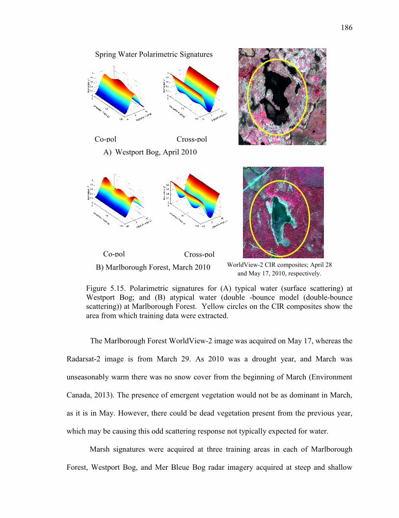
186
The Marlborough Forest WorldView-2 image was acquired on May 17, whereas the
Radarsat-2 image is from March 29. As 2010 was a drought year, and March was
unseasonably warm there was no snow cover from the beginning of March (Environment
Canada, 2013). The presence of emergent vegetation would not be as dominant in March,
as it is in May. However, there could be dead vegetation present from the previous year,
which may be causing this odd scattering response not typically expected for water.
Marsh signatures were acquired at three training areas in each of Marlborough
Forest, Westport Bog, and Mer Bleue Bog radar imagery acquired at steep and shallow
Co-pol Cross-pol A) Westport Bog, April 2010
B) Marlborough Forest, March 2010 WorldView-2 CIR composites; April 28 and May 17, 2010, respectively.
Figure 5.15. Polarimetric signatures for (A) typical water (surface scattering) at Westport Bog; and (B) atypical water (double -bounce model (double-bounce scattering)) at Marlborough Forest. Yellow circles on the CIR composites show the area from which training data were extracted.
Spring Water Polarimetric Signatures
Co-pol Cross-pol
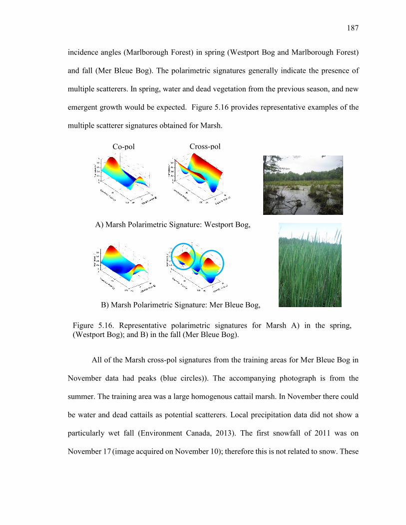
187
incidence angles (Marlborough Forest) in spring (Westport Bog and Marlborough Forest)
and fall (Mer Bleue Bog). The polarimetric signatures generally indicate the presence of
multiple scatterers. In spring, water and dead vegetation from the previous season, and new
emergent growth would be expected. Figure 5.16 provides representative examples of the
multiple scatterer signatures obtained for Marsh.
All of the Marsh cross-pol signatures from the training areas for Mer Bleue Bog in
November data had peaks (blue circles)). The accompanying photograph is from the
summer. The training area was a large homogenous cattail marsh. In November there could
be water and dead cattails as potential scatterers. Local precipitation data did not show a
particularly wet fall (Environment Canada, 2013). The first snowfall of 2011 was on
November 17 (image acquired on November 10); therefore this is not related to snow. These
Co-pol Cross-pol
A) Marsh Polarimetric Signature: Westport Bog, April
B) Marsh Polarimetric Signature: Mer Bleue Bog, November
Figure 5.16. Representative polarimetric signatures for Marsh A) in the spring, (Westport Bog); and B) in the fall (Mer Bleue Bog).
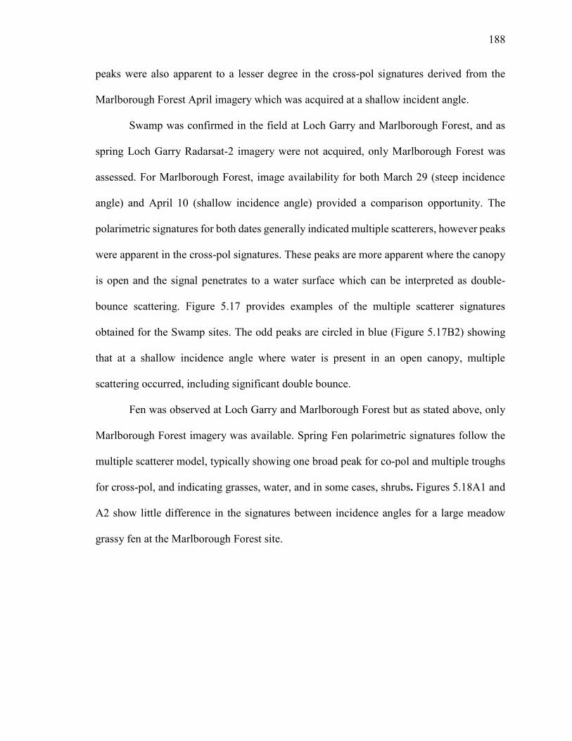
188
peaks were also apparent to a lesser degree in the cross-pol signatures derived from the
Marlborough Forest April imagery which was acquired at a shallow incident angle.
Swamp was confirmed in the field at Loch Garry and Marlborough Forest, and as
spring Loch Garry Radarsat-2 imagery were not acquired, only Marlborough Forest was
assessed. For Marlborough Forest, image availability for both March 29 (steep incidence
angle) and April 10 (shallow incidence angle) provided a comparison opportunity. The
polarimetric signatures for both dates generally indicated multiple scatterers, however peaks
were apparent in the cross-pol signatures. These peaks are more apparent where the canopy
is open and the signal penetrates to a water surface which can be interpreted as double-
bounce scattering. Figure 5.17 provides examples of the multiple scatterer signatures
obtained for the Swamp sites. The odd peaks are circled in blue (Figure 5.17B2) showing
that at a shallow incidence angle where water is present in an open canopy, multiple
scattering occurred, including significant double bounce.
Fen was observed at Loch Garry and Marlborough Forest but as stated above, only
Marlborough Forest imagery was available. Spring Fen polarimetric signatures follow the
multiple scatterer model, typically showing one broad peak for co-pol and multiple troughs
for cross-pol, and indicating grasses, water, and in some cases, shrubs. Figures 5.18A1 and
A2 show little difference in the signatures between incidence angles for a large meadow
grassy fen at the Marlborough Forest site.
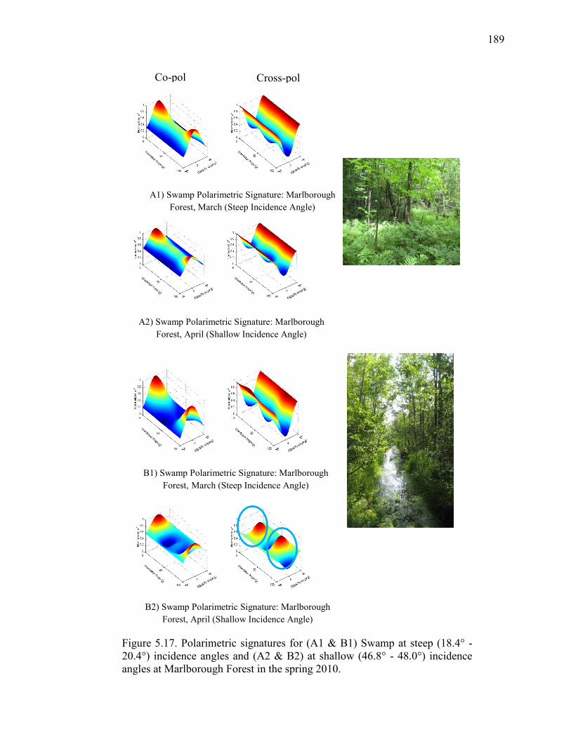
189
Figure 5.17. Polarimetric signatures for (A1 & B1) Swamp at steep (18.4° - 20.4°) incidence angles and (A2 & B2) at shallow (46.8° - 48.0°) incidence angles at Marlborough Forest in the spring 2010.
A1) Swamp Polarimetric Signature: Marlborough Forest, March (Steep Incidence Angle)
A2) Swamp Polarimetric Signature: Marlborough Forest, April (Shallow Incidence Angle)
B1) Swamp Polarimetric Signature: Marlborough Forest, March (Steep Incidence Angle)
B2) Swamp Polarimetric Signature: Marlborough Forest, April (Shallow Incidence Angle)
Co-pol Cross-pol
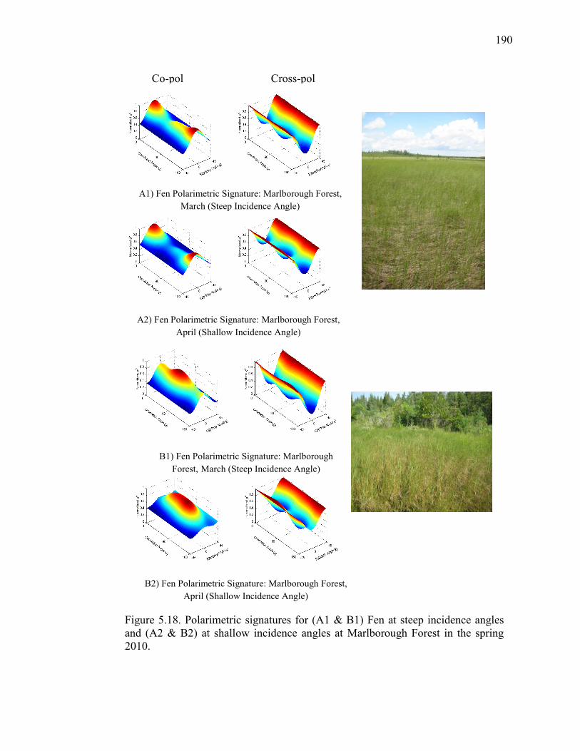
190
Figure 5.18. Polarimetric signatures for (A1 & B1) Fen at steep incidence angles and (A2 & B2) at shallow incidence angles at Marlborough Forest in the spring 2010.
A1) Fen Polarimetric Signature: Marlborough Forest, March (Steep Incidence Angle)
A2) Fen Polarimetric Signature: Marlborough Forest, April (Shallow Incidence Angle)
B1) Fen Polarimetric Signature: Marlborough Forest, March (Steep Incidence Angle)
B2) Fen Polarimetric Signature: Marlborough Forest, April (Shallow Incidence Angle)
Co-pol Cross-pol
191
Bog was observed at Mer Bleue Bog and Westport Bog and polarimetric signatures
were obtained for these during the spring (Westport Bog) and the fall (Mer Bleue Bog) at
steep incidence angles. The results obtained for the fall imagery are similar to those for
spring, indicating that fall imagery might be useful as a substitute for, or in tandem with
spring imagery. The signatures for both bogs and seasons mostly follow a surface scatterer
model (e.g., Figure 5.19A, Mer Bleue Bog fall site #2), with one site (Figure 5.19B,
Westport Bog spring site #3) mimicking a multiple scatterer model.
The taller canopy of trees at Westport Bog could be responsible for the multiple
scattering response. The other bog sites were comprised mostly of short shrubs that had a
continuous, smooth canopy with minor, sporadic seedlings/trees (e.g., Figure 5.20B, red
circle).
Co-pol Cross-pol
B) Bog Polarimetric Signature: Westport Bog, April
Figure 5.19. Polarimetric signatures for Bog in the fall (A, Mer Bleue Bog) and in the spring (B, Westport Bog) at steep incidence angles. Red circle highlights presence of sporadic tamarack.
A) Bog Polarimetric Signature: Mer Bleue Bog, November
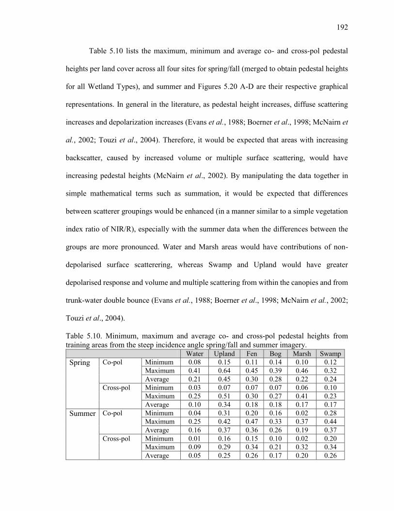
192
Table 5.10 lists the maximum, minimum and average co- and cross-pol pedestal
heights per land cover across all four sites for spring/fall (merged to obtain pedestal heights
for all Wetland Types), and summer and Figures 5.20 A-D are their respective graphical
representations. In general in the literature, as pedestal height increases, diffuse scattering
increases and depolarization increases (Evans et al., 1988; Boerner et al., 1998; McNairn et
al., 2002; Touzi et al., 2004). Therefore, it would be expected that areas with increasing
backscatter, caused by increased volume or multiple surface scattering, would have
increasing pedestal heights (McNairn et al., 2002). By manipulating the data together in
simple mathematical terms such as summation, it would be expected that differences
between scatterer groupings would be enhanced (in a manner similar to a simple vegetation
index ratio of NIR/R), especially with the summer data when the differences between the
groups are more pronounced. Water and Marsh areas would have contributions of non-
depolarised surface scatterering, whereas Swamp and Upland would have greater
depolarised response and volume and multiple scattering from within the canopies and from
trunk-water double bounce (Evans et al., 1988; Boerner et al., 1998; McNairn et al., 2002;
Touzi et al., 2004).
Table 5.10. Minimum, maximum and average co- and cross-pol pedestal heights from training areas from the steep incidence angle spring/fall and summer imagery.
Water Upland Fen Bog Marsh Swamp Spring Co-pol Minimum 0.08 0.15 0.11 0.14 0.10 0.12
Maximum 0.41 0.64 0.45 0.39 0.46 0.32 Average 0.21 0.45 0.30 0.28 0.22 0.24
Cross-pol Minimum 0.03 0.07 0.07 0.07 0.06 0.10 Maximum 0.25 0.51 0.30 0.27 0.41 0.23 Average 0.10 0.34 0.18 0.18 0.17 0.17
Summer Co-pol Minimum 0.04 0.31 0.20 0.16 0.02 0.28 Maximum 0.25 0.42 0.47 0.33 0.37 0.44 Average 0.16 0.37 0.36 0.26 0.19 0.37
Cross-pol Minimum 0.01 0.16 0.15 0.10 0.02 0.20 Maximum 0.09 0.29 0.34 0.21 0.32 0.34 Average 0.05 0.25 0.26 0.17 0.20 0.26
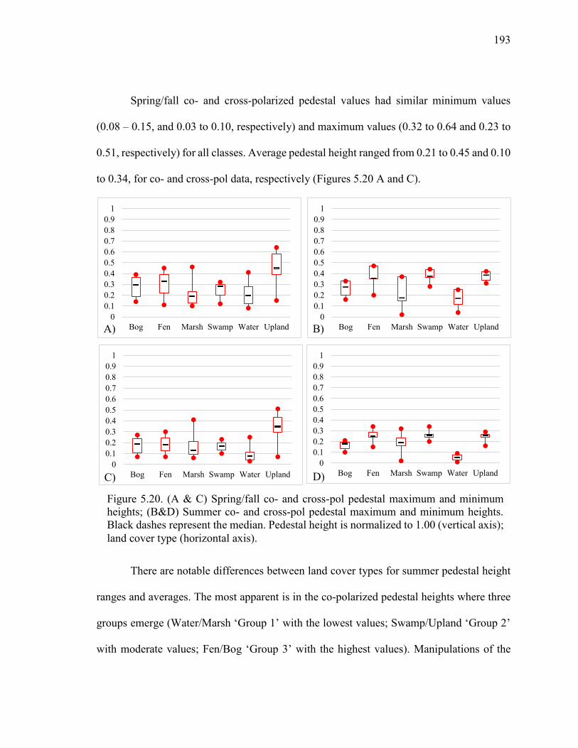
193
Spring/fall co- and cross-polarized pedestal values had similar minimum values
(0.08 – 0.15, and 0.03 to 0.10, respectively) and maximum values (0.32 to 0.64 and 0.23 to
0.51, respectively) for all classes. Average pedestal height ranged from 0.21 to 0.45 and 0.10
to 0.34, for co- and cross-pol data, respectively (Figures 5.20 A and C).
There are notable differences between land cover types for summer pedestal height
ranges and averages. The most apparent is in the co-polarized pedestal heights where three
groups emerge (Water/Marsh ‘Group 1’ with the lowest values; Swamp/Upland ‘Group 2’
with moderate values; Fen/Bog ‘Group 3’ with the highest values). Manipulations of the
00.10.20.30.40.50.60.70.80.9
1
Bog Fen Marsh Swamp Water Upland
Figure 5.20. (A & C) Spring/fall co- and cross-pol pedestal maximum and minimum heights; (B&D) Summer co- and cross-pol pedestal maximum and minimum heights. Black dashes represent the median. Pedestal height is normalized to 1.00 (vertical axis); land cover type (horizontal axis).
00.10.20.30.40.50.60.70.80.9
1
Bog Fen Marsh Swamp Water Upland
00.10.20.30.40.50.60.70.80.9
1
Bog Fen Marsh Swamp Water Upland0
0.10.20.30.40.50.60.70.80.9
1
Bog Fen Marsh Swamp Water Upland
A) B)
C) D)
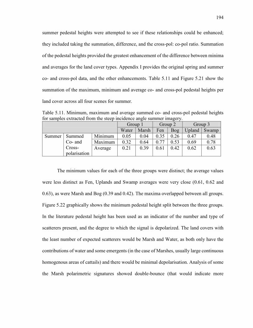
194
summer pedestal heights were attempted to see if these relationships could be enhanced;
they included taking the summation, difference, and the cross-pol: co-pol ratio. Summation
of the pedestal heights provided the greatest enhancement of the difference between minima
and averages for the land cover types. Appendix I provides the original spring and summer
co- and cross-pol data, and the other enhancements. Table 5.11 and Figure 5.21 show the
summation of the maximum, minimum and average co- and cross-pol pedestal heights per
land cover across all four scenes for summer.
Table 5.11. Minimum, maximum and average summed co- and cross-pol pedestal heights for samples extracted from the steep incidence angle summer imagery. Group 1 Group 2 Group 3
Water Marsh Fen Bog Upland Swamp Summer Summed
Co- and Cross-polarisation
Minimum 0.05 0.04 0.35 0.26 0.47 0.48 Maximum 0.32 0.64 0.77 0.53 0.69 0.78 Average 0.21 0.39 0.61 0.42 0.62 0.63
The minimum values for each of the three groups were distinct; the average values
were less distinct as Fen, Uplands and Swamp averages were very close (0.61, 0.62 and
0.63), as were Marsh and Bog (0.39 and 0.42). The maxima overlapped between all groups.
Figure 5.22 graphically shows the minimum pedestal height split between the three groups.
In the literature pedestal height has been used as an indicator of the number and type of
scatterers present, and the degree to which the signal is depolarized. The land covers with
the least number of expected scatterers would be Marsh and Water, as both only have the
contributions of water and some emergents (in the case of Marshes, usually large continuous
homogenous areas of cattails) and there would be minimal depolarisation. Analysis of some
the Marsh polarimetric signatures showed double-bounce (that would indicate more
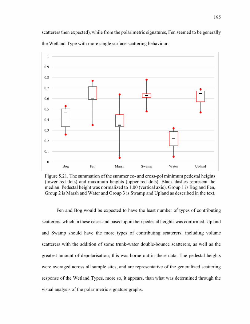
195
scatterers then expected), while from the polarimetric signatures, Fen seemed to be generally
the Wetland Type with more single surface scattering behaviour.
Fen and Bog would be expected to have the least number of types of contributing
scatterers, which in these cases and based upon their pedestal heights was confirmed. Upland
and Swamp should have the more types of contributing scatterers, including volume
scatterers with the addition of some trunk-water double-bounce scatterers, as well as the
greatest amount of depolarisation; this was borne out in these data. The pedestal heights
were averaged across all sample sites, and are representative of the generalized scattering
response of the Wetland Types, more so, it appears, than what was determined through the
visual analysis of the polarimetric signature graphs.
0
0.1
0.2
0.3
0.4
0.5
0.6
0.7
0.8
0.9
1
Bog Fen Marsh Swamp Water Upland
Figure 5.21. The summation of the summer co- and cross-pol minimum pedestal heights (lower red dots) and maximum heights (upper red dots). Black dashes represent the median. Pedestal height was normalized to 1.00 (vertical axis). Group 1 is Bog and Fen, Group 2 is Marsh and Water and Group 3 is Swamp and Upland as described in the text.
196
Entropy, anisotropy and alpha components were derived from the Loch Garry
summer Radarsat-2 image and used in pixel-based MLC and CTA classifications as well as
in object-based segmentation (in addition to WorldView-2 imagery and the DEM) and
classification to see if they improved mapping accuracies for Wetland Type. They were also
used in a Wishart unsupervised classification. Figure 5.22A shows the spring WorldView-2
CIR composite and Figures 5.22B - D show the three CP components. Apart from being
noisy, it can be seen in the entropy image that low values (e.g. water, red circle) indicate
that there was no significant mixing of scattering mechanisms and a low degree of
randomness.
Alpha identifies the dominant scattering mechanism; as expected low values (dark
areas in the created image) occurred for water bodies (Loch Garry, and the small lake to the
North) indicating surface scattering. The brighter areas (red arrows) along the shoreline were
where there was fen and a large dead coniferous swamp, both indicating double bounce and
multiple scatterers. Fen should have mostly surface scattering with some contributions from
volume scattering and double-bounce scattering, as the Fen in this area contained sporadic
tamarack, woody vegetation and some more open water presence in comparison to the Fens
in Marlborough Forest, which were mostly grassy meadows. Swamp in this area included
significant proportions of dead coniferous trees, and therefore volume, multiple and double-
bounce would be expected, resulting in high alpha values and bright tones in the alpha
image.
Anisotropy provides an indication of the mixing between the second and third
scattering mechanisms, higher values (brighter tones in the anisotropy image produced)
indicating that the second mechanism is dominant. It does not make sense that areas with
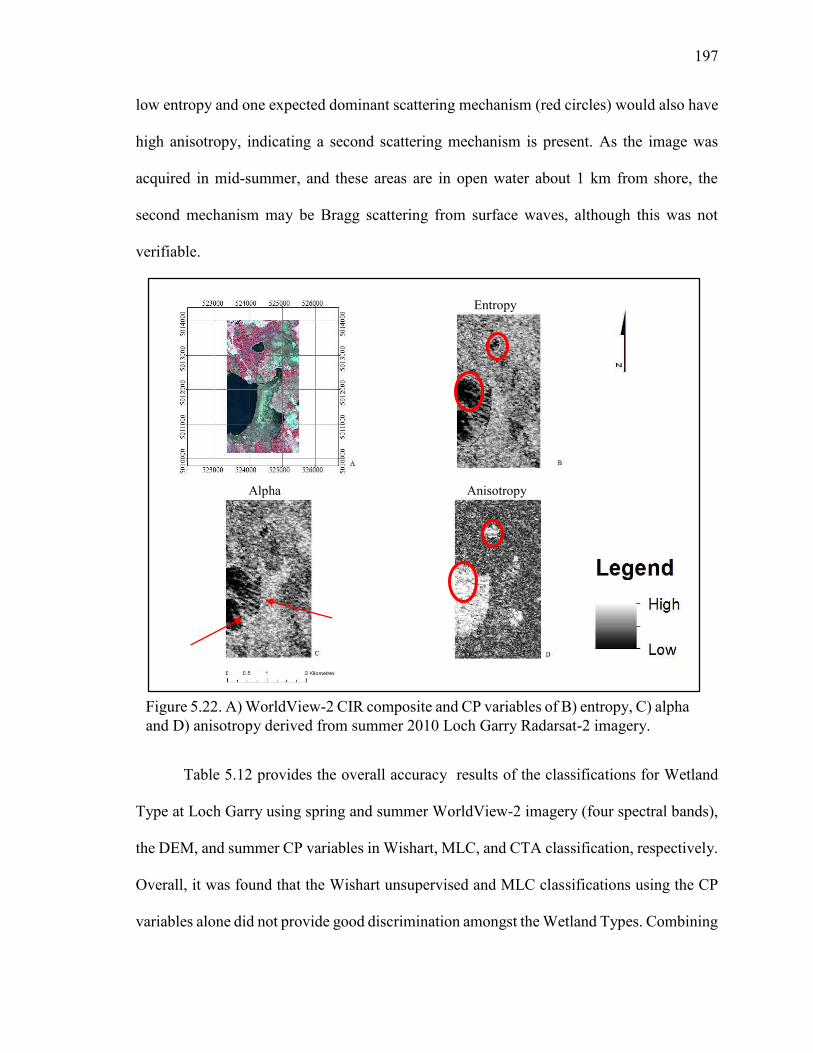
197
low entropy and one expected dominant scattering mechanism (red circles) would also have
high anisotropy, indicating a second scattering mechanism is present. As the image was
acquired in mid-summer, and these areas are in open water about 1 km from shore, the
second mechanism may be Bragg scattering from surface waves, although this was not
verifiable.
Table 5.12 provides the overall accuracy results of the classifications for Wetland
Type at Loch Garry using spring and summer WorldView-2 imagery (four spectral bands),
the DEM, and summer CP variables in Wishart, MLC, and CTA classification, respectively.
Overall, it was found that the Wishart unsupervised and MLC classifications using the CP
variables alone did not provide good discrimination amongst the Wetland Types. Combining
Figure 5.22. A) WorldView-2 CIR composite and CP variables of B) entropy, C) alpha and D) anisotropy derived from summer 2010 Loch Garry Radarsat-2 imagery.
Entropy
Alpha Anisotropy
198
CP variables with optical and DEM data, improved overall accuracy for the summer season
for Loch Garry, but did not improve the overall accuracy over optical imagery alone for the
best season (spring) (for Loch Garry or for the other three sites). Fen class (orange highlight)
improved in accuracy over all seasons.
5.1.4 Summary of main findings for Wetland Type
The following are the main findings from the optical analyses:
Optimal segmentation parameters determined for WorldView-2 were scale value of
45, shape value of 0.1 and compactness value of 0.75; and for Landsat 5 TM imagery
(original data and LSU) were scale value of 2, shape value of 0.1 and compactness
value of 0.1;
CTA was on classification of test site had higher accuracy than MLC for almost all
classes;
5-classes (Water, Upland, Fen, Swamp and Marsh) using merged non-wetland
terrestrial classes had higher accuracy than 7-classes (Water, Forest, Short
Vegetation, Impervious (Roads), Fen, Swamp and Marsh);
WorldView-2 imagery provided a higher accuracy than Landsat 5 TM imagery for
this type of classification; and
Landsat 5 TM imagery was not as useful as WorldView-2 imagery except for a few
classes (e.g. Fen or Swamp), with poorer results for Marsh due to spatial resolution
and extent of the imagery.
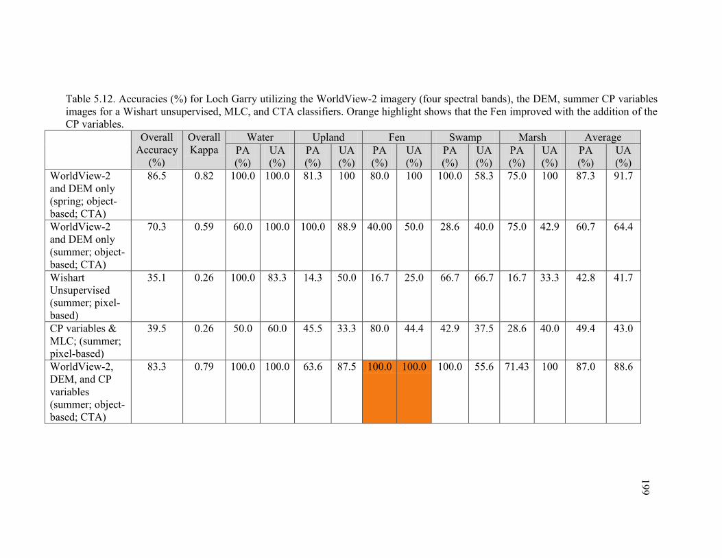
199
Table 5.12. Accuracies (%) for Loch Garry utilizing the WorldView-2 imagery (four spectral bands), the DEM, summer CP variables images for a Wishart unsupervised, MLC, and CTA classifiers. Orange highlight shows that the Fen improved with the addition of the CP variables.
Overall Accuracy
(%)
Overall Kappa
Water Upland Fen Swamp Marsh Average PA (%)
UA (%)
PA (%)
UA (%)
PA (%)
UA (%)
PA (%)
UA (%)
PA (%)
UA (%)
PA (%)
UA (%)
WorldView-2 and DEM only (spring; object-based; CTA)
86.5 0.82 100.0 100.0 81.3 100 80.0 100 100.0 58.3 75.0 100 87.3 91.7
WorldView-2 and DEM only (summer; object-based; CTA)
70.3 0.59 60.0 100.0 100.0 88.9 40.00 50.0 28.6 40.0 75.0 42.9 60.7 64.4
Wishart Unsupervised (summer; pixel-based)
35.1 0.26 100.0 83.3 14.3 50.0 16.7 25.0 66.7 66.7 16.7 33.3 42.8 41.7
CP variables & MLC; (summer; pixel-based)
39.5 0.26 50.0 60.0 45.5 33.3 80.0 44.4 42.9 37.5 28.6 40.0 49.4 43.0
WorldView-2, DEM, and CP variables (summer; object-based; CTA)
83.3 0.79 100.0 100.0 63.6 87.5 100.0 100.0 100.0 55.6 71.43 100 87.0 88.6
200
The following are the main findings from the radar analyses:
Spring, steep (18.4° - 27.6°) incidence angle backscatter images showed better
separation between Wetland Type classes than spring, shallow (46.8° - 48.0°)
incidence angle, or summer and fall HH, HV images;
OBIA and CTA classification of HH, HV images alone, or combined with optical
imagery and a DEM did not improve overall accuracies but the accuracy of the
Swamp class improved;
The summation of the summer co- and cross-pol pedestal minima showed good
distinction amongst groupings of classes (Water/Marsh (‘Group 1’; Swamp/Upland
‘Group 2’; and Fen/Bog ‘Group 3), which related directly to the signal depolarisation
of the waves and types of scatterers present; and
OBIA and CTA classification using CP variables alone, or combined with optical
imagery and a DEM improved overall accuracies for one season for one site, and did
not have a higher accuracy than the best season optical results; however the accuracy
of the Fen class improved overall.
5.2 VCFs
The OWES categorizes VCFs as 14 dominant classes (Figure 3.8). A form must
represent approximately 25% of the vegetation community to be recorded. VCFs can be
present in various numbers and types within a given Wetland Type. Many of the same
201
methods applied for Wetland Type were applied to VCFs and the results are summarized (to
avoid repetition) in the following sections.
5.2.1 VCF classification using OBIA and 2010 spring WorldView-2 imagery
The optimal OBIA parameter values for VCF were: scale value = 25; shape value =
0.1; and compactness value = 0.75. Figure 5.23 provides an example of the objects that were
created using these parameters. Yellow outlines show objects that represent specific
vegetation communities and they are accompanied by corresponding field photographs.
Using the segmented WorldView-2 and DEM data, CTA was implemented for both
the VCF class types and the number of forms (0 – 3 forms (Class A); 4-5 forms (Class B); >
6 forms (Class C); see Section 2.9.2 for details). Table 5.13 provides the accuracy analysis
for Number of Forms. Westport Bog had the highest overall accuracy (70.1%); Marlborough
Forest had the lowest accuracy (53.1%). The classes with the best and worst overall results
were Class A and Class B with an average of 57% and 59% PA and UA, respectively. Class
C had very high PA (average of 93.8%) but extremely poor UA (average of 29.4%).
Figure 5.24 provides a visual representation of the highest accuracy results for the
Number of Forms classification (Westport Bog). Figure 5.24A shows the entire Westport
Bog area classified as classes A, B, and C. Class A (1 to 3 forms) has the largest spatial
extent and is distributed throughout the map. The large patch of Class B in the southwest
(black circle) is a forested area observed in the field, which is comprised of mixed deciduous
and coniferous species.
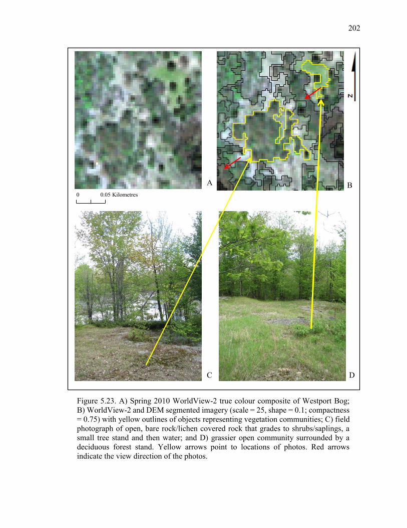
202
Figure 5.23. A) Spring 2010 WorldView-2 true colour composite of Westport Bog; B) WorldView-2 and DEM segmented imagery (scale = 25, shape = 0.1; compactness = 0.75) with yellow outlines of objects representing vegetation communities; C) field photograph of open, bare rock/lichen covered rock that grades to shrubs/saplings, a small tree stand and then water; and D) grassier open community surrounded by a deciduous forest stand. Yellow arrows point to locations of photos. Red arrows indicate the view direction of the photos.
A B
C D
0 0.05 Kilometres
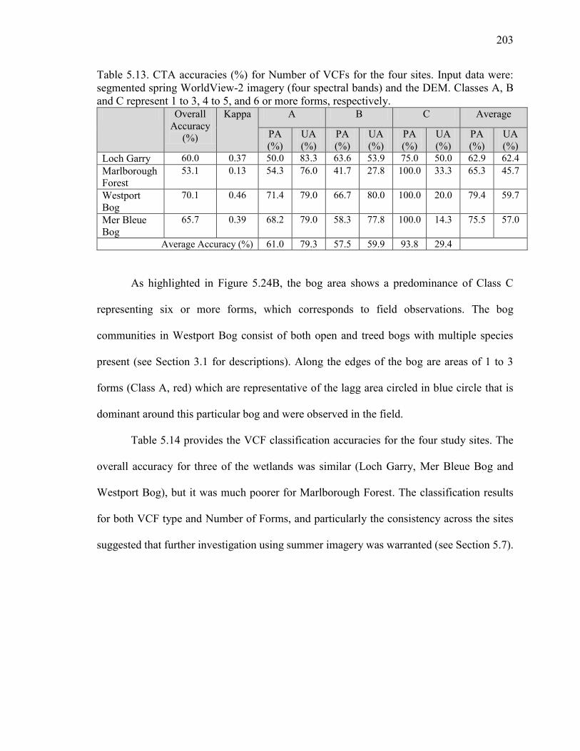
203
Table 5.13. CTA accuracies (%) for Number of VCFs for the four sites. Input data were: segmented spring WorldView-2 imagery (four spectral bands) and the DEM. Classes A, B and C represent 1 to 3, 4 to 5, and 6 or more forms, respectively.
Overall Accuracy
(%)
Kappa A B C Average
PA (%)
UA (%)
PA (%)
UA (%)
PA (%)
UA (%)
PA (%)
UA (%)
Loch Garry 60.0 0.37 50.0 83.3 63.6 53.9 75.0 50.0 62.9 62.4 Marlborough Forest
53.1 0.13 54.3 76.0 41.7 27.8 100.0 33.3 65.3 45.7
Westport Bog
70.1 0.46 71.4 79.0 66.7 80.0 100.0 20.0 79.4 59.7
Mer Bleue Bog
65.7 0.39 68.2 79.0 58.3 77.8 100.0 14.3 75.5 57.0
Average Accuracy (%) 61.0 79.3 57.5 59.9 93.8 29.4
As highlighted in Figure 5.24B, the bog area shows a predominance of Class C
representing six or more forms, which corresponds to field observations. The bog
communities in Westport Bog consist of both open and treed bogs with multiple species
present (see Section 3.1 for descriptions). Along the edges of the bog are areas of 1 to 3
forms (Class A, red) which are representative of the lagg area circled in blue circle that is
dominant around this particular bog and were observed in the field.
Table 5.14 provides the VCF classification accuracies for the four study sites. The
overall accuracy for three of the wetlands was similar (Loch Garry, Mer Bleue Bog and
Westport Bog), but it was much poorer for Marlborough Forest. The classification results
for both VCF type and Number of Forms, and particularly the consistency across the sites
suggested that further investigation using summer imagery was warranted (see Section 5.7).
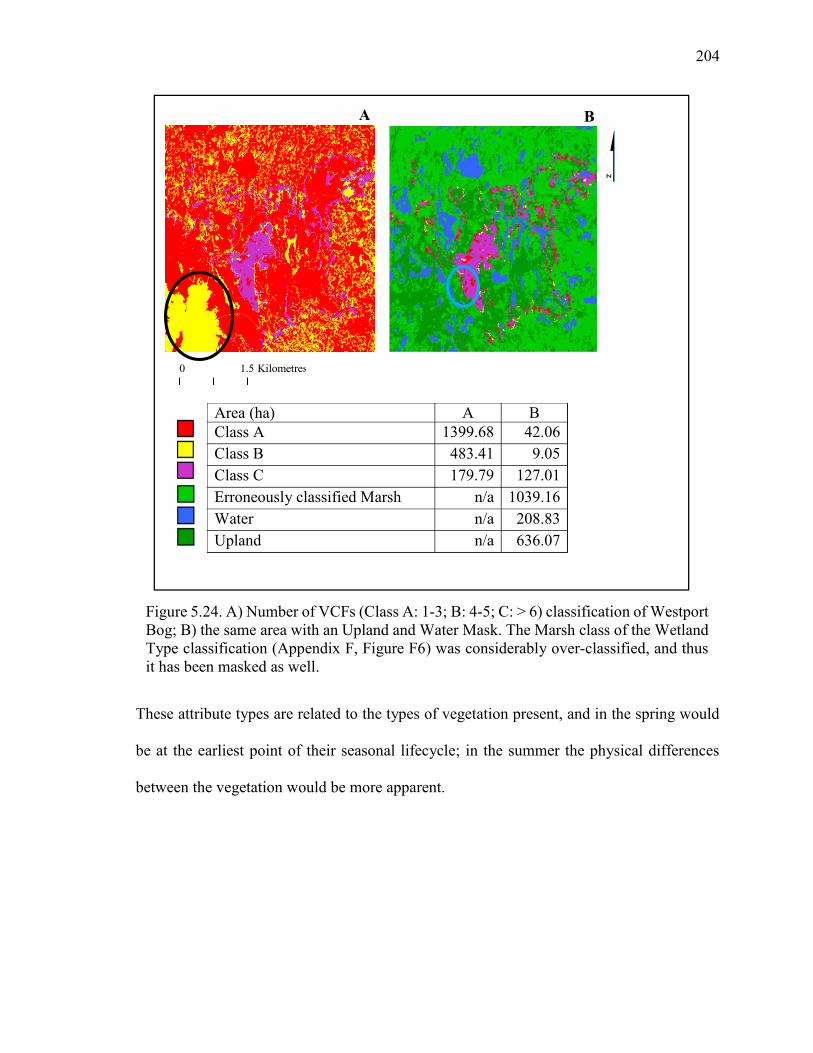
204
These attribute types are related to the types of vegetation present, and in the spring would
be at the earliest point of their seasonal lifecycle; in the summer the physical differences
between the vegetation would be more apparent.
0 1.5 Kilometres
Figure 5.24. A) Number of VCFs (Class A: 1-3; B: 4-5; C: > 6) classification of Westport Bog; B) the same area with an Upland and Water Mask. The Marsh class of the Wetland Type classification (Appendix F, Figure F6) was considerably over-classified, and thus it has been masked as well.
A B
Area (ha) A B Class A 1399.68 42.06 Class B 483.41 9.05 Class C 179.79 127.01 Erroneously classified Marsh n/a 1039.16 Water n/a 208.83 Upland n/a 636.07
205
5.2.2 VCF classification using OBIA and 2010 spring Landsat 5 TM imagery
Small scale values produced objects that were visually more representative of VCFs
than larger values, however, values less than 2 did not produce further significant reduction
in object sizes. From these analyses, it was decided that the optimal segmentation parameter
values for delineation of objects that represented observed groupings of VCFs were: scale
value = 2, shape value = 0.1 and compactness value = 0.1. Based upon the results for
Wetland Type classification, CTA classifications using the unsegmented fraction maps (5
EMs) plus DEM, and the segmented original spectral band data plus DEM were
implemented for comparison (Table 5.15). In general, the VCF classifications were very
poor, which was expected at this spatial resolution. For the three-form classification, the
sites with the highest overall accuracies were Marlborough Forest and Westport Bog. While
Westport Bog was also well classified using the WorldView-2 imagery, Marlborough Forest
had the poorest accuracies with that imagery. The best results for each site type for this
attribute (3 form) were obtained using the segmented original Landsat bands plus DEM.
Kappa values for all tests were very low and in some cases negative, which indicate these
results are no different than from a random assignment of the classes. Since all combinations
of the available Landsat data and DEM did not produce acceptable results, it was decided
that further investigation using the summer imagery would not be completed.
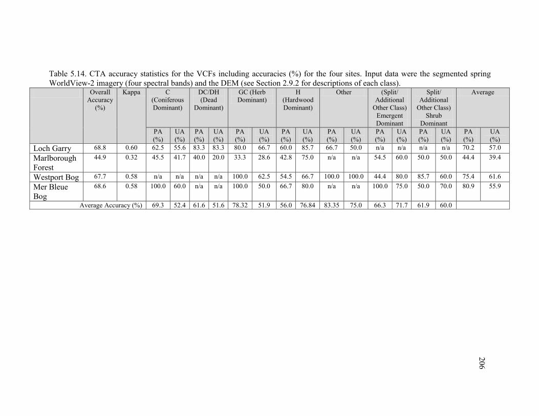
206
Table 5.14. CTA accuracy statistics for the VCFs including accuracies (%) for the four sites. Input data were the segmented spring WorldView-2 imagery (four spectral bands) and the DEM (see Section 2.9.2 for descriptions of each class).
Overall Accuracy
(%)
Kappa C (Coniferous Dominant)
DC/DH (Dead
Dominant)
GC (Herb Dominant)
H (Hardwood Dominant)
Other (Split/ Additional
Other Class) Emergent Dominant
Split/ Additional
Other Class) Shrub
Dominant
Average
PA (%)
UA (%)
PA (%)
UA (%)
PA (%)
UA (%)
PA (%)
UA (%)
PA (%)
UA (%)
PA (%)
UA (%)
PA (%)
UA (%)
PA (%)
UA (%)
Loch Garry 68.8 0.60 62.5 55.6 83.3 83.3 80.0 66.7 60.0 85.7 66.7 50.0 n/a n/a n/a n/a 70.2 57.0 Marlborough Forest
44.9 0.32 45.5 41.7 40.0 20.0 33.3 28.6 42.8 75.0 n/a n/a 54.5 60.0 50.0 50.0 44.4 39.4
Westport Bog 67.7 0.58 n/a n/a n/a n/a 100.0 62.5 54.5 66.7 100.0 100.0 44.4 80.0 85.7 60.0 75.4 61.6 Mer Bleue Bog
68.6 0.58 100.0 60.0 n/a n/a 100.0 50.0 66.7 80.0 n/a n/a 100.0 75.0 50.0 70.0 80.9 55.9
Average Accuracy (%) 69.3 52.4 61.6 51.6 78.32 51.9 56.0 76.84 83.35 75.0 66.3 71.7 61.9 60.0
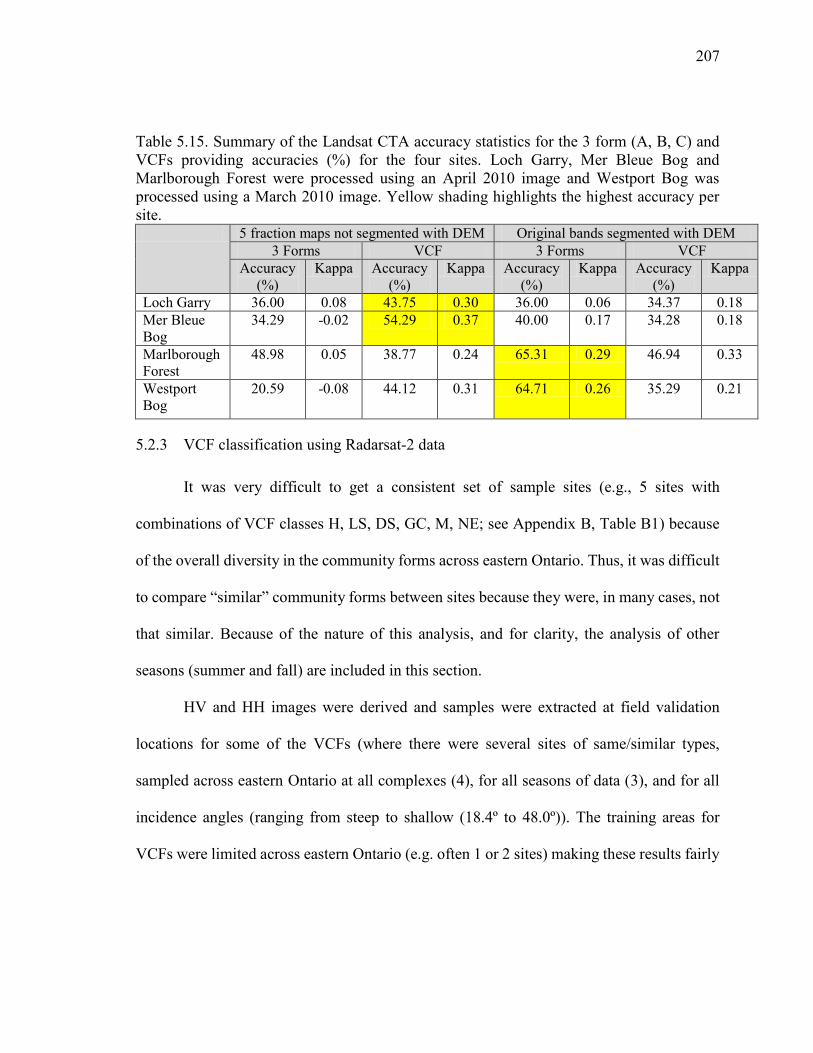
207
Table 5.15. Summary of the Landsat CTA accuracy statistics for the 3 form (A, B, C) and VCFs providing accuracies (%) for the four sites. Loch Garry, Mer Bleue Bog and Marlborough Forest were processed using an April 2010 image and Westport Bog was processed using a March 2010 image. Yellow shading highlights the highest accuracy per site. 5 fraction maps not segmented with DEM Original bands segmented with DEM
3 Forms VCF 3 Forms VCF Accuracy
(%) Kappa Accuracy
(%) Kappa Accuracy
(%) Kappa Accuracy
(%) Kappa
Loch Garry 36.00 0.08 43.75 0.30 36.00 0.06 34.37 0.18 Mer Bleue Bog
34.29 -0.02 54.29 0.37 40.00 0.17 34.28 0.18
Marlborough Forest
48.98 0.05 38.77 0.24 65.31 0.29 46.94 0.33
Westport Bog
20.59 -0.08 44.12 0.31 64.71 0.26 35.29 0.21
5.2.3 VCF classification using Radarsat-2 data
It was very difficult to get a consistent set of sample sites (e.g., 5 sites with
combinations of VCF classes H, LS, DS, GC, M, NE; see Appendix B, Table B1) because
of the overall diversity in the community forms across eastern Ontario. Thus, it was difficult
to compare “similar” community forms between sites because they were, in many cases, not
that similar. Because of the nature of this analysis, and for clarity, the analysis of other
seasons (summer and fall) are included in this section.
HV and HH images were derived and samples were extracted at field validation
locations for some of the VCFs (where there were several sites of same/similar types,
sampled across eastern Ontario at all complexes (4), for all seasons of data (3), and for all
incidence angles (ranging from steep to shallow (18.4º to 48.0º)). The training areas for
VCFs were limited across eastern Ontario (e.g. often 1 or 2 sites) making these results fairly
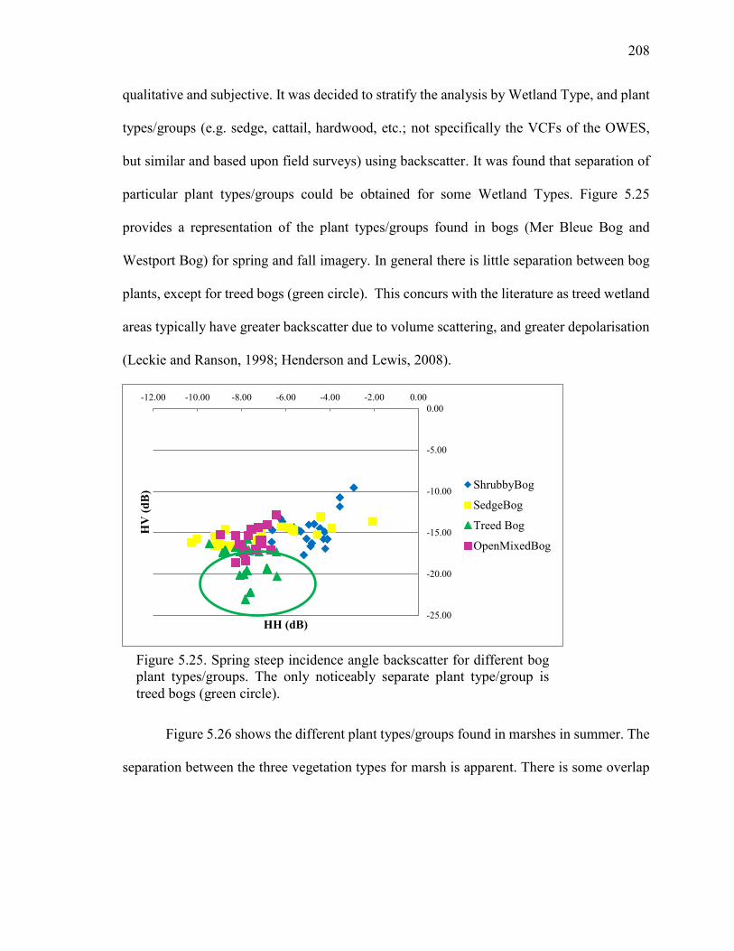
208
qualitative and subjective. It was decided to stratify the analysis by Wetland Type, and plant
types/groups (e.g. sedge, cattail, hardwood, etc.; not specifically the VCFs of the OWES,
but similar and based upon field surveys) using backscatter. It was found that separation of
particular plant types/groups could be obtained for some Wetland Types. Figure 5.25
provides a representation of the plant types/groups found in bogs (Mer Bleue Bog and
Westport Bog) for spring and fall imagery. In general there is little separation between bog
plants, except for treed bogs (green circle). This concurs with the literature as treed wetland
areas typically have greater backscatter due to volume scattering, and greater depolarisation
(Leckie and Ranson, 1998; Henderson and Lewis, 2008).
Figure 5.26 shows the different plant types/groups found in marshes in summer. The
separation between the three vegetation types for marsh is apparent. There is some overlap
-25.00
-20.00
-15.00
-10.00
-5.00
0.00-12.00 -10.00 -8.00 -6.00 -4.00 -2.00 0.00
HV
(dB
)
HH (dB)
ShrubbyBog
SedgeBog
Treed Bog
OpenMixedBog
Figure 5.25. Spring steep incidence angle backscatter for different bog plant types/groups. The only noticeably separate plant type/group is treed bogs (green circle).
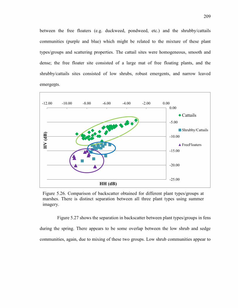
209
between the free floaters (e.g. duckweed, pondweed, etc.) and the shrubby/cattails
communities (purple and blue) which might be related to the mixture of these plant
types/groups and scattering properties. The cattail sites were homogeneous, smooth and
dense; the free floater site consisted of a large mat of free floating plants, and the
shrubby/cattails sites consisted of low shrubs, robust emergents, and narrow leaved
emergents.
Figure 5.27 shows the separation in backscatter between plant types/groups in fens
during the spring. There appears to be some overlap between the low shrub and sedge
communities, again, due to mixing of these two groups. Low shrub communities appear to
-25.00
-20.00
-15.00
-10.00
-5.00
0.00-12.00 -10.00 -8.00 -6.00 -4.00 -2.00 0.00
Cattails
Shrubby/Cattails
FreeFloaters
Figure 5.26. Comparison of backscatter obtained for different plant types/groups at marshes. There is distinct separation between all three plant types using summer imagery.
HH (dB)
HV
(dB
)
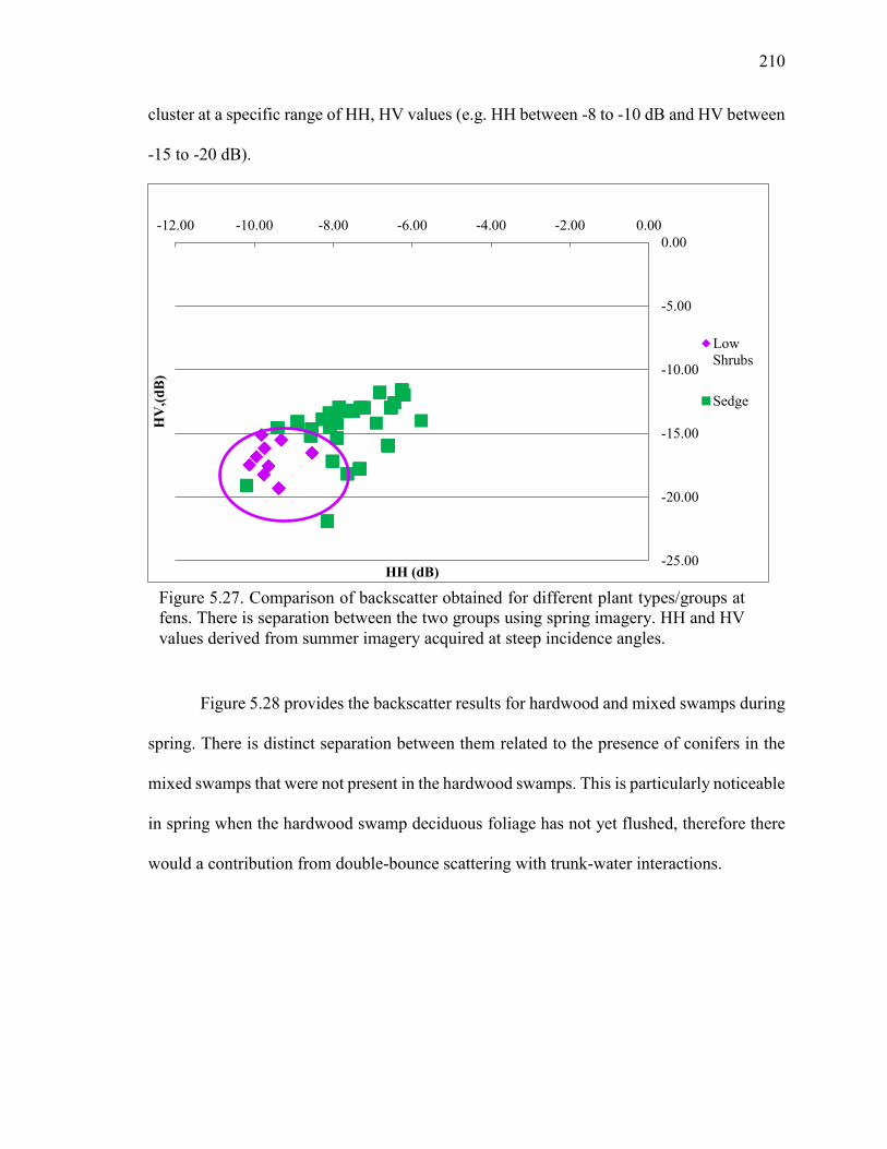
210
cluster at a specific range of HH, HV values (e.g. HH between -8 to -10 dB and HV between
-15 to -20 dB).
Figure 5.28 provides the backscatter results for hardwood and mixed swamps during
spring. There is distinct separation between them related to the presence of conifers in the
mixed swamps that were not present in the hardwood swamps. This is particularly noticeable
in spring when the hardwood swamp deciduous foliage has not yet flushed, therefore there
would a contribution from double-bounce scattering with trunk-water interactions.
Figure 5.27. Comparison of backscatter obtained for different plant types/groups at fens. There is separation between the two groups using spring imagery. HH and HV values derived from summer imagery acquired at steep incidence angles.
-25.00
-20.00
-15.00
-10.00
-5.00
0.00-12.00 -10.00 -8.00 -6.00 -4.00 -2.00 0.00
HV
,(dB
)
HH (dB)
LowShrubs
Sedge
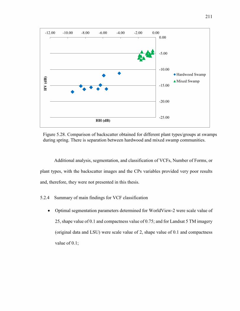
211
Additional analysis, segmentation, and classification of VCFs, Number of Forms, or
plant types, with the backscatter images and the CPs variables provided very poor results
and, therefore, they were not presented in this thesis.
5.2.4 Summary of main findings for VCF classification
Optimal segmentation parameters determined for WorldView-2 were scale value of
25, shape value of 0.1 and compactness value of 0.75; and for Landsat 5 TM imagery
(original data and LSU) were scale value of 2, shape value of 0.1 and compactness
value of 0.1;
-25.00
-20.00
-15.00
-10.00
-5.00
0.00-12.00 -10.00 -8.00 -6.00 -4.00 -2.00 0.00
HV
(dB
)
HH (dB)
Hardwood Swamp
Mixed Swamp
Figure 5.28. Comparison of backscatter obtained for different plant types/groups at swamps during spring. There is separation between hardwood and mixed swamp communities.
212
WorldView-2 imagery provided higher VCF classification accuracy than Landsat 5
TM imagery;
Separation of particular plant types/groups could be obtained for some Wetland
Types with spring backscatter imagery showing good separation for Fen and Swamp
plant types and summer imagery provided good separation for Marsh plant types;
and
Object-based CTA using HH, HV images and CP variables alone, and combined
with optical imagery and a DEM did not improve overall accuracies or accuracies
of individual plant types.
5.3 Open Water Type
There are eight categories of Open Water Types outlined in the OWES manual
(Table 3.3). Many of the same methods applied for Wetland Type and VCFs were applied
to Open Water Types and the results are given in the following sections.
5.3.1 Open Water Type classification using OBIA and 2010 spring WorldView-2 imagery
The optimal segmentation parameter values were scale value = 25, shape value = 0.1,
and compactness value = 0.75. Table 5.16 provides the CTA accuracy results for the four
study sites. The site with the highest accuracy was Loch Garry (73.3%), while the poorest
was Marlborough Forest (40.0%). In general, the classification results were poor, which
could be related to the small amount of reference data. The imagery itself was not useful in
213
providing additional samples. Only Open Water Types in wetland areas are considered in
the OWES and this resulted in the following numbers of reference sample sites:
Marlborough Forest (20 sites), Loch Garry (15 sites), Mer Bleue Bog (15 sites) and Westport
Bog (20 sites) and by Open Water Type (Type 1 = 20; Type 2 = 7; Type 3 = 8; Type 4 = 4;
Type 5 = 9; Type 6 = 6; Type 7 = 2; Type 8 = 6; and 8 that didn’t have permanent open
water (e.g. some bogs and some swamp)). The small numbers of potential sample locations
per site and per class also made selecting samples difficult. Based on this, and since the
spring results were so poor, it was decided not to conduct analysis using the summer
WorldView-2 imagery, since many of the sample sites would be obscured by vegetation,
reducing the sample size further.
Figure 5.29 shows the Open Water Type classification for Loch Garry. The yellow
circle shows an area where a boardwalk traverses a mixed coniferous/deciduous swamp. In
the spring, the canopy over the boardwalk is open, and around the boardwalk there is ponding
and standing water. The red circle highlights ephemeral wetland/ponding found in the spring
within mixed hardwood/coniferous forest. Other areas that were well classified based upon
field knowledge include the areas around the smaller lake in the north which shows open
water presence associated with marsh and fen vegetation that surrounds this lake. The black
circle highlights an area where there was ponding, particularly with hummocks of marsh
vegetation (reeds and cattails, etc.).
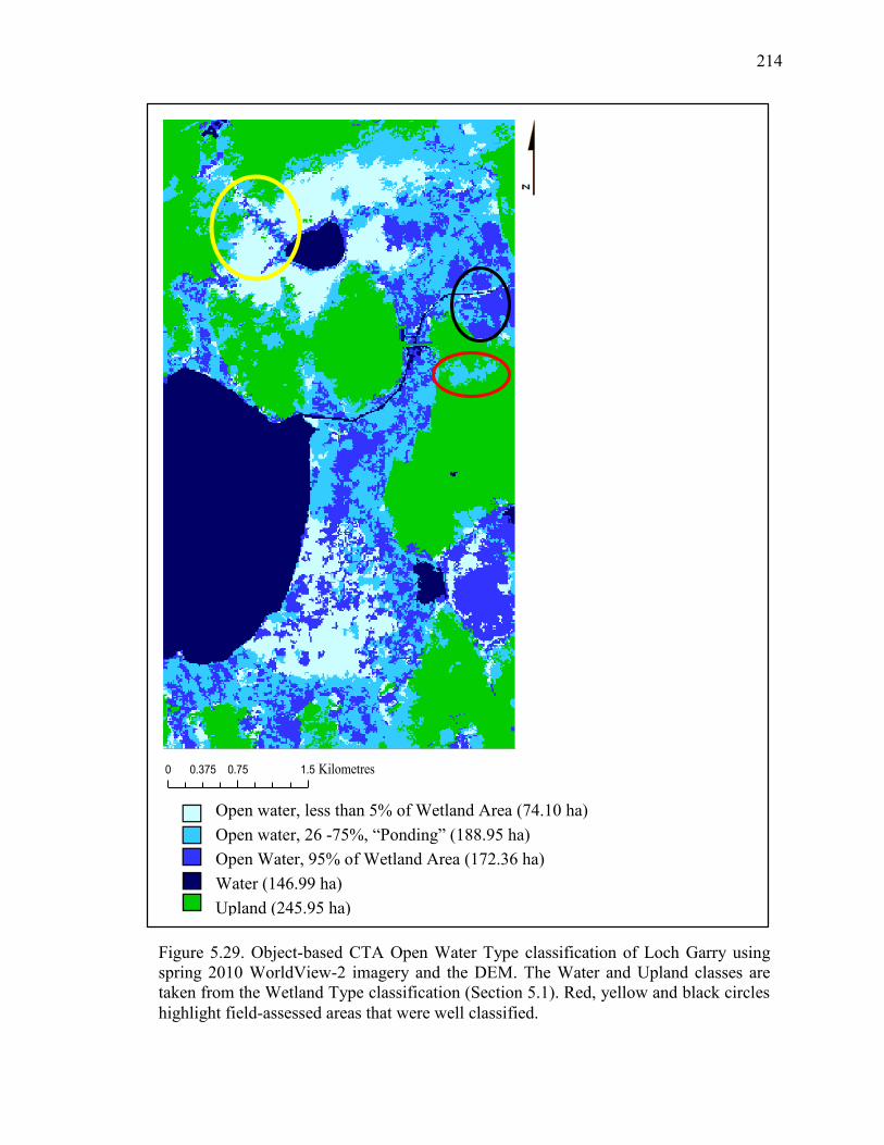
214
Figure 5.29. Object-based CTA Open Water Type classification of Loch Garry using spring 2010 WorldView-2 imagery and the DEM. The Water and Upland classes are taken from the Wetland Type classification (Section 5.1). Red, yellow and black circles highlight field-assessed areas that were well classified.
Open water, less than 5% of Wetland Area (74.10 ha) Open water, 26 -75%, “Ponding” (188.95 ha) Open Water, 95% of Wetland Area (172.36 ha) Water (146.99 ha) Upland (245.95 ha)
0 0.75 1.50.375 Kilometres
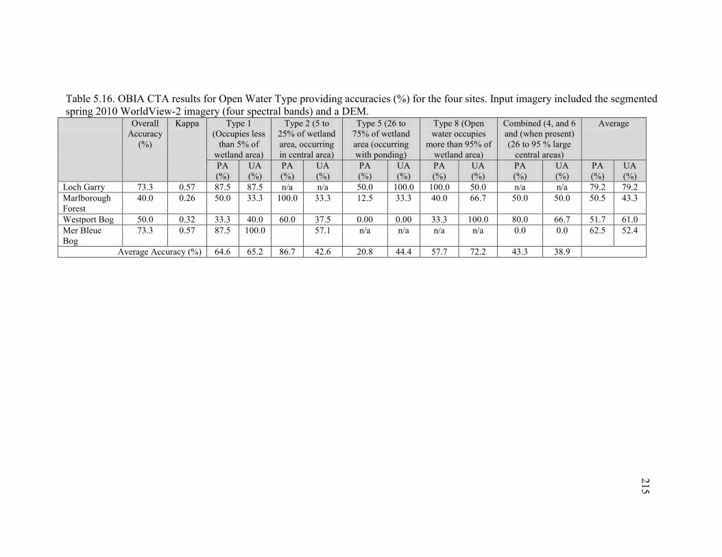
215
Table 5.16. OBIA CTA results for Open Water Type providing accuracies (%) for the four sites. Input imagery included the segmented spring 2010 WorldView-2 imagery (four spectral bands) and a DEM.
Overall Accuracy
(%)
Kappa Type 1 (Occupies less
than 5% of wetland area)
Type 2 (5 to 25% of wetland area, occurring in central area)
Type 5 (26 to 75% of wetland area (occurring with ponding)
Type 8 (Open water occupies
more than 95% of wetland area)
Combined (4, and 6 and (when present) (26 to 95 % large
central areas)
Average
PA (%)
UA (%)
PA (%)
UA (%)
PA (%)
UA (%)
PA (%)
UA (%)
PA (%)
UA (%)
PA (%)
UA (%)
Loch Garry 73.3 0.57 87.5 87.5 n/a n/a 50.0 100.0 100.0 50.0 n/a n/a 79.2 79.2 Marlborough Forest
40.0 0.26 50.0 33.3 100.0 33.3 12.5 33.3 40.0 66.7 50.0 50.0 50.5 43.3
Westport Bog 50.0 0.32 33.3 40.0 60.0 37.5 0.00 0.00 33.3 100.0 80.0 66.7 51.7 61.0 Mer Bleue Bog
73.3 0.57 87.5 100.0
57.1 n/a n/a n/a n/a 0.0 0.0 62.5 52.4
Average Accuracy (%) 64.6 65.2 86.7 42.6 20.8 44.4 57.7 72.2 43.3 38.9
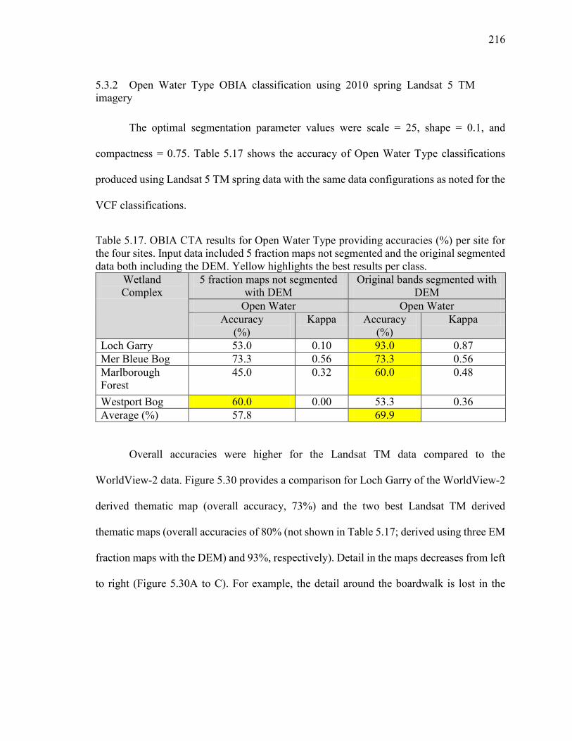
216
5.3.2 Open Water Type OBIA classification using 2010 spring Landsat 5 TM imagery
The optimal segmentation parameter values were scale = 25, shape = 0.1, and
compactness = 0.75. Table 5.17 shows the accuracy of Open Water Type classifications
produced using Landsat 5 TM spring data with the same data configurations as noted for the
VCF classifications.
Table 5.17. OBIA CTA results for Open Water Type providing accuracies (%) per site for the four sites. Input data included 5 fraction maps not segmented and the original segmented data both including the DEM. Yellow highlights the best results per class.
Wetland Complex
5 fraction maps not segmented with DEM
Original bands segmented with DEM
Open Water Open Water Accuracy
(%) Kappa Accuracy
(%) Kappa
Loch Garry 53.0 0.10 93.0 0.87 Mer Bleue Bog 73.3 0.56 73.3 0.56 Marlborough Forest
45.0 0.32 60.0 0.48
Westport Bog 60.0 0.00 53.3 0.36 Average (%) 57.8 69.9
Overall accuracies were higher for the Landsat TM data compared to the
WorldView-2 data. Figure 5.30 provides a comparison for Loch Garry of the WorldView-2
derived thematic map (overall accuracy, 73%) and the two best Landsat TM derived
thematic maps (overall accuracies of 80% (not shown in Table 5.17; derived using three EM
fraction maps with the DEM) and 93%, respectively). Detail in the maps decreases from left
to right (Figure 5.30A to C). For example, the detail around the boardwalk is lost in the
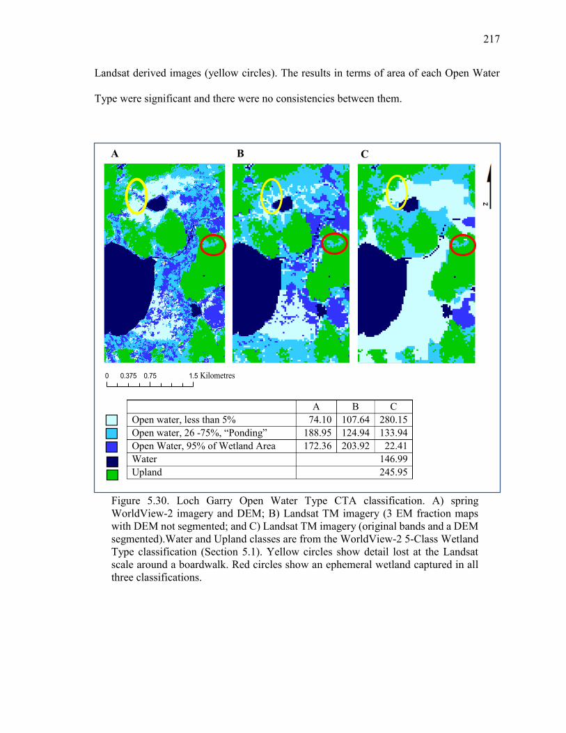
217
Landsat derived images (yellow circles). The results in terms of area of each Open Water
Type were significant and there were no consistencies between them.
A B C Open water, less than 5% 74.10 107.64 280.15 Open water, 26 -75%, “Ponding” 188.95 124.94 133.94 Open Water, 95% of Wetland Area 172.36 203.92 22.41 Water 146.99 Upland 245.95
A B C
Figure 5.30. Loch Garry Open Water Type CTA classification. A) spring WorldView-2 imagery and DEM; B) Landsat TM imagery (3 EM fraction maps with DEM not segmented; and C) Landsat TM imagery (original bands and a DEM segmented).Water and Upland classes are from the WorldView-2 5-Class Wetland Type classification (Section 5.1). Yellow circles show detail lost at the Landsat scale around a boardwalk. Red circles show an ephemeral wetland captured in all three classifications.
0 0.75 1.50.375 Kilometres
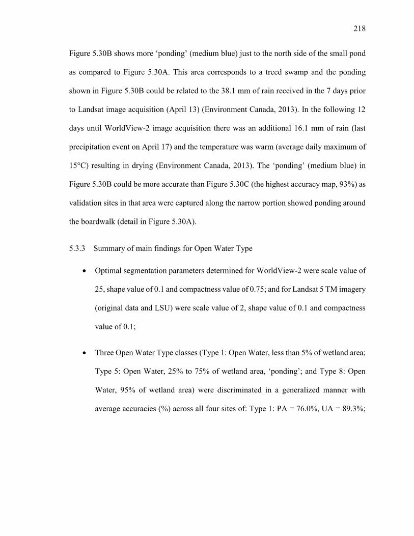
218
Figure 5.30B shows more ‘ponding’ (medium blue) just to the north side of the small pond
as compared to Figure 5.30A. This area corresponds to a treed swamp and the ponding
shown in Figure 5.30B could be related to the 38.1 mm of rain received in the 7 days prior
to Landsat image acquisition (April 13) (Environment Canada, 2013). In the following 12
days until WorldView-2 image acquisition there was an additional 16.1 mm of rain (last
precipitation event on April 17) and the temperature was warm (average daily maximum of
15°C) resulting in drying (Environment Canada, 2013). The ‘ponding’ (medium blue) in
Figure 5.30B could be more accurate than Figure 5.30C (the highest accuracy map, 93%) as
validation sites in that area were captured along the narrow portion showed ponding around
the boardwalk (detail in Figure 5.30A).
5.3.3 Summary of main findings for Open Water Type
Optimal segmentation parameters determined for WorldView-2 were scale value of
25, shape value of 0.1 and compactness value of 0.75; and for Landsat 5 TM imagery
(original data and LSU) were scale value of 2, shape value of 0.1 and compactness
value of 0.1;
Three Open Water Type classes (Type 1: Open Water, less than 5% of wetland area;
Type 5: Open Water, 25% to 75% of wetland area, ‘ponding’; and Type 8: Open
Water, 95% of wetland area) were discriminated in a generalized manner with
average accuracies (%) across all four sites of: Type 1: PA = 76.0%, UA = 89.3%;
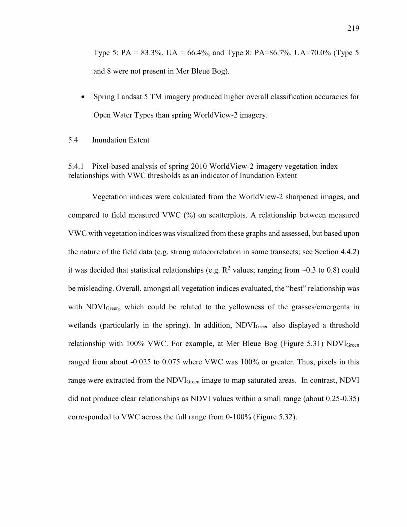
219
Type 5: PA = 83.3%, UA = 66.4%; and Type 8: PA=86.7%, UA=70.0% (Type 5
and 8 were not present in Mer Bleue Bog).
Spring Landsat 5 TM imagery produced higher overall classification accuracies for
Open Water Types than spring WorldView-2 imagery.
5.4 Inundation Extent
5.4.1 Pixel-based analysis of spring 2010 WorldView-2 imagery vegetation index relationships with VWC thresholds as an indicator of Inundation Extent
Vegetation indices were calculated from the WorldView-2 sharpened images, and
compared to field measured VWC (%) on scatterplots. A relationship between measured
VWC with vegetation indices was visualized from these graphs and assessed, but based upon
the nature of the field data (e.g. strong autocorrelation in some transects; see Section 4.4.2)
it was decided that statistical relationships (e.g. R2 values; ranging from ~0.3 to 0.8) could
be misleading. Overall, amongst all vegetation indices evaluated, the “best” relationship was
with NDVIGreen, which could be related to the yellowness of the grasses/emergents in
wetlands (particularly in the spring). In addition, NDVIGreen also displayed a threshold
relationship with 100% VWC. For example, at Mer Bleue Bog (Figure 5.31) NDVIGreen
ranged from about -0.025 to 0.075 where VWC was 100% or greater. Thus, pixels in this
range were extracted from the NDVIGreen image to map saturated areas. In contrast, NDVI
did not produce clear relationships as NDVI values within a small range (about 0.25-0.35)
corresponded to VWC across the full range from 0-100% (Figure 5.32).
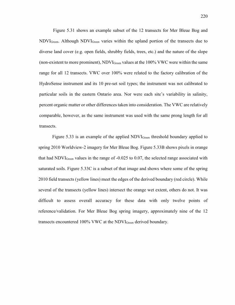
220
Figure 5.31 shows an example subset of the 12 transects for Mer Bleue Bog and
NDVIGreen. Although NDVIGreen varies within the upland portion of the transects due to
diverse land cover (e.g. open fields, shrubby fields, trees, etc.) and the nature of the slope
(non-existent to more prominent), NDVIGreen values at the 100% VWC were within the same
range for all 12 transects. VWC over 100% were related to the factory calibration of the
HydroSense instrument and its 10 pre-set soil types; the instrument was not calibrated to
particular soils in the eastern Ontario area. Nor were each site’s variability in salinity,
percent organic matter or other differences taken into consideration. The VWC are relatively
comparable, however, as the same instrument was used with the same prong length for all
transects.
Figure 5.33 is an example of the applied NDVIGreen threshold boundary applied to
spring 2010 Worldview-2 imagery for Mer Bleue Bog. Figure 5.33B shows pixels in orange
that had NDVIGreen values in the range of -0.025 to 0.07, the selected range associated with
saturated soils. Figure 5.33C is a subset of that image and shows where some of the spring
2010 field transects (yellow lines) meet the edges of the derived boundary (red circle). While
several of the transects (yellow lines) intersect the orange wet extent, others do not. It was
difficult to assess overall accuracy for these data with only twelve points of
reference/validation. For Mer Bleue Bog spring imagery, approximately nine of the 12
transects encountered 100% VWC at the NDVIGreen derived boundary.
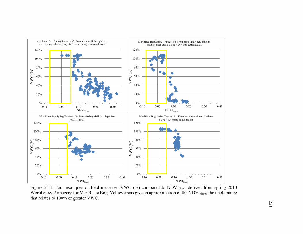
221
Figure 5.31. Four examples of field measured VWC (%) compared to NDVIGreen derived from spring 2010 WorldView-2 imagery for Mer Bleue Bog. Yellow areas give an approximation of the NDVIGreen threshold range that relates to 100% or greater VWC.
0%
20%
40%
60%
80%
100%
120%
-0.10 0.00 0.10 0.20 0.30 0.40
VW
C (%
)
NDVIGreen
Mer Bleue Bog Spring Transect #6: From shrubby field (no slope) into cattail marsh
0%
20%
40%
60%
80%
100%
120%
-0.10 0.00 0.10 0.20 0.30
VW
C (%
)
NDVIGreen
Mer Bleue Bog Spring Transect #3: From open field through birch stand through shrubs (very shallow/no slope) into cattail marsh
0%
20%
40%
60%
80%
100%
120%
-0.10 0.00 0.10 0.20 0.30 0.40
VW
C (%
)
NDVIGreen
Mer Bleue Bog Spring Transect #4: From open sandy field through shrubby birch stand (slope > 20°) into cattail marsh
0%
20%
40%
60%
80%
100%
120%
-0.10 0.00 0.10 0.20 0.30 0.40
VW
C (%
)
NDVIGreen
Mer Bleue Bog Spring Transect #8: From less dense shrubs (shallow slope (<15°)) into cattail marsh
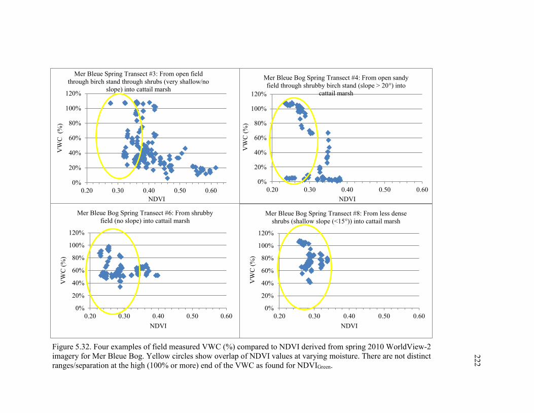
222
0%
20%
40%
60%
80%
100%
120%
0.20 0.30 0.40 0.50 0.60
VW
C (
%)
NDVI
Mer Bleue Spring Transect #3: From open field through birch stand through shrubs (very shallow/no
slope) into cattail marsh
0%
20%
40%
60%
80%
100%
120%
0.20 0.30 0.40 0.50 0.60
VW
C (%
)
NDVI
Mer Bleue Bog Spring Transect #4: From open sandy field through shrubby birch stand (slope > 20°) into
cattail marsh
0%
20%
40%
60%
80%
100%
120%
0.20 0.30 0.40 0.50 0.60
VW
C (%
)
NDVI
Mer Bleue Bog Spring Transect #6: From shrubby field (no slope) into cattail marsh
0%
20%
40%
60%
80%
100%
120%
0.20 0.30 0.40 0.50 0.60
VW
C (%
)
NDVI
Mer Bleue Bog Spring Transect #8: From less dense shrubs (shallow slope (<15°)) into cattail marsh
Figure 5.32. Four examples of field measured VWC (%) compared to NDVI derived from spring 2010 WorldView-2 imagery for Mer Bleue Bog. Yellow circles show overlap of NDVI values at varying moisture. There are not distinct ranges/separation at the high (100% or more) end of the VWC as found for NDVIGreen.
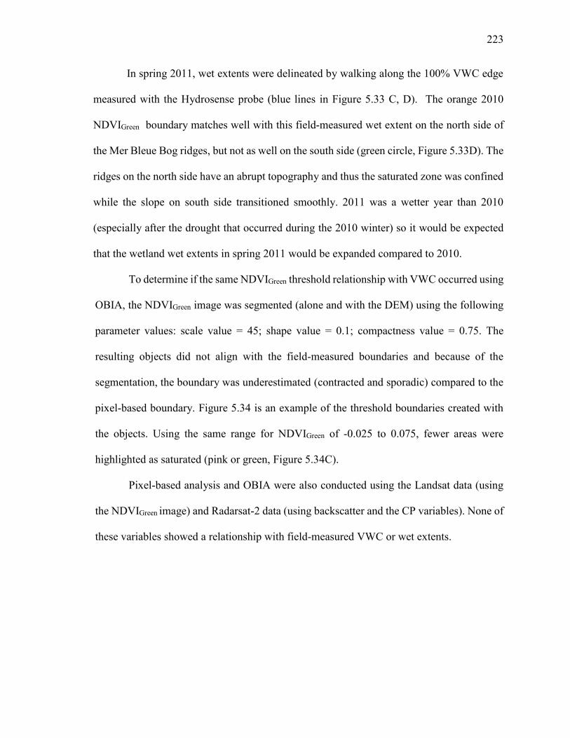
223
In spring 2011, wet extents were delineated by walking along the 100% VWC edge
measured with the Hydrosense probe (blue lines in Figure 5.33 C, D). The orange 2010
NDVIGreen boundary matches well with this field-measured wet extent on the north side of
the Mer Bleue Bog ridges, but not as well on the south side (green circle, Figure 5.33D). The
ridges on the north side have an abrupt topography and thus the saturated zone was confined
while the slope on south side transitioned smoothly. 2011 was a wetter year than 2010
(especially after the drought that occurred during the 2010 winter) so it would be expected
that the wetland wet extents in spring 2011 would be expanded compared to 2010.
To determine if the same NDVIGreen threshold relationship with VWC occurred using
OBIA, the NDVIGreen image was segmented (alone and with the DEM) using the following
parameter values: scale value = 45; shape value = 0.1; compactness value = 0.75. The
resulting objects did not align with the field-measured boundaries and because of the
segmentation, the boundary was underestimated (contracted and sporadic) compared to the
pixel-based boundary. Figure 5.34 is an example of the threshold boundaries created with
the objects. Using the same range for NDVIGreen of -0.025 to 0.075, fewer areas were
highlighted as saturated (pink or green, Figure 5.34C).
Pixel-based analysis and OBIA were also conducted using the Landsat data (using
the NDVIGreen image) and Radarsat-2 data (using backscatter and the CP variables). None of
these variables showed a relationship with field-measured VWC or wet extents.
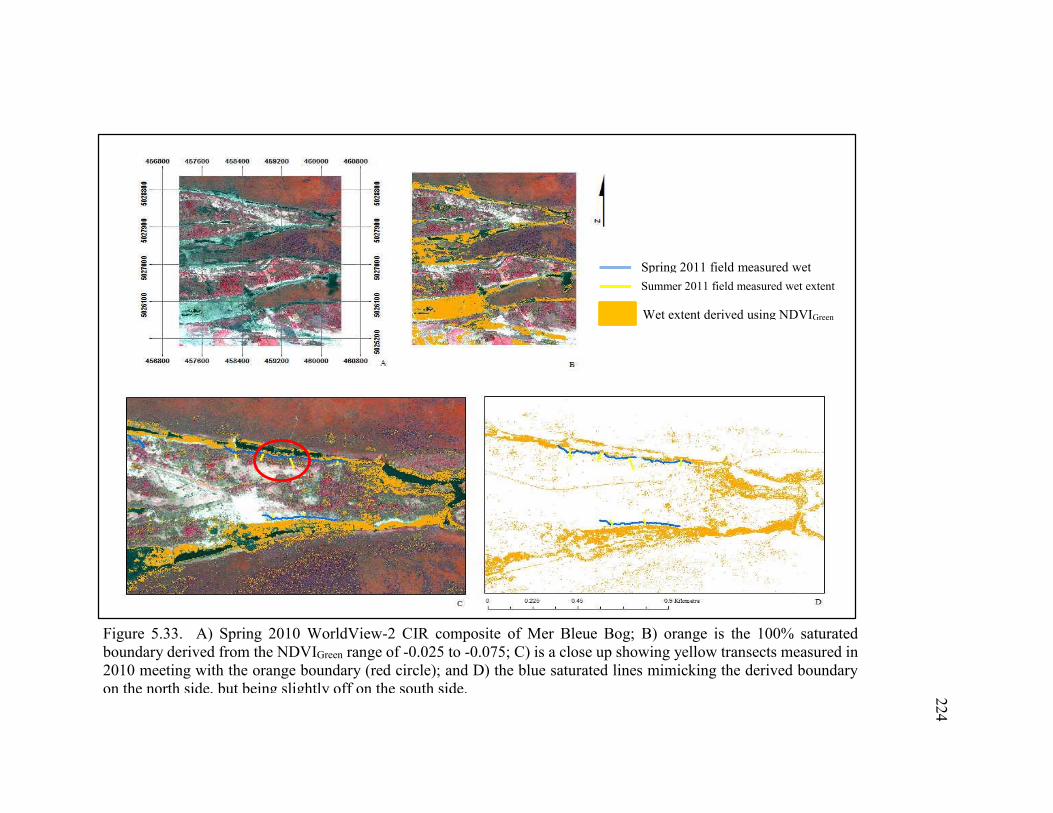
224
Figure 5.33. A) Spring 2010 WorldView-2 CIR composite of Mer Bleue Bog; B) orange is the 100% saturated boundary derived from the NDVIGreen range of -0.025 to -0.075; C) is a close up showing yellow transects measured in 2010 meeting with the orange boundary (red circle); and D) the blue saturated lines mimicking the derived boundary on the north side, but being slightly off on the south side.
Spring 2011 field measured wet Summer 2011 field measured wet extent
Wet extent derived using NDVIGreen
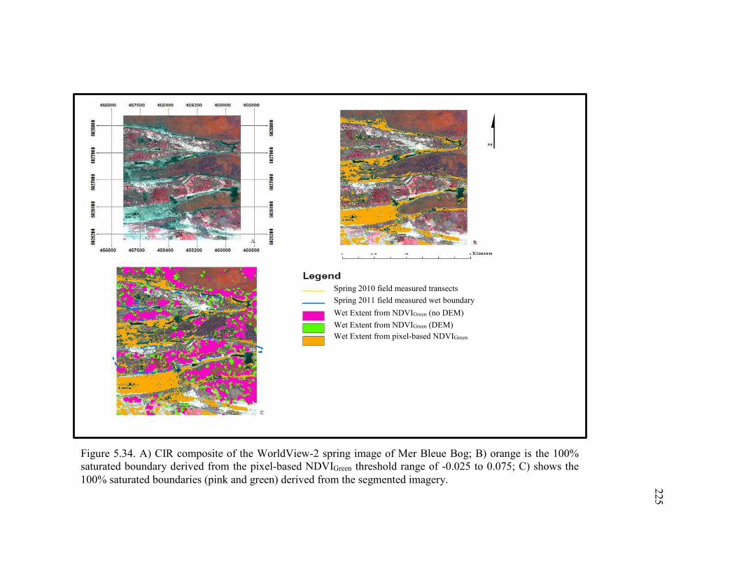
225
Figure 5.34. A) CIR composite of the WorldView-2 spring image of Mer Bleue Bog; B) orange is the 100% saturated boundary derived from the pixel-based NDVIGreen threshold range of -0.025 to 0.075; C) shows the 100% saturated boundaries (pink and green) derived from the segmented imagery.
Spring 2010 field measured transects Spring 2011 field measured wet boundary Wet Extent from NDVIGreen (no DEM) Wet Extent from NDVIGreen (DEM) Wet Extent from pixel-based NDVIGreen
226
226
5.4.2 Summary of main findings for Inundation Extent
From amongst 14 vegetation indices evaluated, spring NDVIGreen corresponded best
with VWC (%), and in particular, it showed a consistent range of values related to
wet extents;
Pixel-based processing was better than OBIA, which lost and underestimated
boundary detail; and
Landsat 5 TM and Radarsat-2 data derived variables did not show relationships with
spring VWC (%).
5.5 GIS analysis of derived imagery and existing LIO layers for selected OWES
attributes
5.5.1 Number of Wetland Types
The Number of Wetland Types determined from the spring WorldView-2
OBIA/CTA classification maps is listed in Table 5.18 for each of the study sites. For Loch
Garry, the same Number of Wetland Types were assessed with both methods, however, there
was a difference in Wetland Type as Bog was assessed during the 1985 OWES field
evaluation and Fen was assessed in 2010 for this research based on observations in the field
of fen vegetation (Section 3.1).
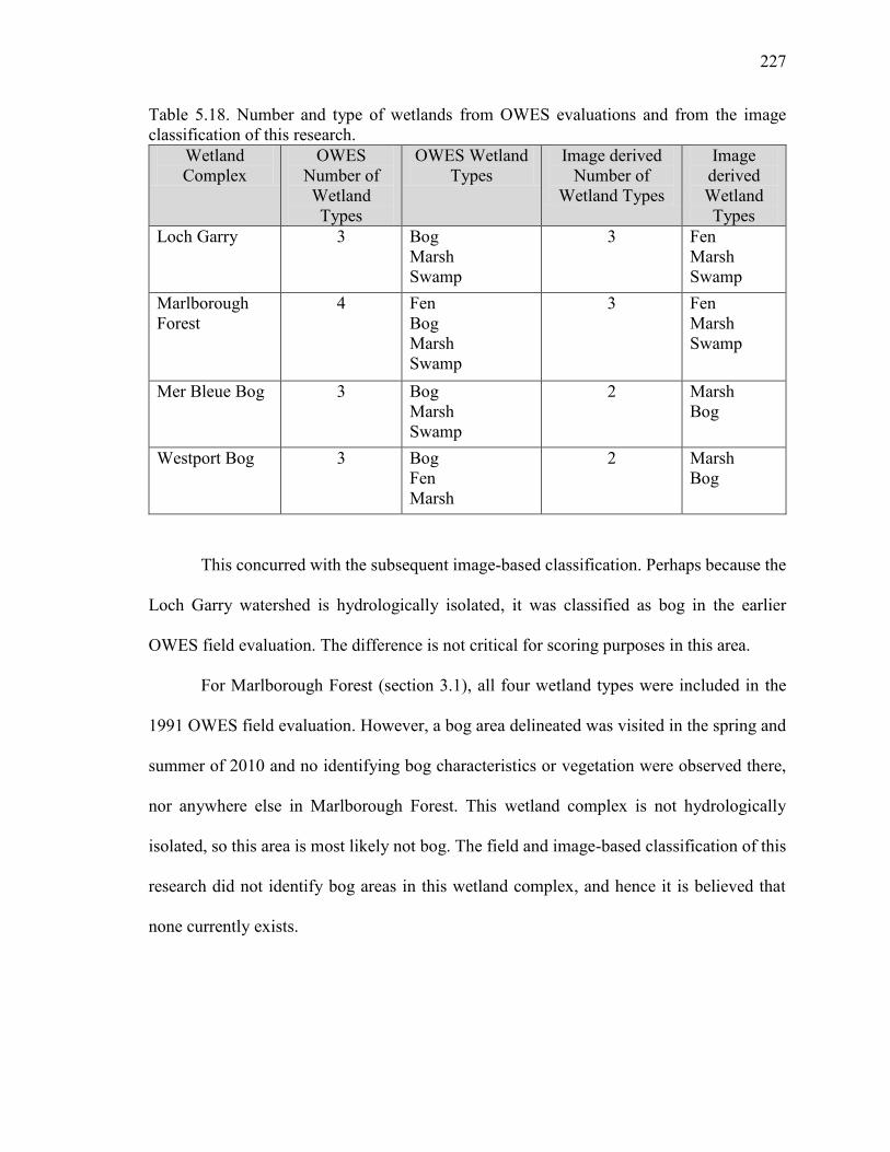
227
227
Table 5.18. Number and type of wetlands from OWES evaluations and from the image classification of this research.
Wetland Complex
OWES Number of Wetland Types
OWES Wetland Types
Image derived Number of
Wetland Types
Image derived Wetland Types
Loch Garry 3 Bog Marsh Swamp
3 Fen Marsh Swamp
Marlborough Forest
4 Fen Bog Marsh Swamp
3 Fen Marsh Swamp
Mer Bleue Bog 3 Bog Marsh Swamp
2 Marsh Bog
Westport Bog 3 Bog Fen Marsh
2 Marsh Bog
This concurred with the subsequent image-based classification. Perhaps because the
Loch Garry watershed is hydrologically isolated, it was classified as bog in the earlier
OWES field evaluation. The difference is not critical for scoring purposes in this area.
For Marlborough Forest (section 3.1), all four wetland types were included in the
1991 OWES field evaluation. However, a bog area delineated was visited in the spring and
summer of 2010 and no identifying bog characteristics or vegetation were observed there,
nor anywhere else in Marlborough Forest. This wetland complex is not hydrologically
isolated, so this area is most likely not bog. The field and image-based classification of this
research did not identify bog areas in this wetland complex, and hence it is believed that
none currently exists.
228
228
For Mer Bleue Bog, the 1983 OWES evaluation includes Swamp, whereas the field
observations and image-based classifications of this research did not identify Swamp. These
results concur with others in this well-studied wetland complex (see Baghdadi et al., 2001;
Touzi et al., 2007; Millard and Richardson, 2013).
For Westport Bog, the 1983 OWES field evaluations included fen while fen
characteristics and vegetation were not observed in the field, nor classified from imagery
during this research.
The OWES field evaluations were completed by expert investigators on the dates
listed in Table 3.1. There were no investigations during the spring; nor was there a repeat
visit the following year as in this research. For determining Wetland Type, there should not
be any limitations by visiting the field in the summer only. Additionally, the field evaluators
may have had hydrological information (e.g. the confusion between bog and fen at Loch
Garry). However, the surveys of the vegetation present in Loch Garry were completed in
field in 2010 and 2011 with fully illustrated guide books. What would need to be determined
is whether or not the presence of fen-indicator species would indicate Fen OR if the overall
general hydrologic condition of the area would supersede the vegetation present and
indicates Bog.
5.5.2 Diversity of Surrounding Habitat
Table 5.19 lists the results from assessing the surrounding habitat in a buffer of 1,500
m around each of the four wetland complexes. This was completed using the 2011 AAFC
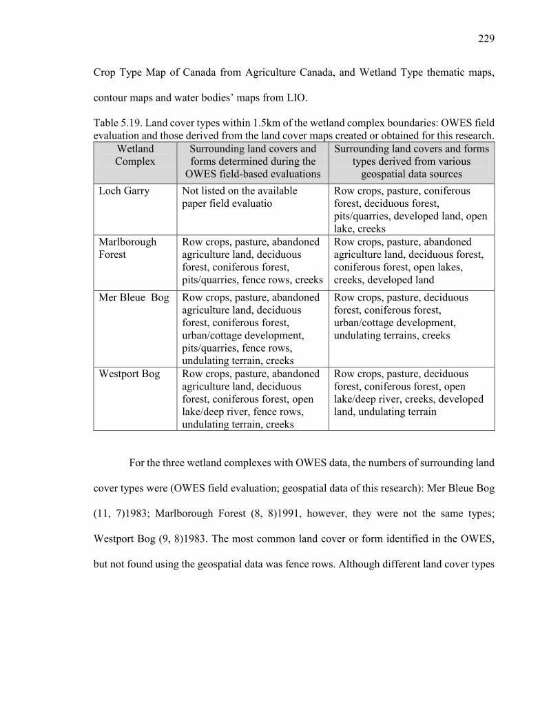
229
229
Crop Type Map of Canada from Agriculture Canada, and Wetland Type thematic maps,
contour maps and water bodies’ maps from LIO.
Table 5.19. Land cover types within 1.5km of the wetland complex boundaries: OWES field evaluation and those derived from the land cover maps created or obtained for this research.
Wetland Complex
Surrounding land covers and forms determined during the
OWES field-based evaluations
Surrounding land covers and forms types derived from various
geospatial data sources Loch Garry Not listed on the available
paper field evaluatio Row crops, pasture, coniferous forest, deciduous forest, pits/quarries, developed land, open lake, creeks
Marlborough Forest
Row crops, pasture, abandoned agriculture land, deciduous forest, coniferous forest, pits/quarries, fence rows, creeks
Row crops, pasture, abandoned agriculture land, deciduous forest, coniferous forest, open lakes, creeks, developed land
Mer Bleue Bog Row crops, pasture, abandoned agriculture land, deciduous forest, coniferous forest, urban/cottage development, pits/quarries, fence rows, undulating terrain, creeks
Row crops, pasture, deciduous forest, coniferous forest, urban/cottage development, undulating terrains, creeks
Westport Bog Row crops, pasture, abandoned agriculture land, deciduous forest, coniferous forest, open lake/deep river, fence rows, undulating terrain, creeks
Row crops, pasture, deciduous forest, coniferous forest, open lake/deep river, creeks, developed land, undulating terrain
For the three wetland complexes with OWES data, the numbers of surrounding land
cover types were (OWES field evaluation; geospatial data of this research): Mer Bleue Bog
(11, 7)1983; Marlborough Forest (8, 8)1991, however, they were not the same types;
Westport Bog (9, 8)1983. The most common land cover or form identified in the OWES,
but not found using the geospatial data was fence rows. Although different land cover types
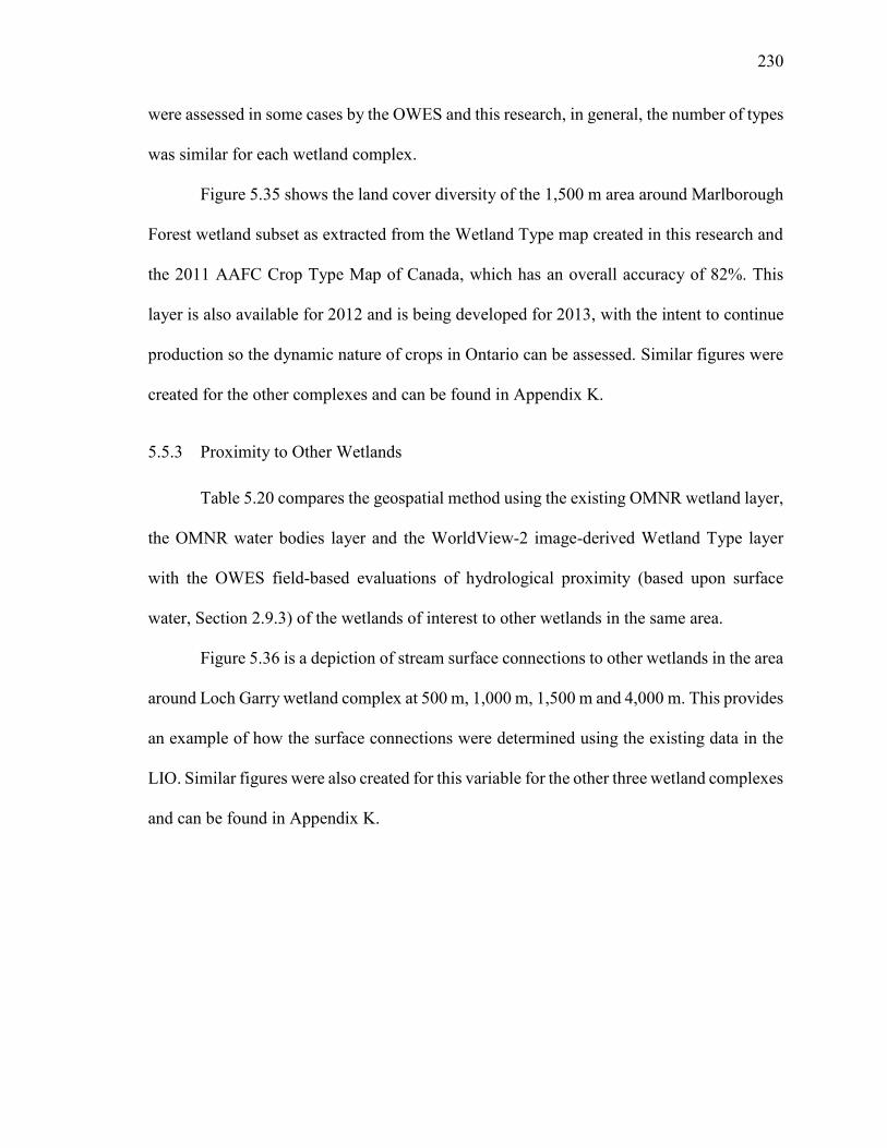
230
230
were assessed in some cases by the OWES and this research, in general, the number of types
was similar for each wetland complex.
Figure 5.35 shows the land cover diversity of the 1,500 m area around Marlborough
Forest wetland subset as extracted from the Wetland Type map created in this research and
the 2011 AAFC Crop Type Map of Canada, which has an overall accuracy of 82%. This
layer is also available for 2012 and is being developed for 2013, with the intent to continue
production so the dynamic nature of crops in Ontario can be assessed. Similar figures were
created for the other complexes and can be found in Appendix K.
5.5.3 Proximity to Other Wetlands
Table 5.20 compares the geospatial method using the existing OMNR wetland layer,
the OMNR water bodies layer and the WorldView-2 image-derived Wetland Type layer
with the OWES field-based evaluations of hydrological proximity (based upon surface
water, Section 2.9.3) of the wetlands of interest to other wetlands in the same area.
Figure 5.36 is a depiction of stream surface connections to other wetlands in the area
around Loch Garry wetland complex at 500 m, 1,000 m, 1,500 m and 4,000 m. This provides
an example of how the surface connections were determined using the existing data in the
LIO. Similar figures were also created for this variable for the other three wetland complexes
and can be found in Appendix K.
231
231
Table 5.20. Hydrological Proximity to Other Wetlands as measured during the OWES evaluation and derived from geospatial data.
Wetland Complex
Proximity to Other Wetlands: OWES field-based evaluation
Proximity to Other Wetlands: image derived method
Loch Garry No indication in field based documentation
Hydrologically connected by surface water to other wetlands (different dominant type), or to open lake or deep river within 1.5 m.
Marlborough Forest
Hydrologically connected by surface water to other wetlands (same dominant type) within 0.5km
Hydrologically connect by surface water to other wetlands (same dominant type) within 0.5km
Mer Bleue Bog No wetland within 1.5 km No wetland within 1 km
Westport Bog Hydrologically connected by surface water to other wetlands (different dominant type) or open water within 1.5 km
Hydrologically connected by surface water to other wetlands (different dominant Wetland Type), or open lake or deep river within 1.5 km.
Figure 5.35. The Diversity of Surrounding Habitat surrounding the Marlborough Forest wetland subset (black boundary). The data layers include the WorldView-2 image derived Wetland Type layer, the 2011 AAFC Crop Type Map of Canada (2011); the OMNR water bodies layer, and the OMNR contour layer.
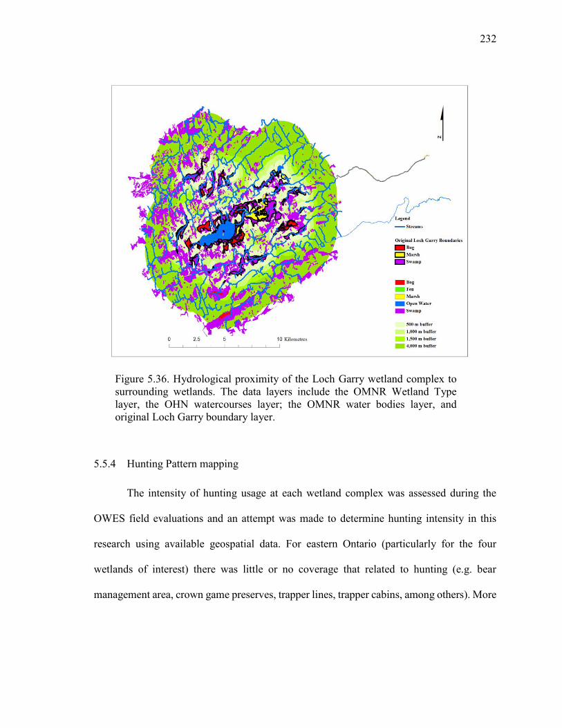
232
232
5.5.4 Hunting Pattern mapping
The intensity of hunting usage at each wetland complex was assessed during the
OWES field evaluations and an attempt was made to determine hunting intensity in this
research using available geospatial data. For eastern Ontario (particularly for the four
wetlands of interest) there was little or no coverage that related to hunting (e.g. bear
management area, crown game preserves, trapper lines, trapper cabins, among others). More
Figure 5.36. Hydrological proximity of the Loch Garry wetland complex to surrounding wetlands. The data layers include the OMNR Wetland Type layer, the OHN watercourses layer; the OMNR water bodies layer, and original Loch Garry boundary layer.
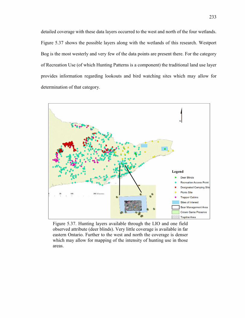
233
233
detailed coverage with these data layers occurred to the west and north of the four wetlands.
Figure 5.37 shows the possible layers along with the wetlands of this research. Westport
Bog is the most westerly and very few of the data points are present there. For the category
of Recreation Use (of which Hunting Patterns is a component) the traditional land use layer
provides information regarding lookouts and bird watching sites which may allow for
determination of that category.
Figure 5.37. Hunting layers available through the LIO and one field observed attribute (deer blinds). Very little coverage is available in far eastern Ontario. Further to the west and north the coverage is denser which may allow for mapping of the intensity of hunting use in those areas.
234
234
5.5.5 Ownership Patterns for the Social category
All of the following data layers from the LIO had no data for the sites of interest in
eastern Ontario: all the conservation layers (including authority and use), cottage residential
area and site, all the crown leased land layers, and the federal land layers. The land
ownership layer does not provide coverage for Loch Garry, Mer Bleue Bog and
Marlborough Forest, but there is partial coverage of Westport Bog, (but only one type of
land ownership (private) and not enough to determine an overall pattern or score for that
area). These layers, once again, may prove useful for mapping of this attribute in other areas
where there is more data coverage. Property parcel layers available from Teranet
(http://www.teranet.ca/, 2013) were examined, but only provide Municipal Property
Assessment Corporation (MPAC) assessment numbers and property address data, which do
not give an indication of ownership. If the type of ownership (e.g. private or crown) is
indicative of particular assessment numbers (e.g. particular number pre-fixes, etc.) then a
determination of private versus public land based upon these might be possible. That
information was not available, but may be at a governmental level.
5.5.6 Wetland area and basin area measurements for Wetland Attenuation Factor
The Wetland Type layer from the LIO was used to calculate the size of the wetland
(in terms of its ability to attenuate floods). As the Wetland Type classifications in this
research were completed on sub-sets of the complexes of interest, these data were not useful
for this method. Therefore, it was necessary to use the existing LIO wetland layer. It was
attempted to assess the size of the catchment basin on the whole, and the portion of the
235
235
catchment basin upstream of the wetland area from the LIO quaternary watershed layer. The
data limitations and required assumptions resulted in this not being suitable for further
investigation with the available data. Data that were required include a wetland basin layer,
and an appropriate catchment basin with the upstream/downstream locations of all wetland
basins located in those catchment layers. Without this data the wetland attenuation factor
cannot be calculated.
5.5.7 Rarity of Wetlands and Rarity in Landscape for the Special Feature category
The rarity of a given Wetland Type and its rarity within the landscape are dependent
upon the location of the wetland, the ecodistrict in which it is located, and the individual
wetland’s proportions to the overall wetland area. The four wetland complexes fall within
three ecodistricts (5E-11, 6E-11, and 6E-12). For two of the districts (6E-11, and 6E-12)
which include Loch Garry, Mer Bleue Bog and Marlborough Forest, wetlands are common.
The rarity of each type of wetland within these ecodistricts indicates that fen and bog are the
rarest, and marsh is slightly rare, while Swamp is common. Ecodistrict 5E-11 is listed in the
Northern OWES Manual and includes Westport Bog (although it is the southernmost study
site of this research). Marsh is not considered rare at this site; Fen is the rarest and Swamp
and Bog are equally and moderately rare.
236
236
5.5.8 Summary of main findings of the GIS analysis of maps created in this research and existing LIO layers for OWES attributes
It was possible to use existing LIO thematic layers and a Land Cover/Wetland Type
map created in this research to derive the Number of Wetland Types, Diversity of
Surrounding Land Covers, Proximity of Surrounding Wetlands, and Rarity of
Wetlands and Rarity in the Landscape;
Due to lack of appropriate data, it was not possible to use existing LIO thematic
layers to assess Ownership Pattern or Hunting Pattern for the wetlands of this
research. However, existing data for other areas in southern Ontario may make this
possible; and
It was not possible to assess Wetland Attenuation Factor because of a lack of existing
basin data.
Objective 2 Results: Compare OWES attribute scores and scores derived from the geo-spatial data of this research
5.6 Comparative analyses of wetland attribute scores derived from geo-spatial data,
and OWES scores
As entire wetland complexes were not assessed using the image based analysis (only
a subset), some of the comparisons to the field scores are skewed. In some cases the existing
OMNR wetland layer is used. The following section relates the attributes derived in this
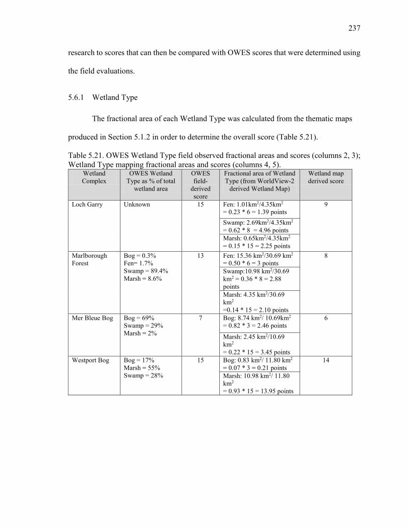
237
237
research to scores that can then be compared with OWES scores that were determined using
the field evaluations.
5.6.1 Wetland Type
The fractional area of each Wetland Type was calculated from the thematic maps
produced in Section 5.1.2 in order to determine the overall score (Table 5.21).
Table 5.21. OWES Wetland Type field observed fractional areas and scores (columns 2, 3); Wetland Type mapping fractional areas and scores (columns 4, 5).
Wetland Complex
OWES Wetland Type as % of total
wetland area
OWES field-
derived score
Fractional area of Wetland Type (from WorldView-2
derived Wetland Map)
Wetland map derived score
Loch Garry Unknown 15 Fen: 1.01km2/4.35km2
= 0.23 * 6 = 1.39 points 9
Swamp: 2.69km2/4.35km2
= 0.62 * 8 = 4.96 points Marsh: 0.65km2/4.35km2
= 0.15 * 15 = 2.25 points Marlborough Forest
Bog = 0.3% Fen= 1.7% Swamp = 89.4% Marsh = 8.6%
13 Fen: 15.36 km2/30.69 km2 = 0.50 * 6 = 3 points
8
Swamp:10.98 km2/30.69 km2 = 0.36 * 8 = 2.88 points Marsh: 4.35 km2/30.69 km2
=0.14 * 15 = 2.10 points Mer Bleue Bog Bog = 69%
Swamp = 29% Marsh = 2%
7
Bog: 8.74 km2/ 10.69km2
= 0.82 * 3 = 2.46 points 6
Marsh: 2.45 km2/10.69 km2 = 0.22 * 15 = 3.45 points
Westport Bog Bog = 17% Marsh = 55% Swamp = 28%
15 Bog: 0.83 km2/ 11.80 km2
= 0.07 * 3 = 0.21 points 14
Marsh: 10.98 km2/ 11.80 km2 = 0.93 * 15 = 13.95 points
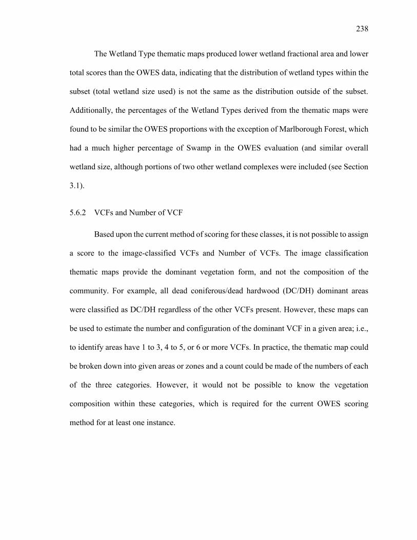
238
238
The Wetland Type thematic maps produced lower wetland fractional area and lower
total scores than the OWES data, indicating that the distribution of wetland types within the
subset (total wetland size used) is not the same as the distribution outside of the subset.
Additionally, the percentages of the Wetland Types derived from the thematic maps were
found to be similar the OWES proportions with the exception of Marlborough Forest, which
had a much higher percentage of Swamp in the OWES evaluation (and similar overall
wetland size, although portions of two other wetland complexes were included (see Section
3.1).
5.6.2 VCFs and Number of VCF
Based upon the current method of scoring for these classes, it is not possible to assign
a score to the image-classified VCFs and Number of VCFs. The image classification
thematic maps provide the dominant vegetation form, and not the composition of the
community. For example, all dead coniferous/dead hardwood (DC/DH) dominant areas
were classified as DC/DH regardless of the other VCFs present. However, these maps can
be used to estimate the number and configuration of the dominant VCF in a given area; i.e.,
to identify areas have 1 to 3, 4 to 5, or 6 or more VCFs. In practice, the thematic map could
be broken down into given areas or zones and a count could be made of the numbers of each
of the three categories. However, it would not be possible to know the vegetation
composition within these categories, which is required for the current OWES scoring
method for at least one instance.
239
239
5.6.3 Open Water Type
Table 5.22 provides the results of the scores for Open Water Type. In general, the
scores derived from the image classified thematic maps were higher than those for the
OWES field evaluations. Only one wetland complex, Mer Bleue Bog, had the same water
type (Type 1, less than 5% of the area is open water) assessed using both methods. The water
types assessed for this research were confirmed in the field and with reference imagery.
Additionally, the spring field work completed in this research may have enabled a better
survey of the Open Water Types present compared to summer, when the OWES field
evaluations were completed. In summer, some water may have dried up or vegetation may
have obscured certain water bodies (e.g. ponding (type 5); open water (types 2 and 4)),
particularly if viewed from an oblique angle in the field.
Table 5.22. Scores derived for Open Water Types were based upon the image-derived thematic map and compared to those listed in the OWES field evaluations. See Section 2.9.3 for type descriptions.
Wetland Complex
OWES Open Water Type
OWES Open Water Type
score
Image- derived
dominant Open Water
Type
Image-derived Open Water Type
score
Loch Garry Type 4 20 Type 5 30 Marlborough Forest
Type 3 14 Type 5 30
Mer Bleue Bog Type 1 8 Type 1 8 Westport Bog Type 3 14 Type 4 20
5.6.4 Number of Wetland Types
The OWES score for the Number of Wetland Types was compared to that found
using the derived Wetland Type thematic maps (Table 5.23). In general, the geospatially
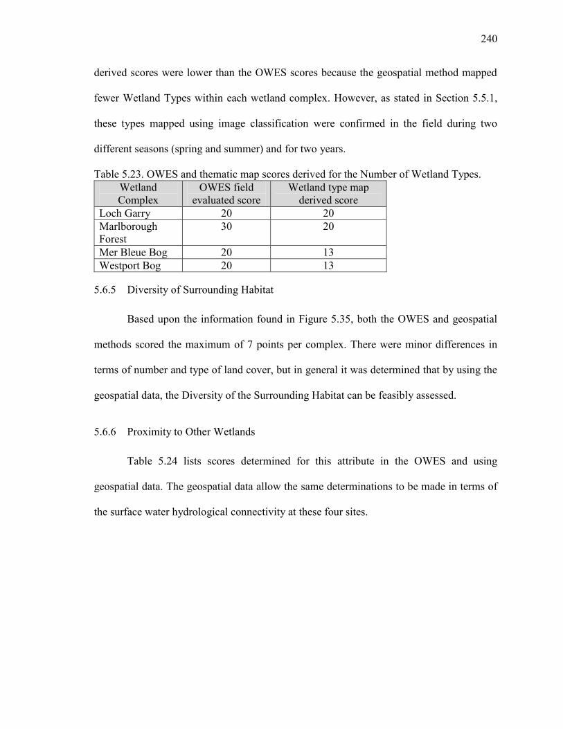
240
240
derived scores were lower than the OWES scores because the geospatial method mapped
fewer Wetland Types within each wetland complex. However, as stated in Section 5.5.1,
these types mapped using image classification were confirmed in the field during two
different seasons (spring and summer) and for two years.
Table 5.23. OWES and thematic map scores derived for the Number of Wetland Types. Wetland Complex
OWES field evaluated score
Wetland type map derived score
Loch Garry 20 20 Marlborough Forest
30 20
Mer Bleue Bog 20 13 Westport Bog 20 13
5.6.5 Diversity of Surrounding Habitat
Based upon the information found in Figure 5.35, both the OWES and geospatial
methods scored the maximum of 7 points per complex. There were minor differences in
terms of number and type of land cover, but in general it was determined that by using the
geospatial data, the Diversity of the Surrounding Habitat can be feasibly assessed.
5.6.6 Proximity to Other Wetlands
Table 5.24 lists scores determined for this attribute in the OWES and using
geospatial data. The geospatial data allow the same determinations to be made in terms of
the surface water hydrological connectivity at these four sites.
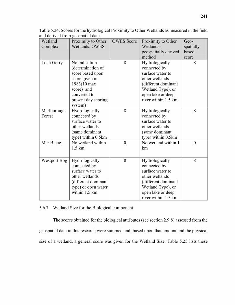
241
241
Table 5.24. Scores for the hydrological Proximity to Other Wetlands as measured in the field and derived from geospatial data. Wetland Complex
Proximity to Other Wetlands: OWES
OWES Score Proximity to Other Wetlands: geospatially derived method
Geo-spatially-based score
Loch Garry No indication (determination of score based upon score given in 1983(10 max score) and converted to present day scoring system)
8 Hydrologically connected by surface water to other wetlands (different dominant Wetland Type), or open lake or deep river within 1.5 km.
8
Marlborough Forest
Hydrologically connected by surface water to other wetlands (same dominant type) within 0.5km
8 Hydrologically connected by surface water to other wetlands (same dominant type) within 0.5km
8
Mer Bleue No wetland within 1.5 km
0 No wetland within 1 km
0
Westport Bog Hydrologically connected by surface water to other wetlands (different dominant type) or open water within 1.5 km
8 Hydrologically connected by surface water to other wetlands (different dominant Wetland Type), or open lake or deep river within 1.5 km.
8
5.6.7 Wetland Size for the Biological component
The scores obtained for the biological attributes (see section 2.9.8) assessed from the
geospatial data in this research were summed and, based upon that amount and the physical
size of a wetland, a general score was given for the Wetland Size. Table 5.25 lists these
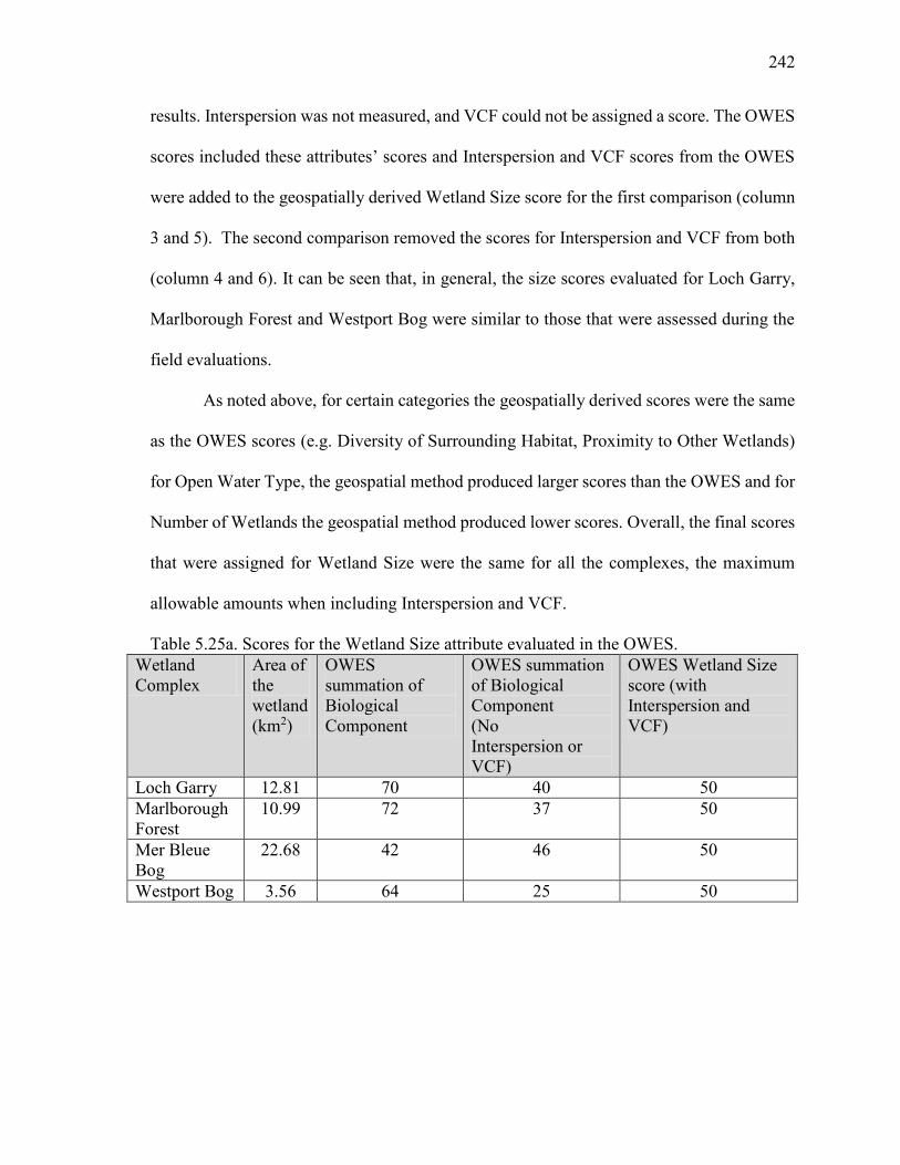
242
242
results. Interspersion was not measured, and VCF could not be assigned a score. The OWES
scores included these attributes’ scores and Interspersion and VCF scores from the OWES
were added to the geospatially derived Wetland Size score for the first comparison (column
3 and 5). The second comparison removed the scores for Interspersion and VCF from both
(column 4 and 6). It can be seen that, in general, the size scores evaluated for Loch Garry,
Marlborough Forest and Westport Bog were similar to those that were assessed during the
field evaluations.
As noted above, for certain categories the geospatially derived scores were the same
as the OWES scores (e.g. Diversity of Surrounding Habitat, Proximity to Other Wetlands)
for Open Water Type, the geospatial method produced larger scores than the OWES and for
Number of Wetlands the geospatial method produced lower scores. Overall, the final scores
that were assigned for Wetland Size were the same for all the complexes, the maximum
allowable amounts when including Interspersion and VCF.
Table 5.25a. Scores for the Wetland Size attribute evaluated in the OWES. Wetland Complex
Area of the wetland (km2)
OWES summation of Biological Component
OWES summation of Biological Component (No Interspersion or VCF)
OWES Wetland Size score (with Interspersion and VCF)
Loch Garry 12.81 70 40 50 Marlborough Forest
10.99 72 37 50
Mer Bleue Bog
22.68 42 46 50
Westport Bog 3.56 64 25 50
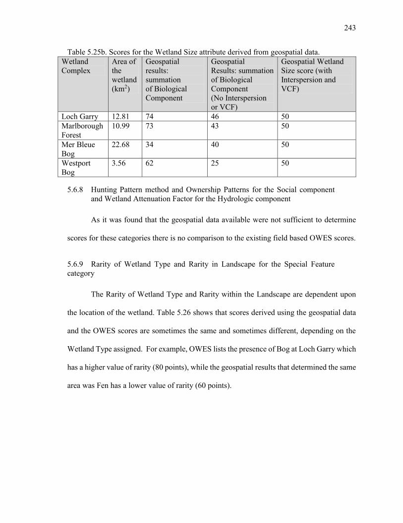
243
243
Table 5.25b. Scores for the Wetland Size attribute derived from geospatial data. Wetland Complex
Area of the wetland (km2)
Geospatial results: summation of Biological Component
Geospatial Results: summation of Biological Component (No Interspersion or VCF)
Geospatial Wetland Size score (with Interspersion and VCF)
Loch Garry 12.81 74 46 50 Marlborough Forest
10.99 73 43 50
Mer Bleue Bog
22.68 34 40 50
Westport Bog
3.56 62 25 50
5.6.8 Hunting Pattern method and Ownership Patterns for the Social component and Wetland Attenuation Factor for the Hydrologic component
As it was found that the geospatial data available were not sufficient to determine
scores for these categories there is no comparison to the existing field based OWES scores.
5.6.9 Rarity of Wetland Type and Rarity in Landscape for the Special Feature category
The Rarity of Wetland Type and Rarity within the Landscape are dependent upon
the location of the wetland. Table 5.26 shows that scores derived using the geospatial data
and the OWES scores are sometimes the same and sometimes different, depending on the
Wetland Type assigned. For example, OWES lists the presence of Bog at Loch Garry which
has a higher value of rarity (80 points), while the geospatial results that determined the same
area was Fen has a lower value of rarity (60 points).
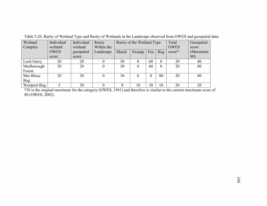
244
Table 5.26. Rarity of Wetland Type and Rarity of Wetlands in the Landscape observed from OWES and geospatial data.
*20 is the original maximum for the category (OWES, 1981) and therefore is similar to the current maximum score of 80 (OWES, 2002).
Wetland Complex
Individual wetland OWES score
Individual wetland geospatial score
Rarity Within the Landscape
Rarity of the Wetland Type Total OWES score*
Geospatial score (Maximum 80)
Marsh Swamp Fen Bog
Loch Garry 20 20 0 30 0 60 0 20 80 Marlborough Forest
20 20 0 30 0 60 0 20 80
Mer Bleue Bog
20 20 0 30 0 0 80 20 80
Westport Bog 5 30 0 0 10 30 10 20 20
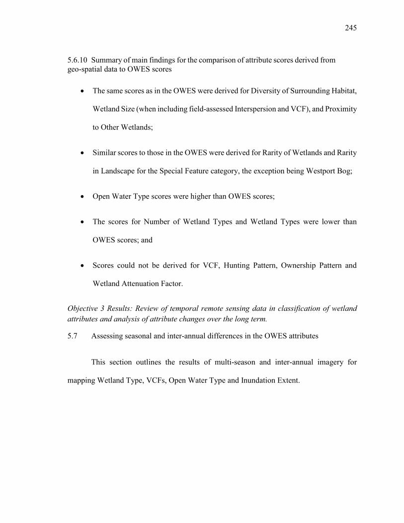
245
5.6.10 Summary of main findings for the comparison of attribute scores derived from geo-spatial data to OWES scores
The same scores as in the OWES were derived for Diversity of Surrounding Habitat,
Wetland Size (when including field-assessed Interspersion and VCF), and Proximity
to Other Wetlands;
Similar scores to those in the OWES were derived for Rarity of Wetlands and Rarity
in Landscape for the Special Feature category, the exception being Westport Bog;
Open Water Type scores were higher than OWES scores;
The scores for Number of Wetland Types and Wetland Types were lower than
OWES scores; and
Scores could not be derived for VCF, Hunting Pattern, Ownership Pattern and
Wetland Attenuation Factor.
Objective 3 Results: Review of temporal remote sensing data in classification of wetland attributes and analysis of attribute changes over the long term.
5.7 Assessing seasonal and inter-annual differences in the OWES attributes
This section outlines the results of multi-season and inter-annual imagery for
mapping Wetland Type, VCFs, Open Water Type and Inundation Extent.
246
5.7.1 Temporal analysis for Wetland Type
The same segmentation parameter values found to be optimal for the spring imagery
were also found to be optimal for the summer and fall imagery: scale value = 45; shape value
= 0.1; and compactness value= 0.75. Table 5.27 summarizes the object-based (imagery and
DEM) CTA results for the four sites using the segmented summer imagery, and the
combined two-season and three season results for Mer Bleue Bog. Using summer imagery,
the overall classification accuracy for two sites (Mer Bleue Bog and Marlborough Forest)
increased over that achieved using spring imagery (73.2% to 80.0%, and 70.0% to 75%,
respectively). For the other two sites (Loch Garry and Westport Bog) the overall
classification accuracy using summer imagery decreased (86.5% to 70.3% and 72.5% to
68.8%, respectively). For both of these classifications, water accuracies (both UA and PA)
declined. The Loch Garry summer imagery water bodies show specular reflectance (see
Figure 5.38A) and at Westport Bog (Figure 5.38B) the water bodies which were clear and
dark in spring had vegetation cover in summer. These conditions could be responsible for
the decline in the water class accuracies and, for the Loch Garry classification, general
confusion amongst all classes.
247
Using summer imagery instead of spring imagery, accuracies for Fen were lower for
Loch Garry and higher for Marlborough Forest. Accuracies for Bog were generally higher,
while for Swamp, they were the same or lower, and for Marsh they were lower at all four
sites. Utilizing a combination of spring and summer imagery in segmentation and
classification did not increase the overall accuracies for three of the four sites. Only Mer
Bleue Bog improved overall, but the Tall Bog class UA was lower (62.5% for summer
imagery alone compared to 54.6% for spring plus summer). Using a combination of three
seasons of images (spring, summer and fall) at Mer Bleue Bog did not significantly
(statistically) change the overall classification accuracies from those for the spring-summer
combination.
Figure 5.38. WorldView-2 CIR composites of A) Loch Garry in the summer showing specular reflectance of water and B) Westport Bog with vegetation present (yellow circles).
0 1.5 30.75 Kilometres0 1 20.5 Kilometres
A B
248
Figure 5.39 is a comparison between the spring, summer and combined spring-
summer Wetland Type maps for Mer Bleue Bog. Areas of illogical class assignment are
found on all three maps (black circles). As outlined in Figure 5.39B (summer) there are areas
of excessive water which were not present in the field, and erroneously classified areas of
Marsh located within the Bog. For Figure 5.39C (spring and summer) there is a large portion
of Upland assigned where Tall Bog (treed bog) was observed in the field. Overall, there is
more Upland classified in areas of Bog on the combined season map than for either the
spring or summer maps; the overall accuracy is higher for the combined imagery but there
are large erroneously classified areas.
The same segmentation parameter values found to be optimal for the spring imagery
were also found to be optimal for the summer and fall imagery: scale value = 2; shape value
= 0.1; and compactness value= 0.1. The highest accuracy results for the spring Landsat TM
5 spring classifications were achieved using the 5 EM fraction maps (various combinations
of segmented and not segmented imagery, plus/minus DEM), and these were initially
assessed for summer imagery. Poor results for these data required further processing of the
other data inputs (3 EM fraction maps, and original band data, plus/minus DEM). Table 5.28
lists the overall accuracies for: the best spring result, the summer result using the same
configuration of data as spring and the best summer result.
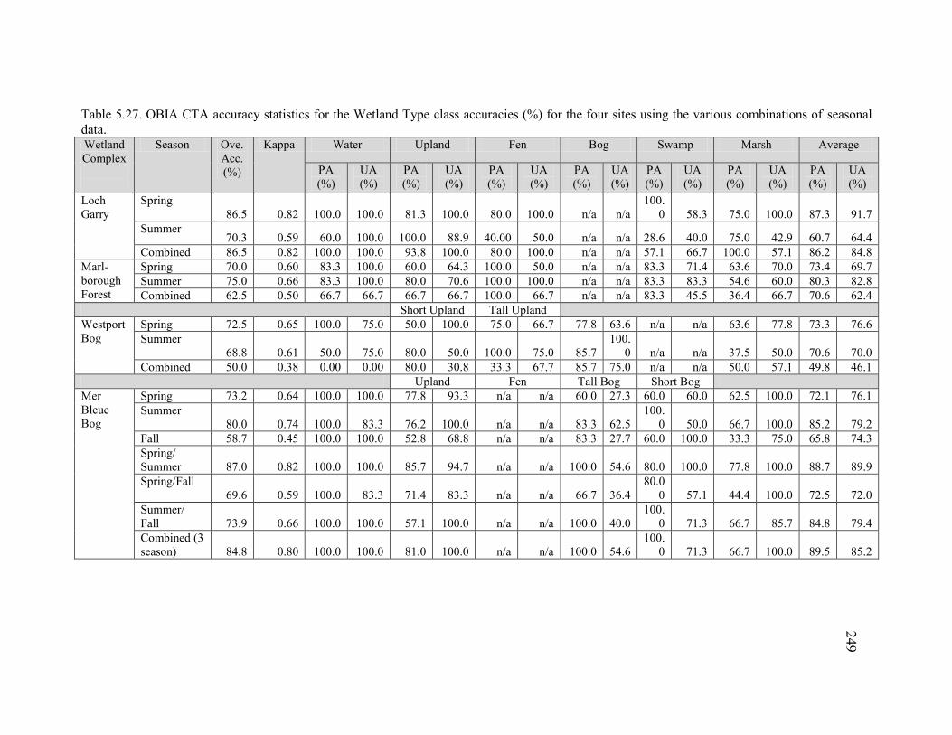
249
Table 5.27. OBIA CTA accuracy statistics for the Wetland Type class accuracies (%) for the four sites using the various combinations of seasonal data. Wetland Complex
Season Ove.Acc. (%)
Kappa Water Upland Fen Bog Swamp Marsh Average
PA (%)
UA (%)
PA (%)
UA (%)
PA (%)
UA (%)
PA (%)
UA (%)
PA (%)
UA (%)
PA (%)
UA (%)
PA (%)
UA (%)
Loch Garry
Spring 86.5 0.82 100.0 100.0 81.3 100.0 80.0 100.0 n/a n/a
100.0 58.3 75.0 100.0 87.3 91.7
Summer 70.3 0.59 60.0 100.0 100.0 88.9 40.00 50.0 n/a n/a 28.6 40.0 75.0 42.9 60.7 64.4
Combined 86.5 0.82 100.0 100.0 93.8 100.0 80.0 100.0 n/a n/a 57.1 66.7 100.0 57.1 86.2 84.8 Marl-borough Forest
Spring 70.0 0.60 83.3 100.0 60.0 64.3 100.0 50.0 n/a n/a 83.3 71.4 63.6 70.0 73.4 69.7 Summer 75.0 0.66 83.3 100.0 80.0 70.6 100.0 100.0 n/a n/a 83.3 83.3 54.6 60.0 80.3 82.8 Combined 62.5 0.50 66.7 66.7 66.7 66.7 100.0 66.7 n/a n/a 83.3 45.5 36.4 66.7 70.6 62.4
Short Upland Tall Upland Westport Bog
Spring 72.5 0.65 100.0 75.0 50.0 100.0 75.0 66.7 77.8 63.6 n/a n/a 63.6 77.8 73.3 76.6 Summer
68.8 0.61 50.0 75.0 80.0 50.0 100.0 75.0 85.7 100.
0 n/a n/a 37.5 50.0 70.6 70.0 Combined 50.0 0.38 0.00 0.00 80.0 30.8 33.3 67.7 85.7 75.0 n/a n/a 50.0 57.1 49.8 46.1
Upland Fen Tall Bog Short Bog Mer Bleue Bog
Spring 73.2 0.64 100.0 100.0 77.8 93.3 n/a n/a 60.0 27.3 60.0 60.0 62.5 100.0 72.1 76.1 Summer
80.0 0.74 100.0 83.3 76.2 100.0 n/a n/a 83.3 62.5 100.
0 50.0 66.7 100.0 85.2 79.2 Fall 58.7 0.45 100.0 100.0 52.8 68.8 n/a n/a 83.3 27.7 60.0 100.0 33.3 75.0 65.8 74.3 Spring/ Summer 87.0 0.82 100.0 100.0 85.7 94.7 n/a n/a 100.0 54.6 80.0 100.0 77.8 100.0 88.7 89.9 Spring/Fall
69.6 0.59 100.0 83.3 71.4 83.3 n/a n/a 66.7 36.4 80.0
0 57.1 44.4 100.0 72.5 72.0 Summer/ Fall 73.9 0.66 100.0 100.0 57.1 100.0 n/a n/a 100.0 40.0
100.0 71.3 66.7 85.7 84.8 79.4
Combined (3 season) 84.8 0.80 100.0 100.0 81.0 100.0 n/a n/a 100.0 54.6
100.0 71.3 66.7 100.0 89.5 85.2
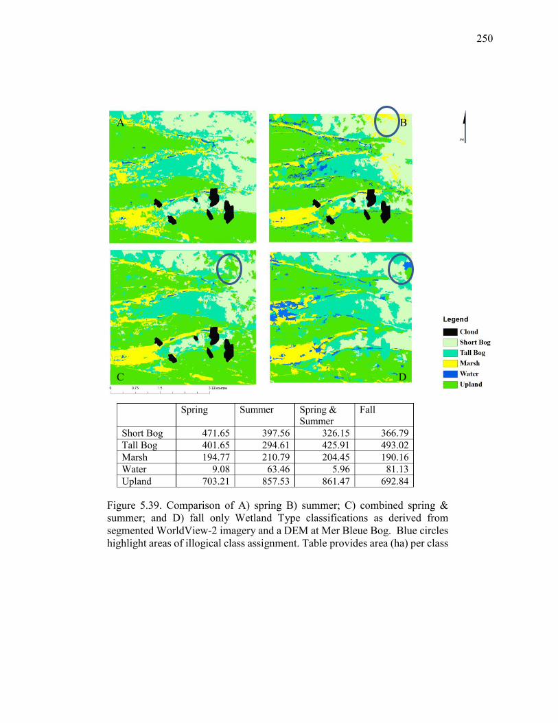
250
B A
C D
Spring Summer Spring & Summer
Fall
Short Bog 471.65 397.56 326.15 366.79 Tall Bog 401.65 294.61 425.91 493.02 Marsh 194.77 210.79 204.45 190.16 Water 9.08 63.46 5.96 81.13 Upland 703.21 857.53 861.47 692.84
Figure 5.39. Comparison of A) spring B) summer; C) combined spring & summer; and D) fall only Wetland Type classifications as derived from segmented WorldView-2 imagery and a DEM at Mer Bleue Bog. Blue circles highlight areas of illogical class assignment. Table provides area (ha) per class type.
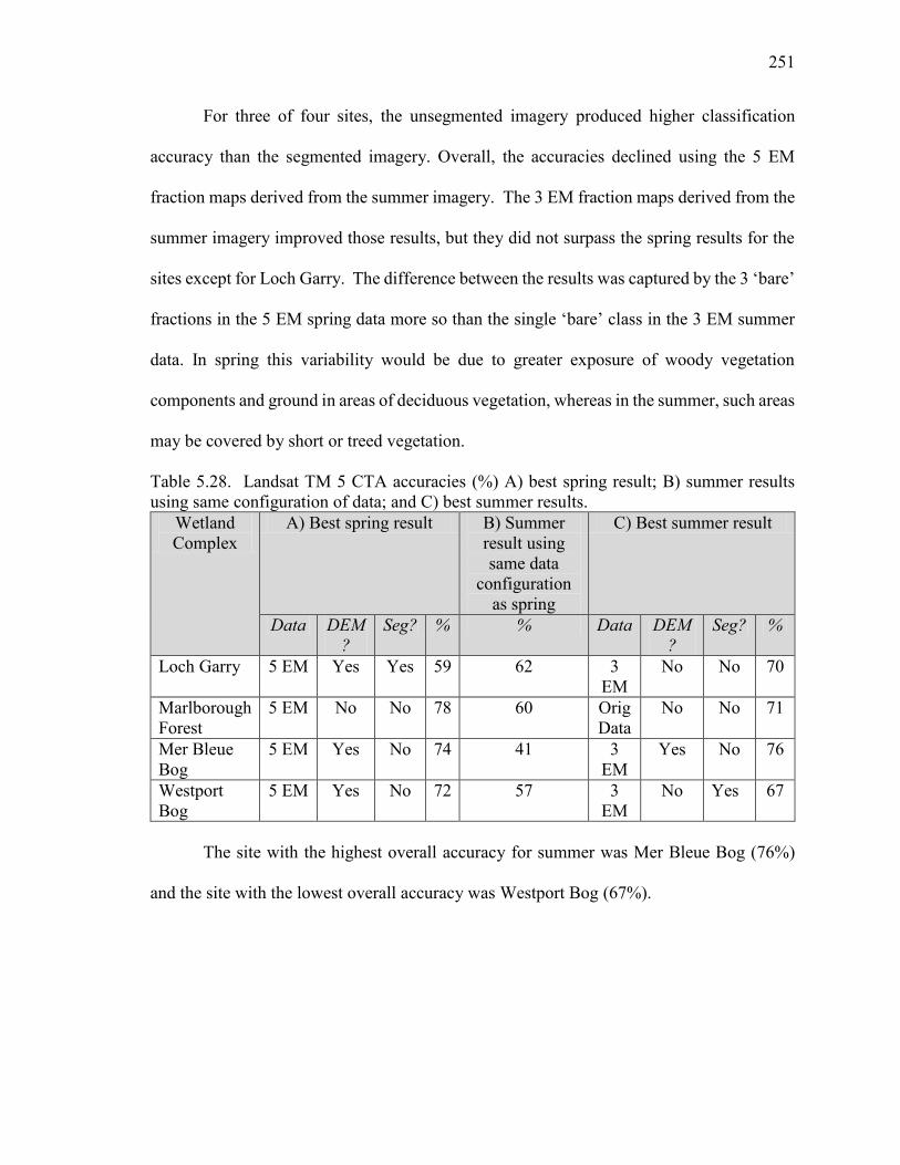
251
For three of four sites, the unsegmented imagery produced higher classification
accuracy than the segmented imagery. Overall, the accuracies declined using the 5 EM
fraction maps derived from the summer imagery. The 3 EM fraction maps derived from the
summer imagery improved those results, but they did not surpass the spring results for the
sites except for Loch Garry. The difference between the results was captured by the 3 ‘bare’
fractions in the 5 EM spring data more so than the single ‘bare’ class in the 3 EM summer
data. In spring this variability would be due to greater exposure of woody vegetation
components and ground in areas of deciduous vegetation, whereas in the summer, such areas
may be covered by short or treed vegetation.
Table 5.28. Landsat TM 5 CTA accuracies (%) A) best spring result; B) summer results using same configuration of data; and C) best summer results.
Wetland Complex
A) Best spring result B) Summer result using same data
configuration as spring
C) Best summer result
Data DEM?
Seg? % % Data DEM?
Seg? %
Loch Garry 5 EM Yes Yes 59 62 3 EM
No No 70
Marlborough Forest
5 EM No No 78 60 Orig Data
No No 71
Mer Bleue Bog
5 EM Yes No 74 41 3 EM
Yes No 76
Westport Bog
5 EM Yes No 72 57 3 EM
No Yes 67
The site with the highest overall accuracy for summer was Mer Bleue Bog (76%)
and the site with the lowest overall accuracy was Westport Bog (67%).
252
The best Marlborough Forest summer classification was produced using the original
band data (no DEM), but its accuracy was not as high as the best spring classification (5EMs,
no DEM). This was different from the WorldView-2 Wetland Type classifications for this
site where overall accuracies were higher for summer data. For Loch Garry, the overall
accuracies were higher in summer while for the WorldView-2 classifications spring
accuracy was higher. Summer accuracy at Mer Bleue Bog and Westport Bog was slightly
lower than spring.
Summary of main findings for temporal analyses for Wetland Type:
WorldView-2 summer imagery produced higher overall classification accuracies for
two of four sites; the remaining two sites’ summer imagery had factors that may
have contributed to the lower accuracies (e.g., specular reflectance and vegetation
growth in water); the poorest class in spring classifications (Marsh), improved
significantly using summer imagery;
Combining multi-season imagery in the segmentation and classification process did
not improve overall accuracies for three of four sites; Mer Bleue Bog classification
accuracies did improve with the combination of two seasons (spring and summer)
of imagery;
Landsat 5 TM summer imagery produced lower overall classification accuracies for
three of four sites; only the accuracy for Loch Garry improved for the summer; and
253
Regardless of season, the best (three out of four for either season) Landsat 5 TM
Wetland Type classifications were pixel-based, produced using unmixed fraction
maps, either with 5 EMs and spring imagery or 3 EMs and summer imagery.
5.7.2 Temporal analyses for VCFs
The optimal parameter values for VCFs were: scale value = 25; shape value = 0.1,
and compactness value = 0.75. Table 5.29 provides the multi-season Worldview-2 CTA
accuracy results for the number of VCF for Mer Bleue Bog (selected because spring,
summer and fall imagery had been acquired for that site). Appendix L contains the accuracy
results for the other 3 sites.
The highest overall accuracy was achieved using the combined summer 2010 and
fall 2011 imagery (74.3%). The lowest overall accuracy (54.3%) was obtained using the
spring 2010 and fall 2011 imagery. For individual seasons, spring provided the highest
overall accuracy (65.7%) while summer produced the lowest overall accuracy (57.1%).
From the multi-season results, it is evident that summer and fall imagery represent a better
combination than spring-summer or spring-fall, even though spring imagery was the best
individually. The error matrices for the summer and fall classifications show similar UA and
PA for all classes (Table 5.30B and C, respectively), while the spring error matrix is different
with more correctly assigned reference samples for Class B; (Table 5.30A). With the
combination of summer and fall, correct class assignment improves for both Classes A and
B over the classifications for either season individually (Table 5.30E). In contrast,
254
combining spring and fall imagery reduced the accuracies of Classes A and B (Table 5.30D)
from the classifications using either season individually.
Low kappa values indicate that for the majority of these classifications were only moderately better
than random class assignment (Congalton and Green, 1995; Foody, 2002). Additionally, the UAs for Class C
for all combinations of data were very low. The spatial variability, and spectral similarity of the forms,
especially in the summer, in the visible to NIR portion of the spectrum contribute to these results. These results
could also be related to the small sample size of the reference and validation data (35 sites in total), and
especially for class C (1 validation site).
Table 5.31 provides the accuracy results for the individual VCF classes for Mer
Bleue Bog using the variety of combinations of seasonal data. Spring imagery produced the
highest overall accuracy (68.8%) while summer imagery produced the lowest (54.3%). This
was not expected as it was thought that unique vegetation signatures would be more apparent
in the summer after a period of vegetation growth. There could be more variability among
the forms in the spring in leaf-off as opposed to summer when vegetation is green and
reflectance similarities in the visible and NIR may be too great. None of the combinations
of seasonal imagery produced higher accuracies than any of the contributing individual
seasons. Appendix L contains the accuracy results for the other 3 sites.
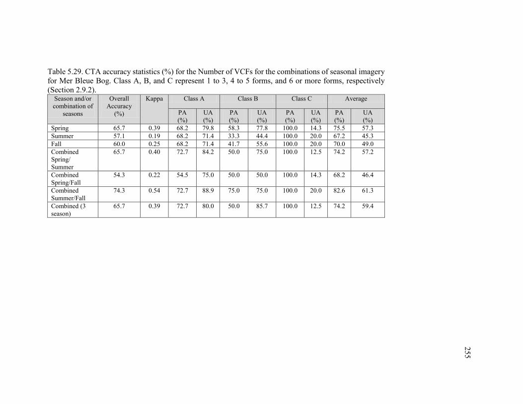
255
Table 5.29. CTA accuracy statistics (%) for the Number of VCFs for the combinations of seasonal imagery for Mer Bleue Bog. Class A, B, and C represent 1 to 3, 4 to 5 forms, and 6 or more forms, respectively (Section 2.9.2).
Season and/or combination of
seasons
Overall Accuracy
(%)
Kappa Class A Class B Class C Average
PA (%)
UA (%)
PA (%)
UA (%)
PA (%)
UA (%)
PA (%)
UA (%)
Spring 65.7 0.39 68.2 79.8 58.3 77.8 100.0 14.3 75.5 57.3 Summer 57.1 0.19 68.2 71.4 33.3 44.4 100.0 20.0 67.2 45.3 Fall 60.0 0.25 68.2 71.4 41.7 55.6 100.0 20.0 70.0 49.0 Combined Spring/ Summer
65.7 0.40 72.7 84.2 50.0 75.0 100.0 12.5 74.2 57.2
Combined Spring/Fall
54.3 0.22 54.5 75.0 50.0 50.0 100.0 14.3 68.2 46.4
Combined Summer/Fall
74.3 0.54 72.7 88.9 75.0 75.0 100.0 20.0 82.6 61.3
Combined (3 season)
65.7 0.39 72.7 80.0 50.0 85.7 100.0 12.5 74.2 59.4
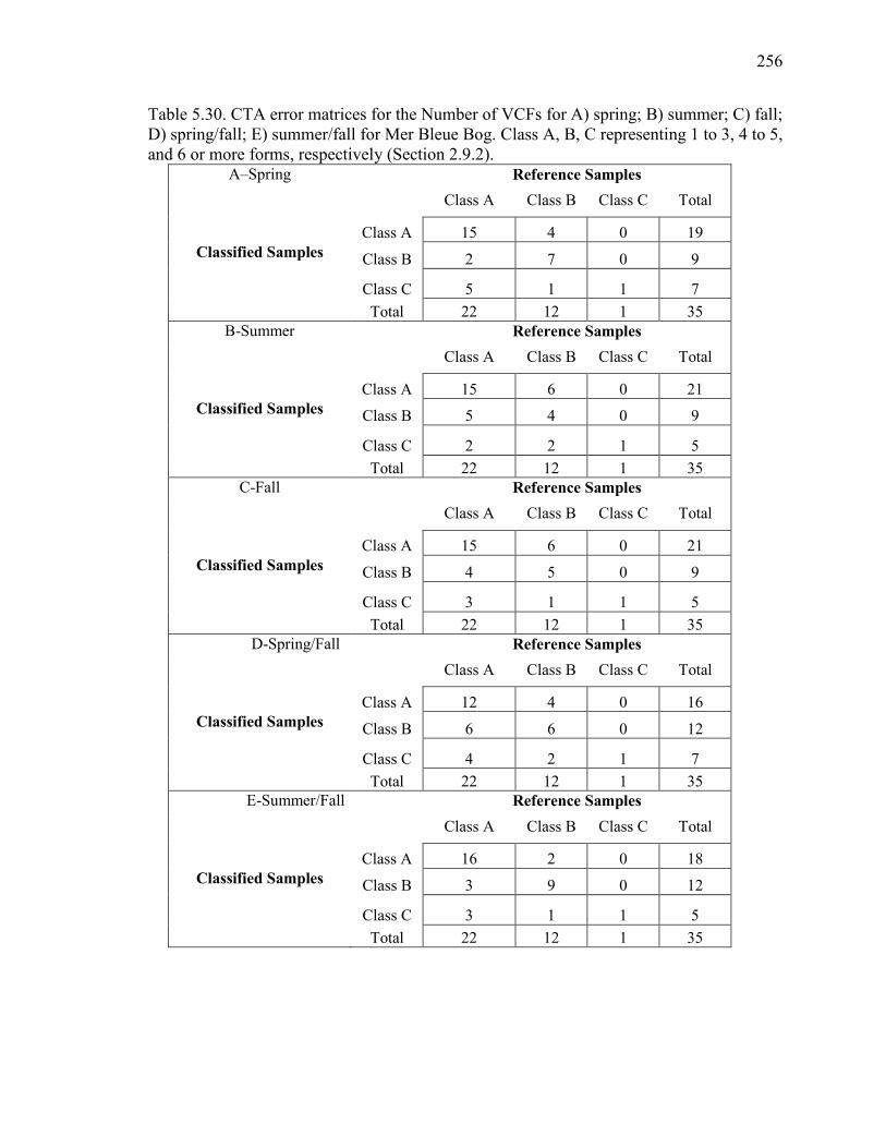
256
Table 5.30. CTA error matrices for the Number of VCFs for A) spring; B) summer; C) fall; D) spring/fall; E) summer/fall for Mer Bleue Bog. Class A, B, C representing 1 to 3, 4 to 5, and 6 or more forms, respectively (Section 2.9.2).
A–Spring Reference Samples Class A Class B Class C Total
Class A 15 4 0 19 Classified Samples Class B 2 7 0 9
Class C 5 1 1 7
Total 22 12 1 35 B-Summer Reference Samples
Class A Class B Class C Total
Class A 15 6 0 21 Classified Samples Class B 5 4 0 9
Class C 2 2 1 5
Total 22 12 1 35 C-Fall Reference Samples
Class A Class B Class C Total
Class A 15 6 0 21 Classified Samples Class B 4 5 0 9
Class C 3 1 1 5
Total 22 12 1 35 D-Spring/Fall Reference Samples
Class A Class B Class C Total
Class A 12 4 0 16 Classified Samples Class B 6 6 0 12
Class C 4 2 1 7
Total 22 12 1 35 E-Summer/Fall Reference Samples
Class A Class B Class C Total
Class A 16 2 0 18 Classified Samples Class B 3 9 0 12
Class C 3 1 1 5
Total 22 12 1 35
257
Summary of main findings for temporal analyses for VCFs:
Using summer WorldView-2 imagery alone for classification of the 3-category
Number of VCF classes or for individual VCFs did not improve overall accuracies
over spring imagery;
Combining summer and fall WorldView-2 imagery improved the accuracies for the
Number of VCF classes by approximately 10%; and
Multi-season WorldView-2 imagery did not improve the overall accuracies of
individual VCF classifications.
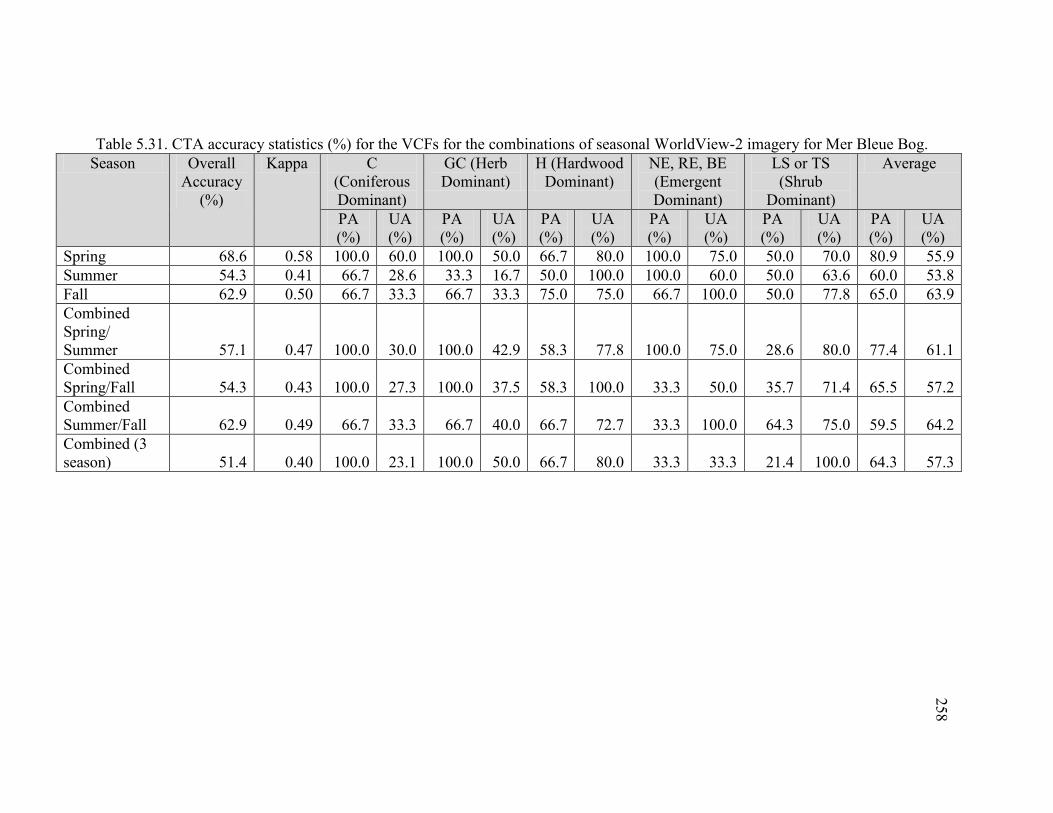
258
Table 5.31. CTA accuracy statistics (%) for the VCFs for the combinations of seasonal WorldView-2 imagery for Mer Bleue Bog. Season Overall
Accuracy (%)
Kappa C (Coniferous Dominant)
GC (Herb Dominant)
H (Hardwood Dominant)
NE, RE, BE (Emergent Dominant)
LS or TS (Shrub
Dominant)
Average
PA (%)
UA (%)
PA (%)
UA (%)
PA (%)
UA (%)
PA (%)
UA (%)
PA (%)
UA (%)
PA (%)
UA (%)
Spring 68.6 0.58 100.0 60.0 100.0 50.0 66.7 80.0 100.0 75.0 50.0 70.0 80.9 55.9 Summer 54.3 0.41 66.7 28.6 33.3 16.7 50.0 100.0 100.0 60.0 50.0 63.6 60.0 53.8 Fall 62.9 0.50 66.7 33.3 66.7 33.3 75.0 75.0 66.7 100.0 50.0 77.8 65.0 63.9 Combined Spring/ Summer 57.1 0.47 100.0 30.0 100.0 42.9 58.3 77.8 100.0 75.0 28.6 80.0 77.4 61.1 Combined Spring/Fall 54.3 0.43 100.0 27.3 100.0 37.5 58.3 100.0 33.3 50.0 35.7 71.4 65.5 57.2 Combined Summer/Fall 62.9 0.49 66.7 33.3 66.7 40.0 66.7 72.7 33.3 100.0 64.3 75.0 59.5 64.2 Combined (3 season) 51.4 0.40 100.0 23.1 100.0 50.0 66.7 80.0 33.3 33.3 21.4 100.0 64.3 57.3
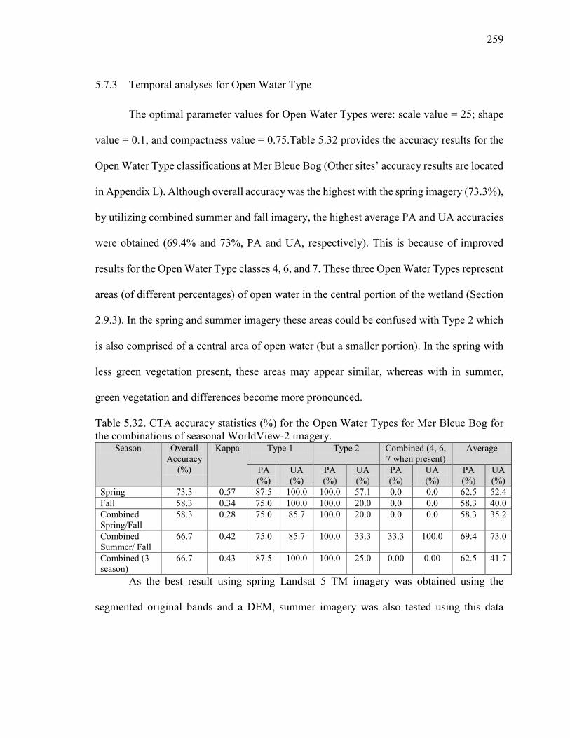
259
5.7.3 Temporal analyses for Open Water Type
The optimal parameter values for Open Water Types were: scale value = 25; shape
value = 0.1, and compactness value = 0.75.Table 5.32 provides the accuracy results for the
Open Water Type classifications at Mer Bleue Bog (Other sites’ accuracy results are located
in Appendix L). Although overall accuracy was the highest with the spring imagery (73.3%),
by utilizing combined summer and fall imagery, the highest average PA and UA accuracies
were obtained (69.4% and 73%, PA and UA, respectively). This is because of improved
results for the Open Water Type classes 4, 6, and 7. These three Open Water Types represent
areas (of different percentages) of open water in the central portion of the wetland (Section
2.9.3). In the spring and summer imagery these areas could be confused with Type 2 which
is also comprised of a central area of open water (but a smaller portion). In the spring with
less green vegetation present, these areas may appear similar, whereas with in summer,
green vegetation and differences become more pronounced.
Table 5.32. CTA accuracy statistics (%) for the Open Water Types for Mer Bleue Bog for the combinations of seasonal WorldView-2 imagery.
As the best result using spring Landsat 5 TM imagery was obtained using the
segmented original bands and a DEM, summer imagery was also tested using this data
Season Overall Accuracy
(%)
Kappa Type 1 Type 2 Combined (4, 6, 7 when present)
Average
PA (%)
UA (%)
PA (%)
UA (%)
PA (%)
UA (%)
PA (%)
UA (%)
Spring 73.3 0.57 87.5 100.0 100.0 57.1 0.0 0.0 62.5 52.4 Fall 58.3 0.34 75.0 100.0 100.0 20.0 0.0 0.0 58.3 40.0 Combined Spring/Fall
58.3 0.28 75.0 85.7 100.0 20.0 0.0 0.0 58.3 35.2
Combined Summer/ Fall
66.7 0.42 75.0 85.7 100.0 33.3 33.3 100.0 69.4 73.0
Combined (3 season)
66.7 0.43 87.5 100.0 100.0 25.0 0.00 0.00 62.5 41.7
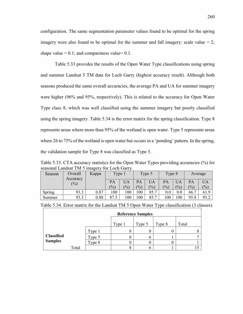
260
configuration. The same segmentation parameter values found to be optimal for the spring
imagery were also found to be optimal for the summer and fall imagery: scale value = 2;
shape value = 0.1; and compactness value= 0.1.
Table 5.33 provides the results of the Open Water Type classifications using spring
and summer Landsat 5 TM data for Loch Garry (highest accuracy result). Although both
seasons produced the same overall accuracies, the average PA and UA for summer imagery
were higher (96% and 95%, respectively). This is related to the accuracy for Open Water
Type class 8, which was well classified using the summer imagery but poorly classified
using the spring imagery. Table 5.34 is the error matrix for the spring classification. Type 8
represents areas where more than 95% of the wetland is open water. Type 5 represents areas
where 26 to 75% of the wetland is open water but occurs in a ‘ponding’ pattern. In the spring,
the validation sample for Type 8 was classified as Type 5.
Table 5.33. CTA accuracy statistics for the Open Water Types providing accuracies (%) for seasonal Landsat TM 5 imagery for Loch Garry.
Season Overall Accuracy
(%)
Kappa Type 1 Type 5 Type 8 Average
PA (%)
UA (%)
PA (%)
UA (%)
PA (%)
UA (%)
PA (%)
UA (%)
Spring 93.3 0.87 100 100 100 85.7 0.0 0.0 66.7 61.9 Summer 93.3 0.88 87.5 100 100 85.7 100 100 95.8 95.2
Table 5.34. Error matrix for the Landsat TM 5 Open Water Type classification (3 classes). Classified Samples
Reference Samples
Type 1 Type 5 Type 8 Total
Type 1 8 0 0 8 Type 5 0 6 1 7 Type 8 0 0 0 1 Total 8 6 1 15
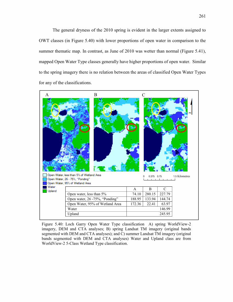
261
The general dryness of the 2010 spring is evident in the larger extents assigned to
OWT classes (in Figure 5.40) with lower proportions of open water in comparison to the
summer thematic map. In contrast, as June of 2010 was wetter than normal (Figure 5.41),
mapped Open Water Type classes generally have higher proportions of open water. Similar
to the spring imagery there is no relation between the areas of classified Open Water Types
for any of the classifications.
A B C
Figure 5.40: Loch Garry Open Water Type classification A) spring WorldView-2 imagery, DEM and CTA analyses; B) spring Landsat TM imagery (original bands segmented with DEM and CTA analyses); and C) summer Landsat TM imagery (original bands segmented with DEM and CTA analyses) Water and Upland class are from WorldView-2 5-Class Wetland Type classification.
A B C Open water, less than 5% 74.10 280.15 227.79 Open water, 26 -75%, “Ponding” 188.95 133.94 144.74 Open Water, 95% of Wetland Area 172.36 22.41 63.97 Water 146.99 Upland 245.95
0 0.75 1.50.375 Kilometres
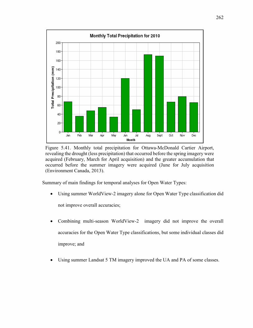
262
Summary of main findings for temporal analyses for Open Water Types:
Using summer WorldView-2 imagery alone for Open Water Type classification did
not improve overall accuracies;
Combining multi-season WorldView-2 imagery did not improve the overall
accuracies for the Open Water Type classifications, but some individual classes did
improve; and
Using summer Landsat 5 TM imagery improved the UA and PA of some classes.
Figure 5.41. Monthly total precipitation for Ottawa-McDonald Cartier Airport, revealing the drought (less precipitation) that occurred before the spring imagery were acquired (February, March for April acquisition) and the greater accumulation that occurred before the summer imagery were acquired (June for July acquisition (Environment Canada, 2013).
263
5.7.4 Temporal analyses for Inundation Extent
Comparison was made of the field measured VWC transects that were completed in
the spring to those completed in the summer of 2010. In general, in spring, 100% VWC
occurred at a greater extent (further upslope) than in summer. This would be expected in a
normal year when spring is wetter than summer, however, this was not expected in 2010,
where spring measurements occurred after a winter drought. In a few cases 100% VWC
occurred further into the wetland in the spring than in summer (e.g. a contracted saturated
boundary), which was expected for 2010. Figure 5.42 provides an example of these different
scenarios. Figure 5.42A is an example of a transect where the wet extent (100% VWC) for
spring expanded past the summer wetland boundary. Figure 5.42B is an example where the
saturated extent in summer was further upslope than in spring. This contracted spring extent
occurred on transects in three marshes (two cattail marshes and one beaver dam marsh) and
the bog example in Figure 5.42B (a lagg). It is believed that these particular features were
influenced by the spring drought of 2010 (see Figure 5.41) and by the influx of precipitation
in June 2010.
Figure 5.43 provides an example of the 2011 field measured wet extents as compared
to the 2010 field measured transects. This example shows that (at the edge of a cattail marsh)
the 2010 spring and summer transects went further into the wetland until 100% VWC was
measured in comparison to the 2011 spring and summer wet extents.
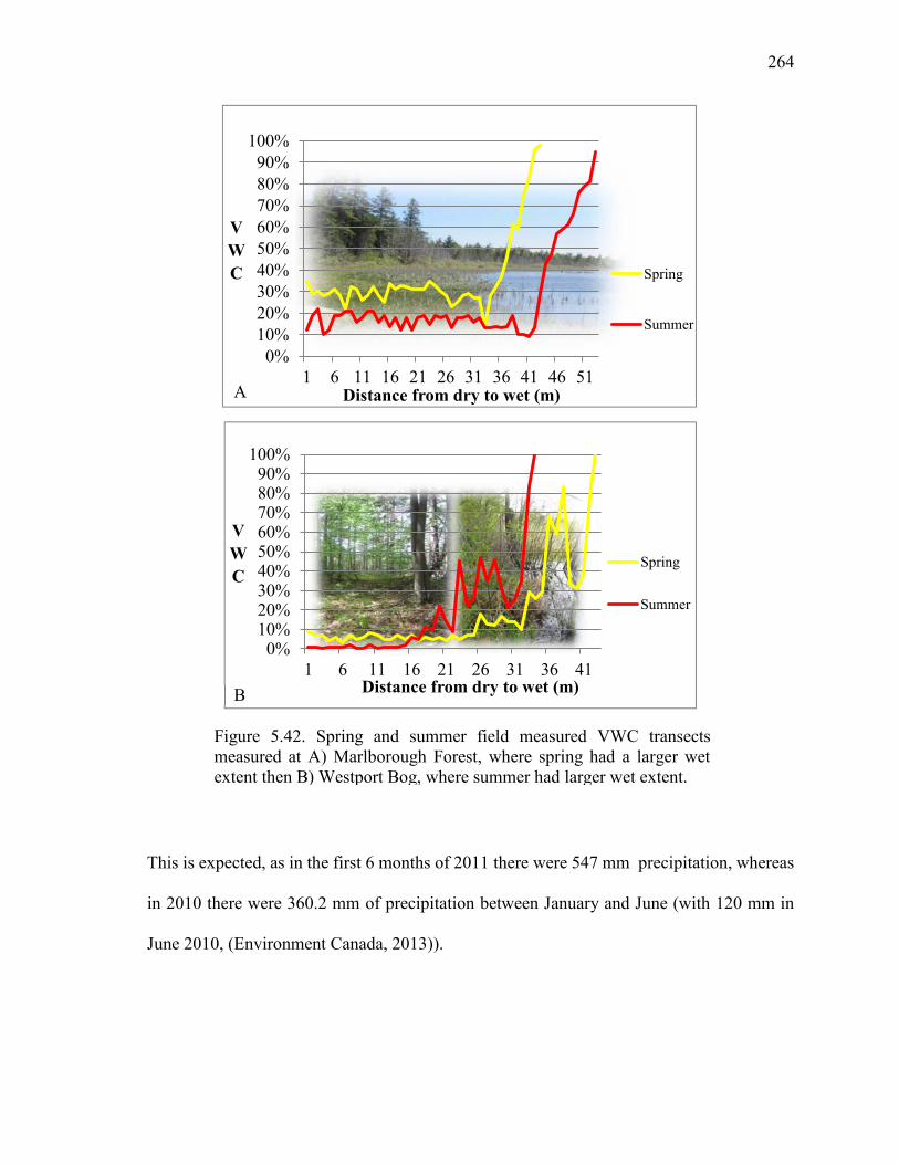
264
This is expected, as in the first 6 months of 2011 there were 547 mm precipitation, whereas
in 2010 there were 360.2 mm of precipitation between January and June (with 120 mm in
June 2010, (Environment Canada, 2013)).
0%10%20%30%40%50%60%70%80%90%
100%
1 6 11 16 21 26 31 36 41 46 51
VWC
Distance from dry to wet (m)
Spring
Summer
0%10%20%30%40%50%60%70%80%90%
100%
1 6 11 16 21 26 31 36 41
VWC
Distance from dry to wet (m)
Spring
Summer
Figure 5.42. Spring and summer field measured VWC transects measured at A) Marlborough Forest, where spring had a larger wet extent then B) Westport Bog, where summer had larger wet extent.
A
B
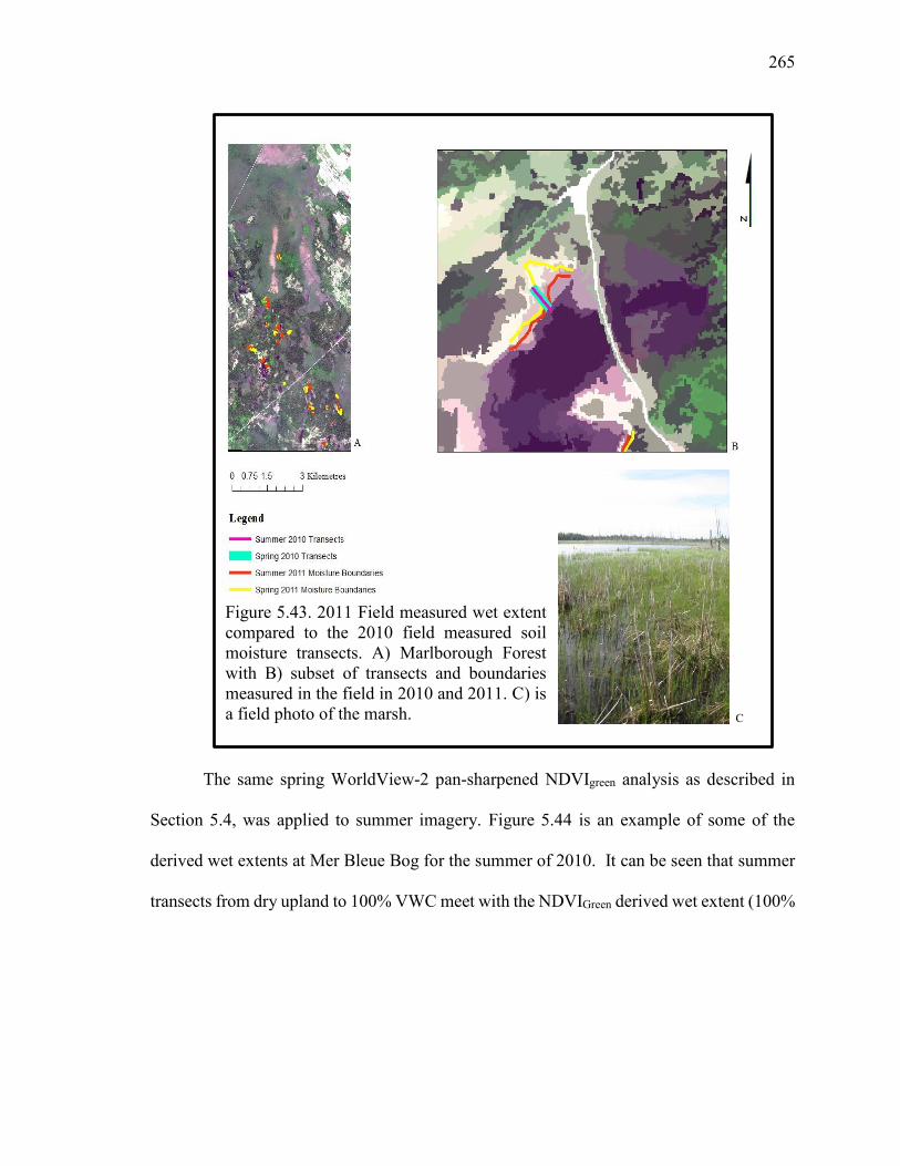
265
The same spring WorldView-2 pan-sharpened NDVIgreen analysis as described in
Section 5.4, was applied to summer imagery. Figure 5.44 is an example of some of the
derived wet extents at Mer Bleue Bog for the summer of 2010. It can be seen that summer
transects from dry upland to 100% VWC meet with the NDVIGreen derived wet extent (100%
Figure 5.43. 2011 Field measured wet extent compared to the 2010 field measured soil moisture transects. A) Marlborough Forest with B) subset of transects and boundaries measured in the field in 2010 and 2011. C) is a field photo of the marsh.
C
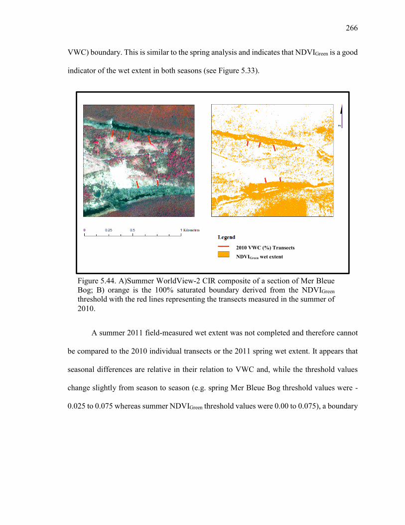
266
VWC) boundary. This is similar to the spring analysis and indicates that NDVIGreen is a good
indicator of the wet extent in both seasons (see Figure 5.33).
A summer 2011 field-measured wet extent was not completed and therefore cannot
be compared to the 2010 individual transects or the 2011 spring wet extent. It appears that
seasonal differences are relative in their relation to VWC and, while the threshold values
change slightly from season to season (e.g. spring Mer Bleue Bog threshold values were -
0.025 to 0.075 whereas summer NDVIGreen threshold values were 0.00 to 0.075), a boundary
Figure 5.44. A)Summer WorldView-2 CIR composite of a section of Mer Bleue Bog; B) orange is the 100% saturated boundary derived from the NDVIGreen threshold with the red lines representing the transects measured in the summer of 2010.
2010 VWC (%) Transects
NDVIGreen wet extent
267
that represents a wetland wet extent can be derived using either spring or summer NDVIGreen
images.
Summary of main findings for temporal analyses for Inundation Extent:
Seasonal and annual differences in wet extent highlighted the need for multiple
season and/or inter-annual mapping of wetlands to determine an overall average
extent for scoring; and
Boundaries representing 100% VWC (a wetland wet extent) were well delineated
using either spring or summer NDVIGreen images derived from WorldView-2
imagery.
5.8 Two-date temporal comparison of fraction maps as an indicator of Anthropogenic
Influence.
Landsat 5 TM imagery acquired on the nearest non-cloudy dates to the original field
based OWES evaluations (Loch Garry and Mer Bleue Bog, 1983; Westport Bog, 1985; and
Marlborough Forest, 1991; see Table 3.1) and the 2010 summer images were converted to
Top-of-Atmosphere (TOA) radiance (Methods section 4.7) and then relatively calibrated
(older image to 2010 image) using PIFs (see Appendix M for calibration details and graphs).
These calibrated images were subsequently unmixed using three and five automatically
selected EMs (Background 2.8.2). The resultant fraction maps were then compared using
RGB image display and simple image differencing.

268
Figure 5.45 provides a visual example of the three fractions derived for Loch Garry
using July 1984 Landsat 5 TM imagery and July 2010 Landsat 5 TM imagery. In Figure
5.45A, there are similarly high vegetation fraction values for both years (light grey/white
areas) in the upland and throughout the wetland complex. There are some small areas (purple
circles) where the vegetation fraction was higher in 2010 than in 1984. These particular areas
are mostly marsh. The total precipitation accumulated until July 2010 was 360.8 mm and
the lake water level was 89.082 m ASL (Environment Canada, 2013; Loch Garry Lake
Association, 2013). The total precipitation accumulated to July 1984 was 450 mm (historic
lake water levels are unavailable). There was more precipitation accumulated to the date of
image acquisition in 1984 than in 2010. It has been found that with an increase in mean
water levels there is often a decrease in above-ground biomass in freshwater marshes
(McKee and Mendelssohn, 1989), although this is not possible to confirm using these data.
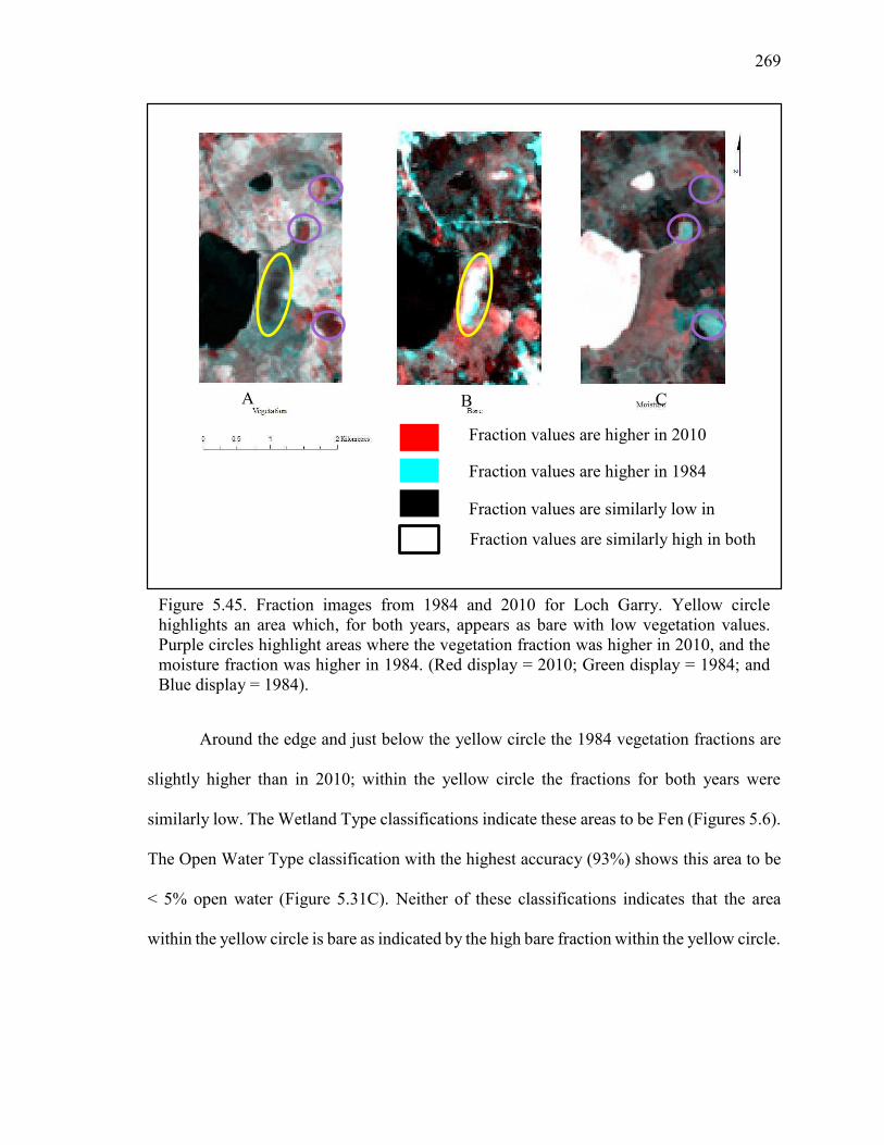
269
Around the edge and just below the yellow circle the 1984 vegetation fractions are
slightly higher than in 2010; within the yellow circle the fractions for both years were
similarly low. The Wetland Type classifications indicate these areas to be Fen (Figures 5.6).
The Open Water Type classification with the highest accuracy (93%) shows this area to be
< 5% open water (Figure 5.31C). Neither of these classifications indicates that the area
within the yellow circle is bare as indicated by the high bare fraction within the yellow circle.
Fraction values are higher in 2010
Fraction values are higher in 1984
Fraction values are similarly low in both years Fraction values are similarly high in both years
Figure 5.45. Fraction images from 1984 and 2010 for Loch Garry. Yellow circle highlights an area which, for both years, appears as bare with low vegetation values. Purple circles highlight areas where the vegetation fraction was higher in 2010, and the moisture fraction was higher in 1984. (Red display = 2010; Green display = 1984; and Blue display = 1984).
A B C
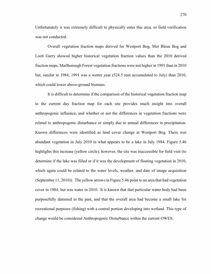
270
Unfortunately it was extremely difficult to physically enter this area, so field verification
was not conducted.
Overall vegetation fraction maps derived for Westport Bog, Mer Bleue Bog and
Loch Garry showed higher historical vegetation fraction values than the 2010 derived
fraction maps. Marlborough Forest vegetation fractions were not higher in 1991 than in 2010
but, similar to 1984, 1991 was a wetter year (524.5 mm accumulated to July) than 2010,
which could lower above-ground biomass.
It is difficult to determine if the comparison of the historical vegetation fraction map
to the current day fraction map for each site provides much insight into overall
anthropogenic influence, and whether or not the differences in vegetation fractions were
related to anthropogenic disturbance or simply due to annual differences in precipitation.
Known differences were identified as land cover change at Westport Bog. There was
abundant vegetation in July 2010 in what appears to be a lake in July 1984. Figure 5.46
highlights this increase (yellow circle); however, the site was inaccessible for field visit (to
determine if the lake was filled or if it was the development of floating vegetation in 2010,
which again could be related to the water levels, weather, and date of image acquisition
(September 11, 2010)). The yellow arrows in Figure 5.46 point to an area that had vegetation
cover in 1984, but was water in 2010. It is known that that particular water body had been
purposefully dammed in the past, and that the overall area had become a small lake for
recreational purposes (fishing) with a central portion developing into wetland. This type of
change would be considered Anthropogenic Disturbance within the current OWES.
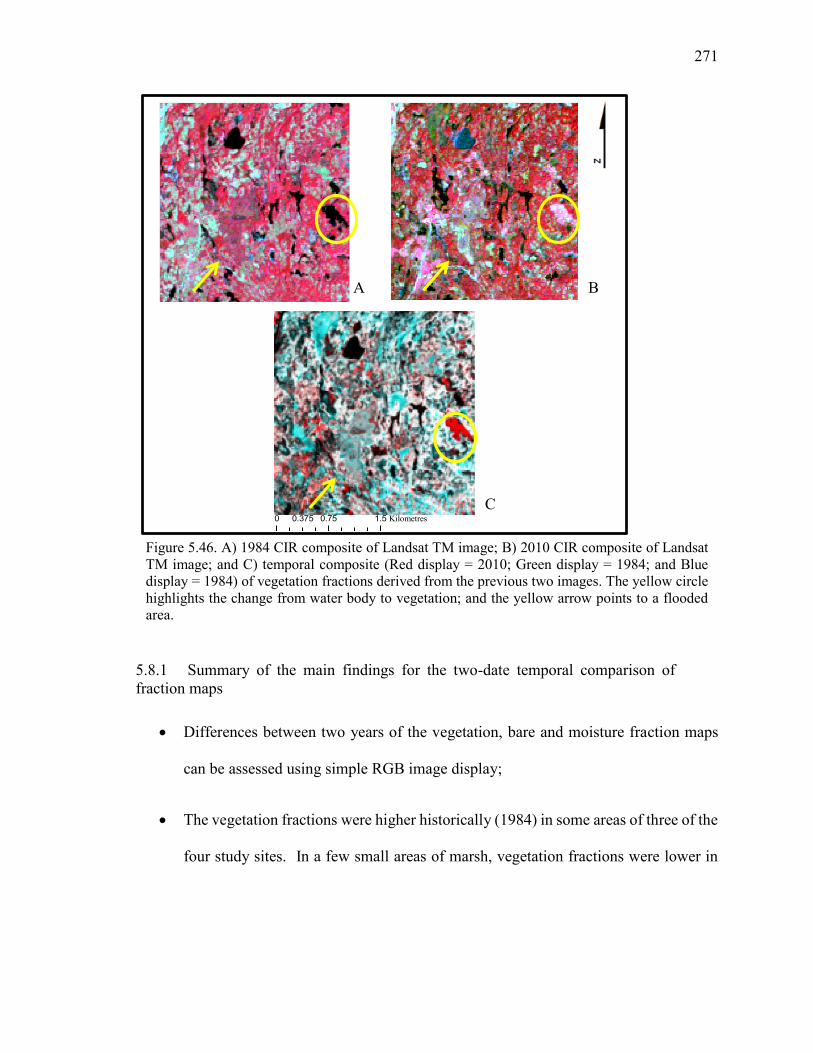
271
5.8.1 Summary of the main findings for the two-date temporal comparison of fraction maps
Differences between two years of the vegetation, bare and moisture fraction maps
can be assessed using simple RGB image display;
The vegetation fractions were higher historically (1984) in some areas of three of the
four study sites. In a few small areas of marsh, vegetation fractions were lower in
A B
C
Figure 5.46. A) 1984 CIR composite of Landsat TM image; B) 2010 CIR composite of Landsat TM image; and C) temporal composite (Red display = 2010; Green display = 1984; and Blue display = 1984) of vegetation fractions derived from the previous two images. The yellow circle highlights the change from water body to vegetation; and the yellow arrow points to a flooded area.
0 0.75 1.50.375 Kilometres

272
1984. This could relate to the increased amount of precipitation received in 1984,
which may have benefited some vegetation, but decreased above-ground biomass in
marsh areas; and
Known changes that were initiated through Anthropogenic Disturbance can be
observed using vegetation fraction maps as seen at Westport Bog with the flooding
of an area for recreational purposes.

273
6.0 Discussion and conclusions
This chapter discusses the results in two sub-sections: 1) the contributions of the
research to the overall understanding of wetlands, wetland dynamics, and using remote
sensing and GIS to evaluate and assess wetlands; and 2) the technical successes and
contributions of the remote sensing and GIS methods used in this research.
Recommendations are given with regards to the best data types, types of analyses, and data
processing. The limitations are presented and future directions for this type of research are
provided. Finally the chapter presents the conclusions of the research.
6.1 Findings and contributions of this research
6.1.1 Contributions of the research to wetland and remote sensing science
Wetlands (in general, and for specific wetland attributes) require examinations that
use a variety of spectral, spatial, and temporal resolution data, and a top-down, overview
perspective that considers many possible combinations of information. Evaluating wetlands
using only one type of data, or one season, or at one site only provides information that is
pertinent to that particular site at that time. This research shows that an overview perspective
can emphasize the inherent differences between wetlands across a regional area; highlight
the benefits and limitations of particular imagery types; illustrate accuracy differences due
to different seasonal assessments; and reveal the unique issues with utilizing remote sensing
and GIS methods within an existing wetland management program. Many studies continue
to focus on only one (or two) of these aspects of wetland mapping (e.g. differences between
274
locations, in season, in spectral type, or spatial resolution of imagery, and/or differences in
methodology).
The research investigated four sites and three seasons for two years, and looked at
change over decades, using three types of imagery (coarse and fine resolution optical and
radar imagery). Many of the outcomes were dependent on the type of imagery used, the
spatial resolution of the imagery (coarse or fine), the season of image acquisition (spring,
summer, fall or combination), and/or particular site location (e.g. on the Canadian Shield as
compared to highly fragmented farmland). The omission of any of the variables would have
resulted in different outcomes. For example, if only three of the four sites were considered
and Westport Bog site was omitted, the lower accuracies and misclassifications that resulted
for the Wetland Type classifications (e.g. of Marsh on the shield landscape) would not be
apparent. Similarly, if Mer Bleue Bog site was omitted the improvements in accuracy seen
using summer (and combined) imagery would also have been missed (and would also be the
case if only spring imagery were used). Additionally, using only high resolution imagery for
all the wetland attributes would omit the improved accuracies for Open Water Type
classifications using coarse resolution imagery. Omitting SAR imagery would overlook the
increases in individual class accuracies (e.g. Swamp class improving with HH, HV images;
or Fen class improving with CP variable images).
From these in-depth analyses it was found that there were significant differences in
overall and specific class related accuracies for all fourteen variables depending upon time
of year, location, and/or data used (alone, or in combination). Similar results to some of
275
those found in this research have been found previous studies. In general, Wetland Type
accuracies in the literature using a variety of methods and data range from 71 to 92%
(Bernier et al., 2003; Rogers and Kearney, 2004; Li and Chen, 2005; Racine et al., 2005;
Wright and Gallant, 2007; Touzi et al., 2007; Grenier et al., 2007; Durieux et al., 2007;
Castaneda and Ducrot, 2009; Kwoun and Lu, 2009; Jiao et al., 2011; Dronova et al., 2011;
Ricaurte et al., 2012). However, almost all of these studies were conducted in one or two
wetlands, whereas this research evaluated capabilities for Wetland Type classification over
a region in four distinctly different wetland complexes, showing that accuracy is context and
site dependent. Particularly in relation to this research, differences in Wetland Type class
accuracies were found in Mwita et al. (2013) for four distinct wetland sites across Kenya
and Tanzania (using single season Landsat and a DEM). These differences reveal the
importance of having several different wetland sites of interest to be able to compare and
understand the spatial variation of the attribute of interest.
The improvements found when combining seasonal imagery, particularly for Mer
Bleue Bog in this research, have also been demonstrated in the literature (Pope et al., 1997,
Baghdadi et al., 2001; Racine et al., 2005; Ghioca-Robrecht et al., 2008; Bourgeau-Chavez
et al., 2010; Dribault et al., 2012; Bourgeau-Chavez et al., 2013; Evans and Costa, 2013).
However, many of these studies revolved around the combination of multiple SAR image
types with fewer concerning optical imagery. Particularly, Ghioca-Robrecht et al. (2008)
found that multi-temporal QuickBird imagery could improve classifications from 41% to
90% PA and from 17 to 91% UA. In the research presented in this thesis, in combining the
276
WorldView-2 spring and summer imagery, the improvements found for Mer Bleue Bog
were not found for the other three sites, although some of the issues in this research could
relate to the problems found with other summer imagery where there were haze or clouds or
strange reflectance especially for water.
The most similar research to this work, with a similar number of components but
only investigating one variable, Wetland Type, was Grenier et al. (2007) who utilized both
summer optical (Landsat) and spring Radarsat1 data in an object-based segmentation and
classification of five Wetland Types at two sites in Quebec, Canada. They had comparable
differences to this research in overall accuracies between the two sites and between Wetland
Type classes at each site independently.
In this research, Marsh consistently had the poorest UA, PA, and average accuracies.
It often had odd spectral response (see Figure 5.16, polarimetric signatures), and was mis-
classified (see Figure 5.14), or in CTA, over-classified, as leftover pixels were assigned to
Marsh class (see Figure 5.7). There appear to be two possible reasons for this, including
vegetation types such as grasses or shrubs that are similar in other wetland types such as Fen
and Swamp, and water levels affecting classifications, vegetation presence, etc. These
results are similar to other studies such Grenier et al. (2007) in which radar and optical
imagery (Landsat ETM+) were combined in classification of wetlands that were
geographically close to this study (Quebec, Canada). Their Marsh class had the highest
commission error (40%) of all wetland classes. They related this to confusion with a
“shallow water” class, which was not a specific class of this research. Millard and
277
Richardson (2013) used different imagery types in a study of Mer Bleue Bog. Their Marsh
class had lower average PA and UA, but it was not classified as poorly as Fen. Conversely,
in this research, Fen and Bog typically had the best accuracies (as described above) and
these were also similar to Grenier et al. (2007) and Millard and Richardson (2013) for Bog.
Other researchers had higher accuracies with different data types at different locations (Pope
et al., 1997, (ENVISAT at Chesapeake Bay Wetlands) and Lang and Kasischke, 2008,
(Radarsat-2 imagery at Gagetown, New Brunswick)).
Remote sensing and GIS can be used to assess attributes of wetlands and to produce
usable, accurate thematic maps (e.g. Wetland Type), or to support wetland management for
scoring. This was not surprising as successes using remote sensing to assess individual
wetland attributes/classes have been found in the literature (see Table 2.5). This and prior
research also revealed that it is not possible to use remote sensing and GIS to assess every
wetland attribute as they are currently assessed in field-based evaluation systems such as the
OWES.
For example, for the OWES categorization of biodiversity, the Number of VCFs
could not be accurately mapped using the data and methods of this research. Stow et al.
(2004) also stated that it was not possible to develop a predictive model for such variables
because current GIS models “do not adequately emulate field-based methods.”
Remote sensing methods may be developed that can emulate the field-based process,
whether in sample design, mapping of vegetation, water or land cover patterns, etc. The
problem is that visible-NIR-SWIR-radar remote sensing data are constrained to
278
representations of reflectance of incident radiation and do not include mapping of many of
the other physical attributes of the wetland that are included (although sometimes
subjectively) in field-based data. In addition, multiple spatial and compositional
configurations of land cover may result in similar reflectance or backscatter at a given scale
of analysis, leading to reduced classification precision using remotely sensed data. In this
research, it was shown that it was possible to map certain groups of wetland plant
types/groups and produce a map of the configuration of the number of VCFs. Rather than
seeing that as a failure or an inability to categorize specific VCFs as represented in the
OWES, it should be investigated whether that product can be incorporated into the
management system in replacement of, or in combination with the existing field-based
methodology.
To integrate a remote sensing approach with the field based approach, current
methods of measurement and scoring should be reviewed. This would entail an adjustment
of the existing management documents and processes, but could enable a functional,
repeatable, and cost-effective framework to monitor and manage wetlands. As an example,
remote sensing/GIS could be used as an initial means to conduct quick evaluations, produce
maps of expected attribute values for those attributes known to have appropriate accuracy,
and to aid in sampling design for subsequent field evaluation. Such data could also be used
in more frequent temporal monitoring than has occurred with the field-based OWES.
Change analysis on a periodic basis (e.g., every five years), could be conducted to determine
279
if and where significant reflectance change has occurred and if further field investigation is
warranted.
6.1.2 Technical successes and contributions
This research had success with several of the OWES attributes under each of the
three research objectives: (1) acceptable attribute mapping accuracies were achieved for
several attributes; 2) derived scoring values were similar to OWES evaluated scores; and 3)
from temporal analysis of remote sensing data, the best single season and multiple seasons
for imagery acquisition were determined, and it was determined that long term analysis
using archival imagery is valuable and can reveal attribute changes that are missing from
the periodic or single field assessments of the current OWES. The following is a detailed
discussion of these technical successes and contributions. Table 6.1 lists the highest
accuracies obtained for each of the four wetland sites for Wetland Type, Number of VCFs,
and Open Water Types, as a reference for the discussion of these results in relation in the
literature. The highest Wetland Type accuracies in this research were achieved using spring
WorldView-2 and DEM data, ranging from 72% to 89%. These results concurred with the
majority of the literature, including studies that used other methods and imagery types,
However, other studies used coarser resolution and/or spectrally different data at single
study sites (Touzi et al., 2007; Dronova et al., 2012); multiple sites closely related within
one watershed and radar data (Racine et al., 2005); synthetic data (Rogers and Kearney,
2004), or distinctly different wetlands in other parts of the world (Wright and Gallant, 2007;
Castaneda and Ducrot, 2009; Dronova et al., 2011). Often, previous studies are comparable
280
to this research in one or two elements (e.g., use of radar backscatter in multiple
polarizations) but are different in other elements, such as the nature of the wetland
environments, or the processing and classification methods. Or they do not give full
information in accuracy assessment. For example, Li and Chen (2005), for three sites,
reported individual class accuracies ranging from 71% to 92% for Marsh, Fen, Bog, Swamp,
but did not report overall accuracies. Grenier et al. (2007), with two sites, presented 80%
overall accuracy at a broader Wetland-non-Wetland level, and overall accuracies of 67%
and 76% for specific Wetland Types. Additionally, for those studies with more sites, this
research achieved higher overall accuracies for Wetland Type classifications (10% higher
than in Grenier et al., 2007; 8% higher than in Li and Chen, 2005). Therefore, in comparison
with studies in simpler or different environments, or studies of individual wetlands, the
results presented in this research are positive, given the complexity of each site and given
that they apply across four different wetland complexes.
The highest accuracies for VCF type and Number of VCFs in this research ranged
from 44 to 71% and were less than the range of 76 to 96% found throughout the literature.
However, some of these studies only looked at one or two sites. For example, Hess et al.
(2003) had accuracies of 78 to 91% for flooded and non-flooded classification, and for
specific flooded herbaceous class (63-65%) for one site using L-band data. Atkinson and
Treitz (2012) using IKONOS imagery and four ecological classes at two sites, achieved
accuracies ranging from 69 to 79%. Wang et al. (2012), using a time-series of ten 32m pixel
Beijing-1 images for one site, classified seven classes with accuracies ranging from 81 to
281
90%. The ranges presented in this research are positively comparable as four study sites
were assessed in this research as opposed to one or two sites. Jiang et al. (2012) classified
four vegetation classes at one lake in China using multiple data types (Landsat and radar)
for overall accuracies of 78 to 90%; however they had over 900 reference data samples.
Such a large sample size for classification and validation may have improved the results of
that research, or at the least provided higher precision in error analysis, however such a
sampling or acquisition scheme would not be logistical or realistic for multiple sites in a
regional wetland evaluation system. The highest Open Water Type accuracies in this
research ranged from 60 to 93%. There was no comparable literature found on classification
of water classes such as those in this research. Other studies generally focus on the temporal
variation of surface water patterns and relationships between backscatter and soil moisture
(Bartsch et al., 2008; Sass and Creed, 2008; Campos et al., 2012; Watts et al., 2012) the
second of which was attempted in this research, but had very poor results and therefore were
not included.
Given the operational nature of the OWES and the need to develop capacity for
geomatics-based mapping and evaluation of wetlands, a reasonable question to ask would
be: “To aid development of such a program, what optimal data set should be used in the
initial stages to provide the greatest potential for successful mapping of Wetland Type,
VCFs and Open Water Type?” Table 6.2 provides the best single data sets based on this
research for these attribute groups.
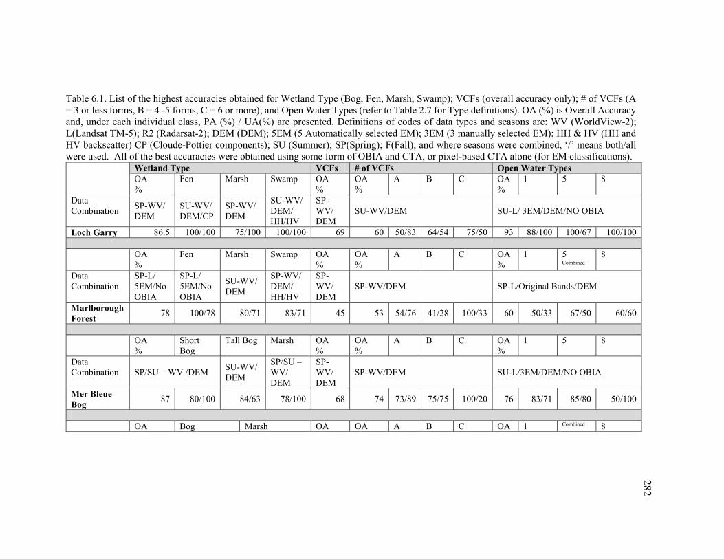
282
Table 6.1. List of the highest accuracies obtained for Wetland Type (Bog, Fen, Marsh, Swamp); VCFs (overall accuracy only); # of VCFs (A = 3 or less forms, B = 4 -5 forms, C = 6 or more); and Open Water Types (refer to Table 2.7 for Type definitions). OA (%) is Overall Accuracy and, under each individual class, PA (%) / UA(%) are presented. Definitions of codes of data types and seasons are: WV (WorldView-2); L(Landsat TM-5); R2 (Radarsat-2); DEM (DEM); 5EM (5 Automatically selected EM); 3EM (3 manually selected EM); HH & HV (HH and HV backscatter) CP (Cloude-Pottier components); SU (Summer); SP(Spring); F(Fall); and where seasons were combined, ‘/’ means both/all were used. All of the best accuracies were obtained using some form of OBIA and CTA, or pixel-based CTA alone (for EM classifications).
Wetland Type VCFs # of VCFs Open Water Types OA %
Fen Marsh Swamp OA %
OA %
A B C OA %
1 5 8
Data Combination SP-WV/
DEM SU-WV/ DEM/CP
SP-WV/ DEM
SU-WV/ DEM/ HH/HV
SP-WV/ DEM
SU-WV/DEM SU-L/ 3EM/DEM/NO OBIA
Loch Garry 86.5 100/100 75/100 100/100 69 60 50/83 64/54 75/50 93 88/100 100/67 100/100 OA
% Fen Marsh Swamp OA
% OA %
A B C OA %
1 5 Combined
8
Data Combination
SP-L/ 5EM/No OBIA
SP-L/ 5EM/No OBIA
SU-WV/ DEM
SP-WV/ DEM/ HH/HV
SP-WV/ DEM
SP-WV/DEM SP-L/Original Bands/DEM
Marlborough Forest 78 100/78 80/71 83/71 45 53 54/76 41/28 100/33 60 50/33 67/50 60/60
OA
% Short Bog
Tall Bog Marsh OA %
OA %
A B C OA %
1 5 8
Data Combination SP/SU – WV /DEM SU-WV/
DEM
SP/SU –WV/ DEM
SP-WV/ DEM
SP-WV/DEM SU-L/3EM/DEM/NO OBIA
Mer Bleue Bog 87 80/100 84/63 78/100 68 74 73/89 75/75 100/20 76 83/71 85/80 50/100
OA Bog Marsh OA OA A B C OA 1 Combined 8
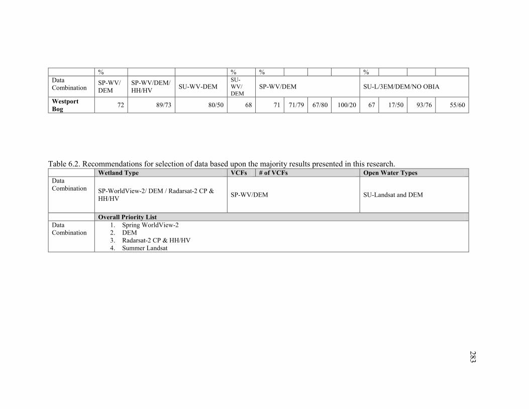
283
% % % % Data Combination
SP-WV/ DEM
SP-WV/DEM/ HH/HV SU-WV-DEM
SU-WV/ DEM
SP-WV/DEM SU-L/3EM/DEM/NO OBIA
Westport Bog 72 89/73 80/50 68 71 71/79 67/80 100/20 67 17/50 93/76 55/60
Table 6.2. Recommendations for selection of data based upon the majority results presented in this research.
Wetland Type VCFs # of VCFs Open Water Types Data Combination SP-WorldView-2/ DEM / Radarsat-2 CP &
HH/HV SP-WV/DEM SU-Landsat and DEM
Overall Priority List Data Combination
1. Spring WorldView-2 2. DEM 3. Radarsat-2 CP & HH/HV 4. Summer Landsat
284
This is followed by the best data set overall, given a single data set was to be used for all of
these attribute groups. Also from this research and supported by the literature, each data set
in Table 6.2 should be used with OBIA and CTA or a similar decision tree classifier.
6.1.3 OBIA segmentation for object creation
The importance of optimal segmentation parameter selection continues to be an
ongoing technical aspect of interest for research using OBIA (Dragut et al., 2010; Marpu et
al., 2010). As many of the current studies utilize eCognition software to create objects,
additional, supportive evidence of the ‘correct’ scale (shape and compactness) values for
particular imagery types is important.
Optimal segmentation values were determined for WorldView-2 imagery for the
attributes: Wetland Type, VCFs and Open Water Types. The scale value ranged from 25 to
45. These values were similar to other wetland studies of Wetland Types that used
eCognition-based OBIA applied to high resolution optical imagery. Examples include:
Dissanka et al. (2009) using Quickbird with a scale parameter value of 50; Wang et al.
(2011) using IKONOS and scale parameter values of 20 and 25; Barker and King (2012)
using 50 cm pixel Digital Orthophotos with a scale parameter value of 300 to first delineate
wetlands, and then a value of 20 to segment within wetland vegetation and logs as specific
turtle habitat features; and in research that used WorldView-2 imagery, Heumann (2011),
who first segmented general land cover classes with a scale value of 25 and then segmented
specific coastal vegetation classes using a scale value of 10.
285
This research found a similar range of segmentation scale values delineated objects
that visually represented spatial entities in the landscapes of the wetland study areas using
WorldView-2 images; however, they were determined using only four bands and without
pan-sharpening. It was difficult to find any study that used only the red, green, blue, and
NIR bands of WorldView-2 imagery. Part of the novelty of WorldView-2 imagery is the
additional four bands, however eight-band imagery is costly, and the additional four bands
are generally highly correlated (redundant) with the four bands used in this research.
Achieving similar results as other 8-band studies using only four bands for segmentation
parameter selection is a benefit of this research.
Optimal segmentation parameter values were also determined for Landsat 5 TM
imagery (original data, and fraction images) for Wetland Type, VCFs and Open Water Types
and ranged with scale values of 2 to 10. In the literature, general object segmentation
parameter values using eCognition and multi-resolution segmentation for Landsat imagery
range from 5 to 10 for similar features to the Wetland Types (Marsh, Swamp, etc.,) and or
VCFs such as (submerged, emergent, open water, aquaculture, etc.) of the study areas of this
research (Kozak et al.¸ 2008; Dingle Robertson and King, 2011; Dronova et al., 2011; Ruan
and Ustin, 2012), but these were for single study sites (Dronova et al., 2011; Ruan and Ustin,
2012); or for broader level land cover types such as Wetland, Urban, etc. (Dingle Robertson
and King, 2011). In particular, the segmentation parameter values in this research for
fraction images are similar to Fernandez-Manso et al. (2009) who used Landsat 7 ETM+
data both as pixel level inputs and as fraction maps inputs to a multi-level multi-resolution
286
segmentation to map fire severity levels. These similar ranges of segmentation values add
to the body of OBIA literature relating scale parameter to image type. No other studies were
found that used fraction images with OBIA for wetland analysis. This research showed that
segmentation of fraction maps creates objects that are visually related to Wetland Types,
agricultural fields, and other landforms.
This research also found that CTA is better than MLC for almost all classes in object-
based classification. Typically, comparative studies use MLC for pixel-based analysis, and
compare its output to that for other classifiers (e.g. nearest neighbour, decision tree, RFs,
support vector machine (SVM), among others (see Duro et al., 2012; Hantson et al., 2012;
Stein et al., 2013; Lewis et al.¸ 2013). Accuracies found in the literature for CTA are
sometimes higher than MLC (e.g., from 1% to 10% higher (Wei et al., 2008; Na et al., 2009;
Hladik et al., 2013), but the differences are often not statistically significant (Dingle
Robertson and King, 2011, Duro et al., 2012). In this research, the difference between
object-based CTA and object-based MLC accuracy was 10%. It was difficult to find a study
that used MLC with objects. The results of this research were, however, similar to Li et al.
(2012) who found that pixel-based CTA (59%) had slightly higher accuracies than pixel-
based MLC (56%) using a combination of ALOS PALSAR L-band HH, HV and derived
textural images for land cover classification.
Immitzer et al. (2012) found object-based RF classification of tree species using 8-
band WorldView-2 imagery to be higher overall than pixel based classification (78% versus
72%). RF has become more widely used in part due to its insensitivity to small sample size
287
(Immitzer et al., 2012). However, in the determination of important data inputs RF can give
same (or higher) priority to highly correlated data (e.g. prioritizing them first) rather than
ignoring correlated data, and shifting the prioritization to the other variables (Millard and
Richardson, 2013). In the research presented here, fewer input variables were used (e.g. four
WorldView-2 bands and a DEM), and typically the spectral bands are correlated, negating
the need for a classifier such as RF. The simple CTA method provided insight as to what
data information (e.g. the blue band or the DEM) was important for assigning pixels or
objects to classes, which will aid in the selection of imagery types or other data types for
these types of classifications.
WorldView-2 imagery provided higher accuracies and more detailed thematic maps
than Landsat 5 TM imagery for Wetland Type and VCF classifications. Most of the literature
generally shows higher accuracies, or increased detail using higher resolution imagery (e.g.
De Roeck et al., 2007; Grenier et al., 2008; Veettil, 2012). For Wetland Type classifications,
Landsat 5 TM imagery may not be useful without added data (e.g. radar variables or other
GIS data) except for a few classes (e.g. Fen or Swamp) and not at all useful alone for VCF
classifications.
Landsat 5 TM imagery had higher classification accuracies than WorldView-2
imagery for Open Water Types. Several studies have shown that Landsat 5 TM imagery is
useful for mapping water and water bodies (e.g. Tulbure and Broich, 2013; Yang et al.,
2013; Zhang et al., 2013 among others). WorldView-2 imagery is often used for bathymetric
and coastal water applications, but studies showing the configuration of water on land (water
288
patterns) are limited. Based on the results of this research, it is believed that excessive detail
was captured with the WorldView-2 classifications resulting in mis-classification of Open
Water Type; the coarseness of the Landsat 5 TM imagery minimized the detail and captured
the generalized configuration of the water and land cover.
Overall for this research, using only the original Landsat TM bands (not segmented)
resulted in the lowest overall accuracies. The difference from the literature is that a
combination of OBIA and fraction images did not produce the highest accuracies for any of
the classifications. Pixel-based classification of fraction images or object-based
classification of the original bands produced the highest overall accuracies for Wetland
Type, VCFs and Open Water Type. This could be due to the complex and dynamic nature
of wetlands as compared to simple, relatively homogenous low, moderate and high burned
areas found in Fernandez-Manso et al. (2009).
6.1.4 Radar analysis
Radar image analyses were completed to obtain an understanding of the potential
contributions of non-optical imagery at different spatial and temporal resolutions,
broadening the overview perspective. While this research showed that particular radar-
derived variables could support classification, radar generally added noise and reduced
overall accuracies over optical imagery alone. However, there were some successes for some
classes using HH, HV analysis, pedestal height analysis, and when combining radar
variables with optical variables.
289
Spring, steep (18.4°-27.6°) incidence angle HH and HV images showed better
separation between Wetland Type classes than spring shallow (46.8°-48.0°) incidence angle,
and any angle summer and fall HH, HV images. This is because for Swamps and treed Bogs,
there was increased penetration at steep angles, increased volume scattering from branches
within crowns, and double-bounce scattering between bare trunks and the water surface
(more particularly for Swamps) resulting in increased depolarisation of the signal.
Consequently, they were more distinct from shorter, more uniformly vegetated wetlands
such as Fens, Marshes and non-treed Bogs in the steep spring imagery than in shallower
angle imagery. This concurs with the majority of the literature that have found that detection
of flooded vegetation is better achieved with steep incidence angle imagery (Raney, 1998;
Baghdadi et al., 2001; McNairn et al., 2002; Li et al., 2007; Westra et al., 2010). In one
example study of Mer Bleue bog, Baghdadi et al. (2001) used airborne C-band quad-pol
SAR data to observe differences in wetland vegetation for three seasons, and found that
there was greater separation at steeper incidence angles than shallower incidence angles.
Classification of HH and HV images using object-based CTA, and combined with
optical imagery and a DEM did not improve overall accuracies over the accuracies obtained
with the optical imagery alone. However, individual class accuracies for Swamp improved
with the addition of either spring or summer HH and HV images at Loch Garry (Summer,
100% each UA and PA), and Marlborough Forest (Spring, 83% and 71%, respectively).
These values match and surpass similar Wetland Type accuracies found in the literature
ranging from 71 to 92% (Table 2.5). It is not surprising that HH and HV images enhanced
290
this Wetland Type as HH has often been shown to be sensitive to vegetation structure in a
variety of studies with different satellite types and locations and for other non-wetland
vegetation (such as agriculture) (Pope et al., 1997; Lang and Kasischke, 2008; Henderson
and Lewis, 2008; Schmitt and Brisco, 2013).
The seasonal differences in this research could be related to the fact that many of the
Swamp areas at Loch Garry were comprised of dead coniferous trees, therefore contributing
scattering mechanisms would include strong trunk-water double-bounce and increased
volume scattering from the branches and the live understory in both spring and summer. At
Marlborough Forest, many of the Swamp areas were hardwood dominated. In spring leaf-
off conditions, like the Loch Garry dead coniferous swamps, there would be strong trunk-
water double-bounce scattering along with volume scattering from crown branches and new
understorey vegetation growth. This resulted in high backscatter, making them more distinct
than with optical imagery alone. This research found that spring radar imagery (as just
described) from March and April provided the best discrimination between Swamp and
other Wetland Types. Kandus et al. (2001) found leaf-off imagery (May and August,
Argentina) best distinguished types of Forest, Marshes and Rushes. Lang et al. (2008) found
better discrimination for flooded forest during the leaf-off period in North Carolina.
For particular plant types (VCFs) within wetlands, the best season for discrimination
was spring for Swamp and Fen vegetation types, and summer for Marsh vegetation. This
could be related to the combined presence in Swamps of standing water and bare deciduous,
dead coniferous or sparse live coniferous in spring, and to flooded Fen meadows in spring,
291
resulting in signal interaction with both the woody vegetation and water surface, resulting
in increased double-bounce and volume/multiple scattering. For Marshes, however, spring
conditions are typically comprised of vegetation (e.g. cattails) that has been crushed and
flattened by snow, while in summer the long upright stocks produce increased volume
scattering that distinguishes them from more uniform Fens and Bogs that are dominated by
surface scattering (Kandus et al., 2001; Baghdadi et al., 2001; Li et al., 2007; Henderson
and Lewis, 2008). There was overlap between the different vegetation types for Bog using
spring imagery, concurring with Baghdadi et al. (2001) and Li et al. (2007) who showed
overlap between forested bog and non-forested bog classes in spring and summer data and
for co-pol data in fall. The overall results obtained by Baghdadi et al. (2001) (ranging from
73% with June and July data to 86% in October) were similar to those obtained in this
research using optical imagery alone. However, as Baghdadi et al. (2001) did not include
optical imagery in their research a direct comparison is not possible. Overall, the accuracies
did not meet the general published accuracies for specific vegetation community forms or
plant types. It is not known if a lack of reference data for training and validation, and/or the
variability of the vegetation community forms are the cause for this.
In the literature pedestal height has been an input variable for classifications or used
in correlation analysis against other biophysical or image variables such as leaf area index
(LAI), textures (Kovacs et al., 2013) or percent residue cover (McNairn et al., 2002). It has
been used to determine differences between surface cover types such as oil-covered and oil-
free sea surfaces (Nunziata et al., 2011), snow pack differences (Sokol et al., 2003), and
292
landslide surfaces (Czuchlewski et al., 2003). Theory and empirical literature shows that as
pedestal height increases, diffuse scattering and depolarization increase (Evans et al., 1988;
Boerner et al., 1998; McNairn et al, 2002; Touzi et al., 2004). Therefore, it would be
expected that areas with increasing backscatter, as is seen with different Wetland Types
caused by increased volume/multiple surface scattering or increased double-bounced
scattering due to flooding, would would have increasing pedestal heights (McNairn et al.,
2002). By manipulating the data together in simple mathematical terms such as summation,
it was expected that differences between scatterer groupings would be enhanced.
In this research, the summation of the summer co- and cross-pol pedestal minimums
showed good separation between three distinct groupings of classes (water/marsh (‘Group
1’; swamp/upland ‘Group 2’; and fen/bog ‘Group 3), which relates directly to the
depolarisation of the waves and types of scatterers present; with increasing surface
roughness and canopy structure there is an increase in depolarisation and number/types of
scatterers (e.g. dominant surface scattering versus multiple/volume and double-bounce
scattering).
There were no studies that used both the co- and cross-pol pedestal height
information, or combined the information, for Wetland Type or wetland plant types/groups
discrimination. While the research presented here was successful in revealing the three
distinct groups through the manipulation of the pedestal height information, it was not
successful in producing thematic maps that could be quantitatively assessed with this
information.
293
Using object-based CTA with CP variables, and combining them with optical
imagery and a DEM did not increase overall accuracies over those obtained with optical
imagery alone for Wetland Type with the exception of the Fen class for summer imagery of
Loch Garry (100% PA and UA, respectively) and spring imagery of Marlborough Forest
(100% and 78%, PA and UA, respectively). Scattering for Fen is expected to be mostly
surface scattering with small contributions from volume scattering in shrub vegetation and
double-bounce scattering where there are sporadic trees (e.g., tamarack in the Loch Garry
Fen) and open water. The Fens at Marlborough Forest were mostly grassy meadow Fens. In
the literature, it was found that CP components could distinguish between Wetland Type
classes such as Upland, Wetland, Forest and Shrub (Sartori et al., 2011) or that higher alpha
values showed more double bounce scattering in flooded vegetation compared to lower
alpha values in non-flooded areas. Higher and lower were quantified in a range of +20° to -
20° with higher positive results (+14° to +20°) relating to double-bounce, and lower negative
results (-4° to -20°) relating to surface scattering (Schmitt and Brisco, 2013). The results
found in this research were the same as in Touzi et al. (2007), in that CP components alone
were not useful for discriminating wetland vegetation, but they were useful in improving the
Fen class using a coarser resolution imagery type (Radarsat-2, in this research of
approximately 8 m, as compared to Convair-580 in Touzi et al., 2007, of approximately 64
cm in azimuth per 5 m in range (Touzi et al., 2004)).
294
6.1.5 Vegetation index thresholding for wet extent mapping
This research found that NDVIGreen derived through pixel-based processing of
WorldView-2 imagery corresponded well with field-measured VWC (%) and allowed for a
spring inundation extent to be derived. The vegetation at the Upland/Wetland ecotone is a
combination of vegetation composition and structure from both areas (Cronk and Fennessy,
2001; Mitsch and Gosselink, 2007). Due to the generally flat topography of the study areas,
in times of flooding such as spring snow melt, Upland areas adjacent to the wetland may be
flooded and the vegetation would be stressed, while in times of drought Wetland vegetation
would be stressed. NDVIGreen was originally developed as a way to estimate plant
chlorophyll (Gitelson and Merzlyak, 1997), which changes throughout a plant’s lifespan and
as it reacts to stressors (such as soil moisture levels). Because of the unique combination of
Upland and Wetland vegetation it would be expected that the values of NDVIGreen in those
areas would be unique. There was no research in the literature that had used NDVIGreen to
assess soil moisture or surface wetness, however De Benedetto et al. (2013) utilized a green
ratio index (NIR/Green) derived from WorldView-2 imagery to assess the response of
tomato crops to different water treatments. NDVIGreen was selected for this research on this
basis, but it was admittedly speculative, as it was not known a priori that it would produce
such distinctive results compared to the other vegetation indices evaluated.
6.1.6 GIS thematic map analyses and scoring
A large portion of this research required manipulation of existing data, particularly
data available in the LIO. Based on the results achieved, it should be possible to derive
295
OWES attributes such as the number of Wetland Types, Diversity of Surrounding Habitat,
Proximity of Surrounding Wetlands, Rarity of Wetlands, and Rarity in the Landscape. LIO
data did not exist for the study sites with respect to Ownership and Hunting Pattern, but they
do exist elsewhere in southern Ontario, so such assessments should be possible. For
ownership patterns, property parcel layers available from Teranet (www.teranet.ca, 2013)
were examined, but they only provide Municipal Property Assessment Corporation (MPAC)
assessment numbers and property address data, which do not give an indication of
ownership. If the type of ownership (e.g. private or crown) is indicative of particular
assessment numbers (e.g. particular number pre-fixes, etc.) then a determination of private
versus public land based upon these data might also be possible. It was not possible to
determine wetland area and basin area measurements for Wetland Attenuation Factor using
the derived and existing thematic layers.
Similar simple data manipulation is common in the literature (e.g. Beazley et al.,
2005; Connor and Gabor, 2006 among others). Findlay (2005), using regression, attempted
without success to statistically predict the OWES scores directly from thematic information
(and underlying derived predictor variables) available from the LIO. He concluded that there
measurement error in the geo-spatial data was probably too large to derive predictive
relationships for the different attributes. He also stated that the landscape variables were not
the most important ones in terms of contribution to the overall wetland score, being simple
land cover classes such as: Coniferous Swamp, Deciduous Swamp Areas, Forest Area,
Forest Edge, Water Edge, per cent Agricultural, and per cent Open Water. They were
296
extracted from existing thematic maps and other geospatial data and not newly derived maps
from high resolution imagery as in this research. This research selected attributes that
contribute highly to the OWES score (e.g. Chisholm et al., 1997) for a given wetland and
variable(s) were extracted from the newly derived maps and/or from existing LIO data.
These were related directly to OWES scores without using surrogates, nor modelling such
as regression. For example, Number of Wetland Types was determined by counting the
classified Wetland Types in the derived Wetland Type thematic maps and/or the existing
OMNR wetland thematic map, etc. These were compared directly to the OWES field based
assessment for the same attribute. Based on this, it is concluded that some of the existing
LIO thematic layers could be used to map certain OWES attributes.
Scores derived from thematic information for Diversity of Surrounding Habitat,
Wetland Size (when including OWES evaluated Interspersion and VCF scores), and
Proximity to Other Wetlands were the same as those assessed during the OWES evaluations.
Similar scores to the OWES were derived for Rarity of Wetlands and Rarity in Landscape
for the Special Feature component using geospatial data, except for Westport Bog.
The 14 attributes of this research were selected because they contribute most to the
overall OWES wetland score and had potential to be assessed using remote sensing and GIS.
For five of the 14 attributes these scores can be assessed from existing data, without costly
field work, and the existing database could be updated using the data available in the LIO.
297
6.1.7 Temporal analyses
The choice of season (or a combination of seasonal imagery) was important for
mapping particular classes (e.g. Wetland Type, VCFs and Open Water Type) and seasonal
variability was inconsistent between sites. Many studies in the literature have used multi-
date or multi-season imagery analysed together, or analysed separately as individual images
to discriminate between Wetland Types and VCFs (Baghdadi et al., 2001; Racine et al.,
2005; Ghioca-Robrecht et al., 2008; Bourgeau-Chavez et al., 2010; Dribault et al., 2012;
Bourgeau-Chavez et al., 2013; Evans and Costa, 2013). There have been a variety of
outcomes, but in general, improved accuracies have been shown when using multi-date
versus single date imagery. When discriminating between seasons, Baghdadi et al. (2001)
found that fall (October) data were best for wetland class discrimination. Racine et al.
(2005) found that summer (June) imagery was best for a 10-class classification. Bourgeau-
Chavez et al. (2010) found that neither July nor August imagery was good for mapping
wetland flooded condition. In this research, summer WorldView-2 Wetland Type
classifications improved overall accuracies over spring classifications for two of four sites.
It was difficult to determine if this was the case for all four sites as the remaining two sites’
summer imagery was substandard (haze present/ acquisition issues). Landsat 5 TM summer
imagery overall Wetland Type accuracies were better than spring for some sites, especially
for the poorest class, Marsh. This could be related to the growth and difference of vegetation
within each wetland type from spring to summer. Using summer WorldView-2 imagery
298
alone for Open Water Type, 3-form and VCF classifications did not improve overall
accuracies.
Combining multi-season imagery did not improve Wetland Type overall accuracies
for three of four sites, and combining multi-season WorldView-2 imagery did not improve
the VCF overall accuracies. However, for Wetland Type, Mer Bleue Bog classification
accuracies did improve with the combination of spring and summer imagery, and combining
summer and fall WorldView-2 imagery improved the overall accuracies for the number of
VCFs by approximately 10%.
In the field, there were seasonal and annual differences in wet extents which could
be related to accumulated precipitation, topographical constraints and time-of-year of the
measurements. These differences highlight the need for multiple season and/or inter-annual
mapping of wetlands to determine an overall average inundation extent. Inundation
dynamics are well-studied and assessed using multiple season imagery (Bourgeau-Chavez
et al., 2005; Lang and Kasischke, 2008; Rebelo et al., 2009; van der Velde et al., 2009; Gala
and Melesse, 2012; Zhang et al., 2012; Chen et al., 2013; Kuenzer et al., 2013) with the
highest R2 values of 0.96 between image variables and continuous field variables such as
soil moisture or per cent area inundated, and the highest overall accuracies in classification
of inundation types of 100%. In particular, some of these studies modelled radar backscatter
against field-measured soil moisture, or percent area inundated (e.g., Lang and Kasischke,
2008), while others used temporal data to classify inundation classes (e.g., Bourgeau-
Chavez et al., 2005) for classes of dry, saturated, standing water, and flooded, achieving
299
accuracies of 70% in mapping change over time). This research showed that boundaries
representing 100% VWC (a wetland wet extent) can be mapped using either spring or
summer NDVIGreen derived from WorldView-2 imagery, which has not been reported in the
literature. A possible reason for this relationship could be that NDVIgreen responds to
vegetation structure and stress found at the Wetland/Upland ecotone. However, a
quantitative assessment of accuracy of this boundary was difficult to conduct using the
validation data collected in the field.
In terms of long term landscape dynamics and vegetation change due to
anthropogenic factors, this research found that vegetation fractions were higher historically
(1984) for three of the four sites. In a few small areas of Marsh, vegetation fractions were
lower in 1984. The cause of this difference is unknown. In the literature, vegetation fractions
have been used to assess vegetation change in a variety of land cover types, successfully
showing both vegetation degradation and regeneration (Sabol et al., 2002; Hostert et al.,
2003; Sunderman and Weisberg, 2011; Dubovyk et al., 2012) with overall accuracies of 85
to 89%. A specific example for coastal wetland vegetation change is Yang et al. (2013) who
assessed the abundance of land cover types using fraction images derived from Landsat TM
images for four time periods (1987, 2004, 2005 and 2006). They were able to relate changes
in the green fraction to increases of low vegetation cover, or decreases in high vegetation
cover related to Hurricane Katrina damage.
Review of the change type (e.g. natural or anthropogenic) can only be made if
changes or causes of changes (e.g. hurricane, infestation) are known. For example, known
300
anthropogenic disturbance such as flooding of an area for recreational purposes in Westport
Bog could be observed comparing vegetation fraction images, but field information was
necessary in order to determine that the changes were anthropogenic.
The literature has shown that these types of comparisons work well over time, and
this research also shows that these kinds of changes in LSU fraction images can be observed
in the eastern Ontario region. These results contribute to the accumulating body of evidence
showing that LSU applied to moderate resolution sensor data such as Landsat can provide
approximations of sub pixel land cover proportions. The long temporal archive of Landsat
and its large spatial coverage, allow for land cover change and trend analysis using LSU
over a region such as eastern Ontario to be conducted at low cost. This is an attractive
approach for an operational wetland evaluation system such as the OWES, because it serves
as an alternative to costly acquisition of a temporal series of many higher resolution images
for wetland and surrounding areas monitoring.
6.2 Recommendations
While this research shows that an overview perspective from a top-down,
investigative approach can reveal the inherent differences of wetlands across a regional area,
it is understandable that such an endeavour is time-consuming and cost-prohibitive, from a
staffing and data perspective. Table 6.3 outlines recommendations for the OMNR to follow
based upon the outcomes of this research. Figure 6.1 provides a workflow for implementing
these methods for the first six attributes in Table 6.3.
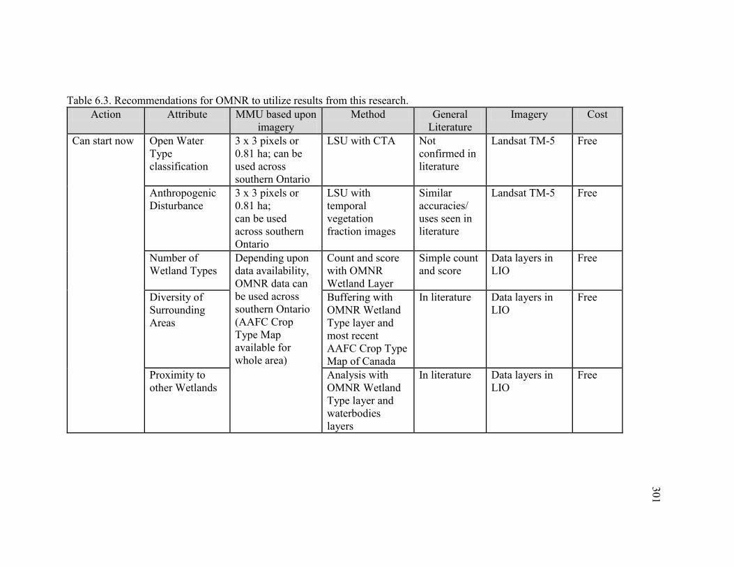
301
Table 6.3. Recommendations for OMNR to utilize results from this research. Action Attribute MMU based upon
imagery Method General
Literature Imagery Cost
Can start now Open Water Type classification
3 x 3 pixels or 0.81 ha; can be used across southern Ontario
LSU with CTA Not confirmed in literature
Landsat TM-5 Free
Anthropogenic Disturbance
3 x 3 pixels or 0.81 ha; can be used across southern Ontario
LSU with temporal vegetation fraction images
Similar accuracies/ uses seen in literature
Landsat TM-5 Free
Number of Wetland Types
Depending upon data availability, OMNR data can be used across southern Ontario (AAFC Crop Type Map available for whole area)
Count and score with OMNR Wetland Layer
Simple count and score
Data layers in LIO
Free
Diversity of Surrounding Areas
Buffering with OMNR Wetland Type layer and most recent AAFC Crop Type Map of Canada
In literature Data layers in LIO
Free
Proximity to other Wetlands
Analysis with OMNR Wetland Type layer and waterbodies layers
In literature Data layers in LIO
Free
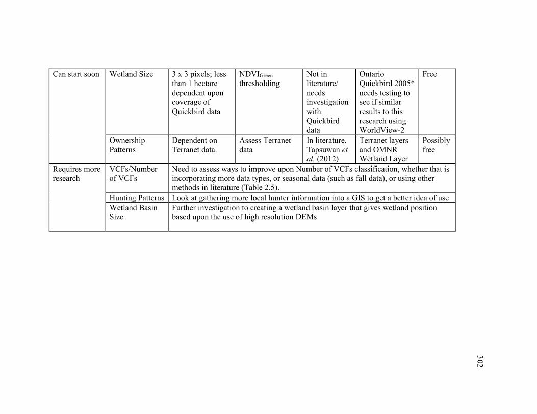
302
Can start soon Wetland Size 3 x 3 pixels; less than 1 hectare dependent upon coverage of Quickbird data
NDVIGreen thresholding
Not in literature/ needs investigation with Quickbird data
Ontario Quickbird 2005* needs testing to see if similar results to this research using WorldView-2
Free
Ownership Patterns
Dependent on Terranet data.
Assess Terranet data
In literature, Tapsuwan et al. (2012)
Terranet layers and OMNR Wetland Layer
Possibly free
Requires more research
VCFs/Number of VCFs
Need to assess ways to improve upon Number of VCFs classification, whether that is incorporating more data types, or seasonal data (such as fall data), or using other methods in literature (Table 2.5).
Hunting Patterns Look at gathering more local hunter information into a GIS to get a better idea of use Wetland Basin Size
Further investigation to creating a wetland basin layer that gives wetland position based upon the use of high resolution DEMs
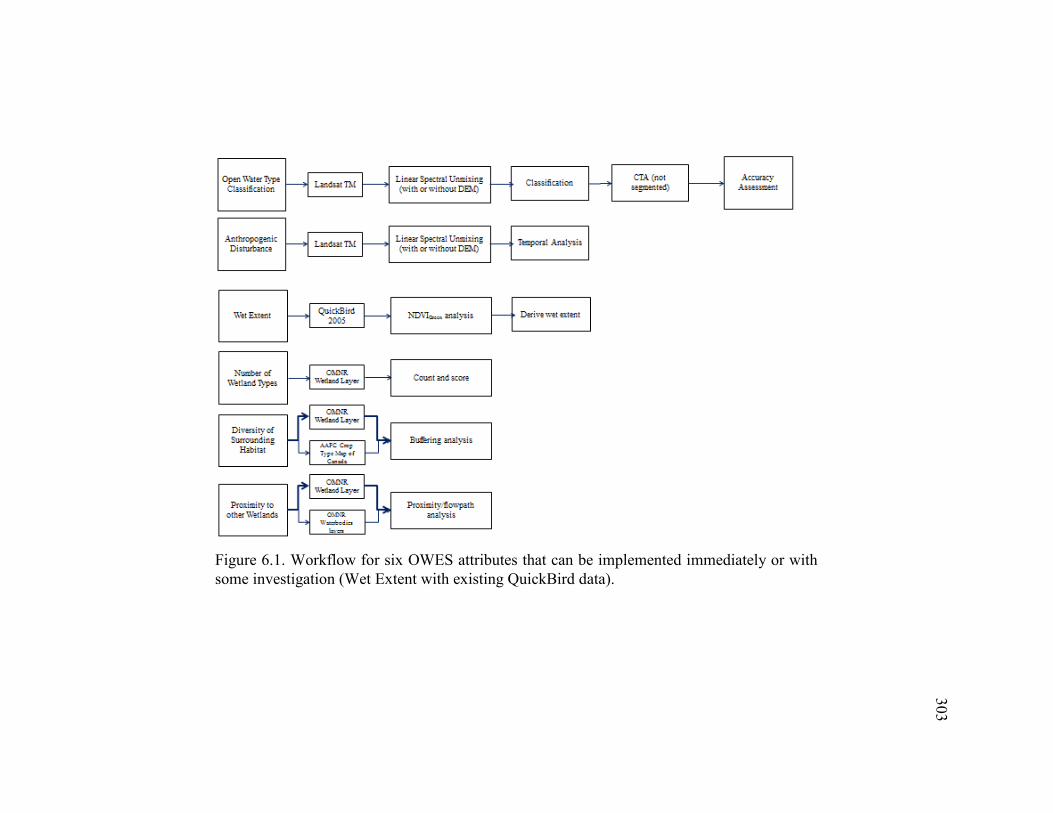
303
Figure 6.1. Workflow for six OWES attributes that can be implemented immediately or with some investigation (Wet Extent with existing QuickBird data).
304
As Landsat imagery is currently available at no cost, it is recommended to obtain spring
images to assess Open Water Type configurations using OBIA with the original band data,
and CTA. Additionally, further comparisons of current vegetation fraction images to
historical vegetation fraction images can be made to understand the historical and ongoing
changes occurring within, and around wetlands in southern Ontario. Vegetation fraction
analysis will aid current OMNR monitoring efforts through the understanding of vegetative
disturbance and growth and have been shown to within the literature (Sabol et al., 2002;
Hostert et al., 2003; Sunderman and Weisberg, 2011; Dubovyk et al., 2012).
Existing QuickBird data (4 band, 60cm) now available in the OMNR LIO could be
assessed with the NDVIGreen methods to map wet extents at the time of imagery acquisition.
This could provide an estimate of overall wetland size, to be further augmented in the future
with other purchases of high–resolution multi-spectral imagery. This has not been
previously reported in the literature, however, therefore more evaluation may be needed.
Three attributes, Number of Wetland Types, Diversity of Surrounding Habitat, and
Proximity to Other Wetlands can be assessed using data available in the LIO.
6.3 Overall limitations of this research
The greatest overall limitation to this research was the size of the reference and
validation data set obtained in the field. Wetlands are very challenging to access, which
make obtaining field-based validation sets difficult. Part of the difficulty of obtaining a large
validation set, was the attempt to obtain field data at four sites. However, by having four
dispersed and unique sites, this research showed that there was variability in classifications
of the attributes that were site specific, and this would not have been apparent with only one
305
or two sites as in most other previous studies. In research studies, a balance is necessary
between the need for comprehensive validation sets and understanding of spatial differences
across regions. It is difficult to recommend a specific proportion for each. In the literature
there are variations in terms of number of study sites, number of images or types of data
used, number and types of attributes investigated, number and types of variables
investigated, and number and spatial representativeness of reference data sites (Pope et al.,
1997; Baghdadi et al., 2001; Bernier et al., 2003; Rogers and Kearney, 2004; Li and Chen,
2005; Racine et al., 2005; Grenier et al., 2007; Durieux et al., 2007; Touzi et al., 2007;
Wright and Gallant, 2007; Ghioca-Robrecht et al., 2008; Castaneda and Ducrot, 2009;
Kwoun and Lu, 2009; Jiao et al., 2011; Dronova et al., 2011; Ricaurte et al., 2012).
Henderson and Lewis (2008) noted that as more studies are published there is less
consistency between results. However, this balance is particularly important when trying to
develop methods that can be utilized in a system like the OWES that covers a large
geographical region. This research addressed the relative lack of scope in most previous
wetland studies by: 1) studying four quite different wetland complexes across a large region,
each with its own set of environmental and ecological conditions (as opposed to 1-2
wetlands (often not wetland complexes) in most studies; 2) evaluating the potential for
mapping and monitoring of 14 common attributes used in an operational wetland evaluation
system (as opposed to 1-3 attributes typical of most studies); 3) evaluating two types of
remote sensing data, optical and radar, and their integration together and with DEM
information; 4) integrating spatial scale through the use of sensor data with different pixel
sizes and coverages, as well as the use of subpixel analysis applied to moderate resolution
imagery; and 5) integrating temporal information and temporal scale through analyses of
seasonal impacts on classification accuracy and multi-decadal vegetation dynamics. Thus,
306
the main limitation of this research in relation to other studies is that, given its much larger
scope, it was difficult to obtain in-depth reference data in large sample sizes.
Limitations with the multitude of data and differences of space, time and spectral
size and response were that statistical associations (if any) through measurement and
observational scale were not analyzed. For example, Michishita et al. (2012) used a nine
image time series of Landsat-5 TM and MODIS from July 2004 to October 2005 to
characterize the trends in LSU fraction images over time, and to statistically compare the
trends between the two scales of imagery. They were able to determine the statistical
correlation of the trends per fraction type between the two pixel sizes. This research was not
able to do this for any of the attributes. These relationships between imagery types and scales
are important in terms of facilitating cost-effectiveness in development of multi-scale
evaluation framework; e.g. using coarser resolution, larger extent and potentially free
imagery for mapping of certain attributes and to guide more detailed sampling and analysis
in selected areas using fewer higher resolution/smaller extent images that are higher cost per
unit area. The broad scope of the research limited the capability for exhaustive analyses of
any one particular attribute, data type, or methodology.
During the implementation of this research several new methodological directions
were initially proposed and evaluated in the literature, but could not be incorporated into
this research due to timing issues. For example, quantitative methods for segmentation
parameter selection were proposed (e.g. ESP, Dragut et al., 2010; Marpu et al., 2010), after
segmentation analysis for this research was completed in 2009. It may be prudent in the
future to investigate such methods and incorporate them for a more robust segmentation
parameter selection.
307
Regardless of these general limitations, this research made some new and significant
findings regarding wetlands, wetland management and remote sensing, and various
technical aspects of wetland attribute mapping.
6.4 Further research directions
There are two key directions recommended for further research with regards to
wetland and remote sensing science. First, further insight into how wetlands differ in space
and time is needed. The spatial and temporal differences found in this research for wetlands
and wetland attributes were also found (albeit at smaller scope) in the literature (Pope et al.,
1997; Baghdadi et al., 2001; Racine et al., 2005; Ghioca-Robrecht et al., 2008; Bourgeau-
Chavez et al., 2010; Dribault et al., 2012; Bourgeau-Chavez et al., 2013; Evans and Costa,
2013). Therefore, it should be apparent that limiting the time and/or space and/or spectral
size and resolution components of analysis will only limit the overall outcomes. Until
consistent results can be found for these components (as a hypothetical example - all
wetlands swamps should be assessed in spring using a combination of optical and radar
data), a broader overview perspective with a top-down approach to analysis should be taken.
Additionally, the issues with Marsh (poor results, misclassification, low accuracies etc.)
should be a focus of future research. The types of data used in this research were different
from the data types used in most of the literature, and this may have influenced the poor
results for Marsh found here (Lang and Kasischke, 2008; Henderson and Lewis, 2008;
Schmitt and Brisco, 2013). However, similar poor results for Marsh were found for other
wetlands within the same geographic region (e.g. Grenier et al., 2007 in Quebec, Canada)
and for the same wetland (Millard and Richardson, 2013, at Mer Bleue Bog) albeit with
308
different methods and data types. This could be an indication of regionally specific issues
related to Marsh vegetation (e.g. water/vegetation interactions, snowpack interactions, etc.)
For remote sensing analyses to be a successful replacement of (or a supplement to)
field-based components of wetland evaluation systems, adaptations to existing methods
should be made. Recent advances in deriving landscape metrics and landscape structure
from remote sensing derived thematic maps have been made. For example, Hou and Walz
(2013) derived landscape metrics such as landscape diversity, edge contrast index and
fragmentation metrics to assess biodiversity utilizing imagery developed from thematic
maps derived from five-band RapidEye imagery for forest/agriculture/mixed-use landscapes
in Germany. Investigation into the replacement of existing field-based indicators with
image/thematic map derived metrics is important.
6.4.1 Technical research directions
Further investigation into object-segmentation with LSU fraction images is
warranted. The poor accuracy obtained in this research was different from the literature
with similar segmentation parameters. Future research should attempt to evaluate variety of
complex land covers in general, using OBIA and LSU.
Further research is also warranted in the ability of HH, HV images, pedestal height
values and CPs to either discriminate between individual Wetland Types such as Swamp
and Fen, VCFS, plant types/groups and/or combinations of classes within, and from those
attributes. One future endeavour would be to separate the imagery by Wetland Type and try
to specifically classify each Wetland Type by particular wetland plant types/communities.
Pedestal height images should be created to be classified based upon the co- and
cross-pol pedestal height data manipulation completed in this research. This research also
309
showed that the addition of some of these variables to the optical imagery variables
improved certain classes. Further research should incorporate a methodology that
determined the importance of these variables (e.g. RFs) and uses these variables to produce
more accurate thematic classification layers.
6.5 Conclusions
The research in this thesis presented methods to assess 14 wetland attributes selected
from the OWES using multiple spectral, spatial and temporal data types. The results support
a top-down investigative tactic, which does not focus on one particular aspect, but takes a
broad approach for wetlands analysis. This perspective can reveal spatial and temporal
consistencies and inconsistencies through analysis of multi-spectral and multiple spatio-
temporal data types.
In general, current wetland literature focuses on one (or two) aspects, but in order to
be comprehensive, all (or as many as possible) components should be considered. However,
a limitation of this approach is that, when multiple attributes are considered, an intensive
examination of every attribute cannot be made. Additionally, with a large and varied spatial
extent, validation set size suffers and this must also be taken into consideration when
attempting to complete a comprehensive project such as this.
This research also showed that if remote sensing methods are to be incorporated into
pre-existing evaluation systems, changes to some of the attributes’ current methods must be
made. This will reduce the reliance on field-based methods, which cannot be conducted
spatially or temporally with any frequency, and make use of remote methods of mapping,
which are cost-effective and repeatable.
310
Some of the technical methods that were derived and tested in this research can be
utilized in conjunction with the existing evaluation system, and some require further
investigation into the repeatability of the results and the availability of other data sources.
For example, boundaries representing 100% soil moisture content (a wetland moisture
boundary) can be derived using either spring or summer NDVIGreen images derived from
WorldView-2 imagery. Further investigation into the usability of this method with available
QuickBird data is needed. Also as an example, this research was successful in deriving the
three distinct groups (Marsh/Water; Bog/Fen; Swamp/Upland) by manipulating the
polarimetric radar pedestal height information. Further investigation into the utility of this
information is needed.
In general, this research has shown that it is possible to carry out diverse and complex
analysis and mapping of the spatial and temporal characteristics of wetland attributes using
remotely sensed data, existing geo-spatial data, and currently available processing and
analysis methods.
311
7.0 References
Adam, E., Mutanga, O., and D. Rugege. 2010. Multispectral and hyperspectral remote sensing for identification and mapping of wetland vegetation: a review. Wetlands Ecology and Management 18: 281-295.
Adams, J.B., Sabol, D.E., Kapos, V., Almeida Filho, R., Roberts, D.A., Smith, M.O., and
A.R. Gillespie. 1995. Classification of multispectral images based on fractions of endmembers: application to land-cover change in the Brazilian Amazon. Remote Sensing of Environment 52: 137-154.
Adamus, P.R. 1995. Validating a habitat evaluation method for predicting avian richness.
Wildlife Society Bulletin 23: 743-749. Adamus, P.R., and Stockwell, L.T. 1983. Critical review and evaluation concepts, v. 1 of
method for wetland functional assessment: Washington, D.C., U.S. Department of Transportation, Federal Highway Administration Report no. FHWA-IP-82-23, 176p.
Aguilar, M.A., Saldana, M.M., and F.J. Aguilar. 2013. GeoEye-1 and WorldView-2 pan-
sharpened imagery for object-based classification in urban environments. International Journal of Remote Sensing 34: 2583-2606.
Alcaraz, D., Paruelo, J., and J. Cabello. 2006. Identification of current ecosystem functional
types in the Iberian Peninsula. Global Ecology and Biogeography 15: 200–212. Allen, J., Lu, K. S., and T. D. Potts. 2002. A GIS-based analysis and prediction of land-use
change in a coastal tourism destination area. IN M. I. Miller, J. Auyong, and N. P. Hadley (eds.) Proceedings of the 1999 International Symposium on Coastal and Marine Tourism: Balancing Tourism and Conservation. April 26–29, 1999, Vancouver, British Columbia, Canada. Washington Sea Grant Program and School of Marine Affairs, University of Washington, Seattle, Washington; Oregon Sea Grant College Program, Oregon State University, Corvallis, Oregon; and Oceans Blue Foundation, Vancouver, British Columbia, Canada.
Anderson, J.E., and J.E. Perry. 1996. Characterization of wetland plant stress using leaf
spectral reflectance: implications for wetland remote sensing. Wetlands 16: 477-487. Anderson, J.R., Hardy, E.E., Roach, J.T., and R.E. Witmer. 1976. A land use and land cover
classification system for use with remote sensor data. US Geological Survey Professional Paper 964. United States Department of the Interior. US Government Printing Office. Washington. 41p.
Anfinsen, S.N., Jensen, R., and T. Eltoft. 2007. Spectral clustering of polarimetric SAR data
with Wishart-derived distance measures. Proc. POLINSAR. 3rd International Workshop on Science and Applications of SAR Polarimetry and Polarimetric Interferometry, Frascati, Italy; 22-26 January, 2007.
312
Apte, C., and S. Weiss. 1997. Data mining with decision trees and decision rules. Future
Generation Computer Systems 13: 197-210. Artigas, F. J. and J. Yang. 2006. Spectral discrimination of marsh vegetation types in the
New Jersey Meadowlands, USA. Wetlands 26: 271-277. Asner, G.P. 1998. Biophysical and biochemical sources of variability in canopy reflectance.
Remote Sensing of Environment 64: 234-253. Atkinson, D.M., and P. Treitz. 2012. Arctic ecological classifications derived from
vegetation community and satellite spectral data. Remote Sensing 4: 3948-3971. Baker, C., Lawrence, R., Montagne, C., and D. Patten. 2006. Mapping wetlands and riparian
areas using Landsat ETM+ imagery and decision-tree-based models. Wetland 26: 465-474.
Baghdadi, N., Bernier, M., Gauthier, R., and I. Neeson. 2001. Evaluation of C-band SAR
data for wetlands mapping. International Journal of Remote Sensing 22: 71-88. Baker, C., Lawrence, R.L., Montagne, C., and D. Patten. 2007. Change detection of wetland
ecosystems using Landsat imagery and change vector analysis. Wetlands 27: 610-619. Baldwin, D.J.B., Desloges, J.R., and L.E. Band. 2000. Physical Geography of Ontario. IN
A.H Perera, D.L. Euler and I.D. Thompson (eds). Ecology of a Managed Terrestrial Landscape: Patterns and Process of Forest Landscapes in Ontario. Vancouver; British Columbia: University of British Columbia Press. (13-29) 336p.
Banks, S.N. King, D.J., Merzouki, A., Duffe, J., and S. Solomon. 2011. Assessing Radarsat-
2 polarimetric SAR for mapping shoreline cleanup and assessment technique (SCAT) classes in the Canadian Artic. IN Proceedings of the 32nd Canadian Symposium on Remote Sensing, June 13-16, 2011, Sherbrooke, Quebec, Canada.
Baraldi, A., and F. Parmiggiani. 1995. An investigation of the textural characteristics
associated with Gray Level Co-occurrence Matrix statistical parameters. IEEE Transactions on Geoscience and Remote Sensing 33: 293-304.
Barker, R., and D.J. King. 2012. Blanding’s Turtle (Emydoidea blandingii) potential habitat
mapping using aerial orthophotographic imagery and object based classification. Remote Sensing 4: 194-219.
Bartoldus, C.C. 1999. A comprehensive review of wetland assessment procedures: A guide
for wetland practitioners. Environmental Concern Inc., St. Michaels, MD. 196p. Bartsch, A., Kidd, R.A., Pathe, C., Scipal, K., and W. Wagner. 2007. Satellite radar imagery
for monitoring inland wetlands in boreal and sub-arctic environments. Aquatic Conservation Marine and Freshwater Ecosystems 17: 305-317.
313
Beazley, K., Smandych, L., Snaith, T., MacKinnon, F., Austen-Smith, P., and P. Duinker.
2005. Biodiversity considerations in conservation system planning: map-based approach for Nova Scotia, Canada. Ecological Applications 15: 2192–2208.
Beeri, O., and R.L. Phillips. 2007. Tracking palustrine water seasonal and annual variability
in agricultural wetland landscapes using Landsat from 1997 to 2005. Global Change Biology 13: 897-912.
Begley, A.J.P., Gray, B.T., and C.A. Paszkowski. 2012. A comparison of restored and
natural wetlands as habitat for birds in the prairie pothole region of Saskatchewan, Canada. The Raffles Bulletin of Zoology 25: 173-187.
Behera, M.D., Chitale, V.S., Shaw, A., Roy, P.S. and M.S.R. Murthy. 2012. Wetland
monitoring, serving as an index of land use change – a study in Samaspur wetlands, Uttar Pradesh, India. Journal of the Indian Society of Remote Sensing 40:287-297.
Belluco, E., Camuffo, M., Ferrari, S., Modenese, L., Silvestri, S., Marani, A., and M.
Marani. 2006. Mapping salt-marsh vegetation by multispectral and hyperspectral remote sensing. Remote Sensing of Environment 105: 54-67.
Benz, U.C., Hofmann, P., Willhauck, G., Lingenfelder, I., and M. Heynen. 2004. Multi-
resolution, object-oriented fuzzy analysis of remote sensing data for GIS-ready information. ISPRS Journal of Photogrammetry & Remote Sensing 58: 239- 258.
Berberoglu, S., Yilmaz, K.T., and C. Özkan. 2004. Mapping and monitoring of coastal
wetlands of Çukurova Delta in the Eastern Mediterranean region. Biodiversity and Conservation 13: 615-633.
Berendes, T.A., Kuo, K.S., Logar, A.M., Corwin, E.M., Welch, R.M., Baum, B.A., Pretre,
A., and R.C. Weger. 1999. A comparison of paired histogram, maximum likelihood, class elimination, and neural network approaches for daylight global cloud classification using AVHRR imagery. Journal of Geophysical Research 104: 6199-6213.
Bernier, M., Ghedira, H., Gauthier, Y., Magagi, R., Rilion, R., De Seve, D., Ouarda,
T.B.M.J., Villeneuve, J.P., and P. Buteau. 2003. Remote sensing and classification bogs in Quebec using RADARSAT-1 images. Canadian Journal of Remote Sensing 29: 88-98.
Boerner, W.M., Mott, H., Luneburg, E., Livingstone, C., Brisco, B., Brown, R.J. and J.S.
Paterson.1998. Polarimetry in radar remote sensing: basic and applied concepts. IN R.M. Henderson and A.J. Lewis, Eds. Principles and applications of imaging radar: manual of remote sensing, vol. 2. 3rd edition. New York: John Wiley and Sons, Inc. 896 p.
314
Bourgeau-Chavez, L.L., Kowalski, K.P., Carlson Mazur, M.L., Scarbrough, K.A., Powell, R.B., Brooks, C.N., Huberty, B., Jenkins, L.K., Banda, E.C. Galbraith, D.M. Laubach, Z., and K. Riordan. 2013. Mapping invasive Phragmites australis, in the coastal Great Lakes with ALOS PALSAR satellite imagery for decision support. Journal of Great Lakes Research 39: 66-77.
Bourgeau-Chavez, L.L., Riordan, K., Powell, R.B., Miller, N., and M. Nowels. 2010.
Improving wetland characterization with multi-sensor, multi-temporal SAR and optical/infrared data fusion. IN G. Jedlovec (ed). Advances in Geoscience and Remote Sensing. Open Access Book: Intech: 742p.
Bourgeau-Chavez, L.L., Smith, K.B., Brunzell, S.M., Kasischke, E.S., Romanowicz, E.A.,
and C.J. Richardson. 2005. Remote monitoring of regional inundation patterns and hydroperiod in the Greater Everglades using synthetic aperture radar. Wetlands 25: 176-191.
Brady, N. and R. Weil. 2002. The Nature and Properties of Soils. 13th Edition, Prentice
Hall. Upper Saddle River, New Jersey. 960p. Breiman, L. 2001. Random forests. Machine Learning 45: 5-32. Brenner, J.C., Christman, Z., and J. Rogan. 2012. Segmentation of Landsat Thematic
Mapper imagery improves buffelgrass (Pennisetum ciliare) pasture mapping in the Sonoran Desert of Mexico. Applied Geography 34: 569-575.
Brinson, M. 1993. A hydrogeomorphic classification for wetlands. Wetlands Research
Program Technical Report WRP-DE-4. US Army Corps of Engineers. 101p. Broseth, H., and H.C. Pedersen.2000. Hunting effort and game vulnerability studies on a
small scale: a new technique combining radio-telemetry, GPS and GIS. Advances in Applied Ecological Techniques 37: 182-190.
Burnett, C., and T. Blaschke. 2003. A multi-scale segmentation/object relationship
modelling methodology for landscape analysis. Ecological Modelling 168: 233-249. Campos, J. C., Sillero, N., and J.C. Brito. 2012. Normalized difference water indexes have
dissimilar performances in detecting seasonal and permanent water in the Sahara-Sahel transition zone. Journal of Hydrology 464-465: 438-446.
Carletti, A., De Leo, G.A., and I. Ferrari. 2004. A critical review of representative wetland
rapid assessment methods in North America. Aquatic Conservation: Marine and Freshwater Ecosystems 14: S103-S113.
Castaneda, C., and D. Ducrot. 2009. Land cover mapping of wetland areas in an agricultural
landscape using SAR and Landsat imagery. Journal of Environmental Management 90: 2270-2277.
315
Castaneda, C. and J. Herrero. 2008. Assessing the degradation of saline wetlands in an arid agricultural region in Spain. Catena 72: 205-213.
Chandler, G., Markham, B. L., and D.L. Helder. 2009. Summary of current radiometric
calibration coefficients for Landsat MSS, TM, ETM+ and EO-1 ALI sensors. Remote Sensing of Environment 113: 893-903.
Chen, Y., Huang, C., Ticehurst, C., Merrin, L., and P Thew. 2013. An evaluation of MODIS
daily and 8-day composite products for floodplain and wetland inundation mapping. Wetlands 33: 823-835.
Chisholm, S., Davies, C., Mulamoottil, G., and D. Capatos. 1997. Predictive models for
identifying potentially valuable wetlands. Canadian Water Resources Journal 22: 249-267.
Chiu, W-Y., and I. Couloigner. 2006. Modified fuzzy c-means classification technique for
mapping vague wetlands using Landsat ETM+ imagery. Hydrological Processes 20: 3623-3634.
Cloude, S.R., and E. Pottier. 1996. A review of target decomposition theorems in radar
polarimetry. IEEE Transactions on Geoscience and Remote Sensing 34: 498-518. Cloude, S.R., and E. Pottier. 1997. An entropy based classification scheme for land
applications of polarimetric SAR. IEEE Transactions on Geoscience and Remote Sensing 35: 68-78.
Congalton, R.G., and K. Green. 1993. A practical look at the sources of confusion in error
matrix generation. Photogrammetric Engineering and Remote Sensing 59: 641-644. Connor, K.J., and S. Gabor. 2006. Breeding water bird wetland habitat availability and
response to water-level management in Saint John River floodplain wetlands, New Brunswick. Hydrobiologia 567: 169-181.
Conservation Ontario, 2009. http://www.conservation-ontario.on.ca/ Date last updated:
2009. Date last accessed: November 2013. Cronk, J., and M. S. Fennessy. 2001. Wetland Plants: Biology and Ecology. London: CRC
Press, Taylor & Francis Group. 462p. Czuchlewski, K.R., Weissel, J.K., and Y. Kim. 2003. Polarimetric synthetic aperture radar
study of the Tsaoling landslide generated by the 1999 Chi-Chi earthquake, Taiwan. Journal of Geophysical Research 108: 7-2 – 7-10.
Dahl, T.E., and M.D. Watmough. 2007. Current approaches to wetland status and trends
monitoring in prairie Canada and the Continental United States of America. Canadian Journal of Remote Sensing 33: S17-S27.
316
Davidson, N.C., and C.M. Finlayson. 2007. Earth observation for wetland inventory, assessment and monitoring. Aquatic Conservation: Marine and Freshwater Ecosystems 17: 219-228.
Davranche, A., Lefebvre, G., and B. Poulin. 2010. Wetland monitoring using classification
trees and SPOT-5 seasonal time series. Remote Sensing of Environment 114: 552-562.
De Benedetto, D., Castrignano, A., Diacono, M, Rinaldi, M., Ruggieri, S. and R.
Tamborrino. 2013. Field partition by proximal and remote sensing data fusion. Biosystems Engineering 114: 372-383.
De Busk, W.F., Newman, S., and K.R. Reddy. 2001. Spatio-temporal patterns of soil
phosphorus enrichment in Everglades water conservation area 2A. Journal of Environmental Quality 30: 1438-446.
De Leeuw, M. R. 2009. Performance evaluation of several adaptive speckle filters for SAR
imaging. IN Proceedings of Anais XIV Simposio Brasileiro de Sensoriamento Remoto, Natal, Brasil, April 25-30, 2009, INPE, 7299-7305.
Delgado, L.E., and V.H. Marin. 2013. Interannual changes in the habitat area of the black-
necked swan, Cygnus melancoryphus, in the Carlos Anwandter Sanctuary, Southern Chile: A remote sensing approach. Wetlands 33: 91-99.
De Roeck, E.R., Verhoest, N.E.C., Miya, M.H., Lievens, H., Batelaan, O., Thomas, A., and
L. Brendonck. 2008. Remote sensing and wetland ecology: A South African case study. Sensors 8: 3542-3556.
Dewan, A. M. and Y. Yamaguchi. 2009. Using remote sensing and GIS to detect and
monitor land use and land cover change in Dhaka Metropolitan of Bangladesh during 1960-2005. Environmental Monitoring and Assessment 150: 237-249.
Dillabaugh, K.A, and D.J. King. 2008. Riparian marshland composition and biomass
mapping using Ikonos imagery. Canadian Journal of Remote Sensing 34: 143-158. Dingle Robertson, L., and D.J. King. 2009. A review of existing wetland evaluation and
assessment methods: Remote sensing and GIS methodologies for modelling and mapping wetland variables and functions and available remotely-sensed imagery and geo-spatial datasets. Report for Ontario Ministry of Natural Resources. 111p. Included with this thesis.
Dingle Robertson L., and D.J. King, 2011. Comparison of pixel- and object-based
classification in land cover change mapping. International Journal of Remote Sensing 32: 1505-1529.
Dingle Robertson, L., King, D.J., and C. Davies. 2011. Spatial analysis of wetlands at
multiple scales in Eastern Ontario using remote sensing and GIS. IN Proceedings of
317
the 32nd Canadian Symposium on Remote Sensing, June 13-16, 2011, Sherbrooke, Quebec, Canada.
Di Sabatino, A., Coscieme, L., Vignini, P., and B. Cicolani. 2013. Scale and ecological
dependence of ecosystem services evaluation: Spatial extension and economic value of freshwater ecosystems in Italy. Ecological Indicators 32: 259-263.
Dissanka, M., Bernier, M., and S. Payette. 2009. Object-based classification of very high
resolution panchromatic images for evaluating recent change in the structure of patterned peatlands. Canadian Journal of Remote Sensing 35: 189-215.
Dobson, M.C., and F. T. Ulaby. 1988. Active microwave soil moisture research. IEEE
Transactions on Geoscience and Remote Sensing GE24: 23-36. Dragut L., Tiede, D., and S. R. Levick. 2010. ESP: A tool to estimate scale parameter for
multiresolution image segmentation of remotely sensed data. International Journal of Geographical Information Science 24: 859-871.
Dribault, Y., Chokmani, K, and M. Bernier. 2012. Monitoring seasonal hydrological
dynamics of minerotrophic peatlands using multi-date GeoEye-1 very high resolution imagery and object-based classification. Remote Sensing 4: 1887-1912.
Dronova, I., Gong, P., Clinton, N.E., Wang, L., Fu, W., Qi, S. and Y. Liu. 2012. Landscape
analysis of wetland plant functional types: The effects of image segmentation scale, vegetation classes, and classification methods. Remote Sensing of Environment 127: 357-368.
Dronova, I., Gong, P., and L., Wang. 2011. Object-based analysis and change detection of
major wetland cover types and their classification uncertainty during the low water period at Poyang Lake, China. Remote Sensing of Environment 115: 3220-3236.
Du P., Zhang, W., and H. Sun. 2010. Multiple classifier combination for hyperspectral
remote sensing image classification. IN J.A. Benediktsson, J., Kittler, and F. Roli (eds.) Proceedings of the 8th International Workshop, MCS 2009, Reykjavik, Iceland, June 10-12, 2009. 538p.
Dubovyk, O., Menz, G., Conrand, C., and A. Khamzina. 2012. Object-based cropland
degradation identification: a case study in Uzbekistan. IN Earth Resources and Environmental Remote Sensing/GIS Applications III, Daniel L. Civco, Manfred Ehlers, Shahid Habib, Antonino Maltese, David Messinger, Ulrich Michel, Konstantinos G. Nikolakopoulos, Karsten Schulz (eds). Proc. of SPIE Vol. 8538.
Ducks Unlimited Canada. 2013. Canadian Wetland Inventory. http://maps.ducks.ca/cwi/.
Date last updated: 2013. Date last accessed: November 2013. Durieux, L., Kropáček, J., De Grandi, G.D., and F. Achard. 2007. Object-oriented and
textural image classification of the Siberia GBFM radar mosaic with MERIS imagery
318
for continental scale land cover mapping. International Journal of Remote Sensing 28: 4175-4182.
Duro, D.C., Franklin, S.E. and M. G. Dube. 2012. A comparison of pixel-based and object-
based image analysis using selected machine learning algorithms for the classification of agricultural landscapes using SPOT-5 HRG imagery. Remote Sensing of Environment 118: 259 – 272.
Dyukarev, E.A., Pologova, N.N., Golovatskaya, E.A., and A.G. Dyukarev. 2012. Forest
cover disturbances in the South Taiga of West Siberia. Environmental Research Letters 6: 1-9.
Eastern Ontario Model Forest (EOMF). 2006. “Ontario’s Living Legacy”. “Forest Coverage
by Age”, State of Eastern Ontario’s Forests. National Resources Canada. Date last modified: 2004-2006. Date of extraction: March-June 2007.
Environment Canada, 1987. Wetland distribution and conversion in Southern Ontario.
Working Paper No. 48. Inland waters and lands directorate. Environment Canada. 2005. A national ecological framework for Canada. State of the
Environment Infobase. http://www.ec.gc.ca/soer ree/English/Framework/default.cfm. Date last updated: April 2005. Date last accessed: October/November 2008.
Environment Canada. 2013. Precipitation Data. http://climate.weather.gc.ca/. Date last
updated: November 2013. Date last accessed: November 2013. Evans, T.L., and M. Costa. 2013. Landcover classification of the Lower Nhecolandia
subregion of the Brazilian Pantanal wetlands using ALOS/PALSAR, RADARSAT-2 and ENVISAT/ASAR imagery. Remote Sensing of Environment 128: 118-137.
Evans, D.L., Farr, T.G., and J.J. van Zyl. 1988. Radar polarimetry: analysis tools and
applications. IEEE Transactions on Geoscience and Remote Sensing 26: 774-789. Fernandez-Manso, O., Quintano, C., and A. Fernandez-Manso. 2009. Combining spectral
mixture analysis and object-based classification for fire severity mapping. Investigacion Agraria: Sistemas y Recursos Forestales 18: 296-313.
Fernandez-Ordonez, Y., Soria-Ruiz, J., and B. Leblon. 2009. Forest inventory using optical
and radar remote sensing. IN Jedlovec (ed). Advances in Geoscience and Remote Sensing. Open Access Book: Intech: 742p.
Ferone, J-M., and K.J. Devito. 2004. Shallow groundwater-surface interactions in pond-
peatland complexes along a Boreal Plain topographic gradient. Journal of Hydrology 292: 75-95.
Filippi, A.M., and J.R. Jensen. 2006. Fuzzy learning vector quantization for hyperspectral
coastal vegetation classification. Remote Sensing of Environment 100: 512-530.
319
Findlay, S. 2005. Predicting Ontario Wetland Evaluation Scores using remote-sensed
information. Report for Ontario Ministry of Natural Resources. 26p. Flanders, D. M., Hall-Beyer, M., and J. Pereverzoff. 2003. Preliminary evaluation of
eCognition object-based software for cut block delineation and feature extraction. Canadian Journal of Remote Sensing 29: 441-452.
Flinn, K.M., Lechowicz, M.J., and M.J. Waterway. 2008. Plant species diversity and
composition of wetlands within an upland forest. American Journal of Botany 95:1216-1224.
Foley, J. A., DeFries, R., Asner, G.P., Barford, C., Bonan, G., Carpenter, S.F., Chapin,
F.S., Coe, M.T., Daily, G.C., Gibbs, H.K., Helkowski, J.H., Holloway, T., Howard, E.A., Kucharik, C.J., Monfreda, C., Patz, J. A., Prentice, I. C., Ramankutty, N., and P. K. Snyder. 2005. Global consequences of land use. Science 309: 570-574.
Foody, G.M. 2002. Status of land cover classification accuracy assessment. Remote Sensing
of Environment 80: 185-201. Freeman, A. and S.L. Durden. 1998. A three-component scattering model for polarimetric
SAR data. IEEE Transactions on Geoscience and Remote Sensing 36: 963-973.
Frick, A., Steffenhagen, P., Zerbe, S., Timmermann, T., and K. Schulz. 2011. Monitoring of the vegetation composition in rewetted peatland with iterative decision tree classification of satellite imagery. Photogrammetrie-Fernerkundung-Geoinformation 3: 109-122.
Friedl, M.A., and C.E. Brodley. 1997. Decision tree classification of land cover from
remotely sensed data. Remote Sensing of Environment 61: 399-409. Frieswyk, C.B., and J.B. Zedler. 2007. Vegetation chance in great lakes coastal wetlands:
deviation from the historical cycle. Journal of Great Lakes Research 33: 366-380. Gala, T.S., and A.M. Melesse. 2012. Monitoring prairie wet area with an integrated Landsat
ETM plus, RADARSAT-1 SAR and ancillary data from LiDAR. Catena 95: 12-23. Gao, B-C. 1996. NDWI – A normalized difference water index for remote sensing of
vegetation liquid water from space. Remote Sensing of Environment 58: 257-266. Gao, J. 2008. Mapping of land degradation from ASTER data: a comparison of object-based
and pixel-based methods. GIScience and Remote Sensing 45: 149-166. Ghioca-Robrecht, D.M., Johnston, C.A., and M.G. Tulbure. 2008. Assessing the use of
multiseason QuickBird imagery for mapping invasive species in a Lake Erie coastal marsh. Wetlands 28: 1028-1039.
320
Gitelson, A.A., and M.N. Merzlyak.1997. Remote estimation of chlorophyll content in higher plant leaves. International Journal of Remote Sensing 18: 2691-2697.
GLWCAP. 2012. Great Lakes Wetlands Conservation Action Plan Highlights Report 2005–
2010. Peterborough, Ontario. 36p. Gofman, E. 2006. Developing an efficient region growing engine for image segmentation.
IBM Haifa Research Laboratories. IEEE ICIP 2006: 2413-2416. Govender, M., Dye, P.J., Witkowski, E.T.F., and F. Ahmed. 2009. Review of commonly
used remote sensing and ground-based technologies to measure plant water stress. South African Water Research Commission. Review Paper.
Government of Canada. 1991. Federal Policy on Wetland Conservation. Ottawa, Canada Grenier, M., Demers, A-M., Labrecque, S., Benoit, M., Fournier, R.A., and B. Drolet. 2007.
An object-based method to map wetland using RADARSAT-1 and Landsat ETM images: test case on two sites in Quebec, Canada. Canadian Journal of Remote Sensing 33: S28-S45.
Hantson, W., Kooistra, L., and P.A. Slim. 2012. Mapping invasive woody species in coastal
dunes in the Netherlands: a remote sensing approach using LiDAR and high-resolution aerial photographs. Applied Vegetation Science 15: 536-547.
Haralick, R.M. and K-S Fu. 1983. Pattern Recognition and Classification. IN J.E. Estes and G.A. Thorley (eds). Manual of Remote Sensing: Second Edition. Falls Church, Virginia. The Sheridan Press. (793- 801). 2440p.
Hardisky, M.A., Daiber, F.C., Roman, C.T. and Klemas, V. 1984. Remote sensing of biomass and annual net aerial primary productivity of a salt marsh. Remote Sensing of Environment 16: 91–106.
Harris, A., Bryant, R.G., and A.J. Baird. 2005. Detecting near-surface moisture stress in
Sphagnum spp. Remote Sensing of Environment 97: 371-381. Harvey, K.R., and G.J.E. Hill. 2003. Mapping the nesting habitats of saltwater crocodiles
(Crocodylus porosus) in Melacca Swamp and the Adelaide River wetlands, Northern Territory: an approach using remote sensing and GIS. Wildlife Research 30: 365-375.
Hay, G.J., Blaschke, T., Marceau, D.J., and A. Bouchard. 2003. A comparison of three
image-object methods for the multiscale analysis of landscape structure. ISPRS Journal of Photogrammetry & Remote Sensing 57: 327-345.
Henderson, F.M., and A.J. Lewis. 2008. Radar detection of wetland ecosystems: a review.
International Journal of Remote Sensing 29: 5809-5835.
321
Hess, L.L., Melack, J.M., Novo, E.M.L.M, Barbosa, C.C.F., and M. Gastil. 2003. Dual season mapping of wetland inundation and vegetation for the central Amazon basin. Remote Sensing of Environment 87: 404-428.
Heumann, B. W. 2011. An object-based classification of mangroves using a hybrid decision
tree-support vector machine approach. Remote Sensing 3: 2440-2460. Hills, G.A. 1959. A Ready Reference to the Description of the Land of Ontario and its
Productivity: A Compendium of Maps, Charts, Tables, and Brief Comments. Division of Research, Ontario Department of Lands and Forests, Maple, One. 142 pp. IN Ontario Wetland Evaluation System: Southern Manual. 2002. Ontario Ministry of Natural Resources. NEST Technical Manual TM-002. MNR Warehouse #50254-1. 178p.
Hills, G.A. 1961. The Ecological Basis for Land-use Planning. Research Report No. 64.
Research Branch, Ontario Department of Lands and Forests, Maple, One. (Reprinted in 1966 with updated maps). IN Ontario Wetland Evaluation System: Southern Manual. 2002. Ontario Ministry of Natural Resources. NEST Technical Manual TM-002. MNR Warehouse #50254-1. 178p.
Hladik, C., Schalles, J., and M. Alber. 2013. Salt marsh elevation and habitat mapping using
hyperspectral and LiDAR data. Remote Sensing of Environment 139: 318-330. Hogg, A.R., and K.W. Todd. 2007. Automated discrimination of upland and wetland using
terrain derivatives. Canadian Journal of Remote Sensing 33: S68–S83. Hogg. A.R., and J. Holland. 2008. An evaluation of DEMs derived from LiDAR and
photogrammetry for wetland mapping. The Forestry Chronicle 84: 840-849. Horitt, M.S., Mason, D.C., Cobby, D.M., Davenport, I.J., and P.D. Bates. 2003. Waterline
mapping in flooded vegetation from airborne SAR imagery. Remote Sensing of Environment 85: 271-281.
Hostert, P., Roder, A., Hill, J., Udelhoven, T., and G. Tsiourlis. 2003. Retrospective studies
of grazing-induced land degradation: a case study in central Crete, Greece. International Journal of Remote Sensing 24: 4019-4034.
Hou, W., and U. Walz. 2013. Enhanced analysis of landscape structure: Inclusion of
transition zones and small-scale landscape elements. Ecological Indicators 31: 15-24. Howie, S.A., and I. Tromp-van Meervald. 2011. The essential role of the lagg in raised bog
function and restoration: a review. Wetlands 31: 613-622. Hruby, T., Granger, T., Brunner, K., Cooke, S., Dublanica, K., Gersib, R., Reinelt, L.,
Richter, K., Sheldon, D., Wald, A., and F. Weinmann. 1998. Methods for assessing wetland functions. Volume I. Riverine and Depressional Wetlands in the Lowlands of
322
Western Washington. Publication No 99-115 Olympia, WA: Washington State Department of Ecology.
Hudon, C., Gagnon, P., and M. Jean. 2005. Hydrological factors controlling the spread of
common reed (Phragmites australis) in the St. Lawrence River (Québec, Canada). Ecoscience 12: 347-357.
Immitzer, M., Atzberger, C., and T. Koukal. 2012. Tree species classification with random
forest using very high spatial resolution 8-band WorldView-2 satellite data. Remote Sensing 4: 2661-2693.
Jensen, J. R. 2005. Introductory Digital Image Processing: A Remote Sensing Perspective.
New Jersey: Pearson Prentice Hall. 526p. Jiang, H., Zhao, D., Cai, Y., and S. An. 2012. A method for application of classification tree
models to map aquatic vegetation using remotely sensed images from different sensors and dates. Sensors 12: 12437-12454.
Jiao, Z., Woodcock, C., Schaaf, C.B., Tan, B., Liu, J., Gao, F., Strahler, Al., Li, X., and J.
Wang. 2011. Improving MODIS land cover classification by combining MODIS spectral and angular signatures in a Canadian boreal forest. Canadian Journal of Remote Sensing 37: 184-203.
Joshi, C., De Leeuw, J., Skidmore, A.K. van Duren, I.C., and H. van Oosten. 2006. Remotely
sensed estimation of forest canopy density: a comparison of the performance of four methods. International Journal of Applied Earth Observation and Geoinformation 8: 84-95.
Ju, W., and J.M. Chen. 2005. Distribution of soil carbon stocks in Canada’s forest and
wetlands simulated based on drainage class, topography and remotely sensed vegetation parameters. Hydrological Processes 19: 77-94.
Kandus, P., Karszenbaum, H., Pultz, T., Parmuchi, G., and J. Bava. 2001. Influence of flood
conditions and vegetation status on the radar backscatter of wetland ecosystems. Canadian Journal of Remote Sensing 27: 651-662.
Karim, F., Kinsey-Henderson, A., Wallace, J., Arthington, A.H., and R.G. Pearson. 2012.
Modelling wetland connectivity during overbank flooding in a tropical floodplain in north Queensland, Australia. Hydrological Processes 26: 2710-2723.
Karszenbaum, H., Kandus, P., Martinez, M., Le Toan, T., Tiffenberg, J., and Parmuchi,
M.G. 2000. ERS-2, RADARSAT SAR backscattering characteristics of the Paraná River Delta wetland, Argentina. European Space Agency, Special Publication SP-461.
Kasischke, E.S., Melack, J.M., and M.C. Dobson. 1997. The use of imaging radars for
ecological applications – a review. Remote Sensing of Environment 59: 141-156.
323
Kavzoglu, T., and P.M. Mather. 2003. The use of back propagating artificial neural networks in land cover classification. International Journal of Remote Sensing 24: 4907-4938.
Keddy, C. 1995. The conservation potential of the Frontenac Axis: Linking Algonquin Park
to the Adirondacks. The Canadian Parks and Wilderness Society, Ottawa Valley Chapter. 59p.
Kent, B.J., and J. Nystrom Mast. 2005. Wetland change analysis of San Dieguito Lagoon,
California, USA: 1928 – 1994. Wetlands 25: 780–787. Khoshgoftaar, T.M., and E.B. Allen. 2001. Controlling overfitting in classification-tree
models of software quality. Empirical Software Engineering 6: 59-79. Kim, J., Grunwald, S., Rivero, R.G., and R. Robbins. 2012. Multi-scale modeling of soil
series using remote sensing in a wetland ecosystem. Soil Science Society of America Journal 76: 2327-2341.
Klemas, V. 2011. Remote sensing techniques for studying coastal ecosystems: an overview.
Journal of Coastal Research 27: 2-17. Kovacs, J.M., Jiao, X., Flores-deSantiago, F., Zhang, C., and F. Flores-Verdugo. 2013.
Assessing relationships between Radarsat-2 C-band and structural parameters of a degraded mangrove forest. International Journal of Remote Sensing 34: 7002-7019.
Kozak, J., Estreguil, C., and K. Ostapowicz. 2008. European forest cover mapping with high
resolution satellite data: the Carpathian case study. International Journal of Applied Earth Observation and Geoinformatics 10: 44-55.
Kuenzer, C., Guo, H., Huth, J., Leinenkugel, P., Li, X., and S. Dech. 2013. Flood mapping
and flood dynamics of the Mekong Delta: ENVISAT-ASAR-WSM based time series analyses. Remote Sensing 5: 687-715.
Kwoun, O., and Z. Lu. 2009. Multi-temporal RADARSAT-1 and ERS backscattering
signatures of coastal wetlands in southeastern Louisiana. Photogrammetric Engineering and Remote Sensing 75: 607-617.
Laba, M., Downs, R., Smith, S., Welsh, S., Neider, C., White, S., Richmond, M., Philpot,
W., and P. Baveye. 2008. Mapping invasive wetland plants in the Hudson River National Estuarine Research Reserve using QuickBird satellite imagery. Remote Sensing of Environment 112: 286-300.
Laliberte, A.S., Rango, A., Havstad, K.M., Paris, J.F., Beck, R.F., McNeely, R., and A.L.
Gonzalez. 2004. Object-oriented image analysis for mapping shrub encroachment from 1937 to 2003 in southern New Mexico. Remote Sensing of Environment 93: 198-210.
324
Lang, M.W., and E.S. Kasischke. 2008. Using C-band synthetic aperture radar data to monitor forested wetland hydrology in Maryland’s coastal plain, USA. IEEE Transactions on Geoscience and Remote Sensing 46: 535-546.
Lang, M.W., Townsend, P.A., and E.S. Kasischke. 2008. Influence of incidence angle on
detecting flooded forests using C-HH synthetic aperture radar data. Remote Sensing of Environment 112: 3898-3907.
Leckie, D.G., and K.J. Ranson. 1998. Forestry applications using imaging radar. IN R.M.
Henderson and A.J. Lewis, Eds. Principles and applications of imaging radar: manual of remote sensing, vol 2. 3rd edition. New York: John Wiley and Sons, Inc. 896 p.
Lee, H., Bakowsky, W., Riley, J., Bowles, J., Puddister, M., Uhlig, P., and S. McMurray.
1998. Ecological land classification for southern Ontario: First approximation and its application. Ontario Ministry of Natural Resources, South-central Science Section, Science Development and Transfer Branch. SCSS Field Guide FG-02. 225p.
Lee, J., Grunes, M., and G. de Grandi. 1999. Polarimetric SAR speckle filtering and its
implication for classification. IEEE transactions on Geoscience and Remote Sensing 37: 2363-2373.
Lee, J-S., and E. Pottier. 2009. Polarimetric radar imaging: From Basics to Applications.
Boca Raton: Taylor and Francis Group, LLC. 414p. Lee, K.H., and R.S. Lunetta. 1995. Wetlands detection methods IN Wetland and
Environmental Applications of GIS. Eds. J.G. Lyon and J. McCarthy. New York: CRC Lewis Publishers. 373p.
Lewis, D., Phinn, S., and L. Arroyo. 2013. Cost-effectiveness of seven approaches to map
vegetation communities – a case study from northern Australia’s tropical savannas. Remote Sensing 5: 377-414.
Li, G., Lu, D., Moran, E., Dutra, L., and M. Batistella. 2012. A comparative analysis of
ALOS PALSAR L-band and RADARSAT-2 C-band data for land-cover classification in a tropical moist region. ISPRS Journal of Photogrammetry and Remote Sensing 70: 26 – 38.
Li, J., and W. Chen. 2005. A rule-based method for mapping Canada’s wetlands using
optical, radar and DEM data. International Journal of Remote Sensing 26: 5051-5069. Li, R., and J. Liu. 2004. Estimating wetland vegetation biomass in the Poyang Lake of
central China from Landsat ETM data. IEEE. 4590-4593. Li, X., Gar-On Yeh, A., Wang, S., Liu, K., Liu, X., Qian, J., and X. Chen. 2007. Regression
and analytical models for estimating mangrove wetland biomass in South China using Radarsat images. International Journal of Remote Sensing 28: 5567-5582.
325
Liao, J., and Q. Wang. 2009. Wetland characterization and classification using polarimetric Radarsat-2 data. IN eds. H. Guo and C. Wang. Proc. of SPIE Vol. 7841. Sixth International Symposium on Digital Earth: Data Processing and Applications.
LiDAR. 2008. LiDAR for stream and wetland assessment. LIDARcomm
www.lidarcomm.com. Date last accessed: October/November 2008. Lillesand, T.M., Kiefer, R.W., and J.W. Chipman. 2008. Remote Sensing and Image
Interpretation. Hoboken: John Wiley & Sons, Inc. 756p. Loch Garry Lake Association. 2012. http://www.lochgarrylakeassociation.ca/. Date last
updated: 2012. Date last accessed November 2013. Lodge, T.E., Hillestad, H.O., Carney, S.W., and R.B. Darling. 1995. Wetland Quality Index
(WQI): A method for determining compensatory mitigation requirements for ecologically impacted wetlands. IN Fennessy, M.S., A.D. Jacobs, and M.E. Kentula. 2004. Review of Rapid Methods for Assessing Wetland Condition. EPA/620/R-04/009. U.S. Environmental Protection Agency, Washington, D.C.
Lu, S., Oki, K., Shimizu, Y., and K. Omasa. 2007. Comparison between several feature
extraction/classification methods for mapping complicated agricultural land use patches using airborne hyperspectral data. International Journal of Remote Sensing 28:936-984.
Lu, Z., and O-I. Kwoun. 2008. Radarsat-1 and ERS InSAR analysis over southeastern
coastal Louisiana: Implications for mapping water-level changes beneath swamp forests. IEEE Transactions on Geoscience and Remote Sensing 46: 2167-2184.
Lynch-Stewart, P. 1994. A coming of age: Policy for wetland conservation in Canada. North
American Wetlands Conservation Council (Canada). Report No. 93-1. 57p. Lyon, J.G. 2001. Wetland Landscape Characterization. Chelsea: Ann Arbour Press. 135p. Marceau, D.J. 1999. The scale issue in social and natural sciences. Canadian Journal of
Remote Sensing 25: 347-356. Marceau, D.J, and G.J. Hay. 1999. Scaling and modeling in forestry: Applications in remote
sensing and GIS. Canadian Journal of Remote Sensing 25: 342-346. Marechal, C., Pottier, E., Hubert-Moy, L., and S. Rapinel. 2012. One year wetland survey
investigations from quad-pol RADARSAT-2 time-series SAR images. Canadian Journal of Remote Sensing 38: 240-252.
Marpu, P.R., Neubert, M., Herold, H., and I. Niemeyer. 2010. Enhanced evaluation of image
segmentation results. Journal of Spatial Science 55: 55-68.
326
Marti-Cardona, B., Tran, T.D., Blade-Castellet, E., and J. Dolz-Ripolles. 2010. ASAR/ENVISAT images for the calibration of wind hydrodynamic effect on Donana wetlands. IAHS-AISH publication 352: 459-463.
McCoy, R.M. 2005. Field methods in remote sensing. The Guildford Press. New York: New
York. 157p. McKee, K.L., and I.A. Mendelssohn. 1989. Response of a freshwater marsh plant
community to increased salinity and increased water level. Aquatic Botany 34: 301-316.
McNairn, H., Duguay, C., Brisco, B., and T.J. Pultz. 2002. The effect of soil and crop residue
characteristics on polarimetric radar response. Remote Sensing of Environment 80: 308-320.
McNemar, Q. 1947. Note on the sampling error of the difference between correlated
proportions or percentages. Psychometrika 12 : 153-157. Melendez-Pastor, I., Navarro-Pedreno, J., Gomez, I, and M. Koch. 2010. Detecting drought
induced environmental changes in a Mediterranean wetland by remote sensing. Applied Geography 30: 254-262.
Melesse, A.M., Oberg, J., Nangia, V., Beeri, O., and D. Baumgartner. 2006. Spatiotemporal
dynamics of evapotranspiration at the Glacial Ridge prairie restoration in northwestern Minnesota. Hydrological Processes 20: 1451-1464.
Meneguzzo, D. M., Liknes, G.C. and M.D. Nelson. 2013. Mapping trees outside forest using
high-resolution aerial imagery: a comparison of pixel- and object-based classification approaches. Environmental Monitor Assessment 185: 6261-6275.
Mertes, L.A.K., Smith, M.O., and J.B. Adams. 1993. Estimating suspended sediment
concentrations in surface waters of the Amazon River wetlands from Landsat images. Remote Sensing of Environment 43: 281-301.
Michishita, R., Jiang, Z., Gong, P., and B. Xu. 2012. Bi-scale analysis of multitemporal land
cover fractions for wetland vegetation mapping. ISPRS Journal of Photogrammetry and Remote Sensing 72: 1-15.
Millard, K., and Richardson, M. (2013). Wetland mapping with LiDAR derivatives, SAR
polarimetric decompositions and LiDAR-SAR fusion using a random forest classifier. Canadian Journal of Remote Sensing 39: 1-18 (pagination not final).
Milton, G.R., and R. Hélie. 2003. Wetland inventory and monitoring partnering to provide
a national coverage. IN Wetland Stewardship in Canada: Contributed papers from the conference on Canadian wetlands stewardship. February 2003, Ottawa, ON. ed.
327
C.D.A. Rubec. North American Wetlands Conservation Council (Canada), Ottawa. Report 03-2. 21-30.
Mita, D., DeKeyser, E., Kirby, D., and G. Eassson. 2007. Developing a wetland condition prediction model using landscape structure variability. Wetlands 27: 1124-1133.
Mitsch, W.J., and J.G. Gosselink. 2007. Wetlands. Hoboken: John Wiley & Sons 582 p. Moffett, K.B., and S.M. Gorelick. 2013. Distinguishing wetland vegetation and channel
features with object-based image segmentation. International Journal of Remote Sensing 20: 1332-1354.
Morrice, J.A., Danz, N.P., Regal, R.R., Kelly, J.R., Niemi, G.J., Reavie, E.D., Hollenhorst,
T., Axler, R.P., Trebitz, A.S., Cotter, A.M., and G.S. Peterson. 2008. Human influences on water quality in Great Lakes coastal wetlands. Environmental Management 41: 347-357.
Munyati, C. 2000. Wetland change detection on the Kafue Flats, Zambia, by classification
of multitemporal remote sensing image dataset. International Journal of Remote Sensing 21: 1787-1806.
Murphy, P.N.C., Ogilvie, J., Connor, K., and P.A. Arp. 2007. Mapping wetlands: a
comparison of two different approaches for New Brunswick, Canada. Wetlands 27: 846-854.
Murphy, P.N.C., Ogilvie, J., and P.A. Arp. 2009. Topographic modelling of soil moisture
conditions: a comparison and verification of two models. European Journal of Soil Science 60: 94-109.
Muster, S., Heim, B., Abnizova, A., and J. Boike. 2013. Water body distributions across
scales: a remote sensing comparison of three arctic tundra wetlands. Remote Sensing 5: 1498-1523.
Mutanga, O., Adam, E., and M.A. Cho. 2012. High density biomass estimation for wetland
vegetation using WorldView-2 imagery and random forest regression algorithm. International Journal of Applied Earth Observation and Geoinformation 18: 399-406.
Mutanga, O., and A.K. Skidmore. 2004. Narrow band vegetation indices overcome the
saturation problem in biomass estimation. International Journal of Remote Sensing 25: 3999-4014.
Mwita, E., Menz, G., Misana, S., Becker, M., Kisanga, D., and B. Boehme. 2013. Mapping
small wetlands of Kenya and Tanzania using remote sensing techniques. International Journal of Applied Earth Observation and Geoinformation 21: 173-183.
328
Na, X., Zhang, S., Zhang, H., Li, X., Yu, H., and C. Liu. 2009. Integrating TM and ancillary geographical data with classification trees for land cover classification of marsh area. China Geographical Science 19: 177-185.
Nagabhatia, N. Wickramasuriya, R., Prasad, N., and C. M. Finlayson. 2010. A multi-scale
geospatial study of wetlands distribution and agricultural zones, and the case of India. Tropical Conservation Science 3: 344-360.
National Wetlands Working Group. 1988. Wetlands of Canada. Ecological Land
Classification Series No. 24. Sustainable Development Branch, Environment Canada, Ottawa, Ontario, and Polyscience Publications Inc., Montreal, Quebec. 452p.
National Wetlands Working Group. 1997. The Canadian Wetland Classification System,
Second Edition. Eds. B.G. Warner and C.D.A. Rubec. Wetlands Research Centre, University of Waterloo, Waterloo, Ontario. 68p.
Neville, R.A., Nadeau, C., Levesque, J., Szeredi, T., Staenz, K., Hauff, P., and G.A. Borstad.
1998. Hyperspectral imagery for mineral exploration: comparison of data from two airborne sensors. IN Proc. of SPIE Vol. 3438. Part of the SPIE Conference on Imaging Spectrometry IV, San Diego, California, July, 1998.
NRCAN.gc.ca/earth-sciences/node/2163. 2008. Polarisation Signatures. Natural Resources
of Canada. Date last modified: 2008-02-06. Date last accessed: November 2013. NRVIS. 2002. Natural Resources and Values Information System (NRVIS): Digital Land
Management Tool (computer file). The Ontario Ministry of Natural Resources. Toronto, Ontario.
Nunziata, F., Migliaccio, M., and A. Gambardella. 2011. Pedestal height for sea oil spill
observation. IET Radar Sonar Navig 5: 103-110. Odum, E. P. and G. W. Barrett. 2005. Fundamentals of Ecology, 5th ed. Belmont: Thomson
Brooks/Cole. 598p. O’Hara, C.G., King, J.S., Cartwright, J.H., and R.L. King. 2003. Multitemporal land use and
land cover of urbanized areas within sensitive coastal environments. IEEE Transactions on Geoscience and Remote Sensing 41: 2005-2014.
Olthof, I., and R.H. Fraser. 2007. Mapping northern land cover fractions using Landsat
ETM+. Remote Sensing of Environment 1007: 496-509. OMNR. 2013. Ontario Ministry of Natural Resources website. Biodiversity: Wetlands.
http://www.mnr.gov.on.ca/en/Business/Biodiversity/2ColumnSubPage/STDPROD_070619.html. Date last modified: August 29, 2012. Date last accessed: November 2013.
329
Ontario Wetland Evaluation System: Southern Manual. 2002. Ontario Ministry of Natural Resources. NEST Technical Manual TM-002. MNR Warehouse #50254-1. 178p.
Ontario Wetland Evaluation System: Southern Manual. 2013. Ontario Ministry of Natural
Resources. 283 p. Ouyang, Z-T., Zhang, M-Q., Xie, X., Shen, Q., Guo, H-Q., and B. Zhao. 2011. A comparison
of pixel-based and object-oriented approaches for VHR imagery for mapping saltmarsh plants. Ecological Informatics 6: 136-146.
Ozesmi, S.L., and M.E. Bauer. 2002. Satellite remote sensing of wetlands. Wetlands
Ecology and Management 10: 381-402. Paola, J.D., and R.A. Schowendgerdt. 1995. A detailed comparison of back propagation
neural-network and maximum likelihood classifiers for urban land-use classification. IEEE Transactions on Geoscience and Remote Sensing 33: 981-996.
Papas, P., and J. Holmes. 2007. The index of wetland condition: Review of wetland
assessment methods. State of Victoria Department of Sustainability and Environment. 24p.
Papastergiadou, E.S., Retalis, A., Apostolakis, A., and Th. Georgiadis. 2008. Environmental
monitoring of spatio-temporal changes using remote sensing and GIS in a Mediterranean wetland of northern Greece. Water Resource Management 22: 579-594.
Pavelsky, T.M., and L.C. Smith. 2008. Remote sensing of hydrologic recharge in the Peace-
Athabasca Delta, Canada. Geophysical Research Letters 35: 1-5. Pax-Lenney, M., C.E. Woodcock, S.A. Macomber, S. Gopal and C. Song. 2001. Forest
mapping with a generalized classifier and Landsat TM data. Remote Sensing of Environment 77: 241-250.
Phillips, R.L., Beeri, O., and E.S. DeKeyser. 2005. Remote wetland assessment for Missouri
Coteau Prairie glacial basins. Wetlands 25: 335-349. Pietroniro, A., and R. Leconte. 2005. A review of Canadian remote sensing and hydrology,
1999-2003. Hydrological Processes 19: 285-301. Pope, K.O., Rejmankova, E., Paris, J.F., and R. Woodruff. 1997. Detecting seasonal
flooding cycles in Marshes of the Yucatan Peninsula with SIR-C Polarimetric Radar Imagery. Remote Sensing of Environment 59: 157-166.
Poulter, B., Christensen Jr., N.L., and P. N. Halpin. 2006. Carbon emissions from a
temperate peat fire and its relevance to interannual variability of trace atmospheric greenhouse gases. Journal of Geophysical Research 111: 1-11.
330
Pu, R., and S. Landry. 2012. A comparative analysis of high spatial resolution IKONOS and WorldView-2 imagery for mapping urban tree species. Remote Sensing of Environment 124: 516-533.
Quattrochi, D.A., and M.F. Goodchild. 1997. Scale in remote sensing and GIS. Boca Raton:
CRC Press LLC. 432p. Quinlan, J.R. 1993. Decision trees and decision making. IEEE Transactions on Systems.
Man. and Cybernetics 20: 339-346. Quinton, W.L., Hayashi, M., and A Pietroniro. 2003. Connectivity and storage functions of
channel fens and flat bogs in northern basins. Hydrological Processes 17: 3665-3684. Racine, M-J., Bernier, M., and T. Ouarda. 2005. Evaluation of RADARSAT-1 images
acquired in fine mode for the study of boreal peatlands: a case study in James Bay, Canada. Canadian Journal of Remote Sensing 31: 450-467.
Ramsar Convention Secretariat, 2006. The Ramsar Convention Manual: A guide to the
Convention on Wetlands (Ramsar, Iran, 1971), 4th ed. Ramsar Convention Secretariat, Gland, Switzerland. 114p.
Ramsey, E. W. 1998. Radar remote sensing of wetlands IN Remote Sensing Change
Detection: Environmental Monitoring Methods and Applications. Eds. R.S. Lunetta and C.D Elvidge. Chelsea: Sleeping Bear Press, Inc. 318p.
Raney, R.K. 1998. Radar fundamentals: technical perspective. IN R.M. Henderson and A.J.
Lewis, Eds. Principles and applications of imaging radar: manual of remote sensing, vol 2. 3rd edition. New York: John Wiley and Sons, Inc. 896 p.
Rebelo, L.-M., Finlayson, C.M., and N. Nagabhatla. 2009. Remote sensing and GIS for
wetland inventory, mapping and change analysis. Journal of Environmental Management 90: 2144-2153.
Reuter, H.I., Hengl, T., Gessler, P., and P. Soille. 2009. Preparation of DEMs for
geomorphic analysis. IN T. Hengl and H.I. Reuter, Eds. Geomorphometry: Concepts, software, applications and developments in soil science. Vol. 33. Amsterdam: Elsevier. 772p.
Ricaurte, L.F., Jokela, J., Siqueira, A., Nunez-Avellaneda, M., Marin, C., Velazquez-
Valencia, A., and K.M. Wantzen. 2012. Wetland habitat diversity in the Amazonian piedmont of Columbia. Wetlands 32: 1189-1202.
Rivero, R.G., Grunwald, S., and G.L. Bruland. 2007. Incorporation of spectral data into
multivariate geostatistical models to map soil phosphorus variability in a Florida wetland. Geoderma 140: 428-443.
331
Rivero, R.G., Grunwald, S., Binford, M.W., and T.Z. Osborne. 2009. Integrating spectral indices into prediction models of soil phosphorus in a subtropical wetland. Remote Sensing of Environment 113: 2389-2402.
Roberts, J.W., Tesfamichael, S., Gebreslasie, M., van Aardt, J., and F.B. Ahmed. 2007.
Forest structural assessment using remote sensing technologies: an overview of the current state of the art. Southern Hemisphere Forestry Journal 69: 183-203.
Rogan, J., Franklin, J., and D.A. Roberts. 2002. A comparison of methods for monitoring
multitemporal vegetation change using Thematic Mapper imagery. Remote Sensing of Environment 80: 143-156.
Rogers, A.S., and M.S. Kearney. 2004. Reducing signature variability in unmixing coastal
marsh Thematic Mapper scenes using spectral indices. International Journal of Remote Sensing 25: 2317-2335.
Roth, E., Olsen, R., Snow, P., and R. Sumner. 1996. Oregon freshwater wetland assessment
methodology. 2nd Edition. Oregon Division of State Lands, Salem, OR. Ruan, R., and S. Ustin. 2012. Mapping of freshwater lake wetlands using object-relations
and rule-based inference. China Geographical Science 22: 462-471. Rundquist, D.C., Narumalani, S., and R.M. Narayanan. 2001. A review of wetlands remote
sensing and defining new considerations. Remote Sensing Reviews 20: 207-226. Sabol, D.E., Gillespie, A. R., Adams, J.B., Smith, M.O., and C.J. Tucker. 2002. Structural
stage in Pacific Northwest forests estimated using simple mixing models of multispectral images. Remote Sensing of Environment 80:1-16.
Sartori, L. R., Imai, N.N., Mura, J.C., Leao de Moraes Novo, E., and Silva, T.S.F. 2011.
Mapping macrophyte species in the Amazon floodplain wetlands using fully polarimetric ALOS/PALSAR data. IEEE Transactions on Geoscience and Remote Sensing 49: 4717-4728.
Sass, G.Z., and I.F. Creed. 2008. Characterizing hydrodynamics on boreal landscapes using
archived synthetic aperture radar imagery. Hydrological Processes 22: 1687-1699. Satyanarayana, B., Azwan Mohamad, K., Idris, I.F., Husain, M-L., and F., Dahdouh-
Guebas. 2011. Assessment of mangrove vegetation based on remote sensing and ground-truth measurements at Tumpat, Kelantan Delta, east coast of peninsular Malaysia. International Journal of Remote Sensing 32: 1635-1650.
Schmid, T., Koch, M., and J. Gumuzzio. 2005. Multisensor approach to determine changes
of wetland characteristics in semiarid environments (Central Spain). IEEE Transactions on Geoscience and Remote Sensing 43: 2516-2525.
332
Schmitt, A., and B. Brisco. 2013. Wetland monitoring using the curvelet-based change detection method on polarimetric SAR imagery. Water 5: 1036-1051.
Schooley, R.L., and L.C. Branch. 2007. Spatial heterogeneity in habitat quality and cross-
scale interactions in metapopulations. Ecosystems 10: 846-853. Schwanghart, W., and T. Heckmann. 2012. Fuzzy delineation of drainage basins through
probabilistic interpretation of diverging flow algorithms. Environmental Modelling and Software 33: 106-113.
Shimabukuro, Y.E., and J.A. Smith. 1991. The least-squares mixing models to generate
fraction images derived from remote sensing multispectral data. IEEE Transactions on Geoscience and Remote Sensing 29: 16-20.
Silva, T.S.F., Costa, M.P.F., Melack, J.M., and E.M.L.M. Novo. 2008. Remote sensing of
aquatic vegetation: theory and applications 140: 131-145. Slatton, K.C., Crawford, M.M., and L-D. Chang. 2008. Modeling temporal variations in
multipolarized radar scattering from intertidal coastal wetlands. ISPRS Journal of Photogrammetry & Remote Sensing 63: 55-577.
Smith, A.M. S., Strand E.K., Steele C.M., Hann, D.B., Garrity, S.R., Falkowski, M.J.,
Michael, J., and J.S. Evans. 2008. Production of vegetation spatial-structure maps by per-object analysis of juniper encroachment in multitemporal aerial photographs. Canadian Journal of Remote Sensing 34: S268-S265.
Smith, K.A., Ball, T., Conen, F., Dobbie, K.E., Massheder, J., and A. Rey. 2003. Exchange
of greenhouse gases between soil and atmosphere: interactions of soil physical factors and biological processes. European Journal of Soil Science 54: 779-791.
Smith, R.D., Ammann, A., Bartoldus, C., and M.M. Brinson. 1995. An approach for
assessing wetland functions using hydrogeomorphic classification, reference wetlands and functional indices. Wetland Research Program Technical Report WRP-DE-9. US Army Corps of Engineers, Waterways Experiment Station. Vicksburg, MS. 88p.
Sokol, J., McNairn, H., and T.J. Pultz. 2004. Case studies demonstrating the hydrological
applications of C-band multipolarized and polarimetric SAR. Canadian Journal of Remote Sensing 30: 470-483.
SOLRIS. 2003. Southern Ontario Land Resource Information System. Methodology
development for wetland and ephemeral water mapping using remote sensing and spatial modelling techniques. The Ontario Ministry of Natural Resources and Ducks Unlimited Canada. 96p.
SOLRIS. 2008. Southern Ontario Land Resource Information System. Phase 2 – Data
Specifications Version 1.2. Ian Smyth. The Ontario Ministry of Natural Resources. 17p.
333
Southern Ontario Wetland Conversion Analysis, SOWCA. 2010. Southern Ontario Wetland
Conversion Analysis Final Report March 2010. Ducks Unlimited Canada. 51p. Stavrakoudis, D.G., Theocharis, J.B., and G.C. Zalidis. 2011. A boosted genetic fuzzy
classifier for land cover classification of remote sensing imagery. Remote Sensors 4: 3948-3971.
Stein, B.R., Zheng, B., Kokkinidis, I., Kayastha, N., Seigler, T., Gokkaya, K.,
Gopalakrishnan, R. and W.H. Hwang. 2013. An efficient remote sensing solution to update the NCWI. Photogrammetric Engineering and Remote Sensing 76: 537-547.
Stevens, C.E., Paszkowski, C.A., and A.L. Foote. 2007. Beaver (Castor canadensis) as a
surrogate species for conserving anuran amphibians on boreal streams in Alberta, Canada. Biological Conservation 134: 1-13.
Stow, N., Pond, B., and R. Jahncke. 2004. Evaluation of a Wetland Rapid Assessment
Technique for Northern Ontario. 14 p. Stuart, N., Barrett, T., and C. Place. 2006. Classifying the Neotropical savannas of Belize
using remote sensing and ground survey. Journal of Biogeography 33: 476-490. Sunderman, S.O., and P.J. Weisberg. 2011. Remote Sensing approaches for reconstructing
fire perimeters and burn severity mosaics in desert spring ecosystems. Remote Sensing of Environment 115: 2384-2389.
Tapsuwan, S., MacDonald, D.H., King, D., and N. Poudyal. 2012. A combined site
proximity and recreation index approach to value natural amenities: an example from a natural resource management region of Murray-Darling basin. Journal of Environmental Management 94: 69-77.
Thiesing, M.A. 2001. An evaluation of wetland assessment techniques and their applications
to decision making. US Environmental Protection Agency. 10p. Thompson, I.D. 2000. Forest Vegetation of Ontario. IN A.H Perera, D.L. Euler and I.D.
Thompson (eds). Ecology of a Managed Terrestrial Landscape: Patterns and Process of Forest Landscapes in Ontario. Vancouver; British Columbia: University of British Columbia Press. (54-73) 336p.
Tian, J., and D.-M. Chen. 2007. Optimization in multi-scale segmentation of high-resolution
satellite images for artificial feature recognition. International Journal of Remote Sensing 20: 4625-4644.
Touzi, R. 2007. Speckle effect on polarimetric target scattering decomposition of SAR
imagery. Canadian Journal of Remote Sensing 33: 60-68.
334
Touzi, R., Boerner, W.M., Lee, J.S., and E. Luneburg. 2004. A review of polarimetry in the context of synthetic aperture radar: concepts and information extraction. Canadian Journal of Remote Sensing 30: 380-407.
Touzi, R., Deschamps, A., and G. Rother. 2007. Wetland characterization using polarimetric
RADARSAT-2 capability. Canadian Journal of Remote Sensing 33: S56-S67. Touzi, R., et al. 2010. Polarimetric Workstation, PWSv5r5.3, November 2010. Downloaded
from:http://www.nrcan.gc.ca/earth-sciences/geography-boundary/remote-sensing/synthetic-aperture-radar/1929 Date of Last Access: November 2013.
Toyra, J., and A. Pietroniro. 2005. Towards operational monitoring of a northern wetland
using geomatics-based techniques. Remote Sensing of Environment 97: 174-191. Tufford, D.L., McKellar, H.N. Jr., and J.R. Hussey. 1998. In-stream nonpoint source nutrient
prediction with land-use proximity and seasonality. Journal of Environmental Quality 27: 100-111.
Tulbure, M.G., and M. Broich. 2013. Spatiotemporal dynamic of surface water bodies using
Landsat time-series data from 1999 to 2011. ISPRS Journal of Photogrammetry and Remote Sensing 79: 44-52.
Turner, M.G., R.H. Gardner and R.V. O’Neill. 2001. Landscape Ecology in Theory and
Practice: Pattern and Process. New York: Springer. 401p. Ulaby, F.T., Haddock, T.F., and R.T. Austin. 1988. Fluctuation statistics of millimeter-wave
scattering from distributed targets. IEEE Transactions on Geoscience and Remote Sensing. 26: 268-281.
Vaiphasa, C., Skidmore, A.K., and W.F. de Boer. 2006. A post-classifier for mangrove
mapping using ecological data. ISPRS Journal of Photogrammetry & Remote Sensing 61: 1-10.
van der Velde, R., Su, Z., Ek, M., Rodell, M., and Y. Ma. 2009. Influence of thermodynamic
soil and vegetation parameterizations on the simulation of soil temperature states and surface fluxes by the Noah LSM over a Tibetan plateau site. Hydrologic Earth Systems Science 13: 759–777.
van Horssen, P.W., Schot, P.P., and A. Barendregt. 1999. A GIS-based plant prediction
model for wetland ecosystems. Landscape Ecology 14: 253-265. van Zyl, J. J., Zebker, H. A., & Elachi, C. (1987). Imaging radar polarisation signatures:
Theory and observation. Radio Science 22: 52-543. Veettil, B.K. 2012. A comparative study of urban change detection techniques using high
spatial resolution images. IN Proceedings of the 4th GEOBIA, May 7 – 9, 2012, Rio de Janeiro, Brazil 29p.
335
Vrabel, J. 2000. Multispectral imagery advanced band sharpening study. Photogrammetric
Engineering and Remote Sensing 66: 73-79. Waddell, P., Moore, T., and S. Edwards. 1998. Transportation, land use and air quality:
making the connection. 1998 ACSE Conference, Portland, Oregon – May 1998. 1-10. Waleska, S., Rodrigues, P., Walfir, P., and M. Souza-Filho. 2011. Use of multi-sensor data
to identify and map tropical coastal wetlands in the Amazon of Northern Brazil. Wetlands. 31: 11-23.
Wang, L., Dronova, I., Gong, P., Yang, W., Li, Y., and Q. Liu. 2012. A new time series
vegetation-water index of phonological-hydrological trait across species and functional types for Poyang Lake wetland ecosystem. Remote Sensing of Environment 125: 49-63.
Wang, X., Wang, K., and B. Zhou. 2011. Object-based classification of IKONOS data for
endemic Torreya mapping. Procedia Environmental Sciences 10: 1887-1891. Wang, Z., Hong, J., and G. Du. 2008. Use of satellite imagery to assess the trophic state of
Miyum Reservoir, Beijing, China. Environmental Pollution 155: 13-19. Watts, J.K., Kimball, J.S., Jones, L.A., Schroeder, R., and K.C. McDonald. 2012. Satellite
microwave remote sensing of contrasting surface water inundation changes within the Arctic-Boreal region. Remote Sensing of Environment 127: 223-236.
Wei, W., Zhang, X., Chen, X., Tang, J., and M. Jiang. 2008. Wetland mapping using
subpixel analysis and decision tree classification in the Yellow River delta area. The International Archives of the Photogrammetry, Remote Sensing and Spatial Information Sciences. Vol. XXXVII. Part B7. Beijing 2008. 667-670.
Welch, R. and W. Ehlers, 1987. Merging multiresolution SPOT HRV and Landsat TM data.
Photogrammetric Engineering & Remote Sensing 53: 301-303. Westra, T., De Wulf, R., Van Coillie, F., and S. Crabbe. 2010. Optimal ENVISAT advanced
synthetic aperture radar image parameters for mapping and monitoring Sahelian floodplains. Journal of Applied Remote Sensing 4: 1-17.
Wilbanks, T.J. 2006. How scale matters: Some concepts and findings. IN Bridging Scales
and Knowledge Systems: Concepts and Applications in Ecosystem Assessment. Reid, W.V., F. Berkes, T.J. Wilbanks, and D. Capistrano. Island Press, Washington, D.C. 21-35.
Wilcox, D.A. 1995. Wetland and aquatic macrophytes as indicators of anthropogenic
hydrologic disturbance. Natural Areas Journal 15: 240-248.
336
Wilcox, D.A., Kowalski, K.P., Hoare, H.L., Carlson, M.L., and H.N. Morgan. 2008. Cattail invasion of sedge/grass meadows in Lake Ontario: Photointerpretation analysis of sixteen wetlands over five decades. J. Great Lakes Res. 34: 301-323.
Wright, C., and A. Gallant. 2007. Improved wetland remote sensing in Yellowstone National
Park using classification trees to combine TM imagery and ancillary environmental data. Remote Sensing of Environment 107: 582-605.
Wu, H., and Z-L. Li. 2009. Scale issues in remote sensing: a review on analysis, processing
and modeling. Sensors 9: 1768-1793. Wu, J. and O.L. Loucks. 1995. From balance of nature to hierarchical patch dynamics: a
paradigm shift. The Quarterly Review of Biology 70: 439-466. Wu, J., Wang, D., and M.E. Bauer. 2007. Assessing broadband vegetation indices and
QuickBird data in estimating leaf area index of corn and potato canopies. Field Crops Research 102: 33-42.
Xu, H. 2006. Modification of normalised difference water index (NDWI) to enhance open
water features in remotely sensed imagery. Int. J. Remote Sens. 27: 3025-3033. Yan, Y., Zhao, B., Chen, J., Guo, H., Gu, Y., Wu, Q., and B. Li. 2008. Closing the carbon
budget of estuarine wetlands with tower-based measurements and MODIS time series. Global Change Biology 14: 1690-1702.
Yang, L., Homer, C., Brock, J., and J. Fry. 2013. An efficient method for change detection
of soil, vegetation, and water in the Northern Gulf of Mexico wetland ecosystem. International Journal of Remote Sensing 34: 6321-6336.
Yu, Q., Gong, P., Clinton, N., Biging, G., Kelly, M., and D. Schirokauer. 2006. Object-
based detailed vegetation classification with airborne high spatial resolution remote sensing imagery. Photogrammetric Engineering and Remote Sensing 72: 799-811.
Zambon, M., Lawrence, R., Bunn, A., and S. Powell. 2006. Effect of alternative splitting
rules on image processing using classification tree analysis. Photogrammetric Engineering & Remote Sensing 72: 25-30.
Zhang, H., Li, D., Li, L., and A. Shi. 2011. Wetland landscape pattern analysis with remote
sensing images in Ximen Island special marine protected area. IN U. Michel, D.L. Civco, eds. Proceedings of SPIE 8181.
Zhang, S.L., Shi, J.C., and Y.J. Dou. 2012. A soil moisture assimilation scheme based on
the microwave land emissivity model and community land model. International Journal of Remote Sensing 33: 2770-2797.
337
Zhang, X., Pan, D., Chen, J., Zhan, Y., and Z. Mao. 2013. Using long time series of Landsat data to monitor impervious surface dynamics: a case study in the Zhoushan Islands. Journal of Applied Remote Sensing. 7: 15p.
Zhao, D., Jiang, H., Yang, T., Ying, C., Xu, D., and S. An. 2012. Remote sensing of aquatic
vegetation distribution in Taihu Lake using an improved classification tree with modified thresholds. Journal of Environment Management 95: 98-107.
Zhou, D., Gong, H., and Z. Liu. 2008. Integrated ecological assessment of biophysical
wetland habitat in water catchments: linking hydro-ecological modelling with geo-information techniques. Ecological Modelling 214: 411-420.
Zhu, L., Zhao, X., Lai, L., Wang, J., Jiang, L., Ding, J., Liu, N., Yu, Y., Li, J., Xiao, N.,
Zheng., Y., and G.M. Rimmington. 2013. Soil TPH concentration estimation using vegetation indices in an oil polluted area of eastern China. PLOS One. 8: 12p.
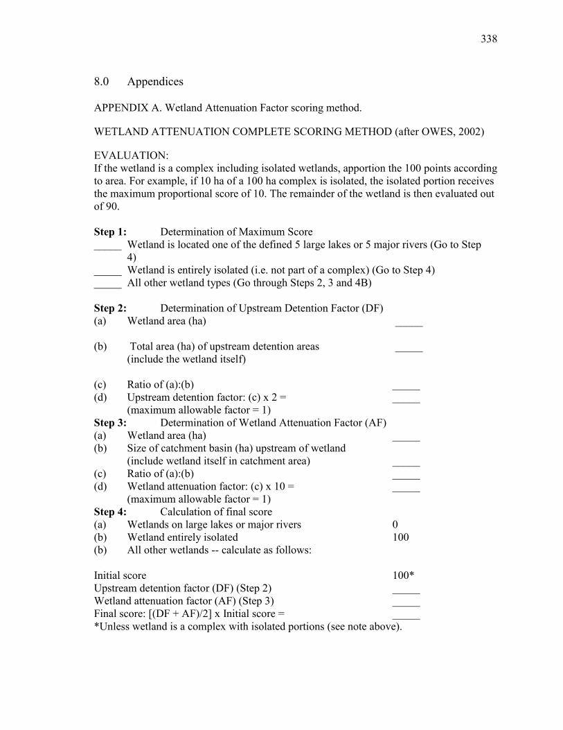
338
8.0 Appendices
APPENDIX A. Wetland Attenuation Factor scoring method.
WETLAND ATTENUATION COMPLETE SCORING METHOD (after OWES, 2002)
EVALUATION: If the wetland is a complex including isolated wetlands, apportion the 100 points according to area. For example, if 10 ha of a 100 ha complex is isolated, the isolated portion receives the maximum proportional score of 10. The remainder of the wetland is then evaluated out of 90. Step 1: Determination of Maximum Score _____ Wetland is located one of the defined 5 large lakes or 5 major rivers (Go to Step
4) _____ Wetland is entirely isolated (i.e. not part of a complex) (Go to Step 4) _____ All other wetland types (Go through Steps 2, 3 and 4B) Step 2: Determination of Upstream Detention Factor (DF) (a) Wetland area (ha) _____ (b) Total area (ha) of upstream detention areas _____
(include the wetland itself) (c) Ratio of (a):(b) _____ (d) Upstream detention factor: (c) x 2 = _____
(maximum allowable factor = 1) Step 3: Determination of Wetland Attenuation Factor (AF) (a) Wetland area (ha) _____ (b) Size of catchment basin (ha) upstream of wetland
(include wetland itself in catchment area) _____ (c) Ratio of (a):(b) _____ (d) Wetland attenuation factor: (c) x 10 = _____
(maximum allowable factor = 1) Step 4: Calculation of final score (a) Wetlands on large lakes or major rivers 0 (b) Wetland entirely isolated 100 (b) All other wetlands -- calculate as follows: Initial score 100* Upstream detention factor (DF) (Step 2) _____ Wetland attenuation factor (AF) (Step 3) _____ Final score: [(DF + AF)/2] x Initial score = _____ *Unless wetland is a complex with isolated portions (see note above).

339
APPENDIX B. Field data including sites and photographs.
Table B1. (Digitally included with this thesis) List of Surveyed Wetland Types, VCF, VCF Categorizations and Open Water Types
Tables B2 -5. Descriptions with photographs of the examples of wetland class training sites by wetland complex for Wetland Type classification and the associated Open Water Type
Tables B6 -9. Descriptions with photos of the examples of training sites by wetland complex for VCF classification and VCF Number of Forms categories (A, 1 – 3 forms; B 4 -5 forms, and C, 6 of greater forms)
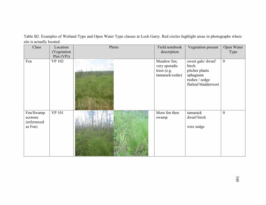
340
Table B2. Examples of Wetland Type and Open Water Type classes at Loch Garry. Red circles highlight areas in photographs where site is actually located.
Class Location (Vegetation Plot (VP))
Photo Field notebook description
Vegetation present Open Water Type
Fen
VP 102
Meadow fen; very sporadic trees (e.g. tamarack/cedar)
sweet gale/ dwarf birch pitcher plants sphagnum rushes / sedge flatleaf bladderwort
0
Fen/Swamp ecotone (referenced as Fen)
VP 101
More fen then swamp
tamarack dwarf birch wire sedge
0
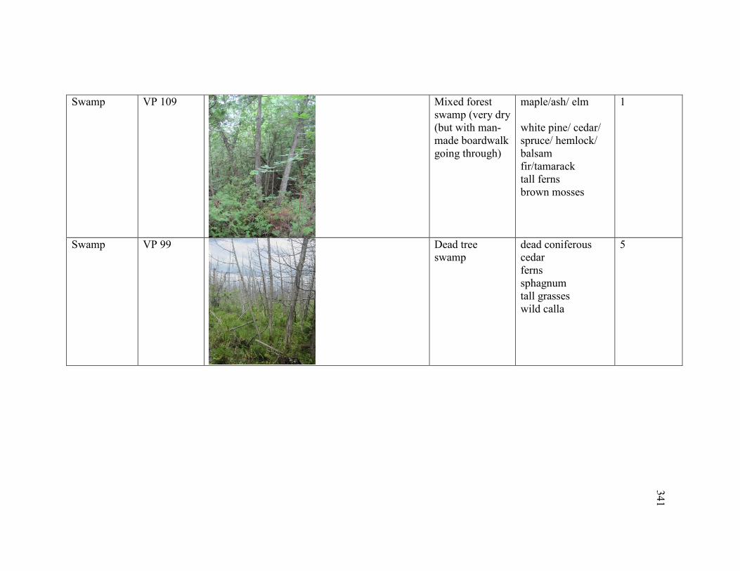
341
Swamp VP 109
Mixed forest swamp (very dry (but with man-made boardwalk going through)
maple/ash/ elm white pine/ cedar/ spruce/ hemlock/ balsam fir/tamarack tall ferns brown mosses
1
Swamp VP 99
Dead tree swamp
dead coniferous cedar ferns sphagnum tall grasses wild calla
5
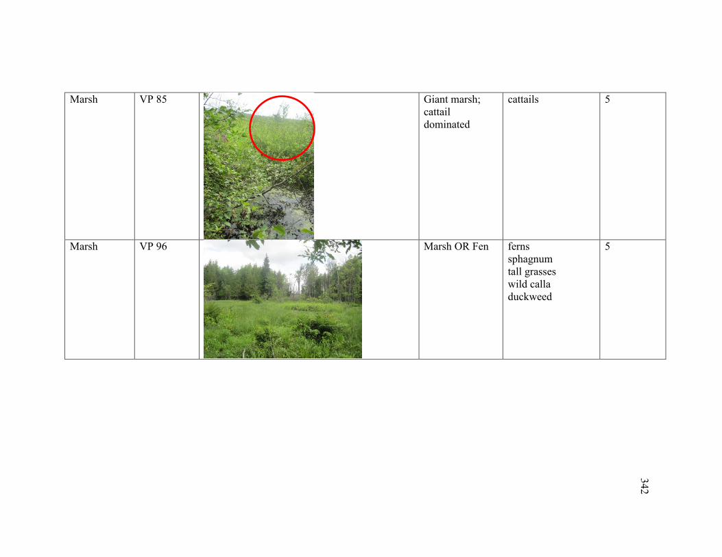
342
Marsh VP 85
Giant marsh; cattail dominated
cattails 5
Marsh VP 96
Marsh OR Fen ferns sphagnum tall grasses wild calla duckweed
5
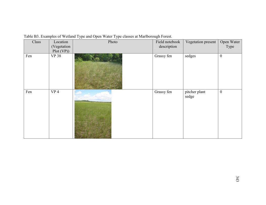
343
Table B3. Examples of Wetland Type and Open Water Type classes at Marlborough Forest. Class Location
(Vegetation Plot (VP))
Photo Field notebook description
Vegetation present Open Water Type
Fen VP 38
Grassy fen sedges 0
Fen VP 4
Grassy fen pitcher plant sedge
0

344
Swamp VP2
Hardwood swamp
black ash poison ivy sphagnum sedge
0
Swamp VP 18
Hardwood swamp
maple ferns sedge
2
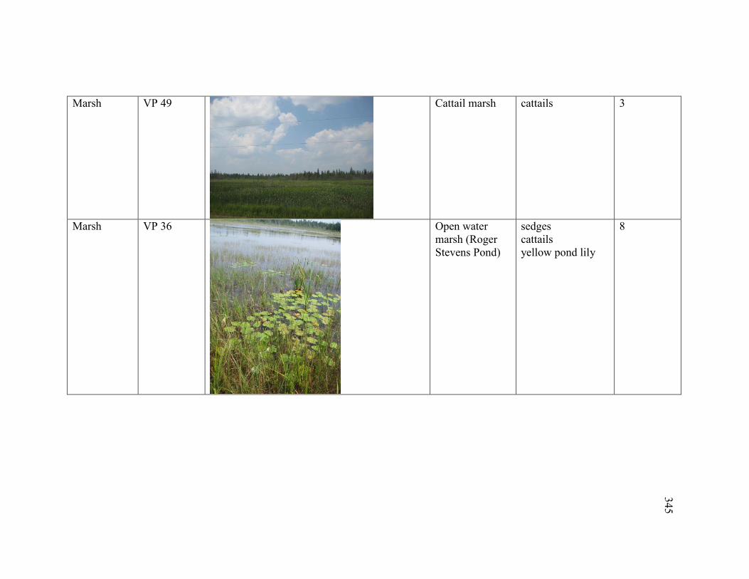
345
Marsh VP 49
Cattail marsh cattails 3
Marsh VP 36
Open water marsh (Roger Stevens Pond)
sedges cattails yellow pond lily
8
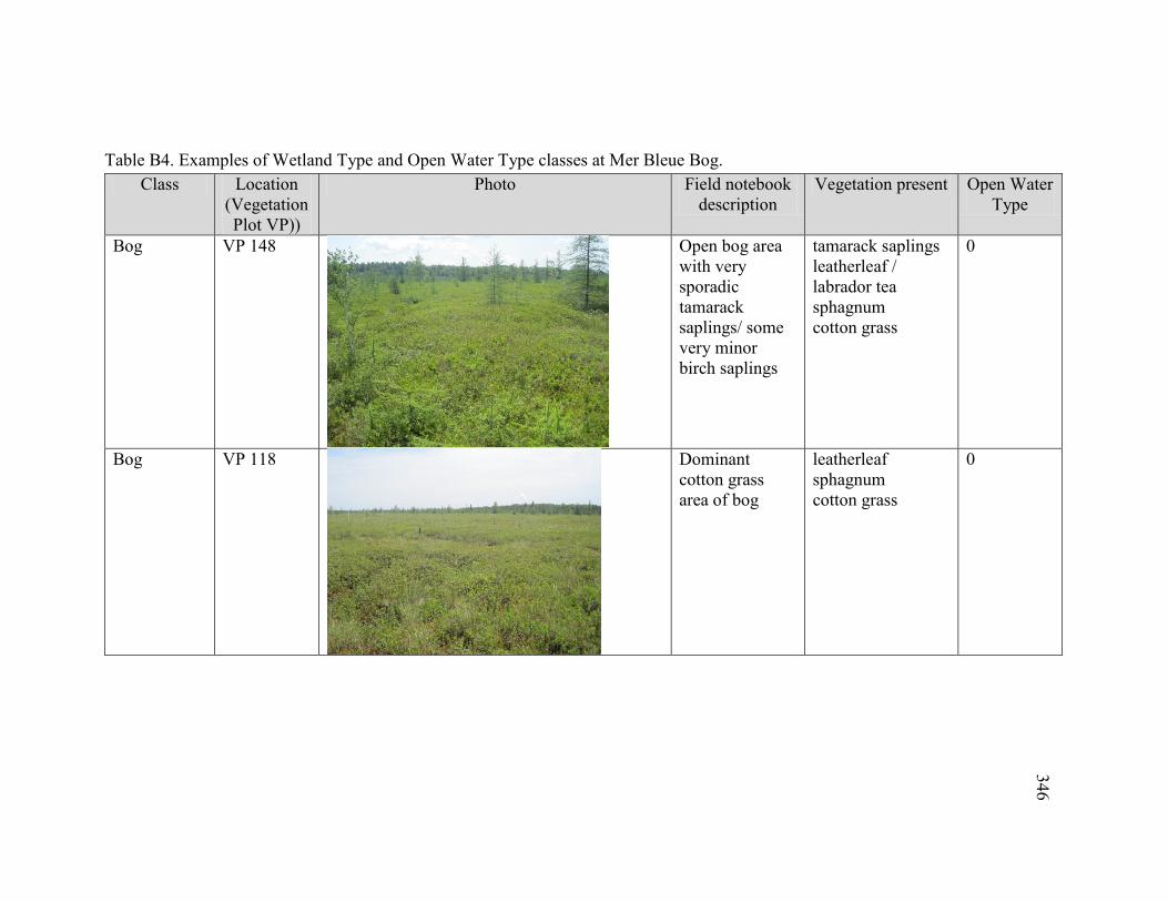
346
Table B4. Examples of Wetland Type and Open Water Type classes at Mer Bleue Bog. Class Location
(Vegetation Plot VP))
Photo Field notebook description
Vegetation present Open Water Type
Bog VP 148
Open bog area with very sporadic tamarack saplings/ some very minor birch saplings
tamarack saplings leatherleaf / labrador tea sphagnum cotton grass
0
Bog VP 118
Dominant cotton grass area of bog
leatherleaf sphagnum cotton grass
0
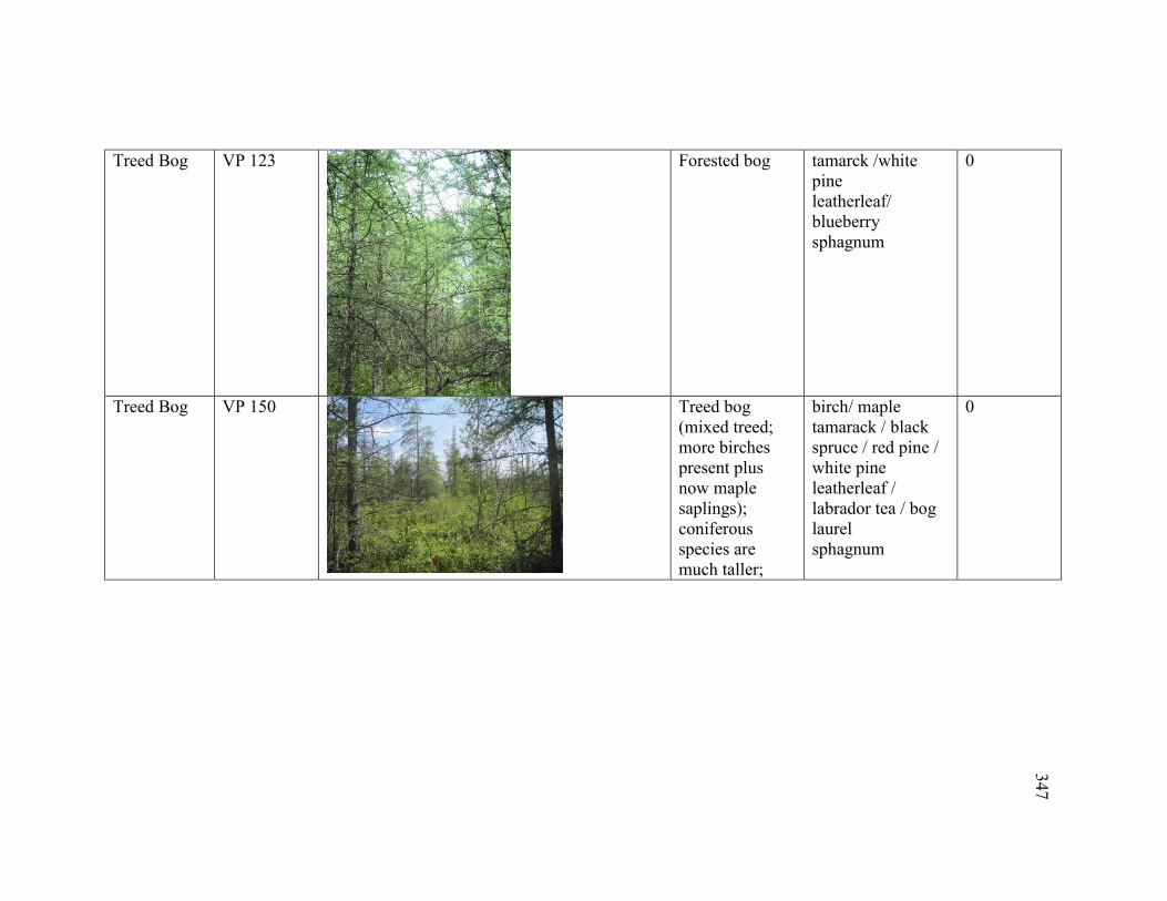
347
Treed Bog VP 123
Forested bog tamarck /white pine leatherleaf/ blueberry sphagnum
0
Treed Bog VP 150
Treed bog (mixed treed; more birches present plus now maple saplings); coniferous species are much taller;
birch/ maple tamarack / black spruce / red pine / white pine leatherleaf / labrador tea / bog laurel sphagnum
0
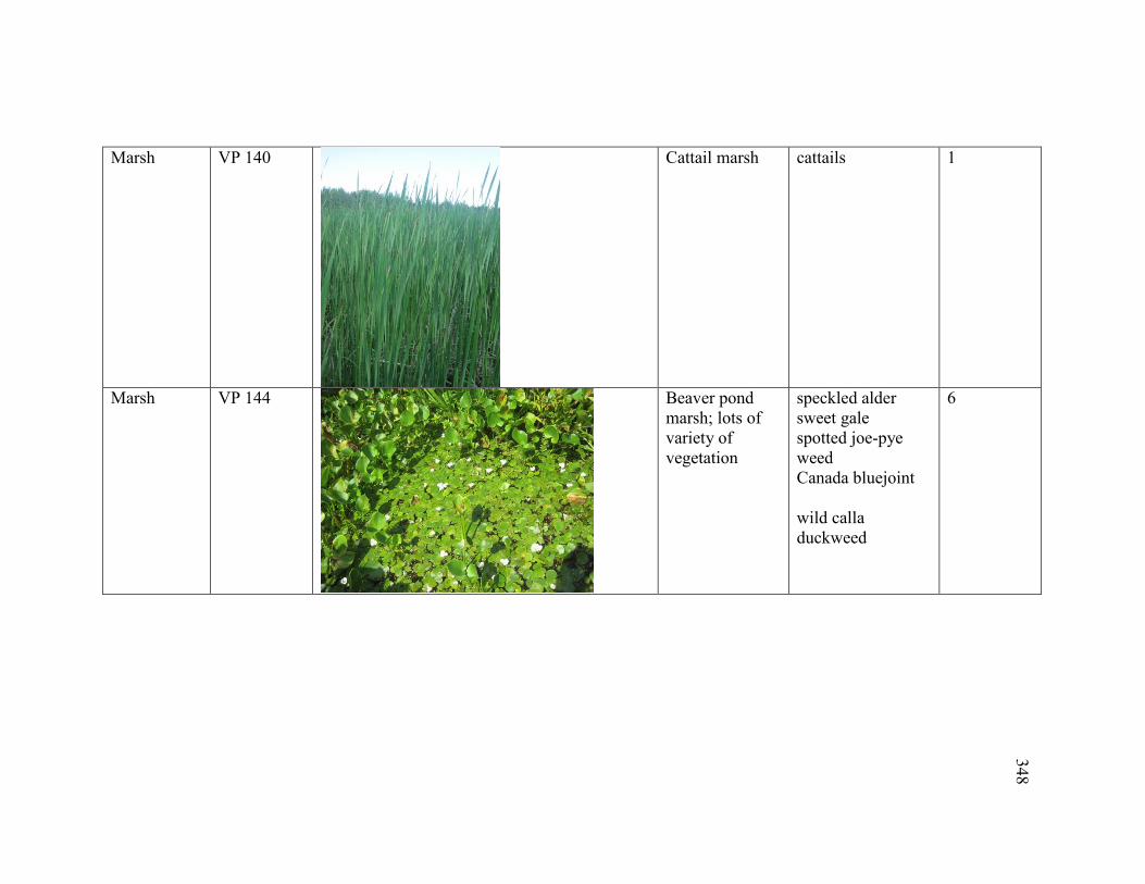
348
Marsh VP 140
Cattail marsh cattails 1
Marsh VP 144
Beaver pond marsh; lots of variety of vegetation
speckled alder sweet gale spotted joe-pye weed Canada bluejoint wild calla duckweed
6
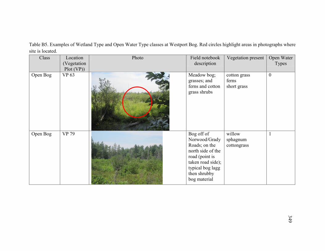
349
Table B5. Examples of Wetland Type and Open Water Type classes at Westport Bog. Red circles highlight areas in photographs where site is located.
Class Location (Vegetation Plot (VP))
Photo Field notebook description
Vegetation present Open Water Types
Open Bog VP 63
Meadow bog; grasses; and ferns and cotton grass shrubs
cotton grass ferns short grass
0
Open Bog VP 79
Bog off of Norwood/Grady Roads; on the north side of the road (point is taken road side); typical bog lagg then shrubby bog material
willow sphagnum cottongrass
1
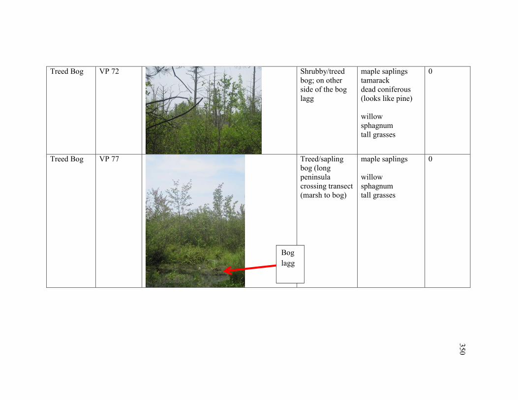
350
Treed Bog VP 72
Shrubby/treed bog; on other side of the bog lagg
maple saplings tamarack dead coniferous (looks like pine) willow sphagnum tall grasses
0
Treed Bog VP 77
Treed/sapling bog (long peninsula crossing transect (marsh to bog)
maple saplings willow sphagnum tall grasses
0
Bog lagg
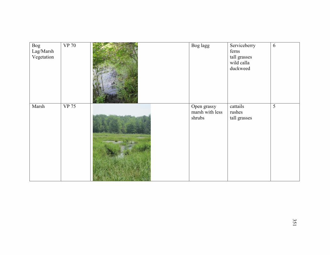
351
Bog Lag/Marsh Vegetation
VP 70
Bog lagg Serviceberry ferns tall grasses wild calla duckweed
6
Marsh VP 75
Open grassy marsh with less shrubs
cattails rushes tall grasses
5
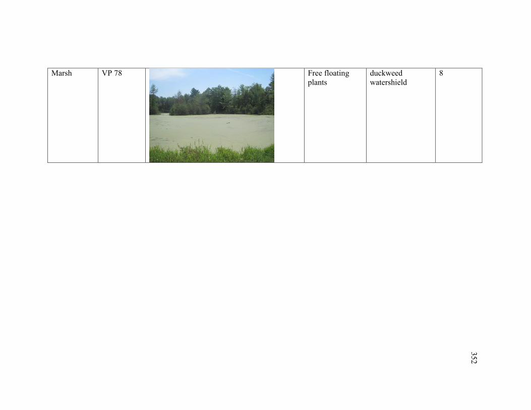
352
Marsh VP 78
Free floating plants
duckweed watershield
8
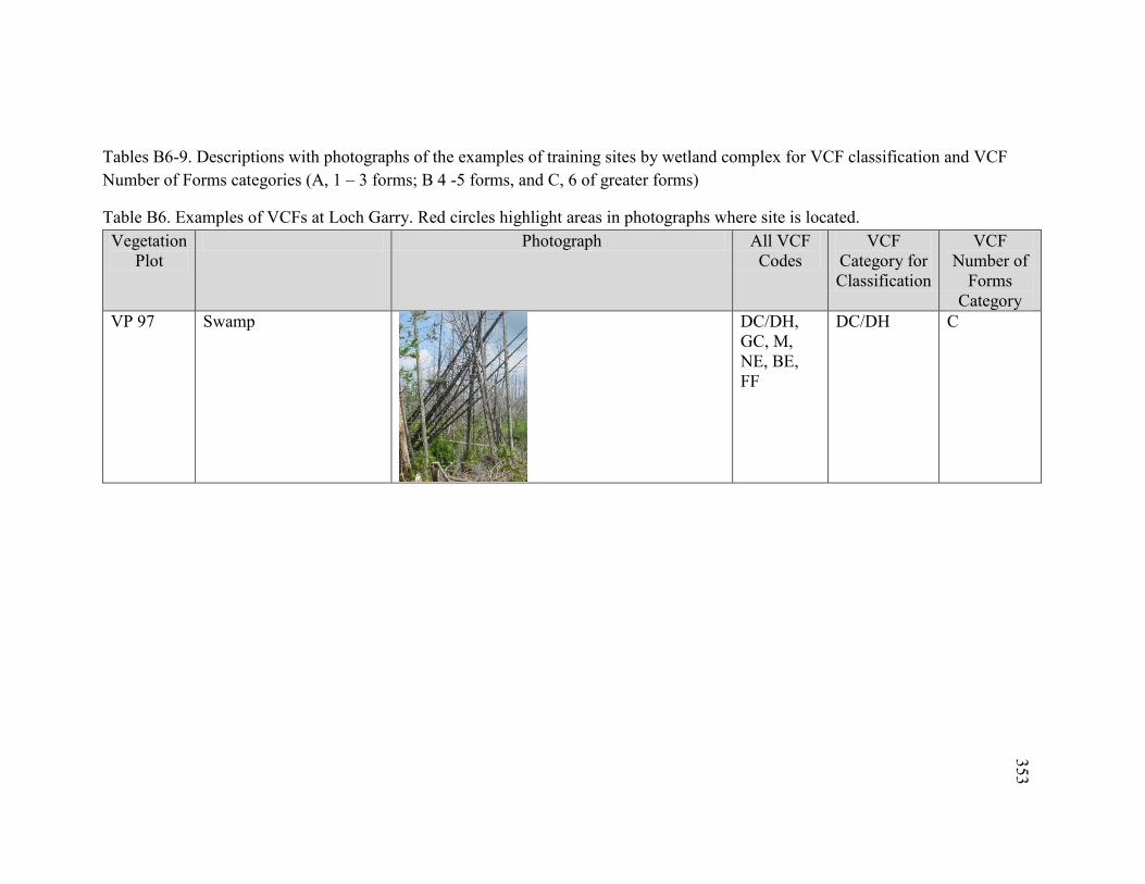
353
Tables B6-9. Descriptions with photographs of the examples of training sites by wetland complex for VCF classification and VCF Number of Forms categories (A, 1 – 3 forms; B 4 -5 forms, and C, 6 of greater forms)
Table B6. Examples of VCFs at Loch Garry. Red circles highlight areas in photographs where site is located. Vegetation
Plot Photograph All VCF
Codes VCF
Category for Classification
VCF Number of
Forms Category
VP 97 Swamp
DC/DH, GC, M, NE, BE, FF
DC/DH C
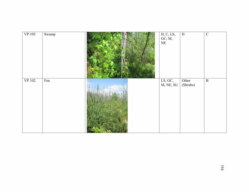
354
VP 105 Swamp
H, C, LS, GC, M, NE
H C
VP 102 Fen
LS, GC, M, NE, SU
Other (Shrubs)
B
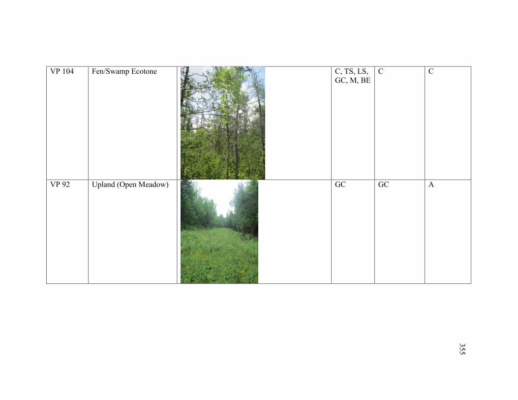
355
VP 104 Fen/Swamp Ecotone
C, TS, LS, GC, M, BE
C C
VP 92 Upland (Open Meadow)
GC GC A
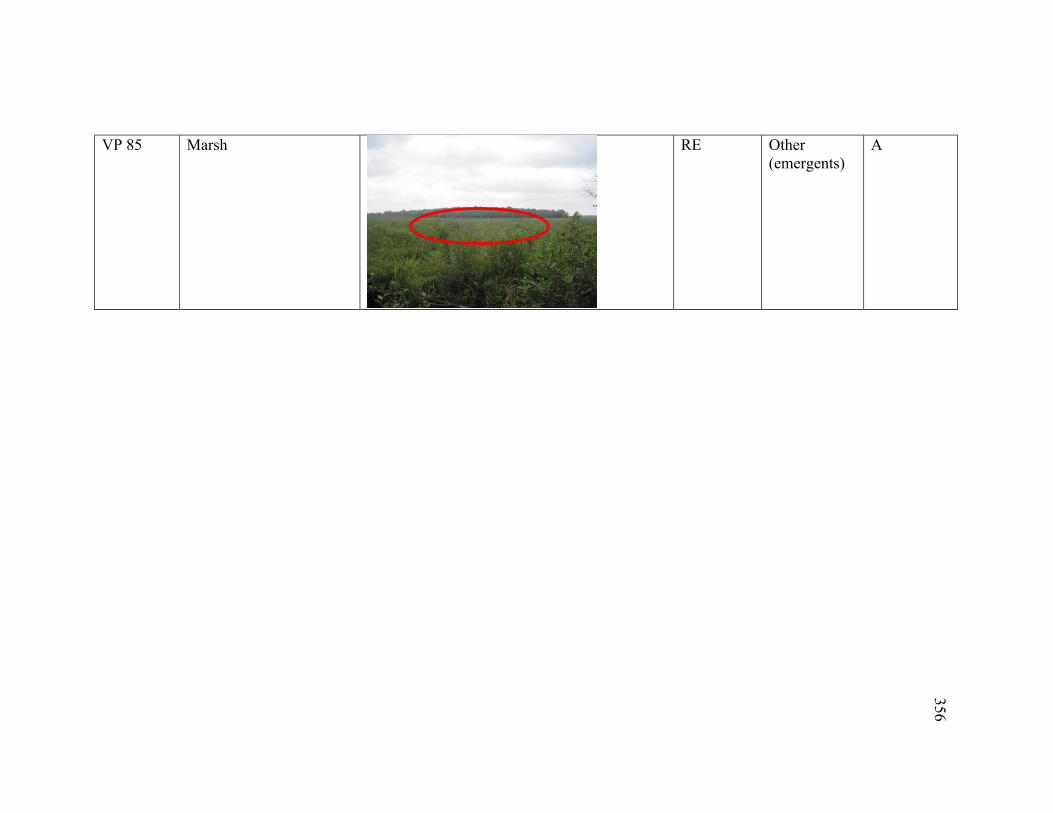
356
VP 85 Marsh
RE Other (emergents)
A
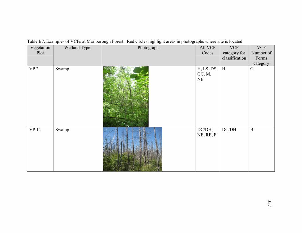
357
Table B7. Examples of VCFs at Marlborough Forest. Red circles highlight areas in photographs where site is located. Vegetation
Plot Wetland Type Photograph All VCF
Codes VCF
category for classification
VCF Number of
Forms category
VP 2 Swamp
H, LS, DS, GC, M, NE
H C
VP 14 Swamp
DC/DH, NE, RE, F
DC/DH B
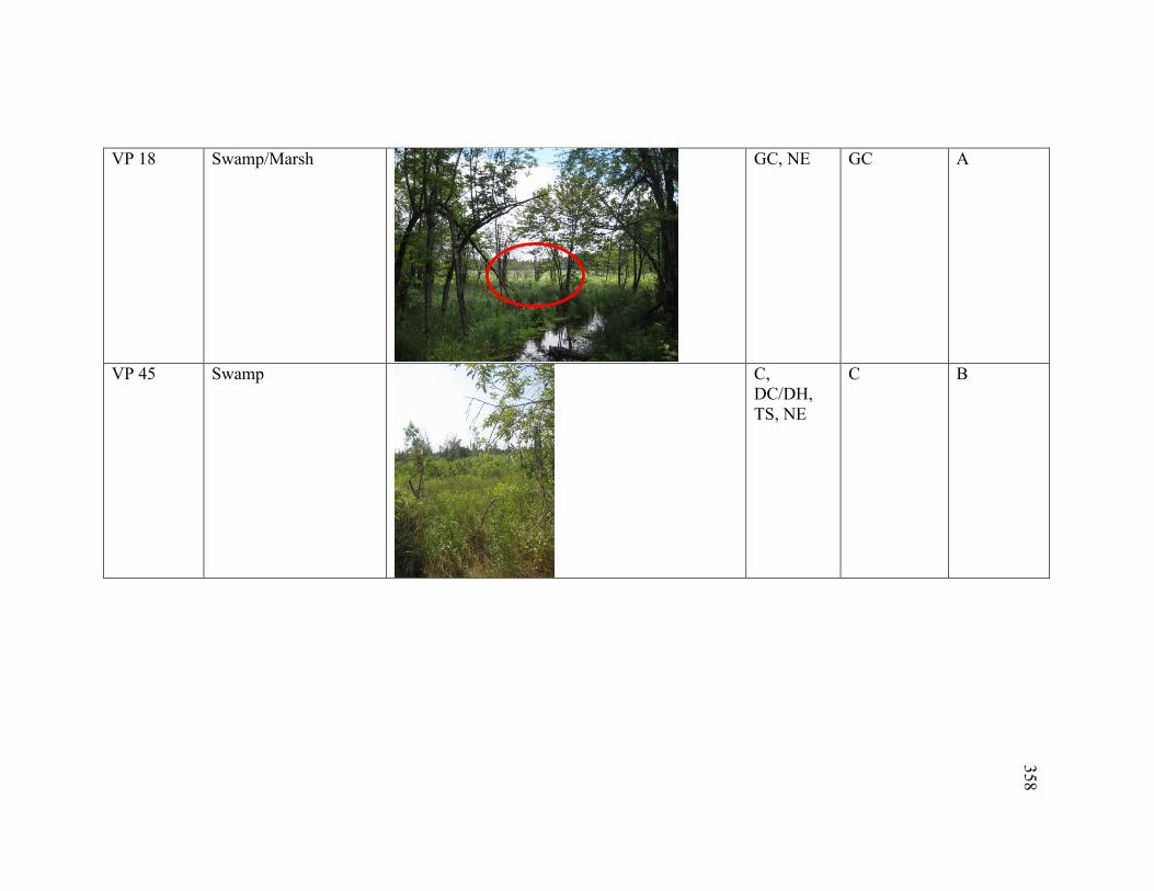
358
VP 18 Swamp/Marsh
GC, NE GC A
VP 45 Swamp
C, DC/DH, TS, NE
C B
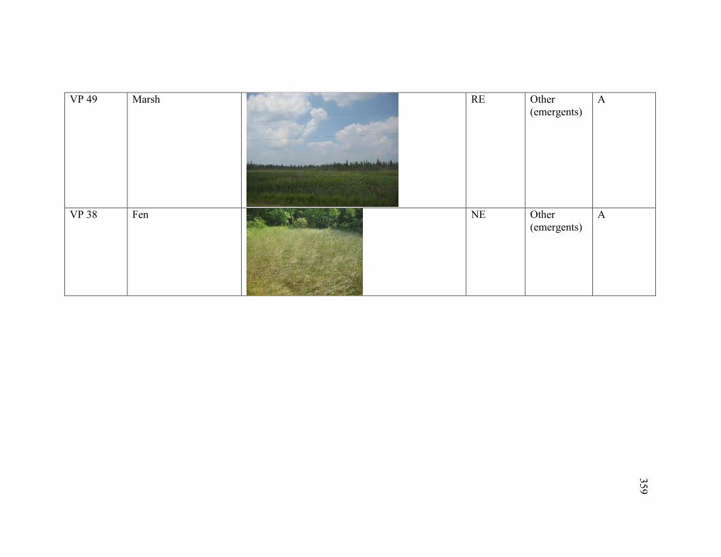
359
VP 49 Marsh
RE Other (emergents)
A
VP 38 Fen
NE Other (emergents)
A
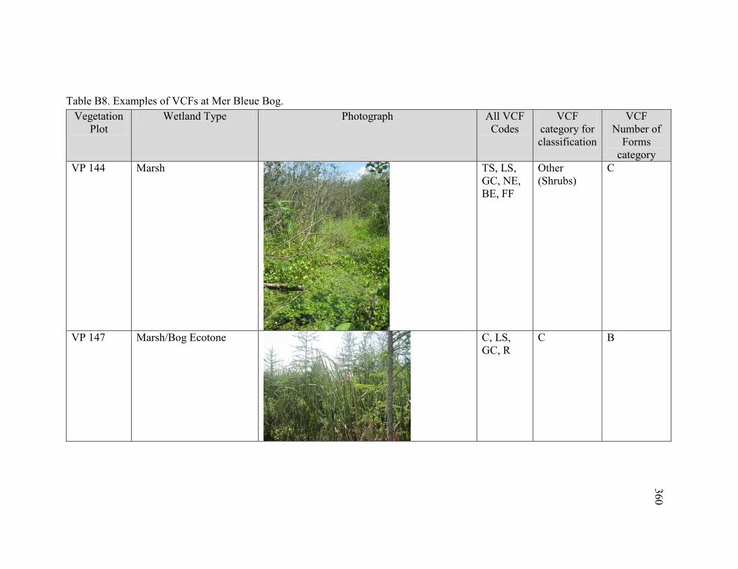
360
Table B8. Examples of VCFs at Mer Bleue Bog. Vegetation
Plot Wetland Type Photograph All VCF
Codes VCF
category for classification
VCF Number of
Forms category
VP 144 Marsh
TS, LS, GC, NE, BE, FF
Other (Shrubs)
C
VP 147 Marsh/Bog Ecotone
C, LS, GC, R
C B
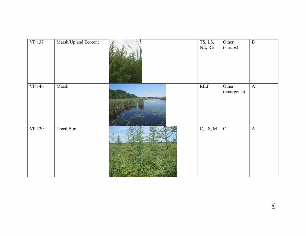
361
VP 137 Marsh/Upland Ecotone
TS, LS, NE, RE
Other (shrubs)
B
VP 146 Marsh
RE,F
Other (emergents)
A
VP 120 Treed Bog
C, LS, M
C A
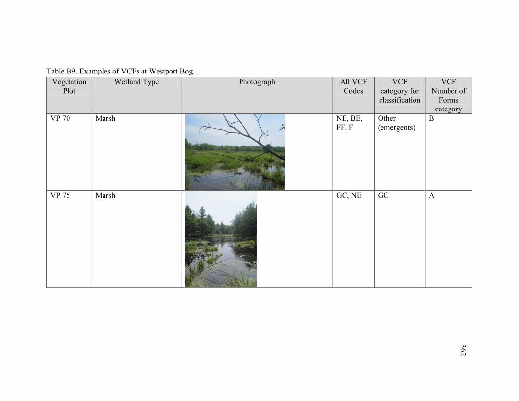
362
Table B9. Examples of VCFs at Westport Bog. Vegetation
Plot Wetland Type Photograph All VCF
Codes VCF
category for classification
VCF Number of
Forms category
VP 70 Marsh
NE, BE, FF, F
Other (emergents)
B
VP 75 Marsh
GC, NE GC A
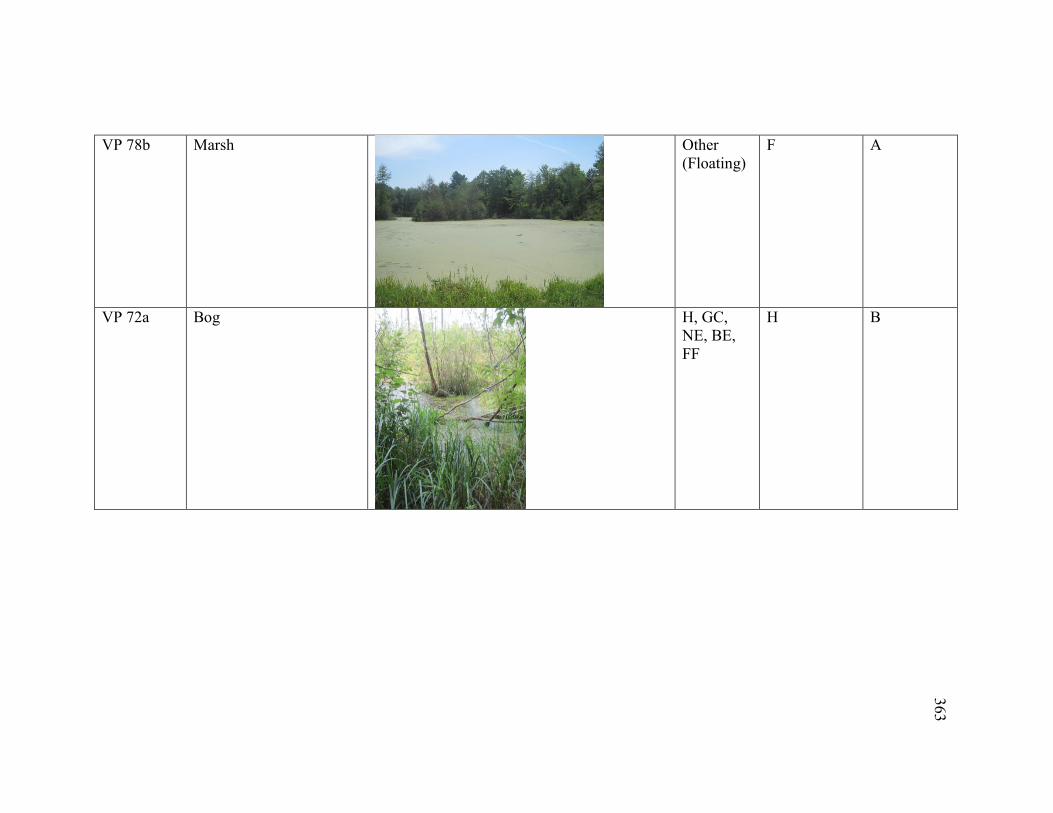
363
VP 78b Marsh
Other (Floating)
F A
VP 72a Bog
H, GC, NE, BE, FF
H B
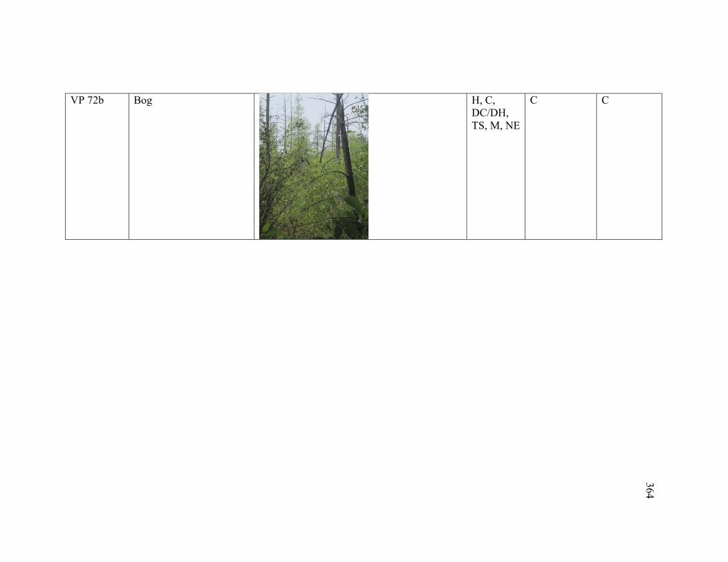
364
VP 72b Bog
H, C, DC/DH, TS, M, NE
C C
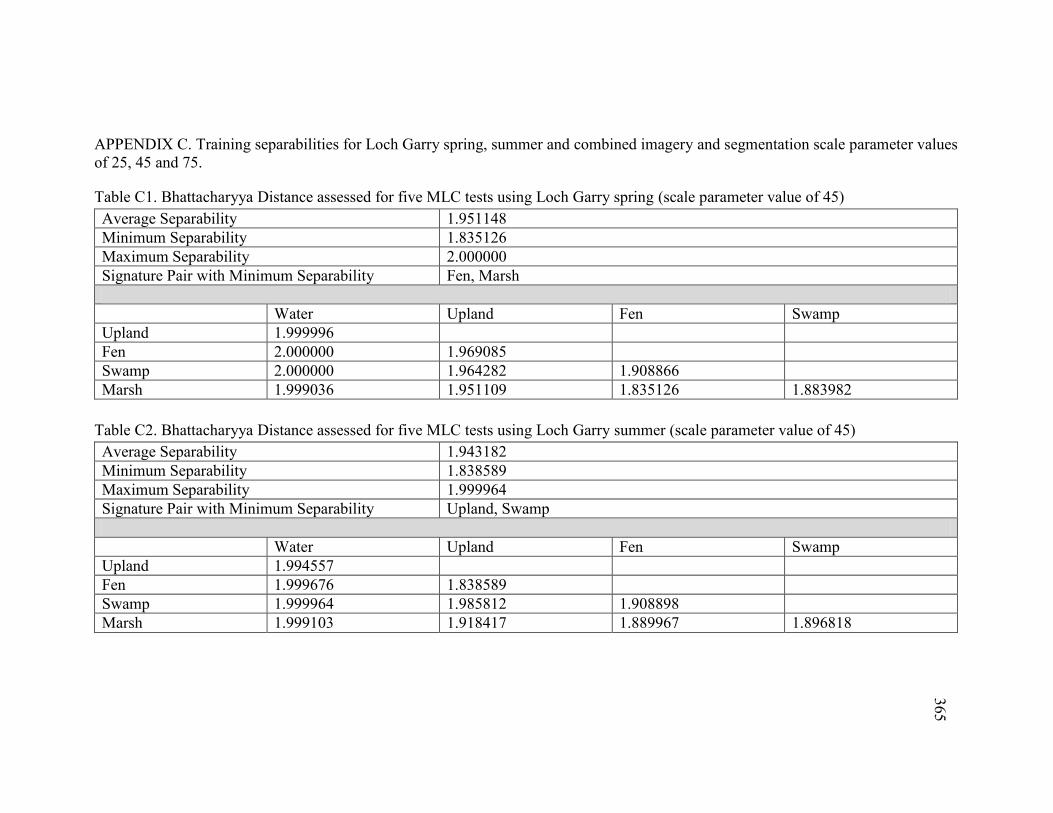
365
APPENDIX C. Training separabilities for Loch Garry spring, summer and combined imagery and segmentation scale parameter values of 25, 45 and 75.
Table C1. Bhattacharyya Distance assessed for five MLC tests using Loch Garry spring (scale parameter value of 45) Average Separability 1.951148 Minimum Separability 1.835126 Maximum Separability 2.000000 Signature Pair with Minimum Separability Fen, Marsh Water Upland Fen Swamp Upland 1.999996 Fen 2.000000 1.969085 Swamp 2.000000 1.964282 1.908866 Marsh 1.999036 1.951109 1.835126 1.883982
Table C2. Bhattacharyya Distance assessed for five MLC tests using Loch Garry summer (scale parameter value of 45) Average Separability 1.943182 Minimum Separability 1.838589 Maximum Separability 1.999964 Signature Pair with Minimum Separability Upland, Swamp Water Upland Fen Swamp Upland 1.994557 Fen 1.999676 1.838589 Swamp 1.999964 1.985812 1.908898 Marsh 1.999103 1.918417 1.889967 1.896818
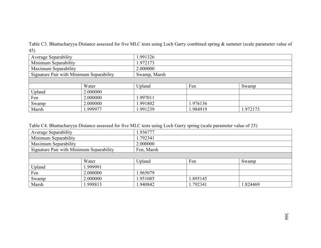
366
Table C3. Bhattacharyya Distance assessed for five MLC tests using Loch Garry combined spring & summer (scale parameter value of 45) Average Separability 1.991326 Minimum Separability 1.972173 Maximum Separability 2.000000 Signature Pair with Minimum Separability Swamp, Marsh Water Upland Fen Swamp Upland 2.000000 Fen 2.000000 1.997011 Swamp 2.000000 1.991802 1.976136 Marsh 1.999977 1.991239 1.984919 1.972173
Table C4. Bhattacharyya Distance assessed for five MLC tests using Loch Garry spring (scale parameter value of 25) Average Separability 1.936777 Minimum Separability 1.792341 Maximum Separability 2.000000 Signature Pair with Minimum Separability Fen, Marsh Water Upland Fen Swamp Upland 1.999991 Fen 2.000000 1.965079 Swamp 2.000000 1.951085 1.895145 Marsh 1.998813 1.940842 1.792341 1.824469
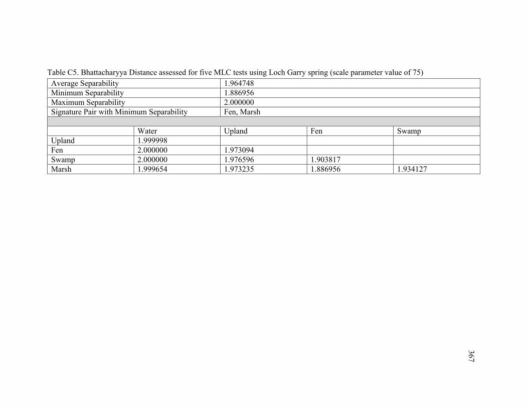
367
Table C5. Bhattacharyya Distance assessed for five MLC tests using Loch Garry spring (scale parameter value of 75) Average Separability 1.964748 Minimum Separability 1.886956 Maximum Separability 2.000000 Signature Pair with Minimum Separability Fen, Marsh Water Upland Fen Swamp Upland 1.999998 Fen 2.000000 1.973094 Swamp 2.000000 1.976596 1.903817 Marsh 1.999654 1.973235 1.886956 1.934127
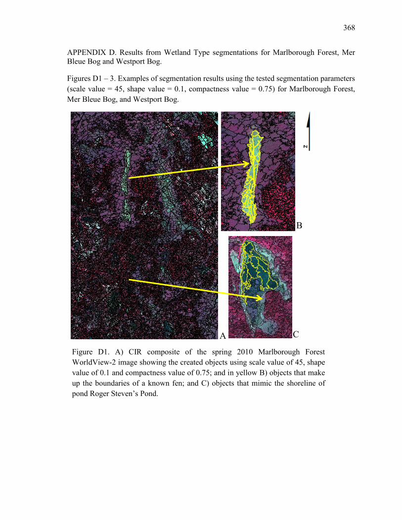
368
APPENDIX D. Results from Wetland Type segmentations for Marlborough Forest, Mer Bleue Bog and Westport Bog.
Figures D1 – 3. Examples of segmentation results using the tested segmentation parameters (scale value = 45, shape value = 0.1, compactness value = 0.75) for Marlborough Forest, Mer Bleue Bog, and Westport Bog.
A
B
C
Figure D1. A) CIR composite of the spring 2010 Marlborough Forest WorldView-2 image showing the created objects using scale value of 45, shape value of 0.1 and compactness value of 0.75; and in yellow B) objects that make up the boundaries of a known fen; and C) objects that mimic the shoreline of pond Roger Steven’s Pond.
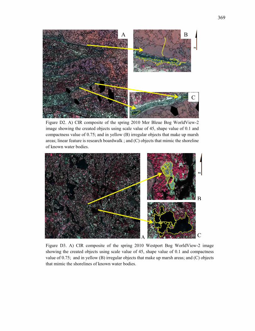
369
A
Figure D2. A) CIR composite of the spring 2010 Mer Bleue Bog WorldView-2 image showing the created objects using scale value of 45, shape value of 0.1 and compactness value of 0.75; and in yellow (B) irregular objects that make up marsh areas; linear feature is research boardwalk ; and (C) objects that mimic the shoreline of known water bodies.
B
C A
B
Figure D3. A) CIR composite of the spring 2010 Westport Bog WorldView-2 image showing the created objects using scale value of 45, shape value of 0.1 and compactness value of 0.75; and in yellow (B) irregular objects that make up marsh areas; and (C) objects that mimic the shorelines of known water bodies.
C
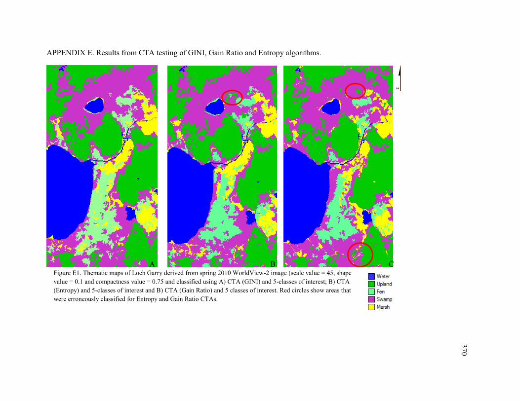
370
APPENDIX E. Results from CTA testing of GINI, Gain Ratio and Entropy algorithms.
B Figure E1. Thematic maps of Loch Garry derived from spring 2010 WorldView-2 image (scale value = 45, shape value = 0.1 and compactness value = 0.75 and classified using A) CTA (GINI) and 5-classes of interest; B) CTA (Entropy) and 5-classes of interest and B) CTA (Gain Ratio) and 5 classes of interest. Red circles show areas that were erroneously classified for Entropy and Gain Ratio CTAs.
A
< C
371
APPENDIX F. Results from Wetland Type classifications for Marlborough Forest, Mer Bleue Bog and Westport Bog.
Figure F1 – F2. 5-Class GINI classification trees for spring 2010 Marlborough Forest, and Mer Bleue Bog.
Figures F3 – F5. Thematic maps of Marlborough Forest, Mer Bleue Bog and Westport Bog derived from spring 2010 WorldView-2 image and DEM segmented using scale value of 45, shape value of 0.1 and compactness value of 0.75 and classified using GINI CTA and 5-classes of interest.
Tables F1A & B – F3A & B. As) Error matrix for the spring 2010 Marlborough Forest, Mer Bleue Bog and Westport Bog WorldView-2 and DEM object-based GINI CTA (5-classes); and Bs) Accuracy statistics for the spring 2010 Marlborough Forest, Mer Bleue Bog and Westport Bog WorldView-2 and DEM object-based GINI CTA (5-classes).
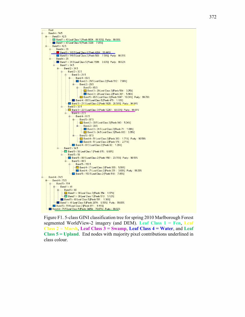
372
Figure F1. 5-class GINI classification tree for spring 2010 Marlborough Forest segmented WorldView-2 imagery (and DEM). Leaf Class 1 = Fen, Leaf Class 2 = Marsh, Leaf Class 3 = Swamp, Leaf Class 4 = Water, and Leaf Class 5 = Upland. End nodes with majority pixel contributions underlined in class colour.
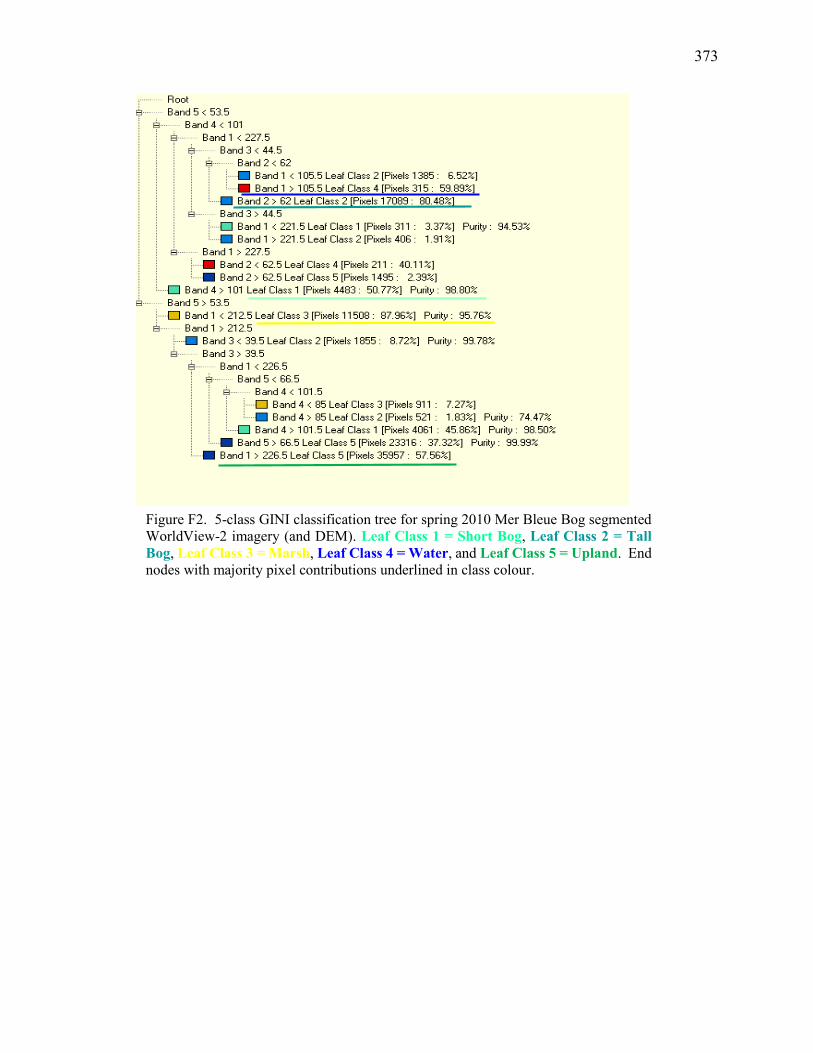
373
Figure F2. 5-class GINI classification tree for spring 2010 Mer Bleue Bog segmented WorldView-2 imagery (and DEM). Leaf Class 1 = Short Bog, Leaf Class 2 = Tall Bog, Leaf Class 3 = Marsh, Leaf Class 4 = Water, and Leaf Class 5 = Upland. End nodes with majority pixel contributions underlined in class colour.
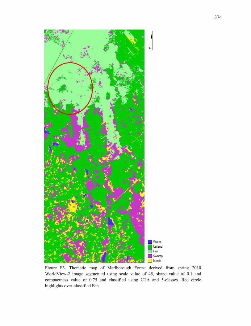
374
Figure F3. Thematic map of Marlborough Forest derived from spring 2010 WorldView-2 image segmented using scale value of 45, shape value of 0.1 and compactness value of 0.75 and classified using CTA and 5-classes. Red circle highlights over-classified Fen.
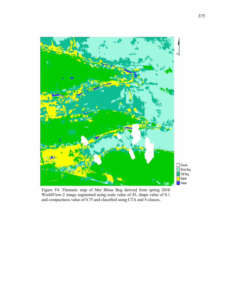
375
Figure F4. Thematic map of Mer Bleue Bog derived from spring 2010 WorldView-2 image segmented using scale value of 45, shape value of 0.1 and compactness value of 0.75 and classified using CTA and 5-classes.
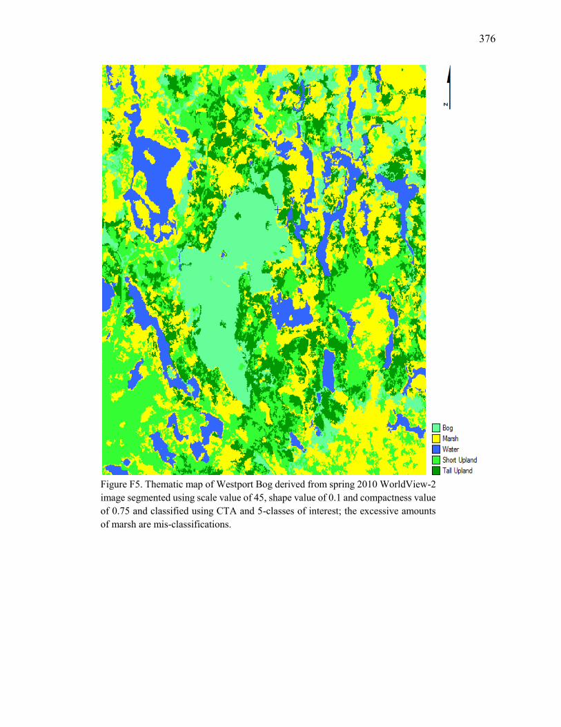
376
Figure F5. Thematic map of Westport Bog derived from spring 2010 WorldView-2 image segmented using scale value of 45, shape value of 0.1 and compactness value of 0.75 and classified using CTA and 5-classes of interest; the excessive amounts of marsh are mis-classifications.
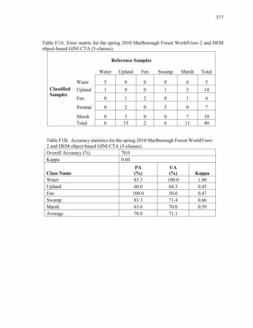
377
Table F1A. Error matrix for the spring 2010 Marlborough Forest WorldView-2 and DEM object-based GINI CTA (5-classes).
Reference Samples
Classified Samples
Water Upland Fen Swamp Marsh
Total
Water 5 0 0 0 0 5 Upland 1 9 0 1 3 14
Fen 0 1 2 0 1 4
Swamp 0 2 0 5 0 7
Marsh 0 3 0 0 7 10 Total 6 15 2 6 11 40
Table F1B. Accuracy statistics for the spring 2010 Marlborough Forest WorldView-2 and DEM object-based GINI CTA (5-classes). Overall Accuracy (%) 70.0
Kappa 0.60
Class Name PA (%)
UA (%) Kappa
Water 83.3 100.0 1.00 Upland 60.0 64.3 0.43 Fen 100.0 50.0 0.47 Swamp 83.3 71.4 0.66 Marsh 63.6 70.0 0.59 Average 78.0 71.1
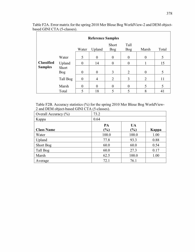
378
Table F2A. Error matrix for the spring 2010 Mer Bleue Bog WorldView-2 and DEM object-based GINI CTA (5-classes).
Reference Samples
Classified Samples
Water Upland Short Bog
Tall Bog Marsh
Total
Water 5 0 0 0 0 5 Upland 0 14 0 0 1 15 Short Bog 0 0 3 2 0 5
Tall Bog 0 4 2 3 2 11
Marsh 0 0 0 0 5 5 Total 5 18 5 5 8 41
Table F2B. Accuracy statistics (%) for the spring 2010 Mer Bleue Bog WorldView-2 and DEM object-based GINI CTA (5-classes). Overall Accuracy (%) 73.2
Kappa 0.64
Class Name PA (%)
UA (%) Kappa
Water 100.0 100.0 1.00 Upland 77.8 93.3 0.88 Short Bog 60.0 60.0 0.54 Tall Bog 60.0 27.3 0.17 Marsh 62.5 100.0 1.00 Average 72.1 76.1
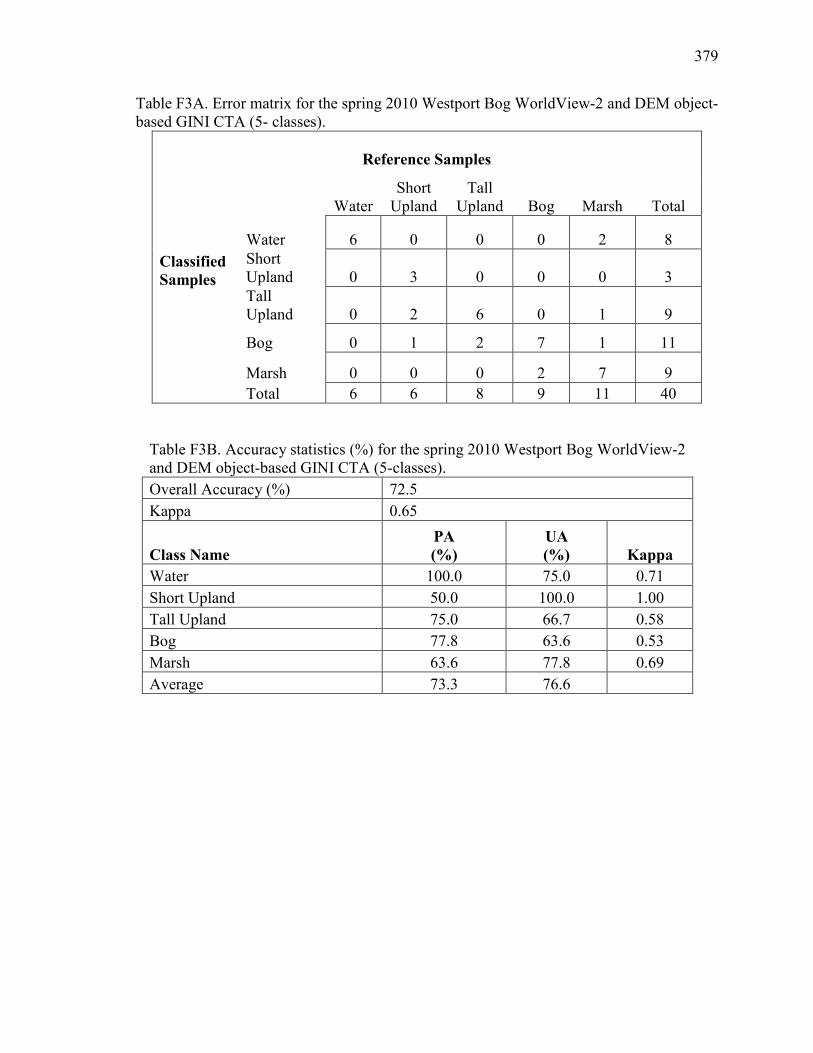
379
Table F3A. Error matrix for the spring 2010 Westport Bog WorldView-2 and DEM object-based GINI CTA (5- classes).
Reference Samples
Classified Samples
Water Short
Upland Tall
Upland Bog Marsh
Total
Water 6 0 0 0 2 8 Short Upland 0 3 0 0 0 3 Tall Upland 0 2 6 0 1 9
Bog 0 1 2 7 1 11
Marsh 0 0 0 2 7 9 Total 6 6 8 9 11 40
Table F3B. Accuracy statistics (%) for the spring 2010 Westport Bog WorldView-2 and DEM object-based GINI CTA (5-classes). Overall Accuracy (%) 72.5
Kappa 0.65
Class Name PA (%)
UA (%) Kappa
Water 100.0 75.0 0.71 Short Upland 50.0 100.0 1.00 Tall Upland 75.0 66.7 0.58 Bog 77.8 63.6 0.53 Marsh 63.6 77.8 0.69 Average 73.3 76.6
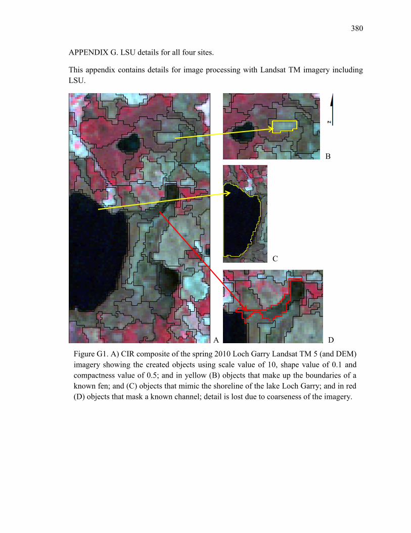
380
APPENDIX G. LSU details for all four sites.
This appendix contains details for image processing with Landsat TM imagery including LSU.
Figure G1. A) CIR composite of the spring 2010 Loch Garry Landsat TM 5 (and DEM) imagery showing the created objects using scale value of 10, shape value of 0.1 and compactness value of 0.5; and in yellow (B) objects that make up the boundaries of a known fen; and (C) objects that mimic the shoreline of the lake Loch Garry; and in red (D) objects that mask a known channel; detail is lost due to coarseness of the imagery.
A
B
C
D
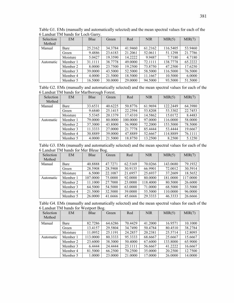
381
Table G1. EMs (manually and automatically selected) and the mean spectral values for each of the 6 Landsat TM bands for Loch Garry.
Selection Method
EM Blue Green Red NIR MIR(5) MIR(7)
Manual
Bare 25.2162 34.3784 41.9460 61.2162 116.5405 53.9460 Green 9.4886 23.6183 21.2061 52.0611 51.1298 21.7786 Moisture 5.0427 19.3590 14.2222 9.9487 7.7180 4.7180
Automatic Member 1 31.1111 38.7778 49.0000 72.1111 138.7778 65.2222 Member 2 8.0000 23.7500 19.2500 73.8750 47.2500 17.6250 Member 3 39.0000 43.5000 52.5000 58.5000 116.5000 76.5000 Member 4 4.0000 21.5000 18.5000 11.1667 10.5000 6.0000 Member 5 16.5000 30.0000 29.0000 94.5000 93.5000 51.5000
Table G2. EMs (manually and automatically selected) and the mean spectral values for each of the 6 Landsat TM bands for Marlborough Forest.
Selection Method
EM Blue Green Red NIR MIR(5) MIR(7)
Manual
Bare 33.6531 40.6225 50.8776 61.9694 122.2449 64.3980 Green 9.6840 25.1415 22.2594 53.8208 53.3302 22.7453 Moisture 5.5345 20.1379 17.4310 14.5862 15.0172 8.4483
Automatic Member 1 79.0000 80.0000 100.0000 97.0000 116.0000 58.0000 Member 2 37.3000 43.8000 56.9000 72.2000 153.5000 78.5000 Member 3 11.3333 27.0000 21.7778 85.4444 53.4444 19.6667 Member 4 30.8889 39.0000 47.8889 52.6667 114.8889 76.1111 Member 5 4.0000 21.5000 18.8750 13.2500 8.2500 5.1250
Table G3. EMs (manually and automatically selected) and the mean spectral values for each of the 6 Landsat TM bands for Mer Bleue Bog.
Selection Method
EM Blue Green Red NIR MIR(5) MIR(7)
Manual
Bare 40.8888 47.7271 62.5169 70.0266 143.0680 79.1932 Green 28.5908 28.5908 30.9135 66.9901 72.0012 30.5914 Moisture 6.5000 22.1087 21.6957 25.6937 37.2609 18.5652
Automatic Member 1 107.0000 75.0000 92.0000 80.0000 181.0000 117.0000 Member 2 11.1000 27.7000 23.0000 118.4000 80.5000 26.6000 Member 3 64.5000 54.5000 63.0000 71.0000 68.5000 33.5000 Member 4 21.5000 32.5000 39.0000 55.5000 110.0000 96.0000 Member 5 26.0000 41.6666 45.6666 29.3333 46.3333 26.6666
Table G4. EMs (manually and automatically selected) and the mean spectral values for each of the 6 Landsat TM bands for Westport Bog.
Selection Method
EM Blue Green Red NIR MIR(5) MIR(7)
Manual
Bare 82.7286 64.6286 70.4429 41.2000 16.9571 10.1000 Green 13.4157 29.5804 34.7490 50.4784 80.4510 38.2784 Moisture 11.0952 25.1191 24.2857 20.2381 25.5714 12.8095
Automatic Member 1 113.0000 80.3333 95.3333 68.6667 25.6667 15.6667 Member 2 23.6000 38.3000 50.4000 67.6000 133.8000 65.9000 Member 3 6.4444 24.4444 23.1111 56.6667 41.2222 16.6667 Member 4 81.5000 66.2500 70.2500 35.0000 20.2500 12.7500 Member 5 1.0000 23.0000 21.0000 17.0000 26.0000 14.0000
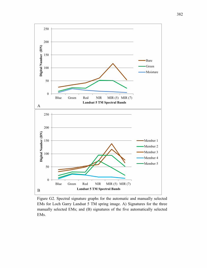
382
0
50
100
150
200
250
Blue Green Red NIR MIR (5) MIR (7)
Dig
ital N
umbe
r (D
N)
Landsat 5 TM Spectral Bands
Bare
Green
Moisture
0
50
100
150
200
250
Blue Green Red NIR MIR (5) MIR (7)
Dig
ital N
umbe
r (D
N)
Landsat 5 TM Spectral Bands
Member 1
Member 2
Member 3
Member 4
Member 5
Figure G2. Spectral signature graphs for the automatic and manually selected EMs for Loch Garry Landsat 5 TM spring image. A) Signatures for the three manually selected EMs; and (B) signatures of the five automatically selected EMs.
A
B
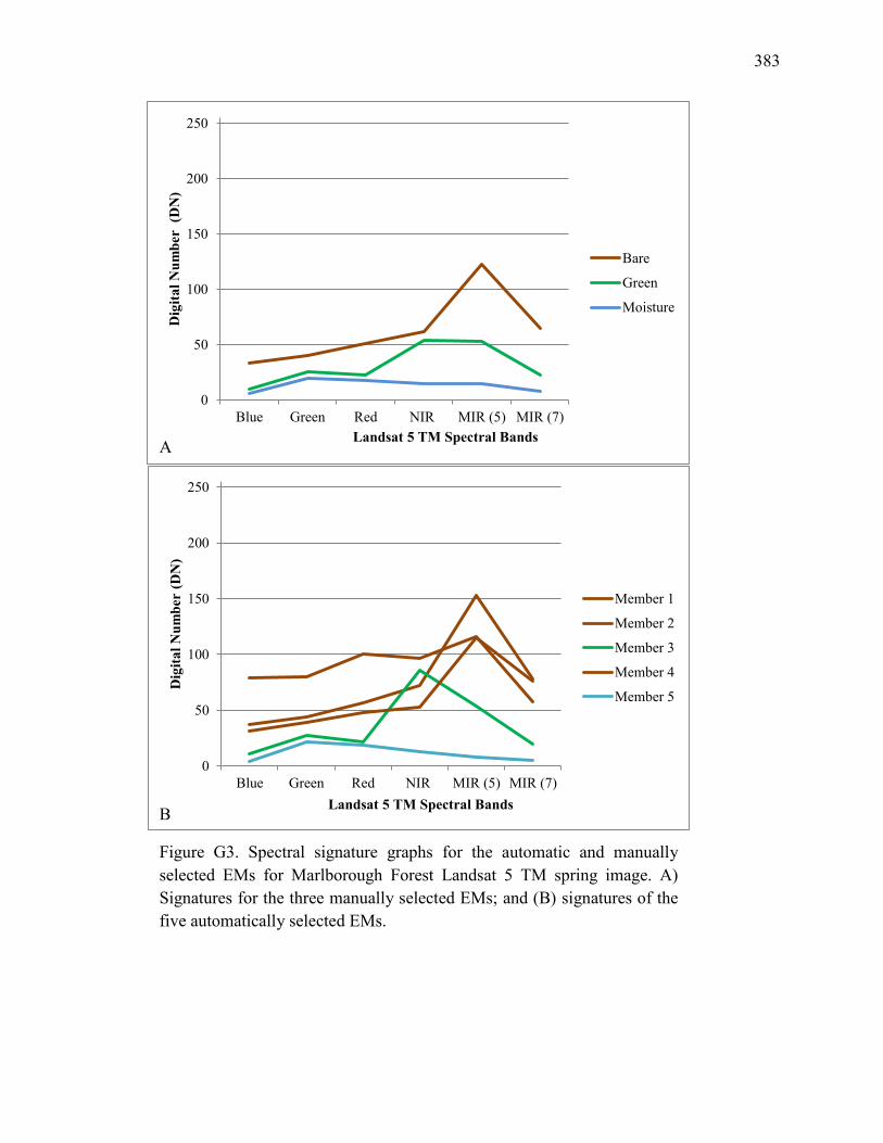
383
0
50
100
150
200
250
Blue Green Red NIR MIR (5) MIR (7)
Dig
ital N
umbe
r (D
N)
Landsat 5 TM Spectral Bands
Bare
Green
Moisture
0
50
100
150
200
250
Blue Green Red NIR MIR (5) MIR (7)
Dig
ital N
umbe
r (D
N)
Landsat 5 TM Spectral Bands
Member 1
Member 2
Member 3
Member 4
Member 5
Figure G3. Spectral signature graphs for the automatic and manually selected EMs for Marlborough Forest Landsat 5 TM spring image. A) Signatures for the three manually selected EMs; and (B) signatures of the five automatically selected EMs.
A
B
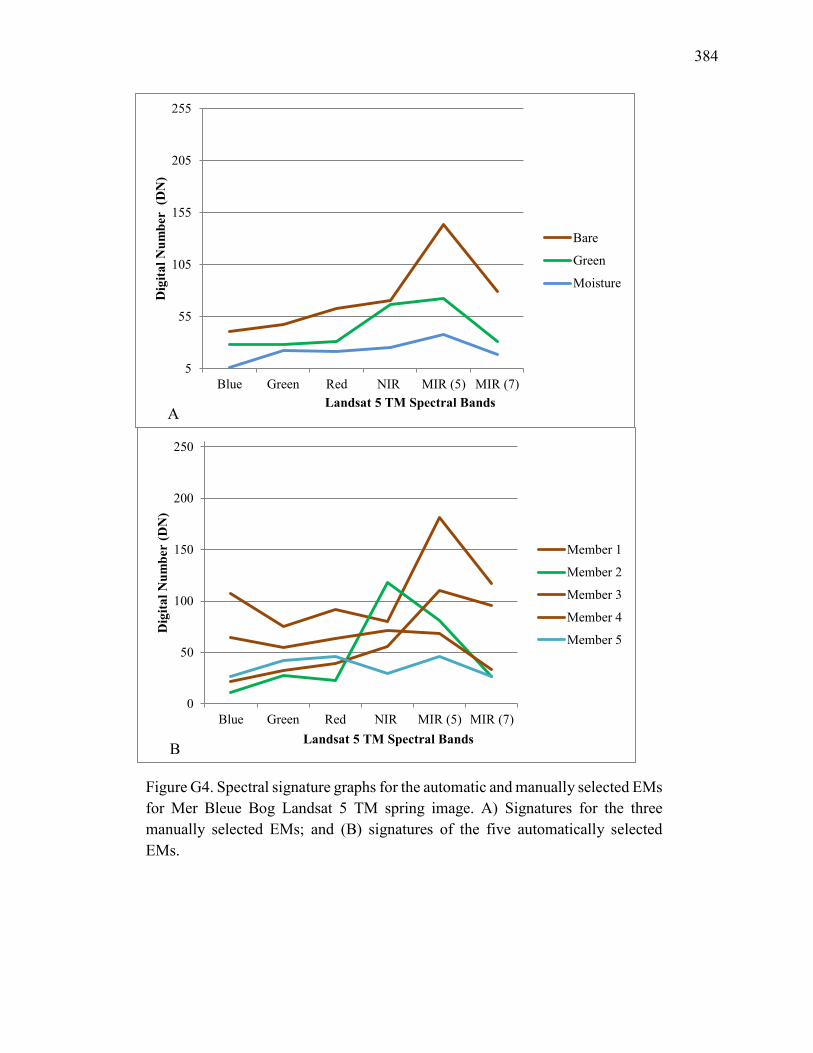
384
5
55
105
155
205
255
Blue Green Red NIR MIR (5) MIR (7)
Dig
ital N
umbe
r (D
N)
Landsat 5 TM Spectral Bands
Bare
Green
Moisture
0
50
100
150
200
250
Blue Green Red NIR MIR (5) MIR (7)
Dig
ital N
umbe
r (D
N)
Landsat 5 TM Spectral Bands
Member 1
Member 2
Member 3
Member 4
Member 5
Figure G4. Spectral signature graphs for the automatic and manually selected EMs for Mer Bleue Bog Landsat 5 TM spring image. A) Signatures for the three manually selected EMs; and (B) signatures of the five automatically selected EMs.
A
B
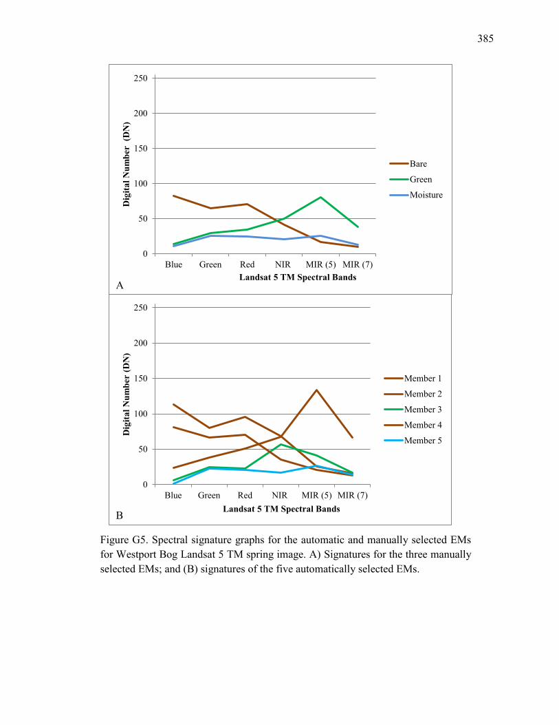
385
0
50
100
150
200
250
Blue Green Red NIR MIR (5) MIR (7)
Dig
ital N
umbe
r (D
N)
Landsat 5 TM Spectral Bands
Member 1
Member 2
Member 3
Member 4
Member 5
Figure G5. Spectral signature graphs for the automatic and manually selected EMs for Westport Bog Landsat 5 TM spring image. A) Signatures for the three manually selected EMs; and (B) signatures of the five automatically selected EMs.
0
50
100
150
200
250
Blue Green Red NIR MIR (5) MIR (7)
Dig
ital N
umbe
r (D
N)
Landsat 5 TM Spectral Bands
Bare
Green
Moisture
A
B
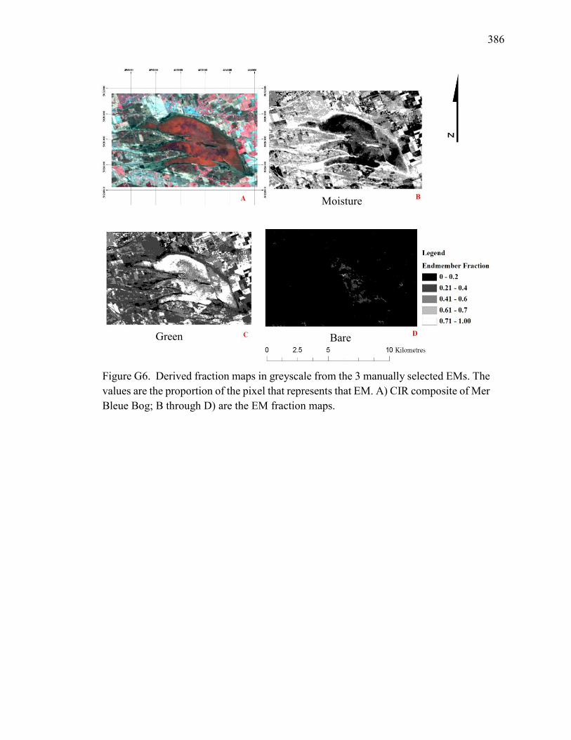
386
Figure G6. Derived fraction maps in greyscale from the 3 manually selected EMs. The values are the proportion of the pixel that represents that EM. A) CIR composite of Mer Bleue Bog; B through D) are the EM fraction maps.
Moisture
Green Bare
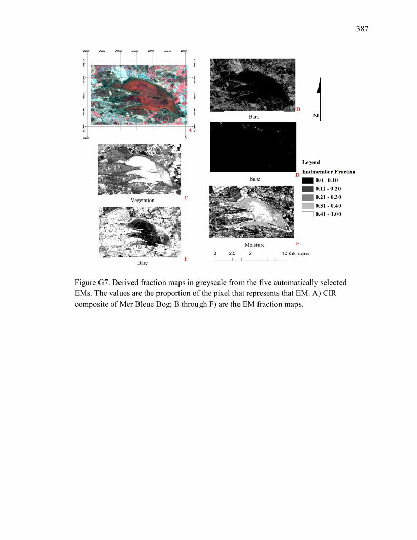
387
Figure G7. Derived fraction maps in greyscale from the five automatically selected EMs. The values are the proportion of the pixel that represents that EM. A) CIR composite of Mer Bleue Bog; B through F) are the EM fraction maps.
Bare
Bare
Bare
Moisture
Vegetation
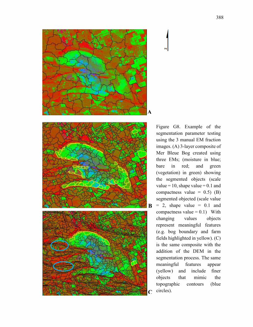
388
Figure G8. Example of the segmentation parameter testing using the 3 manual EM fraction images. (A) 3-layer composite of Mer Bleue Bog created using three EMs; (moisture in blue; bare in red; and green (vegetation) in green) showing the segmented objects (scale value = 10, shape value = 0.1 and compactness value = 0.5) (B) segmented objected (scale value = 2, shape value = 0.1 and compactness value = 0.1) With changing values objects represent meaningful features (e.g. bog boundary and farm fields highlighted in yellow). (C) is the same composite with the addition of the DEM in the segmentation process. The same meaningful features appear (yellow) and include finer objects that mimic the topographic contours (blue circles).
A
B
C
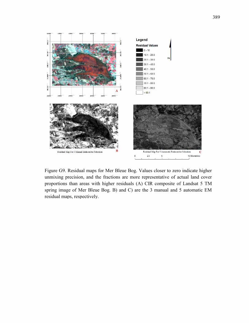
389
Figure G9. Residual maps for Mer Bleue Bog. Values closer to zero indicate higher unmixing precision, and the fractions are more representative of actual land cover proportions than areas with higher residuals (A) CIR composite of Landsat 5 TM spring image of Mer Bleue Bog. B) and C) are the 3 manual and 5 automatic EM residual maps, respectively.
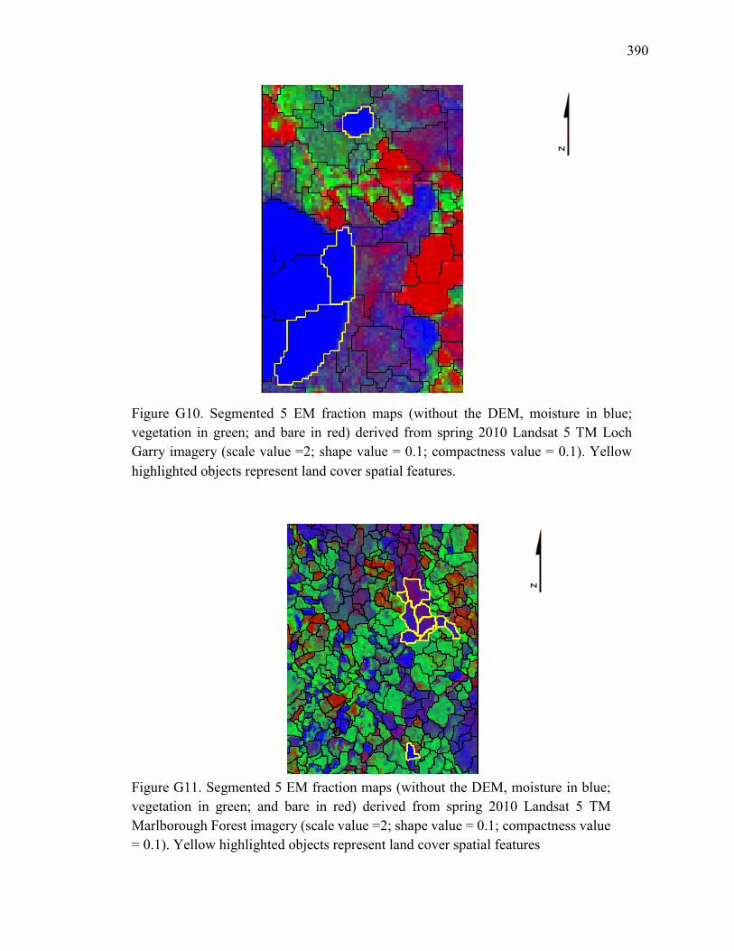
390
Figure G10. Segmented 5 EM fraction maps (without the DEM, moisture in blue; vegetation in green; and bare in red) derived from spring 2010 Landsat 5 TM Loch Garry imagery (scale value =2; shape value = 0.1; compactness value = 0.1). Yellow highlighted objects represent land cover spatial features.
Figure G11. Segmented 5 EM fraction maps (without the DEM, moisture in blue; vegetation in green; and bare in red) derived from spring 2010 Landsat 5 TM Marlborough Forest imagery (scale value =2; shape value = 0.1; compactness value = 0.1). Yellow highlighted objects represent land cover spatial features
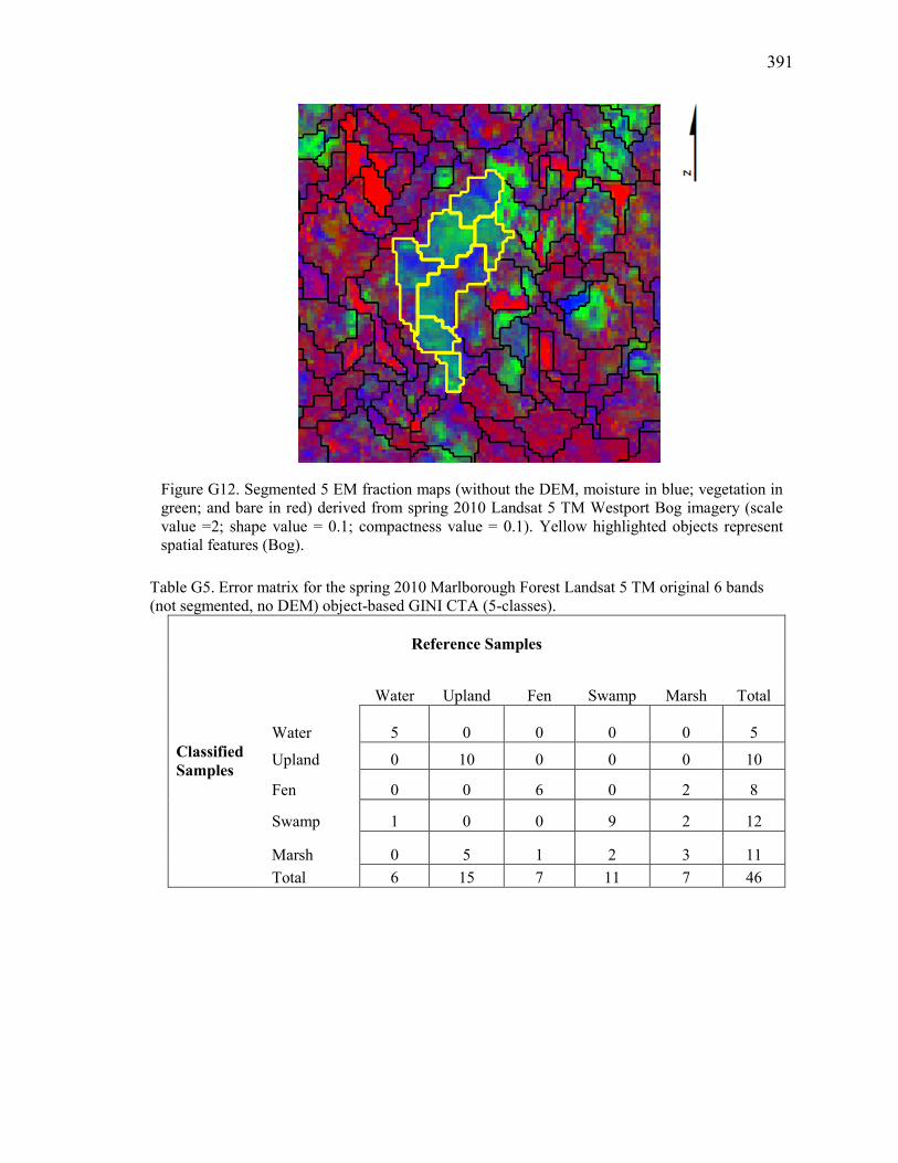
391
Table G5. Error matrix for the spring 2010 Marlborough Forest Landsat 5 TM original 6 bands (not segmented, no DEM) object-based GINI CTA (5-classes).
Reference Samples
Classified Samples
Water Upland Fen Swamp Marsh
Total
Water 5 0 0 0 0 5
Upland 0 10 0 0 0 10
Fen 0 0 6 0 2 8
Swamp 1 0 0 9 2 12
Marsh 0 5 1 2 3 11 Total 6 15 7 11 7 46
Figure G12. Segmented 5 EM fraction maps (without the DEM, moisture in blue; vegetation in green; and bare in red) derived from spring 2010 Landsat 5 TM Westport Bog imagery (scale value =2; shape value = 0.1; compactness value = 0.1). Yellow highlighted objects represent spatial features (Bog).
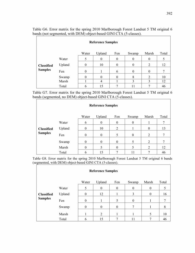
392
Table G6. Error matrix for the spring 2010 Marlborough Forest Landsat 5 TM original 6 bands (not segmented, with DEM) object-based GINI CTA (5-classes).
Reference Samples
Classified Samples
Water Upland Fen Swamp Marsh
Total Water 5 0 0 0 0 5
Upland 0 10 0 0 2 12
Fen 0 1 6 0 0 7 Swamp 0 0 0 8 2 10 Marsh 1 4 1 3 3 12 Total 6 15 7 11 7 46
Table G7. Error matrix for the spring 2010 Marlborough Forest Landsat 5 TM original 6 bands (segmented, no DEM) object-based GINI CTA (5-classes).
Reference Samples
Classified Samples
Water Upland Fen Swamp Marsh
Total
Water 6 0 0 0 1 7
Upland 0 10 2 1 0 13
Fen 0 0 5 0 2 7
Swamp 0 0 0 5 2 7 Marsh 0 5 0 5 2 12 Total 6 15 7 11 7 46
Table G8. Error matrix for the spring 2010 Marlborough Forest Landsat 5 TM original 6 bands (segmented, with DEM) object-based GINI CTA (5-classes).
Reference Samples
Classified Samples
Water Upland Fen Swamp Marsh
Total
Water 5 0 0 0 0 5
Upland 0 12 1 3 0 16
Fen 0 1 5 0 1 7
Swamp 0 0 0 7 1 8
Marsh 1 2 1 1 5 10 Total 6 15 7 11 7 46
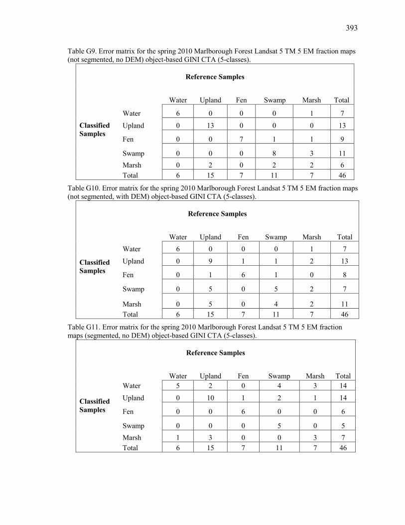
393
Table G9. Error matrix for the spring 2010 Marlborough Forest Landsat 5 TM 5 EM fraction maps (not segmented, no DEM) object-based GINI CTA (5-classes).
Reference Samples
Classified Samples
Water Upland Fen Swamp Marsh
Total
Water 6 0 0 0 1 7
Upland 0 13 0 0 0 13
Fen 0 0 7 1 1 9
Swamp 0 0 0 8 3 11 Marsh 0 2 0 2 2 6 Total 6 15 7 11 7 46
Table G10. Error matrix for the spring 2010 Marlborough Forest Landsat 5 TM 5 EM fraction maps (not segmented, with DEM) object-based GINI CTA (5-classes).
Reference Samples
Classified Samples
Water Upland Fen Swamp Marsh
Total Water 6 0 0 0 1 7
Upland 0 9 1 1 2 13
Fen 0 1 6 1 0 8
Swamp 0 5 0 5 2 7
Marsh 0 5 0 4 2 11 Total 6 15 7 11 7 46
Table G11. Error matrix for the spring 2010 Marlborough Forest Landsat 5 TM 5 EM fraction maps (segmented, no DEM) object-based GINI CTA (5-classes).
Reference Samples
Classified Samples
Water Upland Fen Swamp Marsh
Total Water 5 2 0 4 3 14
Upland 0 10 1 2 1 14
Fen 0 0 6 0 0 6
Swamp 0 0 0 5 0 5 Marsh 1 3 0 0 3 7 Total 6 15 7 11 7 46
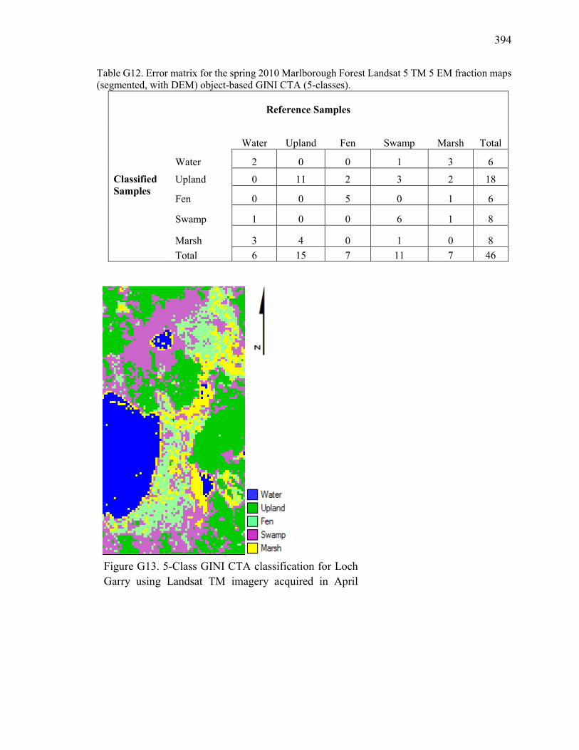
394
Table G12. Error matrix for the spring 2010 Marlborough Forest Landsat 5 TM 5 EM fraction maps (segmented, with DEM) object-based GINI CTA (5-classes).
Reference Samples
Classified Samples
Water Upland Fen Swamp Marsh
Total
Water 2 0 0 1 3 6
Upland 0 11 2 3 2 18
Fen 0 0 5 0 1 6
Swamp 1 0 0 6 1 8
Marsh 3 4 0 1 0 8 Total 6 15 7 11 7 46
Figure G13. 5-Class GINI CTA classification for Loch Garry using Landsat TM imagery acquired in April 2010.
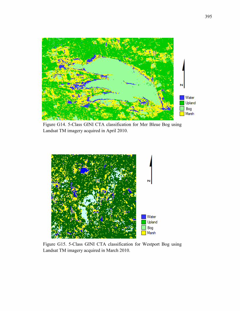
395
Bog
Figure G14. 5-Class GINI CTA classification for Mer Bleue Bog using Landsat TM imagery acquired in April 2010.
Figure G15. 5-Class GINI CTA classification for Westport Bog using Landsat TM imagery acquired in March 2010.
Bog
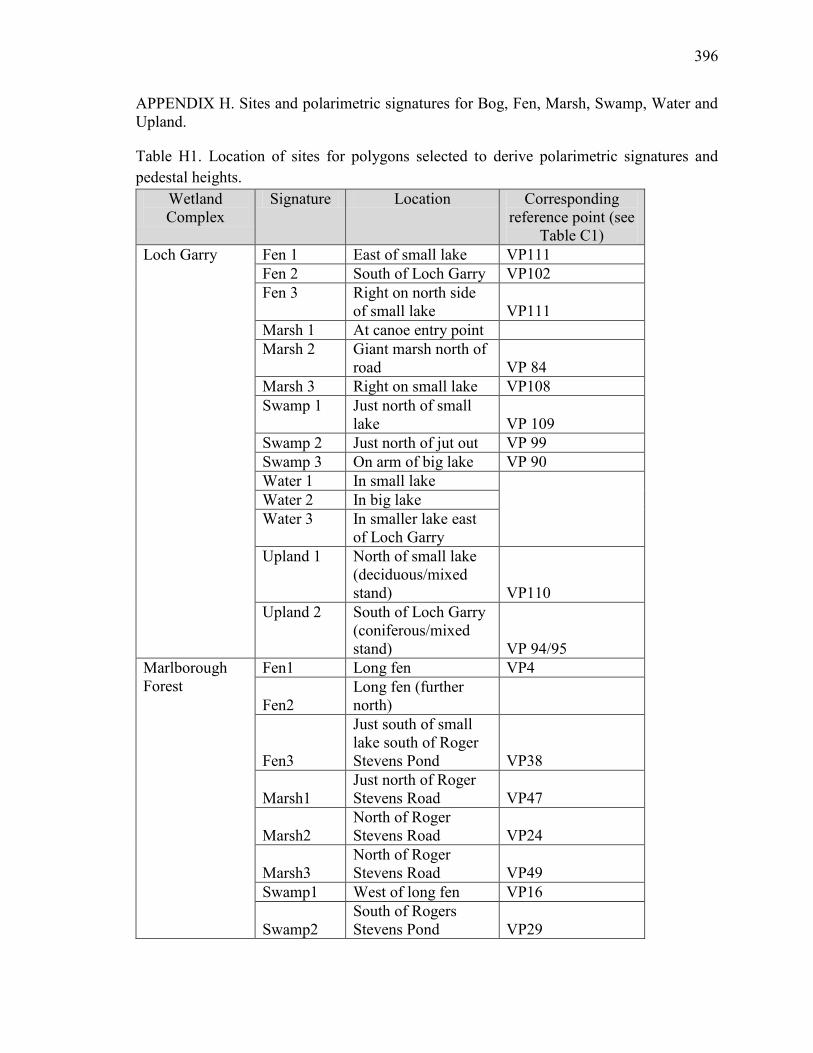
396
APPENDIX H. Sites and polarimetric signatures for Bog, Fen, Marsh, Swamp, Water and Upland.
Table H1. Location of sites for polygons selected to derive polarimetric signatures and pedestal heights.
Wetland Complex
Signature Location Corresponding reference point (see
Table C1) Loch Garry Fen 1 East of small lake VP111
Fen 2 South of Loch Garry VP102 Fen 3 Right on north side
of small lake VP111 Marsh 1 At canoe entry point Marsh 2 Giant marsh north of
road VP 84 Marsh 3 Right on small lake VP108 Swamp 1 Just north of small
lake VP 109 Swamp 2 Just north of jut out VP 99 Swamp 3 On arm of big lake VP 90 Water 1 In small lake
Water 2 In big lake Water 3 In smaller lake east
of Loch Garry Upland 1 North of small lake
(deciduous/mixed stand) VP110
Upland 2 South of Loch Garry (coniferous/mixed stand) VP 94/95
Marlborough Forest
Fen1 Long fen VP4
Fen2 Long fen (further north)
Fen3
Just south of small lake south of Roger Stevens Pond VP38
Marsh1 Just north of Roger Stevens Road VP47
Marsh2 North of Roger Stevens Road VP24
Marsh3 North of Roger Stevens Road VP49
Swamp1 West of long fen VP16
Swamp2 South of Rogers Stevens Pond VP29
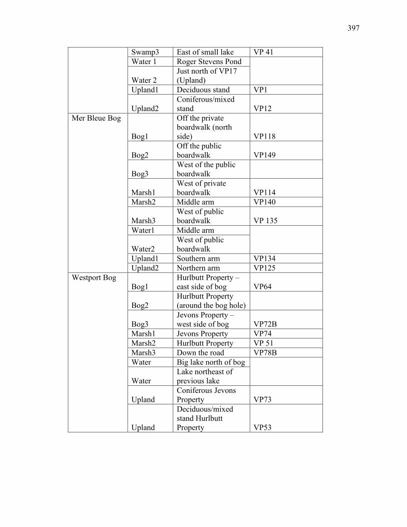
397
Swamp3 East of small lake VP 41 Water 1 Roger Stevens Pond
Water 2 Just north of VP17 (Upland)
Upland1 Deciduous stand VP1
Upland2 Coniferous/mixed stand VP12
Mer Bleue Bog
Bog1
Off the private boardwalk (north side) VP118
Bog2 Off the public boardwalk VP149
Bog3 West of the public boardwalk
Marsh1 West of private boardwalk VP114
Marsh2 Middle arm VP140
Marsh3 West of public boardwalk VP 135
Water1 Middle arm
Water2 West of public boardwalk
Upland1 Southern arm VP134 Upland2 Northern arm VP125
Westport Bog Bog1
Hurlbutt Property – east side of bog VP64
Bog2 Hurlbutt Property (around the bog hole)
Bog3 Jevons Property – west side of bog VP72B
Marsh1 Jevons Property VP74 Marsh2 Hurlbutt Property VP 51 Marsh3 Down the road VP78B Water Big lake north of bog
Water Lake northeast of previous lake
Upland Coniferous Jevons Property VP73
Upland
Deciduous/mixed stand Hurlbutt Property VP53
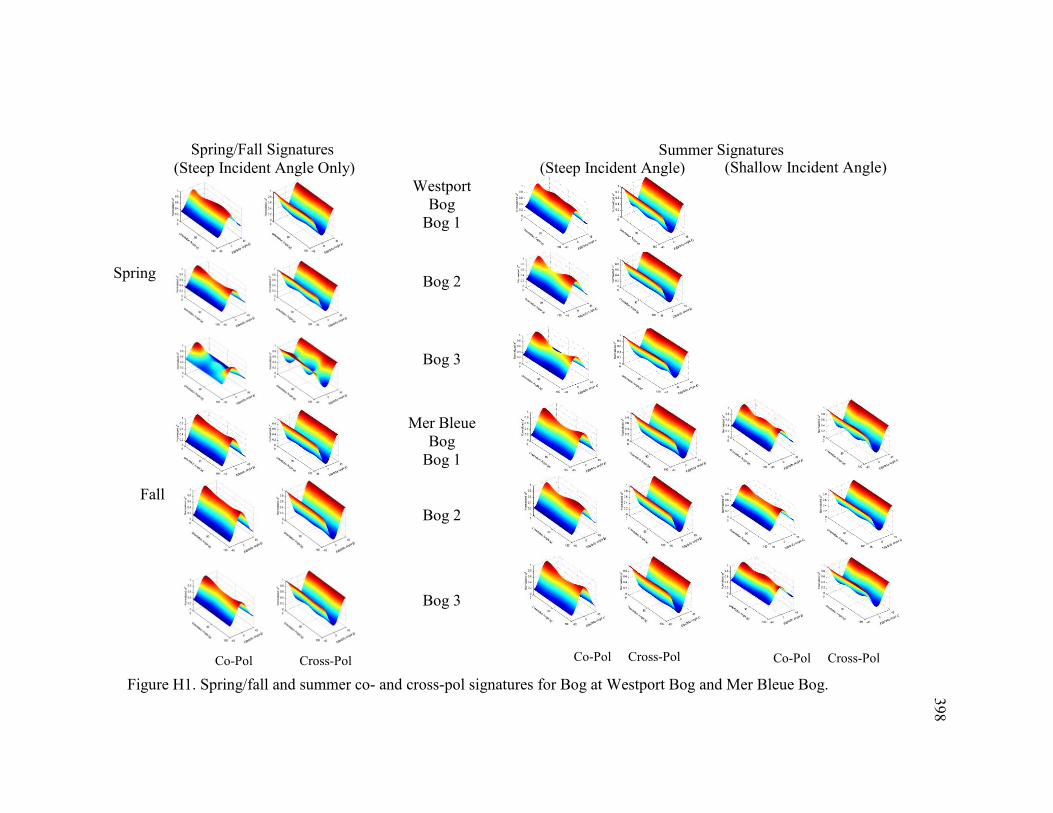
398
Summer Signatures
Figure H1. Spring/fall and summer co- and cross-pol signatures for Bog at Westport Bog and Mer Bleue Bog.
Co-Pol Cross-Pol
(Steep Incident Angle) Westport
Bog Bog 1
Bog 2
Bog 3
Bog 2
Mer Bleue Bog
Bog 1
Bog 3
Spring/Fall Signatures
Co-Pol Cross-Pol
(Steep Incident Angle Only)
Spring
Fall
(Shallow Incident Angle)
Co-Pol Cross-Pol
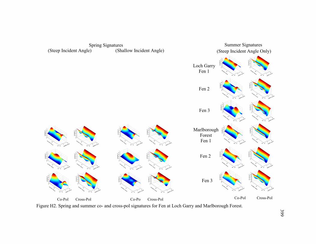
399
Marlborough Forest Fen 1
Fen 2
Loch Garry Fen 1
Fen 3
Fen 2
Fen 3
Summer Signatures Spring Signatures
Co-Pol Cross-Pol Co-Pol Cross-Pol
Figure H2. Spring and summer co- and cross-pol signatures for Fen at Loch Garry and Marlborough Forest.
(Steep Incident Angle Only) (Steep Incident Angle) (Shallow Incident Angle)
Co-Po Cross-Pol
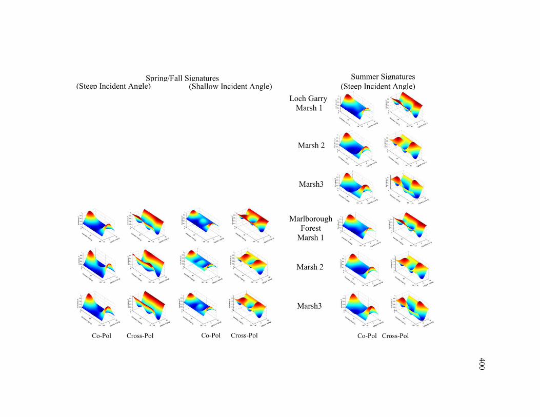
400
(Steep Incident Angle) (Shallow Incident Angle) Spring/Fall Signatures
Marlborough Forest
Marsh 1
Marsh 2
Marsh3
Summer Signatures (Steep Incident Angle)
Co-Pol Cross-Pol Co-Pol Cross-Pol Co-Pol Cross-Pol
Loch Garry Marsh 1
Marsh 2
Marsh3
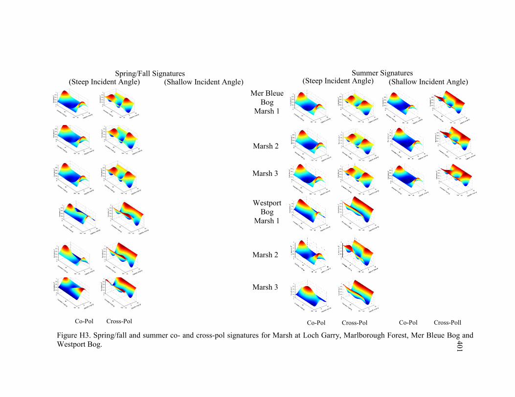
401
Mer Bleue Bog
Marsh 1
Marsh 2
Marsh 3
Westport
Bog Marsh 1
Marsh 2
Marsh 3
Co-Pol Cross-Pol Co-Pol Cross-Pol
Figure H3. Spring/fall and summer co- and cross-pol signatures for Marsh at Loch Garry, Marlborough Forest, Mer Bleue Bog and Westport Bog.
(Steep Incident Angle) Spring/Fall Signatures Summer Signatures
(Steep Incident Angle) (Shallow Incident Angle)
Co-Pol Cross-Poll
(Shallow Incident Angle)
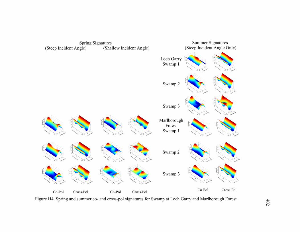
402
Marlborough Forest
Swamp 1
Swamp 2
Loch Garry Swamp 1
Swamp 3
Swamp 2
Swamp 3
Summer Signatures Spring Signatures
Co-Pol Cross-Pol Co-Pol Cross-Pol
Figure H4. Spring and summer co- and cross-pol signatures for Swamp at Loch Garry and Marlborough Forest.
(Steep Incident Angle Only) (Steep Incident Angle) (Shallow Incident Angle)
Co-Pol Cross-Pol
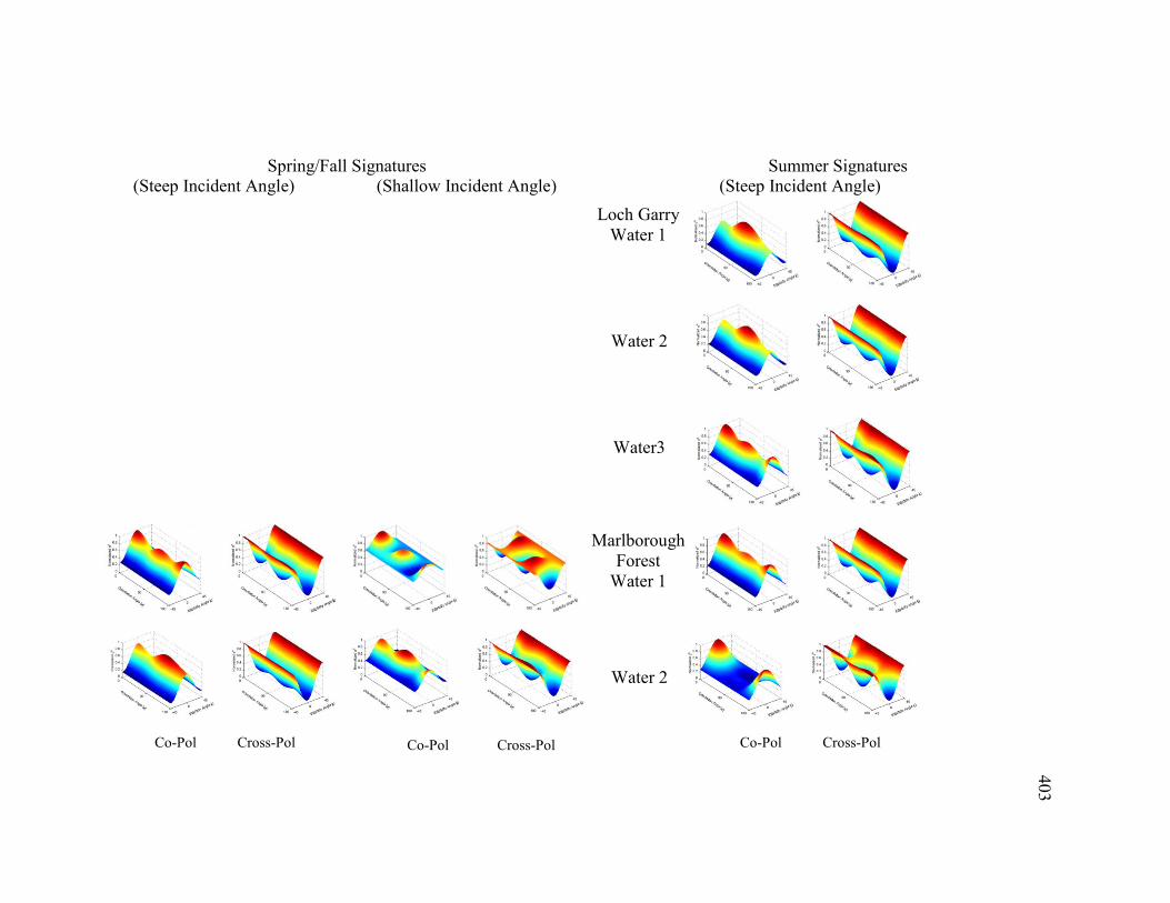
403
(Steep Incident Angle) (Shallow Incident Angle) Spring/Fall Signatures
Loch Garry Water 1
Water 2
Water3
Summer Signatures
Marlborough Forest
Water 1
Water 2
(Steep Incident Angle)
Co-Pol Cross-Pol Co-Pol Cross-Pol Co-Pol Cross-Pol
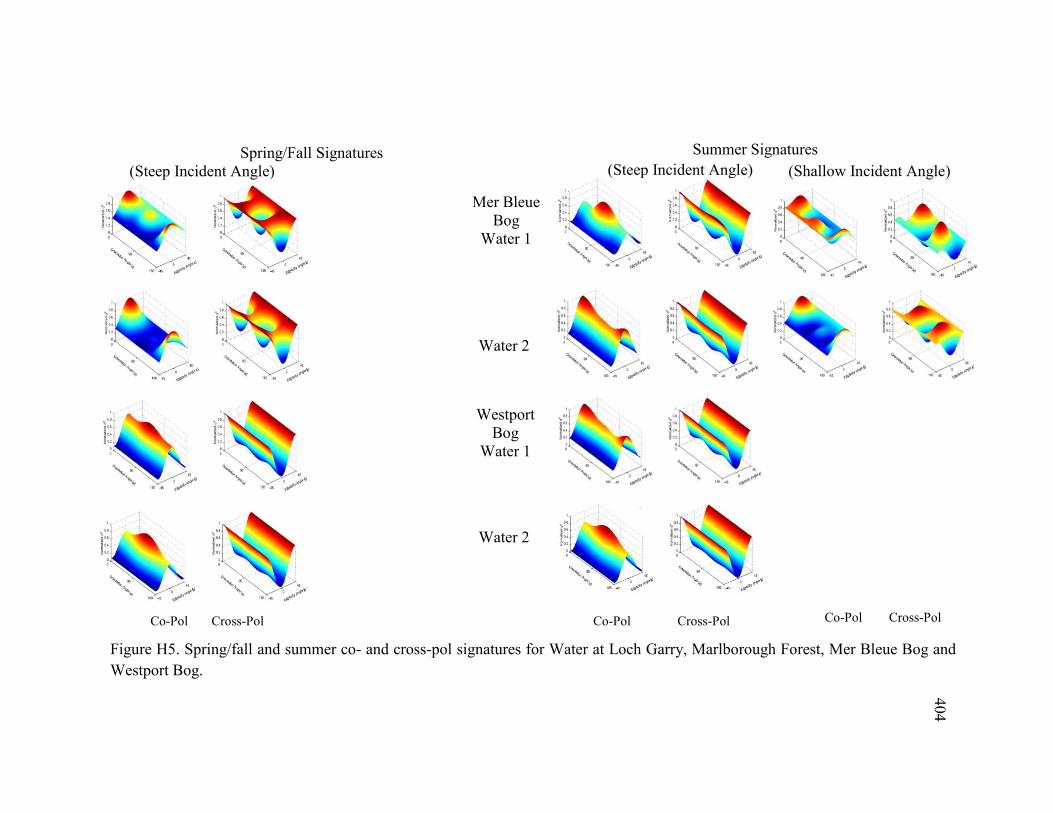
404
Spring/Fall Signatures (Steep Incident Angle)
Summer Signatures
(Steep Incident Angle)
(Shallow Incident Angle)
Mer Bleue Bog
Water 1
Water 2
Westport Bog
Water 1
Water 2
Co-Pol Cross-Pol Co-Pol Cross-Pol
Figure H5. Spring/fall and summer co- and cross-pol signatures for Water at Loch Garry, Marlborough Forest, Mer Bleue Bog and Westport Bog.
Co-Pol Cross-Pol
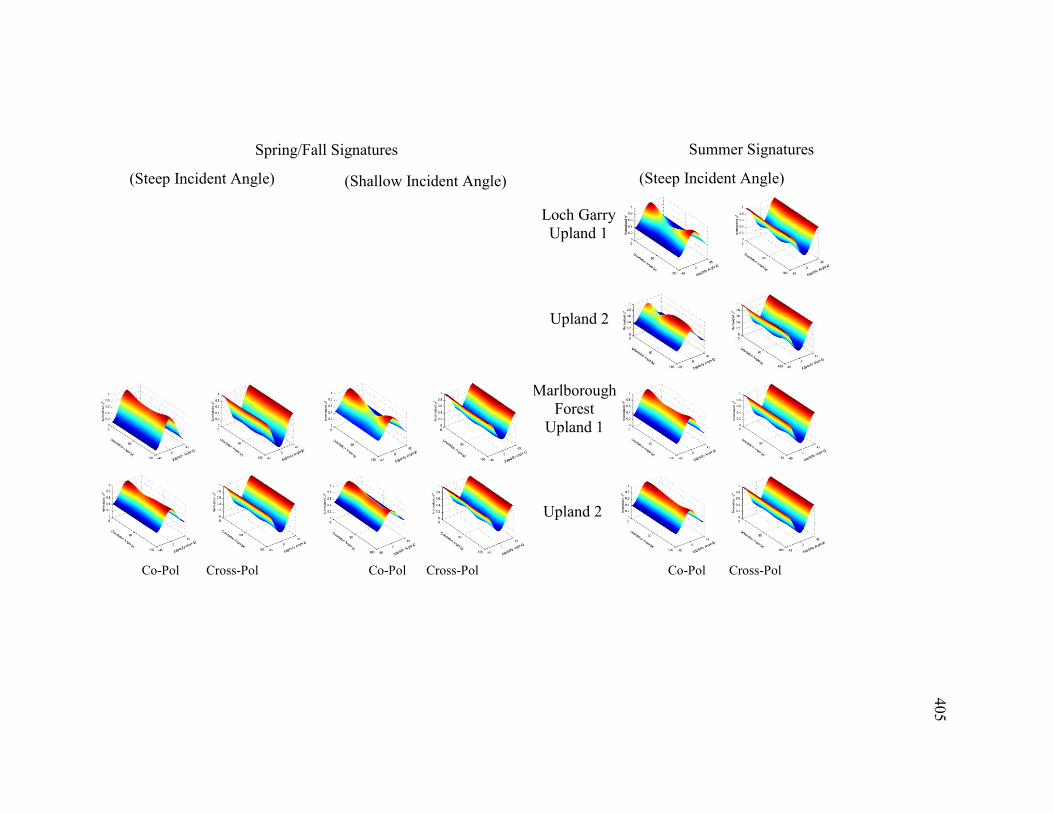
405
(Steep Incident Angle) (Shallow Incident Angle)
Spring/Fall Signatures
Loch Garry Upland 1
Upland 2
Summer Signatures
Marlborough Forest
Upland 1
Upland 2
(Steep Incident Angle)
Co-Pol Cross-Pol Co-Pol Cross-Pol Co-Pol Cross-Pol
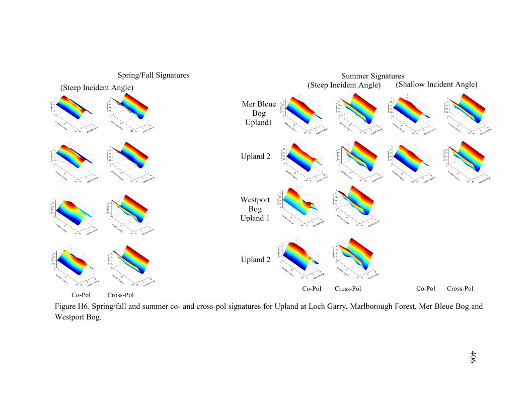
406
Spring/Fall Signatures (Steep Incident Angle)
Summer Signatures (Steep Incident Angle) (Shallow Incident Angle)
Upland 2
Westport Bog
Upland 1
Upland 2
Co-Pol Cross-Pol Co-Pol Cross-Pol
Figure H6. Spring/fall and summer co- and cross-pol signatures for Upland at Loch Garry, Marlborough Forest, Mer Bleue Bog and Westport Bog.
Co-Pol Cross-Pol
Mer Bleue Bog
Upland1
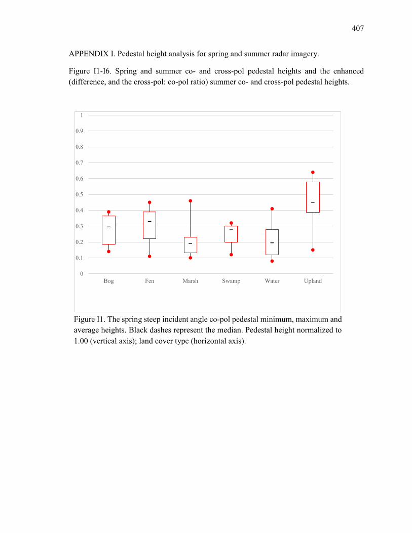
407
APPENDIX I. Pedestal height analysis for spring and summer radar imagery.
Figure I1-I6. Spring and summer co- and cross-pol pedestal heights and the enhanced (difference, and the cross-pol: co-pol ratio) summer co- and cross-pol pedestal heights.
0
0.1
0.2
0.3
0.4
0.5
0.6
0.7
0.8
0.9
1
Bog Fen Marsh Swamp Water Upland
Figure I1. The spring steep incident angle co-pol pedestal minimum, maximum and average heights. Black dashes represent the median. Pedestal height normalized to 1.00 (vertical axis); land cover type (horizontal axis).
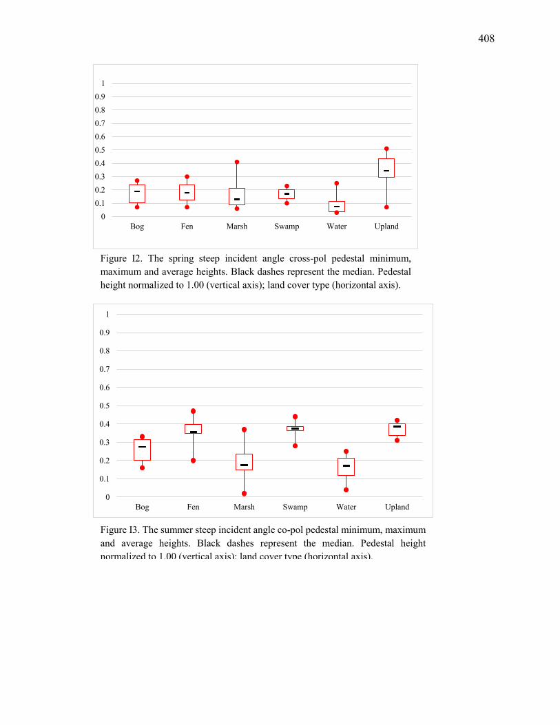
408
Figure I2. The spring steep incident angle cross-pol pedestal minimum, maximum and average heights. Black dashes represent the median. Pedestal height normalized to 1.00 (vertical axis); land cover type (horizontal axis).
00.10.20.30.40.50.60.70.80.9
1
Bog Fen Marsh Swamp Water Upland
Figure I3. The summer steep incident angle co-pol pedestal minimum, maximum and average heights. Black dashes represent the median. Pedestal height normalized to 1.00 (vertical axis); land cover type (horizontal axis).
0
0.1
0.2
0.3
0.4
0.5
0.6
0.7
0.8
0.9
1
Bog Fen Marsh Swamp Water Upland
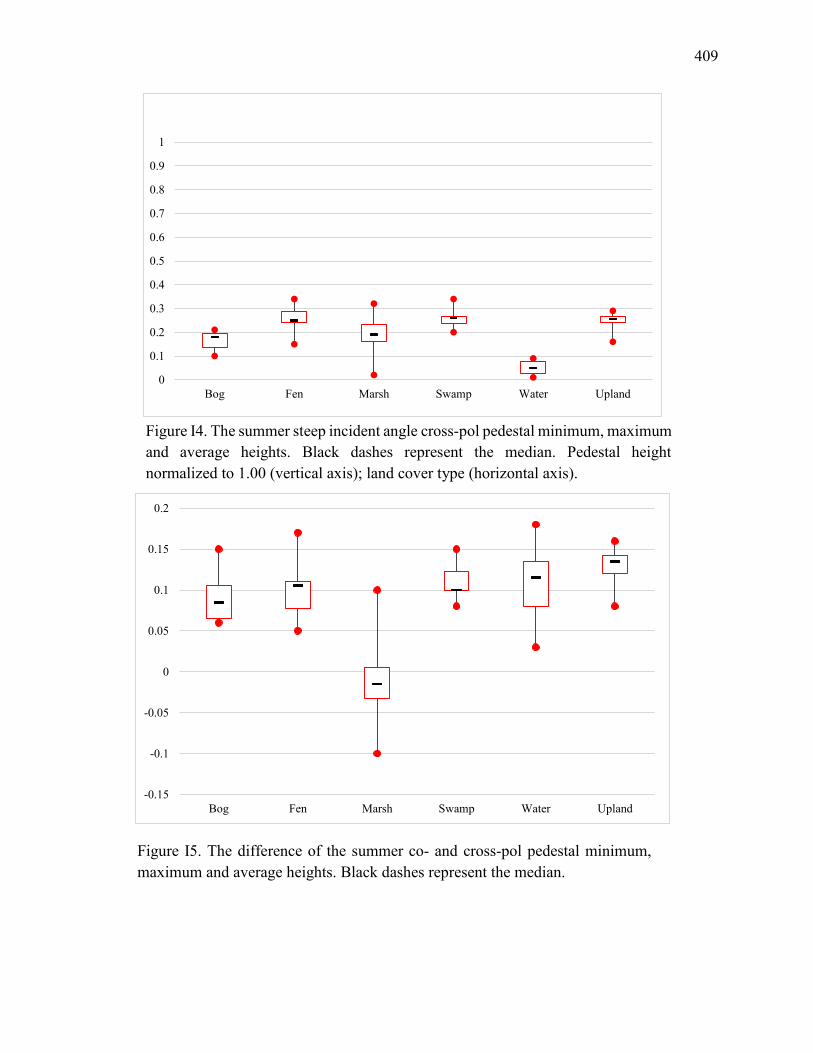
409
Figure I4. The summer steep incident angle cross-pol pedestal minimum, maximum and average heights. Black dashes represent the median. Pedestal height normalized to 1.00 (vertical axis); land cover type (horizontal axis).
0
0.1
0.2
0.3
0.4
0.5
0.6
0.7
0.8
0.9
1
Bog Fen Marsh Swamp Water Upland
Figure I5. The difference of the summer co- and cross-pol pedestal minimum, maximum and average heights. Black dashes represent the median.
-0.15
-0.1
-0.05
0
0.05
0.1
0.15
0.2
Bog Fen Marsh Swamp Water Upland
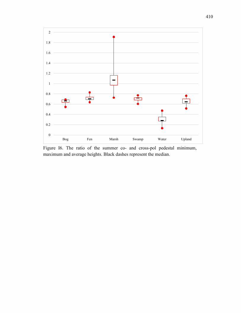
410
Figure I6. The ratio of the summer co- and cross-pol pedestal minimum, maximum and average heights. Black dashes represent the median.
0
0.2
0.4
0.6
0.8
1
1.2
1.4
1.6
1.8
2
Bog Fen Marsh Swamp Water Upland

411
APPENDIX J. Field-measured VWC% for all four sites and two seasons.
Table J1. (Digitally accompanying this thesis) Field-measured VWC (%) at the four sites for two seasons (spring and summer). This workbook first presents the field measured VWC by Wetland Type (Bog, Fen, Marsh, Swamp) and then by site.
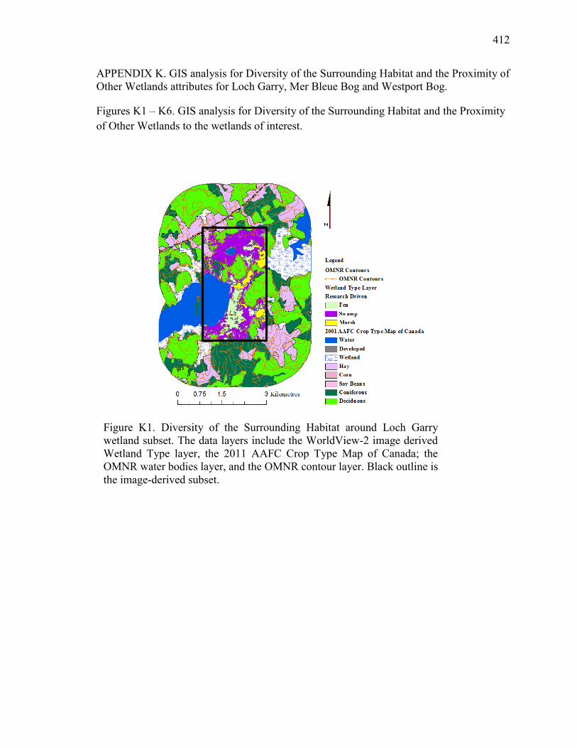
412
APPENDIX K. GIS analysis for Diversity of the Surrounding Habitat and the Proximity of Other Wetlands attributes for Loch Garry, Mer Bleue Bog and Westport Bog.
Figures K1 – K6. GIS analysis for Diversity of the Surrounding Habitat and the Proximity of Other Wetlands to the wetlands of interest.
Figure K1. Diversity of the Surrounding Habitat around Loch Garry wetland subset. The data layers include the WorldView-2 image derived Wetland Type layer, the 2011 AAFC Crop Type Map of Canada; the OMNR water bodies layer, and the OMNR contour layer. Black outline is the image-derived subset.
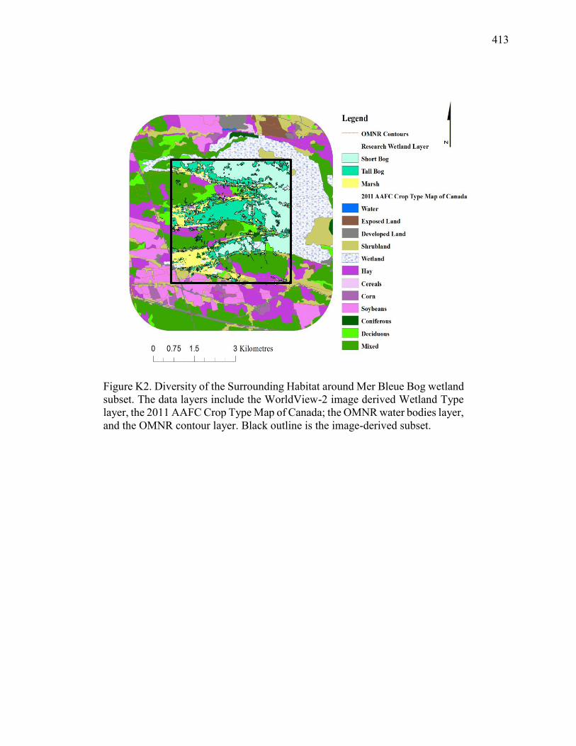
413
Figure K2. Diversity of the Surrounding Habitat around Mer Bleue Bog wetland subset. The data layers include the WorldView-2 image derived Wetland Type layer, the 2011 AAFC Crop Type Map of Canada; the OMNR water bodies layer, and the OMNR contour layer. Black outline is the image-derived subset.
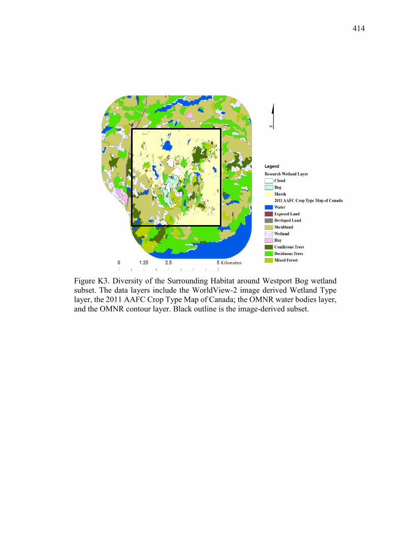
414
Figure K3. Diversity of the Surrounding Habitat around Westport Bog wetland subset. The data layers include the WorldView-2 image derived Wetland Type layer, the 2011 AAFC Crop Type Map of Canada; the OMNR water bodies layer, and the OMNR contour layer. Black outline is the image-derived subset.
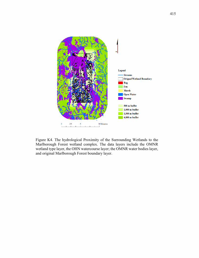
415
Figure K4. The hydrological Proximity of the Surrounding Wetlands to the Marlborough Forest wetland complex. The data layers include the OMNR wetland type layer, the OHN watercourse layer; the OMNR water bodies layer, and original Marlborough Forest boundary layer.
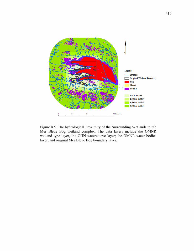
416
Figure K5. The hydrological Proximity of the Surrounding Wetlands to the Mer Bleue Bog wetland complex. The data layers include the OMNR wetland type layer, the OHN watercourse layer; the OMNR water bodies layer, and original Mer Bleue Bog boundary layer.
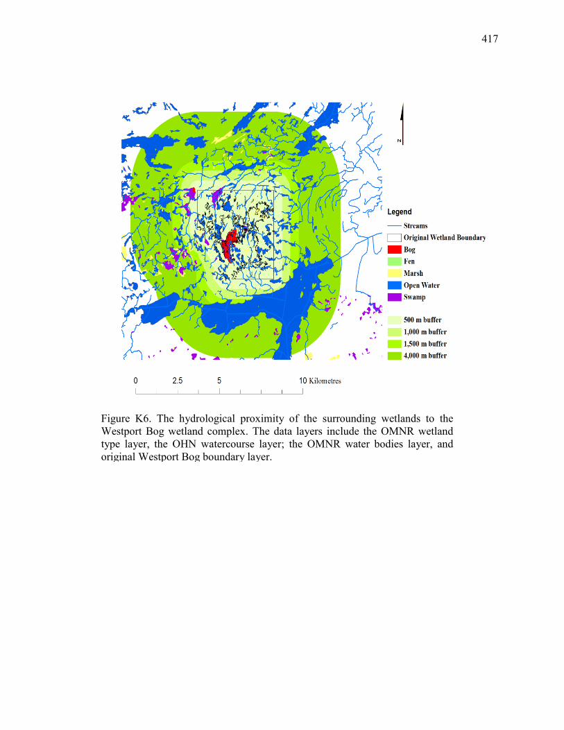
417
Figure K6. The hydrological proximity of the surrounding wetlands to the Westport Bog wetland complex. The data layers include the OMNR wetland type layer, the OHN watercourse layer; the OMNR water bodies layer, and original Westport Bog boundary layer.
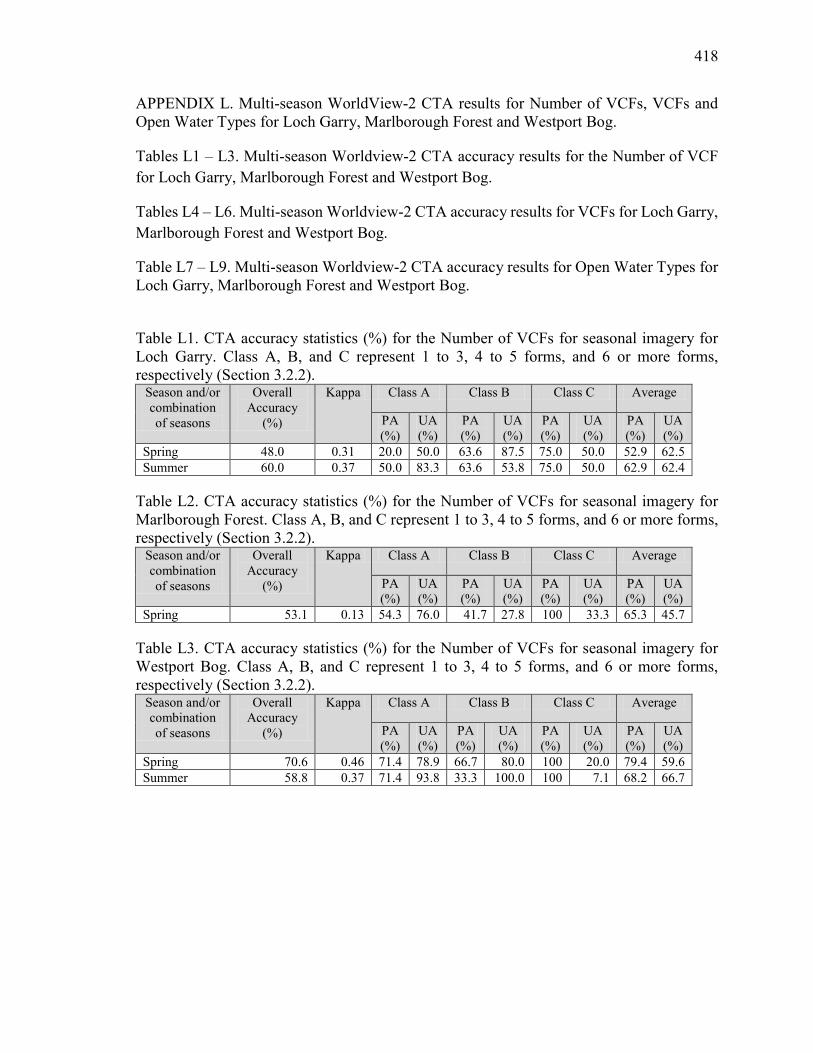
418
APPENDIX L. Multi-season WorldView-2 CTA results for Number of VCFs, VCFs and Open Water Types for Loch Garry, Marlborough Forest and Westport Bog.
Tables L1 – L3. Multi-season Worldview-2 CTA accuracy results for the Number of VCF for Loch Garry, Marlborough Forest and Westport Bog.
Tables L4 – L6. Multi-season Worldview-2 CTA accuracy results for VCFs for Loch Garry, Marlborough Forest and Westport Bog.
Table L7 – L9. Multi-season Worldview-2 CTA accuracy results for Open Water Types for Loch Garry, Marlborough Forest and Westport Bog.
Table L1. CTA accuracy statistics (%) for the Number of VCFs for seasonal imagery for Loch Garry. Class A, B, and C represent 1 to 3, 4 to 5 forms, and 6 or more forms, respectively (Section 3.2.2).
Season and/or combination of seasons
Overall Accuracy
(%)
Kappa Class A Class B Class C Average
PA (%)
UA (%)
PA (%)
UA (%)
PA (%)
UA (%)
PA (%)
UA (%)
Spring 48.0 0.31 20.0 50.0 63.6 87.5 75.0 50.0 52.9 62.5 Summer 60.0 0.37 50.0 83.3 63.6 53.8 75.0 50.0 62.9 62.4
Table L2. CTA accuracy statistics (%) for the Number of VCFs for seasonal imagery for Marlborough Forest. Class A, B, and C represent 1 to 3, 4 to 5 forms, and 6 or more forms, respectively (Section 3.2.2).
Season and/or combination of seasons
Overall Accuracy
(%)
Kappa Class A Class B Class C Average
PA (%)
UA (%)
PA (%)
UA (%)
PA (%)
UA (%)
PA (%)
UA (%)
Spring 53.1 0.13 54.3 76.0 41.7 27.8 100 33.3 65.3 45.7
Table L3. CTA accuracy statistics (%) for the Number of VCFs for seasonal imagery for Westport Bog. Class A, B, and C represent 1 to 3, 4 to 5 forms, and 6 or more forms, respectively (Section 3.2.2).
Season and/or combination of seasons
Overall Accuracy
(%)
Kappa Class A Class B Class C Average
PA (%)
UA (%)
PA (%)
UA (%)
PA (%)
UA (%)
PA (%)
UA (%)
Spring 70.6 0.46 71.4 78.9 66.7 80.0 100 20.0 79.4 59.6 Summer 58.8 0.37 71.4 93.8 33.3 100.0 100 7.1 68.2 66.7
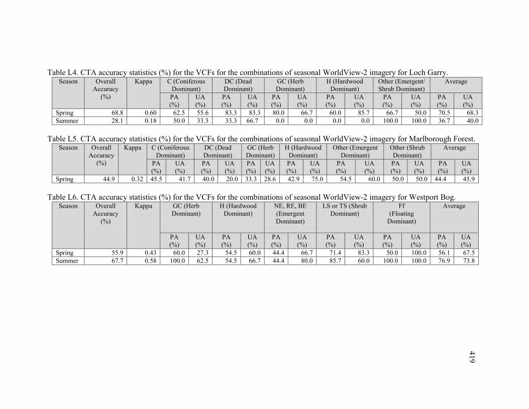
419
Table L4. CTA accuracy statistics (%) for the VCFs for the combinations of seasonal WorldView-2 imagery for Loch Garry. Season Overall
Accuracy (%)
Kappa C (Coniferous Dominant)
DC (Dead Dominant)
GC (Herb Dominant)
H (Hardwood Dominant)
Other (Emergent/ Shrub Dominant)
Average
PA (%)
UA (%)
PA (%)
UA (%)
PA (%)
UA (%)
PA (%)
UA (%)
PA (%)
UA (%)
PA (%)
UA (%)
Spring 68.8 0.60 62.5 55.6 83.3 83.3 80.0 66.7 60.0 85.7 66.7 50.0 70.5 68.3 Summer 28.1 0.18 50.0 33.3 33.3 66.7 0.0 0.0 0.0 0.0 100.0 100.0 36.7 40.0
Table L5. CTA accuracy statistics (%) for the VCFs for the combinations of seasonal WorldView-2 imagery for Marlborough Forest.
Season Overall Accuracy
(%)
Kappa C (Coniferous Dominant)
DC (Dead Dominant)
GC (Herb Dominant)
H (Hardwood Dominant)
Other (Emergent Dominant)
Other (Shrub Dominant)
Average
PA (%)
UA (%)
PA (%)
UA (%)
PA (%)
UA (%)
PA (%)
UA (%)
PA (%)
UA (%)
PA (%)
UA (%)
PA (%)
UA (%)
Spring 44.9 0.32 45.5 41.7 40.0 20.0 33.3 28.6 42.9 75.0 54.5 60.0 50.0 50.0 44.4 45.9 Table L6. CTA accuracy statistics (%) for the VCFs for the combinations of seasonal WorldView-2 imagery for Westport Bog.
Season Overall Accuracy
(%)
Kappa GC (Herb Dominant)
H (Hardwood Dominant)
NE, RE, BE (Emergent Dominant)
LS or TS (Shrub Dominant)
Ff (Floating
Dominant)
Average
PA (%)
UA (%)
PA (%)
UA (%)
PA (%)
UA (%)
PA (%)
UA (%)
PA (%)
UA (%)
PA (%)
UA (%)
Spring 55.9 0.43 60.0 27.3 54.5 60.0 44.4 66.7 71.4 83.3 50.0 100.0 56.1 67.5 Summer 67.7 0.58 100.0 62.5 54.5 66.7 44.4 80.0 85.7 60.0 100.0 100.0 76.9 73.8
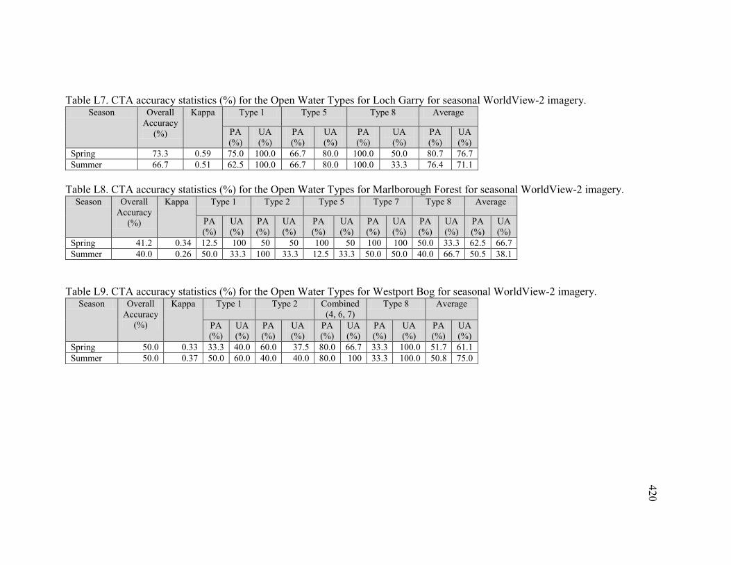
420
Table L7. CTA accuracy statistics (%) for the Open Water Types for Loch Garry for seasonal WorldView-2 imagery.
Table L8. CTA accuracy statistics (%) for the Open Water Types for Marlborough Forest for seasonal WorldView-2 imagery.
Table L9. CTA accuracy statistics (%) for the Open Water Types for Westport Bog for seasonal WorldView-2 imagery.
Season Overall Accuracy
(%)
Kappa Type 1 Type 5 Type 8 Average
PA (%)
UA (%)
PA (%)
UA (%)
PA (%)
UA (%)
PA (%)
UA (%)
Spring 73.3 0.59 75.0 100.0 66.7 80.0 100.0 50.0 80.7 76.7 Summer 66.7 0.51 62.5 100.0 66.7 80.0 100.0 33.3 76.4 71.1
Season Overall Accuracy
(%)
Kappa Type 1 Type 2 Type 5 Type 7 Type 8 Average
PA (%)
UA (%)
PA (%)
UA (%)
PA (%)
UA (%)
PA (%)
UA (%)
PA (%)
UA (%)
PA (%)
UA (%)
Spring 41.2 0.34 12.5 100 50 50 100 50 100 100 50.0 33.3 62.5 66.7 Summer 40.0 0.26 50.0 33.3 100 33.3 12.5 33.3 50.0 50.0 40.0 66.7 50.5 38.1
Season Overall Accuracy
(%)
Kappa Type 1 Type 2 Combined (4, 6, 7)
Type 8 Average
PA (%)
UA (%)
PA (%)
UA (%)
PA (%)
UA (%)
PA (%)
UA (%)
PA (%)
UA (%)
Spring 50.0 0.33 33.3 40.0 60.0 37.5 80.0 66.7 33.3 100.0 51.7 61.1 Summer 50.0 0.37 50.0 60.0 40.0 40.0 80.0 100 33.3 100.0 50.8 75.0
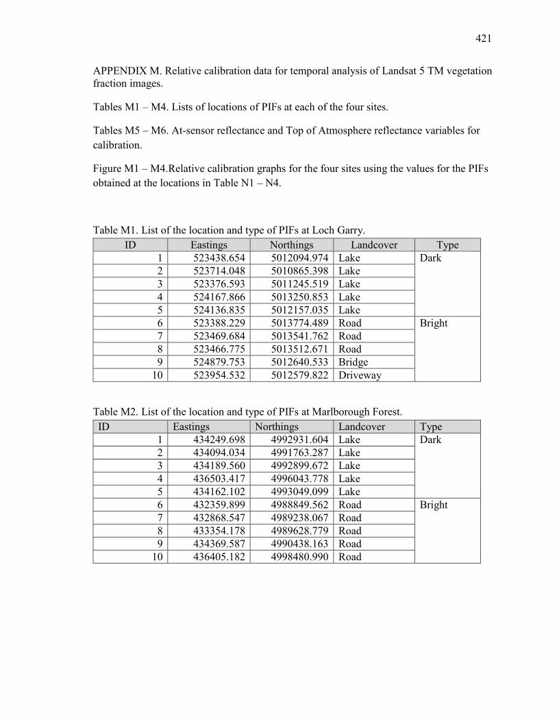
421
APPENDIX M. Relative calibration data for temporal analysis of Landsat 5 TM vegetation fraction images.
Tables M1 – M4. Lists of locations of PIFs at each of the four sites.
Tables M5 – M6. At-sensor reflectance and Top of Atmosphere reflectance variables for calibration.
Figure M1 – M4.Relative calibration graphs for the four sites using the values for the PIFs obtained at the locations in Table N1 – N4.
Table M1. List of the location and type of PIFs at Loch Garry. ID Eastings Northings Landcover Type
1 523438.654 5012094.974 Lake Dark 2 523714.048 5010865.398 Lake 3 523376.593 5011245.519 Lake 4 524167.866 5013250.853 Lake 5 524136.835 5012157.035 Lake 6 523388.229 5013774.489 Road Bright 7 523469.684 5013541.762 Road 8 523466.775 5013512.671 Road 9 524879.753 5012640.533 Bridge
10 523954.532 5012579.822 Driveway
Table M2. List of the location and type of PIFs at Marlborough Forest. ID Eastings Northings Landcover Type
1 434249.698 4992931.604 Lake Dark 2 434094.034 4991763.287 Lake 3 434189.560 4992899.672 Lake 4 436503.417 4996043.778 Lake 5 434162.102 4993049.099 Lake 6 432359.899 4988849.562 Road Bright 7 432868.547 4989238.067 Road 8 433354.178 4989628.779 Road 9 434369.587 4990438.163 Road
10 436405.182 4998480.990 Road
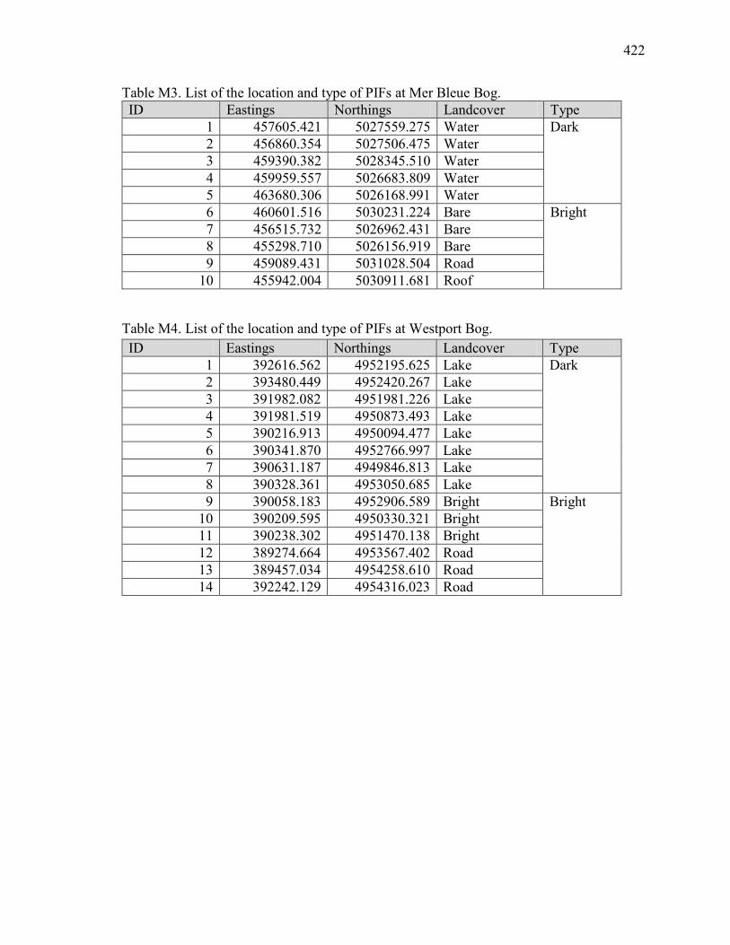
422
Table M3. List of the location and type of PIFs at Mer Bleue Bog. ID Eastings Northings Landcover Type
1 457605.421 5027559.275 Water Dark 2 456860.354 5027506.475 Water 3 459390.382 5028345.510 Water 4 459959.557 5026683.809 Water 5 463680.306 5026168.991 Water 6 460601.516 5030231.224 Bare Bright 7 456515.732 5026962.431 Bare 8 455298.710 5026156.919 Bare 9 459089.431 5031028.504 Road
10 455942.004 5030911.681 Roof
Table M4. List of the location and type of PIFs at Westport Bog. ID Eastings Northings Landcover Type
1 392616.562 4952195.625 Lake Dark 2 393480.449 4952420.267 Lake 3 391982.082 4951981.226 Lake 4 391981.519 4950873.493 Lake 5 390216.913 4950094.477 Lake 6 390341.870 4952766.997 Lake 7 390631.187 4949846.813 Lake 8 390328.361 4953050.685 Lake 9 390058.183 4952906.589 Bright Bright
10 390209.595 4950330.321 Bright 11 390238.302 4951470.138 Bright 12 389274.664 4953567.402 Road 13 389457.034 4954258.610 Road 14 392242.129 4954316.023 Road
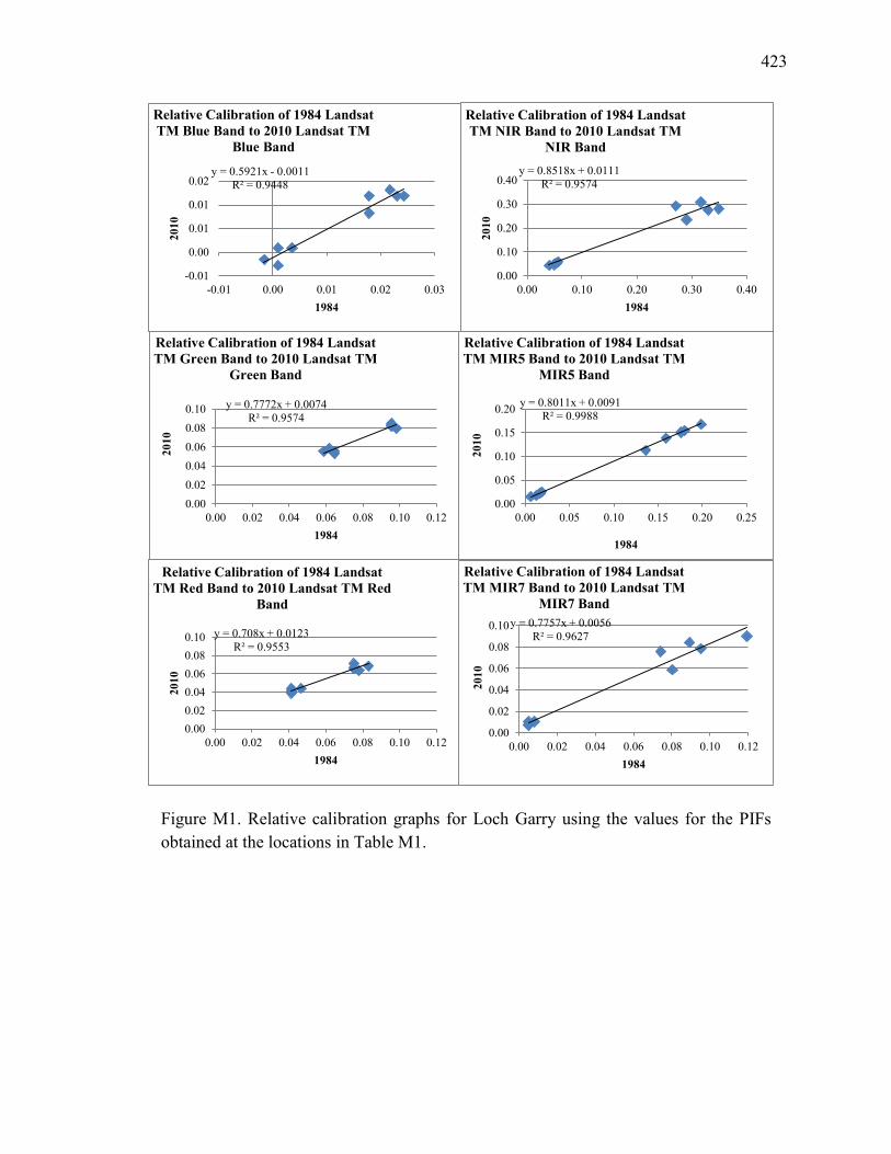
423
y = 0.5921x - 0.0011R² = 0.9448
-0.01
0.00
0.01
0.01
0.02
-0.01 0.00 0.01 0.02 0.03
2010
1984
Relative Calibration of 1984 Landsat TM Blue Band to 2010 Landsat TM
Blue Band
y = 0.7772x + 0.0074R² = 0.9574
0.000.020.040.060.080.10
0.00 0.02 0.04 0.06 0.08 0.10 0.12
2010
1984
Relative Calibration of 1984 Landsat TM Green Band to 2010 Landsat TM
Green Band
y = 0.708x + 0.0123R² = 0.9553
0.000.020.040.060.080.10
0.00 0.02 0.04 0.06 0.08 0.10 0.12
2010
1984
Relative Calibration of 1984 Landsat TM Red Band to 2010 Landsat TM Red
Band
y = 0.8518x + 0.0111R² = 0.9574
0.00
0.10
0.20
0.30
0.40
0.00 0.10 0.20 0.30 0.40
2010
1984
Relative Calibration of 1984 Landsat TM NIR Band to 2010 Landsat TM
NIR Band
y = 0.8011x + 0.0091R² = 0.9988
0.00
0.05
0.10
0.15
0.20
0.00 0.05 0.10 0.15 0.20 0.25
2010
1984
Relative Calibration of 1984 Landsat TM MIR5 Band to 2010 Landsat TM
MIR5 Band
y = 0.7757x + 0.0056R² = 0.9627
0.00
0.02
0.04
0.06
0.08
0.10
0.00 0.02 0.04 0.06 0.08 0.10 0.12
2010
1984
Relative Calibration of 1984 Landsat TM MIR7 Band to 2010 Landsat TM
MIR7 Band
Figure M1. Relative calibration graphs for Loch Garry using the values for the PIFs obtained at the locations in Table M1.
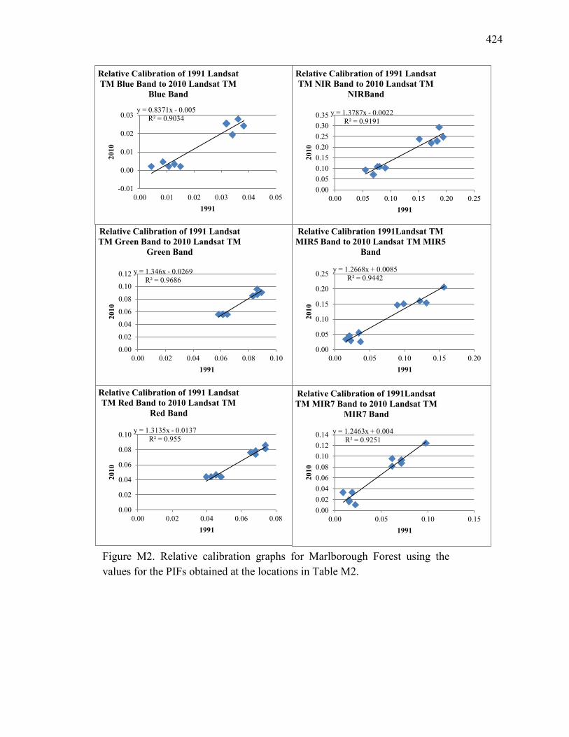
424
Figure M2. Relative calibration graphs for Marlborough Forest using the values for the PIFs obtained at the locations in Table M2.
y = 0.8371x - 0.005R² = 0.9034
-0.01
0.00
0.01
0.02
0.03
0.00 0.01 0.02 0.03 0.04 0.05
2010
1991
Relative Calibration of 1991 Landsat TM Blue Band to 2010 Landsat TM
Blue Band
y = 1.346x - 0.0269R² = 0.9686
0.00
0.02
0.04
0.06
0.08
0.10
0.12
0.00 0.02 0.04 0.06 0.08 0.10
2010
1991
Relative Calibration of 1991 Landsat TM Green Band to 2010 Landsat TM
Green Band
y = 1.3135x - 0.0137R² = 0.955
0.00
0.02
0.04
0.06
0.08
0.10
0.00 0.02 0.04 0.06 0.08
2010
1991
Relative Calibration of 1991 Landsat TM Red Band to 2010 Landsat TM
Red Band
y = 1.3787x - 0.0022R² = 0.9191
0.000.050.100.150.200.250.300.35
0.00 0.05 0.10 0.15 0.20 0.25
2010
1991
Relative Calibration of 1991 Landsat TM NIR Band to 2010 Landsat TM
NIRBand
y = 1.2668x + 0.0085R² = 0.9442
0.00
0.05
0.10
0.15
0.20
0.25
0.00 0.05 0.10 0.15 0.20
2010
1991
Relative Calibration 1991Landsat TM MIR5 Band to 2010 Landsat TM MIR5
Band
y = 1.2463x + 0.004R² = 0.9251
0.000.020.040.060.080.100.120.14
0.00 0.05 0.10 0.15
2010
1991
Relative Calibration of 1991Landsat TM MIR7 Band to 2010 Landsat TM
MIR7 Band
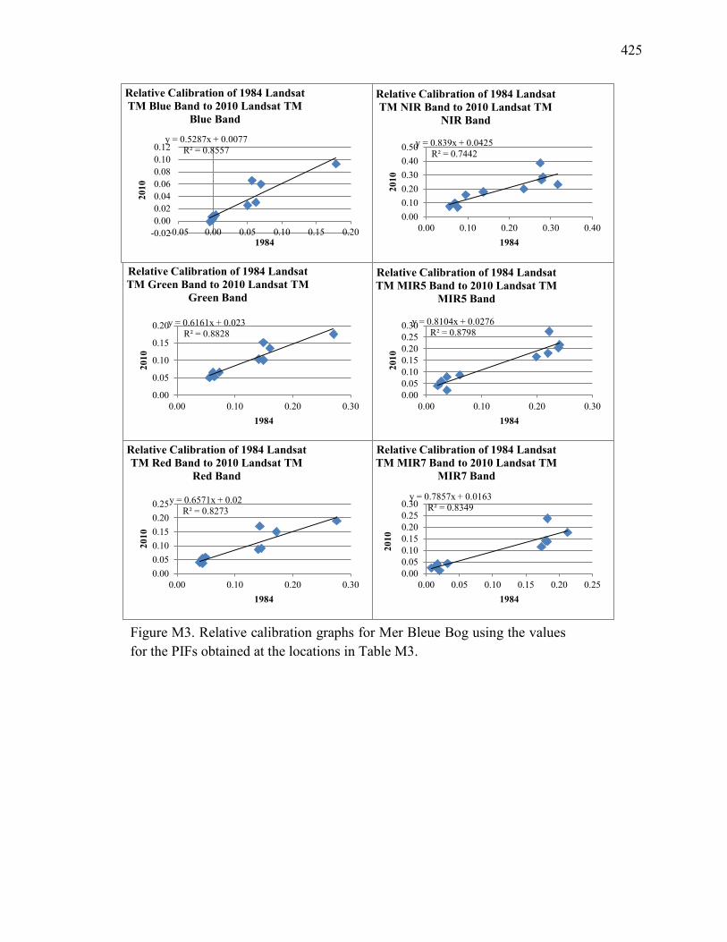
425
y = 0.5287x + 0.0077R² = 0.8557
-0.020.000.020.040.060.080.100.12
-0.05 0.00 0.05 0.10 0.15 0.20
2010
1984
Relative Calibration of 1984 Landsat TM Blue Band to 2010 Landsat TM
Blue Band
y = 0.6161x + 0.023R² = 0.8828
0.00
0.05
0.10
0.15
0.20
0.00 0.10 0.20 0.30
2010
1984
Relative Calibration of 1984 Landsat TM Green Band to 2010 Landsat TM
Green Band
y = 0.6571x + 0.02R² = 0.8273
0.000.050.100.150.200.25
0.00 0.10 0.20 0.30
2010
1984
Relative Calibration of 1984 Landsat TM Red Band to 2010 Landsat TM
Red Band
y = 0.839x + 0.0425R² = 0.7442
0.000.100.200.300.400.50
0.00 0.10 0.20 0.30 0.40
2010
1984
Relative Calibration of 1984 Landsat TM NIR Band to 2010 Landsat TM
NIR Band
y = 0.8104x + 0.0276R² = 0.8798
0.000.050.100.150.200.250.30
0.00 0.10 0.20 0.3020
10
1984
Relative Calibration of 1984 Landsat TM MIR5 Band to 2010 Landsat TM
MIR5 Band
y = 0.7857x + 0.0163R² = 0.8349
0.000.050.100.150.200.250.30
0.00 0.05 0.10 0.15 0.20 0.25
2010
1984
Relative Calibration of 1984 Landsat TM MIR7 Band to 2010 Landsat TM
MIR7 Band
Figure M3. Relative calibration graphs for Mer Bleue Bog using the values for the PIFs obtained at the locations in Table M3.
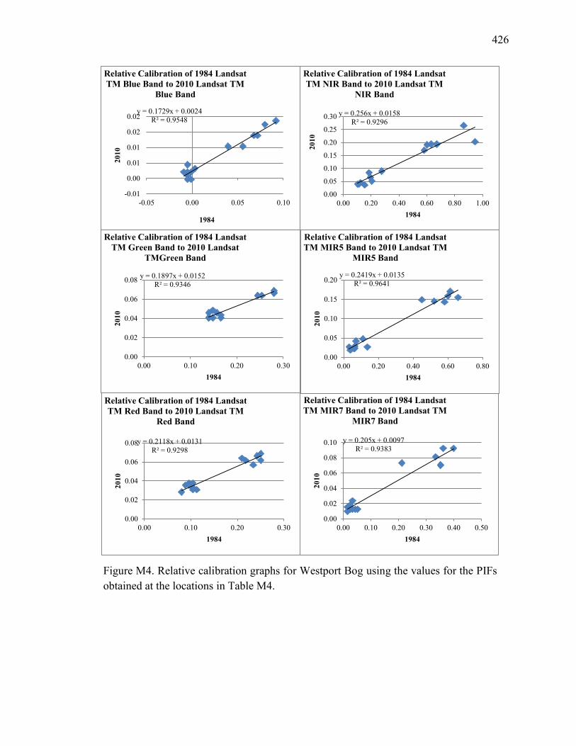
426
y = 0.1729x + 0.0024R² = 0.9548
-0.01
0.00
0.01
0.01
0.02
0.02
-0.05 0.00 0.05 0.10
2010
1984
Relative Calibration of 1984 Landsat TM Blue Band to 2010 Landsat TM
Blue Band
y = 0.1897x + 0.0152R² = 0.9346
0.00
0.02
0.04
0.06
0.08
0.00 0.10 0.20 0.30
2010
1984
Relative Calibration of 1984 Landsat TM Green Band to 2010 Landsat
TMGreen Band
y = 0.2118x + 0.0131R² = 0.9298
0.00
0.02
0.04
0.06
0.08
0.00 0.10 0.20 0.30
2010
1984
Relative Calibration of 1984 Landsat TM Red Band to 2010 Landsat TM
Red Band
y = 0.256x + 0.0158R² = 0.9296
0.00
0.05
0.10
0.15
0.20
0.25
0.30
0.00 0.20 0.40 0.60 0.80 1.00
2010
1984
Relative Calibration of 1984 Landsat TM NIR Band to 2010 Landsat TM
NIR Band
y = 0.205x + 0.0097R² = 0.9383
0.00
0.02
0.04
0.06
0.08
0.10
0.00 0.10 0.20 0.30 0.40 0.50
2010
1984
Relative Calibration of 1984 Landsat TM MIR7 Band to 2010 Landsat TM
MIR7 Band
y = 0.2419x + 0.0135R² = 0.9641
0.00
0.05
0.10
0.15
0.20
0.00 0.20 0.40 0.60 0.80
2010
1984
Relative Calibration of 1984 Landsat TM MIR5 Band to 2010 Landsat TM
MIR5 Band
Figure M4. Relative calibration graphs for Westport Bog using the values for the PIFs obtained at the locations in Table M4.

427
Conversion to at-sensor spectral radiance:
𝐿𝜆 = 𝐺𝑟𝑒𝑠𝑐𝑎𝑙𝑒 ∗ 𝑄𝑐𝑎𝑙 ∗ 𝐵𝑟𝑒𝑠𝑐𝑎𝑙𝑒
Where:
𝐺𝑟𝑒𝑠𝑐𝑎𝑙𝑒 =𝐿𝑀𝐴𝑋𝜆− 𝐿𝑀𝐼𝑁𝜆
𝑄𝑐𝑎𝑙𝑚𝑎𝑥− 𝑄𝑐𝑎𝑙𝑚𝑖𝑛
𝐵𝑟𝑒𝑠𝑐𝑎𝑙𝑒= 𝐿 𝑀𝐼𝑁𝜆− (
𝐿𝑀𝐴𝑋𝜆− 𝐿𝑀𝐼𝑁𝜆𝑄𝑐𝑎𝑙𝑚𝑎𝑥− 𝑄𝑐𝑎𝑙𝑚𝑖𝑛
)𝑄𝑐𝑎𝑙𝑚𝑖𝑛
where Lλ= Spectral radiance at the sensor's aperture, W/m2 sr μm Qcal= Quantized calibrated pixel value, DN Qcalmin= Minimum quantized calibrated pixel value corresponding to LMINλ, DN Qcalmax= Maximum quantized calibrated pixel value corresponding to LMAXλ, DN LMINλ= Spectral at-sensor radiance that is scaled to Qcalmin, W/m2 sr μm LMAXλ= Spectral at-sensor radiance that is scaled to Qcalmax, W/m2 sr μm Grescale= Band-specific rescaling gain factor, (W/m2 sr μm)/DN Brescale= Band-specific rescaling bias factor, W/m2 sr μm
Conversion to TOA reflectance:
𝜌𝜆 = 𝜋∗ 𝐿𝜆 ∗ 𝑑2
𝐸𝑆𝑈𝑁𝜆∗cos 𝜃𝑠
ρλ= Planetary TOA reflectance π = ~3.14159 Lλ= Spectral radiance at the sensor's aperture W/m2 sr μm d= Earth–Sun distance astronomical units ESUNλ= Mean exoatmospheric solar irradiance W/m2 μm θs= Solar zenith angle, °
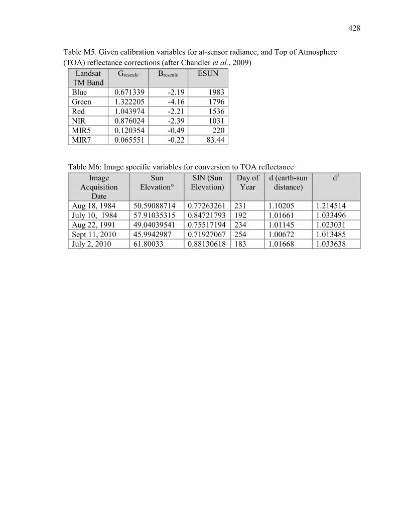
428
Table M5. Given calibration variables for at-sensor radiance, and Top of Atmosphere (TOA) reflectance corrections (after Chandler et al., 2009)
Landsat TM Band
Grescale Brescale ESUN
Blue 0.671339 -2.19 1983 Green 1.322205 -4.16 1796 Red 1.043974 -2.21 1536 NIR 0.876024 -2.39 1031 MIR5 0.120354 -0.49 220 MIR7 0.065551 -0.22 83.44
Table M6: Image specific variables for conversion to TOA reflectance Image
Acquisition Date
Sun Elevation°
SIN (Sun Elevation)
Day of Year
d (earth-sun distance)
d2
Aug 18, 1984 50.59088714 0.77263261 231 1.10205 1.214514 July 10, 1984 57.91035315 0.84721793 192 1.01661 1.033496 Aug 22, 1991 49.04039541 0.75517194 234 1.01145 1.023031 Sept 11, 2010 45.9942987 0.71927067 254 1.00672 1.013485 July 2, 2010 61.80033 0.88130618 183 1.01668 1.033638