Seediscussions,stats,andauthorprofilesforthispublicationat:https://www.researchgate.net/publication/274006141

Segmentationand3Dreconstructionofanimaltissuesinhistologicalimages

CHAPTER·JANUARY2015

DOI:10.1007/978-3-319-15799-3_14

READS

33

3AUTHORS,INCLUDING:

AugustoFaustino

UniversityofPorto

38PUBLICATIONS243CITATIONS

SEEPROFILE

JoaoManuelR.S.Tavares

UniversityofPorto

592PUBLICATIONS1,762CITATIONS

SEEPROFILE

Allin-textreferencesunderlinedinbluearelinkedtopublicationsonResearchGate,

lettingyouaccessandreadthemimmediately.

Availablefrom:JoaoManuelR.S.Tavares

Retrievedon:03February2016

Segmentation and 3D Reconstruction of Animal Tissues in Histological Images Liliana Azevedo*, Augusto M. R. Faustino**, João Manuel R. S. Tavares*

*Faculdade de Engenharia, Universidade do Porto, Porto, PORTUGAL, tavares@fe.up.pt **Instituto de Ciências Biomédicas Abel Salazar, Universidade do Porto, Porto, PORTUGAL Abstract: Histology is considered the "gold standard" to access anatomical infor-mation at a cellular level. In histological studies, tissue samples are cut into very thin sections, stained, and observed under a microscope by a specialist. Such stud-ies, mainly concerning tissue structures, cellular components and their interactions, can be useful to detect and diagnose certain pathologies. Thus, to find new tech-niques and computational solutions to assist this diagnosis, such as the 3D image based tissue reconstruction, is extremely interesting.

In this chapter, a methodology to build 3D models from histological images is proposed, and the results obtained using this methodology in four experimental cas-es are presented and discussed based on quantitative and qualitative metrics.

Keywords: histology, image analysis, image segmentation, image registration.

1 Introduction

Nowadays, histology is an important topic in medical and biological sciences,

since it stands at the intersections between biochemistry, molecular biology and physiology, and related disease processes (Stevens and Lowe 1992).

The most commonly used procedure for tissue studies consists in the preparation of histological sections for microscopic observation. Because tissues are too thick to allow the passage of light, they must be sliced to obtain very thin sections. In order to make these very thin tissues slices, they need to undergo a series of prior treat-ments, such as Fixation (for preserving the tissue structure), Inclusion (the technical process to impregnate the tissue with a rigid substance in order to be able to cut the sample into thin sections, such as paraffin) and Staining (to facilitate the distinction of tissue components) (Bioaula 2007; Carneiro and Junqueira 2004).

The reconstruction of the three-dimensional (3D) structures of tissues from a se-ries of 2D images, i.e. slices, is, at least in theory, a valuable tool to expand the 'hidden' microscopy dimension and thus be able to study the tissues and cells in depth. The possible approach to obtain such 3D models involves the digitalization of the histological slices, the preprocessing of the images obtained, the segmenta-tion of the tissues in the pre-processed images, the registration, i.e. the aliment, of

2

the segmented tissues and, finally, the 3D reconstruction of the tissues registered (Cooper 2009).

Whenever an original image is of poor quality due to, for example, the presence of severe noise, low contrast between relevant and irrelevant features, or intensity in homogeneity, image preprocessing techniques, such as image smoothing, denoising or intensity transformations, can be applied to enhance them (He et al. 2009).

On the other hand, algorithms of image segmentation try to extract the objects or regions of interest, here the tissues to be reconstructed into 3D, from images (He et al. 2009). The algorithms for image segmentation can be classified into three main types: algorithms based on threshold (Gonzalez et al. 2004; Otsu 1979), algorithms based on clustering techniques and algorithms based on deformable models (Zhen et al. 2010).

The goal of image registration is the geometrical alignment of two images - the reference image (also known as a fixed image) and the image to be aligned (also known as the moving image). Image registration is widely used, for example, in cartography, remote sensing and 3D reconstruction (Zitová and Flusser 2003). There are several methods to register images that can be divided according to: Di-mensionality of the images, Nature of the transformation used, Domain of the trans-formation used, Degree of interaction, Optimization Procedures employed, Rules adopted, Subjects and Objects involved (Maintz and Viergever 1998). In general, the image registration methods can be divided into two major groups: feature-based methods (the alignment is made using distinct features from the images, like re-gions, lines or points) and intensity-based methods (the intensity values of the im-age are used directly) (Zitová and Flusser 2003).

Registration accuracy of the algorithms can be evaluated using similarity measures, like the Sum of Square Differences (SSD) and Mean Square Error (MSE) (Zitová and Flusser 2003; Oliveira 2009; Oliveira and Tavares 2011), fiducial mar-kers (Pluim et al. 2000; Mattes et al. 2003; Danilchenko and Fitzpatrick 2011) and Dice Similarity Coefficient (Alterovitz et al. 2006; Klein et al. 2009).

In this work a methodology was developed to build 3D models from histological slices and then it was evaluated using experimental data.

2 Experimental Dataset

The histological images of the four dog tissues used in the experimental evalua-

tion were produced at the Veterinary Pathology Laboratory of the Abel Salazar In-stitute of Biomedical Sciences, in Portugal.

After the selection of the tissue samples, the following steps were carried out: Fixation, Inclusion and Staining, according to standard procedures.

To slice the tissue paraffin blocks, a fully motorized Leica 2255 microtome, from Leica Microsystems (Germany), was used, Figure 1. The slides obtained were

3

then scanned, using an Olympus VS110 device from Olympus America Inc. (USA), in order to obtain the histological images.

Figure 1. Examples of a paraffin block (left) and of a tissue slide (right).

After visual inspection, some of the images scanned were eliminated since sev-

eral noisy artifacts were detected. Table 1 summarizes the procedures, time and tools adopted to obtain the images, i.e. the slices, for the four experimental cases.

Table 1. Details about the tissue preparation procedures and images obtained.

Case Description

Number of orig-

inal / final

images

Tissue Processing Image digitalization

Fixation Inclusion Staining

Scanner: Olympus VS110,

Magnification: 20x

Agent: Formalin

Agent: Paraffin

Protocol: Hematoxylin

and eosin (H&E Stain)

#1 Testicular tu-moral Tissue 124/124 ±2 days ±1 day ± 7 days

#2 Normal lymph

node 100/95 ±1.5 day ±1 day ± 5 days

#3 Lymph node

tumor 100/100 ±1.5 day ±1 day ± 5 days

#4 Mammary

gland tumor 96/95 ±2 days ±1 day ± 6 days

3 Methodology

3.1 Image preprocessing

Since the histological images are digital images, they are prone to various types

of noise resulting from the acquisition. Image smoothing usually refers to spatial filtering in order to highlight the main image structures by removing image noise and fine details using for example a Gaussian filter (Alves 2013; He et al. 2012).

4

A Gaussian filter uses a 2D convolution operator in order to blur the input imag-es and remove details and noise from them. The kernel used in the convolution rep-resents the shape of a Gaussian hump (Ivanovska et al. 2010). A 2D Gaussian filter has the following form:

𝐺 𝑥, 𝑦 =1

2𝜋𝜎!𝑒!

!!!!!!!! , (1)

where (𝑥, 𝑦) are the spatial coordinates and 𝜎 is the standard deviation of the distri-bution (Ivanovska et al. 2010).

As reported in the literature (Alves 2013), testing the images using different Gaussian filters showed that the higher the 𝜎  was the more apparent the blur was; however, this was not so dependent on the filter parameter in terms of the window size. Therefore, in order to obtain a good smoothing effect, but keeping the more relevant tissue details, a Gaussian filter with a window size of [3 3] and 𝜎 equal to 4 was applied to all experimental images.

3.2 Image segmentation

Image Thresholding is commonly used in many applications of image segmenta-

tion because of its intuitive properties and simplicity of implementation; for exam-ple, one simple way to separate similar objects from the image background is by se-lecting a threshold 𝑇 that separates the two classes involved, i.e. objects and background.

The Otsu method is a histogram based thresholding method where the gray-level histogram is treated as a probability distribution (Gonzalez et al. 2004). Supposing there is a dichotomization of the image pixels into two classes 𝐶! and 𝐶!, then the Otsu method selects the threshold value k that maximizes the variance between classes, 𝜎!!, which is defined as:

𝜎𝐵2 = ꙍ0 𝜇0 − 𝜇𝑇

2+ ꙍ1 𝜇1 − 𝜇𝑇

2, (2)

where ꙍ! and ꙍ! are the probability of occurrence, and 𝜇0 and 𝜇1 are the means of the two classes, respectively (Gonzalez et al. 2004; Otsu 1979).

In order to extract the tissues from the histological slices, the Otsu method was applied to the saturation component of the HSV (hue, saturation, value) colour space of the preprocessed images. Figure 2 shows that the smoothing step was es-sential to obtain suitable tissue segmentation masks.

In some of the tissue segmentation masks traces of loose tissue that were re-moved in order to reconstruct consistent tissue volumes were perceived, Figure 3.

5

Afterwards, in order to obtain the final tissue segmentation, the preprocessed RGB images were transformed into grayscale images, and multiplication operations were performed between each tissue segmentation mask and the respective gray im-age, Figure 4.

Since the image registration algorithm requires that the input images are the same size, all experimental images were normalized to the same size.

a)

b)

Figure 2. Results of the Otsu method on the saturation channel of an original image (a) and on the same channel of the corresponding smoothed image (b).

6

Figure 3. Identification of the regions (in green) to be discarded from an experimental image.

Figure 4. An experimental image in grayscale after been multiplied with the corresponding segmentation tissue mask.

3.3 Image registration

Image registration is the process of overlapping two or more images of the same

scene acquired at different time points, from different views and/or by different sen-sors. Usually, this process aligns geometrically two input images - the reference im-age, also known as fixed image, and the moving image, by searching for the opti-mal transformation that best aligns the structures of interest in the images (Zitová and Flusser 2003; Oliveira and Tavares 2012).

In general, image registration methods can be divided into two major groups: feature- and intensity-based methods. The first group is based on the detection and matching of similar features, such as points, lines or regions, between the input im-ages (Zitová and Flusser 2003). This type of registration follows four steps: 1) Fea-ture Detection; 2) Feature Matching, i.e. the establishment of the correspondence between the detected features; 3) Model Transformation Estimation, i.e. the estima-tion of the parameters of the mapping function that register the features matched; and 4) Interpolation and Transformation, i.e. the transformation of the moving im-

7

age according to the estimated parameters of the mapping function used. On the other hand, the Intensity-based registration methods are preferably used when the input images do not present prominent features that can be efficiently detected. To overcome such difficulty, these methods use the intensity values of the pixels of the input images in order to estimate the best mapping function by minimizing a cost function, which is usually based on a similarity measure. The cost function is com-puted using the overlapping regions of the input image and an optimizer tries to ob-tain the best value possible. Additionally, an interpolator is used to map the pixels (or voxels in 3D) into the new coordinate system according to the geometric trans-formation found, Figure 5.

Figure 5. Diagram of a typical intensity-based registration algorithm (adapted from Oliveira

and Tavares 2012). To register the histological images, the Intensity-based image registration algo-

rithm in MATLAB (Mathworks, USA) was used (Mathworks 2013a; Mathworks 2013b). A monomodal registration was involved since the images were acquired us-ing the same device and according to the same protocol. The geometric transfor-mations compared were the rigid, affine and the similarity transformations. The projective transform was excluded because this transformation deals with the tilting transformation, and the slices used were obtained parallel to each other.

Additionally, the number of levels of the multiresolution pyramid used was spec-ified to be equal to 3. For the cost function, the Root Mean Square Error (RMSE) was adopted since this metric is known to be appropriate for monomodal registra-tion. This metric is computed by squaring the differences in terms of intensities of the corresponding pixels in each image and taking the mean of those squared differ-ences. For the optimizer, the One Plus One Evolutionary also in MATLAB was used, which assumes a one-plus-one evolutionary optimization configuration, and an evolutionary algorithm is used to search for the set of parameters that produce the best possible registration result (Mattes et al. 2001). In this algorithm, the num-ber of iterations equal to 1000 was adopted. The registration process started with the application of a rigid transformation to deal with the rigid misalignment in-volved between the images and simplify the posterior finer registration process and facilitate its convergence.

8

For the 3D reconstructing, the registration process started from an image in the middle of the image stack, since the slices closest to the center generally contain more information about the tissue (Roberts et al. 2012). Two approaches were test-ed: 1) Using a reference slice, the registration of each slice of the stack was done taking into account only its spatial information, i.e. all remainder slices were regis-tered to the reference slice, Figure6a; 2) Using a pairwise strategy, the registration is made in cascade, starting from the center slice to the following neighbor slices in the stack, the next slice is registered with the previous one and so forth, Figure6b.

a) b)

Figure 6. Registration using the center slice as reference (a) and from the center slice to neighbor slices in the stack (b).

Three metrics were used to evaluate the registration accuracy: 1) RMSE - First the mean for the errors of the corresponding intensity pixels be-

tween each aligned image pair was calculated, and then the average error between all the images of the registered stack, given the Mean Square Error (MSE). Finally, the RMSE value was obtained by calculating the square root of the correspondent MSE. The RMSE and its variations have been used in many image registration problems, including those with histological images (Egger et al. 2012; Sharma and Katz 2011; Sharma et al. 2011).

2) The Dice Similarity coefficient (DSC or Dice) - The calculation of this metric

is based on the overlap of two registered areas, and it has been a metric commonly used to evaluate the intersection of two areas. The DSC has values between 0 (zero) and 1 (one); the higher values represent registrations of better quality (Alterovitz et al. 2006; Klein et al. 2009). This metric has been widely used to access the registra-tion error of histological images (Alterovitz et al. 2006; Klein et al. 2009), and can be calculated as:

𝐷𝑆𝐶 =2𝐴

𝐴 + 𝐵, (3)

where 𝐴 and 𝐵 are the registered areas. 3) Because the tissues may appear in the slices as a set of regions, in addition to

the DSC, a DSC normalized by the total minor tissue area was defined:

9

𝐷𝑖𝑐𝑒𝑛 =𝑅

𝑚𝑖𝑛𝑜𝑟  𝑎𝑟𝑒𝑎, (4)

where 𝑅 is the area of intersection between total tissue area in slices A and B, and 𝑚𝑖𝑛𝑜𝑟  𝑎𝑟𝑒𝑎, as the name suggests, is the total minor tissue area between these two.

3.4 3D Reconstruction

Finally, for the 3D reconstruction of the tissues presented in the experimental da-

taset, the surfaces were built using the isosurface algorithm included in MATLAB (Mathworks 2013c).

To enhance the visualization and facilitate the comparison among the four exper-imental cases under study, an adjustment on the reconstruction z scale was made, and different colors were chosen for the surfaces built.

4 Results and Discussion

The image preprocessing and the image segmentation were fundamental steps for preparing the images for the 3D registration. The intensity-based registration was carried out with success, but to find the best geometric transform, the registra-tion accuracy needed to be evaluated, Table 2. Analyzing the data shown in Table 2, some conclusions can be pointed out:

The existence of a strong relationship between the metrics used to evaluate the registration accuracy (RMSE, Dice and Dicen); the higher the quadratic registration error is, the lower the dice coefficient is; the registration improved the alignment of the tissue represented along the slices in each dataset.

Table 2. Assessment results for the four cases under study regarding the accuracy achieved using different geometrical transformations (rigid, similarity and affine) and a reference slice or pairwise based approach on the registration procedure (- not performed, * Erroneous registration).

Case #1

Without registration RMSE= 9.3219 Dice= 0.8292 Dicen= 0.8458

Pre-Registration

RMSE= 8.6835 Dice= 0.9441 Dicen= 0.9635

Rigid Similarity Affine

RMSE Dice Dicen RMSE Dice Dicen RMSE Dice Dicen

Reference slice - - - 8.3307 0.9671 0.9753 8.8068 0.9377 0.9454

Pairwise 8.3255 0.9602 0.9798 8.1888 0.9676 0.9772 * * *

10

Case #2

Without registration RMSE= 9.5687

Dice= 0.8606 Dicen= 0.8734

Pre-Registration RMSE= 7.9695 Dice= 0.9356 Dicen= 0.9517

Rigid Similarity Affine

RMSE Dice Dicen RMSE Dice Dicen RMSE Dice Dicen

Reference slice - - - 7.5954 0.9492 0.9598 8.6138 0.9066 0.9156

Pairwise 7.4857 0.9484 0.9651 7.3995 0.9515 0.9618 9.5232 0.7744 0.7820

Case #3

Without registration RMSE= 9.5544 Dice= 0.8222 Dicen= 0.8423

Pre-Registration RMSE= 7.7236 Dice = 0.8271 Dicen= 0.8589

Rigid Similarity Affine

RMSE Dice Dicen RMSE Dice Dicen RMSE Dice Dicen

Reference slice - - - 7.2046 0.8679 0.8927 9.0429 0.6978 0.7211

Pairwise 6.8316 0.8774 0.9121 6.8222 0.8773 0.9052 9.4064 0.5922 0.6110

Case #4 Without registration RMSE= 10.1506

Dice= 0.6705 Dice= 0.7135

Pre-Registration RMSE= 9.9125 Dice = 0.7698 Dicen = 0.8198

Rigid Similarity Affine

RMSE Dice Dicen RMSE Dice Dicen RMSE Dice Dicen

Reference slice - - - 9.7034 0.8080 0.8471 10.0953 0.7273 0.7615

Pairwise 9.6133 0.8114 0.8613 9.5578 0.8191 0.8604 10.4697 0.5747 0.6061

In the preregistration step, a rigid transformation was used to place the tissue in

the center of the image and then low error values and improved Dice values were achieved. The pairwise registration approach had better results than the reference slice based registration approach. Globally, and for the four cases used, the best reg-istration results were obtained using the pairwise registration approach and the similarity transform. The worst results were obtained with the affine transfor-mation: The RMSE values were high, and the dice values were low. The affine transformation copes with rotation, translation, scale and shear, which are too many degrees of freedom when histological images are involved. The registration based on the affine transform and pairwise registration approach was not successful for Case #1 and of bad quality in the other cases. On the other hand, the rigid registra-tion only copes with rotation and translation (simple geometrical transformations), and the error and Dice values obtained indicated good registration results.

It was also possible to verify that the normalized dice (Dicen) presented higher results than the normal dice (Dice). A plausible explanation for this is the fact that the Dicen is less affected by slices with different tissue areas, which is a common

11

situation with histological images, since it is normal that the tissue appears with disconnected areas in each image slice.

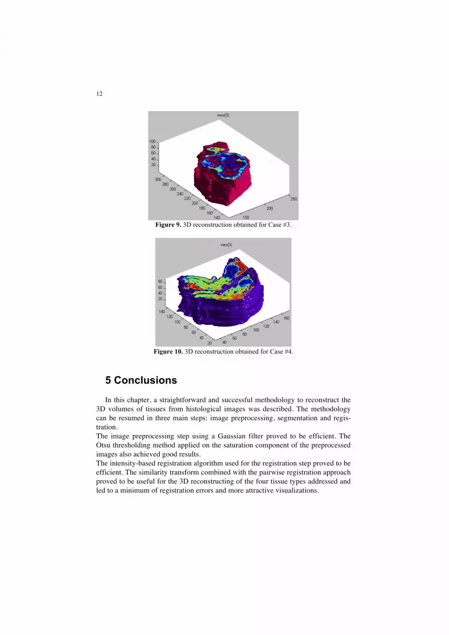
Error! Reference source not found.7-10 show the 3D models built for the four experimental cases under study. These figures show that the best reconstructions built still had rough surfaces. This is due to the fact that the registration process is not totally perfect and also due to the procedure used to prepare the histological im-ages, which is influenced by several features, such as dilation and retraction of the tissue.

Figure 8. 3D reconstruction obtained for Case #2.

Figure 7. 3D reconstruction obtained for Case #1.

12

Figure 9. 3D reconstruction obtained for Case #3.

Figure 10. 3D reconstruction obtained for Case #4. 5 Conclusions

In this chapter, a straightforward and successful methodology to reconstruct the 3D volumes of tissues from histological images was described. The methodology can be resumed in three main steps: image preprocessing, segmentation and regis-tration. The image preprocessing step using a Gaussian filter proved to be efficient. The Otsu thresholding method applied on the saturation component of the preprocessed images also achieved good results. The intensity-based registration algorithm used for the registration step proved to be efficient. The similarity transform combined with the pairwise registration approach proved to be useful for the 3D reconstructing of the four tissue types addressed and led to a minimum of registration errors and more attractive visualizations.

13

Acknowledgment

This work was partially done in the scope of the project with reference PTDC/BBB-BMD/3088/2012, financially supported by Fundação para a Ciência e a Tecnologia (FCT), in Portugal.

References

Alterovitz, R. , Goldberg, K. ., Pouliot, J. , Hsu, I. , Kim, Y. , Noworolski, S., & Kurhanewicz, J. (2006). Registration of MR prostate images with biomechanical modeling and nonlinear parameter estimation. Medical physics, 33(2), 446–454.

Alves, A. (2013). Joint Bilateral Upsampling. Retrieved January 2, 2013, from http://lvelho.impa.br/ip09/demos/jbu/filtros.html#.

Bioaula. (2007). Histologia básica. Retrieved April 16, 2012, from http://www.bioaulas.com.br/aulas/2006/histologia/apostilas/apostila_histologia_basica/apostila_histologia_basica_demo.pdf.

Carneiro, J., & Junqueira, L. (2004). Histologia Básica. In G. K. S.A. (Ed.), Histologia Básica (10a edição., pp. 1–22).

Cooper, L. A. D. (2009). High Performance Image Analysis for Large Histological Datasets. Ohio State University.

Danilchenko, A. , & Fitzpatrick, J. (2011). General approach to firstorder error prediction in rigid point registration. IEEE Transactions on Medical Imaging, 30(3), 679–693.

Egger, R. , Narayanan, R. , Helmstaedter, M. , De Kock, C., & M., O. (2012). 3D reconstruction and standardization of the rat vibrissal cortex for precise registration of single neuron morphology. PLoS Computational Biology, 8(12), 1–18.

Gonzalez, Rafael C.,Woods, Richard E. & Eddins, S. L. . (2004). Digital Image Processing Using MATLAB (pp. 100,194,195,200,205, 378,404–406). PEARSON, Prentice Hall. doi:0-13-008519.

He, L., Long, LR., Antani, S. & Thoma, G. (2009). Computer Assisted Diagnosis in Histopathology. (Vol. 3, pp. 272–287).

Ivanovska, T., Schenk, A., Dahmen, U., Hahn, H. & Linsen, L. (2010). A fast and robust hepatocyte quantification algorithm including vein processing. BMC Bioinformatics., 11(1), 1–18.

14

Klein, A., Andersson, J., Ardekani, BA., Ashburner J., Avants, B., Chiang, MC., Christensen, GE., Collins, DL., Gee, J., Hellier, P., Song, JH., Jenkinson, M., Lepage, C., Rueckert, D., Thompson, P., Vercauteren, T., Woods, RP., Mann, JJ. & Parsey, R. (2009). Evaluation of 14 nonlinear deformation algorithms applied to human brain MRI registration. NeuroImage, 46(3), 786–802.

Maintz, JBA. & Viergever, M. (1998). A survey of medical image registration. Medical Image Analysis, 2(1), 1–36.

Mathworks. (2013a). Estimate Geometric Transformation (R2013a). Retrieved March 4, 2013, from http://www.mathworks.com/help/vision/ref/estimategeometrictransformation.html

Mathworks. (2013b). imregister (R2013a). Retrieved March 4, 2013, from http://www.mathworks.com/help/images/ref/imregister.html.

Mathworks. (2013c). Techniques for Visualizing Scalar Volume Data (R2013a). Retrieved April 6, 2013, from http://www.mathworks.com/help/matlab/visualize/techniques-for-visualizing-scalar-volume-data.html.

Mattes, D. ., Haynor, D. ., Vesselle, H. ., Lewellen, T. ., & Eubank, W. (2003). PET-CT image registration in the chest using free-form deformations. IEEE Transactions on Medical Imaging, 22(1), 120–128.

Mattes, D., Haynor, DR., Vesselle, H., Lewellyn, TK. & Eubank, W. (2001). Nonrigid multimodality image registration. IEEE Transactions on Medical Imaging, 4322, 1609–1620.

Oliveira, F. P. M. (2009). Emparelhamento e alinhamento de estruturas em visão computacional: aplicações em imagens médicas. Faculdade de Engenharia da Universidade do Porto.

Oliveira, F. P. M. . & Tavares, J. M. R. S. (2011). Novel framework for registration of pedobarographic image data. Medical and Biological Engineering and Computing, 49(3), 312–324.

Oliveira, F. & Tavares, J. (2012). Medical image registration: a review. Computer Methods in Biomechanics and Biomedical Engineering, ISSN: 1025-5842 (print) - 1476-8259 (online), Taylor & Francis, 17(2), 73-93. doi: 10.1080/10255842.2012.670855.

15

Otsu, N. (1979). A Threshold Selection Method from Gray-Level Histograms. IEEE Transactions on Systems, Man and Cybernetics., 9(1), 62–66. doi:10.1109/TSMC.1979.4310076.

Pluim, J., Maintz, J. & MA., V. (2000). Image registration by maximization of combinedmutual information and gradient information. IEEE Transactions on Medical Imaging, 19(8), 809–814.

Robert, s N., Magee, D., Song, Y., Brabazon, K.., Shires, M., Crellin, D., Orsi, NM., Quirke, R., Quirke, P. & Treanor, D. (2012). Toward Routine Use of 3D Histopathology as a Research Tool. The American Journal of Pathology, 180(5), 1835–1842.

Sharma, R. & Katz, J. (2011). Taxotere Chemosensitivity Evaluation in Rat Breast Tumor by Multimodal Imaging: Quantitative Measurement by Fusion of MRI, PET Imaging with MALDI and Histology. IEEE Transactions on Medical Imaging, 1(1), 1–14.

Sharma, Y., Moffitt, RA., Stokes, TH., Chaudry, Q. & Wang, M. (2011). Feasibility analysis of high resolution tissue image registration using 3-D synthetic data. Journal of Pathology Informatics, 2(6), 1–7.

Stevens, A. & Lowe, J. (1992). HISTOLOGY. In Mosby (Ed.), (pp. 1–6).

Zhen, M., Tavares, J. M. R. S. ., Natal, R. J., & Mascarenhas, T. (2010). Review of Algorithms for Medical Image Segmentation and their Applications to the Female Pelvic Cavity. Computer Methods in Biomechanics and Biomedical Engineering, 13(2), 235–246. doi:10.1080/10255840903131878.

Zitová, B. & Flusser, J. (2003). Image registration methods: a survey. . Image and Vision Computing, 21(11), 977–1000.