Selection of Variables for Discriminant Analysis of Human Crania for

Ancestry Determination

Adam Kolatorowicz

B.S., Northern Illinois University, 2002

A Thesis Submitted in Partial Fulfillment of the Requirements for the Degree of Master of

Science in Human Biology in the Graduate School of the University of Indianapolis

January 2006

Copyright © 2006 Adam Kolatorowicz. All Rights Reserved.

i

FORM B

Accepted by the faculty of the Graduate School, University of Indianapolis, in the partial

fulfillment of the requirements for the Master of Science degree in

HUMAN BIOLOGY

__________________________________

Thesis Advisor – Dr. Stephen P. Nawrocki, D.A.B.F.A

__________________________________

Reader – Dr. John H. Langdon

Date:

ii

ACKNOWLEDGEMENTS

I would like to thank Noel D. Justice at the Indiana University Glenn A. Black Laboratory of

Archaeology for allowing me access to the Angel Mounds skeletal material on which I refined

my measurement technique.

Thanks go to Dr. Della C. Cook at the Indiana University Anthropology Department

Osteological Collection for allowing me access to the Arkansaw Mounds material.

Additional thanks go to Lyman Jellema at the Cleveland Museum of Natural History for

allowing me access to the Hamann-Todd Osteological Collection and for providing me with the

Mitutoyo direct input tool and foot pedal. Without those instruments I surely would not have

completed data collection on time.

Last, but not least, I would like to extend much gratitude to Dr. Stephen P. Nawrocki for letting

me borrow the very expensive instrumentation to complete the study and for helping me develop

the proper measuring technique.

This project was funded in part by:

The Connective Tissue Graduate Student Research Fund

iii

ABSTRACT

Forensic anthropologists use the computer program FORDISC 2.0 (FD2) as an analytical

tool for the determination of ancestry of unknown individuals. There are an almost endless

number of measurements that can be taken on the human skeleton, yet FORDISC includes only

78 measurements for its analysis. In particular, the program will only utilize up to 24

measurements of the cranium. These 24 cranial variables are used because they require simple,

relatively inexpensive instruments that most biological anthropology laboratories have

(spreading and sliding calipers). Also, individuals with a basic knowledge of the anatomical

landmarks can take the measurements with relative ease. Unconventional measurements of the

cranium require unusual, costly instruments (such as the radiometer and coordinate caliper) and

are more difficult to take. This study will examine which measurements of the human cranium

provide the greatest classificatory power when constructing discriminant function formulae for

the determination of ancestry and will answer the question of whether the use of variables that

require more time, training, and equipment are worth the effort.

Sixty five cranial measurement were taken on 155 adult human crania from three

different ancestral groups: (1) African American (n = 50), (2) European American (n = 50),

and (3) Coyotero Apache (n = 55). The 65 measurements were broken up into four subsets for

statistical analysis: (1) FD2 (1996), (2) Howells (1973), (3) Gill (1984), and (4) All

Measurements. A predictive discriminant analysis with a forward stepwise methodology of

p = 0.05 to enter and p = 0.15 to remove was run using the computer software package SPSS

13.0. The analysis produced 4 sets of discriminant function formulae. The classificatory power

of each set of formulae was determined by comparing the hit-rate estimation (the percent

correctly classified) of each of the subsets. First, the resubstitution rate was compared to the

iv

leave-one-out (LOO) rate for each subset and then both rates were compared across all subsets.

The FD2 subset had a resubstitution rate of 90.3% and LOO rate of 85.8%. The Howells subset

had a resubstitution rate of 92.9% and a LOO rate of 90.3%. The Gill subset had a resubstitution

rate of 63.2% and a LOO rate of 61.9%. Finally, the All Measurements subset had a

resubstitution rate of 95.5% and a LOO rate of 93.5%. The non-standard measurements of the

All Measurements subset performed the best and the standard FD2 measurements performed

third best. Non-standard measurements incorporated in the All Measurements formulae included

frontal subtense, mid-orbital breadth, bistephanic breadth, bimaxillary breadth, and molar

alveolar radius.

The formulae provided the best separation of the Apache group from the other two

groups. Stepwise analysis showed that the use of more variables is not necessarily better, as not

all of the variables were included in the final formulae. Only 12 of the 24 FD2 measurements,

12 of the 57 Howells measurements, 4 of the 6 Gill measurements, and 15 of the 65 All

Measurements were used. Results show that the non-standard measurements can be useful for

determining the ancestry of unknown human crania. These measurements could be especially

useful for incomplete crania. It is suggested that biological anthropology laboratories purchase

radiometers and coordinate calipers to record data that would be missed with spreading and

sliding calipers. Standard measurements can be combined with non-standard measurements to

produce more powerful discriminant function formulae for the determination of ancestry.

v

TABLE OF CONTENTS

Signature Page . . . . . . . . . . . . . . . . . . . . . . . . . . . . . . . . . . . . . . . . . . . . . . . . . . . . . . . . . . . . . . . . i

Acknowledgements . . . . . . . . . . . . . . . . . . . . . . . . . . . . . . . . . . . . . . . . . . . . . . . . . . . . . . . . . . . . .ii

Abstract . . . . . . . . . . . . . . . . . . . . . . . . . . . . . . . . . . . . . . . . . . . . . . . . . . . . . . . . . . . . . . . . . . . . . iii

Chapter 1: Introduction . . . . . . . . . . . . . . . . . . . . . . . . . . . . . . . . . . . . . . . . . . . . . . . . . . . . . . . . . 1

Chapter 2: Multiple Discriminant Function Analysis . . . . . . . . . . . . . . . . . . . . . . . . . . . . . . . . . . 7

Chapter 3: Standard and Non-Standard Measurements . . . . . . . . . . . . . . . . . . . . . . . . . . . . . . . 18

Chapter 4: Materials and Methods . . . . . . . . . . . . . . . . . . . . . . . . . . . . . . . . . . . . . . . . . . . . . . . 27

Chapter 5: Results . . . . . . . . . . . . . . . . . . . . . . . . . . . . . . . . . . . . . . . . . . . . . . . . . . . . . . . . . . . . 33

Chapter 6: Discussion and Conclusions . . . . . . . . . . . . . . . . . . . . . . . . . . . . . . . . . . . . . . . . . . . 53

Literature Cited . . . . . . . . . . . . . . . . . . . . . . . . . . . . . . . . . . . . . . . . . . . . . . . . . . . . . . . . . . . . . . 61

Appendix A: Cranial Measurement Definitions . . . . . . . . . . . . . . . . . . . . . . . . . . . . . . . . . . . . . 69

Appendix B: Craniometrics Recording Form . . . . . . . . . . . . . . . . . . . . . . . . . . . . . . . . . . . . . . . 70

Appendix C: Casewise Statistics . . . . . . . . . . . . . . . . . . . . . . . . . . . . . . . . . . . . . . . . . . . . . . . . 73

1

CHAPTER 1: INTRODUCTION

The term “ancestry” as used by biological anthropologists refers to the population

affiliation, based on geographical location, of an individual. The determination of the ancestry

of human skeletal remains is a key step in the course of identifying unknown individuals. The

predicted ancestry, sex, age, and stature form a biological profile of the decedent which, in turn,

helps with the identification process by narrowing down the number of potential matches.

The biological profile is also used by anthropologists to understand human variation in

historic and prehistoric populations. Bioarcheologists analyze the skeletons of long-deceased

individuals to better understand the history of human populations, including migration patterns,

demographic structure, and the effects of disease. Creating an accurate biological profile,

whether for recent or ancient remains, is the starting point of all future analysis. Therefore, it is

imperative to refine existing methods for determining ancestry and sex and for estimating age

and stature in order to improve the accuracy of the biological profile, and, by extension,

conclusions based on those profiles.

In this thesis the term ancestry is used instead of the term race. Race is an outmoded

term that implies discrete, typological, and thus artificial subdivisions of the human species

based on their overt physical and behavioral characteristics (Nawrocki, 1993). Ancestry, on the

hand, refers to the broad geographical origin of a group of humans and emphasizes ancestral-

descendant relationships between groups and the microevolutionary forces that produce human

variation.

Forensic anthropologists correctly note that certain morphological traits are known to be

present at higher frequencies in certain ancestral populations, and the data suggest that clusters of

traits may occur at higher frequencies in specific groups. However, any specific trait may not

2

occur exclusively in one particular group, and no trait or assemblage of traits can perfectly

distinguish between all members of ancestral groups. In other words, the presence of a trait or a

cluster of traits may suggest, but not confirm, group affiliation. If one were to examine the

global population one would find that many morphological traits are clinally distributed across

the globe with no discrete boundaries between groups of people. In some ways the population of

the United States is an exception because of its unique structure and history.

Groups from all over the world have recently migrated to the United States. In their

native lands, morphological traits can be clinally distributed and grade gradually into

neighboring groups. Migrating subsets of these ancestral groups have largely tended to maintain

their cultural and biological identities in North America, creating non-clinal distributions of traits

and increasing the appearance of biological discreteness relative to their native continents.

Ancestral categories as used in the American medicolegal setting are descriptive tools used to

identify unknown individuals and to communicate with law enforcement agencies. Forensic

anthropologists predict facial, hair, and skin characteristics from skeletal morphology. This

prediction of ancestral appearance can only be accomplished when the anthropologist is familiar

with the variation that exists within populations that are likely to be found in the area that he/she

is working.

Skeletal Ancestry Determination

Determining the ancestry of a decedent from their skeletal remains is perhaps the most

difficult aspect of the biological profile to resolve (Church, 1995). Variables used to determine

ancestry can be placed into one of two categories: (1) non-metric variables or (2) metric

variables. Non-metric variables are traits of the skeleton that are discontinuous, discrete, or

quasi-continuous, such as orbital shape or prognathism curvature. Metric variables rely on

3

continuous measurements of the skeleton, such as maximum cranial breadth or orbital height.

One type of variable is not superior to the other; rather, “. . . the chances of being right in a racial

identification depends largely on the observer’s experience” (Stewart, 1948:318). Nonetheless,

there has long been debate within biological anthropology as to which variables yield the best

results. Classically, non-metric variables were seen as a subjective, less scientific means of

determining ancestry compared to metric variables, which were considered more objective and

scientific. Stewart (1948) notes that measuring bones is a “mechanical procedure,” but that does

not mean that a possibility for error does not exist. Carpenter (1976) examined the utility of non-

metric traits versus metric traits to determine ancestry from the skull, at a time when non-metric

traits dominated the field. He observed both discrete traits and took measurements of skulls from

the Terry Collection and concluded that craniometrics are an excellent way to determine

ancestry, with 86 - 91% correctly identified. Krogman and İşcan (1986) state that on average, 85

- 90% of individuals are correctly identified by using discrete traits and 80 - 88% of individuals

are identified correctly using metric methods. Today, both metric and non-metric traits are used

to estimate one’s ancestry in forensic anthropology (Krogman and İşcan, 1986; Reichs, 1986;

Gill and Rhine, 1990; Church, 1995).

Measurements of a cranium may be used to give a numerical description of an already

recognizable discrete trait. In other words, it is possible to convert features that anthropologists

have traditionally classified as discrete traits into metric traits by measuring the features in one or

more dimensions. Mastoid size is one example. Conversely, some metric traits, such as nasal

breadth and alveolar prognathism, are sometimes treated as discrete traits.

Craniometric Assessment of Ancestry

Out of all the components of the human skeleton, the traits of the skull and face are

4

the most often used and most effective in ancestry determination (Gill, 1986, 1998; Novotný et

al., 1993). Large, geographically-defined populations share similar features of the cranium. It is

the slight variation in the size and shape of these features that allows the anthropologist to

determine ancestral group affiliation (Sauer, 1992; Brace, 1995; Kennedy, 1995).

A feature on one individual will be smaller or larger than the same feature on another

individual; therefore, single measurements describe the size of a feature. It is then easy to

compare sizes of traits between two individuals using simple, univariate statistical methods. If

two measurements are taken of a feature, the second measurement is said to provide a description

of its shape. Shape is the proportion of the two measurements, which will make a feature on one

cranium “look” different from the same feature on another. If more measurements are taken then

one can be more detailed in one’s description of the skull under study. In other words, shape can

be more accurately described. Analyzing multiple variables at the same time requires the use of

multivariate statistical methods. Although having the same foundation as univariate methods,

multivariate methods require the use of advanced statistical computer software.

Some researches have called for the refinement of craniometric techniques as well as

metric techniques in general (Brues, 1990; Church, 1995; Gill, 1998). In the early 1900s, there

was little to no standardization among measurement devices. Instruments were often custom-

made by the researcher and different institutions/laboratories used different instrumentation and

techniques to collect data from the skeleton. It was very difficult to duplicate methodology and

compare results of previous experiments with later studies. Efforts by researchers such as

Hrdlička (1920), Martin (1928), and Howells (1937) helped to standardize osteometric data

collection by providing definitions of measurements and landmarks, which included a

description of the placement of instrumentation on the cranium. In fact, many researchers still

refer to Martin for measurement definitions (Howells, 1973; Krogman and İşcan, 1986; Bass,

5

1995; Buikstra and Ubelaker, 1994; Moore-Jansen et al., 1994). As there are several references

(Hrdlička, 1920; Martin, 1928; Howells, 1937, 1973; Buikstra and Ubelaker, 1994; Moore-

Jansen et al., 1994; Bass, 1995) available today that define measurements of the skeleton, it has

become easier to test the utility of earlier techniques on modern populations. Most of the error in

recording measurements of the cranium no longer lies with the instrumentation but instead

involves interobserver error.

Currently, most biological anthropology laboratories have basic measuring devices as

part of their collection. Instruments such as spreading and sliding calipers are relatively

inexpensive and are simple to learn how to use. A cursory knowledge of anatomical landmark

location will allow the researcher to take measurements of the human cranium with virtual ease.

Using only the spreading and sliding calipers limits the researcher to the amount of data that can

be collected from the cranium. Within forensic anthropology, there is a standard set of 24

measurements that correspond to the measurements on the computer program FORDISC (Jantz

and Ousley, 1993; Ousley and Jantz, 1996), which practitioners turn to in their osteological

analysis. The creators of FORDISC have found the 24 measurements to be the most effective

when using discriminant function analysis to determine the sex and ancestry of an unknown

cranium. There are, however, other measurement devices that allow the researcher to more fully

describe the shape of the cranium by recording different types of measurements. Instruments

such as the coordinate caliper and radiometer are more expensive and require more training to

manipulate properly. The landmarks that define the measurements taken by these instruments

are more difficult to locate, but the instruments can measure features that sliding and/or

spreading calipers cannot.

6

Purpose and Hypothesis

The purpose of this study is to determine which measurements of the human cranium

provide the greatest classificatory power when constructing discriminant function formulae for

the determination of ancestry. The study will identify the most effective combinations of

standard and non-standard measurements and will answer the question of whether the use of

variables that require more time, training, and equipment are worth the effort. Perhaps biological

anthropology laboratories should invest in other instrumentation besides spreading and sliding

calipers. It is hypothesized that a combination of standard and non-standard measurements will

provide higher classificatory power over only standard measurements. The study will test the

null hypothesis that adding non-standard measurements to standard measurements will not

increase the classificatory power of a linear discrimination function.

Chapter 2 provides a description of predictive multiple discriminant function analysis and

its early and later applications to biological anthropology research. Chapter 3 discusses the

different types of measurements used in craniometry as well as special instrumentation. Chapter

4 details the study sample that was used along with the statistical methodology employed. A

description of the results of the statistical analysis is provided in Chapter 5, followed by

conclusions reached from the study in Chapter 6.

7

CHAPTER 2: MULTIPLE DISCRIMINANT FUNCTION ANALYSIS

Multiple discriminant function analysis is a type of multivariate statistical technique

which reduces large data sets to explain the relationship between two types of variables. It

involves both grouping variables (the groups) and response variables (the observed

characteristics). There are two major types of multiple discriminant function analyses: (1)

descriptive (DDA) and (2) predictive (PDA). In DDA, the response variables are viewed as

outcome variables and the grouping variables are viewed as the explanatory variables. In other

words, the response variables are used to separate the groups. DDA is very similar to a

multivariate analysis of variance in that both methods analyze the effect of more than one

response variable on more than one grouping variable. In PDA, the response variables act as

predictor variables and the grouping variables are viewed as outcome variables. In other words,

the response variables are used to predict the grouping variables, or, the roles of the two

variables are reversed compared to DDA. PDA is very similar to multiple regression analysis in

that both methods are used to predict a dependent grouping variable from independent response

variables. As this study examines the applications of PDA; DDA will be discussed no further.

Huberty (1994) provides a detailed explanation of both types of analysis.

It is essential to understand the theoretical and mathematical foundations of PDA before

one can apply the method to a research model. Basic PDA theory is explained below, followed

by a discussion of its most common uses within biological anthropology. Next, a history of PDA

beginning with its inception in statistical analysis will be reviewed along with its development in

the first half of the 20th

century. The later applications of PDA coinciding with the rise of

computer technology will then be addressed.

8

Predictive Discriminant Analysis

PDA is used to predict group membership of unknown objects. The object could be a

living person, an ancient artifact, a car, or a human skull. Applying a PDA to these objects might

tell the researcher if the person has risk factors for a disease, what the artifact was made for, what

make and model the car is, or the geographical origin of the skull. The prediction is based on a

suite of characteristics (response variables) that are measured or observed from objects of known

membership from different groups (grouping variables). The characteristics are used to construct

a model of the average group member. The unknown object is then compared to the average

model of each group. The group to which the unknown object is the closest becomes the

predicted group membership.

When constructing a PDA, the grouping variables must be defined prior to the analysis.

When predicting the grouping variable from the response variables of an unknown object, one

must be certain that it does in fact belong to one of the grouping variables. A PDA will assign

the object to one of the groups regardless of whether or not it actually belongs to one of those

groups.

In its simplest terms, PDA maximizes the ratio of variation between groups to the

variation within a group (Howells, 1973; McLachlan, 1992; Huberty, 1994; Kachigan, 1991;

Afifi et al., 2004). In other words, PDA provides the greatest separation possible of the groups

under study. The response variables are used to create variation and correlation matrices, which,

after undergoing algebraic transformation, are converted into simple, algebraic linear

discriminant functions (LDF) (Fisher, 1936) that look like the following:

f1x1 + f2x2 + f3x3 + . . . . + fnxn + c = L

9

where f is the discriminant coefficient determined by the matrices, x is the response variable, c is

a constant, and L is the function score. The number of LDFs that are produced by the PDA is

determined by the number of grouping variables and it can be described by the following

formula:

n = k – 1

where n is the number of LDFs and k is the number of grouping variables. In other words, there

will be one fewer LDF than there are groups. The score of the unknown object is then compared

to each grouping variables’ average score, or group centroid. All scores are placed in

multidimensional space and the distances between them are calculated. This distance is referred

to as the squared Mahalanobis distance or D2. It is important to differentiate D

2 from Euclidean

distances.

Euclidean distance is the straight line distance between two points (p and q) in space. In

multiple dimensions the Euclidean distance is

√(∑I = 1N (pi - qi)²)

where i is the dimension, N is the number of dimensions, and pi (or qi) is the coordinate of p (or

q) in dimension i. D2 values take into account the variation between grouping variables, so it can

be said that they are distances scaled by the statistical variation of each point (Rao, 1952) or “a

measure of the actual magnitude of divergence between the . . . groups under comparison”

(Mahalanobis et al., 1949:237). In multiple dimensions the Mahalanobis distance is

(pi – qi)’si-1

(pi – qi)

where si-1

is the inverse covariance matrix. The larger the D2 distance of an object from a group

10

centroid, the less likely the object belongs to that particular group. The smaller the D2 distance

of an object from a group centroid, the more likely the object belongs to that particular group.

After LDFs are created, one must test their efficacy on other objects to determine how

well the formulae perform outside of the original sample. The performance of the LDFs is

reported as a percent of correct classification, or hit-rate, of a test sample of objects with known

group membership.

Some researchers state that PDA’s should be used with caution (Klepinger and Giles,

1998). One must be careful of how one uses the functions because they are not easy to interpret

as they do not correspond to something that we can easily identify in the objects. LDFs are used

only to describe the relationships among groups (Howells, 1969; Kowalski, 1972; DiBennardo,

1986). The linear discriminant function score is only a number that abstractly represents an

ancestral group. Applying the technique to anthropological questions of group relationships and

individual identification transforms ancestry and sex into statistical abstractions of trait

complexes (Gill, 1995).

Uses in Anthropology. Within biological anthropology, there are two common uses of

predictive discriminant analysis: (1) evolutionary relationships within hominid studies and (2)

predicting sex and/or ancestry of unknown individuals (Feldesman, 1997). As early as 1948,

Rao suggested using PDA and geographical classification to trace the evolution of species.

Since then, anthropologists have been using PDA to construct evolutionary trees and outline the

history of humankind from australopithecines (Ashton et al., 1957) to the Bushmen-Hottentot

groups of Africa (Rightmire, 1970) to Australia and Oceania (Pietrusewsky, 1990) to Plains

Indians (Key, 1994). Howells (1972, 1973) has completed broader studies using PDA to

understand the variation of cranial morphology across the entire globe as well as the

relationships among different groups. Still, the methodology used to discover evolutionary ties

11

must be used with caution because the sample sizes are small, the number of populations is

unknown, and the degree to which the variables and groups covary is unknown (van Vark, 1994).

Researchers have also used PDA to determine the sex and ancestry of unknown skeletal remains

from historic contexts (Jantz and Owsley, 1994) and modern, forensic contexts (DiBennardo and

Taylor, 1983). PDA plays a particularly important role in identification when morphological

traits are not clear (Novotný et al., 1993), as when remains are damaged or when non-metric

traits are inconclusive. All in all, PDA has been a valuable tool for anthropologists asking

questions about group relationships and individual identification.

Early Applications

The use of PDA to aid in identifying unknown skeletons has its roots in the first half of

the 20th

century. At the height of the Eugenics movement, statisticians were at the forefront in

developing new mathematical classificatory methods as they implemented biometric techniques

to study and classify humans. Journals of the day such as Biometrika were inundated with

articles involving the measurement of human crania. Researchers scoured the globe looking for

crania to measure, including everything from Oxford undergraduates and Royal Engineers

(Benington and Pearson, 1911), Congo and Gabon Africans (Benington and Pearson, 1912),

Bushmen and Hottentots of South Africa (Broom, 1923), dynastic Egyptians (Pearson and

Davin, 1924), Eastern Islanders (von Bonin, 1931), Kenyans (Kitson, 1931), Southern, Eastern,

and Northern Asians (Woo and Morant, 1932), New Britains from Indonesia (von Bonin, 1936),

and Native Americans (von Bonin and Morant, 1938). It seemed as though researchers had an

obsession with craniometrics as they measured skulls to describe and classify groups of humans.

Pearson and Davin (1924) boldly stated, “In vulgar estimation the craniologist is still something

of a body-snatcher.” This was a comment on the fact that researchers were taking skeletons back

12

to their laboratories without necessarily having the permission to do so. At this point,

biometricians were only comparing means and deriving correlations of measurements of the

cranium.

R.A. Fisher developed the first discriminant function formulae in the early 1930’s by

using matrix algebra. This new approach allowed the analyst to maximize the ratio of the

between sample variance to the within sample variance. The result of this procedure is known

today as Fisher’s linear discriminant function (LDF). Fisher’s colleague, Barnard (1935), was

the first to publish the results of the application of PDA to biometry when he examined variation

in skull shape in Egyptian populations. Barnard examined four series of predynastic and

dynastic Egyptian crania to find temporal differences. Although he did not specifically label the

technique as discriminant analysis, he aimed to maximize the difference between the series

relative to the variance within a series. Barnard goes so far as to suggest using the method as a

supplement to anatomical sexing of the skeleton. Fisher (1936) was the first to use the term

discriminant functions and introduced it as a method to separate groups based on multiple

measurements. He used measurements of three species of iris as an example to describe how the

technique worked. Fisher (1938) provided a more detailed statistical explanation of PDA in a

later publication. Thus far, PDA had been limited to studying three or fewer groups at a time.

In the 1940’s and early 1950’s, Rao refined discriminant techniques by examining the

uses of multiple measurements in biological classification and explored its limits within

anthropometry (1946, 1948, 1949, 1952). Mahalanobis and colleagues (1949) undertook an

anthropometric study of colossal proportions as they measured and classified the inbreeding

castes of men in India, which pushed the threshold for the number of variables and groups that

could be included in a discriminant analysis. It was in this study that D2 values were used as a

measure of generalized distance between groups. The use of D2 allowed researchers to better

13

understand group variation.

The process of creating linear discriminant functions was time consuming and all done by

hand, which limited the size of the datasets that could be used. Early uses of PDA lacked

refinement and standardization, which made researchers shy away from metric techniques and

use the more traditional discrete traits for identification purposes (Rightmire, 1976). It was not

until the latter half of the 1900’s that the fields of statistics and anthropology saw a refinement of

these techniques, coinciding with the rise of computer technology.

Later Applications

Anthropologists found the application of PDA especially useful within a medico-legal

context, specifically when called upon to identify recent human skeletal remains. One of the first

anthropological studies that utilized predictive discriminant analysis at the beginning of the

computer era was that of Thieme and Schull (1957). They took seven measurements of the

postcranial skeletons of modern European American and African American specimens from the

Terry Collection. Discriminant functions were calculated and Thieme and Schull found that they

could correctly identify the sex of 98% of the specimens. Richman and colleagues (1979) tested

the method on different European American and African American specimens in the Terry

collection as well as on new specimens from the Howard University Medical School Collection.

They were able to correctly classify 91% of the sample, concluding that the Thieme and Schull

method is useful for sex determination. The original study paved the way for other

anthropologists to use predictive discriminant analysis as an applied technique.

Giles and Elliot (1962, 1963) developed discriminant functions for ancestry and sex

determination using modern European American and African American skeletons from the Terry

and Hamman-Todd Osteological Collections. They also included a Native American sample

14

from the Indian Knoll site in Illinois, dating to 3450 B.C. The authors used 8 measurements of

the cranium to produce formulae for male and female specimens. The only reason given for

selecting those variables was that they required simple measurement devices. Approximately

83% of the males and 88% of the females were classified correctly. The Giles and Elliot method

would be used for the next thirty years by anthropologists employing metric analyses of sex and

ancestry. However, in the years following the publication of the method, other researchers found

that the formulae did not produce the same results with populations other than those used in the

original study.

Birkby (1966) was the first to examine the effectiveness of the Giles and Elliot method.

He applied the formulae to a group of Native American and Labrador Eskimo crania. Birkby

found that the Native American crania were misclassified as European American and African

American 40% of the time. The female crania were misidentified 50% of the time. Birkby

concluded that the Indian Knoll sample used to represent Native Americans was not, in fact,

representative of the Native Americans at all, as shown by the low hit-rates. Giles (1966)

responded to Birkby’s study by commenting on the invalid nature of Birkby’s conclusions

stemming from his misunderstanding of discriminant analysis. Later tests of the Giles and Elliot

method provided evidence that supported Birkby’s conclusions. The method works well when

predicting sex but is not as accurate when predicting ancestry.

Snow and associates (1979) tested the Giles and Elliot method on a sample of forensic

cases from Oklahoma and surrounding areas. Sex was correctly identified for 88% of the crania,

not unlike the original study. However, only 71% of the crania were correctly identified for

ancestry. Specifically, only 14% of the Native American crania were correctly identified.

Researchers began to notice that the formulae were ineffective when applied to different Native

American groups. Fisher and Gill (1990) examined a series of Northwest Plains Native

15

Americans and found that the method correctly identified the ancestry of only 26% of the males

and 38% of the females. The sex of 100% of the males and 75% of the females was correctly

identified. Fisher and Gill remind readers that the one downfall of discriminant analysis is when

one applies the technique to populations not used in its construction. Ayers and colleagues

(1990) tested the method on a sample of forensic cases from the Forensic Data Bank at the

University of Tennessee. A total of 85% of European American males, 83% of European

American females, 48% of African American males, 90% of African American females, 11% of

Native American males, and 50% of Native American females were correctly classified. The

authors state that the sample used to test the method contributes to its inefficacy. Dissatisfied

with the results of the Giles and Elliot method, anthropologists began to develop their own

discriminant functions specific to their geographical location and tried to refine and test the

established methodology.

Using discriminant functions constructed from forensic cases from the New York region,

members of the Metropolitan Forensic Anthropology Team have correctly identified the sex of

82% of forensic cases (Taylor et al., 1984; Zugibe et al., 1985). Scholars outside of the United

States noticed that techniques developed on “white” and “black” populations did not work as

well on non-North American populations. Townsend and associates (1982) used a series of

Australian Aboriginal crania and obtained a success rate of 80%. At an extraordinary rate of

97% correct classification, Song and colleagues (1992) identified the sex of Chinese crania.

Other researchers have developed their own formulae for the identification of South African

“blacks” and “whites”, with an average correct identification of 86% (Steyn and İşcan, 1998;

İşcan and Steyn, 1999; Patriquin et al., 2002).

PDA and Large Databases. Most of the early work on predictive discriminant analysis

centered on discriminating between only two or three populations. As computer technology

16

advanced and more data could be analyzed at one time, anthropologists began to ask much larger

questions concerning relationships among populations from across the globe. Enormous

databases of osteometric data from thousands of crania and multiple groups were constructed and

analyzed. This work was pioneered by W.W. Howells in his landmark monograph Cranial

Variation in Man (1973), a culmination of decades of research in craniometrics. He took 57

measurements of crania from 17 world populations to discover the relationships between the

groups. For years to come, this study would serve as a model for all others, whether for

evolutionary studies or individual identification.

The use of PDA with large databases in anthropology, particularly within a forensic

context, was revolutionized by FORDISC, a personal computer forensic discriminant function

analysis program created by researchers at the University of Tennessee at Knoxville (UTK)

(Jantz and Ousley, 1993; Ousley and Jantz, 1996). This program, available for purchase, allows

the user to create personalized discriminant functions to aid in the identification of unknown

individuals. The functions are produced using the UTK Forensic Database, a collection of 11

populations comprised of ≈1200 individuals born after 1900. The ancestry and sex of most of

the individuals is known. Also included are data from 28 populations measured by Howells

(1973). Cranial and postcranial metric data from an individual specimen are entered into the

program and the user is able to select which ancestry/sex groups to compare their unknown to.

The output of the program includes probabilities of group affiliation. However, the analysis is

based on only 24 cranial measurements and 44 postcranial measurements, chosen because they

are among the easiest and quickest measurements to take. This ease of use is actually one of the

program’s downfalls in that it becomes attractive to those with little experience in skeletal

analysis. The program can produce fast results, which if not interpreted correctly can lead to

erroneous conclusions. Also, observer error of the magnitude of only ± 1 mm can create a

17

misclassification of the specimen (Zambrano et al., 2005).

Summary

Multiple predictive discriminant function analysis was created in the early 1900’s and has

since then been the primary metric method for the prediction of sex and ancestry from the human

skeleton. It has been shown that PDA can correctly identify specimens anywhere from 80-97%

of the time. Understanding the theoretical and mathematical foundations of PDA allows one to

more critically examine the results of a discriminant analysis. It is important to apply the LDF

only to populations that are similar to the ones on which they were constructed. Using a LDF on

a different population will result in low hit-rates. Researchers have developed functions that are

specific to a geographical location, producing much higher hit-rates. Over the past seventy years

scholars have refined the technique to become an invaluable tool for the biological

anthropologist when non-metric methods are not conclusive.

18

CHAPTER 3: STANDARD AND NON-STANDARD MEASUREMENTS

The measurements used in a predictive discriminant analysis are rarely accompanied by

an explanation as to why they were chosen. If an explanation is provided, it oftentimes identifies

the measurements as “standard”, “easily taken”, or “restricted because of time.” For the

purposes of this study, “standard” measurements are defined as the twenty-four cranial

measurements used in a FORDISC analysis, which require the use of conventional

instrumentation and are also included in osteological data collection manuals (Buikstra and

Ubelaker, 1994; Moore-Jansen et al., 1994; Bass, 1995). (See Appendix A, 1-24 for a list and

definition of the FORDISC measurements). “Non-standard” measurements are those not

included in the FORDISC analysis and are less frequently used because they require special

instruments to record (Howells, 1973).

In this chapter, a description of the major categories and types of measurements is

provided. Specific measurements and instrumentation as used in past and current research is

described. The discussion then turns to a survey of the literature to determine which

measurements are currently being used by researchers. Finally, I look at how researchers are

selecting the measurements for inclusion in predictive discriminant analyses and how many they

are choosing.

Types of Measurements

Hursh (1976) classifies cranial measurements into three categories: (1) box

measurements, (2) sutural measurements, and (3) extreme curvature measurements. Box

measurements are those that measure extremes of the skull. There are no specific, fixed points to

identify in order to take a box measurement. Maximum cranial breadth, “the maximum width of

19

the skull perpendicular to the mid-sagittal plane wherever it is located,” (Howells, 1973:172) is

an example of a box measurement. Sutural measurements are distances between two points, one

of which is defined by a suture or similar feature. An example of a sutural measurement is nasal

height, “the direct distance from nasion to nasospinale” (Howells, 1973:175). Extreme curvature

measurements are those based on regions of maximum change in curve of a surface. The frontal

subtense, “the maximum subtense, at the highest point on the convexity of the frontal bone in the

midplane, to the nasion-bregma chord,” (Howells, 1973:181) is one example of an extreme

curvature measurement. Of the three categories, Hursh states that extreme curvature

measurements are of the highest informational value because they can be used to predict the

shape of other parts of the cranium. He also suggests the use of coordinate points because more

information can be gathered from a single coordinate point than from other measurements.

There are numerous types of measurements that one can take on the human skull to

describe its size and shape, most of which fall into one of ten categories: lengths, widths,

breadths, heights, chords, arcs, subtenses, fractions, radii, and angles. The first six are

measurements between two landmarks (or other defined points) on the skull. Lengths are taken

from anterior to posterior, such as cranial base length, “the direct distance from nasion to

basion” (Howells, 1973:171). Breadths are taken from the left to right, such as minimum cranial

breadth, “the breadth across the sphenoid at the base of the temporal fossa, at the infratemporal

crests” (Howells, 1973:173) Heights are taken from superior to inferior (e.g., upper facial

height, “the direct distance from nasion to prosthion” (Howells, 1973:174)). The one width

measurement, mastoid width, is taken through the transverse axis of the base of the mastoid

process, wherever it may lie. Chords are a measure of direct distance and almost always refer to

measurements of the vault in which the shortest distance between two points on a curved surface

is recorded. An example is the occipital chord, “the direct distance from lambda to opisthion”

20

(Howells, 1973:182). An arc is a curved line or segment of a circle as in the bones of the vault

(e.g., frontal arc, the distance from nasion to bregma along the curvature of the vault). The

remaining four measurements are not measurements between two defined landmarks of the skull.

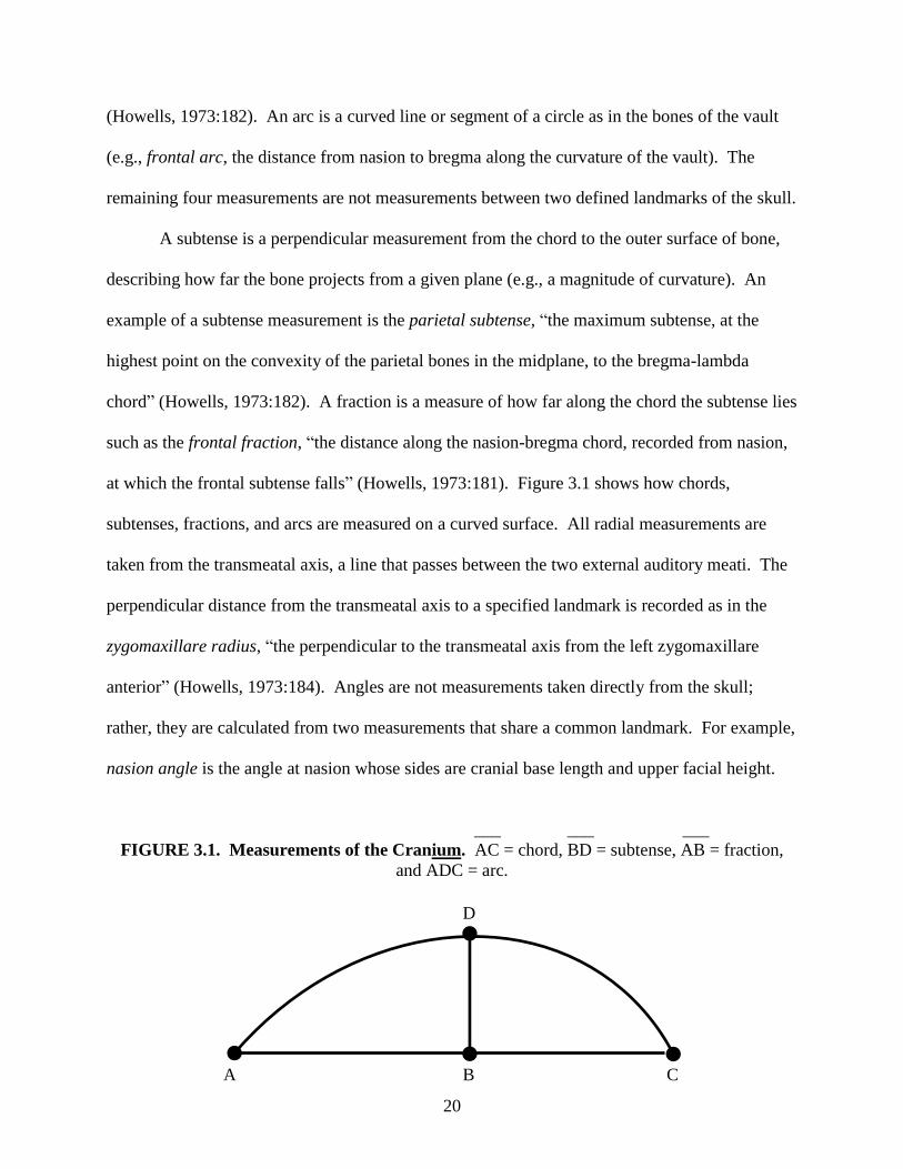
A subtense is a perpendicular measurement from the chord to the outer surface of bone,

describing how far the bone projects from a given plane (e.g., a magnitude of curvature). An

example of a subtense measurement is the parietal subtense, “the maximum subtense, at the

highest point on the convexity of the parietal bones in the midplane, to the bregma-lambda

chord” (Howells, 1973:182). A fraction is a measure of how far along the chord the subtense lies

such as the frontal fraction, “the distance along the nasion-bregma chord, recorded from nasion,

at which the frontal subtense falls” (Howells, 1973:181). Figure 3.1 shows how chords,

subtenses, fractions, and arcs are measured on a curved surface. All radial measurements are

taken from the transmeatal axis, a line that passes between the two external auditory meati. The

perpendicular distance from the transmeatal axis to a specified landmark is recorded as in the

zygomaxillare radius, “the perpendicular to the transmeatal axis from the left zygomaxillare

anterior” (Howells, 1973:184). Angles are not measurements taken directly from the skull;

rather, they are calculated from two measurements that share a common landmark. For example,

nasion angle is the angle at nasion whose sides are cranial base length and upper facial height.

___ ___ ___

FIGURE 3.1. Measurements of the Cranium. AC = chord, BD = subtense, AB = fraction,

and ADC = arc.

C B A

D

21

Specific Measurements and Instrumentation

Sliding and spreading calipers are the standard instruments found in most biological

anthropology laboratories. Special instruments are required to record non-standard

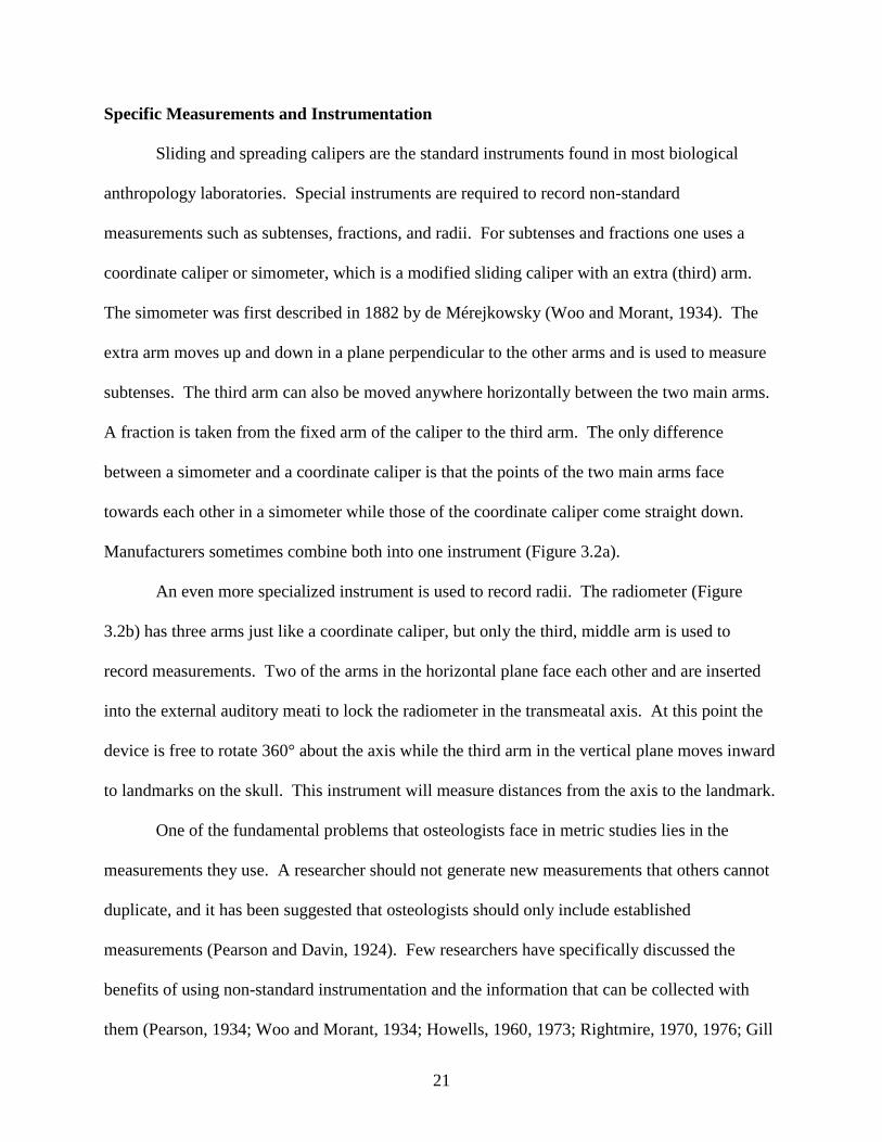
measurements such as subtenses, fractions, and radii. For subtenses and fractions one uses a

coordinate caliper or simometer, which is a modified sliding caliper with an extra (third) arm.

The simometer was first described in 1882 by de Mérejkowsky (Woo and Morant, 1934). The

extra arm moves up and down in a plane perpendicular to the other arms and is used to measure

subtenses. The third arm can also be moved anywhere horizontally between the two main arms.

A fraction is taken from the fixed arm of the caliper to the third arm. The only difference

between a simometer and a coordinate caliper is that the points of the two main arms face

towards each other in a simometer while those of the coordinate caliper come straight down.

Manufacturers sometimes combine both into one instrument (Figure 3.2a).

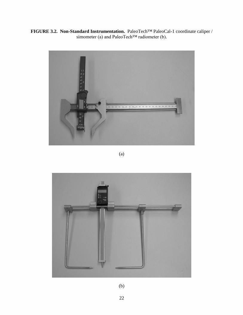
An even more specialized instrument is used to record radii. The radiometer (Figure

3.2b) has three arms just like a coordinate caliper, but only the third, middle arm is used to

record measurements. Two of the arms in the horizontal plane face each other and are inserted

into the external auditory meati to lock the radiometer in the transmeatal axis. At this point the

device is free to rotate 360° about the axis while the third arm in the vertical plane moves inward

to landmarks on the skull. This instrument will measure distances from the axis to the landmark.

One of the fundamental problems that osteologists face in metric studies lies in the

measurements they use. A researcher should not generate new measurements that others cannot

duplicate, and it has been suggested that osteologists should only include established

measurements (Pearson and Davin, 1924). Few researchers have specifically discussed the

benefits of using non-standard instrumentation and the information that can be collected with

them (Pearson, 1934; Woo and Morant, 1934; Howells, 1960, 1973; Rightmire, 1970, 1976; Gill

22

FIGURE 3.2. Non-Standard Instrumentation. PaleoTech™ PaleoCal-1 coordinate caliper /

simometer (a) and PaleoTech™ radiometer (b).

(a)

(b)

23

et al., 1988; Brues, 1990; Cunha and van Vark, 1991). The consensus among researchers who

have used non-standard measurements is that “unconventional measurements . . . are capable of

higher discriminatory power than the more traditional ones” (Jantz and Owsley, 1994:197).

However, as seen in the literature, most researchers remain loyal to standard instrumentation and

measurements.

Selection of Measurements

When selecting measurements for a predictive discriminant analysis, one must consider

three important factors (DiBennardo, 1986): (1) does a combination of measurements better

discriminate between two groups compared to a single measurement?; (2) what is the construct

of the measurements (the theoretical foundation by which the measurements separate the

groups)?; and (3) how well will the LDF created from the measurements perform?

Unfortunately, these factors are not always addressed and the justification of selection criteria for

particular measurements is frequently left unstated.

Studies in craniometrics fall into one of three categories with regards to measurement

selection. The first category is that no explanation is provided. Cunha and van Vark (1991)

examined a series of crania from turn of the 20th

century Portuguese crania. They took 61

measurements as defined by Howells (1973) and were able to correctly identify the sex of 80%

of the individuals. In their study of Chinese crania, Song and colleagues (1992) chose a mixture

of 38 standard and non-standard measurements and produced a hit-rate of 97%. Steyn and İşcan

(1998) selected 12 “standard” measurements in their study of identifying the sex of South

African individuals and were able to do so with a success rate of 86%. Although the hit-rates of

the aforementioned studies are relatively high, the authors give no exact reason why the variables

they used were selected.

24

The second category is that measurements are chosen because they are easy to record.

Giles and Elliot (1962, 1963) chose the eight standard variables to measure in developing their

methodology because of “ease of recording.” In similar fashion, Wright (1992) reduced Howells

set to 29 variables that are the easiest to measure. He used these measurements to develop a

computer program called CRANID, which assigns an unknown skull to an ancestral group, not

unlike FORDISC.

The third category of craniometric studies are those in which measurements are selected

to describe a certain region of the cranium. When Rightmire (1976) examined the skulls of

Bantu-speaking African groups, he selected 37 measurements, some standard and others

specifically designed to measure certain features of the midface, vault, and brow. In an

assessment of craniometric relationships between Plains Indian groups within a cultural-

evolutionary framework, Key (1983) recorded 65 measurements. Most of these came from

Howells’ (1973) set, but 9 were created by the author “to more fully measure particular

morphological complexes” (Key, 1983:40). In his studies of cranial variation, Gill (1984)

noticed that the greatest difference between Northwest Plains Indians and other groups existed in

the nasal bridge. He took six unconventional measurements of the nasal region to develop a

method that is used by many today (Gill, 1995; Gill et al., 1988; Gill and Gilbert, 1990; Curran,

1990). Ross and associates (2004) selected landmarks “that would reveal the overall cranial

morphology of the crania” to help identify Cuban American skulls in forensic contexts.

Number of Measurements. In the early years of PDA, researchers were limited in the

number of response variables they could use because all of the calculations had to be done by

hand, taking a very long time to complete. Rao (1949) stated that, with regards to the number of

variables used, “It does not seem to be, always, the more the better. . .” He noticed that the

discriminatory power leveled off with the addition of more variables and then began to drop

25

when even more were added. Bronowski and Long (1952) agreed with Rao and noted that

additional information from more measurements becomes insignificant after a certain point

because the measurements become more correlated with one another. Using a computer

simulation, Dunn and Varady (1966) found that for a fixed number of variables, as the sample

size used to create the linear discriminant functions increases, so does the probability of correct

classification of the objects. For a fixed sample size, the probability of correct classification

decreases as the number of variables increase from two to ten. The phenomenon of decreased

classificatory power with an increase in the number of response variables has become known as

“Rao’s paradox” (Kowalski, 1972) as noted by other researchers (van Vark, 1976; Johnson et al.,

1989). Others describe an “optimum measurement of complexity,” a phrase used to explain how

the combination of the nature and the number of variables affects discriminant functions (van

Vark and van der Sman, 1982; van Vark and Schaafsma, 1992). The nature of the variables

refers to the shape and size of the cranium that the measurements represent. Although they

discuss how the number of variables and the sample size balance out to reach an optimum level

of discrimination, the authors do not give any exact numbers.

Summary

It is essential that one be aware of the types of measurements of the cranium that can be

taken in order to focus and improve a study. One is only limited by the equipment available and

by the time available to complete the study. Despite inconsistencies between researchers

regarding how standard and non-standard measurements and instruments are selected, there does

appear to be some general agreement on the use of specific types of measurements. Certain

measurements can only be used for certain populations (Howells, 1957) and the variables that are

eventually selected are determined by the questions that the researcher is asking (i.e., ancestry or

26

sex identification) (Pietrusewsky, 2000). Research has shown that the use of non-standard

measurements allows the biological anthropologist to better answer specific questions with

regards to craniometric ancestry determination.

27

CHAPTER 4: MATERIALS AND METHODS

The Study Sample

This study examined three different ancestral groups from different time periods: recent

African Americans (AA), recent European Americans (EA), and prehistoric Coyotero Apache

(CA). The Coyotero Apache crania were drawn from the Indiana University Anthropology

Department Osteological Collection in Bloomington, IN. The collection includes ~6,000 human

skeletons from numerous prehistoric and historic archaeological sites in the United States. The

series of crania used in this study are from the Edward Palmer Arkansaw Mounds located just

outside of Little Rock, AR, comprised of ~100 crania. It is a Late Woodland to Mississippian

site dating from A.D. 700-950 (Jeter, 1990). Nineteen males and thirty six females were selected

from the collection. These crania were the most complete specimens available.

The African American and European American samples were drawn from the Hamman-

Todd Osteological Collection located at the Cleveland Museum of Natural History (CMNH) in

Cleveland, OH. This collection has one of the largest primate skeletal samples in the world.

Specifically, the collection contains 3,100 modern human skeletons from unclaimed bodies at the

Cuyahoga County Morgue and city hospitals. They date from the late 1800s and early 1900’s

and many have known dates of birth, dates of death, age, weight, height, cause of death, sex, and

ancestry. From the AA subsample, 25 males and 24 females were selected, with ages ranging

from 21 to 46 years old and a mean age of 28.9 years. Twenty six males and twenty five females

were selected from the EA subsample, with ages ranging from 19 to 48 years old and a mean age

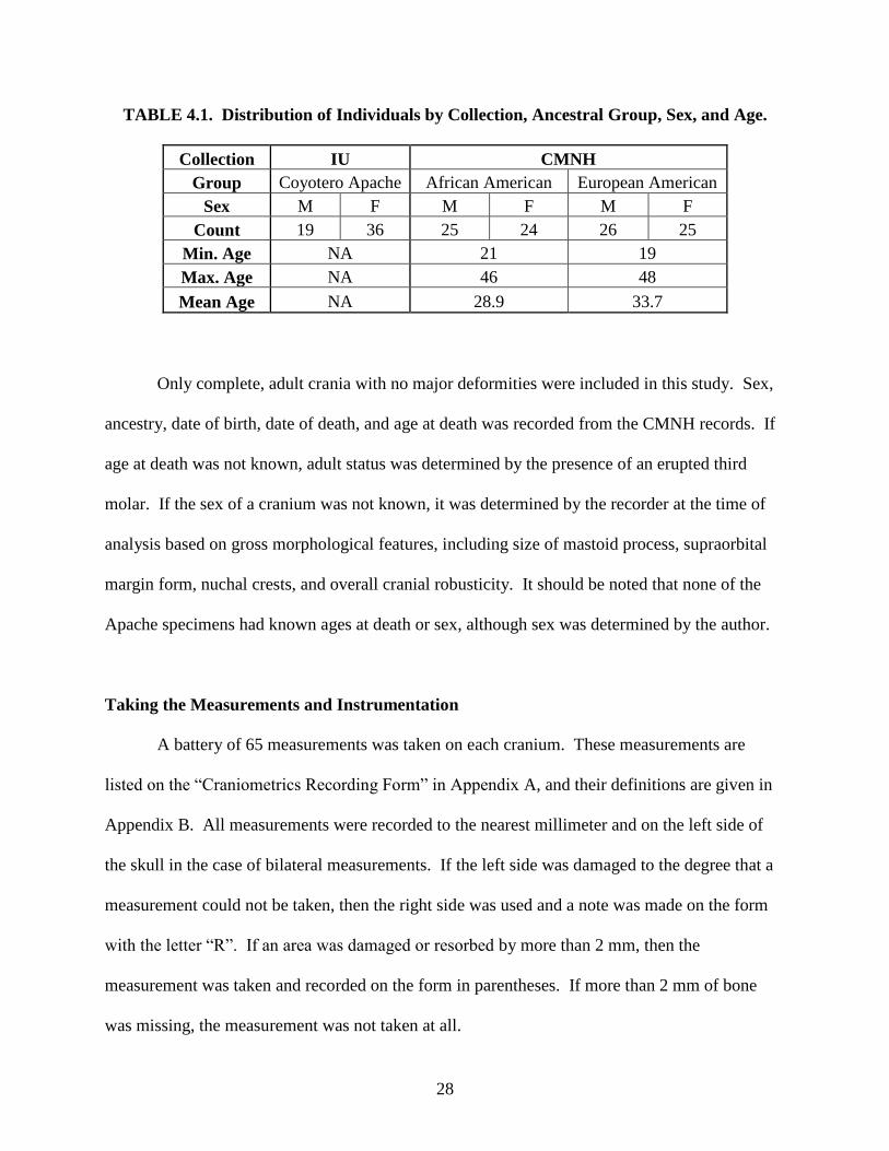
of 33.7 years. A total of 100 crania were measured from the CMNH. Table 4.1 shows the

distribution of the sample by collection, age, and sex.

28

TABLE 4.1. Distribution of Individuals by Collection, Ancestral Group, Sex, and Age.

Collection IU CMNH

Group Coyotero Apache African American European American

Sex M F M F M F

Count 19 36 25 24 26 25

Min. Age NA 21 19

Max. Age NA 46 48

Mean Age NA 28.9 33.7

Only complete, adult crania with no major deformities were included in this study. Sex,

ancestry, date of birth, date of death, and age at death was recorded from the CMNH records. If

age at death was not known, adult status was determined by the presence of an erupted third

molar. If the sex of a cranium was not known, it was determined by the recorder at the time of

analysis based on gross morphological features, including size of mastoid process, supraorbital

margin form, nuchal crests, and overall cranial robusticity. It should be noted that none of the

Apache specimens had known ages at death or sex, although sex was determined by the author.

Taking the Measurements and Instrumentation

A battery of 65 measurements was taken on each cranium. These measurements are

listed on the “Craniometrics Recording Form” in Appendix A, and their definitions are given in

Appendix B. All measurements were recorded to the nearest millimeter and on the left side of

the skull in the case of bilateral measurements. If the left side was damaged to the degree that a

measurement could not be taken, then the right side was used and a note was made on the form

with the letter “R”. If an area was damaged or resorbed by more than 2 mm, then the

measurement was taken and recorded on the form in parentheses. If more than 2 mm of bone

was missing, the measurement was not taken at all.

29

The protocol for data collection was developed at the University of Indianapolis

Archeology and Forensics Laboratory (AFL) using modern human crania and at the Glenn A.

Black Laboratory of Archaeology at Indiana University using prehistoric crania as test subjects.

These crania were used to refine measurement techniques, including locating landmarks, caliper

point placement, and the order in which the measurements were taken. Dr. Stephen Nawrocki

assisted the author in clarifying measurement definitions.

The measurements were derived from three sources: (1) FORDISC 2.0 (FD2) (Ousley

and Jantz, 1996), (2) Howells (1973), and (3) Gill (1984). The 24 FD2 measurements are those

used in a standard FD2 analysis of the cranium. The Howells subset includes 57 measurements,

20 of which are also FD2 measurements. Even though 20 measurements are identical in the two

subsets, they were examined separately as part of each measurement group during the statistical

analysis. Howells also used trigonometry to calculate 13 angles from his 57 measurements. In

this study, however, the angles were omitted. Although angles help to describe more complex

features of the cranium, a computer-aided multivariate analysis will elucidate which variables

describe the complex features without having to perform a calculation prior to data entry

(Corruccini, 1975; Campbell, 1978). The third subset of measurements was used by Gill and

describes the shape of the nasal area. Gill used a simometer for the measurements in his study.

Two of the six measurements are the same as the FD2 and Howells sets.

A Paleo-Tech™ spreading caliper, Mitutoyo™ sliding dial caliper, Paleo-Tech™

PaleoCal-1 coordinate caliper, and a Paleo-Tech™ radiometer were used to take all

measurements of the crania from IU. These instruments were borrowed from the AFL. At the

CMNH, a Mitutoyo™ direct input tool and foot pedal were used in conjunction with a

Mitutoyo™ sliding digital caliper. This caliper was connected directly to a laptop computer so

the measurements could be input directly into a Microsoft™ Office Excel 2003 spreadsheet.

30

Appendix B identifies which instrument was used for each of the measurements.

Statistical Analysis

Three assumptions were made about the data prior to analysis. First, all of the crania

were assumed to be correctly classified as to ancestry as recorded in the collections’ records.

Second, the data is assumed to follow a multivariate normal distribution. Third, the distributions

are uncontaminated. Contamination can take be expressed in two ways: scale contamination

and location contamination. Scale contamination occurs when the instruments vary more than

usual and give erroneous values. Location contamination occurs when instruments slip from the

landmark (Lachenbruch and Goldstein, 1979). To test the data for multivariate normality, a

Box’s M test was performed.

Four sets of discriminant function formulae were constructed with a forward stepwise

method using the statistics computer software package SPSS 13.0. Predictive discriminant

analysis requires that all specimens have all measurements or else they will not be included in

the calculation of the functions. Measurements that could not be taken were substituted with the

‘linear trend at point’ function of SPSS. This function replaces missing values with the linear

regression estimate for that point. The existing series is regressed on an index variable scaled 1

to n. Missing values are replaced with their predicted values. Only 12 (0.001%) of the 10,075

measurements taken were missing and subsequently replaced.

The stepwise selection method followed İşcan and Steyn’s (1999) data entry

methodology, with p values of p = 0.05 to enter and p = 0.15 to remove. This seemingly liberal

cutoff value does not increase the overall error rate (MacLachlan, 1980). Forward stepwise PDA

involves adding a variable that meets the required p-value for the function. The function is

recalculated using the remaining variables and if a new variable meets the cutoff, it is added to

31

the function. This process is repeated until only the statistically significant variables are

included in the final formulae. The functions are built step-by-step in a forward, additive

manner, starting with zero measurements. Stepwise analysis is a useful tool to explore which

variables are helpful in classifying objects (Snapinn and Knoke, 1989).

The crania were divided into three different ancestry groups: (1) African American, (2)

European American, and (3) Coyotero Apache. The data were entered four times to produce

four sets of discriminant function formulae for a total of eight functions. The first set of

functions used the 24 standard measurements of the cranium included in a FD2 analysis. The

second set used the 57 Howells measurements. The third set of formulae used Gill’s 6

measurements of the nasal region. The fourth and final set combined all 65 measurements.

The weights of the variables for each function were calculated. Eigenvalues and Wilk’s λ

values were calculated to test the significance of the discriminant functions. Structure matrices

were constructed to determine how heavily the variables loaded on the functions.

The data were entered into the program with unequal prior probabilities. The prior

probability is the chance that a cranium is selected and correctly randomly assigned to its group.

As there are three groups in this study, the probability of correctly assigning a cranium to its

group by chance alone is 0.333. However, because the sizes of the groups in this study are not

equal, the prior probability must be weighted by the sample size. Therefore, the prior probability

for the African American group is 0.316, the European American group is 0.329, and the

Coyotero Apache group is 0.355. If the power of the discriminant functions is greater than the

prior probability, then it is successful at discriminating between groups.

The four sets of discriminant function formulae were compared side by side to determine

which set was better able to correctly separate groups and sort the individuals. The ability of the

discriminant functions to correctly classify individuals was assessed by testing the functions on

32

the original sample via simple resubstitution as well as a leave-one-out method (LOO).

Resubstituting the entire original sample directly into the discriminant functions will generally

overestimate the ability of the formulae to separate these groups in the population as a whole

(Lachenbruch, 1967; Lachenbruch and Goldstein, 1979). Resubstitution rates will therefore be

used only as a general baseline measure of the formulae’s performance. To avoid the problem of

“statistical incest” and properly test the functions, one must use cases that were not included in

the original study sample (Smith, 1947; Lachenbruch and Mickey, 1968). Unfortunately, this

requires an entirely new dataset. LOO more accurately tests the functions without having to use

a new dataset (van Vark, 1976; Feldesman, 1997). The computer removes one case from the

sample and creates a discriminant function using the remaining cases. The case that was

removed is then entered back into the function to see if will be properly classified into its

original group. The computer then repeats this process for each of the cases in the sample. The

LOO method ensures that the cases used to produce the functions are not used when testing them

for classificatory ability. The success of the discriminant functions is expressed as a percentage

of cases in the original sample that are correctly classified into their groups.

33

CHAPTER 5: RESULTS

Stepwise Statistics

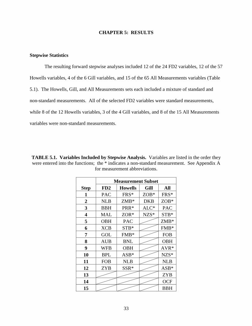
The resulting forward stepwise analyses included 12 of the 24 FD2 variables, 12 of the 57

Howells variables, 4 of the 6 Gill variables, and 15 of the 65 All Measurements variables (Table

5.1). The Howells, Gill, and All Measurements sets each included a mixture of standard and

non-standard measurements. All of the selected FD2 variables were standard measurements,

while 8 of the 12 Howells variables, 3 of the 4 Gill variables, and 8 of the 15 All Measurements

variables were non-standard measurements.

TABLE 5.1. Variables Included by Stepwise Analysis. Variables are listed in the order they

were entered into the functions; the * indicates a non-standard measurement. See Appendix A

for measurement abbreviations.

Measurement Subset

Step FD2 Howells Gill All

1 PAC FRS* ZOB* FRS*

2 NLB ZMB* DKB ZOB*

3 BBH PRR* ALC* PAC

4 MAL ZOR* NZS* STB*

5 OBH PAC ZMB*

6 XCB STB* FMB*

7 GOL FMB* FOB

8 AUB BNL OBH

9 WFB OBH AVR*

10 BPL ASB* NZS*

11 FOB NLB NLB

12 ZYB SSR* ASB*

13 ZYB

14 OCF

15 BBH

34

Linear Discriminant Functions

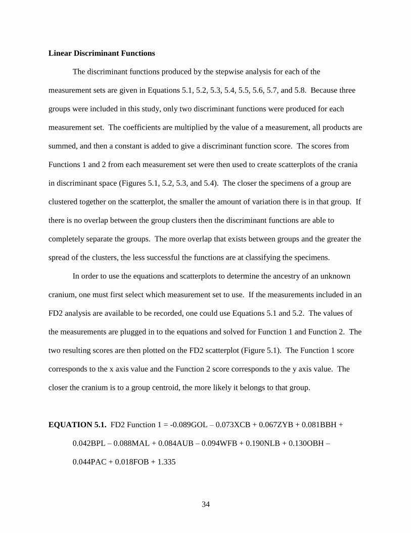
The discriminant functions produced by the stepwise analysis for each of the

measurement sets are given in Equations 5.1, 5.2, 5.3, 5.4, 5.5, 5.6, 5.7, and 5.8. Because three

groups were included in this study, only two discriminant functions were produced for each

measurement set. The coefficients are multiplied by the value of a measurement, all products are

summed, and then a constant is added to give a discriminant function score. The scores from

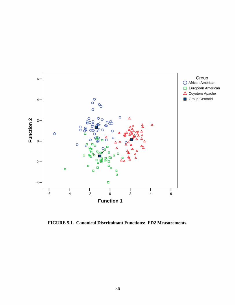
Functions 1 and 2 from each measurement set were then used to create scatterplots of the crania

in discriminant space (Figures 5.1, 5.2, 5.3, and 5.4). The closer the specimens of a group are

clustered together on the scatterplot, the smaller the amount of variation there is in that group. If

there is no overlap between the group clusters then the discriminant functions are able to

completely separate the groups. The more overlap that exists between groups and the greater the

spread of the clusters, the less successful the functions are at classifying the specimens.

In order to use the equations and scatterplots to determine the ancestry of an unknown

cranium, one must first select which measurement set to use. If the measurements included in an

FD2 analysis are available to be recorded, one could use Equations 5.1 and 5.2. The values of

the measurements are plugged in to the equations and solved for Function 1 and Function 2. The

two resulting scores are then plotted on the FD2 scatterplot (Figure 5.1). The Function 1 score

corresponds to the x axis value and the Function 2 score corresponds to the y axis value. The

closer the cranium is to a group centroid, the more likely it belongs to that group.

EQUATION 5.1. FD2 Function 1 = -0.089GOL – 0.073XCB + 0.067ZYB + 0.081BBH +

0.042BPL – 0.088MAL + 0.084AUB – 0.094WFB + 0.190NLB + 0.130OBH –

0.044PAC + 0.018FOB + 1.335

35

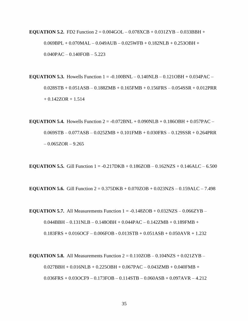
EQUATION 5.2. FD2 Function 2 = 0.004GOL – 0.078XCB + 0.031ZYB – 0.033BBH +

0.069BPL + 0.070MAL – 0.049AUB – 0.025WFB + 0.182NLB + 0.253OBH +

0.040PAC – 0.140FOB – 5.223

EQUATION 5.3. Howells Function 1 = -0.100BNL – 0.140NLB – 0.121OBH + 0.034PAC –

0.028STB + 0.051ASB – 0.188ZMB + 0.165FMB + 0.156FRS – 0.054SSR + 0.012PRR

+ 0.142ZOR + 1.514

EQUATION 5.4. Howells Function 2 = -0.072BNL + 0.090NLB + 0.186OBH + 0.057PAC –

0.069STB – 0.077ASB – 0.025ZMB + 0.101FMB + 0.030FRS – 0.129SSR + 0.264PRR

– 0.065ZOR – 9.265

EQUATION 5.5. Gill Function 1 = -0.217DKB + 0.186ZOB – 0.162NZS + 0.146ALC – 6.500

EQUATION 5.6. Gill Function 2 = 0.375DKB + 0.070ZOB + 0.023NZS – 0.159ALC – 7.498

EQUATION 5.7. All Measurements Function 1 = -0.148ZOB + 0.032NZS – 0.066ZYB –

0.044BBH – 0.131NLB – 0.148OBH + 0.044PAC – 0.142ZMB + 0.189FMB +

0.183FRS + 0.016OCF – 0.006FOB - 0.013STB + 0.051ASB + 0.050AVR + 1.232

EQUATION 5.8. All Measurements Function 2 = 0.110ZOB – 0.104NZS + 0.021ZYB –

0.027BBH + 0.016NLB + 0.225OBH + 0.067PAC – 0.043ZMB + 0.040FMB +

0.036FRS + 0.03OCF9 – 0.173FOB – 0.114STB – 0.060ASB + 0.097AVR – 4.212

36

6420-2-4-6

Function 1

6

4

2

0

-2

-4

Fu

ncti

on

2

3

2

1

Group Centroid

Coyotero Apache

European American

African American

Group

FIGURE 5.1. Canonical Discriminant Functions: FD2 Measurements.

37

420-2-4-6

Function 1

4

2

0

-2

-4

Fu

ncti

on

2

3

2

1

Group Centroid

Coyotero Apache

European American

African American

Group

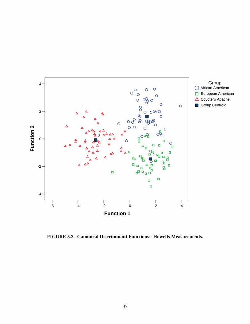
FIGURE 5.2. Canonical Discriminant Functions: Howells Measurements.

38

43210-1-2-3

Function 1

3

2

1

0

-1

-2

-3

Fu

ncti

on

2

32

1

Group Centroid

Coyotero Apache

European American

African American

Group

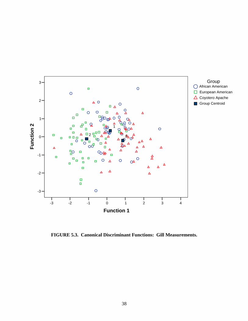
FIGURE 5.3. Canonical Discriminant Functions: Gill Measurements.

39

6420-2-4-6

Function 1

4

2

0

-2

-4

Fu

ncti

on

2

3

2

1

Group Centroid

Coyotero Apache

European American

African American

Group

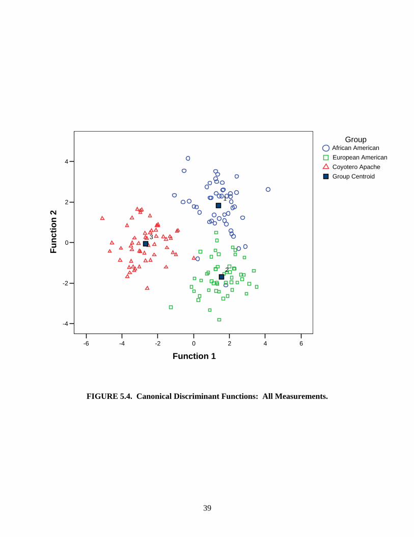
FIGURE 5.4. Canonical Discriminant Functions: All Measurements.

40

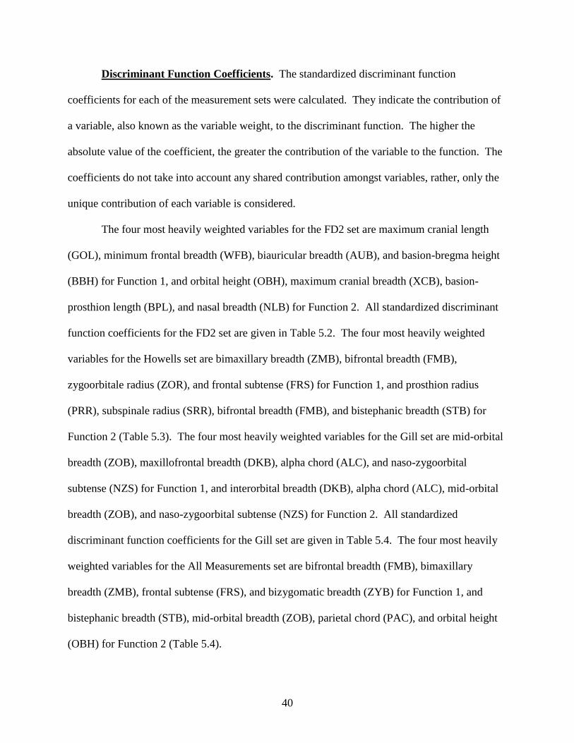
Discriminant Function Coefficients. The standardized discriminant function

coefficients for each of the measurement sets were calculated. They indicate the contribution of

a variable, also known as the variable weight, to the discriminant function. The higher the

absolute value of the coefficient, the greater the contribution of the variable to the function. The

coefficients do not take into account any shared contribution amongst variables, rather, only the

unique contribution of each variable is considered.

The four most heavily weighted variables for the FD2 set are maximum cranial length

(GOL), minimum frontal breadth (WFB), biauricular breadth (AUB), and basion-bregma height

(BBH) for Function 1, and orbital height (OBH), maximum cranial breadth (XCB), basion-

prosthion length (BPL), and nasal breadth (NLB) for Function 2. All standardized discriminant

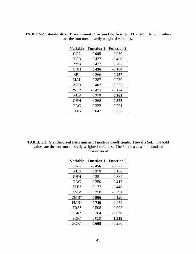
function coefficients for the FD2 set are given in Table 5.2. The four most heavily weighted

variables for the Howells set are bimaxillary breadth (ZMB), bifrontal breadth (FMB),

zygoorbitale radius (ZOR), and frontal subtense (FRS) for Function 1, and prosthion radius

(PRR), subspinale radius (SRR), bifrontal breadth (FMB), and bistephanic breadth (STB) for

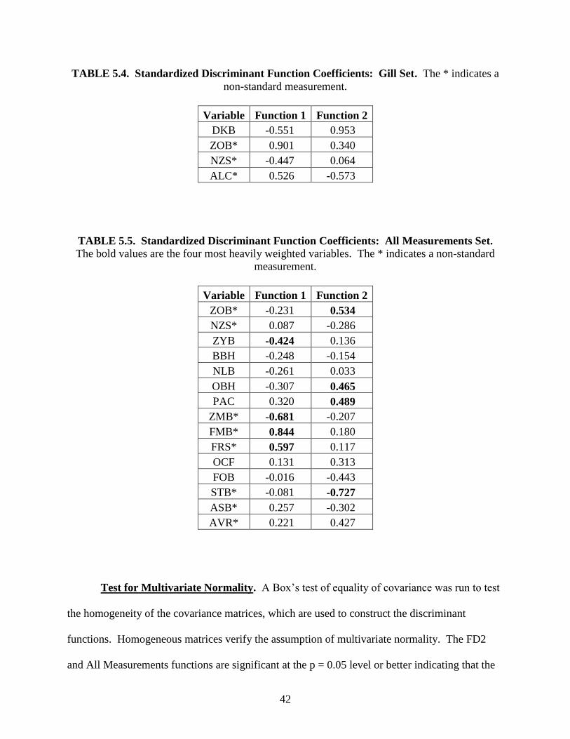
Function 2 (Table 5.3). The four most heavily weighted variables for the Gill set are mid-orbital

breadth (ZOB), maxillofrontal breadth (DKB), alpha chord (ALC), and naso-zygoorbital

subtense (NZS) for Function 1, and interorbital breadth (DKB), alpha chord (ALC), mid-orbital

breadth (ZOB), and naso-zygoorbital subtense (NZS) for Function 2. All standardized

discriminant function coefficients for the Gill set are given in Table 5.4. The four most heavily

weighted variables for the All Measurements set are bifrontal breadth (FMB), bimaxillary

breadth (ZMB), frontal subtense (FRS), and bizygomatic breadth (ZYB) for Function 1, and

bistephanic breadth (STB), mid-orbital breadth (ZOB), parietal chord (PAC), and orbital height

(OBH) for Function 2 (Table 5.4).

41

TABLE 5.2. Standardized Discriminant Function Coefficients: FD2 Set. The bold values

are the four most heavily weighted variables.

Variable Function 1 Function 2

GOL -0.685 0.030

XCB -0.427 -0.456

ZYB 0.432 0.202

BBH 0.456 -0.184

BPL 0.266 0.437

MAL -0.287 0.230

AUB 0.467 -0.272

WFB -0.471 -0.124

NLB 0.378 0.363

OBH 0.268 0.523

PAC -0.322 0.291

FOB 0.047 -0.357

TABLE 5.3. Standardized Discriminant Function Coefficients: Howells Set. The bold

values are the four most heavily weighted variables. The * indicates a non-standard

measurement.

Variable Function 1 Function 2

BNL -0.456 -0.327

NLB -0.278 0.180

OBH -0.251 0.384

PAC 0.250 0.417

STB* -0.177 -0.440

ASB* 0.258 -0.391

ZMB* -0.906 -0.120

FMB* 0.740 0.452

FRS* 0.508 0.097

SSR* -0.264 -0.628

PRR* 0.059 1.319

ZOR* 0.608 -0.280

42

TABLE 5.4. Standardized Discriminant Function Coefficients: Gill Set. The * indicates a

non-standard measurement.

Variable Function 1 Function 2

DKB -0.551 0.953

ZOB* 0.901 0.340

NZS* -0.447 0.064

ALC* 0.526 -0.573

TABLE 5.5. Standardized Discriminant Function Coefficients: All Measurements Set. The bold values are the four most heavily weighted variables. The * indicates a non-standard

measurement.

Variable Function 1 Function 2

ZOB* -0.231 0.534

NZS* 0.087 -0.286

ZYB -0.424 0.136

BBH -0.248 -0.154

NLB -0.261 0.033

OBH -0.307 0.465

PAC 0.320 0.489

ZMB* -0.681 -0.207

FMB* 0.844 0.180

FRS* 0.597 0.117

OCF 0.131 0.313

FOB -0.016 -0.443

STB* -0.081 -0.727

ASB* 0.257 -0.302

AVR* 0.221 0.427

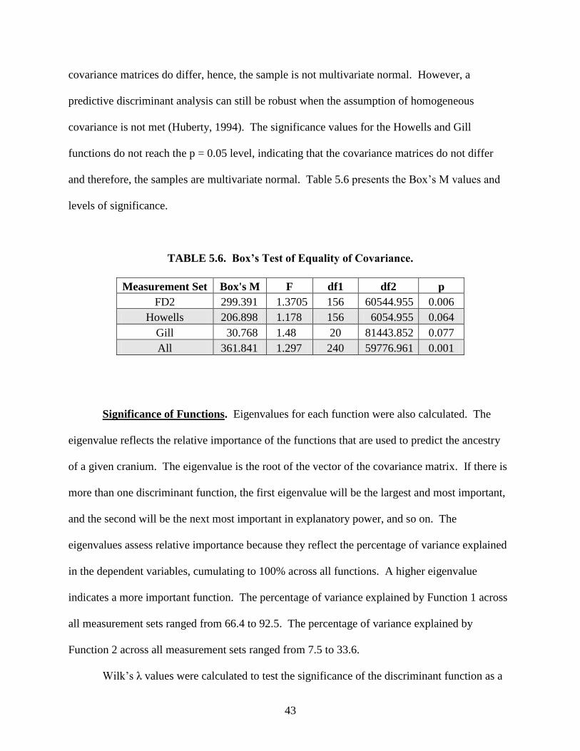
Test for Multivariate Normality. A Box’s test of equality of covariance was run to test

the homogeneity of the covariance matrices, which are used to construct the discriminant

functions. Homogeneous matrices verify the assumption of multivariate normality. The FD2

and All Measurements functions are significant at the p = 0.05 level or better indicating that the

43

covariance matrices do differ, hence, the sample is not multivariate normal. However, a

predictive discriminant analysis can still be robust when the assumption of homogeneous

covariance is not met (Huberty, 1994). The significance values for the Howells and Gill

functions do not reach the p = 0.05 level, indicating that the covariance matrices do not differ

and therefore, the samples are multivariate normal. Table 5.6 presents the Box’s M values and

levels of significance.

TABLE 5.6. Box’s Test of Equality of Covariance.

Measurement Set Box's M F df1 df2 p

FD2 299.391 1.3705 156 60544.955 0.006

Howells 206.898 1.178 156 6054.955 0.064

Gill 30.768 1.48 20 81443.852 0.077

All 361.841 1.297 240 59776.961 0.001

Significance of Functions. Eigenvalues for each function were also calculated. The

eigenvalue reflects the relative importance of the functions that are used to predict the ancestry

of a given cranium. The eigenvalue is the root of the vector of the covariance matrix. If there is

more than one discriminant function, the first eigenvalue will be the largest and most important,

and the second will be the next most important in explanatory power, and so on. The

eigenvalues assess relative importance because they reflect the percentage of variance explained

in the dependent variables, cumulating to 100% across all functions. A higher eigenvalue

indicates a more important function. The percentage of variance explained by Function 1 across

all measurement sets ranged from 66.4 to 92.5. The percentage of variance explained by

Function 2 across all measurement sets ranged from 7.5 to 33.6.

Wilk’s λ values were calculated to test the significance of the discriminant function as a

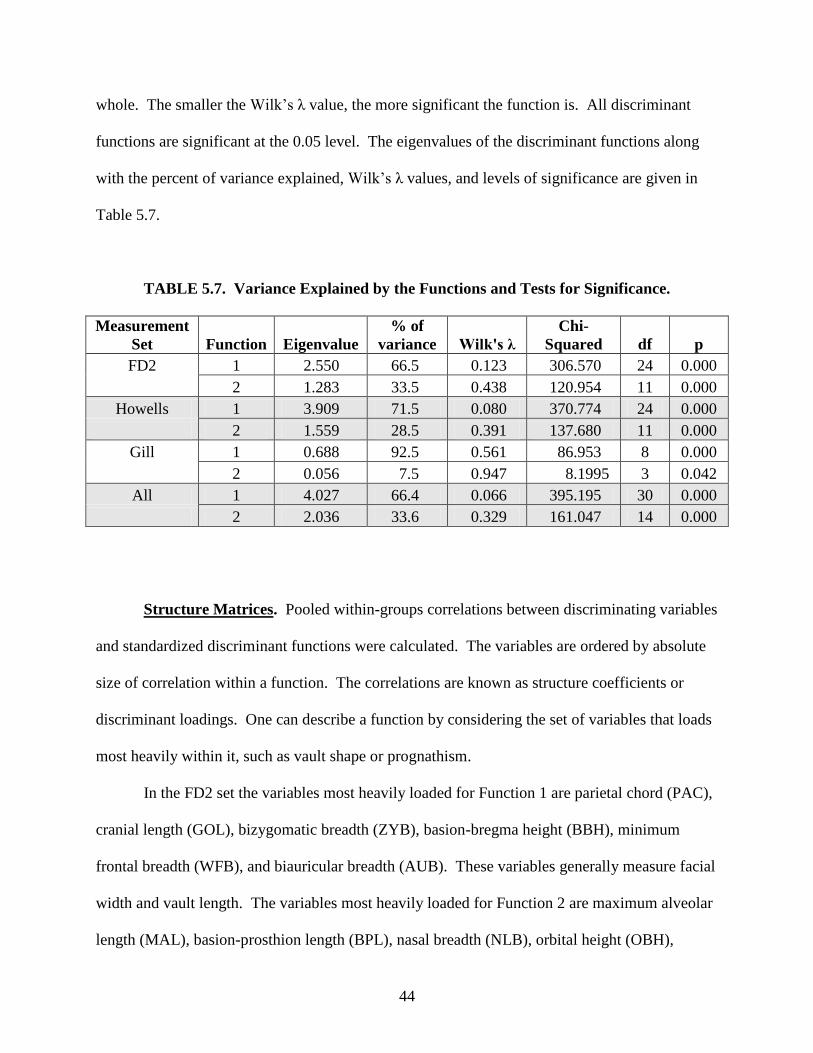
44

whole. The smaller the Wilk’s λ value, the more significant the function is. All discriminant

functions are significant at the 0.05 level. The eigenvalues of the discriminant functions along

with the percent of variance explained, Wilk’s λ values, and levels of significance are given in

Table 5.7.

TABLE 5.7. Variance Explained by the Functions and Tests for Significance.

Measurement

Set Function Eigenvalue

% of

variance Wilk's λ

Chi-

Squared df p

FD2 1 2.550 66.5 0.123 306.570 24 0.000

2 1.283 33.5 0.438 120.954 11 0.000

Howells 1 3.909 71.5 0.080 370.774 24 0.000

2 1.559 28.5 0.391 137.680 11 0.000

Gill 1 0.688 92.5 0.561 86.953 8 0.000

2 0.056 7.5 0.947 8.1995 3 0.042

All 1 4.027 66.4 0.066 395.195 30 0.000

2 2.036 33.6 0.329 161.047 14 0.000

Structure Matrices. Pooled within-groups correlations between discriminating variables

and standardized discriminant functions were calculated. The variables are ordered by absolute

size of correlation within a function. The correlations are known as structure coefficients or

discriminant loadings. One can describe a function by considering the set of variables that loads

most heavily within it, such as vault shape or prognathism.

In the FD2 set the variables most heavily loaded for Function 1 are parietal chord (PAC),

cranial length (GOL), bizygomatic breadth (ZYB), basion-bregma height (BBH), minimum

frontal breadth (WFB), and biauricular breadth (AUB). These variables generally measure facial

width and vault length. The variables most heavily loaded for Function 2 are maximum alveolar

length (MAL), basion-prosthion length (BPL), nasal breadth (NLB), orbital height (OBH),

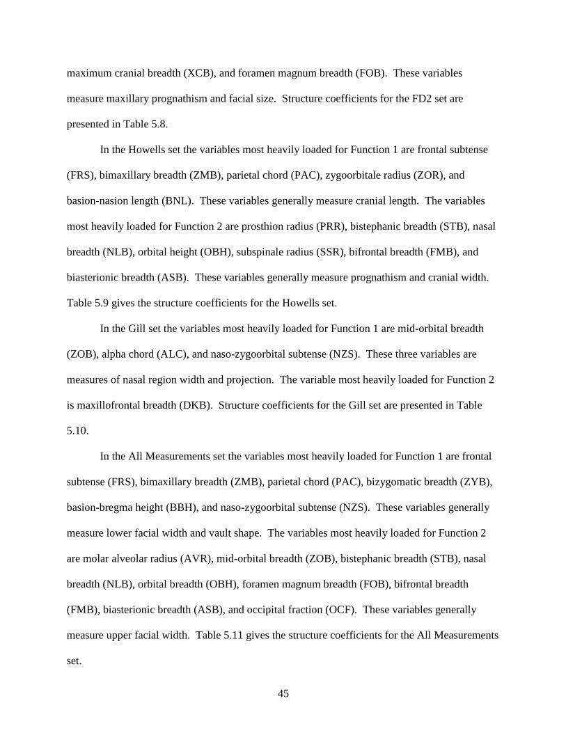
45

maximum cranial breadth (XCB), and foramen magnum breadth (FOB). These variables

measure maxillary prognathism and facial size. Structure coefficients for the FD2 set are

presented in Table 5.8.

In the Howells set the variables most heavily loaded for Function 1 are frontal subtense

(FRS), bimaxillary breadth (ZMB), parietal chord (PAC), zygoorbitale radius (ZOR), and

basion-nasion length (BNL). These variables generally measure cranial length. The variables

most heavily loaded for Function 2 are prosthion radius (PRR), bistephanic breadth (STB), nasal

breadth (NLB), orbital height (OBH), subspinale radius (SSR), bifrontal breadth (FMB), and

biasterionic breadth (ASB). These variables generally measure prognathism and cranial width.

Table 5.9 gives the structure coefficients for the Howells set.

In the Gill set the variables most heavily loaded for Function 1 are mid-orbital breadth

(ZOB), alpha chord (ALC), and naso-zygoorbital subtense (NZS). These three variables are

measures of nasal region width and projection. The variable most heavily loaded for Function 2

is maxillofrontal breadth (DKB). Structure coefficients for the Gill set are presented in Table

5.10.

In the All Measurements set the variables most heavily loaded for Function 1 are frontal

subtense (FRS), bimaxillary breadth (ZMB), parietal chord (PAC), bizygomatic breadth (ZYB),

basion-bregma height (BBH), and naso-zygoorbital subtense (NZS). These variables generally

measure lower facial width and vault shape. The variables most heavily loaded for Function 2

are molar alveolar radius (AVR), mid-orbital breadth (ZOB), bistephanic breadth (STB), nasal

breadth (NLB), orbital breadth (OBH), foramen magnum breadth (FOB), bifrontal breadth

(FMB), biasterionic breadth (ASB), and occipital fraction (OCF). These variables generally

measure upper facial width. Table 5.11 gives the structure coefficients for the All Measurements

set.

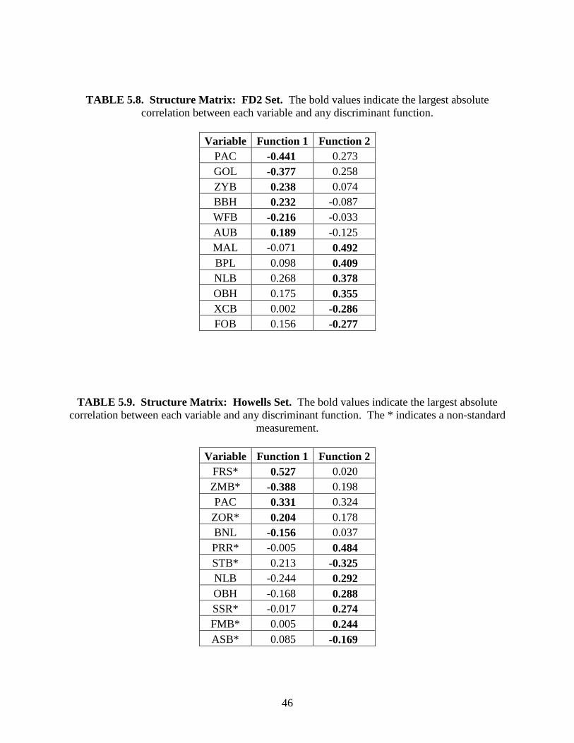
46

TABLE 5.8. Structure Matrix: FD2 Set. The bold values indicate the largest absolute

correlation between each variable and any discriminant function.

Variable Function 1 Function 2

PAC -0.441 0.273

GOL -0.377 0.258

ZYB 0.238 0.074

BBH 0.232 -0.087

WFB -0.216 -0.033

AUB 0.189 -0.125

MAL -0.071 0.492

BPL 0.098 0.409

NLB 0.268 0.378

OBH 0.175 0.355

XCB 0.002 -0.286

FOB 0.156 -0.277

TABLE 5.9. Structure Matrix: Howells Set. The bold values indicate the largest absolute

correlation between each variable and any discriminant function. The * indicates a non-standard

measurement.

Variable Function 1 Function 2

FRS* 0.527 0.020

ZMB* -0.388 0.198

PAC 0.331 0.324

ZOR* 0.204 0.178

BNL -0.156 0.037

PRR* -0.005 0.484

STB* 0.213 -0.325

NLB -0.244 0.292

OBH -0.168 0.288

SSR* -0.017 0.274

FMB* 0.005 0.244

ASB* 0.085 -0.169

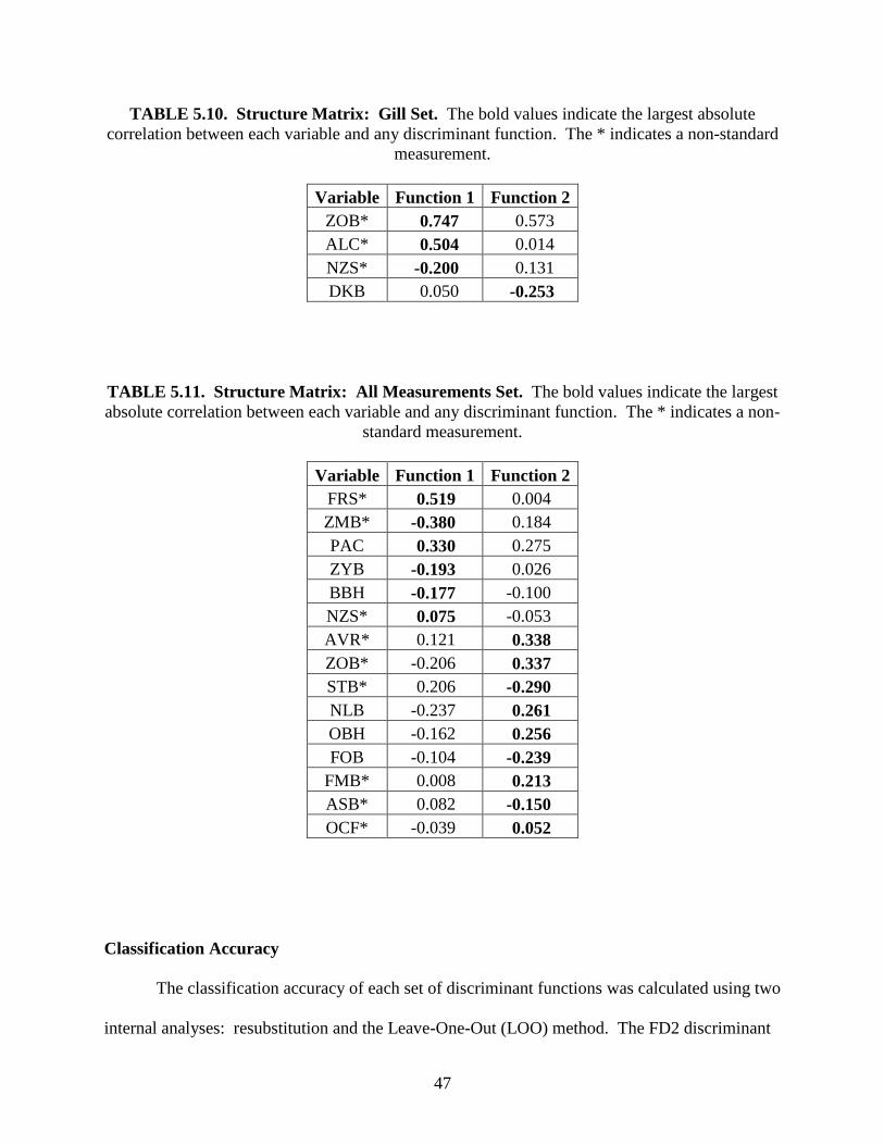
47

TABLE 5.10. Structure Matrix: Gill Set. The bold values indicate the largest absolute

correlation between each variable and any discriminant function. The * indicates a non-standard

measurement.

Variable Function 1 Function 2

ZOB* 0.747 0.573

ALC* 0.504 0.014

NZS* -0.200 0.131

DKB 0.050 -0.253

TABLE 5.11. Structure Matrix: All Measurements Set. The bold values indicate the largest

absolute correlation between each variable and any discriminant function. The * indicates a non-

standard measurement.

Variable Function 1 Function 2

FRS* 0.519 0.004

ZMB* -0.380 0.184

PAC 0.330 0.275

ZYB -0.193 0.026

BBH -0.177 -0.100

NZS* 0.075 -0.053

AVR* 0.121 0.338

ZOB* -0.206 0.337

STB* 0.206 -0.290

NLB -0.237 0.261

OBH -0.162 0.256

FOB -0.104 -0.239

FMB* 0.008 0.213

ASB* 0.082 -0.150

OCF* -0.039 0.052

Classification Accuracy

The classification accuracy of each set of discriminant functions was calculated using two

internal analyses: resubstitution and the Leave-One-Out (LOO) method. The FD2 discriminant

48

functions correctly classified 85.7% of the African American (AA) specimens, 88.2% of the

European American (EA) specimens, and 96.4% of the Coyotero Apache (CA) specimens via

resubstitution. AA crania were sometimes misclassified as EA, EA were misclassified as AA,

and CA were misclassified equally among the AA and EA. The LOO method for the FD2

functions correctly classified 81.6% of the AA crania, 86.3% of the EA crania, and 89.1% of the

CA crania. AA crania were sometimes misclassified as EA, EA were misclassified as AA, and

CA were misclassified as EA. All counts and percentages for the FD2 functions are presented in

Table 5.12.

The Howells discriminant functions correctly classified 91.8% of the AA specimens,

90.2% of the EA specimens, and 96.4% of the CA specimens via resubstitution. The LOO

method for the Howells functions correctly classified 87.8% of the AA crania, 90.2% of the EA

crania, and 92.7% of the CA crania. AA crania were sometimes misclassified as EA, EA were

misclassified as AA, and CA were misclassified equally among the AA and EA for both

resubstitution and LOO. All counts and percentages for the Howells functions are presented in

Table 5.13.

The Gill discriminant functions correctly classified 42.9% of the AA specimens, 76.5%

of the EA specimens, and 69.1% of the CA specimens via resubstitution. The LOO method for

the Gill functions correctly classified 42.9% of the AA crania, 76.5% of the EA crania, and

65.5% of the CA crania. AA crania were sometimes misclassified as CA, EA were misclassified

as AA, and the CA crania were misclassified as AA for both resubstitution and LOO. All counts

and percentages for the Gill functions are presented in Table 5.14.

The All Measurements discriminant functions correctly classified 91.8% of the AA

specimens, 96.1% of the EA specimens, and 98.2% of the CA specimens via resubstitution. AA

crania were sometimes misclassified as EA, EA were misclassified as AA, and CA were

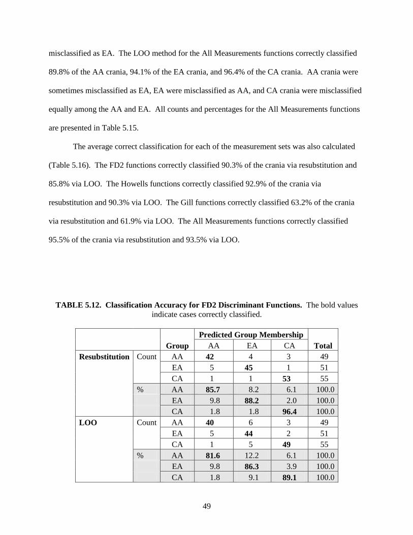
49

misclassified as EA. The LOO method for the All Measurements functions correctly classified

89.8% of the AA crania, 94.1% of the EA crania, and 96.4% of the CA crania. AA crania were

sometimes misclassified as EA, EA were misclassified as AA, and CA crania were misclassified

equally among the AA and EA. All counts and percentages for the All Measurements functions

are presented in Table 5.15.

The average correct classification for each of the measurement sets was also calculated

(Table 5.16). The FD2 functions correctly classified 90.3% of the crania via resubstitution and

85.8% via LOO. The Howells functions correctly classified 92.9% of the crania via

resubstitution and 90.3% via LOO. The Gill functions correctly classified 63.2% of the crania

via resubstitution and 61.9% via LOO. The All Measurements functions correctly classified

95.5% of the crania via resubstitution and 93.5% via LOO.

TABLE 5.12. Classification Accuracy for FD2 Discriminant Functions. The bold values

indicate cases correctly classified.

Predicted Group Membership

Total Group AA EA CA

Resubstitution Count AA 42 4 3 49

EA 5 45 1 51

CA 1 1 53 55

% AA 85.7 8.2 6.1 100.0

EA 9.8 88.2 2.0 100.0

CA 1.8 1.8 96.4 100.0

LOO Count AA 40 6 3 49

EA 5 44 2 51

CA 1 5 49 55

% AA 81.6 12.2 6.1 100.0

EA 9.8 86.3 3.9 100.0

CA 1.8 9.1 89.1 100.0

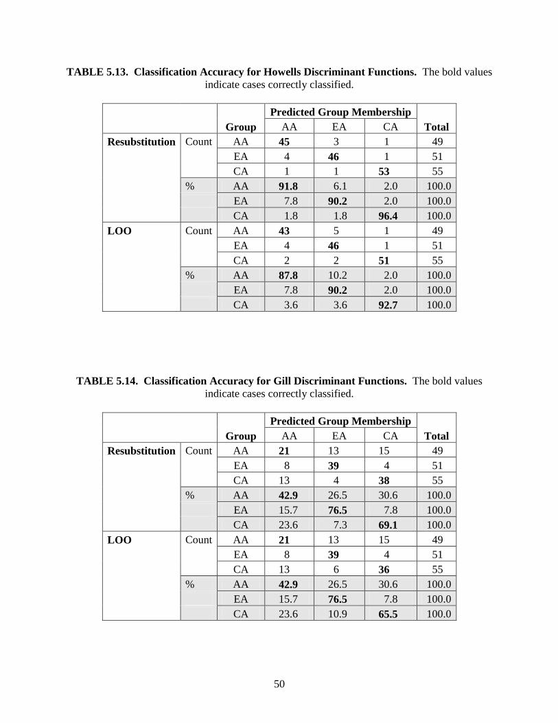
50

TABLE 5.13. Classification Accuracy for Howells Discriminant Functions. The bold values

indicate cases correctly classified.

Predicted Group Membership

Total Group AA EA CA

Resubstitution Count AA 45 3 1 49

EA 4 46 1 51

CA 1 1 53 55

% AA 91.8 6.1 2.0 100.0

EA 7.8 90.2 2.0 100.0

CA 1.8 1.8 96.4 100.0

LOO Count AA 43 5 1 49

EA 4 46 1 51

CA 2 2 51 55

% AA 87.8 10.2 2.0 100.0

EA 7.8 90.2 2.0 100.0

CA 3.6 3.6 92.7 100.0

TABLE 5.14. Classification Accuracy for Gill Discriminant Functions. The bold values

indicate cases correctly classified.

Predicted Group Membership

Total Group AA EA CA

Resubstitution Count AA 21 13 15 49

EA 8 39 4 51

CA 13 4 38 55

% AA 42.9 26.5 30.6 100.0

EA 15.7 76.5 7.8 100.0

CA 23.6 7.3 69.1 100.0

LOO Count AA 21 13 15 49

EA 8 39 4 51

CA 13 6 36 55

% AA 42.9 26.5 30.6 100.0

EA 15.7 76.5 7.8 100.0

CA 23.6 10.9 65.5 100.0

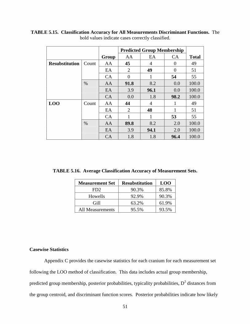
51

TABLE 5.15. Classification Accuracy for All Measurements Discriminant Functions. The

bold values indicate cases correctly classified.

Predicted Group Membership

Total Group AA EA CA

Resubstitution Count AA 45 4 0 49

EA 2 49 0 51

CA 0 1 54 55

% AA 91.8 8.2 0.0 100.0

EA 3.9 96.1 0.0 100.0

CA 0.0 1.8 98.2 100.0

LOO Count AA 44 4 1 49

EA 2 48 1 51

CA 1 1 53 55

% AA 89.8 8.2 2.0 100.0

EA 3.9 94.1 2.0 100.0

CA 1.8 1.8 96.4 100.0

TABLE 5.16. Average Classification Accuracy of Measurement Sets.

Measurement Set Resubstitution LOO

FD2 90.3% 85.8%

Howells 92.9% 90.3%

Gill 63.2% 61.9%

All Measurements 95.5% 93.5%

Casewise Statistics

Appendix C provides the casewise statistics for each cranium for each measurement set

following the LOO method of classification. This data includes actual group membership,

predicted group membership, posterior probabilities, typicality probabilities, D2 distances from

the group centroid, and discriminant function scores. Posterior probabilities indicate how likely

52

it is that a cranium belongs to the group that it has been assigned to. Typicality probabilities

indicate how similar the cranium is to other crania in its group. Smaller D2 values indicate that

the cranium is very similar to the average cranium of that group. Larger D2 values indicate that

the cranium is unlike the average group member.

53

CHAPTER 6: DISCUSSION AND CONCLUSIONS

The purpose of this study was to determine if taking non-standard measurements of the

cranium would be helpful in determining ancestry when utilizing predictive multiple

discriminant function analysis. It was hypothesized that a combination of standard and non-

standard measurements would increase the classificatory power of the linear discriminant

function created from the measurements. The inclusion of non-standard measurements would

perhaps more completely describe the shape of the cranium by measuring features missed by

standard measurements.

Stepwise Analysis

The use of a forward stepwise variable selection method shows that a large number of

variables is not necessary when constructing discriminant functions. Twelve of the FD2

variables, 45 of the Howells variables, 2 of the Gill variables, and 50 of the All Measurements

variables were not included in the final analysis (Table 5.1). The variables that were eliminated

did not make a significant contribution to the discriminant function. It is proposed here that all

discriminant analyses employ a stepwise process for variable selection so as to only include

statistically significant variables and eliminate any ‘statistical noise’ resulting from superfluous

variables. Stepwise analysis is a feature that is not included in FORDISC 2.0. The inability to

cull out variables that are not important discriminators might produce discriminant functions that

are not as powerful as those produced with a stepwise analysis.

For the Howells, Gill, and All Measurements sets, the stepwise method selected

combinations of standard and non-standard measurements to classify the crania. Also, in the All

Measurements set, measurements from the FD2, Howells, and Gill sets were included. The three

54

same standard variables were included in the FD2, Howells, and All Measurements sets: parietal

chord (PAC), nasal breadth (NLB), and orbital height (OBH). Parietal chord measures the length

of the parietal bones along the sagittal suture, which would be a measure of partial cranial length.

African Americans have a larger value (i.e., a longer vault) and Native Americans have a smaller

value (i.e., a shorter vault). Nasal breadth is regarded as an indicator of ancestry, with narrow

nasal apertures being characteristic of European Americans and wide nasal apertures being

characteristic of African Americans. Orbital height does not indicate much by itself except for

the size of the orbital cavity. Although all three of these variables appeared in three sets of

functions, they were not the most heavily weighted as seen by the standardized discriminant

function coefficients (Tables 5.2, 5.3, and 5.5). In the FD2 set, NLB and OBH were heavily

weighted for Function 2. In the Howells set, only PAC was heavily weighted for Function 1.

OBH and PAC were heavily weighted for Function 1 of the All Measurements set. The

inclusion of parietal chord, orbital height, and nasal breadth in the analysis, coupled with their

high discriminant weights, demonstrates that they are important discriminators between the three

ancestral groups in this study.

Data Constructs

Placing a label on the discriminant functions allows one to replace the abstract nature of

the functions with something more comprehensible. A construct is defined as a concept that

comprises the underlying structure of variables (Huberty, 1994). In discriminant analysis the

constructs can be found by examining the structure matrices and the largest absolute correlations

between the variables and the discriminant functions. A construct may help to identify regions

of the cranium that are most useful in separating the groups. Labels were given to the functions

based on how the measurements describe skull shape and size (Table 6.1). Function 2 of both

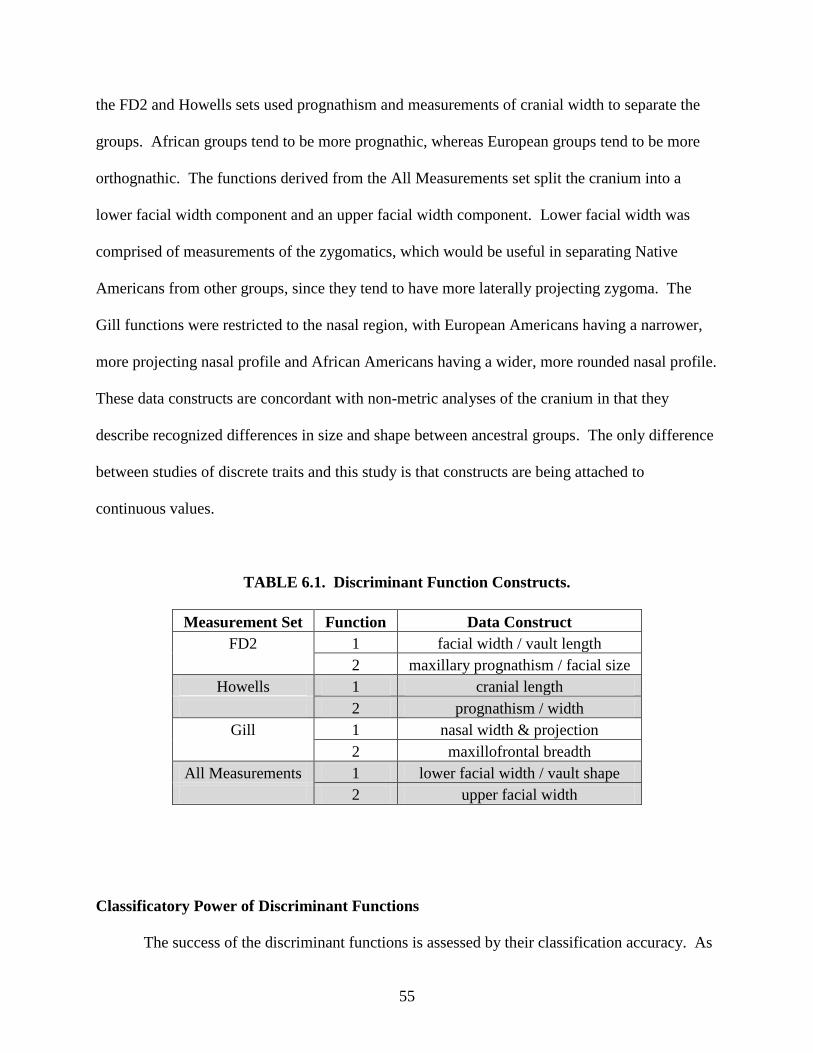
55

the FD2 and Howells sets used prognathism and measurements of cranial width to separate the

groups. African groups tend to be more prognathic, whereas European groups tend to be more

orthognathic. The functions derived from the All Measurements set split the cranium into a

lower facial width component and an upper facial width component. Lower facial width was

comprised of measurements of the zygomatics, which would be useful in separating Native

Americans from other groups, since they tend to have more laterally projecting zygoma. The

Gill functions were restricted to the nasal region, with European Americans having a narrower,

more projecting nasal profile and African Americans having a wider, more rounded nasal profile.

These data constructs are concordant with non-metric analyses of the cranium in that they

describe recognized differences in size and shape between ancestral groups. The only difference

between studies of discrete traits and this study is that constructs are being attached to

continuous values.

TABLE 6.1. Discriminant Function Constructs.

Measurement Set Function Data Construct

FD2 1 facial width / vault length

2 maxillary prognathism / facial size

Howells 1 cranial length

2 prognathism / width

Gill 1 nasal width & projection

2 maxillofrontal breadth

All Measurements 1 lower facial width / vault shape

2 upper facial width

Classificatory Power of Discriminant Functions

The success of the discriminant functions is assessed by their classification accuracy. As

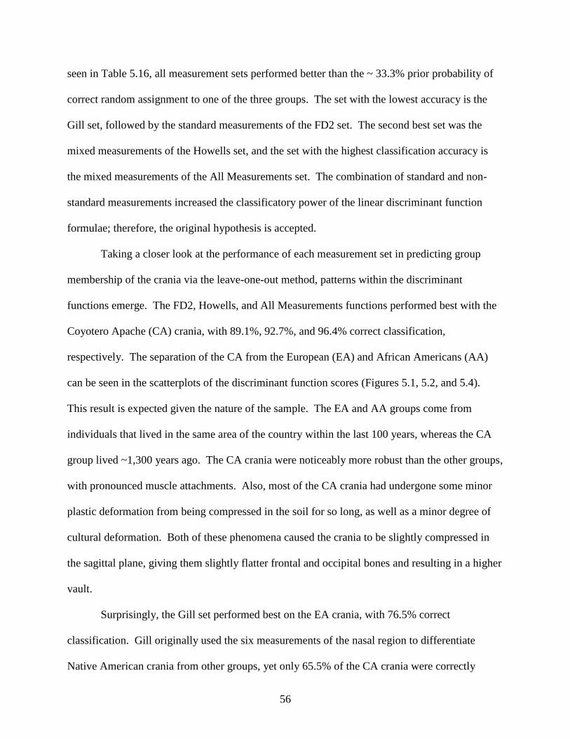
56

seen in Table 5.16, all measurement sets performed better than the ~ 33.3% prior probability of

correct random assignment to one of the three groups. The set with the lowest accuracy is the

Gill set, followed by the standard measurements of the FD2 set. The second best set was the

mixed measurements of the Howells set, and the set with the highest classification accuracy is

the mixed measurements of the All Measurements set. The combination of standard and non-

standard measurements increased the classificatory power of the linear discriminant function

formulae; therefore, the original hypothesis is accepted.

Taking a closer look at the performance of each measurement set in predicting group

membership of the crania via the leave-one-out method, patterns within the discriminant

functions emerge. The FD2, Howells, and All Measurements functions performed best with the

Coyotero Apache (CA) crania, with 89.1%, 92.7%, and 96.4% correct classification,

respectively. The separation of the CA from the European (EA) and African Americans (AA)

can be seen in the scatterplots of the discriminant function scores (Figures 5.1, 5.2, and 5.4).

This result is expected given the nature of the sample. The EA and AA groups come from

individuals that lived in the same area of the country within the last 100 years, whereas the CA

group lived ~1,300 years ago. The CA crania were noticeably more robust than the other groups,

with pronounced muscle attachments. Also, most of the CA crania had undergone some minor

plastic deformation from being compressed in the soil for so long, as well as a minor degree of

cultural deformation. Both of these phenomena caused the crania to be slightly compressed in

the sagittal plane, giving them slightly flatter frontal and occipital bones and resulting in a higher

vault.

Surprisingly, the Gill set performed best on the EA crania, with 76.5% correct

classification. Gill originally used the six measurements of the nasal region to differentiate

Native American crania from other groups, yet only 65.5% of the CA crania were correctly

57

classified. This result is most likely due to the fact that Gill specifically used Northwest Plains

Indian crania to develop the technique, while the current study examined Native American crania

from the Midwest Plains. All four sets of functions had a difficult time classifying the African

American crania, with consistently lower hit rates compared to the other groups. Perhaps the

African American subsample is more variable in cranial form than either the European American

or Coyotero Apache samples. This greater variability can be seen by examining the spread of the

African American specimens on the discriminant function score scatterplots in Figures 5.1, 5.2,

5.3, and 5.4. The African American group is the least tightly clustered group of the three, with

overlap into the European American and Coyotero Apache clusters.

General Conclusions

Taking non-standard measurements would be most useful in the case of incomplete

crania. Limiting data collection to standard measurements would greatly reduce the number of

measurements that could be taken of a particular part of the cranium. For example, the facial

skeleton is the most often damaged portion of the cranium, leaving just the neurocranium for

analysis. There are 12 FORDISC measurements that focus on the neurocranium. An additional

11 neurocranial Howells’ measurements could be used in conjunction with the FORDISC

measurements to aid in identification. Even though more measurements is not necessarily better,

as seen in the results of this study, the combination of standard and non-standard measurements

could aid in the identification of an incomplete cranium.

Twelve non-standard measurements were selected in this study as being important

discriminating variables. These include frontal subtense (FRS), bimaxillary breadth (ZMB),

prosthion radius (PRR), zygoorbitale radius (ZOR), bistephanic breadth (STB), bifrontal breadth

(FMB), biasterionic breadth (ASB), subspinale radius (SSR), mid-orbital breadth (ZOB), alpha

58

chord (ALC), naso-zygoorbital subtense (NZS), and molar alveolus radius (AVR). FRS, NZS,

ZMB, FMB, ZOB, and ALC were taken with the coordinate calipers. PRR, ZOR, SSR, and

AVR are all radial measurements that required the use of the radiometer. STB and ASB were

taken using a sliding caliper. Although ZMB, FMB, ZOB, and ALC were taken using the

coordinate calipers, one can take these four measurements using a sliding caliper. The

coordinate caliper was used in this study because a subtense was measured immediately after and

directly from the breadth/chord measurement. This fact demonstrates the diversity of the

coordinate caliper. It is possible to take up to three measurements at once: chords/breadths,

subtenses, and fractions. With regards to time constraints and data collection, it would take

longer to switch instruments for each measurement instead of using one instrument to take them

all.

The twelve non-standard measurements provide a detailed description of the cranium that

is not achieved with standard measurements. ZMB, ZOR, FMB, ZOB, ALC, and NZS are all

measures of the face. It is not surprising that these measurements were selected because the

facial skeleton tells researchers the most about the population affiliation of an individual. PRR,

SSR, and AVR all measure the projection of the maxilla. These three more fully describe which

portions of the maxilla project the farthest. FRS, STB, and ASB measure aspects of the vault

and add more detail to the overall shape of the vault. Although standard measurements are able

to discriminate between groups with a relatively high level (85.8%) of accuracy by themselves,

the inclusion of non-standard measurements increases the accuracy level (93.5%) of the

functions by ferreting out more subtle shape and size differences.

It is suggested here that biological anthropology laboratories should purchase

instrumentation such as coordinate calipers and radiometers so that non-standard measurements

can be taken to record data that would be missed by just using spreading and sliding calipers.

59

Another instrument that could be used as a replacement for the four aforementioned instruments

is a MicroScribe® digitizer. This instrument works in combination with a personal computer to

record cranial landmarks and their positions in three-dimensional space. The values of the

measurements are subsequently calculated by the computer using the coordinate data. This

instrument allows for much quicker data collection, however, the device is much more expensive

than all of the other calipers put together. Still, the MicroScribe® digitizer could be used with

the latest version of FORDISC: FORDISC 3.0 (FD3). FD3 will expand its battery of

measurements to include those used by Howells and this study (Ousley and Jantz, 2005). As

FORDISC is the ‘industry standard’ for computerized analysis of unknown human crania, it

seems reasonable to postulate that biological anthropology laboratories that adopt FD3 will begin

recording Howells non-standard measurements and entering them into the program more

frequently. As shown in this study, the inclusion of non-standard measurements should increase

the predictive power of FORDISC.

Suggestions for Future Study

Potential research in predictive discriminant analysis for ancestry determination of human

crania could include studying groups other than those used in this study to determine if the same

measurements would be utilized in a stepwise analysis. More population-specific functions need

to be created to more accurately predict ancestral group membership. Perhaps there are certain

measurements that are useful to discriminate between groups no matter what their temporal

distance or geographical location. Arcs could be incorporated in future studies, which only

require flexible measuring tapes and minimal time to record. Although existing measurements

do an excellent job of describing the variation among and between groups, new measurements

could be developed that might increase the power of the discriminant functions. Also, it is

60

important to discover the effects that the sex of a specimen has on the resulting discriminant

functions. Will including sex as a grouping criterion along with ancestry increase or decrease the

classificatory power of the functions?

61

LITERATURE CITED

Afifi AA, Clark V, May S (2004) Computer-Aided Multivariate Analysis. 4th

Ed. Boca Raton:

Chapman & Hall/CRC.

Ashton EH, Healy MJR, and Lipton S (1957) The descriptive use of discriminant functions in

physical anthropology. Proc. Roy. Soc. B. 146:552-572.

Ayers HG, Jantz RL, Moore-Jansen PH (1990) Giles & Elliot race discriminant functions

revisited: A test using recent forensic cases. In GW Gill and S Rhine (eds). Skeletal

Attribution of Race. Maxwell Museum Anthropology, Anthropological Papers, No. 4:

Albequerque, NM. pp. 65-71.

Barnard MM (1935) The secular variations of skull characters in four series of Egyptian skulls.

Annals of Eugenics. 6:352-371.

Bass WM (1995) Human Osteology: A Laboratory and Field Manual, 4th

Edition. Missouri

Archaeological Society, Inc.

Benington RC, Pearson K (1911) Cranial type-contours. Biometrika. 8:123-201.

Benington RC, Pearson K (1912) A study of the Negro skull with special reference to the Congo

and Gaboon crania. Biometrika. 8:292-339.

Birkby WH (1966) An evaluation of race and sex identification from cranial measurements. Am.

J. Phys. Anthrop. 24:21-28.

Brace CL (1995) Region does not mean “race” – reality versus convention in forensic

anthropology. J. For. Sci. 40:171-175.

Bronowski J, Long WM (1952) Statistics of discrimination in anthropology. Am. J. Phys.

Anthrop. 10:385-394.

Broom R (1923) A contribution to the craniology of the yellow-skinned races of South Africa. J.

Roy. Anthrop. Inst. Great Britain and Ireland. 53:132-149.

Brues AM (1990) The once and future diagnosis of race. In GW Gill and S Rhine (eds). Skeletal

Attribution of Race. Maxwell Museum Anthropology, Anthropological Papers, No. 4:

Albequerque, NM. pp. 1-7

Buikstra JE, Ubelaker DH (eds) (1994) Standards for Data Collection from Human Skeletal

Remains. Arkansas Archeological Survey no. 44. Fayetteville, Arkansas.

Campbell NA (1978) Multivariate analysis in biological anthropology: Some further

considerations. J. Hum. Evol. 7:197-203.

62

Carpenter JC (1976) A comparative study of metric and non-metric traits in a series of modern

crania. Am J. Phys. Anthrop. 45:337-344.

Church MS (1995) Determination of race from the skeleton through forensic anthropological

methods. For. Sci. Rev. 7:2-39.

Corruccini RS (1975) Multivariate analysis in biological anthropology: Some considerations. J.

Hum. Evol. 4:1-19.

Cunha E, van Vark GN (1991) The construction of sex discriminant functions from a large

collection of skulls of known sex. Int. J. Anthrop. 6:53-66.

Curran BK (1990) The application of measure of midfacial projection for racial classification. In

GW Gill and S Rhine (eds). Skeletal Attribution of Race. Maxwell Museum

Anthropology, Anthropological Papers, No. 4: Albequerque, NM. pp. 55-57.

de Mérejkowsky C (1882) Sur un nouveau caractére anthropologique. Bulletins de la Société

d’Anthropologie de Paris. 293-304.

DiBennardo R (1986) The use and interpretation of common computer implementations of

discriminant function analysis. In KJ Reichs (ed). Forensic Osteology: Advances in the

Identification of Human Remains. Springfield: Charles C. Thomas. 171-195.

DiBennardo R, Taylor JV (1983) Multiple discriminant function analysis of sex and race in the

postcranial skeleton. Am. J. Phys. Anthrop. 61:305-314.

Dunn OJ, Varady PD (1966) Probabilities of correct classification in discriminant analysis.

Biometrics. 22:908-924.

Feldesman MR (1997) Bridging the chasm: Demystifying some statistical methods used in

biological anthropology. In NT Boaz and LD Wolfe (eds). Biological Anthropology: The

State of the Science. Bend OR: International Institute for Human Evolutionary Research,

pp. 73-99.

Fisher RA (1936) The use of multiple measurements in taxonomic problems. Annals of

Eugenics. 3:179-188.

Fisher RA (1938) The statistical utilization of multiple measurements. Annals of Eugenics.

8:376-386.

Fisher TD, Gill GW (1990) Application of the Giles & Elliot discriminant function formulae to a

cranial sample of Northwestern Plains Indians. In GW Gill and S Rhine (eds). Skeletal

Attribution of Race. Maxwell Museum Anthropology, Anthropological Papers, No. 4:

Albequerque, NM. pp. 59-63.

Giles E (1966) Statistical techniques for race and sex determination: Some comments in

defense. Am. J. Phys. Anthrop. 25:85-86.

63

Giles E, Elliot O (1962) Race identification from cranial measurements. J. For. Sci. 7:147-157.

Giles E, Elliot O (1963) Sex determination by discriminant function. Am. J. Phys. Anthrop.

21:53-68.

Gill GW (1984) A forensic test case for a new method of geographical race determination. In TA

Rathbun and JE Buikstra (eds). Human Identification: Case Studies in Forensic

Anthropology. Springfield: Charles C. Thomas, pp. 229-339.

Gill GW (1986) Craniofacial criteria in forensic race identification. In KJ Reichs (ed). Forensic

Osteology: Advances in the Identification of Human Remains. Springfield: Charles C.

Thomas, pp. 143-159.

Gill GW (1995) Challenge on the frontier: Discerning American Indians from whites

osteologically. J. For. Sci. 40:783-788.

Gill GW (1998) Craniofacial criteria in forensic race identification. In KJ Reichs (ed). Forensic

Osteology: Advances in the Identification of Human Remains. 2nd

Ed. Springfield:

Charles C. Thomas, pp. 143-159.

Gill GW, Gilbert BM (1990) Race identification from the midfacial skeleton: American blacks

and Whites. In GW Gill and S Rhine (eds). Skeletal Attribution of Race. Maxwell

Museum Anthropology, Anthropological Papers, No. 4: Albequerque, NM. pp. 47-53.

Gill GW, Hughes SS, Bennett SM, Gilbert BM (1988) Racial identification from the midfacial

skeleton with special reference to American Indians and whites. J. For. Sci. 33:92-99.

Gill GW, Rhine S (1990) Skeletal Attribution of Race. Maxwell Museum Anthropology,

Anthropological Papers, No. 4: Albequerque.

Howells WW (1937) The designation of the principle anthrometric landmarks of the head and

skull. Am. J. Phys. Anthrop. 22:477-494.

Howells WW (1957) The cranial vault: Factors of size and shape. Am. J. Phys. Anthrop. 15:19-

48.

Howells WW (1960) Criteria for selection of osteometric measurements. Am. J. Phys. Anthrop.

30:451-458.

Howells WW (1966) The Jomon population of Japan. A study by discriminant analysis of

Japanese and Ainu crania. In Craniometry and Multivariate Analysis. Papers of the

Peabody Museum, Harvard University, vol. 57, no. 1, pp. 1-43.

Howells WW (1969) The use of multivariate techniques in the study of skeletal populations. Am.

J. Phys. Anthrop. 31:311-314.

64

Howells WW (1970) Multivariate analysis for the identification of race from crania. In TD

Stewart (ed). Personal Identification in Mass Disasters. Washington: Smithsonian

Institution, pp. 111-118.

Howells WW (1972) Analysis of patterns of variation in crania of recent man. In R Tuttle (ed).

The Functional and Evolutionary Biology of Primates. Chicago: Aldine-Atherton, pp.

123-151.

Howells WW (1973) Cranial Variation in Man: A Study by Multivariate Analysis of Patterns of

Difference Among Recent Human Populations. Papers of the Peabody Museum of

Archaeology and Ethnology, Harvard University, vol. 67.

Hrdlička A (1920) Anthropometry. Philadelphia: The Wistar Institute of Anatomy and Biology.

Huberty CJ (1994) Applied Discriminant Analysis. New York: John Wiley & Sons, Inc.

Hursh TM (1976) The study of cranial form: Measurement techniques and analytical methods.

In E Giles and JS Friedlander (eds). The Measures of Man: Methodologies in Biological

Anthropology. Peabody Museum Press, Cambridge, pp. 465-491.

İşcan MY, Steyn M (1999) Craniometric determination of population affinity in South Africans.

Int. J. Legal Med. 112:91-97.

Jantz RL, Ousley SD (1993) FORDISC 1.0: Computerized Forensic Discriminant Functions.

Knoxville, University of Tennessee.

Jantz RL, Owsley DW (1994) White traders in the upper Missouri: Evidence from the Swan

Creek site. In DW Owsley and RL Jantz (eds). Skeletal Biology in the Great Plains:

Migration, Warfare, Health, and Subsistence. Washington: Smithsonian Institute Press,

pp. 189-201.

Jeter MD (1990) Edward Palmer’s Arkansaw Mounds. The University of Arkansas Press:

Fayetteville.

Johnson DR, O'Higgins P, Moore WJ, McAndrew TJ (1989) Determination of race and sex of

the human skull by discriminant function analysis of linear and angular dimensions – an

appendix. For. Sci. Int. 41:41-53.

Kachigan SK (1991) Multivariate Statistical Analysis: A Conceptual Introduction 2nd

Ed. New

York: Radius.

Kennedy KAR (1995) But professor, why teach race identification if races don't exist? J. For.

Sci. 40:797-800.

Klepinger L, Giles E (1998) Classification or confusion: Statistical interpretation in forensic

anthropology. In KJ Reichs (ed). Forensic Osteology: Advances in Identification of

Human Remains 2nd

Ed. Springfield: Charles C. Thomas, pp. 427-440.

65

Key PJ (1983) Craniometric Relationships Among Plains Indians. Report of Investigations No.

34, The University of Tennessee Department of Anthropology, Knoxville.

Key PJ (1994) Relationships of the Woodland period on the northern and central plains: the

craniometric evidence. In DW Owsley and RL Jantz (eds). Skeletal Biology in the Great

Plains: Migration, Warfare, Health, and Subsistence. Washington: Smithsonian Institute

Press, pp. 179-187.

Kowalski CJ (1972) A commentary on the use of multivariate statistical analysis in

anthropometric research. Am. J. Phys. Anthrop. 30:19-131.

Kitson E (1931) A study of the Negro skull with special reference to the crania from Kenya

Colony. Biometrika. 23:271-314.

Krogman WM, İşcan MY (1986) The Human Skeleton in Forensic Medicine. 2nd

Ed.

Springfield: Charles C. Thomas.

Lachenbruch PA (1967) An almost unbiased method of obtaining confidence intervals for the

probability of misclassification in discriminant analysis. Biometrics. 23:639-645.

Lachenbruch PA, Mickey MR (1968) Estimation of error rates in discriminant analysis.

Technometrics. 10:1-11.

Lachenbruch PA, Goldstein M (1979) Discriminant analysis. Biometrics. 35:69-85.

Mahalanobis PC, Majumdar DN, Rao CR (1949) Anthropometric survey of the United

Provinces, 1941: a statistical study. Sankhyá: The Indian J. Stats. 9:89-342.

Martin R (1928) Lehrbuch der Anthropologie. Band I. Jena, Germany: Verlag Gustave Fischer.

McLachlan GJ (1980) On the relationship between the F test and the overall error rate for

variable selection in two-group discriminant analysis. Biometrics. 36:501-510.

McLachlan GJ (1992) Discriminant Analysis and Statistical Pattern Recognition. New York:

John Wiley and Sons.

Moore-Jansen PM, Ousley SD, Jantz RL (1994) Data Collection Procedures for Forensic

Skeletal Material, 3rd

Edition. Report of Investigations no. 48. The University of

Tennessee, Knoxville. Department of Anthropology.

Nawrocki SP (1993). The concept of race in contemporary physical anthropology. In The

Natural History of Paradigms: Science and the Process of Intellectual Evolution, ed. by J.

Langdon & M. McGann. University of Indianapolis Press, pp. 222-234.

Novotný V, İşcan MY, Loth SR (1993) Morphologic and osteometric assessment of age, sex, and

race from the skull. In MY İşcan, RP Helmer (eds). Forensic Analysis of the Skull. New

York: Wiley-Liss, pp. 71-88.

66

Ousley SD, Jantz RL (1996) FORDISC 2.0: Personal Computer Forensic Discriminant

Functions. Knoxville: University of Tennessee.

Ousley SD, Jantz RL (2005) The Next FORDISC: FORDISC 3. Abstract in the Proceedings of

the American Academy of Forensic Sciences. Vol. XI.

Patriquin ML, Steyn M, Loth SR (2002) Metric assessment of race from the pelvis of South

Africans. For. Sci. Int. 127:104-113.

Pearson K (1934) On simometers and their handling. Biometrika. 26:265-268.

Pearson K, Davin AG (1924) On the biometric constants of the human skull. Biometrika.

16:328-363.

Pietrusewsky M (1990) Craniofacial variation in Australian and Pacific populations. Am. J Phys.

Anthrop. 82:319-340.

Pietrusewsky M (2000) Metric analysis of skeletal remains: Methods and applications. In MA

Katzenberg and SR Saunders (eds). Biological Anthropology of the Human Skeleton.

New York: Wiley-Liss, pp. 375-415.

Rao CR (1946) Tests with discriminant functions in multivariate analysis. Sankhyá: The Indian

J. of Stat. 7:407-414.

Rao CR (1948) The utilization of multiple measurements in problems of biological classification.

J. Roy. Stat. Soc. B. 10:159-203.

Rao CR (1949) On some problems arising out of discrimination with multiple characters.

Sankhyá: The Indian J. of Stats. 9:343-366.

Rao CR (1952) Advanced Statistical Methods in Biometric Research. New York: Wiley.

Reichs KJ (1986) Forensic Osteology: Advances in the Identification of Human Remains.

Springfield: Charles C. Thomas.

Rightmire GP (1970) Bushmen, Hottentot, and South African Negro crania studied by distance

and discrimination. Am. J. Phys. Anthrop. 33:169-195.

Rightmire GP (1976) Metric versus discrete traits in African skulls. In E Giles and JS

Friedlander (eds). The Measures of Man: Methodologies in Biological Anthropology.

Cambridge: Peabody Museum Press, pp. 383-407.

Ross AH, Slice DE, Ubelaker DH, Falsetti AB (2004) Population affinities of 19th

century Cuban

crania: Implications for identification criteria in south Florida Cuban Americans. J. For.

Sci. 49:11-16

67

Sauer NJ (1992) Forensic anthropology and the concept of race: if races don’t exist, why are

forensic anthropologists so good at identifying them? Soc. Sci. Med. 34:107-111.

Smith CA (1947) Some examples of discrimination. Ann. Eugen. 18:272-282.

Snapinn SM, Knoke JD (1989) Estimation of error rates in discriminant analysis with selection

of variables. Biometrics. 45:289-299.

Snow CC, Hartman S, Giles E, Young FA (1979) Sex and race determination of crania by

calipers and computer: A test of the Giles and Elliot discriminant functions in 52 forensic

science cases. J. For. Sci. 24:448-460.

Song H, Lin ZQ, Jia JT (1992) Sex diagnosis of Chinese skulls using multiple stepwise

discriminant function analysis. For. Sci. Int. 54:135-140.

Stewart TD (1948) Medico-legal aspects of the skeleton I: Age, sex, race and stature. Am. J.

Phys. Anthrop. 6:315-322.

Steyn M, İşcan MY (1998) Sexual dimorphism in the crania and mandibles of South African

whites. For. Sci. Int. 98:9-16.

Taylor JV, Roh L, Goldman AD (1984) Metropolitan Forensic Anthropology Team (MFAT)

case studies in identification: 2. Identification of a Vietnamese trophy skull. J. For. Sci.

29:1253-1259.

Thieme FP, Schull WJ (1957) Sex determination from the skeleton. Hum. Bio. 29:242-273.

Townsend GC, Richards LC, Carroll A (1982) Sex determination of Australian Aboriginal skulls

by discriminant function analysis. Australian Dental J. 27:320-326.

van Vark GN (1976) A critical evaluation of the application of multivariate statistical methods to

the study of human populations from their skeletal remains. Homo. 27:94-113.

van Vark GN (1994) Multivariate analysis: Is it useful for hominid studies? Courier

Forschungsinstitut Senckenberg. 171:289-294.

van Vark GN, van der Sman PGM (1982) New discrimination and classification techniques in

anthropological practice. Z. Morph. Anthrop. 73:21-36.

van Vark GN, Schaafsma W (1992) Advances in the quantitative analysis of skeletal

morphology. In SR Saunders and MA Katzenberg (eds). Skeletal Biology of Past

Peoples: Research Methods. New York: Wiley-Liss, pp. 225-257.

von Bonin G (1931) A contribution to the craniology of the Easter Islanders. Biometrika. 23:249-

270.

68

von Bonin G (1936) On the craniology of Oceania. Crania from New Britain. Biometrika.

28:123-148.

von Bonin G, Morant GM (1938) Indian races in the United States. A survey of previously

published cranial measurements. Biometrika. 30:94-129.

Wright RVS (1992) Correlation between cranial form and geography in Homo sapiens: CRANID

– a computer program for forensic and other applications. Archaeology in Oceania.

27:128-134.

Woo TL, Morant GM (1932) A preliminary classification of Asiatic races based on cranial

measurements. Biometrika. 24:108-134.

Woo TL, Morant GM (1934) A biometric study of the “flatness” of the facial skeleton in man.

Biometrika. 26:196-250.

Zambrano CJ, Kolatorowicz A, Nawrocki SP (2005) Performance of FORDISC 2.0 using

inaccurate measurements. Poster presented at the 57th

annual meeting of the American

Academy of Forensic Sciences. New Orleans LA.

Zugibe FT, Taylor J, Weg N, DiBennardo R, Costello JT, Deforest P (1985) Metropolitan

Forensic Anthropology Team (MFAT) case studies in identification: 3. Identification of

John J. Sullivan, the missing journalist. J. For. Sci. 30:221-231.

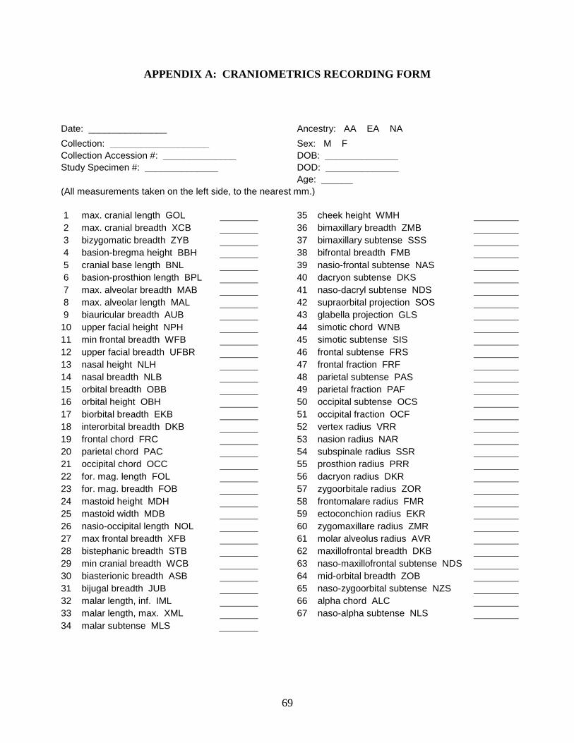
69

APPENDIX A: CRANIOMETRICS RECORDING FORM

Date: _______________ Ancestry: AA EA NA

Collection: ___________________ Sex: M F

Collection Accession #: ______________ DOB: ______________

Study Specimen #: ______________ DOD: ______________

Age: ______

(All measurements taken on the left side, to the nearest mm.)

1 max. cranial length GOL 35 cheek height WMH

2 max. cranial breadth XCB 36 bimaxillary breadth ZMB

3 bizygomatic breadth ZYB 37 bimaxillary subtense SSS

4 basion-bregma height BBH 38 bifrontal breadth FMB

5 cranial base length BNL 39 nasio-frontal subtense NAS

6 basion-prosthion length BPL 40 dacryon subtense DKS

7 max. alveolar breadth MAB 41 naso-dacryl subtense NDS

8 max. alveolar length MAL 42 supraorbital projection SOS

9 biauricular breadth AUB 43 glabella projection GLS

10 upper facial height NPH 44 simotic chord WNB

11 min frontal breadth WFB 45 simotic subtense SIS

12 upper facial breadth UFBR 46 frontal subtense FRS

13 nasal height NLH 47 frontal fraction FRF

14 nasal breadth NLB 48 parietal subtense PAS

15 orbital breadth OBB 49 parietal fraction PAF

16 orbital height OBH 50 occipital subtense OCS

17 biorbital breadth EKB 51 occipital fraction OCF

18 interorbital breadth DKB 52 vertex radius VRR

19 frontal chord FRC 53 nasion radius NAR

20 parietal chord PAC 54 subspinale radius SSR

21 occipital chord OCC 55 prosthion radius PRR

22 for. mag. length FOL 56 dacryon radius DKR

23 for. mag. breadth FOB 57 zygoorbitale radius ZOR

24 mastoid height MDH 58 frontomalare radius FMR

25 mastoid width MDB 59 ectoconchion radius EKR

26 nasio-occipital length NOL 60 zygomaxillare radius ZMR

27 max frontal breadth XFB 61 molar alveolus radius AVR

28 bistephanic breadth STB 62 maxillofrontal breadth DKB

29 min cranial breadth WCB 63 naso-maxillofrontal subtense NDS

30 biasterionic breadth ASB 64 mid-orbital breadth ZOB

31 bijugal breadth JUB 65 naso-zygoorbital subtense NZS

32 malar length, inf. IML 66 alpha chord ALC

33 malar length, max. XML 67 naso-alpha subtense NLS

34 malar subtense MLS

70

APPENDIX B: CRANIAL MEASUREMENT DEFINITIONS

Definitions for #’s 1-61 are taken from Howells (1973).

Definitions for #’s 62-67 are taken from Gill (1984).

Abbreviations for #’s 64-67 were created by the author.

Instrument Codes:

Sliding caliper: A Spreading caliper: B Coordinate Caliper: C Radiometer: D

1. Maximum cranial length (GOL): the distance of glabella from opisthocranion. B

2. Maximum cranial breadth (XCB): the maximum width of the skull perpendicular to the mid-

sagittal plane wherever it is located. B

3. Bizygomatic breadth (ZYB): the direct distance between both zygia located at their most

lateral points of the zygomatic arches. B

4. Basion-bregma height (BBH): the direct distance from the lowest point on the anterior

margin of the foramen magnum, basion to bregma. B

5. Cranial base length (BNL): the direct distance from nasion to basion. B

6. Basion-prosthion length (BPL): the direct distance from basion to prosthion. B

7. Maximum alveolar breadth (MAB): the maximum breadth across the alveolar borders of the

maxilla measured on the lateral surfaces at the location of the first maxillary molar. B

8. Maximum alveolar length (MAL): the direct distance from prosthion to alveolon. A

9. Biauricular breadth (AUB): the least exterior breadth across the roots of the zygomatic

processes. B

10. Upper facial height (NPH): the direct distance from nasion to prosthion. A

11. Minimum frontal breadth (WFB): the direct distance between the two frontotemporale. B

12. Upper facial breadth (UFBR): the direct distance between the two frontomalare temporalia.

13. Nasal height (NLH): the direct distance from nasion to nasospinale. A

14. Nasal breadth (NLB): the maximum breadth of the nasal aperture. A

15. Orbital breadth (OBB): the laterally sloping distance from dacryon to ectoconchion. A

16. Orbital height (OBH): the direct distance between the superior and inferior orbital margins.

A

17. Biorbital breadth (EKB): the direct distance from one ectoconchion to the other. C

18. Interorbital breadth (DKB): the direct distance between right and left dacryon. C

19. Frontal chord (FRC): the direct distance from nasion to bregma. C

20. Parietal chord (PAC): the direct distance from bregma to lambda. C

21. Occipital chord (OCC): the direct distance from lambda to opisthion. C

22. Foramen magnum length (FOL): the direct distance of basion from opisthion. A

23. Foramen magnum breadth (FOB): the distance between the lateral margins of the foramen

magnum at the point of greatest lateral curvature. A

24. Mastoid height (MDH): the projection of the mastoid process below, and perpendicular to,

the eye-ear plane in the vertical plane. A

25. Mastoid width (MDB): width of the mastoid process at its base, through its transverse axis.

A

26. Nasio-occipital length (NOL): greatest cranial length in the median sagittal plane, measured

from nasion. B

71

27. Maximum frontal breadth (XFB): the maximum breadth at the coronal suture, perpendicular

to the median plane. B

28. Bistephanic breadth (STB): breadth between the intersections, on either side, of the coronal

suture and the inferior temporal line marking the origin of the temporal muscle. A

29. Minimum cranial breadth (WCB): the breadth across the sphenoid at the base of the

temporal fossa, at the infratemporal crests. A

30. Biasterionic breadth (ASB): direct measurement from one asterion to the other. A

31. Bijugal breadth (JUB): the external breadth across the malars at the jugalia, i.e., at the

deepest points in the curvature between the frontal and temporal processes of the malars.

A

32. Malar length, inferior (IML): the direct distance from zygomaxillare anterior to the lowest

point of the zygo-temporal suture on the external surface, on the left side. A

33. Malar length, maximum (XML): total direct length of the malar in a diagonal direction,

from the lower end of the zygo-temporal suture on the lateral face of the bone, to

zygoorbitale, the junction of the zygo-maxillary suture with the lowest border of the

orbit, on the left side. C

34. Malar subtense (MLS): the maximum subtense from the convexity of the malar angle to the

maximum length of the bone, at the level of the zygomaticofacial foramen, on the left

side. C

35. Cheek height (WMH): the minimum distance, in any direction, from the lower border of the

orbit to the lower margin of the maxilla, mesial to the masseter attachment, on the left

side. A

36. Bimaxillary breadth (ZMB): the breadth across the maxillae, from one zygomaxillare

anterior to the other. C

37. Bimaxillary subtense (SSS): the projection or subtense from subspinale to the bimaxillary

breadth. C

38. Bifrontal breadth (FMB): the breadth across the frontal bone between frontomalare anterior

on each side, i.e., the most anterior point on the fronto-malar suture. C

39. Nasio-frontal subtense (NAS): the subtense from nasion to the bifrontal breadth. C

40. Dacryon subtense (DKS): the mean subtense from dacryon (average of two sides) to the

biorbital breadth. C

41. Naso-dacryl subtense (NDS): the subtense from the deepest point in the profile of the nasal

bones to the interorbital breadth. C

42. Supraorbital projection (SOS): the maximum projection of the left supraorbital arch

between the midline, in the region of glabella or above, and the frontal bone just anterior

to the temporal line in its forward part, measured as a subtense to the line defined. C

43. Glabella projection (GLS): the maximum projection of the midline profile between nasion

and supraglabellare (or the point at which the curve of the profile of the frontal bone

changes to join the prominence of the glabellar region), measured as a subtense. C

44. Simotic chord (WNB): the minimum transverse breadth across the two nasal bones, or

chord between the naso-maxillary sutures at their closest approach. C

45. Simotic subtense (SIS): the subtense from the nasal bridge to the simotic chord, i.e., from

the highest point in the transverse section which is at the deepest point in the nasal

profile. C

46. Frontal subtense (FRS): the maximum subtense, at the highest point on the convexity of the

frontal bone in the midplane, to the nasion-bregma chord. C

72

47. Frontal fraction (FRF): the distance along the nasion-bregma chord, recorded from nasion,

at which the frontal subtense falls. C

48. Parietal subtense (PAS): the maximum subtense, at the highest point on the convexity of the

parietal bones in the midplane, to the bregma-lambda chord. C

49. Parietal fraction (PAF): the distance along the bregma-lambda chord, recorded from

bregma, at which the parietal subtense falls. C

50. Occipital subtense (OCS): the maximum subtense, at the most prominent point on the basic

contour of the occipital bone in the midplane. C

51. Occipital fraction (OCF): the distance along the lambda-opisthion chord, recorded from

lambda, at which the occipital subtense falls. C

52. Vertex radius (VRR): the perpendicular to the transmeatal axis from the most distant point

on the parietals (including bregma or lambda), wherever found. D

53. Nasion radius (NAR): the perpendicular to the transmeatal axis from nasion. D

54. Subspinale radius (SSR): the perpendicular to the transmeatal axis from subspinale. D

55. Prosthion radius (PRR): the perpendicular to the transmeatal axis from prosthion. D

56. Dacryon radius (DKR): the perpendicular to the transmeatal axis from the left dacryon. D

57. Zygoorbitale radius (ZOR): the perpendicular to the transmeatal axis from the left

zygoorbitale. D

58. Frontomalare radius (FMR): the perpendicular to the transmeatal axis from the left

fromtomalare anterior. D

59. Ectoconchion radius (EKR): the perpendicular to the transmeatal axis from the left

ectoconchion. D

60. Zygomaxillare radius (ZMR): the perpendicular to the transmeatal axis from the left

zygomaxillare anterior. D

61. Molar alveolus radius (AVR): the perpendicular to the transmeatal axis from the most

anterior point on the alveolus of the left first molar. D

62. Maxillofrontal breadth (DKB): distance between maxillofrontale left and right. C

63. Naso-maxillofrontal subtense (NDS): subtense from the maxillofrontal points to the deepest

point on the nasal bridge. C

64. Mid-orbital breadth (ZOB): the distance between zygoorbitale left and right. C

65. Naso-zygoorbital subtense (NZS): subtense from the zygoorbital points to the deepest point

along the nasal bridge. C

66. Alpha cord (ALC): the point alpha is the deepest point on the maxilla, left and right, on a

tangent run between the naso-maxillary suture where it meets the nasal aperture, and

zygoorbitale. C

67. Naso-alpha subtense (NLS): subtense from the alpha points to the deepest point on the nasal

bridge. C

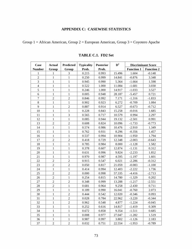
73

APPENDIX C: CASEWISE STATISTICS

Group 1 = African American, Group 2 = European American, Group 3 = Coyotero Apache

TABLE C.1. FD2 Set

Case Actual Predicted Typicality Posterior D2 Discriminant Score

Number Group Group Prob. Prob. Function 1 Function 2

1 1 3 0.215 0.993 15.496 1.604 -0.148

2 1 1 0.250 0.999 14.841 -0.876 3.348

3 1 1 0.945 0.990 5.364 -1.664 1.598

4 1 1 0.522 1.000 11.084 -1.681 3.030

5 1 1 0.246 1.000 14.917 -1.033 3.527

6 1 1 0.005 0.948 28.187 -5.457 0.721

7 2 2 0.846 0.992 7.171 -1.316 -1.833

8 1 1 0.902 0.923 6.272 -0.709 1.084

9 1 2 0.887 0.914 6.527 -0.673 -0.712

10 1 1 0.228 0.843 15.258 -0.016 1.685

11 1 3 0.565 0.717 10.579 0.994 2.297

12 1 1 0.085 0.944 19.132 -2.501 0.991

13 2 2 0.608 0.824 10.096 -1.733 -0.773

14 1 1 0.574 0.986 10.476 -2.910 1.349

15 1 1 0.762 0.931 8.296 -0.356 1.457

16 1 1 0.537 0.994 10.904 -1.950 1.794

17 2 2 0.418 0.729 12.348 -2.003 -0.643

18 1 1 0.785 0.984 8.000 -1.128 1.582

19 1 1 0.378 0.607 12.874 -1.131 0.312

20 1 1 0.631 0.996 9.824 -2.233 1.852

21 1 1 0.970 0.987 4.595 -1.197 1.601

22 2 2 0.915 0.547 6.021 -2.286 -0.312

23 2 2 0.050 0.817 21.059 -0.083 -1.100

24 1 1 0.414 0.994 12.403 -2.222 1.736

25 2 2 0.000 0.998 57.335 -4.416 -2.713

26 2 1 0.254 0.815 14.780 -1.329 0.202

27 2 2 0.348 0.999 13.288 -1.217 -2.551

28 2 1 0.681 0.964 9.258 -2.430 0.711

29 1 1 0.189 0.990 16.041 -0.760 2.073

30 1 2 0.444 0.542 12.020 -0.346 0.093

31 1 2 0.028 0.784 22.962 -3.220 -0.344

32 1 2 0.962 0.548 4.877 -1.224 -0.045

33 1 1 0.252 0.616 14.817 -1.419 0.309

34 1 1 0.672 0.858 9.354 -1.511 0.685

35 1 1 0.008 0.977 27.047 -1.282 1.519

36 1 1 0.987 0.997 3.802 -1.126 2.183

37 2 2 0.032 0.751 22.554 -1.953 -0.789

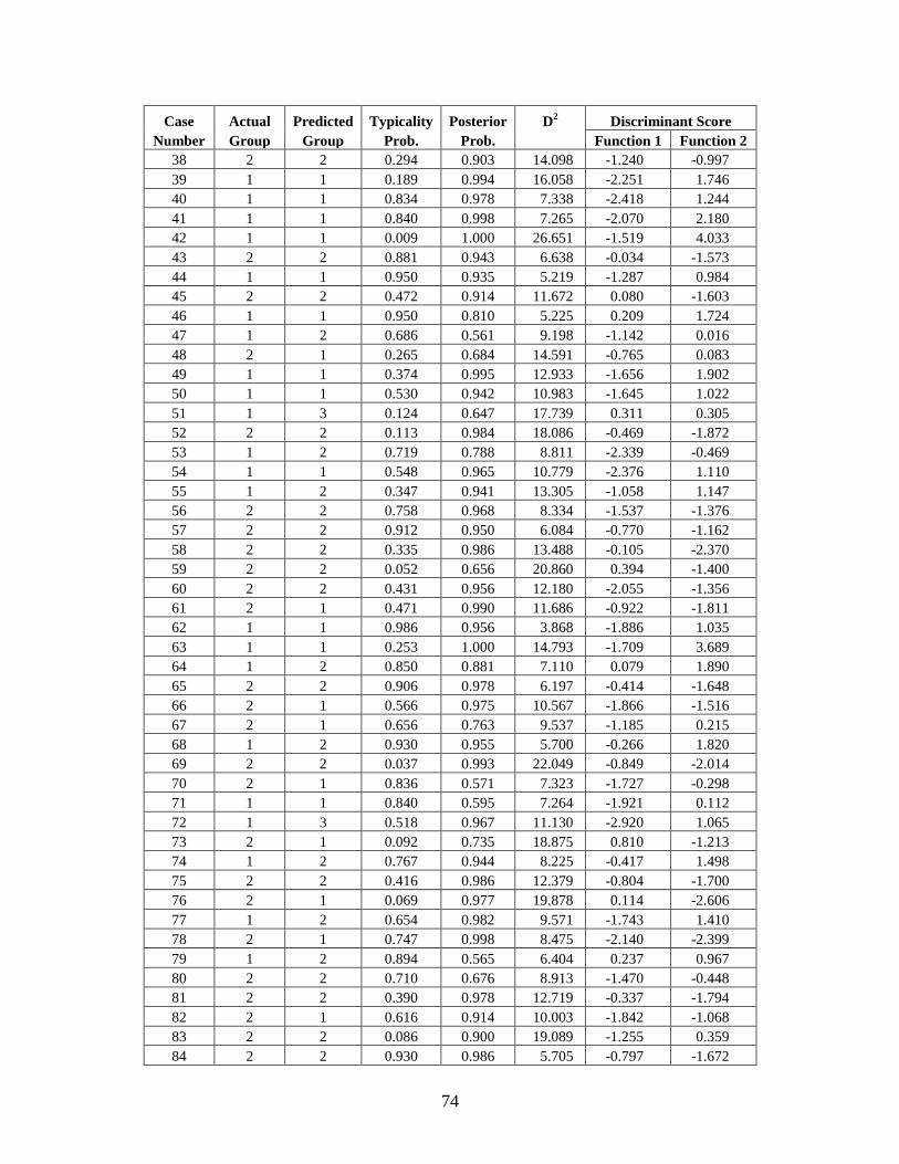
74

Case Actual Predicted Typicality Posterior D2 Discriminant Score

Number Group Group Prob. Prob. Function 1 Function 2

38 2 2 0.294 0.903 14.098 -1.240 -0.997

39 1 1 0.189 0.994 16.058 -2.251 1.746

40 1 1 0.834 0.978 7.338 -2.418 1.244

41 1 1 0.840 0.998 7.265 -2.070 2.180

42 1 1 0.009 1.000 26.651 -1.519 4.033

43 2 2 0.881 0.943 6.638 -0.034 -1.573

44 1 1 0.950 0.935 5.219 -1.287 0.984

45 2 2 0.472 0.914 11.672 0.080 -1.603

46 1 1 0.950 0.810 5.225 0.209 1.724

47 1 2 0.686 0.561 9.198 -1.142 0.016

48 2 1 0.265 0.684 14.591 -0.765 0.083

49 1 1 0.374 0.995 12.933 -1.656 1.902

50 1 1 0.530 0.942 10.983 -1.645 1.022

51 1 3 0.124 0.647 17.739 0.311 0.305

52 2 2 0.113 0.984 18.086 -0.469 -1.872

53 1 2 0.719 0.788 8.811 -2.339 -0.469

54 1 1 0.548 0.965 10.779 -2.376 1.110

55 1 2 0.347 0.941 13.305 -1.058 1.147

56 2 2 0.758 0.968 8.334 -1.537 -1.376

57 2 2 0.912 0.950 6.084 -0.770 -1.162

58 2 2 0.335 0.986 13.488 -0.105 -2.370

59 2 2 0.052 0.656 20.860 0.394 -1.400

60 2 2 0.431 0.956 12.180 -2.055 -1.356

61 2 1 0.471 0.990 11.686 -0.922 -1.811

62 1 1 0.986 0.956 3.868 -1.886 1.035

63 1 1 0.253 1.000 14.793 -1.709 3.689

64 1 2 0.850 0.881 7.110 0.079 1.890

65 2 2 0.906 0.978 6.197 -0.414 -1.648

66 2 1 0.566 0.975 10.567 -1.866 -1.516

67 2 1 0.656 0.763 9.537 -1.185 0.215

68 1 2 0.930 0.955 5.700 -0.266 1.820

69 2 2 0.037 0.993 22.049 -0.849 -2.014

70 2 1 0.836 0.571 7.323 -1.727 -0.298

71 1 1 0.840 0.595 7.264 -1.921 0.112

72 1 3 0.518 0.967 11.130 -2.920 1.065

73 2 1 0.092 0.735 18.875 0.810 -1.213

74 1 2 0.767 0.944 8.225 -0.417 1.498

75 2 2 0.416 0.986 12.379 -0.804 -1.700

76 2 1 0.069 0.977 19.878 0.114 -2.606

77 1 2 0.654 0.982 9.571 -1.743 1.410

78 2 1 0.747 0.998 8.475 -2.140 -2.399

79 1 2 0.894 0.565 6.404 0.237 0.967

80 2 2 0.710 0.676 8.913 -1.470 -0.448

81 2 2 0.390 0.978 12.719 -0.337 -1.794

82 2 1 0.616 0.914 10.003 -1.842 -1.068

83 2 2 0.086 0.900 19.089 -1.255 0.359

84 2 2 0.930 0.986 5.705 -0.797 -1.672

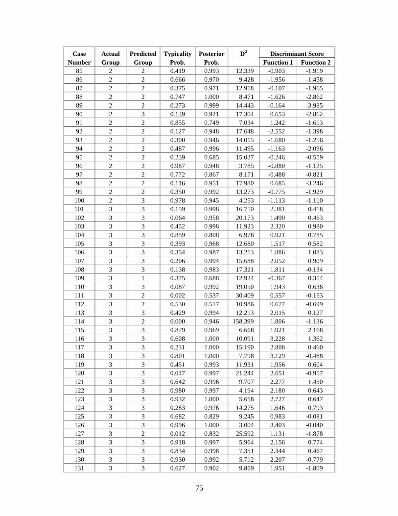
75

Case Actual Predicted Typicality Posterior D2 Discriminant Score

Number Group Group Prob. Prob. Function 1 Function 2

85 2 2 0.419 0.993 12.339 -0.903 -1.919

86 2 2 0.666 0.970 9.428 -1.956 -1.458

87 2 2 0.375 0.971 12.918 -0.107 -1.965

88 2 2 0.747 1.000 8.471 -1.626 -2.862

89 2 2 0.273 0.999 14.443 -0.164 -3.985

90 2 3 0.139 0.921 17.304 0.653 -2.862

91 2 2 0.855 0.749 7.034 1.242 -1.613

92 2 2 0.127 0.948 17.648 -2.552 -1.398

93 2 2 0.300 0.946 14.015 -1.680 -1.256

94 2 2 0.487 0.996 11.495 -1.163 -2.096

95 2 2 0.239 0.685 15.037 -0.246 -0.559

96 2 2 0.987 0.948 3.785 -0.880 -1.125

97 2 2 0.772 0.867 8.171 -0.488 -0.821

98 2 2 0.116 0.951 17.980 0.685 -3.246

99 2 2 0.350 0.992 13.273 -0.775 -1.929

100 2 3 0.978 0.945 4.253 -1.113 -1.110

101 3 3 0.159 0.998 16.750 2.381 0.418

102 3 3 0.064 0.958 20.173 1.490 0.463

103 3 3 0.452 0.998 11.923 2.320 0.980

104 3 3 0.859 0.808 6.978 0.921 0.785

105 3 3 0.393 0.968 12.680 1.517 0.582

106 3 3 0.354 0.987 13.213 1.886 1.083

107 3 3 0.206 0.994 15.688 2.052 0.909

108 3 3 0.138 0.983 17.321 1.811 -0.134

109 3 1 0.375 0.688 12.924 -0.367 0.354

110 3 3 0.087 0.992 19.050 1.943 0.636

111 3 2 0.002 0.537 30.409 0.557 -0.153

112 3 2 0.530 0.517 10.986 0.677 -0.699

113 3 3 0.429 0.994 12.213 2.015 0.127

114 3 2 0.000 0.946 158.399 1.806 -1.136

115 3 3 0.879 0.969 6.668 1.921 2.168

116 3 3 0.608 1.000 10.091 3.228 1.362

117 3 3 0.231 1.000 15.190 2.808 0.460

118 3 3 0.801 1.000 7.798 3.129 -0.488

119 3 3 0.451 0.993 11.931 1.956 0.604

120 3 3 0.047 0.997 21.244 2.651 -0.957

121 3 3 0.642 0.996 9.707 2.277 1.450

122 3 3 0.980 0.997 4.194 2.180 0.643

123 3 3 0.932 1.000 5.658 2.727 0.647

124 3 3 0.283 0.976 14.275 1.646 0.793

125 3 3 0.682 0.829 9.245 0.983 -0.081

126 3 3 0.996 1.000 3.004 3.403 -0.040

127 3 2 0.012 0.832 25.592 1.131 -1.878

128 3 3 0.918 0.997 5.964 2.156 0.774

129 3 3 0.834 0.998 7.351 2.344 0.467

130 3 3 0.930 0.992 5.712 2.207 -0.779

131 3 3 0.627 0.902 9.869 1.951 -1.809

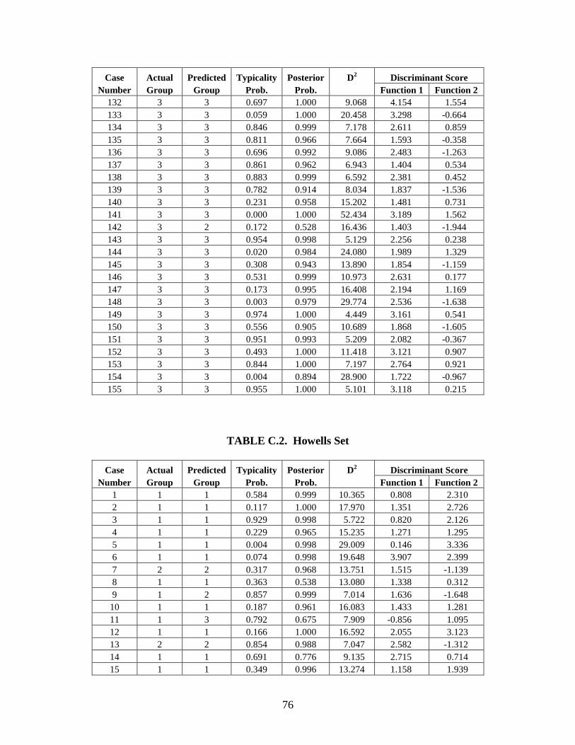
76

Case Actual Predicted Typicality Posterior D2 Discriminant Score

Number Group Group Prob. Prob. Function 1 Function 2

132 3 3 0.697 1.000 9.068 4.154 1.554

133 3 3 0.059 1.000 20.458 3.298 -0.664

134 3 3 0.846 0.999 7.178 2.611 0.859

135 3 3 0.811 0.966 7.664 1.593 -0.358

136 3 3 0.696 0.992 9.086 2.483 -1.263

137 3 3 0.861 0.962 6.943 1.404 0.534

138 3 3 0.883 0.999 6.592 2.381 0.452

139 3 3 0.782 0.914 8.034 1.837 -1.536

140 3 3 0.231 0.958 15.202 1.481 0.731

141 3 3 0.000 1.000 52.434 3.189 1.562

142 3 2 0.172 0.528 16.436 1.403 -1.944

143 3 3 0.954 0.998 5.129 2.256 0.238

144 3 3 0.020 0.984 24.080 1.989 1.329

145 3 3 0.308 0.943 13.890 1.854 -1.159

146 3 3 0.531 0.999 10.973 2.631 0.177

147 3 3 0.173 0.995 16.408 2.194 1.169

148 3 3 0.003 0.979 29.774 2.536 -1.638

149 3 3 0.974 1.000 4.449 3.161 0.541

150 3 3 0.556 0.905 10.689 1.868 -1.605

151 3 3 0.951 0.993 5.209 2.082 -0.367

152 3 3 0.493 1.000 11.418 3.121 0.907

153 3 3 0.844 1.000 7.197 2.764 0.921

154 3 3 0.004 0.894 28.900 1.722 -0.967

155 3 3 0.955 1.000 5.101 3.118 0.215

TABLE C.2. Howells Set

Case Actual Predicted Typicality Posterior D2 Discriminant Score

Number Group Group Prob. Prob. Function 1 Function 2

1 1 1 0.584 0.999 10.365 0.808 2.310

2 1 1 0.117 1.000 17.970 1.351 2.726

3 1 1 0.929 0.998 5.722 0.820 2.126

4 1 1 0.229 0.965 15.235 1.271 1.295

5 1 1 0.004 0.998 29.009 0.146 3.336

6 1 1 0.074 0.998 19.648 3.907 2.399

7 2 2 0.317 0.968 13.751 1.515 -1.139

8 1 1 0.363 0.538 13.080 1.338 0.312

9 1 2 0.857 0.999 7.014 1.636 -1.648

10 1 1 0.187 0.961 16.083 1.433 1.281

11 1 3 0.792 0.675 7.909 -0.856 1.095

12 1 1 0.166 1.000 16.592 2.055 3.123

13 2 2 0.854 0.988 7.047 2.582 -1.312

14 1 1 0.691 0.776 9.135 2.715 0.714

15 1 1 0.349 0.996 13.274 1.158 1.939

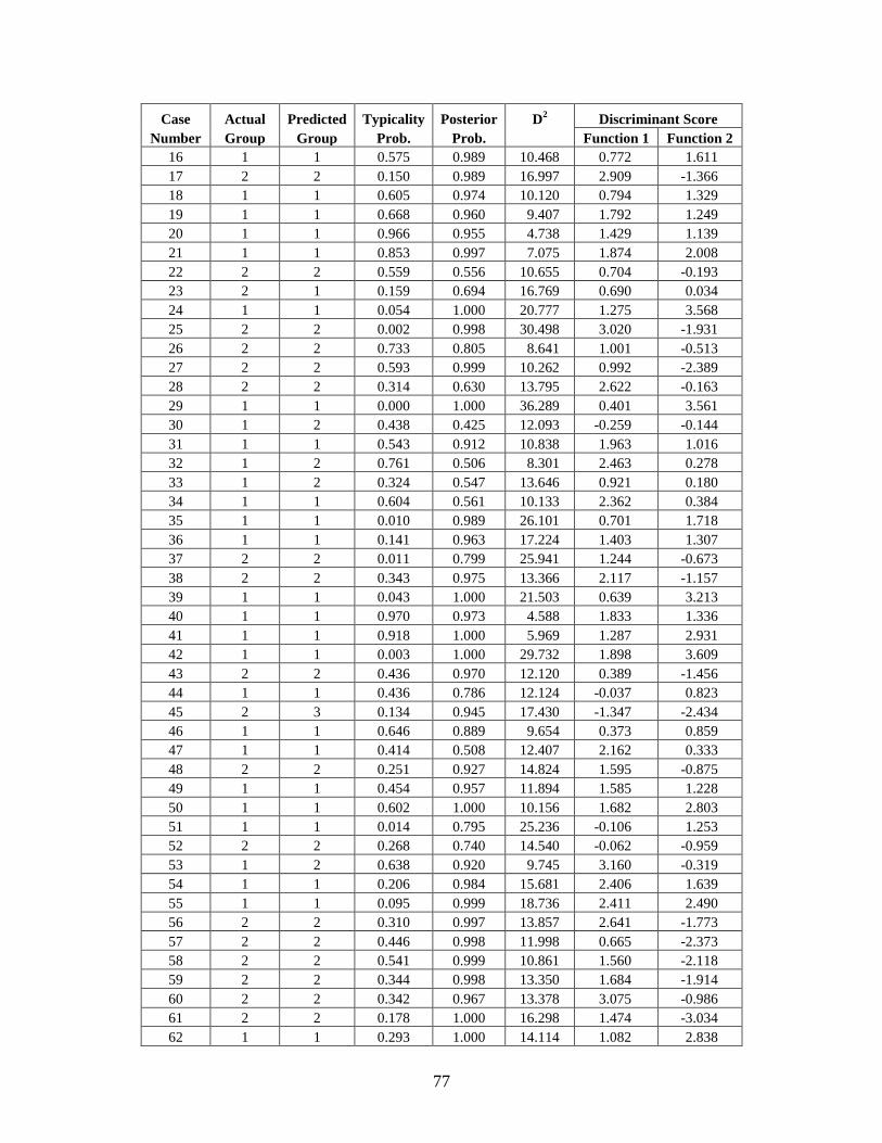
77

Case Actual Predicted Typicality Posterior D2 Discriminant Score

Number Group Group Prob. Prob. Function 1 Function 2

16 1 1 0.575 0.989 10.468 0.772 1.611

17 2 2 0.150 0.989 16.997 2.909 -1.366

18 1 1 0.605 0.974 10.120 0.794 1.329

19 1 1 0.668 0.960 9.407 1.792 1.249

20 1 1 0.966 0.955 4.738 1.429 1.139

21 1 1 0.853 0.997 7.075 1.874 2.008

22 2 2 0.559 0.556 10.655 0.704 -0.193

23 2 1 0.159 0.694 16.769 0.690 0.034

24 1 1 0.054 1.000 20.777 1.275 3.568

25 2 2 0.002 0.998 30.498 3.020 -1.931

26 2 2 0.733 0.805 8.641 1.001 -0.513

27 2 2 0.593 0.999 10.262 0.992 -2.389

28 2 2 0.314 0.630 13.795 2.622 -0.163

29 1 1 0.000 1.000 36.289 0.401 3.561

30 1 2 0.438 0.425 12.093 -0.259 -0.144

31 1 1 0.543 0.912 10.838 1.963 1.016

32 1 2 0.761 0.506 8.301 2.463 0.278

33 1 2 0.324 0.547 13.646 0.921 0.180

34 1 1 0.604 0.561 10.133 2.362 0.384

35 1 1 0.010 0.989 26.101 0.701 1.718

36 1 1 0.141 0.963 17.224 1.403 1.307

37 2 2 0.011 0.799 25.941 1.244 -0.673

38 2 2 0.343 0.975 13.366 2.117 -1.157

39 1 1 0.043 1.000 21.503 0.639 3.213

40 1 1 0.970 0.973 4.588 1.833 1.336

41 1 1 0.918 1.000 5.969 1.287 2.931

42 1 1 0.003 1.000 29.732 1.898 3.609

43 2 2 0.436 0.970 12.120 0.389 -1.456

44 1 1 0.436 0.786 12.124 -0.037 0.823

45 2 3 0.134 0.945 17.430 -1.347 -2.434

46 1 1 0.646 0.889 9.654 0.373 0.859

47 1 1 0.414 0.508 12.407 2.162 0.333

48 2 2 0.251 0.927 14.824 1.595 -0.875

49 1 1 0.454 0.957 11.894 1.585 1.228

50 1 1 0.602 1.000 10.156 1.682 2.803

51 1 1 0.014 0.795 25.236 -0.106 1.253

52 2 2 0.268 0.740 14.540 -0.062 -0.959

53 1 2 0.638 0.920 9.745 3.160 -0.319

54 1 1 0.206 0.984 15.681 2.406 1.639

55 1 1 0.095 0.999 18.736 2.411 2.490

56 2 2 0.310 0.997 13.857 2.641 -1.773

57 2 2 0.446 0.998 11.998 0.665 -2.373

58 2 2 0.541 0.999 10.861 1.560 -2.118

59 2 2 0.344 0.998 13.350 1.684 -1.914

60 2 2 0.342 0.967 13.378 3.075 -0.986

61 2 2 0.178 1.000 16.298 1.474 -3.034

62 1 1 0.293 1.000 14.114 1.082 2.838

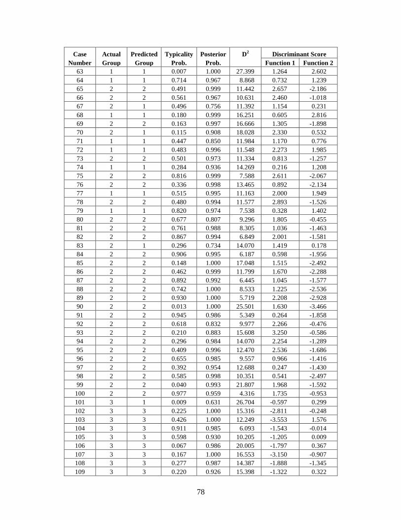
78

Case Actual Predicted Typicality Posterior D2 Discriminant Score

Number Group Group Prob. Prob. Function 1 Function 2

63 1 1 0.007 1.000 27.399 1.264 2.602

64 1 1 0.714 0.967 8.868 0.732 1.239

65 2 2 0.491 0.999 11.442 2.657 -2.186

66 2 2 0.561 0.967 10.631 2.460 -1.018

67 2 1 0.496 0.756 11.392 1.154 0.231

68 1 1 0.180 0.999 16.251 0.605 2.816

69 2 2 0.163 0.997 16.666 1.305 -1.898

70 2 1 0.115 0.908 18.028 2.330 0.532

71 1 1 0.447 0.850 11.984 1.170 0.776

72 1 1 0.483 0.996 11.548 2.273 1.985

73 2 2 0.501 0.973 11.334 0.813 -1.257

74 1 1 0.284 0.936 14.269 0.216 1.208

75 2 2 0.816 0.999 7.588 2.611 -2.067

76 2 2 0.336 0.998 13.465 0.892 -2.134

77 1 1 0.515 0.995 11.163 2.000 1.949

78 2 2 0.480 0.994 11.577 2.893 -1.526

79 1 1 0.820 0.974 7.538 0.328 1.402

80 2 2 0.677 0.807 9.296 1.805 -0.455

81 2 2 0.761 0.988 8.305 1.036 -1.463

82 2 2 0.867 0.994 6.849 2.001 -1.581

83 2 1 0.296 0.734 14.070 1.419 0.178

84 2 2 0.906 0.995 6.187 0.598 -1.956

85 2 2 0.148 1.000 17.048 1.515 -2.492

86 2 2 0.462 0.999 11.799 1.670 -2.288

87 2 2 0.892 0.992 6.445 1.045 -1.577

88 2 2 0.742 1.000 8.533 1.225 -2.536

89 2 2 0.930 1.000 5.719 2.208 -2.928

90 2 2 0.013 1.000 25.501 1.630 -3.466

91 2 2 0.945 0.986 5.349 0.264 -1.858

92 2 2 0.618 0.832 9.977 2.266 -0.476

93 2 2 0.210 0.883 15.608 3.250 -0.586

94 2 2 0.296 0.984 14.070 2.254 -1.289

95 2 2 0.409 0.996 12.470 2.536 -1.686

96 2 2 0.655 0.985 9.557 0.966 -1.416

97 2 2 0.392 0.954 12.688 0.247 -1.430

98 2 2 0.585 0.998 10.351 0.541 -2.497

99 2 2 0.040 0.993 21.807 1.968 -1.592

100 2 2 0.977 0.959 4.316 1.735 -0.953

101 3 1 0.009 0.631 26.704 -0.597 0.299

102 3 3 0.225 1.000 15.316 -2.811 -0.248

103 3 3 0.426 1.000 12.249 -3.553 1.576

104 3 3 0.911 0.985 6.093 -1.543 -0.014

105 3 3 0.598 0.930 10.205 -1.205 0.009

106 3 3 0.067 0.986 20.005 -1.797 0.367

107 3 3 0.167 1.000 16.553 -3.150 -0.907

108 3 3 0.277 0.987 14.387 -1.888 -1.345

109 3 3 0.220 0.926 15.398 -1.322 0.322

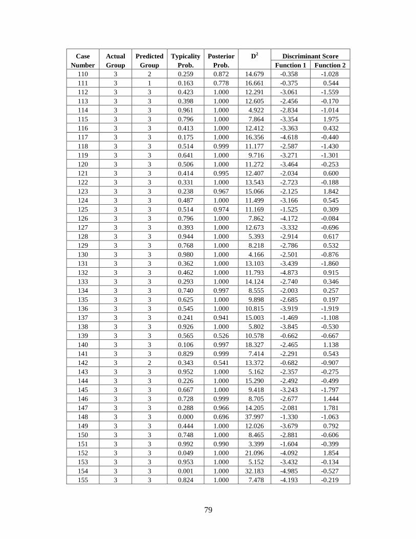
79

Case Actual Predicted Typicality Posterior D2 Discriminant Score

Number Group Group Prob. Prob. Function 1 Function 2

110 3 2 0.259 0.872 14.679 -0.358 -1.028

111 3 1 0.163 0.778 16.661 -0.375 0.544

112 3 3 0.423 1.000 12.291 -3.061 -1.559

113 3 3 0.398 1.000 12.605 -2.456 -0.170

114 3 3 0.961 1.000 4.922 -2.834 -1.014

115 3 3 0.796 1.000 7.864 -3.354 1.975

116 3 3 0.413 1.000 12.412 -3.363 0.432

117 3 3 0.175 1.000 16.356 -4.618 -0.440

118 3 3 0.514 0.999 11.177 -2.587 -1.430

119 3 3 0.641 1.000 9.716 -3.271 -1.301

120 3 3 0.506 1.000 11.272 -3.464 -0.253

121 3 3 0.414 0.995 12.407 -2.034 0.600

122 3 3 0.331 1.000 13.543 -2.723 -0.188

123 3 3 0.238 0.967 15.066 -2.125 1.842

124 3 3 0.487 1.000 11.499 -3.166 0.545

125 3 3 0.514 0.974 11.169 -1.525 0.309

126 3 3 0.796 1.000 7.862 -4.172 -0.084

127 3 3 0.393 1.000 12.673 -3.332 -0.696

128 3 3 0.944 1.000 5.393 -2.914 0.617

129 3 3 0.768 1.000 8.218 -2.786 0.532

130 3 3 0.980 1.000 4.166 -2.501 -0.876

131 3 3 0.362 1.000 13.103 -3.439 -1.860

132 3 3 0.462 1.000 11.793 -4.873 0.915

133 3 3 0.293 1.000 14.124 -2.740 0.346

134 3 3 0.740 0.997 8.555 -2.003 0.257

135 3 3 0.625 1.000 9.898 -2.685 0.197

136 3 3 0.545 1.000 10.815 -3.919 -1.919

137 3 3 0.241 0.941 15.003 -1.469 -1.108

138 3 3 0.926 1.000 5.802 -3.845 -0.530

139 3 3 0.565 0.526 10.578 -0.662 -0.667

140 3 3 0.106 0.997 18.327 -2.465 1.138

141 3 3 0.829 0.999 7.414 -2.291 0.543

142 3 2 0.343 0.541 13.372 -0.682 -0.907

143 3 3 0.952 1.000 5.162 -2.357 -0.275

144 3 3 0.226 1.000 15.290 -2.492 -0.499

145 3 3 0.667 1.000 9.418 -3.243 -1.797

146 3 3 0.728 0.999 8.705 -2.677 1.444

147 3 3 0.288 0.966 14.205 -2.081 1.781

148 3 3 0.000 0.696 37.997 -1.330 -1.063

149 3 3 0.444 1.000 12.026 -3.679 0.792

150 3 3 0.748 1.000 8.465 -2.881 -0.606

151 3 3 0.992 0.990 3.399 -1.604 -0.399

152 3 3 0.049 1.000 21.096 -4.092 1.854

153 3 3 0.953 1.000 5.152 -3.432 -0.134

154 3 3 0.001 1.000 32.183 -4.985 -0.527

155 3 3 0.824 1.000 7.478 -4.193 -0.219

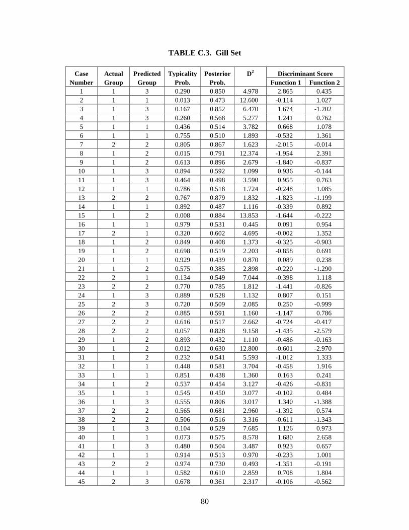
80

TABLE C.3. Gill Set

Case Actual Predicted Typicality Posterior D2 Discriminant Score

Number Group Group Prob. Prob. Function 1 Function 2

1 1 3 0.290 0.850 4.978 2.865 0.435

2 1 1 0.013 0.473 12.600 -0.114 1.027

3 1 3 0.167 0.852 6.470 1.674 -1.202

4 1 3 0.260 0.568 5.277 1.241 0.762

5 1 1 0.436 0.514 3.782 0.668 1.078

6 1 1 0.755 0.510 1.893 -0.532 1.361

7 2 2 0.805 0.867 1.623 -2.015 -0.014

8 1 2 0.015 0.791 12.374 -1.954 2.391

9 1 2 0.613 0.896 2.679 -1.840 -0.837

10 1 3 0.894 0.592 1.099 0.936 -0.144

11 1 3 0.464 0.498 3.590 0.955 0.763

12 1 1 0.786 0.518 1.724 -0.248 1.085

13 2 2 0.767 0.879 1.832 -1.823 -1.199

14 1 1 0.892 0.487 1.116 -0.339 0.892

15 1 2 0.008 0.884 13.853 -1.644 -0.222

16 1 1 0.979 0.531 0.445 0.091 0.954

17 2 1 0.320 0.602 4.695 -0.002 1.352

18 1 2 0.849 0.408 1.373 -0.325 -0.903

19 1 2 0.698 0.519 2.203 -0.858 0.691

20 1 1 0.929 0.439 0.870 0.089 0.238

21 1 2 0.575 0.385 2.898 -0.220 -1.290

22 2 1 0.134 0.549 7.044 -0.398 1.118

23 2 2 0.770 0.785 1.812 -1.441 -0.826

24 1 3 0.889 0.528 1.132 0.807 0.151

25 2 3 0.720 0.509 2.085 0.250 -0.999

26 2 2 0.885 0.591 1.160 -1.147 0.786

27 2 2 0.616 0.517 2.662 -0.724 -0.417

28 2 2 0.057 0.828 9.158 -1.435 -2.579

29 1 2 0.893 0.432 1.110 -0.486 -0.163

30 1 2 0.012 0.630 12.800 -0.601 -2.970

31 1 2 0.232 0.541 5.593 -1.012 1.333

32 1 1 0.448 0.581 3.704 -0.458 1.916

33 1 1 0.851 0.438 1.360 0.163 0.241

34 1 2 0.537 0.454 3.127 -0.426 -0.831

35 1 1 0.545 0.450 3.077 -0.102 0.484

36 1 3 0.555 0.806 3.017 1.340 -1.388

37 2 2 0.565 0.681 2.960 -1.392 0.574

38 2 2 0.506 0.516 3.316 -0.611 -1.343

39 1 3 0.104 0.529 7.685 1.126 0.973

40 1 1 0.073 0.575 8.578 1.680 2.658

41 1 3 0.480 0.504 3.487 0.923 0.657

42 1 1 0.914 0.513 0.970 -0.233 1.001

43 2 2 0.974 0.730 0.493 -1.351 -0.191

44 1 1 0.582 0.610 2.859 0.708 1.804

45 2 3 0.678 0.361 2.317 -0.106 -0.562

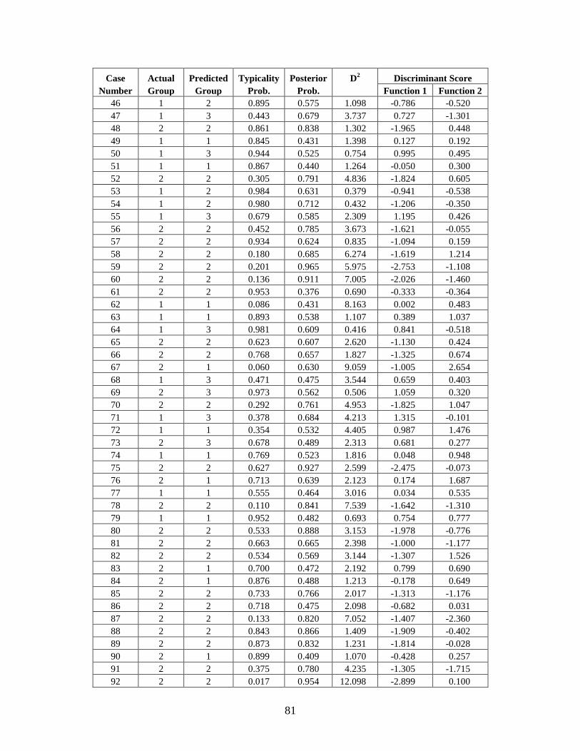
81

Case Actual Predicted Typicality Posterior D2 Discriminant Score

Number Group Group Prob. Prob. Function 1 Function 2

46 1 2 0.895 0.575 1.098 -0.786 -0.520

47 1 3 0.443 0.679 3.737 0.727 -1.301

48 2 2 0.861 0.838 1.302 -1.965 0.448

49 1 1 0.845 0.431 1.398 0.127 0.192

50 1 3 0.944 0.525 0.754 0.995 0.495

51 1 1 0.867 0.440 1.264 -0.050 0.300

52 2 2 0.305 0.791 4.836 -1.824 0.605

53 1 2 0.984 0.631 0.379 -0.941 -0.538

54 1 2 0.980 0.712 0.432 -1.206 -0.350

55 1 3 0.679 0.585 2.309 1.195 0.426

56 2 2 0.452 0.785 3.673 -1.621 -0.055

57 2 2 0.934 0.624 0.835 -1.094 0.159

58 2 2 0.180 0.685 6.274 -1.619 1.214

59 2 2 0.201 0.965 5.975 -2.753 -1.108

60 2 2 0.136 0.911 7.005 -2.026 -1.460

61 2 2 0.953 0.376 0.690 -0.333 -0.364

62 1 1 0.086 0.431 8.163 0.002 0.483

63 1 1 0.893 0.538 1.107 0.389 1.037

64 1 3 0.981 0.609 0.416 0.841 -0.518

65 2 2 0.623 0.607 2.620 -1.130 0.424

66 2 2 0.768 0.657 1.827 -1.325 0.674

67 2 1 0.060 0.630 9.059 -1.005 2.654

68 1 3 0.471 0.475 3.544 0.659 0.403

69 2 3 0.973 0.562 0.506 1.059 0.320

70 2 2 0.292 0.761 4.953 -1.825 1.047

71 1 3 0.378 0.684 4.213 1.315 -0.101

72 1 1 0.354 0.532 4.405 0.987 1.476

73 2 3 0.678 0.489 2.313 0.681 0.277

74 1 1 0.769 0.523 1.816 0.048 0.948

75 2 2 0.627 0.927 2.599 -2.475 -0.073

76 2 1 0.713 0.639 2.123 0.174 1.687

77 1 1 0.555 0.464 3.016 0.034 0.535

78 2 2 0.110 0.841 7.539 -1.642 -1.310

79 1 1 0.952 0.482 0.693 0.754 0.777

80 2 2 0.533 0.888 3.153 -1.978 -0.776

81 2 2 0.663 0.665 2.398 -1.000 -1.177

82 2 2 0.534 0.569 3.144 -1.307 1.526

83 2 1 0.700 0.472 2.192 0.799 0.690

84 2 1 0.876 0.488 1.213 -0.178 0.649

85 2 2 0.733 0.766 2.017 -1.313 -1.176

86 2 2 0.718 0.475 2.098 -0.682 0.031

87 2 2 0.133 0.820 7.052 -1.407 -2.360

88 2 2 0.843 0.866 1.409 -1.909 -0.402

89 2 2 0.873 0.832 1.231 -1.814 -0.028

90 2 1 0.899 0.409 1.070 -0.428 0.257

91 2 2 0.375 0.780 4.235 -1.305 -1.715

92 2 2 0.017 0.954 12.098 -2.899 0.100

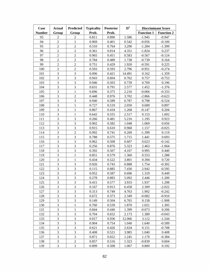
82

Case Actual Predicted Typicality Posterior D2 Discriminant Score

Number Group Group Prob. Prob. Function 1 Function 2

93 2 2 0.811 0.890 1.586 -1.945 -0.947

94 2 1 0.969 0.401 0.542 -0.056 -0.100

95 2 2 0.510 0.764 3.290 -1.284 -1.399

96 2 2 0.361 0.814 4.351 -1.824 0.237

97 2 2 0.965 0.451 0.583 -0.567 -0.124

98 2 2 0.784 0.489 1.738 -0.739 0.164

99 2 2 0.751 0.429 1.920 -0.591 0.225

100 2 2 0.593 0.593 2.796 -0.951 -0.274

101 3 3 0.006 0.421 14.491 0.162 -1.359

102 3 3 0.943 0.604 0.762 0.757 -0.753

103 3 3 0.946 0.503 0.739 0.769 0.196

104 3 3 0.631 0.791 2.577 1.452 -1.376

105 3 1 0.696 0.375 2.216 -0.066 -0.333

106 3 2 0.448 0.976 3.702 -2.866 -0.623

107 3 3 0.940 0.589 0.787 0.798 -0.524

108 3 1 0.727 0.519 2.050 0.689 0.897

109 3 1 0.867 0.434 1.268 -0.147 0.204

110 3 1 0.642 0.555 2.517 0.153 1.002

111 3 3 0.266 0.481 5.216 1.195 0.923

112 3 3 0.902 0.582 1.048 1.069 0.056

113 3 3 0.915 0.610 0.968 1.157 -0.025

114 3 2 0.992 0.741 0.269 -1.399 0.119

115 3 3 0.788 0.575 1.715 1.441 0.693

116 3 3 0.962 0.508 0.607 0.623 -0.142

117 3 3 0.256 0.876 5.323 2.463 -1.064

118 3 3 0.392 0.507 4.107 0.995 0.440

119 3 1 0.851 0.579 1.360 0.553 1.288

120 3 1 0.434 0.522 3.801 0.394 0.720

121 3 3 0.926 0.743 0.888 1.754 -0.302

122 3 3 0.115 0.885 7.430 2.942 -0.595

123 3 3 0.952 0.587 0.696 1.319 0.449

124 3 3 0.278 0.883 5.092 2.446 -1.200

125 3 3 0.415 0.577 3.933 1.937 1.298

126 3 3 0.167 0.913 6.458 2.309 -2.022

127 3 3 0.313 0.749 4.763 1.902 -0.242

128 3 3 0.672 0.373 2.349 -0.082 -0.910

129 3 3 0.149 0.504 6.765 0.158 -1.908

130 3 1 0.760 0.539 1.870 1.021 1.305

131 3 1 0.844 0.440 1.399 -0.073 0.206

132 3 3 0.704 0.652 2.173 1.389 -0.043

133 3 3 0.017 0.936 12.066 3.112 -1.544

134 3 3 0.904 0.754 1.040 1.640 -0.589

135 3 3 0.621 0.426 2.634 0.151 -0.708

136 3 3 0.408 0.521 3.985 1.040 0.408

137 3 3 0.871 0.652 1.245 1.170 -0.384

138 3 2 0.857 0.516 1.323 -0.839 0.604

139 3 3 0.899 0.508 1.067 0.800 0.192

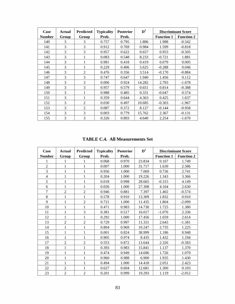
83

Case Actual Predicted Typicality Posterior D2 Discriminant Score

Number Group Group Prob. Prob. Function 1 Function 2

140 3 3 0.757 0.795 1.886 1.988 -0.542

141 3 3 0.912 0.769 0.984 1.599 -0.818

142 3 3 0.957 0.622 0.657 0.953 -0.505

143 3 1 0.083 0.548 8.233 -0.721 1.881

144 3 1 0.981 0.418 0.419 0.079 0.005

145 3 1 0.229 0.406 5.625 -0.288 0.046

146 3 2 0.476 0.356 3.514 -0.170 -0.884

147 3 3 0.747 0.647 1.940 1.456 0.112

148 3 3 0.006 0.924 14.282 2.783 -1.678

149 3 3 0.957 0.579 0.651 0.814 -0.388

150 3 1 0.988 0.485 0.331 -0.047 0.574

151 3 1 0.359 0.644 4.363 0.425 1.637

152 3 2 0.030 0.497 10.685 -0.303 -1.967

153 3 2 0.087 0.372 8.127 -0.144 -0.958

154 3 3 0.003 0.779 15.762 2.367 -0.131

155 3 3 0.326 0.893 4.640 2.254 -1.670

TABLE C.4. All Measurements Set

Case Actual Predicted Typicality Posterior D2 Discriminant Score

Number Group Group Prob. Prob. Function 1 Function 2

1 1 1 0.068 0.970 23.834 0.167 1.749

2 1 1 0.007 1.000 31.717 1.639 2.586

3 1 1 0.956 1.000 7.069 0.736 2.741

4 1 1 0.204 1.000 19.226 1.343 3.366

5 1 1 0.018 0.998 28.665 -0.315 4.149

6 1 1 0.026 1.000 27.308 4.164 2.630

7 2 2 0.946 0.881 7.397 1.402 -0.574

8 1 1 0.578 0.910 13.309 1.832 0.910

9 1 2 0.721 1.000 11.435 1.804 -2.099

10 1 1 0.471 0.983 14.730 1.725 1.380

11 1 3 0.381 0.517 16.017 -1.076 2.336

12 1 1 0.292 1.000 17.456 1.659 2.614

13 2 2 0.729 0.997 11.331 2.643 -1.581

14 1 1 0.804 0.969 10.247 2.735 1.225

15 1 1 0.001 0.824 38.999 1.186 0.948

16 1 1 0.905 0.974 8.435 1.432 1.194

17 2 2 0.553 0.872 13.644 2.326 -0.583

18 1 1 0.393 0.983 15.841 1.137 1.370

19 1 1 0.474 0.949 14.696 1.726 1.079

20 1 1 0.960 0.988 6.900 1.935 1.430

21 1 1 0.494 1.000 14.418 2.051 2.423

22 2 1 0.627 0.694 12.681 1.300 0.103

23 2 2 0.201 0.999 19.293 1.119 -2.012

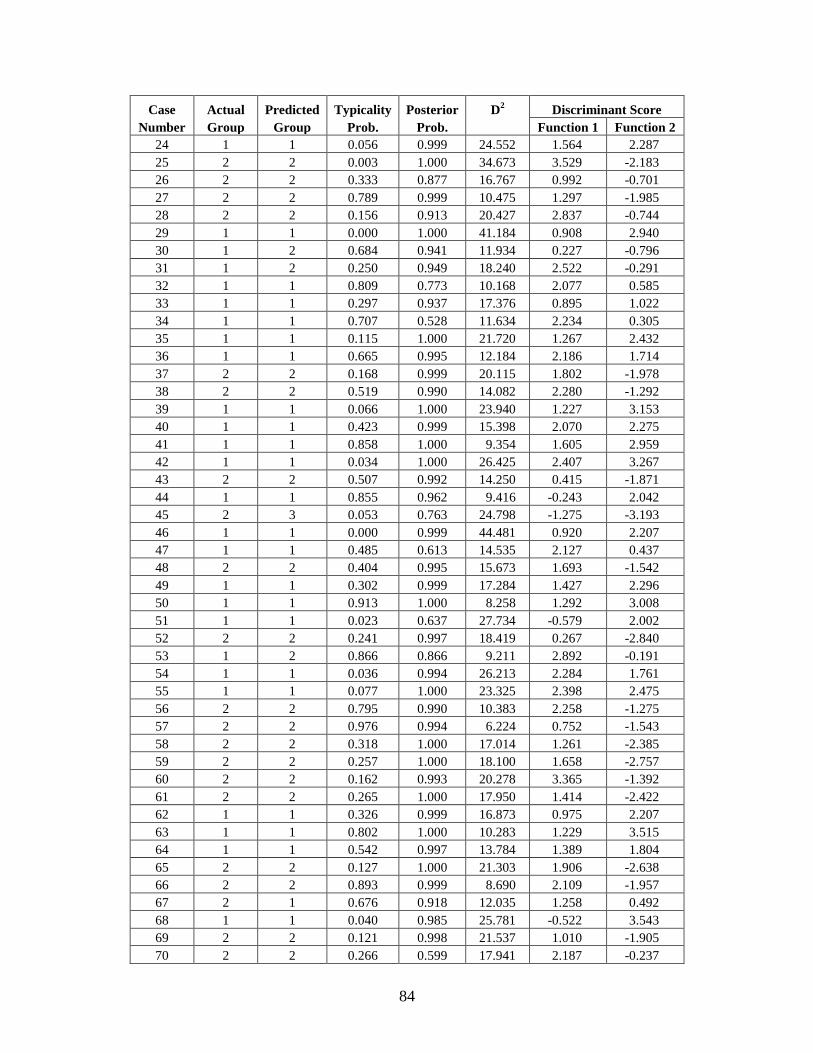
84

Case Actual Predicted Typicality Posterior D2 Discriminant Score

Number Group Group Prob. Prob. Function 1 Function 2

24 1 1 0.056 0.999 24.552 1.564 2.287

25 2 2 0.003 1.000 34.673 3.529 -2.183

26 2 2 0.333 0.877 16.767 0.992 -0.701

27 2 2 0.789 0.999 10.475 1.297 -1.985

28 2 2 0.156 0.913 20.427 2.837 -0.744

29 1 1 0.000 1.000 41.184 0.908 2.940

30 1 2 0.684 0.941 11.934 0.227 -0.796

31 1 2 0.250 0.949 18.240 2.522 -0.291

32 1 1 0.809 0.773 10.168 2.077 0.585

33 1 1 0.297 0.937 17.376 0.895 1.022

34 1 1 0.707 0.528 11.634 2.234 0.305

35 1 1 0.115 1.000 21.720 1.267 2.432

36 1 1 0.665 0.995 12.184 2.186 1.714

37 2 2 0.168 0.999 20.115 1.802 -1.978

38 2 2 0.519 0.990 14.082 2.280 -1.292

39 1 1 0.066 1.000 23.940 1.227 3.153

40 1 1 0.423 0.999 15.398 2.070 2.275

41 1 1 0.858 1.000 9.354 1.605 2.959

42 1 1 0.034 1.000 26.425 2.407 3.267

43 2 2 0.507 0.992 14.250 0.415 -1.871

44 1 1 0.855 0.962 9.416 -0.243 2.042

45 2 3 0.053 0.763 24.798 -1.275 -3.193

46 1 1 0.000 0.999 44.481 0.920 2.207

47 1 1 0.485 0.613 14.535 2.127 0.437

48 2 2 0.404 0.995 15.673 1.693 -1.542

49 1 1 0.302 0.999 17.284 1.427 2.296

50 1 1 0.913 1.000 8.258 1.292 3.008

51 1 1 0.023 0.637 27.734 -0.579 2.002

52 2 2 0.241 0.997 18.419 0.267 -2.840

53 1 2 0.866 0.866 9.211 2.892 -0.191

54 1 1 0.036 0.994 26.213 2.284 1.761

55 1 1 0.077 1.000 23.325 2.398 2.475

56 2 2 0.795 0.990 10.383 2.258 -1.275

57 2 2 0.976 0.994 6.224 0.752 -1.543

58 2 2 0.318 1.000 17.014 1.261 -2.385

59 2 2 0.257 1.000 18.100 1.658 -2.757

60 2 2 0.162 0.993 20.278 3.365 -1.392

61 2 2 0.265 1.000 17.950 1.414 -2.422

62 1 1 0.326 0.999 16.873 0.975 2.207

63 1 1 0.802 1.000 10.283 1.229 3.515

64 1 1 0.542 0.997 13.784 1.389 1.804

65 2 2 0.127 1.000 21.303 1.906 -2.638

66 2 2 0.893 0.999 8.690 2.109 -1.957

67 2 1 0.676 0.918 12.035 1.258 0.492

68 1 1 0.040 0.985 25.781 -0.522 3.543

69 2 2 0.121 0.998 21.537 1.010 -1.905

70 2 2 0.266 0.599 17.941 2.187 -0.237

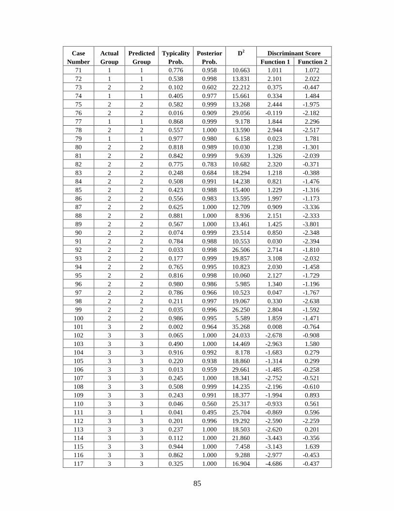
85

Case Actual Predicted Typicality Posterior D2 Discriminant Score

Number Group Group Prob. Prob. Function 1 Function 2

71 1 1 0.776 0.958 10.663 1.011 1.072

72 1 1 0.538 0.998 13.831 2.101 2.022

73 2 2 0.102 0.602 22.212 0.375 -0.447

74 1 1 0.405 0.977 15.661 0.334 1.484

75 2 2 0.582 0.999 13.268 2.444 -1.975

76 2 2 0.016 0.909 29.056 -0.119 -2.182

77 1 1 0.868 0.999 9.178 1.844 2.296

78 2 2 0.557 1.000 13.590 2.944 -2.517

79 1 1 0.977 0.980 6.158 0.023 1.781

80 2 2 0.818 0.989 10.030 1.238 -1.301

81 2 2 0.842 0.999 9.639 1.326 -2.039

82 2 2 0.775 0.783 10.682 2.320 -0.371

83 2 2 0.248 0.684 18.294 1.218 -0.388

84 2 2 0.508 0.991 14.238 0.821 -1.476

85 2 2 0.423 0.988 15.400 1.229 -1.316

86 2 2 0.556 0.983 13.595 1.997 -1.173

87 2 2 0.625 1.000 12.709 0.909 -3.336

88 2 2 0.881 1.000 8.936 2.151 -2.333

89 2 2 0.567 1.000 13.461 1.425 -3.801

90 2 2 0.074 0.999 23.514 0.850 -2.348

91 2 2 0.784 0.988 10.553 0.030 -2.394

92 2 2 0.033 0.998 26.506 2.714 -1.810

93 2 2 0.177 0.999 19.857 3.108 -2.032

94 2 2 0.765 0.995 10.823 2.030 -1.458

95 2 2 0.816 0.998 10.060 2.127 -1.729

96 2 2 0.980 0.986 5.985 1.340 -1.196

97 2 2 0.786 0.966 10.523 0.047 -1.767

98 2 2 0.211 0.997 19.067 0.330 -2.638

99 2 2 0.035 0.996 26.250 2.804 -1.592

100 2 2 0.986 0.995 5.589 1.859 -1.471

101 3 2 0.002 0.964 35.268 0.008 -0.764

102 3 3 0.065 1.000 24.033 -2.678 -0.908

103 3 3 0.490 1.000 14.469 -2.963 1.580

104 3 3 0.916 0.992 8.178 -1.683 0.279

105 3 3 0.220 0.938 18.860 -1.314 0.299

106 3 3 0.013 0.959 29.661 -1.485 -0.258

107 3 3 0.245 1.000 18.341 -2.752 -0.521

108 3 3 0.508 0.999 14.235 -2.196 -0.610

109 3 3 0.243 0.991 18.377 -1.994 0.893

110 3 3 0.046 0.560 25.317 -0.933 0.561

111 3 1 0.041 0.495 25.704 -0.869 0.596

112 3 3 0.201 0.996 19.292 -2.590 -2.259

113 3 3 0.237 1.000 18.503 -2.620 0.201

114 3 3 0.112 1.000 21.860 -3.443 -0.356

115 3 3 0.944 1.000 7.458 -3.143 1.639

116 3 3 0.862 1.000 9.288 -2.977 -0.453

117 3 3 0.325 1.000 16.904 -4.686 -0.437

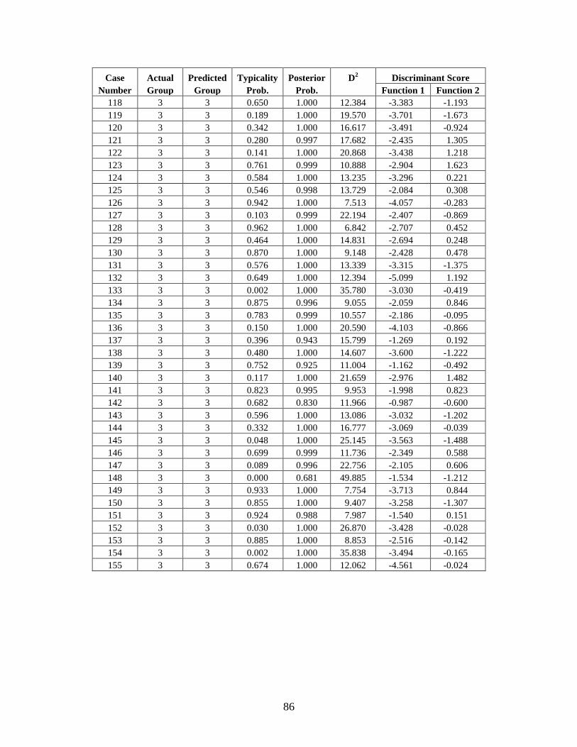
86

Case Actual Predicted Typicality Posterior D2 Discriminant Score

Number Group Group Prob. Prob. Function 1 Function 2

118 3 3 0.650 1.000 12.384 -3.383 -1.193

119 3 3 0.189 1.000 19.570 -3.701 -1.673

120 3 3 0.342 1.000 16.617 -3.491 -0.924

121 3 3 0.280 0.997 17.682 -2.435 1.305

122 3 3 0.141 1.000 20.868 -3.438 1.218

123 3 3 0.761 0.999 10.888 -2.904 1.623

124 3 3 0.584 1.000 13.235 -3.296 0.221

125 3 3 0.546 0.998 13.729 -2.084 0.308

126 3 3 0.942 1.000 7.513 -4.057 -0.283

127 3 3 0.103 0.999 22.194 -2.407 -0.869

128 3 3 0.962 1.000 6.842 -2.707 0.452

129 3 3 0.464 1.000 14.831 -2.694 0.248

130 3 3 0.870 1.000 9.148 -2.428 0.478

131 3 3 0.576 1.000 13.339 -3.315 -1.375

132 3 3 0.649 1.000 12.394 -5.099 1.192

133 3 3 0.002 1.000 35.780 -3.030 -0.419

134 3 3 0.875 0.996 9.055 -2.059 0.846

135 3 3 0.783 0.999 10.557 -2.186 -0.095

136 3 3 0.150 1.000 20.590 -4.103 -0.866

137 3 3 0.396 0.943 15.799 -1.269 0.192

138 3 3 0.480 1.000 14.607 -3.600 -1.222

139 3 3 0.752 0.925 11.004 -1.162 -0.492

140 3 3 0.117 1.000 21.659 -2.976 1.482

141 3 3 0.823 0.995 9.953 -1.998 0.823

142 3 3 0.682 0.830 11.966 -0.987 -0.600

143 3 3 0.596 1.000 13.086 -3.032 -1.202

144 3 3 0.332 1.000 16.777 -3.069 -0.039

145 3 3 0.048 1.000 25.145 -3.563 -1.488

146 3 3 0.699 0.999 11.736 -2.349 0.588

147 3 3 0.089 0.996 22.756 -2.105 0.606

148 3 3 0.000 0.681 49.885 -1.534 -1.212

149 3 3 0.933 1.000 7.754 -3.713 0.844

150 3 3 0.855 1.000 9.407 -3.258 -1.307

151 3 3 0.924 0.988 7.987 -1.540 0.151

152 3 3 0.030 1.000 26.870 -3.428 -0.028

153 3 3 0.885 1.000 8.853 -2.516 -0.142

154 3 3 0.002 1.000 35.838 -3.494 -0.165

155 3 3 0.674 1.000 12.062 -4.561 -0.024