Self-Healing Distributed Scheduling for End-to-End Delay

HAL Id: hal-02565978https://hal.archives-ouvertes.fr/hal-02565978

Submitted on 6 May 2020

HAL is a multi-disciplinary open accessarchive for the deposit and dissemination of sci-entific research documents, whether they are pub-lished or not. The documents may come fromteaching and research institutions in France orabroad, or from public or private research centers.

L’archive ouverte pluridisciplinaire HAL, estdestinée au dépôt et à la diffusion de documentsscientifiques de niveau recherche, publiés ou non,émanant des établissements d’enseignement et derecherche français ou étrangers, des laboratoirespublics ou privés.

Self-Healing Distributed Scheduling for End-to-EndDelay Optimization in Multihop Wireless Networks with

6TiSCHInès Hosni, Fabrice Theoleyre

To cite this version:Inès Hosni, Fabrice Theoleyre. Self-Healing Distributed Scheduling for End-to-End Delay Optimiza-tion in Multihop Wireless Networks with 6TiSCH. Computer Communications, Elsevier, 2017, 110,pp.103-119. �10.1016/j.comcom.2017.05.014�. �hal-02565978�

https://hal.archives-ouvertes.fr/hal-02565978

https://hal.archives-ouvertes.fr

c©2017

This work is licensed under a Creative Commons “Attribution-NonCommercial-NoDerivatives 4.0 International” license.

Self-Healing Distributed Scheduling for End-to-End Delay Optimization inMultihop Wireless Networks with 6TiSCH?

Ines Hosnia,∗, Fabrice Theoleyreb,∗

aLaboratory Systems Communications, University of Tunis El Manar, National Engineering School of Tunis, TunisiabCNRS, ICube Laboratory, University of Strasbourg, Boulevard Sebastien Brant, 67412 Illkirch Cedex, France

Abstract

Time Slotted Channel Hopping (TSCH) is an amendment of the the IEEE 802.15.4 working group toprovide a low-power Medium Access Control (MAC) for the Internet of Things (IoT). This standard relieson techniques such as channel hopping and bandwidth reservation to ensure both energy savings and reliabletransmissions. Since many applications require low end-to-end delay (e.g. alarms), we propose here adistributed algorithm to schedule the transmissions with a short end-to-end delay. We divide the networkin stratums, regrouping all the nodes with the same depth in the DODAG constructed by RPL. Then,different time-frequency blocks are assigned deterministically to each stratum. By appropriately organizingthe blocks in the slotframe, we are able to deliver a packet before the end of the slotframe, whatever theroute length is. We present a simple analytical study to define the initial size of each block in a homogeneousscenario. We experimentally analyze the behavior of our strategy to validate its ability to provide both highreliability and low latency in a distributed manner.

Keywords: IEEE802.15.4-TSCH; end-to-end delay; self-healing; distributed scheduling; autonomous;large-scale experiments

1. Introduction

During the last years we have witnessed the emergence of a new paradigm called the nternet of Things(IoT), able to connect the physical and digital worlds. Smart Objects start to be interconnected, enablingnew usages for e.g. smart buildings or home automation [2].

After best-effort solutions, industrial networks now require high reliability with low latency [3]. TheIEEE802.15 working group has proposed the IEEE802.15.4-2015 amendment [4] to deal with low power lossynetworks. In particular, the TimeSlotted Channel Hopping (TSCH) mode aims to improve the reliability innoisy environments [5]. This standard was designed to cope with the specificities of the Internet of Things,where devices transmit periodically their measures to the Internet, through a border router [6]. A globalschedule provides a deterministic medium access: the standard assigns a set of time-frequency blocks to eachradio link. By appropriately selecting the set of transmitters in a given channel and timeslot, the network

?A short conference version of this paper has already been published [1]∗Corresponding authorsEmail addresses: [email protected] (Ines Hosni), [email protected] (Fabrice Theoleyre)

Preprint submitted to Computer Communications June 13, 2019

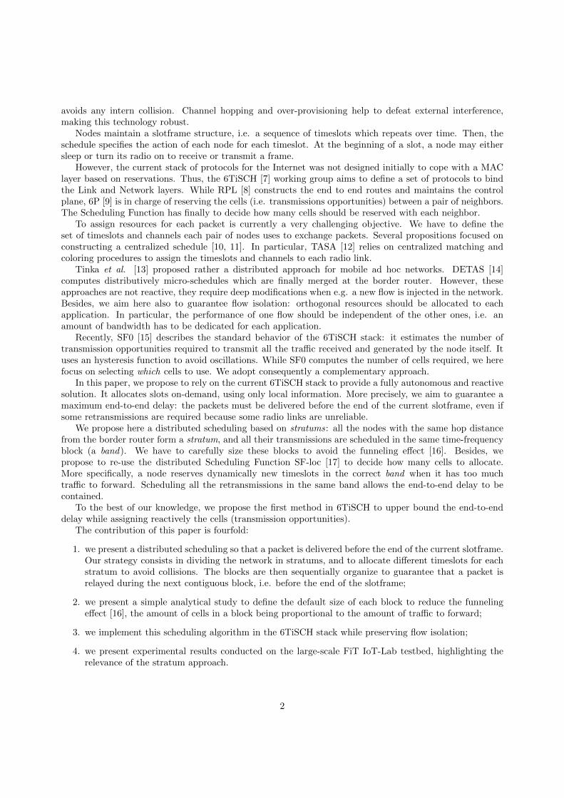
https://creativecommons.org/licenses/by-nc-nd/4.0/deed.en



avoids any intern collision. Channel hopping and over-provisioning help to defeat external interference,making this technology robust.

Nodes maintain a slotframe structure, i.e. a sequence of timeslots which repeats over time. Then, theschedule specifies the action of each node for each timeslot. At the beginning of a slot, a node may eithersleep or turn its radio on to receive or transmit a frame.

However, the current stack of protocols for the Internet was not designed initially to cope with a MAClayer based on reservations. Thus, the 6TiSCH [7] working group aims to define a set of protocols to bindthe Link and Network layers. While RPL [8] constructs the end to end routes and maintains the controlplane, 6P [9] is in charge of reserving the cells (i.e. transmissions opportunities) between a pair of neighbors.The Scheduling Function has finally to decide how many cells should be reserved with each neighbor.

To assign resources for each packet is currently a very challenging objective. We have to define theset of timeslots and channels each pair of nodes uses to exchange packets. Several propositions focused onconstructing a centralized schedule [10, 11]. In particular, TASA [12] relies on centralized matching andcoloring procedures to assign the timeslots and channels to each radio link.

Tinka et al. [13] proposed rather a distributed approach for mobile ad hoc networks. DETAS [14]computes distributively micro-schedules which are finally merged at the border router. However, theseapproaches are not reactive, they require deep modifications when e.g. a new flow is injected in the network.Besides, we aim here also to guarantee flow isolation: orthogonal resources should be allocated to eachapplication. In particular, the performance of one flow should be independent of the other ones, i.e. anamount of bandwidth has to be dedicated for each application.

Recently, SF0 [15] describes the standard behavior of the 6TiSCH stack: it estimates the number oftransmission opportunities required to transmit all the traffic received and generated by the node itself. Ituses an hysteresis function to avoid oscillations. While SF0 computes the number of cells required, we herefocus on selecting which cells to use. We adopt consequently a complementary approach.

In this paper, we propose to rely on the current 6TiSCH stack to provide a fully autonomous and reactivesolution. It allocates slots on-demand, using only local information. More precisely, we aim to guarantee amaximum end-to-end delay: the packets must be delivered before the end of the current slotframe, even ifsome retransmissions are required because some radio links are unreliable.

We propose here a distributed scheduling based on stratums: all the nodes with the same hop distancefrom the border router form a stratum, and all their transmissions are scheduled in the same time-frequencyblock (a band). We have to carefully size these blocks to avoid the funneling effect [16]. Besides, wepropose to re-use the distributed Scheduling Function SF-loc [17] to decide how many cells to allocate.More specifically, a node reserves dynamically new timeslots in the correct band when it has too muchtraffic to forward. Scheduling all the retransmissions in the same band allows the end-to-end delay to becontained.

To the best of our knowledge, we propose the first method in 6TiSCH to upper bound the end-to-enddelay while assigning reactively the cells (transmission opportunities).

The contribution of this paper is fourfold:

1. we present a distributed scheduling so that a packet is delivered before the end of the current slotframe.Our strategy consists in dividing the network in stratums, and to allocate different timeslots for eachstratum to avoid collisions. The blocks are then sequentially organize to guarantee that a packet isrelayed during the next contiguous block, i.e. before the end of the slotframe;

2. we present a simple analytical study to define the default size of each block to reduce the funnelingeffect [16], the amount of cells in a block being proportional to the amount of traffic to forward;

3. we implement this scheduling algorithm in the 6TiSCH stack while preserving flow isolation;

4. we present experimental results conducted on the large-scale FiT IoT-Lab testbed, highlighting therelevance of the stratum approach.

2

dedicated cells

B▶A

3

C▶A

2

1

timeslots

shared cell

B▶A

A

CB

D

unus

ed c

ells

0

E

D▶B

E▶C C▶A

radio link(and DODAG link)

flow

A

E

border router

device

B▶A

4320 1 765

chan

nel o

ffset

s

slotframe length

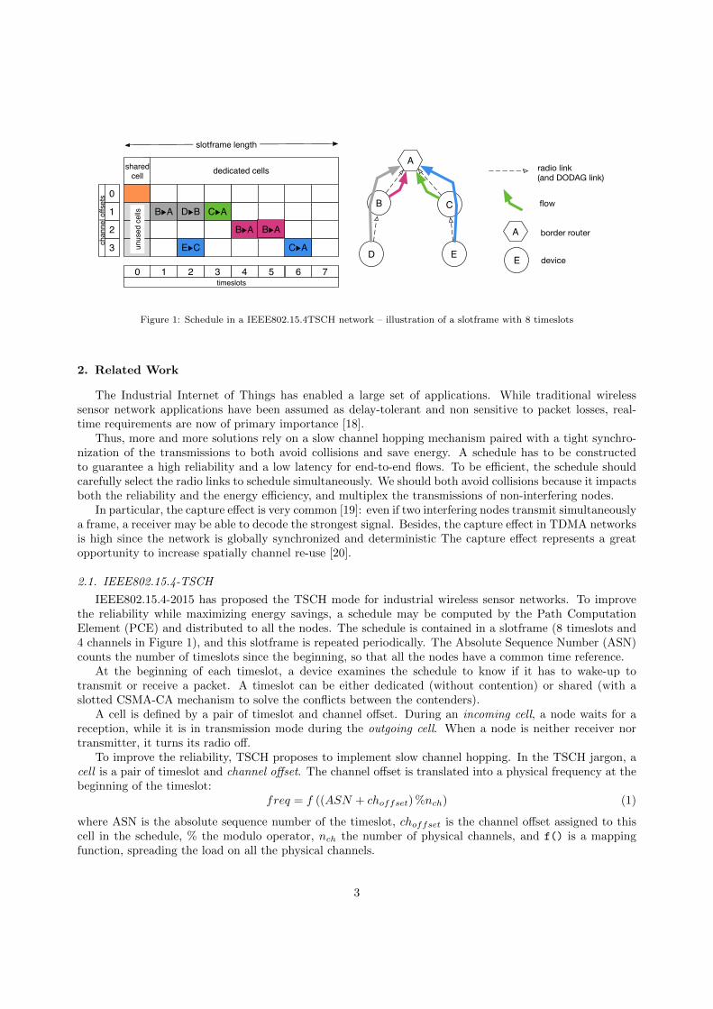
Figure 1: Schedule in a IEEE802.15.4TSCH network – illustration of a slotframe with 8 timeslots

2. Related Work

The Industrial Internet of Things has enabled a large set of applications. While traditional wirelesssensor network applications have been assumed as delay-tolerant and non sensitive to packet losses, real-time requirements are now of primary importance [18].

Thus, more and more solutions rely on a slow channel hopping mechanism paired with a tight synchro-nization of the transmissions to both avoid collisions and save energy. A schedule has to be constructedto guarantee a high reliability and a low latency for end-to-end flows. To be efficient, the schedule shouldcarefully select the radio links to schedule simultaneously. We should both avoid collisions because it impactsboth the reliability and the energy efficiency, and multiplex the transmissions of non-interfering nodes.

In particular, the capture effect is very common [19]: even if two interfering nodes transmit simultaneouslya frame, a receiver may be able to decode the strongest signal. Besides, the capture effect in TDMA networksis high since the network is globally synchronized and deterministic The capture effect represents a greatopportunity to increase spatially channel re-use [20].

2.1. IEEE802.15.4-TSCH

IEEE802.15.4-2015 has proposed the TSCH mode for industrial wireless sensor networks. To improvethe reliability while maximizing energy savings, a schedule may be computed by the Path ComputationElement (PCE) and distributed to all the nodes. The schedule is contained in a slotframe (8 timeslots and4 channels in Figure 1), and this slotframe is repeated periodically. The Absolute Sequence Number (ASN)counts the number of timeslots since the beginning, so that all the nodes have a common time reference.

At the beginning of each timeslot, a device examines the schedule to know if it has to wake-up totransmit or receive a packet. A timeslot can be either dedicated (without contention) or shared (with aslotted CSMA-CA mechanism to solve the conflicts between the contenders).

A cell is defined by a pair of timeslot and channel offset. During an incoming cell, a node waits for areception, while it is in transmission mode during the outgoing cell. When a node is neither receiver nortransmitter, it turns its radio off.

To improve the reliability, TSCH proposes to implement slow channel hopping. In the TSCH jargon, acell is a pair of timeslot and channel offset. The channel offset is translated into a physical frequency at thebeginning of the timeslot:

freq = f ((ASN + choffset) %nch) (1)

where ASN is the absolute sequence number of the timeslot, choffset is the channel offset assigned to thiscell in the schedule, % the modulo operator, nch the number of physical channels, and f() is a mappingfunction, spreading the load on all the physical channels.

3

Let’s consider the schedule illustrated in figure 1. As recommended by 6TiSCH minimal [21], we haveone shared cell at the beginning of the slotframe, using the channel offset 0. The shared cell is typicallyused for control traffic (i.e. new reservations, control packets for routing, beacons, etc.). The other cells arededicated: only the owner of the cell can transmit a packet, without contention. Each DODAG link hasone or several cells to forward the packets. The link A→B (pink) reserved for instance two dedicated cellsbecause it has many packets to forward, or because retransmissions are expected.

2.2. 6TiSCH

The 6TiSCH IETF working group aims to define the protocols to operate IPv6 (6LoWPAN) over areservation-based MAC layer (IEEE802.15.4-TSCH). 6TiSCH introduces the concept of tracks to reservean amount of dedicated cells for a particular flow [22]. Hop by hop, each intermediary node inserts in itsschedule some cells for each non best effort flow (i.e. track instance 6= 0). Label switching may be implicit:a node knows the track associated to an incoming cell, extracted directly from the schedule. Thus, it justhas to forward this packet in an outgoing cell with the same track id.

The protocol 6P defines how a node may negotiate a cell with a neighbor: the enquirer specifies a listof available < timeslot, channel offset > and the number of cells it asks for [9]. The neighbor will acceptthe request if these cells are available also in its schedule: it sends an Information Element to notify theenquirer. However, it does not define which cells should be selected.

Let’s consider the figure 1 which illustrates a possible schedule with 4 different tracks. We see that thelink B → A supports two tracks with respectively the source B (in pink) and the source D (in gray). Sinceeach track uses a different set of cells, flows are isolated : the packets of D do not impact the traffic of B.

Besides, the incoming cell in B for the flow from D (in gray) is scheduled after the outgoing cell. Thismeans the node B has to buffer the packets during a long time, until the next slotframe. Thus, the end-to-end delay is quite large. Thus, we have to carefully schedule the slots for each track to limit this bufferingdelay. In this paper, we use the 6TiSCH stack to reserve reactively the cells for each track: each flow reserveshop-by-bop its own dedicated cells.

6TiSCH makes a clear distinction between how the cells are negotiated (using the protocol 6P [9]), andhow many cells have to be reserved or released (using a Scheduling Function).

2.3. Traffic Aware Scheduling Algorithm

To assign the resources for each packet is currently a very challenging objective: 6P has to define whichcells should be used for each flow, along each hop of the route to the border router. While 6TiSCH defineshow the cells are negotiated (with the 6P protocol), any scheduling algorithm may be actually implemented.

2.3.1. Centralized Approaches

Tsitsiklis et al. [11] study the tradeoff between a centralized and a distributed scheduling. By adopting aqueue theory based approach, they demonstrated a centralized approach is more efficient. Ghosh et al. [23]propose to minimize the schedule length in a multichannel TDMA environment. However, the authors donot consider packet losses.

Yan et al. [24] construct an optimal schedule for time-sensitive flows: new cells are inserted in theschedule if the end-to-end reliability is insufficient until the deadline constraint is not fulfilled. TASA proposeto construct a compact schedule for a multihop IEEE802.15.4TSCH network [12]: the same slotframe maybe repeated more frequently to increase the network capacity. Yigit et al. [25] study the impact of routingon the schedule: using unreliable links increases the number of timeslots required to achieve a minimumreliability. Dobslaw et al. [26] propose to reserve additional timeslots for retransmissions. Modesa [27]exploits a linear programming formulation to minimize the size of the schedule. In particular, the authorsexplore the interest of using a multi-interface sink to improve the network capacity.

Phung et al. [28] propose to use a Reinforcement Learning based scheduling algorithm to cope witha variable traffic. However, the authors do not propose to use dedicated cells: the nodes have always toexecute a CSMA-CA phase before transmitting their packets.

4

Lee et al. [29] address the reliability problem: if a given radio link is broken, it impacts all the flowsforwarded through this link. Thus, the authors propose to exploit substitute paths, so that the packetskeep on being forwarded through alternative radio links, using backup cells. Alternatively, Opportunisticscheduling explores further this direction, by enabling anycast at the link layer. Each node can use a singletransmission to send a packet to all its next hops: the first to acknowledge will be in charge of relaying thepacket. This technique helps to improve the reliability when one of the next hops becomes faulty [30].

All these centralized algorithms have been evaluated with a numerical analysis in C ([24]), Python([14, 12]), Matlab ([25]), or Octave ([31]). The most complex models use a Rayleigh fading to simulateradio links with different ETX values. In particular, we need to know a priori which radio links exist inthe topology, their link quality, the amount of packets generated by each node, etc. Such information isvery complex to collect in many practical situations, and inconsistencies in the schedule may quickly arise ifthe conditions change. Consequently, these approaches are well suited for industrial networks in controlledenvironments with strict requirements on reliability and delay, where everything is known pre-deployment.

2.3.2. Hierarchical Approaches

DeTAS propose a decentralized version of TASA [14]: the children of the border routers collect theradio topology of their subtree to compute independently the schedule of their descendants (called micro-schedule). Finally, the micro-schedules are re-arranged into a globally acceptable schedule. Thus, theschedule computation is still concentrated in a few nodes, which are aware of the radio interference.

Wave [31] constructs a schedule such that a packet is delivered before the end of the slotframe, evenif it has to be relayed by intermediate nodes. The wave is in charge of scheduling the ith transmission ofeach node. However, the authors do not describe the signaling mechanisms to change the schedule on-the-fly, and to take into account the traffic requests of each node at the beginning of a slotframe. Restartingthe scheduling process at the beginning of each slotframe would be particularly expensive. In this paper,we adopt the same objective, i.e. delivering the packet before the end of the slotframe, but we adopt adistributed approach.2.3.3. Distributed Approaches

Orchestra was recently proposed [32] to construct a TSCH schedule in a distributed manner. A realperformance evaluation in a testbed proves the ability of Orchestra to set-up efficiently a distributed schedule.However, the focus was not given on minimizing the end-to-end delay. Besides, the number of cells for eachradio link is fixed, whatever the quantity of traffic a node has to forward to its parent. Finally, Orchestradoes not use the 6TiSCH tracks, and does not guarantee flow isolation.

SF0 [15] represents the default behavior of 6TiSCH: a node monitors the amount of traffic it has to forwardand it generates. The number of cells in its schedule must be at least equal to the amount of packets totransmit (i.e. received and generated packets). Dujovne et al. propose to over-provision a fixed number ofcells toward each neighbor to react to changes. Besides, an hysteresis approach is also implemented for thecell allocation to avoid over-reacting to transient changes. SF0 also provides a relocation policy: when thePDR of a given cell is significantly below the average PDR, the corresponding cell is moved in the schedule,i.e. a collision probably occurs. Recently, Domingo-Prieto et al. [33] propose to adopt a Proportional,Integral, and Derivative approach, inspired from the control world, to accelerate the convergence whilelimiting the number of reconfigurations.

DISCA proposes a lock-based scheduling approach [34]. Each node is assigned a priority, according tothe quantity of traffic they forward. The algorithm proceeds iteratively, allocating in the step i a slot to theith transmission of each node. The transmitter notifies its interfering neighbors of the cell is selects so thatit is locked in the neighborhood.

Duy et al. [35] propose to minimize the number of collisions in the schedule by dividing the slotframe inportions of equal length. Then, each source node selects the portion which contains the lowest number ofalready scheduled cells. Thus, each node has to monitor the occupancy ratio of each portion.

Chang et al. [36] proposed a Scheduling Function to minimize the end-to-end delay. For this purpose,the transmitting cell is allocated as close as possible after the receiving cell, in order to reduce the bufferingdelay. However, the authors do not consider packet losses: only one cell is reserved, whatever the link quality

5

is. We propose here to tackle this problem.3. Problem Statement

We consider a Low Power Lossy network (LLN) organized by RPL in a single DODAG (DestinationOriented Directed Acyclic Graph), anchored in a border router. Each node maintains its rank denotingits virtual distance from the border router. Typically, the rank may be the average cumulative number oftransmissions (ETX) along the path to the border router [8].

We consider here the standard version of RPL, where a node uses only its preferred parent to route itspackets. Thus, a node has to negotiate a set of cells with its parent, next hop to the border router. Thenodes may send their data packets at any periodicity. We use tracks to reserve some dedicated cells for eachflow with traffic isolation.

To maintain a steady state, a node should have enough cells to transmit all the received packets. Moreprecisely, all the packets present in the buffer at the beginning of the slotframe have to be delivered beforethe end of the same slotframe. Thus, a node should have always enough cells to handle the worst case, evenwhen retransmissions are required.

3.1. The Limits of a Centralized Scheduling

Several algorithms assign the timeslots and the channel offsets in a centralized manner. However, cen-tralized scheduling faces to several challenges:

Radio topology: the scheduler needs to know the list of neighbors for each node in the network. This listis used to decide which routes have to be used. For instance, TASA [12] assumes RPL is used to createa DODAG, and the RPL routes are then used by the controller. However, the signaling mechanism tocontinuously monitor the neighbors, and to push the modifications to the controller are not described;

Estimating interference: since the scheduling is centralized, colliding cells would be very prejudicial.Indeed, these cells will waste energy and bandwidth, and a new global schedule has to be recomputed;

Reliability: scheduling algorithms often implicitly assume perfectly reliable links (no packet is lost), suchas TASA does [12]. Practically, the packet delivery ratio may not be 100%, as we measured on ourtestbeds. While Schedex [26] addresses this reliability problem, traffic isolation is not considered;

Efficient distribution of the schedules: the Path Computation Element (PCE) is the central entity tocompute the schedule. Then, the local schedules have to be pushed in every node, using for instanceCoAP. The amount of control packets generated by such configuration is significant. Besides, dealingwith inconsistencies (some nodes may listen to the incorrect schedule because the reconfigurationfailed) may represent a challenge;

Self-healing: the link quality or the traffic may be time-variant. A small change requires to change globallythe schedule and to reconfigure the whole network. This has a very negative impact on the energyconsumption, and on the performance during the reconfiguration phase.

To the best of our knowledge, no centralized scheduling was evaluated experimentally so far. For instance,the numerical analysis were conducted in C ([24]), Python ([14, 12]), Matlab ([25]), Octave ([31]). Whilethe most complex models take into account the radio link quality, most centralized scheduling algorithm donot focus on collecting the control information, change dynamically the schedule, etc.

For all these reasons, we propose here a localized scheduling, which doesn’t assume any specific condition.The schedule is updated on-the-fly to deal with interference, radio topology or traffic variations.

3.2. Large end-to-end Delay with a Random Distributed Scheduling

We first compute here the average end-to-end delay we may obtain with a random scheduling algorithm.More precisely, when a pair of nodes has to negotiate a cell, the transmitter selects randomly a free timeslotand channel offset (algo 1). Then, it sends a request to the receiver to verify if this cell is also free for it.The process reiterates until a common free cell is selected.

6

ETX(A,B) ETX value from A to BnbCellsOut(A,B) Number of outgoing cells (transmissions) from

A to Bncell slotframe length (number of cells in the slot-

frame)nch Number of channelsTslot Timeslot duration (by default 10ms)

p = {S..D} path from S to DWring Euclidean width of a ringRnw Euclidean radius of the network (distance of

the node farthest from the border router)T Quantity of traffic generated by each node

B = {Bi}i∈[1..|B|] Set of Blocks for the stratum scheduling algo-rithm

size(Bk) Size (= number of cells) of the block Bk

dmax Maximum hop distance for block re-utilization(i.e. frequency reuse)

Table 1: Notations

1 2 3 4 5Number of outgoing cells 1 2 3 4 5 6 7 8 9 10

Number of hops

0 20 40 60 80

100

End-

to-e

nd d

elay

(s)

0 15 30 45 60 75

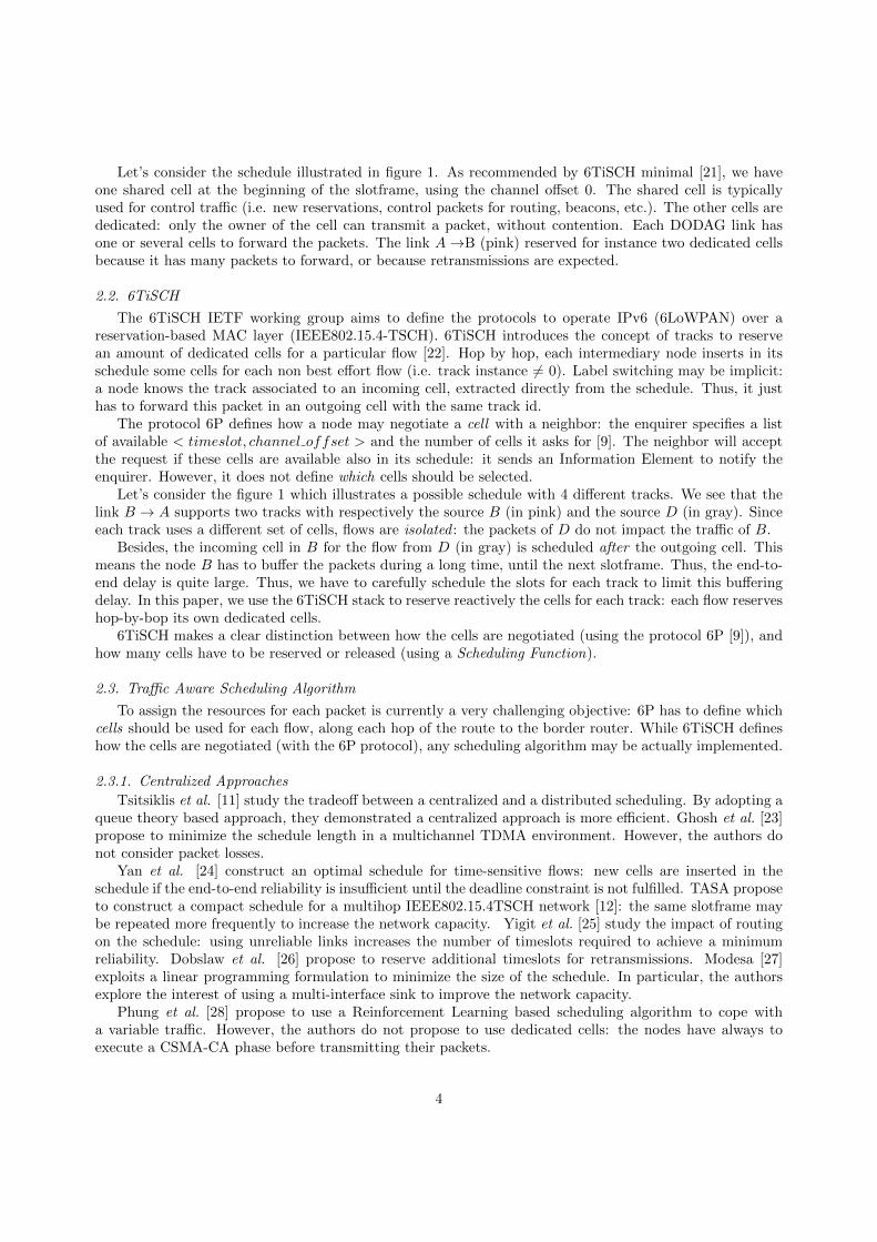
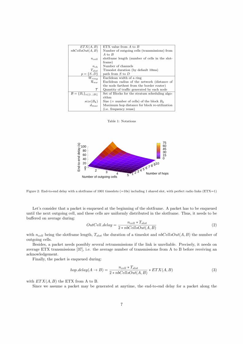
Figure 2: End-to-end delay with a slotframe of 1001 timeslots (=10s) including 1 shared slot, with perfect radio links (ETX=1)

Let’s consider that a packet is enqueued at the beginning of the slotframe. A packet has to be enqueueduntil the next outgoing cell, and these cells are uniformly distributed in the slotframe. Thus, it needs to bebuffered on average during:

OutCell delay =ncell ∗ Tslot

2 ∗ nbCellsOut(A,B)(2)

with ncell being the slotframe length, Tslot the duration of a timeslot and nbCellsOut(A,B) the number ofoutgoing cells.

Besides, a packet needs possibly several retransmissions if the link is unreliable. Precisely, it needs onaverage ETX transmissions [37], i.e. the average number of transmissions from A to B before receiving anacknowledgement.

Finally, the packet is enqueued during:

hop delay(A→ B) =ncell ∗ Tslot

2 ∗ nbCellsOut(A,B)∗ ETX(A,B) (3)

with ETX(A,B) the ETX from A to B.Since we assume a packet may be generated at anytime, the end-to-end delay for a packet along the

7

Algorithm 1: Random Scheduling StrategyData: ncell, nch

Result: timeslot ts and channel offset ch// we don’t have any free cell

1 if NoAvailableCell(0..ncell − 1) then2 return (∅, ∅);3 end

// Selects randomly one free cell for the transmitter

4 do// select randomly a timeslot among the dedicated cells

5 ts← rand(0..ncell − 1);// select randomly a channel offset

6 ch = rand(0..nch − 1);

7 until isCellAvailable(ts, ch);8 return (ts, ch);

Block 1Block 2Block 3Block 4Block 5

stratum 1 uses the block 1

schedule

border router

Wring

Rnw

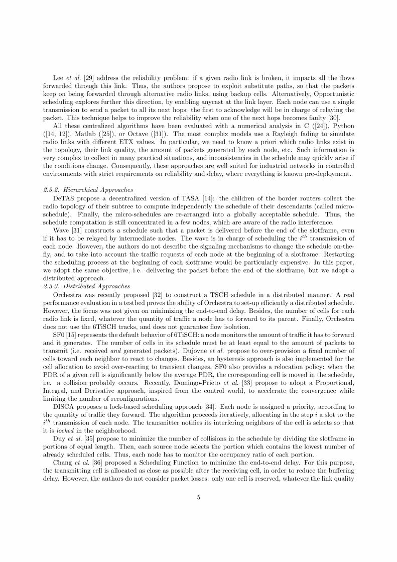
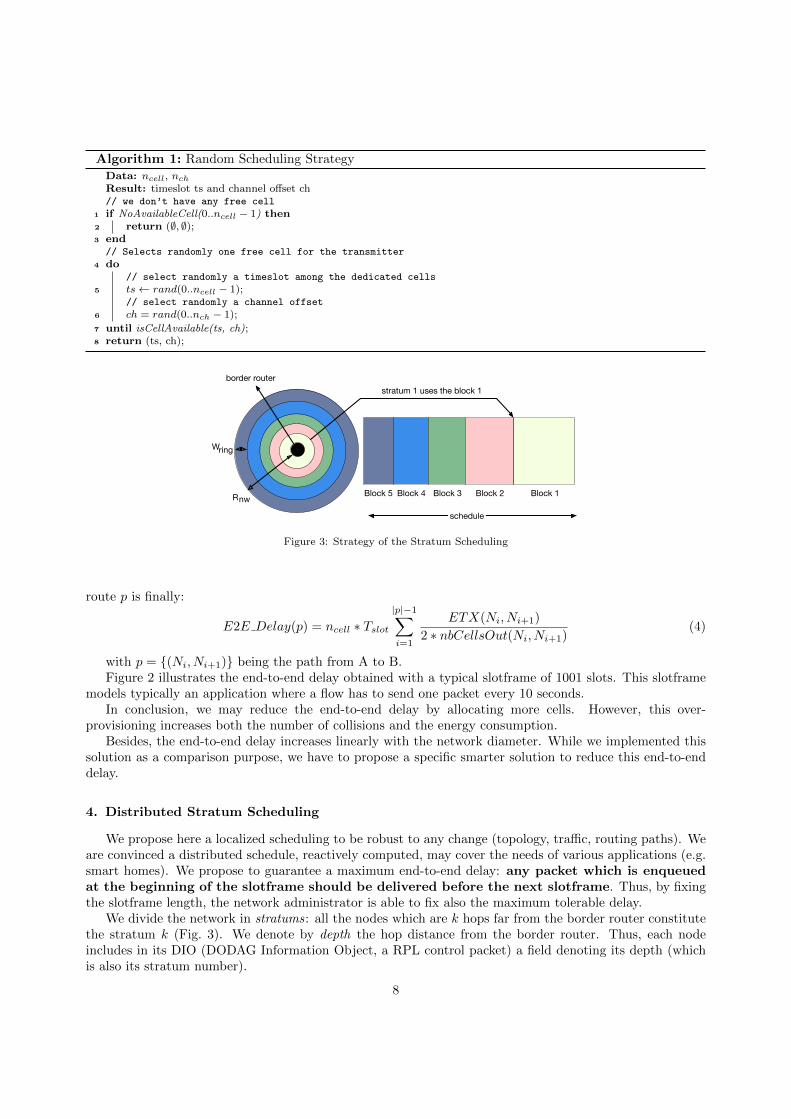
Figure 3: Strategy of the Stratum Scheduling

route p is finally:

E2E Delay(p) = ncell ∗ Tslot|p|−1∑i=1

ETX(Ni, Ni+1)

2 ∗ nbCellsOut(Ni, Ni+1)(4)

with p = {(Ni, Ni+1)} being the path from A to B.Figure 2 illustrates the end-to-end delay obtained with a typical slotframe of 1001 slots. This slotframe

models typically an application where a flow has to send one packet every 10 seconds.In conclusion, we may reduce the end-to-end delay by allocating more cells. However, this over-

provisioning increases both the number of collisions and the energy consumption.Besides, the end-to-end delay increases linearly with the network diameter. While we implemented this

solution as a comparison purpose, we have to propose a specific smarter solution to reduce this end-to-enddelay.

4. Distributed Stratum Scheduling

We propose here a localized scheduling to be robust to any change (topology, traffic, routing paths). Weare convinced a distributed schedule, reactively computed, may cover the needs of various applications (e.g.smart homes). We propose to guarantee a maximum end-to-end delay: any packet which is enqueuedat the beginning of the slotframe should be delivered before the next slotframe. Thus, by fixingthe slotframe length, the network administrator is able to fix also the maximum tolerable delay.

We divide the network in stratums: all the nodes which are k hops far from the border router constitutethe stratum k (Fig. 3). We denote by depth the hop distance from the border router. Thus, each nodeincludes in its DIO (DODAG Information Object, a RPL control packet) a field denoting its depth (whichis also its stratum number).

8

We can note that we don’t use minimum hop routing: the depth metric is uniquely used by our schedulingalgorithm, and RPL may use any routing metric. In other words, the rank and the depth are differentmetrics. The depth is computed as the depth of the preferred parent already selected by RPL (according toany routing metric), increased by one.

We have now to assign a time-frequency block (a band) to each stratum. All the nodes in the stratum kmust reserve a timeslot from the block k. We construct a global schedule in which the blocks from contiguousstratums are consecutive. This way, we guarantee a packet is delivered before the end of the slotframe.

We adopt here the Scheduling Function SFloc proposed in [17]: each node adapts locally and dynamicallythe number of required cells for each track. Besides, in the stratum strategy, a node picks a cell from theblock assigned to its stratum. Since the stratum is directly determined by the depth, a node implementsa localized scheduling strategy. However, any localized Scheduling Function (such as SF0) would be hereaccurate.

We have now to define which block will be assigned to each stratum. We will first focus on the uploadcase (e.g. periodical measures are pushed to a border router), and we will explain further how to adapt oursolution to cope also with the inverse direction.

4.1. Defining the size of each stratum

We have to define which portion of the schedule is assigned to each block. We propose here to consideran ideal case, where the nodes are uniformly distributed in a given area, and generate the same amount oftraffic. This ideal situation helps us to define which values to use to bootstrap the network. In section 4.3,we will detail how the network may change on-the-fly these values, to deal with particular situations (e.g.heterogeneous densities, traffic or topologies).

We denote by block all the nodes which are equidistant (in hops) from the border router. We will firstexplain how we assign a schedule to the nodes which are at most dmax hops far from the border router. Wewill explain in the next subsection which blocks have to be used for the nodes located farther, and how thevalue of dmax should be selected.

If we consider each node generates the same amount of traffic, we should not divide the whole schedulein dmax blocks with an equal size: the nodes close to the border router have more traffic to forward. Moreprecisely, on average, a node in the stratum k forwards the traffic of all the nodes from the stratums with alarger depth.

If the deployment is sufficiently dense and all the nodes have the same transmission power, we mayassume all the rings have a fixed width Wring [38]. When using ETX as a metric, Wring is typically thedistance at which the packet delivery ratio is almost perfect (i.e. 100%). Let Rnw denote the euclideandistance of the node farthest from the border router (i.e. the network radius) (cf. Fig. 3)

If we assume each node generates the same amount of traffic denoted T , the traffic generated by thestratum is directly proportional to the area of the corresponding ring. Thus, the traffic generated by thestratum k is:

Tgen(Bk) = T ∗ π(

(Wring ∗ k)2 − (Wring ∗ (k − 1))2

)(5)

= T ∗ πW 2ring ∗ (k2 − (k − 1)2) (6)

(7)

Inside a given stratum, we have frequency re-use: nodes which are sufficiently far may re-use the samecell without colliding. Unfortunately, frequency re-use is less important for stratums closer from the sink:the interfering area spans the whole stratum. Estimating precisely the impact of frequency re-use wouldrequire to define formally the ratio of the area of the ring, and of the interfering region.

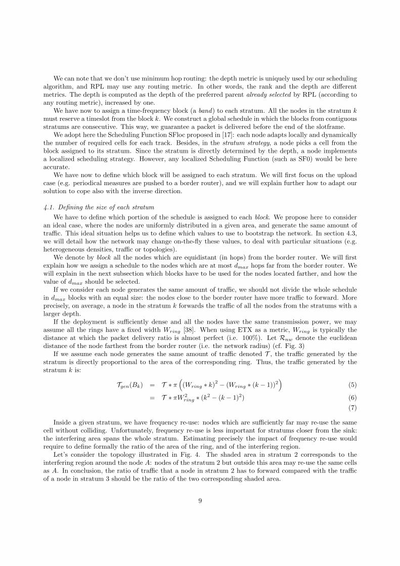
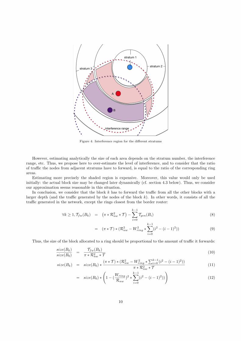
Let’s consider the topology illustrated in Fig. 4. The shaded area in stratum 2 corresponds to theinterfering region around the node A: nodes of the stratum 2 but outside this area may re-use the same cellsas A. In conclusion, the ratio of traffic that a node in stratum 2 has to forward compared with the trafficof a node in stratum 3 should be the ratio of the two corresponding shaded area.

9

stratum 2

stratum 1

stratum 3

interference range

A

B

Figure 4: Interference region for the different stratums

However, estimating analytically the size of each area depends on the stratum number, the interferencerange, etc. Thus, we propose here to over-estimate the level of interference, and to consider that the ratioof traffic the nodes from adjacent stratums have to forward, is equal to the ratio of the corresponding ringareas.

Estimating more precisely the shaded region is expensive. Moreover, this value would only be usedinitially: the actual block size may be changed later dynamically (cf. section 4.3 below). Thus, we considerour approximation seems reasonable in this situation.

In conclusion, we consider that the block k has to forward the traffic from all the other blocks with alarger depth (and the traffic generated by the nodes of the block k). In other words, it consists of all thetraffic generated in the network, except the rings closest from the border router:

∀k ≥ 1, Tfw(Bk) =(π ∗ R2

nw ∗ T)−

k−1∑i=0

Tgen(Bi) (8)

= (π ∗ T ) ∗ (R2nw −W 2

ring ∗k−1∑i=0

(i2 − (i− 1)2)) (9)

Thus, the size of the block allocated to a ring should be proportional to the amount of traffic it forwards:

size(Bk)

size(B0)=

Tfw(Bk)

π ∗ R2nw ∗ T

(10)

size(Bk) = size(B0) ∗(π ∗ T ) ∗ (R2

nw −W 2ring ∗

∑k−1i=0 (i2 − (i− 1)2))

π ∗ R2nw ∗ T

(11)

= size(B0) ∗

(1− (

Wring

Rnw)2 ∗

k−1∑i=0

(i2 − (i− 1)2))

)(12)

10

Algorithm 2: Stratum Scheduling Strategy

// The algorithm needs the depth of the node, the number of dedicated cells, the number of channels,

the network radius (in hops)

Data: depth, ncell, nch, RResult: timeslot ts and channel offset ch// We first compute the size of the first block (B0)

// f() is extracted from eq. 16

1 Cmin ← 0;2 Cmax ← f(ncell, R) ;

// We then compute our own bounds of the block

// size() is extracted from eq. 10

3 for j=0 to depth-1 do4 Cmin ← Cmax;5 Cmax ← Cmax + size(ncell, R, j);

6 end// we don’t have any free cell in the block

7 if NoAvailableCell(Cmin, Cmax) then8 return ∅, ∅;9 end

10 do// select randomly a timeslot in the given block

11 ts← rand(Cmin..Cmax);// select randomly a channel offset

12 ch = rand(0..nch);

13 until isCellAvailable(ts, ch);14 return ts, ch;

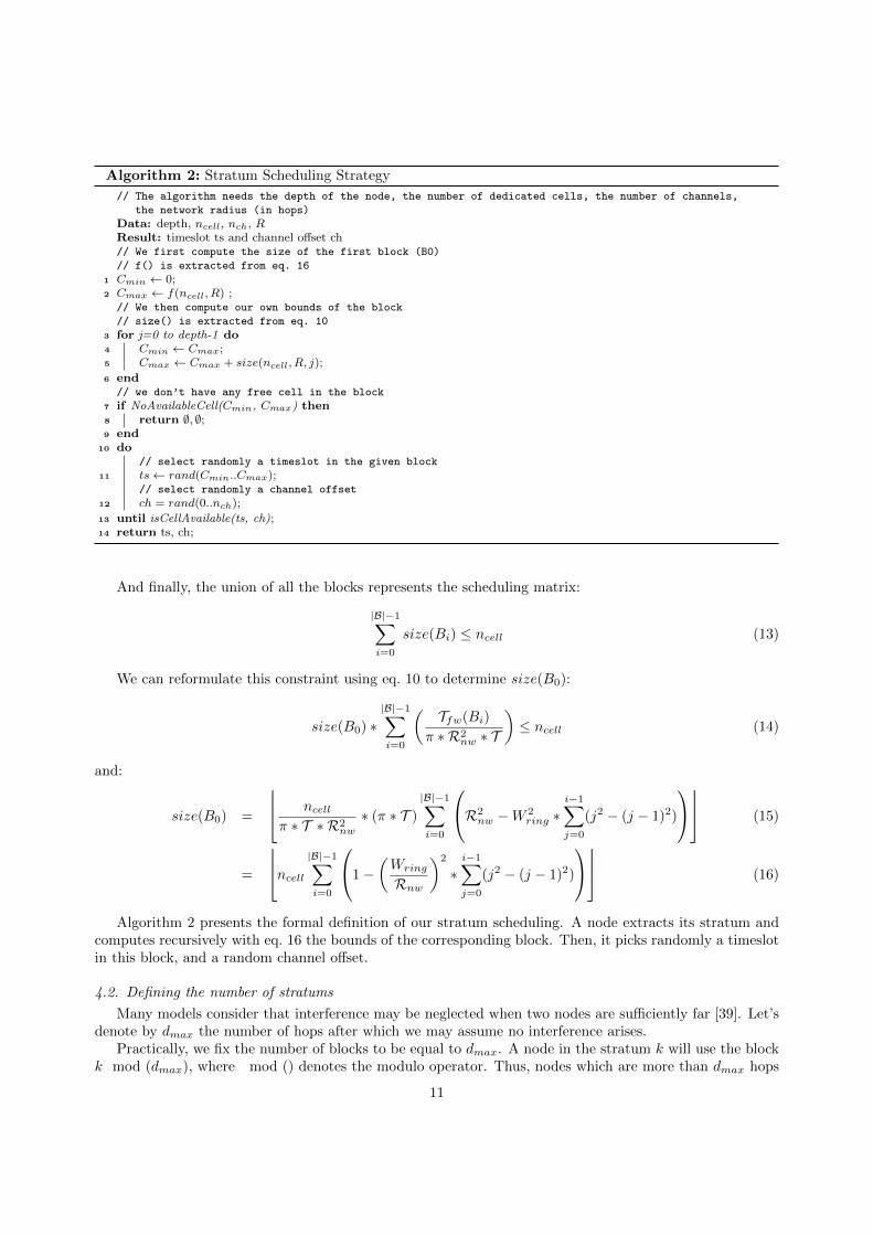
And finally, the union of all the blocks represents the scheduling matrix:

|B|−1∑i=0

size(Bi) ≤ ncell (13)

We can reformulate this constraint using eq. 10 to determine size(B0):

size(B0) ∗|B|−1∑i=0

(Tfw(Bi)

π ∗ R2nw ∗ T

)≤ ncell (14)

and:

size(B0) =

ncellπ ∗ T ∗ R2

nw

∗ (π ∗ T )

|B|−1∑i=0

R2nw −W 2

ring ∗i−1∑j=0

(j2 − (j − 1)2)

(15)

=

ncell |B|−1∑i=0

1−(Wring

Rnw

)2

∗i−1∑j=0

(j2 − (j − 1)2)

(16)

Algorithm 2 presents the formal definition of our stratum scheduling. A node extracts its stratum andcomputes recursively with eq. 16 the bounds of the corresponding block. Then, it picks randomly a timeslotin this block, and a random channel offset.

4.2. Defining the number of stratums

Many models consider that interference may be neglected when two nodes are sufficiently far [39]. Let’sdenote by dmax the number of hops after which we may assume no interference arises.

Practically, we fix the number of blocks to be equal to dmax. A node in the stratum k will use the blockk mod (dmax), where mod () denotes the modulo operator. Thus, nodes which are more than dmax hops

11

far from the border router re-use an already allocated cell, without creating interference since we considerthey are sufficiently far from each other.

The blocks are also sufficiently large. Indeed, the stratum (dmax − 1) has the smallest block in thenetwork. Thus, all the other stratum larger than dmax have a block which is at least as large. Since thestratum k has always less traffic to forward than a stratum j (j < k), these stratums have enough bandwidth.4.3. Updating the blocks size

Our theoretical analysis relies on a uniform distribution of the nodes, with the same quantity of traffic foreach source, etc. Unfortunately, considering realistic conditions would also impact the size of the differentblocks. The size of each block can be pre-computed pre-deployment, if the location and the volume of trafficis known a priori, counting the ratio of traffic in each interfering stratum. Since these conditions may bedynamic or cannot be estimated enough accurately, we propose here a dynamic method.

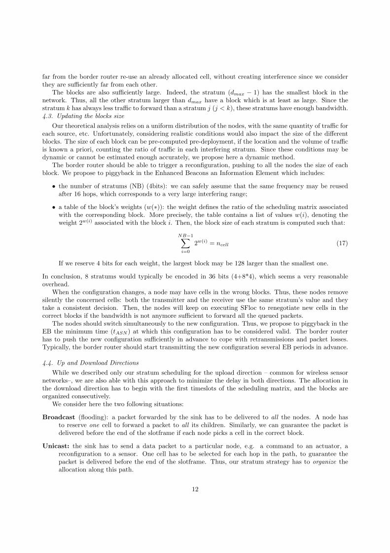
The border router should be able to trigger a reconfiguration, pushing to all the nodes the size of eachblock. We propose to piggyback in the Enhanced Beacons an Information Element which includes:

• the number of stratums (NB) (4bits): we can safely assume that the same frequency may be reusedafter 16 hops, which corresponds to a very large interfering range;

• a table of the block’s weights (w(∗)): the weight defines the ratio of the scheduling matrix associatedwith the corresponding block. More precisely, the table contains a list of values w(i), denoting theweight 2w(i) associated with the block i. Then, the block size of each stratum is computed such that:

NB−1∑i=0

2w(i) = ncell (17)

If we reserve 4 bits for each weight, the largest block may be 128 larger than the smallest one.

In conclusion, 8 stratums would typically be encoded in 36 bits (4+8*4), which seems a very reasonableoverhead.

When the configuration changes, a node may have cells in the wrong blocks. Thus, these nodes removesilently the concerned cells: both the transmitter and the receiver use the same stratum’s value and theytake a consistent decision. Then, the nodes will keep on executing SFloc to renegotiate new cells in thecorrect blocks if the bandwidth is not anymore sufficient to forward all the queued packets.

The nodes should switch simultaneously to the new configuration. Thus, we propose to piggyback in theEB the minimum time (tASN ) at which this configuration has to be considered valid. The border routerhas to push the new configuration sufficiently in advance to cope with retransmissions and packet losses.Typically, the border router should start transmitting the new configuration several EB periods in advance.

4.4. Up and Download Directions

While we described only our stratum scheduling for the upload direction – common for wireless sensornetworks–, we are also able with this approach to minimize the delay in both directions. The allocation inthe download direction has to begin with the first timeslots of the scheduling matrix, and the blocks areorganized consecutively.

We consider here the two following situations:

Broadcast (flooding): a packet forwarded by the sink has to be delivered to all the nodes. A node hasto reserve one cell to forward a packet to all its children. Similarly, we can guarantee the packet isdelivered before the end of the slotframe if each node picks a cell in the correct block.

Unicast: the sink has to send a data packet to a particular node, e.g. a command to an actuator, areconfiguration to a sensor. One cell has to be selected for each hop in the path, to guarantee thepacket is delivered before the end of the slotframe. Thus, our stratum strategy has to organize theallocation along this path.

12

slotframe length

A B

C

0 1 2 3 4 5 6 7 8 9 10 11

DE

…

…

01

10

11

15

chan

nel o

ffset

s

Stratum 1Stratum 2Stratum 3Stratum 4

Stratum 1 Stratum 2 Stratum 3 Stratum 4

dow

nloa

dup

load

border router

dedicated cellsshared cell

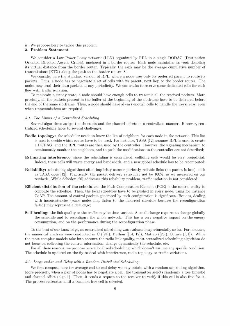
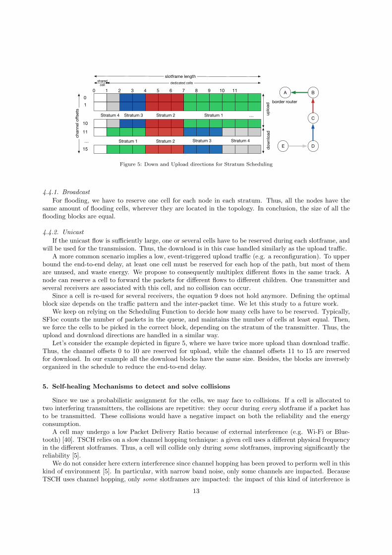
Figure 5: Down and Upload directions for Stratum Scheduling

4.4.1. Broadcast

For flooding, we have to reserve one cell for each node in each stratum. Thus, all the nodes have thesame amount of flooding cells, wherever they are located in the topology. In conclusion, the size of all theflooding blocks are equal.

4.4.2. Unicast

If the unicast flow is sufficiently large, one or several cells have to be reserved during each slotframe, andwill be used for the transmission. Thus, the download is in this case handled similarly as the upload traffic.

A more common scenario implies a low, event-triggered upload traffic (e.g. a reconfiguration). To upperbound the end-to-end delay, at least one cell must be reserved for each hop of the path, but most of themare unused, and waste energy. We propose to consequently multiplex different flows in the same track. Anode can reserve a cell to forward the packets for different flows to different children. One transmitter andseveral receivers are associated with this cell, and no collision can occur.

Since a cell is re-used for several receivers, the equation 9 does not hold anymore. Defining the optimalblock size depends on the traffic pattern and the inter-packet time. We let this study to a future work.

We keep on relying on the Scheduling Function to decide how many cells have to be reserved. Typically,SFloc counts the number of packets in the queue, and maintains the number of cells at least equal. Then,we force the cells to be picked in the correct block, depending on the stratum of the transmitter. Thus, theupload and download directions are handled in a similar way.

Let’s consider the example depicted in figure 5, where we have twice more upload than download traffic.Thus, the channel offsets 0 to 10 are reserved for upload, while the channel offsets 11 to 15 are reservedfor download. In our example all the download blocks have the same size. Besides, the blocks are inverselyorganized in the schedule to reduce the end-to-end delay.

5. Self-healing Mechanisms to detect and solve collisions

Since we use a probabilistic assignment for the cells, we may face to collisions. If a cell is allocated totwo interfering transmitters, the collisions are repetitive: they occur during every slotframe if a packet hasto be transmitted. These collisions would have a negative impact on both the reliability and the energyconsumption.

A cell may undergo a low Packet Delivery Ratio because of external interference (e.g. Wi-Fi or Blue-tooth) [40]. TSCH relies on a slow channel hopping technique: a given cell uses a different physical frequencyin the different slotframes. Thus, a cell will collide only during some slotframes, improving significantly thereliability [5].

We do not consider here extern interference since channel hopping has been proved to perform well in thiskind of environment [5]. In particular, with narrow band noise, only some channels are impacted. BecauseTSCH uses channel hopping, only some slotframes are impacted: the impact of this kind of interference is

13

only temporary. Besides, over-provisioning reserves some additional cells for the retransmissions, makingthe network reliable.

We focus here on detecting collisions inside the network.

5.1. Detecting Colliding Cells

Because of collisions, the Scheduling Function will reserve additional cells for retransmissions. Besides,multiple flows may also be forwarded by the same node to its parent. Thus, we have several outgoing cellsin the slotframe.

Because of over-provisioning and retransmissions, a cell is not used in each slotframe to transmit a frame.If the same cell is allocated to two interfering transmitters, a collision will occur only if both transmittershave a frame to transmit at the same time. This collision ratio depends on the traffic model and thereliability, which impacts the number of retransmissions.

Muraoka et al. [41] already proposed a mechanism to detect collisions. In this tx-housekeeping strategy,a transmitter tries to estimate the probability of collision for a given cell by monitoring the Packet DeliveryRatio of each cell individually. The process considers a cell collides if it exhibits a significantly smaller PDR(by default 66%) compared with the average PDR for all the cells. Thus, the cell has to be relocated: itschannel offset and timeslot are released, and another cell is re-negotiated with the next hop. We reuse herethis strategy to detect colliding cells.

We can note that external interference impacts also the reliability. However, because each cell uses apseudo-random hopping sequence, external interference impacts equally all the channel offsets. Moreover,the traffic profile (inter packet time, transmission durations) is probably different for external traffic, andwill with high probability impact equally all the different timeslots. Thus, this collision detection is triggeredonly by internal interference, which could be solved with a relocation strategy in the schedule. We proposeconsequently to adopt here the same approach.

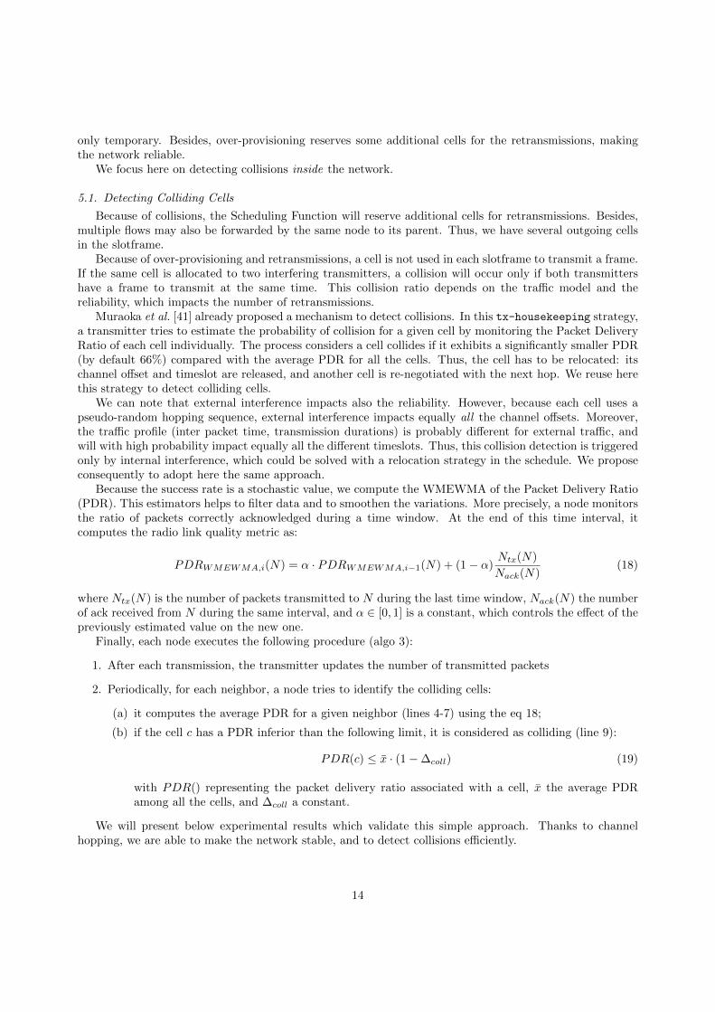
Because the success rate is a stochastic value, we compute the WMEWMA of the Packet Delivery Ratio(PDR). This estimators helps to filter data and to smoothen the variations. More precisely, a node monitorsthe ratio of packets correctly acknowledged during a time window. At the end of this time interval, itcomputes the radio link quality metric as:

PDRWMEWMA,i(N) = α · PDRWMEWMA,i−1(N) + (1− α)Ntx(N)

Nack(N)(18)

where Ntx(N) is the number of packets transmitted to N during the last time window, Nack(N) the numberof ack received from N during the same interval, and α ∈ [0, 1] is a constant, which controls the effect of thepreviously estimated value on the new one.

Finally, each node executes the following procedure (algo 3):

1. After each transmission, the transmitter updates the number of transmitted packets

2. Periodically, for each neighbor, a node tries to identify the colliding cells:

(a) it computes the average PDR for a given neighbor (lines 4-7) using the eq 18;

(b) if the cell c has a PDR inferior than the following limit, it is considered as colliding (line 9):

PDR(c) ≤ x · (1−∆coll) (19)

with PDR() representing the packet delivery ratio associated with a cell, x the average PDRamong all the cells, and ∆coll a constant.

We will present below experimental results which validate this simple approach. Thanks to channelhopping, we are able to make the network stable, and to detect collisions efficiently.

14

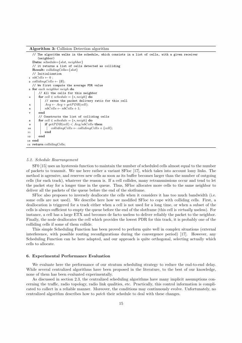
Algorithm 3: Collision Detection algorithm

// The algorithm walks in the schedule, which consists in a list of cells, with a given receiver

(neighbor)

Data: schedule={slot, neighbor}// it returns a list of cells detected as colliding

Result: collidingCells={slot}// Initialization

1 nbCells← 0 ;2 collidingCells← {∅};

// We first compute the average PDR value

3 for each neighbor neigh do// All the cells for this neighbor

4 for cell ∈ schedule = {∗, neigh} do// saves the packet delivery ratio for this cell

5 Avg ← Avg + getPDR(cell);6 nbCells← nbCells+ 1;

7 end// Constructs the list of colliding cells

8 for cell ∈ schedule = {∗, neigh} do9 if getPDR(cell) < Avg/nbCells then

10 collidingCells← collidingCells+ {cell};11 end

12 end

13 end14 return collidingCells;

5.2. Schedule Rearrangement

SF0 [15] uses an hysteresis function to maintain the number of scheduled cells almost equal to the numberof packets to transmit. We use here rather a variant SFloc [17], which takes into account lossy links. Themethod is agressive, and reserves new cells as soon as its buffer becomes larger than the number of outgoingcells (for each track), whatever the reason is. If a cell collides, many retransmissions occur and tend to letthe packet stay for a longer time in the queue. Thus, SFloc allocates more cells to the same neighbor todeliver all the packets of the queue before the end of the slotframe.

SFloc also proposes to inversely deallocate the cells when it considers it has too much bandwidth (i.e.some cells are not used). We describe here how we modified SFloc to cope with colliding cells. First, adeallocation is triggered for a track either when a cell is not used for a long time, or when a subset of thecells is always sufficient to empty the queue before the end of the slotframe (this cell is virtually useless). Forinstance, a cell has a large ETX and becomes de facto useless to deliver reliably the packet to the neighbor.Finally, the node deallocates the cell which provides the lowest PDR for this track, it is probably one of thecolliding cells if some of them collide.

This simple Scheduling Function has been proved to perform quite well in complex situations (externalinterference, with possible routing reconfigurations during the convergence period) [17]. However, anyScheduling Function can be here adapted, and our approach is quite orthogonal, selecting actually whichcells to allocate.

6. Experimental Performance Evaluation

We evaluate here the performance of our stratum scheduling strategy to reduce the end-to-end delay.While several centralized algorithms have been proposed in the literature, to the best of our knowledge,none of them has been evaluated experimentally.

As discussed in section 2.3, the centralized scheduling algorithms have many implicit assumptions con-cerning the traffic, radio topology, radio link qualities, etc. Practically, this control information is compli-cated to collect in a reliable manner. Moreover, the conditions may continuously evolve. Unfortunately, nocentralized algorithm describes how to patch their schedule to deal with these changes.

15

50 m

otes

79 m

otes

50 m

otes

82 m

otes

80 motes

69 motes

80 motes

69 motes22 motes

27 motes

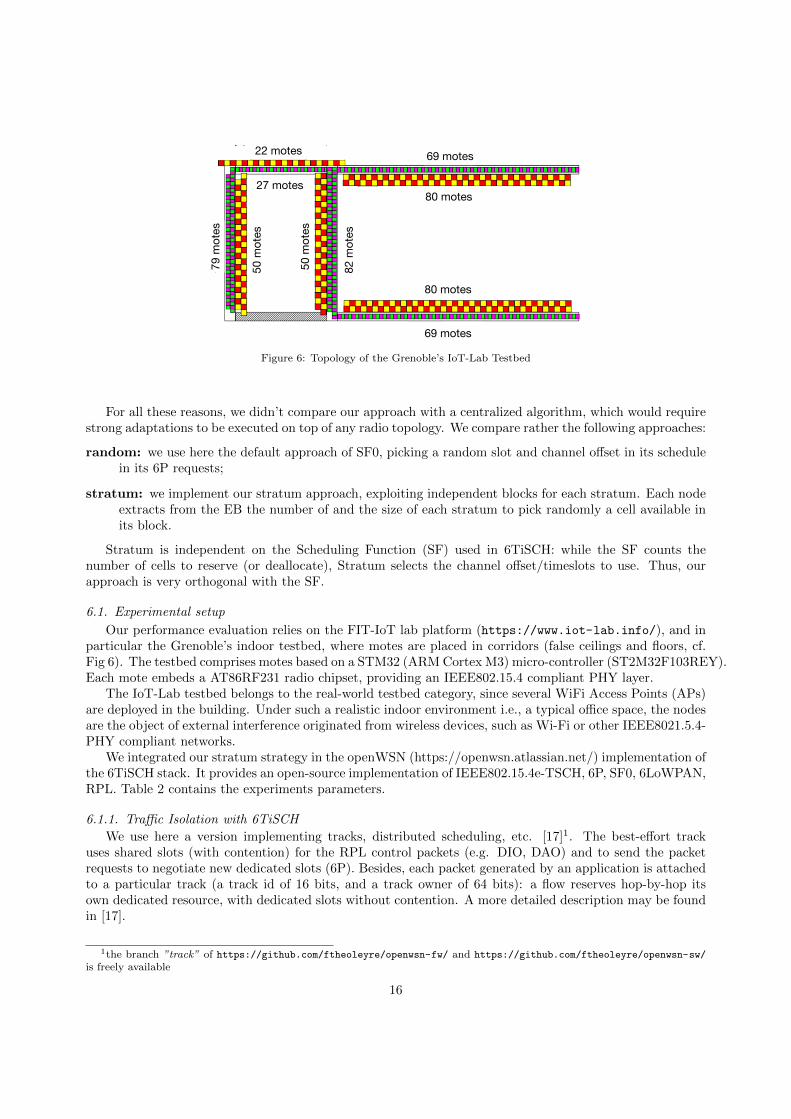
Figure 6: Topology of the Grenoble’s IoT-Lab Testbed

For all these reasons, we didn’t compare our approach with a centralized algorithm, which would requirestrong adaptations to be executed on top of any radio topology. We compare rather the following approaches:

random: we use here the default approach of SF0, picking a random slot and channel offset in its schedulein its 6P requests;

stratum: we implement our stratum approach, exploiting independent blocks for each stratum. Each nodeextracts from the EB the number of and the size of each stratum to pick randomly a cell available inits block.

Stratum is independent on the Scheduling Function (SF) used in 6TiSCH: while the SF counts thenumber of cells to reserve (or deallocate), Stratum selects the channel offset/timeslots to use. Thus, ourapproach is very orthogonal with the SF.

6.1. Experimental setup

Our performance evaluation relies on the FIT-IoT lab platform (https://www.iot-lab.info/), and inparticular the Grenoble’s indoor testbed, where motes are placed in corridors (false ceilings and floors, cf.Fig 6). The testbed comprises motes based on a STM32 (ARM Cortex M3) micro-controller (ST2M32F103REY).Each mote embeds a AT86RF231 radio chipset, providing an IEEE802.15.4 compliant PHY layer.

The IoT-Lab testbed belongs to the real-world testbed category, since several WiFi Access Points (APs)are deployed in the building. Under such a realistic indoor environment i.e., a typical office space, the nodesare the object of external interference originated from wireless devices, such as Wi-Fi or other IEEE8021.5.4-PHY compliant networks.

We integrated our stratum strategy in the openWSN (https://openwsn.atlassian.net/) implementation ofthe 6TiSCH stack. It provides an open-source implementation of IEEE802.15.4e-TSCH, 6P, SF0, 6LoWPAN,RPL. Table 2 contains the experiments parameters.

6.1.1. Traffic Isolation with 6TiSCH

We use here a version implementing tracks, distributed scheduling, etc. [17]1. The best-effort trackuses shared slots (with contention) for the RPL control packets (e.g. DIO, DAO) and to send the packetrequests to negotiate new dedicated slots (6P). Besides, each packet generated by an application is attachedto a particular track (a track id of 16 bits, and a track owner of 64 bits): a flow reserves hop-by-hop itsown dedicated resource, with dedicated slots without contention. A more detailed description may be foundin [17].

1the branch ”track” of https://github.com/ftheoleyre/openwsn-fw/ and https://github.com/ftheoleyre/openwsn-sw/

is freely available

16

https://www.iot-lab.info/

https://github.com/ftheoleyre/openwsn-fw/

https://github.com/ftheoleyre/openwsn-sw/

Parameter ValueExperiment duration 300 sTraffic type, rate CBR, 5 pkts/minData packet size 127 bytesNumber of nodes 20 nodesMAC layer IEEE802.15.4-TSCHType of cells softcells (distributed)Time slot duration 15msSlotframe length 101 slotsRouting protocol RPLRouting metric ETXRadio chipset AT86RF231Radio chipset STM32F103REY (ARM cortex-M3)

Table 2: Experiment parameters

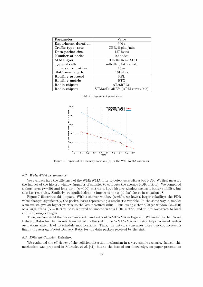
Figure 7: Impact of the memory constant (α) in the WMEWMA estimator

6.2. WMEWMA performance

We evaluate here the efficiency of the WMEWMA filter to detect cells with a bad PDR. We first measurethe impact of the history window (number of samples to compute the average PDR metric). We compareda short-term (w=50) and long-term (w=100) metric: a large history window means a better stability, butalso less reactivity. Similarly, we studied also the impact of the α (alpha) factor in equation 18.

Figure 7 illustrates this impact. With a shorter window (w=50), we have a larger volatility: the PDRvalue changes significantly, the packet losses representing a stochastic variable. In the same way, a smallerα means we give an higher priority to the last measured value. Thus, using either a larger window (w=100)or a large alpha (α = 0.9) value is required to smoothen this PDR metric, and to not over-react to localand temporary changes.

Then, we compared the performance with and without WMEWMA in Figure 8. We measures the PacketDelivery Ratio for the packets transmitted to the sink. The WMEWMA estimator helps to avoid uselessoscillations which lead to schedule modifications. Thus, the network converges more quickly, increasingfinally the average Packet Delivery Ratio for the data packets received by the sink.

6.3. Efficient Collision Detection

We evaluated the efficiency of the collision detection mechanism in a very simple scenario. Indeed, thismechanism was proposed in Muraoka et al. [41], but to the best of our knowledge, no paper presents an

17

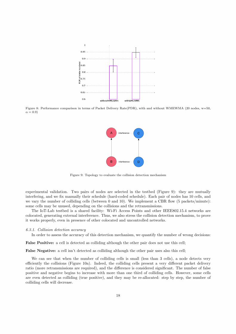
Figure 8: Performance comparison in terms of Packet Delivery Rate(PDR), with and without WMEWMA (20 nodes, w=50,α = 0.9)

A

B

C

D

interference

interference

Figure 9: Topology to evaluate the collision detection mechanism

experimental validation. Two pairs of nodes are selected in the testbed (Figure 9): they are mutuallyinterfering, and we fix manually their schedule (hard-coded schedule). Each pair of nodes has 10 cells, andwe vary the number of colliding cells (between 0 and 10). We implement a CBR flow (5 packets/minute):some cells may be unused, depending on the collisions and the retransmissions.

The IoT-Lab testbed is a shared facility: Wi-Fi Access Points and other IEEE802.15.4 networks arecolocated, generating external interference. Thus, we also stress the collision detection mechanism, to proveit works properly, even in presence of other colocated and uncontrolled networks.

6.3.1. Collision detection accuracy

In order to assess the accuracy of this detection mechanism, we quantify the number of wrong decisions:

False Positive: a cell is detected as colliding although the other pair does not use this cell;

False Negative: a cell isn’t detected as colliding although the other pair uses also this cell;

We can see that when the number of colliding cells is small (less than 3 cells), a node detects veryefficiently the collisions (Figure 10a). Indeed, the colliding cells present a very different packet deliveryratio (more retransmissions are required), and the difference is considered significant. The number of falsepositive and negative begins to increase with more than one third of colliding cells. However, some cellsare even detected as colliding (true positive), and they may be re-allocated: step by step, the number ofcolliding cells will decrease.

18

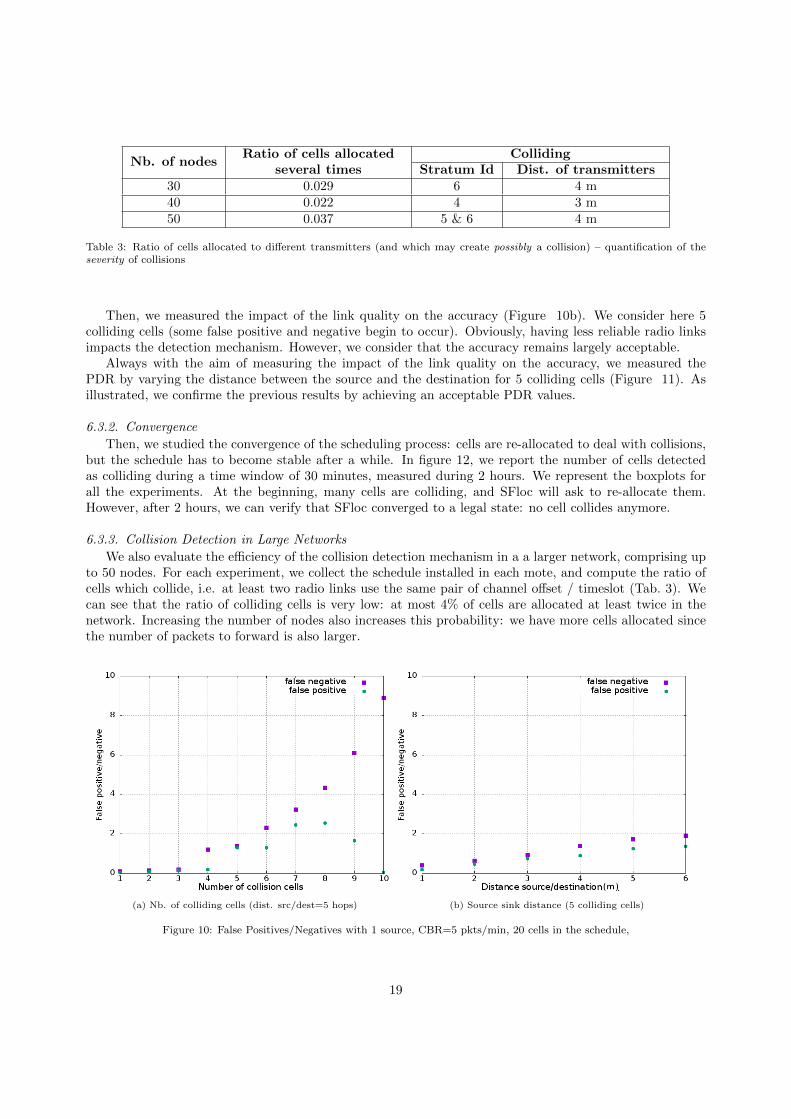
Nb. of nodesRatio of cells allocated Colliding

several times Stratum Id Dist. of transmitters30 0.029 6 4 m40 0.022 4 3 m50 0.037 5 & 6 4 m

Table 3: Ratio of cells allocated to different transmitters (and which may create possibly a collision) – quantification of theseverity of collisions

Then, we measured the impact of the link quality on the accuracy (Figure 10b). We consider here 5colliding cells (some false positive and negative begin to occur). Obviously, having less reliable radio linksimpacts the detection mechanism. However, we consider that the accuracy remains largely acceptable.

Always with the aim of measuring the impact of the link quality on the accuracy, we measured thePDR by varying the distance between the source and the destination for 5 colliding cells (Figure 11). Asillustrated, we confirme the previous results by achieving an acceptable PDR values.

6.3.2. Convergence

Then, we studied the convergence of the scheduling process: cells are re-allocated to deal with collisions,but the schedule has to become stable after a while. In figure 12, we report the number of cells detectedas colliding during a time window of 30 minutes, measured during 2 hours. We represent the boxplots forall the experiments. At the beginning, many cells are colliding, and SFloc will ask to re-allocate them.However, after 2 hours, we can verify that SFloc converged to a legal state: no cell collides anymore.

6.3.3. Collision Detection in Large Networks

We also evaluate the efficiency of the collision detection mechanism in a a larger network, comprising upto 50 nodes. For each experiment, we collect the schedule installed in each mote, and compute the ratio ofcells which collide, i.e. at least two radio links use the same pair of channel offset / timeslot (Tab. 3). Wecan see that the ratio of colliding cells is very low: at most 4% of cells are allocated at least twice in thenetwork. Increasing the number of nodes also increases this probability: we have more cells allocated sincethe number of packets to forward is also larger.

(a) Nb. of colliding cells (dist. src/dest=5 hops) (b) Source sink distance (5 colliding cells)

Figure 10: False Positives/Negatives with 1 source, CBR=5 pkts/min, 20 cells in the schedule,

19

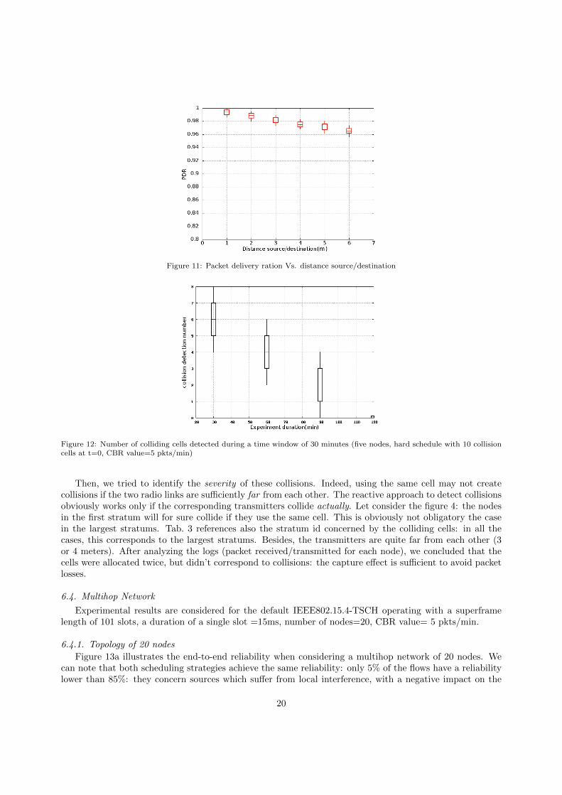
Figure 11: Packet delivery ration Vs. distance source/destination

Figure 12: Number of colliding cells detected during a time window of 30 minutes (five nodes, hard schedule with 10 collisioncells at t=0, CBR value=5 pkts/min)

Then, we tried to identify the severity of these collisions. Indeed, using the same cell may not createcollisions if the two radio links are sufficiently far from each other. The reactive approach to detect collisionsobviously works only if the corresponding transmitters collide actually. Let consider the figure 4: the nodesin the first stratum will for sure collide if they use the same cell. This is obviously not obligatory the casein the largest stratums. Tab. 3 references also the stratum id concerned by the colliding cells: in all thecases, this corresponds to the largest stratums. Besides, the transmitters are quite far from each other (3or 4 meters). After analyzing the logs (packet received/transmitted for each node), we concluded that thecells were allocated twice, but didn’t correspond to collisions: the capture effect is sufficient to avoid packetlosses.

6.4. Multihop Network

Experimental results are considered for the default IEEE802.15.4-TSCH operating with a superframelength of 101 slots, a duration of a single slot =15ms, number of nodes=20, CBR value= 5 pkts/min.

6.4.1. Topology of 20 nodes

Figure 13a illustrates the end-to-end reliability when considering a multihop network of 20 nodes. Wecan note that both scheduling strategies achieve the same reliability: only 5% of the flows have a reliabilitylower than 85%: they concern sources which suffer from local interference, with a negative impact on the

20

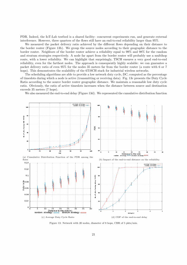
PDR. Indeed, the IoT-Lab testbed is a shared facility: concurrent experiments run, and generate externalinterference. However, three quarters of the flows still have an end-to-end reliability larger than 95%.

We measured the packet delivery ratio achieved by the different flows depending on their distance tothe border router (Figure 13b). We group the source nodes according to their geographic distance to theborder router. Neighbors of the border router achieve a reliability equal to 99% and 98% for the randomand stratum strategies respectively. A node far apart from the border router will probably use a multihoproute, with a lower reliability. We can highlight that surprisingly, TSCH ensures a very good end-to-endreliability, even for the farthest nodes. The approach is consequently highly scalable: we can guarantee apacket delivery ratio of even 95% for the nodes 35 meters far from the border router (a route with 6 or 7hops). This demonstrates the scalability of the 6TiSCH stack for industrial wireless networks.

The scheduling algorithms are able to provide a low network duty cycle, DC, computed as the percentageof timeslots during which a node is active (transmitting or receiving data). Fig. 13c presents the Duty CycleRatio according to the source border router geographic distance. We maintain a reasonable low duty cycleratio. Obviously, the ratio of active timeslots increases when the distance between source and destinationexceeds 35 meters (7 hops).

We also measured the end-to-end delay (Figure 13d). We represented the cumulative distribution function

(a) Cumulative Distribution Function of the PDR among theflows (b) Impact of the end-to-end distance on the reliability

(c) Average Duty Cycle Ratio (d) CDF of the end-to-end delay

Figure 13: Network with 20 nodes, diameter of 8 hops, CBR of 5 pkts/min.

21

0.7

0.75

0.8

0.85

0.9

0.95

1

30 35 40 45 50 55 60

PD

R

Number of nodes

stratum strategyrandom strategy

(a) PDR vs. nb. of nodes (CBR value= 5 pkts/min)

0

20

40

60

80

100

70 75 80 85 90 95 100

No.

of fl

ows

havi

ng P

DR

>=

X(%

)

PDR


(b) Complementary CDF of the end-to-end PDR (60 nodes

Figure 14: CBR of 5 pkts/min, diameter of 10 hops

to also consider the worst case. The stratum strategy is very efficient: while it achieves a similar reliability asthe random strategy, it reduces significantly the end-to-end delay. The stratum strategy achieves a delay of1.5 seconds in the worst case, while the random strategy presents a worst case delay of 4.5 seconds (+300%).

Even for long routes (6 or 7 hops in this instance), the network achieves to deliver all the packets withinthe slotframe (equal here to 1.5 seconds). We are consequently able to provide a distributed schedulingsolution with a high reliability while upper-bounding the end-to-end delay.

In conclusion, we succeed to reduce the end-to-end delay while not impacting the reliability,and presenting also the same duty cycle ratio as a random strategy.

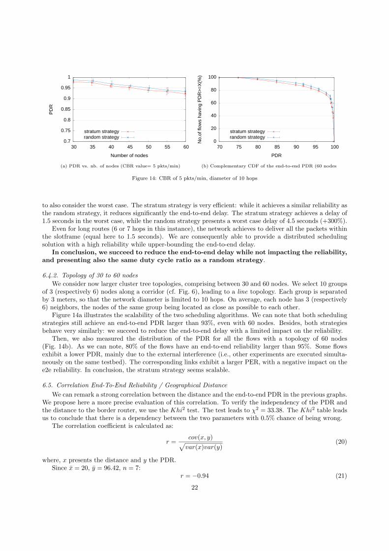
6.4.2. Topology of 30 to 60 nodes

We consider now larger cluster tree topologies, comprising between 30 and 60 nodes. We select 10 groupsof 3 (respectively 6) nodes along a corridor (cf. Fig. 6), leading to a line topology. Each group is separatedby 3 meters, so that the network diameter is limited to 10 hops. On average, each node has 3 (respectively6) neighbors, the nodes of the same group being located as close as possible to each other.

Figure 14a illustrates the scalability of the two scheduling algorithms. We can note that both schedulingstrategies still achieve an end-to-end PDR larger than 93%, even with 60 nodes. Besides, both strategiesbehave very similarly: we succeed to reduce the end-to-end delay with a limited impact on the reliability.

Then, we also measured the distribution of the PDR for all the flows with a topology of 60 nodes(Fig. 14b). As we can note, 80% of the flows have an end-to-end reliability larger than 95%. Some flowsexhibit a lower PDR, mainly due to the external interference (i.e., other experiments are executed simulta-neously on the same testbed). The corresponding links exhibit a larger PER, with a negative impact on thee2e reliability. In conclusion, the stratum strategy seems scalable.

6.5. Correlation End-To-End Reliability / Geographical Distance

We can remark a strong correlation between the distance and the end-to-end PDR in the previous graphs.We propose here a more precise evaluation of this correlation. To verify the independency of the PDR andthe distance to the border router, we use the Khi2 test. The test leads to χ2 = 33.38. The Khi2 table leadsus to conclude that there is a dependency between the two parameters with 0.5% chance of being wrong.

The correlation coefficient is calculated as:

r =cov(x, y)√var(x)var(y)

(20)

where, x presents the distance and y the PDR.Since x = 20, y = 96.42, n = 7:

r = −0.94 (21)

22

We conclude that it is a strong negative linear correlation, so the equation is of the form y = ax+ b (cf.Appendix A for the numerical details).

a =cov(x, y)

S2x

(22)

S2x =

1

n

n∑i=1

(xi − x)2 (23)

b = y − ax (24)

y = −0.18x+ 92 (25)

In conclusion, the correlation coefficient is quite low (a = −0.18). This demonstrates this schedulingsolution scales quite well: even when the source is several hop far from the border router, its packet deliveryratio is reduced but remains acceptable (the PDR decreases by 1,9% per meter).

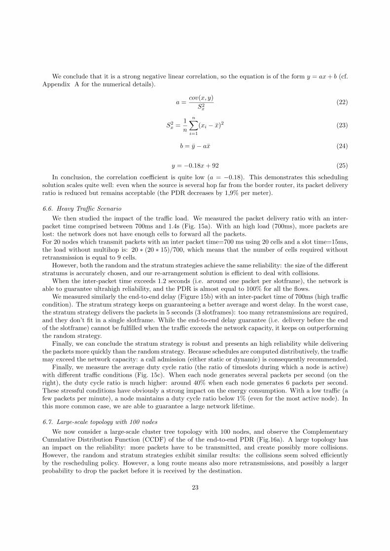
6.6. Heavy Traffic Scenario

We then studied the impact of the traffic load. We measured the packet delivery ratio with an inter-packet time comprised between 700ms and 1.4s (Fig. 15a). With an high load (700ms), more packets arelost: the network does not have enough cells to forward all the packets.For 20 nodes which transmit packets with an inter packet time=700 ms using 20 cells and a slot time=15ms,the load without multihop is: 20 ∗ (20 ∗ 15)/700, which means that the number of cells required withoutretransmission is equal to 9 cells.

However, both the random and the stratum strategies achieve the same reliability: the size of the differentstratums is accurately chosen, and our re-arrangement solution is efficient to deal with collisions.

When the inter-packet time exceeds 1.2 seconds (i.e. around one packet per slotframe), the network isable to guarantee ultrahigh reliability, and the PDR is almost equal to 100% for all the flows.

We measured similarly the end-to-end delay (Figure 15b) with an inter-packet time of 700ms (high trafficcondition). The stratum strategy keeps on guaranteeing a better average and worst delay. In the worst case,the stratum strategy delivers the packets in 5 seconds (3 slotframes): too many retransmissions are required,and they don’t fit in a single slotframe. While the end-to-end delay guarantee (i.e. delivery before the endof the slotframe) cannot be fulfilled when the traffic exceeds the network capacity, it keeps on outperformingthe random strategy.

Finally, we can conclude the stratum strategy is robust and presents an high reliability while deliveringthe packets more quickly than the random strategy. Because schedules are computed distributively, the trafficmay exceed the network capacity: a call admission (either static or dynamic) is consequently recommended.

Finally, we measure the average duty cycle ratio (the ratio of timeslots during which a node is active)with different traffic conditions (Fig. 15c). When each node generates several packets per second (on theright), the duty cycle ratio is much higher: around 40% when each node generates 6 packets per second.These stressful conditions have obviously a strong impact on the energy consumption. With a low traffic (afew packets per minute), a node maintains a duty cycle ratio below 1% (even for the most active node). Inthis more common case, we are able to guarantee a large network lifetime.

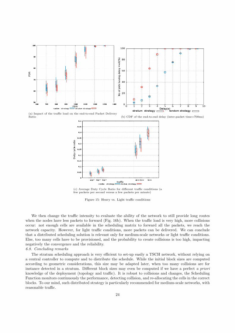
6.7. Large-scale topology with 100 nodes

We now consider a large-scale cluster tree topology with 100 nodes, and observe the ComplementaryCumulative Distribution Function (CCDF) of the of the end-to-end PDR (Fig.16a). A large topology hasan impact on the reliability: more packets have to be transmitted, and create possibly more collisions.However, the random and stratum strategies exhibit similar results: the collisions seem solved efficientlyby the rescheduling policy. However, a long route means also more retransmissions, and possibly a largerprobability to drop the packet before it is received by the destination.

23

(a) Impact of the traffic load on the end-to-end Packet DeliveryRatio (b) CDF of the end-to-end delay (inter-packet time=700ms)

(c) Average Duty Cycle Ratio for different traffic conditions (afew packets per second versus a few packets per minute)

Figure 15: Heavy vs. Light traffic conditions

We then change the traffic intensity to evaluate the ability of the network to still provide long routeswhen the nodes have less packets to forward (Fig. 16b). When the traffic load is very high, more collisionsoccur: not enough cells are available in the scheduling matrix to forward all the packets, we reach thenetwork capacity. However, for light traffic conditions, more packets can be delivered. We can concludethat a distributed scheduling solution is relevant only for medium-scale networks or light traffic conditions.Else, too many cells have to be provisioned, and the probability to create collisions is too high, impactingnegatively the convergence and the reliability.6.8. Concluding remarks

The stratum scheduling approach is very efficient to set-up easily a TSCH network, without relying ona central controller to compute and to distribute the schedule. While the initial block sizes are computedaccording to geometric considerations, this size may be adapted later, when too many collisions are forinstance detected in a stratum. Different block sizes may even be computed if we have a perfect a prioriknowledge of the deployment (topology and traffic). It is robust to collisions and changes, the SchedulingFunction monitors continuously the performance, detecting collision, and re-allocating the cells in the correctblocks. To our mind, such distributed strategy is particularly recommended for medium-scale networks, withreasonable traffic.

24

0

20

40

60

80

100

10 20 30 40 50 60 70 80 90 100

No.

of fl

ows

havi

ng P

DR

>=

X(%

)

PDR


(a) Complementary CDF of the end-to-end PDR (with 100 nodes,inter packet time=12s)

0

0.2

0.4

0.6

0.8

1

1ppm 3ppm 5ppm 7ppm 9ppm 11ppm13ppm15ppm

PD

R

traffic

stratum strategy

(b) Impact of the traffic load on the end-to-end reliability (with100 nodes and 1 sink)

Figure 16: Large-scale topology with 100 nodes and 1 sink, slotframe with 203 cells

For very large-scale networks with a very high traffic to forward, the network must operate close to itsduty cycle limit. Thus, more collisions occur, which slow down the convergence of the relocation algorithm.A centralized schedule would help to improve the performance, but it requires to know precisely the radiotopology, the interfering links, the link qualities, which still constitute a challenging problem in manysituations (cf. section 3.1).

7. Conclusion and Future Work

We presented here a distributed scheduling solution designed for 6TiSCH. It allocates the soft cellsautonomously and minimizes the end-to-end delay: a packet present in the buffer at the beginning of theslotframe should be delivered before the end. We use a stratum scheduling strategy, dividing the wholeschedule into blocks. Then, all the nodes equidistant from the border router share the same block tominimize the buffering delay. By selecting appropriately the size of each block, we are able to guaranteea packet is delivered with a slotframe to the border router, even if it is multihop far away. We re-usedthe self-healing mechanism of SF0 to detect colliding cells, and evaluated its efficiency experimentally: anWMEWMA estimator helps to smoothen the variations, reducing the number of false positives / negatives.

In a future work, we plan to propose a call admission mechanism. Indeed, the network begins to performpoorly when the network capacity is exceeded. We must guarantee on the contrary that the existing flowsare not perturbed by the new ones (i.e. traffic isolation). We also plan to compare stratum, SF0 and SFlocwith a centralized algorithm. However, we have to propose the mechanisms to collect all the informationrequired for the scheduler (radio links, their quality, traffic volume, etc.) Moreover, we also have to providethe protocols to update the schedule on-the-fly, when e.g. a new node is inserted in the network and has tosend packets.

Acknowledgement

This work was partly supported by the University of Strasbourg Idex project Diag@IoT.

References

References

[1] I. Hosni, F. Theoleyre, N. Hamdi, Localized scheduling for end-to-end delay constrained Low Power Lossy networks with6TiSCH, in: International Symposium on Computers and Communication (ISCC), IEEE, 2016. doi:10.1109/ISCC.2016.7543789.

25

https://doi.org/10.1109/ISCC.2016.7543789

https://doi.org/10.1109/ISCC.2016.7543789

[2] L. Atzori, A. Iera, G. Morabito, The internet of things: A survey, Computer Networks 54 (15) (2010) 2787 – 2805.doi:10.1016/j.comnet.2010.05.010.

[3] L. D. Xu, W. He, S. Li, Internet of things in industries: A survey, IEEE Transactions on Industrial Informatics 10 (4)(2014) 2233–2243. doi:10.1109/TII.2014.2300753.

[4] IEEE Std 802.15.4e-2012, IEEE Standard for Local and metropolitan area networks–Part 15.4: Low-Rate Wireless PersonalArea Networks (LR-WPANs) Amendment 1: MAC sublayer (2012).

[5] T. Watteyne, A. Mehta, K. Pister, Reliability through frequency diversity: Why channel hopping makes sense, in: ACMSymposium on Performance Evaluation of Wireless Ad Hoc, Sensor, and Ubiquitous Networks (PE-WASUN), 2009, pp.116–123. doi:10.1145/1641876.1641898.

[6] M. Palattella, N. Accettura, X. Vilajosana, T. Watteyne, L. Grieco, G. Boggia, M. Dohler, Standardized protocol stackfor the internet of (important) things, IEEE Communications Surveys Tutorials 15 (3) (2013) 1389–1406. doi:10.1109/

SURV.2012.111412.00158.[7] D. Dujovne, T. Watteyne, X. Vilajosana, P. Thubert, 6tisch: deterministic ip-enabled industrial internet (of things), IEEE

Communications Magazine 52 (12) (2014) 36–41. doi:10.1109/MCOM.2014.6979984.[8] T. Winter, P. Thubert, A. Brandt, J. Hui, R. Kelsey, P. Levis, K. Pister, R. Struik, J. P. Vasseur, R. Alexander, Rpl: Ipv6

routing protocol for low-power and lossy networks, rfc 6550, IETF (2012). doi:10.17487/RFC6550.[9] Q. Wang, X. Vilajosana, 6top protocol (6p), draft 4, IETF, https://tools.ietf.org/html/

draft-ietf-6tisch-6top-protocol-04 (March 2017).[10] K. Pister, L. Doherty, Tsmp: Time synchronized mesh protocol, in: Parallel and Distributed Computing and Systems,

2008.[11] J. N. Tsitsiklis, K. Xu, On the power of (even a little) centralization in distributed processing, in: ACM SIGMETRICS,

2011, pp. 161–172. doi:10.1145/1993744.1993759.[12] M.R. Palattella, et al., On optimal scheduling in duty-cycled industrial iot applications using IEEE802.15.4e TSCH,

Sensors Journal, IEEE 13 (10) (2013) 3655–3666. doi:10.1109/JSEN.2013.2266417.[13] A. Tinka, T. Watteyne, K. Pister, A decentralized scheduling algorithm for time synchronized channel hopping, in: ICST

Transactions on Mobile Communications and Applications, 2010.[14] N. Accettura, M. Palattella, G. Boggia, L. Grieco, M. Dohler, Decentralized traffic aware scheduling for multi-hop low

power lossy networks in the internet of things, in: World of Wireless, Mobile and Multimedia Networks (WoWMoM), 2013IEEE 14th International Symposium and Workshops on a, 2013, pp. 1–6. doi:10.1109/WoWMoM.2013.6583485.

[15] D. Dujovne, L. A. Grieco, M. R. Palattella, N. Accettura, 6tisch 6top scheduling function zero (sf0), draft 4, IETF,https://tools.ietf.org/html/draft-ietf-6tisch-6top-sf0-04 (July 2017).

[16] C.-Y. Wan, S. B. Eisenman, A. T. Campbell, J. Crowcroft, Siphon: Overload traffic management using multi-radio virtualsinks in sensor networks, in: Conference on Embedded Networked Sensor Systems (SenSys), ACM, 2005, pp. 116–129.doi:10.1145/1098918.1098931.

[17] F. Theoleyre, G. Z. Papadopoulos, Experimental validation of a distributed self-configured 6tisch with traffic isolationin low power lossy networks, in: International Conference on Modeling, Analysis and Simulation of Wireless and MobileSystems (MSWiM), ACM, 2016, pp. 102–110. doi:10.1145/2988287.2989133.

[18] V. C. Gungor, G. P. Hancke, Industrial Wireless Sensor Networks: Challenges, Design Principles, and Technical Ap-proaches, IEEE Transactions on Industrial Electronics 56 (10) (2009) 4258–4265. doi:10.1109/TIE.2009.2015754.

[19] J. Lee, W. Kim, S.-J. Lee, D. Jo, J. Ryu, T. Kwon, Y. Choi, An experimental study on the capture effect in 802.11anetworks, in: International Workshop on Wireless Network Testbeds, Experimental Evaluation and Characterization(WinTECH), ACM, 2007, pp. 19–26. doi:10.1145/1287767.1287772.

[20] M. Sha, G. Xing, G. Zhou, S. Liu, X. Wang, C-MAC: Model-driven concurrent medium access control for wireless sensornetworks, in: INFOCOM, IEEE, 2009, pp. 1845–1853. doi:10.1109/INFCOM.2009.5062105.

[21] X. Vilajosana, K. Pister, Minimal 6TiSCH Configuration, draft 21, IETF (February 2017).[22] Z. Chen, C. Wang, Use cases and requirements for using track in 6tisch networks, draft 0, IETF, https://tools.ietf.

org/html/draft-wang-6tisch-track-use-cases-00 (September 2015).[23] A. Ghosh, O. Incel, V. Kumar, B. Krishnamachari, Multi-channel scheduling algorithms for fast aggregated convergecast

in sensor networks, in: International Conference on Mobile Adhoc and Sensor Systems (MASS), IEEE, Macau, Macau,2009, pp. 363–372. doi:10.1109/MOBHOC.2009.5336979.

[24] M. Yan, K.-Y. Lam, S. Han, E. Chan, Q. Chen, P. Fan, D. Chen, M. Nixon, Hypergraph-based data link layer schedulingfor reliable packet delivery in wireless sensing and control networks with end-to-end delay constraints, Information Sciences278 (2014) 34 – 55. doi:10.1016/j.ins.2014.02.006.

[25] M. Yigit, O. D. Incel, V. C. Gungor, On the interdependency between multi-channel scheduling and tree-based routingfor WSNs in smart grid environments, Computer Networks 65 (0) (2014) 1 – 20. doi:10.1016/j.comnet.2014.02.025.

[26] F. Dobslaw, T. Zhang, M. Gidlund, End-to-end reliability-aware scheduling for wireless sensor networks, IEEE Transactionson Industrial Informatics 12 (2) (2016) 758–767. doi:10.1109/TII.2014.2382335.

[27] R. Soua, P. Minet, E. Livolant, MODESA: An optimized multichannel slot assignment for raw data convergecast in wirelesssensor networks, in: International Performance Computing and Communications Conference (IPCCC), IEEE, 2012, pp.91–100. doi:10.1109/PCCC.2012.6407742.

[28] K.-H. Phung, B. Lemmens, M. Goossens, A. Nowe, L. Tran, K. Steenhaut, Schedule-based multi-channel communicationin wireless sensor networks: A complete design and performance evaluation, Ad Hoc Networks 26 (2015) 88 – 102.doi:10.1016/j.adhoc.2014.11.008.

[29] J. Lee, W. C. Jeong, B. C. Choi, A multi-channel timeslot scheduling algorithm for link recovery in wireless multi-hopsensor networks, in: International Conference on Information and Communication Technology Convergence (ICTC), 2016,

26

https://doi.org/10.1016/j.comnet.2010.05.010

https://doi.org/10.1109/TII.2014.2300753

https://doi.org/10.1145/1641876.1641898

https://doi.org/10.1109/SURV.2012.111412.00158

https://doi.org/10.1109/SURV.2012.111412.00158

https://doi.org/10.1109/MCOM.2014.6979984

https://doi.org/10.17487/RFC6550

https://tools.ietf.org/html/draft-ietf-6tisch-6top-protocol-04

https://tools.ietf.org/html/draft-ietf-6tisch-6top-protocol-04

https://doi.org/10.1145/1993744.1993759

https://doi.org/10.1109/JSEN.2013.2266417

https://doi.org/10.1109/WoWMoM.2013.6583485

https://tools.ietf.org/html/draft-ietf-6tisch-6top-sf0-04

https://doi.org/10.1145/1098918.1098931

https://doi.org/10.1145/2988287.2989133

https://doi.org/10.1109/TIE.2009.2015754

https://doi.org/10.1145/1287767.1287772

https://doi.org/10.1109/INFCOM.2009.5062105

https://tools.ietf.org/html/draft-wang-6tisch-track-use-cases-00

https://tools.ietf.org/html/draft-wang-6tisch-track-use-cases-00

https://doi.org/10.1109/MOBHOC.2009.5336979

https://doi.org/10.1016/j.ins.2014.02.006

https://doi.org/10.1016/j.comnet.2014.02.025

https://doi.org/10.1109/TII.2014.2382335

https://doi.org/10.1109/PCCC.2012.6407742

https://doi.org/10.1016/j.adhoc.2014.11.008

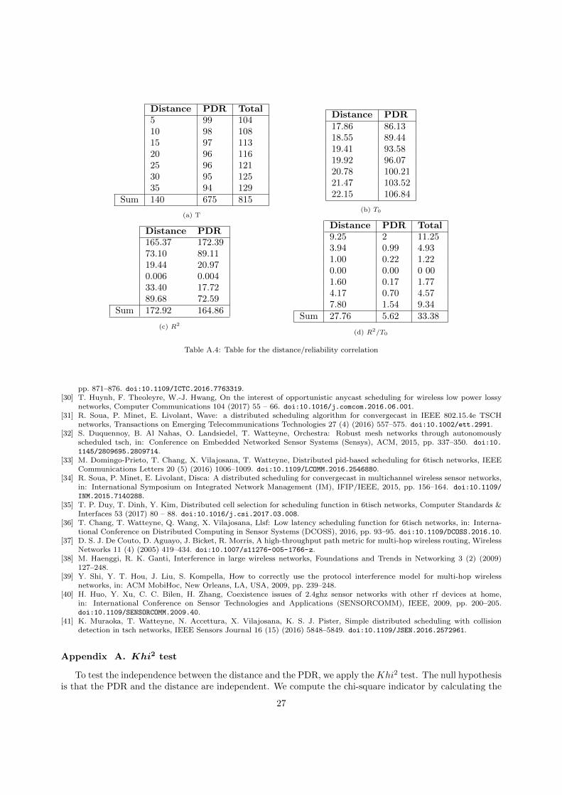
Distance PDR Total5 99 10410 98 10815 97 11320 96 11625 96 12130 95 12535 94 129

Sum 140 675 815

(a) T

Distance PDR17.86 86.1318.55 89.4419.41 93.5819.92 96.0720.78 100.2121.47 103.5222.15 106.84

(b) T0

Distance PDR165.37 172.3973.10 89.1119.44 20.970.006 0.00433.40 17.7289.68 72.59

Sum 172.92 164.86

(c) R2

Distance PDR Total9.25 2 11.253.94 0.99 4.931.00 0.22 1.220.00 0.00 0 001.60 0.17 1.774.17 0.70 4.577.80 1.54 9.34

Sum 27.76 5.62 33.38

(d) R2/T0

Table A.4: Table for the distance/reliability correlation

pp. 871–876. doi:10.1109/ICTC.2016.7763319.[30] T. Huynh, F. Theoleyre, W.-J. Hwang, On the interest of opportunistic anycast scheduling for wireless low power lossy

networks, Computer Communications 104 (2017) 55 – 66. doi:10.1016/j.comcom.2016.06.001.[31] R. Soua, P. Minet, E. Livolant, Wave: a distributed scheduling algorithm for convergecast in IEEE 802.15.4e TSCH

networks, Transactions on Emerging Telecommunications Technologies 27 (4) (2016) 557–575. doi:10.1002/ett.2991.[32] S. Duquennoy, B. Al Nahas, O. Landsiedel, T. Watteyne, Orchestra: Robust mesh networks through autonomously

scheduled tsch, in: Conference on Embedded Networked Sensor Systems (Sensys), ACM, 2015, pp. 337–350. doi:10.

1145/2809695.2809714.[33] M. Domingo-Prieto, T. Chang, X. Vilajosana, T. Watteyne, Distributed pid-based scheduling for 6tisch networks, IEEE

Communications Letters 20 (5) (2016) 1006–1009. doi:10.1109/LCOMM.2016.2546880.[34] R. Soua, P. Minet, E. Livolant, Disca: A distributed scheduling for convergecast in multichannel wireless sensor networks,

in: International Symposium on Integrated Network Management (IM), IFIP/IEEE, 2015, pp. 156–164. doi:10.1109/

INM.2015.7140288.[35] T. P. Duy, T. Dinh, Y. Kim, Distributed cell selection for scheduling function in 6tisch networks, Computer Standards &

Interfaces 53 (2017) 80 – 88. doi:10.1016/j.csi.2017.03.008.[36] T. Chang, T. Watteyne, Q. Wang, X. Vilajosana, Llsf: Low latency scheduling function for 6tisch networks, in: Interna-

tional Conference on Distributed Computing in Sensor Systems (DCOSS), 2016, pp. 93–95. doi:10.1109/DCOSS.2016.10.[37] D. S. J. De Couto, D. Aguayo, J. Bicket, R. Morris, A high-throughput path metric for multi-hop wireless routing, Wireless

Networks 11 (4) (2005) 419–434. doi:10.1007/s11276-005-1766-z.[38] M. Haenggi, R. K. Ganti, Interference in large wireless networks, Foundations and Trends in Networking 3 (2) (2009)

127–248.[39] Y. Shi, Y. T. Hou, J. Liu, S. Kompella, How to correctly use the protocol interference model for multi-hop wireless

networks, in: ACM MobiHoc, New Orleans, LA, USA, 2009, pp. 239–248.[40] H. Huo, Y. Xu, C. C. Bilen, H. Zhang, Coexistence issues of 2.4ghz sensor networks with other rf devices at home,

in: International Conference on Sensor Technologies and Applications (SENSORCOMM), IEEE, 2009, pp. 200–205.doi:10.1109/SENSORCOMM.2009.40.

[41] K. Muraoka, T. Watteyne, N. Accettura, X. Vilajosana, K. S. J. Pister, Simple distributed scheduling with collisiondetection in tsch networks, IEEE Sensors Journal 16 (15) (2016) 5848–5849. doi:10.1109/JSEN.2016.2572961.

Appendix A. Khi2 test

To test the independence between the distance and the PDR, we apply the Khi2 test. The null hypothesisis that the PDR and the distance are independent. We compute the chi-square indicator by calculating the

27

https://doi.org/10.1109/ICTC.2016.7763319

https://doi.org/10.1016/j.comcom.2016.06.001

https://doi.org/10.1002/ett.2991

https://doi.org/10.1145/2809695.2809714

https://doi.org/10.1145/2809695.2809714

https://doi.org/10.1109/LCOMM.2016.2546880

https://doi.org/10.1109/INM.2015.7140288

https://doi.org/10.1109/INM.2015.7140288

https://doi.org/10.1016/j.csi.2017.03.008

https://doi.org/10.1109/DCOSS.2016.10

https://doi.org/10.1007/s11276-005-1766-z

https://doi.org/10.1109/SENSORCOMM.2009.40

https://doi.org/10.1109/JSEN.2016.2572961

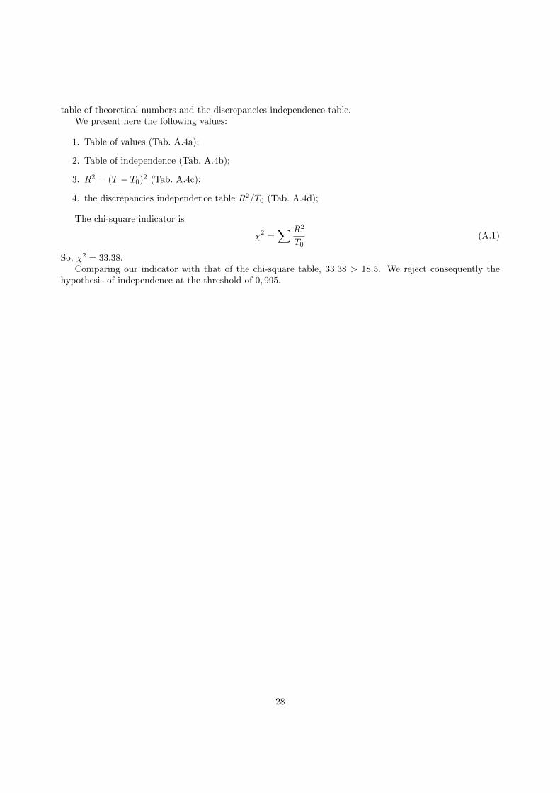
table of theoretical numbers and the discrepancies independence table.We present here the following values:

1. Table of values (Tab. A.4a);

2. Table of independence (Tab. A.4b);

3. R2 = (T − T0)2 (Tab. A.4c);

4. the discrepancies independence table R2/T0 (Tab. A.4d);

The chi-square indicator is

χ2 =∑ R2

T0(A.1)

So, χ2 = 33.38.Comparing our indicator with that of the chi-square table, 33.38 > 18.5. We reject consequently the

hypothesis of independence at the threshold of 0, 995.

28

Documents

Self-Healing Distributed Scheduling for End-to-End Delay