Self-Organization of Topographic Bilinear Networks for Invariant Recognition

LETTER Communicated by Bruno Olshausen

Self-Organization of Topographic Bilinear Networksfor Invariant Recognition

Urs [email protected] von der [email protected] Institute for Advanced Studies, Frankfurt am Main, 60594, Germany

We present a model for the emergence of ordered fiber projections thatmay serve as a basis for invariant recognition. After invariance trans-formations are self-organized, so-called control units competitively acti-vate fiber projections for different transformation parameters. The modelbuilds on a well-known ontogenetic mechanism, activity-based develop-ment of retinotopy, and it employs activity blobs of varying position andsize to install different transformations. We provide a detailed analysisfor the case of 1D input and output fields for schematic input patternsthat shows how the model is able to develop specific mappings. We dis-cuss results that show that the proposed learning scheme is stable forcomplex, biologically more realistic input patterns. Finally, we show thatthe model generalizes to 2D neuronal fields driven by simulated retinalwaves.

1 Introduction

A central problem for visual perception is the generation of representationsof environmental input patterns that are invariant to transformation (e.g.,translation and scale). These representations, which may reside in infer-otemporal cortex (Tanaka, 1996), enable the brain to recognize and examineobjects in spite of rapidly changing retinal images. A possible mechanismfor the construction of invariant representations is based on variable fiberprojections (Hinton, 1981), called dynamic links (von der Malsburg, 1981) orshifter circuits (Anderson & Van Essen, 1987; Wolfrum & von der Malsburg,2007). The underlying idea of these approaches is to normalize input pat-terns by applying a transformation to yield a standardized representation.Hence, the approach factorizes the representation of input data into theinvariant code representing the input independent of the transformationand a code for representing which transformation was needed to achievethis invariance. Invariant object recognition has been modeled on this basis(Olshausen, Anderson, & Van Essen, 1993; Lades et al.,1993; Wiskott & vonder Malsburg, 1996; Arathorn, 2002; Lucke, Keck, & von der Malsburg,

Neural Computation 23, 2770–2797 (2011) c© 2011 Massachusetts Institute of Technology

Ontogeny of Networks for Invariant Recognition 2771

2008; Wolfrum, Wolff, Lucke, & von der Malsburg, 2008). Dynamic linksmay be controlled by temporal correlations of neuronal activities in a rapidreversible version of Hebbian learning, and face recognition has been mod-eled in this way (Wiskott & von der Malsburg, 1996). Unfortunately, thismode of control is too slow to handle the required numbers of specific bind-ings in realistic time, taking more than 100 times longer than adult objectrecognition. However, the switching of connections can be accelerated withthe help of control units able to modulate the links they contact. Controlunits are uncommon in that signal flow on their neurites is bidirectional—incoming during unit activation, outgoing during synaptic control (Hinton,1981). On the one hand, these units collect information on the similarity ofactivity patterns at the pre- and postsynaptic side of the links under theircontrol, and on the other hand, they modulate the strength of these linksand therefore implement transformations. Consequently, we call the set oftheir neurites receptive-and-projective fields (RPFs). Control units could bea special type of cells, which learn to contact with their processes synapsesthat are experiencing strong pre- and postsynaptic signal correlations. Thisis akin to Hebbian learning, with the difference that it is not the synapsethat is strengthened but the modulatory contact of the control unit. It is notclear which cortical cell type or types are to be identified with control units(see, however, the hypothesis that astrocytes play this role; Moller, Lucke,Zhu, Faustmann, & von der Malsburg, 2007). On the other hand, the controlunit hypothesis could be interpreted as being a mathematical abstraction ofnonlinear neuronal network effects that in detail would inevitably be morecomplicated. Although there are plenty of theoretical and experimentalinvestigations of possible multiplicatory neuronal interactions (Salinas& Abbott, 1996; Gabbiani et al., 2004; Rothman, Cathala, Steuber, &Silver, 2009), it is up to future research how the bidirectional multiplica-tions required for normalization based approaches can be implemented indetail.

In bilinear models (Tenenbaum & Freeman, 2000; Grimes & Rao, 2005;Olshausen, Cadieu, Culpepper, & Warland, 2007; Berkes, Turner, & Sahani,2009; Bergmann & von der Malsburg, 2010; Memisevic & Hinton, 2010),the output activities are proportional to a weighted sum of products of twoinput activities. They hence share the underlying idea of controlled signalrouting with the control unit hypothesis, if one of the two input activitiesis taken to originate from a control unit. If control units responsible foralternate transformations compete in a winner-take-all fashion, the stage isset for very rapid transformation detection and subsequent transformation-specific signal routing. This leads to the compensation of variations of inputpatterns and generates an invariant representation that can be exploited forobject recognition (Olshausen et al., 1993; Arathorn, 2002; Lucke et al., 2008;Wolfrum et al., 2008).

In this letter, we are concerned with the problem of the ontogeneticdevelopment of appropriate connectivity patterns for control units that

2772 U. Bergmann and C. von der Malsburg

correspond to meaningful real-world transformations (e.g., transla-tions). These transformations are a necessary ingredient to a completenormalization-based object recognition system (e.g., for a correspondence-based system), where memory patterns are compared with actively trans-formed input patterns and in this way allow invariant recognition of storedmemory patterns with respect to the transformations (Arathorn, 2002).However, no developmental mechanism for the organization of the trans-formations has been proposed so far. Our model is based on the idea thatsynaptic plasticity, driven by temporal signal correlations, generates a ten-dency toward neighborhood-preserving projection patterns (in a style anal-ogous to the activity-based ontogenesis of retinotopy; see Huberman, Feller,& Chapman, 2008). In contrast to the process of the establishment of retino-topy, which leads to a single mapping, we assume that under the influ-ence of slow activity waves, a whole set of different topographic projectionpatterns is gradually installed. Each mapping corresponds to a differenttransformation parameter, induced by the position and size of an activitywave. The waves necessary for our model might be projected retinal waves(Meister, Wong, Baylor, & Shatz, 1991; Warland, Huberman, & Chalupa,2006; Huberman et al., 2008) or spontaneous cortical waves (Chiu & Weliky,2001). Eventually each control unit has an RPF in the form of a topographicmapping. A similar model for the ontogenesis of multiple topographic map-pings has been proposed for the simpler case of one-dimensional input andoutput neuronal fields with periodic boundary conditions and restricted totranslations only (Zhu, Bergmann, & von der Malsburg, 2010).

As proposed in Anderson and Van Essen (1987) and Zhu and von derMalsburg (2004), the RPFs of control units should be intermediate betweencontrolling single links, as in Lucke et al. (2008) and Wolfrum et al. (2008),and the total set of connections involved in a transformation from the inputto the whole invariant output window. The latter, though most efficient (inthat a single active control unit could project a whole figure into an invariantoutput window in inferotemporal cortex) is unrealistic for several reasons:due to the limited spatial range of neurites; because a whole projection has totraverse several cortical areas (e.g., V1-V2-V4-IT), as modeled in Andersonand Van Essen (1987) and Wolfrum and von der Malsburg (2007); and sincethe number of required control units would be too large to cover the spaceof all possible projection patterns. Nevertheless, for the sake of simplicity,our concrete model lets each global projection pattern be controlled by asingle control unit. However, if we considered the output field of our modelas being only a patch of the whole output window, the RPFs of the modelwould indeed be of intermediate size.

It is known that activity plays a role in retinotopy formation and refine-ment during ontogeny (Huberman et al., 2008). The mechanism proposedin this letter is an extension of a model for this process of self-organization(Haussler & von der Malsburg, 1983), which is reviewed in section 2, ap-plied to a bilinear model of neuronal information processing (Tenenbaum &


Figure 1: Interactions leading to the self-organization of topographic mappings.On the one hand, all incoming connections at an output neuron o compete,as depicted by the minus sign. Similarly, at an input neuron i, all outgoingconnections compete. On the other hand, there is cooperation (denoted by theplus sign) between two connections that run from neighboring input units (i′

and i′′) to neighboring output units (o′ and o′′). The strength of this cooperationfalls off with the distance of neurons within the two fields.

Freeman, 2000; Grimes & Rao, 2005; Olshausen et al., 2007), as described insection 3. The results of our model in section 4 show that visual stimuli arenot necessary to organize a network with real-world invariance transfor-mations. Indeed they might even make it more difficult, as it is nontrivial todisentangle pattern information and transformation information containedin visual stimuli. We therefore propose that this ontogenesis happens pre-natally, which also would be of great biological utility, at least for precociousanimals, that is, animals that are mobile at the moment of birth or hatching(Starck & Ricklefs, 1998).

2 The Haussler System

We review an abstract model for topographic map formation that has beenreduced to the essential ingredients. Neuronal activity variables in thismodel have been removed by adiabatic elimination (von der Malsburg,1995), and therefore the dynamics is autonomously formulated in theweight variables.

On an abstract level all self-organizing map formation mechanisms (fora review, see Swindale, 1996; Goodhill, 2007) share two essential ingredi-ents (see Figure 1): cooperation of neighboring connections and divergentand convergent competition. The first of these constitutes a bias towardtopographic structure, because a strong connection favors the growth of

http://www.mitpressjournals.org/action/showImage?doi=10.1162/NECO_a_00195&iName=master.img-000.jpg&w=167&h=134


connections with neighboring input and output coordinates. The secondingredient, competition, ensures convergence to a one-to-one mapping: atan output neuron o, all incoming connections compete, and similarly, at aninput neuron i, all outgoing connections compete.

In the following, we formalize map formation in terms of an abstractmodel that is termed the Haussler system (Haussler & von der Malsburg,1983). It has the advantage that it is simple and analyzable, can be sim-ulated efficiently, and is compatible with a full range of models (Swin-dale, 1996; Goodhill, 2007; Hyvarinen, Hoyer, & Inki, 2001). All detailedmodels for the topography mechanism, which simulate neuronal activities,involve statistical dependencies in neural activity patterns to encode neigh-borhood relationships in the connected neural fields and to drive synapticplasticity.

The mapping from the input to the output area is represented by aset of links (o, i), with o and i representing output and input coordinates,respectively. The weight value woi of link (o, i) indicates the strength withwhich output unit o and input unit i are connected. In the Haussler system,weight values are positive, and a value of 0 represents the absence of aconnection. The set of all links forms a mapping W = (woi).

The Haussler system, which was inspired by an equation proposed byEigen (1971) for the evolution of species in theoretical biology and thereforeshares the essential ingredients, namely competition and cooperation, isformulated by a set of differential equations:

woi = α + woiFoi(W ) − woiBoi(α + WF(W )), (2.1)

where α is a nonnegative unspecific growth term, shared by all weights,that can be used as a control parameter for the pattern formation process(Haussler & von der Malsburg, 1983). Qualitatively, this equation leads toa strong competition (in case of α = 0, a hard winner-take-all competition)of weights that compete in the B-term. Foi(W ) mediates weight cooperationof neighboring weights. The explicit form of the cooperation coefficient Foiis derived in von der Malsburg (1995) using Hebbian learning and yieldsa strictly positive weighted sum of neighboring weights with the couplingmatrices CO and CI:

Foi(W ) =∑o′,i′

COoo′CI

ii′wo′i′ . (2.2)

The coupling matrices COoo′ and CI

ii′ are monotonically falling functions ofboth |o − o′| and |i − i′| and describe the mutual cooperative support thatlink (o, i) receives from its neighbors (o′, i′). The monotonicity of the cou-pling matrices leads to the support of neighboring weights and hence to aneighborhood-dependent growth of the weights.


The competition term Boi contains as argument besides α the matrix WF(the component-wise Hadamard product (WF(W ))oi = woiFoi(W )) and is theaverage of growth rates of all weights with either the same input index i orthe same output index o,

Boi(M) =(∑

o′mo′i/No +

∑i′

moi′/Ni

)/2, (2.3)

where M = (moi) is a matrix. In the following, Ni and No denote, respectively,the number of cells in the input and output fields. The two different sumsin this term implement the divergent and convergent competition, shownin Figure 1, that is necessary for map formation. Biophysically this termmight be implemented by a normalization of weights on the output sideand a competition for growth factors mediated by the input side.

For the case of periodic boundary conditions, the system can be treatedanalytically (Haussler & von der Malsburg, 1983). It has been shown thatstarting with weights that deviate slightly from the homogeneous solution,W = 1 (the matrix in which all entries equal 1), the system, equation 2.1,converges to a diagonal matrix (in case of the same size of the input andthe output fields, Ni = No), hence a topographic one-to-one mapping of theinput to the output. Numerical simulations show that in the case of non-periodic boundary conditions, the system reliably converges to a diagonalmatrix as well. Due to biological plausibility, we restrict our studies in thisletter to the investigation of systems with nonperiodic boundary conditions.

3 The Bilinear Model

The model (see Figure 2, left) consists of two layers of neurons—the inputfield and the output field. There are short-range connections within thefields and excitatory all-to-all connections between them. In addition, thereis a set of control units able to modulate the connections between the layers.

The purpose of the model is to demonstrate that different transforma-tions can be organized on the basis of spontaneous activity in the inputfield. Activity in the input field is restricted to active regions. The activeregions could be retinal waves, spontaneous waves in cortex, or wavesprojected from the retina to cortex. Figure 2 (right) shows an example ofa simulated retinal wave, which was modeled as described in Godfrey& Swindale (2007). Simulated retinal waves were used as inputs to theproposed system in the two-dimensional case. Section 3.1 describes the re-sponse of the input and output field units once a region is active. Usingthe learning rule described in section 3.2, a single control unit active for aregion slightly biases its RPF to get restricted to that region and to form atopographic map from that region to the whole output field. Section 3.3 de-scribes the unsupervised winner-take-all (WTA) mechanism that was used


Figure 2: (Left) Training of control units. Different regions are active at differenttimes in the input field (left panel). These regions might be (projected) retinalwaves. Control units (filled circles) learn to be activated by and to activate con-nections. After self-organization, a control unit activates connections that forma topographic projection from an active region to the output field (right panel),which forms an invariant window (in an upstream cortical area, presumablyIT). The dotted lines indicate the connectivity pattern of an alternative controlunit that topographically routes from the smaller circle in the input field to theoutput field. (Right) An example of a simulated retinal wave, as described inGodfrey and Swindale (2007), which has been used as an active region in thetwo-dimensional simulations. White squares indicate active retinal cells, andblack squares indicate inactive cells. The x- and y-axes denote two orthogonalaxes in the retina.

to determine which control unit gets activated for a given input region. Theincreased bias of a control unit for a region, generated by learning, increasesits chances to win for that region on its next appearance. Iteration of theprocess leads to the emergence of topographic maps specialized to inputregions. In a nutshell, restricted active regions of input activity yield theselection of a dedicated control unit, which then refines its RPF to a trans-formation from this region to the output region. Note that although notmotivated probabilistically, the proposed method bears some similaritiesto the expectation-maximization (EM) algorithm: control unit activities areunobserved latent variables and control unit activities are selected by theWTA mechanism, corresponding to the E-step. Their RPFs are then updatedusing these activities, corresponding to the M-step. This process is iterateduntil convergence.



3.1 Input and Output Activities. Unit activities are denoted by xi(i ∈ {1, .., Ni}), yo (o ∈ {1, .., No}), or ck (k ∈ {1, .., K}) referring to input field,output field, or control units, respectively.

To motivate the topography-generating cooperation between connec-tions described in equation 2.2, activity-based Hebbian models invokeshort-range correlations in the activities (von der Malsburg, 1973; Goodhill,2007): for prenatal models of topographic map emergence, spontaneous in-dependent activity of each cell is usually assumed in the input layer, whilethe output cells are assumed to be driven by the input sheet. As cells are cou-pled laterally in the input and the output sheet, the resulting neighborhoodcorrelations of the cells drive Hebbian learning to yield a neighborhood-preserving, or topographic, map. It is necessary that the correlations fall offmonotonously with the relative distance of two cells.

3.1.1 Inputs. In order for the model to work, there are some additionalconstraints on the input signal statistics. The main goal of the model is todemonstrate that control units can develop different transformations. Inparticular, for different translations and scales, this means that the connec-tivity of control units needs to be specialized on different input regions. Wetherefore assume the input signal to be constrained to regions of activity andto be 0 elsewhere. Note that this assumption is well in line with prenatallyobserved retinal waves (Meister et al., 1991; Warland et al., 2006; Hubermanet al., 2008). In particular, we use simulated retinal waves as inputs to thetwo-dimensional system in section 5.

The neurons within the active region I of the input field produce spon-taneous noise, and this noise is correlated by excitatory coupling betweenneighbors,

xi =Ni∑j

CIi jξ jI j, (3.1)

where ξi is taken to be independent and identically distributed (i.i.d.) noisewith mean value

⟨ξi

⟩ = μ1 and second moment μ2 = ⟨ξ 2

i

⟩. Hence,

⟨ξiξ j

⟩ =μ2

1 + μdδi j with μd = μ2 − μ21. Due to the lateral coupling, the activity in the

input field unavoidably spills beyond the active region I, making restrictionof the RPFs of control units to the input region a little more difficult. For thesimulations, we used a monotonously with distance-decreasing couplingmatrix:

CIi j ∝ exp

(−λ|i − j|) , (3.2)

with λ = √30

/Ni. Further,

∑i j CI

i j was normalized to Ni.


3.1.2 Outputs. The output units receive input in the form of a bilinearterm (Tenenbaum & Freeman, 2000):

yo =K∑k

Ni∑i

wkoixick. (3.3)

According to this, the input yo to output unit o depends linearly on theinput activities xi if the control unit activities ck are constant, and vice versa.The coefficient wkoi is the connection strength of control unit k to the linkfrom input unit i to output unit o. Similar to the input field, the outputfield also needs to code neighborhood relationships for a Hebbian-basedmechanism to develop topographic mappings. Therefore, we assume thatthe final output activities result from the input yo by multiplication with acoupling matrix CO

op,

yo =No∑p

COopyo =

No∑p

COop

K∑k

Ni∑i

wkpixick, (3.4)

where the explicit shape of the coupling matrix COop is the same as for CI

i j

(see equation 3.2), with λ = √30

/No and normalization to No.

3.2 Synaptic Weight Dynamics. We now concentrate on a learning stepof the synaptic weights wkoi of a single control unit k, that is, of its RPF. In theentire model, each learning step is alternated with the selection of a singlecontrol unit, as described in section 3.3, which is the only one allowed tochange its RPF for the current input. Hence, in this section, we set ck′ = δkk′ .

The updates of the weights are to be shaped by two tendencies. Onthe one hand, each has to concentrate their connections to within one ac-tive input region. On the other hand, they have to develop a topographicstructure, connecting the input region to the output field with one-to-oneconnections linking neighbors to neighbors. Note that the specific mapformation mechanism we chose here, the Haussler system described insection 2, is not critical for the mechanism to work and could be substitutedby other map formation mechanisms. We formulate the learning rule as adifference equation:

wkoi(t + 1) = wkoi(t) + �t �wkoi(t). (3.5)

In the following we take all weights to be evaluated at iteration time t.Motivated by the Haussler system, �wkoi becomes

�wkoi = α + wkoi cov(yo, xi

) − wkoiBoi(α + Wk cov(y ⊗ x

)), (3.6)

Boi(M)=(∑

o′mo′i/No +

∑i′

moi′/(ωNi)

)/(1 + 1/ω), (3.7)


where [Wk cov(y ⊗ x

)]oi = wkoi cov

(yo, xi

)and the standard definition of the

covariance cov(x, y

) = ⟨(x − 〈x〉) · (y − ⟨

y⟩)⟩(the brackets 〈〉 denote temporal

averages). Note that the outputs yo are calculated using the weights wkoi fora single k only, as can be seen from substituting ck′ = δkk′ in equation 3.4. Asin the Haussler system, α is a nonnegative unspecific growth term.

As for the Haussler system, the Hebbian-like covariance term Foi :=cov

(yo, xi

)mediates weight cooperation, and by substituting equations 3.1

and 3.4, we see that it is a weighted sum of connections with neighboring oand i,

Foi(Wk)= cov(yo, xi

)=

∑p

∑jlm

COopwkp jC

IjlC

IimIlIm

(⟨ξlξm

⟩ − μ21

)

= μd

∑p

∑jl

COopwkp jI

2l CI

jlCIil, (3.8)

or, in matrix notation,

F(Wk) = cov(y ⊗ x

) = μdCOWkCI, (3.9)

where we defined

CI = CCT and Ci j := CIi jI j. (3.10)

The form of the derived cooperation term, equation 3.9, therefore is a gen-eralization of the cooperation term in the Haussler system. In addition tothe Haussler system, the current active region I modulates this cooperationterm so that only weights connected to an active input unit are allowed tocooperate. This active region-driven modulation results in the specializa-tion of the mapping of control units to specialize to input regions.

The competition term B essentially has the same form as in the originalHaussler system, extended by the parameter ω, which rescales the influenceof the input competition in equation 3.7. Increasing the input competitionrelative to the output competition leads to emerging mappings from only asubdomain in the input to the whole output field, because the final nonzeroweights suppress growth for weights to the unconnected input units bythe increased competition. Hence, ω determines a preferred scale of theresulting transformation. Due to activity spread, equation 3.1, the weightplasticity mechanism has a tendency to let links expand over the wholeinput field. We use an increased input competition, ω < 1, to compensatefor this activity spread effect. Fortunately, as will be seen in section 4, a singlevalue of ω is able to organize a whole range of differently scaled mappingsby allowing the final mappings to be matched to the approximate size of theinput stimuli I. Note that even for ω = 1, differently scaled transformations


emerge, but many are close to the mapping from the whole input to thewhole output fields and hence do not differ as strongly in scale as for ω < 1.If not mentioned otherwise, we set ω = 0.4 and use an iteration constant�t = 0.1 in equation 3.5.

3.3 WTA Control Unit Selection. We have described the nature of theinput signals we assume and the learning rule for a control unit k. In or-der for different transformations to emerge, different control units have tocompete for active input regions and then specialize their RPFs to an inputregion. This section describes the process of competition between controlunits, which we implemented with a WTA mechanism.

The later postnatal functional correspondence-finding mechanism has toselect the control unit (and pattern transformation) that finds the greatestpattern similarity between input and output (see Wolfrum et al., 2008). Forthe prenatal stage we consider, however, it is reasonable to assume that theoutput patterns are unstructured, because of the lack of experience. Theselection of a control unit therefore is based only on the input patterns. Acontrol unit k has the footprint

wki =∑

o

wkoi. (3.11)

We use this definition to write the purely input-based excitation of thecontrol units as a scalar product,

ck =∑

i

wki

⟨xi

⟩, (3.12)

where again the angled brackets express temporal averaging. Substitutingequation 3.1, we get

ck =∑

i

wki

⟨xi

⟩ = μ1

∑i j

wkiCIi jI j, (3.13)

where we have made use of the property⟨ξi

⟩ = μ1.The control unit activities are then determined by a WTA mechanism

(for a neurally plausible WTA mechanism, see Fukai & Tanaka, 1997; Lucke,2004):

ck ={

1 : k = arg maxk′ {ck′ }.0 : otherwise

(3.14)

Accordingly, when a region I is active, the control unit is selected, whosefootprint {wki} has the greatest overlap with the current input activity


Figure 3: (Left) Four active regions of different size, In, where n = 1, . . . , 4specifies the different regions used in an experiment with four control units. Ineach time step, one of the In is selected at random. These regions are subjectedto smoothing and noise (see equation 3.1). (Right) The resulting expected values⟨xi

⟩for the four active regions In. Through a WTA mechanism, equation 3.16, the

active regions determine which control unit is activated and permitted to learn.

distribution xi, as calculated in equation 3.13, and all others are switchedoff.

The model described so far couples a WTA mechanism (see equation 3.14)to learning (see equation 3.6). A unit winning for a given input therefore in-creases its probability to win for the same input again in the future. Note thatthe introduced learning rule does not include an explicit weight normaliza-tion (e.g., the sum of the weights could have been forced to equal unity—theso-called L1 normalization). Therefore, a unit’s increase in winning prob-ability for a given input does not necessarily decrease the probability forall (or most) of the other inputs. On the contrary, for mutually overlappinginput regions (see Figure 3, left), a unit winning for any such input regionincreases its winning probability for all other overlapping input regionsas well. As a result, only a small subset of control units would win andorganize their RPFs, while the other units would remain undifferentiated.We prevent this instability by introducing an additional gain modulation,as inspired by the concept of intrinsic plasticity (IP) (DeSieno, 1988; Desai,Rutherford, & Turrigiano, 1999; Zhang & Linden, 2003). The effect of thishomeostatic mechanism is to let control units fire with equal probability. Tobalance the winning probabilities, we introduce the gain modulating vari-able κk for each control unit, have it downregulated while a unit is activeand upregulated otherwise,

κk = η(pgoal

k − ck(t)), (3.15)



and replace the WTA mechanism (see equation 3.14) by

ck ={

1 : k = arg maxk′ {κk′ ck′ }0 : otherwise

. (3.16)

We set pgoalk = 1/K for all k, so that these parameters can be interpreted as

probabilities, and the κk will stabilize at values such that the⟨ck

⟩ = pgoalk , that

is, the control units all fire with the same probability. The time constant1/η for the dynamics should be large enough to make κk insensitive to fluc-tuations due to the random input selection. A good compromise betweenthis low-pass behavior and equilibration speed turned out to be aroundη = 1/1600, which was used for all simulations unless otherwise noted.

4 Results

The system considered in this section consists of Ni = 60 input units, andNo = 20 output units, and K = 4 control units. Simulations were run withparameters α = 0 and ω = 0.4 and initial random weights drawn from auniform distribution in [0, 1]. Although we have run many simulations withdifferent dimensions of the input and output and larger numbers of possibleactive regions and control units, we limit ourselves to the description ofthis system here for clarity. Figure 3 (left) shows four active regions inthe input field. The active regions are binary Ini ∈ {0, 1} (n specifying thedifferent regions) and are, according to equation 1, subjected to noise andsmoothing by lateral signal exchange (see Figure 3, right). Given that thesignal correlations are important for the establishment of topography, weincluded this smoothing for consistency, although it does not serve anyfunction in the simulations (see section 3.1). We intentionally use activeregions of different sizes and with full overlap in order to show that in spiteof this, the system is able to discriminate these regions.

For each time step, a random active region In is chosen, and the winningcontrol unit is determined using equation 3.16. This winning unit is thenpermitted to update its weights according to equation 3.5. This repeatedselection of control units and subsequent weight modification leads to thereorganization and refinement of the RPF mappings. Figure 4 (upper box)shows the RPFs of the four control units at an intermediate stage of learning(t = 2000 inputs). For the link visualization, the input field is on the bottomand the output field on the top, while in matrix representation, the x-axisdenotes input coordinates and the y-axis output coordinates. As describedin section 3.2, the parameter value ω = 0.4 (see equation 3.6) pushes RPFstoward smaller-scale factors (the ratio of input size to output size), whichis necessary to counteract the tendency of RPFs to spread over the wholeinput field, which happens due to activity leakage to mediate neighborhood


Figure 4: Control unit RPFs are shown for a simulation with K = 4 controlunits and Ni = 60, No = 20, α = 0, and ω = 0.4. (Upper box) Learning at anintermediate stage, t = 2000. For both the link visualization and the matrixrepresentation, stronger weights are darker. (Lower box) The (nearly) convergedweights are drawn (t = 80, 000 inputs).

correlations (see equation 3.1). The shade of a link renders the strength ofthe connection to and from control units—black is strongest and whitethe weakest. RPF entries with less than 10% of the maximum are visuallyclipped for the link visualization, but all entries are shown in the matrixrepresentation. From inspection of the RPFs, it is hard to tell how wellthey specialized to the inputs, while it is easy to see that topography hasalready emerged for units 1 and 2. Evidently the symmetry of the initialRPFs was broken, resulting in one of the two map orientations possible in



the one-dimensional case: the ascending and descending orientation. In oursimulation, control units 1 and 2 preserve the orientation of the inputs. TheRPFs of control units 3 and 4 still contain both map orientations, althoughthe links corresponding to the ascending orientation seem more pronouncedin unit 3. The final map orientation of an RPF is mainly determined bythe initial random weight values but may be influenced by the randomsequence of input stimuli as well.

In the final state, after application of t = 80, 000 inputs (when meanrelative weight changes have fallen below 0.25), the RPFs have convergedto high specificity for one input pattern as well as to good topography (seeFigure 4, lower box). Comparing the final state (Figure 4, upper box) to theintermediate stage of learning (Figure 4, lower box), we see that the maporientations prominent in the intermediate stage were already stable anddid not change in the consecutive RPF refinement.

We have performed simulations with a range of different parametervalues, and the system proves robust against many changes. To consistentlyobtain topographic mappings, a critical upper bound on λ �

√50/N in

equation 3.2 (a lower bound on the extend of lateral correlations in the fields)is to be observed, however. For smaller values the emergent transformationstend to be only piecewise topographic. If, as in Figure 3, the center points ofinput stimuli fall on varying positions, a nonvanishing positive unspecificweight growth factor α can help to allow reorganization and migrationof the RPFs. For the simulation presented, however, α can be set to 0.Nonvanishing α values also allow significantly smaller cooperation in thefields (i.e., bigger λ in equation 3.2), while still preserving final consistenttopographic transformations (Zhu, 2008).

4.1 Quantitative Characterization of RPF Development. In order to beable to gain better insight into progress and parameter dependence of thesystem we introduce three quantities.

4.1.1 Input Specificity ζ (t). This is a measure to analyze the assignment ofthe input regions to the control units and hence a measure of how specificthe control units are active for the different inputs. Let ν

(k|n, t

)be the

conditional normalized winning frequency of control unit k given regionn. We estimate this quantity with the help of a leaky integrator (with timeconstant 5 × 10−3) and the constraint

∑k ν

(k|n, t

) = 1. We define the inputspecificity of the system as

ζ (t) =⟨

maxk

ν(k|n, t)⟩{n}

, (4.1)

which is the highest winning frequency for a given active region, averagedover all possible active regions. Due to the normalization of ν, ζ ∈ [0, 1]. Themaximum ζ = 1 is reached when all active regions considered are assigned


reliably to a specific control unit. Note that due to the intrinsic plasticitymodulation of the WTA mechanism (see section 3.3) the (unconditional)winning frequencies of all control units are close to the equidistributedgoal probability 1/K, ensuring that different control units are assigned todifferent regions.

Of particular importance is the assessment of the scale of a transforma-tion, because the Haussler system tends to organize a mapping from thewhole input field to the whole output field, and hence all mappings wouldhave the same scale. To demonstrate that the proposed model is able toorganize different scales we now define the scale factor S, which is, in anutshell, the ratio of the size of the input region from which a control unitgets significant input to the whole output size. All control units have afootprint (see equation 3.11) in the form of a smoothed version of one ofthe input stimuli, similar to those in Figure 3 but with less smoothing. Asthe size of the footprint, we include all entries that are bigger than 10% ofthe maximum entry and define the scale of a transformation S as the ratioof this footprint size and the (fixed) size of the output field.

4.1.2 Synaptic Spread s(k). The goal of control unit self-organization isthe establishment of RPFs in the form of one-to-one mappings. Progresstoward this goal can be assessed with the help of the synaptic spread,which is a measure for the size of the input patch to which an output unit issignificantly connected. Therefore, for a one-to-one mapping, the synapticspread should be 0, as each output unit is assigned to a single input unit,without any spread. We define it as the synaptic standard deviation s(k),

s(k) =⟨⟨wkoi(ri − r(k, o))2⟩1/2

{i}⟩{o}

, (4.2)

in which we make use of the center of mass of the receptive field of outputunit o under control unit k,

r(k, o) =∑

i

wkoiri, (4.3)

where ri denotes the position of unit i in the input field.The exact time course of our system depends on the details of its formu-

lation, which cannot be fixed on the basis of current biological information.Moreover, topography formation can be seen as a constraint optimizationproblem, and many dynamic formulations have been shown to be consis-tent with a single optimization problem (Wiskott & Sejnowski, 1998). Wenevertheless find it useful to discuss the parameter dependence of the de-velopmental time course of input specificity and topography in our system.

Figure 5 (left) shows the average progress of input specificity, with errorbars indicating standard deviations over 50 trials. Specificity convergeswithin approximately 104 input stimuli to its maximal value. A higher rate


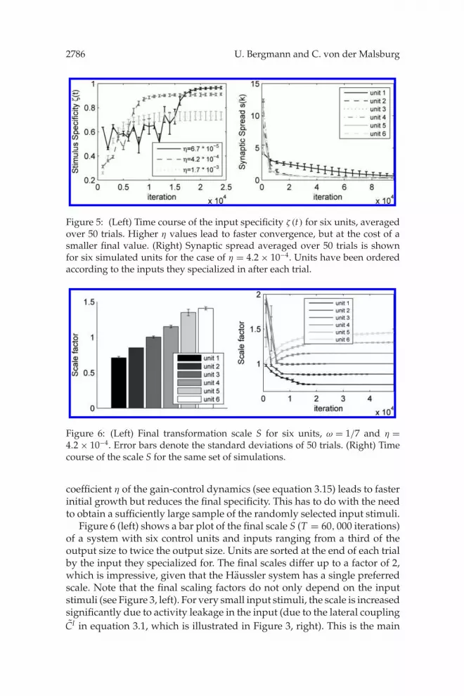
Figure 5: (Left) Time course of the input specificity ζ (t) for six units, averagedover 50 trials. Higher η values lead to faster convergence, but at the cost of asmaller final value. (Right) Synaptic spread averaged over 50 trials is shownfor six simulated units for the case of η = 4.2 × 10−4. Units have been orderedaccording to the inputs they specialized in after each trial.

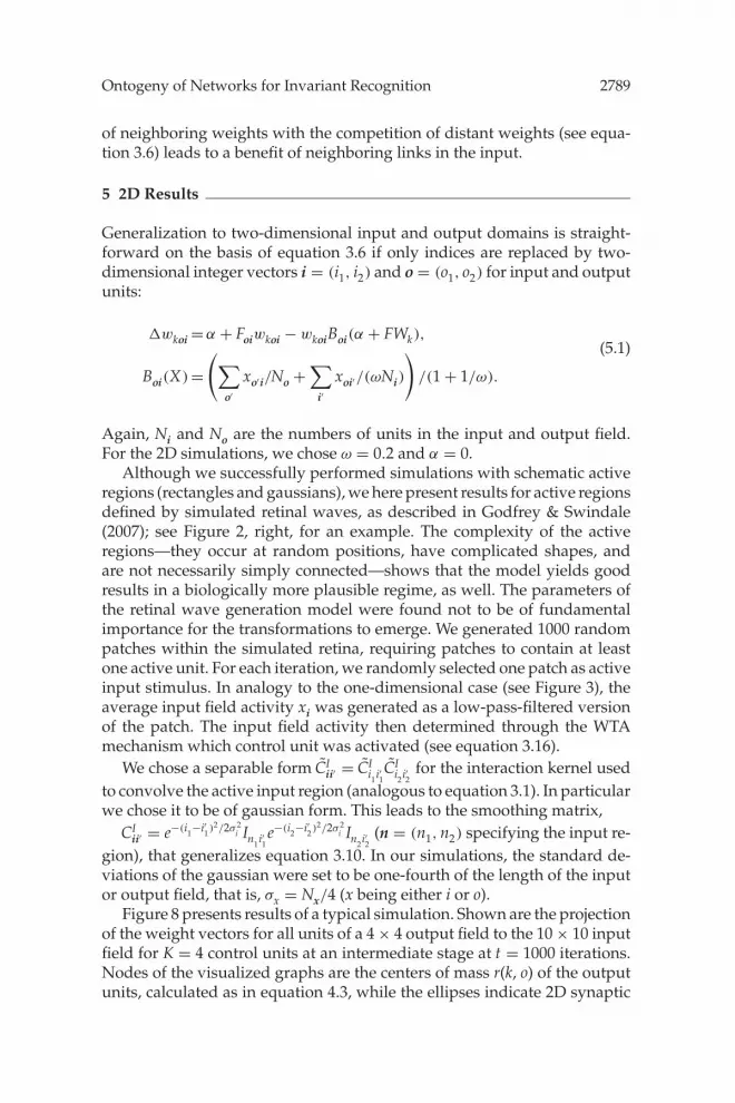
Figure 6: (Left) Final transformation scale S for six units, ω = 1/7 and η =4.2 × 10−4. Error bars denote the standard deviations of 50 trials. (Right) Timecourse of the scale S for the same set of simulations.

coefficient η of the gain-control dynamics (see equation 3.15) leads to fasterinitial growth but reduces the final specificity. This has to do with the needto obtain a sufficiently large sample of the randomly selected input stimuli.

Figure 6 (left) shows a bar plot of the final scale S (T = 60, 000 iterations)of a system with six control units and inputs ranging from a third of theoutput size to twice the output size. Units are sorted at the end of each trialby the input they specialized for. The final scales differ up to a factor of 2,which is impressive, given that the Haussler system has a single preferredscale. Note that the final scaling factors do not only depend on the inputstimuli (see Figure 3, left). For very small input stimuli, the scale is increasedsignificantly due to activity leakage in the input (due to the lateral couplingCI in equation 3.1, which is illustrated in Figure 3, right). This is the main




Figure 7: The average receptive field of all output units of control unit 2 fromFigure 4 (standard deviations are evaluated over all output units and 20 trials),shifted to common center-of-mass position r(k, o) for various values of α aftert = 5 × 105 iterations (�t = 0.5). NN: nearest neighbor.

motivation for an ω value smaller than 1, which counteracts this effect (seesection 3.2). For large-input stimuli, the lateral coupling CI is relativelysmall, and therefore the effect is negligible. The right side of Figure 6 showsthe temporal development of the scales of the transformations implementedby control units. Initially several of the scales decrease. The reason is strong,effective cooperation of weights in the center of the weight matrix of eachcontrol unit relative to the boundary, where there are fewer cooperatingpartners. Comparing this figure with Figure 5 (left panel for η = 4.2 × 10−4),we see that with increasing specificity, the scale increases again for theseunits. Finally, the scales converge to a stable value.

In Figure 5 (right), the synaptic spread, averaged over 50 trials, is shownfor all simulated units, which are again sorted by the inputs they specializedin. Interestingly, units that specialize to larger input stimuli and scalingfactors develop faster (compare Figure 6). The smallest unit stagnates for along time, which is due to the coexistence of the two map orders that arepossible in 1D (compare Figure 4, upper box). The synaptic spread of allunits converges to a small but nonfinite value, indicating that the outputunits keep contact to more than a single unit in the inputs. This observationis confirmed in Figure 7.

The final synaptic spread of RPFs is controlled by the unspecific weightgrowth parameter α (see equation 3.6). In Figure 7 we plot the receptivefield of one control unit, averaged over all output units. All receptive fieldshave been translated (with subpixel accuracy) using linear interpolation sothat their center of mass position r(k, o) (see equation 4.3) is shifted to theorigin. As can be seen, the synaptic spread grows with α. Furthermore, theweights have a strictly monotonic decrease with distance to r(k, o). Hard



WTA competition of the weights would imply that only one weight in eachcolumn and row of the weight matrix could survive. This would correspondto the survival of only the nearest neighbor (NN), which we have drawnfor comparison. In practice however, several weights per column or rowcan survive also for 0 unspecific growth, α = 0, even for very long iterationtimes.1 Hence, the transformations show a low-pass behavior and are ableto suppress aliasing effects that would be produced in the NN case.

4.2 Complex Inputs. In this section we briefly describe the stability ofthe proposed learning scheme to more complex input stimuli. The activeregions I so far were simple step functions. In a biological system, however,it might well be that borders are not this precise. Because the input activ-ities

⟨xi

⟩used for our simulations are spatially low-pass-filtered to impose

neighborhood correlations (see equation 3.1), applying smooth border in-put stimuli should not make a fundamental difference. We confirmed thissuspicion by applying gaussians of the same size and varying position in-stead of step functions and observed consistent topographic mappings toemerge.

Further, the number of different input stimuli so far exactly matched thenumber of possible control units. This is an unrealistic assumption that waschosen only for simplicity and analysis purposes. It is known that retinalwaves (Meister et al., 1991; Warland et al., 2006; Huberman et al., 2008),for example, start at a random position and then migrate over the retina.Therefore, the number of biological input stimuli can be assumed to out-number the number of control units by far. We simulated this by picking arandom position (or size) at each iteration and found topographically con-sistent mappings, varying in the desired parameters, to emerge. Hence, thecompetitive learning scheme used is able to develop mappings for repre-sentative input stimuli, and the WTA mechanism categorizes nonrepresen-tative input stimuli to belong to a certain class. From this perspective, thesystem can be seen as a generalization of vector quantization or K-meansclustering, but instead of selecting prototype vectors, the system developsprototype transformations.

Finally, areas of activity resulting from biological retinal waves are notnecessarily simply connected. However, the desired mappings are sup-posed to map a simply connected area from the input to the output. Wetherefore performed experiments with nonlinear superpositions of two in-put stimuli, each simply connected (as in Figure 3) at random positions,with a cut-off of the superposition at 1. Surprisingly, the resulting mappingswere topographically consistent and map a simply connected area from theinput to the output. The reason is that the combination of cooperation

1This can also be observed in Figure 5 (right), where the synaptic spread does notconverge to 0 but stabilizes at a small, but nonfinite value.


of neighboring weights with the competition of distant weights (see equa-tion 3.6) leads to a benefit of neighboring links in the input.

5 2D Results

Generalization to two-dimensional input and output domains is straight-forward on the basis of equation 3.6 if only indices are replaced by two-dimensional integer vectors i = (i1, i2) and o = (o1, o2) for input and outputunits:

�wkoi = α + Foiwkoi − wkoiBoi(α + FWk),(5.1)

Boi(X) =(∑

o′xo′i/No +

∑i′

xoi′/(ωNi)

)/(1 + 1/ω).

Again, Ni and No are the numbers of units in the input and output field.For the 2D simulations, we chose ω = 0.2 and α = 0.

Although we successfully performed simulations with schematic activeregions (rectangles and gaussians), we here present results for active regionsdefined by simulated retinal waves, as described in Godfrey & Swindale(2007); see Figure 2, right, for an example. The complexity of the activeregions—they occur at random positions, have complicated shapes, andare not necessarily simply connected—shows that the model yields goodresults in a biologically more plausible regime, as well. The parameters ofthe retinal wave generation model were found not to be of fundamentalimportance for the transformations to emerge. We generated 1000 randompatches within the simulated retina, requiring patches to contain at leastone active unit. For each iteration, we randomly selected one patch as activeinput stimulus. In analogy to the one-dimensional case (see Figure 3), theaverage input field activity xi was generated as a low-pass-filtered versionof the patch. The input field activity then determined through the WTAmechanism which control unit was activated (see equation 3.16).

We chose a separable form CIii′ = CI

i1i′1CI

i2i′2for the interaction kernel used

to convolve the active input region (analogous to equation 3.1). In particularwe chose it to be of gaussian form. This leads to the smoothing matrix,

CIii′ = e−(i1−i′1 )2/2σ 2

i In1i′1e−(i2−i′2 )2/2σ 2

i In2i′2(n = (n1, n2) specifying the input re-

gion), that generalizes equation 3.10. In our simulations, the standard de-viations of the gaussian were set to be one-fourth of the length of the inputor output field, that is, σx = Nx/4 (x being either i or o).

Figure 8 presents results of a typical simulation. Shown are the projectionof the weight vectors for all units of a 4 × 4 output field to the 10 × 10 inputfield for K = 4 control units at an intermediate stage at t = 1000 iterations.Nodes of the visualized graphs are the centers of mass r(k, o) of the outputunits, calculated as in equation 4.3, while the ellipses indicate 2D synaptic


Figure 8: 2D projections of the 4 × 4 output units to the 10 × 10 input spacefor K = 4 control units at an intermediate stage, at t = 1000 iterations. Thehorizontal and vertical axes in each plot denote the coordinates in the inputlayer. Control units 1 and 2 have specialized their RPFs to the lower right andupper left regions of the input field, respectively. Unit 3 just started winningand organizing its RPF, and unit 4 is still very close to its initial state.

standard deviations s(k, o), calculated as in equation 4.2 without averag-ing. Arrows connect neighboring output units in increasing order (solidarrows indicate the first dimension in the output and the dashed ones thesecond dimension). For the simulation shown, we used a value of �t = 0.2and η = 2.5 · 10−3 to Euler-iterate equation 5.1. The competition of differentcontrol units for active regions in the input leads to their specialization todifferent input regions. At the intermediate stage, it can be seen that controlunits 1 and 2 specialized on the lower right and upper left regions in the in-put. Control unit 3 just started winning and has slightly specialized for theupper-right input region, while control unit 4 remains largely unspecializedwith its initial weights in the center of the input region.2 After t =20,000

2For all weights independently drawn from a random distribution, the expected cen-ters of mass positions are in the center of the input field.



Figure 9: Two-dimensional projections of the 4 × 4 output units to the 10 × 10input space for K = 4 control units. Shown are the weights in their convergedstate after t = 20, 000 iterations. The horizontal and vertical axes in each plotdenote the coordinates in the input layer. Compared to the intermediate stageof learning (see Figure 8), the RPFs developed good topography and are morebalanced in the sizes of the input regions they cover.

iterations, the mappings do not change significantly, having converged totheir final configuration (see Figure 9). In comparison to the intermediatestage, the weights of each control unit have developed a clear topographyand have specialized to different input regions. In particular, the compe-tition of control unit 4 with the other control units forced its weights tospecialize to the lower-left region. It is noteworthy that the final mappingsare of different orientation (as can be seen by the directions of the blackarrows) and are slightly distorted due to boundary effects.

The 3D cross-product of two arrows in the plots can be used to determineif the corresponding mappings preserve mirror symmetry: if the cross-product, of a solid times a dashed arrow points out of the sheet (toward thereader), the corresponding mapping preserves mirror symmetry; otherwise(away from the reader) it violates it. Hence, for the presented results, allmappings violate this symmetry. As in the one-dimensional case, mainlythe initial values of the weights determine the mirror symmetry.



6 Discussion

The model we propose is based on a generalization of classic retinotopymechanisms (Willshaw & von der Malsburg, 1976; Haussler & von derMalsburg, 1983). The essential difference is that shifter circuits in the formof a whole set of topographical mappings are installed, each of which can beswitched on and off under the command of a control unit in the style of bilin-ear networks (Tenenbaum & Freeman, 2000; Grimes & Rao, 2005; Olshausenet al., 2007). Our main focus lies in investigating the one-dimensionalcase, where the simulations show that different types of transformation—translation, scaling, and reflection—can be reliably self-organized. The ex-tension to two dimensions with simulated retinal wave patterns (Godfrey &Swindale, 2007) as inputs demonstrates the organization of translations, ro-tations, and reflections.

Interestingly, although at first sight, simply connected regions of activ-ity in the neural input field seem crucial for our model, simulations onnon–simply connected inputs show that this is not necessary. The neces-sary input stimuli could arise in random locations as small and graduallygrowing and migrating activity regions. They may correspond to the reti-nal waves as observed in prenatal mammals (Meister et al., 1991; Warlandet al., 2006; Huberman et al., 2008), projected up to visual cortex and/orthey might emerge spontaneously in cortex (Chiu & Weliky, 2001). In ourmodel, these patterns, varying in position and size, serve as teaching signalsto control units and lead to transformations that project topographically toan invariant window in an upstream cortical area.

If indeed the input stimuli necessary for the organization of alternateprojection patterns are generated spontaneously in retina or cortex, in a waysimulating the postnatal appearance of segmented figures separated froma background, the self-organization of projection patterns can take placeprenatally or before eye opening. This is not only biologically desirable butis even likely to alleviate the organization process decisively. In line withthe idea that retinal waves mimic the postnatal appearance of segmentedfigures is the observation that waves propagate more often along the nasal-temporal than the dorsal-ventral axis of the retina (Stafford, Sher, Litke, &Feldheim, 2009).

An important note is that the central claim of this letter is not that theorganization of invariance transformations stops at birth (or eye opening)and transformations are carved in stone for the rest of the animal’s life.In contrast, the claim is that transformations can be organized, at leasttheoretically, before birth, and therefore organization of systems for higher-level vision starts before eye opening. In line with the hypothesis that theproposed self-organization process takes place prior to visual function areobservations on precocial animals, that is, animals that “are (relatively) mo-bile at the moment of birth or hatching” (Starck & Ricklefs, 1998). Theseanimals must, for their survival, be able to solve the invariance problem


immediately, and it is not conceivable that shifter circuits, if they are nec-essary for this purpose, are installed during this extremely short periodafter eye opening. For altricial animals, the necessity for a prenatal setup ofinvariance networks is less obvious. However, as in evolution the precociallifestyle tends to be earlier, it seems plausible to assume that its requisitemechanisms are not lost. Invariance transformations might, for example,help human newborns to detect faces (Goren, Sarty, & Wu, 1975; Morton &Johnson, 1991; Cassia, Turati, & Simion, 2004). Only rather coarse connec-tivity patterns are required at birth, given that spatial resolution is poorat birth in most species, including humans (Hendrickson, 1994). After eyeopening and under the influence of visual input, further learning can thenrefine mappings and can deform them appropriately to take into accountvarying magnification factors due to retinal inhomogeneities (e.g., fovea,visual streak).

Our analysis of the temporal development of connectivity showed thatcontrol unit specificity to input region location and size develops ratherquickly (see Figure 5, left). It reaches a maximum value that depends onthe time constant of the homeostatic regulation, which evens out the firingprobability of the control unit. If this time constant is made too short, theaccidental overrepresentation or underrepresentation of some input stimuliacts to lower the specificity that is finally reached. Note that high-specificityvalues are reached in spite of the absence of inhibitory weights of thecontrol units (apart from those that may be required to implement the WTAmechanism; see equation 3.16), consistent with the finding that GABA playsan excitatory role prenatally (Ben-Ari, Gaiarsa, Tyzio, and Khazipov, 2007).The refinement of topography, as measured by s(k, t) in Figure 5 (right),progresses somewhat more slowly than unit specificity, although for inputstimuli of small size may take longer by more than an order of magnitude.Note that this relative order of specificity versus topography holds for thecase of α = 0. For the more complex case of a nonvanishing α, which allowsfor migration of whole mappings, the learning rate can be increased. In thiscase, it is possible for topography to develop before control units becomespecific to inputs and before subsequent reorganization or migration.

We would like to draw attention to the effect of the unspecific weightgrowth parameter α in equation 3.6 on the point spread (or sampling)function of the resulting mappings (see Figure 7). With increasing α, thefinal sampling function shows more and more low-pass filtering. Note thatthe optimal sampling function (the inverse Fourier transformation of thestep function, i.e., a sinc(x) function) would need the inclusion of inhibitoryconnections between input and output.

7 Future Perspectives and Conclusion

Several issues need further consideration. Receptive field size increaseswithin the cortical hierarchy, and each level therefore can be expected to


have a different feature basis system to optimally represent the statisticsof its inputs. Receptive fields of primary cortical neurons, for example, arespecific for stimulus orientation and size. When shifter circuits are to beused to normalize the image of a given object under change not only inposition but also size and orientation, then also feature types are to betransformed (as modeled in Sato, Wolff, Wolfrum, & von der Malsburg,2008) for the simplified assumption of higher cortical areas sharing thesame representation as V1) to establish correspondence to a stored model.What has been treated here as a single link between input and output sheettherefore could be interpreted as a whole trunk of connections betweenall feature units in the image and model points connected by the link. Inthe functional adult state, the system must be able to activate links thatestablish the correct correspondences not only between points but alsobetween feature units. Appropriate control structure for the latter will haveto be modeled in future work.

The correspondence mapping problem requires a control space of veryhigh dimensionality. It is quantitatively unrealistic to assume the existenceof a separate control unit (as our model suggests) for each combinationof retinal location, size, or orientation. An obvious solution would be tofactorize this transformation configuration space so that one set of controlunits is responsible for position, another for scale, and a third for orientation.A given link would then be activated under the influence of several controlunits. To cope with deformation, the control units should not encompassthe whole projection from an input segment to the output sheet but should,as proposed in Olshausen et al. (1993) or Zhu and von der Malsburg (2004),control only the projections between smaller patches in input and outputsheet. Further, the number of parameters, which is cubic for the three-wayweights used, could be reduced significantly by factorizing them into outerproducts (Memisevic & Hinton, 2010). This is not only a more efficient wayof representing the transformations, but might also speed up the prenatallearning process due to the smaller parameter space.

Another simplifying assumption of our model is the assumption of directlinks between input sheet and output sheet, which would require totallyunrealistic numbers of fibers to converge on a single target unit. As pro-posed under the names of dynamic connections (Feldman, 1982) or shiftercircuits (Olshausen et al., 1993), this problem can be solved, in analogy totelephone exchange systems, by making several consecutive line selections.This is also in line with anatomical and physiological evidence of interme-diate cortical areas between V1 and IT. As shown in an optimization study(Wolfrum & von der Malsburg, 2007), quite modest and realistic numbersof intermediate layers and convergence and divergence factors (and cor-respondingly modest numbers of control units) are sufficient to connect 1million points in V1 to an area in IT.

Although we have concentrated here on a particular case, we suggestthat the underlying mechanisms—network self-organization on the basis


of synaptic plasticity controlled by signal correlations and the provision forstorage and fast retrieval of these networks with the help of control units—might be an important ingredient to the operation of the brain in differentdomains as well.

Acknowledgments

We thank Jenia Jitsev, Junmei Zhu, and Agnieszka Grabska-Barwinska forfruitful discussions and comments on an earlier version of this manuscript.We thank two anonymous referees for carefully reading the manuscript andoffering very useful suggestions for change. This work was supported bythe EU project FP7-216593 SECO and by the Hertie Foundation.

References

Anderson, C. H., & Van Essen, D. C. (1987). Shifter circuits: A computational strategyfor dynamic aspects of visual processing. Proc. Natl. Acad. Sci. USA, 84, 6297–6301.

Arathorn, D. W. (2002). Map-seeking circuits in visual cognition. Palo Alto, CA: StanfordUniversity Press.

Ben-Ari, Y., Gaiarsa, J., Tyzio, R., & Khazipov, R. (2007). GABA: A pioneer transmitterthat excites immature neurons and generates primitive oscillations. Physiol. Rev.,87, 1215–1284.

Bergmann, U., & von der Malsburg, C. (2010). A bilinear model for consistent topo-graphic representations. In Proceedings of the International Conference on ArtificialNetworks (Part 3, pp. 72–81). Berlin: Springer.

Berkes, P., Turner, R. E., & Sahani, M. (2009). A structured model of video reproducesprimary visual cortical organisation. PLoS Comput. Biol., 5.

Cassia, V. M., Turati, C., & Simion, F. (2004). Can a nonspecific bias toward top-heavypatterns explain newborns’ face preference? Psychol. Sci.,15, 379–383.

Chiu, C., & Weliky, M. (2001). Spontaneous activity in developing ferret visual cortexin vivo. J. Neurosci., 21, 8906–8914.

Desai, N. S., Rutherford, L. C., & Turrigiano, G. G. (1999). Plasticity in the intrinsicexcitability of cortical pyramidal neurons. Nat. Neurosci., 2, 515–520.

DeSieno, D. (1988). Adding a conscience to competitive learning. In IEEE InternationalConference on Neural Networks (Vol. 1, pp. 117–124). Piscataway, NJ: IEEE.

Eigen, M. (1971). Self-organization of matter and the evolution of biological macro-molecules. Naturwissenschaften, 58, 465–523.

Feldman, J. A. (1982). Dynamic connections in neural networks. Biol. Cybern., 46,27–39.

Fukai, T., & Tanaka, S. (1997). A simple neural network exhibiting selective acti-vation of neuronal ensembles: From winner-take-all to winners-share-all. NeuralComputation, 9, 77–97.

Gabbiani, F., Krapp, H. G., Hatsopoulos, N., Mo, C., Koch, C., & Laurent, G. (2004).Multiplication and stimulus invariance in a looming-sensitive neuron. J. Physiol.Paris, 98, 19–34.

Godfrey, K. B., & Swindale, N. V. (2007). Retinal wave behavior through activity-dependent refractory periods. PLoS Comput. Biol., 3, e245.


Goodhill, G. J. (2007). Contributions of theoretical modeling to the understanding ofneural map development. Neuron, 56, 301–311.

Goren, C. C., Sarty, M., & Wu, P. Y. (1975). Visual following and pattern discriminationof face-like stimuli by newborn infants. Pediatrics, 56, 544–549.

Grimes, D. B., & Rao, R.P.N. (2005). Bilinear sparse coding for invariant vision. NeuralComputation, 17, 47–73.

Haussler, A. F., & von der Malsburg, C. (1983). Development of retinotopic projec-tions: An analytic treatment. J. Theor. Neurobiol., 2, 47–73.

Hendrickson, A. E. (1994). Primate foveal development: A microcosm of currentquestions in neurobiology. Invest. Ophthalmol. Vis. Sci., 35, 3129–3133.

Hinton, G. E. (1981). A parallel computation that assigns canonical object-basedframes of reference. In Proceedings of the Seventh International Joint Conference onArtificial Intelligence. San Francisco: Morgan Kaufmann.

Huberman, A. D., Feller, M. B., & Chapman, B. (2008). Mechanisms underlyingdevelopment of visual maps and receptive fields. Annu. Rev. Neurosci., 31, 479–509.

Hyvarinen, A., Hoyer, P. O., & Inki, M. (2001). Topographic independent componentanalysis. Neural Comput., 13, 1527–1558.

Lades, M., Vorbruggen, J. C., Buhmann, J., Lange, J., von der Malsburg, C., Wurtz,R. P., et al. (1993). Distortion invariant object recognition in the dynamic linkarchitecture. IEEE Transactions on Computers, 42, 300–311.

Lucke, J. (2004). Hierarchical self-organization of minicolumnar receptive fields.Neural Networks, 17, 1377–1389.

Lucke, J., Keck, C., & von der Malsburg, C. (2008). Rapid convergence to featurelayer correspondences. Neural Computation, 20, 2441–2463.

Meister, M., Wong, R. O., Baylor, D. A., & Shatz, C. J. (1991). Synchronous bursts ofaction potentials in ganglion cells of the developing mammalian retina. Science,252, 939–943.

Memisevic, R., & Hinton, G. E. (2010). Learning to represent spatial transformationswith factored higher-order Boltzmann machines. Neural Comput., 22, 1473–1492.

Moller, C., Lucke, J., Zhu, J., Faustmann, P. M., & von der Malsburg, C. (2007). Glialcells for information routing? Cognitive Systems Research, 8, 28–35.

Morton, J., & Johnson, M. H. (1991). Conspec and Conlern: A two-process theory ofinfant face recognition. Psychol. Rev., 98, 164–181.

Olshausen, B. A., Anderson, C. H., & Van Essen, D. C. (1993). A neurobiologicalmodel of visual attention and invariant pattern recognition based on dynamicrouting of information. J. Neurosci., 13, 4700–4719.

Olshausen, B. A., Cadieu, C., Culpepper, J., & Warland, D. K. (2007). Bilinear modelsof natural images. In B. E. Rogowitz, T. N. Pappas, & S. J. Daly (Eds.), SPIEProceedings: Human Vision and Electronic Imaging XII. Bellingham, WA: SPIE.

Rothman, J. S., Cathala, L., Steuber, V., & Silver, R. A. (2009). Synaptic depressionenables neuronal gain control. Nature, 457, 1015–1020.

Salinas, E., & Abbott, L. F. (1996). A model of multiplicative neural responses inparietal cortex. Proc. Natl. Acad. Sci. USA, 93, 11956–11961.

Sato, Y. D., Wolff, C., Wolfrum, P., & von der Malsburg, C. (2008). Dynamic link match-ing between feature columns of different scale and orientation. In Proceedings ofthe International Conference on Neural Information Processing (Part 1, pp. 385–394).Berlin: Springer.


Stafford, B. K., Sher, A., Litke, A. M., & Feldheim, A. (2009). Spatial-temporal pat-terns of retinal waves underlying activity-dependent refinement of retinofugalprojections. Neuron, 64, 200–212.

Starck, J. M., & Ricklefs, R. E. (1998). Avian growth and development. New York: OxfordUniversity Press.

Swindale, N. V. (1996). The development of topography in the visual cortex: A reviewof models. Network, 7, 161–247.

Tanaka, K. (1996). Inferotemporal cortex and object vision. Annu. Rev. Neurosci., 19,109–139.

Tenenbaum, J. B., & Freeman, W. T. (2000). Separating style and content with bilinearmodels. Neural Computation, 12, 1247–1283.

von der Malsburg, C. (1973). Self-organization of orientation sensitive cells in thestriate cortex. Kybernetik, 14, 85–100.

von der Malsburg, C. (1981). The correlation theory of brain function (Tech. Rep.).Gottingen: Max Planck Institute for Biophysical Chemistry.

von der Malsburg, C. (1995). An introduction to neural and electronic networks. Orlando,FL: Academic Press.

Warland, D. K., Huberman, A. D., & Chalupa, L. M. (2006). Dynamics of spontaneousactivity in the fetal macaque retina during development of retinogeniculate path-ways. J. Neurosci., 26, 5190–5197.

Willshaw, D. J., & von der Malsburg, C. (1976). How patterned neural connectionscan be set up by self-organization. Proc. R. Soc. Lond. B. Biol. Sci., 194, 431–445.

Wiskott, L., & Sejnowski, T. (1998). Constrained optimization for neural map for-mation: A unifying framework for weight growth and normalization. NeuralComputation, 10, 671–716.

Wiskott, L., & von der Malsburg, C. (1996). Recognizing faces by dynamic linkmatching. Neuroimage, 4, S14–S18.

Wolfrum, P., & von der Malsburg, C. (2007). What is the optimal architecture forvisual information routing? Neural Computation, 19, 3293–3309.

Wolfrum, P., Wolff, C., Lucke, J., & von der Malsburg, C. (2008). A recurrent dynamicmodel for correspondence-based face recognition. J. Vis., 8, 34.1–34.18.

Zhang, W., & Linden, D. J. (2003). The other side of the engram: Experience-drivenchanges in neuronal intrinsic excitability. Nat. Rev. Neurosci., 4, 885–900.

Zhu, J. (2008). Synaptic formation rate as a control parameter in a model for the onto-genesis of retinotopy. In Proc. ICANN (Vol. 5164 II pp. 462–470). Berlin: Springer.

Zhu, J., Bergmann, U., & von der Malsburg, C. (2010). Self-organization of steerabletopographic mappings as basis for translation invariance. In ICANN, Part II,LNCS 6353. Berlin: Springer.

Zhu, J., & von der Malsburg, C. (2004). Maplets for correspondence-based objectrecognition. Neural Networks, 17, 1311–1326.

Received September 18, 2009; accepted April 20, 2011.

This article has been cited by:

Documents

Self-Organization of Topographic Bilinear Networks for Invariant Recognition