�����������������

Citation: Sobczyk, J. Semi-Empirical

Approach to Gas Flow Velocity

Measurement by Means of the Thermal

Time-of-Flight Method—Further

Investigation. Energies 2022, 15, 2166.

https://doi.org/10.3390/en15062166

Academic Editor: Boris Igor Palella

Received: 24 January 2022

Accepted: 8 March 2022

Published: 16 March 2022

Publisher’s Note: MDPI stays neutral

with regard to jurisdictional claims in

published maps and institutional affil-

iations.

Copyright: © 2022 by the author.

Licensee MDPI, Basel, Switzerland.

This article is an open access article

distributed under the terms and

conditions of the Creative Commons

Attribution (CC BY) license (https://

creativecommons.org/licenses/by/

4.0/).

energies

Communication

Semi-Empirical Approach to Gas Flow Velocity Measurement byMeans of the Thermal Time-of-Flight Method—Further InvestigationJacek Sobczyk

Strata Mechanics Research Institute, Polish Academy of Sciences, Reymonta 27, 30-059 Krakow, Poland;sobczyk@imgpan.pl

Abstract: This paper describes a study to expand the knowledge as to whether a thermal waveanemometer can be used to measure the velocity of flowing gases or gas mixtures in situ. For thispurpose, several series of measurements were performed in laboratory conditions using both thepreviously used probe and other probes of similar design. The probes were not modified mechanicallyor electrically in any way. The obtained results were compared with each other, and on this basis, theoptimal, though purely empirical, form of the calibration function was determined (4). The analysisof the relative differences between the measured and set velocity values showed that they do notexceed 1% in the velocity range from 0.05 to 2.5 m/s. Lowering the sensitivity of the method forvelocities below approx. 0.05 m/s results in a rapid increase in the observed deviations, reaching15% for 0.015 m/s. The conducted research also revealed an increased resistance of the proposedmeasurement method to small flow disturbances, both longitudinal and transverse, and a reducedsensitivity to non-optimal positioning of the probe in relation to the flow direction, relative to themethods using both detectors.

Keywords: thermal anemometer; thermal time-of-flight (TTOF); thermal wave; low flow velocity

1. Introduction1.1. The Need for Measurements of Slow Flows

Measurements of slow and very slow flows have been gaining prominence in recentyears, including in connection with the growing requirements concerning the energyefficiency of buildings. Precise control of air flow in rooms allows reduction in the costs ofventilation and air conditioning while meeting the requirements of industry standards [1–4].Buildings such as museums, libraries, archives, and many others house valuable historicalobjects, most of which are sensitive, or very sensitive, to microclimatic conditions [5,6]. Thekey preventive measures in these buildings include continuous control of the quantity andquality of air flowing around historic objects. This is of great importance in view of theirprotection against mechanical, chemical, and microbiological degradation [5,7–9]. Specialair flow conditions must be met in buildings with increased cleanliness requirements, e.g.,in hospitals, factories producing electronic components, or cold rooms [2,4,10,11].

The buildings designed and constructed today, especially industrial and public utilitybuildings, usually have a well-developed network of mechanical ventilation tailored totheir structure and purpose. Older buildings, especially historical and recently renovatedbuildings, have a ventilation network that results from a compromise between functionalityand interference in the structure, as well as the visual and practical qualities, of the building.Such a solution requires, at least, periodic inspection of the ventilation conditions, especiallyin spaces that are not connected directly to the ventilation network or show signs ofinsufficient ventilation [1–4].

There are several types of anemometers that are usually chosen for studying air distri-bution in enclosed spaces (mainly vane anemometers and hot-wire anemometers); observa-tions with the use of a marker (e.g., propylene glycol suspension) are also made [1,4,5,12,13].

Energies 2022, 15, 2166. https://doi.org/10.3390/en15062166 https://www.mdpi.com/journal/energies

Energies 2022, 15, 2166 2 of 14

Anemometric methods are suitable for velocities above ~0.10 m/s (hot-wire anemometers)or above ~0.25 m/s (vane anemometers), providing information on instantaneous localflow velocity values. The direction and/or sense of the velocity vector is often inferredindirectly from the observation of measurement conditions. Marker-based methods allowus to visualize air flow in rooms to some extent, providing mainly qualitative information.Combining marker-based methods with optical techniques, such as LDA [14] or PIV [15],provides quantitative information on velocity vectors (LDA) or velocity vector fields (PIV)in the studied areas. However, this is an extremely costly approach, and therefore, it israrely used.

This paper shows that a thermal wave anemometer and a proprietary measurementmethod can be used for the study of air distribution in enclosed spaces [16]. The test resultspresented below show that this device has the potential to perform reliable measurementsat a velocity of 0.01 m/s. Moreover, due to its design, it naturally provides informationabout the sense of the velocity vector. In quasi-stationary conditions, it can also be used todetermine the direction of the velocity vector.

1.2. Motivation of the Study

A thermal wave anemometer is an instrument for precise measurements of the ve-locity of flowing gases and gas mixtures. Until now, this device has only been used inlaboratory conditions due to the requirement of stationary flow conditions. However, themeasurement method proposed in [16] suggests that this device can be used to measurethe velocity of slowly changing flows with a moderate intensity of longitudinal distur-bances. In the present work, which is a continuation of [16], it was checked whether theproposed approach can potentially be used to perform measurements in the presence ofmoderate transverse disturbances, whether the spatial arrangement of the transmitter anddetectors affects the measurement uncertainty, and whether this method allows velocitymeasurements in the range below the diffusion velocity.

2. Materials and Methods2.1. Basics of the Thermal Time-of-Flight Method

The basis for determining the velocity of a flowing gas stream, using the thermal wavemethod, is the measurement of the temperature wave propagation time in the tested flowover a known distance (usually between two detectors). Two interconnected phenomenaare involved in the process of propagation of a temperature wave in flowing gas: wavedrift with the flow velocity and thermal diffusion.

There are many approaches to determining the velocity of a flowing gas. This diversityresults from usage of:

• various types of electric current waveforms heating the wave transmitter, such as:

# a pulse signal [17–20],# a sinusoidal signal [21–26],# a rectangular signal [27,28],# a pseudo-stochastic signal [29],# a signal composed of the sum of sinusoidal waveforms with various appropriatelyselected frequencies and amplitudes [30],# a rectangular multifrequency binary sequence (MBS) signal [31,32];

• various methods for determining the time-of-flight of the thermal wave, such as:

# a direct method [19,26,33],# the determination of mutual correlation of signals on the detectors and calculationof the phase shift of the signals [21,28,29,31,34],# the harmonic analysis of temperature waveforms followed by the determination ofphase shifts of individual harmonics [28,29,31].

All these methods, although based on the physics of flow, propagation of waves, andheat transfer, are burdened with the phenomenon of the so-called aerodynamic shadow

Energies 2022, 15, 2166 3 of 14

formed behind the transmitter and first detector [35,36]. In fact, the very design of thethermal wave anemometer probe results in its mediocre aerodynamic behaviour [37], andsimply changing the geometry cannot solve the problem completely [36]. Thus, althoughthe thermal wave method belongs to the class of absolute methods, in practice, it is necessaryto introduce a calibration function that corrects the negative impact of the aerodynamicshadow phenomenon.

2.2. The Proprietary Measurement Method

In [16], the authors proposed a measurement method that uses a transmitter andonly one thermal wave detector. It is, therefore, applicable in the case of most thermalwave anemometer probes. It is based on the analysis of the time interval between twocharacteristic points of voltage signals: on the transmitter and on the first detector. Thetime interval, thus determined after reference to the distance between the transmitter andreceiver, is the first approximation of the measured flow velocity vNT1′ . A simple correctionusing the Belehradek power function [38] (1) provides a good approximation of the soughtvalue of the inflow velocity v∞ for velocities above the apparent diffusion velocity vp. Thismethod requires a single calibration of the probe in order to determine the parameters ofthe power function.

vNT1 = vNT1′ + a·(vNT1′ − vp

)n (1)

The proposed approach is semi-empirical, as it partially abstracts from the physicsof the processes of diffusion and dispersion of thermal waves, as well as transport andheat exchange. The characteristic point related to the transmitter (N)—the beginning ofthe voltage signal rise—may not be the same as the beginning of the temperature rise ofthe transmitter wire [39]. Similarly, the inflection point of the rising edge of the voltagesignal at the detector (T) is only an approximation of the time of arrival of the thermalwave. However, apart from other metrological reasons, these points were selected becausetheir determination is the easiest with automatic methods and has lowest uncertainties.Moreover, the only measured value related to the flow is the moment of occurrence of theaforementioned point on the detector.

2.3. Measurement Stand

Measurements were carried out on two measuring stands. The first was the TAN-POZ wind tunnel (Strata Mechanics Research Institute of the Polish Academy of Sci-ences, Krakow, Poland) [40]. The inflow velocity was controlled using a Schmidt thermalanemometer (model SS 20.500), whose measurement range is 0.07–2.50 m/s, and measure-ment uncertainty is 1.5% of the indicated value but not less than 0.02 m/s.

A series of measurements, primarily for the velocity range below the diffusion velocity,was carried out on the second measurement stand—a specially designed measurementsetup for generating the lowest flow velocities, based on a water piston driven by a Mariottecylinder [41]. This measurement setup, after a modification that involved increasing thecross-section of the outlet pipe, allows one to obtain flow velocities from 0.01 to 0.20 m/s,with the stability from 5 to 2% and uncertainty of velocity determination from 10 to3%, respectively.

For the generation and detection of temperature waves, a computer-controlled dig-ital anemometer-thermometer (CCC2002) was used [42]. Each of the three probes usedconsisted of the transmitter and the two wave detectors made of tungsten wire: 8 µmin diameter and 6 mm in length (transmitter) and 3 µm in diameter and 3 mm in length(detectors). The transmitter operated in a constant temperature-anemometer (CTA) modewith a rectangular input. The overheating ratio of transmitter wire alternated between 1.0and 1.8. The wave frequency was set to 1.0 Hz.

Data acquisition from both anemometers (Schmidt and thermal wave) was performedat a sampling rate of 10 kHz with 16-bit resolution.

Energies 2022, 15, 2166 4 of 14

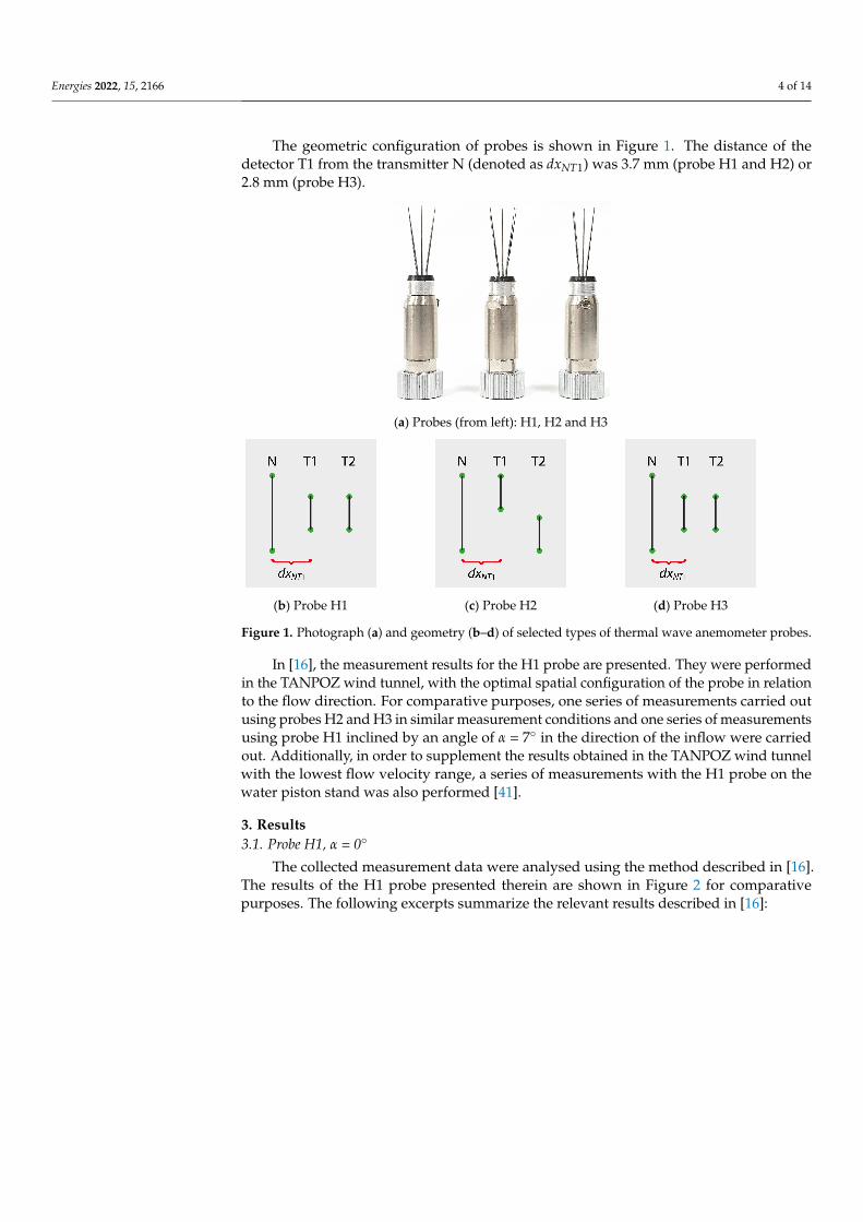
The geometric configuration of probes is shown in Figure 1. The distance of thedetector T1 from the transmitter N (denoted as dxNT1) was 3.7 mm (probe H1 and H2) or2.8 mm (probe H3).

Energies 2022, 15, x FOR PEER REVIEW 4 of 14

with a rectangular input. The overheating ratio of transmitter wire alternated between 1.0 and 1.8. The wave frequency was set to 1.0 Hz.

Data acquisition from both anemometers (Schmidt and thermal wave) was per-formed at a sampling rate of 10 kHz with 16-bit resolution.

The geometric configuration of probes is shown in Figure 1. The distance of the de-tector T1 from the transmitter N (denoted as dxNT1) was 3.7 mm (probe H1 and H2) or 2.8 mm (probe H3).

(a) Probes (from left): H1, H2 and H3

(b) Probe H1 (c) Probe H2 (d) Probe H3

Figure 1. Photograph (a) and geometry (b–d) of selected types of thermal wave anemometer probes.

In [16], the measurement results for the H1 probe are presented. They were per-formed in the TANPOZ wind tunnel, with the optimal spatial configuration of the probe in relation to the flow direction. For comparative purposes, one series of measurements carried out using probes H2 and H3 in similar measurement conditions and one series of measurements using probe H1 inclined by an angle of α = 7° in the direction of the inflow were carried out. Additionally, in order to supplement the results obtained in the TANPOZ wind tunnel with the lowest flow velocity range, a series of measurements with the H1 probe on the water piston stand was also performed [41].

3. Results 3.1. Probe H1, α = 0°

The collected measurement data were analysed using the method described in [16]. The results of the H1 probe presented therein are shown in Figure 2 for comparative pur-poses. The following excerpts summarize the relevant results described in [16]:

Figure 1. Photograph (a) and geometry (b–d) of selected types of thermal wave anemometer probes.

In [16], the measurement results for the H1 probe are presented. They were performedin the TANPOZ wind tunnel, with the optimal spatial configuration of the probe in relationto the flow direction. For comparative purposes, one series of measurements carried outusing probes H2 and H3 in similar measurement conditions and one series of measurementsusing probe H1 inclined by an angle of α = 7◦ in the direction of the inflow were carriedout. Additionally, in order to supplement the results obtained in the TANPOZ wind tunnelwith the lowest flow velocity range, a series of measurements with the H1 probe on thewater piston stand was also performed [41].

3. Results3.1. Probe H1, α = 0◦

The collected measurement data were analysed using the method described in [16].The results of the H1 probe presented therein are shown in Figure 2 for comparativepurposes. The following excerpts summarize the relevant results described in [16]:

Energies 2022, 15, 2166 5 of 14Energies 2022, 15, x FOR PEER REVIEW 5 of 14

(a) (b)

(c)

Figure 2. Direct velocity measurement results (squares), expected relationship (1:1) (broken line), results with the correction applied (circles) (a). Differences between the measurement results and the inflow velocity (b), and residual values of the results with the correction applied (c). The charts are from [16].

Figure 2a “compares the inflow velocity measured with the Schmidt anemometer (horizontal axis) with the velocity determined with the thermal wave anemometer (verti-cal axis). The figure also includes a dashed line that shows the ideal relationship of the two velocities (ratio 1:1). If the velocity values determined with the use of the thermal wave anemometer were close to the actual values, the measurement points (squares) should appear on this straight line.”

The graph in Figure 2a presents that “the higher the inflow velocity, the greater the difference between the results of the measurements using the thermal wave anemometer and the actual values. The presentation of these deviations as a function of the velocity in the wind tunnel reveals their exponential character (Figure 2b). The imposition of a cor-rection in the form of a power function (1) on the measurement results leads to a signifi-cant improvement in the indications of the thermal wave anemometer.” Measurement points with the applied correction (using: a = 0.409; n = 1.650; vp = 0.055 m/s) are marked in Figure 2 with circles.

“Figure 2c shows a graph of the relative differences (expressed as a percentage value) between the velocity values corrected using the power function and the set values in the wind tunnel (residual values). Deviations of the corrected velocity values from the set values amount to about 1% for velocities above 0.5 m/s, and increase to about 4% with a decrease in velocity. The increase is systematic, hence it may be possible to apply another

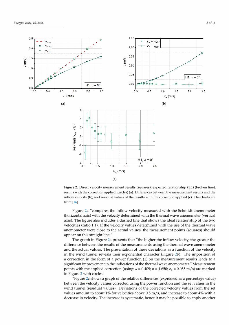
Figure 2. Direct velocity measurement results (squares), expected relationship (1:1) (broken line),results with the correction applied (circles) (a). Differences between the measurement results and theinflow velocity (b), and residual values of the results with the correction applied (c). The charts arefrom [16].

Figure 2a “compares the inflow velocity measured with the Schmidt anemometer(horizontal axis) with the velocity determined with the thermal wave anemometer (verticalaxis). The figure also includes a dashed line that shows the ideal relationship of the twovelocities (ratio 1:1). If the velocity values determined with the use of the thermal waveanemometer were close to the actual values, the measurement points (squares) shouldappear on this straight line.”

The graph in Figure 2a presents that “the higher the inflow velocity, the greater thedifference between the results of the measurements using the thermal wave anemometerand the actual values. The presentation of these deviations as a function of the velocityin the wind tunnel reveals their exponential character (Figure 2b). The imposition ofa correction in the form of a power function (1) on the measurement results leads to asignificant improvement in the indications of the thermal wave anemometer.” Measurementpoints with the applied correction (using: a = 0.409; n = 1.650; vp = 0.055 m/s) are markedin Figure 2 with circles.

“Figure 2c shows a graph of the relative differences (expressed as a percentage value)between the velocity values corrected using the power function and the set values in thewind tunnel (residual values). Deviations of the corrected velocity values from the setvalues amount to about 1% for velocities above 0.5 m/s, and increase to about 4% with adecrease in velocity. The increase is systematic, hence it may be possible to apply another

Energies 2022, 15, 2166 6 of 14

form of the power function to reduce the value of the deviations in the range of lowestvelocities. The higher deviations in the range of lowest velocities may also result from themetrological properties of the instrument used as a reference, the Schmidt anemometer.”

3.2. Probe H1, α = 7◦

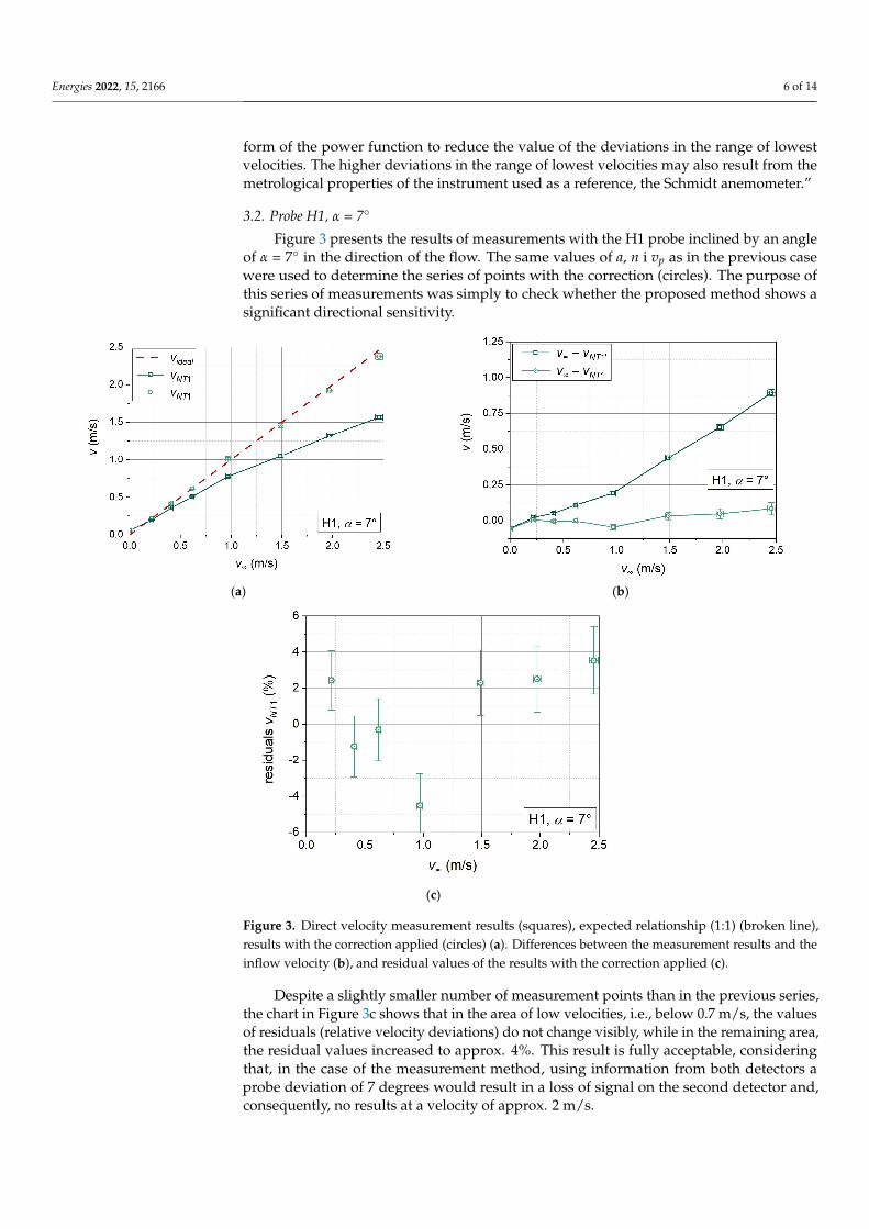
Figure 3 presents the results of measurements with the H1 probe inclined by an angleof α = 7◦ in the direction of the flow. The same values of a, n i vp as in the previous casewere used to determine the series of points with the correction (circles). The purpose ofthis series of measurements was simply to check whether the proposed method shows asignificant directional sensitivity.

Energies 2022, 15, x FOR PEER REVIEW 6 of 14

form of the power function to reduce the value of the deviations in the range of lowest velocities. The higher deviations in the range of lowest velocities may also result from the metrological properties of the instrument used as a reference, the Schmidt anemometer.”

3.2. Probe H1, α = 7° Figure 3 presents the results of measurements with the H1 probe inclined by an angle

of α = 7° in the direction of the flow. The same values of a, n i vp as in the previous case were used to determine the series of points with the correction (circles). The purpose of this series of measurements was simply to check whether the proposed method shows a significant directional sensitivity.

(a) (b)

(c)

Figure 3. Direct velocity measurement results (squares), expected relationship (1:1) (broken line), results with the correction applied (circles) (a). Differences between the measurement results and the inflow velocity (b), and residual values of the results with the correction applied (c).

Despite a slightly smaller number of measurement points than in the previous series, the chart in Figure 3c shows that in the area of low velocities, i.e., below 0.7 m/s, the values of residuals (relative velocity deviations) do not change visibly, while in the remaining area, the residual values increased to approx. 4%. This result is fully acceptable, consider-ing that, in the case of the measurement method, using information from both detectors a probe deviation of 7 degrees would result in a loss of signal on the second detector and, consequently, no results at a velocity of approx. 2 m/s.

Figure 3. Direct velocity measurement results (squares), expected relationship (1:1) (broken line),results with the correction applied (circles) (a). Differences between the measurement results and theinflow velocity (b), and residual values of the results with the correction applied (c).

Despite a slightly smaller number of measurement points than in the previous series,the chart in Figure 3c shows that in the area of low velocities, i.e., below 0.7 m/s, the valuesof residuals (relative velocity deviations) do not change visibly, while in the remaining area,the residual values increased to approx. 4%. This result is fully acceptable, consideringthat, in the case of the measurement method, using information from both detectors aprobe deviation of 7 degrees would result in a loss of signal on the second detector and,consequently, no results at a velocity of approx. 2 m/s.

Energies 2022, 15, 2166 7 of 14

3.3. Probe H2, α = 0◦

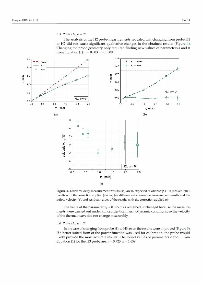
The analysis of the H2 probe measurements revealed that changing from probe H1to H2 did not cause significant qualitative changes in the obtained results (Figure 4).Changing the probe geometry only required finding new values of parameters a and nfrom Equation (1): a = 0.503, n = 1.600.

Energies 2022, 15, x FOR PEER REVIEW 7 of 14

3.3. Probe H2, α = 0° The analysis of the H2 probe measurements revealed that changing from probe H1

to H2 did not cause significant qualitative changes in the obtained results (Figure 4). Changing the probe geometry only required finding new values of parameters a and n from Equation (1): a = 0.503, n = 1.600.

(a) (b)

(c)

Figure 4. Direct velocity measurement results (squares), expected relationship (1:1) (broken line), results with the correction applied (circles) (a), differences between the measurement results and the inflow velocity (b), and residual values of the results with the correction applied (c).

The value of the parameter vp = 0.055 m/s remained unchanged because the measure-ments were carried out under almost identical thermodynamic conditions, so the velocity of the thermal wave did not change measurably.

3.4. Probe H3, α = 0° In the case of changing from probe H1 to H3, even the results were improved (Figure

5). If a better suited form of the power function was used for calibration, the probe would likely provide the most accurate results. The found values of parameters a and n from Equation (1) for the H3 probe are: a = 0.723, n = 1.659.

Figure 4. Direct velocity measurement results (squares), expected relationship (1:1) (broken line),results with the correction applied (circles) (a), differences between the measurement results and theinflow velocity (b), and residual values of the results with the correction applied (c).

The value of the parameter vp = 0.055 m/s remained unchanged because the measure-ments were carried out under almost identical thermodynamic conditions, so the velocityof the thermal wave did not change measurably.

3.4. Probe H3, α = 0◦

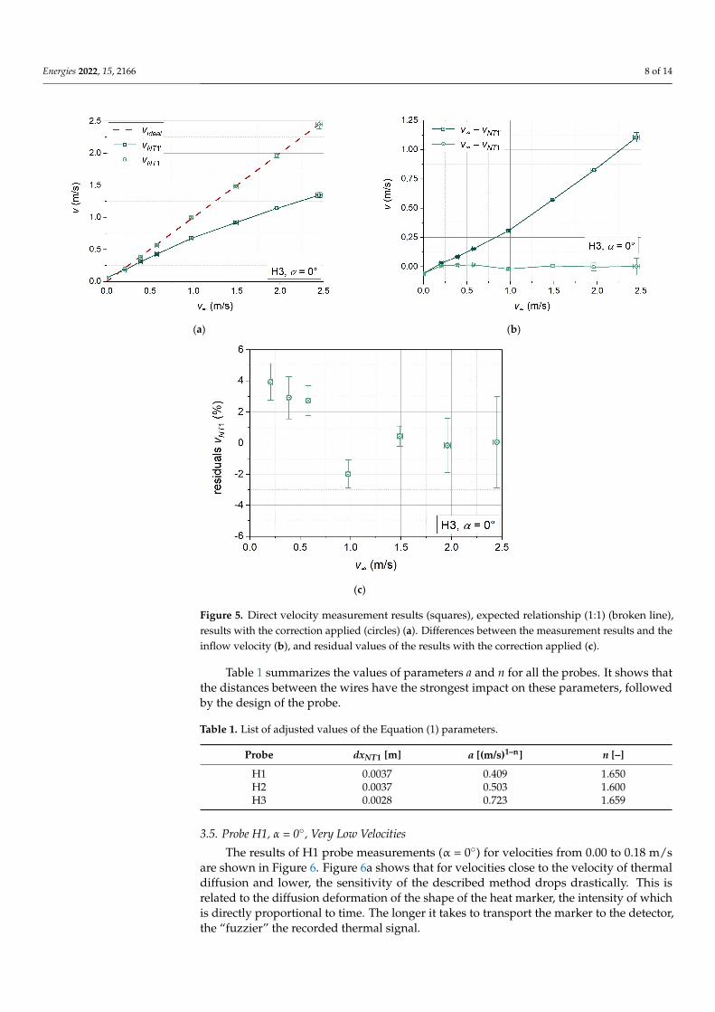
In the case of changing from probe H1 to H3, even the results were improved (Figure 5).If a better suited form of the power function was used for calibration, the probe wouldlikely provide the most accurate results. The found values of parameters a and n fromEquation (1) for the H3 probe are: a = 0.723, n = 1.659.

Energies 2022, 15, 2166 8 of 14Energies 2022, 15, x FOR PEER REVIEW 8 of 14

(a) (b)

(c)

Figure 5. Direct velocity measurement results (squares), expected relationship (1:1) (broken line), results with the correction applied (circles) (a). Differences between the measurement results and the inflow velocity (b), and residual values of the results with the correction applied (c).

Table 1 summarizes the values of parameters a and n for all the probes. It shows that the distances between the wires have the strongest impact on these parameters, followed by the design of the probe.

Table 1. List of adjusted values of the Equation (1) parameters.

Probe dxNT1 [m] a [(m/s)1–n] n [–] H1 0.0037 0.409 1.650 H2 0.0037 0.503 1.600 H3 0.0028 0.723 1.659

3.5. Probe H1, α = 0°, Very Low Velocities The results of H1 probe measurements (α = 0°) for velocities from 0.00 to 0.18 m/s are

shown in Figure 6. Figure 6a shows that for velocities close to the velocity of thermal dif-fusion and lower, the sensitivity of the described method drops drastically. This is related to the diffusion deformation of the shape of the heat marker, the intensity of which is directly proportional to time. The longer it takes to transport the marker to the detector, the “fuzzier” the recorded thermal signal.

Figure 5. Direct velocity measurement results (squares), expected relationship (1:1) (broken line),results with the correction applied (circles) (a). Differences between the measurement results and theinflow velocity (b), and residual values of the results with the correction applied (c).

Table 1 summarizes the values of parameters a and n for all the probes. It shows thatthe distances between the wires have the strongest impact on these parameters, followedby the design of the probe.

Table 1. List of adjusted values of the Equation (1) parameters.

Probe dxNT1 [m] a [(m/s)1–n] n [–]

H1 0.0037 0.409 1.650H2 0.0037 0.503 1.600H3 0.0028 0.723 1.659

3.5. Probe H1, α = 0◦, Very Low Velocities

The results of H1 probe measurements (α = 0◦) for velocities from 0.00 to 0.18 m/sare shown in Figure 6. Figure 6a shows that for velocities close to the velocity of thermaldiffusion and lower, the sensitivity of the described method drops drastically. This isrelated to the diffusion deformation of the shape of the heat marker, the intensity of whichis directly proportional to time. The longer it takes to transport the marker to the detector,the “fuzzier” the recorded thermal signal.

Energies 2022, 15, 2166 9 of 14Energies 2022, 15, x FOR PEER REVIEW 9 of 14

(a) (b)

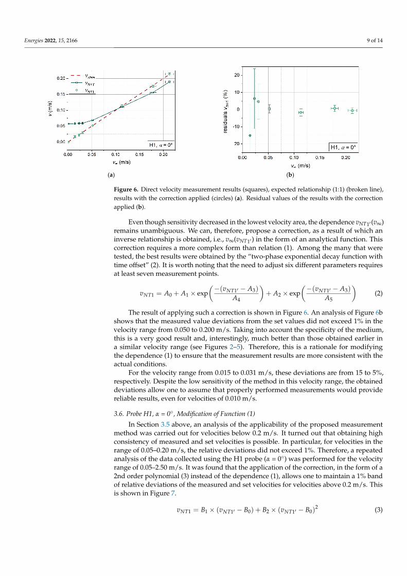
Figure 6. Direct velocity measurement results (squares), expected relationship (1:1) (broken line), results with the correction applied (circles) (a). Residual values of the results with the correction applied (b).

Even though sensitivity decreased in the lowest velocity area, the dependence vNT1′(v∞) remains unambiguous. We can, therefore, propose a correction, as a result of which an inverse relationship is obtained, i.e., v∞(vNT1′) in the form of an analytical func-tion. This correction requires a more complex form than relation (1). Among the many that were tested, the best results were obtained by the “two-phase exponential decay func-tion with time offset” (2). It is worth noting that the need to adjust six different parameters requires at least seven measurement points. 𝑣 = 𝐴 + 𝐴 × exp −(𝑣 − 𝐴 )𝐴 + 𝐴 × exp −(𝑣 − 𝐴 )𝐴 (2)

The result of applying such a correction is shown in Figure 6. An analysis of Figure 6b shows that the measured value deviations from the set values did not exceed 1% in the velocity range from 0.050 to 0.200 m/s. Taking into account the specificity of the medium, this is a very good result and, interestingly, much better than those obtained earlier in a similar velocity range (see Figures 2–5). Therefore, this is a rationale for modifying the dependence (1) to ensure that the measurement results are more consistent with the actual conditions.

For the velocity range from 0.015 to 0.031 m/s, these deviations are from 15 to 5%, respectively. Despite the low sensitivity of the method in this velocity range, the obtained deviations allow one to assume that properly performed measurements would provide reliable results, even for velocities of 0.010 m/s.

3.6. Probe H1, α = 0°, Modification of Function (1) In Section 3.5 above, an analysis of the applicability of the proposed measurement

method was carried out for velocities below 0.2 m/s. It turned out that obtaining high consistency of measured and set velocities is possible. In particular, for velocities in the range of 0.05–0.20 m/s, the relative deviations did not exceed 1%. Therefore, a repeated analysis of the data collected using the H1 probe (α = 0°) was performed for the velocity range of 0.05–2.50 m/s. It was found that the application of the correction, in the form of a 2nd order polynomial (3) instead of the dependence (1), allows one to maintain a 1% band of relative deviations of the measured and set velocities for velocities above 0.2 m/s. This is shown in Figure 7.

Figure 6. Direct velocity measurement results (squares), expected relationship (1:1) (broken line),results with the correction applied (circles) (a). Residual values of the results with the correctionapplied (b).

Even though sensitivity decreased in the lowest velocity area, the dependence vNT1′ (v∞)remains unambiguous. We can, therefore, propose a correction, as a result of which aninverse relationship is obtained, i.e., v∞(vNT1′ ) in the form of an analytical function. Thiscorrection requires a more complex form than relation (1). Among the many that weretested, the best results were obtained by the “two-phase exponential decay function withtime offset” (2). It is worth noting that the need to adjust six different parameters requiresat least seven measurement points.

vNT1 = A0 + A1 × exp(−(vNT1′ − A3)

A4

)+ A2 × exp

(−(vNT1′ − A3)

A5

)(2)

The result of applying such a correction is shown in Figure 6. An analysis of Figure 6bshows that the measured value deviations from the set values did not exceed 1% in thevelocity range from 0.050 to 0.200 m/s. Taking into account the specificity of the medium,this is a very good result and, interestingly, much better than those obtained earlier ina similar velocity range (see Figures 2–5). Therefore, this is a rationale for modifyingthe dependence (1) to ensure that the measurement results are more consistent with theactual conditions.

For the velocity range from 0.015 to 0.031 m/s, these deviations are from 15 to 5%,respectively. Despite the low sensitivity of the method in this velocity range, the obtaineddeviations allow one to assume that properly performed measurements would providereliable results, even for velocities of 0.010 m/s.

3.6. Probe H1, α = 0◦, Modification of Function (1)

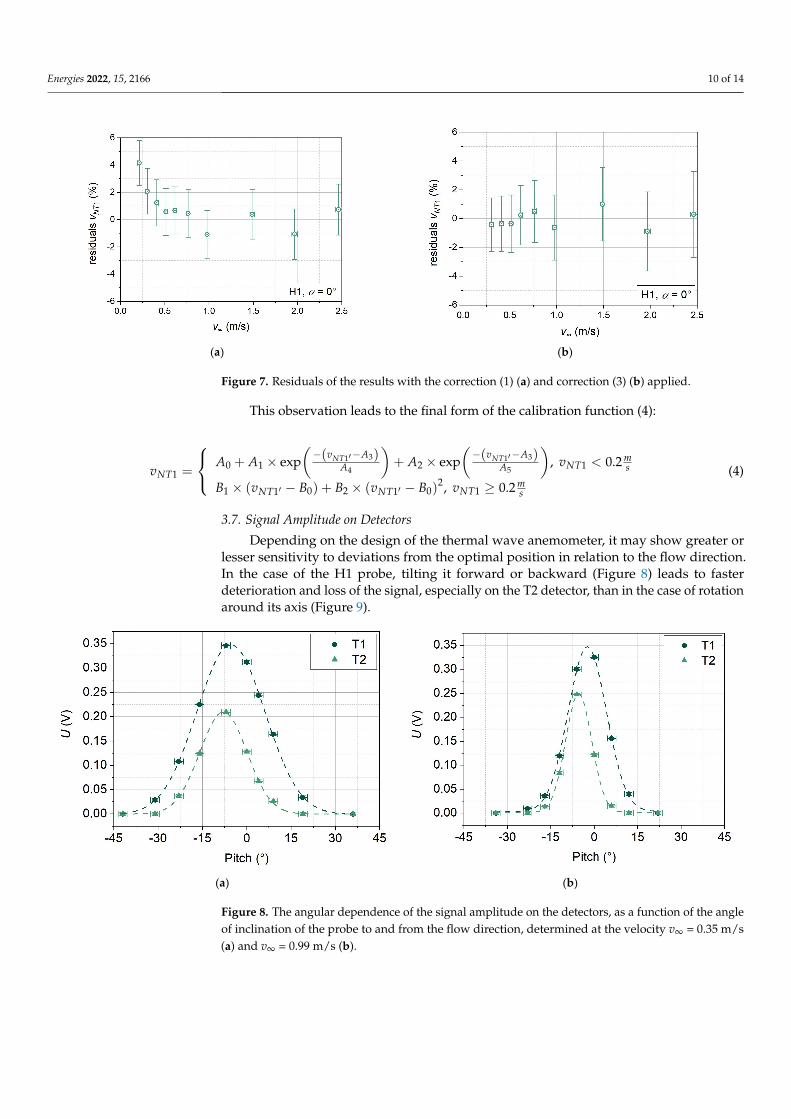
In Section 3.5 above, an analysis of the applicability of the proposed measurementmethod was carried out for velocities below 0.2 m/s. It turned out that obtaining highconsistency of measured and set velocities is possible. In particular, for velocities in therange of 0.05–0.20 m/s, the relative deviations did not exceed 1%. Therefore, a repeatedanalysis of the data collected using the H1 probe (α = 0◦) was performed for the velocityrange of 0.05–2.50 m/s. It was found that the application of the correction, in the form of a2nd order polynomial (3) instead of the dependence (1), allows one to maintain a 1% bandof relative deviations of the measured and set velocities for velocities above 0.2 m/s. Thisis shown in Figure 7.

vNT1 = B1 × (vNT1′ − B0) + B2 × (vNT1′ − B0)2 (3)

Energies 2022, 15, 2166 10 of 14Energies 2022, 15, x FOR PEER REVIEW 10 of 14

(a) (b)

Figure 7. Residuals of the results with the correction (1) (a) and correction (3) (b) applied.

𝑣 = 𝐵 × (𝑣 − 𝐵 ) + 𝐵 × (𝑣 − 𝐵 ) (3)

This observation leads to the final form of the calibration function (4):

𝑣 = ⎩⎨⎧𝐴 + 𝐴 × exp −(𝑣 − 𝐴 )𝐴 + 𝐴 × exp −(𝑣 − 𝐴 )𝐴 , 𝑣 < 0.2 𝑚𝑠𝐵 × (𝑣 − 𝐵 ) + 𝐵 × (𝑣 − 𝐵 ) , 𝑣 ≥ 0.2 𝑚𝑠 (4)

3.7. Signal Amplitude on Detectors Depending on the design of the thermal wave anemometer, it may show greater or

lesser sensitivity to deviations from the optimal position in relation to the flow direction. In the case of the H1 probe, tilting it forward or backward (Figure 8) leads to faster dete-rioration and loss of the signal, especially on the T2 detector, than in the case of rotation around its axis (Figure 9).

(a) (b)

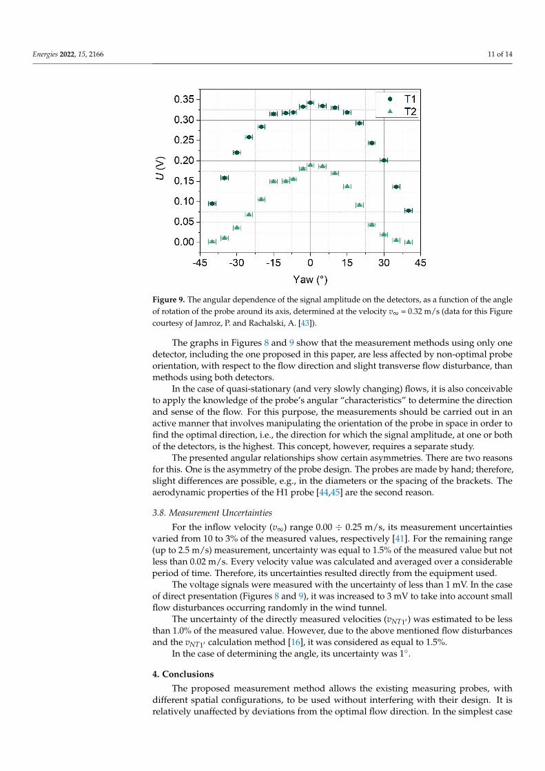
Figure 8. The angular dependence of the signal amplitude on the detectors, as a function of the angle of inclination of the probe to and from the flow direction, determined at the velocity v∞ = 0.35 m/s (a) and v∞ = 0.99 m/s (b).

Figure 7. Residuals of the results with the correction (1) (a) and correction (3) (b) applied.

This observation leads to the final form of the calibration function (4):

vNT1 =

A0 + A1 × exp(−(vNT1′−A3)

A4

)+ A2 × exp

(−(vNT1′−A3)

A5

), vNT1 < 0.2 m

s

B1 × (vNT1′ − B0) + B2 × (vNT1′ − B0)2, vNT1 ≥ 0.2 m

s

(4)

3.7. Signal Amplitude on Detectors

Depending on the design of the thermal wave anemometer, it may show greater orlesser sensitivity to deviations from the optimal position in relation to the flow direction.In the case of the H1 probe, tilting it forward or backward (Figure 8) leads to fasterdeterioration and loss of the signal, especially on the T2 detector, than in the case of rotationaround its axis (Figure 9).

Energies 2022, 15, x FOR PEER REVIEW 10 of 14

(a) (b)

Figure 7. Residuals of the results with the correction (1) (a) and correction (3) (b) applied.

𝑣 = 𝐵 × (𝑣 − 𝐵 ) + 𝐵 × (𝑣 − 𝐵 ) (3)

This observation leads to the final form of the calibration function (4):

𝑣 = ⎩⎨⎧𝐴 + 𝐴 × exp −(𝑣 − 𝐴 )𝐴 + 𝐴 × exp −(𝑣 − 𝐴 )𝐴 , 𝑣 < 0.2 𝑚𝑠𝐵 × (𝑣 − 𝐵 ) + 𝐵 × (𝑣 − 𝐵 ) , 𝑣 ≥ 0.2 𝑚𝑠 (4)

3.7. Signal Amplitude on Detectors Depending on the design of the thermal wave anemometer, it may show greater or

lesser sensitivity to deviations from the optimal position in relation to the flow direction. In the case of the H1 probe, tilting it forward or backward (Figure 8) leads to faster dete-rioration and loss of the signal, especially on the T2 detector, than in the case of rotation around its axis (Figure 9).

(a) (b)

Figure 8. The angular dependence of the signal amplitude on the detectors, as a function of the angle of inclination of the probe to and from the flow direction, determined at the velocity v∞ = 0.35 m/s (a) and v∞ = 0.99 m/s (b).

Figure 8. The angular dependence of the signal amplitude on the detectors, as a function of the angleof inclination of the probe to and from the flow direction, determined at the velocity v∞ = 0.35 m/s(a) and v∞ = 0.99 m/s (b).

Energies 2022, 15, 2166 11 of 14Energies 2022, 15, x FOR PEER REVIEW 11 of 14

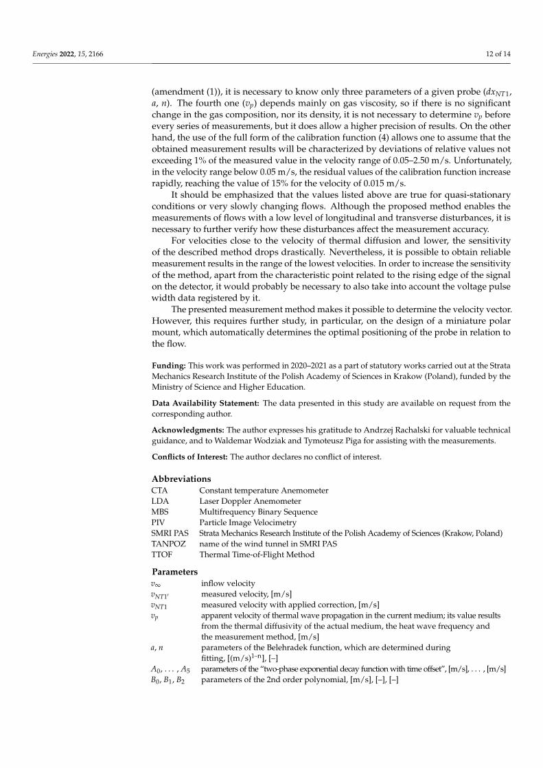
Figure 9. The angular dependence of the signal amplitude on the detectors, as a function of the angle of rotation of the probe around its axis, determined at the velocity v∞ = 0.32 m/s (data for this Figure courtesy of Jamroz, P. and Rachalski, A. [43]).

The graphs in Figures 8 and 9 show that the measurement methods using only one detector, including the one proposed in this paper, are less affected by non-optimal probe orientation, with respect to the flow direction and slight transverse flow disturbance, than methods using both detectors.

In the case of quasi-stationary (and very slowly changing) flows, it is also conceivable to apply the knowledge of the probe’s angular “characteristics” to determine the direction and sense of the flow. For this purpose, the measurements should be carried out in an active manner that involves manipulating the orientation of the probe in space in order to find the optimal direction, i.e., the direction for which the signal amplitude, at one or both of the detectors, is the highest. This concept, however, requires a separate study.

The presented angular relationships show certain asymmetries. There are two rea-sons for this. One is the asymmetry of the probe design. The probes are made by hand; therefore, slight differences are possible, e.g., in the diameters or the spacing of the brack-ets. The aerodynamic properties of the H1 probe [44,45] are the second reason.

3.8. Measurement Uncertainties For the inflow velocity (v∞) range 0.00 ÷ 0.25 m/s, its measurement uncertainties var-

ied from 10 to 3% of the measured values, respectively [41]. For the remaining range (up to 2.5 m/s) measurement, uncertainty was equal to 1.5% of the measured value but not less than 0.02 m/s. Every velocity value was calculated and averaged over a considerable period of time. Therefore, its uncertainties resulted directly from the equipment used.

The voltage signals were measured with the uncertainty of less than 1 mV. In the case of direct presentation (Figures 8 and 9), it was increased to 3 mV to take into account small flow disturbances occurring randomly in the wind tunnel.

The uncertainty of the directly measured velocities (vNT1′) was estimated to be less than 1.0% of the measured value. However, due to the above mentioned flow disturbances and the vNT1′ calculation method [16], it was considered as equal to 1.5%.

In the case of determining the angle, its uncertainty was 1°.

4. Conclusions The proposed measurement method allows the existing measuring probes, with dif-

ferent spatial configurations, to be used without interfering with their design. It is rela-tively unaffected by deviations from the optimal flow direction. In the simplest case

Figure 9. The angular dependence of the signal amplitude on the detectors, as a function of the angleof rotation of the probe around its axis, determined at the velocity v∞ = 0.32 m/s (data for this Figurecourtesy of Jamroz, P. and Rachalski, A. [43]).

The graphs in Figures 8 and 9 show that the measurement methods using only onedetector, including the one proposed in this paper, are less affected by non-optimal probeorientation, with respect to the flow direction and slight transverse flow disturbance, thanmethods using both detectors.

In the case of quasi-stationary (and very slowly changing) flows, it is also conceivableto apply the knowledge of the probe’s angular “characteristics” to determine the directionand sense of the flow. For this purpose, the measurements should be carried out in anactive manner that involves manipulating the orientation of the probe in space in order tofind the optimal direction, i.e., the direction for which the signal amplitude, at one or bothof the detectors, is the highest. This concept, however, requires a separate study.

The presented angular relationships show certain asymmetries. There are two reasonsfor this. One is the asymmetry of the probe design. The probes are made by hand; therefore,slight differences are possible, e.g., in the diameters or the spacing of the brackets. Theaerodynamic properties of the H1 probe [44,45] are the second reason.

3.8. Measurement Uncertainties

For the inflow velocity (v∞) range 0.00 ÷ 0.25 m/s, its measurement uncertaintiesvaried from 10 to 3% of the measured values, respectively [41]. For the remaining range(up to 2.5 m/s) measurement, uncertainty was equal to 1.5% of the measured value but notless than 0.02 m/s. Every velocity value was calculated and averaged over a considerableperiod of time. Therefore, its uncertainties resulted directly from the equipment used.

The voltage signals were measured with the uncertainty of less than 1 mV. In the caseof direct presentation (Figures 8 and 9), it was increased to 3 mV to take into account smallflow disturbances occurring randomly in the wind tunnel.

The uncertainty of the directly measured velocities (vNT1′ ) was estimated to be lessthan 1.0% of the measured value. However, due to the above mentioned flow disturbancesand the vNT1′ calculation method [16], it was considered as equal to 1.5%.

In the case of determining the angle, its uncertainty was 1◦.

4. Conclusions

The proposed measurement method allows the existing measuring probes, withdifferent spatial configurations, to be used without interfering with their design. It isrelatively unaffected by deviations from the optimal flow direction. In the simplest case

Energies 2022, 15, 2166 12 of 14

(amendment (1)), it is necessary to know only three parameters of a given probe (dxNT1,a, n). The fourth one (vp) depends mainly on gas viscosity, so if there is no significantchange in the gas composition, nor its density, it is not necessary to determine vp beforeevery series of measurements, but it does allow a higher precision of results. On the otherhand, the use of the full form of the calibration function (4) allows one to assume that theobtained measurement results will be characterized by deviations of relative values notexceeding 1% of the measured value in the velocity range of 0.05–2.50 m/s. Unfortunately,in the velocity range below 0.05 m/s, the residual values of the calibration function increaserapidly, reaching the value of 15% for the velocity of 0.015 m/s.

It should be emphasized that the values listed above are true for quasi-stationaryconditions or very slowly changing flows. Although the proposed method enables themeasurements of flows with a low level of longitudinal and transverse disturbances, it isnecessary to further verify how these disturbances affect the measurement accuracy.

For velocities close to the velocity of thermal diffusion and lower, the sensitivityof the described method drops drastically. Nevertheless, it is possible to obtain reliablemeasurement results in the range of the lowest velocities. In order to increase the sensitivityof the method, apart from the characteristic point related to the rising edge of the signalon the detector, it would probably be necessary to also take into account the voltage pulsewidth data registered by it.

The presented measurement method makes it possible to determine the velocity vector.However, this requires further study, in particular, on the design of a miniature polarmount, which automatically determines the optimal positioning of the probe in relation tothe flow.

Funding: This work was performed in 2020–2021 as a part of statutory works carried out at the StrataMechanics Research Institute of the Polish Academy of Sciences in Krakow (Poland), funded by theMinistry of Science and Higher Education.

Data Availability Statement: The data presented in this study are available on request from thecorresponding author.

Acknowledgments: The author expresses his gratitude to Andrzej Rachalski for valuable technicalguidance, and to Waldemar Wodziak and Tymoteusz Piga for assisting with the measurements.

Conflicts of Interest: The author declares no conflict of interest.

AbbreviationsCTA Constant temperature AnemometerLDA Laser Doppler AnemometerMBS Multifrequency Binary SequencePIV Particle Image VelocimetrySMRI PAS Strata Mechanics Research Institute of the Polish Academy of Sciences (Krakow, Poland)TANPOZ name of the wind tunnel in SMRI PASTTOF Thermal Time-of-Flight Method

Parametersv∞ inflow velocityvNT1′ measured velocity, [m/s]vNT1 measured velocity with applied correction, [m/s]vp apparent velocity of thermal wave propagation in the current medium; its value results

from the thermal diffusivity of the actual medium, the heat wave frequency andthe measurement method, [m/s]

a, n parameters of the Belehradek function, which are determined duringfitting, [(m/s)1–n], [–]

A0, . . . , A5 parameters of the “two-phase exponential decay function with time offset”, [m/s], . . . , [m/s]B0, B1, B2 parameters of the 2nd order polynomial, [m/s], [–], [–]

Energies 2022, 15, 2166 13 of 14

References1. Cheremisinoff, N.P. Ventilation and Indoor Air Quality Control. Handb. Air Pollut. Prev. Control. 2002, 188–280. [CrossRef]2. Legg, R. Indoor Design Conditions. In Air Conditioning System Design; Elsevier: Amsterdam, The Netherlands, 2017; pp. 53–65.3. Ma, N.; Aviv, D.; Guo, H.; Braham, W.W. Measuring the Right Factors: A Review of Variables and Models for Thermal Comfort

and Indoor Air Quality. Renew. Sustain. Energy Rev. 2021, 135, 110436. [CrossRef]4. Ashrae.Org. Available online: https://www.ashrae.org/ (accessed on 13 December 2021).5. Camuffo, D. Measuring Wind and Indoor Air Motions. In Microclimate for Cultural Heritage; Elsevier: Amsterdam, The Netherlands,

2019; pp. 483–511.6. Elkadi, H.; Al-Maiyah, S.; Fielder, K.; Kenawy, I.; Martinson, D.B. The Regulations and Reality of Indoor Environmental Standards

for Objects and Visitors in Museums. Renew. Sustain. Energy Rev. 2021, 152, 111653. [CrossRef]7. Finlayson-Pitts, B.J.; Pitts, J.N. Indoor Air Pollution: Sources, Levels, Chemistry, and Fates. Chem. Up. Low. Atmos. 2000, 844–870.

[CrossRef]8. Fabbri, K.; Bonora, A. Two New Indices for Preventive Conservation of the Cultural Heritage: Predicted Risk of Damage and

Heritage Microclimate Risk. J. Cult. Herit. 2021, 47, 208–217. [CrossRef]9. Boeri, A.; Longo, D.; Fabbri, K.; Pretelli, M.; Bonora, A.; Boulanger, S. Library Indoor Microclimate Monitoring with and without

Heating System. A Bologna University Library Case Study. J. Cult. Herit. 2022, 53, 143–153. [CrossRef]10. Xue, K.; Cao, G.; Liu, M.; Zhang, Y.; Pedersen, C.; Mathisen, H.M.; Stenstad, L.I.; Skogås, J.G. Experimental Study on the Effect of

Exhaust Airflows on the Surgical Environment in an Operating Room with Mixing Ventilation. J. Build. Eng. 2020, 32, 101837.[CrossRef]

11. Duret, S.; Hoang, H.M.; Flick, D.; Laguerre, O. Experimental Characterization of Airflow, Heat and Mass Transfer in a Cold RoomFilled with Food Products. Int. J. Refrig. 2014, 46, 17–25. [CrossRef]

12. Sui, X.; Tian, Z.; Liu, H.; Chen, H.; Wang, D. Field Measurements on Indoor Air Quality of a Residential Building in Xi’an underDifferent Ventilation Modes in Winter. J. Build. Eng. 2021, 42, 103040. [CrossRef]

13. Calautit, J.K.; Hughes, B.R. Measurement and Prediction of the Indoor Airflow in a Room Ventilated with a Commercial WindTower. Energy Build. 2014, 84, 367–377. [CrossRef]

14. Goodfellow, H.D.; Wang, Y. Industrial Ventilation Design Guidebook. In Engineering Design and Applications; Academic Press:Cambridge, MA, USA, 2021; Volume 2, ISBN 9780128166734.

15. Cao, X.; Liu, J.; Jiang, N.; Chen, Q. Particle Image Velocimetry Measurement of Indoor Airflow Field: A Review of the Technologiesand Applications. Energy Build. 2014, 69, 367–380. [CrossRef]

16. Sobczyk, J.; Rachalski, A.; Wodziak, W. A Semi-Empirical Approach to Gas Flow Velocity Measurement by Means of the ThermalTime-of-Flight Method. Sensors 2021, 21, 5679. [CrossRef] [PubMed]

17. Bradbury, L.J.S.; Castro, I.P. A Pulsed-Wire Technique for Velocity Measurements in Highly Turbulent Flows. J. Fluid Mech. 1971,49, 657–691. [CrossRef]

18. Tombach, I.H. An Evaluation of the Heat Pulse Anemometer for Velocity Measurement in Inhomogeneous Turbulent Flow. Rev.Sci. Instrum. 1973, 44, 141–148. [CrossRef]

19. Avirav, Y.; Guterman, H.; Ben-Yaakov, S. Implementation of Digital Signal Processing Techniques in the Design of Thermal PulseFlowmeters. IEEE Trans. Instrum. Meas. 1990, 39, 761–766. [CrossRef]

20. Mathioulakis, E.; Grignon, M.; Poloniecki, J.G. A Pulsed-Wire Technique for Velocity and Temperature Measurements in NaturalConvection Flows. Exp. Fluids 1994, 18, 82–86. [CrossRef]

21. Jan, K.; Jerzy, P.; Józef, R.; Zdzisław, S.A.; Bolesław, S. Heat Waves In Flow Metrology. In Proceedings of the Flow Measurement ofFluids; North-Holland Publishing Company: Groningen, The Netherlands, 1978; pp. 403–407.

22. Rachalski, A. High-Precision Anemometer with Thermal Wave. Rev. Sci. Instrum. 2006, 77, 095107. [CrossRef]23. Kovasznay, L.S.G. Hot-Wire Investigation of the Wake behind Cylinders at Low Reynolds Numbers. Proc. R. Soc. Lond. Ser. A

Math. Phys. Sci. 1949, 198, 174–190. [CrossRef]24. Walker, R.E.; Westenberg, A.A. Absolute Low Speed Anemometer. Rev. Sci. Instrum. 1956, 27, 844–848. [CrossRef]25. Kiełbasa, J. Measurments of Steady Flow Velocity Using the Termal Wave Method. Arch. Min. Sci. 2005, 50, 191–208.26. Byon, C. Numerical and Analytic Study on the Time-of-Flight Thermal Flow Sensor. Int. J. Heat Mass Transf. 2015, 89, 454–459.

[CrossRef]27. Biernacki, Z. A System of Wave Thermoanemometer with a Thermoresistive Sensor. Sens. Actuators A Phys. 1998, 70, 219–224.

[CrossRef]28. Rachalski, A.; Poleszczyk, E.; Zieba, M. Use of the Thermal Wave Method for Measuring the Flow Velocity of Air and Carbon

Dioxide Mixture. Measurement 2017, 95, 210–215. [CrossRef]29. Berthet, H.; Jundt, J.; Durivault, J.; Mercier, B.; Angelescu, D. Time-of-Flight Thermal Flowrate Sensor for Lab-on-Chip Applica-

tions. Lab Chip 2011, 11, 215–223. [CrossRef] [PubMed]30. Rachalski, A. Absolute Measurement of Low Gas Flow by Means of the Spectral Analysis of the Thermal Wave. Rev. Sci. Instrum.

2013, 84, 25105. [CrossRef] [PubMed]31. Bujalski, M.; Rachalski, A.; Ligeza, P.; Poleszczyk, E. The Use of Multifrequency Binary Sequences MBS Signal in the Anemometer

with Thermal Wave. In Proceedings of the Measurement 2015; Institute of Measurement Science Slovak Academy of Sciences:Smolenice, Slovakia, 2015; pp. 297–300.

Energies 2022, 15, 2166 14 of 14

32. Henderson, I.A.; Mcghee, J. Compact Symmetrical Binary Codes For System Identification. Math. Comput. Model. 1990, 14, 213–218.[CrossRef]

33. Mosse, C.A.; Roberts, S.P. Microprocessor-Based Time-of-Flight Respirometer. Med. Biol. Eng. Comput. 1987, 25, 34–40. [CrossRef]34. Engelien, E.; Ecin, O.; Viga, R.; Hosticka, B.J.; Grabmaier, A. Calibration-Free Volume Flow Measurement Principle Based on

Thermal Time-of-Flight (TToF). Proc. Procedia Eng. 2011, 25, 765–768. [CrossRef]35. Ong, L.; Wallace, J. The Velocity Field of the Turbulent Very near Wake of a Circular Cylinder. Exp. Fluids 1996, 20, 441–453.

[CrossRef]36. Kiełbasa, J. Measurement of Aerodynamic and Thermal Footprints. Arch. Min. Sci. 1999, 44, 71–84. (In Polish)37. Gawor, M.; Sobczyk, J.; Wodziak, W.; Ligeza, P.; Rachalski, A.; Jamróz, P.; Socha, K.; Palacz, J. Flow Velocity Distribution in the

Probe Area of the Anemometer with Thermal Wave. Trans. Strat. Mech. Res. Inst. 2019, 21, 49–53. (In Polish)38. Help Online—Origin Help—Belehradek. Available online: https://www.originlab.com/doc/Origin-Help/Belehradek-FitFunc

(accessed on 28 June 2021).39. Durst, F.; Al-Salaymeh, A.; Bradshaw, P.; Jovanovic, J. The Development of a Pulsed-Wire Probe for Measuring Flow Velocity with

a Wide Bandwidth. Int. J. Heat Fluid Flow 2003, 24, 1–13. [CrossRef]40. Bujalski, M.; Gawor, M.; Sobczyk, J. Closed-Circuit Wind Tunnel with Air Temperature and Humidity Stabilization, Adapted for

Measurements by Means of Optical Methods; Prace Instytutu Mechaniki Górotworu PAN: Krakow, Poland, 2013. (In Polish)41. Piga, T.; Rachalski, A.; Wodziak, W.; Sobczyk, J. Experimental Setup for Very Low Velocity Gas Flow Generation. Meas. Sci. Rev.

2022. in preparation.42. Ligeza, P. Four-Point Non-Bridge Constant-Temperature Anemometer Circuit. Exp. Fluids 2000, 29, 505–507. [CrossRef]43. Rachalski, A.; Jamróz, P. Unpublished Research; Krakow, Poland. 2019.44. Gawor, M.; Sobczyk, J.; Wodziak, W.; Ligeza, P.; Rachalski, A.; Jamróz, P.; Socha, K.; Palacz, J. Distribution of Flow Velocity in the

Vicinity of the Thermal Wave Anemometer Probe; Prace Instytutu Mechaniki Górotworu PAN: Krakow, Poland, 2019. (In Polish)45. Sobczyk, J. Experimental Study of the Flow Field Disturbance in the Vicinity of Single Sensor Hot-Wire Anemometer. EPJ Web

Conf. 2018, 180, 02094. [CrossRef]