Seediscussions,stats,andauthorprofilesforthispublicationat:https://www.researchgate.net/publication/51106480

Sensitivity,robustness,andidentifiabilityinstochasticchemicalkineticsmodels

ArticleinProceedingsoftheNationalAcademyofSciences·May2011

DOI:10.1073/pnas.1015814108·Source:PubMed

CITATIONS

84

READS

53

4authors,including:

DavidRand

TheUniversityofWarwick

175PUBLICATIONS4,374CITATIONS

SEEPROFILE

MichaelPHStumpf

ImperialCollegeLondon

237PUBLICATIONS6,051CITATIONS

SEEPROFILE

AllcontentfollowingthispagewasuploadedbyMichalKomorowskion03December2016.

Theuserhasrequestedenhancementofthedownloadedfile.

Sensitivity, robustness, and identifiabilityin stochastic chemical kinetics modelsMichał Komorowskia,1, Maria J. Costab, David A. Randb,c, and Michael P. H. Stumpfa,1

aDivision of Molecular Biosciences, Imperial College London, London SW7 2AZ, United Kingdom; bSystems Biology Centre, University of Warwick,Coventry CV4 7AL, United Kingdom; and cMathematics Institute, University of Warwick, Coventry CV4 7AL, United Kingdom

Edited* by Dave Higdon, Los Alamos National Laboratory, and accepted by the Editorial Board March 24, 2011 (received for review October 22, 2010)

We present a novel and simple method to numerically calculateFisher informationmatrices for stochastic chemical kinetics models.The linear noise approximation is used to derive model equationsand a likelihood function that leads to an efficient computationalalgorithm. Our approach reduces the problem of calculating theFisher information matrix to solving a set of ordinary differentialequations. This is the first method to compute Fisher informationfor stochastic chemical kinetics models without the need for MonteCarlo simulations. This methodology is then used to study sensitiv-ity, robustness, and parameter identifiability in stochastic chemicalkinetics models. We show that significant differences exist be-tween stochastic and deterministic models as well as betweenstochastic models with time-series and time-point measurements.We demonstrate that these discrepancies arise from the variabilityin molecule numbers, correlations between species, and temporalcorrelations and show how this approach can be used in the ana-lysis and design of experiments probing stochastic processes at thecellular level. The algorithm has been implemented as a Matlabpackage and is available from the authors upon request.

Understanding the design principles underlying complex bio-chemical networks cannot be grasped by intuition alone (1).

Their complexity implies the need to build mathematical modelsand tools for their analysis. One of the powerful tools to elucidatesuch systems’ performances is sensitivity analysis (2). Largesensitivity to a parameter suggests that the system’s output canchange substantially with small variation in a parameter. Similarlylarge changes in an insensitive parameter will have little effect onthe behavior. Traditionally, the concept of sensitivity has been ap-plied to continuous deterministic systems described by differen-tial equations to identify which parameters a given output of thesystem is most sensitive to; here, sensitivities are computed viathe integration of the linearization of the model parameters (2).

In modeling biological processes, however, recent years havehave witnessed rapidly increasing interest in stochastic models(3), as experimental and theoretical investigations have demon-strated the relevance of stochastic effects in chemical networks(4, 5). Although stochastic models of biological processes arenow routinely being applied to study biochemical phenomenaranging from metabolic networks to signal transduction pathways(6), tools for their analysis are in their infancy compared to thedeterministic framework. In particular, sensitivity analysis in astochastic setting is usually, if at all, performed by analysis of asystem’s mean behavior or using computationally intensiveMonte Carlo simulations to approximate finite differences of asystem’s output or the Fisher information matrix with associatedsensitivity measures (7, 8). The Fisher information has a promi-nent role in statistics and information theory: It is defined asthe variance of the score and therefore allows us to measurehow reliably inferences are. Geometrically, it corresponds to thecurvature around the maximum value of the log likelihood.

The interest in characterizing the parametric sensitivity ofthe dynamics of biochemical network models has two importantreasons. First, sensitivity is instrumental for deducing systemproperties, such as robustness (understood as stability of behaviorunder simultaneous changes in model parameters) (9). The con-

cept of robustness is of significance, in turn, as it is related tomany biological phenomena such as canalization, homeostasis,stability, redundancy, and plasticity (10). Robustness is also rele-vant for characterizing the dependence between parameter valuesand system behavior. For instance, it has recently been reportedthat a large fraction of the parameters characterizing a dynamicalsystem are insensitive and can be varied over orders of magnitudewithout significant effect on system dynamics (11–13).

Second, methods for optimal experimental design use sensitiv-ity analysis to define the conditions under which an experiment isto be conducted to maximize the information content of the data(14). Similarly, identifiability analysis uses the concept of sensi-tivity to determine a priori whether certain parameters can beestimated from experimental data of a given type (15).

We use the linear noise approximation (LNA) as a continuousapproximation to Markov jump processes defined by the chemi-cal master equation (CME). This approximation has previouslybeen used successfully for modeling as well as for inference(16, 17, 18). Applying the LNA allows us to represent the Fisherinformation matrix (FIM) as a solution of a set of ordinary dif-ferential equations (ODEs). We use this framework to investigatemodel robustness, study the information content of experimentalsamples and calculate Cramér–Rao (CR) bounds for modelparameters. Analysis is performed for time series (TS) and timepoint (TP) data as well as for a corresponding deterministic (DT)model. Results are compared with each other and provide novelinsights into the consequences of stochasticity in biochemicalsystems. Two biological examples are used to demonstrate ourapproach and its usefulness: a simple model of gene expressionand a model of the p53 system. We show that substantial differ-ences in the structure of FIMs exist between stochastic anddeterministic versions of these models. Moreover, discrepanciesappear also between stochastic models with different data types(TS, TP), and these can have significant impact on sensitivity,robustness, and parameter identifiability. We demonstrate thatdifferences arise from general variability in the number of mole-cules, correlation between them, and temporal correlations.

Chemical Kinetics ModelsWe consider a general system of N chemical species inside a fixedvolume and let x ¼ ðx1;…;xNÞT denote the number of molecules.The stoichiometric matrix S ¼ fsijgi¼1;2…N;j¼1;2…R describeschanges in the population sizes due to R different chemicalevents, where each sij describes the change in the number of mo-lecules of type i from Xi to Xi þ sij caused by an event of type j.The probability that an event of type j occurs in time interval ½t;tþ

Author contributions: M.K., D.A.R., and M.P.H.S. designed research; M.K. and M.J.C.performed research; M.K. and M.P.H..S. analyzed data; and M.K. and M.P.H.S. wrotethe paper.

The authors declare no conflict of interest.

This article is a PNAS Direct Submission. D.H. is a guest editor invited by the Editorial Board.1To whom correspondence may be addressed. E-mail: m.komorowski@imperial.ac.uk orm.stumpf@imperial.ac.uk.

This article contains supporting information online at www.pnas.org/lookup/suppl/doi:10.1073/pnas.1015814108/-/DCSupplemental.

www.pnas.org/cgi/doi/10.1073/pnas.1015814108 PNAS ∣ May 24, 2011 ∣ vol. 108 ∣ no. 21 ∣ 8645–8650

APP

LIED

MAT

HEM

ATICS

BIOPH

YSICSAND

COMPU

TATIONALBIOLO

GY

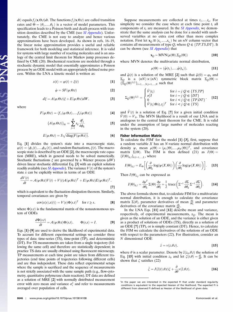
dtÞ equals f jðx;Θ;tÞdt. The functions f jðx;Θ;tÞ are called transitionrates and Θ ¼ ðθ1;…;θLÞ is a vector of model parameters. Thisspecification leads to a Poisson birth and death process with tran-sition densities described by the CME (see SI Appendix). Unfor-tunately, the CME is not easy to analyze and hence variousapproximations have been developed. As shown in refs. 16–19,the linear noise approximation provides a useful and reliableframework for both modeling and statistical inference. It is validfor systems with large number of reacting molecules and is an ana-logy of the central limit theorem for Markov jump processes de-fined by CME (20). Biochemical reactions are modeled through astochastic dynamic model that essentially approximates a Poissonprocess by an ODEmodel with an appropriately defined noise pro-cess. Within the LNA a kinetic model is written as:

xðtÞ ¼ φðtÞ þ ξðtÞ [1]

_φ ¼ SFðφ;Θ;tÞ [2]

dξ ¼ Aðφ;Θ;tÞξþ Eðφ;Θ;tÞdW; [3]

where

Fðφ;Θ;tÞ ¼ ðf 1ðφ;Θ;tÞ;…;f lðφ;Θ;tÞÞ [4]

fAðφ;Θ;tÞgik ¼ ∑R

j¼1

sij∂f j∂ϕk

[5]

Eðφ;Θ;tÞ ¼ SffiffiffiffiffiffiffiffiffiffiffiffiffiffiffiffiffiffiffiffiffiffiffiffiffiffiffiffiffiffidiagðFðφ;Θ;tÞÞ

p: [6]

Eq. [1] divides the system’s state into a macroscopic state,φðtÞ ¼ ðϕ1ðtÞ;…;ϕNðtÞÞ, and random fluctuations, ξðtÞ. Themacro-scopic state is described by anODE [2], the macroscopic rate equa-tion (MRE), which in general needs to be solved numerically.Stochastic fluctuations ξ are governed by a Wiener process (dW )driven linear stochastic differential Eq. [3] with an explicit solutionreadily available (see SI Appendix). The varianceV ðtÞ of the system’sstate x can be explicitly written in terms of an ODE

dV ðtÞdt

¼ Aðφ;Θ;tÞV ðtÞ þ V ðtÞAðφ;Θ;tÞT þ Eðφ;Θ;tÞEðφ;Θ;tÞT;[7]

which is equivalent to the fluctuation-dissipation theorem. Similarly,temporal covariances are given by

covðxðsÞ;xðtÞÞ ¼ V ðsÞΦðs;tÞT for t ≥ s; [8]

where Φðs;tÞ is the fundamental matrix of the nonautonomous sys-tem of ODEs

dΦðs;tÞdt

¼ Aðφ;Θ;tÞΦðs;tÞ; Φðs;sÞ ¼ I: [9]

Eqs. [1]–[9] are used to derive the likelihood of experimental data.To account for different experimental settings we consider threetypes of data: time-series (TS), time-point (TP), and deterministic(DT). For TS measurements are taken from a single trajectory (fol-lowing the same cell) and therefore are statistically dependent; inpractice TS data are usually obtained using fluorescent microscopy.TP measurements at each time point are taken from different tra-jectories (end time points of trajectories following different cells)and are thus independent. These data reflect experimental setupswhere the sample is sacrificed and the sequence of measurementsis not strictly associated with the same sample path (e.g., flow-cyto-metry, quantitative polymerase chain reaction). DT data are definedas a solution of MRE [2] with normally distributed measurementerror with zero mean and variance σ2ϵ and refer to measurementsaveraged over population of cells.

Suppose measurements are collected at times t1;…;tn. Forsimplicity we consider the case where at each time point ti allcomponents of xi are measured. In the SI Appendix, we demon-strate that the same analysis can be done for a model with unob-served variables at no extra cost other than more complexnotation. First let xQ ≡ ðxt1 ;…;xtnÞ be an nN column vector thatcontains all measurements of type Q, where Q ∈ fTP;TS;DTg. Itcan be shown (see SI Appendix) that

xQ ∼MVNðμðΘÞ;ΣQðΘÞÞ [10]

where MVN denotes the multivariate normal distribution,

μðΘÞ ¼ ð ~φðt1Þ;…; ~φðtnÞÞ; [11]

and ~φðtÞ is a solution of the MRE [2] such that ~φð0Þ ¼ φ0 andΣQ is a ðnNÞ × ðnNÞ symmetric block matrix ΣQðΘÞ ¼fΣQðΘÞði;jÞgi¼1;…;N;j¼1;…;N such that

ΣQðΘÞði;jÞ ¼

8>>><>>>:

~V ðtiÞ for i ¼ j Q ∈ fTS;TPgσ2ϵI for i ¼ j Q ∈ fDTg0 for i < j Q ∈ fTP;DTg~V ðtiÞΦðti;tjÞT for i < j Q ∈ fTSg

; [12]

and ~V ðtÞ is a solution of Eq. [7] for a given initial condition~V ð0Þ ¼ V 0. The MVN likelihood is a result of our LNA and isanalogous to the central limit theorem for the CME. It is validunder the assumption of large number of molecules reactingin the system (20).

Fisher Information MatrixTo calculate the FIM† for the model [1]–[3], first, suppose thata random variable X has an N-variate normal distribution withdensity ψ , mean μðΘÞ ¼ ðμ1ðΘÞ;…;μNðΘÞÞT , and covariancematrix ΣðΘÞ. The FIM is then defined (21) as IðΘÞ ¼fIðΘÞk;lgk;l¼1;…;L, where

IðΘÞk;l ¼ EΘ

��∂∂θk

logðψðX;ΘÞÞ��

∂∂θl

logðψðX;ΘÞÞ��

: [13]

Then IðΘÞi;j can be expressed as

IðΘÞk;l ¼∂μT

∂θkΣðΘÞ ∂μ

∂θlþ 1

2trace

�Σ−1 ∂Σ

∂θkΣ−1 ∂Σ

∂θl

�: [14]

The above formula shows that, to calculate FIM for a multivariatenormal distribution, it is enough to calculate the covariancematrix ΣðθÞ, parameter derivatives of mean ∂μ

∂θkand parameter

derivatives of the covariance matrix ∂Σ∂θk.

In the LNA Eqs. [11] and [12] describe mean and variance,respectively, of experimental measurements, xQ. The mean isgiven as the solution of an ODE, and the variance is either givenas a product of solutions of ODEs (TS), directly as a solution ofan ODE [7] (TP), or is simply constant (DT). Hence, to calculatethe FIM we calculate the derivatives of the solutions of an ODEwith respect to the parameters (22). For illustration, consider anN dimensional ODE

_z ¼ vðz;θ;tÞ; [15]

where θ is a scalar parameter. Denote by ~zðz0;θ;tÞ the solution ofEq. [15] with initial condition z0 and let ζðt;θÞ ¼ ∂~z

∂θ. It can beshown that ζ satisfies (22)

_ζ ¼ Jð~zðtÞ;θ;tÞζ þ ∂∂θ

vð~z;θ;tÞ; [16]

†In the paper we are interested in the expected FI that under standard regularityconditions is equivalent to the expected Hessian of the likelihood. The expected FI isdifferent from observed FI defined as Hessian of the likelihood of given data.

8646 ∣ www.pnas.org/cgi/doi/10.1073/pnas.1015814108 Komorowski et al.

where Jð~zðtÞ;Θ;tÞ is the Jacobian ∂∂z vð~z;θ;tÞ. We can thus calculate

derivatives ∂ ~φ∂θk, ∂ ~V∂θk, and ∂Φðti ;tjÞ

∂θkthat give ∂μ

∂θkand ∂Σ

∂θkneeded to com-

pute FIM for the model [1]–[3] (see SI Appendix).The FIM is of special significance for model analysis as it con-

stitutes a tool for sensitivity analysis, robustness, identifiability,and optimal experimental design as we will show below.

The FIM and Sensitivity. The classical sensitivity coefficient for anobservable Q and parameter θ is

S ¼ ∂Q∂θ

:

The behavior of a stochastic system is defined by observables thatare drawn from a probability distribution. The FIM is a measureof how this distribution changes in response to infinitesimalchanges in parameters. Suppose that ℓðΘ;XÞ ¼ logðψðX;ΘÞÞand ℓðΘÞ ¼ −E½ℓðΘ;XÞ�. Then,

IðΘÞk;l ¼ −E�∂2ℓðΘ;XÞ∂θk∂θl

�; [17]

i.e., the FIM is the expected Hessian of ℓðΘ;XÞ. Therefore, ifΘ� is the maximum likelihood estimate of a parameter there isa L × L orthogonal matrix C such that, in the new parametersθ0 ¼ CðΘ − Θ�Þ,

ℓðΘÞ ≈ ℓðΘ�Þ − 1

2∑L

i¼1

λiθ02i ; [18]

for Θ near Θ�. From this it follows that the λi are the eigenvaluesof the FIM and that the matrix C diagonalizes it. If we assumethat the λi are ordered so that λ1 ≥ ⋯ ≥ λL, then it follows thataround the maximum the likelihood is most sensitive when θ01 isvaried and least sensitive when θ0L is varied, and λi is a measure ofthis. Because θ0i ¼ ΣL

j¼1 Cijðθj − θ�j Þ, we can regard Sij ¼ λ1∕2i Cij asthe contribution of the parameter θj to varying θ0i and thus

S2j ¼ ∑

L

i¼1

S2ij [19]

can be regarded as a measure of the sensitivity of the system toθj. It is sometimes appropriate to normalize this and instead con-sider

Tj ¼S2

j

∑L

i¼1S2

i

: [20]

Robustness.Related to sensitivity, robustness in systems biology isusually understood as persistence of a system to perturbations toexternal conditions (23). Sensitivity considers perturbation in asingle parameter whereas robustness takes into account simulta-neous changes in all model parameters. Near to the maximum Θ�the regions of high expected log-likelihood ℓðΘÞ ≥ ℓðΘ�Þ − ε areapproximately the ellipsoids NSðΘ�;εÞ given by the equation

NSðΘ�;εÞ ¼ fΘ: ðΘ − Θ�ÞTIðΘ�ÞðΘ − Θ�Þ < εg: [21]

The ellipsoids have principal directions given by eigenvectors Cand equatorial radii ðλiÞ−1

2. Sets NS are called neutral spacesas they describe regions of parameter space in which a system’sbehavior does not undergo significant changes (10) and arisenaturally in the analysis of robustness.

Confidence Intervals and Asymptotics. The asymptotic normality ofmaximum likelihood estimators implies that if Θ� is a maximumlikelihood estimator then the NS describe confidence ellipsoidsfor Θ with confidence levels corresponding to ε. The equatorial ra-dii decrease naturally with the square root of the sample size (24).

Parameter Identifiability and Optimal Experimental Design. The FIMis of special significance for model analysis as it constitutes a clas-sical criterion for parameter identifiability (15). There exist var-ious definitions of parameter identifiability and here we considerlocal identifiability. The parameter vector Θ is said to be (locally)identifiable if there exists a neighborhood of Θ such that no othervector Θ� in this neighborhood gives raise to the same density asΘ(15). Formula [18] implies that Θ is (structurally) identifiable ifand only if FIM has a full rank (15). Therefore the number ofnonzero eigenvalues of FIM is equal to the number of identifiableparameters, or more precisely, to the number of identifiable lin-ear combinations of parameters.

The FIM is also a key tool to construct experiments in such away that the parameters can be estimated from the resultingexperimental data with the highest possible statistical quality.The theory of optimal experimental design uses various criteriato asses information content of experimental sampling methods;among the most popular are the concepts of D-optimality thatmaximizes the determinant of FIM, and A-optimality that mini-mize the trace of the inverse of FIM (14). Diagonal elements ofthe inverse of FIM constitute a lower-bound for the variance ofany unbiased estimator of elements ofΘ; this is known as the Cra-mér–Rao inequality (see SI Appendix). Finally, it is important tokeep in mind that some parameters may be structurally identifi-able, but not be identifiable in practice due to noise; these wouldcorrespond to small but nonzero eigenvalues of the FIM. Max-imizing the number of eigenvalues above some threshold thatreflects experimental resolution, may therefore be a further cri-terion to optimize experimental design. But all of these criteriarevolve around being able to evaluate the FIM.

ResultsTo demonstrate the applicability of the presented methodologyfor calculation of FIMs for stochastic models we consider twoexamples: a simple model of single gene expression, and a modelof the p53 system. The simplicity of the first model allows us toexplain how the differences between deterministic and stochasticversions of the model as well as TS and TP data arise. In the caseof the p53 system model the informational content, as well assensitivities and neutral spaces are compared between TS, TP,and DT data.

Single Gene Expression Model. Although gene expression involvesnumerous biochemical reactions, the currently accepted consen-sus is to model it in terms of only three biochemical species(DNA, mRNA, and protein) and four reaction channels (tran-scription, mRNA degradation, translation, and protein degrada-tion) (e.g., refs. 12 and 25). Such a simple model has been usedsuccessfully in a variety of applications and can generate data withthe same statistical behavior as more complicated models (26,27). We assume that the process begins with the production ofmRNA molecules ðrÞ at rate kr . Each mRNA molecule maybe independently translated into protein molecules ðpÞ at rate kp.Both mRNA and protein molecules are degraded at rates γr andγp, respectively. Therefore, we have the state vector x ¼ ðr;pÞ, andreaction rates corresponding to transcription of mRNA, transla-tion, degradation of mRNA, and degradation of protein.

FðxÞ ¼ ðkr;kpr;γrr;γppÞ: [22]

Identifiability Study. In a typical experiment, only protein levels aremeasured (17, 28). It is not entirely clear a priori what parametersof gene expression can be inferred; it is also not obvious if andhow the answer depends on the nature of the data (i.e., TS, TP, orDT). We address these questions below.

We assumed that the system has reached the unique steadystate defined by the model and that only protein level is measuredeither as TS

Komorowski et al. PNAS ∣ May 24, 2011 ∣ vol. 108 ∣ no. 21 ∣ 8647

APP

LIED

MAT

HEM

ATICS

BIOPH

YSICSAND

COMPU

TATIONALBIOLO

GY

yTS ¼ ðpt1 ;…;ptnÞ; [23]

or as TP

yTP ¼ ðpð1Þt1 ;…;pðnÞtn Þ; [24]

where the upper indices for TPmeasurements denote the numberof trajectories from which the measurement have been taken toemphasize independence of measurements. Results of the analy-sis are presented in Table S2. For TS data we have four identifi-able parameters whereas time-point measurements provideenough information to estimate only two parameters. To someextent this makes intuitive sense: TS data contain informationabout mean, variance, and autocorrelation functions, which canbe very sensitive to changes in degradation rates; TP measure-ments reflect only information about mean and variance of pro-tein levels therefore only two parameters are identifiable. On theother hand, TP measurements provide independent samples thatis reflected in lower Cramér–Rao bounds. Table S2 also containsa comparison with the corresponding deterministic model. Asone might expect in the deterministic model only one parameteris identifiable as the mean is the only quantity that is described bythe deterministic model, and parameter estimates are informedneither by variability nor by autocorrelation.

Perturbation Experiment. To demonstrate that identifiability is nota model specific but rather an experiment specific feature, weperformed a similar analysis as above for the same model withthe same parameters but with the fivefold increased initial meanand 25-fold increased initial variance. Results are presented inTable S3. Some of the conclusions that can be made are hardto predict without calculating the FIM. The amount of informa-tion in TS data is now much larger than in TP data (higher de-terminant) and also CR bounds are now much lower for TP thanfor TS data. CR bounds for TS and TP are substantially lowerthan for the steady state data (except kr). Interestingly, all fourparameters can be inferred from TS and TP data, but not in thedeterministic scenario. For steady state data all parameters couldonly be inferred from TS data (Table S3).

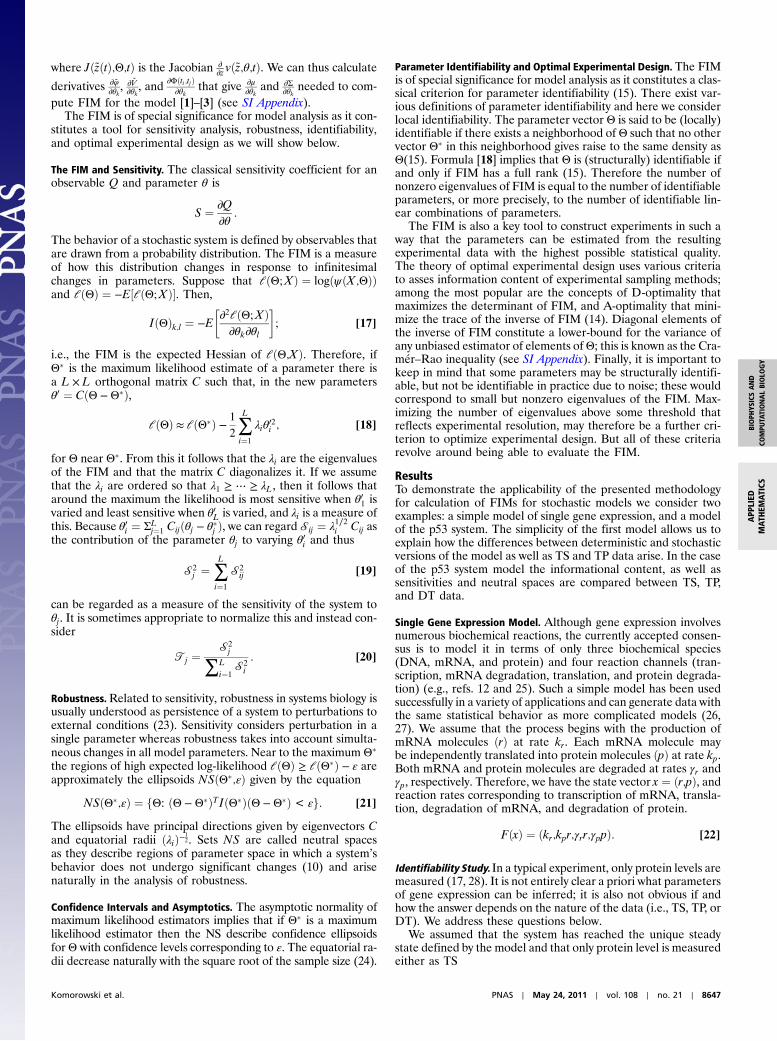
Maximizing the Information Content of Experimental Data. Theamount of information in a sample does not depend solely onthe type of data (TS, TP), but also on other factors that canbe controlled in an experiment. One easily controllable quantityis the sampling frequency Δ. We consider here only equidistantsampling and keep number of measurements constant. Thereforewe define Δ as time between subsequent observations Δ ¼tiþ1 − ti. To show how sampling frequency influences informa-tional content of a sample for the model of gene expressionwe used four parameter sets (Table S1) and assumed that the datahave the form [23]. The amount of information in a sample wasunderstood as the determinant of the FIM, equivalent to the pro-duct of the eigenvalues of the FIM. Results in Fig. 1 demonstratethat our method can be used to determine optimal samplingfrequency, given that at least some rough estimates of modelparameters are known. It is worth noting that equidistant sam-pling is not always the best option and more complex strategieshave been proposed in experimental design literature.

Differences in Sensitivity and Robustness Analysis in TS, TP, and DTVersions of the Model. TS, TP, and DT versions of the model differwhen one considers information content of samples, and such dis-crepancies exist also when sensitivity and robustness are studied.First, deterministic models completely neglect variability in mo-lecular species. Variability, however, is a function of parameters,and like the mean, is sensitive to them. Second, deterministicmodels do not include correlations between molecular species.Third, temporal correlations are neglected in TP and DT models.

To understand these effects we first analyze the analytical formof means, variances, and correlations for this model (see SIAppendix). We start with the effect of incorporating variability.Suppose we consider a change in parameters; e.g., kp, γp by afactor δ ðkp;γpÞ → ðkp þ δkp;γp þ δγpÞ. The means of RNA andprotein concentrations are not affected by this perturbation,whereas the protein variance does change (see formulas [33]–[37]in SI Appendix). This result is related to the number of nonzeroeigenvalues of the FIM. The FIM for the stationary distributionof this model with respect to parameters kp, γp has only onepositive eigenvalue for the deterministic model and two positiveeigenvalues for the stochastic model.

To study the effect of correlation between RNA and proteinlevels ρrp we first note that formulas [33]–[37] in the SI Appendixdemonstrate that at constant mean, correlation increases withγp when accompanied by a compensating increase in kp. Fig. 2(left column) presents neutral spaces (21) for parameter pairs fordifferent values of correlation, ρrp. The differences between DTand TS are enhanced by the correlation.

Similar analysis reveals that taking account of the temporal cor-relations also changes the way the model responds to parameterperturbations. Fig. 2 (right column) shows neutral spaces for threedifferent sampling frequencies and indicates that the differencesbetween stochastic and deterministic models decrease with Δ.

Model of p53 System.Themodel of single gene expression is a linearmodel with only four parameters and a simple stationary state andillustrates how the methodology can be used to provide relevantconclusions and investigate discrepancies between sensitivities ofTS, TP, and DT models. Our methodology, however, can also beused to study more complex models, and here we have chosenthe p53 signalling system, which incorporates a feedback loop be-tween the tumor suppressor p53 and the oncogene Mdm2, and isinvolved in regulation of cell cycle and response to DNA damage.

We use the model introduced in ref. 29 that reduces the systemto three molecular species, p53, mdm2 precursor, and mdm2, de-noted here by p, y0 and y, respectively. The state of the system istherefore given by x ¼ ðp;y0;yÞ, and the deterministic version of themodel can be formulated in terms of macroscopic rate equations

0 0.2 0.4 0.6 0.8 1 1.2 1.4 1.6 1.8 20

10

20

30

40

50

60

70

80

det(

FIM

)

set 1set 2set 3set 4

Fig. 1. Determinant of FIM plotted against sampling frequency Δ (in hours).We used logarithms of four parameter sets (see Table S1). Sets 1 and 3correspond to slow protein degradation ðγp ¼ 0.7Þ; and sets 2 and 4 describefast protein degradation ðγp ¼ 1.2Þ. We assumed that 50 measurementsðn ¼ 50Þ of protein levels were taken from the stationary state. Observedmaximum in information content results from the balance between indepen-dence and correlation of measurements.

8648 ∣ www.pnas.org/cgi/doi/10.1073/pnas.1015814108 Komorowski et al.

S ¼1 −1 −1 0 0 0

0 0 0 1 −1 0

0 0 0 0 1 −1

0@

1A [25]

_ϕp ¼ bx − axϕp − akϕyϕp

ϕp þ k[26]

_ϕy0 ¼ byϕp − a0ϕy0 [27]

_ϕy ¼ a0ϕy0 − ayϕy: [28]

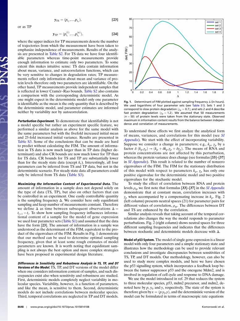
Informational Content of TS and TP Data for the p53 System. In thecase of the single gene expression model we have argued that TSdata are more informative due to accounting for temporal corre-lations. On the other hand, TP measurements provide statisticallyindependent samples, which should increase informational con-tent of the data. Therefore it is not entirely clear what data type isbetter for a particular parameter. If, for instance, a parameter isentirely informed by a system’s mean behavior than TP data willbe more informative because TP data provide statistically inde-pendent samples about the mean. Whereas if a parameter is alsoinformed by temporal correlations, then TS data will turn out tobe more informative. It is difficult to predict a priori which effectwill be dominating. Therefore calculation of FIM and compari-son of their eigenvalues and diagonal elements is necessary.Eigenvalues and diagonal elements of FIMs calculated for para-meters presented in Table S4 are plotted in Fig. S1 and Fig. 3,respectively. Eigenvalues of the FIM for TS data are larger thanfor TP data. Similarly, diagonal elements for all parameters arelarger for TP than for TS data for most parameters difference issubstantial. This indicates that temporal correlation is a sensitivefeature of this system and provides significant information aboutmodel parameters. The lower information content of the TP datacan, however, be compensated for by increasing the number ofindependent measurements, which is easily achievable in current

experimental settings (see Fig. S2). For deterministic models theabsolute value of elements of FIM depends on measurementerror variance and therefore FIMs of TS and TP data can notbe directly compared with the DT model.

Sensitivity. The sensitivity coefficients Ti for TS, TP, and DT dataare presented in Fig. 3. Despite differences outlined previously,here sensitivity coefficients are quite similar for all three types sug-gesting that the hierarchy of sensitive parameters is to a consider-able degree independent on the type of data. The differences exist,however, in contributionsC2

ij (see Fig. S3), suggesting discrepanciesin neutral spaces and robustness analysis that we present below.

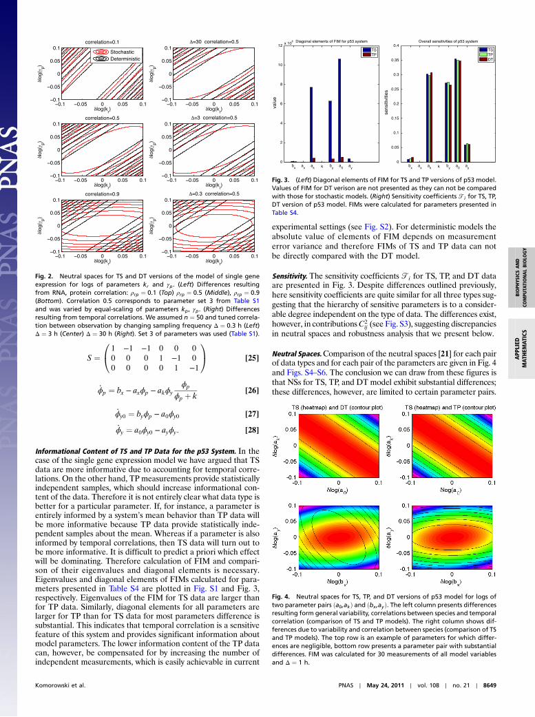
Neutral Spaces.Comparison of the neutral spaces [21] for each pairof data types and for each pair of the parameters are given in Fig. 4and Figs. S4–S6. The conclusion we can draw from these figures isthat NSs for TS, TP, and DT model exhibit substantial differences;these differences, however, are limited to certain parameter pairs.

Fig. 2. Neutral spaces for TS and DT versions of the model of single geneexpression for logs of parameters kr and γp. (Left) Differences resultingfrom RNA, protein correlation: ρrp ¼ 0.1 (Top) ρrp ¼ 0.5 (Middle), ρrp ¼ 0.9(Bottom). Correlation 0.5 corresponds to parameter set 3 from Table S1and was varied by equal-scaling of parameters kp, γp. (Right) Differencesresulting from temporal correlations. We assumed n ¼ 50 and tuned correla-tion between observation by changing sampling frequency Δ ¼ 0.3 h (Left)Δ ¼ 3 h (Center) Δ ¼ 30 h (Right). Set 3 of parameters was used (Table S1).

0

0.05

0.1

0.15

0.2

0.25

0.3

0.35

0.4

bx

ax

ak k b

ya

0a

y

sens

itivi

ties

Overall sensitivities of p53 system

TSTPDT

0

2

4

6

8

10

12 x 106

bx

ax

ak k b

ya

0a

y

valu

e

Diagonal elements of FIM for p53 system

TSTP

Fig. 3. (Left) Diagonal elements of FIM for TS and TP versions of p53 model.Values of FIM for DT verison are not presented as they can not be comparedwith those for stochastic models. (Right) Sensitivity coefficients Ti for TS, TP,DT version of p53 model. FIMs were calculated for parameters presented inTable S4.

Fig. 4. Neutral spaces for TS, TP, and DT versions of p53 model for logs oftwo parameter pairs ða0;akÞ and ðbx;ayÞ. The left column presents differencesresulting form general variability, correlations between species and temporalcorrelation (comparison of TS and TP models). The right column shows dif-ferences due to variability and correlation between species (comparison of TSand TP models). The top row is an example of parameters for which differ-ences are negligible, bottom row presents a parameter pair with substantialdifferences. FIM was calculated for 30 measurements of all model variablesand Δ ¼ 1 h.

Komorowski et al. PNAS ∣ May 24, 2011 ∣ vol. 108 ∣ no. 21 ∣ 8649

APP

LIED

MAT

HEM

ATICS

BIOPH

YSICSAND

COMPU

TATIONALBIOLO

GY

Differences between NPs of TS and DT models are exhibited inpairs involving parameters bx, ay; between TS and TP in pairs in-volving bx; and between TP and DT also pairs involving bx.

This suggests that parameter bx is responsible either for thevariability in molecular numbers or the correlation between spe-cies, as these are responsible for differences between TP and DTmodels. Similarly the lack of differences in pairs involving ay incomparisons of TP and DT, and their presence in comparisonof TP and TS indicates that parameter ay is responsible for reg-ulating the temporal correlations. This analysis agrees with whatone might intuitively predict. Parameter bx describes the produc-tion rate, and therefore the mean expression level of p53, and alsothe variability of all components of the system. It is difficult, how-ever, to say how this parameter influences correlations betweenspecies. Parameter ay, on the other hand, is the degradation rateof mdm2 and therefore clearly determines the temporal correla-tion of not only mdm2 but also of p53, because mdm2 regulatesthe degradation rate of p53. While heuristic, our analysis of theneutral spaces nevertheless clearly demonstrates the differencesbetween the three types ofmodels and creates a theoretical frame-work for investigating the role of parameters in the stochasticchemical kinetics systems and without the need to performMonteCarlo sampling or other computationally expensive schemes.

DiscussionThe aim of this paper was to introduce an innovative theoreticalframework that allows us to gain insights into sensitivity and robust-ness of stochastic reaction systems through analysis of the FIM.Wehave used the linear noise approximation (16, 17, 30) to modelmeans, variances, and correlations in terms of appropriate ODEs.Differentiating the solution of these ODEs with respect to para-meters (22) allowed us to numerically calculate derivatives ofmeans, variances, and correlations, which combined with the nor-mal distribution of model variables implied by the LNA gave us therepresentation of the FIM in terms of solutions of ODEs. To ourknowledge, noothermethod computes FIM for stochastic chemicalkinetics models without the need for Monte Carlo simulations.

Given the role of the FIM in model analysis and increasinginterest in stochastic models of biochemical reactions, our ap-proach is widely applicable. It is primarily aimed at optimizing orguiding experimental design, and here we have shown how it can

be used to test parameter identifiability for different data types,determine optimal sampling frequencies, examine informationcontent of experimental samples and calculate Cramér–Raobounds for kinetic parameter estimates. Its applicability, how-ever, extends much further: it can provide a rationale as to whichvariables should be measured experimentally, or what perturba-tion should be applied to a system to obtain relevant informationabout parameters of interest. Similar strategies can also be em-ployed to optimize model selection procedures. As demonstratedhere, stochastic data incorporating information about noise struc-ture are more informative and therefore experimental optimiza-tion for stochastic models models may be advantageous oversimilar methods for deterministic models.

A second topical application area is the study of robustness ofstochastic systems. Interest in robustnesses results from the ob-servation that biochemical systems exhibit surprizing stabilityin function under various environmental conditions. For determi-nistic models this phenomenon has been partly explained by theexistence of regions in parameter space (neutral spaces) (10), inwhich perturbations to parameters do not result in significantchanges in system output. We have demonstrated that even avery simple stochastic linear model of gene expression exhibitssubstantial differences when its neutral spaces are compared withthe deterministic counterpart. Therefore a stochastic system mayrespond differently to changes in external conditions than thecorresponding deterministic model. Our study presents examplesof changes in parameters that do not affect behavior of a deter-ministic systems but may substantially change a probability distri-bution that defines the behavior of the corresponding stochasticsystem. Thus for systems in which stochasticity plays an importantrole random effects can not be neglected when considering issuesrelated to robustness. More information regarding applicabilityof our method is available in the SI Appendix and Figs. S7–S13.

ACKNOWLEDGMENTS. M.K. and M.P.H.S. acknowledge support from the Bio-technology and Biological Sciences Research Council (BBSRC) (BB/G020434/1).D.A.R. holds an Engineering and Physical Sciences Research Council (EPSRC)Senior Fellowship (GR/S29256/01), and his work and that of M.J.C. werefunded by a BBSRC/EPSRC Systems Approaches to Biological Research (SABR)Grant (BB/F005261/1, ROBuST project). D.A.R. and M.K. were also supportedby the European Union (BIOSIM Network Contract 005137). M.P.H.S. is a RoyalSociety Wolfson Research Merit Award holder.

1. Csete ME, Doyle JC (2002) Reverse engineering of biological complexity. Science295:1664–1669.

2. Varma A, Morbidelli M, Wu H (1999) Parametric Sensitivity in Chemical Systems (Cam-bridge University Press, Cambridge, UK).

3. Maheshri N, O’Shea EK (2007) Living with noisy genes: How cells function reliably withinherent variability in gene expression. Annu Rev Bioph Biom 36:413–434.

4. McAdams HH, Arkin A (1997) Stochastic mechanisms in gene expression. Proc NatlAcad Sci USA 94:814–819.

5. Elowitz MB, Levine AJ, Siggia ED, Swain PS (2002) Stochastic gene expression in asingle cell. Science 297:1183–1186.

6. Wilkinson DJ (2009) Stochastic modelling for quantitative description of heteroge-neous biological systems. Nat Rev Genet 10:122–133.

7. Gunawan R, Cao Y, Petzold L, Doyle FJ, III (2005) Sensitivity analysis of discrete stochas-tic systems. Biophys J 88:2530–2540.

8. Rathinam M, Sheppard PW, Khammash M (2010) Efficient computation of parametersensitivities of discrete stochastic chemical reaction networks. J Chem Phys 132:034103.

9. Rand DA (2008) Mapping the global sensitivity of cellular network dynamics. J R SocInterface 5:S59–S69.

10. Daniels BC, Chen YJ, Sethna JP, Gutenkunst RN, Myers CR (2008) Sloppiness, robust-ness, and evolvability in systems biology. Curr Opin Biotech 19:389–395.

11. Brown KS, Sethna JP (2003) Statistical mechanical approaches to models with manypoorly known parameters. Phys Rev E 68:021904.

12. Rand DA, Shulgin BV, Salazar D, Millar AJ (2006) Uncovering the design principles ofcircadian clocks: Mathematical analysis of flexibility and evolutionary goals. J TheorBiol 238:616–635.

13. Erguler K, Stumpf MPH (2011) Practical limits for reverse engineering of dynamicalsystems: A statistical analysis of sensitivity and parameter inferability in systemsbiology models. Mol Biosyst 7:1595–1602.

14. Emery AF, Nenarokomov AV (1998) Optimal experiment design. Meas Sci Technol9:864–876.

15. Rothenberg TJ (1971) Identification in parametric models. Econometrica 39:577–591.

16. Elf J, Ehrenberg M (2003) Fast evaluation of fluctuations in biochemical networks withthe linear noise approximation. Genome Res 13:2475–2484.

17. Komorowski M, Finkenstadt B, Harper CV, Rand DA (2009) Bayesian inference of bio-chemical kinetic parameters using the linear noise approximation. BMC Bioinformatics10(1):343.

18. Ruttor A, Sanguinetti G, Opper M (2009) Efficient statistical inference for stochasticreaction processes. Phys Rev Lett 103:230601.

19. Komorowski M, Finkenstadt B, Rand DA (2010) Using a single fluorescent reportergene to infer half-life of extrinsic noise and other parameters of gene expression. Bio-phys J 98:2759–2769.

20. Thomas G. Kurtz (1972) The relationship between stochastic and deterministic modelsfor chemical reactions. J Chem Phys 57:2976–2978.

21. Porat B, Friedlander B (1986) Computation of the exact informationmatrix of Gaussiantime series with stationary random components. IEEE T Acoust Speech 34:118–130.

22. Coddington EA, Levinson N (1972) Theory of Ordinary Differential Equations(McGraw-Hill, New York).

23. Felix MA, Wagner A (2006) Robustness and evolution: Concepts, insights and chal-lenges from a developmental model system. Heredity 100:132–140.

24. DeGroot MH, Schervish MJ (2002) Probability and Statistics (Addison-Wesley, NewYork), 3rd Ed.

25. Thattai M, van Oudenaarden A (2001) Intrinsic noise in gene regulatory networks. ProcNatl Acad Sci USA 98:8614–8619.

26. Dong CG, Jakobowski L, McMillen DR (2006) Systematic reduction of a stochasticsignalling cascade model. J Biol Phys 32:173–176.

27. Iafolla MAJ, McMillen DR (2006) Extracting biochemical parameters for cellular mod-eling: A mean-field approach. J Phys Chem B 110:22019–22028.

28. Chabot JR, Pedraza JM, Luitel P, van Oudenaarden A (2007) Stochastic gene expressionout-of-steady-state in the cyanobacterial circadian clock. Nature 450:1249–1252.

29. Geva-Zatorsky N, et al. (2006) Oscillations and variability in the p53 system. Mol SystBiol 2:2006.0033.

30. Van Kampen NG (2006) Stochastic Processes in Physics and Chemistry (Elsevier Science,Amsterdam).

8650 ∣ www.pnas.org/cgi/doi/10.1073/pnas.1015814108 Komorowski et al.

Supplementary Information

Sensitivity, robustness and identifiability in stochastic chemicalkinetics models

Micha l Komorowski1, Maria J. Costa2, David A. Rand2, Michael Stumpf1

1. Centre for Bioinformatics, Imperial College London, UK2. Systems Biology Centre, and Mathematics Institute, University of Warwick, UK

This is supplementary information for the paper Sensitivity, robustness and identifiability instochastic chemical kinetics models which is henceforth referred to as MP.

1 Derivation of the model equations

We consider a general system of chemical reactions that consists of N chemical speciesand interacts in a fixed volume through R reactions. Let x = (x1, . . . , xN)T be the vectorrepresenting the numbers of molecules for the N species and S = {sij}i=1,2...N ; j=1,2...R bethe stoichiometry matrix that describes changes in the population sizes due to each of thereactions, so that occurrence of reaction j results in a change

(x1, ...., xN)→ (x1 + s1j, ..., xN + sNj).

We assume that the probability that a reaction of type j occurs in the time interval [t, t+dt)equals fj(x,Θ)dt, where functions fj(x,Θ) are called the reaction rates and Θ = (θ1, ..., θL) isthe vector of all model parameters. The probability that more than one event will take placein a small time interval is of higher order (dt2) with respect to the length of the interval andcan thus be ignored. Finally, we assume that events taking place in disjoint time intervalsare independent, when conditioned on the events in the previous interval. This specificationleads to a Poisson birth and death process; the Chemical Master Equation [1, 2] is widelyused to describe the temporal evolution of the probability P(x, t) that the system is in thestate x at time t

dP(x, t)

dt=

R∑j=1

(P(x− s· j, t)fj(x− s· j,Θ, t)− P(x, t)fj(x,Θ, t)) . (1)

1

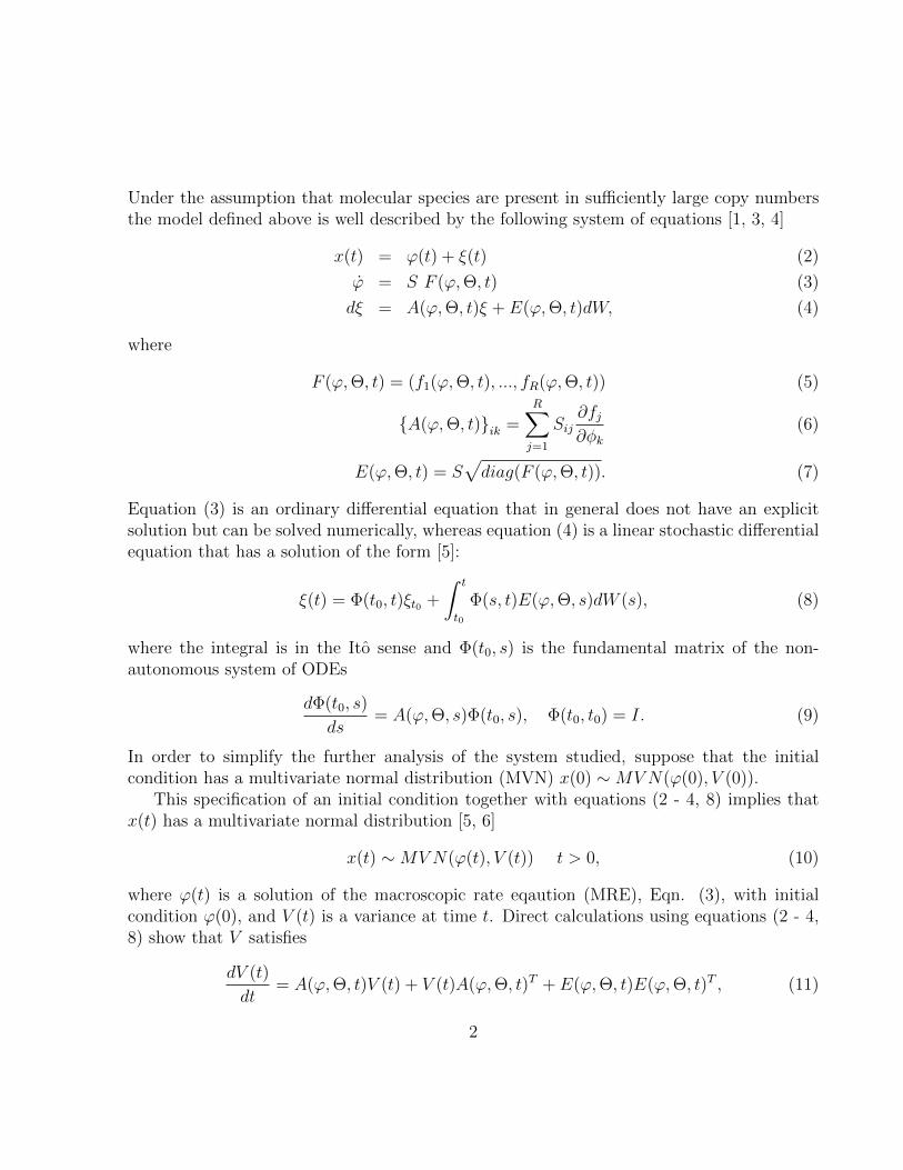
Under the assumption that molecular species are present in sufficiently large copy numbersthe model defined above is well described by the following system of equations [1, 3, 4]

x(t) = ϕ(t) + ξ(t) (2)

ϕ = S F (ϕ,Θ, t) (3)

dξ = A(ϕ,Θ, t)ξ + E(ϕ,Θ, t)dW, (4)

where

F (ϕ,Θ, t) = (f1(ϕ,Θ, t), ..., fR(ϕ,Θ, t)) (5)

{A(ϕ,Θ, t)}ik =R∑j=1

Sij∂fj∂φk

(6)

E(ϕ,Θ, t) = S√diag(F (ϕ,Θ, t)). (7)

Equation (3) is an ordinary differential equation that in general does not have an explicitsolution but can be solved numerically, whereas equation (4) is a linear stochastic differentialequation that has a solution of the form [5]:

ξ(t) = Φ(t0, t)ξt0 +

∫ t

t0

Φ(s, t)E(ϕ,Θ, s)dW (s), (8)

where the integral is in the Ito sense and Φ(t0, s) is the fundamental matrix of the non-autonomous system of ODEs

dΦ(t0, s)

ds= A(ϕ,Θ, s)Φ(t0, s), Φ(t0, t0) = I. (9)

In order to simplify the further analysis of the system studied, suppose that the initialcondition has a multivariate normal distribution (MVN) x(0) ∼MVN(ϕ(0), V (0)).

This specification of an initial condition together with equations (2 - 4, 8) implies thatx(t) has a multivariate normal distribution [5, 6]

x(t) ∼MVN(ϕ(t), V (t)) t > 0, (10)

where ϕ(t) is a solution of the macroscopic rate eqaution (MRE), Eqn. (3), with initialcondition ϕ(0), and V (t) is a variance at time t. Direct calculations using equations (2 - 4,8) show that V satisfies

dV (t)

dt= A(ϕ,Θ, t)V (t) + V (t)A(ϕ,Θ, t)T + E(ϕ,Θ, t)E(ϕ,Θ, t)T , (11)

2

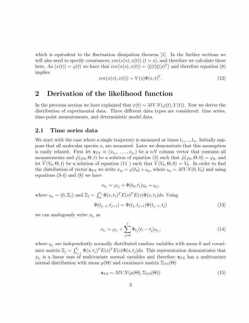
which is equivalent to the fluctuation dissipation theorem [1]. In the further sections wewill also need to specify covariances, cov(x(s), x(t)) (t > s), and therefore we calculate thesehere. As 〈x(t)〉 = ϕ(t) we have that cov(x(s), x(t)) = 〈ξ(t)ξ(s)T 〉 and therefore equation (8)implies

cov(x(s), x(t)) = V (s)Φ(s, t)T . (12)

2 Derivation of the likelihood function

In the previous section we have explained that x(t) ∼MVN(ϕ(t), V (t)). Now we derive thedistribution of experimental data. Three different data types are considered: time series,time-point measurements, and deterministic model data.

2.1 Time series data

We start with the case where a single trajectory is measured at times t1, ..., tn. Initially sup-pose that all molecular species xi are measured. Later we demonstrate that this assumptionis easily relaxed. First let xTS ≡ (xt1 , . . . , xtn) be a nN column vector that contains allmeasurements and ϕ(ϕ0,Θ, t) be a solution of equation (3) such that ϕ(ϕ0,Θ, 0) = ϕ0, andlet V (V0,Θ, t) be a solution of equation (11 ) such that V (V0,Θ, 0) = V0. In order to findthe distribution of vector xTS we write xt0 = ϕ(t0) + ςt0 , where ςt0 ∼MVN(0, V0) and usingequations (3-4) and (8) we have

xt1 = ϕt1 + Φ(t0, t1)ςt0 + ςt1 ,

where ςt1 ∼ (0,Ξ1) and Ξ1 =∫ t1t0

Φ(s, t1)TE(s)TE(s)Φ(s, t1)ds. Using

Φ(tj−1, tj+1) = Φ(tj, tj+1)Φ(tj−1, tj) (13)

we can analogously write xti as

xti = ϕti +i∑

j=0

Φtj(ti − tj)ςtj , (14)

where ςtj are independently normally distributed random variables with mean 0 and covari-

ance matrix Ξj =∫ tjtj−1

Φ(s, tj)TE(s)TE(s)Φ(s, tj)ds. This representation demonstrates that

xti is a linear sum of multivariate normal variables and therefore xTS has a multivariatenormal distribution with mean µ(Θ) and covariance matrix ΣTS(Θ)

xTS ∼MVN(µ(Θ),ΣTS(Θ)) (15)

3

where µ(Θ) = (ϕ(t1), ..., ϕ(tn)) and ΣTS(Θ) is a (n×N)× (n×N) block matrix ΣTS(Θ) ={Σ(Θ)(i,j)

}i=1,...,N ;j=1,...,N

such that diagonal elements contain variances Σ(Θ)(i,i) = V (ti) and

non-diagonal elements (i 6= j) covariances Σ(Θ)(i,j) = cov(x(ti), x(tj)). Diagonal elementsare given by the solution V . From representation (14) we have

Σi,j+1 = Σi,jΦ(tj, tj+1)T , (16)

which demonstrates that non-diagonal elements can be easily computed from diagonal ele-ments given by solutions of equation (11).

2.2 Time-point measurements

Here we consider the case where in an experiment at each time point t1, ..., tn a differenttrajectory is measured. Therefore, measurements come from the same process x(t) but from

its independent realisations. We define the measurement vector as xTP ≡ (x(1)t1 , . . . , x

(n)tn ).

Upper indices indicate the number of trajectories from which the measurements were takenin order to emphasis that each measurement is taken from a different trajectory. The distri-bution of x

(i)ti is given by (10). All measurements are independent so that cov(xti , xtj) = 0

for i 6= j, thereforexTP ∼MVN(µ(Θ),ΣTP (Θ)) (17)

where µ(Θ) = (ϕ(t1), ..., ϕ(tn)) and ΣTP (Θ) has the same diagonal blocks as ΣTS(Θ) andnon-diagaonal blocks are equal to 0

ΣTP (Θ)(i,j) =

{V (ti) for i = j

0 for i 6= j.(18)

2.3 Deterministic model

In order to study differences between stochastic and deterministic regimes we also considera deterministic model where the system state is described entirely by the MRE (3). In sucha model measurements are usually assumed to have the form

x(ti) = ϕ(ti) + εti ,

, where εti is a normally and independently distributed measurement error with mean 0 andconstant variance σ2

ε . We denote the measurements for this model by xDT ≡ (xt1 , . . . , xtn).Finding the data distribution for this case is straightforward,

xDT ∼MVN(µ(Θ),ΣDT ), (19)

where µ(Θ) is as in the previous cases and ΣDT is a N2n2 diagonal matrix with diagonalelements equal to σ2

ε .

4

2.4 Hidden variables

Usually it is not possible to measure all variables present in the system of interest experi-mentally. Hence we here demonstrate that the distribution of observed components can bedirectly extracted from the distributions (15, 17, 19). For simplicity we consider the case oftime series data only; analysis for the two other data types proceeds analogously. First, wepartition the process x(t) into those components y(t) that are observed and those z(t) thatare unobserved. Let yTS ≡ (yt1 , . . . ,ytn) and zTS ≡ (zt1 , . . . , ztn) denote the time seriesthat of y and z,respectively, at times t1, . . . tn.

The distribution of yTS is a marginal distribution of xTS; we thus have

yTS ∼MVN(µy(Θ), Σ(Θ)), (20)

where µy(Θ) and Σ(Θ) are elements of µ(Θ) and ΣTS(Θ) that correspond to the observedcomponents of xTS. If for instance first M out of N components of x are observed thany(t) = (x1(t), ..., xM(t)), and

µy(Θ) = (ϕM(t1), ..., ϕM(tn)) (21)

where ϕM(t) = (φ1(t), ..., φM(t)) and Σ(Θ)= is a MN ×MN block matrix

Σ(Θ) ={

Σ(Θ)(i,j)}i=1,...,N ;j=1,...,N

(22)

whereΣ(i,j)pq (Θ) = Σ(i,j)

pq (Θ) p = 1, ...,M, q = 1, ...,M. (23)

3 Calculation of the Fisher Information Matrix (FIM)

Suppose that a random variable X has an N -variate normal distribution with mean µ(Θ) =(µ1(Θ), ..., µN(Θ))T and covariance matrix Σ(Θ). We define the FIM for this variable to beI(Θ)= {I(Θ)k,l} [7]

I(Θ)k,l = EΘ

[(∂

∂θklog(ψ(X,Θ))

)(∂

∂θllog(ψ(X,Θ))

)], (24)

where ψ(.) is the density function of a multivariate normal distribution with mean µ(Θ) andcovariance Σ(Θ). As the random variable X is normally distributed the elements I(Θ)k,l canbe also expressed explicitly as

I(Θ)k,l =∂µ

∂θk

T

Σ(θ)∂µ

∂θl+

1

2trace(Σ−1 ∂Σ

∂θkΣ−1∂Σ

∂θl). (25)

5

In this section we demonstrate how to calculate the FIM for the models (2- 4). We considerthe model for time series data, as the case of time-point measurements is less general andcan be directly extracted from formulas derived below. Previously, we have shown 15 thatvariable xTS has a multivariate normal distribution and demonstrated how its mean µ(Θ)and covariance matrix Σ(Θ) can be calculated. Formula (25) indicates that two more com-

ponents ∂µ∂θk

and ∂Σ(Θ)∂θk

need to be known in order to be able to compute FIM. Below we showhow these can be obtained.

Let Y (t) be the concatenated vector of ϕ(t) and upper diagonal of the symmetric matrixV

Y (t) = (φ1(t), ..., φN(t), V1,1(t), ..., VN,N(t), ..., V1,2(t), ..., VN−1,N(t)) (26)

and Y (Y0,Θ, t) be the concatenation of ϕ(ϕ0,Θ, t) and upper diagonal of V (V0,Θ, t). Simi-larly denoting the concatenation of the right hand sides of equations (3) and (11) by W wecan write

d

dtY (t) = W (Y (t),Θ, t). (27)

To determine the derivative Zk(t) = Y (t)∂θk

we use the fact that it satisfies the following equation

(see Appendix)d

dtZk(t) = J(Y (t),Θ, t)Zk(t) +Kk(t), (28)

where J(Y (t),Θ, t) is the Jacobian ∂∂Y (t)

W (Y (t),Θ, t) evaluated at the solution Y (t) and

Kk(t) is the vector ∂∂θkW (Y (t),Θ, t) also evaluated at Y (t).

The solution of equation (28), Z(t), provides us with ∂φ(t)∂θk

and therefore with ∂µ∂θk

. Similarly

Z(t) contains diagonal elements of ∂Σ∂θk

.

Non-diagonal elements of ∂Σ∂θk

can be computed from diagonal elements using the recursiverelation

∂

∂θkΣ(i,j+1) =

∂

∂θk

(Σ(i,j)Φ(tj, tj+1)T

)=

∂

∂θk

(Σ(i,j)

)Φ(ti, ti+1)T + Σ(i,j) ∂

∂θk

(Φ(ti, ti+1)T

).

(29)from elements Φ(tj, tj+1), Σ(i,i), ∂

∂θkΣ(i,i) that are given by equations (9), (16) and (28)

respectively. To simplify notation denote Ξk(s, t) = ∂Φ(s,t)∂θk

. As Φ(s, t) is a solution of an

ODE we use similar techniques as in equations (28) and write Ξk(s, t) as a solution of the

6

differential equationdΞk

dt(s, t) = A(ϕ,Θ, t)Ξ(s, t) +Mk(t), (30)

where

Mk(t) =∂

∂θk(A(ϕ,Θ, t)Φ(s, t)) =

(∂

∂θkA(ϕ,Θ, t) + (

∂

∂ϕA(ϕ,Θ, t)ϕ=ϕ)

∂ϕ

∂θk

)Φ(s, t), (31)

and Ξ(s, s) = 0 for all s. To summarise, for the experimental data distribution (15) the FIM(25) can be computed using equations (28 - 31):

• the parameter derivative of the mean, ∂µ(Θ)∂θk

, can be extracted from a solution of (28)

• diagonal elements of the parameter derivatives of the variance, ∂ΣTS(Θ)∂θk

, can be ex-

tracted from a solution of (28)

• non-diagonal elements of parameter derivatives of the variance, ∂ΣTS(Θ)∂θk

, are given by

formula (29), which involves (30) and (31).

3.1 Summary of the numerical computation of the FIM

Below we summarise in more details how the FIM can be calculated numerically. We startwith the case of time series data as it is most general and the remaining two can be derivedfrom it.

Time series measurmens

1 Read input: Stoichiometry matrix S, reaction rates vector F,initial conditions x0, V0

2 Construct equations for ϕ (eq. (3)) and V (eq. (11)) and for Y (eq. (27))

3 Calculate symbolically the Jacobians A (eq. (6)), J (eq. (28)) and vectors

Kk (eq. (28)) , Mk (eq. 30) (k = 1, ..., L)

4 Solve equations for ϕ and V (eq. (27))

5 Compute fundamental matrices Φ(ti, ti+1) i = 1, ..., N − 1 (eq. (9))

6 Construct covariance matrix ΣTS from V (ti) and Φ(ti, ti+1) (i = 1, ..., n) according

to eq. (16)

7

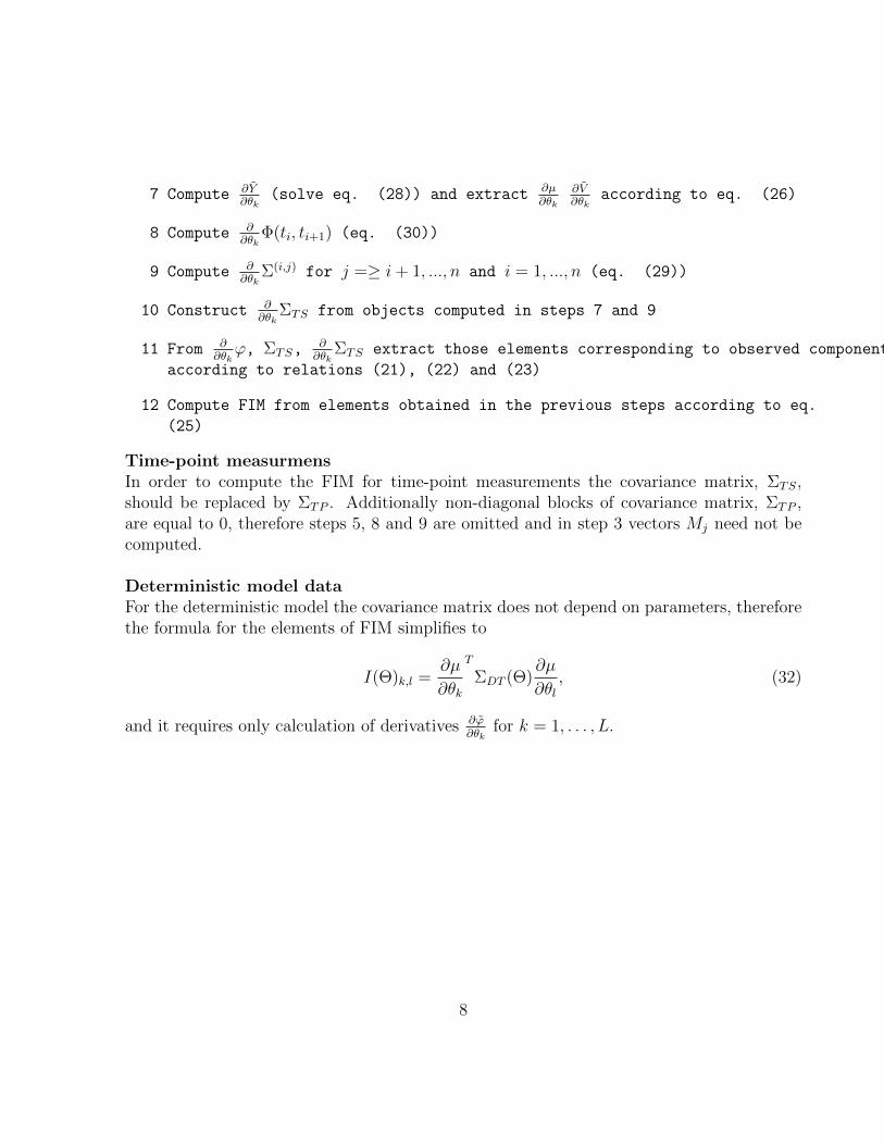
7 Compute ∂Y∂θk

(solve eq. (28)) and extract ∂µ∂θk

∂V∂θk

according to eq. (26)

8 Compute ∂∂θk

Φ(ti, ti+1) (eq. (30))

9 Compute ∂∂θk

Σ(i,j) for j =≥ i+ 1, ..., n and i = 1, ..., n (eq. (29))

10 Construct ∂∂θk

ΣTS from objects computed in steps 7 and 9

11 From ∂∂θkϕ, ΣTS,

∂∂θk

ΣTS extract those elements corresponding to observed components

according to relations (21), (22) and (23)

12 Compute FIM from elements obtained in the previous steps according to eq.

(25)

Time-point measurmensIn order to compute the FIM for time-point measurements the covariance matrix, ΣTS,should be replaced by ΣTP . Additionally non-diagonal blocks of covariance matrix, ΣTP ,are equal to 0, therefore steps 5, 8 and 9 are omitted and in step 3 vectors Mj need not becomputed.

Deterministic model dataFor the deterministic model the covariance matrix does not depend on parameters, thereforethe formula for the elements of FIM simplifies to

I(Θ)k,l =∂µ

∂θk

T

ΣDT (Θ)∂µ

∂θl, (32)

and it requires only calculation of derivatives ∂ϕ∂θk

for k = 1, . . . , L.

8

4 Examples

In this section we present details pertaining to the examples of models of single gene expres-sion and the p53 system.

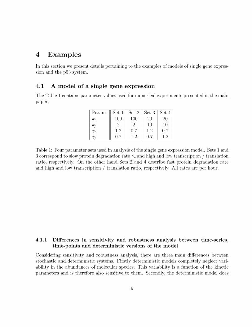
4.1 A model of a single gene expression

The Table 1 contains parameter values used for numerical experiments presented in the mainpaper.

Param. Set 1 Set 2 Set 3 Set 4kr 100 100 20 20kp 2 2 10 10γr 1.2 0.7 1.2 0.7γp 0.7 1.2 0.7 1.2

Table 1: Four parameter sets used in analysis of the single gene expression model. Sets 1 and3 correspond to slow protein degradation rate γp and high and low transcription / translationratio, respectively. On the other hand Sets 2 and 4 describe fast protein degradation rateand high and low transcription / translation ratio, respectively. All rates are per hour.

4.1.1 Differences in sensitivity and robustness analysis between time-series,time-points and deterministic versions of the model

Considering sensitivity and robustness analysis, there are three main differences betweenstochastic and deterministic systems. Firstly deterministic models completely neglect vari-ability in the abundances of molecular species. This variability is a function of the kineticparameters and is therefore also sensitive to them. Secondly, the deterministic model does

9

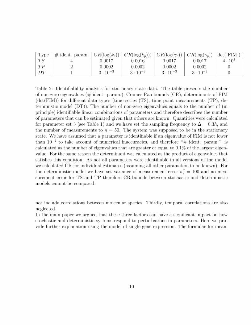
Type # ident. param. CR(log(kr)) CR(log(kp))) CR(log(γr)) CR(log(γp)) det( FIM )TS 4 0.0017 0.0016 0.0017 0.0017 4 · 103

TP 2 0.0002 0.0002 0.0002 0.0002 0DT 1 3 · 10−3 3 · 10−3 3 · 10−3 3 · 10−3 0

Table 2: Identifiability analysis for stationary state data. The table presents the numberof non-zero eigenvalues (# ident. param.), Cramer-Rao bounds (CR), determinants of FIM(det(FIM)) for different data types (time series (TS), time point measurements (TP), de-terministic model (DT)). The number of non-zero eigenvalues equals to the number of (inprinciple) identifiable linear combinations of parameters and therefore describes the numberof parameters that can be estimated given that others are known. Quantities were calculatedfor parameter set 3 (see Table 1) and we have set the sampling frequency to ∆ = 0.3h, andthe number of measurements to n = 50. The system was supposed to be in the stationarystate. We have assumed that a parameter is identifiable if an eigenvalue of FIM is not lowerthan 10−4 to take account of numerical inaccuracies, and therefore “# ident. param.” iscalculated as the number of eigenvalues that are greater or equal to 0.1% of the largest eigen-value. For the same reason the determinant was calculated as the product of eigenvalues thatsatisfies this condition. As not all parameters were identifiable in all versions of the modelwe calculated CR for individual estimates (assuming all other parameters to be known). Forthe deterministic model we have set variance of measurement error σ2

ε = 100 and no mea-surement error for TS and TP therefore CR-bounds between stochastic and deterministicmodels cannot be compared.

not include correlations between molecular species. Thirdly, temporal correlations are alsoneglected.In the main paper we argued that these three factors can have a significant impact on howstochastic and deterministic systems respond to perturbations in parameters. Here we pro-vide further explanation using the model of single gene expression. The formulae for mean,

10

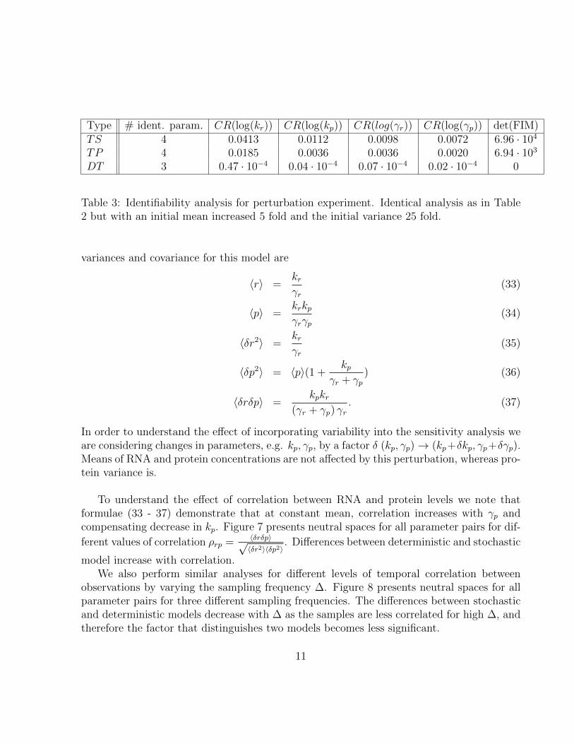
Type # ident. param. CR(log(kr)) CR(log(kp)) CR(log(γr)) CR(log(γp)) det(FIM)TS 4 0.0413 0.0112 0.0098 0.0072 6.96 · 104

TP 4 0.0185 0.0036 0.0036 0.0020 6.94 · 103

DT 3 0.47 · 10−4 0.04 · 10−4 0.07 · 10−4 0.02 · 10−4 0

Table 3: Identifiability analysis for perturbation experiment. Identical analysis as in Table2 but with an initial mean increased 5 fold and the initial variance 25 fold.

variances and covariance for this model are

〈r〉 =krγr

(33)

〈p〉 =krkpγrγp

(34)

〈δr2〉 =krγr

(35)

〈δp2〉 = 〈p〉(1 +kp

γr + γp) (36)

〈δrδp〉 =kpkr

(γr + γp) γr. (37)

In order to understand the effect of incorporating variability into the sensitivity analysis weare considering changes in parameters, e.g. kp, γp, by a factor δ (kp, γp)→ (kp+δkp, γp+δγp).Means of RNA and protein concentrations are not affected by this perturbation, whereas pro-tein variance is.

To understand the effect of correlation between RNA and protein levels we note thatformulae (33 - 37) demonstrate that at constant mean, correlation increases with γp andcompensating decrease in kp. Figure 7 presents neutral spaces for all parameter pairs for dif-

ferent values of correlation ρrp = 〈δrδp〉√〈δr2〉〈δp2〉

. Differences between deterministic and stochastic

model increase with correlation.We also perform similar analyses for different levels of temporal correlation between

observations by varying the sampling frequency ∆. Figure 8 presents neutral spaces for allparameter pairs for three different sampling frequencies. The differences between stochasticand deterministic models decrease with ∆ as the samples are less correlated for high ∆, andtherefore the factor that distinguishes two models becomes less significant.

11

4.2 P53 system

In the study of the 53 system we have used parameter estimates presented in Table 4. Theseparameters has been obtained by appropriate scaling of the parameters given in [8]. For allnumerical experiments for p53 model we assumed sampling frequency ∆ = 1h and numberof measurements n = 30.

Param. Valueβx 90αx 0.002αk 1.7k 0.01βy 1.1α0 0.8αy 0.8

Table 4: Parameters of p53 system.

4.2.1 Sloppiness analysis

Here we compare neutral spaces for all pairs of parameters of the P53 model for treedata types (TS, TP, DT). We use parameter values presented in Table 4 and logarithmicparametrisation. Results are presented in Figues 4, 5 and 6.

4.3 Dependance of analysis on parameter values and qualitativemodel behaviour

Our method allows to study model sensitivity given the parameter values. Here we showthat results depend on parameter values just as the dynamical behaviour of the system does;i.e. the sloppiness of a system also depends on the parameters and is not a fixed propertyof a mathematical model. Figure 9 demonstrates that p53 undergoes a Hopf bifurcation asparameter αy is varied from 0.8 to 2, while all other parameters remain unchanged. Param-eters thus determine the qualitative dynamical behaviour and therefore varying parameters

12

influences the structure of the FIM (compare Figures 4 and 10). Change in the FIM in turnhas consequence for the magnitude of eigenvalues (Figure 9), sensitivity coefficients (compareFigures 4 in MP and 12) and informational content of TS and TP data (Figures 2 and 13).

5 Appendix

5.1 Calculating derivatives of a solution of ODE

In order to derive equations (28) and (30) we differentiated the solution of an ODE withrespect to a parameter. Here we provide more details about this procedure. Suppose thatthe differential equation being considered is

x = F(x,Θ, t),

where x ∈ RN and the set of parameters are collected together into a parameter vectorΘ ∈ RL. Suppose that x(Θ, x0, t) is the solution of interest with an initial condition x0 =

x(Θ, x0, 0). For Y (t) = ∂x(Θ,x0,t)∂θk

it can be shown [9] that

Y = J(t)Y (t) +Kk(t) (38)

where J(t) is the Jacobian of F with respect to x evaluated at x, Kk(t) is the n-dimensionalvector ∂F

∂θkand Y (0) = 0.

5.2 Logarithmic parametrisation

In the analysis of examples presented in our study we used a logarithmic parametrisation.Below we provide a rationale for this and explain that the FIM for logarithmic parametri-sation can be directly obtained from derivatives calculated to obtain the FIM for originalparameters.In biochemical systems, the values of two parameters may differ by orders of magnitudes.Therefore, it is usually not appropriate to consider the absolute changes in the parametersθk, but instead to consider the relative changes. A good way to do this is to introduce newparameters ηk = log(θk), because absolute changes in ηk correspond to relative changes inθk. Then, for small changes δθk to the parameters θk, the changes ηk are scaled and non-dimensional. Analyses in terms of absolute and relative changes are closely related and donot require additional computational cost. For any differentiable function f(θ)

∂f

∂ log(θ)=∂f

∂η= θ

∂f

∂θ. (39)

13

and therefore any element of FIM for η can be easily converted into that for θ or vice versa

I(η)k,l =∂µ

∂ηk

T

Σ(η)∂µ

∂ηl+

1

2trace(Σ−1 ∂Σ

∂ηkΣ−1 ∂Σ

∂ηl)

= θkθl∂µ

∂θk

T

Σ(θ)∂µ

∂θl+ θkθl

1

2trace(Σ−1 ∂Σ

∂θkΣ−1∂Σ

∂θl)

5.3 The FIM as a measure of system’s sensitivity

Here we provide an alternative explanation why the FIM provides a measure of sensitivity fora stochastic system. For notational simplicity we assume that the studied system dependson a single parameter θ as generalisation for multidimensional parameter is straightforward.We start with definitions of classical sensitivity coefficients.

5.3.1 Classical sensitivity coefficient

The classical sensitivity coefficient for observable Q and parameter θ is defined as [10]

S =∂Q

∂θ.

Often sensitivity of relative changes ∆QQ

needs to be considered. Given that ∆ log(Q) ≈ ∆QQ

the formula for sensitivity of relative changes takes the form

S =∂ log(Q)

∂θ.

5.3.2 The FIM as a sensitivity measure for a stochastic system

The behaviour of a stochastic system is not defined by an observable Q that can be measuredexperimentally in a reproducible way. It is instead defined by a distribution form which themeasurements are taken. Suppose we want to construct a measure of a sensitivity of adistribution of a random variable X with density ψ. Assume we want to examine relativechanges of the distribution ψ to changes in θ. This can be written as

ψ(X, θ + ∂θ)− ψ(X, θ)

ψ(X, θ)' log(

ψ(X, θ + ∂θ)

ψ(X, θ)).

Averaging over all possible observations we get∫X

log(ψ(X, θ + ∂θ)

ψ(X, θ))ψ(X, θ)dX.

14

The above is the negative Kullback-Leibler divergence between distributions ψ(X, θ + ∂θ)and ψ(X, θ). In order to study changes in ψ resulting from “small” changes in θ we dividethe above equation by ∂θ and take the limit ∂θ → 0 and get∫

X

∂ log(ψ(X, θ))

∂θψ(X, θ)dX.

The above quantity is the average of the score function and it is basic fact of mathematicalstatistics that it equals to zero [7]. This observation suggests that it is better to study thesquared differences ∫

X

(log(ψ(X, θ)− log(ψ(X, θ + ∂θ))2ψ(X, θ)dX,

that lead to

∫X

(log(ψ(X, θ)− log(ψ(X, θ + ∂θ))2

(∂θ)2ψ(X, θ)dx −−−→

∂θ→0

∫X

(∂

∂θlog

((ψ(X, θ + ∂θ))

ψ(X, θ)

))2

ψ(X, θ)dx,

which is precisely the definition of the FIM.The above derivation suggests that the FIM is a good measure of sensitivity of a proba-bility distribution and that there is a close link between Kulback-Leibler divergence andthe FIM. The KL divergence measures the average relative difference between two distri-butions whereas FIM measures squared relative difference between a distribution and thesame distribution with a perturbed parameter relative to the infinitesimal size of the squaredperturbation.

References

1. N.G. Van Kampen. Stochastic Processes in Physics and Chemistry. North Holland,2006.

2. C. Gardiner. Handbook of stochastic methods. Springer, 1985.

3. J. Elf and M. Ehrenberg. Fast Evaluation of Fluctuations in Biochemical Networks Withthe Linear Noise Approximation. Genome Res., 13(11):2475–2484, 2003.

4. Thomas G. Kurtz. The Relationship between Stochastic and Deterministic Models forChemical Reactions. The Journal of Chemical Physics, 57(7):2976–2978, 1972.

15

5. L. Arnold. Stochastic differential equations: theory and applications. Wiley-Interscience,1974.

6. B. Oksendal. Stochastic differential equations (3rd ed.): an introduction with applica-tions. Springer, 1992.

7. S.D. Silvey. Statistical inference. Chapman & Hall, 1975.

8. N. Geva-Zatorsky, N. Rosenfeld, S. Itzkovitz, R. Milo, A. Sigal, E. Dekel, T. Yarnitzky,Y. Liron, P. Polak, G. Lahav, et al. Oscillations and variability in the p53 system.Molecular Systems Biology, 2(1), 2006.

9. D. Zwillinger. Handbook of Differential Equations. San Diego, 1989.

10. D. A. Rand. Mapping the global sensitivity of cellular network dynamics. Journal ofThe Royal Society Interface, 5:S59, 2008.

16

1 2 3 4 5 6 70

0.1

0.2

0.3

0.4

0.5

0.6

0.7

0.8

0.9

1Eigen values normalized against model maximum

TSTPDT

1 2 3 4 5 6 70

0.1

0.2

0.3

0.4

0.5

0.6

0.7

0.8

0.9

1Eigen values normalized against total maximum

TSTPDT

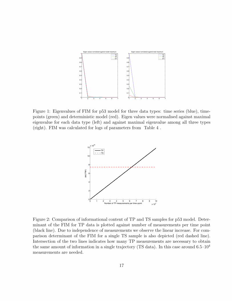
Figure 1: Eigenvalues of FIM for p53 model for three data types: time series (blue), time-points (green) and deterministic model (red). Eigen values were normalised against maximaleigenvalue for each data type (left) and against maximal eigenvalue among all three types(right). FIM was calculated for logs of parameters from Table 4 .

0 1 2 3 4 5 6 7 8 9 10x 104

0

2

4

6

8

10

12x 1023

Number of TP measurements per time point

det(

FIM

)

TPTS

Figure 2: Comparison of informational content of TP and TS samples for p53 model. Deter-minant of the FIM for TP data is plotted against number of measurements per time point(black line). Due to independence of measurements we observe the linear increase. For com-parison determinant of the FIM for a single TS sample is also depicted (red dashed line).Intersection of the two lines indicates how many TP measurements are necessary to obtainthe same amount of information in a single trajectory (TS data). In this case around 6.5 ·104

measurements are needed.

17

12

34

56

7

b_x

a_x

a_k

k

b_y

a_0

a_y

0

0.2

0.4

0.6

0.8

1

eigenvalues

TS

parameters 12

34

56

7

b_x

a_x

a_k

k

b_y

a_0

a_y

0

0.2

0.4

0.6

0.8

1

eigenvalues

TP

parameters

12

34

56

7

b_x

a_x

a_k

k

b_y

a_0

a_y

0

0.2

0.4

0.6

0.8

1

eigenvalues

DT

parameters

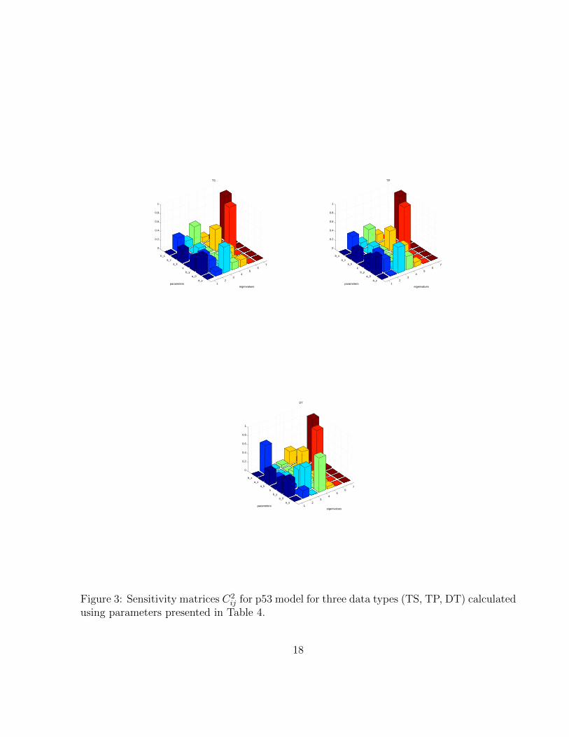
Figure 3: Sensitivity matrices C2ij for p53 model for three data types (TS, TP, DT) calculated

using parameters presented in Table 4.

18

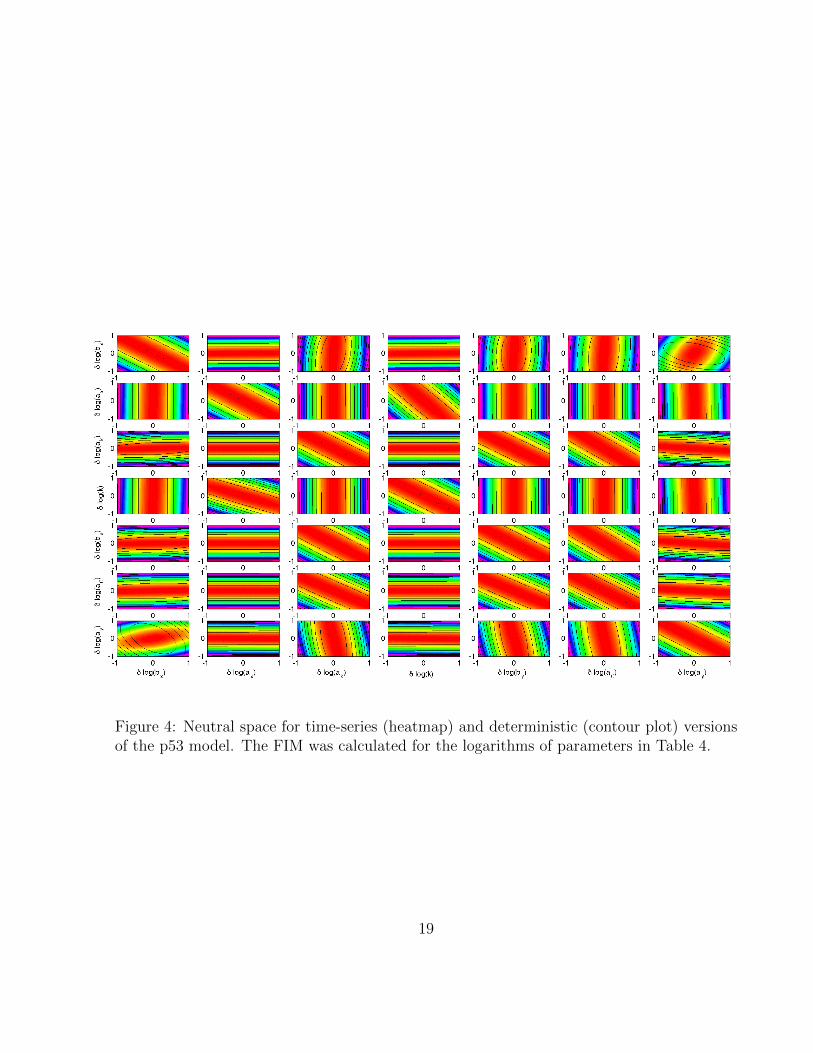
Figure 4: Neutral space for time-series (heatmap) and deterministic (contour plot) versionsof the p53 model. The FIM was calculated for the logarithms of parameters in Table 4.

19

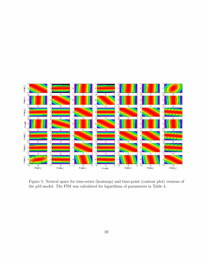
Figure 5: Neutral space for time-series (heatmap) and time-point (contour plot) versions ofthe p53 model. The FIM was calculated for logarithms of parameters in Table 4.

20

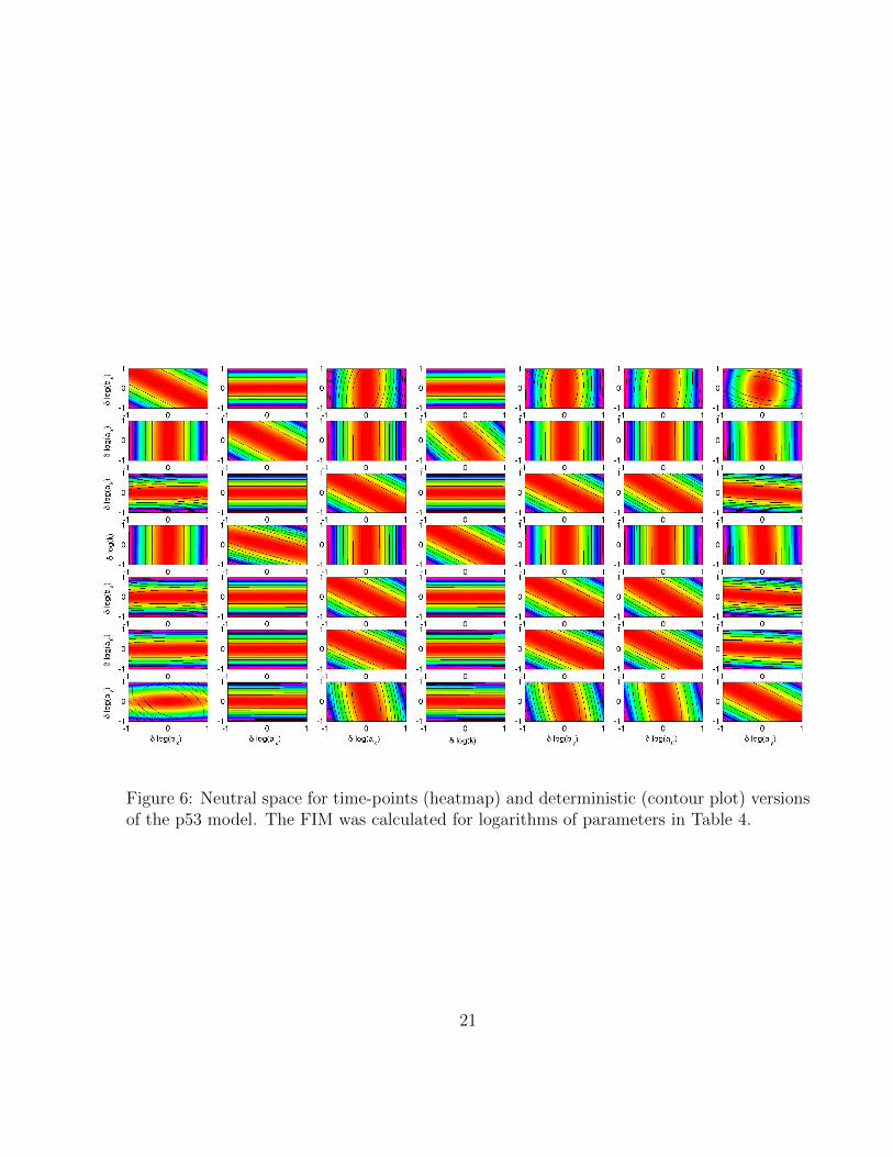
Figure 6: Neutral space for time-points (heatmap) and deterministic (contour plot) versionsof the p53 model. The FIM was calculated for logarithms of parameters in Table 4.

21

log(

p)

0.1 0.05 0 0.05 0.10.1

0.05

0

0.05

0.1

0.1 0.05 0 0.05 0.10.1

0.05

0

0.05

0.1

0.1 0.05 0 0.05 0.10.1

0.05

0

0.05

0.1

0.1 0.05 0 0.05 0.10.1

0.05

0

0.05

0.1

log(

p)

0.1 0.05 0 0.05 0.10.1

0.05

0

0.05

0.1

0.1 0.05 0 0.05 0.10.1

0.05

0

0.05

0.1

0.1 0.05 0 0.05 0.10.1

0.05

0

0.05

0.1

0.1 0.05 0 0.05 0.10.1

0.05

0

0.05

0.1

log(

p)

0.1 0.05 0 0.05 0.10.1

0.05

0

0.05

0.1

0.1 0.05 0 0.05 0.10.1

0.05

0

0.05

0.1

0.1 0.05 0 0.05 0.10.1

0.05

0

0.05

0.1

0.1 0.05 0 0.05 0.10.1

0.05

0

0.05

0.1

log(

p)

log( p)0.1 0.05 0 0.05 0.1

0.1

0.05

0

0.05

0.1

log( p)0.1 0.05 0 0.05 0.1

0.1

0.05

0

0.05

0.1

log( p)0.1 0.05 0 0.05 0.1

0.1

0.05

0

0.05

0.1

correlation=0.1

log( p)

0.1 0.05 0 0.05 0.10.1

0.05

0

0.05

0.1

StochasticDeterministic

log(

p)

0.1 0.05 0 0.05 0.10.1

0.05

0

0.05

0.1

0.1 0.05 0 0.05 0.10.1

0.05

0

0.05

0.1

0.1 0.05 0 0.05 0.10.1

0.05

0

0.05

0.1

0.1 0.05 0 0.05 0.10.1

0.05

0

0.05

0.1

log(

p)

0.1 0.05 0 0.05 0.10.1

0.05

0

0.05

0.1

0.1 0.05 0 0.05 0.10.1

0.05

0

0.05

0.1

0.1 0.05 0 0.05 0.10.1

0.05

0

0.05

0.1

0.1 0.05 0 0.05 0.10.1

0.05

0

0.05

0.1

log(

p)

0.1 0.05 0 0.05 0.10.1

0.05

0

0.05

0.1

0.1 0.05 0 0.05 0.10.1

0.05

0

0.05

0.1

0.1 0.05 0 0.05 0.10.1

0.05

0

0.05

0.1

0.1 0.05 0 0.05 0.10.1

0.05

0

0.05

0.1

log(

p)

log( p)0.1 0.05 0 0.05 0.1

0.1

0.05

0

0.05

0.1

log( p)0.1 0.05 0 0.05 0.1

0.1

0.05

0

0.05

0.1

log( p)0.1 0.05 0 0.05 0.1

0.1

0.05

0

0.05

0.1

correlation=0.5

log( p)

0.1 0.05 0 0.05 0.10.1

0.05

0

0.05

0.1

StochasticDeterministic

log(

p)

0.1 0.05 0 0.05 0.10.1

0.05

0

0.05

0.1

0.1 0.05 0 0.05 0.10.1

0.05

0

0.05

0.1

0.1 0.05 0 0.05 0.10.1

0.05

0

0.05

0.1

0.1 0.05 0 0.05 0.10.1

0.05

0

0.05

0.1

log(

p)

0.1 0.05 0 0.05 0.10.1

0.05

0

0.05

0.1

0.1 0.05 0 0.05 0.10.1

0.05

0

0.05

0.1

0.1 0.05 0 0.05 0.10.1

0.05

0

0.05

0.1

0.1 0.05 0 0.05 0.10.1

0.05

0

0.05

0.1

log(

p)

0.1 0.05 0 0.05 0.10.1

0.05

0

0.05

0.1

0.1 0.05 0 0.05 0.10.1

0.05

0

0.05

0.1

0.1 0.05 0 0.05 0.10.1

0.05

0

0.05

0.1

0.1 0.05 0 0.05 0.10.1

0.05

0

0.05

0.1

log(

p)

log( p)0.1 0.05 0 0.05 0.1

0.1

0.05

0

0.05

0.1

log( p)0.1 0.05 0 0.05 0.1

0.1

0.05

0

0.05

0.1

log( p)0.1 0.05 0 0.05 0.1

0.1

0.05

0

0.05

0.1

correlation=0.9

log( p)

0.1 0.05 0 0.05 0.10.1

0.05

0

0.05

0.1

StochasticDeterministic

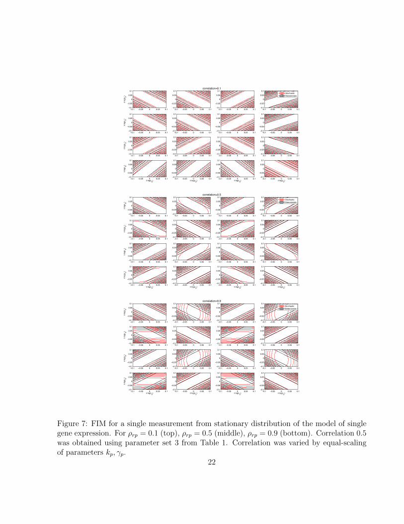
Figure 7: FIM for a single measurement from stationary distribution of the model of singlegene expression. For ρrp = 0.1 (top), ρrp = 0.5 (middle), ρrp = 0.9 (bottom). Correlation 0.5was obtained using parameter set 3 from Table 1. Correlation was varied by equal-scalingof parameters kp, γp.

22

log(

p)

0.1 0.05 0 0.05 0.10.1

0.05

0

0.05

0.1

0.1 0.05 0 0.05 0.10.1

0.05

0

0.05

0.1

0.1 0.05 0 0.05 0.10.1

0.05

0

0.05

0.1

0.1 0.05 0 0.05 0.10.1

0.05

0

0.05

0.1

log(

p)

0.1 0.05 0 0.05 0.10.1

0.05

0

0.05

0.1

0.1 0.05 0 0.05 0.10.1

0.05

0

0.05

0.1

0.1 0.05 0 0.05 0.10.1

0.05

0

0.05

0.1

0.1 0.05 0 0.05 0.10.1

0.05

0

0.05

0.1

log(

p)

0.1 0.05 0 0.05 0.10.1

0.05

0

0.05

0.1

0.1 0.05 0 0.05 0.10.1

0.05

0

0.05

0.1

0.1 0.05 0 0.05 0.10.1

0.05

0

0.05

0.1

0.1 0.05 0 0.05 0.10.1

0.05

0

0.05

0.1

log(

p)

log( p)0.1 0.05 0 0.05 0.1

0.1

0.05

0

0.05

0.1

log( p)0.1 0.05 0 0.05 0.1

0.1

0.05

0

0.05

0.1

log( p)0.1 0.05 0 0.05 0.1

0.1

0.05

0

0.05

0.1

=0.3 correlation=0.5

log( p)

0.1 0.05 0 0.05 0.10.1

0.05

0

0.05

0.1

StochasticDeterministic

log(

p)

0.1 0.05 0 0.05 0.10.1

0.05

0

0.05

0.1

0.1 0.05 0 0.05 0.10.1

0.05

0

0.05

0.1

0.1 0.05 0 0.05 0.10.1

0.05

0

0.05

0.1

0.1 0.05 0 0.05 0.10.1

0.05

0

0.05

0.1

log(

p)

0.1 0.05 0 0.05 0.10.1

0.05

0

0.05

0.1

0.1 0.05 0 0.05 0.10.1

0.05

0

0.05

0.1

0.1 0.05 0 0.05 0.10.1

0.05

0

0.05

0.1

0.1 0.05 0 0.05 0.10.1

0.05

0

0.05

0.1

log(

p)

0.1 0.05 0 0.05 0.10.1

0.05

0

0.05

0.1

0.1 0.05 0 0.05 0.10.1

0.05

0

0.05

0.1

0.1 0.05 0 0.05 0.10.1

0.05

0

0.05

0.1

0.1 0.05 0 0.05 0.10.1

0.05

0

0.05

0.1

log(

p)

log( p)0.1 0.05 0 0.05 0.1

0.1

0.05

0

0.05

0.1

log( p)0.1 0.05 0 0.05 0.1

0.1

0.05

0

0.05

0.1

log( p)0.1 0.05 0 0.05 0.1

0.1

0.05

0

0.05

0.1

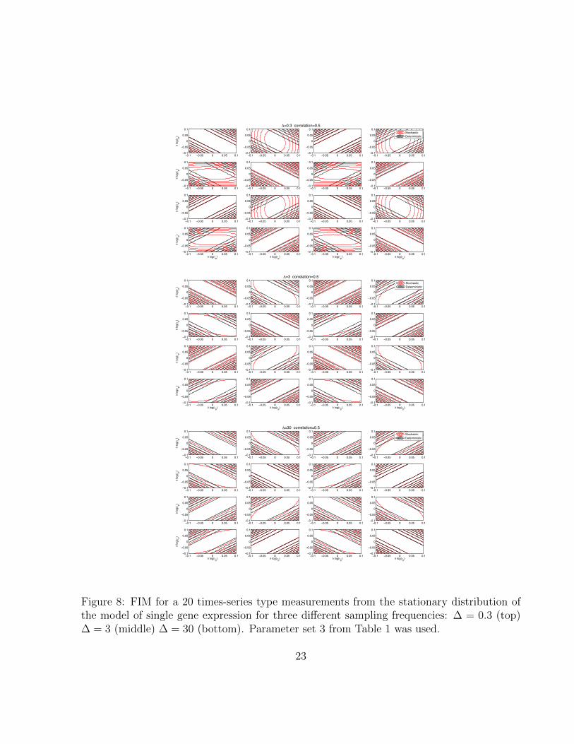
=3 correlation=0.5

log( p)

0.1 0.05 0 0.05 0.10.1

0.05

0

0.05

0.1

StochasticDeterministic

log(

p)

0.1 0.05 0 0.05 0.10.1

0.05

0

0.05

0.1

0.1 0.05 0 0.05 0.10.1

0.05

0

0.05

0.1

0.1 0.05 0 0.05 0.10.1

0.05

0

0.05

0.1

0.1 0.05 0 0.05 0.10.1

0.05

0

0.05

0.1

log(

p)

0.1 0.05 0 0.05 0.10.1

0.05

0

0.05

0.1

0.1 0.05 0 0.05 0.10.1

0.05

0

0.05

0.1

0.1 0.05 0 0.05 0.10.1

0.05

0

0.05

0.1

0.1 0.05 0 0.05 0.10.1

0.05

0

0.05

0.1

log(

p)

0.1 0.05 0 0.05 0.10.1

0.05

0

0.05

0.1

0.1 0.05 0 0.05 0.10.1

0.05

0

0.05

0.1

0.1 0.05 0 0.05 0.10.1

0.05

0

0.05

0.1

0.1 0.05 0 0.05 0.10.1

0.05

0

0.05

0.1

log(

p)

log( p)0.1 0.05 0 0.05 0.1

0.1

0.05

0

0.05

0.1

log( p)0.1 0.05 0 0.05 0.1

0.1

0.05

0

0.05

0.1

log( p)0.1 0.05 0 0.05 0.1

0.1

0.05

0

0.05

0.1

=30 correlation=0.5

log( p)

0.1 0.05 0 0.05 0.10.1

0.05

0

0.05

0.1

StochasticDeterministic

Figure 8: FIM for a 20 times-series type measurements from the stationary distribution ofthe model of single gene expression for three different sampling frequencies: ∆ = 0.3 (top)∆ = 3 (middle) ∆ = 30 (bottom). Parameter set 3 from Table 1 was used.

23

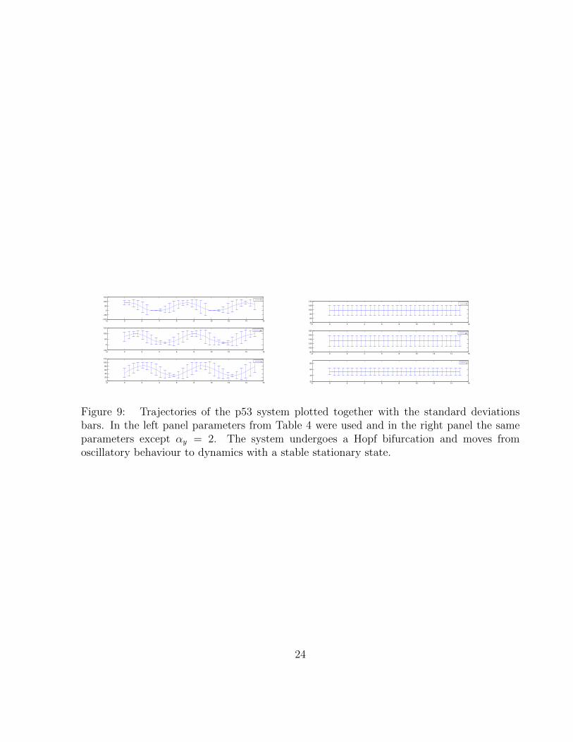
2 0 2 4 6 8 10 12 14 16100

50

0

50

100

150

p

2 0 2 4 6 8 10 12 14 1650

0

50

100

150

y0

2 0 2 4 6 8 10 12 14 160

20

40

60

80

100

120

y

2 0 2 4 6 8 10 12 14 1640

60

80

100

120

140

p

2 0 2 4 6 8 10 12 14 1680

100

120

140

160

180

y0

2 0 2 4 6 8 10 12 14 1620

40

60

80

y

Figure 9: Trajectories of the p53 system plotted together with the standard deviationsbars. In the left panel parameters from Table 4 were used and in the right panel the sameparameters except αy = 2. The system undergoes a Hopf bifurcation and moves fromoscillatory behaviour to dynamics with a stable stationary state.

24

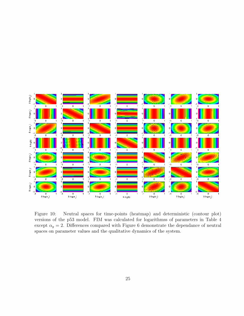
Figure 10: Neutral spaces for time-points (heatmap) and deterministic (contour plot)versions of the p53 model. FIM was calculated for logarithmss of parameters in Table 4except αy = 2. Differences compared with Figure 6 demonstrate the dependance of neutralspaces on parameter values and the qualitative dynamics of the system.

25

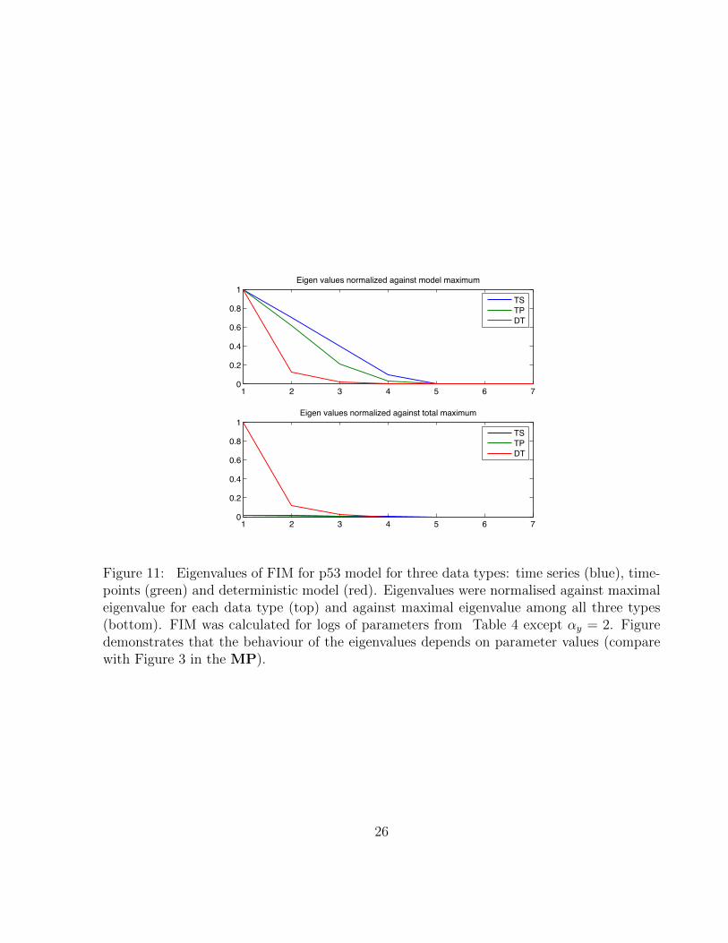
1 2 3 4 5 6 70

0.2

0.4

0.6

0.8

1Eigen values normalized against model maximum

TSTPDT

1 2 3 4 5 6 70

0.2

0.4

0.6

0.8

1Eigen values normalized against total maximum

TSTPDT

Figure 11: Eigenvalues of FIM for p53 model for three data types: time series (blue), time-points (green) and deterministic model (red). Eigenvalues were normalised against maximaleigenvalue for each data type (top) and against maximal eigenvalue among all three types(bottom). FIM was calculated for logs of parameters from Table 4 except αy = 2. Figuredemonstrates that the behaviour of the eigenvalues depends on parameter values (comparewith Figure 3 in the MP).

26

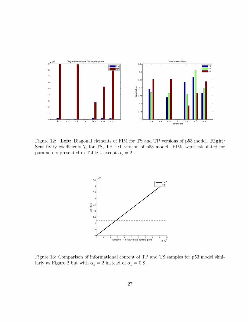
b_x a_x a_k k b_y a_0 a_y0

1

2

3

4

5

6

7

8

9x 104 Diagonal elements of FIM for p53 system

TSTP

b_x a_x a_k k b_y a_0 a_y0

0.05

0.1

0.15

0.2

0.25

0.3

0.35

parameters

sens

itivi

ties

Overall sensitivities

TSTPDT

Figure 12: Left: Diagonal elements of FIM for TS and TP versions of p53 model. Right:Sensitivity coefficients Ti for TS, TP, DT version of p53 model. FIMs were calculated forparameters presented in Table 4 except αy = 2.

0 1 2 3 4 5 6 7 8 9 10x 106

0

0.5

1

1.5

2

2.5

3

3.5

4

4.5x 104

Number of TP measurements per time point

det(

FIM

)

TPTS

Figure 13: Comparison of informational content of TP and TS samples for p53 model simi-larly as Figure 2 but with αy = 2 instead of αy = 0.8.

27