Sensor Data Integrity

Sensor Data Integrity: Final Report ACFR, The University of Sydney Prepared for: Asian Office of Aerospace Research and Development (USA).

Report Documentation Page Form ApprovedOMB No. 0704-0188

Public reporting burden for the collection of information is estimated to average 1 hour per response, including the time for reviewing instructions, searching existing data sources, gathering andmaintaining the data needed, and completing and reviewing the collection of information. Send comments regarding this burden estimate or any other aspect of this collection of information,including suggestions for reducing this burden, to Washington Headquarters Services, Directorate for Information Operations and Reports, 1215 Jefferson Davis Highway, Suite 1204, ArlingtonVA 22202-4302. Respondents should be aware that notwithstanding any other provision of law, no person shall be subject to a penalty for failing to comply with a collection of information if itdoes not display a currently valid OMB control number.

1. REPORT DATE 27 JAN 2009

2. REPORT TYPE Final

3. DATES COVERED 13-05-2008 to 13-10-2008

4. TITLE AND SUBTITLE Sensor Data Integrity

5a. CONTRACT NUMBER FA48690814059

5b. GRANT NUMBER

5c. PROGRAM ELEMENT NUMBER

6. AUTHOR(S) Hugh Durrant-Whyte; Steven Scheding

5d. PROJECT NUMBER

5e. TASK NUMBER

5f. WORK UNIT NUMBER

7. PERFORMING ORGANIZATION NAME(S) AND ADDRESS(ES) University of Sydney,The University of SydneyJ04,Sydney,Australia,NA,NSW 2006

8. PERFORMING ORGANIZATIONREPORT NUMBER N/A

9. SPONSORING/MONITORING AGENCY NAME(S) AND ADDRESS(ES) AOARD, UNIT 45002, APO, AP, 96337-5002

10. SPONSOR/MONITOR’S ACRONYM(S) AOARD

11. SPONSOR/MONITOR’S REPORT NUMBER(S) AOARD-084059

12. DISTRIBUTION/AVAILABILITY STATEMENT Approved for public release; distribution unlimited

13. SUPPLEMENTARY NOTES

14. ABSTRACT This document constitutes the final report for the project ?Sensor Data Integrity? granted by the AsianOffice of Aerospace Research and Development (USA). It describes the data that was collected for thiswork and proposes some preliminary elements of analysis. In particular, the documents enclosed presentA presentation of the UGV System used to collect the data, including all sensors andcalibration parameters A description of the data format and contentA specification of all datasets provided separately A preliminaryanalysis of the performance of sensors depending on the environment conditions and of the search forsensor data integrity, with perspectives of work in this area.

15. SUBJECT TERMS

16. SECURITY CLASSIFICATION OF: 17. LIMITATION OF ABSTRACT Same as

Report (SAR)

18. NUMBEROF PAGES

53

19a. NAME OFRESPONSIBLE PERSON

a. REPORT unclassified

b. ABSTRACT unclassified

c. THIS PAGE unclassified

Standard Form 298 (Rev. 8-98) Prescribed by ANSI Std Z39-18

Sensor Data Integrity

3

Document Control Information

Document Owner: The point of contact for all questions regarding this document is

Project Leader: Dr. Steven Scheding Project Name: Sensor Data Integrity Phone: +61 2 9351 8929 Fax: +61 2 9351 7474 E-mail: [email protected]

Document Creation: This document was created as follows

Creation Date: 2 December 2008 Created By: Dr. Thierry Peynot

Document Identification: This document is identified as

File Name Documents:ACFR:Projects:SensorDataIntegrity:FinalReport:SDIReport.pdf Saved on: 03 December 2008, 11:52:00 Printed on: 10 December 2008, 14:04:00

Distribution Summary: This document is distributed to

Distribution: Brian Skibba Copy-to: At discretion of Brian Skibba

Document Authorization: This revision of the current document is authorized for release in locked PDF form by

Authority Name: Olga Sawtell Signed: ___________________________ Date: ______________

Revision History: The document revision history is listed with the most recent revision first.

Revision Date: Version: Revising Author(s): Section(s) Revised: Page No(s) Revised: Summary of Changes: Reviewed By:

Preface

Document Version Control: It is the Reader’s responsibility to ensure that they have the latest version of this document. All questions should be directed to the Document Owner identified in the previous section of this document.

Privacy Information: This document contains information of a sensitive nature. It should not be transmitted in any form to individuals other than those involved in the project or those under express authorisation by the Project Leader.

Copyright: Copyright © 2008 The University of Sydney, Australia, ABN 15 211 513 464; The University of New South Wales, Australia, ABN 57 195 873 179; University of Technology, Sydney, Australia, ABN 77 257 606 961, (jointly “The Copyright Holder” and “The Universities”).

The copyright of the information herein is the property of The Copyright Holder. The information may be used and/or copied only with the written permission of The Copyright Holders, or in accordance with the terms and conditions stipulated in any contract under which this document has been supplied.

Disclaimer: The Universities make no representation or warranty that these materials, including any software, are free from errors; about the quality or performance of these materials; that these materials are fit for any particular purpose.

These materials are made available on the strict basis that The Universities and their employees or agents have no liability for any direct or indirect loss or damage (including for negligence) suffered by any person as a consequence of the use of this material.

Sensor Data Integrity

5

Executive Summary

This document constitutes the final report for the project “Sensor Data Integrity” granted by the Asian Office of Aerospace Research and Development (USA).

It describes the data that was collected for this work and proposes some preliminary elements of analysis.

In particular, the documents enclosed present:

• A presentation of the UGV System used to collect the data, including all sensors and calibration parameters

• A description of the data format and content

• A specification of all datasets provided separately

• A preliminary analysis of the performance of sensors depending on the environment conditions and of the search for sensor data integrity, with perspectives of work in this area.

Sensor Data Integrity:

Final Report

Thierry Peynot, Sami Terho and Steven SchedingACFR, The University of Sydney

December 2008

Contents

1 Presentation of the System 31.1 The Argo vehicle . . . . . . . . . . . . . . . . . . . . . . . . . . . . . . . . . . 31.2 The Sensors . . . . . . . . . . . . . . . . . . . . . . . . . . . . . . . . . . . . . 4

1.2.1 Laser Range Scanners . . . . . . . . . . . . . . . . . . . . . . . . . . . 41.2.2 FMCW Radar . . . . . . . . . . . . . . . . . . . . . . . . . . . . . . . 51.2.3 Visual Camera . . . . . . . . . . . . . . . . . . . . . . . . . . . . . . . 51.2.4 Infra-Red Camera . . . . . . . . . . . . . . . . . . . . . . . . . . . . . 51.2.5 Calibration parameters . . . . . . . . . . . . . . . . . . . . . . . . . . 61.2.6 Additional Sensors . . . . . . . . . . . . . . . . . . . . . . . . . . . . . 11

2 Data Format and Content 122.1 Files and Directories Organisation . . . . . . . . . . . . . . . . . . . . . . . . 122.2 Ascii Log File Description . . . . . . . . . . . . . . . . . . . . . . . . . . . . . 13

2.2.1 Navigation (Localisation) . . . . . . . . . . . . . . . . . . . . . . . . . 132.2.2 Range Data from Lasers . . . . . . . . . . . . . . . . . . . . . . . . . . 132.2.3 Radar Spectrum . . . . . . . . . . . . . . . . . . . . . . . . . . . . . . 142.2.4 Range Data from Radar (RadarRangeBearing) . . . . . . . . . . . . . 152.2.5 Internal Data . . . . . . . . . . . . . . . . . . . . . . . . . . . . . . . . 162.2.6 Camera Images . . . . . . . . . . . . . . . . . . . . . . . . . . . . . . . 17

3 Data sets 183.1 Environmental conditions . . . . . . . . . . . . . . . . . . . . . . . . . . . . . 18

3.1.1 Dust . . . . . . . . . . . . . . . . . . . . . . . . . . . . . . . . . . . . . 183.1.2 Smoke . . . . . . . . . . . . . . . . . . . . . . . . . . . . . . . . . . . . 193.1.3 Rain in static environment . . . . . . . . . . . . . . . . . . . . . . . . 193.1.4 Rain in dynamic environment . . . . . . . . . . . . . . . . . . . . . . . 19

3.2 Static tests . . . . . . . . . . . . . . . . . . . . . . . . . . . . . . . . . . . . . 193.2.1 Day 1: Afternoon and evening . . . . . . . . . . . . . . . . . . . . . . 193.2.2 Day 2: Morning and midday . . . . . . . . . . . . . . . . . . . . . . . 283.2.3 Day 2: Morning and midday - with added radar reflectors . . . . . . . 313.2.4 Summary of Static Datasets . . . . . . . . . . . . . . . . . . . . . . . . 34

3.3 Dynamic tests . . . . . . . . . . . . . . . . . . . . . . . . . . . . . . . . . . . . 353.3.1 Open area . . . . . . . . . . . . . . . . . . . . . . . . . . . . . . . . . . 353.3.2 Area with houses . . . . . . . . . . . . . . . . . . . . . . . . . . . . . . 393.3.3 Area with trees and water . . . . . . . . . . . . . . . . . . . . . . . . . 393.3.4 Summary of Dynamic Datasets . . . . . . . . . . . . . . . . . . . . . . 46

i

CONTENTS ii

3.4 Calibration Datasets . . . . . . . . . . . . . . . . . . . . . . . . . . . . . . . . 463.4.1 Cameras . . . . . . . . . . . . . . . . . . . . . . . . . . . . . . . . . . . 463.4.2 Range Sensors (Lasers and Radar) . . . . . . . . . . . . . . . . . . . . 47

4 Preliminary Analysis 484.1 Case Study . . . . . . . . . . . . . . . . . . . . . . . . . . . . . . . . . . . . . 484.2 Discussion . . . . . . . . . . . . . . . . . . . . . . . . . . . . . . . . . . . . . . 51

List of Figures

1.1 The Argo Vehicle . . . . . . . . . . . . . . . . . . . . . . . . . . . . . . . . . . 31.2 Argo Sensor Frame . . . . . . . . . . . . . . . . . . . . . . . . . . . . . . . . . 41.3 Sensor, Body and Navigation frames on the Argo . . . . . . . . . . . . . . . . 71.4 Relative locations of sensors . . . . . . . . . . . . . . . . . . . . . . . . . . . . 8

3.1 Static trial setup seen from above . . . . . . . . . . . . . . . . . . . . . . . . . 203.2 Photo of the static trial area (Datasets 01 to 24) . . . . . . . . . . . . . . . . 213.3 Human walking in the test area during a static test (Dataset 03) . . . . . . . 233.4 Static test with light dust (Dataset 04) . . . . . . . . . . . . . . . . . . . . . . 243.5 Static test with smoke(Dataset 07) . . . . . . . . . . . . . . . . . . . . . . . . 263.6 Static test with heavy dust (Dataset 15) . . . . . . . . . . . . . . . . . . . . . 293.7 Static test with smoke (Dataset 17) . . . . . . . . . . . . . . . . . . . . . . . . 303.8 Static test with smoke (Dataset 20) . . . . . . . . . . . . . . . . . . . . . . . . 323.9 Static test area with radar reflectors (Datasets 22 & 23) . . . . . . . . . . . . 333.10 Aerial image of the open area (on the left side of the path) and the houses area

(on the right side of the path) . . . . . . . . . . . . . . . . . . . . . . . . . . . 363.11 Photo of the open area (Datasets 25 to 32) . . . . . . . . . . . . . . . . . . . 363.12 Dynamic test in the open area with dust (Datasets 30 & 31) . . . . . . . . . . 373.13 Dynamic test around the houses (Datasets 33 & 34) . . . . . . . . . . . . . . 403.14 Photo of the area with trees and a lake (Datasets 35 to 40) . . . . . . . . . . 413.15 Dynamic test around the lake with dust (Datasets 36 to 37) . . . . . . . . . . 433.16 Dynamic test around the lake with smoke (Dataset 38) . . . . . . . . . . . . . 443.17 Dynamic test around the lake with simulated rain (Dataset 39) . . . . . . . . 45

4.1 Range returned by the laser for static test in clear conditions . . . . . . . . . 494.2 Range returned by radar for static test in clear conditions . . . . . . . . . . . 494.3 Range returned by laser for static test with heavy dust . . . . . . . . . . . . . 504.4 Range returned by radar for static test with smoke . . . . . . . . . . . . . . . 504.5 Range returned by laser and radar, for static test with rain . . . . . . . . . . 514.6 Filtering dust in laser data . . . . . . . . . . . . . . . . . . . . . . . . . . . . 52

1

Introduction

This project presents the first step towards developing and understanding integrity in percep-tual systems for UGVs (Unmanned Ground Vehicles). Important issues addressed include;

• When do perceptual sensors fail, and why?

• What combination of sensors would be appropriate for a given operational scenario?

• Can perceptual sensor failure be reliably detected and mitigated?

Failure is a very broad term; it is hoped that through this work a UGV systems designer willhave a better understanding of exactly what constitutes perceptual failure, how it may bedesigned for and its effects remediated. Such failures would not just include hardware failure,but also adverse environmental conditions (such as dust or rain), and algorithm failure.

To begin to address these issues, synchronised data have been gathered from a representa-tive UGV platform using a wide variety of sensing modalities. These modalities were chosento sample as much of the electromagnetic spectrum as possible, with the limitation that thesensors be feasible (and available) for use on UGVs. A preliminary analysis has then beenperformed on the data to ascertain the prime areas of competence of the sensors, and thecombination of sensors most promising for a set of representative UGV scenarios.

Further work (not contained in this document) would develop the theoretical frameworkfor sensor data-fusion and on-line integrity monitoring for use in UGV perceptual systems. Inparticular, the latter would provide an on-line “quality” evaluation of the environment per-ception and/or the environment modeling based on that perception [6], with sensor/modelingfault detection and isolation [5, 4]. This would constitute a susbtantial benefit for UGVnavigation efficiency, robustness and safety.

This document is structured as follows: the first chapter presents the system used togather the data, in particular the sensors involved (and their characteristics). The secondchapter presents the datasets collected, listing the kind of environment, the conditions andthe relevant information to be able to exploit the data. Finally, the third chapter gives apreliminary analysis of sensor data integrity, based on the gathered data.

2

Chapter 1

Presentation of the System

This chapter presents the system used to collect the data. It is composed of a ground vehiclecalled the Argo, equipped with various sensors.

1.1 The Argo vehicle

The vehicle used to collect the data, the CAS1 Outdoor Research Demonstrator (CORD), isan 8 wheel skid-steering vehicle with no suspension (see figure 1.1), which turns thanks topressure controlled brakes on both sides. It has a petrol engine, with a 12V alternator, anda 24V alternator to provide power to the computers and sensors on board.

Figure 1.1: The Argo Vehicle

For the purpose of this work, it has been equipped with multiple sensors, described in thefollowing section.

1CAS stands for Centre for Autonomous Systems

3

CHAPTER 1. PRESENTATION OF THE SYSTEM 4

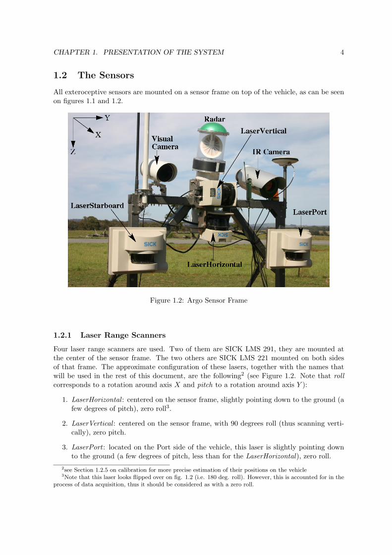
1.2 The Sensors

All exteroceptive sensors are mounted on a sensor frame on top of the vehicle, as can be seenon figures 1.1 and 1.2.

Figure 1.2: Argo Sensor Frame

1.2.1 Laser Range Scanners

Four laser range scanners are used. Two of them are SICK LMS 291, they are mounted atthe center of the sensor frame. The two others are SICK LMS 221 mounted on both sidesof that frame. The approximate configuration of these lasers, together with the names thatwill be used in the rest of this document, are the following2 (see Figure 1.2. Note that rollcorresponds to a rotation around axis X and pitch to a rotation around axis Y ):

1. LaserHorizontal : centered on the sensor frame, slightly pointing down to the ground (afew degrees of pitch), zero roll3.

2. LaserVertical : centered on the sensor frame, with 90 degrees roll (thus scanning verti-cally), zero pitch.

3. LaserPort : located on the Port side of the vehicle, this laser is slightly pointing downto the ground (a few degrees of pitch, less than for the LaserHorizontal), zero roll.

2see Section 1.2.5 on calibration for more precise estimation of their positions on the vehicle3Note that this laser looks flipped over on fig. 1.2 (i.e. 180 deg. roll). However, this is accounted for in the

process of data acquisition, thus it should be considered as with a zero roll.


4. LaserStarboard : located on the Starboard side of the vehicle, this laser is intended tohave zero pitch and zero roll.

Characteristics and Nominal Performances

All four lasers were set to acquire data in the following mode:

• 0.25 degree resolution

• cm accuracy4

• 180 degree angular range5

1.2.2 FMCW Radar

This is a 94GHz Frequency Modulated Continuous Wave (FMCW) Radar (custom built atACFR for environment imaging). Maximum rotation of scan head: 360 degrees at approxi-mately 8Hz, 1KHz sample rate.

• Range resolution: 0.2m.

• Maximum range: 40m.

1.2.3 Visual Camera

The Visual camera (as opposed to the Infra-Red Camera) is a Prosilica Mono-CCD megapixelGigabit Ethernet camera, pointing down (a few degrees of pitch).


• Image Pixel Dimensions: 1360× 1024

• Resolution: 72× 72 ppi (pixels per inch)

• RGB Colour, depth: 8 bits

• Nominal Framerate: 15 images per second in static6 datasets, 10 images per second indynamic datasets (unless specified differently).

1.2.4 Infra-Red Camera

Raytheon Thermal-eye 2000B. The images are acquired through a frame grabber providingdigital images of size 640× 480 pixels.

4except for the cameras to lasers calibration dataset, where the mm accuracy mode was used for moreprecision, but limiting the maximum range to 8m and the angular range to 100 degrees.

5except for the cameras to lasers calibration dataset, for which a 100 degree angular range was used.6see section 3.2



• Image Pixel Dimensions of complete image: 640× 480. In practice, though, the imagesare usually clipped to 511 × 398 to remove useless black bands on the sides. Actualsensor size: 320× 240.

• Average Framerate: 12.5 images per second (unless specified differently).

• Spectral response range: 7− 14µm.

1.2.5 Calibration parameters

The spatial transformations between sensors and reference frames have been estimated usingthorough calibration methods. The frames used are illustrated on Figure 1.3. They arenamed:

• Navigation frame: (fixed) global frame defined by the three axis: Xn = North, Y n =East and Zn = Down in which positions are expressed in UTM coordinates (UniversalTransverse Mercator).

• Body frame: frame linked to the body of the vehicle, its centre being located at thecentre of the IMU (Inertial Measurement Unit), approximately at the centre of thevehicle. The axis are: Xb pointing towards the from of the vehicle, Y b pointing to theStarboard side of the vehicle, and Zb pointing down.

• Sensor frame: frame linked to a particular sensor. It is defined in a similar way asthe previous one (i.e. Xs forward, Y s starboard, Zs down), but centered on the sensorconsidered.

Note that in the rest of the document Navigation (or localisation) will correspond to theglobal positioning of the Body frame in the Navigation frame.

The measured distances between sensors are illustrated in figure 1.4. Note that an actualprocess of calibration usually provides better estimations of the real transformations betweensensors. However these measured values are good initial estimates for calibration processes(and they were actually used as such in this work).

Two categories of calibration have been made:

• Range Sensor Calibration, to estimate the transformations between the frame associatedto each range sensor (laser scanner or radar) and the Body frame.

• Camera Calibration, to estimate the intrinsic (geometric) parameters of each camera,and the extrinsic transformations between cameras and lasers.

Range Sensor Calibration

The estimation of the transformations between the frame associated to each range sensor(laser scanner or radar) and the Body frame was made using a technique detailed in [1, 8].For that purpose, a dataset was acquired in an open area with flat ground and key geometric


Figure 1.3: Sensor, Body and Navigation frames on the Argo

features such as a vertical metallic wall, two vertical poles with high reflectivity for lasers,and two vertical poles for the radar (see section 3.4.2).

The results of this calibration are the estimation of the 3 rotation angles (RollX, PitchYand Y awZ) and 3 translation offsets (dX, dY , dZ) from the Body frame to the Sensor frame.All angles will be expressed here in degrees for convenience and distances in metres.

The following table shows the results obtained after combined calibration of all four rangesensors, i.e. LaserHorizontal (or LaserH ), LaserVertical (or LaserV ), LaserPort (or LaserP),LaserStarboard (or LaserS ) and the Radar. Common features are used for all sensors. It isrecommended to use these calibration results when combining the information from groupsof these sensors.

Transformations Body Frame to Sensor Frame:Sensor RollX PitchY YawZ dX dY dZLaserH -0.732828 -8.586863 -1.631319 0.108987 0.008302 -0.919726LaserV 88.562966 -0.118007 -1.123153 -0.000291 -0.082272 -1.126802LaserP -0.500234 -2.616210 -1.805911 0.190857 -0.548777 -0.763776LaserS -0.608178 -0.431051 -2.349991 0.198663 0.534253 -0.849538Radar -0.151571 191.161703 173.278081 -0.025753 -0.047174 -1.399104

Visual Camera Calibration

Intrinsic parameters The intrinsic calibration of each camera was made using the CameraCalibration Toolbox for Matlab [2].


Figure 1.4: Distances between sensors in the (y, z) plane, in cm. Note that the dashedlines are meant to go through the centre of the sensors (despite any other impression due toperspective of the original picture).


The following is the content of the Calib Results.m file exported by the toolbox, thatdescribes the output of the calibration process in Matlab language:

%-- Focal length:fc = [1023.094873083798120; 1020.891695892045050];%-- Principal point:cc = [643.139025535655492; 482.455417980580421];%-- Skew coefficient:alpha c = 0.000000000000000;%-- Distortion coefficients:kc = [−0.218504818968279; 0.138951469767851;

−0.000755791245166; 0.000175881419552; 0.000000000000000];%-- Focal length uncertainty:fc error = [1.240637187529808; 1.220702756108720];%-- Principal point uncertainty:cc error = [1.338561085455541; 1.362301725972313];%-- Skew coefficient uncertainty:alpha c error = 0.000000000000000;%-- Distortion coefficients uncertainty:kc error = [0.001808042132202; 0.003689996468947;

0.000207366100112; 0.000221355286767; 0.000000000000000];%-- Image size:nx = 1360;ny = 1024;

The reader is invited to consult the toolbox web site [2] for more details on these parameters.These output files from the calibration toolbox are included in the datasets.Note that of the 93 images selected for the calibration process, 74 were actually used

in the final optimisation process (see the file Calib Results.m for details). The pixel errorobtained for this calibration is:

Pixel error: err = [ 0.19209 0.20252 ]

Extrinsic parameters (position of camera with respect to lasers) The extrinsictransformations between each camera and each laser was made using a method adapted from[7]. It uses the ouput of the Matlab Camera Calibration Toolbox to estimate the positionsand orientations of the planes corresponding to the checker board visible in the images.These positions are compared with the positions of the laser points hitting this board. Anoptimisation process gives an estimation of the position of the laser range scanner with respectto the camera.

The following gives the three translations (δXc, δYc and δZc) and three rotations (φXc,φYc and φZc) enabling the placement of a point with original coordinates in the cameraframe (using the convention used for the Matlab Toolbox: +Xc to the right, +Yc down, +Zc

forward) into the sensor frame linked to each laser. Distances are expressed in metres andangles in degrees.

LaserHorizontal to Visual camera:δXc δYc δZc φXc φYc φZc

0.4139 -0.2976 -0.0099 -4.7341 -0.3780 -0.4230


LaserVertical to Visual camera:7δXc δYc δZc φXc φYc φZc

0.5045 -0.0905 -0.208 -13.2030 -0.5851 -0.3140

LaserPort to Visual camera:δXc δYc δZc φXc φYc φZc

0.9592 -0.5011 -0.0867 -10.6026 -0.0747 -0.5791

LaserStarboard to Visual camera:δXc δYc δZc φXc φYc φZc

-0.1343 -0.4976 -0.0532 -12.6652 0.2409 -0.5293

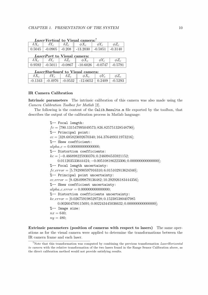
IR Camera Calibration

Intrinsic parameters The intrinsic calibration of this camera was also made using theCamera Calibration Toolbox for Matlab [2].

The following is the content of the Calib Results.m file exported by the toolbox, thatdescribes the output of the calibration process in Matlab language:

%-- Focal length:fc = [790.131547995049573; 826.825751328548790];%-- Principal point:cc = [328.685823692670340; 164.376489311973216];%-- Skew coefficient:alpha c = 0.000000000000000;%-- Distortion coefficients:kc = [−0.466898225930376; 0.246094535921152;

0.011203533644424;−0.005108186223306; 0.000000000000000];%-- Focal length uncertainty:fc error = [5.782890597916310; 6.015102913624340];%-- Principal point uncertainty:cc error = [9.426499879136482; 10.292926183444356];%-- Skew coefficient uncertainty:alpha c error = 0.000000000000000;%-- Distortion coefficients uncertainty:kc error = [0.026759198529728; 0.152385380407985

0.002604709115691; 0.002243445036632; 0.000000000000000];%-- Image size:nx = 640;ny = 480;

Extrinsic parameters (position of cameras with respect to lasers) The same oper-ations as for the visual camera were applied to determine the transformations between theIR camera frame and each laser.

7Note that this transformation was computed by combining the previous transformation LaserHorizontalto camera with the relative transformation of the two lasers found in the Range Sensor Calibration above, asthe direct calibration method would not provide satisfying results.


LaserHorizontal to IR camera:δXc δYc δZc φXc φYc φZc

-0.3391 -0.3278 0.0975 -6.5307 -1.2671 -2.1308

LaserVertical to IR camera:8δXc δYc δZc φXc φYc φZc

-0.2485 -0.1207 -0.0115 -14.9996 -1.4742 -2.0218

LaserPort to IR camera:δXc δYc δZc φXc φYc φZc

0.2090 -0.5400 0.0194 -12.7686 -1.0343 -2.3348

LaserStarboard to IR camera:δXc δYc δZc φXc φYc φZc

-0.8772 -0.5652 0.0584 -15.7179 -0.8259 -3.3619

Note that the images and correspondings laser scans which were used for this calibrationare available in the directory named IRcameraCalibration (see section 3.4.1). The imagesin this dataset are full resolution 640 × 480 as provided by the frame grabber, unlike theIR images in the other datasets which are clipped to keep only the part containing actualinformation.

1.2.6 Additional Sensors

Other sensors available on the Argo platform that will provide useful information are:

• Novatel SPAN System (Synchronized Position Attitude & Navigation) with a Honey-well IMU (Inertial Measurement Unit). This usually provides a 2cm RTK solution forlocalisation,

• Wheel encoders, measuring wheel angular velocities,

• Brakes sensors (position and pressure),

• Engine and gearbox rotation rate sensors.

8Note that this transformation was computed by combining the previous transformation LaserHorizontalto camera with the relative transformation of the two lasers found in the Range Sensor Calibration above.

Chapter 2

Data Format and Content

This chapter presents the format of the data provided. Section 2.1 describes the organisationof directories and files. Section 2.2 then precisely defines the format of the content of eachfile containing data. Note that in the rest of the document the Typewriter font will be usedto designate names of directories or files and text written in ascii files.

2.1 Files and Directories Organisation

Each dataset has its directory containing all data from all sensors. It usually corresponds toa particular test (specific environment and conditions). Its name is composed of a number(corresponding to the chronological order of the data acquisition) and a string roughly de-scribing the environment and conditions1. An example is: 04-StaticLightDust for a static2

test in the presence of light dust.A dataset directory usually contains eleven sub-directories corresponding to the differents

sensors involved (or type of data, see section 1.2); namely:

• LaserHorizontal

• LaserPort

• LaserStarboard

• LaserVertical

• Nav

• Payload

• RadarRangeBearing

• RadarSpectrum

• VideoIR

• VideoVisual1a much more complete description is provided into each directory though2See the more precise definition of static and dynamic test in chapter 3.

12

CHAPTER 2. DATA FORMAT AND CONTENT 13

2.2 Ascii Log File Description

This section describes the content of the ascii files that can be found in each of the directoriesmentioned above.

Note that in all logged ascii files, the default units will be metres for all distances andradians for all angles (except for the Radar Spectrum data). Consequently, anywhere units arenot clearly specified, metres and radians prevail. All files start with a time stamp, expressedin seconds, which corresponds to the Unix time.

Files contain one data sample (complete) message per line. The first columns of all asciifile have the general form:

*<timestamp> TEXT TYPE data

where TEXT TYPE is a string describing the type of data written on this line (e.g. NAV DATAfor navigation data) and data is the actual data from the sensor, written on as many columnsas needed.

More specifically, the next sections describe the actual content of each type of file for eachtype of sensor or data. They will first indicate the name of the directory where the data canbe found and then illustrate the content by a table.

2.2.1 Navigation (Localisation)

Name of directory: Nav.The ascii data are contained in a file named NavQAsciiData.txt. The content of each lineof this file is described in the following table. It corresponds to the global localisation of thevehicle (Body frame) expressed using the UTM coordinate system, in metres and radians.

Column: 1 2 3 4 5 6 7 8Data : *<timestamp> NAV DATA North East Down dNorth dEast dDownColumn: 9 10 11 12 13 14 15-158Data: RollX PitchY YawZ dRoll dPitch dYaw Ci,j

where Ci,j , (i, j) ∈ [[1, 12]]2 are the elements of the covariance matrix describing the co-variances between the 12 elements appearing in columns 3 to 14. Note that this matrix iswritten in rows: the whole row number 1 first, then row 2 etc. . . In other words, it is writtenas: C1,1, C1,2 . . . , C1,12, C2,1, C2,2 . . . C12,12.

2.2.2 Range Data from Lasers

This concerns the directories of the four lasers, namely:

• LaserHorizontal

• LaserVertical

• LaserPort

• LaserStarboard


In each of these directories, the ascii data are contained in a file named RangeBearingQAsciiData.txt.The content of each line of this file is described in the following table. Each line of the filetypically shows the result of a 2D scan of 180 degrees with an increment of 1 degree. The firstpart of the line gives parameters describing this scan and the second part gives the actualrange values returned by the laser sensor. 4 successive scans (i.e. 4 lines in the file), withstarting angles each time incremented by 0.25 degree, will finally provide a full 180 degreewide and 0.25 degree resolution scan.

Column: 1 2 3 4Data : *<timestamp> RANGE DATA StartAngleRads AngleIncrementRads

Column: 5 6 7 8− end

Data : EndAngleRads RangeUnitType NScans Rangei

where:

• StartAngleRads (double) is the value in radians of the first angle of the current scan(i.e. the one described on the current line of the file).

• AngleIncrementRads (double) is the difference of angle between two successive scanvalues (namely Rangei and Rangei+1), in radians.

• EndAngleRads (double) is the value in radians of the last angle of the current scan (i.e.the current line).

• RangeUnitType is an integer showing the unit for the range values that follow in theline (Rangei). The possible integers and their meanings are as follow:

– 1: mm

– 2: cm

– 3: m

– 4: km

• NScans is the number N of scan values. Note that: end = 8 + (NScans− 1)

• Rangei with i ∈ [[1, N ]] are the actual range values for each angle of the current scan(the unit being determined by RangeUnitTypeEnum).

2.2.3 Radar Spectrum

The directory: RadarSpectrum contains the radar spectrum, described as the bins of a FastFourier Transform (FFT). The ascii data are contained in a file named HSR ScalarPoints1.txt.The content of each line of this file is described in the following table:

Col.: 1 2 3 to endData: *<timestamp> Angle(degrees) Reflectivityi

where:

• Angle is the angle, in degrees, of the bins of this line.


• Reflectivityi with i ∈ [[1, N ]] (N being the total number of bins on the line) are thereflectivity of each bin. Each of these bins correspond to a different range, with can bedetermined using the following.

First, note the following parameters, obtained after intrinsic calibration of the radar scanner:

• the Sample Frequency is sampleFreq = 1250000Hz.

• the frequency per metre is: hertzPerM = 4336.384Hz/m.

• the range offset is: offsetM = −0.3507m.

This means that the range associated to a particular bin (namely binRange) can be found bycalculating:

frequencyHzPerBin = sampleFreq/(2 ∗ numberOfBins)rangeMPerBin = frequencyHzPerBin/hertzPerMbinRange = bin× rangeMPerBin + offsetM

(2.1)

where bin represents the bin number (i.e. column number in the file - 2, starting with 1) andbinRange is the range associated to this particular bin.

2.2.4 Range Data from Radar (RadarRangeBearing)

This concerns the directory named RadarRangeBearing. It contains range information fromthe radar, which is estimated from the spectrum. The ascii data are contained in a file namedRangeBearingQAsciiData.txt. Its format is very similar to the laser files seen above, onlywith reflectivity information in addition to the range information. The content of each lineof the file is described in the following table:

Col.: 1 2 3 4Data: *<timestamp> RANGE REFLECTIVITY DATA StartAngleRads AngleIncrRads

Col.: 5 6 7 8Data: EndAngleRads RangeUnitType NScans=1 Range1

Col.: 9Data: Reflectivity1

where:

• StartAngleRads (double) is the value in radians of the first angle of the current scan(i.e. the one described on this line of the file).

• AngleIncrRads (double) is the difference of angle (increment) between two successivescan values. AngleIncrRads = 0 in this file, as there is only one range value per line.

• EndAngleRads (double) is the value in radians of the last angle of the current line. Inpractice, in this file, EndAngleRads = AngleIncrRads.

• RangeUnitType is an integer showing the unit for the range values that follow in theline. The possible integers and their meanings are as follow:

– 1: mm


– 2: cm

– 3: m

– 4: km

• NScans is the number of scan values. Here NScans=1 (one range value per line only).

• Range1 is the actual range value for the current angle of the current scan (the unit beingdetermined by the value of RangeUnitTypeEnum).

• Reflectivity1 is the reflectivity of this current bin.

The range and reflectivity information contained in this file are extracted from the FFT(see section 2.2.3) by searching for the peak of highest reflectivity. The corresponding rangethat can be calculated by direct application of equation (2.1) is limited to the resolutionof the discrete FFT: 0.28m. Thus, to obtain a higher accuracy, a quadratic interpolation isperformed on the peak processed from the signal: the interpolated range is the range obtainedfor the maximum point of the quadratic polynomial that is fitted to the three points of theFFT spectrum defining the peak (see [3] for more details).

2.2.5 Internal Data

Name of directory: Payload.This concerns internal data from the vehicule, such as status of braking, wheel velocityetc. . . Note that this category of data is only relevant for the dynamic tests (moving vehi-cle). Thus they shall be found only in the directories of this category of datasets. The asciidata are contained in a file named PayloadData1.txt. The regular format of each line ofthis file is still:

*<timestamp> TEXT TYPE data

with TEXT TYPE having various possible values. These values and the corresponding line for-mat and content of data are described in the table below. Note that, as previously, the firstline of this table shows the column number.

1 2 3 4*<timestamp> SERVO SETPOINT DATA chokePosition throttlePosition*<timestamp> VELOCITY TURN RATE DATA velocity turnRate*<timestamp> SENSOR DATA sensor value

1 2 3 4*<timestamp> BRAKE DATA leftBrakePosition rightBrakePosition

5 6leftBrakePressure rightBrakePressure

1 2 3 4*<timestamp> ACTUATOR SETPOINT DATA desiredChoke desiredThrottle

5 6desiredLeftBrake desiredRightBrake

When TEXT TYPE = SENSOR DATA, sensor is an integer referring to a particular internal sen-sor. The possibilities and the corresponding meaning for value are illustrated in the following


table:

sensor value (unit)0 Engine Rotation Rate (RPM)1 Gearbox Rotation Rate (RPM)2 12V Battery Voltage (V)3 24V Battery Voltage (V)4 Left Wheel Angular Velocity (rad/s)5 Right Wheel Angular Velocity (rad/s)

Note that these data are provided for information, but a model of the vehicle would beneeded to actually make the BRAKE DATA, ACTUATOR SETPOINT DATA and the RPM informationreally useful for the reader. It is recommended to contact the authors in that case.

2.2.6 Camera Images

Two directories concern camera images: one for the Infra-Red Camera (VideoIR) and onefor the Visual Camera (VideoVisual). Both contain the same kind of data:

• One ascii file named VideoLogAscii.txt, with the following format:

Column: 1 2 3Data: *<timestamp> VISION FRAME <filename>

• One directory Images containing all the bmp images (as files) provided by the camera.Those files have the names described in the VideoLogAscii.txt file. Note that thisname is formed by the prefix ’Image’ followed by a timestamp (where the ’.’ betweenseconds and fractions of seconds has been replaced by a ’-’), plus the extension ’.bmp’.

Chapter 3

Data sets

There are two types of datasets. In the static ones the vehicle is stationary and the sensorsacquire data always from the same area. The area contains: features with known character-istics and dimensions inside an identified frame, and objects and equipment used for creatingthe environmental conditions (e.g. a compressor and a water pump), outside of the frame.In the dynamic datasets the vehicle moves around the test area, which usually contains thesame equipment as mentioned before, plus a car (from which the UGV was operated).

The purpose of the static datasets was to acquire data in different conditions but with thesame features, to enable a comparison of the effects of different environmental conditions.

Note that static or dynamic will refer to the state of the vehicle, not the status of theenvironment, which can be considered as static except if the presence of a moving elementsuch as a human is present.

The beginning and ending times of the datasets are expressed in three formats. The firstcolumn shows the Unix time, that is, seconds after midnight UTC of January 1, 1970. Theleap seconds are not counted in this convention. The second column shows the UTC time.UTC stands for Universal Timing Convention, and is equivalent to the Greenwich MeridianTime (GMT). The third column shows the local AEDT time in the test site. AEDT standsfor: Australian Eastern Daylight Saving Time.

As the data acquisition was made with several (synchronised) computers, sensor datalogging does not necessarily start at the exact same time for all sensors. Thus, for convenience,the Start and End time correspond respectively to the earliest and the latest time of thedataset when all data from all sensors are available.

The next section describes each type of conditions that appear in the datasets.

3.1 Environmental conditions

The simulated environmental conditions include dusty environment, smoke, rain, and clearenvironment without any adverse environmental conditions.

3.1.1 Dust

The dust was generated by blowing air to dusty soil. The blower was a high-power aircompressor with a flexible tube for directing the air. Some of the datasets were gatheredin areas where the soil was naturally very dusty. In these cases the dust was generated by

18

CHAPTER 3. DATA SETS 19

blowing the air to the ground near the vehicle. In the other cases the dusty soil was collectedand piled near the actual test site, and the air was blown to the pile to generate a cloud ofdust.

3.1.2 Smoke

Orange smoke was generated with smoke bombs that worked for about one minute. Thebomb was held by an assistant, choosing their position so that the wind carried the smoketowards the vehicle. Sometimes the direction of the wind varied, so the assistant would moveto compensate.

3.1.3 Rain in static environment

In the static tests the rain was generated with sprinklers attached to the top of a framedefining the test area (see figure 3.2). This frame covered an area being 9.3 meters long and4.3 meters wide. The water was stored in a tank equipped with a pump to bring the waterto the sprinkler system. This device is visible on the right side of the frame and the vehicle.

3.1.4 Rain in dynamic environment

In the dynamic tests the rain was generated with the same tank as in the static tests, butinstead of sprinklers, the rain was simulated by spraying the water with a hand-held hosepointed at the vehicle’s working area.

3.2 Static tests

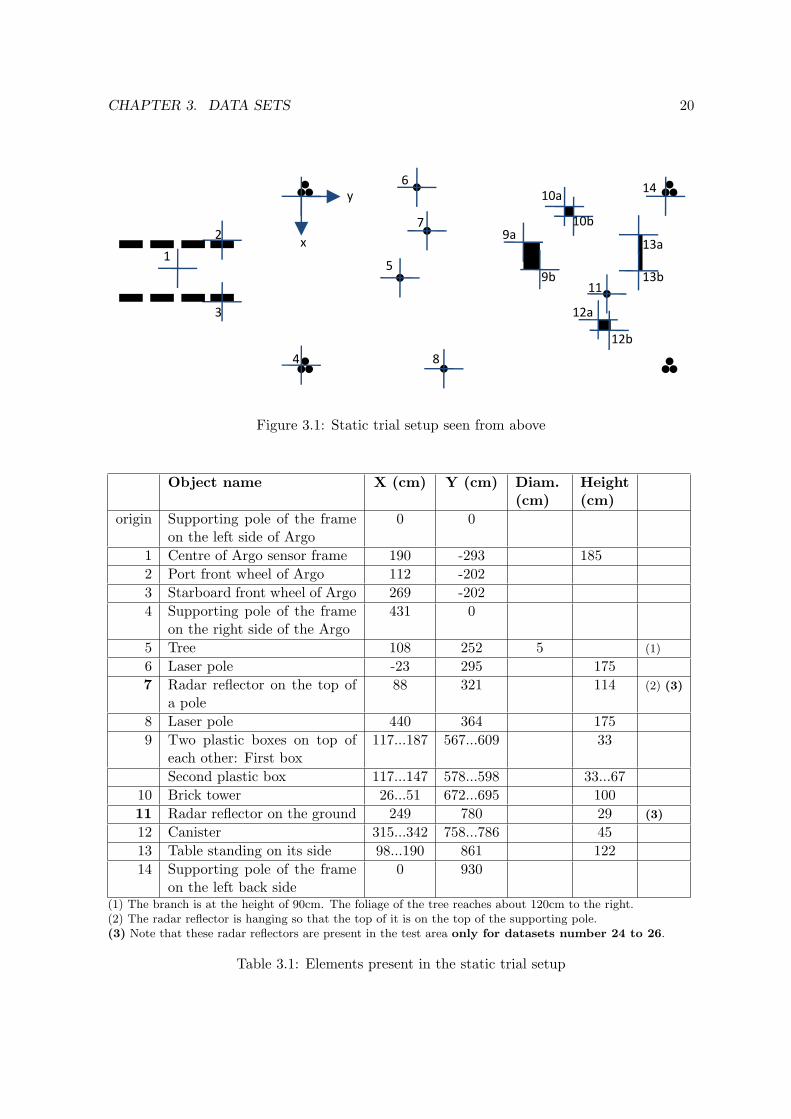
In the static tests the vehicle was standing still and imaging an area with known features,inside the sprinkler frame used for generating the rain. These objects were generally chosento be easily detected by the sensors in clear conditions. Most of them are artificial and ofsimple geometry (e.g. box or pole) and their dimensions are provided: figure 3.1 shows adrawing of this area with location of the features. However, a branch of tree (attached to ametal bar stuck into the ground) was also set in the test area to have a natural feature. Theelements of figure 3.1 are also listed in the table 3.1 for more details. The positions of thesefeatures were chosen so that every sensor (in particular the 2D laser scanners) can see at leastsome of them and the objects are distributed over the area.

The framerate of the visual camera in this series of tests was 15 frames per second, exceptin the first dataset where the framerate was 10 frames per second.

The vehicle was facing south. Therefore the sun was either behind or on the side of thevehicle. As the data sets were collected in Australia, sun shines from the north in the middleof the day. Note that in this section, features mentioned will be located with respect to thevehicle, i.e. left will refer to the Port side if the Argo, while right will refer to its Starboardside.

3.2.1 Day 1: Afternoon and evening

The first set of static trials data was acquired on the 15th of October 2008, in the afternoon andin the evening. Most of the datasets were acquired when the sun was above the horizon, exceptfor one, acquired just after sunset. The wind was quite strong, and it affected significantly


Object name X (cm) Y (cm) Diameter (cm) Height (cm) CommentsoriginSupporting pole of the frame on the left side of

Argo0 0

1Port pole of Argo sensor frame ? ‐293

2Port front wheel of Argo 112 2022Port front wheel of Argo 112 ‐202

3Starboard front wheel of Argo 169 ‐202

4Supporting pole of the frame on the right side of the Argo

431 0

5Tree 108 252 5 The branch is at the height of 90cm. The leafage of the tree reaches about 120cm to the right.

6Laser pole ‐23 295 175

7Radar reflector on the top of a pole 88 321 114 The radar reflector is hanging so that the top of it is on the top of the supporting pole

10Brick tower 26 … 51 672 … 695 100

9Two plastic boxes on top of each other 117 … 187 567 … 609 33

The other plastic box 117 … 147 578 … 598 33 … 67

8Laser pole 440 364 175

12Canister 315 342 758 786 45

6

12Canister 315 … 342 758 … 786 45

11Radar reflector on the ground 249 780 29

13Table standing on its side 98 … 190 861 122

14Supporting pole of the frame on the left back side 0 930

x

y

2

5

6

9a

10a

10b

13a

14

7

1

3

4 8

9b 13b

12a

12b

11

Figure 3.1: Static trial setup seen from above

Object name X (cm) Y (cm) Diam.(cm)

Height(cm)

origin Supporting pole of the frameon the left side of Argo

0 0

1 Centre of Argo sensor frame 190 -293 1852 Port front wheel of Argo 112 -2023 Starboard front wheel of Argo 269 -2024 Supporting pole of the frame

on the right side of the Argo431 0

5 Tree 108 252 5 (1)

6 Laser pole -23 295 1757 Radar reflector on the top of

a pole88 321 114 (2) (3)

8 Laser pole 440 364 1759 Two plastic boxes on top of

each other: First box117...187 567...609 33

Second plastic box 117...147 578...598 33...6710 Brick tower 26...51 672...695 10011 Radar reflector on the ground 249 780 29 (3)

12 Canister 315...342 758...786 4513 Table standing on its side 98...190 861 12214 Supporting pole of the frame

on the left back side0 930

(1) The branch is at the height of 90cm. The foliage of the tree reaches about 120cm to the right.(2) The radar reflector is hanging so that the top of it is on the top of the supporting pole.(3) Note that these radar reflectors are present in the test area only for datasets number 24 to 26.

Table 3.1: Elements present in the static trial setup


Figure 3.2: Photo of the static trial area (Datasets 01 to 24)


dust and smoke spreading. The wind was mainly blowing from the left with respect to thevehicle.

01-02 - Clear conditions

The first two datasets were acquired in clear conditions, without any artificially created dust,smoke or rain. In the first dataset the frame rate of the color camera was 10 frames persecond, and in the second one the frame rate was 15 frames per second.

Dataset name: 01-StaticClear-Video10fpsUnix UTC AEDT

Start 1224050945.437 06:09:05.437 15:09:05.437End 1224051090.447 06:11:30.447 15:11:30.447Duration 145.010 seconds

Dataset name: 02-StaticClear-Video15fpsUnix UTC AEDT


03 - Clear conditions with human

This dataset was acquired in clear conditions. A human (intentionally) is walking throughthe area.

Dataset name: 03-StaticClear-HumanUnix UTC AEDT


04 - Light dust

In this dataset, an assistant blew dust from a pile that was located on the left, out of the testarea. The dust was carried by wind from left to right with respect to the sensors. The dustcloud mainly occurred between the sensors and the test area. The dust density was relativelylow. The dataset started and ended in clear conditions.

Dataset name: 04-StaticLightDustUnix UTC AEDT



Figure 3.3: Human walking in the test area during a static test (Dataset 03)


Figure 3.4: Static test with light dust (Dataset 04)


05 - Heavy dust

As previously, in this dataset an assistant blew dust from a pile that was located on the left,out of the test area. The dust was carried by the wind from left to right with respect to thesensors, and it moved between the sensors and the test area. The dust cloud was denser thanbefore. The dataset started and ended in clear conditions.Note that the lasers and radar data start 14 to 18 seconds later than the other sensors.

Dataset name: 05-StaticHeavyDustUnix UTC AEDT


06 - Light dust with human

As in the two previous cases, an assistant blew dust from a pile that was located on the leftof the test area. The dust was carried by wind from left to right. The dust cloud mainlyoccurred between the sensors and the test area. The dust density was relatively low. A humanwas walking around the test area. The dataset started and ended in clear conditions.

Dataset name: 06-StaticLightDust-HumanUnix UTC AEDT


07 - Smoke

An assistant held a smoke bomb in the left of the test area. The smoke moved almost entirelybetween the sensors and the test area. The dataset started and ended in clear conditions.

Dataset name: 07-StaticSmokeUnix UTC AEDT


08 - Heavy rain

The sprinklers were used to create heavy rain. Wind from the left biased the rain towardsthe right, and therefore the left part of the test area had less rain than the right part. Rainwas present during the whole dataset.

Dataset name: 08-StaticHeavyRainUnix UTC AEDT



Figure 3.5: Static test with smoke(Dataset 07)


09 - Heavy rain with human

As before, the sprinklers were used to create heavy rain. A human was walking around thetest area. Wind from the left biased the rain towards right again. Rain was present duringthe whole dataset.

Dataset name: 09-StaticHeavyRain-HumanUnix UTC AEDT


10 - Light rain

The sprinklers were used to create lighter rain. As in the previous cases, wind from the leftbiased the rain towards right with respect to the sensors. The rain was created during thewhole dataset.

Dataset name: 10-StaticLightRainUnix UTC AEDT


11 - Clear conditions after rain

This dataset was acquired right after the rain datasets, with the sprinklers turned off. Conse-quently, all the objects in the test area were wet, and a few drops of water were occasionallystill falling from the top of the frame. The sun was very low but still above the horizon duringthe acquisition of this dataset.

Dataset name: 11-StaticAfterRainEveningUnix UTC AEDT


12 - Clear conditions after rain and sunset

This dataset was acquired just after sunset. There is still reasonable light, but the sun isalready below the horizon. This dataset was acquired shortly after the rain datasets as well,so all the objects in the test area were still wet, with also the possibility of having a few dropsof water still falling. Note that the lasers data logs stop about 88 seconds before the rest ofthe data.

Dataset name: 12-StaticClearAfterRainAfterSunsetUnix UTC AEDT



3.2.2 Day 2: Morning and midday

The second set of static trials was realized on the 16th of October 2008, starting in themorning and lasting until midday. In all of the datasets sun was high in the sky. There wasmuch less wind than during the first day, and its direction varied.

14 - Clear

This dataset was acquired in clear conditions, without any artificially created dust, smoke orrain.

Dataset name: 14-StaticMorningClearUnix UTC AEDT


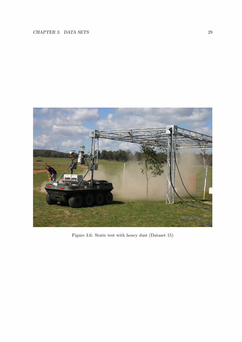
15 - Heavy dust

An assistant blew dust from a pile that was located west of the test area. The dust wascarried by wind from left to right with respect to the sensors. The dust cloud moved a bitto south-east, and therefore the north-eastern corner of the area was not completely coveredwith dust. The dust density was high. The dataset started and ended in clear conditions.The Figure 3.6 shows the dust cloud.

Dataset name: 15-StaticMorningHeavyDustUnix UTC AEDT


16 - Very light dust

An assistant blew dust from a dusty road west of the test area. Part of the dust was carriedby wind from left to right with respect to the sensors. The dust cloud was very thin when itreached the test area. The dataset started and ended in clear conditions.

Dataset name: 16-StaticMorningVeryLightDustUnix UTC AEDT


17 - Smoke

An assistant held a smoke bomb that generated smoke to the test area. The wind was veryweak, but strong enough to carry the smoke towards the test area. The direction of the windchanged during the test. The assistant was first standing at the left side of the test area, then


Figure 3.6: Static test with heavy dust (Dataset 15)


Figure 3.7: Static test with smoke (Dataset 17)

he moved to the back of it and finally to the right side. The assistant was always standingoutside of the test area. The dataset started and ended in clear conditions with no smoke.

Dataset name: 17-StaticMorningSmokeUnix UTC AEDT


18 - Light rain

The sprinklers were used to create light rain. The weak wind did not affect much the directionof the rain. Note that the area closer to the sensors did not get as much rain as the areafurther away. Besides, the rain was not completely uniform in the area, due to a leak in thefront.

Dataset name: 18-StaticMorningLightRainUnix UTC AEDT



19 - Rain

The sprinklers were used to create heavier rain. The weak wind did not affect much thedirection of the rain.

Dataset name: 19-StaticMorningRainUnix UTC AEDT


20 - Smoke

An assistant held a smoke bomb that generated smoke to the test area. In this test thedirection of the wind did not change much. The assistant was mainly standing at the back-right corner of the test area. The assistant’s arm may have entered the test area in thebeginning. The dataset started and ended in clear conditions with no smoke. As this datasetwas acquired after the rain, all the objects were wet.

Dataset name: 20-StaticMorningSmokeUnix UTC AEDT


21 - Clear conditions after rain and smoke

This dataset was acquired after the smoke and rain datasets. All the objects in the test areawere wet, and there might be some residue from the smoke.

Dataset name: 21-StaticMorningClearAfterRainAndSmokeUnix UTC AEDT


3.2.3 Day 2: Morning and midday - with added radar reflectors

The second part of the second day’s tests was done in the same area, but with two additionalfeatures in the area: radar reflectors. Also their positions are marked in the figure 3.1. Thefigure 3.9 shows the test area with the radar reflectors.

22 - Clear

The reflectors are still in the test area. The dataset was acquired in clear conditions.


Figure 3.8: Static test with smoke (Dataset 20)


Figure 3.9: Static test area with radar reflectors (Datasets 22 & 23)


Dataset name: 22-StaticMorningClearWithReflectorsUnix UTC AEDT


23 - Clear, human walking

In this dataset the human was walking around the test area. The human did not interactespecially with the radar reflectors but walked past them.

Dataset name: 23-StaticMorningClearWithReflectors-HumanUnix UTC AEDT


24 - Clear, human walking near reflectors

In this dataset the human was also walking around the test area. Unlike for the previousdataset, the walking pattern was related to the radar reflectors. The human walked near theradar reflectors, first behind the reflector, then between the reflector and the sensors, andfinally, on the side of the reflector. This was repeated for both reflectors.

Dataset name: 24-StaticMorningClearWithReflectors-HumanNearReflectorsUnix UTC AEDT


3.2.4 Summary of Static Datasets

The following table summarizes the conditions for each of these datasets taken with staticvehicle.


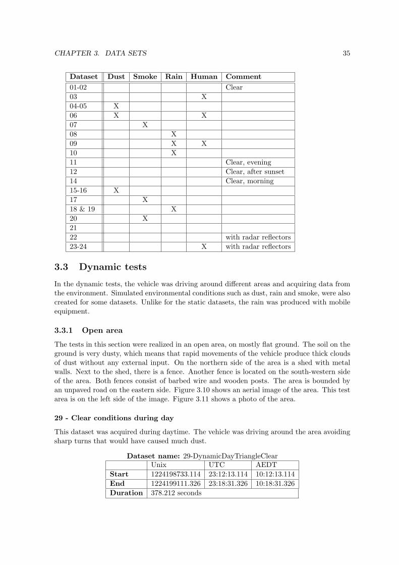
Dataset Dust Smoke Rain Human Comment01-02 Clear03 X04-05 X06 X X07 X08 X09 X X10 X11 Clear, evening12 Clear, after sunset14 Clear, morning15-16 X17 X18 & 19 X20 X2122 with radar reflectors23-24 X with radar reflectors

3.3 Dynamic tests

In the dynamic tests, the vehicle was driving around different areas and acquiring data fromthe environment. Simulated environmental conditions such as dust, rain and smoke, were alsocreated for some datasets. Unlike for the static datasets, the rain was produced with mobileequipment.

3.3.1 Open area

The tests in this section were realized in an open area, on mostly flat ground. The soil on theground is very dusty, which means that rapid movements of the vehicle produce thick cloudsof dust without any external input. On the northern side of the area is a shed with metalwalls. Next to the shed, there is a fence. Another fence is located on the south-western sideof the area. Both fences consist of barbed wire and wooden posts. The area is bounded byan unpaved road on the eastern side. Figure 3.10 shows an aerial image of the area. This testarea is on the left side of the image. Figure 3.11 shows a photo of the area.

29 - Clear conditions during day

This dataset was acquired during daytime. The vehicle was driving around the area avoidingsharp turns that would have caused much dust.

Dataset name: 29-DynamicDayTriangleClearUnix UTC AEDT



Figure 3.10: Aerial image of the open area (on the left side of the path) and the houses area(on the right side of the path)

Figure 3.11: Photo of the open area (Datasets 25 to 32)


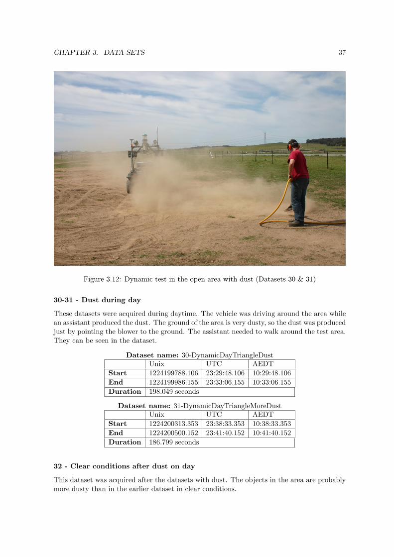
Figure 3.12: Dynamic test in the open area with dust (Datasets 30 & 31)

30-31 - Dust during day

These datasets were acquired during daytime. The vehicle was driving around the area whilean assistant produced the dust. The ground of the area is very dusty, so the dust was producedjust by pointing the blower to the ground. The assistant needed to walk around the test area.They can be seen in the dataset.

Dataset name: 30-DynamicDayTriangleDustUnix UTC AEDT


Dataset name: 31-DynamicDayTriangleMoreDustUnix UTC AEDT


32 - Clear conditions after dust on day

This dataset was acquired after the datasets with dust. The objects in the area are probablymore dusty than in the earlier dataset in clear conditions.


Dataset name: 32-DynamicDayTriangleClearAfterDustUnix UTC AEDT


25-27 - Clear conditions at night with external lights on

These datasets were acquired at nighttime. The sun had set completely, so all the light wasartificially created. A car was parked in the test area. The headlights of the car were on andpointing towards the area where the test vehicle moved. The vehicle’s own headlights alsoilluminated the area in front of it. Note that in dataset 27 the door of the shed was openwith the internal light of the building on. This can be seen in the images of the camera.

Dataset name: 25-DynamicNightClearTriangleWithCarLightsUnix UTC AEDT


Dataset name: 27-DynamicNightClearTriangleWithCarLights2Unix UTC AEDT


26-28 - Clear conditions at night without external lights

These datasets were acquired at nighttime, the only artificial light coming from the vehicle’sown headlights.

Dataset name: 26-DynamicNightClearTriangleNoCarLightsUnix UTC AEDT


Dataset name: 28-DynamicNightClearTriangleNoCarLights2Unix UTC AEDT


Summary

The following table summarizes the conditions for each of these datasets taken in the openarea.


Dataset Dust Daytime Night w.Ext. Light

Night noExt. Light

Comment

29 X Clear30-31 X X32 X After dust25 & 27 X Ext. car lights26 & 28 X

3.3.2 Area with houses

This is an area with three wooden buildings. A long building is standing in the southern sideof the area. Two smaller ones are on the northern side. The area is bounded by a fence. Thisarea can be seen on the right side of the aerial image in figure 3.10.

33 - Clear conditions without humans

This dataset was acquired in the daytime. The vehicle was driving around the area withhouses (see figure 3.13).

Dataset name: 33-DynamicDayHousesClearUnix UTC AEDT


34 - Clear conditions, human walking around

This dataset was acquired at daytime. The vehicle was driving around the same area asbefore and in similar conditions. However, in addition to the previous dataset, a human waswalking around during the test.

Dataset name: 34-DynamicDayHouses-HumanUnix UTC AEDT


3.3.3 Area with trees and water

This is an area next to a lake. On the southern side of the area there is a small eucalyptusforest. A photo of the area is shown in figure 3.14.

35 - Clear conditions

This dataset was acquired at daytime. The vehicle was driving around the area.


Figure 3.13: Dynamic test around the houses (Datasets 33 & 34)


Figure 3.14: Photo of the area with trees and a lake (Datasets 35 to 40)


Dataset name: 35-DynamicDayDamClearUnix UTC AEDT


36-37 - Dust

These datasets were acquired during daytime. An assistant produced the dust by pointingthe blower to the ground. It was not as dusty as in the open area, and therefore there wasless dust in this area. The assistant had to move a little in order to create the dust in frontof the vehicle. The figure 3.15 shows a photo of the actual situation.

Dataset name: 36-DynamicDayDamDustUnix UTC AEDT


Dataset name: 37-DynamicDayDamDust2Unix UTC AEDT


38 - Smoke

This dataset was acquired during daytime. An assistant held a smoke bomb. He tried tostay in a position where the smoke went towards the vehicle, therefore they needed to movea little. The figure 3.16 shows a photo of the situation. The photo was taken by the assistantholding the smoke bomb.

Dataset name: 38-DynamicDayDamSmokeUnix UTC AEDT


39 - Rain

This dataset was acquired at daytime. An assistant created a “water curtain” in front of thevehicle with a hose spraying water. Again, the assistant needed to move in order to keep thewater in front of the vehicle. The figure 3.17 shows a photo of the situation.

Dataset name: 39-DynamicDayDamRainUnix UTC AEDT



Figure 3.15: Dynamic test around the lake with dust (Datasets 36 to 37)


Figure 3.16: Dynamic test around the lake with smoke (Dataset 38)


Figure 3.17: Dynamic test around the lake with simulated rain (Dataset 39)

40 - Clear, sun low in the sky

The dataset was acquired in the evening, just before the sunset. In this dataset there wereno artificially created environmental conditions and no people moving.

Dataset name: 40-DynamicDayDamClear-SunLowUnix UTC AEDT


Summary

The following table summarizes the conditions for each of these datasets taken in this areawith trees and lake.

Dataset Dust Smoke Rain Comment35 Clear36-37 X38 X39 X40 Sun low


3.3.4 Summary of Dynamic Datasets

The following table shows a summary of all conditions covered in all dynamic datasets. Itdoes not precise the area in which the dataset was taken though, this precision can be founddirectly in the appropriate section. The default configuration is at daytime (i.e. the Nightis only precised where appropriate).

Dataset Dust Smoke Rain Human Night Comment25 to 28 X Clear, at night29 & 32 Clear30 & 31 X33 Clear, Houses area34 X Houses area35 Clear36 & 37 X38 X39 X40 Clear

3.4 Calibration Datasets

3.4.1 Cameras

The data used to realize the calibrations concerning the Visual camera and the IR camera canbe found respectively in the directories VisualCameraCalibration and IRcameraCalibration,which are both organised as follow. They contain the following directories:

• LaserHorizontal

• LaserPort

• LaserStarboard

• LaserVertical

• VideoVisual or VideoIR as appropriate

which content is as described for the previous datasets (see section 2.2).In an additional directory, named Calibration, the following files and directories can be

found:

• Calib Results.m and Calib Results.mat are the files exported by the Matlab Cali-bration Toolbox, contains all the calibration parameters estimated.

• Images is a directory containing the images that were used for the camera calibrationprocess, named with successive numbers starting by 1, for convenience when loadingthem in Matlab.

• matlabAsciiLaserData is a directory containing the ascii descriptions of all laser datain files formatted to be suitable for Matlab, for convenience.


• VideoLogAsciiCalibration.txt is a text file figuring the timestamps for all images inImages, the number of line in this file corresponding to the number of the image as it isnamed in Images (e.g. the timestamp corresponding to the image named image002.bmpcan be found at the line number 2 of VideoLogAsciiCalibration.txt).

The images in these datasets show a chess board exposed with various orientations inspace, and at various distances. Note that these chess boards are different for the Visualcamera and the IR camera. The size of the Black and White squares of these chess board arethe following:

• for the IR camera: 114.8mm on both sides.

• for the Visual camera: 74.9mm on the axis left-right as it can be seen in the imagesand 74.7mm on the axis corresponding to the direction up-down.

3.4.2 Range Sensors (Lasers and Radar)

The data used for the range sensors calibration can be found in the directory named:

RangeSensorsCalibration

It is organized exactly as the regular datasets that were presented before (except that itdoes not contain the directories RadarSpectrum and Payload). Data from all sensors werecollected in the so-called open area, with four vertical poles standing on a flat ground. Thesespecial features of known geometry as well as the vertical wall of the shed and the flat partof the ground were used to extract relevant data for the calibration process.

Chapter 4

Preliminary Analysis

This chapter proposes in its first section a preliminary analysis of the performance of thesensors considered in this work. It will focus, as an illustrative example, on the case of thepresence of dust or smoke. In the second section, we propose some ideas to tackle the issueof challenging environments when using sensors for obstacle detection or terrain modeling.

4.1 Case Study

Lasers are extremely affected by dust and smoke. More precisely, a cloud of dust or smoke isalmost seen as an actual obstacle. Thus, a basic analysis of the data provided by them mightlead to false detection of large obstacles. This is all the more true as the SICK lasers onlyprovide the information concerning the first return 1.

The radar operates at mm wavelengths, which makes the size of dust and smoke particlesrelatively much smaller, giving radar waves more penetration. Consequently, it is much lessaffected by dust or smoke, except for a slight increase of the level of noise in the data, andlower reflectivities for the returns. The following figures illustrate that statement.

Figure 4.1 and 4.2 show all the range values returned by the LaserHorizontal and theradar respectively, for a static test in clear conditions (dataset 02). All scans made duringthe complete duration of the dataset collection are drawn in these figures. The angle rangecorresponds to what is perceived in the test area: the first and last notable feature on theleft and right of the graph are respectively the left and right poles of the trial frame (objectsnamed origin and 1 in the table in section 3.2). Note that the laser, providing much moreprecise (raw) range measurements than the radar, detects all the objects that are located inits field of view, while the radar detects only the main ones and provides noiser data.

Figure 4.3 shows the same measurements from the laser and radar in the presence ofdust (dataset 05). We can see that dust generates random points in the laser scans, locatedbetween the vehicle and the actual position of the obstacle.

Figure 4.4 shows that the results are similar in the presence of smoke: the laser sees it asan obstacle whereas the radar data are not significantly affected.

On figure 4.5 we can have a preliminary view of the effect of rain. The laser data areactually not particularly affected, except for a few specific points, which might be due toreflection effects on wet objects surfaces. This case warrants further investigation.

1some other lasers also provide information about a possible additional return. This might at least lead tosome suspicion on the features perceived with a significant difference between these two returns.

48

CHAPTER 4. PRELIMINARY ANALYSIS 49

(a) Dots display (b) Lines display

Figure 4.1: Range returned by LaserHorizontal over angle, for static test in clear conditions(Dataset 02); displayed in dots in (a) and lines in (b)

(a) Dots display (b) Lines display

Figure 4.2: Range returned by the radar (RadarRangeBearing) over angle, for static test inclear conditions (Dataset 02); displayed in dots in (a) and lines in (b)


(a) LaserHorizontal (b) Radar

Figure 4.3: Range returned by the laserHorizontal and the radar (RadarRangeBearing) overangle, for static test with heavy dust (Dataset 05).


Figure 4.4: Range returned by the laserHorizontal and the radar over angle, for static testwith smoke (Dataset 07).



Figure 4.5: Range returned by the laserHorizontal and the radar over angle, for static testwith rain (Dataset 08). The Laser data is here drawn with lines for an easier identification ofthe special reflection effects due to the presence of water on the objects (compare with figure4.1 (b)).

Note that besides the lasers, both visual and thermal camera images are affected by dust(and smoke), but the effect is lower on the infra-red data, as infra-red waves have a higherpenetration power.

4.2 Discussion

To avoid the problem of false obstacles created by conditions such as presence of dust or smoke,and increase the integrity of sensor data in general, one can benefit from the redundancy ofsensors on a vehicle. This redundancy can be of different kinds. Let us consider a particularset of sensors.

• if these sensors are identical, i.e. they measure the same data (e.g. range) using thesame process and the same physical characteristics (e.g. several 2D Sick Lasers), whentheir measurements overlap they may be directly compared to detect major failuresonly, such as a breakdown.

• if the sensors measure the same type of data (e.g. range), but in a different way (e.g. alaser scanner and a radar scanner, operating at different wavelengths), the comparisonof their measurements may provide valuable information about the environment, to takean appropriate decision and be able to keep sensing abilities in an environment whichis challenging for one type of sensor. For example: the radar waves penetrate dust andsmoke much more easily than the laser ones, thus we know that in the presence of dustthe radar will provide more accurate range measurement (it is the opposite in clearconditions).

• if the sensors measure different kinds of data (e.g a laser scanner and a colour camera),a comparison might still be made at a higher level of abstraction, for example afterclassification of pieces of the terrain in classes such as obstacles or flat terrain.


An example of the second case mentioned above is a preliminary study realized by JamesUnderwood at ACFR to filter dust in range measurements provided by a laser and a radar.By comparing these measurements of the same area, knowing a model of the uncertaintiesinvolved, it is possible to identify when the error between data from these two sensors is toohigh, which means that the data should not be validated. In this study, as only two sensors areused, it is not possible to determine which one is wrong. Consequently, the only reasonabledecision is to ignore both types of data (see figure 4.6). If an additional sensor, with differentcharacteristics, is available, a more “informative” decision can be made if, for example, datafrom two sensors match while data from the third one shows a level of discrepancy.

(a) Raw Laser Data (b) Filtered Laser Data

Figure 4.6: 3D points returned by a Laser Range Scanner during a dynamic test in presenceof dust: before (a) and after (b) filtering. The green object visible in both images is a staticcar.

Acknowledgment

The authors of this document would like to thank Craig Rodgers, Marc Calleja, James Un-derwood, Andrew Hill and Tom Allen for their valuable contribution to this work.

Bibliography

[1] A. Alempijevic, S.R. Kodagoda, J.P. Underwood, S. Kumar, and G. Dissanayake. Mutualinformation based sensor registration and calibration. In Procedings of the 2006 IEEE/RSJInt. Conf. on Intelligent Robots and Systems, 2006.

[2] Jean-Yves Bouguet. Camera Calibration Toolbox for Matlab.http://www.vision.caltech.edu/bouguetj/calib doc/.

[3] Ross Hennessy. A generic architecture for scanning range sensors. Master’s thesis, TheUniversity of Sydney, 2005.

[4] Andrea Monteriu, Prateek Asthan, Kimon Valavanis, and Sauro Longhi. Model-basedsensor fault detection and isolation system for unmanned ground vehicles: Experimentalvalidation (part ii). In 2007 IEEE International Conference on Robotics and Automation,2007.

[5] Andrea Monteriu, Prateek Asthan, Kimon Valavanis, and Sauro Longhi. Model-basedsensor fault detection and isolation system for unmanned ground vehicles: Theoreticalaspects (part i). In 2007 IEEE International Conference on Robotics and Automation,2007.

[6] T. Peynot and S. Lacroix. Selection and monitoring of navigation modes for an au-tonomous rover. In 10th International Symposium on Experimental Robotics 2006 (ISER’06), 2006.

[7] Robert Pless and Qilong Zhang. Extrinsic calibration of a camera and laser range finder.Technical report, Washington University in St. Louis, 2003.

[8] James Underwood, Andrew Hill, and Steven Scheding. Calibration of range sensor poseon mobile platforms. In Procedings of the 2007 IEEE/RSJ Int. Conf. on Intelligent Robotsand Systems, 2007.

53

Australian Centre for Field Robotics Rose Street Building J04 The University of Sydney NSW 2006 Australia P +61 2 9351 7126 F +61 2 9351 7126 E [email protected] www.cas.edu.au ARC Centre of Excellence for Autonomous Systems is a partnership between AUSTRALIAN CENTRE FOR FIELD ROBOTICS | The University of Sydney ARTIFICIAL INTELLIGENCE GROUP | The University of New South Wales MECHATRONICS AND INTELLIGENT SYSTEMS GROUP | University of Technology, Sydney