Session-aware Linear Item-Item Models for Session-based

Session-aware Linear Item-Item Models for Session-basedRecommendation

Minjin ChoiSungkyunkwan University

Republic of [email protected]

Jinhong KimSungkyunkwan University


Joonseok LeeGoogle Research, USA

Seoul National UniversityRepublic of Korea

[email protected]

Hyunjung ShimYonsei UniversityRepublic of Korea

[email protected]

Jongwuk Lee∗Sungkyunkwan University


ABSTRACTSession-based recommendation aims at predicting the next itemgiven a sequence of previous items consumed in the session, e.g., one-commerce or multimedia streaming services. Specifically, sessiondata exhibits some unique characteristics, i.e., session consistencyand sequential dependency over items within the session, repeateditem consumption, and session timeliness. In this paper, we proposesimple-yet-effective linear models for considering the holistic as-pects of the sessions. The comprehensive nature of our modelshelps improve the quality of session-based recommendation. Moreimportantly, it provides a generalized framework for reflecting dif-ferent perspectives of session data. Furthermore, since our modelscan be solved by closed-form solutions, they are highly scalable.Experimental results demonstrate that the proposed linear mod-els show competitive or state-of-the-art performance in variousmetrics on several real-world datasets.

CCS CONCEPTS• Information systems→Recommender systems;Collabora-tive filtering; Expert systems.

KEYWORDSCollaborative filtering; Session-based recommendation; Item simi-larity; Item transition; Closed-form solution

ACM Reference Format:Minjin Choi, Jinhong Kim, Joonseok Lee, Hyunjung Shim, and JongwukLee. 2021. Session-aware Linear Item-Item Models for Session-based Rec-ommendation. In Proceedings of the Web Conference 2021 (WWW ’21), April19–23, 2021, Ljubljana, Slovenia. ACM, New York, NY, USA, 12 pages. https://doi.org/10.1145/3442381.3450005

∗Corresponding author

This paper is published under the Creative Commons Attribution 4.0 International(CC-BY 4.0) license. Authors reserve their rights to disseminate the work on theirpersonal and corporate Web sites with the appropriate attribution.WWW ’21, April 19–23, 2021, Ljubljana, Slovenia© 2021 IW3C2 (International World Wide Web Conference Committee), publishedunder Creative Commons CC-BY 4.0 License.ACM ISBN 978-1-4503-8312-7/21/04.https://doi.org/10.1145/3442381.3450005

Session B (Oct 17, 2020)

Session A (Feb 1, 2020)

Session C (Oct 18, 2020)

Next Item

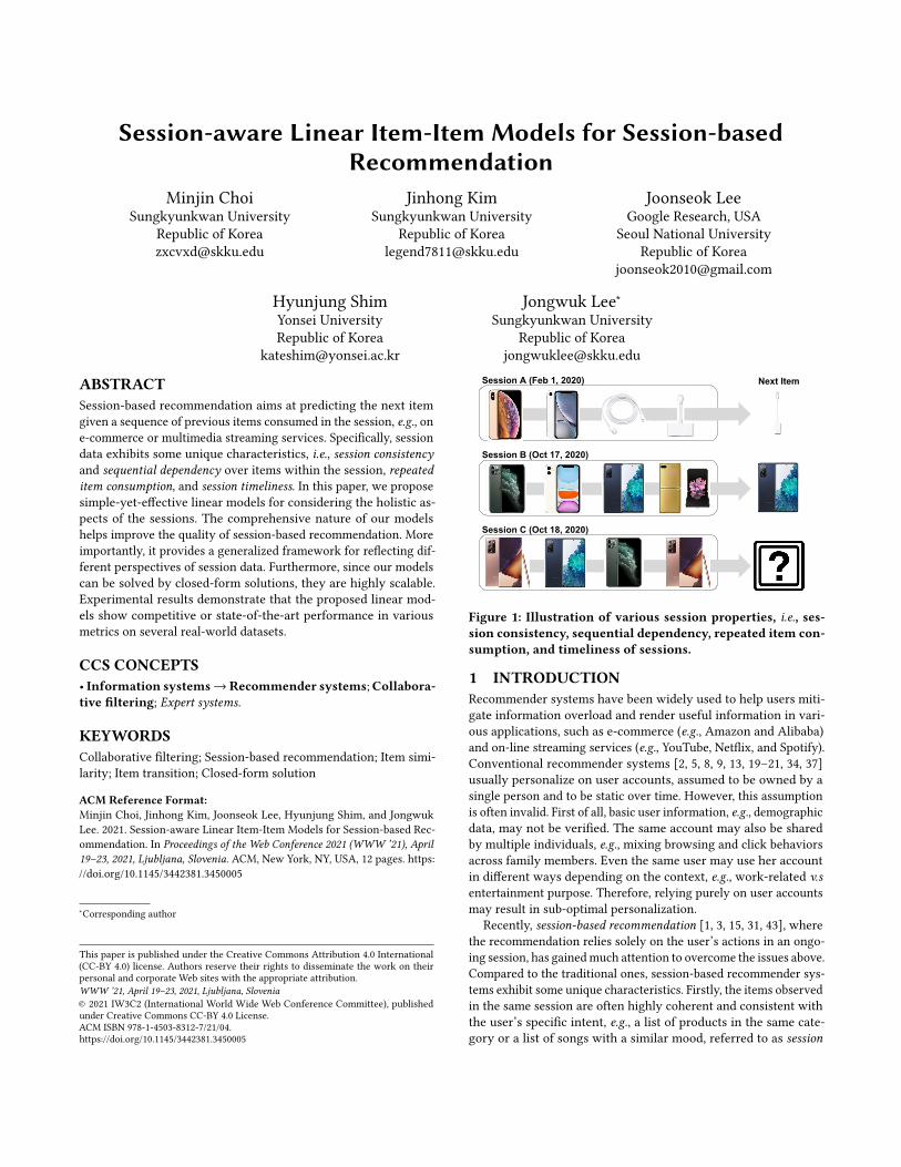
Figure 1: Illustration of various session properties, i.e., ses-sion consistency, sequential dependency, repeated item con-sumption, and timeliness of sessions.

1 INTRODUCTIONRecommender systems have been widely used to help users miti-gate information overload and render useful information in vari-ous applications, such as e-commerce (e.g., Amazon and Alibaba)and on-line streaming services (e.g., YouTube, Netflix, and Spotify).Conventional recommender systems [2, 5, 8, 9, 13, 19–21, 34, 37]usually personalize on user accounts, assumed to be owned by asingle person and to be static over time. However, this assumptionis often invalid. First of all, basic user information, e.g., demographicdata, may not be verified. The same account may also be sharedby multiple individuals, e.g., mixing browsing and click behaviorsacross family members. Even the same user may use her accountin different ways depending on the context, e.g., work-related v.sentertainment purpose. Therefore, relying purely on user accountsmay result in sub-optimal personalization.

Recently, session-based recommendation [1, 3, 15, 31, 43], wherethe recommendation relies solely on the user’s actions in an ongo-ing session, has gainedmuch attention to overcome the issues above.Compared to the traditional ones, session-based recommender sys-tems exhibit some unique characteristics. Firstly, the items observedin the same session are often highly coherent and consistent withthe user’s specific intent, e.g., a list of products in the same cate-gory or a list of songs with a similar mood, referred to as session

https://doi.org/10.1145/3442381.3450005

https://doi.org/10.1145/3442381.3450005

https://doi.org/10.1145/3442381.3450005

WWW ’21, April 19–23, 2021, Ljubljana, Slovenia Minjin Choi, Jinhong Kim, Joonseok Lee, Hyunjung Shim, and Jongwuk Lee

consistency. The brand-new smartphones in “session B” in Figure 1,for example, are highly correlated. Secondly, some items tend to beconsumed in a specific order, namely sequential dependency, e.g.,consecutive episodes of a TV series. As in “session A” of Figure 1,smartphone accessories are usually followed by smartphones, butnot in the other way around. Thirdly, the user might repeatedly con-sume the same items in a session, called repeated item consumption.For instance, the user may listen to her favorite songs repeatedlyor choose the same smartphone for the comparisons as illustratedin “session C” of Figure 1. Lastly, recent sessions are generally astronger indicator of the user’s interest, namely, timeliness of ses-sions. In Figure 1, “Session B” and “session C” are close in time andshare several popular items. The above four properties do not nec-essarily appear in all sessions, and one property may be dominantthan others.

Recent session-based recommender systems have shown out-standing performance by utilizing deep neural networks (DNNs).Recurrent neural networks [10–12] or attention mechanism [22, 24]are applied to model sequential dependency, and graph neural net-works (GNNs) [6, 30, 44, 45] are effective for representing sessionconsistency. However, they mostly focus on some aspects of ses-sions and thus do not generalize well to various datasets. No sin-gle model can guarantee competitive performances across variousdatasets, as reported in Section 5. Furthermore, they generally re-quire high computational cost for model training and inference.

To overcome the scalability issue of DNN-based models, recentstudies [4, 25] suggest neighborhood-based models for session-based recommendation, which are highly scalable. Surprisingly,they also achieve competitive performance comparable to DNN-based models on several benchmark datasets [26, 27]. However,the neighborhood-based models only exploit neighboring sessions,limited to capture global patterns of sessions.

In this paper, we propose novel session-aware linear models, tocomplement the drawback of DNN-based and neighborhood-basedmodels. Specifically, we design a simple-yet-effective model that (i)comprehensively considers various aspects of session-based recom-mendations (ii) and simultaneously achieves scalability. The ideaof the linear models has been successfully applied to traditionalrecommender systems (e.g., SLIM [29] and EASE𝑅 [39]). Notably,EASE𝑅 [39] has shown impressive performance gains and enjoyedhigh scalability thanks to its closed-form solution.

Inspired by the recent successful studies [16, 38–40], we refor-mulate the linear model that captures various characteristics ofsessions. Firstly, we devise two linear models focusing on differ-ent properties of sessions: (i) Session-aware Linear Item Similarity(SLIS) model aims at better handling session consistency, and (ii)Session-aware Linear Item Transition (SLIT) model focuses moreon sequential dependency. With both SLIS and SLIT, we relax theconstraint to incorporate repeated items and introduce a weightingscheme to take the timeliness of sessions into account. Combiningthese two types of models, we then suggest a unified model, namelySession-aware Item Similarity/Transition (SLIST) model, which isa generalized solution to holistically cover various properties ofsessions. Notably, SLIST shows competitive or state-of-the-art per-formance consistently on various datasets with different properties,proving its generalization ability. Besides, both SLIS and SLIT (and

thus the combined SLIST) are solved by closed-form equations,leading to high scalability.

To summarize, the key advantages of SLIST are presented asfollows: (i) It is a generalized solution for session-based recom-mendation by capturing various properties of sessions. (ii) It ishighly scalable thanks to closed-form solutions of linear models.(iii) Despite its simplicity, it achieves competitive or state-of-the-artperformance in various metrics (i.e., HR, MRR, Recall, and MAP)on several benchmark datasets (i.e., YouChoose, Diginetica, Retail-Rocket, and NowPlaying).

2 PRELIMINARIESWe start with defining notations used in this paper, followed by aformal problem statement and review of linear item-item models.Notations. Let S = {𝑠 (𝑖) }𝑚

𝑖=1 denote a set of sessions over an itemset I = {𝑖1, . . . , 𝑖𝑛}. An anonymous session 𝑠 ∈ S is a sequenceof items 𝑠 = (𝑠1, 𝑠2, . . . , 𝑠 |𝑠 |), where 𝑠 𝑗 ∈ I is the 𝑗-th clicked itemand |𝑠 | is the length of the session 𝑠 . Given 𝑠 ∈ S, we representa training example x ∈ R𝑛 , where each element x𝑗 is non-zero ifthe 𝑗-th item in I is observed in the session and zero otherwise.Higher values are assigned if the interacted item is more important.Similarly, the target item is represented as a vector y ∈ R𝑛 , where𝑦 𝑗 = 1 if 𝑖 𝑗 ∈ 𝑠 |𝑠 |+1, and 0 otherwise.

Stacking 𝑚 examples, we denote X,Y ∈ R𝑚×𝑛 for a session-item interaction matrix for training examples and target labels,respectively, where 𝑚 is the number of training examples. Thesession-item interaction matrix is extremely sparse by nature. Gen-erally speaking,𝑚 can be an arbitrary number depending on howwe construct the examples and how much we sample from the data.(See Section 3.3 for more details.)Problem Statement. The goal of session-based recommendationis to predict the next item(s) a user would likely choose to consume,given a sequence of previously consumed items in a session. For-mally, we build a session-based model M(𝑠) that takes a session𝑠 = (𝑠1, 𝑠2, . . . , 𝑠𝑡 ) for 𝑡 = 1, 2, ..., |𝑠 | − 1 as input and returns a list oftop-𝑁 candidate items to be consumed as the next one 𝑠𝑡+1.Linear Item-ItemModels.Given twomatricesX and Y, the linearmodel is formulated with an item-to-item similarity matrix B ∈R𝑛×𝑛 . Formally, a linear item-item model is defined by

Y = X · B, (1)

where B maps the previously consumed items in X to the nextobserved item(s) in Y. A typical objective function of this linearmodel is formulated by ridge regression that minimizes the ordinaryleast squares (OLS).

argminB

∥Y − X · B∥2𝐹 + _∥B∥2𝐹 , (2)

where _ is a regularizer term and ∥ · ∥𝐹 denotes the Frobenius norm.In the traditional recommendation, where each user is repre-

sented as a set of all items consumedwithout the concept of sessions,X and Y are regarded as the same matrix. In this case, with _ = 0, itends up with a trivial solution of B = I in Eq. (2), which is useless forpredictions. To avoid this trivial solution, existing studies [29, 39]add some constraints to the objective function. As the pioneeringwork, SLIM [29] enforces all entries in B to be non-negative with

Session-aware Linear Item-Item Models for Session-based Recommendation WWW ’21, April 19–23, 2021, Ljubljana, Slovenia

zero diagonal elements.

argminB

∥X − X · B∥2𝐹 + _1∥B∥1 + _2∥B∥2𝐹

s.t. diag(B) = 0, B ≥ 0,(3)

where _1 and _2 are regularization coefficients for L1-norm andL2-norm, respectively, and diag(B) ∈ R𝑛 denotes a vector with thediagonal elements of B.

Although SLIM [29] has shown competitive accuracy in litera-ture, it is also well-known SLIM is prohibitively slow to train. (Lianget al. [23] reported that the hyper-parameter tuning of SLIM tookseveral weeks on large-scale datasets with 10K+ items.) Althoughsome extensions [35, 36, 41] propose to reduce the training cost,they are still computationally prohibitive at an industrial scale.

Recently, EASE𝑅 [39] and its variants [38, 40] remove the non-negativity constraint of B and L1-norm constraints from Eq. (3),leaving only the diagonal constraint.

argminB

∥X − X · B∥2𝐹 + _ · ∥B∥2𝐹 s.t. diag(B) = 0. (4)

EASE𝑅 draws the closed-form solution via Lagrange multipliers.

B̂ = I − P̂ · diagMat(1 ⊘ diag(P̂)), (5)

where P̂ = (X⊤X + _I)−1, 1 is a vector of ones, and ⊘ denotes theelement-wise division operator. Also, diagMat(x) denote the diag-onal matrix expanded from vector x. (See [39] for a full derivationof the closed-form solution.) Finally, each learned weight in B isgiven by

B̂𝑖 𝑗 =

{0 if 𝑖 = 𝑗,

− P𝑖 𝑗P𝑗 𝑗

otherwise.(6)

Although inverting the regularized Gram matrix is a bottleneckfor a large-scale dataset, the closed-form expression is significantlyadvantageous in efficiency. The complexity of EASE𝑅 [39] is pro-portional to the number of items, which is usually much smallerthan the number of users in real-world scenarios. It also achievescompetitive prediction accuracy to the state-of-the-art models inthe conventional recommendation setting. Motivated by these ad-vantages, we utilize the benefit of linear models for session-basedrecommendation.

3 PROPOSED MODELS3.1 MotivationWe present the useful characteristics of sessions. The first threeare about the correlation between items in a session, i.e., intra-session properties, while the last one is about the relationship acrosssessions, i.e., inter-session property.• Session consistency: A list of items in a session is often topi-cally coherent, reflecting a specific and consistent user intent.For example, the songs in a user-generated playlist usually havea theme, e.g., similar mood, same genre, or artist.

• Sequential dependency: Some items tend to be observed in aparticular order. An item is usually consumed first, followed byanother, across the majority of sessions. An intuitive example isa TV series, where its episodes are usually sequentially watched.For this reason, the last item in the current session is often themost informative signal to predict the next one.

• Repeated item consumption: A user may repeatedly con-sume an item multiple times in a single session. For instance, auser may listen to her favorite songs repeatedly. Also, a usermay click the same product multiple times to compare it withother products.

• Timeliness of sessions: A session usually reflects user in-terest at the moment, and a collection of such sessions oftenreflects a recent trend. For instance, many users tend to watchnewly released music videos more frequently. Thus, the re-cent sessions may be a better indicator of predicting the user’scurrent interest than the past ones.Recent session-based recommendation models have implicitly

utilized some of these properties. RNN-based [10–12] or attention-based models [22, 24] assume that the last item in the session is themost crucial user intent and mainly focus on sequential dependency.GNN-based models [6, 30, 44, 45] can also utilize session consistency.They leverage graph embeddings between items to analyze hiddenuser intents. Some studies also addressed repeated item consumptionby using the attentionmechanism (e.g., RepeatNet [32]) or timelinessof sessions by using the weighting scheme (e.g., STAN [4]), therebyimproving the prediction accuracy.

However, none of these existing studies holistically deals withthe various session properties. Each model is optimized to handlea few properties, overlooking other essential characteristics. Also,different datasets exhibit quite diverse tendencies. For instance,the Yoochoose dataset tends to show stronger sequential depen-dency than other properties, while the sessions in the Digineticadataset rely less on sequential dependency. As a result, no singlemodel outperforms others across multiple datasets [25–27], fail-ing to generalize on them. Besides, existing DNN-based modelsare inapplicable to resource-limited environments due to the lackof scalability. To overcome these limitations, we develop session-aware linear models that not only simultaneously accommodatevarious properties of sessions but also are highly scalable.

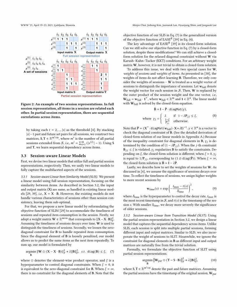
3.2 Session RepresentationsWe describe how to represent the sessions for our linear models.Although the session has a sequential nature, the linear modelonly handles a set of items as a vector. As depicted in Figure 2, weconsider two session representations.• Full session representation: The entire session is representedas a single vector. Specifically, a session 𝑠 = (𝑠1, 𝑠2, . . . , 𝑠 |𝑠 |) isregarded as a set of items s = {𝑠1, 𝑠2, . . . , 𝑠 |𝑠 |}, ignoring the se-quence of items. As depicted in Figure 2, the number of trainingexamples (𝑚) is equal to the number of sessions. It is more suit-able for a case where items in a session tend to have a strongercorrelation among them, relatively insensitive to the order ofconsumption. Note that the repeated items in the session aretreated as a single item as the full session representation mainlyhandles the session consistency across items.

• Partial session representation: A session is divided into twosubsets, past and future, to represent the sequential correlationsacross items. For some time step 𝑡 , the past set consists of itemsthat have been consumed before 𝑡 , i.e., s1:𝑡−1 = {𝑠1, . . . , 𝑠𝑡−1},and the future set consists of items consumed at or after 𝑡 , i.e.,s𝑡 : |𝑠 | = {𝑠𝑡 , . . . , 𝑠 |𝑠 |}. We can produce |𝑠 |−1 such partial sessions


Full session representation

Partial session representation

11 1

111 1 1

1

1

1 11

2 111

11

1 1 11 1 1

11

1 1 11 1 1

11

A set of sessions

Input matrix Output matrix

Input matrix Output matrix

1 1111

11

1

2 1

Figure 2: An example of two session representations. In fullsession representation, all items in a session are related eachother. In partial session representation, there are sequentialcorrelations across items.

by taking each 𝑡 = 2, ..., |𝑠 | as the threshold [4]. By stacking|𝑠 | −1 past and future set pairs for all sessions, we construct twomatrices, S,T ∈ R𝑚′×𝑛 , where𝑚′ is the number of all partialsessions extended from S, i.e.,𝑚′ =

∑𝑚𝑖=1 ( |𝑠 (𝑖) | − 1). Using S

and T, we learn sequential dependency across items.

3.3 Session-aware Linear ModelsFirst, we devise two linear models that utilize full and partial sessionrepresentations, respectively. Then, we unify two linear models tofully capture the multifaceted aspects of the sessions.

3.3.1 Session-aware Linear Item SimilarityModel (SLIS). Wepresenta linear model using full session representation, focusing on thesimilarity between items. As described in Section 3.2, the inputand output matrix (X) are same, as handled in existing linear mod-els [29, 39], i.e., X = X · B. However, the existing models do nothandle various characteristics of sessions other than session con-sistency, leaving them sub-optimal.

For that, we propose a new linear model by reformulating theobjective function of SLIM [29] to accommodate the timeliness ofsessions and repeated item consumption in the session. Firstly, weadopt a weight matrixW ∈ R𝑚×𝑛 that corresponds to ∥X−X ·B∥2

𝐹.

Assuming the timeliness of sessions decays over time,W is used todistinguish the timeliness of sessions. Secondly, we loosen the zero-diagonal constraint for B to handle repeated item consumption.Since the diagonal element of B is loosely penalized, our modelallows us to predict the same items as the next item repeatedly. Tosum up, our model is formulated by

argminB

∥W ⊙ (X − X · B)∥2𝐹 + _∥B∥2𝐹 , 𝑠 .𝑡 . diag(B) ≤ b, (7)

where ⊙ denotes the element-wise product operator, and b is ahyperparameter to control diagonal constraints. When b = 0, itis equivalent to the zero-diagonal constraint for B. When b = ∞,there is no constraint for the diagonal elements of B. Note that the

objective function of our SLIS in Eq. (7) is the generalized versionof the objective function of EASE𝑅 [39] in Eq. (4).

The key advantage of EASE𝑅 [39] is its closed-form solution.Can we still solve our objective function in Eq. (7) by a closed-formsolution, despite those modifications? We can still achieve a closed-form solution for the relaxed diagonal constraint without W viaKarush–Kuhn–Tucker (KKT) conditions. For an arbitrary weightmatrixW, however, it is not trivial to obtain a closed-form solution.

To address this issue, we deal with two special cases for W,weights of sessions and weights of items. As presented in [38], theweights of items do not affect learning B. Therefore, we only con-sider the weights of sessions –W is treated as a weight vector ofsessions to distinguish the importance of sessions. Let wfull denotethe weight vector for each session in S. Then, W is replaced bythe outer product of the session weight and the one vector, i.e.,Wfull = wfull · 1⊤, where wfull ∈ R𝑚 and 1 ∈ R𝑛 . The linear modelwith Wfull is solved by the closed-form equation.

B̂ = I − P̂ · diagMat(𝛾),

where 𝛾 𝑗 =

{_ if 1 − _P𝑗 𝑗 ≤ b,1−b𝑃 𝑗 𝑗

otherwise.(8)

Note that P̂ = (X⊤ ·diagMat(wfull) ·X+_I)−1. 𝛾 ∈ R𝑛 is a vector tocheck the diagonal constraint of B. (See the detailed derivation ofclosed-form solution of our linear models in Appendix A.) Becauseof the inequality constraint for diagonal elements in B, 𝛾 𝑗 is de-termined by the condition of (1 − _P𝑗 𝑗 ). When the 𝑗-th constraintB𝑗 𝑗 ≤ b is violated, 𝛾 𝑗 regularizes B to satisfy the constraints. De-pending on b , the closed-form solution is different; when b = 0, 𝛾 𝑗is equal to 1/P𝑗 𝑗 , corresponding to (1 ⊘ diag(P̂)). When b = ∞,the closed-form solution is B̂ = I − _P̂.

Lastly, we describe how to set the weights of sessions for W. Asdiscussed in [4], we assume the significance of sessions decays overtime. To reflect the timeliness of sessions, we assign higher weightsto more recent sessions by

wtime (𝑠) = exp(− 𝑡max − 𝑡 (𝑠)

𝛿time

)2, (9)

where 𝛿time is the hyperparameter to control the decay rate, 𝑡max isthe most recent timestamp inS, and 𝑡 (𝑠) is the timestamp of the ses-sion 𝑠 . With smaller 𝛿time, we decay more severely the significanceof older sessions.

3.3.2 Session-aware Linear Item Transition Model (SLIT). Usingthe partial session representation in Section 3.2, we design a linearmodel that captures the sequential dependency across items. UnlikeSLIS, each session is split into multiple partial sessions, formingdifferent input and output matrices. Similar to SLIS, we also incor-porate the weight of sessions to SLIT. Meanwhile, we ignore theconstraint for diagonal elements in B as different input and outputmatrices are naturally free from the trivial solution.

Formally, we formulate the objective function of SLIT usingpartial session representations.

argminB

Wpar ⊙ (T − S · B) 2𝐹+ _∥B∥2𝐹 , (10)

where S,T ∈ R𝑚′×𝑛 denote the past and future matrices. Assumingthe partial sessions have the timestamp of the original session,Wpar


is represented by wpar · 1⊤, where the values in wpar are assignedby Eq. (9). Although the S and T are different, we still derive theclosed-form solution:

B̂ = P̂′ · [S⊤diagMat(wpar)T], (11)

where P̂′ = (S⊤diagMat(wpar)S + _I)−1.Lastly, we describe how to adjust the importance of the past and

future item subsets in S and T. As adopted in [4], we utilize theposition gap between two items as the weight of items.

wpos (𝑖, 𝑗, 𝑠) = exp(− |𝑝 (𝑖, 𝑠) − 𝑝 ( 𝑗, 𝑠) |

𝛿pos

), (12)

where 𝛿pos is the hyperparameter to control the position decay inpartial sessions, and 𝑝 (𝑖, 𝑠) is the position of item 𝑖 in session 𝑠 .Also, 𝑖 and 𝑗 are the items in session 𝑠 . When a target item is given,it is possible to decay the importance of items in the partial sessionaccording to sequential order.

3.3.3 Unifying Two Linear Models. Because SLIS and SLIT capturevarious characteristics of sessions, we propose a unified model,called Session-aware Linear Similarity/Transition model (SLIST), byjointly optimizing both models:

argminB

𝛼 ∥Wfull ⊙ (X − X · B)∥2𝐹

+ (1 − 𝛼) Wpar ⊙ (T − S · B)

2𝐹+ _∥B∥2𝐹 ,

(13)

where 𝛼 is the hyperparameter to control the importance ratio ofSLIS and SLIT.

Although it looks impossible to achieve a closed-form solution ata glance, we can still derive it. The intuition is that, when stackingtwo matrices for SLIS and SLIT, e.g., X and S, the objective functionof SLIST is similar to that of SLIT. Formally, the closed-form solutionis given by

B̂ = I − _P̂ − (1 − 𝛼)P̂S⊤diagMat(wpar) (S − T), (14)

where P̂ = (𝛼X⊤diagMat(wfull)X + (1 − 𝛼)S⊤diagMat(wpar)S +_I)−1.

3.3.4 Model Inference. We predict the next item for a given sessionwith a sequence of items using a learned item-item matrix, i.e.,T̂ = S · B̂. For inference, it is necessary to consider the importanceof items depending on a sequence of items in S. Similarly to Eq. (12),we decay the item weights for inference over time by

winf (𝑖, 𝑠) = exp(− |𝑠 | − 𝑝 (𝑖, 𝑠)

𝛿inf

), (15)

where 𝛿inf is a hyperparameter to control the item weight decayfor inference, and |𝑠 | is the length of the session 𝑠 . In other words,SLIST takes a vector with partial representation using the itemweight as input.

4 EXPERIMENTAL SETUPBenchmark datasets. We evaluate our proposed models on fourpublic datasets collected from e-commerce and music streamingservices: YooChoose1 (YC), Diginetica2 (DIGI), RetailRocket3 (RR),1https://2015.recsyschallenge.com/challenge.html2http://cikm2016.cs.iupui.edu/cikm-cup3https://www.dropbox.com/sh/n281js5mgsvao6s/AADQbYxSFVPCun5DfwtsSxeda?dl=0

Table 1: Detailed statistics of the benchmark datasets. #Ac-tions indicates the number of entire user-item interactions.

Split Dataset #Actions #Sessions #Items #Actions #Items/ Sess. / Sess.

1-split YC-1/64 494,330 119,287 17,319 4.14 3.30YC-1/4 7,909,307 1,939,891 30,638 4.08 3.28DIGI1 916,370 188,807 43,105 4.85 4.08

5-split YC 5,426,961 1,375,128 28,582 3.95 3.17DIGI5 203,488 41,755 32,137 4.86 4.08RR 212,182 59,962 31,968 3.54 2.56NOWP 271,177 27,005 75,169 10.04 9.38

and NowPlaying (NOWP). For YC and DIGI, we use single-splitdatasets (i.e., YC-1/64, YC-1/4, DIGI1), following existing studies [10,22, 24, 44]. To evaluate on large-scale datasets, we further employfive-split datasets (i.e., YC, DIGI5, RR, NOWP), used in recent em-pirical analysis [25–27] for session-based recommendation models.Table 1 summarizes detailed statistics of all benchmark datasets.

As pre-processing, we discard the sessions having only one in-teraction and items appearing less than five times following theconvention [25]. We hold-out the sessions from the last 𝑁 -days fortest purposes and used the last 𝑁 days in the training set for thevalidation set. Refer to detailed pre-processing and all source codesat our website4.Competing models. We compare our models with eight competi-tive models, roughly categorized into four groups, Markov-chain-based, neighborhood-based, linear, and DNN models. SR [18] isan effective Markov chain model together with association rules.Among neighborhood-based models, we choose SKNN [14] andSTAN [4]. STAN [4] is an improved version of SKNN [14] by con-sidering sequential dependency and session recency. For the linearmodel baselines, we apply EASE𝑅 [39] for the session-based rec-ommendation problem by using the session-item matrix, namelySEASE𝑅 . For DNN-based models, we employ GRU4Rec+ [10, 11],NARM [22], STAMP [24], and SR-GNN [44]. GRU4Rec+ [10] is animproved version of the original GRU4Rec[12] using the top-𝑘 gainobjective function. NARM [22] and STAMP [24] are attention-basedmodels for facilitating both long-term and short-term sequential de-pendency. SR-GNN [44] utilizes a graph neural network to capturecomplex sequential dependency within a session.Evaluation protocol. To evaluate session-based recommendermodels, we adopt the iterative revealing scheme [12, 22, 44], whichiteratively exposes the item of a session to the model. Each itemin the session is sequentially appended to the input of the model.Therefore, this scheme is useful for reflecting the sequential userbehavior throughout a session.Evaluation metrics. We utilize various evaluation metrics withthe following two application scenarios, e.g., a set of recommendedproducts in e-commerce and the next recommended song for agiven playlist in music streaming services. (i) To predict the nextitem in a session, we use Hit Rate (HR) and Mean Reciprocal Rank(MRR), which have been widely used in existing studies [11, 24, 44].

4https://github.com/jin530/SLIST


Table 2: Accuracy comparison of our models and competing models, following experimental setup in [26, 27]. Gains indicatehow much better the best proposed model is than the best competing model. The best proposed model is marked in bold andthe best baseline model is underlined.

Dataset Metric Non-DNN-based models DNN-based models Ours Gains (%)SR SKNN STAN SEASE𝑅 GRU4Rec+ NARM STAMP SR-GNN SLIS SLIT SLIST

YC-1/64

HR@20 0.6674 0.6423 0.6838 0.5443 0.6528 0.6998 0.6841 0.7021 0.7015 0.6968 0.7088 0.95MRR@20 0.3033 0.2522 0.2820 0.1963 0.2752 0.2957 0.2995 0.3099 0.2837 0.3093 0.3083 -0.19R@20 0.4709 0.4780 0.4955 0.3983 0.4009 0.5051 0.4904 0.5049 0.5051 0.4976 0.5080 0.57

MAP@20 0.0350 0.0363 0.0375 0.0306 0.0285 0.0389 0.0370 0.0388 0.0387 0.0379 0.0388 -0.26

YC-1/4

HR@20 0.6850 0.6329 0.6846 0.5550 0.6940 0.7079 0.7021 0.7118 0.7119 0.7149 0.7175 0.80MRR@20 0.3053 0.2496 0.2829 0.1984 0.2942 0.2996 0.3066 0.3180 0.283 0.3155 0.3161 -0.60R@20 0.4851 0.4756 0.4952 0.4040 0.4887 0.5097 0.5008 0.5095 0.5121 0.511 0.5130 0.65

MAP@20 0.0364 0.0361 0.0373 0.0309 0.0375 0.0395 0.0385 0.0393 0.0394 0.0391 0.0393 -0.25

DIGI1

HR@20 0.4085 0.4846 0.5121 0.3906 0.5097 0.4979 0.4690 0.4904 0.5247 0.4729 0.5291 3.32MRR@20 0.1431 0.1736 0.1851 0.1099 0.1750 0.1585 0.1499 0.1654 0.1877 0.1599 0.1886 1.89R@20 0.3164 0.3788 0.3965 0.3048 0.3957 0.3890 0.3663 0.3811 0.4062 0.3651 0.4091 3.18

MAP@20 0.0212 0.0263 0.0275 0.0209 0.0275 0.0270 0.0252 0.0264 0.0284 0.0250 0.0286 4.00

YC

HR@20 0.6506 0.5996 0.6656 0.5030 0.6488 0.6751 0.6654 0.6713 0.6786 0.6838 0.6867 1.72MRR@20 0.3010 0.2620 0.2933 0.1849 0.2893 0.3047 0.3033 0.3142 0.2854 0.3080 0.3097 -1.43R@20 0.4853 0.4658 0.4986 0.3809 0.4837 0.5109 0.4979 0.5060 0.5074 0.5097 0.5122 0.25

MAP@20 0.0332 0.0318 0.0342 0.0264 0.0334 0.0357 0.0344 0.0351 0.0353 0.0355 0.0357 0.00

DIGI5

HR@20 0.3277 0.4748 0.4800 0.3531 0.4639 0.4188 0.3917 0.4158 0.4939 0.4193 0.5005 4.27MRR@20 0.1216 0.1714 0.1828 0.1004 0.1644 0.1392 0.1314 0.1436 0.1847 0.1400 0.1827 1.04R@20 0.2517 0.3715 0.3720 0.2774 0.3617 0.3254 0.3040 0.3232 0.3867 0.3260 0.3898 4.78

MAP@20 0.0164 0.0255 0.0252 0.0185 0.0247 0.0218 0.0201 0.0217 0.0265 0.0218 0.0267 4.71

RR

HR@20 0.4174 0.5788 0.5938 0.2727 0.5669 0.5549 0.4620 0.5433 0.5983 0.4899 0.6020 1.38MRR@20 0.2453 0.3370 0.3638 0.1032 0.3237 0.3196 0.2527 0.3066 0.3583 0.2691 0.3512 -1.51R@20 0.3359 0.4707 0.4748 0.2209 0.4559 0.4526 0.3917 0.4438 0.4798 0.3925 0.4819 1.50

MAP@20 0.0194 0.0283 0.0285 0.0134 0.0272 0.0270 0.0227 0.0264 0.0289 0.0233 0.0291 2.11

NOWP

HR@20 0.2002 0.2450 0.2414 0.2088 0.2261 0.1849 0.1915 0.2113 0.2522 0.2326 0.2689 9.76MRR@20 0.1052 0.0687 0.0871 0.0625 0.1076 0.0894 0.0882 0.0935 0.0794 0.1171 0.1137 8.83R@20 0.1366 0.1809 0.1696 0.1658 0.1361 0.1274 0.1253 0.1400 0.1802 0.1577 0.1840 1.71

MAP@20 0.0133 0.0186 0.0175 0.0181 0.0116 0.0118 0.0113 0.0125 0.0183 0.0146 0.0184 -1.08

(ii) To consider all subsequent items for the session, we use Recalland Mean Average Precision (MAP) as the standard IR metrics.Implementation details. For SLIST, we tune 𝛼 among {0.2, 0.4,0.6, 0.8}, 𝛿pos and 𝛿inf among {0.125, 0.25, 0.5, 1, 2, 4, 8} and 𝛿timeamong {1, 2, 4, 8, 16, 32, 64, 128, 256}. For baseline models, we usethe best hyperparameters reported in [25, 26]. Note that we conductthe reproducibility for previously reported results of all the baselinemodels. We implement the proposed model and STAN [4] usingNumPy. We use public source code for SR-GNN5 released by [44]and the other baseline models6 released by [27]. (See the detailedhyperparameter settings in Appendix B.) We conduct all experi-ments on a desktop with 2 NVidia TITAN RTX, 256 GB memory,and 2 Intel Xeon Processor E5-2695 v4 (2.10 GHz, 45M cache).

5 RESULTS AND DISCUSSIONIn this section, we discuss the accuracy and efficiency of our pro-posed models in comparison with eight baseline models. From theextensive experimental results, we summarize the following obser-vations:

5https://github.com/CRIPAC-DIG/SR-GNN6https://github.com/rn5l/session-rec

• SLIST shows comparable or state-of-the-art performance onvarious datasets. For HR@20 and Recall@20, SLIST consistentlyoutperforms baseline models. For MRR@20, SLIST is slightlyworse than the best models on YC and RR datasets. Particu-larly, SLIST achieves up to 9.76% and 8.83% gain in HR@20 andMRR@20 over the best baseline model on the NowP dataset.(Section 5.1)

• Thanks to the closed-form solution, SLIST is up to 786x fasterin training than SR-GNN, a state-of-the-art DNN-based model.Also, the SLIST does not take significantlymore timewith largertraining sets, indicating its superior scalability. (Section 5)

• For relatively shorter sessions, SLIST significantly outper-forms STAN and SR-GNN. While SLIT shows comparable per-formance with SLIST on the YC-1/4 dataset, it is much worsethan SLIST on the DIGI1 dataset. (Section 5.3)

• All the components of SLIST directly contribute to performancegains (i.e., up to 18.35% improvement relative to whose com-ponents are all removed). The priority of components followsitem weight decay (winf) > position decay (wpos) > time decay(wtime). (Section 5.4)


5.1 Evaluation of AccuracyTable 2 reports the accuracy of the proposed models and othercompetitors on seven datasets. (See the entire results for the othercut-offs (i.e., 5 and 10) in Appendix C.)

First of all, we analyze the existing models based on the proper-ties of datasets. We observe that no existing models ever establishstate-of-the-art performance over all datasets. Either NARM or SR-GNN is the best model on YC datasets, but either SKNN or STAN isthe best model on DIGI, RR, and NOWP datasets. This result impliesthat the performance of existing models suffers from high variancedepending on the datasets. It is a natural consequence becausedifferent models mainly focus on a few different characteristics ofsessions. DNN-based models commonly focus on sequential depen-dency, thus more advantageous to handle YC datasets presentingstrong sequential dependency. On the other hand, neighborhood-based models generally show outstanding performance on DIGI5,RR, andNOWP datasets, showing stronger session consistency. Thistendency explains that neighborhood-based models successfullyexploit session consistency.

From this observation, we emphasize that achieving consistentlyhigher performance across various datasets on session-based recom-mendation has been particularly challenging. Nevertheless, SLISTconsistently records competitive performance, comparable to orbetter than state-of-the-art models. The consistent and competi-tive performance is a clear indicator that SLIST indeed effectivelylearns various aspects of sessions, not over-focusing on a subsetof them. Specifically, SLIST achieves accuracy gains up to 9.76% inHR@20 and 8.83 % in MRR@20 over the best previous model. (Wemight achieve better performance for other metrics by tuning thehyperparameter 𝛼 as shown in Figure 5).

In most cases, SLIST outperforms its sub-components, SLIS andSLIT. It tells us that our unifying strategy is effective. Althoughsome datasets might have a clear bias (i.e., one property is dominantwhile others are negligible), our joint training strategy still finds areasonable solution considering the holistic aspects of the sessions.Similarly, STAN, an improved SKNN considering sequential depen-dency, also reports higher accuracy than SKNN. As a result, SLISTis the best or second-best model across all datasets.

Lastly, SEASE𝑅 does not show successful performance in thesession-based scenario. Notably, SEASE𝑅 is muchworse than SKNN,although both methods consider session consistency. It is becausethe diagonal penalty term in SEASE𝑅 prevents recommending therepeated items and leads to severe performance degradation. There-fore, we conclude that our modification to facilitate repeated itemconsumption is essential for building session-based recommenda-tion models.

5.2 Evaluation of ScalabilityTable 3 compares the training time (in seconds) of SLIST and thatof DNN-based models on the YC-1/4 dataset (i.e., the largest sessiondataset) with the various number of training sessions. Because thecomputational complexity of SLIST is mainly proportional to thenumber of items, the training time of SLIST is less dependent on thenumber of training sessions. For example, with 10% of the entiretraining sessions, SLIST is only 90x faster than SR-GNN.Meanwhile,SLIST is 768x faster than SR-GNN with the entire training data.

Table 3: Training time (in seconds) of SLIST and DNN-based models on the YC-1/4 dataset. Gains indicate how fastSLIST is compared to SR-GNN.While DNN-basedmodels aretrained using GPU, SLIST is trained using CPU.

Models The ratio of training sessions on YC-1/45% 10% 20% 50% 100%

GRU4Rec+ 177.4 317.8 614.0 1600.2 3206.9NARM 2137.6 3431.2 7454.2 27804.5 72076.8STAMP 434.1 647.5 985.3 2081.2 4083.3SR-GNN 6780.5 18014.7 31444.3 68581.9 185862.5SLIST 202.7 199.0 199.9 227.0 241.9Gains 33.5x 90.6x 157.3x 302.1x 768.2x

Also, SLIST takes a similar time to train on both the entire YCdataset and the YC-1/4 dataset. This is highly desirable in practice,especially on popular online services, where millions of users createbillions of session data every day.

5.3 Effect of Session LengthsFigure 3 compares the accuracy of the proposed and state-of-the-artmodels (i.e., STAN and SR-GNN) under the short- (5 or fewer items)and long-session (more than 5 items) scenarios. The ratio of shortsessions is 70.3% (YC-1/4) and 76.4% (DIGI1), respectively. First of all,all three methods show stronger performance in shorter sessions.This is probably because the user’s intent may change over time,making it difficult to capture her intent. Second, the relative strengthof each method tends to be larger with longer sessions, comparedto STAN and SR-GNN. However, SLIST consistently outperformsboth baselines in most scenarios, except for long sessions on YC-1/4,where SR-GNN slightly outperforms SLIST.

Figure 4 compares the accuracy between our models. Comparedto SLIS, SLIST improves the accuracy in MRR@20 up to 10.35% and0.35% for the short sessions, and up to 13.85% and 0.98% for the longsessions, on YC-1/4 and DIGI1 datasets, respectively. Based on thisexperiment, we confirm that sequential dependency in YC-1/4 isprominent for long sessions because the user can change her intentduring the session. This tendency is different from DIGI1 as SLISoutperforms SLIT for both short and long sessions. Consequently,we conclude that SLIST works well most flexibly on diverse datasetsexhibiting highly different characteristics, while the baseline mod-els and our sub-components (SLIS, SLIT) perform well only in aparticular setting.

5.4 Ablation StudyWe conducted an ablation study to analyze the effect of each com-ponent (i.e., position decay, item weight decay, time decay) in SLIST.For that, we removed each component from SLIST and observedperformance degradation. Table 4 summarizes the accuracy changeswhen each or a combination of components removed.

First of all, having all components is always better than the mod-els without one or more components. For all three datasets, the itemweight decay is the most influential factor for accuracy. The secondmost influential one is position decay, and the least significant com-ponent is time decay. We consistently observe the same tendency


Short LongSession length

0.55

0.6

0.65

0.7

0.75

HR

@20


0.2

0.25

0.3

0.35

MR

R@

20(a) YC-1/4


0.45

0.475

0.5

0.525

0.55

HR

@20


0.12

0.14

0.16

0.18

0.2M

RR

@20

(b) DIGI1Figure 3:HR@20 andMRR@20 of SLIST and state-of-the-artmodels with different session lengths (Short ≤ 5, Long > 5)on YC-1/4 and DIGI1.


0.65

0.675

0.7

0.725

0.75

HR

@20


0.2

0.25

0.3

0.35

MR

R@

20

(a) YC-1/4


0.45

0.475

0.5

0.525

0.55

HR

@20


0.12

0.14

0.16

0.18

0.2

MR

R@

20

(b) DIGI1Figure 4: HR@20 and MRR@20 of our three models withdifferent session lengths (Short ≤ 5, Long > 5) on YC-1/4 andDIGI1.

over different datasets. This tendency can be interpreted as thefactors for considering sequential dependency (i.e., item weightdecay and position decay) is more crucial than the factor relatedto the timeliness of sessions (i.e., time decay). Also, time decay isno longer effective in YC-1/64 because it is the latest 1/16 out ofYC-1/4, implying that YC-1/64 has already satisfied the timelinessof sessions.

Those three components are less significant in DIGI1, e.g., thegain from all three components in MRR@20 is 18.35% and 5.59% inYC-1/4 and DIGI1, respectively. As discussed earlier, the DIGI1 ismore affected by session consistency than sequential dependency.For this reason, item weight decay and position decay are less

Table 4: HR@20 and MRR@20 of SLIST when some compo-nents are removed: item weight decay winf, position decaywpos, and time decay wtime.

winf

wpo

s

wtim

e YC-1/64 YC-1/4 DIGI1HR MRR HR MRR HR MRR

✓ ✓ ✓ 0.7088 0.3083 0.7175 0.3161 0.5291 0.1886✓ ✓ 0.7078 0.3077 0.7096 0.3115 0.5253 0.1880✓ ✓ 0.6880 0.2973 0.7004 0.3031 0.5202 0.1855

✓ ✓ 0.6761 0.2697 0.6841 0.2753 0.5145 0.1820✓ 0.6898 0.2980 0.6947 0.3005 0.5173 0.1852

✓ 0.6764 0.2697 0.6784 0.2723 0.5111 0.1817✓ 0.6570 0.2651 0.6675 0.2693 0.5055 0.1789

0.6592 0.2652 0.6626 0.2671 0.5025 0.1786

0.0 0.2 0.4 0.6 0.8 1.00.7

0.71

0.72

0.73

0.74

0.75

HR

@20

0.27

0.28

0.29

0.3

0.31

0.32

MR

R@

20

HR@20 MRR@20

0.0 0.2 0.4 0.6 0.8 1.00.46

0.48

0.5

0.52

0.54

HR

@20

0.13

0.15

0.17

0.19

0.21

MR

R@

20

HR@20 MRR@20

(a) YC-1/4 (b) DIGI1

Figure 5: HR@20 and MRR@20 over varying 𝛼 in SLIST onYC-1/4 and DIGI1.

influential in DIGI1 than those in YC datasets. (More experimentalresults and analysis on the effect of components are in Appendix D.)

Figure 5 depicts the effect of 𝛼 , controlling the importance ofSLIS and SLIT in SLIST. SLIST with 𝛼 = 0 is equivalent to SLIT, andSLIST with 𝛼 = 1 is same as SLIS. For the datasets dominated bysequential dependency (e.g., YC-1/4), SLIT is more advantageousthan SLIS. Thus, a small 𝛼 is recommended, e.g., 0.2 is a good defaultvalue. On the contrary, when the target dataset exhibits sessionconsistency more dominant than others (e.g., DIGI1), we observebetter performance with higher 𝛼 (e.g., 0.8), with more impact fromSLIS.

The best performance is achieved with different 𝛼 , depending onthe datasets and metrics. On YC-1/4, the best MRR@20 is achievedwith 𝛼 = 0.2 (i.e., 0.3161), while the best HR@20 is with 𝛼 = 0.8(i.e., 0.7198). As DIGI1 exhibits different characteristics of sessions,the best results are achieved when 𝛼 = 0.8 in both metrics.

6 RELATEDWORKWe briefly review session-based models with three categories. Formore details, refer to recent survey papers [1, 15].Markov-chain-based models. Markov chains (MC) are widelyused to model dependency from sequential data. FPMC [33] pro-posed the tensor factorization that combines MC with traditionalmatrix factorization. Later, FOSSIL [7] combined FISM [17] withfactorized MC. Recently, SR [18] combined MC with associationrules. Because MC-based models merely focus on the short-termdependency between items, they are limited for analyzing complexdependency between them.


DNN-based models. Recently, session-based models have widelyemployed deep neural networks (DNNs), such as recurrent neu-ral networks (RNNs), attention mechanisms, convolutional neuralnetworks (CNNs), and graph neural networks (GNNs). As the pi-oneering work, Hidasi et al. [11] proposed GRU4Rec+ with gatedrecurrent units (GRU) for session-based recommendation and thendeveloped its optimized model [10]. Later, NARM [22] extendedGRU4Rec+ with an attention mechanism to capture short- and long-term dependency of items, and STAMP [24] combined an attentionmechanism with memory priority models to reflect the user’s gen-eral interests. RepeatNet [32] focused on analyzing the patternsfor repeated items in the session. Recently, SR-GNN [44] exploitedgated graph neural networks (GGNN) to analyze the complex itemtransitions within a session. Then, GC-SAN [45] improved SR-GNNwith a self-attention mechanism for contextualized non-local rep-resentations, and FGNN [30] adopted a weighted graph attentionnetwork (WGAT) to enhance SR-GNN. The GNN-based modelseffectively capture both the session consistency and sequential de-pendency in the session. Due to the extreme data sparsity, however,they are often vulnerable to overfitting [6].

To summarize, DNN-based models show outstanding perfor-mance using the powerful model capacity. Because they usuallyincur slow training and inference time, however, it is difficult tosupport the scalability for large-scale datasets.Neighborhood-based models. To overcome the scalability issue,Jannach and Ludewig [14] proposed SKNN that adopts the tradi-tional K-nearest neighbor approach (KNN) for session recommenda-tion, and STAN [4] improved SKNN using various weight schemesfor sequential dependency and the recency of sessions. Later, [25–27] extensively conducted an empirical study with various session-based models. Surprisingly, although non-neural models are simple,they show competitive performance in several benchmark datasets.To leverage the correlations between inter-session items, recentstudies (e.g., CSRM [42] and CoSAN [28]) incorporated neighborsessions into DNN-based models. While KNN-based models cancapture session consistency, they are generally limited to representcomplex dependency. Besides, they are also sensitive to similaritymetrics between sessions.

7 CONCLUSIONThis paper presents Session-aware Linear Item Similarity/Transitionmodel (SLIST) to tackle session-based recommendation. To comple-ment the drawback of existing models, we unify two linear modelswith different perspectives to fully capture various characteristicsof sessions. To the best of our knowledge, our model is the firstwork that adopts the linear item-item models to fully utilize vari-ous characteristics of sessions. Owing to its closed-form solution,SLIST is also highly scalable. Through comprehensive evaluation,we demonstrate that SLIST achieves comparable or state-of-the-artaccuracy over existing DNN-based and neighborhood-based modelson multiple benchmark datasets.

ACKNOWLEDGMENTThis work was supported by the National Research Foundation ofKorea (NRF) (NRF-2018R1A5A1060031). Also, this work was sup-ported by Institute of Information & communications Technology

Planning & evaluation (IITP) grant funded by the Korea government(MSIT) (No.2019-0-00421, AI Graduate School Support Program andIITP-2020-0-01821, ICT Creative Consilience Program).

REFERENCES[1] Geoffray Bonnin and Dietmar Jannach. 2014. Automated Generation of Music

Playlists: Survey and Experiments. ACM Comput. Surv. 47, 2 (2014), 26:1–26:35.[2] Minjin Choi, Yoonki Jeong, Joonseok Lee, and Jongwuk Lee. 2021. Local Collabo-

rative Autoencoders. In WSDM.[3] Hui Fang, Guibing Guo, Danning Zhang, and Yiheng Shu. 2019. Deep Learning-

Based Sequential Recommender Systems: Concepts, Algorithms, and Evaluations.In ICWE. 574–577.

[4] Diksha Garg, Priyanka Gupta, Pankaj Malhotra, Lovekesh Vig, and Gautam M.Shroff. 2019. Sequence and Time Aware Neighborhood for Session-based Recom-mendations: STAN. In SIGIR. 1069–1072.

[5] David Goldberg, David A. Nichols, Brian M. Oki, and Douglas B. Terry. 1992.Using Collaborative Filtering to Weave an Information Tapestry. Commun. ACM35, 12 (1992), 61–70.

[6] Priyanka Gupta, Diksha Garg, Pankaj Malhotra, Lovekesh Vig, and Gautam M.Shroff. 2019. NISER: Normalized Item and Session Representations with GraphNeural Networks. CoRR abs/1909.04276 (2019).

[7] Ruining He and Julian J. McAuley. 2016. Fusing Similarity Models with MarkovChains for Sparse Sequential Recommendation. In ICDM. 191–200.

[8] Xiangnan He, Lizi Liao, Hanwang Zhang, Liqiang Nie, Xia Hu, and Tat-SengChua. 2017. Neural Collaborative Filtering. In WWW. 173–182.

[9] Jonathan L. Herlocker, Joseph A. Konstan, Al Borchers, and John Riedl. 1999.An Algorithmic Framework for Performing Collaborative Filtering. In SIGIR.230–237.

[10] Balázs Hidasi and Alexandros Karatzoglou. 2018. Recurrent Neural Networkswith Top-k Gains for Session-based Recommendations. In CIKM. 843–852.

[11] Balázs Hidasi, Alexandros Karatzoglou, Linas Baltrunas, and Domonkos Tikk.2016. Session-based Recommendations with Recurrent Neural Networks. InICLR.

[12] Balázs Hidasi, Massimo Quadrana, Alexandros Karatzoglou, and Domonkos Tikk.2016. Parallel Recurrent Neural Network Architectures for Feature-rich Session-based Recommendations. In RecSys. 241–248.

[13] Yifan Hu, Yehuda Koren, and Chris Volinsky. 2008. Collaborative Filtering forImplicit Feedback Datasets. In ICDM. 263–272.

[14] Dietmar Jannach and Malte Ludewig. 2017. When Recurrent Neural Networksmeet the Neighborhood for Session-Based Recommendation. In RecSys. 306–310.

[15] Dietmar Jannach, Malte Ludewig, and Lukas Lerche. 2017. Session-based itemrecommendation in e-commerce: on short-term intents, reminders, trends anddiscounts. User Model. User Adapt. Interact. 27, 3-5 (2017), 351–392.

[16] Olivier Jeunen, Jan Van Balen, and Bart Goethals. 2020. Closed-Form Models forCollaborative Filtering with Side-Information. In RecSys. 651–656.

[17] Santosh Kabbur, Xia Ning, and George Karypis. 2013. FISM: factored item simi-larity models for top-N recommender systems. In KDD. 659–667.

[18] Iman Kamehkhosh, Dietmar Jannach, and Malte Ludewig. 2017. A Comparisonof Frequent Pattern Techniques and a Deep Learning Method for Session-BasedRecommendation. In RecSys. 50–56.

[19] Joonseok Lee, Sami Abu-El-Haija, Balakrishnan Varadarajan, and Apostol Natsev.2018. Collaborative Deep Metric Learning for Video Understanding. 481–490.

[20] Joonseok Lee, Samy Bengio, Seungyeon Kim, Guy Lebanon, and Yoram Singer.2014. Local collaborative ranking. 85–96.

[21] Joonseok Lee, Seungyeon Kim, Guy Lebanon, Yoram Singer, and Samy Bengio.2016. LLORMA: Local Low-Rank Matrix Approximation. Journal of MachineLearning Research 17 (2016), 15:1–15:24.

[22] Jing Li, Pengjie Ren, Zhumin Chen, Zhaochun Ren, Tao Lian, and Jun Ma. 2017.Neural Attentive Session-based Recommendation. In CIKM. 1419–1428.

[23] Dawen Liang, Rahul G. Krishnan, Matthew D. Hoffman, and Tony Jebara. 2018.Variational Autoencoders for Collaborative Filtering. In WWW. 689–698.

[24] Qiao Liu, Yifu Zeng, Refuoe Mokhosi, and Haibin Zhang. 2018. STAMP: Short-Term Attention/Memory Priority Model for Session-based Recommendation. InKDD. 1831–1839.

[25] Malte Ludewig and Dietmar Jannach. 2018. Evaluation of session-based recom-mendation algorithms. User Model. User Adapt. Interact. 28, 4-5 (2018), 331–390.

[26] Malte Ludewig, Noemi Mauro, Sara Latifi, and Dietmar Jannach. 2019. EmpiricalAnalysis of Session-Based Recommendation Algorithms. CoRR abs/1910.12781(2019).

[27] Malte Ludewig, Noemi Mauro, Sara Latifi, and Dietmar Jannach. 2019. Per-formance comparison of neural and non-neural approaches to session-basedrecommendation. In RecSys. 462–466.

[28] Anjing Luo, Pengpeng Zhao, Yanchi Liu, Fuzhen Zhuang, Deqing Wang, Jiajie Xu,Junhua Fang, and Victor S. Sheng. 2020. Collaborative Self-Attention Networkfor Session-based Recommendation. In IJCAI. 2591–2597.


[29] Xia Ning and George Karypis. 2011. SLIM: Sparse Linear Methods for Top-NRecommender Systems. In ICDM. 497–506.

[30] Zhiqiang Pan, Fei Cai, Yanxiang Ling, and Maarten de Rijke. 2020. RethinkingItem Importance in Session-based Recommendation. In SIGIR. 1837–1840.

[31] Massimo Quadrana, Paolo Cremonesi, and Dietmar Jannach. 2018. Sequence-Aware Recommender Systems. ACM Comput. Surv. 51, 4 (2018), 66:1–66:36.

[32] Pengjie Ren, Zhumin Chen, Jing Li, Zhaochun Ren, Jun Ma, and Maarten deRijke. 2019. RepeatNet: A Repeat Aware Neural Recommendation Machine forSession-Based Recommendation. In AAAI. 4806–4813.

[33] Steffen Rendle, Christoph Freudenthaler, and Lars Schmidt-Thieme. 2010. Factor-izing personalized Markov chains for next-basket recommendation. InWWW.811–820.

[34] Francesco Ricci, Lior Rokach, and Bracha Shapira (Eds.). 2015. RecommenderSystems Handbook. Springer.

[35] Suvash Sedhain, Hung Hai Bui, Jaya Kawale, Nikos Vlassis, Branislav Kveton,Aditya Krishna Menon, Trung Bui, and Scott Sanner. 2016. Practical LinearModels for Large-Scale One-Class Collaborative Filtering. In IJCAI. 3854–3860.

[36] Suvash Sedhain, Aditya Krishna Menon, Scott Sanner, and Darius Braziunas. 2016.On the Effectiveness of Linear Models for One-Class Collaborative Filtering. InAAAI. 229–235.

[37] Suvash Sedhain, Aditya Krishna Menon, Scott Sanner, and Lexing Xie. 2015.AutoRec: Autoencoders Meet Collaborative Filtering. In WWW. 111–112.

[38] Harald Steck. 2019. Collaborative Filtering via High-Dimensional Regression.CoRR abs/1904.13033 (2019).

[39] Harald Steck. 2019. Embarrassingly Shallow Autoencoders for Sparse Data. InWWW. 3251–3257.

[40] Harald Steck. 2019. Markov Random Fields for Collaborative Filtering. In NeurIPS.5474–5485.

[41] Harald Steck, Maria Dimakopoulou, Nickolai Riabov, and Tony Jebara. 2020.ADMM SLIM: Sparse Recommendations for Many Users. In WSDM. 555–563.

[42] Meirui Wang, Pengjie Ren, Lei Mei, Zhumin Chen, Jun Ma, and Maarten de Rijke.2019. A Collaborative Session-based Recommendation Approach with ParallelMemory Modules. In SIGIR. 345–354.

[43] Shoujin Wang, Longbing Cao, and Yan Wang. 2019. A Survey on Session-basedRecommender Systems. CoRR (2019).

[44] Shu Wu, Yuyuan Tang, Yanqiao Zhu, Liang Wang, Xing Xie, and Tieniu Tan.2019. Session-Based Recommendation with Graph Neural Networks. In AAAI.346–353.

[45] Chengfeng Xu, Pengpeng Zhao, Yanchi Liu, Victor S. Sheng, Jiajie Xu, FuzhenZhuang, Junhua Fang, and Xiaofang Zhou. 2019. Graph Contextualized Self-Attention Network for Session-based Recommendation. In IJCAI. 3940–3946.

A PROOF OF CLOSED-FORM SOLUTIONSWe provide detailed derivation of the closed-form solutions in Sec-tion 3.3.

A.1 Session-aware Linear Item SimilarityModel (SLIS)

To solve the constrained optimization problem, we define a newobjective function L(B, `) by applying a Lagrangian multiplier anda KKT condition:

L(B) = ∥Wfull ⊙ (X − X · B)∥2𝐹 + _∥B∥2𝐹s.t. diag(B) ≤ b

(16)

L(B, `) = ∥Wfull ⊙ (X − X · B)∥2𝐹 + _∥B∥2𝐹+ 2`⊤diag(B − bI),

(17)

where ` ∈ R𝑛 is the KKT multipliers, which satisfies ∀i, `𝑖 ≥ 0. Forconvenience, we denote diagMat(wfull) as Dfull. Then, we differ-entiate L(B, `) with respect to B to minimize Eq. (17):

12𝜕L(B, `)

𝜕B= (−X⊤)Dfull (X − X · B) + _B + diagMat(`) (18)

= −X⊤DfullX + X⊤DfullX · B + _B + diagMat(`)= (X⊤DfullX + _I)B − X⊤DfullX + diagMat(`) .

Setting this to 0 and solving by B gives the optimal B̂ as

B̂ = (X⊤DfullX + _I)−1 · [X⊤DfullX + _I − _I − diagMat(`)]= P̂[P̂−1 − _I − diagMat(`)]= I − P̂[_I + diagMat(`)]= I − _P̂ − P̂ · diagMat(`), (19)

where P̂ =(X⊤diagMat(wfull)X + _I

)−1.Also, a KKT multiplier ` 𝑗 is zero only if B𝑗 𝑗 ≤ b . Otherwise,

` 𝑗 has a non-zero value. In this case, `𝑖 serves to regularize thevalue of B𝑗 𝑗 as B𝑗 𝑗 = b . For B𝑗 𝑗 , we can develop the the followingequation:

B𝑗 𝑗 = b = 1 − _P𝑗 𝑗 − P𝑗 𝑗 ` 𝑗 . (20)

Finally, ` 𝑗 can be expressed as follows:

` 𝑗 =(1 − _P𝑗 𝑗 − b)

P𝑗 𝑗=

(1 − b)P𝑗 𝑗

− _. (21)

Substituting ` in Eq. (19) and enforcing the non-negative ele-ments in B̂ give B̂:

B̂ = I − P̂ · diagMat(𝛾), (22)

𝛾 𝑗 =

{_ if 1 − _P𝑗 𝑗 ≤ b1−bP𝑗 𝑗

otherwise.(23)

Here, 𝛾 is a vector defined by 𝛾 = ` + _ · 1.

A.2 Session-aware Linear Item TransitionModel (SLIT)

Given the input matrix S ∈ R𝑚×𝑛 and the output matrix T ∈ R𝑚×𝑛 ,the objective function is expressed by

argminB

L(B) = Wpar ⊙ (T − S · B)

2𝐹+ _∥B∥2𝐹 . (24)

LetDpar denote diagMat(wpar). The first-order derivative on Eq. (24)over B is then given by

12· 𝜕L𝜕B

= (−S⊤)Dpar (T − S · B) + _B,

= (S⊤DparS + _I) · B − S⊤DparT.(25)

Letting Eq. (25) to 0 and solving for B gives the closed-formsolution of Eq. (24):

B̂ = P̂′ · [S⊤DparT], (26)

where P̂′ =(S⊤DparS + _I

)−1.A.3 Session-aware Linear Item

Similarity/Transition Model (SLIST)The objective function of SLIST is expressed as follows:

L(B) = 𝛼 ∥Wfull ⊙ (X − X · B)∥2𝐹+ (1 − 𝛼)

Wpar ⊙ (T − S · B) 2𝐹+ _∥B∥2𝐹 ,

(27)


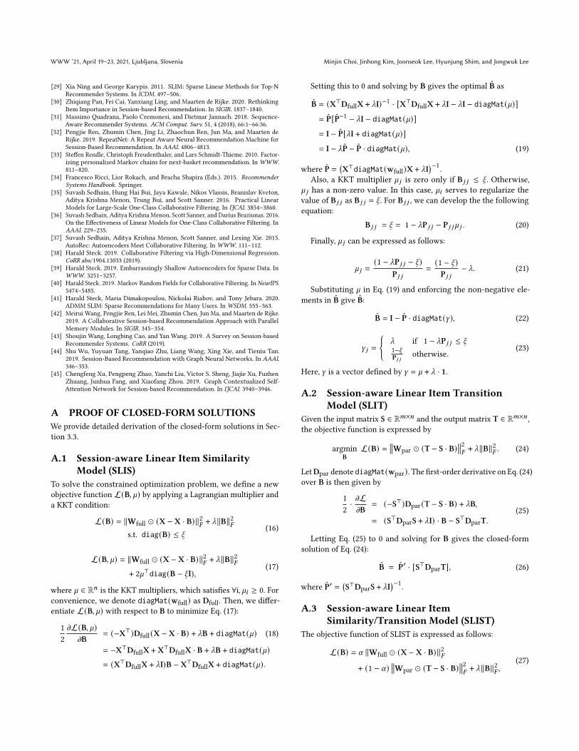
Table 5: Optimized hyperparameters of SLIST. _ is a L2-weight decay, 𝛼 is a mix-ratio between SLIS and SLIT. 𝛿posis a weight decay by item position, 𝛿inf is a weight decay byinference item position and 𝛿time is a weight decay by ses-sion recency.

Dataset _ 𝛼 𝛿pos 𝛿inf 𝛿time

YC-1/64 10 0.4 1 1 4YC-1/4 10 0.2 1 1 8DIGI1 10 0.8 1 2 128

YC 10 0.2 1 1 8DIGI5 10 0.8 1 2 256RR 10 0.2 0.25 4 256

NOWP 10 0.8 1 1 128

We differentiate L(B) with B gives12𝜕L𝜕B

= (−𝛼X⊤)Dfull (X − XB)

+ (−(1 − 𝛼)S⊤)Dpar (T − SB) + _B,

= (𝛼X⊤DfullX + (1 − 𝛼)S⊤DparS + _I) · B− 𝛼X⊤DfullX − (1 − 𝛼)S⊤DparT.

(28)

The optimal B̂ is derived by

B̂ = P̂ · [𝛼X⊤DfullX + (1 − 𝛼)S⊤DparT],= P̂ · [P̂−1 − (1 − 𝛼)S⊤DparS − _I + (1 − 𝛼)S⊤DparT],= I − P̂[_I + (1 − 𝛼)S⊤Dpar (S − T)],= I − P̂_ − (1 − 𝛼)P̂S⊤Dpar (S − T) .

(29)

where P̂ =(𝛼X⊤DfullX + (1 − 𝛼)S⊤DparS + _I

)−1.B REPRODUCIBILITYWe set aside a subset from the training set as a validation set, suchthat the validation contains the same number of days as the testset, e.g., the last 𝑁 days of sessions from the training set.

We use a grid search method for hyperparameter searching.Since the proposed model guarantees the unique answer given thesession via the closed-form solution, it always returns the samerecommendations for the same setting. Thus, the hyperparameteris evaluated only once.

Table 5 summarizes all the hyperparameters for SLIST. The per-formances of the baseline models are taken from the papers [25, 26].For the hyperparameter setting of each model, we refer to [4, 6] forthe setting of STAN and SR-GNN, respectively. For other models,we refer to [25, 26]78. We verify that the performance of baselinemodels is reproduced with an error of 1–2% or less in our imple-mentation environments.

C ADDITIONAL EXPERIMENTAL RESULTSTable 6 reports additional experimental results with different cut-offs, 5 and 10, for all datasets. We observe a similar tendency as

7https://rn5l.github.io/session-rec/umuai/8https://rn5l.github.io/session-rec/index.html

2-3 2-2 2-1 20 21 22 23

pos

0.625

0.65

0.675

0.7

0.725

0.75

0.775

HR

@20

0.225

0.25

0.275

0.3

0.325

0.35

0.375

MR

R@

20

HR@20 MRR@20

2-3 2-2 2-1 20 21 22 23

pos

0.3

0.35

0.4

0.45

0.5

0.55

0.6

HR

@20

0.1

0.125

0.15

0.175

0.2

0.225

0.25

MR

R@

20

HR@20 MRR@20


Figure 6: HR@20 and MRR@20 over varying 𝛿pos in SLISTon YC-1/4 and DIGI1.

2-3 2-2 2-1 20 21 22 23

inf

0.625

0.65

0.675

0.7

0.725

0.75

0.775

HR

@20

0.225

0.25

0.275

0.3

0.325

0.35

0.375

MR

R@

20

HR@20 MRR@20

2-3 2-2 2-1 20 21 22 23

inf

0.3

0.35

0.4

0.45

0.5

0.55

0.6

HR

@20

0.1

0.125

0.15

0.175

0.2

0.225

0.25

MR

R@

20

HR@20 MRR@20


Figure 7: HR@20 and MRR@20 over varying 𝛿inf in SLISTon YC-1/4 and DIGI1.

2-2 20 22 24 26 28 210

time

0.625

0.65

0.675

0.7

0.725

0.75

0.775

HR

@20

0.225

0.25

0.275

0.3

0.325

0.35

0.375

MR

R@

20

HR@20 MRR@20

2-2 20 22 24 26 28 210

time

0.3

0.35

0.4

0.45

0.5

0.55

0.6

HR

@20

0.1

0.125

0.15

0.175

0.2

0.225

0.25

MR

R@

20

HR@20 MRR@20


Figure 8: HR@20 and MRR@20 over varying 𝛿time in SLISTon YC-1/4 and DIGI1.

shown in Table 2. No competing models show the best performanceon all the datasets. For instance, SR-GNN is the best baseline in YC-1/4 and YC-1/64 datasets, and STAN is the best baseline in the otherdatasets. In contrast, SLIST consistently shows the best or second-best performance up to 12.86% in HR@20 and 9.62% in MRR@20over the best competing model.

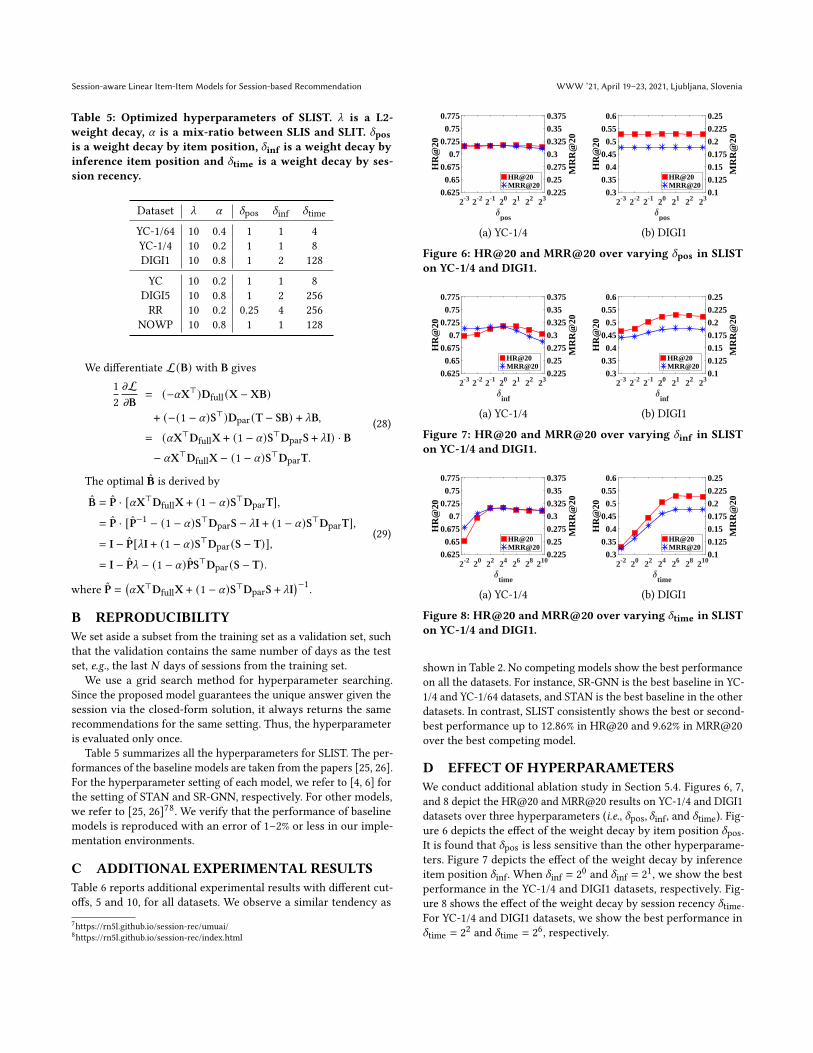
D EFFECT OF HYPERPARAMETERSWe conduct additional ablation study in Section 5.4. Figures 6, 7,and 8 depict the HR@20 and MRR@20 results on YC-1/4 and DIGI1datasets over three hyperparameters (i.e., 𝛿pos, 𝛿inf, and 𝛿time). Fig-ure 6 depicts the effect of the weight decay by item position 𝛿pos.It is found that 𝛿pos is less sensitive than the other hyperparame-ters. Figure 7 depicts the effect of the weight decay by inferenceitem position 𝛿inf. When 𝛿inf = 20 and 𝛿inf = 21, we show the bestperformance in the YC-1/4 and DIGI1 datasets, respectively. Fig-ure 8 shows the effect of the weight decay by session recency 𝛿time.For YC-1/4 and DIGI1 datasets, we show the best performance in𝛿time = 22 and 𝛿time = 26, respectively.


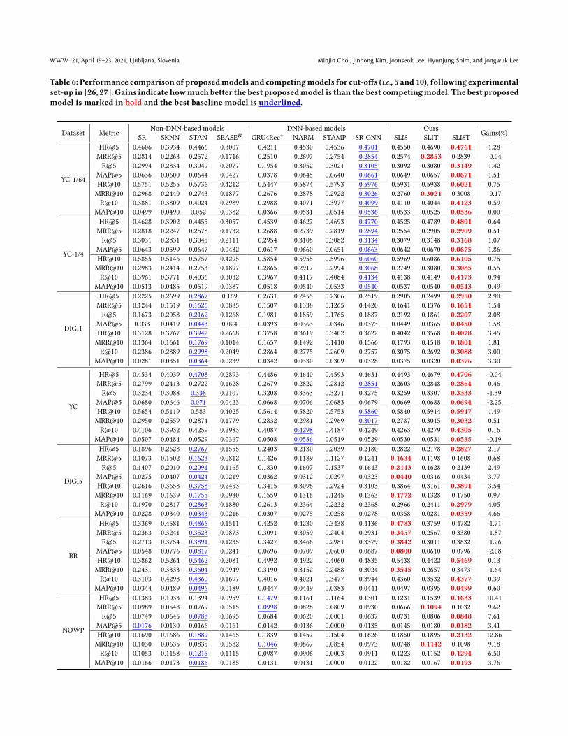
Table 6: Performance comparison of proposedmodels and competingmodels for cut-offs (i.e., 5 and 10), following experimentalset-up in [26, 27]. Gains indicate howmuch better the best proposedmodel is than the best competingmodel. The best proposedmodel is marked in bold and the best baseline model is underlined.

Dataset Metric Non-DNN-based models DNN-based models Ours Gains(%)SR SKNN STAN SEASE𝑅 GRU4Rec+ NARM STAMP SR-GNN SLIS SLIT SLIST

YC-1/64

HR@5 0.4606 0.3934 0.4466 0.3007 0.4211 0.4530 0.4536 0.4701 0.4550 0.4690 0.4761 1.28MRR@5 0.2814 0.2263 0.2572 0.1716 0.2510 0.2697 0.2754 0.2854 0.2574 0.2853 0.2839 -0.04R@5 0.2994 0.2834 0.3049 0.2077 0.1954 0.3052 0.3021 0.3105 0.3092 0.3080 0.3149 1.42

MAP@5 0.0636 0.0600 0.0644 0.0427 0.0378 0.0645 0.0640 0.0661 0.0649 0.0657 0.0671 1.51HR@10 0.5751 0.5255 0.5736 0.4212 0.5447 0.5874 0.5793 0.5976 0.5931 0.5938 0.6021 0.75MRR@10 0.2968 0.2440 0.2743 0.1877 0.2676 0.2878 0.2922 0.3026 0.2760 0.3021 0.3008 -0.17R@10 0.3881 0.3809 0.4024 0.2989 0.2988 0.4071 0.3977 0.4099 0.4110 0.4044 0.4123 0.59

MAP@10 0.0499 0.0490 0.052 0.0382 0.0366 0.0531 0.0514 0.0536 0.0533 0.0525 0.0536 0.00

YC-1/4

HR@5 0.4628 0.3902 0.4455 0.3057 0.4539 0.4627 0.4693 0.4770 0.4525 0.4789 0.4801 0.64MRR@5 0.2818 0.2247 0.2578 0.1732 0.2688 0.2739 0.2819 0.2894 0.2554 0.2905 0.2909 0.51R@5 0.3031 0.2831 0.3045 0.2111 0.2954 0.3108 0.3082 0.3134 0.3079 0.3148 0.3168 1.07

MAP@5 0.0643 0.0599 0.0647 0.0432 0.0617 0.0660 0.0651 0.0663 0.0642 0.0670 0.0675 1.86HR@10 0.5855 0.5146 0.5757 0.4295 0.5854 0.5955 0.5996 0.6060 0.5969 0.6086 0.6105 0.75MRR@10 0.2983 0.2414 0.2753 0.1897 0.2865 0.2917 0.2994 0.3068 0.2749 0.3080 0.3085 0.55R@10 0.3961 0.3771 0.4036 0.3032 0.3967 0.4117 0.4084 0.4134 0.4138 0.4149 0.4173 0.94

MAP@10 0.0513 0.0485 0.0519 0.0387 0.0518 0.0540 0.0533 0.0540 0.0537 0.0540 0.0543 0.49

DIGI1

HR@5 0.2225 0.2699 0.2867 0.169 0.2631 0.2455 0.2306 0.2519 0.2905 0.2499 0.2950 2.90MRR@5 0.1244 0.1519 0.1626 0.0885 0.1507 0.1338 0.1265 0.1420 0.1641 0.1376 0.1651 1.54R@5 0.1673 0.2058 0.2162 0.1268 0.1981 0.1859 0.1765 0.1887 0.2192 0.1861 0.2207 2.08

MAP@5 0.033 0.0419 0.0443 0.024 0.0393 0.0363 0.0346 0.0373 0.0449 0.0365 0.0450 1.58HR@10 0.3128 0.3767 0.3942 0.2668 0.3758 0.3619 0.3402 0.3622 0.4042 0.3568 0.4078 3.45MRR@10 0.1364 0.1661 0.1769 0.1014 0.1657 0.1492 0.1410 0.1566 0.1793 0.1518 0.1801 1.81R@10 0.2386 0.2889 0.2998 0.2049 0.2864 0.2775 0.2609 0.2757 0.3075 0.2692 0.3088 3.00

MAP@10 0.0281 0.0351 0.0364 0.0239 0.0342 0.0330 0.0309 0.0328 0.0375 0.0320 0.0376 3.30

YC

HR@5 0.4534 0.4039 0.4708 0.2893 0.4486 0.4640 0.4593 0.4631 0.4493 0.4679 0.4706 -0.04MRR@5 0.2799 0.2413 0.2722 0.1628 0.2679 0.2822 0.2812 0.2851 0.2603 0.2848 0.2864 0.46R@5 0.3234 0.3088 0.338 0.2107 0.3208 0.3363 0.3271 0.3275 0.3259 0.3307 0.3333 -1.39

MAP@5 0.0680 0.0646 0.071 0.0423 0.0668 0.0706 0.0683 0.0679 0.0669 0.0688 0.0694 -2.25HR@10 0.5654 0.5119 0.583 0.4025 0.5614 0.5820 0.5753 0.5860 0.5840 0.5914 0.5947 1.49MRR@10 0.2950 0.2559 0.2874 0.1779 0.2832 0.2981 0.2969 0.3017 0.2787 0.3015 0.3032 0.51R@10 0.4106 0.3932 0.4259 0.2983 0.4087 0.4298 0.4187 0.4249 0.4263 0.4279 0.4305 0.16

MAP@10 0.0507 0.0484 0.0529 0.0367 0.0508 0.0536 0.0519 0.0529 0.0530 0.0531 0.0535 -0.19

DIGI5

HR@5 0.1896 0.2628 0.2767 0.1555 0.2403 0.2130 0.2039 0.2180 0.2822 0.2178 0.2827 2.17MRR@5 0.1073 0.1502 0.1623 0.0812 0.1426 0.1189 0.1127 0.1241 0.1634 0.1198 0.1608 0.68R@5 0.1407 0.2010 0.2091 0.1165 0.1830 0.1607 0.1537 0.1643 0.2143 0.1628 0.2139 2.49

MAP@5 0.0275 0.0407 0.0424 0.0219 0.0362 0.0312 0.0297 0.0323 0.0440 0.0316 0.0434 3.77HR@10 0.2616 0.3658 0.3758 0.2453 0.3415 0.3096 0.2924 0.3103 0.3864 0.3161 0.3891 3.54MRR@10 0.1169 0.1639 0.1755 0.0930 0.1559 0.1316 0.1245 0.1363 0.1772 0.1328 0.1750 0.97R@10 0.1970 0.2817 0.2863 0.1880 0.2613 0.2364 0.2232 0.2368 0.2966 0.2411 0.2979 4.05

MAP@10 0.0228 0.0340 0.0343 0.0216 0.0307 0.0275 0.0258 0.0278 0.0358 0.0281 0.0359 4.66

RR

HR@5 0.3369 0.4581 0.4866 0.1511 0.4252 0.4230 0.3438 0.4136 0.4783 0.3759 0.4782 -1.71MRR@5 0.2363 0.3241 0.3523 0.0873 0.3091 0.3059 0.2404 0.2931 0.3457 0.2567 0.3380 -1.87R@5 0.2713 0.3754 0.3891 0.1235 0.3427 0.3466 0.2981 0.3379 0.3842 0.3011 0.3832 -1.26

MAP@5 0.0548 0.0776 0.0817 0.0241 0.0696 0.0709 0.0600 0.0687 0.0800 0.0610 0.0796 -2.08HR@10 0.3862 0.5264 0.5462 0.2081 0.4992 0.4922 0.4060 0.4835 0.5438 0.4422 0.5469 0.13MRR@10 0.2431 0.3333 0.3604 0.0949 0.3190 0.3152 0.2488 0.3024 0.3545 0.2657 0.3473 -1.64R@10 0.3103 0.4298 0.4360 0.1697 0.4016 0.4021 0.3477 0.3944 0.4360 0.3532 0.4377 0.39

MAP@10 0.0344 0.0489 0.0496 0.0189 0.0447 0.0449 0.0383 0.0441 0.0497 0.0395 0.0499 0.60

NOWP

HR@5 0.1383 0.1033 0.1394 0.0959 0.1479 0.1161 0.1164 0.1301 0.1231 0.1539 0.1633 10.41MRR@5 0.0989 0.0548 0.0769 0.0515 0.0998 0.0828 0.0809 0.0930 0.0666 0.1094 0.1032 9.62R@5 0.0749 0.0645 0.0788 0.0695 0.0684 0.0620 0.0001 0.0637 0.0731 0.0806 0.0848 7.61

MAP@5 0.0176 0.0130 0.0166 0.0161 0.0142 0.0136 0.0000 0.0135 0.0145 0.0180 0.0182 3.41HR@10 0.1690 0.1686 0.1889 0.1465 0.1839 0.1457 0.1504 0.1626 0.1850 0.1895 0.2132 12.86MRR@10 0.1030 0.0635 0.0835 0.0582 0.1046 0.0867 0.0854 0.0973 0.0748 0.1142 0.1098 9.18R@10 0.1053 0.1158 0.1215 0.1115 0.0987 0.0906 0.0003 0.0911 0.1223 0.1152 0.1294 6.50

MAP@10 0.0166 0.0173 0.0186 0.0185 0.0131 0.0131 0.0000 0.0122 0.0182 0.0167 0.0193 3.76

Documents

Session-aware Linear Item-Item Models for Session-based