Set Similarity Joins on MapReduce: An ExperimentalSurvey

Fabian FierHumboldt-Universitat zu Berlin

Unter den Linden 610099 Berlin, Germany

fier@informatik.hu-berlin.de

Nikolaus AugstenUniversitat Salzburg

Jakob-Haringer-Str. 25020 Salzburg, Austria

nikolaus.augsten@sbg.ac.at

Panagiotis BourosJohannes Gutenberg

University MainzSaarstr. 21

55122 Mainz, Germany

bouros@uni-mainz.deUlf Leser

Humboldt-Universitat zu BerlinUnter den Linden 6

10099 Berlin, Germany

leser@informatik.hu-berlin.de

Johann-ChristophFreytag

Humboldt-Universitat zu BerlinUnter den Linden 6

10099 Berlin, Germany

freytag@informatik.hu-berlin.de

ABSTRACTSet similarity joins, which compute pairs of similar sets, consti-tute an important operator primitive in a variety of applications,including applications that must process large amounts of data. Tohandle these data volumes, several distributed set similarity join al-gorithms have been proposed. Unfortunately, little is known aboutthe relative performance, strengths and weaknesses of these tech-niques. Previous comparisons are limited to a small subset of rele-vant algorithms, and the large differences in the various test setupsmake it hard to draw overall conclusions.

In this paper we survey ten recent, distributed set similarity joinalgorithms, all based on the MapReduce paradigm. We empiricallycompare the algorithms in a uniform test environment on twelvedatasets that expose different characteristics and represent a broadrange of applications. Our experiments yield a surprising result:All algorithms in our test fail to scale for at least one dataset and aresensitive to long sets, frequent set elements, low similarity thresh-olds, or a combination thereof. Interestingly, some algorithms evenfail to handle the small datasets that can easily be processed in anon-distributed setting. Our analytic investigation of the algorithmspinpoints the reasons for the poor performance and targeted exper-iments confirm our analytic findings. Based on our investigation,we suggest directions for future research in the area.

PVLDB Reference Format:Fabian Fier, Nikolaus Augsten, Panagiotis Bouros, Ulf Leser, and Johann-Christoph Freytag. Set Similarity Joins on MapReduce: An ExperimentalSurvey. PVLDB, 11(10): 1110 - 1122, 2018.DOI: https://doi.org/10.14778/3231751.3231760

Permission to make digital or hard copies of all or part of this work forpersonal or classroom use is granted without fee provided that copies arenot made or distributed for profit or commercial advantage and that copiesbear this notice and the full citation on the first page. To copy otherwise, torepublish, to post on servers or to redistribute to lists, requires prior specificpermission and/or a fee. Articles from this volume were invited to presenttheir results at The 44th International Conference on Very Large Data Bases,August 2018, Rio de Janeiro, Brazil.Proceedings of the VLDB Endowment, Vol. 11, No. 10Copyright 2018 VLDB Endowment 2150-8097/18/06.DOI: https://doi.org/10.14778/3231751.3231760

1. INTRODUCTIONThe set similarity join (SSJ) computes all pairs of similar sets

from two collections of sets. Two sets are similar if their normal-ized overlap exceeds some user-defined threshold; the most popularnormalizations are Jaccard and Cosine similarity1. Applications ofSSJ are, for instance, the detection of pairs of similar texts (mod-eled as sets of tokens) [29], strings or trees (modeled as sets ofn-grams resp. pq-grams) [31, 3], entities (modeled as sets of at-tribute values) [11], the identification of click fraudsters in onlineadvertising [20], or collaborative filtering [6].

Conceptually, the set similarity join between two collections Sand R must perform |S| · |R| set comparisons, which is not fea-sible. Efficient techniques for SSJ use filters to avoid comparinghopeless set pairs, i.e., pairs that provably cannot pass the thresh-old [6, 7, 34]. We distinguish two classes of filters. Filter-and-verification techniques use set prefixes or signatures followed byan explicit verification of candidate pairs (e.g., [6, 34]). Metric-based approaches partition the space of all sets such that similarsets fall into the same or nearby partitions (e.g. [13]). The lattermethods require the set similarity function to be metric.

For large datasets, which cannot be handled by a single computenode, distributed SSJ algorithms are required. In recent years, anumber of solutions for the distributed SSJ have been proposed,most of which are based on the MapReduce paradigm. These so-lutions include (by publication year) FullFiltering [12], Vernica-Join [30], SSJ-2R [5], FuzzyJoin [1], V-SMART [21], MRSim-Join [27], MG-Join [24], MAPPS [32], ClusterJoin [25], Mass-Join [9], MRGroupJoin [10], FS-Join [23], DIMA [28]. While non-distributed solutions have been recently compared in experimen-tal studies [14, 19], we are not aware of any comprehensive com-parison of distributed SSJ algorithms. The only exception is thework by Silva et al. [26], which compares FuzzyJoin [1], MRTheta-Join [22], MRSimJoin [22], Vernica [30], and V-SMART [21]. How-ever, many relevant competitors are missing in this benchmark, andthe experiments were performed on a single dataset, which limits

1Algorithms for edit-based string similarity joins often use SSJ toreduce the number of candidate pairs, e.g. [2].

1110

� � �� �� � �� �� � �� ��

������ �� ���� �

������������ ������!

������ �� ��"� � #

���������$ �� ���� �� %

�� �� ��&� �� # % #

���� �� �'� � # % # %

���� �� ��(� �� % % %

�� )�� ��� �� % %

����*� �� �+"� � # # # # # # #

�)��,�� ���� �� % % % %

��) �� ��+� �� # % # % # # # % #

��������������������-������ ��������������������!

./���� #����

%��� %���

#��&�

#�'� %��+�

#���

%�����#���� %��+�

%��+�

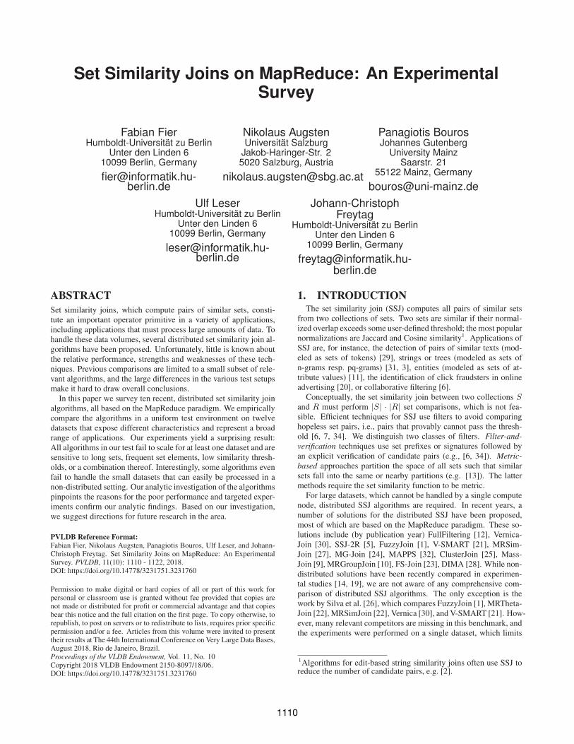
Figure 1: Overview over previous (upper right triangle) com-parisons and those performed in this work (lower left triangle).A ”>” indicates that the algorithm in the row is faster than theone in the column according to the respective publication.

their expressiveness. The empirical evaluations in the original pub-lications of the algorithms provide only an incomplete picture (seeFigure 1).

In this paper, we perform a comparative evaluation of the ten dis-tributed SSJ approaches listed in Figure 1 that build on top of theMapReduce framework [8]. To provide a fair experimental setup,we do not tailor parameters, data preprocessing, implementationdetails, system configuration details or the problem statement towork especially well with one algorithm. We do not include [28]in our study since the DIMA in-memory system (i) builds on top ofSpark by extending the Catalyst optimizer and (ii) the proposed ap-proach for similarity joins employs offline distributed indexing. Wealso exclude FuzzyJoin [1] which focuses on string similarity mea-sures; although arguing that the proposed methods can be adaptedfor set similarity measures, the authors do not elaborate on this is-sue. Further, we do not consider MAPSS [32] which is tailored todense vectors; note that vector representations of sets are typicallyextremely sparse. Last, we exclude [16, 18, 17], which also focuson vector data and on Euclidian distance rendering the proposedtechniques not applicable to set similarity measures.

We base our comparison on twelve datasets (ten real-life andtwo synthetic datasets) of varying sizes and characteristics. Allmethods were reimplemented or adapted to remove bias stemmingfrom different code quality. We further removed pre- and/or post-processing steps and thus reduced all methods to their core: thecomputation of SSJ. Since all tested algorithms are based on theHadoop implementation of MapReduce, we run all comparisonson the same Hadoop cluster. We repeat experiments from the orig-inal works and – where the results differ – discuss reasons for thedeviations. We further perform a qualitative comparison of all al-gorithms. We systematically discuss and illustrate their map andreduce steps and provide an example for most algorithms. We an-alyze their expected intermediate dataset sizes and distribution andother factors that may have an impact on runtime and scalability.This analysis forms the basis for the subsequent discussion andhelps to explain our experimental results.

Our findings are sobering for various reasons. First, the dis-tributed SSJ algorithms are often orders of magnitude slower thantheir non-distributed counterparts for the same datasets and thresh-old settings (runtimes as reported by Mann et al. [19]). This can beonly partially explained by the overhead of the Hadoop framework,which we measure. Second, we expected the distributed algorithmsto scale to very large datasets that cannot be handled by a singlemachine. However, we observe that all algorithms in our test runinto timeouts for at least one of the datasets. This cannot be fixedby increasing the cluster size since the algorithms fail to evenlydistribute the workload and individual nodes are overloaded.

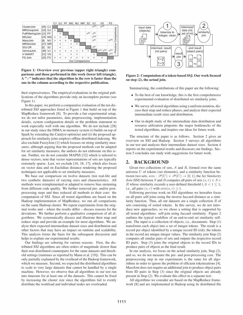
Figure 2: Computation of a token-based SSJ. Our work focusedon step (2), the actual join.

Summarizing, the contributions of this paper are the following:

• To the best of our knowledge, this is the first comprehensiveexperimental evaluation of distributed set similarity joins.

• We survey all tested algorithms using a uniform notation, dis-cuss their map and reduce phases, and analyze their expectedintermediate result sizes and distribution.

• Our in-depth study of the intermediate data distribution andresource utilization pinpoints the major bottlenecks of thetested algorithms, and inspires our ideas for future work.

The structure of the paper is as follows. Section 2 gives anoverview on SSJ and Hadoop. Section 3 surveys all algorithmsin our test and analyses their intermediate dataset sizes. Section 4reports on the experimental results and discusses our findings. Sec-tion 5 concludes our study with suggestions for future work.

2. BACKGROUNDGiven two collections of sets, S and R, formed over the same

universe U of tokens (set elements), and a similarity function be-tween two sets, sim : P(U)× P(U) → [0, 1]; the Set SimilarityJoin (SSJ) between S and R computes all pairs of sets (s, r) ∈ S×R whose similarity exceeds a user-defined threshold t, 0 < t ≤ 1,i.e., all pairs (s, r) with sim(s, r) ≥ t.

Following previous work on SSJ algorithms we hereafter focuson all-pairs self-joins using the inverse Jaccard distance as a simi-larity function. Thus, all our datasets are a single collection R ofsets consisting of sorted tokens. In this survey, we do not intro-duce new approaches, so we chose a setting that is supported byall tested algorithms: self-join using Jaccard similarity. Figure 2outlines the typical workflow of an end-to-end set similarity self-join. The input is a collection of objects, i.e., documents. Step (1)transforms each object into a set of integer tokens. The result is arecord per object identified by a unique record ID (rid); the tokensin the record are unique integer values. The similarity join Step (2)computes all similar pairs of sets and outputs the respective recordID pairs. Step (3) joins the original objects to the record IDs toproduce pairs of objects as the final result.

In our analysis, we focus on the actual similarity join, Step (2),and so, we do not measure the pre- and post-processing cost. Thepreprocessing step in our experiments is the same for all algo-rithms in order to ignore the problem of efficient tokenizations [4].MassJoin does not require an additional join to produce object pairsfrom ID pairs in Step (3) since the original objects are alreadypresent in Step (2). We evaluate this effect in a separate test.

All algorithms we consider are based on the MapReduce frame-work [8] and are implemented in Hadoop using its distributed file

1111

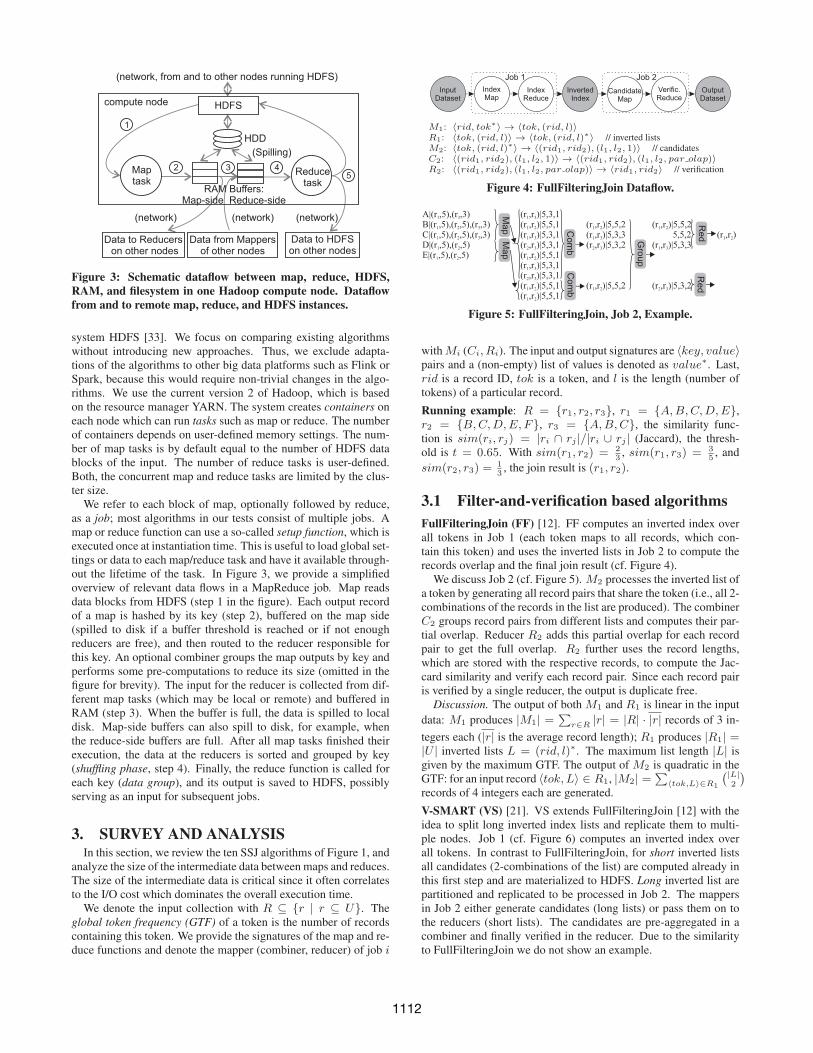
Figure 3: Schematic dataflow between map, reduce, HDFS,RAM, and filesystem in one Hadoop compute node. Dataflowfrom and to remote map, reduce, and HDFS instances.

system HDFS [33]. We focus on comparing existing algorithmswithout introducing new approaches. Thus, we exclude adapta-tions of the algorithms to other big data platforms such as Flink orSpark, because this would require non-trivial changes in the algo-rithms. We use the current version 2 of Hadoop, which is basedon the resource manager YARN. The system creates containers oneach node which can run tasks such as map or reduce. The numberof containers depends on user-defined memory settings. The num-ber of map tasks is by default equal to the number of HDFS datablocks of the input. The number of reduce tasks is user-defined.Both, the concurrent map and reduce tasks are limited by the clus-ter size.

We refer to each block of map, optionally followed by reduce,as a job; most algorithms in our tests consist of multiple jobs. Amap or reduce function can use a so-called setup function, which isexecuted once at instantiation time. This is useful to load global set-tings or data to each map/reduce task and have it available through-out the lifetime of the task. In Figure 3, we provide a simplifiedoverview of relevant data flows in a MapReduce job. Map readsdata blocks from HDFS (step 1 in the figure). Each output recordof a map is hashed by its key (step 2), buffered on the map side(spilled to disk if a buffer threshold is reached or if not enoughreducers are free), and then routed to the reducer responsible forthis key. An optional combiner groups the map outputs by key andperforms some pre-computations to reduce its size (omitted in thefigure for brevity). The input for the reducer is collected from dif-ferent map tasks (which may be local or remote) and buffered inRAM (step 3). When the buffer is full, the data is spilled to localdisk. Map-side buffers can also spill to disk, for example, whenthe reduce-side buffers are full. After all map tasks finished theirexecution, the data at the reducers is sorted and grouped by key(shuffling phase, step 4). Finally, the reduce function is called foreach key (data group), and its output is saved to HDFS, possiblyserving as an input for subsequent jobs.

3. SURVEY AND ANALYSISIn this section, we review the ten SSJ algorithms of Figure 1, and

analyze the size of the intermediate data between maps and reduces.The size of the intermediate data is critical since it often correlatesto the I/O cost which dominates the overall execution time.

We denote the input collection with R ⊆ {r | r ⊆ U}. Theglobal token frequency (GTF) of a token is the number of recordscontaining this token. We provide the signatures of the map and re-duce functions and denote the mapper (combiner, reducer) of job i

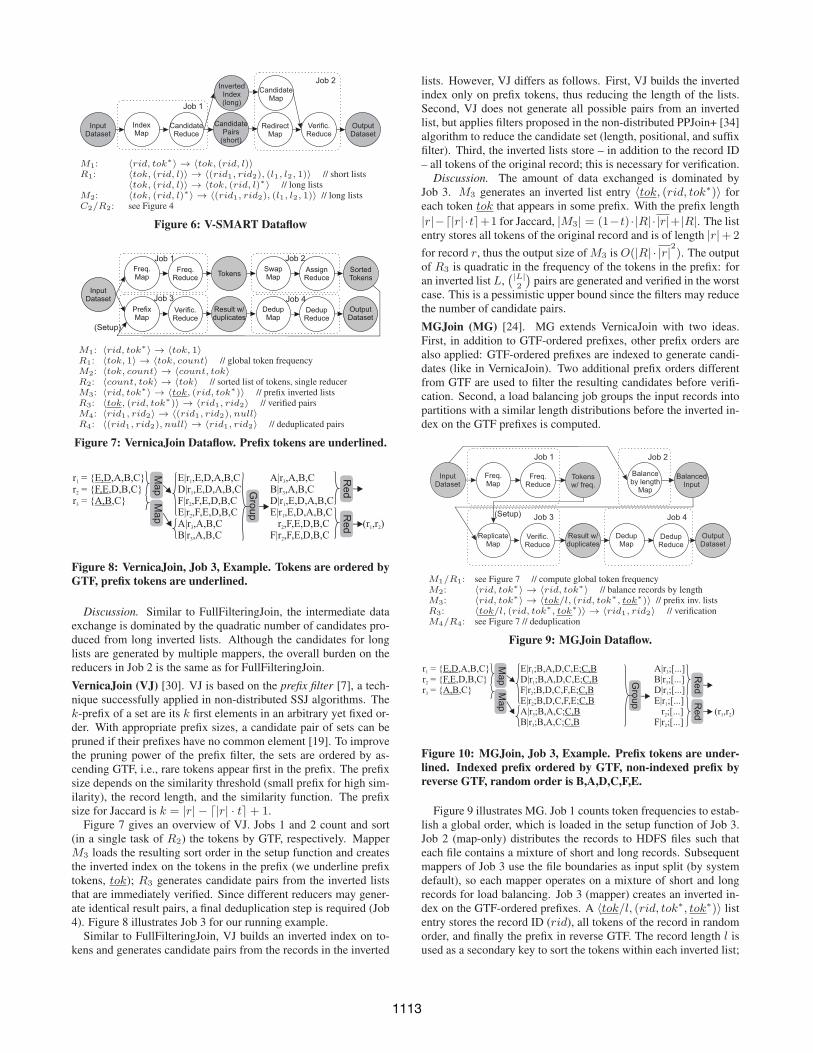
M1: 〈rid, tok∗〉 → 〈tok, (rid, l)〉R1: 〈tok, (rid, l)〉 → 〈tok, (rid, l)∗〉 // inverted listsM2: 〈tok, (rid, l)∗〉 → 〈(rid1, rid2), (l1, l2, 1)〉 // candidatesC2: 〈(rid1, rid2), (l1, l2, 1)〉 → 〈(rid1, rid2), (l1, l2, par olap)〉R2: 〈(rid1, rid2), (l1, l2, par olap)〉 → 〈rid1, rid2〉 // verification

Figure 4: FullFilteringJoin Dataflow.

Figure 5: FullFilteringJoin, Job 2, Example.

with Mi (Ci, Ri). The input and output signatures are 〈key, value〉pairs and a (non-empty) list of values is denoted as value∗. Last,rid is a record ID, tok is a token, and l is the length (number oftokens) of a particular record.

Running example: R = {r1, r2, r3}, r1 = {A,B,C,D,E},r2 = {B,C,D,E, F}, r3 = {A,B,C}, the similarity func-tion is sim(ri, rj) = |ri ∩ rj |/|ri ∪ rj | (Jaccard), the thresh-old is t = 0.65. With sim(r1, r2) = 2

3, sim(r1, r3) = 3

5, and

sim(r2, r3) =13

, the join result is (r1, r2).

3.1 Filter-and-verification based algorithmsFullFilteringJoin (FF) [12]. FF computes an inverted index overall tokens in Job 1 (each token maps to all records, which con-tain this token) and uses the inverted lists in Job 2 to compute therecords overlap and the final join result (cf. Figure 4).

We discuss Job 2 (cf. Figure 5). M2 processes the inverted list ofa token by generating all record pairs that share the token (i.e., all 2-combinations of the records in the list are produced). The combinerC2 groups record pairs from different lists and computes their par-tial overlap. Reducer R2 adds this partial overlap for each recordpair to get the full overlap. R2 further uses the record lengths,which are stored with the respective records, to compute the Jac-card similarity and verify each record pair. Since each record pairis verified by a single reducer, the output is duplicate free.

Discussion. The output of both M1 and R1 is linear in the input

data: M1 produces |M1| = ∑r∈R |r| = |R| · |r| records of 3 in-

tegers each (|r| is the average record length); R1 produces |R1| =|U | inverted lists L = (rid, l)∗. The maximum list length |L| isgiven by the maximum GTF. The output of M2 is quadratic in theGTF: for an input record 〈tok, L〉 ∈ R1, |M2| = ∑

〈tok,L〉∈R1

(|L|2

)

records of 4 integers each are generated.

V-SMART (VS) [21]. VS extends FullFilteringJoin [12] with theidea to split long inverted index lists and replicate them to multi-ple nodes. Job 1 (cf. Figure 6) computes an inverted index overall tokens. In contrast to FullFilteringJoin, for short inverted listsall candidates (2-combinations of the list) are computed already inthis first step and are materialized to HDFS. Long inverted list arepartitioned and replicated to be processed in Job 2. The mappersin Job 2 either generate candidates (long lists) or pass them on tothe reducers (short lists). The candidates are pre-aggregated in acombiner and finally verified in the reducer. Due to the similarityto FullFilteringJoin we do not show an example.

1112

M1: 〈rid, tok∗〉 → 〈tok, (rid, l)〉R1: 〈tok, (rid, l)〉 → 〈(rid1, rid2), (l1, l2, 1)〉 // short lists

〈tok, (rid, l)〉 → 〈tok, (rid, l)∗〉 // long listsM2: 〈tok, (rid, l)∗〉 → 〈(rid1, rid2), (l1, l2, 1)〉 // long listsC2/R2: see Figure 4

Figure 6: V-SMART Dataflow

M1: 〈rid, tok∗〉 → 〈tok, 1〉R1: 〈tok, 1〉 → 〈tok, count〉 // global token frequencyM2: 〈tok, count〉 → 〈count, tok〉R2: 〈count, tok〉 → 〈tok〉 // sorted list of tokens, single reducerM3: 〈rid, tok∗〉 → 〈tok, (rid, tok∗)〉 // prefix inverted listsR3: 〈tok, (rid, tok∗)〉 → 〈rid1, rid2〉 // verified pairsM4: 〈rid1, rid2〉 → 〈(rid1, rid2), null〉R4: 〈(rid1, rid2), null〉 → 〈rid1, rid2〉 // deduplicated pairs

Figure 7: VernicaJoin Dataflow. Prefix tokens are underlined.

Figure 8: VernicaJoin, Job 3, Example. Tokens are ordered byGTF, prefix tokens are underlined.

Discussion. Similar to FullFilteringJoin, the intermediate dataexchange is dominated by the quadratic number of candidates pro-duced from long inverted lists. Although the candidates for longlists are generated by multiple mappers, the overall burden on thereducers in Job 2 is the same as for FullFilteringJoin.

VernicaJoin (VJ) [30]. VJ is based on the prefix filter [7], a tech-nique successfully applied in non-distributed SSJ algorithms. Thek-prefix of a set are its k first elements in an arbitrary yet fixed or-der. With appropriate prefix sizes, a candidate pair of sets can bepruned if their prefixes have no common element [19]. To improvethe pruning power of the prefix filter, the sets are ordered by as-cending GTF, i.e., rare tokens appear first in the prefix. The prefixsize depends on the similarity threshold (small prefix for high sim-ilarity), the record length, and the similarity function. The prefixsize for Jaccard is k = |r| − �|r| · t�+ 1.

Figure 7 gives an overview of VJ. Jobs 1 and 2 count and sort(in a single task of R2) the tokens by GTF, respectively. MapperM3 loads the resulting sort order in the setup function and createsthe inverted index on the tokens in the prefix (we underline prefixtokens, tok); R3 generates candidate pairs from the inverted liststhat are immediately verified. Since different reducers may gener-ate identical result pairs, a final deduplication step is required (Job4). Figure 8 illustrates Job 3 for our running example.

Similar to FullFilteringJoin, VJ builds an inverted index on to-kens and generates candidate pairs from the records in the inverted

lists. However, VJ differs as follows. First, VJ builds the invertedindex only on prefix tokens, thus reducing the length of the lists.Second, VJ does not generate all possible pairs from an invertedlist, but applies filters proposed in the non-distributed PPJoin+ [34]algorithm to reduce the candidate set (length, positional, and suffixfilter). Third, the inverted lists store – in addition to the record ID– all tokens of the original record; this is necessary for verification.

Discussion. The amount of data exchanged is dominated byJob 3. M3 generates an inverted list entry 〈tok, (rid, tok∗)〉 foreach token tok that appears in some prefix. With the prefix length

|r|−�|r| ·t�+1 for Jaccard, |M3| = (1−t) · |R| · |r|+ |R|. The listentry stores all tokens of the original record and is of length |r|+2

for record r, thus the output size of M3 is O(|R| · |r|2). The outputof R3 is quadratic in the frequency of the tokens in the prefix: foran inverted list L,

(|L|2

)pairs are generated and verified in the worst

case. This is a pessimistic upper bound since the filters may reducethe number of candidate pairs.

MGJoin (MG) [24]. MG extends VernicaJoin with two ideas.First, in addition to GTF-ordered prefixes, other prefix orders arealso applied: GTF-ordered prefixes are indexed to generate candi-dates (like in VernicaJoin). Two additional prefix orders differentfrom GTF are used to filter the resulting candidates before verifi-cation. Second, a load balancing job groups the input records intopartitions with a similar length distributions before the inverted in-dex on the GTF prefixes is computed.

M1/R1: see Figure 7 // compute global token frequencyM2: 〈rid, tok∗〉 → 〈rid, tok∗〉 // balance records by lengthM3: 〈rid, tok∗〉 → 〈tok/l, (rid, tok∗, tok∗)〉 // prefix inv. listsR3: 〈tok/l, (rid, tok∗, tok∗)〉 → 〈rid1, rid2〉 // verificationM4/R4: see Figure 7 // deduplication

Figure 9: MGJoin Dataflow.

Figure 10: MGJoin, Job 3, Example. Prefix tokens are under-lined. Indexed prefix ordered by GTF, non-indexed prefix byreverse GTF, random order is B,A,D,C,F,E.

Figure 9 illustrates MG. Job 1 counts token frequencies to estab-lish a global order, which is loaded in the setup function of Job 3.Job 2 (map-only) distributes the records to HDFS files such thateach file contains a mixture of short and long records. Subsequentmappers of Job 3 use the file boundaries as input split (by systemdefault), so each mapper operates on a mixture of short and longrecords for load balancing. Job 3 (mapper) creates an inverted in-dex on the GTF-ordered prefixes. A 〈tok/l, (rid, tok∗, tok∗)〉 listentry stores the record ID (rid), all tokens of the record in randomorder, and finally the prefix in reverse GTF. The record length l isused as a secondary key to sort the tokens within each inverted list;

1113

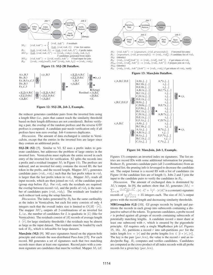
M1: 〈rid, tok∗〉 →{

〈rid, tok∗〉 // residuals

〈tok, (rid, tok, l)〉 // inv. list entries

R1: 〈tok, (rid, tok, l)〉 → 〈tok, (rid, tok, l)∗〉 // prefix indexMC2: 〈tok, (rid, tok, l)∗〉 → 〈(rid1, rid2), (rid2, tok, l2)〉

// candidates generated from indexMI 2: 〈rid, tok∗〉 → 〈(rid, null), tok∗〉 // load input for joinR2: 〈(rid1, rid2|null), tok∗|(rid2, tok, l2)〉→〈rid1, rid2〉

Figure 11: SSJ-2R Dataflow.

Figure 12: SSJ-2R, Job 2, Example.

the reducer generates candidate pairs from the inverted lists usinga length filter (i.e., pairs that cannot reach the similarity thresholdbased on their length difference are not considered). Before verify-ing a pair, the overlap of the random prefixes and the reverse GTFprefixes is computed. A candidate pair needs verification only if allprefixes have non-zero overlap. Job 4 removes duplicates.

Discussion. The amount of data exchanged is similar to Verni-caJoin, except that the entries in the inverted lists are larger sincethey contain an additional prefix.

SSJ-2R (S2) [5]. Similar to VJ, S2 uses a prefix index to gen-erate candidates, but addresses the problem of large entries in theinverted lists. VernicaJoin must replicate the entire record in eachentry of the inverted list for verification. S2 splits the records intoa prefix and a residual (mapper M1 in Figure 11). The prefixes areindexed, and an inverted list entry contains the record ID, the lasttoken in the prefix, and the record length. Mapper MC 2 generatescandidate pairs (rid1, rid2) such that the last prefix token in rid1is larger than the last prefix token in rid2. Mapper MI 2 reads allinput records, which are then joined on rid1 of the candidate pairs(group step before R2). For rid2 only the residuals are required:the overlap between record rid1 and the prefix of rid2 is the num-ber of candidates pairs (rid1, rid2). The residuals are loaded toeach reducer task using the setup function.

Discussion. The index generated by R2 has the same cardinalityas the index in VernicaJoin, but each list entry consists of only 4

integers such that the overall index size is limited to O(|R| · |r|).The mapper MC 2 outputs all 2-combinations of an inverted listL, i.e., the number of candidates for L is quadratic in |L| (like forVernicaJoin). The residuals consist of |R| records of average length

t · |r|; for large similarity thresholds t the residuals may be almostas large as the input dataset. The residuals must be loaded by eachtask of R2, which is infeasible for large datasets.

MassJoin (MJ) [9]. MJ uses signatures based on the pigeon-holeprinciple and extends the non-distributed Pass-Join [15]. For eachrecord, MJ generates a set of signatures such that two matchingrecords must share at least one signature. Record pairs with a com-mon signature are candidates that must be verified. Mapper M1 (cf.

M1: 〈rid, tok∗〉 → 〈signature, (rid, pruneinfo)〉 // inverted list entryR1: 〈signature, (rid, pruneinfo)〉 → 〈rid1, rid

∗2〉 // candidate list of rid1

M2: (identity)R2: 〈rid1, (rid

∗2 |tok∗)〉 → 〈rid1, (rid

∗2 , tok

∗)〉 // get tokens of rid1

M3a:〈rid1, (rid∗2 , tok

∗)〉 → 〈rid2, (rid1, tok∗)〉 // prepare join on rid2

M3b: (identity)R3: 〈rid2, (rid1, tok

∗)|tok∗〉 → 〈rid1, rid2〉 // get tokens of rid2, verify

Figure 13: MassJoin Dataflow.

Figure 14: MassJoin, Job 1, Example.

Figures 13) computes an inverted index on signatures. The list en-tries are record IDs with some additional information for pruning.Reducer R1 generates candidate pairs (all 2-combinations) from aninverted list; the pruning info is leveraged to decrease the candidateset. The output format is a record ID with a list of candidates (inFigure 14 the candidate lists are of length 1). Jobs 2 and 3 join theinput to the candidate pairs to verify the candidates in R3.

Discussion. The amount of exchanged data is dominated byM1’s output. In [9], the authors show that M1 generates |M1| =∑

r∈R(1+t3)(1−t)3

t3· |r| · C + 1−t

t· |r| (C is a constant) signature

records of|r|

1−tt

·|r|+1+ 35 integers each. The size of M1’s output

grows with the record length and decreasing similarity thresholds.

MRGroupJoin (GJ) [10]. GJ groups records by length and par-titions the records in each group into subrecords containing a dis-junctive subset of the tokens. To generate candidates, a probe recordr is probed against all groups of records containing subrecords ofpotentially matching lengths. A candidate record s must share atleast one subrecord with r, which is ensured by the pigeonholeprinciple. GJ requires only a single MapReduce job (cf. Figures15, 16). M1 partitions a record r into sub-partitions par for theindex length len = |r| and the probe lengths len ∈ [t ∗ |r|, |r|].The key is the pair (par, len), the value is the record r and an in-dex/probe flag. R1 computes and verifies candidates. Candidatesare computed as the cross product of all index records with all proberecords for a given key (par, len).

1114

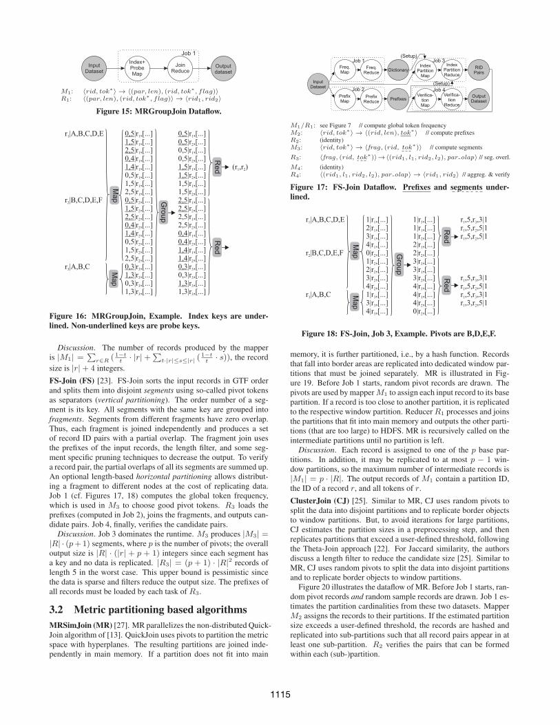
M1: 〈rid, tok∗〉 → 〈(par, len), (rid, tok∗, flag)〉R1: 〈(par, len), (rid, tok∗, flag)〉 → 〈rid1, rid2〉

Figure 15: MRGroupJoin Dataflow.

Figure 16: MRGroupJoin, Example. Index keys are under-lined. Non-underlined keys are probe keys.

Discussion. The number of records produced by the mapperis |M1| = ∑

r∈R ( 1−tt

· |r|+∑t·|r|≤s≤|r| (

1−tt

· s)), the record

size is |r|+ 4 integers.

FS-Join (FS) [23]. FS-Join sorts the input records in GTF orderand splits them into disjoint segments using so-called pivot tokensas separators (vertical partitioning). The order number of a seg-ment is its key. All segments with the same key are grouped intofragments. Segments from different fragments have zero overlap.Thus, each fragment is joined independently and produces a setof record ID pairs with a partial overlap. The fragment join usesthe prefixes of the input records, the length filter, and some seg-ment specific pruning techniques to decrease the output. To verifya record pair, the partial overlaps of all its segments are summed up.An optional length-based horizontal partitioning allows distribut-ing a fragment to different nodes at the cost of replicating data.Job 1 (cf. Figures 17, 18) computes the global token frequency,which is used in M3 to choose good pivot tokens. R3 loads theprefixes (computed in Job 2), joins the fragments, and outputs can-didate pairs. Job 4, finally, verifies the candidate pairs.

Discussion. Job 3 dominates the runtime. M3 produces |M3| =|R| · (p+1) segments, where p is the number of pivots; the overalloutput size is |R| · (|r| + p + 1) integers since each segment hasa key and no data is replicated. |R3| = (p + 1) · |R|2 records oflength 5 in the worst case. This upper bound is pessimistic sincethe data is sparse and filters reduce the output size. The prefixes ofall records must be loaded by each task of R3.

3.2 Metric partitioning based algorithmsMRSimJoin (MR) [27]. MR parallelizes the non-distributed Quick-Join algorithm of [13]. QuickJoin uses pivots to partition the metricspace with hyperplanes. The resulting partitions are joined inde-pendently in main memory. If a partition does not fit into main

M1/R1: see Figure 7 // compute global token frequencyM2: 〈rid, tok∗〉 → 〈(rid, len), tok∗〉 // compute prefixesR2: (identity)M3: 〈rid, tok∗〉 → 〈frag, (rid, tok∗)〉 // compute segments

R3: 〈frag, (rid, tok∗)〉→〈(rid1, l1, rid2, l2), par olap〉 // seg. overl.

M4: (identity)R4: 〈(rid1, l1, rid2, l2), par olap〉 → 〈rid1, rid2〉 // aggreg. & verify

Figure 17: FS-Join Dataflow. Prefixes and segments under-lined.

Figure 18: FS-Join, Job 3, Example. Pivots are B,D,E,F.

memory, it is further partitioned, i.e., by a hash function. Recordsthat fall into border areas are replicated into dedicated window par-titions that must be joined separately. MR is illustrated in Fig-ure 19. Before Job 1 starts, random pivot records are drawn. Thepivots are used by mapper M1 to assign each input record to its basepartition. If a record is too close to another partition, it is replicatedto the respective window partition. Reducer R1 processes and joinsthe partitions that fit into main memory and outputs the other parti-tions (that are too large) to HDFS. MR is recursively called on theintermediate partitions until no partition is left.

Discussion. Each record is assigned to one of the p base par-titions. In addition, it may be replicated to at most p − 1 win-dow partitions, so the maximum number of intermediate records is|M1| = p · |R|. The output records of M1 contain a partition ID,the ID of a record r, and all tokens of r.

ClusterJoin (CJ) [25]. Similar to MR, CJ uses random pivots tosplit the data into disjoint partitions and to replicate border objectsto window partitions. But, to avoid iterations for large partitions,CJ estimates the partition sizes in a preprocessing step, and thenreplicates partitions that exceed a user-defined threshold, followingthe Theta-Join approach [22]. For Jaccard similarity, the authorsdiscuss a length filter to reduce the candidate size [25]. Similar toMR, CJ uses random pivots to split the data into disjoint partitionsand to replicate border objects to window partitions.

Figure 20 illustrates the dataflow of MR. Before Job 1 starts, ran-dom pivot records and random sample records are drawn. Job 1 es-timates the partition cardinalities from these two datasets. MapperM2 assigns the records to their partitions. If the estimated partitionsize exceeds a user-defined threshold, the records are hashed andreplicated into sub-partitions such that all record pairs appear in atleast one sub-partition. R2 verifies the pairs that can be formedwithin each (sub-)partition.

1115

M1: 〈rid, tok∗〉 → 〈partition, (rid, tok∗)〉R1: 〈partition, (rid, tok∗)〉 → 〈rid1, rid2〉

Figure 19: MRSimJoin Dataflow.

M1: 〈rid, tok∗〉 → 〈partition, size〉 // estimate partition sizesM2: 〈rid, tok∗〉 → 〈partition, (rid, tok∗)〉R2: 〈partition, (rid, tok∗)〉 → 〈rid1, rid2〉

Figure 20: ClusterJoin Dataflow until no intermediate data isleft.

Discussion. The size of the intermediate results is at least M2 =|R| (if no records fall into a window partition and all partitions aresmall). In addition, there may be at most (p − 1) · |R| records inwindow partitions. Finally, large partitions are split and replicated;the size of all sub-partitions is quadratic in the partition size, whichmay substantially increase the intermediate result size.

4. COMPARATIVE EVALUATIONWe next present our experimental analysis. We implemented all

algorithms from Section 3 (FF, GJ, MG, MJ, VS) or adapted exist-ing code if available (CJ, FS, MR, S2, VJ). We evaluated the algo-rithms using 12 datasets. Our analysis focuses on runtime, but wealso discuss data grouping, data replication, and cluster utilization.

4.1 SetupHadoop. We deployed all methods on Hadoop 2.7 (using YARN,cf. Section 2). The experiments run on an exclusively used clusterof 12 nodes equipped with two Xeon E5-2620 2GHz of 6 cores each(with Hyper-threading enabled, i.e., 24 logical cores per node),24GBs of RAM, and two 1TB hard disks. All nodes are con-nected via a 10GBit Ethernet connection. We configured Hadoopaccording to Table 1. We assigned twice as much memory to re-duce compared to map tasks, because a reducer needs to bufferdata. The number of mappers is limited to the number of HDFSblocks of the input; by default, the HDFS block size is 64MBs or128MBs but as our input data is usually smaller, we set this value to10MBs. The maximum number of reduce tasks is set to 4 reducersper node, which underutilizes the available memory slightly. Thisis recommended, because other Hadoop system tasks (especiallyHDFS) need memory as well. We vary these memory settings andthe number of reducers in our experiments. The speculative taskexecution allows Hadoop to start an already running part of a job(for example, a reduce task) on another node in parallel. The fasterjob wins, the slower one is killed. Since we run each test three timesand report the mean of the measured runtimes, we disable this fea-ture to ensure consistent results. By default we also disable mapoutput compression since the bottleneck turns out to be reduce-sidebuffering, not network traffic; we run a separate experiments to testthe effect of enabling compression.

Datasets. We use 10 real-world and 2 synthetic datasets from thenon-distributed experimental survey in [19]; Table 2 summarizes

Table 1: Hadoop configuration.Parameter Value Parameter Value

Map task memory 4GB Min vcores/container 1Reduce task mem. 8GB Max vcores/container 32Reduce tasks/node 4 Min mem/container 2GBCompute nodes 12 Max mem/container 8GBHDFS replication 3 times Speculative task exec. disabledHDFS block size 10MB Map output compr. disabled

Table 2: Characteristics of the experimental datasets.# recs Record length Universe ·103

Dataset ·105 max avg size maxFreqSize (B)

AOL 100 245 3 3900 420 396MBPOS 3.2 164 9 1.7 240 17MDBLP 1.0 869 83 6.9 84 41MENRO 2.5 3162 135 1100 200 254MFLIC 12 102 10 810 550 92MKOSA 6.1 2497 12 41 410 46MLIVE 31 300 36 7500 1000 873MNETF 4.8 18000 210 18 230 576MORKU 27 40000 120 8700 320 2.5GSPOT 4.4 12000 13 760 9.7 41M

UNI 1.0 25 10 0.21 18 4.5MZIPF 4.4 84 50 100 98 33M

the characteristics of these datasets. Records in AOL are veryshort, but draw tokens from a large universe. In contrast, BPOSand DBLP have a small universe, but short and long records, re-spectively. The token frequency roughly follows a Zipfian distri-bution in all datasets, i.e., there is a large number of infrequenttokens (less than 10 occurrences). As an exception, NETF involvesvery few infrequent tokens. By maxFreq, we denote the maximumfrequency of the tokens in a dataset. LIVE has a high maxFreq,while SPOT has a very low maxFreq. Synthetic datasets UNI andZIPF are generated following a uniform and a Zipfian token distri-bution, respectively. ORKU is the only dataset above 1GB, whichis still small enough to compute SSJ without parallelization, i.e.,using methods from [19]. Last, all datasets are free from exact du-plicates, because exact duplicate elimination is a different problemfrom similarity joins and it makes our results comparable to theexisting non-distributed study [19].

Tests. To compare the performance of the investigated algorithms,we conducted three types of tests. First, we applied all methods tocompute a self-join of the datasets in Table 2. Second, we inves-tigated the scalability of the algorithms by artificially increasingthe size of the datasets. Third, we describe the effects when vary-ing other parameters such as memory settings, which determine thenumber of YARN containers. Subsequently, we discuss how the al-gorithms replicate and distribute intermediate data, show results ofrepeated experiments from the literature, and summarize our find-ings for each algorithm.

4.2 Performance and RobustnessPerformance. Table 3 reports the join runtime of the examinedalgorithms while varying the Jaccard similarity threshold inside{0.6, 0.7, 0.8, 0.9, 0.95}. For practical reasons, we consider a time-out of 30mins after which the execution of an algorithm is ter-minated. Our timeout is higher than 3 times the highest runtimeamongst the winners over all datasets and all thresholds of the non-distributed study (494 seconds for NETF threshold 0.6) [19]. Insideeach table cell, we report the lowest observed runtime in secondsfollowed by the corresponding algorithm (underlined); note thatbelow this “winner”, we also list the algorithms (if any) that came

1116

Table 3: Fastest algorithms; runtime in seconds, timeout30mins. Fastest algorithm underlined.

Jaccard thresholdDataset

0.6 0.7 0.8 0.9 0.95

AOL166 155 84 68 64VJ VJ GJ GJ GJMG MG

BPOS123 116 101 101 106VJ VJ GJ GJ VJMG MG GJ, MJ

DBLP342 174 129 112 111VJ VJ VJ VJ FS

MG VJ

ENRO323 230 161 130 127VJ MG MG FS FS

VJ FS MG VJ MG, VJ

FLIC234 163 119 86 85MG MG GJ GJ GJVJ VJ MG

KOSA138 121 117 113 112VJ VJ VJ VJ VJMG MG MG FS, MG FS, MG

LIVE313 285 278 254 243VJ VJ VJ VJ VJ

MG MG GJ, MG

NETFT T 527 215 161

VJ VJ VJ

ORKUT 1592 941 761 681

MG VJ GJ VJMG VJ

SPOT128 120 119 118 114MG FS FS FS FSFS MG MG MG, VJ MG, VJ

UNI89 74 70 45 39GJ GJ GJ GJ GJ

ZIPF114 109 105 103 59VJ VJ FS FS GJMG FS, MG MG, VJ, GJ, MG

VJ

out as at most 10% slower. We mark the enforcement of the time-out by the letter “T”. We observe that VJ is the clear winner of thetests; VJ reported the lowest runtime 27 times, followed by GJ with15, FS with 9, and MG with 6. Notice that neither the filter-and-verification algorithms FF, VS, S2 nor the metric-based algorithmsMR, CJ ever appear in Table 3, as they failed to produce compet-itive runtimes (i.e., at most 10% above the best) or timed out. Weelaborate on the reasons behind this behavior in Section 4.5.

Figure 1 summarizes our findings on the relative performance ofthe algorithms compared to the results reported on the correspond-ing publications. Our experiments confirm that VJ is faster than FFfrom [5], VJ is faster than VS [25], and FS is faster than VS [23].However, in our experiments, VJ is faster than CJ (equal runtimein [25]), VJ is faster than MG (contrary to [24]), VJ is faster thanMJ (contrary to [9]), VJ is faster than S2 (contrary to [5]), VJ isfaster than VS (contrary to [21]), and VJ is faster than FS (contraryto [23]). In Section 4.6, we investigate these inconsistencies byrepeating experiments from the original publications.

Robustness. We next analyze the robustness of the algorithms;we omit the results on CJ, FF, MR, S2, VS, which timed out onmore than 60% of our experiments. We adopt the notion of thegap factor employed in [19]; more specifically, we measure the av-erage, median, and maximum deviation of an algorithm’s runtimefrom the best reported runtime. Table 4 reports the deviation fac-tors for FS, GJ, MG, MJ, and VJ over all datasets and all thresholdsin {0.6, 0.7, 0.8, 0.9, 0.95}. We excluded experimental runs with

Table 4: Gap factors: deviation from best runtime.FS GJ MG MJ VJ

mean 3.85 4.91 1.31 8.32 1.18median 1.97 2.21 1.07 2.52 1.00maximum 21.63 16.59 3.65 139.19 2.67

Table 5: Timeouts (30mins) per algorithm, dataset, and thresh-old.

FS 0.6 0.7 0.8 0.9 0.95

AOL, DBLP, LIVE, UNI TORKU T TNETF T T T

GJ 0.6 0.7 0.8 0.9 0.95

DBLP T TKOSA, LIVE T T TENRO, NETF, ORKU, SPOT T T T T TZIPF T

MJ 0.6 0.7 0.8 0.9 0.95

DBLP, FLIC, ZIPF TENRO, NETF, ORKU T T T TKOSA, LIVE T T

MG 0.6 0.7 0.8 0.9 0.95

NETF T T T TORKU T

VJ 0.6 0.7 0.8 0.9 0.95

ORKU, NETF T T

timeouts in the calculation. The most robust algorithm is VJ. Onaverage, it shows 1.18 times the runtime of the winner (includingthe cases when VJ records the best runtime), 1.0 time in the median,and only 2.67 times maximum. The second most robust algorithmis MG which in the worst case has 3.65 times the runtime of thefastest algorithm. Finally, Table 5 summarizes for which combina-tions of algorithm, threshold, and dataset, a timeout occurred.

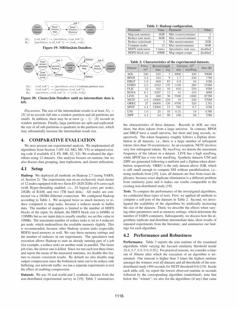
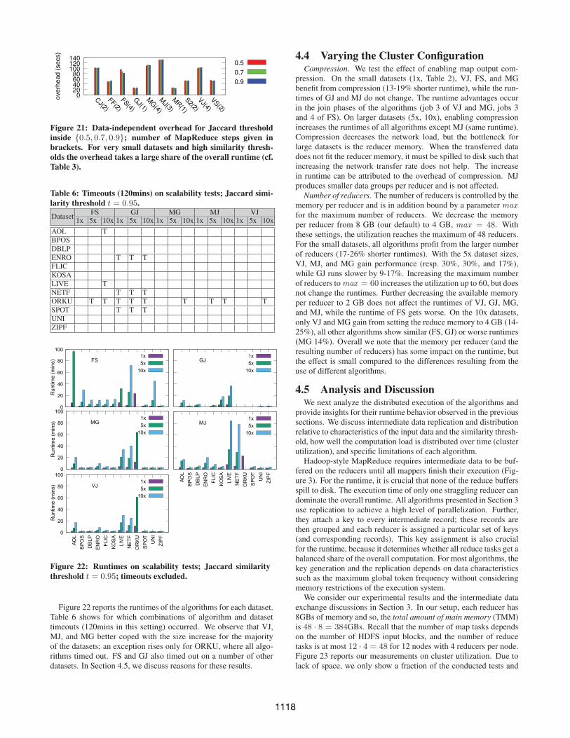
4.3 ScalabilityPractically, the datasets of Table 2 can be processed by state-

of-the-art non-distributed algorithms in main memory; [19] pro-vides a competitive experimental analysis under this setup. In fact,non-distributed algorithms outperform Hadoop-based solutions inthe majority of the datasets (cf. Table 4 in [19]). This behaviorcomes as no surprise due to the overhead induced by the MapRe-duce framework for starting/stopping jobs and transferring data be-tween the cluster nodes. Figure 21 reports this data-independentoverhead for all algorithms using a sample of 100 records of AOL.

However, distributed algorithms should be able to process muchlarger datasets than non-distributed ones. In this spirit, we reporton the scalability of the algorithms in settings that justify the needfor MapReduce. We focus only on FS, GJ, MG, MJ, and VJ as theother methods failed to handle even the small datasets of Table 2.For our scalability tests, we artificially increased the size of ourdatasets. We adopted the procedure from [30], which preservesthe original universe size and the record lengths, but increases thenumber of similar record pairs linearly with respect to an increasefactor n. Each record is copied n times while every token in arecord is shifted by n positions in the global token frequency. Thus,the number of records for each dataset is increased n times as wellas the maximum frequency of each token is roughly increased ntimes. The record lengths and the universe size do not change. Weused moderate values n = 5 and 10 for the enlargement factor anda Jaccard threshold of 0.95.

1117

0 20 40 60 80

100 120 140

CJ(2)FF(2)

FS(4)GJ(1)

MG(4)MJ(3)

MR(1)S2(2)

VJ(4)VS(2)

over

head

(sec

s)0.50.70.9

Figure 21: Data-independent overhead for Jaccard thresholdinside {0.5, 0.7, 0.9}; number of MapReduce steps given inbrackets. For very small datasets and high similarity thresh-olds the overhead takes a large share of the overall runtime (cf.Table 3).

Table 6: Timeouts (120mins) on scalability tests; Jaccard simi-larity threshold t = 0.95.

FS GJ MG MJ VJDataset

1x 5x 10x 1x 5x 10x 1x 5x 10x 1x 5x 10x 1x 5x 10x

AOL TBPOSDBLPENRO T T TFLICKOSALIVE TNETF T T TORKU T T T T T T T T TSPOT T T TUNIZIPF

Figure 22: Runtimes on scalability tests; Jaccard similaritythreshold t = 0.95; timeouts excluded.

Figure 22 reports the runtimes of the algorithms for each dataset.Table 6 shows for which combinations of algorithm and datasettimeouts (120mins in this setting) occurred. We observe that VJ,MJ, and MG better coped with the size increase for the majorityof the datasets; an exception rises only for ORKU, where all algo-rithms timed out. FS and GJ also timed out on a number of otherdatasets. In Section 4.5, we discuss reasons for these results.

4.4 Varying the Cluster ConfigurationCompression. We test the effect of enabling map output com-

pression. On the small datasets (1x, Table 2), VJ, FS, and MGbenefit from compression (13-19% shorter runtime), while the run-times of GJ and MJ do not change. The runtime advantages occurin the join phases of the algorithms (job 3 of VJ and MG, jobs 3and 4 of FS). On larger datasets (5x, 10x), enabling compressionincreases the runtimes of all algorithms except MJ (same runtime).Compression decreases the network load, but the bottleneck forlarge datasets is the reducer memory. When the transferred datadoes not fit the reducer memory, it must be spilled to disk such thatincreasing the network transfer rate does not help. The increasein runtime can be attributed to the overhead of compression. MJproduces smaller data groups per reducer and is not affected.

Number of reducers. The number of reducers is controlled by thememory per reducer and is in addition bound by a parameter maxfor the maximum number of reducers. We decrease the memoryper reducer from 8 GB (our default) to 4 GB, max = 48. Withthese settings, the utilization reaches the maximum of 48 reducers.For the small datasets, all algorithms profit from the larger numberof reducers (17-26% shorter runtimes). With the 5x dataset sizes,VJ, MJ, and MG gain performance (resp. 30%, 30%, and 17%),while GJ runs slower by 9-17%. Increasing the maximum numberof reducers to max = 60 increases the utilization up to 60, but doesnot change the runtimes. Further decreasing the available memoryper reducer to 2 GB does not affect the runtimes of VJ, GJ, MG,and MJ, while the runtime of FS gets worse. On the 10x datasets,only VJ and MG gain from setting the reduce memory to 4 GB (14-25%), all other algorithms show similar (FS, GJ) or worse runtimes(MG 14%). Overall we note that the memory per reducer (and theresulting number of reducers) has some impact on the runtime, butthe effect is small compared to the differences resulting from theuse of different algorithms.

4.5 Analysis and DiscussionWe next analyze the distributed execution of the algorithms and

provide insights for their runtime behavior observed in the previoussections. We discuss intermediate data replication and distributionrelative to characteristics of the input data and the similarity thresh-old, how well the computation load is distributed over time (clusterutilization), and specific limitations of each algorithm.

Hadoop-style MapReduce requires intermediate data to be buf-fered on the reducers until all mappers finish their execution (Fig-ure 3). For the runtime, it is crucial that none of the reduce buffersspill to disk. The execution time of only one straggling reducer candominate the overall runtime. All algorithms presented in Section 3use replication to achieve a high level of parallelization. Further,they attach a key to every intermediate record; these records arethen grouped and each reducer is assigned a particular set of keys(and corresponding records). This key assignment is also crucialfor the runtime, because it determines whether all reduce tasks get abalanced share of the overall computation. For most algorithms, thekey generation and the replication depends on data characteristicssuch as the maximum global token frequency without consideringmemory restrictions of the execution system.

We consider our experimental results and the intermediate dataexchange discussions in Section 3. In our setup, each reducer has8GBs of memory and so, the total amount of main memory (TMM)is 48 · 8 = 384GBs. Recall that the number of map tasks dependson the number of HDFS input blocks, and the number of reducetasks is at most 12 · 4 = 48 for 12 nodes with 4 reducers per node.Figure 23 reports our measurements on cluster utilization. Due tolack of space, we only show a fraction of the conducted tests and

1118

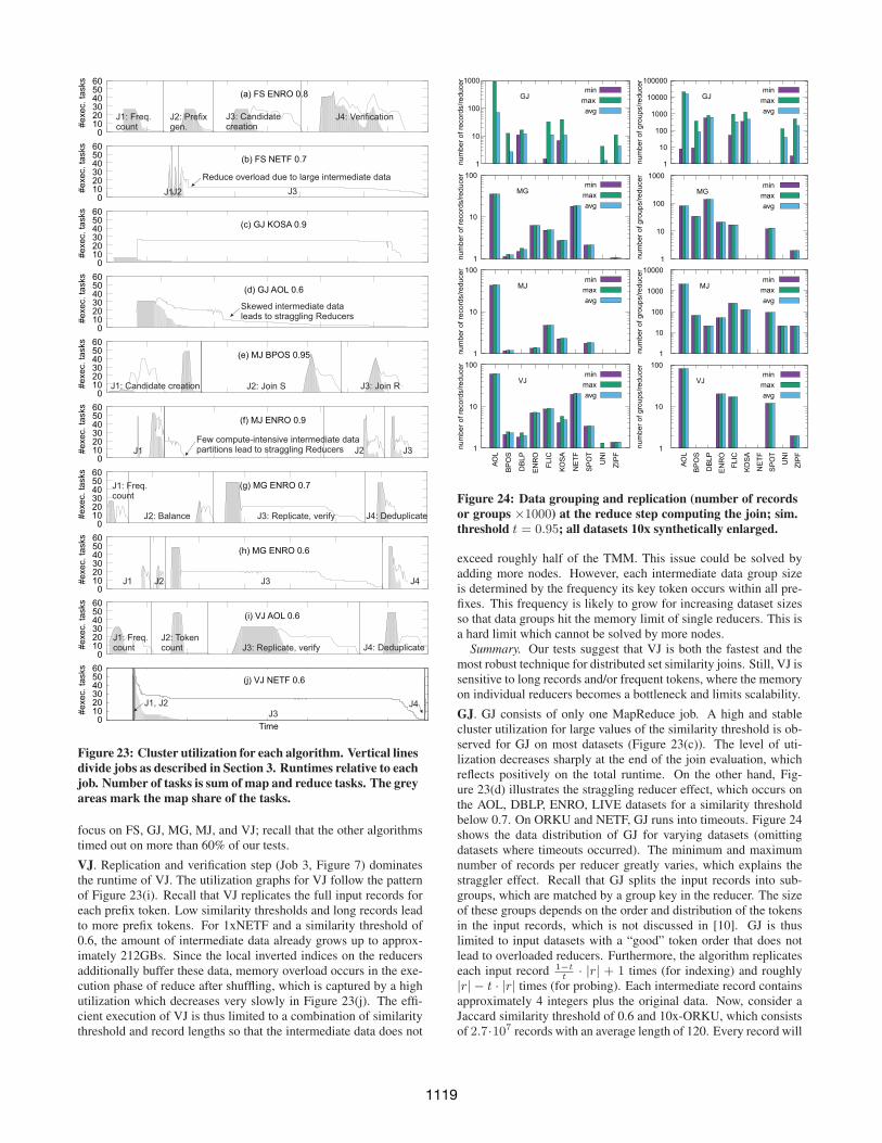
Figure 23: Cluster utilization for each algorithm. Vertical linesdivide jobs as described in Section 3. Runtimes relative to eachjob. Number of tasks is sum of map and reduce tasks. The greyareas mark the map share of the tasks.

focus on FS, GJ, MG, MJ, and VJ; recall that the other algorithmstimed out on more than 60% of our tests.

VJ. Replication and verification step (Job 3, Figure 7) dominatesthe runtime of VJ. The utilization graphs for VJ follow the patternof Figure 23(i). Recall that VJ replicates the full input records foreach prefix token. Low similarity thresholds and long records leadto more prefix tokens. For 1xNETF and a similarity threshold of0.6, the amount of intermediate data already grows up to approx-imately 212GBs. Since the local inverted indices on the reducersadditionally buffer these data, memory overload occurs in the exe-cution phase of reduce after shuffling, which is captured by a highutilization which decreases very slowly in Figure 23(j). The effi-cient execution of VJ is thus limited to a combination of similaritythreshold and record lengths so that the intermediate data does not

Figure 24: Data grouping and replication (number of recordsor groups ×1000) at the reduce step computing the join; sim.threshold t = 0.95; all datasets 10x synthetically enlarged.

exceed roughly half of the TMM. This issue could be solved byadding more nodes. However, each intermediate data group sizeis determined by the frequency its key token occurs within all pre-fixes. This frequency is likely to grow for increasing dataset sizesso that data groups hit the memory limit of single reducers. This isa hard limit which cannot be solved by more nodes.

Summary. Our tests suggest that VJ is both the fastest and themost robust technique for distributed set similarity joins. Still, VJ issensitive to long records and/or frequent tokens, where the memoryon individual reducers becomes a bottleneck and limits scalability.

GJ. GJ consists of only one MapReduce job. A high and stablecluster utilization for large values of the similarity threshold is ob-served for GJ on most datasets (Figure 23(c)). The level of uti-lization decreases sharply at the end of the join evaluation, whichreflects positively on the total runtime. On the other hand, Fig-ure 23(d) illustrates the straggling reducer effect, which occurs onthe AOL, DBLP, ENRO, LIVE datasets for a similarity thresholdbelow 0.7. On ORKU and NETF, GJ runs into timeouts. Figure 24shows the data distribution of GJ for varying datasets (omittingdatasets where timeouts occurred). The minimum and maximumnumber of records per reducer greatly varies, which explains thestraggler effect. Recall that GJ splits the input records into sub-groups, which are matched by a group key in the reducer. The sizeof these groups depends on the order and distribution of the tokensin the input records, which is not discussed in [10]. GJ is thuslimited to input datasets with a “good” token order that does notlead to overloaded reducers. Furthermore, the algorithm replicateseach input record 1−t

t· |r| + 1 times (for indexing) and roughly

|r| − t · |r| times (for probing). Each intermediate record containsapproximately 4 integers plus the original data. Now, consider aJaccard similarity threshold of 0.6 and 10x-ORKU, which consistsof 2.7·107 records with an average length of 120. Every record will

1119

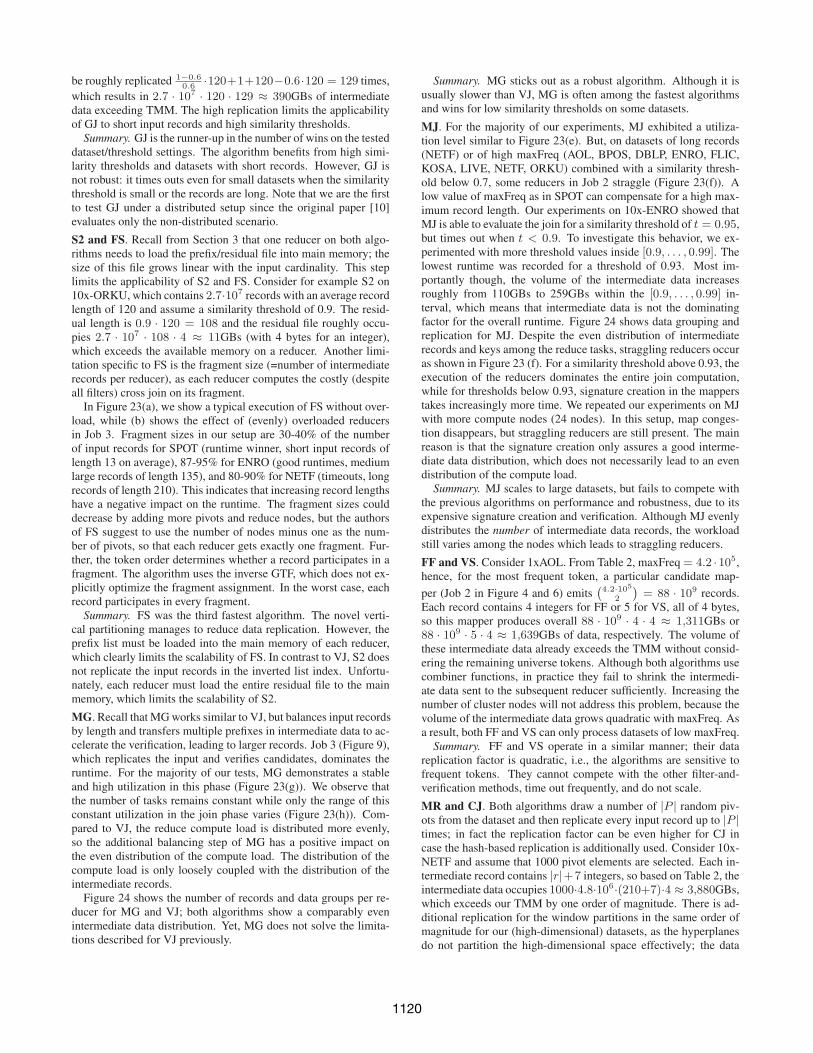
be roughly replicated 1−0.60.6

·120+1+120−0.6·120 = 129 times,

which results in 2.7 · 107 · 120 · 129 ≈ 390GBs of intermediatedata exceeding TMM. The high replication limits the applicabilityof GJ to short input records and high similarity thresholds.

Summary. GJ is the runner-up in the number of wins on the testeddataset/threshold settings. The algorithm benefits from high simi-larity thresholds and datasets with short records. However, GJ isnot robust: it times outs even for small datasets when the similaritythreshold is small or the records are long. Note that we are the firstto test GJ under a distributed setup since the original paper [10]evaluates only the non-distributed scenario.

S2 and FS. Recall from Section 3 that one reducer on both algo-rithms needs to load the prefix/residual file into main memory; thesize of this file grows linear with the input cardinality. This steplimits the applicability of S2 and FS. Consider for example S2 on10x-ORKU, which contains 2.7·107 records with an average recordlength of 120 and assume a similarity threshold of 0.9. The resid-ual length is 0.9 · 120 = 108 and the residual file roughly occu-pies 2.7 · 107 · 108 · 4 ≈ 11GBs (with 4 bytes for an integer),which exceeds the available memory on a reducer. Another limi-tation specific to FS is the fragment size (=number of intermediaterecords per reducer), as each reducer computes the costly (despiteall filters) cross join on its fragment.

In Figure 23(a), we show a typical execution of FS without over-load, while (b) shows the effect of (evenly) overloaded reducersin Job 3. Fragment sizes in our setup are 30-40% of the numberof input records for SPOT (runtime winner, short input records oflength 13 on average), 87-95% for ENRO (good runtimes, mediumlarge records of length 135), and 80-90% for NETF (timeouts, longrecords of length 210). This indicates that increasing record lengthshave a negative impact on the runtime. The fragment sizes coulddecrease by adding more pivots and reduce nodes, but the authorsof FS suggest to use the number of nodes minus one as the num-ber of pivots, so that each reducer gets exactly one fragment. Fur-ther, the token order determines whether a record participates in afragment. The algorithm uses the inverse GTF, which does not ex-plicitly optimize the fragment assignment. In the worst case, eachrecord participates in every fragment.

Summary. FS was the third fastest algorithm. The novel verti-cal partitioning manages to reduce data replication. However, theprefix list must be loaded into the main memory of each reducer,which clearly limits the scalability of FS. In contrast to VJ, S2 doesnot replicate the input records in the inverted list index. Unfortu-nately, each reducer must load the entire residual file to the mainmemory, which limits the scalability of S2.

MG. Recall that MG works similar to VJ, but balances input recordsby length and transfers multiple prefixes in intermediate data to ac-celerate the verification, leading to larger records. Job 3 (Figure 9),which replicates the input and verifies candidates, dominates theruntime. For the majority of our tests, MG demonstrates a stableand high utilization in this phase (Figure 23(g)). We observe thatthe number of tasks remains constant while only the range of thisconstant utilization in the join phase varies (Figure 23(h)). Com-pared to VJ, the reduce compute load is distributed more evenly,so the additional balancing step of MG has a positive impact onthe even distribution of the compute load. The distribution of thecompute load is only loosely coupled with the distribution of theintermediate records.

Figure 24 shows the number of records and data groups per re-ducer for MG and VJ; both algorithms show a comparably evenintermediate data distribution. Yet, MG does not solve the limita-tions described for VJ previously.

Summary. MG sticks out as a robust algorithm. Although it isusually slower than VJ, MG is often among the fastest algorithmsand wins for low similarity thresholds on some datasets.

MJ. For the majority of our experiments, MJ exhibited a utiliza-tion level similar to Figure 23(e). But, on datasets of long records(NETF) or of high maxFreq (AOL, BPOS, DBLP, ENRO, FLIC,KOSA, LIVE, NETF, ORKU) combined with a similarity thresh-old below 0.7, some reducers in Job 2 straggle (Figure 23(f)). Alow value of maxFreq as in SPOT can compensate for a high max-imum record length. Our experiments on 10x-ENRO showed thatMJ is able to evaluate the join for a similarity threshold of t = 0.95,but times out when t < 0.9. To investigate this behavior, we ex-perimented with more threshold values inside [0.9, . . . , 0.99]. Thelowest runtime was recorded for a threshold of 0.93. Most im-portantly though, the volume of the intermediate data increasesroughly from 110GBs to 259GBs within the [0.9, . . . , 0.99] in-terval, which means that intermediate data is not the dominatingfactor for the overall runtime. Figure 24 shows data grouping andreplication for MJ. Despite the even distribution of intermediaterecords and keys among the reduce tasks, straggling reducers occuras shown in Figure 23 (f). For a similarity threshold above 0.93, theexecution of the reducers dominates the entire join computation,while for thresholds below 0.93, signature creation in the mapperstakes increasingly more time. We repeated our experiments on MJwith more compute nodes (24 nodes). In this setup, map conges-tion disappears, but straggling reducers are still present. The mainreason is that the signature creation only assures a good interme-diate data distribution, which does not necessarily lead to an evendistribution of the compute load.

Summary. MJ scales to large datasets, but fails to compete withthe previous algorithms on performance and robustness, due to itsexpensive signature creation and verification. Although MJ evenlydistributes the number of intermediate data records, the workloadstill varies among the nodes which leads to straggling reducers.

FF and VS. Consider 1xAOL. From Table 2, maxFreq = 4.2 ·105,hence, for the most frequent token, a particular candidate map-

per (Job 2 in Figure 4 and 6) emits(4.2·105

2

)= 88 · 109 records.

Each record contains 4 integers for FF or 5 for VS, all of 4 bytes,so this mapper produces overall 88 · 109 · 4 · 4 ≈ 1,311GBs or88 · 109 · 5 · 4 ≈ 1,639GBs of data, respectively. The volume ofthese intermediate data already exceeds the TMM without consid-ering the remaining universe tokens. Although both algorithms usecombiner functions, in practice they fail to shrink the intermedi-ate data sent to the subsequent reducer sufficiently. Increasing thenumber of cluster nodes will not address this problem, because thevolume of the intermediate data grows quadratic with maxFreq. Asa result, both FF and VS can only process datasets of low maxFreq.

Summary. FF and VS operate in a similar manner; their datareplication factor is quadratic, i.e., the algorithms are sensitive tofrequent tokens. They cannot compete with the other filter-and-verification methods, time out frequently, and do not scale.

MR and CJ. Both algorithms draw a number of |P | random piv-ots from the dataset and then replicate every input record up to |P |times; in fact the replication factor can be even higher for CJ incase the hash-based replication is additionally used. Consider 10x-NETF and assume that 1000 pivot elements are selected. Each in-termediate record contains |r|+7 integers, so based on Table 2, theintermediate data occupies 1000·4.8·106·(210+7)·4 ≈ 3,880GBs,which exceeds our TMM by one order of magnitude. There is ad-ditional replication for the window partitions in the same order ofmagnitude for our (high-dimensional) datasets, as the hyperplanesdo not partition the high-dimensional space effectively; the data

1120

points are too close. The tests in [25] and [10] suggest that the al-gorithms perform better on data with a low number of dimensions.

Summary. The metric-based approaches did not perform well inour tests; CJ and MR often time out even for small inputs. This isdue to their high level of data replication.

4.6 Reproducing Previous ResultsWe repeated core experiments for VJ [30], S2 [5], MJ [9], and

FS [23]. It was not possible to repeat tests for CJ [25], as the ex-perimental setup (parameters of the method, hardware setting) isnot specified and a publicly unavailable dataset was used. The ex-perimental parameters for FF were not given on [12] either, whilefor VS [21], a larger cluster than ours and a publically unavailabledataset were used. Also, MG [24] used a larger cluster and a DBLPdataset which was tokenized/preprocessed in a way we could notreproduce, leading to large deviations in maxFreq. Finally, GJ [10]was never tested on a distributed setup, and for MR [27], a differentsimilarity function (Euclidean) was used. Unless stated otherwise,our Hadoop cluster is configured according to Table 1. Our testscan reproduce the results of VJ and S2. Due to lack of space, weonly report on algorithms with deviating results.

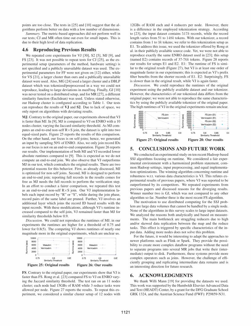
MJ. Contrary to the original paper, our experiments showed that VJis faster than MJ. In [9], MJ is compared to VJ on ENRO with a 10nodes cluster, varying the Jaccard similarity threshold. As MJ com-putes an end-to-end non-self R×S join, the dataset is split into twoequal-sized parts. Figure 25 reports the results of this comparison.On the other hand, our focus is on self-joins; hence, we generatedan input by sampling 50% of ENRO. Also, we only join record IDsas our focus is not on an end-to-end computation. Figure 26 reportsour results. Our implementation of both MJ and VJ recorded lowerabsolute runtimes compared to [9]. This is expected as we do notcompute an end-to-end join. We also observe that VJ outperformsMJ in our test, which contradicts the original results. There are twopotential reasons for this behavior. First, as already discussed, MJis optimized for non-self joins. Second, MJ is designed to performan end-to-end join; reporting full records in the results comes forfree as MJ needs the full records to perform the verification step.In an effort to conduct a fairer comparison, we repeated this testas an end-to-end non-self R×S join. Our VJ implementation la-bels each input record by “R” or “S”, while during the join phase,record pairs of the same label are pruned. Further, VJ involves anadditional layer which joins the record ID based results with theinput records. With these modifications, although VJ’s runtime in-creased compared to the self-join, VJ remained faster than MJ forsimilarity thresholds below 0.9.

Discussion. We could not reproduce the runtimes of MJ; in ourexperiments the runtimes are higher for a threshold of 0.75 andlower for 0.8(5). The competing VJ shows runtimes of nearly onemagnitude more in the original experiments, which are unclear us.

0 2000 4000 6000 8000

10000

0.75 0.8 0.85

Runt

ime (

secs

)

Similarity Threshold

MassJoinVernicaJoin

Figure 25: Original results

0 2000 4000 6000 8000

10000

0.75 0.8 0.85

Runt

ime (

secs

)

Similarity Threshold

MassJoinVernicaJoin

Figure 26: Our results

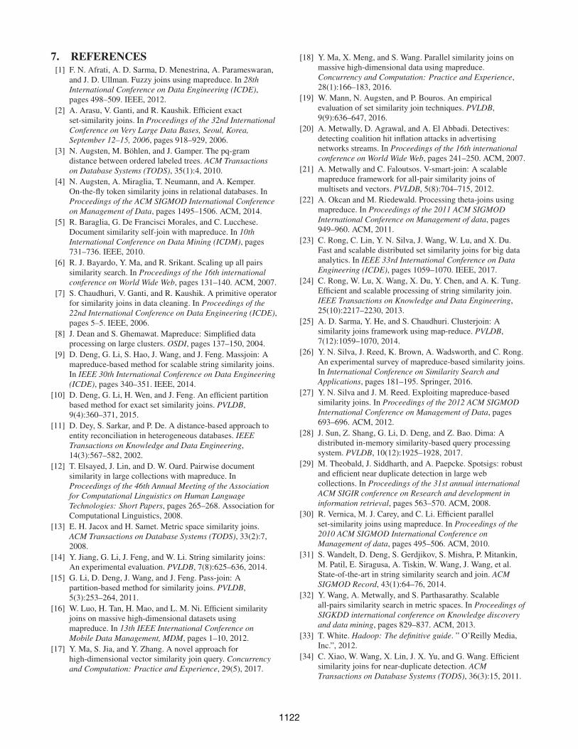
FS. Contrary to the original paper, our experiments show that VJ isfaster than FS. Rong et al. [23] compared FS to VJ on ENRO vary-ing the Jaccard similarity threshold. The test ran on an 11 nodescluster; each node had 15GBs of RAM while 3 reduce tasks wereallowed per node. Figure 27 reports the results. To repeat this ex-periment, we considered a similar cluster setup of 12 nodes with

12GBs of RAM each and 4 reducers per node. However, thereis a difference in the employed tokenization strategy. Accordingto [23], the input dataset contains 517k records, while the recordlength varies from 51 to 148k tokens. With our tokenizer, a recordcontains from 1 to 3k tokens; we refer to this tokenization setup asE1. To address this issue, we used the tokenizer offered by Rong etal. in their publicly available source code. Yet, we were not able toreproduce exactly the same ENRO dataset used in [23]; this setup(named E2) contains records of 37-76k tokens. Figure 28 reportsour results for setups E1 and E2. E1: The runtime of FS is simi-lar to the original result (Figure 27), but VJ is at least one order ofmagnitude faster in our experiments; this is expected as VJ’s prefixfilter benefits from the shorter records of E1. E2: Surprisingly, FSis slower than in the original result, while VJ is again faster.

Discussion. We could reproduce the runtimes of the originalexperiment using the publicly available dataset and our tokenizer.However, the characteristics of our tokenized data differs from theoriginal paper; we were not able to reproduce the same characteris-tics by using the publicly available tokenizer of the original paper.The high runtimes of VJ in the original experiments remain unclear.

0 500

1000 1500 2000 2500 3000 3500 4000 4500

0.75 0.8 0.85 0.9Ru

ntim

e (se

cs)

Similarity Threshold

FS-JoinVernicaJoin

Figure 27: Original results

0 500

1000 1500 2000 2500 3000 3500 4000 4500

0.75 0.8 0.85 0.9

Runt

ime (

secs

)

Similarity Threshold

FS-Join (E1)VernicaJoin (E1)

FS-Join (E2)VernicaJoin (E2)

Figure 28: Our results

5. CONCLUSIONS AND FUTURE WORKWe conducted an experimental study on ten recent Hadoop-based

SSJ algorithms focusing on runtime. We considered a fair exper-imental environment with a harmonized problem statement, com-mon Hadoop settings, input preprocessing, and equal implementa-tion optimizations. The winning algorithm concerning runtime androbustness w.r.t. various data characteristics is VJ. This refutes ex-perimental results of previous papers, where VJ was reported to beoutperformed by its competitors. We repeated experiments fromprevious papers and discussed reasons for the diverging results.Winner number two is GJ, which was not compared to any otheralgorithm so far. Number three is the most recent FS algorithm.

The motivation to use distributed computing for the SSJ prob-lem are large data volumes that cannot be handled by a single node.None of the algorithms in this survey scales to large input datasets.We analyzed the reasons both analytically and based on measure-ments. The main bottleneck are straggling reducers due to highand/or skewed data replication between the map and the reducetasks. This effect is triggered by specific characteristics of the in-put data. Adding more nodes does not solve this problem.

For the future, it would be interesting to adapt the approaches tonewer platforms such as Flink or Spark. They provide the possi-bility to create more complex dataflow programs without the needto separate programs into several MR jobs that write their (inter-mediate) output to disk. Furthermore, these systems provide morecomplex operators such as joins. However, the challenge of effi-ciently grouping and replicating intermediate data remains and isan interesting direction for future research.

6. ACKNOWLEDGMENTSWe thank Willi Mann [19] for providing the datasets we used.

This work was supported by the Humboldt Elsevier Advanced Dataand Text (HEADT) Center, by a grant for the DFG Graduate SchoolGRK 1324, and the Austrian Science Fund (FWF): P29859-N31.

1121

7. REFERENCES[1] F. N. Afrati, A. D. Sarma, D. Menestrina, A. Parameswaran,

and J. D. Ullman. Fuzzy joins using mapreduce. In 28thInternational Conference on Data Engineering (ICDE),pages 498–509. IEEE, 2012.

[2] A. Arasu, V. Ganti, and R. Kaushik. Efficient exactset-similarity joins. In Proceedings of the 32nd InternationalConference on Very Large Data Bases, Seoul, Korea,September 12–15, 2006, pages 918–929, 2006.

[3] N. Augsten, M. Bohlen, and J. Gamper. The pq-gramdistance between ordered labeled trees. ACM Transactionson Database Systems (TODS), 35(1):4, 2010.

[4] N. Augsten, A. Miraglia, T. Neumann, and A. Kemper.On-the-fly token similarity joins in relational databases. InProceedings of the ACM SIGMOD International Conferenceon Management of Data, pages 1495–1506. ACM, 2014.

[5] R. Baraglia, G. De Francisci Morales, and C. Lucchese.Document similarity self-join with mapreduce. In 10thInternational Conference on Data Mining (ICDM), pages731–736. IEEE, 2010.

[6] R. J. Bayardo, Y. Ma, and R. Srikant. Scaling up all pairssimilarity search. In Proceedings of the 16th internationalconference on World Wide Web, pages 131–140. ACM, 2007.

[7] S. Chaudhuri, V. Ganti, and R. Kaushik. A primitive operatorfor similarity joins in data cleaning. In Proceedings of the22nd International Conference on Data Engineering (ICDE),pages 5–5. IEEE, 2006.

[8] J. Dean and S. Ghemawat. Mapreduce: Simplified dataprocessing on large clusters. OSDI, pages 137–150, 2004.

[9] D. Deng, G. Li, S. Hao, J. Wang, and J. Feng. Massjoin: Amapreduce-based method for scalable string similarity joins.In IEEE 30th International Conference on Data Engineering(ICDE), pages 340–351. IEEE, 2014.

[10] D. Deng, G. Li, H. Wen, and J. Feng. An efficient partitionbased method for exact set similarity joins. PVLDB,9(4):360–371, 2015.

[11] D. Dey, S. Sarkar, and P. De. A distance-based approach toentity reconciliation in heterogeneous databases. IEEETransactions on Knowledge and Data Engineering,14(3):567–582, 2002.

[12] T. Elsayed, J. Lin, and D. W. Oard. Pairwise documentsimilarity in large collections with mapreduce. InProceedings of the 46th Annual Meeting of the Associationfor Computational Linguistics on Human LanguageTechnologies: Short Papers, pages 265–268. Association forComputational Linguistics, 2008.

[13] E. H. Jacox and H. Samet. Metric space similarity joins.ACM Transactions on Database Systems (TODS), 33(2):7,2008.

[14] Y. Jiang, G. Li, J. Feng, and W. Li. String similarity joins:An experimental evaluation. PVLDB, 7(8):625–636, 2014.

[15] G. Li, D. Deng, J. Wang, and J. Feng. Pass-join: Apartition-based method for similarity joins. PVLDB,5(3):253–264, 2011.

[16] W. Luo, H. Tan, H. Mao, and L. M. Ni. Efficient similarityjoins on massive high-dimensional datasets usingmapreduce. In 13th IEEE International Conference onMobile Data Management, MDM, pages 1–10, 2012.

[17] Y. Ma, S. Jia, and Y. Zhang. A novel approach forhigh-dimensional vector similarity join query. Concurrencyand Computation: Practice and Experience, 29(5), 2017.

[18] Y. Ma, X. Meng, and S. Wang. Parallel similarity joins onmassive high-dimensional data using mapreduce.Concurrency and Computation: Practice and Experience,28(1):166–183, 2016.

[19] W. Mann, N. Augsten, and P. Bouros. An empiricalevaluation of set similarity join techniques. PVLDB,9(9):636–647, 2016.

[20] A. Metwally, D. Agrawal, and A. El Abbadi. Detectives:detecting coalition hit inflation attacks in advertisingnetworks streams. In Proceedings of the 16th internationalconference on World Wide Web, pages 241–250. ACM, 2007.

[21] A. Metwally and C. Faloutsos. V-smart-join: A scalablemapreduce framework for all-pair similarity joins ofmultisets and vectors. PVLDB, 5(8):704–715, 2012.

[22] A. Okcan and M. Riedewald. Processing theta-joins usingmapreduce. In Proceedings of the 2011 ACM SIGMODInternational Conference on Management of data, pages949–960. ACM, 2011.

[23] C. Rong, C. Lin, Y. N. Silva, J. Wang, W. Lu, and X. Du.Fast and scalable distributed set similarity joins for big dataanalytics. In IEEE 33rd International Conference on DataEngineering (ICDE), pages 1059–1070. IEEE, 2017.

[24] C. Rong, W. Lu, X. Wang, X. Du, Y. Chen, and A. K. Tung.Efficient and scalable processing of string similarity join.IEEE Transactions on Knowledge and Data Engineering,25(10):2217–2230, 2013.

[25] A. D. Sarma, Y. He, and S. Chaudhuri. Clusterjoin: Asimilarity joins framework using map-reduce. PVLDB,7(12):1059–1070, 2014.

[26] Y. N. Silva, J. Reed, K. Brown, A. Wadsworth, and C. Rong.An experimental survey of mapreduce-based similarity joins.In International Conference on Similarity Search andApplications, pages 181–195. Springer, 2016.

[27] Y. N. Silva and J. M. Reed. Exploiting mapreduce-basedsimilarity joins. In Proceedings of the 2012 ACM SIGMODInternational Conference on Management of Data, pages693–696. ACM, 2012.

[28] J. Sun, Z. Shang, G. Li, D. Deng, and Z. Bao. Dima: Adistributed in-memory similarity-based query processingsystem. PVLDB, 10(12):1925–1928, 2017.

[29] M. Theobald, J. Siddharth, and A. Paepcke. Spotsigs: robustand efficient near duplicate detection in large webcollections. In Proceedings of the 31st annual internationalACM SIGIR conference on Research and development ininformation retrieval, pages 563–570. ACM, 2008.

[30] R. Vernica, M. J. Carey, and C. Li. Efficient parallelset-similarity joins using mapreduce. In Proceedings of the2010 ACM SIGMOD International Conference onManagement of data, pages 495–506. ACM, 2010.

[31] S. Wandelt, D. Deng, S. Gerdjikov, S. Mishra, P. Mitankin,M. Patil, E. Siragusa, A. Tiskin, W. Wang, J. Wang, et al.State-of-the-art in string similarity search and join. ACMSIGMOD Record, 43(1):64–76, 2014.

[32] Y. Wang, A. Metwally, and S. Parthasarathy. Scalableall-pairs similarity search in metric spaces. In Proceedings ofSIGKDD international conference on Knowledge discoveryand data mining, pages 829–837. ACM, 2013.

[33] T. White. Hadoop: The definitive guide. ” O’Reilly Media,Inc.”, 2012.

[34] C. Xiao, W. Wang, X. Lin, J. X. Yu, and G. Wang. Efficientsimilarity joins for near-duplicate detection. ACMTransactions on Database Systems (TODS), 36(3):15, 2011.

1122