Embed Size (px)
Citation preview
2015
Faculty of Electrical Engineering, University of Ljubljana Vitomir Štruc
[LABORATORY ASSIGNMENTS FOR SIGNAL PROCESSING] Workbook, First Edition, 2015
Signal Processing
U N I V E R S I T Y O F L J U B L J A N A
Faculty of Electrical Engineering
Vitomir Štruc
LABORATORY ASSIGNMENTS FOR
SIGNAL PROCESSING
WORKBOOK
FOR EXCHANGE STUDENTS ATTENDING THE UNIVERSITY PROGRAM ELECTRICAL ENGINEERING FIRST
BOLOGNA CYCLE
FIRST EDITION
Ljubljana, 2015
Foreword [LABORATORY ASSIGNMENTS FOR SIGNAL PROCESSING]
Foreword
Every year more and more exchange students are attending the Signal Processing course and join the
obligatory laboratory assignments. This workbook was written to show our exchange students what kind
of assignments they need to solve to pass the course and what they can expect to learnduring the course.
The assignments in this book represent sample assignments from the winter semester 2014/2015.
The workbook contains five chapters (with five assignments) that cover different areas of signal
processing, such as the representation of signals with various families of basis functions, spectral analysis,
correlation analysis, linear stacionary systems and convolution.
The author would like to thank all member oft he Laboratory for Artificial Perception, Systems and
Cybernetics that contributed in any way to this workbook.
Ljubljana, November 2015
Vitomir Štruc
Content [LABORATORY ASSIGNMENTS FOR SIGNAL PROCESSING]
Content
1. Laboratory assignments (5 points) ............................................................................................................ 1
Part one (2 points) ..................................................................................................................................... 1
Hints .......................................................................................................................................................... 2
Part two (2 points) ..................................................................................................................................... 3
Part three (1 point) .................................................................................................................................... 4
2. Laboratory assignments (5 points) ............................................................................................................ 5
Part one (2 points) ..................................................................................................................................... 5
Hints ........................................................................................................................................................... 7
Part two (2 points) ..................................................................................................................................... 8
Part three (1 point) .................................................................................................................................. 10
3. Laboratory assignments (5 points) .......................................................................................................... 11
Part one (3 points) ................................................................................................................................... 11
Hints ......................................................................................................................................................... 14
Part two (2 points) ................................................................................................................................... 15
Hints ........................................................................................................................................................ 16
4. Laboratory assignments (5 points) .......................................................................................................... 18
Part one (3 points) ................................................................................................................................... 18
Hints ......................................................................................................................................................... 20
Part two (2 points) ................................................................................................................................... 22
Hints ......................................................................................................................................................... 22
5. Laboratory assignments (5 points) .......................................................................................................... 23
Part one (3 points) ................................................................................................................................... 23
Hints ......................................................................................................................................................... 25
Part two (2 points) ................................................................................................................................... 26
Laboratory Assignment 1 [LABORATORY ASSIGNMENTS FOR SIGNAL PROCESSING]
1
1.Laboratoryassignments(5points)
Student information:
Exchange/Regularstudent FirstandLastname Date
The goal of this assignment is to study basic (analytical and numerical) computational
techniques used in the field of signal processing and to apply them for the computation of the
average power and energy of a few sample signals. The underlying theory for this assignment
was presented prior to the assignment.
Partone(2points)Consider a periodic continuous signal defined by the following elementary periodic function
cos .
1. Compute the period and average power of the above periodic signal analytically. Compute
the average power of the signal based on the general equation and then based on the
simplified equation for periodic signals.
Laboratory Assignment 1 [LABORATORY ASSIGNMENTS FOR SIGNAL PROCESSING]
2
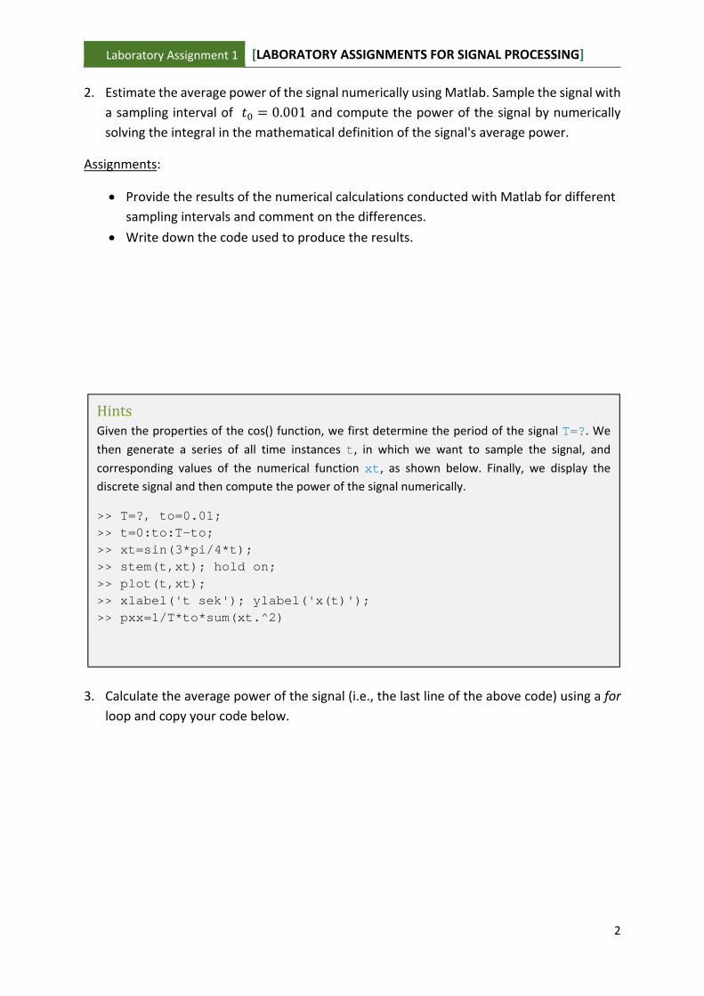
2. Estimate the average power of the signal numerically using Matlab. Sample the signal with
a sampling interval of 0.001 and compute the power of the signal by numerically
solving the integral in the mathematical definition of the signal's average power.
Assignments:
Provide the results of the numerical calculations conducted with Matlab for different
sampling intervals and comment on the differences.
Write down the code used to produce the results.
3. Calculate the average power of the signal (i.e., the last line of the above code) using a for
loop and copy your code below.
HintsGiven the properties of the cos() function, we first determine the period of the signal T=?. We
then generate a series of all time instances t, in which we want to sample the signal, and
corresponding values of the numerical function xt, as shown below. Finally, we display the discrete signal and then compute the power of the signal numerically.
>> T=?, to=0.01; >> t=0:to:T-to; >> xt=sin(3*pi/4*t); >> stem(t,xt); hold on; >> plot(t,xt); >> xlabel('t sek'); ylabel('x(t)'); >> pxx=1/T*to*sum(xt.^2)

Laboratory Assignment 1 [LABORATORY ASSIGNMENTS FOR SIGNAL PROCESSING]
3
Parttwo(2points)Similarly as during the first part of the assignment, compute the average power of the periodic
signal first analytically (using the simplified formula for periodic signals) and then numerically
using Matlab.
2 2 0 22 ∀ ∧ ∈
Hint: You can use Matlab's 'sawtooth' function to produce the signal (look at the
documentation of the function using "doc" command).
1. Analytical solution:
2. Numerical solution (code and results):

Laboratory Assignment 1 [LABORATORY ASSIGNMENTS FOR SIGNAL PROCESSING]
4
Partthree(1point)In the last part of the assignment first calculate the energy of the following aperiodic signal
analytically
00 0
Next, do the same using Matlab. Sample the signal and estimate its energy. Observe the
impact of the sampling interval and the duration of the observed interval on the numerical
error, when computing the signal's energy (you cannot use infinity in Matlab, but need to
select a high value for the upper bound of the observed interval).
1. Analytical solution:
2. Numerical solution (code and results):
Laboratory Assignment 2 [LABORATORY ASSIGNMENTS FOR SIGNAL PROCESSING]
5
2.Laboratoryassignments(5points)
Student information:
Exchange/Regularstudent FirstandLastname Date
The goal of this assignment is to learn express signals in the form a linear combination of some
family of orthogonal basis functions. Students solve the assignments first analytically and then
numerically using Matlab. The underlying theory for this assignment was presented prior to
the assignment itself.
Partone(2points)Consider the following signal:
cos 0 4
0 otherwise
Approximate the signal on the interval [0,4] using the first four Walsh basis functions
Φ ,Φ ,Φ ,Φ as follows:
Φ Φ Φ Φ .
Calculate the mean‐squared error ̅ and sketch/draw the approximation.
1. Solve the assignment analytically (i.e., calculate , , , ).

Laboratory Assignment 2 [LABORATORY ASSIGNMENTS FOR SIGNAL PROCESSING]
6
Laboratory Assignment 2 [LABORATORY ASSIGNMENTS FOR SIGNAL PROCESSING]
7
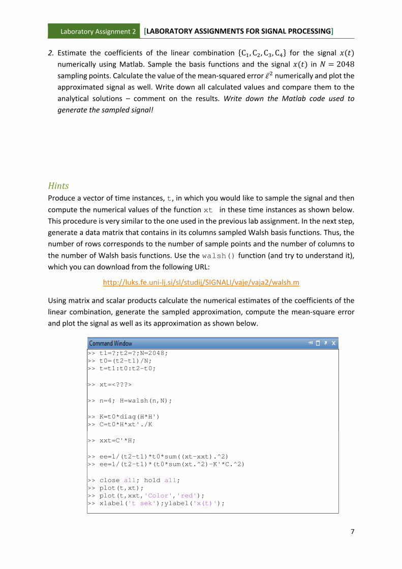
2. Estimate the coefficients of the linear combination C , C , C , C for the signal
numerically using Matlab. Sample the basis functions and the signal in 2048 sampling points. Calculate the value of the mean‐squared error ̅ numerically and plot the
approximated signal as well. Write down all calculated values and compare them to the
analytical solutions – comment on the results. Write down the Matlab code used to
generate the sampled signal!
HintsProduce a vector of time instances, t, in which you would like to sample the signal and then
compute the numerical values of the function xt in these time instances as shown below.
This procedure is very similar to the one used in the previous lab assignment. In the next step,
generate a data matrix that contains in its columns sampled Walsh basis functions. Thus, the
number of rows corresponds to the number of sample points and the number of columns to
the number of Walsh basis functions. Use the walsh() function (and try to understand it), which you can download from the following URL:
http://luks.fe.uni‐lj.si/sl/studij/SIGNALI/vaje/vaja2/walsh.m
Using matrix and scalar products calculate the numerical estimates of the coefficients of the
linear combination, generate the sampled approximation, compute the mean‐square error
and plot the signal as well as its approximation as shown below.
>> t1=?;t2=?;N=2048;>> t0=(t2-t1)/N; >> t=t1:t0:t2-t0; >> xt=<???> >> n=4; H=walsh(n,N); >> K=t0*diag(H*H') >> C=t0*H*xt'./K >> xxt=C'*H; >> ee=1/(t2-t1)*t0*sum((xt-xxt).^2) >> ee=1/(t2-t1)*(t0*sum(xt.^2)-K'*C.^2) >> close all; hold all; >> plot(t,xt); >> plot(t,xxt,'Color','red'); >> xlabel('t sek');ylabel('x(t)');

Laboratory Assignment 2 [LABORATORY ASSIGNMENTS FOR SIGNAL PROCESSING]
8
Parttwo(2points)Approximate the signal from part one with the first four Haar basis functions and calculate the
mean‐square error ̅ . Sketch/draw the approximation.
1. Similarly as in part one of the assignment, calculate the coefficients of the approximation
analytically.

Laboratory Assignment 2 [LABORATORY ASSIGNMENTS FOR SIGNAL PROCESSING]
9
2. Repeat all calculations with Matlab and estimate the values of the coefficients and the
mean‐square error. Plot the approximated and original signal as well. For this assignment you
can use the haar()function (try to understand it) that can be downloaded from:
http://luks.fe.uni‐lj.si/sl/studij/SIGNALI/vaje/vaja2/haar.m
Write down all calculated values and compare them to the analytical solutions – comment on
the results. In the space below also provide the commented code from the haar() function, where you explain the meaning of all non‐empty code lines from line 30 onwards.

Laboratory Assignment 2 [LABORATORY ASSIGNMENTS FOR SIGNAL PROCESSING]
10
Partthree(1point)In the last part write your own function called trigonometric() with a similar
functionality as the functions used in part one and two of the assignment. The function should
be used to represent the signal defined in part one of the assignment as a linear combination
of the first four trigonometric basis functions. Validate your numeric solutions by expressing
the signal from part one and two with the trigonometric basis functions analytically. Write
down the code for the trigonometric()function and provide the values of the
coefficients C , C , C , C in the space below.
Laboratory Assignment 3 [LABORATORY ASSIGNMENTS FOR SIGNAL PROCESSING]
11
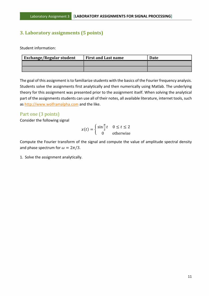
3.Laboratoryassignments(5points)
Student information:
Exchange/Regularstudent FirstandLastname Date
The goal of this assignment is to familiarize students with the basics of the Fourier frequency analysis.
Students solve the assignments first analytically and then numerically using Matlab. The underlying
theory for this assignment was presented prior to the assignment itself. When solving the analytical
part of the assignments students can use all of their notes, all available literature, internet tools, such
as http://www.wolframalpha.com and the like.
Partone(3points)Consider the following signal
sin 0 2
0 otherwise
Compute the Fourier transform of the signal and compute the value of amplitude spectral density
and phase spectrum for 2 /3.
1. Solve the assignment analytically.

Laboratory Assignment 3 [LABORATORY ASSIGNMENTS FOR SIGNAL PROCESSING]
12
Laboratory Assignment 3 [LABORATORY ASSIGNMENTS FOR SIGNAL PROCESSING]
13
2. Estimate the value of the amplitude spectral density and phase spectrum of the signal for
2 /3 numerically using Matlab. When numerically estimating the value of the Fourier integral
sample the signal with 1000 sampling points. Comment on the comparison with your
analytical solution.
In the next part compute the spectrum numerically using 1001 points distributed evenly between 10 and 10 and show a graphical representation of the sampled complex
spectrum, the amplitude spectral density and phase spectrum. Graphically show the amplitude
spectral density you computed analytically and compare the graph to the graph of the numerical
solution. Write down your findings.
Furthermore, write down your additions to the Matlab source code from the »Hints« section,
write down the code for the function you used to generate the signal from page one and sketch
all spectra.
Laboratory Assignment 3 [LABORATORY ASSIGNMENTS FOR SIGNAL PROCESSING]
14
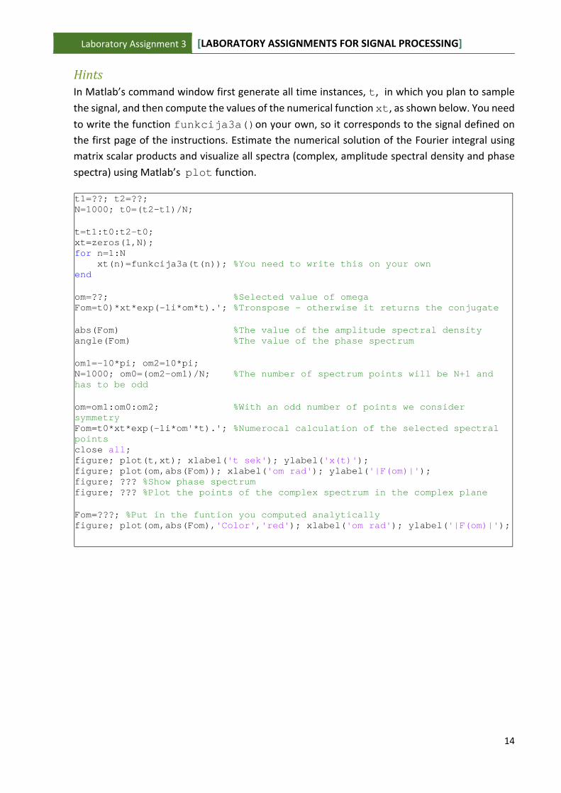
HintsIn Matlab’s command window first generate all time instances, t, in which you plan to sample
the signal, and then compute the values of the numerical function xt, as shown below. You need
to write the function funkcija3a()on your own, so it corresponds to the signal defined on the first page of the instructions. Estimate the numerical solution of the Fourier integral using
matrix scalar products and visualize all spectra (complex, amplitude spectral density and phase
spectra) using Matlab’s plot function.
t1=??; t2=??; N=1000; t0=(t2-t1)/N; t=t1:t0:t2-t0; xt=zeros(1,N); for n=1:N xt(n)=funkcija3a(t(n)); %You need to write this on your own end om=??; %Selected value of omega Fom=t0)*xt*exp(-1i*om*t).'; %Tronspose – otherwise it returns the conjugate abs(Fom) %The value of the amplitude spectral density angle(Fom) %The value of the phase spectrum om1=-10*pi; om2=10*pi; N=1000; om0=(om2-om1)/N; %The number of spectrum points will be N+1 and has to be odd om=om1:om0:om2; %With an odd number of points we consider symmetry Fom=t0*xt*exp(-1i*om'*t).'; %Numerocal calculation of the selected spectral points close all; figure; plot(t,xt); xlabel('t sek'); ylabel('x(t)'); figure; plot(om,abs(Fom)); xlabel('om rad'); ylabel('|F(om)|'); figure; ??? %Show phase spectrum figure; ??? %Plot the points of the complex spectrum in the complex plane Fom=???; %Put in the funtion you computed analytically figure; plot(om,abs(Fom),'Color','red'); xlabel('om rad'); ylabel('|F(om)|');
Laboratory Assignment 3 [LABORATORY ASSIGNMENTS FOR SIGNAL PROCESSING]
15
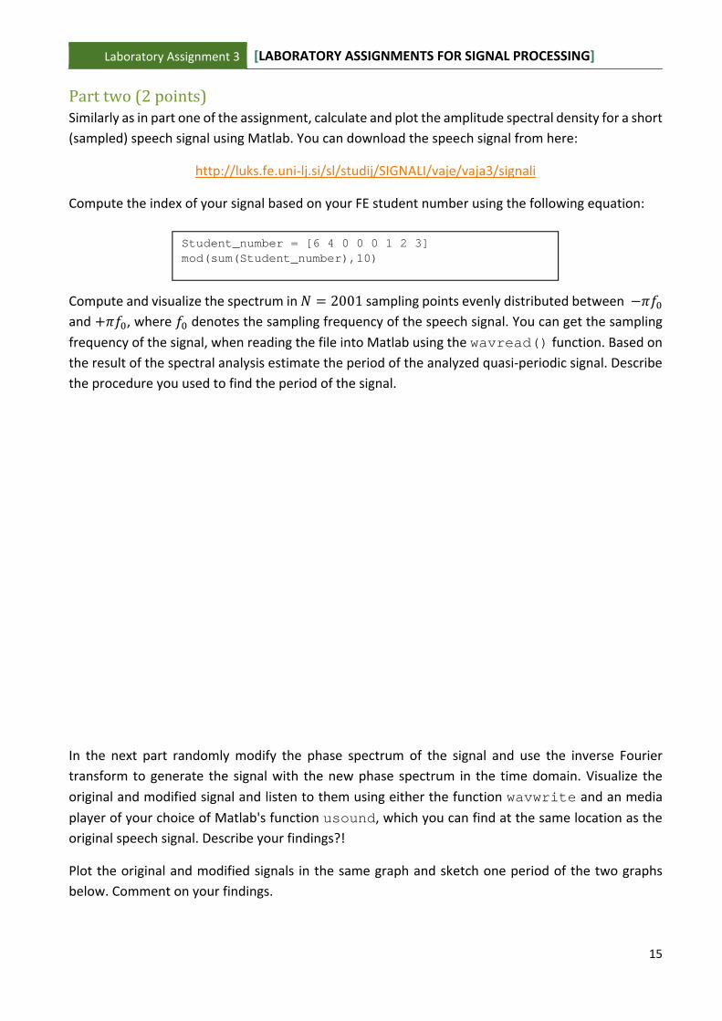
Parttwo(2points)Similarly as in part one of the assignment, calculate and plot the amplitude spectral density for a short
(sampled) speech signal using Matlab. You can download the speech signal from here:
http://luks.fe.uni‐lj.si/sl/studij/SIGNALI/vaje/vaja3/signali
Compute the index of your signal based on your FE student number using the following equation:
Compute and visualize the spectrum in 2001 sampling points evenly distributed between
and , where denotes the sampling frequency of the speech signal. You can get the sampling
frequency of the signal, when reading the file into Matlab using the wavread() function. Based on the result of the spectral analysis estimate the period of the analyzed quasi‐periodic signal. Describe
the procedure you used to find the period of the signal.
In the next part randomly modify the phase spectrum of the signal and use the inverse Fourier
transform to generate the signal with the new phase spectrum in the time domain. Visualize the
original and modified signal and listen to them using either the function wavwrite and an media
player of your choice of Matlab's function usound, which you can find at the same location as the
original speech signal. Describe your findings?!
Plot the original and modified signals in the same graph and sketch one period of the two graphs
below. Comment on your findings.
Student_number = [6 4 0 0 0 1 2 3] mod(sum(Student_number),10)
Laboratory Assignment 3 [LABORATORY ASSIGNMENTS FOR SIGNAL PROCESSING]
16
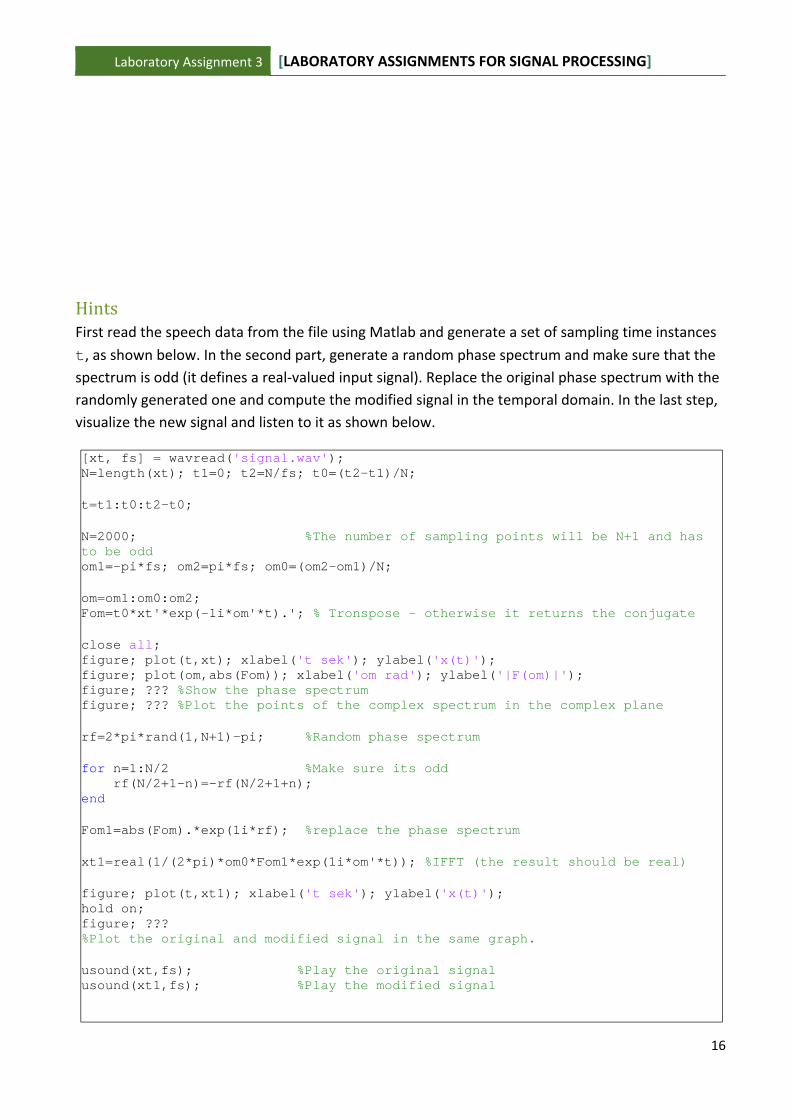
HintsFirst read the speech data from the file using Matlab and generate a set of sampling time instances
t, as shown below. In the second part, generate a random phase spectrum and make sure that the
spectrum is odd (it defines a real‐valued input signal). Replace the original phase spectrum with the
randomly generated one and compute the modified signal in the temporal domain. In the last step,
visualize the new signal and listen to it as shown below.
[xt, fs] = wavread('signal.wav');N=length(xt); t1=0; t2=N/fs; t0=(t2-t1)/N; t=t1:t0:t2-t0; N=2000; %The number of sampling points will be N+1 and has to be odd om1=-pi*fs; om2=pi*fs; om0=(om2-om1)/N; om=om1:om0:om2; Fom=t0*xt'*exp(-1i*om'*t).'; % Tronspose – otherwise it returns the conjugate close all; figure; plot(t,xt); xlabel('t sek'); ylabel('x(t)'); figure; plot(om,abs(Fom)); xlabel('om rad'); ylabel('|F(om)|'); figure; ??? %Show the phase spectrum figure; ??? %Plot the points of the complex spectrum in the complex plane rf=2*pi*rand(1,N+1)-pi; %Random phase spectrum for n=1:N/2 %Make sure its odd rf(N/2+1-n)=-rf(N/2+1+n); end Fom1=abs(Fom).*exp(1i*rf); %replace the phase spectrum xt1=real(1/(2*pi)*om0*Fom1*exp(1i*om'*t)); %IFFT (the result should be real) figure; plot(t,xt1); xlabel('t sek'); ylabel('x(t)'); hold on; figure; ??? %Plot the original and modified signal in the same graph. usound(xt,fs); %Play the original signal usound(xt1,fs); %Play the modified signal

Laboratory Assignment 3 [LABORATORY ASSIGNMENTS FOR SIGNAL PROCESSING]
17
Laboratory Assignment 4 [LABORATORY ASSIGNMENTS FOR SIGNAL PROCESSING]
18
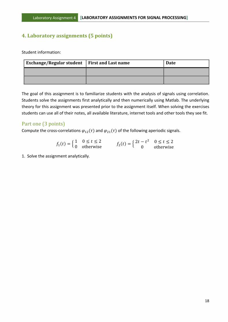
4.Laboratoryassignments(5points)
Student information:
Exchange/Regularstudent FirstandLastname Date
The goal of this assignment is to familiarize students with the analysis of signals using correlation.
Students solve the assignments first analytically and then numerically using Matlab. The underlying
theory for this assignment was presented prior to the assignment itself. When solving the exercises
students can use all of their notes, all available literature, internet tools and other tools they see fit.
Partone(3points)Compute the cross‐correlations and of the following aperiodic signals.
1 0 20 otherwise
2 0 20 otherwise
1. Solve the assignment analytically.

Laboratory Assignment 4 [LABORATORY ASSIGNMENTS FOR SIGNAL PROCESSING]
19
Laboratory Assignment 4 [LABORATORY ASSIGNMENTS FOR SIGNAL PROCESSING]
20
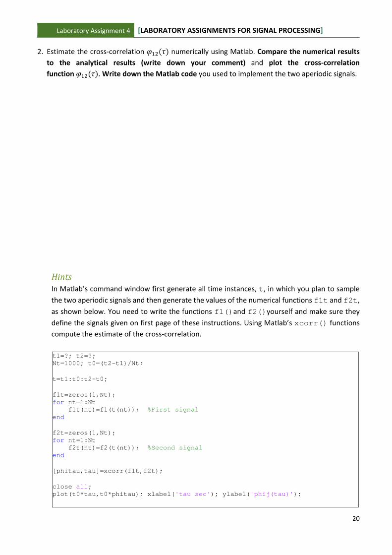
2. Estimate the cross‐correlation numerically using Matlab. Compare the numerical results
to the analytical results (write down your comment) and plot the cross‐correlation
function . Write down the Matlab code you used to implement the two aperiodic signals.
HintsIn Matlab’s command window first generate all time instances, t, in which you plan to sample
the two aperiodic signals and then generate the values of the numerical functions f1t and f2t,
as shown below. You need to write the functions f1()and f2()yourself and make sure they
define the signals given on first page of these instructions. Using Matlab’s xcorr() functions compute the estimate of the cross‐correlation.
t1=?; t2=?; Nt=1000; t0=(t2-t1)/Nt; t=t1:t0:t2-t0; f1t=zeros(1,Nt); for nt=1:Nt f1t(nt)=f1(t(nt)); %First signal end f2t=zeros(1,Nt); for nt=1:Nt f2t(nt)=f2(t(nt)); %Second signal end [phitau,tau]=xcorr(f1t,f2t); close all; plot(t0*tau,t0*phitau); xlabel('tau sec'); ylabel('phij(tau)');

Laboratory Assignment 4 [LABORATORY ASSIGNMENTS FOR SIGNAL PROCESSING]
21
Laboratory Assignment 4 [LABORATORY ASSIGNMENTS FOR SIGNAL PROCESSING]
22
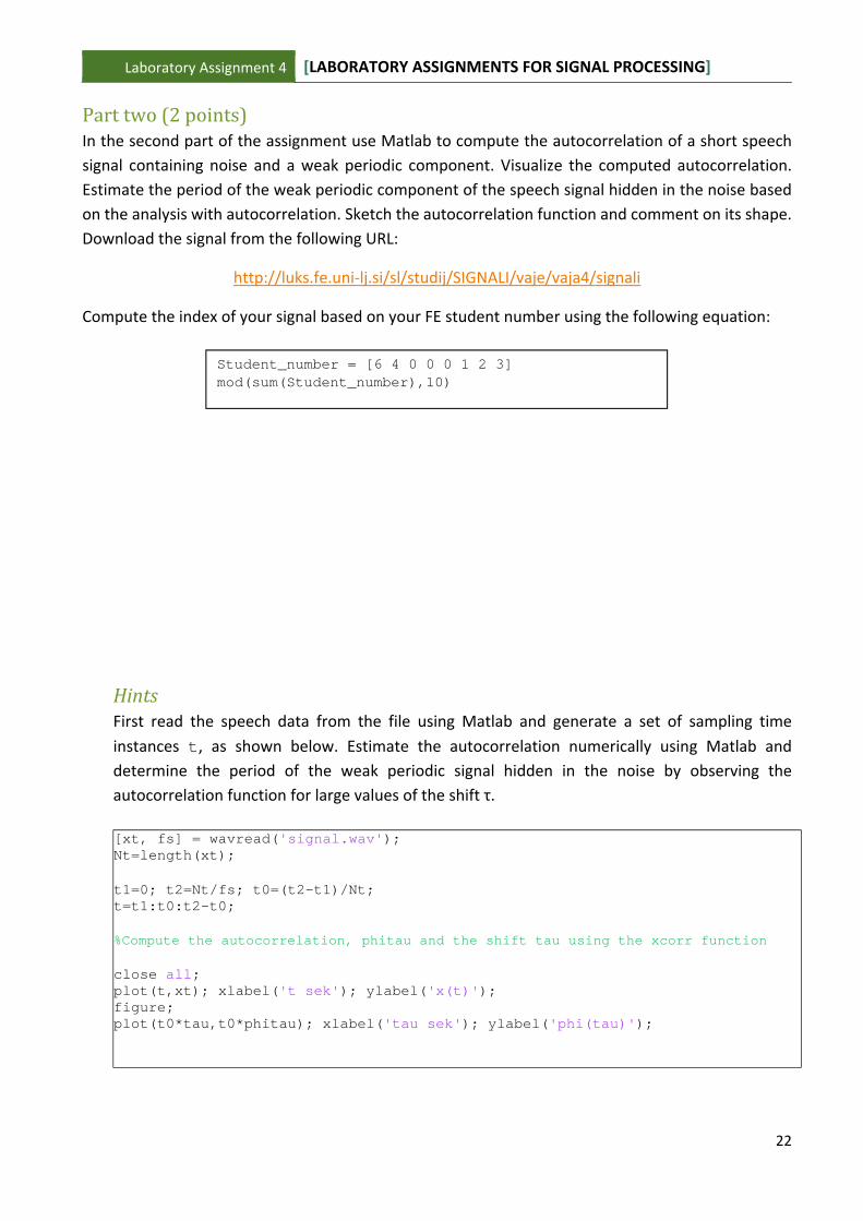
Parttwo(2points)In the second part of the assignment use Matlab to compute the autocorrelation of a short speech
signal containing noise and a weak periodic component. Visualize the computed autocorrelation.
Estimate the period of the weak periodic component of the speech signal hidden in the noise based
on the analysis with autocorrelation. Sketch the autocorrelation function and comment on its shape.
Download the signal from the following URL:
http://luks.fe.uni‐lj.si/sl/studij/SIGNALI/vaje/vaja4/signali
Compute the index of your signal based on your FE student number using the following equation:
HintsFirst read the speech data from the file using Matlab and generate a set of sampling time
instances t, as shown below. Estimate the autocorrelation numerically using Matlab and
determine the period of the weak periodic signal hidden in the noise by observing the
autocorrelation function for large values of the shift τ.
[xt, fs] = wavread('signal.wav');Nt=length(xt); t1=0; t2=Nt/fs; t0=(t2-t1)/Nt; t=t1:t0:t2-t0; %Compute the autocorrelation, phitau and the shift tau using the xcorr function close all; plot(t,xt); xlabel('t sek'); ylabel('x(t)'); figure; plot(t0*tau,t0*phitau); xlabel('tau sek'); ylabel('phi(tau)');
Student_number = [6 4 0 0 0 1 2 3] mod(sum(Student_number),10)
Laboratory Assignment 5 [LABORATORY ASSIGNMENTS FOR SIGNAL PROCESSING]
23
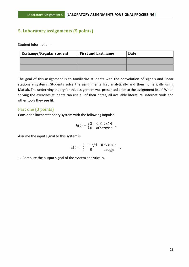
5.Laboratoryassignments(5points)
Student information:
Exchange/Regularstudent FirstandLastname Date
The goal of this assignment is to familiarize students with the convolution of signals and linear
stationary systems. Students solve the assignments first analytically and then numerically using
Matlab. The underlying theory for this assignment was presented prior to the assignment itself. When
solving the exercises students can use all of their notes, all available literature, internet tools and
other tools they see fit.
Partone(3points)Consider a linear stationary system with the following impulse
2 0 40 otherwise
.
Assume the input signal to this system is
1 /4 0 4
0 drugje .
1. Compute the output signal of the system analytically.

Laboratory Assignment 5 [LABORATORY ASSIGNMENTS FOR SIGNAL PROCESSING]
24
Laboratory Assignment 5 [LABORATORY ASSIGNMENTS FOR SIGNAL PROCESSING]
25
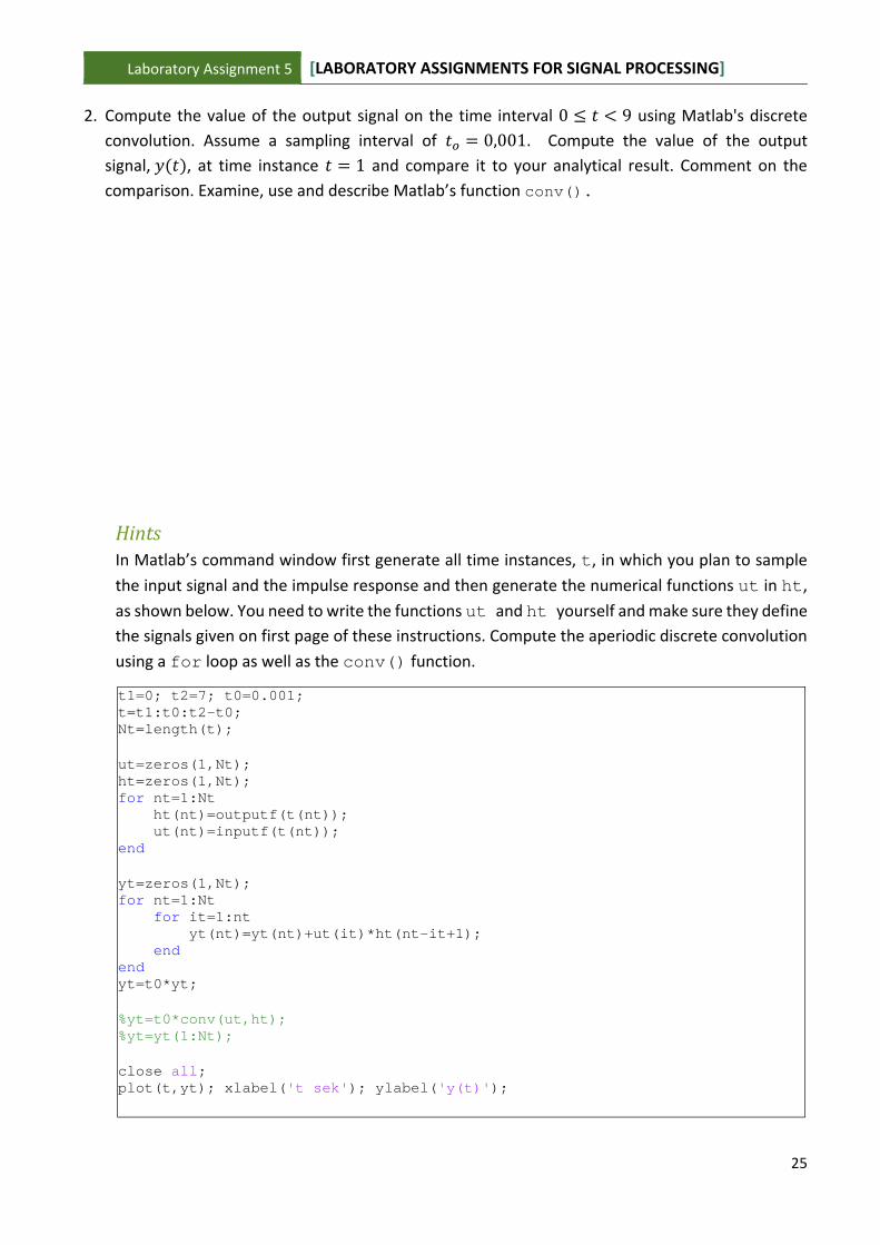
2. Compute the value of the output signal on the time interval 0 9 using Matlab's discrete
convolution. Assume a sampling interval of 0,001. Compute the value of the output
signal, , at time instance 1 and compare it to your analytical result. Comment on the
comparison. Examine, use and describe Matlab’s function conv().
HintsIn Matlab’s command window first generate all time instances, t, in which you plan to sample
the input signal and the impulse response and then generate the numerical functions ut in ht,
as shown below. You need to write the functions ut and ht yourself and make sure they define
the signals given on first page of these instructions. Compute the aperiodic discrete convolution
using a for loop as well as the conv() function.
t1=0; t2=7; t0=0.001; t=t1:t0:t2-t0; Nt=length(t); ut=zeros(1,Nt); ht=zeros(1,Nt); for nt=1:Nt ht(nt)=outputf(t(nt)); ut(nt)=inputf(t(nt)); end yt=zeros(1,Nt); for nt=1:Nt for it=1:nt yt(nt)=yt(nt)+ut(it)*ht(nt-it+1); end end yt=t0*yt; %yt=t0*conv(ut,ht); %yt=yt(1:Nt); close all; plot(t,yt); xlabel('t sek'); ylabel('y(t)');

Laboratory Assignment 5 [LABORATORY ASSIGNMENTS FOR SIGNAL PROCESSING]
26
Parttwo(2points)Compute the discrete convolution from part one using the Fourier (Matlab’s function fft()) and
inverse Fourier transforms (Matlab’s function ifft()). Visualize the output signal that you computed using this method and compare it to the result you obtained in part one (assignment 2) of
the assignment. Pay special attention to the value of the output signal at time instance 1. Write
down your results (plots of the output signal, ) and the Matlab code you wrote.


