Hindawi Publishing CorporationMathematical Problems in EngineeringVolume 2012, Article ID 958101, 21 pagesdoi:10.1155/2012/958101

Research ArticleSimplicial Approach to Fractal Structures

Carlo Cattani, Ettore Laserra, and Ivana Bochicchio

Department of Mathematics, University of Salerno, Via Ponte don Melillo, 84084 Fisciano, Italy

Correspondence should be addressed to Ivana Bochicchio, ibochicchio@unisa.it

Received 28 July 2011; Accepted 16 November 2011

Academic Editor: Cristian Toma

Copyright q 2012 Carlo Cattani et al. This is an open access article distributed under the CreativeCommons Attribution License, which permits unrestricted use, distribution, and reproduction inany medium, provided the original work is properly cited.

A fractal lattice is defined by iterative maps on a simplex. In particular, Sierpinski gasket and vonKoch flake are explicitly obtained by simplex transformations.

1. Introduction

Simplicial calculus [1–3] has been since the beginning a suitable tool for investigating discretemodels in many physical problems such as discrete models in space-time [4–9] complexnetworks [10–13], molecular crystals, aggregates and diamond lattices [14–17], computergraphics [18, 19], and more recently signal processing and computer vision, such as stereomatching and image segmentation [20, 21].

In some recent papers [22–25], fractals [26–29] generated by simplexes, also calledfractal lattices, were proposed for the analysis of nonconventional materials as some kind ofpolymers [24, 25] or nanocomposites [22, 23, 30, 31] having extreme physical and chemicalproperties. Moreover, the analysis of complex traffic on networks [32, 33] and image analysis[20, 21] based on fractal geometry and simplicial lattices has focussed on the importance ofthese methods in handling modern challenging problems.

However, only a few attempts were made in order to define the fractal lattice(structure) by an iterated system of functions on simplexes [34, 35]. The main scheme foraffine contraction has been given in [35], whereas some generation of fractals by simplicialmaps can be found in [34].

In this paper, we define a method based on simple algorithms for the generationof fractal-like structures by continuously deforming a simplex. This algorithm is based ona well-defined analytical map, which can be used to finitely describe fractals. Instead ofrecursive law, or nested maps (see, e.g., [1, 2, 15]), we propose a method which can be moreeasily implemented.

2 Mathematical Problems in Engineering

In the following, we will study an m-dimensional fractal structure defined by thetransformation group of a simplicial complex. Starting from a simplex, it will define the groupof transformation on it, so that the intrinsic (affine)metric remains scale invariant. The groupof transformations (isometries and homotheties) will be characterized by matrices acting onthe skeleton of the simplex. We will derive the basic properties of the fractal lattice and givea suitable definition of self-similarity on lattices. The concept of self-similarity is shown tobe fulfilled by some classical transformation on simplices (homothety) and, simplicial based,fractals as the Sierpinski tessellations and the von Koch flake.

2. Euclidean Simplexes

In the ordinary Euclidean space Rn, we assume that there exists a triangulation of R

n, in thesense that there is at least a finite set of n+1 points geometrically independent (simplexes). Asimplex will be considered both as a set of points and as the convex subspace of R

n, definedby the geometrical support of the simplex. Union of n-adjacent simplexes is an n-polyhedronP [4, 18, 19].

The euclidean m-simplex σm, of independent vertices V0, V1, . . . , Vm, is defined [1–3]as the subset of R

n,

σm def=

{P ∈ R

n | Pm∑i=0

λiVi withm∑i=0

λi = 1, 0 ≤ λi ≤ 1

}. (2.1)

Let us denote with [σm] = [V0, V1, . . . , Vm] the set of points which form the skeleton of σm, andlet #σm = m + 1 be the cardinality of the set of points. The p-face of σm, with p ≤ m, is anysimplex σp such that [σp] ∩ [σm]/= ∅, and we write σp � σm.

The number of p-faces of σm is (m+1p+1 ).

The m-dimensional simplicial complex Σm is defined as the finite set of p simplexes(p ≤ m) such that

(1) for all σk ∈ Σm if σh � σk, then σh ∈ Σm,(2) for all σk, σh ∈ Σm, then either [σh] ∩ [σk] = ∅ or [σh] ∩ [σk] = [σj] with σj ∈ Σm.The set of points P such that P ∈ σp, p ≤ m, and σp ∈ Σm is the geometric support

of Σm also called m-polyhedron Mm. The p-skeleton of Σm is [Σm]p def= [σp] for all σp ∈ Σm.The boundary ∂Σm of Σm is the complex Σm−1 such that each σm−1 ∈ Σm−1 is face of only onem-simplex of Σm. A finite set of simplexes is also called lattice (or tessellation).

2.1. Barycentric Coordinates and Barycentric Bases

In each simplex, it is possible to define the barycentric basis as follows: given the m-simplexσm with vertices V0, . . . , Vm, the barycentric basis is the set of (m + 1) vectors

eidef= Vi − Gm, (2.2)

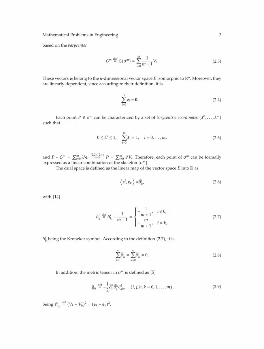
Mathematical Problems in Engineering 3

based on the barycenter

Gm def= G(σm) =m∑i=0

1m + 1

Vi. (2.3)

These vectors ei belong to the n-dimensional vector space E isomorphic to Rn. Moreover, they

are linearly dependent, since according to their definition, it is

m∑i=0

ei = 0. (2.4)

Each point P ∈ σm can be characterized by a set of barycentric coordinates (λ0, . . . , λm)such that

0 ≤ λi ≤ 1,m∑i=0

λi = 1, i = 0, . . . , m, (2.5)

and P − Gm =∑m

i=0 λiei

(2.2),(2.4)=⇒ P =

∑mi=0 λ

iVi. Therefore, each point of σm can be formallyexpressed as a linear combination of the skeleton [σm].

The dual space is defined as the linear map of the vector space E into R as

⟨ei, ek⟩=δi

k, (2.6)

with [14]

δik

def= δik −

1m + 1

=

⎧⎪⎪⎨⎪⎪⎩− 1m + 1

, i /= k,

+m

m + 1, i = k,

(2.7)

δik being the Kroneker symbol. According to the definition (2.7), it is

m∑i=0

δik =

m∑k=0

δik = 0. (2.8)

In addition, the metric tensor in σm is defined as [5]

gijdef= −1

2δhi δ

kj �

2hk,

(i, j, h, k = 0, 1, . . . , m

)(2.9)

being �2hk

def= (Vk − Vh)2 = (ek − eh)

2.

4 Mathematical Problems in Engineering

2.2. Measures of the m-Simplex

Let

Lijdef= Vj − Vi

(= ej − ei

), lij

def=⟨Lij ,Lij

⟩, (2.10)

by using the ordinary wedge product of the vectors ej1 , . . . , ejp , we can define the p-form ω,

ω =1p!

∑j1,...,jm

ωj1...jpej1 ∧ · · · ∧ ejp , (2.11)

whose affine components are ωj1...jp def= 〈ω, ej1 ∧ ej2 ∧ · · · ∧ ejp〉 [14].The euclidean measure of them-simplex σ (volume) is [14]

εΩ2 def=1m!

|L01 ∧ · · · ∧ L0m|, (2.12)

from where, it follows that

Ω2 =(

1m!

)3 ∑j1 ,...,jmk1,...,km

εj1...jmεk1...kmm∏a=1

l2jaka , (2.13)

being

εj1...jmdef= ±1, (2.14)

according to the even/odd permutation j0, j1, . . . , jm of the indices 0, 1, . . . , m.In particular, the volume of each p-face σi1...im−p (see also [9]) is

Ω2i1...im−p =

(−12

)p( 1p!

)3 ∑j1 ,...,jpk1,...,kp

εj1...jp εk1...kpp∏

a=1

l2jaka(0 < p ≤ m

), (2.15)

where j1, . . . , jp, k1, . . . , kp /= i1, . . . , im−p.

3. m-Dimensional Homothety

Let I(σi) be the subspace of Rm to which σi belongs; it can be easily proved that [14]

∀ v ∈ I(σi)⟨ni,v⟩= 0 ( i fixed ), (3.1)

Mathematical Problems in Engineering 5

where the normal vector ni is defined as

ni def= −mΩΩi

ei, hi def=mΩΩi

. (3.2)

The above definition of vector orthogonal to a (m − 1)-face allows us to characterizethe m-parallelism of simplexes as follows. Let σ,

σ be two simplexes in R

m; let σi,σi be the ith

(m − 1)-faces of σ andσ, respectively, and let ni,

nibe their normal vectors, then we say that

σ ism-parallel toσ ( σ‖m

σ) if and if only σi‖σi, that is, ni =ni(i = 0, . . . , m).

Let ϕ be a map

ϕ : Rm −→ R

m, σϕ�−→

σ (3.3)

such that(1) ϕ is a bijective simplicial map on σ,(2) the s-adjacent faces of σ correspond (under the map ϕ) to s-adjacent faces of

σ,

(3) σ andσ are m-parallel.

We also assume that this transformation depends on the edge vectors and in particularon the edge lengths, so that any quantity, defined on the simplex, transforming under the action ofϕ, is a function of the edge lengths. Furthermore, we assume the following conditions:

(4) there exists a fixed point under the action of ϕ:

∃O ∈ Rm | ϕ(O) ≡ O, (3.4)

(5) each (m − 1)-face σi translates of an amount t ∈ [0,∞).Let us choose as a fixed point one of the vertices, for example, V0. We define this

bijective simplicial map applying any P ∈ σ into

P ∈ σ (t ∈ [0,∞)) as

Pdef= P + t

Ω0

mΩ

m∑i=0

λiL0i; (3.5)

in particular, this function acts on any vertex Vi as

V i = Vi + tΩ0

mΩL0i,

(

V 0 = V0

), (3.6)

so that we can easily prove that all the previous conditions are easily satisfied [14]. Accordingto the above equations, each edge transforms as

Lij =

(1 + t

Ω0

mΩ

)Lij , (3.7)

whereLij =

V j −

V i.

6 Mathematical Problems in Engineering

3.1. Variation Law of the p-Faces of σ

The variation law of the edge lengths, resulting from (3.7), is given by the formula

l ij =(1 + t

Ω0

mΩ

)lij , (3.8)

where lij is the length of the edge Lij , and

l ij is the length of the edgeLij .

According to (2.13), the volumeΩ is a homogeneous function of degreem of them(m+1)/2 variable {l2ij}i<j , so that its variation law is

Ω =(1 + t

Ω0

mΩ

)m

Ω, (3.9)

and for any p-face,

Ωi1...im−p =(1 + t

Ω0

mΩ

)p

Ωi1...im−p(0 < p < m

); (3.10)

analogously, taking into account the definition (5.5)2, we have the transformation law of hi:

hi = m

(1 + t

Ω0

mΩ

)hi. (3.11)

There follows, for the fundamental vectors ofσ, that

⎧⎪⎪⎪⎪⎪⎪⎪⎨⎪⎪⎪⎪⎪⎪⎪⎩

e i

def=

V i −

G =(1 + t

Ω0

mΩ

)ei,

ni

= ni,

ei

=

Ωi/Ωi

Ω/Ωei =(1 + t

Ω0

mΩ

)−1ei.

(3.12)

4. Self-Similar Structure

Let (Rn, d) be the complete metric space with the standard Euclidean metric d, and letK(Rn)be the set

K(Rn) ={K ⊆ R

n : K is a nonempty compact set}. (4.1)

The iterated function system (IFS)

{wi} = (Rn, d,w1, w2, . . . , wn) (4.2)

Mathematical Problems in Engineering 7

is the finite set of contractions wi on the complete metric space (Rn, d), being the contractionw defined as

d(w(x), w

(y)) ≤ cd

(x, y), ∀x, y ∈ R

n, (4.3)

with c contraction coefficient.For each A ∈ K(Rn), the (IFS) contracting mapping is

w : A ∈ K(Rn) −→ w1(A)⋃

· · ·⋃

wn(A) ∈ K(Rn), (4.4)

with contraction coefficient c = max{c1, . . . , cn}. Each function wi usually is linear, or moregenerally an affine transformation, but sometimes it can be nonlinear, including projectiveand Mobius transformations [27].

According to the Banach fixed-point theorem (see, e.g., [36]), every contractionmapping on a nonempty complete metric space has a unique fixed point, so that there existsa unique compact (i.e., closed and bounded) fixed set A such that A = w(A). The set A isalso known as the fixed set of the Hutchinson operator [28].

One way of constructing such fixed set is to start with an initial set A and by iteratingthe actions of w. Hence,

A =⋃

i1,...,ih=1,...,n

wi1 ◦ · · · ◦wih(A), (4.5)

so that A is a self-similar set, expressed as the finite union of its conformal copies, each onereduced by a factor ch.

The attractor A of IFS is characterized by a similarity dimension as follows.

Definition 4.1. Given an IFS of n contraction mappings with the same contraction coefficientc, the similarity dimension is defined as

s =log n

log 1/c

(= − log n

log c

). (4.6)

Sets having noninteger similarity dimensions are called fractal sets, or simply fractals.There follows that the iterated function systems are a method of constructing fractals; theresulting constructions are always self-similar such that w(μx) = μHw(x). Hence, each mapw is also called a self-similar map [27].

5. Fractal Structures from Simplicial Maps

In this section, some examples of self-similar (scale invariant) structures obtained by IFS onsimplexes are given in R

2. In particular, the IFS will be defined by affine transformations, asconformal maps of the affine metrics.

8 Mathematical Problems in Engineering

In the following, wewill introduce some self-similarmaps defined both on 2-simplexesand 1-simplexes, so that, from (4.1),

K(R

2)={σ2; σ1;σ0

},

w : K(R

2) �−→ K(R

2).(5.1)

In particular, let σ2 be the simplex [V1, V2, V3], then it is

K(R

2)= {[V1, V2, V3]; [V1, V2], [V1, V3], [V2, V3]; [V1], [V2], [V3]}, (5.2)

so that a map w on K(R2) could be the more general function defined on any face of σ2.

Examples. If the skeleton of σ2 is the set of vertices {V1, V2, V3}with V1 = (x1, y1),V2 = (x2, y2),and V3 = (x3, y3), the affine map w is defined by the matrix

W =

⎛⎜⎜⎜⎜⎜⎜⎜⎜⎜⎜⎜⎝

a11 a12 a13 a14 a15 a16

a21 a22 a23 a24 a25 a26

a31 a32 a33 a34 a35 a36

a41 a42 a43 a44 a45 a46

a51 a52 a53 a54 a55 a56

a61 a62 a63 a64 a65 a66

⎞⎟⎟⎟⎟⎟⎟⎟⎟⎟⎟⎟⎠

(5.3)

and the constant vector

U = (u1, u2, u3, u4, u5, u6). (5.4)

The function w maps a 2-simplex into a 2-simplex whereas, by a matrix product, the vector

X =(x1, y1, x2, y2, x3, y3

)(5.5)

is mapped into the vector

WX +U, (5.6)

Mathematical Problems in Engineering 9

so that the skeleton of w(σ2) is given by the vector WX + U. For instance, a rotation withfixed point V1 is given by the matrix

W =

⎛⎜⎜⎜⎜⎜⎜⎜⎜⎜⎜⎜⎝

1 0 0 0 0 0

0 1 0 0 0 0

0 0 a33 a34 0 0

0 0 a43 a44 0 0

0 0 0 0 a55 a56

0 0 0 0 a65 a66

⎞⎟⎟⎟⎟⎟⎟⎟⎟⎟⎟⎟⎠

, (5.7)

with

a33a44 − a34a43 = ±1, a55a66 − a56a65 = ±1, (5.8)

and the vector U = {0, 0, 0, 0, 0, 0}.

Some more special maps will be given in the following where, in particular, weconsider, without restriction, some special maps on the 1-faces of σ2 such that

w(σ2)= w1

(σ21

)∪w2

(σ22

)∪w3

(σ23

), #w

(σ2)= 3. (5.9)

In this case, the matrix W , acting on σ2, follows from the direct sum of lower-order matricesacting on σ1 simplexes, as follows:

(a) the first vertex V1 remains fixed, and the map w on σ2 is a consequence of thetransformation of the simplex σ1 = [V2, V3], that is, by defining

I =

(1 0

0 1

), W1 =

⎛⎜⎜⎜⎜⎜⎝

a33 a34 a35 a36

a43 a44 a45 a46

a53 a54 a55 a56

a63 a64 a65 a66

⎞⎟⎟⎟⎟⎟⎠, (5.10)

it is

W = I ⊕W1 =

⎛⎜⎜⎜⎜⎜⎜⎜⎜⎜⎜⎜⎝

1 0 0 0 0 0

0 1 0 0 0 0

0 0 a33 a34 a35 a36

0 0 a43 a44 a45 a46

0 0 a53 a54 a55 a56

0 0 a63 a64 a65 a66

⎞⎟⎟⎟⎟⎟⎟⎟⎟⎟⎟⎟⎠

, (5.11)

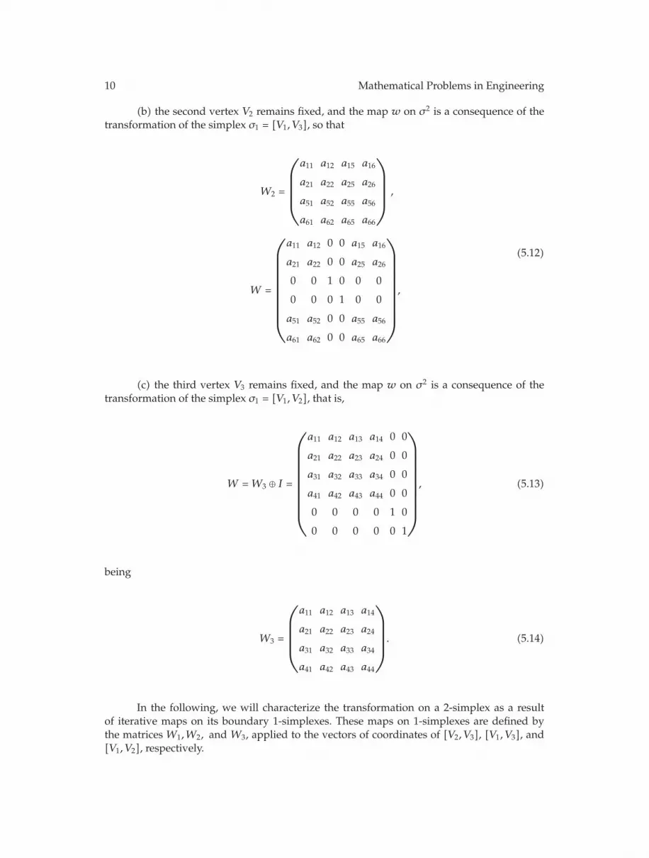
10 Mathematical Problems in Engineering

(b) the second vertex V2 remains fixed, and the map w on σ2 is a consequence of thetransformation of the simplex σ1 = [V1, V3], so that

W2 =

⎛⎜⎜⎜⎜⎜⎝

a11 a12 a15 a16

a21 a22 a25 a26

a51 a52 a55 a56

a61 a62 a65 a66

⎞⎟⎟⎟⎟⎟⎠ ,

W =

⎛⎜⎜⎜⎜⎜⎜⎜⎜⎜⎜⎜⎝

a11 a12 0 0 a15 a16

a21 a22 0 0 a25 a26

0 0 1 0 0 0

0 0 0 1 0 0

a51 a52 0 0 a55 a56

a61 a62 0 0 a65 a66

⎞⎟⎟⎟⎟⎟⎟⎟⎟⎟⎟⎟⎠

,

(5.12)

(c) the third vertex V3 remains fixed, and the map w on σ2 is a consequence of thetransformation of the simplex σ1 = [V1, V2], that is,

W = W3 ⊕ I =

⎛⎜⎜⎜⎜⎜⎜⎜⎜⎜⎜⎜⎝

a11 a12 a13 a14 0 0

a21 a22 a23 a24 0 0

a31 a32 a33 a34 0 0

a41 a42 a43 a44 0 0

0 0 0 0 1 0

0 0 0 0 0 1

⎞⎟⎟⎟⎟⎟⎟⎟⎟⎟⎟⎟⎠

, (5.13)

being

W3 =

⎛⎜⎜⎜⎜⎜⎝

a11 a12 a13 a14

a21 a22 a23 a24

a31 a32 a33 a34

a41 a42 a43 a44

⎞⎟⎟⎟⎟⎟⎠. (5.14)

In the following, we will characterize the transformation on a 2-simplex as a resultof iterative maps on its boundary 1-simplexes. These maps on 1-simplexes are defined bythe matrices W1,W2, and W3, applied to the vectors of coordinates of [V2, V3], [V1, V3], and[V1, V2], respectively.

Mathematical Problems in Engineering 11

C C′

B ′

A

B

C

B

A C′

B ′

Figure 1: Homothety map.

5.1. Homothety

Let us consider the 2-simplex σ2 = {A,B,C} and the map (Figure 1)

σ2 = {A,B,C} =⇒ w(σ2)={A,B′, C′}, (5.15)

such that nC = ±nC′ . This map, according to (5.9), is obtained as a combination of 3 mapsacting on the faces of σ2, since

w(σ2)= w1([A,B]) ∪w2([B,C]) ∪w3([A,C]). (5.16)

This map is a scale invariant, since there results

�2AB = λ�2A′B′ , (0 ≤ λ), (5.17)

�2BC = λ�2B′C′ , and �2AC = λ�2A′C′ , as well.So that when λ < 1, we have a contraction and a dilation when λ > 1.Moreover, according to (2.9), the metric g ′

ij of the transformed simplex is given by aconformal transformation g ′

ij = λgij .

5.2. Sierpinski Gasket

As a first example of fractal defined by IFS on simplexes, we will consider the Sierpinskigasket. To this end, let us introduce an orthogonal coordinate system 0xy in R

2 and threehomothety maps w1, w2, and w3. Each wi is uniquely and completely determined once weknow as it acts on the paired points A = (xA, yA), B = (xB, yB), and C = (xC, yC), vertices ofthe 2-simplex [σ2] = [A,B,C].

12 Mathematical Problems in Engineering

In order to define the Sierpinski gasket by IFS of maps, we consider a sequence ofmaps that, at each step, shrink the area of σ2 by a factor 0.25 and move the edges by a suitablehomothety (Figure 2). In particular, the 3 maps are explicitly defined as follows:

w1 :

⎛⎜⎜⎜⎜⎜⎜⎜⎜⎜⎜⎜⎝

xA

yA

xB

yB

xC

yC

⎞⎟⎟⎟⎟⎟⎟⎟⎟⎟⎟⎟⎠

=⇒ M ·

⎛⎜⎜⎜⎜⎜⎜⎜⎜⎜⎜⎜⎝

xA

yA

xB

yB

xC

yC

⎞⎟⎟⎟⎟⎟⎟⎟⎟⎟⎟⎟⎠

,

w2 :

⎛⎜⎜⎜⎜⎜⎜⎜⎜⎜⎜⎜⎝

xA

yA

xB

yB

xC

yC

⎞⎟⎟⎟⎟⎟⎟⎟⎟⎟⎟⎟⎠

=⇒ M ·

⎛⎜⎜⎜⎜⎜⎜⎜⎜⎜⎜⎜⎝

xA

yA

xB

yB

xC

yC

⎞⎟⎟⎟⎟⎟⎟⎟⎟⎟⎟⎟⎠

+

⎛⎜⎜⎜⎜⎜⎜⎜⎜⎜⎜⎜⎝

0

1/2

0

1/2

0

1/2

⎞⎟⎟⎟⎟⎟⎟⎟⎟⎟⎟⎟⎠

,

w3 :

⎛⎜⎜⎜⎜⎜⎜⎜⎜⎜⎜⎜⎝

xA

yA

xB

yB

xC

yC

⎞⎟⎟⎟⎟⎟⎟⎟⎟⎟⎟⎟⎠

=⇒ M ·

⎛⎜⎜⎜⎜⎜⎜⎜⎜⎜⎜⎜⎝

xA

yA

xB

yB

xC

yC

⎞⎟⎟⎟⎟⎟⎟⎟⎟⎟⎟⎟⎠

+

⎛⎜⎜⎜⎜⎜⎜⎜⎜⎜⎜⎜⎝

1/2

0

1/2

0

1/2

0

⎞⎟⎟⎟⎟⎟⎟⎟⎟⎟⎟⎟⎠

,

(5.18)

where M is the matrix

M =

⎛⎜⎜⎜⎜⎜⎜⎜⎜⎜⎜⎜⎝

1/2 0 0 0 0 0

0 1/2 0 0 0 0

0 0 1/2 0 0 0

0 0 0 1/2 0 0

0 0 0 0 1/2 0

0 0 0 0 0 1/2

⎞⎟⎟⎟⎟⎟⎟⎟⎟⎟⎟⎟⎠

. (5.19)

Once we get the vertices ofw(σ2), we can easily define the map for each point P of theσ2 convex domain.

Mathematical Problems in Engineering 13

Figure 2: Fundamental maps.

Comment. In fact, let λ1, λ2, and λ3 be the barycentric coordinates of a given point P insideσ2, as given by (2.1), then we can write the barycentric expansion of P ≡ (x, y) in terms of thecoordinates of vertices A,B, and C as

x = λ1xA + λ2xB + λ3xC,

y = λ1yA + λ2yB + λ3yC.(5.20)

Substituting λ3 = 1 − λ1 − λ2 into the above and rearranging, this linear transformation can bewritten as

H ·Λ = P − C, (5.21)

14 Mathematical Problems in Engineering

where Λ is the vector of barycentric coordinates, andH is the matrix

H =

(xA − xC xB − xC

yA − yC yB − yC

). (5.22)

Since H is invertible, we can easily obtain the barycentric coordinates of P = (x, y):

λ1 =

(yB − yC

)(x − xC) + (xC − xB)

(y − yC

)(yB − yC

)(xA − xC) + (xC − xB)

(yA − yC

) ,λ2 =

(yC − yA

)(x − xC) + (xA − xC)

(y − yC

)(yC − yA

)(xB − xC) + (xA − xC)

(yB − yC

) ,λ3 = 1 − λ1 − λ2.

(5.23)

According to (5.9) each map wi, i = {1, 2, 3} is a contraction (dilation) of the σ2 faces,

such that the union gives rise to a 2-simplex (Figure 2). Any P ∈ [σ2] is mapped into

P ∈ σ =

wi([σ2]) as

P = P − 12

m∑i=0

λiL0i. (5.24)

Moreover, each vertex in the wi([σ2]), i = 1, 2, 3 can be expressed as in (3.6)

V i = Vi − 12L0i, (5.25)

so that

Lij =

12Lij ,

l ij =12lij ,

Ω =14Ω.

(5.26)

Reiterating this process for each remaining triangle, at the step k, we will obtain thecompact set Tk given by 3k triangles whose edges are contracted by (1/2k). In other words,

Lij =

12k

Lij ;

l ij =12k

lij ,

Ω =122k

Ω.

(5.27)

Finally, we note that through the three simplicial maps inR2, providedwith the natural

metric d, we are able to construct the IFS (R2, d,w1, w2w3) that has the well-known Sierpinski

Mathematical Problems in Engineering 15

Figure 3: Sierpinski gasket.

gasket T =⋂

k Tk as fractal attractor. So, we have obtained the Sierpinski gasket, as thecombination of homothety maps (Figure 2). The iterating function will generate the knownfractal-shaped curve (Figure 3).

The Sierpinski gasket supplies one of the most simple cases of construction of fractalsthrough simplicial maps. In fact, the fractal structure is obtained acting on the 2-simplex onlywith homothetic transformations. Sometimes a fractal object can be constructed not onlyacting on simplexes with one map, but considering the compositions of different suitabletransformations. Hereafter, in order to obtain another fractal object, we will consider, indetails, some more elementary maps: the translation and the rotation (which are special casesof the matrix W).

6. Von Koch Curve

The von Koch curve [27, 28] can be obtained as a combination of homothety, translation, androtation maps, so that the von Koch snowflake is obtained by their iteration.

6.1. Translation

Let the translation operator be defined as the operator

T : Rm −→ R

m, σT�−→

σ (6.1)

such that

T(P) = P + v, (6.2)

16 Mathematical Problems in Engineering

where v = (v1, v2, . . . , vm) is a given vector of Rm, then the image of a simplex σ under the

function T is the translation of σ by T so that any vertex Vi is transformed into

V i = Vi + v. (6.3)

Since in a Euclidean space, any translation is an isometry, we have no variation of the edgelengths of σ.

According to the definitions (5.3), (5.4) in R2, it is

U = (v1, v2, v1, v2, v1, v2), v1 = Cnst., v2 = Cnst., (6.4)

being W the zero matrix.

6.2. Rotation

Rotation is characterized by having a fixed point, however, like the translation which is anisometry. This is like the previous maps on simplexes that can be defined by a suitable matrix(5.3). R

2 rotation is defined by (5.7), which however can be expressed by a single parameter(rotation angle). Hence, in two dimensions, a rotation with fixed point V0 is the operator

R : R2 −→ R

2, σR�−→

σ (6.5)

such that

R(P) = V0 + Rθ(P − V0), (6.6)

where Rθ is the matrix

Rθ =

(cos θ − sin θ

sin θ cos θ

), (6.7)

so that (5.7), when applied to the simplex σ2 = [V0, V1, V2]with one fixed vertex, becomes

W =

⎛⎜⎜⎜⎜⎜⎜⎜⎜⎜⎜⎜⎝

1 0 0 0 0 0

0 1 0 0 0 0

0 0 cos θ − sin θ 0 0

0 0 sin θ cos θ 0 0

0 0 0 0 cos θ − sin θ

0 0 0 0 sin θ cos θ

⎞⎟⎟⎟⎟⎟⎟⎟⎟⎟⎟⎟⎠

. (6.8)

Mathematical Problems in Engineering 17

With respect to an orthogonal coordinate system with origin O, for any P ∈ σ, we

define the rotation as the bijective simplicial map which applies P ∈ σ into

P ∈ σ,

Pdef= [Rθ(P − v)] + v, (6.9)

where v = V0 −O; in particular, the vertices V0, V1, and V2 are transformed into

V 0 = V0,

V i = [Rθ(L0i +O)] + (V0 −O), (i = 1, 2). (6.10)

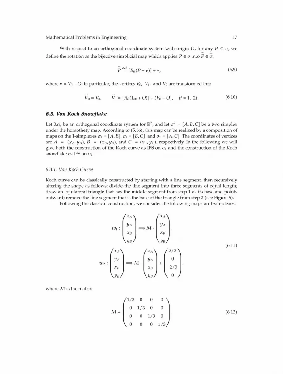
6.3. Von Koch Snowflake

Let 0xy be an orthogonal coordinate system for R2, and let σ2 = [A,B,C] be a two simplex

under the homothety map. According to (5.16), this map can be realized by a composition ofmaps on the 1-simplexes σ1 = [A,B], σ1 = [B,C], and σ1 = [A,C]. The coordinates of verticesare A = (xA, yA), B = (xB, yB), and C = (xC, yC), respectively. In the following we willgive both the construction of the Koch curve as IFS on σ1 and the construction of the Kochsnowflake as IFS on σ2.

6.3.1. Von Koch Curve

Koch curve can be classically constructed by starting with a line segment, then recursivelyaltering the shape as follows: divide the line segment into three segments of equal length;draw an equilateral triangle that has the middle segment from step 1 as its base and pointsoutward; remove the line segment that is the base of the triangle from step 2 (see Figure 5).

Following the classical construction, we consider the following maps on 1-simplexes:

w1 :

⎛⎜⎜⎜⎜⎜⎝

xA

yA

xB

yB

⎞⎟⎟⎟⎟⎟⎠ =⇒ M ·

⎛⎜⎜⎜⎜⎜⎝

xA

yA

xB

yB

⎞⎟⎟⎟⎟⎟⎠,

w2 :

⎛⎜⎜⎜⎜⎜⎝

xA

yA

xB

yB

⎞⎟⎟⎟⎟⎟⎠ =⇒ M ·

⎛⎜⎜⎜⎜⎜⎝

xA

yA

xB

yB

⎞⎟⎟⎟⎟⎟⎠ +

⎛⎜⎜⎜⎜⎜⎝

2/3

0

2/3

0

⎞⎟⎟⎟⎟⎟⎠,

(6.11)

where M is the matrix

M =

⎛⎜⎜⎜⎜⎜⎝

1/3 0 0 0

0 1/3 0 0

0 0 1/3 0

0 0 0 1/3

⎞⎟⎟⎟⎟⎟⎠. (6.12)

18 Mathematical Problems in Engineering

Hence, w1 is a factor of the homothety w having A as a fixed vertex, while w2 leaves Bunchanged:

w1(P) = P − 23λiL0i, L0i = Vi −A,

w2(P) = P − 23λiL0i, L0i = Vi − B.

(6.13)

Moreover, each vertex in the wi([σ1]), i = 1, 2, can be expressed as in(3.6)

V i = Vi − 23L0i. (6.14)

Let us now consider the transformation, on two steps, which first rotates w1([A,B])of an angle θ = 60◦ around the fixed point A, and then it translates the rotated simplex by avector v = (1/3, 0).

So that we obtain

w3 :

⎛⎜⎜⎜⎜⎜⎝

xA

yA

xB

yB

⎞⎟⎟⎟⎟⎟⎠ =⇒ M′ ·

⎛⎜⎜⎜⎜⎜⎝

xA

yA

xB

yB

⎞⎟⎟⎟⎟⎟⎠ +

⎛⎜⎜⎜⎜⎜⎝

1/3

0

1/3

0

⎞⎟⎟⎟⎟⎟⎠, (6.15)

where M′ is the matrix

M′ =

⎛⎜⎜⎜⎜⎜⎝

1/6 −√3/6 0 0√3/6 1/6 0 0

0 0 1/6 −√3/6

0 0√3/6 1/6

⎞⎟⎟⎟⎟⎟⎠. (6.16)

Finally, let us apply the transformation which first rotates w1([A,B]) of an angle θ =120◦ around the fixed point A, and then it translates the rotated simplex by the vector v =(2/3, 0). Accordingly, it is

w4 :

⎛⎜⎜⎜⎜⎜⎝

xA

yA

xB

yB

⎞⎟⎟⎟⎟⎟⎠ =⇒ M′′ ·

⎛⎜⎜⎜⎜⎜⎝

xA

yA

xB

yB

⎞⎟⎟⎟⎟⎟⎠ +

⎛⎜⎜⎜⎜⎜⎝

2/3

0

2/3

0

⎞⎟⎟⎟⎟⎟⎠, (6.17)

Mathematical Problems in Engineering 19

Figure 4: Image of w([σ1]) =⋃

i = 1,...,4 wi([σ1]), where the 1-simplex σ1 is the unitary interval.

where M′′ is the matrix

M′′ =

⎛⎜⎜⎜⎜⎜⎝

−1/6 −√3/6 0 0√3/6 −1/6 0 0

0 0 −1/6 −√3/6

0 0√3/6 −1/6

⎞⎟⎟⎟⎟⎟⎠. (6.18)

Since, as previously shown, rotation and translation are isometries, for each wi([σ1]),i = 1, 2, 3, 4, we obtain

Lij =

13Lij ,

l ij =13lij ,

Ω =13Ω.

(6.19)

In order to visualize the von Koch pattern, let us consider the 1-simplex {A,B} ={{0, 0}, {1, 0}}; since the point A has been chosen as the origin of the reference system, andw3 and w4 are obtained as rotation leaving fixed the origin, the transformed instances can beeasily computed so that, at the first step, the IFSmaps on 1-simplexes can be drawn (Figure 4).

Reiterating this process for each remaining segment, at the step k we will obtain thecompact set Tk made of 22k segments whose sides are contracted by a factor (1/3)k. The IFSmap (R1, d,w1, w2, w3, w4) gives us the Koch curve L =

⋂k Lk with similarity dimension

equal to

s =log 4

log 1/(1/3)=

log 4log 3

. (6.20)

This is also the similarity dimension of the Koch snowflake [27, 28]. So, the Koch curve(Figure 5) is obtained as a combination of IFS simplicial maps generating the known fractal-shaped curve.

6.3.2. Koch Flake

According to (5.16) and to the examples previously given, Koch flake (snowflake) can beconstructed in a non-classical approach as IFS of maps on a 2-simplex. Koch snowflake canbe seen as the image of a suitable system of iterated homotheties acting on a 2-simplex, givenby suitable translations of the boundary 1-simplexes.

20 Mathematical Problems in Engineering

Figure 5: Koch curve.

In this process, the total length of each side of a triangle increases by one-third, andthus, the total length at the kth step will be (4/3)k of the original triangle perimeter.

7. Conclusion

In this paper, a nonclassical approach to fractal generation based on IFS of maps on simplexeshas been given. Some of the most popular fractals, as the Sierpinski gasket and the von Kochflake, were obtained by iterative maps on simplexes. All maps were also intrinsically definedby using the affine (barycentric) coordinates and some basic measures on simplexes. Themethod proposed in this paper could be used to generate some new classes of fractals in anydimension, by simply defining suitable IFS on simplexes, thus opening new perspectives infractal lattice geometry.

References

[1] A. T. Fomenko, Differential Geometry and Topology, Contemporary Soviet Mathematics, ConsultantsBureau, New York, NY, USA, 1987.

[2] G. L. Naber, Topological Methods in Euclidean Spaces, Cambridge University Press, Cambridge, UK,1980.

[3] I. M. Singer and J. A. Thorpe, Lecture notes on elementary topology and geometry, Scott, Foresman andCo., Glenview, Ill, USA, 1967.

[4] C. Cattani, “Variational method and Regge equations,” in Proceedings of the 8th Marcel GrossmannMeeting, Gerusalem, Palestine, June 1997.

[5] C. Cattani and E. Laserra, “Discrete electromagnetic action on a gravitational simplicial net,” Journalof Interdisciplinary Mathematics, vol. 3, no. 2-3, pp. 123–132, 2000.

[6] I. T. Drummond, “Regge-Palatini calculus,” Nuclear Physics. B, vol. 273, no. 1, pp. 125–136, 1986.[7] C. W. Misner, K. S. Thorne, and J. A. Wheeler, “Regge Calculus,” in Gravitation, p. ii+xxvi+1279+iipp,

W. H. Freeman and Co., San Francisco, Calif, USA, 1973.[8] T. Regge, “General relativity without coordinates,” Il Nuovo Cimento Series 10, vol. 19, no. 3, pp. 558–

571, 1961.[9] R. Sorkin, “The electromagnetic field on a simplicial net,” Journal of Mathematical Physics, vol. 16, no.

12, pp. 2432–2440, 1975.[10] A. L. Barabasi, Linked: How Everything is Connected to Everything Else and What It Means for Business,

Science and Everyday Life, Plume Books, 2003.[11] A. L. Barabasi, E. Ravasz, and T. Vicsek, “Deterministic scale-free networks,” Physica A, vol. 299, no.

3-4, pp. 559–564, 2001.

Mathematical Problems in Engineering 21

[12] S. H. Strogatz, “Exploring complex networks,” Nature, vol. 410, no. 6825, pp. 268–276, 2001.[13] D. J. Watts and S. H. Strogatz, “Collective dynamics of ’small-world9 networks,” Nature, vol. 393, no.

6684, pp. 440–442, 1998.[14] C. Cattani and E. Laserra, “Simplicial geometry of crystals,” Journal of Interdisciplinary Mathematics,

vol. 2, no. 2-3, pp. 143–151, 1999.[15] N. Goldenfeld, Lectures on Phase Transitions and the Renormalization Group, Addison-Wesley, Reading,

Mass, USA, 1992.[16] V. M. Kenkre and P. Reineker, Exciton Dynamics in Molecular Crystals and Aggregates, Springer, Berlin,

Germany, 1982.[17] F. Vogtle, Ed., Dendrimers, Springer, Berlin, Germany, 1998.[18] C. Cattani and A. Paoluzzi, “Boundary integration over linear polyhedra,” Computer-Aided Design,

vol. 22, no. 2, pp. 130–135, 1990.[19] C. Cattani and A. Paoluzzi, “Symbolic analysis of linear polyhedra,” Engineering with Computers, vol.

6, no. 1, pp. 17–29, 1990.[20] S. Y. Chen, H. Tong, and C. Cattani, “Markov models for image labeling,” Mathematical Problems in

Engineering, vol. 2012, Article ID 814356, 18 pages, 2012.[21] S. Y. Chen, H. Tong, Z. Wang, S. Liu, M. Li, and B. Zhang, “Improved generalized belief propagation

for vision processing,” Mathematical Problems in Engineering, vol. 2011, Article ID 416963, 12 pages,2011.

[22] J. P. Blondeau, C. Orieux, and L. Allam, “Morphological and fractal studies of silicon nanoaggregatesstructures prepared by thermal activated reaction,”Materials Science and Engineering B, vol. 122, no. 1,pp. 41–48, 2005.

[23] C. C. Doumanidis, “Nanomanufacturing of random branchingmaterial architectures,”MicroelectronicEngineering, vol. 86, no. 4-6, pp. 467–478, 2009.

[24] D. Lekic and S. Elezovic-Hadizic, “Semi-flexible compact polymers on fractal lattices,” Physica A, vol.390, no. 11, pp. 1941–1952, 2011.

[25] R. Lua, A. L. Borovinskiy, and A. Y. Grosberg, “Fractal and statistical properties of large compactpolymers: a computational study,” Polymer, vol. 45, no. 2, pp. 717–731, 2004.

[26] M. F. Barnsley, Fractal Everywhere, Academic Press, 1988.[27] K. Falconer, Fractal Geometry: Mathematical Foundations and Applications, John Wiley & Sons,

Chichester, UK, 1990.[28] J. E. Hutchinson, “Fractals and self-similarity,” Indiana University Mathematics Journal, vol. 30, no. 5,

pp. 713–747, 1981.[29] B. B. Mandelbrot, The Fractal Geometry of Nature, W. H. Freeman and Co., San Francisco, Calif, USA,

1982.[30] C. Cattani and J. Rushchitsky, Wavelet and Wave Analysis as Applied to Materials with Micro or

Nanostructure, vol. 74 of Series on Advances in Mathematics for Applied Sciences, World Scientific,Hackensack, NJ, USA, 2007.

[31] E. V. Pashkova, E. D. Solovyova, I. E. Kotenko, T. V. Kolodiazhnyi, and A. G. Belous, “Effect ofpreparation conditions on fractal structure and phase transformations in the synthesis of nanoscaleM-type barium hexaferrite,” Journal of Magnetism and Magnetic Materials, vol. 323, no. 20, pp. 2497–2503, 2011.

[32] M. Li, “Fractal time series—a tutorial review,” Mathematical Problems in Engineering, vol. 2010, ArticleID 157264, 26 pages, 2010.

[33] M. Li, S. C. Lim, and S. Chen, “Exact solution of impulse response to a class of fractional oscillatorsand its stability,” Mathematical Problems in Engineering, vol. 2011, Article ID 657839, 9 pages, 2011.

[34] C. Cattani and E. Laserra, “Self-similar hierarchical regular lattices,” in the International Conference onComputational Science and Its Applications (ICCSA ’10), D. Taniar et al., Ed., vol. 6017 of Lecture Notes inComputer Science, pp. 225–240, 2010.

[35] L. Kocic, S. Gegovska-Zajkova, and L. Stefanovska, “Affine invariant contractions of simplices,”Kragujevac Journal of Mathematics, vol. 30, pp. 171–179, 2007.

[36] M.A. Khamsi andW. A. Kirk,An Introduction toMetric Spaces and Fixed Point Theory, Pure andAppliedMathematics, Wiley-Interscience, New York, NY, USA, 2001.

Submit your manuscripts athttp://www.hindawi.com

OperationsResearch

Advances in

Hindawi Publishing Corporationhttp://www.hindawi.com Volume 2013

Hindawi Publishing Corporationhttp://www.hindawi.com Volume 2013

Mathematical Problems in Engineering

Abstract and Applied AnalysisHindawi Publishing Corporationhttp://www.hindawi.com Volume 2013

ISRN Applied Mathematics

Hindawi Publishing Corporationhttp://www.hindawi.com Volume 2013

Hindawi Publishing Corporationhttp://www.hindawi.com

Volume 2013

International Journal of

Combinatorics

Hindawi Publishing Corporationhttp://www.hindawi.com Volume 2013

Journal of Function Spaces and Applications

International Journal of Mathematics and Mathematical Sciences

Hindawi Publishing Corporationhttp://www.hindawi.com Volume 2013

ISRN Geometry

Hindawi Publishing Corporationhttp://www.hindawi.com Volume 2013

Discrete Dynamics in Nature and Society

Hindawi Publishing Corporationhttp://www.hindawi.com Volume 2013

Hindawi Publishing Corporationhttp://www.hindawi.com

Volume 2013

Advances in

Mathematical Physics

ISRN Algebra

Hindawi Publishing Corporationhttp://www.hindawi.com Volume 2013

ProbabilityandStatistics

Journal of

Hindawi Publishing Corporationhttp://www.hindawi.com Volume 2013

ISRN Mathematical Analysis

Hindawi Publishing Corporationhttp://www.hindawi.com Volume 2013

Journal ofApplied Mathematics

Hindawi Publishing Corporationhttp://www.hindawi.com Volume 2013

Advances in

DecisionSciences

Hindawi Publishing Corporationhttp://www.hindawi.com Volume 2013

Hindawi Publishing Corporationhttp://www.hindawi.com Volume 2013

Stochastic AnalysisInternational Journal of

Hindawi Publishing Corporation http://www.hindawi.com Volume 2013Hindawi Publishing Corporation http://www.hindawi.com Volume 2013

The Scientific World Journal

Hindawi Publishing Corporationhttp://www.hindawi.com Volume 2013

ISRN Discrete Mathematics

Hindawi Publishing Corporationhttp://www.hindawi.com

Differential EquationsInternational Journal of

Volume 2013