hydrology

Article

Simplified Interception/Evaporation Model

Giorgio Baiamonte

�����������������

Citation: Baiamonte, G. Simplified

Interception/Evaporation Model.

Hydrology 2021, 8, 99. https://

doi.org/10.3390/hydrology8030099

Academic Editors: Aristoteles Tegos

and Nikolaos Malamos

Received: 6 June 2021

Accepted: 30 June 2021

Published: 2 July 2021

Publisher’s Note: MDPI stays neutral

with regard to jurisdictional claims in

published maps and institutional affil-

iations.

Copyright: © 2021 by the author.

Licensee MDPI, Basel, Switzerland.

This article is an open access article

distributed under the terms and

conditions of the Creative Commons

Attribution (CC BY) license (https://

creativecommons.org/licenses/by/

4.0/).

Department of Agricultural, Food and Forest Sciences (SAAF), University of Palermo, Viale delle Scienze,90128 Palermo, Italy; giorgio.baiamonte@unipa.it

Abstract: It is known that at the event scale, evaporation losses of rainfall intercepted by canopyare a few millimeters, which is often not much in comparison to other stocks in the water balance.Nevertheless, at yearly scale, the number of times that the canopy is filled by rainfall and thendepleted can be so large that the interception flux may become an important fraction of rainfall.Many accurate interception models and models that describe evaporation by wet canopy havebeen proposed. However, they often require parameters that are difficult to obtain, especially forlarge-scale applications. In this paper, a simplified interception/evaporation model is proposed,which considers a modified Merrian model to compute interception during wet spells, and a simplepower-law equation to model evaporation by wet canopy during dry spells. Thus, the model canbe applied for continuous simulation, according to the sub hourly rainfall data that is appropriateto study both processes. It is shown that the Merrian model can be derived according to a simplelinear storage model, also accounting for the antecedent intercepted stored volume, which is usefulto consider for the suggested simplified approach. For faba bean cover crop, an application of thesuggested procedure, providing reasonable results, is performed and discussed.

Keywords: interception; linear storage model; evaporation; cover crop; water balance; faba bean

1. Introduction

According to Brutsaert [1], the interception process is determined by the rainfallfraction that moistens vegetation and that is temporarily stored on it, before evaporating.When the vegetation cover is fully saturated, the interception storage capacity is achieved.In practice, the interception storage capacity is denoted as rainfall left on the canopy atthe end of the rainfall after all drip has ceased [2]. The water stored on the canopy mayevaporate soon after, thus short-circuiting the hydrologic cycle.

Although most surfaces can store only a few millimeters of rainfall, which is often notmuch in comparison to other stocks in the water balance, interception is generally a signifi-cant process and its impact becomes evident at longer time scales [3]. Thus, interceptionstorage is generally small, but the number of times that the storage is filled and depletedcan be so large that the evaporation losses by wet canopy may become of the same order ofmagnitude as the transpiration flux [4].

Evaporation flux by canopy exerts a negative effect on plant water consumption bypreventing water from reaching the soil surface, thus the plant roots [2,3]. In contrast, theremaining rainfall (i.e., the net rainfall) reaches the soil surface either as throughfall orby flowing down branches and stems as stemflow. Throughfall is the fraction of waterthat reaches the soil surface directly through the canopy gaps without hitting the canopysurfaces, or indirectly through dripping from the leaves and branches [5].

The interception may also exert important effects on surface runoff [6], providinga certain delay compared with the time of the beginning of the rain. For the Dunnian mech-anism of runoff generation, Baiamonte [7] showed the effect induced by the interceptionprocess on the delay time, and emphasized that the effect is more frequent for well-drainedsoils [8,9] in humid regions, for low rainfall intensities and high groundwater table, wheninfiltration capacity exceeds the rainfall intensity. Indeed, the latter conditions also occurs

Hydrology 2021, 8, 99. https://doi.org/10.3390/hydrology8030099 https://www.mdpi.com/journal/hydrology

Hydrology 2021, 8, 99 2 of 16

for high density of cover crops or forest soils that are reach in organic carbon and are verystructured [10].

The proportion of the precipitation that does not reach the ground, i.e., the intercep-tion loss, depends on the type of vegetation (forest, tree, or grassland), its age, density ofplanting and the season of the year. The interception loss also depends on rainfall regime,thus on climate. For example, in tall dense forest vegetation at temperate latitudes intercep-tion loss as large as 30–40% of the gross precipitation has been observed [11], whereas intropical forest with high rainfall intensity was of the order 10–15% [12] and in heather andshrub also 10–15% [13]. In arid and semi-arid areas, where there is little vegetation, theinterception loss is negligible.

Since interception is an important component of the water balance, a comprehensiveevaluation of interception loss by prediction tools has been considered of great value inthe study of hydrological processes, and different formulations, at hourly and event scale,have been introduced in the hydrologic literature. Muzylo et al. [14] wrote an interestingreview paper, where the principal models proposed in the literature are described, andtheir characteristics reported (input temporal scale, output variable, number of parameters,layers, spatial scale).

Linsley et al. [15] modified the very simple interception model first introduced byHorton [16], which did not account for the amount of gross rainfall, since it assumed thatthe rainfall in each storm completely filled the interception storage. Linsley et al. [15]assumed that the interception loss approached exponentially to the interception capacityas the amount of rainfall increased [17]. Then, this simple sketch was applied and tested byMerrian [18], who studied the effect of fog intensity and leaf shape on water storage onleaves, by using a simple fog wind tunnel and leaves of aluminum and plastic. Merrian [18]found that drip measurements were reasonably close to values predicted, by using anexponential equation based on fog flow and leaf storage capacity.

Rutter et al. [19,20] were the first to model forest rainfall interception recognizing thatthe process was primarily driven by evaporation from the wetted canopy. The conceptualmodel developed by Rutter et al. [19,20] describes the interception loss in terms of both thestructure of the forest and the climate in which it is growing. The model is physicallybased, thus it has potential for application in all areas, where there are suitable data. InRutter et al. [20], the model’s definitive version was developed by adding a stemflowmodule, in which a fraction of the rainfall input is diverted to a compartment comprisingthe trunks. Early applications of Rutter-type models were made by Calder [21] and Gashand Morton [22].

The rate of evaporation increases with solar radiation and temperature. The processalso depends on the air humidity and the wind speed. The greater the humidity, the lessthe evaporation. Wind carries moist air away from the ground surface, so wind decreasesthe local humidity and allows more water to evaporate. Therefore, in the Rutter model,the evaporation flux was calculated from the form of the Monteith–Penman equation [23].Later, Gash [24] provided a simplification of the data-demanding Rutter model. Althoughsome of the assumptions of the Gash model may not be suitable, the model has been shownto work well under a variety of forest types, including different species and sites [11,25–27].

For agricultural crops and for grassland, where interception loss is of the order 13–19% [28],Von Hoyningen-Hüne [29] and Braden [30], proposed a general formula, which was used inthe SWAP model [31] that however can be applied only at daily scale.

By the experimental point of view, the interception evaporation process requires mon-itoring intercepted mass and interception loss with high accuracy and time resolution,to provide accurate estimates. Net precipitation techniques, in which interception evap-oration is determined from the difference between gross precipitation and throughfall,fulfill many of the requirements but usually have too-low accuracy and time resolution forprocess studies. Furthermore, for grassland, these techniques are unsuitable.

In this paper, we explored the rainfall partitioning in net rainfall and evaporationlosses by canopy, by using a very simplified sketch of the interception process, which

Hydrology 2021, 8, 99 3 of 16

combines a modified exponential equation applied and tested by Merrian [18], accountingfor the antecedent volume stored on the canopy, and a simple power-law equation tocompute evaporation by wet canopy. We are aware that the considered approach is farfrom the sophisticated physically based developments that were performed to quantifyinterception and evaporations losses. However, the latter may require many parametersthat are not easy to determine. It is shown that the simplified parsimonious approachmay lead to a reasonable quantification of this important component of the hydrologiccycle, which can be useful when a rough estimate is required, in absence of a detailedcharacterization of the canopy and of the climate conditions. It is also shown that theMerrian model can be derived by considering a simple linear storage model. For faba beancover crop, an application of the suggested procedure is performed and discussed.

2. Rainfall Data Set, Wet and Dry Spells

Rainfall time series were analyzed according to Agnese et al. [32], who applied thediscrete three-parameter Lerch distribution to model the frequency distribution of interar-rival times, IT, derived from daily precipitation time-series, for the Sicily region, in Italy.Agnese et al. [32] showed a good fitting of the Lerch distribution, thus evidencing the wideapplicability of this kind of distribution [33], also allowing us to jointly model dry spells,DS, and wet spells, WS.

Since this work aimed at modelling by continuous rainfall data series the interceptionlosses, during the WS and the evaporation losses during DS, only the frequency distribu-tion of the two latter were considered, which are defined in the following, according toAgnese et al. [32].

For any rainfall data series, the ten minutes temporal scale, τ, which is appropriateto model both interception and evaporation processes, could be considered in order todescribe clustering and intermittency characters of continuous rainfall data series.

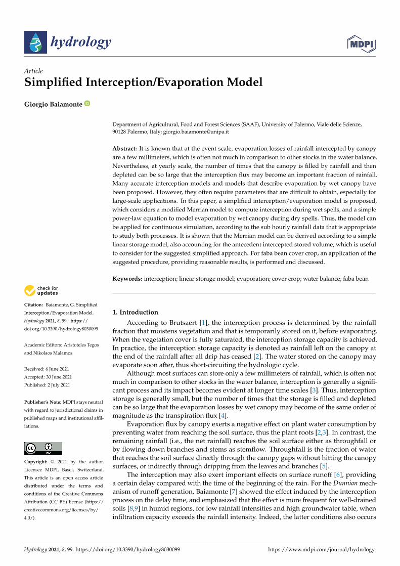
Let H = {h1, h2, . . . , hn}, a time-series of rainfall data of size n, spaced at uniformtime-scale τ. The sub-series of H can be defined as the event series, E {t1, t2, . . . , tnE}, wherenE (0 < nE < n) is the size of E, which is an integer multiple of time-scale τ. The successionconstituted by the times elapsed between each element of the E series, with exception ofthe first one and the immediately preceding one, is defined as the inter-arrival time-series,IT {T1, T2, . . . , TnE}, with size nE−1 (Figure 1). It can be observed the sequence of dry spells,DS, can be derived from IT dataset by using the relationship {DSk} = {Tk} − 1 for any Tk > 1.

Hydrology 2021, 8, x FOR PEER REVIEW 3 of 16

In this paper, we explored the rainfall partitioning in net rainfall and evaporation

losses by canopy, by using a very simplified sketch of the interception process, which

combines a modified exponential equation applied and tested by Merrian [18], accounting

for the antecedent volume stored on the canopy, and a simple power-law equation to

compute evaporation by wet canopy. We are aware that the considered approach is far

from the sophisticated physically based developments that were performed to quantify

interception and evaporations losses. However, the latter may require many parameters

that are not easy to determine. It is shown that the simplified parsimonious approach may

lead to a reasonable quantification of this important component of the hydrologic cycle,

which can be useful when a rough estimate is required, in absence of a detailed character-

ization of the canopy and of the climate conditions. It is also shown that the Merrian model

can be derived by considering a simple linear storage model. For faba bean cover crop, an

application of the suggested procedure is performed and discussed.

2. Rainfall Data Set, Wet and Dry Spells

Rainfall time series were analyzed according to Agnese et al. [32], who applied the

discrete three-parameter Lerch distribution to model the frequency distribution of inter-

arrival times, IT, derived from daily precipitation time-series, for the Sicily region, in Italy.

Agnese et al. [32] showed a good fitting of the Lerch distribution, thus evidencing the

wide applicability of this kind of distribution [33], also allowing us to jointly model dry

spells, DS, and wet spells, WS.

Since this work aimed at modelling by continuous rainfall data series the interception

losses, during the WS and the evaporation losses during DS, only the frequency distribu-

tion of the two latter were considered, which are defined in the following, according to

Agnese et al. [32].

For any rainfall data series, the ten minutes temporal scale, τ, which is appropriate to

model both interception and evaporation processes, could be considered in order to de-

scribe clustering and intermittency characters of continuous rainfall data series.

Let H = {h1, h2, …, hn}, a time-series of rainfall data of size n, spaced at uniform time-

scale τ. The sub-series of H can be defined as the event series, E {t1, t2, …, tnE}, where nE (0

< nE < n) is the size of E, which is an integer multiple of time-scale τ. The succession con-

stituted by the times elapsed between each element of the E series, with exception of the

first one and the immediately preceding one, is defined as the inter-arrival time-series, IT

{T1, T2, …, TnE}, with size nE−1 (Figure 1). It can be observed the sequence of dry spells, DS,

can be derived from IT dataset by using the relationship {DSk} = {Tk} − 1 for any Tk > 1.

Figure 1. Sketch of inter-arrival times (IT), dry spells (DS) and wet spells (WS). Reprinted with

permission from ref. [32], Copyright 2014, Elsevier (Amsterdam, The Netherlands).

Figure 1 shows an example of a sequence of wet and dry spells. In the context of this

work, which aims at modelling the interception process during WS and the evaporation

process from the canopy, as previously observed, only the frequency distribution of wet

spells (WS) and dry spells (DS) were derived.

For the 2009 rainfall data series of Fontanasalsa station (Trapani, 37°56′37″ N,

12°33′12″ E, western Sicily, Italy), which will be considered for an example application,

Figure 2 shows the complete characteristics of the rainfall regime. In particular, Figure 2a

Figure 1. Sketch of inter-arrival times (IT), dry spells (DS) and wet spells (WS). Reprinted with permission from ref. [32],Copyright 2014, Elsevier (Amsterdam, The Netherlands).

Figure 1 shows an example of a sequence of wet and dry spells. In the context of thiswork, which aims at modelling the interception process during WS and the evaporationprocess from the canopy, as previously observed, only the frequency distribution of wetspells (WS) and dry spells (DS) were derived.

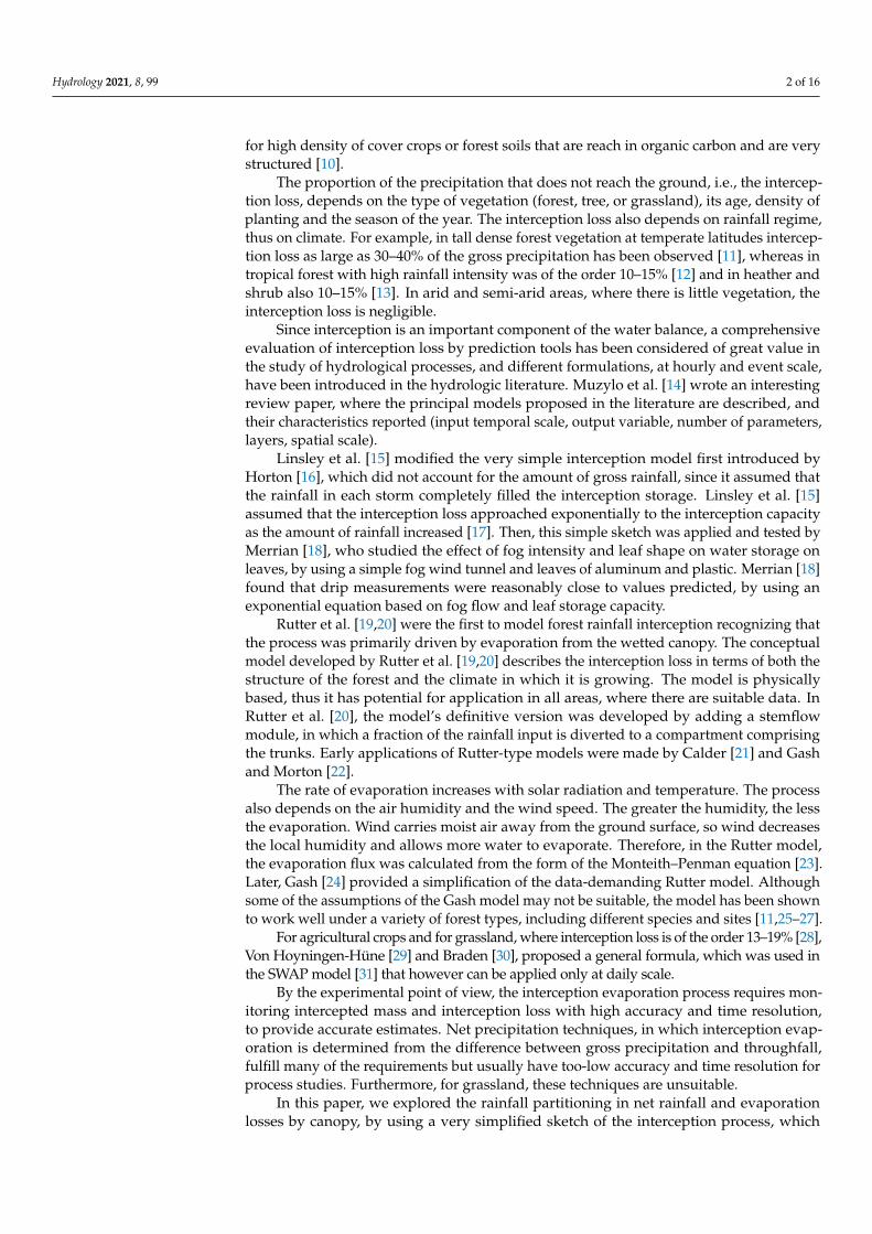
For the 2009 rainfall data series of Fontanasalsa station (Trapani, 37◦56′37′′ N, 12◦33′12′′ E,western Sicily, Italy), which will be considered for an example application, Figure 2 showsthe complete characteristics of the rainfall regime. In particular, Figure 2a describes the DSdistribution of frequency, F, whereas Figure 2b plots the WS distribution associated with thecumulated rainfall depth collected with 10 min time resolution. Both figures also illustratethe frequency of non-exceedance, corresponding the selected time resolution (τ = 1 = 10 min)

Hydrology 2021, 8, 99 4 of 16

that equals 0.189 for DS and much higher for WS (0.596), indicating that a high fraction ofrainfall with WS = 1 occurs, which could play an important role in the interception process.Figure 2b also plots the rainfall depth distribution corresponding to WS, where the frequencyis calculated with respect to the yearly rainfall depth, hyear, which equals 885.2 mm. Therefore,in Figure 2b, to WS = 1 (F1 = 0.115) corresponds a rainfall depth equals to 101.6 mm that, ifassociated with subsequent large enough DS, may potentially evaporate from the canopy.

Hydrology 2021, 8, x FOR PEER REVIEW 4 of 16

describes the DS distribution of frequency, F, whereas Figure 2b plots the WS distribution

associated with the cumulated rainfall depth collected with 10 min time resolution. Both

figures also illustrate the frequency of non-exceedance, corresponding the selected time

resolution (τ = 1 = 10 min) that equals 0.189 for DS and much higher for WS (0.596), indi-

cating that a high fraction of rainfall with WS = 1 occurs, which could play an important

role in the interception process. Figure 2b also plots the rainfall depth distribution corre-

sponding to WS, where the frequency is calculated with respect to the yearly rainfall

depth, hyear, which equals 885.2 mm. Therefore, in Figure 2b, to WS = 1 (F1 = 0.115) corre-

sponds a rainfall depth equals to 101.6 mm that, if associated with subsequent large

enough DS, may potentially evaporate from the canopy.

Figure 2. For the investigated year (2009), distributions of frequency, F, (a) of dry spells (DS), and (b) of wet spells (WS)

and of the rainfall depth (hτ) corresponding to WS.

3. Interception Rate and Stored Volumes during Wet Spells

The interception Merrian [18]’s model states that:

��� � � �1 � � �� ��� (1)

where S (mm) is the interception capacity of the canopy, and ICS (mm) is the interception

storage volume corresponding to the cumulated rainfall volume R (mm). Equation (1) can

be applied for dry initial condition, i.e., when the no water volume is stored on the canopy

at the beginning of the rainfall.

However, it is demonstrated here that the Merrian model can be derived by consid-

ering a simple linear stored model, also used in other hydrological contexts [34], which

made it possible to also account for the antecedent interception volume. The latter is use-

ful for the applications, when in between two consecutive WSs, DS is not long enough to

result in full evaporation of the rainfall volume intercepted by the canopy starting from

the end of a WS. Thus, a residual water volume, ICS0, is still stored on the canopy at the

beginning of the subsequent WS, and it needs to be considered as initial condition. There-

fore, for the purpose of this study, which aims at estimating interception losses during WS

and DS sequences of different amount and duration, Equation (1) needs to be extended to

different antecedent water interception storage volume, ICS0 (mm), before a new WS takes

place, after a DS when evaporation process ceases.

Consider a simple linear reservoir, miming the interception storage volume (Figure

3). A stationary rainfall of intensity r (mm h−1) uniformly distributed over the canopy, is

applied to the reservoir. In the time dt, the interception storage, ICS (mm), stored in the

canopy equals dICS. The interception capacity, i.e., the maximum rainfall volume that can

be stored on the canopy, is denoted as S (mm). The duration of rainfall that needs to

Figure 2. For the investigated year (2009), distributions of frequency, F, (a) of dry spells (DS), and (b) of wet spells (WS) andof the rainfall depth (hτ) corresponding to WS.

3. Interception Rate and Stored Volumes during Wet Spells

The interception Merrian [18]’s model states that:

ICS = S[

1− exp(−R

S

)](1)

where S (mm) is the interception capacity of the canopy, and ICS (mm) is the interceptionstorage volume corresponding to the cumulated rainfall volume R (mm). Equation (1) canbe applied for dry initial condition, i.e., when the no water volume is stored on the canopyat the beginning of the rainfall.

However, it is demonstrated here that the Merrian model can be derived by consider-ing a simple linear stored model, also used in other hydrological contexts [34], which madeit possible to also account for the antecedent interception volume. The latter is useful forthe applications, when in between two consecutive WSs, DS is not long enough to result infull evaporation of the rainfall volume intercepted by the canopy starting from the end ofa WS. Thus, a residual water volume, ICS0, is still stored on the canopy at the beginningof the subsequent WS, and it needs to be considered as initial condition. Therefore, forthe purpose of this study, which aims at estimating interception losses during WS and DSsequences of different amount and duration, Equation (1) needs to be extended to differentantecedent water interception storage volume, ICS0 (mm), before a new WS takes place,after a DS when evaporation process ceases.

Consider a simple linear reservoir, miming the interception storage volume (Figure 3).A stationary rainfall of intensity r (mm h−1) uniformly distributed over the canopy, isapplied to the reservoir. In the time dt, the interception storage, ICS (mm), stored in thecanopy equals dICS. The interception capacity, i.e., the maximum rainfall volume thatcan be stored on the canopy, is denoted as S (mm). The duration of rainfall that needs toachieve the saturation of the canopy, without dripping out from the reservoir, ts (h), can beexpressed as:

ts =Sr

(2)

Hydrology 2021, 8, 99 5 of 16

Hydrology 2021, 8, x FOR PEER REVIEW 5 of 16

achieve the saturation of the canopy, without dripping out from the reservoir, ts (h), can

be expressed as:

�� � �� (2)

From a physical point of view, ts is not very meaningful since it describes the duration

of rainfall that is required for the canopy saturation, for dry antecedent conditions (ICS0 =

0), and with no losses from the reservoir, e.g., no dripping and no net rainfall intensity pn

(mm h−1), which actually occurs (Figure 3). However, ts represents a characteristic time of

the interception process that it is useful to introduce for the following derivations.

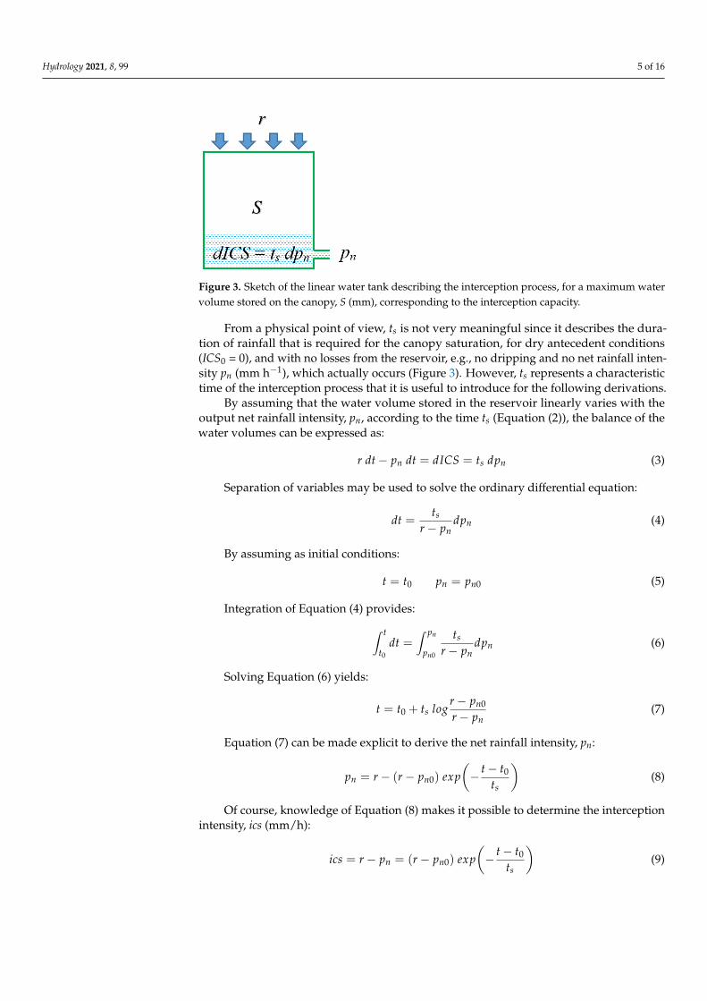
Figure 3. Sketch of the linear water tank describing the interception process, for a maximum water

volume stored on the canopy, S (mm), corresponding to the interception capacity.

By assuming that the water volume stored in the reservoir linearly varies with the

output net rainfall intensity, pn, according to the time ts (Equation (2)), the balance of the

water volumes can be expressed as:

� �� � �� �� � ���� � �� ��� (3)

Separation of variables may be used to solve the ordinary differential equation:

�� � ��� � �� ��� (4)

By assuming as initial conditions:

� � �� �� � ��� (5)

Integration of Equation (4) provides:

� �����

� � ��� � �� �����

��� (6)

Solving Equation (6) yields:

� � �� + �� ��� � � ���� � �� (7)

Equation (7) can be made explicit to derive the net rainfall intensity, pn:

�� � � � �� � ��� � �� � � ���� � (8)

Of course, knowledge of Equation (8) makes it possible to determine the interception

intensity, ics (mm/h):

!"# � � � �� � �� � ��� � �� � � ���� � (9)

Figure 3. Sketch of the linear water tank describing the interception process, for a maximum watervolume stored on the canopy, S (mm), corresponding to the interception capacity.

From a physical point of view, ts is not very meaningful since it describes the dura-tion of rainfall that is required for the canopy saturation, for dry antecedent conditions(ICS0 = 0), and with no losses from the reservoir, e.g., no dripping and no net rainfall inten-sity pn (mm h−1), which actually occurs (Figure 3). However, ts represents a characteristictime of the interception process that it is useful to introduce for the following derivations.

By assuming that the water volume stored in the reservoir linearly varies with theoutput net rainfall intensity, pn, according to the time ts (Equation (2)), the balance of thewater volumes can be expressed as:

r dt− pn dt = dICS = ts dpn (3)

Separation of variables may be used to solve the ordinary differential equation:

dt =ts

r− pndpn (4)

By assuming as initial conditions:

t = t0 pn = pn0 (5)

Integration of Equation (4) provides:∫ t

t0

dt =∫ pn

pn0

ts

r− pndpn (6)

Solving Equation (6) yields:

t = t0 + ts logr− pn0

r− pn(7)

Equation (7) can be made explicit to derive the net rainfall intensity, pn:

pn = r− (r− pn0) exp(− t− t0

ts

)(8)

Of course, knowledge of Equation (8) makes it possible to determine the interceptionintensity, ics (mm/h):

ics = r− pn = (r− pn0) exp(− t− t0

ts

)(9)

Hydrology 2021, 8, 99 6 of 16

Due to the assumption of a linear storage model, the antecedent net rainfall intensity,pn0, in Equations (8) and (9), is linked to the antecedent interception volume, ICS0, by:

pn0 =ICS0

ts= r

ICS0

S(10)

For a compacted graphical illustration, a constant rainfall intensity, r, and a zero timeantecedent condition t0 = 0 can be assumed. Thus, Equations (8) and (9) normalized withrespect to r can be expressed as:

pn

r= 1−

(1− ICS0

S

)exp(−R

S

)(11)

icsr

=

(1− ICS0

S

)exp(−R

S

)(12)

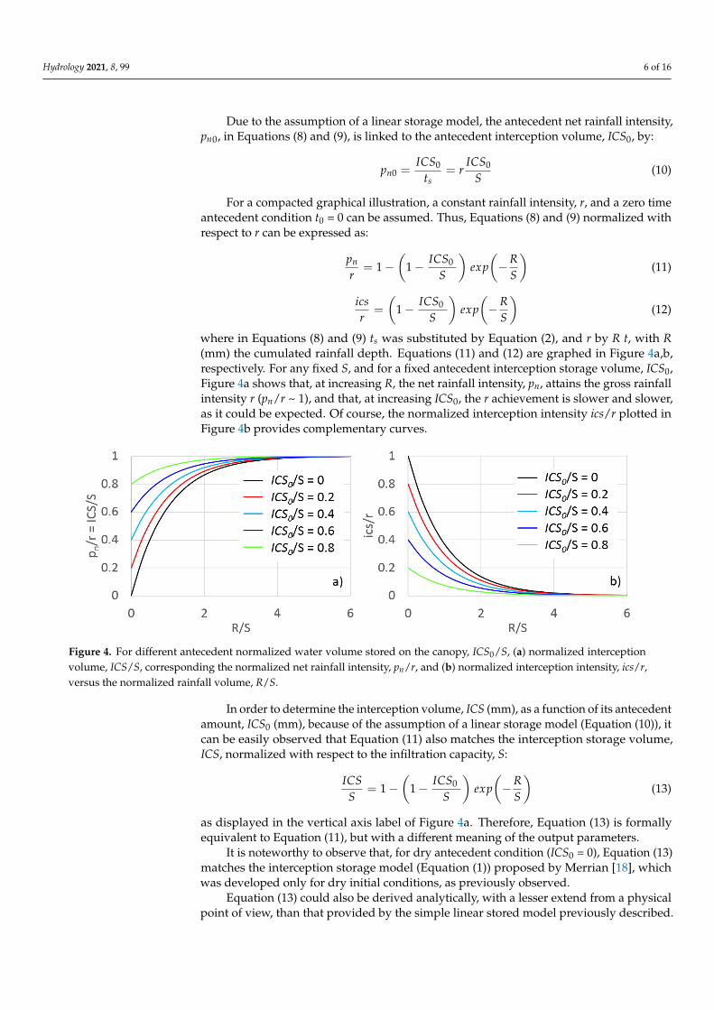
where in Equations (8) and (9) ts was substituted by Equation (2), and r by R t, with R(mm) the cumulated rainfall depth. Equations (11) and (12) are graphed in Figure 4a,b,respectively. For any fixed S, and for a fixed antecedent interception storage volume, ICS0,Figure 4a shows that, at increasing R, the net rainfall intensity, pn, attains the gross rainfallintensity r (pn/r ~ 1), and that, at increasing ICS0, the r achievement is slower and slower,as it could be expected. Of course, the normalized interception intensity ics/r plotted inFigure 4b provides complementary curves.

Hydrology 2021, 8, x FOR PEER REVIEW 6 of 16

Due to the assumption of a linear storage model, the antecedent net rainfall intensity,

pn0, in Equations (8) and (9), is linked to the antecedent interception volume, ICS0, by:

��� � ������ � � ����� (10)

For a compacted graphical illustration, a constant rainfall intensity, r, and a zero time

antecedent condition t0 = 0 can be assumed. Thus, Equations (8) and (9) normalized with

respect to r can be expressed as:

��� � 1 � �1 � ���� � � � ��

�� (11)

!"#� � �1 � ����

� � � �� �� (12)

where in Equations (8) and (9) ts was substituted by Equation (2), and r by R t, with R

(mm) the cumulated rainfall depth. Equations (11) and (12) are graphed in Figure 4a and

4b, respectively. For any fixed S, and for a fixed antecedent interception storage volume,

ICS0, Figure 4a shows that, at increasing R, the net rainfall intensity, pn, attains the gross

rainfall intensity r (pn/r ~ 1), and that, at increasing ICS0, the r achievement is slower and

slower, as it could be expected. Of course, the normalized interception intensity ics/r plot-

ted in Figure 4b provides complementary curves.

Figure 4. For different antecedent normalized water volume stored on the canopy, ICS0/S, (a) normalized interception

volume, ICS/S, corresponding the normalized net rainfall intensity, pn/r, and (b) normalized interception intensity, ics/r,

versus the normalized rainfall volume, R/S.

In order to determine the interception volume, ICS (mm), as a function of its anteced-

ent amount, ICS0 (mm), because of the assumption of a linear storage model (Equation

(10)), it can be easily observed that Equation (11) also matches the interception storage

volume, ICS, normalized with respect to the infiltration capacity, S:

���� � 1 � �1 � ����

� � � �� �� (13)

as displayed in the vertical axis label of Figure 4a. Therefore, Equation (13) is formally

equivalent to Equation (11), but with a different meaning of the output parameters.

It is noteworthy to observe that, for dry antecedent condition (ICS0 = 0), Equation (13)

matches the interception storage model (Equation (1)) proposed by Merrian [18], which

was developed only for dry initial conditions, as previously observed.

Equation (13) could also be derived analytically, with a lesser extend from a physical

point of view, than that provided by the simple linear stored model previously described.

Indeed, denoting R0 the antecedent rainfall volume corresponding to ICS0, the Merrian’s

model (Equation (1)) yields:

Figure 4. For different antecedent normalized water volume stored on the canopy, ICS0/S, (a) normalized interceptionvolume, ICS/S, corresponding the normalized net rainfall intensity, pn/r, and (b) normalized interception intensity, ics/r,versus the normalized rainfall volume, R/S.

In order to determine the interception volume, ICS (mm), as a function of its antecedentamount, ICS0 (mm), because of the assumption of a linear storage model (Equation (10)), itcan be easily observed that Equation (11) also matches the interception storage volume,ICS, normalized with respect to the infiltration capacity, S:

ICSS

= 1−(

1− ICS0

S

)exp(−R

S

)(13)

as displayed in the vertical axis label of Figure 4a. Therefore, Equation (13) is formallyequivalent to Equation (11), but with a different meaning of the output parameters.

It is noteworthy to observe that, for dry antecedent condition (ICS0 = 0), Equation (13)matches the interception storage model (Equation (1)) proposed by Merrian [18], whichwas developed only for dry initial conditions, as previously observed.

Equation (13) could also be derived analytically, with a lesser extend from a physicalpoint of view, than that provided by the simple linear stored model previously described.

Hydrology 2021, 8, 99 7 of 16

Indeed, denoting R0 the antecedent rainfall volume corresponding to ICS0, the Merrian’smodel (Equation (1)) yields:

ICS = S[

1− exp(−R

S− R0

S

)](14)

The antecedent rainfall volume, R0, can be expressed as a function of ICS0 by usingEquation (1):

R0 = −S log(

1− ICS0

S

)(15)

Substituting Equation (15) into Equation (14), and normalizing ICS with respect to S,provides Equation (13), which was to be demonstrated.

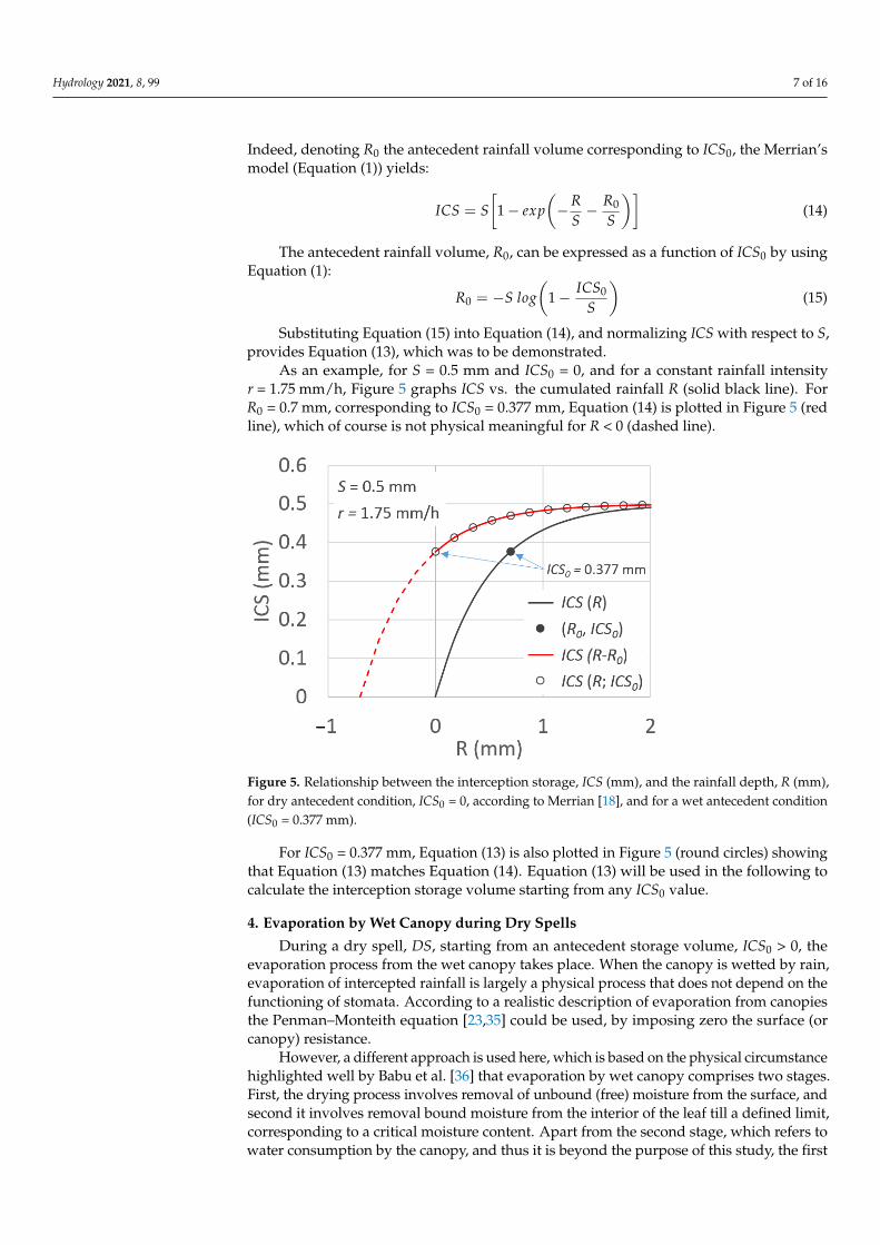
As an example, for S = 0.5 mm and ICS0 = 0, and for a constant rainfall intensityr = 1.75 mm/h, Figure 5 graphs ICS vs. the cumulated rainfall R (solid black line). ForR0 = 0.7 mm, corresponding to ICS0 = 0.377 mm, Equation (14) is plotted in Figure 5 (redline), which of course is not physical meaningful for R < 0 (dashed line).

Hydrology 2021, 8, x FOR PEER REVIEW 7 of 16

��� � � �1 � � �� � � �� �� (14)

The antecedent rainfall volume, R0, can be expressed as a function of ICS0 by using

Equation (1):

� � � � ��� �1 � ����� � (15)

Substituting Equation (15) into Equation (14), and normalizing ICS with respect to S,

provides Equation (13), which was to be demonstrated.

As an example, for S = 0.5 mm and ICS0 = 0, and for a constant rainfall intensity r =

1.75 mm/h, Figure 5 graphs ICS vs. the cumulated rainfall R (solid black line). For R0 = 0.7

mm, corresponding to ICS0 = 0.377 mm, Equation (14) is plotted in Figure 5 (red line),

which of course is not physical meaningful for R < 0 (dashed line).

Figure 5. Relationship between the interception storage, ICS (mm), and the rainfall depth, R (mm),

for dry antecedent condition, ICS0 = 0, according to Merrian [18], and for a wet antecedent condi-

tion (ICS0 = 0.377 mm).

For ICS0 = 0.377 mm, Equation (13) is also plotted in Figure 5 (round circles) showing

that Equation (13) matches Equation (14). Equation (13) will be used in the following to

calculate the interception storage volume starting from any ICS0 value.

4. Evaporation by Wet Canopy during Dry Spells

During a dry spell, DS, starting from an antecedent storage volume, ICS0 > 0, the

evaporation process from the wet canopy takes place. When the canopy is wetted by rain,

evaporation of intercepted rainfall is largely a physical process that does not depend on

the functioning of stomata. According to a realistic description of evaporation from cano-

pies the Penman–Monteith equation [23,35] could be used, by imposing zero the surface

(or canopy) resistance.

However, a different approach is used here, which is based on the physical circum-

stance highlighted well by Babu et al. [36] that evaporation by wet canopy comprises two

stages. First, the drying process involves removal of unbound (free) moisture from the

surface, and second it involves removal bound moisture from the interior of the leaf till a

defined limit, corresponding to a critical moisture content. Apart from the second stage,

which refers to water consumption by the canopy, and thus it is beyond the purpose of

this study, the first stage comprises (i) a “preheat period”, where the drying speed quickly

Figure 5. Relationship between the interception storage, ICS (mm), and the rainfall depth, R (mm),for dry antecedent condition, ICS0 = 0, according to Merrian [18], and for a wet antecedent condition(ICS0 = 0.377 mm).

For ICS0 = 0.377 mm, Equation (13) is also plotted in Figure 5 (round circles) showingthat Equation (13) matches Equation (14). Equation (13) will be used in the following tocalculate the interception storage volume starting from any ICS0 value.

4. Evaporation by Wet Canopy during Dry Spells

During a dry spell, DS, starting from an antecedent storage volume, ICS0 > 0, theevaporation process from the wet canopy takes place. When the canopy is wetted by rain,evaporation of intercepted rainfall is largely a physical process that does not depend on thefunctioning of stomata. According to a realistic description of evaporation from canopiesthe Penman–Monteith equation [23,35] could be used, by imposing zero the surface (orcanopy) resistance.

However, a different approach is used here, which is based on the physical circumstancehighlighted well by Babu et al. [36] that evaporation by wet canopy comprises two stages.First, the drying process involves removal of unbound (free) moisture from the surface, andsecond it involves removal bound moisture from the interior of the leaf till a defined limit,corresponding to a critical moisture content. Apart from the second stage, which refers towater consumption by the canopy, and thus it is beyond the purpose of this study, the first

Hydrology 2021, 8, 99 8 of 16

stage comprises (i) a “preheat period”, where the drying speed quickly increases, and then(ii) a “constant rate period”, where evaporation takes place at the outside surface for theremoval of unbound moisture (free water) from the surface of the leaf [36].

The evaporation mechanism by wet canopy of the first stage could be also describedby the physical equations requiring the knowledge of climatic parameters and structureparameters of the canopy. However, in agreement with the simple sketch also consideredfor the interception process, in this simplified study the first stage evaporation mechanismis described by a simple power-law, according to two parameters. A similar power-lawequation was also considered by Black et al. [37] to model the cumulative evaporationof an initially wet, deep soil. For the same power-law equation, Ritchie [38] reports theexperimental parameters obtained by other researchers for different soils.

One limited experimental campaign, described in the next section for the faba bean,supported this choice and revealed that for fixed outdoor air temperature, Tex (◦C) thecumulated evaporation volume, per unit leaf surface area, E (mm), could be actuallydescribed by the power-law equation:

E = m tn for a fixed Tex (◦C) (16)

where t (h) is the time spent after the canopy interception capacity, S, is achieved, m is a scaleparameter and n a shape parameter to be determined by experimental measurements.

In order to upscale Equation (16) to any values of air temperature, a regional equationdeveloped for the Sicily region was considered [39]:

Em = 0.38 T1.93m (17)

where Em (mm) is the monthly evaporation depth and Tm (◦C) is the monthly temperature.By scaling Equation (16) with Equation (17), provides:

E = LAI m tn(

Tm

Tex

)1.93(18)

where the leaf area index, LAI, was introduced, accounting for the actual leaf surfacefrom which the water evaporates. Of course, Equation (18) gives the same experimentalevaporation amount derived by Equation (17), when the experimental air temperature, Tex,is equal to Tm.

It should be noted that Equation (18) does not account for wind speed, thus evapora-tion losses are linked to the wind experimental conditions for which m and n parametersare determined, otherwise losses are underestimated or overestimated for wind speedslower and higher than the experimental ones, respectively. Moreover, application of thisprocedure in regions different from Sicily would require modifying Equations (17) and (18).

For LAI = 2 and Tex = 18 ◦C, and for fixed experimental values of m and n parameters,Figure 6 shows evaporation losses, E, during the time, with the air temperature, Tm, asa parameter.

In order to apply the suggested procedure, according to the discrete nature of rainfall,the cumulated evaporation volume (Equation (18)) needs to be expressed in discrete termsby accounting, as per the interception model, for the antecedent conditions, at the aim todetermine the E fraction, ∆E, which occurs during the dry spells, DS, starting from t0:

∆E = LAI m(

Tm

Tex

)1.93 ((DS + t0)

n − tn0)

(19)

where the antecedent initial condition, t0, refers to the end of the wet spell, WS, when theevaporation process starts. Thus, t0 needs to be calculated by Equation (19), by assuming

Hydrology 2021, 8, 99 9 of 16

that the evaporation initial condition, E0, equals the interception capacity minus the waterstored in the canopy as interception, S − ICS:

t0 =

((Tex

Tm

)1.93 S− ICSLAI m

)1/n

(20)Hydrology 2021, 8, x FOR PEER REVIEW 9 of 16

Figure 6. For LAI = 2 and an experimental temperature, Tex = 18 °C, evaporation losses by canopy

per unit surface leaf, E (mm), during the time t (h), starting from the interception capacity (E = 0, t =

0), with air temperature, Tm (°C), as a parameter. For Tm = 22 °C and DS = 3 h, the figure also illus-

trates the evaporation loss, ∆E (mm), corresponding to the segment B–C, starting from an initial

condition A = (t0, E0) drier than saturation.

In order to apply the suggested procedure, according to the discrete nature of rainfall,

the cumulated evaporation volume (Equation (18)) needs to be expressed in discrete terms

by accounting, as per the interception model, for the antecedent conditions, at the aim to

determine the E fraction, ∆E, which occurs during the dry spells, DS, starting from t0:

Δ$ � /0� % �+&+12�,.-. ��4� + �� � � ��� (19)

where the antecedent initial condition, t0, refers to the end of the wet spell, WS, when the

evaporation process starts. Thus, t0 needs to be calculated by Equation (19), by assuming

that the evaporation initial condition, E0, equals the interception capacity minus the water

stored in the canopy as interception, S − ICS:

�� � 5�+12+& �,.-. � � ���/0� % 6

,/� (20)

By using Equations (18) and (20), an example of ∆E calculation (Equation (19)), which

is useful for the applications that will be shown, is performed here. Let assume m = 0.047,

n = 0.657, Tex = 22 °C (Figure 6), and an evaporation loss ∆E for a mean temperature of Tm

= 22 °C needs to be determined. The interception capacity S equals 1.5 mm, and the inter-

ception volume stored in the canopy ICS when the evaporation process takes place equals

0.8 mm, thus the difference S − ICS = 0.7 mm mimics the amount water loss due to a virtual

evaporation till E0 (Figure 6). The corresponding initial condition t0, calculated by Equa-

tion (20) provides 12 h. The pair (t0, E0) is illustrated in Figure 6 (point A).

Assuming that ∆E needs to be calculated after a DS = 3 h, Equation (19) yields ∆E =

0.111 mm, which corresponds to the segment B–C in Figure 6, also indicating an evapora-

tion loss E = E0 + ∆E = 0.816 mm (point C).

In order to consider that ∆E computation is limited by the antecedent volume stored

water on the canopy, ICS, actually available to evaporate, the following condition was

imposed, and a corrected ∆E, denoted as Δ$∗ evaluated:

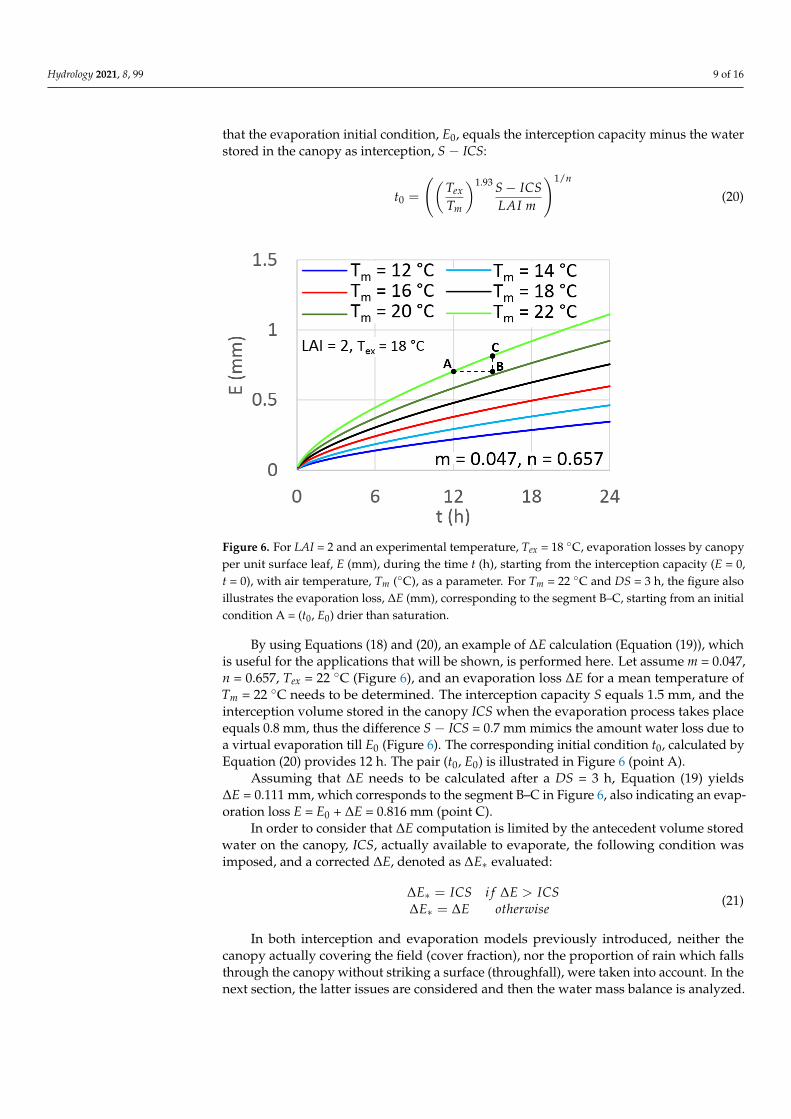
Figure 6. For LAI = 2 and an experimental temperature, Tex = 18 ◦C, evaporation losses by canopyper unit surface leaf, E (mm), during the time t (h), starting from the interception capacity (E = 0,t = 0), with air temperature, Tm (◦C), as a parameter. For Tm = 22 ◦C and DS = 3 h, the figure alsoillustrates the evaporation loss, ∆E (mm), corresponding to the segment B–C, starting from an initialcondition A = (t0, E0) drier than saturation.

By using Equations (18) and (20), an example of ∆E calculation (Equation (19)), whichis useful for the applications that will be shown, is performed here. Let assume m = 0.047,n = 0.657, Tex = 22 ◦C (Figure 6), and an evaporation loss ∆E for a mean temperature ofTm = 22 ◦C needs to be determined. The interception capacity S equals 1.5 mm, and theinterception volume stored in the canopy ICS when the evaporation process takes placeequals 0.8 mm, thus the difference S − ICS = 0.7 mm mimics the amount water loss due toa virtual evaporation till E0 (Figure 6). The corresponding initial condition t0, calculated byEquation (20) provides 12 h. The pair (t0, E0) is illustrated in Figure 6 (point A).

Assuming that ∆E needs to be calculated after a DS = 3 h, Equation (19) yields∆E = 0.111 mm, which corresponds to the segment B–C in Figure 6, also indicating an evap-oration loss E = E0 + ∆E = 0.816 mm (point C).

In order to consider that ∆E computation is limited by the antecedent volume storedwater on the canopy, ICS, actually available to evaporate, the following condition wasimposed, and a corrected ∆E, denoted as ∆E∗ evaluated:

∆E∗ = ICS i f ∆E > ICS∆E∗ = ∆E otherwise

(21)

In both interception and evaporation models previously introduced, neither thecanopy actually covering the field (cover fraction), nor the proportion of rain which fallsthrough the canopy without striking a surface (throughfall), were taken into account. In thenext section, the latter issues are considered and then the water mass balance is analyzed.

Hydrology 2021, 8, 99 10 of 16

5. Water Mass Balance

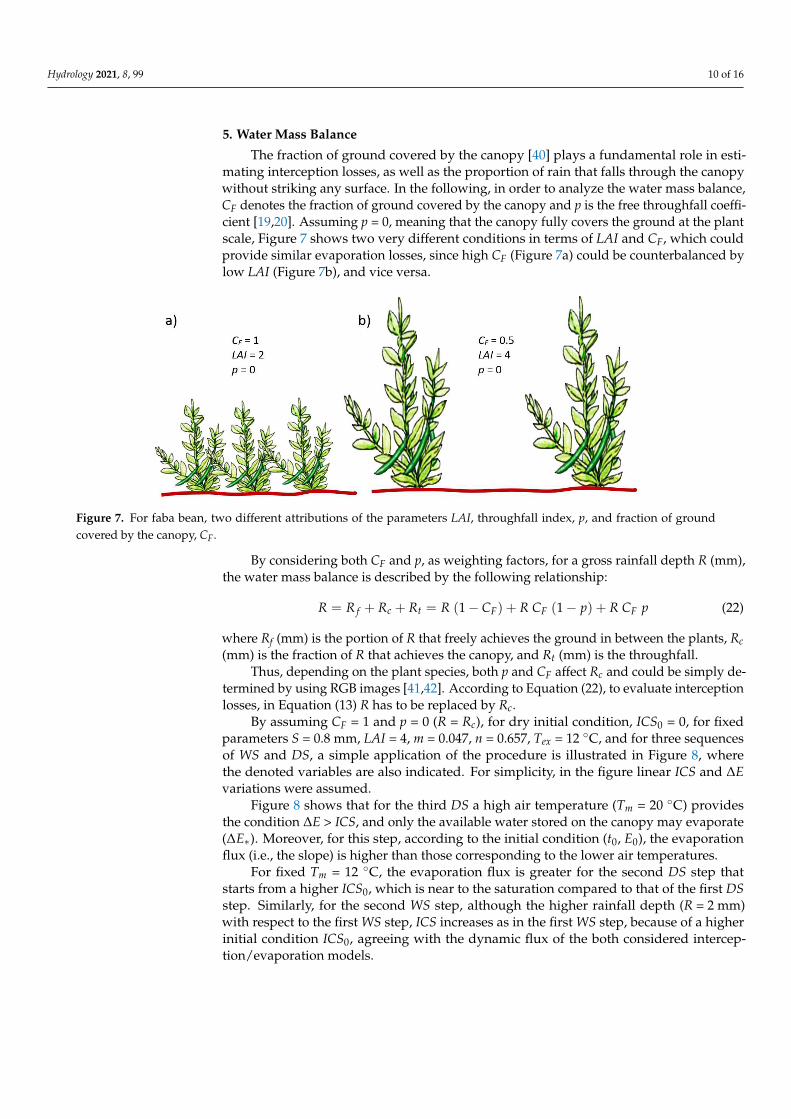
The fraction of ground covered by the canopy [40] plays a fundamental role in esti-mating interception losses, as well as the proportion of rain that falls through the canopywithout striking any surface. In the following, in order to analyze the water mass balance,CF denotes the fraction of ground covered by the canopy and p is the free throughfall coeffi-cient [19,20]. Assuming p = 0, meaning that the canopy fully covers the ground at the plantscale, Figure 7 shows two very different conditions in terms of LAI and CF, which couldprovide similar evaporation losses, since high CF (Figure 7a) could be counterbalanced bylow LAI (Figure 7b), and vice versa.

Hydrology 2021, 8, x FOR PEER REVIEW 10 of 16

Δ$∗ � ��� !9 Δ$ > ���Δ$∗ � Δ$ ��ℎ�<!# (21)

In both interception and evaporation models previously introduced, neither the can-

opy actually covering the field (cover fraction), nor the proportion of rain which falls

through the canopy without striking a surface (throughfall), were taken into account. In

the next section, the latter issues are considered and then the water mass balance is ana-

lyzed.

5. Water Mass Balance

The fraction of ground covered by the canopy [40] plays a fundamental role in esti-

mating interception losses, as well as the proportion of rain that falls through the canopy

without striking any surface. In the following, in order to analyze the water mass balance,

CF denotes the fraction of ground covered by the canopy and p is the free throughfall co-

efficient [19,20]. Assuming p = 0, meaning that the canopy fully covers the ground at the

plant scale, Figure 7 shows two very different conditions in terms of LAI and CF, which

could provide similar evaporation losses, since high CF (Figure 7a) could be counterbal-

anced by low LAI (Figure 7b), and vice versa.

Figure 7. For faba bean, two different attributions of the parameters LAI, throughfall index, p, and

fraction of ground covered by the canopy, CF.

By considering both CF and p, as weighting factors, for a gross rainfall depth R (mm),

the water mass balance is described by the following relationship:

� = + > + � � �1 � �? + �? �1 � � + �? � (22)

where Rf (mm) is the portion of R that freely achieves the ground in between the plants,

Rc (mm) is the fraction of R that achieves the canopy, and Rt (mm) is the throughfall.

Thus, depending on the plant species, both p and CF affect Rc and could be simply

determined by using RGB images [41,42]. According to Equation (22), to evaluate inter-

ception losses, in Equation (13) R has to be replaced by Rc.

By assuming CF = 1 and p = 0 (R = Rc), for dry initial condition, ICS0 = 0, for fixed

parameters S = 0.8 mm, LAI = 4, m = 0.047, n = 0.657, Tex = 12 °C, and for three sequences of

WS and DS, a simple application of the procedure is illustrated in Figure 8, where the

denoted variables are also indicated. For simplicity, in the figure linear ICS and ∆E varia-

tions were assumed.

Figure 8 shows that for the third DS a high air temperature (Tm = 20 °C) provides the

condition ∆E > ICS, and only the available water stored on the canopy may evaporate

(Δ$∗). Moreover, for this step, according to the initial condition (t0, E0), the evaporation

flux (i.e., the slope) is higher than those corresponding to the lower air temperatures.

Figure 7. For faba bean, two different attributions of the parameters LAI, throughfall index, p, and fraction of groundcovered by the canopy, CF.

By considering both CF and p, as weighting factors, for a gross rainfall depth R (mm),the water mass balance is described by the following relationship:

R = R f + Rc + Rt = R (1− CF) + R CF (1− p) + R CF p (22)

where Rf (mm) is the portion of R that freely achieves the ground in between the plants, Rc(mm) is the fraction of R that achieves the canopy, and Rt (mm) is the throughfall.

Thus, depending on the plant species, both p and CF affect Rc and could be simply de-termined by using RGB images [41,42]. According to Equation (22), to evaluate interceptionlosses, in Equation (13) R has to be replaced by Rc.

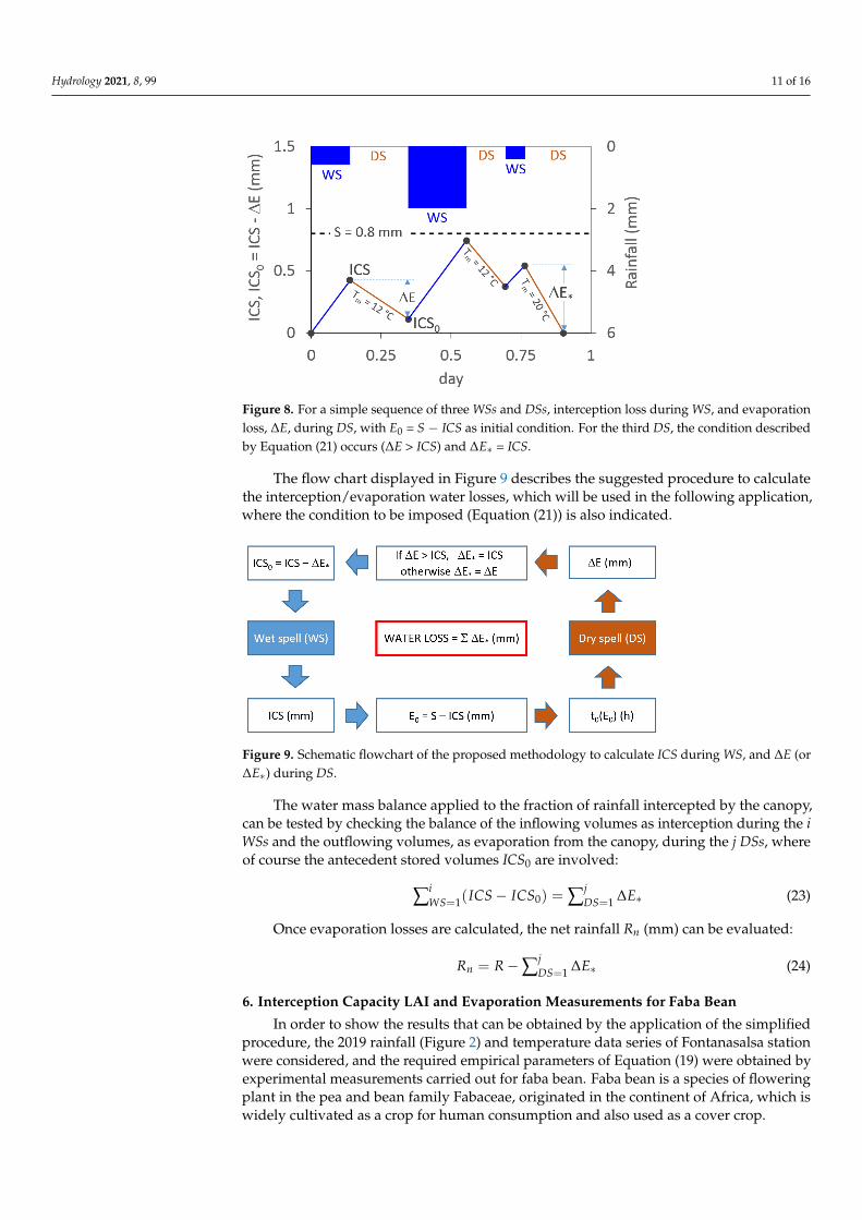
By assuming CF = 1 and p = 0 (R = Rc), for dry initial condition, ICS0 = 0, for fixedparameters S = 0.8 mm, LAI = 4, m = 0.047, n = 0.657, Tex = 12 ◦C, and for three sequencesof WS and DS, a simple application of the procedure is illustrated in Figure 8, wherethe denoted variables are also indicated. For simplicity, in the figure linear ICS and ∆Evariations were assumed.

Figure 8 shows that for the third DS a high air temperature (Tm = 20 ◦C) providesthe condition ∆E > ICS, and only the available water stored on the canopy may evaporate(∆E∗). Moreover, for this step, according to the initial condition (t0, E0), the evaporationflux (i.e., the slope) is higher than those corresponding to the lower air temperatures.

For fixed Tm = 12 ◦C, the evaporation flux is greater for the second DS step thatstarts from a higher ICS0, which is near to the saturation compared to that of the first DSstep. Similarly, for the second WS step, although the higher rainfall depth (R = 2 mm)with respect to the first WS step, ICS increases as in the first WS step, because of a higherinitial condition ICS0, agreeing with the dynamic flux of the both considered intercep-tion/evaporation models.

Hydrology 2021, 8, 99 11 of 16Hydrology 2021, 8, x FOR PEER REVIEW 11 of 16

Figure 8. For a simple sequence of three WSs and DSs, interception loss during WS, and evaporation

loss, ∆E, during DS, with E0 = S − ICS as initial condition. For the third DS, the condition described

by Equation (21) occurs (∆E > ICS) and Δ$∗ = ICS.

For fixed Tm = 12 °C, the evaporation flux is greater for the second DS step that starts

from a higher ICS0, which is near to the saturation compared to that of the first DS step.

Similarly, for the second WS step, although the higher rainfall depth (R = 2 mm) with

respect to the first WS step, ICS increases as in the first WS step, because of a higher initial

condition ICS0, agreeing with the dynamic flux of the both considered interception/evap-

oration models.

The flow chart displayed in Figure 9 describes the suggested procedure to calculate

the interception/evaporation water losses, which will be used in the following application,

where the condition to be imposed (Equation (21)) is also indicated.

Figure 9. Schematic flowchart of the proposed methodology to calculate ICS during WS, and ∆E

(or Δ$∗) during DS.

The water mass balance applied to the fraction of rainfall intercepted by the canopy,

can be tested by checking the balance of the inflowing volumes as interception during the

i WSs and the outflowing volumes, as evaporation from the canopy, during the j DSs,

where of course the antecedent stored volumes ICS0 are involved:

∑ ���� � ���� ABCD, � ∑ Δ$∗EFCD, (23)

Once evaporation losses are calculated, the net rainfall Rn (mm) can be evaluated:

� � � ∑ Δ$∗EFCD, (24)

Figure 8. For a simple sequence of three WSs and DSs, interception loss during WS, and evaporationloss, ∆E, during DS, with E0 = S − ICS as initial condition. For the third DS, the condition describedby Equation (21) occurs (∆E > ICS) and ∆E∗ = ICS.

The flow chart displayed in Figure 9 describes the suggested procedure to calculatethe interception/evaporation water losses, which will be used in the following application,where the condition to be imposed (Equation (21)) is also indicated.

Hydrology 2021, 8, x FOR PEER REVIEW 11 of 16

Figure 8. For a simple sequence of three WSs and DSs, interception loss during WS, and evaporation

loss, ∆E, during DS, with E0 = S − ICS as initial condition. For the third DS, the condition described

by Equation (21) occurs (∆E > ICS) and Δ$∗ = ICS.

For fixed Tm = 12 °C, the evaporation flux is greater for the second DS step that starts

from a higher ICS0, which is near to the saturation compared to that of the first DS step.

Similarly, for the second WS step, although the higher rainfall depth (R = 2 mm) with

respect to the first WS step, ICS increases as in the first WS step, because of a higher initial

condition ICS0, agreeing with the dynamic flux of the both considered interception/evap-

oration models.

The flow chart displayed in Figure 9 describes the suggested procedure to calculate

the interception/evaporation water losses, which will be used in the following application,

where the condition to be imposed (Equation (21)) is also indicated.

Figure 9. Schematic flowchart of the proposed methodology to calculate ICS during WS, and ∆E

(or Δ$∗) during DS.

The water mass balance applied to the fraction of rainfall intercepted by the canopy,

can be tested by checking the balance of the inflowing volumes as interception during the

i WSs and the outflowing volumes, as evaporation from the canopy, during the j DSs,

where of course the antecedent stored volumes ICS0 are involved:

∑ ���� � ���� ABCD, � ∑ Δ$∗EFCD, (23)

Once evaporation losses are calculated, the net rainfall Rn (mm) can be evaluated:

� � � ∑ Δ$∗EFCD, (24)

Figure 9. Schematic flowchart of the proposed methodology to calculate ICS during WS, and ∆E (or∆E∗) during DS.

The water mass balance applied to the fraction of rainfall intercepted by the canopy,can be tested by checking the balance of the inflowing volumes as interception during the iWSs and the outflowing volumes, as evaporation from the canopy, during the j DSs, whereof course the antecedent stored volumes ICS0 are involved:

∑iWS=1(ICS− ICS0) = ∑j

DS=1 ∆E∗ (23)

Once evaporation losses are calculated, the net rainfall Rn (mm) can be evaluated:

Rn = R−∑jDS=1 ∆E∗ (24)

6. Interception Capacity LAI and Evaporation Measurements for Faba Bean

In order to show the results that can be obtained by the application of the simplifiedprocedure, the 2019 rainfall (Figure 2) and temperature data series of Fontanasalsa stationwere considered, and the required empirical parameters of Equation (19) were obtained byexperimental measurements carried out for faba bean. Faba bean is a species of floweringplant in the pea and bean family Fabaceae, originated in the continent of Africa, which iswidely cultivated as a crop for human consumption and also used as a cover crop.

Hydrology 2021, 8, 99 12 of 16

For a single plant, planted in mid-November, and sampled after 95 days, the temporalvariation of water loss by evaporation starting from the interception capacity, the numberof leaves, # Leaves, and the corresponding surface area were measured. Saturation ofthe canopy was achieved by using sprinkler irrigation, for a fixed outdoor temperature,Tex = 12 ◦C.

Starting from the interception capacity condition, after dripping has ceased, waterloss by evaporation was measured by weighing during the time. The # Leaves (45), andthe corresponding surface area (0.043 m2), made it possible to calculate the cumulativeevaporation volume, per unit leaf surface area, E (mm).

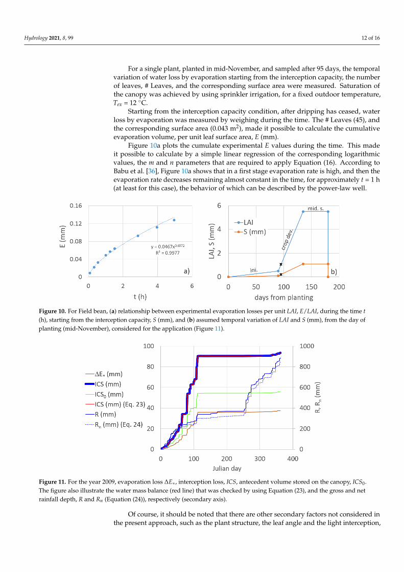
Figure 10a plots the cumulate experimental E values during the time. This madeit possible to calculate by a simple linear regression of the corresponding logarithmicvalues, the m and n parameters that are required to apply Equation (16). According toBabu et al. [36], Figure 10a shows that in a first stage evaporation rate is high, and then theevaporation rate decreases remaining almost constant in the time, for approximately t = 1 h(at least for this case), the behavior of which can be described by the power-law well.

Hydrology 2021, 8, x FOR PEER REVIEW 12 of 16

6. Interception Capacity LAI and Evaporation Measurements for Faba Bean

In order to show the results that can be obtained by the application of the simplified

procedure, the 2019 rainfall (Figure 2) and temperature data series of Fontanasalsa station

were considered, and the required empirical parameters of Equation (19) were obtained

by experimental measurements carried out for faba bean. Faba bean is a species of flow-

ering plant in the pea and bean family Fabaceae, originated in the continent of Africa,

which is widely cultivated as a crop for human consumption and also used as a cover

crop.

For a single plant, planted in mid-November, and sampled after 95 days, the tem-

poral variation of water loss by evaporation starting from the interception capacity, the

number of leaves, # Leaves, and the corresponding surface area were measured. Satura-

tion of the canopy was achieved by using sprinkler irrigation, for a fixed outdoor temper-

ature, Tex = 12 °C.

Starting from the interception capacity condition, after dripping has ceased, water

loss by evaporation was measured by weighing during the time. The # Leaves (45), and

the corresponding surface area (0.043 m2), made it possible to calculate the cumulative

evaporation volume, per unit leaf surface area, E (mm).

Figure 10a plots the cumulate experimental E values during the time. This made it

possible to calculate by a simple linear regression of the corresponding logarithmic values,

the m and n parameters that are required to apply Equation (16). According to Babu et al.

[36], Figure 10a shows that in a first stage evaporation rate is high, and then the evapora-

tion rate decreases remaining almost constant in the time, for approximately t = 1 h (at

least for this case), the behavior of which can be described by the power-law well.

Of course, it should be noted that there are other secondary factors not considered in

the present approach, such as the plant structure, the leaf angle and the light interception,

although not easy to consider, which may affect the considered parameters [43], especially

when upscaling is needed.

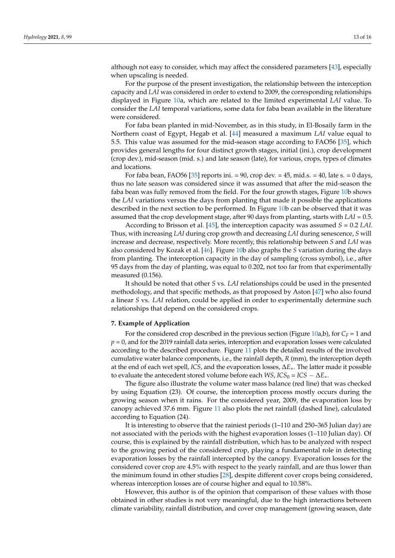
Figure 10. For Field bean, (a) relationship between experimental evaporation losses per unit LAI, E/LAI, during the time t

(h), starting from the interception capacity, S (mm), and (b) assumed temporal variation of LAI and S (mm), from the day

of planting (mid-November), considered for the application (Figure 11).

For the purpose of the present investigation, the relationship between the intercep-

tion capacity and LAI was considered in order to extend to 2009, the corresponding rela-

tionships displayed in Figure 10a, which are related to the limited experimental LAI value.

To consider the LAI temporal variations, some data for faba bean available in the literature

were considered.

Figure 10. For Field bean, (a) relationship between experimental evaporation losses per unit LAI, E/LAI, during the time t(h), starting from the interception capacity, S (mm), and (b) assumed temporal variation of LAI and S (mm), from the day ofplanting (mid-November), considered for the application (Figure 11).

Hydrology 2021, 8, x FOR PEER REVIEW 13 of 16

Figure 11. For the year 2009, evaporation loss Δ$∗, interception loss, ICS, antecedent volume stored

on the canopy, ICS0. The figure also illustrate the water mass balance (red line) that was checked by

using Equation (23), and the gross and net rainfall depth, R and Rn (Equation (24)), respectively

(secondary axis).

For faba bean planted in mid-November, as in this study, in El-Bosaily farm in the

Northern coast of Egypt, Hegab et al. [44] measured a maximum LAI value equal to 5.5.

This value was assumed for the mid-season stage according to FAO56 [35], which pro-

vides general lengths for four distinct growth stages, initial (ini.), crop development (crop

dev.), mid-season (mid. s.) and late season (late), for various, crops, types of climates and

locations.

For faba bean, FAO56 [35] reports ini. = 90, crop dev. = 45, mid.s. = 40, late s. = 0 days,

thus no late season was considered since it was assumed that after the mid-season the faba

bean was fully removed from the field. For the four growth stages, Figure 10b shows the

LAI variations versus the days from planting that made it possible the applications de-

scribed in the next section to be performed. In Figure 10b can be observed that it was

assumed that the crop development stage, after 90 days from planting, starts with LAI =

0.5.

According to Brisson et al. [45], the interception capacity was assumed S = 0.2 LAI.

Thus, with increasing LAI during crop growth and decreasing LAI during senescence, S

will increase and decrease, respectively. More recently, this relationship between S and

LAI was also considered by Kozak et al. [46]. Figure 10b also graphs the S variation during

the days from planting. The interception capacity in the day of sampling (cross symbol),

i.e., after 95 days from the day of planting, was equal to 0.202, not too far from that exper-

imentally measured (0.156).

It should be noted that other S vs. LAI relationships could be used in the presented

methodology, and that specific methods, as that proposed by Aston [47] who also found

a linear S vs. LAI relation, could be applied in order to experimentally determine such

relationships that depend on the considered crops.

7. Example of Application

For the considered crop described in the previous section (Figure 10a,b), for CF = 1

and p = 0, and for the 2019 rainfall data series, interception and evaporation losses were

calculated according to the described procedure. Figure 11 plots the detailed results of the

involved cumulative water balance components, i.e., the rainfall depth, R (mm), the inter-

ception depth at the end of each wet spell, ICS, and the evaporation losses, Δ$∗. The latter

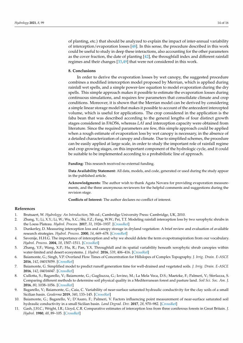
Figure 11. For the year 2009, evaporation loss ∆E∗, interception loss, ICS, antecedent volume stored on the canopy, ICS0.The figure also illustrate the water mass balance (red line) that was checked by using Equation (23), and the gross and netrainfall depth, R and Rn (Equation (24)), respectively (secondary axis).

Of course, it should be noted that there are other secondary factors not considered inthe present approach, such as the plant structure, the leaf angle and the light interception,

Hydrology 2021, 8, 99 13 of 16

although not easy to consider, which may affect the considered parameters [43], especiallywhen upscaling is needed.

For the purpose of the present investigation, the relationship between the interceptioncapacity and LAI was considered in order to extend to 2009, the corresponding relationshipsdisplayed in Figure 10a, which are related to the limited experimental LAI value. Toconsider the LAI temporal variations, some data for faba bean available in the literaturewere considered.

For faba bean planted in mid-November, as in this study, in El-Bosaily farm in theNorthern coast of Egypt, Hegab et al. [44] measured a maximum LAI value equal to5.5. This value was assumed for the mid-season stage according to FAO56 [35], whichprovides general lengths for four distinct growth stages, initial (ini.), crop development(crop dev.), mid-season (mid. s.) and late season (late), for various, crops, types of climatesand locations.

For faba bean, FAO56 [35] reports ini. = 90, crop dev. = 45, mid.s. = 40, late s. = 0 days,thus no late season was considered since it was assumed that after the mid-season thefaba bean was fully removed from the field. For the four growth stages, Figure 10b showsthe LAI variations versus the days from planting that made it possible the applicationsdescribed in the next section to be performed. In Figure 10b can be observed that it wasassumed that the crop development stage, after 90 days from planting, starts with LAI = 0.5.

According to Brisson et al. [45], the interception capacity was assumed S = 0.2 LAI.Thus, with increasing LAI during crop growth and decreasing LAI during senescence, S willincrease and decrease, respectively. More recently, this relationship between S and LAI wasalso considered by Kozak et al. [46]. Figure 10b also graphs the S variation during the daysfrom planting. The interception capacity in the day of sampling (cross symbol), i.e., after95 days from the day of planting, was equal to 0.202, not too far from that experimentallymeasured (0.156).

It should be noted that other S vs. LAI relationships could be used in the presentedmethodology, and that specific methods, as that proposed by Aston [47] who also founda linear S vs. LAI relation, could be applied in order to experimentally determine suchrelationships that depend on the considered crops.

7. Example of Application

For the considered crop described in the previous section (Figure 10a,b), for CF = 1 andp = 0, and for the 2019 rainfall data series, interception and evaporation losses were calculatedaccording to the described procedure. Figure 11 plots the detailed results of the involvedcumulative water balance components, i.e., the rainfall depth, R (mm), the interception depthat the end of each wet spell, ICS, and the evaporation losses, ∆E∗. The latter made it possibleto evaluate the antecedent stored volume before each WS, ICS0 = ICS − ∆E∗.

The figure also illustrate the volume water mass balance (red line) that was checkedby using Equation (23). Of course, the interception process mostly occurs during thegrowing season when it rains. For the considered year, 2009, the evaporation loss bycanopy achieved 37.6 mm. Figure 11 also plots the net rainfall (dashed line), calculatedaccording to Equation (24).

It is interesting to observe that the rainiest periods (1–110 and 250–365 Julian day) arenot associated with the periods with the highest evaporation losses (1–110 Julian day). Ofcourse, this is explained by the rainfall distribution, which has to be analyzed with respectto the growing period of the considered crop, playing a fundamental role in detectingevaporation losses by the rainfall intercepted by the canopy. Evaporation losses for theconsidered cover crop are 4.5% with respect to the yearly rainfall, and are thus lower thanthe minimum found in other studies [28], despite different cover crops being considered,whereas interception losses are of course higher and equal to 10.58%.

However, this author is of the opinion that comparison of these values with thoseobtained in other studies is not very meaningful, due to the high interactions betweenclimate variability, rainfall distribution, and cover crop management (growing season, date

Hydrology 2021, 8, 99 14 of 16

of planting, etc.) that should be analyzed to explain the impact of inter-annual variabilityof interception/evaporation losses [48]. In this sense, the procedure described in this workcould be useful to study in deep these interactions, also accounting for the other parametersas the cover fraction, the date of planting [42], the throughfall index and different rainfallregimes and their changes [33,49] that were not considered in this work.

8. Conclusions

In order to derive the evaporation losses by wet canopy, the suggested procedurecombines a modified interception model proposed by Merrian, which is applied duringrainfall wet spells, and a simple power-law equation to model evaporation during the dryspells. This simple approach makes it possible to estimate the evaporation losses duringcontinuous simulations, and requires few parameters that consolidate climate and cropconditions. Moreover, it is shown that the Merrian model can be derived by consideringa simple linear storage model that makes it possible to account of the antecedent interceptedvolume, which is useful for applications. The crop considered in the application is thefaba bean that was described according to the general lengths of four distinct growthstages considered in FAO56, whereas LAI and interception capacity were obtained fromliterature. Since the required parameters are few, this simple approach could be appliedwhen a rough estimate of evaporation loss by wet canopy is necessary, in the absence ofa detailed characterization of canopy and climate. Due to simplified schemes, the procedurecan be easily applied at large scale, in order to study the important role of rainfall regimeand crop growing stages, on this important component of the hydrologic cycle, and it couldbe suitable to be implemented according to a probabilistic line of approach.

Funding: This research received no external funding.

Data Availability Statement: All data, models, and code, generated or used during the study appearin the published article.

Acknowledgments: The author wish to thank Agata Novara for providing evaporation measure-ments, and the three anonymous reviewers for the helpful comments and suggestions during therevision stage.

Conflicts of Interest: The author declares no conflict of interest.

References1. Brutsaert, W. Hydrology: An Introduction, 5th ed.; Cambridge University Press: Cambridge, UK, 2010.2. Zhang, Y.; Li, X.Y.; Li, W.; Wu, X.C.; Shi, F.Z.; Fang, W.W.; Pei, T.T. Modeling rainfall interception loss by two xerophytic shrubs in

the Loess Plateau. Hydrol. Process. 2017, 31, 1926–1937. [CrossRef]3. Dunkerley, D. Measuring interception loss and canopy storage in dryland vegetation: A brief review and evaluation of available

research strategies. Hydrol. Process. 2000, 14, 669–678. [CrossRef]4. Savenije, H.H.G. The importance of interception and why we should delete the term evapotranspiration from our vocabulary.

Hydrol. Process. 2004, 18, 1507–1511. [CrossRef]5. Zhang, Y.F.; Wang, X.P.; Hu, R.; Pan, Y.X. Throughfall and its spatial variability beneath xerophytic shrub canopies within

water-limited arid desert ecosystems. J. Hydrol. 2016, 539, 406–416. [CrossRef]6. Baiamonte, G.; Singh, V.P. Overland Flow Times of Concentration for Hillslopes of Complex Topography. J. Irrig. Drain. E-ASCE

2016, 142, 04015059. [CrossRef]7. Baiamonte, G. Simplified model to predict runoff generation time for well-drained and vegetated soils. J. Irrig. Drain. E-ASCE

2016, 142, 04016047. [CrossRef]8. Cullotta, S.; Bagarello, V.; Baiamonte, G.; Gugliuzza, G.; Iovino, M.; La Mela Veca, D.S.; Maetzke, F.; Palmeri, V.; Sferlazza, S.

Comparing different methods to determine soil physical quality in a Mediterranean forest and pasture land. Soil Sci. Soc. Am. J.2016, 80, 1038–1056. [CrossRef]

9. Bagarello, V.; Baiamonte, G.; Caia, C. Variability of near-surface saturated hydraulic conductivity for the clay soils of a smallSicilian basin. Geoderma 2019, 340, 133–145. [CrossRef]

10. Baiamonte, G.; Bagarello, V.; D’Asaro, F.; Palmeri, V. Factors influencing point measurement of near-surface saturated soilhydraulic conductivity in a small Sicilian basin. Land Degrad. Dev. 2017, 28, 970–982. [CrossRef]

11. Gash, J.H.C.; Wright, I.R.; Lloyd, C.R. Comparative estimates of interception loss from three coniferous forests in Great Britain. J.Hydrol. 1980, 48, 89–105. [CrossRef]

Hydrology 2021, 8, 99 15 of 16

12. Ubarana, V.N. Observations and Modelling of Rainfall Interception at Two Experimental Sites in Amazonia. In AmazonianDeforestation and Climate; Gash, J.H.C., Nobre, C.A., Roberts, J.M., Victoria, R.L., Eds.; John Wiley & Sons: Hoboken, NJ, USA,1996; 611p.

13. Calder, I. Evaporation in the Uplands; Wiley: Chichester, UK; New York, NY, USA, 1990.14. Muzylo, A.; Llorens, P.; Valente, F.; Keizer, J.J.; Domingo, F.; Gash, J.H.C. A review of rainfall interception modelling. J. Hydrol.

2009, 370, 191–206. [CrossRef]15. Linsley, R.K., Jr.; Kohler, M.A.; Paulhus, J.L. Applied Hydrology; McGraw-Hill Book Co.: New York, NY, USA, 1988.16. Horton, R.E. Rainfall interception. Mon. Weather Rev. 1919, 47, 603–623. [CrossRef]17. Merriam, R.A. A note on the interception loss equation. J. Geophys. Res. 1960, 5, 3850–3851. [CrossRef]18. Merriam, R.A. Fog drip from artificial leaves in a fog wind tunnel. Water Resour. Res. 1973, 9, 1591–1598. [CrossRef]19. Rutter, A.J.; Kershaw, K.A.; Robins, P.C.; Morton, A.J. A predictive model of rainfall interception in forests, 1. Derivation of the

model from observations in a plantation of Corsican pine. Agric. Meteorol. 1971, 9, 367–384. [CrossRef]20. Rutter, A.J.; Morton, A.J.; Robins, P.C. A predictive model of rainfall interception in forests. II. Generalization of the model and

comparison with observations in some coniferous and hardwood stands. J. Appl. Ecol. 1975, 12, 367–380. [CrossRef]21. Calder, I. A model of transpiration and interception loss from a spruce forest in Plynlimon, Central Wales. J. Hydrol. 1977, 33,

247–265. [CrossRef]22. Gash, J.; Morton, A. Application of the Rutter model to the estimation of the interception loss from Thetford forest. J. Hydrol.

1978, 38, 49–58. [CrossRef]23. Monteith, J.L. Evaporation and environment. Syrup. Soc. Exp. Biol. 1965, 19, 205–234.24. Gash, J.H.C. An analytical model of rainfall interception by forests. Q. J. R. Meteorol. Soc. 1979, 105, 43–55. [CrossRef]25. Pearce, A.J.; Rowe, L.K.; Stewart, J.B. Nightime, wet canopy evaporation rates and the water balance of an evergreen mixed forest.

Water Resour. Res. 1980, 16, 955–959. [CrossRef]26. Dolman, A.J. Summer and winter rainfall interception in an oak forest. Predictions with an analytical and a numerical simulation

model. J. Hydrol. 1987, 90, 1–9. [CrossRef]27. Lloyd, C.R.; Gash, J.H.C.; Shuttleworth, W.J.; Marques, A.O. The measurement and modelling of rainfall interception by

amazonian rain forest. Agric. For. Meteorol. 1988, 43, 277–294. [CrossRef]28. Coutuntrn, D.E.; Ripley, E.A. Rainfall interception in mixed grass prairie. Can. J. Plant Sci. 1973, 53, 659–663.29. Von Hoyningen-Hüne, J. Die Interception des Niederschlags in landwirtschaftlichen Beständen. Schr. Des. DVWK 1983, 57, 1–53.30. Braden, H. Ein Energiehaushalts- und Verdunstungsmodell for Wasser und Stoffhaushaltsuntersuchungen landwirtschaftlich

genutzer Einzugsgebiete. Mittelungen Dtsch. Bodenkd. Geselschaft 1985, 42, 294–299.31. van Dam, J.C.; Huygen, J.; Wesseling, J.G.; Feddes, R.A.; Kabat, P.; van Walsum, P.E.V.; Groenendijk, P.; van Diepen, C.A. Theory

of SWAP Version 2.0. Simulation of Water Flow, Solute Transport and Plant Growth in the Soil-Water-Atmosphere-Plant Environment;Technical Document 45; Wageningen Agricultural University; DLOW Winand Staring Centre: Wageningen, The Netherlands, 1997.

32. Agnese, C.; Baiamonte, G.; Cammalleri, C. Modelling the occurrence of rainy days under a typical Mediterranean climate. Adv.Water Res. 2014, 64, 62–76. [CrossRef]

33. Baiamonte, G.; Mercalli, L.; Cat Berro, D.; Agnese, C.; Ferraris, S. Modelling the frequency distribution of interarrival times fromdaily precipitation time-series in North-West Italy. Hydrol. Res. 2019, 50, 339–357. [CrossRef]

34. Baiamonte, G.; Agnese, C. Quick and Slow Components of the Hydrologic Response at the Hillslope Scale. J. Irrig. Drain. E-ASCE2016, 142, 04016038. [CrossRef]

35. Allen, R.G.; Pereira, L.S.; Raes, D.; Smith, M. Crop Evapotranspiration. Guidelines for Computing Crop Water Requirements; FAOIrrigation and Drainage Paper 56; FAO: Rome, Italy, 1998; 300p.

36. Babu, A.K.; Kumaresan, G.; Raj, V.A.A.; Velraj, R. Review of leaf drying: Mechanism and influencing parameters, drying methods,nutrient preservation, and mathematical models. Renew. Sustain. Energy Rev. 2018, 90, 536–556. [CrossRef]

37. Black, T.A.; Gardner, W.R.; Thurtell, G.W. The prediction of evaporation, drainage, and soil water storage for a bare soil. Soil Sci.Soc. Am. Proc. 1969, 33, 655–660. [CrossRef]

38. Ritchie, J.T. Model for predicting evaporation from a row crop with incomplete cover. Water Resour. Res. 1972, 8, 1204–1213.[CrossRef]

39. Pumo, D. L’Approvvigionamento Idrico per l’Agricoltura; Aracne Editrice SRL: Rome, Italy, 2008; ISBN 978-88-548-1708-1. (In Italian).40. Pereira, L.S.; Paredes, P.; Melton, F.; Johnson, L.; Wang, T.; López-Urrea, R.; Cancela, J.J.; Allen, R.G. Prediction of crop coefficients

from fraction of ground cover and height. Background and validation using ground and remote sensing data. Agric. Water Manag.2020, 241, 106197. [CrossRef]

41. Lee, K.J.; Lee, B.W. Estimating canopy cover from color digital camera image of rice field. J. Crop Sci. Biotechnol. 2011, 14, 151–155.[CrossRef]

42. Fernandez-Gallego, J.A.; Kefauver, S.C.; Kerfal, S.; Araus, J.L. Comparative canopy cover estimation using RGB images fromUAV and ground. In Proceedings of the Remote Sensing for Agriculture, Ecosystems, and Hydrology XX, Berlin, Germany, 10–13September 2018; p. 107830J. [CrossRef]

43. Knapp, A.K.; Smith, D.L. Leaf Angle, Light Interceptoon & Water Relations, Demonstrating How Plants Cope with MultipleResource Limitations in the Field. Am. Biol. Teach. 1997, 59, 365–368.

Hydrology 2021, 8, 99 16 of 16

44. Hegab, A.S.A.; Fayed, M.T.B.; Hamada, M.M.A.; Abdrabbo, M.A.A. Productivity and irrigation requirements of faba-bean inNorth Delta of Egypt in relation to planting dates. Ann. Agric. Sci. 2014, 59, 185–193. [CrossRef]

45. Brisson, N.; Mary, B.; Riposche, D.; Jeuffroy, M.; Ruget, F.; Gate, P.; Devienne-Barret, F.; Antonioletti, R.; Durr, C.; Nicoullaud, B.; et al.STICS: A generic model for the simulation of crops and their water and nitrogen balance. I. Theory and parameterization applied towheat and corn. Agronomie 1998, 18, 311–316. [CrossRef]

46. Kozak, J.A.; Ahuja, L.R.; Green, T.R.; Ma, L. Modelling crop canopy and residue rainfall interception effects on soil hydrologicalcomponents for semi-arid agriculture. Hydrol. Process. 2007, 21, 229–241. [CrossRef]

47. Aston, A.R. Rainfall interception by eight small trees. J. Hydrol. 1979, 42, 383–396. [CrossRef]48. Meyer, N.; Bergez, J.E.; Constantin, J.; Belleville, P.; Justes, E. Cover crops reduce drainage but not always soil water content due

to interactions between rainfall distribution and management. Agric. Water Manag. 2020, 231, 105998. [CrossRef]49. Tripathi, S.; Govindaraju, R.S. Change detection in rainfall and temperature patterns over India. In Proceedings of the Third

International Workshop on Knowledge Discovery from Sensor Data (SensorKDD 2009), Paris, France, 28 June 2009; Association forComputing Machinery: New York, NY, USA, 2009; pp. 133–141. [CrossRef]