Simulating urban growth on the US–Mexico border: Nogales, Arizona, and Nogales, Sonora

Simulating urban growth on the US–Mexicoborder: Nogales, Arizona, and Nogales, Sonora

Soe W. Myint, Jyoti Jain, Christopher Lukinbeal, and Francisco Lara-Valencia

Abstract. The paired US–Mexico border cities of Nogales, Arizona, and Nogales, Sonora (known as Ambos Nogales), are

the largest and most rapidly growing cities on the Arizona–Sonora border. The growing urban population is producing

extensive land-use and land-cover change in the region. The continued expansion of paired cities presents many

environmental management and urban planning challenges. This research employs a cellular automata model to

examine the difference between the patterns and rates of urban growth and land-use change under different

environmental and planning strategies in the two cities over the next 20 years (2004–2025). A series of Landsat

Thematic Mapper (TM) images acquired over different time periods (October 1985, July 1991, February 1995,

September 2000, and July 2004) were used to simulate urban growth using four planning scenarios, namely business as

usual, environmental protection, road network, and antigrowth strategy. The study reveals that the unchecked urban

growth trend in the business as usual, environmental protection, and road network scenarios simulates significant (99.5%)

edge developments or organic growth throughout the region. In contrast, the antigrowth scenario, which emphasizes

environmental protection, allows for more green and open space and is therefore considered the most desirable for

planning future urban land use and development.

Resume. Les villes jumelles de Nogales, Arizona, et de Nogales, Sonora, communement appelee Ambos Nogales, situees de

part et d’autre de la frontiere Etats-Unis–Mexique sont les deux plus grandes villes de meme que les villes avec la croissance

la plus rapide a la frontiere de l’Arizona et de l’etat de Sonora. La population urbaine grandissante entraıne des

changements majeurs au niveau de l’utilisation du sol et du couvert dans la region. L’expansion constante des villes

jumelles pose plusieurs defis aux plans de la gestion environnementale et de la planification urbaine. Dans cette

recherche, on utilise un modele base sur les automates cellulaires pour etudier la difference, d’une part, entre les

patrons et les taux de croissance urbaine et, d’autre part, les changements de l’utilisation du sol en fonction de

differentes strategies environnementales et de planification dans les deux villes au cours des 20 prochaines annees

(2004–2025). Une serie d’images TM (« Thematic Mapper ») de Landsat acquises a differentes periodes (octobre 1985,

juillet 1991, fevrier 1995, septembre 2000 et juillet 2004) ont ete utilisees pour simuler la croissance urbaine en utilisant

quatre scenarios de planification: comme d’habitude (business as usual), protection environnementale, reseau de routes et

strategie anti-croissance. L’etude revele que la tendance a la croissance urbaine non reglementee presente dans les scenarios

comme d’habitude, protection environnementale et reseau de routes simule de tres forts developpements (99,5 %) a la

peripherie ou encore une croissance organique sur l’ensemble de la region. Par contraste, le scenario anti-croissance, qui

met l’accent sur la protection environnementale, fait place a plus de verdure et d’espaces libres et est ainsi considere le plus

souhaitable des scenarios pour la planification de l’utilisation du sol et du developpement dans le futur.

[Traduit par la Redaction]

Introduction

Urbanization is the general process of city growth and has

often been viewed as a necessary component of regional eco-

nomic growth; however, unplanned and mismanaged urban

growth has provoked concerns over land-use and land-cover

change, such as the loss of large areas of primary forest and

agricultural land, inadvertent climate repercussions, and

environmental degradation (Yang, 2002). Li and Yeh

(2000) stated that under current growth trends the complete

depletion of agricultural land resources could occur in some

fast-growing areas. Land-use and land-cover change is one

of the most significant forms of global environmental change

and is felt in both developing and developed countries

(Turner et al., 1993). Furthermore, land-use change has

received growing attention alongside other human-induced

environmental change, such as climate and atmosphere

(Walker and Steffen, 1997; 1999; Cihlar and Jansen, 2001).

Urbanization alters the biophysical and socioeconomic

environment. Urban storm water runoff is a major contrib-

uting factor to water quality degradation (Driver and Trout-

man, 1989; US EPA, 1997). Storm water changes hydrologic

patterns, accelerates natural stream flows, destroys aquatic

habitat, and elevates pollutant concentrations (Burton and

Received 5 November 2009. Accepted 5 April 2010. Published on the Web at http://pubservices.nrc-cnrc.ca/cjrs on 28 October 2010.

S.W. Myint,1 J. Jain, C. Lukinbeal, and F. Lara-Valencia. School of Geographical Sciences and Urban Planning, Arizona State University, POBox 875302, Tempe, AZ 85287-5302, USA.

1Corresponding author (e-mail: [email protected]).

Can. J. Remote Sensing, Vol. 36, No. 3, pp. 166–184, 2010

166 E 2010 CASI

Pitt, 2002). In addition, urbanization changes the soil phys-

ical and chemical properties, water availability, vegetation,

and associated animal and microbial communities (Jenerette

and Wu, 2001). Urbanization poses other socioeconomic

challenges, such as demographic pressure, infrastructure

problems, inadequate resources for service delivery, and

planning (UN Human Settlement Programme, 2003). The

inability to effectively manage these related challenges is

rapidly increasing the risks associated with poor housing

conditions, uncollected solid waste, overconsumption of lim-

ited freshwater supplies, untreated waste water, and urban

air pollution (Masser, 2001). Furthermore, complex interac-

tions among physical, biological, economic, and social forces

in both the spatial and temporal domain control urban

growth and sprawl (Turner, 1987).

Cities along the US–Mexico border have grown at an

unprecedented pace over the last few decades. The urban

growth that began with the emergence of ‘‘maquila’’ indus-

tries and passage of the North American Free Trade Agree-

ment (NAFTA) has resulted in drastic land-use and land-

cover change across the region (Esparza et al., 2001). Land-

use and land-cover change has been extensive in paired bor-

der cities and produces a plethora of urban problems and

social pathologies (SCERP, 2005). Furthermore, rapidly

growing border cities are placing strains on the landscape

to accommodate growth (Esparza et al., 2001).

Researchers have studied various aspects of urban growth

along the US–Mexico border, such as air quality (US EPA,

2006), water quality (Reynolds, 2000), soil contamination,

and hazardous waste (Guhathakurta et al., 2000). Social,

cultural, and quality-of-life issues along the border have also

been discussed (SCERP, 2005). The paired US–Mexico bor-

der cities of Nogales, Arizona, and Nogales, Sonora (known

as Ambos Nogales), are the most rapidly growing cities on

the Arizona–Sonora border. Recently, much research has

been done on the Ambos Nogales watershed such as model-

ing land-use change and the impact of water quality on

urban growth and human health (Norman, 2005), Colonia

development and settlement patterns (Norman et al., 2006),

and modeling nonpoint source pollution (Norman, 2007;

Norman et al., 2008). Continuous urban growth not only

reduces the amount of open space, vegetation, and forest

areas but also threatens the scenic, historic, and biological

value of the Ambos Nogales region. Therefore, more

research is needed that simulates the spatial consequences

of urban growth and how it changes the landscape of US–

Mexico border cities.

Traditional change detection methods can only provide a

static diagnosis of changes that occur during fixed periods of

time. However, urban growth and sprawl is a continuous

and ongoing process that requires dynamic information that

often goes beyond the temporally fixed coverage of remote

sensing data. The most useful information for the decision-

maker is not just what and where change occurs but why

such change happens and at what pace and what will the

landscape look like if the driving factors continue under

normal or alternative conditions (Weng, 2002). Answers to

these questions rely on an effective change process model to

predict the spatial distribution of the specific land-use and

land-cover classes in future years by utilizing knowledge

gained from previous years. Spatial transition-based models

such as the Markov chain model (Muller and Middleton,

1994; Myint and Wang, 2006) and the Cellular Automata

(CA) model (Clarke and Gaydos, 1998) have been instru-

mental in predicting land-cover and land-use change.

It may not be feasible to evaluate and compare the effec-

tiveness of numerous land change models because they are

completely different in many ways. For example, Pontius

and Chen (2003) developed IDRISI’s GEOMOD that simu-

lates change between two land categories (Pontius et al.,

2001), whereas the IDRISI’s cellular automata and Markov

change (CA_MARKOV) simulates change among several

land categories (Wagner, 1997; Wu and Webster, 1998; Pon-

tius and Malanson, 2005). Other models such as the dynamic

georeferenced land-use – land-cover model (CLUE-CR)

(Veldkamp and Fresco, 1996) simulate change in quantitat-

ive parameters as opposed to categorical variables. Some

land change models are built in raster format, and others

are in vector or grid format (Pontius and Chen, 2003). Pija-

nowski et al. (2002) developed a land transformation model

that employs an artificial neural network (ANN) and a geo-

graphical information system (GIS) to predict development

patterns within the six-county Grand Traverse Bay water-

shed in Michigan. The study examined the relationship

between several predictor variables and urbanization and

reported that the model performed with a relatively good

predictive ability (46%) at a resolution of 100 m. Silva and

Clarke (2005) employed the slope, land cover, exclusion,

urbanization, transportation, and hill-shade (SLEUTH)

model (Clarke et al., 1997) to examine the differences in

the model’s behavior when different environmental variables

of a European city are entered and modeled to predict future

urban growth. Jantz et al. (2010) developed methods that

expand the capability of SLEUTH to incorporate economic,

cultural, and policy information forecasts to 2030 of urban

development under a current-trends scenario across the

entire Chesapeake Bay drainage basin. Herold et al. (2003)

explored combining remote sensing, spatial metrics, and spa-

tial modeling using the SLEUTH model to analyze and

model urban growth in Santa Barbara, California. It is

widely accepted that there is no perfect landscape change

model, but there are models that have been developed to

achieve significantly different objectives (Baker, 1989; US

EPA, 2000; Pontius and Chen, 2003).

The US EPA (2000) reviewed various landscape change

models for assessing the effects of community growth and

change on land-use patterns and provides explicitly defined

criteria to select the best fit land change model to project

future land use. The criteria to choose the right model

include relevancy, availability of resources (e.g., hardware,

software), model support (e.g., model document, user discus-

sion, training), technical expertise, data requirements, reli-

Canadian Journal of Remote Sensing / Journal canadien de teledetection

E 2010 CASI 167

ability and accuracy, data resolution, temporal capabilities,

versatility (multiple variables), linkage potential, public

accessibility, transferability, and third-party use. Consider-

ing the aforementioned criteria, we believe that the

SLEUTH model, a dynamic CA model (Clarke et al.,

1997; Yang and Lo, 2003), is relevant and reliable and fits

well with almost all criteria listed previously. The growth

rules that influence urban growth in the model consider

not only the spatial properties of surrounding pixels but also

existing urban area extent, transportation (i.e., road), and

terrain condition (i.e., slope). Moreover, the model is scale

independent, dynamic, and future oriented, conforming to

the essential requirement of urban growth simulation in the

study. The simulation procedure also allows the US Geo-

logical Survey (USGS) level I land-use and land-cover trans-

ition to be incorporated in the urban growth simulation

(Anderson et al., 1976). One of the most important points

to be considered is that the model can be used to simulate

urban growth under different scenarios by modifying condi-

tions and changing input data. This is useful not only for

studying urban dynamics but also for making a better urban

management plan for a sustainable future. Furthermore, this

model has been extensively used in ‘‘real-world’’ situations

and has been generally recognized as an effective model by

third-party users. Hence, we employed the SLEUTH model

to answer the following research questions: (1) What impacts

will different urban growth planning scenarios have on the

landscape over the next 20 years (2004–2025) in the paired

US–Mexico border cities of Nogales, Arizona, and Nogales,

Sonora? (2) How do the patterns and rates of urban growth

and land-use change vary under these different planning

scenarios?

Model overview

The SLEUTH model is comprised of four major compo-

nents, namely model input, parameter initialization, growth

computation, and model output (Project Gigalopolis, 2001).

The SLEUTH model requires six types of input data, namely

slope, land use and land cover, exclusion, urban extent,

transportation, and hill shade. The land-use and land-cover

theme is not required for the SLEUTH urban growth model.

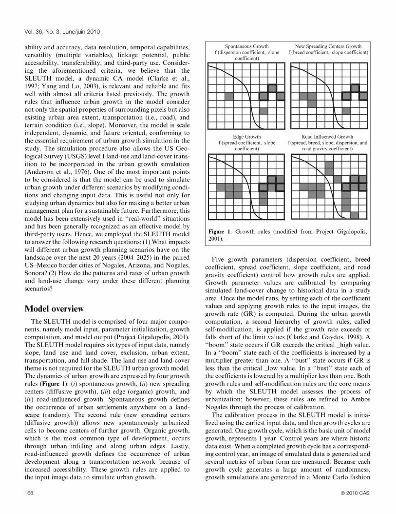
The dynamics of urban growth are expressed by four growth

rules (Figure 1): (i) spontaneous growth, (ii) new spreading

centers (diffusive growth), (iii) edge (organic) growth, and

(iv) road-influenced growth. Spontaneous growth defines

the occurrence of urban settlements anywhere on a land-

scape (random). The second rule (new spreading centers

(diffusive growth)) allows new spontaneously urbanized

cells to become centers of further growth. Organic growth,

which is the most common type of development, occurs

through urban infilling and along urban edges. Lastly,

road-influenced growth defines the occurrence of urban

development along a transportation network because of

increased accessibility. These growth rules are applied to

the input image data to simulate urban growth.

Five growth parameters (dispersion coefficient, breed

coefficient, spread coefficient, slope coefficient, and road

gravity coefficient) control how growth rules are applied.

Growth parameter values are calibrated by comparing

simulated land-cover change to historical data in a study

area. Once the model runs, by setting each of the coefficient

values and applying growth rules to the input images, the

growth rate (GR) is computed. During the urban growth

computation, a second hierarchy of growth rules, called

self-modification, is applied if the growth rate exceeds or

falls short of the limit values (Clarke and Gaydos, 1998). A

‘‘boom’’ state occurs if GR exceeds the critical _high value.

In a ‘‘boom’’ state each of the coefficients is increased by a

multiplier greater than one. A ‘‘bust’’ state occurs if GR is

less than the critical _low value. In a ‘‘bust’’ state each of

the coefficients is lowered by a multiplier less than one. Both

growth rules and self-modification rules are the core means

by which the SLEUTH model assesses the process of

urbanization; however, these rules are refined to Ambos

Nogales through the process of calibration.

The calibration process in the SLEUTH model is initia-

lized using the earliest input data, and then growth cycles are

generated. One growth cycle, which is the basic unit of model

growth, represents 1 year. Control years are where historic

data exist. When a completed growth cycle has a correspond-

ing control year, an image of simulated data is generated and

several metrics of urban form are measured. Because each

growth cycle generates a large amount of randomness,

growth simulations are generated in a Monte Carlo fashion

Figure 1. Growth rules (modified from Project Gigalopolis,

2001).

Vol. 36, No. 3, June/juin 2010

168 E 2010 CASI

to provide a greater amount of stability for the modeled

results. The best-fit values identified from calibration are

the starting values for the prediction.

Data and study area

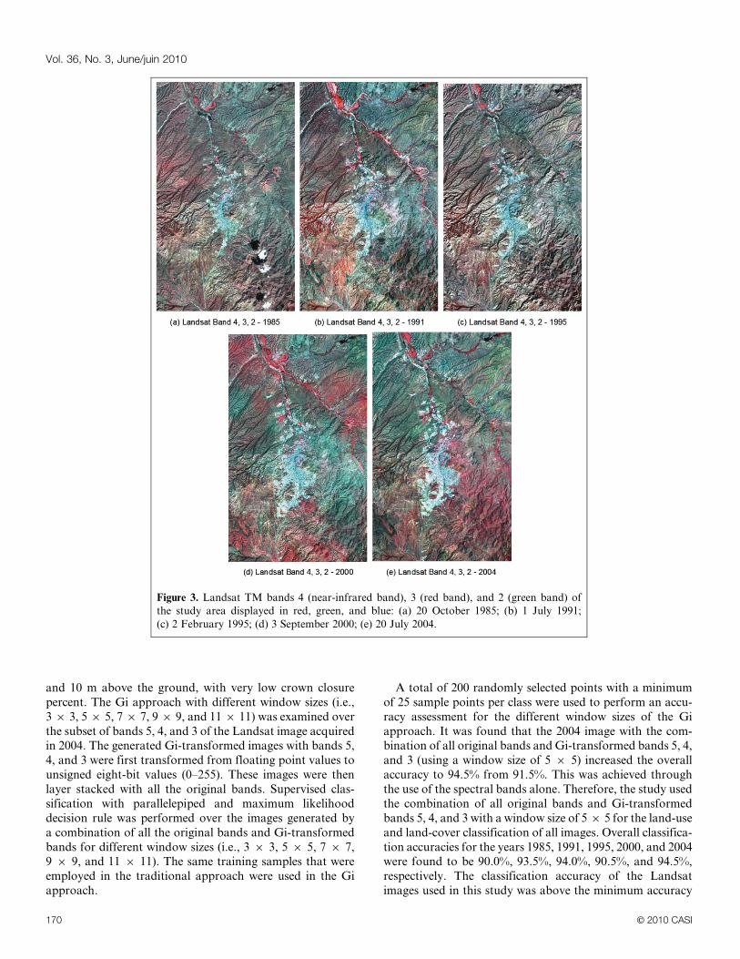
A series of Landsat (TM) images at 28.50 m spatial reso-

lution with path–row locations of 36–38 acquired over dif-

ferent time periods (20 October 1985, 1 July 1991, 2 February

1995, 3 September 2000, and 20 July 2004) were used for thisstudy. Six channels of Landsat (TM) bands were selected for

this study: blue band B1 (0.45–0.52 mm), green band B2

(0.52–0.60 mm), red band B3 (0.63–0.69 mm), near-infrared

band B4 (0.75–0.90 mm), mid-infrared band B5 (1.55–

1.75 mm), and mid-infrared band B7 (2.09–2.35 mm). The

thermal infrared band B6 (10.4–2.50 mm) was not used

because of its coarse resolution. A subset of the images

extent (762 pixels by 1258 pixels), which contains the pairedUS–Mexico border cities of Nogales, Arizona, and Nogales,

Sonora, was selected for this research (Figure 2). The study

area spans 77 862 ha. The area on the Arizona side encom-

passes 40 912 ha, and that on the Sonora side encompasses

36 950 ha. The Arizona side covers 762 columns by 661 rows

in the image of the study area, and the Sonora side covers

762 columns by 597 rows. All Landsat (TM) images were

orthorectified. Landsat TM bands 4 (near-infrared band), 3

(red band), and 2 (green band) of the study area are shown in

Figure 3.

We employed a spatial autocorrelation approach known

as the Getis index (Gi) to improve the classification accuracy

of a traditional spectral-based classification approach. We

performed a supervised classification using spatial trans-

formed bands (i.e., Getis index) to identify seven classes,

namely urban, agriculture and grassland, riparian vegeta-

tion, forest, shrubs, exposed soil, and water. The forest cat-

egory in this arid–semi-arid region is referred to as a desert

deciduous forest and is generally composed of dwarf woody

plants and small deciduous trees normally ranging between 5

Figure 2. Location map of the study area showing Nogales, Arizona, and Nogales,

Sonora (1 mile 5 1.609 km).


E 2010 CASI 169

and 10 m above the ground, with very low crown closure

percent. The Gi approach with different window sizes (i.e.,

3 6 3, 5 6 5, 7 6 7, 9 6 9, and 11 6 11) was examined over

the subset of bands 5, 4, and 3 of the Landsat image acquiredin 2004. The generated Gi-transformed images with bands 5,

4, and 3 were first transformed from floating point values to

unsigned eight-bit values (0–255). These images were then

layer stacked with all the original bands. Supervised clas-

sification with parallelepiped and maximum likelihood

decision rule was performed over the images generated by

a combination of all the original bands and Gi-transformed

bands for different window sizes (i.e., 3 6 3, 5 6 5, 7 6 7,9 6 9, and 11 6 11). The same training samples that were

employed in the traditional approach were used in the Gi

approach.

A total of 200 randomly selected points with a minimum

of 25 sample points per class were used to perform an accu-

racy assessment for the different window sizes of the Gi

approach. It was found that the 2004 image with the com-bination of all original bands and Gi-transformed bands 5, 4,

and 3 (using a window size of 5 6 5) increased the overall

accuracy to 94.5% from 91.5%. This was achieved through

the use of the spectral bands alone. Therefore, the study used

the combination of all original bands and Gi-transformed

bands 5, 4, and 3 with a window size of 5 6 5 for the land-use

and land-cover classification of all images. Overall classifica-

tion accuracies for the years 1985, 1991, 1995, 2000, and 2004were found to be 90.0%, 93.5%, 94.0%, 90.5%, and 94.5%,

respectively. The classification accuracy of the Landsat

images used in this study was above the minimum accuracy

Figure 3. Landsat TM bands 4 (near-infrared band), 3 (red band), and 2 (green band) of

the study area displayed in red, green, and blue: (a) 20 October 1985; (b) 1 July 1991;

(c) 2 February 1995; (d) 3 September 2000; (e) 20 July 2004.


170 E 2010 CASI

of 85% required by most resource management applications

(Anderson et al., 1976).

Model input database

The SLEUTH model requires a binary map of urban and

nonurban extent. The theme of urban extent was extractedfrom the classified land-use and land-cover map of the study

area by assigning the pixel value of zero for nonurban and

255 for urban. The urban extent for the year 1985 was used

as the seed to initialize the model, and subsequent urban

layers for the years 1991, 1995, 2000, and 2004 were used

to calculate best-fit statistics for calibration.

Road layers were prepared for the 1985 and 2004 imagery.

For 1985, a road map of the study area was digitized from a

USGS 7.59 series topographic sheet (Arizona–Sonora, SW/4Nogales 159 quadrangle). For the year 2004, a road map for

the US side was downloaded from the Census Bureau

TIGER shapefiles, and a road map for Nogales, Sonora,

was digitized from a USGS 7.59 series topographic sheet

(Arizona–Sonora, SW/4 Nogales 159 quadrangle). The road

network is a binary theme, with all roads given a value of 100

and nonroad pixels given a value of zero.

The exclusion layer defines the areas where urbanization

cannot occur, e.g., water bodies. The exclusion layer was

extracted from the land-use and land-cover map for the year2004. All water bodies were assigned a pixel value of 100, and

all other pixels were assigned a value of zero.

The slope layer was derived from a USGS digital elevation

model (DEM). The DEM was acquired as a single scene

from the USGS 30 m DEM that covers both Nogales, Ari-

zona, and Nogales, Sonora. However, a difference in reso-

lution was found. The resolution for the US side was much

finer (30 m) than that for the Mexican side (90 m). The DEM

was transformed to percent slope and then truncated to

integer values from floating point, which is required for the

SLEUTH model input image format. The difference in

DEM resolutions for the US and Mexican sides could have

potentially influenced the outcomes for both cities. It can be

expected that the coarser resolution DEM will lead to lower

slope percentages because the differences in elevation among

neighborhood pixels are generalized. This situation might

have created more favorable conditions for urban develop-

ments. This is because the slope coefficient influences all

growth rules; as value increases, the likelihood of urbanized

steeper slopes decreases.

The hill-shade layer was derived from the same USGS 30 m

DEM as that used to generate the slope layer. The hill-shade

layer is used as a background image to give a topographic

spatial context to the model image output.

Input data formatting

The SLEUTH model requires input data to be standar-

dized in terms of format, dimension, projection, resolution,

map extent, and naming format. All input layers were pre-

pared in Erdas Imagine (raster format) and separated by

country. Grid dimensions were 762 columns by 661 rows

for the US images and 762 columns by 597 rows for the

Mexico images. All images had a resolution of 28.50 m

and were projected to Universal Transverse Mercator

(UTM) World Geodetic Survey for 1984 (WGS 84).

SLEUTH accepts input data in gray-scale eight-bit graphic

image file (GIF) format, which is not an export option in

Erdas Imagine software. Hence, all the input layers were

transformed first into tagged image file (TIF) format and

then converted into GIF in Adobe Photoshop. A list of input

data is given in Table 1, and the images are displayed in

Figures 4 and 5.

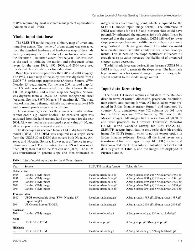
Table 1. List of model input data for the different themes.

Year Source SLEUTH naming format Schedule files

Urban extent

1985 Landsat (TM) image location.urban.date.gif AZnog.urban.1985.gif; SNnog.urban.1985.gif





Transportation

1985 USGS topographic sheet (SW/4 Nogales 159

quadrangle)

location.roads.date.gif AZnog.roads.1985.gif; SNnog.roads.1985.gif

2004 US Census Bureau TIGER location.roads.date.gif AZnog.roads.2004.gif; SNnog.roads.2004.gif

Exclusion

2004 Landsat (TM) images location.excluded.gif AZnog.excluded.gif; SNnog.excluded.gif

Slope

— USGS 30 m DEM location.slope.gif AZnog.slope.gif; SNnog.slope.gif

Hillshade

— USGS 30 m DEM location.hillshade.gif AZnog.hillshade.gif; SNnog.hillshade.gif


E 2010 CASI 171

Model calibration

Calibration determines the best-fit values for the five

growth-control parameters, namely dispersion coefficient,

breed coefficient, spread coefficient, slope coefficient, and

road gravity coefficient, by fitting simulated data to histor-

ical spatial data. In the calibration process, the _start coef-

ficient values initialize the first simulation, a coefficient value

is increased by its _step value, and another simulation is

performed. The process is continued until the _stop value

is reached or exceeded. This was repeated for all possible

permutations for all given ranges and increments.

The five coefficients of the SLEUTH model range between

zero and 100 and require extensive computation for cal-

ibration. A brute-force method was used to calibrate the

coefficient values. The methodology of brute force involves

calibrating the model to the data in steps, sequentially nar-rowing the range of coefficient values, and increasing the

data resolution. The calibration process was accomplished

in three phases referred to as the coarse phase, fine phase,

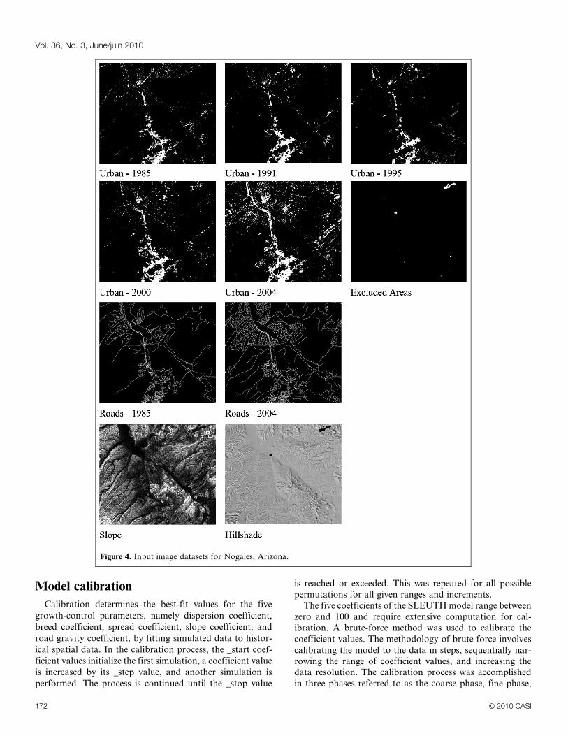
Figure 4. Input image datasets for Nogales, Arizona.


172 E 2010 CASI

and final phase. During the calibration process, the

SLEUTH model generates best-fit statistics for 11 metrics,

namely compare, pop, edges, clusters, cluster size, Lee–

Sallee, slope, percent urban, X mean, Y mean, and rad. These

metrics are generated for each control year. The simulated

data are then compared with the metrics of the historical

data and linear regression values are calculated. These

best-fit values are written to the output file called

control_stats.log, which is the main file used to score the

many runs executed during each calibration phase.

A compare metric is run that examines the amount of

modeled urban areas compared with known urban areas

for the stop year. The pop, edges, clusters, cluster size, slope,

and percent urban are used to calculate the least squares

regression for the modeled urban area, urban perimeter

(edges), number of urban clusters, average cluster size, aver-

age slope of urbanized cells, and percent of available pixels

urbanized compared with actual urban area variables. The

Lee–Sallee metric measures the shape index, the spatial fit

between the modeled urban growth, and the known urban

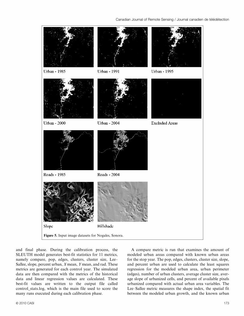
Figure 5. Input image datasets for Nogales, Sonora.


E 2010 CASI 173

extent for the control year. The X mean and Y mean metrics

are used to calculate the least squares regression of average

longitude and latitude, respectively, for modeled urbanized

locations compared with the known urban locations for the

control years. The last metric, rad, measures urban dispersal.The best coefficient sets can be found by sorting one or

more of the metrics contained in the control_stats log file.

However, there is no definitive way of sorting these ranges.

The various approaches may include sorting all metrics

equally, weighting some metrics more heavily than others,

and sorting only one metric. The algorithm for narrowing

these ranges is a continuous topic of discussion among the

users of Project Gigalopolis (2001). The coefficient sets inthis research were selected by sorting by the Lee–Sallee

metric.

Coarse phase

The coarse phase of calibration explores the entire range

(0–100) of the five coefficients using large increments. In this

phase all the coefficients were set to (0–100, 25), where the

first number (0) is the _start value, the second number (100)

is the _stop value, and the third number (25) is the _step

value. The full resolution of the dataset was 28.50 m, and

therefore all the input images were resampled to 114 m spa-

tial resolution. A small value (4) was assigned for the numberof Monte Carlo iterations. Given these conditions, the res-

ultant number of iterations in this phase was 3125. The best

statistical fit measurements were stored in the control_stats

log file. Using the control_stats log file, the top three ranking

scores were identified by sorting the Lee–Sallee metric. The

high and low values of the each coefficient were selected

from the top three scores. The low values were set to _start,

the high values were set to _stop, and the _step values were

selected as an increment of four to six times between _start

and _stop values. The selected coefficient ranges from the

coarse calibration phase that were used to run the fine cal-

ibration phase are given in Table 2.

Fine phase

The fine phase of calibration narrowed the coefficient

ranges derived from the coarse phase and applied to the

input data that were resampled to 57 m spatial resolution

(half of its full size 5 28.50 m). The goal for the fine phase is

to further narrow down the coefficient ranges. The number

of Monte Carlo iterations was then increased to seven to

reduce the level of errors. Given these conditions, the result-

ant number of iterations in this phase was 6480. The best-fit

coefficient values were selected from the control_stats log file

using the top three scores by sorting only the Lee–Sallee

metric. The selected coefficient ranges from the fine cal-

ibration phase that were used to run the final calibration

phase are given in Table 2.

Final phase

In the final phase of calibration the narrowed coefficient

ranges selected from the fine phase were applied to the full-

resolution (28.50 m) input data. The goal for the final phase

of calibration was to determine the best coefficient values.

The number of Monte Carlo iterations was increased to 10 in

this phase. Given these conditions, the resultant number of

iterations in this phase was 5400. Using the control_stats log

file, the coefficient values corresponding to the top score of

the Lee–Sallee metric were identified. In the case where more

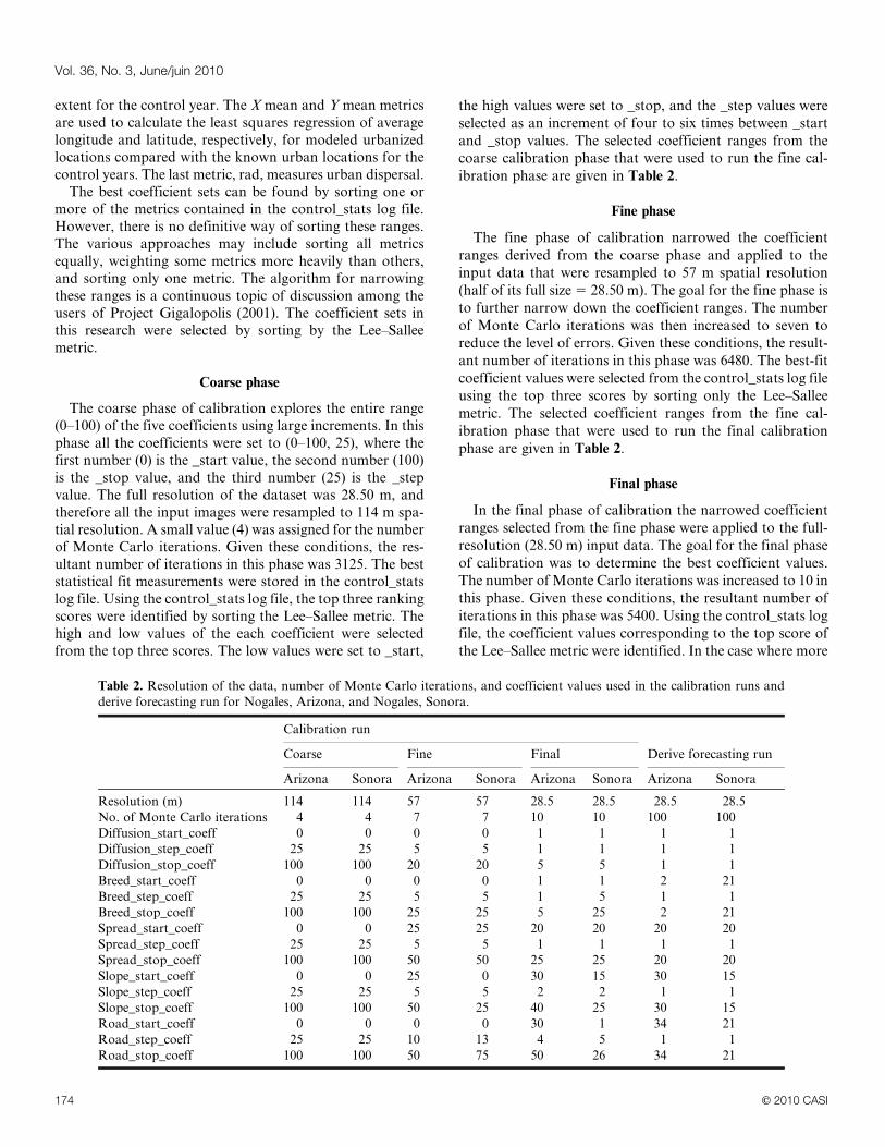
Table 2. Resolution of the data, number of Monte Carlo iterations, and coefficient values used in the calibration runs and

derive forecasting run for Nogales, Arizona, and Nogales, Sonora.

Calibration run

Coarse Fine Final Derive forecasting run

Arizona Sonora Arizona Sonora Arizona Sonora Arizona Sonora

Resolution (m) 114 114 57 57 28.5 28.5 28.5 28.5

No. of Monte Carlo iterations 4 4 7 7 10 10 100 100

Diffusion_start_coeff 0 0 0 0 1 1 1 1

Diffusion_step_coeff 25 25 5 5 1 1 1 1

Diffusion_stop_coeff 100 100 20 20 5 5 1 1

Breed_start_coeff 0 0 0 0 1 1 2 21

Breed_step_coeff 25 25 5 5 1 5 1 1

Breed_stop_coeff 100 100 25 25 5 25 2 21

Spread_start_coeff 0 0 25 25 20 20 20 20

Spread_step_coeff 25 25 5 5 1 1 1 1

Spread_stop_coeff 100 100 50 50 25 25 20 20

Slope_start_coeff 0 0 25 0 30 15 30 15

Slope_step_coeff 25 25 5 5 2 2 1 1

Slope_stop_coeff 100 100 50 25 40 25 30 15

Road_start_coeff 0 0 0 0 30 1 34 21

Road_step_coeff 25 25 10 13 4 5 1 1

Road_stop_coeff 100 100 50 75 50 26 34 21


174 E 2010 CASI

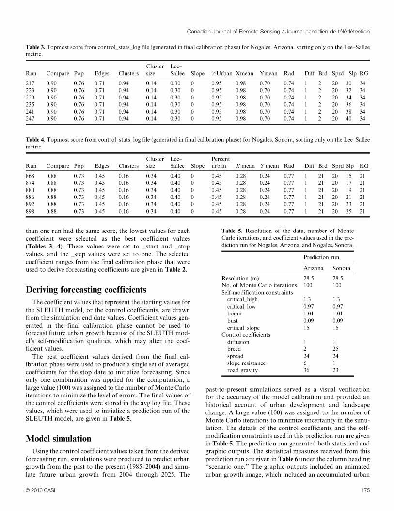
than one run had the same score, the lowest values for each

coefficient were selected as the best coefficient values

(Tables 3, 4). These values were set to _start and _stop

values, and the _step values were set to one. The selected

coefficient ranges from the final calibration phase that were

used to derive forecasting coefficients are given in Table 2.

Deriving forecasting coefficients

The coefficient values that represent the starting values for

the SLEUTH model, or the control coefficients, are drawn

from the simulation end date values. Coefficient values gen-

erated in the final calibration phase cannot be used to

forecast future urban growth because of the SLEUTH mod-

el’s self-modification qualities, which may alter the coef-

ficient values.

The best coefficient values derived from the final cal-

ibration phase were used to produce a single set of averaged

coefficients for the stop date to initialize forecasting. Since

only one combination was applied for the computation, a

large value (100) was assigned to the number of Monte Carlo

iterations to minimize the level of errors. The final values of

the control coefficients were stored in the avg log file. These

values, which were used to initialize a prediction run of the

SLEUTH model, are given in Table 5.

Model simulation

Using the control coefficient values taken from the derived

forecasting run, simulations were produced to predict urban

growth from the past to the present (1985–2004) and simu-

late future urban growth from 2004 through 2025. The

past-to-present simulations served as a visual verification

for the accuracy of the model calibration and provided an

historical account of urban development and landscape

change. A large value (100) was assigned to the number of

Monte Carlo iterations to minimize uncertainty in the simu-

lation. The details of the control coefficients and the self-

modification constraints used in this prediction run are given

in Table 5. The prediction run generated both statistical and

graphic outputs. The statistical measures received from this

prediction run are given in Table 6 under the column heading

‘‘scenario one.’’ The graphic outputs included an animated

urban growth image, which included an accumulated urban

Table 3. Topmost score from control_stats_log file (generated in final calibration phase) for Nogales, Arizona, sorting only on the Lee–Sallee

metric.

Run Compare Pop Edges Clusters

Cluster

size

Lee–

Sallee Slope %Urban Xmean Ymean Rad Diff Brd Sprd Slp RG

217 0.90 0.76 0.71 0.94 0.14 0.30 0 0.95 0.98 0.70 0.74 1 2 20 30 34

223 0.90 0.76 0.71 0.94 0.14 0.30 0 0.95 0.98 0.70 0.74 1 2 20 32 34

229 0.90 0.76 0.71 0.94 0.14 0.30 0 0.95 0.98 0.70 0.74 1 2 20 34 34

235 0.90 0.76 0.71 0.94 0.14 0.30 0 0.95 0.98 0.70 0.74 1 2 20 36 34

241 0.90 0.76 0.71 0.94 0.14 0.30 0 0.95 0.98 0.70 0.74 1 2 20 38 34

247 0.90 0.76 0.71 0.94 0.14 0.30 0 0.95 0.98 0.70 0.74 1 2 20 40 34

Table 4. Topmost score from control_stats_log file (generated in final calibration phase) for Nogales, Sonora, sorting only on the Lee–Sallee

metric.

Run Compare Pop Edges Clusters

Cluster

size

Lee–

Sallee Slope

Percent

urban X mean Y mean Rad Diff Brd Sprd Slp RG

868 0.88 0.73 0.45 0.16 0.34 0.40 0 0.45 0.28 0.24 0.77 1 21 20 15 21

874 0.88 0.73 0.45 0.16 0.34 0.40 0 0.45 0.28 0.24 0.77 1 21 20 17 21

880 0.88 0.73 0.45 0.16 0.34 0.40 0 0.45 0.28 0.24 0.77 1 21 20 19 21

886 0.88 0.73 0.45 0.16 0.34 0.40 0 0.45 0.28 0.24 0.77 1 21 20 21 21

892 0.88 0.73 0.45 0.16 0.34 0.40 0 0.45 0.28 0.24 0.77 1 21 20 23 21

898 0.88 0.73 0.45 0.16 0.34 0.40 0 0.45 0.28 0.24 0.77 1 21 20 25 21

Table 5. Resolution of the data, number of Monte

Carlo iterations, and coefficient values used in the pre-

diction run for Nogales, Arizona, and Nogales, Sonora.

Prediction run

Arizona Sonora

Resolution (m) 28.5 28.5

No. of Monte Carlo iterations 100 100

Self-modification constraints

critical_high 1.3 1.3

critical_low 0.97 0.97

boom 1.01 1.01

bust 0.09 0.09

critical_slope 15 15

Control coefficients

diffusion 1 1

breed 2 25

spread 24 24

slope resistance 6 1

road gravity 36 23


E 2010 CASI 175

growth image for the stop year (2025), and yearly image

predictive outputs for 2004–2025.

Planning scenarios

Four planning scenarios were considered in this research

by altering the composition of the SLEUTH model input

layers to simulate the spatial consequences of urban growth:

(1) business as usual, (2) environmental protection, (3) road

network, and (4) an antigrowth strategy. The purpose of

these simulations was to investigate how various planning

scenarios will affect urban growth patterns and landscape

structures in the Ambos Nogales region. All these scenarios

were simulated for the same time span, i.e., 2004–2025. The

number of Monte Carlo iterations was assigned the value of

100 for each scenario. The business as usual, environmental

protection, and road network scenarios used the same con-

trol coefficient values for their prediction runs (Table 5).

Coefficient values were changed to simulate urban growth

under the antigrowth scenario.

Business as usual scenario

In the business as usual scenario the same initial condi-

tions that were used for the past to the present (1985–2004)

simulation were considered while other environmental and

developmental conditions were not altered. Thus, this scen-

ario provides a benchmark for comparison with other scen-

arios that consider alternative planning strategies.

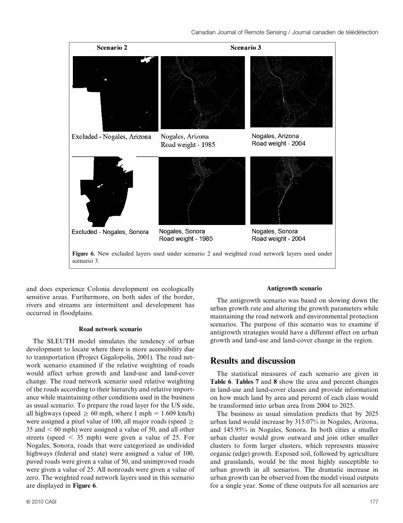
Environmental protection scenario

The environmental protection scenario protected environ-

mentally sensitive lands, such as water bodies, national for-

ests, national parks, wetlands, and floodplains while

maintaining other conditions used in scenario 1. Two exclu-

sion input layers were prepared for the US and Mexican

parts of the study area. For the US portion, the exclusion

layer was prepared using two shape files: (i) national parks

and forest, and (ii) federal and state government lands in

Arizona. Both shape files are derived from the ESRI Data

and Maps 2000 CD-ROM set available as part of the ESRI

software. Two major public lands were selected for exclu-

sion: the Coronado National Forest and the Patagonia Lake

State Park. In addition to these, all water bodies were

excluded, including lakes, rivers, and streams. Excluded

areas were grouped together to form a binary excluded–non-

excluded layer. For the Mexican portion of the study area,

the exclusion layer relied on land-use maps (1997–2000) pre-

pared by the Secretary of Urban Planning and Ecology of

the Government of Sonora. Two classes were created using

these maps, namely areas of ecological preservation and

areas of ecological preservation where high restrictions were

identified. In addition, all water bodies were excluded. All

the excluded areas were assigned a pixel value of 100, and

nonexcluded areas had a pixel value of zero. The new

excluded layers are displayed in Figure 6. While the envir-

onmental protection exclusion layer may seem standard for

the US portion, the Mexican portion of the study area can

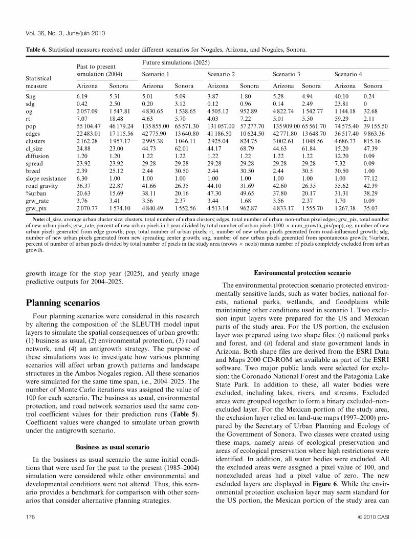
Table 6. Statistical measures received under different scenarios for Nogales, Arizona, and Nogales, Sonora.

Statistical

measure

Past to present

simulation (2004)

Future simulations (2025)

Scenario 1 Scenario 2 Scenario 3 Scenario 4

Arizona Sonora Arizona Sonora Arizona Sonora Arizona Sonora Arizona Sonora

Sng 6.19 5.31 5.01 5.09 3.87 1.80 5.28 4.94 40.10 0.24

sdg 0.42 2.50 0.20 3.12 0.12 0.96 0.14 2.49 23.81 0

og 2 057.09 1 547.81 4 830.65 1 538.65 4 505.12 952.89 4 822.74 1 542.77 1 144.18 32.68

rt 7.07 18.48 4.63 5.70 4.03 7.22 5.01 5.50 59.29 2.11

pop 55 104.47 46 179.24 135 855.00 65 571.30 131 057.00 57 277.70 135 909.00 65 561.70 74 575.40 39 155.50

edges 22 483.01 17 115.56 42 775.90 13 640.80 41 186.50 10 624.50 42 771.80 13 648.70 36 517.40 9 863.36

clusters 2 162.28 1 957.17 2 995.38 1 046.11 2 925.04 824.75 3 002.61 1 048.56 4 686.73 815.16

cl_size 24.88 23.00 44.73 62.01 44.17 68.79 44.63 61.84 15.20 47.39

diffusion 1.20 1.20 1.22 1.22 1.22 1.22 1.22 1.22 12.20 0.09

spread 23.92 23.92 29.28 29.28 29.28 29.28 29.28 29.28 7.32 0.09

breed 2.39 25.12 2.44 30.50 2.44 30.50 2.44 30.5 30.50 1.00

slope resistance 6.30 1.00 1.00 1.00 1.00 1.00 1.00 1.00 1.00 77.12

road gravity 36.37 22.87 41.66 26.35 44.10 31.69 42.60 26.35 55.62 42.39

%urban 20.63 15.69 38.11 20.16 47.30 49.65 37.80 20.17 31.31 38.29

grw_rate 3.76 3.41 3.56 2.37 3.44 1.68 3.56 2.37 1.70 0.09

grw_pix 2 070.77 1 574.10 4 840.49 1 552.56 4 513.14 962.87 4 833.17 1 555.70 1 267.38 35.03

Note: cl_size, average urban cluster size; clusters, total number of urban clusters; edges, total number of urban–non-urban pixel edges; grw_pix, total numberof new urban pixels; grw_rate, percent of new urban pixels in 1 year divided by total number of urban pixels (100 6 num_growth_pix/pop); og, number of newurban pixels generated from edge growth; pop, total number of urban pixels; rt, number of new urban pixels generated from road-influenced growth; sdg,number of new urban pixels generated from new spreading center growth; sng, number of new urban pixels generated from spontaneous growth; %urban,percent of number of urban pixels divided by total number of pixels in the study area (nrows 6 ncols) minus number of pixels completely excluded from urbangrowth.


176 E 2010 CASI

and does experience Colonia development on ecologically

sensitive areas. Furthermore, on both sides of the border,

rivers and streams are intermittent and development has

occurred in floodplains.

Road network scenario

The SLEUTH model simulates the tendency of urban

development to locate where there is more accessibility due

to transportation (Project Gigalopolis, 2001). The road net-

work scenario examined if the relative weighting of roads

would affect urban growth and land-use and land-cover

change. The road network scenario used relative weighting

of the roads according to their hierarchy and relative import-

ance while maintaining other conditions used in the business

as usual scenario. To prepare the road layer for the US side,

all highways (speed § 60 mph, where 1 mph 5 1.609 km/h)

were assigned a pixel value of 100, all major roads (speed §

35 and , 60 mph) were assigned a value of 50, and all other

streets (speed , 35 mph) were given a value of 25. For

Nogales, Sonora, roads that were categorized as undivided

highways (federal and state) were assigned a value of 100,

paved roads were given a value of 50, and unimproved roads

were given a value of 25. All nonroads were given a value of

zero. The weighted road network layers used in this scenario

are displayed in Figure 6.

Antigrowth scenario

The antigrowth scenario was based on slowing down the

urban growth rate and altering the growth parameters while

maintaining the road network and environmental protection

scenarios. The purpose of this scenario was to examine if

antigrowth strategies would have a different effect on urban

growth and land-use and land-cover change in the region.

Results and discussion

The statistical measures of each scenario are given in

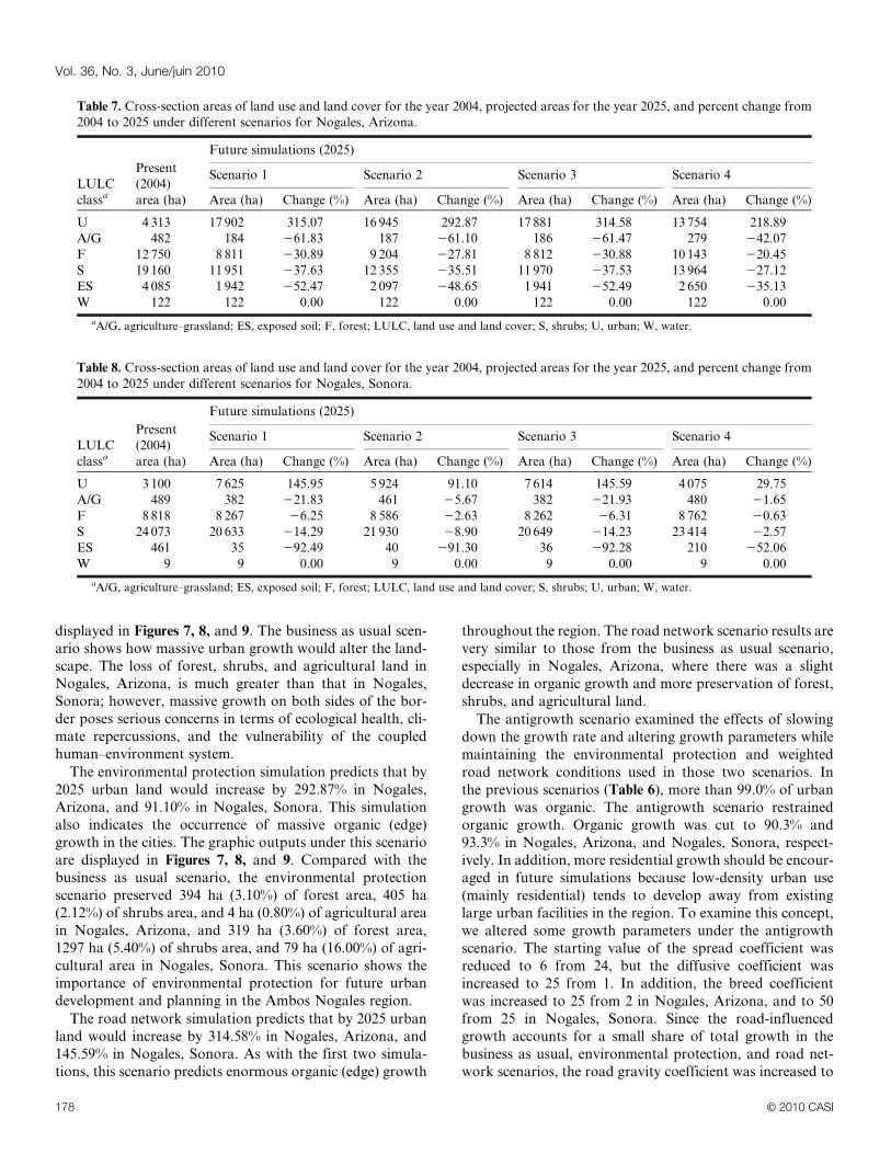
Table 6. Tables 7 and 8 show the area and percent changes

in land-use and land-cover classes and provide information

on how much land by area and percent of each class would

be transformed into urban area from 2004 to 2025.

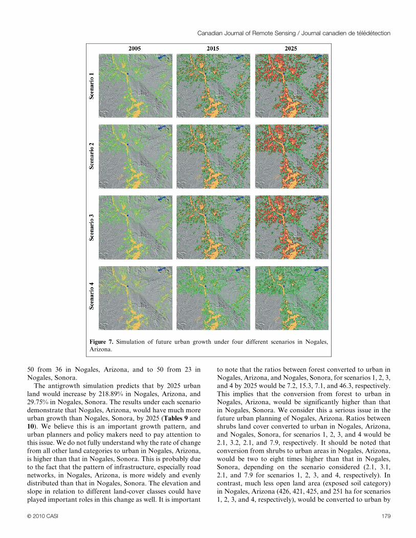
The business as usual simulation predicts that by 2025

urban land would increase by 315.07% in Nogales, Arizona,

and 145.95% in Nogales, Sonora. In both cities a smaller

urban cluster would grow outward and join other smaller

clusters to form larger clusters, which represents massive

organic (edge) growth. Exposed soil, followed by agriculture

and grasslands, would be the most highly susceptible to

urban growth in all scenarios. The dramatic increase in

urban growth can be observed from the model visual outputs

for a single year. Some of these outputs for all scenarios are

Figure 6. New excluded layers used under scenario 2 and weighted road network layers used under

scenario 3.


E 2010 CASI 177

displayed in Figures 7, 8, and 9. The business as usual scen-

ario shows how massive urban growth would alter the land-

scape. The loss of forest, shrubs, and agricultural land in

Nogales, Arizona, is much greater than that in Nogales,

Sonora; however, massive growth on both sides of the bor-

der poses serious concerns in terms of ecological health, cli-

mate repercussions, and the vulnerability of the coupled

human–environment system.

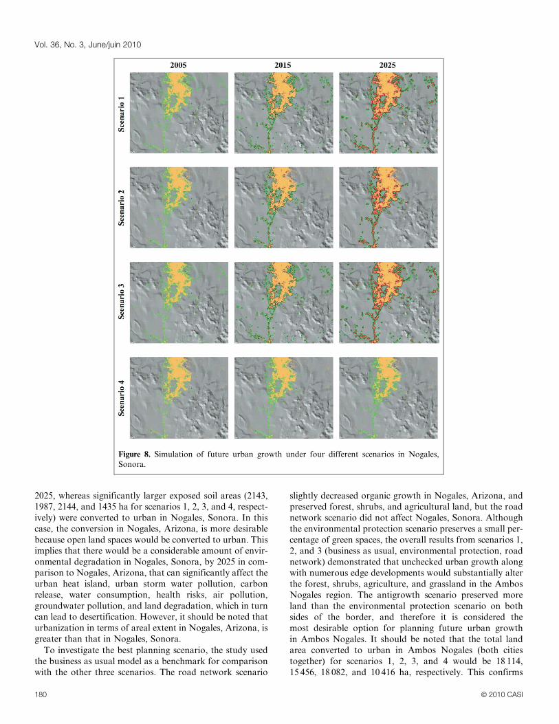
The environmental protection simulation predicts that by

2025 urban land would increase by 292.87% in Nogales,

Arizona, and 91.10% in Nogales, Sonora. This simulation

also indicates the occurrence of massive organic (edge)

growth in the cities. The graphic outputs under this scenario

are displayed in Figures 7, 8, and 9. Compared with the

business as usual scenario, the environmental protection

scenario preserved 394 ha (3.10%) of forest area, 405 ha

(2.12%) of shrubs area, and 4 ha (0.80%) of agricultural area

in Nogales, Arizona, and 319 ha (3.60%) of forest area,

1297 ha (5.40%) of shrubs area, and 79 ha (16.00%) of agri-

cultural area in Nogales, Sonora. This scenario shows the

importance of environmental protection for future urban

development and planning in the Ambos Nogales region.

The road network simulation predicts that by 2025 urban

land would increase by 314.58% in Nogales, Arizona, and

145.59% in Nogales, Sonora. As with the first two simula-

tions, this scenario predicts enormous organic (edge) growth

throughout the region. The road network scenario results are

very similar to those from the business as usual scenario,

especially in Nogales, Arizona, where there was a slight

decrease in organic growth and more preservation of forest,

shrubs, and agricultural land.

The antigrowth scenario examined the effects of slowing

down the growth rate and altering growth parameters while

maintaining the environmental protection and weighted

road network conditions used in those two scenarios. In

the previous scenarios (Table 6), more than 99.0% of urban

growth was organic. The antigrowth scenario restrained

organic growth. Organic growth was cut to 90.3% and

93.3% in Nogales, Arizona, and Nogales, Sonora, respect-

ively. In addition, more residential growth should be encour-

aged in future simulations because low-density urban use

(mainly residential) tends to develop away from existing

large urban facilities in the region. To examine this concept,

we altered some growth parameters under the antigrowth

scenario. The starting value of the spread coefficient was

reduced to 6 from 24, but the diffusive coefficient was

increased to 25 from 1. In addition, the breed coefficient

was increased to 25 from 2 in Nogales, Arizona, and to 50

from 25 in Nogales, Sonora. Since the road-influenced

growth accounts for a small share of total growth in the

business as usual, environmental protection, and road net-

work scenarios, the road gravity coefficient was increased to

Table 7. Cross-section areas of land use and land cover for the year 2004, projected areas for the year 2025, and percent change from

2004 to 2025 under different scenarios for Nogales, Arizona.

LULC

classa

Present

(2004)

area (ha)



Area (ha) Change (%) Area (ha) Change (%) Area (ha) Change (%) Area (ha) Change (%)

U 4 313 17 902 315.07 16 945 292.87 17 881 314.58 13 754 218.89

A/G 482 184 261.83 187 261.10 186 261.47 279 242.07

F 12 750 8 811 230.89 9 204 227.81 8 812 230.88 10 143 220.45

S 19 160 11 951 237.63 12 355 235.51 11 970 237.53 13 964 227.12

ES 4 085 1 942 252.47 2 097 248.65 1 941 252.49 2 650 235.13

W 122 122 0.00 122 0.00 122 0.00 122 0.00

aA/G, agriculture–grassland; ES, exposed soil; F, forest; LULC, land use and land cover; S, shrubs; U, urban; W, water.

Table 8. Cross-section areas of land use and land cover for the year 2004, projected areas for the year 2025, and percent change from

2004 to 2025 under different scenarios for Nogales, Sonora.

LULC

classa

Present

(2004)

area (ha)




U 3 100 7 625 145.95 5 924 91.10 7 614 145.59 4 075 29.75

A/G 489 382 221.83 461 25.67 382 221.93 480 21.65

F 8 818 8 267 26.25 8 586 22.63 8 262 26.31 8 762 20.63

S 24 073 20 633 214.29 21 930 28.90 20 649 214.23 23 414 22.57

ES 461 35 292.49 40 291.30 36 292.28 210 252.06

W 9 9 0.00 9 0.00 9 0.00 9 0.00

aA/G, agriculture–grassland; ES, exposed soil; F, forest; LULC, land use and land cover; S, shrubs; U, urban; W, water.


178 E 2010 CASI

50 from 36 in Nogales, Arizona, and to 50 from 23 in

Nogales, Sonora.

The antigrowth simulation predicts that by 2025 urban

land would increase by 218.89% in Nogales, Arizona, and

29.75% in Nogales, Sonora. The results under each scenario

demonstrate that Nogales, Arizona, would have much moreurban growth than Nogales, Sonora, by 2025 (Tables 9 and

10). We believe this is an important growth pattern, and

urban planners and policy makers need to pay attention to

this issue. We do not fully understand why the rate of change

from all other land categories to urban in Nogales, Arizona,

is higher than that in Nogales, Sonora. This is probably due

to the fact that the pattern of infrastructure, especially road

networks, in Nogales, Arizona, is more widely and evenlydistributed than that in Nogales, Sonora. The elevation and

slope in relation to different land-cover classes could have

played important roles in this change as well. It is important

to note that the ratios between forest converted to urban in

Nogales, Arizona, and Nogales, Sonora, for scenarios 1, 2, 3,

and 4 by 2025 would be 7.2, 15.3, 7.1, and 46.3, respectively.

This implies that the conversion from forest to urban in

Nogales, Arizona, would be significantly higher than that

in Nogales, Sonora. We consider this a serious issue in thefuture urban planning of Nogales, Arizona. Ratios between

shrubs land cover converted to urban in Nogales, Arizona,

and Nogales, Sonora, for scenarios 1, 2, 3, and 4 would be

2.1, 3.2, 2.1, and 7.9, respectively. It should be noted that

conversion from shrubs to urban areas in Nogales, Arizona,

would be two to eight times higher than that in Nogales,

Sonora, depending on the scenario considered (2.1, 3.1,

2.1, and 7.9 for scenarios 1, 2, 3, and 4, respectively). Incontrast, much less open land area (exposed soil category)

in Nogales, Arizona (426, 421, 425, and 251 ha for scenarios

1, 2, 3, and 4, respectively), would be converted to urban by

Figure 7. Simulation of future urban growth under four different scenarios in Nogales,

Arizona.


E 2010 CASI 179

2025, whereas significantly larger exposed soil areas (2143,

1987, 2144, and 1435 ha for scenarios 1, 2, 3, and 4, respect-

ively) were converted to urban in Nogales, Sonora. In this

case, the conversion in Nogales, Arizona, is more desirable

because open land spaces would be converted to urban. This

implies that there would be a considerable amount of envir-

onmental degradation in Nogales, Sonora, by 2025 in com-

parison to Nogales, Arizona, that can significantly affect the

urban heat island, urban storm water pollution, carbon

release, water consumption, health risks, air pollution,

groundwater pollution, and land degradation, which in turn

can lead to desertification. However, it should be noted that

urbanization in terms of areal extent in Nogales, Arizona, is

greater than that in Nogales, Sonora.

To investigate the best planning scenario, the study used

the business as usual model as a benchmark for comparison

with the other three scenarios. The road network scenario

slightly decreased organic growth in Nogales, Arizona, and

preserved forest, shrubs, and agricultural land, but the road

network scenario did not affect Nogales, Sonora. Although

the environmental protection scenario preserves a small per-

centage of green spaces, the overall results from scenarios 1,

2, and 3 (business as usual, environmental protection, road

network) demonstrated that unchecked urban growth along

with numerous edge developments would substantially alter

the forest, shrubs, agriculture, and grassland in the Ambos

Nogales region. The antigrowth scenario preserved more

land than the environmental protection scenario on both

sides of the border, and therefore it is considered the

most desirable option for planning future urban growth

in Ambos Nogales. It should be noted that the total land

area converted to urban in Ambos Nogales (both cities

together) for scenarios 1, 2, 3, and 4 would be 18 114,

15 456, 18 082, and 10 416 ha, respectively. This confirms

Figure 8. Simulation of future urban growth under four different scenarios in Nogales,

Sonora.


180 E 2010 CASI

that the antigrowth scenario is the most advantageous. How-

ever, conversion from forests to urban in Nogales, Sonora,

would result in only 2% of the forests being converted to

urban in Nogales, Arizona. In contrast, conversion from

open land to urban in Nogales, Sonora, would be six times

smaller than that in Nogales, Arizona. This type of conver-

sion in Nogales, Arizona, is more desirable. Under all scen-

arios, the conversion of agricultural areas to urban areas

would be greater in Nogales, Arizona (298, 298, 294, 296,

and 203 ha for scenarios 1, 2, 3, and 4, respectively) than in

Nogales, Sonora (107, 28, 107, and 8 ha for scenarios 1, 2, 3,

and 4, respectively). This suggests that there is a need to

formulate better policy and planning strategies and law-

enforcement actions to protect forests in Nogales, Arizona,

and encourage more developments and urbanization in open

land areas in Nogales, Sonora. One other option would be to

encourage conversion from agriculture to urban by intro-

ducing intensive agriculture practices to increase the produc-

tion or at least maintain the same level of production with

smaller agricultural areas.

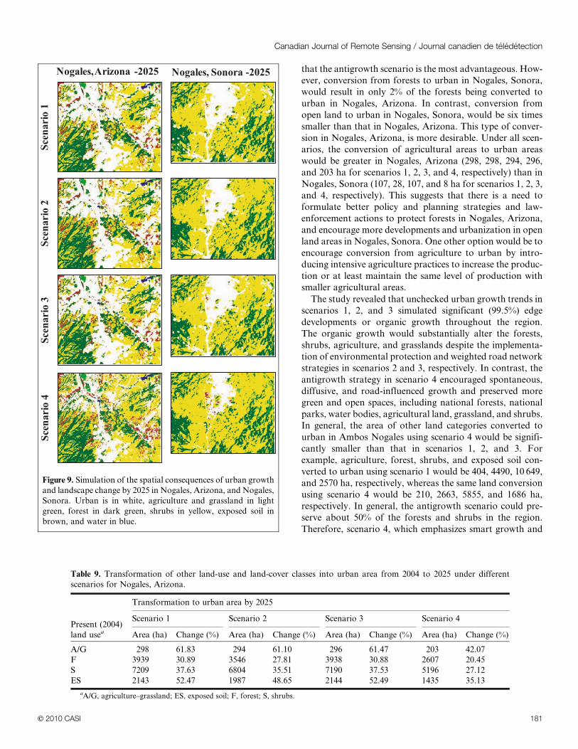
The study revealed that unchecked urban growth trends in

scenarios 1, 2, and 3 simulated significant (99.5%) edge

developments or organic growth throughout the region.

The organic growth would substantially alter the forests,

shrubs, agriculture, and grasslands despite the implementa-

tion of environmental protection and weighted road network

strategies in scenarios 2 and 3, respectively. In contrast, the

antigrowth strategy in scenario 4 encouraged spontaneous,

diffusive, and road-influenced growth and preserved more

green and open spaces, including national forests, national

parks, water bodies, agricultural land, grassland, and shrubs.

In general, the area of other land categories converted to

urban in Ambos Nogales using scenario 4 would be signifi-

cantly smaller than that in scenarios 1, 2, and 3. For

example, agriculture, forest, shrubs, and exposed soil con-

verted to urban using scenario 1 would be 404, 4490, 10 649,

and 2570 ha, respectively, whereas the same land conversion

using scenario 4 would be 210, 2663, 5855, and 1686 ha,

respectively. In general, the antigrowth scenario could pre-

serve about 50% of the forests and shrubs in the region.

Therefore, scenario 4, which emphasizes smart growth and

Figure 9. Simulation of the spatial consequences of urban growth

and landscape change by 2025 in Nogales, Arizona, and Nogales,

Sonora. Urban is in white, agriculture and grassland in light

green, forest in dark green, shrubs in yellow, exposed soil in

brown, and water in blue.

Table 9. Transformation of other land-use and land-cover classes into urban area from 2004 to 2025 under different

scenarios for Nogales, Arizona.

Present (2004)

land usea

Transformation to urban area by 2025



A/G 298 61.83 294 61.10 296 61.47 203 42.07

F 3939 30.89 3546 27.81 3938 30.88 2607 20.45

S 7209 37.63 6804 35.51 7190 37.53 5196 27.12

ES 2143 52.47 1987 48.65 2144 52.49 1435 35.13

aA/G, agriculture–grassland; ES, exposed soil; F, forest; S, shrubs.


E 2010 CASI 181

environmental protection, is the most desirable for future

urban development and planning in Ambos Nogales.

Arizona’s border communities are interconnected eco-

nomically, politically, and socially with their sister cities in

Sonora because of their binational heritage. Thousands of

people and vehicles cross the border daily to work, shop,

attend school, and visit family. The air they breathe, the

water they use, and the waste they generate are shared.

Therefore the overall problems that affect infrastructure

development and quality-of-life issues are vital. Although

the simulated spatial patterns of urban growth for 2025 were

very different for the paired cities, with more urban growth

on the Arizona side of the US–Mexico border, the region

as a whole will have considerable urban growth coupled

with the loss of green space. The results from this study

suggest the need for both cities to work together to formulate

planning strategies and policies for future smart growth

that would achieve sustainable development in the region.

We believe that the two cities must work together to

formulate better management plans to achieve a healthy

environment and better economic development because

socioecological systems and ecosystem services in both cities

and their surrounding environments are strongly inter-

connected and highly interdependent. The findings of

this study can be expected to be useful to the local and

regional governments on both sides of the border to assess

risks of environmental degradation, ecological health,

climate repercussions, and the vulnerability of coupled

human–environment systems and aide in the development

of binational management strategies.

Conclusion

This study has demonstrated the effectiveness of the slope,

land cover, exclusion, urbanization, transportation, and hill-

shade (SLEUTH) model for urban land use and planning.

The calibration results in the context of Ambos Nogales have

proven the model’s portability and universality of applica-

tion. The strength of the SLEUTH model relies on the

fact that it can incorporate urban extent, transportation

gravity, and slope resistance along with four types of

urban growth (spontaneous, new spreading centers, organic,

and road influenced). In addition, the model is capable of

incorporating different locational conditions, such as road

networks, with various weights and different environmental

protection definitions. These properties present a significant

potential for modeling urban growth and land-use and land-

cover changes under different planning scenarios by altering

some initial conditions and changing input data.

The study examined the spatial consequences of urban

growth on landscape change under four different scenarios

in the paired border cities of Nogales, Arizona, and Nogales,

Sonora. Each scenario demonstrates that Nogales, Arizona,

would have much greater urban growth and loss of green

spaces than Nogales, Sonora, by the year 2025. Scenario 1

(business as usual) simulates the massive urban growth and

huge loss of forests, shrubs, and agricultural land in Ambos

Nogales if the current rate and pattern of urban growth are

not altered. Scenario 2 (environmental protection) is import-

ant because it preserves a small percentage of green space.

The results from scenario 3 (road network) are quite similar

to those from the business as usual scenario except for

slightly decreased organic growth and the preservation of

some green space. The study reveals that the unchecked

urban growth trend in the business as usual, environmental

protection, and road network scenarios simulate significant

(99.5%) edge developments or organic growth throughout

the region. In contrast, the antigrowth scenario allows for

more green and open space and is therefore the most desir-

able for planning future urban land use and development.

The technical frameworks developed in this research can

be deployed to simulate future urban growth for other inter-

national border cities. These findings can contribute to bina-

tional planning communities, municipalities, countries, and

other public and private organizations that need to manage

resources and provide services to people living in rapidly

changing paired border cities. Furthermore, this research

can be extended to other paired US–Mexico border cities

for achieving desired smart and responsible urban growth

and sustainable development.

Acknowledgements

The study was supported by the Southwest Consortium

for Environmental Research and Policy (CERP FY2006)

Applied Border Environmental Research Program (grant

Table 10. Transformation of other land-use and land-cover classes into urban area from 2004 to 2025 under different

scenarios for Nogales, Sonora.

Present (2004)

land usea

Transformation to urban area by 2025



A/G 107 21.83 28 5.67 107 21.93 8 1.71

F 551 6.25 232 2.63 556 6.31 56 0.64

S 3440 14.29 2143 8.90 3425 14.23 659 2.74

ES 426 92.49 421 91.30 425 92.28 251 54.51

aA/G, agriculture–grassland; ES, exposed soil; F, forest; S, shrubs.


182 E 2010 CASI

EIR-05-04). The authors would like to thank Subhro

Guhathakurta and Jana Hutchins for their valuable sugges-

tions and support. We are also grateful for the commentsand suggestions of anonymous reviewers that significantly

improved the manuscript.

References

Anderson, J.R., Hardy, E.E., Roach, J.T., and Witmer, R.E. 1976. A land-

use and land-cover classification system for use with remote sensor data. US

Geological Survey, Professional Paper 964.

Baker, W.L. 1989. Landscape ecology and nature reserve design in the

Boundary Waters Canoe area, Minnesota. Ecology, Vol. 70, pp. 23–35.

doi:10.2307/1938409.

Burton, A., and Pitt, R. 2002. Stormwater effects handbook: a toolbox for

watershed managers, scientists, and engineers. Lewis Publishers, Boca

Raton, Fla.

Cihlar, J., and Jansen, L.J.M. 2001. From land cover to land use: a meth-

odology for efficient land use mapping over large areas. Professional

Geographer, Vol. 53, No. 2, pp. 275–289.

Clarke, K.C., and Gaydos, L. 1998. Loose-coupling a cellular automaton

model and GIS: long-term urban growth prediction for San Francisco

and Washington/Baltimore. International Journal of Geographical

Information Science, Vol. 12, pp. 699–714. doi:10.1080/136588198241617.

Clarke, K.C., Hoppen, S., and Gaydos, L. 1997. A self-modifying cellular

automaton model of historical urbanization in the San Francisco Bay

area. Environment and Planning B: Planning and Design, Vol. 24, No. 2,

pp. 247–261. doi:10.1068/b240247.

Driver, N.E., and Troutman, B.M., 1989. Regression models for estimating

urban storm-runoff quality and quantity in the United States. Journal of

Hydrology, Vol. 109, pp. 221–236. doi:10.1016/0022-1694(89)90017-6.

Esparza, A.X., Chavez, J., and Waldorf, B. 2001. Industrialization and land-

use change in Mexican Border cities: the case of Ciudad Juarez, Mexico.

Journal of Borderlands Studies, Vol. 16, No. 1, pp. 15–30.

Guhathakurta, S., Pijawka, K.D., and Ashur, S. 2000. Planning for hazard

mitigation in the U.S.–Mexican Border region: an assessment of hazard-

ous waste generation rates for transportation. Journal of Borderlands

Studies, Vol. 15, No. 2, pp. 75–90.

Herold, M., Goldstein, N., and Clarke, K. 2003. The spatio-temporal form

of urban growth: measurement, analysis and modeling. Remote Sensing

of Environment, Vol. 85, pp. 95–105.

Jantz, C.A., Goetz, S.J., Donato, D., and Claggett, P. 2010. Designing and

implementing a regional urban modeling system using the SLEUTH

cellular urban model. Computers, Environment and Urban Systems,

Vol. 34, pp. 1–16.

Jenerette, G.D., and Wu, J. 2001. Analysis and simulation of land-use

change in the central Arizona – Phoenix region, USA. Landscape Eco-

logy, Vol. 16, No. 7, pp. 611–626. doi:10.1023/A:1013170528551.

Li, X., and Yeh, A. 2000. Modelling sustainable urban development by the

integration of constrained cellular automata and GIS. International

Journal of Geographical Information Science, Vol. 14, pp. 131–152.

doi:10.1080/136588100240886.

Masser, I. 2001. Managing our urban future: the role of remote sensing and

geographic information system. Habitat International, Vol. 25, pp. 503–

512. doi:10.1016/S0197-3975(01)00021-2.

Muller, M.R., and Middleton, J. 1994. A Markov model of land-use change

dynamics in the Niagara Region, Ontario, Canada. Landscape Ecology,

Vol. 9, pp. 151–157.

Myint, S.W., and Wang, L. 2006. Multicriteria decision approach for land use

land cover change using Markov chain analysis and a cellular automata

approach. Canadian Journal of Remote Sensing, Vol. 32, No. 6, pp. 390–404.

Norman, L.M. 2007. United States – Mexican border watershed assessment:

modeling nonpoint source pollution in Ambos Nogales. Journal of Bor-

derland Studies, Vol. 22, No. 1, pp. 54–79.

Norman, L.M. 2005. Modeling land use change and associate water quality

impacts in the Ambos Nogales watershed, U.S.–Mexico border. Ph.D.

dissertation, University of Arizona, Tucson, Ariz. 216 pp.

Norman, L.M., Donelson, A., Pfeifer, E., and Lam, A.H. 2006. Colonia

development and land use change in Ambos Nogales, United States – Mex-

ican border. US Geological Survey, Open-file Report 2006-1112. Avail-

able from http://pubs.usgs.gov/of/2006/1112 [accessed 23 January 2010].

Norman, L.M., Guertin, D.P., and Feller, M. 2008. A coupled model approach

to reduce nonpoint-source pollution resulting from predicted urban growth:

a case study in the Ambos Nogales watershed. Journal of Urban Geography,

Vol. 29, No. 5, pp. 496–516. doi:10.2747/0272-3638.29.5.496.

Pijanowski, B.C., Brown, D.G., Manik, G., and Shellito, B. 2002. Using

neural nets and GIS to forecast land use changes: a land transformation

model. Computers, Environment and Urban Systems, Vol. 26, pp. 553–

575. doi:10.1016/S0198-9715(01)00015-1.

Pontius, R., and Chen, H. 2003. Land change modelling with GEOMOD.

Idrisi Kilimanjaro version. Clark Laboratories, Worcester, Mass.

Pontius, R.G., Jr., and Malanson, J. 2005. Comparison of the structure and

accuracy of two land change models. International Journal of Geographical

Information Science, Vol. 19, pp. 243–265. doi:10.1080/13658810410001713434.

Pontius, R.G., Jr., Cornell, J., and Hall, C. 2001. Modeling the spatial

pattern of land-use change with Geomod2: application and validation

for Costa Rica. Agriculture, Ecosystems & Environment, Vol. 85,

pp. 191–203. doi:10.1016/S0167-8809(01)00183-9.

Project Gigalopolis. 2001. Urban growth model (UGM) version 3.0. Difference

between version 2.0 and 2.1. US Geological Survey, Washington, D.C., and

University of California at Santa Barbara, Santa Barbara, Calif. Available

from www.ncgia.ucsb.edu/projects/gig/ [accessed 23 January 2010].

Reynolds, K.A. 2000. Water quality issues along the U.S.–Mexico border.

Water Conditioning and Purification Magazine, Vol. 44, No. 10. Available

from www.wcponline.com/column.cfm?T5T&ID51776&AT5T [accessed

23 January 2010].

SCERP. 2005. The border observatory. Interim Research Report to Southwest

Center for Environmental Research and Policy. Available from http://bop.

caed.asu.edu/resources/Publications/Report%20to%20SCERP%20about%

20ongoing%20project_12_15_05.pdf [accessed 23 January 2010].

Silva, E., and Clarke, K. 2005. Calibration of the SLEUTH urban growth

model for Lisbon and Porto, Portugal. Computers, Environment and Urban

Systems, Vol. 26, pp. 525–552. doi:10.1016/S0198-9715(01)00014-X.

Turner, M.G. 1987. Spatial simulation of landscape changes in Georgia: A

comparison of 3 transition models. Landscape Ecology, Vol. 1, pp. 29–36.

doi:10.1007/BF02275263.

Turner, B.L., II, Moss, R.H., and Skole, D.L. (Editors). 1993. Relating

land-use and global land-cover change: a proposal for an IGBP-HDP

core project. International Geosphere–Biosphere Programme (IGBP),

Stockholm, Sweden. IGBP Report 24 and HDP Report 5. 65 pp.


E 2010 CASI 183

UN Human Settlement Programme. 2003. The challenge of slums: global report

on human settlements 2003. Earthscan Publications Ltd., London, UK.

US EPA. 1997. Urbanization and streams: studies of hydrologic impacts.

Office of Water, US Environmental Protection Agency (US EPA),

Washington, D.C. EPA-841-R-97-009.

US EPA. 2000. Projecting land-use change: a summary of models for asses-

sing the effects of community growth and change on land-use patterns.

US Environmental Protection Agency (US EPA), Washington, D.C.

EPA/600/R-00/098. 264 pp.

US EPA. 2006. Air quality and transportation and cultural and natural

resources. Ninth Report of the Good Neighbor Environmental Board

to the President and Congress of the United States. US Environmental

Protection Agency (US EPA), Washington, D.C.

Veldkamp, A., and Fresco, L.O. 1996. CLUE-CR: An integrated multi-scale

model to simulate land use change scenarios in Costa Rica. Ecological

Modelling, Vol. 91, pp. 231–248. doi:10.1016/0304-3800(95)00158-1.

Wagner, D.F. 1997. Cellular automata and geographic information systems.

Environment and Planning B: Planning and Design, Vol. 24, No. 2,

pp. 219–234. doi:10.1068/b240219.

Walker, B., and Steffen, W. 1997. An overview of the implications of global

change for natural and managed terrestrial ecosystems. Conservation

Ecology [online], Vol. 1, No. 2, p. 2. Available from www.consecol.org/

vol1/iss2/art2/ [accessed 23 January 2010].

Walker, B., and Steffen, W. 1999. The nature of global change. In

The terrestrial biosphere and global change. implications for natural and

managed ecosystems. Edited by B.H. Walker, W.L. Steffen, J. Canadell,

and J.S.I. Ingram. Cambridge University Press, London, UK.

pp. 1–18.

Weng, Q. 2002. Land use change analysis in the Zhujiang Delta of China

using satellite remote sensing, GIS and stochastic modeling. Journal of

Environmental Management, Vol. 64, pp. 273–284. doi:10.1006/jema.

2001.0509.

Wu, F., and Webster, C.J. 1998. Simulation of land development through

the integration of cellular automata and multicriteria evaluation. Envir-

onment and Planning B: Planning and Design, Vol. 25, pp. 103–126.

doi:10.1068/b250103.

Yang, X. 2002. Satellite monitoring of urban spatial growth in the Atlanta

metropolitan area. Photogrammetric Engineering & Remote Sensing,

Vol. 68, pp. 725–734.

Yang, X., and Lo, C.P. 2003. Modelling urban growth and landscape

changes in the Atlanta metropolitan area. International Journal of Geo-

graphical Information Science, Vol. 17, pp. 463–488. doi:10.1080/

1365881031000086965.


184 E 2010 CASI

Documents

Simulating urban growth on the US–Mexico border: Nogales, Arizona, and Nogales, Sonora