Embed Size (px)
Citation preview
Department of Mechatronics, Faculty of Mechanical Engineering, Ho Chi Minh City – University of Technology
Viet Nam
Presenter: MAI THANH THAI
October 31, 2015
A New Approaches for Dynamic and Kinematic Modeling of a Snake-like Robot
NATIONAL CONFERENCE ON MACHINES AND MECHANISMS 2015
1

Contents
2. Mathematical Modelling of a Snake-Like Robot1. Introduction
5. Numerical Simulation
3. Kinematics of a Snake-Like Robot
6. Conclusion
4. Dynamics model of the modular robot
2NATIONAL CONFERENCE ON MACHINES AND MECHANISMS 2015

Introduction SNAKE ROBOT
Fig.1. Anna KondaNorwegian University of Science and Technology
Fig.2. ACM R3 Tokyo Institute of Technology
3NATIONAL CONFERENCE ON MACHINES AND MECHANISMS 2015

Mathematical Modelling of a Snake-Like Robot
Ox
y
Fig.3. N-link model of a snake robot
4NATIONAL CONFERENCE ON MACHINES AND MECHANISMS 2015
Ox
y

Mathematical Modelling of a Snake-Like Robot
Ox
y
{¿ 𝑥 𝑖=𝑥h+2 𝑙∑𝑗=1
𝑖− 1
𝑐𝑜𝑠𝜃 𝑗+𝑙𝑐𝑜𝑠 𝜃𝑖
¿ 𝑦 𝑖=𝑦h+2𝑙∑𝑗=1
𝑖−1
𝑠𝑖𝑛𝜃 𝑗+ 𝑙𝑠𝑖𝑛𝜃 𝑖¿
𝑖=1 ,…,8
(1)
5NATIONAL CONFERENCE ON MACHINES AND MECHANISMS 2015
Ox
y

Kinematics of a Snake-Like Robot
[3]
1 1
2 1 2 2
3 1 3 2 3 3
4 1 4 2 4 3 4 4
8 1 8 2 8 3 8 8
0 0 0 sin cos2 cos( ) 0 0 sin cos2 cos( ) 2 cos( ) 0 sin cos2 cos( ) 2 cos( ) 2 cos( ) 0 sin cos
02 cos( ) 2 cos( ) 2 cos( ) sin cos
ll ll l ll l l
l l l l
1
2
8
0
h
h
xy
(𝐹 𝐴 ,−𝐹𝐵 )[ �̇��̇� ]=0 :𝜃=[𝜃 1,𝜃2 ,𝜃3 ,𝜃4 ,𝜃 5 ,𝜃6 ,𝜃7 ,𝜃8 ]𝑇 ,𝑟= [𝑥h , 𝑦h ]𝑇
�̇�=𝐹 �̇� h𝑤 𝑒𝑟𝑒𝐹=𝐹 𝐴− 1𝐹𝐵 (3)
x
y
[ 𝐼 8−𝐹 ] [ �̇��̇� ]=𝐴 (𝑞 ) �̇�=0 𝐴 (𝑞 )∈𝑅8 𝑋 10
6NATIONAL CONFERENCE ON MACHINES AND MECHANISMS 2015
1 1
2 1 2 2
3 1 3 2 3 3
4 1 4 2 4 3 4 4
8 1 8 2 8 3 8 8
0 0 0 sin cos2 cos( ) 0 0 sin cos2 cos( ) 2 cos( ) 0 sin cos2 cos( ) 2 cos( ) 2 cos( ) 0 sin cos
02 cos( ) 2 cos( ) 2 cos( ) sin cos
ll ll l ll l l
l l l l
1
2
8
0
h
h
xy

Dynamics model of the modular robot
Fig.4. Free body diagram for a single module of snake robot
7NATIONAL CONFERENCE ON MACHINES AND MECHANISMS 2015

Dynamics model of the modular robot
𝑑𝑑𝑡𝜕𝐿𝜕�̇� −
𝜕𝐿𝜕𝑞+ 𝐴𝑇 (𝑞) 𝜆−Υ=0
Equations of motion
¿𝑇=12∑1
8
[𝑚 ( �̇� 𝑖2+ �̇� 𝑖2 )+ 𝐽 �̇�𝑖2 ]=12�̇�𝑇𝑀 (𝑞 )�̇�
𝑀 (𝑞 )�̈�+𝐶 (𝑞 , �̇�) �̇�+𝑁 (𝑞 ,�̇� )+ 𝐴𝑇 (𝑞 ) 𝜆=𝐹
The equations of motion can be written as [1]:
𝑀 (𝜃 ) [�̈��̈� ]+𝐶 ( �̇� ,𝜃 ) [�̇��̇� ]+𝑁 [�̇��̇� ]−[ 𝐼8
−𝐹𝑇 (𝜃 )]𝜆−[𝐸𝑢00 ]=𝑄 (4)
8
)
NATIONAL CONFERENCE ON MACHINES AND MECHANISMS 2015
Dynamics model of the modular robot
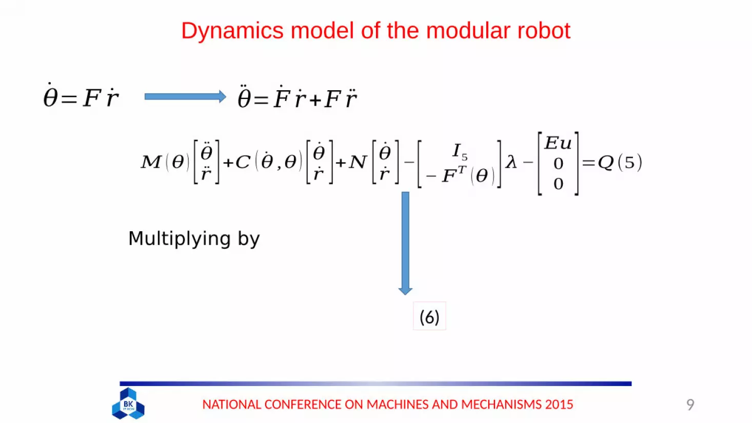
�̈�= �̇� �̇�+𝐹 �̈�
Multiplying by
(6)
�̇�=𝐹 �̇�
𝑀 (𝜃 ) [ �̈��̈� ]+𝐶 ( �̇� ,𝜃 ) [�̇��̇� ]+𝑁 [ �̇��̇� ]−[ 𝐼5
−𝐹𝑇 (𝜃 )]𝜆−[𝐸𝑢00 ]=𝑄 (5)
9NATIONAL CONFERENCE ON MACHINES AND MECHANISMS 2015

Numerical Simulation
Number of real unit 8 Ai 0.81 Rad Tangential Coulomb friction coefficient
0.015
Length of unit 0.15 m 0.47 Hz
Mass of unit 0.7 kg -pi/8 Normal Coulomb friction coefficient
0.4Inertia of unit 0.0053 kg.m2 0.1
Input joint torques
10NATIONAL CONFERENCE ON MACHINES AND MECHANISMS 2015

Numerical Simulation
First line: (xh, yh) Robot head. Second line: Center Gravity of Module 1. Third line: Center Gravity of Module 2.
Fig.5. Trajectory of the snake robot’s head and 2 modules
11NATIONAL CONFERENCE ON MACHINES AND MECHANISMS 2015

Numerical Simulation
Fig.6. Plot of the joint angles , i = 1~7.
12NATIONAL CONFERENCE ON MACHINES AND MECHANISMS 2015

Numerical Simulation
Fig.7. Velocity of the head along y-direction and x-direction
Left chart: Velocity of the head along y-direction. Right chart: Velocity of the head along x-direction.
13NATIONAL CONFERENCE ON MACHINES AND MECHANISMS 2015

Conclusion
14NATIONAL CONFERENCE ON MACHINES AND MECHANISMS 2015
We can see that the behavior of the snake robot system is similar to the motion of the real snake in nature.
In the next steps, we will design some controllers to control the motions of the snake robot in order to meet some requirements such as: direction control, trajectory control, etc.


