Embed Size (px)
Citation preview

WORK ZONE TRAFFIC MANAGEMENT ANALYSIS USING ANALYTICAL METHODS
Participants Handout(Updated 4/1/2020)
Rahim (Ray) F. [email protected]
Hani [email protected]
Juan C. [email protected]
University of Illinois at Urbana-Champaign
Sponsored by:Federal Highway Administration
Hongjae [email protected]
Training Class for Nevada DOT, January 20-21, 2021
This material is based upon work supported by the U.S. Department of Transportation under Cooperative Agreement No. DTFH693JJ31750005. The material was prepared by University of Illinois at Urbana-Champaign. Any opinions, findings and conclusions or recommendations expressed in this publication are those of the author(s) and do not necessarily reflect the view of the U.S. Department of Transportation. This publication does not constitute a national standard, specification, or regulation. The U.S. Government does not endorse products or manufacturers. Trademarks or manufacturers’ names appear in this document only because they are considered essential to the objective of the document.
2
Disclaimers
Learn:
1. Analytical methods (tools) for work zone traffic management analysis
2. Computation of work zone performance measures (WZPM)• WZPM are: capacity, speed, queue length, delay, and users’ costs
3. Hands-on experience on solving example problems to demonstrate how the tools are used to evaluate:• Various traffic management strategies including ITS in work zone
to manage back-of-queue and delay
3
Course Objectives
1 1
1
11
1
2013 Grant2016 Grant
1
1
1
1
11
1
1
1
1
1
1
1
1
4
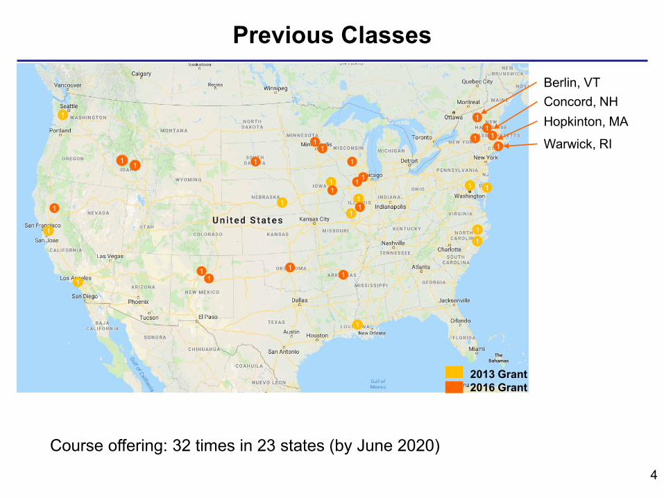
Previous Classes
Berlin, VT
Hopkinton, MA
Warwick, RI
1
1
Concord, NH
11
11
11
Course offering: 32 times in 23 states (by June 2020)
11
1
1
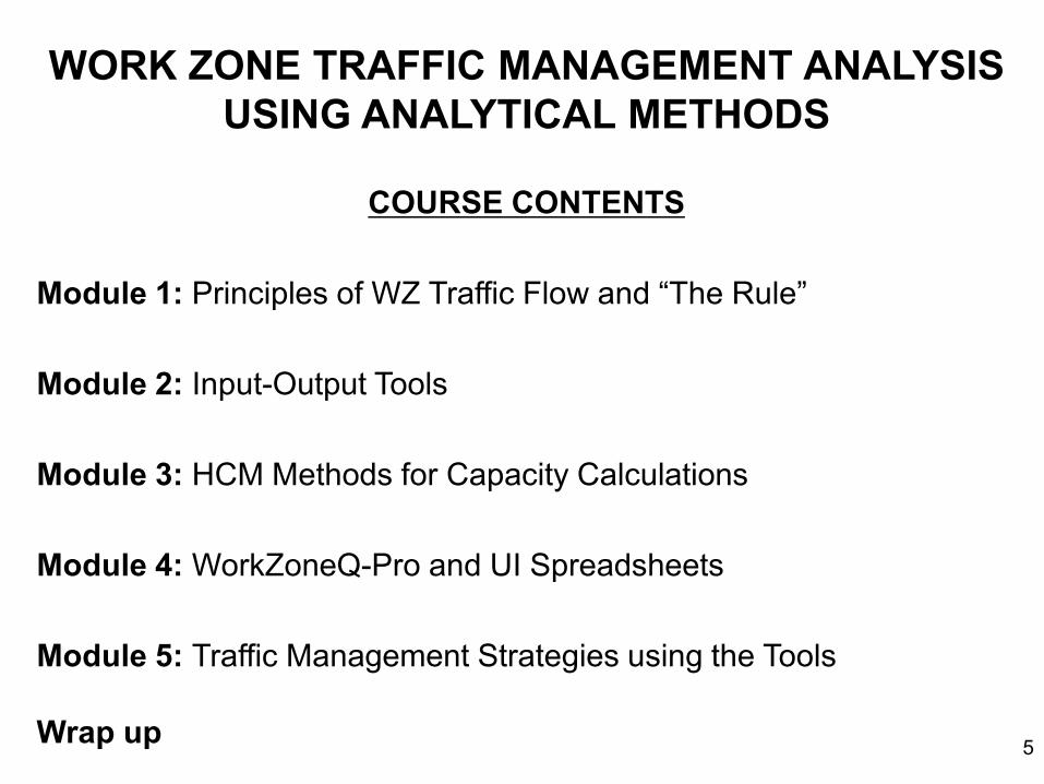
COURSE CONTENTS
Module 1: Principles of WZ Traffic Flow and “The Rule”
Module 2: Input-Output Tools
Module 3: HCM Methods for Capacity Calculations
Module 4: WorkZoneQ-Pro and UI Spreadsheets
Module 5: Traffic Management Strategies using the Tools
Wrap up 5
WORK ZONE TRAFFIC MANAGEMENT ANALYSIS USING ANALYTICAL METHODS
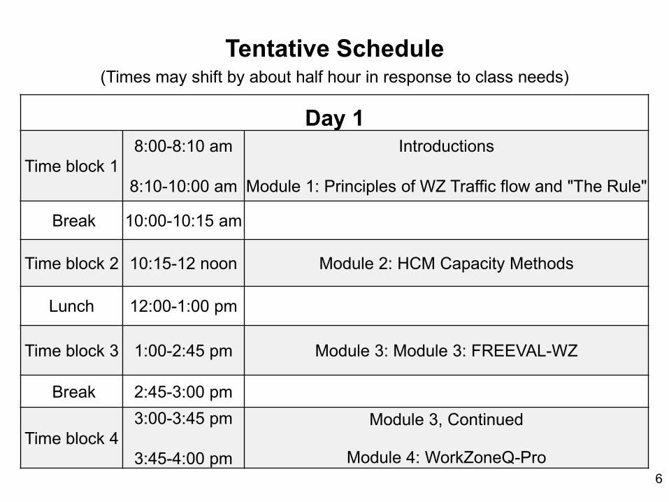
Tentative Schedule(Times may shift by about half hour in response to class needs)
6
Day 1
Time block 18:00-8:10 am
8:10-10:00 am
Introductions
Module 1: Principles of WZ Traffic flow and "The Rule"
Break 10:00-10:15 am
Time block 2 10:15-12 noon Module 2: HCM Capacity Methods
Lunch 12:00-1:00 pm
Time block 3 1:00-2:45 pm Module 3: Module 3: FREEVAL-WZ
Break 2:45-3:00 pm
Time block 43:00-3:45 pm
3:45-4:00 pm
Module 3, Continued
Module 4: WorkZoneQ-Pro
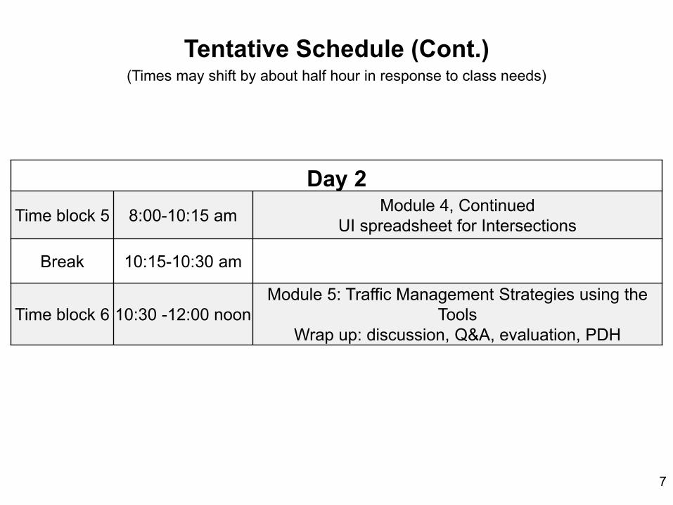
Tentative Schedule (Cont.)(Times may shift by about half hour in response to class needs)
7
Day 2Time block 5 8:00-10:15 am Module 4, Continued
UI spreadsheet for Intersections
Break 10:15-10:30 am
Time block 6 10:30 -12:00 noonModule 5: Traffic Management Strategies using the
ToolsWrap up: discussion, Q&A, evaluation, PDH
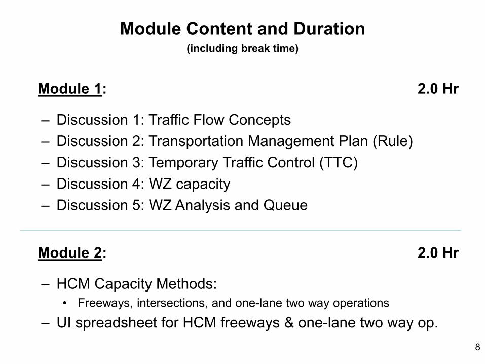
Module 1: 2.0 Hr
– Discussion 1: Traffic Flow Concepts– Discussion 2: Transportation Management Plan (Rule) – Discussion 3: Temporary Traffic Control (TTC) – Discussion 4: WZ capacity– Discussion 5: WZ Analysis and Queue
Module 2: 2.0 Hr
– HCM Capacity Methods: • Freeways, intersections, and one-lane two way operations
– UI spreadsheet for HCM freeways & one-lane two way op.
Module Content and Duration(including break time)
8
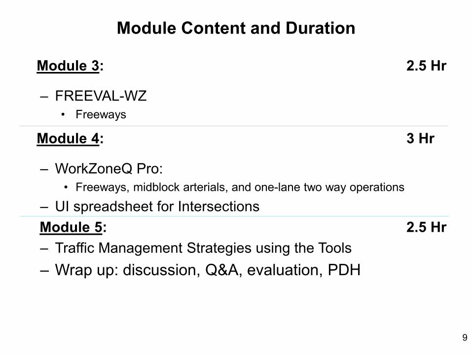
Module Content and Duration
Module 3: 2.5 Hr
– FREEVAL-WZ• Freeways
Module 4: 3 Hr
– WorkZoneQ Pro: • Freeways, midblock arterials, and one-lane two way operations
– UI spreadsheet for IntersectionsModule 5: 2.5 Hr– Traffic Management Strategies using the Tools– Wrap up: discussion, Q&A, evaluation, PDH
9
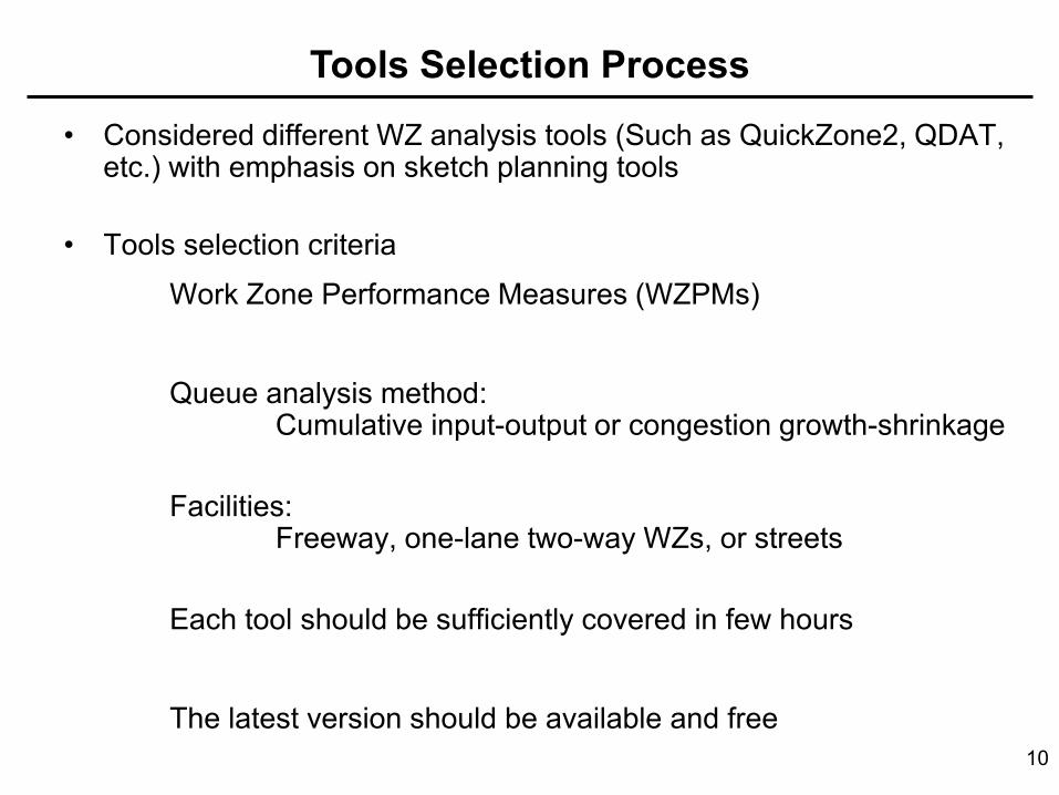
• Considered different WZ analysis tools (Such as QuickZone2, QDAT, etc.) with emphasis on sketch planning tools
• Tools selection criteriaWork Zone Performance Measures (WZPMs)
Queue analysis method: Cumulative input-output or congestion growth-shrinkage
Facilities:Freeway, one-lane two-way WZs, or streets
Each tool should be sufficiently covered in few hours
The latest version should be available and free
Tools Selection Process
10
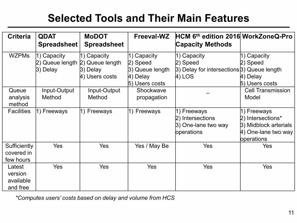
Criteria QDAT Spreadsheet
MoDOT Spreadsheet
Freeval-WZ HCM 6th edition 2016 Capacity Methods
WorkZoneQ-Pro
WZPMs 1) Capacity 2) Queue length3) Delay
1) Capacity 2) Queue length3) Delay4) Users costs
1) Capacity 2) Speed3) Queue length4) Delay5) Users costs
1) Capacity 2) Speed3) Delay for intersections4) LOS
1) Capacity 2) Speed3) Queue length4) Delay5) Users costs
Queue analysis method
Input-OutputMethod
Input-OutputMethod
Shockwave propagation
_ Cell Transmission Model
Facilities 1) Freeways 1) Freeways 1) Freeways 1) Freeways 2) Intersections3) One-lane two way operations
1) Freeways2) Intersections*3) Midblock arterials4) One-lane two way operations
Sufficiently covered in few hours
Yes Yes Yes / May Be Yes Yes
Latest version available and free
Yes Yes Yes Yes Yes
Selected Tools and Their Main Features
11
*Computes users’ costs based on delay and volume from HCS
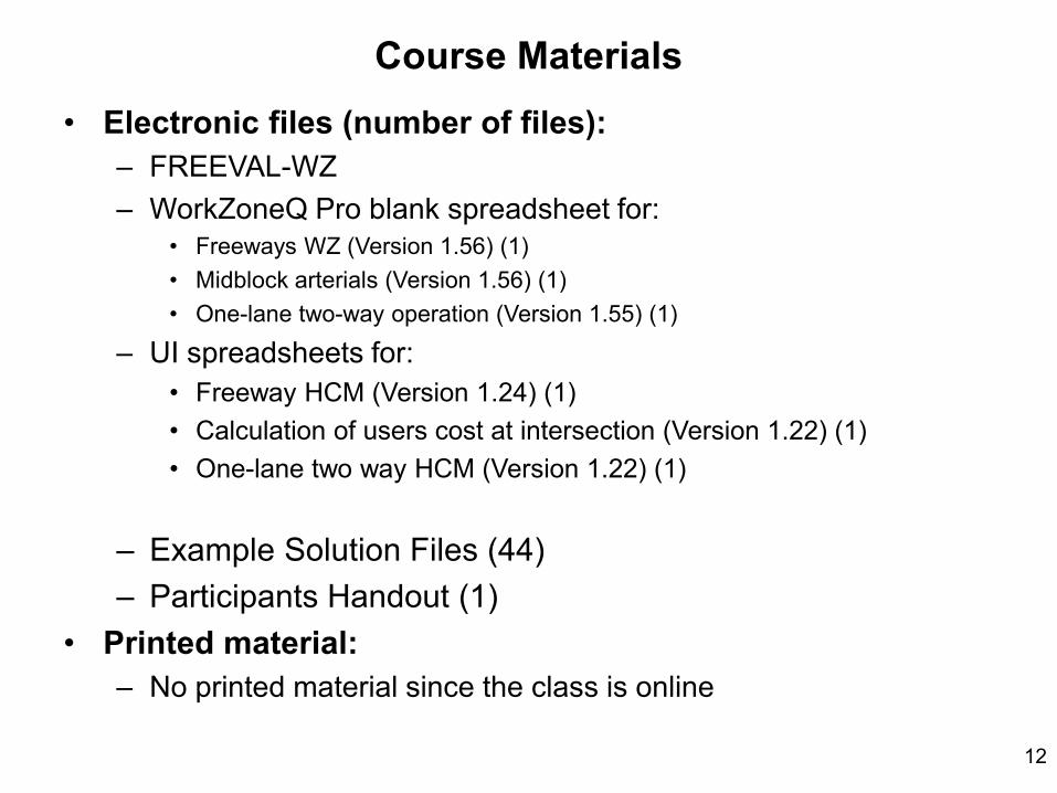
Course Materials• Electronic files (number of files):
– FREEVAL-WZ– WorkZoneQ Pro blank spreadsheet for:
• Freeways WZ (Version 1.56) (1)• Midblock arterials (Version 1.56) (1)• One-lane two-way operation (Version 1.55) (1)
– UI spreadsheets for: • Freeway HCM (Version 1.24) (1)• Calculation of users cost at intersection (Version 1.22) (1)• One-lane two way HCM (Version 1.22) (1)
– Example Solution Files (44)– Participants Handout (1)
• Printed material:– No printed material since the class is online
12
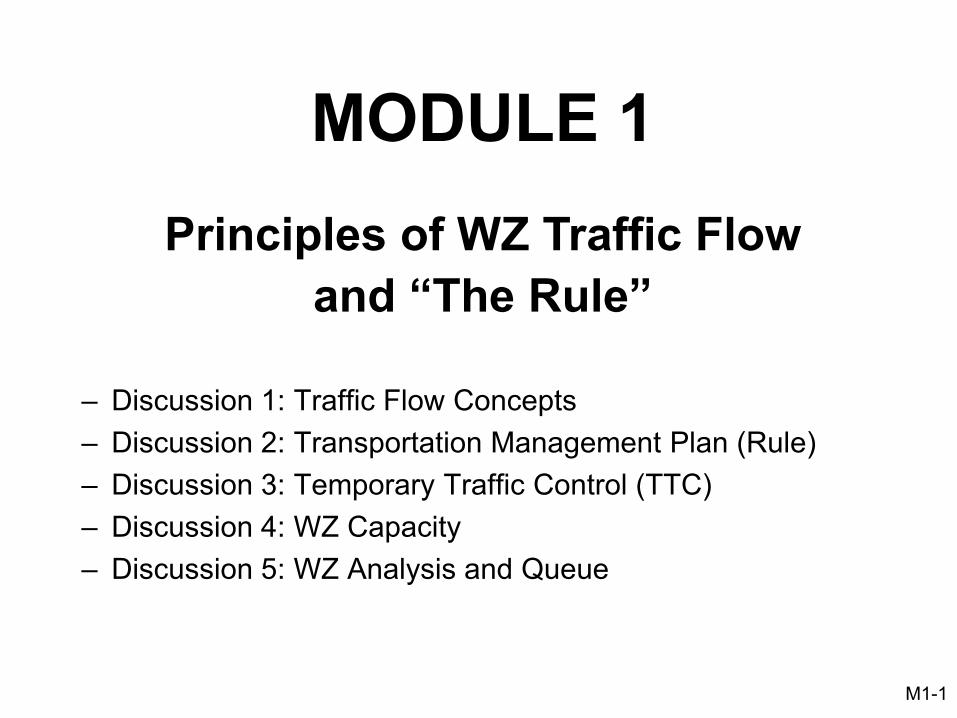
MODULE 1Principles of WZ Traffic Flow
and “The Rule”
– Discussion 1: Traffic Flow Concepts– Discussion 2: Transportation Management Plan (Rule) – Discussion 3: Temporary Traffic Control (TTC) – Discussion 4: WZ Capacity– Discussion 5: WZ Analysis and Queue
M1-1
DISCUSSION #1TRAFFIC FLOW CONCEPTS
Learning Objectives:
1) Understand variables affecting traffic flow
2) Learn how variables are interrelated
Module 1Discussion 1
M1-2
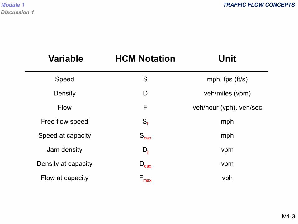
Variable HCM Notation Unit
Speed S mph, fps (ft/s)
Density D veh/miles (vpm)
Flow F veh/hour (vph), veh/sec
Free flow speed Sf mph
Speed at capacity Scap mph
Jam density Dj vpm
Density at capacity Dcap vpm
Flow at capacity Fmax vph
TRAFFIC FLOW CONCEPTSModule 1Discussion 1
M1-3
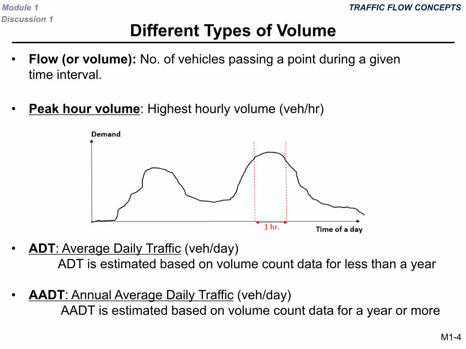
• Flow (or volume): No. of vehicles passing a point during a given time interval.
• Peak hour volume: Highest hourly volume (veh/hr)
• ADT: Average Daily Traffic (veh/day)ADT is estimated based on volume count data for less than a year
• AADT: Annual Average Daily Traffic (veh/day)AADT is estimated based on volume count data for a year or more
Different Types of VolumeTRAFFIC FLOW CONCEPTSModule 1
Discussion 1
M1-4
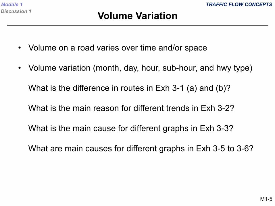
• Volume on a road varies over time and/or space
• Volume variation (month, day, hour, sub-hour, and hwy type)
What is the difference in routes in Exh 3-1 (a) and (b)?
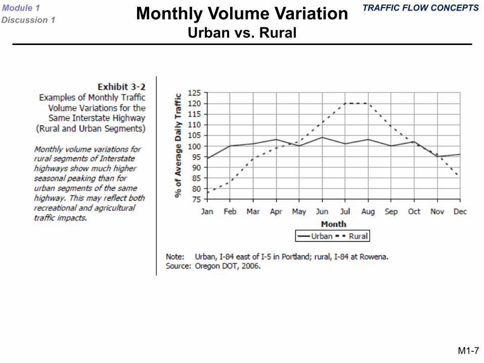
What is the main reason for different trends in Exh 3-2?
What is the main cause for different graphs in Exh 3-3?
What are main causes for different graphs in Exh 3-5 to 3-6?
Volume VariationTRAFFIC FLOW CONCEPTSModule 1
Discussion 1
M1-5
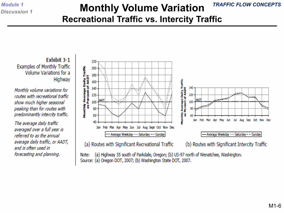
Monthly Volume VariationRecreational Traffic vs. Intercity Traffic
TRAFFIC FLOW CONCEPTSModule 1Discussion 1
M1-6
TRAFFIC FLOW CONCEPTSModule 1Discussion 1 Monthly Volume Variation
Urban vs. Rural
M1-7
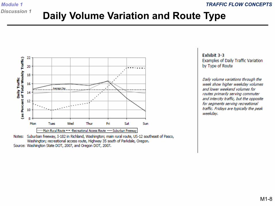
TRAFFIC FLOW CONCEPTSModule 1Discussion 1 Daily Volume Variation and Route Type
M1-8
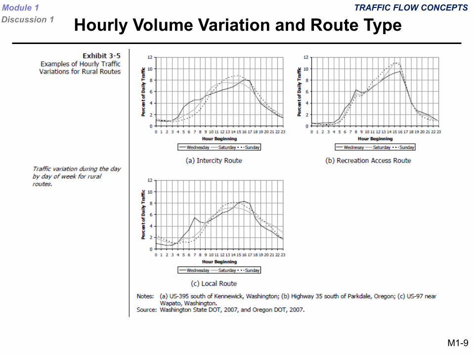
Hourly Volume Variation and Route TypeTRAFFIC FLOW CONCEPTSModule 1
Discussion 1
M1-9
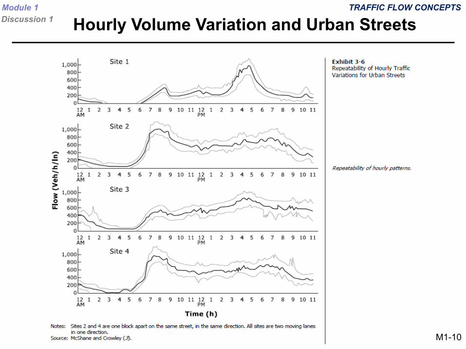
Hourly Volume Variation and Urban StreetsTRAFFIC FLOW CONCEPTSModule 1
Discussion 1
M1-10
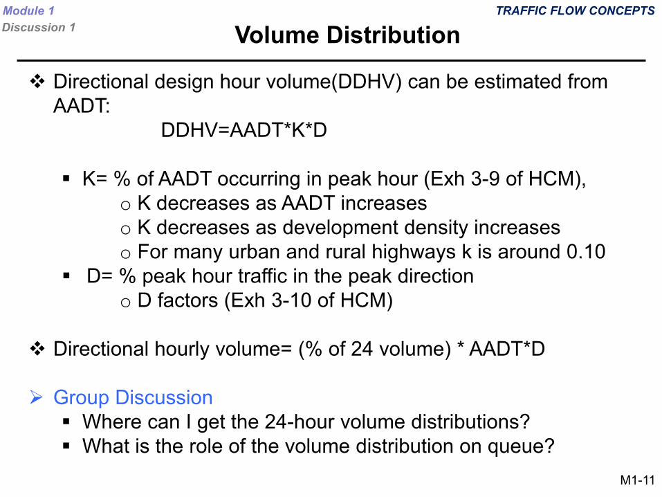
Directional design hour volume(DDHV) can be estimated from AADT:
DDHV=AADT*K*D
K= % of AADT occurring in peak hour (Exh 3-9 of HCM), o K decreases as AADT increaseso K decreases as development density increaseso For many urban and rural highways k is around 0.10
D= % peak hour traffic in the peak directiono D factors (Exh 3-10 of HCM)
Directional hourly volume= (% of 24 volume) * AADT*D
Group Discussion Where can I get the 24-hour volume distributions? What is the role of the volume distribution on queue?
Volume DistributionTRAFFIC FLOW CONCEPTSModule 1
Discussion 1
M1-11
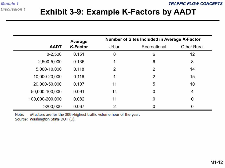
Exhibit 3-9: Example K-Factors by AADTTRAFFIC FLOW CONCEPTSModule 1
Discussion 1
M1-12
AADTAverageK-Factor
Number of Sites Included in Average K-Factor Urban Recreational Other Rural
0-2,500 0.151 0 6 12
2,500-5,000 0.136 1 6 8
5,000-10,000 0.118 2 2 14
10,000-20,000 0.116 1 2 15
20,000-50,000 0.107 11 5 10
50,000-100,000 0.091 14 0 4
100,000-200,000 0.082 11 0 0
>200,000 0.067 2 0 0
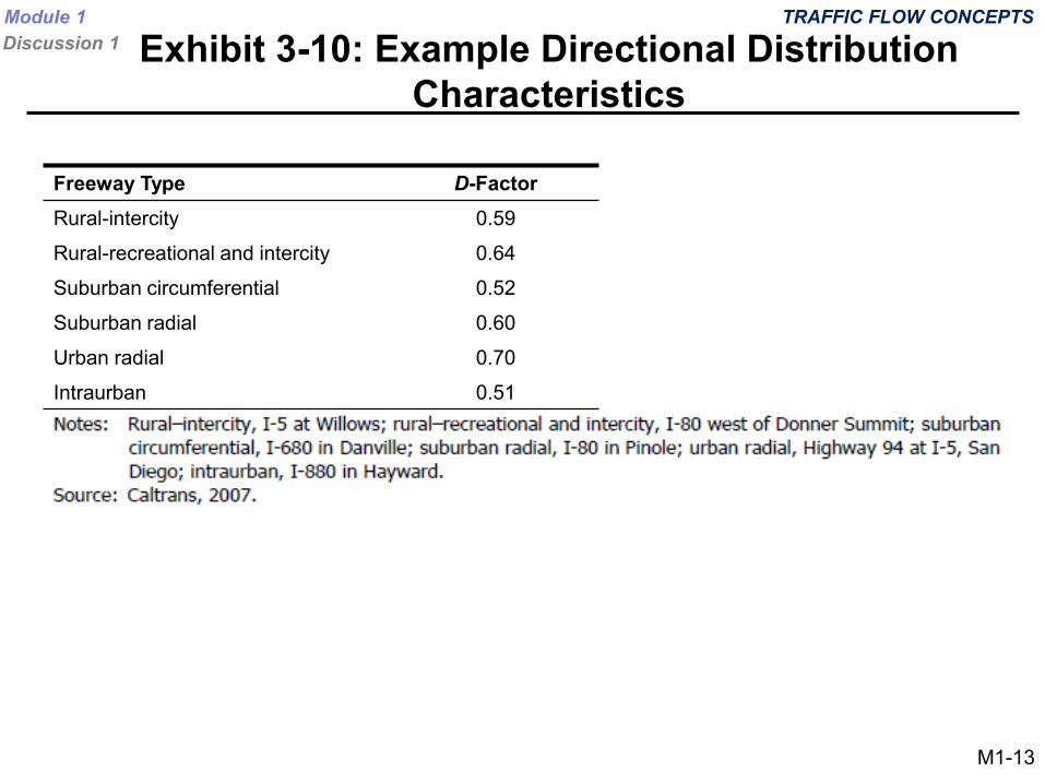
Exhibit 3-10: Example Directional Distribution Characteristics
TRAFFIC FLOW CONCEPTSModule 1Discussion 1
M1-13
Freeway Type D-FactorRural-intercity 0.59
Rural-recreational and intercity 0.64
Suburban circumferential 0.52
Suburban radial 0.60
Urban radial 0.70
Intraurban 0.51
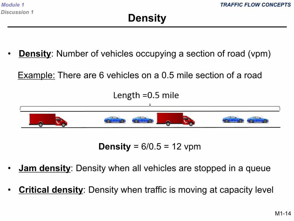
• Density: Number of vehicles occupying a section of road (vpm)
Example: There are 6 vehicles on a 0.5 mile section of a road
Density =No. of vehicleslength
= 60.5
= 12 vpm
Density = 6/0.5 = 12 vpm
• Jam density: Density when all vehicles are stopped in a queue
• Critical density: Density when traffic is moving at capacity level
DensityTRAFFIC FLOW CONCEPTSModule 1
Discussion 1
M1-14
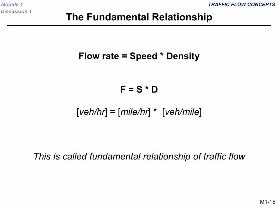
Flow rate = Speed * Density
F = S * D
[veh/hr] = [mile/hr] * [veh/mile]
This is called fundamental relationship of traffic flow
The Fundamental RelationshipTRAFFIC FLOW CONCEPTSModule 1
Discussion 1
M1-15
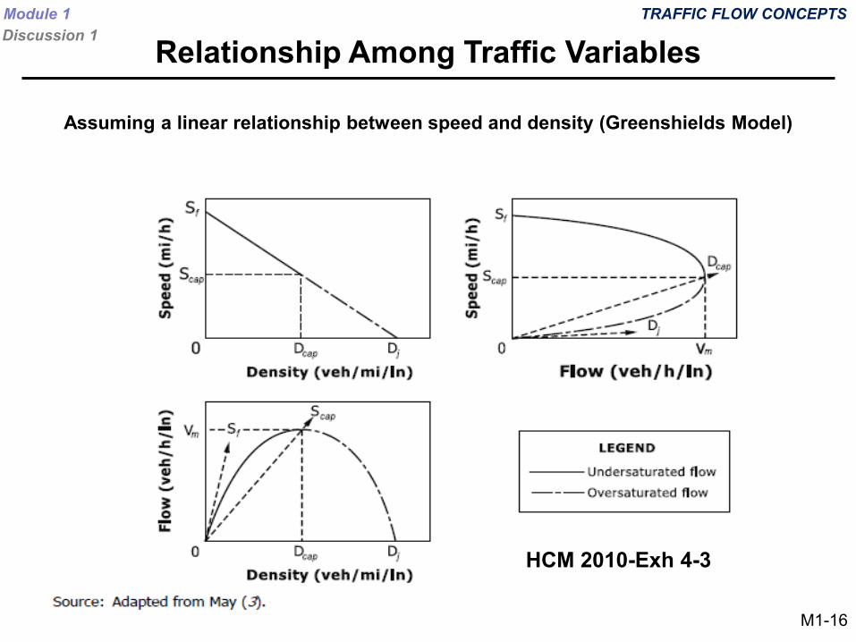
Relationship Among Traffic Variables
HCM 2010-Exh 4-3
Assuming a linear relationship between speed and density (Greenshields Model)
TRAFFIC FLOW CONCEPTSModule 1Discussion 1
M1-16
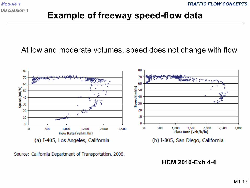
At low and moderate volumes, speed does not change with flow
HCM 2010-Exh 4-4
Example of freeway speed-flow dataTRAFFIC FLOW CONCEPTSModule 1
Discussion 1
M1-17
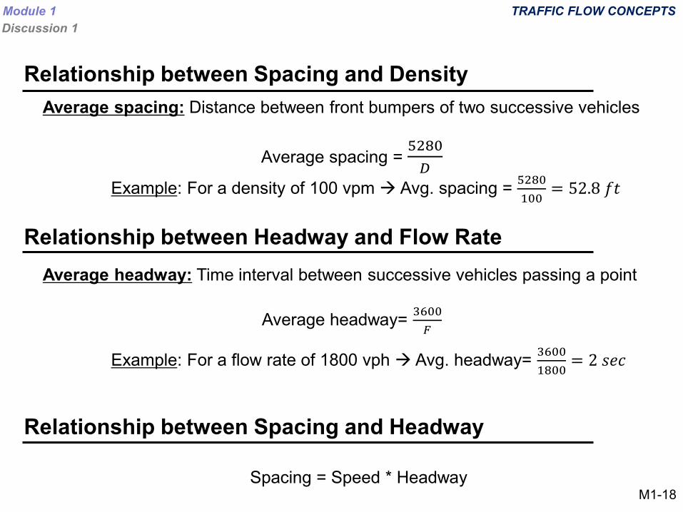
Average spacing: Distance between front bumpers of two successive vehicles
Average spacing = 5280𝐷𝐷
Example: For a density of 100 vpm Avg. spacing = 5280100
= 52.8 𝑓𝑓𝑓𝑓
Average headway: Time interval between successive vehicles passing a point
Average headway= 3600𝐹𝐹
Example: For a flow rate of 1800 vph Avg. headway= 36001800
= 2 𝑠𝑠𝑠𝑠𝑠𝑠
Relationship between Spacing and Density
TRAFFIC FLOW CONCEPTS
Relationship between Headway and Flow Rate
Relationship between Spacing and Headway
Spacing = Speed * Headway
Module 1Discussion 1
M1-18
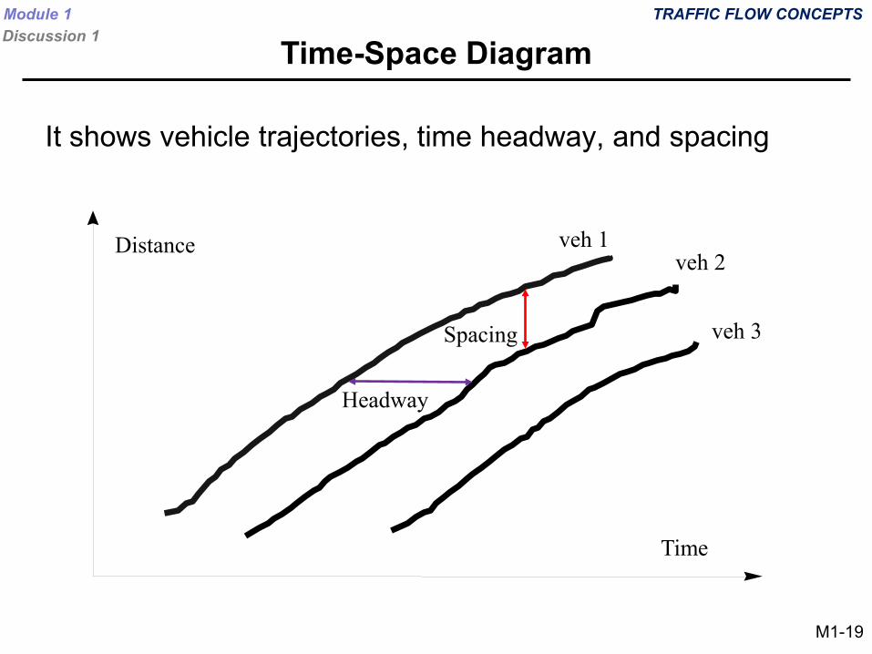
It shows vehicle trajectories, time headway, and spacing
Distance
Time
veh 1veh 2
veh 3
Headway
Spacing
Time-Space DiagramTRAFFIC FLOW CONCEPTSModule 1
Discussion 1
M1-19
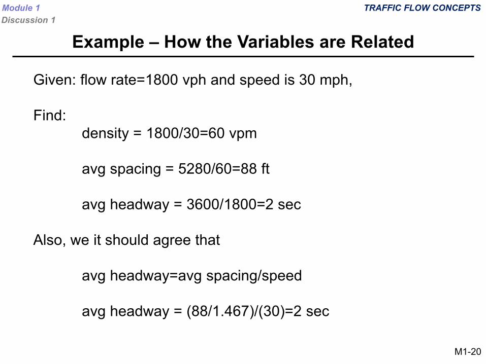
Given: flow rate=1800 vph and speed is 30 mph,
Find:density = 1800/30=60 vpm
avg spacing = 5280/60=88 ft
avg headway = 3600/1800=2 sec
Also, we it should agree that
avg headway=avg spacing/speed
avg headway = (88/1.467)/(30)=2 sec
TRAFFIC FLOW CONCEPTS
Example – How the Variables are Related
Module 1Discussion 1
M1-20
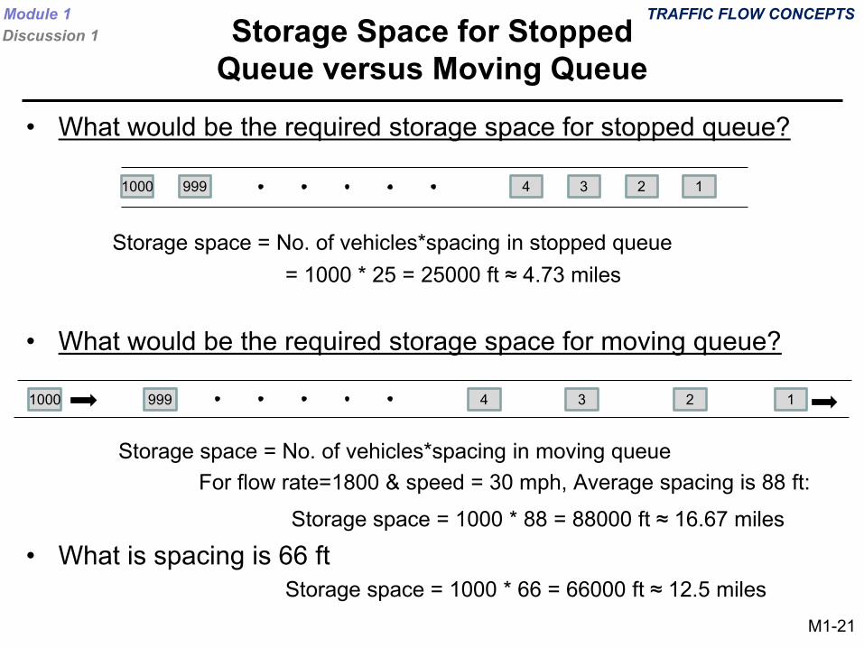
• What would be the required storage space for stopped queue?
Storage space = No. of vehicles*spacing in stopped queue= 1000 * 25 = 25000 ft ≈ 4.73 miles
• What would be the required storage space for moving queue?
Storage space = No. of vehicles*spacing in moving queueFor flow rate=1800 & speed = 30 mph, Average spacing is 88 ft:
Storage space = 1000 * 88 = 88000 ft ≈ 16.67 miles
• What is spacing is 66 ftStorage space = 1000 * 66 = 66000 ft ≈ 12.5 miles
TRAFFIC FLOW CONCEPTSStorage Space for Stopped
Queue versus Moving Queue
Module 1Discussion 1
12349991000
M1-21
12349991000
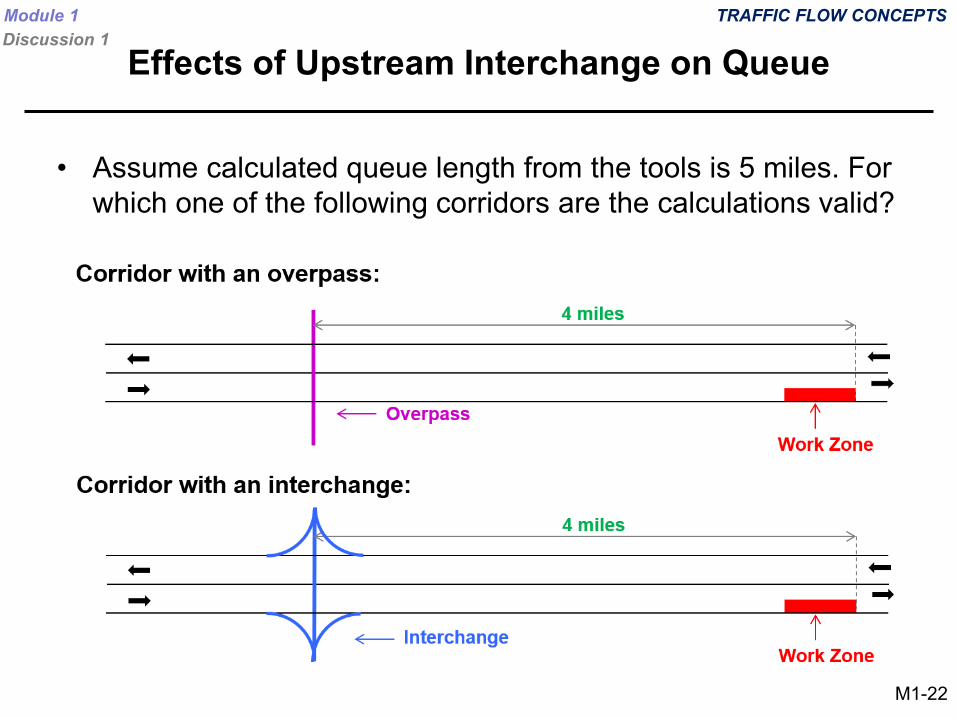
• Assume calculated queue length from the tools is 5 miles. For which one of the following corridors are the calculations valid?
TRAFFIC FLOW CONCEPTS
Effects of Upstream Interchange on QueueModule 1Discussion 1
M1-22
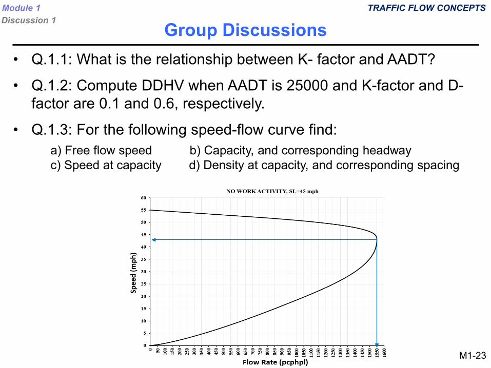
• Q.1.1: What is the relationship between K- factor and AADT?
• Q.1.2: Compute DDHV when AADT is 25000 and K-factor and D-factor are 0.1 and 0.6, respectively.
• Q.1.3: For the following speed-flow curve find:
Group DiscussionsTRAFFIC FLOW CONCEPTS
a) Free flow speed b) Capacity, and corresponding headway c) Speed at capacity d) Density at capacity, and corresponding spacing
Module 1Discussion 1
M1-23
DISCUSSION #2TRANSPORTATION MANAGEMENT PLANS
Learning Objectives:
1) Understand the requirements of the “Work Zone Safety andMobility” Rule (known as the Rule or Subpart J)
2) Review of FHWA guidance on Developing andImplementing Transportation Management Plans (TMP)for Work Zones
Module 1Discussion 2
M1-24
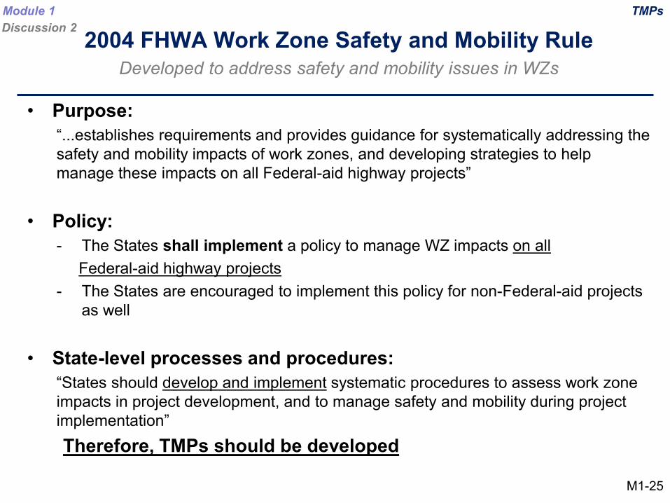
2004 FHWA Work Zone Safety and Mobility RuleDeveloped to address safety and mobility issues in WZs
• Purpose:“...establishes requirements and provides guidance for systematically addressing the safety and mobility impacts of work zones, and developing strategies to help manage these impacts on all Federal-aid highway projects”
• Policy:- The States shall implement a policy to manage WZ impacts on all
Federal-aid highway projects- The States are encouraged to implement this policy for non-Federal-aid projects
as well
• State-level processes and procedures:“States should develop and implement systematic procedures to assess work zone impacts in project development, and to manage safety and mobility during project implementation”Therefore, TMPs should be developed
TMPsModule 1Discussion 2
M1-25
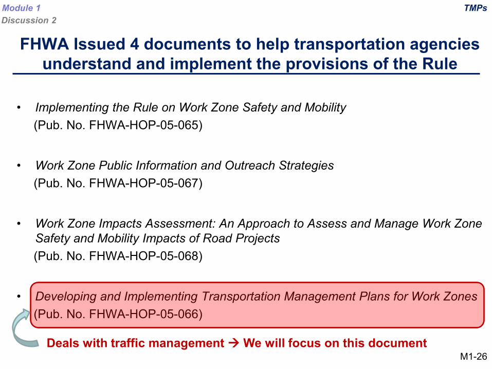
FHWA Issued 4 documents to help transportation agencies understand and implement the provisions of the Rule
• Implementing the Rule on Work Zone Safety and Mobility(Pub. No. FHWA-HOP-05-065)
• Work Zone Public Information and Outreach Strategies(Pub. No. FHWA-HOP-05-067)
• Work Zone Impacts Assessment: An Approach to Assess and Manage Work Zone Safety and Mobility Impacts of Road Projects(Pub. No. FHWA-HOP-05-068)
• Developing and Implementing Transportation Management Plans for Work Zones(Pub. No. FHWA-HOP-05-066)
Deals with traffic management We will focus on this document
TMPsModule 1Discussion 2
M1-26
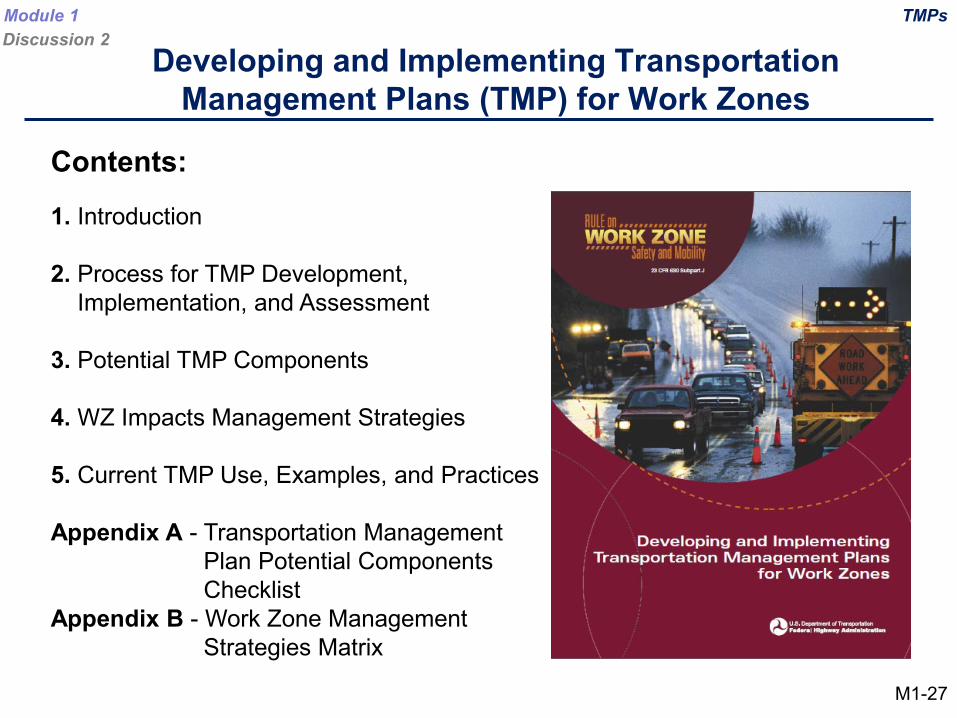
Developing and Implementing Transportation Management Plans (TMP) for Work Zones
Contents:
1. Introduction
2. Process for TMP Development, Implementation, and Assessment
3. Potential TMP Components
4. WZ Impacts Management Strategies
5. Current TMP Use, Examples, and Practices
Appendix A - Transportation Management Plan Potential Components Checklist
Appendix B - Work Zone Management Strategies Matrix
TMPsModule 1Discussion 2
M1-27
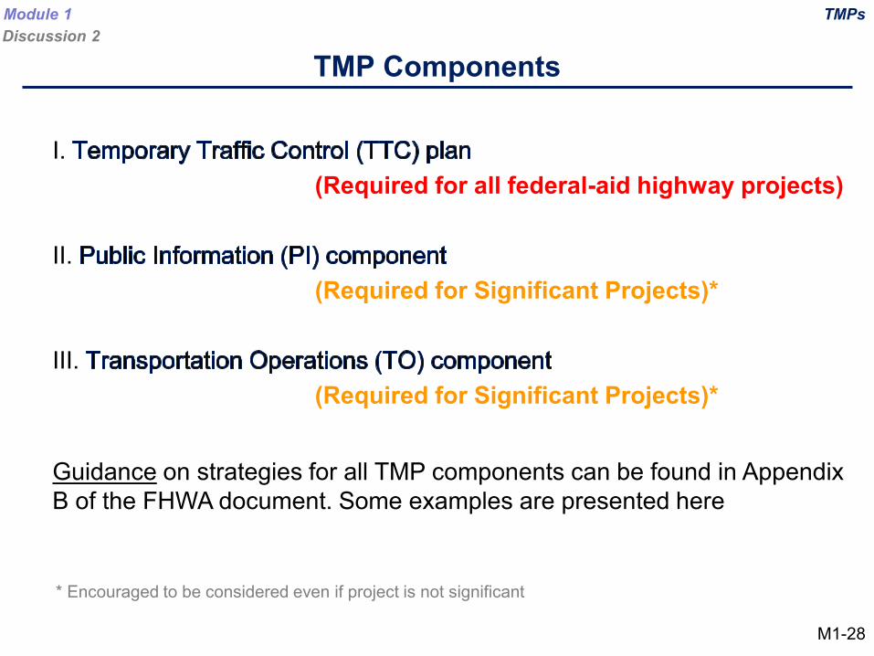
I. (Required for all federal-aid highway projects)
II. (Required for Significant Projects)*
III. (Required for Significant Projects)*
TMP Components
* Encouraged to be considered even if project is not significant
Guidance on strategies for all TMP components can be found in Appendix B of the FHWA document. Some examples are presented here
TMPsModule 1Discussion 2
M1-28
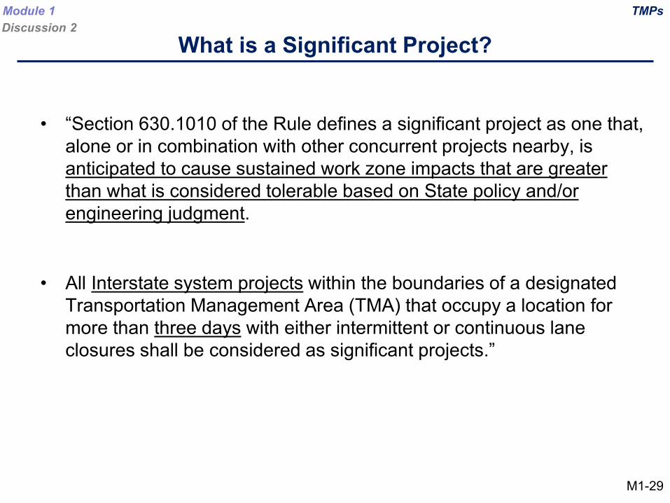
• “Section 630.1010 of the Rule defines a significant project as one that, alone or in combination with other concurrent projects nearby, is anticipated to cause sustained work zone impacts that are greater than what is considered tolerable based on State policy and/or engineering judgment.
• All Interstate system projects within the boundaries of a designated Transportation Management Area (TMA) that occupy a location for more than three days with either intermittent or continuous lane closures shall be considered as significant projects.”
What is a Significant Project?TMPsModule 1
Discussion 2
M1-29
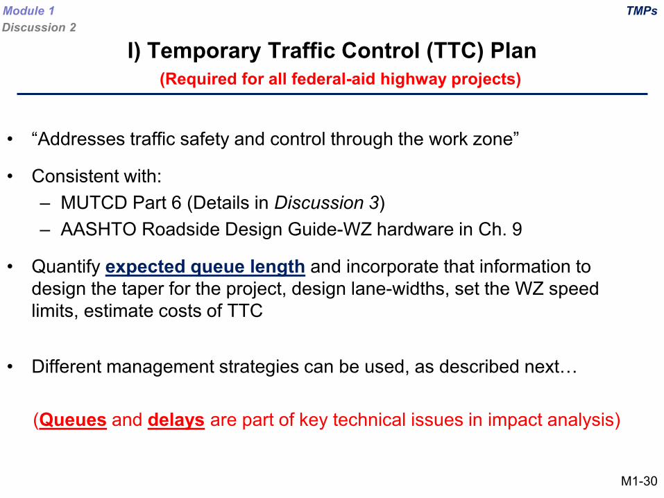
• “Addresses traffic safety and control through the work zone”
• Consistent with: – MUTCD Part 6 (Details in Discussion 3)– AASHTO Roadside Design Guide-WZ hardware in Ch. 9
• Quantify expected queue length and incorporate that information to design the taper for the project, design lane-widths, set the WZ speed limits, estimate costs of TTC
• Different management strategies can be used, as described next…
(Queues and delays are part of key technical issues in impact analysis)
(Required for all federal-aid highway projects)I) Temporary Traffic Control (TTC) Plan
TMPsModule 1Discussion 2
M1-30
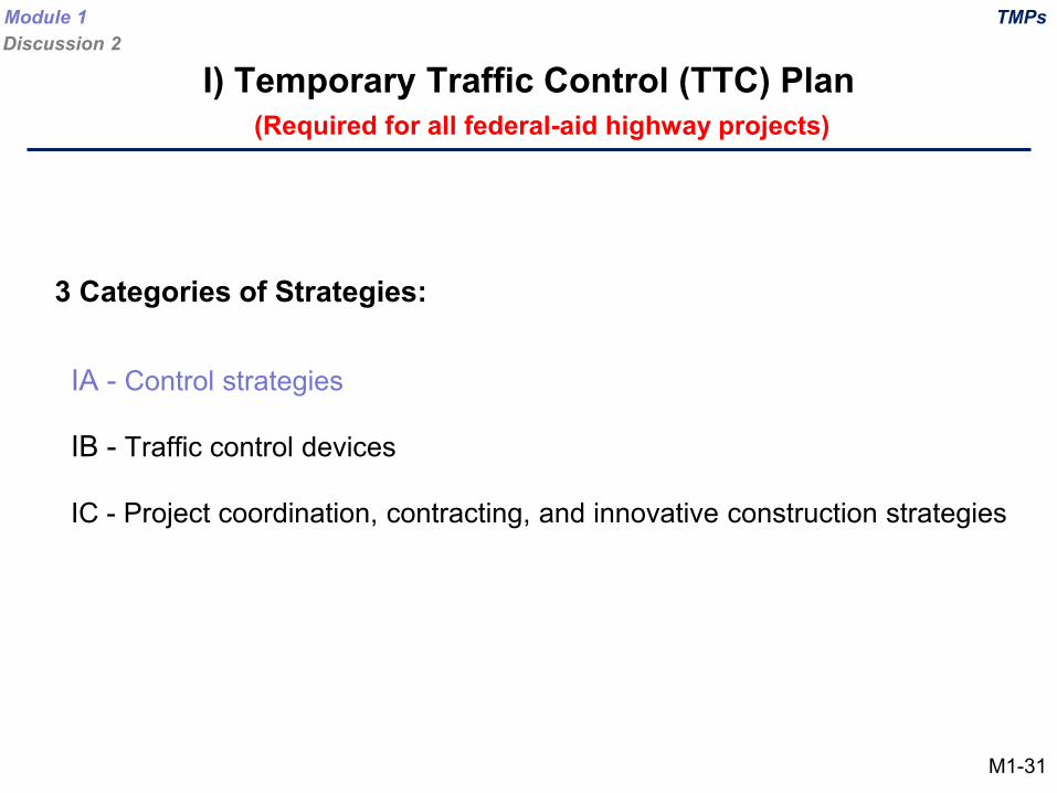
3 Categories of Strategies:
IA - Control strategies
IB - Traffic control devices
IC - Project coordination, contracting, and innovative construction strategies
I) Temporary Traffic Control (TTC) Plan(Required for all federal-aid highway projects)
TMPsModule 1Discussion 2
M1-31
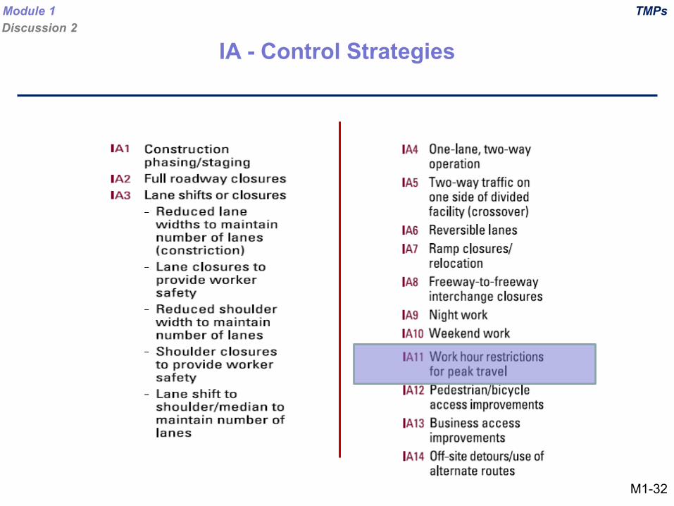
IA - Control Strategies
M1-32
TMPsModule 1Discussion 2
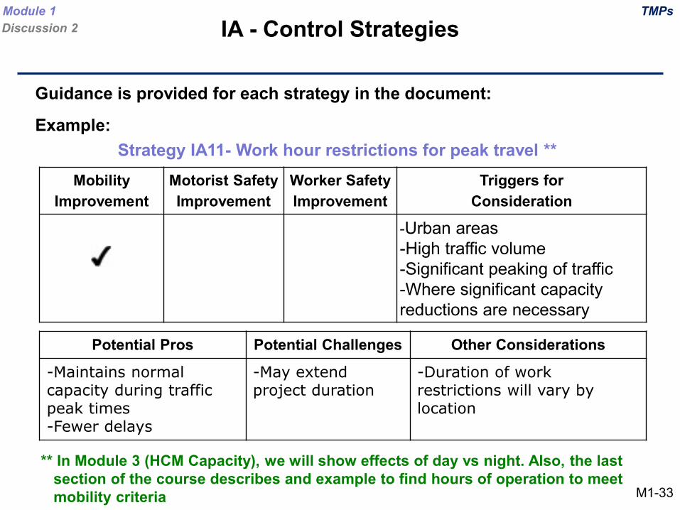
Mobility Improvement
Motorist Safety Improvement
Worker Safety Improvement
Triggers for Consideration
-Urban areas-High traffic volume-Significant peaking of traffic-Where significant capacity reductions are necessary
Potential Pros Potential Challenges Other Considerations
-Maintains normal capacity during traffic peak times-Fewer delays
-May extend project duration
-Duration of work restrictions will vary by location
Guidance is provided for each strategy in the document:
Example:
IA - Control Strategies
Strategy IA11- Work hour restrictions for peak travel **
** In Module 3 (HCM Capacity), we will show effects of day vs night. Also, the last section of the course describes and example to find hours of operation to meet mobility criteria M1-33
TMPsModule 1Discussion 2

2 Categories of Strategies:
IIA - Public awareness strategies
IIB - Motorist information strategies
* Encouraged to be considered even if project is not significant
II) Public Information (PI) Component(Required for Significant Projects*)
TMPsModule 1Discussion 2
M1-34
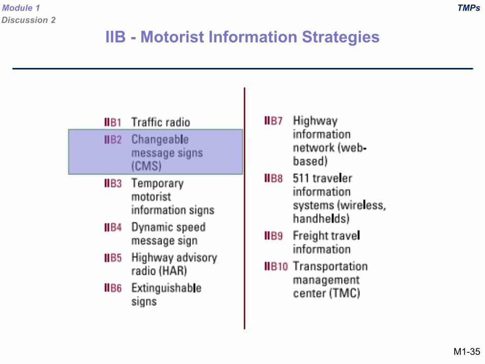
IIB - Motorist Information Strategies
TMPsModule 1Discussion 2
M1-35
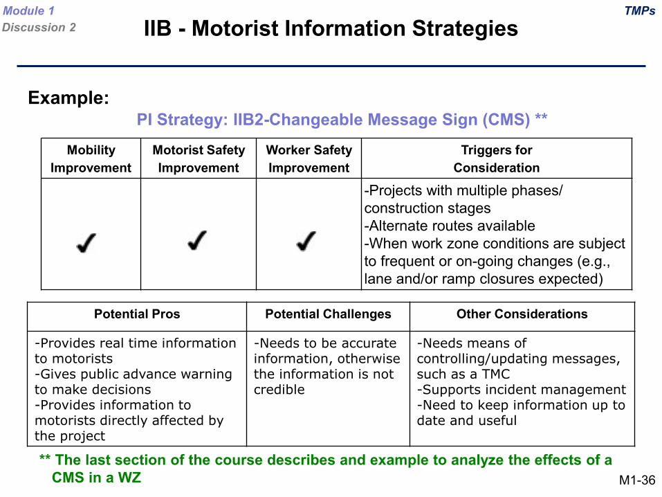
Potential Pros Potential Challenges Other Considerations
-Provides real time information to motorists-Gives public advance warning to make decisions-Provides information to motorists directly affected by the project
-Needs to be accurate information, otherwise the information is not credible
-Needs means of controlling/updating messages, such as a TMC-Supports incident management-Need to keep information up to date and useful
PI Strategy: IIB2-Changeable Message Sign (CMS) ** Mobility
ImprovementMotorist Safety Improvement
Worker Safety Improvement
Triggers for Consideration
-Projects with multiple phases/ construction stages-Alternate routes available-When work zone conditions are subject to frequent or on-going changes (e.g., lane and/or ramp closures expected)
** The last section of the course describes and example to analyze the effects of a CMS in a WZ
IIB - Motorist Information Strategies
Example:
TMPsModule 1Discussion 2
M1-36
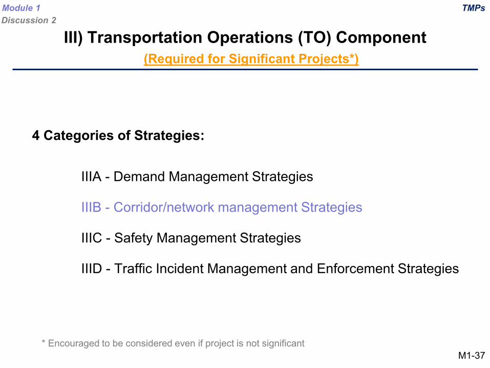
4 Categories of Strategies:
IIIA - Demand Management Strategies
IIIB - Corridor/network management Strategies
IIIC - Safety Management Strategies
IIID - Traffic Incident Management and Enforcement Strategies
* Encouraged to be considered even if project is not significant
III) Transportation Operations (TO) Component(Required for Significant Projects*)
TMPsModule 1Discussion 2
M1-37
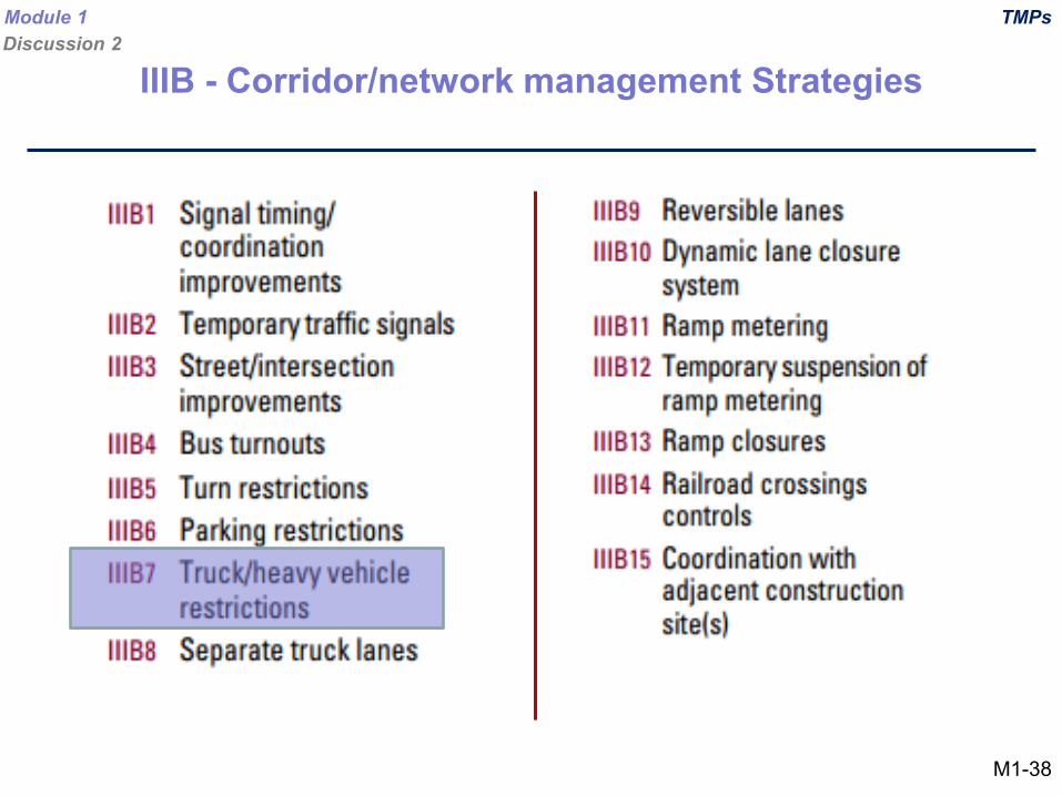
IIIB - Corridor/network management Strategies
TMPsModule 1Discussion 2
M1-38
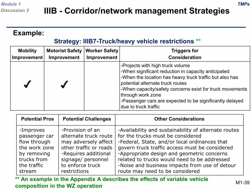
Strategy: IIIB7-Truck/heavy vehicle restrictions **Mobility
ImprovementMotorist Safety Improvement
Worker Safety Improvement
Triggers for Consideration
-Projects with high truck volume-When significant reduction in capacity anticipated-When the location has heavy truck traffic but also has potential alternate truck routes-When capacity/safety concerns exist for truck movements through work zone-Passenger cars are expected to be significantly delayed due to truck traffic
Potential Pros Potential Challenges Other Considerations
-Improves passenger car flow through the work zone by removing trucks from the traffic stream
-Provision of an alternate truck route may adversely affect other traffic or roads-Requires additional signage/ personnel to enforce truck restrictions
-Availability and sustainability of alternate routes for the trucks must be considered-Federal, State, and/or local ordinances that govern truck traffic access must be considered-Appropriate design and geometric concerns related to trucks would need to be addressed-Noise and business impacts from use of detour route may need to be considered
** An example in the Appendix A describes the effects of variable vehicle composition in the WZ operation
Example:
IIIB - Corridor/network management StrategiesTMPsModule 1
Discussion 2
M1-39
TMP Use, Examples, and Practices
States use a variety of criteria to specify work zone mobility and operational performance, including:
• Delay (total, average per vehicle)• Queue (length, duration)• Capacity (volume/capacity ratio, LOS)• Volume (throughput)• Speed (average speed, % of time at free-flow speed)• % work zones meeting expectations for traffic flow• User complaints, road user surveys• Frequency, duration of incidents
TMPsModule 1Discussion 2
* Sources:- Best Practices in Work Zone Assessment, Data Collection, and Performance Evaluation. NCHRP – Scan 08-04. 2010.- Synthesis of Work-Zone Performance Measures. Center for Transportation Research and Education (CTRE). Iowa State
University. 2013- FHWA Best Practices compilation: http://www.ops.fhwa.dot.gov/wz/practices/practices.htm
M1-40
TMP Use, Examples, and PracticesIndiana DOT establishes different queue length thresholds depending on their duration:- No queues present 6 continuous hours or more than 12 hours total per day- Queues between 0.5 and 1 mile are limited to 4 continuous hours- Queues between 1 and 1.5 miles are limited to 2 continuous hours - Queues greater than 1.5 miles are not permitted
Maryland SHA has different mobility criteria for different facilities:- For freeways, queues greater than 1.5 miles are not acceptable, and queues between
1.0 and 1.5 miles are limited up to 2 hours- For arterials, delays are restricted to 15 minutes- For signalized intersections the increase in control delay and change in LOS are
restricted; and a similar criteria is imposed for unsignalized intersections.
- What is your state’s policy?
TMPsModule 1Discussion 2
M1-41
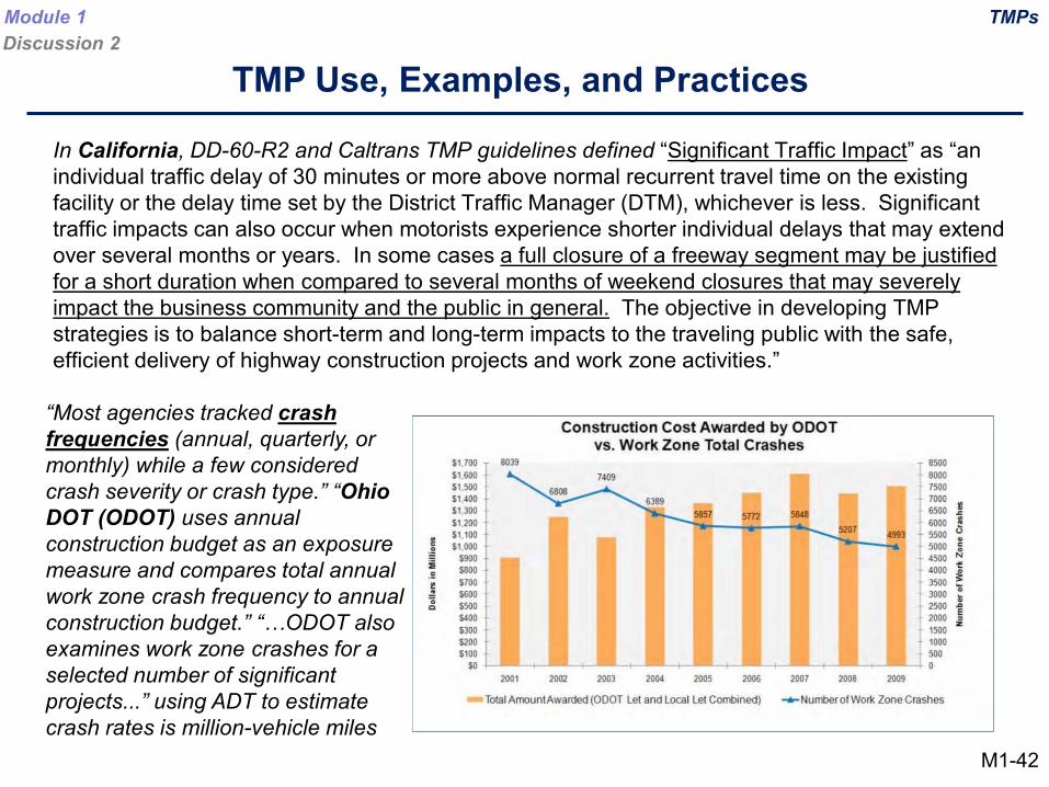
In California, DD-60-R2 and Caltrans TMP guidelines defined “Significant Traffic Impact” as “an individual traffic delay of 30 minutes or more above normal recurrent travel time on the existing facility or the delay time set by the District Traffic Manager (DTM), whichever is less. Significant traffic impacts can also occur when motorists experience shorter individual delays that may extend over several months or years. In some cases a full closure of a freeway segment may be justified for a short duration when compared to several months of weekend closures that may severely impact the business community and the public in general. The objective in developing TMP strategies is to balance short-term and long-term impacts to the traveling public with the safe, efficient delivery of highway construction projects and work zone activities.”
TMPsModule 1Discussion 2
TMP Use, Examples, and Practices
“Most agencies tracked crash frequencies (annual, quarterly, or monthly) while a few considered crash severity or crash type.” “Ohio DOT (ODOT) uses annual construction budget as an exposure measure and compares total annual work zone crash frequency to annual construction budget.” “…ODOT also examines work zone crashes for a selected number of significant projects...” using ADT to estimate crash rates is million-vehicle miles
M1-42
Group DiscussionTMPsModule 1
Discussion 2
M1-43
Q. 2.1. What are the components of a TMP?
Q. 2.2. What is a Significant Project and what are the implications of significant projects in the components required for TMPs?
Q. 2.3. Do you know what are the mobility and safety criteria used in your State?
DISCUSSION #3TEMPORARY TRAFFIC CONTROL (TTC)
Learning Objectives:
1) Overview of MUTCD Part 6 -Temporary Traffic Control
2) WZ components, duration, typical applications, and signage
3) Provide basic information about TTC used in this training course
Module 1Discussion 3
M1-44
MUTCD
TEMPORARY TRAFFIC CONTROLModule 1Discussion 3
M1-45
• Manual on Uniform Traffic Control Devices (MUTCD)
• Written by National Committee on Uniform Traffic Control Devices; latest edition is 2009
• Published by US DOT (FHWA)
• “By setting minimum standards and providing guidance, ensures uniformity of traffic control devices across the nation.” (Source : http://mutcd.fhwa.dot.gov/kno-overview.htm)
• Chapter 6 describes Temporary Traffic Control
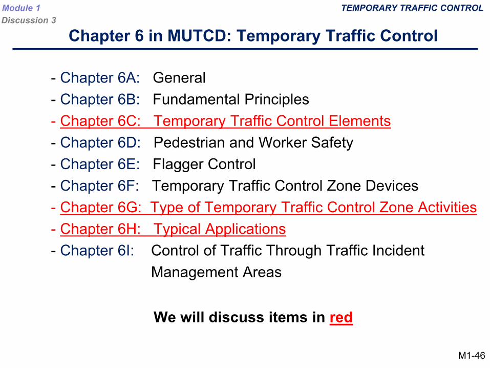
Chapter 6 in MUTCD: Temporary Traffic Control
- Chapter 6A: General- Chapter 6B: Fundamental Principles- Chapter 6C: Temporary Traffic Control Elements- Chapter 6D: Pedestrian and Worker Safety- Chapter 6E: Flagger Control- Chapter 6F: Temporary Traffic Control Zone Devices- Chapter 6G: Type of Temporary Traffic Control Zone Activities- Chapter 6H: Typical Applications- Chapter 6I: Control of Traffic Through Traffic Incident
Management Areas
We will discuss items in red
TEMPORARY TRAFFIC CONTROLModule 1Discussion 3
M1-46

Definition of TTC zone:
“an area of a highway where road user conditions are changed because of a work zone, an incident zone, or a planned special event through the use of TTC devices, uniformed law enforcement officers, or other authorized personnel.”
Chapter 6C: Temporary Traffic Control Elements
TEMPORARY TRAFFIC CONTROLModule 1Discussion 3
M1-47
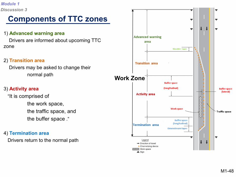
Components of TTC zones1) Advanced warning area
Drivers are informed about upcoming TTC zone
2) Transition areaDrivers may be asked to change their
normal path
3) Activity area“It is comprised of
the work space, the traffic space, and the buffer space .“
4) Termination areaDrivers return to the normal path
Module 1Discussion 3
Work Zone
M1-48
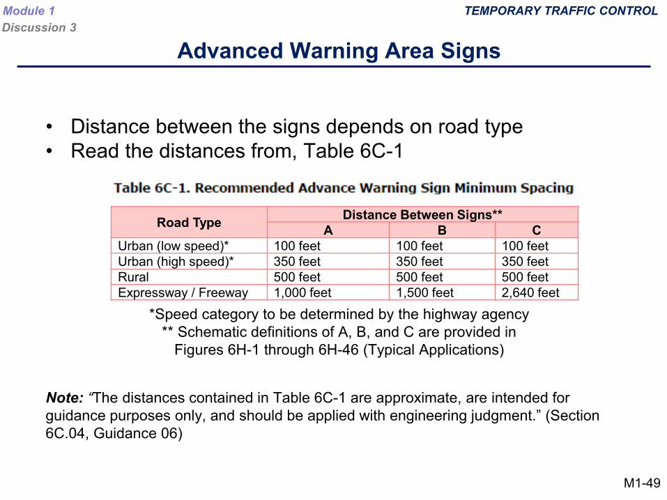
Advanced Warning Area Signs
• Distance between the signs depends on road type• Read the distances from, Table 6C-1
*Speed category to be determined by the highway agency** Schematic definitions of A, B, and C are provided in
Figures 6H-1 through 6H-46 (Typical Applications)
Note: “The distances contained in Table 6C-1 are approximate, are intended for guidance purposes only, and should be applied with engineering judgment.” (Section 6C.04, Guidance 06)
TEMPORARY TRAFFIC CONTROLModule 1Discussion 3
M1-49
Road Type Distance Between Signs**A B C
Urban (low speed)* 100 feet 100 feet 100 feetUrban (high speed)* 350 feet 350 feet 350 feetRural 500 feet 500 feet 500 feetExpressway / Freeway 1,000 feet 1,500 feet 2,640 feet
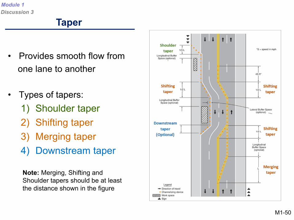
• Provides smooth flow from one lane to another
• Types of tapers:1) Shoulder taper2) Shifting taper3) Merging taper4) Downstream taper
Note: Merging, Shifting and Shoulder tapers should be at least the distance shown in the figure
Taper
Module 1Discussion 3
M1-50
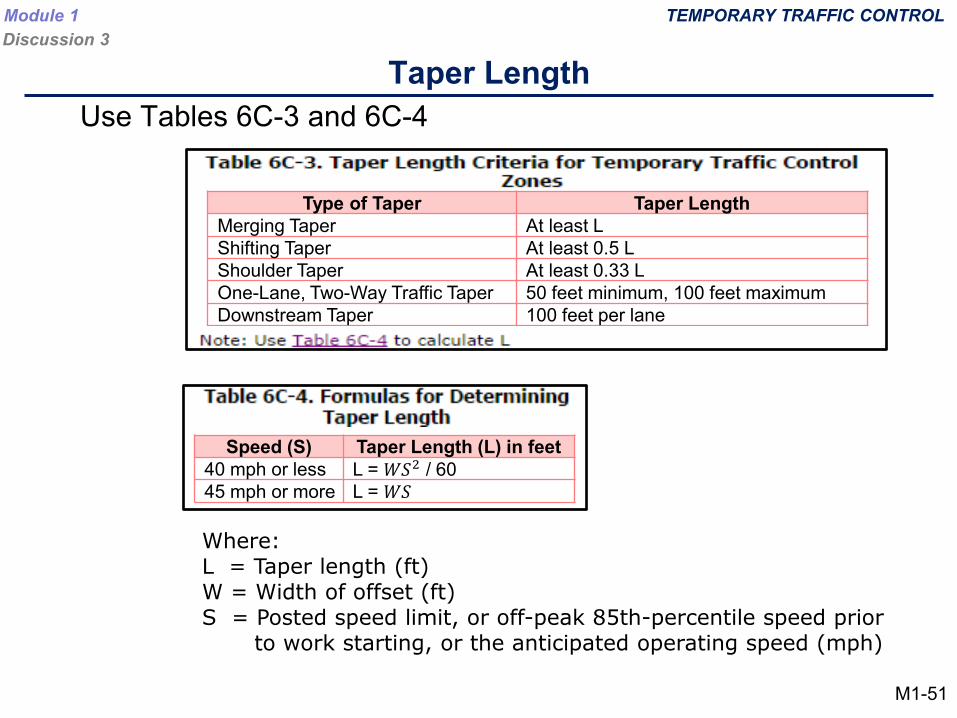
Taper Length Use Tables 6C-3 and 6C-4
Where:L = Taper length (ft)W = Width of offset (ft)S = Posted speed limit, or off-peak 85th-percentile speed prior
to work starting, or the anticipated operating speed (mph)
TEMPORARY TRAFFIC CONTROLModule 1Discussion 3
M1-51
Type of Taper Taper LengthMerging Taper At least LShifting Taper At least 0.5 LShoulder Taper At least 0.33 LOne-Lane, Two-Way Traffic Taper 50 feet minimum, 100 feet maximumDownstream Taper 100 feet per lane
Speed (S) Taper Length (L) in feet40 mph or less L = 𝑊𝑊𝑊𝑊2 / 6045 mph or more L = 𝑊𝑊𝑊𝑊
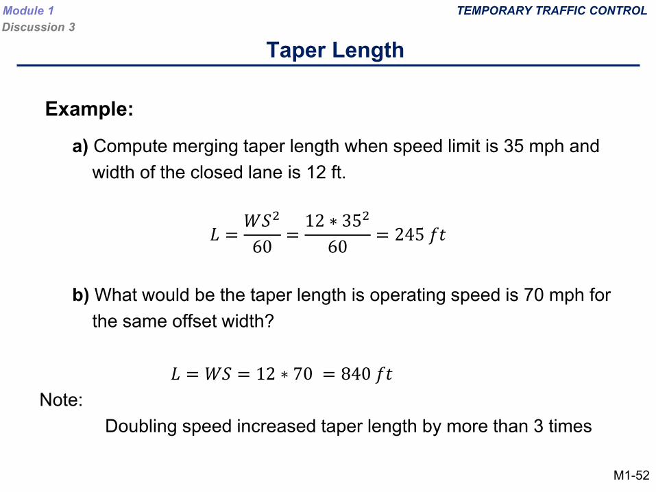
a) Compute merging taper length when speed limit is 35 mph and width of the closed lane is 12 ft.
𝐿𝐿 =𝑊𝑊𝑊𝑊2
60=
12 ∗ 352
60= 245 𝑓𝑓𝑓𝑓
b) What would be the taper length is operating speed is 70 mph for the same offset width?
𝐿𝐿 = 𝑊𝑊𝑊𝑊 = 12 ∗ 70 = 840 𝑓𝑓𝑓𝑓Note:
Doubling speed increased taper length by more than 3 times
Taper Length
Example:
TEMPORARY TRAFFIC CONTROLModule 1Discussion 3
M1-52
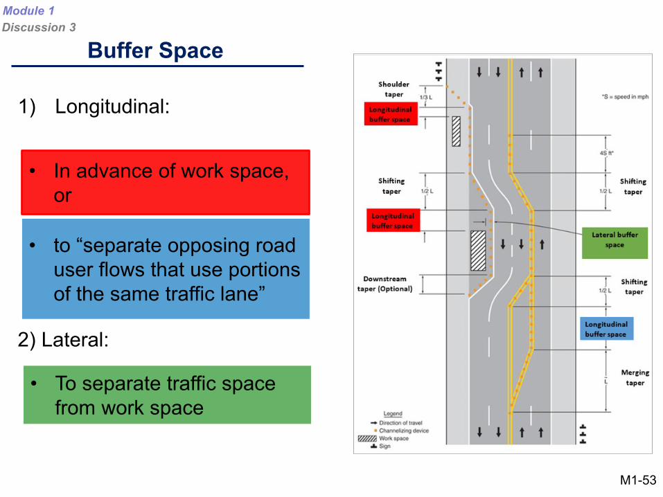
1) Longitudinal:
2) Lateral:
• to “separate opposing road user flows that use portions of the same traffic lane”
• In advance of work space, or
• To separate traffic space from work space
Buffer Space
Module 1Discussion 3
M1-53
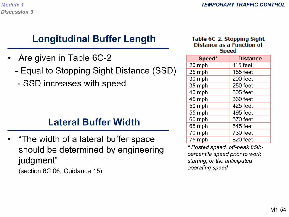
Longitudinal Buffer Length
• Are given in Table 6C-2 - Equal to Stopping Sight Distance (SSD)- SSD increases with speed
Lateral Buffer Width• “The width of a lateral buffer space
should be determined by engineering judgment” (section 6C.06, Guidance 15)
* Posted speed, off-peak 85th-percentile speed prior to work starting, or the anticipated operating speed
TEMPORARY TRAFFIC CONTROLModule 1Discussion 3
M1-54
Speed* Distance20 mph 115 feet25 mph 155 feet30 mph 200 feet35 mph 250 feet40 mph 305 feet45 mph 360 feet50 mph 425 feet55 mph 495 feet60 mph 570 feet65 mph 645 feet70 mph 730 feet75 mph 820 feet
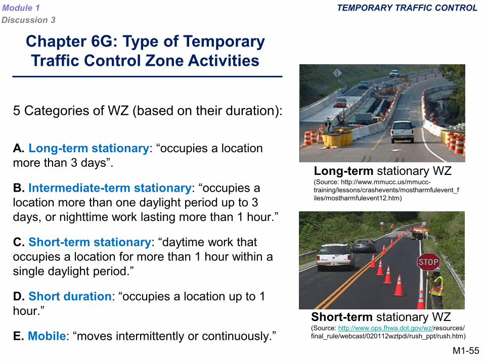
5 Categories of WZ (based on their duration):
A. Long-term stationary: “occupies a location more than 3 days”.
B. Intermediate-term stationary: “occupies a location more than one daylight period up to 3 days, or nighttime work lasting more than 1 hour.”
C. Short-term stationary: “daytime work that occupies a location for more than 1 hour within a single daylight period.”
D. Short duration: “occupies a location up to 1 hour.”
E. Mobile: “moves intermittently or continuously.”
Long-term stationary WZ(Source: http://www.mmucc.us/mmucc-training/lessons/crashevents/mostharmfulevent_files/mostharmfulevent12.htm)
Short-term stationary WZ(Source: http://www.ops.fhwa.dot.gov/wz/resources/ final_rule/webcast/020112wztpdi/rush_ppt/rush.htm)
Chapter 6G: Type of Temporary Traffic Control Zone Activities
TEMPORARY TRAFFIC CONTROLModule 1Discussion 3
M1-55

Typical Application Description Typical Application NumberWork Outside of the Shoulder (see Section 6G.06)
Work Beyond the Shoulder TA-1Blasting Zone TA-2
Work on the Shoulder (see Section 6G.07 and 6G.08)Work on the Shoulder TA-3Short Duration or Mobile Operation on a Shoulder TA-4Shoulder Closure on a Freeway TA-5Shoulder Work with Minor Encroachment TA-6
Work Within the Traveled Way of a Two-Lane Highway (see Section 6G.10)Road Closed with a Diversion TA-7Roads Closed with an Off-Site Detour TA-8Overlapping Routes with a Detour TA-9Lane Closure on a Two-Lane Road Using Flaggers TA-10Lane Closure on a Two-Lane Road with Low Traffic Volumes TA-11Lane Closure on a Two-Lane Road with Traffic Control Signals TA-12Temporary Road Closure TA-13Haul Road Crossing TA-14Work in the Center of a Road with Low Traffic Volumes TA-15Surveying Along the Center Line of a Road with Low Traffic Volumes TA-16Mobile Operations on a Two-Lane Road TA-17
Work Within the Traveled Way of an Urban Street (see Section 6G.11)Lane Closure on a Minor Street TA-18Detour for One Travel Direction TA-19Detour for a Closed Street TA-20
Chapter 6H. Typical Applications (Standard Plans )
46 Typical Applications (TAs), based on work duration and location
TEMPORARY TRAFFIC CONTROLModule 1Discussion 3
TAs highlighted are later analyzed with the WZ tools M1-56
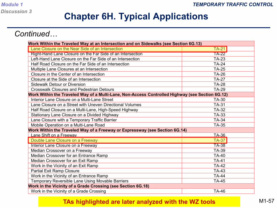
Work Within the Traveled Way at an Intersection and on Sidewalks (see Section 6G.13)Lane Closure on the Near Side of an Intersection TA-21Right-Hand Lane Closure on the Far Side of an Intersection TA-22Left-Hand Lane Closure on the Far Side of an Intersection TA-23Half Road Closure on the Far Side of an Intersection TA-24Multiple Lane Closures at an Intersection TA-25Closure in the Center of an Intersection TA-26Closure at the Side of an Intersection TA-27Sidewalk Detour or Diversion TA-28Crosswalk Closures and Pedestrian Detours TA-29
Work Within the Traveled Way of a Multi-Lane, Non-Access Controlled Highway (see Section 6G.12)Interior Lane Closure on a Multi-Lane Street TA-30Lane Closure on a Street with Uneven Directional Volumes TA-31Half Road Closure on a Multi-Lane, High-Speed Highway TA-32Stationary Lane Closure on a Divided Highway TA-33Lane Closure with a Temporary Traffic Barrier TA-34Mobile Operation on a Multi-Lane Road TA-35
Work Within the Traveled Way of a Freeway or Expressway (see Section 6G.14)Lane Shift on a Freeway TA-36Double Lane Closure on a Freeway TA-37Interior Lane Closure on a Freeway TA-38Median Crossover on a Freeway TA-39Median Crossover for an Entrance Ramp TA-40Median Crossover for an Exit Ramp TA-41Work in the Vicinity of an Exit Ramp TA-42Partial Exit Ramp Closure TA-43Work in the Vicinity of an Entrance Ramp TA-44Temporary Reversible Lane Using Movable Barriers TA-45
Work in the Vicinity of a Grade Crossing (see Section 6G.18)Work in the Vicinity of a Grade Crossing TA-46
Chapter 6H. Typical Applications
Continued…
TEMPORARY TRAFFIC CONTROLModule 1Discussion 3
TAs highlighted are later analyzed with the WZ tools M1-57
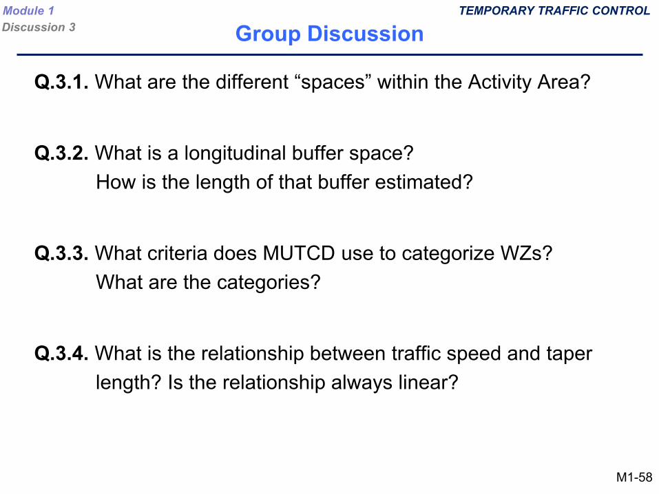
Q.3.1. What are the different “spaces” within the Activity Area?
Q.3.2. What is a longitudinal buffer space? How is the length of that buffer estimated?
Q.3.3. What criteria does MUTCD use to categorize WZs? What are the categories?
Q.3.4. What is the relationship between traffic speed and taper length? Is the relationship always linear?
Group DiscussionTEMPORARY TRAFFIC CONTROLModule 1
Discussion 3
M1-58
DISCUSSION #4WZ CAPACITY
Learning Objectives:
1) Learn the concept of WZ capacity
2) Identify factors that affect WZ capacity
3) Understand different models to estimate WZ capacity
Module 1Discussion 4
M1-59
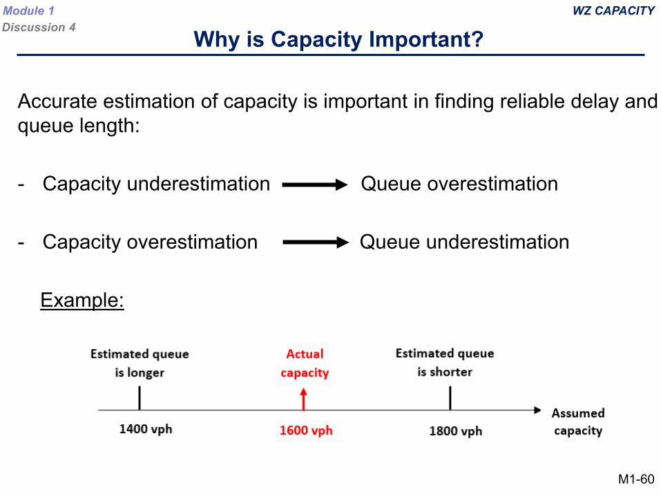
Why is Capacity Important?
Accurate estimation of capacity is important in finding reliable delay and queue length:
- Capacity underestimation Queue overestimation
- Capacity overestimation Queue underestimation
Example:
WZ CAPACITYModule 1Discussion 4
M1-60
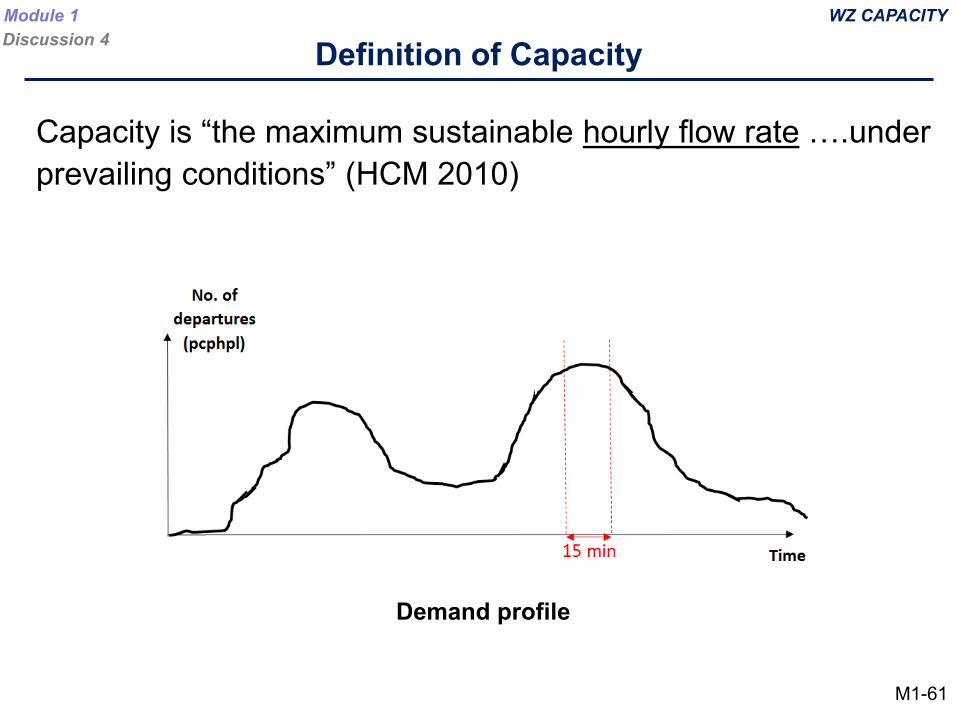
Definition of Capacity
Capacity is “the maximum sustainable hourly flow rate ….under prevailing conditions” (HCM 2010)
Demand profile
WZ CAPACITYModule 1Discussion 4
M1-61
Factors Affecting Capacity *
There are 4 categories of factors:
1) Construction Factors
2) WZ Geometry
3) Traffic-related Factors
4) General Factors
WZ CAPACITYModule 1Discussion 4
* Source:- Traffic Analysis Toolbox Volume XII:
Work Zone Traffic Analysis – Applications and Decision Framework M1-62
1) Construction Factors:
a) Work intensityb) Work zone duration (long-term or short-term)c) Work time (daytime or nighttime)d) Work day (weekday or weekend)
These factors will be discussed in Modules 2, 3, and 4
Factors Affecting Capacity *WZ CAPACITYModule 1
Discussion 4
M1-63
2) WZ Geometry:
a) Number of lanesb) Number of lanes closedc) Lane widthd) Lateral clearancee) Work zone layout
(e.g. Lane closure, crossover, and lane shifting only)f) Length of work zoneg) Presence of ramps
Factors Affecting Capacity *
These factors will be discussed in Modules 2, 3, and 4
WZ CAPACITYModule 1Discussion 4
M1-64
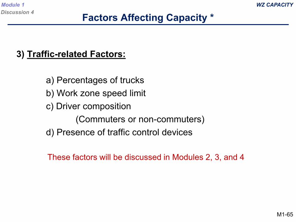
3) Traffic-related Factors:
a) Percentages of trucksb) Work zone speed limitc) Driver composition
(Commuters or non-commuters) d) Presence of traffic control devices
Factors Affecting Capacity *
These factors will be discussed in Modules 2, 3, and 4
WZ CAPACITYModule 1Discussion 4
M1-65
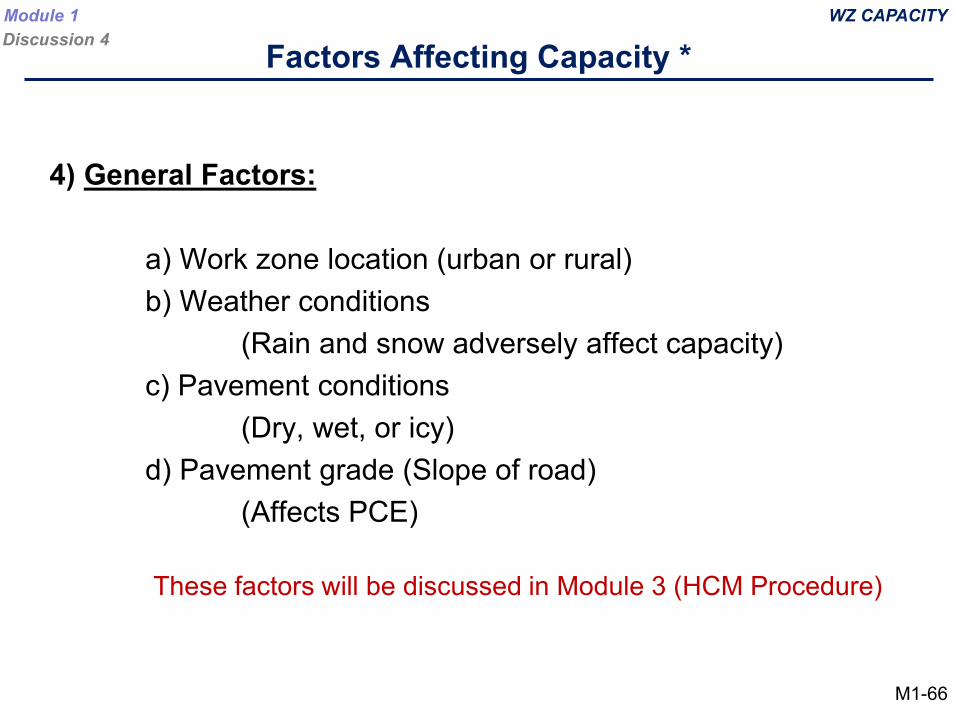
4) General Factors:
a) Work zone location (urban or rural)b) Weather conditions
(Rain and snow adversely affect capacity)c) Pavement conditions
(Dry, wet, or icy)d) Pavement grade (Slope of road)
(Affects PCE)
Factors Affecting Capacity *
These factors will be discussed in Module 3 (HCM Procedure)
WZ CAPACITYModule 1Discussion 4
M1-66
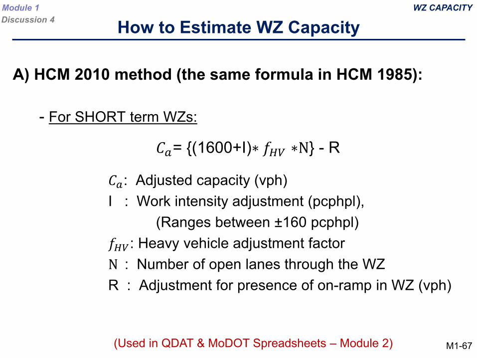
A) HCM 2010 method (the same formula in HCM 1985):
- For SHORT term WZs:
𝐶𝐶𝑎𝑎: Adjusted capacity (vph)I : Work intensity adjustment (pcphpl),
(Ranges between ±160 pcphpl)𝑓𝑓𝐻𝐻𝐻𝐻: Heavy vehicle adjustment factorN : Number of open lanes through the WZR : Adjustment for presence of on-ramp in WZ (vph)
𝐶𝐶𝑎𝑎= {(1600+I)∗ 𝑓𝑓𝐻𝐻𝐻𝐻 ∗N} - R
WZ CAPACITY
How to Estimate WZ Capacity
(Used in QDAT & MoDOT Spreadsheets – Module 2)
Module 1Discussion 4
M1-67
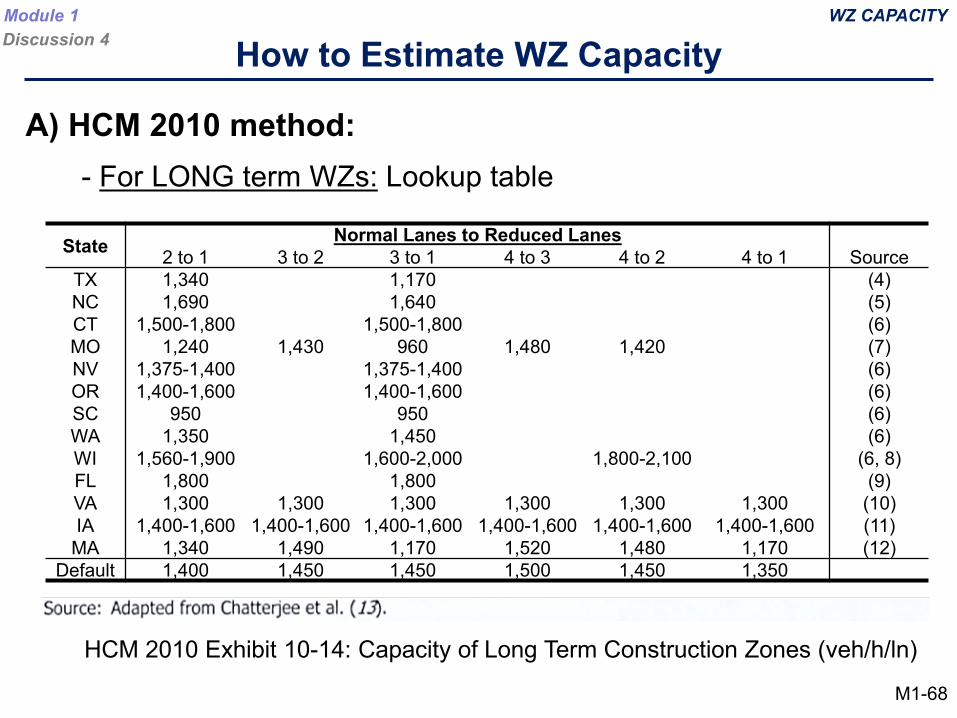
- For LONG term WZs: Lookup table
A) HCM 2010 method:
WZ CAPACITY
How to Estimate WZ CapacityModule 1Discussion 4
HCM 2010 Exhibit 10-14: Capacity of Long Term Construction Zones (veh/h/ln)
M1-68
State Normal Lanes to Reduced Lanes2 to 1 3 to 2 3 to 1 4 to 3 4 to 2 4 to 1 Source
TX 1,340 1,170 (4)NC 1,690 1,640 (5)CT 1,500-1,800 1,500-1,800 (6)MO 1,240 1,430 960 1,480 1,420 (7)NV 1,375-1,400 1,375-1,400 (6)OR 1,400-1,600 1,400-1,600 (6)SC 950 950 (6)WA 1,350 1,450 (6)WI 1,560-1,900 1,600-2,000 1,800-2,100 (6, 8)FL 1,800 1,800 (9)VA 1,300 1,300 1,300 1,300 1,300 1,300 (10)IA 1,400-1,600 1,400-1,600 1,400-1,600 1,400-1,600 1,400-1,600 1,400-1,600 (11)MA 1,340 1,490 1,170 1,520 1,480 1,170 (12)
Default 1,400 1,450 1,450 1,500 1,450 1,350
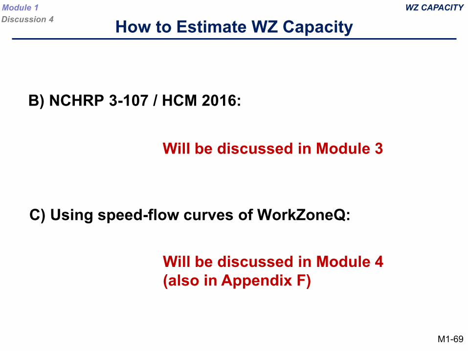
B) NCHRP 3-107 / HCM 2016:
Will be discussed in Module 3
C) Using speed-flow curves of WorkZoneQ:
Will be discussed in Module 4 (also in Appendix F)
WZ CAPACITY
How to Estimate WZ CapacityModule 1Discussion 4
M1-69
Q.4.1. What is the effect of capacity overestimation on queue length?
Q.4.2. Mention at least 3 geometry factors and 3 traffic-related factors that affect capacity
Q.4.3. How does HCM 2010 estimate capacity for short-term WZs?Is it similar for long-term WZs?
WZ CAPACITY
Group DiscussionModule 1Discussion 4
M1-70
Module 1 Discussion 5
Discussion #5 Work Zone Analysis and Queue
Learning Objectives:
1) Identify typical methods for WZ analysis
2) Learn the different types of queue and how to estimate it using input-output methods
M1-71
• Appropriate WZ analysis can improve planning, design, operation and safety
• Mobility and safety criteria vary between states. Common performance measures are:
– Delay– Queue length and duration
• Different WZ analysis approaches are available
WZ AnalysisWZ ANALYSISModule 1
Discussion 5
M1-72
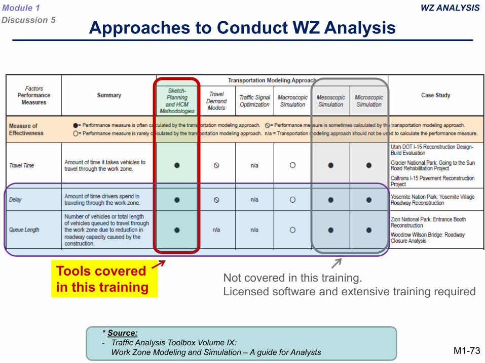
Tools covered in this training
Not covered in this training. Licensed software and extensive training required
Approaches to Conduct WZ AnalysisWZ ANALYSISModule 1
Discussion 5
* Source:- Traffic Analysis Toolbox Volume IX:
Work Zone Modeling and Simulation – A guide for Analysts M1-73
• Simple methods, yield approximate results and estimates before deciding if more complex tools are needed
• Require fewer calculations/equations and fewer inputs
• They also provide fewer outcomes compared to simulation
• Suitable for: – Individual WZs– Straightforward cases/conditions– Analysis of immediate area surroundings of the WZ
WZ ANALYSIS
Sketch-planning ToolsModule 1Discussion 5
M1-74
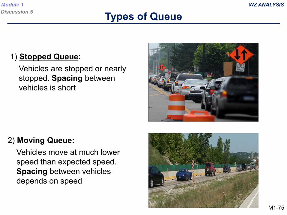
2) Moving Queue:Vehicles move at much lowerspeed than expected speed. Spacing between vehicles depends on speed
1) Stopped Queue:Vehicles are stopped or nearly stopped. Spacing between vehicles is short
WZ ANALYSIS
Types of QueueModule 1Discussion 5
M1-75
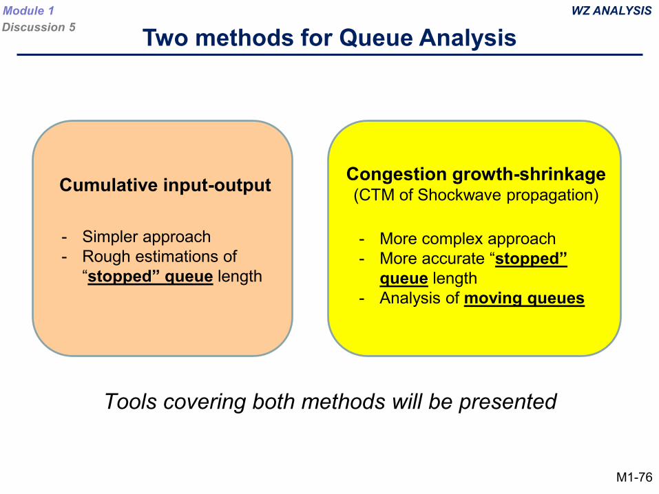
Cumulative input-output
- Simpler approach- Rough estimations of
“stopped” queue length
Congestion growth-shrinkage(CTM of Shockwave propagation)
- More complex approach- More accurate “stopped”
queue length - Analysis of moving queues
Tools covering both methods will be presented
WZ ANALYSIS
Two methods for Queue AnalysisModule 1Discussion 5
M1-76
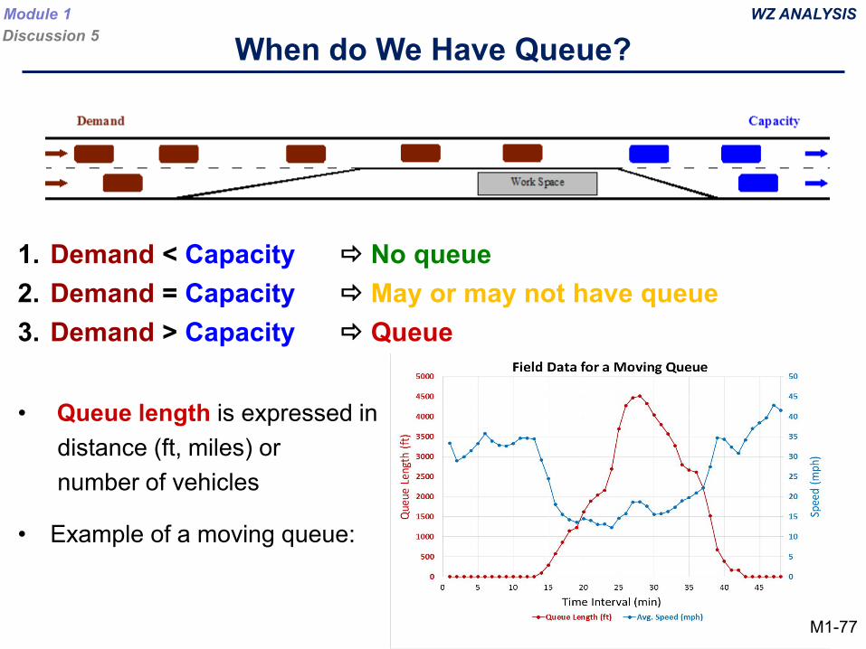
1. Demand < Capacity No queue2. Demand = Capacity May or may not have queue3. Demand > Capacity Queue
• Queue length is expressed in distance (ft, miles) ornumber of vehicles
• Example of a moving queue:
WZ ANALYSIS
When do We Have Queue?Module 1Discussion 5
M1-77
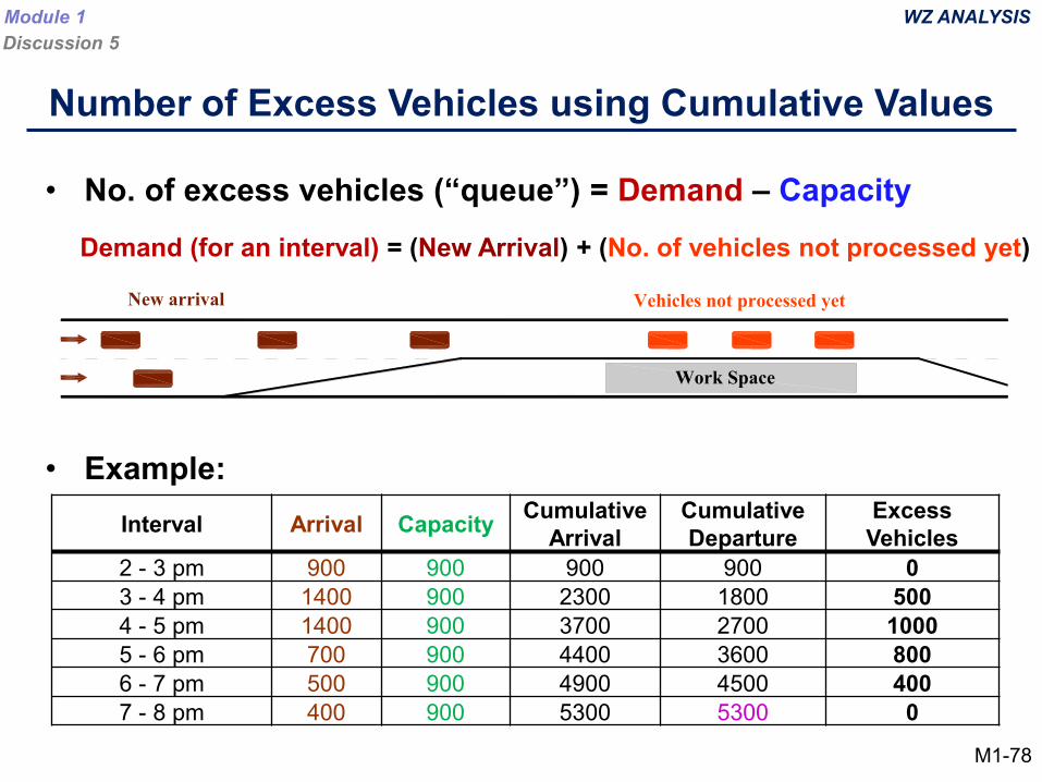
• No. of excess vehicles (“queue”) = Demand – Capacity Demand (for an interval) = (New Arrival) + (No. of vehicles not processed yet)
Work Space
New arrival Vehicles not processed yet
• Example:
WZ ANALYSIS
Number of Excess Vehicles using Cumulative Values
Module 1Discussion 5
M1-78
Interval Arrival Capacity Cumulative Arrival
Cumulative Departure
Excess Vehicles
2 - 3 pm 900 900 900 900 03 - 4 pm 1400 900 2300 1800 5004 - 5 pm 1400 900 3700 2700 10005 - 6 pm 700 900 4400 3600 8006 - 7 pm 500 900 4900 4500 4007 - 8 pm 400 900 5300 5300 0
WZ ANALYSIS
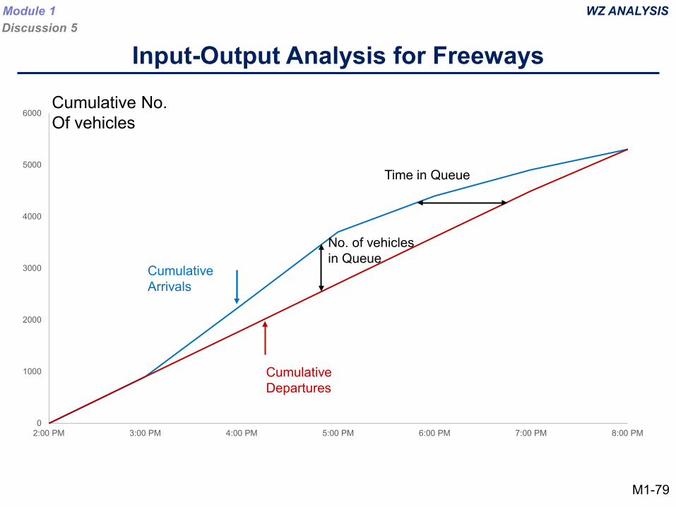
Input-Output Analysis for Freeways
Module 1Discussion 5
M1-79
0
1000
2000
3000
4000
5000
6000
2:00 PM 3:00 PM 4:00 PM 5:00 PM 6:00 PM 7:00 PM 8:00 PM
Cumulative No.Of vehicles
CumulativeArrivals
CumulativeDepartures
Time in Queue
No. of vehiclesin Queue
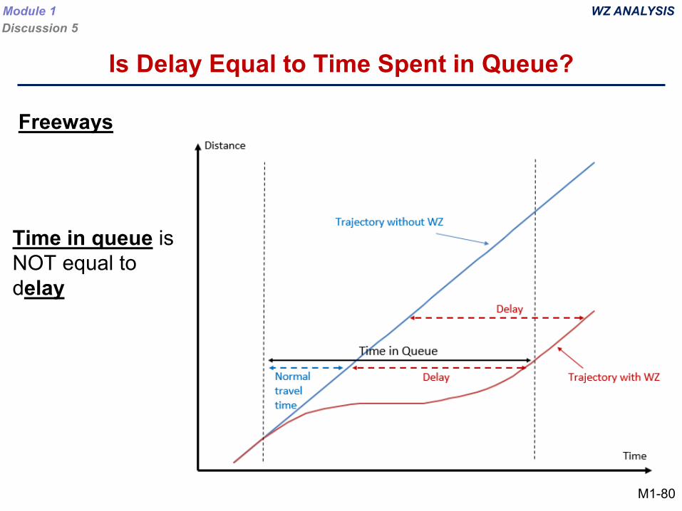
Is Delay Equal to Time Spent in Queue?
Time in queue is NOT equal to delay
Freeways
WZ ANALYSISModule 1Discussion 5
M1-80
WZ ANALYSIS
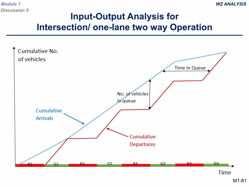
Input-Output Analysis for Intersection/ one-lane two way Operation
Module 1Discussion 5
M1-81
• Q 5.1 : What are some advantages/disadvantages of cumulative input-output analysis?
• Q 5.2 : In general, do vehicles have larger spacing in stopped queue or in moving queue?
• Q 5.3 : Which method of queue estimation is appropriate for stopped queues? (Cell transmission, cumulative input-output, or both)
• Q 5.4 : Which method of queue estimation is appropriate for moving queues? (Cell transmission, cumulative input-output, or both)
WZ ANALYSIS
Group DiscussionModule 1Discussion 5
M1-82
3 comes before 2
Please note:
Module 3 (HCM 2016 Methods for Work Zone Capacity Calculations) is presented
next because Module 2 which is FREEVAL-WZ uses the HCM procedure
MODULE 2
HCM 2016 Methods for Work Zone Capacity Calculations
HCM-1
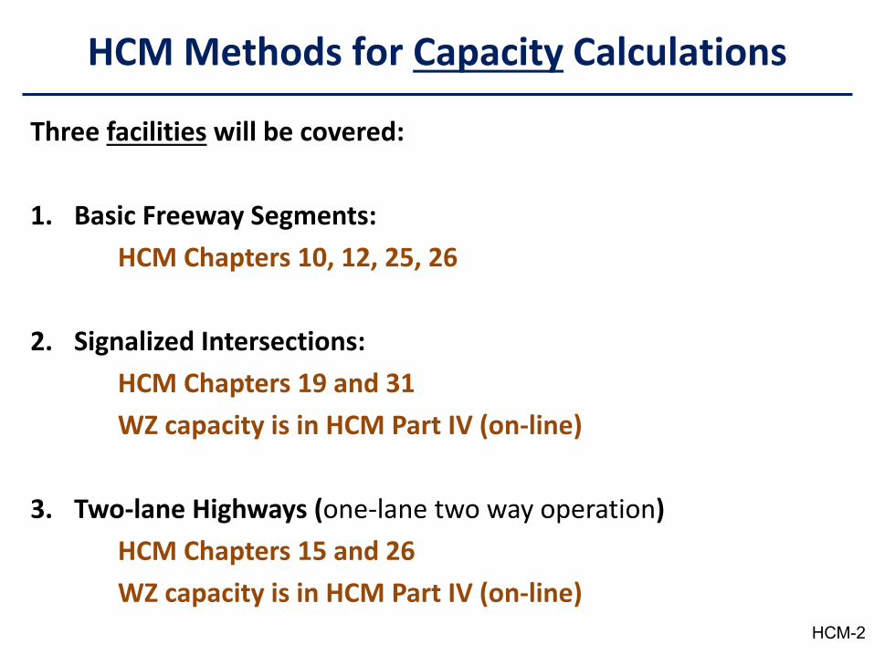
Three facilities will be covered:
1. Basic Freeway Segments:HCM Chapters 10, 12, 25, 26
2. Signalized Intersections:HCM Chapters 19 and 31WZ capacity is in HCM Part IV (on-line)
3. Two-lane Highways (one-lane two way operation)HCM Chapters 15 and 26WZ capacity is in HCM Part IV (on-line)
HCM Methods for Capacity Calculations
HCM-2
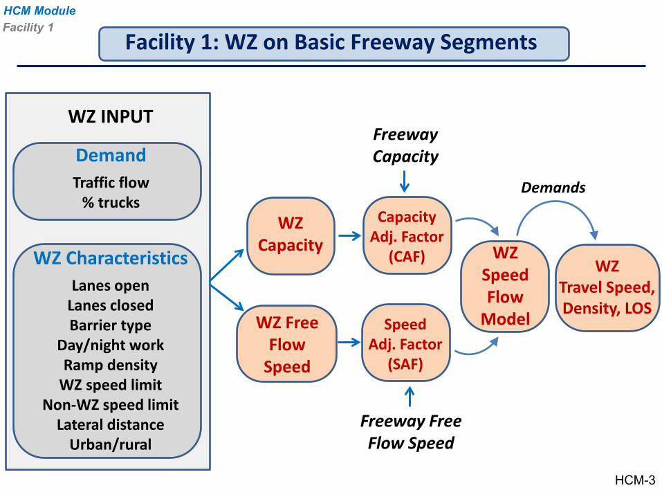
Facility 1: WZ on Basic Freeway Segments
DemandTraffic flow
% trucks
WZ CharacteristicsLanes open
Lanes closedBarrier type
Day/night workRamp density
WZ speed limitNon-WZ speed limit
Lateral distanceUrban/rural
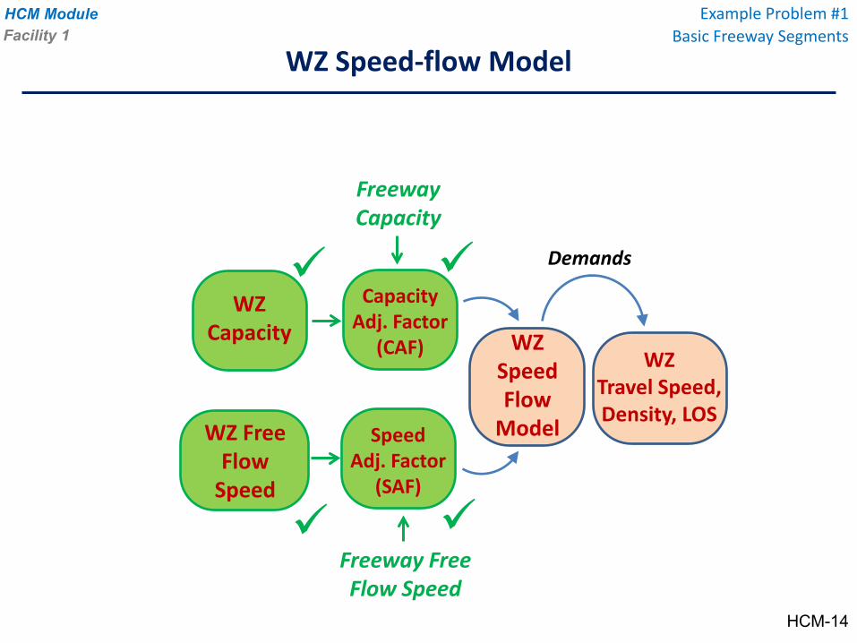
WZ Capacity
WZ FreeFlow
Speed
WZ SpeedFlow
Model
WZTravel Speed, Density, LOS
WZ INPUT
Demands
Freeway Capacity
Capacity Adj. Factor
(CAF)
Speed Adj. Factor
(SAF)
Freeway Free Flow Speed
Facility 1
HCM-3
HCM Module
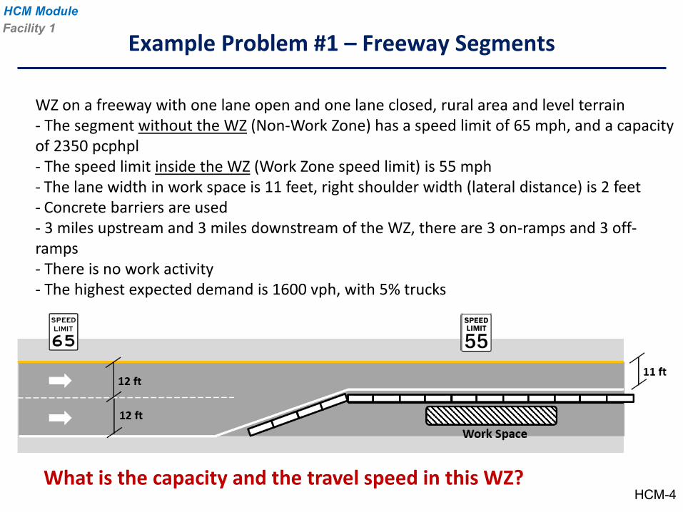
WZ on a freeway with one lane open and one lane closed, rural area and level terrain- The segment without the WZ (Non-Work Zone) has a speed limit of 65 mph, and a capacity of 2350 pcphpl- The speed limit inside the WZ (Work Zone speed limit) is 55 mph- The lane width in work space is 11 feet, right shoulder width (lateral distance) is 2 feet- Concrete barriers are used- 3 miles upstream and 3 miles downstream of the WZ, there are 3 on-ramps and 3 off-ramps- There is no work activity- The highest expected demand is 1600 vph, with 5% trucks
What is the capacity and the travel speed in this WZ?
Example Problem #1 – Freeway SegmentsFacility 1
HCM-4
HCM Module
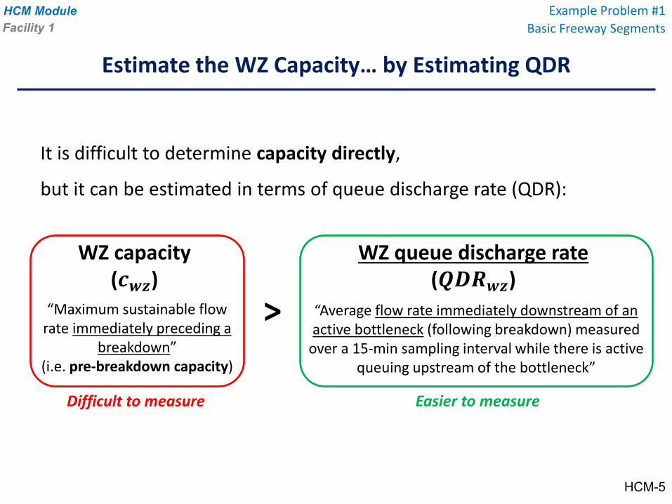
It is difficult to determine capacity directly,
but it can be estimated in terms of queue discharge rate (QDR):
WZ capacity (𝒄𝒄𝒘𝒘𝒘𝒘)
“Maximum sustainable flow rate immediately preceding a
breakdown” (i.e. pre-breakdown capacity)
WZ queue discharge rate (𝑸𝑸𝑸𝑸𝑸𝑸𝒘𝒘𝒘𝒘)
“Average flow rate immediately downstream of an active bottleneck (following breakdown) measured
over a 15-min sampling interval while there is active queuing upstream of the bottleneck”
>
Difficult to measure Easier to measure
Example Problem #1Basic Freeway Segments
Estimate the WZ Capacity… by Estimating QDR
Facility 1
HCM-5
HCM Module
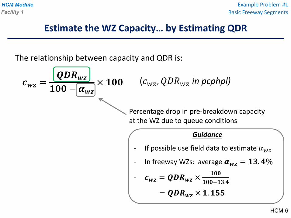
𝒄𝒄𝒘𝒘𝒘𝒘 =𝑸𝑸𝑸𝑸𝑸𝑸𝒘𝒘𝒘𝒘
𝟏𝟏𝟏𝟏𝟏𝟏 − 𝜶𝜶𝒘𝒘𝒘𝒘× 𝟏𝟏𝟏𝟏𝟏𝟏 (𝑠𝑠𝑤𝑤𝑤𝑤,𝑄𝑄𝑄𝑄𝑄𝑄𝑤𝑤𝑤𝑤 in pcphpl)
Percentage drop in pre-breakdown capacity at the WZ due to queue conditions
Guidance
- If possible use field data to estimate 𝛼𝛼𝑤𝑤𝑤𝑤- In freeway WZs: average 𝜶𝜶𝒘𝒘𝒘𝒘 = 𝟏𝟏𝟏𝟏.𝟒𝟒𝟒
- 𝒄𝒄𝒘𝒘𝒘𝒘 = 𝑸𝑸𝑸𝑸𝑸𝑸𝒘𝒘𝒘𝒘 × 𝟏𝟏𝟏𝟏𝟏𝟏𝟏𝟏𝟏𝟏𝟏𝟏−𝟏𝟏𝟏𝟏.𝟒𝟒
= 𝑸𝑸𝑸𝑸𝑸𝑸𝒘𝒘𝒘𝒘 × 𝟏𝟏.𝟏𝟏𝟏𝟏𝟏𝟏
The relationship between capacity and QDR is:
Example Problem #1Basic Freeway Segments
Estimate the WZ Capacity… by Estimating QDR
Facility 1
HCM-6
HCM Module
How to Estimate 𝑸𝑸𝑸𝑸𝑸𝑸𝒘𝒘𝒘𝒘
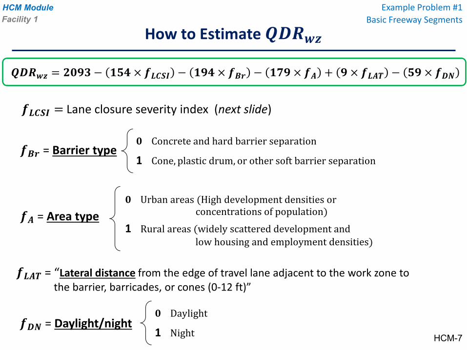
𝑸𝑸𝑸𝑸𝑸𝑸𝒘𝒘𝒘𝒘 = 𝟐𝟐𝟏𝟏𝟐𝟐𝟏𝟏 − 𝟏𝟏𝟏𝟏𝟒𝟒 × 𝒇𝒇𝑳𝑳𝑳𝑳𝑳𝑳𝑳𝑳 − 𝟏𝟏𝟐𝟐𝟒𝟒 × 𝒇𝒇𝑩𝑩𝑩𝑩 − 𝟏𝟏𝟏𝟏𝟐𝟐 × 𝒇𝒇𝑨𝑨 + 𝟐𝟐 × 𝒇𝒇𝑳𝑳𝑨𝑨𝑳𝑳 − 𝟏𝟏𝟐𝟐 × 𝒇𝒇𝑸𝑸𝑫𝑫
𝒇𝒇𝑩𝑩𝑩𝑩 = Barrier type
𝒇𝒇𝑨𝑨 = Area type
𝒇𝒇𝑳𝑳𝑨𝑨𝑳𝑳 = “Lateral distance from the edge of travel lane adjacent to the work zone to the barrier, barricades, or cones (0-12 ft)”
𝟏𝟏 Concrete and hard barrier separation
1 Cone, plastic drum, or other soft barrier separation
𝟏𝟏 Urban areas (High development densities orconcentrations of population)
1 Rural areas (widely scattered development andlow housing and employment densities)
𝒇𝒇𝑸𝑸𝑫𝑫 = Daylight/night𝟏𝟏 Daylight
1 Night
𝒇𝒇𝑳𝑳𝑳𝑳𝑳𝑳𝑳𝑳 = Lane closure severity index (next slide)
Example Problem #1Basic Freeway SegmentsFacility 1
HCM-7
HCM Module
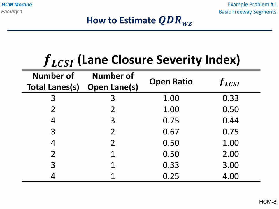
Number of Total Lanes(s)
Number of Open Lane(s) Open Ratio 𝒇𝒇𝑳𝑳𝑳𝑳𝑳𝑳𝑳𝑳
3 3 1.00 0.332 2 1.00 0.504 3 0.75 0.443 2 0.67 0.754 2 0.50 1.002 1 0.50 2.003 1 0.33 3.004 1 0.25 4.00
𝒇𝒇𝑳𝑳𝑳𝑳𝑳𝑳𝑳𝑳 (Lane Closure Severity Index)
How to Estimate 𝑸𝑸𝑸𝑸𝑸𝑸𝒘𝒘𝒘𝒘
Example Problem #1Basic Freeway SegmentsFacility 1
HCM-8
HCM Module
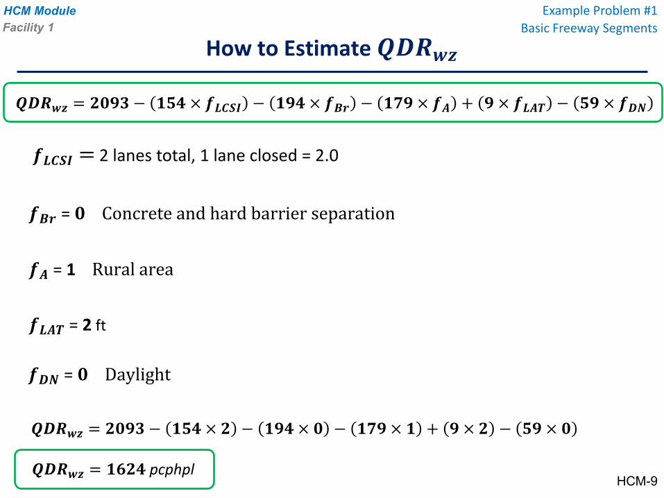
𝑸𝑸𝑸𝑸𝑸𝑸𝒘𝒘𝒘𝒘 = 𝟐𝟐𝟏𝟏𝟐𝟐𝟏𝟏 − 𝟏𝟏𝟏𝟏𝟒𝟒 × 𝒇𝒇𝑳𝑳𝑳𝑳𝑳𝑳𝑳𝑳 − 𝟏𝟏𝟐𝟐𝟒𝟒 × 𝒇𝒇𝑩𝑩𝑩𝑩 − 𝟏𝟏𝟏𝟏𝟐𝟐 × 𝒇𝒇𝑨𝑨 + 𝟐𝟐 × 𝒇𝒇𝑳𝑳𝑨𝑨𝑳𝑳 − 𝟏𝟏𝟐𝟐 × 𝒇𝒇𝑸𝑸𝑫𝑫
𝒇𝒇𝑩𝑩𝑩𝑩 = 𝟏𝟏 Concrete and hard barrier separation
𝒇𝒇𝑨𝑨 = 1 Rural area
𝒇𝒇𝑳𝑳𝑨𝑨𝑳𝑳 = 2 ft
𝒇𝒇𝑸𝑸𝑫𝑫 = 𝟏𝟏 Daylight
𝒇𝒇𝑳𝑳𝑳𝑳𝑳𝑳𝑳𝑳 = 2 lanes total, 1 lane closed = 2.0
𝑸𝑸𝑸𝑸𝑸𝑸𝒘𝒘𝒘𝒘 = 𝟐𝟐𝟏𝟏𝟐𝟐𝟏𝟏 − 𝟏𝟏𝟏𝟏𝟒𝟒 × 𝟐𝟐 − 𝟏𝟏𝟐𝟐𝟒𝟒 × 𝟏𝟏 − 𝟏𝟏𝟏𝟏𝟐𝟐 × 𝟏𝟏 + 𝟐𝟐 × 𝟐𝟐 − 𝟏𝟏𝟐𝟐 × 𝟏𝟏
𝑸𝑸𝑸𝑸𝑸𝑸𝒘𝒘𝒘𝒘 = 𝟏𝟏𝟏𝟏𝟐𝟐𝟒𝟒 pcphpl
How to Estimate 𝑸𝑸𝑸𝑸𝑸𝑸𝒘𝒘𝒘𝒘
Example Problem #1Basic Freeway SegmentsFacility 1
HCM-9
HCM Module
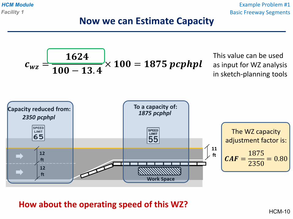
𝒄𝒄𝒘𝒘𝒘𝒘 =𝟏𝟏𝟏𝟏𝟐𝟐𝟒𝟒
𝟏𝟏𝟏𝟏𝟏𝟏 − 𝟏𝟏𝟏𝟏.𝟒𝟒× 𝟏𝟏𝟏𝟏𝟏𝟏 = 𝟏𝟏𝟏𝟏𝟏𝟏𝟏𝟏 𝒑𝒑𝒄𝒄𝒑𝒑𝒑𝒑𝒑𝒑𝒑𝒑
This value can be used as input for WZ analysis in sketch-planning tools
11 ft
Capacity reduced from:2350 pcphpl
To a capacity of:1875 pcphpl
How about the operating speed of this WZ?
The WZ capacity adjustment factor is:
𝑳𝑳𝑨𝑨𝑪𝑪 =18752350 = 0.80
Now we can Estimate Capacity
Example Problem #1Basic Freeway SegmentsFacility 1
HCM-10
HCM Module
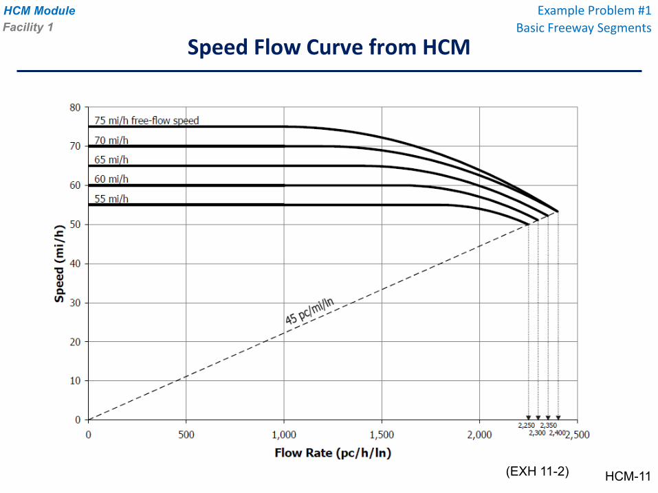
Speed Flow Curve from HCM
Example Problem #1Basic Freeway SegmentsFacility 1
HCM-11(EXH 11-2)
HCM Module
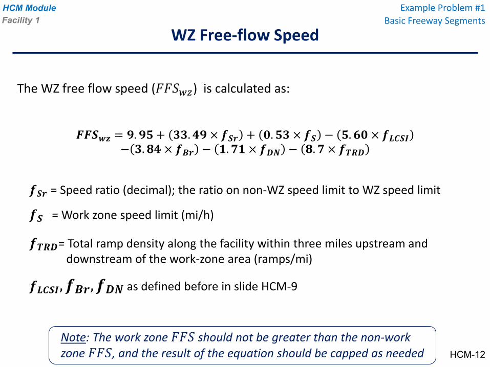
The WZ free flow speed (𝐹𝐹𝐹𝐹𝑊𝑊𝑤𝑤𝑤𝑤) is calculated as:
Note: The work zone 𝐹𝐹𝐹𝐹𝑊𝑊 should not be greater than the non-work zone 𝐹𝐹𝐹𝐹𝑊𝑊, and the result of the equation should be capped as needed
𝑪𝑪𝑪𝑪𝑳𝑳𝒘𝒘𝒘𝒘 = 𝟐𝟐.𝟐𝟐𝟏𝟏 + 𝟏𝟏𝟏𝟏.𝟒𝟒𝟐𝟐 × 𝒇𝒇𝑳𝑳𝑩𝑩 + 𝟏𝟏.𝟏𝟏𝟏𝟏 × 𝒇𝒇𝑳𝑳 − 𝟏𝟏.𝟏𝟏𝟏𝟏 × 𝒇𝒇𝑳𝑳𝑳𝑳𝑳𝑳𝑳𝑳− 𝟏𝟏.𝟏𝟏𝟒𝟒 × 𝒇𝒇𝑩𝑩𝑩𝑩 − 𝟏𝟏.𝟏𝟏𝟏𝟏 × 𝒇𝒇𝑸𝑸𝑫𝑫 − 𝟏𝟏.𝟏𝟏 × 𝒇𝒇𝑳𝑳𝑸𝑸𝑸𝑸
𝒇𝒇𝑳𝑳𝑩𝑩 = Speed ratio (decimal); the ratio on non-WZ speed limit to WZ speed limit
𝒇𝒇𝑳𝑳 = Work zone speed limit (mi/h)
𝒇𝒇𝑳𝑳𝑸𝑸𝑸𝑸= Total ramp density along the facility within three miles upstream and downstream of the work-zone area (ramps/mi)
𝒇𝒇𝑳𝑳𝑳𝑳𝑳𝑳𝑳𝑳,𝒇𝒇𝑩𝑩𝑩𝑩,𝒇𝒇𝑸𝑸𝑫𝑫 as defined before in slide HCM-9
WZ Free-flow Speed
Example Problem #1Basic Freeway SegmentsFacility 1
HCM-12
HCM Module
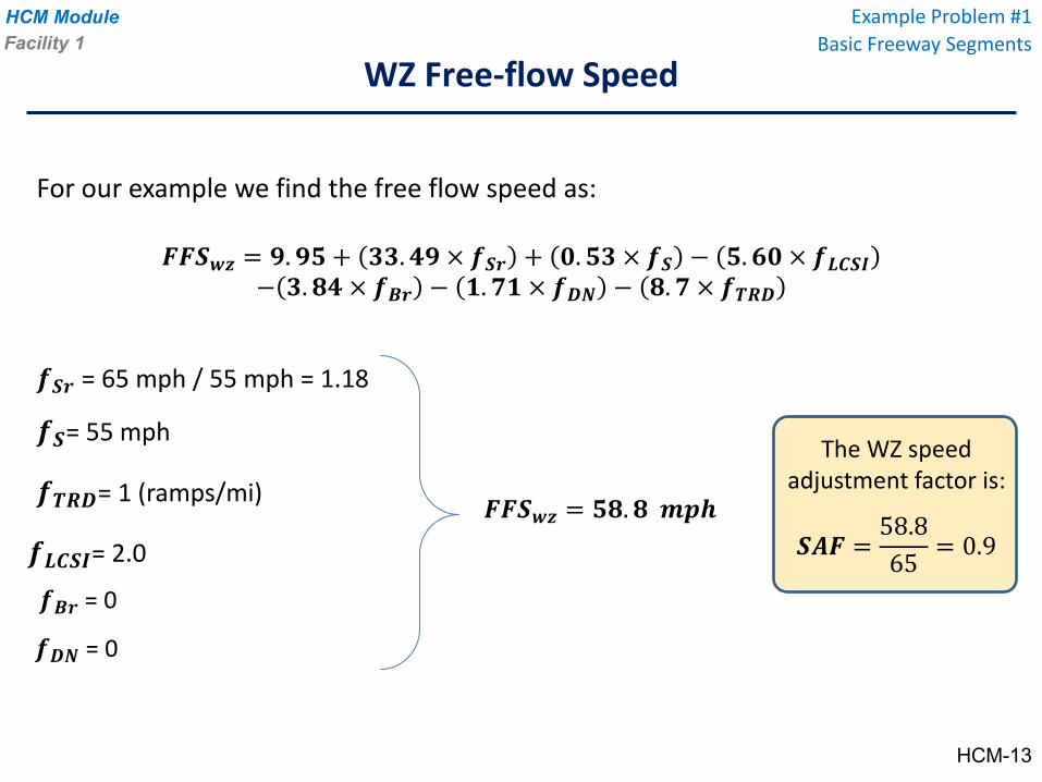
For our example we find the free flow speed as:
𝑪𝑪𝑪𝑪𝑳𝑳𝒘𝒘𝒘𝒘 = 𝟐𝟐.𝟐𝟐𝟏𝟏 + 𝟏𝟏𝟏𝟏.𝟒𝟒𝟐𝟐 × 𝒇𝒇𝑳𝑳𝑩𝑩 + 𝟏𝟏.𝟏𝟏𝟏𝟏 × 𝒇𝒇𝑳𝑳 − 𝟏𝟏.𝟏𝟏𝟏𝟏 × 𝒇𝒇𝑳𝑳𝑳𝑳𝑳𝑳𝑳𝑳− 𝟏𝟏.𝟏𝟏𝟒𝟒 × 𝒇𝒇𝑩𝑩𝑩𝑩 − 𝟏𝟏.𝟏𝟏𝟏𝟏 × 𝒇𝒇𝑸𝑸𝑫𝑫 − 𝟏𝟏.𝟏𝟏 × 𝒇𝒇𝑳𝑳𝑸𝑸𝑸𝑸
𝒇𝒇𝑳𝑳𝑩𝑩 = 65 mph / 55 mph = 1.18
𝒇𝒇𝑳𝑳= 55 mph
𝒇𝒇𝑳𝑳𝑸𝑸𝑸𝑸= 1 (ramps/mi)
𝒇𝒇𝑳𝑳𝑳𝑳𝑳𝑳𝑳𝑳= 2.0
𝒇𝒇𝑩𝑩𝑩𝑩 = 0
𝒇𝒇𝑸𝑸𝑫𝑫 = 0
𝑪𝑪𝑪𝑪𝑳𝑳𝒘𝒘𝒘𝒘 = 𝟏𝟏𝟏𝟏.𝟏𝟏 𝒎𝒎𝒑𝒑𝒑𝒑
The WZ speed adjustment factor is:
𝑳𝑳𝑨𝑨𝑪𝑪 =58.865 = 0.9
WZ Free-flow Speed
Example Problem #1Basic Freeway SegmentsFacility 1
HCM-13
HCM Module
WZ Capacity
WZ FreeFlow
Speed
WZ SpeedFlow
Model
WZTravel Speed, Density, LOS
Demands
Freeway Capacity
Capacity Adj. Factor
(CAF)
Speed Adj. Factor
(SAF)
Freeway Free Flow Speed
WZ Speed-flow Model
Example Problem #1Basic Freeway SegmentsFacility 1
HCM-14
HCM Module
WZ Speed-flow Model
Example Problem #1Basic Freeway SegmentsFacility 1
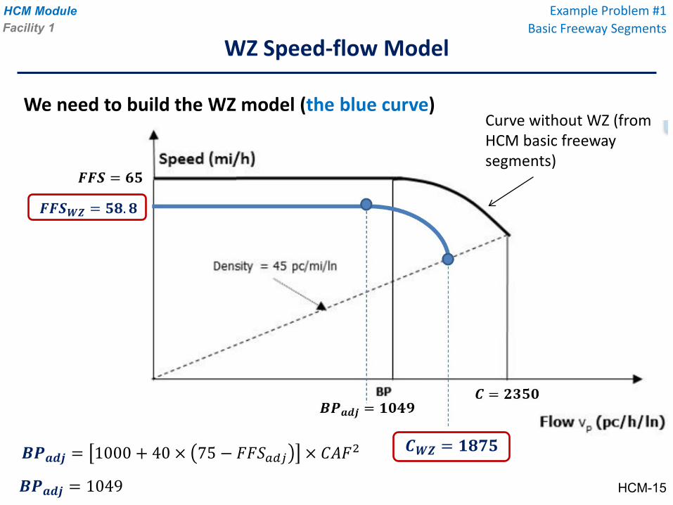
𝑳𝑳𝑾𝑾𝑾𝑾 = 𝟏𝟏𝟏𝟏𝟏𝟏𝟏𝟏
𝑪𝑪𝑪𝑪𝑳𝑳𝑾𝑾𝑾𝑾 = 𝟏𝟏𝟏𝟏.𝟏𝟏
We need to build the WZ model (the blue curve)
𝑩𝑩𝑩𝑩𝒂𝒂𝒂𝒂𝒂𝒂 = 1000 + 40 × 75 − 𝐹𝐹𝐹𝐹𝑊𝑊𝑎𝑎𝑎𝑎𝑎𝑎 × 𝐶𝐶𝐶𝐶𝐹𝐹2
𝑩𝑩𝑩𝑩𝒂𝒂𝒂𝒂𝒂𝒂 = 1049
Curve without WZ (from HCM basic freeway segments)
𝑪𝑪𝑪𝑪𝑳𝑳 = 𝟏𝟏𝟏𝟏
HCM-15
HCM Module
WZ Speed-flow Model
Example Problem #1Basic Freeway SegmentsFacility 1
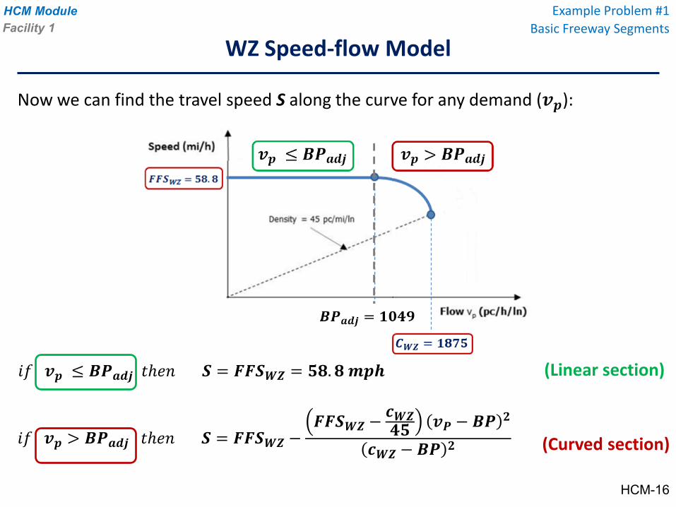
𝑖𝑖𝑓𝑓 𝒗𝒗𝒑𝒑 ≤ 𝑩𝑩𝑩𝑩𝒂𝒂𝒂𝒂𝒂𝒂 𝑓𝑓𝑡𝑠𝑠𝑡𝑡 𝑳𝑳 = 𝑪𝑪𝑪𝑪𝑳𝑳𝑾𝑾𝑾𝑾 = 𝟏𝟏𝟏𝟏.𝟏𝟏𝒎𝒎𝒑𝒑𝒑𝒑
Now we can find the travel speed S along the curve for any demand (𝒗𝒗𝒑𝒑):
𝑖𝑖𝑓𝑓 𝒗𝒗𝒑𝒑 > 𝑩𝑩𝑩𝑩𝒂𝒂𝒂𝒂𝒂𝒂 𝑓𝑓𝑡𝑠𝑠𝑡𝑡 𝑳𝑳 = 𝑪𝑪𝑪𝑪𝑳𝑳𝑾𝑾𝑾𝑾 −𝑪𝑪𝑪𝑪𝑳𝑳𝑾𝑾𝑾𝑾 −
𝒄𝒄𝑾𝑾𝑾𝑾𝟒𝟒𝟏𝟏 𝒗𝒗𝑩𝑩 − 𝑩𝑩𝑩𝑩 𝟐𝟐
𝒄𝒄𝑾𝑾𝑾𝑾 − 𝑩𝑩𝑩𝑩 𝟐𝟐
(Linear section)
(Curved section)
HCM-16
HCM Module
WZ Speed-flow Model
Example Problem #1Basic Freeway SegmentsFacility 1
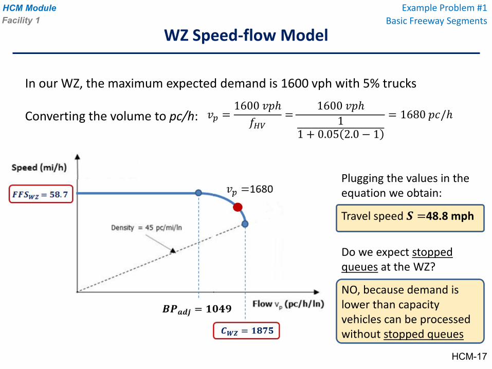
In our WZ, the maximum expected demand is 1600 vph with 5% trucks
Converting the volume to pc/h: 𝑣𝑣𝑝𝑝 =1600 𝑣𝑣𝑣𝑣𝑡
𝑓𝑓𝐻𝐻𝐻𝐻=
1600 𝑣𝑣𝑣𝑣𝑡1
1 + 0.05 2.0 − 1
= 1680 𝑣𝑣𝑠𝑠/𝑡
Plugging the values in the equation we obtain:
Travel speed 𝑳𝑳 =48.8 mph
Do we expect stopped queues at the WZ?
NO, because demand is lower than capacity vehicles can be processed without stopped queues
HCM-17
HCM Module
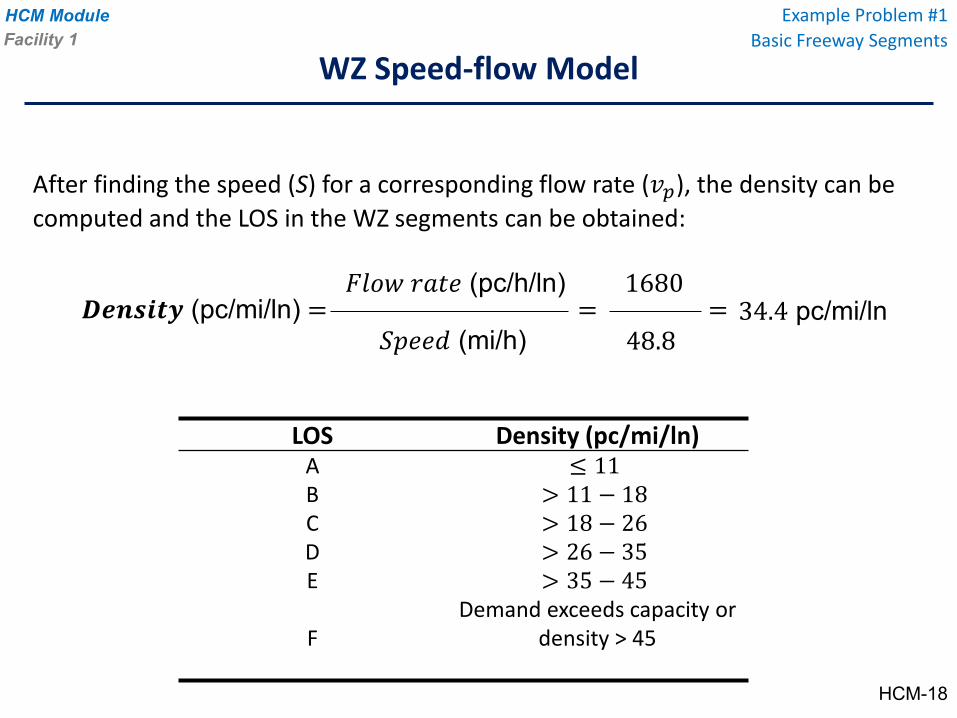
LOS Density (pc/mi/ln)A ≤ 11B > 11 − 18C > 18 − 26D > 26 − 35E > 35 − 45
FDemand exceeds capacity or
density > 45
WZ Speed-flow Model
Example Problem #1Basic Freeway SegmentsFacility 1
After finding the speed (S) for a corresponding flow rate (𝑣𝑣𝑝𝑝), the density can be computed and the LOS in the WZ segments can be obtained:
𝑸𝑸𝑫𝑫𝑫𝑫𝑫𝑫𝑫𝑫𝑫𝑫𝑫𝑫 (pc/mi/ln) = = =𝐹𝐹𝐹𝐹𝐹𝐹𝐹𝐹 𝑟𝑟𝑟𝑟𝑓𝑓𝑠𝑠 (pc/h/ln)
𝑊𝑊𝑣𝑣𝑠𝑠𝑠𝑠𝑆𝑆 (mi/h)
1680
48.834.4 pc/mi/ln
HCM-18
HCM Module
Group Discussion about HCM WZ capacity & speed Basic Freeway Segments
Facility 1
1. Is capacity of a WZ at night higher (lower) than its capacity in day time?
By how much?
2. Is capacity of a WZ with concrete barriers higher(lower) than its capacity with non-concrete barrier (cone, drums, ...)?
By how much?
3. Is capacity an urban WZ higher(lower) than rural WZ?
By how much?
HCM-19
HCM Module
Group Discussion about HCM WZ capacity & speed Basic Freeway Segments
Facility 1
4. Does HCM consider effects of work intensity on WZ capacity?
5. Does HCM consider WZ speed limit on WZ capacity?
6. Does HCM consider effects of lane width on WZ capacity?
7. Does HCM consider effects of lane width on WZ speed?
8. Does HCM consider effects of lateral clearance on WZ capacity?
9. Does HCM consider effects of lateral clearance on WZ speed?
HCM-20
HCM Module
(according to HCM)
• The methodology estimates the capacity, speed, and density of the WZ segment, given the segment’s traffic demand and characteristics. However, “Alternative tools offer additional performance measures, including
• delay,• stops,• queue length,• fuel consumption,• pollution, • and operating costs.”
Limitations of the Speed-Flow MethodologyFacility 1
Basic Freeway Segments
HCM-21
HCM Module
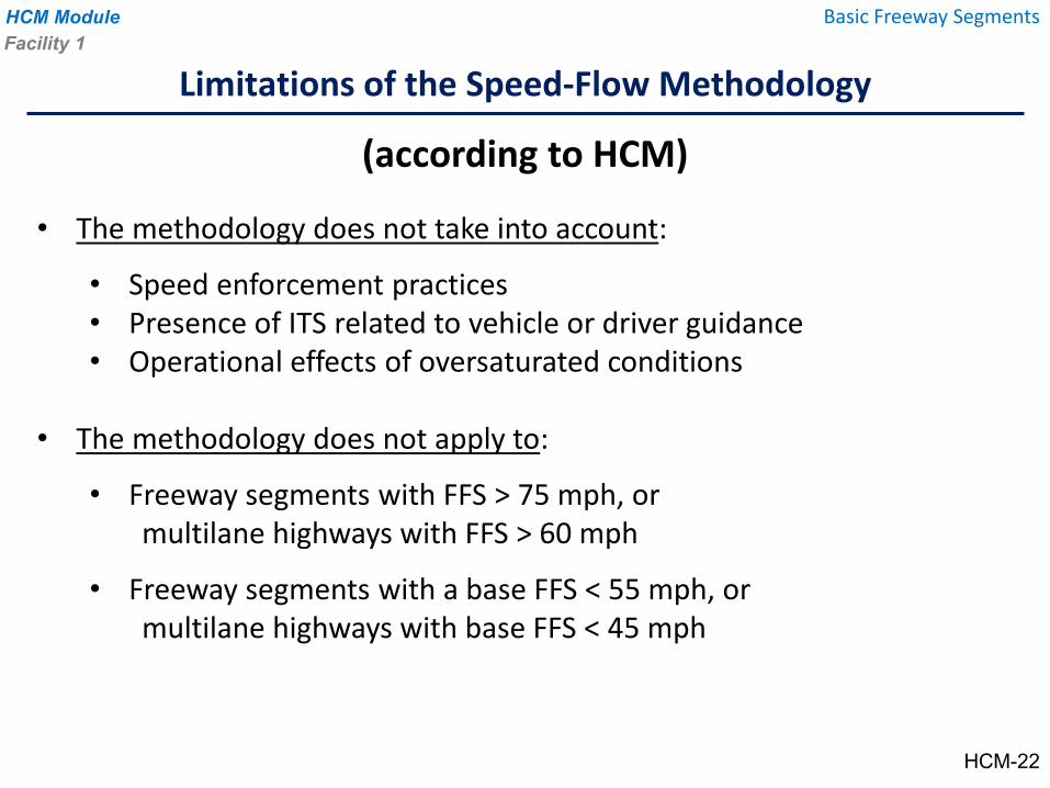
• The methodology does not take into account:
• Speed enforcement practices• Presence of ITS related to vehicle or driver guidance• Operational effects of oversaturated conditions
• The methodology does not apply to:
• Freeway segments with FFS > 75 mph, ormultilane highways with FFS > 60 mph
• Freeway segments with a base FFS < 55 mph, ormultilane highways with base FFS < 45 mph
(according to HCM)
Limitations of the Speed-Flow MethodologyFacility 1
Basic Freeway Segments
HCM-22
HCM Module
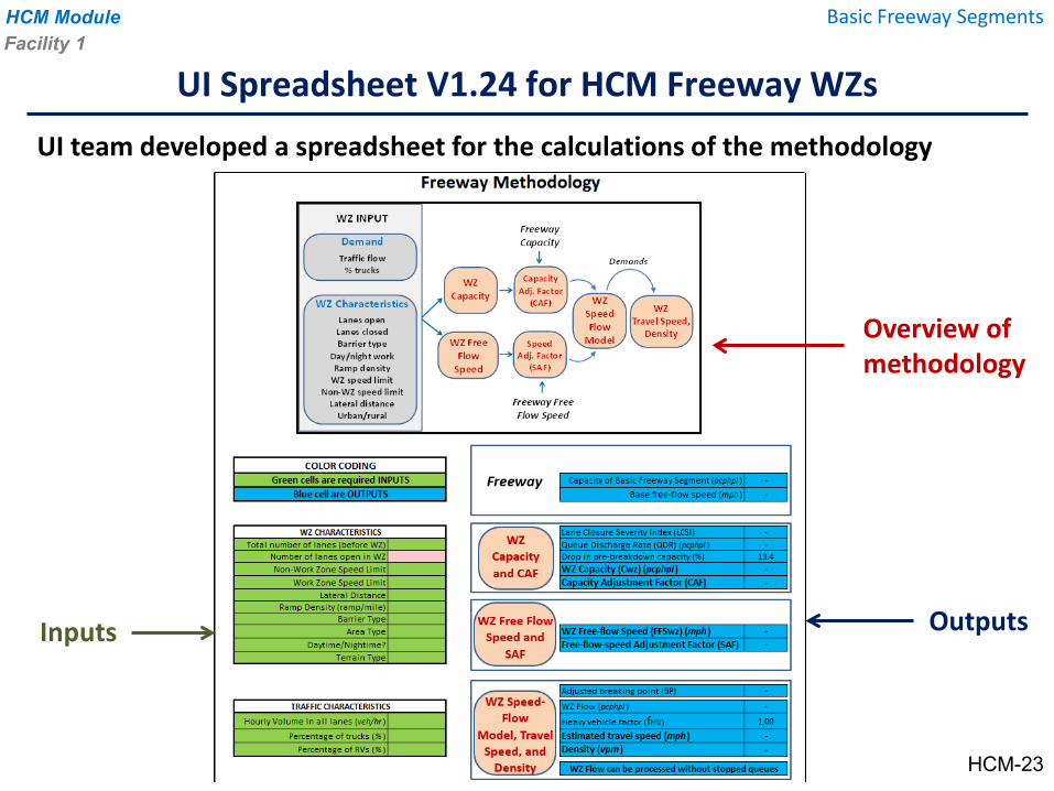
UI team developed a spreadsheet for the calculations of the methodology
UI Spreadsheet V1.24 for HCM Freeway WZsFacility 1
Basic Freeway Segments
Overview of methodology
OutputsInputs
HCM-23
HCM Module
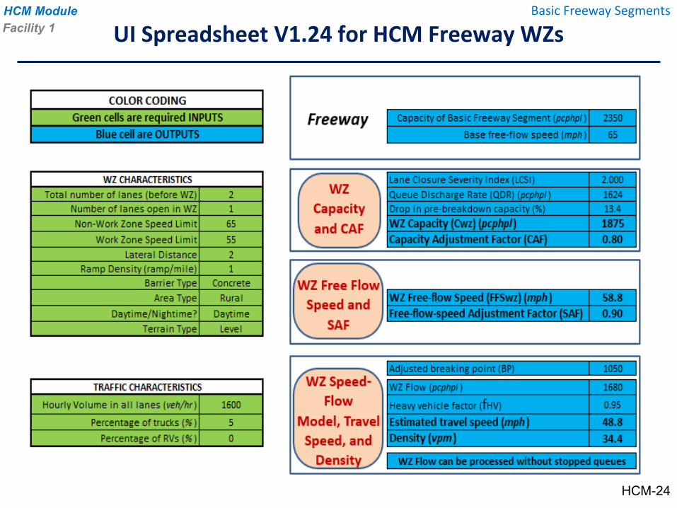
UI Spreadsheet V1.24 for HCM Freeway WZsFacility 1Basic Freeway Segments
HCM-24
HCM Module
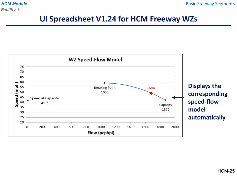
UI Spreadsheet V1.24 for HCM Freeway WZsFacility 1
Basic Freeway Segments
Displays the corresponding speed-flow model automatically
HCM-25
HCM Module
Facility 2: WZ at Intersections
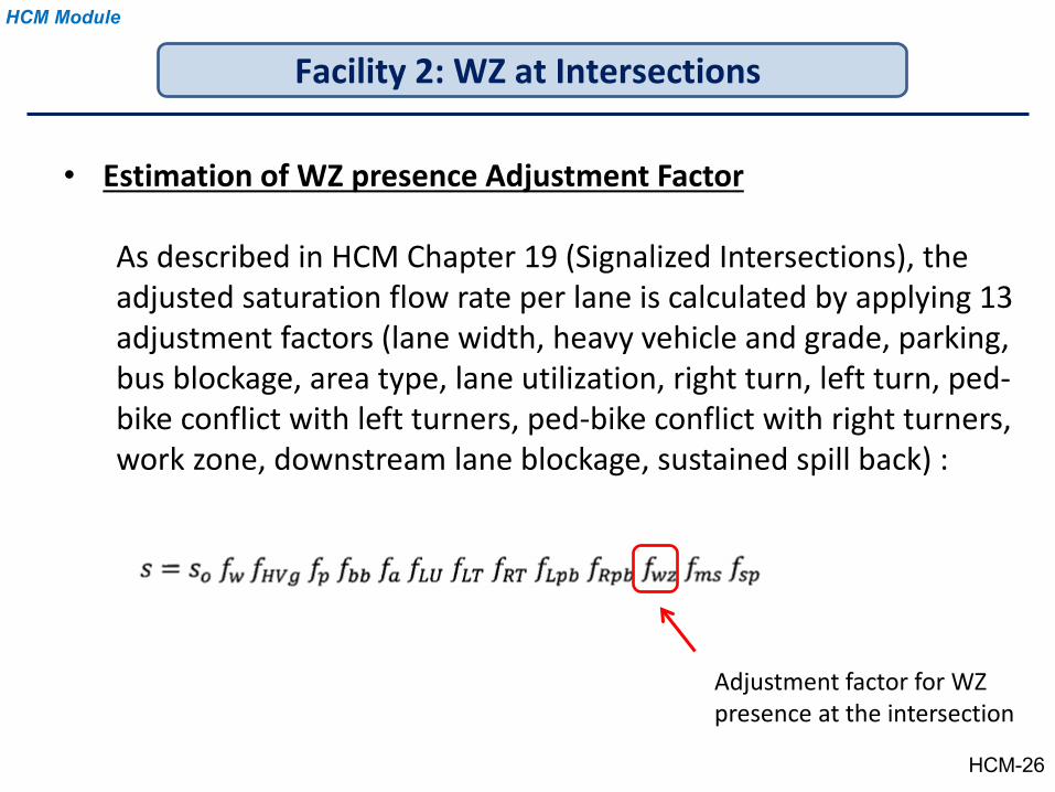
• Estimation of WZ presence Adjustment Factor
As described in HCM Chapter 19 (Signalized Intersections), the adjusted saturation flow rate per lane is calculated by applying 13 adjustment factors (lane width, heavy vehicle and grade, parking, bus blockage, area type, lane utilization, right turn, left turn, ped-bike conflict with left turners, ped-bike conflict with right turners, work zone, downstream lane blockage, sustained spill back) :
Adjustment factor for WZ presence at the intersection
HCM-26
HCM Module
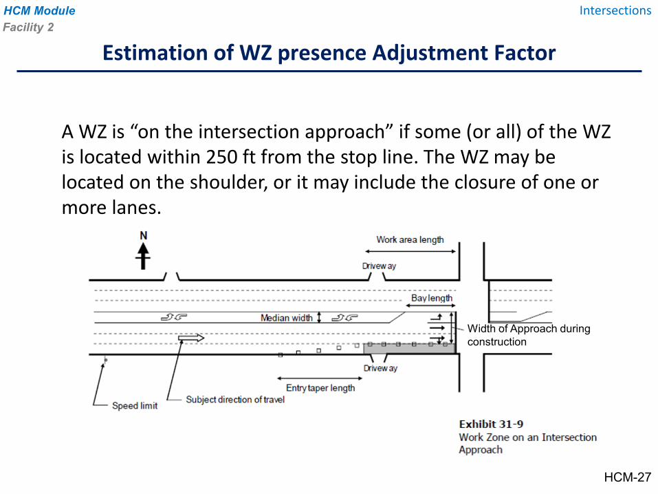
Estimation of WZ presence Adjustment Factor
A WZ is “on the intersection approach” if some (or all) of the WZ is located within 250 ft from the stop line. The WZ may be located on the shoulder, or it may include the closure of one or more lanes.
Facility 2Intersections
HCM-27
Width of Approach during construction
HCM Module
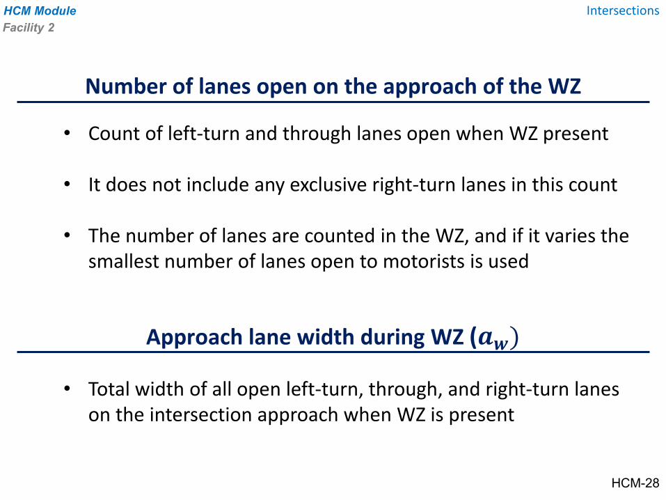
• Count of left-turn and through lanes open when WZ present
• It does not include any exclusive right-turn lanes in this count
• The number of lanes are counted in the WZ, and if it varies the smallest number of lanes open to motorists is used
• Total width of all open left-turn, through, and right-turn lanes on the intersection approach when WZ is present
Number of lanes open on the approach of the WZ
Facility 2Intersections
Approach lane width during WZ (𝒂𝒂𝒘𝒘)
HCM-28
HCM Module
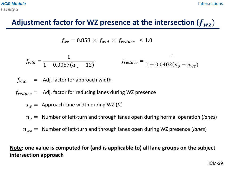
𝑓𝑓𝑤𝑤𝑤𝑤 = 0.858 × 𝑓𝑓𝑤𝑤𝑤𝑤𝑎𝑎 × 𝑓𝑓𝑟𝑟𝑟𝑟𝑎𝑎𝑟𝑟𝑟𝑟𝑟𝑟 ≤ 1.0
𝑓𝑓𝑤𝑤𝑤𝑤𝑎𝑎 =1
1 − 0.0057 𝑟𝑟𝑤𝑤 − 12𝑓𝑓𝑟𝑟𝑟𝑟𝑎𝑎𝑟𝑟𝑟𝑟𝑟𝑟 =
11 + 0.0402 𝑡𝑡𝑜𝑜 − 𝑡𝑡𝑤𝑤𝑤𝑤
𝑓𝑓𝑤𝑤𝑤𝑤𝑎𝑎 = Adj. factor for approach width
𝑓𝑓𝑟𝑟𝑟𝑟𝑎𝑎𝑟𝑟𝑟𝑟𝑟𝑟 = Adj. factor for reducing lanes during WZ presence
𝑟𝑟𝑤𝑤 = Approach lane width during WZ (ft)
𝑡𝑡𝑜𝑜 = Number of left-turn and through lanes open during normal operation (lanes)
𝑡𝑡𝑤𝑤𝑤𝑤 = Number of left-turn and through lanes open during WZ presence (lanes)
Note: one value is computed for (and is applicable to) all lane groups on the subject intersection approach
Adjustment factor for WZ presence at the intersection (𝒇𝒇𝒘𝒘𝒘𝒘)
Facility 2Intersections
HCM-29
HCM Module
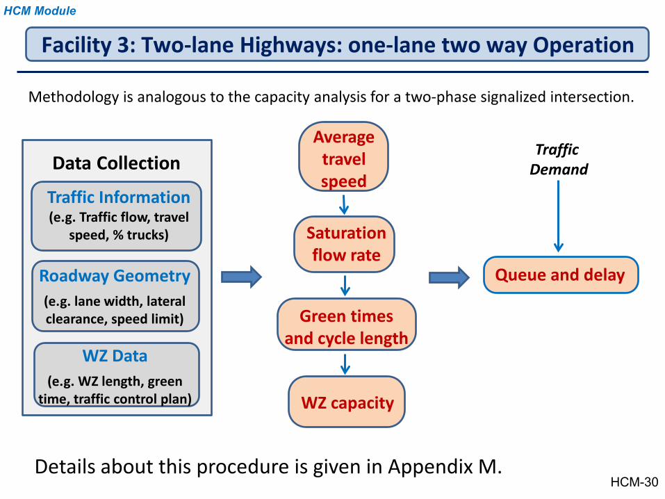
Facility 3: Two-lane Highways: one-lane two way Operation
Methodology is analogous to the capacity analysis for a two-phase signalized intersection.
Traffic Information(e.g. Traffic flow, travel
speed, % trucks)
Roadway Geometry(e.g. lane width, lateral clearance, speed limit)
Average travel speed
Data Collection
WZ Data(e.g. WZ length, green
time, traffic control plan)
Saturation flow rate
Green times and cycle length
WZ capacity
Queue and delay
Traffic Demand
HCM-30Details about this procedure is given in Appendix M.
HCM Module
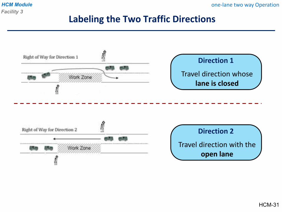
Labeling the Two Traffic Directions
Direction 1
Travel direction whose lane is closed
Direction 2
Travel direction with the open lane
Facility 3one-lane two way Operation
HCM-31
HCM Module
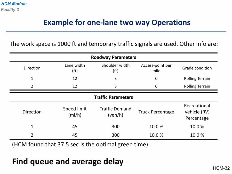
The work space is 1000 ft and temporary traffic signals are used. Other info are:
(HCM found that 37.5 sec is the optimal green time).
Find queue and average delay
Example for one-lane two way Operations
Facility 3
HCM-32
Roadway Parameters
Direction Lane width(ft)
Shoulder width(ft)
Access-point per mile Grade condition
1 12 3 0 Rolling Terrain
2 12 3 0 Rolling Terrain
Traffic Parameters
Direction Speed limit(mi/h)
Traffic Demand(veh/h) Truck Percentage
Recreational Vehicle (RV) Percentage
1 45 300 10.0 % 10.0 %
2 45 300 10.0 % 10.0 %
HCM Module
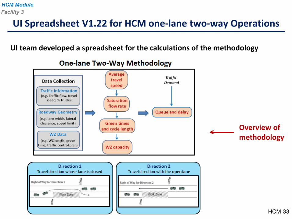
UI team developed a spreadsheet for the calculations of the methodology
UI Spreadsheet V1.22 for HCM one-lane two-way OperationsFacility 3
Overview of methodology
HCM-33
HCM Module
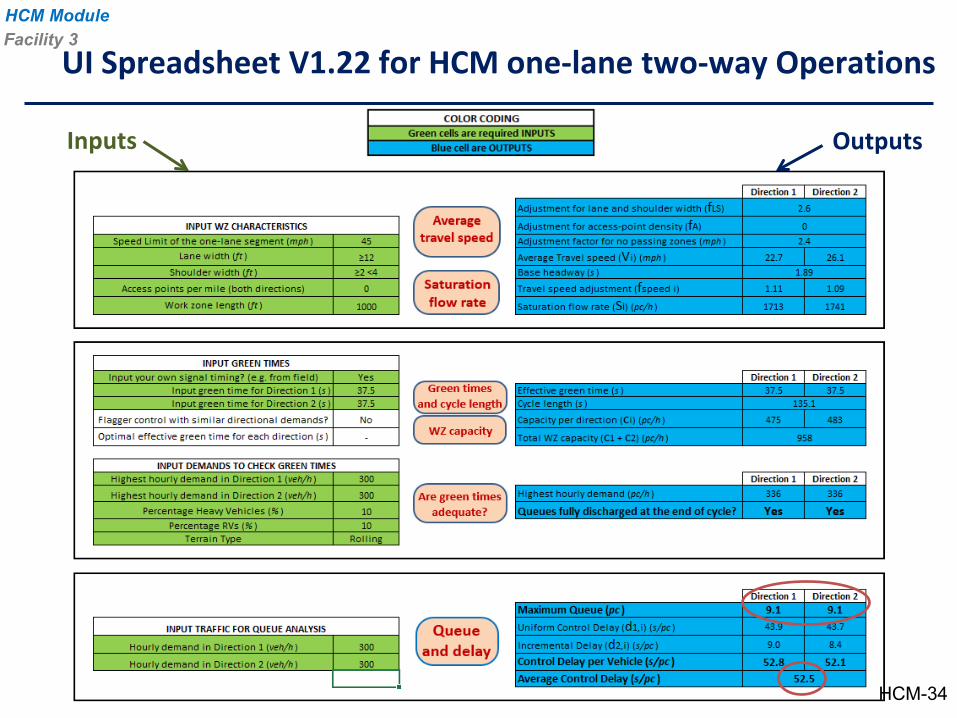
UI Spreadsheet V1.22 for HCM one-lane two-way OperationsFacility 3
OutputsInputs
HCM-34
HCM Module
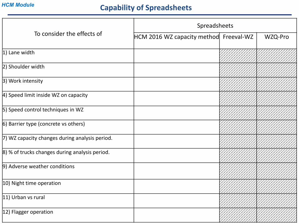
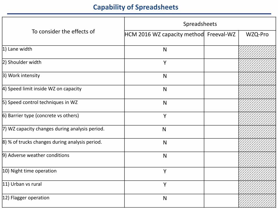
Capability of SpreadsheetsHCM Module
To consider the effects of Spreadsheets
HCM 2016 WZ capacity method Freeval-WZ WZQ-Pro
1) Lane width
2) Shoulder width
3) Work intensity
4) Speed limit inside WZ on capacity
5) Speed control techniques in WZ
6) Barrier type (concrete vs others)
7) WZ capacity changes during analysis period.
8) % of trucks changes during analysis period.
9) Adverse weather conditions
10) Night time operation
11) Urban vs rural
12) Flagger operation
FREEVAL-WZ MODULE
Planning-Level Assessment of FreewayWork Zone Impacts
FREEVAL-WZ Tool
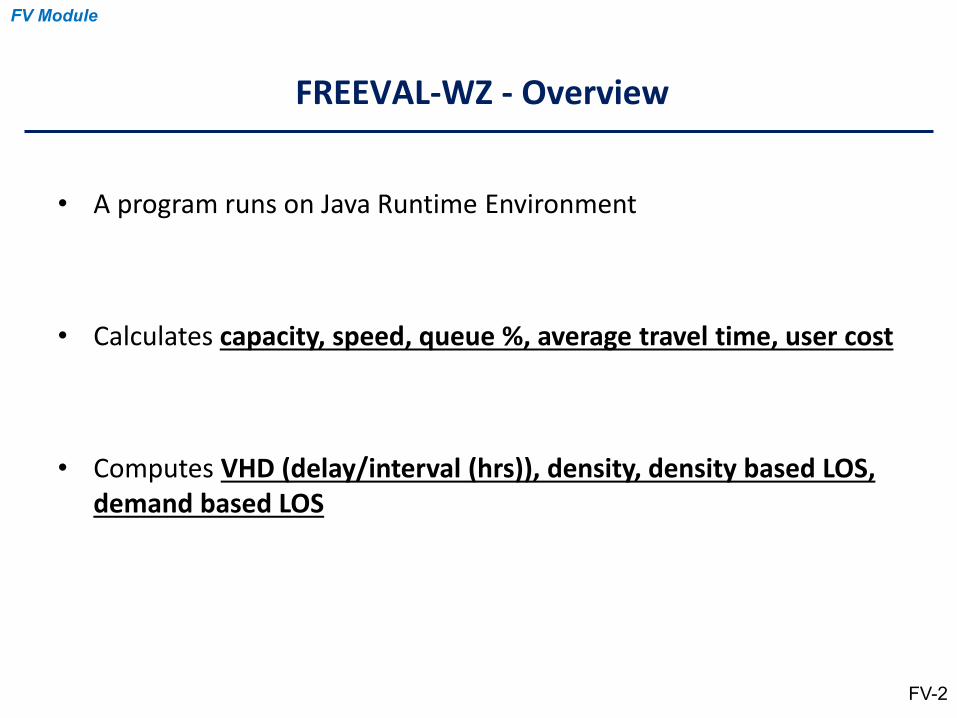
• A program runs on Java Runtime Environment
• Calculates capacity, speed, queue %, average travel time, user cost
• Computes VHD (delay/interval (hrs)), density, density based LOS, demand based LOS
FREEVAL-WZ - Overview
FV-2
FV Module
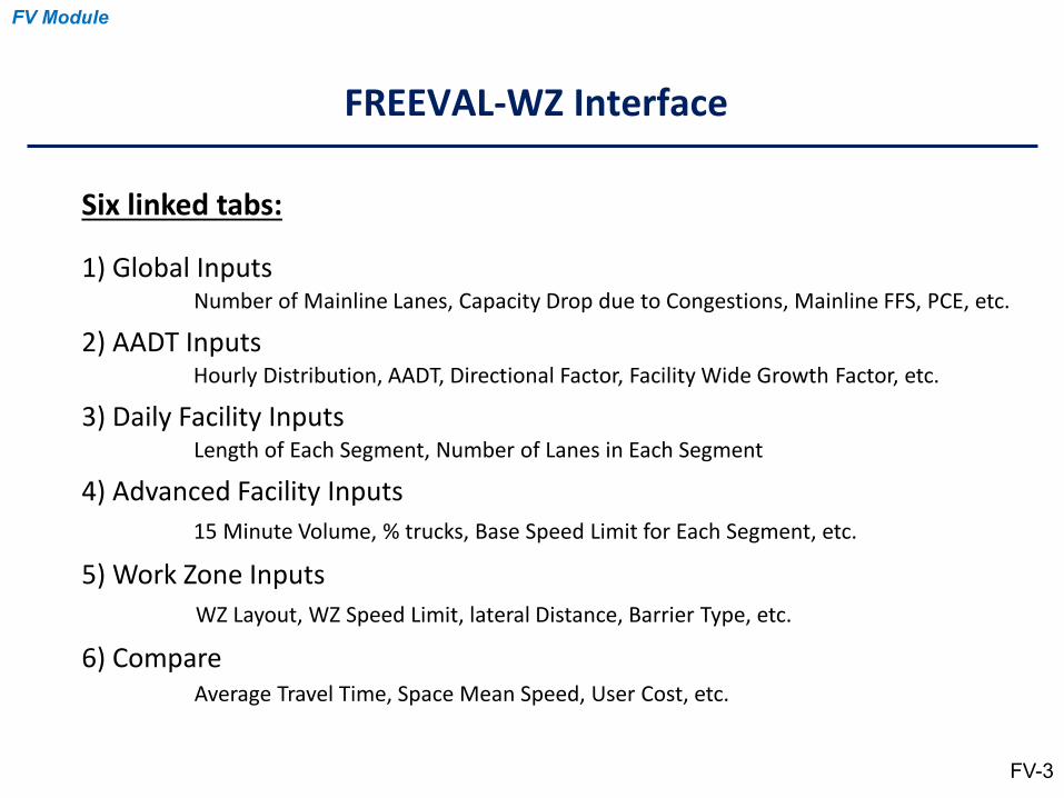
Six linked tabs:
1) Global InputsNumber of Mainline Lanes, Capacity Drop due to Congestions, Mainline FFS, PCE, etc.
2) AADT InputsHourly Distribution, AADT, Directional Factor, Facility Wide Growth Factor, etc.
3) Daily Facility InputsLength of Each Segment, Number of Lanes in Each Segment
4) Advanced Facility Inputs15 Minute Volume, % trucks, Base Speed Limit for Each Segment, etc.
5) Work Zone InputsWZ Layout, WZ Speed Limit, lateral Distance, Barrier Type, etc.
6) CompareAverage Travel Time, Space Mean Speed, User Cost, etc.
FREEVAL-WZ Interface
FV-3
FV Module
• FREEVAL is a macroscopic (not micro simulation) model for analyzing freeway facilities based on HCM methods
• It analyzes freeway facilities using HCM procedures
• Facilities may have multiple segments along the freeway
• Uses distribution of ADT is 24 hours
• Current release is developed in Java
What is FREEVAL ?
FV Module
FV-4
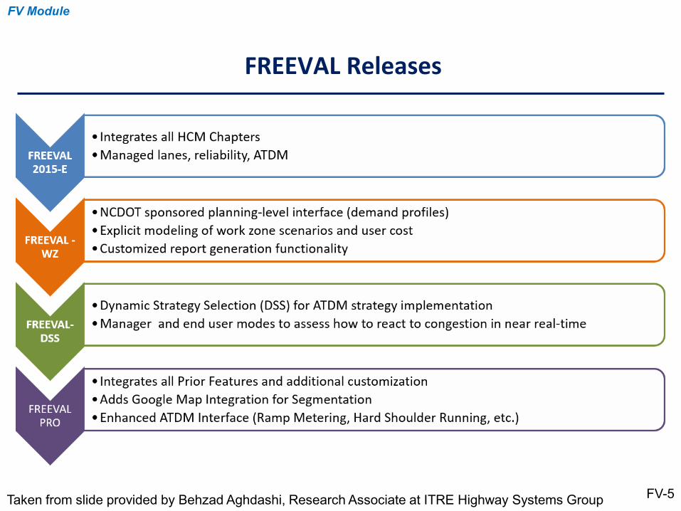
FREEVAL Releases
FV Module
FV-5Taken from slide provided by Behzad Aghdashi, Research Associate at ITRE Highway Systems Group
• Based on FREEVAL-2015e computational engine
• Volume data entered as AADT
• Hourly volumes are computed using a 24 distribution
• Gives defaults 24 hour distributions for 3 volume profiles
– (Unimodal, Bimodal-AM Peak, and Bimodal-PM Peak)
• Multiple scenarios can be included in an one run
FREEVAL-WZ
FV Module
FV-6
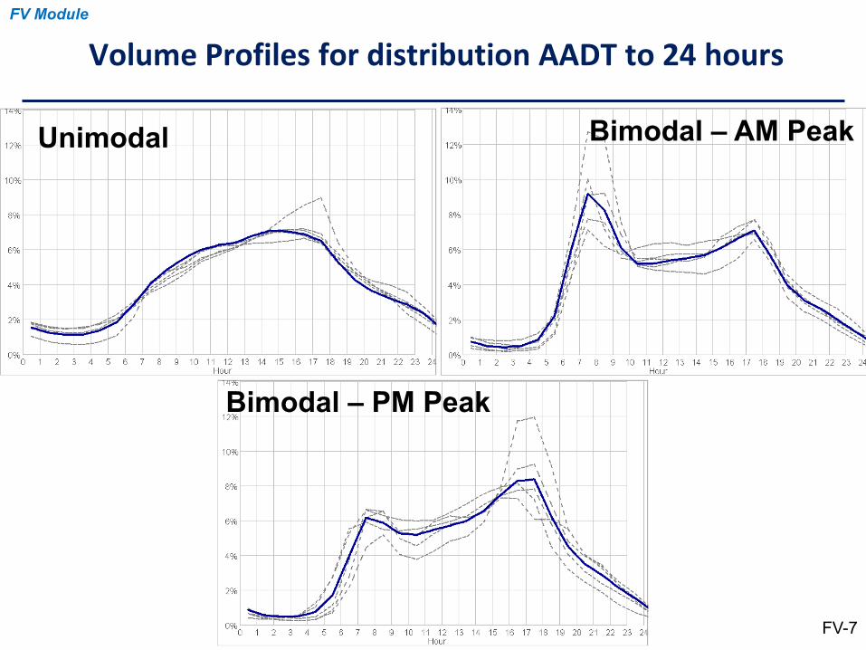
Volume Profiles for distribution AADT to 24 hours FV Module
FV-7
Unimodal Bimodal – AM Peak
Bimodal – PM Peak
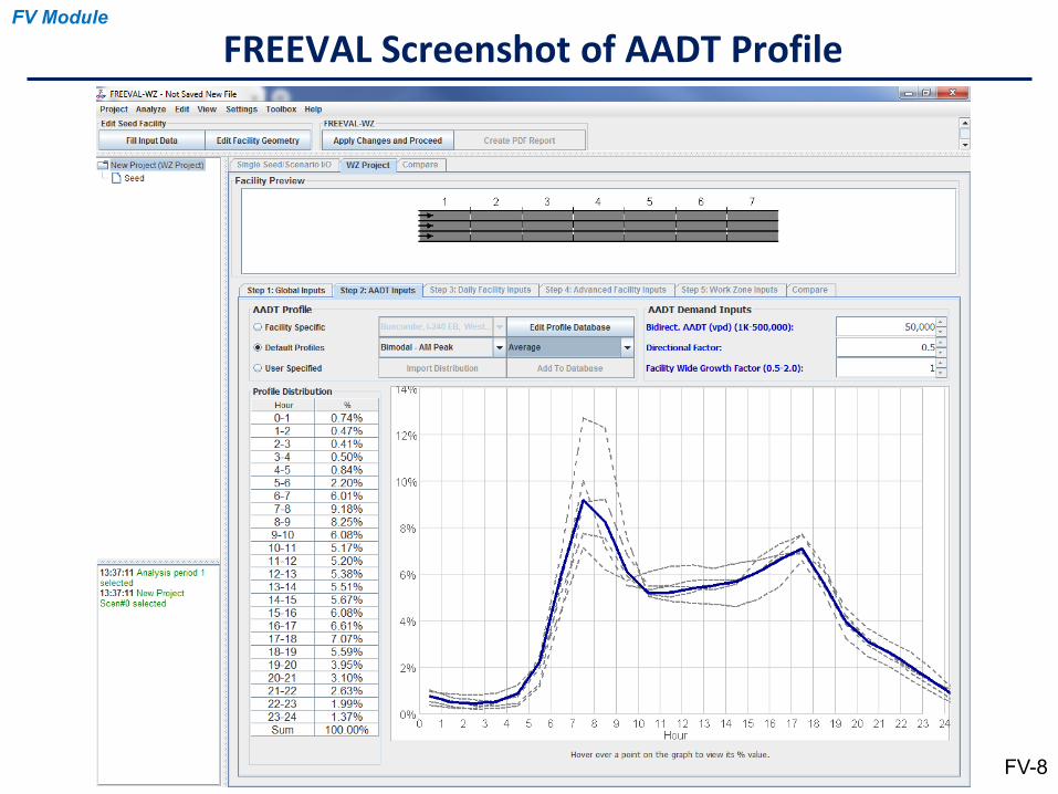
FREEVAL Screenshot of AADT ProfileFV Module
FV-8
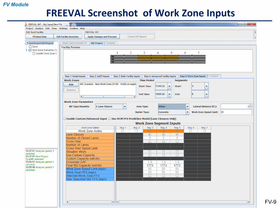
FREEVAL Screenshot of Work Zone InputsFV Module
FV-9
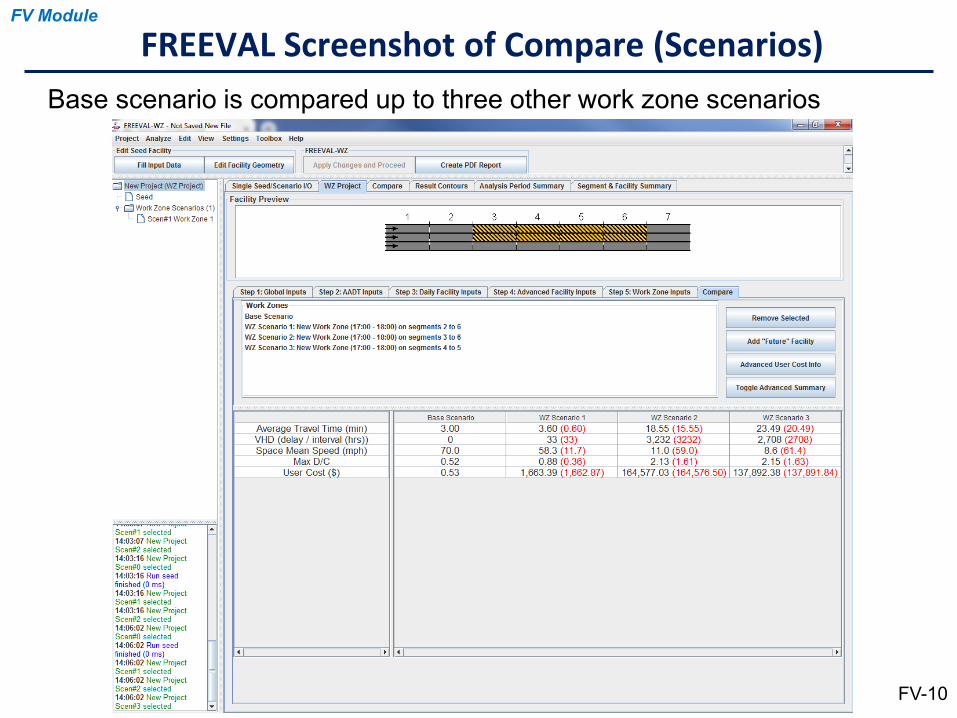
FREEVAL Screenshot of Compare (Scenarios)FV Module
FV-10
Base scenario is compared up to three other work zone scenarios
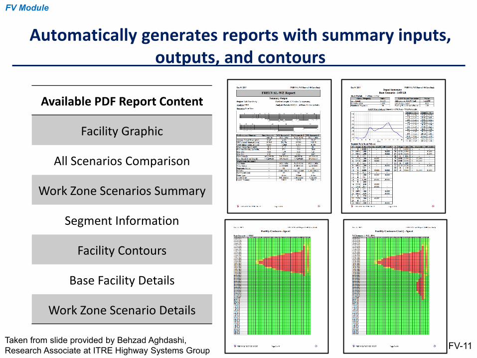
Automatically generates reports with summary inputs, outputs, and contours
FV Module
FV-11
Available PDF Report Content
Facility Graphic
All Scenarios Comparison
Work Zone Scenarios Summary
Segment Information
Facility Contours
Base Facility Details
Work Zone Scenario Details
Taken from slide provided by Behzad Aghdashi, Research Associate at ITRE Highway Systems Group
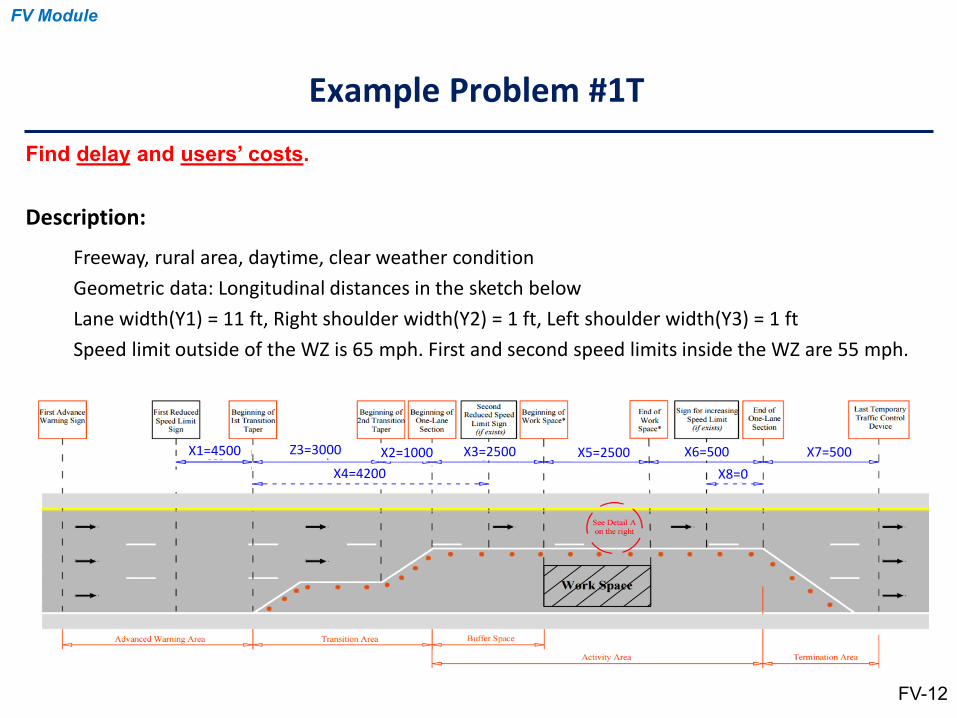
Description:
Freeway, rural area, daytime, clear weather conditionGeometric data: Longitudinal distances in the sketch belowLane width(Y1) = 11 ft, Right shoulder width(Y2) = 1 ft, Left shoulder width(Y3) = 1 ftSpeed limit outside of the WZ is 65 mph. First and second speed limits inside the WZ are 55 mph.
Example Problem #1T
Find delay and users’ costs.
FV Module
FV-12
X4=4200X3=2500 X5=2500 X6=500
X8=0X7=500X2=1000Z3=3000X1=4500
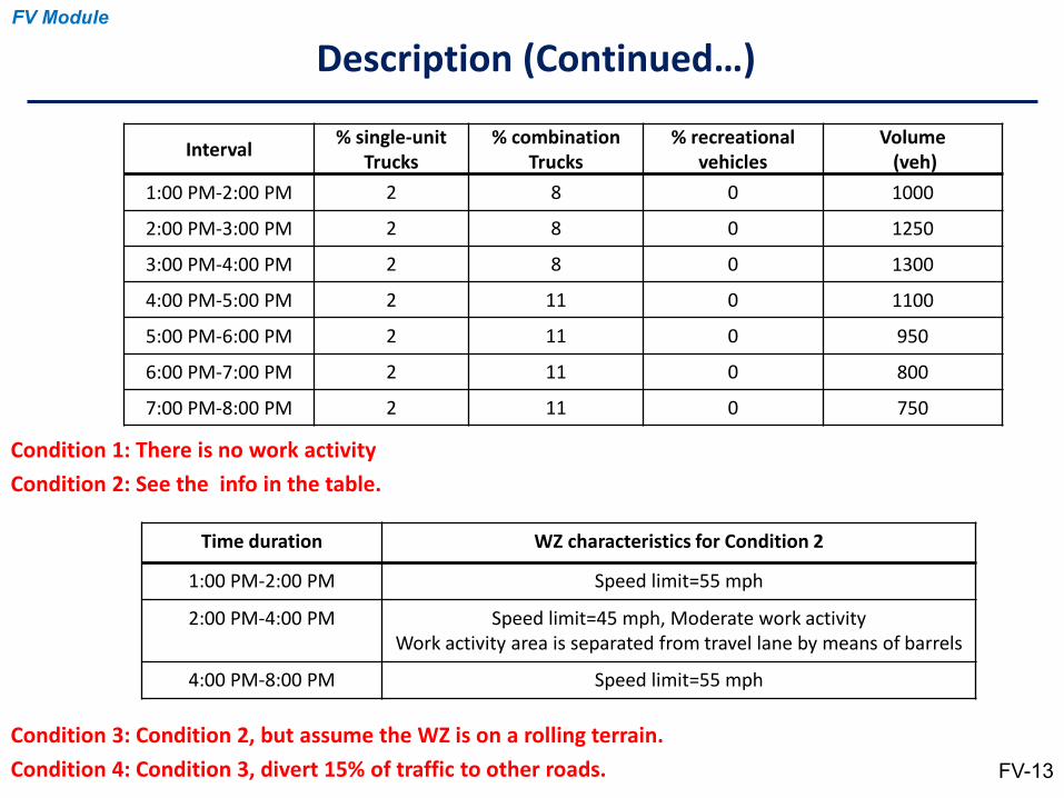
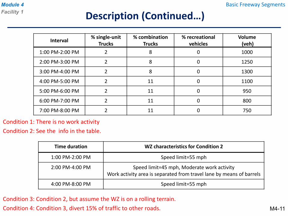
Condition 1: There is no work activity Condition 2: See the info in the table.
Condition 3: Condition 2, but assume the WZ is on a rolling terrain.Condition 4: Condition 3, divert 15% of traffic to other roads.
Description (Continued…)FV Module
FV-13
Interval % single-unitTrucks
% combination Trucks
% recreational vehicles
Volume(veh)
1:00 PM-2:00 PM 2 8 0 1000
2:00 PM-3:00 PM 2 8 0 1250
3:00 PM-4:00 PM 2 8 0 1300
4:00 PM-5:00 PM 2 11 0 1100
5:00 PM-6:00 PM 2 11 0 950
6:00 PM-7:00 PM 2 11 0 800
7:00 PM-8:00 PM 2 11 0 750
Time duration WZ characteristics for Condition 2
1:00 PM-2:00 PM Speed limit=55 mph
2:00 PM-4:00 PM Speed limit=45 mph, Moderate work activity Work activity area is separated from travel lane by means of barrels
4:00 PM-8:00 PM Speed limit=55 mph
X4=4200X3=2500 X5=2500 X6=500
X8=0X7=500X2=1000Z3=3000X1=4500
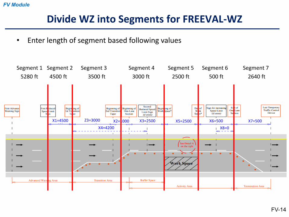
Divide WZ into Segments for FREEVAL-WZ
• Enter length of segment based following values
Segment 1 Segment 2 Segment 3 Segment 4 Segment 5 Segment 6 Segment 75280 ft 4500 ft 3500 ft 3000 ft 2500 ft 500 ft 2640 ft
FV-14
FV Module
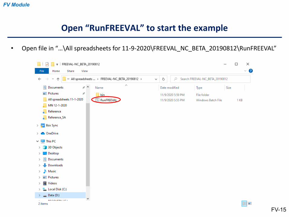
• Open file in “…\All spreadsheets for 11-9-2020\FREEVAL_NC_BETA_20190812\RunFREEVAL”
Open “RunFREEVAL” to start the example
FV Module
FV-15
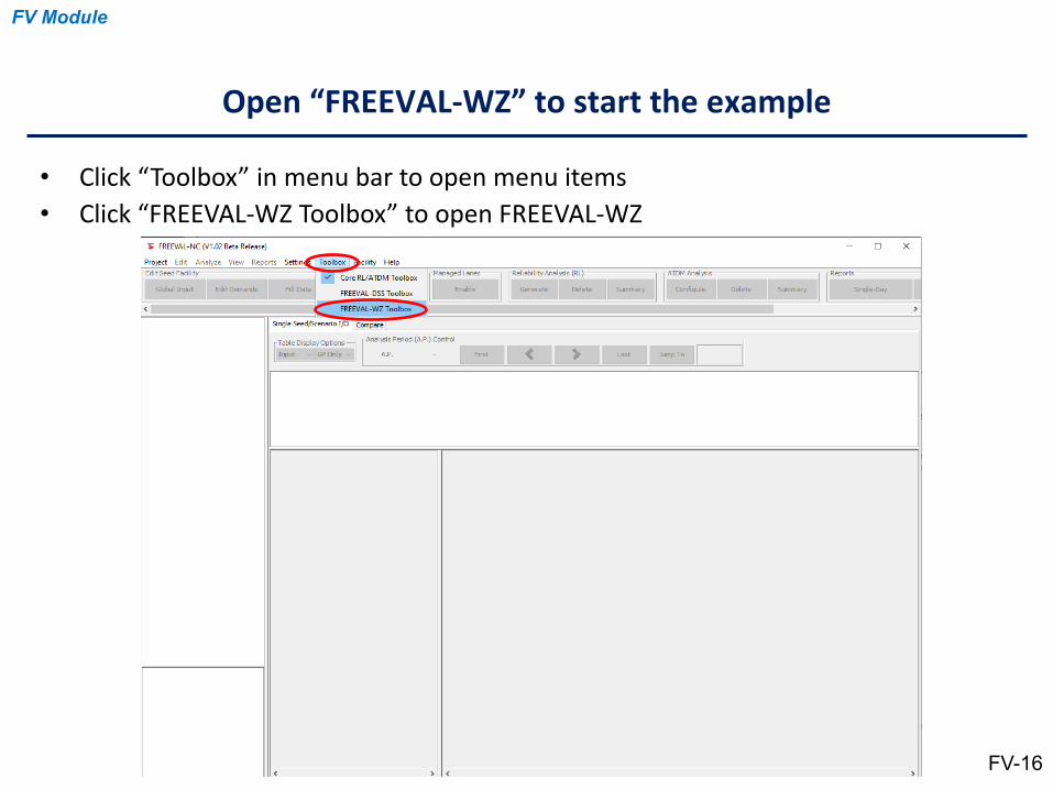
• Click “Toolbox” in menu bar to open menu items• Click “FREEVAL-WZ Toolbox” to open FREEVAL-WZ
Open “FREEVAL-WZ” to start the example
FV Module
FV-16
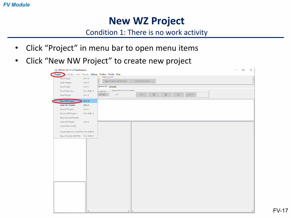
• Click “Project” in menu bar to open menu items• Click “New NW Project” to create new project
New WZ ProjectCondition 1: There is no work activity
FV-17
FV Module
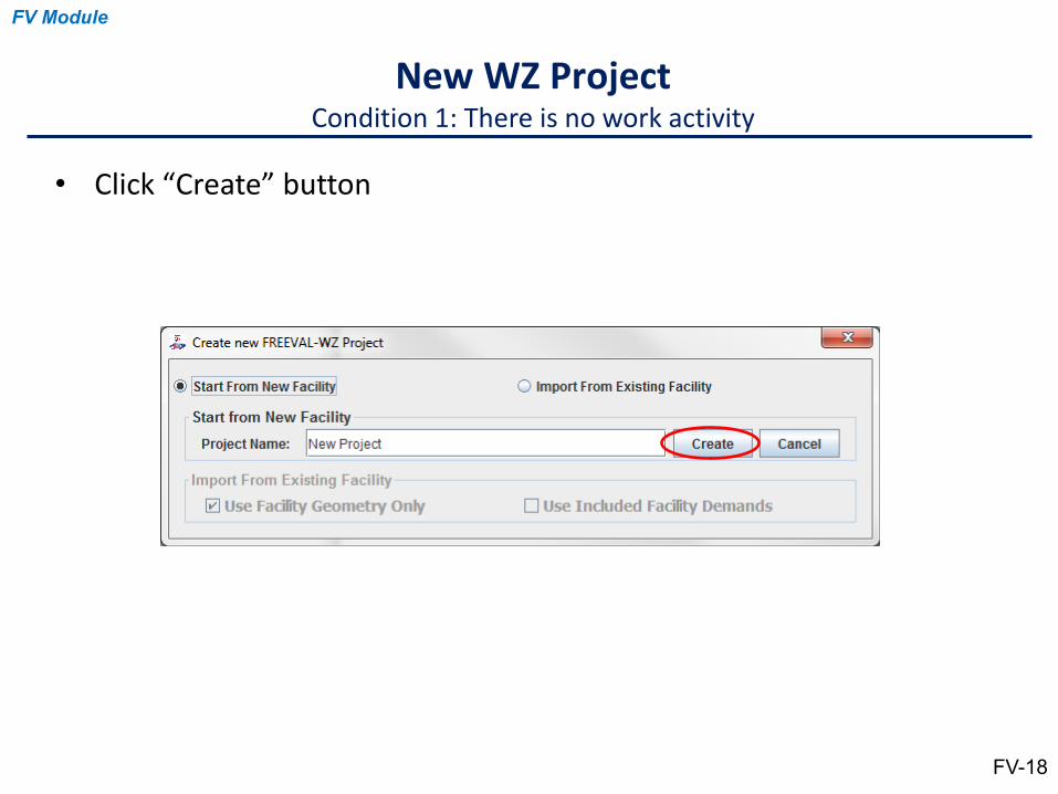
• Click “Create” button
New WZ ProjectCondition 1: There is no work activity
FV-18
FV Module
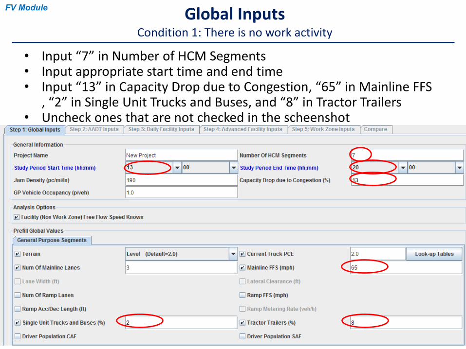
• Input “7” in Number of HCM Segments• Input appropriate start time and end time• Input “13” in Capacity Drop due to Congestion, “65” in Mainline FFS
, “2” in Single Unit Trucks and Buses, and “8” in Tractor Trailers• Uncheck ones that are not checked in the scheenshot
Global InputsCondition 1: There is no work activity
FV Module
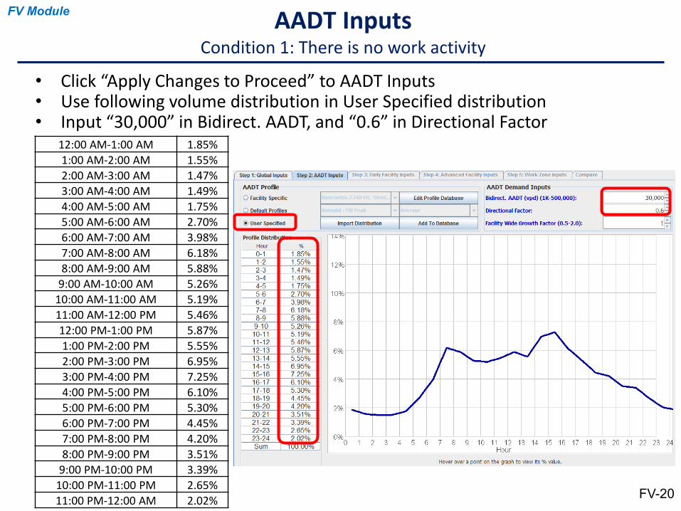
• Click “Apply Changes to Proceed” to AADT Inputs• Use following volume distribution in User Specified distribution• Input “30,000” in Bidirect. AADT, and “0.6” in Directional Factor
AADT InputsCondition 1: There is no work activity
12:00 AM-1:00 AM 1.85%1:00 AM-2:00 AM 1.55%2:00 AM-3:00 AM 1.47%3:00 AM-4:00 AM 1.49%4:00 AM-5:00 AM 1.75%5:00 AM-6:00 AM 2.70%6:00 AM-7:00 AM 3.98%7:00 AM-8:00 AM 6.18%8:00 AM-9:00 AM 5.88%
9:00 AM-10:00 AM 5.26%10:00 AM-11:00 AM 5.19%11:00 AM-12:00 PM 5.46%12:00 PM-1:00 PM 5.87%1:00 PM-2:00 PM 5.55%2:00 PM-3:00 PM 6.95%3:00 PM-4:00 PM 7.25%4:00 PM-5:00 PM 6.10%5:00 PM-6:00 PM 5.30%6:00 PM-7:00 PM 4.45%7:00 PM-8:00 PM 4.20%8:00 PM-9:00 PM 3.51%
9:00 PM-10:00 PM 3.39%10:00 PM-11:00 PM 2.65%11:00 PM-12:00 AM 2.02% FV-20
FV Module
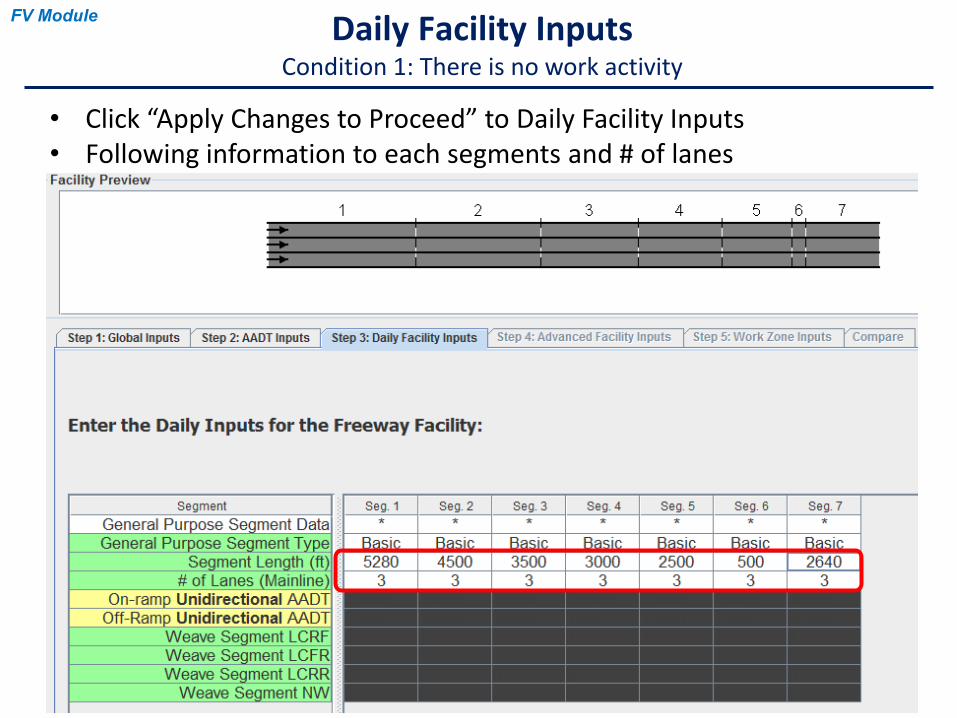
• Click “Apply Changes to Proceed” to Daily Facility Inputs• Following information to each segments and # of lanes
Daily Facility InputsCondition 1: There is no work activity
FV Module
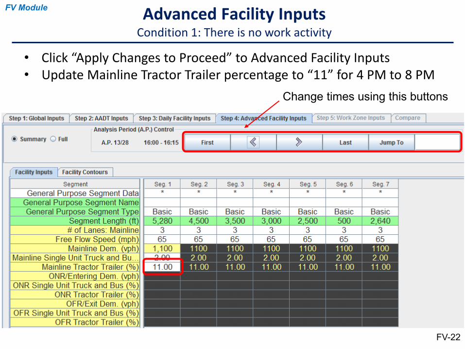
• Click “Apply Changes to Proceed” to Advanced Facility Inputs• Update Mainline Tractor Trailer percentage to “11” for 4 PM to 8 PM
Advanced Facility InputsCondition 1: There is no work activity
Change times using this buttons
FV-22
FV Module
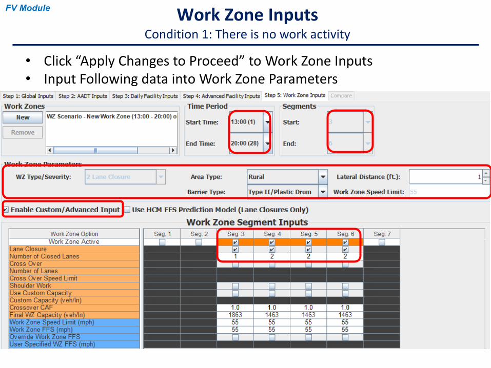
• Click “Apply Changes to Proceed” to Work Zone Inputs• Input Following data into Work Zone Parameters
Work Zone InputsCondition 1: There is no work activity
FV Module
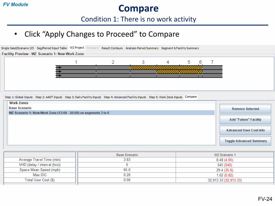
• Click “Apply Changes to Proceed” to Compare
CompareCondition 1: There is no work activity
FV-24
FV Module
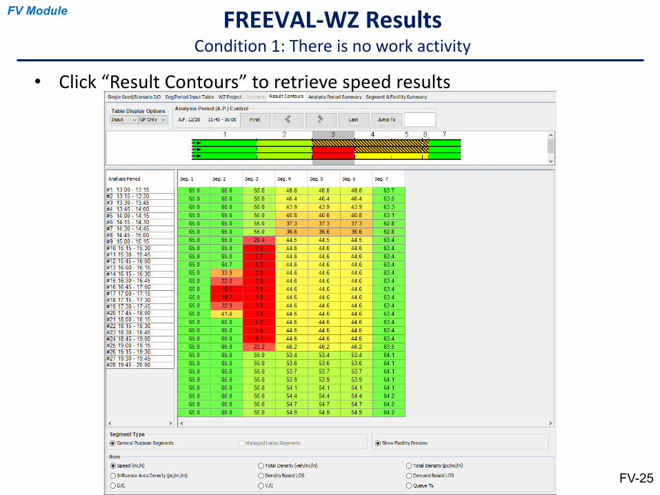
• Click “Result Contours” to retrieve speed results
FREEVAL-WZ ResultsCondition 1: There is no work activity
FV-25
FV Module
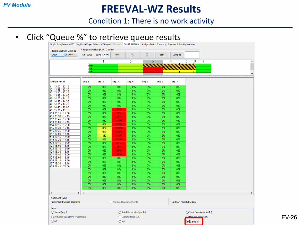
• Click “Queue %” to retrieve queue results
FREEVAL-WZ ResultsCondition 1: There is no work activity
FV-26
FV Module
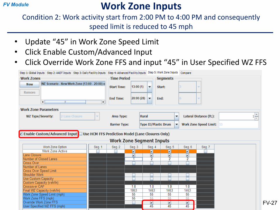
• Update “45” in Work Zone Speed Limit• Click Enable Custom/Advanced Input• Click Override Work Zone FFS and input “45” in User Specified WZ FFS
Work Zone InputsCondition 2: Work activity start from 2:00 PM to 4:00 PM and consequently
speed limit is reduced to 45 mph
FV-27
FV Module
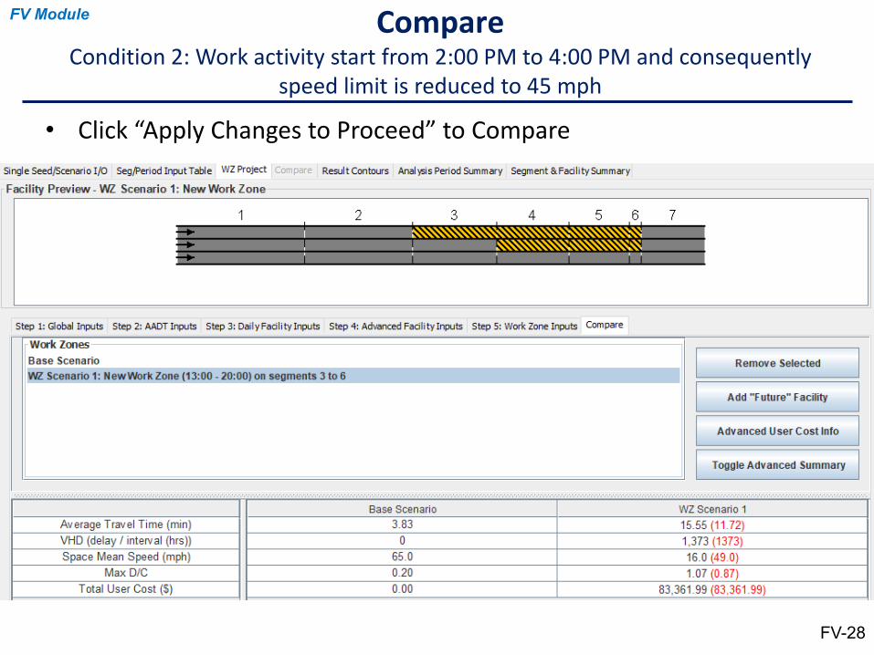
• Click “Apply Changes to Proceed” to Compare
CompareCondition 2: Work activity start from 2:00 PM to 4:00 PM and consequently
speed limit is reduced to 45 mph
FV-28
FV Module
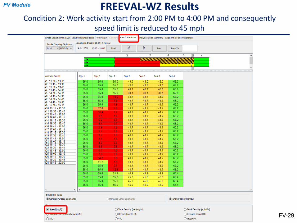
FREEVAL-WZ ResultsCondition 2: Work activity start from 2:00 PM to 4:00 PM and consequently
speed limit is reduced to 45 mph
FV-29
FV Module
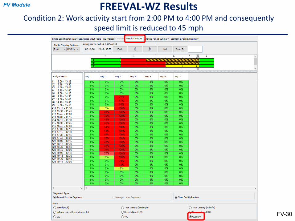
FREEVAL-WZ ResultsCondition 2: Work activity start from 2:00 PM to 4:00 PM and consequently
speed limit is reduced to 45 mph
FV-30
FV Module
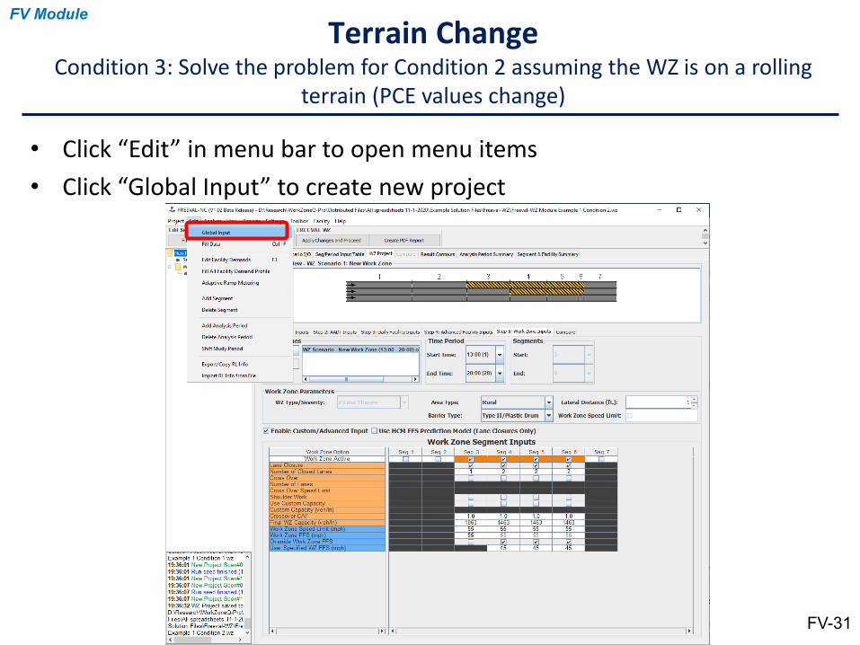
• Click “Edit” in menu bar to open menu items• Click “Global Input” to create new project
Terrain ChangeCondition 3: Solve the problem for Condition 2 assuming the WZ is on a rolling
terrain (PCE values change)
FV-31
FV Module
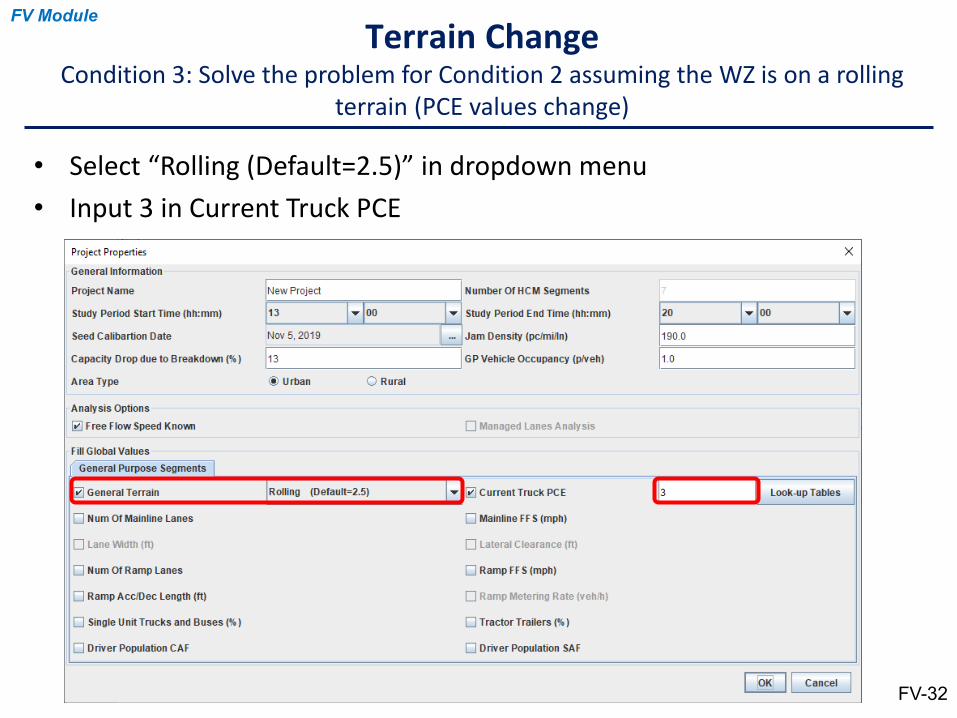
• Select “Rolling (Default=2.5)” in dropdown menu• Input 3 in Current Truck PCE
Terrain ChangeCondition 3: Solve the problem for Condition 2 assuming the WZ is on a rolling
terrain (PCE values change)
FV-32
FV Module
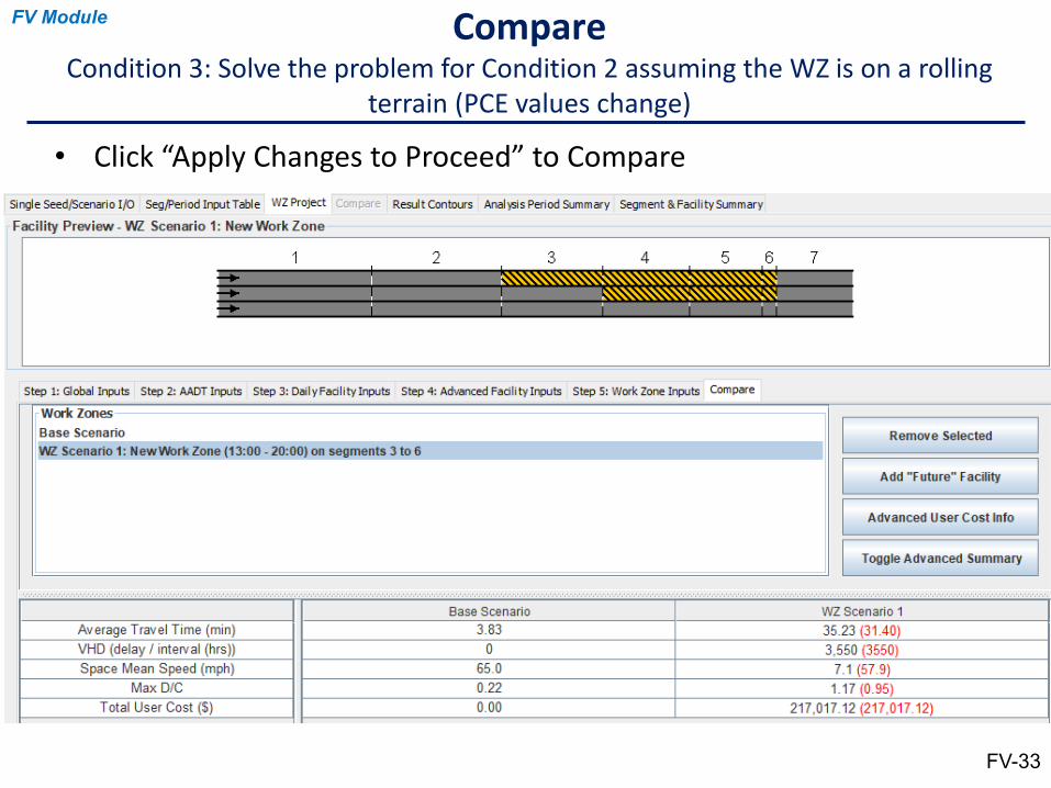
• Click “Apply Changes to Proceed” to Compare
CompareCondition 3: Solve the problem for Condition 2 assuming the WZ is on a rolling
terrain (PCE values change)
FV-33
FV Module
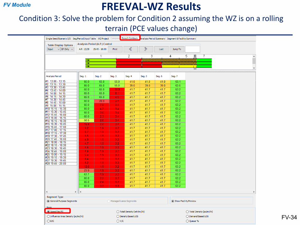
FREEVAL-WZ ResultsCondition 3: Solve the problem for Condition 2 assuming the WZ is on a rolling
terrain (PCE values change)
FV-34
FV Module
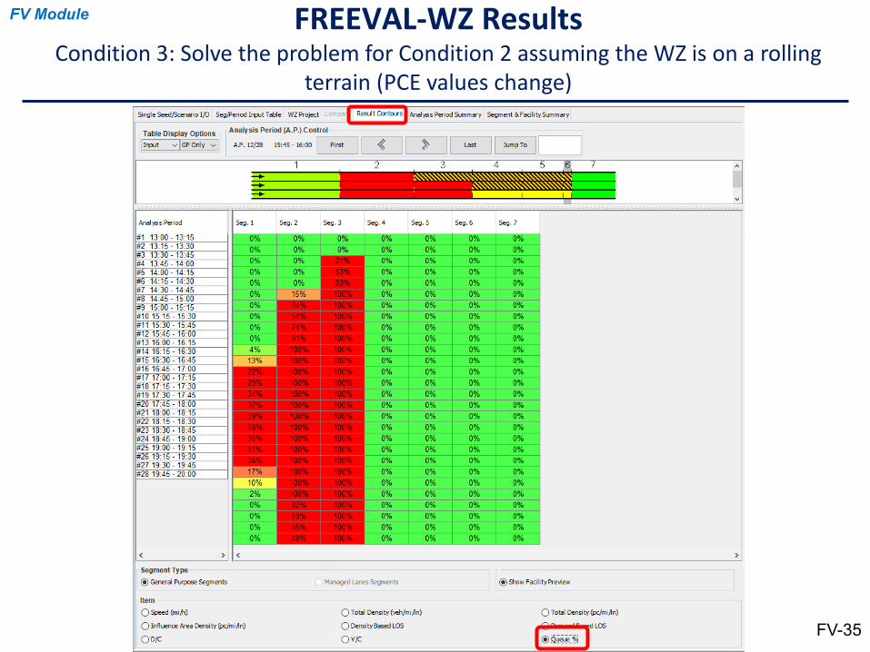
FREEVAL-WZ ResultsCondition 3: Solve the problem for Condition 2 assuming the WZ is on a rolling
terrain (PCE values change)
FV-35
FV Module
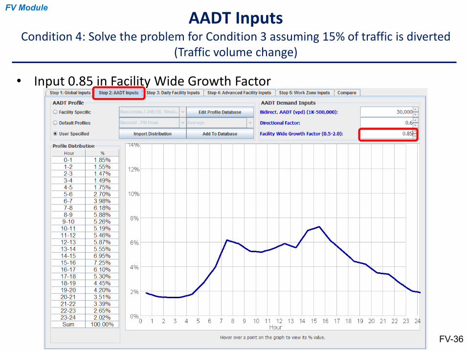
• Input 0.85 in Facility Wide Growth Factor
AADT InputsCondition 4: Solve the problem for Condition 3 assuming 15% of traffic is diverted
(Traffic volume change)
FV-36
FV Module
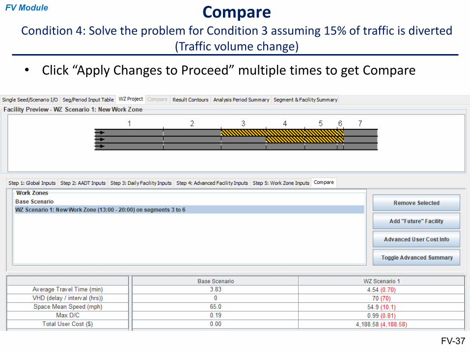
• Click “Apply Changes to Proceed” multiple times to get Compare
CompareCondition 4: Solve the problem for Condition 3 assuming 15% of traffic is diverted
(Traffic volume change)
FV-37
FV Module
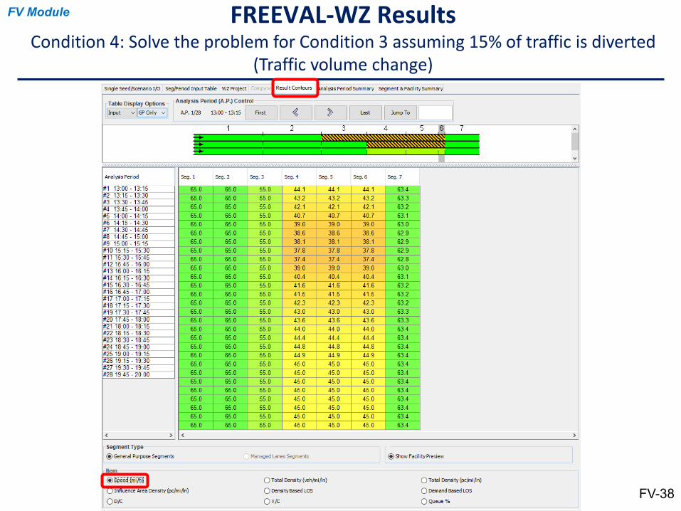
FREEVAL-WZ ResultsCondition 4: Solve the problem for Condition 3 assuming 15% of traffic is diverted
(Traffic volume change)
FV-38
FV Module
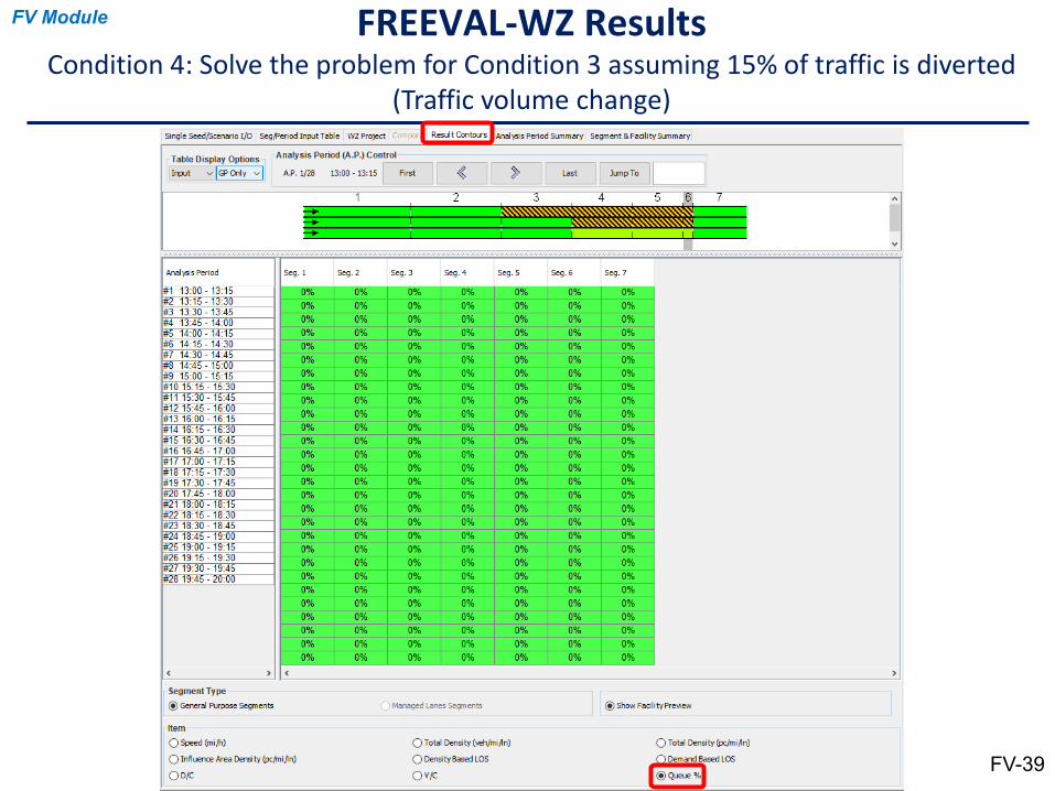
FREEVAL-WZ ResultsCondition 4: Solve the problem for Condition 3 assuming 15% of traffic is diverted
(Traffic volume change)
FV-39
FV Module
To consider the effects of Spreadsheets
HCM 2016 WZ capacity method Freeval-WZ WZQ-Pro
1) Lane width N
2) Shoulder width Y
3) Work intensity N
4) Speed limit inside WZ on capacity N
5) Speed control techniques in WZ N
6) Barrier type (concrete vs others) Y
7) WZ capacity changes during analysis period. N
8) % of trucks changes during analysis period. N
9) Adverse weather conditions N
10) Night time operation Y
11) Urban vs rural Y
12) Flagger operation N
Capability of Spreadsheets
MODULE 4
WorkZoneQ – Pro and
UI spreadsheet for Intersections*
*Computes users’ costs based on delay and volume from HCSM4-1
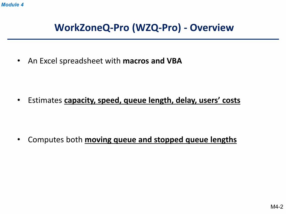
• An Excel spreadsheet with macros and VBA
• Estimates capacity, speed, queue length, delay, users’ costs
• Computes both moving queue and stopped queue lengths
WorkZoneQ-Pro (WZQ-Pro) - Overview
Module 4
M4-2
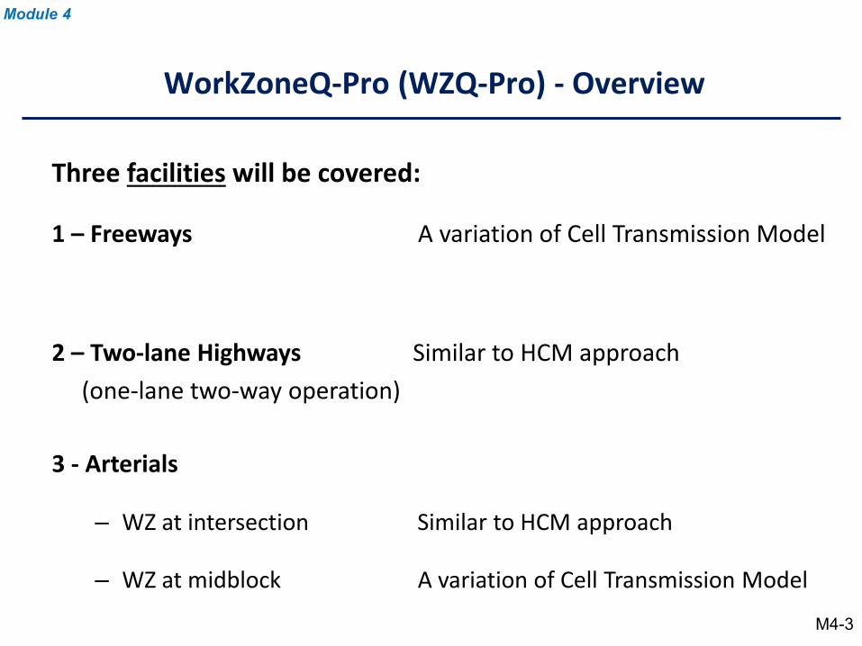
Three facilities will be covered:
1 – Freeways A variation of Cell Transmission Model
2 – Two-lane Highways Similar to HCM approach(one-lane two-way operation)
3 - Arterials
– WZ at intersection Similar to HCM approach
– WZ at midblock A variation of Cell Transmission Model
WorkZoneQ-Pro (WZQ-Pro) - Overview
Module 4
M4-3
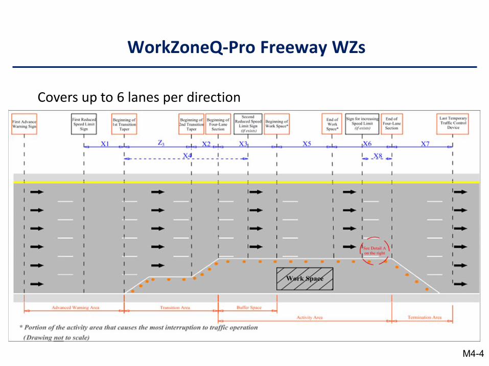
WorkZoneQ-Pro Freeway WZs
Covers up to 6 lanes per direction
M4-4
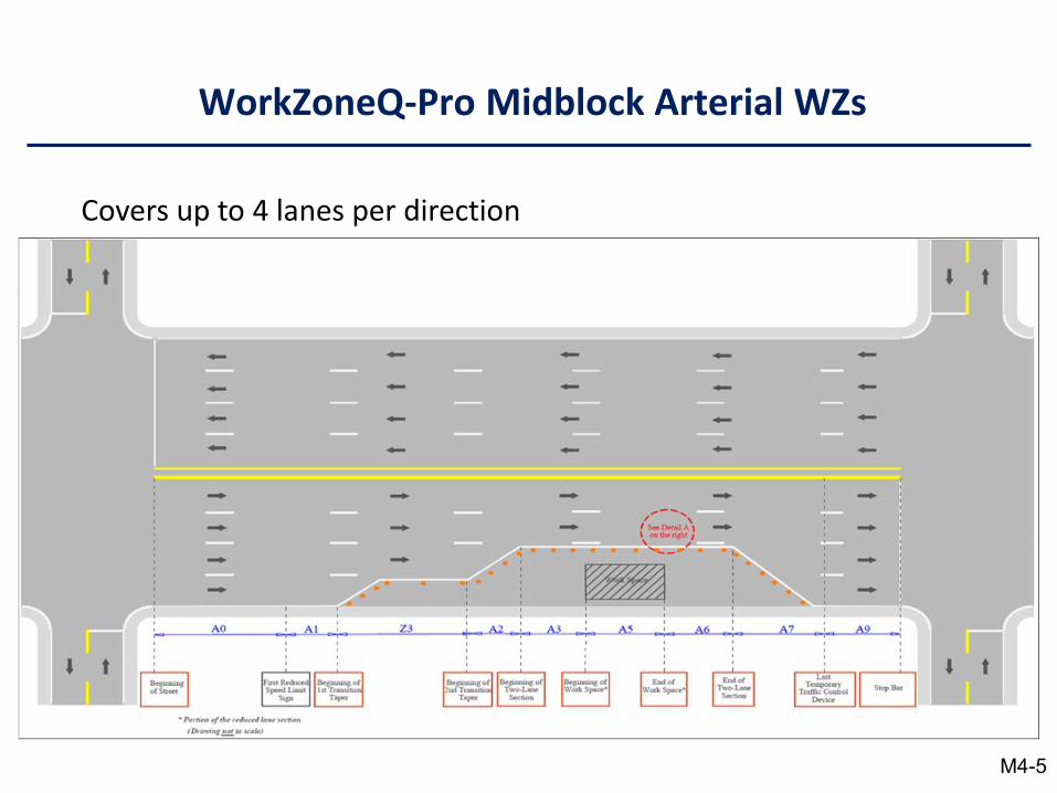
WorkZoneQ-Pro Midblock Arterial WZs
Covers up to 4 lanes per direction
M4-5
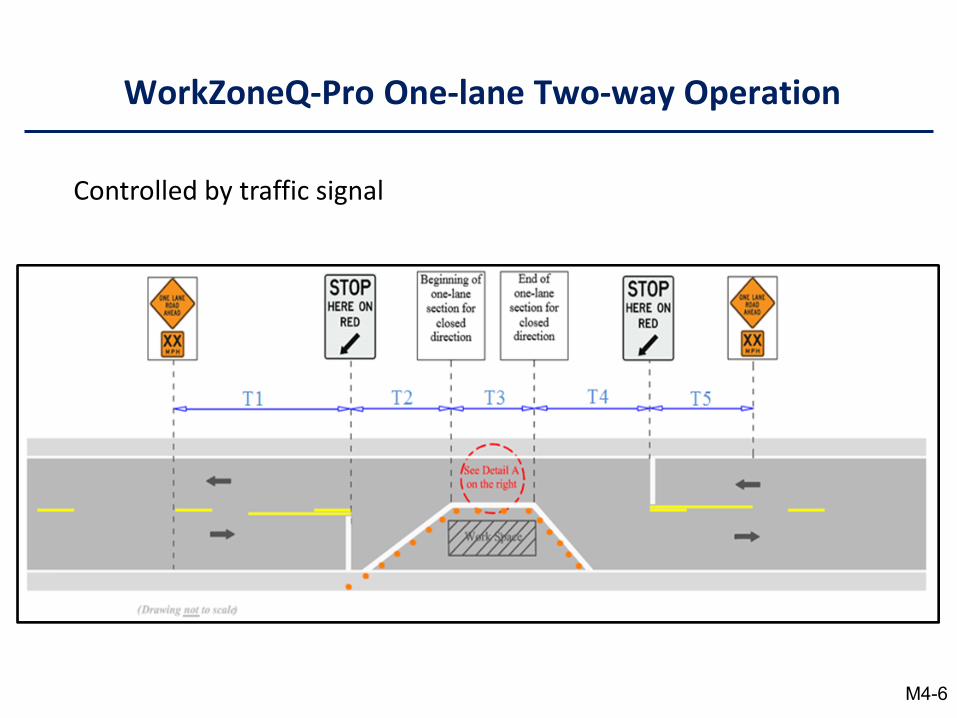
WorkZoneQ-Pro One-lane Two-way Operation
Controlled by traffic signal
M4-6
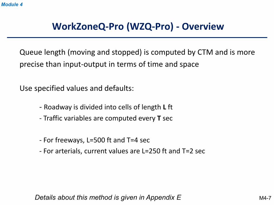
Queue length (moving and stopped) is computed by CTM and is more precise than input-output in terms of time and space
Use specified values and defaults:
- Roadway is divided into cells of length L ft- Traffic variables are computed every T sec
- For freeways, L=500 ft and T=4 sec - For arterials, current values are L=250 ft and T=2 sec
WorkZoneQ-Pro (WZQ-Pro) - Overview
Module 4
Details about this method is given in Appendix E M4-7
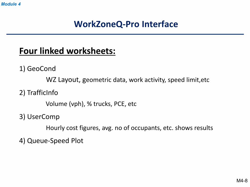
Four linked worksheets:
1) GeoCond WZ Layout, geometric data, work activity, speed limit,etc
2) TrafficInfoVolume (vph), % trucks, PCE, etc
3) UserCompHourly cost figures, avg. no of occupants, etc. shows results
4) Queue-Speed Plot
Module 4
WorkZoneQ-Pro Interface
M4-8
WZQ-Pro
Facility 1: Freeway WZs
M4-9
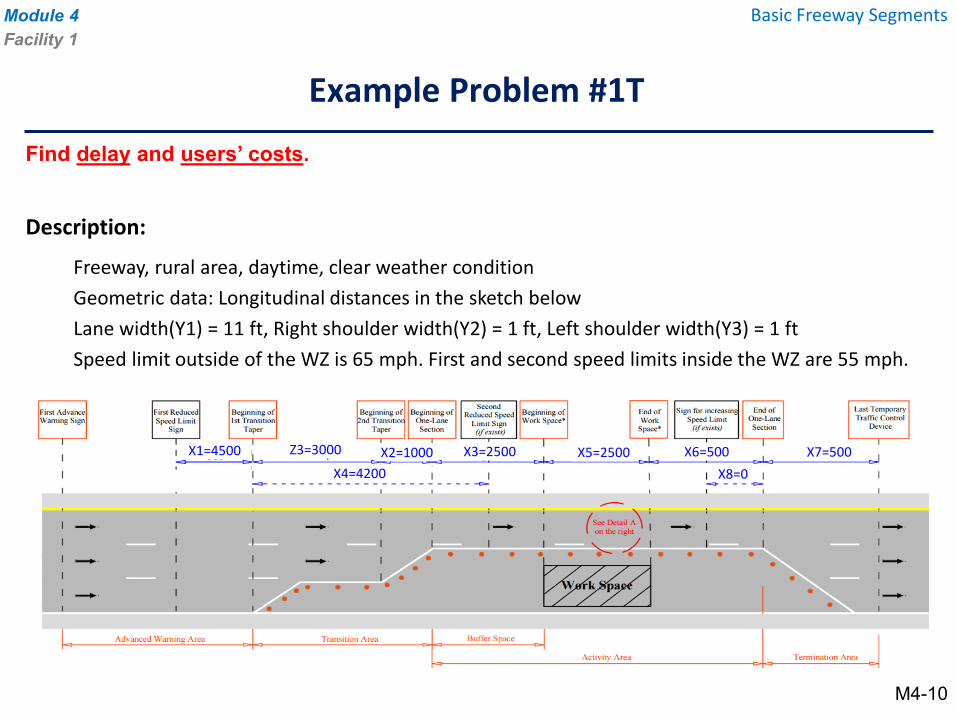
Description:
Freeway, rural area, daytime, clear weather conditionGeometric data: Longitudinal distances in the sketch belowLane width(Y1) = 11 ft, Right shoulder width(Y2) = 1 ft, Left shoulder width(Y3) = 1 ftSpeed limit outside of the WZ is 65 mph. First and second speed limits inside the WZ are 55 mph.
Module 4Facility 1
Basic Freeway Segments
Example Problem #1T
Find delay and users’ costs.
X4=4200X3=2500 X5=2500 X6=500
X8=0X7=500X2=1000Z3=3000X1=4500
M4-10
Condition 1: There is no work activity Condition 2: See the info in the table.
Condition 3: Condition 2, but assume the WZ is on a rolling terrain.Condition 4: Condition 3, divert 15% of traffic to other roads.
Interval % single-unitTrucks
% combination Trucks
% recreational vehicles
Volume(veh)
1:00 PM-2:00 PM 2 8 0 1000
2:00 PM-3:00 PM 2 8 0 1250
3:00 PM-4:00 PM 2 8 0 1300
4:00 PM-5:00 PM 2 11 0 1100
5:00 PM-6:00 PM 2 11 0 950
6:00 PM-7:00 PM 2 11 0 800
7:00 PM-8:00 PM 2 11 0 750
Module 4Facility 1
Basic Freeway Segments
Description (Continued…)
Time duration WZ characteristics for Condition 2
1:00 PM-2:00 PM Speed limit=55 mph
2:00 PM-4:00 PM Speed limit=45 mph, Moderate work activity Work activity area is separated from travel lane by means of barrels
4:00 PM-8:00 PM Speed limit=55 mph
M4-11
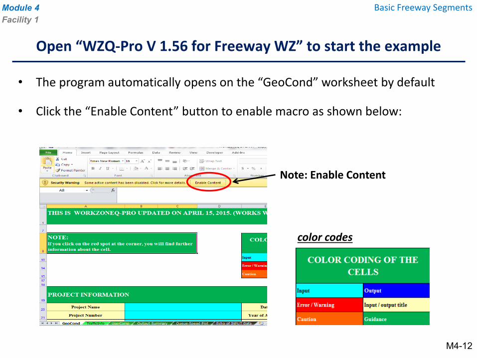
• The program automatically opens on the “GeoCond” worksheet by default
• Click the “Enable Content” button to enable macro as shown below:
Open “WZQ-Pro V 1.56 for Freeway WZ” to start the example
Module 4Facility 1
Basic Freeway Segments
Note: Enable Content
color codes
M4-12
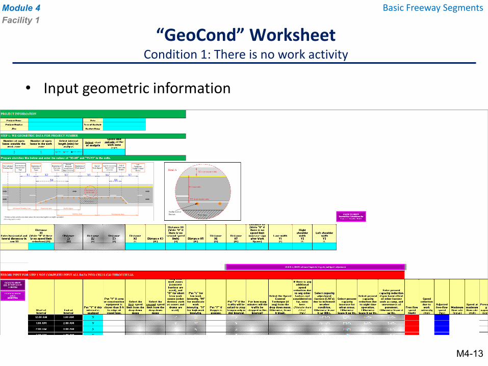
• Input geometric information
“GeoCond” WorksheetCondition 1: There is no work activity
Module 4Facility 1
Basic Freeway Segments
M4-13

• Input project information on cells from B20 to F22
• Input number of open lanes inside and outside of the WZ
• Select interval length, start of analysis, and speed limit outside of
WZ
“GeoCond” WorksheetCondition 1: There is no work activity
Module 4Facility 1
Basic Freeway Segments
M4-14
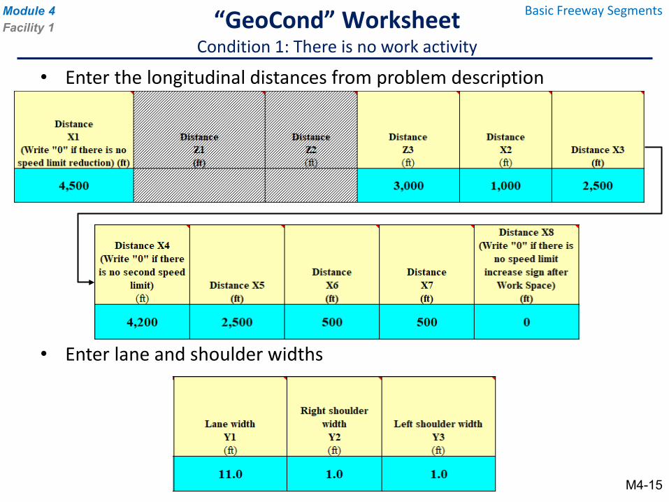
• Enter the longitudinal distances from problem description
• Enter lane and shoulder widths
“GeoCond” WorksheetCondition 1: There is no work activity
Module 4Facility 1
Basic Freeway Segments
M4-15
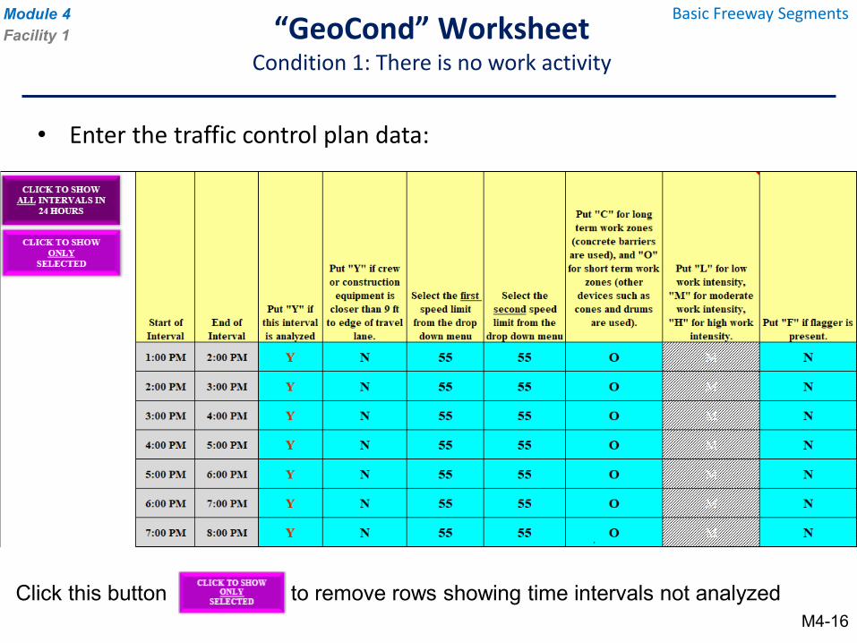
• Enter the traffic control plan data:
“GeoCond” WorksheetCondition 1: There is no work activity
Module 4Facility 1
Basic Freeway Segments
M4-16Click this button to remove rows showing time intervals not analyzed
“GeoCond” WorksheetCondition 1: There is no work activity
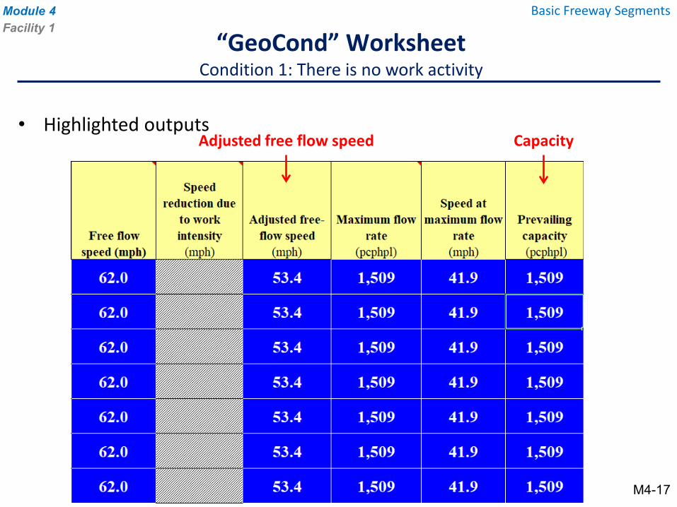
• Highlighted outputs
Module 4Facility 1
Basic Freeway Segments
CapacityAdjusted free flow speed
M4-17
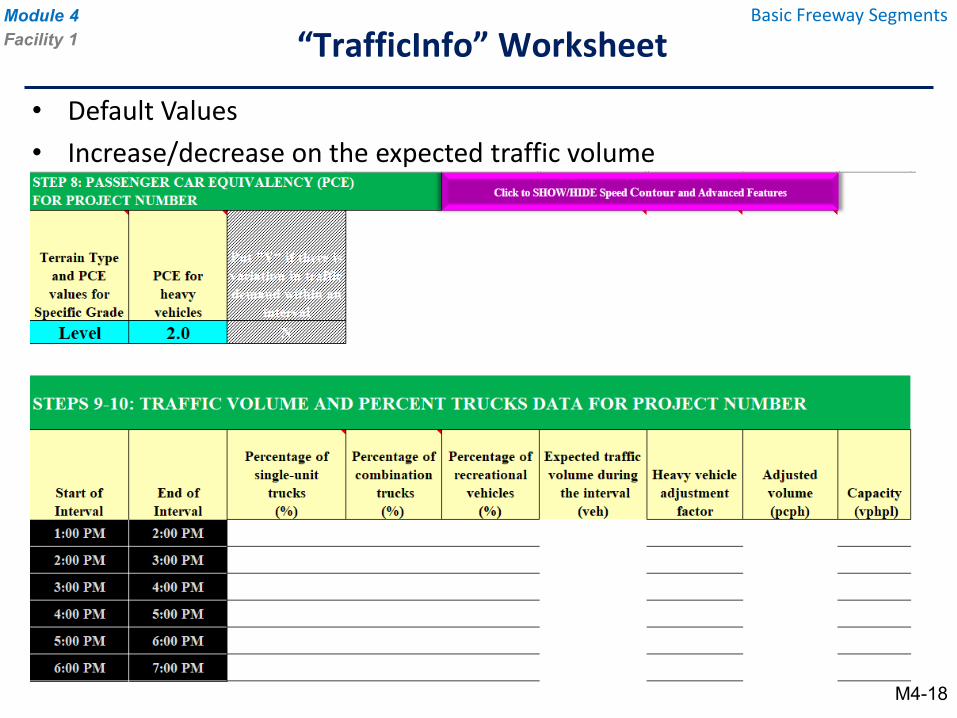
• Default Values• Increase/decrease on the expected traffic volume
“TrafficInfo” WorksheetModule 4Facility 1
Basic Freeway Segments
M4-18
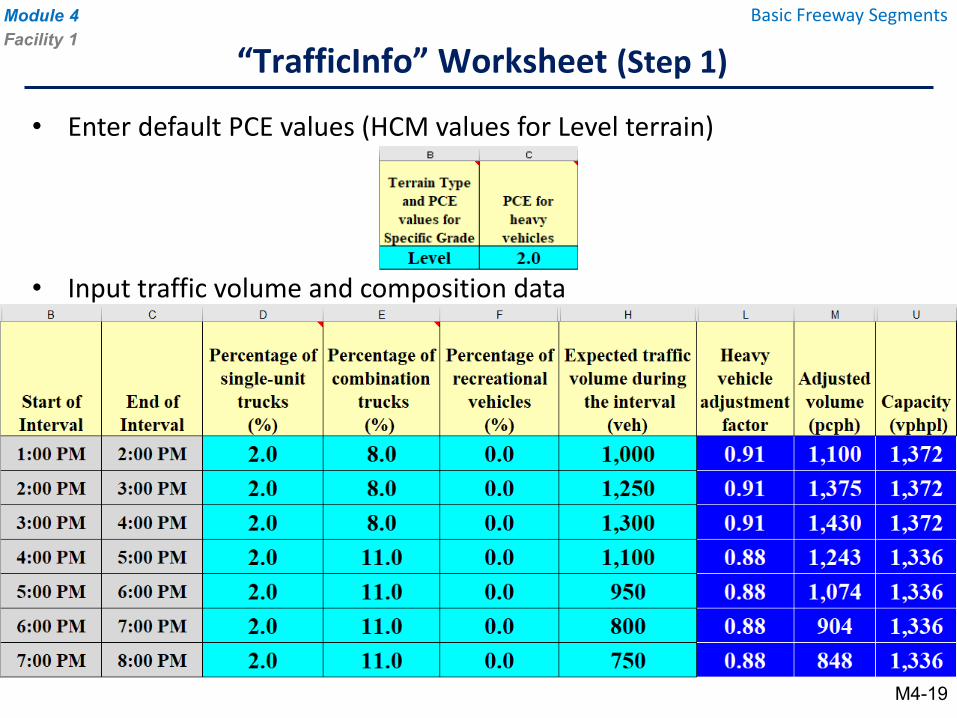
• Enter default PCE values (HCM values for Level terrain)
• Input traffic volume and composition data
“TrafficInfo” Worksheet (Step 1)Module 4Facility 1
Basic Freeway Segments
M4-19
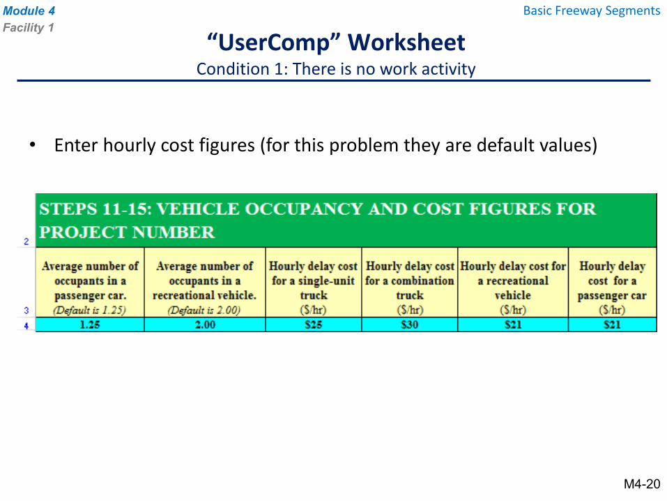
• Enter hourly cost figures (for this problem they are default values)
“UserComp” WorksheetCondition 1: There is no work activity
Module 4Facility 1
Basic Freeway Segments
M4-20
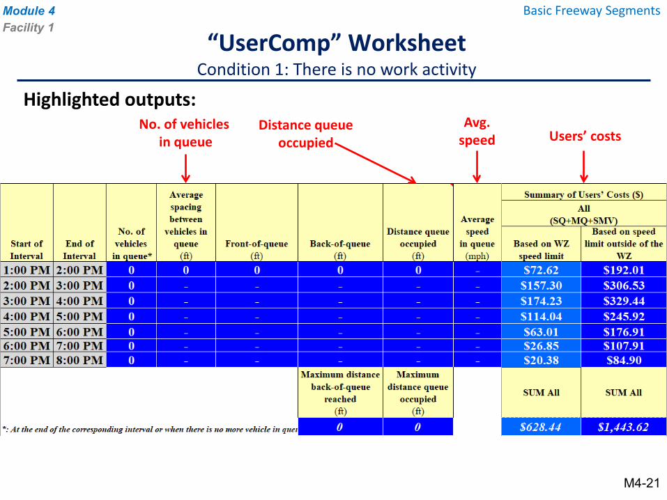
Highlighted outputs:
“UserComp” WorksheetCondition 1: There is no work activity
Module 4Facility 1
Basic Freeway Segments
No. of vehicles in queue
Avg.speed Users’ costs
Distance queue occupied
M4-21
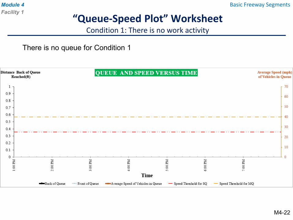
“Queue-Speed Plot” WorksheetCondition 1: There is no work activity
Module 4Facility 1
Basic Freeway Segments
There is no queue for Condition 1
M4-22
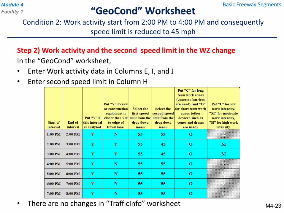
Step 2) Work activity and the second speed limit in the WZ changeIn the “GeoCond” worksheet, • Enter Work activity data in Columns E, I, and J• Enter second speed limit in Column H
• There are no changes in “TrafficInfo” worksheet
“GeoCond” WorksheetCondition 2: Work activity start from 2:00 PM to 4:00 PM and consequently
speed limit is reduced to 45 mph
Basic Freeway SegmentsModule 4Facility 1
M4-23
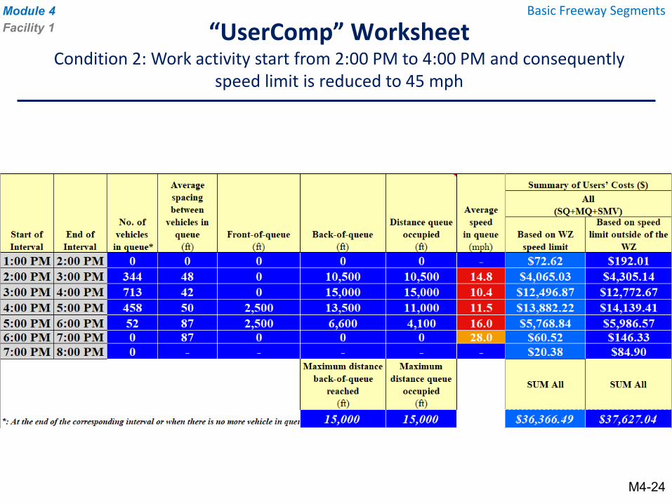
“UserComp” WorksheetCondition 2: Work activity start from 2:00 PM to 4:00 PM and consequently
speed limit is reduced to 45 mph
Basic Freeway SegmentsModule 4Facility 1
M4-24
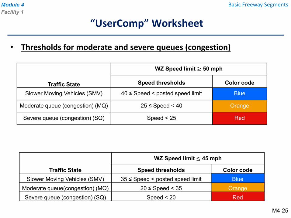
• Thresholds for moderate and severe queues (congestion)
Traffic State
WZ Speed limit ≥ 50 mph
Speed thresholds Color code
Slower Moving Vehicles (SMV) 40 ≤ Speed < posted speed limit Blue
Moderate queue (congestion) (MQ) 25 ≤ Speed < 40 Orange
Severe queue (congestion) (SQ) Speed < 25 Red
“UserComp” Worksheet
Module 4Facility 1
Basic Freeway Segments
M4-25
Traffic State
WZ Speed limit ≤ 45 mph
Speed thresholds Color codeSlower Moving Vehicles (SMV) 35 ≤ Speed < posted speed limit Blue
Moderate queue(congestion) (MQ) 20 ≤ Speed < 35 OrangeSevere queue (congestion) (SQ) Speed < 20 Red
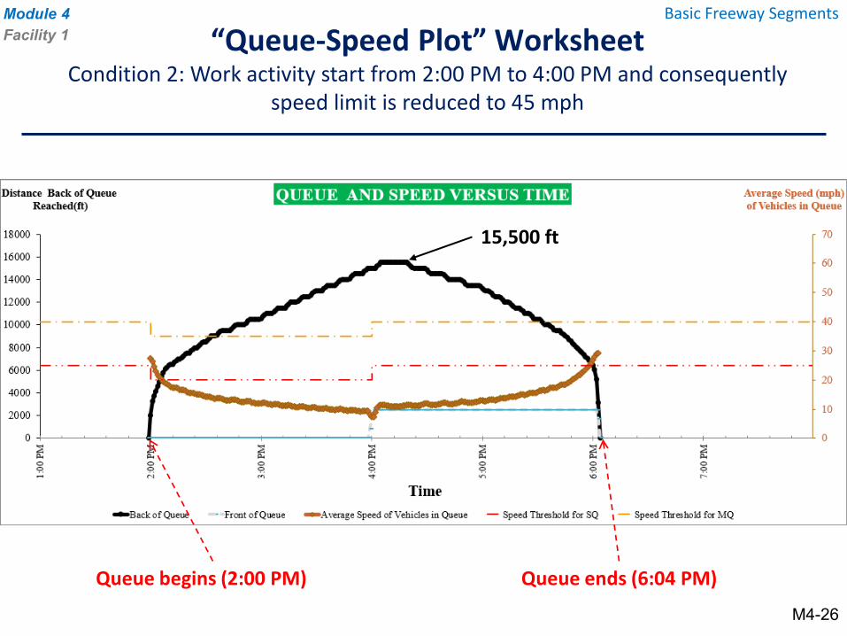
“Queue-Speed Plot” WorksheetCondition 2: Work activity start from 2:00 PM to 4:00 PM and consequently
speed limit is reduced to 45 mph
Basic Freeway SegmentsModule 4Facility 1
Queue begins (2:00 PM) Queue ends (6:04 PM)
M4-26
15,500 ft
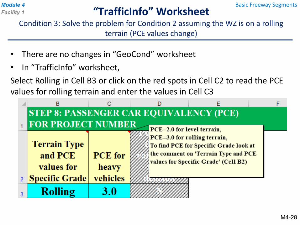
• There are no changes in “GeoCond” worksheet• In “TrafficInfo” worksheet,Select Rolling in Cell B3 or click on the red spots in Cell C2 to read the PCE values for rolling terrain and enter the values in Cell C3
“TrafficInfo” WorksheetCondition 3: Solve the problem for Condition 2 assuming the WZ is on a rolling
terrain (PCE values change)
Basic Freeway SegmentsModule 4Facility 1
M4-28
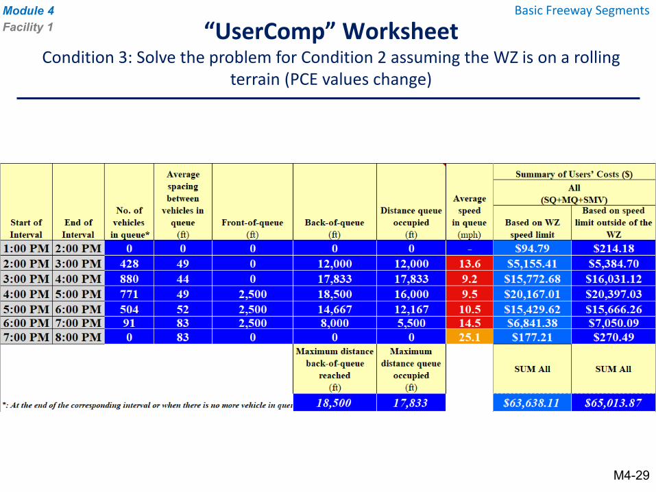
“UserComp” WorksheetCondition 3: Solve the problem for Condition 2 assuming the WZ is on a rolling
terrain (PCE values change)
Basic Freeway SegmentsModule 4Facility 1
M4-29
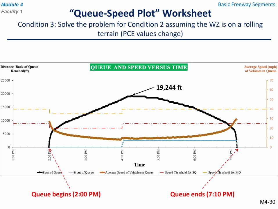
“Queue-Speed Plot” WorksheetCondition 3: Solve the problem for Condition 2 assuming the WZ is on a rolling
terrain (PCE values change)
Basic Freeway SegmentsModule 4Facility 1
M4-30Queue begins (2:00 PM) Queue ends (7:10 PM)
19,244 ft
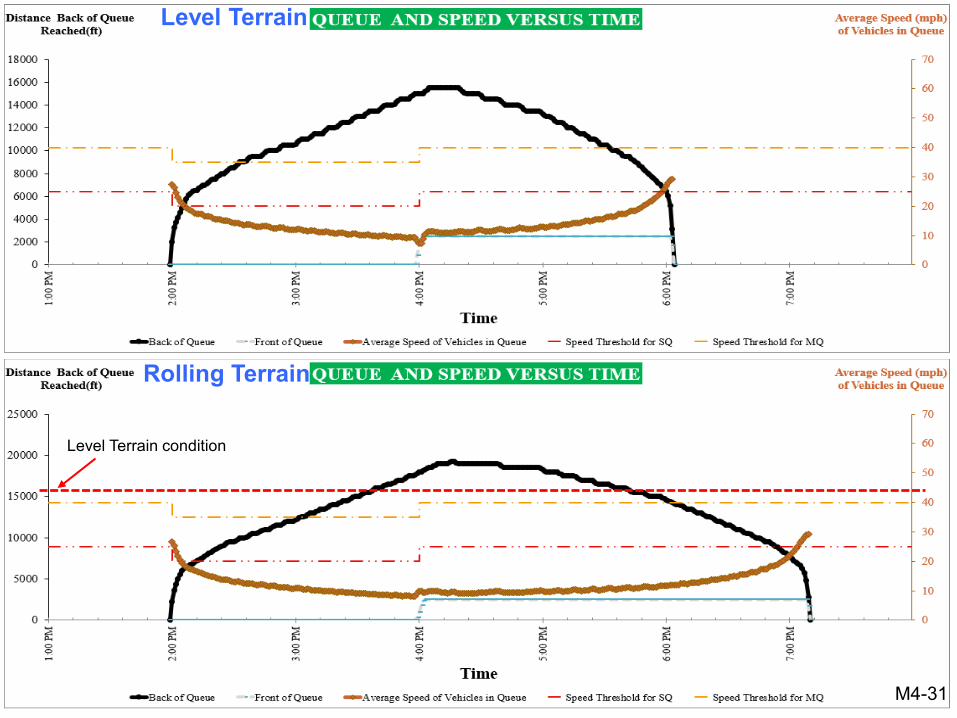
M4-31
Level Terrain condition
Rolling Terrain
Level Terrain
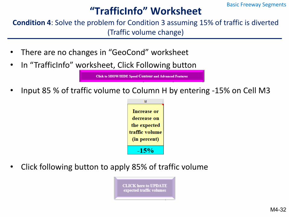
• There are no changes in “GeoCond” worksheet• In “TrafficInfo” worksheet, Click Following button
• Input 85 % of traffic volume to Column H by entering -15% on Cell M3
• Click following button to apply 85% of traffic volume
“TrafficInfo” WorksheetCondition 4: Solve the problem for Condition 3 assuming 15% of traffic is diverted
(Traffic volume change)
Basic Freeway Segments
M4-32
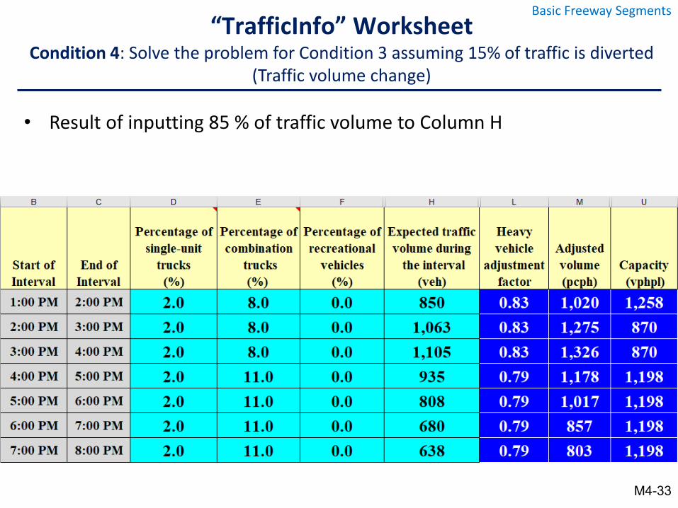
• Result of inputting 85 % of traffic volume to Column H
“TrafficInfo” WorksheetCondition 4: Solve the problem for Condition 3 assuming 15% of traffic is diverted
(Traffic volume change)
Basic Freeway Segments
M4-33
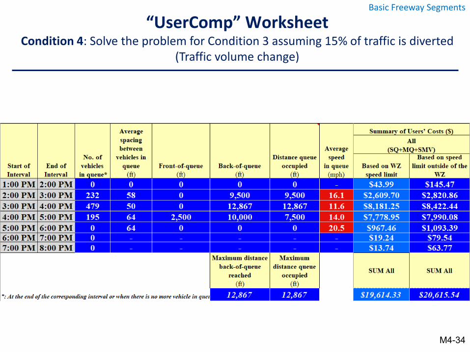
“UserComp” WorksheetCondition 4: Solve the problem for Condition 3 assuming 15% of traffic is diverted
(Traffic volume change)
Basic Freeway Segments
M4-34
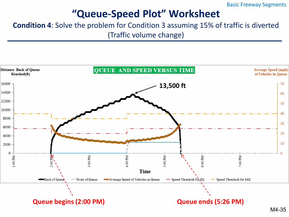
“Queue-Speed Plot” WorksheetCondition 4: Solve the problem for Condition 3 assuming 15% of traffic is diverted
(Traffic volume change)
Basic Freeway Segments
M4-35Queue begins (2:00 PM) Queue ends (5:26 PM)
13,500 ft
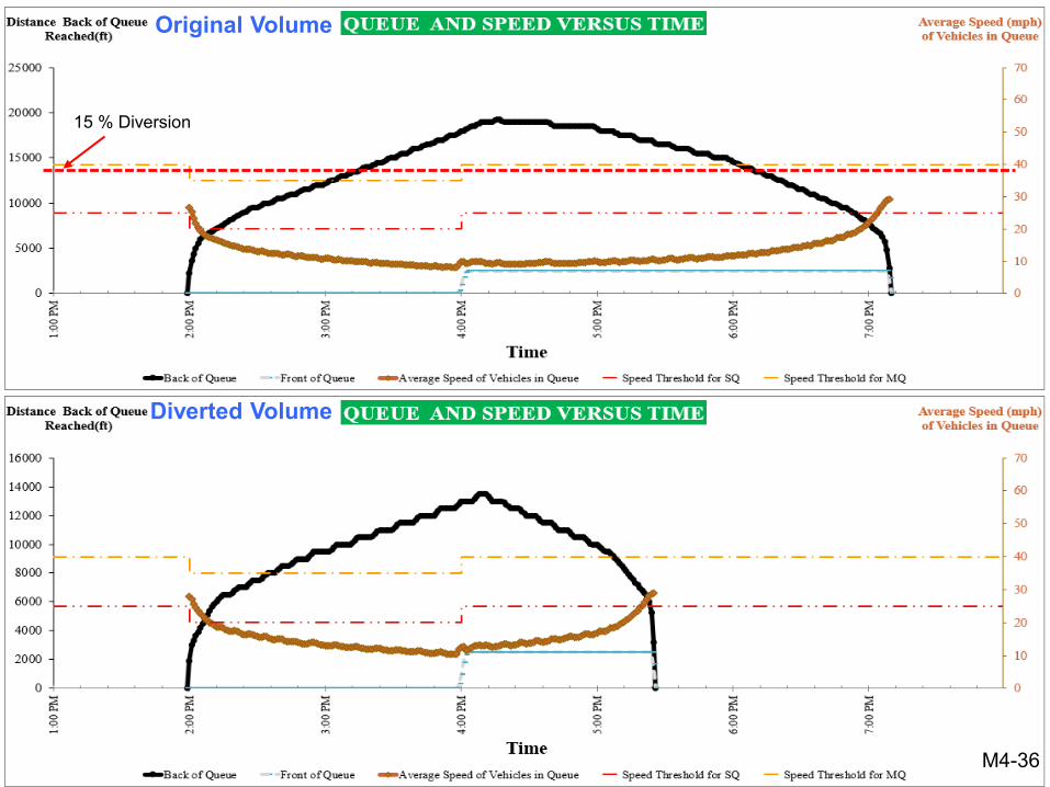
15 % Diversion
Original Volume
Diverted Volume
M4-36
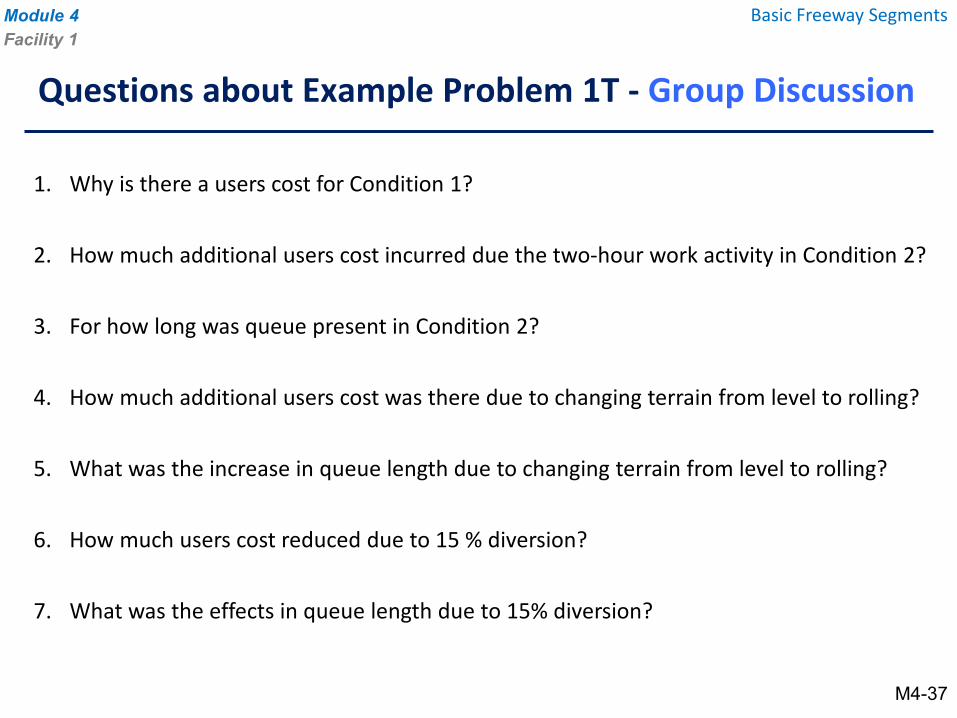
1. Why is there a users cost for Condition 1?
2. How much additional users cost incurred due the two-hour work activity in Condition 2?
3. For how long was queue present in Condition 2?
4. How much additional users cost was there due to changing terrain from level to rolling?
5. What was the increase in queue length due to changing terrain from level to rolling?
6. How much users cost reduced due to 15 % diversion?
7. What was the effects in queue length due to 15% diversion?
Module 4Facility 1
Basic Freeway Segments
Questions about Example Problem 1T - Group Discussion
M4-37
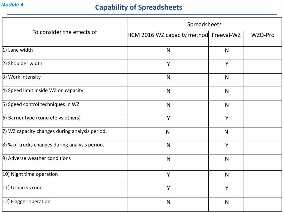
Capability of SpreadsheetsModule 4
To consider the effects of Spreadsheets
HCM 2016 WZ capacity method Freeval-WZ WZQ-Pro
1) Lane width N N
2) Shoulder width Y Y
3) Work intensity N N
4) Speed limit inside WZ on capacity N N
5) Speed control techniques in WZ N N
6) Barrier type (concrete vs others) Y Y
7) WZ capacity changes during analysis period. N N
8) % of trucks changes during analysis period. N Y
9) Adverse weather conditions N N
10) Night time operation Y N
11) Urban vs rural Y Y
12) Flagger operation N N
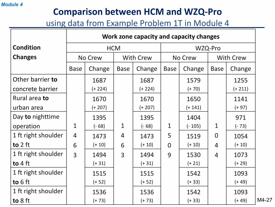
Comparison between HCM and WZQ-Prousing data from Example Problem 1T in Module 4
Module 4
M4-27
Condition Changes
Work zone capacity and capacity changes
HCM WZQ-ProNo Crew With Crew No Crew With Crew
Base Change Base Change Base Change Base ChangeOther barrier toconcrete barrier
1463
1687(+ 224)
1463
1687(+ 224)
1509
1579(+ 70)
1044
1255(+ 211)
Rural area tourban area
1670(+ 207)
1670(+ 207)
1650(+ 141)
1141(+ 97)
Day to nighttime operation
1395(- 68)
1395(- 68)
1404(- 105)
971(- 73)
1 ft right shoulder to 2 ft
1473(+ 10)
1473(+ 10)
1519(+ 10)
1054(+ 10)
1 ft right shoulder to 4 ft
1494(+ 31)
1494(+ 31)
1530(+ 21)
1073(+ 29)
1 ft right shoulder to 6 ft
1515(+ 52)
1515(+ 52)
1542(+ 33)
1093(+ 49)
1 ft right shoulder to 8 ft
1536(+ 73)
1536(+ 73)
1542(+ 33)
1093(+ 49)
Module 4Facility 1
Basic Freeway Segments
Example Problem #2T
M4-39
Example Problem # 2T is moved to Appendix O
It is very similar to Example Problem 1
WZQ-Pro
Facility 2: Two-lane Highways(one-lane two-way operation)
M4-40
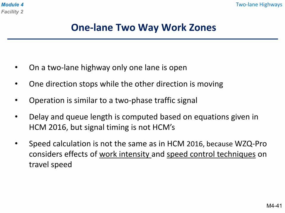
• On a two-lane highway only one lane is open
• One direction stops while the other direction is moving
• Operation is similar to a two-phase traffic signal
• Delay and queue length is computed based on equations given in HCM 2016, but signal timing is not HCM’s
• Speed calculation is not the same as in HCM 2016, because WZQ-Pro considers effects of work intensity and speed control techniques on travel speed
One-lane Two Way Work Zones
Module 4Facility 2
Two-lane Highways
M4-41
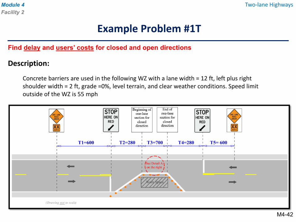
Description:
Concrete barriers are used in the following WZ with a lane width = 12 ft, left plus right shoulder width = 2 ft, grade =0%, level terrain, and clear weather conditions. Speed limit outside of the WZ is 55 mph
Example Problem #1T
Module 4Facility 2
Two-lane Highways
Find delay and users’ costs for closed and open directions
M4-42
T4=280T3=700 T5= 600T2=280T1=600
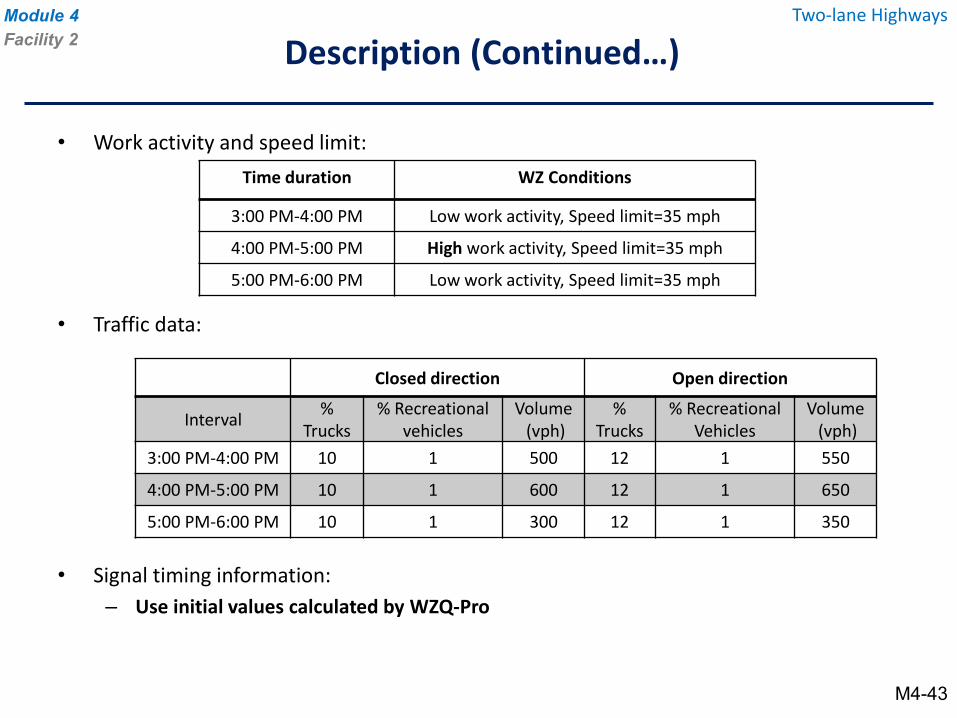
• Work activity and speed limit:
• Traffic data:
• Signal timing information:– Use initial values calculated by WZQ-Pro
Time duration WZ Conditions
3:00 PM-4:00 PM Low work activity, Speed limit=35 mph
4:00 PM-5:00 PM High work activity, Speed limit=35 mph
5:00 PM-6:00 PM Low work activity, Speed limit=35 mph
Closed direction Open direction
Interval % Trucks
% Recreational vehicles
Volume(vph)
% Trucks
% Recreational Vehicles
Volume(vph)
3:00 PM-4:00 PM 10 1 500 12 1 550
4:00 PM-5:00 PM 10 1 600 12 1 650
5:00 PM-6:00 PM 10 1 300 12 1 350
Module 4Facility 2 Description (Continued…)
Two-lane Highways
M4-43
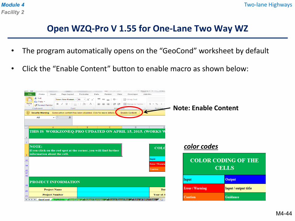
• The program automatically opens on the “GeoCond” worksheet by default
• Click the “Enable Content” button to enable macro as shown below:
Open WZQ-Pro V 1.55 for One-Lane Two Way WZ
Module 4Facility 2
Two-lane Highways
Note: Enable Content
color codes
M4-44
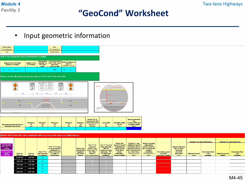
• Input geometric information
“GeoCond” WorksheetModule 4Facility 2
Two-lane Highways
M4-45
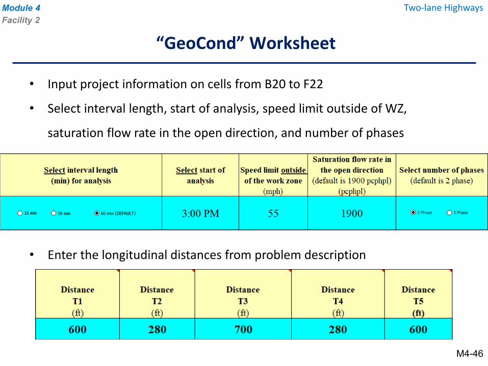
• Input project information on cells from B20 to F22
• Select interval length, start of analysis, speed limit outside of WZ,
saturation flow rate in the open direction, and number of phases
• Enter the longitudinal distances from problem description
“GeoCond” Worksheet
Module 4Facility 2
Two-lane Highways
M4-46
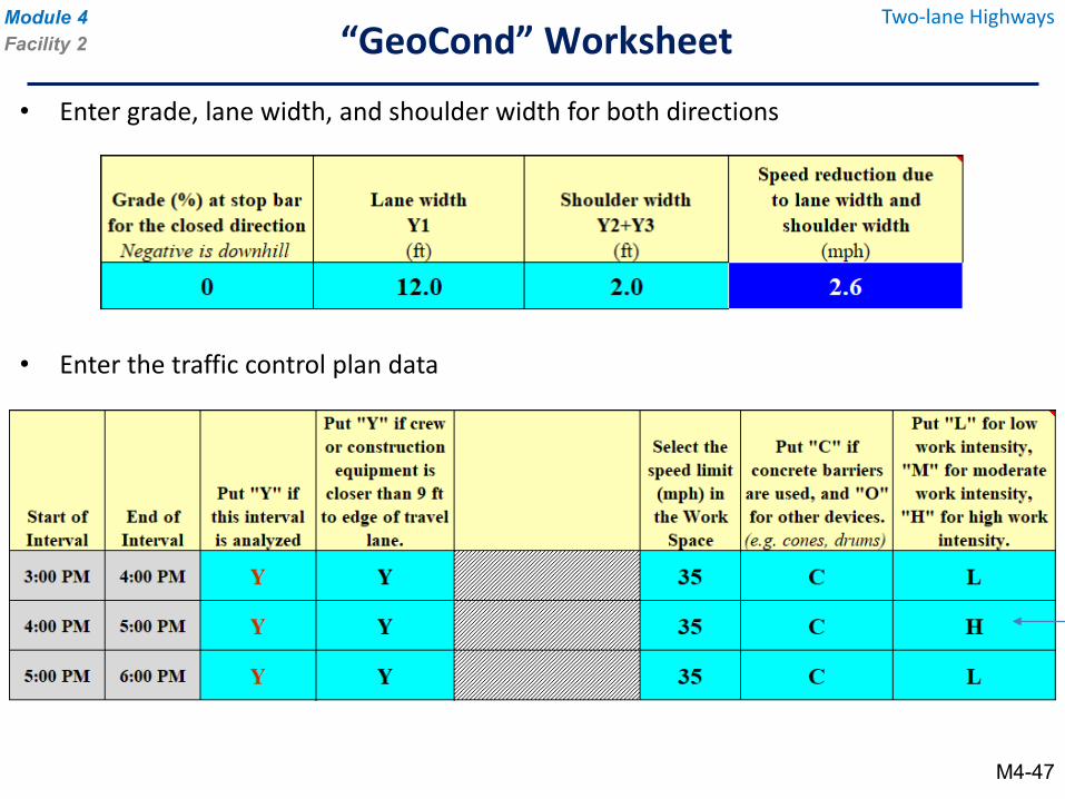
• Enter grade, lane width, and shoulder width for both directions
• Enter the traffic control plan data
“GeoCond” WorksheetModule 4Facility 2
Two-lane Highways
M4-47
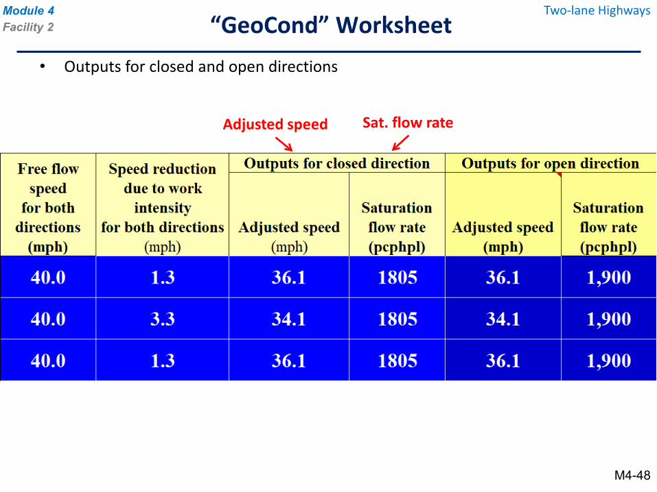
• Outputs for closed and open directions
Adjusted speed Sat. flow rate
“GeoCond” WorksheetModule 4Facility 2
Two-lane Highways
M4-48
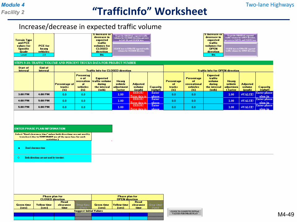
Increase/decrease in expected traffic volume
“TrafficInfo” WorksheetModule 4Facility 2
Two-lane Highways
M4-49
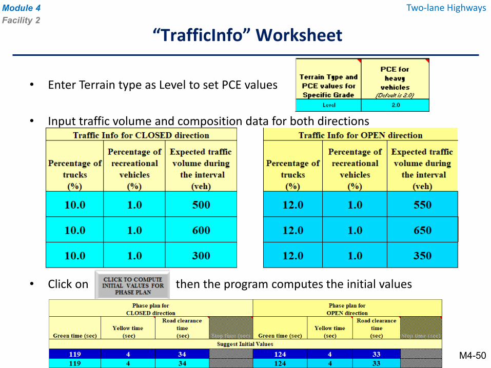
• Enter Terrain type as Level to set PCE values
• Input traffic volume and composition data for both directions
• Click on then the program computes the initial values
“TrafficInfo” WorksheetModule 4Facility 2
Two-lane Highways
M4-50
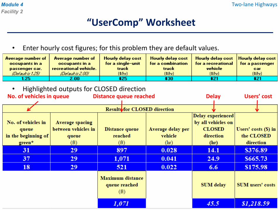
• Enter hourly cost figures; for this problem they are default values.
• Highlighted outputs for CLOSED direction
“UserComp” Worksheet
Module 4Facility 2
Two-lane Highways
No. of vehicles in queue Distance queue reached Delay Users’ cost
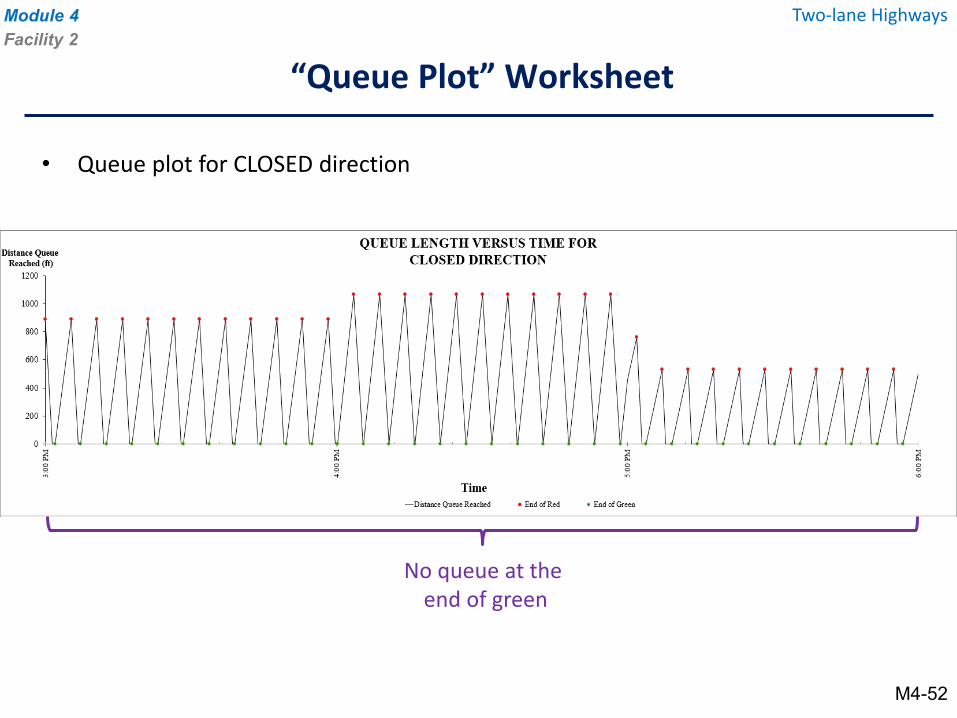
“Queue Plot” Worksheet
Module 4Facility 2
Two-lane Highways
No queue at theend of green
• Queue plot for CLOSED direction
M4-52
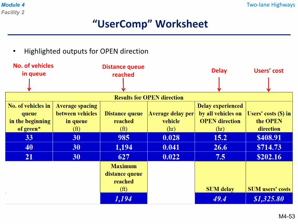
• Highlighted outputs for OPEN direction
“UserComp” Worksheet
Module 4Facility 2
Two-lane Highways
No. of vehicles in queue
Distance queuereached Delay Users’ cost
M4-53
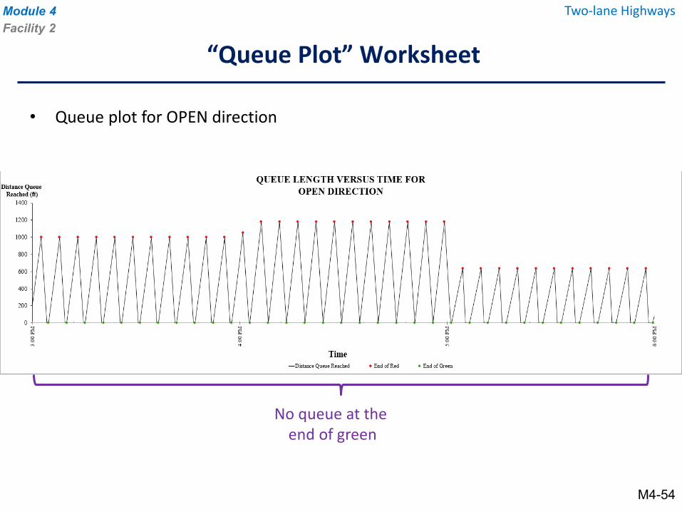
“Queue Plot” Worksheet
Module 4Facility 2
Two-lane Highways
No queue at theend of green
• Queue plot for OPEN direction
M4-54
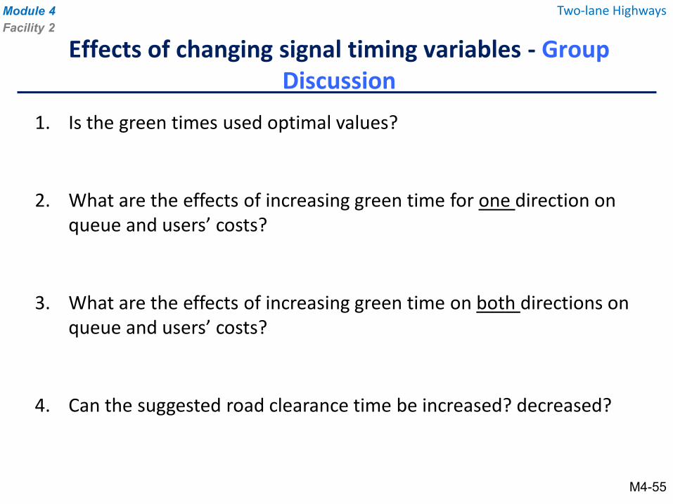
1. Is the green times used optimal values?
2. What are the effects of increasing green time for one direction on queue and users’ costs?
3. What are the effects of increasing green time on both directions on queue and users’ costs?
4. Can the suggested road clearance time be increased? decreased?
Effects of changing signal timing variables - Group Discussion
Module 4Facility 2
Two-lane Highways
M4-55
WZQ-Pro
Facility 3: Arterials3.1: Midblock WZ
M4-56
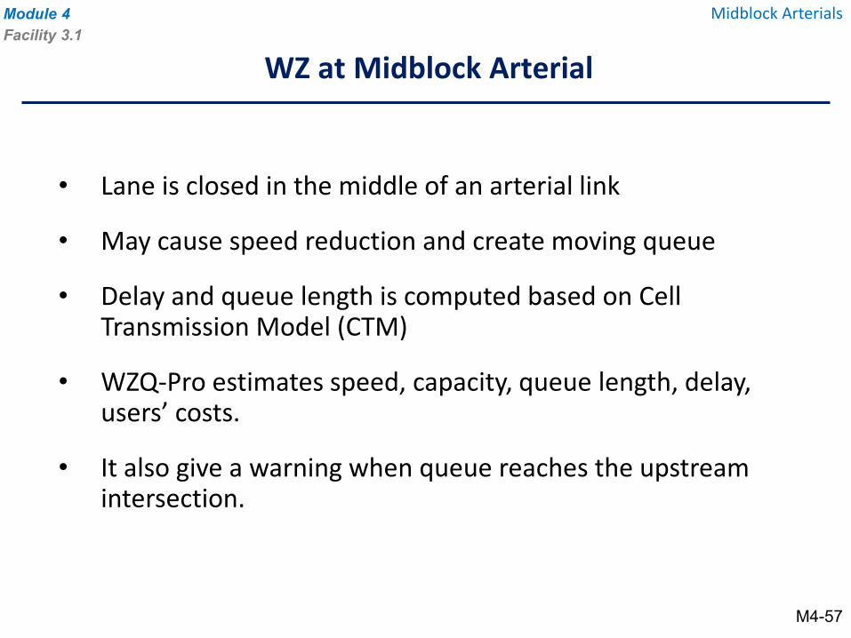
WZ at Midblock Arterial
• Lane is closed in the middle of an arterial link
• May cause speed reduction and create moving queue
• Delay and queue length is computed based on Cell Transmission Model (CTM)
• WZQ-Pro estimates speed, capacity, queue length, delay, users’ costs.
• It also give a warning when queue reaches the upstream intersection.
Module 4Facility 3.1
Midblock Arterials
M4-57
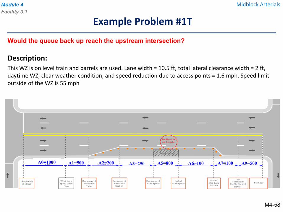
Description:This WZ is on level train and barrels are used. Lane width = 10.5 ft, total lateral clearance width = 2 ft, daytime WZ, clear weather condition, and speed reduction due to access points = 1.6 mph. Speed limit outside of the WZ is 55 mph
Example Problem #1T
Module 4 Midblock ArterialsFacility 3.1
Would the queue back up reach the upstream intersection?
A0=1000 A1=500 A2=200 A3=250 A5=800 A6=100 A7=100 A9=500
M4-58
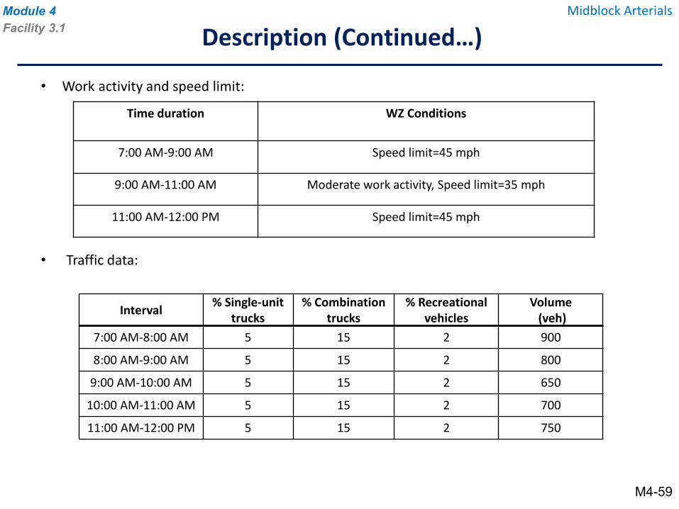
Description (Continued…)Module 4 Midblock ArterialsFacility 3.1
• Work activity and speed limit:
• Traffic data:
Time duration WZ Conditions
7:00 AM-9:00 AM Speed limit=45 mph
9:00 AM-11:00 AM Moderate work activity, Speed limit=35 mph
11:00 AM-12:00 PM Speed limit=45 mph
Interval % Single-unittrucks
% Combination trucks
% Recreational vehicles
Volume(veh)
7:00 AM-8:00 AM 5 15 2 900
8:00 AM-9:00 AM 5 15 2 800
9:00 AM-10:00 AM 5 15 2 650
10:00 AM-11:00 AM 5 15 2 700
11:00 AM-12:00 PM 5 15 2 750
M4-59

• The program automatically opens on the “GeoCond” worksheet by default
• Click the “Enable Content” button to enable macro as shown below:
Open WZQ-Pro 1.56 for Midblock Arterials to start the example
Module 4 Midblock ArterialsFacility 3.1
Note: Enable Content
color codes
M4-60
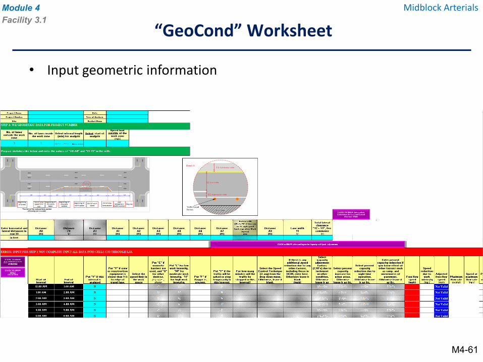
• Input geometric information
“GeoCond” WorksheetModule 4 Midblock ArterialsFacility 3.1
M4-61
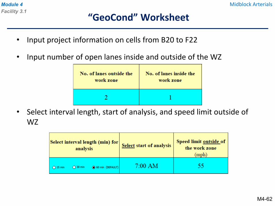
• Input project information on cells from B20 to F22
• Input number of open lanes inside and outside of the WZ
• Select interval length, start of analysis, and speed limit outside of WZ
“GeoCond” WorksheetModule 4 Midblock ArterialsFacility 3.1
M4-62
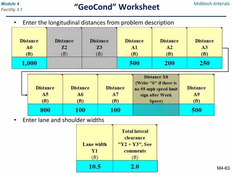
• Enter the longitudinal distances from problem description
• Enter lane and shoulder widths
“GeoCond” WorksheetModule 4 Midblock ArterialsFacility 3.1
M4-63
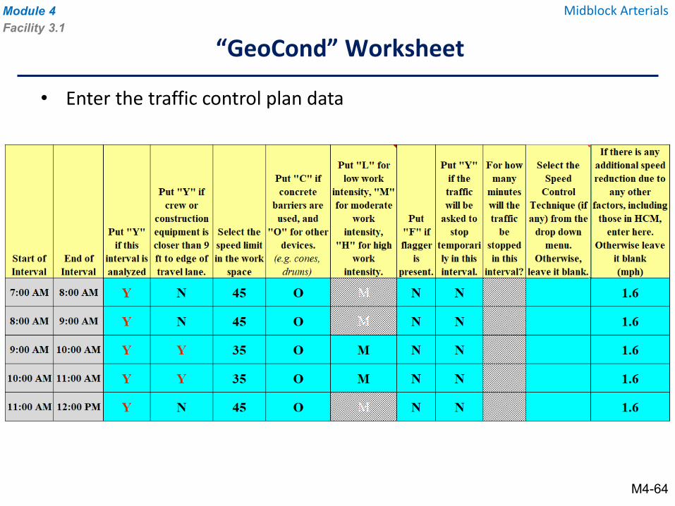
• Enter the traffic control plan data
“GeoCond” WorksheetModule 4 Midblock ArterialsFacility 3.1
M4-64
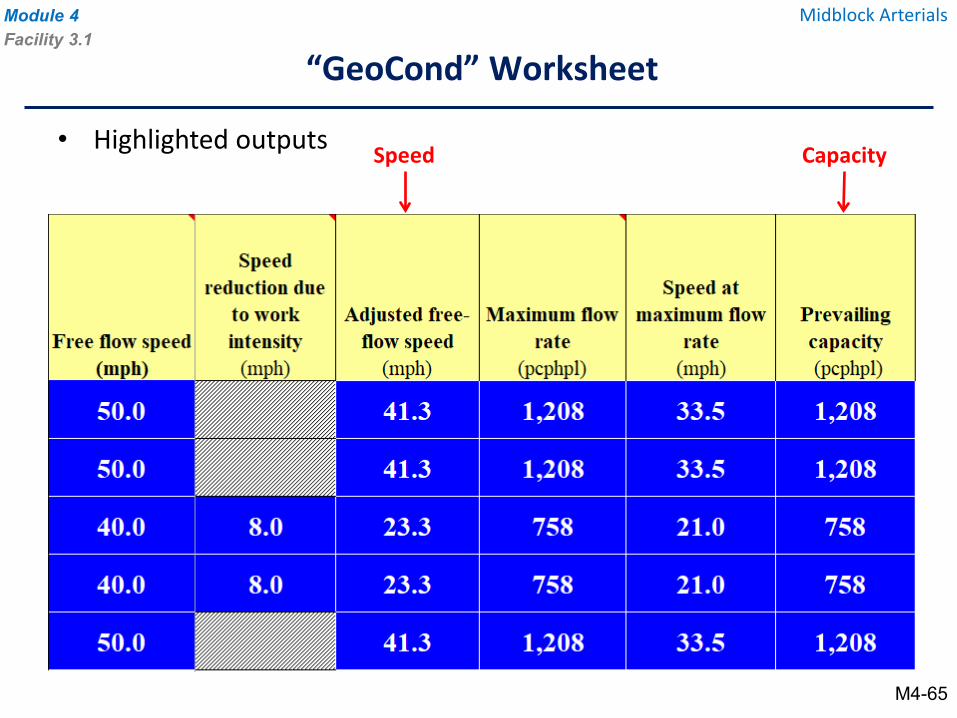
• Highlighted outputs Speed
“GeoCond” WorksheetModule 4 Midblock ArterialsFacility 3.1
M4-65
Capacity
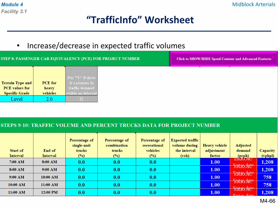
• Increase/decrease in expected traffic volumes
“TrafficInfo” WorksheetModule 4 Midblock ArterialsFacility 3.1
M4-66
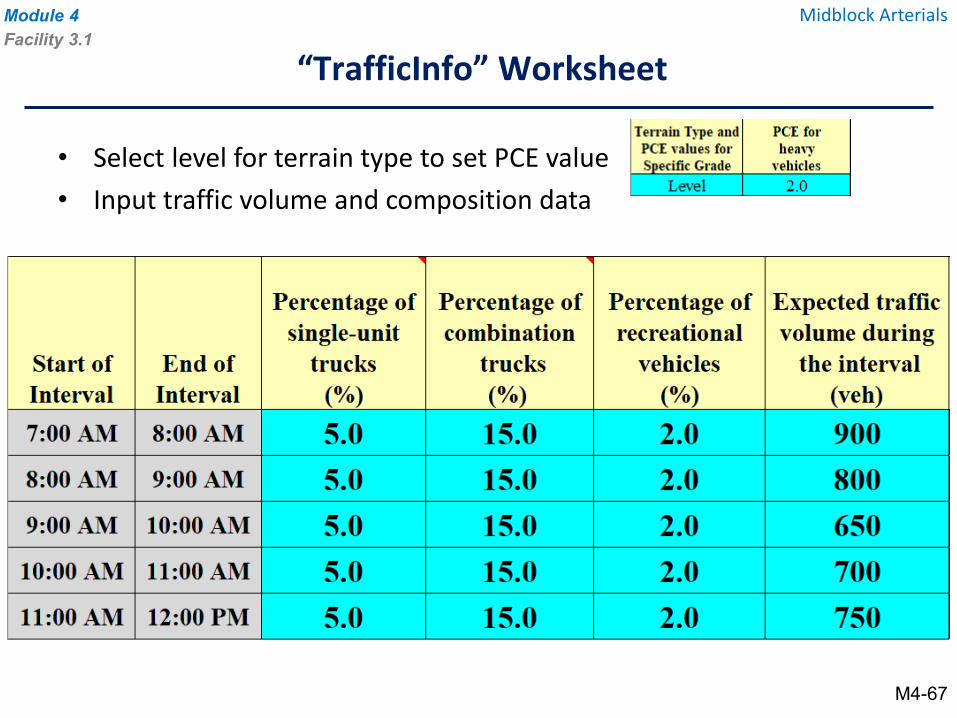
• Select level for terrain type to set PCE value• Input traffic volume and composition data
“TrafficInfo” WorksheetModule 4 Midblock ArterialsFacility 3.1
M4-67
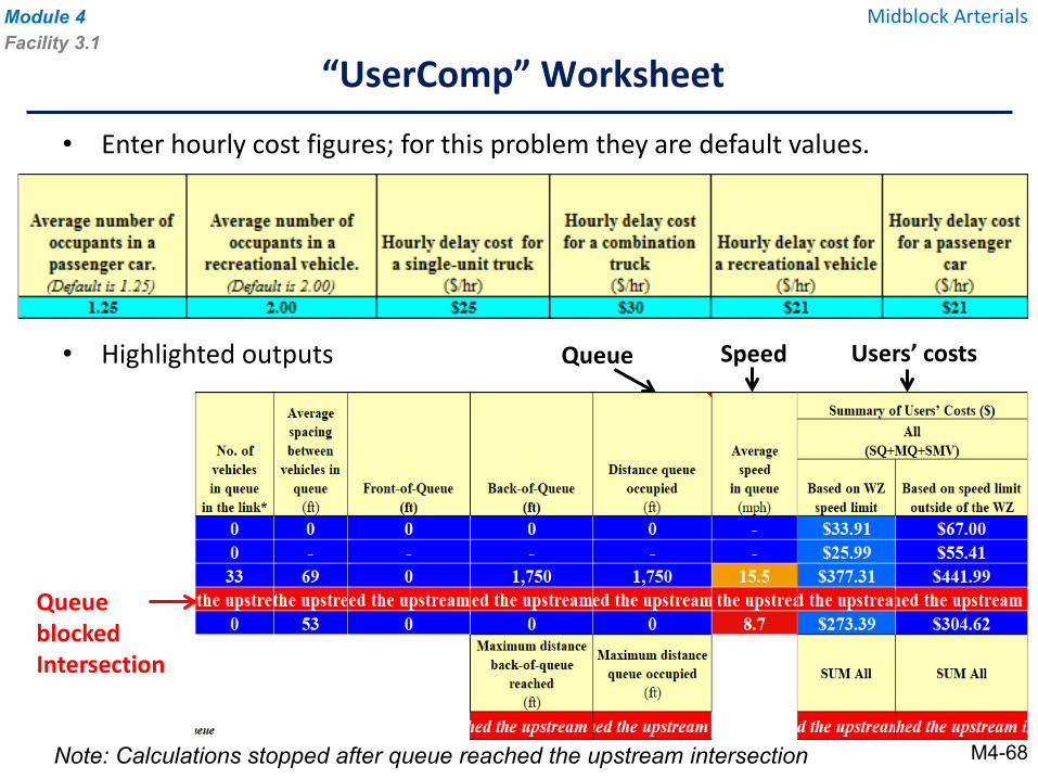
• Enter hourly cost figures; for this problem they are default values.
• Highlighted outputs Users’ costsSpeedQueue
Queue blocked Intersection
“UserComp” WorksheetModule 4 Midblock ArterialsFacility 3.1
Note: Calculations stopped after queue reached the upstream intersection M4-68
1. How would I “estimate/guestimate” how far the queue is extended beyond the upstream intersection?
2. What can I do if the queue reaches upstream intersection?
3. Should this procedure be used for “multilane” highways?
Midblock WZ Effects - Group Discussion
Module 4Facility 3
Midblock Arterials
M4-69
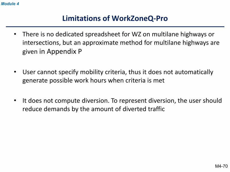
• There is no dedicated spreadsheet for WZ on multilane highways or intersections, but an approximate method for multilane highways are given in Appendix P
• User cannot specify mobility criteria, thus it does not automatically generate possible work hours when criteria is met
• It does not compute diversion. To represent diversion, the user should reduce demands by the amount of diverted traffic
Limitations of WorkZoneQ-Pro
Module 4
M4-70
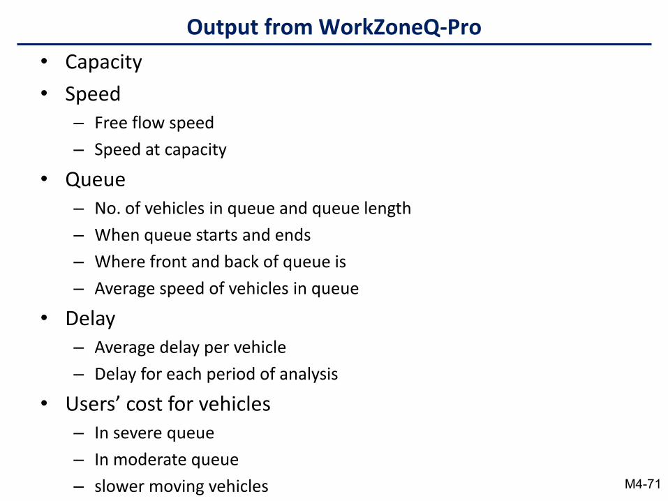
• Capacity• Speed
– Free flow speed– Speed at capacity
• Queue– No. of vehicles in queue and queue length– When queue starts and ends– Where front and back of queue is– Average speed of vehicles in queue
• Delay– Average delay per vehicle– Delay for each period of analysis
• Users’ cost for vehicles– In severe queue– In moderate queue– slower moving vehicles
Output from WorkZoneQ-Pro
M4-71
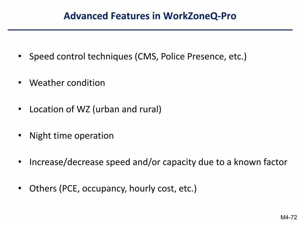
• Speed control techniques (CMS, Police Presence, etc.)
• Weather condition
• Location of WZ (urban and rural)
• Night time operation
• Increase/decrease speed and/or capacity due to a known factor
• Others (PCE, occupancy, hourly cost, etc.)
Advanced Features in WorkZoneQ-Pro
M4-72
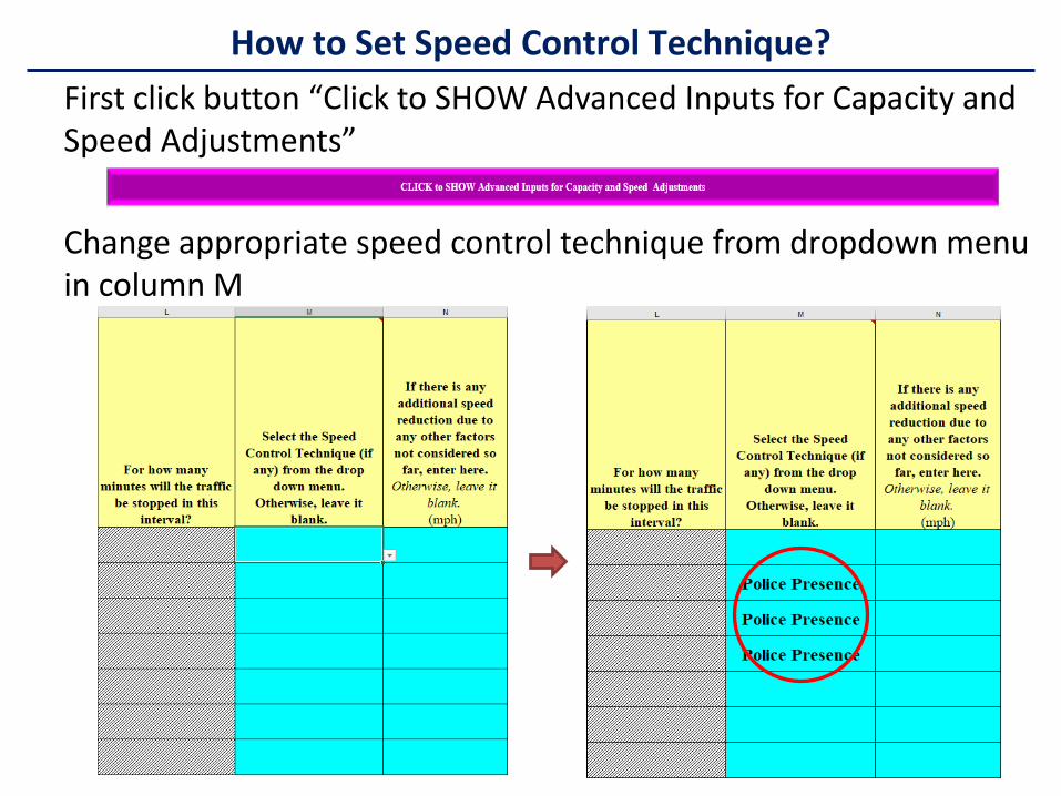
First click button “Click to SHOW Advanced Inputs for Capacity and Speed Adjustments”
Change appropriate speed control technique from dropdown menu in column M
How to Set Speed Control Technique?
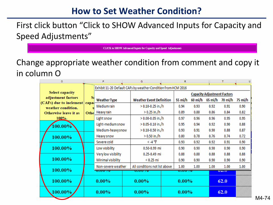
First click button “Click to SHOW Advanced Inputs for Capacity and Speed Adjustments”
Change appropriate weather condition from comment and copy it in column O
How to Set Weather Condition?
M4-74
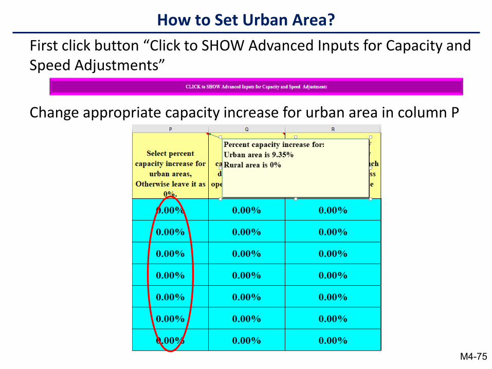
First click button “Click to SHOW Advanced Inputs for Capacity and Speed Adjustments”
Change appropriate capacity increase for urban area in column P
How to Set Urban Area?
M4-75
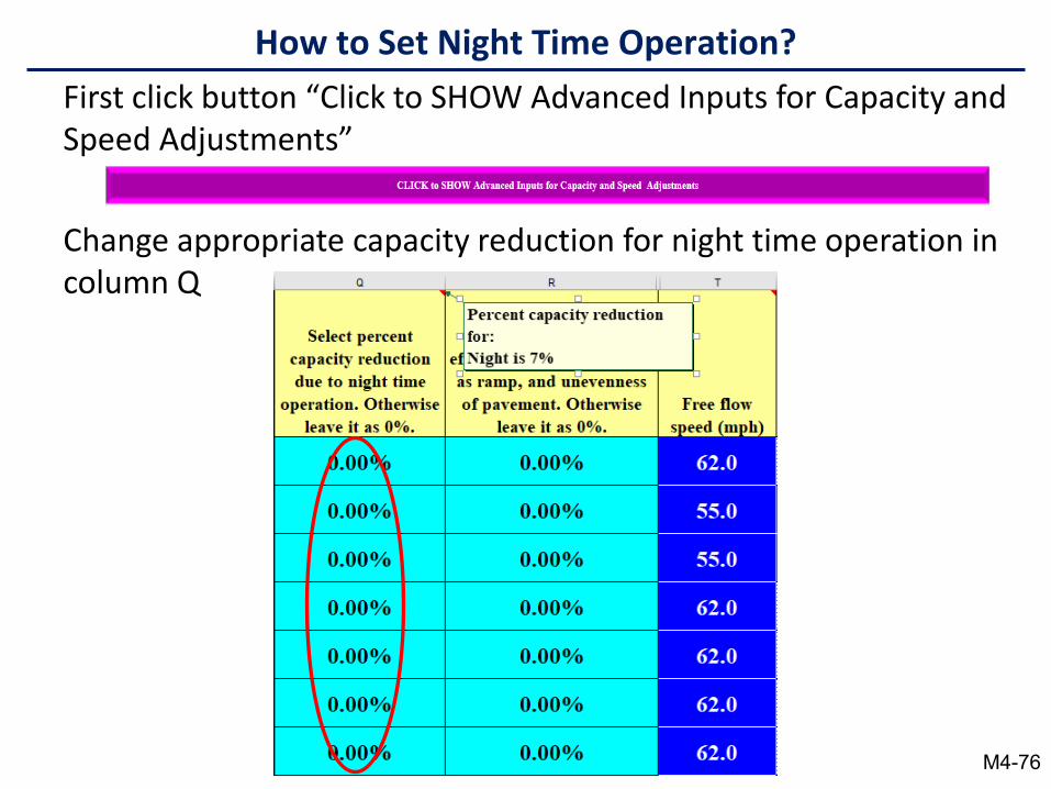
First click button “Click to SHOW Advanced Inputs for Capacity and Speed Adjustments”
Change appropriate capacity reduction for night time operation in column Q
How to Set Night Time Operation?
M4-76
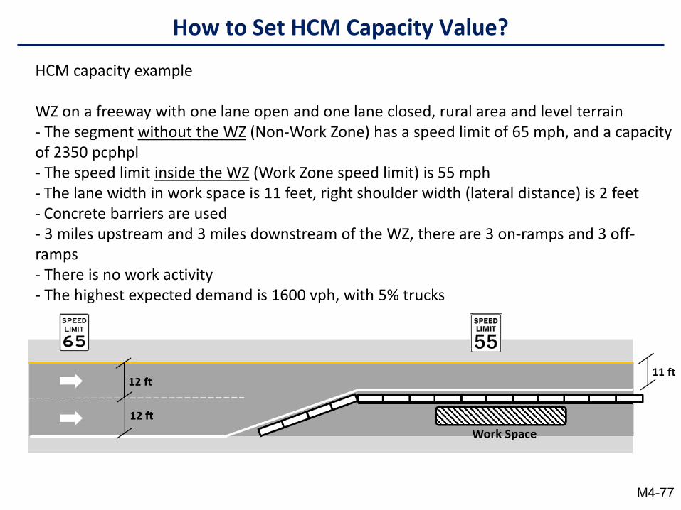
How to Set HCM Capacity Value?
HCM capacity example
WZ on a freeway with one lane open and one lane closed, rural area and level terrain- The segment without the WZ (Non-Work Zone) has a speed limit of 65 mph, and a capacity of 2350 pcphpl- The speed limit inside the WZ (Work Zone speed limit) is 55 mph- The lane width in work space is 11 feet, right shoulder width (lateral distance) is 2 feet- Concrete barriers are used- 3 miles upstream and 3 miles downstream of the WZ, there are 3 on-ramps and 3 off-ramps- There is no work activity- The highest expected demand is 1600 vph, with 5% trucks
M4-77
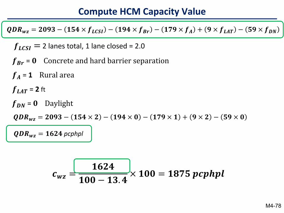
Compute HCM Capacity Value
𝑸𝑸𝑸𝑸𝑸𝑸𝒘𝒘𝒘𝒘 = 𝟐𝟐𝟏𝟏𝟐𝟐𝟏𝟏 − 𝟏𝟏𝟏𝟏𝟒𝟒 × 𝒇𝒇𝑳𝑳𝑳𝑳𝑳𝑳𝑳𝑳 − 𝟏𝟏𝟐𝟐𝟒𝟒 × 𝒇𝒇𝑩𝑩𝑩𝑩 − 𝟏𝟏𝟏𝟏𝟐𝟐 × 𝒇𝒇𝑨𝑨 + 𝟐𝟐 × 𝒇𝒇𝑳𝑳𝑨𝑨𝑳𝑳 − 𝟏𝟏𝟐𝟐 × 𝒇𝒇𝑸𝑸𝑫𝑫
𝒇𝒇𝑩𝑩𝑩𝑩 = 𝟏𝟏 Concrete and hard barrier separation
𝒇𝒇𝑨𝑨 = 1 Rural area
𝒇𝒇𝑳𝑳𝑨𝑨𝑳𝑳 = 2 ft
𝒇𝒇𝑸𝑸𝑫𝑫 = 𝟏𝟏 Daylight
𝒇𝒇𝑳𝑳𝑳𝑳𝑳𝑳𝑳𝑳 = 2 lanes total, 1 lane closed = 2.0
𝑸𝑸𝑸𝑸𝑸𝑸𝒘𝒘𝒘𝒘 = 𝟐𝟐𝟏𝟏𝟐𝟐𝟏𝟏 − 𝟏𝟏𝟏𝟏𝟒𝟒 × 𝟐𝟐 − 𝟏𝟏𝟐𝟐𝟒𝟒 × 𝟏𝟏 − 𝟏𝟏𝟏𝟏𝟐𝟐 × 𝟏𝟏 + 𝟐𝟐 × 𝟐𝟐 − 𝟏𝟏𝟐𝟐 × 𝟏𝟏
𝑸𝑸𝑸𝑸𝑸𝑸𝒘𝒘𝒘𝒘 = 𝟏𝟏𝟏𝟏𝟐𝟐𝟒𝟒 pcphpl
𝒄𝒄𝒘𝒘𝒘𝒘 =𝟏𝟏𝟏𝟏𝟐𝟐𝟒𝟒
𝟏𝟏𝟏𝟏𝟏𝟏 − 𝟏𝟏𝟏𝟏.𝟒𝟒× 𝟏𝟏𝟏𝟏𝟏𝟏 = 𝟏𝟏𝟏𝟏𝟏𝟏𝟏𝟏 𝒑𝒑𝒄𝒄𝒑𝒑𝒑𝒑𝒑𝒑𝒑𝒑
M4-78
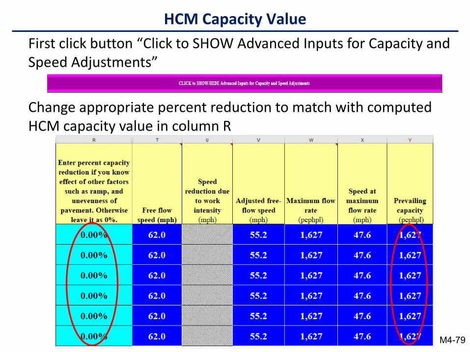
First click button “Click to SHOW Advanced Inputs for Capacity and Speed Adjustments”
Change appropriate percent reduction to match with computed HCM capacity value in column R
HCM Capacity Value
M4-79
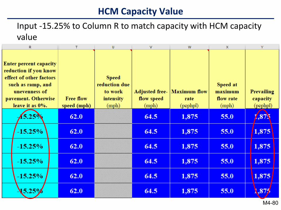
Input -15.25% to Column R to match capacity with HCM capacity value
HCM Capacity Value
M4-80
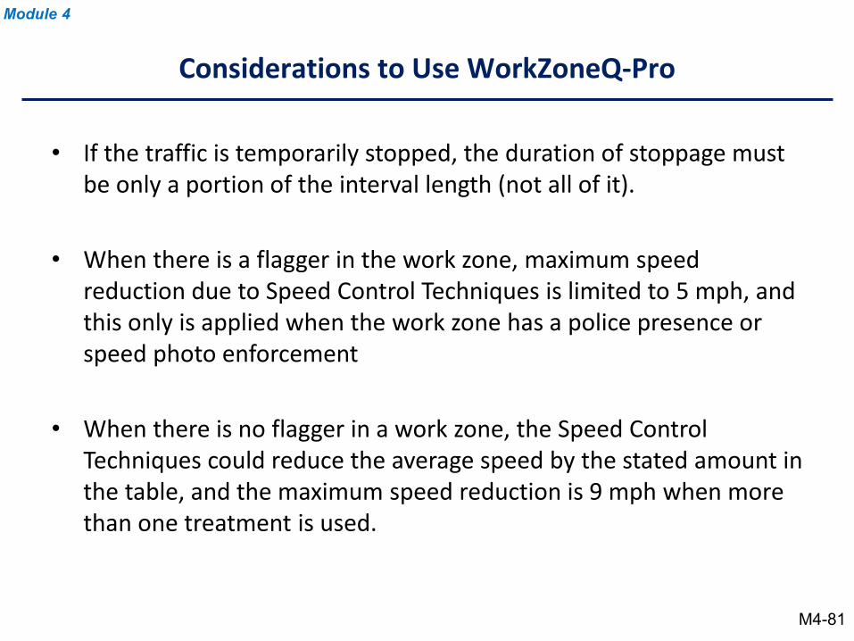
• If the traffic is temporarily stopped, the duration of stoppage must be only a portion of the interval length (not all of it).
• When there is a flagger in the work zone, maximum speed reduction due to Speed Control Techniques is limited to 5 mph, and this only is applied when the work zone has a police presence or speed photo enforcement
• When there is no flagger in a work zone, the Speed Control Techniques could reduce the average speed by the stated amount in the table, and the maximum speed reduction is 9 mph when more than one treatment is used.
Considerations to Use WorkZoneQ-Pro
Module 4
M4-81
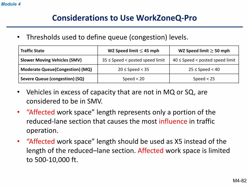
Considerations to Use WorkZoneQ-Pro
Module 4
• Thresholds used to define queue (congestion) levels.
• Vehicles in excess of capacity that are not in MQ or SQ, are considered to be in SMV.
• “Affected work space” length represents only a portion of the reduced-lane section that causes the most influence in traffic operation.
• “Affected work space” length should be used as X5 instead of the length of the reduced–lane section. Affected work space is limited to 500-10,000 ft.
Traffic State WZ Speed limit ≤ 45 mph WZ Speed limit ≥ 50 mph
Slower Moving Vehicles (SMV) 35 ≤ Speed < posted speed limit 40 ≤ Speed < posted speed limit
Moderate Queue(Congestion) (MQ) 20 ≤ Speed < 35 25 ≤ Speed < 40
Severe Queue (congestion) (SQ) Speed < 20 Speed < 25
M4-82
Facility3 : Arterial 3.2: Intersection
UseUI Spreadsheet for Intersections
M4-83
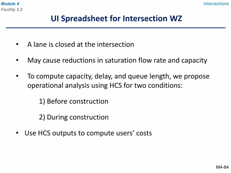
• A lane is closed at the intersection
• May cause reductions in saturation flow rate and capacity
• To compute capacity, delay, and queue length, we propose operational analysis using HCS for two conditions:
1) Before construction
2) During construction
• Use HCS outputs to compute users’ costs
UI Spreadsheet for Intersection WZ
Module 4 IntersectionsFacility 3.2
M4-84
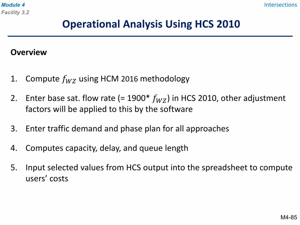
Overview
1. Compute 𝑓𝑓𝑊𝑊𝑊𝑊 using HCM 2016 methodology
2. Enter base sat. flow rate (= 1900* 𝑓𝑓𝑊𝑊𝑊𝑊) in HCS 2010, other adjustment factors will be applied to this by the software
3. Enter traffic demand and phase plan for all approaches
4. Computes capacity, delay, and queue length
5. Input selected values from HCS output into the spreadsheet to compute users’ costs
Operational Analysis Using HCS 2010
Module 4 IntersectionsFacility 3.2
M4-85
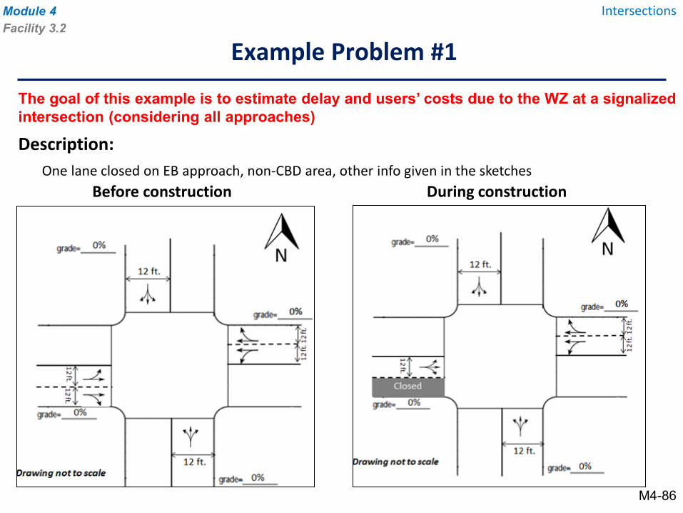
Description:One lane closed on EB approach, non-CBD area, other info given in the sketches
Before construction During construction
Example Problem #1
Module 4 IntersectionsFacility 3.2
The goal of this example is to estimate delay and users’ costs due to the WZ at a signalized intersection (considering all approaches)
M4-86
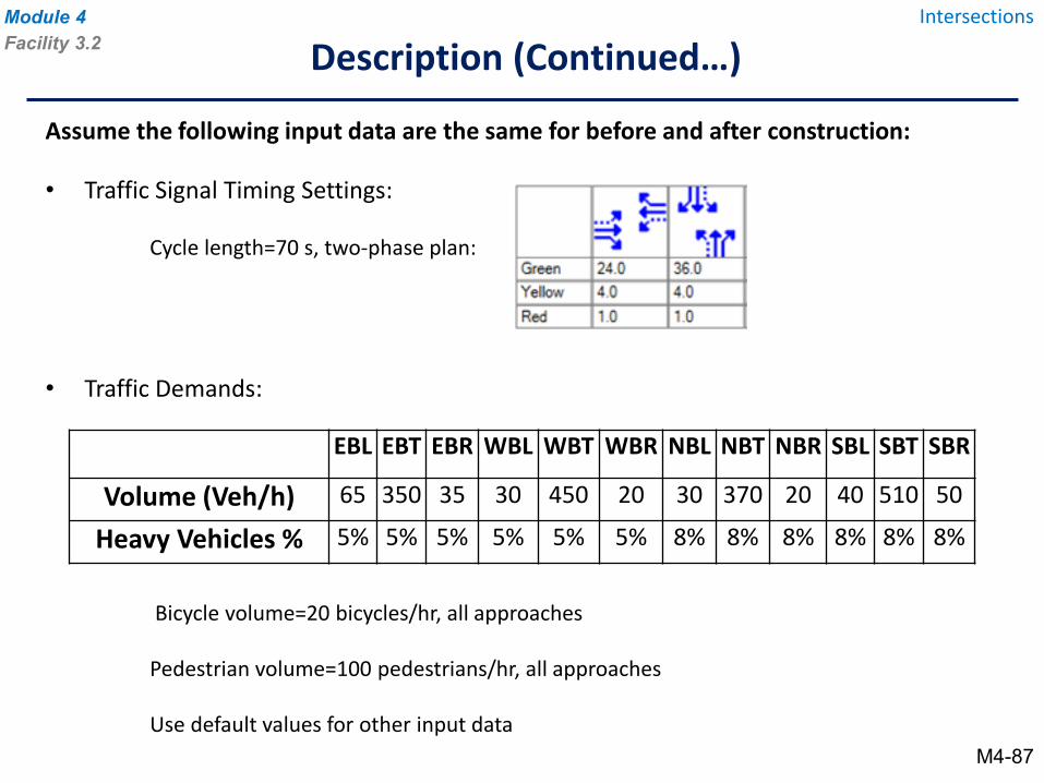
Assume the following input data are the same for before and after construction:
• Traffic Signal Timing Settings:
Cycle length=70 s, two-phase plan:
• Traffic Demands:
Bicycle volume=20 bicycles/hr, all approaches
Pedestrian volume=100 pedestrians/hr, all approaches
Use default values for other input data
EBL EBT EBR WBL WBT WBR NBL NBT NBR SBL SBT SBR
Volume (Veh/h) 65 350 35 30 450 20 30 370 20 40 510 50
Heavy Vehicles % 5% 5% 5% 5% 5% 5% 8% 8% 8% 8% 8% 8%
Description (Continued…)Module 4 IntersectionsFacility 3.2
M4-87
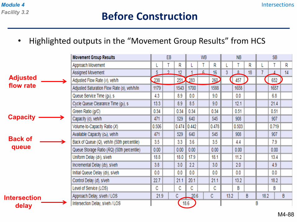
Movement Group Results EB WB NB SB
Approach Movement l T R L T R L l R L T R
Assigned Movernen· 5 l 12 1 h 16 3 JL 18 7 ---'-- u ) Adjusted Flow :Rate (vt veM1 ~ 8 2~ u_&3 2~ \ 457 lJ t 652 )
Adjusted Saturat on Flow Rate (s). eh/ntrn 1179 1543 HOO 1583 1658 1657 -
Queue Servt e ime (g~). s 4.3 8.9 0.0 9.0 0.0 6.8 cycle Queue Clearance Time (g~}, s 13.3 8.9 8.5 9.0 12.1 21.4
Green Ra ·o (g/C) 0.34 0.34 0.34 0.34 0.51 0.51 ) capacity (c), vehlh 471 529 GAO 545 908 907
Vo!ume-:to-Capacity Ra io (XJ 0,506 0,414 0,442 0,478 0,503 0.119 Avallab e Capacity (ca,), vehlh 471 529 640 545 908 907
) Back 01 Queue (Q), veMn (50th pen:erillle) 3.5 3 .. 3 3.6 3.5 4.4 7.9 Queue Storage Ratto (RQ) (50lh1 percenme) 0.00 0.00 0.00 0.00 0.00 0.00 ~
UnifOrm Delay (dt), s eh 18.8 18.0 H.9 18.1 11 .2 1i3.4
lncrementa'I Delay (d ), s eh 3.8 3.0 2.2 3.0 2.0 4.9
lnitia11 Queue Delay (d1), slveh 0,0 0,0 0,0 0.0 0,0 0.0 Control Delay {cf), s/Veh 22.7 21 ,1 20.1 21.1 13.2 18,2
Level of Service ~ OS) C C C C 8 1B
I r l l -I Approach Delay, s/Veh / LOS 21.9 C - - 20.6 C 13.2 8 118.2 B
) lnters~uon Dela , srve11 J OS l 1s.6 J B -
Module 4 Intersections Facility 3.2 Before Construction
• Highlighted outputs in the “Movement Group Results” from HCS
Adjusted flow rate
Capacity
Back of queue
Intersection delay
M4-88
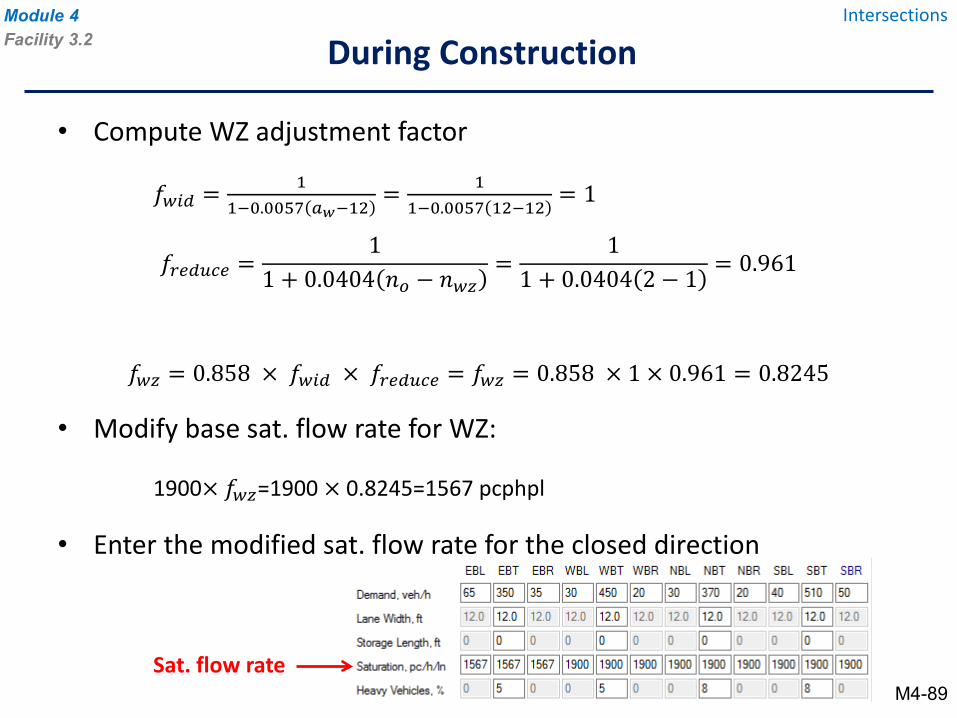
• Compute WZ adjustment factor
𝑓𝑓𝑤𝑤𝑤𝑤𝑎𝑎 = 11−0.0057 𝑎𝑎𝑤𝑤−12
= 11−0.0057 12−12
= 1
𝑓𝑓𝑟𝑟𝑟𝑟𝑎𝑎𝑟𝑟𝑟𝑟𝑟𝑟 =1
1 + 0.0404 𝑡𝑡𝑜𝑜 − 𝑡𝑡𝑤𝑤𝑤𝑤=
11 + 0.0404 2 − 1
= 0.961
𝑓𝑓𝑤𝑤𝑤𝑤 = 0.858 × 𝑓𝑓𝑤𝑤𝑤𝑤𝑎𝑎 × 𝑓𝑓𝑟𝑟𝑟𝑟𝑎𝑎𝑟𝑟𝑟𝑟𝑟𝑟 = 𝑓𝑓𝑤𝑤𝑤𝑤 = 0.858 × 1 × 0.961 = 0.8245
• Modify base sat. flow rate for WZ:
1900× 𝑓𝑓𝑤𝑤𝑤𝑤=1900 × 0.8245=1567 pcphpl
• Enter the modified sat. flow rate for the closed direction
During ConstructionModule 4 IntersectionsFacility 3.2
Sat. flow rateM4-89
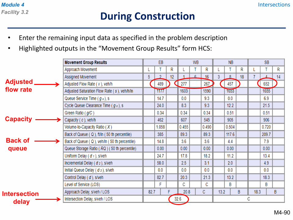
During ConstructionModule 4 IntersectionsFacility 3.2
• Enter the remaining input data as specified in the problem description • Highlighted outputs in the “Movement Group Results” form HCS:
Capacity
Intersection delay
Adjusted flow rate
Back ofqueue
M4-90
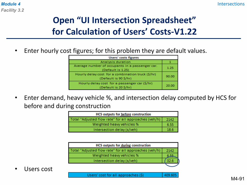
• Enter hourly cost figures; for this problem they are default values.
• Enter demand, heavy vehicle %, and intersection delay computed by HCS for before and during construction
• Users cost
Open “UI Intersection Spreadsheet” for Calculation of Users’ Costs-V1.22
Module 4 IntersectionsFacility 3.2
M4-91

Left Blank Intentionally
Module 5
Traffic Management Strategies using the Tools
Example Problems
M5-1
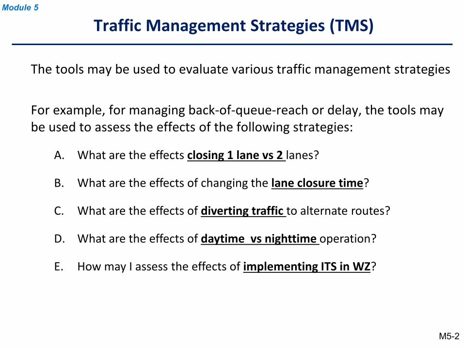
A. What are the effects closing 1 lane vs 2 lanes?
B. What are the effects of changing the lane closure time?
C. What are the effects of diverting traffic to alternate routes?
D. What are the effects of daytime vs nighttime operation?
E. How may I assess the effects of implementing ITS in WZ?
Traffic Management Strategies (TMS)
The tools may be used to evaluate various traffic management strategies
For example, for managing back-of-queue-reach or delay, the tools may be used to assess the effects of the following strategies:
Module 5
M5-2
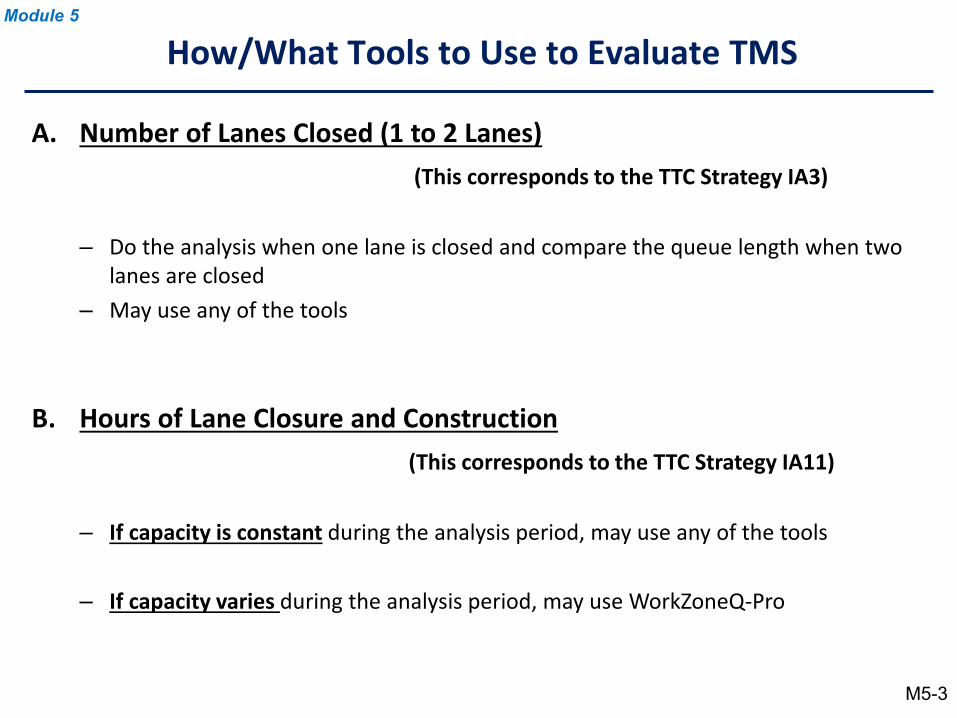
A. Number of Lanes Closed (1 to 2 Lanes)(This corresponds to the TTC Strategy IA3)
– Do the analysis when one lane is closed and compare the queue length when two lanes are closed
– May use any of the tools
B. Hours of Lane Closure and Construction(This corresponds to the TTC Strategy IA11)
– If capacity is constant during the analysis period, may use any of the tools
– If capacity varies during the analysis period, may use WorkZoneQ-Pro
How/What Tools to Use to Evaluate TMSModule 5
M5-3
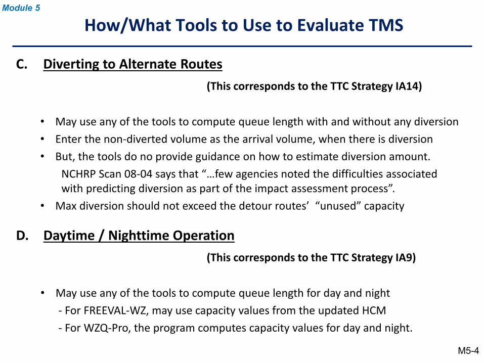
C. Diverting to Alternate Routes(This corresponds to the TTC Strategy IA14)
• May use any of the tools to compute queue length with and without any diversion • Enter the non-diverted volume as the arrival volume, when there is diversion • But, the tools do no provide guidance on how to estimate diversion amount.
NCHRP Scan 08-04 says that “…few agencies noted the difficulties associated with predicting diversion as part of the impact assessment process”.
• Max diversion should not exceed the detour routes’ “unused” capacity
D. Daytime / Nighttime Operation(This corresponds to the TTC Strategy IA9)
• May use any of the tools to compute queue length for day and night - For FREEVAL-WZ, may use capacity values from the updated HCM - For WZQ-Pro, the program computes capacity values for day and night.
How/What Tools to Use to Evaluate TMSModule 5
M5-4
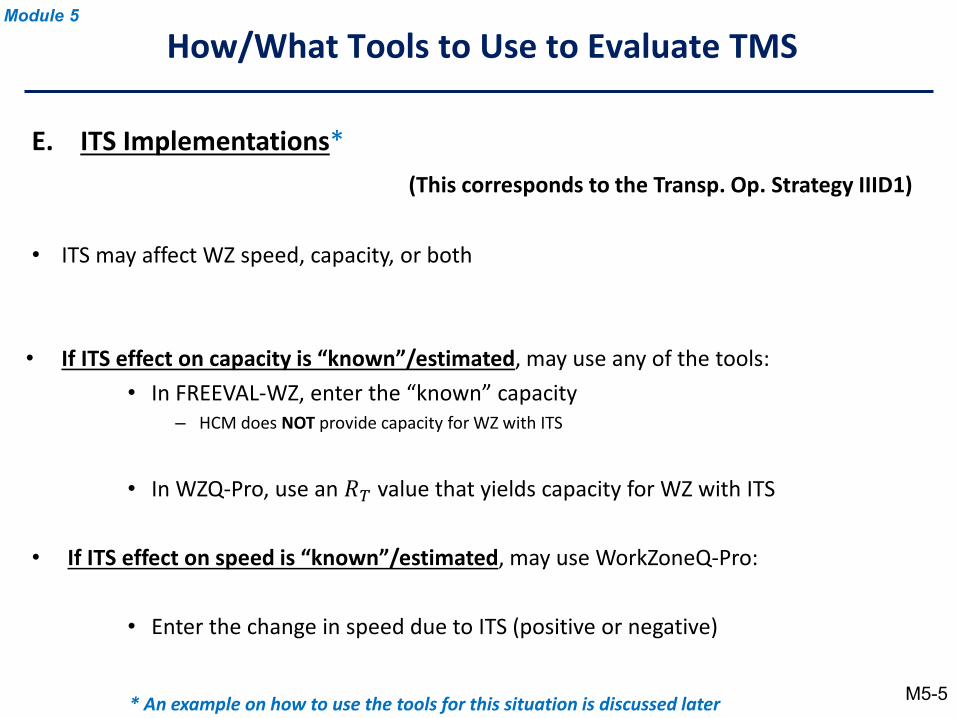
E. ITS Implementations*(This corresponds to the Transp. Op. Strategy IIID1)
• ITS may affect WZ speed, capacity, or both
• If ITS effect on capacity is “known”/estimated, may use any of the tools:• In FREEVAL-WZ, enter the “known” capacity
– HCM does NOT provide capacity for WZ with ITS
• In WZQ-Pro, use an 𝑄𝑄𝑇𝑇 value that yields capacity for WZ with ITS
• If ITS effect on speed is “known”/estimated, may use WorkZoneQ-Pro:
• Enter the change in speed due to ITS (positive or negative)
How/What Tools to Use to Evaluate TMS
* An example on how to use the tools for this situation is discussed later
Module 5
M5-5
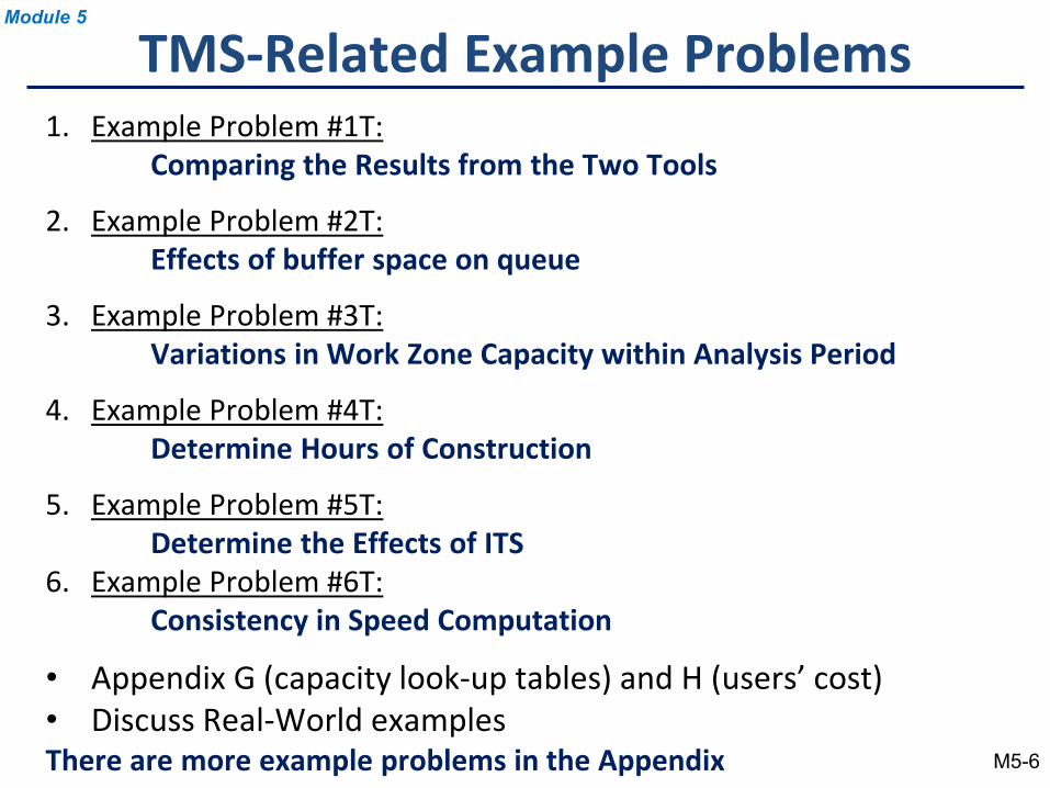
TMS-Related Example Problems1. Example Problem #1T:
Comparing the Results from the Two Tools
2. Example Problem #2T: Effects of buffer space on queue
3. Example Problem #3T: Variations in Work Zone Capacity within Analysis Period
4. Example Problem #4T:Determine Hours of Construction
5. Example Problem #5T:Determine the Effects of ITS
6. Example Problem #6T:Consistency in Speed Computation
• Appendix G (capacity look-up tables) and H (users’ cost)• Discuss Real-World examplesThere are more example problems in the Appendix
Module 5
M5-6
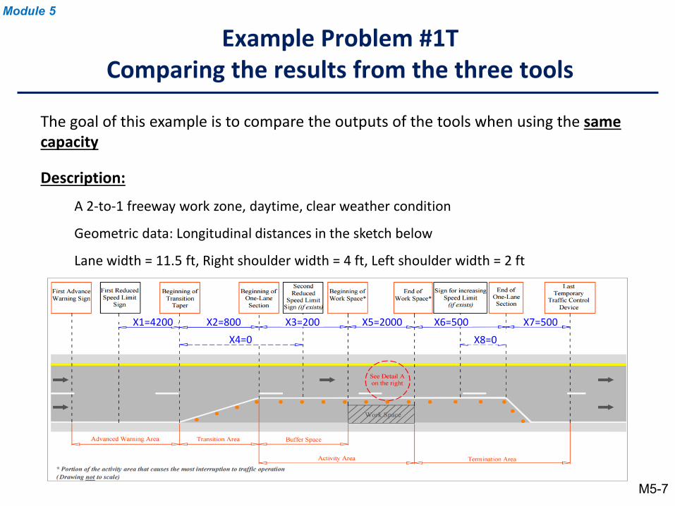
Description:
A 2-to-1 freeway work zone, daytime, clear weather condition
Geometric data: Longitudinal distances in the sketch below
Lane width = 11.5 ft, Right shoulder width = 4 ft, Left shoulder width = 2 ft
Example Problem #1TComparing the results from the three tools
The goal of this example is to compare the outputs of the tools when using the same capacity
X1=4200 X2=800X4=0 X8=0
X7=500X6=500X5=2000X3=200
Module 5
M5-7
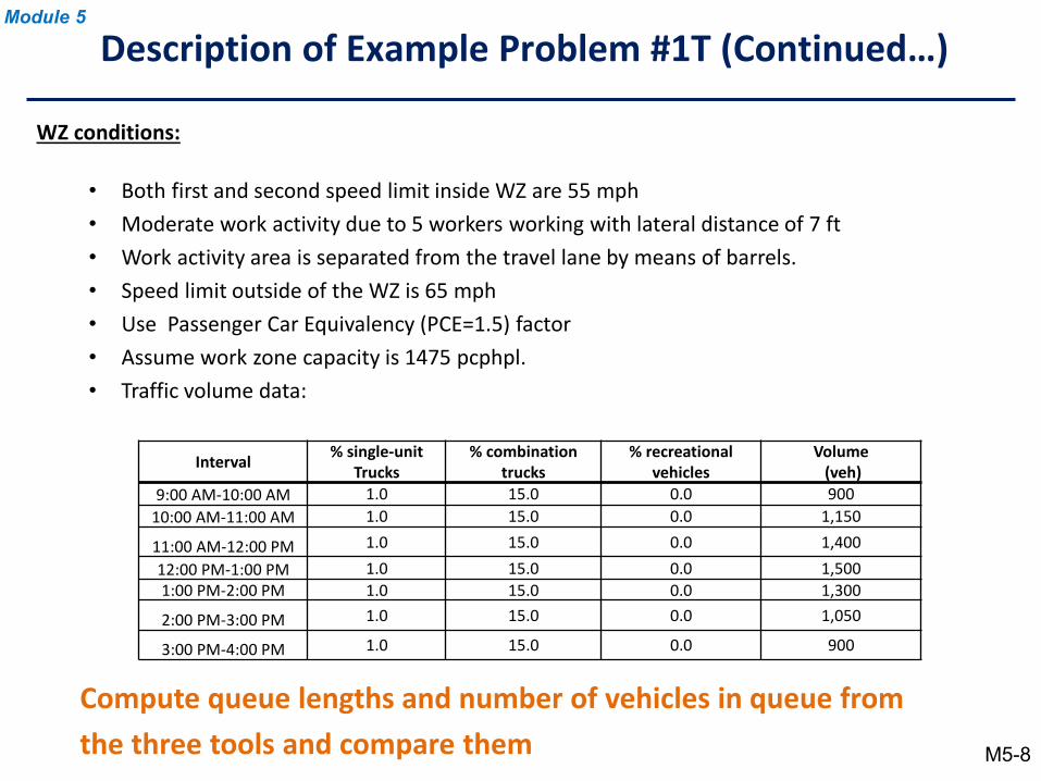
WZ conditions:
• Both first and second speed limit inside WZ are 55 mph• Moderate work activity due to 5 workers working with lateral distance of 7 ft • Work activity area is separated from the travel lane by means of barrels. • Speed limit outside of the WZ is 65 mph• Use Passenger Car Equivalency (PCE=1.5) factor• Assume work zone capacity is 1475 pcphpl. • Traffic volume data:
Compute queue lengths and number of vehicles in queue from the three tools and compare them
Interval % single-unitTrucks
% combination trucks
% recreational vehicles
Volume(veh)
9:00 AM-10:00 AM 1.0 15.0 0.0 90010:00 AM-11:00 AM 1.0 15.0 0.0 1,150
11:00 AM-12:00 PM 1.0 15.0 0.0 1,40012:00 PM-1:00 PM 1.0 15.0 0.0 1,5001:00 PM-2:00 PM 1.0 15.0 0.0 1,300
2:00 PM-3:00 PM 1.0 15.0 0.0 1,050
3:00 PM-4:00 PM 1.0 15.0 0.0 900
Description of Example Problem #1T (Continued…)Module 5
M5-8
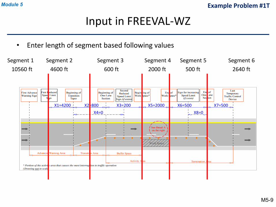
Example Problem #1TModule 5
M5-9
Input in FREEVAL-WZ
• Enter length of segment based following values
Segment 1 Segment 2 Segment 3 Segment 4 Segment 5 Segment 610560 ft 4600 ft 600 ft 2000 ft 500 ft 2640 ft
X1=4200 X2=800X4=0 X8=0
X7=500X6=500X5=2000X3=200
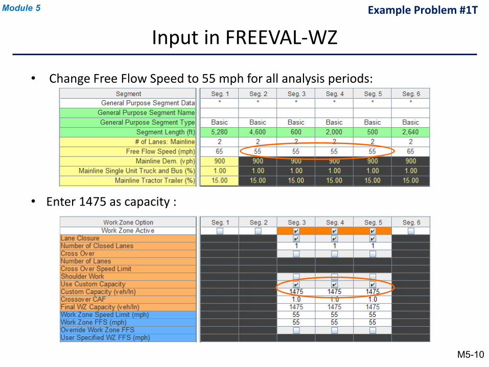
• Change Free Flow Speed to 55 mph for all analysis periods:
Module 5
M5-10
Example Problem #1T
Input in FREEVAL-WZ
• Enter 1475 as capacity :
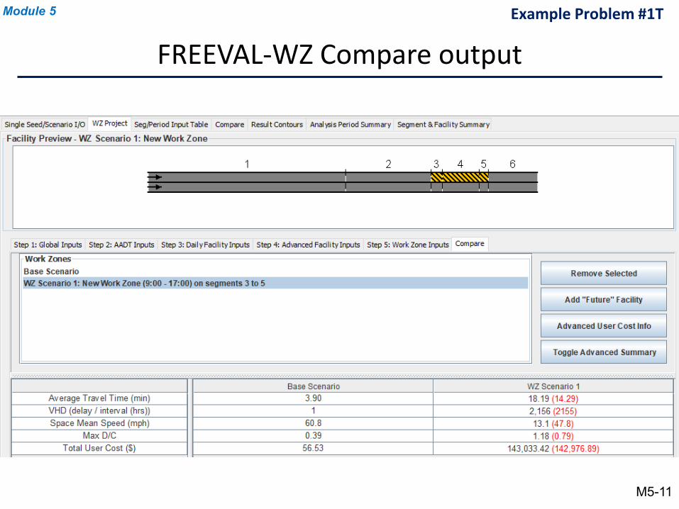
FREEVAL-WZ Compare output
Module 5
M5-11
Example Problem #1T
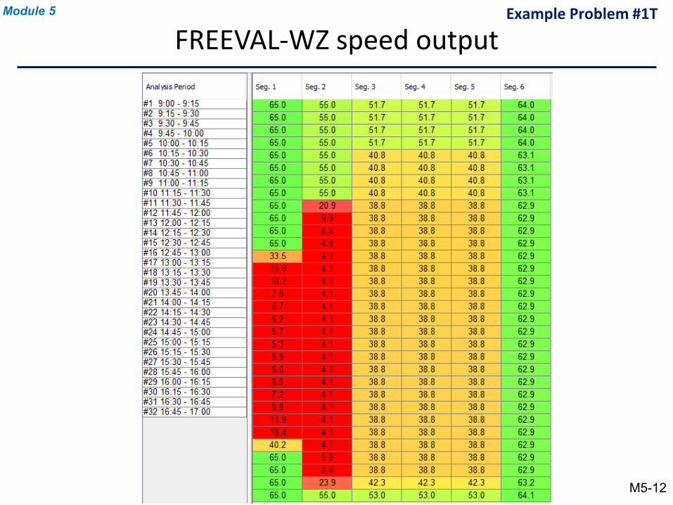
FREEVAL-WZ speed outputModule 5
M5-12
Example Problem #1T
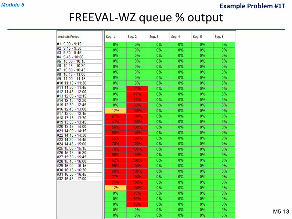
FREEVAL-WZ queue % outputModule 5
M5-13
Example Problem #1T
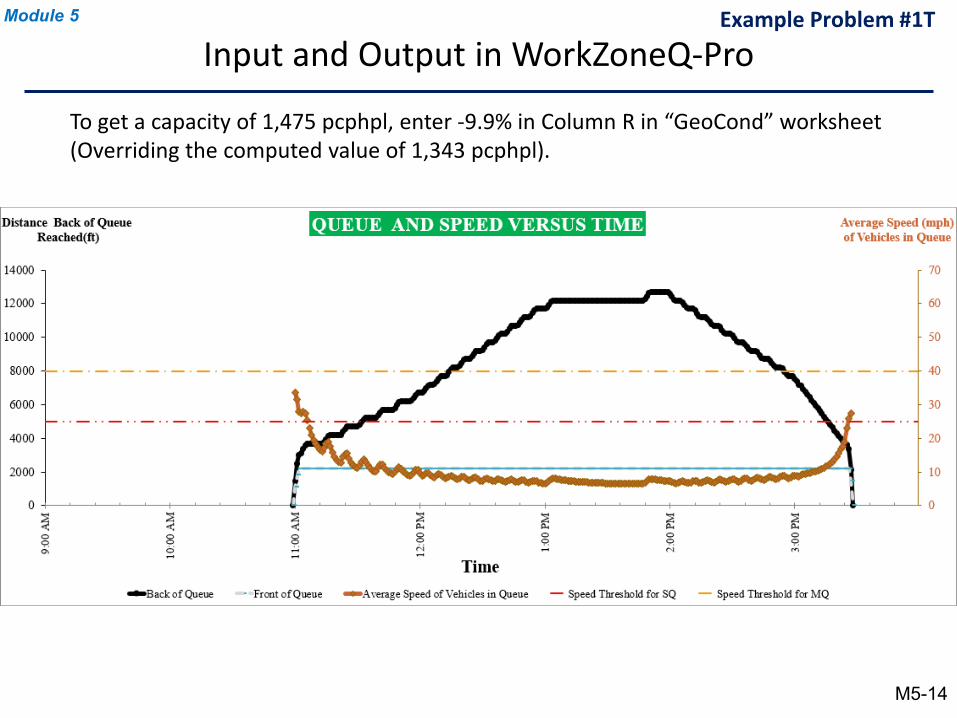
Input and Output in WorkZoneQ-ProModule 5
M5-14
Example Problem #1T
To get a capacity of 1,475 pcphpl, enter -9.9% in Column R in “GeoCond” worksheet (Overriding the computed value of 1,343 pcphpl).
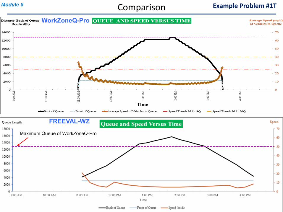
ComparisonModule 5 Example Problem #1T
Maximum Queue of WorkZoneQ-Pro
WorkZoneQ-Pro
FREEVAL-WZ
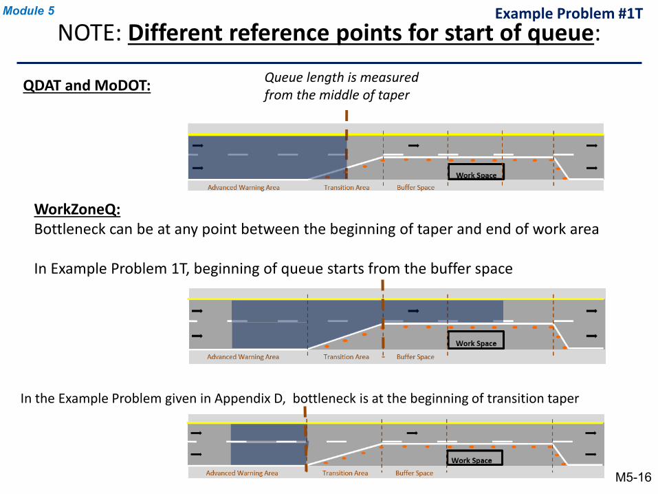
NOTE: Different reference points for start of queue:
WorkZoneQ:Bottleneck can be at any point between the beginning of taper and end of work area
In Example Problem 1T, beginning of queue starts from the buffer space
QDAT and MoDOT: Queue length is measured from the middle of taper
In the Example Problem given in Appendix D, bottleneck is at the beginning of transition taper
Module 5
M5-16
Example Problem #1T
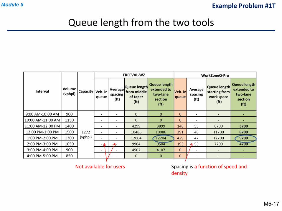
Queue length from the two tools
Module 5
M5-17
Example Problem #1T
Spacing is a function of speed and density
Interval Volume(vphpl) Capacity
FREEVAL-WZ WorkZoneQ-Pro
Veh. in queue
Average spacing
(ft)
Queue length from middle
of taper(ft)
Queue length extended to
two-lane section
(ft)
Veh. in queue
Average spacing
(ft)
Queue lengthstarting from work space
(ft)
Queue length extended to
two-lane section
(ft)
9:00 AM-10:00 AM 900
1272(vphpl)
- - 0 0 0 - - -10:00 AM-11:00 AM 1150 - - 0 0 0 - - -11:00 AM-12:00 PM 1400 - - 4299 3899 148 55 6700 370012:00 PM-1:00 PM 1500 - - 10486 10086 391 48 11700 87001:00 PM-2:00 PM 1300 - - 12604 12204 429 47 12700 97002:00 PM-3:00 PM 1050 - - 9904 9504 193 53 7700 47003:00 PM-4:00 PM 900 - - 4507 4107 0 - - -4:00 PM-5:00 PM 850 - - 0 0 0 - - -
Not available for users
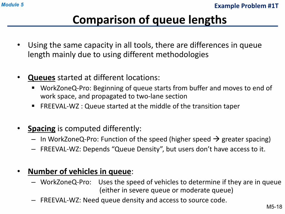
Comparison of queue lengths
• Using the same capacity in all tools, there are differences in queue length mainly due to using different methodologies
• Queues started at different locations: WorkZoneQ-Pro: Beginning of queue starts from buffer and moves to end of
work space, and propagated to two-lane section FREEVAL-WZ : Queue started at the middle of the transition taper
• Spacing is computed differently: – In WorkZoneQ-Pro: Function of the speed (higher speed greater spacing)– FREEVAL-WZ: Depends “Queue Density”, but users don’t have access to it.
• Number of vehicles in queue:– WorkZoneQ-Pro: Uses the speed of vehicles to determine if they are in queue
(either in severe queue or moderate queue)– FREEVAL-WZ: Need queue density and access to source code.
Module 5
M5-18
Example Problem #1T
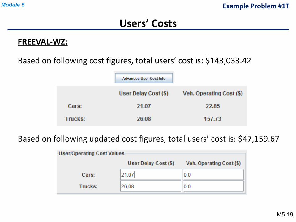
Users’ Costs
Module 5 Example Problem #1T
FREEVAL-WZ:
Based on following cost figures, total users’ cost is: $143,033.42
Based on following updated cost figures, total users’ cost is: $47,159.67
M5-19
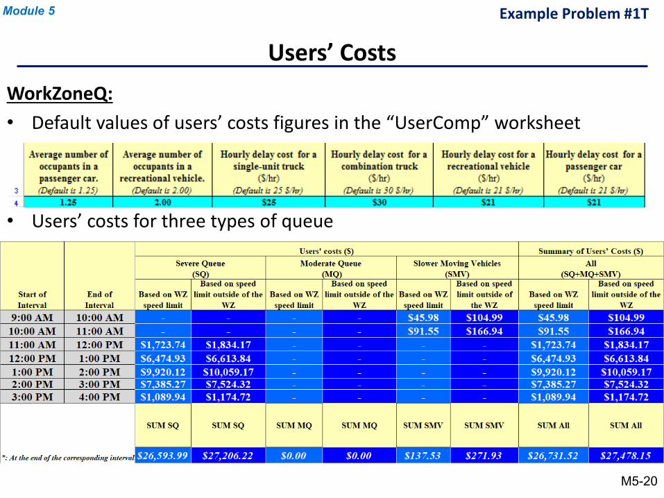
WorkZoneQ:• Default values of users’ costs figures in the “UserComp” worksheet
• Users’ costs for three types of queue
Users’ Costs
Module 5
M5-20
Example Problem #1T
Example Problem #2TEffects of buffer space on queue
Example Problem # 2T is moved to Appendix K
Module 5
M5-21
Example Problem #3TVariations in Work Zone Capacity within Analysis Period
Module 5
M5-22
Example Problem # 3T is moved to Appendix N
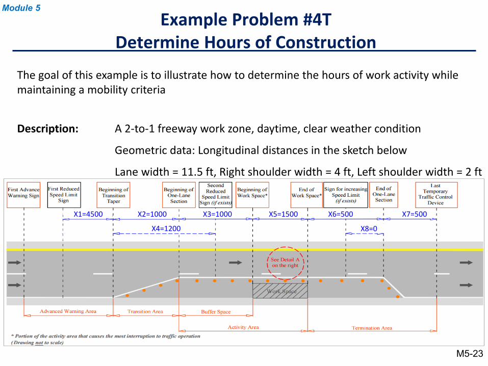
Description: A 2-to-1 freeway work zone, daytime, clear weather condition
Geometric data: Longitudinal distances in the sketch below
Lane width = 11.5 ft, Right shoulder width = 4 ft, Left shoulder width = 2 ft
Example Problem #4TDetermine Hours of Construction
The goal of this example is to illustrate how to determine the hours of work activity while maintaining a mobility criteria
X1=4500 X2=1000
X4=1200 X8=0
X7=500X6=500X5=1500X3=1000
Module 5
M5-23
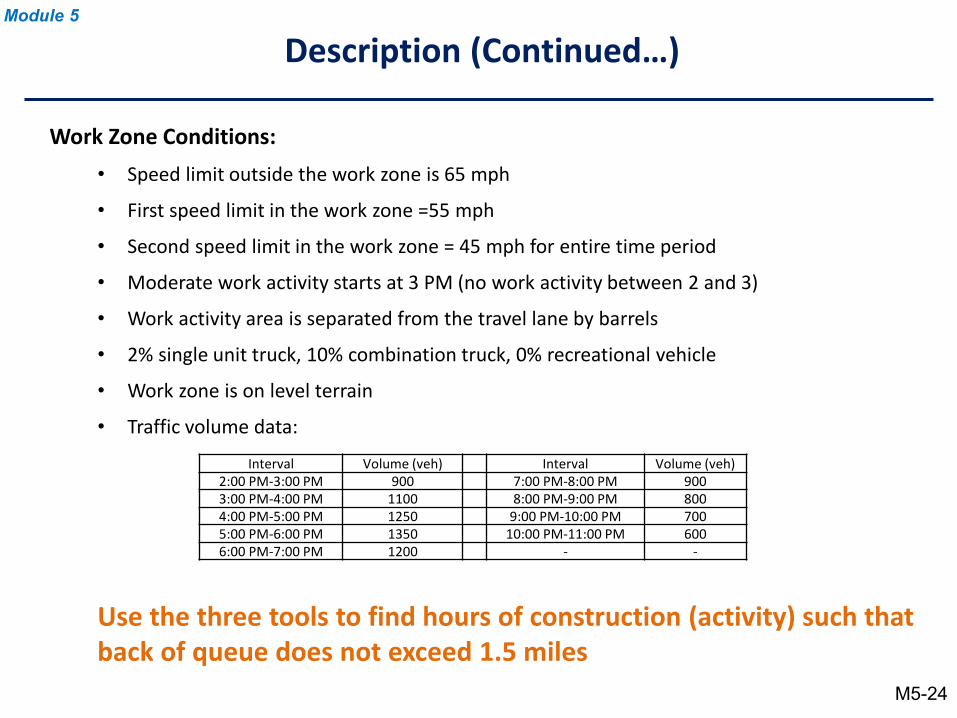
Work Zone Conditions: • Speed limit outside the work zone is 65 mph
• First speed limit in the work zone =55 mph
• Second speed limit in the work zone = 45 mph for entire time period
• Moderate work activity starts at 3 PM (no work activity between 2 and 3)
• Work activity area is separated from the travel lane by barrels
• 2% single unit truck, 10% combination truck, 0% recreational vehicle
• Work zone is on level terrain
• Traffic volume data:
Use the three tools to find hours of construction (activity) such that back of queue does not exceed 1.5 miles
Description (Continued…)
Interval Volume (veh) Interval Volume (veh)2:00 PM-3:00 PM 900 7:00 PM-8:00 PM 9003:00 PM-4:00 PM 1100 8:00 PM-9:00 PM 8004:00 PM-5:00 PM 1250 9:00 PM-10:00 PM 7005:00 PM-6:00 PM 1350 10:00 PM-11:00 PM 6006:00 PM-7:00 PM 1200 - -
Module 5
M5-24
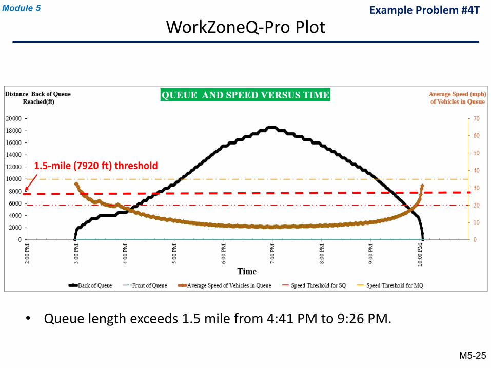
• Queue length exceeds 1.5 mile from 4:41 PM to 9:26 PM.
WorkZoneQ-Pro PlotExample Problem #4TModule 5
M5-25
1.5-mile (7920 ft) threshold
Determine Hours of Construction
Module 5
M5-26
• FREEVAL-WZ developer said, “it cannot change WZ configuration across time periods.” Means you cannot change capacity.
• For WZQ-Pro, the queue exceeded 1.5 mile limit from 4:56 pm to 9:18 pm. So avoid construction during those hours
Example Problem #4T
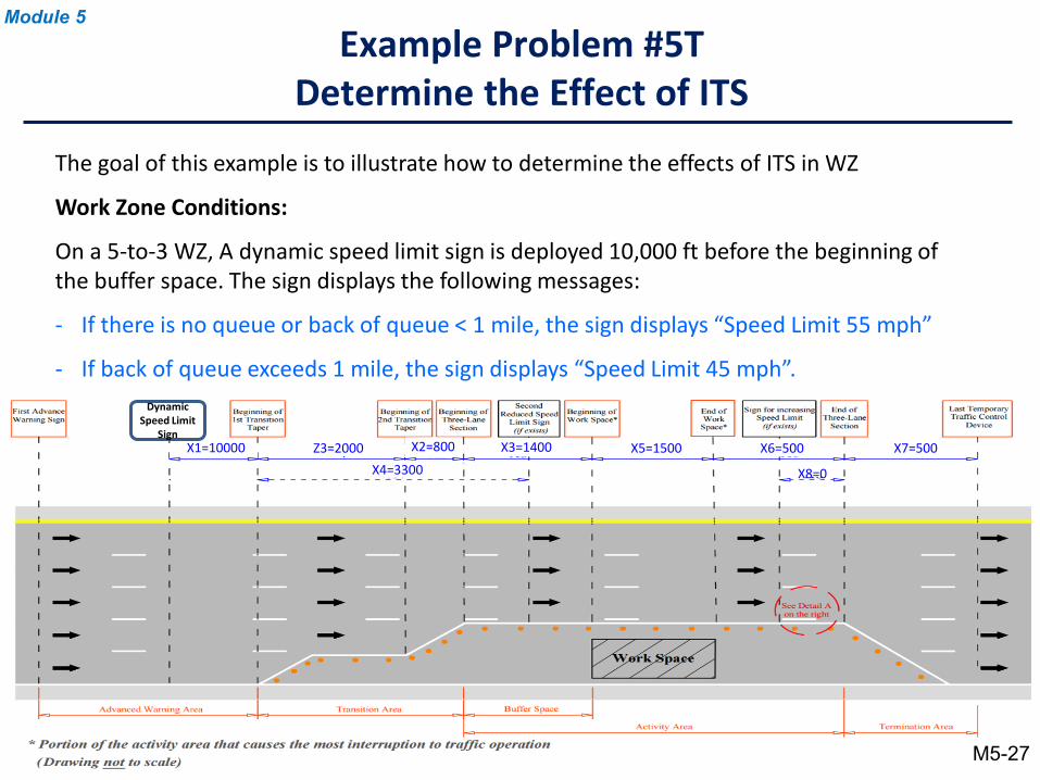
The goal of this example is to illustrate how to determine the effects of ITS in WZ
Work Zone Conditions:
On a 5-to-3 WZ, A dynamic speed limit sign is deployed 10,000 ft before the beginning of the buffer space. The sign displays the following messages:
- If there is no queue or back of queue < 1 mile, the sign displays “Speed Limit 55 mph”
- If back of queue exceeds 1 mile, the sign displays “Speed Limit 45 mph”.
Example Problem #5TDetermine the Effect of ITS
X1=10000 X2=800
X4=3300 X8=0
X7=500X6=500X5=1500X3=1400
DynamicSpeed Limit
SignZ3=2000
Module 5
M5-27
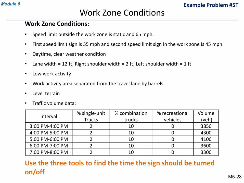
Work Zone Conditions:• Speed limit outside the work zone is static and 65 mph.
• First speed limit sign is 55 mph and second speed limit sign in the work zone is 45 mph
• Daytime, clear weather condition
• Lane width = 12 ft, Right shoulder width = 2 ft, Left shoulder width = 1 ft
• Low work activity
• Work activity area separated from the travel lane by barrels.
• Level terrain
• Traffic volume data:
Use the three tools to find the time the sign should be turned on/off
Interval % single-unitTrucks
% combination trucks
% recreational vehicles
Volume(veh)
3:00 PM-4:00 PM 2 10 0 38504:00 PM-5:00 PM 2 10 0 43005:00 PM-6:00 PM 2 10 0 41006:00 PM-7:00 PM 2 10 0 36007:00 PM-8:00 PM 2 10 0 3300
Example Problem #5TWork Zone Conditions
Module 5
M5-28
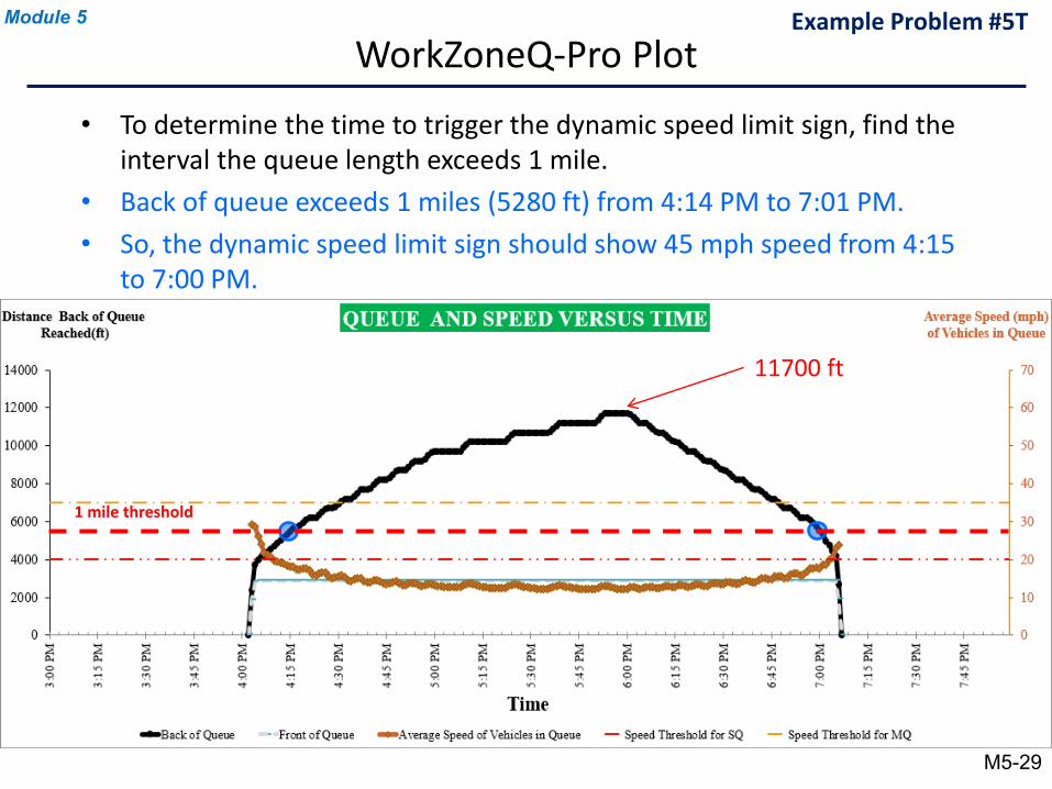
• To determine the time to trigger the dynamic speed limit sign, find the interval the queue length exceeds 1 mile.
• Back of queue exceeds 1 miles (5280 ft) from 4:14 PM to 7:01 PM. • So, the dynamic speed limit sign should show 45 mph speed from 4:15
to 7:00 PM.
WorkZoneQ-Pro Plot
11700 ft
Module 5
M5-29
Example Problem #5T
1 mile threshold
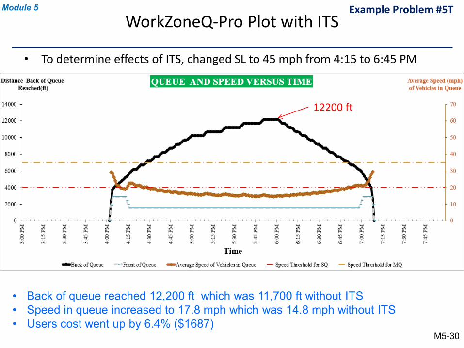
• To determine effects of ITS, changed SL to 45 mph from 4:15 to 6:45 PM
WorkZoneQ-Pro Plot with ITSModule 5
M5-30
12200 ft
Example Problem #5T
• Back of queue reached 12,200 ft which was 11,700 ft without ITS• Speed in queue increased to 17.8 mph which was 14.8 mph without ITS• Users cost went up by 6.4% ($1687)
Determine the Effect of ITS with FREEVAL-WZ
Module 5
M5-31
• FREEVAL-WZ do not determine effects of ITS on speed or capacity
• FREEVAL-WZ do NOT say how to evaluate the effects of ITS in WZ even if speed and capacity are known
Example Problem #5T
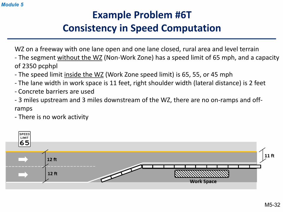
Example Problem #6TConsistency in Speed Computation
Module 5
M5-32
WZ on a freeway with one lane open and one lane closed, rural area and level terrain- The segment without the WZ (Non-Work Zone) has a speed limit of 65 mph, and a capacity of 2350 pcphpl- The speed limit inside the WZ (Work Zone speed limit) is 65, 55, or 45 mph- The lane width in work space is 11 feet, right shoulder width (lateral distance) is 2 feet- Concrete barriers are used- 3 miles upstream and 3 miles downstream of the WZ, there are no on-ramps and off-ramps- There is no work activity
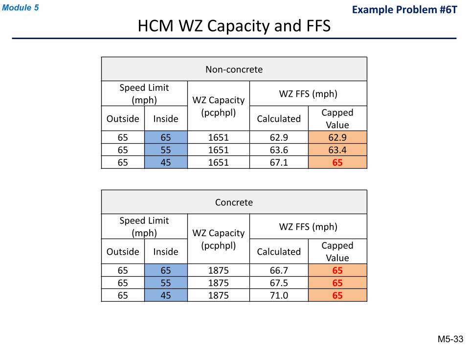
Non-concrete
Speed Limit (mph) WZ Capacity
(pcphpl)
WZ FFS (mph)
Outside Inside Calculated Capped Value
65 65 1651 62.9 62.965 55 1651 63.6 63.465 45 1651 67.1 65
Example Problem #6TModule 5
M5-33
HCM WZ Capacity and FFS
Concrete
Speed Limit (mph) WZ Capacity
(pcphpl)
WZ FFS (mph)
Outside Inside Calculated Capped Value
65 65 1875 66.7 6565 55 1875 67.5 6565 45 1875 71.0 65
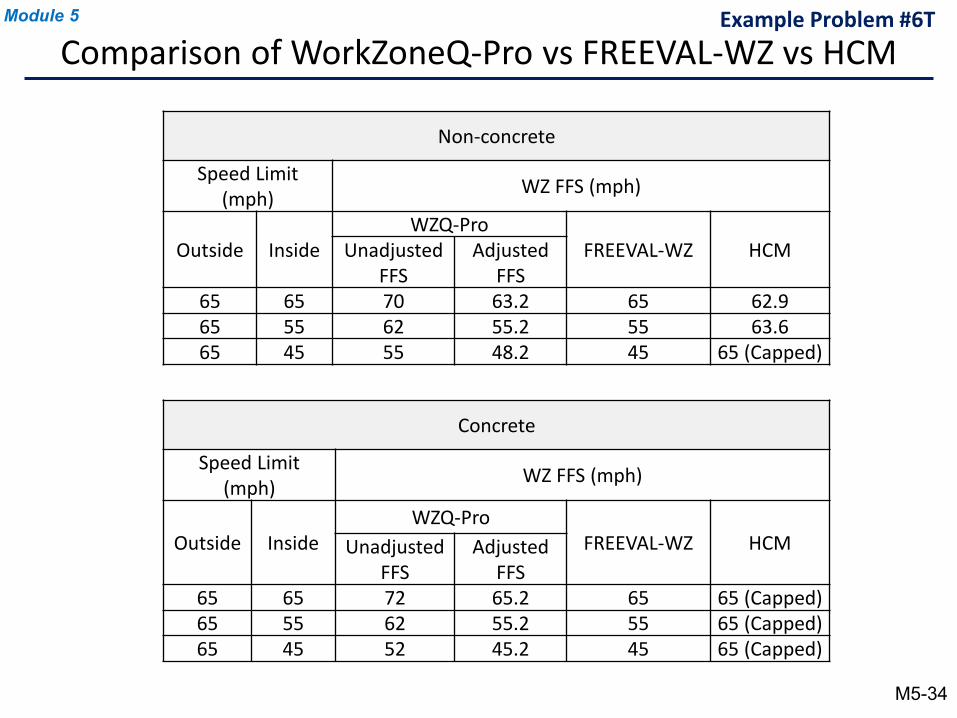
Non-concrete
Speed Limit (mph) WZ FFS (mph)
Outside InsideWZQ-Pro
FREEVAL-WZ HCMUnadjustedFFS
Adjusted FFS
65 65 70 63.2 65 62.965 55 62 55.2 55 63.665 45 55 48.2 45 65 (Capped)
Example Problem #6TModule 5
M5-34
Comparison of WorkZoneQ-Pro vs FREEVAL-WZ vs HCM
Concrete
Speed Limit (mph) WZ FFS (mph)
Outside InsideWZQ-Pro
FREEVAL-WZ HCMUnadjustedFFS
Adjusted FFS
65 65 72 65.2 65 65 (Capped)65 55 62 55.2 55 65 (Capped)65 45 52 45.2 45 65 (Capped)
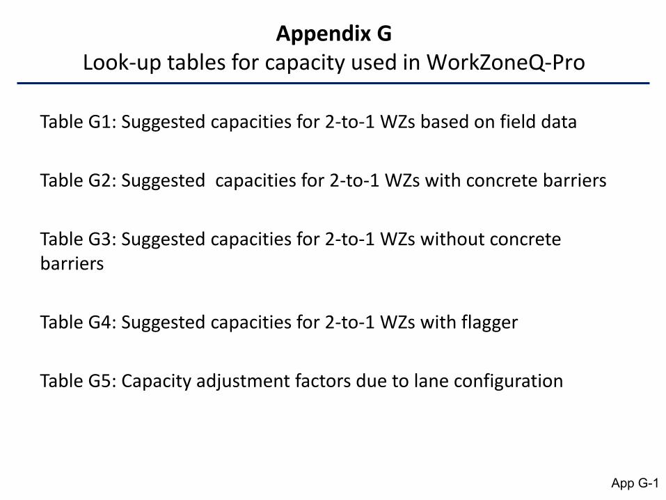
Table G1: Suggested capacities for 2-to-1 WZs based on field data
Table G2: Suggested capacities for 2-to-1 WZs with concrete barriers
Table G3: Suggested capacities for 2-to-1 WZs without concrete barriers
Table G4: Suggested capacities for 2-to-1 WZs with flagger
Table G5: Capacity adjustment factors due to lane configuration
Appendix GLook-up tables for capacity used in WorkZoneQ-Pro
App G-1
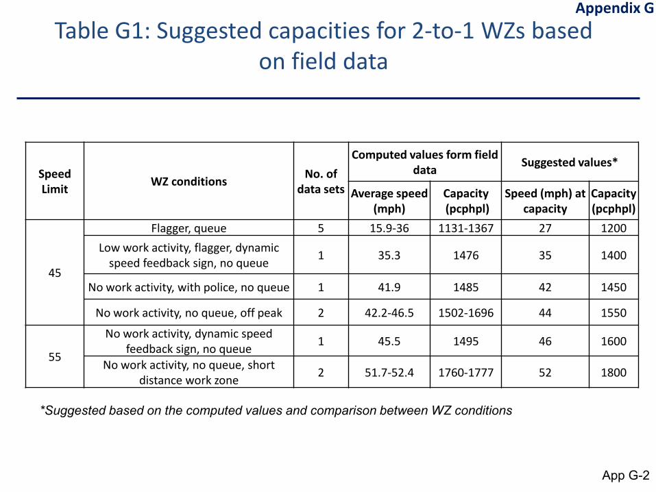
Table G1: Suggested capacities for 2-to-1 WZs based on field data
Speed Limit WZ conditions No. of
data sets
Computed values form field data Suggested values*
Average speed (mph)
Capacity (pcphpl)
Speed (mph) at capacity
Capacity (pcphpl)
45
Flagger, queue 5 15.9-36 1131-1367 27 1200Low work activity, flagger, dynamic
speed feedback sign, no queue 1 35.3 1476 35 1400
No work activity, with police, no queue 1 41.9 1485 42 1450
No work activity, no queue, off peak 2 42.2-46.5 1502-1696 44 1550
55
No work activity, dynamic speed feedback sign, no queue 1 45.5 1495 46 1600
No work activity, no queue, short distance work zone 2 51.7-52.4 1760-1777 52 1800
*Suggested based on the computed values and comparison between WZ conditions
Appendix G
App G-2
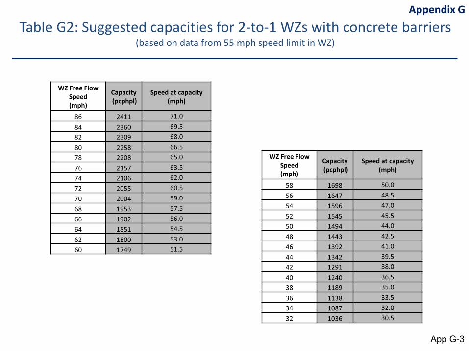
Table G2: Suggested capacities for 2-to-1 WZs with concrete barriers(based on data from 55 mph speed limit in WZ)
Appendix G
App G-3
WZ Free Flow Speed (mph)
Capacity(pcphpl)
Speed at capacity(mph)
58 1698 50.056 1647 48.554 1596 47.052 1545 45.550 1494 44.048 1443 42.546 1392 41.044 1342 39.542 1291 38.040 1240 36.538 1189 35.036 1138 33.534 1087 32.032 1036 30.5
WZ Free Flow Speed (mph)
Capacity(pcphpl)
Speed at capacity(mph)
86 2411 71.084 2360 69.582 2309 68.080 2258 66.578 2208 65.076 2157 63.574 2106 62.072 2055 60.570 2004 59.068 1953 57.566 1902 56.064 1851 54.562 1800 53.060 1749 51.5
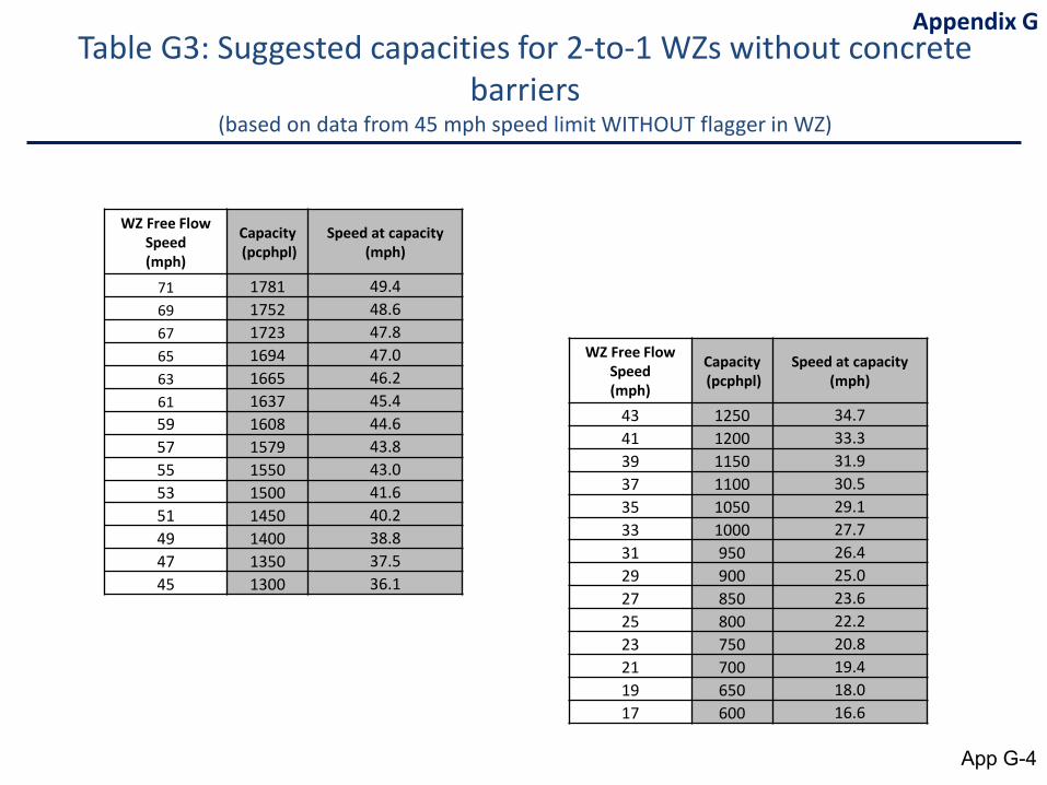
Appendix GTable G3: Suggested capacities for 2-to-1 WZs without concrete
barriers(based on data from 45 mph speed limit WITHOUT flagger in WZ)
App G-4
WZ Free Flow Speed (mph)
Capacity(pcphpl)
Speed at capacity(mph)
71 1781 49.469 1752 48.667 1723 47.865 1694 47.063 1665 46.261 1637 45.459 1608 44.657 1579 43.855 1550 43.053 1500 41.651 1450 40.249 1400 38.847 1350 37.545 1300 36.1
WZ Free Flow Speed (mph)
Capacity(pcphpl)
Speed at capacity(mph)
43 1250 34.741 1200 33.339 1150 31.937 1100 30.535 1050 29.133 1000 27.731 950 26.429 900 25.027 850 23.625 800 22.223 750 20.821 700 19.419 650 18.017 600 16.6
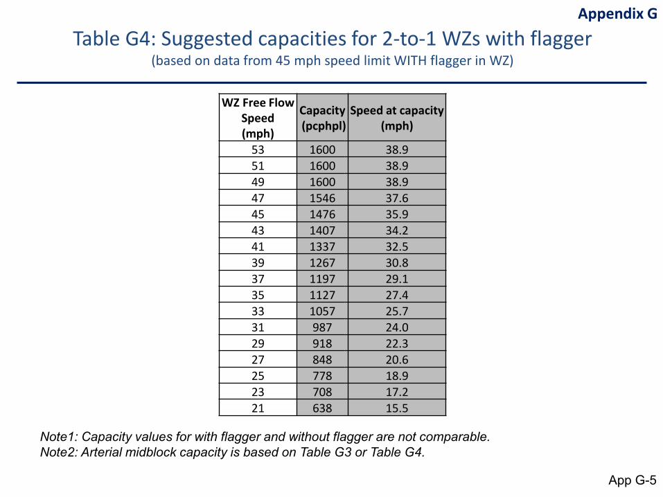
Appendix G
Table G4: Suggested capacities for 2-to-1 WZs with flagger(based on data from 45 mph speed limit WITH flagger in WZ)
App G-5
Note1: Capacity values for with flagger and without flagger are not comparable.Note2: Arterial midblock capacity is based on Table G3 or Table G4.
WZ Free Flow Speed (mph)
Capacity(pcphpl)
Speed at capacity(mph)
53 1600 38.951 1600 38.949 1600 38.947 1546 37.645 1476 35.943 1407 34.241 1337 32.539 1267 30.837 1197 29.135 1127 27.433 1057 25.731 987 24.029 918 22.327 848 20.625 778 18.923 708 17.221 638 15.5
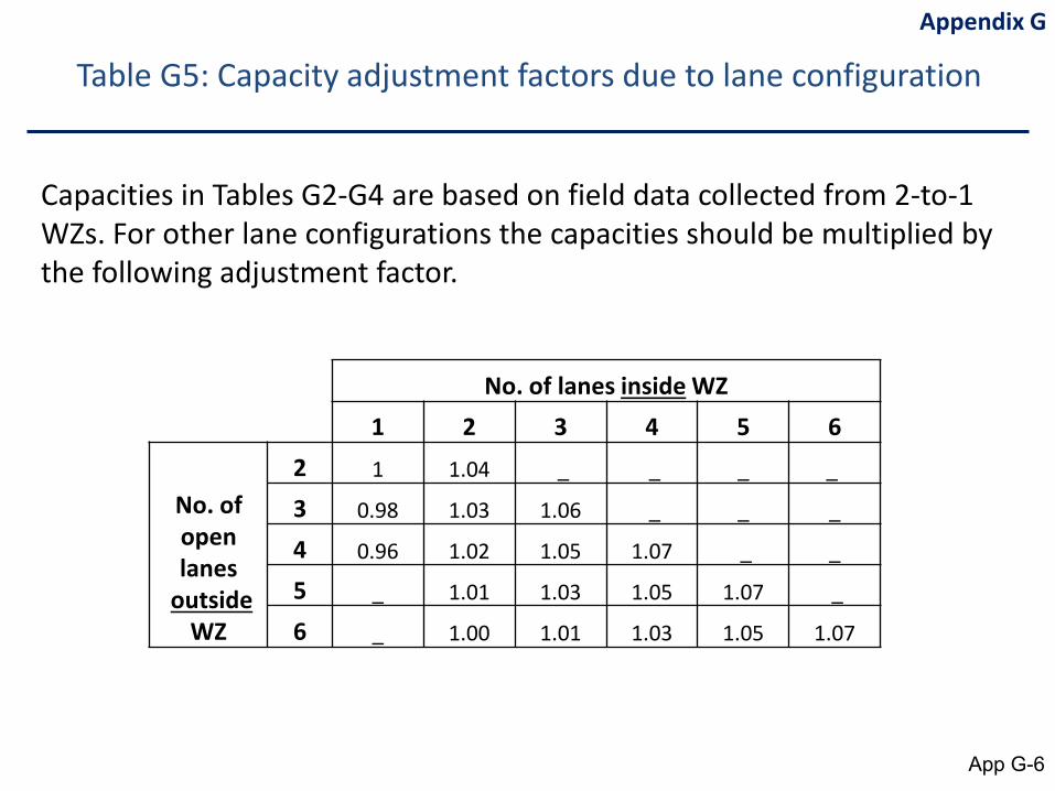
Table G5: Capacity adjustment factors due to lane configuration
Capacities in Tables G2-G4 are based on field data collected from 2-to-1 WZs. For other lane configurations the capacities should be multiplied by the following adjustment factor.
Appendix G
No. of lanes inside WZ1 2 3 4 5 6
No. of open lanes
outsideWZ
2 1 1.04 _ _ _ _
3 0.98 1.03 1.06 _ _ _
4 0.96 1.02 1.05 1.07 _ _
5 _ 1.01 1.03 1.05 1.07 _
6 _ 1.00 1.01 1.03 1.05 1.07
App G-6
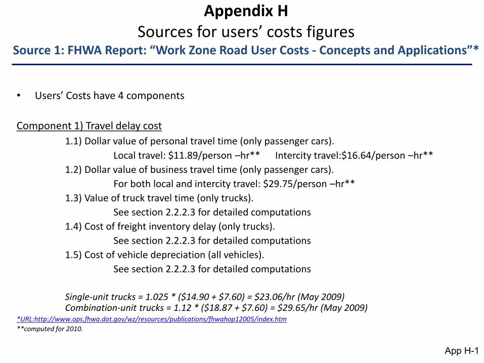
• Users’ Costs have 4 components
Component 1) Travel delay cost 1.1) Dollar value of personal travel time (only passenger cars).
Local travel: $11.89/person –hr** Intercity travel:$16.64/person –hr**1.2) Dollar value of business travel time (only passenger cars).
For both local and intercity travel: $29.75/person –hr**1.3) Value of truck travel time (only trucks).
See section 2.2.2.3 for detailed computations1.4) Cost of freight inventory delay (only trucks).
See section 2.2.2.3 for detailed computations1.5) Cost of vehicle depreciation (all vehicles).
See section 2.2.2.3 for detailed computations
Single-unit trucks = 1.025 * ($14.90 + $7.60) = $23.06/hr (May 2009)Combination-unit trucks = 1.12 * ($18.87 + $7.60) = $29.65/hr (May 2009)
*URL:http://www.ops.fhwa.dot.gov/wz/resources/publications/fhwahop12005/index.htm**computed for 2010.
Appendix HSources for users’ costs figures
Source 1: FHWA Report: “Work Zone Road User Costs - Concepts and Applications”*
App H-1
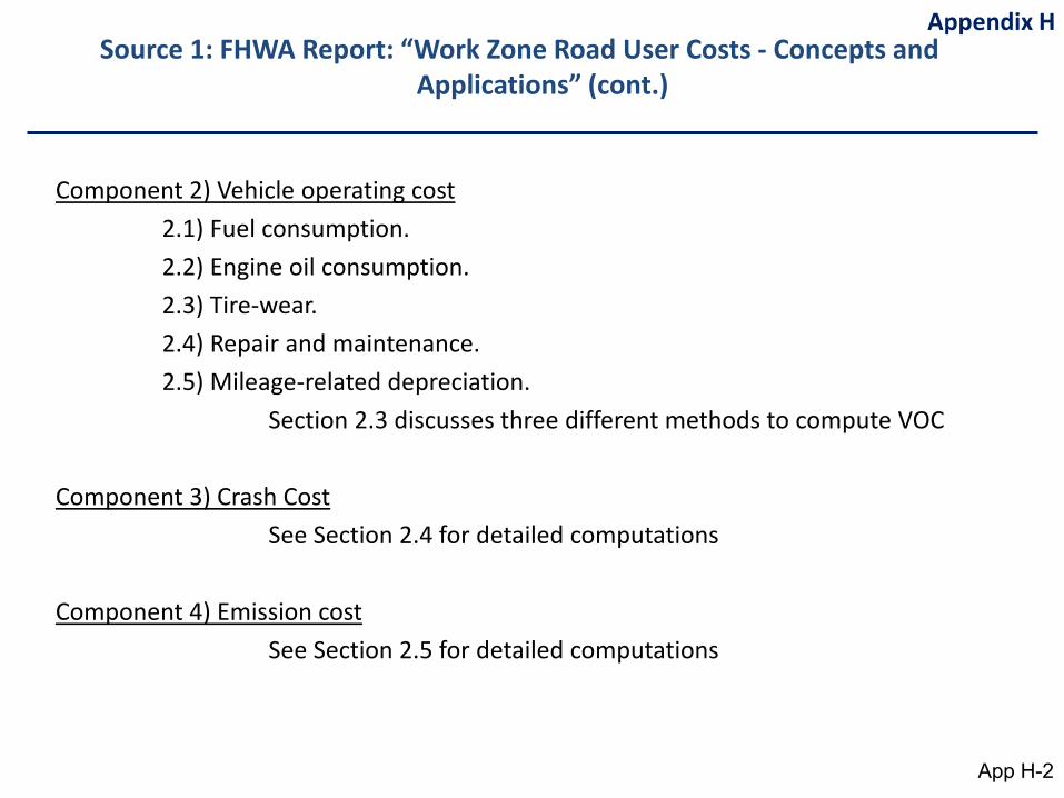
Component 2) Vehicle operating cost 2.1) Fuel consumption.2.2) Engine oil consumption.2.3) Tire-wear.2.4) Repair and maintenance.2.5) Mileage-related depreciation.
Section 2.3 discusses three different methods to compute VOC
Component 3) Crash Cost See Section 2.4 for detailed computations
Component 4) Emission cost See Section 2.5 for detailed computations
Source 1: FHWA Report: “Work Zone Road User Costs - Concepts and Applications” (cont.)
Appendix H
App H-2
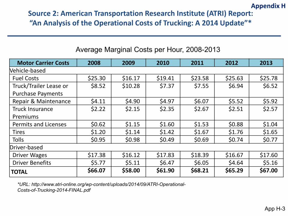
Motor Carrier Costs 2008 2009 2010 2011 2012 2013Vehicle-basedFuel Costs $25.30 $16.17 $19.41 $23.58 $25.63 $25.78Truck/Trailer Lease or Purchase Payments
$8.52 $10.28 $7.37 $7.55 $6.94 $6.52
Repair & Maintenance $4.11 $4.90 $4.97 $6.07 $5.52 $5.92Truck Insurance Premiums
$2.22 $2.15 $2.35 $2.67 $2.51 $2.57
Permits and Licenses $0.62 $1.15 $1.60 $1.53 $0.88 $1.04Tires $1.20 $1.14 $1.42 $1.67 $1.76 $1.65Tolls $0.95 $0.98 $0.49 $0.69 $0.74 $0.77
Driver-basedDriver Wages $17.38 $16.12 $17.83 $18.39 $16.67 $17.60Driver Benefits $5.77 $5.11 $6.47 $6.05 $4.64 $5.16
TOTAL $66.07 $58.00 $61.90 $68.21 $65.29 $67.00
Average Marginal Costs per Hour, 2008-2013
*URL: http://www.atri-online.org/wp-content/uploads/2014/09/ATRI-Operational-Costs-of-Trucking-2014-FINAL.pdf
Source 2: American Transportation Research Institute (ATRI) Report: “An Analysis of the Operational Costs of Trucking: A 2014 Update”*
Appendix H
App H-3
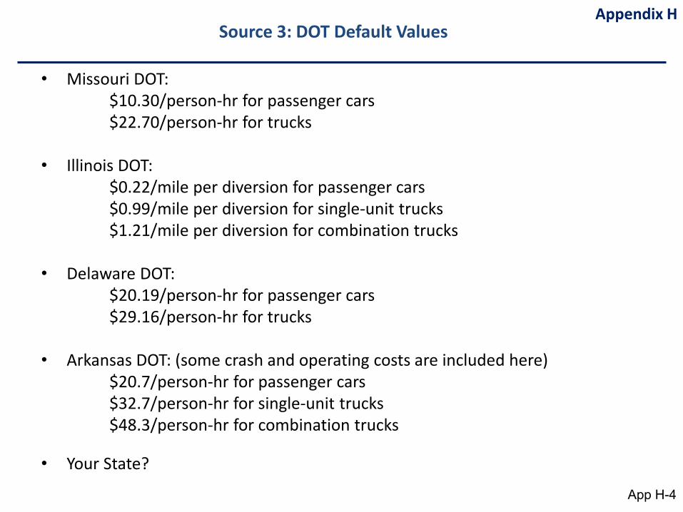
• Missouri DOT:$10.30/person-hr for passenger cars$22.70/person-hr for trucks
• Illinois DOT:$0.22/mile per diversion for passenger cars$0.99/mile per diversion for single-unit trucks$1.21/mile per diversion for combination trucks
• Delaware DOT: $20.19/person-hr for passenger cars$29.16/person-hr for trucks
• Arkansas DOT: (some crash and operating costs are included here)$20.7/person-hr for passenger cars$32.7/person-hr for single-unit trucks$48.3/person-hr for combination trucks
• Your State?
Source 3: DOT Default ValuesAppendix H
App H-4

1. Which package should I use?
2. What is covered in appendices
3. Additional Resources
4. Q &A and Discussions
5. Course Evaluation
6. PDH Certificate Distribution
Wrap-up
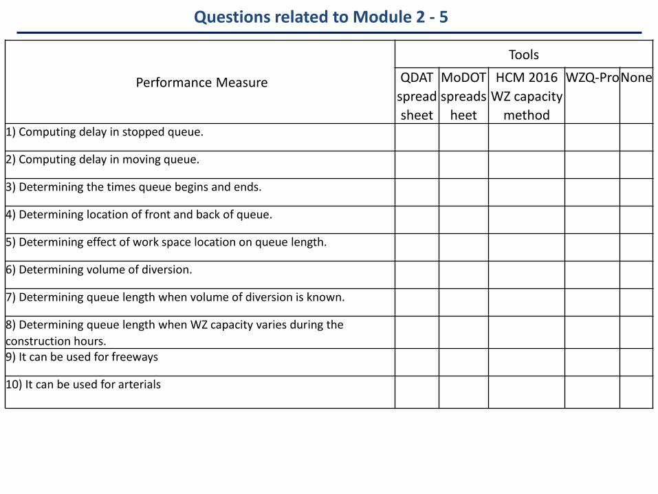
Performance Measure
ToolsQDAT
spreadsheet
MoDOTspreads
heet
HCM 2016 WZ capacity
method
WZQ-ProNone
1) Computing delay in stopped queue.
2) Computing delay in moving queue.
3) Determining the times queue begins and ends.
4) Determining location of front and back of queue.
5) Determining effect of work space location on queue length.
6) Determining volume of diversion.
7) Determining queue length when volume of diversion is known.
8) Determining queue length when WZ capacity varies during the construction hours. 9) It can be used for freeways
10) It can be used for arterials
Questions related to Module 2 - 5
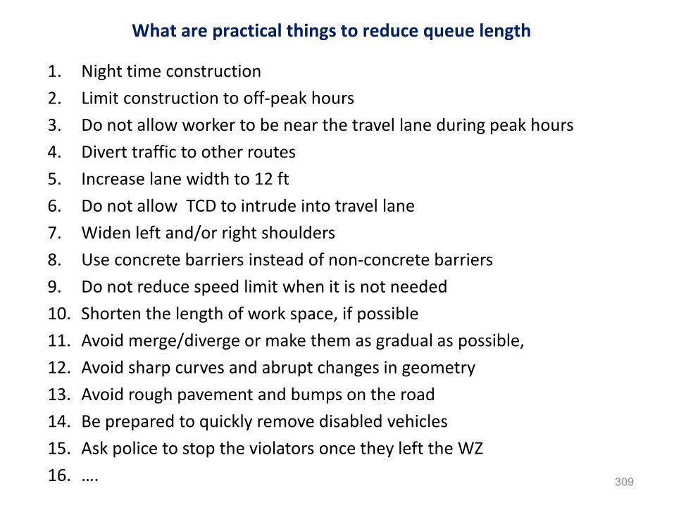
1. Night time construction2. Limit construction to off-peak hours 3. Do not allow worker to be near the travel lane during peak hours 4. Divert traffic to other routes5. Increase lane width to 12 ft6. Do not allow TCD to intrude into travel lane 7. Widen left and/or right shoulders8. Use concrete barriers instead of non-concrete barriers9. Do not reduce speed limit when it is not needed10. Shorten the length of work space, if possible11. Avoid merge/diverge or make them as gradual as possible, 12. Avoid sharp curves and abrupt changes in geometry13. Avoid rough pavement and bumps on the road14. Be prepared to quickly remove disabled vehicles15. Ask police to stop the violators once they left the WZ 16. …. 309
What are practical things to reduce queue length
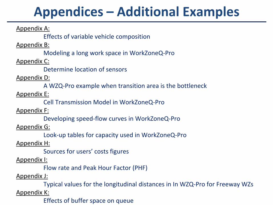
Appendices – Additional ExamplesAppendix A:
Effects of variable vehicle compositionAppendix B:
Modeling a long work space in WorkZoneQ-ProAppendix C:
Determine location of sensorsAppendix D:
A WZQ-Pro example when transition area is the bottleneckAppendix E:
Cell Transmission Model in WorkZoneQ-ProAppendix F:
Developing speed-flow curves in WorkZoneQ-ProAppendix G:
Look-up tables for capacity used in WorkZoneQ-ProAppendix H:
Sources for users’ costs figuresAppendix I:
Flow rate and Peak Hour Factor (PHF)Appendix J:
Typical values for the longitudinal distances in In WZQ-Pro for Freeway WZsAppendix K:
Effects of buffer space on queue
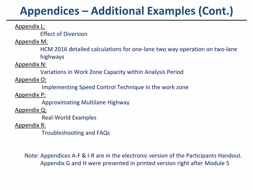
Appendices – Additional Examples (Cont.)Appendix L:
Effect of DiversionAppendix M:
HCM 2016 detailed calculations for one-lane two way operation on two-lane highways
Appendix N:Variations in Work Zone Capacity within Analysis Period
Appendix O:Implementing Speed Control Technique in the work zone
Appendix P:Approximating Multilane Highway
Appendix Q:Real-World Examples
Appendix R:Troubleshooting and FAQs
Note: Appendices A-F & I-R are in the electronic version of the Participants Handout. Appendix G and H were presented in printed version right after Module 5

Course website
https://publish.illinois.edu/workzone-traffic-management/
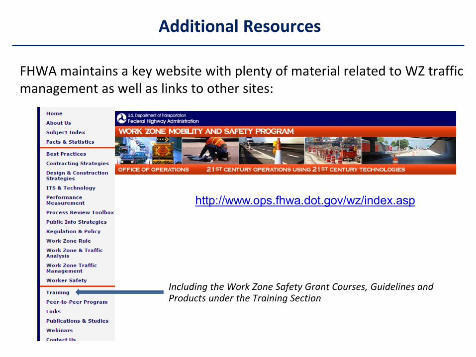
Additional Resources
FHWA maintains a key website with plenty of material related to WZ traffic management as well as links to other sites:
http://www.ops.fhwa.dot.gov/wz/index.asp
Including the Work Zone Safety Grant Courses, Guidelines and Products under the Training Section

Appendices(Not Printed)
They are on the USB Drive
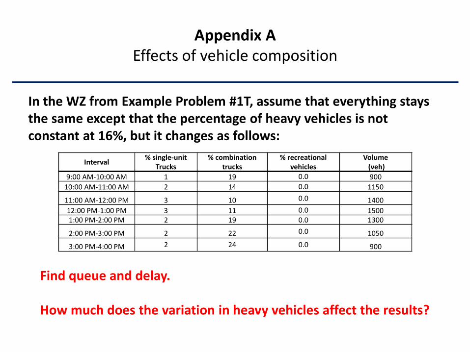
In the WZ from Example Problem #1T, assume that everything stays the same except that the percentage of heavy vehicles is not constant at 16%, but it changes as follows:
Find queue and delay.
How much does the variation in heavy vehicles affect the results?
Appendix AEffects of vehicle composition
Interval % single-unitTrucks
% combination trucks
% recreational vehicles
Volume(veh)
9:00 AM-10:00 AM 1 19 0.0 90010:00 AM-11:00 AM 2 14 0.0 1150
11:00 AM-12:00 PM 3 10 0.0 140012:00 PM-1:00 PM 3 11 0.0 15001:00 PM-2:00 PM 2 19 0.0 1300
2:00 PM-3:00 PM 2 22 0.0 1050
3:00 PM-4:00 PM 2 24 0.0 900
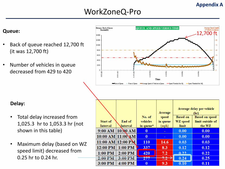
WorkZoneQ-Pro
Queue:
• Back of queue reached 12,700 ft (it was 12,700 ft)
• Number of vehicles in queue decreased from 429 to 420
Delay:
• Total delay increased from 1,025.3 hr to 1,053.3 hr (not shown in this table)
• Maximum delay (based on WZ speed limit) decreased from 0.25 hr to 0.24 hr.
Appendix A
12,700 ft
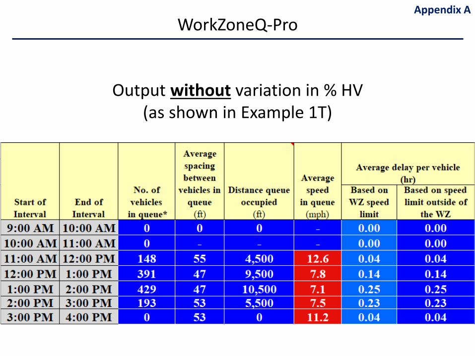
Output without variation in % HV (as shown in Example 1T)
WorkZoneQ-ProAppendix A

Outputs with variation in %HV
WorkZoneQ-ProAppendix A
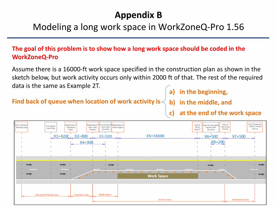
The goal of this problem is to show how a long work space should be coded in the WorkZoneQ-Pro
Assume there is a 16000-ft work space specified in the construction plan as shown in the sketch below, but work activity occurs only within 2000 ft of that. The rest of the required data is the same as Example 2T.
Find back of queue when location of work activity is
Appendix BModeling a long work space in WorkZoneQ-Pro 1.56
a) in the beginning, b) in the middle, andc) at the end of the work space
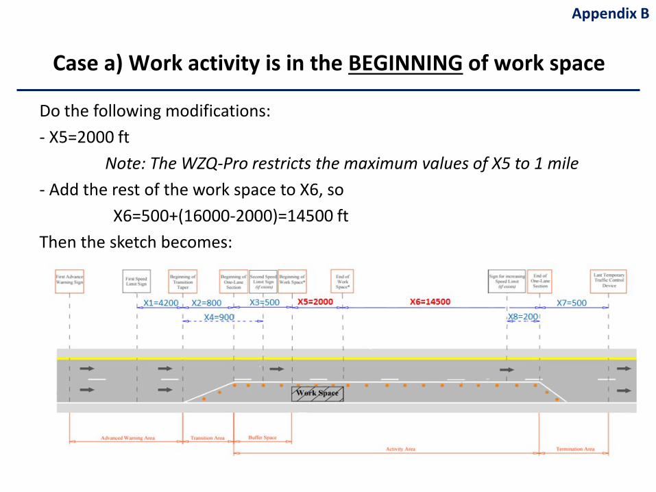
Do the following modifications:- X5=2000 ft
Note: The WZQ-Pro restricts the maximum values of X5 to 1 mile- Add the rest of the work space to X6, so
X6=500+(16000-2000)=14500 ftThen the sketch becomes:
Case a) Work activity is in the BEGINNING of work space
Appendix B
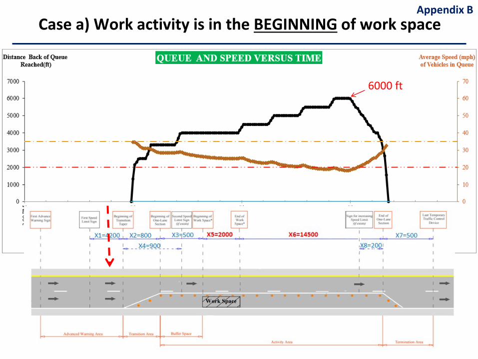
Appendix BCase a) Work activity is in the BEGINNING of work space
6000 ft
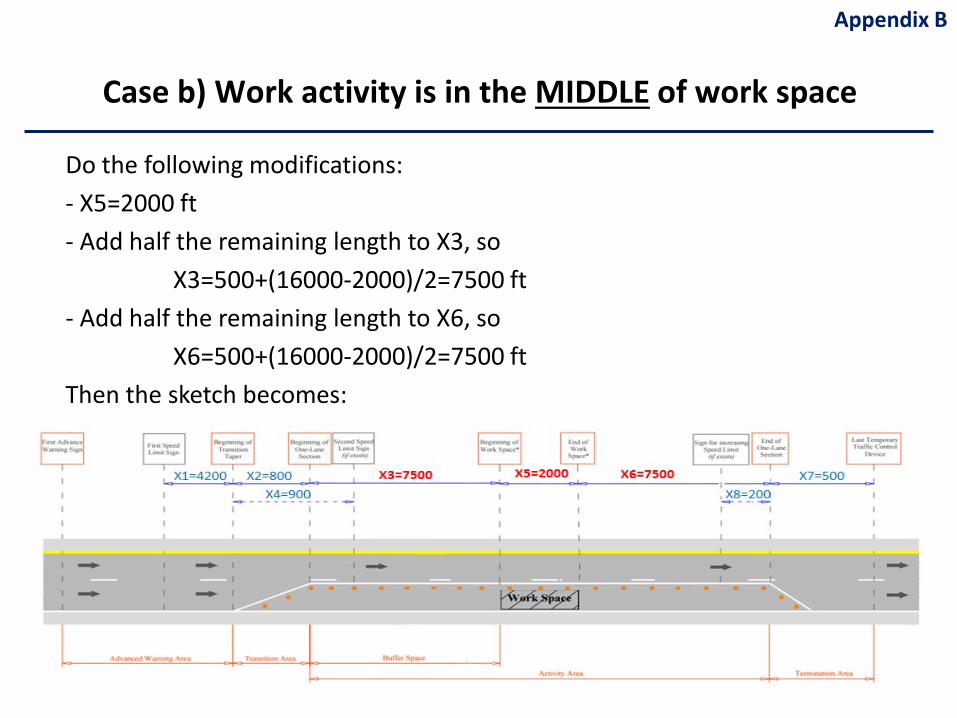
Do the following modifications:- X5=2000 ft- Add half the remaining length to X3, so
X3=500+(16000-2000)/2=7500 ft- Add half the remaining length to X6, so
X6=500+(16000-2000)/2=7500 ftThen the sketch becomes:
Case b) Work activity is in the MIDDLE of work space
Appendix B
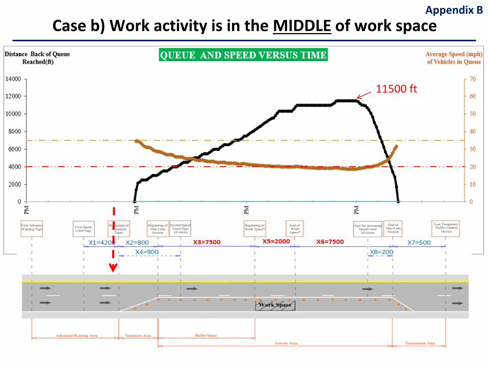
Case b) Work activity is in the MIDDLE of work space Appendix B
11500 ft
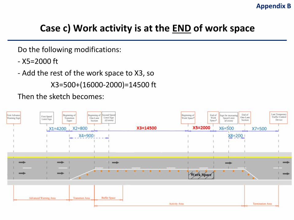
Do the following modifications:- X5=2000 ft- Add the rest of the work space to X3, so
X3=500+(16000-2000)=14500 ftThen the sketch becomes:
Case c) Work activity is at the END of work space
Appendix B
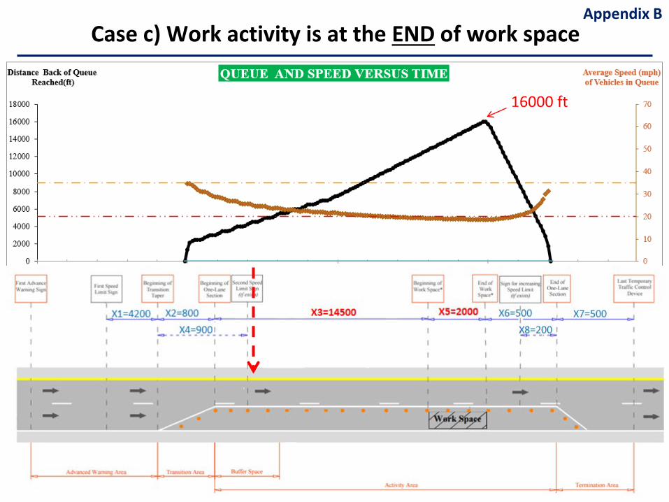
Case c) Work activity is at the END of work space Appendix B
16000 ft
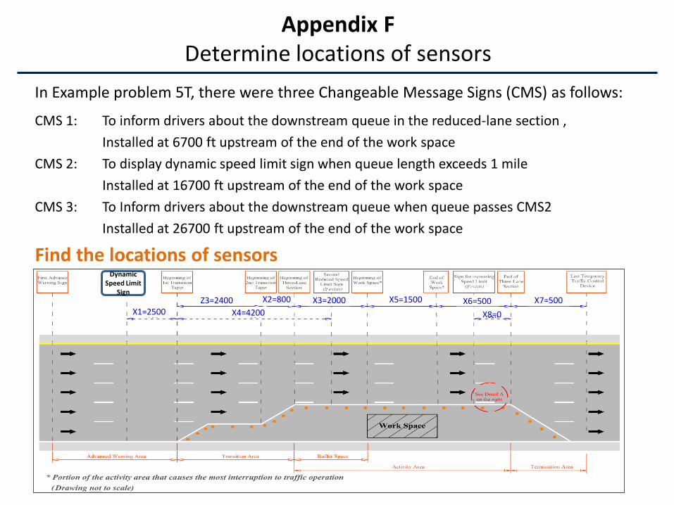
In Example problem 5T, there were three Changeable Message Signs (CMS) as follows:
CMS 1: To inform drivers about the downstream queue in the reduced-lane section , Installed at 6700 ft upstream of the end of the work space
CMS 2: To display dynamic speed limit sign when queue length exceeds 1 mileInstalled at 16700 ft upstream of the end of the work space
CMS 3: To Inform drivers about the downstream queue when queue passes CMS2Installed at 26700 ft upstream of the end of the work space
Find the locations of sensors
Appendix F Determine locations of sensors
X1=2500X2=800
X4=4200 X8=0X7=500X6=500X5=1500X3=2000
DynamicSpeed Limit
SignZ3=2400
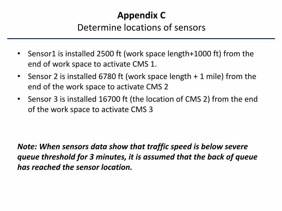
• Sensor1 is installed 2500 ft (work space length+1000 ft) from the end of work space to activate CMS 1.
• Sensor 2 is installed 6780 ft (work space length + 1 mile) from the end of the work space to activate CMS 2
• Sensor 3 is installed 16700 ft (the location of CMS 2) from the end of the work space to activate CMS 3
Note: When sensors data show that traffic speed is below severe queue threshold for 3 minutes, it is assumed that the back of queue has reached the sensor location.
Appendix CDetermine locations of sensors
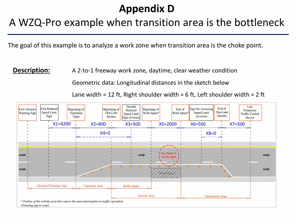
Description: A 2-to-1 freeway work zone, daytime, clear weather condition
Geometric data: Longitudinal distances in the sketch below
Lane width = 12 ft, Right shoulder width = 6 ft, Left shoulder width = 2 ft
Appendix DA WZQ-Pro example when transition area is the bottleneck
The goal of this example is to analyze a work zone when transition area is the choke point.
X1=4200 X2=800
X4=0 X8=0
X7=500X6=500X5=2000X3=500
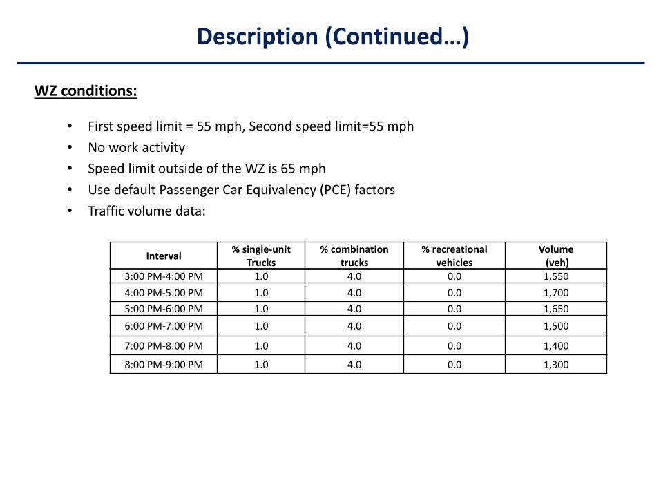
WZ conditions:
• First speed limit = 55 mph, Second speed limit=55 mph• No work activity • Speed limit outside of the WZ is 65 mph• Use default Passenger Car Equivalency (PCE) factors• Traffic volume data:
Interval % single-unitTrucks
% combination trucks
% recreational vehicles
Volume(veh)
3:00 PM-4:00 PM 1.0 4.0 0.0 1,5504:00 PM-5:00 PM 1.0 4.0 0.0 1,7005:00 PM-6:00 PM 1.0 4.0 0.0 1,6506:00 PM-7:00 PM 1.0 4.0 0.0 1,500
7:00 PM-8:00 PM 1.0 4.0 0.0 1,400
8:00 PM-9:00 PM 1.0 4.0 0.0 1,300
Description (Continued…)
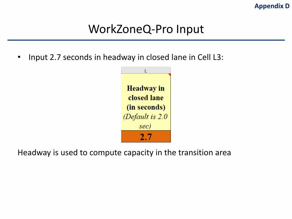
• Input 2.7 seconds in headway in closed lane in Cell L3:
WorkZoneQ-Pro Input
Appendix D
Headway is used to compute capacity in the transition area
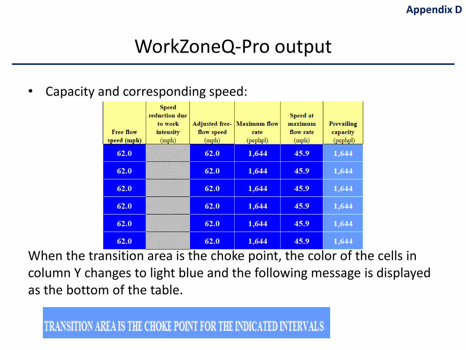
• Capacity and corresponding speed:
When the transition area is the choke point, the color of the cells in column Y changes to light blue and the following message is displayed as the bottom of the table.
WorkZoneQ-Pro output
Appendix D
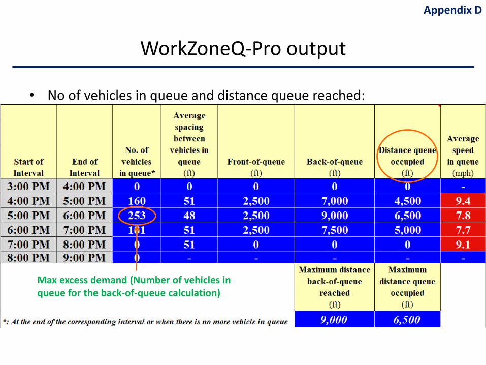
• No of vehicles in queue and distance queue reached:
WorkZoneQ-Pro output
Max excess demand (Number of vehicles in queue for the back-of-queue calculation)
Appendix D
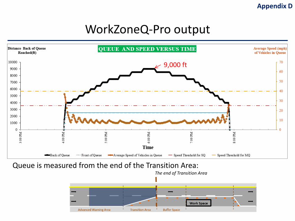
The end of Transition Area
WorkZoneQ-Pro output
Queue is measured from the end of the Transition Area:
Appendix D
9,000 ft
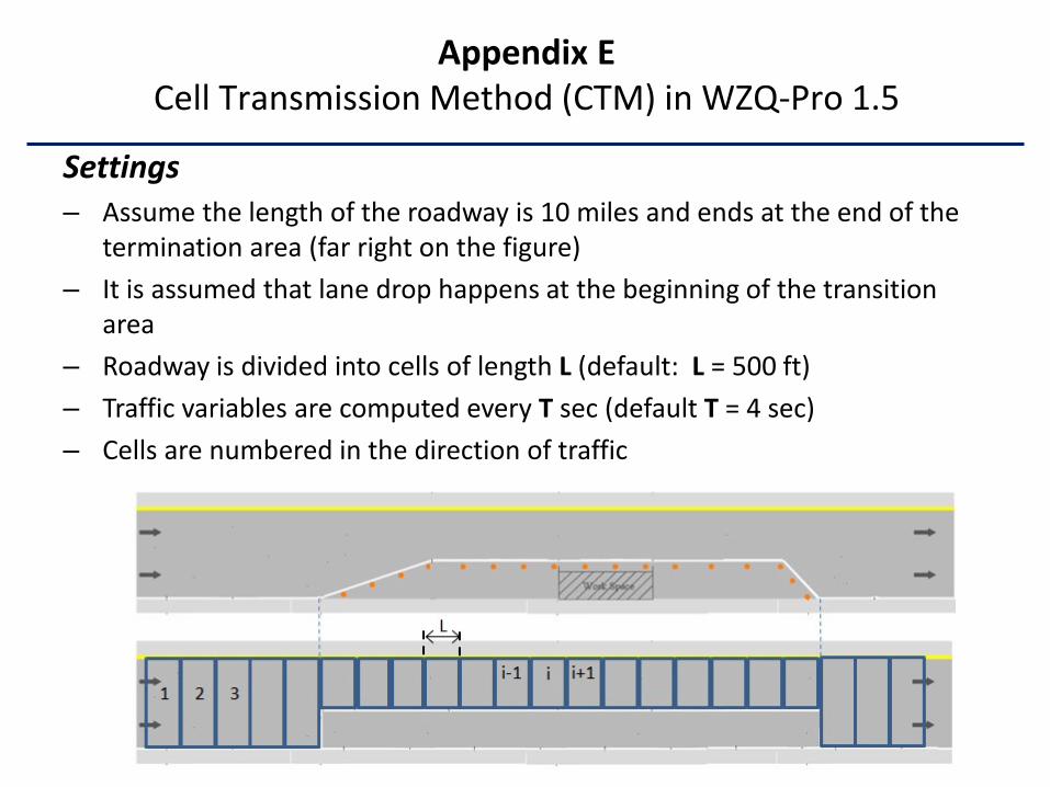
Settings– Assume the length of the roadway is 10 miles and ends at the end of the
termination area (far right on the figure)– It is assumed that lane drop happens at the beginning of the transition
area– Roadway is divided into cells of length L (default: L = 500 ft) – Traffic variables are computed every T sec (default T = 4 sec)– Cells are numbered in the direction of traffic
Appendix ECell Transmission Method (CTM) in WZQ-Pro 1.5
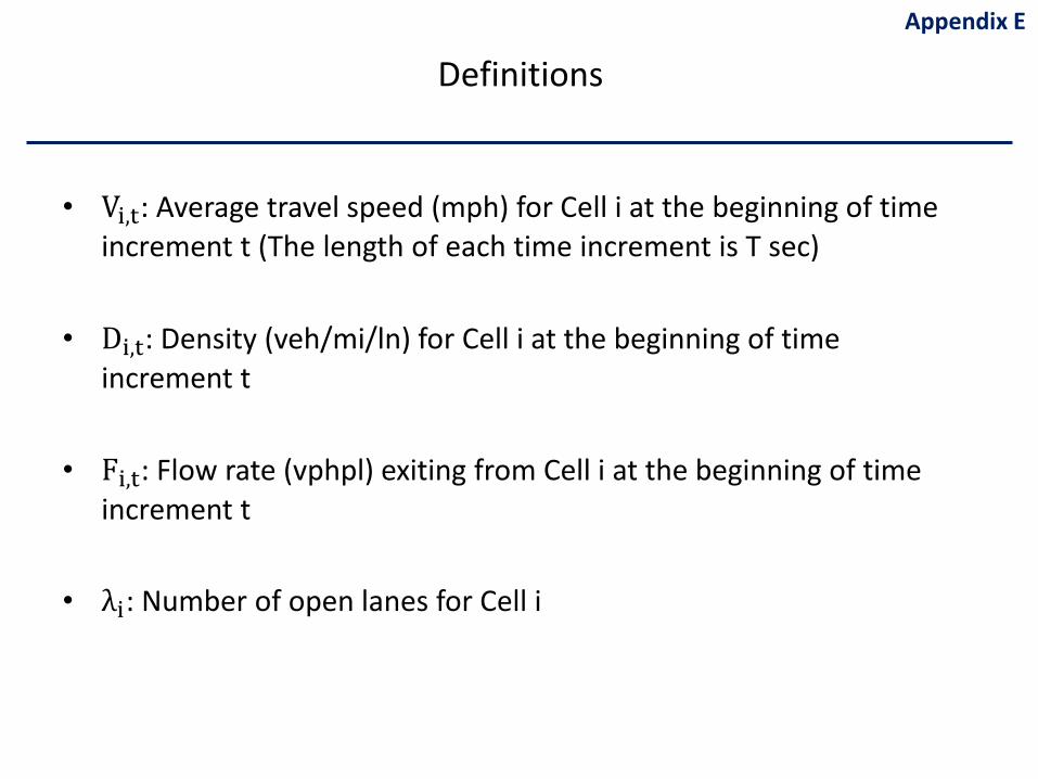
• Vi,t: Average travel speed (mph) for Cell i at the beginning of time increment t (The length of each time increment is T sec)
• Di,t: Density (veh/mi/ln) for Cell i at the beginning of time increment t
• Fi,t: Flow rate (vphpl) exiting from Cell i at the beginning of time increment t
• λi: Number of open lanes for Cell i
Appendix E
Definitions
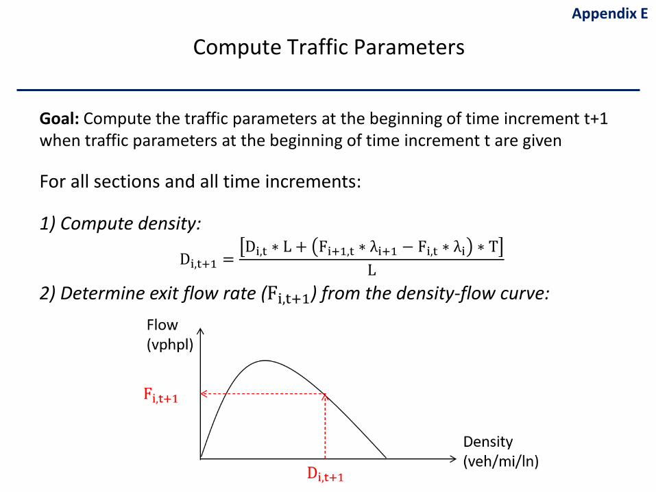
Goal: Compute the traffic parameters at the beginning of time increment t+1 when traffic parameters at the beginning of time increment t are given
For all sections and all time increments:
1) Compute density:
Di,t+1 =Di,t ∗ L + Fi+1,t ∗ λi+1 − Fi,t ∗ λi ∗ T
L2) Determine exit flow rate (Fi,t+1) from the density-flow curve:
Appendix E
Compute Traffic Parameters
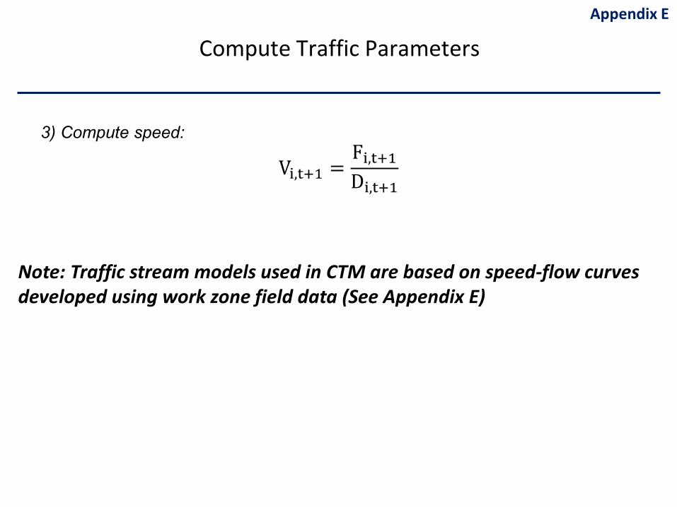
Vi,t+1 =Fi,t+1Di,t+1
Note: Traffic stream models used in CTM are based on speed-flow curves developed using work zone field data (See Appendix E)
Appendix E
Compute Traffic Parameters
3) Compute speed:
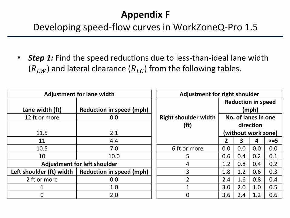
• Step 1: Find the speed reductions due to less-than-ideal lane width (𝑄𝑄𝐿𝐿𝑊𝑊) and lateral clearance (𝑄𝑄𝐿𝐿𝐶𝐶) from the following tables.
Adjustment for lane width Adjustment for right shoulder
Lane width (ft) Reduction in speed (mph)Right shoulder width
(ft)
Reduction in speed (mph)
12 ft or more 0.0 No. of lanes in one direction
(without work zone)11.5 2.111 4.4 2 3 4 >=5
10.5 7.0 6 ft or more 0.0 0.0 0.0 0.010 10.0 5 0.6 0.4 0.2 0.1Adjustment for left shoulder 4 1.2 0.8 0.4 0.2
Left shoulder (ft) width Reduction in speed (mph) 3 1.8 1.2 0.6 0.32 ft or more 0.0 2 2.4 1.6 0.8 0.4
1 1.0 1 3.0 2.0 1.0 0.50 2.0 0 3.6 2.4 1.2 0.6
Appendix FDeveloping speed-flow curves in WorkZoneQ-Pro 1.5
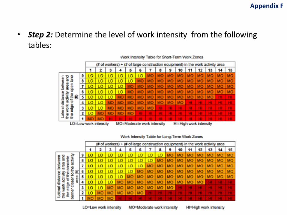
• Step 2: Determine the level of work intensity from the following tables:
Appendix F
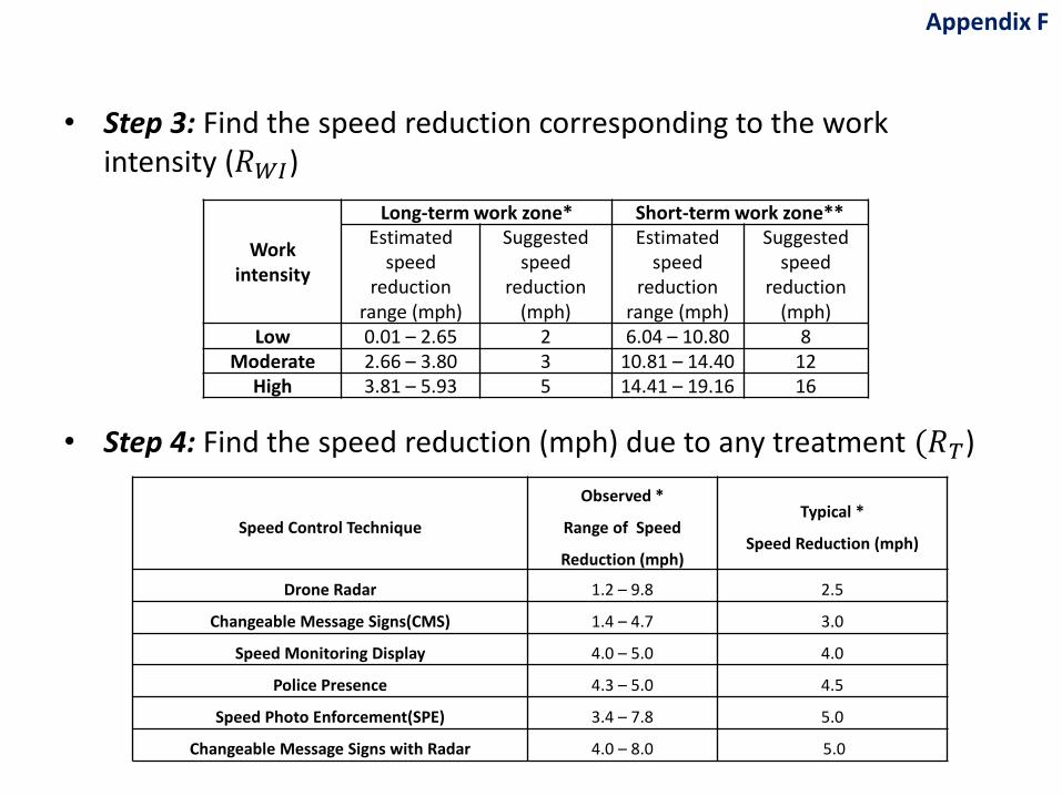
• Step 3: Find the speed reduction corresponding to the work intensity (𝑄𝑄𝑊𝑊𝑊𝑊)
• Step 4: Find the speed reduction (mph) due to any treatment (𝑄𝑄𝑇𝑇)
Work intensity
Long-term work zone* Short-term work zone**Estimated
speed reduction
range (mph)
Suggested speed
reduction (mph)
Estimated speed
reduction range (mph)
Suggested speed
reduction (mph)
Low 0.01 – 2.65 2 6.04 – 10.80 8Moderate 2.66 – 3.80 3 10.81 – 14.40 12
High 3.81 – 5.93 5 14.41 – 19.16 16
Speed Control Technique
Observed *
Range of Speed
Reduction (mph)
Typical *
Speed Reduction (mph)
Drone Radar 1.2 – 9.8 2.5
Changeable Message Signs(CMS) 1.4 – 4.7 3.0
Speed Monitoring Display 4.0 – 5.0 4.0
Police Presence 4.3 – 5.0 4.5
Speed Photo Enforcement(SPE) 3.4 – 7.8 5.0
Changeable Message Signs with Radar 4.0 – 8.0 5.0
Appendix F
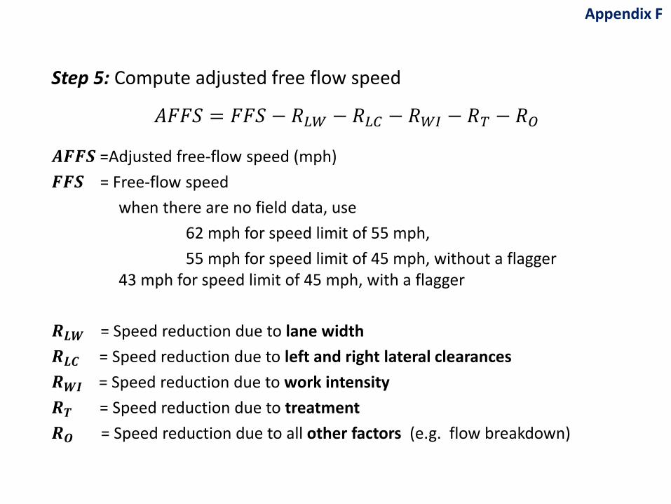
Step 5: Compute adjusted free flow speed
𝐶𝐶𝐹𝐹𝐹𝐹𝑊𝑊 = 𝐹𝐹𝐹𝐹𝑊𝑊 − 𝑄𝑄𝐿𝐿𝑊𝑊 − 𝑄𝑄𝐿𝐿𝐶𝐶 − 𝑄𝑄𝑊𝑊𝑊𝑊 − 𝑄𝑄𝑇𝑇 − 𝑄𝑄𝑂𝑂
𝑨𝑨𝑪𝑪𝑪𝑪𝑳𝑳 =Adjusted free-flow speed (mph)𝑪𝑪𝑪𝑪𝑳𝑳 = Free-flow speed
when there are no field data, use62 mph for speed limit of 55 mph, 55 mph for speed limit of 45 mph, without a flagger
43 mph for speed limit of 45 mph, with a flagger
𝑸𝑸𝑳𝑳𝑾𝑾 = Speed reduction due to lane width 𝑸𝑸𝑳𝑳𝑳𝑳 = Speed reduction due to left and right lateral clearances𝑸𝑸𝑾𝑾𝑳𝑳 = Speed reduction due to work intensity 𝑸𝑸𝑳𝑳 = Speed reduction due to treatment 𝑸𝑸𝑶𝑶 = Speed reduction due to all other factors (e.g. flow breakdown)
Appendix F
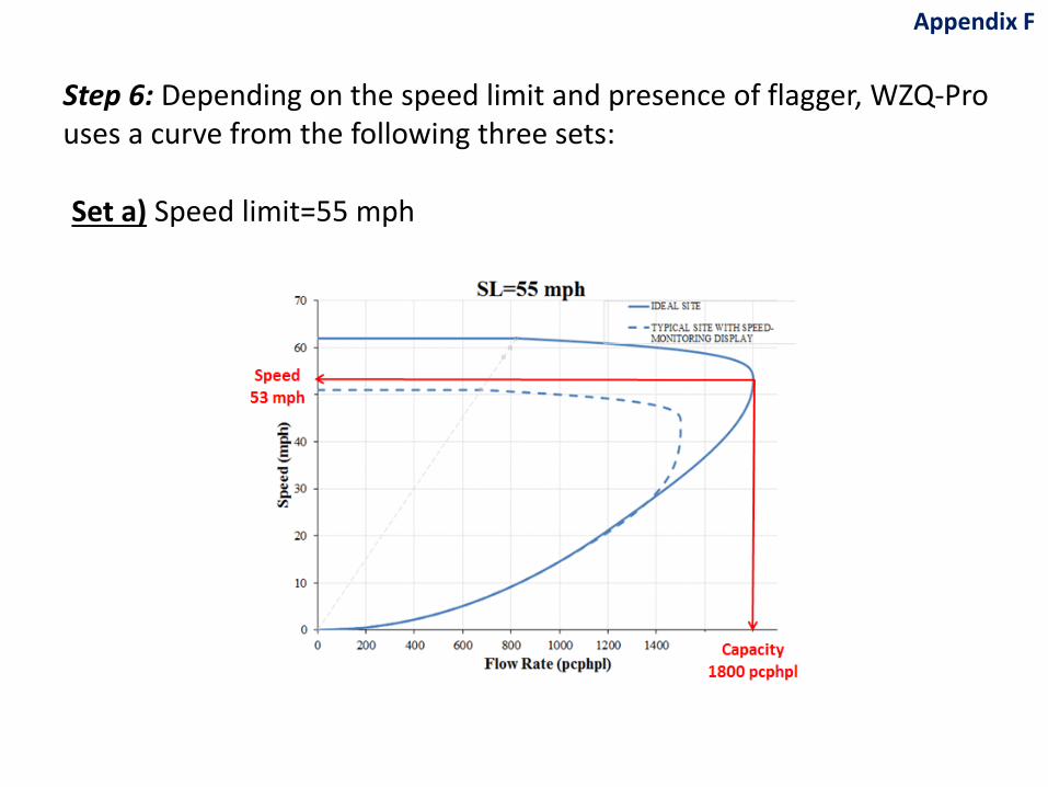
Set a) Speed limit=55 mph
Step 6: Depending on the speed limit and presence of flagger, WZQ-Pro uses a curve from the following three sets:
Appendix F
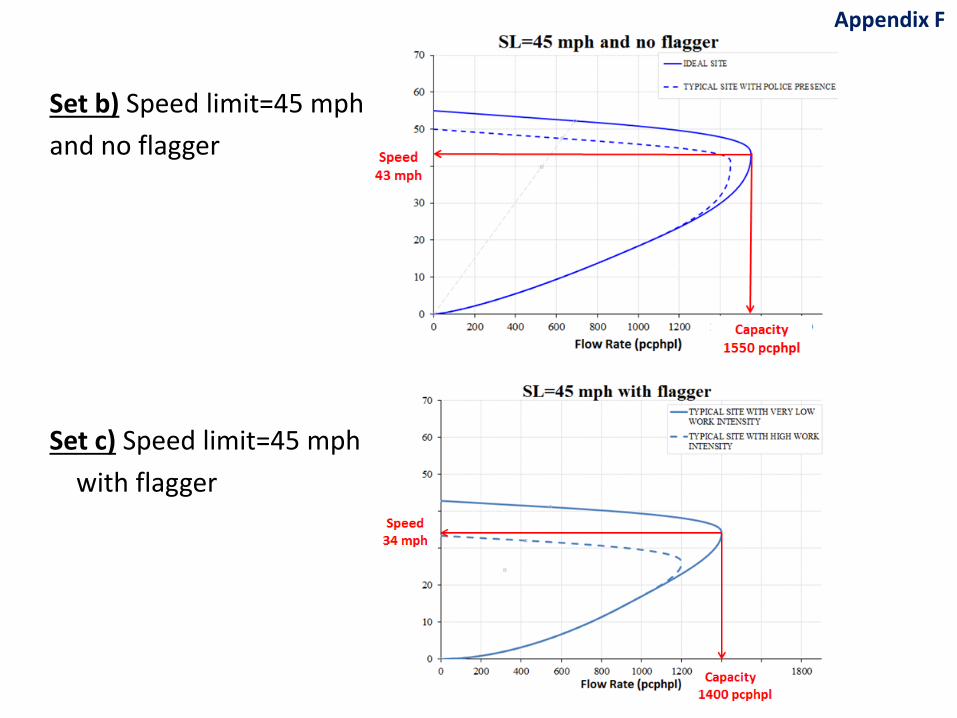
Set b) Speed limit=45 mph and no flagger
Set c) Speed limit=45 mph with flagger
Appendix F

Appendix G and H are presented right after Module 5
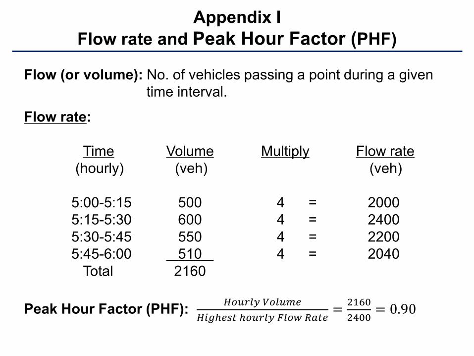
Flow (or volume): No. of vehicles passing a point during a given time interval.
Flow rate:
Time Volume Multiply Flow rate (hourly) (veh) (veh)
5:00-5:15 500 4 = 20005:15-5:30 600 4 = 24005:30-5:45 550 4 = 22005:45-6:00 510 4 = 2040
Total 2160
Peak Hour Factor (PHF): 𝐻𝐻𝑜𝑜𝑟𝑟𝑟𝑟𝐻𝐻𝐻𝐻 𝐻𝐻𝑜𝑜𝐻𝐻𝑟𝑟𝑉𝑉𝑟𝑟𝐻𝐻𝑤𝑤𝐻𝐻𝐻𝑟𝑟𝐻𝐻𝐻𝐻 𝐻𝑜𝑜𝑟𝑟𝑟𝑟𝐻𝐻𝐻𝐻 𝐹𝐹𝐻𝐻𝑜𝑜𝑤𝑤 𝑅𝑅𝑎𝑎𝐻𝐻𝑟𝑟
= 21602400
= 0.90
Appendix IFlow rate and Peak Hour Factor (PHF)
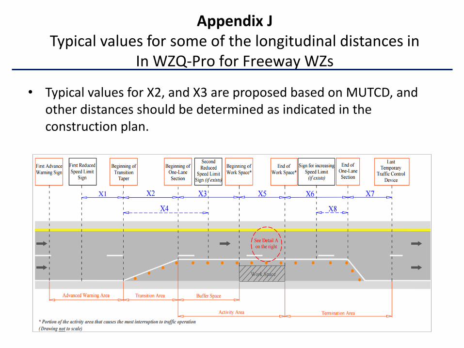
• Typical values for X2, and X3 are proposed based on MUTCD, and other distances should be determined as indicated in the construction plan.
Appendix JTypical values for some of the longitudinal distances in
In WZQ-Pro for Freeway WZs
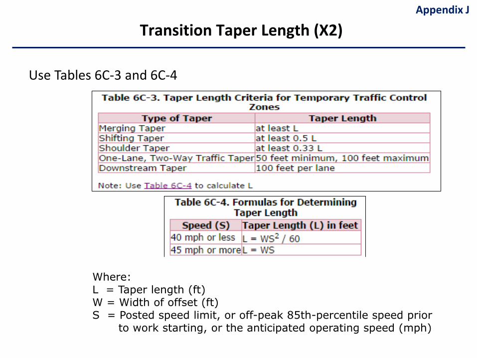
Use Tables 6C-3 and 6C-4
Transition Taper Length (X2)
Where:L = Taper length (ft)W = Width of offset (ft)S = Posted speed limit, or off-peak 85th-percentile speed prior
to work starting, or the anticipated operating speed (mph)
Appendix J
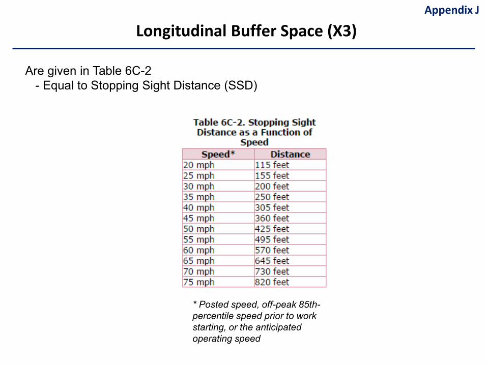
Longitudinal Buffer Space (X3)
Are given in Table 6C-2 - Equal to Stopping Sight Distance (SSD)
* Posted speed, off-peak 85th-percentile speed prior to work starting, or the anticipated operating speed
Appendix J
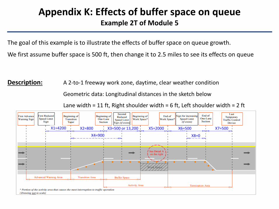
Description: A 2-to-1 freeway work zone, daytime, clear weather condition
Geometric data: Longitudinal distances in the sketch below
Lane width = 11 ft, Right shoulder width = 6 ft, Left shoulder width = 2 ft
Appendix K: Effects of buffer space on queue Example 2T of Module 5
The goal of this example is to illustrate the effects of buffer space on queue growth.
We first assume buffer space is 500 ft, then change it to 2.5 miles to see its effects on queue
X1=4200 X2=800
X4=900 X8=0
X7=500X6=500X5=2000X3=500 or 13,200
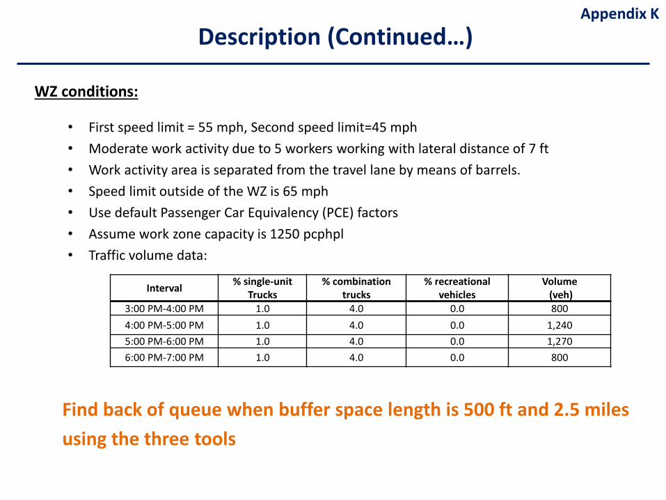
WZ conditions:
• First speed limit = 55 mph, Second speed limit=45 mph• Moderate work activity due to 5 workers working with lateral distance of 7 ft • Work activity area is separated from the travel lane by means of barrels.• Speed limit outside of the WZ is 65 mph• Use default Passenger Car Equivalency (PCE) factors• Assume work zone capacity is 1250 pcphpl • Traffic volume data:
Find back of queue when buffer space length is 500 ft and 2.5 miles using the three tools
Interval % single-unitTrucks
% combination trucks
% recreational vehicles
Volume(veh)
3:00 PM-4:00 PM 1.0 4.0 0.0 8004:00 PM-5:00 PM 1.0 4.0 0.0 1,2405:00 PM-6:00 PM 1.0 4.0 0.0 1,2706:00 PM-7:00 PM 1.0 4.0 0.0 800
Description (Continued…)Appendix K
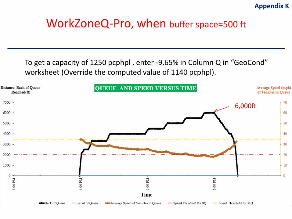
To get a capacity of 1250 pcphpl , enter -9.65% in Column Q in “GeoCond” worksheet (Override the computed value of 1140 pcphpl).
WorkZoneQ-Pro, when buffer space=500 ft
Appendix K
6,000ft
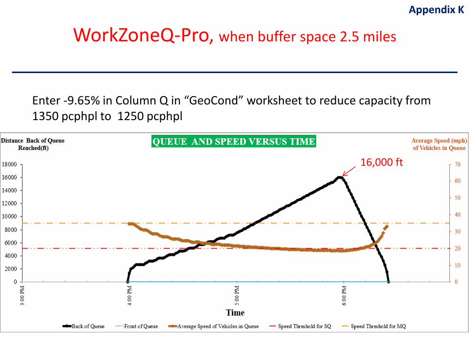
Enter -9.65% in Column Q in “GeoCond” worksheet to reduce capacity from 1350 pcphpl to 1250 pcphpl
WorkZoneQ-Pro, when buffer space 2.5 miles
Appendix K
16,000 ft
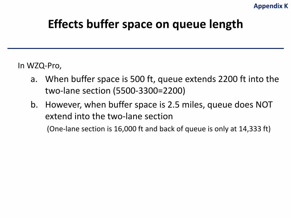
Effects buffer space on queue length
In WZQ-Pro, a. When buffer space is 500 ft, queue extends 2200 ft into the
two-lane section (5500-3300=2200)b. However, when buffer space is 2.5 miles, queue does NOT
extend into the two-lane section (One-lane section is 16,000 ft and back of queue is only at 14,333 ft)
Appendix K
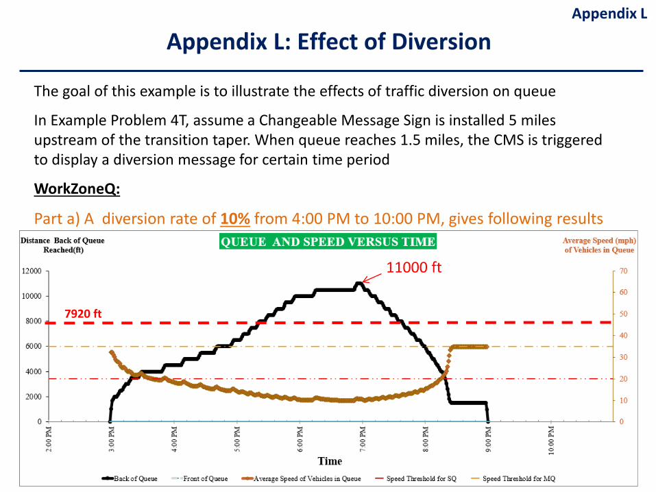
The goal of this example is to illustrate the effects of traffic diversion on queue
In Example Problem 4T, assume a Changeable Message Sign is installed 5 miles upstream of the transition taper. When queue reaches 1.5 miles, the CMS is triggered to display a diversion message for certain time period
WorkZoneQ:
Part a) A diversion rate of 10% from 4:00 PM to 10:00 PM, gives following results
Appendix L: Effect of DiversionAppendix L
11000 ft
7920 ft
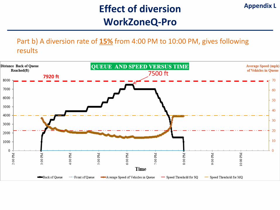
Part b) A diversion rate of 15% from 4:00 PM to 10:00 PM, gives following results
Effect of diversionWorkZoneQ-Pro
Appendix L
7920 ft 7500 ft
Appendix M
HCM 2016 detailed calculations for one-lane two way operation on two-lane highways

𝒇𝒇𝑫𝑫𝒑𝒑,𝑨𝑨𝑳𝑳𝑳𝑳 = 𝟐𝟐.𝟒𝟒𝒎𝒎𝒑𝒑𝒑𝒑 for all conditions
Tables from two-lane highways analysis (HCM Chapter 15)
𝑉𝑉1 = 0.615 × 𝑊𝑊𝐿𝐿 − 𝑓𝑓𝐿𝐿𝐿𝐿 − 𝑓𝑓𝐴𝐴 − 𝑓𝑓𝑛𝑛𝑝𝑝,𝐴𝐴𝑇𝑇𝐿𝐿
𝑉𝑉2 = 0.692 × 𝑊𝑊𝐿𝐿 − 𝑓𝑓𝐿𝐿𝐿𝐿 − 𝑓𝑓𝐴𝐴 − 𝑓𝑓𝑛𝑛𝑝𝑝,𝐴𝐴𝑇𝑇𝐿𝐿
Estimating Average Travel Speed
APP M - one-lane two way Operation
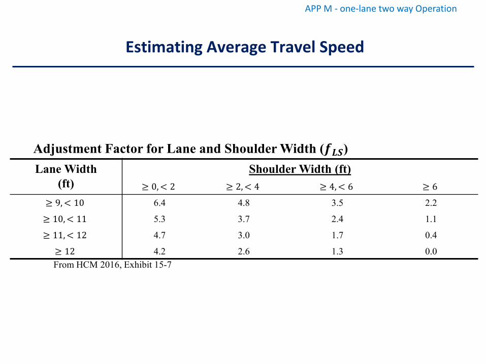
Estimating Average Travel Speed
APP M - one-lane two way Operation
Lane Width(ft)
Shoulder Width (ft)≥ 0, < 2 ≥ 2, < 4 ≥ 4, < 6 ≥ 6
≥ 9, < 10 6.4 4.8 3.5 2.2
≥ 10, < 11 5.3 3.7 2.4 1.1
≥ 11, < 12 4.7 3.0 1.7 0.4
≥ 12 4.2 2.6 1.3 0.0
Adjustment Factor for Lane and Shoulder Width (𝒇𝒇𝑳𝑳𝑳𝑳)
From HCM 2016, Exhibit 15-7
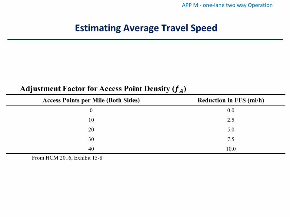
Estimating Average Travel Speed
APP M - one-lane two way Operation
Access Points per Mile (Both Sides) Reduction in FFS (mi/h)0 0.0
10 2.5
20 5.0
30 7.5
40 10.0
Adjustment Factor for Access Point Density (𝒇𝒇𝑨𝑨)
From HCM 2016, Exhibit 15-8
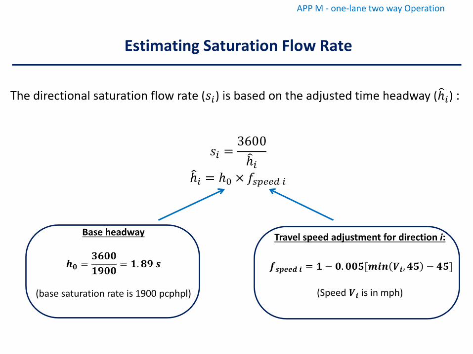
Base headway
𝒑𝒑𝟏𝟏 =𝟏𝟏𝟏𝟏𝟏𝟏𝟏𝟏𝟏𝟏𝟐𝟐𝟏𝟏𝟏𝟏
= 𝟏𝟏.𝟏𝟏𝟐𝟐 𝑫𝑫
(base saturation rate is 1900 pcphpl)
Travel speed adjustment for direction i:
𝒇𝒇𝑫𝑫𝒑𝒑𝑫𝑫𝑫𝑫𝒂𝒂 𝑫𝑫 = 𝟏𝟏 − 𝟏𝟏.𝟏𝟏𝟏𝟏𝟏𝟏[𝒎𝒎𝑫𝑫𝑫𝑫 𝑽𝑽𝑫𝑫,𝟒𝟒𝟏𝟏 − 𝟒𝟒𝟏𝟏]
(Speed 𝑽𝑽𝑫𝑫 is in mph)
Estimating Saturation Flow Rate
APP M - one-lane two way Operation
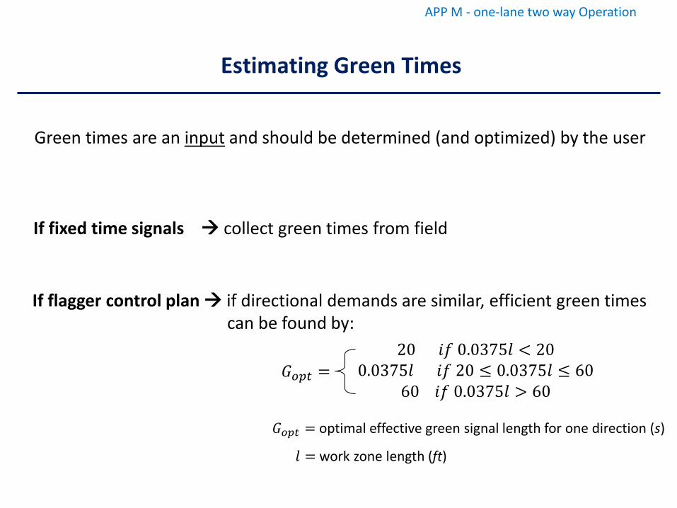
If fixed time signals collect green times from field
If flagger control plan if directional demands are similar, efficient green times can be found by:
𝐺𝐺𝑜𝑜𝑝𝑝𝐻𝐻 =20 𝑖𝑖𝑓𝑓 0.0375𝐹𝐹 < 20
0.0375𝐹𝐹 𝑖𝑖𝑓𝑓 20 ≤ 0.0375𝐹𝐹 ≤ 6060 𝑖𝑖𝑓𝑓 0.0375𝐹𝐹 > 60
𝐺𝐺𝑜𝑜𝑝𝑝𝐻𝐻 = optimal effective green signal length for one direction (s)
𝐹𝐹 = work zone length (ft)
Green times are an input and should be determined (and optimized) by the user
Estimating Green Times
APP M - one-lane two way Operation
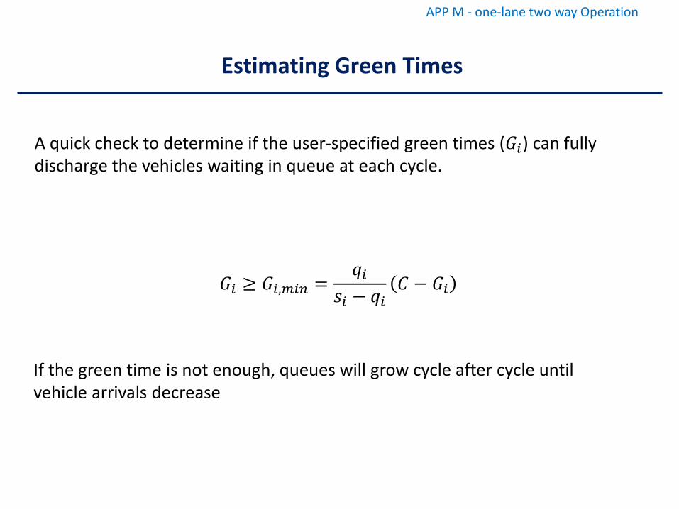
A quick check to determine if the user-specified green times (𝐺𝐺𝑤𝑤) can fully discharge the vehicles waiting in queue at each cycle.
𝐺𝐺𝑤𝑤 ≥ 𝐺𝐺𝑤𝑤,𝑉𝑉𝑤𝑤𝑛𝑛 =𝑞𝑞𝑤𝑤
𝑠𝑠𝑤𝑤 − 𝑞𝑞𝑤𝑤𝐶𝐶 − 𝐺𝐺𝑤𝑤
If the green time is not enough, queues will grow cycle after cycle until vehicle arrivals decrease
Estimating Green Times
APP M - one-lane two way Operation
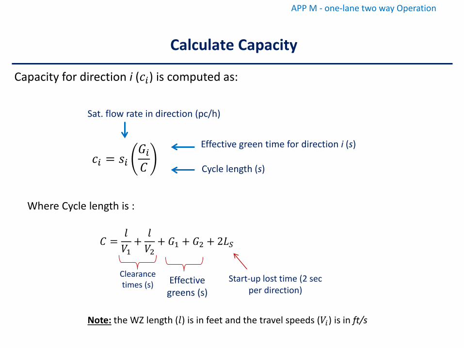
Capacity for direction i (𝑠𝑠𝑤𝑤) is computed as:
𝑠𝑠𝑤𝑤 = 𝑠𝑠𝑤𝑤𝐺𝐺𝑤𝑤𝐶𝐶
Effective green time for direction i (s)
Cycle length (s)
Sat. flow rate in direction (pc/h)
𝐶𝐶 =𝐹𝐹𝑉𝑉1
+𝐹𝐹𝑉𝑉2
+ 𝐺𝐺1 + 𝐺𝐺2 + 2𝐿𝐿𝐿𝐿
Effective greens (s)
Start-up lost time (2 sec per direction)
Clearance times (s)
Note: the WZ length (𝐹𝐹) is in feet and the travel speeds (𝑉𝑉𝑤𝑤) is in ft/s
Where Cycle length is :
Calculate Capacity
APP M - one-lane two way Operation
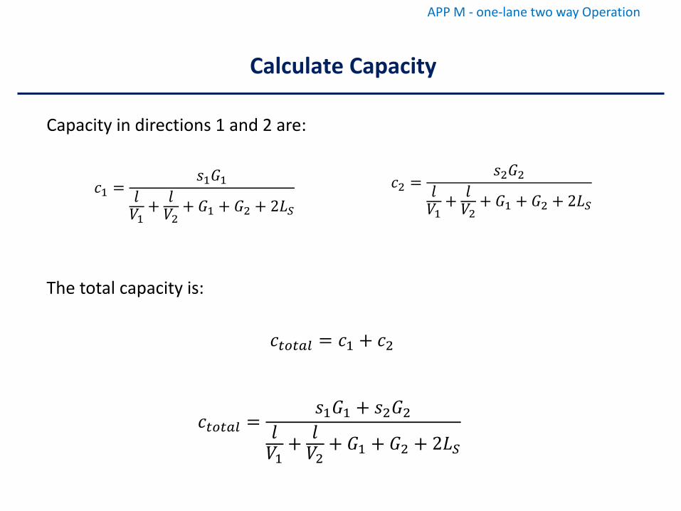
The total capacity is:
𝑠𝑠𝐻𝐻𝑜𝑜𝐻𝐻𝑎𝑎𝐻𝐻 = 𝑠𝑠1 + 𝑠𝑠2
𝑠𝑠𝐻𝐻𝑜𝑜𝐻𝐻𝑎𝑎𝐻𝐻 =𝑠𝑠1𝐺𝐺1 + 𝑠𝑠2𝐺𝐺2
𝐹𝐹𝑉𝑉1
+ 𝐹𝐹𝑉𝑉2
+ 𝐺𝐺1 + 𝐺𝐺2 + 2𝐿𝐿𝐿𝐿
𝑠𝑠1 =𝑠𝑠1𝐺𝐺1
𝐹𝐹𝑉𝑉1
+ 𝐹𝐹𝑉𝑉2
+ 𝐺𝐺1 + 𝐺𝐺2 + 2𝐿𝐿𝐿𝐿
𝑠𝑠2 =𝑠𝑠2𝐺𝐺2
𝐹𝐹𝑉𝑉1
+ 𝐹𝐹𝑉𝑉2
+ 𝐺𝐺1 + 𝐺𝐺2 + 2𝐿𝐿𝐿𝐿
Capacity in directions 1 and 2 are:
Calculate Capacity
APP M - one-lane two way Operation
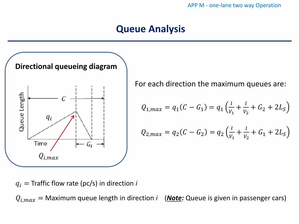
Directional queueing diagram
𝑄𝑄1,𝑉𝑉𝑎𝑎𝑚𝑚 = 𝑞𝑞1 𝐶𝐶 − 𝐺𝐺1 = 𝑞𝑞1𝐻𝐻𝐻𝐻1
+ 𝐻𝐻𝐻𝐻2
+ 𝐺𝐺2 + 2𝐿𝐿𝐿𝐿
𝑄𝑄2,𝑉𝑉𝑎𝑎𝑚𝑚 = 𝑞𝑞2 𝐶𝐶 − 𝐺𝐺2 = 𝑞𝑞2𝐻𝐻𝐻𝐻1
+ 𝐻𝐻𝐻𝐻2
+ 𝐺𝐺1 + 2𝐿𝐿𝐿𝐿
For each direction the maximum queues are:
𝑞𝑞𝑤𝑤 = Traffic flow rate (pc/s) in direction i
𝑄𝑄𝑤𝑤,𝑉𝑉𝑎𝑎𝑚𝑚 = Maximum queue length in direction i (Note: Queue is given in passenger cars)
𝑞𝑞𝑤𝑤
𝑄𝑄𝑤𝑤,𝑉𝑉𝑎𝑎𝑚𝑚
Queue Analysis
APP M - one-lane two way Operation
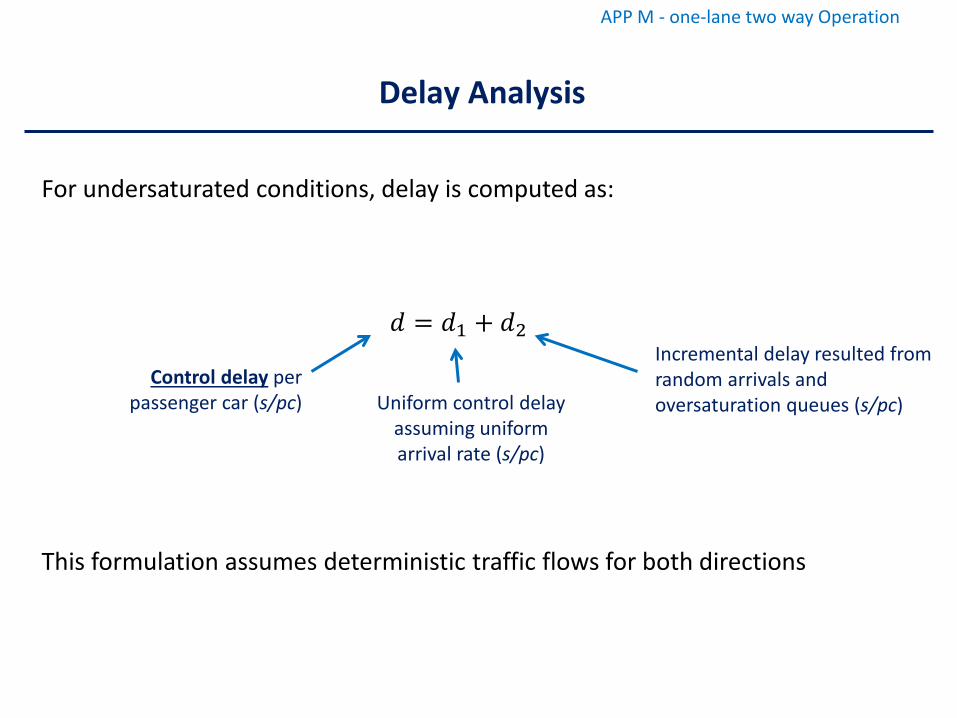
Uniform control delay assuming uniform arrival rate (s/pc)
For undersaturated conditions, delay is computed as:
𝑆𝑆 = 𝑆𝑆1 + 𝑆𝑆2
Control delay per passenger car (s/pc)
Incremental delay resulted from random arrivals and oversaturation queues (s/pc)
This formulation assumes deterministic traffic flows for both directions
Delay Analysis
APP M - one-lane two way Operation
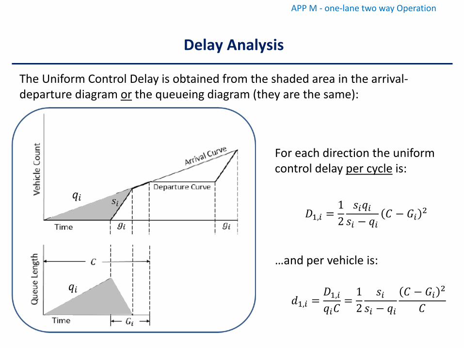
The Uniform Control Delay is obtained from the shaded area in the arrival-departure diagram or the queueing diagram (they are the same):
For each direction the uniform control delay per cycle is:
𝑄𝑄1,𝑤𝑤 =12
𝑠𝑠𝑤𝑤𝑞𝑞𝑤𝑤𝑠𝑠𝑤𝑤 − 𝑞𝑞𝑤𝑤
𝐶𝐶 − 𝐺𝐺𝑤𝑤 2
𝑆𝑆1,𝑤𝑤 =𝑄𝑄1,𝑤𝑤𝑞𝑞𝑤𝑤𝐶𝐶
=12
𝑠𝑠𝑤𝑤𝑠𝑠𝑤𝑤 − 𝑞𝑞𝑤𝑤
𝐶𝐶 − 𝐺𝐺𝑤𝑤 2
𝐶𝐶
…and per vehicle is:
Delay Analysis
APP M - one-lane two way Operation
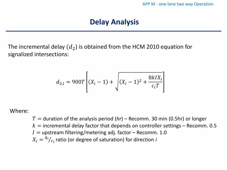
The incremental delay (𝑆𝑆2) is obtained from the HCM 2010 equation for signalized intersections:
𝑆𝑆2,𝑤𝑤 = 900𝑇𝑇 𝑋𝑋𝑤𝑤 − 1 + 𝑋𝑋𝑤𝑤 − 1 2 +8𝑘𝑘𝑘𝑘𝑋𝑋𝑤𝑤𝑠𝑠𝑤𝑤𝑇𝑇
Where:𝑇𝑇 = duration of the analysis period (hr) – Recomm. 30 min (0.5hr) or longer𝑘𝑘 = incremental delay factor that depends on controller settings – Recomm. 0.5𝑘𝑘 = upstream filtering/metering adj. factor – Recomm. 1.0𝑋𝑋𝑤𝑤 = ⁄𝑞𝑞𝑖𝑖 𝑟𝑟𝑖𝑖 ratio (or degree of saturation) for direction i
Delay Analysis
APP M - one-lane two way Operation
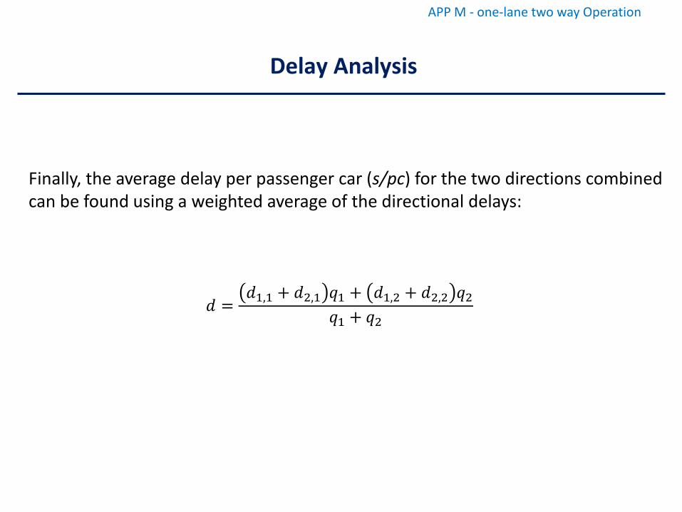
Finally, the average delay per passenger car (s/pc) for the two directions combined can be found using a weighted average of the directional delays:
𝑆𝑆 =𝑆𝑆1,1 + 𝑆𝑆2,1 𝑞𝑞1 + 𝑆𝑆1,2 + 𝑆𝑆2,2 𝑞𝑞2
𝑞𝑞1 + 𝑞𝑞2
Delay Analysis
APP M - one-lane two way Operation
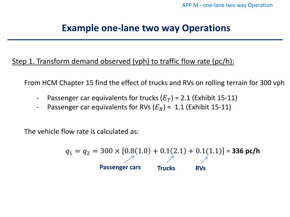
Step 1. Transform demand observed (vph) to traffic flow rate (pc/h):
From HCM Chapter 15 find the effect of trucks and RVs on rolling terrain for 300 vph
- Passenger car equivalents for trucks (𝐸𝐸𝑇𝑇) = 2.1 (Exhibit 15-11)- Passenger car equivalents for RVs (𝐸𝐸𝑅𝑅) = 1.1 (Exhibit 15-11)
The vehicle flow rate is calculated as:
𝑞𝑞1 = 𝑞𝑞2 = 300 × 0.8 1.0 + 0.1 2.1 + 0.1(1.1) = 336 pc/h
Passenger cars Trucks RVs
Example one-lane two way Operations
APP M - one-lane two way Operation
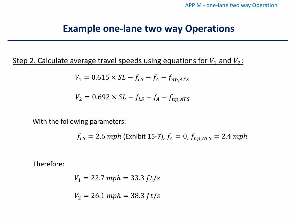
𝑉𝑉1 = 0.615 × 𝑊𝑊𝐿𝐿 − 𝑓𝑓𝐿𝐿𝐿𝐿 − 𝑓𝑓𝐴𝐴 − 𝑓𝑓𝑛𝑛𝑝𝑝,𝐴𝐴𝑇𝑇𝐿𝐿
Step 2. Calculate average travel speeds using equations for 𝑉𝑉1 and 𝑉𝑉2:
𝑉𝑉2 = 0.692 × 𝑊𝑊𝐿𝐿 − 𝑓𝑓𝐿𝐿𝐿𝐿 − 𝑓𝑓𝐴𝐴 − 𝑓𝑓𝑛𝑛𝑝𝑝,𝐴𝐴𝑇𝑇𝐿𝐿
With the following parameters:
𝑓𝑓𝐿𝐿𝐿𝐿 = 2.6 𝑚𝑚𝑣𝑣𝑡 (Exhibit 15-7), 𝑓𝑓𝐴𝐴 = 0, 𝑓𝑓𝑛𝑛𝑝𝑝,𝐴𝐴𝑇𝑇𝐿𝐿 = 2.4 𝑚𝑚𝑣𝑣𝑡
Therefore:
𝑉𝑉1 = 22.7 𝑚𝑚𝑣𝑣𝑡 = 33.3 𝑓𝑓𝑓𝑓/𝑠𝑠
𝑉𝑉2 = 26.1 𝑚𝑚𝑣𝑣𝑡 = 38.3 𝑓𝑓𝑓𝑓/𝑠𝑠
Example one-lane two way Operations
APP M - one-lane two way Operation
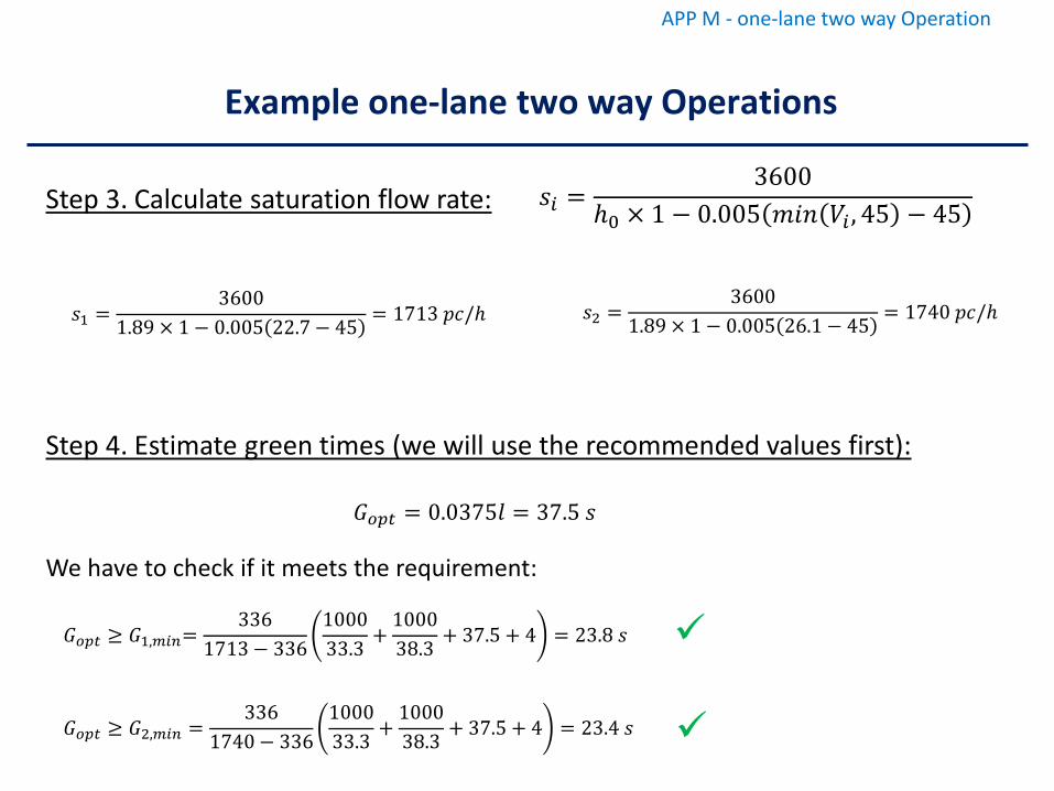
Step 3. Calculate saturation flow rate: 𝑠𝑠𝑤𝑤 =3600
𝑡0 × 1 − 0.005 𝑚𝑚𝑖𝑖𝑡𝑡 𝑉𝑉𝑤𝑤 , 45 − 45
𝑠𝑠1 =3600
1.89 × 1 − 0.005 22.7− 45 = 1713 𝑣𝑣𝑠𝑠/𝑡 𝑠𝑠2 =3600
1.89 × 1 − 0.005 26.1 − 45 = 1740 𝑣𝑣𝑠𝑠/𝑡
Step 4. Estimate green times (we will use the recommended values first):
𝐺𝐺𝑜𝑜𝑝𝑝𝐻𝐻 = 0.0375𝐹𝐹 = 37.5 𝑠𝑠
We have to check if it meets the requirement:
𝐺𝐺𝑜𝑜𝑝𝑝𝐻𝐻 ≥ 𝐺𝐺1,𝑉𝑉𝑤𝑤𝑛𝑛=336
1713− 336100033.3 +
100038.3 + 37.5 + 4 = 23.8 𝑠𝑠
𝐺𝐺𝑜𝑜𝑝𝑝𝐻𝐻 ≥ 𝐺𝐺2,𝑉𝑉𝑤𝑤𝑛𝑛 =336
1740− 336100033.3 +
100038.3 + 37.5 + 4 = 23.4 𝑠𝑠
Example one-lane two way Operations
APP M - one-lane two way Operation
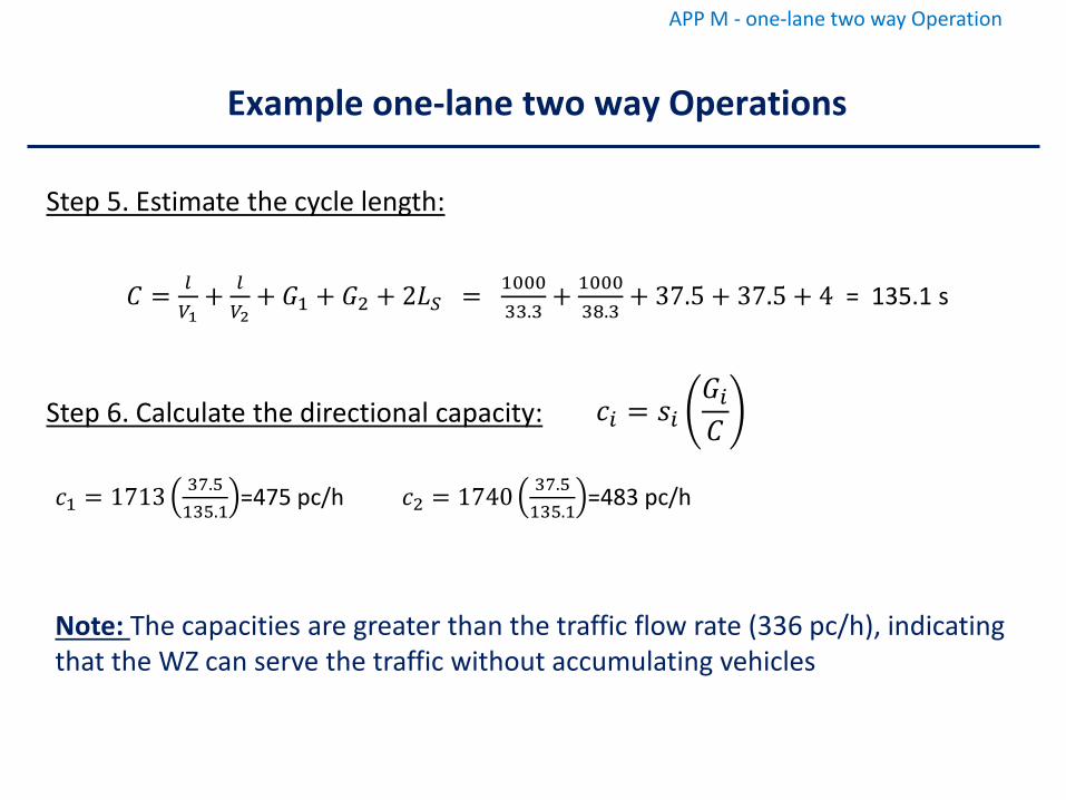
Step 5. Estimate the cycle length:
𝐶𝐶 = 𝐻𝐻𝐻𝐻1
+ 𝐻𝐻𝐻𝐻2
+ 𝐺𝐺1 + 𝐺𝐺2 + 2𝐿𝐿𝐿𝐿 = 100033.3
+ 100038.3
+ 37.5 + 37.5 + 4 = 135.1 s
Step 6. Calculate the directional capacity: 𝑠𝑠𝑤𝑤 = 𝑠𝑠𝑤𝑤𝐺𝐺𝑤𝑤𝐶𝐶
𝑠𝑠1 = 1713 37.5135.1
=475 pc/h 𝑠𝑠2 = 1740 37.5135.1
=483 pc/h
Note: The capacities are greater than the traffic flow rate (336 pc/h), indicating that the WZ can serve the traffic without accumulating vehicles
Example one-lane two way Operations
APP M - one-lane two way Operation
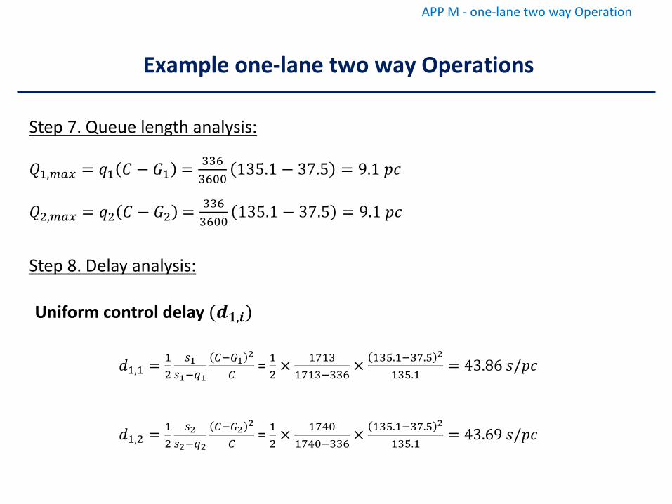
Step 7. Queue length analysis:
𝑄𝑄1,𝑉𝑉𝑎𝑎𝑚𝑚 = 𝑞𝑞1 𝐶𝐶 − 𝐺𝐺1 = 3363600
135.1 − 37.5 = 9.1 𝑣𝑣𝑠𝑠
𝑄𝑄2,𝑉𝑉𝑎𝑎𝑚𝑚 = 𝑞𝑞2 𝐶𝐶 − 𝐺𝐺2 = 3363600
135.1 − 37.5 = 9.1 𝑣𝑣𝑠𝑠
Step 8. Delay analysis:
𝑆𝑆1,1 = 12
𝐻𝐻1𝐻𝐻1−𝑞𝑞1
𝐶𝐶−𝐺𝐺1 2
𝐶𝐶= 12
× 17131713−336
× 135.1−37.5 2
135.1= 43.86 𝑠𝑠/𝑣𝑣𝑠𝑠
𝑆𝑆1,2 = 12
𝐻𝐻2𝐻𝐻2−𝑞𝑞2
𝐶𝐶−𝐺𝐺2 2
𝐶𝐶= 12
× 17401740−336
× 135.1−37.5 2
135.1= 43.69 𝑠𝑠/𝑣𝑣𝑠𝑠
Uniform control delay (𝒂𝒂𝟏𝟏,𝑫𝑫)
Example one-lane two way Operations
APP M - one-lane two way Operation
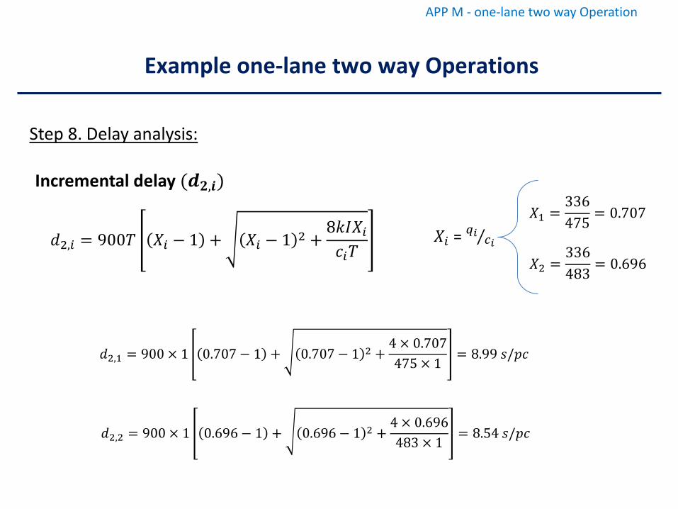
Step 8. Delay analysis:
Incremental delay (𝒂𝒂𝟐𝟐,𝑫𝑫)
𝑆𝑆2,𝑤𝑤 = 900𝑇𝑇 𝑋𝑋𝑤𝑤 − 1 + 𝑋𝑋𝑤𝑤 − 1 2 +8𝑘𝑘𝑘𝑘𝑋𝑋𝑤𝑤𝑠𝑠𝑤𝑤𝑇𝑇
𝑋𝑋𝑤𝑤 = ⁄𝑞𝑞𝑖𝑖 𝑟𝑟𝑖𝑖
𝑋𝑋1 =336475
= 0.707
𝑋𝑋2 =336483
= 0.696
𝑆𝑆2,1 = 900 × 1 0.707 − 1 + 0.707 − 1 2 +4 × 0.707475 × 1
= 8.99 𝑠𝑠/𝑣𝑣𝑠𝑠
𝑆𝑆2,2 = 900 × 1 0.696 − 1 + 0.696 − 1 2 +4 × 0.696483 × 1
= 8.54 𝑠𝑠/𝑣𝑣𝑠𝑠
Example one-lane two way Operations
APP M - one-lane two way Operation
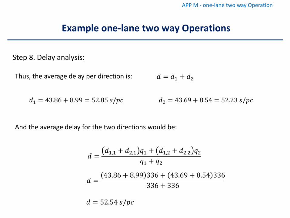
Step 8. Delay analysis:
And the average delay for the two directions would be:
𝑆𝑆 =𝑆𝑆1,1 + 𝑆𝑆2,1 𝑞𝑞1 + 𝑆𝑆1,2 + 𝑆𝑆2,2 𝑞𝑞2
𝑞𝑞1 + 𝑞𝑞2
𝑆𝑆 =43.86 + 8.99 336 + 43.69 + 8.54 336
336 + 336
𝑆𝑆 = 52.54 𝑠𝑠/𝑣𝑣𝑠𝑠
Thus, the average delay per direction is: 𝑆𝑆 = 𝑆𝑆1 + 𝑆𝑆2
𝑆𝑆1 = 43.86 + 8.99 = 52.85 𝑠𝑠/𝑣𝑣𝑠𝑠 𝑆𝑆2 = 43.69 + 8.54 = 52.23 𝑠𝑠/𝑣𝑣𝑠𝑠
Example one-lane two way Operations
APP M - one-lane two way Operation
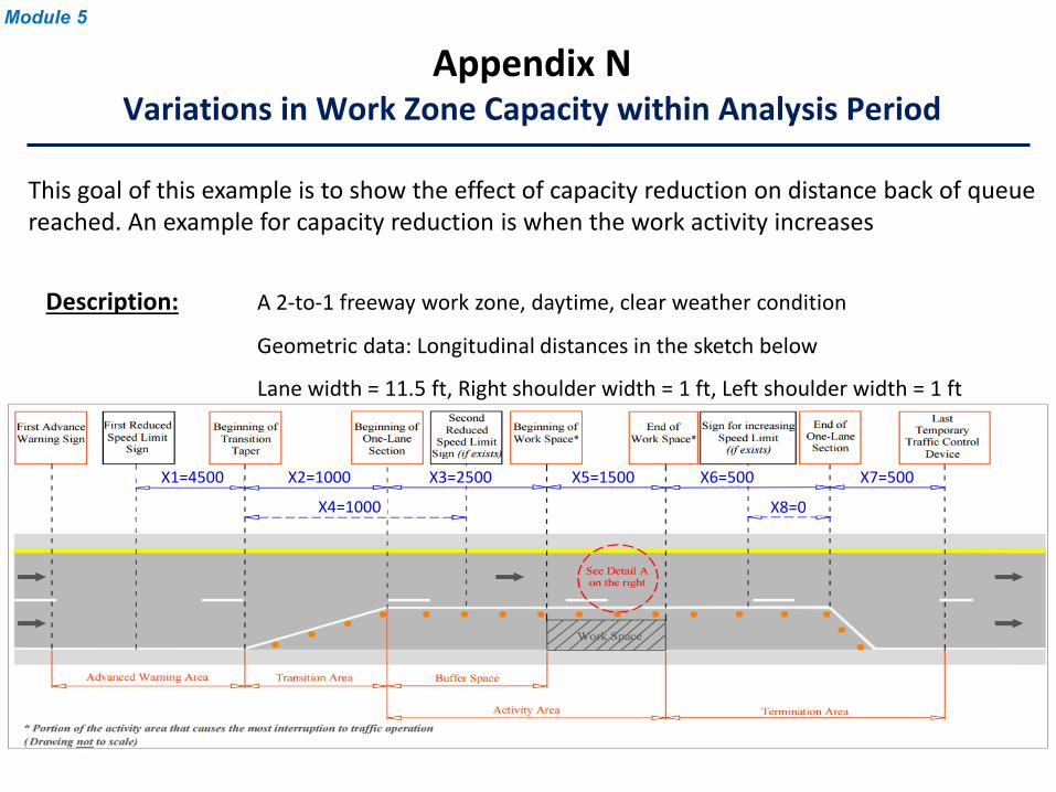
Description: A 2-to-1 freeway work zone, daytime, clear weather condition
Geometric data: Longitudinal distances in the sketch below
Lane width = 11.5 ft, Right shoulder width = 1 ft, Left shoulder width = 1 ft
Appendix NVariations in Work Zone Capacity within Analysis Period
This goal of this example is to show the effect of capacity reduction on distance back of queue reached. An example for capacity reduction is when the work activity increases
X1=4500 X2=1000
X4=1000 X8=0
X7=500X6=500X5=1500X3=2500
Module 5
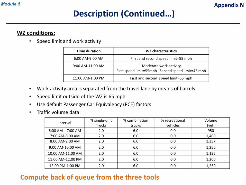
WZ conditions:• Speed limit and work activity
• Work activity area is separated from the travel lane by means of barrels • Speed limit outside of the WZ is 65 mph• Use default Passenger Car Equivalency (PCE) factors• Traffic volume data:
Compute back of queue from the three tools
Interval % single-unitTrucks
% combination trucks
% recreational vehicles
Volume(veh)
6:00 AM – 7:00 AM 2.0 6.0 0.0 9507:00 AM-8:00 AM 2.0 6.0 0.0 1,4008:00 AM-9:00 AM 2.0 6.0 0.0 1,357
9:00 AM-10:00 AM 2.0 6.0 0.0 1,25010:00 AM-11:00 AM 2.0 6.0 0.0 1,13511:00 AM-12:00 PM 2.0 6.0 0.0 1,20012:00 PM-1:00 PM 2.0 6.0 0.0 1,250
Description (Continued…)
Time duration WZ characteristics
6:00 AM-9:00 AM First and second speed limit=55 mph
9:00 AM-11:00 AM Moderate work activity, First speed limit=55mph , Second speed limit=45 mph
11:00 AM-1:00 PM First and second speed limit=55 mph
Module 5 Appendix N
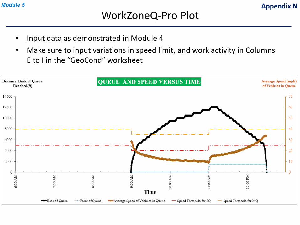
• Input data as demonstrated in Module 4• Make sure to input variations in speed limit, and work activity in Columns
E to I in the “GeoCond” worksheet
Appendix NWorkZoneQ-Pro Plot
Module 5
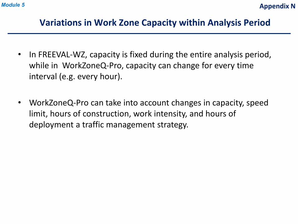
Variations in Work Zone Capacity within Analysis Period
Module 5
• In FREEVAL-WZ, capacity is fixed during the entire analysis period, while in WorkZoneQ-Pro, capacity can change for every time interval (e.g. every hour).
• WorkZoneQ-Pro can take into account changes in capacity, speed limit, hours of construction, work intensity, and hours of deployment a traffic management strategy.
Appendix N
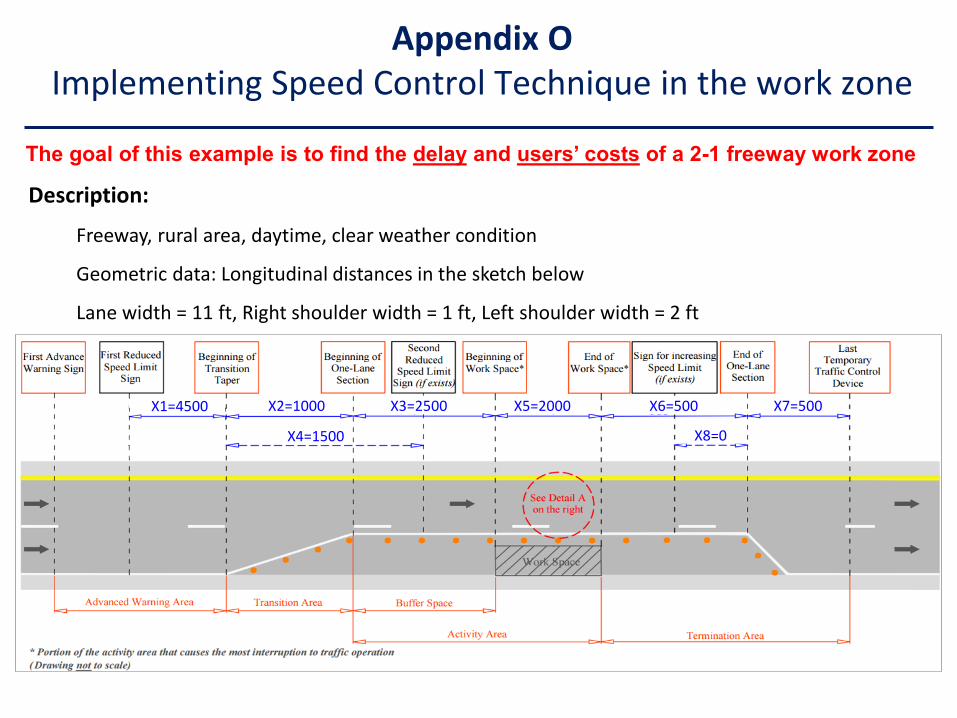
Description:
Freeway, rural area, daytime, clear weather condition
Geometric data: Longitudinal distances in the sketch below
Lane width = 11 ft, Right shoulder width = 1 ft, Left shoulder width = 2 ft
Appendix OImplementing Speed Control Technique in the work zone
The goal of this example is to find the delay and users’ costs of a 2-1 freeway work zone
X1=4500 X2=1000
X4=1500 X8=0
X7=500X6=500X5=2000X3=2500
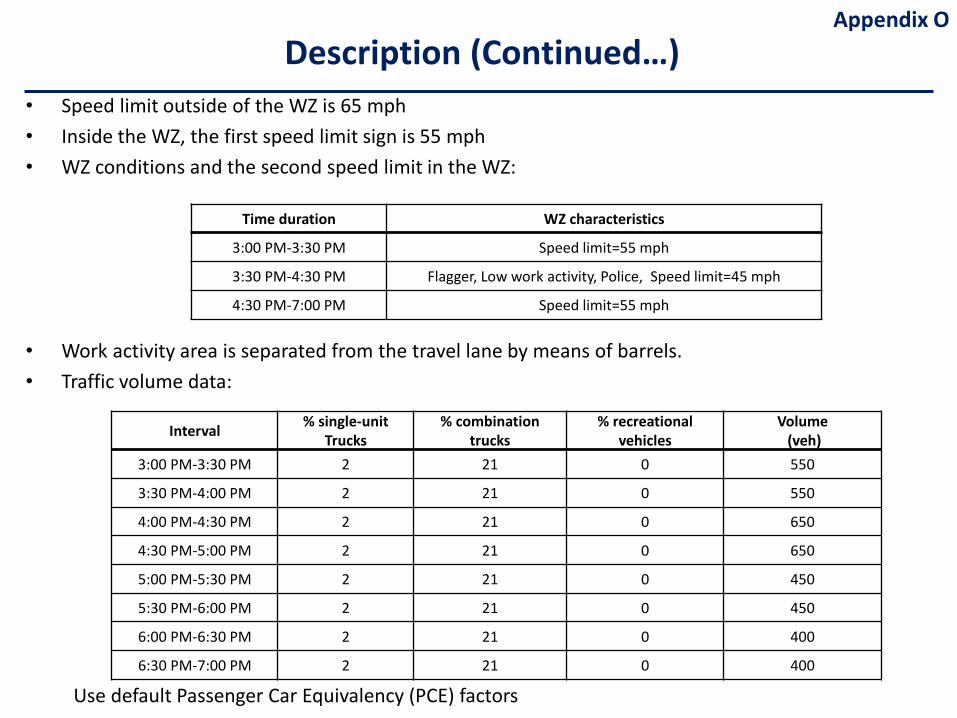
• Speed limit outside of the WZ is 65 mph • Inside the WZ, the first speed limit sign is 55 mph• WZ conditions and the second speed limit in the WZ:
• Work activity area is separated from the travel lane by means of barrels. • Traffic volume data:
Use default Passenger Car Equivalency (PCE) factors
Time duration WZ characteristics
3:00 PM-3:30 PM Speed limit=55 mph
3:30 PM-4:30 PM Flagger, Low work activity, Police, Speed limit=45 mph
4:30 PM-7:00 PM Speed limit=55 mph
Interval % single-unitTrucks
% combination trucks
% recreational vehicles
Volume(veh)
3:00 PM-3:30 PM 2 21 0 550
3:30 PM-4:00 PM 2 21 0 550
4:00 PM-4:30 PM 2 21 0 650
4:30 PM-5:00 PM 2 21 0 650
5:00 PM-5:30 PM 2 21 0 450
5:30 PM-6:00 PM 2 21 0 450
6:00 PM-6:30 PM 2 21 0 400
6:30 PM-7:00 PM 2 21 0 400
Description (Continued…)Appendix O
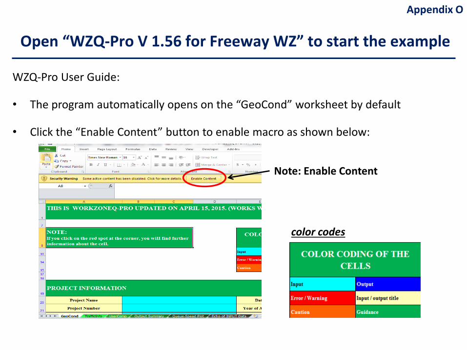
WZQ-Pro User Guide:
• The program automatically opens on the “GeoCond” worksheet by default
• Click the “Enable Content” button to enable macro as shown below:
Open “WZQ-Pro V 1.56 for Freeway WZ” to start the example
Note: Enable Content
color codes
Appendix O
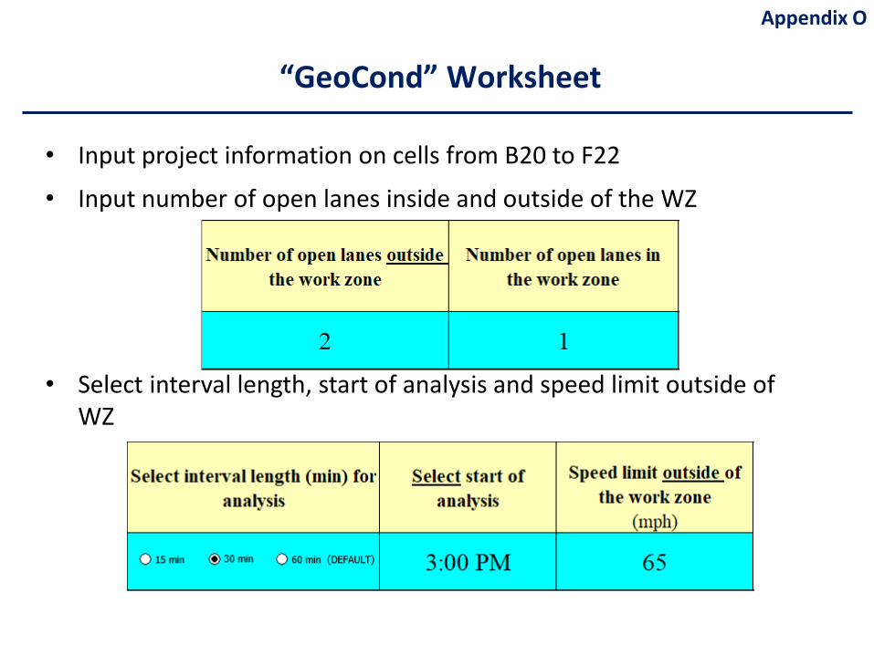
• Input project information on cells from B20 to F22
• Input number of open lanes inside and outside of the WZ
• Select interval length, start of analysis and speed limit outside of WZ
“GeoCond” Worksheet
Appendix O
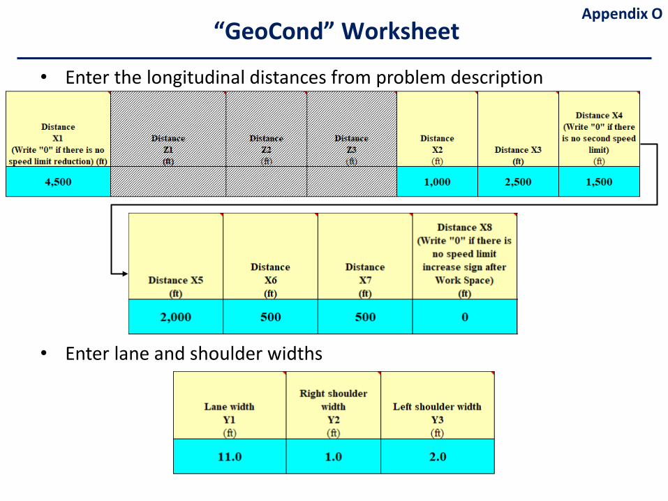
“GeoCond” Worksheet
• Enter the longitudinal distances from problem description
• Enter lane and shoulder widths
Appendix O
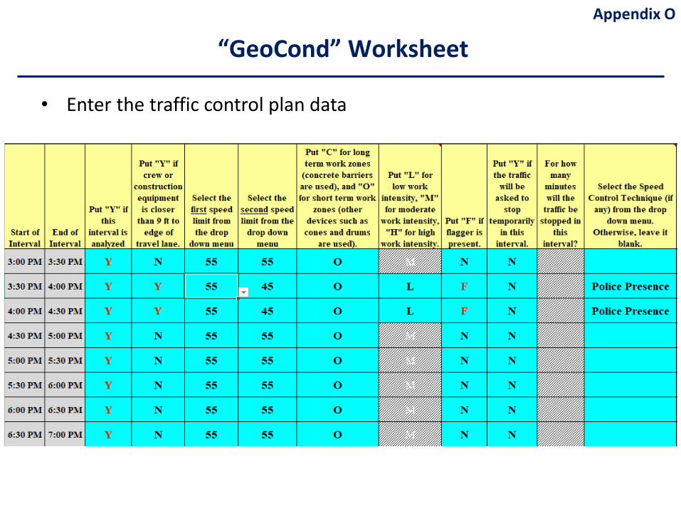
• Enter the traffic control plan data
“GeoCond” WorksheetAppendix O
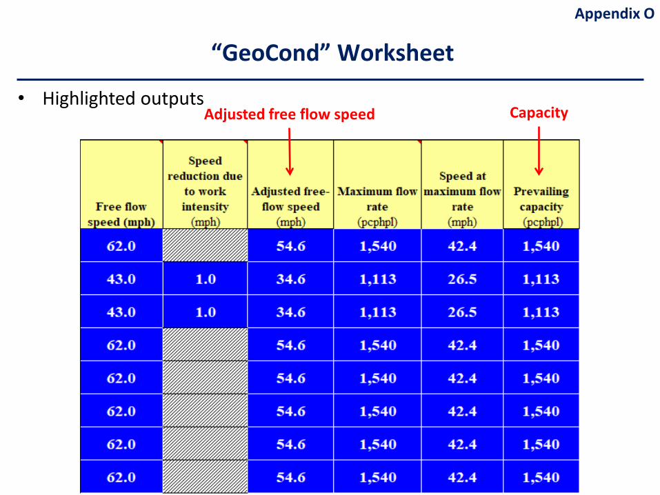
“GeoCond” Worksheet
• Highlighted outputsCapacityAdjusted free flow speed
Appendix O
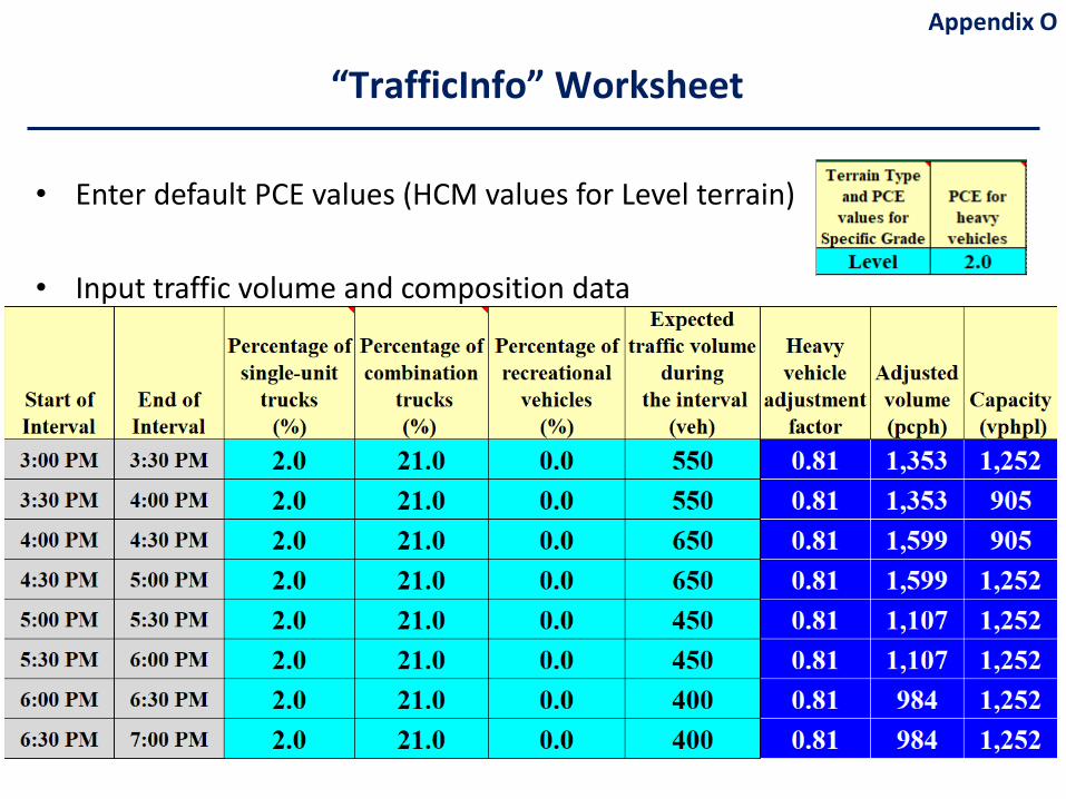
• Enter default PCE values (HCM values for Level terrain)
• Input traffic volume and composition data
“TrafficInfo” Worksheet
Appendix O
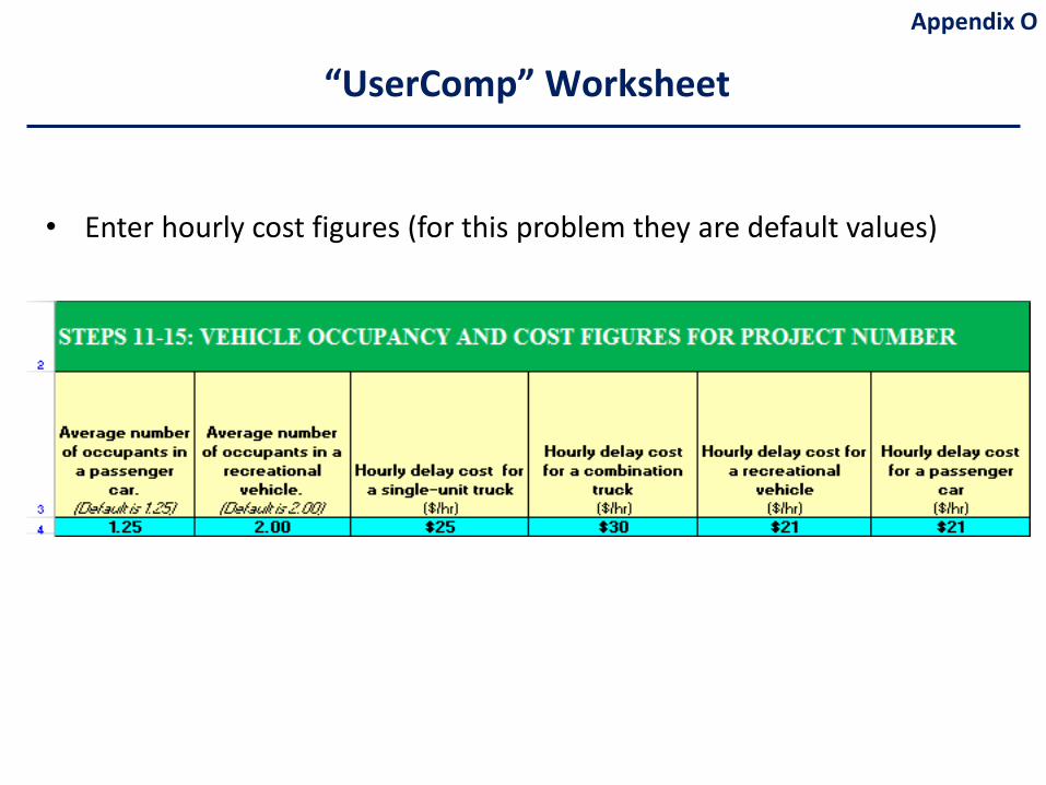
• Enter hourly cost figures (for this problem they are default values)
“UserComp” Worksheet
Appendix O
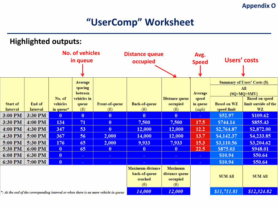
Highlighted outputs:
“UserComp” Worksheet
Distance queue occupied Users’ costs
No. of vehicles in queue
Avg.Speed
Appendix O
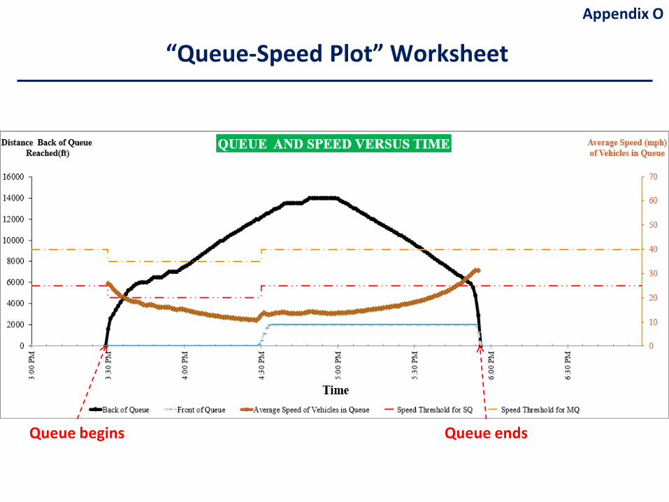
“Queue-Speed Plot” Worksheet
Queue begins Queue ends
Appendix O
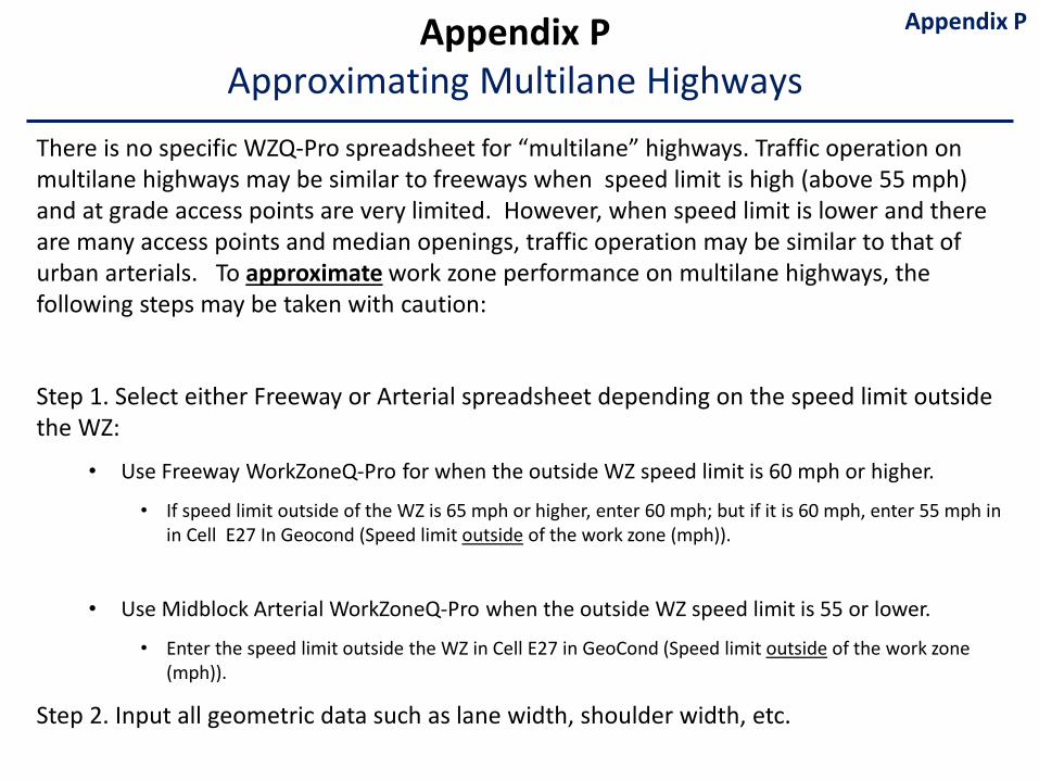
There is no specific WZQ-Pro spreadsheet for “multilane” highways. Traffic operation on multilane highways may be similar to freeways when speed limit is high (above 55 mph) and at grade access points are very limited. However, when speed limit is lower and there are many access points and median openings, traffic operation may be similar to that of urban arterials. To approximate work zone performance on multilane highways, the following steps may be taken with caution:
Step 1. Select either Freeway or Arterial spreadsheet depending on the speed limit outside the WZ:
• Use Freeway WorkZoneQ-Pro for when the outside WZ speed limit is 60 mph or higher.
• If speed limit outside of the WZ is 65 mph or higher, enter 60 mph; but if it is 60 mph, enter 55 mph in in Cell E27 In Geocond (Speed limit outside of the work zone (mph)).
• Use Midblock Arterial WorkZoneQ-Pro when the outside WZ speed limit is 55 or lower.
• Enter the speed limit outside the WZ in Cell E27 in GeoCond (Speed limit outside of the work zone (mph)).
Step 2. Input all geometric data such as lane width, shoulder width, etc.
Appendix PAppendix PApproximating Multilane Highways
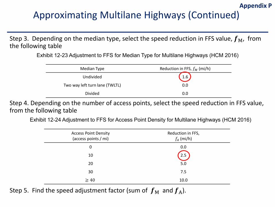
Step 3. Depending on the median type, select the speed reduction in FFS value, 𝒇𝒇M, from the following table
Step 4. Depending on the number of access points, select the speed reduction in FFS value, from the following table
Step 5. Find the speed adjustment factor (sum of 𝒇𝒇M and 𝒇𝒇A).
Exhibit 12-23 Adjustment to FFS for Median Type for Multilane Highways (HCM 2016)
Exhibit 12-24 Adjustment to FFS for Access Point Density for Multilane Highways (HCM 2016)
Appendix PApproximating Multilane Highways (Continued)
Median Type Reduction in FFS, 𝑓𝑓𝑀𝑀 (mi/h)
Undivided 1.6
Two way left turn lane (TWLTL) 0.0
Divided 0.0
Access Point Density(access points / mi)
Reduction in FFS, 𝑓𝑓𝐴𝐴 (mi/h)
0 0.0
10 2.5
20 5.0
30 7.5
≥ 40 10.0
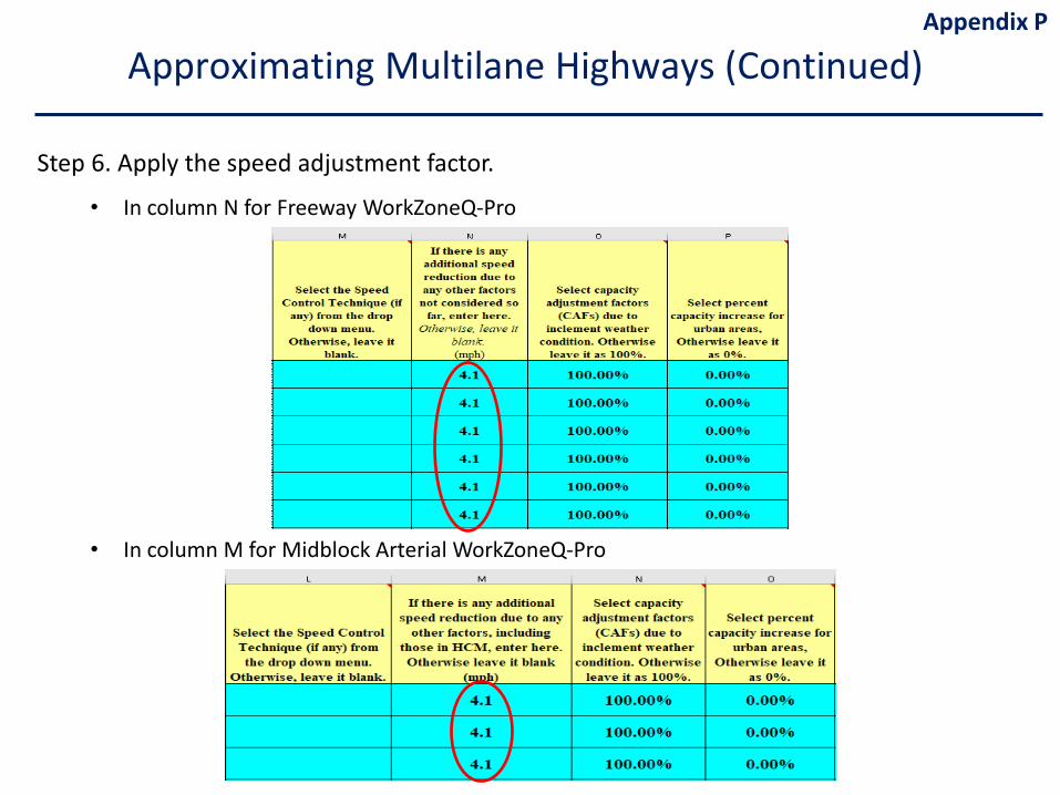
Step 6. Apply the speed adjustment factor.
• In column N for Freeway WorkZoneQ-Pro
• In column M for Midblock Arterial WorkZoneQ-Pro
Appendix P
Approximating Multilane Highways (Continued)
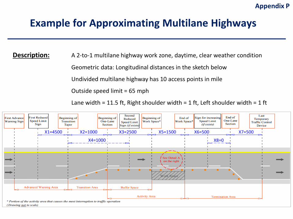
Example for Approximating Multilane Highways
Description: A 2-to-1 multilane highway work zone, daytime, clear weather condition
Geometric data: Longitudinal distances in the sketch below
Undivided multilane highway has 10 access points in mile
Outside speed limit = 65 mph
Lane width = 11.5 ft, Right shoulder width = 1 ft, Left shoulder width = 1 ft
Appendix P
X1=4500 X2=1000
X4=1000 X8=0
X7=500X6=500X5=1500X3=2500
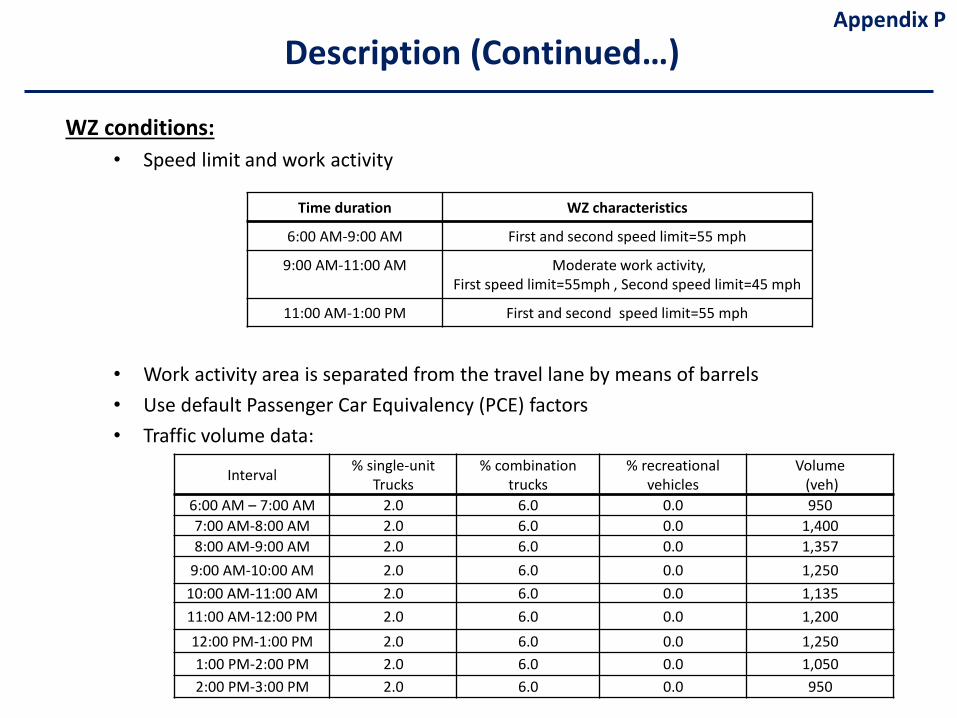
WZ conditions:• Speed limit and work activity
• Work activity area is separated from the travel lane by means of barrels • Use default Passenger Car Equivalency (PCE) factors• Traffic volume data:
Interval % single-unitTrucks
% combination trucks
% recreational vehicles
Volume(veh)
6:00 AM – 7:00 AM 2.0 6.0 0.0 9507:00 AM-8:00 AM 2.0 6.0 0.0 1,4008:00 AM-9:00 AM 2.0 6.0 0.0 1,357
9:00 AM-10:00 AM 2.0 6.0 0.0 1,25010:00 AM-11:00 AM 2.0 6.0 0.0 1,13511:00 AM-12:00 PM 2.0 6.0 0.0 1,20012:00 PM-1:00 PM 2.0 6.0 0.0 1,2501:00 PM-2:00 PM 2.0 6.0 0.0 1,0502:00 PM-3:00 PM 2.0 6.0 0.0 950
Description (Continued…)
Time duration WZ characteristics
6:00 AM-9:00 AM First and second speed limit=55 mph
9:00 AM-11:00 AM Moderate work activity, First speed limit=55mph , Second speed limit=45 mph
11:00 AM-1:00 PM First and second speed limit=55 mph
Appendix P
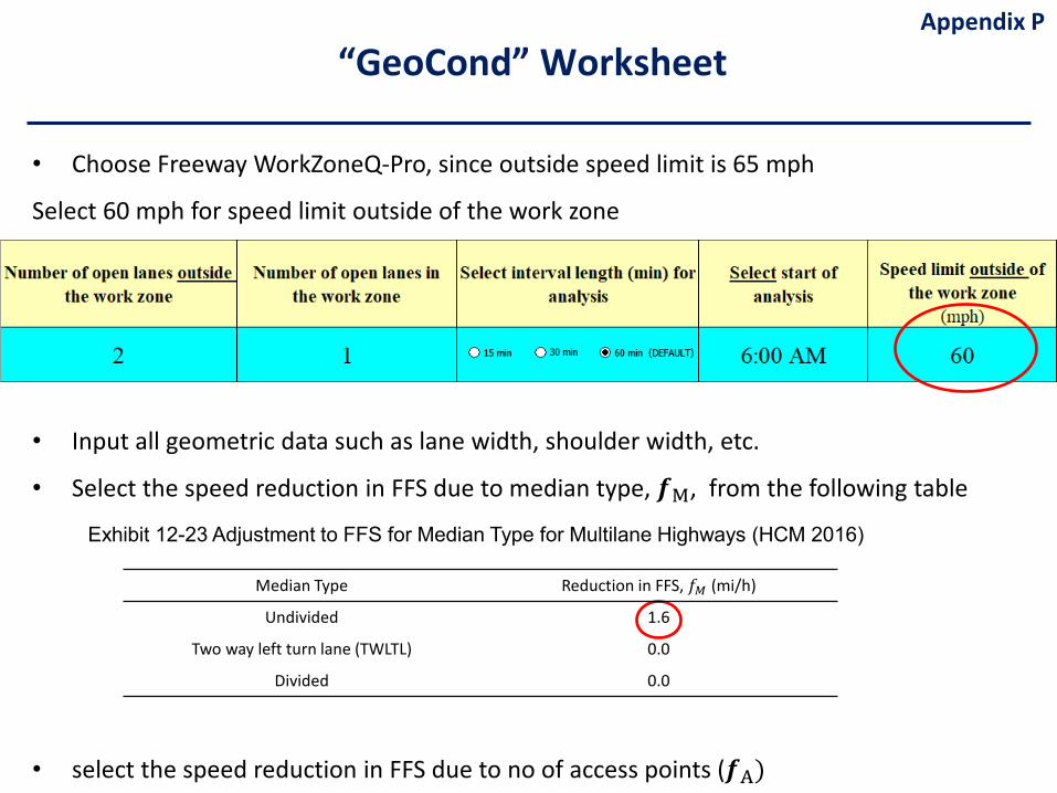
• Choose Freeway WorkZoneQ-Pro, since outside speed limit is 65 mph
Select 60 mph for speed limit outside of the work zone
• Input all geometric data such as lane width, shoulder width, etc.
• Select the speed reduction in FFS due to median type, 𝒇𝒇M, from the following table
• select the speed reduction in FFS due to no of access points (𝒇𝒇A)
“GeoCond” WorksheetAppendix P
Exhibit 12-23 Adjustment to FFS for Median Type for Multilane Highways (HCM 2016)
Median Type Reduction in FFS, 𝑓𝑓𝑀𝑀 (mi/h)
Undivided 1.6
Two way left turn lane (TWLTL) 0.0
Divided 0.0
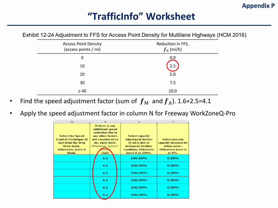
• Find the speed adjustment factor (sum of 𝒇𝒇M and 𝒇𝒇A). 1.6+2.5=4.1
• Apply the speed adjustment factor in column N for Freeway WorkZoneQ-Pro
Appendix P
Access Point Density(access points / mi)
Reduction in FFS, 𝒇𝒇A (mi/h)
0 0.0
10 2.5
20 5.0
30 7.5
≥ 40 10.0
Exhibit 12-24 Adjustment to FFS for Access Point Density for Multilane Highways (HCM 2016)
“TrafficInfo” Worksheet
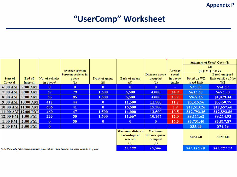
“UserComp” Worksheet
Appendix P
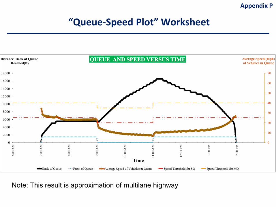
“Queue-Speed Plot” Worksheet
Note: This result is approximation of multilane highway
Appendix P
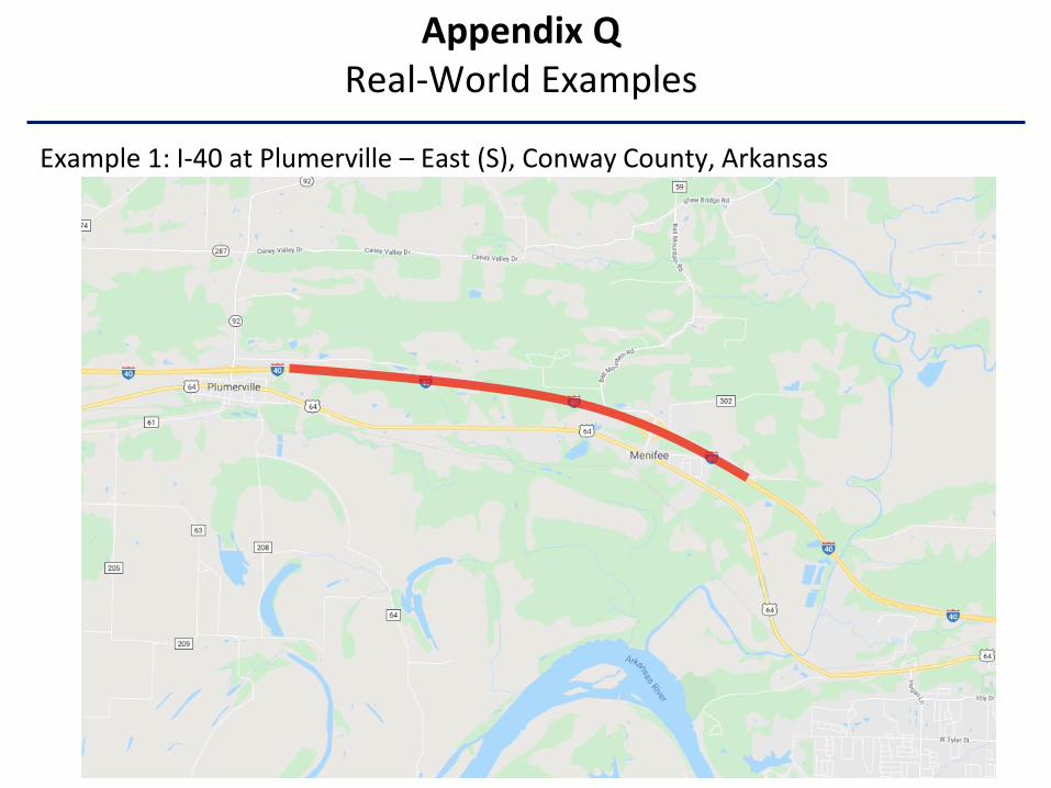
Example 1: I-40 at Plumerville – East (S), Conway County, Arkansas
Appendix QReal-World Examples
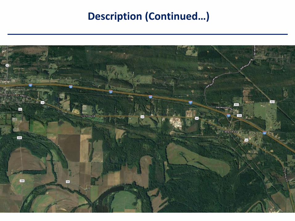
Description (Continued…)

This project is one lane closure on two lane freeway
Description:
Lane width = 12 ft, left shoulder right = 4 ft, and right shoulder width = 0 ft
Rural area and level terrain
Assumed night-time: 6 PM – 6 AM
WZ conditions:
Speed limit inside work zone is 60 mph and outside is 70 mph
Drum barrier, moderate work intensity (Assumed)
Appendix QDescription (Continued…)
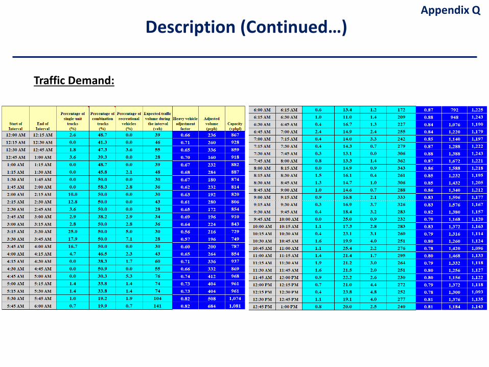
Traffic Demand:
Appendix QDescription (Continued…)
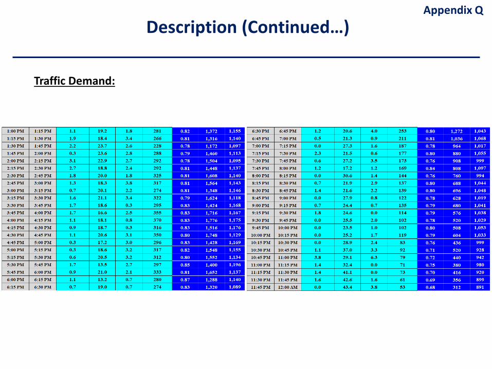
Traffic Demand:
Appendix QDescription (Continued…)
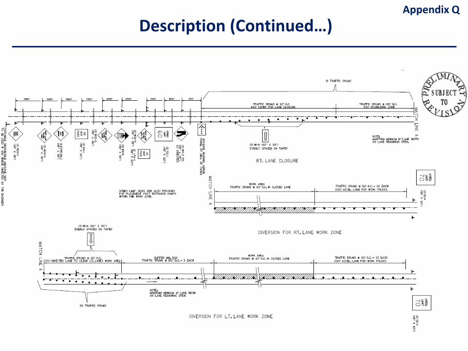
Appendix QDescription (Continued…)
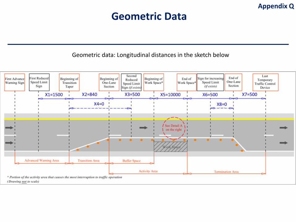
Geometric data: Longitudinal distances in the sketch below
Appendix QGeometric Data
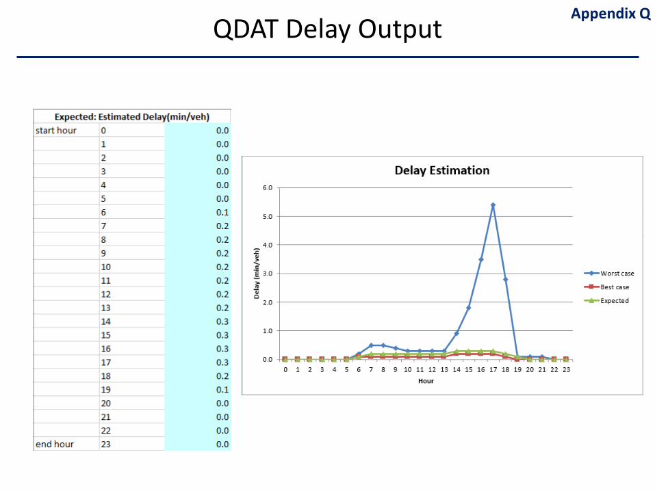
QDAT Delay OutputAppendix Q
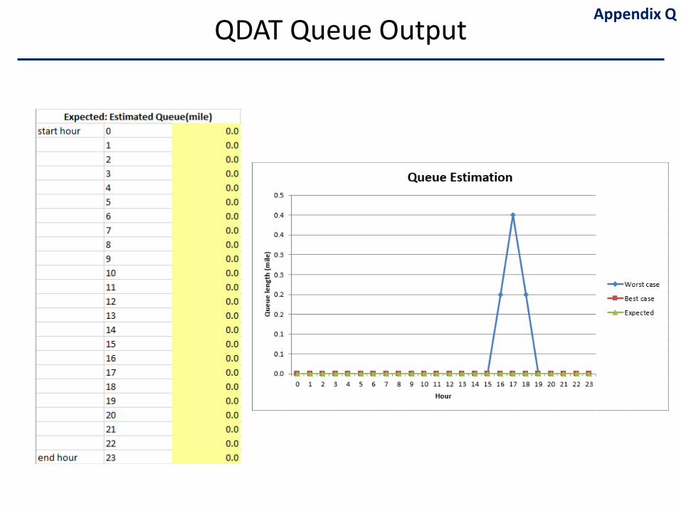
QDAT Queue OutputAppendix Q
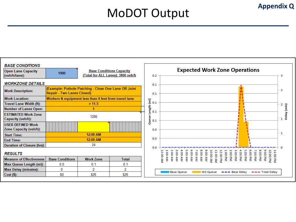
MoDOT OutputAppendix Q
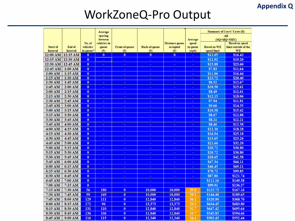
WorkZoneQ-Pro OutputAppendix Q
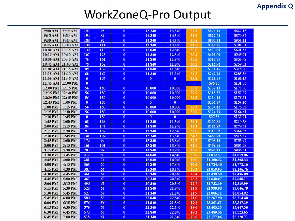
WorkZoneQ-Pro OutputAppendix Q
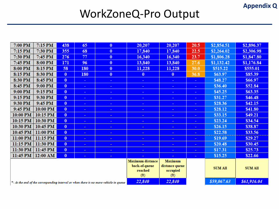
WorkZoneQ-Pro OutputAppendix Q
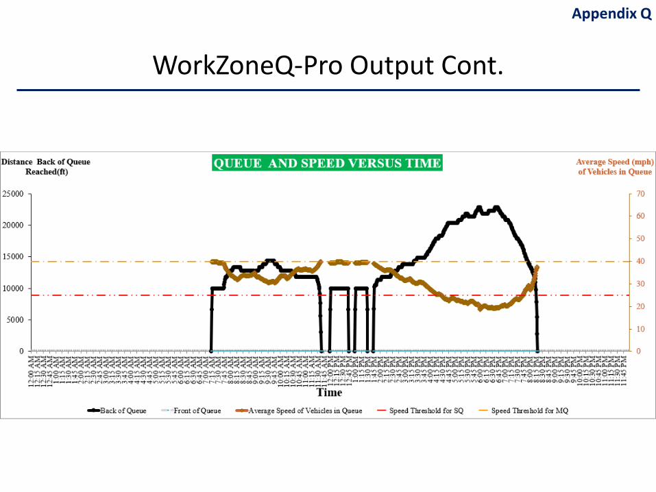
WorkZoneQ-Pro Output Cont.
Appendix Q
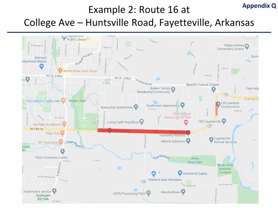
Example 2: Route 16 at College Ave – Huntsville Road, Fayetteville, Arkansas
Appendix Q
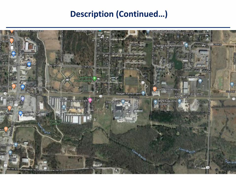
Description (Continued…)
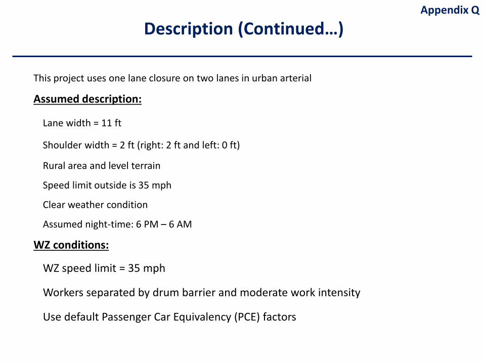
This project uses one lane closure on two lanes in urban arterial
Assumed description:
Lane width = 11 ft
Shoulder width = 2 ft (right: 2 ft and left: 0 ft)
Rural area and level terrain
Speed limit outside is 35 mph
Clear weather condition
Assumed night-time: 6 PM – 6 AM
WZ conditions:
WZ speed limit = 35 mph
Workers separated by drum barrier and moderate work intensity
Use default Passenger Car Equivalency (PCE) factors
Appendix Q
Description (Continued…)
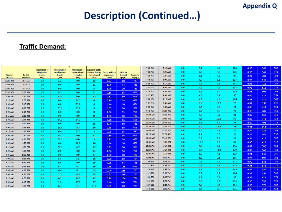
Traffic Demand:
Appendix QDescription (Continued…)
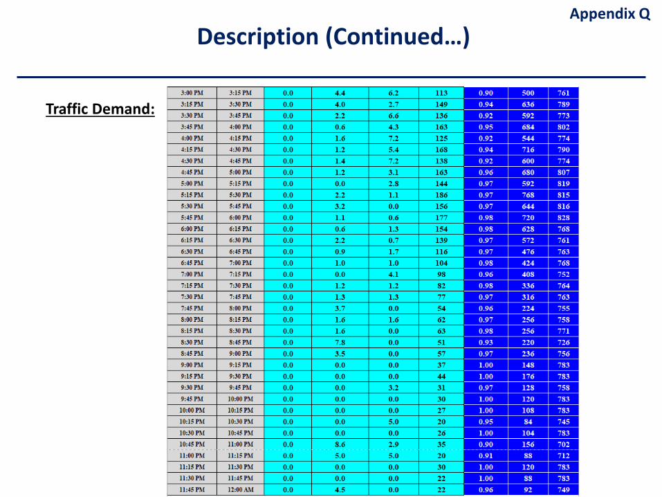
Traffic Demand:
Appendix QDescription (Continued…)
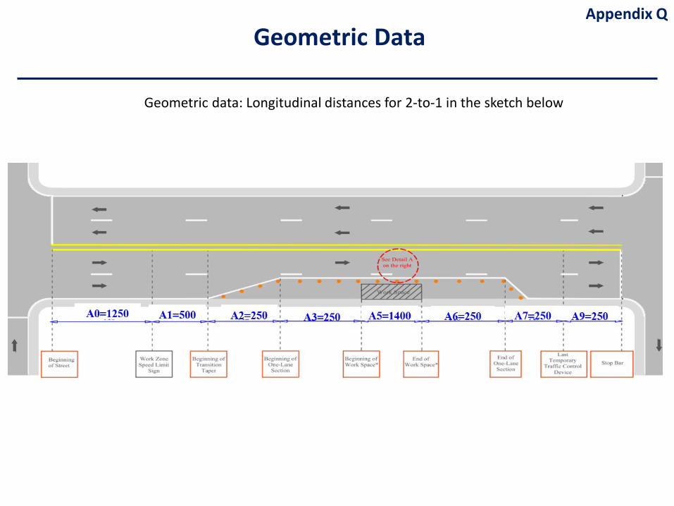
Geometric data: Longitudinal distances for 2-to-1 in the sketch below
Appendix QGeometric Data
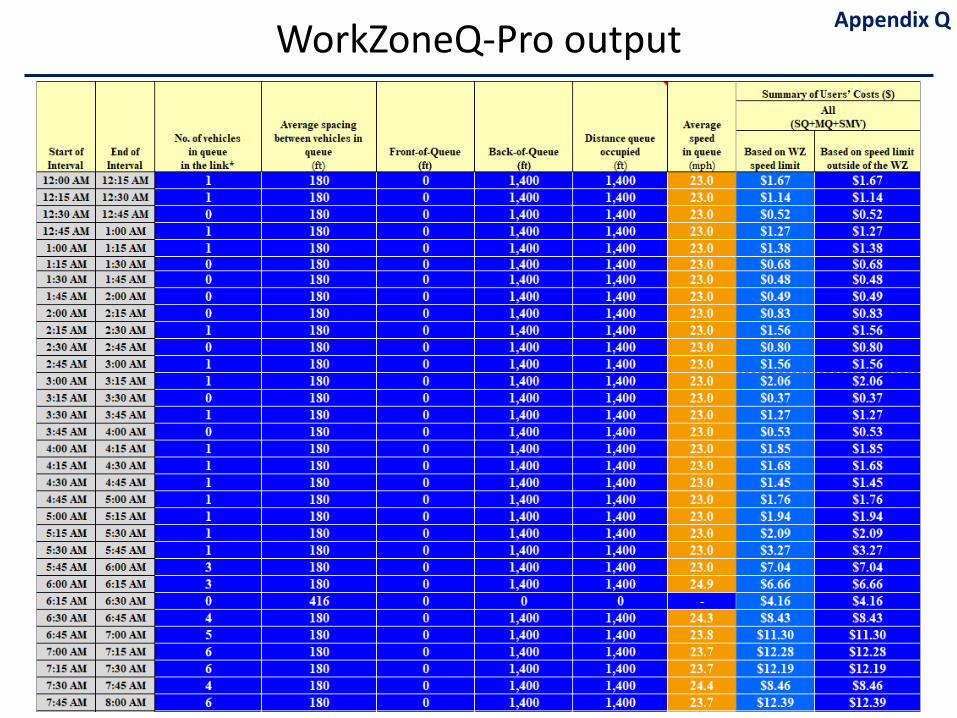
WorkZoneQ-Pro output Appendix Q
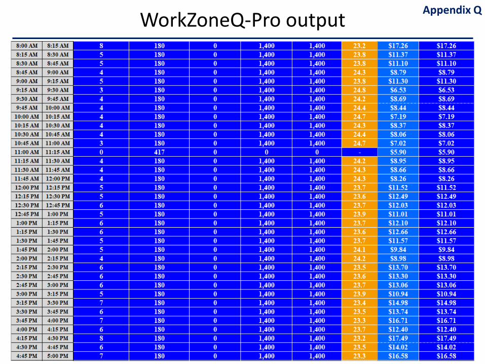
WorkZoneQ-Pro output Appendix Q
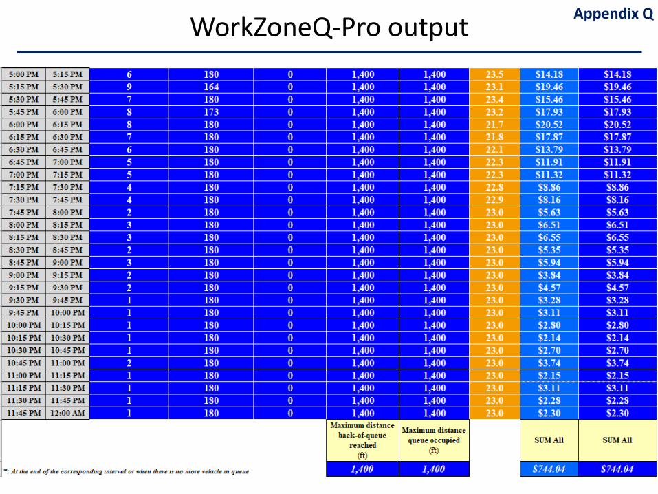
WorkZoneQ-Pro output Appendix Q
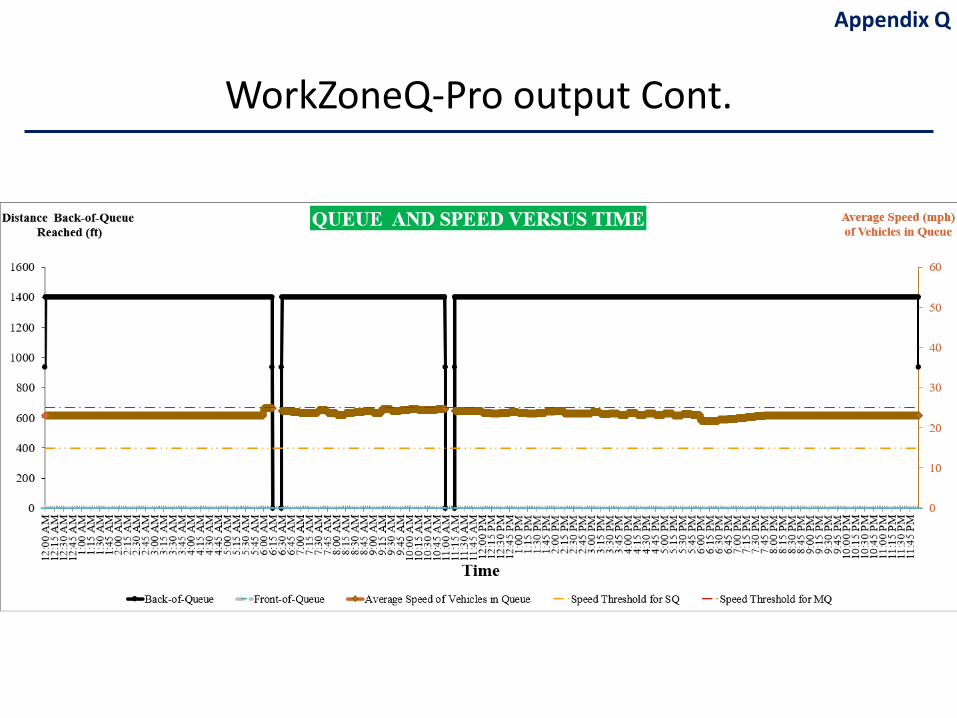
WorkZoneQ-Pro output Cont.
Appendix Q
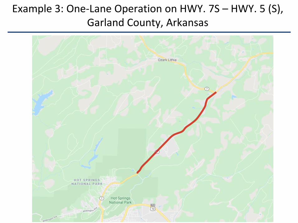
Example 3: One-Lane Operation on HWY. 7S – HWY. 5 (S), Garland County, Arkansas
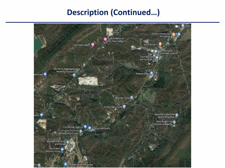
Description (Continued…)
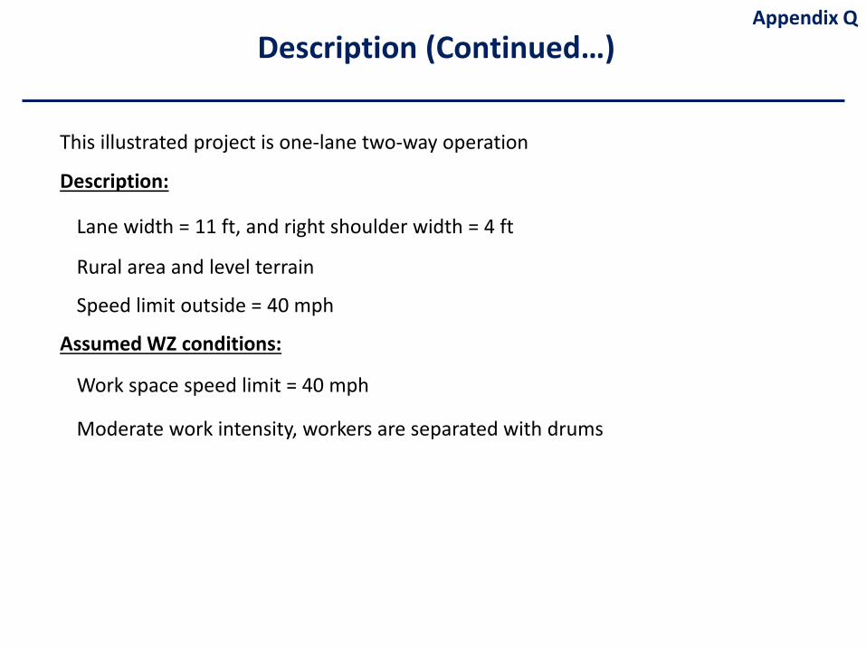
This illustrated project is one-lane two-way operation
Description:
Lane width = 11 ft, and right shoulder width = 4 ft
Rural area and level terrain
Speed limit outside = 40 mph
Assumed WZ conditions:
Work space speed limit = 40 mph
Moderate work intensity, workers are separated with drums
Appendix QDescription (Continued…)
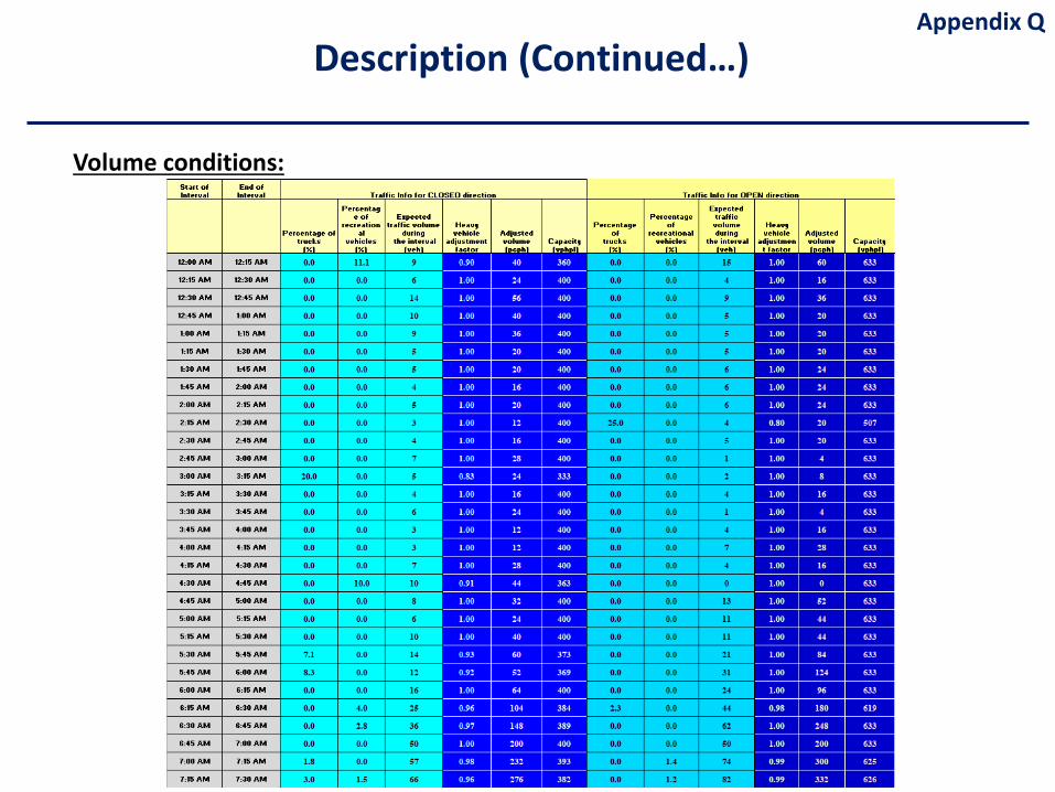
Volume conditions:
Appendix QDescription (Continued…)
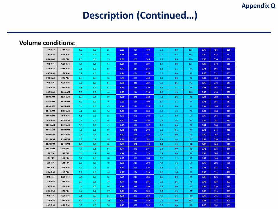
Volume conditions:
Appendix QDescription (Continued…)
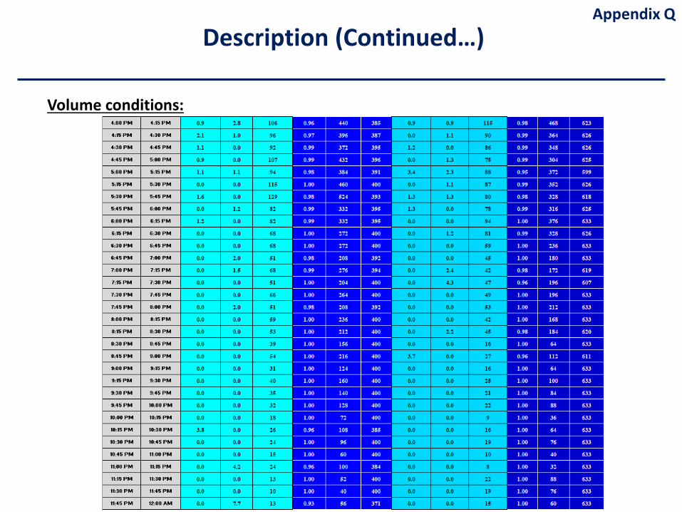
Volume conditions:
Appendix QDescription (Continued…)

Geometric data: Longitudinal distances in the sketch below
Geometric DataAppendix Q
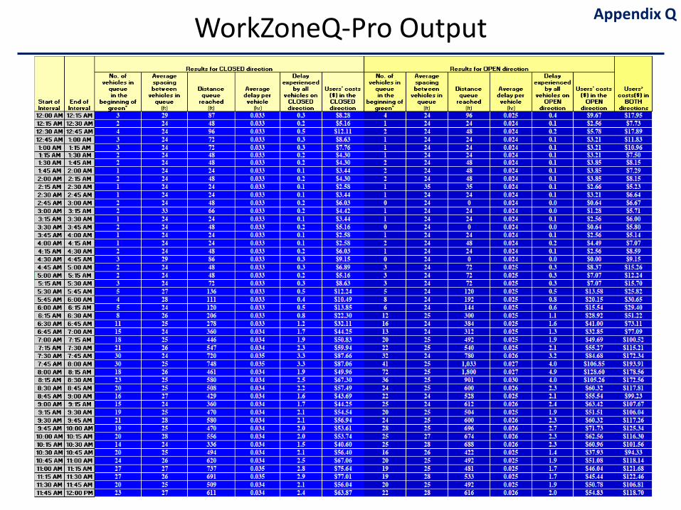
WorkZoneQ-Pro Output Appendix Q
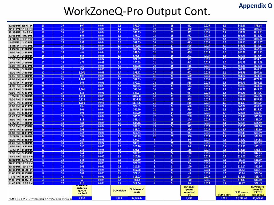
WorkZoneQ-Pro Output Cont. Appendix Q
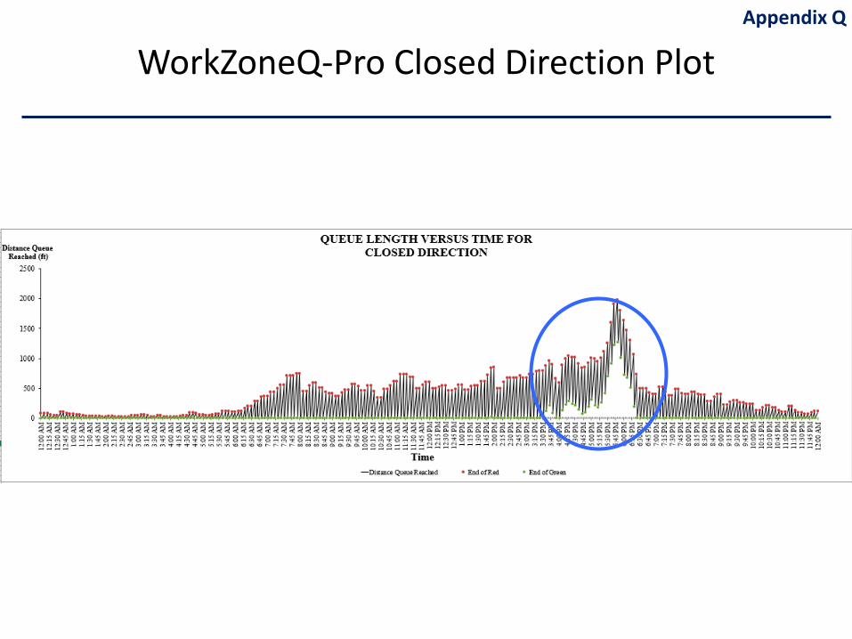
WorkZoneQ-Pro Closed Direction PlotAppendix Q
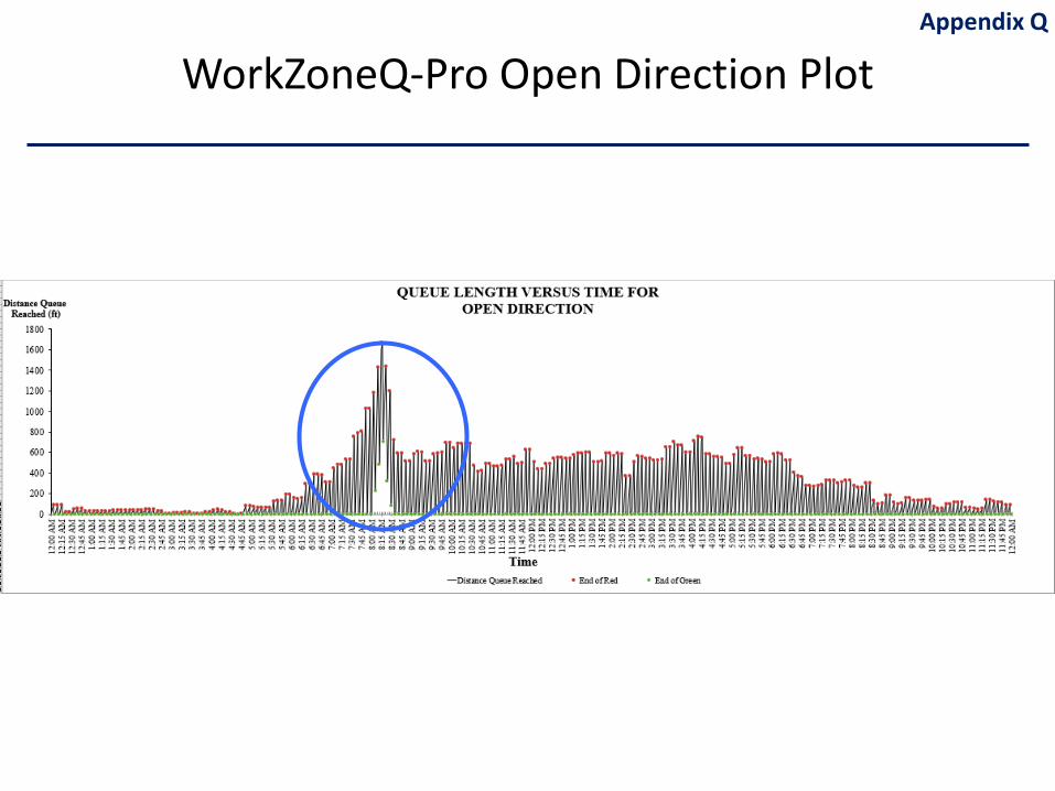
Appendix Q
WorkZoneQ-Pro Open Direction Plot
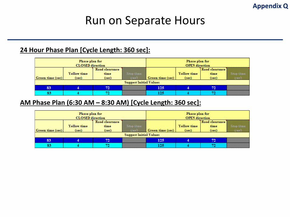
Appendix Q
Run on Separate Hours
24 Hour Phase Plan [Cycle Length: 360 sec]:
AM Phase Plan (6:30 AM – 8:30 AM) [Cycle Length: 360 sec]:
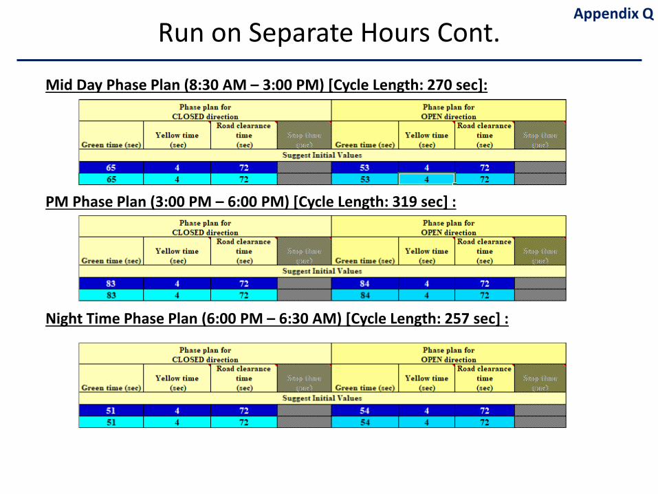
Appendix QRun on Separate Hours Cont.
Mid Day Phase Plan (8:30 AM – 3:00 PM) [Cycle Length: 270 sec]:
PM Phase Plan (3:00 PM – 6:00 PM) [Cycle Length: 319 sec] :
Night Time Phase Plan (6:00 PM – 6:30 AM) [Cycle Length: 257 sec] :
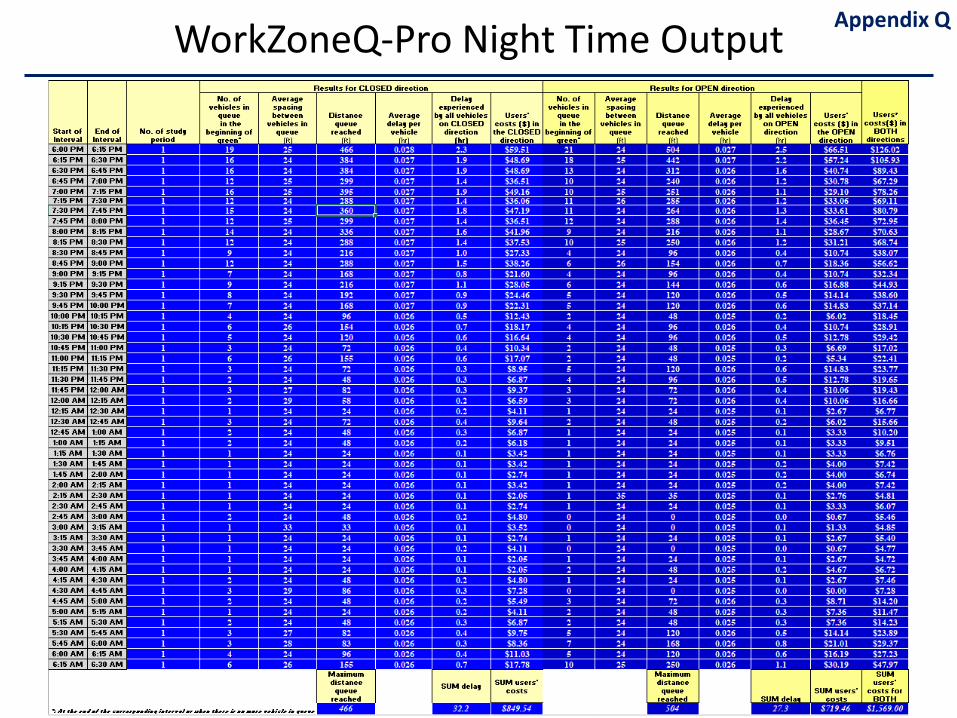
WorkZoneQ-Pro Night Time Output Appendix Q
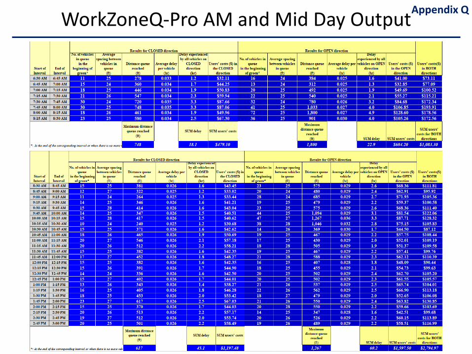
WorkZoneQ-Pro AM and Mid Day OutputAppendix Q
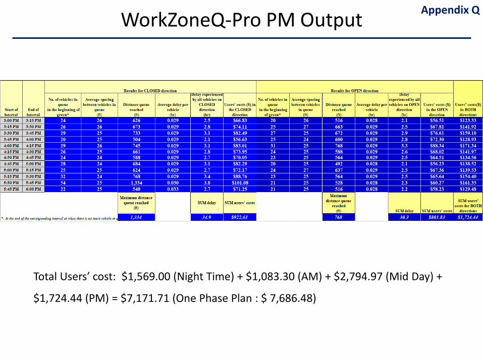
WorkZoneQ-Pro PM Output Appendix Q
Total Users’ cost: $1,569.00 (Night Time) + $1,083.30 (AM) + $2,794.97 (Mid Day) +
$1,724.44 (PM) = $7,171.71 (One Phase Plan : $ 7,686.48)
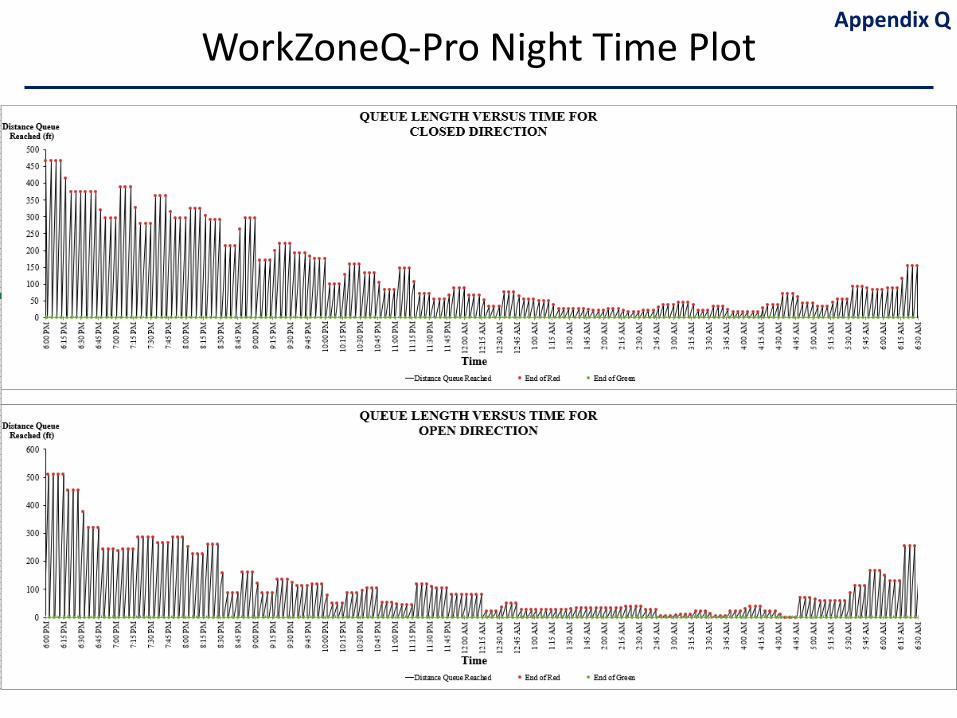
WorkZoneQ-Pro Night Time PlotAppendix Q
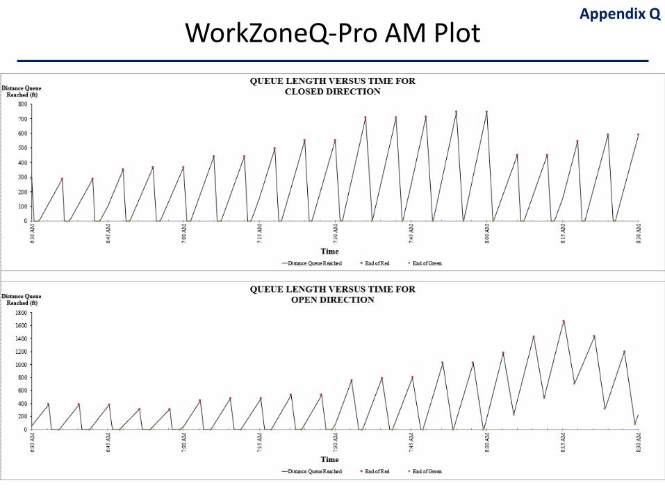
WorkZoneQ-Pro AM PlotAppendix Q
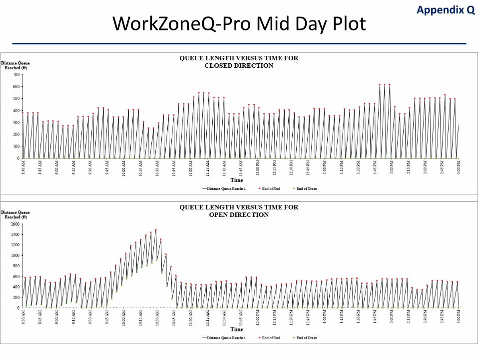
WorkZoneQ-Pro Mid Day PlotAppendix Q
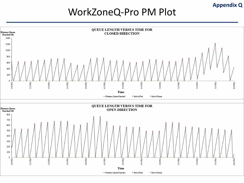
WorkZoneQ-Pro PM PlotAppendix Q
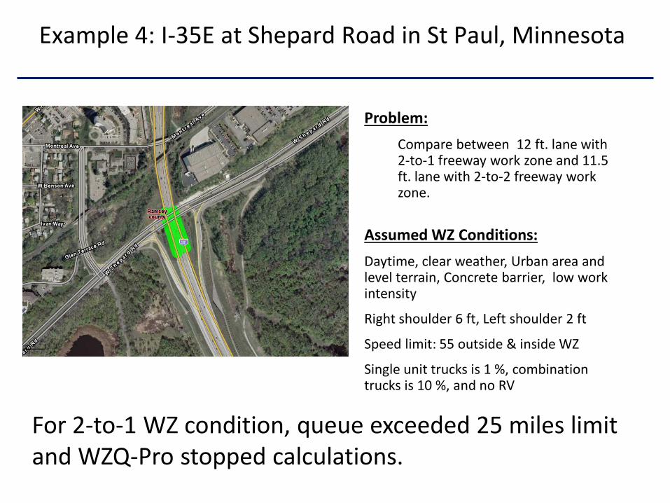
Problem:Compare between 12 ft. lane with 2-to-1 freeway work zone and 11.5 ft. lane with 2-to-2 freeway work zone.
Assumed WZ Conditions:Daytime, clear weather, Urban area and level terrain, Concrete barrier, low work intensity
Right shoulder 6 ft, Left shoulder 2 ft
Speed limit: 55 outside & inside WZ
Single unit trucks is 1 %, combination trucks is 10 %, and no RV
For 2-to-1 WZ condition, queue exceeded 25 miles limit and WZQ-Pro stopped calculations.
Example 4: I-35E at Shepard Road in St Paul, Minnesota
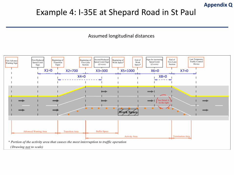
Assumed longitudinal distances
Example 4: I-35E at Shepard Road in St PaulAppendix Q
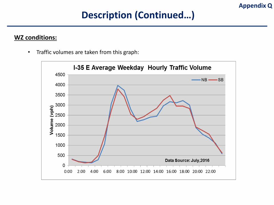
WZ conditions:
• Traffic volumes are taken from this graph:
Description (Continued…)Appendix Q
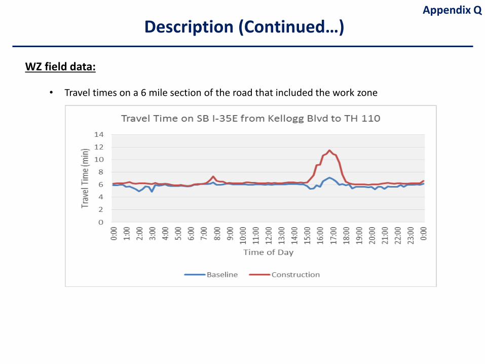
WZ field data:
• Travel times on a 6 mile section of the road that included the work zone
Description (Continued…)Appendix Q
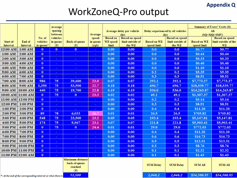
WorkZoneQ-Pro outputAppendix Q
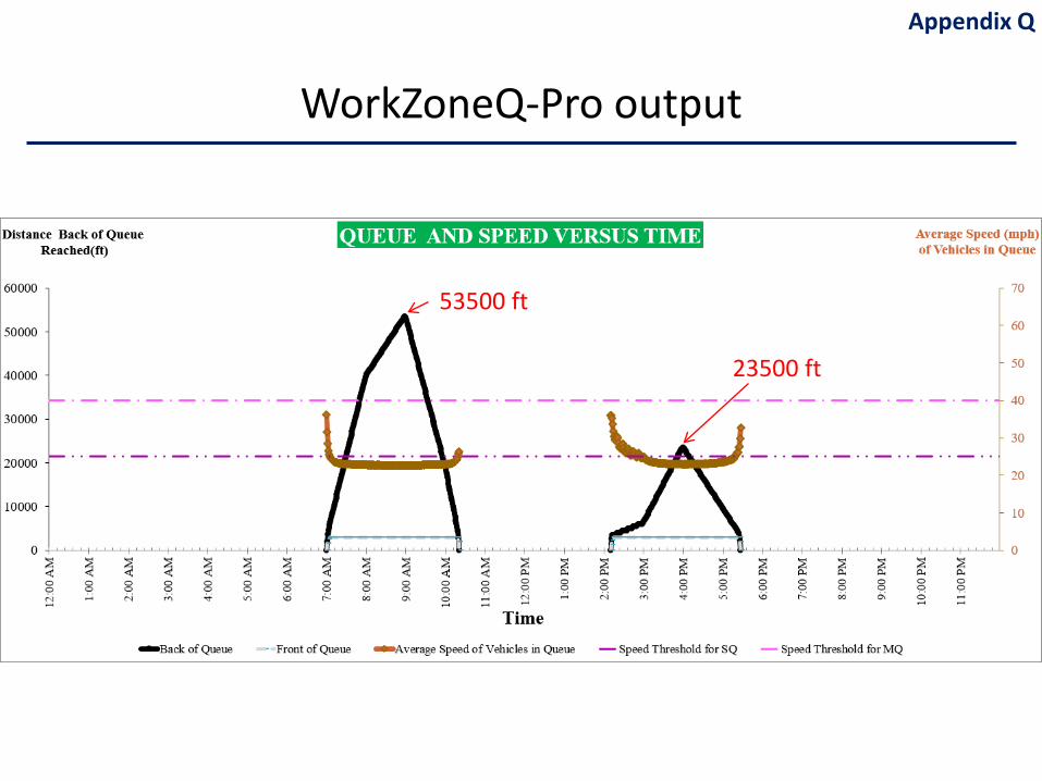
WorkZoneQ-Pro output
53500 ft
23500 ft
Appendix Q
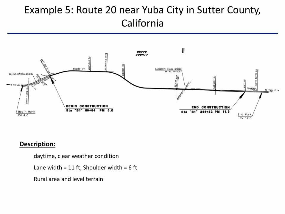
Description:
daytime, clear weather condition
Lane width = 11 ft, Shoulder width = 6 ft
Rural area and level terrain
Example 5: Route 20 near Yuba City in Sutter County, California
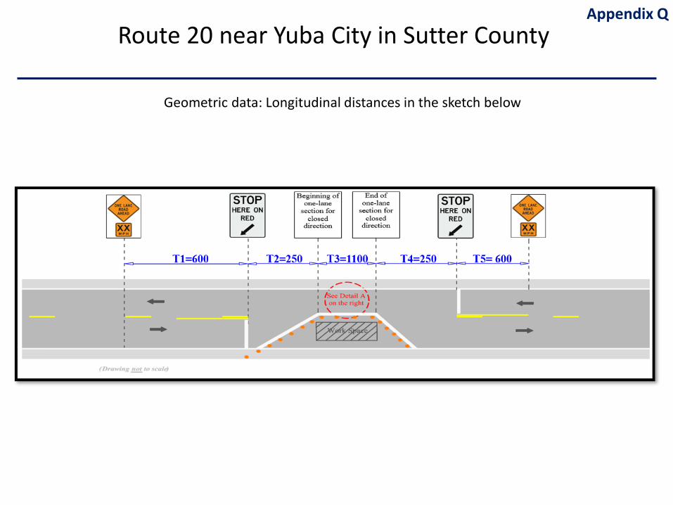
Geometric data: Longitudinal distances in the sketch below
Route 20 near Yuba City in Sutter CountyAppendix Q
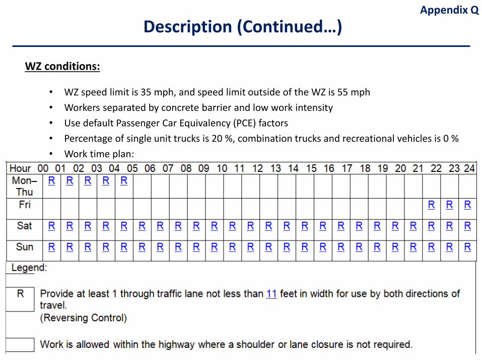
WZ conditions:
• WZ speed limit is 35 mph, and speed limit outside of the WZ is 55 mph• Workers separated by concrete barrier and low work intensity• Use default Passenger Car Equivalency (PCE) factors• Percentage of single unit trucks is 20 %, combination trucks and recreational vehicles is 0 %• Work time plan:
Description (Continued…)Appendix Q
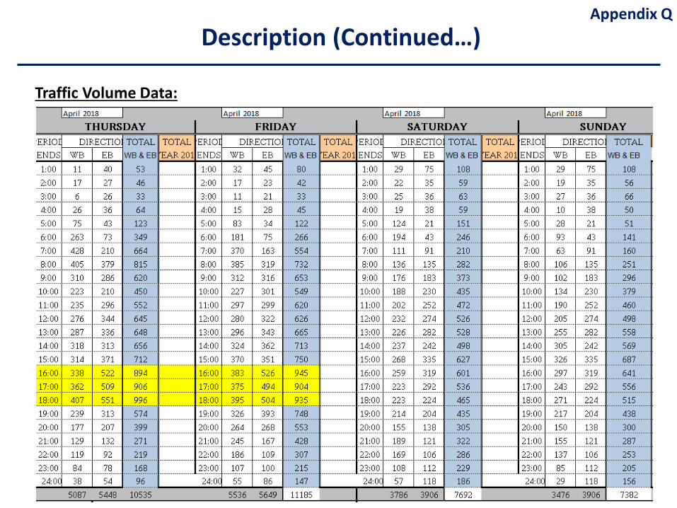
Traffic Volume Data:
Description (Continued…)Appendix Q
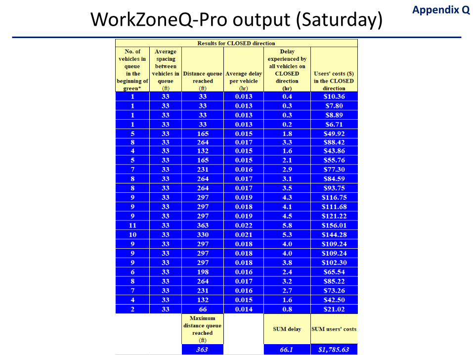
WorkZoneQ-Pro output (Saturday) Appendix Q
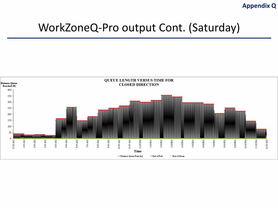
WorkZoneQ-Pro output Cont. (Saturday)
Appendix Q
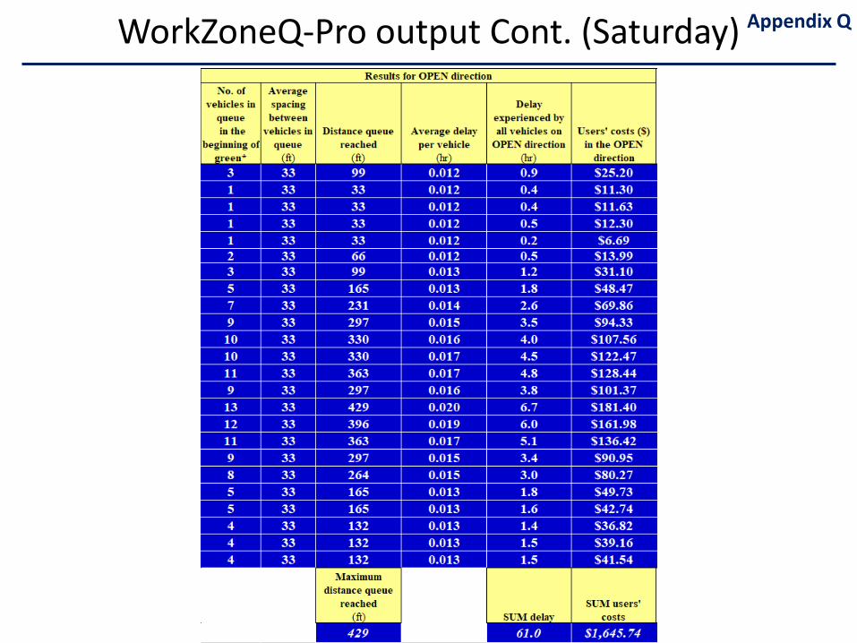
WorkZoneQ-Pro output Cont. (Saturday) Appendix Q
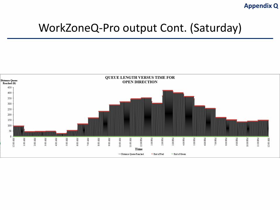
WorkZoneQ-Pro output Cont. (Saturday)
Appendix Q
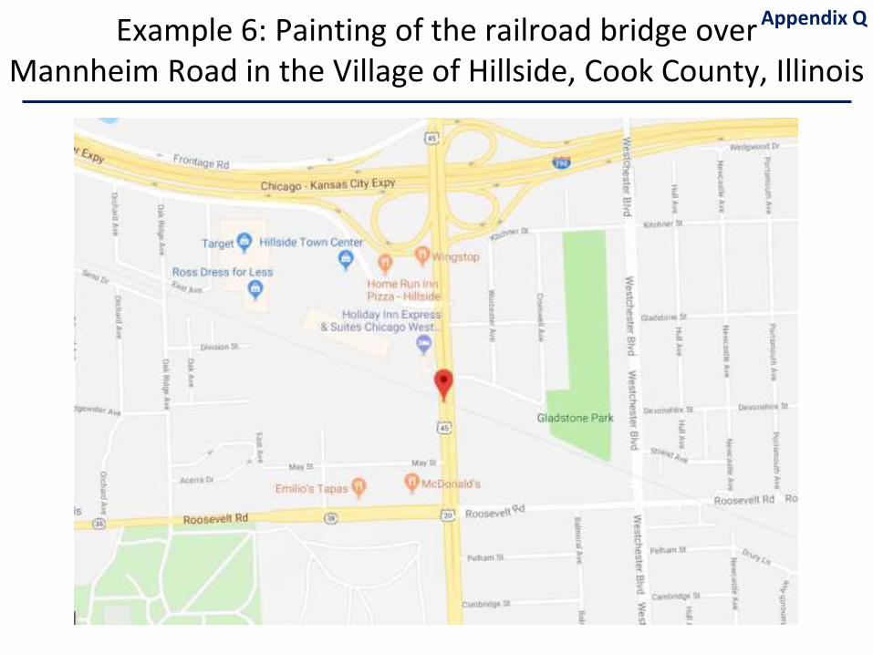
Example 6: Painting of the railroad bridge overMannheim Road in the Village of Hillside, Cook County, Illinois
Appendix Q
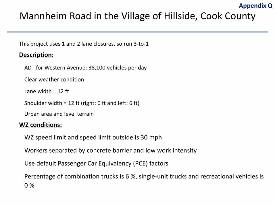
This project uses 1 and 2 lane closures, so run 3-to-1
Description:
ADT for Western Avenue: 38,100 vehicles per day
Clear weather condition
Lane width = 12 ft
Shoulder width = 12 ft (right: 6 ft and left: 6 ft)
Urban area and level terrain
WZ conditions:
WZ speed limit and speed limit outside is 30 mph
Workers separated by concrete barrier and low work intensity
Use default Passenger Car Equivalency (PCE) factors
Percentage of combination trucks is 6 %, single-unit trucks and recreational vehicles is 0 %
Mannheim Road in the Village of Hillside, Cook CountyAppendix Q
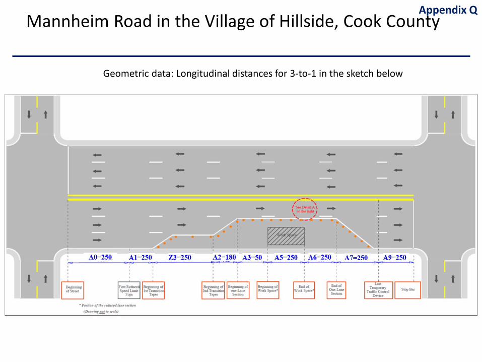
Geometric data: Longitudinal distances for 3-to-1 in the sketch below
Appendix QMannheim Road in the Village of Hillside, Cook County
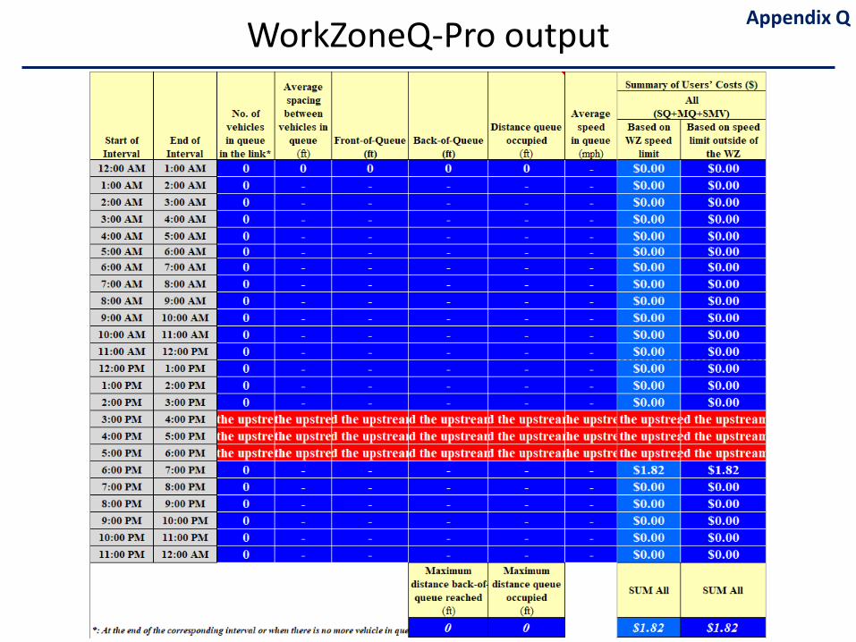
WorkZoneQ-Pro output Appendix Q
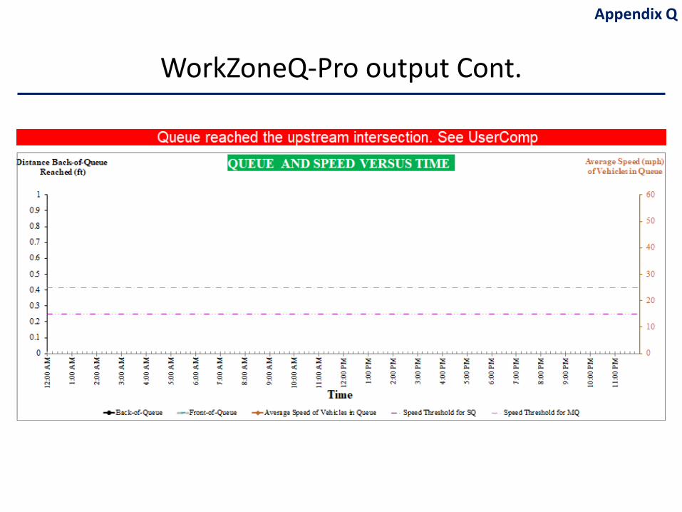
WorkZoneQ-Pro output Cont.
Appendix Q
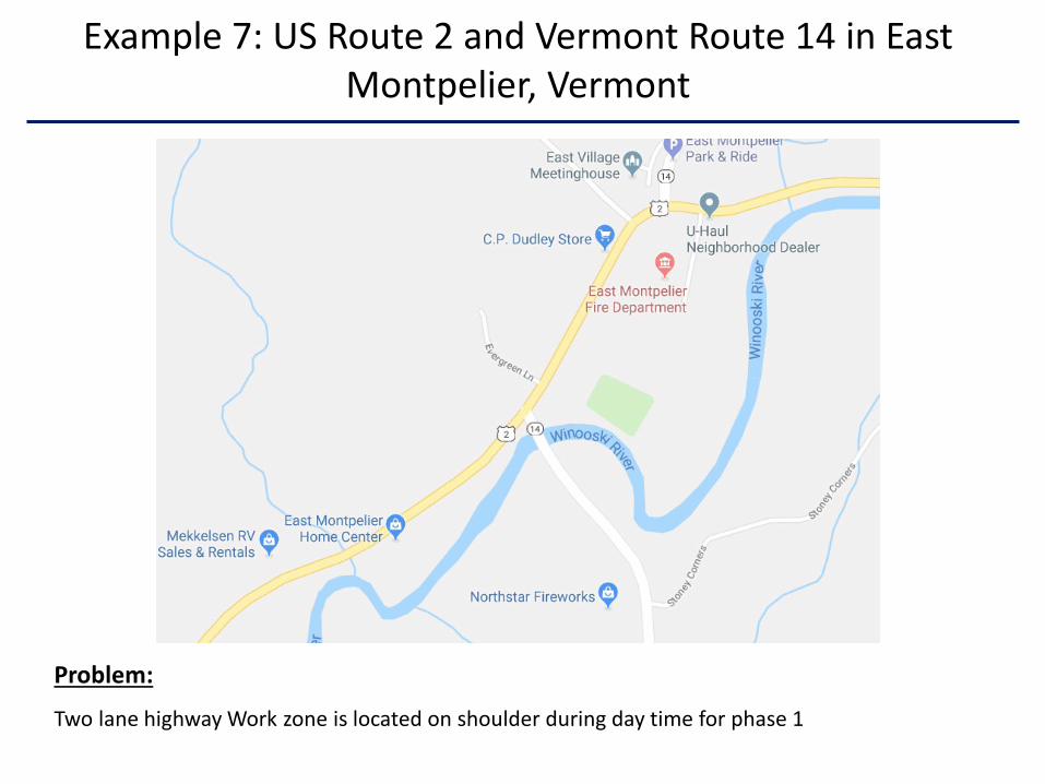
Problem:
Two lane highway Work zone is located on shoulder during day time for phase 1
Example 7: US Route 2 and Vermont Route 14 in East Montpelier, Vermont
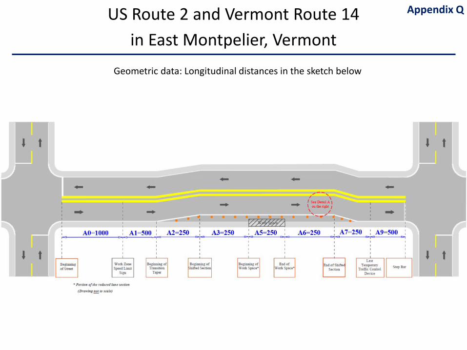
Geometric data: Longitudinal distances in the sketch below
US Route 2 and Vermont Route 14 in East Montpelier, Vermont
Appendix Q
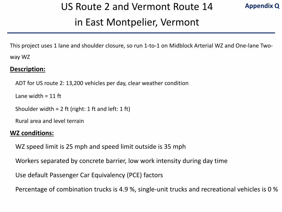
This project uses 1 lane and shoulder closure, so run 1-to-1 on Midblock Arterial WZ and One-lane Two-
way WZ
Description:
ADT for US route 2: 13,200 vehicles per day, clear weather condition
Lane width = 11 ft
Shoulder width = 2 ft (right: 1 ft and left: 1 ft)
Rural area and level terrain
WZ conditions:
WZ speed limit is 25 mph and speed limit outside is 35 mph
Workers separated by concrete barrier, low work intensity during day time
Use default Passenger Car Equivalency (PCE) factors
Percentage of combination trucks is 4.9 %, single-unit trucks and recreational vehicles is 0 %
Appendix QUS Route 2 and Vermont Route 14 in East Montpelier, Vermont
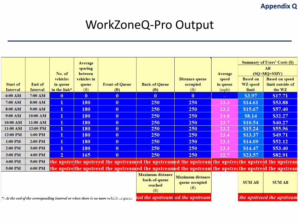
WorkZoneQ-Pro OutputAppendix Q
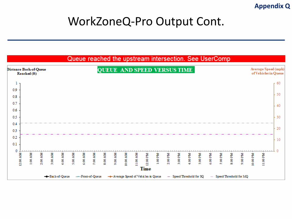
WorkZoneQ-Pro Output Cont. Appendix Q
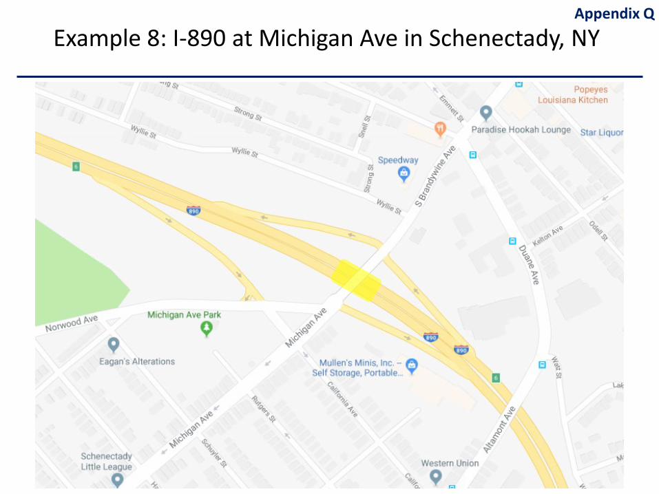
Example 8: I-890 at Michigan Ave in Schenectady, NYAppendix Q
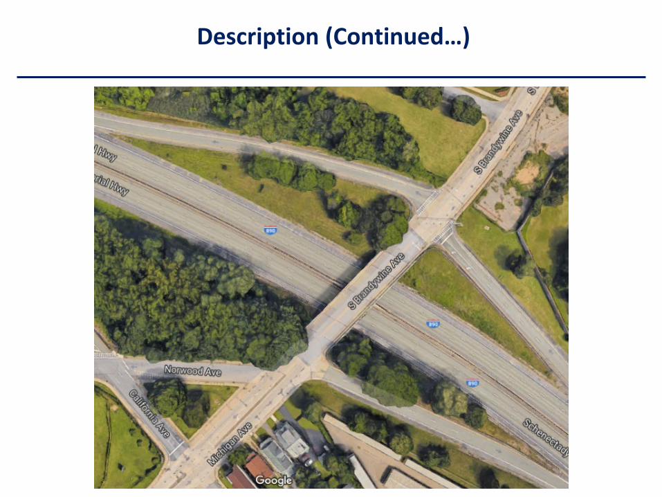
Description (Continued…)
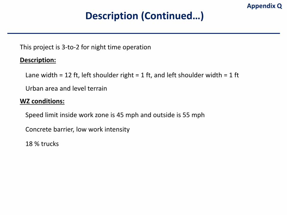
This project is 3-to-2 for night time operation
Description:
Lane width = 12 ft, left shoulder right = 1 ft, and left shoulder width = 1 ft
Urban area and level terrain
WZ conditions:
Speed limit inside work zone is 45 mph and outside is 55 mph
Concrete barrier, low work intensity
18 % trucks
Appendix QDescription (Continued…)
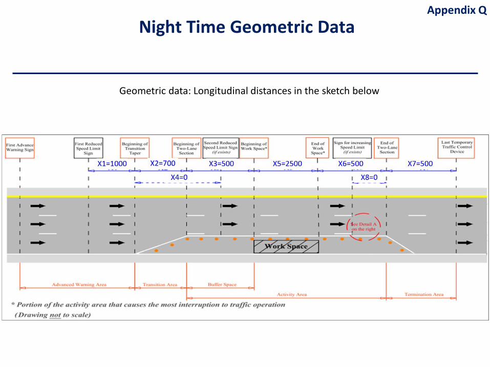
Geometric data: Longitudinal distances in the sketch below
Appendix QNight Time Geometric Data
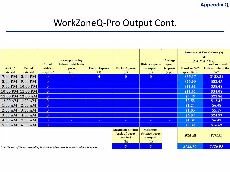
WorkZoneQ-Pro Output Cont.
Appendix Q
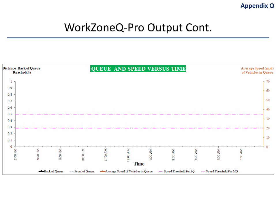
WorkZoneQ-Pro Output Cont.
Appendix Q
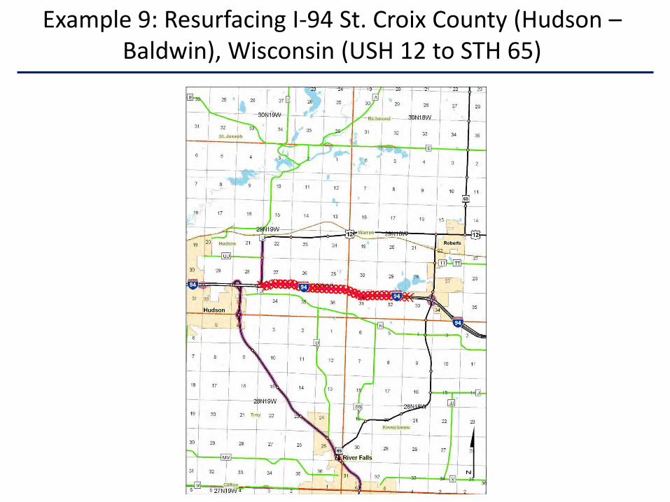
Example 9: Resurfacing I-94 St. Croix County (Hudson –Baldwin), Wisconsin (USH 12 to STH 65)
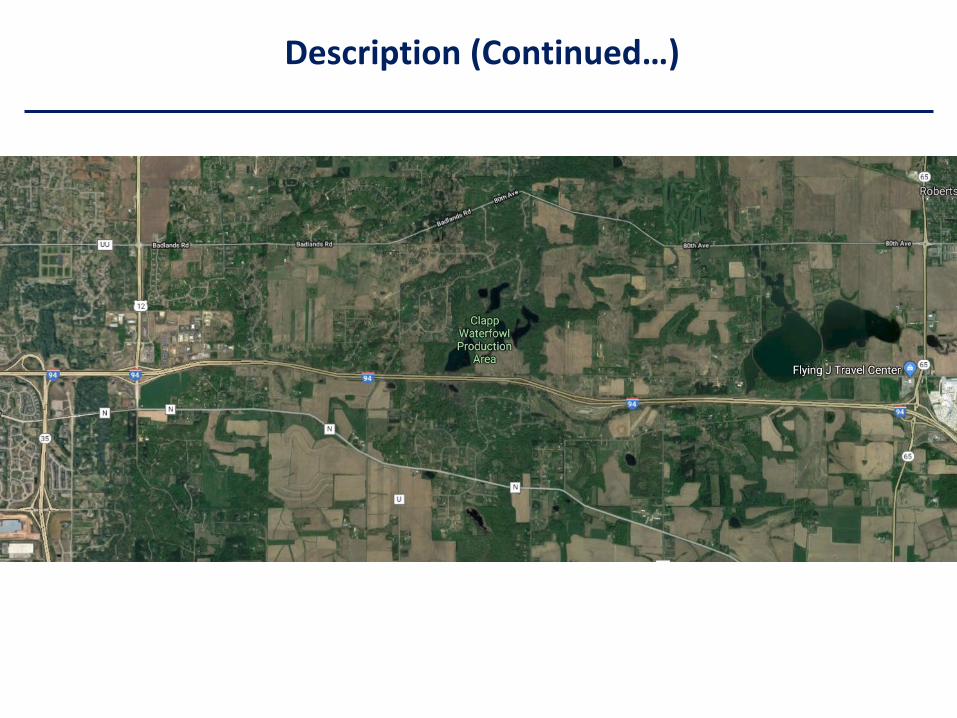
Description (Continued…)
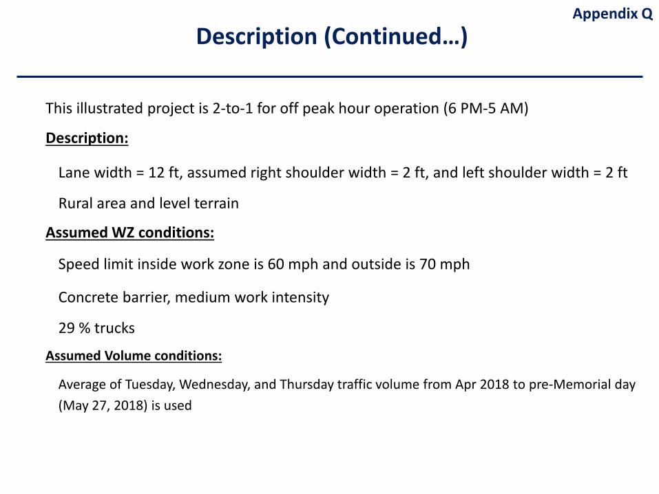
This illustrated project is 2-to-1 for off peak hour operation (6 PM-5 AM)
Description:
Lane width = 12 ft, assumed right shoulder width = 2 ft, and left shoulder width = 2 ft
Rural area and level terrain
Assumed WZ conditions:
Speed limit inside work zone is 60 mph and outside is 70 mph
Concrete barrier, medium work intensity
29 % trucks
Assumed Volume conditions:
Average of Tuesday, Wednesday, and Thursday traffic volume from Apr 2018 to pre-Memorial day (May 27, 2018) is used
Appendix QDescription (Continued…)
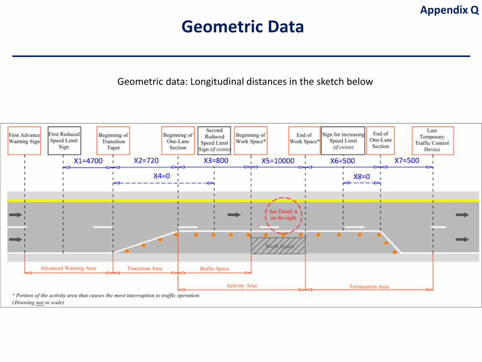
Geometric data: Longitudinal distances in the sketch below
Appendix QGeometric Data
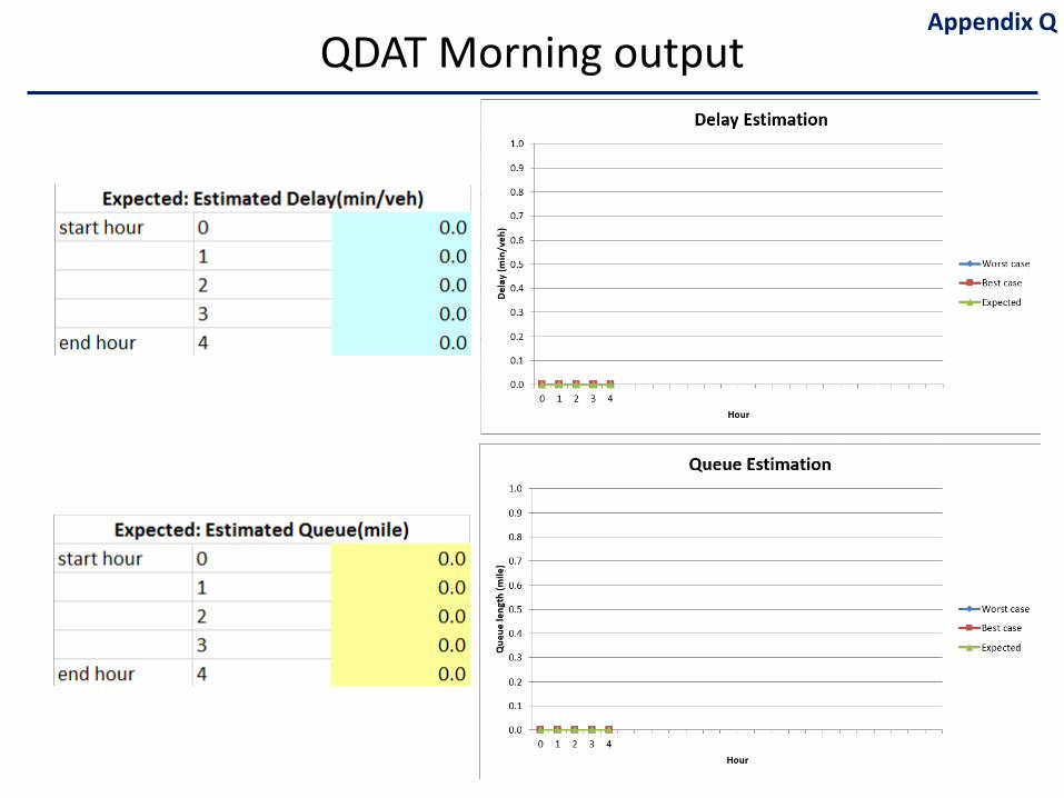
QDAT Morning outputAppendix Q
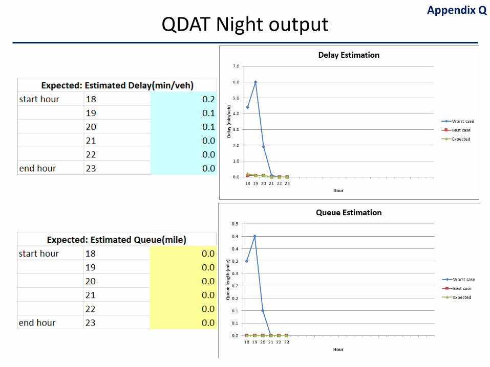
QDAT Night outputAppendix Q
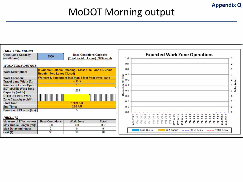
MoDOT Morning outputAppendix Q
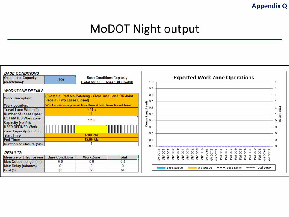
MoDOT Night output
Appendix Q
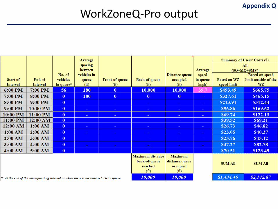
WorkZoneQ-Pro outputAppendix Q
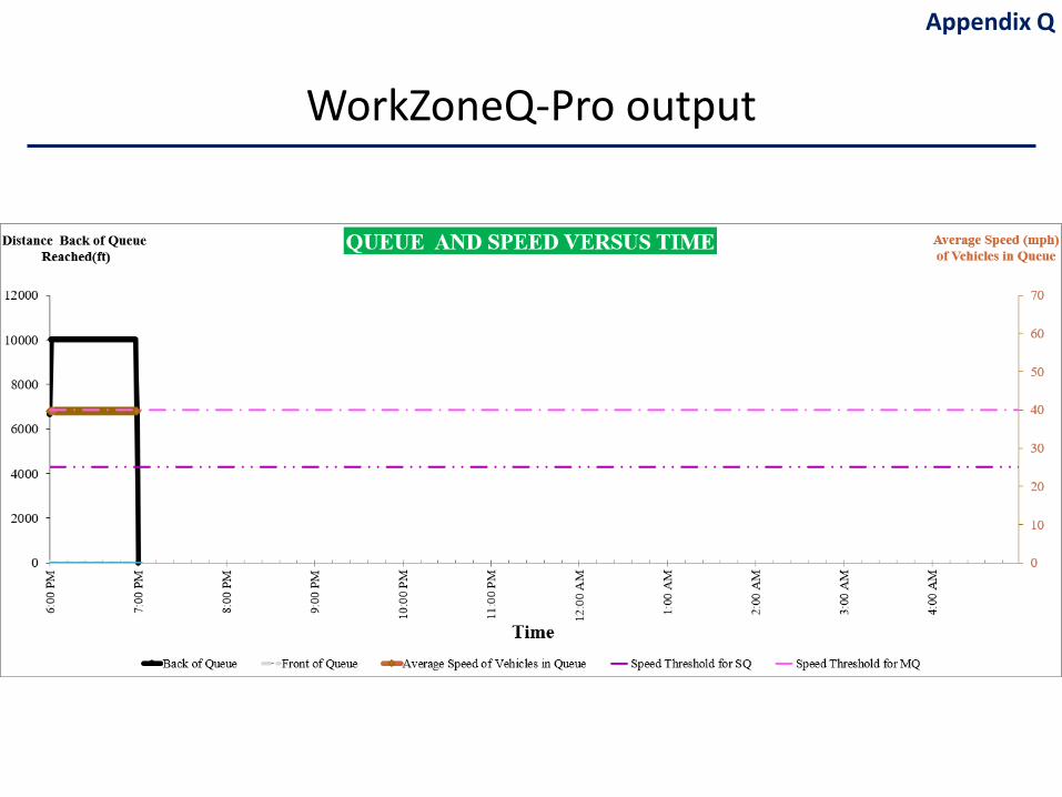
WorkZoneQ-Pro output
Appendix Q
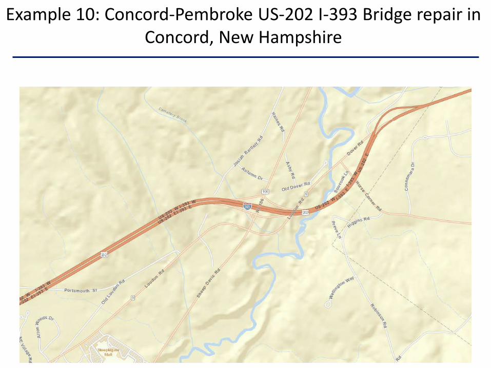
Example 10: Concord-Pembroke US-202 I-393 Bridge repair in Concord, New Hampshire
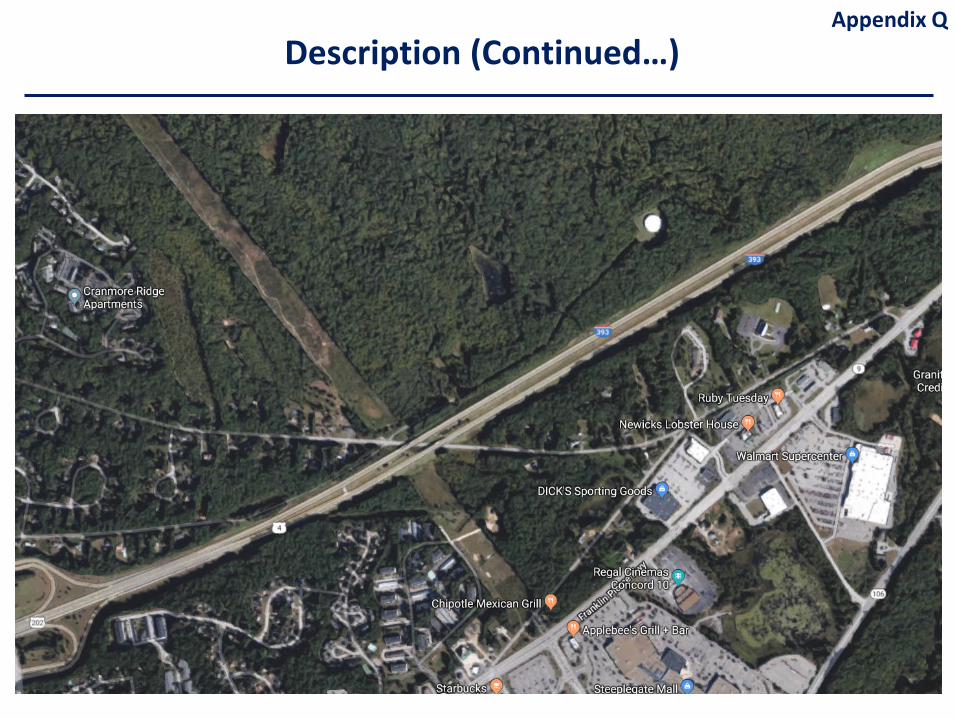
Description (Continued…)Appendix Q
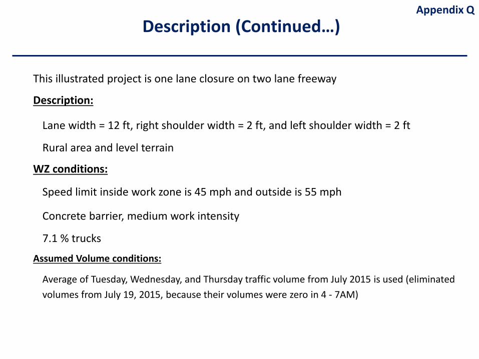
This illustrated project is one lane closure on two lane freeway
Description:
Lane width = 12 ft, right shoulder width = 2 ft, and left shoulder width = 2 ft
Rural area and level terrain
WZ conditions:
Speed limit inside work zone is 45 mph and outside is 55 mph
Concrete barrier, medium work intensity
7.1 % trucks
Assumed Volume conditions:
Average of Tuesday, Wednesday, and Thursday traffic volume from July 2015 is used (eliminated volumes from July 19, 2015, because their volumes were zero in 4 - 7AM)
Appendix QDescription (Continued…)
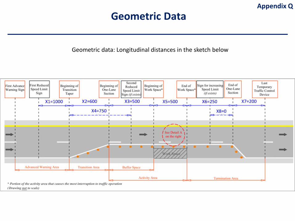
Geometric data: Longitudinal distances in the sketch below
Appendix QGeometric Data
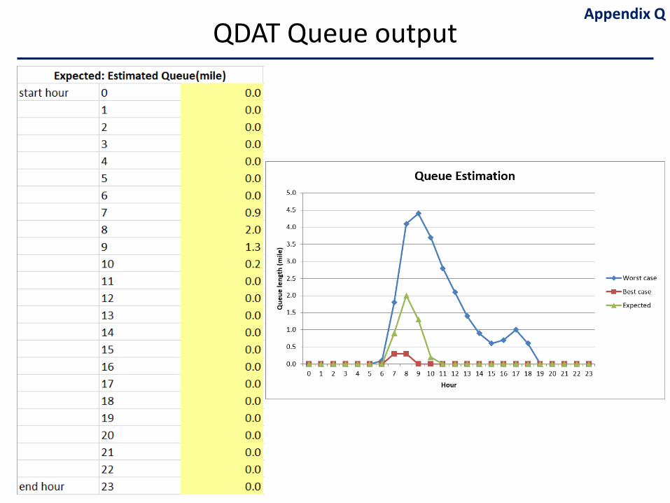
QDAT Queue outputAppendix Q
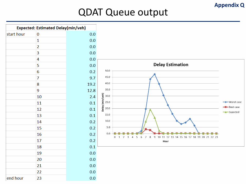
QDAT Queue outputAppendix Q
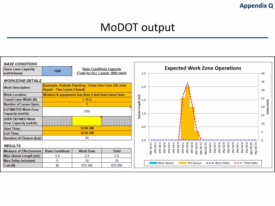
MoDOT output
Appendix Q
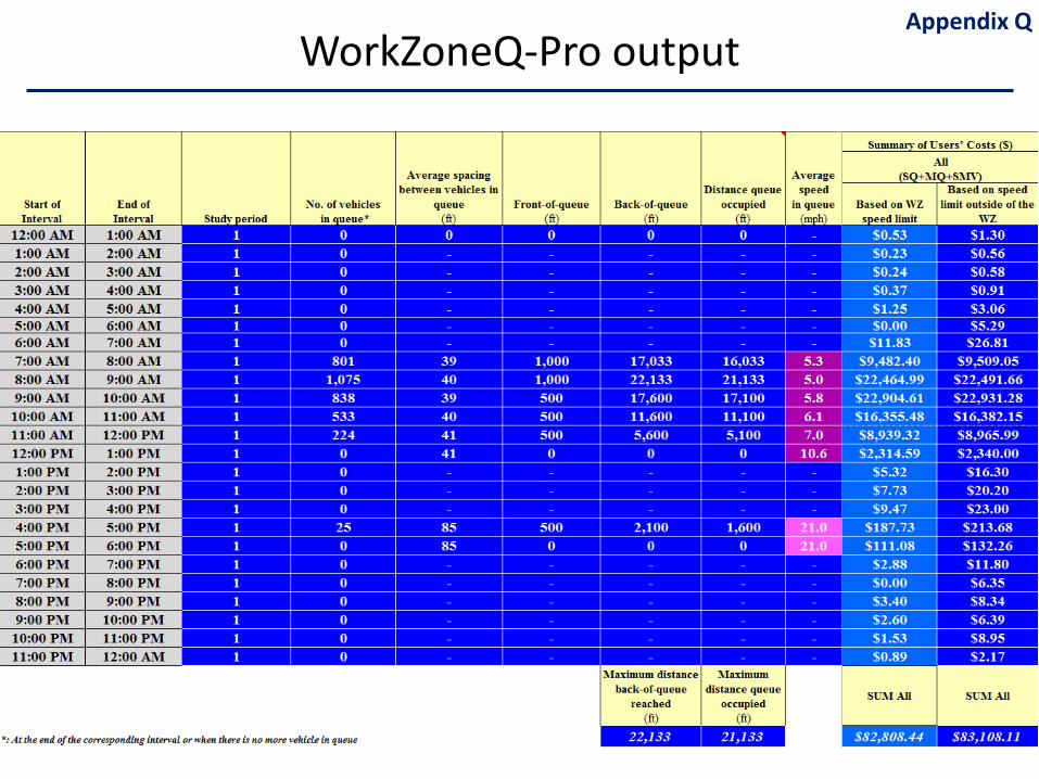
WorkZoneQ-Pro outputAppendix Q
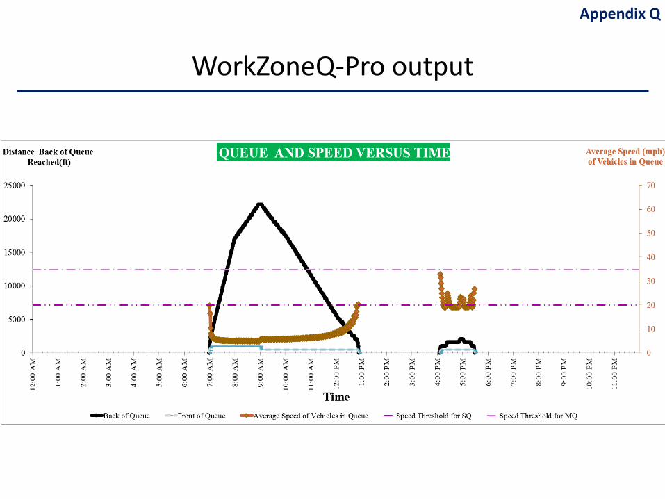
WorkZoneQ-Pro output
Appendix Q
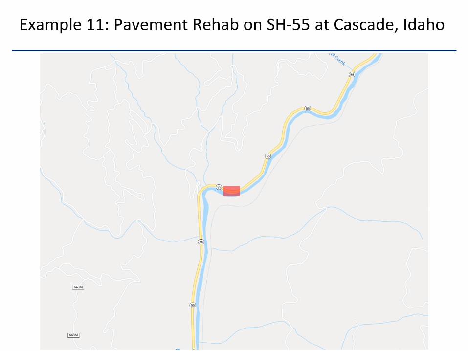
Example 11: Pavement Rehab on SH-55 at Cascade, Idaho
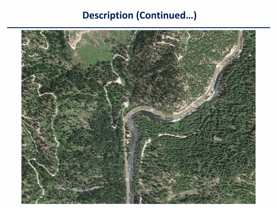
Description (Continued…)
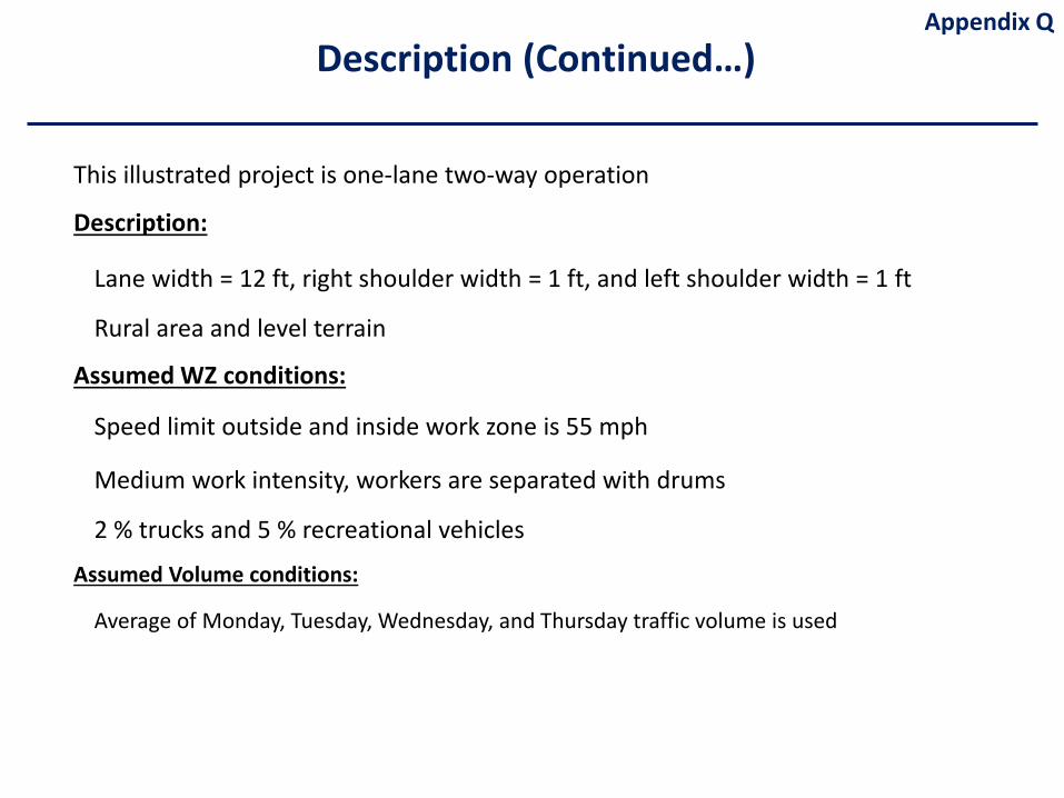
This illustrated project is one-lane two-way operation
Description:
Lane width = 12 ft, right shoulder width = 1 ft, and left shoulder width = 1 ft
Rural area and level terrain
Assumed WZ conditions:
Speed limit outside and inside work zone is 55 mph
Medium work intensity, workers are separated with drums
2 % trucks and 5 % recreational vehicles
Assumed Volume conditions:
Average of Monday, Tuesday, Wednesday, and Thursday traffic volume is used
Appendix QDescription (Continued…)
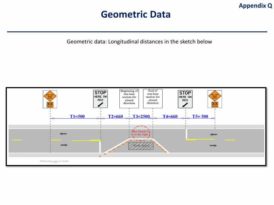
Geometric data: Longitudinal distances in the sketch below
Geometric DataAppendix Q
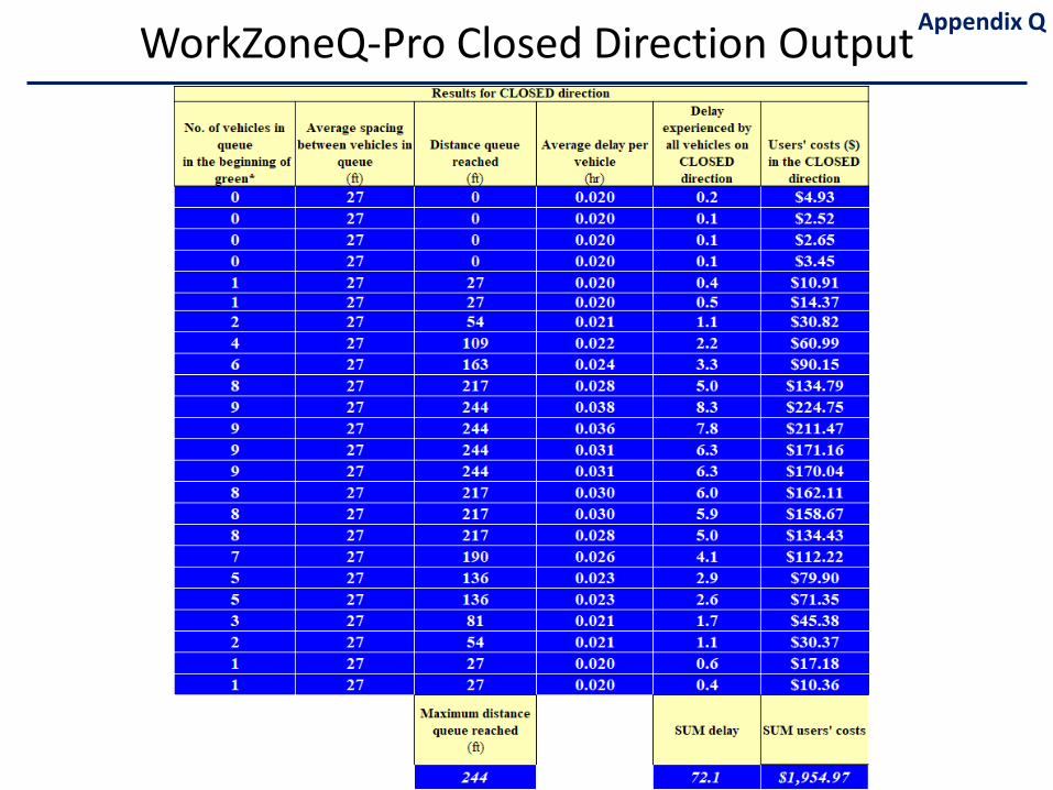
WorkZoneQ-Pro Closed Direction OutputAppendix Q
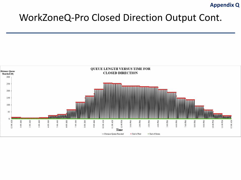
WorkZoneQ-Pro Closed Direction Output Cont. Appendix Q
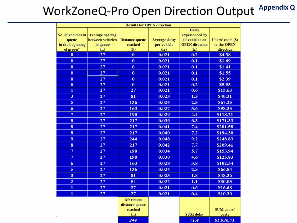
WorkZoneQ-Pro Open Direction Output Appendix Q
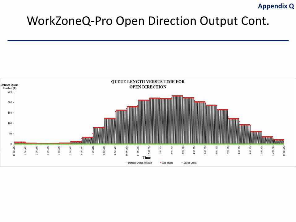
Appendix Q
WorkZoneQ-Pro Open Direction Output Cont.
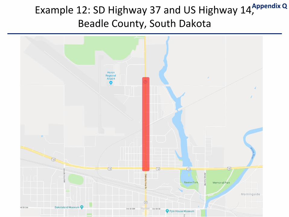
Example 12: SD Highway 37 and US Highway 14, Beadle County, South Dakota
Appendix Q
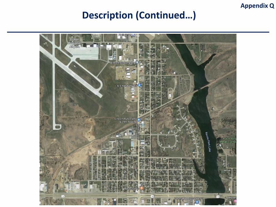
Appendix QDescription (Continued…)
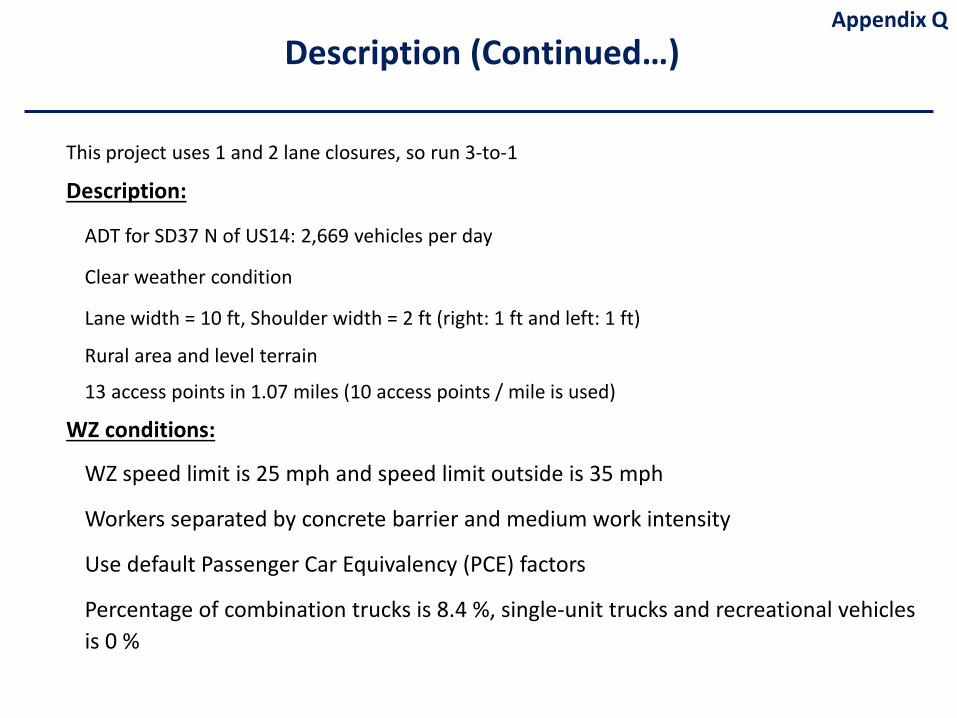
This project uses 1 and 2 lane closures, so run 3-to-1
Description:
ADT for SD37 N of US14: 2,669 vehicles per day
Clear weather condition
Lane width = 10 ft, Shoulder width = 2 ft (right: 1 ft and left: 1 ft)
Rural area and level terrain
13 access points in 1.07 miles (10 access points / mile is used)
WZ conditions:
WZ speed limit is 25 mph and speed limit outside is 35 mph
Workers separated by concrete barrier and medium work intensity
Use default Passenger Car Equivalency (PCE) factors
Percentage of combination trucks is 8.4 %, single-unit trucks and recreational vehicles is 0 %
Appendix QDescription (Continued…)
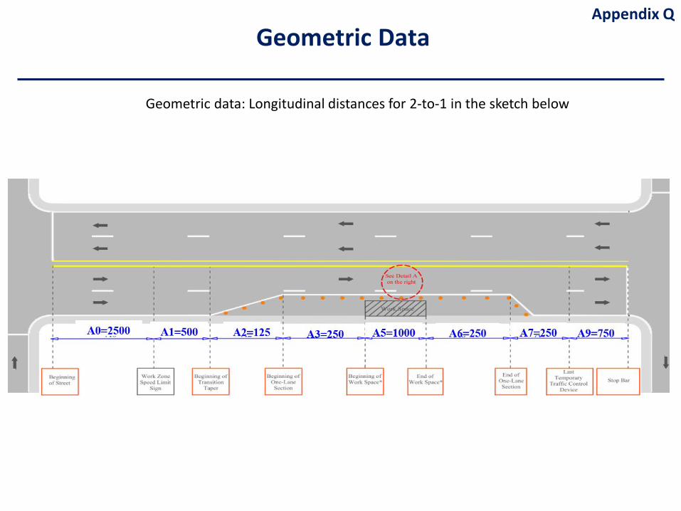
Geometric data: Longitudinal distances for 2-to-1 in the sketch below
Appendix QGeometric Data
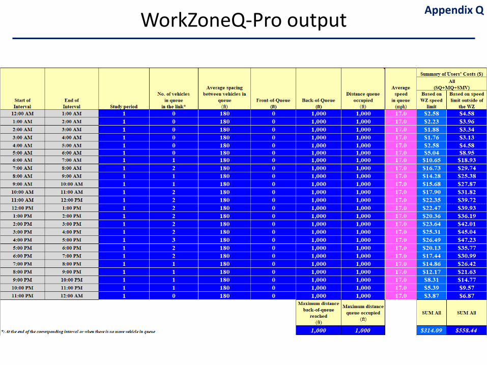
WorkZoneQ-Pro output Appendix Q
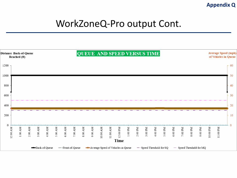
WorkZoneQ-Pro output Cont.
Appendix Q
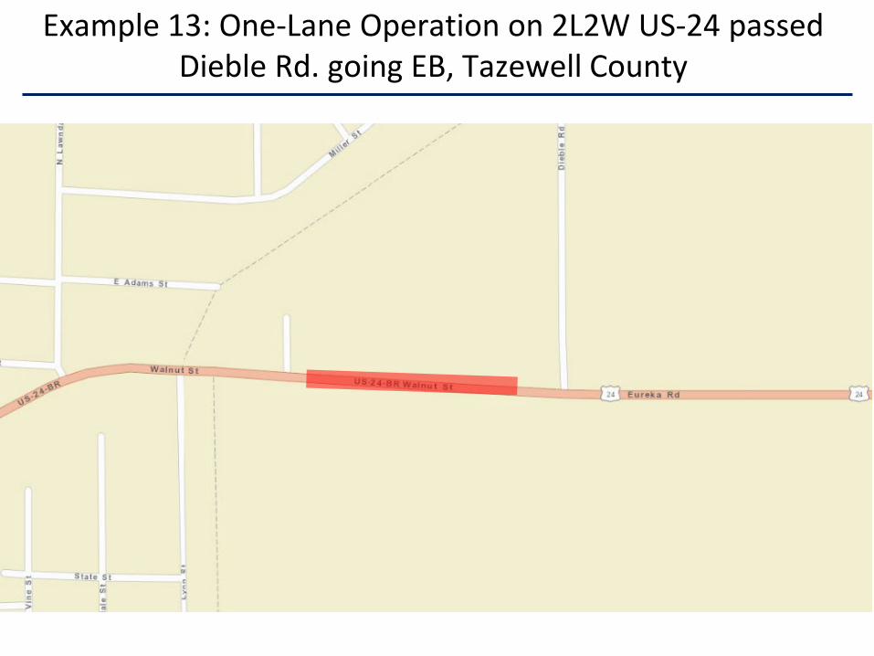
Example 13: One-Lane Operation on 2L2W US-24 passed Dieble Rd. going EB, Tazewell County
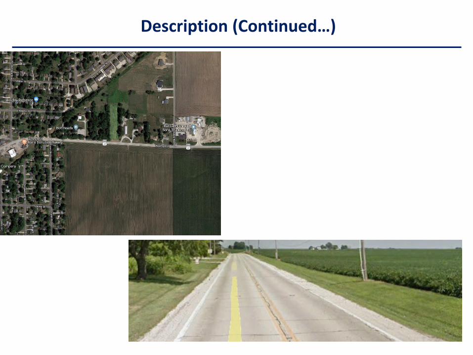
Description (Continued…)
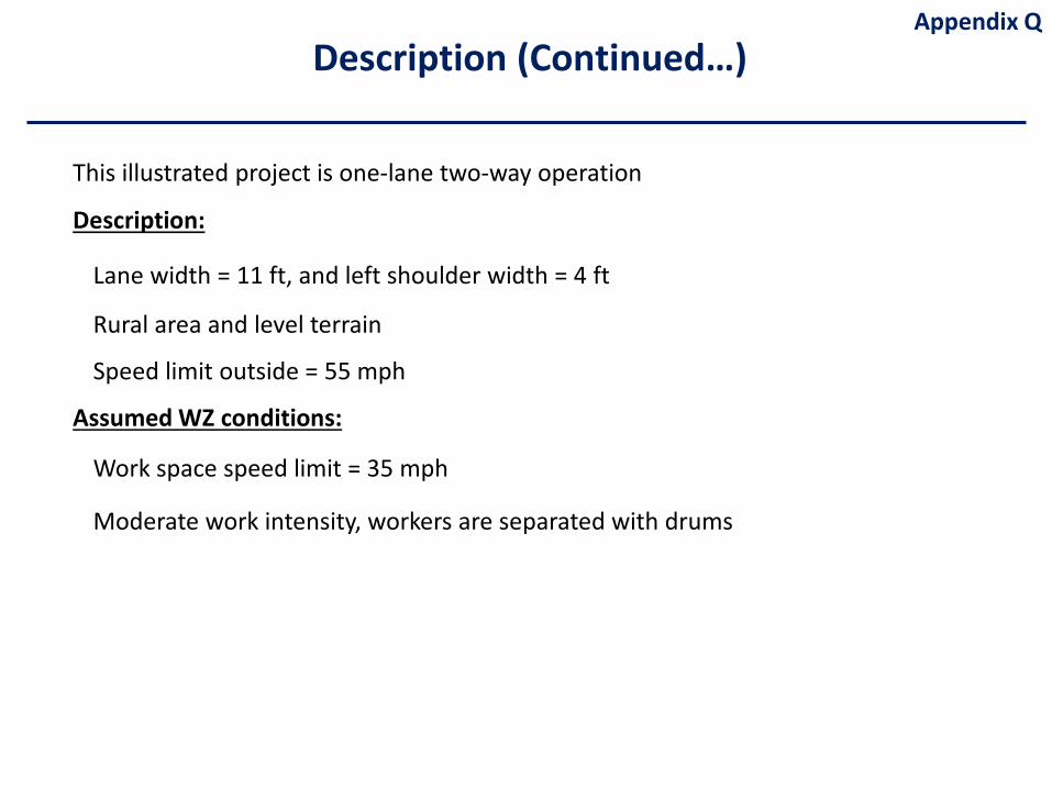
This illustrated project is one-lane two-way operation
Description:
Lane width = 11 ft, and left shoulder width = 4 ft
Rural area and level terrain
Speed limit outside = 55 mph
Assumed WZ conditions:
Work space speed limit = 35 mph
Moderate work intensity, workers are separated with drums
Appendix QDescription (Continued…)
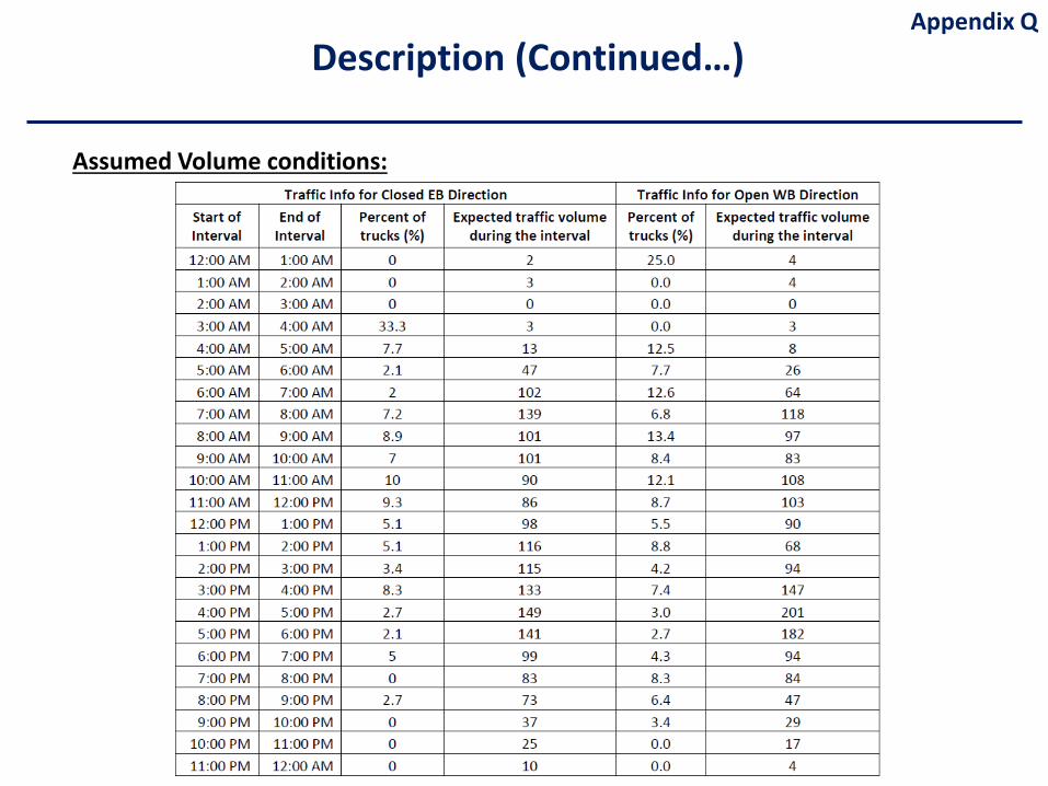
Assumed Volume conditions:
Appendix QDescription (Continued…)

Geometric data: Longitudinal distances in the sketch below
Geometric DataAppendix Q
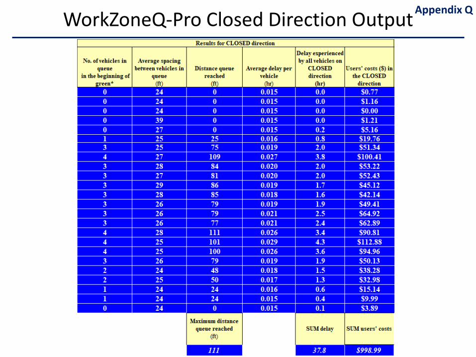
WorkZoneQ-Pro Closed Direction OutputAppendix Q
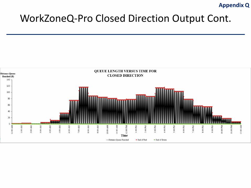
WorkZoneQ-Pro Closed Direction Output Cont. Appendix Q

WorkZoneQ-Pro Open Direction Output Appendix Q
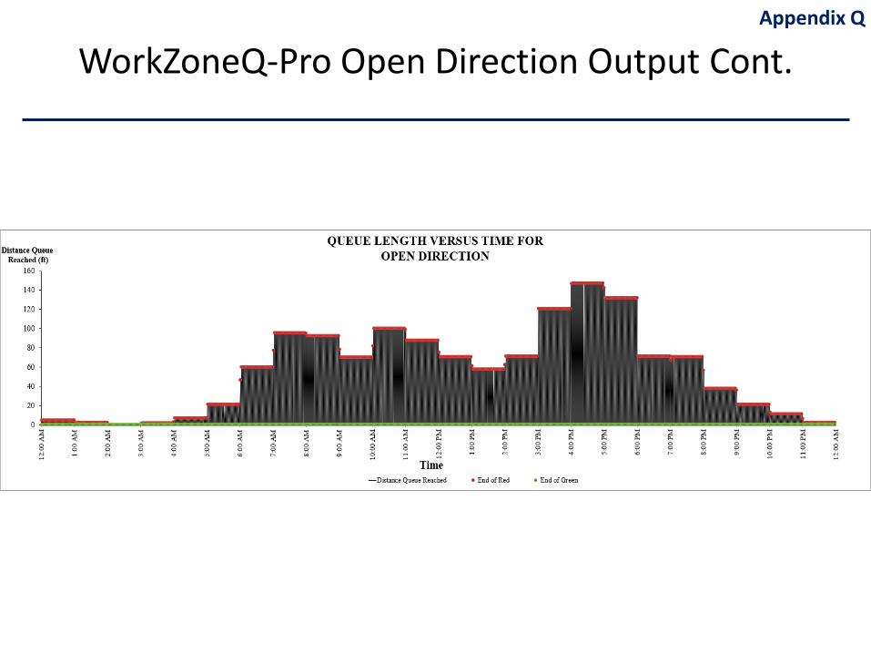
Appendix Q
WorkZoneQ-Pro Open Direction Output Cont.
Appendix R
Troubleshooting and FAQsFor
WorkZoneQ-Pro
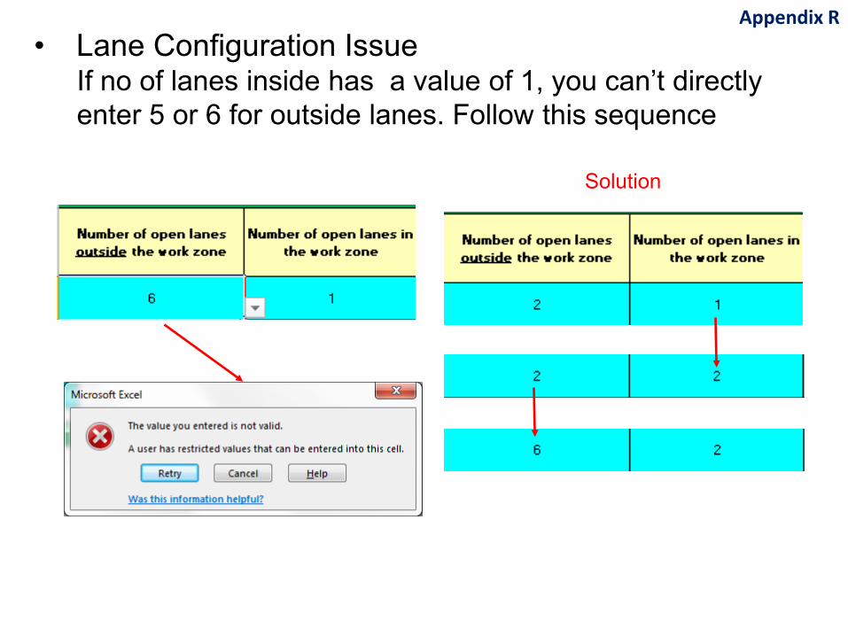
• Lane Configuration Issue If no of lanes inside has a value of 1, you can’t directly enter 5 or 6 for outside lanes. Follow this sequence
Appendix R
Solution
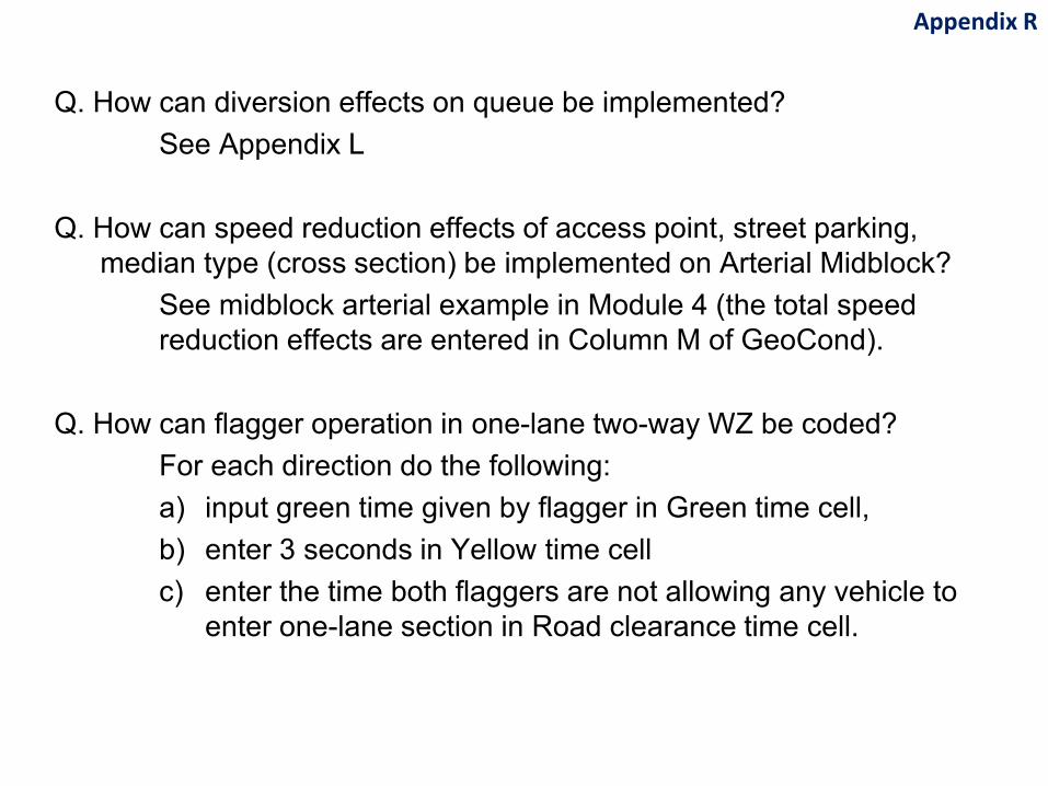
Appendix R
Q. How can diversion effects on queue be implemented?See Appendix L
Q. How can speed reduction effects of access point, street parking, median type (cross section) be implemented on Arterial Midblock?
See midblock arterial example in Module 4 (the total speed reduction effects are entered in Column M of GeoCond).
Q. How can flagger operation in one-lane two-way WZ be coded?For each direction do the following:a) input green time given by flagger in Green time cell, b) enter 3 seconds in Yellow time cellc) enter the time both flaggers are not allowing any vehicle to
enter one-lane section in Road clearance time cell.
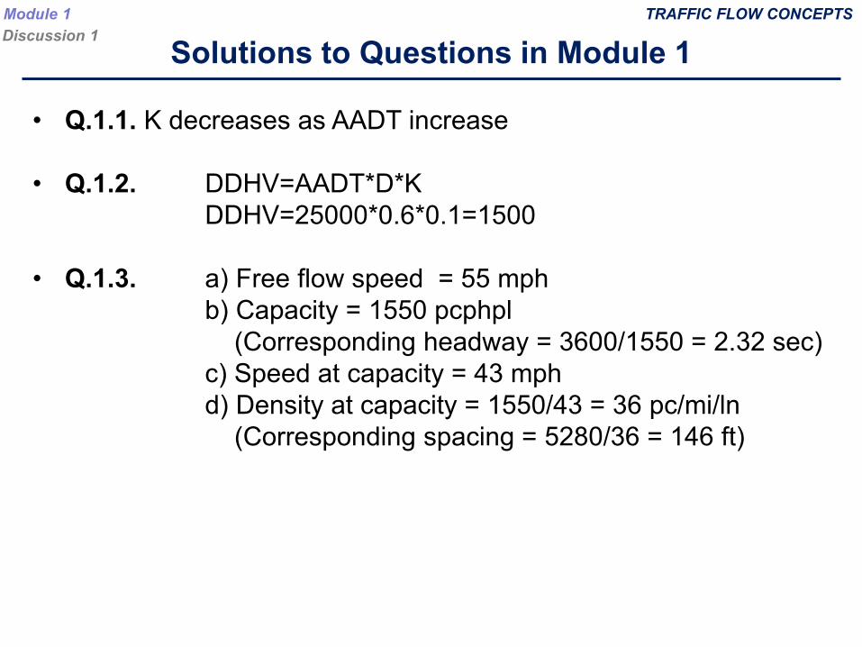
Solutions to Questions in Module 1TRAFFIC FLOW CONCEPTSModule 1
Discussion 1
• Q.1.1. K decreases as AADT increase
• Q.1.2. DDHV=AADT*D*KDDHV=25000*0.6*0.1=1500
• Q.1.3. a) Free flow speed = 55 mph b) Capacity = 1550 pcphpl
(Corresponding headway = 3600/1550 = 2.32 sec)c) Speed at capacity = 43 mphd) Density at capacity = 1550/43 = 36 pc/mi/ln
(Corresponding spacing = 5280/36 = 146 ft)
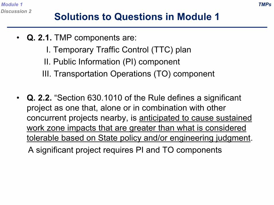
• Q. 2.1. TMP components are:I. Temporary Traffic Control (TTC) plan
II. Public Information (PI) component III. Transportation Operations (TO) component
• Q. 2.2. “Section 630.1010 of the Rule defines a significant project as one that, alone or in combination with other concurrent projects nearby, is anticipated to cause sustained work zone impacts that are greater than what is considered tolerable based on State policy and/or engineering judgment. A significant project requires PI and TO components
Module 1Discussion 2
TMPs
Solutions to Questions in Module 1
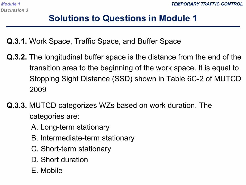
Q.3.1. Work Space, Traffic Space, and Buffer Space
Q.3.2. The longitudinal buffer space is the distance from the end of the transition area to the beginning of the work space. It is equal to Stopping Sight Distance (SSD) shown in Table 6C-2 of MUTCD 2009
Q.3.3. MUTCD categorizes WZs based on work duration. The categories are: A. Long-term stationary B. Intermediate-term stationaryC. Short-term stationary D. Short durationE. Mobile
TEMPORARY TRAFFIC CONTROLModule 1Discussion 3
Solutions to Questions in Module 1
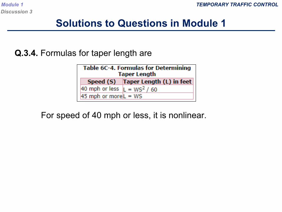
Q.3.4. Formulas for taper length are
For speed of 40 mph or less, it is nonlinear.
TEMPORARY TRAFFIC CONTROLModule 1Discussion 3
Solutions to Questions in Module 1
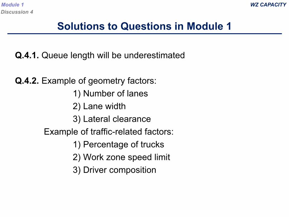
Q.4.1. Queue length will be underestimated
Q.4.2. Example of geometry factors:1) Number of lanes2) Lane width3) Lateral clearance
Example of traffic-related factors:1) Percentage of trucks2) Work zone speed limit 3) Driver composition
WZ CAPACITYModule 1Discussion 4
Solutions to Questions in Module 1
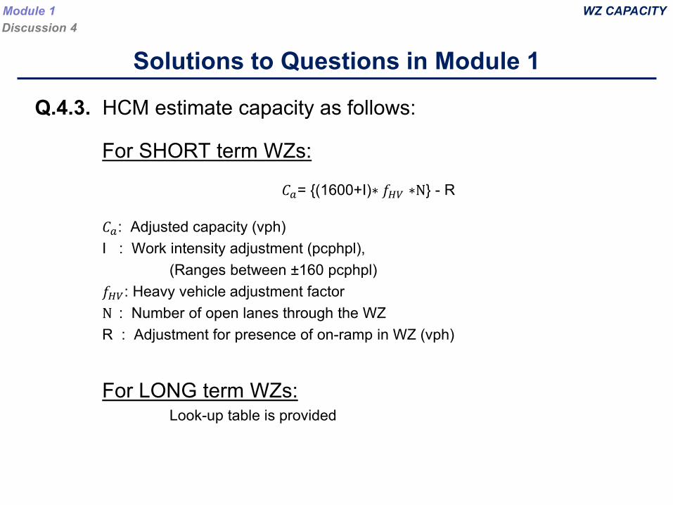
Q.4.3. HCM estimate capacity as follows:
For SHORT term WZs:
𝐶𝐶𝑎𝑎: Adjusted capacity (vph)I : Work intensity adjustment (pcphpl),
(Ranges between ±160 pcphpl)𝑓𝑓𝐻𝐻𝐻𝐻: Heavy vehicle adjustment factorN : Number of open lanes through the WZR : Adjustment for presence of on-ramp in WZ (vph)
For LONG term WZs:Look-up table is provided
WZ CAPACITYModule 1Discussion 4
𝐶𝐶𝑎𝑎= {(1600+I)∗ 𝑓𝑓𝐻𝐻𝐻𝐻 ∗N} - R
Solutions to Questions in Module 1
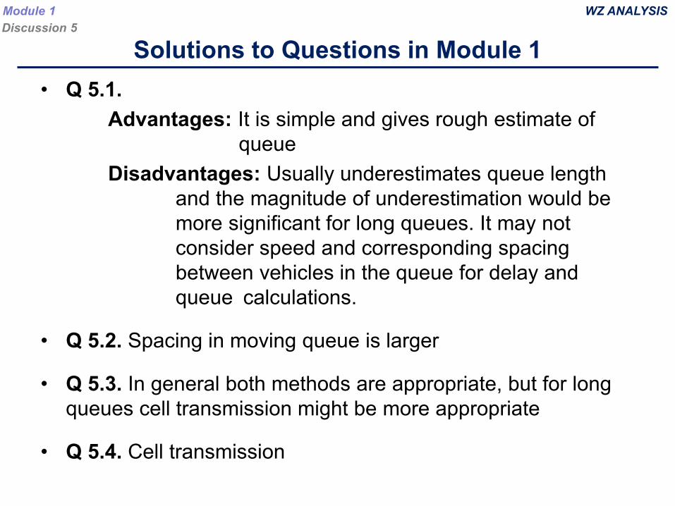
• Q 5.1. Advantages: It is simple and gives rough estimate of
queueDisadvantages: Usually underestimates queue length
and the magnitude of underestimation would be more significant for long queues. It may not consider speed and corresponding spacing between vehicles in the queue for delay and queue calculations.
• Q 5.2. Spacing in moving queue is larger
• Q 5.3. In general both methods are appropriate, but for long queues cell transmission might be more appropriate
• Q 5.4. Cell transmission
Module 1Discussion 5
WZ ANALYSIS
Solutions to Questions in Module 1
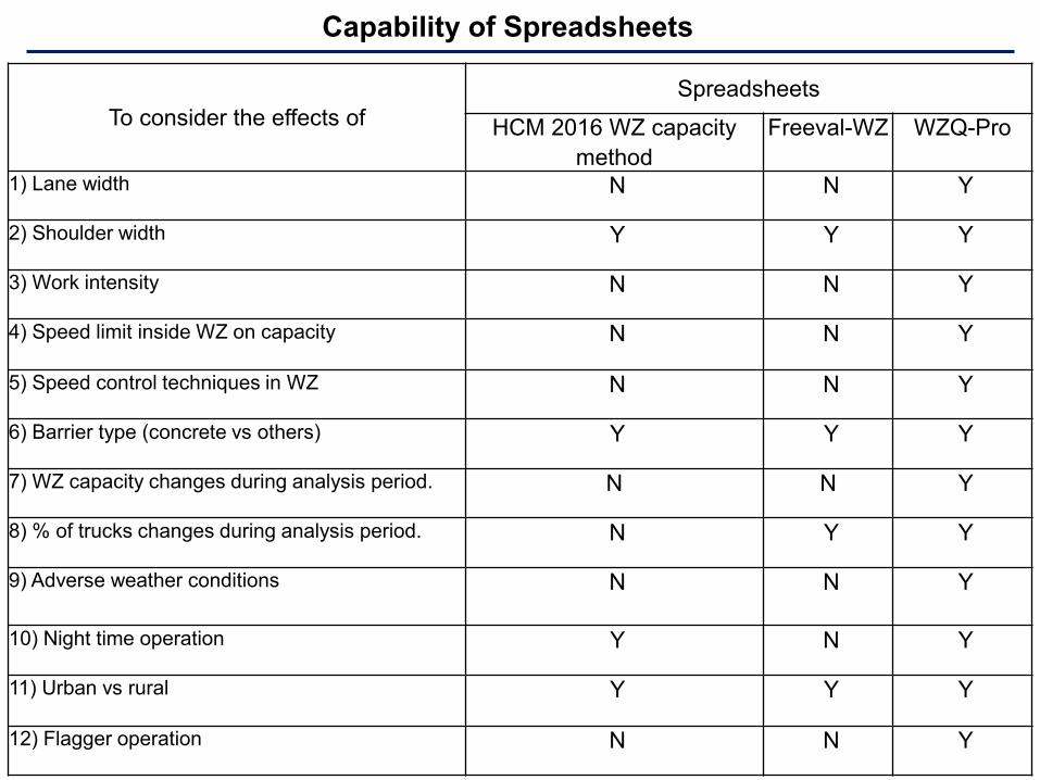
Capability of Spreadsheets
To consider the effects of Spreadsheets
HCM 2016 WZ capacity method
Freeval-WZ WZQ-Pro
1) Lane width N N Y
2) Shoulder width Y Y Y
3) Work intensity N N Y
4) Speed limit inside WZ on capacity N N Y
5) Speed control techniques in WZ N N Y
6) Barrier type (concrete vs others) Y Y Y
7) WZ capacity changes during analysis period. N N Y
8) % of trucks changes during analysis period. N Y Y
9) Adverse weather conditions N N Y
10) Night time operation Y N Y
11) Urban vs rural Y Y Y
12) Flagger operation N N Y
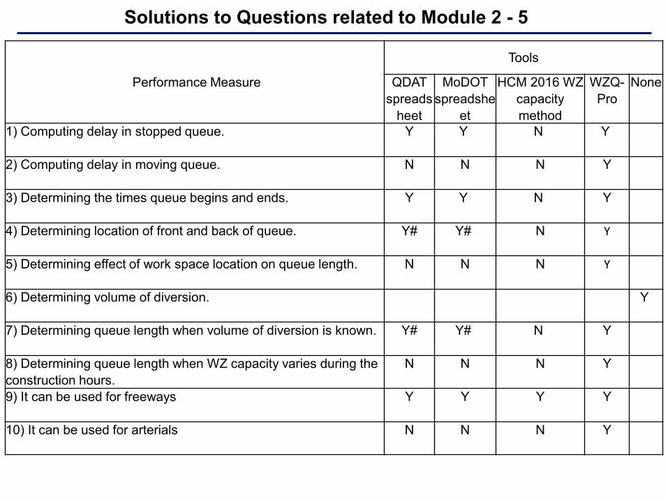
Performance Measure
Tools
QDAT spreads
heet
MoDOTspreadshe
et
HCM 2016 WZ capacity method
WZQ-Pro
None
1) Computing delay in stopped queue. Y Y N Y
2) Computing delay in moving queue. N N N Y
3) Determining the times queue begins and ends. Y Y N Y
4) Determining location of front and back of queue. Y# Y# N Y
5) Determining effect of work space location on queue length. N N N Y
6) Determining volume of diversion. Y
7) Determining queue length when volume of diversion is known. Y# Y# N Y
8) Determining queue length when WZ capacity varies during the construction hours.
N N N Y
9) It can be used for freeways Y Y Y Y
10) It can be used for arterials N N N Y
Solutions to Questions related to Module 2 - 5