REVIEW

COPY

NOT FOR D

ISTRIB

UTION

Slow dynamics in semiconductor multilongitudinal-mode laser transients governed by

a master mode

N. DokhaneDepartement de Physique, Faculte de Sciences, Universite de Boumerdes, Algeria

G.P. PuccioniIstituto dei Sistemi Complessi, CNR, Via Madonna del Piano 10, I-50019 Sesto Fiorentino, Italy

G.L. Lippi1,2∗1Universite de Nice Sophia Antipolis, Institut Non Lineaire de Nice

2CNRS, UMR 7335

1361 Route des Lucioles, F-06560 Valbonne, France

email: Gian-Luca.Lippi@inln.cnrs.fr

(Dated: March 23, 2012)

We examine the response to the sudden switch of the pump parameter in a multimode semicon-ductor laser with intensity coupling on a model whose validity has been successfully compared toexperimental results. We find the existence of a very slow modal evolution governed by a master

mode, which reaches its steady state on a time scale a couple of orders of magnitude longer thanthat of the total intensity. The practical consequences for applications are examined, such as thetemporal evolution of the spectral width of the laser emission and the time at which its steady stateis attained. Issues related to modeling choices, such as the number of modes and their placementwith respect to line center are discussed.

PACS numbers: 42.55.Px,42.55.-f,42.60.Mi,05.45.-a

I. INTRODUCTION

When turning on a laser, the typical variable which isexperimentally, and most easily, monitored is the totaloutput intensity. While on the practical side this choiceis a sensible one, earlier results have shown, both theoret-ically and experimentally, that multi-longitudinal moderegimes exist where an underlying, long-term, residualintermodal dynamics may exist[1–6]. In such a case,the information gathered through the total intensityis incomplete and may hide important aspects of thephysics of the problem, but also some technologicallyimportant side-effects. Semiconductor lasers may alsohide their modal dynamics under a constant or nearly-constant laser intensity – the so-called antiphase dynam-

ics regimes–, where the individual modes oscillate in sucha way as to share the available gain in a cooperativefashion [7–9], while slow, dynamical modal features mayremain hidden in the modeling of strongly multimodesystems [10–12].

In order to investigate the switch-on transient in asemiconductor laser, we have studied a multi-longitudinalmode, with intensity coupling, whose predictions in thetransient regime have been compared to experimental re-sults [13].

In this investigation we consider the crossing of thelaser threshold in response to a sudden switch in thepump. The focus of our attention is the evolution of

∗Corresponding author

the transient from the moment when the control param-eter (pump in our case) is suddenly increased, to the timewhen the system has attained its final steady state. Theproblem is well-posed for semiconductor lasers, becausethere exist regimes of stable multimode operation abovethreshold, contrary to what happens for classic homoge-neously broadened systems [14]. The interest for such aquestion is mainly fundamental: understanding the inter-mode dynamics which underlies the global temporal laserbehaviour usually monitored through the total laser out-put. We remark that these results may apply to otherClass B lasers [15], since the findings do not depend onthe specifics of the model, but rather on the generic struc-ture of the coupling.

Finally, our results may also benefit applications insituations where the temporal evolution of the spectralcontent of the laser output is crucial (e.g., in the spectralcontent of short temporal pulses).

Section II briefly presents the model under study withsome discussion about the physics of the system and thechoices we have made for its numerical integration; thedefinitions for the various parameters and their valuescan be found in the Appendix, Section VII. The numer-ical results obtained by the straightforward integrationof the model when switching the pump parameter frombelow to above threshold are discussed in Section III. Ananalytical approach is developed in the different subsec-tions of section IV, where we interpret, on the basis ofthe model’s structure, the numerical findings. The slowenergy redistribution among modes is discussed in Sec-tion IVA, while a simplified, toy model is used in Sec-tion IVB to explain the global behaviour of the modal

2

variables in the slow evolution phase. Section IVC high-lights the role of the Master Mode in the dynamics. Issuesrelated to the choice of mode positioning relative to thegain peak are examined in Section V. A summary of thepaper and some conclusions are offered in Section VI.

II. MODEL

We study a model for a multi-longitudinal mode semi-conductor laser whose parameter values have been de-termined to match experimental results [13]. As in allrate equations models, the dynamics here are describedin terms of time-dependent ODEs, for each modal inten-sity. All interference phenomena are neglected, since theintermode spacing (typically ∆ν ≈ 1.5×1011Hz) is smallenough compared to the laser’s internal rates (relaxationoscillation frequency < 1010Hz) to average out the fastoscillations [16]. A thorough discussion of the conditionsunder which the phase dynamics (intermode beating) canbe neglected can be found in [17].Coupling between the different laser modes occurs

through the population inversion, which acts as a globalenergy reservoir for them all. The model equationsare [13]:

dIj(t)

dt= [ΓGj(N)−

1

τp]Ij + βjBN(N + P0), (1a)

dN(t)

dt=

J

q−R(N)−

∑

j

ΓGj(N)Ij , (1b)

where Ij(t) is the intensity of each longitudinal mode ofthe electromagnetic (e.m.) field (1 ≤ j ≤ M), N(t) is thenumber of carriers as a function of time, Γ is the opti-cal confinement factor, Gj(N) is the optical gain for thej-th lasing mode (function of carrier number and wave-length), τp is the photon lifetime in the cavity, βj is thefraction of spontaneous emission coupled in the j-th las-ing mode, B is the band-to-band recombination constant,P0 is the intrinsic hole number in the absence of injectedcurrent, J is the current injected into the active region,q is the electron charge, and R(N) is the incoherent re-combination term (including radiative and nonradiativerecombination) which represents the global loss terms forthe carrier number (i.e., the population inversion in theusual laser language). All definitions for the functionsand all values for the physical parameters are given inthe Appendix.The bracket in eq. (1a) represents the global gain for

each laser mode, with the first part accounting for theactual source terms and the second for the outcouplinglosses. The last term in the equation takes into accountthe average contribution of the spontaneous emission toeach lasing mode. In the equation for the number ofcarriers in the conduction band, the first term representsthe pump. The second term in eq. (1b) describes thelosses for the carrier density due to different processes,while the last term accounts for the (global) reduction in

population due to the energy transferred to the differentintensity modes. This last term is the source of couplingamong all modes.In the numerical simulations, we have included 113

modes to cover approximately 1.5 times the Full-Width-at-Half-Maximum (FWHM) of the gain curve (cf. Ap-pendix for additional details). Only a subset of thesemodes actually lases at steady state, but their large num-ber ensures that the slow dynamics is initiated withreliable, simulation-independent initial conditions for thelasing modes.

III. THRESHOLD CROSSING

We analyze the laser’s behaviour, when it crosses thethreshold, in the total intensity (the variable that is nor-mally measured – Fig. 1.1) and in the modal intensities.The total intensity shows the characteristic turn-on withintensity overshoot and damped oscillations which dis-appear at t ≃ 0.7ns. Fig. 1.2 shows the correspondingphase space portrait, with the typical spiralling relax-ation towards the stable focus [19] (lasing solution).

0 0.2 0.4 0.6 0.8 1t (ns)

0

1

2

3

4

5

6

Tot

al I

nten

sity

(no

rm. u

nits

) (1)

1.35 1.4 1.45 1.5N (norm. units)

0

1

2

3

4

5

6

Tot

al I

nten

sity

(no

rm. u

nits

) (2)

FIG. 1: Time evolution of the total laser intensity (panel 1)following a sudden switch-on of the injected current (pumprate) in form of a Heaviside function. Phase space represen-tation (panel 2) of the switch picturing the total intensity,It, as a function of the carrier number, N . Initial currentvalue: Ji = 15.5mA, final current value Jf = 37.5mA. Thethreshold current for this laser is Jth = 17.5mA. Number ofmodes used for the integration: 113. All other parameters asin Table III. All parameter values are kept constant through-out the paper, unless otherwise explicitly noted. The delay atturn-on is approximately td ≈ 0.1ns, while the steady stateis attained at t ≃ 0.7ns. Here and in all subsequent figures(unless otherwise noted) the total intensity It is divided by105, and the number of carriers N is divided by 108.

Fig. 2 shows a detail of Fig. 1.2, where crossing trajec-tories become apparent. They are due to the 2-D projec-tion onto the (N, It) plane of the 114-D space and implythe existence of an underlying dynamics hidden underthe apparent steady state of Fig. 1. Accompanying tinyvariations in It are present, even though they are notclearly visible in Fig. 2.Fig. 3 shows the long-time evolution of selected modes:

central (j = 57 – curve (d)), first side-mode (j = 56 –curve (c)), and two additional side modes close to linecenter (j = 54 – curve (b), and j = 52 – curve (a)); for

3

1.4088 1.409 1.4092 1.4094 1.4096 1.4098N ( norm. units)

2.76

2.77

2.78

2.79

2.8

2.81

2.82

Tot

al I

nten

sity

(no

rm. u

nits

)

FIG. 2: Detail of the phase space of Fig. 1.2 suggesting thepresence of a residual evolution arising from the interplayamong the different lasing modes.

0 2.5 5t (ns)

0

0.5

1

1.5

2

N, I

nten

sity

(no

rm. u

nits

)

0 10 20 300

0.5

1

1.5

(a)(b)

(c)

(d)

(e)

(f)

(c)

(d)

FIG. 3: Total intensity (e) and carrier number (f) as a func-tion of time. The other curves show the individual modeintensities for the central mode (j = 57, (d)), and side modesclose to line center (blue side): j = 56 (c), j = 54 (b), j = 52(a). The symmetric modes, relative to the central one, arenot shown but are identical. Notice that in the first phases ofthe transient (peak) curves (c) and (d) are superposed: theyseparate only at the second oscillation. For graphical pur-poses the curves are scaled as follows: here It is divided by2.5 × 105, and the individual mode intensities by 105 (hereand in all subsequent figures, unless otherwise noted). Theinset shows the long time evolution of the central mode (d)and of the first side mode (c): steady state is attained by thecentral mode at t ≈ 35ns.

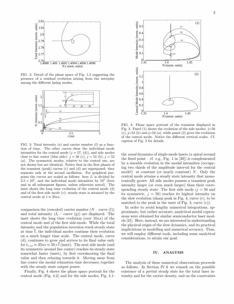
comparison the (rescaled) carrier number (N – curve (f))and total intensity (It – curve (g)) are displayed. Theinset shows the long time evolution (over 35ns) of thecentral mode and of the first side-mode. While the totalintensity and the population inversion reach steady stateat time t, the individual modes continue their evolutionon a much longer time scale. The central mode, curve(d), continues to grow and arrives to its final value onlyfor tc,ss ≈ 35ns ≈ 50×t (inset). The next side mode (andits symmetric around line center) reaches its steady statesomewhat faster (inset), by first overshooting the finalvalue and then relaxing towards it. Moving away fromline center the modal relaxation time decreases, togetherwith the steady state output power.Finally, Fig. 4 shows the phase space portrait for the

central mode (Fig. 4.2) and for the side modes, Fig. 4.1:

1.35 1.4 1.45N (norm. units)

0

0.1

0.2

0.3

0.4

0.5

Mod

e In

tens

ity (

norm

. uni

ts)

(a)

(b)

(c)

(1)

1.35 1.4 1.45N (norm. units)

0

0.2

0.4

0.6

0.8

1

1.2

Cen

tral

Mod

e In

tens

ity (

norm

. uni

ts)

(2)

FIG. 4: Phase space portrait of the transient displayed inFig. 3. Panel (1) shows the evolution of the side modes: j=56(c), j=54 (b) and j=52 (a), while panel (2) gives the evolutionof the central mode. Notice the different vertical scales. Cf.caption of Fig. 3 for details.

the usual dynamics of single-mode lasers (a spiral aroundthe fixed point – cf. e.g., Fig. 1 in [20]) is complementedby a sizeable evolution in the modal intensities (occupy-ing two thirds of the amplitude interval for the centralmode!) at constant (or nearly constant) N . Only thecentral mode attains a steady state intensity that mono-tonically grows: All side modes possess a transient peakintensity larger (or even much larger) than their corre-sponding steady state. The first side mode (j = 56 andits symmetric, j = 58) reaches its highest intensity onthe slow evolution (sharp peak in Fig. 4, curve (c), to bematched to the peak in the inset of Fig. 3, curve (c)).In order to avoid lengthy numerical integrations, ap-

proximate, but rather accurate, analytical modal expres-sions were obtained for similar semiconductor laser mod-els [21]. Here, instead, we are interested in understandingthe physical origin of the slow dynamics, and its practicalimplications in modelling and numerical accuracy. Thus,we will employ different tools, including some analyticalconsiderations, to attain our goal.

IV. ANALYSIS

The analysis of these numerical observations proceedsas follows. In Section IVA we remark on the possibleexistence of a partial steady state for the total laser in-tensity and for the carrier density, and on the constraints

4

which its existence imposes on the ensuing modal dynam-ics. Section IVB highlights, with the help of a stronglysimplified analysis, the crucial role of the modal gain vs.losses and shows the existence of a master mode. Theinfluence of the latter on the slow laser dynamics are dis-cussed in Section IVC.

A. Slow dynamics

The numerical results convincingly suggest that oneshould analyze the dynamics by introducing one global

variable in eqs. (1): the total intensity It. The laserdescription is therefore based on It and N as global vari-ables and M − 1 individual modal intensities:

dIt

dt=

M∑

j

ΓGj(N)Ij −1

τpIt + βtBN(N + P0),(2a)

dN(t)

dt=

J

q−R(N)−

M∑

j

ΓGj(N)Ij , (2b)

dIj(t)

dt= [ΓGj(N)−

1

τp]Ij + βjBN(N + P0), (2c)

1 ≤ j ≤ M − 1,

where we have defined the contribution of the sponta-

neous emission to all modes βt =∑M

j βj .

Inspection of eqs. (2a,b) for the global variables (N, It)shows a high degree of symmetry and a strong resem-blance to an equivalent model for a single-longitudinalmode laser [22]. The coupling between these two vari-

ables is entirely symmetric (∑M

j ΓGj(N)Ij), as for the

single mode laser, whence the (N, It) dynamics of Fig. 1,reminiscent of a single-mode laser, where the competitionbetween the (slow) energy reservoir (population inver-sion) and the fast relaxing electromagnetic field (inten-sity) produce an oscillatory approach towards the lasingstate.A more formal analysis is based on the steady states,

denoted by the overstrike and obtained from eqs. (2a,b):

M∑

j

ΓGj(N)Ij =1

τpIt − βtBN(N + P0), (3a)

M∑

j

ΓGj(N)Ij =J

q−R(N) . (3b)

These two conditions define It and N . Combiningeqs. (3a,b) we find

It =

[

J

q−R(N) + βtBN(N + P0)

]

τp, (4)

independently of the individual mode intensity values.The expression for N is given in implicit form by eq. (3b).

In spite of the fact that its explicit expression involves thesum over all individual intensity modes, each multipliedby its gain function Gj(N) calculated atN = N , it is cer-tain that the expression is satisfied at steady state andthat a unique value exists. Indeed, although the individ-ual mode intensities come into play, Gj(N) represents a

set of constants once N = N . In other words, startingfrom time t = t (at which It(t) = It and N(t) = N),then N remains constant (since dN

dt t=t= 0 ⇒ N(t >

t) = N) [23].The residual modal dynamics must there-fore comply with the constraint that the l.h.s. of eq. (3b)remain constant (since the r.h.s. will not change in time).More formally, the following constraints hold:

∑

j

Ij = It = K1, (5a)

∑

j

ΓGj(N)Ij =J

q−R(N) = K2, (5b)

where K1 and K2 are two constants which characterizethe laser operation for each set of parameter values.The fact that the sum in the l.h.s. of eq. (5b) is a

constant, K2, does not exclude a residual time evolutionamong the modes, which are numerous enough to arrangefor that. This becomes apparent by rewriting the evolu-tion equation for the individual modes, after the equilib-rium condition for the total intensity and the populationvariable have been attained (hence, with N = N every-where):

dIj

dt=

[

ΓGj(N)−1

τp

]

Ij + βjBN(N + P0). (6)

Three remarks are necessary here:

1. The term in square bracket on the r.h.s. of eq. (6)– coefficient of Ij – plays the role of an effective

relaxation constant for each field intensity, givenby the difference between the individual gain termfor the individual mode and the cavity losses (equalfor all modes). The second term in the equation isa constant in time (different for each mode via βj)

now that the N = N state has been attained;

2. The different values of Gj(N) imply that the effec-tive relaxation constant is different for each mode;hence, those modes that have larger coefficientsin front of Ij will evolve more rapidly, while thelong-term dynamics will be governed by the slowermodes (cf. Table I for numerical values);

3. Since the steady state values N = N and It = Ithave been attained, the evolution equations for theindividual modes, eqs. (6), are now almost decou-pled: they only need to obey to the constraints,eqs. (5), for all t > t (t being the time at which theglobal variables attain their equilibrium condition).

5

TABLE I: Numerical values for the two terms which composethe r.h.s. of the evolution equation for the modal intensity,eq. (6) listed for selected modes after steady state has beenattained by the global variables. Column A: ΓGj(N)−(1/τp);column B: βjBN(N + P0). The values are estimated at t =35ns to eliminate any the residual dynamics on N .

Mode (j) λj(µm) A(s−1) B(s−1)

57 1.3 −8.44× 107 1.0623 × 1013

56 1.2994 −2.58× 108 1.0621 × 1013

54 1.29819 −1.65× 109 1.0601 × 1013

52 1.29698 −4.43× 109 1.0563 × 1013

50 1.29578 −8.59× 109 1.0506 × 1013

40 1.28974 −5.03 × 1010 9.9673 × 1012

30 1.2837 −1.27 × 1011 9.1109 × 1012

20 1.27767 −2.38 × 1011 8.0987 × 1012

10 1.27163 −3.84 × 1011 7.0681 × 1012

Notice that there is no contradiction between theglobal constraint

∑M

j Ij = It = K1 and the fact thatthe time scales for the evolution may be different. In-deed, the evolution for each mode is the result of thedifference between It and all other modes, thus allowingfor the appearance of different time scales in the modecombination.Table I clearly shows that the spontaneous emission

contribution B varies very little between the central andthe side modes (B57 ≈ 1.5 × B10). Instead, the effectiverelaxation constant A (Table I) changes by more thanfour orders of magnitude and dominates the dynamics.The ratio A(j = 57) ≈ 2× 10−2A(j = 52) suggests thatmode j = 52 should attain its steady state in a time ap-proximately 50 times shorter than the central mode. In-spection of Fig. 3 qualitatively confirms this result, thusvalidating our simple interpretation of the dynamics interms of (nearly) decoupled groups of variables: (N, It)on the one hand, and Ij (j = 1 . . .M − 1) on the other.From the data in Table I we can also draw additional

information about the long-term dynamics of the indi-vidual modes. The evolution of each mode is determinedby eq. (6) whose r.h.s. reads AjIJ +Bj . Reading the in-tensity values for modes with j = 57, j = 56 and j = 54off Fig. 3 at the end of the transient for the total inten-sity It (and the population N), we estimate the r.h.s. togive dI57

dt|t≈0.7ns ≈ 7 × 1012 (I57(t ≈ 0.7ns) ≈ 4 × 104),

dI56dt

|t≈0.7ns ≈ 3 × 1011 (I56(t ≈ 0.7ns) ≈ 4 × 104) anddI54dt

|t≈0.7ns ≈ −2× 1013 (I54(t ≈ 0.7ns) ≈ 2× 104). Wesee immediately that modes j = 57 and j = 56 mustgrow, while all other modes should decay from the valuethat they have reached at the end of the transient forthe global variables. This prediction is confirmed by theresults displayed in Fig. (3). Note that the values forthe constants given in Table I apply, since starting fromthe end of the transient for the global variables the coeffi-cients A and B no longer depend on time. We can furtherremark that the reversal in the growth of mode j = 56

can also be interpreted on the basis of the effective relax-ation constant, since during the slow evolution – due tothe interplay with all other modes – this mode acquiresan intensity value which inverts the sign of its r.h.s. ineq. (6): dI56

dt|t≈3ns ≈ −4×1012 (I56(t ≈ 3ns) ≈ 5.5×104).

In the following section we show that the time scaleover which the steady state for all modes is attained (thetrue steady state for the system), is determined by themode with the highest gain. We will see that the initialconditions play only a minor role (determining the quan-titative aspects of the dynamics) and that the contribu-tion of the spontaneous emission (last term in eq. (6))can be neglected.

B. Role of the physical constants

Since we analyse the dynamics after the global variableshave attained their steady state condition (t > t ≃ 0.7ns)and the constraint over the sum of all the modes holds, allexpressions involving these variables can be taken to beconstants. Thus the following simplified analysis holdsand pertinently highlights the influence of the variouselements on the slow modal evolution. For the purposeof illustration (Fig. 5), we use a number of modes muchsmaller than in the full simulations. Our arguments are,however, independent of this choice.Rewriting eq. (6) as:

dIj

dt′= −ajIj + bj , aj , bj > 0, (7)

(t′ being a time variable different from that of eqs. (1)),and integrating it formally [24], one obtains

Ij(t′) = Cje

−ajt′

+bj

aj. (8)

The constraint on the total laser intensity still holds, eventhough it does not appear explicitly. The sign of Cj , aconstant which functionally depends on the initial condi-tion, Ij(t), determines whether the further evolution ofthe mode consists in a decrease (Cj > 0) or an increase(Cj < 0) of each Ij . The explicit form of the Cj ’s caneasily be written as a function of the initial condition foreach mode Ij0

Cj =

(

Ij0 −bj

aj

)

, (9)

where we have taken t′ = t − t, so that our initial con-dition is specified at t′ = 0. Thus the explicit form ofeq. (8) becomes

Ij(t′) =

bj

aj

[

1 +aj

bj

(

Ij0 −bj

aj

)

e−ajt′

]

, (10)

where Ij0 is the intensity of each mode when the global

variables attain steady state (at t′ = 0). It is easy to

6

see that neither the value of Ij0 nor that of bj play asubstantial role in the subsequent dynamics. Indeed, ifwe consider two constants I0 and b equal for all modesand write therefore the solution, eq. (10), as:

Ij(t′) =

b

aj

[

1 +aj

b

(

I0 −b

aj

)

e−ajt′

]

, (11)

we are still able to reproduce the overall slow dynamicsof the various laser modes by appropriately choosing theaj ’s.

0 20 40 60 80 100t (norm. units)

0

5

10

15

20

25

Mod

e In

tens

ity (

norm

.uni

ts)

(a)

(b)

(c)

(d)

(1)

0 20 40 60 80 100t (norm. units)

0

5

10

15

20

25

Mod

e In

tens

ity (

norm

. uni

ts)

(b)

(a)

(c)

(d)

(2)

FIG. 5: Illustration of the evolution of a mode described bythe simplified approach of eq. (10) – panel (1) – with differentinitial values for the modal intensity, Ij0 , at t′ = 0, and forthe bj ’s. Panel (2) shows the equivalent calculation based oneq. (11), obtained with only one value for I0 and b. Asidefrom a small quantitative difference, the evolution shown inpanels (1) and (2) is qualitatively the same. Panel (1) curves:(a) I0a = 4, aa

ba= 1.33; (b) I0b = 5, ab

bb= 0.667; (c) I0c = 6,

ac

bc= 6.67 × 10−2; (d) I0d = 7, ad

bd= 3.33 × 10−2. Panel (2)

I0 = 5, b = 0.3; aa = 0.4; (b) ab = 0.2; (c) ac = 0.02; (d)ad = 0.01. The values for the coefficients are chosen in such away as to obtain a good qualitative illustration of the actualevolution of the different laser modes.

The numerical integration of the two sets of equations,eqs. (10) and (11), shows that the difference in the evo-lution is only quantitative (cf. Figs. 5 panels 1,2, respec-tively). Hence, we conclude that the slow dynamics re-sult from the equivalent relaxation constants, aj , for eachmode and depend only in a minor fashion on the valuesactually taken by each mode at t = t (the end of thetransient for the global variables) or on the fraction ofspontaneous emission injected in each mode (representedby bj). Instead, through the factor Cj(Ij0 = I0), the aj ’sdetermine the exponential growth/decay (small/large aj ,thus Cj ≶ 0) to a finite/zero value for the correspondingmode. Inspection of eq. (11) shows that the smaller aj ,

the larger the asymptotic value Ij(t′ → ∞) = b

aj.

In our semiconductor laser model, aj corresponds tothe square bracket in eq. (1a)), thus to the loss/gain bal-ance. As is the case in all dynamical systems [25], theslowest growth will be that of the mode with the (nega-tive) value of aj closest to zero: the mode with the largestgain. Only after this mode has reached its steady statethe dynamics will be completed.

C. Master mode

The previous, simplified analysis clearly shows how themode with the highest gain possesses the slowest relax-ation constant and is therefore the last to attain equi-librium. This mode can be considered to be the mas-

ter mode which enslaves [26] the other modes, as is bestseen by the following considerations. The constraints,eqs. (5a-5b), imply that at time t > t the individualmodes must maintain the total output power constant.The slow growth of the master mode forces the other lat-eral modes to compensate for its sluggishness. Duringthe transient (t ≤ t), the modes farthest away from linecenter acquire values which are well beyond their steadystates and then fade away. However, even during theslow dynamics the lateral modes are not the actors ofthe dynamics, but only the followers. Indeed, the firsttwo side modes (j = 56 and, symmetrically, j = 58) areinitially forced to grow beyond their steady state value(Fig. 4.1, curve(c)) towards which they eventually decayaway. This non-monotonic behaviour, which character-izes all the enslaved modes, is the proof of the fact thatonly one master mode exists and that it, alone, deter-mines all the dynamics.

V. EVEN VS. ODD NUMBER OF MODES

The simulations discussed so far are performed with anodd number of modes, with the central one placed exactlyat the peak of the gain line. It is crucial to know whether,and how, a different choice may influence the numericalresults. Indeed, the results should be invariant with re-spect to this choice, otherwise the reliability of the wholeapproach is called into question. More interestingly, inexperimental situations there is no guarantee that a cen-tered mode exists on the gain line. First, because the po-sition of each mode depends on the cavity length – whichvaries as a function of numerous parameters: construc-tion, temperature, saturation, etc. –; Second because itis well-known that in semiconductor lasers the gain line issubject to a nonnegligible frequency shift (not included inthe present model); Third because the real lineshape of asemiconductor laser is asymmetric [27–29] and thereforea line center is only ill-defined.The maximum deviation from the computation with an

odd number of modes, exactly centered at the gain peak,is obtained by choosing an even number of modes, placedsymmetrically with respect to line center. All other con-figurations are intermediate between these two and willbe covered by the two extreme choices that we examine.Simulation of the same equations with M = 112 modes

provides predictions for the global variables which areindistinguishable from those obtained with M = 113modes, thus confirming the validity of the approach.Problems, however, are detected by looking at the in-dividual mode evolution.Fig. 6 compares the long-term evolution of the cen-

7

TABLE II: M = 112 modes. Numerical values for the twoterms which compose the r.h.s. of the evolution equation forthe modal intensity, eq. (6), listed for selected modes aftersteady state has been attained by the global variables. Col-umn A: ΓGj(N) − (1/τp); column B: βjBN(N + P0). Thevalues are taken at t = 35ns to ensure convergence. No-tice the sizeable change in the values of the coefficients of Ijin eq. (1a) between Table I and the present one, due to thechange in wavelength – thus of position relative to line center(peak wavelength λp = 1.3µm). The relative change for thecentral mode is approximately 40%. The spontaneous emis-sion contribution remains, instead, practically unchanged.

Mode (j) λi(µm) A(s−1) B(s−1)

56 1.2997 −1.16× 108 6.610 × 108

54 1.29849 −1.16× 109 6.604 × 108

52 1.29728 −3.59× 109 6.586 × 108

50 1.29608 −7.41× 109 6.556 × 108

40 1.29004 −4.73× 1010 6.246 × 108

30 1.28401 −1.22× 1011 5.728 × 108

20 1.27797 −2.31× 1011 5.104 × 108

10 1.27193 −3.76× 1011 4.461 × 108

tral mode for M = 113 (j = 57) – curve (a) – and forM = 112 (j = 56) – curve (c). Aside from the differ-ence in height in the two curves (i.e., their relative inten-sity) – a trivial fact directly related to the difference inenergy distribution –, we notice that the time to reachthe asymptotic value differs. The explanation for thefaster convergence lies in the fact that the central mode,off line center, has a more negative (larger in absolutevalue) effective relaxation rate (Table II). Comparingthe numerical derivatives for the central mode Ic (corre-sponding to j = 57 for M = 113 modes and to j = 56 forM = 112 modes) directly on the integration, we find thatdIcdt

∣

∣

M=112(t = 14ns) ≈ dIc

dt

∣

∣

M=113(t = 27ns): conver-

gence appears to be approximately double as fast whenusing an even number of modes symmetrically placedwith respect to line center!Fig. 6 also compares two side modes. For both modal

placements the first side modes display an initial over-shoot, with exponential relaxation towards their respec-tive steady states. The difference in amplitude (curves(b) and (d)) is, not surprisingly, due to their different po-sition underneath the gain line and to the energy distri-bution among modes for even vs. odd number of modes,but the relaxation time is, again and for the same rea-sons, shorter for an even number of modes.Thus, we conclude there is again “one” master mode

(doubled, due to the symmetric choice in modal place-ment) mode which dominates the dynamics, but its nu-merical convergence is now double as fast, speeding upalso the convergence towards the complete steady state.When looking at the evolution of the emitted spectrum

(i.e., intensity distribution over the different modes) theplacement of the modes under the gain line acquires ad-ditional importance. On the one hand, the later con-

0 2 4t (ns)

0

5

10

15

20

25

30

Full

Spec

tral

Wid

th (

nm)

5 10 15 20 25 301

1.5

2

2.5

3

(b)

(a)

FIG. 6: Comparison of the long-time evolution for odd andeven number of modes in the simulation. (a) center mode(j = 57) and (b) first side mode (j = 56) for M = 113modes. (c) center mode (j = 56) and (d) first side mode (j =55) for M = 112 modes. The difference in height betweenthe modes at line center is explained by the fact that for Meven, the intensity is distributed between the two symmetricmodes, while for M odd more of it is concentrated in thecentral mode. Overall, the intensity distribution is somewhatdifferent. Conditions for integration, same as for odd numberof modes (save for the value of M). For graphical purposes,the modal intensities are still divided by 105.

vergence of the central mode, when perfectly centered,delays the spectrum from attaining its asymptotic form.On the other hand, we see that the predicted spec-tral width strongly depends on this choice. Indeed, bydefining the Full Spectral Width (FSW20) as the fre-quency interval (interpolated between the two closestmodes) in which the intensity passes the -20dB mark rel-ative to the total intensity, one sees from Fig. 7 thatFSW20(113modes)−FSW20(112modes)

FSW20(112modes) ≈ 1.6.

0 5 10 15 20 25 30t(ns)

1

1.5

2

2.5

3

Full

Spec

tral

Wid

th (

nm)

(b)

(a)

FIG. 7: Spectral footprint of the laser evolution during tran-sient. Curves (a) and (b) show the Full Spectral Width, innanometers, at -20 dB (FSW20) calculated for 113 modes(solid line) and for 112 modes (dashed line). The level iscalculated relative to the instantaneous total intensity. Thelate start of the FSW20 curves indicates that the intensity isspread on a large number of modes in the fast part of thetransient, a fact that also is reflected in the wider spectralwidth at times (1 < t < 5)ns. Notice that the final value ofthe spectral width differs considerably – by approximately 1.6times – depending on the modeling choice.

We can therefore conclude that depending on the

8

choice of modal arrangement (symmetry with respect tothe peak of the gain line and distance between modalwavelength and peak wavelength):

a. The global variables are not affected;

b. The intensity distribution among modes changesrather substantially;

c. The frequency spectrum is substantially differentwhen looking at the FSW20;

d. The time necessary to attain the asymptotic spec-tral distribution of intensity changes very substan-tially.

The latter remark can be particularly problematicwhen one tries to obtain information about the time-resolved spectral content. Indeed, on the one hand it isknown that for long semiconductor lasers the time neces-sary to attain the asymptotic spectrum is long comparedto the total intensity transient [21]. On the other hand,the great variations (a factor two) in the time necessaryto reach spectral equilibrium depending on the simula-tion choices should make one wonder about the mean-ingfulness of the predictions. Further work, with closecomparison to experimental results, is necessary to an-swer this question.In practice, semiconductor lasers are intrinsically very

sensitive to temperature – and thus to power level. Car-rier density can also influence the width of the gain lineand/or the location of its maximum. Finally, as in anyresonator, temperature variations are of concern. De-pending on the cavity’s Free Spectral Range (and thispoint is more crucial for longer devices) the actual posi-tion of the modes close to the gain peak may change dur-ing the transient evolution (or even during operation).The predictions of this model indicate that the laser maypass from one situation which can be correctly modeledwith an even number of modes, to one where an oddnumber of modes may be more appropriate (passing fromall intermediate configurations). Thus, we may have toexpect properties which correspond to some kind of aver-age over the two extreme configurations we have chosento examine.

VI. SUMMARY AND CONCLUSIONS

We have numerically investigated the dynamics of amultimode semiconductor laser in response to a suddenturn-on by a switch of a parameter (pump). The modelconsists of (M +1) Ordinary Differential Equations thatrepresent the M modal intensities, with coupling occur-ring through the population inversion (i.e., the carrierdensity).We have first numerically shown, using a large num-

ber of modes (M = 113), that the two global variables –total intensity and population inversion – reach their re-spective steady state values in a time much shorter thanthe one necessary to attain a global steady state, while

the individual modal intensities continue to evolve overa much longer time scale, internally redistributing theirenergy to satisfy the constraint of constant output. Thenumerics show that the mode with the highest gain is theslowest to reach steady state, over times which are ap-proximately two orders of magnitude longer than thosenecessary to reach constant output intensity.

With the help of a simplified analysis, we have shownthe existence of one master mode – the closest one to linecenter – which governs all the dynamical evolution of themodal content, thus of the optical emission spectrum,towards its final state. The hidden time evolution (i.e.,the energy redistribution among lasing modes) presentspotential difficulties in obtaining meaningful predictions,in particular for the spectral content.

Since it has already been proven that the shape of thegain line has only a minor influence on the quantitativeaspects of the predictions [30], we can confidently as-sume that our considerations hold beyond the specificaspects of the semiconductor laser model considered. In-deed, the existence of a master mode, and the consequentslow evolution of the optical spectrum, holds true for allthose lasers whose multi-longitudianl mode operation canbe described by intensity-coupled ODEs, since it is thestructure of the coupling which determines the dynam-ics, rather than the details of the model. It is thereforereasonable to expect that our results will apply – at leastin part – to all Class B lasers.

We are grateful to S. Balle, M. Brambilla, C.R. Mi-rasso, M. San Miguel and J.R. Tredicce for helpful dis-cussions.

VII. APPENDIX

The model used in this paper [13] has been chosenbecause of its favourable comparison with experimentalresults and of the fact that the model’s parameters havebeen determined through this comparison.

The model equations are [13]:

dIj(t)

dt= [ΓGj(N)−

1

τp]Ij + βjBN(N + P0), (12a)

dN(t)

dt=

J

q−R(N)−

∑

j

ΓGj(N)Ij , (12b)

whereN(t) is the number of carriers as a function of time,Ij(t) is the number of photons in the j-th longitudinalmode of the e.m. field, J is the current injected intothe active region, q is the electron charge, R(N) is theincoherent recombination term (including radiative andnonradiative recombination) which represents the globalloss terms for the carrier number (i.e., the populationinversion in the usual laser language), Γ is the opticalconfinement factor, τp is the photon lifetime in the cavity,defined by

9

TABLE III: Values of all parameters used for the simulationof the model equations of Ref. [13].

Parameter Value Parameter Value

P0 1.5× 107 A 108s−1

Γ 0.3 B 2.788s−1

ǫ 9.6× 10−8 C 7.3× 10−9s−1

N0 7.8× 107 gp 2.628 × 104s−1

ng 4.0 λp 1.3µm

nr 3.54 L 350µm

R1, R2 0.3 α0 30cm−1

q 1.6× 10−19C Vact 5.2× 10−11cm3

∆λs 80nm ∆λG 45nm

τp =ng

c(

α0 +12L ln 1

R1R2

) , (13)

with ng group refractive index, c speed of light in vacuum,α0 intrinsic attenuation coefficient, L geometric length ofthe laser cavity, R1 and R2 (intensity) reflectivity coeffi-cients for the two laser end-faces.The coefficient βj is the fraction of sponta-

neous emission coupled into the j-th lasing modeas defined in [13]. For convenience, we hereuse the index k with the following correspondence{k = kmin, (kmin + 1) . . . ↔ j = 1, 2 . . .}:

βk =β0

1 + fk(∆λD,∆λs), (14)

fk(∆λD ,∆λs) =

[

k 2∆λD

∆λs

]2

−M−12 ≤ k ≤ M−1

2 , M odd[

(

k + 12

)

2∆λD

∆λs

]2

−M2 ≤ k ≤ M

2 − 1, M even(15)

where ∆λD represents the mode spacing:

∆λD =λ2p

2ngL, (16)

with λp wavelength at the peak of the gain curve,∆λs wavelength interval denoting the Full-Width-at-Half-Maximum (FWHM) of the spontaneous emission,and β0 maximum value of the spontaneous emission co-efficient, defined by:

β0 =λ4p

8π2ngn2r∆λsVact

, (17)

with nr index of refraction and Vact active laser volume.B is the band-to-band recombination coefficient, P0 is theintrinsic hole number in the absence of injected current,and Gj(N) is the optical gain for the j-th lasing modeand is also a function of carriers number and wavelength.R(N) and G(N), defined in [13], are explicitly given

by:

R(N) = AN +BN(N + P0) + CN(N + P0)2,(18)

Gj(N) = gp(N −N0)(1− ǫIt)[

1− 2

(

λj − λp

∆λG

)2]

, (19)

where A describes recombination processes via traps andsurface states, B is the band-to-band recombination co-efficient and C is the Auger recombination constant. Forthe gain function, G(N), gp is the gain peak value, N0 isthe carriers number at transparency, λj is the wavelengthof the j-th laser mode, λp is the wavelength of the gainpeak, ∆λG is the FWHM wavelength of the gain curve, Itis the total number of photons present in all the modes,and ǫ is the gain compression factor (taking into accountgain saturation effects). All parameter values are givenin Table III.

In this paper we only consider the deterministic laserresponse and therefore do not add noise to the model.

[1] P.A. Khandokhin, P. Mandel, I.V. Koryukin, B.A.Nguyen, Ya.I. Khanin, Phys. Lett A235, 248 (1997).

[2] G. Kozyreff and P. Mandel, Phys. Rev. A 58, 4946(1998).

[3] I.V. Koryukin and P. Mandel, Phys. Rev. A 70, 053819(2004).

[4] K. Otsuka, P. Mandel, S. Bielawski, D. Derozier, and P.Glorieux, Phys. Rev. A 46, 1692 (1992).

[5] B. Peters, J. Hunkemeier, V.M. Baev, and Ya.I. Khanin,Phys. Rev. A 64, 023816 (2001).

[6] P. Mandel, E. A. Viktorov, C. Masoller, and M. Torre,Physica (Amsterdam) 327A, 129 (2003).

[7] A. M. Yacomotti, L. Furfaro, X. Hachair, F. Pedaci, M.Giudici, J.R. Tredicce, J. Javaloyes, S. Balle, E. A. Vik-torov, and P. Mandel, Phys. Rev. A 69, 053816 (2004).

[8] Y. Tanguy, J. Houlihan, G. Huyet, E.A. Viktorov, andP. Mandel, Phys. Rev. Lett. 96, 053902 (2006).

[9] S. Osborne, A. Amann, K. Buckley, G. Ryan, S.P.Hegarty, G. Huyet, and S. OBrien, Phys. Rev. A 79,023834 (2009).

[10] M. Peil, I. Fischer, and W. Elsaßer, Phys. Rev. A 73,023805 (2006).

[11] G. Huyet, J.K. White, A.J. Kent, S.P. Hegarty, J.V.Moloney, and J.G. McInerney, Phys. Rev. A 60, 1534

10

(1999)[12] X. Zhang, H. Ye, and Z. Song, Chinese Opt. Lett.6, 120

(2008).[13] D.M. Byrne, J. Lightwave Technol. LT-10, 1086 (1992).[14] L.M. Narducci and N.B. Abraham Laser Physics & Laser

Instabilities, (World Scientific, Singapore, 1988).[15] J.R. Tredicce, F.T. Arecchi, G.L. Lippi, and G.P. Puc-

cioni, J. Opt. Soc. Am. B2, 173 (1985).[16] In a single-mode, Class B laser analysis this frequency

would be ∝√

γ‖K, with γ‖ et K relaxation rates for thepopulation and for the intracavity field, respectively [15].

[17] Cf. Chapter 7 of [18].[18] P. Mandel, Theoretical Problems in Cavity Nonlinear Op-

tics, (Cambridge University Press, Cambridge, 1997).[19] J.M.T. Thompson and H.B. Stewart, Nonlinear Dynam-

ics and Chaos (Wiley, New York, 1986).[20] G.L. Lippi, S. Barland, N. Dokhane, F. Monsieur, P.A.

Porta, H. Grassi, and L.M. Hoffer, J. Opt. B: QuantumSemiclass. Opt. 2, 375 (2000).

[21] D. Marcuse and T.P. Lee, IEEE J. Quantum Electron.QE-19, 1397 (1983).

[22] N. Dokhane and G.L. Lippi, Appl. Phys. Lett. 78, 3938(2001).

[23] The numerics show that the condition dNdt

|t=t = 0 is only

approximate, but the relative deviation is at most ∆NN

≃

10−5. Thus we can consider our analysis to hold quitewell.

[24] Table I shows that the actual values of the prefactor forIj is negative. We have put the sign explicitly in eq. (7)and therefore take aj > 0 for all values of j.

[25] The control of the dynamics by the slowest mode is afeature common to all dynamical systems close to a bi-furcation (or a “phase transition”). Cf, e.g., [26] for theso-called slaving dynamics, or [18] for time scale dynam-ics near a bifurcation point.

[26] H. Haken, Synergetics: An Introduction, (Springer,Berlin, 1978).

[27] S. Balle, Optics Commun. 119, 227 (1995).[28] S. Balle, Phys. Rev. A 57, 1304 (1998).[29] W.W. Chow and S.W. Koch, Semiconducotr-Laser Fun-

damentals, (Springer, Berlin, 1999).[30] N. Dokhane, Amelioration de la Modulation Logique Di-

recte des Diodes Laser par la Technique de l’Espace des

Phases, Ph.D. Thesis, 2000, Universite de Nice-SophiaAntipolis (France). In French.