Slow motion dynamics of turret mooring and its approximation as single point mooring

Slow motion dynamics of turret mooring and its approximation as singlepoint mooring

Luis O. Garza-Rios* , Michael M. Bernitsas

Department of Naval Architecture and Marine Engineering, University of Michigan, Ann Arbor, MI 48109-2145, USA

Received 24 July 1997; accepted 15 September 1998

Abstract

The mathematical model for the nonlinear dynamics of slow motions in the horizontal plane of Turret Mooring Systems (TMS) ispresented. It is shown that the TMS model differs from the classical Single Point Mooring (SPM) model, which is used generally tostudy the TMS dynamics. The friction moment exerted between the turret and the vessel, and the mooring line damping moment resultingfrom the turret rotation are the sources of difference between TMS and SPM. Qualitative differences in the dynamical behavior between thesetwo mooring systems are identified using nonlinear dynamics and bifurcation theory. In two- and three-dimensional parametric designspaces, the dependence of stability boundaries and singularities of bifurcations for given TMS and SPM configurations is revealed. It isshown that the static loss of stability of a TMS can be located approximately by the SPM static bifurcation. The dynamic loss of stability ofTMS and the associated morphogenesis may be affected strongly by the friction/damping moment, and to a lesser extent, by the mooring linedamping. Nonlinear time simulations are used to assess the effects of these properties on TMS and compared to SPM systems. The TMSmathematical model consists of the nonlinear horizontal plane fifth-order, large drift, low speed maneuvering equations. Mooring linebehavior is modeled quasistatically by submerged catenaries, including nonlinear drag and touchdown. External excitation consists of timeindependent current, steady wind, and second-order mean drift forces.q 1999 Published by Elsevier Science Ltd. All rights reserved.

Keywords:Turrent mooring systems; Single point mooring model; Nonlinear time simulations

Nomenclature

CG,CGT centers of gravity of system and turretDCG distance between CG and CGT

DT turret diameterf �i�a attachment point ofith mooring line atDT f �i�a

IT turret moment of inertiaIzz moment of inertia of system (vessel1 turret)Jzz added moment of inertia in yawL vessel lengthm mass of system (vessel1 turret)mx added mass in surgemy added mass in swayn number of mooring linesNH yaw hydrodynamic momentNV moment exerted by the vessel on the turretNT moment exerted by the turret on the vesselSPM Single Point MooringT�i�H horizontal tension inith mooring lineTMS Turret Mooring System

(x, y) inertial reference frame on sea bed with originat mooring terminal 1

(X,Y,Z) body fixed reference frame with origin at CGXH hydrodynamic force in surgeYH hydrodynamic force in swaya current angle w.r.t. (x, y)g (i) angle betweenx-axis andith mooring lineg�i�0 fixed angle ofith catenary attachment w.r.t.

turret reference framet moment friction coefficient between turret and

vesself angle of external excitation w.r.t. (x, y)c drift anglecT absolute yaw angle of turret

1. Introduction

Turret Mooring Systems (TMS) are used widely instationkeeping of ships and floating/production systems. Ingeneral, TMS consists of a vessel and a turret, to whichseveral mooring/anchoring legs are attached (see Fig. 1).Bearings constitute the interface between turret and vessel

Applied Ocean Research 21 (1999) 27–39

APOR 364

0141-1187/99/$ - see front matterq 1999 Published by Elsevier Science Ltd. All rights reserved.PII: S0141-1187(98)00035-2

* Corresponding author. Fax:1 1-734-936-8820.

allowing the latter to rotate around the anchored turret inresponse to the changes in environmental conditions.Turrets can be mounted externally ahead of the bow or aftof the stern, or internally within the vessel, and may also bedisconnectable or permanent depending on the type ofmooring, projected time of operation, and the environmentalconditions. The weathervaning capability of TMS, alongwith its functions of production, storage and offloading inone facility, make this concept a flexible and effective solu-tion for a wide range of applications [15].

Presently, several TMS have been designed for anddeployed in relatively deep waters under harsh environmen-tal conditions [16,18]. TMS design methods, however,depend mostly on experience and limited data, and thereforeTMS design can be studied only on a case by case basis.Owing to the complexity of these types of systems,presently TMS are modeled mathematically as SinglePoint Mooring (SPM) systems [5–7,17,21]. Limited experi-mental and field data for TMS in shallow and intermediatewater depths [17,26], show that SPM models have provenuseful, especially in determining the turret locations forwhich the system is statically stable.

The main purposes of this work are: (i) to provide acomplete mathematical model for the horizontal planeslow motion dynamics of TMS; (ii) to develop a methodol-ogy to understand TMS dynamical behavior as function ofdesign parameters; (iii) to determine the validity of model-ing TMS as SPM systems based on their slow motionnonlinear dynamics; and (iv) to assess the impact of approx-imating TMS as SPM systems in design. The slow motionnonlinear dynamics of SPM systems have been extensivelystudied by Bernitsas and Papoulias [3] for a single line, andby Bernitsas and Garza-Rios [1] for multiple lines. Thelatter is used in this paper for direct comparisons to theTMS model developed in Section 2.

The TMS nonlinear mathematical model, including

vessel hydrodynamics, mooring lines and external excita-tion is presented in Section 2. The concepts of state spacerepresentation and equilibria of the TMS model are coveredin Section 3. These concepts are used to establish the TMSequations to determine its stability properties around anequilibrium position. Section 4 introduces the concepts ofnonlinear stability analysis and bifurcations of equilibria forTMS, and are used to develop a design methodology forTMS by performing bifurcation sequences around eachequilibrium position. Such a methodology makes it possibleto assess the dynamics of the system by studying qualitativechanges in behavior as function of design parameters. Theseinclude the number, length, fairlead coordinates, orienta-tion, pretension and material of the mooring lines; waterdepth; environmental conditions, etc. The design methodol-ogy is applied in Section 5 to compare SPM and TMSdynamics. Design charts that separate regions of qualita-tively different dynamics in the parametric design spaceare constructed in the two- and three-dimensional spacesto evaluate the dynamical behavior of the systems. Thelocation of the turret and direction of external excitationare used to determine the effects of these parameters onthe system dynamics. A third parameter, the frictionmoment exerted between the turret and the vessel, whicharises from the relative rotation between them, is studied aswell. Nonlinear time simulations show how the frictionmoment, along with the mooring line damping, affectTMS behavior. Finally, a discussion on the results obtainedis presented along with some closing remarks.

2. TMS mathematical model

The slow motion dynamics of TMS in the horizontalplane (surge, sway and yaw) is modeled in terms of thevessel/turret equations of motion without memory, mooring

L.O. Garza-Rios, M.M. Bernitsas / Applied Ocean Research 21 (1999) 27–3928

Fig. 1. Geometry of Turrent Mooring System (TMS).

line model, and external excitation. Fig.1 depicts the geome-try of TMS, with two principal reference frames: (x, y) �inertial reference frame with its origin located on the sea bedat mooring terminal 1; (X,Y,Z) � body fixed referenceframe with its origin located at the center of gravity of thesystem CG, i.e. of the vessel and turret combined. In addi-tion, n is the number of mooring lines;�x�i�m ; y�i�m � are thehorizontal plane coordinates of theith mooring terminalwith respect to the (x, y) frame;` 0�i� is the horizontal projec-tion of the ith mooring line;g�i� is the horizontal anglebetween thex-axis and theith mooring line, measured coun-terclockwise; andc is the drift angle. The direction of theexternal excitation (current, wind, waves) is measured withrespect to the (x, y) frame as shown in Fig. 1.

Fig. 2 shows the intermediate reference frames of thevessel/turret system from which the TMS mathematicalmodel is derived:�X 0Y0Z 0� is the turret reference framewith its origin located at the center of gravity of the turret(CGT); and�X 00Y00Z 00� is the vessel reference frame with itsorigin located at the center of gravity of the vessel (CGV).Moreover,DCG is the distance between the centers of gravityof the system (CG) and the turret; andDCG is the distancebetween the centers of gravity of the system and the vessel.These are related as follows:

DCG � 2mT

mVDCG; �1�

wheremV is the mass of the vessel andmT is the mass of theturret. In addition,c1 is the relative yaw angle between theturret and the vessel measured counterclockwise as shownin Fig. 2, andcT is the absolute yaw angle of the turret withrespect to the (x, y) frame, where

cT � c 1 c1: �2�

2.1. TMS equations of motion

The equations of motion of the TMS in the (X,Y,Z) refer-

ence frame in surge, sway, and yaw are [11]:

m1 mx

ÿ �_u 2 m1 my

� �vr � XH u; v; r� �

1Xni�1

T i� �H 2 F i� �

P

h icosb i� � 1 F i� �

N sinb i� �n o1 Fsurge; �3�

m1 my

� �_v 1 m1 mx

ÿ �ur � YH u; v; r� �

1Xni�1

T i� �H 2 F i� �

P

h isinb i� � 2 F i� �

N cosb i� �n o1 Fsway; �4�

�Izz1 Jzz�_r � NH u; v; r� �1 DCG

Xni�1

T i� �H 2 F i� �

P

h in

� sinb i� � 2 F i� �N cosb i� �o 1 Nyaw 1 NT; �5�

where, (u,v,r) and _u; _v; _r� � are the relative velocities andaccelerations of the center of gravity of the system withrespect to water in surge, sway, and yaw, respectively;mis the total mass of the systemm� mv 1 mT

ÿ �; Izz is the

moment of inertia of the system about theZ-axis; mx, my,andJzz are the added mass and moment terms;Fsurge, Fsway,and Nyaw are external forces and moment acting on thevessel, such as wind and second-order drift forces [1, 3];NT is the moment exerted on the vessel by the turret; andXH,YH andNH are the velocity dependent hydrodynamic forcesand moment expressed in terms of the fifth-order, large drift,slow motion derivatives [25] following the non-dimensio-nalization by Takashina [24]:

XH � X0 1 Xuu 112

Xuuu2 1

16

Xuuuu3 1 Xvrvr; �6�

YH � Yvv 1 Xvvvv3 1 Yvvvvv

5 1 Yurur 1 Yur rj jur rj j1 Yv rj jv rj j;�7�

NH � Nvv 1 Nuvuv1 Nvvvv3 1 Nuvvvuv3 1 Nrr 1 Nr rj jr rj j

1 Nuv rj juv rj j1 Nvvrv2r :

�8�In Eq. (6), the first four terms represent the third order

approximation of the resistance of the vessel,R, such that[1]:

R� 2 X0 1 Xuu 112

Xuuu2 1

16

Xuuuu3

� �: �9�

In addition, the terms inside the summation in (3)–(5)apply to each of the mooring lines (i � 1, …, n), and aredescribed as follows:TH is the horizontal tension componentof the ith catenary;FP andFN are the drag forces on theithcatenary in the directions parallel and perpendicular to themotion of the mooring line [12]. They depend on the posi-tion of the turret with respect to the mooring points and thevelocities of the mooring lines; andb is the horizontal angle

L.O. Garza-Rios, M.M. Bernitsas / Applied Ocean Research 21 (1999) 27–39 29

Fig. 2. Intermediate reference frames in TMS.

between theX-axis and theith mooring line, measuredcounterclockwise,b � g 2 C.

A fourth equation of motion describes the relative rota-tion of the turret with respect to the earth-fixed referenceframe, and consists of a moment equation about an axisparallel to theZ-axis (i.e.Z0-axis). Such equation need notbe transferred to the (X,Y,Z) reference frame. In the(X0,Y0,Z0) frame it is given by [11]:

IT _rT � DT

2

Xni�1

f i� �a T i� �

H 2 F 0�i�P

h isin b 0 i� � 2 g i� �

0

� �n2 F 0�i�N cos b 0 i� � 2 g i� �

0

� �o1 NV; �10�

where_rT is the rotational acceleration of the turret;IT is theturret moment of inertia about theZ0-axis; DT is the turretdiameter;NV is the moment exerted on the turret by thevessel. The terms inside the summation in Eq. (10) aredefined as follows:fa is the fraction of the turret diameterat which theith catenary is attached 0# fa # 1

ÿ �; F 0P and

F 0N are the drag forces on theith catenary in the directionsparallel and perpendicular to the mooring line motion,respectively [12];b 0 is the horizontal angle between theX0-axis and the mooring line measured counterclockwise�b 0 � g 2 cT�; andg0 is the horizontal angle at which theith catenary is attached to the turret with respect to theX0-axis (fixed to the turret). In equations of motion Eqs. (3)–(5)and (10), it has been assumed that the turret is internal to thevessel and that no hydrodynamic or external forces ormoments act directly on the turret.

The exerted moments between the turret and the vesselare a result of the relative rotation between them. Thesemoments are generally negligible. They incorporate thedamping between the turret and the vessel, as well as thefriction exerted as the turret rotates with respect to thevessel. The exerted moments are modeled as follows [11]:

NV � 2NT � 2t rT 2 rÿ �

; �11�wheret is a small friction factor that depends on the geome-try, mooring line damping, relative size of the turret, separa-tion between the turret and the vessel, and externalexcitation; andrT is the rotational velocity of the turret.

Equations of motion (5) and (10) show the coupling thatexists between the turret and the system via the transmittedfriction moment Eq. (11). This coupling becomes strongerwith increasing friction between the turret and the vessel. Inthe absence of such a moment, equations of motion (3)–(5)and (10) show that the TMS mathematical model resemblesthat of SPM systems in the absence of the turret [1,3],provided that both types of systems have the same inertialproperties. In such a case, one major difference remainsbetween equations of motion (3)–(5) and their SPM coun-terparts: the mooring lines are all attached on the turret andmove with it. This results in differences in mooring linedamping forces and moments as the turret rotates withrespect to the vessel. The difference in the position/velocity

dependent mooring line forces is negligible; the dampingmoment created as a result of these forces, however, maydiffer considerably between SPM and TMS. This is becausein the SPM case, the damping moment as a result of themooring lines is negligible as the vessel rotates because allmooring lines are attached at the centerline of the vessel. InTMS, however, the damping moment is non-zero, as themooring lines are attached off the center of gravity of theturret. As the turret rotates, the mooring line dampingmoment becomes non-zero.

The moment equation for the turret (10) shows that, evenin the absence of a moment exerted by the vessel, the turretitself has a non-zero rotational acceleration. Exception tothis presents the case in which all the mooring lines areattached at the center of the turret; in that case a SPMmodel would be appropriate. In practice, however, thisscenario is not possible, because a number of risers andother production/recovery devices pass through the centerof the turret. In conclusion, the oscillatory motion of theturret affects the dynamical behavior of the system as themooring lines attached to the turret oscillate with it, trans-mitting turret motion to the system. It is worth pointing outthat, in the limit, as the mass and diameter of the turret go tozero in (10), the SPM model is recovered.

The kinematics of the TMS are governed by Eqs. (12)–(15) [11]:

_x� ucosc 2 vsinc 1 Ucosa; �12�

_y� usinc 1 vcosc 1 Usina; �13�_c � r ; �14�_c T � rT; �15�whereU � Uj j is the absolute value of the relative velocityof the vessel with respect to water, anda is the currentangle, with direction as shown in Fig. 1. The first threekinematic conditions apply also to SPM systems [1–3]. InSPM systems, however, the last kinematic condition doesnot exist because of the absence of the turret.

2.2. Mooring line model

The mooring lines of the system are modeled quasistati-cally as submerged catenary chains with nonlinear drag andtouchdown. The total tensionT in each of the catenaries isgiven by [12]:

T ��T2

H 1 T2V

q� THcosh

P`

TH

� �; �16�

whereTV is the vertical tension in the mooring line,P is theweight of the line per unit length, and̀ is the horizontallyprojected length of the suspended part of the line [12].

2.3. External excitation

The model for external excitation in surge, sway and yaw


in this work consists of time-independent current, steadywind, and mean second-order drift forces. Their directionsof excitation are defined in Fig. 1. The current forces aremodeled in equations of motion (3)–(5) by introducing therelative velocities of the system with respect to water. Forthe other two sources of excitation, we have

Fsurge� Fxwind 1 Fxwave; �17�

Fsway� Fywind 1 Fywave; �18�

Nyaw � Fzwind 1 Fzwave; �19�Wind forces as a result of time-independent wind velocity

and direction are modeled as [19]:

Fxwind � 12raU2

wCxw ar

ÿ �AT; �20�

Fywind � 12raU2

wCyw ar

ÿ �AL ; �21�

Fzwind � 12raU2

wCzw ar

ÿ �LAL ; �22�

wherera is the air density;Uw is the wind speed at a stan-dard height of 10 m above water;ar is the relative angle ofattack;AT andAL are the transverse and longitudinal areas ofthe vessel projected to the wind, respectively;L is the lengthof the vessel;Cxw ar

ÿ �;Cyw ar

ÿ �and Czw ar

ÿ �are the wind

forces and moment coefficients, expressed in Fourier Seriesas follows:

Cxw ar

ÿ � � j0 1X∞k�1

jkcoskar

ÿ �; �23�

Cyw ar

ÿ � �X∞k�1

qksin kar

ÿ �; �24�

Czw ar

ÿ � �X∞k�1

zksin kar

ÿ �; �25�

Coefficientsjo; jk;qk andzk in Eqs. (23)–(25) depend onthe type of vessel, location of the superstructure, and load-ing conditions.

The mean second-order drift excitation in the horizontalplane is given by [4]:

Fxwave� rwgLCxdcos3 u0 2 cÿ �

; �26�

Fywave� rwgLCydsin3 u0 2 cÿ �

; �27�

Fzwave� rwgL2Czdsin2 u0 2 cÿ �

; �28�whererw is the water density,u0 is the absolute angle ofattack;g is the gravitational constant; andCxd;Cyd; andCzd

are the drift excitation coefficients in surge, sway, and

yaw, respectively:

Cxd �Z∞

0Sv0

ÿ � FXD v0

ÿ �0:5rwga2

� �dv0; �29�

Cyd �Z∞

0Sv0

ÿ � FYD v0

ÿ �0:5rwga2

� �dv0; �30�

Czd�Z∞

0Sv0

ÿ � FZD v0

ÿ �0:5rwLga2

� �dv0: �31�

In the expressions above, the quantities in square bracketsare the drift excitation operators;a is the wave amplitude;andv0 is the wave frequency. The two-parameter Bretsch-nider spectrum is used to expressS(v0) in terms of thesignificant wave heightH1=3 and significant wave periodT1=3 as:

Sv0

ÿ � � Av250 e2Bv024 �32�

whereA andB are nonlinear functions ofH1=3 andT1=3[4].

3. State space representation and equilibria of TMS

The nonlinear TMS mathematical model presented inSection 2 is autonomous, and consists of equations ofmotion Eqs. (3)–(5) and (10), kinematic relations (12)–(15), and auxiliary equations for the system geometry, themooring lines, and the external excitations. These relationsare grouped below into a compact form that allows us toanalyze the TMS dynamics by representing the stronglynonlinear flow as a vector field.

3.1. State space representation

The TMS mathematical model can be recast as a set ofeight first-order nonlinear coupled differential equations byeliminating all but eight variables (the equivalent SPMsystem yields six first-order differential equations [1,2]).For general TMS, where the number of mooring lines canbe unspecified, it is convenient to represent the state spaceflow in terms of the position and velocity vectors of thesystem. Thus, by selecting the following state variables:(x1 � u, x2 � v, x3 � r, x4 � rT, x5 � x, x6 � y, x7 � c,x8 � cT), the system nonlinear model can be written inCauchy standard from [14] as:

_x1 � 1m1 mx

ÿ � XH x1; x2; x3

ÿ �1 m1 my

� �x2x3

h

1Xni�1

T i� �H 2 F i� �

P

h icosb i� � 1 F i� �

N sinb i� �n o1 Fsurge

i; �33�


_x2 � 1

m1 my

� � �YH x1; x2; x3

ÿ �2 m1 mx

ÿ �x1x3

1Xni�1

T i� �H 2 F i� �

P

h isinb i� � 2 F i� �

N cosb i� �n o1 Fsway

�; �34�

_x3 � 1Izz 1 Jzz

ÿ � NH x1; x2; x3

ÿ �1 DCG

Xni�1

nhT i� �

H 2 F i� �P

i"

� sinb i� � 2 F i� �N cosb i� �o 1 Nyaw 1 t x4 2 x3

ÿ �#; �35�

_x4 � 1IT

DT

2

Xni�1

f i� �a

nhT i� �

H 2 F 0�i�P

isin b 0 i� � 2 g i� �

0

� �"

2 F 0�i�N cos b 0 i� � 2 g i� �o

� �o2 t x4 2 x3

ÿ �#; �36�

_x5 � x1cosx7 2 x2sinx7 1 Ucosa; �37�

_x6 � x1sinx7 1 x2cosx7 1 Usina; �38�

_x7 � x3; �39�

_x8 � x4: �40�In (33)–(40), the quantities inside the summation signs

TH, b andb 0 are functions of the state position variables (x5,x6, x7, x8) andFP, F 0P, FN andF 0N are functions of all statevariables. The expressions for the external excitation,Fsurge,Fsway andNyaw, vary with the orientation of the vessel and,thus, are explicit functions of the vessel drift angle (x7).State space evolution (33)–(40) are denoted by the vectorfield:

_x � f x� �; f [ C1; f : R8 ! R8 �41�

whereR8 is the eight-dimensional Euclidean space andC1

is the class of continuously differentiable functions [14]. Forthe state space representation selected above, all variables,vector field f, and the corresponding JacobianDf(x) arecontinuous functions ofx.

3.2. Equilibria of TMS

The equilibria of the nonlinear TMS model can becomputed as intersections of null clines [23]. All systemequilibria, also called stationary solutions or singular points,can be found by setting the time derivatives of the statevector (41) equal to zero, i.e.

f �x� � � 0; �42�where the overbar on the state vectorx represents equili-brium. All TMS exhibit a principal equilibrium position(hereafter denoted as ‘‘equilibrium A’’) in which the vesselweathervanes. Other equilibria may exist as a result of static

bifurcations, depending on the configuration of the TMS andexternal excitation.

Eqs. (37)–(40) show that, at equilibrium:

�x1 � 2Ucos �x7 2 aÿ �

; �43�

�x2 � Usin �x7 2 aÿ �

; �44�

�x3 � 0; �45�

�x4 � 0: �46�The above conditions to the flow indicate that the rota-

tional velocities at equilibrium are zero, and the linear velo-cities at equilibrium are exclusively functions of the relativeangle of attack between the heading of the vessel and thecurrent. Substitution of relations (43)–(46) into (33)–(36)yields the following set of four nonlinear algebraic equationsthat must be solved simultaneously for�x5; �x6; �x7 and �x8 :

0� 2UXucos �x7 2 aÿ �

112

U2Xuucos2 �x7 2 aÿ �

216

XuuuU3cos3 �x7 2 a

ÿ �1Xni�1

�T i� �H 2 �F i� �

P

h icos�b i� � 1 �F i� �

N sin �b i� �n o1 Fsurge �x7

ÿ �;

�47�

0� UYvsin �x7 2 aÿ �

1 U3Yvvvsin3 �x7 2 aÿ �

1 U5Yvvvvsin5 �x7 2 aÿ �

1Xni�1

�T i� �H 2 �F i� �

P

h isin �b i� � 2 �F i� �

N cos�b i� �n o1 Fsway �x7

ÿ �;

�48�

0� UNvsin �x7 2 aÿ �

2 U2Nuvcos �x7 2 aÿ �

sin �x7 2 aÿ �

1 U3Nvvvsin3 �x7 2 aÿ �

2 U4Nuvvvcos �x7 2 aÿ �

sin3 �x7 2 aÿ �

1 DCG

Xni�1

�T i� �H 2 �F i� �

P

h isin �b i� � 2 �F i� �

N cos�b i� �n o1 Nyaw �x7

ÿ �; �49�

0� DT

2

Xni�1

f i� �a

��T i� �

H 2 �F 0�i�P

�sin �b 0 i� � 2 g i� �

o

� �

2 �F 0�i�N cos �b 0 i� � 2 g i� �o

� ��: �50�

Eqs. (47)–(50) can be solved numerically using aNewton–Rapson [22] or any other suitable algorithm tofind all equilibria of particular TMS configuration. SPM


[2] and weakly coupled TMS exhibit three solutions to theequilibrium equations.

The concepts of state space representation in Section 3.1and equilibria of TMS in 3.2 are used in the next section tostudy the stability properties of the TMS around an equili-brium position.

4. Dynamic analysis of TMS

The slow motion dynamics of TMS can be analyzed usingnonlinear stability analysis and bifurcation theory around anequilibrium position as shown in the following subsections.To facilitate discussion, and for the purposes of comparisonto SPM dynamics, the TMS dynamics in this work focusesaround three equilibria: its principal equilibrium position A,which is the preferred orientation; and the two alternateequilibria that appear as a result of static bifurcation ofthe principal equilibrium A. Dynamic analysis of SPM hasbeen thoroughly studied in Ref. [3].

4.1. TMS stability analysis

Equilibria of nonlinear systems are special degeneratetrajectories. Local analysis near an equilibrium solutionreveals the behavior of trajectories in its vicinity. Localanalysis can be performed by studying the linear system

_h � �A�h;h [ R8; �A� [ R8×8

; �51�

whereh t� � � x t� �2 �x is the deviation from equilibrium,and [A] is the Jacobian matrix off evaluated at the equili-brium condition. If all eigenvalues of [A] have negative realparts, equilibrium position�x is asymptotically stable, and alltrajectories initiated near�x will converge toward it inforward time. If at least one eigenvalue of [A] has a positivereal part,�x is unstable, and all trajectories initiated near suchan equilibrium will deviate from it in forward time [14].Local stability analysis can be performed near each andevery equilibrium position of a particular system configura-tion to determine its global behavior.

4.2. Bifurcations of equilibria in TMS

The principle of nonlinear stability analysis applies to aspecific TMS configuration under prescribed external exci-tation. It can be used to determine the dynamical behavior ofthe system in forward time around an equilibrium positionwithout the need to perform extensive nonlinear time simu-lations. This principle is used to develop a TMS designmethodology by performing bifurcation analysis as one ormore system parameters (or design variables) change. Thisis achieved by studying the bifurcation sequences around anequilibrium position to find the qualitative behavior of theTMS as such system parameters are varied.

In TMS design, several design variables must be consid-ered. These include the vessel hydrodynamic properties; thenumber, length, pretension, orientation and material of themooring lines; the size and position of the turret with respectto the vessel; the fraction of the turret diameter where themooring lines are attached; the gap between the turret andthe vessel, etc. In addition, other parameters that must betaken into account, such as variation in water depth, and themagnitude and direction of the external excitation (current,wind, waves), make the design process even more compli-cated.

The dynamic behavior of TMS around an equilibriumposition may change significantly with systematic variationsof the system parameters. In order to perform bifurcationanalysis on the TMS, evolution Eq. (41) are written as

_x � f x;mÿ �

; x [ R8; m [ RNp

; �52�where m is the design parameter vector, andNP is thenumber of parameters in the system. For the purpose ofnumerical applications in this paper, we study the behaviorof the system in terms of the position of the turret underdifferent directions of external excitation. Thus, the princi-pal design variables considered in the numerical applica-tions are limited to the position of the turret with respectto the system (DCG), and the direction of external excitation.For the numerical applications it is assumed that current,waves and wind are collinear, i.e. act in the same direction,hereafter denoted asf . The value ofDCG for the correspond-ing SPM model is the distance of attachment of the mooringlines from the center of gravity of the system. A third para-meter, the damping/friction factor between the turret and the


Table 1Geometric properties of the system

Property

Length overall (LOA) 272.8 mLength of the waterline (L) 259.4 mBeam (B) 43.10 mDraft (D) 16.15 mTurret diameter (DT)

a 22.50 mBlock coefficient (CB) 0.83Total displacement (D) 1.5374 × 105 tons

a Not applicable to SPM.

Table 2Design parameters of the system

Mooring line properties Environmental conditions

Number of mooring lines� 4Average breaking strength�5159 KN/line

Water depth� 750 m

Length of mooring lines� 2625 m Current speed� 3.3 knotsOrientation of mooring line 1� 08 Significant wave height� 3.66 mMooring line spacing� 908 Significant wave period� 8.5 sPretension� 1444 KN/line Wind speed� 15 knotsFraction of attachment� 0.75a

a Not applicable to SPM.

vessel,t , is considered to illustrate the dynamical differ-ences between TMS and SPM systems.

Thus, a total of three-design variables are used in thenumerical applications. That is,NP � 3 and m �DCG;f; t� �T

; while the other design variables are fixed.The behavior of the solutions to the dynamical system(described by Eq. (52)) in theNP-dimensional space isgraphically illustrated with stability or design charts. Theset of lines shown in a stability chart is called a ‘‘catastropheset,’’ which constitutes the boundaries between regions ofqualitatively different dynamics [1,2]. These boundaries,also known as ‘‘bifurcation’’ or ‘‘stability’’ boundaries,are a result of loss of stability in the system. Elementarycatastrophes, such as fold or cusp [14,23], which correspondto the bifurcations mentioned above, play an important rolein the nonlinear dynamical behavior of the system.

5. TMS numerical applications and comparisons withSPM

As mentioned previously, the concepts of nonlineardynamics and bifurcation theory serve to construct design

charts (or catastrophe sets) in two- or three-dimensionalparametric design spaces. These sets can be used to selectappropriate values for the mooring system parameters inTMS (and SPM) design without resorting to trial anderror.

The geometric properties of the system used in thenumerical applications are shown in Table 1. These proper-ties correspond to a TMS tanker [13] for which the completeset of slow motion derivatives are available. Table 2 showsthe values of the TMS design parameters that remain fixedin this analysis. The turret diameter is not taken into accountas a design variable, as its size is set generally by thestrength of the ship hull and the beam limitations of thevessel [20]. These parameters are used in the numericalapplications for purposes of demonstration only.

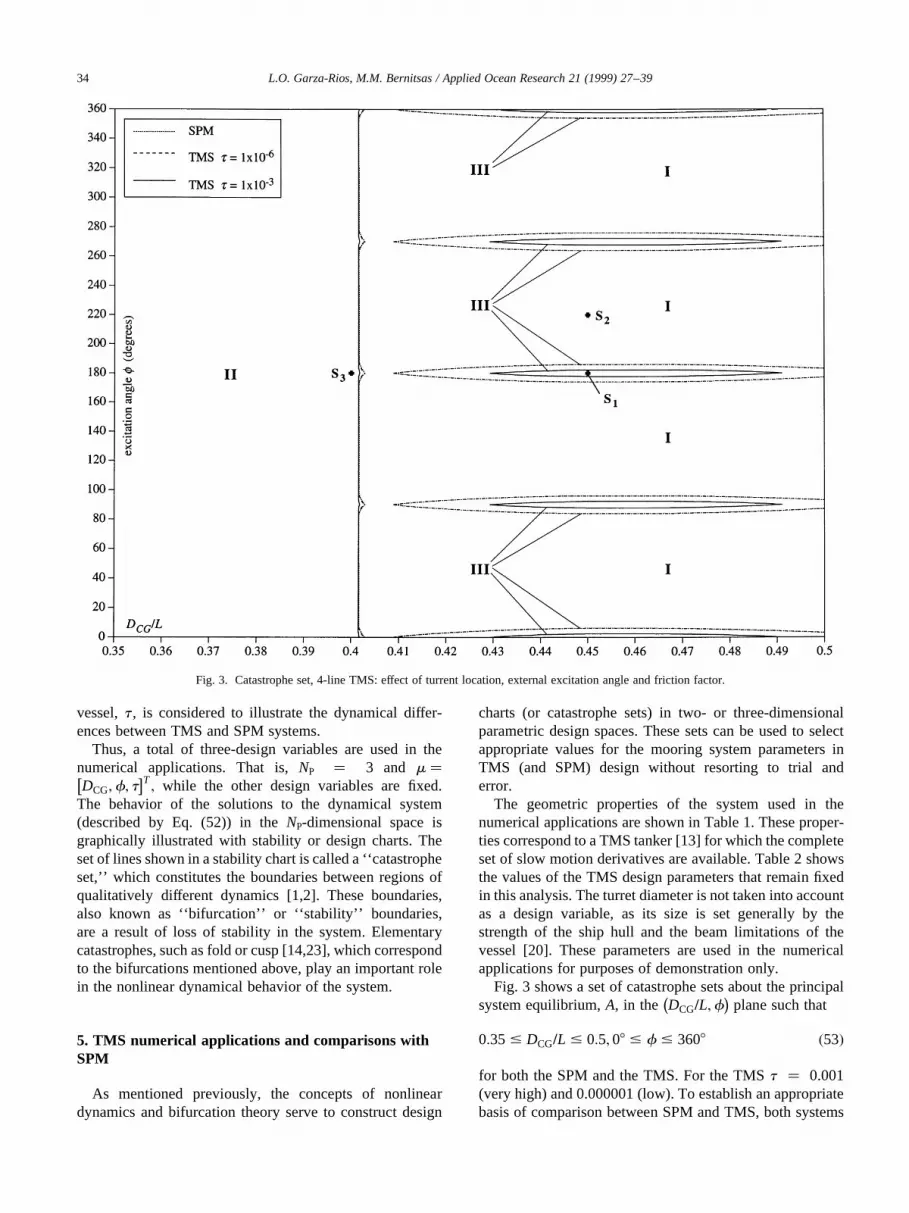
Fig. 3 shows a set of catastrophe sets about the principalsystem equilibrium,A, in the DCG=L;f

ÿ �plane such that

0:35 # DCG=L # 0:5; 08 # f # 3608 �53�

for both the SPM and the TMS. For the TMSt � 0.001(very high) and 0.000001 (low). To establish an appropriatebasis of comparison between SPM and TMS, both systems


Fig. 3. Catastrophe set, 4-line TMS: effect of turrent location, external excitation angle and friction factor.

have the same vessel hydrodynamics, mooring line model,center of gravity, added and structural mass, added andstructural second moment of inertia.

In the catastrophe sets of Fig. 3, there exist three regions(numbered I to III) of qualitatively different dynamicalbehavior.

Region I (R-I):The principal equilibrium A is stable. All eight TMS eigen-values (six in the case of SPM systems) have negative realparts and therefore equilibrium A is a stable focus. Since noother equilibria are present to attract the trajectories, all flowtrajectories converge toward equilibrium A in forward time.The resulting relative angle of attack between the orienta-tion of the system at equilibrium and the environmentalexcitation is zero.

Region II (R-II):The principal equilibrium A is unstable with a one-dimen-sional unstable manifold. One real eigenvalue has a positivereal part. Equilibrium A is an unstable node and therefore alltrajectories initiated in the vicinity of A deviate from it inforward time. A static bifurcation of the supercritical

pitchfork type [14] occurs, when crossing the bifurcationboundary from R-I and R-II, resulting in static loss ofstability with the appearance of two additional staticallystable equilibria The flow trajectories will converge to oneof these alternate equilibria depending on the initial con-ditions of the system. These new equilibria have a non-zerorelative angle of attack between the orientation of thesystem and the environmental excitation. This angleincreases as the system parameterDCG moves to the leftdeeper in R-II.

Region III (R-III):The principal equilibrium A is unstable with a two-dimen-sional unstable manifold (i.e. a complex conjugate pair ofeigenvalues with a positive real part). A dynamic bifurca-tion of the Hopf type occurs when crossing from R-I to R-III[14] resulting in dynamic loss of stability. The correspond-ing morphogenesis is the appearance of a limit cycle aroundequilibrium A.

The catastrophe sets in Fig. 3 show that qualitatively thedynamics of the TMS and SPM systems are similar in theDCG=L;fÿ �

plane. As noted in Fig. 3, the static stability of


Fig. 4. Stable limit cycle about equilibrium A: SPM and TMS (region R-III).

both systems depends primarily on the value ofDCG.Obviously, they differ quantitatively. The location of theturret (mooring lines in the SPM case) largely determineswhether or not the principal equilibrium will bifurcate tocreate two additional equilibria irrespective of the directionof the external excitation. Both SPM and TMS tend toachieve their principal weathervaning equilibrium as theturret (or location of the mooring lines) is moved forward,i.e. with increasingDCG values, as shown by stable region R-I in Fig. 3. Alternative stable equilibria (region R-II) appearas a result of moving the turret toward the center of gravityof the system. These results are in accordance with theconclusions reached by Yashima et al. [26] for large scaleexperiments on TMS. Notice that the static bifurcationsthat occur in both SPM and TMS in Fig. 3 are very similar.This characteristic of TMS’s is well captured with SPMmodels [3,6,7,17,21]. The position of the turret has impor-tant design considerations, since higher hydrodynamicforces act on the vessel when achieving a non-weather-vaning configuration.

Fig. 3 also shows that the dynamic stability for bothsystems is affected by the direction of external excitation.

Both SPM and TMS dynamics may fall in R-III achievinga stable limit cycle around equilibriumA for large valuesof DCG. This occurs for excitation angles for which thetotal projected area of the catenaries to the inflow issmaller, resulting in less damping as a result of themooring lines.

The third parameter, which corresponds to the magnitudeof the moment exerted between the turret and the vessel, isshown to alter significantly the region where dynamic lossof stability occurs. For non-zero friction coefficientt , theTMS dynamic stability increases with increasing values oft . As the friction coefficient decreases, the region of limitcycles (R-III) exhibited by the TMS approaches that of SPMsystems.

It is significant to point out that the static bifurcationboundaries (i.e. the boundary between R-I and R-II) forTMS and SPM systems do not coincide as shown in Fig.3. As the turret diameter decreases (and therefore its massdecreases), the TMS catastrophe set approaches that of theSPM system, and their bifurcation boundaries betweenregions R-I and R-II, and R-I and R-III, converge in thelimit of zero turret mass.


Fig. 5. Stable focus, equilibrium A: SPM and TMS (region R-I).

Figs. 4–6 show nonlinear time simulations of the driftanglec for the TMS and SPM system in each of the threeregions depicted in Fig. 3. To additionally demonstratesome of the differences between these types of systems,the non-dimensional friction coefficientt for the TMS inFigs. 4–6 is taken as 0.001.

Fig. 4 shows the simulation for geometry pointS1 DCG=L � 0:45;f � 1808ÿ �

; which falls in R-III in Fig. 3for both the SPM and the TMS. As anticipated from Fig. 3, itshows oscillatory behavior about the principal equilibrium.Notice that the TMS takes longer time to achieve its stablelimit cycle as compared to its SPM counterpart, and exhibitssmaller amplitude oscillations. This difference in behavioris due both to the exerted moment that exists between theturret and vessel, and the damping moment created by themooring lines as the turret rotates. This also results in lowerfrequency of oscillations for the TMS, as shown in Fig. 4.

An increase in the angle of external excitation for bothsystems (from 1808 to 2208) yields stable configurationsaround equilibriumA, as proven by the catastrophe sets ofFig. 3. This is shown in Fig. 5 for geometry pointS2 DCG=L � 0:45;f � 2208ÿ �

. Both systems align to the

direction of the external excitation in forward time (an exci-tation angle of 2208 corresponds to a drift anglec of 408).The TMS oscillations are slower with smaller amplitude.Notice that convergence to the principal equilibrium exhib-ited by the TMS is not slower than that for the SPM system.

The simulations in Fig. 6 show the effect of reducedDCG for both systems for geometry pointS3 DCG=L � 0:40;f � 1808ÿ �

. This results in an unstableprincipal equilibrium, as inferred from Fig. 3, with thetrajectories converging to stable alternative equilibria inforward time. Fig. 6 also shows slower oscillations by theTMS due to the damping moment created by the mooringlines and the friction between the turret and the vessel.Notice that in this case the TMS converges faster to itsstable equilibrium.

These differences in response between SPM and TMS canbe explained in terms of the Degree Of Stability (DOS)inherent in the system. The DOS is defined as the maximumvalue of the real parts of the system eigenvalues, and repre-sents a certain measure of minimum damping (if negative)or maximum growth rate (if positive), and therefore ameasure of stability or instability of a specific equilibrium.


Fig. 6. Stable focus, alternate equilibrium: SPM and TMS (region R-II).

In Fig. 4, where the principal equilibrium has two eigenva-lues with positive real parts, the DOS of the SPM system ishigher. In Fig. 5, the DOS for both systems is approximatelythe same, while in Fig. 6 the TMS has a higher DOS.

6. Conclusions

The mathematical model for the nonlinear slow motiondynamics of TMS presented in Section 2 includes the vesselhydrodynamics, mooring line dynamics and external excita-tion. This model is general, and it is not restricted to anyspecific application. The model takes into account the exactlocation of the mooring lines, which are attached to theturret, and the friction moment exerted as the turret rotateswith respect to the vessel. The former results in mooring linedamping moment as a result of the hydrodynamic dragcreated as the turret rotates. In analyzing TMS dynamics,these two components are often neglected, and SPM modelsare used instead. As shown in this paper, the effect of thesescomponents may not be negligible. Each of these compo-nents results in coupling of the equations of motion of thesystem and the turret.

The TMS dynamics was analyzed with the concepts ofnonlinear dynamics and bifurcation theory presented inSection 4 to construct stability or design graphs in the para-metric design space as shown in Section 5. These charts,also known as catastrophe sets, give qualitative informationregarding the TMS dynamics, and constitute the basis for adesign methodology used to select appropriate design para-meters without trial and error and lengthy nonlinear timesimulations. This design methodology has been used toillustrate the differences in qualitative behavior that TMSand SPM systems exhibit as a parameter or group of para-meters are varied.

It has been shown that, if the friction moment between theturret and the vessel is ignored, both SPM and TMS exhibitqualitatively the same dynamics in the parametric designspace described in this work. The TMS mooring line damp-ing moment (not present in SPM systems) does not affectsignificantly the qualitative behavior of the system as shownin Fig. 3, and TMS can be approximated by a SPM system.Inclusion of the friction moment in the TMS equations ofmotion could result in major differences with respect to theSPM model, particularly in the dynamic behavior of thesystem. This is shown in Fig. 3 by the expansion of unstableregion R-III, corresponding to stable limit cycle behavior.Notice that the friction moment has little effect on the staticloss of stability of the system, which is marked in Fig. 3 bythe boundary between regions R-I and R-II.

The nonlinear time simulations in Figs. 4–6 help visua-lize the effects of the friction moment and the mooring linedamping moment on the TMS. For purposes of comparisonto SPM systems, these simulations have been performedusing the same geometries. As shown in all simulations,the frequency and amplitude of oscillation of the TMS are

lower than those exhibited by the SPM systems in each case.The frequency of oscillations may interact with excitationsuch as that arising from slowly-varying drift forces.Accordingly, the fact that the SPM approximation resultsin a limit cycle of frequency different than that of the corre-sponding TMS, renders the SPM approximation invalid. Inaddition, Fig. 4 shows that the TMS takes longer to achievea stable limit cycle, while Figs. 5 and 6 show rapid conver-gence to stable equilibria with respect to the SPM system.

The friction moment between the turret and the vesselbecomes less significant as the turret diameter decreases.Mooring line damping becomes less important as the moor-ing lines are moved closer to the center of gravity of theturret. As the turret diameter decreases, the TMS tendstoward a SPM system, provided that the inertia propertiesof both types of systems are equal.

While SPM models can predict the static properties of theTMS and its associated morphogeneses, a complete TMSmodel is needed to study its complete dynamical behavior,particularly the associated bifurcations. This is important fordesign and implementation of TMS in deeper waters, wheredynamic instabilities, not captured with SPM models,become increasingly important [10].

In this work, only three design parameters have beenstudied: the location of the turret (the distance of mooringline attachment from the center of gravity for SPM systems),the direction of external excitation, and the magnitude of theexerted moment. To gain a complete understanding of TMSbehavior, it is essential to determine the effect of each para-meter on the system dynamics. This can be achieved byconstructing catastrophe sets around each equilibrium posi-tion and superposing them. This task, however, becomesdifficult in the sense that it is impossible to plot graphs inparametric spaces of dimensions higher than three. In futurework, analytical expressions for the stability/bifurcationboundaries will be derived for TMS following Garza-Riosand Bernitsas [8,9] that will help understand better thedynamics of TMS. These physics-based expressions canbe used to develop a design methodology for TMS capableof revealing TMS dependence on any number of parameterswithout the need to recur to plotting and superposing severalthree-dimensional stability charts [2].

Acknowledgements

This work is sponsored by the University of Michigan/Industry Consortium in Offshore Engineering. Industryparticipants include Amoco, Inc.; Conoco, Inc.; ExxonProduction Research; Mobil Research and Development;and Shell Oil Company.

References

[1] Bernitsas MM, Garza-Rios LO. Effect of mooring line arrangement


on the dynamics of spread mooring systems. Journal of OffshoreMechanics and Arctic Engineering 1996;118(1):7–20.

[2] Bernitsas MM, Garza-Rios LO. Mooring system design based onanalytical expressions of catastrophes of slow-motion dynamics. Jour-nal of Offshore Mechanics and Arctic Engineering 1997;119(2):86–95.

[3] Bernitsas MM, Papoulias FA. Nonlinear stability and maneuveringsimulation of single point mooring systems. Proceedings of OffshoreStation Keeping Symposium, SNAME, Houston, TX, 1990:1–19.

[4] Cox JV. Statmoor—a single point mooring static analysis program.Report No. AD-A119 979, Naval Civil Engineering Laboratory, 1982.

[5] Dercksen A, Wichers JEW. A discrete element method on chain turrettanker exposed to survival conditions. Proceedings of the Sixth Inter-national Conference on the Behaviour of Offshore Structures (BOSS),1, London, UK, 1992:238–250.

[6] Fernandes AC, Aratanha M. Classical assessment to the single pointmooring and turret dynamics stability problems. Proceedings of the15th International Conference on Offshore Mechanics and ArcticEngineering (OMAE), I-A, Florence, Italy, 1996:423–430.

[7] Fernandes AC, Sphaier S. Dynamic analysis of a FPSO system.Proceedings of the 7th International Offshore and Polar EngineeringConference (ISOPE), 1, Honolulu, HI, 1997:330–335.

[8] Garza-Rios LO, Bernitsas MM. Analytical expressions of the bifurca-tion boundaries for symmetric spread mooring systems. Journal ofApplied Ocean Research 1995;17:325–341.

[9] Garza-Rios LO, Bernitsas MM. Analytical expressions of the stabilityand bifurcation boundaries for general spread mooring systems. .Journal of Ship Research, SNAME 1996;40(4):337–350.

[10] Garza-Rios LO, Bernitsas MM. Nonlinear slow motion dynamics ofturret mooring systems in deep water. Proceedings of the Eight Inter-national Conference on the Behaviour of Offshore Structures (BOSS),2, Delft, The Netherlands, 1997:177–188.

[11] Garza-Rios LO, Bernitsas MM. Mathematical model for the slowmotion dynamics of turret mooring systems. Report to the Universityof Michigan/Sea Grant/Industry Consortium in Offshore Engineer-ing., Publication No. 336, Ann Arbor, MI, February, 1998.

[12] Garza-Rios LO, Bernitsas MM, Nishimoto K. Catenary mooring lineswith nonlinear drag and touchdown. Report to the University ofMichigan/Industry Consortium in Offshore Engineering., PublicationNo. 333, Ann Arbor, MI, January, 1997.

[13] Garza-Rios LO, Bernitsas MM, Nishimoto K, Masetti IQ. Preliminarydesign of a DICAS mooring system for the brazilian Campos basin.Proceedings of the 16th International Conference on Offshore

Mechanics and Arctic Engineering (OMAE), I-A, Yokohama,Japan, 1997:153–161.

[14] Guckenheimer J, Holmes P. Nonlinear oscillations, dynamicalsystems and bifurcations of vector fields. New York: Springer-Verlag,1983.

[15] Henery D, Inglis RB. Prospects and challenges for the FPSO.Proceedings of the 27th Offshore Technology Conference, PaperOTC-7695, 2, Houston, 1995:9–21.

[16] Laures JP, de Boom WC. Analysis of turret moored storage vessel forthe Alba field. Proceedings of the Sixth International Conference onthe Behaviour of Offshore Structures (BOSS), 1, London, UK, 1992:211–223.

[17] Leite AJP, Aranha JAP, Umeda C, De Conti MB. Current forces intankers and bifurcation of equilibrium of turret systems: hydrody-namic model and experiments. Journal of Applied Ocean Research1998;20:145–156.

[18] Mack RC, Gruy RH, Hall RA. Turret moorings for extreme designconditions. Proceedings of the 27th Offshore Technology Conference,Paper OTC-7696, 2 Houston, 1995:23–31.

[19] Martin LL. Ship maneuvering and control in wind. SNAME Transac-tions 1980;88:257–281.

[20] McClure B, Gay TA, Slagsvold L. Design of a turret-moored produc-tion system (TUMOPS), Proceedings of the 21st Offshore TechnologyConference, Paper OTC-5979, 2, Houston, 1989:213–222.

[21] Nishimoto K, Brinati HL, Fucatu CH. Dynamics of moored tankersSPM and turret., Proceedings of the 7th International Offshore andPolar Engineering Conference (ISOPE), 1, Honolulu, HI, 1997:370–378.

[22] Press WH, Flannery BP, Teukolsky SA, Vetterling WT. Numericalrecipes: the art of scientific computing. New York: CambridgeUniversity Press, 1989.

[23] Seydel R. From equilibrium to chaos. New York: Elsevier, 1988.[24] Takashina J. Ship maneuvering motion due to tugboats and its math-

ematical model. Journal of the Society of Naval Architects of Japan1986;160:93–104.

[25] Tanaka S. On the hydrodynamic forces acting on a ship at large driftangles. Journal of the West Society of Naval Architects of Japan1995;91:81–94.

[26] Yashima N, Matsunaga E, Nakamura M. A large-scale model test ofturrent mooring system for floating production storage offloading(FPSO). Proceedings of the 21st Offshore Technology Conference,Paper OTC-5980, 2, Houston, 1989:223–232.


Documents

Slow motion dynamics of turret mooring and its approximation as single point mooring