water

Article

Smart Water Infrastructures Laboratory: ReconfigurableTest-Beds for Research in Water Infrastructures Management

Jorge Val Ledesma 1,* , Rafał Wisniewski 1 and Carsten Skovmose Kallesøe 1,2

�����������������

Citation: Val Ledesma, J.;

Wisniewski, R.; Kallesøe, C.S. Smart

Water Infrastructures Laboratory:

Reconfigurable Test-Beds for

Research in Water Infrastructures

Management. Water 2021, 13, 1875.

https://doi.org/10.3390/w13131875

Academic Editors: Armando Di

Nardo, Robert Sitzenfrei

Received: 17 May 2021

Accepted: 28 June 2021

Published: 5 July 2021

Publisher’s Note: MDPI stays neutral

with regard to jurisdictional claims in

published maps and institutional affil-

iations.

Copyright: © 2021 by the authors.

Licensee MDPI, Basel, Switzerland.

This article is an open access article

distributed under the terms and

conditions of the Creative Commons

Attribution (CC BY) license (https://

creativecommons.org/licenses/by/

4.0/).

1 Control & Automation, Electronic Systems Department, Aalborg University, 9200 Aalborg, Denmark;raf@es.aau.dk (R.W.); csk@es.aau.dk or ckallesoe@grundfos.com (C.S.K.)

2 Technology Innovation, Grundfos Holding A/S. 8820 Bjerringbro, Denmark* Correspondence: jvl@es.aau.dk; Tel.: +45-50336971

Abstract: The smart water infrastructures laboratory is a research facility at Aalborg University,Denmark. The laboratory enables experimental research in control and management of water in-frastructures in a realistic environment. The laboratory is designed as a modular system that can beconfigured to adapt the test-bed to the desired network. The water infrastructures recreated in thislaboratory are district heating, drinking water supply, and waste water collection systems. This paperfocuses on the first two types of infrastructure. In the scaled-down network the researchers can repro-duce different scenarios that affect its management and validate new control strategies. This paperpresents four study-cases where the laboratory is configured to represent specific water distributionand waste collection networks allowing the researcher to validate new management solutions in asafe environment. Thus, without the risk of affecting the consumers in a real network. The outcome ofthis research facilitates the sustainable deployment of new technology in real infrastructures.

Keywords: water distribution; waste water; smart city; laboratory; test-bed; experiment; monitoring;real-time control; water management

1. Introduction1.1. Motivation

A steadily growing population that is continuously demanding increasing livingstandards puts great pressure on availability of resources including energy and water [1].The increasing demand and the need to provide it in a sustainable way challenge the urbaninfrastructures for transporting water, waste-water, and energy, leading to a need for theircontinuous development [2]. Energy savings together with renewable energy productionare environmentally friendly strategies to meet these growing demands [3].

Many water resources are wasted due to leakages in the distribution network. It isestimated that around 35% in average, and in worst case up to 70%, of produced drinkingwater is wasted in the water infrastructures, summing up to 26.7 cubic kilometres per yearin developing countries [4].

Uncontrolled sewage overflows have a severe impact on the ecosystem. The min-imisation of waste water overflows is an important goal in the utility management [5].In combined sewer systems, the rain-events are not always predicted and their uncertaintycomplicates the real-time control task [6].

In addition to the previous challenges, water utilities must ensure an adequate waterquality during its distribution. The continuous use of chemicals in extensive agricultureand industry increases the environmental pollution and threatens the sources of potable wa-ter [7]. There are other elements that can cause loss of water quality, such as bio-film growth,corrosion, water age, or stagnation. Water age is one of the major causes of deteriorationof water quality [8], and the utilities must maintain an adequate residual concentrationof disinfectant, typically chlorine, to avoid microbial and bio-film growth [9]. However,the concentration of chlorine decays in time and so does the quality of water. Other water

Water 2021, 13, 1875. https://doi.org/10.3390/w13131875 https://www.mdpi.com/journal/water

Water 2021, 13, 1875 2 of 24

distribution networks, such as WDN with clean groundwater sources, that do not rely onchlorine for disinfection, are also affected by the degradation of the water quality in time.In order to avoid the water ageing, the utility management prevents the storage of volumesof water for a long period of time.

Understanding these challenges can help preventing faults in the operation of theinfrastructures [10], for instance by helping the development of new solutions for moni-toring and management of urban water networks. The use of decision-support tools cansave time and resources to the utility management [7,11]. These control solutions canalso improve the infrastructures’ resilience to changes that threaten the operation. In thisway, interruption of service, water leakages, waste water overflow, inefficient operation,contamination, or cyber-attacks can be reduced or avoided.

Some researchers provide innovative control strategies for leakage detection [12–15],energy saving [16,17], and water quality [18] for water distribution networks. In wastewater collection, several researchers propose the use of advanced control strategies in themanagement of these infrastructures to improve their performance [19–21]. Furthermore,the transformation of urban areas to smart cities [22], concept often linked with digitali-sation and data collection, gives access to additional network information and enablesthe possibility of adopting smart management solutions [23], for example by using artificialintelligence (AI) techniques. These new solutions must be flexible such that the infras-tructure management adapts to the dynamical needs of the city. For instance, by usingthe enhanced monitoring capabilities the management can provide a response to specificweather forecast or end-user demand [24].

Although the digitalisation of these critical infrastructures with AI, wireless networksand IoT sensors considerably improve the monitoring and management of the infrastruc-ture, it can make them more vulnerable to malicious attacks including, among others,cyber-attacks [25]. Some studies have addressed the security in water systems for improv-ing the next generation of cyber-physical systems [26].

1.2. Project Objectives

The aforementioned research studies are great contributions to the modernisation ofwater infrastructures. The future development of these techniques and the deploymentof new technology in real infrastructures require of extensive validation. However, waterutilities are cautious when testing new solutions that might put the robustness of the dailyoperation at risk. There are certain scenarios that practically cannot be studied due to theirnon affordable consequences such as leakages, waste-water overflow, contamination ofwater, or interruption of the infrastructure service. The proposed methods can benefitfrom customised experimental tests that support the understanding of the problem andthe proposed solution. The need of realistic test environments that allow the validationof the control methods on different networks motivates the smart water infrastructureslaboratory (SWIL) project.

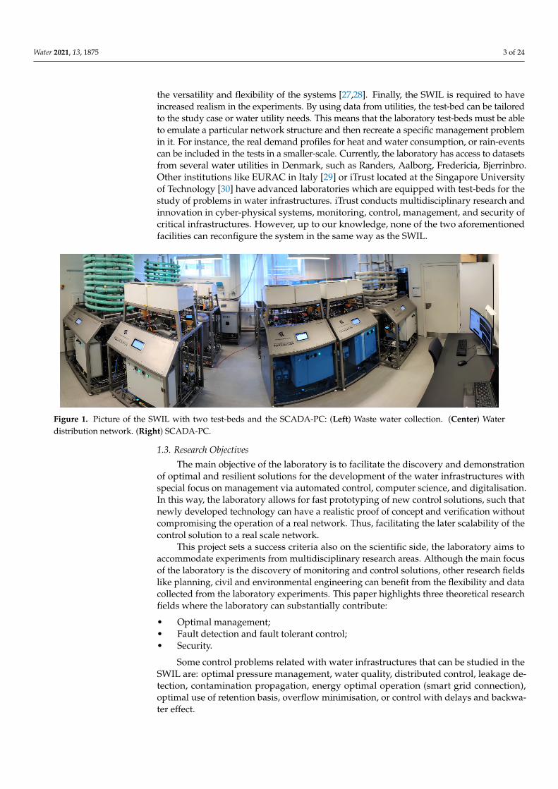
The SWIL at Aalborg University (AAU) is a facility that can replicate three types ofwater infrastructures: district heating, water supply and waste-water collection. Due to thedomain of this journal, only water distribution networks and waste water collection aredescribed in this paper, Figure 1 shows the control room of the SWIL with two test-beds.This laboratory is built around three points:

1. Build a test facility which emulates the operation of three water infrastructures;2. Flexibility to configure test-beds according to specific water networks;3. Recreate real management problems.

Firstly, the laboratory emulates the operation of several water infrastructures. Thismeans that the physical behaviour of the systems is qualitatively emulated and the real-timemonitoring and control systems are replicated. Secondly, the SWIL is required to be versatileand replicate a wide variety of water networks. For this, this project proposes a modularlaboratory which opens the possibility to replicate different topologies and network features.Modular architectures are also used in other disciplines in product development to increase

Water 2021, 13, 1875 3 of 24

the versatility and flexibility of the systems [27,28]. Finally, the SWIL is required to haveincreased realism in the experiments. By using data from utilities, the test-bed can be tailoredto the study case or water utility needs. This means that the laboratory test-beds must be ableto emulate a particular network structure and then recreate a specific management problemin it. For instance, the real demand profiles for heat and water consumption, or rain-eventscan be included in the tests in a smaller-scale. Currently, the laboratory has access to datasetsfrom several water utilities in Denmark, such as Randers, Aalborg, Fredericia, Bjerrinbro.Other institutions like EURAC in Italy [29] or iTrust located at the Singapore Universityof Technology [30] have advanced laboratories which are equipped with test-beds for thestudy of problems in water infrastructures. iTrust conducts multidisciplinary research andinnovation in cyber-physical systems, monitoring, control, management, and security ofcritical infrastructures. However, up to our knowledge, none of the two aforementionedfacilities can reconfigure the system in the same way as the SWIL.

Figure 1. Picture of the SWIL with two test-beds and the SCADA-PC: (Left) Waste water collection. (Center) Waterdistribution network. (Right) SCADA-PC.

1.3. Research Objectives

The main objective of the laboratory is to facilitate the discovery and demonstrationof optimal and resilient solutions for the development of the water infrastructures withspecial focus on management via automated control, computer science, and digitalisation.In this way, the laboratory allows for fast prototyping of new control solutions, such thatnewly developed technology can have a realistic proof of concept and verification withoutcompromising the operation of a real network. Thus, facilitating the later scalability of thecontrol solution to a real scale network.

This project sets a success criteria also on the scientific side, the laboratory aims toaccommodate experiments from multidisciplinary research areas. Although the main focusof the laboratory is the discovery of monitoring and control solutions, other research fieldslike planning, civil and environmental engineering can benefit from the flexibility and datacollected from the laboratory experiments. This paper highlights three theoretical researchfields where the laboratory can substantially contribute:

• Optimal management;• Fault detection and fault tolerant control;• Security.

Some control problems related with water infrastructures that can be studied in theSWIL are: optimal pressure management, water quality, distributed control, leakage de-tection, contamination propagation, energy optimal operation (smart grid connection),optimal use of retention basis, overflow minimisation, or control with delays and backwa-ter effect.

Water 2021, 13, 1875 4 of 24

The remainder of the paper is structured as follows: Section 2 presents the designcriteria and methods followed to develop the modular laboratory. Both hydraulic networkand the instrumentation and the data acquisition system in this laboratory are designed toreplicate the listed management problems. In Section 3 several case studies are presentedand the corresponding validation of the methods with laboratory experiments is describedfor each case. These study cases are part of the aforementioned research problem list, thispaper only gives evidence of the usefulness of the SWIL for optimal management and faulttolerant control domains. In Section 4, the results are interpreted, the laboratory contri-butions are highlighted and ideas for future projects in the laboratory are also discussed.In Section 5 the conclusions of this work are summarised.

Remark that, this document does not present a collection of control solutions forwater infrastructures. The scope of this paper is to inform about the development of a testfacility and validation methods of control solutions via laboratory tests, it demonstratesthe functionality and applicability of the modular SWIL test-beds.

2. Materials and Methods

This section presents the methods used to develop a laboratory that meets the require-ments presented in Section 1.2 and accommodates test of the research problems presentedin Section 1.3. Firstly, the module design is presented and the main components of the waterinfrastructures are identified and described by means of a mathematical model. Then,the abstraction process that encapsulates the physical effects of the network componentsinto four modules test-beds is described.

Secondly, the network design presents the factors that are considered important whenscaling-down a real network. The mathematical models are used to build a simulationframework that supports the design of the test-beds. This includes the adequate sizing ofthe pipes and the maximum capacity of the test-beds. Finally, in hardware design the dataacquisition system (DAQ), the instrumentation installed and communication architectureof the laboratory are described.

2.1. Module Design

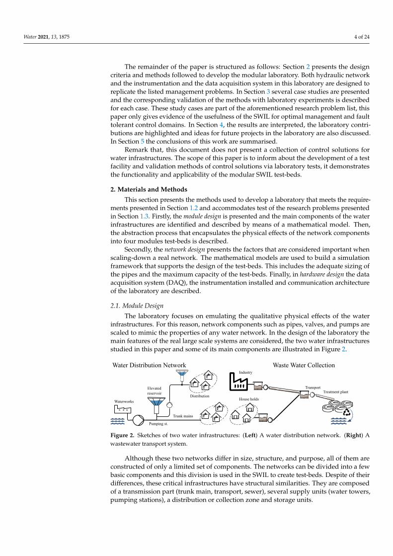
The laboratory focuses on emulating the qualitative physical effects of the waterinfrastructures. For this reason, network components such as pipes, valves, and pumps arescaled to mimic the properties of any water network. In the design of the laboratory themain features of the real large scale systems are considered, the two water infrastructuresstudied in this paper and some of its main components are illustrated in Figure 2.

Waterworks

Trunk mains

Distribution

Water Distribution Network

Treatment plant

Waste Water CollectionIndustry

Transport

House holds

Elevatedreservoir

Pumping st.

Figure 2. Sketches of two water infrastructures: (Left) A water distribution network. (Right) Awastewater transport system.

Although these two networks differ in size, structure, and purpose, all of them areconstructed of only a limited set of components. The networks can be divided into a fewbasic components and this division is used in the SWIL to create test-beds. Despite of theirdifferences, these critical infrastructures have structural similarities. They are composedof a transmission part (trunk main, transport, sewer), several supply units (water towers,pumping stations), a distribution or collection zone and storage units.

Water 2021, 13, 1875 5 of 24

Moreover, the emulated network can be easily extended by integrating additionalelements, such as tanks, consumers, suppliers, therefore, covering a wider range of testscenarios with multiple producers or interconnected networks.

The features of each infrastructure are encapsulated into five types of modules (units):A brief system description is given for each unit with mathematical models representingeach network’s main component.

2.1.1. Supply—Pumping Station/Storage

This unit has different functionalities: supply and storage. It consists of a set of pumpswhich boost the pressure in the pipe network. A model describing the pressure drop in acentrifugal pump is derived in [31]. Hence, the pump model is denoted by the polynomial

∆ppu,k = −a2q2k + a1qkω− a0ω2, (1)

where qk is the flow through the pump k, a2 > 0, a1 and a0 > 0 are constants describing thepump and ω is the rotational speed of the pump. Furthermore, the unit is equipped witha tank that can be used for water storage. The tank dynamics is given by the followingdifferential equation

Aerddt

h(t) = q(t), with h(t0) = h0, (2)

where Aer is the cross sectional area of the elevated reservoir, h is the tank level and q isthe inflow to the tank. When working as an elevated reservoir, the pressure at the elevatedreservoir node per is given by the algebraic relation,

per(t) = µ(h(t) + z) + pair, (3)

where µ is a constant scaling the water level and pressure unit and z is the elevation of thetank inlet. The air pressure pair inside the tank is locally regulated such that it emulates areal geodesic level or tower elevation z.

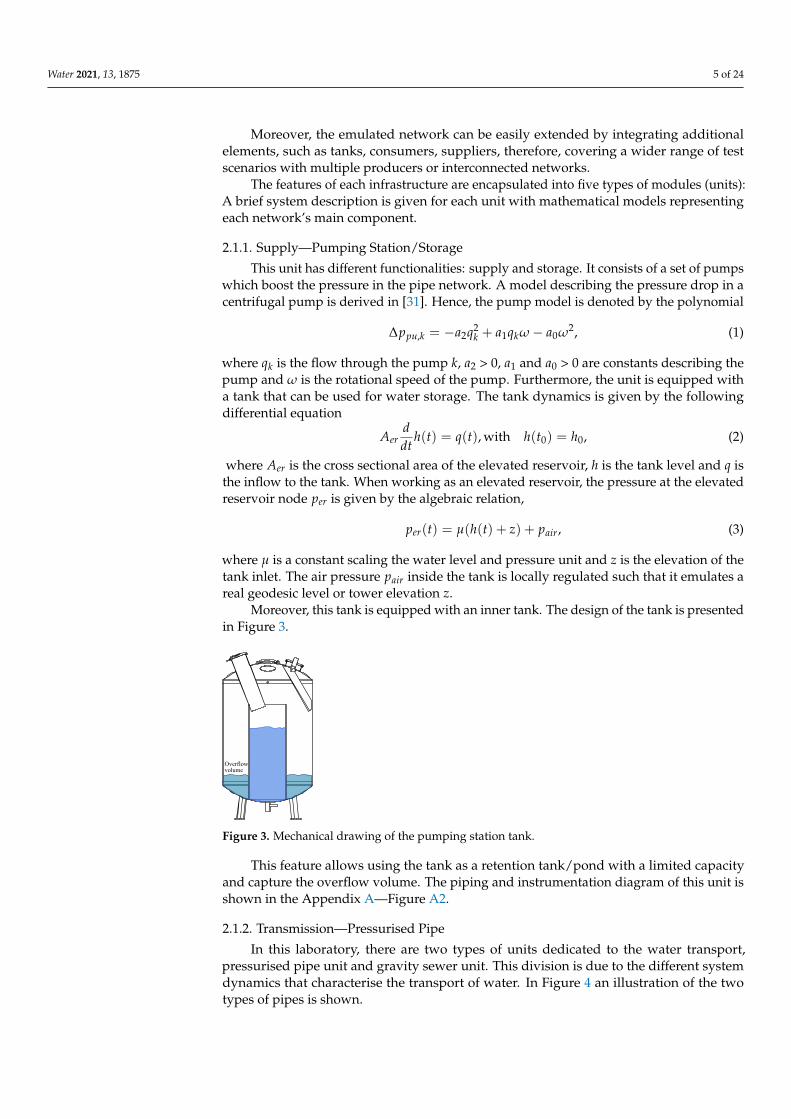
Moreover, this tank is equipped with an inner tank. The design of the tank is presentedin Figure 3.

Overflowvolume

Figure 3. Mechanical drawing of the pumping station tank.

This feature allows using the tank as a retention tank/pond with a limited capacityand capture the overflow volume. The piping and instrumentation diagram of this unit isshown in the Appendix A—Figure A2.

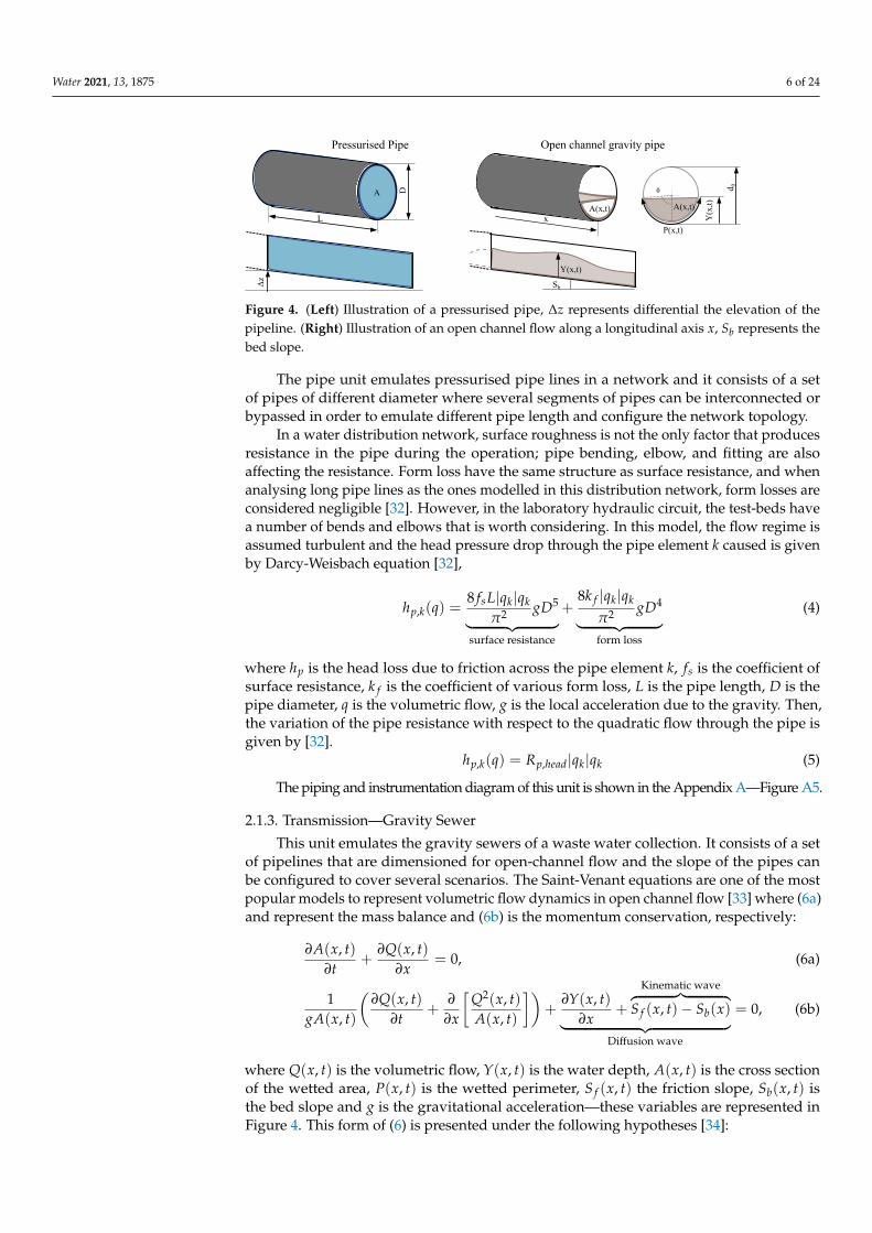
2.1.2. Transmission—Pressurised Pipe

In this laboratory, there are two types of units dedicated to the water transport,pressurised pipe unit and gravity sewer unit. This division is due to the different systemdynamics that characterise the transport of water. In Figure 4 an illustration of the twotypes of pipes is shown.

Water 2021, 13, 1875 6 of 24

P(x,t)

Y(x

,t)

Sb

d 0

Pressurised Pipe Open channel gravity pipe

Y(x,t)

LA(x,t)

A

A(x,t)

θq(t)

D

Δz

Q(x,t)

x

Figure 4. (Left) Illustration of a pressurised pipe, ∆z represents differential the elevation of thepipeline. (Right) Illustration of an open channel flow along a longitudinal axis x, Sb represents thebed slope.

The pipe unit emulates pressurised pipe lines in a network and it consists of a setof pipes of different diameter where several segments of pipes can be interconnected orbypassed in order to emulate different pipe length and configure the network topology.

In a water distribution network, surface roughness is not the only factor that producesresistance in the pipe during the operation; pipe bending, elbow, and fitting are alsoaffecting the resistance. Form loss have the same structure as surface resistance, and whenanalysing long pipe lines as the ones modelled in this distribution network, form losses areconsidered negligible [32]. However, in the laboratory hydraulic circuit, the test-beds havea number of bends and elbows that is worth considering. In this model, the flow regime isassumed turbulent and the head pressure drop through the pipe element k caused is givenby Darcy-Weisbach equation [32],

hp,k(q) =8 fsL|qk|qk

π2 gD5︸ ︷︷ ︸surface resistance

+8k f |qk|qk

π2 gD4︸ ︷︷ ︸form loss

(4)

where hp is the head loss due to friction across the pipe element k, fs is the coefficient ofsurface resistance, k f is the coefficient of various form loss, L is the pipe length, D is thepipe diameter, q is the volumetric flow, g is the local acceleration due to the gravity. Then,the variation of the pipe resistance with respect to the quadratic flow through the pipe isgiven by [32].

hp,k(q) = Rp,head|qk|qk (5)

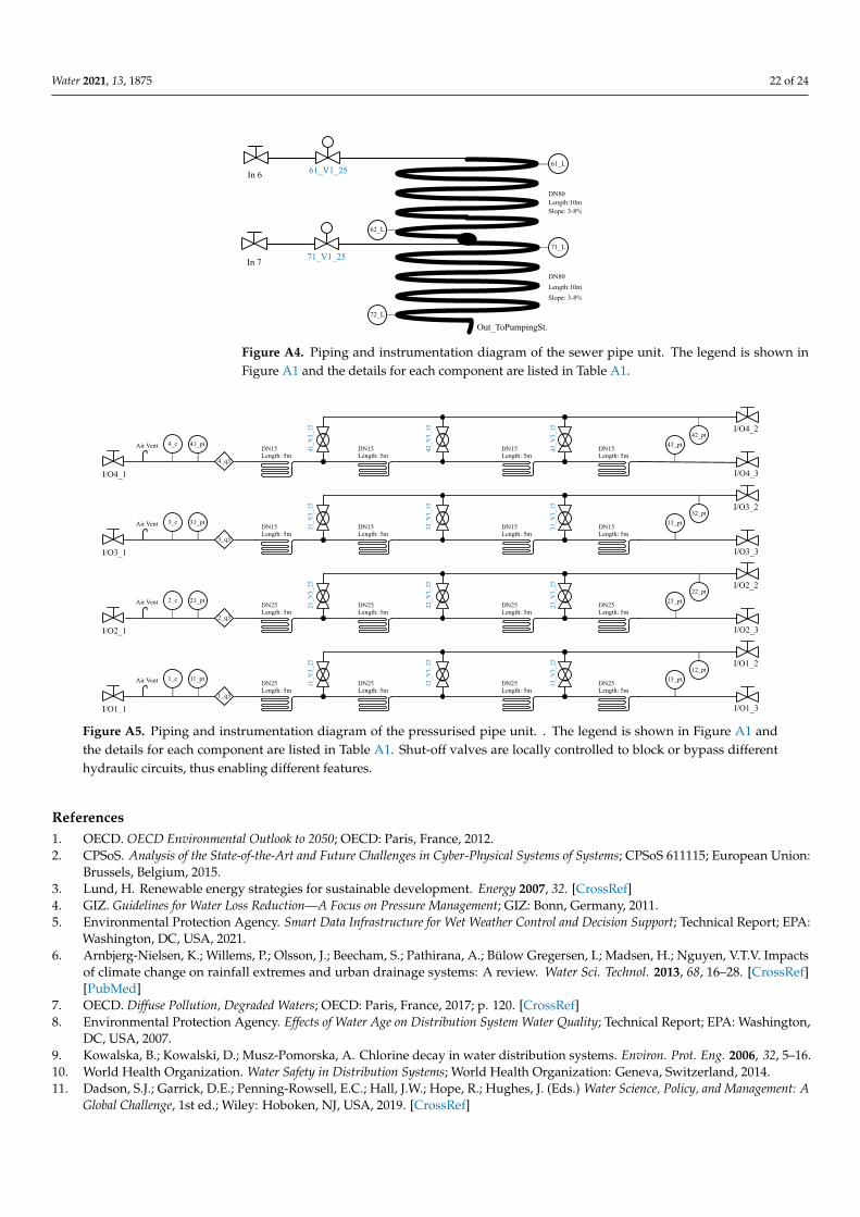
The piping and instrumentation diagram of this unit is shown in the Appendix A—Figure A5.

2.1.3. Transmission—Gravity Sewer

This unit emulates the gravity sewers of a waste water collection. It consists of a setof pipelines that are dimensioned for open-channel flow and the slope of the pipes canbe configured to cover several scenarios. The Saint-Venant equations are one of the mostpopular models to represent volumetric flow dynamics in open channel flow [33] where (6a)and represent the mass balance and (6b) is the momentum conservation, respectively:

∂A(x, t)∂t

+∂Q(x, t)

∂x= 0, (6a)

1gA(x, t)

(∂Q(x, t)

∂t+

∂

∂x

[Q2(x, t)A(x, t)

])+

∂Y(x, t)∂x

+

Kinematic wave︷ ︸︸ ︷S f (x, t)− Sb(x)︸ ︷︷ ︸

Diffusion wave

= 0, (6b)

where Q(x, t) is the volumetric flow, Y(x, t) is the water depth, A(x, t) is the cross sectionof the wetted area, P(x, t) is the wetted perimeter, S f (x, t) the friction slope, Sb(x, t) isthe bed slope and g is the gravitational acceleration—these variables are represented inFigure 4. This form of (6) is presented under the following hypotheses [34]:

Water 2021, 13, 1875 7 of 24

1. The flow is one-dimensional. The velocity is uniform over the cross-section and thewater across the section is horizontal;

2. The streamline curvature is small and vertical accelerations are negligible, hence thepressure is hydro-static;

3. The average channel bed slope is small, therefore the cosine of the angle can beapproximated to 1;

4. The variation of channel width along x is small.

The algorithms that use these simplifications can be verified in the laboratory test-beds.For the design of the laboratory sewer, a steady flow solution of Saint-Venant equationsis considered where ∂

∂t is replaced by 0 and constant water depth along the channel [34].Then, the volumetric flow Q and wetted area Aw, the equations (6) are simplified to

S f (x, t)− Sb = 0. (7)

For these operating conditions, the uniform flow in open channels can be describedby the Manning’s equation [35].

q = Aw(Kn/n)R2/3h S1/2

b , (8)

where, for this work, the cross sectional area Aw = 18 (2θ − sin(2θ))d2

0, the wetted perimeterPw = θd0, the hydraulic radius Rh = A/Pw, Kn is constant coefficient corresponding to SIunits, n is the Manning’s roughness coefficient and the bed slope is defined as Sb = arctan α.

The piping and instrumentation diagram of this unit is shown in the Appendix A—Figure A4.

2.1.4. City District—Consumer

This unit represents the end-users in a city district. The drinking water consumerconsists of a valve that regulates the consumed water and a tank that collects it, the collectedwater is used as in-feed in the waste water system. Additionally, the geodesic level of theconsumers can be emulated by introducing the equivalent air pressure in the tank.

In this project, controllable valves are used to represent the pressure drop generatedat the end-users. Each valve varies its opening degree (OD) and it allows to control thepressure drop across it. The pressure drop due to the resistance factor is proportional tothe quadratic term of the flow.

pcv,k =1

Kcv,k2 |qk|qk, (9)

where Kcv,k is the conductivity of the valve k, q is the flow through the valve and ∆p is thepressure drop over the component. Valve manufacturers provide an accurate parameterfor the controllable valve conductivity Kkv which depends on the opening degree of thevalve and relates the flow and pressure drop as shown in [36].

The piping and instrumentation diagram of this unit is shown in the Appendix A—Figure A3.

2.2. Network Design

The operation of the main components, or laboratory modules, in the water infras-tructures must be also analysed as part of a network. When working with a small scalenetwork, this analysis must consider the scaling effect, a list of the main factors consideredfor the scaling process is given in network scaling.

Then, simulations of the scaled down networks are developed based on the mathemat-ical models presented in the previous subsections [37]. The objective of these simulationsis to design the correct size of the module components and evaluate the capacity of themodules when they are interconnected through a pipe network. Furthermore, havinga simulation environment of the test-bed can support the preparation of the laboratorymodules for a given study case. For example, by choosing certain topology, pipe length ormagnitude of the signals input and disturbance signals.

Water 2021, 13, 1875 8 of 24

2.2.1. Network Scaling

In order to transform a large-scale water infrastructure into a laboratory test-bed, thisproject has performed some simplifications to reduce the network size. This size reductionis based on four factors:

• Number of nodes: The end-users that are geographically close are aggregated andthey are considered as a single consumer [38]. This node reduction does not affect theoverall network structure;

• Number of pipe types: A real pipe network contains a large amount of pipe typeswhich differ in size and material. In order to adapt the pipelines to a laboratorymodule, the piping is designed with a limited number of pipe diameters and lengths.The pipe networks at the laboratory are built with two pipe diameters for pressurisedpipes (mains and branches), and one pipe diameter for gravity pipes (sewer pipes);

• Dimensionality: The magnitude of the network pressures and flows are reduced tomeet the test-bed component requirements (sensors and actuators range). For instance,to get an idea of reduction in the magnitude, in the case of Bjerrinbro (a small waterutility) the maximum supply pressure is approximately reduced from 5 bar to 4 mand the maximum supply flow from 80 m3/h to 0.4 m3/h;

• Time scale: The scaled-down test-beds allow accelerated tests. A test that would lastseveral days in real-life can be replicated at the laboratory in hours. The tank moduleshave fixed dimensions, but its dynamics can be adjusted by varying the time scale ofthe tests.

All real networks differ in size and characteristics, and, therefore, the abstraction thattransforms any full-scale water infrastructure into a test-bed introduces an error. In orderto meet the laboratory physical limitations, an approximation of the network characteristicsis required.

When choosing a smaller size for the modules, the focus of the design is to emulatemost of the qualitative properties of a real network, such as pipe network topology, geodesiclevels, flow regimes (turbulent and open-channel flow), system delays, actuation, anddisturbance dynamics. For this reason, this study assumes that some errors introduced bythe scaling, such as exact scale friction loss in the pipe network or pressure and flow ratio,have a minor impact on the tests of control solutions, since the verification method thatthis paper proposes relies on a proof of concept validation. The scalability of the solution isnot addressed here.

2.2.2. Water Distribution Network Design

There are multiple elements that characterise a pipe network structure, such as groundlevels, pipe size, or topology [32]. Two of the most representative topologies branchedand looped geometry (ring) are illustrated in Figure 5. Next to each topology, examples ofequivalent networks constructed with laboratory modules are shown.

Branch topology network Ring topology network

Figure 5. (Left): Scheme of a standard branched topology and its laboratory equivalent. (Right):Scheme of a standard ring topology and its laboratory equivalent.

It can be observed that by changing the position of few modules, the structure and man-agement of the network are significantly changed. The test-bed in Figure 5 is transformedfrom being a branched structure with a single pumping station and elevated reservoir to aring topology with two pumping stations and an increased number of end-users.

Water 2021, 13, 1875 9 of 24

The ground levels of each urban district can be emulated by using the pressurisedtank systems at the consumer and pumping modules.

Simulation

A simulation of a WDN is built with the purpose of determining a reduced pipe sizeand the maximum capacity of the test-beds. The network structure used for this simulationis a standard WDN with an arbitrary ring topology network that connects a pumpingstation (green block) and six end-users (red blocks), see Figure 6. This network structure isinspired by the network examples studied in [32]. The capacity of this network is restrictedby the pumping station, the number of consumers and pipe size. The pumping stationand consumer operation is fixed and the length and diameter of the pipe units, mains andbranches, are adjusted accordingly to fulfil the following conditions:

• The flow regime is turbulent in all the network pipes. Then, the friction losses arecalculated with the model developed in (5);

• The total head is supplied by a set of Grundfos-UPM3 pumps, its nominal operation isaround q = 2 m3/h and ∆ppu = 0.4 bar with speed ω = 80% for each pump, see curvein Figure 7;

• A fraction of the total head loss (1/3) corresponds to friction loss (pipe), and the otherfraction (2/3) corresponds to the pressure drop at the end-users (valves).

As mentioned on Section 2.2.1, a generalisation of the structure and sizing of a pipenetwork implies the introduction of some error since the ratio between these fractions variesfrom network to network. The simulations of the reference network models are developedin modelica—Dymola. Remark that the simulation package is built with a modular structuresuch that the network topology can be easily modified.

DN15Length:20m

Consumer 2 (+1m)

DN15Length: 20m

DN15Length: 20m

DN25Length: 20m

DN15Length: 20m

DN15Length: 20m

DN15Length:20m

DN15Length: 20m

DN15Length: 20m

Consumer 1 (0m)

DN15Length:20m

DN15Length:20m

DN25Length: 40m

Pumping station (0m)

p pq q

Consumer 3 (+2.0m)q

p

pq

Figure 6. Diagram of the hydraulic network used as reference for the design of the modules with asingle pumping station and three consumer units representing aggregated end-users in a city district.

Figure 7. Graph of a pump curve extracted from the data-sheet of Grundfos-UPM3. The performanceof PWM controlled pumps is measured with A profile (heating) at eight PWM values: 5% (max.),20%, 31%, 41%, 52%, 62%, 73%, 88% (min.), PWM regulates the speed of the pumps ω.

Water 2021, 13, 1875 10 of 24

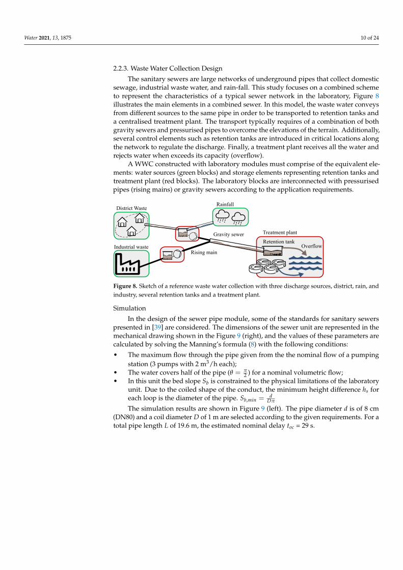
2.2.3. Waste Water Collection Design

The sanitary sewers are large networks of underground pipes that collect domesticsewage, industrial waste water, and rain-fall. This study focuses on a combined schemeto represent the characteristics of a typical sewer network in the laboratory, Figure 8illustrates the main elements in a combined sewer. In this model, the waste water conveysfrom different sources to the same pipe in order to be transported to retention tanks anda centralised treatment plant. The transport typically requires of a combination of bothgravity sewers and pressurised pipes to overcome the elevations of the terrain. Additionally,several control elements such as retention tanks are introduced in critical locations alongthe network to regulate the discharge. Finally, a treatment plant receives all the water andrejects water when exceeds its capacity (overflow).

A WWC constructed with laboratory modules must comprise of the equivalent ele-ments: water sources (green blocks) and storage elements representing retention tanks andtreatment plant (red blocks). The laboratory blocks are interconnected with pressurisedpipes (rising mains) or gravity sewers according to the application requirements.

Overflow

District WasteRainfall

Industrial wasteRetention tank

Gravity sewer

Rising main

Treatment plant

Figure 8. Sketch of a reference waste water collection with three discharge sources, district, rain, andindustry, several retention tanks and a treatment plant.

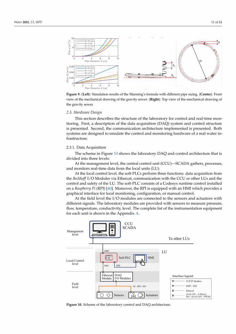
Simulation

In the design of the sewer pipe module, some of the standards for sanitary sewerspresented in [39] are considered. The dimensions of the sewer unit are represented in themechanical drawing shown in the Figure 9 (right), and the values of these parameters arecalculated by solving the Manning’s formula (8) with the following conditions:

• The maximum flow through the pipe given from the the nominal flow of a pumpingstation (3 pumps with 2 m3/h each);

• The water covers half of the pipe (θ = π2 ) for a nominal volumetric flow;

• In this unit the bed slope Sb is constrained to the physical limitations of the laboratoryunit. Due to the coiled shape of the conduct, the minimum height difference hs foreach loop is the diameter of the pipe. Sb,min = d

Dπ

The simulation results are shown in Figure 9 (left). The pipe diameter d is of 8 cm(DN80) and a coil diameter D of 1 m are selected according to the given requirements. For atotal pipe length L of 19.6 m, the estimated nominal delay toc = 29 s.

Water 2021, 13, 1875 11 of 24

D

d

Sb

hs

Figure 9. (Left): Simulation results of the Manning’s formula with different pipe sizing. (Center): Frontview of the mechanical drawing of the gravity sewer. (Right): Top view of the mechanical drawing ofthe gravity sewer.

2.3. Hardware Design

This section describes the structure of the laboratory for control and real-time mon-itoring. First, a description of the data acquisition (DAQ) system and control structureis presented. Second, the communication architecture implemented is presented. Bothsystems are designed to emulate the control and monitoring hardware of a real water in-frastructure.

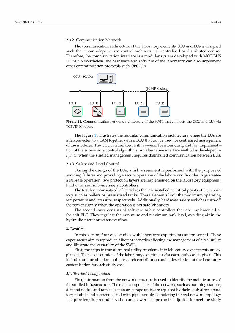
2.3.1. Data Acquisition

The scheme in Figure 10 shows the laboratory DAQ and control architecture that isdivided into three levels:

At the management level, the central control unit (CCU)—SCADA gathers, processes,and monitors real-time data from the local units (LU).

At the local control level, the soft-PLCs perform three functions: data acquisition fromthe Beckhoff I/O Modules via Ethercat, communication with the CCU or other LUs and thecontrol and safety of the LU. The soft-PLC consists of a Codesys runtime control installedon a Raspberry Pi (RPI) [40]. Moreover, the RPI is equipped with an HMI which provides agraphical interface for local monitoring, configuration, or manual control.

At the field level the I/O modules are connected to the sensors and actuators withdifferent signals. The laboratory modules are provided with sensors to measure pressure,flow, temperature, conductivity, level. The complete list of the instrumentation equipmentfor each unit is shown in the Appendix A.

To other LUs

CCU SCADA

EthercatModule

DAQ I/O Modules

Sensors Actuators

Soft PLC

Managementlevel

Local Controllevel

Fieldlevel

HMI

AI - DO / AO

Eth1

Eth0

DSI

TCP/IP Modbus

Ethercat

AI (0-10V , 4-20mA)DO / AO (0-10V / PWM)

MIPI - DSI

LU

Interface legend:

Figure 10. Scheme of the laboratory control and DAQ architecture.

Water 2021, 13, 1875 12 of 24

2.3.2. Communication Network

The communication architecture of the laboratory elements CCU and LUs is designedsuch that it can adapt to two control architectures: centralised or distributed control.Therefore, the communication interface is a modular system developed with MODBUSTCP-IP. Nevertheless, the hardware and software of the laboratory can also implementother communication protocols such OPC-UA.

CCU - SCADA

LU_41 LU_31 LU_42 LU_21 LU_22

TCP/IP Modbus

Figure 11. Communication network architecture of the SWIL that connects the CCU and LUs viaTCP/IP Modbus.

The Figure 11 illustrates the modular communication architecture where the LUs areinterconnected to a LAN together with a CCU that can be used for centralised managementof the modules. The CCU is interfaced with Simulink for monitoring and fast implementa-tion of the supervisory control algorithms. An alternative interface method is developed inPython when the studied management requires distributed communication between LUs.

2.3.3. Safety and Local Control

During the design of the LUs, a risk assessment is performed with the purpose ofavoiding failures and providing a secure operation of the laboratory. In order to guaranteea fail-safe operation, two protection layers are implemented on the laboratory equipment,hardware, and software safety controllers:

The first layer consists of safety valves that are installed at critical points of the labora-tory such as boilers or pressurised tanks. These elements limit the maximum operatingtemperature and pressure, respectively. Additionally, hardware safety switches turn-offthe power supply when the operation is not safe laboratory.

The second layer consists of software safety controllers that are implemented atthe soft-PLC. They regulate the minimum and maximum tank level, avoiding air in thehydraulic circuit or water overflow.

3. Results

In this section, four case studies with laboratory experiments are presented. Theseexperiments aim to reproduce different scenarios affecting the management of a real utilityand illustrate the versatility of the SWIL.

First, the steps to transform real utility problems into laboratory experiments are ex-plained. Then, a description of the laboratory experiments for each study case is given. Thisincludes an introduction to the research contribution and a description of the laboratorycustomisation for each study case.

3.1. Test-Bed Configuration

First, information from the network structure is used to identify the main features ofthe studied infrastructure. The main components of the network, such as pumping stations,demand nodes, and rain collection or storage units, are replaced by their equivalent labora-tory module and interconnected with pipe modules, emulating the real network topology.The pipe length, ground elevation and sewer’s slope can be adjusted to meet the study

Water 2021, 13, 1875 13 of 24

requirements while considering the laboratory restrictions, recall scaling considerations inSection 2.2.1.

The laboratory test-beds are equipped with multiple sensors and actuators, this meansthat in most studies there is redundancy of the measurements. With a vast number ofsensors it is possible to choose a subset that matches the configuration of a real system.These experiments restrict the use of the sensors according to the characteristics (numberand relative position) of the studied network.

Then, real datasets of the network operation, such as water consumption, rain-events,or industrial discharge are used to adapt the test to the given problem. Note that, the labo-ratory experiments are performed in a smaller scale, this means that the magnitude of thereal signals and time scale are adapted to meet the operation range of the test-bed.

3.2. Study Cases for Water Distribution Networks

This study case is inspired by the WDN at Bjerringbro, a small city district in Denmark,see Figure 12. This water utility has one pumping station, one elevated reservoir andmultiple end-users distributed along a pipe network. The main elements of Bjerringbro’snetwork are identified (ring topology, number of pumping stations, elevated reservoirs,consumers, and sensors), and an equivalent scaled-down network is emulated with thelaboratory modules as Figure 13 shows.

A graph with real data from this district is presented in Figure 14 as a reference of thewater distribution network operation. This utility operates with an ON/OFF controllerthat regulates the elevated reservoir level.

Pumping station

Elevated reservoir

sensor p1

sensor p2

sensor q

sensor dp

Figure 12. Map of Bjerringbro and its water distribution network scheme. Green and red blocksrepresent the main elements of the network which can be emulated with laboratory modules.

q1

pn

DN25Length:5m

q2

q3

DN25Length:5m

DN15Length:5m

DN25Length:5m

DN25Length:5m

DN25Length:5m

DN20Length:5m

DN20Length:5m

DN25Length:5mDN15

Length:5m

DN25Length:5m

DN25Length:5m

Out3 IO2.1

IO2.2

IO1.1

IO1.2In1.2 IO1.3 IO3.1

IO2.3 IO4.1 IO4.2 IO1.3

IO4.3

IO3.2

IO3.3 IO2.2

IO2.2

IO1.1

IO2.1 Out3

IO1.2 In1.1

In4

In1

Out5

Out3

In1

Out5 In4

Out3

To tank

Pump #1

Consumer #1.2

Elevated Res. #2

Consumer #1.1

Pump #2

Figure 13. Diagram of the a ring topology water distribution network that is built with laboratorymodules. This network is inspired by the structure from Figure 12.

Note that, the laboratory test-bed is equipped with an additional pumping stationwhich is not existing in the real network, this component is added with the objective ofevaluating the network management with two supply nodes.

Water 2021, 13, 1875 14 of 24

Jul 30 Aug 01 Aug 036065707580

Tank

Leve

l

Jul 30 Aug 01 Aug 030

20406080

100

Inflo

w[m

3 /h]

Jul 30 Aug 01 Aug 032

3

4

Pres

sure

[bar

]

p1 p2

Figure 14. Graphs of real data collected by Bjerringbro´s water utility. The measurement nodes arerepresented in Figure 12 and the tank filling is regulated with a standard ON/OFF control.

3.2.1. Optimal Management with Multiple Supplies in Bjerringbro

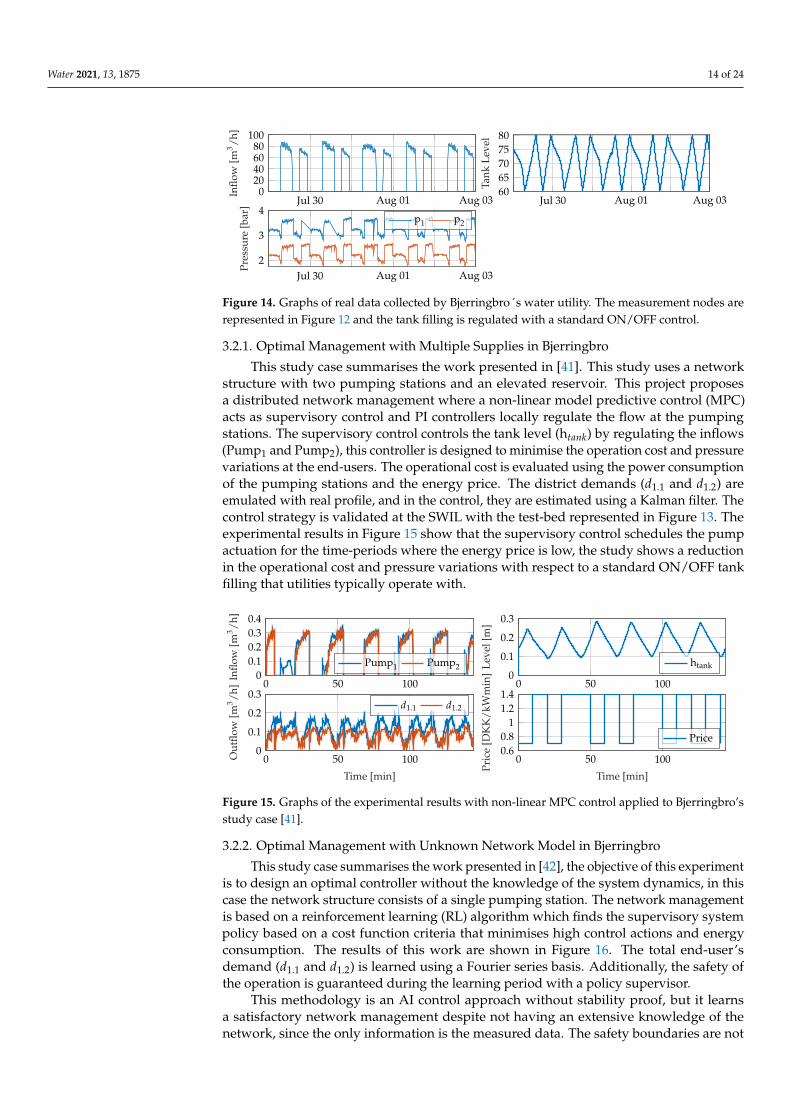
This study case summarises the work presented in [41]. This study uses a networkstructure with two pumping stations and an elevated reservoir. This project proposesa distributed network management where a non-linear model predictive control (MPC)acts as supervisory control and PI controllers locally regulate the flow at the pumpingstations. The supervisory control controls the tank level (htank) by regulating the inflows(Pump1 and Pump2), this controller is designed to minimise the operation cost and pressurevariations at the end-users. The operational cost is evaluated using the power consumptionof the pumping stations and the energy price. The district demands (d1.1 and d1.2) areemulated with real profile, and in the control, they are estimated using a Kalman filter. Thecontrol strategy is validated at the SWIL with the test-bed represented in Figure 13. Theexperimental results in Figure 15 show that the supervisory control schedules the pumpactuation for the time-periods where the energy price is low, the study shows a reductionin the operational cost and pressure variations with respect to a standard ON/OFF tankfilling that utilities typically operate with.

0 50 1000

0.10.20.30.4

Inflo

w[m

3 /h]

Pump1 Pump2

0 50 1000

0.1

0.2

0.3

Time [min]

Out

flow

[m3 /h

]

d1.1 d1.2

0 50 1000

0.1

0.2

0.3

Leve

l[m

]

htank

0 50 1000.60.8

11.21.4

Time [min]

Pric

e[D

KK

/kW

min

]

Price

Figure 15. Graphs of the experimental results with non-linear MPC control applied to Bjerringbro’sstudy case [41].

3.2.2. Optimal Management with Unknown Network Model in Bjerringbro

This study case summarises the work presented in [42], the objective of this experimentis to design an optimal controller without the knowledge of the system dynamics, in thiscase the network structure consists of a single pumping station. The network managementis based on a reinforcement learning (RL) algorithm which finds the supervisory systempolicy based on a cost function criteria that minimises high control actions and energyconsumption. The results of this work are shown in Figure 16. The total end-user’sdemand (d1.1 and d1.2) is learned using a Fourier series basis. Additionally, the safety ofthe operation is guaranteed during the learning period with a policy supervisor.

This methodology is an AI control approach without stability proof, but it learnsa satisfactory network management despite not having an extensive knowledge of thenetwork, since the only information is the measured data. The safety boundaries are not

Water 2021, 13, 1875 15 of 24

violated and the end-user’s water supply is guaranteed during the operation of the network.The laboratory experiment gives evidence of the robustness of the method, enabling thefurther investigation of AI techniques for control of real systems.

0 20 40 600

100200300400

leve

l[m

m]

Water Distribution Network

htank rtank unsafe

0 20 40 600

0.2

0.4

0.6

time [days]

Flow

[m3 /h

]

Pump1 -d1.2 -d1.1

0 20 40 60−10−8−6−4−2

0

Polic

y-K

Q-learning

0 20 40 600

20406080

100

time [days]

TD-e

rror ε

Figure 16. Graphs of the experimental results with RL control applied to Bjerringbro’s study case [42].

3.3. Study Cases for Waste Water Collection3.3.1. Optimal Management of a Treatment Plant with Inlet Flow Variations in Fredericia

This study case summarises the work presented in [43], in this work the managementof the waste water collection in Fredericia (Denmark) is studied. In this city, severalindustrial zones (red area), residential zones (blue area) and precipitations discharge wastewater to a collection network that conveys to a treatment plant, see Figure 17.

Treatment plant

Industrialzone

Residentialzone

Residentialzone

Retention tank

Level sensor

Figure 17. Map of Fredericia and its waste water collection scheme. Green and red blocks representthe main elements of the network which are emulated with laboratory modules.

The treatment plant operation is based on a chemical process that increases the per-formance when the working conditions are stable. The waste water discharges fromindustry are stochastic disturbances that have a big impact on the treatment plant’s per-formance. Therefore, the network management must regulate the inlet flow and pollutantconcentration such that their variations are minimised at the treatment plant.

This work aims to minimise the inlet flow variation by controlling the industrialdischarge, For this reason, the potential installation of a retention tank that regulates thevarying discharge using MPC is studied. The controller considers an estimation of thehousehold discharge via Kalman filter and takes into account the transport delay of thesewer network.

This scenario is reproduced in test-bed where the main components of the network arerepresented (main waste water sources, retention tank, and sewer scheme), see Figure 18.The industry and residential discharge is locally controlled to reproduce the pattern ex-tracted from real-data. Additionally, the only real-time measurement available is the sewer

Water 2021, 13, 1875 16 of 24

level at the inlet of the treatment plant, the controller in the experiments uses only onelevel sensor (72_L) to estimate the inlet flow.

61_L

72_L

DN80Length:10mSlope: 3-8%

62_L

71_L

DN80

Length:10m

Slope: 3-8%

1_dp

2_dp

L2

dp2

1_q3

DN25Length: 5m

3_q3

DN15Length: 5m

4_q3

DN15Length: 5m

Discharge flow

Residential flow

Retentiontank

Treatment plant

Water reservoir

Industry flowPump #1Consumer #1

Figure 18. Diagram of the emulated waste water collection at the SWIL.

The graph in Figure 19 shows a clear minimisation of the flow variations with respectto the non-controlled operation. The experimental results show that the installation ofa new control element in the network is feasible since it can considerably improve theoperation of a real network.

time [seconds]

Flo

w [

dm3 /m

in]

(72_L) No tank control(72_L) Control tank - filter(72_L) Control tank - raw

200 400 600 800 1000 1200 1400 160010

15

20

25

Figure 19. Graph from the experimental results of Fredericia’s study case [43]. The graph shows acomparison of the inlet flow at the treatment plant (sensor 72_L) between non-controlled industrydischarge and a controlled one with MPC.

3.3.2. Fault Tolerant Control of a Sewer Network with the Backwater Effect in IshøJ

This study case is summarises the work presented in [44]. In this work a section of thewaste water collection system in Ishøj (Denmark) is analysed, see Figure 20.

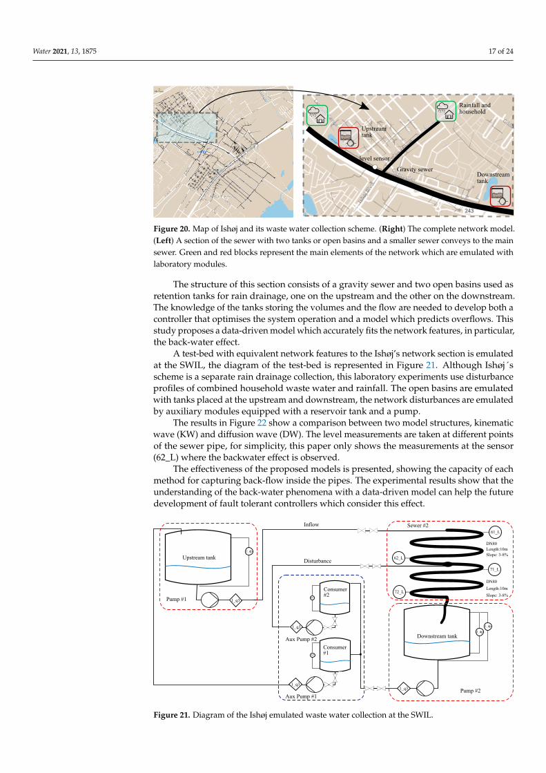
Water 2021, 13, 1875 17 of 24

Rainfall and household

Gravity sewer

Upstreamtank

Downstreamtank

level sensor

Figure 20. Map of Ishøj and its waste water collection scheme. (Right) The complete network model.(Left) A section of the sewer with two tanks or open basins and a smaller sewer conveys to the mainsewer. Green and red blocks represent the main elements of the network which are emulated withlaboratory modules.

The structure of this section consists of a gravity sewer and two open basins used asretention tanks for rain drainage, one on the upstream and the other on the downstream.The knowledge of the tanks storing the volumes and the flow are needed to develop both acontroller that optimises the system operation and a model which predicts overflows. Thisstudy proposes a data-driven model which accurately fits the network features, in particular,the back-water effect.

A test-bed with equivalent network features to the Ishøj’s network section is emulatedat the SWIL, the diagram of the test-bed is represented in Figure 21. Although Ishøj´sscheme is a separate rain drainage collection, this laboratory experiments use disturbanceprofiles of combined household waste water and rainfall. The open basins are emulatedwith tanks placed at the upstream and downstream, the network disturbances are emulatedby auxiliary modules equipped with a reservoir tank and a pump.

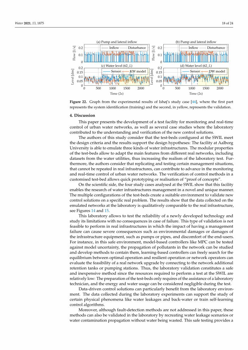
The results in Figure 22 show a comparison between two model structures, kinematicwave (KW) and diffusion wave (DW). The level measurements are taken at different pointsof the sewer pipe, for simplicity, this paper only shows the measurements at the sensor(62_L) where the backwater effect is observed.

The effectiveness of the proposed models is presented, showing the capacity of eachmethod for capturing back-flow inside the pipes. The experimental results show that theunderstanding of the back-water phenomena with a data-driven model can help the futuredevelopment of fault tolerant controllers which consider this effect.

61_L

72_L

DN80Length:10mSlope: 3-8%

62_L

71_L

DN80

Length:10m

Slope: 3-8%

1_dp

2_dp

1_q3

1_dp

dp2

dp2

Upstream tank

Downstream tank

1_q3

1_q31_q3

Aux Pump #1

Pump #1

Pump #2

Aux Pump #2

Consumer#2

Consumer#1

Sewer #2

Disturbance

Inflow

Figure 21. Diagram of the Ishøj emulated waste water collection at the SWIL.

Water 2021, 13, 1875 18 of 24

0

0.1

0.2

Flow

[l/s

]

(a) Pump and lateral inflow

Inflow Disturbance

0 500 1000 1500 20000

0.050.1

0.150.2

Time (2s)

Leve

l[dm

]

(c) Water level (62_L)

Sensor KW model

0

0.1

0.2

Flow

[l/s

]

(b) Pump and lateral inflow

Inflow Disturbance

0 500 1000 1500 20000

0.050.1

0.150.2

Time (2s)

Leve

l[dm

]

(d) Water level (62_L)

Sensor DW model

Figure 22. Graph from the experimental results of Ishøj’s study case [44], where the first partrepresents the system identification (training) and the second, in yellow, represents the validation.

4. Discussion

This paper presents the development of a test facility for monitoring and real-timecontrol of urban water networks, as well as several case studies where the laboratorycontributed to the understanding and verification of the new control solutions.

The authors of this study consider that the test-beds configured at the SWIL meetthe design criteria and the results support the design hypotheses: The facility at AalborgUniversity is able to emulate three kinds of water infrastructures. The modular propertiesof the test-beds allow to adapt the main features from different real networks, includingdatasets from the water utilities, thus increasing the realism of the laboratory test. Fur-thermore, the authors consider that replicating and testing certain management situations,that cannot be repeated in real infrastructures, can contribute to advance in the monitoringand real-time control of urban water networks. The verification of control methods in acustomised test-bed allows quick prototyping or realisation of “proof of concepts”.

On the scientific side, the four study cases analysed at the SWIL show that this facilityenables the research of water infrastructures management in a novel and unique manner.The multiple configurations of the test-beds create a suitable environment to validate newcontrol solutions on a specific real problem. The results show that the data collected on theemulated networks at the laboratory is qualitatively comparable to the real infrastructure,see Figures 14 and 15.

This laboratory allows to test the reliability of a newly developed technology andstudy its limitations with no consequences in case of failure. This type of validation is notfeasible to perform in real infrastructures in which the impact of having a managementfailure can cause severe consequences such as environmental damages or damages ofthe infrastructure equipment, such as pumps or pipes, and discomfort of the end-users.For instance, in this safe environment, model-based controllers like MPC can be testedagainst model uncertainty, the propagation of pollutants in the network can be studiedand develop methods to contain them, learning-based controllers can freely search for theequilibrium between optimal operation and resilient operation or network operators canevaluate the feasibility of a real network upgrade by connecting to the network additionalretention tanks or pumping stations. Thus, the laboratory validation constitutes a safeand inexpensive method since the resources required to perform a test at the SWIL arerelatively low: The preparation of the test-beds only requires of the assistance of a laboratorytechnician, and the energy and water usage can be considered negligible during the test.

Data-driven control solutions can particularly benefit from the laboratory environ-ment. The data collected during the laboratory experiments can support the study ofcertain physical phenomena like water leakages and back-water or train self-learningcontrol algorithms.

Moreover, although fault-detection methods are not addressed in this paper, thesemethods can also be validated in the laboratory by recreating water leakage scenarios orwater contamination propagation without water being wasted. This safe testing provides a

Water 2021, 13, 1875 19 of 24

sustainable manner of discovering new technology. The laboratory is equipped to studycontamination, it uses conductivity sensors measuring salt concentration as a proxy tocontamination sensors and a reverse osmosis unit to purify water.

Although the presented experiments satisfactorily reproduce the qualitative physicaleffects and the monitoring and management of a real water infrastructure, having scaled-down networks reduce the degree of realism. This means that the dimensionality of thetests is bounded by the number of modules available and the laboratory space, actuatorsare not ideally scaled-down and might introduce unwanted effects in the experiments andsmall networks can cause coupling between network elements.

In this work, the management scenarios are studied for each infrastructure individu-ally. However, the infrastructure interconnection can and should also be studied. Variousnetworks—water, heat, electricity—are no longer independent. Tons of water are usedduring electricity production. Vice-versa, electricity is needed for water distribution andheat production. This laboratory facility allows the study of different water networks andtheir interconnections, as well as links to the power supply and the internet. Research fieldsrelated with cyber-security and critical infrastructures can also be studied in this facility.The laboratory modules are already equipped with power meters at pumping and heatingstations to study these problems.

5. Conclusions

The development of the smart water infrastructures laboratory has been presented.Here, the design process followed to reproduce a scaled-down water network with differentmodules is summarised. The main elements and features of the water infrastructures arerepresented in the laboratory modules. The configuration of these basic components suchas pumps, tanks, or network topology are elements which characterise a network. Calcula-tions based on component models are performed to adjust the sizing of the components tothe water network properties, laboratory requirements and restrictions. The implementedDAQ system and communication interface recreate a real communication network withlocal smart-meters and controllers interconnected with a SCADA. This system has a mod-ular architecture that facilitates the expansion of the test-bed and the integration of newtechnology or management solutions.

The aforementioned case studies are examples of the many possible configurationsof the laboratory, where the SWIL demonstrates the capacity to replicate real problems inlaboratory test-beds and reproduce real management scenarios in a scaled-down network.

Author Contributions: All authors have contributed equally to this manuscript, all the authors haveread and agreed to the published version of the manuscript. All authors have read and agreed to thepublished version of the manuscript.

Funding: This research was funded by Poul Due Jensen Foundation (Grundfos Foundation).

Institutional Review Board Statement: Not applicable.

Informed Consent Statement: Not applicable.

Data Availability Statement: The datasets supporting the laboratory studies have been provided bydifferent local water utilities in Denmark: Bjerringbro vandforsyning, Fredericia vandforsyning andIshøj Forsyning.

Acknowledgments: Financial support from Poul Due Jensen Foundation (Grundfos Foundation) forthis research is gratefully acknowledged. Water utilities for sharing the network datasets. The CodesysGroup [40] contributed to the project by providing software licenses to part of the laboratory equip-ment. We are also grateful to Saruch Satishkumar Rathore, Kirsten Mølgaard, Krisztian Mark Ballafor sharing their experimental results and Tom Nørgaard Jensen for his input and advice during thedesign process of the laboratory modules. Finally, we would like to express our gratitude to the waterutilities, Bjerringbro vandforsyning, Fredericia vandforsyning and Ishøj Forsyning for providing thenetwork data.

Conflicts of Interest: The authors declare no conflicts of interest.

Water 2021, 13, 1875 20 of 24

AbbreviationsThe following abbreviations are used in this manuscript:

MDPI Multidisciplinary Digital Publishing InstituteSWIL Smart Water Infrastructure LaboratoryAAU Aalborg UniversityWDN Water Distribution NetworkWWC Waste Water CollectionMPC Model Predictive ControlRL Reinforcement LearningRPI Raspberry PiCCU Central Control UnitLU Local UnitLAN Local Area NetworkHMI Human-Machine InterfaceSCADA Supervisory Control and Data AcquisitionDAQ Data AcquisitionI/O Input /OutputOPC UA Open Platform Communication Unified ArchitecturePLC Programmable Logic ControllerPWM Pulse Width ModulationKM Kinematic ModelDM Diffusion Model

Appendix A

This appendix shows the piping and instrumentation diagrams for each of the labora-tory units with a complete list of installed components.

Table A1. List of sensors and actuators installed on the laboratory units.

Tag Type Model

#_L Sensor: Level Microsonic ZWS-15/CU/QS#_c Sensor: Conductivity GF - Type 159001730#_pt1 Sensor: Pressure and temperature Grundfos Direct Sensor RPI+T 0-1.6#_dp Sensor: Differential pressure JUMO 404382#_p2 Sensor: Pressure JUMO 404327#_q1 Sensor: Volumetric flow Festo SFAW-32#_q2 Sensor: Volumetric flow Festo SFAW-100#_q3 Sensor: Volumetric flow Endress+Hauser Proline Promag 10#_V1_15 Actuator: Valve DN 15 Belimo LQR24A-SR+R2015-1-S1#_V3_25 Actuator: Valve DN 25 Bürkert 8804SV1 Actuator: Valve Danfoss EV210B+BE024DSP# Actuator: Pump Grundfos UPM3 25-75-130Aircontrol Actuator: Air Control Festo: VPPE

Water 2021, 13, 1875 21 of 24

Check valveManual ball valve

Automatic shut-off valve

Controllable valve Tank

Pressurised pipe

Gravity pipe Controllable pump

Sensor

Flow sensor

Safety levelsensor

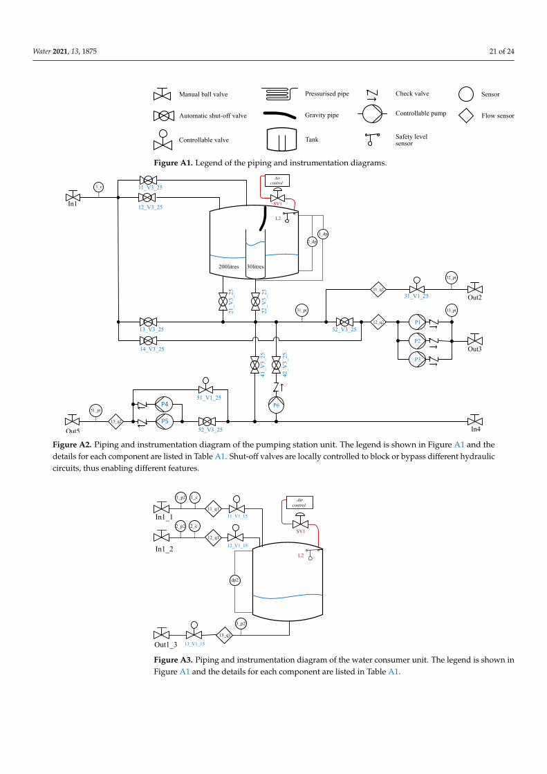
Figure A1. Legend of the piping and instrumentation diagrams.

11_q2

In1

Out3

P1

P2

P3

32_V3_2513_V3_25

14_V3_25

12_V3_25

51_V1_25

In4Out5

P4

P5

P6

21_V3_25

22_V3_25

41_V3_25

42_V3_25

52_V3_25

31_V1_25 Out2

11_V3_25

SV1

L2

Air control

31_pt

51_pt

33_pt

32_pt

13_q2

12_q2

1_c

1_dp

2_dp

200litres 30litres

Figure A2. Piping and instrumentation diagram of the pumping station unit. The legend is shown in Figure A1 and thedetails for each component are listed in Table A1. Shut-off valves are locally controlled to block or bypass different hydrauliccircuits, thus enabling different features.

11_V1_15

12_V1_15

SV1

L2

Air control

In1_1

In1_2

Out1_3 13_V1_15

1_p2 1_c

2_p2 2_c

12_q1

11_q1

13_q1

dp2

3_p2

Figure A3. Piping and instrumentation diagram of the water consumer unit. The legend is shown inFigure A1 and the details for each component are listed in Table A1.

Water 2021, 13, 1875 22 of 24

61_L

72_L

In 6

In 7

DN80Length:10mSlope: 3-8%

61_V1_25

71_V1_25

62_L

71_L

DN80

Length:10m

Slope: 3-8%

Out_ToPumpingSt.

Figure A4. Piping and instrumentation diagram of the sewer pipe unit. The legend is shown inFigure A1 and the details for each component are listed in Table A1.

DN15Length: 5m

Air Vent

I/O4_2

41_V

3_15

42_V

3_15

43_V

3_15

42_pt

4_q3

43_ptDN15Length: 5m

DN15Length: 5m

DN15Length: 5m

41_pt

I/O4_3I/O4_1

4_c

DN15Length: 5m

Air Vent

I/O3_2

31_V

3_15

32_V

3_15

33_V

3_15

32_pt

3_q3

33_ptDN15Length: 5m

DN15Length: 5m

DN15Length: 5m

31_pt

I/O3_3I/O3_1

3_c

DN25Length: 5m

Air Vent

I/O2_2

21_V

3_25

22_V

3_25

23_V

3_25

22_pt

2_q3

23_ptDN25Length: 5m

DN25Length: 5m

DN25Length: 5m

21_pt

I/O2_3I/O2_1

2_c

DN25Length: 5m

Air Vent

I/O1_2

11_V

3_25

12_V

3_25

13_V

3_25

12_pt

1_q3

13_ptDN25Length: 5m

DN25Length: 5m

DN25Length: 5m

11_pt

I/O1_3I/O1_1

1_c

Figure A5. Piping and instrumentation diagram of the pressurised pipe unit. . The legend is shown in Figure A1 andthe details for each component are listed in Table A1. Shut-off valves are locally controlled to block or bypass differenthydraulic circuits, thus enabling different features.

References1. OECD. OECD Environmental Outlook to 2050; OECD: Paris, France, 2012.2. CPSoS. Analysis of the State-of-the-Art and Future Challenges in Cyber-Physical Systems of Systems; CPSoS 611115; European Union:

Brussels, Belgium, 2015.3. Lund, H. Renewable energy strategies for sustainable development. Energy 2007, 32. [CrossRef]4. GIZ. Guidelines for Water Loss Reduction—A Focus on Pressure Management; GIZ: Bonn, Germany, 2011.5. Environmental Protection Agency. Smart Data Infrastructure for Wet Weather Control and Decision Support; Technical Report; EPA:

Washington, DC, USA, 2021.6. Arnbjerg-Nielsen, K.; Willems, P.; Olsson, J.; Beecham, S.; Pathirana, A.; Bülow Gregersen, I.; Madsen, H.; Nguyen, V.T.V. Impacts

of climate change on rainfall extremes and urban drainage systems: A review. Water Sci. Technol. 2013, 68, 16–28. [CrossRef][PubMed]

7. OECD. Diffuse Pollution, Degraded Waters; OECD: Paris, France, 2017; p. 120. [CrossRef]8. Environmental Protection Agency. Effects of Water Age on Distribution System Water Quality; Technical Report; EPA: Washington,

DC, USA, 2007.9. Kowalska, B.; Kowalski, D.; Musz-Pomorska, A. Chlorine decay in water distribution systems. Environ. Prot. Eng. 2006, 32, 5–16.10. World Health Organization. Water Safety in Distribution Systems; World Health Organization: Geneva, Switzerland, 2014.11. Dadson, S.J.; Garrick, D.E.; Penning-Rowsell, E.C.; Hall, J.W.; Hope, R.; Hughes, J. (Eds.) Water Science, Policy, and Management: A

Global Challenge, 1st ed.; Wiley: Hoboken, NJ, USA, 2019. [CrossRef]

Water 2021, 13, 1875 23 of 24

12. Adedeji, K.B.; Hamam, Y.; Abu-Mahfouz, A.M. Impact of Pressure-Driven Demand on Background Leakage Estimation in WaterSupply Networks. Water 2019, 11, 1600. [CrossRef]

13. Bosco, C.; Campisano, A.; Modica, C.; Pezzinga, G. Application of Rehabilitation and Active Pressure Control Strategies forLeakage Reduction in a Case-Study Network. Water 2020, 12, 2215. [CrossRef]

14. Wu, Z.; Sage, P. Pressure dependent demand optimization for leakage detection in water distribution systems. In WaterManagement Challenges in Global Change; Taylor & Francis: Oxfordshire, UK, 2007; pp. 353–361.

15. Morosini, A.F.; Veltri, P.; Costanzo, F.; Savic, D. Identification of leakages by calibration of WDS models. Procedia Eng. 2014,70, 660–667. [CrossRef]

16. Jensen, T.; Kallesøe, C. Application of a Novel Leakage Detection Framework for Municipal Water Supply on AAU Water SupplyLab. In Proceedings of the 2016 3rd Conference on Control and Fault-Tolerant Systems (SysTol), Barcelona, Spain, 7–9 Septemer2016; IEEE: Piscataway, NJ, USA, 2016; pp. 428–433. [CrossRef]

17. Bendtsen, J.; Val, J.; Kallesøe, C.; Krstic, M. Control of District Heating System with Flow-dependent Delays. IFAC-PapersOnLine2017, 50, 13612–13617. [CrossRef]

18. Sakomoto, T.; Lutaaya, M.; Abraham, E. Managing Water Quality in Intermittent Supply Systems: The Case of Mukono Town,Uganda. Water 2020, 12, 806. [CrossRef]

19. García, L.; Barreiro-Gomez, J.; Escobar, E.; Téllez, D.; Quijano, N.; Ocampo-Martinez, C. Modeling and real-time control of urbandrainage systems: A review. Adv. Water Resour. 2015, 85, 120–132. [CrossRef]

20. Mollerup, A.; Mikkelsen, P.; Sin, G. A methodological approach to the design of optimising control strategies for sewer systems.Environ. Model. Softw. 2016, 83, 103–115. [CrossRef]

21. Lund, N.; Falk, A.K.; Borup, M.; Madsen, H.; Mikkelsen, P. Model predictive control of urban drainage systems: A review andperspective towards smart real-time water management. Crit. Rev. Environ. Sci. Technol. 2018, 48, 1–61. [CrossRef]

22. Roche, S.; Nabian, N.; Kloeckl, K.; Ratti, C. Are ‘Smart Cities’ Smart Enough? In Spatially Enabling Government, Industry andCitizens: Research Development and Perspectives; GSDI Association Press: Needham, MA, USA, 2012; pp. 215–236.

23. Eggimann, S.; Mutzner, L.; Wani, O.; Schneider, M.; Spuhler, D.; Moy de Vitry, M.; Beutler, P.; Maurer, M. The Potential ofKnowing More: A Review of Data-Driven Urban Water Management. Environ. Sci. Technol. 2017, 51. [CrossRef] [PubMed]

24. Kerkez, B.; Gruden, C.; Lewis, M.; Montestruque, L.; Quigley, M.; Wong, B.; Bedig, A.; Kertesz, R.; Braun, T.; Cadwalader, O.; et al.Smarter Stormwater Systems. Environ. Sci. Technol. 2016, 50. [CrossRef]

25. Nikolopoulos, D.; Ostfeld, A.; Salomons, E.; Makropoulos, C. Resilience Assessment of Water Quality Sensor Designs underCyber-Physical Attacks. Water 2021, 13, 647. [CrossRef]

26. Tuptuk, N.; Hazell, P.; Watson, J.; Hailes, S. A Systematic Review of the State of Cyber-Security in Water Systems. Water 2021,13, 81. [CrossRef]

27. Madsen, O.; Møller, C. The AAU Smart Production Laboratory for Teaching and Research in Emerging Digital ManufacturingTechnologies. Procedia Manuf. 2017, 9, 106–112. [CrossRef]

28. Aicher, T.; Regulin, D.; Schütz, D.; Lieberoth-Leden, C.; Spindler, M.; Günthner, W.; Vogel-Heuser, B. Increasing flexibility ofmodular automated material flow systems: A meta model architecture. IFAC-PapersOnLine 2016, 49, 1543–1548. [CrossRef]

29. Eurac. Eurac Research, Ifrastructure Labs. 1992. Available online: http://www.eurac.edu (accessed on 14 April 2019).30. iTrust. Itrust—Singapore University of Technology and Design. 2017. Available online: https://itrust.sutd.edu.sg/ (accessed on

14 April 2019).31. Kallesøe, C. Fault Detection and Isolation in Centrifugal Pumps. Ph.D. Thesis, Aalborg University, Aalborg Øst, Denmark, 2005.32. Swamee, P.K.; Sharma, A.K. Design of Water Supply Pipe Networks; Wiley: Hoboken, NJ, USA, 2008. [CrossRef]33. Schuetze, M.; Butler, D.; Beck, M. Modelling, Simulation and Control of Urban Wastewater Systems; Springer: Berlin/Heidelberg,

Germany, 2002. [CrossRef]34. Litrico, X.; Fromion, V. Modeling and Control of Hydrosystems; Springer: Berlin/Heidelberg, Germany, 2009.35. Te Chow, V. Open Channel Hydraulics; McGraw-Hill International Book Company: New York, NY, USA, 1982.36. Boysen, H. kv: What, Why, How, Whence?; Technical Paper; Danfoss A/S: Nordborg, Denmark, 2009. Available online: https:

//assets.danfoss.com/documents/90621/AC026186467824en-010201.pdf (accessed on 4 July 2021).37. Val, J. GitHub repository, SWIL. 2021. Available online: https://github.com/jvledesma/SWIL (accessed on 26 March 2021).38. Maschler, T.; Savic, D.A. Simplification of Water Supply Network Models through Linearisation; Technical Report 99/01; University of

Exeter: Exeter, UK, 1999.39. Bizier, P. (Ed.) Gravity Sanitary Sewer Design and Construction; ASCE manuals and reports on engineering practice; American

Society of Civil Engineers: Reston, VA, USA, 2007.40. 3S-Smart Software Solutions GmbH. CODESYS V3.5 SP14. Available online: https://www.codesys.com (accessed on

19 December 2018).41. Rathore, S.S. Nonlinear Optimal Control in Water Distribution Network. Master’s Thesis, Aalborg University, Aalborg,

Denmark, 2020.42. Val, J.; Wisniewski, R.; Kallesøe, C. Safe Reinforcement Learning Control for Water Distribution Networks. In Proceedings of the

Conference on Control Technology and Applications, San Diego, CA, USA, 8–11 August 2021; IEEE: Piscataway, NJ, USA, 2021.

Water 2021, 13, 1875 24 of 24

43. Nielsen, K.; Pedersen, T.; Kallesøe, C.; Andersen, P.; Mestre, L.; Murigesan, P. Control of Sewer Flow Using a Buffer Tank. InProceedings of the 17th International Conference on Informatics in Control, Automation and Robotics, Paris, France, 7–9 July 2020;pp. 63–70. [CrossRef]

44. Balla, K.; Knudsen, C.; Hodzic, A.; Bendtsen, J.; Kallesøe, C. Nonlinear Grey-box Identification of Gravity-driven Sewer Networkswith the Backwater Effect. In Proceedings of the Conference on Control Technology and Applications, San Diego, VA, USA,8–11 August 2021; IEEE: Piscataway, NJ, USA, 2021.