Embed Size (px)
Citation preview
sustainability
Article
Smart Water Quality Monitoring System Design andKPIs Analysis: Case Sites of Fiji Surface Water
K. A. Mamun 1, F. R. Islam 2,*, R. Haque 2 , M. G. M. Khan 3 , A. N. Prasad 1, H. Haqva 1,R. R. Mudliar 1 and F. S. Mani 4
1 School of Engineering and Physics, The University of the South Pacific, Suva, Fiji;[email protected] (K.A.M.); [email protected] (A.N.P.); [email protected] (H.H.);[email protected] (R.R.M.)
2 School of Science and Engineering, University of the Sunshine Coast, Queensland 4556, Australia;[email protected]
3 School of Computing, Information and Mathematical Sciences, The University of the South Pacific, Suva, Fiji;[email protected]
4 School of Biological and Chemical Sciences, The University of the South Pacific, Suva, Fiji;[email protected]
* Correspondence: [email protected]
Received: 22 August 2019; Accepted: 6 December 2019; Published: 11 December 2019
Abstract: Over recent years, waters in and around Fiji has increasingly succumbed to a reasonable levelof contamination. Water quality is defined with set of standards that clearly state the parameters ofdifferent properties in water. These standards are different at various geographic locations. The specificquantitative values of these parameters for the Fiji Islands are established by the Fiji National DrinkingWater Quality Standards (FNDWQS). Fiji is geographically located in the vast Pacific Ocean, andrequires a data collection framework for different water parameters to monitor water quality. The GISframework system can effectively solve this continuously in real-time. With the end goal being toquantify different parameters; four (04) key performance indicators (KPI) are identified: Temperature,potential of hydrogen (pH), Oxidation Reduction Potential (ORP), and Conductivity. This paperpresents a Smart Water Quality Monitoring System (SWQMS) which has been developed and deployedin five (05) Fijian locations (nodes) for the aforementioned KPIs measurement. The SWQMS interfacedwith GIS and were powered using solar based Renewable Energy Source (REs). Finally, obtaineddata were tested and analyzed using statistical methods and verified comparing with the FNDWQS.The findings demonstrated that the system is capable of delivering an accurate and consistentmeasurement of water quality in real-time. Hence SWQMS could be a smart choice for various PacificIsland Countries (PICs) to use to monitor the water quality and in turn develop sustainable citiesand societies.
Keywords: GIS; sensor data; water quality; pacific region; renewable energy; sustainable cities
1. Introduction
Environmental and ecological changes have put various marine species at risk of exterminationand poses a real threat to biodiversity. Several species in coastal areas are vulnerable to climatechange and environmental pollution. Similar circumstances are also applicable for human beings.Frequent monitoring and observation of various water parameters are required to maintain the highwater quality levels that are necessary for living beings. An appropriate range for various waterparameters can be identified as a key performance indicator (KPI), for the water quality, particularlyfor a geographic location [1–3]. Water is an unavoidable requirement of livelihood for billions of
Sustainability 2019, 11, 7110; doi:10.3390/su11247110 www.mdpi.com/journal/sustainability
Sustainability 2019, 11, 7110 2 of 21
people all over the world, due to industrialization, the massive growth in population, excessive useof chemicals for agricultural activities, reclamation of land, and oil spillage into the water, and it isbeing contaminated at an alarming rate which is now a matter of concern. Therefore, it is important tomonitor and test water quality real-time on a regular basis to take necessary steps in order to reducewater pollution and control the quality of water whenever it is necessary. The accessibility of qualitywater is essential for disease control and for enhancing health.
Natural impurities caused by weathering and the decay of marine organisms and variousmanmade activities introduce impurities in the water, like iron, lead, chromium, and even radioactiveuranium [4,5]. A set of standards for both surface and drinking water which are established andregulated by the authority of a country, clearly state the limits of the potential of hydrogen (pH),dissolved oxygen (DO), alkalinity, ORP, conductivity, and salinity to maintain a high quality of water.Standards are different from country to country due to differing geographical locations [6]; however, astandard is not yet well established for Fiji. Henceforward, it is necessary to classify and define theexact values of the parameters for various sources of water available here in Fiji, and this case studywill partially address this issue. The Fiji National Drinking Water Quality Standards (FNDWQS) [3]state that the frequency of measurement for water parameters of the local water supply occur be on adaily basis, which is currently being conducted using portable/mobile testing tools or by the watersamples being brought to a central laboratory test water quality parameters, which is obviously not aconvenient method. The islands are scattered and therefore there is a need for a robust monitoringdevice that could provide real-time data and inform stakeholders of any undesired activities impactingon water quality.
The experiment in this research setup has been carried out in Fiji’s capital city (Suva) and Sigatoka,due to locality and ease of access. The challenges that lead to the development of such technologiesmainly involve the availability of resources in remote places. To conduct water testing in islandswith the present situation and technology available here in this country is quite challenging as thesamples need to be brought in every hour or two and have analysis performed on them in Suva. In Fiji,there are not many such technologies or devices available that can investigate the quality of waterbeing supplied to each household. While, people can use water filters as a precaution to ensure safehealth, this is an expensive approach for persons with normal middle incomes, so the major sources ofdrinking water in Fiji are either bore-hole or supplied tap water. The Water Authority of Fiji (WAF)normally performs the water quality test before the water is pumped out to the consumers, but thereare still uncertainties regarding the water quality on the consumer end side.
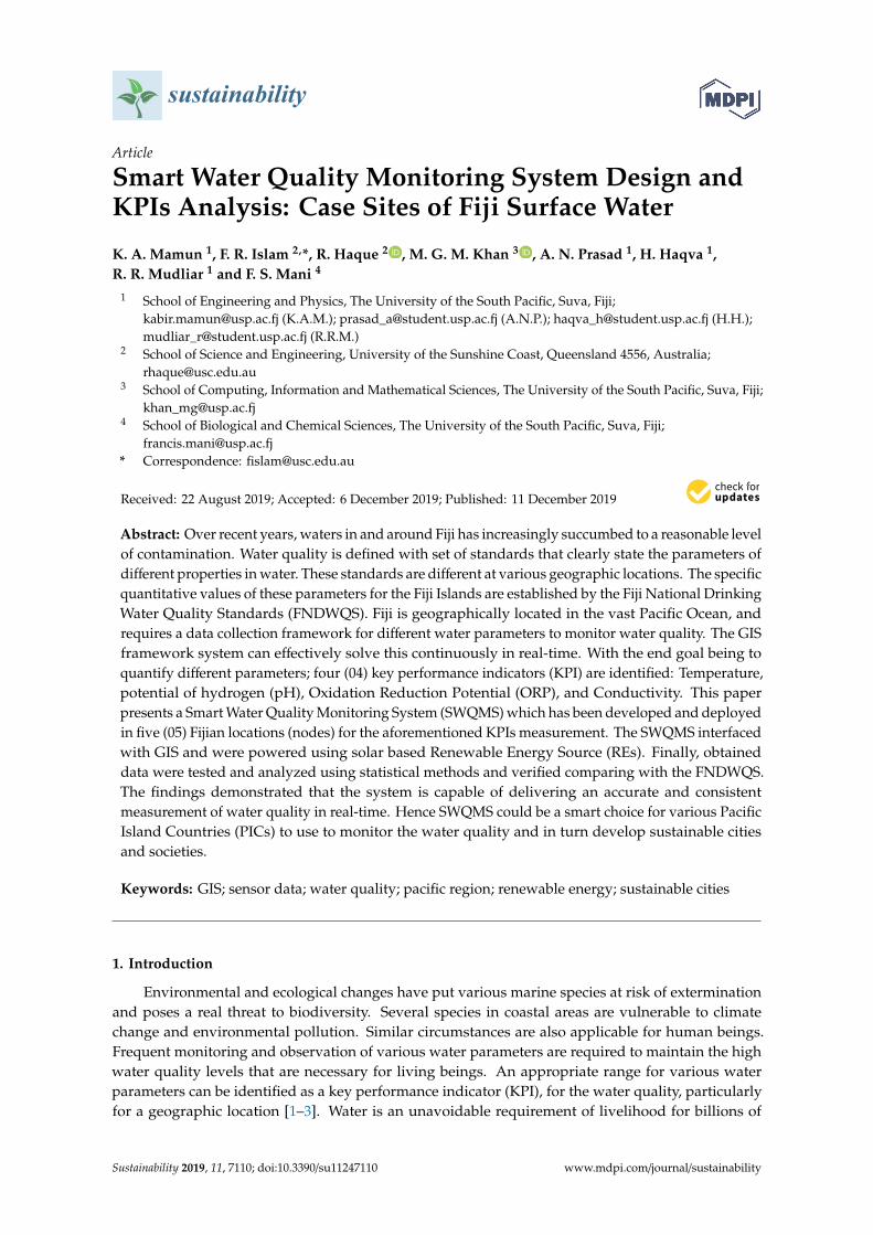
Accordingly, there is a requirement for further improvement of a network based, automated,real-time water quality measurement system that can deliver instant information of the local waterquality and also help in controlling the quality of water for different applications ranging fromaquaculture farmhouses and coastlines to articulated reservoirs. The proposed system in this researchhas been designed based on Internet of Things (IoT) [7] integrated with a wireless sensor network that isnot only able to sense various water quality parameter remotely but also able to investigate and providewater quality KPIs information in real-time progressively utilizing GIS. The fundamental objective ofthis GIS integration and sensor-based water monitoring system is the automation of the measurementof the KPIs [8] of surface water, resulting in improved reliability and performance. This systemwill further simplify the respective tasks involved by the various interested parties (i.e., the Waterand Environment Management Authority) within the scope of water quality management [9–12].This proposed system enables automated measurement of KPIs at various sites at regular intervalsto have reliable quality assurance. Moreover, this sensor-based GIS integrated Smart Water QualityMonitoring System (SWQMS) helps to monitor water quality from a central workbench and providesaccess to the information whenever required by the various respective stake holders. Figure 1 showsthe schematic of the SWQMS working principle for the experimental setup used here in Fiji to monitorsurface water quality during this case study.
Sustainability 2019, 11, 7110 3 of 21
The structure of this article is as follows: Section 2 introduce the KPIs modeling for a specificwater quality monitoring system, in Section 3 the proposed SWQMS is illustrated in detail, Section 4presents the GIS interface design, results and discussion are presented in Section 5, and lastly Section 6presents the conclusion.Sustainability 2019, 11, x FOR PEER REVIEW 3 of 21
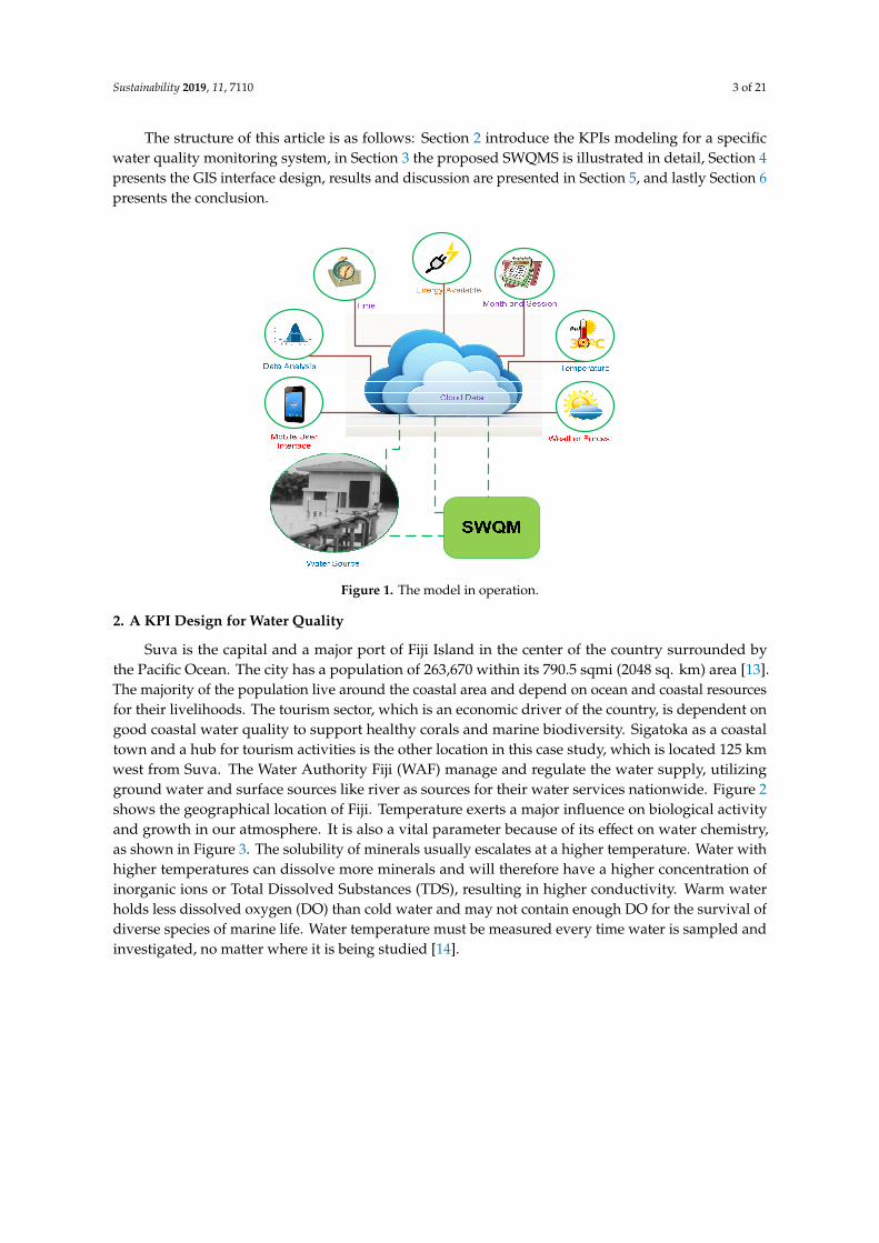
Figure 1. The model in operation.
2. A KPI Design for Water Quality
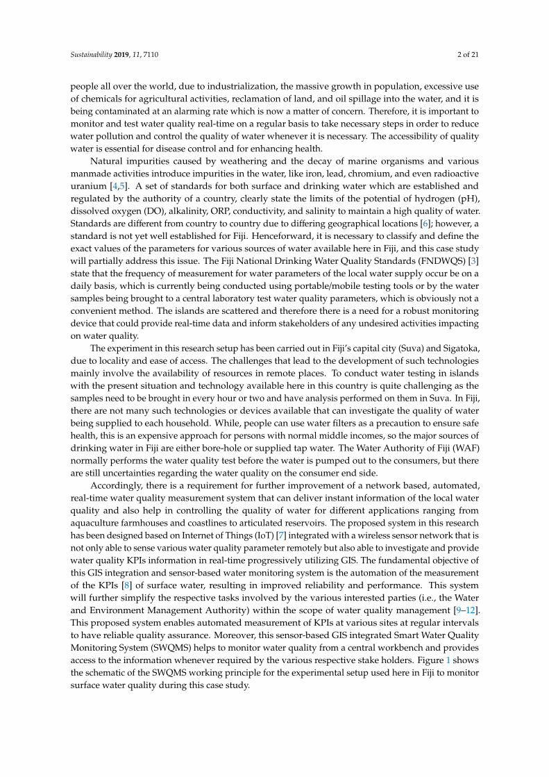
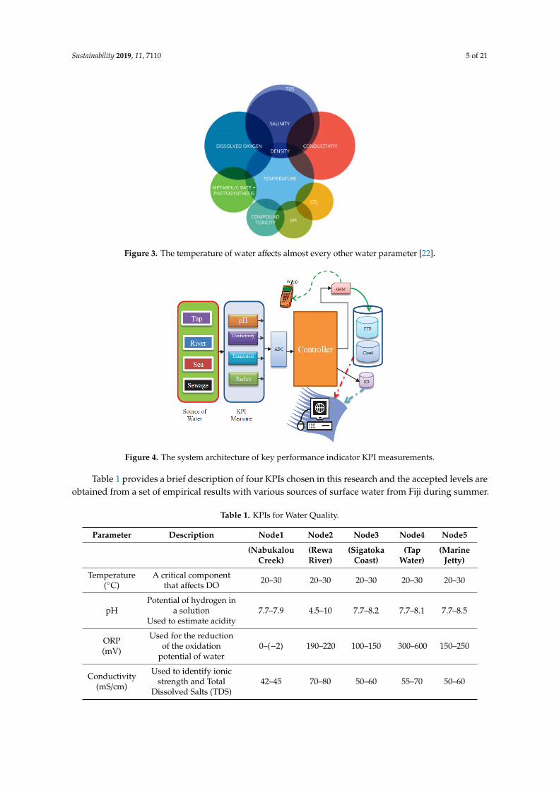
Suva is the capital and a major port of Fiji Island in the center of the country surrounded by the Pacific Ocean. The city has a population of 263,670 within its 790.5 sqmi (2048 sq. km) area [13]. The majority of the population live around the coastal area and depend on ocean and coastal resources for their livelihoods. The tourism sector, which is an economic driver of the country, is dependent on good coastal water quality to support healthy corals and marine biodiversity. Sigatoka as a coastal town and a hub for tourism activities is the other location in this case study, which is located 125 km west from Suva. The Water Authority Fiji (WAF) manage and regulate the water supply, utilizing ground water and surface sources like river as sources for their water services nationwide. Figure 2 shows the geographical location of Fiji. Temperature exerts a major influence on biological activity and growth in our atmosphere. It is also a vital parameter because of its effect on water chemistry, as shown in Figure 3. The solubility of minerals usually escalates at a higher temperature. Water with higher temperatures can dissolve more minerals and will therefore have a higher concentration of inorganic ions or Total Dissolved Substances (TDS), resulting in higher conductivity. Warm water holds less dissolved oxygen (DO) than cold water and may not contain enough DO for the survival of diverse species of marine life. Water temperature must be measured every time water is sampled and investigated, no matter where it is being studied [14].
Commonly used basic water quality monitoring parameters are temperature, pH, conductivity, turbidity, and DO [15]. DO is the free oxygen in water necessary to sustain life. However, any increase in the microbial decomposition of organic matter in water bodies due to pollution leads to DO depletion. Oxidation-reduction potential (ORP) is measured in addition to DO as there are other chemical elements apart from oxygen that affect the oxidative capacity of rivers and lakes and provide additional information on the water quality and the degree of pollution. ORP is a measure of reducing or oxidizing potential that governs the biochemical processes in water and is an important monitoring parameter in drinking water and waste water processes and applications. ORP measurements are an indication of some oxidation- reduction reactions such as the corrosion of distribution pipes in drinking water systems, precipitation of iron and manganese compounds, nitrification and denitrification reactions, and microbial disinfection. ORP measurements are becoming a widespread parameter to monitor disinfection through chlorination in drinking water, and show that ORP is affected by pH as well [16]. There is a strong positive correlation between DO and ORP, and higher values create an optimum environment for nitrogen removal and enhanced microbial activity to break down organic matter [17]. It is apparent that for water quality monitoring,
Figure 1. The model in operation.
2. A KPI Design for Water Quality
Suva is the capital and a major port of Fiji Island in the center of the country surrounded bythe Pacific Ocean. The city has a population of 263,670 within its 790.5 sqmi (2048 sq. km) area [13].The majority of the population live around the coastal area and depend on ocean and coastal resourcesfor their livelihoods. The tourism sector, which is an economic driver of the country, is dependent ongood coastal water quality to support healthy corals and marine biodiversity. Sigatoka as a coastaltown and a hub for tourism activities is the other location in this case study, which is located 125 kmwest from Suva. The Water Authority Fiji (WAF) manage and regulate the water supply, utilizingground water and surface sources like river as sources for their water services nationwide. Figure 2shows the geographical location of Fiji. Temperature exerts a major influence on biological activityand growth in our atmosphere. It is also a vital parameter because of its effect on water chemistry,as shown in Figure 3. The solubility of minerals usually escalates at a higher temperature. Water withhigher temperatures can dissolve more minerals and will therefore have a higher concentration ofinorganic ions or Total Dissolved Substances (TDS), resulting in higher conductivity. Warm waterholds less dissolved oxygen (DO) than cold water and may not contain enough DO for the survival ofdiverse species of marine life. Water temperature must be measured every time water is sampled andinvestigated, no matter where it is being studied [14].
Sustainability 2019, 11, 7110 4 of 21
Sustainability 2019, 11, x FOR PEER REVIEW 4 of 21
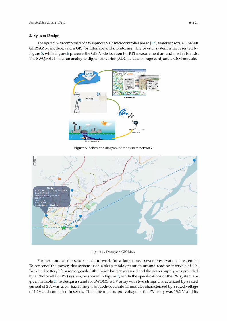
DO, ORP, and pH should be measured in conjunction. DO measures “residual oxygen” which is instantaneously available at a short period of time. However, ORP measures a kind of cumulative longer-term potential value. So for a continuous measurement, ORP is a much more reliable parameter to avoid any mislaid interpretation from the long-term measurement value of DO. To categorize the water quality pH, conductivity and ORP have been considered as important parameters in this research and were selected as KPIs for the comparison. Afterwards, a quality level is established to determine whether the water sample is polluted or non-polluted with the specific KPI range for the tested water samples. DO could be included in the suite of measurements in future, as there are additional channels that could be utilized. However, for the current measurements, the sites chosen such as Sigatoka, Rewa River, and Nabukalou Creek in Suva are all subjected to wastewater discharge, and perhaps ORP would be a better indicator for industrial and wastewater pollution. Figure 4 shows the schematic system architecture of the proposed SWQMS. FNDWQS [3,18], defined the pH ranges from 6.5 to 8.5 for drinking water with a temperature of 4 °C. However, since the SWQMS system of this research works in real-time, therefore the temperature is used as a dynamic parameter which is directly co-related to the other KPIs. The first essential task was to identify the water parameters that can provide an indication of water contamination through an extensive review and research [19,20]; the parameters were selected to be composed of pH, ORP, conductivity, and temperature.
Figure 2. Position of the Fiji Islands in the Pacific Ocean [21].
Figure 3. The temperature of water affects almost every other water parameter [22].
Figure 2. Position of the Fiji Islands in the Pacific Ocean [21].
Commonly used basic water quality monitoring parameters are temperature, pH, conductivity,turbidity, and DO [15]. DO is the free oxygen in water necessary to sustain life. However, any increasein the microbial decomposition of organic matter in water bodies due to pollution leads to DOdepletion. Oxidation-reduction potential (ORP) is measured in addition to DO as there are otherchemical elements apart from oxygen that affect the oxidative capacity of rivers and lakes and provideadditional information on the water quality and the degree of pollution. ORP is a measure of reducingor oxidizing potential that governs the biochemical processes in water and is an important monitoringparameter in drinking water and waste water processes and applications. ORP measurements are anindication of some oxidation- reduction reactions such as the corrosion of distribution pipes in drinkingwater systems, precipitation of iron and manganese compounds, nitrification and denitrificationreactions, and microbial disinfection. ORP measurements are becoming a widespread parameterto monitor disinfection through chlorination in drinking water, and show that ORP is affected bypH as well [16]. There is a strong positive correlation between DO and ORP, and higher valuescreate an optimum environment for nitrogen removal and enhanced microbial activity to break downorganic matter [17]. It is apparent that for water quality monitoring, DO, ORP, and pH should bemeasured in conjunction. DO measures “residual oxygen” which is instantaneously available at ashort period of time. However, ORP measures a kind of cumulative longer-term potential value. So fora continuous measurement, ORP is a much more reliable parameter to avoid any mislaid interpretationfrom the long-term measurement value of DO. To categorize the water quality pH, conductivity andORP have been considered as important parameters in this research and were selected as KPIs forthe comparison. Afterwards, a quality level is established to determine whether the water sampleis polluted or non-polluted with the specific KPI range for the tested water samples. DO couldbe included in the suite of measurements in future, as there are additional channels that could beutilized. However, for the current measurements, the sites chosen such as Sigatoka, Rewa River,and Nabukalou Creek in Suva are all subjected to wastewater discharge, and perhaps ORP wouldbe a better indicator for industrial and wastewater pollution. Figure 4 shows the schematic systemarchitecture of the proposed SWQMS. FNDWQS [3,18], defined the pH ranges from 6.5 to 8.5 fordrinking water with a temperature of 4 C. However, since the SWQMS system of this research worksin real-time, therefore the temperature is used as a dynamic parameter which is directly co-relatedto the other KPIs. The first essential task was to identify the water parameters that can provide anindication of water contamination through an extensive review and research [19,20]; the parameterswere selected to be composed of pH, ORP, conductivity, and temperature.
Sustainability 2019, 11, 7110 5 of 21
Sustainability 2019, 11, x FOR PEER REVIEW 4 of 21
DO, ORP, and pH should be measured in conjunction. DO measures “residual oxygen” which is instantaneously available at a short period of time. However, ORP measures a kind of cumulative longer-term potential value. So for a continuous measurement, ORP is a much more reliable parameter to avoid any mislaid interpretation from the long-term measurement value of DO. To categorize the water quality pH, conductivity and ORP have been considered as important parameters in this research and were selected as KPIs for the comparison. Afterwards, a quality level is established to determine whether the water sample is polluted or non-polluted with the specific KPI range for the tested water samples. DO could be included in the suite of measurements in future, as there are additional channels that could be utilized. However, for the current measurements, the sites chosen such as Sigatoka, Rewa River, and Nabukalou Creek in Suva are all subjected to wastewater discharge, and perhaps ORP would be a better indicator for industrial and wastewater pollution. Figure 4 shows the schematic system architecture of the proposed SWQMS. FNDWQS [3,18], defined the pH ranges from 6.5 to 8.5 for drinking water with a temperature of 4 °C. However, since the SWQMS system of this research works in real-time, therefore the temperature is used as a dynamic parameter which is directly co-related to the other KPIs. The first essential task was to identify the water parameters that can provide an indication of water contamination through an extensive review and research [19,20]; the parameters were selected to be composed of pH, ORP, conductivity, and temperature.
Figure 2. Position of the Fiji Islands in the Pacific Ocean [21].
Figure 3. The temperature of water affects almost every other water parameter [22]. Figure 3. The temperature of water affects almost every other water parameter [22].Sustainability 2019, 11, x FOR PEER REVIEW 5 of 21
Figure 4. The system architecture of key performance indicator KPI measurements.
Table 1 provides a brief description of four KPIs chosen in this research and the accepted levels are obtained from a set of empirical results with various sources of surface water from Fiji during summer.
Table 1. KPIs for Water Quality.
Parameter Description Node1 Node2 Node3 Node4 Node5
(Nabukalou
Creek) (Rewa River)
(Sigatoka Coast)
(Tap Water) (Marine Jetty)
Temperature
(°C)
A critical component that affects DO
20–30 20–30 20–30 20–30 20–30
pH Potential of hydrogen in
a solution∇ Used to estimate acidity
7.7–7.9 4.5–10 7.7–8.2 7.7–8.1 7.7–8.5
ORP∇ (mV)
Used for the reduction of the oxidation
potential of water 0–(−2) 190–220 100–150 300–600 150–250
Conductivity∇
(mS/cm)
Used to identify ionic strength and Total
Dissolved Salts (TDS) 42–45 70–80 50–60 55–70 50–60
3. System Design
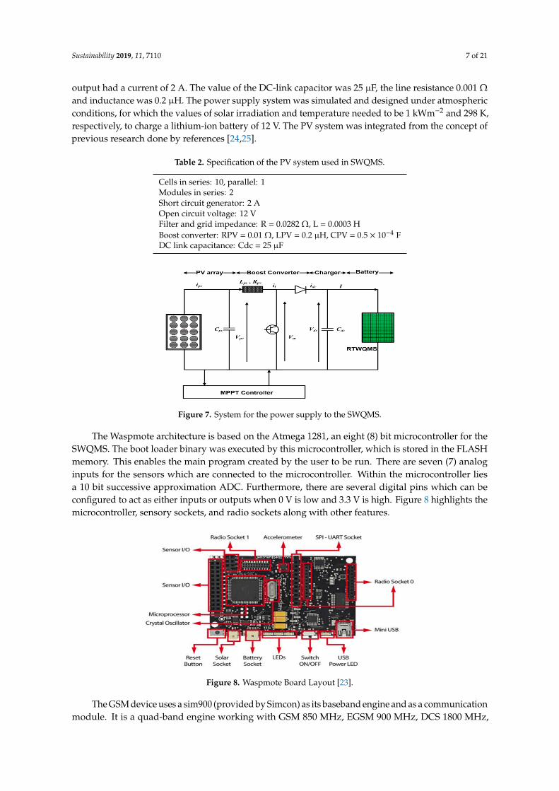
The system was comprised of a Waspmote V1.2 microcontroller board [23], water sensors, a SIM-900 GPRS/GSM module, and a GIS for interface and monitoring. The overall system is represented by Figure 5, while Figure 6 presents the GIS Node location for KPI measurement around the Fiji Islands. The SWQMS also has an analog to digital converter (ADC), a data storage card, and a GSM module.
Figure 4. The system architecture of key performance indicator KPI measurements.
Table 1 provides a brief description of four KPIs chosen in this research and the accepted levels areobtained from a set of empirical results with various sources of surface water from Fiji during summer.
Table 1. KPIs for Water Quality.
Parameter Description Node1 Node2 Node3 Node4 Node5
(NabukalouCreek)
(RewaRiver)
(SigatokaCoast)
(TapWater)
(MarineJetty)
Temperature(C)
A critical componentthat affects DO 20–30 20–30 20–30 20–30 20–30
pHPotential of hydrogen in
a solutionUsed to estimate acidity
7.7–7.9 4.5–10 7.7–8.2 7.7–8.1 7.7–8.5
ORP(mV)
Used for the reductionof the oxidation
potential of water0–(−2) 190–220 100–150 300–600 150–250
Conductivity(mS/cm)
Used to identify ionicstrength and Total
Dissolved Salts (TDS)42–45 70–80 50–60 55–70 50–60
Sustainability 2019, 11, 7110 6 of 21
3. System Design
The system was comprised of a Waspmote V1.2 microcontroller board [23], water sensors, a SIM-900GPRS/GSM module, and a GIS for interface and monitoring. The overall system is represented byFigure 5, while Figure 6 presents the GIS Node location for KPI measurement around the Fiji Islands.The SWQMS also has an analog to digital converter (ADC), a data storage card, and a GSM module.Sustainability 2019, 11, x FOR PEER REVIEW 6 of 21
Environment
Sensor
RF 868
MHz
BaseMapsWi-Fi/3G
Figure 5. Schematic diagram of the system network.
Figure 6. Designed GIS Map.
Furthermore, as the setup needs to work for a long time, power preservation is essential. To conserve the power, this system used a sleep mode operation around reading intervals of 1 h. To extend battery life, a rechargeable Lithium-ion battery was used and the power supply was provided by a Photovoltaic (PV) system, as shown in Figure 7, while the specifications of the PV system are given in Table 2. To design a stand for SWQMS, a PV array with two strings characterized by a rated current of 2 A was used. Each string was subdivided into 11 modules characterized by a rated voltage of 1.2V and connected in series. Thus, the total output voltage of the PV array was 13.2 V, and its output had a current of 2 A. The value of the DC-link capacitor was 25 μF, the line resistance 0.001 Ω and inductance was 0.2 μH. The power supply system was simulated and designed under atmospheric conditions, for which the values of solar irradiation and temperature needed to be 1 kWm−2 and 298 K, respectively, to charge a lithium-ion battery of 12 V. The PV system was integrated from the concept of previous research done by references [24,25].
Figure 5. Schematic diagram of the system network.
Sustainability 2019, 11, x FOR PEER REVIEW 6 of 21
Environment
Sensor
RF 868
MHz
BaseMapsWi-Fi/3G
Figure 5. Schematic diagram of the system network.
Figure 6. Designed GIS Map.
Furthermore, as the setup needs to work for a long time, power preservation is essential. To conserve the power, this system used a sleep mode operation around reading intervals of 1 h. To extend battery life, a rechargeable Lithium-ion battery was used and the power supply was provided by a Photovoltaic (PV) system, as shown in Figure 7, while the specifications of the PV system are given in Table 2. To design a stand for SWQMS, a PV array with two strings characterized by a rated current of 2 A was used. Each string was subdivided into 11 modules characterized by a rated voltage of 1.2V and connected in series. Thus, the total output voltage of the PV array was 13.2 V, and its output had a current of 2 A. The value of the DC-link capacitor was 25 μF, the line resistance 0.001 Ω and inductance was 0.2 μH. The power supply system was simulated and designed under atmospheric conditions, for which the values of solar irradiation and temperature needed to be 1 kWm−2 and 298 K, respectively, to charge a lithium-ion battery of 12 V. The PV system was integrated from the concept of previous research done by references [24,25].
Figure 6. Designed GIS Map.
Furthermore, as the setup needs to work for a long time, power preservation is essential.To conserve the power, this system used a sleep mode operation around reading intervals of 1 h.To extend battery life, a rechargeable Lithium-ion battery was used and the power supply was providedby a Photovoltaic (PV) system, as shown in Figure 7, while the specifications of the PV system aregiven in Table 2. To design a stand for SWQMS, a PV array with two strings characterized by a ratedcurrent of 2 A was used. Each string was subdivided into 11 modules characterized by a rated voltageof 1.2V and connected in series. Thus, the total output voltage of the PV array was 13.2 V, and its
Sustainability 2019, 11, 7110 7 of 21
output had a current of 2 A. The value of the DC-link capacitor was 25 µF, the line resistance 0.001 Ωand inductance was 0.2 µH. The power supply system was simulated and designed under atmosphericconditions, for which the values of solar irradiation and temperature needed to be 1 kWm−2 and 298 K,respectively, to charge a lithium-ion battery of 12 V. The PV system was integrated from the concept ofprevious research done by references [24,25].
Table 2. Specification of the PV system used in SWQMS.
Cells in series: 10, parallel: 1Modules in series: 2Short circuit generator: 2 AOpen circuit voltage: 12 VFilter and grid impedance: R = 0.0282 Ω, L = 0.0003 HBoost converter: RPV = 0.01 Ω, LPV = 0.2 µH, CPV = 0.5 × 10⁻⁴ FDC link capacitance: Cdc = 25 µF
Sustainability 2019, 11, x FOR PEER REVIEW 7 of 21
Table 2. Specification of the PV system used in SWQMS.
Cells in series: 10, parallel: 1 Modules in series: 2 Short circuit generator: 2 A Open circuit voltage: 12 V Filter and grid impedance: R = 0.0282 Ω, L = 0.0003 H Boost converter: RPV = 0.01 Ω, LPV = 0.2 μH, CPV = 0.5 × 10⁻⁴ F DC link capacitance: Cdc = 25 μF
Figure 7. System for the power supply to the SWQMS.
The Waspmote architecture is based on the Atmega 1281, an eight (8) bit microcontroller for the SWQMS. The boot loader binary was executed by this microcontroller, which is stored in the FLASH memory. This enables the main program created by the user to be run. There are seven (7) analog inputs for the sensors which are connected to the microcontroller. Within the microcontroller lies a 10 bit successive approximation ADC. Furthermore, there are several digital pins which can be configured to act as either inputs or outputs when 0 V is low and 3.3 V is high. Figure 8 highlights the microcontroller, sensory sockets, and radio sockets along with other features.
Figure 8. Waspmote Board Layout [23].
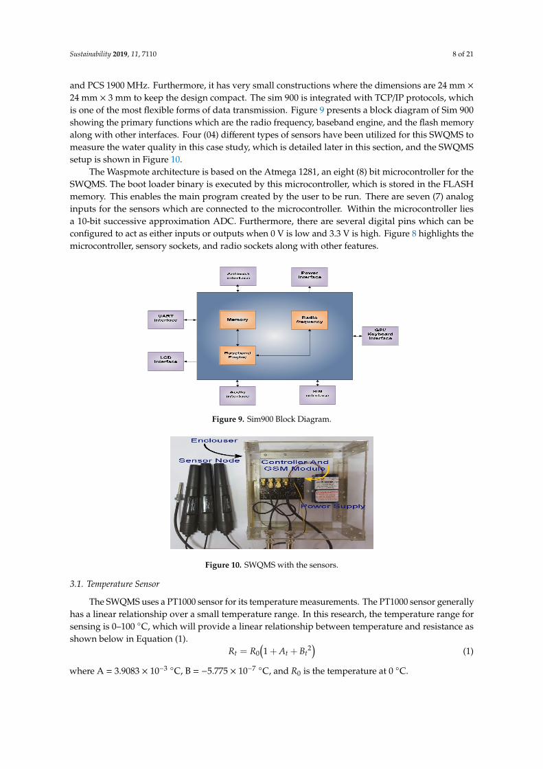
The GSM device uses a sim900 (provided by Simcon) as its baseband engine and as a communication module. It is a quad-band engine working with GSM 850 MHz, EGSM 900 MHz, DCS 1800 MHz, and PCS 1900 MHz. Furthermore, it has very small constructions where the dimensions are 24 mm × 24 mm × 3 mm to keep the design compact. The sim 900 is integrated with TCP/IP protocols, which is one of the most flexible forms of data transmission. Figure 9 presents a block diagram of Sim 900 showing the primary functions which are the radio frequency, baseband engine, and the flash memory along with other interfaces. Four (04) different types of sensors have been utilized for this SWQMS to measure the water quality in this case study, which is detailed later in this section, and the SWQMS setup is shown in Figure 10.
Figure 7. System for the power supply to the SWQMS.
The Waspmote architecture is based on the Atmega 1281, an eight (8) bit microcontroller for theSWQMS. The boot loader binary was executed by this microcontroller, which is stored in the FLASHmemory. This enables the main program created by the user to be run. There are seven (7) analoginputs for the sensors which are connected to the microcontroller. Within the microcontroller liesa 10 bit successive approximation ADC. Furthermore, there are several digital pins which can beconfigured to act as either inputs or outputs when 0 V is low and 3.3 V is high. Figure 8 highlights themicrocontroller, sensory sockets, and radio sockets along with other features.
Sustainability 2019, 11, x FOR PEER REVIEW 7 of 21
Table 2. Specification of the PV system used in SWQMS.
Cells in series: 10, parallel: 1 Modules in series: 2 Short circuit generator: 2 A Open circuit voltage: 12 V Filter and grid impedance: R = 0.0282 Ω, L = 0.0003 H Boost converter: RPV = 0.01 Ω, LPV = 0.2 μH, CPV = 0.5 × 10⁻⁴ F DC link capacitance: Cdc = 25 μF
Figure 7. System for the power supply to the SWQMS.
The Waspmote architecture is based on the Atmega 1281, an eight (8) bit microcontroller for the SWQMS. The boot loader binary was executed by this microcontroller, which is stored in the FLASH memory. This enables the main program created by the user to be run. There are seven (7) analog inputs for the sensors which are connected to the microcontroller. Within the microcontroller lies a 10 bit successive approximation ADC. Furthermore, there are several digital pins which can be configured to act as either inputs or outputs when 0 V is low and 3.3 V is high. Figure 8 highlights the microcontroller, sensory sockets, and radio sockets along with other features.
Figure 8. Waspmote Board Layout [23].
The GSM device uses a sim900 (provided by Simcon) as its baseband engine and as a communication module. It is a quad-band engine working with GSM 850 MHz, EGSM 900 MHz, DCS 1800 MHz, and PCS 1900 MHz. Furthermore, it has very small constructions where the dimensions are 24 mm × 24 mm × 3 mm to keep the design compact. The sim 900 is integrated with TCP/IP protocols, which is one of the most flexible forms of data transmission. Figure 9 presents a block diagram of Sim 900 showing the primary functions which are the radio frequency, baseband engine, and the flash memory along with other interfaces. Four (04) different types of sensors have been utilized for this SWQMS to measure the water quality in this case study, which is detailed later in this section, and the SWQMS setup is shown in Figure 10.
Figure 8. Waspmote Board Layout [23].
The GSM device uses a sim900 (provided by Simcon) as its baseband engine and as a communicationmodule. It is a quad-band engine working with GSM 850 MHz, EGSM 900 MHz, DCS 1800 MHz,
Sustainability 2019, 11, 7110 8 of 21
and PCS 1900 MHz. Furthermore, it has very small constructions where the dimensions are 24 mm ×24 mm × 3 mm to keep the design compact. The sim 900 is integrated with TCP/IP protocols, whichis one of the most flexible forms of data transmission. Figure 9 presents a block diagram of Sim 900showing the primary functions which are the radio frequency, baseband engine, and the flash memoryalong with other interfaces. Four (04) different types of sensors have been utilized for this SWQMS tomeasure the water quality in this case study, which is detailed later in this section, and the SWQMSsetup is shown in Figure 10.
The Waspmote architecture is based on the Atmega 1281, an eight (8) bit microcontroller for theSWQMS. The boot loader binary is executed by this microcontroller, which is stored in the FLASHmemory. This enables the main program created by the user to be run. There are seven (7) analoginputs for the sensors which are connected to the microcontroller. Within the microcontroller liesa 10-bit successive approximation ADC. Furthermore, there are several digital pins which can beconfigured to act as either inputs or outputs when 0 V is low and 3.3 V is high. Figure 8 highlights themicrocontroller, sensory sockets, and radio sockets along with other features.
Sustainability 2019, 11, x FOR PEER REVIEW 8 of 21
The Waspmote architecture is based on the Atmega 1281, an eight (8) bit microcontroller for the SWQMS. The boot loader binary is executed by this microcontroller, which is stored in the FLASH memory. This enables the main program created by the user to be run. There are seven (7) analog inputs for the sensors which are connected to the microcontroller. Within the microcontroller lies a 10-bit successive approximation ADC. Furthermore, there are several digital pins which can be configured to act as either inputs or outputs when 0 V is low and 3.3 V is high. Figure 8 highlights the microcontroller, sensory sockets, and radio sockets along with other features.
Figure 9. Sim900 Block Diagram.
Figure 10. SWQMS with the sensors.
3.1. Temperature Sensor
The SWQMS uses a PT1000 sensor for its temperature measurements. The PT1000 sensor generally has a linear relationship over a small temperature range. In this research, the temperature range for sensing is 0–100 °C, which will provide a linear relationship between temperature and resistance as shown below in Equation (1).
( )20 1t t tR R A B= + + (1)
where A = 3.9083 × 10⁻³ °C, B = −5.775 × 10⁻⁷ °C, and R0 is the temperature at 0 °C. The temperature sensor is used in a voltage divider configuration with a 1 K ohm resistor, hence
Vt can be obtained using Equation (2) as follows:
0
tt ref
t
RV VR R
= +
. (2)
This is then amplified by an instrumental amplifier with a gain of 11 and fed to a 24 bit ADC. Figure 11 below shows a summarized model of the temperature sensors.
Figure 9. Sim900 Block Diagram.
Sustainability 2019, 11, x FOR PEER REVIEW 8 of 21
The Waspmote architecture is based on the Atmega 1281, an eight (8) bit microcontroller for the SWQMS. The boot loader binary is executed by this microcontroller, which is stored in the FLASH memory. This enables the main program created by the user to be run. There are seven (7) analog inputs for the sensors which are connected to the microcontroller. Within the microcontroller lies a 10-bit successive approximation ADC. Furthermore, there are several digital pins which can be configured to act as either inputs or outputs when 0 V is low and 3.3 V is high. Figure 8 highlights the microcontroller, sensory sockets, and radio sockets along with other features.
Figure 9. Sim900 Block Diagram.
Figure 10. SWQMS with the sensors.
3.1. Temperature Sensor
The SWQMS uses a PT1000 sensor for its temperature measurements. The PT1000 sensor generally has a linear relationship over a small temperature range. In this research, the temperature range for sensing is 0–100 °C, which will provide a linear relationship between temperature and resistance as shown below in Equation (1).
( )20 1t t tR R A B= + + (1)
where A = 3.9083 × 10⁻³ °C, B = −5.775 × 10⁻⁷ °C, and R0 is the temperature at 0 °C. The temperature sensor is used in a voltage divider configuration with a 1 K ohm resistor, hence
Vt can be obtained using Equation (2) as follows:
0
tt ref
t
RV VR R
= +
. (2)
This is then amplified by an instrumental amplifier with a gain of 11 and fed to a 24 bit ADC. Figure 11 below shows a summarized model of the temperature sensors.
Figure 10. SWQMS with the sensors.
3.1. Temperature Sensor
The SWQMS uses a PT1000 sensor for its temperature measurements. The PT1000 sensor generallyhas a linear relationship over a small temperature range. In this research, the temperature range forsensing is 0–100 C, which will provide a linear relationship between temperature and resistance asshown below in Equation (1).
Rt = R0(1 + At + Bt
2)
(1)
where A = 3.9083 × 10⁻³ C, B = −5.775 × 10⁻⁷ C, and R0 is the temperature at 0 C.
Sustainability 2019, 11, 7110 9 of 21
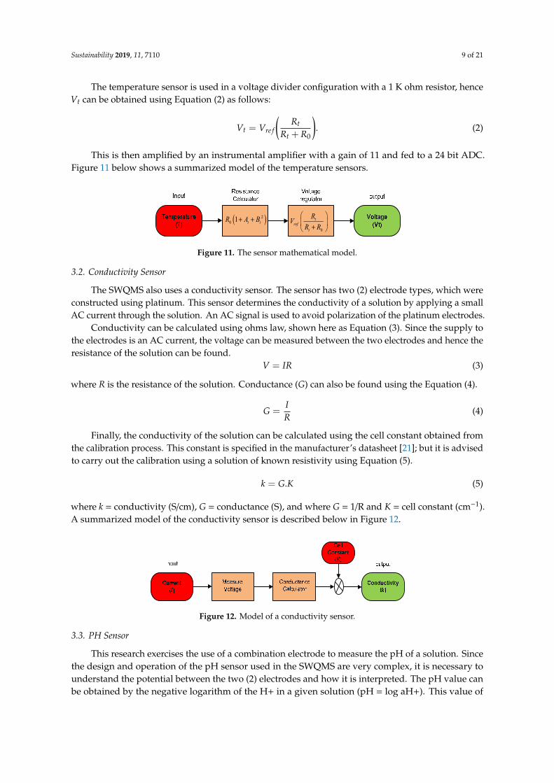
The temperature sensor is used in a voltage divider configuration with a 1 K ohm resistor, henceVt can be obtained using Equation (2) as follows:
Vt = Vre f
(Rt
Rt + R0
). (2)
This is then amplified by an instrumental amplifier with a gain of 11 and fed to a 24 bit ADC.Figure 11 below shows a summarized model of the temperature sensors.Sustainability 2019, 11, x FOR PEER REVIEW 9 of 21
( )20 1 t tR A B+ +
0
tref
t
RVR R
+
Figure 11. The sensor mathematical model.
3.2. Conductivity Sensor
The SWQMS also uses a conductivity sensor. The sensor has two (2) electrode types, which were constructed using platinum. This sensor determines the conductivity of a solution by applying a small AC current through the solution. An AC signal is used to avoid polarization of the platinum electrodes.
Conductivity can be calculated using ohms law, shown here as Equation (3). Since the supply to the electrodes is an AC current, the voltage can be measured between the two electrodes and hence the resistance of the solution can be found.
V IR= (3)
where R is the resistance of the solution. Conductance (G) can also be found using the Equation (4).
IGR
= (4)
Finally, the conductivity of the solution can be calculated using the cell constant obtained from the calibration process. This constant is specified in the manufacturer’s datasheet [21]; but it is advised to carry out the calibration using a solution of known resistivity using Equation (5).
.k G K= (5)
where k = conductivity (S/cm), G = conductance (S), and where G = 1/R and K = cell constant (cm−1). A summarized model of the conductivity sensor is described below in Figure 12.
Figure 12. Model of a conductivity sensor.
3.3. PH Sensor
This research exercises the use of a combination electrode to measure the pH of a solution. Since the design and operation of the pH sensor used in the SWQMS are very complex, it is necessary to understand the potential between the two (2) electrodes and how it is interpreted. The pH value can be obtained by the negative logarithm of the H+ in a given solution (pH = log aH+). This value of pH needs to be converted into a voltage signal using the following the Equation (6) to obtain the sensor’s output.
( )0 H.T logaph nfE E k += + (6)
where Nernst factor is 2.3026nfRTk xF
= , E = measured potential (mV), T = Temperature in K, and
F = the Faraday constant (96,485 C mol−1); As the voltage produced by the electrodes has a linear relationship to the pH of the solution, at
the reference pH of 7, the potential between the electrodes is 0 V. At an acidic or low pH level, the potential between the electrodes is linear. Likewise, at a high pH, the potential between the electrodes
Figure 11. The sensor mathematical model.
3.2. Conductivity Sensor
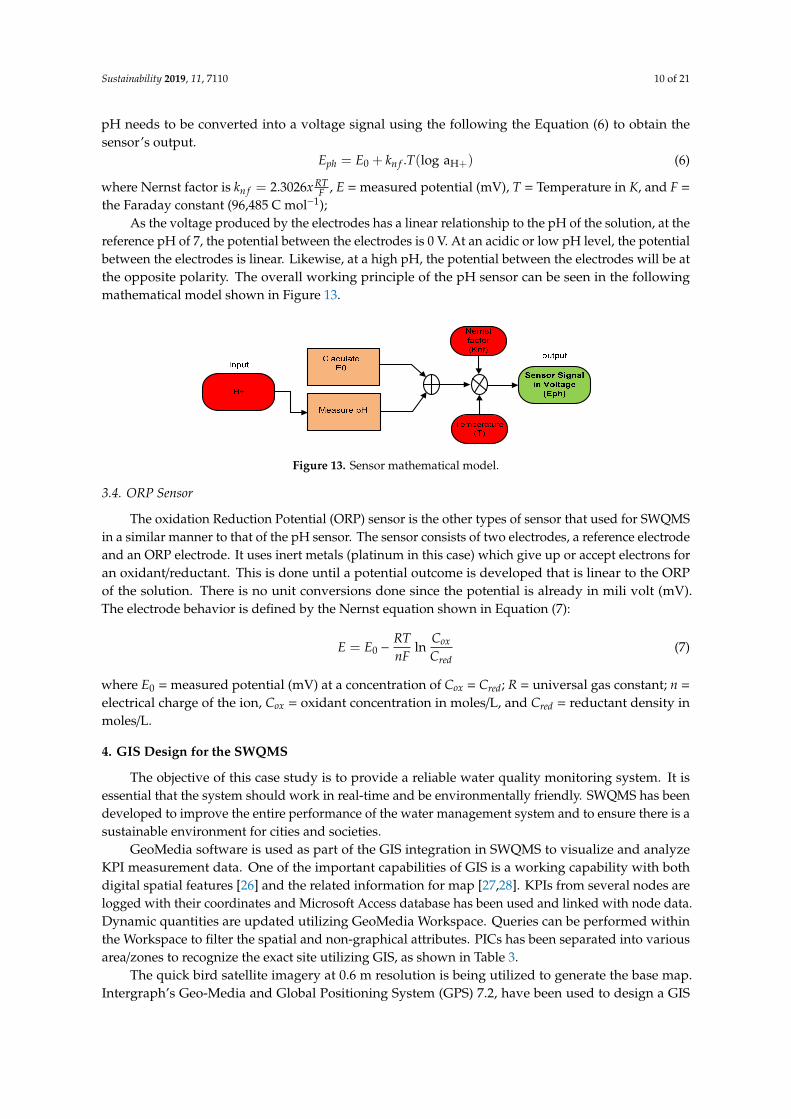
The SWQMS also uses a conductivity sensor. The sensor has two (2) electrode types, which wereconstructed using platinum. This sensor determines the conductivity of a solution by applying a smallAC current through the solution. An AC signal is used to avoid polarization of the platinum electrodes.
Conductivity can be calculated using ohms law, shown here as Equation (3). Since the supply tothe electrodes is an AC current, the voltage can be measured between the two electrodes and hence theresistance of the solution can be found.
V = IR (3)
where R is the resistance of the solution. Conductance (G) can also be found using the Equation (4).
G =IR
(4)
Finally, the conductivity of the solution can be calculated using the cell constant obtained fromthe calibration process. This constant is specified in the manufacturer’s datasheet [21]; but it is advisedto carry out the calibration using a solution of known resistivity using Equation (5).
k = G.K (5)
where k = conductivity (S/cm), G = conductance (S), and where G = 1/R and K = cell constant (cm−1).A summarized model of the conductivity sensor is described below in Figure 12.
Sustainability 2019, 11, x FOR PEER REVIEW 9 of 21
( )20 1 t tR A B+ +
0
tref
t
RVR R
+
Figure 11. The sensor mathematical model.
3.2. Conductivity Sensor
The SWQMS also uses a conductivity sensor. The sensor has two (2) electrode types, which were constructed using platinum. This sensor determines the conductivity of a solution by applying a small AC current through the solution. An AC signal is used to avoid polarization of the platinum electrodes.
Conductivity can be calculated using ohms law, shown here as Equation (3). Since the supply to the electrodes is an AC current, the voltage can be measured between the two electrodes and hence the resistance of the solution can be found.
V IR= (3)
where R is the resistance of the solution. Conductance (G) can also be found using the Equation (4).
IGR
= (4)
Finally, the conductivity of the solution can be calculated using the cell constant obtained from the calibration process. This constant is specified in the manufacturer’s datasheet [21]; but it is advised to carry out the calibration using a solution of known resistivity using Equation (5).
.k G K= (5)
where k = conductivity (S/cm), G = conductance (S), and where G = 1/R and K = cell constant (cm−1). A summarized model of the conductivity sensor is described below in Figure 12.
Figure 12. Model of a conductivity sensor.
3.3. PH Sensor
This research exercises the use of a combination electrode to measure the pH of a solution. Since the design and operation of the pH sensor used in the SWQMS are very complex, it is necessary to understand the potential between the two (2) electrodes and how it is interpreted. The pH value can be obtained by the negative logarithm of the H+ in a given solution (pH = log aH+). This value of pH needs to be converted into a voltage signal using the following the Equation (6) to obtain the sensor’s output.
( )0 H.T logaph nfE E k += + (6)
where Nernst factor is 2.3026nfRTk xF
= , E = measured potential (mV), T = Temperature in K, and
F = the Faraday constant (96,485 C mol−1); As the voltage produced by the electrodes has a linear relationship to the pH of the solution, at
the reference pH of 7, the potential between the electrodes is 0 V. At an acidic or low pH level, the potential between the electrodes is linear. Likewise, at a high pH, the potential between the electrodes
Figure 12. Model of a conductivity sensor.
3.3. PH Sensor
This research exercises the use of a combination electrode to measure the pH of a solution. Sincethe design and operation of the pH sensor used in the SWQMS are very complex, it is necessary tounderstand the potential between the two (2) electrodes and how it is interpreted. The pH value canbe obtained by the negative logarithm of the H+ in a given solution (pH = log aH+). This value of
Sustainability 2019, 11, 7110 10 of 21
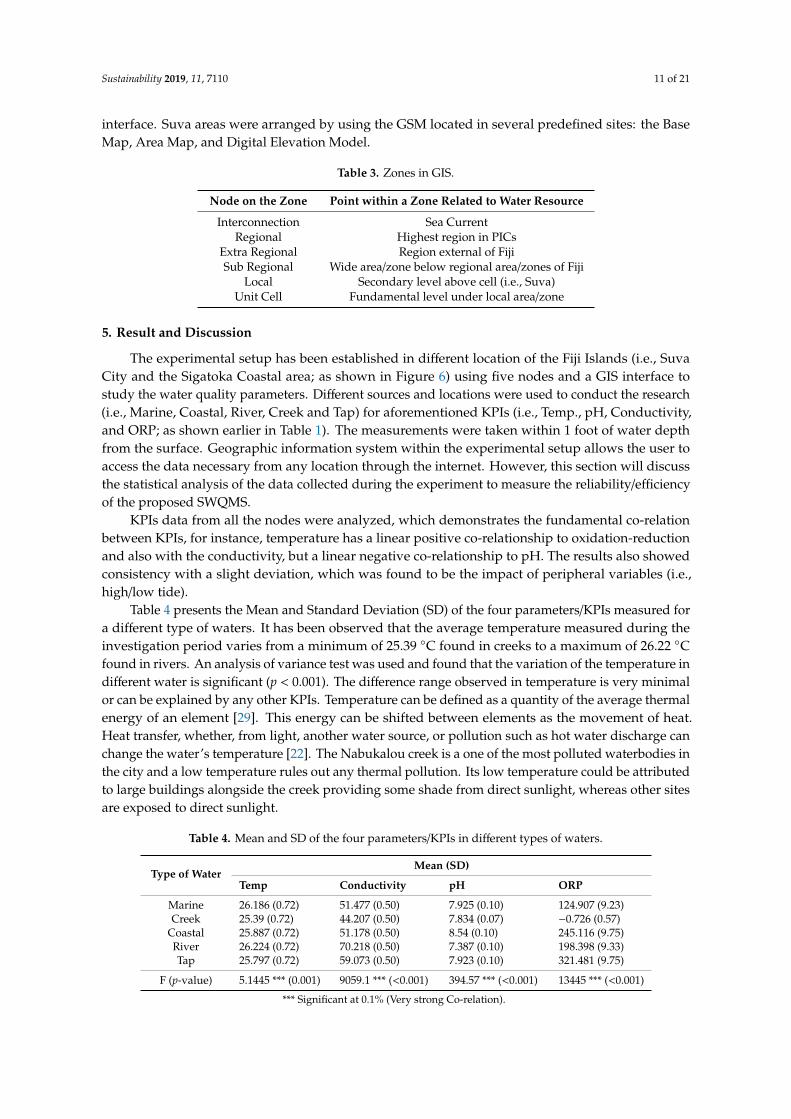
pH needs to be converted into a voltage signal using the following the Equation (6) to obtain thesensor’s output.
Eph = E0 + kn f .T(log aH+) (6)
where Nernst factor is kn f = 2.3026x RTF , E = measured potential (mV), T = Temperature in K, and F =
the Faraday constant (96,485 C mol−1);As the voltage produced by the electrodes has a linear relationship to the pH of the solution, at the
reference pH of 7, the potential between the electrodes is 0 V. At an acidic or low pH level, the potentialbetween the electrodes is linear. Likewise, at a high pH, the potential between the electrodes will be atthe opposite polarity. The overall working principle of the pH sensor can be seen in the followingmathematical model shown in Figure 13.
Sustainability 2019, 11, x FOR PEER REVIEW 10 of 21
will be at the opposite polarity. The overall working principle of the pH sensor can be seen in the following mathematical model shown in Figure 13.
Figure 13. Sensor mathematical model.
3.4. ORP Sensor
The oxidation Reduction Potential (ORP) sensor is the other types of sensor that used for SWQMS in a similar manner to that of the pH sensor. The sensor consists of two electrodes, a reference electrode and an ORP electrode. It uses inert metals (platinum in this case) which give up or accept electrons for an oxidant/reductant. This is done until a potential outcome is developed that is linear to the ORP of the solution. There is no unit conversions done since the potential is already in mili volt (mV). The electrode behavior is defined by the Nernst equation shown in Equation (7):
0 ln ox
red
CRTE EnF C
= − (7)
where Eo = measured potential (mV) at a concentration of Cox = Cred; R = universal gas constant; n = electrical charge of the ion, Cox = oxidant concentration in moles/L, and Cred = reductant density in moles/L.
4. GIS Design for the SWQMS
The objective of this case study is to provide a reliable water quality monitoring system. It is essential that the system should work in real-time and be environmentally friendly. SWQMS has been developed to improve the entire performance of the water management system and to ensure there is a sustainable environment for cities and societies.
GeoMedia software is used as part of the GIS integration in SWQMS to visualize and analyze KPI measurement data. One of the important capabilities of GIS is a working capability with both digital spatial features [26] and the related information for map [27,28]. KPIs from several nodes are logged with their coordinates and Microsoft Access database has been used and linked with node data. Dynamic quantities are updated utilizing GeoMedia Workspace. Queries can be performed within the Workspace to filter the spatial and non-graphical attributes. PICs has been separated into various area/zones to recognize the exact site utilizing GIS, as shown in Table 3.
The quick bird satellite imagery at 0.6 m resolution is being utilized to generate the base map. Intergraph’s Geo-Media and Global Positioning System (GPS) 7.2, have been used to design a GIS interface. Suva areas were arranged by using the GSM located in several predefined sites: the Base Map, Area Map, and Digital Elevation Model.
Figure 13. Sensor mathematical model.
3.4. ORP Sensor
The oxidation Reduction Potential (ORP) sensor is the other types of sensor that used for SWQMSin a similar manner to that of the pH sensor. The sensor consists of two electrodes, a reference electrodeand an ORP electrode. It uses inert metals (platinum in this case) which give up or accept electrons foran oxidant/reductant. This is done until a potential outcome is developed that is linear to the ORPof the solution. There is no unit conversions done since the potential is already in mili volt (mV).The electrode behavior is defined by the Nernst equation shown in Equation (7):
E = E0 −RTnF
lnCox
Cred(7)
where E0 = measured potential (mV) at a concentration of Cox = Cred; R = universal gas constant; n =
electrical charge of the ion, Cox = oxidant concentration in moles/L, and Cred = reductant density inmoles/L.
4. GIS Design for the SWQMS
The objective of this case study is to provide a reliable water quality monitoring system. It isessential that the system should work in real-time and be environmentally friendly. SWQMS has beendeveloped to improve the entire performance of the water management system and to ensure there is asustainable environment for cities and societies.
GeoMedia software is used as part of the GIS integration in SWQMS to visualize and analyzeKPI measurement data. One of the important capabilities of GIS is a working capability with bothdigital spatial features [26] and the related information for map [27,28]. KPIs from several nodes arelogged with their coordinates and Microsoft Access database has been used and linked with node data.Dynamic quantities are updated utilizing GeoMedia Workspace. Queries can be performed withinthe Workspace to filter the spatial and non-graphical attributes. PICs has been separated into variousarea/zones to recognize the exact site utilizing GIS, as shown in Table 3.
The quick bird satellite imagery at 0.6 m resolution is being utilized to generate the base map.Intergraph’s Geo-Media and Global Positioning System (GPS) 7.2, have been used to design a GIS
Sustainability 2019, 11, 7110 11 of 21
interface. Suva areas were arranged by using the GSM located in several predefined sites: the BaseMap, Area Map, and Digital Elevation Model.
Table 3. Zones in GIS.
Node on the Zone Point within a Zone Related to Water Resource
Interconnection Sea CurrentRegional Highest region in PICs
Extra Regional Region external of FijiSub Regional Wide area/zone below regional area/zones of Fiji
Local Secondary level above cell (i.e., Suva)Unit Cell Fundamental level under local area/zone
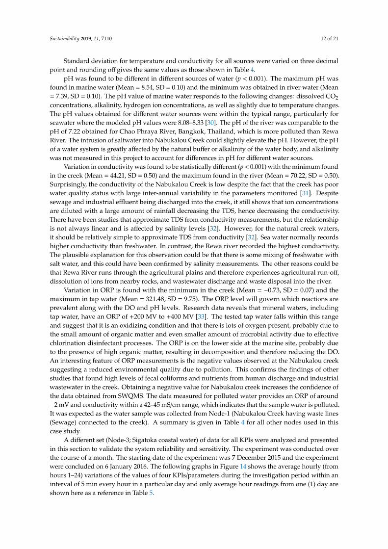
5. Result and Discussion
The experimental setup has been established in different location of the Fiji Islands (i.e., SuvaCity and the Sigatoka Coastal area; as shown in Figure 6) using five nodes and a GIS interface tostudy the water quality parameters. Different sources and locations were used to conduct the research(i.e., Marine, Coastal, River, Creek and Tap) for aforementioned KPIs (i.e., Temp., pH, Conductivity,and ORP; as shown earlier in Table 1). The measurements were taken within 1 foot of water depthfrom the surface. Geographic information system within the experimental setup allows the user toaccess the data necessary from any location through the internet. However, this section will discussthe statistical analysis of the data collected during the experiment to measure the reliability/efficiencyof the proposed SWQMS.
KPIs data from all the nodes were analyzed, which demonstrates the fundamental co-relationbetween KPIs, for instance, temperature has a linear positive co-relationship to oxidation-reductionand also with the conductivity, but a linear negative co-relationship to pH. The results also showedconsistency with a slight deviation, which was found to be the impact of peripheral variables (i.e.,high/low tide).
Table 4 presents the Mean and Standard Deviation (SD) of the four parameters/KPIs measured fora different type of waters. It has been observed that the average temperature measured during theinvestigation period varies from a minimum of 25.39 C found in creeks to a maximum of 26.22 Cfound in rivers. An analysis of variance test was used and found that the variation of the temperature indifferent water is significant (p < 0.001). The difference range observed in temperature is very minimalor can be explained by any other KPIs. Temperature can be defined as a quantity of the average thermalenergy of an element [29]. This energy can be shifted between elements as the movement of heat.Heat transfer, whether, from light, another water source, or pollution such as hot water discharge canchange the water’s temperature [22]. The Nabukalou creek is a one of the most polluted waterbodies inthe city and a low temperature rules out any thermal pollution. Its low temperature could be attributedto large buildings alongside the creek providing some shade from direct sunlight, whereas other sitesare exposed to direct sunlight.
Table 4. Mean and SD of the four parameters/KPIs in different types of waters.
Type of WaterMean (SD)
Temp Conductivity pH ORP
Marine 26.186 (0.72) 51.477 (0.50) 7.925 (0.10) 124.907 (9.23)Creek 25.39 (0.72) 44.207 (0.50) 7.834 (0.07) −0.726 (0.57)
Coastal 25.887 (0.72) 51.178 (0.50) 8.54 (0.10) 245.116 (9.75)River 26.224 (0.72) 70.218 (0.50) 7.387 (0.10) 198.398 (9.33)Tap 25.797 (0.72) 59.073 (0.50) 7.923 (0.10) 321.481 (9.75)
F (p-value) 5.1445 *** (0.001) 9059.1 *** (<0.001) 394.57 *** (<0.001) 13445 *** (<0.001)
*** Significant at 0.1% (Very strong Co-relation).
Sustainability 2019, 11, 7110 12 of 21
Standard deviation for temperature and conductivity for all sources were varied on three decimalpoint and rounding off gives the same values as those shown in Table 4.
pH was found to be different in different sources of water (p < 0.001). The maximum pH wasfound in marine water (Mean = 8.54, SD = 0.10) and the minimum was obtained in river water (Mean= 7.39, SD = 0.10). The pH value of marine water responds to the following changes: dissolved CO2
concentrations, alkalinity, hydrogen ion concentrations, as well as slightly due to temperature changes.The pH values obtained for different water sources were within the typical range, particularly forseawater where the modeled pH values were 8.08–8.33 [30]. The pH of the river was comparable to thepH of 7.22 obtained for Chao Phraya River, Bangkok, Thailand, which is more polluted than RewaRiver. The intrusion of saltwater into Nabukalou Creek could slightly elevate the pH. However, the pHof a water system is greatly affected by the natural buffer or alkalinity of the water body, and alkalinitywas not measured in this project to account for differences in pH for different water sources.
Variation in conductivity was found to be statistically different (p < 0.001) with the minimum foundin the creek (Mean = 44.21, SD = 0.50) and the maximum found in the river (Mean = 70.22, SD = 0.50).Surprisingly, the conductivity of the Nabukalou Creek is low despite the fact that the creek has poorwater quality status with large inter-annual variability in the parameters monitored [31]. Despitesewage and industrial effluent being discharged into the creek, it still shows that ion concentrationsare diluted with a large amount of rainfall decreasing the TDS, hence decreasing the conductivity.There have been studies that approximate TDS from conductivity measurements, but the relationshipis not always linear and is affected by salinity levels [32]. However, for the natural creek waters,it should be relatively simple to approximate TDS from conductivity [32]. Sea water normally recordshigher conductivity than freshwater. In contrast, the Rewa river recorded the highest conductivity.The plausible explanation for this observation could be that there is some mixing of freshwater withsalt water, and this could have been confirmed by salinity measurements. The other reasons could bethat Rewa River runs through the agricultural plains and therefore experiences agricultural run-off,dissolution of ions from nearby rocks, and wastewater discharge and waste disposal into the river.
Variation in ORP is found with the minimum in the creek (Mean = −0.73, SD = 0.07) and themaximum in tap water (Mean = 321.48, SD = 9.75). The ORP level will govern which reactions areprevalent along with the DO and pH levels. Research data reveals that mineral waters, includingtap water, have an ORP of +200 MV to +400 MV [33]. The tested tap water falls within this rangeand suggest that it is an oxidizing condition and that there is lots of oxygen present, probably due tothe small amount of organic matter and even smaller amount of microbial activity due to effectivechlorination disinfectant processes. The ORP is on the lower side at the marine site, probably dueto the presence of high organic matter, resulting in decomposition and therefore reducing the DO.An interesting feature of ORP measurements is the negative values observed at the Nabukalou creeksuggesting a reduced environmental quality due to pollution. This confirms the findings of otherstudies that found high levels of fecal coliforms and nutrients from human discharge and industrialwastewater in the creek. Obtaining a negative value for Nabukalou creek increases the confidence ofthe data obtained from SWQMS. The data measured for polluted water provides an ORP of around−2 mV and conductivity within a 42–45 mS/cm range, which indicates that the sample water is polluted.It was expected as the water sample was collected from Node-1 (Nabukalou Creek having waste lines(Sewage) connected to the creek). A summary is given in Table 4 for all other nodes used in thiscase study.
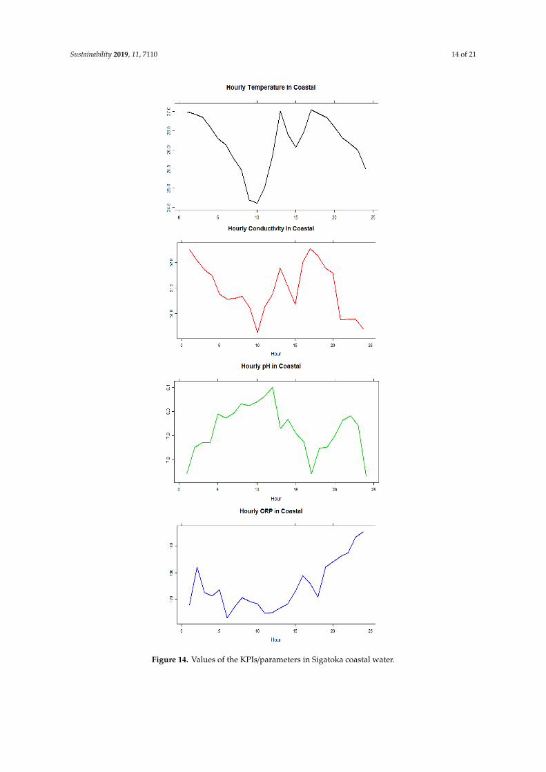
A different set (Node-3; Sigatoka coastal water) of data for all KPIs were analyzed and presentedin this section to validate the system reliability and sensitivity. The experiment was conducted overthe course of a month. The starting date of the experiment was 7 December 2015 and the experimentwere concluded on 6 January 2016. The following graphs in Figure 14 shows the average hourly (fromhours 1–24) variations of the values of four KPIs/parameters during the investigation period within aninterval of 5 min every hour in a particular day and only average hour readings from one (1) day areshown here as a reference in Table 5.
Sustainability 2019, 11, 7110 13 of 21
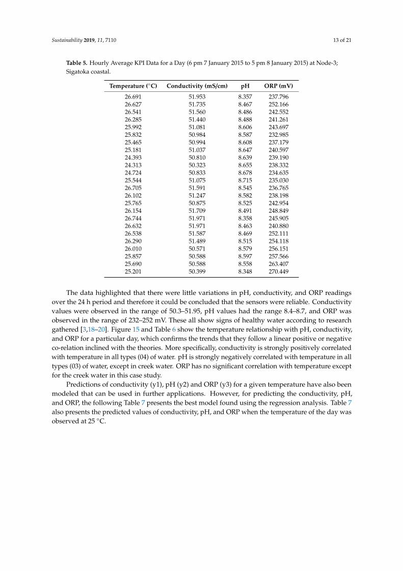
Table 5. Hourly Average KPI Data for a Day (6 pm 7 January 2015 to 5 pm 8 January 2015) at Node-3;Sigatoka coastal.
Temperature (C) Conductivity (mS/cm) pH ORP (mV)
26.691 51.953 8.357 237.79626.627 51.735 8.467 252.16626.541 51.560 8.486 242.55226.285 51.440 8.488 241.26125.992 51.081 8.606 243.69725.832 50.984 8.587 232.98525.465 50.994 8.608 237.17925.181 51.037 8.647 240.59724.393 50.810 8.639 239.19024.313 50.323 8.655 238.33224.724 50.833 8.678 234.63525.544 51.075 8.715 235.03026.705 51.591 8.545 236.76526.102 51.247 8.582 238.19825.765 50.875 8.525 242.95426.154 51.709 8.491 248.84926.744 51.971 8.358 245.90526.632 51.971 8.463 240.88026.538 51.587 8.469 252.11126.290 51.489 8.515 254.11826.010 50.571 8.579 256.15125.857 50.588 8.597 257.56625.690 50.588 8.558 263.40725.201 50.399 8.348 270.449
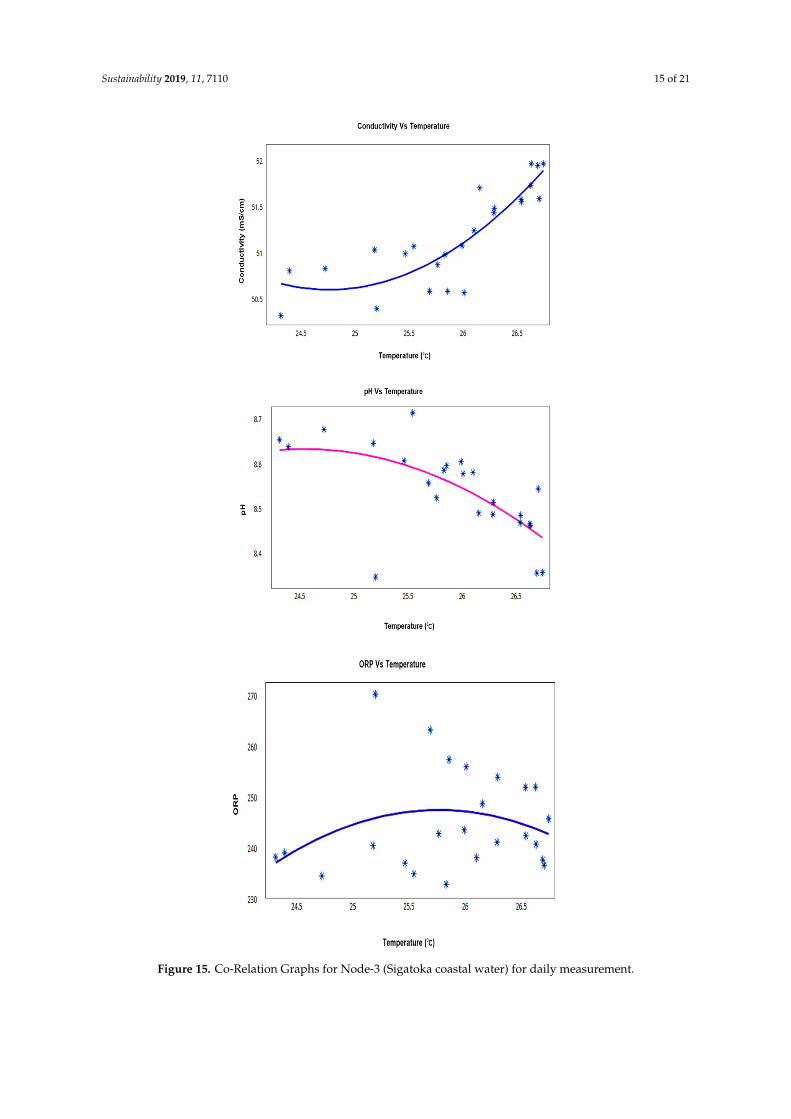
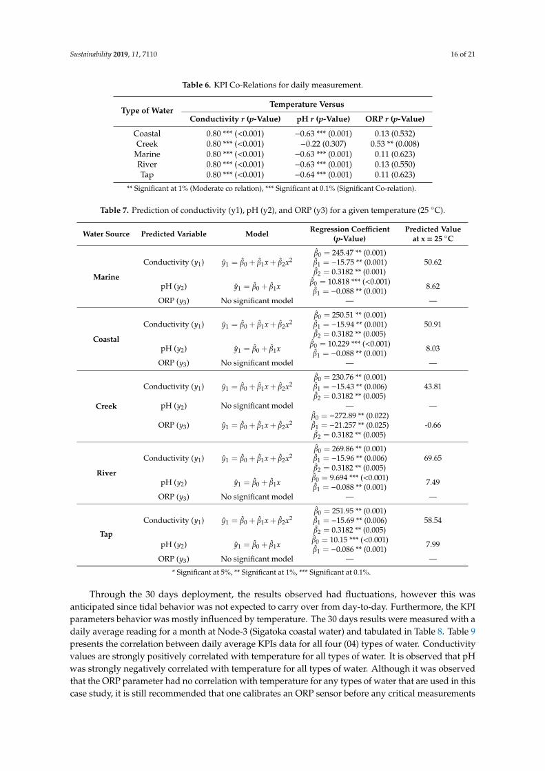
The data highlighted that there were little variations in pH, conductivity, and ORP readingsover the 24 h period and therefore it could be concluded that the sensors were reliable. Conductivityvalues were observed in the range of 50.3–51.95, pH values had the range 8.4–8.7, and ORP wasobserved in the range of 232–252 mV. These all show signs of healthy water according to researchgathered [3,18–20]. Figure 15 and Table 6 show the temperature relationship with pH, conductivity,and ORP for a particular day, which confirms the trends that they follow a linear positive or negativeco-relation inclined with the theories. More specifically, conductivity is strongly positively correlatedwith temperature in all types (04) of water. pH is strongly negatively correlated with temperature in alltypes (03) of water, except in creek water. ORP has no significant correlation with temperature exceptfor the creek water in this case study.
Predictions of conductivity (y1), pH (y2) and ORP (y3) for a given temperature have also beenmodeled that can be used in further applications. However, for predicting the conductivity, pH,and ORP, the following Table 7 presents the best model found using the regression analysis. Table 7also presents the predicted values of conductivity, pH, and ORP when the temperature of the day wasobserved at 25 C.
Sustainability 2019, 11, 7110 14 of 21
Sustainability 2019, 11, x FOR PEER REVIEW 14 of 21
Figure 14. Values of the KPIs/parameters in Sigatoka coastal water. Figure 14. Values of the KPIs/parameters in Sigatoka coastal water.
Sustainability 2019, 11, 7110 15 of 21Sustainability 2019, 11, x FOR PEER REVIEW 15 of 21
Figure 15. Co-Relation Graphs for Node-3 (Sigatoka coastal water) for daily measurement.
Table 6. KPI Co-Relations for daily measurement.
Type of Water
Temperature Versus Conductivity r (p-
Value) pH r (p-Value) ORP r (p-Value)
Coastal 0.80 *** (<0.001) −0.63 *** (0.001) 0.13 (0.532) Creek 0.80 *** (<0.001) −0.22 (0.307) 0.53 ** (0.008)
Marine 0.80 *** (<0.001) −0.63 *** (0.001) 0.11 (0.623) River 0.80 *** (<0.001) −0.63 *** (0.001) 0.13 (0.550) Tap 0.80 *** (<0.001) −0.64 *** (0.001) 0.11 (0.623)
** Significant at 1% (Moderate co relation), *** Significant at 0.1% (Significant Co-relation).
Figure 15. Co-Relation Graphs for Node-3 (Sigatoka coastal water) for daily measurement.
Sustainability 2019, 11, 7110 16 of 21
Table 6. KPI Co-Relations for daily measurement.
Type of WaterTemperature Versus
Conductivity r (p-Value) pH r (p-Value) ORP r (p-Value)
Coastal 0.80 *** (<0.001) −0.63 *** (0.001) 0.13 (0.532)Creek 0.80 *** (<0.001) −0.22 (0.307) 0.53 ** (0.008)
Marine 0.80 *** (<0.001) −0.63 *** (0.001) 0.11 (0.623)River 0.80 *** (<0.001) −0.63 *** (0.001) 0.13 (0.550)Tap 0.80 *** (<0.001) −0.64 *** (0.001) 0.11 (0.623)
** Significant at 1% (Moderate co relation), *** Significant at 0.1% (Significant Co-relation).
Table 7. Prediction of conductivity (y1), pH (y2), and ORP (y3) for a given temperature (25 C).
Water Source Predicted Variable Model Regression Coefficient(p-Value)
Predicted Valueat x = 25 C
Marine
Conductivity (y1) y1 = β0 + β1x + β2x2β0 = 245.47 ** (0.001)β1 = −15.75 ** (0.001)β2 = 0.3182 ** (0.001)
50.62
pH (y2) y1 = β0 + β1x β0 = 10.818 *** (<0.001)β1 = −0.088 ** (0.001)
8.62
ORP (y3) No significant model — —
Coastal
Conductivity (y1) y1 = β0 + β1x + β2x2β0 = 250.51 ** (0.001)β1 = −15.94 ** (0.001)β2 = 0.3182 ** (0.005)
50.91
pH (y2) y1 = β0 + β1x β0 = 10.229 *** (<0.001)β1 = −0.088 ** (0.001)
8.03
ORP (y3) No significant model — —
Creek
Conductivity (y1) y1 = β0 + β1x + β2x2β0 = 230.76 ** (0.001)β1 = −15.43 ** (0.006)β2 = 0.3182 ** (0.005)
43.81
pH (y2) No significant model — —
ORP (y3) y1 = β0 + β1x + β2x2β0 = −272.89 ** (0.022)β1 = −21.257 ** (0.025)β2 = 0.3182 ** (0.005)
-0.66
River
Conductivity (y1) y1 = β0 + β1x + β2x2β0 = 269.86 ** (0.001)β1 = −15.96 ** (0.006)β2 = 0.3182 ** (0.005)
69.65
pH (y2) y1 = β0 + β1x β0 = 9.694 *** (<0.001)β1 = −0.088 ** (0.001)
7.49
ORP (y3) No significant model — —
Tap
Conductivity (y1) y1 = β0 + β1x + β2x2β0 = 251.95 ** (0.001)β1 = −15.69 ** (0.006)β2 = 0.3182 ** (0.005)
58.54
pH (y2) y1 = β0 + β1x β0 = 10.15 *** (<0.001)β1 = −0.086 ** (0.001)
7.99
ORP (y3) No significant model — —
* Significant at 5%, ** Significant at 1%, *** Significant at 0.1%.
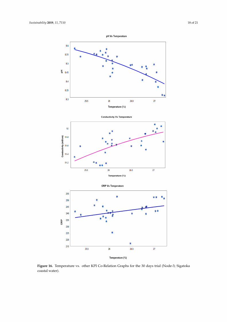
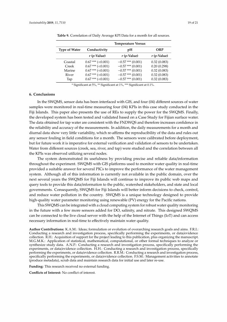
Through the 30 days deployment, the results observed had fluctuations, however this wasanticipated since tidal behavior was not expected to carry over from day-to-day. Furthermore, the KPIparameters behavior was mostly influenced by temperature. The 30 days results were measured with adaily average reading for a month at Node-3 (Sigatoka coastal water) and tabulated in Table 8. Table 9presents the correlation between daily average KPIs data for all four (04) types of water. Conductivityvalues are strongly positively correlated with temperature for all types of water. It is observed that pHwas strongly negatively correlated with temperature for all types of water. Although it was observedthat the ORP parameter had no correlation with temperature for any types of water that are used in thiscase study, it is still recommended that one calibrates an ORP sensor before any critical measurements

Sustainability 2019, 11, 7110 17 of 21
and uses multiple ORP sensors to cross-reference or conduct further research with other measurementssuch as sulfides or nitrates. As the values of correlations are the same for all three (03) types ofwater, except for the ORP in creeks, the results in Table 9 also presents these values with changes oftemperature, the rate of change of conductivity, and pH in any types of water at the same ratio, whileORP does not follow this phenomenon.
Table 8. Daily Average KPI Data for a month at Node-3: Sigatoka coastal Water.
Conductivity ORP
Temperature (C) (mS/cm) pH (mV)
25.858 51.137 8.549 245.37925.671 51.212 8.555 246.20225.724 51.194 8.551 250.30126.068 51.604 8.518 225.55026.074 51.650 8.501 241.81525.808 51.135 8.571 236.15925.944 51.185 8.581 242.19726.726 51.603 8.481 243.23226.816 51.876 8.484 244.93927.029 52.100 8.398 241.81927.080 52.003 8.369 242.00326.735 51.709 8.408 244.48726.831 51.507 8.472 245.23826.507 51.588 8.493 239.97626.471 51.770 8.491 217.25925.937 51.690 8.515 234.03725.925 51.438 8.561 236.76725.241 51.335 8.585 241.54226.025 51.891 8.428 240.43725.866 51.771 8.486 237.71626.073 51.737 8.449 238.12526.082 51.940 8.472 239.21625.978 51.644 8.541 240.45625.368 51.586 8.539 239.01126.818 51.881 8.441 239.72627.221 51.695 8.321 251.41327.173 52.057 8.324 252.67426.992 51.944 8.495 252.33727.048 51.918 8.451 252.37426.174 51.621 8.539 252.816
The relationship with temperature is seen to be consistent throughout the deployment durationand also confirms the temperature relation theories explained earlier in this paper. Scatter plot resultsof 30 days trial at Node-3 (Sigatoka coastal water) are shown in Figure 16 which shows that theconductivity and ORP maintain a linear positive co-relationship with temperature but pH showed alinear negative co-relationship with temperature change that again validates SWQMS reliability.
Sustainability 2019, 11, 7110 18 of 21Sustainability 2019, 11, x FOR PEER REVIEW 18 of 21
Figure 16. Temperature vs. other KPI Co-Relation Graphs for the 30 days trial (Node-3; Sigatoka coastal water).
Table 9. Correlation of Daily Average KPI Data for a month for all sources.
Temperature versus Type of Water Conductivity pH ORP
r (p-Value) r (p-Value) r (p-Value) Coastal 0.67 *** (<0.001) −0.57 *** (0.001) 0.32 (0.083) Creek 0.67 *** (<0.001) −0.57 *** (0.001) 0.20 (0.298)
Marine 0.67 *** (<0.001) −0.57 *** (0.001) 0.32 (0.083) River 0.67 *** (<0.001) −0.57 *** (0.001) 0.32 (0.083) Tap 0.67 *** (<0.001) −0.57 *** (0.001) 0.32 (0.083)
* Significant at 5%, ** Significant at 1%, *** Significant at 0.1%.
Figure 16. Temperature vs. other KPI Co-Relation Graphs for the 30 days trial (Node-3; Sigatokacoastal water).
Sustainability 2019, 11, 7110 19 of 21
Table 9. Correlation of Daily Average KPI Data for a month for all sources.
Temperature Versus
Type of Water Conductivity pH ORP
r (p-Value) r (p-Value) r (p-Value)
Coastal 0.67 *** (<0.001) −0.57 *** (0.001) 0.32 (0.083)Creek 0.67 *** (<0.001) −0.57 *** (0.001) 0.20 (0.298)
Marine 0.67 *** (<0.001) −0.57 *** (0.001) 0.32 (0.083)River 0.67 *** (<0.001) −0.57 *** (0.001) 0.32 (0.083)Tap 0.67 *** (<0.001) −0.57 *** (0.001) 0.32 (0.083)
* Significant at 5%, ** Significant at 1%, *** Significant at 0.1%.
6. Conclusions
In the SWQMS, sensor data has been interfaced with GIS, and four (04) different sources of watersamples were monitored in real-time measuring four (04) KPIs in this case study conducted in theFiji Islands. This paper also presents the use of REs to supply the power for the SWQMS. Finally,the developed system has been tested and validated based on a Case Study for Fijian surface water.The data obtained for tap water are consistent with the FNDWQS and therefore increases confidence inthe reliability and accuracy of the measurements. In addition, the daily measurements for a month anddiurnal data show very little variability, which re-affirms the reproducibility of the data and rules outany sensor fouling in field conditions for a month. The sensors were calibrated before deployment,but for future work it is imperative for external verification and validation of sensors to be undertaken.Water from different sources (creek, sea, river, and tap) were studied and the correlation between allthe KPIs was observed utilizing several nodes.
The system demonstrated its usefulness by providing precise and reliable data/informationthroughout the experiment. SWQMS with GIS platforms used to monitor water quality in real-timeprovided a suitable answer for several PICs to improve the performance of the water managementsystem. Although all of this information is currently not available in the public domain, over thenext several years the SWQMS for Fiji Islands will continue to improve its public web maps andquery tools to provide this data/information to the public, watershed stakeholders, and state and localgovernments. Consequently, SWQMS for Fiji Islands will better inform decisions to check, control,and reduce water pollution in the country. SWQMS is a unique technology designed to providehigh-quality water parameter monitoring using renewable (PV) energy for the Pacific nations.
This SWQMS can be integrated with a cloud computing system for robust water quality monitoringin the future with a few more sensors added for DO, salinity, and nitrate. This designed SWQMScan be connected to the live cloud server with the help of the Internet of Things (IoT) and can accessnecessary information in real-time to effectively maintain water quality.
Author Contributions: K.A.M.: Ideas; formulation or evolution of overarching research goals and aims. F.R.I.:Conducting a research and investigation process, specifically performing the experiments, or data/evidencecollection. R.H.: Acquisition of support for the project leading to this publication, plus organizing the manuscript.M.G.M.K.: Application of statistical, mathematical, computational, or other formal techniques to analyze orsynthesize study data. A.N.P.: Conducting a research and investigation process, specifically performing theexperiments, or data/evidence collection. H.H.: Conducting a research and investigation process, specificallyperforming the experiments, or data/evidence collection. R.R.M.: Conducting a research and investigation process,specifically performing the experiments, or data/evidence collection. F.S.M.: Management activities to annotate(produce metadata), scrub data and maintain research data for initial use and later re-use.
Funding: This research received no external funding.
Conflicts of Interest: No conflict of interest.
Sustainability 2019, 11, 7110 20 of 21
References
1. Jenkins, J.O. Organisational arrangements and drinking water quality. Water Sci. Technol. Water Supply 2010,10, 227–241. [CrossRef]
2. Shrestha, S.; Kazama, F. Assessment of surface water quality using multivariate statistical techniques: A casestudy of the Fuji river basin. JPN. Environ. Model. Softw. 2007, 4, 464–475. [CrossRef]
3. Ministry of Health, Fiji Island. Fiji National Drinking Water Quality Standards; Ministry of Health: Suva, Fiji, 2005.4. Costa, D.; Burlando, P.; Priadi, C. The importance of integrated solutions to flooding and water quality
problems in the tropical megacity of Jakarta. Sustain. Cities Soc. 2016, 1, 199–209. [CrossRef]5. Khan, S.; Kordek, G. Coal Seam Gas: Produced Water and Solids. Report Commissioned for the Independent Review
of Coal Seam Gas Activities in NSW; The NSW Chief Scientist & Engineer; School of Civil EnvironmentalEngineering, The University of New South Wales: Sydney, Australia, 2014.
6. Bichai, F.; Ashbolt, N. Public health and water quality management in low-exposure storm water schemes:A critical review of regulatory frameworks and path forward. Sustain. Cities Soc. 2017, 1, 453–465. [CrossRef]
7. Atzori, L.; Iera, A.; Morabito, G. The internet of things: A survey. Comput. Netw. 2010, 54, 2787–2805.[CrossRef]
8. Gallone, G.; Gueli, R.; Patti, A.; Tropea, A. Improving automatic control of complex water systems, using AItechniques: Design ofan expert component for the alarms analysis. Water Sci. Technol. Water Supply 2005, 4,375–381. [CrossRef]
9. Jensen, O.; Wu, H. Urban water security indicators: Development and pilot. Environ. Sci. Policy 2018, 83,33–45. [CrossRef]
10. Bateman, I.J.; Lovett, A.A.; Brainard, J.S. Applied Environmental Economics: A GIS Approach to Cost-BenefitAnalysis; Cambridge University Press: Cambridge, UK, 2003.
11. Takada, T.; Kashiyama, K. Development of an accurate urbanmodeling system using CAD/GIS data foratmosphere environmental simulation. IEEE Tsinghua Sci. Technol. 2008, 13, 412–417. [CrossRef]
12. Fang, S.; Da Xu, L.; Zhu, Y.; Ahati, J.; Pei, H.; Yan, J.; Liu, Z. An integrated system for regional environmentalmonitoring and management based on internet of things. IEEE Trans. Ind. Inform. 2014, 10, 1596–14605.[CrossRef]
13. Fiji Bureau of Statistics (FBS). Population Censuses and Surveys. 2009. Available online: http://www.statsfiji.gov.fj/index.php/census-and-surveys (accessed on 11 September 2017).
14. Wilde, F. Temperature 6.1. In USGS Field Manual. 2006. Available online: http://water.usgs.gov/owq/
FieldManual/Chapter6/6.1_ver2.pdf (accessed on 15 May 2019).15. World Water Monitoring Challenge (WWMC), U.S. Department of the Interior. U.S. Geological Survey. 2016.
Available online: https://water.usgs.gov/edu/temperature.html (accessed on 15 May 2019).16. James, C.N.; Copeland, R.; Lytle, D.A. Relationships between oxidation- reduction potential, oxidant, and
pH in drinking water. In Proceedings of the AWWA Water Quality Technology Conference, San Antonio, TX,USA, 14–18 November 2004.
17. Zhai, J.; Zhu, J.; He, Q.; Ning, K.; Xiao, H. variation of Dissolved oxygen and redox potential and theircorrelations with microbial population alond novel horizontal subsurface flow wetland. J. Environ. Technol.2012, 33, 1999–2006. [CrossRef] [PubMed]
18. World Health Organization (WHO). Report on Drinking Water Quality Surveillance and Safety; Regional Officefor the Western Pacific: Nadi, Fiji, 2001.
19. Islam, F.R.; Mamun, K.A. GIS based water quality monitoring system in pacific coastal area: A case study forFiji. In Proceedings of the IEEE 2nd Asia-Pacific World Congress on Computer Science and Engineering(APWC on CSE), Nadi, Fiji, 2–4 December 2015; pp. 1–7.
20. Prasad, A.N.; Mamun, K.A.; Islam, F.R.; Haqva, H. Smart Water Quality Monitoring System. In Proceedingsof the IEEE 2nd Asia-Pacific World Congress on Computer Science and Engineering (APWC on CSE), Nadi,Fiji, 2–4 December 2015.
21. The Pacific Ocean. Available online: http://www.bluebirdelectric.net/oceanography/pacificocean.htm(accessed on 15 May 2019).
22. Fondriest Environmental, Inc. Water Temperature. Fundamentals of Environmental Measurements. 2014.Available online: http://www.fondriest.com/environmentalmeasurements/parameters/water-quality/water-temperature (accessed on 15 May 2019).

Sustainability 2019, 11, 7110 21 of 21
23. Libelium. Waspmote Datasheet. 2016. Available online: http://www.libelium.com/downloads/documentation/waspmote_datasheet.pdf (accessed on 15 May 2019).
24. Islam, F.R.; Pota, H.R. Design a PV-AF system using V2Gtechnology to improve power quality. In Proceedingsof the IEEE 37th Annual Conference on IEEE Industrial Electronics Society, Melbourne, Australia, 7–10November 2011; pp. 861–866.
25. Islam, F.R.; Pota, H.R. Impact of Dynamic PHEV Load on Photovoltaic System. Int. J. Electr. Comput. Eng.2012, 2088–8708. [CrossRef]
26. Yu-Kun, H.; Chun-Hui, Z.; Yu-Chung, H. A GIS-based waterdistribution model for Zhengzhou city, China.Water Sci. Technol. Water Supply 2011, 11, 497–503. [CrossRef]
27. Huang, B.; Jiang, B.; Li, H. An integration of GIS, virtual reality and the Internet for visualization, analysisand exploration of spatial data. Int. J. Geogr. Inf. Sci. 2001, 15, 439–456. [CrossRef]
28. Gabbar, H.A.; Bower, L.; Pandya, D.; Agarwal, A.; Tomal, M.U.; Islam, F.R. Resilient micro energy gridswith gas-power and renewable technologies. In Proceedings of the IEEE International Conference on PowerEngineering and Renewable Energy (ICPERE), Bali, Indonesia, 9–11 December 2014; pp. 1–6.
29. Brown, W. Kinetic vs. Thermal Energy. In Ask A Scientist; 1999. Available online: http://www.newton.dep.anl.gov/askasci/chem99/chem99045.htm (accessed on 15 May 2019).
30. Marion, G.M.; Millero, F.J.; Camoes, M.F.; Spitzer, F.; Fiestal, R.; Chen, C.-T.A. pH of seawater. Mar. Chem.2011, 126, 89–96. [CrossRef]
31. SPREP. Fiji’s State of Environment Report 2013; SPREP: Apia, Samoa, 2014; pp. 63–64.32. Anna, F.R. Correlation between Conductivity and total Dissolved solids in various type of water: A review.
IOP Conf. Ser. Earth Environ. Sci. 2018, 118, 012019.33. Suslow, T.V. Oxidation-Reduction Potential (ORP) for Water Disinfection Monitoring, Control, and Documentation;
University of California Division of Agriculture and Natural Resources: Davis, CA, USA, 2004.
© 2019 by the authors. Licensee MDPI, Basel, Switzerland. This article is an open accessarticle distributed under the terms and conditions of the Creative Commons Attribution(CC BY) license (http://creativecommons.org/licenses/by/4.0/).


