Electronic copy available at: http://ssrn.com/abstract=1857040

SOCIAL SECURITY REFORM AND MALE LABOR FORCE PARTICIPATION

AROUND THE WORLD

Jocelyn E. Finlay And Günther Fink

CRR WP 2011-12 Date Released: June 2011 Date Submitted: May 2011

Center for Retirement Research at Boston College Hovey House

140 Commonwealth Avenue Chestnut Hill, MA 02467

Tel: 617-552-1762 Fax: 617-552-0191 http://crr.bc.edu

Jocelyn Finlay is a research associate at the Harvard School of Public Health. Günther Fink is an assistant professor of international health economics at the Harvard School of Public Health. The research reported here was performed pursuant to a grant from the U.S. Social Security Administration (SSA) funded as part of the Retirement Research Consortium (RRC). The opinions and conclusion expressed are solely those of the authors and do not represent the opinions or policy of SSA, any agency of the federal government, the RRC, Harvard University, or Boston College. © 2011, Jocelyn E. Finlay and Günther Fink. All rights reserved. Short sections of text, not to exceed two paragraphs, may be quoted without explicit permission provided that full credit, including © notice, is given to the source.

Electronic copy available at: http://ssrn.com/abstract=1857040

About the Steven H. Sandell Grant Program This paper received funding from the Steven H. Sandell Grant Program for Junior Scholars in Retirement Research. Established in 1999, the Sandell program’s purpose is to promote research on retirement issues by scholars in a wide variety of disciplines, including actuarial science, demography, economics, finance, gerontology, political science, psychology, public administration, public policy, sociology, social work, and statistics. The program is funded through a grant from the Social Security Administration (SSA). For more information on the Sandell program, please visit our website at http://crr.bc.edu/opportunities/steven_h._sandell_grant_program_2.html, send e-mail to crr@bc.edu, or call Marina Tsiknis at (617) 552-1092.

About the Center for Retirement Research

The Center for Retirement Research at Boston College, part of a consortium that includes parallel centers at the University of Michigan and the National Bureau of Economic Research, was established in 1998 through a grant from the Social Security Administration. The Center’s mission is to produce first-class research and forge a strong link between the academic community and decision-makers in the public and private sectors around an issue of critical importance to the nation’s future. To achieve this mission, the Center sponsors a wide variety of research projects, transmits new findings to a broad audience, trains new scholars, and broadens access to valuable data sources.

Center for Retirement Research at Boston College Hovey House

140 Commonwealth Avenue Chestnut Hill, MA 02467

phone: 617-552-1762 fax: 617-552-0191 e-mail: crr@bc.edu

crr.bc.edu

Affiliated Institutions:

The Brookings Institution Massachusetts Institute of Technology

Syracuse University Urban Institute

Abstract

In this paper we analyze the effect of Social Security regime changes on labor force participation

of 50-80-year-old men across and within 13 countries: Argentina, Austria, Brazil, Chile, France,

Greece, Malaysia, Mexico, Panama, Portugal, South Africa, Spain, and the United States. Labor

force participation of men ages 50-80 has declined dramatically since 1960, despite increases in

life expectancy and the compression of morbidity. We use three variables to capture information

regarding the Social Security regime: the Social Security tax rate as a fraction of the wage; the

replacement rates as a fraction of the wage; and the delay incentive as a fraction of the wage. We

find that the tax rate has an inconsistent effect on labor force participation rates across countries,

but the replacement rate has a strong negative effect on labor force participation incentives. That

is, a higher replacement rate will encourage men to retire. The delay incentive has a small

positive effect on labor force participation. Stratifications by regions within France and the

United States show that within country variation in the labor market response to national Social

Security regimes exists. We also stratify by education attainment and find that those with higher

levels of education have a weaker labor market response to changes in the Social Security

regime.

1

1. Introduction

Longer lifespans and aging populations are putting pressure on the retirement systems of many countries. The

compression of morbidity and delay in the onset of disability mean that old people today are healthier than

previous generations, which, in theory, allows them longer working lives. However, male old-age labor force

participation has fallen rapidly over the past several decades, triggering a policy debate about how to sustain

Social Security systems in the long run. An important issue in debating potential solutions is the magnitude of

the labor supply response to Social Security reforms.

In conducting this project we analyze variation in male labor force participation response to Social Security

reform at the global, country, and individual levels. We focus on cross-country comparisons across different

Social Security regimes, and within-country variation in response to the national reform along differences in

education attainment. We also consider within country differences across provinces in France and regional

divisions within the United States. We also consider differences in marital status, age, cohort, education

attainment, dwelling type, number of children alive, as well as information on the spouse (age, education

attainment, and labor force participation) and how these covariates affect the male labor force participation in

the face of different Social Security regimes and reforms.

The work by Gruber and Wise (1998; 1999; 2004; 2007) (and their extensive network of researchers around

the globe) has set a gold standard in cross national comparisons of the labor force participation response to

Social Security reform. Gruber and Wise (1998; 1999; 2004; 2007) document the effect of Social Security

systems on male retirement in a select group of countries, and show that in each country retirement peaks at

exactly the ages at which the retirement incentives are strongest. However, their approach is static in the sense

that it analyzes labor force behavior in each country at only one point in time. Using the census data from

IPUMS International we are able to draw on time variation within a country to identify the effects of regime

changes on male labor force participation behavior. From a policy perspective, it is important to understand

how changes in the Social Security systems affect behavior to inform us of how changes instituted in the future

may impact on the labor force across different countries. In a previous country level study Bloom, Canning,

Fink, and Finlay (Bloom, Canning et al. 2009) examine the role of Social Security reform in shaping male

labor supply trends around the world. The results from that empirical analysis suggest that raising the Social

2

Security eligibility or normal retirement age, or reducing the number of early retirement years allowed,

significantly increases the labor market participation of older men.

Using the country level data is useful to gain insight over general trends, but it does not lend itself to identifying

within-country-variation in the response to Social Security reform. Factors such as an individual's age and

cohort, as well as household composition and household type, will have bearing on an individual’s decision to

retire in conjunction with the country’s Social Security regime. Marital status and, where relevant,

characteristics of the spouse, such as age, employment status, and education attainment are factors that will

also influence retirement decisions.

As populations age, the pressure for further reform of Social Security systems toward a more sustainable

model increases, and for effective policy making countries need to understand how different sub-groups within

the population respond to various reform options. In this paper we highlight how Social Security regime

change has different effects across countries and within countries by region and by education attainment. By

controlling for a number of individual, spouse, and household characteristics we come closer to understanding

how individuals from different backgrounds vary in their response to the same Social Security reform.

We find that the Social Security tax rate has little consistent effect on labor force participation across countries.

The effect of the replacement rate as a fraction of the wage has a strong negative effect -- a higher pension

encourages men to leave the workforce. The delay incentive has a small negative effect on labor force

participation. We find that there is some variation in the response across regions within France and within the

U.S. We also find that there is a very striking variation in the response when we stratify by education

attainment -- those with higher education respond far less to Social Security incentives than those with lower

levels of education attainment.

The paper is structured as follows. In the next section we discuss the data that we use for this study, providing

details of the Social Security regime data base we constructed, as well as the use of census data through

IPUMS International. The empirical strategy is then discussed. Results are presented and discussed. A

discussion concludes the paper.

3

2. Data

2.1 Social Security Variables

Our main interest lies in identifying the effect of the Social Security systems on labor supply.

We define three age-year specific indicators that describe the features of Social Security systems

in a given country and point of time1. Our first indicator is the total (combining worker and

employer contributions) Social Security tax rate on labor income. The second is the age-specific

replacement rate (the portion of his wage replaced by his Social Security pension) for a worker if

he retires at that age. This is zero below the minimum retirement age and usually rises between

the minimum and normal retirement ages. After the normal retirement age some countries

increase the replacement rate for delaying retirement while others do not. This is captured in the

third variable that is the age-specific increase in the net present value of future expected benefits

if retirement is delayed by a year relative to retiring immediately.

Data on Social Security systems are coded from the Social Security Administration’s (SSA)

“Social Security Programs Throughout the World.”2 This database originates from a survey

conducted by SSA to summarize the key features of national Social Security systems. The survey

covers more than 150 countries from 1958 to 2010. We restrict our analysis to 13 countries that

have a universal Social Security system, i.e., a system covering employees of all sectors in the

country and also have IPUMS International census data.3

To explain the Social Security variable in more detail, our first Social Security variable is the tax

rate. Since we are interested in the taxation of labor income relative to the taxation of Social

Security payments, we ignore general income taxes, and focus on taxes specifically raised for

Social Security.

1 Social Security laws at a point in time often treat cohorts differently; for example a law may only apply to men born after a certain year. 2 http://www.ssa.gov/policy/docs/progdesc/ssptw/ 3 We count as “universal” systems that have separate rules for public sector and agricultural workers, though we use in our analysis only the system for the rest of the workforce.

4

The second Social Security variable we compute is the replacement rate faced by workers of a

given age in a given country in a given year. The replacement rate is the annual pension

received upon retirement as a percentage of the representative worker’s pre-retirement income.

Given that countries generally have minimum ages for retirement, workers cannot receive any

Social Security payments prior to reaching the minimum eligibility age, so that replacement rates

up to this age are zero. Most countries offer small pensions for workers retiring early, and larger

pensions once a certain "normal retirement" age is achieved.4

Accordingly, replacement rates

faced are generally small or zero for mean ages 50-59 in our sample, and increase as workers

reach “standard” or “normal” retirement age. It is important to note here that some countries

have mixed systems with both a defined benefit, and a defined contribution scheme. In defined

benefit systems, the pension levels are fixed by law; the pension level can be a fixed amount, or

it can be dependent on the worker’s income, contributions, or years of work, or on a mix of

these. We calculate the percentage of income the benefits would replace for an average worker

given the assumed wage rates and number of working years. In defined contribution systems,

workers contribute to investment or savings accounts, and receive the accumulated savings upon

reaching a certain age. Since defined contribution systems are conceptually identical to private

savings and should thus in theory not distort retirement decisions, we do not take these systems

into consideration in our analysis.

Our third variable measures the incentive to postpone retirement. As discussed extensively in

Gruber and Wise (1999; 2004), retirement incentives come in many forms that generally

translate into very high net effective tax rates on income earned once the worker passes a certain

retirement age. Many pension systems do not adjust annual or monthly benefits at all if the

worker decides to work and contribute beyond the Social Security eligibility rate, while other

pension systems increase benefits in a more or less actuarially fair way.5

4 Some countries link Social Security eligibility ages to years of contributions rather than to age; for the purpose of this paper, we convert contribution years into ages based on our labor market entry and participation assumptions.

The deferred retirement

bonus variable we use in our empirical analysis captures the increase in Social Security pension,

5 Postponing retirement at age 65 by one year should lead to an increase in pensions by about 6-10 percent, depending on the conditional life expectancy at age 65.

5

measured as a percentage point increase in the replacement rate, for each additional year of

work.

For countries that introduce new pension systems, we assume that individuals greater than age 65

are grandfathered by the regime that existed when they were 65. The change is only effective for

those 65 or younger. In our coding, we align each cohort and age with the appropriate system,

i.e., the new rules do not apply to individuals older than 65 and we apply the laws that existed

when they were 65. This coding is not clear-cut for countries (such as Chile or Argentina) that

introduced new pension schemes and allowed some workers to choose between switching to the

new scheme and remaining on the old scheme. In these cases we assume that all workers who get

the choice between an old and a new system fall under the old system and calculate our measures

accordingly. Further work on the Social Security data base is required to accurately assign laws

by cohort and age to ensure that this grandfathering rule is precise rather than the estimate of age

65.

2.1a Country Specific Changes in Social Security Law

Argentina

Prior to 1994 Argentina operated a defined-benefits system. In 1960 social insurance coverage

was fragmented in its coverage through multiple systems. The basic pension was 82 percent of

average earnings. 30 years of employment were required to draw the pension, but only five years

of contributions were required. Retirement before 60 led to a 5 percent reduction in benefits per

year. By 1965 the retirement age was lowered from 60 to 55.

The 1968 reform raised the retirement age back to 60, and increased the contribution requirement

to 10 years. A significant penalty for continued employment post-retirement was introduced.

Pension payment changed to become 70 percent of earnings plus 1 percent per year of

employment beyond 30 years. By 1975 the contribution requirement rose to 15 years. In 1980

the additional benefits for more than 30 years of employment were dropped. The benefit of

deferral was 8 percent after three years deferral, 10 percent after four, and 12 percent after five.

6

The 1994 reform resulted in a system with three parts to it. The first two are compulsory, the

third offers a choice to existing employees to either take a defined contribution or a defined

benefit option. The system is built around the AMPO (aporte medio previsional obligitorio;

average mandatory provisional contribution), a measure of average employee contributions to the

system. The three pillars are:

1. The basic pension: calculated as 2.5 AMPO plus 1 percent for every year of contributions

beyond 30.

2. The compensatory pension: 1.5 percent for every year of contribution prior to 1994 up to

a maximum of 35 years.

3. Second tier: either a defined benefit option of 0.85 percent per year of contributions since

1994, or a defined contribution option with a 7 percent earnings contribution by the

employee.

In the document we assumed that employees preferred the defined contribution option to the

defined benefit, since the great majority of those eligible to switch did so (see CBO document).

The value of an AMPO was 63 Pesos in 1995, raised to 80 Pesos by 20006

.

Austria

Austria has had a defined-benefits system since 1960. In 1960 the basic benefit was 30 percent

of average earnings, plus 0.6 percent per year for 0-10 yrs; 0.9 percent for 11-20 yrs; 1.2 percent

for 21-30 yrs; 1.5 percent thereafter. A minimum of 15 years of contributions was requirement

for any pension and early retirement was possible at 60 after 35 years of contributions.

Theoretically, early retirement would reduce the pension benefit paid, however, in practice the

benefit ceiling was reached before age 60, so early retirement had no impact on final benefit.

Pensions were reduced for other earnings or income.

6 http://www.cbo.gov/doc.cfm?index=1065&type=0&sequence=6 http://econ.worldbank.org/external/default/main?pagePK=64165259&theSitePK=469382&piPK=64165421&menuPK=64166093&entityID=000009265_3971110141402

7

In 1980 a deferral benefit was introduced, but this was no longer present by 1985. In 1985 the

benefit structure was simplified to 1.9 percent per year of contributions for first 30 years, then

1.5 percent for each additional year up to 45. The ceiling remained at 79.5 percent.

In 2000 those taking early pensions saw their payments reduced by 3 percent of the assessment

base per year and the benefit for each year of contributions coverage became a flat rate of 2

percent per year. The 2004 change to pensions law did not affect retirees in 2005 (the cut off

was “age 50 on Jan. 1, 2005”), however it did raise the age for early retirement to 62, and make

the penalty for early retirement 4.2 percent p.a. up to 15 percent total7.

Brazil

Brazil has had a defined-benefit system since 1960. In 1960 the system paid out 100 percent of

the past year’s income, with a 75 percent reduction for those who were still working. By 1965

this had changed to 70 percent of past earnings, plus 1 percent for every year of contributions

beyond 15, to a maximum of 100 percent. There was also a ‘long-service’ pension of 80 percent

of earnings available after 30 years contributions, rising to 100 percent after 35 years of

contributions. This meant that early retirement was possible at 50, based on contributions alone,

with a full pension; or retirement at 45 was possible with an 80 percent pension.

In 1970, the benefit was based on the past 36 months of “benefit salary”, which was 50 percent

of average covered earnings, and thus the maximum benefit was 75 percent of annual earnings.

By 1975, the system had reverted to the earlier form.

By 1985 the basic pension paid up to 95 percent of an individual’s average earnings if they were

less than 10 times the minimum wage, but only up to 80 percent if higher. The annual raise in the

long-service pension was adjusted to reach a maximum of 95 percent. By 1995 the ceiling

benefit had returned to 100 percent. 7 http://books.google.com/books?id=M0IOAAAAQAAJ&pg=PA140&lpg=PA140&dq=austria+average+retirement+age&source=bl&ots=6MvNB3G4vm&sig=ezvo3FH4rPD1iuJXpQw4tNk-6JY&hl=en&ei=_KlUSryII5DElAeW4bnsCA&sa=X&oi=book_result&ct=result&resnum=9

8

In 1990, the service period required for the full/partial “long-service” pension rose briefly to

40/35 years. By 1995 this had returned to the earlier 35/30 years, but with a reduced pension (70

percent of average earnings) at 30 years.

Following the 1999 pension reform, a minimum retirement age of 53 was instituted and 35 years

of contributions were required to by paid the contributory pension. The payment under this

system is based on the highest 80 percent of wages earned and the fator previdenciário (FP,

Social Security factor), which is determined using residual life expectancy at retirement and

contribution rates and period. Early retirement therefore leads to reduced benefits, but the

amount is hard to specify.

Chile

Chile ran a dual system in 1960: one for salaried workers (EMPART); the other for wage earners

(SSS). Since the latter was far larger (see SAFP reference), we used this for coding purposes, up

to the 1981 reform. Both provided pensions from age 65, although EMPART required 35 years

of contributions and retirement, while SSS required 16 years of contributions but not retirement.

The maximum replacement rate under SSS was 70 percent; under EMPART 100 percent.

From 1981 a defined-contribution system was put in place, with existing employees having the

choice of the old or new systems. The large majority of individuals chose the DC system (see

Tübingen reference), so we assume everyone had changed by 1985, with an average take-up date

of 1983. Contributions prior to an individual’s switch were converted into a recognition bond

which earned 4 percent p.a. in real terms until retirement. The bond is intended to achieve a

replacement rate of 80 percent based on the old system and 35 contributory years. We therefore

reduce the DB system in proportion to the number of years of DC income, as a proportion of 80

percent. For example, in 1990, after seven years of DC contributions, the DB benefit would be

(80 percent*(35-7)/35) = 64 percent.

Deferral benefits were 10 percent for three years, so we annualized this to 3.33 percent p.a.

After 1980 this applied only to DB scheme, and is therefore only an estimate of the true benefit

of deferral: the relative values and benefits of the DB and DC system are not calculable in this

dataset8

.

France

France has had a contributions-based defined-benefits pension system since 1960. The retirement

age was 60 throughout the period. The number of years contributions required for a full pension

rose from 30 to 40. From 1985 onward, retirement from the pre-retirement firm was required

and any other earnings were subject to a special tax.

From 1995, the DB payment varied depending on the year of birth, however, no one in the

relevant cohorts was affected, with the replacement rate remaining at 50 percent for these

individuals, so long as they have made 37.5 years of contributions, which we assume for our

representative individual.

Greece

Greece has had a defined-benefit system since 1960. The headline retirement age was 62 from

1965 until 1980. The length of contributions required for a full pension prior to 1961 was 2,500

days. From 1961 until 1981 it was 6,000 days prior to 1961, plus the full number of years since

1961. From 1985, retirement with a full pension could be taken at 62 with 10,000 days of

contributions, or at 65 with 4,500 days.

In 1960, the base replacement rate was 80 percent of mid-point of the lowest wage-class, plus 10

percent of difference between this and the individual’s average wage-class. Bonuses were then

paid for extra years of service: 2 percent per 250 days for 1,000-3,000 days, 1.5 percent per 250

days for 3,000-6,000 days, and 1 percent per 250 days thereafter. No information was provided

8 http://www.safp.cl/573/articles-3523_chapter2.pdf http://tiss.zdv.uni-tuebingen.de/webroot/sp/spsba01_W98_1/chile6.htm http://www.cbo.gov/doc.cfm?index=1065&type=0&sequence=2

9

10

in SSTTW on values for wage-classes; we therefore left the replacement rate as missing

information.

In 1965, the replacement rate ranged from 28 to 98 percent replacement of average earnings, plus

1-2.5 percent for each 300 days beyond 3,000 of contributions; with a maximum benefit of 100

percent. We assumed our representative individual received the midpoint of the range of

replacement rates and bonuses (63 percent and 1.75 percent per 3,000 days). In 1970 the

maximum benefit was GDr 4,537/month, which was more than 150 percent of average earnings,

and thus non-binding.

By 1975, the base replacement rate range changed to 32 percent to 70 percent and the annual

contributory bonus to 1 to 2.3 percent per 300 days; we continued to use the midpoints. The

maximum benefit was 25 times the daily wage of the relevant class – we assume this to be

equivalent to a 120 percent replacement rate (25*12 / 250). By 1980 the base replacement rate

range changed to 30 percent to 70 percent and the annual contributory bonus to 1 to 2.5 percent

per 300 days; we continued to use the midpoints.

By 1990, the contributory bonus was 1 percent per 300 days between 3,300 and 7,800 days, and

then between 1.5 percent and 2.5 percent per 300 days for subsequent days (again, we assumed

the midpoint, 2 percent per 300 days). The maximum pension had reverted to a 100 percent

replacement rate.

Early retirement was penalized from 1965 onward, although the penalty rate of 6 percent p.a.

was first mentioned in SSTTW in 1981. We assume this was the penalty rate throughout. In

addition, the annual contribution bonus was included in the penalty term (i.e., 1.65 or 1.75

percent).

By 2000, early retirement at 58 was extended to men with 10,500 days of contributions. This

can be achieved by 57, so was equivalent to a full retirement at 58. To reach the 100 percent

replacement rate, individuals had to remain in employment until 58.5.

11

By 2005, early retirement could be taken with 10,500 days at 58, or at any age with 11,100 days.

In practice, the 10,500 days method was reached earlier with 250 days/year of contributions, and

is therefore the one we included.

Malaysia

Malaysia has had a defined-contribution system since 1951. Contribution rates rose from 10

percent in 1960 to a total of 23 percent by 1997. The final payout includes an assured interest

payment which rose from 2.5 percent in 1960 to 5.75 percent by 1970 and 6.6 percent by 1980.

The DC percentages we used were calculated as weighted averages of the contributions made in

each year up to the past 40 (the maximum number of contribution years prior to retirement at

55).

From 1975, early withdrawal of some capital could be made at 50. The accounts also were

available for home loans and from 1995 onward, 10 percent of contributions were put toward

healthcare, and therefore excluded from the pension system. We assumed that no voluntary

withdrawals were made by our representative individuals.

Mexico

Mexico has had a defined-benefit pension since 1942. In 1960 the base replacement rate was 34

percent of earnings after 500 weeks of contributions, plus 1 percent p.a. for each year of

contributions beyond 10 years. The maximum replacement rate was 85 percent. For those born

before 1912, years of employment above the age of 30 prior to 1942 were credited as

contributions. Thus someone retiring at 65 in 1960 would have been credited with contributions

from 1925 to 1942, as well as their actual contributions from 1942 to 1960, for a total of 35 years

of contributions, and thus a pension replacement rate of 34+25=59 percent.

In 1975, the base replacement rate had become 35-45 percent and contribution-year benefit 1.25-

1.5 percent p.a.; we used the mean for each. The maximum replacement rate was raised to 100

percent after 40 years of contributions.

12

From 1980, those with no dependents were paid a 15 percent additional benefit and those with

dependents a minimum of 10 percent more. We add in the lowest of these figures. From 1985

onward the base replacement rate was 35 percent and contribution-year benefit 1.25 percent p.a..

Following reforms in 1992, a defined-contribution system was begun. Initially it was voluntary,

but from July 1997 the DB system was closed to new contributions. Those with at least 24 years

of contributions under the old system could choose at retirement which system they wished to be

paid by.

Our last cohort (and thus all previous ones), those retiring in 2005, would have contributed since

1955, and thus would have made sufficient contributions to be covered by the DB system. Since

the DC system in 2005 had compulsory contributions of only 1.125 percent for employees, 5.15

percent for employers and 0.225 percent by government, over a maximum of 13 years, we

assume that individuals in our cohorts will choose the DB system.

Between 1960 and 1975, deferral of the pension by one year raised the value of pension

payments by 2 percent of earnings. In 1960 retirement from employment was required; from

1965 retirement from the current employer and a six-month cooling-off period was required.

From 2000 onward, early retirement was possible with 500 weeks contributions and with a

penalty of 25 percent of the pension value9

.

Panama

Panama has had a defined-benefit pension since 1941. In 1960 the scheme required 20 years of

contributions and retirement from employment; we assume that the 20-year requirement was just

met by this cohort. The base replacement rate was 50 percent, plus 2 percent for each year of

contributions beyond 20.

9 http://www.aegonglobalpensions.com/Documents/AGP/Newsletters/Q4%202008/Pension_reform_in_Mexico.pdf

13

By 1965, only 15 years of contributions were required, the annual bonus began after 10 years of

contributions at the rate of 1 percent per additional year. Contribution years after age 60 were

paid an additional 5 percent of earnings.

By 1970, a maximum replacement rate had been set at 80 percent. In 1975 the deferral benefit

was not specified; because no other changes in the law had occurred since 1970, we assumed that

the benefit remained 5 percent of earnings per year.

By 1980, the DB was changed to a base replacement rate of 60 percent, plus 1.25 percent per

years of contributions between 10 and 20 years, and 1.5 percent for years over 20. A ceiling of a

100 percent replacement rate was also set. Retirement was not required, but pensions were

reduced by the amount of earnings, creating an effective taxation rate of 100 percent on work;

we therefore code this as requiring retirement.

From 1980 until 1990, early retirement at 55 was possible with a penalty of 3.5 percent of the

pension value p.a.. No additional penalty for reduced contribution-years applied, since the

ceiling of 100 percent replacement rate was reached at age 53.33 based on continuous

employment since age 15.

By 1995, the retirement age had been raised to 62, early retirement abolished and the annual

contribution bonus changed to 1.25 percent for all years over 1510

.

Portugal

Portugal has had a defined-benefit system since 1935. In 1960 the scheme required 10 years of

contributions and paid out a base replacement rate of 20 percent plus 2 percent per year of

contributions beyond 10, up to a maximum pension of 80 percent. Retirement from insured

employment was required until age 70; we code this as a partial loss of income.

10 http://www.imf.org/external/pubs/ft/scr/2006/cr0626.pdf

14

By 1975 the DB benefit was 2 percent p.a. for all years of contributions, up to a maximum of 35

years of contributions. By 1985 the benefit was 2.2 percent p.a. up to a maximum of 80 percent

replacement; this was reduced to 2 percent p.a. again by 1995.

By 2000 an early retirement at 55 was possible, and since the maximum pension was payable

after 40 years of contributions, this early retirement incurred no loss of pension payments.

Deferral of retirement was also possible in 2000, although no benefit was mentioned in SSTTW.

By 2005, the accrual rate per year of contributions depended on the ratio of an individual’s

earnings to the minimum wage, which was around 40 percent of average wages (various

sources). Based on the table below, taken from Pensions Panorama, we therefore used the

accrual rate of 2.2 percent for 2005.

Earnings/minimum wage <1.1 1.1 2.0 4.0 8.0

Accrual rate (%) 2.3 2.25 2.2 2.1 2.0

In 2005 the maximum replacement rate had been raised to 92 percent and deferral provided a

benefit of 10 percent p.a. of deferral. Pensions were only calculated on the first 40 years of

contributions and thus early retirement still incurred no loss of pension.

South Africa

South Africa has had a flat-rate pension scheme since 1928. Payments were dependent on racial

classification until 1995. We used the African classification for coding purposes, noting that the

replacement rates calculated are almost certainly underestimates, since average incomes from the

nation as a whole were used in their calculations. The absolute figures for each population (in SA

Rands) are shown below:

African Asian Coloured European

1960 1.7 4.4 3.9 10.5

15

1965 3.7 12.8 12.8 30.0

1970 5.8 18.0 18.0 38.0

1975 11.3 29.5 29.5 57.0

1980 33.0 62.0 62.0 109.0

1985 65.0 103.0 103.0 166.0

1990 225.0 263.0 263.0 304.0

1995 390.0 390.0 390.0 390.0

2000 640.0 640.0 640.0 640.0

2005 740.0 740.0 740.0 740.0

All payments were means-tested throughout the period, so we coded work as reducing pension

payout.

Spain

In 1960, Spain had a flat-rate scheme which required 1,800 days of contributions (we assumed

250 day per year).

By 1965, the flat-rate scheme paid a minimum amount (Pts 500) to those who were also eligible

for one of various industry-specific mutual pensions. These mutual pensions paid defined-

benefits pensions varying from 40 percent to 90 percent of earnings. We assume that our

representative individual was in a scheme earning a little more than the minimum (45 percent).

From 1970, the flat-rate payment was dropped, and the DB benefit consisted of a 25 percent base

rate plus 1 percent p.a. for each year of contributions between 10 and 35. By 1980, the base rate

was 50 percent and the accrual rate 2 percent p.a., with a maximum overall replacement rate of

100 percent.

16

By 1990, the base rate was 60 percent and the accrual rate 2 percent p.a. over 15 years of

contributions, up to a maximum of 100 percent of the benefit base. The benefit base was 96/112

times the average earnings in the past 96 months.

In 2005, the base rate was 50 percent times 180/210 = 42.9 percent and the accrual rate was 3

percent for contribution-years between 16 and 25, and 2 percent for years over 25, up to a

maximum of 100 percent.

In 1995 and 2000, early retirement at 60 was possible with an 8 percent penalty for each year of

early retirement. In 1960 retirement from insured employment was required. From 1965 to

2000 retirement from all employment was required. From 2005, retirement from full-time

employment was required. Additionally, a 2 percent bonus was paid for each year of pension

deferral.

United States

In 1960, the USA had a defined-benefit scheme which paid 58.85 percent of the first $110/month

of earnings (first bendpoint), plus 21.4 percent of the next $290 (second bendpoint), up to a

ceiling replacement rate of 80 percent of earnings.

By 1965, the replacement rates had been raised to 62.97 percent of income up to $110 and 22.9

percent of income above that. By 1970, the replacement rates had been raised to 81.83 percent

of income up to $110 and 29.76 percent of income above that.

Following a reform in the calculation process in 1978, a three-tier system was instituted, with

replacement rates of 90 percent of income below the first bendpoint, 32 percent of income

between the first and second bendpoints, and 15 percent of income above the second bendpoint,

up to an annual maximum. Data on annual bendpoints was found in the first reference below,

using the figure set in the previous year, and thus in force on January of the year in question. At

no time did our representative individual earn more than the second bendpoint.

17

Since no information is available on bendpoints for 1975, either from the Social Security website

or SSTTW, we assumed that the overall replacement rate in that year was the mean of the figures

in 1970 and 1980.

In 1960, the pension was reduced for earnings during retirement, prior to age 72, over

$1,200/year. Although the threshold and age was changed in later years, this policy remained

throughout the period.

In 1960, early retirement was possible at 62 with a reduction of 5/9ths of 1 percent of pension for

each month retirement was early. This has continued to be the policy up to the present (see

second reference below). From 1975 onward, a deferral benefit was available, rising from 1

percent of pension in 1975 to 8 percent by 200511

.

2.2 Economic and Social Variables

IPUMS (Integrated Public Use Microdata Series) International is a free online data base of harmonized census

data from around the world. Country samples range between 1 percent and 10 percent and census data from

the 1960s through to the 2000s are incorporated in the dataset. There are 13 countries for which we have

access to IPUMS International data and have Social Security policy data: Argentina, Austria, Brazil, Chile,

France, Greece, Malaysia, Mexico, Panama, Portugal, South Africa, Spain, and the United States. Table 1

summarizes the samples by country and by year, as well as showing the average labor force participation and

standard deviation of labor force participation by country and census year.

One of the key advantages of applying the IPUMS International data to the questions in this project is that the

data date back into the 1960s prior to the periods of Social Security reform in the 1970s and 1980s that many

countries underwent. IPUMS International is not a longitudinal dataset, however, and thus we draw on cohort

analysis rather than tracking an individual across time. Another key advantage of using the IPUMS

International data is that the set of countries covered is more comprehensive than the longitudinal retirement

surveys. Our selection of countries overlaps with a few HRS, SHARE, and ELSA countries, but our sample

11 https://s044a90.ssa.gov/apps10/poms.nsf/lnx/0300605900 http://www.socialsecurity.gov/retire2/agereduction.htm

18

includes a broader geographical representation with representative countries from South American, Africa, and

Asia along with Europe and North America in our sample. Thus, to study cross country comparisons to

different Social Security regimes and consider how people respond differentially to different reforms within a

country, IPUMS International offers us a more comprehensive set of case studies than we would have by

using existing longitudinal data.

The main outcome variable of interest in this analysis is labor force participation. For this study, we take labor

force participation as the classic definition and thus include those who are employed and those who are

unemployed but looking for work. Those who are not in the labor force are classified as inactive. We discuss

this choice of the outcome variable over the use of employed/unemployed in the limitations section (Section

4).

The three explanatory variables of interest are discussed above in Section 2.1. Each is a continuous variable

and captures information on the Social Security tax rate, the replacement rate as a fraction of the wage, and the

delay incentive as a fraction of the wage. These Social Security variables are country, year, and age specific.

Changes in a regime can affect an individual of a given cohort, but it is unlikely that changes in the Social

Security regime will affect cohorts who are older than 65 at the time of the change. While our Social Security

data base is not cohort specific, we estimate that individuals will be grandfathered by existing regimes and

exempt from any changes once they are older than age 65. This is an estimation, and further work on the

Social Security data base is necessary to make it more precise in its reflection of cohort and age specific

regime.

Using IPUMS International data we control for a number of covariates that may affect an individual's incentive

to work in the face of changes in the Social Security regime. We control for age, cohort, (and thus implicitly

the census year) each as continuous variables. As continuous variables, the assumption is that age and cohort

affect labor supply linearly. For the age covariate, we thus interpret it as if an individual ages one year he or she

is more or less likely to be in the workforce. If we were not to control for the Social Security variables, age

would affect labor force participation non-linearly. As the Social Security variables are age specific, their

presence in the equation picks up the age-related variation in labor supply attributable to the Social Security

regime. Entering age dummies would cause a collinearly with the Social Security variables. The same applies

for cohorts.

19

We control for education attainment in the main equation. This variable is categorical and indicates the highest

level of education achieved by the respondent. There are four categories: no education or incomplete primary;

completed primary; completed secondary; and completed university. Through the efforts of the administrators

of IPUMS International these categories have been standardized across the different countries. Austria stood

out as an exception with no man reporting no education or incomplete primary. This may be a reflection of the

compulsory schooling laws that were introduced in 1775.

We control for whether the household is a family household or not. A man is classified as living in a family

household if he is living with one's spouse, children, relative, or extended family. Those who do not live in a

family household include those who live alone, live with non-family member, or live in group quarters. We

also control for whether the male respondent has children alive or not. This is an indicator variable that takes

the value of one if the male respondent has any children alive (one or more) and a value of zero if the male

respondent has no children alive. Both the family household and children alive indicator variables proxy for

support within the family unit, whether coming from those he lives with or from his children if they are alive.

An important contribution of this paper is the inclusion of information regarding the spouse. Information

regarding the spouse also is taken into consideration. Whether the spouse is in the labor market, their education

attainment, and their age. Each of these variables specific to the spouse is coded as for the male respondent.

For those men who do not have a spouse a zero is assigned to the spouse characteristic. For the continuous

variable of age, the mean age is assigned.

2.3 Merging the Social Security Variables with Economic and Social Variables

The two datasets used in this paper are merged. The Social Security data set has unique observations by

country, year, and age, thus also capturing cohort differences. The IPUMS International is unique by country,

year, and individual (individual characteristics include the age of the man). Thus we merge the Social Security

data base onto the IPUMS International data by country, year, and age. Thus each individual within a country

and year who is of the same age in that year will be subject to the same Social Security regime.

20

Two elements add to the complexity of the merge. The first is the grandfathering rule that we apply.

Individuals ages 50-65 are subject to the Social Security regime of the given year. Individuals ages 65-80 are

subject to the Social Security regime that existed when they were 65. Thus, we take account not only the laws

that existed at the time of the census, but also all past laws so that we can merge on the Social Security data for

the year in which an individual was 65.

The second element that adds complexity to the merge is that the census does not occur every year and also the

Social Security laws are not cataloged by SSA every year. Thus, we take the two years that are closest to each

other from the census year and the SSA's file year and we merge on these years for those individuals who are

subject to the current law. (For those older than 65, we go back to the SSA's file year that is closest to the year

in which the individual was 65).

3. Empirical Strategy

In this paper we analyze the effects of Social Security regime changes on male labor force participation of

those ages 50-80 years old. In addition to the Social Security variables of interest, we control for individual

demographic variables, household characteristics, and spouse characteristics as detailed in Section 2.

In establishing the equation for estimation, we based it on the theoretical work of Bloom, Canning, Fink, and

Finlay (2011). In this paper, the authors show that labor force participation is a function of the Social Security

tax rate, the replacement rate as a function of the wage, the delay incentive as a function of the wage as well as

other country specific variables. In that paper the authors use macroeconomic data, and not individual level

data as we do in this project. Given the breadth of the data available for this project, we take the three key

variables of interest but we also control for age, cohort, and education attainment of the individual, as well as

household characteristics such as family household and number of children alive, and spouse characteristics

such as their labor force participation, education attainment, and age.

The individual is either in the labor force or not, and thus is a dichotomous variable. We use a probit model to

estimate the effect of the Social Security change on the probability of the individual being in the labor force. To

assist with interpreting the results, we present the marginal effects (dprobit) of a unit change in the continuous

variable (or the switch from 0 to 1 on a dichotomous variable) around the mean.

21

In our analysis we assume that changes to Social Security system are exogenous and are set independently of

labor supply. As pointed out by Gruber and Wise (1998), this assumption may be problematic if governments

change Social Security schemes in response to labor market conditions. However, individual country studies

(e.g., Börsch-Supan and Schnabel 1998) have shown that changes in policy generally precede changes in labor

supply. While Social Security reforms do respond to retirement behavior, in most cases reforms are

implemented very slowly. Reforms generally do not apply to those who are about to retire, but are phased in

gradually to apply to those that will retire in the future. Thus the system under which the current elderly are

operating is likely not affected by their own retirement decisions. However, the decisions of the current elderly

can depend on the retirement decisions of previous generations. To the extent that there is an endogenous

policy response (e.g., raising the Social Security eligibility age to counteract increasing early retirement) we

will underestimate the true effect of Social Security reforms, so that our estimates could be interpreted as a

lower bound for the true policy impact.

With this, we estimate the following probit model for individual i in country k at time t, given age a:

( ) 1 2 3

1 2 3 4

5 6

7 3 4

Pr 1 [

__ _ _ ]

ikt akt akt akt

m mikt ikt ikt e eiktm e

ikt ikt

ikt ikt p pikt k iktp

LFP Tax RR DI

marital age cohort educ

family hh childsp age sp LFP sp educ

β β β

γ γ γ γ

γ γ

γ γ γ α ε

= = Φ + +

+ + + +

+ +

+ + + + +

∑ ∑

∑

The probability of an individual i being in the labor force (LFP) in country k at time t is a

function of the Social Security tax that individual i of age a in country k at time t will face (Tax).

The probability of an individual being in the labor force is also a function of the replacement rate

as a fraction of the wage (RR) and the delay incentive as a fraction of the wage (DI). The

categorical variable of marital status over m categories of individual i in country k at time t is

also accounted for. As is the continuous variable of age (age) of the individual i and the cohort

(birth year) of the individual i (cohort). Education attainment enters the equation as a categorical

variable (categories e) of individual i. A dummy variable for whether the household is a family

household (family_hh) or not and a dummy variable for whether the individual has a child alive

(child) or not. Characteristics of the spouse are also considered, the spouse of individual i's age

22

(sp_age), a dummy variable of individual i's spouse's labor force participation (sp_LFP). The

education over p categories of the spouse (sp_educ) is also controlled for. In the pooled

regression country fixed effects are applied, (αk ). An independently and identically distributed

random error term ε ikt is distributed according to the standard normal distribution.

We expect that the tax rate will have a negative influence on the probability of an individual

working with a higher tax rate providing a disincentive to stay in the labor market. Increases in

the replacement rate will likely encourage men to exit the labor market, and the delay incentive

is expected to have a positive effect on labor force participation.

5. Results

In this section we present summary plots and details of each country's Social Security system.

All tables of results and figures are presented in the appendix. We consider the labor force

participation behavior of men ages 50 to 80-years-old at the time of the census. In Table 1 we

present the sample sizes for each country and year, which yields a total of 12,462,569

observations in the pooled analysis. Census years range between 1960 (Brazil, Panama, and the

USA), and 2005 (USA). Eleven of the 13 countries have three or more census years. Spain only

has two, and South Africa has one. In Table 1 we show the average labor force participation for

50-80-year-olds in each census year for each country. For nine of the 13 countries male labor

force participation has declined monotonically over the census years. This decline has been most

rapid for the European countries, such as France, which has experienced average annual decline

in labor force participation of -1.28 percent among the 50-80-year-olds between 1962 and 1999.

The average annual decline in labor force participation for other European countries is not far

behind France: Greece (-1.34 percent), Portugal (-1.06 percent) and Spain (-1.03 percent). The

Duggan and Singleton explore the dramatic decline in labor force participation (Duggan, Singleton et al. 2007)

as does Gustman and Steinmeier (2005). Male labor force participation in the United States declined

between 1960 and 1990 census, but has risen successively in 2000 and 2005. Mastrobuoni (2009)

examines this recent cut in Social Security benefits and the effect on labor force participation in the United

States. To show the earlier downward trend in labor force participation, work by Costa exemplified the effects

of Social Security regime changes within the United States on male labor force participation (Costa 1995).

23

In Table 2 we show the average Social Security Tax Rate, Replacement Rate as a Fraction of the

Wage, and the Delay Inceptive as a Fraction of the Wage, and how these variables have changed

over time within each country. We report rates at the time of the census year, and the Social

Security regime that the 50-80-year-olds faced at that time.

In Table 3 we show the distribution of covariates within each country. Sample sizes for each

country are given, and of the 12,462,569 individuals in the study, 39.79 percent are from the

United States. Thus, pooled regressions will be weighted heavily by the U.S. experience, and

individual country regressions will be representative of a given country's experience through

changes in their Social Security regimes. The distribution of marital status is very similar across

countries, with most people declaring to be married or in union. For the samples here, most of

the spouses are not in the labor force, the South American countries have the most extreme cases

in Chile (88.5 percent), Mexico (88.1 percent), and Panama (87.8 percent). The average age in

the sample is around 62 for each country. But spouses are significantly younger on average at

around 45. Education attainment is lowest in Brazil and Portugal where in these countries 84.6

percent and 81.5 percent, respectively, report to have incomplete primary or no education.

Similar cross country patterns exist for the education of the spouse. Most men live in family

households. There is much variation across countries in those who report to have at least one

child alive.

Figures 1 through to 13 show a dramatic and systematic picture of the systematic decline in labor

force participation at each age. In the case of France, Figure 5, the top left figure shows labor

force participation by age for each of the census year. It shows an alarming story of the delay of

young individuals in entering the labor force, and the dramatic decrease in labor force

participation of men ages 50 to 80. The top right figure, magnifies the top left figure to highlight

the age range that is the focus of this paper -- the 50 to 80-year-olds. We see that in the 1962

census, 75 percent of 60-year-olds were in the labor force. By the 1999 census, 17 percent of 60-

year-olds reported to be in the labor force. This decline in labor force participation is in the face

of Social Security reform reflected in the bottom left figure. We also see in the bottom right

figure that labor force participation systematically varies by average characteristics of an

24

individual. Men who are married, have a spouse who also works, have a university education

(and as does his spouse), lives in a family household, and has children alive is more likely to be

in the labor force than those men without these characteristics.

The systematic decline in labor force participation for the 50-80-year-olds and the variation in

labor supply across the covariates is glaring. Only the United States stands out as an exception,

and from 2001 to 2005 we see a slight increase in male labor force participation by age for those

50-80-year-olds.

Results from Table 4, graphically presented in Figure 14, show that the effect of the Social

Security tax rate has a small positive effect on labor force participation in the pooled analysis,

but this small positive effect is an average of the wide variation that exists across countries in the

labor supply response to the Social Security tax rate. The labor force participation response to the

replacement rate as a fraction of the wage is systematic across the countries: higher replacement

rates are associated with lower probability of being in the workforce. Replacement rates are very

generous in most countries, and are often above 1.0 (the U.S. has one of the lowest replacement

rates with 50-80-year-olds facing an average rate of 0.78 of their wage in 1999 or when they

were 65). With such generous replacement rates, the strong response of exiting the labor force is

no surprise. The delay incentive has a small positive effect on labor market retention. This is

especially true in the case of France. However, in all countries the response is very small. The

small response may be due to the subtly of the incentive, and only those who investigate the

Social Security rules in detail will understand the effect of delaying retirement a further year.

In Table 5.2 and Table 6.2 we show regional analysis for the France and the United States

respectively. The average response in France to the replacement rate as a fraction of the wage is

-0.155 (or a decline in the probability of being in the labor force by 15.5 percent for each

percentage point increase in the replacement rate) this ranges from a 12.1 percent decline in

Lorraine to an 18.4 percent decline in Limousin. For the delay incentive, the average response is

1.61 percent increase in labor force participation for a percentage point increase in the delay

incentive. Lorraine has the lowest regional response rate for the delay incentive with a 1.17

percent increase, and Haute-Normandie has the highest with a 1.98 percent increase in labor

25

force participation as the delay incentive increases. In the case of the United States, the average

labor force response to the replacement rate is 11.6 percent decrease in the probability of being

in the labor force. This ranges from a 9.34 percent decline in the Mountain Division to a 13.2

percent in New England and a 13.9 percent decline in Middle Atlantic. The delay incentive has a

very weak effect in the United States as a whole, and across the regions.

Referring back to Tables 5.1 and 6.1, we can see the cross regional variation within both France

and the United States. In France, Lorraine had a very weak response to the Social Security

variables. In this region of France, all covariates seemed to be consistent with the national

average except the labor force participation of the spouse. In this region, the spouses labor force

participation was particularly low with 85.1 percent reporting not to be in the labor market

compared to the national average of 78.6 percent reporting not to be in the labor market. For the

United States, New England had a particularly strong response to the Social Security regime

changes. In this region we see that spouses had high labor force participation relative to the

national average and education attainment of the man was high, relative to the national average.

From comparing the two country's regional analyses, it would appear that a spouse in the labor

force dampened the influence of the Social Security regime changes.

In Table 7 through to Table 10 the effect of the Social Security regime changes on labor force

participation is analyzed for each education attainment level. Education attainment may

influence the type of work an individual had throughout their working life, or potentially

influence their engagement and attachment to their profession. Thus we may expect to observe

differential responses to changes in the Social Security regimes across education differences. To

easily visualize the marginal effects of the three Social Security regime measures, Figures 15, 16,

and 17 illustrate the marginal effects by country and education level. The response to the tax rate

is not systematic (Figure 15), consistent with the pooled analysis in Table 4 and Figure 14. In

Figure 16, we show the effects of the replacement rate as a fraction of the wage on labor force

participation by country and by education attainment. We see that France and Spain are the most

responsive on average (consistent with Table 4 and Figure 14). As highlighted in Figure 16, it

seems that in many countries those men with a completed primary education are most responsive

to the replacement rate changes. These men respond more strongly than those with no education

26

or incomplete primary and also those with greater levels of education attainment. In the case of

Brazil and Panama, those who completed secondary education are the most responsive to

increases in the replacement rate.

Figure 17 highlights the effect of the delay incentive by country and by education attainment.

The strong effects in France are evident, and particularly for those with who have completed

primary education. But the effects are generally small for the delay incentive.

6. Discussion

6.1 Summary

In this paper we found that male labor force participation responds to changes in the Social Security regime.

We found that increases in replacement rate as a fraction of the wage, that is increase in the pension a man will

receive on retirement, encourages men to exit the labor force. This finding of the negative effect of the pension

on labor force participation was consistent across countries, within countries (France and the United States),

and across education attainment levels. The Social Security tax rate had varying effects on labor force

participation, and did not tell a consistent story across the countries within this study. The delay incentive had a

small positive effect on labor force participation -- encouraging men to stay in the labor market by rewarding

them with a higher future pension has a very small effect on labor force participation. The fact that the

response to the delay incentive is small may be a reflection of the value of leisure relative to income around the

years of retirement.

We found that within France and the United States, variation within the respective countries existed in terms of

the labor market response to national socials security regime changes. This variation within countries may be a

reflection of the variation across regions in the average characteristics of men ages 50-80. For these two

countries, it seemed that regions with higher labor force participation of the spouse strengthened the labor

market response to Social Security reform.

We also stratified our results by education attainment, and found that men with higher levels of education

attainment have a weaker response to Social Security regime changes. This may be due to a tendency for those

27

who have higher education attainment to have higher job satisfaction and thus the gap between the utility from

work and the utility from leisure is less than that gap for someone with lower education attainment who may

hold a job that is repetitive (factory work) or physically demanding.

6.2 Limitations

As discussed above, the grandfathering of the laws has been done as an estimate at the age of 65

for each country and cohort. That is, if there is a legal change when the individual is older than

65, then this individual is not subject to the legal change and they are grandfathered by the law

that existed when they were 65. Estimating this to be at age 65 for all countries and cohorts is

purely an estimation. Further work on the Social Security data base would be needed to construct

a legal data base by country, year, and cohort (and thus age) to ensure that the grandfathering

rules apply precisely in the way the law specified.

A further limitation of the current coding of the Social Security laws is that they are not sector

specific. People across different sectors within a country may be subject to different Social

Security laws and as yet this has not been accounted for in the Social Security data base. Once

coded, the sector specific laws can be associated with individuals in the IPUMS International

where sectors of work are declared. This would require a cohort analysis to identify the average

behavior of people within a sector by cohort across the census years as individuals are not

identifiable over time in the census.

In this paper, we have treated labor force participation as a dichotomous variable, in the labor

force (which includes those employed and those unemployed but looking for work) and out of

the labor force. Further investigation into the links between employed, unemployed, and inactive

would be an interesting extension. We chose not to do this in the current paper, as the interest in

this differentiation may lie in the longitudinal nature of the shift around retirement years from

employed to unemployed and then to inactive. This pattern, that is a period of unemployment

before retirement, may be indicative of involuntary retirement and may reflect other workplace

policies, attitudes or cultural practices that discriminate against older workers and make it

28

difficult for them to re-enter the workforce once redundant. Exploring the intensity of work, as in

Burtless and Moffitt (1985) would also be a valuable extension.

Despite three censuses for South Africa made available through IPUMS International, more

recent years classified age up to 65 and did not differentiate age between 66 and 80. A separate

study of South Africa, working with the limitation on age, is a worthy investigation especially

given the publicity surrounding the cash transfers and the effect on household size and behavior.

But this case study is beyond the scope of this paper, and we limit the analysis to a uniform

treatment across all countries. In this case, we drop the census years 2001 and 2007 for which

we lack information on the full age range considered in this paper.

6.3 Further Work

To further this analysis we plan to draw out the cohort differences in greater detail -- including cohort and age

fixed effects rather than including these factors as continuous variables in the model. Moreover, we plan to

expand the analysis of analyzing the labor supply outcomes by various stratifications. In this paper we have

stratified by regions within France and divisions within the United States. We have also stratified by education

attainment. These results proved illuminating in the differential responses within a country geographically, and

by characteristic. We will further explore these stratifications to examine how the labor supply response to

Social Security laws varies by marital status, spouse labor force participation, and other variables of interest.

29

7. References

Bloom, D. E., D. Canning, et al. (2009). "The Effect of Social Security Reform on Male

Retirement in High and Middle Income Countries." PGDA Working Paper 48.

Bloom, D. E., D. Canning, et al. (2011). "The Effect of Social Security Reform on Male

Retirement." Mimeo.

Börsch-Supan, A. and R. Schnabel (1998). "Social Security and Declining Labor-Force

Participation in Germany." American Economic Review 88(2): 173-178.

Burtless, G. and R. A. Moffitt (1985). "The Joint Choice of Retirement Age and Postretirement

Hours of Work " Journal of Labor Economics 3(2): 209-236.

Costa, D. (1995). "Pensions and Retirement: Evidence from Union Army Veterans." Quarterly

Journal of Economics 110(2): 297-320.

Duggan, M., P. Singleton, et al. (2007). "Aching to retire? The rise in the full retirement age and

its impact on the Social Security disability rolls " Journal of Public Economics 91(7-8):

1327-1350.

Gruber, J. and D. Wise (1998). "Social Security and Retirement: An International Comparison."

The American Economic Review 88(2): 158-163.

Gruber, J. and D. A. Wise (1999). Social Security and Retirement around the World. Chicago,

The University of Chicago Press.

Gruber, J. and D. A. Wise (2004). Social Security Programs and Retirement around the World:

Micro-Estimation. Chicago, The University of Chicago Press.

30

Gustman, A. L. and T. L. Steinmeier (2005). "The Social Security early entitlement age in a

structural model of retirement and wealth." Journal of Public Economics 89(2-3): 441-

463.

Mastrobuoni, G. (2009). "Labor supply effects of the recent Social Security benefit cuts:

Empirical estimates using cohort discontinuities." Journal of Public Economics 93(11-

12): 1224-1233.

31

Appendix: Tables of Results and Figures

Table 1: Sample Size of the 13 Countries

Year N

Male Labor Force Participation

Mean SD Year N

Male Labor Force Participation

Mean SD

Argentina

Austria

Brazil

Chile

France

Greece

1970 1980 1991 2001

39,033216,506 364,910 331,663

0.6420.5940.6090.615

0.4790.4910.4880.487

Malaysia

Mexico

Panama

Portugal

South Africa

Spain

United States

1970 1980 1991 2000

8,379 8,949

17,464 25,009

0.6900.7190.6510.625

0.4620.4490.4770.484

Total 952,112 0.609 0.488 Total 59,801 0.656 0.475

1971 1981 1991 2001

86,668 88,652 94,227

109,947

0.4570.4300.3810.373

0.4980.4950.4860.484

1970 1990 1995 2000

15,129344,944

12,255552,854

0.8660.7030.7710.696

0.3410.4570.4200.460

Total 379,494 0.407 0.491 Total 925,182 0.702 0.457

1960 1970 1980 1991 2000

147,106 223,053 342,682 522,470 709,568

0.8180.7760.6500.6370.600

0.3850.4170.4770.4810.490

1960 1970 1980 1990 2000

2,366 7,710

10,834 14,020 19,276

0.8250.8200.6460.6100.675

0.3800.3840.4780.4880.468

Total 1,944,879 0.656 0.475 Total 54,206 0.680 0.467

1970 1982 1992 2002

49,443 70,764 91,926

124,404

0.7020.6060.5560.568

0.4570.4890.4970.495

1981 1991 2001

55,890 62,820 71,242

0.5400.4480.425

0.4980.4970.494

Total 189,952 0.466 0.499Total 336,537 0.592 0.491

1996 141,451 0.514 0.5001962 1968 1975 1982 1990 1999

275,143 277,063 293,672 306,861 276,691

81,283

0.6510.5540.4800.4500.3630.342

0.4770.4970.5000.4980.4810.474

Total 141,451 0.514 0.500

1991 2001

241,589 272,764

0.4570.410

0.4980.492

Total 514,353 0.432 0.495

1960 1970 1980 1990 2000 2005

184,251 208,570

1,213,354 1,342,484 1,605,281

405,457

0.6870.6520.5760.5190.5400.561

0.4640.4760.4940.5000.4980.496

Total 1,510,713 0.490 0.500

1971 1981 1991 2001

87,152118,209 137,542 151,589

0.6620.6180.4780.397

0.4730.4860.5000.489

Total 494,492 0.519 0.500 Total 4,959,397 0.555 0.497

Source: IPUMS InternationalMale Labor Force Participation of 50 to 80 year oldsSample restricted to that applied in the main regression analysis

32

Table 2: Changes in Social Security Policy over time.

YearSocial Security

Tax Rate

Replacement Rate

as a Fraction of Wage

Delay Incentive

as a Fraction of Wage Year

Social Security Tax Rate

Replacement Rate

as a Fraction of Wage

Delay Incentive

as a Fraction of Wage

Argentina

Austria

Brazil

Chile

France

Greece

1970198019912001

1971198119912001

19601970198019912000

1970198219922002

196219681975198219901999

1971198119912001

0.2000.2600.2600.270

0.1700.1780.2280.228

0.1600.1600.1600.1930.290

0.1850.2320.1000.100

0.0850.0850.0850.1290.1580.148

0.1000.1430.1430.200

0.8200.7000.7000.179

0.7650.7650.7950.680

0.7500.7500.9500.9501.000

0.0000.0000.0000.000

0.2000.2000.2000.2500.5000.500

1.0700.9310.8550.855

0.5700.2330.2330.051

0.0000.3190.0000.417

0.0000.0000.0000.0000.000

0.0000.0000.0000.000

0.1110.1110.1110.1740.0000.000

0.4310.4250.4450.000

Malaysia

Mexico

Panama

Portugal

South Africa

Spain

United States

1970198019912000

1970199019952000

19601970198019902000

198119912001

1996

19912001

196019701980199020002005

0.000.000.000.00

0.050.050.060.08

0.120.120.160.090.09

0.260.340.35

0.00

0.290.28

0.080.080.100.120.120.12

0.000.000.000.00

0.000.000.000.70

0.690.691.001.000.60

1.131.181.57

0.00

0.000.51

0.240.240.220.230.220.22

0.000.000.000.00

0.000.000.000.70

0.700.700.280.280.17

11.3811.8249.59

0.00

0.001.11

0.560.560.560.560.560.56

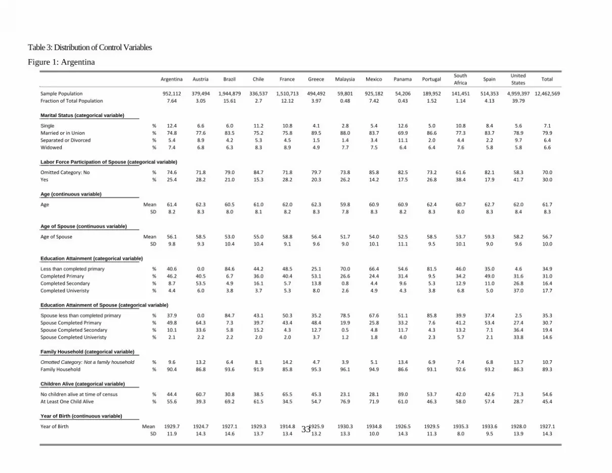
Table 3: Distribution of Control Variables

Figure 1: Argentina

Argentina Austria Brazil Chile France Greece Malaysia Mexico Panama PortugalSouth Africa

SpainUnited States

Total

Sample Population 952,112 379,494 1,944,879 336,537 1,510,713 494,492 59,801 925,182 54,206 189,952 141,451 514,353 4,959,397 12,462,569Fraction of Total Population 7.64 3.05 15.61 2.7 12.12 3.97 0.48 7.42 0.43 1.52 1.14 4.13 39.79

Marital Status (categorical variable)

Single % 12.4 6.6 6.0 11.2 10.8 4.1 2.8 5.4 12.6 5.0 10.8 8.4 5.6 7.1Married or in Union % 74.8 Separated or Divorced % 5.4

77.68.9

83.54.2

75.25.3

75.84.5

89.51.5

88.01.4

83.73.4

69.911.1

86.62.0

77.34.4

83.72.2

78.99.7

79.96.4

Widowed % 7.4 6.8 6.3 8.3 8.9 4.9 7.7 7.5 6.4 6.4 7.6 5.8 5.8 6.6

Labor Force Participation of Spouse (categorical variable) Omitted Category: No % 74.6 71.8 79.0 84.7 71.8 79.7 73.8 85.8 82.5 73.2 61.6 82.1 58.3 70.0Yes % 25.4 28.2 21.0 15.3 28.2 20.3 26.2 14.2 17.5 26.8 38.4 17.9 41.7 30.0

Age (continuous variable) Age Mean 61.4 SD 8.2

Age of Spouse (continuous variable) Age of Spouse Mean 56.1

62.38.3

58.5

60.58.0

53.0

61.08.1

55.0

62.08.2

58.8

62.38.3

56.4

59.87.8

51.7

60.98.3

54.0

60.98.2

52.5

62.48.3

58.5

60.78.0

53.7

62.78.3

59.3

62.08.4

58.2

61.78.3

56.7SD 9.8 9.3 10.4 10.4 9.1 9.6 9.0 10.1 11.1 9.5 10.1 9.0 9.6 10.0

Education Attainment (categorical variable)

Less than completed primary % 40.6 0.0 84.6 44.2 48.5 25.1 70.0 66.4 54.6 81.5 46.0 35.0 4.6 34.9Completed Primary % 46.2 40.5 6.7 36.0 40.4 53.1 26.6 24.4 31.4 9.5 34.2 49.0 31.6 31.0Completed Secondary % 8.7 53.5 4.9 16.1 5.7 13.8 0.8 4.4 9.6 5.3 12.9 11.0 26.8 16.4Completed Univeristy % 4.4 6.0 3.8 3.7 5.3 8.0 2.6 4.9 4.3 3.8 6.8 5.0 37.0 17.7

Education Attainment of Spouse (categorical variable)

Spouse less than completed primary % 37.9 0.0 84.7 43.1 50.3 35.2 78.5 67.6 51.1 85.8 39.9 37.4 2.5 35.3Spouse Completed Primary % 49.8 Spouse Completed Secondary % 10.1

64.333.6

7.35.8

39.715.2

43.44.3

48.412.7

19.90.5

25.84.8

33.211.7

7.64.3

41.213.2

53.47.1

27.436.4

30.719.4

Spouse Completed Univeristy % 2.1 2.2 2.2 2.0 2.0 3.7 1.2 1.8 4.0 2.3 5.7 2.1 33.8 14.6

Family Household (categorical variable) Omotted Category: Not a family household % 9.6 13.2 6.4 8.1 14.2 4.7 3.9 5.1 13.4 6.9 7.4 6.8 13.7 10.7Family Household % 90.4 86.8 93.6 91.9 85.8 95.3 96.1 94.9 86.6 93.1 92.6 93.2 86.3 89.3

Children Alive (categorical variable) No children alive at time of census % 44.4 60.7 30.8 38.5 65.5 45.3 23.1 28.1 39.0 53.7 42.0 42.6 71.3 54.6At Least One Child Alive % 55.6 39.3 69.2 61.5 34.5 54.7 76.9 71.9 61.0 46.3 58.0 57.4 28.7 45.4

Year of Birth (continuous variable)

Year of Birth Mean 1929.7SD 11.9

1924.7

14.31927.1

14.61929.3

13.71914.8

13.41925.933

13.21930.3

13.31934.8

10.01926.5

14.31929.5

11.31935.3

8.01933.6

9.51928.0

13.91927.1

14.3

35

1971

1971

1971

1981

1981

1981

1991

1991

1991

2001

200120010

.2.4

.6.8

1M

ale

Labo

r For

ce P

artic

ipat

ion

50 60 70 80Age

Austria: MLFP 50-80 Year Olds by Census Year

1971

1971

1981

1981

1991

1991

2001

2001

0.2

.4.6

.81

Frac

tion

of E

ach

Age

in th

e La

bor F

orce

20 40 60 80 100Age

Austria

Figure 2: Austria

36

0

.2.4

.6.8

1M

ale

Labo

r For

ce P

artic

ipat

ion

50 60 70 80Age

Single Married

Divorced Widowed

MLFP by Marital Status

0.2

.4.6

.81

Mal

e La

bor F

orce

Par

ticip

atio

n

50 60 70 80Age

Spouse Not Working Spouse Working

MLFP by Spouse LFP

0.2

.4.6

.81

Mal

e La

bor F

orce

Par

ticip

atio

n

50 60 70 80Age

<Primary Primary

Secondary University

MLFP by Education0

.2.4

.6.8

1M

ale

Labo

r For

ce P

artic

ipat

ion

50 60 70 80Age

Spouse <Primary Spouse Primary

Spouse Secondary Spouse University

MLFP by Spouse Education

0.2

.4.6

.81

Mal

e La

bor F

orce

Par

ticip

atio

n

50 60 70 80Age

Not a Family Household Family Household

MLFP by Family Household

0.2

.4.6

.81

Mal

e La

bor F

orce

Par

ticip

atio

n

50 60 70 80Age

No Kids Alive Kids Alive

MLFP by Children Alive

Austria

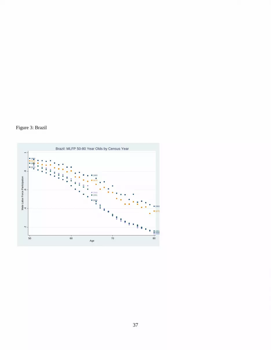
37

1960

1960

1960

1970

1970

1970

1980

1980

1980

1991

1991

1991

2000

2000

2000

.2.4

.6.8

1M

ale

Labo

r For

ce P

artic

ipat

ion

50 60 70 80Age

Brazil: MLFP 50-80 Year Olds by Census Year

Figure 3: Brazil

38

1960

1960

1970

1970

1980

1980

1991

1991

2000

2000

0.2

.4.6

.81

Frac

tion

of E

ach

Age

in th

e La

bor F

orce

20 40 60 80 100Age

Brazil.2

.4.6

.81

Mal

e La

bor F

orce

Par

ticip

atio

n

50 60 70 80Age

Single Married

Divorced Widowed

MLFP by Marital Status

.2.4

.6.8

1M

ale

Labo

r For

ce P

artic

ipat

ion

50 60 70 80Age

Spouse Not Working Spouse Working

MLFP by Spouse LFP

.2.4

.6.8

1M

ale

Labo

r For

ce P

artic

ipat

ion

50 60 70 80Age

<Primary Primary

Secondary University

MLFP by Education

.2.4

.6.8

1M

ale

Labo

r For

ce P

artic

ipat

ion

50 60 70 80Age

Spouse <Primary Spouse Primary

Spouse Secondary Spouse University

MLFP by Spouse Education

.2.4

.6.8

1M

ale

Labo

r For

ce P

artic

ipat

ion

50 60 70 80Age

Not a Family Household Family Household

MLFP by Family Household

.2.4

.6.8

1M

ale

Labo

r For

ce P

artic

ipat

ion

50 60 70 80Age

No Kids Alive Kids Alive

MLFP by Children Alive

Brazil

39

Figure 4: Chile

1960

1960

1960

1970

1970

1970

1982

1982

1982

1992

1992

1992

2002

2002

2002

0.2

.4.6

.81

Mal

e La

bor F

orce

Par

ticip

atio

n

50 60 70 80Age

Chile: MLFP 50-80 Year Olds by Census Year

1960

1960

1970

1970

1982

1982

1992

1992

2002

2002

0.2

.4.6

.81

Frac

tion

of E

ach

Age

in th

e La

bor F

orce

20 40 60 80 100Age

Chile

40

0

.2.4

.6.8

Mal

e La

bor F

orce

Par

ticip

atio

n

50 60 70 80Age

Single Married

Divorced Widowed

MLFP by Marital Status

0.2

.4.6

.81

Mal

e La

bor F

orce

Par

ticip

atio

n

50 60 70 80Age

Spouse Not Working Spouse Working

MLFP by Spouse LFP

0.2

.4.6

.81

Mal

e La

bor F

orce

Par

ticip

atio

n

50 60 70 80Age

<Primary Primary

Secondary University

MLFP by Education0

.2.4

.6.8

1M

ale

Labo

r For

ce P

artic

ipat

ion

50 60 70 80Age

Spouse <Primary Spouse Primary

Spouse Secondary Spouse University

MLFP by Spouse Education

0.2

.4.6

.8M

ale

Labo

r For

ce P

artic

ipat

ion

50 60 70 80Age

Not a Family Household Family Household

MLFP by Family Household

0.2

.4.6

.8M

ale

Labo

r For

ce P

artic

ipat

ion

50 60 70 80Age

No Kids Alive Kids Alive

MLFP by Children Alive

Chile

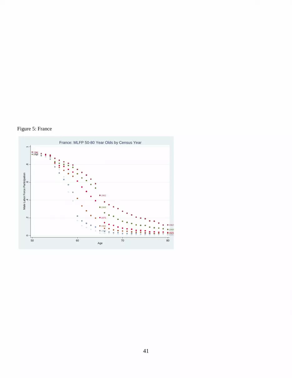
41

Figure 5: France

1962

1962

1962

1968

1968

1968

1975

1975

1975

1982

1982

1982

1990

1990

1990

1999

1999 19990.2

.4.6

.81

Mal

e La

bor F

orce

Par

ticip

atio

n

50 60 70 80Age

France: MLFP 50-80 Year Olds by Census Year

42

Figure 6: Greece

1962

1962

1968

1968

1975

1975

1982

1982

1990

1990

1999

1999

0.2

.4.6

.81

Frac

tion

of E

ach

Age

in th

e La

bor F

orce

20 40 60 80 100Age

France0

.2.4

.6.8

1M

ale

Labo

r For

ce P

artic

ipat

ion

50 60 70 80Age

Single Married

Divorced Widowed

MLFP by Marital Status

0.2

.4.6

.81

Mal

e La

bor F

orce

Par

ticip

atio

n

50 60 70 80Age

Spouse Not Working Spouse Working

MLFP by Spouse LFP

0.2

.4.6

.81

Mal

e La

bor F

orce

Par

ticip

atio

n

50 60 70 80Age

<Primary Primary

Secondary University

MLFP by Education

0.2

.4.6

.81

Mal

e La

bor F

orce

Par

ticip

atio

n

50 60 70 80Age

Spouse <Primary Spouse Primary

Spouse Secondary Spouse University

MLFP by Spouse Education

0.2

.4.6

.81

Mal

e La

bor F

orce

Par

ticip

atio

n

50 60 70 80Age

Not a Family Household Family Household

MLFP by Family Household

0.2

.4.6

.81

Mal

e La

bor F

orce

Par

ticip

atio

n

50 60 70 80Age

No Kids Alive Kids Alive

MLFP by Children Alive

France

43

1971

1971

1971

1981

1981

1981

1991

1991

1991

2001

2001

20010.2

.4.6

.81

Mal

e La

bor F

orce

Par

ticip

atio

n

50 60 70 80Age

Greece: MLFP 50-80 Year Olds by Census Year

1971

1971

1981

1981

1991

1991

2001

2001

0.2

.4.6

.81

Frac

tion

of E

ach

Age

in th

e La

bor F

orce

20 40 60 80 100Age

Greece

44

0.2

.4.6

.81

Mal

e La

bor F

orce

Par

ticip

atio

n

50 60 70 80Age

Single Married

Divorced Widowed

MLFP by Marital Status

0.2

.4.6

.81

Mal

e La

bor F

orce

Par

ticip

atio

n

50 60 70 80Age

Spouse Not Working Spouse Working

MLFP by Spouse LFP

0.2

.4.6

.81

Mal

e La

bor F

orce

Par

ticip

atio

n

50 60 70 80Age

<Primary Primary

Secondary University

MLFP by Education0

.2.4

.6.8

1M

ale

Labo

r For

ce P

artic

ipat

ion

50 60 70 80Age

Spouse <Primary Spouse Primary

Spouse Secondary Spouse University

MLFP by Spouse Education

0.2

.4.6

.81

Mal

e La

bor F

orce

Par

ticip

atio

n

50 60 70 80Age

Not a Family Household Family Household

MLFP by Family Household

0.2

.4.6

.81

Mal

e La

bor F

orce

Par

ticip

atio

n

50 60 70 80Age

No Kids Alive Kids Alive

MLFP by Children Alive

Greece

Figure 7: Malaysia

45

1970

1970

1970

1980

1980

1980

1991

1991

1991

2000

2000

2000

0.2

.4.6

.81

Mal

e La

bor F

orce

Par

ticip

atio

n

50 60 70 80Age

Malaysia: MLFP 50-80 Year Olds by Census Year

1970

1970

1980

1980

1991

1991

2000

2000

0.2

.4.6

.81

Frac

tion

of E

ach

Age

in th

e La

bor F

orce

20 40 60 80 100Age

Malaysia

46

.2.4

.6.8

1M

ale

Labo

r For

ce P

artic

ipat

ion

50 60 70 80Age

Single Married

Divorced Widowed

MLFP by Marital Status

.2.4

.6.8

1M

ale

Labo

r For

ce P

artic

ipat

ion

50 60 70 80Age

Spouse Not Working Spouse Working

MLFP by Spouse LFP

0.2

.4.6

.81

Mal

e La

bor F

orce

Par

ticip

atio

n

50 60 70 80Age

<Primary Primary

Secondary University

MLFP by Education0

.2.4

.6.8

1M

ale

Labo

r For

ce P

artic

ipat

ion

50 60 70 80Age

Spouse <Primary Spouse Primary

Spouse Secondary Spouse University

MLFP by Spouse Education

.2.4

.6.8

1M

ale

Labo

r For

ce P

artic

ipat

ion

50 60 70 80Age

Not a Family Household Family Household

MLFP by Family Household

.2.4

.6.8

1M

ale

Labo

r For

ce P

artic

ipat

ion

50 60 70 80Age

No Kids Alive Kids Alive

MLFP by Children Alive

Malaysia

47

1970

1970

1970

1990

1990

1990

1995

1995

1995

2000

2000

2000

.2.4

.6.8

1M

ale

Labo

r For

ce P

artic

ipat

ion

50 60 70 80Age

Mexico: MLFP 50-80 Year Olds by Census Year

Figure 8: Mexico

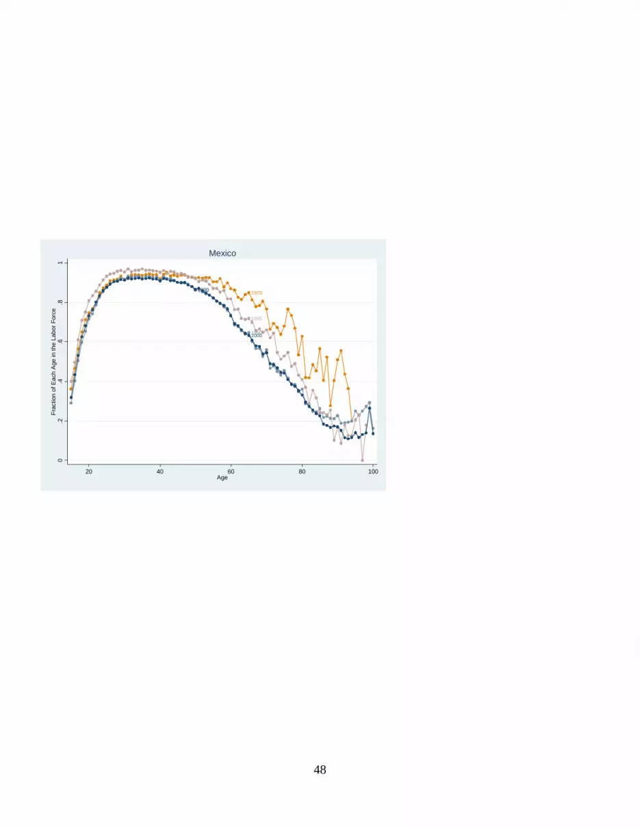
48

1970

19701990

1990

1995

1995

2000

2000

0.2

.4.6

.81

Frac

tion

of E

ach

Age

in th

e La

bor F

orce

20 40 60 80 100Age

Mexico

49

.2.4

.6.8

1M

ale

Labo

r For

ce P

artic

ipat

ion

50 60 70 80Age

Single Married

Divorced Widowed

MLFP by Marital Status

.2.4

.6.8

1M

ale

Labo

r For

ce P

artic

ipat

ion

50 60 70 80Age

Spouse Not Working Spouse Working

MLFP by Spouse LFP

.2.4

.6.8

1M

ale

Labo

r For

ce P

artic

ipat

ion

50 60 70 80Age

<Primary Primary

Secondary University

MLFP by Education

.2.4

.6.8

1M

ale

Labo

r For

ce P

artic

ipat

ion

50 60 70 80Age

Spouse <Primary Spouse Primary

Spouse Secondary Spouse University

MLFP by Spouse Education

.2.4

.6.8

1M

ale

Labo

r For

ce P

artic

ipat

ion

50 60 70 80Age

Not a Family Household Family Household

MLFP by Family Household

.2.4

.6.8

1M

ale

Labo

r For

ce P

artic

ipat

ion

50 60 70 80Age

No Kids Alive Kids Alive

MLFP by Children Alive

Mexico

50

Figure 9: Panama

1960

1960

1960

1970

1970

1970

1980

1980

1980

1990

1990

1990

2000

2000

2000.2.4

.6.8

1M

ale

Labo

r For

ce P

artic

ipat

ion

50 60 70 80Age

Panama: MLFP 50-80 Year Olds by Census Year

51

1960

1960

1970

1970

1980

1980

1990

1990

2000

2000

0.2

.4.6

.81

Frac

tion

of E

ach

Age

in th

e La

bor F

orce

20 40 60 80 100Age

Panama.2

.4.6

.81

Mal

e La

bor F

orce

Par

ticip

atio

n

50 60 70 80Age

Single Married

Divorced Widowed

MLFP by Marital Status

.2.4

.6.8

1M

ale

Labo

r For

ce P

artic

ipat

ion

50 60 70 80Age

Spouse Not Working Spouse Working

MLFP by Spouse LFP

0.2

.4.6

.81

Mal

e La

bor F

orce

Par

ticip

atio

n

50 60 70 80Age

<Primary Primary

Secondary University

MLFP by Education

0.2

.4.6

.81

Mal

e La

bor F

orce

Par

ticip

atio

n

50 60 70 80Age

Spouse <Primary Spouse Primary

Spouse Secondary Spouse University

MLFP by Spouse Education

.2.4

.6.8

1M

ale

Labo

r For

ce P

artic

ipat

ion

50 60 70 80Age

Not a Family Household Family Household

MLFP by Family Household

.2.4

.6.8

1M

ale

Labo

r For

ce P

artic

ipat

ion

50 60 70 80Age

No Kids Alive Kids Alive

MLFP by Children Alive

Panama

52

Figure 10: Portugal

1981

1981

1991

1991

2001

2001

0.2

.4.6

.81

Frac

tion

of E

ach

Age

in th

e La

bor F

orce

20 40 60 80 100Age

Portugal

1981

1981

1981

1991

1991

1991

2001

2001

2001

0.2

.4.6

.81

Mal

e La

bor F

orce

Par

ticip

atio

n

50 60 70 80Age

Portugal: MLFP 50-80 Year Olds by Census Year

53

Figure 11: South Africa

0.2

.4.6

.81

Mal

e La

bor F

orce

Par

ticip

atio

n

50 60 70 80Age

Single Married

Divorced Widowed

MLFP by Marital Status

0.2

.4.6

.81

Mal

e La

bor F

orce

Par

ticip

atio

n

50 60 70 80Age

Spouse Not Working Spouse Working

MLFP by Spouse LFP

0.2

.4.6

.81

Mal

e La

bor F

orce

Par

ticip

atio

n

50 60 70 80Age

<Primary Primary

Secondary University

MLFP by Education0

.2.4

.6.8

1M

ale

Labo

r For

ce P

artic

ipat

ion

50 60 70 80Age

Spouse <Primary Spouse Primary

Spouse Secondary Spouse University

MLFP by Spouse Education

0.2

.4.6

.81

Mal

e La

bor F

orce

Par

ticip

atio

n

50 60 70 80Age

Not a Family Household Family Household

MLFP by Family Household

0.2

.4.6

.81

Mal

e La

bor F

orce

Par

ticip

atio

n

50 60 70 80Age

No Kids Alive Kids Alive

MLFP by Children Alive

Portugal

1996

1996

1996

0.2

.4.6

.8M

ale

Labo

r For

ce P

artic

ipat

ion

50 60 70 80Age

South Africa: MLFP 50-80 Year Olds by Census Year

54

1996

1996

2001

2001

0.2

.4.6

.81

Frac

tion

of E

ach

Age

in th

e La

bor F

orce

20 40 60 80 100Age

South Africa0

.2.4

.6.8

Mal

e La

bor F

orce

Par

ticip

atio

n

50 60 70 80Age

Single Married

Divorced Widowed

MLFP by Marital Status

0.2

.4.6

.81

Mal

e La

bor F

orce

Par

ticip

atio

n

50 60 70 80Age

Spouse Not Working Spouse Working

MLFP by Spouse LFP

0.2

.4.6

.81

Mal

e La

bor F

orce

Par

ticip

atio

n

50 60 70 80Age

<Primary Primary

Secondary University

MLFP by Education

0.2

.4.6

.81

Mal

e La

bor F

orce

Par

ticip

atio

n

50 60 70 80Age

Spouse <Primary Spouse Primary

Spouse Secondary Spouse University

MLFP by Spouse Education

0.2

.4.6

.81

Mal

e La

bor F

orce

Par

ticip

atio

n

50 60 70 80Age

Not a Family Household Family Household

MLFP by Family Household

0.2

.4.6

.8M

ale

Labo

r For

ce P

artic

ipat

ion

50 60 70 80Age

No Kids Alive Kids Alive

MLFP by Children Alive

South Africa

55

Figure 12: Spain

1981

1981

1991

1991

2001

2001

0.2

.4.6

.81

Frac

tion

of E

ach

Age

in th

e La

bor F

orce

20 40 60 80 100Age

Spain

1981

1981

1981

1991

1991

1991

2001

2001

20010.2

.4.6

.81

Mal

e La

bor F

orce

Par

ticip

atio

n

50 60 70 80Age

Spain: MLFP 50-80 Year Olds by Census Year

56

0.2

.4.6

.81

Mal

e La

bor F

orce

Par

ticip

atio

n

50 60 70 80Age

Single Married

Divorced Widowed

MLFP by Marital Status

0.2

.4.6

.81

Mal

e La

bor F

orce

Par

ticip

atio

n

50 60 70 80Age

Spouse Not Working Spouse Working

MLFP by Spouse LFP

0.2

.4.6

.81

Mal

e La

bor F

orce

Par

ticip

atio

n

50 60 70 80Age

<Primary Primary

Secondary University

MLFP by Education

0.2

.4.6

.81

Mal

e La

bor F

orce

Par

ticip

atio

n

50 60 70 80Age

Spouse <Primary Spouse Primary

Spouse Secondary Spouse University

MLFP by Spouse Education

0.2

.4.6

.81

Mal

e La

bor F

orce

Par

ticip

atio

n

50 60 70 80Age

Not a Family Household Family Household

MLFP by Family Household

0.2

.4.6

.81

Mal

e La

bor F

orce

Par

ticip

atio

n

50 60 70 80Age

No Kids Alive Kids Alive

MLFP by Children Alive

Spain

Figure 13: United States of America

57

1960

1960

1960

1970

1970

1970

1980

1980

1980

1990

1990

1990

2000

2000

2000

2005

2005

2005

0.2

.4.6

.81

Mal

e La

bor F

orce

Par

ticip

atio

n

50 60 70 80Age

United States: MLFP 50-80 Year Olds by Census Year

1960

1960

1970

1970

1980

1980

1990

1990

2000

2000

2005

2005

0.2

.4.6

.81

Frac

tion

of E

ach

Age

in th

e La

bor F

orce

20 40 60 80 100Age

United States

58

0.2

.4.6

.81

Mal

e La

bor F

orce

Par

ticip

atio

n

50 60 70 80Age

Single Married

Divorced Widowed

MLFP by Marital Status

0.2

.4.6

.81

Mal

e La

bor F

orce

Par

ticip

atio

n

50 60 70 80Age

Spouse Not Working Spouse Working

MLFP by Spouse LFP

0.2

.4.6

.81

Mal

e La

bor F

orce

Par

ticip

atio

n

50 60 70 80Age

<Primary Primary

Secondary University

MLFP by Education0

.2.4

.6.8

1M

ale

Labo

r For

ce P

artic

ipat

ion

50 60 70 80Age

Spouse <Primary Spouse Primary

Spouse Secondary Spouse University

MLFP by Spouse Education

0.2

.4.6

.81

Mal

e La

bor F

orce

Par

ticip

atio

n

50 60 70 80Age

Not a Family Household Family Household

MLFP by Family Household

0.2

.4.6

.81

Mal

e La

bor F

orce

Par

ticip

atio

n

50 60 70 80Age

No Kids Alive Kids Alive

MLFP by Children Alive

United States

59

Table 4: The Effect of Social Security Tax, Replacement Rate, and Delay Incentive on Male Labor Force Participation. Pooled and by Country

Pooled Argentina Austria Brazil Chile France Greece Malaysia Mexico Panama Portugal South Africa Spain United States

Social Security Variables (continuous variables)

Social Security Tax Rate 0.0701*** 0.184*** -1.544*** 0.684*** -0.0125 0.422*** -0.744*** 2.152*** -1.070*** 0.0695 -0.397*** -2.521***(0.00512) (0.0228) (0.0725) (0.0129) (0.0153) (0.0134) (0.0581) (0.0863) (0.106) (0.0457) (0.0690) (0.0497)

Replacement Rate as a Fraction of Wage -0.119*** -0.0635*** -0.113*** 0.000460 -0.0760*** -0.155*** -0.0668*** -0.0964*** -0.0159*** -0.0618*** -0.130*** -0.0910*** -0.283*** -0.116***(0.000364) (0.00138) (0.00185) (0.00176) (0.00280) (0.00110) (0.00196) (0.00389) (0.00135) (0.00783) (0.00517) (0.00582) (0.00270) (0.000737)

Delay Incentive as a Fraction of Wage 0.000636*** 0.00130*** -0.00240*** 1.94e-05 0.00147*** 0.0161*** 0.000304*** -0.00587 -0.000257*** -0.000311** 0.00193*** 0.00627*** 0.00148*** 0.000149***(9.04e-06) (9.20e-05) (0.000125) (2.52e-05) (7.46e-05) (0.000150) (3.30e-05) (0.0111) (2.62e-05) (0.000158) (6.42e-05) (0.000436) (2.08e-05) (2.50e-05)

Marital Status

Omitted Category: SingleMarried or in Union 0.250*** 0.273*** 0.194*** 0.367*** 0.241*** 0.0978*** 0.196*** 0.464*** 0.339*** 0.314*** 0.288*** 0.250*** 0.301*** 0.237***

(0.00170) (0.00589) (0.0118) (0.00326) (0.00848) (0.00649) (0.00977) (0.0208) (0.00519) (0.0193) (0.0122) (0.0128) (0.00721) (0.00359)Separated or Divorced 0.0379*** 0.0374*** 0.0606*** 0.0625*** 0.0414*** 0.0179*** 0.0376*** 0.0264 0.0304*** 0.0447*** 0.0746*** -0.000944 0.00351 0.0666***

(0.000842) (0.00276) (0.00517) (0.00201) (0.00472) (0.00278) (0.00776) (0.0195) (0.00307) (0.00796) (0.0113) (0.00840) (0.00589) (0.00127)Widowed -0.0295*** -0.0520*** -0.0644*** -0.0101*** -0.0284*** -0.103*** -0.0304*** -0.0352** -0.00519* 0.0311*** -0.00556 -0.106*** -0.0667*** 0.0238***

(0.000899) (0.00265) (0.00559) (0.00207) (0.00443) (0.00245) (0.00597) (0.0147) (0.00275) (0.00955) (0.00872) (0.00723) (0.00489) (0.00157)

Labor Force Participation of Spouse

Omitted Category: NoYes 0.166*** 0.126*** 0.165*** 0.0986*** 0.115*** 0.259*** 0.245*** 0.171*** 0.0839*** 0.0674*** 0.164*** 0.278*** 0.0972*** 0.163***

(0.000410) (0.00152) (0.00292) (0.000980) (0.00315) (0.00134) (0.00220) (0.00455) (0.00148) (0.00671) (0.00365) (0.00354) (0.00267) (0.000621)

Age (continuous variable)

Age -0.0298*** -0.0255*** -0.0525*** -0.0295*** -0.0298*** -0.0481*** -0.0436*** -0.0194*** -0.0187*** -0.0216*** -0.0385*** -0.0279*** -0.0287*** -0.0258***(4.40e-05) (0.000156) (0.000344) (0.000106) (0.000318) (0.000177) (0.000296) (0.000463) (0.000169) (0.000683) (0.000560) (0.000591) (0.000423) (9.15e-05)

Age of Spouse (continuous variable)

Age of Spouse -0.00337*** -0.00442*** -0.00356*** -0.00388*** -0.00350*** -0.00361*** -0.00206*** -0.00595*** -0.00379*** -0.00330*** -0.00443*** -0.00567*** -0.00690*** -0.00251***(2.70e-05) (9.22e-05) (0.000209) (4.80e-05) (0.000131) (0.000107) (0.000158) (0.000316) (6.90e-05) (0.000281) (0.000257) (0.000234) (0.000211) (4.86e-05)

Education Attainment

Omitted Category: Less than completed primaryCompleted Primary -0.00614*** -0.0160*** -0.344*** -0.0788*** -0.0353*** 0.0546*** 0.0194*** -0.0567*** -0.0242*** -0.116*** 0.0535*** 0.0294*** 0.0615*** 0.0902***

(0.000524) (0.00134) (0.00408) (0.00162) (0.00229) (0.00123) (0.00231) (0.00549) (0.00132) (0.00550) (0.00520) (0.00390) (0.00274) (0.00137)Completed Secondary 0.0501*** 0.0183*** -0.301*** -0.0787*** 0.0612*** 0.135*** -0.0644*** -0.107*** -0.0173*** -0.158*** 0.0563*** 0.0872*** 0.103*** 0.166***

(0.000655) (0.00236) (0.00468) (0.00196) (0.00314) (0.00244) (0.00339) (0.0249) (0.00269) (0.00923) (0.00702) (0.00585) (0.00392) (0.00136)Completed Univeristy 0.150*** 0.170*** 0.0592*** 0.223*** 0.270*** 0.0581*** -0.0274* 0.0554*** -0.0845*** 0.298*** 0.127*** 0.263*** 0.256***

(0.000654) (0.00265) (0.00208) (0.00442) (0.00230) (0.00426) (0.0156) (0.00255) (0.0131) (0.00787) (0.00757) (0.00558) (0.00134)

Education Attainment of Spouse

Omitted Category: Spouse less than completed primarySpouse Completed Primary -0.0264*** -0.00303* -0.0660*** -0.0481*** -0.0466*** 0.00409*** -0.0599*** -0.0527*** -0.0308*** -0.104*** 0.00765 -0.0121*** 0.0118*** 0.000183

(0.000569) (0.00155) (0.00910) (0.00173) (0.00263) (0.00137) (0.00234) (0.00673) (0.00148) (0.00678) (0.00636) (0.00445) (0.00292) (0.00204)Spouse Completed Secondary -0.00490*** 0.00133 -0.0262*** -0.0345*** -0.0250*** -0.0256*** -0.0762*** -0.0872** -0.0229*** -0.111*** 0.00472 0.0307*** 0.00370 0.0146***

(0.000715) (0.00277) (0.00887) (0.00205) (0.00404) (0.00328) (0.00379) (0.0359) (0.00309) (0.0105) (0.00862) (0.00706) (0.00478) (0.00206)Spouse Completed Univeristy 0.0196*** 0.00610 -0.0278*** -0.0347*** -0.00428 -0.0928*** -0.0853*** -0.0146*** -0.0898*** -0.0360*** 0.0466*** -0.00480 0.0310***

(0.000832) (0.00574) (0.00326) (0.00991) (0.00484) (0.00592) (0.0261) (0.00494) (0.0163) (0.0117) (0.00987) (0.00799) (0.00209)

Family Household

Omotted Category: Not a family householdFamily Household -0.0145*** -0.0623*** -0.0232*** -0.0743*** -0.0225*** 0.0473*** -0.0351*** -0.0852*** -0.0675*** -0.0641*** -0.0196** -0.137*** -0.000227 -0.00607***

(0.000718) (0.00218) (0.00448) (0.00161) (0.00393) (0.00213) (0.00535) (0.0107) (0.00224) (0.00715) (0.00789) (0.00658) (0.00437) (0.00117)

Children Alive

Omitted Category: No children alive at time of censusAt Least One Child Alive 0.0515*** 0.0306*** 0.0827*** 0.0474*** 0.0107*** 0.107*** 0.0416*** -0.0179*** 0.0167*** 0.0100* 0.0428*** 0.0481*** 0.0658*** 0.0537***

(0.000385) (0.00129) (0.00226) (0.000907) (0.00225) (0.00122) (0.00185) (0.00526) (0.00126) (0.00522) (0.00304) (0.00357) (0.00205) (0.000639)

Year of Birth (continuous variable)

Year of Birth -0.00696*** 0.000417*** -0.00793*** -0.00804*** -0.00394*** -0.0123*** -0.00820*** -0.00235*** -0.00561*** -0.00360*** -0.00949*** -0.00690*** -0.00330***(1.79e-05) (7.47e-05) (0.000160) (5.97e-05) (0.000106) (5.92e-05) (0.000197) (0.000206) (0.000165) (0.000229) (0.000277) (0.000176) (6.42e-05)

Country Fixed Effects Yes

Observations 12,466,335 952,112 379,494 1,944,879 336,537 1,510,713 494,492 59,801 925,182 54,206 189,952 141,451 514,353 4,959,397

Robust standard errors in parentheses. *** p<0.01, ** p<0.05, * p<0.1Marginal effects around the mean calculated from a probit estimation. dy/dx is for discrete change of dummy variable from 0 to 1

60

Figure 14: Graphical Display of Marginal Effects Presented in Table X

-3

-2

-1

0

1

2

3

Pool

ed

Arg

entin

a

Aus

tria

Braz

il

Chile

Fran

ce

Gre

ece

Mal

aysi

a

Mex

ico

Pana

ma

Port

ugal

Sout

h A

fric

a

Spai

n

Uni

ted

Stat

es

DProbit Coefficients: The Effect of Social Security Tax Rat on Male Labor Force Participation

-0.3

-0.25

-0.2

-0.15

-0.1

-0.05

0

0.05

Pool

ed

Arg

entin

a

Aus

tria

Braz

il

Chile

Fran

ce

Gre

ece

Mal

aysi

a

Mex

ico

Pana

ma

Port

ugal

Sout

h A

fric

a

Spai

n

Uni

ted

Stat

es

DPobit Coefficients: The Effect of Replacement Rate as a Fraction of the Wage on Male Labor

Force Participation

61

-0.02

-0.015

-0.01

-0.005

0

0.005

0.01

0.015

0.02Po

oled

Arg

entin

a

Aus

tria

Braz

il

Chile

Fran

ce

Gre

ece

Mal

aysi

a

Mex

ico

Pana

ma

Port

ugal

Sout

h A

fric

a

Spai

n

Uni

ted

Stat

es

DProbit Coefficients: The Effect of Delay Incentive as a Fraction of Wage on Male Labor Force Participation

Table 5.1: Regional Variation in Labor Force Participation and its Covariates. France, by Region.

62

Basse- Champagne- Franche- Haute- Lanquedoc- Midi- Nord-Pas-de- Pays de la Poitou- Provence- Region d'Île France Alsace Aquitaine Auvergne Bourgogne Bretagne Centre Corse Limousin Lorraine Picardie Rhône-Alpes

Normandie Ardenne Comté Normandie Roussillon Pyrénées Calais Loire Charentes Côte d'Azur de France

Sample Population 1,510,713 40,557 85,502 44,313 36,420 50,570 78,277 67,823 36,529 6,674 28,911 41,606 63,682 28,157 60,424 78,005 100,767 76,694 45,646 50,314 108,323 248,928 132,591Fraction of Total Population 12.12 2.7 5.7 2.9 2.4 3.3 5.2 4.5 2.4 0.4 1.9 2.8 4.2 1.9 4.0 5.2 6.7 5.1 3.0 3.3 7.2 16.5 8.8

Labor Force Participation (categorical variable)

Omitted Category: No % 51.0 52.7 51.0 51.8 49.1 54.3 53.9 53.0 51.3 62.2 51.7 49.3 56.4 52.5 54.9 51.8 58.0 51.8 52.7 54.0 55.0 41.8 48.1Yes % 49.0 47.3 49.0 48.2 50.9 45.7 46.1 47.0 48.7 37.8 48.3 50.7 43.6 47.5 45.1 48.2 42.0 48.2 47.3 46.0 45.0 58.2 51.9

Marital Status (categorical variable)

Single % 10.8 9.5 11.8 14.4 10.3 11.7 12.9 10.5 9.9 18.1 12.0 8.8 11.0 13.1 9.7 13.5 7.6 9.5 9.4 9.9 10.8 9.9 11.9Married or in Union % 75.8 77.4 74.9 72.5 76.0 75.7 75.0 76.2 76.5 67.6 75.6 77.3 75.7 75.0 77.5 73.6 78.0 78.1 76.0 76.8 74.4 75.9 74.7Separated or Divorced % 4.5 3.5 4.6 3.7 4.4 3.9 2.7 4.3 4.4 4.3 3.8 4.9 4.4 3.1 3.6 4.0 3.6 3.4 4.7 4.1 6.3 6.2 4.6Widowed % 8.9 9.5 8.6 9.5 9.3 8.7 9.5 9.0 9.2 10.0 8.6 9.0 8.9 8.8 9.3 8.9 10.7 9.0 9.9 9.2 8.5 7.9 8.7

Labor Force Participation of Spouse (categorical variable)

Omitted Category: No % 71.8 78.2 71.2 71.4 61.9 73.1 67.3 69.4 72.2 90.3 71.9 70.6 82.7 66.7 80.8 73.7 80.5 68.8 74.3 74.0 79.3 63.2 69.9Yes % 28.2 21.8 28.8 28.6 38.1 26.9 32.7 30.6 27.8 9.7 28.1 29.4 17.3 33.3 19.2 26.3 19.5 31.2 25.7 26.0 20.7 36.8 30.1

Age (continuous variable)

Age Mean 62.0 61.8 62.5 62.5 61.8 62.7 61.9 62.7 62.2 62.3 62.0 61.8 62.8 62.9 61.5 62.5 61.7 62.0 62.2 62.7 62.5 61.2 61.8SD 8.2 8.1 8.3 8.3 8.1 8.3 8.1 8.3 8.3 8.1 8.3 8.2 8.3 8.3 8.1 8.3 8.1 8.2 8.2 8.3 8.3 8.1 8.2

Age of Spouse (continuous variable)

Age of Spouse Mean 58.8 58.6 58.9 59.1 58.5 59.4 58.7 59.4 59.0 57.7 58.8 58.7 59.4 59.4 58.1 58.9 58.9 59.0 59.2 59.5 59.0 58.0 58.5SD 9.1 8.9 9.2 9.0 9.1 9.1 8.7 9.1 9.2 9.8 9.1 9.1 9.2 8.9 8.9 9.2 8.9 8.9 9.3 9.0 9.5 9.4 9.1

Education Attainment (categorical variable)

Less than completed primary % 48.5 50.0 50.8 50.6 55.8 48.7 49.6 49.9 47.7 59.4 47.1 53.4 52.7 50.7 50.8 53.0 50.8 52.9 52.3 53.7 46.5 38.6 47.0Completed Primary % 40.4 35.4 38.7 41.3 36.7 43.4 42.5 42.0 45.2 31.7 44.4 38.1 36.9 42.6 40.2 37.6 41.6 39.1 40.1 39.1 38.7 41.8 42.1Completed Secondary % 5.7 9.4 5.8 4.8 4.1 4.4 4.6 4.7 4.2 5.0 5.0 4.8 5.6 4.0 5.4 5.2 4.5 4.6 4.4 4.2 7.5 8.0 5.9Completed Univeristy % 5.3 5.2 4.8 3.3 3.3 3.5 3.3 3.4 2.8 3.9 3.5 3.7 4.8 2.7 3.6 4.2 3.1 3.4 3.2 3.0 7.3 11.5 5.0

Education Attainment of Spouse (categorical variable)

Spouse less than completed primary % 50.3 59.3 52.7 47.5 55.2 47.4 51.9 49.4 49.1 63.6 45.9 55.0 55.6 48.1 55.7 53.9 54.9 54.3 53.6 53.9 50.0 41.7 46.2Spouse Completed Primary % 43.4 34.9 41.2 47.3 40.5 47.8 43.9 45.9 46.8 30.2 49.0 40.3 38.2 47.5 40.3 40.3 41.4 41.6 42.2 41.7 41.5 46.5 47.4Spouse Completed Secondary % 4.3 4.1 4.4 3.8 3.1 3.5 3.0 3.3 3.1 4.6 3.7 3.3 4.3 3.4 2.8 4.1 2.7 3.0 3.0 3.2 5.7 7.3 4.4Spouse Completed Univeristy % 2.0 1.7 1.8 1.5 1.2 1.3 1.3 1.3 1.0 1.6 1.5 1.4 1.9 1.1 1.2 1.7 0.9 1.2 1.2 1.2 2.8 4.5 2.0

Family Household (categorical variable)

Omotted Category: Not a family household % 14.2 12.5 12.7 15.7 15.1 15.0 14.8 14.5 14.2 11.8 14.5 13.6 13.4 13.6 13.1 13.4 12.2 13.8 13.9 13.1 14.9 15.1 15.4Family Household % 85.8 87.5 87.3 84.3 84.9 85.0 85.2 85.5 85.8 88.2 85.5 86.4 86.6 86.4 86.9 86.6 87.8 86.2 86.1 86.9 85.1 84.9 84.6

Children Alive (categorical variable)

No children alive at time of census % 65.5 60.0 63.9 65.1 66.1 69.7 63.1 70.2 67.1 59.7 64.3 67.2 66.3 66.6 60.9 60.9 64.3 65.5 66.9 68.4 67.8 66.7 64.3At Least One Child Alive % 34.5 40.0 36.1 34.9 33.9 30.3 36.9 29.8 32.9 40.3 35.7 32.8 33.7 33.4 39.1 39.1 35.7 34.5 33.1 31.6 32.2 33.3 35.7

Year of Birth (continuous variable)

Year of Birth Mean 1914.8 1914.7 1914.5 1914.0 1915.6 1913.8 1915.1 1914.3 1914.3 1912.8 1914.9 1915.2 1914.6 1913.2 1915.1 1914.3 1914.5 1915.1 1914.5 1914.1 1914.9 1915.3 1915.4SD 13.4 13.6 13.3 13.4 13.0 13.4 13.0 13.4 13.5 14.1 13.4 13.3 13.2 13.1 13.3 13.3 13.3 13.2 13.6 13.3 13.6 13.6 13.5

63

Table 5.2: The Effect of Social Security Tax Rate, Replacement Rate and Delay Incentive on Male Labor Force Participation in France. By Region.

Region Champagn Haute- Basse- Nord-Pas- Franche- Pays de la Poitou- Midi- Rhtne- Lanquedoc- Provence-France d'Nle de Picardie Centre Bourgogne Lorraine Alsace Bretagne Aquitaine Limousin Auvergne Corsee-Ardenne Normandie Normandie de-Calais Comti Loire Charentes Pyrinies Alpes Roussillon Ctte d'AzurFranceSocial Security Variables (continuous variables)

Social Security Tax Rate 0.422*** 0.307*** 0.351*** 0.304*** 0.145* 0.392*** 0.0810 0.267*** 0.429*** 0.275*** 1.007*** 0.140 0.394*** 0.205*** 0.560*** 0.576*** 0.527*** 0.701*** 0.515*** 0.525*** 0.563*** 0.405*** 0.513***(0.0134) (0.0327) (0.0865) (0.0772) (0.0842) (0.0663) (0.0906) (0.0709) (0.0459) (0.0638) (0.0809) (0.0998) (0.0644) (0.0593) (0.0753) (0.0570) (0.0582) (0.0961) (0.0472) (0.0767) (0.0626) (0.0478) (0.147)

Replacement Rate as a Fraction of Wage -0.155*** -0.151*** -0.155*** -0.151*** -0.170*** -0.173*** -0.161*** -0.141*** -0.124*** -0.121*** -0.170*** -0.171*** -0.170*** -0.144*** -0.156*** -0.163*** -0.156*** -0.184*** -0.166*** -0.162*** -0.142*** -0.141*** -0.122***(0.00110) (0.00258) (0.00724) (0.00651) (0.00683) (0.00533) (0.00702) (0.00607) (0.00424) (0.00569) (0.00680) (0.00831) (0.00518) (0.00493) (0.00616) (0.00454) (0.00474) (0.00822) (0.00366) (0.00639) (0.00506) (0.00400) (0.0154)

Delay Incentive as a Fraction of Wage 0.0161*** 0.0176*** 0.0177*** 0.0178*** 0.0198*** 0.0179*** 0.0144*** 0.0136*** 0.0165*** 0.0117*** 0.0139*** 0.0178*** 0.0166*** 0.0132*** 0.0157*** 0.0146*** 0.0128*** 0.0148*** 0.0175*** 0.0145*** 0.0162*** 0.0149*** 0.0147***(0.000150) (0.000366) (0.000974) (0.000875) (0.000924) (0.000715) (0.000970) (0.000814) (0.000555) (0.000734) (0.000924) (0.00110) (0.000675) (0.000654) (0.000805) (0.000624) (0.000648) (0.00111) (0.000508) (0.000876) (0.000682) (0.000523) (0.00194)

Marital Status

Omitted Category: SingleMarried or in Union 0.0978*** 0.271*** 0.128*** 0.185*** 0.206*** 0.144*** 0.00589 -0.0624* 0.0446* 0.0442 0.278*** -0.0598 0.127*** -0.0183 0.155*** 0.113*** 0.0719** -0.0650 0.100*** 0.0582 0.155*** 0.208*** 0.0567

(0.00649) (0.0157) (0.0438) (0.0353) (0.0385) (0.0325) (0.0425) (0.0375) (0.0233) (0.0313) (0.0347) (0.0517) (0.0321) (0.0324) (0.0372) (0.0268) (0.0280) (0.0517) (0.0227) (0.0388) (0.0280) (0.0195) (0.0650)Separated or Divorced 0.0179*** 0.0287*** -0.0423** 0.0163 0.0365** 0.0203 -0.00734 -0.0274* 0.0315*** 0.00194 0.0245 -0.0268 0.0407*** -0.0230* 0.0176 0.00822 -0.0192 0.00479 0.0174* -0.0285* 0.0375*** 0.0255*** 0.0129

(0.00278) (0.00612) (0.0179) (0.0163) (0.0176) (0.0138) (0.0182) (0.0148) (0.0115) (0.0150) (0.0189) (0.0212) (0.0146) (0.0138) (0.0161) (0.0115) (0.0121) (0.0238) (0.00931) (0.0165) (0.0135) (0.00904) (0.0338)Widowed -0.103*** -0.0717*** -0.139*** -0.0691*** -0.0471*** -0.0478*** -0.0562*** -0.126*** -0.0980*** -0.151*** -0.117*** -0.136*** -0.0747*** -0.150*** -0.0931*** -0.0841*** -0.143*** -0.0555*** -0.104*** -0.129*** -0.0862*** -0.0778*** -0.114***

(0.00245) (0.00646) (0.0157) (0.0146) (0.0168) (0.0123) (0.0164) (0.0124) (0.00876) (0.0113) (0.0151) (0.0177) (0.0120) (0.00940) (0.0135) (0.0102) (0.00980) (0.0180) (0.00845) (0.0131) (0.0112) (0.00894) (0.0251)

Labor Force Participation of Spouse

Omitted Category: NoYes 0.259*** 0.123*** 0.250*** 0.221*** 0.217*** 0.282*** 0.338*** 0.325*** 0.284*** 0.250*** 0.203*** 0.290*** 0.329*** 0.395*** 0.301*** 0.251*** 0.257*** 0.342*** 0.212*** 0.280*** 0.199*** 0.185*** 0.233***

(0.00134) (0.00312) (0.00887) (0.00840) (0.00825) (0.00656) (0.00742) (0.00743) (0.00572) (0.00773) (0.00939) (0.00996) (0.00590) (0.00539) (0.00784) (0.00563) (0.00606) (0.00902) (0.00451) (0.00794) (0.00796) (0.00572) (0.0296)

Age (continuous variable)

Age -0.0481*** -0.0494*** -0.0493*** -0.0514*** -0.0518*** -0.0501*** -0.0470*** -0.0488*** -0.0453*** -0.0552*** -0.0455*** -0.0516*** -0.0530*** -0.0447*** -0.0507*** -0.0473*** -0.0445*** -0.0450*** -0.0489*** -0.0461*** -0.0447*** -0.0435*** -0.0252***(0.000177) (0.000436) (0.00120) (0.00107) (0.00115) (0.000881) (0.00114) (0.000963) (0.000675) (0.000947) (0.00110) (0.00140) (0.000897) (0.000797) (0.00102) (0.000714) (0.000723) (0.00124) (0.000598) (0.000988) (0.000787) (0.000611) (0.00197)

Age of Spouse (continuous variable)

Age of Spouse -0.00361*** -0.00518*** -0.00484*** -0.00437*** -0.00447*** -0.00373*** -0.00215*** -0.00212*** -0.00247*** -0.00359*** -0.00672*** -0.00208** -0.00415*** -0.00345*** -0.00397*** -0.00347*** -0.00350*** -0.00110 -0.00392*** -0.00356*** -0.00402*** -0.00457*** -0.00195*(0.000107) (0.000246) (0.000736) (0.000628) (0.000669) (0.000559) (0.000684) (0.000594) (0.000396) (0.000525) (0.000678) (0.000828) (0.000550) (0.000523) (0.000658) (0.000442) (0.000453) (0.000830) (0.000364) (0.000628) (0.000501) (0.000356) (0.00110)

Education Attainment

Omitted Category: Less than completed primaryCompleted Primary 0.0546*** 0.0635*** 0.0515*** 0.0517*** 0.0529*** 0.0324*** 0.0538*** 0.0396*** 0.110*** 0.0897*** 0.0622*** 0.0510*** 0.0457*** 0.0265*** 0.0394*** 0.0306*** 0.0431*** 0.0602*** 0.0623*** 0.0548*** 0.0314*** 0.0307*** -0.0322**

(0.00123) (0.00318) (0.00764) (0.00695) (0.00749) (0.00582) (0.00779) (0.00644) (0.00428) (0.00597) (0.00789) (0.00887) (0.00563) (0.00533) (0.00661) (0.00521) (0.00534) (0.00880) (0.00417) (0.00697) (0.00578) (0.00458) (0.0159)Completed Secondary 0.135*** 0.148*** 0.127*** 0.138*** 0.126*** 0.107*** 0.143*** 0.106*** 0.256*** 0.196*** 0.196*** 0.103*** 0.127*** 0.163*** 0.0812*** 0.0575*** 0.0903*** 0.104*** 0.120*** 0.144*** 0.0613*** 0.0589*** 0.0130

(0.00244) (0.00460) (0.0189) (0.0160) (0.0160) (0.0136) (0.0177) (0.0157) (0.0100) (0.0128) (0.0118) (0.0201) (0.0132) (0.0125) (0.0169) (0.0107) (0.0114) (0.0220) (0.00781) (0.0150) (0.0118) (0.00813) (0.0318)Completed Univeristy 0.270*** 0.235*** 0.293*** 0.316*** 0.288*** 0.228*** 0.246*** 0.249*** 0.421*** 0.374*** 0.322*** 0.247*** 0.273*** 0.282*** 0.256*** 0.213*** 0.195*** 0.260*** 0.248*** 0.270*** 0.192*** 0.146*** 0.173***

(0.00230) (0.00374) (0.0190) (0.0164) (0.0154) (0.0150) (0.0179) (0.0169) (0.0102) (0.0131) (0.0133) (0.0209) (0.0134) (0.0132) (0.0177) (0.0104) (0.0118) (0.0232) (0.00755) (0.0160) (0.0128) (0.00832) (0.0396)

Education Attainment of Spouse

Omitted Category: Spouse less than completed primarySpouse Completed Primary 0.00409*** -0.0109*** 0.0167* 0.0157** 0.0218*** -0.0126* 0.0120 0.0116 0.0317*** 0.0402*** -0.00876 0.00716 0.000208 -0.00717 -0.00421 -0.0169*** -0.0244*** -0.00308 0.00990** -0.00183 -2.65e-05 -0.0179*** -0.0466**

(0.00137) (0.00356) (0.00856) (0.00776) (0.00832) (0.00646) (0.00870) (0.00721) (0.00468) (0.00654) (0.00854) (0.00986) (0.00614) (0.00598) (0.00736) (0.00584) (0.00603) (0.00992) (0.00466) (0.00792) (0.00639) (0.00504) (0.0189)Spouse Completed Secondary -0.0256*** 0.00774 -0.0718*** -0.0219 -0.0429** -0.0652*** -0.0352 -0.0487** 0.0198 -0.0156 0.00399 -0.0384 -0.0908*** -0.101*** -0.0627*** -0.0622*** -0.0717*** -0.0628** -0.0431*** -0.0251 -0.0480*** -0.0456*** -0.0446

(0.00328) (0.00662) (0.0244) (0.0223) (0.0218) (0.0171) (0.0246) (0.0194) (0.0141) (0.0185) (0.0199) (0.0252) (0.0169) (0.0158) (0.0205) (0.0137) (0.0143) (0.0269) (0.0109) (0.0198) (0.0139) (0.0101) (0.0392)Spouse Completed Univeristy -0.00428 0.0212** -0.0556 -0.0566* 0.00741 -0.0707*** -0.0649 0.0208 0.0453* 0.0420 -0.0258 0.0513 -0.0529* -0.0135 -0.0949*** -0.0603*** -0.0523** -0.0768 -0.0317** -0.0344 0.000777 -0.0215 -0.0920

(0.00484) (0.00835) (0.0418) (0.0340) (0.0354) (0.0264) (0.0396) (0.0345) (0.0257) (0.0298) (0.0311) (0.0424) (0.0288) (0.0277) (0.0306) (0.0210) (0.0230) (0.0478) (0.0159) (0.0346) (0.0220) (0.0138) (0.0567)

Family Household

Omotted Category: Not a family householdFamily Household 0.0473*** 0.0119** 0.0968*** 0.0533*** 0.0855*** 0.0488*** 0.0658*** 0.0549*** 0.0102 0.0313*** 0.0593*** 0.0882*** 0.0708*** 0.0979*** 0.0420*** 0.0505*** 0.0695*** 0.0964*** 0.0646*** 0.110*** 0.0482*** 0.0443*** -0.0236

(0.00213) (0.00534) (0.0138) (0.0124) (0.0138) (0.0104) (0.0139) (0.0112) (0.00834) (0.0112) (0.0138) (0.0156) (0.0104) (0.00872) (0.0120) (0.00869) (0.00869) (0.0148) (0.00725) (0.0112) (0.00969) (0.00732) (0.0252)

Children Alive

Omitted Category: No children alive at time of censusAt Least One Child Alive 0.107*** 0.0629*** 0.0951*** 0.103*** 0.0788*** 0.116*** 0.0998*** 0.135*** 0.0767*** 0.0731*** 0.103*** 0.133*** 0.106*** 0.147*** 0.117*** 0.124*** 0.134*** 0.136*** 0.124*** 0.129*** 0.113*** 0.0903*** 0.108***

(0.00122) (0.00303) (0.00816) (0.00717) (0.00767) (0.00627) (0.00810) (0.00694) (0.00431) (0.00586) (0.00719) (0.00898) (0.00568) (0.00534) (0.00692) (0.00498) (0.00507) (0.00885) (0.00414) (0.00704) (0.00564) (0.00444) (0.0150)

Year of Birth (continuous variable)

Year of Birth -0.0123*** -0.0106*** -0.0121*** -0.0128*** -0.0129*** -0.0121*** -0.0130*** -0.0129*** -0.0106*** -0.0160*** -0.0123*** -0.0133*** -0.0139*** -0.0117*** -0.0129*** -0.0133*** -0.0130*** -0.0151*** -0.0131*** -0.0139*** -0.0120*** -0.00896*** -0.00270***(5.92e-05) (0.000143) (0.000388) (0.000345) (0.000366) (0.000296) (0.000386) (0.000326) (0.000206) (0.000289) (0.000359) (0.000446) (0.000287) (0.000265) (0.000338) (0.000254) (0.000261) (0.000456) (0.000204) (0.000349) (0.000276) (0.000204) (0.000659)

Observations 248,928 36,529 45,646 41,606 67,823 36,420 50,570 100,767 60,424 40,557 28,911 76,694 78,277 50,314 85,502 78,005 28,157 132,591 44,313 63,682 108,323 6,674Robust standard errors in parentheses. *** p<0.01, ** p<0.05, * p<0.1Marginal effects around the mean calculated 1,510,713

64

65

Table 6.1: Regional Variation in Labor Force Participation and its Covariates. United States, by Division.

66

United States

East North Central division

East South Central division

Middle Atlantic division

Mountain division

New England division

Pacific division

South Atlantic division

West North Central division

West South Central division

Sample Population 4,959,397 851,752 301,306 803,837 267,163 267,829 690,425 887,653 374,160 497,984Fraction of Total Population 39.79 17.2 6.1 16.2 5.4 5.4 13.9 17.9 7.5 10.0

Labor Force Participation (categorical variable)

Omitted Category: No % 44.5 43.5 48.7 42.9 45.5 40.5 43.9 47.7 42.3 44.7Yes % 55.5 56.5 51.3 57.1 54.5 59.5 56.1 52.3 57.7 55.3

Marital Status (categorical variable)

Single % 5.6 5.5 4.5 7.3 4.4 7.1 5.9 4.9 5.8 4.1Married or in Union % 78.9 79.8 79.7 77.7 79.3 78.0 77.1 78.7 81.3 80.1Separated or Divorced % 9.7 8.9 9.8 8.4 11.4 8.9 11.9 10.5 7.7 10.1Widowed % 5.8 5.8 6.0 6.5 4.9 6.1 5.1 5.9 5.2 5.7

Labor Force Participation of Spouse (categorical variable)

Omitted Category: No % 58.3 58.2 61.1 57.6 59.0 52.5 58.1 59.3 55.7 60.5Yes % 41.7 41.8 38.9 42.4 41.0 47.5 41.9 40.7 44.3 39.5

Age (continuous variable)

Age Mean 62.0 61.9 62.0 62.0 62.0 62.0 61.8 62.3 62.5 61.9SD 8.4 8.3 8.3 8.3 8.4 8.4 8.4 8.4 8.5 8.3

Age of Spouse (continuous variable)

Age of Spouse Mean 58.2 58.3 57.9 58.2 58.3 58.4 57.9 58.5 58.8 57.9SD 9.6 9.4 9.6 9.4 9.8 9.5 9.9 9.8 9.5 9.7

Education Attainment (categorical variable)

Less than completed primary % 4.6 2.8 9.0 3.3 3.0 2.9 4.4 5.9 2.1 8.4Completed Primary % 31.6 34.0 38.5 34.1 23.2 30.3 23.4 31.9 34.5 32.0Completed Secondary % 26.8 31.2 24.0 29.1 26.4 27.7 23.5 23.7 32.3 23.3Completed Univeristy % 37.0 32.1 28.5 33.5 47.4 39.1 48.8 38.5 31.0 36.3

Education Attainment of Spouse (categorical variable)

Spouse less than completed primary % 2.5 1.3 3.3 2.2 1.9 2.0 3.6 2.4 0.8 4.8Spouse Completed Primary % 27.4 27.9 36.5 28.4 20.0 24.3 21.3 29.2 25.5 30.2Spouse Completed Secondary % 36.4 41.5 33.2 40.3 35.2 37.6 31.4 33.5 41.3 32.2Spouse Completed Univeristy % 33.8 29.4 27.0 29.1 42.9 36.1 43.7 35.0 32.5 32.9

Family Household (categorical variable)

Omotted Category: Not a family household % 13.7 13.4 12.8 13.8 14.4 14.0 15.2 13.6 13.2 13.0Family Household % 86.3 86.6 87.2 86.2 85.6 86.0 84.8 86.4 86.8 87.0

Children Alive (categorical variable)

No children alive at time of census % 71.3 71.5 72.5 66.3 74.9 67.6 69.8 73.7 76.4 72.8At Least One Child Alive % 28.7 28.5 27.5 33.7 25.1 32.4 30.2 26.3 23.6 27.2

Year of Birth (continuous variable)

Year of Birth Mean 1928.0 1927.5 1928.3 1926.8 1930.2 1927.4 1928.9 1928.8 1927.1 1928.7SD 13.9 14.0 13.9 14.1 13.3 14.1 13.7 13.5 14.3 13.8

67

US Pooled New England Middle Atlantic East North Central

West North Central South Atlantic East South

CentralWest South

Central Mountain Pacific

Social Security Variables (continuous variables)

Social Security Tax Rate -2.521*** -1.460*** -1.916*** -3.496*** -2.688*** -1.649*** -1.759*** -3.104*** -3.843*** -1.957***(0.0497) (0.211) (0.123) (0.121) (0.178) (0.119) (0.204) (0.155) (0.220) (0.135)

Replacement Rate as a Fraction of Wage -0.116*** -0.132*** -0.139*** -0.126*** -0.114*** -0.0980*** -0.107*** -0.0960*** -0.0934*** -0.116***(0.000737) (0.00310) (0.00180) (0.00178) (0.00263) (0.00177) (0.00302) (0.00232) (0.00325) (0.00200)

Delay Incentive as a Fraction of Wage 0.000149*** 0.000735*** 0.000514*** 8.47e-05 0.000178** -0.000330*** -0.000161 -0.000147* -0.000314*** 0.000293***(2.50e-05) (0.000104) (6.09e-05) (5.95e-05) (8.89e-05) (6.02e-05) (0.000103) (7.95e-05) (0.000110) (6.80e-05)

Marital Status

Omitted Category: SingleMarried or in Union 0.237*** 0.248*** 0.324*** 0.241*** 0.145*** 0.246*** 0.189*** 0.297*** 0.175*** 0.218***

(0.00359) (0.0169) (0.00901) (0.0100) (0.0175) (0.00807) (0.0135) (0.00978) (0.0163) (0.00904)Separated or Divorced 0.0666*** 0.0756*** 0.0907*** 0.0624*** 0.0223*** 0.0775*** 0.0854*** 0.0747*** 0.0701*** 0.0630***

(0.00127) (0.00490) (0.00291) (0.00318) (0.00487) (0.00314) (0.00581) (0.00437) (0.00581) (0.00323)Widowed 0.0238*** 0.0390*** 0.0359*** 0.0393*** 0.00812 0.0251*** 0.0774*** 0.0438*** 0.00212 -0.0121***

(0.00157) (0.00596) (0.00351) (0.00380) (0.00572) (0.00385) (0.00688) (0.00526) (0.00752) (0.00435)

Labor Force Participation of Spouse

Omitted Category: NoYes 0.163*** 0.149*** 0.133*** 0.152*** 0.171*** 0.184*** 0.136*** 0.141*** 0.205*** 0.174***

(0.000621) (0.00265) (0.00157) (0.00152) (0.00219) (0.00148) (0.00256) (0.00194) (0.00263) (0.00166)

Age (continuous variable)

Age -0.0258*** -0.0261*** -0.0261*** -0.0268*** -0.0246*** -0.0252*** -0.0267*** -0.0247*** -0.0244*** -0.0260***(9.15e-05) (0.000386) (0.000229) (0.000227) (0.000325) (0.000215) (0.000378) (0.000283) (0.000391) (0.000243)

Age of Spouse (continuous variable)

Age of Spouse -0.00251*** -0.00270*** -0.00372*** -0.00237*** -0.00181*** -0.00254*** -0.00137*** -0.00247*** -0.00237*** -0.00310***(4.86e-05) (0.000212) (0.000126) (0.000124) (0.000185) (0.000112) (0.000194) (0.000147) (0.000204) (0.000124)

Education Attainment

Omitted Category: Less than completed primaryCompleted Primary 0.0902*** 0.0991*** 0.0862*** 0.109*** 0.152*** 0.0776*** 0.110*** 0.0729*** 0.0730*** 0.0372***

(0.00137) (0.00715) (0.00387) (0.00409) (0.00670) (0.00292) (0.00418) (0.00331) (0.00735) (0.00391)Completed Secondary 0.166*** 0.169*** 0.166*** 0.198*** 0.225*** 0.135*** 0.206*** 0.144*** 0.137*** 0.107***

(0.00136) (0.00688) (0.00379) (0.00396) (0.00644) (0.00303) (0.00436) (0.00344) (0.00726) (0.00388)Completed Univeristy 0.256*** 0.266*** 0.274*** 0.291*** 0.281*** 0.226*** 0.303*** 0.238*** 0.205*** 0.206***

(0.00134) (0.00685) (0.00360) (0.00374) (0.00614) (0.00297) (0.00423) (0.00337) (0.00732) (0.00387)

Education Attainment of Spouse

Omitted Category: Spouse less than completed primarySpouse Completed Primary 0.000183 -0.0116 0.00697 -0.00115 0.0144 -0.00403 0.0489*** -0.0176*** 0.0129 0.0144***

(0.00204) (0.00971) (0.00534) (0.00653) (0.0122) (0.00490) (0.00712) (0.00466) (0.0102) (0.00487)Spouse Completed Secondary 0.0146*** -0.000413 0.0215*** 0.0243*** 0.0452*** -0.0156*** 0.0788*** -0.00371 0.0249** 0.0204***

(0.00206) (0.00969) (0.00536) (0.00654) (0.0122) (0.00499) (0.00733) (0.00483) (0.0102) (0.00491)Spouse Completed Univeristy 0.0310*** 0.0187* 0.0399*** 0.0375*** 0.0709*** 0.00868* 0.1000*** 0.0177*** 0.0371*** 0.0388***

(0.00209) (0.00978) (0.00545) (0.00659) (0.0121) (0.00506) (0.00751) (0.00495) (0.0102) (0.00493)

Family Household

Omotted Category: Not a family householdFamily Household -0.00607*** 0.0377*** 0.00703** -0.00884*** 0.00165 -0.0242*** -0.0206*** -0.0174*** -0.0123** 0.00625**

(0.00117) (0.00484) (0.00279) (0.00292) (0.00466) (0.00273) (0.00491) (0.00379) (0.00525) (0.00305)

Children Alive

Omitted Category: No children alive at time of censusAt Least One Child Alive 0.0537*** 0.0478*** 0.0420*** 0.0527*** 0.0515*** 0.0661*** 0.0395*** 0.0443*** 0.0636*** 0.0502***

(0.000639) (0.00263) (0.00154) (0.00156) (0.00249) (0.00154) (0.00259) (0.00204) (0.00289) (0.00171)

Year of Birth (continuous variable)

Year of Birth -0.00330*** -0.00437*** -0.00517*** -0.00343*** -0.00269*** -0.00230*** -0.00465*** -0.00223*** -0.000637** -0.00328***(6.42e-05) (0.000276) (0.000163) (0.000158) (0.000233) (0.000151) (0.000261) (0.000197) (0.000272) (0.000171)

Observations 4,959,397 267,829 803,837 851,752 374,160 887,653 301,306 497,984 267,163 690,425Robust standard errors in parentheses. *** p<0.01, ** p<0.05, * p<0.1Marginal effects around the mean calculated from a probit estimation. dy/dx is for discrete change of dummy variable from 0 to 1

Divisions

Table 6: The Effect of Social Security Tax Rate, Replacement Rate and Delay Incentive on Male Labor Force Participation in the USA. By Division.

68

Table 7: The Effect of Social Security Tax Rate, Replacement Rate and Delay Incentive on Male Labor Force Participation Stratified by Education

Attainment -- No Education or Incomplete Primary

69

Pooled Argentina Brazil Chile France Greece Malaysia Mexico Panama Portugal South Africa SpainUnited States

Social Security Variables (continuous variables)

Social Security Tax Rate 0.305*** 0.320*** 0.774*** -0.197*** 0.428*** 0.544*** 2.441*** -1.316*** 0.0469 -0.320*** -1.769***(0.00635) (0.0357) (0.0137) (0.0213) (0.0173) (0.112) (0.103) (0.126) (0.0490) (0.0765) (0.209)

Replacement Rate as a Fraction of Wage -0.0942*** -0.0581*** 0.0136*** -0.0939*** -0.142*** -0.0590*** -0.0573*** -0.0108*** -0.0180* -0.138*** -0.0927*** -0.223*** -0.112***(0.000596) (0.00210) (0.00205) (0.00422) (0.00166) (0.00415) (0.00494) (0.00165) (0.00946) (0.00560) (0.00819) (0.00371) (0.00292)

Delay Incentive as a Fraction of Wage 0.000831*** 0.00131*** 0.000199*** 0.00212*** 0.0156*** 0.000248*** -0.000961 -4.10e-05 -0.000416** 0.00231*** 0.00837*** 0.00111*** 0.00163***(1.42e-05) (0.000130) (2.73e-05) (0.000109) (0.000218) (6.36e-05) (0.0119) (3.25e-05) (0.000198) (7.05e-05) (0.000634) (2.51e-05) (0.000102)

Marital Status

Omitted Category: SingleMarried or in Union 0.295*** 0.288*** 0.386*** 0.222*** 0.133*** 0.249*** 0.455*** 0.330*** 0.309*** 0.285*** 0.229*** 0.233*** 0.286***

(0.00241) (0.00826) (0.00349) (0.0124) (0.00833) (0.0171) (0.0241) (0.00621) (0.0241) (0.0122) (0.0162) (0.00628) (0.00885)Separated or Divorced 0.0429*** 0.0299*** 0.0644*** 0.0467*** 0.0180*** 0.0457** 0.0553*** 0.0316*** 0.0606*** 0.0918*** 0.00379 0.0139 0.131***

(0.00153) (0.00448) (0.00218) (0.00744) (0.00423) (0.0193) (0.0207) (0.00394) (0.00906) (0.0136) (0.0125) (0.00999) (0.00522)Widowed -0.0348*** -0.0592*** -0.00133 -0.0160*** -0.0779*** 0.0365*** -0.0162 0.000106 0.0482*** 0.0192** -0.0839*** -0.0272*** 0.103***

(0.00133) (0.00369) (0.00216) (0.00608) (0.00314) (0.0115) (0.0165) (0.00330) (0.0104) (0.00962) (0.00928) (0.00579) (0.00559)

Labor Force Participation of Spouse

Omitted Category: NoYes 0.162*** 0.138*** 0.0933*** 0.0891*** 0.277*** 0.286*** 0.189*** 0.0850*** 0.0308*** 0.163*** 0.305*** 0.0680*** 0.142***

(0.000759) (0.00274) (0.00110) (0.00637) (0.00199) (0.00485) (0.00546) (0.00200) (0.0114) (0.00413) (0.00549) (0.00406) (0.00330)

Age (continuous variable)

Age -0.0300*** -0.0271*** -0.0294*** -0.0354*** -0.0462*** -0.0466*** -0.0208*** -0.0193*** -0.0217*** -0.0379*** -0.0266*** -0.0164*** -0.0213***(6.52e-05) (0.000235) (0.000112) (0.000474) (0.000236) (0.000573) (0.000534) (0.000198) (0.000800) (0.000606) (0.000810) (0.000536) (0.000356)

Age of Spouse (continuous variable)

Age of Spouse -0.00393*** -0.00461*** -0.00392*** -0.00293*** -0.00379*** -0.00150*** -0.00542*** -0.00352*** -0.00279*** -0.00415*** -0.00498*** -0.00585*** -0.00218***(3.95e-05) (0.000138) (5.17e-05) (0.000196) (0.000143) (0.000309) (0.000374) (8.43e-05) (0.000352) (0.000282) (0.000310) (0.000272) (0.000175)

Education Attainment of Spouse

Omitted Category: Spouse less than completed primarySpouse Completed Primary -0.0235*** -0.0239*** -0.0719*** -0.0285*** 0.0332*** -0.0296*** -0.0477*** -0.0383*** -0.140*** 0.0568*** -0.00628 0.0135*** -0.0222***

(0.000974) (0.00255) (0.00241) (0.00435) (0.00209) (0.00455) (0.0118) (0.00221) (0.0101) (0.0105) (0.00631) (0.00460) (0.00279)Spouse Completed Secondary -0.0394*** -0.0323*** -0.0748*** -0.0137 0.0461*** -0.0833*** -0.187* -0.0662*** -0.226*** 0.0895*** 0.134*** -0.00269 -0.00856*

(0.00259) (0.0110) (0.00346) (0.0128) (0.0109) (0.0200) (0.113) (0.0106) (0.0309) (0.0188) (0.0200) (0.0160) (0.00472)Spouse Completed Univeristy -0.0134*** -0.135*** -0.0930*** -0.0614 0.0649*** -0.142*** -0.0296 -0.0578*** -0.146 0.127*** 0.119*** 0.00564 0.0110

(0.00512) (0.0486) (0.00838) (0.0677) (0.0174) (0.0483) (0.0709) (0.0198) (0.0917) (0.0336) (0.0338) (0.0352) (0.00683)

Family Household

Omotted Category: Not a family householdFamily Household -0.0377*** -0.0916*** -0.0757*** -0.0462*** 0.0816*** -0.0721*** -0.0832*** -0.0755*** -0.0655*** -0.0144* -0.184*** -0.00436 0.00737*

(0.00115) (0.00316) (0.00172) (0.00559) (0.00271) (0.0104) (0.0123) (0.00271) (0.00836) (0.00870) (0.00938) (0.00553) (0.00401)

Children Alive

Omitted Category: No children alive at time of censusAt Least One Child Alive 0.0491*** 0.0345*** 0.0485*** 0.0163*** 0.0949*** 0.0261*** -0.0260*** 0.0118*** 0.00577 0.0396*** 0.0258*** 0.0350*** 0.0318***

(0.000639) (0.00207) (0.000989) (0.00355) (0.00172) (0.00363) (0.00622) (0.00154) (0.00675) (0.00329) (0.00534) (0.00260) (0.00258)

Year of Birth (continuous variable)

Year of Birth -0.00807*** -0.000755*** -0.00847*** -0.00797*** -0.0126*** -0.0163*** -0.00222*** -0.00707*** -0.00462*** -0.00947*** -0.00311*** -0.00322***(2.91e-05) (0.000115) (6.28e-05) (0.000156) (8.34e-05) (0.000394) (0.000237) (0.000193) (0.000268) (0.000301) (0.000233) (0.000288)

Country Fixed Effects YES

Observations 4,350,394 387,033 1,646,238 148,600 732,254 124,039 41,858 614,362 29,620 154,784 65,132 180,240 226,234Robust standard errors in parentheses. *** p<0.01, ** p<0.05, * p<0.1Marginal effects around the mean calculated from a probit estimation. dy/dx is for discrete change of dummy variable from 0 to 1

70

Table 8: The Effect of Social Security Tax Rate, Replacement Rate and Delay Incentive on Male Labor Force Participation

Stratified by Education Attainment -- Completed Primary

71

Pooled Argentina Austria Brazil Chile France Greece Malaysia Mexico Panama Portugal South Africa Spain United States

Social Security Variables (continuous variables)

Social Security Tax Rate -0.107*** 0.231*** -0.989*** 0.0452 0.245*** 0.338*** -0.373*** 2.008*** -0.666*** -0.231 -0.532*** -1.874***(0.0115) (0.0340) (0.0912) (0.0593) (0.0287) (0.0235) (0.0792) (0.199) (0.212) (0.172) (0.124) (0.0887)

Replacement Rate as a Fraction of Wage -0.137*** -0.0657*** -0.0918*** -0.00481 -0.0684*** -0.166*** -0.0792*** -0.139*** -0.0187*** -0.101*** -0.104*** -0.105*** -0.301*** -0.145***(0.000652) (0.00212) (0.00246) (0.00548) (0.00482) (0.00172) (0.00268) (0.00670) (0.00281) (0.0160) (0.0175) (0.0103) (0.00401) (0.00124)

Delay Incentive as a Fraction of Wage 0.000886*** 0.00108*** -0.00212*** -0.000441*** 0.00120*** 0.0167*** 0.000421*** -0.0473 -0.000429*** -0.000189 0.00107*** 0.00729*** 0.00163*** 0.000860***(1.64e-05) (0.000145) (0.000191) (0.000103) (0.000126) (0.000233) (4.55e-05) (0.0371) (5.34e-05) (0.000305) (0.000203) (0.000741) (3.18e-05) (4.19e-05)

Marital Status

Omitted Category: SingleMarried or in Union 0.202*** 0.255*** 0.319*** 0.256*** -0.00621 0.173*** 0.478*** 0.383*** 0.307*** 0.264*** 0.305*** 0.304*** 0.220***

(0.00326) (0.00928) (0.0126) (0.0141) (0.0114) (0.0141) (0.0445) (0.0107) (0.0358) (0.0496) (0.0230) (0.0123) (0.00542)Separated or Divorced 0.0150*** 0.0304*** 0.0998*** 0.0251*** 0.0200** -0.00212 -0.00249 -0.122** 0.0245*** 0.0241 0.0260 -0.0205 -0.00129 0.0631***

(0.00159) (0.00426) (0.00696) (0.00861) (0.00822) (0.00445) (0.0116) (0.0595) (0.00608) (0.0164) (0.0310) (0.0140) (0.00878) (0.00241)Widowed -0.0319*** -0.0511*** -0.0247*** -0.0605*** -0.0498*** -0.122*** -0.0292*** -0.103*** -0.0186*** -0.000165 -0.0537* -0.124*** -0.0641*** 0.0443***

(0.00167) (0.00430) (0.00677) (0.0102) (0.00813) (0.00430) (0.00868) (0.0356) (0.00602) (0.0216) (0.0324) (0.0127) (0.00772) (0.00269)

Labor Force Participation of Spouse

Omitted Category: NoYes 0.165*** 0.116*** 0.189*** 0.121*** 0.117*** 0.247*** 0.253*** 0.130*** 0.0774*** 0.0666*** 0.132*** 0.244*** 0.0946*** 0.134***

(0.000783) (0.00213) (0.00446) (0.00349) (0.00499) (0.00205) (0.00290) (0.00895) (0.00279) (0.0118) (0.0103) (0.00594) (0.00380) (0.00120)

Age (continuous variable)

Age -0.0313*** -0.0247*** -0.0396*** -0.0263*** -0.0275*** -0.0514*** -0.0440*** -0.0179*** -0.0191*** -0.0218*** -0.0373*** -0.0326*** -0.0249***(9.02e-05) (0.000239) (0.000406) (0.000488) (0.000552) (0.000306) (0.000412) (0.00104) (0.000401) (0.00148) (0.00190) (0.000644) (0.000156)

Age of Spouse (continuous variable)

Age of Spouse -0.00334*** -0.00450*** -0.00281*** -0.00531*** -0.00447*** -0.00272*** -0.00187*** -0.00792*** -0.00482*** -0.00419*** -0.00487*** -0.00687*** -0.00712*** -0.00257***(5.38e-05) (0.000141) (0.000264) (0.000195) (0.000223) (0.000182) (0.000218) (0.000640) (0.000145) (0.000540) (0.000788) (0.000425) (0.000324) (8.30e-05)

Education Attainment of Spouse

Omitted Category: Spouse less than completed primarySpouse Completed Primary 0.00480*** 0.0174*** 0.141*** 0.0150*** -0.0395*** 0.0219*** -0.0495*** -0.0511*** -0.0211*** -0.0588*** 0.0123 -0.0149* 0.0276*** 0.0394***

(0.000962) (0.00226) (0.0135) (0.00351) (0.00399) (0.00209) (0.00294) (0.00843) (0.00228) (0.0111) (0.0102) (0.00762) (0.00464) (0.00318)Spouse Completed Secondary 0.0332*** 0.0143*** 0.191*** -0.000350 -0.0279*** 0.00937* -0.0903*** -0.0983* -0.0319*** -0.108*** 0.0183 0.0124 0.0294*** 0.0685***

(0.00132) (0.00402) (0.0212) (0.00480) (0.00655) (0.00567) (0.00623) (0.0593) (0.00524) (0.0173) (0.0170) (0.0136) (0.00907) (0.00329)Spouse Completed Univeristy 0.0422*** 0.00129 0.324*** 0.00947 -0.0696*** 0.0124 -0.175*** -0.152** -0.0470*** -0.0855** -0.0315 0.0315 0.0534*** 0.0762***

(0.00191) (0.0117) (0.0518) (0.00865) (0.0236) (0.0109) (0.0159) (0.0650) (0.0116) (0.0336) (0.0273) (0.0237) (0.0196) (0.00356)

Family Household

Omotted Category: Not a family householdFamily Household 0.0138*** -0.0381*** -0.00930* -0.0537*** -0.0106 0.0273*** -0.0275*** -0.108*** -0.0543*** -0.0763*** -0.0282 -0.0946*** 0.0157** 0.0151***

(0.00135) (0.00358) (0.00536) (0.00727) (0.00716) (0.00369) (0.00785) (0.0232) (0.00490) (0.0145) (0.0258) (0.0116) (0.00663) (0.00200)

Children Alive

Omitted Category: No children alive at time of censusAt Least One Child Alive 0.0509*** 0.0243*** 0.0750*** 0.0392*** 0.00517 0.109*** 0.0442*** 0.00241 0.0238*** 0.00313 0.0517*** 0.0591*** 0.0687*** 0.0413***

(0.000706) (0.00187) (0.00297) (0.00354) (0.00372) (0.00195) (0.00253) (0.0108) (0.00265) (0.00991) (0.00971) (0.00598) (0.00305) (0.00112)

Year of Birth (continuous variable)

Year of Birth -0.00752*** 0.00185*** -0.00616*** -0.00323*** -0.00154*** -0.0129*** -0.00949*** -0.00286*** -0.00373*** -0.00132*** -0.00916*** 0.0274*** -0.00714*** -0.00508***(3.26e-05) (0.000109) (0.000214) (0.000296) (0.000179) (9.66e-05) (0.000269) (0.000438) (0.000392) (0.000470) (0.000888) (0.00107) (0.000256) (0.000123)

Country Fixed Effects YES

Observations 3,864,534 440,034 153,601 129,668 121,212 610,959 262,331 15,890 225,308 17,044 17,997 48,327 252,279 1,566,118Robust standard errors in parentheses. *** p<0.01, ** p<0.05, * p<0.1Marginal effects around the mean calculated from a probit estimation. dy/dx is for discrete change of dummy variable from 0 to 1

72

Table 9: The Effect of Social Security Tax Rate, Replacement Rate and Delay Incentive on Male Labor Force Participation Stratified by Education

Attainment -- Completed Secondary

73

Pooled Argentina Austria Brazil Chile France Greece Malaysia Mexico Panama Portugal South Africa Spain United States

Social Security Variables (continuous variables)

Social Security Tax Rate -0.210*** -0.0575 -2.163*** -0.136* 0.241*** 0.205*** -2.170*** -0.475 -0.268 -0.175 -0.481** -2.177***(0.0221) (0.0901) (0.108) (0.0758) (0.0424) (0.0689) (0.161) (0.522) (0.455) (0.246) (0.231) (0.0977)

Replacement Rate as a Fraction of Wage -0.129*** -0.0608*** -0.122*** -0.0210*** -0.0510*** -0.148*** -0.0549*** -0.177*** -0.0229*** -0.170*** -0.0437* -0.0626*** -0.260*** -0.117***(0.000967) (0.00526) (0.00264) (0.00619) (0.00659) (0.00410) (0.00518) (0.0401) (0.00666) (0.0317) (0.0237) (0.0158) (0.00837) (0.00142)

Delay Incentive as a Fraction of Wage 0.000309*** 0.000191 -0.00228*** -0.000829*** 0.000301 0.0115*** 0.000383*** -0.000553*** 0.000719 -6.98e-05 0.000362 0.00128*** -0.000328***(2.61e-05) (0.000503) (0.000177) (0.000124) (0.000196) (0.000612) (9.21e-05) (0.000123) (0.000578) (0.000278) (0.00118) (6.98e-05) (4.78e-05)

Marital Status

Omitted Category: SingleMarried or in Union 0.179*** 0.176*** 0.213*** 0.283*** 0.103*** 0.237*** 0.361 0.288*** 0.245*** 0.218*** 0.248*** 0.213*** 0.186***

(0.00531) (0.0250) (0.0163) (0.0240) (0.0291) (0.0243) (0.287) (0.0273) (0.0732) (0.0697) (0.0514) (0.0379) (0.00964)Separated or Divorced 0.0283*** 0.0677*** 0.0315*** 0.0391*** 0.0265** -0.130*** 0.0335** 0.00309 -0.0296 0.0956** -0.000955 -0.0117 0.0591***

(0.00212) (0.00773) (0.00812) (0.00999) (0.0109) (0.0109) (0.0165) (0.0138) (0.0357) (0.0391) (0.0248) (0.0151) (0.00253)Widowed -0.0237*** -0.0262*** -0.0833*** -0.0419*** -0.0689*** -0.253*** -0.0875*** -0.0364 -0.0653*** -0.0612 0.0443 -0.156*** -0.158*** 0.0269***

(0.00261) (0.0101) (0.00896) (0.0128) (0.0132) (0.0110) (0.0166) (0.241) (0.0160) (0.0504) (0.0415) (0.0272) (0.0187) (0.00313)

Labor Force Participation of Spouse

Omitted Category: NoYes 0.160*** 0.123*** 0.127*** 0.135*** 0.118*** 0.191*** 0.166*** 0.0377 0.0673*** 0.0862*** 0.192*** 0.259*** 0.127*** 0.160***

(0.000964) (0.00426) (0.00393) (0.00398) (0.00549) (0.00534) (0.00616) (0.0563) (0.00578) (0.0193) (0.0137) (0.00897) (0.00679) (0.00116)

Age (continuous variable)

Age -0.0299*** -0.0250*** -0.0601*** -0.0301*** -0.0180*** -0.0449*** -0.0396*** -0.0245*** -0.0157*** -0.0192*** -0.0466*** -0.0276*** -0.0411*** -0.0256***(0.000128) (0.000566) (0.000538) (0.000636) (0.000754) (0.000737) (0.000866) (0.00823) (0.00104) (0.00297) (0.00266) (0.00167) (0.00132) (0.000179)

Age of Spouse (continuous variable)

Age of Spouse -0.00285*** -0.00346*** -0.00362*** -0.00385*** -0.00421*** -0.00523*** -0.00451*** -0.00127 -0.00429*** -0.00500*** -0.00319*** -0.00517*** -0.00555*** -0.00249***(7.55e-05) (0.000330) (0.000314) (0.000237) (0.000320) (0.000440) (0.000431) (0.00413) (0.000329) (0.00102) (0.00107) (0.000759) (0.000635) (9.60e-05)

Education Attainment of Spouse

Omitted Category: Spouse less than completed primarySpouse Completed Primary 0.00154 0.0401*** 0.113*** 0.0182*** -0.0413*** -0.0294*** -0.0617*** 0.0232 0.00859 0.0323 -0.0482*** -0.107*** 0.0293** 0.0402***

(0.00254) (0.00980) (0.0197) (0.00479) (0.00910) (0.00716) (0.0120) (0.0587) (0.00828) (0.0342) (0.0169) (0.0249) (0.0116) (0.00740)Spouse Completed Secondary 0.0298*** 0.0405*** 0.183*** 0.0385*** -0.0322*** -0.0766*** -0.0633*** -0.0715 0.0148* 0.0115 -0.0342** -0.0580** 0.0211* 0.0627***

(0.00253) (0.00992) (0.0199) (0.00446) (0.00908) (0.00839) (0.0121) (0.0822) (0.00871) (0.0348) (0.0155) (0.0244) (0.0123) (0.00743)Spouse Completed Univeristy 0.0342*** 0.0155 0.285*** 0.0173** -0.0553*** -0.00568 -0.0806*** -0.163 0.0253** 0.00823 -0.0556** -0.0440 0.00280 0.0623***

(0.00272) (0.0130) (0.0255) (0.00691) (0.0161) (0.0134) (0.0144) (0.116) (0.0125) (0.0412) (0.0246) (0.0286) (0.0181) (0.00732)

Family Household

Omotted Category: Not a family householdFamily Household -0.000143 -0.0148* -0.0135** -0.0515*** -0.00831 -0.0571*** 0.00547 -0.190 -0.0346*** -0.00214 0.0213 -0.0343* -0.00458 0.00173

(0.00187) (0.00776) (0.00686) (0.00876) (0.00988) (0.00953) (0.0134) (0.139) (0.0115) (0.0322) (0.0351) (0.0206) (0.0137) (0.00228)

Children Alive

Omitted Category: No children alive at time of censusAt Least One Child Alive 0.0544*** 0.0338*** 0.0720*** 0.0394*** 0.00534 0.118*** 0.0349*** 0.0636 0.0388*** 0.0140 0.0427*** 0.0830*** 0.101*** 0.0527***

(0.000963) (0.00415) (0.00321) (0.00418) (0.00504) (0.00491) (0.00516) (0.0695) (0.00604) (0.0183) (0.0133) (0.00928) (0.00667) (0.00121)

Year of Birth (continuous variable)

Year of Birth -0.00604*** -0.00188*** -0.00854*** -0.00481*** 0.00236*** -0.0106*** -0.000206 -0.00290 0.000903 -0.00249** -0.0111*** -0.0150*** -0.00334***(5.09e-05) (0.000335) (0.000224) (0.000395) (0.000268) (0.000259) (0.000526) (0.00318) (0.00109) (0.00110) (0.00127) (0.000595) (0.000122)

Country Fixed Effects YES

Observations 2,049,951 82,934 202,982 94,350 54,146 86,727 68,464 492 40,320 5,196 9,979 18,310 56,334 1,329,717Robust standard errors in parentheses. *** p<0.01, ** p<0.05, * p<0.1Marginal effects around the mean calculated from a probit estimation. dy/dx is for discrete change of dummy variable from 0 to 1

74

Table 10: The Effect of Social Security Tax Rate, Replacement Rate and Delay Incentive on Male Labor Force Participation

Stratified by Education Attainment -- Completed University

Pooled Argentina Austria Brazil Chile France Greece Malaysia Mexico Panama Portugal South Africa Spain United States

Social Security Variables (continuous variables)

Social Security Tax Rate -0.292*** 0.0124 -0.341 -0.365*** 0.101* 0.245*** -2.238*** -0.0662 0.404 0.127 0.657*** -1.732***(0.0236) (0.0745) (0.302) (0.0662) (0.0565) (0.0655) (0.213) (0.382) (0.664) (0.181) (0.207) (0.0772)

Replacement Rate as a Fraction of Wage -0.0827*** -0.0373*** -0.0744*** -0.0281*** -0.0324*** -0.124*** -0.0360*** -0.159*** -0.00587 -0.130*** -0.0116 -0.0271 -0.224*** -0.0753***(0.000927) (0.00468) (0.00787) (0.00693) (0.00946) (0.00373) (0.00641) (0.0194) (0.00527) (0.0439) (0.0201) (0.0204) (0.0111) (0.00114)

Delay Incentive as a Fraction of Wage 3.04e-05 0.000775** -0.00237*** -0.000367*** 0.000522* 0.0101*** -0.000102 -0.000294*** 0.00116 -0.000206 -0.000845 0.00173*** -0.000357***(2.65e-05) (0.000345) (0.000359) (0.000116) (0.000278) (0.000584) (0.000118) (9.34e-05) (0.000827) (0.000241) (0.00156) (9.62e-05) (3.87e-05)

Marital Status

Omitted Category: SingleMarried or in Union 0.110*** 0.0845** 0.0560*** 0.227*** 0.174*** 0.229*** 0.408** 0.219*** -0.0822 -0.0522 0.113 -0.00716 0.0839***

(0.00560) (0.0341) (0.0175) (0.0604) (0.0284) (0.0449) (0.171) (0.0292) (0.109) (0.0602) (0.0781) (0.0507) (0.00937)Separated or Divorced 0.0279*** 0.0404*** -0.165*** 0.00690 0.0571*** -0.0575*** 0.0239 0.199*** 0.00715 -0.00772 -0.0904** -0.0235 -0.0876*** 0.0450***

(0.00171) (0.00780) (0.0195) (0.00944) (0.0125) (0.0100) (0.0199) (0.0472) (0.0105) (0.0510) (0.0367) (0.0359) (0.0209) (0.00185)Widowed -0.0365*** -0.0122 -0.302*** -0.0815*** -0.00346 -0.188*** -0.0770*** 0.0352 -0.0315** -0.0335 -0.136*** -0.117*** -0.146*** -0.0159***

(0.00241) (0.0111) (0.0270) (0.0138) (0.0200) (0.0125) (0.0221) (0.0962) (0.0134) (0.0746) (0.0418) (0.0410) (0.0269) (0.00262)

Labor Force Participation of Spouse

Omitted Category: NoYes 0.156*** 0.0889*** 0.174*** 0.111*** 0.0747*** 0.145*** 0.139*** 0.104*** 0.0517*** 0.115*** 0.145*** 0.240*** 0.142*** 0.163***

(0.000789) (0.00439) (0.01000) (0.00392) (0.00792) (0.00539) (0.00763) (0.0264) (0.00439) (0.0239) (0.0140) (0.0116) (0.00926) (0.000862)

Age (continuous variable)

Age -0.0257*** -0.0155*** -0.0498*** -0.0245*** -0.0131*** -0.0428*** -0.0369*** -0.0198*** -0.0153*** -0.0186*** -0.0329*** -0.0306*** -0.0240***(0.000111) (0.000551) (0.00126) (0.000544) (0.00110) (0.000673) (0.00103) (0.00390) (0.000774) (0.00419) (0.00216) (0.00166) (0.000137)

Age of Spouse (continuous variable)

Age of Spouse -0.00223*** -0.00193*** -0.00386*** -0.00203*** -0.00206*** -0.00457*** -0.00405*** -0.00584*** -0.00294*** -0.000615 -0.00196** -0.00304*** -0.00307*** -0.00221***(6.45e-05) (0.000329) (0.000750) (0.000237) (0.000509) (0.000394) (0.000557) (0.00204) (0.000278) (0.00148) (0.000953) (0.00103) (0.000756) (7.28e-05)

Education Attainment of Spouse

Omitted Category: Spouse less than completed primarySpouse Completed Primary 0.00733** 0.0602*** -0.0238 0.0328*** -0.0268 -0.0626*** -0.115*** 0.0381 0.00392 0.0644 0.0350* -0.108*** 0.0696*** 0.0464***

(0.00320) (0.0160) (0.0519) (0.00594) (0.0250) (0.00758) (0.0295) (0.0341) (0.0101) (0.0704) (0.0183) (0.0372) (0.0198) (0.00700)Spouse Completed Secondary 0.0372*** 0.0605*** -0.0146 0.0634*** -0.0103 -0.0192** -0.0521* 0.0993** 0.0218** 0.124* 0.0320* -0.0552 0.0870*** 0.0763***

(0.00306) (0.0165) (0.0496) (0.00540) (0.0228) (0.00828) (0.0283) (0.0479) (0.00997) (0.0686) (0.0181) (0.0345) (0.0199) (0.00688)Spouse Completed Univeristy 0.0672*** 0.0716*** 0.00323 0.0684*** -0.0322 -0.0187** -0.0562* 0.0506 0.0229** 0.112 0.0231 -0.0354 0.0660*** 0.110***

(0.00314) (0.0149) (0.0510) (0.00575) (0.0260) (0.00845) (0.0290) (0.0364) (0.0102) (0.0687) (0.0189) (0.0340) (0.0206) (0.00741)

Family Household

Omotted Category: Not a family householdFamily Household -0.0175*** -0.0188** -0.0136 -0.0587*** 0.0130 -0.0331*** 0.00761 -0.0965 -0.0269*** -0.0346 -0.0299 -0.0302 -0.0309* -0.0177***

(0.00164) (0.00774) (0.0182) (0.00757) (0.0158) (0.00854) (0.0169) (0.0738) (0.00868) (0.0443) (0.0263) (0.0292) (0.0169) (0.00182)

Children Alive

Omitted Category: No children alive at time of censusAt Least One Child Alive 0.0572*** 0.0188*** 0.104*** 0.0335*** 0.0187** 0.106*** 0.0338*** 0.0399 0.0343*** 0.0164 0.0738*** 0.0353*** 0.107*** 0.0573***

(0.000841) (0.00433) (0.00916) (0.00410) (0.00772) (0.00464) (0.00675) (0.0304) (0.00485) (0.0249) (0.0129) (0.0125) (0.00939) (0.000937)

Year of Birth (continuous variable)

Year of Birth -0.00439*** 8.27e-05 -0.00852*** -0.00327*** 0.00132*** -0.00949*** 0.00352*** -0.00818*** 0.000349 -0.00154 -0.00735*** 0.0310*** -0.0106*** -0.00271***(4.69e-05) (0.000289) (0.000750) (0.000338) (0.000384) (0.000252) (0.000693) (0.00211) (0.000775) (0.00147) (0.00117) (0.00218) (0.000777) (9.04e-05)

Country Fixed Effects YES

Observations 2,201,456 42,111 22,911 74,623 12,579 80,773 39,658 1,561 45,192 2,346 7,192 9,682 25,500 1,837,328Robust standard errors in parentheses. *** p<0.01, ** p<0.05, * p<0.1Marginal effects around the mean calculated from a probit estimation. dy/dx is for discrete change of dummy variable from 0 to 1

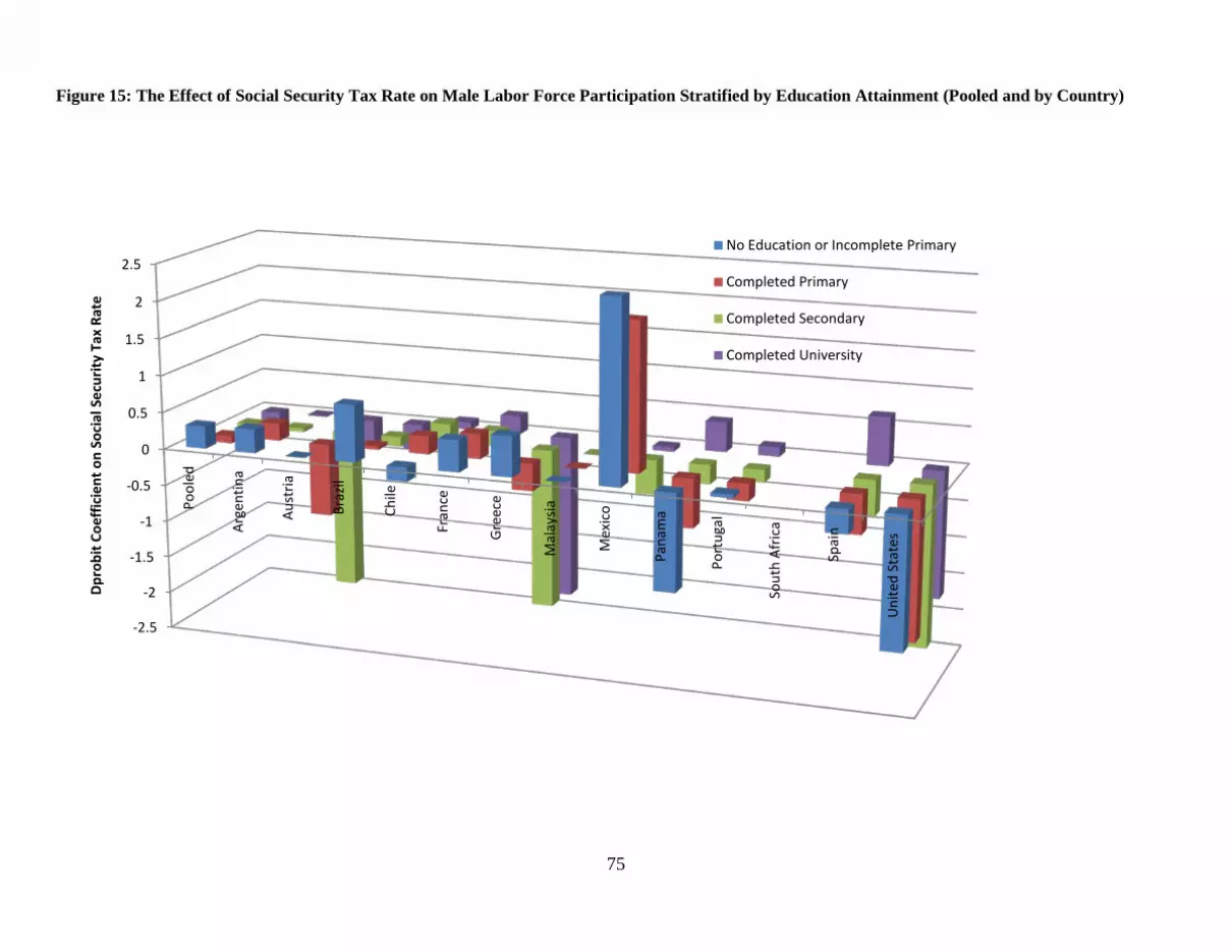
75

Figure 15: The Effect of Social Security Tax Rate on Male Labor Force Participation Stratified by Education Attainment (Pooled and by Country)

-2.5

-2

-1.5

-1

-0.5

0

0.5

1

1.5

2

2.5

Pool

ed

Arg

entin

a

Aus

tria

Braz

il

Chile

Fran

ce

Gre

ece

Mal

aysi

a

Mex

ico

Pana

ma

Port

ugal

Sout

h A

fric

a

Spai

n

Uni

ted

Stat

es

Dpr

obit

Coe

ffic

ient

on

Soci

al S

ecur

ity

Tax

Rate

No Education or Incomplete Primary

Completed Primary

Completed Secondary

Completed University

76

Figure 16: The Effect of Replacement Rate as a Fraction of Wage on Male Labor Force Participation Stratified by Education (Pooled and by Country)

77

-0.3

-0.25

-0.2

-0.15

-0.1

-0.05

0

0.05Po

oled

Arg

entin

a

Aus

tria

Braz

il

Chile

Fran

ce

Gre

ece

Mal

aysi

a

Mex

ico

Pana

ma

Port

ugal

Sout

h A

fric

a

Spai

n

Uni

ted

Stat

es

Dpr

obit

Coe

ffic

ient

on

Repl

acem

ent R

ate

as a

Fra

ctio

n of

Wag

e

No Education or Incomplete Primary

Completed Primary

Completed Secondary

Completed University

78

Figure 17: The Effect of Delay Incentive as a Fraction of Wage on Male Labor Force Participation Stratified by Education Attainment (Pooled and by

Country)

-0.004

-0.002

0

0.002

0.004

0.006

0.008

0.01

0.012

0.014

0.016

0.018

Pool

ed

Arg

entin

a

Aus

tria

Braz

il

Chile

Fran

ce

Gre

ece

Mal

aysi

a

Mex

ico

Pana

ma

Port

ugal

Sout

h A

fric

a

Spai

n

Uni

ted

Stat

es

Dpr

obit

Coe

ffic

ient

on

the

Del

ay In

cent

ive

as a

Fra

ctio

n of

Wag

e

No Education or Incomplete Primary

Completed Primary

Completed Secondary

Completed University

RECENT WORKING PAPERS FROM THE CENTER FOR RETIREMENT RESEARCH AT BOSTON COLLEGE

An In-Depth Look into Intergenerational Flows Oksana Leukhina and Marika Santoro, May 2011 Who Retires Early? Henry J. Aaron and Jean Marie Callan, May 2011 The Potential Impact of the Great Recession on Future Retirement Incomes Barbara A. Butrica, Richard W. Johnson, and Karen E. Smith, May 2011 Immigrant Diversity and Social Security: Recent patterns and Future Prospects Melissa M. Favreault and Austin Nichols, May 2011 Why Aren’t More Families Buying Life Insurance? Matthew S. Chambers, Don E. Schlagenhauf, and Eric R. Young, March 2011 Changes in Firm Pension Policy: Trends Away From Traditional Defined Benefit Plans Kandice A. Kapinos, February 2011 Interdependent Durations in Joint Retirement Bo Honoré and Áureo de Paula, February 2011 Health and Retirement Effects in a Collective Consumption Model of Elderly Households Arthur Lewbel and Shannon Seitz, February 2011 Age Differences in Job Displacement, Job Search, and Reemployment Richard W. Johnson and Corina Mommaerts, January 2011 The Earnings and Social Security Contributions of Documented and Undocumented Mexican Immigrants Gary Burtless and Audrey Singer, January 2011

How Important Are Intergenerational Transfers for Baby Boomers? Alicia H. Munnell, Anthony Webb, Zhenya Karamcheva, and Andrew Eschtruth, January 2011 Effect of Informal Care on Work, Wages, and Wealth Courtney Harold Van Houtven, Norma B. Coe, and Meghan Skira, December 2010 Recessions, Wealth Destruction, and the Timing of Retirement Barry P. Bosworth and Gary Burtless, December 2010

All working papers are available on the Center for Retirement Research website (http://crr.bc.edu) and can be requested by e-mail (crr@bc.edu) or phone (617-552-1762).